This article was downloaded by: [Ministry of Earth Sciences]On: 04 October 2014, At: 21:17Publisher: Taylor & FrancisInforma Ltd Registered in England and Wales Registered Number: 1072954 Registeredoffice: Mortimer House, 37-41 Mortimer Street, London W1T 3JH, UK

New Zealand Journal of Marine andFreshwater ResearchPublication details, including instructions for authors andsubscription information:http://www.tandfonline.com/loi/tnzm20

Variability of fronts, fresh water inputand chlorophyll in the Indian Oceansector of the Southern OceanN Anilkumara, JV Georgea, R Chackoa, N Nuncioa & P Sabua

a National Centre for Antarctic and Ocean Research, Vasco DaGama, IndiaPublished online: 25 Sep 2014.

To cite this article: N Anilkumar, JV George, R Chacko, N Nuncio & P Sabu (2014): Variability offronts, fresh water input and chlorophyll in the Indian Ocean sector of the Southern Ocean, NewZealand Journal of Marine and Freshwater Research, DOI: 10.1080/00288330.2014.924972

To link to this article: http://dx.doi.org/10.1080/00288330.2014.924972

PLEASE SCROLL DOWN FOR ARTICLE

Taylor & Francis makes every effort to ensure the accuracy of all the information (the“Content”) contained in the publications on our platform. However, Taylor & Francis,our agents, and our licensors make no representations or warranties whatsoever as tothe accuracy, completeness, or suitability for any purpose of the Content. Any opinionsand views expressed in this publication are the opinions and views of the authors,and are not the views of or endorsed by Taylor & Francis. The accuracy of the Contentshould not be relied upon and should be independently verified with primary sourcesof information. Taylor and Francis shall not be liable for any losses, actions, claims,proceedings, demands, costs, expenses, damages, and other liabilities whatsoever orhowsoever caused arising directly or indirectly in connection with, in relation to or arisingout of the use of the Content.

This article may be used for research, teaching, and private study purposes. Anysubstantial or systematic reproduction, redistribution, reselling, loan, sub-licensing,systematic supply, or distribution in any form to anyone is expressly forbidden. Terms &Conditions of access and use can be found at http://www.tandfonline.com/page/terms-and-conditions

RESEARCH ARTICLE

Variability of fronts, fresh water input and chlorophyll in theIndian Ocean sector of the Southern Ocean

N Anilkumar*, JV George, R Chacko, N Nuncio and P Sabu

National Centre for Antarctic and Ocean Research, Vasco Da Gama, India

(Received 3 April 2013; accepted 30 April 2014)

The aim of this study was to understand the variability in the fronts and water masses, and the effect ofmelt water on the concentration of chlorophyll (Chl a) in the Indian Ocean sector of the SouthernOcean using hydrographic data collected during the austral summer (February 2010 and 2011). TheSouthern Subtropical Front (SSTF) and Northern Sub Antarctic Front (SAF1) were found to be furthersouth at 57°30′E than at 47–48°E. This southward shift of the fronts was consistent with the southwardmeandering (c. 2°) of the Antarctic Circumpolar Current (ACC) core from the western section to theeastern section, which could have been caused by the bottom topography. The intrusion of watermasses also differed between the western and eastern transects of the study region as a result of themeandering of the ACC core. Fresh water layer thickness relative to the winter water in 2011 wasmore compared to that during 2010. This could have been due to the larger amount of sea ice that waspresent in the winter of 2010, which subsequently melted, resulting in the advection of melt waterfrom the south and west of the study region. In situ observations and satellite data detected a high Chla concentration (c. 0.38 mg m−3) south of the Northern Polar Front (PF1) in 2011, which was causedby this melt water.

Keywords: Argo floats; geostrophic currents; Indian sector of Southern Ocean; oceanic fronts;water masses

Introduction

The Indian Ocean sector of the Southern Ocean(SO) has a complicated quasi-zonal frontal systemthat has remarkable regional differences deter-mined by peculiarities of the bottom topography(Kostianoy et al. 2004) and variability of the Agul-has Return Current (ARC) (Belkin & Gordon1996). The intensity of these fronts (as measuredby the meridional property gradients) varies, andthe individual branches often merge and diverge inresponse to interactions with the bathymetry(Sokolov & Rintoul 2007a, 2009a). Together, thesefrontal systems form the eastward-flowing Ant-arctic Circumpolar Current (ACC), the inter-basinconnectivity of which allows water masses, heatand climatic anomalies to propagate between the

ocean basins (Rintoul et al. 2001). The ACC ischaracterised by a high degree of eddy activity,largely as a result of the dynamic instability of thefrontal systems (Stammer 1998; Hughes 2005).Further, it is composed of many jets and high-speed filaments (Sokolov & Rintoul 2007a; Lennet al. 2011), which are often marked by oceanfronts where the thermohaline properties changerapidly with latitude. The ACC plays a major rolein the climate system (Gordon 1986; Rintoul 1991;Speich et al. 2001), making it imperative that wehave a detailed understanding of the fronts flow-ing across it.

The Agulhas Return Front (ARF), which isassociated with the Agulhas retroflection, mergeswith the Subtropical Front (STF) in some parts of

*Corresponding author. Email: anil@ncaor.gov.in

New Zealand Journal of Marine and Freshwater Research, 2014http://dx.doi.org/10.1080/00288330.2014.924972

© 2014 The Royal Society of New Zealand

Dow

nloa

ded

by [

Min

istr

y of

Ear

th S

cien

ces]

at 2

1:17

04

Oct

ober

201

4

the Indian Ocean (Lutjeharms & Ansorge 2001).The STF marks the boundary between subtropicaland subantarctic waters (Deacon 1937; Hamilton2006), and lies between 35°S and 45°S. Furthersouth, the major ACC fronts are the SubantarcticFront (SAF), Polar Front (PF), Southern ACCFront (SACCF) and southern boundary of the ACC(SB). Since the ACC is a deep-reaching barotropiccurrent, the fronts across it also extend through thewater column (Belkin & Gordon 1996; Meijerset al. 2010). Earlier studies have investigated theconcurrence of frontal positions across the ACC usingmaps of absolute dynamic topography (MADT) andin situ hydrographic data (Sokolov & Rintoul 2007a;Swart et al. 2008; Sokolov & Rintoul, 2009a, b;Swart & Speich 2010). Jasmine et al. (2009) foundthat the fronts and zones in the ACC exhibit widedifferences in hydrographic as well as biologicalcharacteristics. Previous studies have also high-lighted the significance of the Crozet Plateau, wherethe fronts join to form one of the strongest oceanicfrontal systems in the world (Orsi et al. 1995; Belkin& Gordon 1996; Sparrow et al. 1996; Holliday &Read 1998; Kostianoy et al. 2004).

Another important feature of the SO during theaustral summer is the presence of winter water(WW), which is the remnant of the mixed layer ofthe previous winter capped by seasonal warmingand freshening (Deacon 1937). The SO is char-acterised by a temperature minimum subsurfacelayer in the upper 300 m (Park et al. 1998). Duringthe ice-free period, the ocean surface is exposed towinds, which enhances mixing, resulting in thistemperature minimum layer becoming mixed withthe surface and subsurface layers, thereby alteringthe heat budget of the region (Yuan et al. 2004).Since the WW has a close relationship with theheat budget, ice melt and freshening in the SO isbelieved to be a major source of micronutrients(Boyd & Ellwood 2010), and may regulate thechlorophyll (Chl a) blooms in the region. Thestudy of WW also has climatic relevance.

In this study, we investigate the inter-annualvariability in the fronts, the north–south intrusionof water masses from the subtropics to the coastalwaters of Antarctica and the role of melt water inenhancing the Chl a concentration in the Indian

Ocean sector of the SO. The frontal positions arecompared using MADT, satellite SST and in situhydrographic data, and the influence of the ACCon frontal variability has been delineated. Further,the sources of fresh water input into the study areaand its influence on variations in Chl a concen-trations across the ACC, as well as in the coastalwaters of Antarctica, are discussed.

Data and methods

This study used hydrographic measurements takenfrom the Indian Ocean sector of the SO duringthe austral summers (February) of 2010 and 2011.In both years, expeditions were made onboardthe Oceanographic Research Vessel Sagar Nidhi(ORV-SN), which launched from Mauritius. Dur-ing 2010, observations were made from 40°S 57°30′E to the coastal waters of Antarctica (65°27′S53°28′E), and were then continued along a trackbetween 65°27′S and 40°S, and between 53°28′Eand 48°E (hereafter referred to as Track-1; seeFig. 1A). During 2011, observations were madefrom 40°S to 60°S along the meridional section57°30′E, and from 60°S to 40°S along the meridi-onal section 47°E.

During both expeditions, a CTD (Sea-BirdElectronics, USA; temperature: ± 0.001 °C; con-ductivity: ± 0.0001 S m−1; and depth: ± 0.005% ofthe full scale) and XCTDs (Tsurumi-Seiki Co. TSKLtd,Yokohama, Japan; type: XCTD-3; temperature:± 0.02 °C; conductivity: ± 0.03 mS cm−1; anddepth: ± 2%) were deployed to collect the temper-ature and salinity profiles. XCTD probes werelaunched at c. 30 nautical mile intervals betweenthe CTD stations. The station locations for CTD andXCTD operations during 2010 and 2011 are shownin Fig. 1A and B, respectively. The XCTD profileswere quality controlled by following the guidelinesin the CSIRO Cookbook (1993). The salinity datafrom the CTD were calibrated against water sam-ples analysed using a high-precision salinometer(Guildline AUTOSAL).

Oceanic fronts were identified using the char-acteristic property indicators following the criterialisted by Belkin & Gordon (1996), Sparrow et al.(1996), Holliday & Read (1998), Kostianoy et al.

2 N Anilkumar et al.

Dow

nloa

ded

by [

Min

istr

y of

Ear

th S

cien

ces]

at 2

1:17

04

Oct

ober

201

4

Figure 1 CTD/XCTD locations in A, February 2010 and B, February 2011; and Argo locations in C, February2010 and D, February 2011.

Variability of fronts, fresh water input and chlorophyll in the Indian Ocean 3

Dow

nloa

ded

by [

Min

istr

y of

Ear

th S

cien

ces]

at 2

1:17

04

Oct

ober

201

4

(2004), and Billany et al. (2010). The propertiesthat were used to identify fronts in the study areaare provided in Table 1. In addition, MADT fromCLS/AVISO and monthly SSTs from the Groupfor High Resolution Sea Surface Temperature(GHRSST) on 1/4° grids (http://podaac.jpl.nasa.gov/dataset/NCDC-L4LRblend-GLOB-AVHRR_AMSR_OI) were also used to identify the frontsin the study region. The thickness of the freshwater input in the surface layer relative to theWW in the study region was estimated using theformula of Park et al. (1998):

h ¼ DCðSW � SbarÞSW

; Sbar ¼ 1

DC

Z0

�DC

Sdz

264

375; ð1Þ

where h is the thickness of the fresh water inputper unit surface area, Dc is the WW depth, Sw isthe WW salinity, and Sbar is the depth-averagedsalinity between the surface and WW depth. Sur-face ocean currents were plotted using OceanSurface Current Analysis–Realtime data (OSCAR,

http://www.oscar.noaa.gov) (Bonjean & Lagerloef2002). Monthly ASCAT wind stress, Ekmancurrent, MODIS Aqua photosynthetically avail-able radiation (PAR) and AMSR-E ice coveragedata from ERDDAP were used in the presentstudy. The Argo data during February 2010 andFebruary 2011 from the Coriolis Data Center(http://www.coriolis.eu.org/cdc) were also used.The locations of the Argo floats that were usedduring February 2010 and 2011 are shown inFig. 1C and D, respectively. The western box isover the southwest Indian ridge centred at 50°Eand the eastern box is over a flat-bottomed deepregion centred at 60°E.

Results and discussion

Frontal system variability

The temperature and salinity structures derivedfrom the CTD/XCTD data collected during 2010along Track-1 are shown in Fig. 2A and B. Nosignature of the northern branch of the SubtropicalFront (NSTF) was noticed along this track, whichis not surprising given that the NSTF is always

Table 1 Properties used for the identification of various fronts in the study area.

Front Temperature Salinity

Northern SubtropicalFront (NSTF)

21–22 °C at surface surface salinity c. 35.5

Agulhas Return Front (AF) 19–17 °C at surface; 10 °C isothermfrom 300 to 800 m

35.54–35.39 at surface; 35.57–34.90at 200 m

Southern SubtropicalFront (SSTF)

17–11 °C at surface; 12–10 °C at 100 m 35.35–34.05 at surface; 35–34.6at 100 m; 34.92–34.42 at 200 m

Subantarctic Front (SAF1) 11–9 °C at surface; 8–5 °C at 200 m(along 45°E) 11–10 °C at surface;8–5 °C at 200 m (along 57°30′E)

34.0–33.85 at surface; 34.40–34.11at 200 m

Subantarctic Front (SAF2) 7–6 °C at surface 4 °C isotherm at200 m depth (along 45°E) 9–8 °C atsurface 4 °C isotherm at 200 m depth(along 57°30′E)

surface salinity c. 33.85 southof SAF

Polar Front (PF1) 5–4 °C at surface northern limit of the2 °C isotherm below 200 m

33.8–33.9 at surface

Polar Front (PF2) 3–2 °C at surface 33.8–33.9 surfaceSouthern Antarctic CircumpolarCurrent Front (SACCF)

Temperature maximum Tmax > 1.8 °C Salinity maximum Smax > 34:73

Southern Boundary of ACC (SB) 1.5 °C isotherm

4 N Anilkumar et al.

Dow

nloa

ded

by [

Min

istr

y of

Ear

th S

cien

ces]

at 2

1:17

04

Oct

ober

201

4

located north of 40°S (Belkin & Gordon 1996),whereas our observations were from south of 40°S.Along this section, the Southern Subtropical Front(SSTF) and Northern Subantarctic Front (SAF1)were observed between 40°S and 41°30′S, andbetween 41°30′S and 44°S, respectively, with adrop in temperature from 16 to 9 °C (Fig. 2A) and adecrease in salinity from 35.54 to 34.11 (Fig. 2B).The Southern Subantarctic Front (SAF2), Northern

Polar Front (PF1) and Southern Polar Front (PF2)were identified between 46°30′S and 48°S, 50°Sand 52°30′S, and 54°30′S and 59°30′S, respect-ively (Table 2). The SACCF and SB can be identifiedfrom the most southerly position of the subsurface1.8 °C and 1.5 °C isotherms, respectively. However,in the present study, the SACCF was demarcatedbetween 60°S and 61°S, and the SB was between64°30′S and 64°S.

Figure 2 Vertical structure of A, temperature (°C) and B, salinity along the track between 65°41′S 57°30′E and 55°S 48°E, and further northwards along 48°E (Track-1); and C, temperature (°C) and D, salinity along 57°30′Ein 2010.

Variability of fronts, fresh water input and chlorophyll in the Indian Ocean 5

Dow

nloa

ded

by [

Min

istr

y of

Ear

th S

cien

ces]

at 2

1:17

04

Oct

ober

201

4

The temperature and salinity sections along 57°30′E during 2010 are presented in Fig. 2C and D.Along this transect, the SSTF was identifiedbetween 41°S and 45°S; SAF1 between 45°S and47°S; SAF2 between 47°S and 48°S; PF1 between50°S and 52°30′S; and PF2 as a wide front between55°S and 59°30′S. The SACCF and SB were iden-tified at the same latitudes as observed along Track-1. Holliday & Read (1998) reported the occurrenceof the STF between 40°S and 42°S along 55°E; andduring 2004, the merged Agulhas Front (AF) andthe SSTF were identified between 43°30′S and 45°S, SAF1 was between 45°30′S and 46°30′S, andSAF2 was south of 47°S along 57°30′E (see Figs5 and 6 in Anilkumar et al. 2006).

During 2011, the AF+SSTF+SAF1 front wasobserved (Fig. 3A and B) between 41°S and 44°30′S along 47°E. However, along 57°30′E, thiscomplex front was identified as a wide frontalsystem between 40°30′S and 46°30′S (Fig. 3Cand D). East of 54°E, Belkin & Gordon (1996)identified this merged frontal system as the CrozetFront. Park et al. (1993) Sparrow et al. (1996) andKostianoy et al. (2004) reported more spatial vari-ation in this merged frontal system than was seenin the present study. The SAF2 was identifiedbetween 47°30′S and 48°30′S along 47°E, whereasits position was observed to be relatively more

northward along 57°30′E, lying between 46°30′Sand 47°30′S. The PF1 was identified between 50°30′S and 52°S, lying almost in the same positionalong 47°E and 57°30′E; while the PF2 was seenas a relatively wider front along 57°30′E (between53°30′S and 56°30′S) than along 47°E (between52°30′S and 54°S). Moore et al. (1997, 1999)used satellite SST maps to study the dynamics ofthe PF, and showed its position as lying between49°30′S and 52°S; however, this was not compat-ible with the positions of the PF1 and PF2 thatwere identified in this study. During 2011, the AFwas identified as a separate front along 47°E and57°30′E, confirming the earlier findings of Belkin &Gordon (1996). Kostianoy et al. (2004) opined thatthe AF’s cyclonic meander can increase the distancebetween theAF and theSTF/SAFby up to 3° latitude.

In the present study, a southward shift of > 2°latitude from west (Track-1 and 47°E) to east(57°30′E) was observed in the positions of theSSTF and SAF1 (Figs 2A–D and 3A–D). Glady-shev et al. (2008) reported that the locations ofthe SAF, PF and SACCF are controlled by theneighbouring ridges. The position of the SAF inthe present study differed from that found in pre-vious studies (Park et al. 1993; Belkin & Gordon1996; Sparrow et al. 1996). In earlier reports, itwas observed to be surrounding the Crozet Plateau

Table 2 Comparison of frontal locations between the present and previous studies.

FrontsPresent location alongTrack-1 and 47°E Previously reported locations west of 48°E

Northern SubtropicalFront (NSTF)

Not encountered 31°S–38°S (Belkin & Gordon 1996)

Agulhas Return Front (AF) 40°S–41°18′S 38°S–41.5°S (Holliday & Read 1998)Southern SubtropicalFront (SSTF)

40°S–41°30′S Observed as a merged front along with ARF andSAF at about 43°S, 45°E (Read et al. 2000) 40°Sand 42°S along 55°E, (Holliday & Read 1998)

Subantarctic Front (SAF1) 41°30′S–44°S 44°S–45°S (Kostianoy et al. 2004)Subantarctic Front (SAF2) 46°30′S–48°S 48.5°S–49°S (Kostianoy et al. 2004)Polar Front (PF1) 50°S–52°30′S 50°S–52°S (Holliday & Read 1998)Polar Front (PF2) 54°30′S–59°30′S 55°S–57°S (Holliday & Read 1998)Southern Antarctic CircumpolarCurrent Front (SACCF)

60°S–61°S c. 60°S–63°S (Meijers et al. 2010)

Southern Boundary of ACC (SB) 64°S–64°30′S c. 64°S–65°S (Meijers et al. 2010)

6 N Anilkumar et al.

Dow

nloa

ded

by [

Min

istr

y of

Ear

th S

cien

ces]

at 2

1:17

04

Oct

ober

201

4

(Moore et al. 1999); and Holliday & Read (1998)reported a width of c. 1.5° latitude along 45°E,while Lutjeharms & Valentine (1984) reported awidth of c. 2.5° latitude. By contrast, the SAF wasdistinguished as two separate fronts (SAF1 andSAF2) along all the tracks in the present study,and so its width was not comparable with previousfindings. These results attest to the significantinter-annual variability in the frontal systems ofthe SO. A comparison of the frontal locations

observed in the present and previous studiesis provided in Table 2.

Following the method of Swart & Speich.(2010), the mean MADT calculated from 1992 to2010 was used to compute the meridional gradientsper 100 km of mean MADT. These gradients werethen used to identify the core locations of variousfronts along 48°E and 57°30′E (Fig. 4A and B).Swart & Speich (2010) suggested that isolinesof MADT coincide with constant water mass

Figure 3 Vertical structure of A, temperature (°C) and B, salinity along 47°E; and C, temperature (°C) andD, salinity along 57°30′E in 2011.

Variability of fronts, fresh water input and chlorophyll in the Indian Ocean 7

Dow

nloa

ded

by [

Min

istr

y of

Ear

th S

cien

ces]

at 2

1:17

04

Oct

ober

201

4

Figure 4 Mean MADT gradient (cm 100 km−1) (computed from weekly MADT data from 1992 to 2010) along A, 48°30′E and B, 57°30′E; core frontallocations determined using MADT along C, 48°E and D, 57°30′E; and frontal location and its width using satellite SST (GHRSST) along E, 48°E andF, 57°30′E.

8N

Anilkum

aret

al.

Dow

nloa

ded

by [

Min

istr

y of

Ear

th S

cien

ces]

at 2

1:17

04

Oct

ober

201

4

properties and thus the fronts. Along 48°E, theMADT gradient exhibited the SSTF at 41°S, theSAF1 at 42°30′S and the SAF2 at 48°30′S. The PF1was observed to be located at 51°30′S and the PF2at 54°30′S. Along 57°30′E, the SSTF, SAF1 andSAF2 were identified at 43°30′S, 45°S and 48°30′S, respectively. Further, the PF1 and PF2 wereobserved at 51°30′S and 57°30′S, respectively.Table 3 shows the mean characteristic MADT foreach frontal position located in the study region.The frontal locations from the MADT gradientshowed a southward meandering of the SSTF andSAF1 by > 2° latitude. In the present study, thelocations of the gradient maxima and the associatedlines of MADTwere almost identical to the frontalpositions identified using the hydrographic data.The characteristic MADT for each front in Table 3was used to analyse frontal variability during Feb-ruary 2010 and February 2011 (Fig. 4C and D); andbased on the SST characteristics of fronts given inTable 1, the satellite-derived SST plots were alsoused to depict the frontal locations during these 2years (Fig. 4E and F). The core locations of frontsderived from both the MADT and the satellite SSTwere consistent with those of the hydrographic data.

Therefore, from the present study it can bededuced that the meandering of fronts in the ACCwas only exhibited by the SSTF and SAF1. Theother fronts had almost identical positions alongthe western and eastern transects of the studyregion. In the following sections, we discuss thesources for the input of fresh water in the study

region and further delineate the strength of currentsin the study area where meandering fronts wereobserved in the ACC.

Water masses and winter water properties

Water masses

The characteristics of the water masses in thestudy area are given in Table 4. Signatures of theSubtropical Surface Water (STSW) were identifiedup to 41°S along Track-1 in 2010 and up to 42°Salong 47°E in 2011 (Fig. 5A and C). The south-ward intrusion of this water mass was observed upto 44°S in 2010 and 45°S in 2011 along 57°30′E(Fig. 5B and D). The signatures of the SubtropicalMode Water (STMW) that were observed in thepresent investigation (Fig. 5) were similar to thosereported previously by McCartney (1977) and Parket al. (1991), whereas Tsubouchi et al. (2010)observed its signatures in the regions 28°E–45°Eand 60°E–80°E. The STMW can be identified inthe depth range of 400 to 700 m, with a potentialdensity anomaly range of 26.5 to 26.8 kg m−3,where the potential density pycnostad develops(Park et al. 1993). It has been reported that theSTMW is formed in the Crozet Basin (see Fig. 4of Belkin & Gordon 1996). Along Track-1 and47°E, we identified the southward extent of theSTMW up to 41°S and 42°S, respectively (Fig. 5Aand C), concurring with the findings of Park et al.(1993) and Belkin & Gordon (1996). Along 57°30′E, the STMW was identified up to 44°Sand 45°S in 2010 and 2011, respectively, with

Table 3 Mean frontal locations as determined using mean MADT at (a) 48°E and (b) 57°30′E.

Along 48°E Along 57°30′E

FrontsMean location

(°S)Mean

MADT (cm)Mean location

(°S)Mean

MADT (cm)

Southern SubtropicalFront (SSTF)

41.30 29.4 43.76 25.20

Subantarctic Front (SAF1) 42.54 –8.40 44.95 –7Subantarctic Front (SAF2) 48.38 –42.80 48.38 –43.80Polar Front (PF1) 51.59 –74.90 51.59 –66.2Polar Front (PF2) 54.59 –97.80 57.39 –99.50

Variability of fronts, fresh water input and chlorophyll in the Indian Ocean 9

Dow

nloa

ded

by [

Min

istr

y of

Ear

th S

cien

ces]

at 2

1:17

04

Oct

ober

201

4

the southward intrusion of more than 4° latitude(Fig. 5B and D) compared with Track-1 and 47°E.

The Antarctic Intermediate Water (AAIW) wasidentified up to 43°S (Fig. 5A and C) along Track-1and 47°E. The AAIW from the southwest Indian

Ocean sector of the SO is the dominant AAIW typeeast of the Agulhas Current retroflection (Roman &Lutjeharms 2010). The AAIW identified in theCrozet Basin mainly originates from the region nearthe Kerguelen Plateau (Molinelli 1981; Fine 1993;

Figure 5 Water masses along A, Track-1 and B, 57°30′E in 2010; and C, 47°E and D, 57°30′E in 2011.

Table 4 Water mass characteristics.

Characteristics

Water mass Temperature (°C) Salinity (psu) Density (kg m−3) Depth (m)

Subtropical Surface Water (STSW) > 12 > 35.1 0–200Subantarctic Surface Water (SASW) 9 < 34 0–200Antarctic Surface Water (AASW) < 5 < 34 0–200Sub Tropical Mode Water (STMW) 11 to 14 35 to 35.4 26.5 to 26.8 400–700Antarctic Intermediate Water (AAIW) c. 4.4 c. 34.42 c. 27.24 700–1200Circumpolar Deep Water (CDW) c. 2 c. 34.77 c. 27.8 2000–3800Antarctic Bottom Water (ABW) c. 0.165 to 0.62 c. 34.67 to 34.652 c. 27.85 to 27.85 > 3000

10 N Anilkumar et al.

Dow

nloa

ded

by [

Min

istr

y of

Ear

th S

cien

ces]

at 2

1:17

04

Oct

ober

201

4

Toole&Warren 1993). The depth of this water masshas been reported to be between c. 1000 andc. 1300 m (Park et al. 1993; Bindoff & McDougall1999). In the present study, the features of theAAIW were observed between 1000 and 1500 m.The southward extent of the AAIW was observedup to 45°S in 2010 and 2011 along 57°30′E (Fig. 5Band D), which is more than 2° latitude southwardsof that observed along Track-1 and 47°E.

Signatures of the Subantarctic Surface Water(SASW) were observed between 42° and 43°Salong Track-1, and between 43°S and 47°S along47°E (Fig. 5A and C); however, this water mass wasidentified between 45°S and 47°S along 57°30′E(Fig. 5B and D). The Antarctic Surface Water(AASW) was identified up to 42°S along Track-1in 2010 (Fig. 5A) and up to 43°S along 47°E in 2011(Fig. 5C); however, the signatures of this watermass were observed only up to 45°S along 57°30′Ein 2010 and 2011 (Fig. 5B and D). This means thatthe northward intrusion of the SASW and AASWwas more pronounced in the western transects(Track-1 and 47°E). Along these transects, theCircumpolar Deep Water (CDW) was identifiedup to 42°S (Fig. 5A and C), while it was observedup to 58°S–60°S along 57°30′E. However, theCDW was observed deeper than 2000 m north of45°S, and its northward intrusion was seen beyond42°S during 2010 and 2011 (Fig. 5B and C).According to Toole & Warren (1993), the CDWoccupies a depth range of 2000–3800 m north of45°S and rises sharply to shallower depths south ofthis latitude. A northward intrusion of AntarcticBottom Water (AABW) was observed up to 55°Sand 56°S along Track-1 and 57°30′E, respectively,in 2010 (Fig. 5A and B). In 2011, the intrusion ofAABW was seen up to 54°S and 50°S along 47°Eand 57°30′E, respectively (Fig. 5C and D). Obser-vations fromArgo data (Fig. 6) were consistent withthe in situ CTD results, showing a more northwardintrusion of SASW and AASW in the westernregion (45°E–55°E). By contrast, the STSW,STMW and AAIW showed a further southwardintrusion in the eastern region (57°E–65°E).

Anilkumar et al. (2006) previously identifiedwater masses along 45°E; however, this was basedon CTD data from only one transect, and so the

north–south movement of water masses in thewestern and eastern regions could not be com-pared. Here, we compared the spreading of watermasses along Track-1, 47°E and 57°30′E during2010 and 2011, and found disparity in their intru-sion along the western and eastern transects of thestudy region. It is likely that the intrusions ofwater masses in the upper layers are controlled bythe meandering of the ACC flow.

Winter water properties

The temperature minimum layer (c. 1.4 °C lowerthan the surface temperature) was located 50–200m south of 50°S in the study region in both 2010and 2011 (Figs 2 and 3). This temperature min-imum layer corresponds with the AASW and iscapped above the CDW (Yuan et al. 2004), andcan be attributed to the WW. Below this layer, thetemperature gradually increased by c. 2 °C up to350 m and then exhibited isothermal characteris-tics further down. Following Park et al. (1998), theWW depth (Dc) is defined as the WW core depthat which the absolute minimum subsurface tem-perature is observed. During 2010 and 2011, theWW was observed up to the PF1 from the south,and the temperature and core depth of WWincreased from south to north in both meridionalsections. The shallowest WW depth was noted inthe Antarctic divergence region (c. 63°S to 60°S).In general, cooler WW was observed in 2011 than2010 along Track-1/47°E (Fig. 7A and B), and thefresh water thickness (as calculated following Parket al. 1998) showed higher values during 2011 than2010 along the western section (Track-1/48°E)(Fig. 7C and D).

This layer of low temperature is the result ofsurface freshening during the austral summer,mainly due to ice melting and subsequent warm-ing of the surface layer (Park et al. 1998), but alsofrom precipitation and the advection of melt water.Bromwich et al. (1995) reported a low level ofprecipitation (30 cm yr−1) at 50°S, based on theanalysis of zonal averaged net precipitation derivedfrom the European Centre for Medium-RangeWeather Forecasts, and in the present study, thefresh water input received south of 50°S along

Variability of fronts, fresh water input and chlorophyll in the Indian Ocean 11

Dow

nloa

ded

by [

Min

istr

y of

Ear

th S

cien

ces]

at 2

1:17

04

Oct

ober

201

4

both transects has not been attributed to net pre-cipitation. Rather, the source of fresh water couldbe locally produced melt water and/or advectionfrom the in situ melting of sea ice originating fromthe south and west. The extent of sea ice along 48°E and 57°30′E during 2009 and 2010 is shown inFig. 8A and B, from which it can be seen that themaximum sea ice limit was up to c. 59°S duringthe winter of 2009 and up to c. 57°S during thewinter of 2010 along both sections. The peak extentof the sea ice was observed in September, afterwhich it started to melt through to March. Thislarger and more northward extent of sea ice duringwinter 2010 could explain the greater thickness ofthe fresh water layer and cooler WW temperatureobserved during the summer of 2011.

The Ekman currents overlaid on the averagedwind stress suggest the northward Ekman transportof melt water from south (Fig. 8C and D). It canalso be seen that the high stress patch (c. 0.3 Pa) ofwesterlies that was centred at 50°S during February2010 shifted further south to 56°S during February2011, which may have caused the increase inthe northward Ekman transport from the south(c. 60°S) during February 2011. The shifting of thewesterlies could be a manifestation of the positiveSouthern Annular Mode (SAM) during February2011 (SAM index = 0.86) and the negative SAMduring February 2010 (SAM index = −2.12)(Marshall 2003), and so the increased northwardEkman transport of melt water from the south couldalso explain the comparative increase in fresh water

Figure 6 Water masses from Argo data in two regions: A, from 45°E to 55°E (eastern region) and B, from 56°E to65°E (western region) in 2010; and C, from 45°E to 55°E and D, from 56°E to 65°E in 2011.

12 N Anilkumar et al.

Dow

nloa

ded

by [

Min

istr

y of

Ear

th S

cien

ces]

at 2

1:17

04

Oct

ober

201

4

thickness during February 2011. In general, how-ever, the Ekman currents in the SO are weakcompared with the background geostrophic cur-rents (Lenn & Chereskin 2009).

Recent studies suggest an increased rate ofmelting in the Bellingshausen–Amundsen Sea, westof the Antarctic Peninsula (Pritchard et al. 2012;Rignot et al. 2013), and this low-saline melt waterenters the Indian Ocean sector, possibly via the ACC.Hence, themelt water that is transported fromwest ofthe Antarctic Peninsula may contribute to the lowsalinity waters that are observed in the Indian Oceansector of the SO. The total current during February2010 and 2011, as derived from the OSCAR (Fig.9A and B), also suggested a net eastward flow in theSO. It is also expected that melting in the WeddellSeawould contribute to the observed thickness of the

fresh water layer. The Weddell Gyre is a cycloniccirculation regime centred at c. 30°W, which has amajor role in transferring heat and salt from the ACCto the Antarctic continental shelves (Orsi et al. 1993),and which eventually helps with the sea ice meltingin the region. However, the northward flow in theWeddell Sea was found to be weak during summer2010 (Fig. 8C).

Finally, it should be noted that there wasgreater variability in the thickness of the freshwater layer and WW temperature between Febru-ary 2010 and February 2011 along Track-1 and47°E than along 57.5°E (Fig. 7). However, moreobservations are required to explain this variabil-ity. In the following section, we have delineatedthe strength of currents in the study area in regionswhere meandering of the ACC was observed.

Figure 7 Winter water temperature (°C) A, along Track-1 in 2010 and along 47°E in 2011, and B, along 57°30′Ein 2010 and 2011; and fresh water thickness (m) C, along Track-1 in 2010 and along 47°E in 2011, and D, along57°30′E in 2010 and 2011.

Variability of fronts, fresh water input and chlorophyll in the Indian Ocean 13

Dow

nloa

ded

by [

Min

istr

y of

Ear

th S

cien

ces]

at 2

1:17

04

Oct

ober

201

4

ACC variability in the study region

In the study region, the ACC flows from west toeast and depicts a complex current pattern, withstrong zonal currents in the merged frontal region.Geostrophic currents across the cruise tracks were

computed for 2010 and 2011 (Fig. 10). Along 57°30′E, the current velocity was stronger (> 30 cm s−1)in the SSTF+SAF1 region (ACC core) during 2010(Fig. 10B). Two patches of high geostrophic currentswere observed, with velocities of c. 30 cm s−1

Figure 8 Sea ice fraction derived from AMSRE along A, 48°E and B, 57°30′E; and wind stress (Pa) overlaid byEkman currents (m s−1) derived from ASCAT during C, February 2010 and D, February 2011.

14 N Anilkumar et al.

Dow

nloa

ded

by [

Min

istr

y of

Ear

th S

cien

ces]

at 2

1:17

04

Oct

ober

201

4

and c. 15 cm s−1, which were separated by anopposite current of 5 cm s−1 (Fig. 10C) (unlessspecified otherwise, the directions of geostrophiccurrents were positive eastward). This pattern couldhave been caused by an eddy that has been identifiedin this region (Chacko et al. in press). In the SSTF+SAF1 region, a stronger geostrophic current (c. 30cm s−1) was observed along 47°E and 57°30′E in2011 than along Track-1 (< 5 cm s−1) and 57°30′E(< 25 cm s−1) in 2010 (Fig. 10). These resultsdemonstrate the inter-annual variability in the ACC.

A southward shift of the ACC core was alsoobserved in the geostrophic currents between the 47°E/Track-1 and 57°30′E transects during both 2010and 2011. The OSCAR monthly averaged currentsoverlaid by the 3000 m and 4000m deep isobaths areshown in Fig. 9. From this, it can be seen that theACC core was observed between 42°S and 44°S in

the western region (westwards of 56°E), and between44°S and 47°S in the eastern region (eastwards of56° E). It can also be seen that, along the core of theACC (c. 42°S to c. 47°S), the meandering wasassociated with the bottom topography. When theACC passes from a shallow (< 4000 m, Crozetplateau and Southwest Indian ridge) to a deep (> 4000m) region, the ACC meanders southwards to con-serve its potential vorticity. Previous studies byKostianoy et al. (2004), Anilkumar et al. (2007) andNuncio et al. (2011) have also shown that themeandering of the ACC was governed by the bottomtopography. Analysis of the wind stress curl (data notshown) and the Ekman currents (Fig. 8) suggests thatthe meandering of the ACC in the study regionmay not be driven by wind. It can also be noted fromFig. 10 that the meandering of the ACC is not asurface feature, but rather extends to deeper depths.The fronts in this region also meander, and mark thenorthward extension of the SASW and AASWin the west (45°E to 55°E) and the southwardintrusion of the STSW, STMW and AAIW in theeast (57°E to 65°E).

In the Indian Ocean sector of the SO, the PFwas found to be bifurcated into two components,PF1 and PF2, which is compatible with the previ-ous observations of Holliday & Read (1998).Further, the SB was observed up to 64°30′S alongboth Track-1 and 57°30′E in 2010. Previous stud-ies have reported that the maximum southwardmovement of the SB was apparent in the IndianOcean sector of the SO (Orsi et al. 1995, 1999;Meijers et al. 2010; Couldrey et al. 2013), ratherthan the Atlantic or Pacific sectors. The regionbetween 50°E and 60°E is located between twodistinct gyres—the Weddell Gyre in the west andPrydz Bay Gyre in the east. The transport of theAntarctic Slope Current (ASC) is greatest at 80°E(westwards), and becomes steadily weaker to-wards the west, reaching a minimum at 50°E.This weakening could be a result of the Prydz BayGyre (Meijers et al. 2010). The present study area(between 45°E and 60°E) lies between the twogyres, where the transport of the ASC is weakerand the ACC extends more southwards, resultingin the peculiar behaviour of the ACC in the IndianOcean sector of the SO.

Figure 9 OSCAR monthly averaged currents (m s−1)in A, 2010 and B, 2011. The 3000 m and 4000 m deepisobaths are overlaid as dashed lines.

Variability of fronts, fresh water input and chlorophyll in the Indian Ocean 15

Dow

nloa

ded

by [

Min

istr

y of

Ear

th S

cien

ces]

at 2

1:17

04

Oct

ober

201

4

Chlorophyll variability

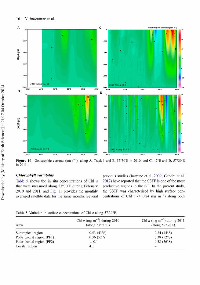
Table 5 shows the in situ concentrations of Chl athat were measured along 57°30′E during February2010 and 2011, and Fig. 11 provides the monthlyaveraged satellite data for the same months. Several

previous studies (Jasmine et al. 2009; Gandhi et al.2012) have reported that the SSTF is one of the mostproductive regions in the SO. In the present study,the SSTF was characterised by high surface con-centrations of Chl a (> 0.24 mg m−3) along both

Table 5 Variation in surface concentrations of Chl a along 57.30°E.

AreaChl a (mg m−3) during 2010

(along 57°30′E)Chl a (mg m−3) during 2011

(along 57°30′E)

Subtropical region 0.53 (43°S) 0.24 (44°S)Polar frontal region (PF1) 0.36 (52°S) 0.38 (52°S)Polar frontal region (PF2) c. 0.1 0.38 (56°S)Coastal region 4.1 –

Figure 10 Geostrophic currents (cm s−1) along A, Track-1 and B, 57°30′E in 2010; and C, 47°E and D, 57°30′Ein 2011.

16 N Anilkumar et al.

Dow

nloa

ded

by [

Min

istr

y of

Ear

th S

cien

ces]

at 2

1:17

04

Oct

ober

201

4

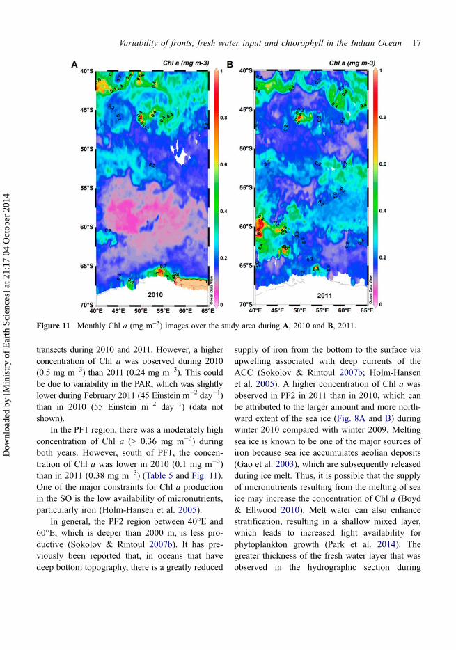
transects during 2010 and 2011. However, a higherconcentration of Chl a was observed during 2010(0.5 mg m−3) than 2011 (0.24 mg m−3). This couldbe due to variability in the PAR, which was slightlylower during February 2011 (45 Einstein m−2 day−1)than in 2010 (55 Einstein m−2 day−1) (data notshown).

In the PF1 region, there was a moderately highconcentration of Chl a (> 0.36 mg m−3) duringboth years. However, south of PF1, the concen-tration of Chl a was lower in 2010 (0.1 mg m−3)than in 2011 (0.38 mg m−3) (Table 5 and Fig. 11).One of the major constraints for Chl a productionin the SO is the low availability of micronutrients,particularly iron (Holm-Hansen et al. 2005).

In general, the PF2 region between 40°E and60°E, which is deeper than 2000 m, is less pro-ductive (Sokolov & Rintoul 2007b). It has pre-viously been reported that, in oceans that havedeep bottom topography, there is a greatly reduced

supply of iron from the bottom to the surface viaupwelling associated with deep currents of theACC (Sokolov & Rintoul 2007b; Holm-Hansenet al. 2005). A higher concentration of Chl a wasobserved in PF2 in 2011 than in 2010, which canbe attributed to the larger amount and more north-ward extent of the sea ice (Fig. 8A and B) duringwinter 2010 compared with winter 2009. Meltingsea ice is known to be one of the major sources ofiron because sea ice accumulates aeolian deposits(Gao et al. 2003), which are subsequently releasedduring ice melt. Thus, it is possible that the supplyof micronutrients resulting from the melting of seaice may increase the concentration of Chl a (Boyd& Ellwood 2010). Melt water can also enhancestratification, resulting in a shallow mixed layer,which leads to increased light availability forphytoplankton growth (Park et al. 2014). Thegreater thickness of the fresh water layer that wasobserved in the hydrographic section during

Figure 11 Monthly Chl a (mg m−3) images over the study area during A, 2010 and B, 2011.

Variability of fronts, fresh water input and chlorophyll in the Indian Ocean 17

Dow

nloa

ded

by [

Min

istr

y of

Ear

th S

cien

ces]

at 2

1:17

04

Oct

ober

201

4

February 2011 (especially in the western regionalong c. 47°E) also supports the observed highconcentration of Chl a.

A high in situ concentration of Chl a wasobserved in the coastal waters of Antarctica during2010 (c. 4 mg m−3) (Table 5). The monthly aver-aged satellite data also showed high concentra-tions of Chl a (c. 0.8 mg m−3) in the coastalregion during 2010 and 2011 (Fig. 11). The ele-vated levels of micronutrients in the coastal watersas a result of glacial melting may stimulate thesignificant phytoplankton blooms in the SO (Smith& Nelson 1985; Park et al. 1999). Previous studieshave reported that the SO is a high nutrient–lowchlorophyll (HN-LC) region due to light limitationbecause of the deep mixing (Mitchell et al. 1991;Nelson & Smith 1991), grazing pressure (Dubischar& Bathmann 1997), non-availability of trace metals(Martin et al. 1990) and limited photosynthetic rateas a result of low water temperatures (Tilzer et al.1986; Sakshaug & Slagstad 1991). However, thehigh concentrations of Chl a observed south of PF1during 2011 in the present investigation can be attrib-uted to the local melting of sea ice and advectedmelt water from the south and west.

Conclusion

This study investigated inter-annual variability inthe fronts and water masses, and variation in theconcentration of Chl a across various frontal sys-tems in the Indian Ocean sector of the SO. TheSSTF and SAF1 were characterised by a south-ward shift of 2° latitude along 57°30′E comparedwith their position along 47°E/Track-1, which wasconsistent with the southward meandering of theACC core from west to east. This meandering waslikely to have been caused by topographic steeringof the ACC between the western and eastern trans-ects. While passing through the shallow topo-graphic features (Crozet plateau and SouthwestIndian ridge) to the deep region (> 4000 m), theACCmeanders southwards to conserve its potentialvorticity. The northward extension of the SASWand AASW in the west (45°E to 55°E), and thesouthward intrusion of the STSW, STMW andAAIW in the east (57°E to 65°E), are probably

linked to the meandering of the ACC. A largeamount of sea ice was present in the study regionduring winter 2010 compared with winter 2009,and our findings suggest that the greater thicknessof the fresh water layer in 2011 compared with2010 was the result of the melting of the previouswinter’s sea ice, and advection of the melt waterfrom the south and west of the study region. One ofthe major consequences of this advection was thegreater concentration of Chl a (c. 0.38 mg m−3)south of PF1 during 2011 compared with 2010.More detailed in situ hydrographic observations inthe future may provide a comprehensive under-standing of the biophysical coupling that occurs inthe SO.

Acknowledgements

The authors sincerely thank Secretary Ministry of EarthSciences, Government of India, for implementing thetwo expeditions. The constant encouragement and sup-port extended by the Director, National Centre for Ant-arctic and Ocean Research (NCAOR), Goa, for theexecution of the expeditions is gratefully acknowledged.Help rendered by the cruise participants and the NCAORstaff for the implementation and successful completionof this study is acknowledged. We are grateful to DrC.T. Achuthankutty, Visiting Scientist, NCAOR, for hiscritical comments and suggestions for improving thequality and presentation of the manuscript. We thank DrSini Pavithran for Chl a analysis. We are also grateful tothe anonymous reviewers for their critical commentsand suggestions. This is NCAOR contribution number09/2014.

References

Anilkumar N, Alvarinho JL, Somayajulu YK, RameshBabu V, Dash MK, Pednekar SM et al. 2006.Fronts, water masses and heat content variability inthe Western Indian sector of the Southern Oceanduring austral summer 2004. Journal of MarineSystems 63: 20–34.

Anilkumar N, Pednekar SM, Sudhakar M 2007 Influ-ence of ridges on hydrographic parameters in theSouthwest Indian Ocean. Marine GeophysicalResearches 28: 191–199.

Belkin IM, Gordon AL 1996. Southern Ocean frontsfrom the Greenwich Meridian to Tasmania. Journalof Geophysical Research 101: 3675–3696.

18 N Anilkumar et al.

Dow

nloa

ded

by [

Min

istr

y of

Ear

th S

cien

ces]

at 2

1:17

04

Oct

ober

201

4

Billany W, Swart S, Hermes J, Reason CJC 2010.Variability of Southern Ocean fronts at the GreenwichMeridian. Journal of Marine Systems 82: 304–310.

Bindoff NL, McDougall 1999. Decadal changes alongan Indian Ocean section at 32°S and their inter-pretation. Journal of Physical Oceanography 30:1207–1222.

Bonjean F, Lagerloef GSE 2002. Diagnostic model andanalysis of the surface currents in the Tropical Paci-fic Ocean. Journal of Physical Oceanography 32:2938–2954.

Boyd, PW, Ellwood MJ 2010. The biogeochemicalcycle of iron in the ocean. Nature Geoscience 3:675–682.

Bromwich DH, Robasky FM, Culather RI, Van WoertML 1995. The atmospheric hydrologic cycle overthe Southern Ocean and Antarctica from opera-tional numerical analyses. Monthly Weather Re-view 123: 3518–3538.

Chacko R, Nuncio M, George JV, Anilkumar N in press.Observational evidence of the southward transport ofwatermasses in the Indian sector of Southern Ocean.Current Science.

CSIRO Cookbook for Quality Control of ExpendableBathythermograph (XBT) Data. (1993). Hobart,Tasmania, CSIRO. 74 p.

Couldrey MP, Jullion L, Naveira Garabato AC, Rye C,Herráiz-Borreguero L, Brown PJ et al. 2013.Remotely induced warming of Antarctic BottomWater in the eastern Weddell gyre. GeophysicalResearch Letters 40: 2755–2760.

Deacon GER 1937. The hydrology of the SouthernOcean. Discovery Reports 15: 3–122.

Dubischar CD, Bathmann, UV 1997. Grazing impactof copepods and salps on phytoplankton in theAtlantic sector of the southern ocean. Deep-SeaResearch II 44: 415–433.

Fine RA 1993. Circulation of Antarctic interme-diate water in the South Indian Ocean. Deep SeaResearch Part I: Oceanographic Research Papers40: 2021–2042.

Gandhi N, Ramesh R, Laskar AH, Sheshshayee MS,Suhas Shetye, Anilkumar N et al. 2012. Zonalvariability in primary production and nitrogenuptake rates in the southwestern Indian Oceanand the Southern Ocean. Deep Sea Research PartI: Oceanographic Research Papers 67: 32–43.

Gao Y, Fan SM, Sarmiento JL 2003. Aeolian iron inputto the ocean through precipitation scavenging: Amodeling perspective and its implication for nat-ural iron fertilization in the ocean. Journal ofGeophysical Research 108: 4221.

Gladyshev S, Arhan M, Sokov A, Speich S 2008.A hydrographic section from South Africa to thesouthern limit of the Antarctic Circumpolar Current

at the Greenwich meridian. Deep Sea Research PartI: Oceanographic Research Papers 55: 1284–1303.

Gordon AL 1986. Interocean exchange of thermoc-line water. Journal of Geophysical Research 91:5037–5046.

Hamilton LJ 2006. Structure of the subtropical frontin the Tasman Sea. Deep-Sea Research I 53:1989–2009.

Holliday NP, Read JF 1998. Surface oceanic frontsbetween Africa and Antarctica. Deep-Sea ResearchI 45: 217–238.

Holm-Hansen O, Kahru M, Christopher DH 2005. Deepchlorophyll a maxima (DCMs) in pelagic Antarcticwaters. II. Relation to bathymetric features anddissolved iron concentrations. Marine EcologyProgress Series 297: 71–81.

Hughes CW 2005. Nonlinear vorticity balance of theAntarctic Circumpolar Current. Journal of Geo-physical Research 110: C11008.

Jasmine P, Muraleedharan KR, Madhu NV, Ashadevi,CR, Alagarsamy R, Achuthankutty CT et al. 2009.Hydrographic and productivity characteristics along45°E longitude in the southwestern Indian Oceanand Southern Ocean during austral summer 2004.Marine Ecological Progress Series 389: 97–116.

Kostianoy AG, Ginzburg AI, Frankignoulle M, DelilleB 2004. Fronts in the Southern Indian Ocean asinferred from satellite sea surface temperature data.Journal of Marine Systems 45: 55–73.

Lenn YD, Chereskin TK, Sprintall J, McClean JL 2011.Near-surface eddy heat and momentum fluxes in theAntarctic Circumpolar Current in Drake Passage.Journal of Physical Oceanography 41: 1385–1407.

Lenn YD, Chereskin TK 2009. Observations of Ekmancurrents in the Southern Ocean. Journal of PhysicalOceanography 39: 768–779.

Lutjeharms JRE, Ansorge IJ 2001. The Agulhas returncurrent. Journal of Marine Systems 30: 115–138.

Lutjeharms JRE, Valentine HR 1984. Southern oceanthermal fronts south of Africa. Deep Sea ResearchPart A. Oceanographic Research Papers 31:1461–1475.

Marshall GJ 2003. Trends in the Southern AnnularMode from observations and reanalyses. Journal ofClimate 16: 4134–4143.

Martin JH, Gordon RM, Fitzwater SE 1990. Iron inAntarctic waters. Nature 345: 156–158.

McCartney MS 1977. Sub Antarctic mode water. In:Angel, MV ed. A voyage of discovery. New York,Pergamon. Pp. 103–119.

Meijers, AJS, Klocker A, Bindoff NL, Williams GD,Marsland SJ 2010. The circulation and watermasses of the Antarctic shelf and continental slopebetween 30 and 80° E. Deep Sea Research Part II:Topical Studies in Oceanography 57: 723–737.

Variability of fronts, fresh water input and chlorophyll in the Indian Ocean 19

Dow

nloa

ded

by [

Min

istr

y of

Ear

th S

cien

ces]

at 2

1:17

04

Oct

ober

201

4

Mitchell BG, Brody EA, Holm-Hansen O, McClain C,Bishop J 1991. Light limitation of phytoplanktonbiomass and macronutrient utilization in the South-ern Ocean. Limnology and Oceanography 36:1662–1677.

Molinelli EJ 1981. The Antarctic influence on AntarcticIntermediate Water. Journal of Marine Research39: 267–293.

Moore JK, Abbott MR, Richman JG 1997. Variability inthe location of the Antarctic Polar Front (90–20W)from satellite sea surface temperature data. Journalof Geophysical Research 102: 27825–27833.

Moore JK, Abbott MR, Richman JG 1999. Location anddynamics of the Antarctic Polar Front from satellitesea surface temperature data. Journal of Geophys-ical Research 104: 3059–3073.

Nelson DM, Smith WO Jr. 1991. Sverdrup revisited:critical depths, maximum chlorophyll levels, andthe control of southern ocean productivity by theirradiance-mixing regime. Limnology and Oceano-graphy 36: 1650–1661.

Nuncio M, Alvarinho JL, Yuan X 2011. Topographicmeandering of Antarctic Circumpolar Current andAntarctic Circumpolar Wave in the ice-ocean-atmosphere system. Geophysical Research Letters38, 13: n/a.

Orsi AH, Nowlin WD Jr, Whitworth T 1993. On thecirculation and stratification of the Weddell Gyre.Deep Sea Research Part I: Oceanographic ResearchPapers 1 40: 169–203.

Orsi AH, Johnson GC, Bullister JL 1999. Circulation,mixing, and production of Antarctic Bottom Water.Progress in Oceanography 43: 55–109.

Orsi AH, Whitworth T III, Nowlin WD Jr. 1995. Onthe meridional extent and fronts of the AntarcticCircumpolar Current. Deep Sea Research Part I:Oceanographic Research Papers 42: 641–673.

Park YH, Charriaud E, Fieux M 1998. Thermohalinestructure of Antarctic surface water/winter water inthe Indian sector of the Southern Ocean. Journal ofMarine Systems 17: 5–23.

Park YH, Gamberoni L, Charriaud E 1991. Frontalstructure and transport of the Antarctic Circumpo-lar Current in the South Indian Ocean sector, 40°–80°E. Marine Chemistry 35: 45–62.

Park YH, Gamberoni L, Charriaud E 1993. Frontalstructure, water masses and circulation in the CrozetBasin. Journal of Geophysical Research 98: 12361–12385.

Park K, Kang C-K, Kim K-R, Park J-E 2014. Role ofsea ice on satellite-observed chlorophyll a concen-tration variations during spring bloom in the East/Japan sea. Deep Sea Research Part I 83: 34–44.

Park MG, Yang SR, Kang SH, Chung KH, Shim JH1999. Phytoplankton biomass and primary produc-tion in the marginal ice zone of the northwesternWeddell Sea during austral summer. Polar Biology21: 251–261.

Pritchard HD, Ligtenberg SRM, Fricker HA, VaughanDG, Van den Broeke MR, Padman, L 2012. Ant-arctic ice-sheet loss driven by basal melting of iceshelves. Nature 484: 502–505.

Read JF, Lucas MI, Holley SE, Pollard RT 2000. Phyto-plankton, nutrients and hydrography in the frontalzone between the Southwest Indian Subtropical gyreand the Southern Ocean. Deep Sea Research I 47:2341–2368.

Rignot E, Jacobs S, Mouginot J, Scheuchl B 2013.Ice shelf melting around Antarctica. Science 341:266–270.

Rintoul SR 1991. South Atlantic interbasin exchange.Journal of Geophysical Research 96: 2675–2692.

Rintoul SR, Hughes C, Olbers D 2001. The AntarcticCircumpolar System, in Ocean Circulation andclimate. International Geophysical Services 77:271–302.

Roman RE, Lutjeharms JRE 2010. Antarctic Inter-mediate Water at the Agulhas Current retro-flection region. Journal of Marine Systems 81:273–285.

Sakshaug E, Slagstad D 1991. Light and productivity ofphytoplankton in polar marine ecosystems – aphysiological review. Polar Research 10: 69–85.

Smith WO Jr., Nelson DM 1985. Phytoplankton bloomproduced by a receding ice edge in the Ross Sea:spatial coherence with the density field. Science227: 163–166.

Sokolov S, Rintoul SR 2007a. Multiple jets of theAntarctic Circumpolar Current south of Australia.Journal of Physical Oceanography 37: 1394–1412.

Sokolov S, Rintoul SR 2007b. On the relationshipbetween fronts of the Antarctic Circumpolar Cur-rent and surface chlorophyll concentrations in theSouthern Ocean. Journal of Geophysical Research112: C07030.

Sokolov S, Rintoul SR 2009a. Circumpolar structureand distribution of the Antarctic CircumpolarCurrent fronts: 1.Mean circumpolar paths. Journalof Geophysical Research 114: C11018.

Sokolov S, Rintoul SR 2009b. Circumpolar structureand distribution of the Antarctic Circumpolar Cur-rent fronts: 2. Variability and relationship to seasurface height. Journal of Geophysical Research114: C11019.

Sparrow MD, Heywood KJ, Brown J, Stevens DP 1996.Current structure of the South Indian Ocean.Journal of Geophysical Research 101: 6377–6391.

20 N Anilkumar et al.

Dow

nloa

ded

by [

Min

istr

y of

Ear

th S

cien

ces]

at 2

1:17

04

Oct

ober

201

4

Speich S, Blanke B, Madec G 2001 Warm and coldwater routes of an OGCM thermohaline ConveyorBelt. Geophysical Research Letters 28: 311–314.

Stammer D 1998. On eddy characteristics, eddy trans-ports, and mean flow properties. Journal of Phys-ical Oceanography 28: 727–739.

Swart S, Speich S 2010. An altimetry-based gravestempirical mode south of Africa: 2. Dynamic natureof the Antarctic Circumpolar Current fronts. Jour-nal of Geophysical Research 115: C03003.

Swart S, Speich S, Ansorge IJ, Goni GJ, Gladyshev S,Lutjeharms JRE 2008. Transport and variabilityof the Antarctic Circumpolar Current south ofAfrica. Journal of Geophysical Research 113:C09014.

Tilzer MM, Elbrachter M, Gieskes WW, Beese B 1986.Light-temperature interactions in the control of

photosynthesis in Antarctic phytoplankton. PolarBiology 5: 105–111.

Toole JM, Warren BA 1993. A hydrographic sectionacross the subtropical South Indian Ocean. DeepSea Research Part I: Oceanographic ResearchPapers 40: 1973–2019.

Tsubouchi T, Suga T, Hanawa K 2010. Indian OceanSubtropical Mode Water: its water characteris-tics and spatial distribution. Ocean Science 6:41–50.

Yuan X, Martinson DG, Dong Z 2004. Upper oceanthermohaline structure and its temporal variabilityin the southeast Indian Ocean. Deep Sea ResearchPart I: Oceanographic Research Papers 51:333–347.

Variability of fronts, fresh water input and chlorophyll in the Indian Ocean 21

Dow

nloa

ded

by [

Min

istr

y of

Ear

th S

cien

ces]

at 2

1:17

04

Oct

ober

201

4