NAVIGATING OCEAN RISK

NAVIGATING OCEAN RISK

Value at Risk in the Global Blue Economy


2

COLOPHON

WWF and Metabolic are working in partnership to explore the potential of system dynamics modeling in informing financial advocacy in the blue economy, with the ultimate goal of supporting sustainable

practices that drive positive economic and environmental outcomes in marine sectors.

Authors and co-authorsErin Kennedy (Metabolic)

Dora Xu (Metabolic)Rudri Mankad (Metabolic)

Louise Heaps (WWF)Alison Midgley (WWF)Lucy Holmes (WWF)

Valerie de Liedekerke (WWF)

Research and modelling team (Metabolic)Dora Xu

Erin KennedyRudri MankadEva Laláková

Seadna QuigleyJaime Vazquez Bustelo

Luja von KöckritzMatilde Breda

Steering Group (WWF)Metta Wiese

Pauli MerrimanJoanne Lee

Magnus EmfelMauro Randone

Olivier Vardakoulias

Additional contributors:Susanne SchmittToby Roxburgh

Karen Ellis

Acknowledgements for Peer Review to: Dennis Fritsch, UNEP FI

François Gardin, Green Digital Finance AllianceGillian Mollod, MSCI

James Lockhart Smith, Verisk MaplecroftRichard Peers, Responsible Risk

Nick Wise, Ocean Mind

3


FOREWORDWith trillions of dollars of investment in ocean and coastal development expected over the next decade, financial institutions have a growing interest in the ocean. At the same time, ocean-related risks, such as sea level rise and

coastal habitat destruction, are growing and will only be exacerbated by climate change.

According to the World Economic Forum (2020), around US$44 trillion – more than half of global GDP – is moderately or highly dependent upon nature and at risk from nature loss. Yet while impacts on some maritime sectors are already evident, especially those most reliant on natural resources, understanding the implications of nature loss continues to be a significant challenge for investors.

The overall asset value of the ocean is currently about US$25 trillion, providing annual goods and services worth at least US$2.5 trillion. And a healthy ocean could continue to provide the blue natural capital on which our economies, our societies and our futures depend, not least through ocean-based climate mitigation, adaptation and resilience.

To fully integrate ocean-related risks into decision-making, investors need to better understand the short, medium and longer-term risks associated with business-as-usual. This will enable them to

manage these risks and support a shift in financial flows, directing investment away from potential stranded assets and negative environmental impacts, towards nature-positive outcomes.

In this report, WWF and Metabolic further develop the Value at Risk in the Blue Economy approach created in 2019. This new model undertakes a global assessment of ocean-related risks for major ocean sectors and clearly shows that business-as-usual will increase exposure to risks. Most significantly, it highlights the value and benefit of a bluer investment strategy – one that follows a sustainable development trajectory and that ensures the health and integrity of the ocean and its natural capital. The report demonstrates that such an approach will not only pay financial dividends but will also support communities and help create a net zero nature-positive future.

With this new model, we are in a stronger position to steer investment towards positive outcomes. Applying it together with the Sustainable Blue Economy Finance Principles and associated guidance, we can transform the way in which the ocean’s assets are used and managed, ensuring that investment decisions deliver long-term value without negative impact on marine ecosystems, or on efforts to reduce carbon emissions.

The perilous state of our ocean and the compelling findings in this report all point in one direction – the need to quickly reorient investment in ways that support a nature-positive global economy, deliver on the Paris Agreement on climate change, and realise the promise of the Sustainable Development Goals – prosperity for all on a healthy planet.

Margaret Kuhlow


4

5


EXECUTIVE SUMMARY 6

01 INTRODUCTION 12

Background: growing pressures in the blue economy 12Aim of this project 15Background: current VaR assessments 16Why a systems thinking approach? 17

02 APPROACH 18

Approach at a glance 18System dynamics conceptual model 19Implementing the system dynamics model 22Defining scenarios 23Translation to financial index 23

03 RESULTS 24

Sector-level risk outcomes 24Translation to the MSCI ACWI IMI Index 35Model limitations and next steps 37

04 CONCLUSIONS 40

Reflection on the outcomes 40Recommendations 42

BIBLIOGRAPHY 44 APPENDICES 53 COLOPHON 69

INDEX

6 EXECUTIVE SUMMARY


EXECUTIVE SUMMARYThe ocean contributes an estimated US$24 trillion to the global economy, which would make it the seventh largest economy in the world (Hoegh-Guldberg et al., 2015). But ocean health is in decline. WWF’s Living Planet Report warns that the capacity for global ecosystems to regenerate has plummeted, transformed by trade pressures, over-consumption and carbon emissions. At this point in time, no area of the ocean remains entirely unaffected by human impact. Waste and marine litter are found even in the deepest trenches (WWF, 2020a).

The ‘blue economy’ comprises sectors that can sustainably use the ocean for commercial activities, such as shipping, tourism, aquaculture, wild capture fisheries, marine renewable energy, and industries that use coastlines and ports for trade. These sectors contributed US$1.5 trillion to global gross added value in 2010, which is set to increase to US$3 trillion by 2030 (OECD, 2016a). Despite the importance of these sectors and their dependence on a healthy environment and stable climate, activities within them continue to put pressure on marine ecosystems.

Managed sustainably, these resources could continue to yield great benefits. The World Bank estimates, for example, that global fisheries are losing up to US$83 billion each year as overfishing limits fisheries regeneration; while sustainable management could increase catches by 13% (World Bank Group, 2017). Other studies have shown that investing in nature-based-solutions (NbS), for example the restoration of mangroves and their sediments, could have substantial benefits for climate mitigation, adaptation and resilience-building. Although mangroves only cover 0.1% of the Earth’s surface, they sequester 22.8 Mt CO2 per year, stabilize sediments, and protect coastlines from extreme weather events (Kumar et al., 2014).

Given the importance of a healthy ocean for all sectors of the blue economy, it is clear that investors need a better understanding of the risks and impacts that exist within it.

For the first time, this study presents a method for valuing the financial risks arising from the continued loss of ocean health and ecosystem integrity. It examines a selection of companies from across the global investable universe, seeking to understand their level of exposure to environmental risks from ocean health decline. It then demonstrates a pathway towards managing such risks by suggesting a sustainable development scenario; one that prioritizes the management of carbon emissions and environmental impacts, as well as the scale-up of investment in green ocean assets.

The study reveals that up to 66% of publicly listed companies are exposed to, and to some degree dependent on, the need for a healthy ocean.

Beyond obvious sectors of focus like ports and shipping, many other sectors – such as airlines, restaurants and retailers – also derive revenues from the blue economy. The exposure of each sector has been estimated across the MSCI ACWI IMI Index, which captures large, mid and small cap representation across 23 Developed Markets and 27 Emerging Markets countries. It currently includes 9,226 constituents, 7,796 of which were assessed in this study. The index is comprehensive, covering approximately 99% of the global equity investment opportunity set.

Our global model estimates that around US$8.4 trillion of assets and revenues are at risk in the coming 15 years: in other words, there is significant Value at Risk (VaR) in a business-as-usual (BAU) trajectory for the blue economy.

As would be expected, the sectors most dependent on a healthy ocean – such as fisheries and coastal tourism – have the most to lose as a share of total sector value. Other growing sectors – such as the blue bioeconomy, ports and shipping, coastal real estate and infrastructure, and marine renewable energy – will be increasingly exposed to risks due to climate change. The urgency of these exponentially increasing risks may not be clear in the short-term evaluations generally considered by the financial sector. This is because these risks are rarely if ever priced into the value of assets, either because they are not seen at all (given that holistic environmental risk assessment is not part of the status quo) or because they are interpreted incorrectly.

While the methodology in this report is designed for equities investors, the model is relevant for a wide range of financial services industries, including insurance, reinsurance, fund managers, those with sovereign debt and asset managers. The results are even relevant for

7EXECUTIVE SUMMARY


Fig.1 Fig. 1.1: Cumulative value at risk for all sectors, assets and revenues over 15 years if we continue business as

usual.Fig 1.2: Cumulative value at risk for all sectors, assets and revenues over 15 years if we transition to a Sustainable Development Pathway.

USD

valu

e at

risk

$ 10,000 Bn

$ 7,500 Bn

$ 5,000 Bn

$ 2,500 Bn

0

2020YEARS 2022 2024 2026 2028 2030 2032

Commercial fisheries Coastal real estate and infrastructure Coastal tourism

Aquaculture Marine Renewable Energy Ports and shipping

Figure 1.1:

$8.5trillion

$ 10,000 Bn

$ 7,500 Bn

$ 5,000 Bn

$ 2,500 Bn

2020YEARS 2022 2024 2026 2028 2030 2032

0

USD

valu

e at

risk



Figure 1.2:

$3.3trillion

$ 10,000 Bn

$ 7,500 Bn

$ 5,000 Bn

$ 2,500 Bn

2YEARS 4 6 8 10 12 14

0

USD

valu

e at

risk



governments and financial regulators whose jurisdictions are dependent on a healthy ocean. The current model does not delve into the sectoral and geographic variability

that may leave certain jurisdictions more vulnerable to blue economy risks than others. The methodology can be further developed for other asset classes.

8 EXECUTIVE SUMMARY


By contrast, it is estimated that more than US$5 trillion could be saved with the adoption of a more sustainable pathway.

The sustainable development scenario developed for the model is ambitious and the savings are substantial. Furthermore, the risks and interventions assessed are by no means exhaustive, so these savings are likely to be conservative estimates.

Sustainable investment, supported by an enabling policy environment, must be leveraged to manage the risks and seize the opportunities.

It is crucial that investors understand the impacts to the environment and the risks arising from environmental degradation, and that they work with portfolio companies to identify, manage and mitigate them. Integrating environmental factors into financial decision-making will direct capital more effectively towards sustainable activities and away from the BAU trajectory. There are a growing number of resources that can support finance institutions (FIs) in making decisions that underpin the sustainable development scenario. UNEP FI has recently released ocean guidance for FIs, Turning the Tide (UNEP, 2021), which outlines how to avoid and mitigate environmental and social risks, and highlights sustainable pathways and opportunities.

Fig.2

Difference in the value at risk in the sustainable development scenario, compared to the business as usual scenario, estimating potential savings over 15 years per Blue Economy sector.

$ Savings for revenues $ Savings for asset value$ 4,000 Bn

$ 3,000 Bn

$ 2,000 Bn

$ 1,000 Bn

- $ 100 Bn

0

0,5 Bn0,5 Bn821 Bn

54,734 Bn

337 Bn337 Bn

204 Bn204 Bn

612 Bn

N/AN/A

0,026 Bn0,026 Bn3,127 Bn

208 Bn208 Bn0,03 Bn

2,5 Bn2,5 Bn

- 265,000- 265,000- 14 Bn

Ports & shipping MRE Fisheries Coastal tourism Real estate & infra Aquaculture

9EXECUTIVE SUMMARY


Fig.3 System dynamics model scope and interactions.

The model described in this report can be used to calculate how risk develops over time with the implementation of different types of intervention: it serves as a means of engagement and a tool for scenario-building. However, more work is needed on data collection, sharing and collaboration.

The Value at Risk is only a small portion of the total value of the blue economy, but this hides significant regional and company-level variability in risk. Although the system dynamics model used to calculate VaR in this report has nearly 300 parameters, data gaps still exist. This is mainly due to a lack of information on how environmental degradation quantifiably affects business revenues, and how complex interactions between sectors and drivers manifest as material risks to the sectors and businesses that depend on them. Company-level information is also not included at this stage.

Fishing boatstranded assets

Recreational fishing value

Recreationalfishing

Fishing boats& assets

Global fishstocks

Fisheriesrevenues

Fishingeffort

Fish stockloss drivers

Real estaterevenues

MRE revenue andrevenue loss

MRE capacity andcapacity loss

MRE energy production

MRE assets and asset value loss

Seafoodproduction

Downstream seafood value chain revenues

Aquaculturelosses

Aquacultureassets

Aquaculturerevenues

Aquaculture production

Shipping tonnageexcluding fossil fuels

Total shipping tonnage

Shipping tonnage from fossil fuels

Portassets

Portrevenues

Real estateasset value

Greyinfrastructure

Beach quality

Mangroves

Coralreefs

Coral reefs availablefor tourism

Mangroves availablefor tourism

Numberof tourists

Tourismassets

Tourismrevenues

COASTAL TOURISM

AQUACULTURE

MARINE RENEWABLE ENERGY

FISHERIES

SHIPPING AND PORTS

COAS

TAL R

EAL ESTATE & INFRASTRUCTURE

10 EXECUTIVE SUMMARY


The model provides a pathway for individual asset and portfolio managers to identify where exposure within an unsustainably managed blue economy may arise.

The methodology demonstrates how scenario analysis within a certain portfolio can help to identify priority areas of action and mitigate areas of risk, and presents a unique approach to analysing financial risks arising from environmental degradation in the complex and connected ocean environment. It provides key learnings not only to investors, but to financial regulators, policymakers and financial data providers. Developing and adopting such approaches to portfolio analysis will become ever more crucial as global economies strive to shift to low carbon and sustainable alternatives.

To achieve the sustainable development scenario, all stakeholders have responsibilities. But asset owners and asset managers in particular must approach environmental risk in the following ways:

(1) Adopt and implement the Sustainable Blue Economy Finance Principles and associated guidance on decision-making frameworks and approaches. The Principles offer an overarching framework to support decision-making and ensure that investments are directed towards development opportunities that will contribute to the delivery of a sustainable blue economy. Supporting guidance – Turning the Tide (UNEP, 2021) – contains detailed criteria for five blue economy sectors including seafood, ports, shipping, coastal and marine tourism, and marine renewables. It provides recommended actions and guidelines for when to seek out and explore an opportunity, when to challenge and engage a company due to a specific indicator, and when to avoid a financing opportunity due to the severity of an environmental indicator. The Sustainable Blue Economy Finance Initiative provides further information for financial institutions who have joined.

(2) Integrate environmental considerations into mainstream risk assessments. Climate risks are now increasingly recognized as financial risks, although decades of evidence gathered by the scientific community should have prompted this movement much earlier. Asset managers and investors must address impacts that cause risks to materialize across the blue economy. Information should be sought out and companies challenged where there is a potential failure to mitigate environmental risks and impacts. Where a company has shown no efforts to mitigate such risks, such activities should no longer be financed. Rather, investors should identify and incentivize companies with a long-term perspective who are taking action to mitigate their risks and safeguard natural resources.

11EXECUTIVE SUMMARY


(3) Seek out and pilot risk-based models and approaches to inform decisions on sustainable development pathways. This model offers an important methodology for assessing complex risks across the global blue economy, but it needs further resourcing and development and to be complemented by regional ‘deep dives’ that demonstrate the variability of environmental change at a local level. Investors should work collaboratively with WWF and others across the scientific, public sector and NGO community to develop, pilot and use innovative approaches towards risk analysis, in order to gain a better understanding of the material risks of BAU and to create the knowledge and tools needed to support sound decision-making. For example, WWF is a member of the Ocean Risk and Resilience Action Alliance (ORRAA), a multi-stakeholder initiative to develop and scale finance and insurance products that incentivize investment in nature and provide returns for investors. ORRAA’s goals are to drive US$500 million of investment into marine and coastal nature-based solutions by 2030, and to launch at least 15 novel finance products by 2025.

(4) Encourage and implement transparency and disclosure as a priority. Continuously assessing and reporting on material risks, at company level and throughout supply chains, will substantially strengthen understanding relating to these risks and will further support the transition to best practice. It is therefore important to co-develop and use frameworks and metrics that encourage consistent reporting, such as the newly-launched Taskforce on Nature-related Disclosures (TNFD). UNEP FI is also in the process of developing an accountability framework for the Sustainable Blue Economy Finance Principles. In addition, transparency should be integral to investment criteria to ensure full traceability across the investment and along supply chains. This also allows a more accurate assessment of supply-chain carbon emissions, which is essential for climate reporting and regulation.

(5) Drive the creation of credible science-based information sources that better inform investors on the risks of unsustainable BAU activities, guide best practice, and assess progress. Although this industry is changing swiftly, with investors demanding more stringent and granular information, current ESG-related risk assessments are limited in the extent to which they enable investors to understand the degree of environmental and social risks that could impact a company. Current industry classification systems, even those to sub-industry level, lack sufficient asset-level data to assess environmental and supply chain risks when in proximity to at-risk natural areas. This is particularly true of the ocean, given its interconnected nature: greater levels of granularity are needed in order to clearly distinguish blue economy sectors. It is also important to consider how to act in data-poor situations. The precautionary principle should apply to investment decisions that could be exposed to environmental risks, ensuring that activities do no significant harm before proceeding with development.

A taxonomy of activity-level information of what is sustainable (‘blue’), transition (‘amber’) and unsustainable (‘red’) is needed to mark out best practice and incentivize companies – this has begun in the development of various regional green and blue financial taxonomies, which are currently focussed on climate risks. However, the model evidences a suite of other environmental factors that may impact companies in the future and that should be considered for advanced assessments.

(6) Proactively influence the enabling environment to further de-risk investments. FIs should recognize the significant positive influence that they can have on banking authority and public sector policies, and encourage stronger regulation, governance and incentives for companies that will support best practice, environmental reporting and due diligence. This will enable investors to better understand and manage environmental risks, increase the flow of investment into the sustainable blue economy, and disincentivize unsustainable practices.

12 INTRODUCTION


01INTRO- DUCTION

BACKGROUND: GROWING PRESSURES IN THE BLUE ECONOMY Worldwide, billions of people depend on the ocean for food security, livelihoods, and cultural and economic benefits. Despite rising pressures on the ocean, it has enormous capacity to regenerate and provide substantial gains. WWF has estimated that global ocean assets are worth at least US$24 trillion, most of which is derived from global fisheries, trade and shipping industries, natural coastal protection, and carbon storage (Hoegh-Guldberg et al., 2015). There is an enormous amount of value inherent in marine ecosystem services: the ocean produces 50% of global oxygen, and absorbs 30% of our carbon emissions and 93% of the heat arising from changes to the atmosphere. Coastal habitats provide storm protection and buffer coastal infrastructure against the impacts of climate change. They protect agricultural land and provide habitats for fish to spawn and breed in, which is essential for global food security (Mbow et al., 2019). Furthermore, they support biodiversity that is vital for tourism and fisheries (Hoegh-Guldberg et al., 2015).

The health of the ocean is recognized as being pivotal for the wellbeing of humanity, and is central to discussions related to climate change, biodiversity and sustainable development. In 2019, the Intergovernmental Panel on Climate Change’s Special Report on the Ocean and Cryosphere in a Changing Climate (IPCC, 2019) highlighted the critical role that ocean health plays in maintaining the global climate and supporting thriving ecosystems. It also demonstrated that, while the ocean holds many of the solutions required to respond to climate change, it is suffering from increasing climate change impacts. These impacts create a feedback loop which negatively affects the ocean’s capacity to cope with the current onslaught of emissions and mismanagement. Addressing the combined crises requires integrated ocean and climate approaches and solutions (WWF, 2021). These messages were showcased widely during the 2019 Conference of the Parties (COP 25) to the UN Climate Change Conference (UNFCCC), otherwise christened the ‘Blue COP’ (Bax et al., 2021; IPCC, 2019), and are included in a growing number of studies, discussions and sustainability initiatives related to the blue economy.


13INTRODUCTION

The World Bank has defined the blue economy as encompassing all sources of financial and non-financial value that humanity derives from marine environments, including the following list developed by the World Bank Group (2017):

• Harvesting and trade of living marine resources: Including seafood harvesting (and related sectors), harvesting of non-food bio resources, and marine biotechnology and marine prospecting for pharmaceuticals.

• Extraction and use of non-living marine resources: Mining, oil & gas extraction, and freshwater production through desalination.

• Use of renewable, non-exhaustible natural forces: Marine renewable energy from wind, waves, and tides.

• Commerce and trade in and around the oceans: Transportation and shipping, coastal development, tourism and recreation.

• Indirect contribution to economic activities and environments: Ecosystem services such as coastal protection, carbon sequestration, waste processing and biodiversity.

Nevertheless, unsustainable development is impacting the health and integrity of the ocean and the goods and services it provides more than ever before (IPBES, 2019; WWF, 2018; IPCC, 2019). The IPCC (2019) has recorded that the global ocean has been warming, unabated, since 1970. The rate of ocean warming has doubled in the last 20 years, while the intensity and frequency of heatwaves continues to increase, leading to ocean acidification and deoxygenation (IPCC, 2019; FAO, 2020a). Overexploitation and poor management are eroding natural capital and creating risks for those with a high dependency on the ocean. With a projected doubling of the ocean economy by 2030 (OECD, 2016a), biodiversity loss is set to escalate – and will be further exacerbated by a changing and erratic climate. The risks associated with the loss of marine natural capital are many and varied, and have far-reaching implications for global business and our global economy.

14 INTRODUCTION


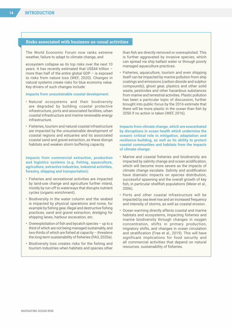
Risks associated with business-as-usual activities

The World Economic Forum now ranks extreme weather, failure to adapt to climate change, and

ecosystem collapse as its top risks over the next 10 years. It has recently estimated that US$44 trillion – more than half of the entire global GDP – is exposed to risks from nature loss (WEF, 2020). Changes in natural systems create risks for blue economy value. Key drivers of such changes include:

Impacts from unsustainable coastal development:

• Natural ecosystems and their biodiversity are degraded by building coastal protective infrastructure, ports and associated facilities, urban coastal infrastructure and marine renewable energy infrastructure.

• Fisheries, tourism and natural coastal infrastructure are impacted by the unsustainable development of coastal regions and estuaries and its associated coastal sand and gravel extraction, as these disrupt habitats and weaken storm buffering capacity.

Impacts from commercial extraction, production and logistics systems (e.g. fishing, aquaculture, agriculture, extractive industries, industrial activities, forestry, shipping and transportation):

• Fisheries and recreational activities are impacted by land-use change and agriculture further inland, mostly by run-off to waterways that disrupts nutrient cycles (organic enrichment).

• Biodiversity in the water column and the seabed is impacted by physical operations and noise, for example by fishing gear, illegal and destructive fishing practices, sand and gravel extraction, dredging for shipping lanes, harbour excavation, etc.

• Overexploitation of fish and bycatch species – up to a third of which are not being managed sustainably, and two-thirds of which are fished at capacity – threatens the long-term sustainability of fisheries (FAO, 2020a).

• Biodiversity loss creates risks for the fishing and tourism industries when habitats and species other

than fish are directly removed or overexploited. This is further aggravated by invasive species, which can spread via ship ballast water or through poorly managed aquaculture practices.

• Fisheries, aquaculture, tourism and even shipping itself can be impacted by marine pollution from ship coatings and emissions (carbon dioxide and sulphur compounds), ghost gear, plastics and other solid waste, pesticides and other hazardous substances from marine and terrestrial activities. Plastic pollution has been a particular topic of discussion, further brought into public focus by the 2016 estimate that there will be more plastic in the ocean than fish by 2050 if no action is taken (WEF, 2016).

Impacts from climate change, which are exacerbated by disruptions in ocean health which undermine the ocean’s critical role in mitigation, adaptation and resilience-building, as well as its ability to protect coastal communities and habitats from the impacts of climate change:

• Marine and coastal fisheries and biodiversity are impacted by salinity change and ocean acidification, which will become more severe as the impacts of climate change escalate. Salinity and acidification have dramatic impacts on species distribution, successful spawning and the overall growth of key fish, in particular shellfish populations (Meier et al., 2006).

• Ports and other coastal infrastructure will be impacted by sea level rise and an increased frequency and intensity of storms, as well as coastal erosion.

• Ocean warming directly affects coastal and marine habitats and ecosystems, impacting fisheries and marine biodiversity through changes in oxygen concentration, shifts in primary production, migratory shifts, and changes in ocean circulation and stratification (Free et al., 2019). This will have significant implications for food security and all commercial activities that depend on natural resources. sustainability of fisheries.


15INTRODUCTION

The potential intensity and scope of these risks, however, are still not being sufficiently considered in development and investment decisions. While mainstream finance actors have a substantial role to play in achieving a systemic shift away from these destructive activities, few are aware that the ocean is relevant to them (Fritsch, 2020). The result is that the financial system may be building up liabilities in the form of margin-diluting risks and portfolios that are exposed to stranded assets. Data, information and evidence are critical to improve decision-making. As such, new tools and approaches are needed to quantify the social and environmental risks, impacts and benefits of ocean-based projects, as well as to put in place systems and processes that will encourage transparency and traceability and support sound decision-making. This will ensure that investments are targeted in the right way, and will incentivize and spread best practice.

Such instruments should serve to manage both the risks to and the impacts on our global resources, and enable business to move beyond business-as-usual (BAU) practices, towards sustainable development pathways and a truly sustainable blue economy. This is defined by WWF and partners as one that:

• Provides social and economic benefits for current and future generations;

• Restores, protects and maintains diverse, productive and resilient marine ecosystems; and is

• Based on clean technologies, renewable energy and circular material flows.

This definition aligns with Sustainable Development Goal (SDG) 14, Life Below Water, by providing a clear reference in order to deliver a sustainable blue economy that minimizes risk and restores ocean health, thereby securing long-term environmental, social and economic resilience.

This work aims to explore the extent to which degradation in the blue economy could manifest as financial risk to asset owners and investors in a global listed universe of equities. There is increasing understanding of the financial risks arising from the increasing impacts of climate change, and of the need to deliver stronger and sustained mitigation and adaptation actions without delay to meet the objectives of the Paris Agreement, including limiting average global temperature rise to no more than 1.5°C from pre-industrial levels. Previous studies have estimated the risk to manageable assets from climate change to be US$4.2 trillion (of a total global stock of US$143 trillion of assets), rising to US$13.8 trillion with more significant warming (Economist Intelligence Unit, 2015). But the overall impact is still poorly understood at company level due to the many systemic interdependencies, feedback

loops and tipping points which translate to non-linear patterns of risk development. In this study, we have addressed such issues and provided our solution in the chapter below on ‘Why a systems thinking approach?’.

As with our atmosphere, ocean decline is noticed but not managed because oceans form part of the global commons. The ocean serves as a sink for waste and a source for over-exploitation, highlighted by the Dasgupta Review on the Economics of Biodiversity (Dasgupta, 2021). Lessons in managing the global commons must be learned, with all stakeholders recognizing the role that they must play in creating guardrails and guidelines to ensure sustainability. For global asset owners and investors, environmental considerations should be integrated into mainstream risk assessments and financial decisions. This report will highlight where such risks are, and demonstrate that a sustainable pathway can benefit all stakeholders in the value chain.

AIM OF THIS PROJECTThe current project was established to explore the extent to which environmental impacts in the blue economy result in economic risks to financial stakeholders and asset owners. While approaches exist to estimate the risk from such drivers (in particular related to the impacts from climate change) to asset value and revenues, there are some shortcomings associated with existing models in general and their application to marine sectors in particular, described in the following section. The goal of this project was to estimate the total financial Value at Risk (VaR) in the global blue economy by using a systems model approach. This represents a departure from the traditional means of assessing environmental risk by incorporating environmental modules into traditional financial risk models. The methodology aims to model the dynamics of different environmental, economic, and regulatory drivers that create risk for sector-level revenues and assets. This then enables the sector-level VaR to be calculated and translated to different company typologies, and ultimately to an index or portfolio of listed equities.

VaR is a measure of financial risk that quantifies the maximum amount of losses that a portfolio could sustain over time given a certain confidence interval. VaR is used to understand and manage the size of potential losses over an entire portfolio’s value.

Value at Risk (VaR)

16 INTRODUCTION


BACKGROUND: CURRENT VAR ASSESSMENTSA bottom-up approach starts with the impacts or drivers that influence economic activity and models the effect of shifts in the parameters of those elements on the outcome of the overall system. It is used to model the relationship between different elements in the system and how they influence each other. The result is a more fine-grained and detailed understanding of the interplay between drivers, such as environmental impacts, and economic activity in a system such as the blue economy, which also provides information necessary to take action to reduce risks. However, this approach is significantly more model- and data-intensive, and it is not always certain that the added detail also leads to increased accuracy in the risk outcomes. Despite the data requirements of this approach, it provides a lot of value in terms of exploring potential scenarios for changes in drivers and the corresponding financial risk, and as such was the chosen approach in this assessment.

VaR is a key metric for assessing the risk of an investment (Damodaran, 2007), one of the main responsibilities of asset managers. It measures how much a portfolio stands to lose over a given time period at a certain confidence level, and answers the question, “What is the maximum that an investment can expect to lose in given circumstances?” VaR therefore provides a consistent way to measure risk across different investment activities. It is a useful risk metric because it is able to express the risk to a holding or portfolio in clear dollar terms or as a percentage, making it easy to understand and interpret. Regulators such as the Bank of International Settlements recommend using it. There are essentially two conventional approaches to modeling the financial risk of environmental impacts: top-down or bottom-up (Economist Intelligence Unit, 2015). The top-down approach, which is by far the most common method, integrates relevant environmental impact data such as emissions or climate modules into a macroeconomic model. It is known as a top-down approach because it starts from the perspective of the overall economy and estimates a reduction in aggregate economic activity resulting from certain high-level parameters.


17INTRODUCTION

SLOW-BUILDING DE-ANCHORING POINT-IN-TIME

Time

Risk

Risk

Risk

Time Time

Fig.1 Some types of risks not captured in linear VaR assessments.

WHY A SYSTEMS THINKING APPROACH?These non-linear risks come in three forms: slow-building, de-anchoring, and point-in-time (see Figure 1 below). Slow-building risks are trends or events, such as climate change, which increase slowly but gain momentum over time in a non-linear fashion. De-anchoring risks materialize when technological, regulatory or socio-economic safeguards maintaining an artificial status quo are removed, resulting in spiking exposure to incumbents reliant on that risk. Petrol-powered car manufacturers are a good example of this, as a result of the sudden electric vehicle revolution. Lastly, point-in-time risks are those whereby a high-impact event is almost certain to happen at some point in the future, though it is uncertain when. Extreme sea level events are a good example of this type of risk.

In order to capture the dynamic nature of risk, a system dynamics modeling approach has been applied, where we can explore how drivers interact to create dynamic patterns of risk over time. To achieve this, we use a bottom-up approach, working with estimates of the impacts of individual drivers and development of those drivers over time. In this way, the model allows the exploration of tipping points, feedback loops and other dynamic interaction effects when evaluating risk.

In addition to understanding individual drivers, it is also important to understand how drivers interact with one another. The relationships between environmental drivers and the blue economy are dynamic. Current approaches to evaluate the associated risks, such as conventional VaR methodologies, are insufficient to account for such interactions and the cumulative effects of drivers.

There are two key disadvantages to common VaR methodologies used today. Firstly, most assume that the risk probability distribution is a ‘normal’ bell curve, and therefore underestimate the probability of extreme events and hence of the value of an asset falling below a certain threshold.

Secondly, most VaR approaches assume that risks remain relatively constant over time or that they develop in a more or less linear fashion – yet the non-linear nature of the environmental drivers that affect financial returns is exactly what this model aims to capture. Integrating environmental drivers into common financial risk models is difficult due to the short (usually five-year) time horizon to which the majority of such models are calibrated (Naqvi et al., 2017). Because of this, financial risk models will tend to miss and therefore underprice well-documented non-linear risks. Part of the reason that risk is often not linear is that it is not driven by one individual element. Instead, there are an enormous number of complex and interacting global challenges which produce synergistic or antagonistic effects.

18


APPROACH

02APPROACH

APPROACH AT A GLANCEThe project involved four main tasks. The first was to build a conceptual model of the blue economy which we aimed to capture in approach. Next was to work towards implementation of the model by collecting data and building out the logic using Stella Architect. Two scenarios were then defined for use in the model – the first a ‘business as usual’ (BAU) scenario, and the second a ‘sustainable development’ scenario. Finally, the sector-level risk identified in the system dynamics modeling was translated into financial terms by allocating these impacts across a financial index of listed companies (the outcomes could also be applied to an individual portfolio of companies). This was estimated using GICS (Global Industry Classification Standard) sector codes, to create an exposure table for companies as an estimate of the proportion of sector revenues and assets exposed to blue economy risks identified in the systems model.

System DynamicsModel Concept

Implementing the System Dynamics Model

Scenarios

Translation to theFinancial Index

19APPROACH


SECTOR SCOPE EXAMPLES OF KEY DRIVERS

Ports and shippingPort assets and shipping and port revenues

Climate change policy, climate change, tourism, fisheries, energy sector

Fisheries

Commercial and recreational fishing, seafood value chain, fishing boats

Commercial and recreational fishing efforts and methods, pollutants, habitat destruction, climate change

AquacultureMarine aquaculture/mariculture

Harmful algal blooms, disease outbreaks, demand for seafood, declining wild catch

Coastal tourismTourism revenues (asset-level data unavailable)

Coral reef and mangrove habitats, recreational fishing, climate change, pollution, beach quality

Coastal real estate and infrastructure

Coastal real estate and coastal protection infrastructure

Climate change policy, climate change, grey and green coastal protection infrastructure, tourism

Marine renewable energy

Offshore wind energy Renewable energy policy, climate change

SYSTEM DYNAMICS CONCEPTUAL MODELSector selectionThis project included six sectors of the blue economy. Key considerations determining the selection included the size and importance of the sector; the potential sector risk from environmental and regulatory drivers (i.e. the sectors most dependent on a healthy ocean to continue to

provide industry value); the level of risk posed by the sector to other sectors (where interactions would be crucial to capture); and the potential of the sector to be transformed into part of a sustainable blue economy.

The six sectors selected are described below:

20


APPROACH

Conceptual modelFollowing sector selection, research was undertaken to build out a conceptual system dynamics model. This involved a structured approach of documenting causal relationships between drivers and sectors described in scientific literature.

At the highest level of abstraction, the model has six sectors: fisheries, aquaculture, marine renewable energy, ports and shipping, coastal real estate and infrastructure, and coastal tourism. These sectors interact with one another in the model. For example, expansion of marine renewable energy could reduce port throughput, as around a third of shipped mass is fossil fuels (United Nations Conference on Trade and Development [UNCTAD], 2020).

Coastal tourism also affects the number of people who travel through ports and the amount of coastal real estate that is developed. Our model captures these types of interaction effects between sectors.

All of these sectors also affect or are affected by either chronic environmental degradation such as pollution or habitat change on the one hand, and/or by event-based damage with an associated risk factor, such as extreme sea level events caused by climate change, on the other. This means that in addition to sectors directly affecting each other, there are also indirect effects through these environmental risk elements. For example, aquaculture results in nutrient pollution, which can have a negative effect on fisheries and tourism.

Fig.2 High-level conceptual model providing a first layer of insights on the interactions between sectors

and environmental and socio-political risks. Fig. 3 provides the more detailed schematic of the relationship between sectors

COASTAL TOURISM

COAS

TAL R

EAL STATE & INFRASTRUCTURE

AQUACULTUREMARINE RENEWABLE ENERGY

FISHERIES

SHIPPING AND PORTS

Event-based damage

Chronic environmental degradation

21APPROACH


Fig.3 System dynamics model scope and interactions.

Finally, there are other socio-economic or regulatory drivers that could occur and would have cascading effects on these sectors. A socio-economic/demand driver could be for example a change in diets that increases or decreases demand for seafood. Policy drivers could include the establishment of marine protected areas or incentive structures that drive fast growth of renewable energy capacity.

The model starts out with some existing projections, such as how demand for resources might change, but more importantly these parameters allow alternative scenarios

to be modeled, for example to calculate what would happen if marine renewable energy was more aggressively expanded due to shifts in regulatory incentive structures (see the ‘Defining scenarios’ section below).

Underneath this high-level conceptual model are much greater levels of granularity. Figure 3 shows the model’s ‘modules’, which aim to capture a single dynamic. Beyond this level of detail, it becomes impossible to show the full model in one overview. To find out more about all of the parameters included, see Appendix 1: ‘Full model overview.’

Fishing boatstranded assets

Recreational fishing value

Recreationalfishing

Fishing boats& assets

Global fishstocks

Fisheriesrevenues

Fishingeffort

Fish stockloss drivers

Real estaterevenues

MRE revenue andrevenue loss

MRE capacity andcapacity loss


MRE assets and asset value loss

Seafoodproduction

Downstream seafood value chain revenues

Aquaculturelosses

Aquacultureassets

Aquaculturerevenues


Shipping tonnageexcluding fossil fuels


Shipping tonnage from fossil fuels

Portassets

Portrevenues

Real estateasset value

Greyinfrastructure

Beach quality

Mangroves

Coralreefs

Coral reefs availablefor tourism

Mangroves availablefor tourism

Numberof tourists

Tourismassets

Tourismrevenues

COASTAL TOURISM

AQUACULTURE

MARINE RENEWABLE ENERGY

FISHERIES

SHIPPING AND PORTS

COAS

TAL R

EAL ESTATE & INFRASTRUCTURE

22


APPROACH

Model gaps and exclusionsThe model encompassed close to 300 parameters. Nevertheless, it was not possible to include everything. Many elements were excluded following an assessment of the materiality of different drivers. Although there are dozens of factors that affect fisheries, a few are consistently cited as the most relevant (e.g. fishing efforts and methods, nutrient pollution, etc.): this enabled prioritization of the largest drivers.

Certain drivers that were not included in this phase provide an opportunity for further expansion of the model. Most frequently, these elements were excluded due to gaps in knowledge, usually a lack of data or formulas to quantify the relationships between elements. Often a relationship has been established between two elements, but there is not enough information available to quantify that relationship on a global scale. For example, while it is known that plastics affect fisheries, no mathematical relationship has yet been established between the amount of global plastic pollution and fish stock levels.

Finally, some other drivers were excluded on the basis that they were already implicitly included in the model, for example as an aggregated factor. A bottom-up system dynamics modeling approach allows flexibility in determining the level of granularity to go into. Given the complexity of the model, aggregated relationships and parameters were preferred where there was no dynamic element to explore. For example, nutrient pollution from aquaculture production was captured as a separate factor which is dependent on the amount of aquaculture and the share of sustainable aquaculture practices. On the other hand, nutrient pollution from all other sources (such as agriculture and sewage) was included as an aggregate factor with a fixed rate of change, since it was not possible to investigate the dynamics of how individual nutrient sources are expected to change over time.

For a summary table, followed by a more detailed explanation of the reasoning behind model gaps and exclusions, please see Appendix 2: ‘Model gaps and exclusions’.

IMPLEMENTING THE SYSTEM DYNAMICS MODELIn implementing the system dynamics model, significant amounts of information and data were needed to build the model logic in Stella Architect. It is worth noting that implementing these two steps is an iterative process – while there may be a clear idea of what needs to be achieved conceptually, data availability may necessitate setting up the model in a different way as work progresses.

For the data collection process, evidence and data were gathered through desk research and interviews with industry/subject matter experts. This was done in a transparent and collaborative way, to facilitate sharing, reviewing, and to obtain feedback from peers. Another objective was to enable the use of this data in the long term by other interested partners. Data collection took place over multiple passes, to ensure good data quality and calculations. We tried to use the most recent data available for each parameter, though many data sources were from 2018 or 2019, instead of 2020 (the baseline year considered).

Owing to the global scope of the model, finding data that was either global or could be generalized to suit a global model was a challenge. We tried to limit the model components to those parameters for which reliable data could be found that could be generalized or adjusted to fit a global scope. In case of data gaps due to a lack of global data availability, a dummy variable was used to approximate the outcomes. These were mostly only used for appreciation, depreciation, and growth rates where data was unavailable on a global level.

Data was collected in an open Google sheets format with flags on its quality, as well as documentation of references and any calculations or assumptions made. In further development of this model, the aim is to share this data with more experts for review and collaboration.

The model was built in Stella Architect (a leading system dynamics software). An overview of its core concepts is provided in Appendix 3: ‘Brief introduction to Stella and systems modeling’. The model runs for a set time period and provides output data for each parameter’s values in each year.

23APPROACH


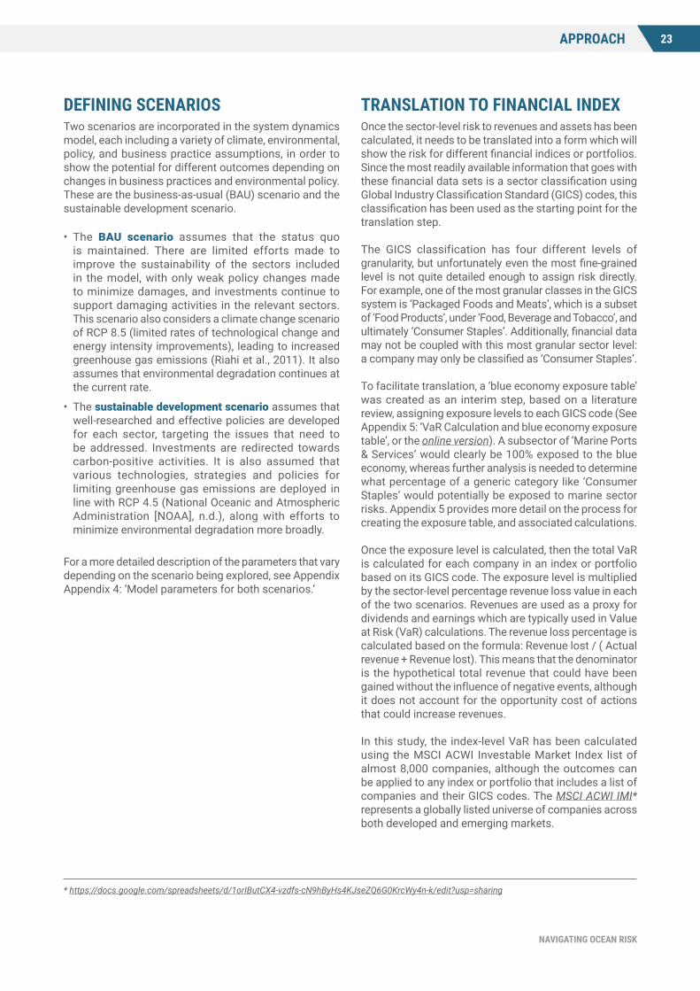
DEFINING SCENARIOSTwo scenarios are incorporated in the system dynamics model, each including a variety of climate, environmental, policy, and business practice assumptions, in order to show the potential for different outcomes depending on changes in business practices and environmental policy. These are the business-as-usual (BAU) scenario and the sustainable development scenario.

• The BAU scenario assumes that the status quo is maintained. There are limited efforts made to improve the sustainability of the sectors included in the model, with only weak policy changes made to minimize damages, and investments continue to support damaging activities in the relevant sectors. This scenario also considers a climate change scenario of RCP 8.5 (limited rates of technological change and energy intensity improvements), leading to increased greenhouse gas emissions (Riahi et al., 2011). It also assumes that environmental degradation continues at the current rate.

• The sustainable development scenario assumes that well-researched and effective policies are developed for each sector, targeting the issues that need to be addressed. Investments are redirected towards carbon-positive activities. It is also assumed that various technologies, strategies and policies for limiting greenhouse gas emissions are deployed in line with RCP 4.5 (National Oceanic and Atmospheric Administration [NOAA], n.d.), along with efforts to minimize environmental degradation more broadly.

For a more detailed description of the parameters that vary depending on the scenario being explored, see Appendix Appendix 4: ‘Model parameters for both scenarios.’

TRANSLATION TO FINANCIAL INDEXOnce the sector-level risk to revenues and assets has been calculated, it needs to be translated into a form which will show the risk for different financial indices or portfolios. Since the most readily available information that goes with these financial data sets is a sector classification using Global Industry Classification Standard (GICS) codes, this classification has been used as the starting point for the translation step.

The GICS classification has four different levels of granularity, but unfortunately even the most fine-grained level is not quite detailed enough to assign risk directly. For example, one of the most granular classes in the GICS system is ‘Packaged Foods and Meats’, which is a subset of ‘Food Products’, under ‘Food, Beverage and Tobacco’, and ultimately ‘Consumer Staples’. Additionally, financial data may not be coupled with this most granular sector level: a company may only be classified as ‘Consumer Staples’.

To facilitate translation, a ‘blue economy exposure table’ was created as an interim step, based on a literature review, assigning exposure levels to each GICS code (See Appendix 5: ‘VaR Calculation and blue economy exposure table’, or the online version). A subsector of ‘Marine Ports & Services’ would clearly be 100% exposed to the blue economy, whereas further analysis is needed to determine what percentage of a generic category like ‘Consumer Staples’ would potentially be exposed to marine sector risks. Appendix 5 provides more detail on the process for creating the exposure table, and associated calculations.

Once the exposure level is calculated, then the total VaR is calculated for each company in an index or portfolio based on its GICS code. The exposure level is multiplied by the sector-level percentage revenue loss value in each of the two scenarios. Revenues are used as a proxy for dividends and earnings which are typically used in Value at Risk (VaR) calculations. The revenue loss percentage is calculated based on the formula: Revenue lost / ( Actual revenue + Revenue lost). This means that the denominator is the hypothetical total revenue that could have been gained without the influence of negative events, although it does not account for the opportunity cost of actions that could increase revenues.

In this study, the index-level VaR has been calculated using the MSCI ACWI Investable Market Index list of almost 8,000 companies, although the outcomes can be applied to any index or portfolio that includes a list of companies and their GICS codes. The MSCI ACWI IMI* represents a globally listed universe of companies across both developed and emerging markets.

* https://docs.google.com/spreadsheets/d/1orIButCX4-vzdfs-cN9hByHs4KJseZQ6G0KrcWy4n-k/edit?usp=sharing

24 RESULTS


03RESULTS

SECTOR-LEVEL RISK OUTCOMES

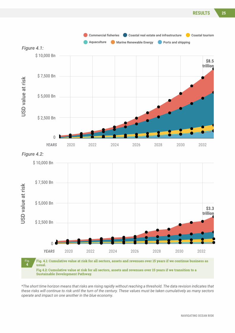
The total cumulative risk to assets and revenues over 15 years for all sectors is $8.4 trillion for the BAU scenario and $3.3 trillion for the sustainable development scenario.

The composition of this cumulative risk is shown in the next two graphs, while the following sections describe the results for each sector.

For all sectors except marine renewable energy, the absolute risk to assets and revenues is marginally or significantly reduced under a sustainable development scenario. For all sectors, the share of assets and revenues at risk decreases in the sustainable development scenario.

25RESULTS


USD

valu

e at

risk

$ 10,000 Bn

$ 7,500 Bn

$ 5,000 Bn

$ 2,500 Bn

0

2020YEARS 2022 2024 2026 2028 2030 2032



Figure 1.1:

$8.5trillion

$ 10,000 Bn

$ 7,500 Bn

$ 5,000 Bn

$ 2,500 Bn

2020YEARS 2022 2024 2026 2028 2030 2032

0

USD

valu

e at

risk



Figure 1.2:

$3.3trillion

Fig.4

Fig. 4.1: Cumulative value at risk for all sectors, assets and revenues over 15 years if we continue business as usual.Fig 4.2: Cumulative value at risk for all sectors, assets and revenues over 15 years if we transition to a Sustainable Development Pathway.

$ 10,000 Bn

$ 7,500 Bn

$ 5,000 Bn

$ 2,500 Bn

2YEARS 4 6 8 10 12 14

0

USD

valu

e at

risk



Figure 4.1:

Figure 4.2:

*The short time horizon means that risks are rising rapidly without reaching a threshold. The data revision indicates that these risks will continue to risk until the turn of the century. These values must be taken cumulatively as many sectors operate and impact on one another in the blue economy.

26 RESULTS


Ports and shipping

Ports are centres for global trade and economic activity, supporting a broad range of private industries including fishing, shipping, fuel transport, leisure and tourism (e.g. cruise liners). They also host a suite of supporting services including shipbuilding, technical and nautical services, cargo handling, logistics, energy, warehousing etc. Ports have impacts on the land, the air and the sea in the course of their full lifecycle. Most notably, dredging activities and the siting of port facilities spatially leads to substantial harm to critical habitats and biodiversity, as well as creating geophysical and hydrological changes.

Shipping carries around 80% of global trade by volume and 70% by revenue, and is still growing significantly. Container shipping was valued at around US$14 trillion in 2019, and deadweight tonnage is estimated to have grown from 11 to 275 million tonnes between 1980 and 2020 (Statista, 2020). Shipping emits various greenhouse gases and pollutants into the water and air. Most significantly, carbon-intensive heavy fuel oil (HFO) is used in 80% of marine fuel consumption, with shipping being responsible for close to a billion tonnes of carbon dioxide (CO2) emissions annually (ShareAction, 2019).The design, construction and operation of ships can also have substantial polluting impacts (diffuse and noise) on surrounding habitats, and ships can have a direct impact on marine mammals through collisions. The shipping sector is heavily regulated

through the International Maritime Organization (IMO), so regulatory risks to the sector are becoming more onerous. For example, important IMO 2020 regulations to reduce sulphur oxide (SOx) content in heavy fuel oils to below 0.5% (from current levels of 3.5%) are expected to cost container ships between US$5-30 billion annually, an increase of 20-85% (OECD, 2016b).

Ports are asset-heavy, and are therefore exposed to climate impacts such as storms and sea level rise. As major global players in the energy industry, shipping 2 billion tonnes of crude oil and 11 billion tons of goods annually (ICS, 2020), they are vulnerable to policy changes that promote low-carbon growth, alongside the economic volatility of trading goods. The shipping sector is also extremely difficult to decarbonize, which exposes it to a host of regulatory, market and reputational risks.

The assessment of the ports and shipping sector shows that while there are some risks included from oil spills and collisions, the major risk factor is from event-based damage, which is significantly reduced in the sustainable development scenario from around US$874 billion to around US$52 billion. In other words, the model predicts 15-year impact savings of US$822 billion could be realized by switching from the BAU to the sustainable development scenario. The main driver of this decrease in risk is simply the change in risk probability associated with the climate scenario, although revenues from fishery-related activities are also lower in the BAU scenario.

Fig.5 Cumulative sector-level risk comparison for the ports and shipping sector.

USD

valu

e at

risk

$ 1,000 Bn

$ 750 Bn

$ 500 Bn

$ 250 Bn

0

YEARS

Sustainable Development ScenarioBAU

2020 2022 2024 2026 20322028 2030

USD

valu

e at

risk

$ 1,000 Bn

$ 750 Bn

$ 500 Bn

$ 250 Bn

0

YEARS

Sustainable Development ScenarioBAU

2 4 6 8 1410 12

27RESULTS


Fig.6

System dynamics model components for fishing effort and balancing feedback loops, see Appendix 3: ‘Brief introduction to Stella and systems modeling’

However, this only represents part of the picture: it does not explicitly account for opportunity costs as lost revenues. In the sustainable development scenario, for example, dynamics between marine renewable energy and shipping mean that less tonnage is shipped than in the BAU scenario (Marine Renewable Energy (MRE) expansion would result in less fossil fuels being shipped, while fossil fuels currently account for a third of shipped tonnage). This means that while not considered part of sector-level risk, there is nevertheless an economic impact on the shipping and ports sector, which shows up as lower overall sector revenues.

Fisheries and aquaculture

Seafood is a highly traded natural commodity, and provides livelihoods for millions and essential protein for billions of people worldwide. FAO (2020a) estimates that around 179 million tonnes of fish from wild capture fisheries and from seafood farming (aquaculture) are produced annually, with aquaculture accounting for 46% of this total and still growing rapidly.

Overall, there are enormous pressures on wild capture fisheries, which mainly stem from fishing effort. FAO (2020a) estimates that over a third (32.4%) of marine capture fisheries are overexploited, meaning they are fished above their ability to regenerate. Sixty per cent of fisheries are at their maximum sustainable yield. Losses due to overfishing are estimated at US$83 billion/year (World Bank Group, 2017). The situation is further exacerbated by climate and environmental shocks.

In the model, fishing effort is captured in a balancing feedback loop dynamic. When overall fish stocks dip below a maximum sustainable yield (MSY) threshold value, the assumption is that this will trigger a decrease in fishing efforts. Logically, as it becomes more expensive to fish, efforts will eventually decrease (for economic reasons or because of policy levers), in principle giving stocks some time to recover. We recognize that in reality fishing subsidies make it possible to continue fishing beyond economically-viable levels, and there may be other issues (such as immediate food security) that prevent an appropriate reduction in efforts, so the decrease in fishing effort once the MSY level is reached in the BAU case is minimal.

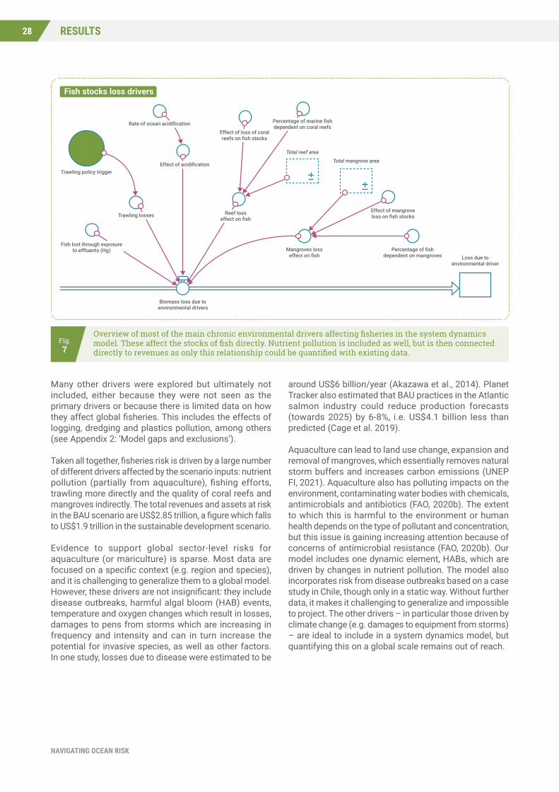
Beyond fishing efforts, there are multiple other environmental drivers that affect fisheries, from damaging fishing practices to habitat disruption or destruction, overexploitation of non-target species (bycatch), and different types of pollution. Even with much simplification, choosing the most impactful pressures became the most complex aspect of the model. The model captures dynamic elements from the loss of coral reefs and mangroves, which are critical habitats for a large share of commercial fisheries. Acidification, mercury in effluents, and trawling are not dynamic in this model, but are increasing due to existing trends. Trawling damages are, however, affected by the scenarios. An additional driver (not pictured below) is nutrient pollution: this includes both a linear effect due to anticipated increases from sources like agriculture and fossil fuels, as well as a dynamic element driven by the aquaculture sector.

Recreational fishingFishing effort

Fishing effort policy trigger


Biomass at MSY

Biomass at MSY

Globalfish mass

Globalfish mass

Wild fish commercialexploitation rate

Wild fish extractionfor recreation

Wild fish recreationalfish extraction rate



Biomass at MSY

Biomass at MSY

Globalfish mass

Globalfish mass

Wild fish commercialexploitation rate

Wild fish extractionfor recreation

Wild fish recreationalfish extraction rate

28 RESULTS


Many other drivers were explored but ultimately not included, either because they were not seen as the primary drivers or because there is limited data on how they affect global fisheries. This includes the effects of logging, dredging and plastics pollution, among others (see Appendix 2: ‘Model gaps and exclusions’).

Taken all together, fisheries risk is driven by a large number of different drivers affected by the scenario inputs: nutrient pollution (partially from aquaculture), fishing efforts, trawling more directly and the quality of coral reefs and mangroves indirectly. The total revenues and assets at risk in the BAU scenario are US$2.85 trillion, a figure which falls to US$1.9 trillion in the sustainable development scenario.

Evidence to support global sector-level risks for aquaculture (or mariculture) is sparse. Most data are focused on a specific context (e.g. region and species), and it is challenging to generalize them to a global model. However, these drivers are not insignificant: they include disease outbreaks, harmful algal bloom (HAB) events, temperature and oxygen changes which result in losses, damages to pens from storms which are increasing in frequency and intensity and can in turn increase the potential for invasive species, as well as other factors. In one study, losses due to disease were estimated to be

around US$6 billion/year (Akazawa et al., 2014). Planet Tracker also estimated that BAU practices in the Atlantic salmon industry could reduce production forecasts (towards 2025) by 6-8%, i.e. US$4.1 billion less than predicted (Cage et al. 2019).

Aquaculture can lead to land use change, expansion and removal of mangroves, which essentially removes natural storm buffers and increases carbon emissions (UNEP FI, 2021). Aquaculture also has polluting impacts on the environment, contaminating water bodies with chemicals, antimicrobials and antibiotics (FAO, 2020b). The extent to which this is harmful to the environment or human health depends on the type of pollutant and concentration, but this issue is gaining increasing attention because of concerns of antimicrobial resistance (FAO, 2020b). Our model includes one dynamic element, HABs, which are driven by changes in nutrient pollution. The model also incorporates risk from disease outbreaks based on a case study in Chile, though only in a static way. Without further data, it makes it challenging to generalize and impossible to project. The other drivers – in particular those driven by climate change (e.g. damages to equipment from storms) – are ideal to include in a system dynamics model, but quantifying this on a global scale remains out of reach.

Fig.7

Overview of most of the main chronic environmental drivers affecting fisheries in the system dynamics model. These affect the stocks of fish directly. Nutrient pollution is included as well, but is then connected directly to revenues as only this relationship could be quantified with existing data.

Fish stocks loss drivers

Trawling policy trigger

Total reef area

Total mangrove area

Trawling losses

Rate of ocean acidification

Effect of acidification

Fish lost through exposureto effluents (Hg)

Reef losseffect on fish

Effect of loss of coralreefs on fish stocks

Effect of mangroveloss on fish stocks

Percentage of fishdependent on mangroves Loss due to

environmental driver

Mangroves losseffect on fish

Percentage of marine fishdependent on coral reefs

Biomass loss due toenvironmental drivers

29RESULTS


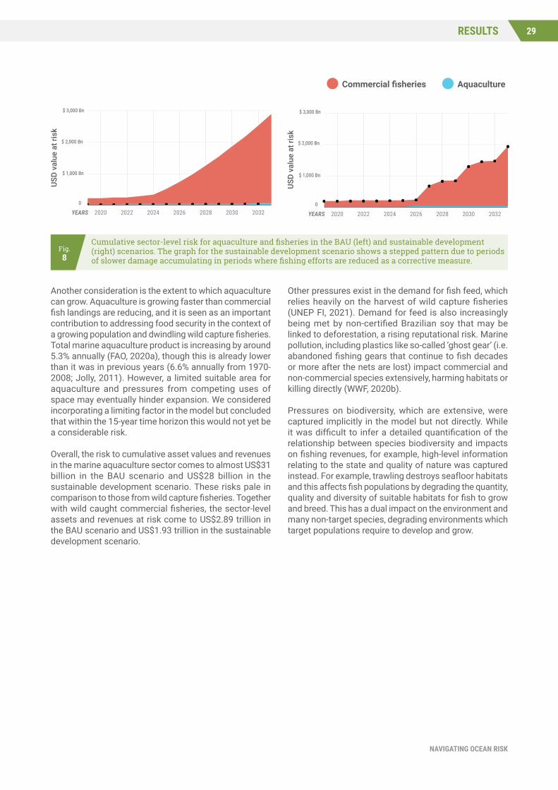
Another consideration is the extent to which aquaculture can grow. Aquaculture is growing faster than commercial fish landings are reducing, and it is seen as an important contribution to addressing food security in the context of a growing population and dwindling wild capture fisheries. Total marine aquaculture product is increasing by around 5.3% annually (FAO, 2020a), though this is already lower than it was in previous years (6.6% annually from 1970-2008; Jolly, 2011). However, a limited suitable area for aquaculture and pressures from competing uses of space may eventually hinder expansion. We considered incorporating a limiting factor in the model but concluded that within the 15-year time horizon this would not yet be a considerable risk.

Overall, the risk to cumulative asset values and revenues in the marine aquaculture sector comes to almost US$31 billion in the BAU scenario and US$28 billion in the sustainable development scenario. These risks pale in comparison to those from wild capture fisheries. Together with wild caught commercial fisheries, the sector-level assets and revenues at risk come to US$2.89 trillion in the BAU scenario and US$1.93 trillion in the sustainable development scenario.

Other pressures exist in the demand for fish feed, which relies heavily on the harvest of wild capture fisheries (UNEP FI, 2021). Demand for feed is also increasingly being met by non-certified Brazilian soy that may be linked to deforestation, a rising reputational risk. Marine pollution, including plastics like so-called ‘ghost gear’ (i.e. abandoned fishing gears that continue to fish decades or more after the nets are lost) impact commercial and non-commercial species extensively, harming habitats or killing directly (WWF, 2020b).

Pressures on biodiversity, which are extensive, were captured implicitly in the model but not directly. While it was difficult to infer a detailed quantification of the relationship between species biodiversity and impacts on fishing revenues, for example, high-level information relating to the state and quality of nature was captured instead. For example, trawling destroys seafloor habitats and this affects fish populations by degrading the quantity, quality and diversity of suitable habitats for fish to grow and breed. This has a dual impact on the environment and many non-target species, degrading environments which target populations require to develop and grow.

Fig.8

Cumulative sector-level risk for aquaculture and fisheries in the BAU (left) and sustainable development (right) scenarios. The graph for the sustainable development scenario shows a stepped pattern due to periods of slower damage accumulating in periods where fishing efforts are reduced as a corrective measure.

USD

valu

e at

risk

$ 3,000 Bn

$ 2,000 Bn

$ 1,000 Bn

0

YEARS

AquacultureCommercial fisheries

2020 2022 2024 2026 20322028 2030

USD

valu

e at

risk

0

YEARS


$ 3,000 Bn

$ 2,000 Bn

$ 1,000 Bn

2020 2022 2024 2026 20322028 2030

USD

valu

e at

risk

$ 3,000 Bn

$ 2,000 Bn

$ 1,000 Bn

0

2YEARS 4 6 8 10 12 14


30 RESULTS


Coastal tourism

Global tourism contributes about 10% of global GDP (WTTC, 2020), a substantial proportion of which is located in coastal areas. Particular economies are more dependent on tourism than others – for example, tourism can account for over 20% of GDP in small island developing states (SIDS) (Hutniczak & Delpeuch, 2018). The intactness of the local environment is a key attraction in many of these cases, although estimating the proportion of global tourism in the blue economy specifically and identifying who derives these benefits can be a challenge to capture quantitatively. However, certain studies have attempted to calculate the benefits of natural ecosystems like corals to the tourism sector, and estimate the value to be US$36 billion per year (Spalding et al., 2017).

Overall, the model shows that coastal tourism produces a financial risk of US$655 billion in the BAU scenario due to degradation of coral reefs and mangroves, increasing impacts of storms, and plastic pollution, which were the elements that could be captured quantitatively. This is reduced to an overall of US$451 billion in the sustainable development scenario as coral reefs are protected and restored, while overall sector-level revenues also increase. Taken together, the percentage of the total revenues at risk account for 5.3% of the total value in the BAU scenario and 3.7% in the sustainable development scenario. Adequate proxies to quantify the value added by tourism-related assets were missing, and revenue data was used.

Not captured in this risk is the opportunity cost of lost revenues from recreational fishing, which falls in between fisheries and coastal tourism. These revenues could grow over time, but due to decreasing fish stocks in the fisheries model, they drop from almost US$200 billion a year to less than US$50 billion a year in year 15 of the model. This comes to an additional lost value of around US$432 billion over the 15-year period.


More than 600 million people live less than 10 metres above sea level (approximately 10% of the global population), and nearly 2.4 billion people live within 100km of the coast (40% of the world’s population) (United Nations, 2017). Between 1980 and 2019, climate-related extreme events led to an estimated EUR 446 billion in economic losses in the European Economic Area alone (EEA, 2020). Urbanized, coastal populations and development rates are rising, especially in low-lying regions, as coastal areas are rich in resources and have logistical benefits (Neumann et al., 2015). Most of the world’s megacities are located in coastal zones.

The risk for coastal real estate and infrastructure is therefore unsurprisingly very high in the BaU scenario: US$3.98 trillion over the 15-year period. In the sustainable development scenario, this is reduced to US$854 billion. There are two main reasons for this large reduction. On the one hand, the actual intensity of storms is lower if we consider an RCP 4.5 scenario instead of an RCP 8.5 scenario. On the other hand, green infrastructure such as mangroves and coral reefs can buffer the impact of storms and reduce coastal real estate damages. There is also a small impact through a feedback loop: grey infrastructure erodes beach quality/width, which results in faster coastal real estate depreciation and reduced storm buffering capabilities.

Coastal real estate and infrastructure has a lower average annual asset value in the sustainable development scenario compared to that in the BAU scenario. This counterintuitive projection highlights some critical tradeoffs: 1) a more stringent carbon tax policy discourages investment in emission-intensive industries such as steel and construction, hence limits the growth in real estate assets; and 2) a sustainable scenario assumes all coastal storm protection investments are made in “green infrastructure” or “nature-based coastal protection”, thus the asset value of grey infrastructure specifically for coastal protection is zero. Nevertheless, when taken into perspective, the share of coastal real estate and infrastructure asset value loss is significantly reduced in the sustainable development scenario, due to mitigated risk and improved climate resilience. The risks to coastal real estate are also highly relevant for the insurance and reinsurance sector.

31RESULTS


Marine renewable energy

While marine renewable energy refers to a range of sources including tidal, wind, wave, solar, ocean thermal energy conversion and others, offshore wind energy is the most mature and most significant, and was included in the model. Spurred by favourable regulatory incentives, offshore wind is becoming more and more price-competitive with non-renewable energy, with lower cost volatility (UNEP FI, 2021).

As mentioned previously, marine renewable energy is the exception in that the absolute sector-level risk in the sustainable development scenario is higher than in the BAU scenario. The total risk to assets and revenues is 8.6 billion in the business-as-usual scenario and 22.8 billion in the sustainable development scenario. Marine renewable energy is currently increasing at 28% annually, which is

an extremely high growth rate. In this model, an annual growth rate of 11.5% is used for the BAU scenario (based on projections to 2050, accounting for a slowdown in expansion), while the growth rate remains at 28% for the sustainable development scenario. As this sector expands exponentially in the coming years, this will mean a higher level of overall exposure to risk from storm damages.

This outcome does not mean that the sustainable development scenario is less economically attractive. The overall value of assets and revenues for the marine renewable energy sector are three to four times higher in the sustainable development scenario, and the percentage of that value that is at risk is also lower. Additionally, the model currently calculates a very small amount of risk, both in absolute and relative terms.

32 RESULTS


Putting the sector-level risk in perspective Overall, the share of total revenues or assets at risk is relatively low in the 15-year period, which highlights the drawback of using a short time horizon: many of these risks are expected to accelerate towards the middle of the century, and a short-term perspective downplays the urgency of addressing the exponential growth of risk. For ports and shipping, as an illustration, the risk as a share of total assets is 0.48% in the 15-year period for the BAU scenario, but it starts at 0.21% and rises to 0.66% by year 15.

All the same, the potential savings between the two scenarios are not insignificant, and highlight the potential that taking action can create. The average annual risk to assets and revenues across the sectors is US$550 billion in the BAU scenario and US$221 billion in the sustainable development scenario. This comes out to total annual savings of US$303 billion in asset value damages and US$36 billion in revenue losses. These risks are also not equally spread across sectors. Notably, fisheries and coastal tourism are most at risk in the short term due to their strong dependence on a healthy ocean, and stand to lose the most.

33RESULTS


Fig.9

Scenarios compared – total cumulative revenues/revenue loss and average annual asset value and cumulative asset value loss.

TOTAL CUMULATIVE REVENUES

$ 38, 582 Bln $ 40,185 Bln

$ 17,851Bn

$ 555,8 Bn

$ 2,909 Bn

$ 11,732 Bn

$ 3,905 Bn

$ 3,233 Bn

$ 18,132 Bn

$ 141 Bn

$ 2,165 Bn

$ 11,614 Bn

$ 3,868 Bn

$ 2,662 Bn

TOTAL AVERAGE ANNUAL ASSET VALUE

$ 179,571 Bln

$ 126,899 Bln

$ 756 Bn

$ 790 Bn

$ 493 Bn

$ 109 Bn

$ 124,748 Bn

$ 2,5 Bn

$ 12,054 Bn

$ 285 Bn

$ 437,6 Bn

$ 108,6 Bn

$ 166,683 Bn

$ 2,5 Bn

TOTAL CUMULATIVE REVENUE LOSSES

$ 977 Bln$ 1,522 Bln

$ 8,3 Bn

$ 368,845

$ 489 Bn

$ 451 Bn

$ 0,21 Bn

$ 28,2 Bn

$ 8,9 Bn

$ 103,931

$ 826 Bn

$ 656 Bn

$ 0,24 Bn

$ 30,7 Bn

$ 6,883 Bln $ 2,337 Bln$ 44 Bn

23 Bn

$ 1,417 Bn

N/A

$ 854 Bn

N/A

$ 865 Bn

$ 8,6 Bn

$ 2,028 Bn

N/A

$ 3,981 Bn

N/A

TOTAL CUMULATIVE ASSET LOSSES

BAU Scenario Sustainable Development Scenario

34 RESULTS


Fig.10 Difference in the value at risk in the sustainable development scenario, compared to the business as usual

scenario, estimating potential savings over 15 years per Blue Economy sector.

$ Savings for revenues $ Savings for asset value$ 4,000 Bn

$ 3,000 Bn

$ 2,000 Bn

$ 1,000 Bn

- $ 100 Bn

0

0,5 Bn0,5 Bn821 Bn

54,734 Bn

337 Bn337 Bn

204 Bn204 Bn

612 Bn

N/AN/A

0,026 Bn0,026 Bn3,127 Bn

208 Bn208 Bn0,03 Bn

2,5 Bn2,5 Bn

- 265,000- 265,000- 14 Bn

Ports & shipping MRE Fisheries Coastal tourism Real estate & infra Aquaculture

Note: Marine Renewable Energy (MRE) has negligible savings because it is assumed that the value of this sector is 3-4 times higher in the SD scenario, lending it to greater risks than the BE scenario. Assessments of aquaculture were limited by data in this sector. Revenues for ports and shipping and real estate were not included due to data gaps.

35RESULTS


TRANSLATION TO THE MSCI ACWI IMI INDEXIn order to make truly accurate VaR estimates for a diversified equities index like the MSCI ACWI, we would need to know not only how many companies are at different levels of risk, but also the total revenues of those companies or an alternative proxy for their relative size (e.g. market cap). However, we can make an approximation if we assume all companies are equal in terms of revenues or market cap.

When making this assumption, the calculated risk to the full index from the blue economy sectors is 0.4% in the BAU scenario and 0.3% in the sustainable development scenario over the 15-year period.

Fig.11

Scenario risk distribution for the two scenarios – the number of companies in portfolio at different overall risk percentages, excluding companies with no risk.


1500

1000

500

00.00% 0.50%0.25% 0.75% 1.0%

Num

ber o

f com

pani

es in

inde

x at

risk

leve

l


1500

1000

500

00.00% 0.50%0.25% 0.75% 1.0%

Num

ber o

f com

pani

es in

inde

x at

risk

leve

l

Across the entire MSCI ACWI IMI index, there are currently over 9,000 companies, 7,796 of which were assessed in this study (based on the GICS Exposure Table, Appendix 5). When accounting for both the level of risk to specific sector-level revenues and the level of exposure of companies in the index, the total risk for an individual company ends up being low (up to around 1%).

The following figure shows the distribution of companies in the ACWI index by risk level in the two scenarios. The risk distribution for the two scenarios looks very similar, though the risk distribution in the sustainable development scenario is shifted slightly to the left.

36 RESULTS


Fig.12

Percentage of companies in the index at different levels of risk exposure (log scale), broken down by blue economy sectors.

20 %

0 - 0.0001 % 0.0001 - 0.001 % 0.001 - 0.01 % 0.01 - 0.1 % 0.1 - 1 %

15 %

10 %

5 %

0

Perc

enta

ge o

f the

inde

x

Value at Risk (log scale)

Commercial fisheries / Aquaculture

Coastal real estate and infrastructure Coastal tourism

Marine Renewable Energy Ports and shipping

BAUSD

BAUSD

BAUSD

BAUSD

BAUSD

BAU

SD

BAU

SD

BAUSD

BAUSD BAU

SD

20 %

0 - 0.0001 % 0.0001 - 0.001 % 0.001 - 0.01 % 0.01 - 0.1 % 0.1 - 1 %

15 %

10 %

5 %

0

Perc

enta

ge o

f the

inde

x

Value at Risk (log scale)

Commercial fisheries / Aquaculture

Coastal real estate and infrastructure Coastal tourism

Marine Renewable Energy Ports and shipping

BAUSD

BAUSD

BAUSD

BAUSD

BAUSD

BAU

SD

BAU

SD

BAUSD

BAUSD BAU

SD

If companies in the highest risk sectors are dispropor-tionately large this represents an underestimation, while if they are disproportionately small this could be an overestimation.

The percentage of the index that falls into different VaR buckets is shown in the following figure (log scale, VaR up to 1%). Blue economy related companies have varying levels of representations in the index. About 36.8% of the companies in the index are associated with coastal real estate and infrastructure, while the figure is 18.5% for coastal tourism, 6.52% for commercial fisheries and aquaculture, 3.25% for MRE and 1.06% for ports and shipping.

In both the BAU and sustainable development scenarios, 36.8% of the companies in the index are exposed to risks linked to the coastal real estate and infrastructure industry, albeit risk exposure is low. This is because an average exposure is estimated over these sectors, and a lack of granularity on the origin of revenues impedes more in-depth analysis of the risks per company. About half of these companies have a VaR of 0.0001-0.001%, and the other half 0.001-0.01%.

The next most highly exposed are companies associated with the coastal tourism industry, such as consumer services (hotels, cruises, restaurants), retail and transportation. In the BAU scenario, most of the tourism-related companies have a VaR between 0.01-0.1%, while the sustainable development scenario, with stricter climate and plastic pollution policies, could reduce this risk level to 0.001-0.01% for some of the companies.

Although commercial fisheries and aquaculture represent a relatively small percentage of the index (6.52%), companies affiliated with fisheries and aquaculture are faced with a higher VaR, compared to that in other blue economy sectors. However, by switching to sustainable aquaculture and implementing more stringent fishing policies, most of the VaR could be reduced from 0.1-1% to 0.01-0.1%.

Companies in the marine renewable energy and ports and shipping industries have relatively lower VaR, which may be due to the low risk profile of these industries, but can also partly be explained by their limited representation in the index.

37RESULTS


MODEL LIMITATIONS AND NEXT STEPSScope and limitations of the current approachMaterial risks assessed separately to impacts: Although we have outlined some of the extensive impacts that these sectors have on the natural world, this model limits the scope to drivers that have an impact on the selected blue economy sectors and relevant downstream sectors (e.g. commercial fisheries, but also food retail). The blue economy sectors themselves have an impact on the broader economy, which is not captured in the model. This includes some regulating ecosystem services like carbon storage and climate regulation; but economic risk driven by blue economy sectors that do not ultimately affect blue economy sectors is excluded. It will be possible in the future to include more ecosystem services related to ocean health.

Gaps in data and knowledge on global relationships. There are still many gaps in information that could be fed into the model. These gaps are widespread, not only in terms of scientific data or case studies, but more importantly in terms of equations/relationships between different elements. For example, we have data on how different climate change scenarios will affect average marine oxygen levels, and we may have information on how oxygen levels affect fish species in one region, but we lack information about how a relative change in global oxygen levels would affect global fish stocks and landings. The full list of model gaps is given in Appendix 2: ‘Model gaps and exclusions’. This is a critical shortcoming of almost all assessments related to materiality, and is a factor in a number of issues in data transparency. Aggregated data, more commonly published by governments and international organizations, is more often public and more likely to be targeted towards policymakers. However, it may not be useful for interpretation by the private sector except in the case of, for example, large regional investors or sovereign debt investors. Disaggregated data is more useful for decision-making in the private sector, but is not commonly in the public domain.

The use of GICS codes for financial allocation. GICS codes typically reflect the most information known about companies within an index or portfolio, so it makes sense to build a model that can use them. However, GICS codes are not granular enough to differentiate companies truly specialized in the blue economy. Additionally, there are some discrepancies in how companies are classified, which may be a shortcoming of the sector classification approach. For example, while marine renewable energy (MRE) companies should technically be classified as “Utilities”, we noticed MRE companies in the index under “Energy” (which only includes oil and gas) and “Industrials”, in addition to “Utilities”.

Companies assessed within the MSCI ACWI IMI. Whether the sector-level outcomes are applied to an index or a portfolio, there are some shortcomings in what the outcomes can tell us. For example, the choice of using the MSCI ACWI index means the model has only been applied to listed equities, while it is possible that VaR is higher for non-listed companies. For example, more than half of the top 100 seafood companies are privately owned (Undercurrent News, 2019).

Further model developmentCompared to the initial pilot study in the Baltic Sea, this assessment has made some important improvements, which include:

• Modeling six instead of two sectors, which provides a more complete picture of risk.

• Including sector interactions, which provide interesting insights and a more realistic picture of risk.

• Eliminating complexities due to different spatial scales and spatial interaction effects. For example, if a company has a global portfolio, but the VaR is being calculated for a specific region, it is important to understand how the region interacts with a global market. If a fish stock collapses in one region it will have an enormous impact on the local economy, but it might not affect global seafood retail if another region can make up for the shortfall.

• Many additional drivers were included in this iteration of the model, and a lot of effort went into understanding which would be the most appropriate to use.

At the same time, this model is still not a perfect or complete representation of the global blue economy and its critical drivers, as described in the previous section. Key steps we would propose for improving the model in a future iteration include the following:

Including more global/generalized data. A lot of data is available that could be applied to the model with significant additional processing. The only large data set used in this model was the RAM Legacy Stock Assessment database, which has data for more than 1,000 stocks of fish globally. While this data set does not cover all commercially fished species, it provides enough coverage to use in making generalizations. With some further work, other large data sets like this one could ultimately be processed to generate aggregated global data and relationships.

Collaboration for further development. A lot of other organizations are working on related topics around blue economy value and risk. This creates an opportunity for collaboration in further development of the model. At the same time, we can bring the modeling expertise and synthesis to help organize and explore complexities that experts in the field may have trouble getting oversight on.

38 RESULTS


Need for collaborative review. We have prioritized our efforts on what we deemed the most relevant drivers and spent time on extra scrutiny of model components which we felt were most significant. However, the model could easily be expanded and improved through expert review. In particular, we would recommend iterations of review with a collaborative network to build out the complexity and robustness of the model.

Translating to a regional approach to vet outcomes and building more capacity for identifying and evaluating interventions. Part of the drive for creating a global model was to build a more generalized approach that we could deepen in regional assessments. However, we also recognize that neither risk nor company activities are evenly distributed across regions. One important next step would be to regionalize our model in one or more case studies to vet our approach and outcomes when applied at a regional scale. This approach would also allow us to evaluate more granular marine management and planning measures.

Using this model for risk assessmentThe results from this model are not intended to dictate investment decisions at this stage. Rather, it is meant to provide a proof of concept to demonstrate that a systems modelling approach can be used to better capture how environmental risk can transpire materially to businesses and their financiers and provide insights to understand exposure to high-impact sectors. Such an approach can be applied to an individual portfolio where a much more granular assessment of risk is possible, as was originally carried out for Value at Risk in the Baltic sea, with a regional asset owner, albeit for a smaller portfolio and number of sectors.

The model provides a blueprint to capture quantitative environmental risks in a systematic way and map interdependencies between sectors across a financial portfolio. It can enable asset owners, asset managers, fund managers and even financial regulators to better understand risk and the opportunities for taking action in different scenarios, especially if further development of the model focuses more on potential interventions. The method provides a clear alternative for many of the parameters in the BAU scenario – and shows how, taken holistically, such actions can lead to a huge reduction in potential risks.

For example, how does an aquaculture company avoid mangrove deforestation and mitigate its exposure to nutrient pollution, and how would this affect overall risk when combined with other changes taking place? The recently released Turning the Tide report (UNEP, 2021) provides an excellent framework to help financial institutions understand risk materiality to different blue economy sectors, but they still need a tool to explore the potential impact of taking action in order to understand where to focus their efforts. This is where our approach can come into play. The VaR tool can help to provide a means to measure how such actions can translate into risk mitigation and impact on assets and revenues.

Beyond engaging with companies on their portfolios, financial institutions also need to engage with shareholders and the broader public on the topic of environmental impacts. An increasing number of private and institutional investors are using proxy voting, shareholder resolutions and other methods to support good stewardship, and are holding laggards accountable to ESG standards. Investors should be looking for innovations and more holistic risk assessment methods that can also enable transformative change in business practice. Portfolios should have an intentional mix of investments for collective direction-setting and to enable more sustainable utilization of marine resources and services. Our model can fill a gap in terms of this type of engagement.

Finally, in addition to engaging investors from the perspective of risk, it is also important to point out the tremendous investment opportunities in sustainable ocean innovations, even though this is beyond the current scope of our model. For instance, marine protected areas can regenerate habitats in seven years, tripling investment returns. Nature-based solutions, such as mangrove restoration, have been proven to be five times more cost-effective than concrete coastal armouring. The commercial seaweed market is forecasted to grow at a compound annual growth rate of 9.1%, and has the potential to replace virgin plastics and make the aquaculture industry carbon-neutral. In fact, Credit Suisse reported that over a third of large institutional investors rank a sustainable blue economy as one of the most important investment topics – but it remains one of the least invested themes across investors, possibly because it is less well understood. Both understanding the implications of existing financing in marine sectors as well as opportunities for investing in new innovations would enable decision-making that helps redirect an unsustainable blue economy into a sustainable blue economy.

39RESULTS


What next?The assessment covered more than 300 parameters and incorporated strong scientific information on impacts and risks to the ocean from and to blue economy business and ecosystems. However, the full quantification of such risks at scale is challenging (see Appendix: ‘Gaps and exclusions’), and the values are still likely to be conservative. While the systems approach is able to capture some of these interdependencies between sectors that are often overlooked in linear risk assessments, the current scope of the model still only covers direct blue economy sectors and companies listed in the MSCI ACWI IMI.

Regional and sectoral concentration and specialization is common in the blue economy. Around 82% of the marine shipping industry is dominated by only 10 major container shipowners (UNCTAD, 2019); 50% of the shipbuilding market is concentrated in China (Bureau Veritas, 2020); the world’s top 50 ports control 70% of the global container

business (IAPH, 2018); and 13 seafood companies dominate 40% of the world’s largest commercial fisheries (Osterblom et al., 2015). As environmental risk is often linked to a biome, region, activity or supply chain, incorporating regional-level assessments or portfolio-level assessments will likely enable better coverage of environmental risk.

Global trade is focussed in coastal regions, and disruptions to operations can ripple across a broader range of industries and their supply chains. In the next phases, the model should therefore look at sectors and supply chains beyond the blue economy. As equity is not necessarily the primary instrument for investment in many of these sectors (for example, direct lending from banks and governments may be more common instruments for shipping (Maritime London, 2020), ports and fisheries), the model may be extended to a wider range of financial instruments to better capture different levels of risk.

40 CONCLUSIONS


04CONCLUSIONS

REFLECTION ON THE OUTCOMESThis assessment shows that at least two-thirds of listed companies within the MSCI ACWI IMI Index have a degree of dependency on the blue economy, and therefore on a healthy ocean. The study has revealed that substantial risk reduction could be realized in the blue economy under a sustainable development scenario compared to a BAU scenario: an estimated US$8.4 trillion worth of assets and revenues are at risk under BAU in the coming 15 years, with the amount increasing exponentially over time. Sectors most dependent on a healthy ocean, such as fisheries and coastal tourism, have the most to lose as a share of total sector value. Other growing sectors such as ports and shipping, coastal real estate and infrastructure, and marine renewable energy, will be increasingly exposed to risks due to climate change.

Overall, achieving the sustainable development scenario would lead to a significant decrease in overall risk in absolute terms – this model estimates hundreds of billions of US dollars on an annual basis. Businesses and the financial sector therefore have a clear economic rationale to pursue strategies to reduce their impacts on the ocean and to manage resources effectively. However, businesses may also be affected by the damaging activities of others. This points to a clear economic incentive for regulators to implement ecosystem-based Marine Spatial Planning and resilience-building approaches, as well as incentivize best practice and circular economy approaches, to ensure that environmental safeguards are in place and are regulated.

Companies can reduce their risks by applying appropriate mitigation strategies, but also by reducing their impact on the environment and atmosphere. Net-zero strategies and alignment with the IPCC recommendations to keep global warming to less than 1.5°C above pre-industrial levels are an essential starting point for governments, businesses and the financial sector. Addressing the climate crisis has been extensively identified to be critical to managing impacts on the blue economy and safeguarding natural resources (Diz et al., 2021; IPCC, 2019; FAO, 2020a; IPBES, 2019). But the scope of current financial risk assessments must expand beyond climate if better risk-adjusted investment decisions are to be made. Such considerations will become ever more important as we see a shift to a ‘new normal’ over the course of this century.

41CONCLUSIONS


This study provides a methodology that could be used to test VaR and the implications of potential financial, corporate and policy risk mitigation efforts. It demonstrates the value of safeguarding environmental resources in a holistic sense, and presents future scenarios that can help to inform a pathway for action. Such a tool, when used in conjunction with other existing resources such as the Sustainable Blue Economy Finance Principles and UNEP FI’s recently published guidance in its Turning the Tide report (UNEP, 2021), can help to effectively inform investors how to act in the face of such impacts and risks.

The sustainable blue economy offers many opportunities, if the diversity, productivity, resilience, core functions and intrinsic value of marine ecosystems are sustainably managed. In order to do so, we need to consider the aggregate value of all capital assets. Calculation of a value contribution of ecosystems into economic activity (both production and consumption) is needed, and would enable ecosystem service accounts to be used to manage the ocean – this is something most governments have yet to do. This study has estimated savings of more than US$5 trillion in the sustainable development scenario compared to the BAU scenario. With ocean-based development set to double over the coming decade, it is critical that policy and investment are leveraged and directed to enable ocean-based sectors to transition towards sustainability, as well as to seek out those ocean-based businesses that contribute to the delivery of a sustainable blue economy. Divestment is recommended for business activities that lead to significant harm to marine ecosystems, are illegal or which contravene legislation.

Damaging BAU practices are exposing the investment sector to increasing risks, which, cumulatively, can lead to irreversible tipping points. Tipping points – where small, accumulating changes lead to a wider systemic impact in an ecosystem – have significant implications for coastal communities and the wider economy.

It is therefore critical that financial institutions recognize the significant role they can play in ensuring a sustainable development scenario plays out. While resources are increasingly becoming available, more work is needed to price these risks and ensure that investors are asking the correct questions to companies exposed to such risks. Data providers have a key role to play in collating such data and applying new risk-based tools to their company assessments. Asset owners should ensure that those managing their investments are aware of the risks related to the blue economy and are asking relevant questions to stakeholders. Companies with market dominance and regional or sectoral exposure should be transparently demonstrating greater risk and impact awareness. And regulators and policymakers should be aware that changes in the real economy that harm or hinder the blue economy can have broader impacts on the investment community. Integrating environmental considerations into decision-making, engaging stakeholders and joining multi-partner collaborations, is a pathway to overcome information barriers in this sector.

It is important to consider the context when translating sector-level risks to a global index that is not specialized in marine sectors, and in the absence of a globally agreed blue taxonomy. Most significantly, this value does not include the VaR for stocks that are linked to natural capital but are not directly ocean-related. Thus, it is likely that this study presents a conservative estimate of the VaR in the BAU scenario. Nevertheless, the methodology presents an estimate of the extent to which better business practices, incentivized through collaboration and with strong policy measures, can reduce risk to ocean-related assets in the medium term. It also demonstrates a clear pathway to sustainable business practice and its systemic benefits. Investors and policymakers should therefore consider the issues outlined in this report now, rather than delaying action.

42 CONCLUSIONS


The Sustainable Blue Economy Finance Principles

In 2018, WWF joined the European Commission, the European Investment Bank (EIB), and the Prince of Wales’ International Sustainability Unit to develop and launch the Sustainable Blue Economy Finance Principles. These 14 Principles provide the first global framework to guide investment decisions and development policy towards the most sustainable pathways possible, ensuring that ocean-related investment delivers long-term value without having a negative impact on marine ecosystems, on efforts to reduce carbon emissions, or on the revenue streams of ocean-based businesses of all sizes and the livelihoods of people who depend on them.

As such, they are designed to align with the Sustainable Development Goals, in particular Life Below Water (SDG14), and complement existing frameworks for governing responsible investment (such as the Equator Principles and UN PRI). By fostering cooperation and communication on everything from ocean health and scientific research to data collection and technical innovation, the Principles aim to encourage a multi-sector shift towards a sustainable blue economy.

They are intended to be taken as a collective whole rather than pursued individually, and in that way they recognize that the ocean context requires a systems-based

approach. They also recognize the need to address some of the governance challenges associated with the ocean, and that we already have many of the necessary tools and approaches to build ocean resilience and improve long-term investment opportunities. As such they point to the need to shift away from viewing ocean protection and restoration as being ‘nice-to-have’ to that of being central to securing national economies and business in the long term.

They also recognize the importance of compliance, transparency and disclosure, and while they are voluntary and non-regulatory, widespread adoption of the Principles could transform future development – showing how profitability must go hand-in-hand with environmental and social stewardship.

They are now the guiding framework of UNEP FI’s newly formed Sustainable Blue Economy Finance Initiative. As of June 2021, there are over 50 signatories to the Principles and 64 members of the Initiative, including both public and private sector partners such as the World Bank, EIB and the Asian Development Bank, Aviva Investors, Rockefeller Asset Management and Storebrand. The private sector membership currently represents assets under management of US$6.9 trillion.

RECOMMENDATIONSThe ocean is not at present governed in a way that safeguards the natural capital upon which our societies and economies depend. If we are to secure a sustainable blue economy we need to transition to a net zero, nature positive, inclusive and circular global economy that follows a sustainable development scenario. For this to happen, all stakeholders in the blue economy have a role to play. Most critical to the equation, however, are asset owners with stakes in the blue economy. Asset owners and their asset managers should adopt the following recommendations to address some of the key data and policy challenges that have been highlighted in this study.

(1) Adopt and implement the Sustainable Blue Economy Finance Principles and associated guidance into decision-making frameworks and approaches. As mentioned above, the Principles offer an overarching framework and guidance to support decision-making and ensure that investments are directed at the opportunities that contribute to the delivery of a sustainable blue economy. Supporting guidance, Turning the Tide (UNEP, 2021),

provides detailed criteria for five blue economy sectors – seafood, ports, shipping, coastal and marine tourism, and marine renewable energy – and provides recommended actions based on a suite of criteria and indicators relating to each of these sectors. These are:

• Seek out – where an indicator denotes current best practice on a particular issue and where financing is encouraged.

• Challenge – where financial institutions are recommended to address a specific issue highlighted by an indicator, for example through engagement with a company or project developer.

• Avoid – where it is recommended financial institutions divest from and do not provide financing due to the severity of a given indicator.

By joining the Sustainable Blue Economy Finance Initiative financial institutions will be able to seek information and support on the use of the guidance.

43CONCLUSIONS


(2) Integrate environmental considerations into mainstream risk assessments. Climate risks are now increasingly recognized as financial risks, although decades of evidence gathered by the scientific community should have prompted this movement much earlier. Asset managers and investors must address impacts that cause risks to materialize across the blue economy, ensuring that information is sought out and that companies are challenged where there is a potential failure to mitigate environmental risks and impacts. Where a company has shown no efforts to mitigate such risks, avoid continuing to finance such activities. Rather identify and incentivize those that have taken a long-term risk management perspective and are taking action to mitigate their risks and safeguard natural resources.

(3) Seek and pilot risk-based models and approaches to inform decisions towards sustainable development pathways. This model offers an important methodology for assessing complex risks across the global blue economy, but it needs further resourcing and development and to be complemented by regional ‘deep dives’ that demonstrate the variability of environmental change at a local level. It is recommended that investors work collaboratively with WWF and others across the scientific, public sector and NGO community to develop, pilot and use innovative approaches to risk analysis, with a view to better understanding the material risks of BAU and to create the knowledge and tools needed to support sound decision-making. For example, WWF is a member of the Ocean Risk and Resilience Action Alliance (ORRAA), a multi-stakeholder initiative to develop and scale finance and insurance products that incentivize investment in nature and provide returns for investors. ORRAA’s goals are to drive US$500 million of investment into marine and coastal nature-based solutions by 2030, and to surface at least 15 novel finance products by 2025.

(4) Encourage and implement transparency and disclosure as a priority. Continuously assessing and reporting on material risks, at company level and throughout supply chains, will substantially strengthen information and understanding relating to these risks, and will further support the transition to best practice. It is therefore important to co-develop and use frameworks and metrics that encourage consistent reporting – such as the newly launched v. UNEP FI is also in the process of developing an accountability framework for the Sustainable Blue Economy Finance Principles. In addition, it is important to make transparency integral to investment criteria to ensure traceability is inherent across the investment and throughout supply chains. This can also allow a more accurate assessment of links to supply-chain carbon emissions, which is imperative for climate reporting and regulation.

(5) Drive the creation of credible science-based information sources that better inform investors on the risks of unsustainable BAU activities, guide best practice, and assess how progress is being achieved. Credible, science-based risk assessments need to be applied from the bottom up, disaggregating scientific data to understand the impacts on the real economy. Company targets and metrics to mitigate such risks should also be science-based and robust. Although this industry is changing swiftly, with investors demanding more stringent and granular information, current ESG-related risk assessments have several limitations when it comes to enabling investors to understand the degree of environmental and social risks that could impact a company. Current industry classification systems, even those at sub-industry level, lack sufficient asset-level data to assess environmental and supply chain risks where in proximity to at-risk natural areas. This is particularly true of the ocean given its interconnected nature. It is therefore important to encourage greater levels of granularity in order to clearly distinguish blue economy sectors. It is also important to consider how to act in data-poor situations. The precautionary principle should apply to investment decisions that could be exposed to environmental risks, ensuring that activities do no significant harm before proceeding with development.

A taxonomy of activity-level information of what is sustainable (‘blue’), transition (‘amber’) and unsustainable (‘red’) is needed to differentiate best practice and incentivize companies: this has been started with the development of different regional ‘green’ and ‘blue’ financial taxonomies. Such assessments are currently focussed on climate risks – however, this model evidences a suite of other environmental factors that may impact companies in the future and that should be considered for advanced assessments.

(6) Proactively influence the enabling environment to further de-risk investments. Financial institutions should recognize the significant positive influence that they can have on banking authority policy and public sector policy, and encourage stronger regulation, governance and incentives for companies that will support best practice, environmental reporting and due diligence. This will enable investors to better understand and manage environmental risks, and increase the flow of investment into the sustainable blue economy while disincentivizing unsustainable practices.


44

BIBLIOGRAPHY

45


1. Accenture. 2017. Principles for sustainable investment in the blue economy. Retrieved from https://ec.europa.eu/maritimeaffairs/sites/maritimeaffairs/files/principles-sustainable-investment-in-blue-economy-report_en.pdf

2. Akazawa, N., Alvial, A., Blanc, P., Burgos, J., Chamberlain, G., Forster, J., Hoang, T., Ibarra, R., Khoa, L., Kibenge, F. et al. 2014. Reducing disease risk in aquaculture. World Bank Report Number 88257-GLB. 10.13140/RG.2.1.4525.5529.

3. Alizadeh, A.H., and Nomikos, N.K. 2009. Value-at-Risk in Shipping and Freight Risk Management. In: Shipping Derivatives and Risk Management (pp. 303–337). Palgrave Macmillan UK. doi.org/10.1057/9780230235809_9

4. Anneboina, L.R., & Kavi Kumar, K.S. 2017. Economic analysis of mangrove and marine fishery linkages in India. Ecosystem Services, 24, 114–123. doi.org/10.1016/j.ecoser.2017.02.004

5. Aranda, M., Ulrich, C., Le Gallic, B., Borges, L., Metz, S., Prezello, R. and M. Santurtún. 2019. Research for PECH Committee — EU fisheries policy – latest developments and future challenges. Brussels. Retrieved from www.europarl.europa.eu/RegData/etudes/STUD/2019/629202/IPOL_STU(2019)629202_EN.pdf

6. Arthur, J.R., Bondad-Reantaso, M.G., Campbell, M.L., Hewitt, C.L., Phillips, M.J. and R.P. Subasinghe. 2009. Understanding and applying risk analysis in aquaculture – A manual for decision-makers. Retrieved from www.fao.org/3/i1136e/i1136e.pdf

7. Attrill, M., Godley, B.J., Thompson, R., Truebano, M., Bicknell, A., Votier, S. and R. Inger. 2012. Marine Renewables, Biodiversity and Fisheries. Retrieved from https://tethys.pnnl.gov/sites/default/files/publications/marine_renewables_biodiver.pdf

8. Baldauf, M., Garlappi, L., Yannelis, C., Beaudry, P., Berk, J., Fisher, A. and L. Bretz. 2019. Does Climate Change Affect Real Estate Prices? Only If You Believe In It *.

9. Barbier, E.B. 2015. Valuing the storm protection service of estuarine and coastal ecosystems. Ecosystem Services, 11, 32–38. doi.org/10.1016/j.ecoser.2014.06.010

10. Barnard, A. 2020. The $119 Billion Sea Wall That Could Defend New York … or Not. The New York Times. Retrieved from www.nytimes.com/2020/01/17/nyregion/sea-wall-nyc.html

11. Bassi, A.M., Pallaske, G., Wuennenberg, L., Graces, L. and L. Silber. 2019. Sustainable Asset Valuation Tool – Natural Infrastructure. Retrieved from www.iisd.org/publications/sustainable-asset-valuation-tool-natural-infrastructure

12. Beck, M.W., Losada, I.J., Menéndez, P., Reguero, B.G., Díaz-Simal, P. and F. Fernández. 2018. The global flood protection savings provided by coral reefs. doi.org/10.1038/s41467-018-04568-z

13. Bennett, N.J., Blythe, J., White, C. and C. Campero. 2020. Blue Growth and Blue Justice. Marine Policy.

14. Bennington-Castro, J. 2017. Walls Won’t Save Our Cities From Rising Seas. Here’s What Will. NBC News. Retrieved from www.nbcnews.com/mach/science/walls-won-t-save-our-cities-rising-seas-here-s-ncna786811

15. Bentley, J.W., Serpetti, N., Fox, C.J., Heymans, J.J. and D.G. Reid. 2020. Retrospective analysis of the influence of environmental drivers on commercial stocks and fishing opportunities in the Irish Sea. Fisheries Oceanography, 29(5), 415–435. doi.org/10.1111/fog.12486

16. Bosma, R.H., Debrot, D., Rejeki, S., Tonneijck, F., Yuniati, W. and W. Sihombing. 2020. Associated Mangrove Aquaculture Farms; Building with Nature to restore eroding tropical muddy coasts. Retrieved from www.wetlands.org/publications/technical-guidelines-associated-mangrove-aquaculture-farms/

17. Boteler, B., Grünig, M., Lago, M., Iglesias-Campos, A., Reker, J. and A. Meiner. 2014. European maritime transport and port activities: identifying policy gaps towards reducing environmental impacts of socio-economic activities. Retrieved from www.ecologic.eu/sites/default/files/presentation/2014/european-maritime-transport-and-port-activities_0.pdf

18. Braathen, N.A. 2011. Environmental impacts of international shipping: The role of ports. (Vol. 9789264097339). Organisation for Economic Cooperation and Development (OECD). doi.org/10.1787/9789264097339-en

19. Brucal, A. and Lynham, J. 2021. Coastal armoring and sinking property values: the case of seawalls in California. Environmental Economics and Policy Studies, 23(1), 55–77. doi.org/10.1007/s10018-020-00278-3

20. Buchana, P. and McSharry, P. E. 2019. Windstorm risk assessment for offshore wind farms in the North Sea. Wind Energy, 22(9), 1219–1229. doi.org/10.1002/we.2351

21. Building and Construction Authority, Singapore Government. 2016. Construction Costs for Different Types of Development. Retrieved from www.bca.gov.sg/Infonet/others/dls.pdf

22. Cacho, O.J. 1997. Systems modelling and bioeconomic modelling in aquaculture. Aquaculture Economics and Management, 1(1–2), 45–64. doi.org/10.1080/13657309709380202

23. Cage, A., McLuckie, M., Thoumi, G., Baldock, C. and N. Sukh. 2019. Briefing: Salmon Feels the Heat. Planet Tracker.

24. Cleary, P., Harding, W., Mcdaniels, J., Svoronos, J.-P. and J. Yong. 2019. Turning up the heat – climate risk assessment in the insurance sector. Retrieved from www.bis.org/fsi/publ/insights20.pdf

25. Costanza, R. and Farley, J. 2007. Ecological economics of coastal disasters: Introduction to the special issue. doi.org/10.1016/j.ecolecon.2007.03.002

26. Credit Suisse. 2020. Investors and the blue economy. Retrieved from www.esg-data.com/blue-economy


46

27. Crossland, C.J., Baird, D., Ducrotoy, J.-P., Lindeboom, H., Buddemeier, R. W., Dennison, W. C. and D. P. Swaney. 2005. The Coastal Zone — a Domain of Global Interactions (pp. 1–37). doi.org/10.1007/3-540-27851-6_1

28. Dahl, R. E. 2017. A study on price volatility in the aquaculture market using value-at-Risk (VaR). Aquaculture Economics and Management, 21(1), 125–143. doi.org/10.1080/13657305.2017.1262475

29. Dalsøren, S.B., Eide, M.S., Endresen, Ø., Mjelde, A., Gravir, G. and I.S.A. Isaksen. 2009. Update on emissions and environmental impacts from the international fleet of ships: the contribution from major ship types and ports. Atmospheric Chemistry and Physics, 9, 2171–2194. Retrieved from www.atmos-chem-phys.net/9/2171/2009/

30. Dasgupta, P. 2021. The Economics of Biodiversity: The Dasgupta Review. Abridged Version. London: HM Treasury.

31. Davies, A. 2020. Wamberal beach erosion: seawall would deliver no net benefit, study finds. The Guardian. Retrieved from www.theguardian.com/environment/2020/jul/27/nsw-coastal-councils-face-dilemma-over-land-erosion-and-who-should-pay-for-building-seawalls

32. Diz, D., Merriman, P., De Vos, K., Sommerkorn, M. and S. Walmsley. 2021. Blueprint for a Living Planet: Four Principles for Integrated Ocean-Climate Strategies. WWF International, Gland, Switzerland. Accessed: wwfeu.awsassets.panda.org/downloads/wwf_blueprint_for_a_living_planet_2021.pdf

33. Dorn, M.W. and Zador, S.G. 2020. A risk table to address concerns external to stock assessments when developing fisheries harvest recommendations. Ecosystem Health and Sustainability, 6(1), 1813634. doi.org/10.1080/20964129.2020.1813634

34. Dowling, N.A., Dichmont, C.M., Venables, W., Smith, A.D.M., Smith, D.C., Power, D. and D. Galeano, D. 2013. From low- to high-value fisheries: Is it possible to quantify the trade-off between management cost, risk and catch? Marine Policy, 40(1), 41–52. doi.org/10.1016/j.marpol.2012.12.009

35. Earth Security. 2020. Financing the Earth’s Assets: the Case for Mangroves As a Nature-Based Climate Solution. Retrieved from www.sustainablefinance.hsbc.com/carbon-transition/financing-the-earths-assets

36. EU Commission. 2009. Review of the EU Aquaculture Sector and Results of Costs and Earnings Survey.

37. European Environment Agency. 2018. Marine environmental pressures. Retrieved from www.eea.europa.eu/themes/water/europes-seas-and-coasts/marine-environmental-pressures

38. European Environmental Agency (EEA). 2020. Indicator assessment on economic losses from environmental extremes in Europe. Available: www.eea.europa.eu/data-and-maps/indicators/direct-losses-from-weather-disasters-4/assessment.

39. European Fisheries Control Agency. 2018. Guidelines on Risk Assessment Methodology on Fisheries Compliance. Retrieved from https://www.efca.europa.eu/sites/default/files/Risk%20Assessment%20Methodology.pdf

40. Food and Agriculture Organization of the United Nations (FAO). 2020a. The State of World Fisheries and Aquaculture 2020. Retrieved from www.fao.org/3/ca9229en/ca9229en.pdf

41. Food and Agriculture Organization of the United Nations (FAO). 2020b. Understanding Antimicrobial Resistance in Aquaculture. Asian Fisheries Society. Asian Fisheries Science 33.S1. Accessed: http://www.fao.org/3/cb2601en/cb2601en.pdf

42. FAO. 2019. FAO’s work on climate change – Fisheries & aquaculture.

43. Fay, G., Link, J.S. and J.A. Hare. 2017. Assessing the effects of ocean acidification in the Northeast US using an end-to-end marine ecosystem model. Ecological Modelling, 347(September 2018), 1–10. doi.org/10.1016/j.ecolmodel.2016.12.016

44. Food and Agriculture Organization of the United Nations. 2018. Impacts of climate change on fisheries and aquaculture: synthesis of current knowledge, adaptation and mitigation options. Retrieved from www.fao.org/3/i9705en/I9705EN.pdf

45. Food and Agriculture Organization of the United Nations. 2019. FAO’s work on climate change – Fisheries & aquaculture 2019. Retrieved from www.fao.org/3/ca7166en/ca7166en.pdf

46. Food and Agriculture Organization of the United Nations (FAO). 1992. Cost-benefit Analysis of Individual Fish Farms and Fry Production Centers.

47. Food and Agriculture Organization of the United Nations (FAO). 2017. The role of Recreational Fisheries in the sustainable management of marine resources. Retrieved from www.fao.org/in-action/globefish/fishery-information/resource-detail/en/c/1013313/

48. Four Twenty Seven. 2018. Climate Risk, Real Estate, and the Bottom Line. Retrieved from http://427mt.com/wp-content/uploads/2018/10/ClimateRiskRealEstateBottomLine_427GeoPhy_Oct2018-4.pdf

49. Free, C.M., Thorson, J.T., Pinsky, M.L., Oken, K.L., Wiedenmann, J. and O.P. Jensen. 2019. Impacts of historical warming on marine fisheries production. Science, 363(6430), 979–983. doi.org/10.1126/science.aau1758

50. Freire, K.M.F., Belhabib, D., Espedido, J.C., Hood, L., Kleisner, K.M., Lam, V.W.L., Pauly, D. et al. 2020. Estimating Global Catches of Marine Recreational Fisheries. Frontiers in Marine Science, 7, 12. doi.org/10.3389/fmars.2020.00012

51. Fritsch, D. 2020. Investors and the Blue Economy. Credit Suisse, London. Available: https://www.esg-data.com/blue-economy

47


52. Fu, C., Travers-Trolet, M., Velez, L., Grüss, A., Bundy, A., Shannon, L. J., Shin, Y.J. et al. 2018. Risky business: The combined effects of fishing and changes in primary productivity on fish communities. Ecological Modelling, 368, 265–276. doi.org/10.1016/j.ecolmodel.2017.12.003

53. Fu, C., Xu, Y., Grüss, A., Bundy, A., Shannon, L., Heymans, J.J., Shin, Y.J. et al. 2020. Responses of ecological indicators to fishing pressure under environmental change: Exploring non-linearity and thresholds. ICES Journal of Marine Science, 77(4), 1516–1531. doi.org/10.1093/icesjms/fsz182

54. Gaichas, S.K., DePiper, G.S., Seagraves, R.J., Muffley, B.W., Sabo, M.G., Colburn, L.L., and A.J. Loftus. 2018. Implementing Ecosystem Approaches to Fishery Management: Risk Assessment in the US Mid-Atlantic. Frontiers in Marine Science, 5(NOV), 442. doi.org/10.3389/fmars.2018.00442

55. Gaines, S., Cabral, R., Free, C.M., Golbuu, Y., Arnason, R., Battista, W., Turley, C. et al. 2019. The Expected Impacts of Climate Change on the Ocean Economy. Retrieved from www.oceanpanel.org/expected-impacts-climate-change-ocean-economy

56. Gopalakrishnan, S., Smith, M.D., Slott, J.M. and B. Murray. 2009. The Value of Disappearing Beaches: A Hedonic Pricing Model with Endogenous Beach Width. Journal of Environmental Economics and Management, 61(3). Retrieved from www.sciencedirect.com/science/article/abs/pii/S0095069610001221

57. Gudmundsson, E., Asche, F. and M. Nielsen. 2006. Revenue distribution through the seafood value chain. FAO Fisheries Circular (Vol. 1019).

58. Hallegatte, S., Ranger, N., Mestre, O., Dumas, P., Corfee-Morlot, J., Herweijer, C. and R.M. Wood. 2011. Assessing climate change impacts, sea level rise and storm surge risk in port cities: A case study on Copenhagen. Climatic Change, 104(1), 113–137. doi.org/10.1007/s10584-010-9978-3

59. Halpern, B., Longo, C., Hardy, D., McLeod, K., Samhouri, J.F., Katona, S.K., Best, B.D. et al. 2001. An index to assess the health and benefits of the global ocean. Nature, 61(16), 5985–5991. doi.org/10.1038/nature

60. Hambrey, J. and Southall, T. 2002. Environmental risk assessment and communication in coastal aquaculture. A background and discussion paper for GESAMP WG31 Food and Agriculture Organization of the United Nations. Retrieved from www.fao.org/fi;http://www.fao.org/fi/body/body.asp#gesamp

61. Hare, J.A., Morrison, W.E., Nelson, M.W., Stachura, M.M., Teeters, E.J., Griffis, R.B., Griswold, C.A. et al. 2016. A Vulnerability Assessment of Fish and Invertebrates to Climate Change on the Northeast US Continental Shelf. PLoS ONE, 11(2), e0146756. doi.org/10.1371/journal.pone.0146756

62. Heenan, A., Pomeroy, R., Bell, J., Munday, P.L., Cheung, W., Logan, C., Yasin, Z. et al. 2015. A climate-informed, ecosystem approach to fisheries management. Marine Policy, 57, 182–192. doi.org/10.1016/j.marpol.2015.03.018

63. Herweijer, C., Evison, W., Mariam, S., Khatri, A., Albani, M., Semov, A., Pope, K. et al. 2020. Nature Risk Rising: Why the Crisis Engulfing Nature Matters for Business and the Economy. New Nature Economy Project, (January), 36. Retrieved from http://www3.weforum.org/docs/WEF_New_Nature_Economy_Report_2020.pdf

64. Hilborn, R., Amoroso, R.O., Anderson, C.M., Baum, J.K., Branch, T.A., Costello, C., Ye, Y. et al. 2020. Effective fisheries management instrumental in improving fish stock status. Proceedings of the National Academy of Sciences of the United States of America, 117(4), 2218–2224. doi.org/10.1073/pnas.1909726116

65. Hoegh-Guldberg, O., Beal, D. and T. Chaudhry, T. 2015. Reviving the Ocean Economy: the case for action–2015. Gland, Switzerland: WWF International. Accessed: www.worldwildlife.org/publications/reviving-the-oceans-economy-the-case-for-action-2015

66. Honey, M., and Krantz, D. 2007. Global Trends in Coastal Tourism. Center on Ecotourism and Sustainable Development. Retrieved from www.responsibletravel.org/docs/Global_Trends_in_Coastal_Tourism_by_CESD_Jan_08.pdf

67. Hornborg, S., Bergman, K. and F. Ziegler. 2016. The drivers of fisheries and aquaculture production in the EU. Retrieved from https://susfans.eu/system/files/public_files/Publications/Reports/SUSFANS%20D4.2_V1.pdf

68. Huppert, D. 1995. Precautionary approach to fisheries. Retrieved 23 October 23 2020, from www.fao.org/3/w1238e/W1238E00.htm

69. Hutniczak, B. and Delpeuch, C. 2018. Combatting Illegal, Unreported and Unregulated Fishing – Where countries stand and where efforts should concentrate in the future. Trade And Agriculture Directorate, Fisheries Committee of the OECD. Available: www.oecd.org/officialdocuments/publicdisplaydocumentpdf/?cote=TAD/FI(2017)16/FINAL&docLanguage=En

70. Imhoff, D. 2009. Chile’s Salmon Farms: On the Verge of Collapse. Retrieved from https://civileats.com/2009/07/15/chiles-salmon-farms-on-the-verge-of-collapse/

71. International Chamber of Shipping (ICTS). 2020. Shipping and world trade: driving prosperity. Available: https://www.ics-shipping.org/shipping-fact/shipping-and-world-trade-driving-prosperity/

72. International Energy Agency. 2019. Offshore Wind Outlook 2019: World Energy Outlook Special Report. International Energy Association.

73. International Renewable Energy Agency. 2020. Renewable power generation costs in 2019. Retrieved from www.irena.org/-/media/Files/IRENA/Agency/Publication/2020/Jun/IRENA_Power_Generation_Costs_2019.pdf

74. International Renewable Energy Agency. 2020. Renewable Energy Capacity Statistics 2020. Retrieved from www.irena.org/-/media/Files/IRENA/Agency/Publication/2020/Mar/IRENA_RE_Capacity_Statistics_2020.pdf


48

75. International Renewable Energy Agency. 2020. Wind energy. Retrieved from www.irena.org/wind

76. International Renewable Energy Agency. 2018. Global Energy Transformation: A Roadmap to 2050. Retrieved from www.irena.org

77. International Union for Conservation of Nature and Natural Resources. 2008. Maritime traffic effects on biodiversity in the Mediterranean Sea: Review of impacts, priority areas and mitigation measures. Retrieved from www.iucn.org/sites/dev/files/import/downloads/maritime_v1_lr.pdf

78. IPBES. 2019. Global assessment report on biodiversity and ecosystem services of the Intergovernmental Science-Policy Platform on Biodiversity and Ecosystem Services. Bonn, Germany. Retrieved from https://ipbes.net/global-assessment

79. IPCC. 2019. The Ocean and Cryosphere in a Changing Climate. A Special Report of the Intergovernmental Panel on Climate Change. Intergovernmental Panel on Climate Change. Retrieved from www.ipcc.ch/srocc/chapter/summary-for-policymakers/

80. IRENA. 2019. Future of Wind: Deployment, investment, technology, grid integration and socio-economic aspects. International Renewable Energy Agency (IRENA). Retrieved from www.irena.org/-/media/Files/IRENA/Agency/Publication/2019/Oct/IRENA_Future_of_wind_2019.pdf

81. Isa, S.H., Ramlee, M.N.A., Lola, M.S., Ikhwanuddin, M., Azra, M.N., Abdullah, M.T., Ibrahim, Y. et al. 2020. A system dynamics model for analysing the eco-aquaculture system of integrated aquaculture park in Malaysia with policy recommendations. Environment, Development and Sustainability, 1–23. doi.org/10.1007/s10668-020-00594-4

82. Stuart, J., Yozell, S. and T. Rouleau. 2020. The Climate and Ocean Risk Vulnerability Index. Stimson. Retrieved from www.stimson.org/2020/corvi-report-climate-and-ocean-risk-vulnerability-index/

83. Jolly, D. 2011. Experts Debate Limits of Fish Farming. Retrieved from www.nytimes.com/2011/02/01/science/earth/01fish.html

84. Jones, G.P., McCormick, M.I., Srinivasan, M. and J.V. Eagle. 2004. Coral decline threatens fish biodiversity in marine reserves. Proceedings of the National Academy of Sciences of the United States of America, 101(21), 8251–8253. doi.org/10.1073/pnas.0401277101

85. Jørgensen, C. and R.E. Holt. 2013. Natural mortality: Its ecology, how it shapes fish life histories, and why it may be increased by fishing. Journal of Sea Research, 75, 8–18. doi.org/10.1016/j.seares.2012.04.003

86. Jouffray, J.-B., Crona, B., Wassénius, E., Bebbington, J. and B. Scholtens. 2019. Leverage points in the financial sector for seafood sustainability. Science Advances, 5(10). Retrieved from https://advances.sciencemag.org/content/5/10/eaax3324

87. Kantamaneni, K. 2016. Coastal infrastructure vulnerability: an integrated assessment model. Natural Hazards, 84(1), 139–154. doi.org/10.1007/s11069-016-2413-y

88. Kibria, G. 2015. Ocean Acidification and Its Impact on Marine Biodiversity, Seafood Security & Livelihoods – A Short Review. doi.org/10.13140/RG.2.1.5138.4808

89. King, A.S., Elliott, N.G., James, M.A., MacLeod, C.K. and T. Bjorndal. 2018. Technology selection—the impact of economic risk on decision making. Aquaculture Economics and Management, 22(4), 383–409. doi.org/10.1080/13657305.2016.1261962

90. Kirezci, E., Young, I.R., Ranasinghe, R., Muis, S., Nicholls, R.J., Lincke, D. and J. Hinkel. 2020. Projections of global-scale extreme sea levels and resulting episodic coastal flooding over the 21st Century. Scientific Reports, 10(1), 1–12. doi.org/10.1038/s41598-020-67736-6

91. Kirkpatrick, S. 2011. The Economic Value of Natural and Built Coastal Assets Part 1: Natural Coastal Assets. Retrieved from https://www.accarnsi.unsw.edu.au/sites/accarnsi/files/uploads/PDF/Discussion/The%20Economic%20Value%20of%20Natural%20Coastal%20Assets%20-%20Part%201.pdf

92. Klein, Y.L., Osleeb, J.P. and M.R. Viola. 2004. Tourism-generated earnings in the coastal zone: A regional analysis. Journal of Coastal Research, 20(4), 1080–1088. doi.org/10.2112/003-0018.1

93. Kruger, A. 2018. Climate Change Risk Premium for Residential Coastal Real Estate. Retrieved from www.researchgate.net/publication/340503836_Climate_Change_Risk_Premium_for_Residential_Coastal_Real_Estate

94. Kumar, J., Kumar, V., Rajanna, K., Naik, K. and A. Pandey. 2014. Ecological Benefits Of Mangrove. Life Sciences Leaflets. 48. 85-88.

95. Laffoley, D. and Baxter, J.M. 2018. Ocean connections – An introduction to rising risks from a warming, changing ocean. Retrieved from doi.org/10.2305/IUCN.CH.2018.09.en

96. Landry, C.E. and Allen, T. 2014. Hedonic Property Prices and Coastal Beach Width. SSRN Electronic Journal. doi.org/10.2139/ssrn.2474276

97. Large, S., Fay, G., Friedland, K. and J. Link. 2015. Critical points in ecosystem responses to fishing and environmental pressures. Marine Ecology Progress Series, 521, 1–17. doi.org/10.3354/meps11165

98. Leary, D. and Esteban, M. 2009. Climate change and renewable energy from the ocean and tides: Calming the sea of regulatory uncertainty. International Journal of Marine and Coastal Law, 24(4), 617–651. doi.org/10.1163/092735209X12499043518269

99. Leung, P.S. 1986. Applications of systems modeling in aquaculture. Aquacultural Engineering, 5(2–4), 171–182. doi.org/10.1016/0144-8609(86)90015-4

49


100. Lind, C.E., Dana, G.V, Perera, R.P. and M.J. Phillips. 2015. Risk analysis in aquaculture: A step-by-step introduction with worked examples. Retrieved from http://pubs.iclarm.net/resource_centre/2015-08.pdf

101. Linley, E.A., Wilding, T.A, Black, K., Hawkins, A. and S. Mangi. 2008. Review of the reef effects of offshore wind farm structures and their potential for enhancement and mitigation. Report from PML Applications Ltd and the Scottish Association for Marine Science to the Department for Business, Enterprise and Regulatory Reform (BERR).

102. Macgill, S.M. and Siu, Y. L. 2004. The nature of risk. Journal of Risk Research, 7(3), 315–352. doi.org/10.1080/1366987042000176253

103. Mair, V. 2020. The world’s oceans are under pressure, but investors still have time to help solve the challenge. Retrieved from www.responsible-investor.com/articles/the-world-s-oceans-are-under-pressure-but-investors-still-have-time-to-help-solve-the-challenge

104. Maritime London. 2020. The UK’s Maritime Financial Services Continue to Dominate the International Shipping Sector. maritimelondon.com/service/finance. Accessed 15 June 2021.

105. Martinez-Porchas, M. and Martinez-Cordova, L. R. 2012. World aquaculture: Environmental impacts and troubleshooting alternatives. The Scientific World Journal, 2012. doi.org/10.1100/2012/389623

106. Mase, H., Tamada, T., Yasuda, T., Karunarathna, H. and D.E. Reeve. 2015. Analysis of Climate Change Effects on Seawall Reliability. Coastal Engineering Journal, 57(3). doi.org/10.1142/S0578563415500102

107. Mbow, C., Rosenzweig, C., Barioni, L.G., Benton, T.G., Herrero, M., Krishnapillai, M., Xu, Y. et al. 2019. Food Security. In P.R. Shukla, J. Skea, E. C. Buendia, V. Masson-Delmotte, H.-O. Pörtner, D. C. Roberts, J. Malley et al. (eds.) Climate Change and Land: an IPCC special report on climate change, desertification, land degradation, sustainable land management, food security, and greenhouse gas fluxes in terrestrial ecosystems (pp. 437–550). Retrieved from www.ipcc.ch/site/assets/uploads/2019/11/08_Chapter-5.pdf

108. McCarron, B.. 2017. Empty Nets—How Overfishing Risks Leaving Investors Stranded. Fish Tracker Initiative.

109. McInnes, R. 2006. Responding to the Risks from Climate Change in Coastal Zones: A Good Practice Guide.

110. Meier, H.E.M., Kjellström, E., and L.P. Graham. 2006. Estimating uncertainties of projected Baltic Sea salinity in the late 21st century. Geophysical Research Letters, 33(15). doi.org/10.1029/2006GL026488

111. Menéndez, P., Losada, I.J., Torres-Ortega, S., Narayan, S. and M.W. Beck. 2020. The Global Flood Protection Benefits of Mangroves. Scientific Reports, 10(1), 1–11. doi.org/10.1038/s41598-020-61136-6

112. Moehl, J. 2013. Triggers and drivers for establishing a profitable aquaculture sub-sector. Retrieved from www.fao.org/3/i3363e/i3363e.pdf

113. Mosman Council. 2012. Asset Management Plan – Marine Structures. Retrieved from https://ehq-production-australia.s3.ap-southeast-2.amazonaws.com/1dfb1c9953dbde9e2497b9e84e78217880eb6096/documents/attachments/000/017/310/original/Asset_Management_Plan_-_Marine_Structures.pdf

114. Mossler, M. 2020. Fish populations around the world are improving. Retrieved from https://sustainablefisheries-uw.org/fish-populations-are-improving/

115. Muis, S., Apecechea, M.I., Dullaart, J., de Lima Rego, J., Madsen, K S., Su, J., Verlaan, M. et al. 2020. A High-Resolution Global Dataset of Extreme Sea Levels, Tides, and Storm Surges, Including Future Projections. Frontiers in Marine Science, 7, 263. doi.org/10.3389/fmars.2020.00263

116. Mumford, J.D., Leach, A.W., Levontin, P. and L.T. Kell. 2009. Insurance mechanisms to mediate economic risks in marine fisheries. ICES Journal of Marine Science, 66(5), 950–959. doi.org/10.1093/icesjms/fsp100

117. Munich Re and PGGM. 2019. Climate risk assessment in global real estate investing. Retrieved from www.inrev.org/system/files/2020-07/pggm-position-paper-climate-risk-assessment-in-global-real-investing_september_2019.pdf

118. Nagrawala, F. and Springer, K. 2020. Point of No Returns. Retrieved from https://shareaction.org/wp-content/uploads/2020/03/Point-of-no-Returns.pdf

119. National Oceanic and Atmospheric Administration. 2021. Climate Model: Temperature Change (RCP 4.5) - 2006 - 2100. Retrieved from https://sos.noaa.gov/datasets/climate-model-temperature-change-rcp-45-2006-2100/

120. Neumann, B., Vafeidis, A.T., Zimmermann, J., and R.J. Nicholls. 2015 Future Coastal Population Growth and Exposure to Sea-Level Rise and Coastal Flooding - A Global Assessment. PLOS ONE 10(3): e0118571. doi.org/10.1371/journal.pone.0118571

121. Niehörster, F. and Murnane, R.J. 2018. Ocean Risk and the Insurance Industry. XL Catlin Services SE, UK.

122. Niehörster, F. 2018. Ocean Risk and the Insurance Industry. Retrieved from www.oceanrisksummit.com/Content/press-releases/FALK-MAIN-REPORT-FINAL-LOW-RES.pdf

123. OECD. 2016a. The Ocean Economy in 2030. OECD Publishing, Paris, France. Available: doi.org/10.1787/9789264251724-en.

124. OECD. 2016b. Reducing sulphur emissions from ships: the impact of international regulation. Report, 9 May 2016. Paris: International Transport Forum, Corporate Partnership Board. Available online at: https://www.itf-oecd.org/sites/default/files/docs/sulphur-emissions-shipping.pdf


50

125. Oh, K.Y., Nam, W., Ryu, M.S., Kim, J.Y. and B.I. Epureanu. 2018. A review of foundations of offshore wind energy convertors: Current status and future perspectives. Renewable and Sustainable Energy Reviews, 88, 16–36. doi.org/10.1016/j.rser.2018.02.005

126. One Ocean Foundation. 2019. Business for Ocean sustainability First edition – Focus on Mediterranean Sea.

127. Österblom, H., Jouffray, J.B., Folke, C., Crona, B., Troell, M., Merrie, A. et al. 2015. Transnational corporations as ‘keystone actors’ in marine ecosystems. PLoS ONE. 10(5): e0127533. doi.org/10.1371/journal.pone.0127533. Accessed 15 June 2021.

128. Pascal, N., Allenbach, M., Brathwaite, A., Burke, L., Le Port, G. and E. Clua. 2016. Economic valuation of coral reef ecosystem service of coastal protection: A pragmatic approach. Ecosystem Services, 21, 72–80. doi.org/10.1016/j.ecoser.2016.07.005

129. Patil, P.G., Virdin, J., Diez, S.M., Roberts, J. and A. Singh. 2016. Toward a blue economy: a promise for sustainable growth in the Caribbean. An overview. The World Bank. Retrieved from http://documents.worldbank.org/curated/en/965641473449861013/pdf/AUS16344-REVISED-v1-BlueEconomy-FullReport-Oct3.pdf

130. Patterson, D., Schimitt, S., Singh, S., Eerdmans, P., Hugman, M. and A. Roux. 2020. Climate & Nature Sovereign Index. Retrieved from https://wwf-sight.org/climate-and-nature-sovereign-index-cnsi/

131. Pfeiffer, L. and Gratz, T. 2016. The effect of rights-based fisheries management on risk taking and fishing safety. PNAS 8(10), 2615–2620. doi.org/10.1073/pnas.1509456113

132. Phys.org. 2009. Researcher gives first-ever estimate of worldwide fish biomass and impact on climate change. Retrieved from https://phys.org/news/2009-01-first-ever-worldwide-fish-biomass-impact.html

133. Plagányi, É., Skewes, T., Dowling, N. and M. Haddon. 2011. Risk management tools for sustainable fisheries management. Retrieved from www.wamis.org/agm/meetings/wofish11/S5-Plaganyi.pdf

134. Pueyo-Ros, J. 2018. The role of tourism in the Ecosystem Services Framework. Land, 7(3). doi.org/10.3390/land7030111

135. PWC and WWF. 2020. Nature is too big to fail. Retrieved from www.pwc.ch/wwf-report

136. Riahi, K., Rao, S., Krey, V., Cho, C., Chirkov, V., Fischer, G., Rafaj, P. et al. 2011. RCP 8.5-A scenario of comparatively high greenhouse gas emissions. Climatic Change, 109, 33–57. doi.org/10.1007/s10584-011-0149-y

137. Ricard, D., Minto, C., Jensen, O.P. and J.K. Baum. 2012. Evaluating the knowledge base and status of commercially exploited marine species with the RAM Legacy Stock Assessment Database. Fish and Fisheries, 3(4), 380–398. Retrieved from www.ramlegacy.org/

138. Richens, J. and Koehring, M. 2020. A Sustainable Ocean Economy in 2030: Opportunities and Challenges. The Economist Group World Ocean Initiative. Retrieved from www.sprep.org/sites/default/files/documents/publications/sustainable_ocean_economy_opportunities_challenges.pdf

139. Rico, A., Vighi, M., Van den Brink, P.J., ter Horst, M., Macken, A., Lillicrap, A., Telfer, T. C. et al. 2018. Use of models for the environmental risk assessment of veterinary medicines in European aquaculture: Current situation and future perspectives. doi.org/10.1111/raq.12274

140. Ritchie, H. 2019. The world now produces more seafood from fish farms than wild catch. Retrieved from https://ourworldindata.org/rise-of-aquaculture

141. Rosay, C., Gillet, S., Lenoël, B., Lagadec, M. and M. Vargas-Gonzalez. 2019. Aligning Portfolios for One Planet (AP1P Project) – Proposal for a Conceptual Framework. Retrieved from https://wwfeu.awsassets.panda.org/downloads/1907_wwf_af1p_conceptualframework_final.pdf

142. Rousset, A. and Buisson, P. 2017. Decision Making and Coastal Risks: A Good Practice Guide. Retrieved from https://corimat.net/wp-content/uploads/2017/03/3_Outil3_56P_EN.pdf

143. Rubel, H., Woods, W., Pérez, D., Unnikrishnan, S., zum Felder, A.M., Zielcke, S., Lanfer, C. et al. 2019. A Strategic Approach to Sustainable Shrimp Production in Indonesia. Retrieved from https://media-publications.bcg.com/BCG-A-Strategic-Approach-to-Sustainable-Shrimp-Production-in-Indonesia-Nov-2019.pdf

144. Ruckelshaus, M.H., Guannel, G., Arkema, K., Verutes, G., Griffin, R., Guerry, A., Rosenthal, A. et al. 2016. Evaluating the Benefits of Green Infrastructure for Coastal Areas: Location, Location, Location. Coastal Management, 44(5), 504–516. doi.org/10.1080/08920753.2016.1208882

145. Rui, S. 2018. Report on World Tourism Economy Trends (2018).

146. Samhouri, J.F., Ramanujam, E., Bizzarro, J.J., Carter, H., Sayce, K. and S. Shen. 2019. An ecosystem-based risk assessment for California fisheries co-developed by scientists, managers, and stakeholders. Biological Conservation, 231, 103–121. doi.org/10.1016/j.biocon.2018.12.027

147. Sandilyan, S. and Kathiresan, K. 2012. Mangrove conservation: A global perspective. Biodiversity and Conservation, 21(14), 3523–3542. doi.org/10.1007/s10531-012-0388-x

148. Schuhbauer, A., Skerritt, D.J., Ebrahim, N., Le Manach, F. and U.R. Sumaila. 2020. The Global Fisheries Subsidies Divide Between Small- and Large-Scale Fisheries. Frontiers in Marine Science, 7, 1–9. doi.org/10.3389/fmars.2020.539214

149. Sedarati, P., Santos, S. and P. Pintassilgo. 2019. System Dynamics in Tourism Planning and Development. Tourism Planning and Development, 16(3), 256–280. doi.org/10.1080/21568316.2018.1436586

51


150. Serpetti, N., Baudron, A.R., Burrows, M.T., Payne, B.L., Helaouët, P., Fernandes, P.G. and J.J. Heymans. 2017. Impact of ocean warming on sustainable fisheries management informs the Ecosystem Approach to Fisheries. Scientific Reports, 7(1). doi.org/10.1038/s41598-017-13220-7

151. Sethi, S.A. 2010. Risk management for fisheries. Fish and Fisheries, 11, 341–365. Retrieved from https://www.webpages.uidaho.edu/fish510/PDF/Sethi%202010%20Risk%20Mgt%20for%20fisheries%202010.pdf

152. Simpfendorfer, C.A., Bonfil, R. and R.J. Latour. 2005. Mortality estimation. In J.A. Musick & R. Bonfil (eds.), Management Techniques for Elasmobranch Fisheries. Retrieved from https://scholarworks.wm.edu/vimsbooks/24/

153. Spalding, M., Burke, L., Wood, S.A., Ashpole, J., Hutchison, J. and P. zu Ermgassen. 2017. Mapping the global value and distribution of coral reef tourism. Marine Policy 82, 104–113. doi.org/10.1016/j.marpol.2017.05.014.

154. Springer, K. 2020. Point of No Returns – Biodiversity. Retrieved from https://shareaction.org/wp-content/uploads/2020/03/Point-of-no-Returns.pdf

155. Statista. 2020. Global international tourism revenue from 2010 to 2019. Retrieved from www.statista.com/statistics/273123/total-international-tourism-receipts/

156. Statista. 2020. Number of international tourist arrivals worldwide from 1950 to 2019. Retrieved from www.statista.com/statistics/262750/number-of-international-tourist-arrivals-worldwide/

157. Statista Research Department. 2021. Container shipping - statistics & facts. www.statista.com/topics/1367/container-shipping/. Accessed 22 June 2021.

158. Stelzenmüller, V., Gimpel, A., Letschert, J., Kraan, C. and R. Döring. 2020. Research for PECH committee – Impact of the use of offshore wind and other marine renewables on European fisheries. Retrieved from www.europarl.europa.eu/cmsdata/215224/652.212EN_rev.pdf

159. STIMSON. 2019. The Climate and Ocean Risk Vulnerability Index. Retrieved from https://www.stimson.org/wp-content/files/file-attachments/Climate%20and%20Ocean%20Risk%20Vulnerability%20Index%20Report%20Summary%20FINAL.pdf

160. Task Force on Climate-related Financial Disclosures. 2017. Recommendations of the Task Force on Climate-related Financial Disclosures. Retrieved from https://www.fsb-tcfd.org/wp-content/uploads/2017/06/FINAL-2017-TCFD-Report-11052018.pdf

161. Taveira-Pinto, F., Rosa-Santos, P. and T. Fazeres-Ferradosa. 2020. Marine renewable energy. Renewable Energy. doi.org/10.1016/j.renene.2019.10.014

162. Tesco PLC. 2020. Tesco PLC Annual Report 2020. Retrieved from www.tescoplc.com/media/474793/tesco_ar_2018.pdf

163. The Economist Intelligence Unit. 2015. The cost of inaction: Recognising the value at risk from climate change. Retrieved from https://eiuperspectives.economist.com/sustainability/cost-inaction

164. The Nature Conservancy. 2014. Coast at Risk.

165. The WorldFish Center. 2007. The threat to fisheries and aquaculture from climate change. Retrieved from http://pubs.iclarm.net/resource_centre/ClimateChange2.pdf

166. Tsagaraki, T.M., Petihakis, G., Tsiaras, K., Triantafyllou, G., Tsapakis, M., Korres, G., Karakassis, I. et al. 2011. Beyond the cage: Ecosystem modelling for impact evaluation in aquaculture. Ecological Modelling, 222(14), 2512–2523. doi.org/10.1016/j.ecolmodel.2010.11.027

167. U.S. Fish & Wildlife Service. 2019. Standard Operating Procedures for the Risk Assessment Mapping Program (RAMP). Retrieved from https://www.fws.gov/science/pdf/RAMPPeerReview20150831.pdf

168. Uihlein, A. 2016. Life cycle assessment of ocean energy technologies. International Journal of Life Cycle Assessment, 21(10), 1425–1437. doi.org/10.1007/s11367-016-1120-y

169. Undercurrent News. 2019. World’s 100 Largest Seafood Companies 2019. https://www.undercurrentnews.com/report/worlds-100-largest-seafood-companies-2019/. Accessed 17 December 2020

170. UNEP. 2021. Turning the Tide: How to finance a sustainable ocean recovery.

171. Union of Concerned Scientists. 2018. Underwater: Rising Seas, Chronic Floods, and the Implications for US Coastal Real Estate. Retrieved from www.ucsusa.org/resources/underwater

172. UN. 2017. Factsheet: People and Oceans. Available online: www.un.org/sustainabledevelopment/wp-content/uploads/2017/05/Ocean-fact-sheet-package.pdf. Accessed 15 June 2021.

173. United Nations Conference on Trade and Development [UNCTAD]. 2019. Review of Maritime Transport. Chapter 1. https://unctad.org/system/files/official-document/rmt2019ch1_en.pdf. Accessed 15 June 2021.

174. United Nations Conference on Trade and Development (UNCTAD). 2020. Review of Maritime Transport 2020.

175. United Nations Food and Agriculture Organization (FAO). 2004. General situation of world fish stocks.

176. Virdin, J., Vegh, T., Jouffray, J.-B., Blasiak, R., Mason, S., Österblom, H., Werner, N. et al. 2021. The Ocean 100: Transnational corporations in the ocean economy. Science Advances, 7(3), eabc8041. doi.org/10.1126/sciadv.abc8041

177. Vivid Economics. 2019. Longline fleet in the Western and Central Pacific Ocean and the Japanese sashimi market.

178. Vourdoubas, J. 2019. Estimation of Carbon Emissions due to Tourism in the Island of Crete, Greece. Journal of Tourism and Hospitality Management, 7(2). doi.org/10.15640/jthm.v7n2a3

179. Watson, J.R., Armerin, F., Klinger, D.H. and B. Belton. 2018. Resilience through risk management: cooperative insurance in small-holder aquaculture systems. Heliyon, 4(9), e00799. doi.org/10.1016/j.heliyon.2018.e00799


52

180. WEF (World Economic Forum). 2016. The New Plastics Economy — Rethinking the future of plastics. Ellen MacArthur Foundation and McKinsey & Company. Available: www.ellenmacarthurfoundation.org/publications/the-new-plastics-economy-rethinking-the-future-of-plastics

181. WEF (World Economic Forum). 2020. The Global Risks Report 2020. Accessed: http://www3.weforum.org/docs/WEF_Global_Risk_Report_2020.pdf

182. Whitmarsh, D. and Palmieri, M.G. 2008. Aquaculture in the coastal zone: Pressures, interactions and externalities. In: Aquaculture in the Ecosystem (pp. 251–269). Springer Netherlands. doi.org/10.1007/978-1-4020-6810-2_8

183. WindEurope. 2020. Accelerating Wind Turbine Blade Circularity.

184. World Bank. 2016. Managing Coasts with Natural Solutions. Washington, DC. Retrieved from https://documents1.worldbank.org/curated/en/995341467995379786/pdf/Managing-coasts-with-natural-solutions-guidelines-for-measuring-and-valuing-the-coastal-protection-services-of-mangroves-and-coral-reefs.pdf

185. World Bank Group. 2017. The Sunken Billions Revisited. Washington, DC. Retrieved from https://openknowledge.worldbank.org/handle/10986/24056

186. World Ports Sustainability Program. 2020. World Ports Sustainability Report 2020. Retrieved from https://sustainableworldports.org/wp-content/uploads/WORLD-PORTS-SUSTAINABILITY-REPORT-2020-FIN.pdf

187. World Travel and Tourism Council [WTTC]. 2020. Travel & Tourism: Global Economic Impact & Trends 2020. wttc.org/Research/Economic-Impact. Accessed June 2021.

188. WWF. 2018. Living Planet Report 2018. Aiming Higher. Grooten, M. and Almond, R.E.A. (eds). Available: www.worldwildlife.org/pages/living-planet-report-2018

189. WWF. 2020a. Living Planet Report 2020: Bending the curve of biodiversity loss. Almond, R.E.A., Grooten M. and T. Petersen. (eds). Available: www.zsl.org/sites/default/files/LPR%202020%20Full%20report.pdf

190. WWF. 2020b. Stop Ghost Gear. Accessed: https://wwfint.awsassets.panda.org/downloads/wwfintl_ghost_gear_report_1.pdf

191. WWF-France. 2019. Into the wild: Integrating nature into investment strategies. Museum (Vol. 90).

192. WWF and World Bank Group. 2020. Spatial Finance: Challenges and Opportunities in a Changing World. Retrieved from https://www.wwf.org.uk/sites/default/files/2020-12/Spatial%20Finance_Challenges%20and%20Opportunities_Final.pdf

193. WWF-US. 2019. The Impact of Blue Swimming Crab Fishery Management on the Profitability of US Buyers. Retrieved from www.vivideconomics.com/wp-content/uploads/2019/08/Vivid-BSC-Blue-Swimmer-Crab-Fishery-Management-2019-1.pdf

53


APPENDICES


54

Appendix 1: Full model overview

Elimination of harmful fishing subsidies

Lost commercial fishing revenues

Seafood demand

Marine protected areas (MPAs)

Fishing boats stranded assets

Marine nutrient Pollution


Seafood production

Fishing boat assets

Recreational fishing

Fish stocks loss driversGlobal fish stocks

55


Shipping tonnage from fossil fuel

Shipping tonnage excl.fossil fuel

Port revenues


Port assets

Vessel collisions

Port assets value


56

Revenues from tourism

Tourism assests Number of tourists

Coral reefs Mangrove

57


MRE capacity and capacity loss

MRE revenues and revenues loss

MRE assets and assets value loss


Coastal real estate asset protected by natural ecosystem

Coastal real estate revenues

Coastal real estate asset

Grey infrastructure Beach quality

Coastal real estate assets value


58

Appendix 2: Model gaps and exclusionsThe following summary table shows the elements we discussed or researched as we identified potential model elements which were ultimately not included in the model. The reasons for exclusion include the following:

Materiality: This relationship or element was excluded because it was found that it was less significant for the outcomes than other elements which were included.

Data: No data was available to quantify these elements.

Relationships: No data was available to quantify the relationships between two elements (e.g. what

the marginal change in one is due to the marginal change in another).

Granularity: This element was included implicitly in a more aggregated element of the model. It was decided that this should not be pulled out as a separate element and that the aggregate is sufficient.

ELEMENT EXPLANATION REASONS FOR EXCLUSION

Beach quality effect on number of tourists

We found that the main beach quality element of relevance is beach width and this is included in the model. We could not find any data on other beach quality elements.

Extreme sea level (ESL) event effects on tourism

Excluded due to difficulties with finding data to show the linkage between ESL and tourism levels/revenues. Another thing to note is that while ESL events can lead to reduced tourism and revenue streams in one location, they can induce increased tourism levels in another location, so it may not be very relevant in a global model.

Effects of grey infrastructure on tourism revenues

The relationship between the effects of grey infrastructure on the number of tourists or tourism revenues does not appear significant enough to be included in the model based on the secondary research undertaken.

Effects on nutrient pollution through increased sewage

Already covered under the nutrient pollution module with increasing pollution rate, just not handled separately as a dynamic value.

Effects of sunscreen pollution on coral reefs

The effect between the two variables has been found not to be significant enough to be included in the model, as there are many other more substantial drivers of coral reef mortality (De’ath et al., 2020; Nunes et al., 2020).

Coastal tourism

59



Dredging for port expansion effect on fish habitats/fisheries

We found that dredging is not as relevant for fisheries as the other drivers we included. We do see this dynamic link to ports and shipping as interesting to include, but were unable to find any global data about the relationships between port expansion and fish mortality through dredging activities.

Dredging for port expansion/improvement of waterways and its effect on coral reefs

Dredging poses a potential threat to coral reefs, yet quantifying impacts is often difficult due to the large spatial footprint of potential effects and co-occurrence of other disturbances, and largely indirect impacts (Cunning et al., 2019). Only some very small-scale and specific case studies are available. We know that every year, approximately 100 million cubic metres of marine sediments are dredged worldwide to maintain or improve waterways, but we do not know how this affects coral reefs. Additionally, compared to temperature and ph/acidification, dredging is not as strong a driver of global coral reef loss.

Port expansion and its effects on beach area and associated tourism revenues

No information available on how much port expansion globally affects coastal tourism.

Ship pollution/discharges and effects on fish habitats/fisheries

Ships are responsible for 18-30% of nitrogen oxide globally, but we are already accounting for nutrient pollution as an aggregate factor. Oil spills are included in tonnes of oil spilled/year, but there is no good indication exactly how this affects global values. For the other pollutants, it is really challenging to generalize to a global model.

Use of oil spill cleanup costs to restore habitats

We found evidence that, if anything, the cleanup costs do not fully cover the social and environmental costs of the spills. Additionally, it is unclear how to quantify the relationship between oil spills and (positive changes to) habitats

Carbon tax effect on shipping sector

We did not include a carbon tax effect on shipping tonnages as a potential regulatory risk scenario element. The reason for this is that we do not look at costs of shipping in our model, but only revenues. These revenues may actually increase with a carbon tax, even while the overall tonnage might decrease.

Dredging for port expansion effect on beach erosion (due to littoral drift changes)

The model includes a general beach erosion rate already, estimated at the global level. In addition, the linkage between dredging and beach erosion is indirect (dredging may cause changes to littoral drifts in the shore zone, which can eventually lead to beach erosion or accretion) (UNESCAP, no date), and is therefore difficult to quantify.

Dredging/port expansion effect on mangroves

The model includes aquaculture as the core driver of mangrove loss. In comparison, dredging and port expansion activities and its effects on mangroves were found to be rather negligible and were therefore excluded from the model.

Effects of oil spills on fish mortality

The costs of oil spills are included as a risk under ports and shipping. All costs associated with those spills are allocated there.

Noise pollution related to port operations and its effect on coastal tourism

Noise pollution in port areas can be caused by many sources, such as ship engines, fans, cranes, tractors and trucks. The extent to which noise from harbour activities is perceived as a nuisance depends on different factors, including the sound pressure and frequency, or the distance to local communities or tourism areas. Therefore, its direct effect on coastal tourism globally is hard to quantify (OECD, 2011).

Ports & shipping


60


Impact of nutrient pollution on coral reefs and mangroves

Lack of relationship quantification

Fish displacement This is more relevant on a regional scale and will certainly need to be considered in a regionalized model. On a global scale, this is less relevant. No information was found on how to quantify these effects on a global scale as there are a lot of regional context issues (e.g. will fish displacement result in increased catch elsewhere?).

Effect of MPAs on shipping sector

Not enough evidence to quantify this relationship. Additionally, we are currently only evaluating total revenues and asset value which would not be affected by this change (only costs would be affected).

Marine spatial planning effect on various sectors, including fisheries

Plenty of information is available on the effects of marine spatial planning, small case studies, etc., but nothing that can be generalized to a global model. Additionally, the effects of marine spatial planning are quite case-specific – it could lead to better identifying areas for marine protected areas, for example, which is already included in the model.

Invasive species link to fisheries

Difficult to quantify at a global level as studies focus on specific species (Carey & Wahl, 2010) and specific regions, often not in marine environments, but rather lakes, estuaries, and rivers (Gallardo et al., 2015). Studies that focus on marine ecosystems discuss the impacts of invasive species at the granularity of trophic levels, for example, in studies by Maggi et al. (2014) and Thomsen et al. (2014), which is beyond the granularity scope of this model.

Logging Effects of logging are mostly observed through sedimentation deposits in the waters. Although effects have been discussed in literature (Kawanishi et al., 2014; Kukuła & Bylak, 2020 etc.), there is not enough evidence to quantify the relationship. In addition to that, logging is not one of the major threats to marine biodiversity globally (Chatterjee, 2017).

Plastics effect on fisheries

While there are lots of qualitative claims about the impacts of plastics on fisheries, we found no good studies quantifying the relationship between plastic pollution and fish stocks.

Demands from aquaculture on seafood demand (through fishmeal consumption)

We have data on total fishmeal consumption for aquaculture, but the question is how that demand will change over time in line with increased aquaculture production and overall seafood value chains. This requires more effort to understand how the production of specific aquaculture products will change. Currently our model only focuses at the level of overall product and does not differentiate between different species.

Fish species effect on coral reef health

Many fish species are dependent on coral reefs, but the opposite is also true: fish also promote the health of coral reefs. We were unable to find good data on how overall fish stocks changing over time might affect coral reefs.

Aquaculture expansion effect on coastal real estate

We had a sound hypothesis that coastal aquaculture might reduce the value of nearby coastal real estate, however we were unable to find any evidence to quantify this relationship. Even if this is demonstrated in case studies, it may not be material in a global model as coastal real estate might instead just shift to a different region.

Commercial fisheries/Aquaculture

61



Impact of coastal real estate on MRE or vice versa

We discussed the possibility that MRE construction increases coastal development, since you need employees to construct and maintain the MRE. Also, coastal real estate development can be a driver for MRE expansion to meet new coastal energy demands. However, we found no evidence to allow us to quantify this relationship.

Other MRE sources beyond wind

Excluded because offshore wind accounts for the vast majority of total installed capacity, and other offshore energy technologies (for example, tidal energy, offshore solar energy) are mostly still in pilot stages. For a few regions, such as the UK, more energy comes from other MRE sources, but on a global level this is marginal.

MRE impact on fisheries

There are both negative and positive effects of MRE on fisheries, which are well described, but not well quantified on a global or even regional scale (Stelzenmüller et al., 2020). Construction of MRE can lead to damages to fish stocks and fisheries are often prohibited from fishing in the vicinity of MRE, which can reduce landings. On the other hand, during use, MRE can serve as a marine protected area (MPA), which may have a positive effect on fish stocks. MPAs are already included as a scenario element apart from MRE.

Marine renewable energy (MRE)


Coastal real estate effect on sewage

Included as an aggregate nutrient pollution element.

Coastal real estate area expansion on mangroves

Unclear how to quantify how additional coastal real estate development globally will affect mangrove loss.

Loss of coastal real estate value due to uninsurability

When coastal real estate is not insurable, the asset depreciates faster. The current model includes accelerated depreciation of coastal real estate asset value for the percentage of assets facing chronic flooding risk, though it is not linked specifically to insurance.

Beach quality effects on coastal real estate value

The benefit of a wide beach can be seen within the property market value generally due to the protection from storms and improved amenity (Kirkpatrick, 2012). While beach width, often used interchangeably with the term beach quality, is included in the model, beach quality as a cumulative, stand-alone variable was excluded from the model, due to difficulties in finding evidence to justify its effect on coastal real estate values.



62

Appendix 3: Brief introduction to Stella and systems modelingThere are three types of elements within a system dynamics model.

things like deaths or births of a population, growth or loss of value over time, building or decommissioning equipment, etc. While parameter values can be hardcoded in flows, generally flows are represented by equations with the values of converters/modifiers as inputs to the equation.

• Converters/modifiers – Converters/modifiers are parameters or equations that affect flows directly or alter other parameters. These are shown in the model as text with no icon or box.

Simple system dynamics model of population. The stock is the population with an outflow that represents deaths. A converter could be “Mortality rate”, and the outflow (deaths) would be the population multiplied by the mortality rate. The mortality rate could in turn be affected by other converters or parameters such as “Natural mortality rate”, “Fatal accident rate”, etc. Then the converter for “Mortality rate” would be an equation adding the natural mortality rate and fatal accident mortality rate to get the total mortality rate.

Once the data and equations for all model parameters have been populated, the model is run over a certain time period. The model provides outputs for every stock’s value every year. It is easy to change the value of one parameter in the model and see the outcomes for every stock in a given run to explore sensitivity.

• Stocks – Stocks of materials, populations, revenues over time, etc. These are depicted in the model as boxes. When the model is run over a number of iterations (usually years), data is output for the size of the stock in each year. The size of the stock at year 0 is put into the model as a starting point and over time it decreases or increases based on the size of inflow and outflow.

• Flows – Flows are shown as thick blue arrows, which generally flow into or out of a stock. These can represent

63


Appendix 4: Model parameters for both scenariosModel parameters, and their meaning for the two scenarios, as relevant for each economic sector, are provided below.

PARAMETER BAU SCENARIO SUSTAINABLE DEVELOPMENT SCENARIO

Energy efficiency trigger

Business as usual scenario under current and planned policies, global energy demand increases 40% by 2050

Energy efficiency increases dramatically to keep the global energy demand at the current level


Share of sustainable aquaculture

In the BAU, we assume sustainable aquaculture remains a marginal niche activity and the majority of aquaculture results in habitat destruction and nutrient pollution

A high share of aquaculture is assumed to improve ecosystem services, reduce nutrient pollution, and relieve pressure from wild catch fisheries, without resulting in habitat loss


Trawling/fishing gear policy trigger

Current damages due to trawling sustained Damages due to trawling eliminated

Fishing effort/quota/discard policy trigger

When fish stocks reach MSY, fishing effort drops by 25% due to fishing efforts slowing because of economic pressures alone

When fish stocks reach MSY, fishing effort drops by 90% due to fishing efforts slowing due to policy measures as well as economic pressures

Nutrient pollution policy trigger

No reduction in nutrient pollution growth rate 50% reduction in all nutrient emissions entering the marine environment

Policy scenario Marine Protected Areas (MPAs)/spatial management

Fully or highly protected MPAs are not expanded or further enforced beyond the current situation

Fully or highly protected MPAs expand to 30%, increasing fish landings

Policy scenario – shifting subsidies to sustainable activities

No effect on any elements (e.g. current share of sustainable aquaculture remains unchanged)

Scenario policy triggered, which results in a number of effects: reducing fishing effort, increasing fish stocks, increasing fishing vessels, increasing overall revenues. This is based on an OECD scenario which assumes that subsidies shift from capacity-increasing elements (like fuel) to business support activities

Ports & shipping

Aquaculture

Fisheries


64


Investment available for reef restoration

No investment for reef restoration Total investment cost to restore all coral reef that has been lost

Plastics policy scenario trigger

The total amount of plastic entering the ocean every year remains stable

Plastic entering the ocean each year is brought down to 25% of its current value


Climate policy trigger

RCP 8.5 Scenario is the business-as-usual scenario where temperature increases by 4.3 degrees by 2100. The risk probabilities are extrapolated from the global mean of future frequency of present day 100-year extreme sea level events in 2050 and 2100. This is a high probability scenario as modelled by the IPCC.

RCP 4.5 Scenario is an intermediate scenario where global warming is limited to 2.4 degrees by 2100. The risk probabilities are extrapolated from the global mean of future frequency of present day 100-year extreme sea level events in 2050 and 2100.

Investment available for grey infrastructure

Total estimated investment costs needed till 2050 All coastal defence investment goes to green infrastructure (e.g. natural habitats and features such as dunes that can minimize risk)

Investment available for mangrove restoration

No investment for mangrove restoration Total investment needed to restore all restorable mangroves

Carbon tax Investment in coastal real estate follows normal growth rate

Carbon tax policy discourages investment in heavy emission industries such as coastal real estate. Growth in real estate asset development significantly slows


Coastal tourism

65


Appendix 5: VaR Calculation and blue economy exposure tableThe blue economy exposure table is also contained in the online version*. The process of creating the exposure table went as follows:

• We screened all GICS classification at the most granular level (GICS level 4) and selected the sub-industry that aligned the best with BE sectors covered by the model. For example, the GICS category for Construction Materials is linked to Coastal Real Estate & Infrastructure, and the GICS category for Hotel & Resort REITs is linked to Coastal Tourism, etc.

• We then mapped the exposure to BE sector risk based on the share of revenues in that GICS classification derived from the BE sector. For example, companies classified as marine ports and services (GICS level 4) derive 100% of their revenue from the BE sector, so the exposure is 100%, while only 0.8% of Packaged Foods and Meats is exposed (based on the share of canned seafood in the total sector size).

• The companies in the index are matched in the following order: GICS level 4, 3, 2, 1. And the level of exposure applies to corresponding GICS levels as well. When there is not a match at the most granular level (GICS level 4), then we assume the exposure level of a less granular GICS category. For example:

» Marine Ports & Services (GICS level 4) fall under the category Transportation Infrastructure (GICS level 3), making up about 24.21% of the total revenue in this category. For companies that fall under the Transportation Infrastructure category (GICS level 3) but are not a match with Marine Ports & Services (GICS level 4), we assume they are exposed to 24.21% of risk from the BE sector.

» Transportation Infrastructure in turn belongs to the Transportation Industry group, where Marine Ports & Services contribute 6.12% of the total revenue. For companies that fall under the Transportation Industry group, but are not a match at GICS 4 or GICS 3 level, we assume they are exposed to 6.12% of risk. The same logic applies to GICS level 1.

GICS L1 GICS L2 GICS L3 GICS L4 GICS L1 EXPO-SURE TO BE

GICS L2 EXPO-SURE TO BE



Industrials Transportation Marine Marine 0.81% 2.42% 100.00% 100.00%

Transportation Infrastructure

Marine Ports & Services

2.04% 6.12% 24.21% 100.00%





Consumer Staples

Food & Staples Retailing

Food & Staples Retailing

Food Distributors 0.01% 0.02% 0.02% 0.86%

Food Retail 0.29% 0.57% 0.57% 1.37%

Hypermarkets & Super Centers

0.09% 0.18% 0.18% 0.35%

Food Products Agricultural Products

0.15% 0.44% 0.89% 4.31%

Packaged Foods & Meats

0.11% 0.31% 0.63%

Ports & shipping

Commercial fisheries/Aquaculture

* https://docs.google.com/spreadsheets/d/1orIButCX4-vzdfs-cN9hByHs4KJseZQ6G0KrcWy4n-k/edit?usp=sharing


66





Materials Materials Construction Materials

Construction Materials

5.20% 5.20% 40.00% 40.00%

Industrials Capital Goods Building Products Building Products 0.00% 3.75% 40.00% 40.00%

Construction & Engineering

Construction & engineering

0.00% 3.76% 40.00% 40.00%

Machinery Construction Machinery & Heavy Trucks

0.00% 1.99% 40.00% 40.00%

Real Estate Real Estate Real Estate Management & Development

Diversified REITs 40.00% 40.00% 40.00% 40.00%

Industrial REITs 40.00% 40.00% 40.00% 40.00%

Hotel & Resort REITs

40.00% 40.00% 40.00% 16.85 %

Office REITs 40.00% 40.00% 40.00% 40.00%

Health Care REITs 40.00% 40.00% 40.00% 40.00%

Residential REITs 40.00% 40.00% 40.00% 40.00%

Retail REITs 40.00% 40.00% 40.00% 40.00%

Specialized REITs 40.00% 40.00% 40.00% 40.00%

Diversified Real Estate Activities

40.00% 40.00% 40.00% 40.00%

Real Estate Operating Companies

40.00% 40.00% 40.00% 40.00%

Real Estate Development

40.00% 40.00% 40.00% 40.00%

Real Estate Services

40.00% 40.00% 40.00% 40.00%

Financials Banks Thrifts & Mortgage Finance

Thrifts & Mortgage Finance

1.46% 7.22% 40.00% 40.00%

Diversified Financials

Mortgage Real Estate Investment Trusts (REITs)

Mortgage REITs 1.46% 6.00% 40.00% 40.00%

Insurance Insurance Property & Casualty Insurance

5.32% 13.44% 13.44% 40.00%


67






Industrials Transportation Road & Rail Railroads 0.03% 0.10% 0.22% 0.90%

Trucking 1.76% 5.29% 12.43% 16.58%

Airlines Airlines 0.47% 1.42% 16.85% 16.85%

Consumer Discretionary

Consumer Services

Hotels, Restaurants & Leisure

Hotels, Resorts & Cruise Lines

1.37% 6.27% 12.44% 16.86 %

Leisure Facilities 0.27% 1.25% 2.48% 16.19%

Restaurants 0.17% 0.77% 1.52% 16.19%

Financials Diversified Financials

Consumer Finance

Consumer Finance

0.05% 0.20% 1.36% 1.36%





Utilities Utilities Independent Power and Renewable Electricity Producers

Renewable Electricity

0.14% 0.14% 1.07% 1.10%

Coastal tourism

Marine renewable energy (MRE)


68

Appendix 6: VaR calculation applied to the Financial IndexOnce the exposure level is calculated, then the total VaR is calculated for each company in an index or portfolio based on its GICS code. The exposure level is multiplied by the sector-level percentage revenue loss value in the two scenarios. Revenues are used as a proxy for dividends and earnings which are typically used in VaR calculations.

The revenue loss percentage is calculated based on the formula: Revenue Lost / ( Actual Revenue + Revenue Lost). This means that the denominator is the hypothetical total revenue that could have been gained without the influence of negative events, though it does not account for the opportunity cost of actions that could increase revenues.

Calculation example for the above steps for the financial allocation

In the BAU scenario:

• Cumulative actual revenue of coastal tourism over 15 years is US$11.6 trillion

• Cumulative revenue loss due to extreme sea level events, reef loss, etc. during the same period is US$656 billion.

Then the percentage of sector-level revenue loss is:

Sector-level risk = US$656 billion / (US$11.6 trillion + US$656 billion) = 5.3%

For a company classified as Hotels, Restaurants & Leisure (GICS level 3), the exposure would be 12.44%. This is multiplied by the sector-level risk to arrive at the VaR:

Company-level VaR = 5.3% * 12.44% = 0.66%

69


70 INTRODUCTION

NAVIGATING OCEAN RISK +31 (0) [email protected]

Klimopweg 1501032HX AmsterdamThe Netherlands

NAVIGATING OCEAN RISK

Documents

Transcript of NAVIGATING OCEAN RISK