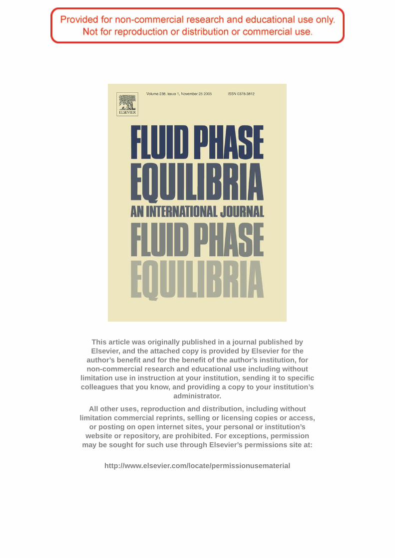
This article was originally published in a journal published byElsevier, and the attached copy is provided by Elsevier for the

author’s benefit and for the benefit of the author’s institution, fornon-commercial research and educational use including without

limitation use in instruction at your institution, sending it to specificcolleagues that you know, and providing a copy to your institution’s

administrator.

All other uses, reproduction and distribution, including withoutlimitation commercial reprints, selling or licensing copies or access,

or posting on open internet sites, your personal or institution’swebsite or repository, are prohibited. For exceptions, permission

may be sought for such use through Elsevier’s permissions site at:

http://www.elsevier.com/locate/permissionusematerial

Auth

or’s

per

sona

l c

opy

Fluid Phase Equilibria 238 (2005) 95–105

Vapor–liquid equilibrium of methane and methane + nitrogen and anequimolar hexane + decane mixture under isothermal conditions

Veronica Uribe-Vargas, Arturo Trejo∗

Instituto Mexicano del Petroleo, Programa de Ingenierıa Molecular, Area de Investigacion en Termofısica,Eje Lazaro Cardenas 152, 07730 Mexico, D.F.; Mexico

Received 2 September 2005; accepted 5 September 2005

Abstract

Experimental vapor–liquid equilibrium data of the ternary system composed of methane and an equimolar hexane + decane mixture are reported.The experimental measurements were carried out under isothermal conditions at 258, 273, and 298 K in the pressure range 1–19 MPa. Also,experimental vapor–liquid measurements were carried out for the quaternary system methane + nitrogen and an equimolar hexane + decane mixture,at 258 K in the range 3.5–12 MPa. The results for the ternary system show that the solubility of methane in the equimolar mixture of alkanes increaseswhen the pressure is increased at constant temperature and it increases as the temperature decreases in the whole pressure range studied. For thequaternary system with a constant amount of nitrogen, the solubility of methane in the liquid phase increases as the pressure increases at the studiedtemperature. The experimental results for the ternary system were satisfactorily correlated with the Peng–Robinson equation of state in the rangesof pressure and temperature studied. The equation of state was used to predict the behavior of the quaternary system using binary interactionparameters. The applicability of the principle of congruence was corroborated by comparing the vapor–liquid behavior of methane in the equimolarhexane + decane mixture with that in pure octane, at the three temperatures studied in this work.© 2005 Elsevier B.V. All rights reserved.

Keywords: Methane; Nitrogen; Hexane; Decane; Vapor–liquid equilibrium; Bronsted’s principle

1. Introduction

The injection of nitrogen as an enhanced oil recovery oper-ation in oilfields promotes that the associated natural gas willhave a certain content of nitrogen, which clearly will increasegradually with time along the exploitation of the oil reservoirs.The presence of nitrogen in natural gas beyond the internation-ally acceptable concentration limits becomes a commercial anda processing drawback. In order to have different options to solvethis problem it is necessary to carry out experimental studies onthe vapor–liquid equilibrium of selected systems with the aim ofobtaining a reliable body of information that will be the basis forthe development of separation schemes that will allow the effi-cient separation of nitrogen from natural gas streams to achievecommercially acceptable concentration standards.

Much of the experimental work reported in the literatureon the thermodynamic behavior of mixtures of linear paraf-

∗ Corresponding author. Tel.: +52 55 9175 8373; fax: +52 55 9175 6239.E-mail address: atrejo@imp.mx (A. Trejo).

finic hydrocarbons was performed to test the empirical prin-ciple of congruence proposed by Bronsted and Koefoed[1].This principle permits to determine in a simple way ther-modynamic properties of a mixture of two or more normalalkanes of known concentration by equating to the proper-ties, at the same pressure and temperature as the mixture, ofa congruent pure alkane whose carbon chain length is equalto the average chain length of the mixture of alkanes. Sev-eral authors have demonstrated the applicability of this prin-ciple with the determination of many thermodynamic properties[2] like vapor pressure[1], excess enthalpy, excess entropy,excess heat capacity, and excess Gibbs energy[3], Henry’s con-stant [4], partial molar quantities at finite concentration andat infinite dilution [4], excess molar volumes[5], and morerecently the principle has been applied to dew and bubble points[6].

In this study we present the experimental pressure–tempera-ture–concentration (P, T, x, y) results for the vapor–liquidequilibrium of the ternary system formed by methane and anequimolar (solute-free basis) hexane + decane mixture at 258,273, and 298 K in the pressure range 1–19 MPa, and also for

0378-3812/$ – see front matter © 2005 Elsevier B.V. All rights reserved.doi:10.1016/j.fluid.2005.09.002

Auth

or’s

per

sona

l c

opy

96 V. Uribe-Vargas, A. Trejo / Fluid Phase Equilibria 238 (2005) 95–105

the quaternary system of methane + nitrogen and an equimo-lar (solute-free basis) hexane + decane mixture, at 258 K, inthe range 3.5–12 MPa. The experimentalP, T, x, y results forthe ternary system were correlated using the Peng–Robinsonequation of state with the well known van der Waals one-fluidmixing rule. In order to correct the geometric mean of theenergy parameters to obtain the corresponding cross parame-ter we adjusted one binary interaction parameter,kij, for eachpair of components of the studied ternary system. The standarddeviation of the fits shows that the data are correlated withinthe experimental uncertainty, in the whole range of pressureand temperature considered. The adjusted binary interactionparameters were employed to predict the behavior of the qua-ternary system with satisfactory results. Also, we have testedthe validity of Bronsted’s principle of congruence by comparingthe results of this work for methane and the equimolar hex-ane + decane solvent mixture with literature data for methane inthe congruent puren-octane, at the three isotherms mentionedabove.

2. Literature search

We carried out a comprehensive bibliographic search togetherwith the analysis of experimental data from the open literatureon the phase equilibria of nitrogen and methane in differentliquid solvents with the purpose to find the best prospects assolvents for the efficient separation of nitrogen from natural gasand to establish the most adequate conditions of pressure andtemperature for such separation by absorption.

In recent work[7] we reported the results of the biblio-graphical search on the vapor–liquid and gas–liquid equilib-rium for nitrogen in liquid hydrocarbons (paraffins, aromaticsand naphthenic hydrocarbons). In the present work we includethe results of the same exercise for literature experimentaldata of methane in the same type of hydrocarbons as above.The review for binary systems is shown inTable 1. It can beobserved in this table that the open literature gives extensiveresults on the phase equilibria for different systems in whichmethane is one of the components, in large ranges of temper-

Table 1Previous works reported in the literature on the vapor–liquid (VL), vapor–liquid–solid (VLS) and vapor–liquid–liquid (VLL) equilibria for methane in liquidhydrocarbons

Solvent Conditions Uncertainty Reference

T (K) P (MPa) Mole fraction T (K) P (MPa)

Pentane VL 311–411 0.1–16 0.015 0.01 0.0001 Reiff et al.[8]Pentane VL 173–273 0.1–15 0.005 0.02 0.007 Chu et al.[9]Pentane VL 186–282 4–15 – 0.01 0.001 Voronov et al.[10]Pentane VL 378 7–14 – 0.3 0.02 Prodany and Williams[11]Pentane VL 311–377 3–21 0.002 0.05 0.0007 Sage et al.[12]Hexane VL 348–383 2–20 0.003 – – Cebola et al.[13]Hexane VL 311–423 10 0.002 0.1 0.04 Srivatsan et al.[14]Hexane VLS 138–164 0.6–2 – – – Luks et al.[15]Hexane VL 190–273 0.1–18 0.0050 0.02 0.0007 Lin et al.[16]Hexane VLL 190–273 0.1–18 0.00001 – – Chen et al.[17]Hexane VL 311–444 2–20 0.002 0.11 0.01 Poston and McKetta[18]Hexane VLS 163–423 0.2–16 0.002 0.1 0.02 Shim and Kohn[19]Hexane VL 311–378 6–41 – – – Schoch et al.[20]Hexane VL 311–377 3–21 0.002 0.05 0.0007 Sage et al.[12]Heptane VLL 273–313 0.1–23 0.00001 – – Chen et al.[17]Heptane VL 278–511 1–68 0.0020 0.02 0.0007 Reamer et al.[21]Octane VLS 155–191 1–5 – 0.2 0.01 Kohn et al.[22]Octane VLS 163–423 0.1–7 0.0015 0.07 0.01 Kohn and Bradish[23]Nonane VLS 223–423 1–32 0.0015 0.07 0.01 Shipman and Kohn[24]Nonane VL 323–423 2–28 – – 0.14 Rousseaux et al.[25]Decane VL 311–423 10 0.002 0.1 0.04 Srivatsan et al.[14]Decane VL 423–583 3–15 0.01 0.2 – Lin et al.[26]Decane VL 248–423 1–10 0.0014 0.07 0.01 Beaudoin and Kohn[27]Decane VL 311–377 3–17 0.003 0.01 0.14 Reamer et al.[28]Decane VL 294–394 2–31 0.002 0.04 – Sage et al.[29]Decane VLS 240–315 1–40 1× 10−8 0.1 0.002 Rijkers et al.[30]Dodecane VL 311–423 10 0.002 0.1 0.04 Srivatsan et al.[14]Dodecane VLS 240–315 1–25 1× 10−8 0.1 0.02 Rijkers et al.[31]Tetradecane VL 320–440 0.2–120 0.001 0.1 0.1 de Leeuw et al.[32]Hexadecane VLS 285–360 2–85 0.005 0.01 0.2 Glaser et al.[33]Hexadecane VL 463–703 2–25 – 0.01 – Lin et al.[34]Eicosane VL 323–423 1–11 0.002 0.1 0.04 Darwish et al.[35]Octacosane VL 323–423 1–7 0.002 0.1 0.04 Darwish et al.[35]Hexatriacontane VL 323–423 1–8 0.002 0.1 0.04 Darwish et al.[35]Hexatriacontane VL 373–453 3–128 0.001 – 0.4 Marteau et al.[36]Hexatriacontane VL 273–373 1–5 0.003 0.1 0.005 Tsal et al.[37]

Auth

or’s

per

sona

l c

opy

V. Uribe-Vargas, A. Trejo / Fluid Phase Equilibria 238 (2005) 95–105 97

Table 1 (Continued )

Solvent Conditions Uncertainty Reference

T (K) P (MPa) Mole fraction T (K) P (MPa)

Isopentane VL 160–280 3–15 – 0.3 0.002 Prodany and William[11]Neopentane VL 160–280 2–12 – 0.3 0.002 Prodany and William[11]3-Methylpentane VL 298–373 0.5–3 0.002 0.05 0.01 Kohn and Haggin[38]Benzene VL 280–315 0.2–25 1× 10−8 0.1 0.02 Rijkers et al.[39]Benzene VL 260–350 0.2–80 1× 10−8 0.1 0.02 Rijkers et al.[40]Benzene VL 313 4–37 0.007 0.25 0.2 Legret et al.[41]Benzene VL 323–423 1–9 0.001 0.1 0.035 Darwish et al.[42]Benzene VLS 165–278 1–17 – – – Luks et al.[15]Benzene VL 423–503 2–24 – 0.6 – Lin et al.[26]Benzene VL 339 1–33 – – – Elbishlawi and Spencer[43]Benzene L 311–377 3–21 0.002 0.05 0.0007 Sage et al.[12]Toluene VL 313–423 1–9 0.001 0.1 0.003 Srivatsan et al.[44]Toluene VL 313 10–42 0.007 0.25 0.2 Legret et al.[41]Toluene VL 423–543 2–25 – 0.7 – Lin et al.[26]Toluene VLL 188–277 0.3–49 0.005 0.01 0.07 Lin et al.[45]Toluene VL 255–278 0.3–17 0.00005 0.01 0.02 Hwang and Kobayashi[46]Toluene VL 338 1–36 – – – Elbishlawi and Spenser[43]Naphthalene VL 373–423 2–9 0.001 0.1 0.07 Darwish et al.[35]Phenanthrene VL 383–423 2–11 0.001 0.1 0.07 Darwish et al.[35]Phenanthrene VL 360–460 9–400 0.008 0.08 0.1 Floter et al.[47]m-Xylene VL 313 5–46 0.007 0.25 0.2 Legret et al.[41]Mesitylene VL 313 10–52 0.007 0.25 0.2 Legret et al.[41]Pyrene VL 423 2–11 0.001 0.1 0.07 Darwish et al.[35]Metylnaphthalene VL 463–703 2–25 – 0.1 0.01 Sebastian et al.[48]trans-Decalin VL 294–423 1–77 0.005 0.5 0.4 Tobaly et al.[49]trans-Decalin VL 323–423 1–10 0.001 0.1 0.003 Darwish et al.[50]Acenaphthene VL 398–453 1–144 0.005 0.5 0.4 Tobaly et al.[49]Tetralin VL 463–663 2–25 0.01 0.1 0.01 Sebastian et al.[48]1-Phenyl-dodecane VLS 260–400 0.1–400 0.008 0.08 0.1 Floter et al.[47]Diphenylmethane VL 463–703 2–25 0.01 0.1 0.01 Sebastian et al.[48]Cyclohexane VL 323–423 1–9 0.001 0.1 0.003 Darwish et al.[50]Cyclohexane VLS 154–280 0.9–1.2 – 0.2 0.01 Kohn et al.[22]Cyclohexane VL 294–444 4–69 – – – Berry and Sage[51]Cyclohexane VL 311–377 4–41 0.003 0.03 – Schoch et al.[52]Cyclohexane VLL 311–377 3–21 0.002 0.05 0.0007 Sage et al.[12]

ature (154–703 K) and pressure (0.1–400 MPa). Most of thestudies have been devoted to fluid phase equilibria with two andthree phases present (i.e. vapor–liquid and vapor–liquid–liquid),although a few works include the presence of a solid phasein equilibrium with two fluid phases (i.e. vapor–liquid–solidphases). It is worthwhile to note that most of the reported dataare for systems in which one of the components is a linearparaffin or an aromatic hydrocarbon. Also, it can be observedthat experimental information on the phase equilibria for sys-tems with branched paraffins and naphthenic compounds isscarce.

Table 2contains the results of the review on phase equilib-ria data for essentially ternary systems that include methane asone of the components. It is possible to note fromTable 2thatthe literature data for ternary systems of interest for this studyare related, with a few exceptions, to the study of three-phaseequilibria (vapor–liquid–liquid) at extreme conditions (i.e. tem-peratures below ambient and high pressure), hence it is clearthat neither the ternary system studied in this work of methanein a mixture of hexane + decane nor its vapor–liquid equilibriumhave been reported previously in the literature.

We included in previous work[7] a review of the experi-mental data reported in the literature on the phase equilibria forternary systems composed of methane + nitrogen + a hydrocar-bon. It was observed that most of those studies were carriedout on three phase equilibria, including vapor–liquid–liquid andvapor–liquid–solid equilibria at low temperatures.

Regarding the studies reported in the literature on the fluidphase equilibria of quaternary systems in which methane andnitrogen are two of the componentsTable 2shows that thereexists only one system reported in a previous work. However,this study considered three fluid phases at a single temperature.Therefore, the experimental vapor–liquid equilibrium data pre-sented here for the quaternary system of methane + nitrogen in amixture of hexane + decane have not been reported previously.

It is evident from the review reported previously[7] and fromthe information given inTables 1 and 2that most of the reportedphase equilibria data are for binary systems in which either nitro-gen or methane is one of the components.

As a result of the bibliographical review on experimentalvapor–liquid data several observations arise[7]: the solubilityof methane is larger than that of nitrogen at the same temperature

Auth

or’s

per

sona

l c

opy

98 V. Uribe-Vargas, A. Trejo / Fluid Phase Equilibria 238 (2005) 95–105

Table 2Previous works reported in the literature on the vapor–liquid (VL), vapor–liquid–solid (VLS) and vapor–liquid–liquid (VLL) equilibria for methane and nitrogen inhydrocarbons

Conditions Uncertainty Reference

T (K) P (MPa) Mole fraction T (K) P (MPa)

Methane + nitrogenEthane VLL 116–160 14–61 0.003 0.03 0.07 Llave et al.[53]Propane VLL 116–160 14–61 0.003 0.03 0.07 Llave et al.[53]Butane VL 311–411 3–21 0.002 0.1 0.03 Roberts and Mcketta[54]Pentane VLL 160–190 2–5 0.001 0.03 0.007 Merrill et al.[55]Hexane VLL 160–190 2–5 0.001 0.03 0.007 Merrill et al.[55]Heptane VLS 156–168 2–3 0.003 0.03 0.07 Chen et al.[56]Heptane VLL 169–192 24–50 0.003 0.03 0.07 Chen et al.[56]Octane VLS 160–180 2–4 0.004 0.2 0.01 Chen et al.[57]Decane VL 311–411 7–34 – – – Azarnoos and McKetta[58]Butane–decane VLL 353 1–28 0.0005 0.05 0.03 Llave et al.[59]

Methane + ethaneHexane VLL 194–204 60 0.003 0.03 0.07 Llave et al.[60]Heptane VLL 194–204 60 0.003 0.03 0.07 Llave et al.[60]Heptane VL 200–255 11 0.002 0.05 0.01 Van Horn[61]Heptane VLL 168–210 70 0.003 0.03 0.07 Llave et al.[60]Octane VLL 198–222 7 0.003 0.03 0.007 Hottovy et al.[62]

Methane + propaneHeptane VL 200–255 11 0.002 0.05 0.01 Van Horn[61]Octane VLL 198–213 6 0.003 0.03 0.007 Hottovy et al.[63]Decane VL 278–511 3–28 – 0.01 0.001 Wiese et al.[64]Decane VL 278–511 69 0.001 0.02 0.0007 Reamer et al.[65]Toluene VL 200–255 11 0.002 0.05 0.01 Van Horn[61]

Methane + butaneOctane VLL 196–206 6 0.003 0.03 0.007 Llave and Chung[66]Octane VL 253–473 3–83 – 0.1 0.1 Yang et al.[67]Decane VLL 353 3–28 0.0005 0.05 0.03 Wiese et al.[64]Hexadecane VL 295–350 8–50 0.001 0.01 0.005 Fenghour et al.[68]Heptane–hexadecane VL 317–460 27–50 0.001 0.01 0.005 Fenghour et al.[68]

MethanePentane–octane VLL 190–200 6 0.001 0.03 0.007 Merrill et al.[69]Hexane–octane VLL 178–194 5 0.001 0.03 0.007 Merrill et al.[69]Carbon dioxide–octane VLL 202–219 7 0.003 0.03 0.007 Hottovy et al.[63]Neopentane–pentane VL 344 12 – 0.3 0.02 Prodany and Williams[11]Isopentane–pentane VL 344–411 12 – 0.3 0.02 Prodany and Williams[11]Carbon dioxide-hexane VLL 184–204 6 0.001 0.03 0.007 Merrill et al.[69]

and pressure in pure liquid hydrocarbons that belong to any ofthe three types of hydrocarbons mentioned above. Also, methanepresents larger solubility in paraffinic compounds that in eitheraromatic or naphthenic hydrocarbons under the same conditionsof pressure and temperature. At temperature lower than ambi-ent, the solubility of methane in liquid hydrocarbons increasesas the carbon number of the paraffinic hydrocarbon decreasesand pressure increases, while at temperature higher than ambientthe solubility of methane increases as the carbon number of theparaffin increases in a given range of pressure under isothermalconditions. For ternary systems the vapor–liquid–liquid equi-librium data from the literature show that the concentration ofmethane is larger than that for nitrogen in both liquid phases.

These observations, derived from the experimental behaviorreported in the literature, are clearly the basis to have chosen inthis work linear paraffins as solvent, a mixed solvent, and tem-peratures below and about ambient to perform the experimentalwork in a relative large range of pressure.

3. Experimental

3.1. Materials

Praxair Mexico supplied the ultra high purity (99.999 mol.%)methane and nitrogen used in this study. Hexane anddecane were from Aldrich Chemical Co., both with purityof 99+ mol.%. No further purification was carried out onthe samples of methane and nitrogen. The liquid hydro-carbons received additional purification to eliminate someimpurities. In a first stage metallic sodium was addedwith the purpose of eliminating traces of water, and dur-ing a second stage the air dissolved in the equimolar mix-ture of hydrocarbons was eliminated by freeze with liquidnitrogen-pump-thaw cycles[7]. Chromatographic analyses wereperformed on each of the four substances used and no impuri-ties were found using the arrangement of columns describedbelow.

Auth

or’s

per

sona

l c

opy

V. Uribe-Vargas, A. Trejo / Fluid Phase Equilibria 238 (2005) 95–105 99

3.2. Apparatus and procedure

In this work, an experimental apparatus was designed andbuilt, which was based on the static method with sampling andon-line chromatographic analysis of the liquid and vapor phasesin equilibrium. This device consists of three sections: the gasloading and storage section, the equilibrium section, and thesampling and analytical section. The complete apparatus wasshown schematically together with details of the equilibriumcell and its sampling ports[7].

The temperature at equilibrium inside the stainless steel cellwas measured with an accuracy of±0.005 K, traceable to theNational Institute of Standards and Technology (US-NIST) andthe stability in the thermal bath was of±0.02 K. The equilibriumpressure was measured with an accuracy of±0.0001 MPa, alsotraceable to the NIST, and an uncertainty of±0.007 MPa.

The experimental procedure was described in great detailin previous work[7]. Briefly, the thoroughly degassed mixtureof liquid hydrocarbons of known concentration is fed into theequilibrium cell once the whole apparatus has been evacuated.For the ternary system methane is injected slowly into the cellup to a desired pressure. Accurate values of temperature andpressure are registered when the equilibrium is reached. Forthe quaternary system nitrogen was bubbled into the solventup to a chosen pressure. After the equilibrium was achieved,methane was injected to reach the desired pressure for differentequilibrium points.

The equilibrium concentration of each component wasobtained from representative samples of the liquid and vaporphases in equilibrium using the corresponding chromatographiccalibrations as discussed in the following section.

3.3. Analytical procedure

In order to obtain the calibration of the signal of the ther-mal conductivity detector (TCD) an arrangement in series oftwo packed chromatographic columns with a switching valvewas selected. The first column is a 6 ft stainless steel columnpacked with 5% SP-2100 (methyl silicone) on 80–100 meshChromosorb PAW, and the second column is a HAYESEP stain-less steel column, Q 80–100 mesh, 8 ft long. The employedarrangement and optimum conditions of temperature and car-rier gas flow to achieve the separation and quantitative analysisof the different components were reported in detail[7]. Thegas chromatograph, HP model 6890, is connected to a personalcomputer which uses commercial software (HP ChemStation) tointegrate the signals from the TCD and convert them into valuesof areas.

Although the calibration results of the TCD signal as a func-tion of amount of substance, so-called response factor, for nitro-gen, hexane, and decane were given in previous work[7], wedecided to include them in this work together with the new resultsfor methane since they are important to evaluate the final orcombined uncertainty of the equilibrium concentrations. Thisevaluation included a complete statistical analysis on the prop-agation of uncertainties for all the known variables involved inthe experimental work which considered the use of the so-called

Student’st distribution. Therefore, the uncertainty reported inthis work was always determined with a 95% of confidence, forthe best values of concentration experimentally determined.

The chromatographic calibration for hexane and decane wasobtained by injecting different volumes of the pure liquids in therange 0.01–0.1�L with precision syringes. The resulting cali-bration functions were those corresponding to a straight line forboth pure substances (hexane and decane). Due to the large spec-trum of concentration values expected for each component ineach phase, typical for this type of investigation, two calibrationcurves were defined for each component. For hexane, the fittingof the experimental chromatographic area results versus amountof substance for the first calibration curve gave a standard devi-ation of ±0.001�mol, whereas the uncertainty for the valuesof the amount of substance was estimated as mentioned aboveas±0.002�mol in the interval from 0.076 to 0.382�mol; thestandard deviation of the fit for the second calibration curve was±0.007�mol with an estimated uncertainty of±0.015�mol inthe interval from 0.459 to 0.765�mol. For decane the stan-dard deviation of the fit was±0.002�mol with an estimateduncertainty of±0.004�mol in the range 0.051–0.256�molwhereas the standard deviation was±0.004�mol with anestimated uncertainty of±0.008�mol in the interval 0.308–0.612�mol.

The chromatographic calibration for methane and nitrogenwas carried out by injecting each gas directly into the chro-matographic gas valve (Valco, model A6UWP). Samples underdifferent well known pressures were injected at constant tem-perature. Since the volume of the valve loop was previouslycalibrated (250�l), the amount of substance of the individuallyinjected samples of nitrogen and methane was determined withthe Peng–Robinson equation of state. Two calibration curveswere also defined for methane and nitrogen. For methane theresults of the straight-line fit to the experimental results ofchromatographic area versus amount of substance gave a stan-dard deviation of±0.003�mol with an estimated uncertaintyequal to±0.0060�mol in the interval 0.112–0.528�mol andfor the second calibration curve the standard deviation of the fitwas±0.007�mol with an uncertainty of±0.015�mol in theinterval 1.049–5.220�mol. The results for the two calibrationcurves for nitrogen are: the standard deviation of the fit was±0.004�mol with an uncertainty equal to±0.008�mol in therange 0.112–0.528�mol and for the second curve the standarddeviation of the fit was±0.024�mol with an uncertainty of±0.051�mol in the range 1.049–5.220�mol.

4. Experimental results

The experimental method and apparatus were tested[7] bycomparing our vapor–liquid equilibriumP–T–x results for thesystem methane + hexane at 338.7 K with literature data reportedin four different works. The comparison showed that within theestimated average uncertainty of our results for the methaneconcentration in mole fraction,±0.006 (±5%), the average dif-ferences in concentration between our values and literature datafrom four different authors were highly satisfactory, so that, thereported results are accurate within the given uncertainty.

Auth

or’s

per

sona

l c

opy

100 V. Uribe-Vargas, A. Trejo / Fluid Phase Equilibria 238 (2005) 95–105

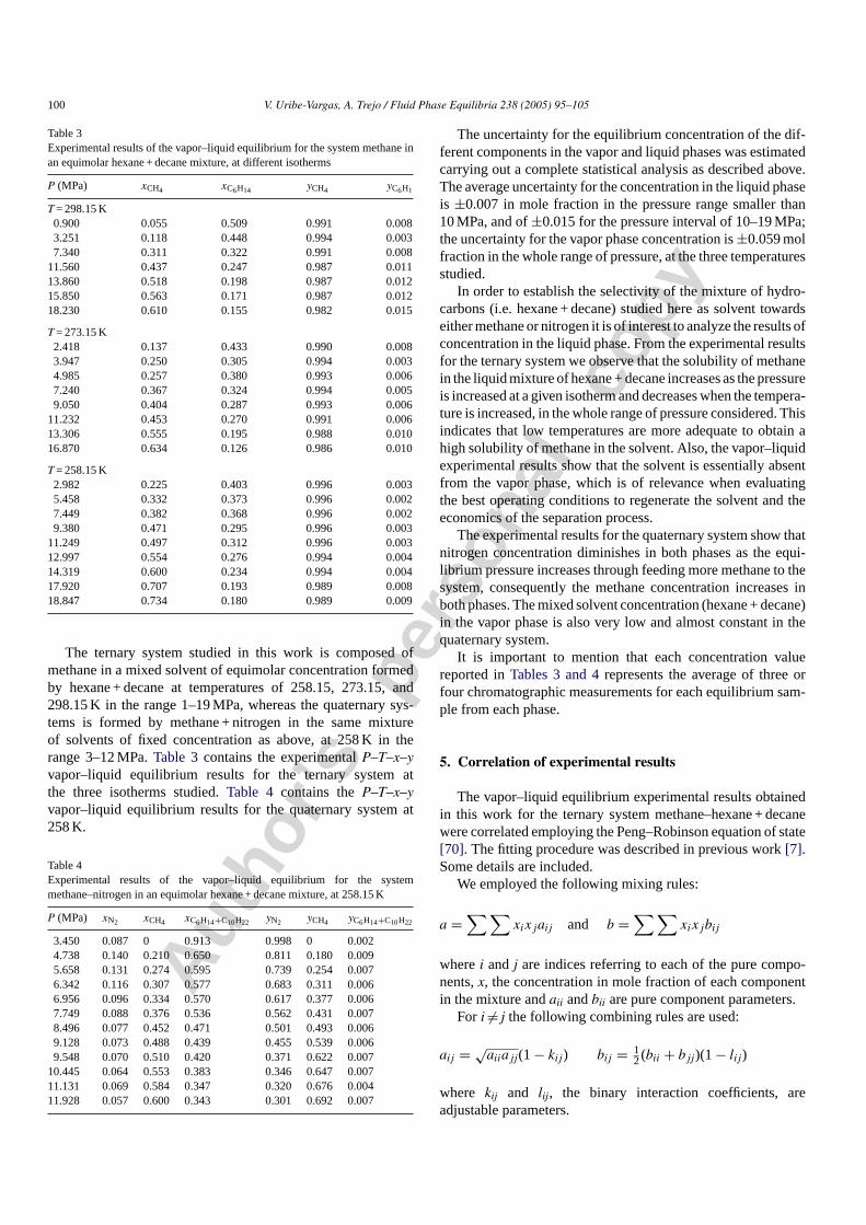
Table 3Experimental results of the vapor–liquid equilibrium for the system methane inan equimolar hexane + decane mixture, at different isotherms

P (MPa) xCH4 xC6H14 yCH4 yC6H1

T = 298.15 K0.900 0.055 0.509 0.991 0.0083.251 0.118 0.448 0.994 0.0037.340 0.311 0.322 0.991 0.008

11.560 0.437 0.247 0.987 0.01113.860 0.518 0.198 0.987 0.01215.850 0.563 0.171 0.987 0.01218.230 0.610 0.155 0.982 0.015

T = 273.15 K2.418 0.137 0.433 0.990 0.0083.947 0.250 0.305 0.994 0.0034.985 0.257 0.380 0.993 0.0067.240 0.367 0.324 0.994 0.0059.050 0.404 0.287 0.993 0.006

11.232 0.453 0.270 0.991 0.00613.306 0.555 0.195 0.988 0.01016.870 0.634 0.126 0.986 0.010

T = 258.15 K2.982 0.225 0.403 0.996 0.0035.458 0.332 0.373 0.996 0.0027.449 0.382 0.368 0.996 0.0029.380 0.471 0.295 0.996 0.003

11.249 0.497 0.312 0.996 0.00312.997 0.554 0.276 0.994 0.00414.319 0.600 0.234 0.994 0.00417.920 0.707 0.193 0.989 0.00818.847 0.734 0.180 0.989 0.009

The ternary system studied in this work is composed ofmethane in a mixed solvent of equimolar concentration formedby hexane + decane at temperatures of 258.15, 273.15, and298.15 K in the range 1–19 MPa, whereas the quaternary sys-tems is formed by methane + nitrogen in the same mixtureof solvents of fixed concentration as above, at 258 K in therange 3–12 MPa.Table 3contains the experimentalP–T–x–yvapor–liquid equilibrium results for the ternary system atthe three isotherms studied.Table 4 contains theP–T–x–yvapor–liquid equilibrium results for the quaternary system at258 K.

Table 4Experimental results of the vapor–liquid equilibrium for the systemmethane–nitrogen in an equimolar hexane + decane mixture, at 258.15 K

P (MPa) xN2 xCH4 xC6H14+C10H22 yN2 yCH4 yC6H14+C10H22

3.450 0.087 0 0.913 0.998 0 0.0024.738 0.140 0.210 0.650 0.811 0.180 0.0095.658 0.131 0.274 0.595 0.739 0.254 0.0076.342 0.116 0.307 0.577 0.683 0.311 0.0066.956 0.096 0.334 0.570 0.617 0.377 0.0067.749 0.088 0.376 0.536 0.562 0.431 0.0078.496 0.077 0.452 0.471 0.501 0.493 0.0069.128 0.073 0.488 0.439 0.455 0.539 0.0069.548 0.070 0.510 0.420 0.371 0.622 0.007

10.445 0.064 0.553 0.383 0.346 0.647 0.00711.131 0.069 0.584 0.347 0.320 0.676 0.00411.928 0.057 0.600 0.343 0.301 0.692 0.007

The uncertainty for the equilibrium concentration of the dif-ferent components in the vapor and liquid phases was estimatedcarrying out a complete statistical analysis as described above.The average uncertainty for the concentration in the liquid phaseis ±0.007 in mole fraction in the pressure range smaller than10 MPa, and of±0.015 for the pressure interval of 10–19 MPa;the uncertainty for the vapor phase concentration is±0.059 molfraction in the whole range of pressure, at the three temperaturesstudied.

In order to establish the selectivity of the mixture of hydro-carbons (i.e. hexane + decane) studied here as solvent towardseither methane or nitrogen it is of interest to analyze the results ofconcentration in the liquid phase. From the experimental resultsfor the ternary system we observe that the solubility of methanein the liquid mixture of hexane + decane increases as the pressureis increased at a given isotherm and decreases when the tempera-ture is increased, in the whole range of pressure considered. Thisindicates that low temperatures are more adequate to obtain ahigh solubility of methane in the solvent. Also, the vapor–liquidexperimental results show that the solvent is essentially absentfrom the vapor phase, which is of relevance when evaluatingthe best operating conditions to regenerate the solvent and theeconomics of the separation process.

The experimental results for the quaternary system show thatnitrogen concentration diminishes in both phases as the equi-librium pressure increases through feeding more methane to thesystem, consequently the methane concentration increases inboth phases. The mixed solvent concentration (hexane + decane)in the vapor phase is also very low and almost constant in thequaternary system.

It is important to mention that each concentration valuereported inTables 3 and 4represents the average of three orfour chromatographic measurements for each equilibrium sam-ple from each phase.

5. Correlation of experimental results

The vapor–liquid equilibrium experimental results obtainedin this work for the ternary system methane–hexane + decanewere correlated employing the Peng–Robinson equation of state[70]. The fitting procedure was described in previous work[7].Some details are included.

We employed the following mixing rules:

a =∑ ∑

xixjaij and b =∑ ∑

xixjbij

wherei and j are indices referring to each of the pure compo-nents,x, the concentration in mole fraction of each componentin the mixture andaii andbii are pure component parameters.

For i �= j the following combining rules are used:

aij = √aiiajj(1 − kij) bij = 1

2(bii + bjj)(1 − lij)

where kij and lij, the binary interaction coefficients, areadjustable parameters.

Auth

or’s

per

sona

l c

opy

V. Uribe-Vargas, A. Trejo / Fluid Phase Equilibria 238 (2005) 95–105 101

When lij is zero, the extended mixing rule reduces to theoriginal mixing rule whereb is giving by

bij =∑

xibii

The parameterm which appears in the function that calculatesα was determined with the relationships reported in the work byPeng and Robinson[70].

The binary parameterkij in the combining rule for the crossparameteraii was obtained by means of a commercial processsimulator (ASPEN-Plus). The objective function was defined bythe maximum likelihood principle. The algorithm used was thatof Britt and Luecke[71] and the initialization method appliedwas the one by Deming[72].

The objective function is the following one:

S=∑ {

(Pci −Pe

i )2

σ2Pi

+ (T ci −T e

i )2

σ2Ti

+ (xci − xe

i )2

σ2xi

+ (yci −ye

i )2

σ2yi

}

where the superscripte refers to an experimental value and thesuperscriptc refers to the estimated value corresponding to eachmeasured point,σ, the estimated experimental uncertainty ofeach measured variable, i.e. pressure, temperature, liquid andvapor phases concentration in mole fraction.

Figs. 1 and 2show the difference for the liquid and vaporphase concentration in mole fraction of methane between exper-imental and calculated results, the latter obtained with the bestfit employing the Peng–Robinson equation of the state withone interaction parameter for each pair of components. It canbe observed that the Peng–Robinson equation reproduces withacceptable accuracy the experimental results of the ternary sys-tem under study. The standard deviation of the calculated valuesfor the liquid phase concentration of methane is±0.029,±0.023,and±0.017 mol fraction for the isotherms at 258.15, 273.15, and298.15 K, respectively. Also, the standard deviation for the vaporphase concentration of methane is±0.015,±0.005, and±0.011for the same isotherms as above, respectively.

Since the real value of any model is obtained when it isapplied to reproduce the behavior of systems that were not usedin the derivation of the fitted parameters, we have employed thebinary parameterskij obtained from the simultaneous correlation

Fig. 1. Differences for the liquid phase concentration of methane in the equimo-lar hexane–decane mixture between experimental and calculated results. Thelatter with the Peng–Robinson equation of state with one interaction parameterfor each pair of components: (�) 258.15 K; (�) 273.15 K; (�) 298.15 K.

Fig. 2. Differences for the vapor phase concentration of methane in the equimo-lar hexane–decane mixture between experimental and calculated results. Thelatter with the Peng–Robinson equation of state with one interaction parameterfor each pair of components: (�) 258.15 K; (�) 273.15 K; (�) 298.15 K.

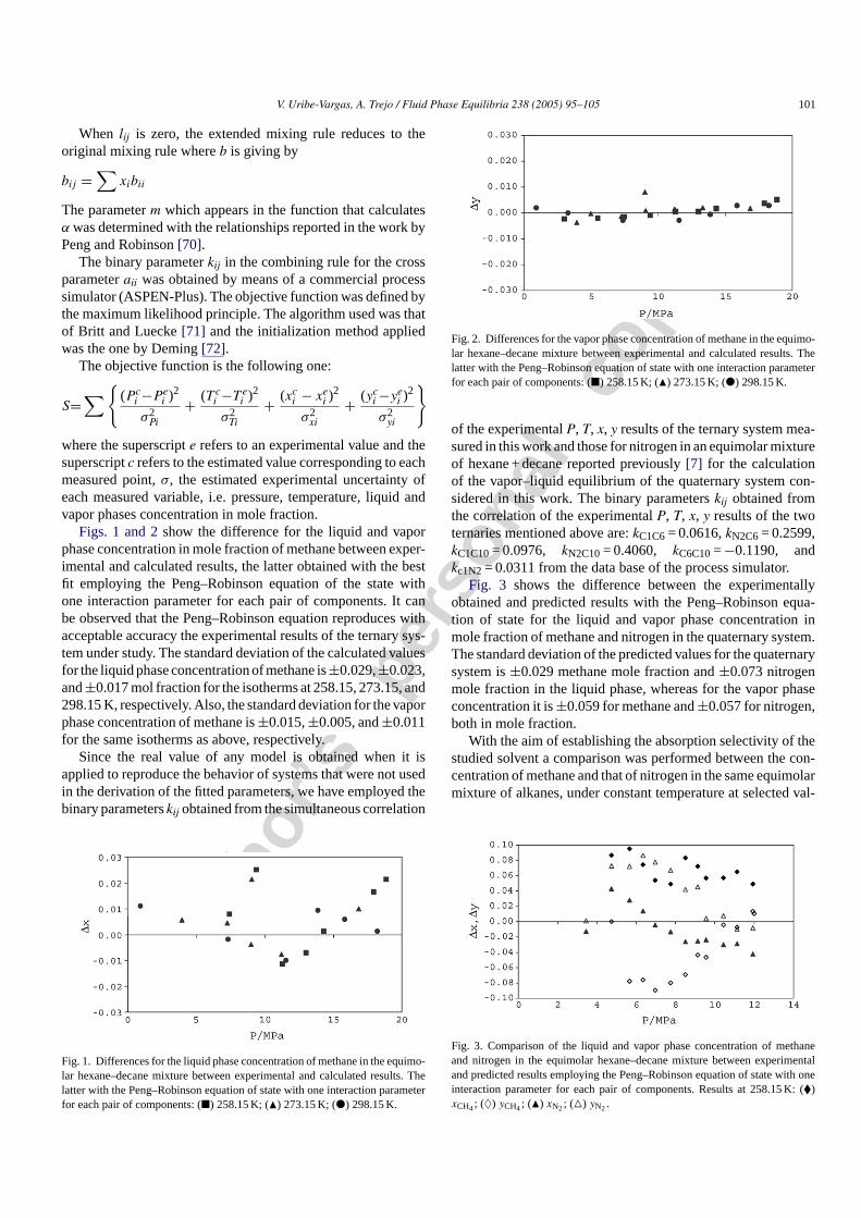
of the experimentalP, T, x, y results of the ternary system mea-sured in this work and those for nitrogen in an equimolar mixtureof hexane + decane reported previously[7] for the calculationof the vapor–liquid equilibrium of the quaternary system con-sidered in this work. The binary parameterskij obtained fromthe correlation of the experimentalP, T, x, y results of the twoternaries mentioned above are:kC1C6= 0.0616,kN2C6= 0.2599,kC1C10= 0.0976, kN2C10= 0.4060, kC6C10=−0.1190, andkc1N2= 0.0311 from the data base of the process simulator.

Fig. 3 shows the difference between the experimentallyobtained and predicted results with the Peng–Robinson equa-tion of state for the liquid and vapor phase concentration inmole fraction of methane and nitrogen in the quaternary system.The standard deviation of the predicted values for the quaternarysystem is±0.029 methane mole fraction and±0.073 nitrogenmole fraction in the liquid phase, whereas for the vapor phaseconcentration it is±0.059 for methane and±0.057 for nitrogen,both in mole fraction.

With the aim of establishing the absorption selectivity of thestudied solvent a comparison was performed between the con-centration of methane and that of nitrogen in the same equimolarmixture of alkanes, under constant temperature at selected val-

Fig. 3. Comparison of the liquid and vapor phase concentration of methaneand nitrogen in the equimolar hexane–decane mixture between experimentaland predicted results employing the Peng–Robinson equation of state with oneinteraction parameter for each pair of components. Results at 258.15 K: (�)xCH4; (♦) yCH4; (�) xN2; (�) yN2.

Auth

or’s

per

sona

l c

opy

102 V. Uribe-Vargas, A. Trejo / Fluid Phase Equilibria 238 (2005) 95–105

Fig. 4. Relative volatility, as a function of pressure, of methane to nitrogenin ternary systems with an equimolar hexane–decane mixture as solvent: (�)258.15 K; (�) 273.15 K; (�) 298.15 K.

ues of total pressure using the equation of state to obtain thecorresponding smoothed values. It has been observed that themixed solvent shows large selectivity towards methane and thatthis selectivity increases as the pressure increases. For example,considering the results for the isotherm at which larger solu-bility values were obtained for both gases studied, 258.15 K,at P = 1.0 MPa the concentration in mole fraction of methaneis 0.067 whereas that for nitrogen is 0.017; atP = 10.13 MPathe concentration for methane is 0.498 and that for nitrogenis 0.113, whereas atP = 20.27 MPax = 0.789 for methane andfor nitrogenx = 0.141. The corresponding values for the rela-tive volatility or mole ratio of methane to nitrogen in the liquidphase are 3.94, 4.40, and 5.59, respectively. These results clearlyshow that the relative volatility of methane to nitrogen is alwayssubstantially greater than unity which is a clear indication thatthe mixture of liquid alkanes studied presents a high selectivitytowards methane.

Fig. 4 shows the plot of smoothed values from thePeng–Robinson equation of the mole ratio in the liquid phaseof methane to nitrogen as a function of pressure for each of thethree isotherms studied in this work. It can be observed thatthe mole ratio is always greater than unity at any of the stud-ied isotherms in the whole range of pressure. This means thatthe separation of the methane–nitrogen mixture is highly fea-sible. The plots corresponding to the 273 and 298 K isothermsshow virtually identical functionality with pressure, although theeffect of temperature on the magnitude of the ratio is evident. Alarge improvement in the methane–nitrogen relative volatility isobtained at 258 K. Further, it is observed that the selectivity ofthe studied mixture of alkanes towards methane increases as thepressure increases at the latter isotherm.

The three sets of results inFig. 4clearly show that the mix-ture of solvents is more efficient to absorb methane relative tonitrogen as the pressure rises at the lowest isotherm studied inthis work.

6. Bronsted’s principle

The Bronsted’s principle points out that a mixture of knownconcentration of twon-alkanes with carbon number equal ton1

andn2, respectively, is congruent with a puren-alkane of carbonnumbern according to

n = x1n1 + x2n2

The congruent mixture and the puren-alkane should have thesame values in their molar properties. In this work we show thatthe phase behavior of methane in an equimolar mixture of hexaneand decane is congruent with the phase behavior of methane inpure octane.

The experimental vapor–liquid equilibrium results of theternary system methane + (hexane + decane) at 258.15, 273.15,and 298.15 K obtained in this work were compared with datareported by Kohn and Bradish[23] for the binary systemmethane + octane.

Since the values of the equilibrium pressure for the dif-ferent experimental points are not the same in each work, itis then not possible to carry out a straightforward compari-son. Therefore, the data reported by Kohn and Bradish werecorrelated in this work using the Peng–Robinson equation ofstate as explained above. The binary parameterkij fitted hereto correlate their 21 data points was 0.0872. It is observedthat this value is consistent with the corresponding values ofkij for the binaries methane–hexane and methane–decane givenabove. The standard deviation of the fit was±0.003,±0.005,and±0.002 for methane liquid mole fraction at 248.15, 273.15,and 298.15 K, respectively. These deviations are of the sameorder of magnitude as the average deviation of the bubbleand dew points reported by Kohn and Bradish:±0.002 molfraction.

It is important to underline that the data of Kohn and Bradishare reported only in the range 0.1–7.0 MPa (10–70 atm. in theoriginal publication) and that no concentration values werereported for the vapor phase for the isotherms at 273 and 248 K.Thus, we used the equation of state to obtain predicted values ofthe vapor–liquid equilibrium for methane in octane above 7 MPaand up to 19 MPa.Table 5shows calculatedP–T–x–y valuesfor the liquid–vapor equilibrium for the binary methane–octanesystem at the same pressure values considered in this work forthe ternary system. The standard deviation between the resultsof this work for the liquid phase concentration of methane inthe equimolar mixture of hexane and decane and the interpo-lated and extrapolated values for the same quantity in the binarymethane–octane system is±0.048,±0.038, and±0.033 for theisotherms at 258.15, 273.15, and 298.15 K, respectively. Fur-ther, the standard deviation between both sets of results for thevapor phase concentration of methane is±0.004,±0.009, and±0.008 mol fraction for the same isotherms as above, respec-tively.

The comparison shows that the vapor–liquid equilibriumresults of methane in the equimolar hexane + decane mixtureare congruent with those for methane in pure octane within thestandard deviation given above for the correlation of the resultsof this work with the P–R equation of state at the three temper-atures considered.

Figs. 5 and 6show the differences of methane concentra-tion in the liquid and vapor phase, respectively, between theresults obtained in this work and the interpolated and extrapo-

Auth

or’s

per

sona

l c

opy

V. Uribe-Vargas, A. Trejo / Fluid Phase Equilibria 238 (2005) 95–105 103

Table 5CalculatedP–T–x–y values with the Peng–Robinson equation of state for theliquid–vapor equilibrium of the methane–octane system, for three isotherms

P (MPa) xCH4 xC8H18 yCH4 yC8H18

298.15 K0.90 0.043 0.957 0.998 0.0023.25 0.146 0.854 0.999 0.0017.34 0.295 0.705 0.999 0.001

11.56 0.419 0.581 0.997 0.00313.86 0.476 0.524 0.995 0.00515.85 0.521 0.479 0.994 0.00618.23 0.571 0.429 0.991 0.009

273.15 K2.42 0.130 0.870 1.000 0.0003.95 0.201 0.799 1.000 0.0004.99 0.246 0.754 1.000 0.0007.24 0.331 0.669 0.999 0.0019.05 0.391 0.609 0.999 0.001

11.23 0.454 0.546 0.998 0.00213.31 0.507 0.493 0.997 0.00316.87 0.585 0.415 0.994 0.006

258.15 K2.98 0.177 0.823 1.000 0.0005.46 0.294 0.706 1.000 0.0007.45 0.373 0.627 1.000 0.0009.38 0.438 0.562 0.999 0.001

11.25 0.491 0.509 0.999 0.00113.00 0.535 0.465 0.998 0.00214.32 0.565 0.435 0.997 0.00317.92 0.635 0.365 0.993 0.00718.85 0.652 0.348 0.991 0.009

lated values with the equation of state for the methane–octanesystem.

This result leads to an interesting and very useful observation,that information on the phase behavior of multicomponent mix-tures of homologues of the series of normal alkanes, which isscarce, can be represented with an adequate degree of accuracyby congruent binary systems ofn-alkanes, the latter being gen-erally easier to study either experimentally or through adequatemodels.

Fig. 5. Differences for the liquid phase concentration of methane between exper-imental results of this work for the ternary system and calculated (interpolatedand extrapolated) values with the equation of state for the methane–octane sys-tem: (�) 258.15 K; (�) 273.15 K; (�) 298.15 K.

Fig. 6. Differences for the vapor phase concentration of methane between exper-imental results of this work for the ternary system and calculated (interpolatedand extrapolated) with the equation of state for the methane–octane system: (�)258.15 K; (�) 273.15 K; (�) 298.15 K.

7. Conclusions

Vapor–liquid equilibrium results were obtained for methanein an equimolar hexane + decane mixture at temperatures of258.15, 273.15, and 298.15 K in the range 1–19 MPa, andmethane + nitrogen in an equimolar hexane + decane mixtureat 258 K in the range 3.5–12 MPa. No data are available inthe literature for these systems. The methane solubility inhexane + decane increases with increasing the pressure, atany of the isotherms studied. Also, the solubility of methaneincreases at decreasing temperature in the ranges of temperatureand pressure considered. The methane solubility is larger thanthe nitrogen solubility at a given pressure and temperature,therefore, the separation of the mixture methane–nitrogen ishighly feasible with the use of mixtures of alkanes at lowtemperature. The Peng–Robinson equation of state repro-duces within the experimental uncertainty the experimentalbehavior for the system methane in hexane + decane and itis capable of giving satisfactory predicted results for thequaternary system of methane + nitrogen in hexane + decane.The applicability of Bronsted’s principle was tested withthe vapor–liquid equilibria of methane–hexane + decane andthat of methane–octane, at three different temperatures. Theresults presented here will be useful for the design and assess-ment of separation processes involving natural gas–nitrogenmixtures.

List of symbolsa parameter of the equation of stateb parameter of the equation of statek binary interaction parametern carbon number of alkaneP pressure (MPa)S objective functionT temperature (K)VL vapor–liquid equilibriumVLL vapor–liquid–liquid equilibriumVLS vapor–liquid–solid equilibriumx mole fraction in the liquid phasey mole fraction in the vapor phase

Auth

or’s

per

sona

l c

opy

104 V. Uribe-Vargas, A. Trejo / Fluid Phase Equilibria 238 (2005) 95–105

Greek letters� difference between experimental and calculated valuesσ estimated experimental uncertainty

Subscriptsi, j components

Superscriptc estimated value with the equation of statee experimental value

Acknowledgments

This work was supported by the Mexican Petroleum Instituteunder research projects D.00127 and I.00102 in the MolecularEngineering Program. The authors thank the financial help fromthe Universidad Nacional Autonoma de Mexico to purchasesome chemicals and spare parts. We thank Prof. Rene Molnar ofthe Universidad Autonoma Metropolitana-Azcapotzalco (Mex-ico) for the construction of a prototype of the equilibrium cell.We also thank Mr. Raul Bocanegra and Mr. Apolinar Jimenezfor their assistance to build up the experimental apparatus. V.Uribe-Vargas thanks the Mexican Petroleum Institute for a fullscholarship to carry out postgraduate studies.

References

[1] J.N. Bronsted, J. Koefoed, Kgl. Danske Videnskabernes Selskab,Matematisk-Fysiske Meddelelser 22 (1946) 1–32.

[2] J.S. Rowlinson, F.L. Swinton, Liquids and Liquid Mixtures, ButterworthScientific, London, 1982.

[3] A. Trejo Rodrıguez, D. Patterson, J. Chem. Soc. Faraday Trans. 2 78(1982) 501–523.

[4] A. Trejo Rodrıguez, D. Patterson, Fluid Phase Equilib. 17 (1984)265–279.

[5] A. Trejo-Rodrıguez, D. Patterson, J. Chem. Soc. Faraday Trans. 2 81(1985) 177–187.

[6] C.J. Peters, L.J. Florusse, J.L. de Roo, J. de Swaan Arons, J.M.H. LeveltSengers, Fluid Phase Equilib. 105 (1995) 193–219.

[7] V. Uribe-Vargas, A. Trejo, Fluid Phase Equilib. 220 (2004) 137–145.[8] W.E. Reiff, P. Peters-Gerth, K. Lucas, J. Chem. Thermodyn. 19 (1987)

467–477.[9] T.-C. Chu, R.J.J. Chen, P.S. Chappelear, R. Kobayashi, J. Chem. Eng.

Data 21 (1976) 41–44.[10] V.P. Voronov, M.Yu. Belyakov, E.E. Gorodetskii, V.D. Kulikov, A.R.

Muratov, V.B. Nagaev, Transport Porous Media 52 (2003) 123–140.[11] N.W. Prodany, B. Williams, J. Chem. Eng. Data 16 (1971) 1–6.[12] B.H. Sage, D.C. Webster, W.N. Lacey, Ind. Eng. Chem. Res. 8 (1936)

1045–1047.[13] M.J. Cebola, G. Saville, W.A. Wakeham, J. Chem. Thermodyn. 32

(2000) 1265–1284.[14] S. Srivatsan, N.A. Darwish, K.A.M. Gasem, R.L. Robinson Jr., J. Chem.

Eng. Data 37 (1992) 516–520.[15] K.D. Luks, J.D. Hottovy, J.P. Kohn, J. Chem. Eng. Data 26 (1981)

402–403.[16] Y.-N. Lin, R.J.J. Chen, P.S. Chappelear, R. Kobayashi, J. Chem. Eng.

Data 22 (1977) 402–408.[17] R.J.J. Chen, P.S. Chappelear, R. Kobayashi, J. Chem. Eng. Data 21

(1976) 213–219.[18] R.S. Poston, J.J. Mcketta, J. Chem. Eng. Data 11 (1966) 362–364.[19] J. Shim, J.P. Kohn, J. Chem. Eng. Data 7 (1962) 3–8.[20] E.P. Schoch, A.E. Hoffmann, F.D. Mayfield, Ind. Eng. Chem. 33 (1941)

688–691.

[21] H.H. Reamer, B.H. Sage, W.N. Lacey, Chem. Eng. Data Ser. 1 (1956)29–42.

[22] J.P. Kohn, K.D. Luks, P.H. Liu, D.L. Tiffin, J. Chem. Eng. Data 22(1977) 419–421.

[23] J.P. Kohn, W.F. Bradish, J. Chem. Eng. Data 9 (1964) 5–8.[24] L.M. Shipman, J.P. Kohn, J. Chem. Eng. Data 11 (1966) 176–180.[25] P. Rousseaux, D. Richon, H. Renon, Fluid Phase Equilib. 11 (1983)

153–168.[26] H.-M. Lin, H.M. Sebastian, J.J. Simmick, K.-Ch. Chao, J. Chem. Eng.

Data 24 (1979) 146–149.[27] J.M. Beaudoin, J.P. Kohn, J. Chem. Eng. Data 12 (1967) 189–191.[28] H.H. Reamer, R.H. Olds, B.H. Sage, W.N. Lacey, Ind. Eng. Chem. 34

(1942) 1526–1531.[29] B.H. Sage, H.M. Lavender, W.N. Lacey, Ind. Eng. Chem. 32 (1940)

743–747.[30] M.P.W.M. Rijkers, M. Malais, C.J. Peters, J. de Swaan Arons, Fluid

Phase Equilib. 71 (1992) 143–168.[31] M.P.W.M. Rijkers, V.B. Maduro, C.J. Peters, J. de Swaan Arons, Fluid

Phase Equilib. 72 (1992) 309–324.[32] V.V. de Leeuv, Th.W. de Loos, H.A. Kooijman, J. de Swaan Arons,

Fluid Phase Equilib. 73 (1992) 285–321.[33] M. Glaser, C.J. Peters, H.J. Van der Kooi, J. Chem. Thermodyn. 17

(1985) 803–815.[34] H.-M. Lin, H.M. Sebastian, K.-Ch. Chao, J. Chem. Eng. Data 25 (1980)

252–254.[35] N.A. Darwish, J. Fathikalajahi, K.A.M. Gasem, R.L. Robinson Jr., J

Chem. Eng. Data 38 (1993) 44–48.[36] P. Marteau, P. Tobaly, V. Ruffier-Meray, J.C. de Hemptinne, J. Chem.

Eng. Data 43 (1998) 362–366.[37] F.-N. Tsal, S.H. Huang, H.-M. Lin, K.-Ch. Chao, J. Chem. Eng. Data

32 (1987) 467–469.[38] J.P. Kohn, J.H.S. Haggin, J. Chem. Eng. Data 12 (1967) 313–315.[39] M.P.W.M. Rijkers, M. Malais, C.J. Peters, J. de Swaan Arons, Fluid

Phase Equilib. 77 (1992) 343–353.[40] M.P.W.M. Rijkers, M. Malais, C.J. Peters, J. de Swaan Arons, Fluid

Phase Equilib. 77 (1992) 327–342.[41] D. Legret, D. Richon, H. Renon, J Chem. Eng. Data 27 (1982) 165–169.[42] N.A. Darwish, K.A.M. Gasem, R.L. Robinson Jr., J. Chem. Eng. Data

39 (1994) 781–784.[43] M. Elbishlawi, J.R. Spencer, Ind. Eng. Chem. 43 (1951) 1811–1815.[44] S. Srivatsan, W. Gao, K.A.M. Gasem, R.L. Robinson Jr., J. Chem. Eng.

Data 43 (1998) 623–625.[45] Y.-N. Lin, Sh.-Ch. Hwang, R. Kobayashi, J. Chem. Eng. Data 23 (1978)

231–234.[46] Sh.-Ch. Hwang, R. Kobayashi, J. Chem. Eng. Data 22 (1977) 409–410.[47] E. Floter, P. Van der Pijl, Th.W. de Loos, J. de Swaan Arons, Fluid

Phase Equilib. 134 (1997) 1–19.[48] H.M. Sebastian, J.J. Simmick, H.-M. Lin, K.-Ch. Chao, J. Chem. Eng.

Data 24 (1979) 149–152.[49] P. Tobaly, P. Marteau, V. Ruffier-Meray, J. Chem. Eng. Data 46 (2001)

1269–1273.[50] N.A. Darwish, K.A.M. Gasem, R.L. Robinson Jr., J. Chem. Eng. Data

43 (1998) 238–240.[51] V. Berry, B.H. Sage, J. Chem. Eng. Data 4 (1959) 204–210.[52] E.P. Schoch, A.E. Hoffmann, F.D. Mayfield, Ind. Eng. Chem. 32 (1940)

1351–1353.[53] F.M. Llave, K.D. Luks, J.P. Kohn, J. Chem. Eng. Data 32 (1987) 14–17.[54] L.R. Roberts, J. McKetta, J. Chem. Eng. Data 8 (1963) 161–163.[55] R.C. Merrill Jr., K.D. Luks, J.P. Kohn, J. Chem. Eng. Data 29 (1984)

272–276.[56] W.L. Chen, K.D. Luks, J.P. Kohn, J. Chem. Eng. Data 34 (1989)

312–314.[57] W.L. Chen, S.F. Callahan, K.D. Luks, J.P. Kohn, J. Chem. Eng. Data

26 (1981) 166–168.[58] A. Azarnoosh, J.J. McKetta, J. Chem. Eng. Data 8 (1963) 513–519.[59] F.M. Llave, T.H. Chung, J. Chem. Eng. Data 33 (1988) 123–128.[60] F.M. Llave, K.D. Luks, J.P. Kohn, J. Chem. Eng. Data 31 (1986)

418–421.

Auth

or’s

per

sona

l c

opy

V. Uribe-Vargas, A. Trejo / Fluid Phase Equilibria 238 (2005) 95–105 105

[61] L.L.D. Van Horn, J. Chem. Eng. Data 12 (1967) 294–303.[62] J.D. Hottovy, J.P. Kohn, K.D. Luks, J. Chem. Eng. Data 26 (1981)

135–137.[63] J.D. Hottovy, J.P. Kohn, K.D. Luks, J. Chem. Eng. Data 27 (1982)

298–302.[64] H.C. Wiese, H.H. Reamer, B.H. Sage, J. Chem. Eng. Data 15 (1970)

75–82.[65] H.H. Reamer, V.M. Berry, B.H. Sage, J. Chem. Eng. Data 14 (1969)

447–454.

[66] F.M. Llave, T.H. Chung, J. Chem. Eng. Data 33 (1988) 123–128.[67] T. Yang, W.D. Cheu, T.-M. Guo, Chem. Eng. Sci. 52 (1997) 259–267.[68] A. Fenghour, J.P.M. Trusler, W.A. Wakeham, Fluid Phase Equilib. 182

(2001) 111–119.[69] R.C. Merrill Jr., K.D. Luks, J.P. Kohn, J. Chem. Eng. Data 28 (1983)

210–215.[70] D.D.Y. Peng, D.B. Robinson, Ind. Eng. Chem. Fund. 15 (1976) 59–64.[71] H.I. Britt, R.H. Luecke, Technometrics 15 (1973) 233–247.[72] W.E. Deming, Statistical Adjustment of Data, Wiley, New York, 1943.