Satellite-derived methane hotspot emission estimates using a ...

1

Satellite-derived methane hotspot emission estimates using a fast

data-driven method

Michael Buchwitz1, Oliver Schneising

1, Maximilian Reuter

1, Jens Heymann

1, Sven Krautwurst

1,

Heinrich Bovensmann1, John P. Burrows

1, Hartmut Boesch

2,3, Robert J. Parker

2,3, Rob G. Detmers

4,

Otto P. Hasekamp4, Ilse Aben

4, André Butz

5, Christian Frankenberg

6,7 5

1Institute of Environmental Physics (IUP), University of Bremen, Bremen, Germany

2Earth Observation Science, University of Leicester, Leicester, UK

3NERC National Centre for Earth Observation, Leicester, UK

4SRON Netherlands Institute for Space Research, Utrecht, The Netherlands 10

5Karlsruhe Institute of Technology (KIT), Karlsruhe, Germany

6Division of Geological and Planetary Sciences, California Institute of Technology, California, Pasadena, CA, USA

7Jet Propulsion Laboratory, Pasadena, CA, USA

Correspondence to: Michael Buchwitz ([email protected])

Abstract. Methane is an important atmospheric greenhouse gas and an adequate understanding of its emission sources is 15

needed for climate change assessments, predictions and the development and verification of emission mitigation strategies.

Satellite retrievals of near-surface-sensitive column-averaged dry-air mole fractions of atmospheric methane, i.e., XCH4, can

be used to quantify methane emissions. Here we present a simple and fast method to estimate emissions of methane hotspots

from satellite-derived XCH4 maps. We apply this method to an ensemble of XCH4 data products consisting of two products

from SCIAMACHY/ENVISAT and two products from TANSO-FTS/GOSAT covering the time period 2003-2014. We 20

obtain annual emissions of the source areas Four Corners in the southwestern USA, for the southern part of Central Valley,

California, and for Azerbaijan and Turkmenistan. We find that our estimated emissions are in good agreement with

independently derived estimates for Four Corners and Azerbaijan. For the Central Valley and Turkmenistan our estimated

annual emissions are higher compared to the EDGAR v4.2 anthropogenic emission inventory. For Turkmenistan we find on

average about 50% higher emissions with our annual emission uncertainty estimates overlapping with the EDGAR 25

emissions. For the region around Bakersfield in the Central Valley we find a factor of 6-9 higher emissions compared to

EDGAR albeit with large uncertainty. Major methane emission sources in this region are oil/gas and livestock. Our findings

corroborate recently published studies based on aircraft and satellite measurements and new bottom-up estimates reporting

significantly underestimated methane emissions of oil/gas and/or livestock in this area in inventories.

30

Atmos. Chem. Phys. Discuss., doi:10.5194/acp-2016-755, 2016Manuscript under review for journal Atmos. Chem. Phys.Published: 24 August 2016c© Author(s) 2016. CC-BY 3.0 License.

2

1 Introduction

Methane (CH4) is the second most important human-emitted greenhouse gas - directly after carbon dioxide - and increases in

its atmospheric abundance contribute significantly to global warming (IPCC, 2013). Accurate knowledge of its sources and

sinks and the origins of any changes are needed for the accurate prediction of future climate change, the attribution of 5

change, and the development of mitigation strategies, but our current knowledge about the various natural and

anthropogenic methane sources and sinks has significant gaps (e.g., Rigby et al., 2008; Dlugokencky et al., 2009; IPCC,

2013; Kirschke et al., 2013; Houweling et al., 2014; Nisbet et al., 2014; Jeong et al., 2014; Alexe et al., 2015; Schaefer et al.,

2016; Miller and Michalak et al., 2016).

10

Near-surface-sensitive satellite observations of atmospheric methane have been used in recent years to obtain quantitative

information on methane emissions (e.g., Alexe et al., 2015; Bergamaschi et al., 2007, 2009, 2013; Bloom et al., 2010; Turner

et al., 2015, 2016; Fraser et al., 2013; Monteil et al., 2013; Cressot et al., 2014; Wecht et al., 2014a, 2014b; Kort et al.,

2014). Nevertheless, there are still many important aspects, which need further investigation. For example, aspects related to

the recent renewed methane growth (e.g., Houweling et al., 2014) need an unambiguous explanation, and better knowledge 15

about aspects related to specific but evolving man-made emission sources (e.g., Schneising et al., 2014) is required.

Several important issues for the future management and mitigation of methane emissions have not yet been addressed

adequately such as verification of emission inventories and reported emissions per region (country down to city scale) (e.g.,

Ciais et al., 2014). The latter aspect has been addressed for future satellite missions, especially for CO2 in the context of the 20

proposed CarbonSat mission (Bovensmann et al., 2010; Velazco et al., 2011; Buchwitz et al., 2013; Pillai et al., 2016) using

performance assessments based on simulated satellite observations (ESA, 2015) but so far only few studies have been

published using real satellite data (e.g., Wecht et al., 2014a; Turner et al., 2015, 2016, for USA methane emissions). Here we

report on an attempt to use satellite methane retrievals to estimate the methane emissions of Azerbaijan and Turkmenistan,

which are both important oil and gas producing countries, and also apply our method to two regions in the USA. All four 25

studied regions show methane enhancements relative to their surrounding area in satellite-derived XCH4 maps.

This manuscript is structured as follows: In Sect. 2 we introduce briefly the satellite data which have been used in this study.

In Sect. 3 we describe the analysis method developed to derive methane emissions of (relatively) well localized emission hot

spots from satellite XCH4 retrievals. The results are presented and discussed in Sect. 4 and a summary and conclusions are 30

given in Sect. 5.


3

2 Satellite data

During recent years the retrieval of near-surface-sensitive column-averaged dry-air mole fractions of atmospheric methane

(CH4) and carbon dioxide (CO2), i.e., XCH4 and XCO2, from the satellite sensors SCIAMACHY (Burrows et al., 1995; 5

Bovensmann et al., 1999) onboard ENVISAT and TANSO-FTS onboard GOSAT (Kuze et al., 2009, 2016) significantly

evolved and improved (e.g., Buchwitz et al., 2015, 2016a, 2016b; Butz et al., 2011; Dils et al., 2014; Frankenberg et al.,

2011; Parker et al., 2011, 2015; Schneising et al., 2011, 2012, 2014; Yoshida et al., 2013).

For this study we use the latest data sets of XCH4 retrievals from SCIAMACHY and GOSAT as generated by different 10

research teams of the GHG-CCI project (Buchwitz et al., 2015) of ESA’s Climate Change Initiative (CCI, Hollmann et al.,

2013). The four satellite XCH4 products used for this study are publicly available and have been obtained from the GHG-

CCI website (http://www.esa-ghg-cci.org), where also detailed documentation is available (e.g., Algorithm Theoretical Basis

Documents (ATBDs), Comprehensive Error Characterization Reports (CECRs), Product Validation and Intercomparison

Report (PVIR, Buchwitz et al., 2016a)). 15

Table 1 presents an overview about the four XCH4 satellite data products used in this study. As can be seen, these comprise

two SCIAMACHY XCH4 data products retrieved with the WFMD (Buchwitz et al., 2000; Schneising et al., 2011, 2012,

2013) and IMAP (Frankenberg et al., 205, 2006, 2008a, 2008b, 2011) retrieval algorithms, i.e., the GHG-CCI products

CH4_SCI_WFMD and CH4_SCI_IMAP. In addition, we use the two GOSAT products CH4_GOS_OCPR (Parker et al., 20

2011, 2015) and CH4_GOS_SRFP (Butz et al., 2011, 2012). The XCH4 “full physics” (FP) retrieval algorithm used to

generate the latter product is also known as “RemoTeC” and the algorithm to generate the CH4_GOS_OCPR product is the

University of Leicester XCH4 “CO2 proxy” (PR) algorithm. The two SCIAMACHY XCH4 algorithms are also “proxy”

algorithms. Here, the XCH4 product is obtained by computing the ratio of the retrieved methane column and the

simultaneously retrieved CO2 column multiplied by a correction factor for XCO2 variations using a CO2 model (Frankenberg 25

et al., 2005). The FP algorithm does not require this CO2 correction as XCH4 is retrieved directly, which is an advantage

compared to PR algorithms. However, each algorithm has different advantages and disadvantages. An advantage of the

XCH4 PR algorithms is that atmospheric light path related errors due to not perfectly considered wavelength dependent

scattering by aerosols and clouds largely cancel in the CH4 to CO2 column ratio. This source of error is consequently less of

a problem for PR algorithms compared to FP algorithms, which require more complex radiative transfer modelling and 30

stricter quality filtering compared to the PR products (see also Schepers et al., 2012, for PR and FP algorithms and


4

corresponding data products but also Buchwitz et al., 2015, 2016a, 2016b). As a consequence, FP data products are typically

much sparser compared to PR products, but are independent of the CO2 model used.

The latest validation results for the GHG-CCI XCH4 data products are presented and discussed in Buchwitz et al., 2016a.

These were obtained by comparison of the satellite retrievals with ground-based XCH4 observations of the Total Carbon 5

Column Observing Network, TCCON (Wunch et al., 2011, 2015). As shown in Buchwitz et al., 2016a, the GOSAT XCH4

products are very stable, i.e., do not show any significant trend of the difference with respect to TCCON. For SCIAMACHY

the situation is more complex due to detector problems in later years resulting in larger noise but also bias issues. For

example, as shown in Buchwitz et al., 2016a, the IMAP product suffers from a bias (a discontinuity in XCH4) in 2010. For

this reason, we decided to restrict the use of the SCIAMACHY products in this study to the period 2003 – 2009. The 10

achieved single measurement precision (random error) for SCIAMACHY XCH4 is in the range 30-80 ppb (2-5%) depending

on time period and product and approximately 16 ppb (~1%) for GOSAT. Systematic errors (“relative accuracy” or “relative

bias”) are around 10-15 ppb (~0.6%) for SCIAMACHY and approximately 6 ppb (~0.3%) for GOSAT.

Annual average composite maps of the four data products are shown in Figs. 1 and 2. Figure 1 shows year 2004 15

SCIAMACHY XCH4 at 0.5o x 0.5

o resolution as retrieved using the WFM-DOAS (WFMD) algorithm (Schneising et al.,

2011). Also shown are zooms for the three target regions investigated in this study. Figure 2 shows year 2004 SCIAMACHY

IMAP-DOAS (IMAP) XCH4 and year 2010 XCH4 as retrieved using the two GOSAT algorithms. As can be seen, the spatial

coverage of the GOSAT products is quite sparse. A single GOSAT observation requires more time (4 seconds) compared to

a SCIAMACHY observation (typically 0.25 seconds for the spectral regions relevant for this study) and, therefore, GOSAT 20

provides less observations in a given time period than SCIAMACHY. On the other hand, the GOSAT ground pixel size is

smaller (10 km diameter) compared to SCIAMACHY (approximately 30 km along track times 60 km across track), which

results in a higher fraction of cloud free observations for GOSAT. Furthermore, SCIAMACHY is in nadir (downlooking)

observation mode only about 50% of the time. Overall the total number of quality filtered observations as contained in the

data products is larger for SCIAMACHY compared to GOSAT. Furthermore, the spatial sampling of GOSAT comprises 25

non-contiguous ground pixels, which results in large data gaps (even in yearly averages). Consequently, GOSAT is typically

(i.e., in normal observation mode) not optimal for small-scale hotspot applications but as shown in this manuscript, GOSAT

provides results for the selected source regions which agree reasonably well with the results obtained using SCIAMACHY.

In the remainder of this manuscript we focus on obtaining methane emission estimates for the source areas shown in Fig. 1.

30


5

3 Analysis method

In this section we describe the analysis method used to obtain methane emission estimates for source regions such as those

shown in Fig. 1, i.e., for regions showing elevated methane relative to their surrounding area in time-averaged satellite-5

derived XCH4 maps.

The satellite XCH4 input data used in this study are the GHG-CCI Level 2 (i.e., individual ground-pixel observations) data

products as described in the previous section (see also Tab. 1). The first step in the analysis comprises gridding (averaging)

these products using a regular latitude/longitude grid (here: 0.5ox0.5

o) to obtain maps of annual averages (see Figs. 1 and 2). 10

These mapped XCH4 products are then used in this study for further analysis.

The second step comprises the definition of a source region and a surrounding (or background) region. The latter is an

extended region surrounding the source region (specific examples are shown in Sect. 4).

15

The third step comprises the determination of the methane enhancement over the source region relative to its surrounding

area, ΔXCH4. This methane enhancement is computed by subtracting the mean value of XCH4 in the surrounding region

from the mean XCH4 value over the source region.

To reduce potential effects related to a location dependent weighting of tropospheric and stratospheric contributions on 20

XCH4 (note that mean stratospheric CH4 mixing ratios are typically lower compared to tropospheric mixing ratios) we apply

a correction called “elevation correction” (EC) similar as also described in Kort et al., 2014 (and implicitly also applied in

Schneising et al., 2014). The purpose is to correct for XCH4 variations due to variations of surface elevation/pressure and

tropospause height. The corrected XCH4 is obtained from the original XCH4 by adding 7 ppb per 1 km surface elevation

increase relative to mean sea level. For surface elevation we use a surface elevation map (also 0.5ox0.5

o) based on the 25

GTOPO30 Digital Elevation Model (DEM) (obtained from https://lta.cr.usgs.gov/GTOPO30). The value of 7 ppb/km has

been obtained by fitting a linear function to pairs of uncorrected original XCH4 and corresponding surface elevation. We

found that the exact value depends somewhat on region, time period and satellite data product but is typically within 7 +/- 2

ppb/km. We found that applying EC typically results in similar or somewhat lower emission estimates compared to

inversions where this correction is not applied. 30


6

The fourth step comprises the conversion of the methane enhancement over the source region, ΔXCH4, to a source region

emission estimate (Ee; unit: MtCH4/year = TgCH4/year) using conversion factor CF:

Ee = ΔXCH4 ∙ CF. (1)

5

The basic idea is that a relatively well isolated emission source will result in an XCH4 enhancement, ΔXCH4, in an area at

and around the emission hotspot relative to its surrounding, i.e., that there will be a spatial correlation between a local

emission and a local XCH4 enhancement (compare also the two maps shown in Fig. 3 top left and top right, which will be

discussed in detail below).

10

The conversion factor CF in Eq. (1) is computed as follows (see Annex A for additional explanations):

CF = M ∙ Mexp ∙ L ∙ V∙ C . (2)

Here M is a constant conversion factor (5.345∙10-9

MtCH4/km2/ppb) needed to convert a methane mole fraction change to a 15

methane mass change per area for standard conditions, i.e., for surface pressure psurf = 1013 hPa. Mexp is a dimensionless

factor used to approximately correct for the actual mass (mass Mi of the i-th grid cell). It is calculated using the surface

elevation map also used for the determination of the elevation correction (EC) as described above:

Mexp = <Mi>

M ≈

<pi>

1013.0 ≈ < e−zi H⁄ >i . (3) 20

Here pi is the surface pressure of the i-th grid cell (in hPa) and zi is the surface elevation of the i-th grid cell (in km), H is the

assumed scale height (8.5 km) and <∙> and <∙>i denotes averaging over all grid cells of the source region. As shown below,

the uncertainty of our method is not dominated by the approximation used to compute Mexp (namely the use of surface

pressure or elevation rather than actual mass). 25

The dimension of the remaining factor (L∙V∙C) is km2/year, i.e., area divided by time or length times velocity and can be

interpreted as the effective methane emission accumulation time of air parcels travelling over the source region area or the

effective velocity V of air parcels travelling an effective length L over the source region. Here we use the latter

interpretation, i.e., L is length (in km) and V is velocity (in km/year). We compute L as the square root of the (pre-defined) 30

source area.


7

Factor C is dimensionless and in this study we use C = 2.0. This choice is motivated using the simple model of an air parcel

travelling with constant horizontal wind speed V over a homogeneous source region of length L accumulating methane

during an accumulation time L/V (see Annex A). When leaving the source area, the methane enhancement of the air parcel,

i.e., the concentration difference after and before entering the source region, is twice the mean methane enhancement over

the source region due to the assumed linear increase of the methane enhancement of the air parcel when travelling over the 5

source region (see Annex A). Our method basically assumes that the emission of the source region only results in a XCH4

enhancement over the source region. However, also the surrounding area may contain elevated XCH4 from sources located

in the surrounding area or from methane inflow from other regions into the surrounding area (including the source region).

As our method neglects this, our method tends to underestimate the emission of the source region. As explained below, we

aim at quantifying the impact of the choice of the surrounding region by varying its size and shape. 10

The value of V has been obtained by “calibrating” our method using global methane data sets obtained from the Copernicus

Atmosphere Monitoring Service (CAMS, https://atmosphere.copernicus.eu/). Specifically, we use CAMS methane emissions

and atmospheric methane version v10-S1NOAA as generated via the TM5-4DVAR assimilation system assimilating

National Oceanic and Atmospheric Administration (NOAA) CH4 surface observations (an earlier version of this method and 15

resulting data products is described in Bergamaschi et al., 2009). Based on this data set we computed annual emissions and

corresponding annual XCH4 at the original CAMS data set resolution of 6o longitude times 4

o latitude. The corresponding

maps for the year 2003 are shown in Fig. 3 (top row).

The CAMS year 2003 XCH4 map shown in Fig. 3 top left has been used to derive methane emissions using Eq. (1) and 20

varying parameter V (the only free parameter of our model) until the mean difference between our estimated emissions and

the “true” CAMS emissions is zero. We found that this is the case for V = 1.1 m/s (converted to km/year). The resulting map

of retrieved emissions is shown in Fig. 3 bottom right. This map has been obtained using an automatic procedure: For all

CAMS 6ox4

o grid cells (except for the ones at the border) the XCH4 value of this grid cell has been obtained and is

interpreted as a potential source region value. The neighboring cells define the surrounding (background) of the potential 25

source region and its XCH4 mean value and standard deviation has been computed. A methane enhancement, ΔXCH4, has

been computed as “source minus background value” as described above. If the resulting ΔXCH4 value is larger than 0.5

times the standard deviation of the XCH4 values in the surrounding, then the corresponding cell is flagged as a methane

“hotspot cell” and its ΔXCH4 value is converted to an emission using the approach described above (Eq. (1)). The

corresponding results are shown as map in Fig. 3 bottom right and can be compared with the “true” emission map shown in 30

Fig. 3 top right. As can be seen in Fig. 3, N = 125 hotspot cells have been found using the described procedure.

Figure 3 bottom left shows x-y plots of estimated emissions versus “true” (i.e., CAMS) emissions (top) and estimated minus

true emissions versus true emissions (bottom). The mean difference “estimated-true” is 0.00 MtCH4/year (this must be the


8

case as V = 1.1 m/s has been determined by minimizing this difference). The standard deviation of the difference is 0.59

MtCH4/year, the linear correlation coefficient R is 0.81 and the red line shows the resulting line from a linear fit. As can be

seen, the (red) line originating from the linear fit has a positive slope but does not perfectly agree with the (green) 1:1 line

(our single parameter model does not permit to also optimize the slope of the fitted line).

5

Figure 4 is similar as Fig. 3 but shows results for the year 2012. Here the difference “estimated-true” is not exactly zero but

0.01 MtCH4/year. In contrast to Fig. 3, V has not been fitted. Instead, the pre-defined value of V = 1.1 m/s has been used.

Figure 4 shows very similar “estimated-true” differences compared to Fig. 3. This demonstrates that the effective wind speed

V as obtained from year 2003 data is valid also for other years.

10

The results shown in Figs. 3 and 4 are combined in the single Fig. 5. As can be seen from Fig. 5 (top), the overall correlation

of the retrieved and true emissions is 0.81, the mean difference (estimated minus true) is 0.00 MtCH4/year and the standard

deviation of the difference is 0.53 MtCH4/year. As explained, these results have been obtained using constant values for fit

parameter V (= 1.1 m/s) and correction factor C (= 2.0) (Eq. (2)). Several attempts have been undertaken in order to find out

if the use of regionally and/or time dependent C values can reduce the difference of the estimated and the true methane 15

emission, however (so far) without success. For example, it has been investigated if the emission difference is correlated

with mean wind speed (using ECMWF ERA Interim from www.ecmwf.int/, Dee et al., 2011) but no significant correlation

between emission error and mean wind has been found. The time dependence of the estimated emission, Ee, is therefore

nearly entirely driven by the satellite-derived methane enhancement, ΔXCH4.

20

Finally, the (1-sigma) uncertainty of Ee has been estimated. This has been done as follows: Figure 5 also shows the emission

difference (estimated minus true; see middle and bottom panels) as a function of the estimated emission. Figure 5 middle

also shows (in red) the corresponding mean values (crosses) and standard deviations (vertical bars) for several emission bins

(non-equidistant to ensure a sufficiently large number of data points within each bin). Also shown in Fig. 5 (middle and

bottom) are dotted red lines computed as f(Ee) = 0.3 + 0.5∙Ee. This function and its parameters has been chosen such that the 25

red vertical bars (1-sigma range) are located within the range defined by f(Ee), i.e., most of the emission differences are

located within +/- f(Ee) (Fig. 5 middle). Therefore, f(Ee) is a reasonable description of the 1-sigma uncertainty of the

estimated emissions. Based on this it is concluded that the 1-sigma uncertainty of the estimated emission due to uncertainty

of the overall conversion factor (CF) can be well described using this formula:

30

σCF = 0.3 + 0.5 ∙ Ee. (4)

Here the units of σCF and Ee are MtCH4/year. The total uncertainty, σtot, consists of the uncertainty of the conversion factor,

σCF, and the uncertainty of the obtained methane enhancement, σΔXCH4, as obtained from the satellite data (see Eq. (1)). The


9

latter is assumed to be dominated by methane variations in the surrounding area (primarily because the surrounding region

may contain regions of elevated methane due to sources located outside the target region). This contribution to the total

uncertainty is estimated by varying the size of the surrounding region (see following section). The total uncertainty is

computed as follows:

5

σtot = √σΔXCH42 + σCF

2 (5)

The method described in this section has been applied to the described SCIAMACHY and GOSAT XCH4 data products and

for each of the pre-defined source regions annual average emissions and their uncertainties have been obtained for all

products. The results are presented in the following section. 10

4 Results and discussion

In this section we present the results from applying the methane emission inversion method described in the previous section 15

to obtain emission estimates for four areas: the Four Corners area in the south-western USA (Sect. 4.1), in the southern part

of the Central Valley in California (Sect. 4.2) and the two countries Azerbaijan and Turkmenistan (Sect. 4.3). All these areas

show elevated methane relative to their surrounding (Fig. 1). The spatial locations of these areas as well as key parameters

used to convert the observed methane enhancements to annual methane emissions are listed in Tab. 2.

20

4.1 Four Corners area, USA

Four Corners is a region in the USA named after the quadripoint where the boundaries of the four states Utah, Colorado,

Arizona and New Mexico meet. The Four Corners area is one of the largest methane hotspots in the USA (Kort et al., 2014;

Wecht et al., 2014b; Frankenberg et al., 2016). The San Juan Basin, located in the Four Corners area, is a geologic structural 25

basin and primarily a natural gas production area, mostly from coal bed methane and shale formations (e.g., Frankenberg et

al., 2016, and references given therein). Figure 6 shows annually averaged XCH4 from the four satellite XCH4 products as

used in this study at and around Four Corners. Here the XCH4 is shown as anomaly, to be able to better compare the spatial

pattern of the shown products. As can be seen, all satellite products show that XCH4 is enhanced in the Four Corners area

relative to the surrounding area (for the OCPR product this is difficult to see because the obtained enhancement is the 30

smallest of all products). Figure 6 shows the chosen source region as (inner) rectangle. The outer rectangle (last column and

last row) shows the “default” surrounding area. As described above, the methane enhancement ΔXCH4 is computed as the

difference between the XCH4 mean value in the source region minus the XCH4 mean value in the surrounding region. For

the inversion the size of the surrounding area is varied to determine the sensitivity of the computed ΔXCH4 with respect to


10

the chosen background region. For this purpose the latitudes and longitudes of the rectangular box, which defines the

surrounding area, are varied by adding all combinations of 0o, 1

o, 2

o, and 3

o in the latitude and longitude directions. The

standard deviation of the resulting ΔXCH4 is used as an estimate of σΔXCH4 (see Eq. (5)).

Figure 7 shows the resulting XCH4 enhancements for all years and all satellite data products including (1-sigma) uncertainty 5

estimates (i.e., σΔXCH4) as vertical bars. As can be seen, all ΔXCH4 values are positive. This shows that a positive Four

Corners methane enhancement is present for all years in all satellite products. The methane enhancement is on average about

10 ppb but shows significant variation depending on satellite product and year.

These methane enhancements and their uncertainties are converted to Four Corners area annual methane emissions using the 10

method described in Sect. 3. The results are shown in Fig. 8. The estimated emissions are in the range 0.42 – 0.57

MtCH4/year (range of annual mean values of the four satellite products). Taking into account the (large) uncertainty of the

estimated annual emissions, this is in good agreement with published values as shown in Fig. 8. For example, Kort et al.,

2014, report 0.59 MtCH4/year for the time period 2003-2009 (based on SCIAMACHY and ground-based Fourier-Transform

(FT) spectrometer observations) and Turner et al., 2015, report the range of 0.45 -1.39 MtCH4/year for the time period 2009-15

2011 (based on an analysis of GOSAT data). The good agreement with the published values indicates that the method used

here appears to be capable to deliver reasonable emission estimates even if the source area is much smaller than the 6ox4

o

regions used for calibrating our inversion method. The agreement is surprisingly good given the large (1-sigma) uncertainty

values shown in Fig. 8 (approx. 0.6 MtCH4/year (~100%) and dominated by σCF as can be concluded from a comparison with

σΔXCH4 shown in Fig. 7 (~20%)). Our reported uncertainty of the annual averages seems to be too conservative (at least for 20

quantifying the Four Corners area emissions).

Figure 8 also shows the total anthropogenic emissions during 2003-2008 as obtained from the EDGAR v4.2 data base

(obtained from http://edgar.jrc.ec.europa.eu/part_CH4.php) for the Four Corners source region. The mean value of the

annual EDGAR emissions is 0.17 MtCH4/year. As can be seen, the EDGAR emissions are too low by approximately a factor 25

of three.

4.2 Central Valley, California, USA

California emits large amounts of methane, approximately 2-3 MtCH4/year (Turner et al., 2015) and major emission sources 30

are livestock, gas/oil and landfills/wastewater (e.g., Wecht et al., 2014b). According to the EDGAR v4.2 emission data base

total anthropogenic methane emissions are largest around Los Angeles and San Francisco dominated by landfill/wastewater

and gas/oil related emissions and in the area in between, in the Central Valley, emissions are dominated by livestock

emissions (see Wecht et al., 2014b, their Fig. 1).


11

The Central Valley in California shows up as a methane hotspot in satellite data (see Fig. 9) with largest values in the

southern part of the Central Valley around Bakersfield, an important oil and gas producing area (e.g., Jeong et al., 2014;

Guha et al., 2015) and an area with significant methane emissions from dairy and livestock (e.g,, Wecht et al., 2014b; Guha

et al., 2015), extending up to the city of Fresno or even further towards Modesto / San Francisco. This southern part of the 5

Central Valley is the San Joaquin Valley. In this study we define Central Valley as the rectangular region specified by the

latitude/longitude range as listed in Tab. 2, corresponding to the region where the satellite XCH4 is highest. This region

roughly corresponds to the San Joaquin Valley. According to EDGAR this region is dominated by livestock methane

emissions with significant contributions from gas/oil and landfill/wastewater related emissions.

10

Figure 9 shows SCIAMACHY WFMD (and IMAP) XCH4 for year 2004 over California and also shows the Central Valley

source region as defined for this study (inner rectangle of Fig. 9 top left) and its “default” surrounding area (outer rectangle

Fig. 9 top right). Figure 9 also shows EDGAR v4.2 total anthropogenic methane emissions for the year 2004 regridded to

0.5ox0.5

o. As can be seen, the spatial pattern of the EDGAR emissions significantly deviates from the spatial pattern of the

satellite XCH4. Whereas in EDGAR the highest values are around San Francisco and around Los Angeles, the satellite-15

derived atmospheric methane is highest in the area in between, in the Central Valley, particularly in the area around

Bakersfield. Methane emissions in the Bakersfield region are supposed to be dominated by dairy and livestock operations

(Guha et al., 2015, and references given therein).

For comparison with the satellite data and the EDGAR emissions also the CAMS emissions are shown (Fig. 9 bottom row). 20

On the left (Fig. 9e) the CAMS v10-S1NOAA product is shown, which is based on the assimilation of NOAA methane

observations and on the right product v10-S1SCIA (Fig. 9f) based on the additional assimilation of SCIAMACHY IMAP

XCH4. Surprisingly, the assimilation of SCIAMACHY XCH4 reduces the derived methane emissions in this region. That the

Central Valley SCIAMACHY XCH4 enhancement is not modelled well with optimized emissions obtained from assimilating

SCIAMACHY data using the global TM5-4DVAR system is also clearly visible in Bergamaschi et. al., 2009 (their Fig. 2), 25

discussing an earlier (pre-CAMS) version of this data set. As already mentioned, the emissions of California are expected to

be in the range 2-3 MtCH4/year (see Turner et al., 2015, their Fig. 6), i.e., larger than the v10-S1NOAA (Fig. 9e) and v10-

S1SCIA (Fig. 9f) products suggests. The exact reason why the assimilation of the SCIAMACHY data does not lead to larger

estimated emissions in this region is unclear but very likely this is due to the fact that the CAMS inversion system is a global

system at quite low spatial resolution and therefore not necessarily optimal for proving reliable emission estimates for 30

regions which are smaller or just on the order of the size of the 6ox4

o grid cells shown in Fig. 9 bottom.

As can be seen from Fig. 10, we obtain mean annual emissions in the range 1.05-1.55 MtCH4/year, depending on data

product. The estimated uncertainty of the annual emissions is ~1 MtCH4/year (1-sigma) and the inter-annual variations are


12

20-50% (1-sigma) of the mean emissions, depending on product. Our annual emission estimates are quite uncertain with

mean values much higher compared to the emissions as given in the EDGAR v4.2 anthropogenic methane emission

inventory. According to EDGAR the total anthropogenic methane emissions in the selected source area are around 0.17

MtCH4/year, i.e., a factor of 6-9 lower than our annual mean estimates. This is unlikely due to the fact that our emissions are

total emissions whereas EDGAR only reports anthropogenic emissions as the fraction of natural methane emissions in 5

California is estimated to be only approximately 3% percent (Wecht et al., 2014b). Our results are broadly consistent with

recently published results from CalNex campaign (May – June 2010) aircraft observations (Wecht et al., 2014b) also

showing high atmospheric methane concentrations over the southern Central Valley compared to the rest of California and

concluding that EDGAR emissions in this region need to be scaled with factors up to around five (see their Fig. 2). Wecht et

al., 2014a, also derived emissions in this area using SCIAMACHY IMAP retrievals. They report that their derived emissions 10

are consistent with the ones presented in Wecht et al., 2014b, and for the Central Valley they found that the derived

emissions are a factor of 2-4 higher compared to EDGAR v4.2 (note that their definition of Central Valley is not identical

with our definition, which is restricted to the southern part of the Central Valley). They conclude that the livestock emissions

in EDGAR are significantly underestimated.

Jeong et al., 2013, present an analysis of methane emissions using atmospheric observations from five sites in California’s 15

Central Valley across different seasons (September 2010 to June 2011). They obtained spatially resolved (13 sub-regions)

top-down estimates of California’s CH4 emissions using in-situ tower data. They report for their region R12, which is similar

to but not exactly identical with the area chosen in our assessment, emissions of 0.85 and 0.94 MtCH4/yr (depending on a

priori assumptions) based on inversion of in-situ tower data (see their Tab. 5 reporting methane emissions in TgCO2eq

computed assuming a global warming potential of 21 gCO2eqCH4/gCH4), which is a factor of 3.6 (= 17.89 / 5.01, see their 20

Tab. 5) higher than EDGAR v4.2.

Jeong et al., 2014, also studied this region and presented a new spatially resolved bottom-up inventory of methane for 2010

focusing on methane emissions from petroleum production and natural gas systems in California. They showed that the

region around Bakersfield is a major oil and gas production and transmission region in California (see their Fig. 1) and they

found that their emission estimates are 3-7 times higher for the petroleum and gas production sectors compared to official 25

California bottom-up inventories.

Our results corroborate the findings of these independent studies that inventory emissions are underestimated in this region.

However we acknowledge the large uncertainty of our estimated annual emissions and cannot rule out that our emission

estimates are overestimated, e.g., due to possible methane accumulation in the southern part of the Central Valley.

30


13

4.3 Azerbaijan and Turkmenistan

Azerbaijan and Turkmenistan are located next to the Caspian Sea (to the west and to the east, respectively) and both

countries are important oil and gas producers. Azerbaijan and Turkmenistan are clearly visible as methane emission hotspots 5

in satellite XCH4 data sets (Fig. 1, Fig. 11).

Figure 11 shows SCIAMACHY WFMD year 2004 XCH4 in the Azerbaijan / Turkmenistan area and emission data base

results from EDGAR v4.2 (Fig. 11, bottom left), CAMS v10-S1NOAA (Fig. 11, bottom middle) and CAMS v10-S1SCIA

(Fig. 11, bottom right). In contrast to the results discussed in the previous section, the assimilation of SCIAMACHY data in 10

the TM5-4DVAR assimilation system enhances the emissions around Azerbaijan / Turkmenistan (compare Fig. 11 bottom

middle with bottom right).

Figure 12 shows Azerbaijan methane emissions as obtained with our inversion method compared to EDGAR v4.2 emissions.

As can be seen, the satellite-derived emissions are consistent with EDGAR. Note that the CH4_GOS_SRFP product is not 15

shown. Due to the sparse spatial sampling of this product the inter-annual variability is dominated by year-to-year sampling

differences. Azerbaijan is surrounded by many other methane emission areas and, therefore, not a well-isolated emission

hotspot, i.e., not ideal for our inversion method. The impact of this is largest for the CH4_GOS_SRFP product, which is a

sparse data set as the underlying “full physics” retrieval algorithm requires strict quality filtering.

20

Turkmenistan is much larger in size compared to Azerbaijan (see Fig. 11) but also not a well-isolated emission hotspot. The

results for Turkmenistan are shown in Fig. 13. Here the mean values of all estimated emissions are positive (in contrast to

Azerbaijan) indicating that the methane concentration over Turkmenistan is higher than its surrounding for all years and all

four satellite products. The mean values of the derived emissions are in the range 1.85 – 2.08 MtCH4/year, which is about

50% larger compared to EDGAR (1.33 MtCH4/year). This may be due to an underestimation of Turkmenistan’s oil and gas 25

related methane emissions in EDGAR but one also has to note the large uncertainty of our satellite-derived annual emissions.

Furthermore, Turkmenistan is not an ideally-isolated methane hotspot, although the Azerbaijan results do not indicate that

this is necessarily a significant issue. Note also that mountains are located southward and eastward of Turkmenistan and this

may contribute to a local accumulation (trapping) of atmospheric methane (resulting in an overestimation of our estimated

emissions) and may explain why the elevated methane over Turkmenistan as shown in Fig. 11 is well correlated with the 30

country boundaries. Clearly, more studies are needed to clarify this but this likely requires much more complex inversion

methods than the one used in this study (e.g., similar to those presented in Wecht et al., 2014a, and Gentner et al., 2014).


14

5 Summary and conclusions

We have presented a simple but fast method to estimate methane surface emissions of areas showing elevated atmospheric

methane concentrations relative to their surrounding area (“methane hotspots”) in satellite-derived XCH4 maps, especially in

those derived from SCIAMACHY/ENVISAT. The described “inversion method” is applicable to time-averaged XCH4 data 5

sets (as complex variations due to varying meteorological conditions cannot be considered by our method) and we focus on

annual XCH4 maps to derive annual emissions. The method is based on a direct conversion of a localized methane

enhancement (relative to its surrounding) using a conversion factor, which mainly depends on the size of the region of

interest. The method is calibrated using (low resolution) 2-dimensional methane emission maps and corresponding 2-

dimensional XCH4 maps generated from Copernicus Atmospheric Monitoring Service (CAMS) 3-dimensional atmospheric 10

methane fields. A limitation of our method is its quite large uncertainty. We estimate that the uncertainty of the method is

about 80% for annual emissions around 1 MtCH4/year but having better relative uncertainty for larger emissions (down to

about 50% for large emissions).

We applied this method to an ensemble of satellite XCH4 data products using two products from SCIAMACHY/ENVISAT 15

and two products from TANSO-FTS/GOSAT as made available via the GHG-CCI project website (http://www.esa-ghg-

cci.org/) of ESA’s Climate Change Initiative (CCI). These products cover the time period 2003-2014.

The inversion method has been applied to four source areas. Two of the source areas are located in the USA (the Four

Corners area located in the southwestern USA and the southern part of the Central Valley, i.e., the region around Bakersfield 20

and Fresno, in California) and the two other source regions are Azerbaijan and Turkmenistan, which are both important oil

and gas producing countries. All four regions clearly show elevated methane relative to their surrounding in satellite-derived

XCH4 maps.

For Four Corners we obtain annual emissions in the range 0.42 – 0.57 MtCH4/year in agreement with published values. For 25

Azerbaijan our estimates are on average close to the total anthropogenic methane emissions of Azerbaijan as given in the

EDGARv4.2 (FT2012) emission inventory but for Turkmenistan we obtain about 50% higher emissions on average albeit

with large uncertainty. Further study is needed toinvestigate if this is due to an underestimation of Turkmenistan’s oil and

gas related emissions in EDGAR.

30

For the region around Bakersfield located in the Central Valley of California, a region of significant oil and gas production

and large expected methane emissions from dairy and livestock operations, we obtain mean emissions in the range 1.05-1.55

MtCH4/year, depending on satellite data product. This is about a factor of 6-9 higher than the total methane emissions as

given in the EDGAR v4.2 inventory, but of similar magnitude as reported in Jeong et al., 2013, (0.85 – 0.94 MtCH4/year)


15

based on inverse modelling of tower measurements. Our findings also corroborate published results from CalNex campaign

aircraft observations during May to June 2010 (Wecht et al., 2014b) showing high methane concentrations over the southern

part of the Central Valley, in the San Joaquin Valley, compared to other parts of California and concluding that EDGAR

emissions in this area need to be scaled with factors up to around five. They conclude that livestock emissions in EDGAR

are significantly underestimated. Another more recent study (Joeng et al., 2014) presented a new bottom-up methane 5

inventory for the year 2010 for California concluding that their emissions are 3-7 times higher compared to official

California bottom-up inventories for the petroleum and natural gas production sectors. Nevertheless, our results need to be

interpreted with care as the uncertainty of our annual emission estimates is quite large and we cannot rule out that our

estimates are somewhat overestimated, e.g., due to possible methane accumulation in the valley.

10

We recommend further studies to investigate in more detail the reported discrepancy of the satellite-derived emissions with

emission inventories in particular for the southern part of the Central Valley in California and for Turkmenistan. We also

recommend to use ensembles of satellite products as done in this study in order to determine to what extent key findings are

depending on the algorithmic choices which have to be made when developing a retrieval algorithm used to generate a

particular XCH4 data product and to what extent the findings depend on the particular satellite instrument used to derive the 15

results. More detailed assessments likely require the use of much more complex approaches compared to the simple method

uses in this study. Nevertheless, simple and fast approaches also have a role to play as they permit to perform quick

assessments on possible discrepancies with respect to emission inventories or other data sets and can also be used for

plausibility checks for more complex approaches.

20

It is also important to monitor the emissions of major methane source regions in the future. In this context the upcoming

satellite mission Sentinel-5-Precursor (S5P) will potentially play an important role. S5P is planned to be launched end of

2016 and will deliver XCH4 at high spatial resolution (7 km at nadir) and with good spatial coverage (2600 km swath width,

i.e., daily coverage) (Veefkind et al., 2012; Butz et al., 2012) resulting in methane observations with dense spatio-temporal

coverage, which is a significant advantage for methane hotspot detection and related emission quantification compared to the 25

past and present satellites used in this study.

The longer term objective of releasing an observing system comprising instruments having the performance of CarbonSat

within a CarbonSat constellation (Bovensmann et al., 2010; Velazco et al., 2011; Buchwitz et al., 2013; Pillai et al., 2016;

ESA, 2015) is currently being discussed by the European Space Agency (ESA) and European Union (EU) representatives 30

within the Copernicus program focusing on CO2 (e.g., Ciais et al., 2015). Such a system will provide, when coupled with

sparse but accurate ground-based systems, the objective evidence about the global CH4 and CO2 surface fluxes needed for

verification and monitoring of emissions and to improve our knowledge on natural carbon fluxes.


16

Acknowledgements

This study has been funded by ESA via the GHG-CCI project of ESA’s Climate Change Initiative (CCI). J. H. and R.P. are

also funded by an ESA Living Planet Fellowship. The University of Leicester GOSAT retrievals used the ALICE High

Performance Computing Facility at the University of Leicester. We thank ESA/DLR for providing us with SCIAMACHY 5

Level 1 data products and JAXA for GOSAT Level 1B data. We also thank ESA for making these GOSAT products

available via the ESA Third Party Mission archive. The satellite XCH4 data products have been obtained from the ESA

project GHG-CCI website (http://www.esa-ghg-cci.org/) maintained by University of Bremen. Methane emissions and

corresponding atmospheric methane fields have been obtained from the Copernicus Atmospheric Monitoring Service

(CAMS) website (https://atmosphere.copernicus.eu/; we thank P. Bergamaschi, European Commission Joint Research 10

Centre (EC-JRC), Institute for Environment and Sustainability (IES), Climate Change Unit, Ispra, Italy, for providing us

with earlier versions of this data set). We thank the EDGAR team for making available EDGAR anthropogenic methane

emission inventory data (obtained from http://edgar.jrc.ec.europa.eu/part_CH4.php). We also thank USGS for making

available the GTOPO30 Digital Elevation Model (DEM) data base (obtained from https://lta.cr.usgs.gov/GTOPO30) and

ECMWF for meteorological data (obtained from www.ecmwf.int/). 15

Annex A: Illustration of emission estimation method

Figure A1 illustrates the basic idea of the methane emission estimation method explained in Sect. 3. In particular it is 20

illustrated how the observed methane enhancement over the source region (region A in Fig. A1 (a)), ∆XCH4, is related to the

source region emission (E, in mass per time), wind speed magnitude V, and length of the source region. The source region

shown here is a rectangle of area A = LxLy, where wind speed is in the x-direction. Note that length L as given in Eq. (2)

corresponds to length Ly of Fig. A1.

25

The computation of the methane mole fraction enhancement over the source region relative to its surrounding, ∆XCH4, is

computed (see Sect. 3 and Sect. 4) by subtracting the mean value of XCH4 in the surrounding region (region B in Fig. A1

(a)) by the mean value of XCH4 over the source region (region A in Fig. A1 (a)) assuming that the surrounding region does

not contain any (significant) emission sources and neglecting atmospheric methane enhancements in the surrounding due to

outflow from the source region into the surrounding region (region C in Fig. A1 (a); note that this requires that region B is 30

much larger than region C). As a consequence, the computed mean value of XCH4 in the surrounding is typically

overestimated and, therefore ∆XCH4 and the computed methane emission is too low, i.e., the estimated emission is

(typically) a conservative estimate.


17

Note that the method described in Sect. 3 and used in Sect. 4 is only applied to time averages of atmospheric CH4 to obtain

time averaged emissions. This typically means that meteorological situations vary significantly during the selected time

period (including large wind speed and wind direction variations) so that detailed structures of the atmospheric methane

emission “plumes” originating from local emission sources largely average out resulting in enhanced atmospheric methane

over the source region. Note that Fig. A1 (b) only illustrates a “snapshot” in time but not the average over a range of wind 5

speeds and wind directions (assumed to be reasonably well approximated by Fig. A1 (a)).

References

Alexe, M., Bergamaschi, P., Segers, A., Detmers, R., Butz, A., Hasekamp, O., Guerlet, S., Parker, R., Boesch, H.,

Frankenberg, C., Scheepmaker, R. A., Dlugokencky, E., Sweeney, C., Wofsy, S. C., and Kort, E. A.: Inverse

modeling of CH4 emissions for 2010–2011 using different satellite retrieval products from GOSAT and 10

SCIAMACHY, Atmos. Chem. Phys., 15, 113–133, www.atmos-chem-phys.net/15/113/2015/, doi:10.5194/acp-15-

113-2015, 2015.

Bergamaschi, P., Frankenberg, C., Meirink, J. F., Krol, M., Dentener, F., Wagner, T., Platt, U., Kaplan, J.O., Körner, S.,

Heimann, M., Dlugokencky, E., and Goede, A. P. H.: Satellite chartography of atmospheric methane from

SCIAMACHY onboard ENVISAT: 2. Evaluation based on inverse model simulations, J. Geophys. Res., 112, 15

D02304, doi:10.1029/2006JD007268, 2007.

Bergamaschi, P., Frankenberg, C., Meirink, J. F., Krol, M., Villani, M. G., Houweling, S., Dentener, F., Dlugokencky, E. J.,

Miller, J. B., Gatti, L. V., Engel, A., and Levin, I.: Inverse modeling of global and regional CH4 emissions using

SCIAMACHY satellite retrievals, J. Geophys. Res., 114, D22301, doi:10.1029/2009JD01228, 2009.

Bergamaschi, P., Houweling, H., Segers, A., Krol, M., Frankenberg, C., Scheepmaker, R. A., Dlugokencky, E., Wofsy, S. 20

C., Kort, E. A., Sweeney, C., Schuck, T., Brenninkmeijer, C., Chen, H., Beck, V., and Gerbig, C.: Atmospheric CH4

in the first decade of the 21st century: Inverse modeling analysis using SCIAMACHY satellite retrievals and

NOAA surface measurements, J. Geophys. Res., 118, 7350-7369, doi:10.1002/jrgd.5048, 2013.

Bloom, A. A., Palmer, P. I., Fraser, A., Reay, D. S., and Frankenberg, C.: Large-scale controls of methanogenesis inferred

from methane and gravity spaceborne data, Science, 327, 322–325, doi:10.1126/science.1175176, 2010. 25

Bovensmann, H., Burrows, J. P., Buchwitz, M., Frerick, J., Noël, S., Rozanov, V. V., Chance, K. V., and Goede, A. H. P.:

SCIAMACHY - Mission objectives and measurement modes, J. Atmos. Sci., 56 (2), 127-150, 1999.

Bovensmann, H., Buchwitz, M., Burrows, J. P., Reuter, M., Krings, T., Gerilowski, K., Schneising, O., Heymann, J.,

Tretner, A., and Erzinger, J.: A remote sensing technique for global monitoring of power plant CO2 emissions from

space and related applications, Atmos. Meas. Tech., 3, 781-811, 2010. 30


18

Buchwitz, M., Rozanov, V. V., and Burrows, J. P.: A near-infrared optimized DOAS method for the fast global retrieval of

atmospheric CH4, CO, CO2, H2O, and N2O total column amounts from SCIAMACHY Envisat-1 nadir radiances, J.

Geophys. Res. 105, 15,231-15,245, 2000.

Buchwitz, M., de Beek, R., Burrows, J. P., Bovensmann, H., Warneke, T., Notholt, J., Meirink, J. F., Goede, A. P. H.,

Bergamaschi, P., Körner, S., Heimann, M., and Schulz, A.: Atmospheric methane and carbon dioxide from 5

SCIAMACHY satellite data: Initial comparison with chemistry and transport models, Atmos. Chem. Phys., 5, 941-

962, 2005.

Buchwitz, M., Reuter, M., Bovensmann, H., Pillai, D., Heymann, J., Schneising, O., Rozanov, V., Krings, T., Burrows, J. P.,

Boesch, H., Gerbig, C., Meijer, Y., and Loescher, A.: Carbon Monitoring Satellite (CarbonSat): assessment of

atmospheric CO2 and CH4 retrieval errors by error parameterization, Atmos. Meas. Tech., 6, 3477-3500, 2013. 10

Buchwitz, M., Reuter, M., Schneising, O., Boesch, H., Guerlet, S., Dils, B., Aben, I., Armante, R., Bergamaschi, P.,

Blumenstock, T., Bovensmann, H., Brunner, D., Buchmann, B., Burrows, J. P., Butz, A., Chédin, A., Chevallier, F.,

Crevoisier, C. D., Deutscher, N. M., Frankenberg, C., Hase, F., Hasekamp, O. P., Heymann, J., Kaminski, T.,

Laeng, A., Lichtenberg, G., De Mazière, M., Noël, S., Notholt, J., Orphal, J., Popp, C., Parker, R., Scholze, M.,

Sussmann, R., Stiller, G. P., Warneke, T., Zehner, C., Bril, A., Crisp, D., Griffith, D. W. T., Kuze, A., O’Dell, C., 15

Oshchepkov, S., Sherlock, V., Suto, H., Wennberg, P., Wunch, D., Yokota, T., and Yoshida, Y.: The Greenhouse

Gas Climate Change Initiative (GHG-CCI): comparison and quality assessment of near-surface-sensitive satellite-

derived CO2 and CH4 global data sets, Remote Sensing of Environment, 162, 344-362,

doi:10.1016/j.rse.2013.04.024, 2015.

Buchwitz, M., Dils, B., Boesch, H., Crevoisier, C., Detmers, D., Frankenberg, C., Hasekamp, O., Hewson, W., Laeng, A., 20

Noël, S., Notholt, J., Parker, R., Reuter, M., and Schneising, O.: ESA Climate Change Initiative (CCI) Product

Validation and Intercomparison Report (PVIR) for the Essential Climate Variable (ECV) Greenhouse Gases (GHG)

for data set Climate Research Data Package No. 3 (CRDP#3), Version 4.0, 24. Feb. 2016 (link: http://www.esa-ghg-

cci.org/?q=webfm_send/300), 2016a.

Buchwitz, M., Reuter, M., Schneising, O., Hewson, W., Detmers, R. G., Boesch, H., Hasekamp, O. P., Aben, I., 25

Bovensmann, H., Burrows, J. P., Butz, A., Chevallier, F., Dils, B., Frankenberg, C., Heymann, J., Lichtenberg, G.,

De Mazière, M., Notholt, J., Parker, R., Warneke, T., Zehner, C., Griffith, D. W. T., Deutscher, N. M., Kuze, A.,

Suto, H., and Wunch, D.:, Global satellite observations of column-averaged carbon dioxide and methane: The

GHG-CCI XCO2 and XCH4 CRDP3 data, submitted to Remote Sensing of Environment, Special Issue on Essential

Climate Variables, 2016b. 30


19

Burrows, J. P., Hölzle, E., Goede, A. P. H., Visser, H., and Fricke, W.: SCIAMACHY—Scanning Imaging Absorption

Spectrometer for Atmospheric Chartography, Acta Astronaut., 35(7), 445–451, doi:10.1016/0094-5765(94)00278-t,

1995.

Butz, A., Hasekamp, O.P., Frankenberg, C., Vidot, J., and Aben, I.: CH4 retrievals from space‐based solar backscatter

measurements: Performance evaluation against simulated aerosol and cirrus loaded scenes, J. Geophys. Res., VOL. 5

115, D24302, doi:10.1029/2010JD014514. 2010.

Butz, A., Guerlet, S., Hasekamp, O., Schepers, D., Galli, A., Aben, I., Frankenberg, C., Hartmann, J.-M., Tran, H., Kuze,

A., Keppel-Aleks, G., Toon, G., Wunch, D., Wennberg, P., Deutscher, N., Griffith, D., Macatangay, R.,

Messerschmidt, J., Notholt, J., and Warneke, T.: Towards accurate CO2 and CH4 observations from GOSAT,

Geophys. Res. Lett., Geophys. Res. Lett., doi:10.1029/2011GL047888, 2011. 10

Butz, A., Galli, A., Hasekamp, O., Landgraf, J., Tol, P., and Aben, I.: Remote Sensing of Environment, TROPOMI aboard

Sentinel-5 Precursor : Prospective performance of CH4 retrievals for aerosol and cirrus loaded atmospheres, 120,

267-276, doi:10.1016/j.rse.2011.05.030, 2012.

Chevallier, F., Buchwitz, M., Bergamaschi, P., Houweling, S., van Leeuwen, T., and Palmer, P. I.: User Requirements

Document for the GHG-CCI project of ESA’s Climate Change Initiative, version 2 (URDv2), 28. August 2014, 15

(link: http://www.esa-ghg-cci.org/?q=webfm_send/173), 2014b.

Chevallier, F., Alexe, M., Bergamaschi, P., Brunner, D., Feng, L., Houweling, S., Kaminski, T., Knorr, W., van Leeuwen, T.

T., Marshall, J., Palmer, P. I., Scholze, M., Sundström, A.-M., and Voßbeck, M.: ESA Climate Change Initiative

(CCI) Climate Assessment Report (CAR) for Climate Research Data Package No. 3 (CRDP#3) of the Essential

Climate Variable (ECV) Greenhouse Gases (GHG), Version 3, pp. 94, 3 May 2016 (link: http://www.esa-ghg-20

cci.org/?q=webfm_send/318 ), 2016.

Ciais, P., Dolman, A. J., Bombelli, A., et al.: Current systematic carbon cycle observations and needs for implementing a

policy-relevant carbon observing system, Biogeosciences, 11, 3547-3602, www.biogeosciences.net/11/3547/2014/,

doi:10.5194/bg-11-3547-2014, 2014.

Ciais, P., et al.: Towards a European Operational Observing System to Monitor Fossil CO2 emissions - Final Report from the 25

expert group, http://www.copernicus.eu/main/towards-european-operational-observing-system-monitor-fossil-co2-

emissions, pp. 68, October 2015, 2015.

Cressot, C., Chevallier, F., Bousquet, P., Crevoisier, C., Dlugokencky, E. J., Fortems-Cheiney, A., Frankenberg, C.,

Parker, P., Pison, I., Scheepmaker, R. A., Montzka, S. A., Krummel, P. B., Steele, L. P., and Langenfelds, R. L.: On the

consistency between global and regional methane emissions inferred from SCIAMACHY, TANSO-FTS, IASI and surface 30

measurements, Atmos. Chem. Phys., 14, 577-592, 2014.


20

Dee, D. P., Uppala, S. M., Simmons, A. J., Berrisford, P., Poli, P., Kobayashi, S., Andrae, U., Balmaseda, M. A., Balsamo,

G., Bauer, P., Bechtold, P., Beljaars, A. C. M., van de Berg, L., Bidlot, J., Bormann, N., Delsol, C., Dragani, R.,

Fuentes, M., Geer, A. J., Haimberger, L., Healy, S. B., Hersbach, H., Hólm, E. V., Isaksen, L., Kållberg, P., Köhler,

M., Matricardi, M., McNally, A. P., Monge-Sanz, B. M., Morcrette, J.-J., Park, B.-K., Peubey, C., de Rosnay, P.,

Tavolato, C., Thépaut, J.-N. and Vitart, F.: The ERA-Interim reanalysis: configuration and performance of the data 5

assimilation system. Q.J.R. Meteorol. Soc., 137: 553–597. doi:10.1002/qj.828, 2011.

Dils, B., Buchwitz, M., Reuter, M., Schneising, O., Boesch, H., Parker, R., Guerlet, S., Aben, I., Blumenstock, T., Burrows,

J. P., Butz, A., Deutscher, N. M., Frankenberg, C., Hase, F., Hasekamp, O. P., Heymann, J., De Maziere, M.,

Notholt, J., Sussmann, R., Warneke, T., Griffith, D., Sherlock, V., and Wunch, D.: The Greenhouse Gas Climate

Change Initiative (GHG-CCI): comparative validation of GHG-CCI SCIAMACHY/ENVISAT and TANSO-10

FTS/GOSAT CO2 and CH4 retrieval algorithm products with measurements from the TCCON, Atmos. Meas. Tech.,

7, 1723-1744, 2014.

ESA: Report for Mission Selection: CarbonSat, ESA SP-1330/1 (2 volume series), Noordwijk, The Netherlands. Available

at: http://esamultimedia.esa.int/docs/EarthObservation/SP1330-1_CarbonSat.pdf, 2015.

Frankenberg, C., Meirink, J. F., van Weele, M., Platt, U., and Wagner, T.: Assessing methane emissions from global space-15

borne observations, Science, 308, 1010–1014, doi:10.1126/science.1106644, 2005.

Frankenberg, C., Meirink, J. F., Bergamaschi, P., Goede, A. P. H., Heimann, M., Körner, S., Platt, U., van Weele, M., and

Wagner, T.: Satellite chartography of atmospheric methane from SCIAMACHY onboard ENVISAT: Analysis of

the years 2003 and 2004, J. Geophys. Res., 111, D07303, doi:10.1029/2005JD006235, 2006.

Frankenberg, C., Warneke, T., Butz, A., Aben, I., Hase, F., Spietz, P., and Brown, L. R.: Pressure broadening in the 2ν3 band 20

of methane and its implication on atmospheric retrievals, Atmos. Chem. Phys., 8, 5061 – 5075, 2008a.

Frankenberg, C., Bergamaschi, P., Butz, A., Houweling, S., Meirink, J. F., Notholt, J., Petersen, A. K., Schrijver, H.,

Warneke, T., Aben, I.: Tropical methane emissions: A revised view from SCIAMACHY onboard ENVISAT,

Geophys. Res. Lett., 35, L15811, doi:10.1029/2008GL034300, 2008b.

Frankenberg, C., Aben, I., Bergamaschi, P., Dlugokencky, E. J., van Hees, R., Houweling, S., van der Meer, P., Snel, R., and 25

Tol, P.: Global column-averaged methane mixing ratios from 2003 to 2009 as derived from SCIAMACHY: Trends

and variability, J. Geophys. Res., doi:10.1029/2010JD014849, 2011.

Frankenberg, C., Thorpe, A. K., Thompson, D. R., Hulley, G., Kort, E. A., Vanceb, N., Borchardt, J., Krings, T., Gerilowski,

K., Sweeney, C., Conley, S., Bueb, B. D.,Aubrey, A. D., Hook, S., and Green, R. O., Airborne methane remote

measurements reveal heavytail flux distribution in Four Corners region, Proc. Natl. Acad. Sci USA (PNAS), 30

http://www.pnas.org/content/early/2016/08/10/1605617113, pp. 6, 2016.


21

Fraser, A., Palmer, P. I., Feng, L., Boesch, H., Cogan, A., Parker, R., Dlugokencky, E. J., Fraser, P. J., Krummel, P. B.,

Langenfelds, R. L., O’Doherty, S., Prinn, R. G., Steele, L. P., van der Schoot, M., and Weiss, R. F.: Estimating

regional methane surface fluxes: the relative importance of surface and GOSAT mole fraction measurements,

Atmos. Chem. Phys., 13, 5697-5713, doi:10.5194/acp-13-5697-2013. 2013.

Gentner, D. R., Ford, T. B., Guha, A., Boulanger, K., Brioude, J., Angevine, W. M., de Gouw, J. A., Warneke, C., Gilman, J. 5

B., Ryerson, T. B., Peischl, J., Meinardi, S., Blake, D. R., Atlas, E., Lonneman, W. A., Kleindienst, T. E., Beaver,

M. R., St. Clair, J. M., Wennberg, P. O., VandenBoer, T. C., Markovic, M. Z., Murphy, J. G., Harley, R. A., and

Goldstein, A. H.: Emissions of organic carbon and methane from petroleum and dairy operations in California’s San

Joaquin Valley, Atmos. Chem. Phys., 14, 4955–4978, www.atmos-chem-phys.net/14/4955/2014/, doi:10.5194/acp-

14-4955-2014, 2014. 10

Guha, A., Gentner, D. R., Weber, R. J., Provencal, R., and Goldstein, A. H.: Source apportionment of methane and nitrous

oxide in California’s San Joaquin Valley at CalNex 2010 via positive matrix factorization, Atmos. Chem. Phys., 15,

12043–12063, www.atmos-chem-phys.net/15/12043/2015/, doi:10.5194/acp-15-12043-2015, 2015.

Hollmann, R., Merchant, C. J., Saunders, R., Downy, C., Buchwitz, M., Cazenave, A., Chuvieco, E., Defourny, P., de

Leeuw, G. , Forsberg, R., Holzer-Popp, T., Paul, F., Sandven, S., Sathyendranath, S., van Roozendael, M., and 15

Wagner, W.: The ESA Climate Change Initiative: satellite data records for essential climate variables, Bulletin of

the American Meteorological Society (BAMS), 0.1175/BAMS-D-11-00254.1, 2013.

Houweling, S., Krol, M., Bergamaschi, P., Frankenberg, C., Dlugokencky, E. J., Morino, I., Notholt, J., Sherlock, V.,

Wunch, D., Beck, V., Gerbig, C., Chen, H., Kort, E. A., Röckmann, T., and Aben, I.: A multi-year methane

inversion using SCIAMACHY, accounting for systematic errors using TCCON measurements, Atmos. Chem. 20

Phys., 14, 3991-4012, http://www.atmos-chem-phys.net/14/3991/2014/, doi:10.5194/acp-14-3991-2014, 2014.

IPCC (2013), Climate Change 2013: The Physical Science Basis, Working Group I Contribution to the Fifth Assessment

Report of the Intergovernmental Report on Climate Change, http://www.ipcc.ch/report/ar5/wg1/, 2013.

Jacob, D. J., Turner, A. J., Massakkers, J. D., Sheng, J., Sun, K., Liu, X., Chance, K., Aben, I., McKeever, J., and

Frankenberg, C.: Satellite observations of atmospheric methane and their value for quantifying methane emissions, 25

Atmos. Chem. Phys. Discuss., doi:10.5194/acp-2016-5551-41, 2016.

Jeong, S., Hsu, Y.-K., Andrews, A. E., Bianco, L., Vaca, P., Wilczak, J. M., and Fischer, M. L._ A multitower measurement

network estimate of California’s methane emissions, J. Geophys. Res. Atmos., 118, 11,339–11,351,

doi:10.1002/jgrd.50854, 2013.

Jeong, S., Millstein, D., and Fischer, M. L.: Spatially Explicit Methane Emissions from Petroleum Production and the 30

Natural Gas System in California, dx.doi.org/10.1021/es4046692, Environ. Sci. Technol., 48, 5982-5990, 2014.


22

Kirschke, S., Bousquet, P., Ciais, P., et al.: Three decades of global methane sources and sinks, Nat. Geosci., 6, 813–823,

doi:10.1038/ngeo1955, 2013.

Kort, E. A., Frankenberg, C., Costigan, K. R., Lindenmaier, R., Dubey, M. K., and Wunch, D.: Four corners: The largest US

methane anomaly viewed from space, Geophys. Res. Lett., 41, doi:10.1002/2014GL061503, 2014.

Kuze, A., Suto, H., Nakajima, M., and Hamazaki, T.: Thermal and near infrared sensor for carbon observation Fourier-5

transform spectrometer on the Greenhouse Gases Observing Satellite for greenhouse gases monitoring, Appl. Opt.,

48, 6716–6733, 2009.

Kuze, A., Suto, H., Shiomi, K., Kawakami, S., Tanaka, M., Ueda, Y., Deguchi, A., Yoshida, J., Yamamoto, Y., Kataoka, F.,

Taylor, T. E., and Buijs, H. L.: Update on GOSAT TANSO-FTS performance, operations, and data products after

more than 6 years in space, Atmos. Meas. Tech., 9, 2445-2461, doi:10.5194/amt-9-2445-2016, 2016. 10

Miller, S. M., and Michalak, A. M.: Constraining sector-specific CO2 and CH4 emissions in the United States, Atmos. Chem.

Phys. Discuss., doi:10.5194/acp-2016-643, 2016.

Monteil, G., Houweling, S., Butz, A., Guerlet, S., Schepers, D., Hasekamp, O., Frankenberg, C., Scheepmaker, R., Aben, I.,

and Röckmann, T.: Comparison of CH4 inversions based on 15 months of GOSAT and SCIAMACHY observations,

J. Geophy. Res., doi: 10.1002/2013JD019760, Vol 118, Issue 20, 11807-11823, 2013. 15

Nisbet, E., Dlugokencky, E., and Bousquet, P.: Methane on the rise – again, Science, 343, 493–495,

doi:10.1126/science.1247828, 2014.

Parker, R., Boesch, H., Cogan, A., Fraser, A., Feng, L, Palmer, P., Messerschmidt, J., Deutscher, N., Griffth, D., Notholt, J .,

Wennberg, and P. Wunch, D.: Methane Observations from the Greenhouse gases Observing SATellite: Comparison

to ground-based TCCON data and Model Calculations, Geophys. Res. Lett., doi:10.1029/2011GL047871, 2011. 20

Parker, R. J., Boesch, H., Byckling, K., Webb, A. J., Palmer, P. I., Feng, L., Bergamaschi, P., Chevallier, F., Notholt, J.,

Deutscher, N., Warneke, T., Hase, F., Sussmann, R., Kawakami, S., Kivi, R., Griffith, D. W. T., and Velazco, V.:

Assessing 5 years of GOSAT Proxy XCH4 data and associated uncertainties, Atmos. Meas. Tech., 8, 4785-4801,

doi:10.5194/amt-8-4785-2015, 2015.

Pillai, D., Buchwitz, M., Gerbig, C., Koch, T., Reuter, M., Bovensmann, H., Marshall, J., and Burrows, J. P.: Tracking city 25

CO2 emissions from space using a high resolution inverse modeling approach: A case study for Berlin, Germany,

Atmos. Chem. Phys., 16, 9591-9610, doi:10.5194/acp-16-9591-2016, 2016.

Rigby, M., Prinn, R. G., Fraser, P. J., Simmonds, P. G., Langenfelds, R. L., Huang, J., Cunnold, D. M., Steele, L. P.,

Krummel, P. B., Weiss, R. F., O’Doherty, S., Salameh, P. K., Wang, H. J., Harth, C. M., Mühle, J. and Porter, L.

W.: Renewed growth of atmospheric methane, Geophys. Res. Lett., 35, L22805, doi:10.1029/2008GL036037, 2008. 30

Rodgers, C. D., Inverse Methods for Atmospheric Sounding: Theory and Practice, World Scientific Publishing, 2000.


23

Schaefer, H., Mikaloff Fletcher, S. E., Veidt, C., Lassey, K. R., Brailsford, G. W., Bromley, T. M., Dlugokencky, E. J.,

Michel, S. E., Miller, J. B., Levin, I., Lowe, D. C., Martin, R. J., Vaughn, B. H., and White, J. W. C.: A 21st-century

shift from fossil-fuel to biogenic methane emissions indicated by 13

CH4, Science, Vol. 352, Issue 6281, pp. 80-84,

doi 10.1126/science.aad2705, 2016.

Schepers, D., Guerlet, S., Butz, A., Landgraf, J., Frankenberg, C., Hasekamp, O., Blavier, J.-F., Deutscher, N. M., Griffith, 5

D. W. T., Hase, F., Kyro, E., Morino, I., Sherlock, V., Sussmann, R., and Aben, I.: Methane retrievals from

Greenhouse Gases Observing Satellite (GOSAT) shortwave infrared measurements: Performance comparison of

proxy and physics retrieval algorithms, J. Geophys. Res., 117, D10307, doi:10.1029/2012JD017549, 2012.

Schneising, O., Buchwitz, M., Reuter, M., Heymann, J., Bovensmann, H., and Burrows, J. P.: Long-term analysis of carbon

dioxide and methane column-averaged mole fractions retrieved from SCIAMACHY, Atmos. Chem. Phys., 11, 10

2881-2892, 2011.

Schneising, O., Bergamaschi, P., Bovensmann, H., Buchwitz, M., Burrows, J. P., Deutscher, N. M., Griffith, D. W. T.,

Heymann, J., Macatangay, R., Messerschmidt, J., Notholt, J., Rettinger, M., Reuter, M., Sussmann, R., Velazco, V.

A., Warneke, T., Wennberg, P. O., and Wunch, D.: Atmospheric greenhouse gases retrieved from SCIAMACHY:

comparison to ground-based FTS measurements and model results, Atmos. Chem. Phys., 12, 1527-1540, 2012. 15

Schneising, O., Heymann, J., Buchwitz, M., Reuter, M., Bovensmann, H., and Burrows, J. P.: Anthropogenic carbon dioxide

source areas observed from space: assessment of regional enhancements and trends, Atmos. Chem. Phys., 13, 2445-

2454, doi:10.5194/acp-13-2445-2013, 2013.

Schneising, O., Burrows, J. P., Dickerson, R. R., Buchwitz, M., Reuter, M., and Bovensmann, H.: Remote sensing of

fugitive methane emissions from oil and gas production in North American tight geologic formations, Earth's 20

Future, 2, DOI: 10.1002/2014EF000265, pp. 11, 2014.

Turner, A. J., Jacob, D. J., Wecht, K. J., Maasakkers, J. D., Biraud, S. C., Boesch, H., Bowman, K. W., Deutscher, N. M.,

Dubey, M. K., Griffith, D. W. T., Hase, F., Kuze, A., Notholt, J., Ohyama, H., Parker, R., Payne, V. H., Sussmann,

R., Velazco, V. A., Warneke, T., Wennberg, P. O., and Wunch, D.: Estimating global and North American methane

emissions with high spatial resolution using GOSAT satellite data, Atmos. Chem. Phys., 15, 7049-7069, 25

doi:10.5194/acp-15-7049-2015, 2015.

Turner, A. J., Jacob, D. J., Benmergui, J., Wofsy, S. C., Maasakkers, J. D., Butz, A., Hasekamp, O., and Biraud, S. C.: A

large increase in U.S. methane emissions over the past decade inferred from satellite data and surface observations,

Geophys. Res. Lett., 43, 2218–2224, doi:10.1002/2016GL067987, 2016.

Veefkind, J. P., Aben, I., McMullan, K., Förster, H., De Vries, J., Otter, G., Claas, J., Eskes, H. J., De Haan, J. F., Kleipool, 30

Q., Van Weele, M., Hasekamp, O., Hoogeveen, R., Landgraf, J., Snel, R., Tol, P.,Ingmann, P., Voors, R.,

Kruizinga, B., Vink, R., Visser, H., and Levelt, P. F.: TROPOMI on the ESA Sentinel-5 Precursor: A GMES


24

mission for global observations of the atmospheric composition for climate, air quality and ozone layer

applications. Rem. Sens. Environment, 120:70–83, 2012.

Velazco, V. A., Buchwitz, M., Bovensmann, H., Reuter, M., Schneising, O., Heymann, J., Krings, T., Gerilowski, K., and

Burrows, J. P.: Towards space based verification of CO2 emissions from strong localized sources: fossil fuel power

plant emissions as seen by a CarbonSat constellation, Atmos. Meas. Tech., 4, 2809-2822, 2011. 5

Wecht, K. J., Jacob, D. J., Frankenberg, C., Jiang, Z., and Blake, D. R.: Mapping of North American methane emissions with

high spatial resolution by inversion of SCIAMACHY satellite data, J. Geophys. Res. Atmos., 119, 7741–7756,

doi:10.1002/2014JD021551, 2014a.

Wecht, K. J, Jacob, D. J., Sulprizio, M. P., Santoni, G. W., Wofsy, S. C., Parker, R., Bösch, H., and Worden, J.: Spatially

resolving methane emissions in California: constraints from the CalNex aircraft campaign and from present 10

(GOSAT, TES) and future (TROPOMI, geostationary) satellite observations, Atmos. Chem. Phys., 14, 8173-8184,

www.atmos-chem-phys.net/14/8173/2014/, doi:10.5194/acp-14-8173-2014, 2014b.

Wunch, D., Toon, G. C., Blavier, J.-F. L., Washenfelder, R. A., Notholt, J., Connor, B. J., Griffith, D. W. T., Sherlock, V.,

and Wennberg, P. O.: The Total Carbon Column Observing Network, Phil. Trans. R. Soc. A, 369, 2087–2112,

doi:10.1098/rsta.2010.0240, 2011. 15

Wunch, D., Toon, G. C., Sherlock, V., Deutscher, N. M, Liu, X., Feist, D. G., and Wennberg, P. O.: The Total Carbon

Column Observing Network’s GGG2014 Data Version. Carbon Dioxide Information Analysis Center, Oak Ridge

National Laboratory, Oak Ridge, Tennessee, USA, available at:

doi:10.14291/tccon.ggg2014.documentation.R0/1221662, 2015.

Yoshida, Y., Kikuchi, N., Morino, I., Uchino, O., Oshchepkov, S., Bril, A., Saeki, T., Schutgens, N., Toon, G. C., Wunch, 20

D., Roehl, C. M., Wennberg, P. O., Griffith, D. W. T, Deutscher, N. M., Warneke, T., Notholt, J., Robinson, J.,

Sherlock, V., Connor, B., Rettinger, M., Sussmann, R., Ahonen, P., Heikkinen, P., Kyrö, E., Mendonca, J., Strong,

K., Hase, F., Dohe, S., and Yokota, T.: Improvement of the retrieval algorithm for GOSAT SWIR XCO2 and XCH4

and their validation using TCCON data, Atmos. Meas. Tech., 6, 1533–1547, doi:10.5194/amt-6-1533-2013, 2013.

25


25

Product Sensor Algorithm Version Institute References

CH4_SCI_WFMD SCIAMACHY

on ENVISAT

WFM-DOAS

(WFMD)

4.0

IUP, Univ.

Bremen

Buchwitz et al., 2000;

Schneising et al., 2011,

2012, 2013

CH4_SCI_IMAP SCIAMACHY

on ENVISAT

IMAP-DOAS

(IMAP)

7.1 JPL/SRON Frankenberg et al.,

2005, 2006, 2008a,

2008b, 2011

CH4_GOS_OCPR TANSO-FTS

on GOSAT

UoL-Proxy 6.0 Univ.

Leicester

Parker et al., 2011

CH4_GOS_SRFP TANSO-FTS

on GOSAT

RemoTeC 2.3.7 SRON/KIT Butz et al., 2011

Table 1. Overview of the used satellite XCH4 data products.

5

Source region Latitude range

[deg]

Longitude range

[deg]

Mexp (*)

[-]

Length L

[km]

Overall

conversion factor

CF (*)

[MtCH4/yr/ppb]

Four Corners 36.2 – 37.4 109.6W - 107.0W 0.79 176.5 0.0518

Central Valley

(southern part)

35.0 – 37.0 120.0W – 118.5W 0.94 174.4 0.0605

Azerbaijan Country shape 0.94 294.3 0.1026

Turmenistan Country shape 0.98 698.6 0.2529

Table 2. Details related to the four source regions and their parameters as used for the emission estimation. (*) Approximate

values (the exact values depend on the sampling of the satellite data in the source region, which depends on satellite product

and year). 10


26

Estimated methane emissions [MtCH4/year]

Comments /

Other estimates

SCIAMACHY GOSAT

Source region WFMD IMAP OCPR SRFP

Four Corners 0.50

[0.40, 0.59]

0.57

[0.34, 0.80]

0.45

[0.14, 0.76]

0.42

[0.20, 0.64]

Kort et al., 2014 (*):

0.59 [0.54, 0.64]

Turner et al., 2015:

[0.45, 1.39]

EDGAR v4.2:

0.17

Central Valley

(southern part)

1.05

[0.53, 1.57]

1.10

[0.92, 1.28]

1.35

[0.96, 1.75]

1.55

[1.15, 1.95]

EDGAR v4.2:

0.17

Jeong et al., 2013:

0.85 – 0.94 (for their

region R12)

Azerbaijan 0.60

[-0.01, 1.21]

0.53

[0.23, 0.83]

0.51

[-0.16, 1.18]

- EDGAR v4.2

(FT2012):

0.74

Turkmenistan 1.89

[1.22, 2.55]

1.93

[1.66, 2.19]

2.08

[1.67, 2.49]

1.85

[1.31, 2.39]

EDGAR v4.2

(FT2012):

1.33

Table 3. Summary of estimated methane emissions in terms of annual mean value and 1-sigma range obtained from

computing the standard deviation of the annual emissions. (*) Kort et al., 2014, report the 2-sigma range [0.50, 0.67], not the

(approximate) 1-sigma range listed here. 5


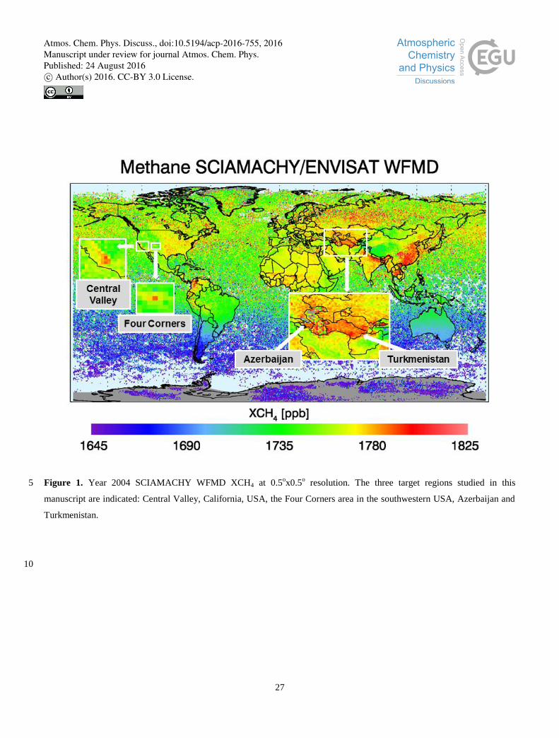
27

Figure 1. Year 2004 SCIAMACHY WFMD XCH4 at 0.5ox0.5

o resolution. The three target regions studied in this 5

manuscript are indicated: Central Valley, California, USA, the Four Corners area in the southwestern USA, Azerbaijan and

Turkmenistan.

10


28

Figure 2. As Fig. 1 but for (a) SCIAMACHY IMAP XCH4, (b) year 2010 GOSAT OCPR XCH4 and (c) year 2010 GOSAT

SRFP (“RemoTeC”) XCH4.

5


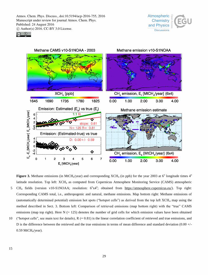
29

Figure 3. Methane emissions (in MtCH4/year) and corresponding XCH4 (in ppb) for the year 2003 at 6o longitude times 4

o

latitude resolution. Top left: XCH4 as computed from Copernicus Atmosphere Monitoring Service (CAMS) atmospheric

CH4 fields (version v10-S1NOAA; resolution: 6ox4

o; obtained from https://atmosphere.copernicus.eu/). Top right: 5

Corresponding CAMS total, i.e., anthropogenic and natural, methane emissions. Map bottom right: Methane emissions of

(automatically determined potential) emission hot spots (“hotspot cells”) as derived from the top left XCH4 map using the

method described in Sect. 3. Bottom left: Comparison of retrieved emissions (map bottom right) with the “true” CAMS

emissions (map top right). Here N (= 125) denotes the number of grid cells for which emission values have been obtained

(“hotspot cells”, see main text for details), R (= 0.81) is the linear correlation coefficient of retrieved and true emissions, and 10

D is the difference between the retrieved and the true emissions in terms of mean difference and standard deviation (0.00 +/-

0.59 MtCH4/year).

15


30

Figure 4. As Fig. 3 but for year 2012.

5


31

Figure 5. Top: “True” (i.e., CAMS) emission, Et, versus estimated emissions, Ee, as obtained from the simulation-based

assessment results shown in Figs. 3 and 4 (i.e., shown are all “hotspot cells” also shown in these two figures, see caption Fig. 5

3 and main text for details). Middle and bottom: Emission difference “estimated minus true” versus estimated emission. The

grey vertical bars denote the boundaries of emission bins for which mean differences (red crosses) and standard deviations of

the differences (red vertical lines) have been computed. The red dotted line shows that the relationship between the estimated

emission (Ee) and its 1-sigma uncertainty (σ) can be approximately described by σ(Ee) = 0.3 + 0.5 Ee.

10


32

Figure 6. Satellite-derived XCH4 anomalies (i.e., the mean value of XCH4 has been subtracted) in and around the Four 5

Corners region. Top row: SCIAMACHY WFMD year 2004 XCH4 anomaly at 0.5ox0.5

o resolution. (a) Originally gridded

data. The black rectangle indicates the assumed source area (taken from Kort et al., 2014). (b) As (a) but after elevation

correction (see main text for details). (c) As (b) but replacing the individual XCH4 values by their averages in the indicated

source region (inner rectangle) and its surrounding (outer rectangle). The difference between these two values defines the

methane enhancement of the source region, i.e., ΔXCH4. Middle row: As top row but for IMAP XCH4. Bottom row: As last 10

column of first two rows but for GOSAT OCPR (g) and SRFP (h) for the year 2010.


33

Figure 7. Methane enhancements over the Four Corners area for all years and all four satellite data products used in this

study. The error bars show the standard deviation of the methane enhancements obtained by varying the size and shape of 5

the surrounding area.


34

Figure 8. Methane emission estimates for Four Corners as obtained from the methane enhancements shown in Fig. 7. Shown

here are the satellite-derived annual methane emissions and their 1-sigma uncertainty as derived from the four satellite data 5

products used in this study using the method described in Sect. 3. The listed numerical values for the satellite-derived

emissions are the mean value and a range defined as mean value plus/minus one times the standard deviation of the annual

averages. The results are compared with published values as listed in Kort et al., 2014, (for 2003-2009; shown in dark green)

and Turner et al., 2015 (for 2009-2011; shown in grey). Also shown are the EDGAR v4.2 total anthropogenic emissions

during 2003-2008 (in light blue). 10


35

Figure 9. Methane maps for Central Valley, California. (a) SCIAMACHY year 2004 WFMD XCH4 at 0.5ox0.5

o resolution.

The rectangle shows the chosen source region. (b) As (a) but showing the source region (inner rectangle) and the default 5

background region (outer rectangle) with their corresponding XCH4 mean values. (c) As (a) but for IMAP. (d) EDGAR v4.2

year 2004 total anthropogenic methane emissions (regridded to 0.5ox0.5

o resolution). (e) CAMS v10-S1NOAA year 2004

total methane, i.e., anthropogenic and natural, emissions obtained by assimilation of NOAA methane observations (at 6ox

o4).

(f) As (e) but for CAMS version v10-S1SCIA, i.e., including the assimilation of SCIAMACHY IMAP retrievals in addition

to the assimilation of NOAA data. 10


36

Figure 10. Methane emission estimates for Central Valley area in California, USA, as defined for this study (see Fig. 9 and

Tab. 2). The blue line shows the EDGAR v4.2 (annual) anthropogenic methane emissions as computed for the Central

Valley source region. 5


37

Figure 11. Top row: (a) SCIAMACHY WFMD year 2004 XCH4 in and around Azerbaijan and Turkmenistan (resolution

0.5ox0.5

o). (b) As (a) but showing the Azerbaijan source region (entire country of Azerbaijan) and the default background 5

region (rectangle) (note that this map is shifted relative to all other maps shown in this figure to place Azerbaijan in the

center of the map). (c) As (a) but showing the Turkmenistan source and default background regions. Bottom row: (d):

EDGAR v4.2 year 2004 total anthropogenic methane emissions (at 0.5ox0.5

o resolution). (e) CAMS year 2004 total

anthropogenic and natural methane emissions based on assimilation of NOAA data (at 6ox4

o resolution). (f) As (e) but with

additional assimilation of SCIAMACHY IMAP XCH4. 10


38

Figure 12. Methane emission estimates for Azerbaijan (see also Fig. 11). The blue line shows the EDGAR v4.2 (FT2012)

emissions for Azerbaijan. 5


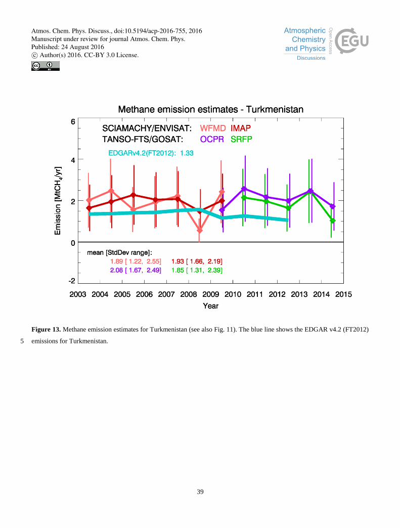
39

Figure 13. Methane emission estimates for Turkmenistan (see also Fig. 11). The blue line shows the EDGAR v4.2 (FT2012)

emissions for Turkmenistan. 5


40

Figure A1. Sketch of a simple model used to explain the methane emission estimation method described in Sect. 3. (a)

Source region A (of size LxLy and with Lx in wind speed direction (wind speed magnitude V)) with elevated XCH4 (light 5

red) and surrounding (background) region B. (b) Air parcels (blue squares) moving with constant speed V over a source

region with emission E/(LxLy), where E is the source area emission in CH4 mass per time, while accumulating methane

during accumulation time τ (= Lx/V). (c) Before entering the source region, the air parcels are characterized by a background

methane vertical column, VCb, in units of CH4 mass per area. When leaving the source area their vertical column has been

enhanced by ∆VC = E/(LxLy) ∙ τ. When passing over the source region, their vertical column increases linearly and, 10

therefore, the average column enhancement over the source region is 0.5 ∙ ∆VC. VC (CH4 mass per area) can be converted to

XCH4 (ppb) via a factor M (in units of mass and per area and per ppb).


Satellite-derived methane hotspot emission estimates using a ...

Documents

Transcript of Satellite-derived methane hotspot emission estimates using a ...