Mantle transition zone topography and structurebeneath the central Tien Shan orogenic belt

Xiaobo Tian,1 Dapeng Zhao,2 Hongshuang Zhang,1 You Tian,3 and Zhongjie Zhang1

Received 25 November 2008; revised 23 May 2010; accepted 8 June 2010; published 20 October 2010.

[1] In this study we calculated receiver functions (RFs) from teleseismic P waveformsrecorded by stations of four seismic networks to determine the topography of the mantletransition zone (MTZ) beneath the central Tien Shan. We converted the RFs from the timedomain to the depth domain and selected the depths of 410 and 660 km discontinuitiesafter stacking the RFs in narrow raypath bins. To better determine the MTZ topography,we applied an updated RF method to invert the depth differences between the 410 and660 km discontinuities in each RF for lateral depth variations of the two discontinuities.Using this approach, we detected several anomalies in the 410 and 660 km discontinuitydepths beneath the central Tien Shan region. Extensive synthetic tests were carried out toconfirm the main features of the result. Beneath the south and east of Lake Issyk‐Kul, the410 km discontinuity becomes shallower while the 660 km discontinuity becomes deeper,leading to a thicker MTZ with a lower temperature, possibly caused by pieces of thickenedlithosphere dropping down to at least the bottom of the MTZ. Beneath the northwest ofLake Issyk‐Kul, the 410 km discontinuity becomes deeper while the 660 km discontinuitybecomes shallower, resulting in a thinner MTZ with a higher temperature, which mayreflect a small‐scale hot upwelling from the lower mantle.

Citation: Tian, X., D. Zhao, H. Zhang, Y. Tian, and Z. Zhang (2010), Mantle transition zone topography and structure beneaththe central Tien Shan orogenic belt, J. Geophys. Res., 115, B10308, doi:10.1029/2008JB006229.

1. Introduction

[2] The Tien Shan is located over 1500 km north of thecollision zone between the Indian and Eurasian plates and isthe largest and most active intracontinental orogen in theworld. It extends over 2500 km in the E‐W direction andabout 300–500 km in the N‐S direction; its highest peakexceeds 7000 m. The Tien Shan orogenic belt is composedof several parallel ranges and intermontane basins and sur-rounded by several stable blocks, such as the Kazakh Shieldand the Tarim Basin, which lie to the north and south of thecentral Tien Shan, respectively (Figure 1a).[3] The ancestral Tien Shan formed in the late Paleozoic

through the convergence of a few continental blocks, e.g.,the Tarim, Yili‐central Tien Shan, and Junggar plates[Windley et al., 1990; Carroll et al., 1995; Gao et al., 1998].After erosion during the Mesozoic to the early Cenozoiceras, the ancestral Tien Shan Mountains became a peneplain[Avouac et al., 1993; Métivier and Gaudemer, 1997]. Itstectonic activity resumed in the Oligocene, presumably as aconsequence of the India‐Eurasia collision, and has con-

tinued to the present [Sobel and Dumitru, 1997; Yin et al.,1998; Molnar and Ghose, 2000; Fu et al., 2003; Huanget al., 2006; Ji et al., 2008; Sun et al., 2009].[4] A number of studies have focused on the Tien Shan

orogenic belt, but the dynamics of the tectonic rejuvenationare still not well understood. Some researchers suggest thatthe Tien Shan mountain building was caused by the short-ening of the crust, accompanied by a thickening of thelithosphere [Fleitout and Froidevaux, 1982]. Such shorten-ing may have been caused by the collision between theIndian and Eurasian plates, which transferred the stress fromthe collision front through an abnormally strong lithospherein the Tarim Basin to the Tien Shan [England and Houseman,1985]. The shortening, which amounts up to 20 mm/yr acrossthe Tien Shan, has been demonstrated by GPS observationsand geologic surveys [e.g., Abdrakhmatov et al., 1996;Thompson et al., 2002]. Using evidence from earthquakefocal mechanisms and tomographic images, other researcherssuggest that the Tien Shan orogenic belt was caused by theunderthrusting of the Tarim Basin and the Kazakh Shieldbeneath the Tien Shan [e.g., Ni, 1978; Nelson et al., 1987;Roecker et al., 1993; Ghose et al., 1998; Zhao et al., 2003;Guo et al., 2006; Lei and Zhao, 2007]. Furthermore, someresearchers speculate that the underthrusting could form aroot that can lead to further crustal shortening because of itsgreater density and subsequent gravitational instability, andwith time, the root will detach and be filled by the under-lying asthenospheric materials. Some rootlike structureshave been revealed under certain mountainous regions, such

1State Key Laboratory of Lithospheric Evolution, Institute of Geologyand Geophysics, Chinese Academy of Sciences, Beijing, China.

2Department of Geophysics, Tohoku University, Sendai, Japan.3College of Geoexploration Science and Technology, Jilin University,

Changchun, China.

Copyright 2010 by the American Geophysical Union.0148‐0227/10/2008JB006229

JOURNAL OF GEOPHYSICAL RESEARCH, VOL. 115, B10308, doi:10.1029/2008JB006229, 2010

B10308 1 of 20

Figure 1. (a) Topographic map of the central Tien Shan showing the locations of 44 seismic stationsfrom four seismic networks. XW, GHENGIS (blue triangles); KN, KNET (red inverted triangles); KZ,KZNET (red inverted triangles); and G, GEOSCOPE (red inverted triangles). The station code is shownbeside each station. The bold trace denotes the Talas‐Fergana Fault and the thin lines denote the bound-aries of the states. F. Basin, Fergana Basin; Lake I‐K, Lake Issyk Kul. (b) Distribution of 1537 teleseismicevents (squares) used in this study, which shows a relatively uniform distribution, although more eventsare located in the Eastern Hemisphere. The triangle denotes the center of the study area.

TIAN ET AL.: MTZ TOPOGRAPHY BENEATH THE TIEN SHAN B10308B10308

2 of 20

as the Transverse Ranges in western United States[Humphreys and Clayton, 1990] and the Karakorum inPakistan [Pandey et al., 1991]. However, in other regions, arootlike structure is not visible or its appearance is incon-sistent, such as under the Alps [Babushka et al., 1984] andthe Sierra Nevada [Jones et al., 1994]. So far, seismologicalstudies have not found such a root beneath the Tien Shan[e.g., Roecker et al., 1993; Vinnik et al., 2004; Lei and Zhao,2007].[5] Many RF and tomography studies have been con-

ducted on the Tien Shan region [e.g., Roecker et al., 1993;Kosarev et al., 1993; Chen et al., 1997; Bump and Sheehan,1998; Xu et al., 2002; Vinnik et al., 2004; Kumar et al.,2005; Lei and Zhao, 2007]. The crustal thickness variesfrom 45–70 km in the Tien Shan to approximately 42 km inthe southern Kazakh Shield [Bump and Sheehan, 1998;Vinnik et al., 2004]. The thickness of the lithosphere is about90 km underneath the Tien Shan, but it increases to 120 and160 km beneath the Kazakh Shield and the Tarim Basin,respectively [Oreshin et al., 2002; Kumar et al., 2005]. Coollithospheric materials residing near the 410 km depthbeneath the Tien Shan have been revealed in the analysis ofconverted seismic phases from the 410 km discontinuity[Chen et al., 1997]. Recent tomographic studies revealed ahigh‐velocity (high‐V) anomaly at 150–200 km depths thatextends down to the MTZ under the Tien Shan [Yang et al.,2003; Lei and Zhao, 2007]. In addition, some low‐velocity(low‐V) anomalies are revealed beneath the Tien Shan at50–60 km depths, which also extend downward beneath theTarim Basin and the Kazakh Shield [Roecker et al., 1993;Xu et al., 2002, 2007; Vinnik et al., 2004; Lei and Zhao,2007]. Some researchers suggest the existence of a small‐scale convection [e.g., Roecker et al., 1993; Wolfe andVernon, 1998], while others propose the presence of asmall mantle plume under the Tien Shan [e.g., Sobel andArnaud, 2000; Xu et al., 2002; Friederich, 2003; Vinniket al., 2004; Kumar et al., 2005; Lei and Zhao, 2007].The origin of the low‐V zones observed beneath the TienShan and its surrounding regions has important implica-tions with respect to the dynamics of the tectonic rejuve-nation. To clarify these problems, we need to determineprecisely the structure in and around the MTZ under theTien Shan.[6] The MTZ is bounded by two sharp seismic dis-

continuities at depths of approximately 410 and 660 km.According to the commonly accepted view, the 410 and660 km discontinuities caused by phase transformations inolivine in an olivine‐dominated mantle. For a typical mantleadiabat, the olivine‐wadsleyite transition (a → b) occurs ata pressure corresponding to a depth of 410 km, whichcauses a jump in the elastic properties of the mantle rock.The breakdown of the spinel phase (ringwoodite) intoperovskite and magnesiowüstite (sp → pv + mw) occursnear 660 km in the mantle, which is commonly believed tobe the cause of the 660 km seismic discontinuity [Ringwood,1969]. An important characteristic of a phase transformationis its Clapeyron slope, the temperature derivative of thepressure at which the transformation occurs. In the Earth,pressure increases with depth, and lateral variations intemperature can create topography on the seismic disconti-

nuity. The Clapeyron slope of the a → b transformation ispositive [e.g., Katsura and Ito, 1989; Bina and Helffrich,1994], so a low‐temperature anomaly can cause a localelevation of the 410 km discontinuity, whereas a high‐temperature anomaly can cause a local depression of the410 km discontinuity. In contrast, the slope of the sp→ pv +mw transformation is negative [e.g., Ito and Takahashi,1989; Bina and Helffrich, 1994], which implies a depres-sion of the 660 km discontinuity in a low‐temperatureenvironment and its elevation at high‐temperature. Thus,lateral variations in the discontinuity depths provide infor-mation on lateral temperature variations in MTZ, which canbe diagnostic of the depth of origin of mantle plumes [Shenet al., 1998; Fee and Dueker, 2004] and the deep structureof subducting slabs [Li et al., 2000; Chen and Ai, 2009].[7] With the rapidly growing number of permanent and

temporary seismic stations deployed during the last decadein Tien Shan, much information on the crust and upper‐mantle structure has been obtained [e.g., Yang et al., 2003;Vinnik et al., 2004; Kumar et al., 2005; Lei and Zhao,2007]. However, the detailed deep structure and dynamicprocesses remain unclear. Understanding the dynamicsdriving this enigmatic mountain belt is very important,and studying the MTZ topography can extract importantand independent information on the thermal structure anddynamic process beneath the Tien Shan.[8] The RF method has become an important tool in the

imaging of the MTZ topography. In many previous studies,the MTZ topography has been obtained from the P‐to‐Sconverted phases at the discontinuities (P410s and P660s)by migrating or stacking RFs. However, the topography ofthe 410 and 660 km discontinuities that is obtained usingsuch a conventional approach suffers from the lateralvelocity variations in the crust and upper mantle. Conse-quently, the topography results depend on the velocitymodel adopted [Niu et al., 2004]. To remove the effect ofthe velocity heterogeneity in the crust and upper mantle, inthis work we have developed an updated RF method thatdetermines the MTZ topography from the differential traveltime TP660s – TP410s (or the differential depth D660−410), andwe have applied the new method to investigate the MTZstructure beneath the central Tien Shan.

2. Data and Method

2.1. Data

[9] We used 44 seismic stations belonging to four seismicnetworks of GHENGIS (28 stations), GEOSCOPE (1 sta-tion, WUS), KZNET (2 stations, PDG and TLG), andKNET (13 stations) (Figure 1a). The GHENGIS networkwas in operation for about 18 months, while the stations ofthe other three networks had operated for at least a fewyears.[10] Figure 1b shows the epicentral distribution of 1537

earthquakes used in this study. The magnitude of theseevents is M > 5.3. All of the events are located at epicentraldistances of 30°–90° from the center of the study area. Thedistribution of the selected events is not uniform. Most ofthem are located in the subduction zones in the northernand western Pacific as well as Indonesia, and only a fewevents are located in the Western Hemisphere. We used the

TIAN ET AL.: MTZ TOPOGRAPHY BENEATH THE TIEN SHAN B10308B10308

3 of 20

P waveforms from these events and isolated the P‐to‐S con-versions from the seismic discontinuities to compute RFs in thefrequency domain using a band‐pass filter of 0.03∼0.2 Hz[Ammon, 1991]. After removing poorly deconvolved RFs,we obtained 8855 high‐quality RFs and calculated the ray-paths of the RFs using the IASP91 Earth model [Kennettand Engdahl, 1991]. The piercing points of the RFs at410 and 660 km depths cover the study area densely anduniformly (Figure 2).

2.2. Measuring D660−410 in Common Raypath Stacking

[11] To study the MTZ topography and structure, wemeasure the depths of the 410 and 660 km discontinuities(D410 and D660). In the first step, we convert all the RFsfrom the time domain to the depth domain [Chevrot et al.,1999]. The IASP91 Earth model is used as the referencemodel of seismic velocities (Vp and Vs) to calculate theraypaths and the delay times between the converted phasesand the direct P wave. The elevations of seismic stations aretaken into account in the calculation. After converting all theRFs to the depth domain, the effects of the epicentral dis-tance on travel time are corrected automatically. The secondstep is to stack RFs. Some bins are designed for stackingRFs to improve the signal‐to‐noise ratio, for example, thecommon conversion point (CCP) bins [Dueker and Sheehan,1998; Kind et al., 2002; Ozacar et al., 2008]. To measure theD410 andD660 with a high spatial resolution, we stack RFs in anarrow cylindrical bin (with a radius of 25 km) along theraypath of each RF between 410 and 660 km depths. We callthis process common raypath (CRP) stacking. The third stepis to measure the D410 and D660. For identifying the P410sand P660s correctly, we perform CRP stacking with dif-ferent radii (e.g., 150, 100, 75, and 50 km), and identify theconverted phases in CRP stacking by comparing the resultswith different radii. The depths for the peak value of phases

in stacking RFs are measured. To further quantify the D410

and D660, we use the bootstrap resampling method [Efronand Tibshirani, 1986] that estimates the standard devia-tions (STDs) of the discontinuity depths for each CRPstacking. The STDs of D410 and D660 are generally smallerthan 5 km. In Appendix A, we describe the CRP stackingin detail and show some examples and statistics of ourmeasurements.

2.3. Construction of the Grid Model

[12] To map the MTZ topography, we used 2 two‐dimensional grid meshes to express the depth variations ofthe 410 and 660 km discontinuities. Figure 3 shows theconfigurations of the grid meshes in the horizontal and depthdirections. The lateral grid spacing is 0.5° (∼50 km) for eachdiscontinuity. Taking the discontinuity depth anomaly ateach grid node as the unknown parameter, we calculated thediscontinuity depth anomaly at any point in the study areaby using the following linear interpolation function:

DD410 x; yð Þ ¼X2i¼1

X2j¼1

DD410 xi; yj� �

� 1� x� xix2 � x1

��������

� �1� y� yj

y2 � y1

��������

� �� �

¼X2i¼1

X2j¼1

DD410 xi; yj� �

Yij; ð1aÞ

where Yij = (1 − |x − xi/x2 − x1|)(1 − |y − yj/y2 − y1|) representsthe weight coefficients for the linear interpolation at the410 km discontinuity, x is the longitude, and y is the latitude;xi and yj are the coordinates of the four grid nodes surroundinga point (x, y). DD410(xi, yj) denotes the depth anomaly at a

Figure 2. Map showing the locations of the ray‐piercing points at 410 (blue crosses) and 660 (redcrosses) km depths. Black lines denote the national boundaries.

TIAN ET AL.: MTZ TOPOGRAPHY BENEATH THE TIEN SHAN B10308B10308

4 of 20

grid node for the 410 km discontinuity. For the 660 kmdiscontinuity, we have the following expression:

DD660 x; yð Þ ¼X2i¼1

X2j¼1

DD660 xi; yj� �

� 1� x� xix2 � x1

��������

� �1� y� yj

y2 � y1

��������

� �� �

¼X2i¼1

X2j¼1

DD660 xi; yj� �

Fij; ð1bÞ

where Fij = (1 − |x − xi/x2 − x1|)(1 − |y − yj/y2 − y1|) representsthe weight coefficients for the linear interpolation at the660 km discontinuity. DD660(xi, yj) denotes the depthanomaly at a grid node for the 660 km discontinuity.

2.4. Inversion for the MTZ Topography

[13] For better imaging of the MTZ topography, weincorporated the D660−410 data in our new RF method ineach CRP bin with a radius of 25 km, instead of using theindividual measurements of D410 and D660. This is becausethe D660−410 data are not sensitive to velocity heterogeneitiesabove the 410 km discontinuity, since the paths of P410sand P660s are nearly identical above that depth [Shen et al.,1998]. Note that the value of D660−410 in a RF is not a truemeasurement of the MTZ thickness, because the piercingpoints at the two discontinuities have a horizontal offset of60–120 km. By considering the raypaths in and around the

MTZ, the measurement of D660−410 can be expressed asfollows:

D660 x6k ; y6kð Þ � D410 x4k ; y4kð Þ ¼ D660�410 kð Þ

or

DD660 x6k ; y6kð Þ �DD410 x4k ; y4kð Þ ¼ DD660�410 kð Þ; ð2Þ

where D660−410(k) is the D660−410 measured from the kth RFstacking bin and D660(x6k, y6k) and D410(x4k, y4k) are themeasurements for the 660 and 410 km discontinuity depthsat the ray‐piercing points (x6k, y6k) and (x4k, y4k), respec-tively. In addition, DD410, DD660, and DD660−410 areequivalent to D410 – 410 km, D660 – 660 km, and D660−410 –250 km, respectively. The measurements of DD660−410 forma data column vector d with dimension N (N = 4738).[14] As in the seismic tomography method [Zhao et al.,

1992, 1994], we can express the depth variations of the410 and 660 km discontinuities with two‐dimensional grids(Figure 3). Taking the depth anomaly at each grid node to bethe unknown parameter, we calculate the discontinuity depthanomaly at any point using a linear interpolation function asin equations (1a, 1b). Thus equation (2) can be rewritten as

X2i¼1

X2j¼1

DD660 x6ki; y6kj� �

Fkij

�X2i¼1

X2j¼1

DD410 x4ki; y4kj� �

Ykij ¼ DD660�410 kð Þ: ð3Þ

Figure 3. Distribution of the grid nodes used to map the 410 and 660 km discontinuities in (a) mapview, (b) north‐south, and (c) east‐west vertical crosssections. The grid spacing is 0.5° in both the lati-tudinal and longitudinal directions. The shaded lines in Figure 3a denote the national boundaries.

TIAN ET AL.: MTZ TOPOGRAPHY BENEATH THE TIEN SHAN B10308B10308

5 of 20

The depth anomaly parameters can be expressed as a columnvector m as follows:

mT ¼ DD410 x1; y1� �

; DD410 x1; y2ð Þ; . . . ; DD410 xK ; yLð Þ�DD660 x1; y1ð Þ; DD660 x1; y2ð Þ; . . . ;DD660 xK ; yLð Þ�:

Note that the total number of depth anomaly parameters inthis study is 2 × K × L (K = 25, L = 13).[15] The column vectors specifying the data set and the

unknown parameters are related through the followingobservation equation:

d ¼ Gmþ e; ð4Þwhere e is an error vector and G is an N × (2 × K × L) matrixwhose elements consist of the coefficients of the depthanomaly in equation (3). Figure 4 shows the distribution ofthe raypaths used in the inversion.[16] The damped leastsquares method was adopted by Aki

and Lee [1976] to solve equation (4) in the early tomo-graphic studies. They used

GTGþQ� �

m ¼ GTd; ð5Þ

which can be obtained by minimizing |d − Gm|2 + mT Qm,where Q = "2I and " is the damping parameter. The draw-back of this inversion method is that the matrix GTG needslarge memory storage and its inversion is time consuming,though G is a relatively sparse matrix [Zhao et al., 1992]. Toavoid such a problem, we follow Zhao [2001, 2004] andadopt a conjugate‐gradient algorithm [Paige and Saunders,

1982], which yields a solution equivalent to that obtained byresolving equation (5) [Carroll and Beresford, 1997].

3. Results and Resolution Tests

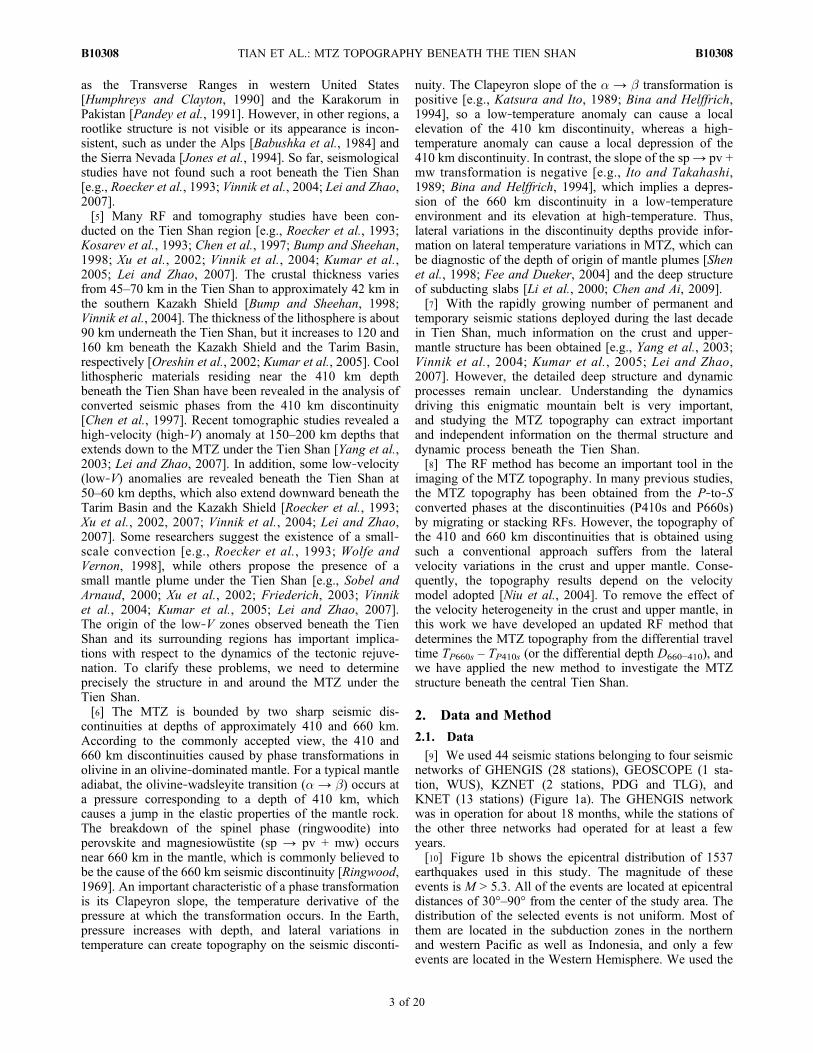
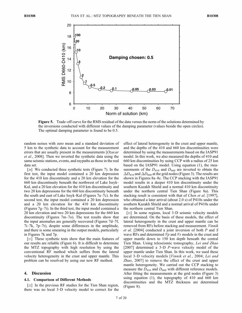
[17] We performed many inversions with different valuesof the damping parameter. Figure 5 shows the trade‐offcurve for the norm of the solution versus the final RMSdepth residual. We found the optimal value of the dampingparameter to be 0.5, because it best balances the reduction ofthe RMS residual and the smoothness of the model for the410 and 660 km discontinuities. The results obtained areshown in Figure 6. The MTZ thickness (TMTZ) is defined bysubtracting the depth of 410 km discontinuity from the depthof 660 km discontinuity at the same horizontal location. Theanomaly of the MTZ thickness, DTMTZ, is obtained by sub-tracting 250 km from TMTZ.[18] To the northwest of Lake Issyk‐Kul, the 410 km

discontinuity is depressed while the 660 km discontinuity iselevated (Figures 6a and 6b). Beneath the south and east ofLake Issyk‐Kul, the 410 km discontinuity is elevated whilethe 660 km discontinuity is depressed. As a result, theMTZ becomes thin to the northwest of Lake Issyk‐Kul andbecomes thick to the east and south of the lake (Figure 6c).[19] In order to confirm the main features of our MTZ

topographic image (Figure 6), we performed several synthetictests following the approach of Zhao [2001]. In the inputmodels (Figure 7), we assumed a few topographic anomalieswith an amplitude of 20 km relative to the IASP91model. Wecomputed the synthetic data for the input models and added

Figure 4. Distribution of RF raypaths used in this study in (a) map view, (b) north‐south, and (c) east‐west vertical cross‐sections. White triangles denote the seismic stations used in this study. The shadedlines in Figure 4a denote the national boundaries. The shaded dashed lines in Figures 4b and 4c denotethe 410 and 660 km discontinuities.

TIAN ET AL.: MTZ TOPOGRAPHY BENEATH THE TIEN SHAN B10308B10308

6 of 20

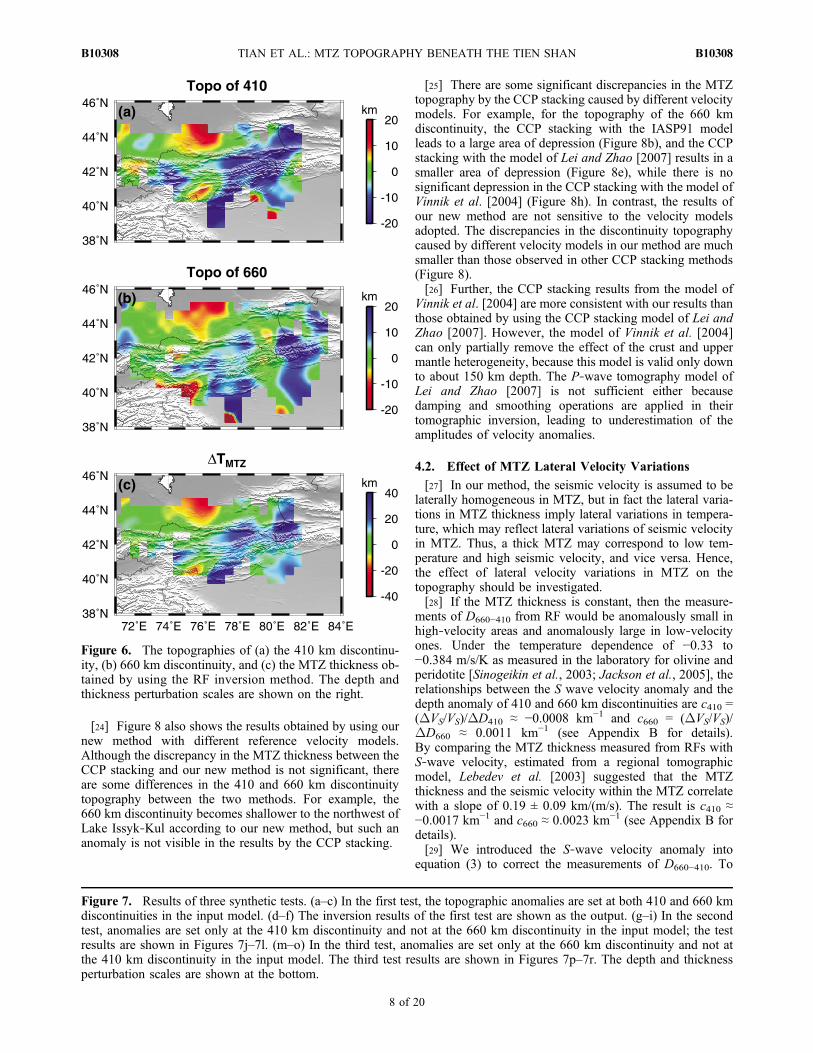
random noises with zero mean and a standard deviation of5 km to the synthetic data to account for the measurementerrors that are usually present in the measurements [Ozacaret al., 2008]. Then we inverted the synthetic data using thesame seismic stations, events, and raypaths as those in the realdata set.[20] We conducted three synthetic tests (Figure 7). In the

first test, the input model contained a 20 km depressionfor the 410 km discontinuity and a 20 km elevation for the660 km discontinuity beneath the northwest of Lake Issyk‐Kul, and a 20 km elevation for the 410 km discontinuity andtwo 20 km depressions for the 660 km discontinuity beneaththe south and east of Lake Issyk‐Kul (Figures 7a–7c). In thesecond test, the input model contained a 20 km depressionand a 20 km elevation for the 410 km discontinuity(Figures 7g–7i). In the third test, the input model contained a20 km elevation and two 20 km depressions for the 660 kmdiscontinuity (Figures 7m–7o). The test results show thatthe input anomalies are generally recovered (Figures 7d–7f,7i–7k, 7p–7r), despite some differences in the amplitude,and there is some smearing in the output models, particularlyin Figures 7k and 7p.[21] These synthetic tests show that the main features of

our results are reliable (Figure 6). It is difficult to determinethe MTZ topography with high resolution by using theconventional RF method which suffers from the lateralvelocity heterogeneity in the crust and upper mantle. Thisproblem can be resolved by using our new RF method.

4. Discussion

4.1. Comparison of Different Methods

[22] In the previous RF studies for the Tien Shan region,there was no local 3‐D velocity model to correct for the

effect of lateral heterogeneity in the crust and upper mantle,and the depths of the 410 and 660 km discontinuities weredetermined by using the measurements based on the IASP91model. In this work, we also measured the depths of 410 and660 km discontinuities by using CCP with a radius of 25 kmbased on the IASP91 model. Using equation (1), the mea-surements of the D410 and D660 are inverted to obtain theDD410 andDD660 at the grid nodes (Figure 3). The results areshown in Figures 8a–8c. The CCP stacking with the IASP91model results in a deeper 410 km discontinuity under thesouthern Kazakh Shield and a normal 410 km discontinuityunder the northern central Tien Shan (Figure 8a). Thisstacking result is consistent with that of Chen et al. [1997],who obtained a later arrival (about 2.0 s) of P410s under thesouthern Kazakh Shield and a normal arrival of P410s underthe northern central Tien Shan.[23] In some regions, local 3‐D seismic velocity models

are determined. On the basis of these models, the effect oflateral heterogeneity in the crust and upper mantle can beremoved from RFs before stacking and measurement. Vinniket al. [2004] conducted a joint inversion of both P and Swave RFs and determined Vp and Vs models in the crust andupper mantle down to 150 km depth beneath the centralTien Shan. Using teleseismic tomography, Lei and Zhao[2007] determined a 3‐D P‐wave velocity model of theupper mantle under Tien Shan. In this work, we used theselocal 3‐D velocity models [Vinnik et al., 2004; Lei andZhao, 2007] to remove the effect of the crust and uppermantle heterogeneity. We carried out the CCP stacking tomeasure the D410 and D660 with different reference models.After fitting the measurements at the grid nodes (Figure 3)using equation (1), the topography of 410 and 660 kmdiscontinuities and the MTZ thickness are determined(Figure 8).

Figure 5. Trade‐off curve for the RMS residual of the data versus the norm of the solutions determined bythe inversions conducted with different values of the damping parameter (values beside the open circles).The optimal damping parameter is found to be 0.5.

TIAN ET AL.: MTZ TOPOGRAPHY BENEATH THE TIEN SHAN B10308B10308

7 of 20

[24] Figure 8 also shows the results obtained by using ournew method with different reference velocity models.Although the discrepancy in the MTZ thickness between theCCP stacking and our new method is not significant, thereare some differences in the 410 and 660 km discontinuitytopography between the two methods. For example, the660 km discontinuity becomes shallower to the northwest ofLake Issyk‐Kul according to our new method, but such ananomaly is not visible in the results by the CCP stacking.

[25] There are some significant discrepancies in the MTZtopography by the CCP stacking caused by different velocitymodels. For example, for the topography of the 660 kmdiscontinuity, the CCP stacking with the IASP91 modelleads to a large area of depression (Figure 8b), and the CCPstacking with the model of Lei and Zhao [2007] results in asmaller area of depression (Figure 8e), while there is nosignificant depression in the CCP stacking with the model ofVinnik et al. [2004] (Figure 8h). In contrast, the results ofour new method are not sensitive to the velocity modelsadopted. The discrepancies in the discontinuity topographycaused by different velocity models in our method are muchsmaller than those observed in other CCP stacking methods(Figure 8).[26] Further, the CCP stacking results from the model of

Vinnik et al. [2004] are more consistent with our results thanthose obtained by using the CCP stacking model of Lei andZhao [2007]. However, the model of Vinnik et al. [2004]can only partially remove the effect of the crust and uppermantle heterogeneity, because this model is valid only downto about 150 km depth. The P‐wave tomography model ofLei and Zhao [2007] is not sufficient either becausedamping and smoothing operations are applied in theirtomographic inversion, leading to underestimation of theamplitudes of velocity anomalies.

4.2. Effect of MTZ Lateral Velocity Variations

[27] In our method, the seismic velocity is assumed to belaterally homogeneous in MTZ, but in fact the lateral varia-tions in MTZ thickness imply lateral variations in tempera-ture, which may reflect lateral variations of seismic velocityin MTZ. Thus, a thick MTZ may correspond to low tem-perature and high seismic velocity, and vice versa. Hence,the effect of lateral velocity variations in MTZ on thetopography should be investigated.[28] If the MTZ thickness is constant, then the measure-

ments of D660−410 from RF would be anomalously small inhigh‐velocity areas and anomalously large in low‐velocityones. Under the temperature dependence of −0.33 to−0.384 m/s/K as measured in the laboratory for olivine andperidotite [Sinogeikin et al., 2003; Jackson et al., 2005], therelationships between the S wave velocity anomaly and thedepth anomaly of 410 and 660 km discontinuities are c410 =(DVS/VS)/DD410 ≈ −0.0008 km−1 and c660 = (DVS/VS)/DD660 ≈ 0.0011 km−1 (see Appendix B for details).By comparing the MTZ thickness measured from RFs withS‐wave velocity, estimated from a regional tomographicmodel, Lebedev et al. [2003] suggested that the MTZthickness and the seismic velocity within the MTZ correlatewith a slope of 0.19 ± 0.09 km/(m/s). The result is c410 ≈−0.0017 km−1 and c660 ≈ 0.0023 km−1 (see Appendix B fordetails).[29] We introduced the S‐wave velocity anomaly into

equation (3) to correct the measurements of D660−410. To

Figure 6. The topographies of (a) the 410 km discontinu-ity, (b) 660 km discontinuity, and (c) the MTZ thickness ob-tained by using the RF inversion method. The depth andthickness perturbation scales are shown on the right.

Figure 7. Results of three synthetic tests. (a–c) In the first test, the topographic anomalies are set at both 410 and 660 kmdiscontinuities in the input model. (d–f) The inversion results of the first test are shown as the output. (g–i) In the secondtest, anomalies are set only at the 410 km discontinuity and not at the 660 km discontinuity in the input model; the testresults are shown in Figures 7j–7l. (m–o) In the third test, anomalies are set only at the 660 km discontinuity and not atthe 410 km discontinuity in the input model. The third test results are shown in Figures 7p–7r. The depth and thicknessperturbation scales are shown at the bottom.

TIAN ET AL.: MTZ TOPOGRAPHY BENEATH THE TIEN SHAN B10308B10308

8 of 20

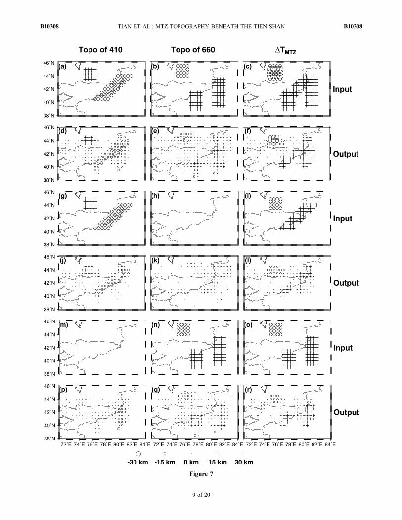
Figure 7

TIAN ET AL.: MTZ TOPOGRAPHY BENEATH THE TIEN SHAN B10308B10308

9 of 20

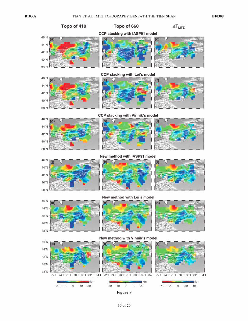
Figure 8

TIAN ET AL.: MTZ TOPOGRAPHY BENEATH THE TIEN SHAN B10308B10308

10 of 20

simplify the problem, the S velocity anomaly or the tem-perature anomaly is assumed to be linear between the 410and 660 km discontinuities. According to the above dis-cussion, when c410 and c660 are assumed to be constant, wecan obtain an equation relating the unknown parametersDD410 and DD660 with the measurements DD660−410 (seeAppendix C for details).[30] Figure 9 shows the results with different values of c410

and c660. In Figures 9d–9f, we assumed c410 = −0.0008 km−1

and c660 = 0.0011 km−1 which are equal to those measured inthe laboratory for olivine and peridotite. In Figures 9g–9i,c410 = −0.0017 km−1 and c660 = 0.0023 km−1, which are equalto those induced from RF and surface wave studies. InFigures 9j–9l, c410 = −0.0025 km−1 and c660 = 0.0034 km−1,indicating that the temperature variation may lead to a largervelocity anomaly than those estimated by previous studies[Sinogeikin et al., 2003; Jackson et al., 2005; Lebedev et al.,2003]. In Figures 9m–9o, c410 = −0.003 km−1 and c660 =0.003 km−1. These results show a pattern similar to thosewithout the velocity anomaly in MTZ, but the amplitude ofthe 410 and 660 km discontinuity topography is somewhatdiminished and enlarged, respectively, suggesting that ourresults are not sensitive to the lateral velocity variations inMTZ.

4.3. Geodynamic Implications

[31] With the IASP91 model, our topographic imageshows a depression (10–20 km) at the 410 km discontinuityand an uplift (10–20 km) at the 660 km discontinuity beneaththe northwest of Lake Issyk‐Kul (Figures 6a and 6b). Byassuming that the depth variations of the discontinuities arecaused solely by the temperature effect and using thelaboratory‐obtained depth dependence of 3.1 MPa/K and−2.0 MPa/K for the olivine‐wadsleyite transition (a → b)and the breakdown of the spinel phase (ringwoodite) intoperovskite and magnesiowüstite (sp → pv + mw) [Katsuraand Ito, 1989; Bina and Helffrich,1994], respectively, re-searchers estimate that the depression of the 410 km dis-continuity corresponds to a temperature increase of 125–250 K, and the uplift of the 660 km discontinuity correspondsto a temperature increase of 200–400 K [Revenaugh andJordan, 1991; Bina and Helffrich, 1994]. Beneath the southand east of Lake Issyk‐Kul (Figures 6a and 6b), our resultindicate an uplift (10–20 km) at the 410 km discontinuity andtwo depressions (10–20 km) at the 660 km discontinuity. Theuplift of the 410 km discontinuity corresponds to a temper-ature decrease of 125–250 K, and the depressions of the660 km discontinuity correspond to a temperature decrease of200–400 K.[32] Figure 10 summarizes our results schematically. The

lateral temperature variations at the 410 and 660 km dis-continuities provide information on the mantle circulationpatterns. The higher temperature at the 410 and 660 kmdiscontinuities beneath the northwest of Lake Issyk‐Kul

may be indicative of a mantle plume raising from the lowermantle [Shen et al., 1998; Li et al., 2003], while the lowertemperature at the 410 and 660 km discontinuities beneaththe south and east of Lake Issyk‐Kul may reflect the coldlithosphere subducting or sinking to the MTZ [Li et al.,2000; Chen and Ai, 2009].[33] If the temperature variations exist only at the 410 km

discontinuity, the origin of the mantle plume and the coldlithosphere subducting or sinking may be limited to theshallow part of the MTZ. The CCP stacking result shows thehigh‐temperature anomaly only at the 410 km discontinuity(Figure 8), but depends on the velocity model adopted. Ournew method revealed a high‐temperature anomaly existingat both 410 and 660 km discontinuities even differentvelocity models are adopted, suggesting that it is a reliablefeature.[34] Many previous studies with different approaches

support the tectonic model of the Tarim and the Kazakhlithospheres underthrusting beneath the Tien Shan [e.g., Ni,1978; Nelson et al., 1987; Roecker et al., 1993; Ghose et al.,1998; Xu et al., 2002; Yang et al., 2003; Lei and Zhao,2007]. For example, seismicity studies indicate that theKazakh lithosphere underthrusts under the Tien Shan[Roecker et al., 1993]. Regional seismic tomography showsthat the underthrusting of the Tarim and the Kazakh litho-sphere formed an active mountain belt [Xu et al., 2002].Yang et al. [2003] suggested that the primary cause of ahigh‐V anomaly beneath the Tien Shan is a delaminatedlithosphere or a detached piece of the subducting Tarimlithosphere. Teleseismic tomography revealed a high‐Vanomaly extending from the upper mantle to the MTZ,suggesting that the Tarim and Kazakh lithospheres under-thrust beneath the Tien Shan, and pieces of the thickenedlithosphere detached and descended to the deep mantlebecause of gravitational instability [Lei and Zhao, 2007].The detached cold lithosphere may have penetrated throughthe MTZ and changed the depth of phase transformations inolivine. According to the first‐order thermal calculations[Chen and Tseng, 2007], a temperature difference of 200–300 K between the coldest core of sinking lithosphere andthe surrounding mantle may remain 20–30 Ma after thedetachment. Our results reveal low‐temperature anomalieslocated beneath the south and east of Lake Issyk‐Kul,suggesting that the detached cold lithosphere has sunk downto at least 660 km depth (as shown by the blue arrows inFigure 10). Analyses of converted phases show the exis-tence of some cool materials near 410 km depth beneathTien Shan and, thus, also support the idea that the thickenedlithosphere detached and descended to the deep mantle[Chen et al., 1997]. A high Pn velocity anomaly with NEstrike beneath the western Tarim Basin may be associatedwith the cold relic lithosphere in MTZ [Liang et al., 2004].[35] A tomographic inversion of Pn travel times revealed

a low‐V anomaly in the uppermost mantle beneath the

Figure 8. The topography of the 410 and 660 km discontinuities and the MTZ thickness determined by using differentmethods and velocity models: (a–c) by the CCP stacking with the IASP91 model; (d–f) by the CCP stacking with the modelof Lei and Zhao [2007]; (g–i) by the CCP stacking with the model of Vinnik et al. [2004]; (j–l) by our new method with theIASP91 model; (m–o) by our new method with the model of Lei and Zhao [2007]; (p–r) by our new method with the modelof Vinnik et al. [2004]. The black lines denote the national boundaries. The depth and thickness perturbation scales areshown at the bottom.

TIAN ET AL.: MTZ TOPOGRAPHY BENEATH THE TIEN SHAN B10308B10308

11 of 20

northwest of Lake Issyk‐Kul [Liang et al., 2004]. Local,regional, and teleseismic tomographic studies show someprominent low‐V anomalies in the upper mantle beneath thecentral Tien Shan [e.g., Vinnik and Saipbekova, 1984;Woodward and Masters, 1991; Roecker et al., 1993; Yanget al., 2003; Lei and Zhao, 2007], which are consistent withthe existence of negative Bouguer gravity anomalies [Burov

et al., 1990]. However, several studies have suggested avariety of depth ranges for the low‐V anomalies. Roeckeret al. [1993] found that the low‐V anomalies beneath thecentral Tien Shan extend down to 150 km depth but nodeeper than 300 km depth. Xu et al. [2002] showed that thelow‐V anomalies beneath the Tien Shan extend down tothe Tarim asthenosphere. Friederich [2003] suggested that

Figure 9. Results showing the effect of lateral velocity variation in MTZ with different ratios betweenthe S‐velocity anomaly and the depth anomaly (c410 and c660): (a–c) c410 = 0 km−1 and c660 = 0 km−1;(d–f) c410 = −0.0008 km−1 and c660 = 0.0011 km−1; (g–i) c410 = −0.0017 km−1 and c660 = 0.0023 km−1;(j–l) c410 = −0.0025 km−1 and c660 = 0.0034 km−1; (m–o) c410 = −0.003 km−1 and c660 = 0.003 km−1. Thedepth and thickness perturbation scale is shown at the bottom.

TIAN ET AL.: MTZ TOPOGRAPHY BENEATH THE TIEN SHAN B10308B10308

12 of 20

the low‐V anomalies connect with the MTZ. Lei and Zhao[2007] revealed prominent low‐V anomalies down to 150–200 km depth beneath the Tien Shan and suggested that theseanomalies may be related to two branches of hot upwel-lings: one rising up from the lower mantle beneath theTarim Basin and the other rising up from the top of MTZbeneath the western Kazakh Shield. Our present results(Figure 6) indicate that the hot anomaly has penetratedthrough the MTZ beneath the southern Kazakh Shield. Weconsider a hot upwelling to be rising from the lower mantleand penetrating the 410 and 660 km discontinuities beneaththe northwest of Lake Issyk‐Kul (as shown by the red arrowsin Figure 10), which corresponds to the low‐V zone in theupper mantle the previous studies [e.g., Vinnik et al., 2004;Liang et al., 2004; Lei and Zhao, 2007].[36] In this study, the main features of the MTZ topog-

raphy beneath the central Tien Shan have been revealed bythe updated RF method. However, it is possible that thedepth anomalies of the 410 and 660 km discontinuities are

underestimated because of the damping and smoothingoperations applied in the inversion for the MTZ topography,similar to the velocity anomalies imaged by seismic tomog-raphy [e.g., Zhao et al., 1992, 1994].

4.4. Conclusions

[37] In this study, we estimated the MTZ topography andstructure beneath the central Tien Shan using a new RFmethod. The conventional CCP method is affected signifi-cantly by lateral velocity heterogeneities in the crust andupper mantle, which can lead to an inaccurate estimation ofthe 410 and 660 km discontinuity topography. By utilizingthe difference between D660 and D410 found in the RF, ournew method is less sensitive to the velocity heterogeneitiesabove the 410 km discontinuity since the paths of P410s andP660s are nearly identical above 410 km depth. The depthdistributions of the 410 and 660 km discontinuities aredetermined with an inversion method. We performed syn-thetic resolution tests and examined the effects of different

Figure 10. A schematic showing the MTZ structure and dynamics underneath the central Tien Shan.Yellow to red colors show high temperature at the 410 and 660 km discontinuities, while cyan to bluecolors show low temperature. Blue arrows denote the cold detached lithosphere penetrating or residingat the bottom of the MTZ. Red arrows denote the tilted plume conduit that penetrates the MTZ and formsa hot upwelling. LVZ denotes a low S‐wave velocity zone at depths of 110 to 130 km [Vinnik et al.,2004]. The surface topography of the Tien Shan region is shown by the 3‐D color image where theyellow and red colors represent the mountains, while the green colors represent the basins.

TIAN ET AL.: MTZ TOPOGRAPHY BENEATH THE TIEN SHAN B10308B10308

13 of 20

velocity models on our inversion result. We also evaluatedthe effect of the lateral velocity variations in MTZ on theestimated topography of the 410 and 660 km discontinuities.[38] Our results show a few prominent features in the

MTZ topography under the Tien Shan, which may reflecttemperature variations in MTZ. The 410 km discontinuitybecomes shallow and the 660 km discontinuity becomesdeep beneath the south and east of Lake Issyk‐Kul, which

may reflect a lower temperature caused by a thickenedlithosphere that has detached and descended to at least thebottom of the MTZ. The lithospheric thickening may resultfrom the underthrusting of the Tarim and Kazakh litho-spheres under the Tien Shan due to the collision between theIndian and Eurasian plates. We also found a depression ofthe 410 km discontinuity and an elevation of the 660 kmdiscontinuity beneath the northwest of Lake Issyk‐Kul,which may reflect a small‐scale hot anomaly ascendingfrom the lower mantle and penetrating through the 410 and660 km discontinuities into the upper mantle. The hotupwelling may have caused a low‐V anomaly in the uppermantle and played an important role in the ongoing moun-tain building in the central Tien Shan.

Appendix A: Common Raypath (CRP) Stacking

[39] To study the MTZ topography and structure, manyresearchers have used the common conversion point (CCP)stacking [e.g., Dueker and Sheehan, 1998; Kind et al., 2002;Ozacar et al., 2008]. A plane is assumed at a given depth,the piercing point of each receiver function (RF) is locatedon the plane, and the plane is divided into many cells. RFswith piercing points located in the same cell are stackedtogether to improve the signal‐to‐noise ratio. To ensurecoherent stacking, a velocity model is used to remove theeffect of the difference in the epicenter distance or to convertRF from the time domain to the depth domain. To measureor image the 410 and 660 km discontinuities, CCP stackingis often carried out for the depths of 410 and 660 or 530 km.Raypaths of RFs in a CCP stacking may be distributed overa large region (with a horizontal range of 200–300 km) inthe crust and upper mantle; therefore, any lateral velocityvariations above the depth of 410 km can debase coherentstacking. On the other hand, there is a horizontal offset of60–120 km between the piercing points at the 410 and660 km discontinuities for a RF (Figure A1). As a result, theCCP stacking yields a measurement of the MTZ thicknesswith low lateral resolution.[40] In an RF, the D660−410 is not sensitive to velocity

heterogeneities above the 410 km discontinuity, since theraypaths of P410s and P660s are nearly identical above thatdepth. To image the 410 and 660 km discontinuities with ahigh spatial resolution, we measure theD660−410 along an RF.For improving the signal‐to‐noise ratio, a common raypath(CRP) stacking is introduced in this study (Figure A1). First,a RF is taken as the host, the piercing points of the host RFat the depths of 410 and 660 km are taken as the centers oftwo circles with a given radius (such as 25 km), which areintroduced at the depth 410 and 660 km, respectively.Second, for other RFs, if their piercing points at the depths

Figure A1. A schematic showing the CRP stacking. Thetriangles represent seismic stations on the surface. The boldline denotes the raypath of the host RF, while thin lines rep-resent the raypaths of the guest RFs. The circles at the 410and 660 km discontinuities have the same size with a givenradius (e.g., 25 km), and the centers of the circles are thepiercing points of the host RF. RFs with raypaths passingthrough both the circles at the 410 and 660 km discontinuitiesare used to conduct the CRP stacking with the host RF.

Figure A2. An example of measuring D410 and D660 by the CRP stacking. The piercing points of the host RF and guestRFs are shown as a large black cross and small shaded crosses, respectively. The vertical dashed lines on the stack traceof RFs show the range of searching P410s or P660s. The arrows denote the maximum amplitude as D410 or D660. Thenumbers of RFs in the stacking are shown under the stack trace. Results of the CRP stackings with different radii areshown: (a–c) 150 km radius; (d–f) 100 km radius; (g–i) 75 km radius; (j–l) 50 km radius; and (m–o) 25 km radius. The23 RFs used in the CRP stacking with a radius of 25 km are shown in Figure A2p, and the host RF is shown at thebottom. In Figure A2o, the open circles and the vertical bars represent the mean values and the standard deviations esti-mated by using the bootstrap resampling procedure [Efron and Tibshirani, 1986].

TIAN ET AL.: MTZ TOPOGRAPHY BENEATH THE TIEN SHAN B10308B10308

14 of 20

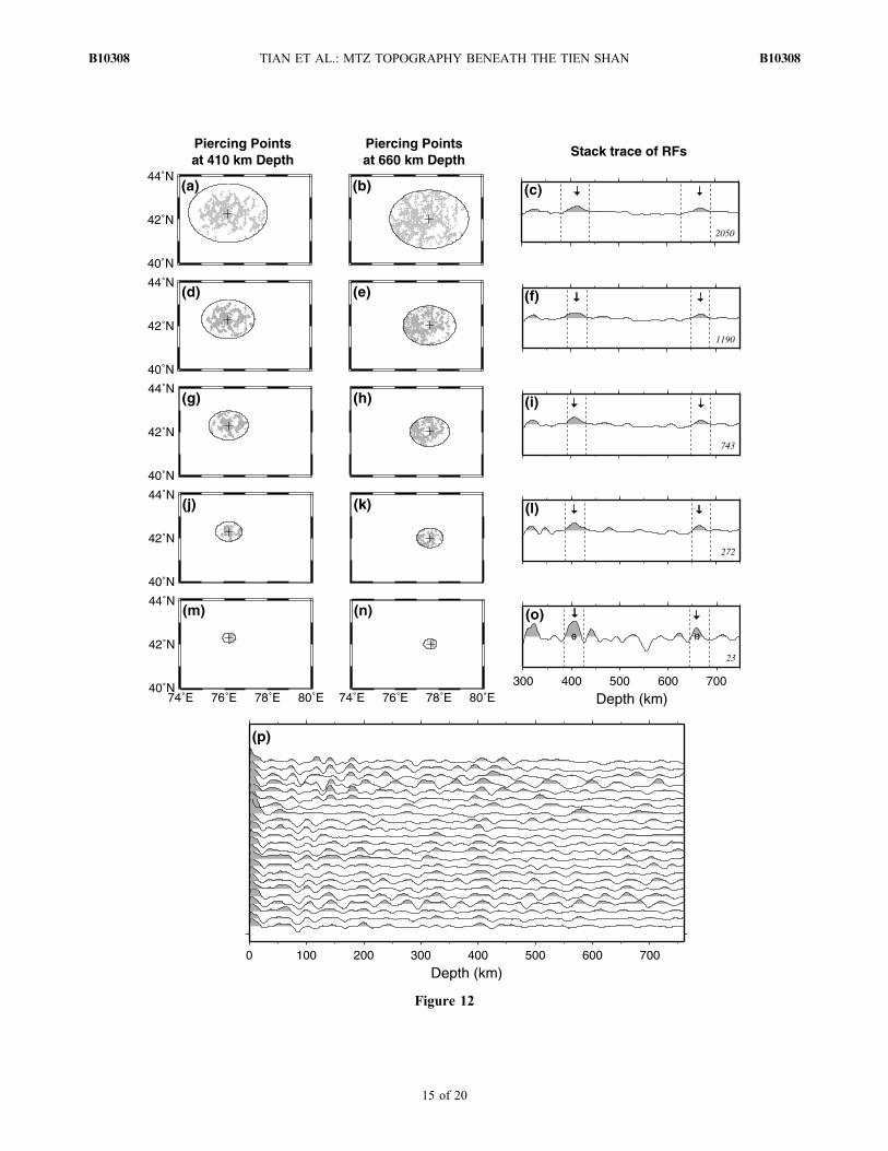
Figure 12

TIAN ET AL.: MTZ TOPOGRAPHY BENEATH THE TIEN SHAN B10308B10308

15 of 20

Figure A3. Same as Figure A2, but for a poor example with large standard deviations.

TIAN ET AL.: MTZ TOPOGRAPHY BENEATH THE TIEN SHAN B10308B10308

16 of 20

Figure A4. Histograms showing (a) the number of RFs in each CRP stacking, (b) depth measurementsof the 410 km discontinuity, (c) depth measurements of the 660 km discontinuity, (d) difference in thedepth measurements between the 410 and 660 km discontinuities, (e) STD in the depth measurementsof the 410 km discontinuity, and (f) STD in the depth measurements of the 660 km discontinuity.

TIAN ET AL.: MTZ TOPOGRAPHY BENEATH THE TIEN SHAN B10308B10308

17 of 20

of 410 and 660 km are located within the two circles, theyare taken as the guest RFs. Finally, the guest RFs and thehost RF are stacked after being converted from the timedomain to the depth domain with the velocity modelIASP91.[41] The CRP stacking looks like stacking in a narrow

cylindrical bin along the raypath of the host RF between 410and 660 km depths. The distance between the host RF rayand the guest RFs rays is lesser than or equal to the givenradius in MTZ, but may be somewhat larger than the givenradius in the crust and upper mantle.[42] As shown in Figure A2, to identify the P410s and

P660s correctly, we perform CRP stacking with differentradii (e.g., 150, 100, 75, 50, and 25 km) and identify theconverted phases in the CRP stacking by comparing theresults with different radii. When the radius is 150 km,the number of RFs in the CRP stacking is 2050. We firstpick up the maximum amplitudes as the P410s and P660s inthe depth ranges of 410 ± 30 km and 660 ± 30 km from thestacked trace and get D410 = 414 km and D660 = 668 km.When the radius is 100 km, the number of RFs in the CRPstacking is 1190, and we pick up the maximum amplitudes asthe P410s and P660s in the depth ranges of 414 ± 20 km and668 ± 20 km from the stacked trace and getD410 = 412 km andD660 = 669 km. When the radius is 75 km, the number of RFsis 743, and we pick up the maximum amplitudes as theP410s and P660s in the depth ranges of 412 ± 20 km and669 ± 20 km from the stacked trace and get D410 = 407 kmand D660 = 669 km. When the radius is 50 km, the numberof RFs is 272, and we pick up the maximum amplitudes asthe P410s and P660s in the depth ranges of 407 ± 20 km and669 ± 20 km from the stacked trace and get D410 = 406 kmand D660 = 665 km. When the radius is 25 km, the numberof RFs is 23 in the CRP stacking, then we pick up themaximum amplitudes as the P410s and P660s in the depthranges of 406 ± 20 km and 665 ± 20 km from the stackedtrace and get D410 = 407 km and D660 = 659 km.[43] Another example is shown in Figure A3. The P410s

and P660s can be measured accurately from the stackedtrace when the CRP stacking radius is larger than 75 km,while they are measured with low reliability when a smallerradius is used because there are multiple wave peaks withcomparable amplitudes in the search range. Such data, asshown in Figure A3, are not used in the further analysis andinversion.[44] The bootstrap resampling procedure [Efron and

Tibshirani, 1986] was use to estimate the standard devia-tions (STDs) of the discontinuity depths for each CRPstacking. The STD, sD410 and sD660, are calculated using s =ffiffiffiffiffiffiffiffiffiffiffiffiffiffiffiffiffiffiffiffiffiffiffiffiffiffiffiffiffiffiffiffiffiffiffiffiffiffiffiffiffiffiffiffiffiffiffiffiffiffiffiffiffi1= M � 1ð ÞPM

i¼1 Di � D� �2q

, where M is the number ofbootstrap steps (which is taken as 40 in this study), Di is theresulting depth of the ith step, and D is the mean depth. TheSTDs of the D660−410 are calculated by using sD660‐410 =ffiffiffiffiffiffiffiffiffiffiffiffiffiffiffiffiffiffiffiffiffiffiffiffiffiffiffi�2D410 þ �2D660

p. We reject those measurements with sD410

or sD660 larger than 10 km or with the number of RFs perstacking less than 10, such as the example shown in Figure A3where sD410 = 13.4 km. As a result, we obtain 4738 mea-surements (see Figure A4 for details). The average number ofRFs per stacking is 40. The averages of D410, D660, andD660−410 are 411, 667, and 255 km, respectively. The

averages of sD410, sD660, and sD660‐410 are 3.0, 4.3, and5.7 km, respectively.

Appendix B: Relationship Between the MTZS‐Velocity Anomaly and the MTZ Topography

[45] We define the relationship between the S‐wavevelocity anomaly in MTZ and the depth of the 410 or 660 kmdiscontinuities as c = (DVS/VS)/DD ≈ dVS/dT · dT/dP ·dP/dD · 1/VS = dVS/dT · (dP/dT · dD/dP · VS)

−1, where dD/dP = 0.03 km/MPa. For the 410 km discontinuity, dP/dT =3.1MPa/K [Katsura and Ito, 1989; Bina and Helffrich,1994],VS = 5.07 km/s [Kennett and Engdahl, 1991], dVS/dT = −0.33 to−0.384 m/s/K [Sinogeikin et al., 2003; Jackson et al., 2005],and c410 = −0.0008 km−1. For the 660 km discontinuity,dP/dT = −2.0 MPa/K [Katsura and Ito, 1989; Bina andHelffrich,1994], VS = 5.6 km/s [Kennett and Engdahl,1991], dVS/dT = −0.33 to −0.384 m/s/K [Sinogeikin et al.,2003; Jackson et al., 2005], and c660 = 0.0011 km−1.[46] By comparing the MTZ thickness measured from

RFs with S‐wave velocity estimated from a regional tomo-graphic model, Lebedev et al. [2003] suggested that theMTZ thickness and the seismic velocity within the MTZcorrelate with a slope of 0.19 ± 0.09 km/(m/s). Consideringthe Clapeyron slopes (3.1 and −2.0 MPa/K at 410 and660 km discontinuities, respectively) [Katsura and Ito,1989; Bina and Helffrich,1994], dD/dVS values are −0.114and 0.076 km/(m/s) for the 410 and 660 km discontinuities,respectively. Using c = (DVS/VS)/DD ≈ dVS/dD · 1/VS =(dD/dVS · VS)

−1, we obtain c410 = −0.0017 km−1 and c660 =0.0023 km−1.

Appendix C: Equation for the DepthMeasurements Considering Lateral S‐VelocityVariations in MTZ

[47] By dividing the raypath of a converted wave in MTZinto J segments (in this study J = 5) and using the IASP91velocity model, the travel time of the converted wave can beexpressed as

t ¼XJi¼1

liVsi

;

where li and Vsi are the length of the raypath and the averageS‐wave velocity in the ith segment, respectively.[48] If there is a velocity anomaly in MTZ and the real

velocity is V′S, we have DVs = DVS/VS = (V′S − VS)/VS. If|DVs| � 1, and we can neglect the difference in the raypathbetween the IASP91 model and the real velocity structure.Then the real travel time of the converted wave is expressed as

t0 ¼

XJi¼1

liVs

0i

¼XJi¼1

liVsi 1þDVsið Þ :

Assume that the error of the measurement DD660−410 is −"V,p = 1/Vs and Dp = −DVs, then we have

"V ¼ t � t0

t� 250 ¼ 250� 250PJ

i¼1lipi

XJi¼1

lipi � 1�Dpi

� �:

TIAN ET AL.: MTZ TOPOGRAPHY BENEATH THE TIEN SHAN B10308B10308

18 of 20

Assume c0 = 250/PJi¼1

lipi; then

"V ¼ c0XJi¼1

lipiDpi :

Assume c410 = −Dp410/DD410 and c660 = −Dp660/DD660; wecan get Dp410 = −c410 · DD410 and Dp660 = −c660 · DD660.Expressing Dpi using a linear interpolation function fromeight grid nodes (four grid nodes at the 410 km discontinuityand four grid nodes at the 660 km discontinuity), we have

"V ¼ �c0XJi¼1

lipi �X4n¼1

wi;nc410DD410 i; nð Þ "

þX8n¼5

wi;nc660DD660 i; n� 4ð Þ!#

;

where w is the weight for the linear interpolation. Thusequation (2) can be rewritten as follows:

DD660 x6k ; y6kð Þ �DD410 x4k ; y4kð Þ þ "V ¼ DD660�410 kð Þ:

[49] Acknowledgments. The IRIS Data Center provided the wave-form data for this study. We are grateful to L. Vinnik and Jianshe Leifor providing their velocity models. We thank editors Patrick Taylor andJeanette Panning as well as two anonymous reviewers for their constructivecomments and suggestions, which improved the manuscript. This researchwas supported by grants from the Chinese National Natural Science Foun-dation (40504005 and 40974025 to X.Tian, and 40721003 to Z.Zhang) anda grant from Japan Society for the Promotion of Science to D.Zhao (Kiban‐A 17204037). Most of the figures were generated by using the GenericMapping Tools software package [Wessel and Smith, 1998].

ReferencesAbdrakhmatov, K., et al. (1996), Relatively recent construction of the TienShan inferred from GPS measurements of present‐day crustal deforma-tion rates, Nature, 384, 450–453.

Aki, K., and W. H. K. Lee (1976), Determination of three‐dimensionalvelocity anomalies under a seismic array using first P arrival times fromlocal earthquakes: 1. A homogeneous initial model, J. Geophys. Res.,81(23), 4381–4399.

Ammon, C. J. (1991), The isolation of receiver effects from teleseismicP waveforms, Bull. Seismol. Soc. Am., 81, 2504–2510.

Avouac, J., P. Tapponnier, M. Bai, H. You, and G. Wang (1993), Activethrusting and folding along the northern Tien Shan and late Cenozoicrotation of Tarim relative to Dzungaria and Kazakhstan, J. Geophys.Res., 98(B4), 6755–6804.

Babushka, V., J. Plomerova, and J. Sileny (1984), Spatial variations ofP residuals and deep structure of the European continent, Geophys.J. R. Astron. Soc., 79, 363–383.

Bina, C. R., and G. Helffrich (1994), Phase transition Clapeyron slopesand transition zone seismic discontinuity topography, J. Geophys. Res.,99(B8), 15,853–15,860.

Bump, H., and A. Sheehan (1998), Crustal thickness variations across thenorthern Tien Shan from teleseismic receiver functions, Geophys. Res.Lett., 25, 1055–1058.

Burov, V., M. Kogan, H. Lyon‐Caen, and P. Molnar (1990), Gravityanomalies, the deep structure, and dynamics processes beneath the TienShan, Earth Planet. Sci. Lett., 96, 367–383.

Carroll, A. R., S. A. Graham, M. A. Hendrix, D. Yang, and D. Zhou(1995), Late Paleozoic tectonics amalgamation of northwestern China:Sedimentary record of the northern Tarim, northwestern Turpan, andsouthern Junggar basin, Geol. Soc. Am. Bull., 107, 571–594.

Carroll, S., and G. Beresford (1997), Techniques to improve imaging ofseismic tomographic data, Explor. Geophys., 28, 369–378.

Chen, L., and Y. Ai (2009), Discontinuity structure of the mantle transitionzone beneath the North China Craton from receiver function migration,J. Geophys. Res., 114, B06307, doi:10.1029/2008JB006221.

Chen, W. ‐P., and T. ‐L. Tseng (2007), Small 660 km seismic discontinuitybeneath Tibet implies resting ground for detached lithosphere, J. Geo-phys. Res., 112, B05309, doi:10.1029/2006JB004607.

Chen, Y., S. Roecker, and G. Kosarev (1997), Elevation of the 410 km dis-continuity beneath the central Tien Shan: Evidence for a detached litho-spheric root, Geophys. Res. Lett., 24, 1531–1534.

Chevrot, S., L. Vinnik, and J. ‐P. Montagner (1999), Global scale analysisof the mantle Pds phases, J. Geophys. Res., 104(B9), 20,203–20,219.

Dueker, K. G., and A. F. Sheehan (1998), Mantle discontinuity structurebeneath the Colorado Rocky Mountains and High Plains, J. Geophys.Res., 103(B4), 7153–7169.

Efron, B., and R. Tibshirani (1986), Bootstrap methods for standard errors,confidence intervals, and other measures of statistical accuracy, Stat. Sci.,1, 54–77.

England, C., and G. Houseman (1985), The influence of lithospheric strengthheterogeneities on the tectonics of Tibet and surrounding regions, Nature,315, 297–310.

Fee, D., and K. Dueker (2004), Mantle transition zone topography andstructure beneath the Yellowstone hotspot, Geophys. Res. Lett., 31,L18603, doi:10.1029/2004GL020636.

Fleitout, L., and C. Froidevaux (1982), Tectonics and topography for a lith-osphere containing density heterogeneities, Tectonics, 1, 21–56.

Friederich, W. (2003), The S‐velocity structure of the East Asian mantlefrom inversion of shear and surface waveforms, Geophys. J. Int., 153,88–102.

Fu, B. H., A. M. Lin, K. Kano, T. Maruyama, and J. M. Guo (2003), Quater-nary folding of the eastern Tian Shan, northwest China, Tectonophysics,369, 79–101, doi:10.1016/S0040‐1951(03)00137‐9.

Gao, J., M. S. Li, X. C. Xiao, Y. Q. Tang, and G. Q. He (1998), Paleozoictectonic evolution of the Tianshan Orogen, northwestern China, Tectono-physics, 287, 213–231, doi:10.1016/S0040‐1951(98)80070‐X.

Ghose, S.,M.Hamburger, and J. Virieux (1998), Three‐dimensional velocitystructure and earthquake locations beneath the northern Tien Shan of Kyr-gyzstan, central Asia, J. Geophys. Res., 103(B2), 2725–2748.

Guo, B., Q. Liu, J. Chen, D. Zhao, S. Li, and Y. Lai (2006), Seismic tomog-raphy of the crust and upper mantle structure underneath the Chinese Tian-shan (in Chinese), Chin. J. Geophys., 49(6), 1693–1699.

Huang, B. C., J. D. A. Piper, S. Peng, T. Liu, Z. Li, Q. Wang, and R. Zhu(2006), Magnetostratigraphic study of the Kuche Depression, TarimBasin, and Cenozoic uplift of the Tian Shan Range, western China, EarthPlanet. Sci. Lett., 251, 346–364, doi:10.1016/j.epsl.2006.09.020.

Humphreys, D., and R. Clayton (1990), Tomographic image of the south-ern California mantle, J. Geophys. Res., 95(B12), 19,725–19,746.

Ito, E., and E. Takahashi (1989), Postspinel transformations in the systemMg2SiO4‐Fe2SiO4 and some geophysical implications, J. Geophys. Res.,94(B8), 10,646–10.673.

Jackson, I., S. Webb, L. Weston, and D. Boness (2005), Frequency depen-dence of elastic wave speeds at high temperature: A direct experimentaldemonstration, Phys. Earth Planet. Inter., 148, 85–96.

Ji, J., P. Luo, P. White, H. Jiang, L. Gao, and Z. Ding (2008), Episodicuplift of the Tianshan Mountains since the late Oligocene constrainedbymagnetostratigraphy of the Jingou River section, in the southern marginof the Junggar Basin, China, J. Geophys. Res., 113, B05102, doi:10.1029/2007JB005064.

Jones, H., H. Kanamori, and S. Roecker (1994), Missing roots and mantle“drip”: Regional Pn and teleseismic arrival times in the southern SierraNevada and vicinity, California, J. Geophys. Res., 99(B3), 4567–4602.

Katsura, T., and E. Ito (1989), The system Mg2SiO4‐Fe2SiO4 at high pres-sures and temperatures: Precise determination of stabilities of olivine,modified spinel and spinel, J. Geophys. Res., 94(B11), 15,663–15,670.

Kennett, B. L. N., and E.R. Engdahl (1991), Traveltimes for global earth-quake location and phase identification, Geophys. J. Int., 105, 429–465.

Kind, R., et al. (2002), Seismic images of crust and upper mantle beneathTibet: Evidence for Eurasia plate subduction, Science, 298(5596),1219–1221.

Kosarev, L., N. Petersen, L. Vinnik, and S. Roecker (1993), Receiver func-tion for the Tien Shan analog broaden network: On constraints in the evo-lution of structures across the Talasso‐Fergana fault, J. Geophys. Res., 98(B3), 4437–4448.

Kumar, P., X. Yuan, R. Kind, and G. Kosarev (2005), The lithosphere‐asthenosphere boundary in the Tien Shan‐Karakoram region from Sreceiver functions: Evidence for continental subduction, Geophys. Res.Lett., 32, L07305, doi:10.1029/2004GL022291.

Lebedev, S., S. Chevrot, and R. D. Van der Hilst (2003), Correlationbetween the shear‐speed structure and thickness of the mantle transitionzone, Phys. Earth Planet. Inter., 136, 25–40.

Lei, J., and D. Zhao (2007), Teleseismic P‐wave tomography and the uppermantle structure of the central Tien Shan orogenic belt, Phys. EarthPlanet. Inter., 162, 165–185.

TIAN ET AL.: MTZ TOPOGRAPHY BENEATH THE TIEN SHAN B10308B10308

19 of 20

Li, X., R. Kind, and X. Yuan (2003), Seismic study of upper mantle andtransition zone beneath hotspots, Phys. Earth Planet. Inter., 136, 79–92.

Li, X., S. V. Sobolev, R. Kind, X. Yuan, and C. Estabrook (2000), Adetailed receiver function image of the upper mantle discontinuities inthe Japan subduction zone, Earth Planet. Sci. Lett., 183, 527–541.

Liang, C., X. Song, and J. Huang (2004), Tomographic inversion of Pntravel times in China, J. Geophys. Res., 109, B11304, doi:10.1029/2003JB002789.

Métivier, F., and Y. Gaudemer (1997), Mass transfer between eastern TienShan and adjacent basins (central Asia): Constraints on regional tectonicsand topography, J. Geophys. Int., 128, 1–17.

Molnar, P., and S. Ghose (2000), Seismic moments of major earthquakesand the rate of shortening across the Tien Shan, Geophys. Res. Lett.,27(16), 2377–2380.

Nelson, M., R. McCaffrey, and P. Molnar (1987), Source parameters for 11earthquakes in the Tien Shan, central Asia, determined by P and SHwaveform inversion, J. Geophys. Res., 92(B12), 12,629–12,648.

Ni, J. (1978), Contemporary tectonics in the Tien Shan region, EarthPlanet. Sci. Lett., 41, 347–354.

Niu, F., A. Levander, C. M. Cooper, C. A. Lee, A. Lenardic, and D. E.James (2004), Seismic constraints on the depth and composition of themantle keel beneath the Kaapvaal craton, Earth Planet. Sci. Lett., 224,337–346.

Oreshin, S., L. Vinnik, D. Peregudov, and S. Roecker (2002), Lithosphereand asthenosphere of the Tien Shan imaged by S receiver functions, Geo-phys. Res. Lett., 29(8), 1191, doi:10.1029/2001GL014441.

Ozacar, A. A., H. Gilbert, and G. Zandt (2008), Upper mantle discontinuitystructure beneath East Anatolian Plateau (Turkey) from receiver func-tions, Earth Planet. Sci. Lett., 269, 426–434.

Paige, C. C., and M. A. Saunders (1982), LSQR: An algorithm for sparselinear equations and spare least squares, ACM Trans. Math. Softw., 8(1),43–71.

Pandey, R., S. Roecker, and P. Molnar (1991), P‐wave residuals at stationsin Nepal: Evidence for a high velocity region beneath the Karakorum,Geophys. Res. Lett., 18(10), 1909–1912.

Revenaugh, J., and T. H. Jordan (1991), Mantle layering from ScS rever-berations: 2. The transition zone, J. Geophys. Res., 96(B12), 19763–19780.

Ringwood, A. E. (1969), Phase transformations in the mantle, Earth Planet.Sci. Lett., 5, 401–412.

Roecker, S., T. Sabitova, L. Vinnik, Y. Burmakov, M. Golvanov,R. Mamatkanova, and L. Munirova (1993), Three‐dimensional elasticwave velocity structure of the western and central Tien Shan, J. Geophys.Res., 98(B9), 15779–15795.

Shen, Y., S. C. Solomon, I. T. Bjarnason, and C. J. Wolfe (1998), Seismicevidence for a lower‐mantle origin of the Iceland plume, Nature, 395,62–65.

Sinogeikin, S. V., J. D. Bass, and T. Katsura (2003), Single‐crystal elastic-ity of ringwoodite to high pressures and high temperatures: Implicationsfor 520 km seismic discontinuity, Phys. Earth Planet. Inter., 136, 41–66.

Sobel, E., and N. Arnaud (2000), Cretaceous‐Paleogene basaltic rocks ofthe Tuyon Basin, NW China and the Kyrgyz Tien Shan: The trace of asmall plume, Lithos, 50, 191–215.

Sobel, E., and T. Dumitru (1997), Thrusting and exhumation around themargins of the western Tarim basin during the India‐Asia collision,J. Geophys. Res., 102(B3), 5043–5064.

Sun, J., Y. Li, Z. Zhang, and B. Fu (2009), Magnetostratigraphic data onNeogene growth folding in the foreland basin of the southern TianshanMountains, Geology, 37, 1051–1054, doi:10.1130/G30278A.1.

Thompson, S., R. Weldon, C. Rubin, K. Abdrakhmatov, P. Molnar, andG. Berger (2002), Late Quaternary slip rates across the central TienShan, Kyrgyzstan, central Asia, J. Geophys. Res., 107(B9), 2203,doi:10.1029/2001JB000596.

Vinnik, L., and M. Saipbekova (1984), Structure of the lithosphere andasthenosphere of the Tien Shan, Ann. Geophys., 2(6), 621–626.

Vinnik, L., C. Reigber, I. Aleshin, G. Kosarev, M. Kaban, S. Oreshin, andS. Roecker (2004), Receiver function tomography of the central TienShan, Earth Planet. Sci. Lett., 225, 131–146.

Wessel, P., and W. Smith (1998), New, improved version of the genericmapping tools released, Eos Trans. AGU, 79, 579.

Windley, B. F., M. B. Allen, C. Zhang, Z. Y. Zhao, and G. R. Wang(1990), Paleozoic accretion and Cenozoic re‐deformation of the ChineseTien Shan range, central Asia, Geology, 18, 128–131.

Wolfe, C., and F. Vernon (1998), Shear‐wave splitting at central TienShan: Evidence for rapid variation of anisotropic patterns, Geophys.Res. Lett., 25(8), 1217–1220.

Woodward, J., and G. Masters (1991), Global upper mantle structure fromthe long‐period differential travel times, J. Geophys. Res., 96(B4),6351–6377.

Xu, Y., F. Liu, J. Liu, and H. Chen (2002), Crust and upper mantle struc-ture beneath western China from P wave travel time tomography, J. Geo-phys. Res., 107(B10), 2220, doi:10.1029/2001JB000402.

Yang, X., L. Pavlis, S. Roecker, and F. Vernon (2003), Teleseismic tomo-graphic images of the central Tien Shan, Eos Trans. AGU, 84(46), FallMeet. Suppl., Abstract S31E‐0807.

Yin, A., S. Nie, P. Craig, T.M. Harrison, F. J. Ryerson, X. Qian, and G. Yang(1998), Late Cenozoic tectonic evolution of the southern Chinese TianShan, Tectonophysics, 17, 1–27.

Zhao, D. (2001), Seismic structure and origin of hotspots and mantleplumes., Earth Planet. Sci. Lett., 192, 251–265.

Zhao, D. (2004), Global tomographic images of mantle plumes and sub-ducting slabs: Insight into deep Earth dynamics., Phys. Earth Planet.Inter., 146, 3–34.

Zhao, D., A. Hasegawa, and S. Horiuchi (1992), Tomographic imaging ofP and S wave velocity structure beneath northeastern Japan, J. Geophys.Res., 97(B13), 19909–19928.

Zhao, D., A. Hasegawa, and H. Kanamori (1994), Deep structure of Japansubduction zone as derived from local, regional and teleseismic events,J. Geophys. Res., 99(B11), 22313–22329.

Zhao, J., G. Liu, Z. Lu, X. Zhang, and G. Zhao (2003), Lithospheric struc-ture and dynamic processes of the Tianshan orogenic belt and the Jung-gar basin, Tectonophysics, 376, 199–239.

X. Tian, H. Zhang, and Z. Zhang, State Key Laboratory of LithosphericEvolution, Institute of Geology and Geophysics, Chinese Academy ofSciences, Beijing, 100029, China. (txbgeophysics@sohu.com)Y. Tian, College of Geoexploration Science and Technology, Jilin

University, Changchun 130026, China.D. Zhao, Department of Geophysics, Tohoku University, Sendai

980‐8578, Japan.

TIAN ET AL.: MTZ TOPOGRAPHY BENEATH THE TIEN SHAN B10308B10308

20 of 20