1

Biogeografía histórica reciente de los vertebrados del

“hotspot” de Chile Mediterráneo:

Dinámicas de distribución y nicho climático de linajes intraespecíficos, desde el Ultimo

Máximo Glacial hasta el presente.

Tesis entregada a la Pontificia Universidad Católica de Chile en cumplimiento parcial de los requisitos para

optar al Grado de Doctor en Ciencias con mención en ecología por:

PABLO ANDRES GUTIERREZ TAPIA

Director de tesis: R. Eduardo Palma V., Ph.D.

Comisión de tesis: Dr. Pablo Marquet, Dr. Sylvain Faugeron, Dr. Claudio Latorre, Dr. Juan

Carlos Marín.

Abril 2015.

2

Dedicado a mi familia.

“En el gran mundo como en una jaula

afino un instrumento peligroso…”

Enrique Lihn

3

Agradecimientos

Comienzo agradeciendo al Laboratorio de Biología Evolutiva de la PUC, dirigido

por mi tutor, el Dr. Eduardo Palma, en donde desarrollé mi formación científica desde los

estudios de pregrado. Este ha sido un lugar privilegiado para adquirir la particular

combinación de rigurosidad teórica y temple en el trabajo de campo que debe caracterizar a

todo biólogo evolutivo. Entre los miembros de este laboratorio, hago especial mención al

jefe de laboratorio, Ricardo Cancino, y al ex alumno de este programa y actual académico

de la Universidad de Concepción, Dr. Enrique Rodríguez Serrano.

Debo agradecer al Dr. Brett Riddle, de la UNLV, USA, quien me abrió las puertas

de su laboratorio durante mi pasantía doctoral. Su estímulo intelectual fue clave en la

concepción de varias de las ideas presentadas en este trabajo. Dentro de su grupo de

trabajo, destaco a los Doctores Adam Leland y Mathew Graham, por su dedicación y

desinteresada ayuda en el ámbito de los sistemas de información geográfica.

Un especial agradecimiento a Iván Barría, del laboratorio del Dr. Marquet, quien es

responsable de la edición final de varias figuras provenientes de sistemas de información

geográfica en este trabajo.

Este trabajo fue posible gracias a varias fuentes de financiamiento, entre ellas la

beca de estudios de doctorado, pasantía doctoral en el extranjero y apoyo de tesis de

CONICYT. Los proyectos que en conjunto financiaron esta investigación son FONDECYT

1100558 , 1130467; Hantavirus NIH y Fondecyt CASEB 1501-0001.

4

Indice de contenidos

Índice

Introducción general 8

Capítulo 1 15

Capítulo 2 61

Capítulo 3 101

Conclusiones generales 140

Apéndices 144

5

Indice de Figuras

Capítulo 1

Figura 1 50

Figura 2 51

Figura 3 52

Figura 4 53

Figura 5 54

Figura 6 55

Figura 7 56

Figura 7.1 57

Capítulo 2

Figura 1 91

Figura 2 92

Figura 3 93

Figura 4 94

Figura 5 94

Figura 6 95

Figura 7 96

Figura 8 97

Figura 9 98

Figura 10 99

Figura 10.1 100

Capítulo 3

6

Figura 1 136

Figura 2 137

Figura 3 138

Figura 4 139

Indice de tablas

Capítulo 1

Tabla 1 49

Tabla 2 49

Capítulo 2

Tabla 1 89

Tabla 2 90

Capítulo 3

Tabla 1 134

Tabla 2 135

7

Lista de abreviaturas

AUC: Area under the ROC curve

DNA: Desoxyrribonucleic acid

ESUs: Evolutionary significant units

GCC: Global climate change

LGM: Last glacial maximum

mtDNA: Mitochondrial DNA

PCR: Polymerase chain reaction

ROC: Receiver operating characteristic curve

SDM: Species distribution model

8

Introducción general

Se ha señalado recientemente la necesidad de considerar los efectos del cambio climático

global (CCG) en los niveles de biodiversidad por debajo de la categoría de especie. En este

contexto y a pesar del consenso general respecto de la importancia de delimitar las unidades

evolutivamente significativas (UESs) en las estrategias de conservación, existe un serio

déficit de estudios de efecto de CCG al nivel de la diversidad genética intraespecífica en

comparación a la gran cantidad de publicaciones en los niveles de organización comunitaria

y ecosistémica (Fraser & Bernatchez 2001). En esta línea de argumentos, Bálint et al.

(2011) han demostrado que las especies con estructura genético-poblacional

experimentarán masivas pérdidas de diversidad al nivel intraespecífico en un escenario de

cambio global. Es decir, las estimaciones del impacto del CCG en la diversidad basadas en

criterios de morfo-especies cometerían severas subestimaciones de la pérdida de diversidad

críptica, y por tanto las estrategias de conservación de la diversidad biológica basadas en

los niveles de organización comunitaria, ecosistémica y específica podrían ser una

aproximación sobre-simplificada toda vez que no pueden cuantificar la pérdida de linajes

intraespecíficos. Por estas razones, será crítico para las futuras estrategias de conservación

no solo cuantificar la cantidad de diversidad críptica en riesgo (ej. variantes genéticas

locales con potencial adaptativo, variabilidad relacionada al fitness o linajes

intraespecíficos con una distribución geográfica característica), sino además comprender

cuáles serán las respuestas ecológicas y evolutivas de las UESs bajo el nivel de especie al

CCG.

Algunos trabajos han enfatizado de distintas formas la independencia en las respuestas

distribucionales de los linajes de una especie, pero la integración explícita de estructura

genealógica en modelos de distribución de especies (MDEs) es aun un área escasamente

explorada: Integrando MDEs y medidas de la diversidad genética (Schorr et al. 2012) han

concluido que esta aproximación integrada a nivel intraespecífico puede cambiar la historia

distribucional inferida a partir de la información filogeográfica por sí sola. Estudiando la

relación entre el proceso de formación de linajes y la variación en el nicho ecológico en el

grupo de especies de Peromyscus maniculatus (Kalkvik et al. 2011) han demostrado que la

mayoría de los linajes genéticos al interior de una especie en efecto ocupan diferentes

9

nichos ambientales. En otra aproximación integrada de filogeografía y MDEs, (Fontanella

et al. 2012) concluyeron que los haploclados principales encontrados en la lagartija

Liolaemus petrophilus presentan distintas respuestas distribucionales al CCG en el

Pleistoceno. Estos hallazgos en conjunto sugieren que los cambios de rango de distribución

gatillados por cambio climático podrían ser complejos si las especies poseen estructura

filogenética y algún grado de de divergencia de nicho intraespecífica asociada a estos

linajes filogenéticos crípticos. Por este motivo, predicciones realistas de los cambios en

rango de distribución para futuros escenarios de CCG deben necesariamente considerar

información filogeográfica para implementar modelos de distribución de linajes, pues las

especies no necesariamente responderán como unidades ecológicas simples a futuras

alteraciones del régimen climático.

En esta tesis, se eligió como modelo de estudio de las respuestas distribucionales de linajes

crípticos ante un forzamiento climático, cinco especies de vertebrados endémicos de un

área con alto grado de endemismo y que ha sido sometida a forzamientos climáticos

drásticos en el pasado geológico reciente: la subregión biogeográfica de Chile central

(Morrone, 2006). Esta extensión de territorio (28°S – 36°S) corresponde aproximadamente

con la definición original del hotspot de Chile mediterráneo (Myers 2000) y alberga al 50%

de los vertebrados endémicos de Chile en un área que no supera el 16% de la superficie

continental del país (Simonetti 1999). Si bien esta subregión no estuvo cubierta por masas

de hielo durante la última glaciación, se sabe que los glaciares descendieron en la

Cordillera de los Andes hasta los 1100 m, con el consecuente descenso en temperatura e

incremento de las precipitaciones en Chile central (Heusser, 1983; Heusser, 1990; Lamy et

al., 1999). Se ha demostrado a través de evidencia palinológica que este forzamiento

climático durante el último máximo glacial (LGM) desencadenó el desplazamiento de los

cinturones vegetacionales de la Cordillera de los Andes hacia menor altitud, alcanzando el

valle y la Cordillera de la Costa; una vez que los hielos retroceden, la vegetación Andina

habría recuperado su distribución previa a la glaciación, dejando ínsulas de vegetación

andina remanente en las cumbres de la Cordillera de la Costa (Darwin, 1859; Simpson,

1983; Heusser, 1990; Villagrán & Armesto, 1991; Villagrán & Hinojosa, 2005). El motivo

por el cual estos forzamientos climáticos son relevantes en el contexto de la distribución de

la diversidad críptica de vertebrados, es que dinámicas de distribución del tipo de las

10

descritas para la vegetación andina, son una buena analogía para predecir el

comportamiento de este sistema en futuros escenarios de cambio climático y variaciones

drásticas en la cantidad de hábitat disponible. En este contexto, la hipótesis más general de

esta tesis, de la cual derivan otras más específicas, es simple: La distribución de

vertebrados terrestres de Chile central debió sufrir variaciones asociadas al

desplazamiento de los cinturones vegetacionales andinos, ya sea porque este fenómeno

implica el desplazamiento del hábitat de los vertebrados, o bien porque están directamente

determinados por la configuración climática.

Respecto de la relación entre la distribución de vertebrados terrestres de Chile central y las

glaciaciones del Pleistoceno, la única hipótesis que relaciona la diversificación de este

grupo y su distribución presente con las glaciaciones, es de larga data y fue postulada en un

trabajo titulado “Lizards & Rodents: an explanation for their relative species diversity in

Chile” (Fuentes & Jaksic 1979). En general, esta hipótesis postula que la diversidad

relativa de especies de lagartijas y roedores de Chile central es explicada por diferentes

modos de especiación en ambos grupos, como resultado de la interacción entre la geografía

de los dos cordones montañosos de la región, glaciaciones del Pleistoceno y los rasgos

ecológicos de ambos grupos. Específicamente, se propone que roedores y lagartijas

obedecen a dos modos de especiación asincrónicos: i) la llamada “especiación de montaña”

ocurre durante períodos interglaciales y su mecanismo de acción es el alto recambio

altitudinal de especies sumado al aislamiento entre montañas; ii) la “especiación de valle”

ocurriría durante los períodos glaciales, en donde las especies debiesen ocupar rangos de

menor altitud. Dados los atributos ecológicos de ambos grupos, se espera que las lagartijas

presenten ambos modos de especiación, pues dada su reducida vagilidad este grupo

experimentaría severa disminución de conectividad en el valle durante períodos glaciales, y

también en las montañas en el interglacial; esto debido a su ámbito de hogar, alta

especificidad de hábitat y alto recambio de especies entre montañas. Esta hipótesis también

predice que los roedores solo experimentarían el modo de especiación de valle, pues este

grupo sufriría una disminución de conectividad en el valle durante el período glacial, pero

no aislamiento en las montañas durante el interglacial, debido a su mayor vagilidad y

menor recambio de especies entre montañas en comparación con las lagartijas. Estas

diferencias en modos de especiación serían finalmente explicadas por diferencias en

11

movilidad entre ambos grupos, como consecuencia de sus diferentes modos de

termorregulación y requerimientos energéticos. Si bien el objeto de esta tesis no es la

explicación de la diversidad relativa de los distintos grupos de vertebrados, existe una

relación con el mecanismo hipotético de diversificación para roedores y lagartijas explicado

más arriba, a través de la modelación explícita de la distribución de linajes de vertebrados

en el presente y durante el último máximo glacial, pues la hipótesis general del presente

trabajo también descansa en la interacción entre los forzamientos climáticos de los ciclos

glaciales, rangos de distribución y sistemas montañosos de Chile central; se espera que la

evidencia presentada sea al menos de modo indirecto un contraste empírico de la hipótesis

de diversificación de Fuentes & Jaksic, que es hasta el momento la única propuesta de un

mecanismo general de diversificación de vertebrados en el área de estudio.

Desde una perspectiva teórica, este trabajo explora el supuesto implícito en muchas

predicciones de cambios de rango de distribución: homogeneidad en la respuesta

distribucional de una especie frente a una transición climática. Esta tesis introduce la idea

de que la estructura filogenética intraespecífica a menudo determina dinámicas de

distribución mixtas al interior de una misma especie; predicciones realistas de los efectos

del cambio climático futuro debiesen considerar la posibilidad de que linajes crípticos

presenten respuestas independientes del resto de la especie.

Estructura de la tesis

La presente tesis está organizada en tres capítulos, cada uno de ellos es el manuscrito de

una publicación científica pronta a ser sometida a evaluación.

El primer capítulo versa sobre una particular segregación altitudinal de linajes al interior de

una especie de roedor endémico, cuya actual distribución disyunta es potencialmente

explicada como una recolonización postglacial diferencial a través de valles y cordones

montañosos.

El segundo capítulo extiende las conclusiones del capítulo 1, esta vez con un diseño de

muestreo específicamente ideado para dilucidar la historia de las poblaciones de cumbres

de montaña para dos especies de roedores; a su vez se explora la relación entre la

genealogía y distribución de dichas poblaciones con los conocidos desplazamientos de

12

vegetación altoandina hacia la Cordillera de la Costa, durante y después del LGM. Se

incluye una hipótesis para el origen de la diversificación intraespecífica asociada a las

transiciones glacial/interglacial del Pleistoceno.

El tercer capítulo pretende generalizar las conclusiones de los dos capítulos precedentes;

para este fin se implementó una aproximación filogeográfica comparada para 4 especies de

vertebrados endémicos, que sintetiza información genealógica y modelos de distribución en

hipótesis biogeográficas explícitas contrastadas empíricamente.

13

REFERENCIAS

BÁLINT, M., DOMISCH, S., ENGELHARDT, C.H.M., HAASE, P., LEHRIAN, S., SAUER, J.,

THEISSINGER, K., PAULS, S.U. & NOWAK, C. (2011) CRYPTIC BIODIVERSITY LOSS

LINKED TO GLOBAL CLIMATE CHANGE. NATURE CLIMATE CHANGE, 1, 313-318.

DARWIN, C. (1859) THE ORIGIN OF SPECIES. PENGUIN BOOKS, OXFORD, UNITED KINGDOM.

FONTANELLA, F.M., FELTRIN, N., AVILA, L.J., SITES, J.W. & MORANDO, M. (2012) EARLY

STAGES OF DIVERGENCE: PHYLOGEOGRAPHY, CLIMATE MODELING, AND

MORPHOLOGICAL DIFFERENTIATION IN THE SOUTH AMERICAN LIZARD LIOLAEMUS

PETROPHILUS (SQUAMATA: LIOLAEMIDAE). ECOLOGY AND EVOLUTION, 2, 792-808.

FRASER, D.J. & BERNATCHEZ, L. (2001) ADAPTIVE EVOLUTIONARY CONSERVATION : TOWARDS

A UNIFIED CONCEPT FOR DEFINING CONSERVATION UNITS. MOLECULAR ECOLOGY, 10,

2741-2752.

FUENTES, E.R. & JAKSIC, F.M. (1979) LIZARDS AND RODENTS: AN EXPLANATION FOR THEIR

RELATIVE SPECIES DIVERSITY IN CHILE. ARCH. BIOL. MED. EXPER., 12, 179-190.

HEUSSER, C. (1983) QUATERNARY POLLEN RECORD FROM LAGUNA DE TAGUA TAGUA, CHILE.

SCIENCE, 219, 1429-1432.

HEUSSER, C.J. (1990) ICE AGE VEGETATION AND CLIMATE OF SUBTROPICAL CHILE.

PALAEOGEOGRAPHY,PALAEOCLIMATOLOGY, PALAEOECOLOGY, 80, 107-127.

KALKVIK, H.M., STOUT, I.J., DOONAN, T.J. & PARKINSON, C.L. (2011) INVESTIGATING NICHE

AND LINEAGE DIVERSIFICATION IN WIDELY DISTRIBUTED TAXA: PHYLOGEOGRAPHY

AND ECOLOGICAL NICHE MODELING OF THE PEROMYSCUS MANICULATUS SPECIES

GROUP. ECOGRAPHY, 35, 54-64.

LAMY, F., HEBBELN, D. & WEFER, G. (1999) HIGH-RESOLUTION MARINE RECORD OF CLIMATIC

CHANGE IN MID-LATITUDE CHILE DURING THE LAST 28,000 YEARS BASED ON

TERRIGENOUS SEDIMENT PARAMETERS. QUATERNARY RESEARCH, 51, 83-93.

14

MORRONE, J (2006) BIOGEOGRAPHIC AREAS AND TRANSITION ZONES OF LATIN AMERICA AND

THE CARIBBEAN ISLANDS BASED ON PANBIOGEOGRAPHIC AND CLADISTIC ANALYSES

OF THE ENTOMOFAUNA. ANNUAL REVIEW OF ENTOMOLOGY, 51, 467-494.

MYERS N., R.A. MITTERMEIER, C.G. MITTERMEIER, G.A.B. DA FONSECA & J. KENT. 2000.

BIODIVERSITY HOTSPOTS FOR CONSERVATION PRIORITIES. NATURE 403: 853-858.

SCHORR, G., HOLSTEIN, N., PEARMAN, P.B., GUISAN, A. & KADEREIT, J.W. (2012) INTEGRATING

SPECIES DISTRIBUTION MODELS (SDMS) AND PHYLOGEOGRAPHY FOR TWO SPECIES OF

ALPINE PRIMULA. ECOLOGY AND EVOLUTION, 2, 1260-1277.

SIMONETTI, J.A. 1999. DIVERSITY AND CONSERVATION OF TERRESTRIAL VERTEBRATES IN

MEDITERRANEAN CHILE. REVISTA CHILENA DE HISTORIA NATURAL 72: 493-500.

SIMPSON, B.B. (1983) AN HISTORICAL PHYTOGEOGRAPHY OG THE HIGH ANDEAN FLORA.

REVISTA CHILENA DE HISTORIA NATURAL, 56, 109-122.

VILLAGRÁN, C. & HINOJOSA, L. (2005) ESQUEMA BIOGEOGRÁFICO DE CHILE.

REGIONALIZACIÓN BIOGEOGRÁFICA EN IBEROÁMERÍCA Y TÓPICOS AFINES (ED. BY

J.J.M. JORGE LLORENTE BOUSQUETS), PP. 551-577. EDICIONES DE LA UNIVERSIDAD

NACIONAL AUTÓNOMA DE MÉXICO, JIMÉNEZ EDITORES, MÉXICO.

15

Send proofs to:

Pablo Gutierrez-Tapia

Departamento de Ecología

Pontificia Universidad Católica de Chile

Alameda 340, Santiago 6513677, Chile

Running head: Molecular Phylogeography of Phyllotis darwini.

Integrating phylogeography and species distribution models: cryptic

distributional responses to past climate change in an endemic rodent from

the central Chile hotspot.

PABLO GUTIÉRREZ-TAPIA* AND R. EDUARDO PALMA

Laboratorio de Biología Evolutiva, Departamento de Ecología, Pontificia Universidad

Católica de Chile, Casilla 114-D, Santiago 6513677, Chile.

ABSTRACT

Biodiversity losses under the species level (i.e. cryptic diversity) may have been severely

undersestimated in future global climate change scenarios. Therefore, it’s important to

characterize diversity units at this level, and also understand its ecological responses to

climatic forcings. We have chosen an endemic rodent from a highly endangered area as a

model to look for cryptic distributional responses below the species level: Phyllotis

darwini in the central Chile biodiversity hotspot. This area harbors a high amount of

endemic species, and it’s known to have experienced vegetational displacements between

two mountain systems during and after the Last Glacial Maximum. We’ve implemented an

approach which integrates phylogeographic information into species distribution models.

Our major findings are that the species is compossed of two major phylogroups: one of

16

them has a broad distribution mainly accros valley but also in mountain ranges, meanwhile

the other displays a disjunct distribution across both mountain ranges and always above a

1500 m altitude limit. Lineage distribution model under LGM climatic conditions sugget

that both lineages were codistributed in the southern portion of P. darwini’s current

geographic range, and mainly at the valley and coast. We’ve concluded that present

distribution of lineages in P. darwini is the consequence of this cryptic distributional

response to climate change after LGM, with a postglacial colonization with strict altitudinal

segregation of both phylogroups.

INTRODUCTION

It is well known that climate regime may affect species distribution and therefore future

climate change could potentially induce geographical range dynamics such as contraction,

expansion or geographical range shifts (Walther et al., 2002; Pearson & Dawson, 2003;

Summers et al., 2012). It is also agreed that the climatic impact on species distribution can

be extrapolated in community and ecosystem shifts (Walther et al., 2002; Hamann &

Wang, 2006). For these reasons, the species level might be critical for conservation issues

in a global climate change scenario (GCC).

At the species level, climate change is expected to affect the geographical range mainly

through physiological restrictions as temperature and precipitation tolerances in

conjunction with species dispersal abilities (Walther et al., 2002). Altogether, those factors

may determine species ability to keep up with climate change. From an ecological

perspective, expected species responses to climate change are i) to tolerate or spread in the

new climatic set up (either by physiological tolerance or phenotypic plasticity) ii) to change

17

its distribution in order to catch up the new climate regime iii) to get extinct (Pettorelli,

2012). From an evolutionary perspective, range shifts may change the distribution of

genetic diversity and range contractions will most likely reduce the genetic diversity (Alsos

et al., 2012; Pauls et al., 2012). Nevertheless, the emphasis on the role of evolution in

species responses to climate change has been usually focused on evolutionary adaptations

and the relationship between species’ adaptation speed and climatic change rate (Hoffmann

& Sgrò, 2011).

It has been recently pointed out the need to consider GCC effects on biodiversity below the

species level, other than the usually advocated adaption potential and phenotypical

plasticity issues. There exists a severe lack of studies on GCC effects on biodiversity, at the

level of intraspecific genetic diversity. This is highly evident if we compare it with the vast

amount of publications at the ecosystem, community and species levels (Fraser &

Bernatchez, 2001), despite the general agreement on the importance of Evolutionary

Significant Units (ESUs) delimitation for conservation planning. On this line of arguments,

(Bálint et al., 2011) demonstrated that species with strong population genetic structure will

face massive losses of diversity at the intraspecific level in a GCC scenario. That is to say

that morpho-species based estimation on GCC impacts on biodiversity will severely

underestimate cryptic diversity loss; therefore conservation strategies based solely on

species, community, or ecosystem organization levels could be an oversimplified approach.

For the above reasons, it might be critical for future conservation planning not just to

quantify the amount of cryptic diversity at risk (i.e. local genetic variants with adaptative

potential, fitness related variability or intraspecific lineages with a characteristic

distribution), but to also understand what could be the ecological and evolutionary

18

responses of ESUs below the species level to GCC. There exist a substantial number of

publications trying to understand the relationship between evolutionary and ecological

species’s responses to climate change, mainly through phylogeographical information and

species distribution models (SDMs) (Carstens & Richards, 2007; Waltari et al., 2007;

Kozak et al., 2008; Provan & Bennett, 2008; Cordellier & Pfenninger, 2009; Marske et al.,

2009; Waltari & Guralnick, 2009; Buckley et al., 2010; Lim et al., 2010; Allal et al., 2011;

Eckert, 2011; Gugger et al., 2011; Marske et al., 2011; Svenning et al., 2011; Marske et al.,

2012; Qi et al., 2012). However, approaches using intraspecific phylogenetic information to

build lineage distribution models (lineages bellow species level) are less frequent. Even

though this approach has been used with success in systematics for species delimitation and

cryptic speciation issues (Raxworthy et al., 2007; Rissler & Apodaca, 2007; Engelbrecht et

al., 2011; du Toit et al., 2012; Florio et al., 2012), the need to discern lineage-specific

ecological responses to GCC at the intraspecific level (and its potential applicability in

conservation strategies, as a measure of distributional shifts experimented by cryptic

phylogenetic lineages) is a relatively new issue in the scientific literature. Several efforts

have been recently made on this concern: by using SDMs and genetic diversity measures

Schorr et al. (2012) have concluded that this integrated approach may change the

distributional history inferred from phylogeographic information alone at the species level.

Studying the relationship between lineage formation and variation in the ecological niche in

the Peromyscus maniculatus species group (Kalkvik et al., 2011) have demonstrated that

the majority of genetic lineages within species does occupy distinct environmental niches.

In another integrated approach using SDMs and phylogeography, Fontanella et al. (2012)

concluded that two main haploclades in the lizard Liolaemus petrophilus shared different

distributional responses to climate change during the Pleistocene. Those findings suggest

19

that geographical range shifts triggered by climatic shifts might be complex if the species

share phylogenetic structure, and some degree of intraspecific niche divergence related to

cryptic phylogenetic lineages. Therefore, realistic predictions of range shifts for future

climate change scenarios should consider phylogenetic information in order to perform

lineage-specific distribution models, because species might not necessarily respond as an

ecological unit to future GCC.

In this work, we expect to hindcast the geographic range responses of an endemic rodent

species from a biodiversity hotspot to past climate change. We will specifically evaluate the

responses to climate change after Last Glacial Maximum (LGM), by integrating

intraspecific diversity information and intraspecific lineage distribution models for present

and past climatic conditions. This information will be very valuable to understand what

should be the relevant implications of considering cryptic diversity in conservation

strategies planning, compared to approaches based only in species or ecosystem levels. This

kind of information should be relevant for conservation strategies in general, by setting

more realistic assumptions on species responses to GCC.

We have chosen a sigmodontine rodent species, endemic to a biodiversity hotspot area in

central Chile as our study model because: i) We want to know how vertebrate species have

responded to climate change in a currently endangered area; there is a strong need of that

information for future conservation planning; ii) There is some evidence that general

genetic structure of species in a hotspot shows features that are characteristic of the region

and its particular evolutionary and geo-climatic history. Among the world biodiversity

hotspots, the African “Cape Floristic Region” (CFR) is one of the better known with

respect to the evolutionary origin of its biota (Verboom et al., 2009a). In fact, a

20

phylogeographic study in the genus of dwarf chameleons Bradypodium (Fitzinger, 1843)

suggested that there was a concerted phylogeographic pattern between species of this

genus, and between these and two other endemic lizards associated to the emergency of the

Cape Flora (Tolley et al., 2006; Tolley et al., 2009). At he same time, the Cape Flora may

display a complex diversification history with ancient and recent speciation events,

probably caused by a combination of climatically induced fragmentation and adaptative

radiation (Verboom et al., 2009b). On the other hand, a comparison of the phylogeographic

pattern conducted in six taxonomic groups, endemic to the “California Floristic Province”

hotspot, concluded that the genetic structure of these taxa show major splits highly

consistent across most taxa (Calsbeek et al., 2003). The latter authors concluded that

diversification can be spatially and temporally explained by the climatic and geographic

history of the California hotspot. Finally, in the “Brazilian Atlantic Forest” hotspot,

Carnaval et al. (2009) demonstrated that climatic stability in Pleistocene refugia is a good

predictor of the current genetic diversity within this hotspot. Altogether those evidences

suggest that biodiversity hotspots may be appropriate systems to study the relationship

between climate dynamics and genetic differentiation in currently endangered areas.

Sixty one species of endemic vertebrates have been described in the hotspot of

central Chile representing 0.2% of the global vertebrate diversity (Simonetti, 1999).The

central Chile area, or Mediterranean ecoregion of Chile, is one of the 25 areas proposed as

hotspots based on the levels of endemism and threat of habitats (Myers et al., 2000).

Regarding mammals, of the 150 species described for Chile, 56 are distributed in central

Chile with nine endemics, with rodents representing the greatest diversity (12 species;

Palma, 2007). One of the endemic forms in central Chile is our model species Phyllotis

21

darwini (Waterhouse, 1837), the Darwin’s leaf-eared mouse. This is a sigmodontine mouse

distributed along a narrow fringe from Atacama southward to Bío Bío regions (27 to 36˚ S),

and from coastal areas up to 2000 m (Redford & Eisenberg, 1992). The species is part of

the tribe Phyllotini (46 species, 19 in Chile; Spotorno et al., 2001; Iriarte, 2008) whose

original diversification area was the southern Altiplano (Reig, 1986; Spotorno et al., 2001).

P. darwini and P. magister are sequential sister groups to P. xanthopygus from the Andes

and southward to central Chile (Steppan et al., 2007). The systematics of P. darwini does

not recognize sub-specific forms as was earlier demonstrated by the complete hybrid

sterility between true P. darwini (formerly known as P. darwini darwini) and the current

recognized subspecies P. xanthopygus vaccarum (formerly known as P. darwini vaccarum

(Walker et al., 1984). Therefore, P. darwini is an endemic taxon from the Mediterranean

ecoregion of Chile, which have no previously described intraspecific lineages, and its

geographic distribution roughly agrees with the central Chile “hotspot”.

We expect that potential genetic splits in Phyllotis darwini might be associated to

the altitudinal gradient given by the Andes, the valleys, and the Coastal Cordillera. The

latter topography constitutes the most important geographic feature in the central Chile

hotspot. We also expect that the history of the species’ geographic range may display

signatures of one of the most important geo-climatic events in central Chile: the Last

Glacial Maximum (LGM). This event was chosen to test the hypothesys because in

addition to being one of the greatest episodes of recent climate change, it is known that

Quaternary glaciations in general have been one of the most important factors in

determining the current genetic structure of many populations, species and communities

(Hewitt, 2000). Even though central Chile was not extensively covered by ice sheets at

22

LGM, the glacial advanced northward through the Cordillera de los Andes (Clapperton,

1990; Clapperton, 1994) descending to about 1,100 m with a subsequent drop in the

temperature and an increased rainfall in the whole region (Heusser, 1983; Heusser, 1990;

Lamy et al., 1999). The palinological evidence has demonstrated that high Andean

vegetational belt shifts downwards the valley during the glacial advance, and then moved

upwards, reaching its original high altitude distribution after glacial retreat. This

vegetational shift may have given rise to the existing biogeographical insulas of Andean

vegetation in both, the Andes and the Coastal cordilleras of central Chile (Darwin, 1859;

Simpson, 1983; Heusser, 1990; Villagrán & Armesto, 1991; Villagrán & Hinojosa, 2005).

In addition, it has been suggested that lizards and rodent’s relative species diversity in

central Chile is explained by different speciation modes in both groups, as a result of

differential interaction between mountain geography, Quaternary glaciations, and

ecological features in both groups (Fuentes & Jaksic, 1979).

Having the former scenario, the goals of this paper were i) to evaluate the genetic

and phylogenetic structure of Phyllotis darwini in order to look for cryptic intraspecific

lineages; ii) to build lineage distribution models at present and at LGM, to assess the

existence of lineage-specific distributional responses to climate change, in order to

investigate if species have behaved as a single distributional unit in response to past

climate change. To achieve these goals, we sequenced the Hypervariable domain II of the

mitochondrial DNA (mtDNA) control region in Phyllotis darwini to recover the

morphologically cryptic phylogenetic lineages, and build distribution models for each

lineage at present and at LGM. We expect to discern if Phyllotis darwini have shifted its

geographical range as a single ecological unit since LGM to present, or if there exist cryptic

23

phylogenetic lineages which shared independent distributional responses to past climate

change after glacial retreat.

METHODS

Specimens and localities.- Sixty eight specimens of Phyllotis darwini were analyzed

representing 18 localities across central Chile (Fig. 1). The southern distribution of

Phyllotis was poorly represented because we were unable to capture individuals between

34° S and 36° S. The same is true for the northernmost portion of the range since we did

not obtain samples between “Parque Nacional Pan de Azúcar” (26° S) and “Parque

Nacional Llanos de Challe” (28°S). Voucher specimens were deposited in the Colección de

Flora y Fauna Profesor Patricio Sánchez Reyes (SSUC), Departamento de Ecología,

Pontificia Universidad Católica de Chile, Santiago, Chile, and the Museum of

Southwestern Biology (MSB), University of New Mexico, Albuquerque, New Mexico. The

list of specimens, localities and abbreviations is given in Appendix I. Tissues and data

associated to each specimen are cross-referenced and stored in the collection under a field

catalog number: NK is the field catalog used by the SSUC and the MSB; ER is the field

catalog of Dr. Enrique Rodriguez-Serrano. We followed the ASM guidelines during the

collection and care of the animals used in this work (Sikes & Gannon, 2011)

DNA extraction and sequencing.- We used frozen liver for DNA extraction using

the Wizard Genomic DNA Purification Kit (PROMEGA, Madison, Wisconsin). The DNA

extraction in Phyllotis magister (used as outgroup) was performed from ethanol preserved

ear tissue. We amplified via the Polymerase Chain Reaction (PCR) the Hypervariable

domain II (HV2) of the mitochondrial DNA (mtDNA) control region in 72 individuals. We

24

used HV2 instead of the traditionally Hipervariable domain I (HV1) because the

substitution rate of the former was enough to solve the evolutionary relationships among

Phyllotis darwini´s haplotypes. Although the HV1 has a significantly higher variability

than HV2 (measure as nucleotide diversity), the former was about only 10% more variable

than HV2 (data not shown). Primers used for PCR were 282 and 283 (Bacigalupe et al.,

2004), and the thermal profile was: initial denaturation at 95°C for 7 min, followed by 30

cycles of 94°C (30 s), 59°C (16 s), and 72 °C (1 min 15 s). A final extension followed at 72

°C for 4 min. PCR products were purified with PCR Preps (QIAGEN). Cycle sequencing

(Murray 1989) was performed using primer 283 labeled with the Big Dye terminator kit

(Perkin Elmer, Norwalk, Connecticut). Sequencing reactions were analyzed on an Applied

Byosystems Prism 310 (Foster City, California) automated sequencer. We sequenced a total

of 412 base pairs of the mtDNA control region and those sequences have been deposited in

GeneBank (GeneBank accession numbers JN226664 - JN226735). Sequences were aligned

using BIOEDIT (Hall, 1999) and by eye. In addition, the complete sequence of Auliscomys

pictus mtDNA control region (GeneBank accession number AF296272) was used as a

reference for alignment. Finally, saturation of the molecular marker was evaluated using

the Xia test (Xia et al., 2003a) implemented in DAMBE (Xia & Xie, 2001). The

assumption of neutrality was tested calculating Tajima’s D index (Tajima, 1989)

implemented in the DnaSP 4.1 software (Rozas et al., 2003), as well as the nucleotide and

haplotype diversity indexes.

Haplotype Network and Intraspecific Phylogeny._Haplotype network and

demographic analyses were performed over an haplotype file, built in the DnaSP 4.1

software (Rozas et al., 2003). For phylogenetic analyses four specimens of Phyllotis

25

magister, the sister species of P. darwini (Steppan, 1998), was used as outgroup. The

Markov Chain Monte Carlo (MCMC) method within a Bayesian framework (hereafter

BMCMC) was used to estimate the posterior probability of phylogenetic trees. The MCMC

procedure ensures that trees are sampled in proportion to their probabilities of occurrence

under the model of gene-sequence evolution. Approximately 10,000,000 phylogenetic trees

were generated using the BMCMC procedure, sampling every 1000th

trees to ensure that

successive samples were independent. The first 50 trees of the sample were removed to

avoid including trees sampled before convergence of the Markov Chain. The pattern of

molecular evolution from the control region in mammals is very complex. In rodents, a

strong rate heterogeneity among sites has been detected, as well as a variable length and

number of tandem repeated elements, even between subspecies. Moreover, the HV2

domain may feature heterogeneous patterns of molecular evolution because it posses three

conserved blocks, and it is functionally important given the presence of the replication

origin of the H (Heavy) strand (Larizza et al., 2002). Because of this, we used a general

likelihood-based mixture model (MM; Pagel & Meade, 2004), based on the general time-

reversible (GTR) model of gene-sequence evolution to estimate the likelihood of each tree.

This model accommodates cases in which different sites in the alignment evolved in

qualitatively distinct ways, but does not require prior knowledge of these patterns or

partitioning of the data. These analyses were conducted using the software

BayesPhylogenies, available at the website

http://www.evolution.rdg.ac.uk/SoftwareMain.html. In order to find the best mixture model

of gene-sequence evolution, we obtained the likelihood of the trees by first using a GTR

matrix plus the gamma distributed rate heterogeneity model (1GTR + G) and then

continuing to add up to five GTR + G matrices were determined. For the posterior analyses,

26

only the combination of matrices with the fewest number of parameters that significantly

increased the likelihood was used. Posterior probabilities for topologies were assessed as

the proportion of trees sampled after burn-in, in which that particular topology was

observed.

To assess whether the hierarchical relationships between haplotypes (inferred from

BMCMC) were consistent with its reticulate associations, and to explicitly assess the

geographical pattern and frequency associated with each haplotype, a network of

haplotypes was calculated using the median joining algorithm (Bandelt et al., 1999)

implemented in NETWORK 4.5 (Rohl & Mihn, 1997).

Population genetic analysis._ To evaluate the genetic structure within P. darwini

we identified the populations within the species using the GENELAND software (Guilliot

et al., 2005). This approach is a Bayesian cluster analysis that uses individual geo-

referenced genetic data to detect the number and geographic position of populations

(Guilliot et al., 2008). The algorithm identifies genetic discontinuities while estimates both

the number and locations of populations without any a priori knowledge on the

populational units and limits. Once the number and limits of populations are established,

the population membership probability is calculated from the posterior probability

distribution of the MCMC. First, one independent run was performed by 10,000,000 of

generations, sampling every 1000 generations of the markov chain and treating the number

of populations as unknown. Then, we choose the better of five independent runs, each of

10,000,000 of generations and sampling every 1,000 but now treating the number of

populations as a fix parameter estimated from the first independent run. From the posterior

27

distribution, we draw a map of probability isoclines of population membership, one for

each population or cluster inferred by the model.

Once the geographic location of cluster units and phylogenetic relationships was

known, we assigned the haplotypes to each of the two major phylogenetic groups according

to its geographic location and performed a Mantel test (Mantel, 1967). Across populations

of each clade, we evaluated correlations between the genetic and the geographic distance to

test for isolation by distance (Rousset, 1997). The Mantel test was performed in the

PopTools software (Hood, 2010); first we computed two matrices for populations of each

of the two major clades, one of genetic differentiation index (pairwise Fst), and another of

pairwise geographic distances between localities. The frequency distribution of correlation

coefficients expected by chance was approximated through randomization of both genetic

and geographic distances matrices between the haplotypes, with 10.000 replicates for each

matrix. The significance of the correlation between genetic and geographic distances was

assessed as the cumulative probability of the correlation coefficients from the random

distribution that exceeded the value of the observed correlation coefficient between genetic

and geographic distances.

To achieve insights about the demographic history of Phyllotis darwini that could

explain the genealogical patterns, we evaluated the sudden expansion model in the

distribution of pairwise genetic differences (Rogers & Harpending, 1992; Schneider &

Excoffier, 1999). This analysis was performed from the haplotypes dataset using an

infinite-sites model that took into account multiple substitutions and allow mutation rates to

vary through DNA sequence. To compute this Mismatch distribution and test its goodness-

of-fit to the sudden expansion model (Schneider & Excoffier, 1999), we used the software

28

ARLEQUIN 3.1 (Schneider et al., 2000). The least-squares deviation method was used as a

test of goodness-of-fit (Schneider & Excoffier, 1999).

Clock calibration.- The age of intraspecific divergence events was estimated in a relaxed

molecular clock approach implemented in the software BEAST v.1.7.4 (Drummond et al.,

2006). The node ages for the main phylogroups recovered inside Phyllotis darwini were co-

estimated from a subsample of the intraspecific phylogeny, but rooted with a D-loop

sequence from Auliscomys pictus (GeneBank accession number AF296272). To make a

gross estimation, we used the 3.0 -5.1 Myr basal split in Phyllotis suggested by (Steppan et

al., 2007) and 10% molecular divergence rate estimated for D-loop in rodents (Brown,

1986). The analysis implemented a GTR + G + I model with rate variation (four gamma

categories) and a Yule branching rate prior. Rate variation across branches was assumed to

be uncorrelated and lognormally distributed (Drummond et al., 2006). The MCMC chain

was run for 10 000 000 generations (burn-in 10 000 generations), with parameters sampled

every 1000 steps.

Distribution models .- We modeled the climatic niche of each intraspecific lineage to

approximate the whole species’ current distribution, and its distribution during the LGM

under the assumptions that: (1) climate is an important factor driving the species’

distribution; (2) the climatic niche of species remained conserved between the LGM and

present time, and (3) Overlapped lineage’s distribution ranges will approach the whole

species geographic range. The latter assumption was tested by overlapping distribution

models of each intraspecific lineage in order to approach the full species distributional

range, as the sum of ranges estimated for each lineage. The resultant distributional range

29

was roughly contrasted with another model built for the whole species without considering

phylogenetic structure.

The climatic niches were reconstructed using the methodology of ecological niche

modeling, where environmental data are extracted from occurrence records and random

points (represented by geographic coordinates). Habitat suitability was evaluated across the

landscape using program specific algorithms (Elith et al., 2006). The current models were

then projected on the climatic reconstructions of the LGM. For occurrence records, we used

our unique sampling localities. In addition to full geographic distribution models for the

species, we built climatic models for each major lineage recovered in the intraspecific

phylogeny following the same approach. As a test of consistency we overlap the

intraspecific lineage distribution models, in order to compare it to the full species

distribution models.

The current climate was represented by bioclimatic variables from the WorldClim

dataset v. 1.4 (http://www.world clim.org/; Hijmans et al., 2005) that are derived from

monthly temperature and precipitation data, and represent biologically meaningful aspects

of local climate (Waltari et al., 2007; Jezkova et al., 2009).

For environmental layers representing the climatic conditions of the LGM, we used

ocean–atmosphere simulations (Harrison, 2000) available through the Paleoclimatic

Modeling Intercomparison Project (Braconnot et al., 2007). These reconstructions of the

LGM climate are based on simulated changes in concentration of greenhouse gases, ice

sheet coverage, insulation and topography (caused by lowering sea levels). We used two

models that have been previously downscaled for the purpose of ecological niche modeling

(Waltari et al., 2007): Community Climate System Model v. 3 (CCSM; Otto-Bliesner et al.,

2006) and the Model for Interdisciplinary Research on Climate v. 3.2 (MIROC; Hasumi &

30

Emori, 2004). The original climatic variables used in these models have been downscaled

to the spatial resolution of 2.5 min under the assumption that changes in climate are

relatively stable over space (high spatial autocorrelation) and were converted to bioclimatic

variables (Peterson & Nyári, 2007).

Climatic niche models were built in the software package MAXENT v. 3.2.1 (Phillips et

al., 2006), a program that calculates relative probabilities of the species’ presence in the

defined geographic space, with high probabilities indicating suitable environmental

conditions for the species (Phillips et al., 2004). Trapping coordinates of each individual

captured for DNA extraction were used as presence points. We used the default parameters

in MAXENT (500 maximum iterations, convergence threshold of 0.00001, regularization

multiplier of 1, and 10 000 background points) with the application of random seed and

logistic probabilities for the output (Phillips & Dudik, 2008). We masked our models to

four altitudinal categories resuming both, the abrupt altitudinal clines characteristic of

central Chile, and some known altitudinal distribution limits for several vertebrate taxa in

this area (Fuentes & Jaksic, 1979). This procedure was conducted because reducing the

climatic variation being modeled to that which exists within a geographically realistic area

improves model accuracy and reduces problems with extrapolation (Pearson et al., 2002;

Thuiller et al., 2004; Randin et al., 2006). We ran 10 replicates for each model, and an

average model was presented using logistic probability classes of climatic niche suitability.

The presence– absence map was determined using the ‘maximum training sensitivity plus

specificity logistic threshold’ where the omission error of all occurrence records is set to

zero (i.e., locations of all occurrence records are predicted as ‘suitable’). Nevertheless, we

arbitrary defined a second threshold as the 50% highest logistic probability values observed

between the maximum training sensitivity plus specificity logistic threshold and the

31

maximum observed logistic value, in order to depict the areas with highest probability of

suitability. We used the receiver operating characteristic for its area under the curve (AUC)

value to evaluate the model performance (Fielding & Bell, 1997; Raes & ter Steege, 2007).

AUC values range from 0.5 for a random prediction to 1 for perfect prediction (Phillips et

al., 2004).

RESULTS

Molecular Marker.- The Tajima’s D value of 0.54865 was not significative (p > 0.10),

thus the neutral mutation hypothesis could not be rejected for the HVII domain. The Index

of Substitution Saturation (Iss) obtained with the Xia test (Xia et al., 2003b) was

significantly lower than the Critical Index of Substitution Saturation Value (Iss.c), with

Iss=0.4211 Iss.c=0.7035 and a p value of 0.0053. Therefore, the molecular marker shows a

very small saturation and it meets both, the neutrality and non-saturation assumptions.

Thirty seven haplotypes were recovered representing 68 sequences of P. darwini,

whereas the four sequences of P. magister corresponded to haplotypes Phm3_7 and

Phm4_5. Most of the darwini haplotypes were private haplotypes (32 haplotypes) and 27 of

them were represented by only one individual. Among the five most frequent haplotypes

three were shared haplotypes and two had a broad geographic distribution encompassing

several localities (see Appendix II): DIV1 (11 individuals from Llanos de Challe and

Observatorio la Silla, four individuals from Fray Jorge, two from Pelambres, two from

Chillepín and one from Quebrada del Tigre); DIV2 (five individuals from Fray Jorge,

Chillepín, Cerro Santa Inés and two from San Carlos de Apoquindo) (Appendix II). In

summary, haplotype diversity in Phyllotis darwini D-loop HV2 consists mostly of private

32

haplotypes of low frequency and two frequent haplotypes with exceptionally wide

distribution.

Intraspecific Phylogeny and Haplotype Network ._ The intraspecific phylogeny

confirms Phyllotis darwini as a monophyletic group, and shows a clear division in two

major clusters with a posterior probability value of 1.0 (Fig.2). This pattern disagrees with

the genetic homogeneity suggested for this species by Steppan (2007). One of the recovered

clades included haplotypes from almost all localities sampled in this work (hereafter

“Lineage B”; Fig. 2). In fact, lineage B included two widely distributed haplotypes, namely

DIV1 and DIV2, whose distributional range encompasses from Llanos de Challe to

Quebrada del Tigre (28°-32° S), and from Fray Jorge to San Carlos de Apoquindo (30°-33°

S), respectively (Figs. 1 and 2). The phylogenetic topology suggests some structuring

within lineage B towards the southernmost distributional range (Agua Tendida and

Quirihue, 36˚ S; Fig.1). Despite the low number of localities representing the southernmost

range, we recovered the haplotypes from Agua Tendida and Quirihue as a well-supported

subclade, reciprocally monophyletic with respect to the northernmost haplotypes belonging

to lineage B. Taken together, haplotypes from B are distributed throughout almost the

entire latitudinal range of P. darwini. The other well supported group (hereafter Lineage A)

is restricted to the northernmost locality of Pan de Azúcar National Park (26°S) in the

Coastal Desert, and to the highland localities of Observatorio La Silla, Pelambres, and

Tranque de Relaves Barahona in the Andean Cordillera, and to Cerro el Roble in the

Coastal Cordilllera (Figs. 1 and 2). Lineage A is clearly differentiated from the

geographically widespread lineage B. All haplotypes in lineage A were sampled in disjunct

33

localities, with altitudes above 1500 m with the exception of one haplotype sampled in the

coast (Pan de Azúcar National Park).

The Median Joining Network was totally congruent in recovering both major groups

(lineages A and B) inferred from MultiBayes (Figs. 2 and 3). It is remarkable that lineage B

included the most frequent and widespread haplotypes. It is also interesting the large

number of mutational steps (34) that separate lineages A and B despite the geographical

proximity between both phylogroups (less than 30 km at the narrower points in the valley).

This contrasts with the nine mutational steps that separates Agua Tendida and Quirihue

haplotypes (Fig. 1), 400 km away from the rest of haplotypes of lineage B.

Molecular clock.-

The 95% highest posterior density (HDP) interval for node ages are 0.47 – 2.9 MYa for

lineage B, and 0.057 – 1.99 Mya for lineage A (Fig 5). Those values are not meant to be a

precise estimation of phylogroup’s ages, because clock calibration using the estimated age

for the entire genus is somehow an indirect way to calibrate intraspecific divergence times.

Nevertheless, those values allow us to demonstrate that main intraspecific lineages in

Phyllotis darwini were established long before LGM (21 KYa).

Population Genetics Analyses._ In the first run of Geneland we treated the number

of clusters as an unknown parameter in order to establish the most probable number of

populations within the species. After 50,000 generations burn in, the highest posterior

probability density occurs in a value of three for the number of populations parameter.

Then, we set the number of populations at three for the next independent runs; we choose

34

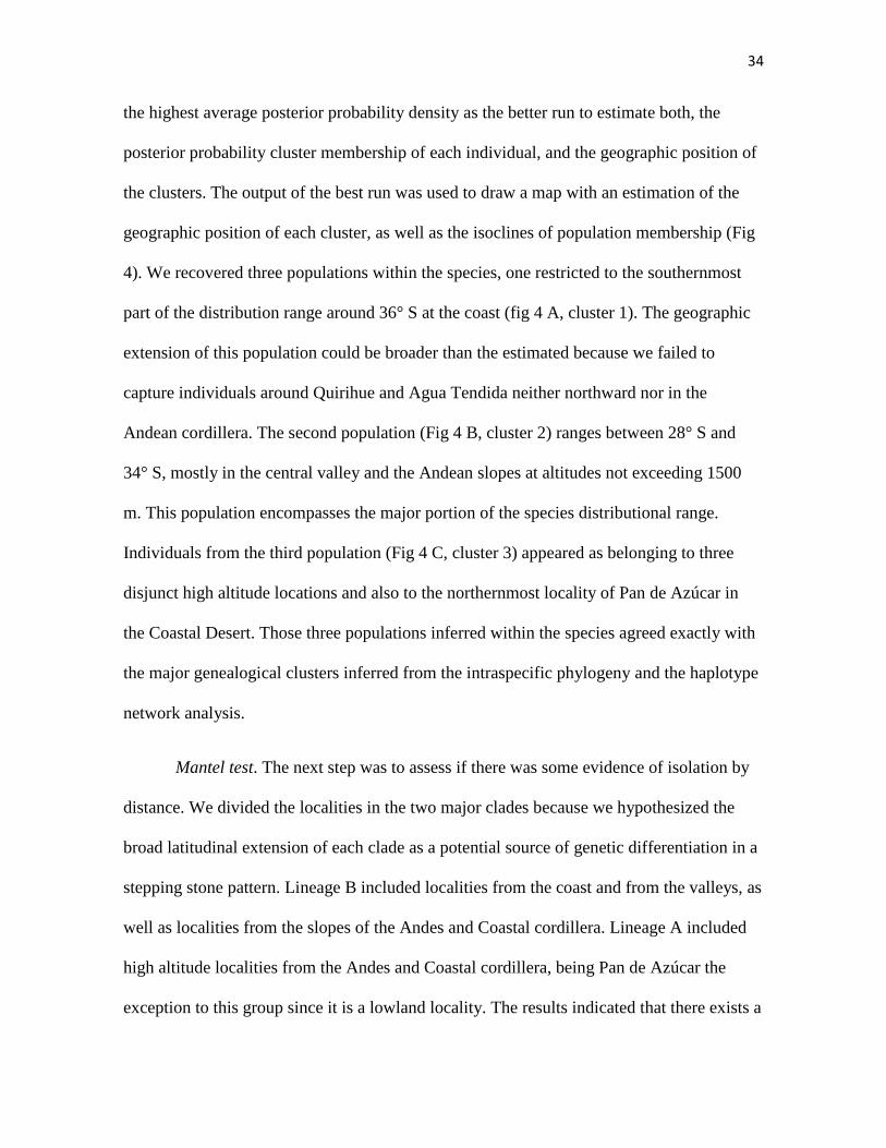
the highest average posterior probability density as the better run to estimate both, the

posterior probability cluster membership of each individual, and the geographic position of

the clusters. The output of the best run was used to draw a map with an estimation of the

geographic position of each cluster, as well as the isoclines of population membership (Fig

4). We recovered three populations within the species, one restricted to the southernmost

part of the distribution range around 36° S at the coast (fig 4 A, cluster 1). The geographic

extension of this population could be broader than the estimated because we failed to

capture individuals around Quirihue and Agua Tendida neither northward nor in the

Andean cordillera. The second population (Fig 4 B, cluster 2) ranges between 28° S and

34° S, mostly in the central valley and the Andean slopes at altitudes not exceeding 1500

m. This population encompasses the major portion of the species distributional range.

Individuals from the third population (Fig 4 C, cluster 3) appeared as belonging to three

disjunct high altitude locations and also to the northernmost locality of Pan de Azúcar in

the Coastal Desert. Those three populations inferred within the species agreed exactly with

the major genealogical clusters inferred from the intraspecific phylogeny and the haplotype

network analysis.

Mantel test. The next step was to assess if there was some evidence of isolation by

distance. We divided the localities in the two major clades because we hypothesized the

broad latitudinal extension of each clade as a potential source of genetic differentiation in a

stepping stone pattern. Lineage B included localities from the coast and from the valleys, as

well as localities from the slopes of the Andes and Coastal cordillera. Lineage A included

high altitude localities from the Andes and Coastal cordillera, being Pan de Azúcar the

exception to this group since it is a lowland locality. The results indicated that there exists a

35

significant correlation, major than the expected by chance, between genetic differentiation

and geographic distance into the populations belonging to lineage B with a p-value of

0.049. Meanwhile, in the localities belonging to lineage A the correlation was not

significantly distinct from the expected by chance with a p-value of 0.4915. We repeated

the test for lineage A now excluding the locality of Pelambres because it is the only one

that shares haplotypes assigned to both major phylogroups. However, the correlation was

still not significantly distinct from the expected by chance with a p-value of 0.2073.

Distribution of Pairwise Genetic Differences.- Since there is an haplogroup

distributed throughout the range of P. darwini (lineage B), whereas the other it is mainly

restricted to high altitude locations (lineage A, which agreed with the clusters inferred

from GENELAND), we considered each lineage as separate demes. We evaluated if each

haplogroup had independently experienced an abrupt demographic expansion during its

evolutionary history. Finally, to test the goodness of fit from the observed mismatch

distribution to the simulated distribution under the assumption of sudden expansion, we

implemented the least square deviation method. The Sum of Square Deviations (SSD)

value was 0.025 for lineage B, and 0.031 for lineage A; its associated p-value was 0.85 and

0.29 respectively. Accordingly, the hypothesis of sudden expansion cannot be rejected and

we concluded that populations of both clades have experienced at least one important and

sudden population size expansion across its evolutionary history

Distribution models .-

In order to test the assumption that overlapped lineage distribution models may

approximate whole species distribution models, we compared our estimations of Phyllotis

36

darwini’s distribution range from i) all trapping localities as a single distributional unit

(Fig. 6, table 1), and ii) independent models for each intraspecific lineage as an

independent distributional unit (Fig 7, Tables 1 and 2). The result shows that the whole

species’s range model is an accurate approximation of the observed distribution range for

P. darwini (26°S to 36°S observed, 25°S to 36.5°S predicted) and also, with high model

performance (AUC, Table 1), whereas overlapped lineage distribution models appeared to

slightly over-predict northern distribution (22°S to 36.5°S). Both models (whole specie’s

and overlapped lineage’s ranges) are good and consistent approximations of current

Phyllotis darwini’s geographic range.

As expected, distribution model for lineage B encompasses the whole distributional range

of P. darwini (Fig 7, table 2). Interestingly, when considering an arbitrary high threshold

(50% highest logistic probability value, red area in Figs. 6 and 7) the predicted range is

mainly restricted to the lowlands in the valley and the coast. On the other hand, the

distribution model for lineage A shares lower AUC value and clearly over-predict the

observed distribution of this phylogroup. Nevertheless, when considering our arbitrary high

threshold, the estimated distribution for lineage A is surprisingly well delimited and

restricted almost exclusively to Andean mountain ranges above the 1500 m elevation limit

detected for this phylogroup in this work. In summary, overlapped lineage distribution

models has slightly worst performance and some over-prediction compared to the whole

species’s distribution model, but when considering our arbitrary 50% highest logistic

probability threshold, lineage distribution models reproduced very accurately the altitudinal

pattern reported for both phylogroups at present. This information is missed in the whole

species’ distribution range model (Fig. 6).

37

Past lineage distribution estimated by both LGM models is conflicting (CCSM and

MIROC, Fig. 7, table 2): the CCSM model predicts a distributional gap during LGM for

both phylogroups, but MIROC based distribution models predicts that both phylogroups

were restricted to the southern portion of Phyllotis present distribution range. Nevertheless,

both models consistently predicted the area between 31°S-35°S as suitable for both

phylogroups during LGM. This latitudinal distribution dynamics must be considered with

caution because downscaled climatic data may not represent local geographic complexity

with accuracy. It is important to emphasize that altitudinal particularities reported for both

lineages at present were already established during LGM: lineages A and B might have

been restricted to approximately the same latitude, but only lineage A displayed suitability

areas at Andean mountain range during LGM (Table 2), which also has been sampled

mainly at the Andes and at localities above 1500 m. at present.

DISCUSSION

One of the most important features in the genetic structure of Phyllotis darwini is the major

split found between the widespread haplogroup (lineage B) and the high altitude

haplogroup (lineage A). The phylogroup B has the most frequent and widely distributed

haplotypes, whereas lineage A shares only private haplotypes separated by 34 mutational

steps from lineage B, and it is mostly restricted to high altitude localities. Lineage’s ages

are at least 47 and 57 KYa for lineages A and B, respectively (lowest 95% HPD value), and

according to GENELAND analysis, the inter-lineage gene flow appeared to be restricted at

present. Meanwhile, both lineages displayed signal of past population expansions; only

38

lineage B had a significative isolation by distance pattern. Altogether, those phylogenetic

and populational features suggested that main lineages in P. darwini had ancient and

independent evolutionary trajectories. Since the pioneer work of Fuentes & Jaksic, (1979) it

has been hypothesized that there exist two asynchronous speciation modes for lizards and

rodents in central Chile: i) Mountain speciation occurred during interglacial periods,

because of high species replacement with altitude and between mountains isolation, and ii)

valley speciation should occur during glacial periods, when species may not reach high

altitude elevations and connectivity in the valleys is reduced. Given the ecological

attributes of both groups, lizards are expected to display both speciation modes because this

group might be affected by severe decrease in connectivity in the valley during glacial

periods, and also are restricted in high altitude localities during interglacial periods because

its low vagility, high habitat specificity, and high species turnover between mountains.

Rodents would only exhibit the valley speciation mode because they might have been

affected by a decrease in connectivity in the valley during glacial periods, but not by high

altitude isolation during interglacial, because its high vagility and lower “between-

mountains species turnover” compared to lizards. Those differences in speciation modes

would be finally explained by differences in mobility between groups, as a consequence of

its different thermoregulation modes and energy requirements (Fuentes & Jaksic, 1979).

Our results show that P. darwini displays differentiation inside the lowland phylogroup

(Lineage B) with an isolation by distance pattern and restricted gene flow between

subgroups. This could be considered as evidence of the valley speciation mode inside this

endemic rodent species. Nevertheless, the fact that postglacial recolonization in mountain

ranges has occurred only in the apparently high-altitude adapted lineage A, suggests that

mountain speciation mode could be most likely the cause of the origin for this lineage,

39

which show non-latitudinal structure despite being distributed in several disjunct localities

along mountain ranges. In conclusion, and contrary to the “lizards and rodents”

hypothesis, the lineages in this species appear to have originated by the same speciation

mode suggested for lizards in the central Chile area (both, valley and mountain speciation

modes in the whole species). The specific historic event which could have triggered those

intraspecific diversification events remains elusive, because lineage ages in P. darwini

could be older than Quaternary times.

The fact that P. darwini’s distribution range at present can be estimated by overlapping

lineage distribution models is non-trivial. Even though model performance is slightly worst

in lineage distribution models compared to whole species distribution model, it is clear that

by using below species level ESUs and more restrictive probability thresholds in SDMs, we

are able to recover very important distributional information. In fact, in this approach we

have demonstrated that P. darwini is composed of two ancient lineages which, despite their

latitudinal overlap, it shares a very strict segregation in its altitudinal distribution at present.

An important methodological consideration is that intraspecific lineages may have more

restricted climatic niches than the whole species, and given the low resolution of

downscaled climatic models regards local conditions, it is not surprising that the

distribution models at intraspecific level suffered more over-prediction than the whole

species distribution models (Merow et al., 1992; Laughlin et al., 2012). Therefore, more

restrictive probability thresholds for distribution models below species level must be

considered.

Once we have established the phylogenetic and population structure, main lineage´s ages

and meaningful lineage distribution models at present, the next step was to project our

40

lineage distribution model to climatic conditions at LGM. The rational|e behind this

procedure is as follows: if we can estimate geographic distribution for intraspecific lineages

at present and also at some point in the past, with very different climatic conditions, then

we can compare past to present lineage distribution, and interpret the differences between

those geographic ranges as distributional responses to climate change. LGM was chosen

because is one of the biggest recent climatic events (Heusser, 1990; Clapperton, 1994;

Heusser et al., 2006), and it has been hypothesized as a major forcing in vegetation range

dynamics in the central Chile biodiversity hotspot (Villagrán & Armesto, 1991; Villagrán

& Hinojosa, 2005). In this context, the results shows that at LGM, both lineages were

restricted to aproximately the same latitudes (28°S-31°S) but only lineage A displayed

suitability areas at the high altitude andean mountain ranges. After the LGM event,

temperature may have rise and precipitation may have declined at those latitudes, and

besides other minor climatic oscilations, present day temperature is higher and precipitation

is lower than during LGM. Therefore, this comparison suggests that after post-LGM

warming, both lineages expanded their northern distribution to their present geographic

range limits around 26°S. However, only lineage A colonized Andean mountain ranges

above 1500 m altitude, being the lineage that retained its Andean distribution during the

maximum northward glacial advance through the Andes during LGM (Clapperton, 1990;

Clapperton, 1994). In conclusion, after glaciation, both lineages expanded their distribution

northward to the same latitudes, but clearly not to the same altitudes. This would explain

the present day segregation of lineage B which shows a wide distribution although

restricted to the lowlands and the coast, whereas lineage A is mainly distributed through the

Andes and the coastal mountain ranges above a threshold of 1500 m aproximately.

Specifically, the distributional response to an increase of temperature and a decline of

41

precipitation was independent for each lineage: lineage B colonized a broad latitudinal

range but restricted to low elevations, whereas lineage A was able to colonize mountain

ranges.Thus,we hypothesize that both lineages will display independent distributional

responses to future GCC scenarios, as they did in the past. This conclusion would be

impossible to achieve if we consider that species behaves as simple ecological units to

climate change.

It is important to notice that we refer to the distribution range for both lineages as restricted

to 30°S- 35°S during LGM, but the distribution model projected in CCSM climatic data

disagree with this interpretation and it predicts another relict between 25°S-28°S. We can

not rule out this possibility; in fact, it could be a good explanation for the only lowland

locality in wich lineage B has been sampled, the current northern P. darwini distribution’s

limit. We have deliberately chosed the MIROC based distribution model at LGM because

this area is predicted as suitable by both models. We do not expect to provide precise

distribution models because high resolution climatic models wich reproduce the local

conditions and the complex geography of the central Chile hotspot are lacking.

Nevertheless, the essential altitudinal pattern and independent post-LGM colonization with

altitudinal segregation for intraspecific lineages is supported by both, CCSM and MIROC

based distribution models.

In conclusion, this work is an example not only that species in endangered areas had cryptic

diversity below the species level, but also those lineages appeared to have responded

independently to climate change in the past, and therefore species may not behave as

ecological units to future GCC scenarios. In order to prevent massive cryptic biodiversity

losses in the future (Bálint et al., 2011), the integration of genetic and ecological tools must

42

be encouraged (May et al., 2011) as a way to understand the complex distributional

responses of species and biotas. This could be the only way to make realistic predictions for

conservation planning.

43

References

Alsos, I.G., Ehrich, D., Thuiller, W., Eidesen, P.B., Tribsch, A., Schönswetter, P., Lagaye, C.,

Taberlet, P. & Brochmann, C. (2012) Genetic consequences of climate change for northern

plants. Proceedings. Biological sciences / The Royal Society, 279, 2042-2051.

Allal, F., Sanou, H., Millet, L., Vaillant, a., Camus-Kulandaivelu, L., Logossa, Z.a., Lefèvre, F. &

Bouvet, J.-M. (2011) Past climate changes explain the phylogeography of Vitellaria

paradoxa over Africa. Heredity, 107, 174-86.

Bacigalupe, L.D., Nespolo, R.F., Opazo, J.C. & Bozinovic, F. (2004) Phenotypic Flexibility in a

Novel Thermal Environment: Phylogenetic Inertia in Thermogenic Capacity and

Evolutionary Adaptation in Organ Size. Physiological and Biochemical Zoology, 77, 805-

815.

Bálint, M., Domisch, S., Engelhardt, C.H.M., Haase, P., Lehrian, S., Sauer, J., Theissinger, K.,

Pauls, S.U. & Nowak, C. (2011) Cryptic biodiversity loss linked to global climate change.

Nature Climate Change, 1, 313-318.

Bandelt, H.-J., Forster, P. & Rohl, A. (1999) Median-joining networks for inferring intraspecific

phylogenies. Molecular Biology and Evolution, 16, 37-48.

Braconnot, P., Otto-Bliesner, B., Harrison, S., Joussaume, S., Peterchmitt, J.Y., Abe-Ouchi, A.,

Crucifix, M., Driesschaert, E., Fichefet, T., Hewitt, C.D., Kageyama, M., Kitoh, A., Lainé,

A., Loutre, M.-F., Marti, O., Merkel, u., Ramstein, G., Valdes, P., Weber, S.L., Yu, Y. &

Zhao, Y. (2007) Results of PMIP2 coupled simulations of the Mid-Holocene and Last

Glacial Maximum – Part 1: experiments and large-scale features. Climate of the Past 3,

261-277.

Brown, G.G. (1986) Structural conservation and variation in the D-loop-containing region of

vertebrate mitochondrial DNA. Journal of Molecular Biology, 192, 503-511.

Buckley, T.R., Marske, K. & Attanayake, D. (2010) Phylogeography and ecological niche

modelling of the New Zealand stick insect Clitarchus hookeri (White) support survival in

multiple coastal refugia. Journal of Biogeography, 37, 682-695.

Calsbeek, R., Thompson, J.N. & Richardson, J.E. (2003) Patterns of molecular evolution and

diversification in a biodiversity hotspot: the California Floristic Province. Molecular

ecology, 12, 1021-9.

Carnaval, A.C., Hickerson, M.J., Haddad, C.F.B., Rodrigues, M.T. & Moritz, C. (2009) Stability

predicts genetic diversity in the Brazilian Atlantic forest hotspot. Science, 323, 785-789.

Carstens, B.C. & Richards, C.L. (2007) Integrating coalescent and ecological niche modeling in

comparative phylogeography. Evolution; international journal of organic evolution, 61,

1439-54.

Clapperton, C. (1994) The quaternary glaciation of Chile: a review. Revista Chilena de Historia

Natural, 67, 369-383.

Clapperton, J.R.a.C.M. (1990) Quaternary glaciations of the southern Andes. Quaternary Science

Reviews, 9, 153-174.

Cordellier, M. & Pfenninger, M. (2009) Inferring the past to predict the future: climate modelling

predictions and phylogeography for the freshwater gastropod Radix balthica (Pulmonata,

Basommatophora). Molecular ecology, 18, 534-44.

Darwin, C. (1859) The origin of species. Penguin Books, Oxford, United Kingdom.

Drummond, A., Ho, S., Phillips, M. & Rambaut, A. (2006) Relaxed phylogenetics and dating with

confidenc. Plos Biology, 4, 699-710.

du Toit, N., van Vuuren, B.J., Matthee, S. & Matthee, C.a. (2012) Biome specificity of distinct

genetic lineages within the four-striped mouse Rhabdomys pumilio (Rodentia: Muridae)

from southern Africa with implications for taxonomy. Molecular phylogenetics and

evolution, 65, 75-86.

44

Eckert, A. (2011) Seeing the forest for the trees: statistical phylogeography in a changing world.

New Phytologist, 189, 894-897.

Elith, J., Graham, C.H., Anderson, R.P., Dudik, M., Ferrier, S., Guisan, A., Hijmans, R.J.,

Huettmann, F., Leathwick, J.R., Lehmann, A., Li, J., Lohmann, L.G., Loiselle, B.A.,

Manion, G., Moritz, C., Nakamura, M., Nakazawa, Y., Overton, J.M.M., Peterson, A.T.,

Phillips, S.J., Richardson, K., Scachetti-Pereira, R., Schapire, R.E., Soberón, J., Williams,

S., Wisz, M.S. & Zimmermann, N.E. (2006) Novel methods improve prediction of species’

distributions from occurrence data. Ecography, 29, 129-151.

Engelbrecht, A., Taylor, P.J., Daniels, S.R. & Rambau, R.V. (2011) Cryptic speciation in the

southern African vlei rat Otomys irroratus complex: evidence derived from mitochondrial

cyt b and niche modelling. Biological Journal of …, 104, 192-206.

Fielding, a.H. & Bell, J.f. (1997) A review of methods for the assessment of prediction errors in

conservation presence/absence models. Environmental Conservation, 24, 38-49.

Florio, a.M., Ingram, C.M., Rakotondravony, H.a., Louis, E.E. & Raxworthy, C.J. (2012) Detecting

cryptic speciation in the widespread and morphologically conservative carpet chameleon

(Furcifer lateralis) of Madagascar. Journal of evolutionary biology, 25, 1399-14414.

Fontanella, F.M., Feltrin, N., Avila, L.J., Sites, J.W. & Morando, M. (2012) Early stages of

divergence: phylogeography, climate modeling, and morphological differentiation in the

South American lizard Liolaemus petrophilus (Squamata: Liolaemidae). Ecology and

evolution, 2, 792-808.

Fraser, D.J. & Bernatchez, L. (2001) Adaptive evolutionary conservation : towards a unified

concept for defining conservation units. Molecular Ecology, 10, 2741-2752.

Fuentes, E.R. & Jaksic, F.M. (1979) Lizards and rodents: an explanation for their relative species

diversity in Chile. Arch. Biol. Med. Exper., 12, 179-190.

Gugger, P.F., González-Rodríguez, A., Rodríguez-Correa, H., Sugita, S. & Cavender-Bares, J.

(2011) Southward Pleistocene migration of Douglas-fir into Mexico: phylogeography,

ecological niche modeling, and conservation of 'rear edge' populations. The New

phytologist, 189, 1185-99.

Guilliot, G., Mortier, F. & Estoup, A. (2005) Geneland: a computer package for landscape genetics.

Molecular Ecology, 5, 712-715.

Guilliot, G., Santos, F. & Estoup, A. (2008) Analysing georeferenced population genetics data with

Geneland: a new algorithm to deal with null alleles and a friendly graphical user interface.

Bioinformatics, 24, 1406-1407.

Hall (1999) BioEdit: a user-friendly biological sequence alignment editor and analysis program for

Windows 95/98/NT. Nucl. Acids. Symp, 41, 95-98.

Hamann, A. & Wang, T. (2006) Potential effects of climate change on ecosystem and tree species

distribution in british Columbia. Ecology, 87, 2773-2786.

Harrison, S. (2000) Palaeoenvironmental data sets and model evaluation in PMIP. In: Proceedings

of the Third PMIP Workshop (ed. P. Braconnot), pp. 9-25, La Huardiere, Canada.

Hasumi, H. & Emori, S. (2004) K-1 coupled model (MIROC) description. K-1 Tech. Rep. 1. In, p.

34 pp. University of Tokyo, Center for climate system research.

Heusser, C. (1983) Quaternary Pollen Record from Laguna de Tagua Tagua, Chile. Science, 219,

1429-1432.

Heusser, C.J. (1990) Ice age vegetation and climate of subtropical Chile.

Palaeogeography,Palaeoclimatology, Palaeoecology, 80, 107-127.

Heusser, L., Heusser, C., Mix, A. & McManus, J. (2006) Chilean and Southeast Pacific

paleoclimate variations during the last glacial cycle: directly correlated pollen and δ18O

records from ODP Site 1234. Quaternary Science Reviews, 25, 3404-3415.

Hewitt, G. (2000) The genetic legacy of the Quaternary ice ages. Nature, 405, 907-913.

45

Hijmans, R.J., Cameron, S.E., Parra, J.L., Jones, P.G. & Jarvis, A. (2005) Very high resolution

interpolated climate surfaces for global land areas. International Journal of Climatology,

25, 1965-1978.

Hoffmann, A.A. & Sgrò, C.M. (2011) Climate change and evolutionary adaptation. Nature, 470,

479-85.

Hood, G.M. (2010) PopTools version 3.2.3.

Iriarte, A. (2008) Mamíferos de Chile. Lynx editions, Barcelona, España.

Jezkova, T., Jaeger, J.R., Marshall, Z.L. & Riddle, B.R. (2009) Pleistocene Impacts on the

Phylogeography of the Desert Pocket Mouse (Chaetodipus penicillatus). Journal of

Mammalogy, 90, 306-320.

Kalkvik, H.M., Stout, I.J., Doonan, T.J. & Parkinson, C.L. (2011) Investigating niche and lineage

diversification in widely distributed taxa: phylogeography and ecological niche modeling of

the Peromyscus maniculatus species group. Ecography, 35, 54-64.

Kozak, K.H., Graham, C.H. & Wiens, J.J. (2008) Integrating GIS-based environmental data into

evolutionary biology. Trends in ecology & evolution, 23, 141-8.

Lamy, F., Hebbeln, D. & Wefer, G. (1999) High-Resolution Marine Record of Climatic Change in

Mid-latitude Chile during the Last 28,000 Years Based on Terrigenous Sediment

Parameters. Quaternary Research, 51, 83-93.

Larizza, A., Pesole, G., Reyes, A., Sbisa, E. & Saccone, C. (2002) Lineage Specificity of the

Evolutionary Dynamics of the mtDNA D-Loop region in Rodents. Journal of Molecular

Evolution, 54, 145-155.

Laughlin, D.C., Joshi, C., van Bodegom, P.M., Bastow, Z.A. & Z., F.P. (2012) A predictive model

of community assembly that incorporates intraspecific trait variation. Ecology letters, 15,

1291-1299.

Lim, H.C., Rahman, M.a., Lim, S.L.H., Moyle, R.G. & Sheldon, F.H. (2010) Revisiting Wallace's

haunt: coalescent simulations and comparative niche modeling reveal historical

mechanisms that promoted avian population divergence in the Malay Archipelago.

Evolution; international journal of organic evolution, 65, 321-334.

Mantel, N. (1967) The detection of disease clusstering and a generalized regression approach.

Cancer Research, 27, 209-220.

Marske, K., Leschen, R. & Buckley, T. (2012) Concerted versus independent evolution and the

search for multiple refugia: Comparative phylogeography of four forest beetles. Evolution,

66, 1862-1877.

Marske, K.a., Leschen, R.a.B. & Buckley, T.R. (2011) Reconciling phylogeography and ecological

niche models for New Zealand beetles: Looking beyond glacial refugia. Molecular

phylogenetics and evolution, 59, 89-102.

Marske, K.a., Leschen, R.a.B., Barker, G.M. & Buckley, T.R. (2009) Phylogeography and

ecological niche modelling implicate coastal refugia and trans-alpine dispersal of a New

Zealand fungus beetle. Molecular ecology, 18, 5126-42.

May, S.E., Medley, K.a., Johnson, S.a. & Hoffman, E.a. (2011) Combining genetic structure and

ecological niche modeling to establish units of conservation: A case study of an imperiled

salamander. Biological Conservation, 144, 1441-1450.

Merow, C., Latimer, A.M. & Silander, J.A. (1992) Can entropy maximization use functional traits

to explain species abundances? A comprehensive evaluation. Ecology 92, 1523-1537.

Myers, N., Mittermeier, R.A., Mittermeier, C.G., Fonseca, G.A.B. & Kent, J. (2000) Biodiversity

hotspots for conservation priorities. Nature, 403, 853-858.

Otto-Bliesner, B., Brady, E., Clauzet, G., Tomas, R., Levis, S. & Kothavala, Z. (2006) Last Glacial

Maximum and Holocene Climate in CCSM3. Journal of Climate, 19, 2526-2544.

Pagel, M. & Meade, A. (2004) A phylogenetic mixture model for detecting pattern-heterogeneity in

gene sequence or character state data. Systematic Biology, 53, 571-581.

46

Palma, R.E. (2007) Estado actual de la Mastozoología en Chile. Mastozoología Neotropical, 14, 5-

9.

Pauls, S.U., Nowak, C., Bálint, M. & Pfenninger, M. (2012) The impact of global climate change

on genetic diversity within populations and species. Molecular Ecology, n/a-n/a.

Pearson, R.G. & Dawson, T.P. (2003) Predicting the impacts of climate change on the distribution

of species: are bioclimate envelope models useful? Global Ecology and Biogeography, 12,

361-371.

Pearson, R.G., Dawson, T.P., Berry, P.M. & Harrison, P.A. (2002) SPECIES: A Spatial Evaluation

of Climate Impact on the Envelope of Species. Ecological Modelling, 154, 289-300.

Peterson, T.A. & Nyári, A.S. (2007) Ecological niche conservatism and pleistocene refugia in the

trush-like mourner, Schiffornis sp., in the Neotropics. Evolution, 62, 173-183.

Pettorelli, N. (2012) Climate change as a main driver of ecological research. Journal of Applied

Ecology, 49, 542-545.

Phillips, S.J. & Dudik, M. (2008) Modeling of species distributions with Maxent: new extensions

and a comprehensive evaluation. Ecography, 31, 161-175.

Phillips, S.J., Dudik, M. & Schapire, R.E. (2004) A maximum entropy approach to species

distribution modeling. In: Proceedings of the twenty-first international conference on

machine learning, pp. 655-662, Banff, Canada.

Phillips, S.J., Anderson, R.P. & Schapire, R.E. (2006) Maximum entropy modeling of species

geographic distributions. Ecological Modelling, 190, 231-259.

Provan, J. & Bennett, K.D. (2008) Phylogeographic insights into cryptic glacial refugia. Trends in

ecology & evolution, 23, 564-71.

Qi, X.-S., Chen, C., Comes, H.P., Sakaguchi, S., Liu, Y.-H., Tanaka, N., Sakio, H. & Qiu, Y.-X.

(2012) Molecular data and ecological niche modelling reveal a highly dynamic

evolutionary history of the East Asian Tertiary relict Cercidiphyllum (Cercidiphyllaceae).

The New phytologist, 196, 617-630.

Raes, N. & ter Steege, H. (2007) A null-model for significance testing of presence-only species

distribution models. Ecography, 30, 727-736.

Randin, C.F., Dirnbock, T., Dullinger, s., Zimmermann, N.E., Zappa, M. & Guisan, A. (2006) Are

niche-based species distribution models transferable in space?

. Journal of Biogeography, 33, 1689-1703.

Raxworthy, C.J., Ingram, C.M., Rabibisoa, N. & Pearson, R.G. (2007) Applications of ecological

niche modeling for species delimitation: a review and empirical evaluation using day

geckos (Phelsuma) from Madagascar. Systematic biology, 56, 907-923.

Redford, K.H. & Eisenberg, J.F. (1992) Mammals of the Neotropics. The University of Chicago

Press.

Reig, O.A. (1986) Diversitty patterns and differentiation of high Andean rodents. High Altitude

tropical Biogeography (ed. by F.V.a.M. Monasterio), pp. 404-439. Oxford University press,

London.

Rissler, L.J. & Apodaca, J.J. (2007) Adding more ecology into species delimitation: ecological

niche models and phylogeography help define cryptic species in the black salamander

(Aneides flavipunctatus). Systematic biology, 56, 924-42.

Rogers, A. & Harpending, H. (1992) Population Growth Makes Waves in the Distribution of

Pairwise Genetic Differences. Molecular Biology and Evolution, 9, 552-569.

Rohl, A. & Mihn, L. (1997).Network: A Program Package for Calculating Phylogenetic Networks.

Rousset, F. (1997) Genetic Differentiation and Estimation of Gene Flow from F-Statistics Under

Isolation by Distance. Genetics 145

Rozas, J., Sanchez-Del Barrio, J.C., Messeguer, X. & Rozas, R. (2003) DnaSP, DNA

polymorphism analyses by the coalescent and other methods. Bioinformatics, 19, 2496-

2497.

47

Schneider, S. & Excoffier, L. (1999) Estimation of Past Demographic Parameters From the

Distribution of Pairwise Differences When the Mutation Rates Vary Among Sites:

Application to Human Mitochondrial DNA. Genetics, 152, 1079-1089.

Schneider, S., Roessli, D. & Excoffier, L. (2000) Arlequin: A Software for population genetics data

analysis.

Schorr, G., Holstein, N., Pearman, P.B., Guisan, A. & Kadereit, J.W. (2012) Integrating species

distribution models (SDMs) and phylogeography for two species of Alpine Primula.

Ecology and evolution, 2, 1260-1277.

Sikes, R.S. & Gannon, W.L. (2011) Guidelines of the American Society of Mammalogists for the

use of wild mammals in research. Journal of Mammalogy, 92, 235-253.

Simonetti, J.A. (1999) Diversity and Conservation of terrestrial vertebrates in mediterranean Chile.

Revista Chilena de Historia Natural, 72, 493-500.

Simpson, B.B. (1983) An Historical Phytogeography og the High Andean Flora. Revista Chilena de

Historia Natural, 56, 109-122.

Spotorno, A.E., Walker, L.I., Flores, S.V., Yevenes, M., Marín, J.C. & Zuleta, C. (2001) Evolución

de los filotinos (Rodentia, Muridae) en los Andes del Sur. Evolution of phyllotines

(Rodentia, Muridae) in the southern Andes. Revista Chilena de Historia Natural, 74, 151-

166.

Steppan, S., Ramírez, O., Banbury, J., Huchon, D., Pacheco, V., Walker, L.I. & Spotorno, A.E.

(2007) A Molecular Reappraisal of the Leaf-Eared Mice Phyllotis and their Relatives. The

Quintessential naturalist: Honoring the Life and Legacy of Oliver. P. Pearson (ed. by J.S.-

B. Dougals A. Kelt, James L. Patton), pp. 799-826.

Steppan, S.J. (1998) Phylognetic Relationships and Species Limits within Phyllotis (Rodentia:

Sigmodontinae): Concordance between mtDNA Sequence and Morphology. Journal of

Mammalogy, 79, 573-593.

Summers, D.M., Bryan, B.a., Crossman, N.D. & Meyer, W.S. (2012) Species vulnerability to

climate change: impacts on spatial conservation priorities and species representation.

Global Change Biology, 18, 2335-2348.

Svenning, J.-C., Fløjgaard, C., Marske, K.a., Nógues-Bravo, D. & Normand, S. (2011) Applications

of species distribution modeling to paleobiology. Quaternary Science Reviews, 30, 2930-

2947.

Tajima, F. (1989) Statistical Method for testing the Neutral Mutation Hypotesis by DNA

Polymorphism. Genetics, 123, 585-595.

Thuiller, W., Brotons, L., Araújo, M.B. & Lavorel, S. (2004) Effects of restricting environmental

range of data to project current and future species distributions. Ecography, 27, 165-172.

Tolley, K.a., Burguer, M., Turner, A.A. & Matthee, C.A. (2006) Biogeographic patterns and

phylogeography of dwarf chameleons (Bradypodion) in an African biodiversity hotspot.

Molecular Ecology 15, 781-793.

Tolley, K.a., Makokha, J.S., Houniet, D.T., Swart, B.L. & Matthee, C.a. (2009) The potential for

predicted climate shifts to impact genetic landscapes of lizards in the South African Cape

Floristic Region. Molecular phylogenetics and evolution, 51, 120-30.

Verboom, G.a., Dreyer, L.L. & Savolainen, V. (2009a) Understanding the origins and evolution of

the world’s biodiversity hotspots: The biota of the African ‘Cape Floristic Region’ as a case

study. Molecular Phylogenetics and Evolution, 51, 1-4.

Verboom, G.A., Archibald, J.K., Bakker, F.T., Bellstedt, D.U., Conrad, F., Dreyer, L.L., Forest, F.,

Galley, C., Goldblatt, P. & Henning, J.F. (2009b) Origin and diversification of the Greater

Cape flora: Ancient species repository, hot-bed of recent radiation, or both? Molecular

Phylogenetics and Evolution, 51, 44-53.

Villagrán, C. & Armesto, J. (1991) Historical phytogeography of the Chilean Coastal Range.

Revista Chilena de Historia Natural, 64, 105-123.

48

Villagrán, C. & Hinojosa, L. (2005) Esquema biogeográfico de Chile. Regionalización

Biogeográfica en Iberoámeríca y tópicos afines (ed. by J.J.M. Jorge Llorente Bousquets),

pp. 551-577. Ediciones de la Universidad Nacional Autónoma de México, Jiménez

Editores, México.

Walker, L.I., Spotorno, A.E. & Arrau, J. (1984) Cytogenetic and Reproductive Studies of Two

nominal Subspecies of Phyllotis darwini and Their Experimental Hybrids. Journal of

Mammalogy, 65, 220-230.

Waltari, E. & Guralnick, R.P. (2009) Ecological niche modelling of montane mammals in the Great

Basin, North America: examining past and present connectivity of species across basins and

ranges. Journal of Biogeography, 36, 148-161.

Waltari, E., Hijmans, R.J., Peterson, a.T., Nyári, Á.S., Perkins, S.L. & Guralnick, R.P. (2007)

Locating Pleistocene Refugia: Comparing Phylogeographic and Ecological Niche Model

Predictions. PLoS ONE, 2, e563.

Walther, G.-R., Post, E., Convey, P., Menzel, A., Parmesan, C., Beebee, T.J.C., Fromentin, J.-M.,

Hoegh-Guldberg, O. & Bairlein, F. (2002) Ecological responses to recent climate change.

Nature, 416, 389-395.

Xia, X. & Xie, Z. (2001) DAMBE: Data analysis in molecular biology and evolution. Journal of

Heredity, 92, 371-373.

Xia, X., Xie, Z., Salemi, M., Chen, L. & Wang, Y. (2003a) An index of substitution saturation and

its application. Molecular Phylogenetics and Evolution, 26, 1-7.

Xia, X., Xie, Z., Salemi, M., Chen, L. & Wang, Y. (2003b) An index of substitution saturation and

its application. Molecular Phylogenetics and Evolution, 26, 1–7.

49

Tables and Figures

Table 1.

Model AUC AUC stdv.

P. darwini whole

specie's range

0.971 0.022

P darwini lineage A

0.968 0.025

P. darwini lineage B 0.83 0.15

Table 2._

P darwini lineage A P. darwini lineage B

Present

25°S - 34°S (Highest logistic

probability values at the valley and

at the coast)

24°S - 36°S (Highest logistic probability

values exclusively at the Andean mountain

range)

CCSM

Distributional gap between 28°S-

31°S. Not distributed in the Andean

mountain range. Distributional gap between 28°S -31°S

MIROC

31°S-35°S (mainly distributed in

the valley and the coast) 30°S - 35°S (andes, valley and coast)

50

FIG. 1

51

B

A

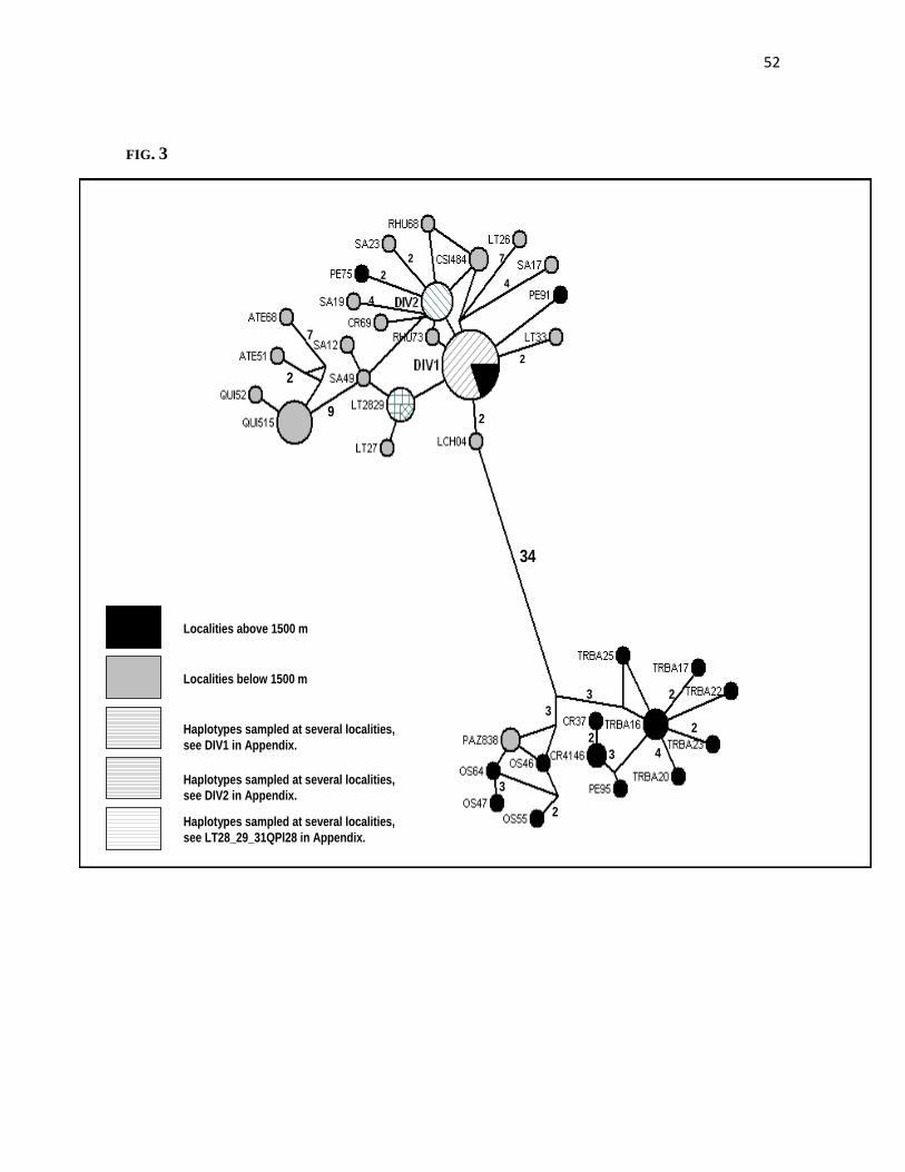
52

FIG. 3

34

9

7

2

2

4

2

2 7

4

2

3

3

2

3 2

2

43

2

Localities above 1500 m

Localities below 1500 m

Haplotypes sampled at several localities,

see DIV1 in Appendix.

Haplotypes sampled at several localities,

see DIV2 in Appendix.

Haplotypes sampled at several localities,

see LT28_29_31QPl28 in Appendix.

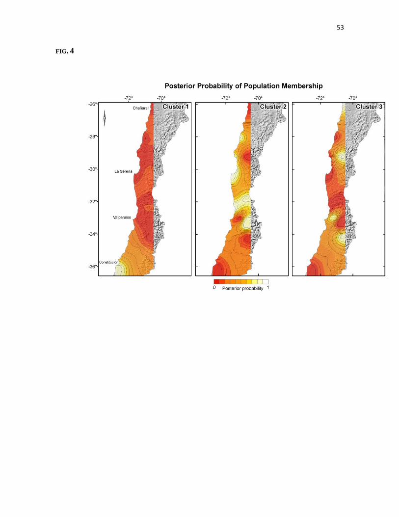
53

FIG. 4

54

Fig. 5

0.7

0,01,02,03,04,05,06,07,08,0

Pdarw_A_ATe51

Pdarw_A_QT38

Pmagister7

Pmagister5

Pdarw_B_PAz83

Pdarw_B_OS64

Pdarw_B_OS55

Pmagister4

Auliscomys_pictus

Pmagister3

Pdarw_A_LlCh_81

[0,0,8862]

[0,4683,2,9064]

[1,8461,5,2677]

[0,0566,1,9899]

[0,1,0373]

[0,0,7299]

[0,0032,0,9735]

[0,0817,2,7169][2,9274,12,6973]

[2,5587,5,8217]

0,7835

0,7311

0,2156

0,297

0,2447

0,8223

0,3414

0,2447

6,9492

2,754

1,6096

1,9689

0,6166

2,7562

1,394

0,3414

0,4809

3,167

0,297

0,2156

55

Present CCSM MIROC

Wholespecie’srange

Overlappedlineage’sranges

FIG. 6

56

Fig. 7

57

Fig. 7.1

58

Legends

Table 1_ AUC values and standard deviation for whole species’s distribution and

individual lineage’s distribution models.

Table 2_ Lineage´s distribution model summary, at present and at LGM (current

conditions, CCSM and MIROC).

Figure 1 _ Geographic distribution of localities sampled in Phyllotis darwini distributional

range.

Figure 2 _ Phyllotis darwini intraspecific phylogeny based on Bayes Markov Chain Monte

Carlo method (BMCMC). The phylogeny was obtained for the Hipervariable Domain II

(HV2) from the mitochondrial control region sequence data, whereas for BMCMC

represents a consensus tree from the n = 9950 trees from the converged Markov chain.

Posterior probability values over 0.5 are represented on each node.

Figure 3 _ Median-Joining haplotype network for the Phyllotis darwini mitochondrial DNA

dataset. The size of the Haplotype tip is proportional to its frequency. Numbers on the

branches are mutational steps between haplotype tips; when the branch has no number the

tips are separated by just one mutational step. Filled black and grey are private haplotypes

sampled at localities above and below 1500 m altitude respectively. Dashed are shared

haplotypes. The DIV 1 is a shared haplotype, but the proportion of individuals sampled

above 1500 m altitude are designated by filled black.

59

Figure 4 _ Map of population membership posterior probability. According to Geneland

analysis, the species is composed of three genetic units, designated as cluster 1, 2 and 3.

Map depicts posterior probability iso-lines of belong to each cluster.

Figure 5 _ D-loop based Phylogeny for intraspecific lineages in P. darwini and other

related species. Diversification times (expressed in millions years) appears above the

branches. Blue bars on the nodes represent 95% highest prior density estimates (95% HPD,

range in brackets) for the molecular rate.

Figure 6 _ P. darwini’s distribution models. The figure shows specie’s distribution models

for present and two LGM climatic models (columns). Models were built for the whole

distribution range as a single unit, and also by overlapping independent lineage distribution

models (rows). Yellow represents suitability areas for the specie according to the maximum

training sensitivity plus specificity logistic threshold; red areas represents suitability areas

according to an arbitrary restrictive threshold, defined as the 50% highest values observed

between the maximum training sensitivity plus specificity logistic threshold, and the

maximum logistic probability value for each model.

Figure 7.1 _ Lineage distribution models. The figure shows the species distribution models

for present and two LGM climatic models (columns). Models were built independently for

each P. darwini’s intraspecific lineage (rows). Yellow areas represents suitability areas for

the lineages according to the maximum training sensitivity plus specificity logistic

threshold; red areas represents suitability areas according to an arbitrary restrictive

threshold, defined as the 50% highest values observed between the maximum training

60

sensitivity plus specificity logistic threshold, and the maximum logistic probability value

for each model.

7.2 Detailed view of 4 lineages from figure 7.1

61

Mountaintops phylogeography: a case study using small mammals from

the Andes and the Coast of central Chile.

R. Eduardo Palma#*

1, Pablo Gutierrez-Tapia

#1, Juan F. Gonzalez

1 and Dusan Boric-Bargetto

2

1 Departamento de Ecología, Pontificia Universidad Católica de Chile, Alameda 340, Santiago

6513677, Chile, 2Departamento de Zoología, Universidad de Concepción, Concepción, Chile

Running head: Phylogeography of mountaintop small mammals

# REP and PG are equally contributed authors

*Correspondence: R. Eduardo Palma, Departamento de Ecología, Pontificia Universidad Católica

de Chile, Alameda 340, Santiago 6513677, Chile.

E-mail: epalma@bio.puc.cl

62

ABSTRACT

Aim We evaluated if selected species of small vertebrate taxa (and its intraspecific lineages) at the

Andes and Coastal mountaintops of central Chile had experienced distributional shifts due to

altitudinal movements of plant biota and climate change during and after the Last Glacial Maximum

(LGM) of the Pleistocene. We used two sigmodontine rodent taxa inhabitant of both mountain

ranges, Phyllotis darwini and Abrothrix olivaceus, as study models. The major hypothesis to test

was that during LGM populations of both, P. darwini and A. olivaceus, experienced altitudinal

descents due to range shifts of habitats from the Andes to the Coast. The retraction events during

postglacial may have leave remnants of these two rodent species populations on the Coastal

Cordillera of central Chile, leaving disjunct populations on the mountaintops of the Cordillera de la

Costa and Cordillera de los Andes.

Location Coastal Cordillera and Cordillera de los Andes, central Chile

Methods We sampled specimens of both study model taxa from the Andes and the Coast of central

Chile. Samples were phylogeographically analyzed based on nucleotide sequences of the

mitochondrial control region and the intron 7 of the nuclear b-fibrinogen gene (FGB). Intraspecific

phylogenies were reconstructed for each and concatenated molecular markers using maximum

likelihood and Bayesian methodology; a haplotype network was also reconstructed for each studied

species. Structuring of populations was analyzed using Geneland. Finally, we modeled the climatic

niche of the two rodent species’ lineages to approximate the species’ current distribution and

distribution during the Last Glacial Maximum (LGM).

Results We recovered a strong and well supported phylogenetic split within P. darwini and A.

olivaceus, patterns that were also evident with network analyses. Current distribution in A.

olivaceus displays one lineage with shared haplotypes between both mountain systems, whereas the

other haplogroup is restricted to the Andean mountain range, contrary to the shared haplotype

pattern between the Andes and the Coast for both P. darwini’s intraspecific lineages. Geneland

analyses recovered coastal and Andean localities conforming panmictic units for P. darwini despite

63

current disjunct distribution, whereas for A. olivaceus there exists an strictly Andean panmictic unit,

and another which includes localities from the valley, coast, and Coastal Cordillera. Finally, the

niche modelling analyses depicted differential postglacial expansions in several lineages, mainly

from the valley and coastal mountain tops towards the Andes and coastal cordilleras, since the

LGM to present.

Main conclusions Our results suggested that historical events as the LGM, would have triggered

the descending of populations from the Andes to lower elevations and refuge areas in the lowlands

and the Coastal Cordillera. Further movements of populations backwards after glacial retreats may

have followed, leaving population isolates on the mountaintops of the Coastal Cordillera. The

haplotype admixture between phyllogroups sampled at both mountain ranges, along with evidence

of postglacial expansion of the climatic niche for both species’s lineages, suggest that current

distribution of those mammals is the outcome of climate change and habitat reconfiguration after

LGM; the fact that the only one strictly Andean intraspecific lineage appears to have been

persistently distributed at this mountain range since LGM, strongly agreed with this hypothesis.

Assuming that this process may have repeated across several glacial/interglacial transitions during

Pleistocene, allows us to hypothesize that climate change and habitat shifts played an important role

in the intraspecific diversification of mammals distributed in the mountain ranges of central Chile.

Keywords

Andean Cordillera, Coastal Cordillera, central Chile, sigmodontine mice, population disjunction,

Last Glacial Maxima, niche modelling.

64

INTRODUCTION

The Pleistocene is characterized by worldwide climatic changes associated with glacial cycles,

forcing species to shift their ranges, and subsequently impacting the structure of their populations.

Under glacial-dominated scenarios, species at higher latitudes might have experienced strong

demographic and genetic changes in their populations (Hewitt, 2004). In boreal communities,

organisms contracted to refugia during glacial maxima, and then colonized or expanded into newly

available habitats after glacial retreat (e.g. Hewitt, 2000; Lessa et al., 2003). In South America,

Pleistocene glacial events would have had severe effects on populations associated with Andean

mountains, where ice sheets and permafrost were focused on the southern cone (Clapperton, 1993;

1994; Hollin & Schilling, 1981; Mercer, 1983). Populations inhabiting these latitudes would have

suffered local extinctions, expansions and retractions following the Quaternary glacial oscillations

(Brown & Lomolino, 1998; Hewitt, 2000; Viulleumier, 1971).

Montane regions are of particular interest when assessing species’ responses to historical

climate oscillations because they can cause favorable environments for a species to shift, contract,

or expand along not only elevational (Hewitt, 2000; 2004) but also latitudinal gradients (Guralnick,

2007). During climatic fluctuations, mountain populations may experience alternating periods of

isolation and connectivity, with for example, range expansion during glacial periods and range

contractions during warmer interglacials (Brown, 1971; Hewitt, 1999; Knowles, 2000; Patton &

Smith, 2002; Provan & Bennet, 2008; Rowe et al., 2004).

Montane environments are a major component of the Chilean biogeography, particularly in

central Chile where a Mediterranean ecosystem is located along the western margin of the Andes

between 30-37˚ S (Arroyo et al., 1994). This ecosystem is conformed by highly heterogeneous

vegetation mosaic and major vegetation types are dry, xerophytic thorn scrub dominated by summer

deciduous shrubs and succulents. The mesic communities of this ecosystem are dominated by

evergreen sclerophyllous trees in the coastal and Andean foothills, and the forests are dominated by

winter-deciduous trees in the southern edge of the region. The southern border of the Mediterranean

ecoregion is the Bio-Bío River (37˚ S), whereas the northern limit is the Atacama Desert in the

Copiapó region (27˚ S).

65

Biogeographers, when intending to explain disjunct patterns in species distribution on the

Cordillera de los Andes and the Cordillera de la Costa (that run in parallel along the country),

hypothesize that the disjunction would have occurred by downward shifts of mountaintop habitats

during the glaciation events of the Pleistocene (Villagrán & Armesto, 2005), with a subsequent shift

upwards during postglacial. Geological and glaciological data on the Last Glacial Maximum (LGM)

during Pleistocene times, demonstrated that about two thirds of the Temperate and Patagonian

forests were reached by glaciers (Hollin & Schilling, 1981; Denton, 1999; Heusser et al., 1999).

Towards the north, ice masses advanced throughout the Cordillera de los Andes, and in central

Chile descended to around 1,100-1,300 m (Clapperton, 1990; 1994; Rabassa & Clapperton, 1990).

These ice masses triggered a local drop of temperatures of about 6-7˚ C and an increase in the

rainfall (Heusser, 1983; Graf, 1994; Lamy et al., 1999). As a consequence, the Andean vegetational

belts shift downwards, to the central valley depression (Darwin, 1859; Simpson, 1983; Heusser,

1990; Villagrán, 2001; Villagrán, et al. 2004). Following glacial cycles, a warmer climate prevailed

with a subsequent shift of the vegetational belts upwards not only to the Andes, but also to Coastal

altitudes. These events created true “biogeographic islands” at different localities on the top of the

Cordillera de la Costa in central Chile, now hosting disjunct biota whose main ranges are at similar

altitudes in the Andes.

To date, there are no studies on those habitat shifts of biota between both mountain systems

in Mediterranean Chile from a genetic perspective. Most studies have been focused on vegetation

showing the floristic affinities between the high-andean biotas of the Cordillera de la Costa and

Cordillera de los Andes (García, 2006; Romero & Teiller, 2003), and probable terrestrial corridors

from the Andes to coastal mountaintops due to the descent of temperatures and vegetational habitats

during the last glaciation (García, 2006). However, there are some studies using molecular tools for

some of the coniferous species of the southern flora of Chile (37-43˚ S), particularly for the coastal

mountaintops that have a distribution that is mainly Andean (i.e., Araucaria araucana [pehuén];

Fitzroya cupressoides [the “alerce”]; Austrocedrus chilensis [“ciprés de la cordillera”] (Villagrán &

Armesto, 2005). In all these case studies a marked fragmentation of coastal areas populations is

reported with strong genetic segregation of populations between the Coast and Andean taxa (Allnutt

et al. 1999, Premoli et al. 2000, Marchelli & Gallo 2006) ).

The major goal of this paper was to investigate the relationships between small mammal’s

genetic structure and altitudinal species’ distribution across the Andes and Coastal mountaintops of

central Chile, and how that relationships may have changed due to altitudinal shifts of plant biota

during and after the Last Glacial Maximum (LGM) of the Pleistocene. To that goal, we used two

66

sigmodontine rodent taxa as study models, inhabitant of both mountain ranges: Phyllotis darwini

and Abrothrix olivaceus. Phyllotis darwini is an endemic species of Mediterranean Chile and

altitudinally it is found between the coast up to 2000 m (Iriarte, 2008). A. olivaceus has a wide

distributional range, from southern Peru downward to the Patagonia of Chile and Argentina, and

altitudinally it is also found up to 2000 m (Rodríguez-Serrano et al., 2006; Spotorno et al., 2001).

Therefore, the major hypothesis to evaluate in this paper is that during LGM populations of both P.

darwini and A. olivaceus experienced altitudinal shifts due to displacement of habitats from the

Andes to the Coast. Current distribution of intraspecific lineages must have been largely determined

by postglacial climate changes and habitat reconfiguration. Hypothetically, the contraction events

during postglacial may have leave remnants of these two rodent species populations on the Coastal

Cordillera of central Chile, leaving disjunct populations on the mountaintops of the Cordillera de la

Costa and Cordillera de los Andes in central Chile. We analyzed the phylogenetic and population

structure, climatic niche and distributional shifts since LGM on the Andean and Coastal populations

for the two above sigmodontine rodent species. We used mitochondrial and nuclear markers in a

phylogeographic approach.

MATERIALS AND METHODS

Study area and taxon sampling

For the purposes of this study we sampled a complex of localities between the Aconcagua and

Metropolitana of Santiago regions encompassing Coastal, valley, pre Andean and Andean areas,

located between 32 and 33˚ S in Mediterranean Chile (see Fig. 1 for the study area, and Table 1 for

a detailed list of localities sampled). A total of 14 localities were sampled in central Chile of which

four were Coastal localities (Cerro La Campana, Cerro El Roble, Altos de Chicauma, Altos de

Cantillana), 6 were central valley localities (Villa Alemana, Rinconada de Maipú, Melipilla,

Rabuco, La Florida and Paine), and 4 were Andean localities (Farellones, Campos Ahumada, San

Carlos de Apoquindo and Cajón del Maipo). A total of 141 mice were trapped in all these localities

of which 79 were Abrothrix olivaceus and 62 were Phyllotis darwini. Rodent trapping was

performed with Sherman traps (8 x 9 x 23 cm) using a mixture of oat and canned fish as bait. For

each specimen the heart, kidney, spleen, liver, and lung was extracted and stored in liquid nitrogen.

67

Specimens were sacrificed in the field via cervical dislocation previously anesthetized using

ketamine. We followed established safety guidelines for small mammal captures and processing

according to the Center for Disease Control and Prevention (CDC) protocols (Mills et al., 1995),

American Society of Mammalogists (ASM) safety guidelines for mammalogists from Hantavirus

(Kelt et al., 2010), ASM guidelines for the use of wild mammals in research (Sikes et al., 2011),

and the Bioethical Protocols established from the Facultad de Ciencias Biológicas, Pontificia

Universidad Católica de Chile.

PCR and sequencing protocols

DNA was extracted from frozen liver samples treated with the Wizard Genomic DNA Purification

Kit (Promega, Madison, Wisconsin). We amplified via PCR a region of 486 and 574 bp of the

mitochonfrial DNA (mtDNA) control region for A. olivaceus and P. darwini, respectively. We

amplified 79 specimens of A. olivaceus and 62 of P. darwini using primers LBE08 and 12S1

(Rodríguez-Serrano et al., 2006 for A. olivaceus), and primers 283F and 282R for P. darwini

(Bacigalupe et al., 2004). In addition, we amplified a region of 680 bp for A. olivaceus and 584 bp

for P. darwini of the intron 7 of the nuclear b-fibrinogen gene (FGB) for 30 specimens of A.

olivaceus and 23 P. darwini using primers β17-mammL and βfib-mammU (Matocq et al. 2007; see

Appendix 1 for FGB gene sequenced localities). The thermal cycle to amplify the A. olivaceus

control region followed the protocol used in Rodríguez-Serrano et al. (2006), whereas the thermal

cycle to amplify the P. darwini control region was: initial denaturation for 7 min at 95˚ C, followed

by 30 cycles of 94˚ C (30 s), 58˚ C (15 s), and 72˚ C (1 min 15s). A final extension at 72˚ C for 4

min terminated the reaction. The thermal cycle used to amplify the FGB gene for both species was

performed using the following protocol: initial denaturation for 5 min at 94˚ C, followed by 30

cycles of 94˚ C (1 min), 64˚ C (15 s), and 72˚ C (40 s). The final extension was at 72˚ C for 4 min.

Double- stranded polymerase chain reaction products were purified with Qiaquik (Qiagen,

Valencia, California). Cycle sequencing (Murray, 1989) was performed using primers 14724,

MVZ14, and 15162 (Irwin et al., 1991) for Cytb, and b17- mammL and bfib-mammU for FGB,

labeled with the Big Dye Terminator kit (Perkin Elmer, Norwalk, Connecticut). Sequencing

reactions were analyzed on an Applied Biosystems Prism 3100 automated sequencer (Applied

Biosystems, Foster City, California). Sequences were aligned using the CLUSTAL_X program

(Thompson et al., 1997) and by eye. All sequences have been deposited in GenBank under

68

accession numbers GU564005–GU564084 and HM004435 for the control region and GU564085–

GU564113 for the FGB.

Phylogenetic Analyses

Phylogenetic analyses were conducted using maximum likelihood (ML) performed with the

Treefinder version of October 2008 (Jobb 2008). We selected the best-fitting model of nucleotide

substitution using the corrected Akaike Information Criterion (AICc—Akaike 1974) in Treefinder.

Support for the nodes was evaluated with 1000 bootstrap replicates (Felsenstein, 1985). For control

region sequences the AICc identified the GTR + I + Γ model (Tavaré 1986) as the best model of

base substitution. The proportion of invariable sites value was 0.5520, and the gamma shape

parameter was = 1.7661. The proportions of nucleotides were A = 0.2806, C = 0.2867, G = 0.1287,

and T = 0.3038. For the concatenated sequences the AICc identified the GTR + Γ (Tavaré 1986) as

the substitution model. The gamma shape parameter was 0.1116, and the proportions of nucleotides

were A = 0.3003, C = 0.2306, G = 0.1504, and T= 0.3185. Sequences also were analyzed in a

Bayesian framework to estimate the posterior probabilities of phylogenetic trees. Ten million

phylogenetic trees were generated, sampling every 1,000 trees to assure that successive samples

were independent. The first 1000 trees of the sample were removed to avoid including trees before

convergence of the Markov Chain. Given that we used two independent molecular markers, we

applied a general likelihood-based mixture model (MM) as described by Pagel & Meade (2004,

2005), based on the general time-reversible (GTR) model (Rodríguez et al., 1990) of sequence

evolution. This model accommodates cases in which different sites in the alignment evolved in

qualitatively distinct ways but does not require prior knowledge of these patterns or partitioning

data. These analyses were conducted using the Bayes Phylogenies software

(http://www.evolution.rdg.ac.uk/SoftwareMain.html). To find the best mixture model of evolution

we estimated the number of GTR matrices by using a reversible-jump Markov Chain Monte Carlo

method (RJMCMC—Pagel & Meade, 2006). The RJMCMC visits the different mixtures of GTR

matrices in proportion to their posterior probabilities, “jumping” from simple to complex models or

vice-versa, making a direct estimate of the support of 1GTR, 2GTR, 3GTR, and so on. Only the

combination of matrices with the fewest number of parameters that significantly increased the

likelihood was used (1GTR + Γ for cytochrome b data; 2GTR + Γ for concatenated data) to

compute a 50% majority rule consensus tree. The percentage of samples that recover any particular

69

clade on this tree represents the posterior probability of that clade; these are the p values, and p

95% was considered evidence of significant support for a clade (Huelsenbeck & Ronquist, 2001).

Population genetic and demographic analyses

We used the DnaSP v 5.10.01 software to describe the genetic diversity in all groups and the

complete data set. We calculated the number of haplotypes (Nh), the haplotype diversity (Hd), the

nucleotide diversity pi (the average number of pairwise nucleotide differences per site, and the

segregating sites (S). We also assessed demographic history of the mountaintop groups by

performing Fu’s Fs neutrality test statistics [Fu, 1997], and Tajimas’s D test [Tajima, 1989] testing

the significance of the statistics from 10,000 simulated samples (Table 1) using DnaSP 5.10.01

[Librado & Rozas, 2009]. To evaluate the presence of population structure for each species, we

used the program GENELAND v. 1.0.7 [Guillot et al., 2008] in the R-Package [Ihaka &

Gentleman, 1996], which implements a population statistical model with Bayesian inference in a set

of georeferenced individuals with DNA sequences data

(http://www2.imm.dtu.dk/~gigu/Geneland/#). This model’s objective is to infer and locate the

genetic discontinuities between populations of geo-referenced genotypes, considering the uncertain

localization of the sampled individuals. The number of clusters was determined by running MCMC

(Markov chain Monte Carlo) iterations five times, allowing K (i.e., the most probable number of

populations) to vary, with the following parameters: 5 x 106 MCMC iterations, maximum rate of the

Poisson process fixed to 100 (this is the default value of the software). The minimum K = 1,

maximum K = 10 (values that allow us to explore a wide potential number of populations, and

considering the maximum spatial subdivision in the latitudinal range. The maximum number of

nuclei in the Poisson-Voronoi tessellation was fixed to 300 (3 x maximum rate was suggested by

Guillot et al., (2005). After inferring the number of populations in the data set from these five runs,

the MCMC was run 30 times with K fixed to the inferred number of clusters, with the other

parameters the same as above. The mean logarithm of the posterior probability was calculated for

each of the 30 runs and the posterior probability of population membership for each pixel of the

spatial domain was then computed for the three runs with the highest values.

To establish the relationships between haplotypes, we constructed a haplotype network

using the Neighbor-Net (Bryant, 2004) distances transformation and equal angle splits

transformation (Dress & Huson, 2004). Splits computed from the data are represented as parallel

70

edges rather than single branches, allowing visualization of ambiguous and conflicting signals in the

data set providing an implicit representation of evolutionary history (Huson, 2006).

Climatic niche models

Distribution models .- We modeled the climatic niche of each intraspecific lineage to approximate

the whole species’ current distribution, and its distribution during the LGM under the assumptions

that: (1) climate is an important factor driving the species’ distribution; (2) the climatic niche of

species remained conserved between the LGM and present time, and (3) overlapped lineage’s

distribution ranges will approach the whole species geographic range. The latter assumption was

tested by overlapping distribution models of each intraspecific lineage in order to approach the full

species distributional range, as the sum of ranges estimated for each lineage. The resultant

distributional range was roughly contrasted with another model built for the whole species without

considering phylogenetic structure.

The climatic niches were reconstructed using the methodology of ecological niche modeling, where

environmental data are extracted from occurrence records and random points (represented by

geographic coordinates). Habitat suitability was evaluated across the landscape using program

specific algorithms (Elith et al., 2006). The current models were then projected on the climatic

reconstructions of the LGM. For occurrence records, we used our unique sampling localities. In

addition to full geographic distribution models for each species, we built climatic models for each

major lineage recovered in the intraspecific phylogenies following the same approach. As a test of

consistency we overlapped the lineage distribution models for the lineages of each species, to

compare it to the full species distribution models.

The current climate was represented by bioclimatic variables from the WorldClim dataset v. 1.4

(http://www.world clim.org/; Hijmans et al., 2005) that are derived from monthly temperature and

precipitation data, and represent biologically meaningful aspects of local climate (Waltari et al.,

2007; Jezkova et al., 2009). For environmental layers representing the climatic conditions of the

LGM, we used ocean–atmosphere simulations (Harrison, 2000) available through the Paleoclimatic

Modelling Intercomparison Project (Braconnot et al., 2007). These reconstructions of the LGM

climate are based on simulated changes in concentration of greenhouse gases, ice sheet coverage,

insulation and topography (caused by lowering sea levels). We used two models that have been

71

previously downscaled for the purpose of ecological niche modeling (Waltari et al., 2007):

Community Climate System Model v. 3 (CCSM; Otto-Bliesner et al., 2006) and the Model for

Interdisciplinary Research on Climate v. 3.2 (MIROC; Hasumi & Emori, 2004). The original

climatic variables used in these models have been downscaled to the spatial resolution of 2.5 min

under the assumption that changes in climate are relatively stable over space (high spatial

autocorrelation) and were converted to bioclimatic variables (Peterson & Nyári, 2007).

Climatic niche models were built in the software package MAXENT v. 3.2.1 (Phillips et al., 2006),

a program that calculates relative probabilities of the species’ presence in the defined geographic

space, with high probabilities indicating suitable environmental conditions for the species (Phillips

et al., 2004). Trapping coordinates of each individual captured for DNA extraction were used as

presence points. We used the default parameters in MAXENT (500 maximum iterations,

convergence threshold of 0.00001, regularization multiplier of 1, and 10 000 background points)

with the application of random seed and logistic probabilities for the output (Phillips & Dudik,

2008). We masked our models to four altitudinal categories resuming both, the abrupt altitudinal

clines characteristic of central Chile, and some known altitudinal distribution limits for several

vertebrate taxa in this area (Fuentes & Jaksic, 1979). This procedure was conducted because

reducing the climatic variation being modeled to that which exists within a geographically realistic

area improves model accuracy and reduces problems with extrapolation (Pearson et al., 2002;

Thuiller et al., 2004; Randin et al., 2006). We ran 10 replicates for each model, and an average

model was presented using logistic probability classes of climatic niche suitability. The presence–

absence map was determined using the ‘maximum training sensitivity plus specificity logistic

threshold’ where the omission error of all occurrence records is set to zero (i.e., locations of all

occurrence records are predicted as ‘suitable’). Nevertheless, we arbitrary defined a second

threshold as the 50% highest logistic probability values observed between the maximum training

sensitivity plus specificity logistic threshold and the maximum observed logistic value, in order to

depict the areas with highest probability of suitability. We used the receiver operating characteristic

for its area under the curve (AUC) value to evaluate the model performance (Fielding & Bell, 1997;

Raes & ter Steege, 2007). AUC values range from 0.5 for a random prediction to 1 for perfect

prediction (Phillips et al., 2004).

RESULTS

As we mentioned in the former section, for the d-loop we sequenced 79 specimens of A.

olivaceus of which 27 were from the Andes, 29 from the valley and 23 from the coast recovering

20, 10 and 14 polymorphic sites for each of the sequenced sites; and 12, 7 and 9 haplotypes,

72

respectively. On the other hand, we sequenced 62 specimens of P. darwini of which 27 were from

the Andes and 35 from the coast obtaining 59 polymorphic sites (S) for the Andean specimens and

51 for the coastal forms, and 22 and 13 haplotypes, respectively. The haplotype diversity (Hd) for

A. olivaceus was 0.895 in the Andes, 0.603 in the Valley and 0.727 in the Coast; for P. darwini was

0.983 in the Andes and 0.780 for the Coast. The nucleotide diversity (pi) of A. olivaceus was 0.013,

0.003 and 0.004 for the Andes, the Valley and the Coast respectively; whereas that of P. darwini

was 0.037 and 0.023 for the Andes and for the Coast respectively. Fu’s test values for A. olivaceus

were significantly different from zero for the Valley (-1.475) and the Coast localities (-3.041),

indicating population expansion, whereas for the Andes it was not significantly different from zero

suggesting a population in equilibrium (-0.654). Fu’s neutrality test statistics for P. darwini was

negative and significantly different from zero for the Andes (- 3.12), whereas for the Coast was

positive (3.437) and significantly different from zero, indicating that the null hypothesis of

population equilibrium is rejected in favor of a population expansion.

The d-loop based intraspecific phylogeny for A. olivaceus is similar for both, maximum

likelihood and Bayesian analyses, thus we show a single tree (Fig. 2). For this species we observed

a well-supported split between two major clusters. One of them is constituted of haplotypes

sampled exclusively at Andean localities (e.g., Farellones, San Carlos de Apoquindo; lineage A).

The other major group mostly included haplotypes sampled at central valley and coastal localities

(lineage B) (Fig. 2) mixed with some haplotypes sampled at the Andes, as for example the localities

of Farellones and San Carlos de Apoquindo (Andean). However in the Andean haplogroup (lineage

A) we did not obtain any coastal haplotype for A. olivaceus (Fig. 2). As for P. darwini, we also

recovered a well-supported dichotomy of two differentiated phylogroups, although we could not

recognize any of the clusters strictly associated to a specific mountain range. In fact, the largest

cluster (Fig. 3, lineage A) reunited coastal (e.g., Cantillana, El Roble, Chicauma) and Andean

localities (e.g., Farellones, Campos Ahumada), as well as for lineage B. Nevertheless, P. darwini’s

lineage A is distributed in both mountain ranges. It is important to notice that this lineage is

distributed exclusively in localities above 1500 m altitude; this pattern has been previously reported

for the species with completely different samples and using only the D-loop mithochondrial marker

(Gutiérrez-Tapia & R.E. Palma, in prep.).The neighbor-net analysis, on the other hand, showed

similar patterns of divergence to that of intraspecific phylogenies between the Coastal (blue) and

Andean (red) haplogroups both for A. olivaceus and P. darwini (Fig. 4 and Fig. 5, respectively).

A similar topology to that of d-loop was obtained for Abrothrix olivaceus when analyzing

phylogenetically the concatenated d-loop and FGB sequences (Fig. 6), in which it is clear the

73

dichotomy between strictly Andean haplogroup and a mixed haplogroup. The combined d-

loop/FGB phylogenetic analysis (likelihood and Bayes) for P. darwini showed a similar topology to

that obtained with d-loop, recognizing two well supported clusters that combined DNA sequences

from the coast and the Andes, with lineage A distributed above 1500 m altitude (Fig. 7).

The results of Geneland analyses recovered two clusters in each species, A. olivaceus and P.

darwini (Fig. 8 and Fig. 9, respectively). Cluster 1 for A. olivaceus suggested that Andean localities

of Farellones and Campos Ahumada constitute a single population with high probability values as it

is shown through the posterior probability isocline (Fig. 8). Cluster 2 for the same species suggested

that coastal areas such as Rabuco, La Campana and Villa Alemana belong to a panmictic unit

together with La Florida from the Andes. For Phyllotis darwini, on the other hand, cluster 1 shows

that Andean populations of El Canelo, San Carlos de Apoquindo and Farellones seem to have

constituted a single genetic unit along with populations of Rabuco and La Campana in the Coast,

despite being currently distributed in disjunction. Whereas for cluster 2 the coastal mountaintop

populations of Chicauma, Cantillana and El Roble seem to have formed a single genetic unit with

Andean populations of Campos Ahumada and Farellones (Fig. 9). Current disjunct distribution

could be attributed to recent fragmentation.

Distribution models

In order to test the assumption that overlapped lineage distribution models may approximate whole

species distribution models, we compared our estimations of each species’ distribution range at

present from i) all trapping localities, considering whole species as single distributional unit (data

not shown), and ii) submodels for trapping localities assigned to different intraspecific lineages as

independent distributional units (Fig 10, Tables 1 and 2). The results show that whole species’

range models are good approximations of the observed distribution range for each species, and also

with high model performance (AUC, Table 1). Overlapped lineage distribution models in P.darwini

performs as well as does the whole species model; in the case of A. olivaceus, overlapped lineage

models performs even better than the whole species range model. Consequently, both model

approaches (whole species and overlapped lineage’s ranges) are good and consistent

74

approximations of current species´ geographic ranges (considering the whole species’ range as the

portion of the distribution of A. olivaceus and P. darwini assessed in this work).

Range dynamics

Phillotis darwini

Distribution model at current climatic conditions for this species shows that lineage B has suitable

areas across the Andes between 32°S and 34°S, and in some spots of the coastal mountain range

within the same latitude; the valley is also suitable for this lineage between 32°S and 33°S. The

distribution model for P. darwini’s lineage A is surprisingly well defined across the Andes between

27°S and 35°S; this lineage also displays suitable spots across the coastal mountain range between

31°S and 34°S, with high logistic probability values (Fig. 10, red areas). Lineage A has also suitable

areas in the points where both, Andean and coastal mountain ranges are very close to each other and

the valley becomes narrow.

Both distribution models for lineage B at LGM (CCSM and MIROC, Fig. 10) shows that latitudinal

distribution was approximately the same that at present, but high altitude spots at the Andes were

absent at those climatic conditions; there is some disagreement between both models: according to

the CCSM model, lineage B distribution at the valley and the coastal mountain range was

approximately the same that at current conditions. On the other hand, MIROC based distribution

model displays a relictual distribution for lineage B during LGM (Fig. 10), restricted to a narrow

low altitude fringe at the Andean border, and some isolated populations at coastal mountain range at

32°S and 34°S. On the other hand, differences between current and past distribution models for

lineage A in P. darwini are far more dramatic: CCSM and MIROC based models shows that the

broad Andean distribution observed at present was almost absent during LGM, when this lineage

had notoriously expanded its distribution towards the valley and coastal mountain range (northern

75

distribution limit for the species could have been located at 32°S at LGM, five latitude degrees

south from current northern limit).

Abrothrix olivaceus

Distribution model at current climatic conditions for this species shows that lineage B has a broad

suitable distribution area between 31°S to 35°S, at the Andes, the valley and the coastal mountain

range. Meanwhile, lineage A displays suitable areas at the Andes between 32°S-34°S, and some

suitable spots in the coastal mountain range (nevertheless, all individuals assigned to this lineage

have been sampled at Andean localities).

Hypothesized distribution at LGM for lineage B is almost identical to its current distribution

according to both, CCSM and MIROC based distribution models (Fig. 10). A very similar behavior

is observed for the “Andean” lineage A; the only disagreement occurs in MIROC based distribution

models, which shows a smallest suitable area for this lineage at LGM, but with very similar

latitudinal and altitudinal distribution. According to this model, it is possible that A. olivaceus’s

lineage A may have been restricted to a narrow low altitude fringe at the Andean border.

Consequently, the distribution of both lineages in A. olivaceus has remained relatively

constant since LGM to present, with probably small postglacial expansions towards the Andes; it is

possible that lineage A have had remained distributed exclusivey in Andean localities. On the other

hand, P. darwini’s lineage A has notouriously expanded its distribution northwards through the

Andean mountain range, and to suitable areas in the valley, and in the coastal mountain range has

contracted its distribution since LGM until present day, leaving just some isolated populations at the

top of the Coastal Cordillera.

76

DISCUSSION

Our results exhibited an evident split of haplogroups for both species of sigmodontines of

the Andes and the Coastal Cordillera in the study area. For Abrothrix olivaceus we observed that

one of the haplogroups is strictly restricted to Andean localities (lineage A), while the other is

distributed in both mountain ranges, and also in some valley and coastal localities (lineage B). This

was not the case for the other studied species Phyllotis darwini, for which we recovered two

haplogroups, both of them distributed in the Andes and in the Coastal mountain ranges.

Nevertheless, the geographical segregation of haplogroups within the latter species is clear: one

haplogroup is distributed in the valley and both mountain ranges (lineage B), whereas the other

(lineage A) is strictly restricted to localities above 1500 m altitude, across both mountain ranges but

with a broad latitudinal extension across the Andean mountain range.

The first cluster obtained for A. olivaceus with Geneland analysis grouped sequences from

the Andean populations of Campos Ahumada and Farellones, whereas the second cluster obtained

for this species joined sequences from the Andes, central valley and coastal localities; that is to say,

lineages inside A. olivaceus are currently panmictic units. For P. darwini on the other hand, cluster

one grouped localities from the Andes and the Coast, pattern that was also recovered for cluster 2

that joined Andean populations of Farellones and Campus Ahumada with those of the El Roble,

Cantillana and Chicauma at the Coast. This strongly disjunct distribution of populations suggest that

those lineages were panmictic units which have been recently fragmented, but probably still keeps

some degree of genetic flux.

We suggest that the biogeographic mechanism that may have triggered the dynamic range

shift in the recent evolutionary history of both P. darwini and A. olivaceus was the downwards

displacement of the Andean vegetational belts towards the valley, as a consequence of the 7° C drop

of temperature driven by the ice advance throughout the Andes of central Chile in the LGM

(Clapperton, 1990; 1994). Our results thus suggest that mountain populations of P. darwini and A.

olivaceus moved between both cordilleras, and that these movements might have been triggered by

the glaciation events that affected the Andes during the glaciation cycles of the Pleistocene.

Glaciations may have allowed Andean populations to be refuged at low altitudes in the Andes

mountains (e.g., A. olivaceus’ lineage A at San Carlos de Apoquindo) and/or in areas free of ice in

77

the Coastal Cordillera. But what evidence do we have of these movements and when these might

have occurred since during the Pleistocene several glaciation cycles have been reported?.

Niche modeling analyses for both species suggest that there has been lineages with

persistant distribution at valley and coastal mountain ranges wich have slightly expanded its

distribution towards Andean mountain ranges after glacial retreat (P. darwini’s lineage B and A.

olivaceus’s lineage B), whereas other lineages have dramatically expanded their range exclusively

across mountain ranges (P. darwini’s lineage A). The only lineage which apparently has not move

between mountain ranges since LGM to present is A. olivaceus’s lineage A, which is also the only

intraspecific lineage without mixed haplotypes between coastal and Andean mountain ranges; in

addition is currently a panmictic unit.

The fact that A. olivaceus displays an strictly Andean haplogroup, and another lineage with broad

distribution in both mountain ranges, suggests that the mixed haplogroup is the result of range

displacements between mountain ranges, while the Andean haplogroup appears to have remained

restricted to the Andes, even with relictual distribution during glacial cycles (as is suggested by its

hypothesized distribution during LGM according to MIROC based distribution model). On the

other hand, both linneages inside P. darwini are distributed at both mountain ranges (one of them

strictly restricted to elevations above 1500 m, with disjunct distribution along both cordilleras). In

adittion, lineages in this species displayed the largest distributional shifts from LGM until current

conditions, with a high altitude lineage which has dramatically expanded its distribution across

mountain ranges. Therefore, we hypothesize that P. darwini’s current distribution has been

determinated by at least the last glacial cycle (differential postglacial colonization for each

intraspecific lineage), and the origin of its lineages is probably related to ancient range shifts across

mountain ranges.

Why do we have different biogeographic patterns on the mountaintops for the two species

of sigmodontine rodents that coexist in central Chile?. Our results showed that Phyllotis darwini

shares more haplotypes between both mountain systems compared with the other studied species A.

olivaceus, which possess one lineage that remained in the Andes, even during LGM. In general, the

former species exhibited higher genetic variability as expressed in the number of polymorphic sites

and haplotype numbers if compared to A. olivaceus. In fact, Phyllotis darwini characterizes for

being one of the most ubiquitous in the semiarid and arid regions of northern and central Chile and

appears to be capable of seasonally adjusting its resistance to desiccation utilizing seeds and

78

succulents (Meserve & Glanz, 1978; Meserve & Le Boulengé, 1987). In contrast, A. olivaceus

characterizes for preferring habitats with less shrub and greater herbaceous cover (Meserve, 1981).

A phylogeographic study on A. olivaceous recovered a structured pattern, suggesting local

adaptation of populations along their range from semiarid, to Mediterranean, to forest environments

in the southern part of the country (Rodríguez-Serrano et al., 2006).

Thus, our hypothesis to explain current patterns on mountaintop populations for both

species of sigmodontine mice in central Chile would rest on historical events as the LGM (and

probably former glacial/interglacial transitions) that would have triggered the descent of

populations from the Andes to lower elevations and refuge areas in Coastal Cordillera as suggested

by our phylogeographic analyses. Further movements of populations backwards after glacial

retreats may have followed, leaving, in some cases, population isolates on the mountaintops of the

Coastal Cordillera. These “mountain island isolates” occurring mainly at the valley and coastal

cordillera during LGM, may have recolonized the Andean mountains range after glacial retreat,

explaining the current pattern of haplotype admixture but current disjunct distribution across both

mountain ranges. The fact that the only lineage (A. olivaceous A) which remained associated to a

single mountain range through the last glacial/interglacial transition is the only one which lacks of

haplotype admixture between mountain ranges, strongly agreed with this hypothesis.

79

REFERENCES

Akaike, H. (1974). A new look at the statistical model identification. IEEE Transactions on

Automatic Control, 19, 716-723.

Allnutt, T.R., C.A. Newton, A. Lara, A. Premoli, J.J. Armesto, R. Vergara, M. Gardner (1999).

Genetic variation in Fitzroya cupressoides (alerce), a threatened South American conifer.

Molecular Ecology, 8, 975-987.

Arroyo, M.T.K., Cavieres, L., Marticorena, C. & Muñoz-Shick, M. (1994). Convergence in the

Mediterranean Floras in Central Chile and California: Insights from Comparative

Biogeography. Ecology and Biogeography of Mediterranean Ecosystems in Chile,

California and Australia (ed. by M.T.K Arroyo, P. H. Zedler and M.D. Fox), pp. 43-88.

Springer-Verlag, New York, USA.

Bacigalupe, L.D., Nespolo, R.F., Opazo, J.C. & Bozinovic, F. (2004) Phenotypic flexibility In a

novel thermal environment: phylogenetic inertia in thermogenic capacity and evolutionary

adaptation in organ size. Physiological and Biochemical Zoology, 77, 805-815.

Braconnot, P., Otto-Bliesner, B., Harrison, S., Joussaume, S., Peterchmitt, J.Y., Abe-Ouchi, A.,

Crucifix, M., Driesschaert, E., Fichefet, T., Hewitt, C.D., Kageyama, M., Kitoh, A., Lainé,

A., Loutre, M.-F., Marti, O., Merkel, U., Ramstein, G., Valdes, P., Weber, S.L., Yu, Y. &

Zhao, Y. (2007) Results of PMIP2 coupled simulations of the Mid-Holocene and Last

Glacial Maximum – Part 1: experiments and large-scale features. Climate of the Past, 3,

261-277.

Brown, J.H. (1971). Mammals on mountaintops: nonequilibrium insular biogeography. The

American Naturalist, 171, 467-478.

Brown, J.H. & Lomolino, M.V. (1998). Biogeography. 2nd

ed. Sinauer Associates, Inc.,

Publishers, Sunderland, Massachusetts.

Bryant, D. (2004). Neighbor-Net: An Agglomerative Method for the Construction of

Phylogenetic Networks. Molecular Biology and Evolution, 21, 255–265.

Clapperton, C.M. (1990). Quaternary Glaciations in the Southern Hemisphere: An Overview.

Quaternary Science Reviews, 9, 299-304.

80

Clapperton, C.M. (1993). Nature of environmental changes in South America at the last glacial

maximum. Palaeogeography, Palaeoclimatology, Palaeoecology, 101, 189-208.

Clapperton, C.M. (1994). The Quaternary glaciation of Chile: a review. Revista Chilena de

Historia Natural, 67, 369-383.

Darwin, C. (1859). The origin of species. Penguin Books, Oxford, UK.

Denton, G.H., Lowell, T.V., Moreno, P.I., Andersen, B.G. & Schlüchter, C. (1999).

Geomorphology, stratigraphy, and radiocarbon chronology of Llanquihue Drift in

the area of the Southern Lake District, Seno Reloncaví, and Isla Grande de Chiloé,

Chile. Geografiska Annaler Series A-Physical Geography, 81, 167-229.

Dress, A.W. & Huson, D.H. (2004). Constructing splits graphs. IEEE/ACM. Transactions

on Computational Biology and Bioinformatics. 1, 109–115.

Elith, J., Graham, C.H., Anderson, R.P., Dudik, M., Ferrier, S., Guisan, A., Hijmans, R.J.,

Huettmann, F., Leathwick, J.R., Lehmann, A., Li, J., Lohmann, L.G., Loiselle, B.A.,

Manion, G., Moritz, C., Nakamura, M., Nakazawa, Y., Overton, J.M.M., Peterson, A.T.,

Phillips, S.J., Richardson, K., Scachetti-Pereira, R., Schapire, R.E., Soberón, J., Williams,

S., Wisz, M.S. & Zimmermann, N.E. (2006) Novel methods improve prediction of species’

distributions from occurrence data. Ecography, 29, 129-151.

Felsenstein, J. (1985). Confidence limits on phylogenies: an approach using bootstrap. Evolution,

39, 783–791.

Fielding, A.H. & Bell, J.f. (1997). A review of methods for the assessment of prediction errors in

conservation presence/absence models. Environmental Conservation, 24, 38-49.

Fu, Y.X. (1997). Statistical tests of neutrality of mutations against population growth, hitchhiking

and background selection. Genetics, 147, 915–925.

García, N. (2006). Análisis florístico comparativo de la vegetación altoandina de la Cordillera de la

Costa y de los Andes de Chile central. Memoria de título, Facultad de Ciencias

Agronómicas, Universidad de Chile, Santiago, Chile. 68 pp.

Graf, K. (1994). Discussion of palynological methods and paleoclimatical interpretations in

northern Chile and the whole Andes. Revista Chilena de Historia Natural, 67, 405-

415.

81

Guillot, G., Estoup, A., Mortier, F. & Cosson, J.F. (2005). A spatial statistical model for landscape

genetics. Genetics, 170, 1261–1280.

Guillot, G, Santos, F. & Estoup, A. (2008). Analysing georeferenced population genetics data with

Geneland: a new algorithm to deal with null alleles and a friendly graphical user interface.

Bioinformatics, 24, 1406–1407.

Guralnick, R. (2007). Differential effects of past climate warming on mountain and flatland

species distributions: a multispecies North American mammal assessment. Global

Ecology and Biogeography, 16, 14-23.

Harrison, S. (2000). Palaeoenvironmental data sets and model evaluation in PMIP. In:

Proceedings of the Third PMIP Workshop (ed. P. Braconnot), pp. 9-25, La

Huardiere, Canada.

Hasumi, H. & Emori, S. (2004) K-1 coupled model (MIROC) description. K-1 Tech. Rep. 1. In, p.

34 pp. University of Tokyo, Center for climate system research.

Heusser, C.J., (1983). Quaternary pollen record from Laguna de Tagua Tagua, Chile. Science,

219, 1429-1432.

Heusser, C.J. (1990). Ice age vegetation and climate of subtropical Chile. Paleogeography,

Paleoclimatology, Paleoecology, 80, 107-127.

Heusser, C.J., Heusser, L.E., Lowell, T.V. (1999). Paleoecology of the Southern Chilean Lake

District Isla Grande de Chiloé during middle-late Llanquihue Glaciation and deglaciaion.

Geografiska Annaler, 81 A, 231-284.

Hewitt, G. (1999). Post-glacial re-colonization of European biota. Biological Journal of the

Linnean Society, 68, 87-112.

Hewitt, G. (2000). The genetic legacy of the Quaternary ice ages. Nature, 405, 907-913.

Hewitt, G. (2004). Genetic consequences of climatic oscillations in the Quaternary. Philosophical

Transactions of the Royal Society of London B, 359, 183-195.

Hijmans, R.J., Cameron, S.E., Parra, J.L., Jones, P.G. & Jarvis, A. (2005) Very high resolution

interpolated climate surfaces for global land areas. International Journal of Climatology,

25, 1965-1978.

82

Hollin, J.T. & Schilling D.H. (1981). Late Wisconsin-Weichselian mountain glaciers and small ice

caps. The Last great Ice Sheets (ed. by G. Denton and T. G. Hughes), pp. 179-206. Wiley,

New York.

Huelsenbeck, J. P. & Ronquist, F. (2001). MRBAYES: Bayesian inference of phylogenetic trees.

Bioinformatics, 17, 754-755.

Huson, D.H. (2006). Application of Phylogenetic Networks in Evolutionary Studies. Molecular

Biology and Evolution. 23, 254–267.

Ihaka, R. & Gentleman, R. (1996). R: A Language for Data Analysis and Graphics. Journal of

Computational and Graphical Statistics, 5, 299–314

Irwin, D. M., Kocher, T. D. & Wilson, A. C. (1991). Evolution of the cytochrome b gene of

mammals. Journal of Molecular Evolution, 32, 128-144.

Jezkova, T., Jaeger, J.R., Marshall, Z.L. & Riddle, B.R. (2009). Pleistocene Impacts on the

Phylogeography of the Desert Pocket Mouse (Chaetodipus penicillatus). Journal of

Mammalogy, 90, 306-320.

Jobb, G. (2008). TREEFINDER version of October 2008. Munich, Germany. Distributed by the

author at www.treefinder.de.

Kelt, D.A., Hafner, M.S., and The American Society of Mammalogists ad hoc Committee

for guidelines on handling small mammals in the field. (2010). Updated guidelines

for protection of mammalogists and wildlife researchers from hantavirus pulmonary

syndrome (HPS). Journal of Mammalogy, 91, 1524-1526.

Knowles, L.L. (2000). Tests of Pleistocene speciation in montane grasshoppers from the sky

islands of western North America (Genus Melanoplus). Evolution, 54, 1337–1348.

Lamy, F., Hebbeln, D. & Wefer, G. (1999). High-resolution marine record of climatic change in

mid-latitude Chile in the last 28,000 years based on terrigenous sediment parameters.

Quaternary Research, 51, 83-93.

Lessa, E.P., Cook J.A. & Patton, J.L. (2003) Genetic footprints of demographic expansion in North

America, but not Amazonia, during the Late Quaternary. Proceedings of the National

Academy of Sciences USA, 100, 10331–10334.

83

Librado, P. & Rozas, J. (2009). DnaSP v5: a software for comprehensive analysis of DNA

polymorphism data. Bioinformatics, 25, 1451–1452.

Marcelli, P., L. Gallardo (2006). Multiple ice-age refugia in a southern beech of South America as

evidenced by chloroplast DNA markers. Conservation Genetics, 7, 591-603.

Matocq, M.D., Shurtliff, Q.R. & Feldman, C.R. (2007). Phylogenetics of the woodrat genus

Neotoma (Rodentia: Muridae): implications for the evolution of phenotypic variation in

male external genitalia. Molecular Phylogenetics and Evolution, 42, 637–652.

Mercer, J.H. (1983). Cenozoic glaciation in the Southern Hemisphere. Annual Review of Earth and

Planetary Sciences, 11, 99-132.

Meserve, P.L. & Glanz, W. (1978). Geographical ecology of small mammal in the northern Chilean

arid zone. Journal of Biogeography, 5, 135-148.

Meserve, P.L. (1981). Resource partitioning in a Chilean semi-arid small mammal community.

Journal of Animal Ecology, 50, 745-757.

Meserve, P.L. & Le Boulengé, E. (1987). Population dynamics and ecology of small mammals in

the northern Chilean semi-arid region. Fieldiana Zoology New Series, 39, 413-431.

Mills, J.N., Yates, T.L., Childs, J.E., Parmenter, R.R., Ksiazek, T.G., Rollin, P.E. & Peters,

C. J. (1995). Guidelines for working with rodents potentially infected with

hantavirus. Journal of Mammalogy, 76, 716–722.

Otto-Bliesner, B., Brady, E., Clauzet, G., Tomas, R., Levis, S. & Kothavala, Z. (2006). Last

Glacial Maximum and Holocene Climate in CCSM3. Journal of Climate, 19, 2526-

2544.

Pagel, M. & Meade, A. (2006). Bayesian analysis of correlated evolution of discrete characters by

reversible-jump Markov chain Monte Carlo. American Naturalist, 167, 808-825.

Patton, J.L. & Smith, M.F. (1992). mtDNA phylogeny of Andean mice: a test of diversification

across ecological gradients. Evolution, 46, 174-183.

Pearson, R.G., Dawson, T.P., Berry, P.M. & Harrison, P.A. (2002). SPECIES: A Spatial Evaluation

of Climate Impact on the Envelope of Species. Ecological Modeling, 154, 289-300.

84

Peterson, T.A. & Nyári, A.S. (2007). Ecological niche conservatism and Pleistocene refugia in the

trush-like mourner, Schiffornis sp., in the Neotropics. Evolution, 62, 173-183.

Philips, S.J., Anderson, R.P. & Schapire, R.E. (2006). Maximum entropy modeling of species

geographic distributions. Ecological Modelling, 190, 231-259.

Phillips, S.J., Dudik, M. & Schapire, R.E. (2004) A maximum entropy approach to species

distribution modeling. In: Proceedings of the twenty-first international conference

on machine learning, pp. 655-662, Banff, Canada.

Premoli, A.C., T. Kitzberger, T.T. Veblen (2000). Isozyme variation and recent biogeographical

history of the long-lived conifer Fitzroya. Journal of Biogeography, 27, 251-260.

Provan, J. & Bennett, K.D. (2008). Phylogeographic insights into cryptic glacial refugia. Trends in

Ecology and Evolution, 23, 564–571.

Rabassa, J. & Clapperton, C.M. (1990). Quaternary glaciations of the southern Andes.

Quaternary Science Reviews, 9, 153–174.

Raes, N. & ter Steege, H. (2007). A null-model for significance testing of presence-only species

distribution models. Ecography, 30, 727-736.

Randin, C.F., Dirnbock, T., Dullinger, s., Zimmermann, N.E., Zappa, M. & Guisan, A. (2006) Are

niche-based species distribution models transferable in space?

Rodríguez, F., Oliver, J.F., Marín, A & Medina, J.R. (1990). The general stochastic model of

nucleotide substitution. Journal of Theoretical Biology, 142, 485-501.

Rodríguez-Serrano, E., Cancino, R.A. & Palma, R.E. (2006). Molecular phylogeography of

Abrothrix olivaceus (Rodentia: Sigmodontinae) in Chile. Journal of Mammalogy,

87, 971-980.

Romero, F. & Teillier, S. (2003). Flora andina de Altos de Cantillana, Cordillera de la Costa,

Región Metropolitana, Chile. XXIX Jornadas Argentinas de Botánica y XV Reunión Anual

de la Sociedad de Botánica de Chile. Universidad Nacional de San Luis, San Luis,

Argentina, 19 al 23 de Octubre de 2003. Boletín de la Sociedad Argentina de Botánica, 38,

237-238.

85

Rowe, K.C., Heske, E.J., Brown, P.W. & Paige, K.N. (2004). Surviving the ice: Northern refugia

and postglacial colonization. Proceedings of the National Academy of Sciences USA, 101,

10355–10359.

Sikes, R.S., Gannon, W.L., and the Animal Care and Use Committee of the Amercan Society of

Mammalogists. (2011). Guidelines of the American Soceity of Mammalogists for the use of

wild mammals in research. Journal of Mammalogy, 92, 235-253.

Simpson, B.B., (1983). An historical phytogeography of the high andean flora. Revista Chilena

Historia Natural, 56, 109-122.

Spotorno, A.E., Walker, L.I., Flores, S.V., Yevenes, M., Marin, J.C. & Zuleta, C. (2001). Evolución

de los filotinos (Rodentia, Muridae) en los Andes del sur. Revista Chilena de Historia

Natural, 74, 151-166.

Tajima, F. (1989). The effect of change in population size on DNA polymorphism. Genetics, 123,

597–601.

Tavaré, S. (1986). Some probabilistic and statistical problems on the analysis of DNA sequences.

Some mathematical questions in Biology-DNA analysis (ed. by R. M. Miura), pp. 57-86.

Providence, RI, USA: American Mathematical Society.

Thompson, J. D., Gibson, T. J., Plewniak, F., Jeanmougin, F. & Higgins, D. G. (1997). The

CLUSTAL_X Windows interface: flexible strategies for multiple sequence alignment aided

by quality analysis tools. Nucleic Acids Research, 25, 4876-4882.

Thuiller, W., Brotons, L., Araújo, M.B. & Lavorel, S. (2004). Effects of restricting environmental

range of data to project current and future species distributions. Ecography, 27, 165-172.

Villagrán, C. (2001). Un modelo de la historia de la vegetación de la Cordillera de la Costa de Chile

central-sur: la hipótesis glacial de Darwin. Revista Chilena de Historia Natural, 74, 793-

803.

Villagrán, C., Armesto J.J., Hinojosa, L.F., Cuvertino, J., Pérez, C. & Medina, C. (2004). El

enigmático origen del bosque relicto de Fray Jorge. Historia Natural del Parque Nacional

Bosque Fray Jorge (ed. by F. A. Squeo, J. R. Gutiérrez and I. R. Hernández, I.R), pp. 3-43.

Ediciones Universidad de La Serena, La Serena, Chile.

Villagrán, C. & Armesto J.J. (2005). Fitogeografía histórica de la Cordillera de la Costa de

Chile. Historia, biodiversidad y ecología de los bosques costeros de Chile (ed. by

86

C. Smith-Ramirez, J.J. Armesto and C. Valdovinos), pp. 99-116. Editorial

Universitaria, Santiago, Chile.

Viulleumier, B.S. (1971). Pleistocene changes in the fauna and flora of South America. Science,

173, 771-780.

Waltari, E., Hijmans, R.J., Peterson, a.T., Nyári, Á.S., Perkins, S.L. & Guralnick, R.P. (2007).

Locating Pleistocene Refugia: Comparing Phylogeographic and Ecological Niche Model

Predictions. PLoS ONE, 2, e563.

87

Figure Captions.

Figure 1. Map showing the localities sampled in central Chile, from the coast, central valley and

Andean areas.

Figure 2. Bayesian and Maximum likelihood tree based on d-loop sequences, representing the

intraspecific relationships of Abrothrix olivaceus from central Chile mountaintop and lowland areas.

Numbers on the nodes represent the posterior probability and 1000 bootstrap support values.

Figure 3. Bayesian and Maximum likelihood tree based on d-loop sequences, representing the

intraspecific relationships of Phyllotis darwini from central Chile mountaintop and lowland areas.

Numbers on the nodes represent the posterior probability and 1000 bootstrap support values.

Figure 4. Neighbornet of d-loop sequences of Abrothrix olivaceus haplotypes. Labels for haplotypes

represent the following zones: red: Andean areas, blue: coastal areas and green lowland areas.

Figure 5. Neighbornet of d-loop sequences of Phyllotis darwini haplotypes. Labels for haplotypes

represent the following zones: red: Andean areas, blue: coastal areas and green lowland areas.

Figure 6. Bayesian and Maximum likelihood tree of the concatenated d-loop and FGB sequences,

representing the intraspecific relationships of Abrothrix olivaceus from central Chile mountaintop

and lowland areas. Numbers on the nodes represent the posterior probability and 1000 bootstrap

support values.

Figure 7. Bayesian and Maximum likelihood tree of the concatenated d-loop and FGB sequences,

representing the intraspecific relationships of Phyllotis darwini from central Chile mountaintop and

lowland areas. Numbers on the nodes represent the posterior probability and 1000 bootstrap support

values.

88

Figure 8. GENELAND analyses with posterior probability isoclines denoting the extent of genetic

landscapes for the two clusters recovered in Abrothrix olivaceus. Coastal and Andean mountaintops

are recovered in the figure. To facilitate interpretation, GENELAND output has been cropped, re-

scaled and superimposed over the map of central Chile where this study was conducted for A.

olivaceus. Black dots represent localities analyzed in this study. Regions with the greatest

probability of inclusion are indicated by white, whereas diminishing probabilities of inclusion are

proportional to the degree of coloring.

Figure 9. GENELAND analyses with posterior probability isoclines denoting the extent of genetic

landscapes for the two clusters recovered in Phyllotis darwini. Coastal and Andean mountaintops

are recovered in the figure. To facilitate interpretation, GENELAND output has been cropped, re-

scaled and superimposed over the map of central Chile where this study was conducted for P.

darwini. Black dots represent localities analyzed in this study. Regions with the greatest probability

of inclusion are indicated by white, whereas diminishing probabilities of inclusion are proportional

to the degree of coloring.

Figure 10. Lineage distribution models. The figure shows the species distribution models for

present and two LGM climatic models (rows). Models were built independently for P. darwini and

A. olivaceus intraspecific lineages (columns). Yellow represents suitability areas for lineages

according to the maximum training sensitivity plus specificity logistic threshold; red areas represent

suitability areas according to an arbitrary restrictive threshold, defined as the 50% highest value

observed between the maximum training sensitivity plus specificity logistic threshold, and the

maximum logistic probability value for each model.

89

Table legends.

Table 1. AUC average values for each distribution model.

Table 2. General description of hypothesized distribution with latitudinal extension and orographic

characteristics in suitable areas. Rows are intraspecific lineages and files represent climatic models

for current conditions (current) and LGM conditions (CCSM and MIROC). The last row indicates if

a lineage has an stable distribution since LGM until present day, or its distribution range has

changed.

90

Table 1

MaxEnt Model

AUC

Average

AUC

stdv.

Phyllotis darwini whole specie´s range 0.971 0.022

Phyllotis darwini A 0.970 0.050

Phyllotis darwini B 0.969 0.023

Abrothrix olivaceus whole specie´s range 0.875 0.046

Abrothrix olivaceus A 0.916 0.028

Abrothrix olivaceus B 0.916 0.086

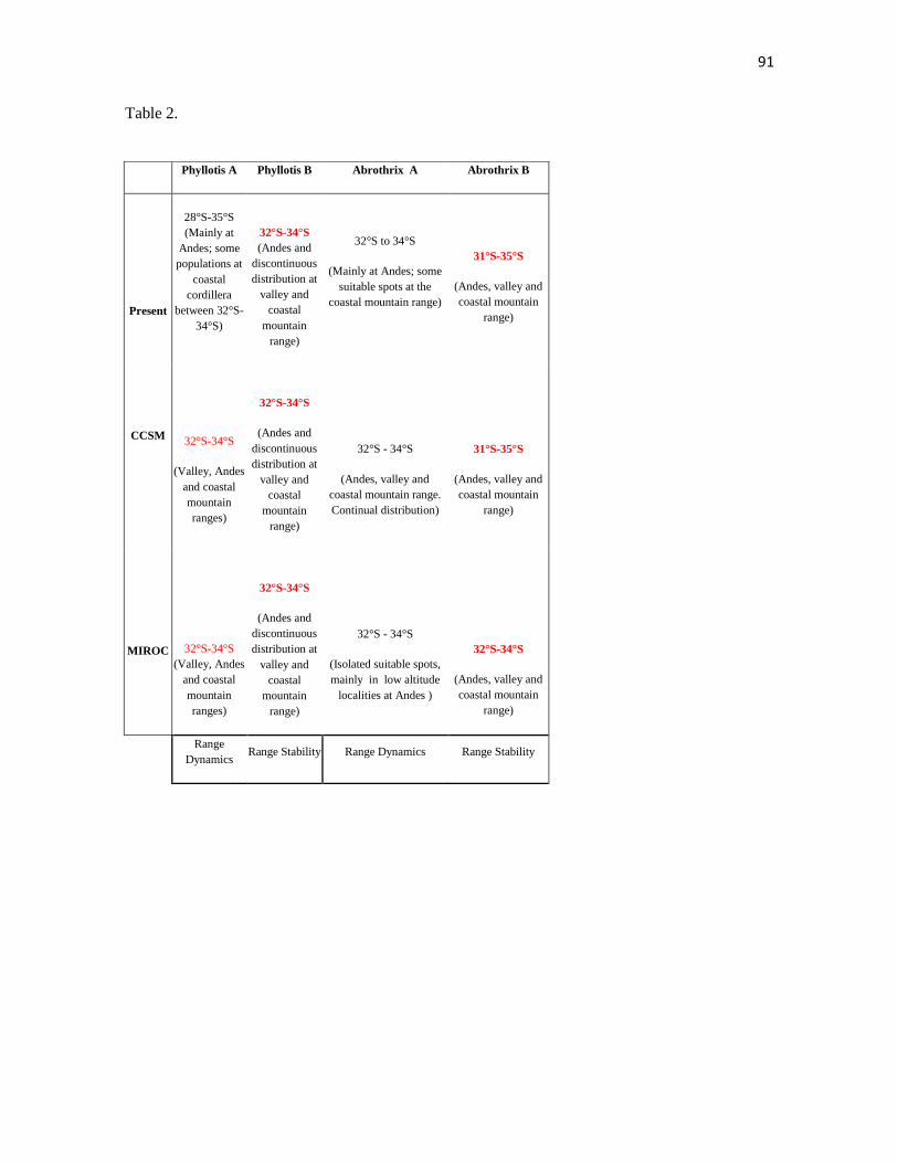
91

Table 2.

Phyllotis A Phyllotis B Abrothrix A Abrothrix B

Present

28°S-35°S

(Mainly at

Andes; some

populations at

coastal

cordillera

between 32°S-

34°S)

32°S-34°S

(Andes and

discontinuous

distribution at

valley and

coastal

mountain

range)

32°S to 34°S

(Mainly at Andes; some

suitable spots at the

coastal mountain range)

31°S-35°S

(Andes, valley and

coastal mountain

range)

CCSM

32°S-34°S

(Valley, Andes

and coastal

mountain

ranges)

32°S-34°S

(Andes and

discontinuous

distribution at

valley and

coastal

mountain

range)

32°S - 34°S

(Andes, valley and

coastal mountain range.

Continual distribution)

31°S-35°S

(Andes, valley and

coastal mountain

range)

MIROC

32°S-34°S

(Valley, Andes

and coastal

mountain

ranges)

32°S-34°S

(Andes and

discontinuous

distribution at

valley and

coastal

mountain

range)

32°S - 34°S

(Isolated suitable spots,

mainly in low altitude

localities at Andes )

32°S-34°S

(Andes, valley and

coastal mountain

range)

Range

Dynamics Range Stability Range Dynamics Range Stability

92

Figure 1

93

Figure 2

EP554ElRobleEP562ElRoble

NK105924VAlemanaEP617FarellonesEP629Farellones

NK105917VAlemanaNK105925VAlemanaNK105909VAlemanaNK105920VAlemanaNK105921VAlemanaNK120008Paine

EP492ElRobleNK105804Rabuco

NK106157MelipillaNK106159MelipillaNK105910VAlemanaNK105923VAlemanaNK106143ElRobleNK96787RMaipuNK106144ElRobleNK106164Melipilla

NK95341SCApoqNK95720SCApoqNK95812SCApoqNK106136ElRobleNK106138ElRobleNK106142ElRoble

NK106145ElRobleNK106147ElRobleNK106148ElRobleNK106149ElRobleEP557ElRobleNK96786RMaipuNK96788RMaipuNK105808RabucoNK106153MelipillaNK106154MelipillaNK106156MelipillaNK106158Melipilla

NK106162MelipillaNK106163MelipillaNK105908VAlemanaNK105915VAlemanaNK105919VAlemanaNK105922VAlemanaNK129190LaFloridaNK129191LaFloridaNK129192LaFloridaNK129194LaFloridaNK129195LaFloridaNK129196LaFloridaNK129198LaFloridaNK129199LaFloridaNK129200LaFloridaNK120005PaineNK120007Paine

NK106155MelipillaEP583FarellonesEP622Farellones

EP581FarellonesEP624Farellones

NK95549SCApoqNK95671SCApoqNK105427SCApoqEP623Farellones

NK95672SCApoqNK96309SCApoqNK96348SCApoqNK104631SCApoqEP580FarellonesEP582FarellonesEP585FarellonesEP619Farellones

EP586FarellonesEP628Farellones

NK108712CAhumadaNK108719CAhumada

NK108717CAhumadaNK108720CAhumada

EP410QTarapacaEP413QTarapaca

EP435QCamaronesEP438QCamarones

0.001 substitutions/site

1.00/100

0.63/64

0.82/94

1.00/92

0.82/88

A

B

94

Figure 3

EP588Farellones

NK108715CAhumada

NK108716CAhumada

UCK181Chicauma

EP493ElRoble

EP544ElRoble

EP546ElRoble

EP548ElRoble

EP553ElRoble

EP558ElRoble

EP560ElRoble

EP566ElRoble

EP567ElRoble

EP569ElRoble

EP575ElRoble

NK106137ElRoble

NK106141ElRoble

NK106146ElRoble

UCK177Chicauma

UCK183Chicauma

EP606Farellones

EP614Farellones

EP626Farellones

EP563Farellones

EP625Farellones

EP633Farellones

NK108714CAhumada

NK108718CAhumada

EP630Farellones

NK108713CAhumada

NK108723CAhumada

EP587Farellones

UCK156Cantil lana

UCK157Cantil lana

UCK162Cantil lana

UCK163Cantil lana

UCK164Cantil lana

EP621Farellones

UCK159Cantil lana

UCK166Cantil lana

UCK168Cantil lana

UCK158Cantil lana

UCK160Cantil lana

UCK165Cantil lana

UCK167Cantil lana

NK108721CAhumada

EP539LaCampana

EP540LaCampana

NK96359SCApoq

NK95544SCApoq

UCK178Chicauma

NK96318SCApoq

NK95336SCApoq

NK120403SCApoq

EP571ElRoble

NK108722CAhumada

NK95305SCApoq

EP542LaCampana

NK95531SCApoq

NK106069ElRoble

NK160855SCApoq

NK108791Elcanelo

4Pmagister

5Pmagister

0.005 substitutions/site

1.00/100

1.00/

082/85

0.92/97

A

B

95

Figure 4

Figure 5

NK95305SCApoq

NK120403SCApoq

EP587Farellones

UCK160Cantillana

UCK165Cantillana

UCK164Cantillana

EP621Farellones

EP630Farellones

EP625Farellones

EP563Farellones

EP633Farellones

EP614Farellones

EP567ElRobleEP558ElRoble

EP553ElRoble

EP544ElRoble

EP588Farellones

NK95544SCApoq

NK108721CAhumada

EP540LaCampana

NK108791Elcanelo

NK95531SCApoq

NK106069ElRoble

NK96318SCApoqNK96359SCApoq

NK160855SCApoq

EP542LaCampana

EP560ElRoble

EP566ElRoble

NK106137ElRoble

EP575ElRoble

NK106141ElRoble

UCK159Cantillana

NK108723CAhumada

NK108718CAhumada, NK108714CAhumada

UCK156Cantillana

UCK166Cantillana

UCK167Cantillana

NK108722CAhumada

EP539LaCampana

NK108715CAhumada

NK106146ElRoble

EP546ElRoble

EP626Farellones, EP606Farellones

NK108713CAhumada

UCK162Cantillana

UCK163Cantillana

UCK158Cantillana

UCK178Chicauma

NK108716CAhumada

UCK177Chicauma

UCK181ChicaumaUCK183Chicauma

EP493ElRoble

EP548ElRoble

EP569ElRoble

UCK168Cantillana

UCK157Cantillana

NK95336SCApoq

EP571ElRoble

0.01

96

Figure 6

NK129194LaFlorida

NK105925VAlemana

NK105921VAlemana

NK106157Melipilla

NK105923VAlemana

EP492ElRoble

EP557ElRoble

NK95812SCApoq

NK105922VAlemana

NK95341SCApoq

NK106155Melipilla

NK120005Paine

NK129190LaFlorida

EP562ElRoble

EP554ElRoble

NK108720CAhumada

NK108717CAhumada

NK108719CAhumada

NK108712CAhumada

EP628Farellones

EP624Farellones

EP581Farellones

EP623Farellones

EP583Farellones

NK104631SCApoq

NK95671SCApoq

NK95549SCApoq

NK96348SCApoq

EP582Farellones

EP580Farellones

EP410QTarapaca

EP435QCamarones

100

83

74

8

73

4

5

9

90

30

90

13

7

13

100

85

90

90

100

88

86

37

79

65

8

3

3

8

90

100

0.01

97

Figure 7

UCK162Cantillana

UCK163Cantillana

UCK167Cantillana

EP625Farellones

EP614Farellones

EP626Farellones

EP606Farellones

EP553ElRoble

UCK183Chicauma

EP566ElRoble

EP575ElRoble

NK106137ElRoble

UCK181Chicauma

NK108714CAhumada

NK108718CAhumada

EP567ElRoble

NK95336SCApoq

EP571ElRoble

NK108722CAhumada

NK160855SCApoq

EP542LaCampana

NK95544SCApoq

NK108721CAhumada

UCK178Chicauma

EP539LaCampana

EP540LaCampana

NK106069ElRoble

4Pmagister

5Pmagister

100

100

97

54

98

75

86

96

100

36

93

12

14

6

12

91

100

79

58

49

65

94

80

94

34

99

100

10000000

98

Figure 8

Cluster 1 Cluster 2

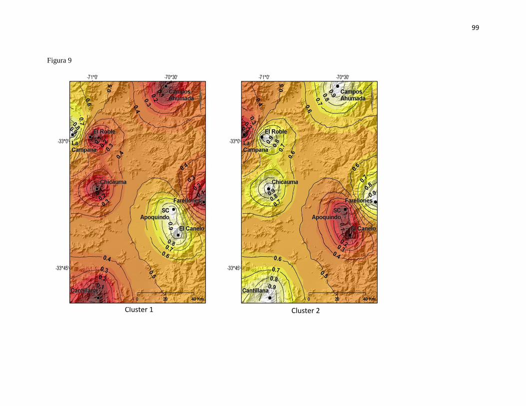
99

Figura 9

Cluster 1 Cluster 2

100

Figure 10

101

Fig 10.1

102

Comparative phylogeography of vertebrates in the hotspot of central Chile: influence

of the Last Glacial Maximum on the distribution of intraspecific lineages.

Pablo Gutiérrez-Tapia1, Dusan Boric-Bargetto

2, Claudio Correa

1, Brett R. Riddle

3,

Fernando Torres-Perez4 & R. Eduardo Palma

1.

1-Pontificia Universidad Católica de Chile . 2- Universidad de Concepción, Chile. 3- ,

University of Nevada, Las Vegas. 4- Pontificia Universidad Católica de Valparaíso, Chile.

Abstract

Distributional responses to climate change after the Last Glacial Maximum (LGM) , in

currently endangered areas as biodiversity hotspots, are an appropriate model to search for

mechanisms involved in the current threat of cryptic biodiversity loss in a global change

scenario. In this work, we investigated the past distributional responses of four vertebrate

species, endemic to the central Chile hotspot. We combined current and LGM distribution

models with phylogenetic information at the intraspecific level to test alternative

biogeographic scenarios. Our main conclusion is that lineages inside species have had

independent distributional responses often associated with differential recolonization of

mountain ranges and lowlands, and also stable and dynamic distribution for lineages within

the same species. We have also identified an area around 33°S and 36°S which have

hypothetically behaved as a refuge for cryptic biodiversity through several

glacial/interglacial transitions. In current interglacial conditions, mountain ranges at central

Chile are important biological corridors which may be considered a conservation priority,

103

while coastal cordillera around 33- 36°S is an important cryptic biodiversity reservoir

through major climatic oscillations.

Introduction

It is well known that climate regime may affect species distributions and therefore future

climate change could potentially induce geographical range dynamics such as contraction,

expansion or geographical range shifts (Walther et al., 2002; Pearson & Dawson, 2003;

Summers et al., 2012). It is also agreed that the climatic impact on species distribution can

be extrapolated in community and ecosystem shifts (Walther et al., 2002; Hamann &

Wang, 2006). For these reasons, the species level might be critical for conservation issues

in a global climate change scenario (GCC).

At the species level, climate change is expected to affect the geographical range mainly

through physiological restrictions as temperature and precipitation tolerances in

conjunction with species dispersal abilities (Walther et al., 2002). Altogether, those factors

may determine species ability to keep up with climate change. From an ecological

perspective, expected species responses to climate change are i) to tolerate or spread in the

new climatic scenario (either by physiological tolerance or phenotypic plasticity) ii) to

change its distribution in order to catch up the new climate regime iii) to go extinct

(Pettorelli, 2012). From an evolutionary perspective, range shifts may change the

distribution of genetic diversity and range contractions will most likely reduce genetic

diversity (Alsos et al., 2012; Pauls et al., 2012). Nevertheless, the emphasis on the role of

evolution in species responses to climate change has been usually focused on evolutionary

104

adaptations and the relationship between species’ adaptation speed and climatic change rate

(Hoffmann & Sgrò, 2011).

It has been recently emphasized about the need to consider GCC effects on biodiversity

below the species level, other than the usually advocated adaption potential and

phenotypical plasticity issues. There exists a severe lack of studies on GCC effects on

biodiversity, at the level of intraspecific genetic diversity. This is highly evident if we

compare the vast amount of publications at the ecosystem, community and species levels,

with approaches below species level (Fraser & Bernatchez, 2001) despite the general

agreement on the importance of Evolutionary Significant Units (ESUs) for conservation

planning. On this line of arguments, (Bálint et al., 2011) demonstrated that species with

strong population genetic structure will face massive losses of diversity at the intraspecific

level in a GCC scenario. That is to say morphospecies based estimation on GCC impacts on

biodiversity will severely underestimate cryptic diversity loss, therefore conservation

strategies based solely on above species organization levels might be an oversimplified

approach.

For the above reasons, it might be critical for future conservation planning not just to

quantify the amount of cryptic diversity at risk (i.e. local genetic variants with adaptative

potential, fitness related variability, or intraspecific lineages with a characteristic

distribution), but to also understand what could be the ecological and evolutionary

responses of ESUs below the species level to GCC. There exist a substantial number of

publications trying to understand the relationship between species’ evolutionary and

ecological responses to climate change, mainly through phylogeographic information and

species distribution models (SDMs) (Carstens & Richards, 2007; Waltari et al., 2007;

105

Kozak et al., 2008; Provan & Bennett, 2008; Cordellier & Pfenninger, 2009; Marske et al.,

2009; Waltari & Guralnick, 2009; Buckley et al., 2010; Lim et al., 2010; Allal et al., 2011;

Eckert, 2011; Gugger et al., 2011; Marske et al., 2011; Svenning et al., 2011; Marske et al.,

2012; Qi et al., 2012). However, approaches using intraspecific phylogenetic information to

build lineage distribution models (lineages below species level) are less frequent. Even

though this approach has been used with success in systematics for species delimitation and

cryptic speciation issues (Raxworthy et al., 2007; Rissler & Apodaca, 2007; Engelbrecht et

al., 2011; du Toit et al., 2012; Florio et al., 2012), the need to discern lineage-specific

ecological responses to GCC at the intraspecific level (and its potential applicability in

conservation strategies, as a measure of distributional shifts experimented by cryptic

phylogenetic lineages) is a relatively new issue in the scientific literature. Several efforts

have been recently made on this concern: by using SDMs and genetic diversity measures

Schorr et al., (2012) concluded that this integrated approach may change the distributional

history inferred from phylogeographic information at the species level. Studying the

relationship between lineage formation and variation in the ecological niche in the

Peromyscus maniculatus species group Kalkvik et al., (2011) demonstrated that the

majority of genetic lineages within species do occupy distinct environmental niches. In

another integrated approach using SDMs and phylogeography Fontanella et al., (2012)

concluded that two main haploclades in the lizard Liolaemus petrophilus shared different

distributional responses to climate change during the Pleistocene. Those findings suggested

that geographical range shifts triggered by climatic shifts might be complex if the species

share phylogenetic structure, and some degree of intraspecific niche divergence related to

cryptic phylogenetic lineages. Therefore, realistic predictions of range shifts for future

climate change scenarios should consider phylogenetic information to perform lineage-

106

specific distribution models, because species might not necessarily respond as a simple

ecological unit to future GCC.

Among the world biodiversity hotspots, the African “Cape Floristic Region” (CFR) is one

of the better known with respect to the evolutionary origin of its biota (Verboom et al.,

2009a). In fact, a phylogeographic study in the genus of dwarf chameleons Bradypodium

(Fitzinger, 1843) suggested that there was a concerted phylogeographic pattern between

species of this genus, and between these and two other endemic lizards associated to the

emergency of the Cape Flora (Tolley et al., 2006; Tolley et al., 2009). At he same time, the

Cape Flora may display a complex diversification history with ancient and recent speciation

events, probably caused by a combination of climatically induced fragmentation and

adaptative radiation (Verboom et al., 2009b). On the other hand, a comparison of the

phylogeographic pattern conducted in six taxonomic groups, endemic to the “California

Floristic Province” hotspot, concluded that genetic structure of these taxa show major splits

highly consistent across most taxa (Calsbeek et al., 2003). The latter authors concluded that

diversification can be spatially and temporally explained by the climatic and geographic

history of the California hotspot. Finally, in the “Brazilian Atlantic Forest” hotspot,

Carnaval et al., (2009) demonstrated that climatic stability in Pleistocene refugia is a good

predictor of the current genetic diversity within this hotspot. Altogether those evidences

suggest that biodiversity hotspots may be appropriate systems to study the relationship

between climate dynamics and genetic differentiation in currently endangered areas.

Within the former scenario, we have chosen four vertebrate species (see below)

endemic to the biodiversity hotspot of central Chile focused 1) to evaluate how vertebrate

species have responded to climate change in a currently endangered area (there is a strong

107

need of that information for future conservation planning); 2) to evaluate the genetic

structure of species in the Chilean hotspot, since this feature may be characteristic of the

region due to its particular evolutionary and geo-climatic history. To those goals we

reconstructed intraspecific phylogenies for each taxa to characterize cryptic lineages, and

we built lineage distribution models at present and paleodistribution models at LGM to

assess the existence of lineage-specific distributional responses to climate change, by using

a climatic niche approach. In addition, we integrated phylogenetic information with lineage

distribution models into alternative biogeographic scenarios, and we tested the alternative

hypothetical scenarios in a comparative phylogeographic framework. For this purpose,

simulations of the expected distribution of the number of deep coalescens were

implemented. Our main objective is to characterize the distributional responses of species

and cryptic intraspecific lineages to climate change after LGM, in order to understand how

cryptic diversity may affect our criteria for delimiting Evolutionary Significative Units

(ESUs) for conservation planning, in an endangered area as a biodiversity hotspot.

To evaluate the above proposed goals we have chosen four vertebrate species

endemic to the biodiversity hotspot of central Chile. The criteria used to choose the

appropriate vertebrate taxa to test the hypothesis in the central Chile hotspot were i) taxa

should be endemic to the region of interest ii) the set should represent a broad spectrum of

terrestrial vertebrate taxa. Accordingly, the selected taxa were: 1) the sigmodontine rodent

Phyllotis darwini 2) the didelphid marsupial Thylamys elegans 3) the iguanid lizard

Liolaemus monticola 4) and the anuran toad Rhinella arunco.

108

Methods

Study area and main distributional hypothesis Fifty percent of all endemic species of

vertebrates in Chile occur in an area that does not exceed 16% of its land area (Simonetti

1999): This region has been identified as the globally significant ‘biodiversity hotspot of

central Chile’ (Myers et al. 2000). Understanding the processes responsible for this

biodiversity pattern is an important concern in the context of global change. The central

Chile Sub-region extends between 28°S to 36°S (Morrone 2006), which approximately

matches Myers (2000) definition. In this work, we chose vertebrate species endemic to the

hotspot to assess the effects of GCC after one glacial maximum on the geographic

distribution of lineages, in order to construct a potentially more general model of

intraspecific responses to climate change in a hotspot area. In addition, this information will

be very valuable in order to understand what should be the relevant implications of

considering cryptic diversity in conservation strategies planning, compared to approaches

based only in species or ecosystem level, and therefore to improve conservation strategies

by using more realistic assumptions on distributional responses to GCC. We expect that

potential cryptic lineages inside vertebrate species might be associated to the altitudinal

gradient given by the Andes, the valleys, and the Coastal Cordillera. The latter topography

constitutes the most important geographic features in the central Chile hotspot. We also

expect that the specie’s geographic range history may display signatures of one of the most

important geo-climatic events in central Chile: the Last Glacial Maximum (LGM). This

event was chosen to test the hypothesys because in addition to being one of the greatest

episodes of recent climate change (represents the opposite climatic extreme from the

current interglacial period) it is known that Quaternary glaciations in general have been one

109

of the most important factors in determining the current genetic structure of many

populations, species and communities (Hewitt, 2000). Even though central Chile was not

extensively covered by ice sheets at LGM, the glacial advanced northward through the

Cordillera de los Andes (Clapperton, 1990; Clapperton, 1994) descending to about 1,100 m

with a subsequent drop in the temperature and an increased rainfall in the whole region

(Heusser, 1983; Heusser, 1990; Lamy et al., 1999). The palinological evidence has

demonstrated that high Andean vegetational belt shifts downwards the valley during the

glacial advance, and then move upwards, reaching its original high altitude distribution

after glacial retreat. This vegetational shift may have given rise to the existing

biogeographical insulas of Andean vegetation in both, the Andes and the Coastal cordilleras

of central Chile (Darwin, 1859; Simpson, 1983; Heusser, 1990; Villagrán & Armesto,

1991; Villagrán & Hinojosa, 2005). In addition, it has been suggested that lizards and

rodent’s relative species diversity in central Chile is explained by different speciation

modes in both groups, as a result of differential interaction between mountain geography,

Quaternary glaciations, and ecological features in both groups (Fuentes & Jaksic, 1979).

We have previous evidence which suggests that the rodent Phyllotis darwini does not

behave as a simple distributional unit to climate change after LGM, but is composed of two

cryptic lineages which have expanded its range following an strict altitudinal segregation

(valley and mountain ranges) after glacial retreat, and it’s phylogeographic structure pattern

accommodates more to the “lizard speciation mode” rather than the “rodent speciation

mode” postulated by Fuentes & Jaksic 1979 (Gutiérrez-Tapia & R.E. Palma, in prep.).

Those findings had lead us to hypothesize that species with intraspecific phylogenetic

structure may not behave as distributional units to climate change, but as a mosaic of

independent distributional responses by each cryptic lineage.

110

Specimens and molecular markers All specimens and sequences used in this paper come

from previous work in molecular phylogeography of the central Chile hotspot, part of

previous studies of our research group. For Phyllotis darwini we used mitochondrial D-

loop sequences from 68 individuals, 412 bp and four specimens of P. magister were used

as outgroups (Gutiérrez-Tapia & Palma, in prep.). For Thylamys elegans we used 69

mitochondrial cytochrome b sequences, 983 bp, and we used the sister taxa T. pallidior

and T. tatei as outgroups (Boric-Bargetto, in prep.). For Liolaemus monticola we used 45

mitochondrial cytochrome b sequences, 700 bp, using L. nigroviridis, L. tenuis and L.

pictus as outgroups (Torres-Pérez et al., 2007). Finally, for Rhinella arunco we used 163

mithochondrial D-loop sequences, 899 bp (Vasquez et al., 2013). Since this study

constituted a multi-taxa approach, we considered that using a single molecular marker per

species would be suitable to characterize the general distributional responses among taxa.

On the other hand, coalescent simulations of molecular evolution inside each species give

support to our species trees. Individual sampling roughly represents all species’ geographic

ranges. The full list of specimens, geographic cooordinates and GeneBank accession

numbers is given in Appendix I.

Intraspecific Phylogeny For phylogenetic reconstruction, sequences from each species were

transformed into haplotypes to simplify the analysis, but data about haplotype frequency

was not take into account in this work.

The Markov Chain Monte Carlo (MCMC) method within a Bayesian framework (hereafter

BMCMC) was used to estimate the posterior probability of phylogenetic trees. The MCMC

111

procedure ensures that trees are sampled in proportion to their probabilities of occurrence

under the model of gene-sequence evolution. Approximately 10,000,000 phylogenetic trees

were generated using the BMCMC procedure, sampling every 1000th

trees to ensure that

successive samples were independent. The first 50 trees of the sample were removed to

avoid including trees sampled before convergence of the Markov Chain. We used a general

likelihood-based mixture model (MM; Pagel & Meade, 2004), based on the general time-

reversible (GTR) model of gene-sequence evolution to estimate the likelihood of each tree.

This model accommodates cases in which different sites in the alignment evolved in

qualitatively distinct ways, but does not require prior knowledge of these patterns or

partitioning of the data. These analyses were conducted using the software

BayesPhylogenies, available at the website

http://www.evolution.rdg.ac.uk/SoftwareMain.html. In order to find the best mixture model

of gene-sequence evolution, we obtained the likelihood of the trees by first using a GTR

matrix plus the gamma distributed rate heterogeneity model (1GTR + G) and then

continuing to add up to five GTR + G matrices were determined. For the posterior analyses,

only the combination of matrices with the fewest number of parameters that significantly

increased the likelihood was used. Posterior probabilities for topologies were assessed as

the proportion of trees sampled after burn-in, in which that particular topology was

observed.

Distribution models .- We modeled the climatic niche of each intraspecific lineage to

approximate the whole species’ current distribution, and its distribution during the LGM

under the assumptions that: (1) climate is an important factor driving the species’

distribution; (2) the climatic niche of species remained conserved between the LGM and

112

present time, and (3) overlapped lineage’s distribution ranges will approach the whole

species geographic range. The latter assumption was tested by overlapping distribution

models of each intraspecific lineage to approach the full species distributional range, as the

sum of ranges estimated for each lineage. The resultant distributional range was roughly

contrasted with another model built for the whole species without considering phylogenetic

structure.

The climatic niches were reconstructed using the methodology of ecological niche

modeling, where environmental data are extracted from occurrence records and random

points (represented by geographic coordinates). Habitat suitability was evaluated across the

landscape using program specific algorithms (Elith et al., 2006). The current models were

then projected on the climatic reconstructions of the LGM. For occurrence records, we used

our unique sampling localities. In addition to full geographic distribution models for each

species, we built climatic models for each major lineage recovered in the intraspecific

phylogenies following the same approach. As a test of consistency we overlapped the

lineage distribution models for the lineages of each species, to compare it to the full species

distribution models.

The current climate was represented by bioclimatic variables from the WorldClim dataset

v. 1.4 (http://www.world clim.org/; Hijmans et al., 2005) that are derived from monthly

temperature and precipitation data, and represent biologically meaningful aspects of local

climate (Waltari et al., 2007; Jezkova et al., 2009).

For environmental layers representing the climatic conditions of the LGM, we used

ocean–atmosphere simulations (Harrison, 2000) available through the Paleoclimatic

Modelling Intercomparison Project (Braconnot et al., 2007). These reconstructions of the

LGM climate are based on simulated changes in concentration of greenhouse gases, ice

113

sheet coverage, insulation and topography (caused by lowering sea levels). We used two

models that have been previously downscaled for the purpose of ecological niche modeling

(Waltari et al., 2007): Community Climate System Model v. 3 (CCSM; Otto-Bliesner et al.,

2006) and the Model for Interdisciplinary Research on Climate v. 3.2 (MIROC; Hasumi &

Emori, 2004). The original climatic variables used in these models have been downscaled

to the spatial resolution of 2.5 min under the assumption that changes in climate are

relatively stable over space (high spatial autocorrelation) and were converted to bioclimatic

variables (Peterson & Nyári, 2007).

Climatic niche models were built in the software package MAXENT v. 3.2.1 (Phillips et

al., 2006), a program that calculates relative probabilities of the species’ presence in the

defined geographic space, with high probabilities indicating suitable environmental

conditions for the species (Phillips et al., 2004). Trapping coordinates of each individual

captured for DNA extraction was used as presence points. We used the default parameters

in MAXENT (500 maximum iterations, convergence threshold of 0.00001, regularization

multiplier of 1, and 10 000 background points) with the application of random seed and

logistic probabilities for the output (Phillips & Dudik, 2008). We masked our models to

four altitudinal categories resuming both, the abrupt altitudinal clines characteristic of

central Chile, and some known altitudinal distribution limits for several vertebrate taxa in

this area (Fuentes & Jaksic, 1979). This procedure was conducted because reducing the

climatic variation being modeled to that which exists within a geographically realistic area

improves model accuracy and reduces problems with extrapolation (Pearson et al., 2002;

Thuiller et al., 2004; Randin et al., 2006). We ran 10 replicates for each model, and an

average model was presented using logistic probability classes of climatic niche suitability.

The presence– absence map was determined using the ‘maximum training sensitivity plus

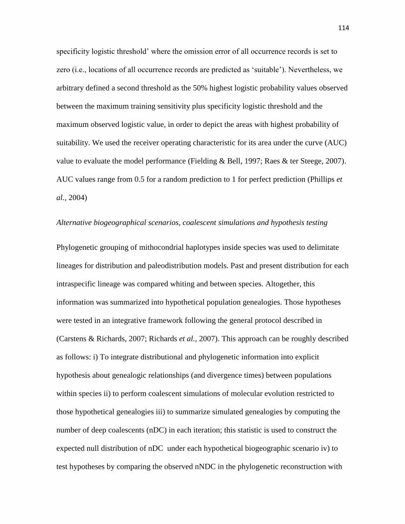
114

specificity logistic threshold’ where the omission error of all occurrence records is set to

zero (i.e., locations of all occurrence records are predicted as ‘suitable’). Nevertheless, we

arbitrary defined a second threshold as the 50% highest logistic probability values observed

between the maximum training sensitivity plus specificity logistic threshold and the

maximum observed logistic value, in order to depict the areas with highest probability of

suitability. We used the receiver operating characteristic for its area under the curve (AUC)

value to evaluate the model performance (Fielding & Bell, 1997; Raes & ter Steege, 2007).

AUC values range from 0.5 for a random prediction to 1 for perfect prediction (Phillips et

al., 2004)

Alternative biogeographical scenarios, coalescent simulations and hypothesis testing

Phylogenetic grouping of mithocondrial haplotypes inside species was used to delimitate

lineages for distribution and paleodistribution models. Past and present distribution for each

intraspecific lineage was compared whiting and between species. Altogether, this

information was summarized into hypothetical population genealogies. Those hypotheses

were tested in an integrative framework following the general protocol described in

(Carstens & Richards, 2007; Richards et al., 2007). This approach can be roughly described

as follows: i) To integrate distributional and phylogenetic information into explicit

hypothesis about genealogic relationships (and divergence times) between populations

within species ii) to perform coalescent simulations of molecular evolution restricted to

those hypothetical genealogies iii) to summarize simulated genealogies by computing the

number of deep coalescents (nDC) in each iteration; this statistic is used to construct the

expected null distribution of nDC under each hypothetical biogeographic scenario iv) to

test hypotheses by comparing the observed nNDC in the phylogenetic reconstruction with

115

the expected null distribution of nDC of each alternative hypotheses. If the observed nDC is

less or equal than 5% of the expected nDC distribution, that particular biogeographic

scenario can be rejected. Coalescent simulations of DNA evolution for each species and

hypothesis were performed in the software MESQUITE 2.75 (Maddison & Maddison,

2011). One hundred coalescent simulations were performed to construct the expected null

distribution of nDC for each hypothesis. The same number of characters and also the same

molecular evolution parameters estimated in phylogenetic reconstruction were used for

DNA sequence evolution simulations.

Two main modifications to the protocol described by Richards et al. were made: First, as

we knew a priori that phylogeographic patterns of interest were pseudo-congruents (i.e.

similar topology and distribution, but different divergence time), we did not build the

general genealogical hypothesis with explicit divergence time or number of generations;

instead we used the maximum observed branch length for each haplogroup, because we

were more interested in the effect of long term distributional patterns on genealogy (i.e.

species tree) rather than specific historical events. Second, we sacrificed realism in

coalescent simulations regarding the effective population size parameter (Ne), because

when we introduced skyline estimations of Ne (Ho & Shapiro, 2011) in coalescent

simulations, null distributions of nDC were incommensurable with observed nDC.

Therefore, we defined the Ne in simulations as the minimum value allowed by MESQUITE

in all coalescent simulations.

116

Results

Intraspecific Phylogenies

General topology is similar among species’ phylogenetic trees, except for Rhinella arunco

which shows no intraspecific phylogenetic structure (very low posterior probability values

for internal nodes Fig. 1). All other species display an intraspecific split between two major

phylogroups (A and B; Fig. 1), with one of the major groups divided into two subgroups

(A1 and A2 subgroups Fig. 1). There is one supported subgroup within phylogroup B for P.

darwini, but this whole B group has a wide and almost continuous distribution across the

species’ latitudinal range. Posterior probability values for the nodes which define this

pattern is high (values between 0.94 to 1.0; Fig 1).

Distribution models

To test the assumption that overlapped lineage distribution models may approximate whole

species distribution models, we compared our estimations of each species’ distribution

range at present from i) all trapping localities, considering whole species as single

distributional units (data not shown), and ii) models with trapping localities assigned to

different intraspecific lineages as independent distributional units (independent lineage

distribution models) (Fig 7, Tables 1 and 2). The result shows that whole species’ range

models are good approximations of the observed distribution range for each species, and

also with high model performance (AUC, Table 1), whereas overlapped lineage distribution

models slightly over-predict the northern distribution of Phylloti darwini. Both model

117

approaches (whole species and overlapped lineage’s ranges) are good and consistent

approximations of species´ current geographic ranges.

Range dynamics

Phyllotis darwini Distribution model for lineage B encompasses the whole distributional

range of P. darwini (Fig 2, table 2) and slightly over-predicts its southern distributional

range until 37° S. Interestingly, when considering an arbitrary high threshold (50% highest

logistic probability value, red areas in Fig. 2) the predicted distribution range is mainly

restricted to lowlands in the valley and coast. On the other hand, distribution model for

lineage A shares lower AUC value and clearly over-predicts the observed distribution of

this phylogroup (sampled at disjunct localities across both mountain ranges). Nevertheless,

when considering our arbitrary high threshold, the estimated distribution for lineage A is

surprisingly well delimited and restricted almost exclusively to Andean mountain ranges

(some populations in coastal mountain range) above the 1500 m elevation limit detected for

this phylogroup in a previous work (Gutiérrez-Tapia et al. in prep). This mountain-

restricted lineage occurs between 25°S and 36°S.

In summary, overlapped lineage distribution models for P. darwini has slightly worst

performance and some over-prediction compared to the whole species distribution model,

but when considering our arbitrary 50% highest logistic probability threshold, lineage

distribution models reproduced very accurately the altitudinal pattern reported for both

phylogroups at present, with phylogroup A currently distributed across mountain ranges

above 1500 m, and phylogroup B mainly distributed in the lowlands and low elevation

118

mountain belts. This information is missed in the whole species distribution range model

(data not shown).

Past lineage distribution estimated by both LGM models is conflicting (CCSM and

MIROC, Fig. 2, table 2): the CCSM model predicts a distributional gap during LGM for

both phylogroups, but MIROC based distribution models predicts that both phylogroups

were restricted to the southern portion of the current distributional range. Nevertheless,

both models consistently predicted the area between 31°S-35°S as suitable for both

phylogroups during LGM. This latitudinal distribution dynamics must be considered with

caution because downscaled climatic data may not represent local geographic complexity

with accuracy.

It is important to emphasize that altitudinal particularities reported for both lineages at

present were already established during LGM: lineages A and B might have been restricted

to approximately the same latitude, but only lineage A displayed suitable areas at the

Andean mountain range during LGM (Table 2), which also has been sampled mainly in the

Andes and above 1500 m. at present.

Thylamys elegans This species possess two main intraspecific lineages with essentially

allopatric distribution at present. Our model suggests that northern phylogroup A is

distributed from 30°S to 34°S by the coast, the valley and mountain ranges, whereas

southern phylogroup B ranges from 33°S to 36°S at the coast, the valley and mountain

ranges, and even until 37°S across coastal mountain ranges (Fig. 2, Table 2).

MIROC and CCSM past distribution models consistently shows a more restricted

distribution range for phylogroup A which may have been confined to 31°S to 33°S during

119

LGM, and its altitudinal distribution at Andean mountain ranges appears to have also

retracted to lower elevations. Southern phylogroup B on the contrary, had apparently

retained its distributional range between 33°S to 36°S at the coast, the valley and mountain

ranges since LGM, according to both MIROC and CCSM based distribution models (Fig.

2, Table 2) .

Liolaemus monticola Our distribution models at present describes surprisingly well the

altitudinal distribution of the species, which is known to be currently distributed above 300

m. until 2200 m. in both, coastal and Andean mountain ranges (Mella, 2005). The model

displays very little over-prediction in lowlands for both phylogroups. Phylogroup A is

distributed from 32° S to 34° S according to the model for current climatic conditions; there

is a slight over-prediction in the lowlands, but as in Phyllotis darwini ´s phylogroup A, red

areas (which correspond to our arbitrariy threshold of 50% highest logistic probability

values) are a good descriptor of the mountain-range-restricted distributional pattern in this

species. The same altitudinal pattern is truth for the southern phylogroup B, but distributed

between 33° S and 36° S mainly in the Andes and some populations at the coastal

mountain range (Fig. 2, Table 2) .

Past lineage distribution based on MIROC suggests that phylogroup A distribution at LGM

was roughly the same than its present distribution, but maybe confined to lower elevations

at the Andes mountain range compared to present distribution. On the other hand, CCSM

based distribution model clearly over-predicts the past distribution of phylogroup A in a

disjunct population of southern Argentina, at the eastern side of the Andes, far away from

the southern distributional limit of the species. In contrast, phylogroup B appears to have

had a much broader distribution towards the lowlands and the Coastal Cordillera at LGM,

120

according to both, CCSM and MIROC based distribution models. Nevertheless, latitudinal

boundaries appear to remain constant since LGM (Fig. 2, Table 2).

Rhinella arunco This is the only species for which we did not obtain phylogenetic structure

(Fig. 1). According to the distribution model at present conditions, R. arunco has suitable

habitats between 31°S and 37°S. Both CCSM and MIROC based distribution models at

LGM predict that R. arunco’s distributional range could have been slightly contracted

(32°S to 36°S) in its latitudinal boundaries compared to its distribution at present (31°S to

37°S) (Fig. 2, Table 2) .

Alternative Biogeographic scenarios

To develop a biogeographic hypothesis to explain current distribution of vertebrate’s

cryptic diversity in the central Chile hotspot, we have made a comparison of present and

past distribution at LGM, among lineages and across species. Our first conclusion was that,

despite the highly similar intraspecific phylogenetic topology among species (except for R.

arunco for which we did not recover intraspecific structure), there exists a general lack of

phylogeographic congruence (i.e lineages among species are not codistributed, nor at

present or during LGM). Nevertheless, we have identified some generalities in the

distribution of those phylogroups with no internal subdivision (“B” phylogroups, Fig.1): all

“B” phylogroups are currently distributed at, or were restricted to, approximately the same

area between 32°S to 36°S (Fig 2) mainly at the valley and coastal cordillera but never in

the Andes; that is to say this is an area of persistant distribution for vertebrate lineages

during LGM, with the max degree of codistribution between 32°S – 35°S (Fig. 4).

Therefore, our results consistently suggests that this geographic area appears to be a highly

121

persistent distribution center for vertebrate lineages in the central Chile hotspot, since the

LGM to present times. Assuming that this hypothetically highly persistent distribution area

could have behaved in a similar way across several glacial/interglacial cycles through the

evolutionary history of those vertebrate species, we postulate that this area has harbored the

most ancient haplotypes of the studied species. If this is true, we expect to see this

phenomena reflected in the intraspecific phylogenetic trees: our hypothesis is that all

phylogroups distributed independently of this high persistence area (“A1” and “A2”

phylogroups, Fig. 1) must be more related to each other than any of them with “B”

phylogroups from the persistence area, because “A” haplotypes must be derived from

ancestral haplotypes which have been most likely preserved inside the area between 32°S

and 35°S across glacial/ interglacial transitions; therefore “A” phylogroups could be a

consequence of postglacial expansions from the area of persistent distribution.

As our intraspecific phylogenies were built from a single mitochondrial marker per species,

we implemented a coalescent simulation approach (see Methods) to measure if our gene

trees agreed with the hypothetical intraspecific trees expected according to our

biogeographic hypothesis, or if those topologies could be expected by chance from a

different biogeographic scenario. In order to perform the test, we defined the following

hypothetical biogeographic scenarios:

H1) “Refuge” for ancestral haplotypes in the persistant distribution area across

glacial/interglacial cycles explains current distribution of cryptic diversity: “A”

phylogroups are expected to be more related to each other than any of them with “B”

phylogroups in the intraspecific phylogeny , because “A” phylogroups are descendants

from ancient phylogroups harbored inside the area between 32°S – 35°S (Figs. 3, 4).

122

H2) Ancient fragmentation: All phylogroups are expected to share an equally ancestral

common ancestor in the intraspecific phylogeny, because current distribution of cryptic

diversity is not related to the area between 32°S-35°S, but to fragmentation of a formerly

continual distribution.

H3) and H4) “No refuge”: Persistant distribution at the 32°S-35°S area does not explain

current distribution of cryptic diversity because ancient haplotypes have no particular

relationship with the area of persistant distribution across the last glacial/interglacial

transition, and therefore any “A” phylogroup could be more related to “B” phylogroup than

to the other “A” phylogroup in the intraspecific phylogeny.

Coalescent simulations were performed for each species (except Rhinella arunco) and each

alternative hypothesis. Molecular evolution was constrained to observed parameters of

length of DNA sequences, nucleotide frequencies, maximum observed long branches,

expected topology, etc. In each iteration the number of deep coalescences was registered to

build the expected null distribution of the nDC for each hypothesis (Fig. 3). Then we

simply counted the observed nDC (blue arrows in Fig. 3) by contrasting the observed

intraspecific phylogenies with the hypothetical tree used to constrain simulations. Results

of this test were not conclusive because observed values for nDC were in the rejection zone

for all the hypothesis with the exception of H1 in Phyllotis darwini. For the latter species

we were able to confidently say that intraspecific genealogy agreeds with the null

distribution of nDC expected for our biogeographic scenario H1. Even though we lack of

statistical power to fully discern which hypothesis is closer to the real biogeographic

scenario in the other two species (L. monticola and T. elegans), we can assure that the

123

smallest degree of discordance between the observed nDC and the expected null

distribution of nDC, occurs also in the H1 biogeographic scenario.

Discussion

Phylogenetic structure of the endemic species studied is interesting in several ways. First,

when we compared the intraspecific structure among four species belonging to three

different classes of vertebrates (and two infraclasses of mammals), the general phylogenetic

topology is remarkably similar among the species: with the exception of the amphibian, all

the species with phylogenetic structure have two major intraspecific lineages and one of

them is subdivided in two other phylogroups. Second, this topological pattern must not be

interpreted as phylogeographic congruence, because the distribution of phylogroups at

present is far from congruent despite many of the intraspecific lineages are largely

sympatric (it is impossible to find coincidence in latitudinal or altitudinal boundaries

between lineages among species). And third, we know from previous work that nodes

which define major phylogroups have very different ages among species. For example, the

major split in P. darwini may have occurred about 0.47 – 2.9 MYa for lineage B, and

between 0.057 – 1.99 Mya for lineage A (Gutiérrez-Tapia & Palma, in prep.); in L.

monticola confidence intervals for ages are: 0.41 – 0.94 Mya. for lineage A and 0.5 – 1.7

Mya. For lineage B (Gonzalez, 2013). However, for T. elegans the subdivision into

lineages A and B it was hypothesized to have occurred long before 3.0 – 6.0 Mya (Boric-

Bargetto, in prep.). Therefore, these apparently similar topologies are not necessarily the

result of a synchronized intraspecific diversification triggered by some historical events; it

124

could be the outcome of chance or another historical process at the region without the need

of synchronic diversification.

Once we established the occurrence of cryptic intraspecific lineages whit pseudo-

congruent distributional pattern, the next step was to asses if species’ distributional

responses after LGM were homogenous or if lineages displayed independent distributional

responses, and therefore species would not behave as distributional units after glacial

retreat. Without considering intraspecific structure, we have found that those vertebrate

species displayed two kinds of distributional responses after LGM until present: the

ectothermic species Rhinella arunco and Liolaemus monticola seem to have a stable

distribution through the last glacial/interglacial transition with only small latitudinal and

altitudinal expansions after glacial retreat; the only notorious contraction occured in the

southern portion of L. monticola’s distributional range. Whereas endothermic species

Thylamys elegans and Phyllotis darwini exhibited the most dynamic distributional

responses when its past distribution is compared to present distribution, with remarkable

postglacial expansions towards the north and up to the Andean mountain range.

If we consider intraspecific lineage’s distributional responses, the pattern is not dichotomic:

within ectothermic species, Rhinella arunco (that with no intraspecific structure) displayed

a small and homogenous expansion after glacial retreat (northward, southward and up to

Andean mountain range). On the other hand, Liolaemus monticola’s lineages shared very

different responses: even though latitudinal distribution has not change since LGM, lineage

A has moderately expanded towards higher altitudes at Andean mountain ranges, whereas

lineage B has experienced a more notorious contraction from lowlands and retreated to

coastal and andean mountain ranges. Among ectothermic species, Thylamys elegans’s

125

lineages behave independently after glacial retreat: meanwhile lineage B has remained

stable, lineage A appears to have expanded northward and upward into the andean

mountain range. The other endothermic (Phyllotis darwini ) displayed the most dynamic

distributional responses after glacial retreat in both lineages: lineage B has notoriously

expanded its latitudinal range but remains restricted mainly to the lowlands; meanwhile

lineage A has largely expanded northwards but appears to be almost exclusively restricted

to mountain ranges above 1500 m. Altogether those results indicated that complex

distributional responses to climate change after LGM appeared to be a general phenomenon

for vertebrate’s species in the central Chile hotspot.

Despite largely independent distributional responses of vertebrate’s lineages, we have

identified an area around 32°S and 35°S with high persistence in situ and codistribution

during LGM (Figs. 2, 4). Two of the three species with intraspecific phylogenetic structure

has one lineage persistently distributed in that area since the LGM until present times

(Liolaemus B and Thylamys B), and lineages from the third species were largely associated

to this area during LGM (Phyllotis A and B). Besides the species with no phylogenetic

structure, Rhinella arunco, was restricted to the same area during LGM and displayed a

moderate expansion at present. For the above reasons, we hypothesized that the 32°S-35°S

area could have behaved as a high distributional persistance area for vertebrates across

previous glacial/interglacial transitions, and if this is truth, ancient haplotypes must be

harbored here and the species trees should reflect this pattern (hypothetical scenario H1).

This assumption is largely coincident with some conclusions reported in a review of

phylogeographic patterns in Patagonia (Sercic et al., 2011) which reports i) a

phylogeographical break for terrestrial vertebrates in Chile between 33°S and 35°S, ii) a

126

high persistence area for terrestrial vertebrates north from 36°S in Chile, and iii) a high

diversity spot for plants and terrestrial vertebrates combined, approximately at 35°S

approximately.

Hypothesis testing for alternative biogeographical hypothesis rejected scenarios H2, H3 and

H4 for the three examined species. Observed nDc value was inside the expected null

distribution for scenario H1 only in Phyllotis darwini , but observed nDc in Thylamys

elegans and Liolaemus monticola were always closer for expected distribution of nDc in

that same scenario. Therefore, statistical performance was poor, but this approach is known

to have a limited statistical power (Knowles & Maddison, 2002). Nevertheless, considering

the observations of Sercic et al. for the area around 32° and 35°S along with the fact that

scenario H1 is accepted for P. darwini and shares the lowest disagreement between

observed and expected nDc null distribution in Liolaemus monticola and Thylamys elegans,

we concluded that evidence is sufficient to suggest that current distribution of cryptic

intraspecific diversity in vertebrates of the central Chile hotspot is explained by both,

complex distributional responses in species with phylogenetic structure and high

persistance of lineages in a common area through glacial/interglacial transitions.

Vertebrate’s distribution dynamics and conservation priorities in the central Chile hotspot

Our main intention here is to raise the argument about the importance of detecting cryptic

diversity as independent ESUs, and propose specific predictions of distributional dynamics

for conservation issues, particularly in endangered areas with high endemism as

biodiversity hotspots. Not just for practical reasons, but also because real distributional

127

dynamics of species have been (and probably will be) strongly determinate by phylogenetic

structure at the intraspecific level.

The way in which vertebrate’s cryptic diversity distribution has behaved across a major

climatic transition allows us to asseverate that in current interglacial conditions, mountain

ranges in central Chile are important biological corridors which may be considered as a

conservation priority, while Coastal cordillera around 36°S is an important cryptic

biodiversity reservoir through major climatic oscillations. We encourage considering this

information in a long term conservation strategy in this biodiversity hotspot.

128

References

Alsos, I.G., Ehrich, D., Thuiller, W., Eidesen, P.B., Tribsch, A., Schönswetter, P., Lagaye, C.,

Taberlet, P. & Brochmann, C. (2012) Genetic consequences of climate change for northern plants.

Proceedings. Biological sciences / The Royal Society, 279, 2042-2051.

Allal, F., Sanou, H., Millet, L., Vaillant, a., Camus-Kulandaivelu, L., Logossa, Z.a., Lefèvre, F. &

Bouvet, J.-M. (2011) Past climate changes explain the phylogeography of Vitellaria paradoxa over

Africa. Heredity, 107, 174-86.

Bálint, M., Domisch, S., Engelhardt, C.H.M., Haase, P., Lehrian, S., Sauer, J., Theissinger, K.,

Pauls, S.U. & Nowak, C. (2011) Cryptic biodiversity loss linked to global climate change. Nature

Climate Change, 1, 313-318.

Boric-Bargetto, D. (in prep.) Evaluación filogeográfica de linajes en Thylamys elegans: los ríos

como límites geográficos de distribución y barreras al flujo génico.

Braconnot, P., Otto-Bliesner, B., Harrison, S., Joussaume, S., Peterchmitt, J.Y., Abe-Ouchi, A.,

Crucifix, M., Driesschaert, E., Fichefet, T., Hewitt, C.D., Kageyama, M., Kitoh, A., Lainé, A.,

Loutre, M.-F., Marti, O., Merkel, u., Ramstein, G., Valdes, P., Weber, S.L., Yu, Y. & Zhao, Y.

(2007) Results of PMIP2 coupled simulations of the Mid-Holocene and Last Glacial Maximum –

Part 1: experiments and large-scale features. Climate of the Past 3, 261-277.

Buckley, T.R., Marske, K. & Attanayake, D. (2010) Phylogeography and ecological niche

modelling of the New Zealand stick insect Clitarchus hookeri (White) support survival in multiple

coastal refugia. Journal of Biogeography, 37, 682-695.

Calsbeek, R., Thompson, J.N. & Richardson, J.E. (2003) Patterns of molecular evolution and

diversification in a biodiversity hotspot: the California Floristic Province. Molecular Ecology, 12,

1021-9.

Carnaval, A.C., Hickerson, M.J., Haddad, C.F.B., Rodrigues, M.T. & Moritz, C. (2009) Stability

predicts genetic diversity in the Brazilian Atlantic forest hotspot. Science, 323, 785-789.

Carstens, B.C. & Richards, C.L. (2007) Integrating coalescent and ecological niche modeling in

comparative phylogeography. Evolution; international journal of organic evolution, 61, 1439-54.

Clapperton, C. (1994) The quaternary glaciation of Chile: a review. Revista Chilena de Historia

Natural, 67, 369-383.

Clapperton, J.R.a.C.M. (1990) Quaternary glaciations of the southern Andes. Quaternary Science

Reviews, 9, 153-174.

Cordellier, M. & Pfenninger, M. (2009) Inferring the past to predict the future: climate modelling

predictions and phylogeography for the freshwater gastropod Radix balthica (Pulmonata,

Basommatophora). Molecular Ecology, 18, 534-44.

Darwin, C. (1859) The origin of species. Penguin Books, Oxford, United Kingdom.

du Toit, N., van Vuuren, B.J., Matthee, S. & Matthee, C.a. (2012) Biome specificity of distinct

genetic lineages within the four-striped mouse Rhabdomys pumilio (Rodentia: Muridae) from

southern Africa with implications for taxonomy. Molecular phylogenetics and evolution, 65, 75-86.

Eckert, A. (2011) Seeing the forest for the trees: statistical phylogeography in a changing world.

New Phytologist, 189, 894-897.

Elith, J., Graham, C.H., Anderson, R.P., Dudik, M., Ferrier, S., Guisan, A., Hijmans, R.J.,

Huettmann, F., Leathwick, J.R., Lehmann, A., Li, J., Lohmann, L.G., Loiselle, B.A., Manion, G.,

Moritz, C., Nakamura, M., Nakazawa, Y., Overton, J.M.M., Peterson, A.T., Phillips, S.J.,

Richardson, K., Scachetti-Pereira, R., Schapire, R.E., Soberón, J., Williams, S., Wisz, M.S. &

Zimmermann, N.E. (2006) Novel methods improve prediction of species’ distributions from

occurrence data. Ecography, 29, 129-151.

129

Engelbrecht, A., Taylor, P.J., Daniels, S.R. & Rambau, R.V. (2011) Cryptic speciation in the

southern African vlei rat Otomys irroratus complex: evidence derived from mitochondrial cyt b and

niche modelling. Biological Journal of …, 104, 192-206.

Fielding, a.H. & Bell, J.f. (1997) A review of methods for the assessment of prediction errors in

conservation presence/absence models. Environmental Conservation, 24, 38-49.

Florio, a.M., Ingram, C.M., Rakotondravony, H.a., Louis, E.E. & Raxworthy, C.J. (2012) Detecting

cryptic speciation in the widespread and morphologically conservative carpet chameleon (Furcifer

lateralis) of Madagascar. Journal of evolutionary biology, 25, 1399-14414.

Fontanella, F.M., Feltrin, N., Avila, L.J., Sites, J.W. & Morando, M. (2012) Early stages of

divergence: phylogeography, climate modeling, and morphological differentiation in the South

American lizard Liolaemus petrophilus (Squamata: Liolaemidae). Ecology and evolution, 2, 792-

808.

Fraser, D.J. & Bernatchez, L. (2001) Adaptive evolutionary conservation : towards a unified

concept for defining conservation units. Molecular Ecology, 10, 2741-2752.

Fuentes, E.R. & Jaksic, F.M. (1979) Lizards and rodents: an explanation for their relative species

diversity in Chile. Arch. Biol. Med. Exper., 12, 179-190.

Gonzalez, H. (2013) DIVERGENCIA GENETICA ENTRE RAZAS CROMOSOMICAS DE

LIOLAEMUS MONTICOLA (Squamata, Liolaemidae). Trabajo de Titulacion para optar al grado

de Licenciado en Biología y al Título de Biólogo. P. Univerisidad Catolica de Valparaiso,

Valparaiso, Chile.

Gugger, P.F., González-Rodríguez, A., Rodríguez-Correa, H., Sugita, S. & Cavender-Bares, J.

(2011) Southward Pleistocene migration of Douglas-fir into Mexico: phylogeography, ecological

niche modeling, and conservation of 'rear edge' populations. The New phytologist, 189, 1185-99.

Gutiérrez-Tapia, P. & Palma, R.E. (in prep.) Integrating phylogeography and species distribution

models: cryptic distributional responses to past climate change in an endemic rodent from the

central Chile hotspot.

Hamann, A. & Wang, T. (2006) Potential effects of climate change on ecosystem and tree species

distribution in british Columbia. Ecology, 87, 2773-2786.

Harrison, S. (2000) Palaeoenvironmental data sets and model evaluation in PMIP. In: Proceedings

of the Third PMIP Workshop (ed. P. Braconnot), pp. 9-25, La Huardiere, Canada.

Hasumi, H. & Emori, S. (2004) K-1 coupled model (MIROC) description. K-1 Tech. Rep. 1. In, p.

34 pp. University of Tokyo, Center for climate system research.

Heusser, C. (1983) Quaternary Pollen Record from Laguna de Tagua Tagua, Chile. Science, 219,

1429-1432.

Heusser, C.J. (1990) Ice age vegetation and climate of subtropical Chile.

Palaeogeography,Palaeoclimatology, Palaeoecology, 80, 107-127.

Hewitt, G. (2000) The genetic legacy of the Quaternary ice ages. Nature, 405, 907-913.

Hijmans, R.J., Cameron, S.E., Parra, J.L., Jones, P.G. & Jarvis, A. (2005) Very high resolution

interpolated climate surfaces for global land areas. International Journal of Climatology, 25, 1965-

1978.

Ho, S.Y.W. & Shapiro, B. (2011) Skyline-plot methods for estimating demographic history from

nucleotide sequences. Molecular Eclogy Resources, 11, 423-434.

Hoffmann, A.A. & Sgrò, C.M. (2011) Climate change and evolutionary adaptation. Nature, 470,

479-85.

Jezkova, T., Jaeger, J.R., Marshall, Z.L. & Riddle, B.R. (2009) Pleistocene Impacts on the

Phylogeography of the Desert Pocket Mouse (Chaetodipus penicillatus). Journal of Mammalogy,

90, 306-320.

Kalkvik, H.M., Stout, I.J., Doonan, T.J. & Parkinson, C.L. (2011) Investigating niche and lineage

diversification in widely distributed taxa: phylogeography and ecological niche modeling of the

Peromyscus maniculatus species group. Ecography, 35, 54-64.

130

Knowles, L.L. & Maddison, W.P. (2002) Statistical phylogeography. Molecular Ecology, 11, 2623-

2635.

Kozak, K.H., Graham, C.H. & Wiens, J.J. (2008) Integrating GIS-based environmental data into

evolutionary biology. Trends in ecology & evolution, 23, 141-8.

Lamy, F., Hebbeln, D. & Wefer, G. (1999) High-Resolution Marine Record of Climatic Change in

Mid-latitude Chile during the Last 28,000 Years Based on Terrigenous Sediment Parameters.

Quaternary Research, 51, 83-93.

Lim, H.C., Rahman, M.a., Lim, S.L.H., Moyle, R.G. & Sheldon, F.H. (2010) Revisiting Wallace's

haunt: coalescent simulations and comparative niche modeling reveal historical mechanisms that

promoted avian population divergence in the Malay Archipelago. Evolution; international journal

of organic evolution, 65, 321-334.

Maddison, W.P. & Maddison, D.R. (2011) Mesquite: a modular system for

evolutionary analysis. Version 2.75 http://mesquiteproject.org. In:

Marske, K., Leschen, R. & Buckley, T. (2012) Concerted versus independent evolution and the

search for multiple refugia: Comparative phylogeography of four forest beetles. Evolution, 66,

1862-1877.

Marske, K.a., Leschen, R.a.B. & Buckley, T.R. (2011) Reconciling phylogeography and ecological

niche models for New Zealand beetles: Looking beyond glacial refugia. Molecular phylogenetics

and evolution, 59, 89-102.

Marske, K.a., Leschen, R.a.B., Barker, G.M. & Buckley, T.R. (2009) Phylogeography and

ecological niche modelling implicate coastal refugia and trans-alpine dispersal of a New Zealand

fungus beetle. Molecular Ecology, 18, 5126-42.

Mella, J. (2005) Guía de campo reptiles de Chile: Zona Central.

Otto-Bliesner, B., Brady, E., Clauzet, G., Tomas, R., Levis, S. & Kothavala, Z. (2006) Last Glacial

Maximum and Holocene Climate in CCSM3. Journal of Climate, 19, 2526-2544.

Pagel, M. & Meade, A. (2004) A phylogenetic mixture model for detecting pattern-heterogeneity in

gene sequence or character state data. Systematic Biology, 53, 571-581.

Pauls, S.U., Nowak, C., Bálint, M. & Pfenninger, M. (2012) The impact of global climate change

on genetic diversity within populations and species. Molecular Ecology, n/a-n/a.

Pearson, R.G. & Dawson, T.P. (2003) Predicting the impacts of climate change on the distribution

of species: are bioclimate envelope models useful? Global Ecology and Biogeography, 12, 361-371.

Pearson, R.G., Dawson, T.P., Berry, P.M. & Harrison, P.A. (2002) SPECIES: A Spatial Evaluation

of Climate Impact on the Envelope of Species. Ecological Modelling, 154, 289-300.

Peterson, T.A. & Nyári, A.S. (2007) Ecological niche conservatism and pleistocene refugia in the

trush-like mourner, Schiffornis sp., in the Neotropics. Evolution, 62, 173-183.

Pettorelli, N. (2012) Climate change as a main driver of ecological research. Journal of Applied

Ecology, 49, 542-545.

Phillips, S.J. & Dudik, M. (2008) Modeling of species distributions with Maxent: new extensions

and a comprehensive evaluation. Ecography, 31, 161-175.

Phillips, S.J., Dudik, M. & Schapire, R.E. (2004) A maximum entropy approach to species

distribution modeling. In: Proceedings of the twenty-first international conference on machine

learning, pp. 655-662, Banff, Canada.

Phillips, S.J., Anderson, R.P. & Schapire, R.E. (2006) Maximum entropy modeling of species

geographic distributions. Ecological Modelling, 190, 231-259.

Provan, J. & Bennett, K.D. (2008) Phylogeographic insights into cryptic glacial refugia. Trends in

ecology & evolution, 23, 564-71.

Qi, X.-S., Chen, C., Comes, H.P., Sakaguchi, S., Liu, Y.-H., Tanaka, N., Sakio, H. & Qiu, Y.-X.

(2012) Molecular data and ecological niche modelling reveal a highly dynamic evolutionary history

of the East Asian Tertiary relict Cercidiphyllum (Cercidiphyllaceae). The New phytologist, 196,

617-630.

131

Raes, N. & ter Steege, H. (2007) A null-model for significance testing of presence-only species

distribution models. Ecography, 30, 727-736.

Randin, C.F., Dirnbock, T., Dullinger, s., Zimmermann, N.E., Zappa, M. & Guisan, A. (2006) Are

niche-based species distribution models transferable in space?. Journal of Biogeography, 33, 1689-

1703.

Raxworthy, C.J., Ingram, C.M., Rabibisoa, N. & Pearson, R.G. (2007) Applications of ecological

niche modeling for species delimitation: a review and empirical evaluation using day geckos

(Phelsuma) from Madagascar. Systematic biology, 56, 907-923.

Richards, C.L., Carstens, B.C. & Knowles, L. (2007) Distribution modelling and statistical

phylogeography: an integrative framework for generating and testing alternative biogeographical

hypotheses. Journal of Biogeography, 34, 1833-1845.

Rissler, L.J. & Apodaca, J.J. (2007) Adding more ecology into species delimitation: ecological

niche models and phylogeography help define cryptic species in the black salamander (Aneides

flavipunctatus). Systematic biology, 56, 924-42.

Schorr, G., Holstein, N., Pearman, P.B., Guisan, A. & Kadereit, J.W. (2012) Integrating species

distribution models (SDMs) and phylogeography for two species of Alpine Primula. Ecology and

evolution, 2, 1260-1277.

Sercic, A.N., Cosacov, A., Cocucci, A.A., Jhonson, L.A., Pozner, R., Avila, L.J., Sites Jr., J.W. &

Morando, M. (2011) Emerging phylogeographical patterns of plants and terrestrial vertebrates from

Patagonia. Biological Journal of the Linnean Society, 103, 475-494.

Simpson, B.B. (1983) An Historical Phytogeography og the High Andean Flora. Revista Chilena de

Historia Natural, 56, 109-122.

Summers, D.M., Bryan, B.a., Crossman, N.D. & Meyer, W.S. (2012) Species vulnerability to

climate change: impacts on spatial conservation priorities and species representation. Global

Change Biology, 18, 2335-2348.

Svenning, J.-C., Fløjgaard, C., Marske, K.a., Nógues-Bravo, D. & Normand, S. (2011) Applications

of species distribution modeling to paleobiology. Quaternary Science Reviews, 30, 2930-2947.

Thuiller, W., Brotons, L., Araújo, M.B. & Lavorel, S. (2004) Effects of restricting environmental

range of data to project current and future species distributions. Ecography, 27, 165-172.

Tolley, K.a., Burguer, M., Turner, A.A. & Matthee, C.A. (2006) Biogeographic patterns and

phylogeography of dwarf chameleons (Bradypodion) in an African biodiversity hotspot. Molecular

Ecology, 15, 781-793.

Tolley, K.a., Makokha, J.S., Houniet, D.T., Swart, B.L. & Matthee, C.a. (2009) The potential for

predicted climate shifts to impact genetic landscapes of lizards in the South African Cape Floristic

Region. Molecular phylogenetics and evolution, 51, 120-30.

Torres-Pérez, F., Lamborot, M., Boric-Bargetto, D., Hernández, C.E., Ortiz, J.C. & Palma, R.E.

(2007) Phylogeography of a mountain lizard species: an ancient fragmentation process mediated by

riverine barriers in the Liolaemus monticola complex (Sauria: Liolaemidae). J Zool syst Evol Res,

45, 72-81.

Vasquez, D., Correa, C., Pastenes, L., Palma, R.E. & Méndez, M.A. (2013) Low phylogeographic

structure of Rhinella arunco (Anura: Bufonidae), an endemic amphibian from the Chilean

Mediterranean hotspot. Zoological studies, 52

Verboom, G.a., Dreyer, L.L. & Savolainen, V. (2009a) Understanding the origins and evolution of

the world’s biodiversity hotspots: The biota of the African ‘Cape Floristic Region’ as a case study.

Molecular phylogenetics and evolution, 51, 1-4.

Verboom, G.A., Archibald, J.K., Bakker, F.T., Bellstedt, D.U., Conrad, F., Dreyer, L.L., Forest, F.,

Galley, C., Goldblatt, P. & Henning, J.F. (2009b) Origin and diversification of the Greater Cape

flora: Ancient species repository, hot-bed of recent radiation, or both? Molecular phylogenetics and

evolution, 51, 44-53.

132

Villagrán, C. & Armesto, J. (1991) Historical phytogeography of the Chilean Coastal Range.

Revista Chilena de Historia Natural, 64, 105-123.

Villagrán, C. & Hinojosa, L. (2005) Esquema biogeográfico de Chile. Regionalización

Biogeográfica en Iberoámeríca y tópicos afines (ed. by J.J.M. Jorge Llorente Bousquets), pp. 551-

577. Ediciones de la Universidad Nacional Autónoma de México, Jiménez Editores, México.

Waltari, E. & Guralnick, R.P. (2009) Ecological niche modelling of montane mammals in the Great

Basin, North America: examining past and present connectivity of species across basins and ranges.

Journal of Biogeography, 36, 148-161.

Waltari, E., Hijmans, R.J., Peterson, a.T., Nyári, Á.S., Perkins, S.L. & Guralnick, R.P. (2007)

Locating Pleistocene Refugia: Comparing Phylogeographic and Ecological Niche Model

Predictions. PLoS ONE, 2, e563.

Walther, G.-R., Post, E., Convey, P., Menzel, A., Parmesan, C., Beebee, T.J.C., Fromentin, J.-M.,

Hoegh-Guldberg, O. & Bairlein, F. (2002) Ecological responses to recent climate change. Nature,

416, 389-395.

133

Table legends.

Table 1. AUC average values for each distribution model.

Table 2. General description of hypothesized distribution with latitudinal extension and

orographic characteristics in suitable areas. Rows are intraspecific lineages and files

represent climatic models for current conditions (current) and LGM conditions (CCSM and

MIROC). The last row indicates if a lineage has an stable distribution since LGM until

present day, or its distribution range has changed.

134

Figure captions

Figure 1 - Molecular intraspecific phylogenies reconstructed in MultiBayes; numbers above

the nodes are posterior probability values. Blue bars depict main intraspecific lineages (A

and B) inside each species. A) Liolaemus monticola B) Phyllotis darwini C) Thylamys

elegans D) Rhinella arunco

Figure 2 - The figure shows the species distribution models for present and two LGM

climatic models (rows). Models were built independently for each intraspecific lineage

(columns). Yellow represents suitability areas for lineages according to the maximum

training sensitivity plus specificity logistic threshold; red areas represent suitability areas

according to an arbitrary restrictive threshold, defined as the 50% highest value observed

between the maximum training sensitivity plus specificity logistic threshold, and the

maximum logistic probability value for each model.

Figure 3 – Number of deep coalescens (nDc) distribution. In columns are the simulated

distribution for each species with phylogenetic structure. Rows are alternative

biogeographical scenarios H1, H2, H3 and H4 (described in results section). Curves are the

registered nDC value for each iteration by species and hypothesis; therefore it represents

the expected null distribution of nDc under a particular hypothesis. Blue arrows are the

observed nDc value for each reconstructed molecular phylogeny when compared to a

particular genealogical hypothesis for each alternative biogeographic scenario.

Figure 4 – Summary of codistributed lineages during LGM. Colours represent the number

of lineages that were codistributed in the same area during LGM.

135

Table 1

MaxEnt Model

AUC

Average

AUC

stdv.

Phyllotis darwini whole specie´s range 0.971 0.022

Phyllotis darwini A 0.973 0.025

Phyllotis darwini B 0.835 0.157

Thylamys elegans whole specie´s range 0.965 0.023

Thylamys elegans A 0.978 0.043

Thylamys elegans B 0.984 0.012

Liolaemus monticola whole specie´s range 0.992 0.006

Liolaemus monticola A 0.986 0.029

Liolaemus monticola B 0.996 0.002

Rhinella arunco whole specie´s range 0.981 0.01

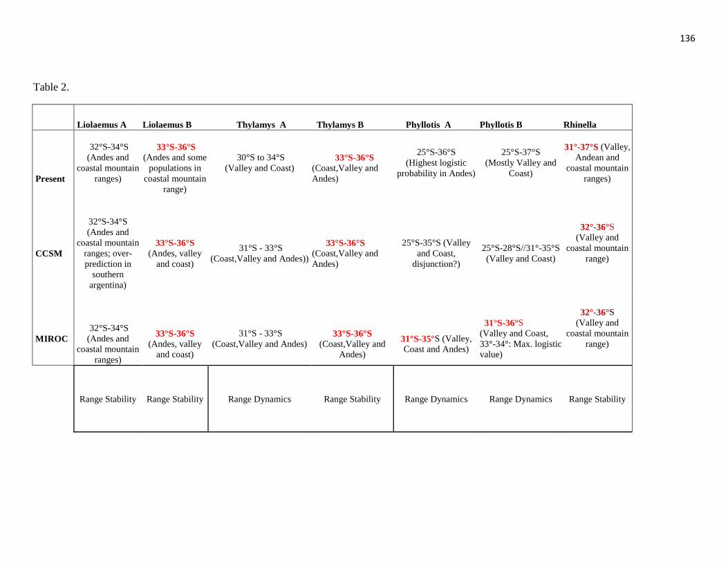
136

Table 2.

Liolaemus A Liolaemus B Thylamys A Thylamys B Phyllotis A Phyllotis B Rhinella

Present

32°S-34°S

(Andes and

coastal mountain

ranges)

33°S-36°S

(Andes and some

populations in

coastal mountain

range)

30°S to 34°S

(Valley and Coast)

33°S-36°S

(Coast,Valley and

Andes)

25°S-36°S

(Highest logistic

probability in Andes)

25°S-37°S

(Mostly Valley and

Coast)

31°-37°S (Valley,

Andean and

coastal mountain

ranges)

CCSM

32°S-34°S

(Andes and

coastal mountain

ranges; over-

prediction in

southern

argentina)

33°S-36°S

(Andes, valley

and coast)

31°S - 33°S

(Coast,Valley and Andes))

33°S-36°S

(Coast,Valley and

Andes)

25°S-35°S (Valley

and Coast,

disjunction?)

25°S-28°S//31°-35°S

(Valley and Coast)

32°-36°S

(Valley and

coastal mountain

range)

MIROC

32°S-34°S

(Andes and

coastal mountain

ranges)

33°S-36°S

(Andes, valley

and coast)

31°S - 33°S

(Coast,Valley and Andes)

33°S-36°S

(Coast,Valley and

Andes)

31°S-35°S (Valley,

Coast and Andes)

31°S-36°S

(Valley and Coast,

33°-34°: Max. logistic

value)

32°-36°S

(Valley and

coastal mountain

range)

Range Stability Range Stability Range Dynamics Range Stability Range Dynamics Range Dynamics Range Stability

137

Fig.1

0.55

0,98

0.94

B

A2

A1

0.01

LT27

Ate51

TrBa20

SA19

SA49

Phm3_7

OS64

Qui52

Ate68

LCh04

OS55

LT28_29_31QPl38

CSI48_49

OS47

TrBa16_21_24

DIV2

LT33

Phm4_5

CR37_41_46

TrBa25

SA17

Paz83_84

TrBa23

CR69

SA12

Pe95

Pe75DIV1

Pe91

RHu68

Qui51_53_57_58_59_60

SA23

TrBa17

OS46

RHu73

LT26

TrBa22

B

A2

A1

1.0

1.0

1.0

1.0

0.98

0.64

0.95

0.99

0.99

0.96

0.76 0.99

B

A2

A1

A)B)

C) D)

138

Fig.2

Liolaemus ThylamysPhyllotis Rhinella

A B A B A B

Present

LGM: CCSM

LGM: MIROC

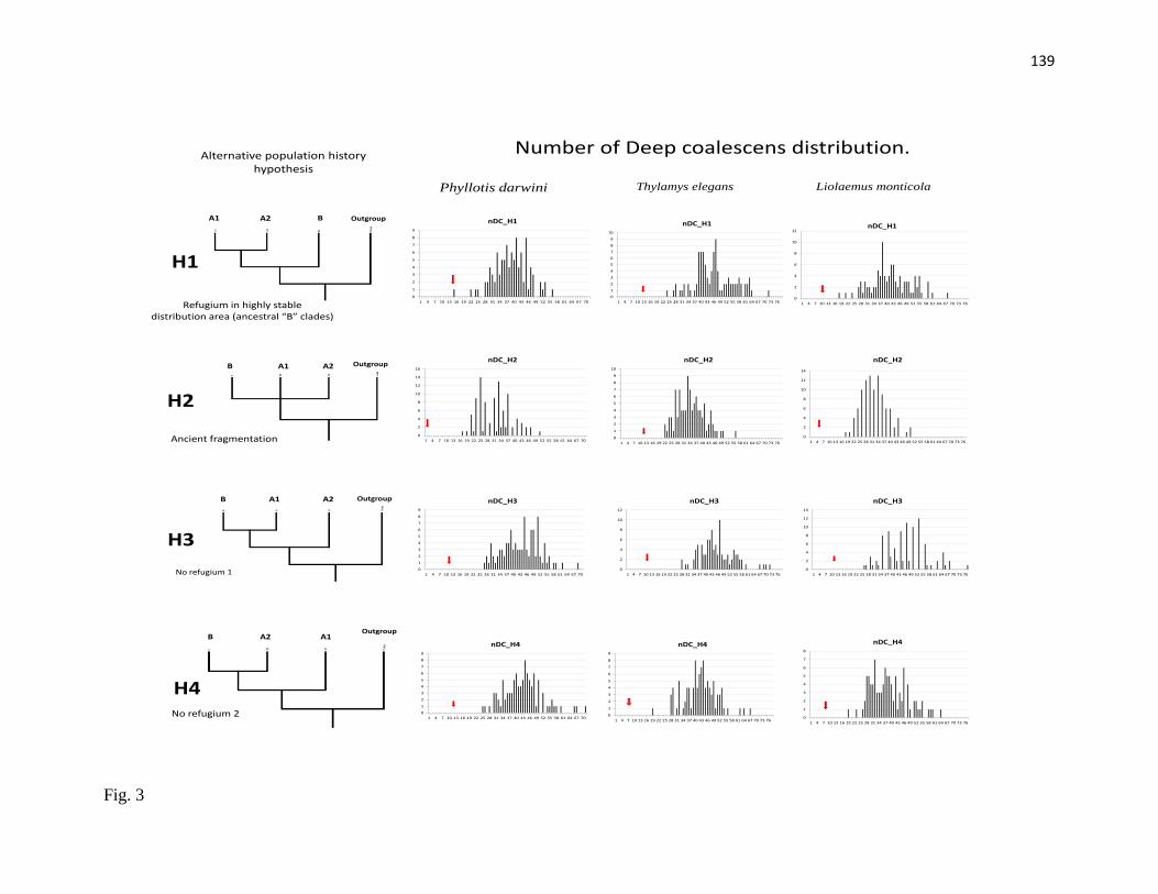
139

Fig. 3

H1

H2

H3

H4

Number of Deep coalescens distribution.Alternative population historyhypothesis

Refugium in highly stabledistribution area (ancestral “B” clades)

Ancient fragmentation

No refugium 1

No refugium 2

Phyllotis darwini

B A1 A2 Outgroup

B A1 A2 Outgroup

A1 A2 B Outgroup

B A2 A1Outgroup

Thylamys elegans Liolaemus monticola

0

1

2

3

4

5

6

7

8

9

1 4 7 10 13 16 19 22 25 28 31 34 37 40 43 46 49 52 55 58 61 64 67 70

nDC_H1

0

2

4

6

8

10

12

14

16

1 4 7 10 13 16 19 22 25 28 31 34 37 40 43 46 49 52 55 58 61 64 67 70

nDC_H2

0

1

2

3

4

5

6

7

8

9

1 4 7 10 13 16 19 22 25 28 31 34 37 40 43 46 49 52 55 58 61 64 67 70

nDC_H3

0

1

2

3

4

5

6

7

8

9

1 4 7 10 13 16 19 22 25 28 31 34 37 40 43 46 49 52 55 58 61 64 67 70

nDC_H4

0

1

2

3

4

5

6

7

8

9

10

1 4 7 10 13 16 19 22 25 28 31 34 37 40 43 46 49 52 55 58 61 64 67 70 73 76

nDC_H1

0

1

2

3

4

5

6

7

8

9

10

1 4 7 10 13 16 19 22 25 28 31 34 37 40 43 46 49 52 55 58 61 64 67 70 73 76

nDC_H2

0

2

4

6

8

10

12

1 4 7 10 13 16 19 22 25 28 31 34 37 40 43 46 49 52 55 58 61 64 67 70 73 76

nDC_H3

0

1

2

3

4

5

6

7

8

9

1 4 7 10 13 16 19 22 25 28 31 34 37 40 43 46 49 52 55 58 61 64 67 70 73 76

nDC_H4

0

2

4

6

8

10

12

1 4 7 10 13 16 19 22 25 28 31 34 37 40 43 46 49 52 55 58 61 64 67 70 73 76

nDC_H1

0

2

4

6

8

10

12

14

1 4 7 10 13 16 19 22 25 28 31 34 37 40 43 46 49 52 55 58 61 64 67 70 73 76

nDC_H2

0

2

4

6

8

10

12

14

1 4 7 10 13 16 19 22 25 28 31 34 37 40 43 46 49 52 55 58 61 64 67 70 73 76

nDC_H3

0

1

2

3

4

5

6

7

8

1 4 7 10 13 16 19 22 25 28 31 34 37 40 43 46 49 52 55 58 61 64 67 70 73 76

nDC_H4

140

Fig. 4

141

Conclusiones Generales

Uno de los patrones más llamativos reportados en este trabajo es la particular distribución

de los linajes intraespecíficos en el roedor Phyllotis darwini; el rasgo más característico de

dicho patrón es la presencia de segregación altitudinal estricta entre ambos linajes, con uno

de ellos distribuido en poblaciones disyuntas a lo largo de los Andes y Cordillera de la

Costa siempre sobre los 1500 m, con la excepción de una localidad costera en la porción

más septentrional de su rango. Considerando solamente la genealogía e información de la

distribución actual de la especie este patrón resulta muy difícil de explicar, pero al modelar

la distribución pasada de los linajes fue posible observar que frente a la configuración

climática del LGM, la distribución montañosa del linaje de altura no era posible, y ambos

linajes se encontraban aparentemente codistribuídos en el sur de la distribución presente, y

principalmente en el valle y Cordillera de la Costa. Esta observación permitió hipotetizar

que la distribución de los linajes en el presente, altitudinalmente segregada a través de toda

la extensión latitudinal de la especie, es consecuencia de un mecanismo de recolonización

post-glacial diferencial, con un linaje que expande su rango de distribución a través de

ambos cordones montañosos, mientras que el segundo se distribuye predominantemente en

el valle. En consecuencia, bajo el supuesto de conservación de nicho desde el LGM hasta el

presente, debemos asumir que el nicho realizado del linaje distribuído sobre 1500 m en el

presente, no le permitía alcanzar esa altitud en condiciones de temperaturas más bajas y

precipitación incrementada, y que en la configuración climática presente no solo es capaz

de estar distribuido en los cordones montañosos, sino que no se distribuye en casi ninguna

localidad bajo este límite altitudinal; esta segregación distribucional entre ambos linajes

aparece solo cuando el umbral de temperatura mínima se relaja, sugiriendo fuertemente que

la divergencia intraespecífica de nicho ejerce algún efecto sobre la posibilidad de

coexistencia de los linajes en diferentes configuraciones climáticas. En el segundo capítulo

se exploró estas conclusiones preliminares sobre las dinámicas de rango de distribución de

vertebrados en la última transición glacial/interglacial, esta vez con mayor resolución

geográfica y añadiendo un segundo taxón (Abrothrix olivaceus). La principal conclusión de

este capítulo es que el patrón de mezcla de haplotipos de ambos cordones cordilleranos al

interior de los linajes de mamíferos es consistente con la hipótesis de desplazamientos de

142

rango de distribución de vertebrados análogos a los bien conocidos movimientos de

cinturones vegetacionales desde los Andes hacia la costa durante el LGM. La única

excepción observada a este patrón es un único linaje estrictamente andino en A. olivaceus,

que está restringido a los Andes en el presente y es además el único de los linajes de

mamíferos analizados que, de acuerdo al modelo de distribución en el LGM, no habría sido

capaz de colonizar el valle durante ese evento, permaneciendo restringido a los faldeos

cordilleranos. En conjunto, la evidencia sugiere fuertemente que el patrón de mezcla de

haplotipos en la mayoría de los linajes (de ambos cordones montañosos) se debe a repetidas

expansiones y contracciones del rango de distribución (del tipo de la descrita en el capítulo

1), a través de varias oscilaciones glacial/interglacial; es posible hipotetizar en

consecuencia que la repetición de este fenómeno durante el Pleistoceno podría explicar en

parte la diferenciación intraespecífica y la presente distribución geográfica de dichos

linajes.

El tercer capítulo es un intento de encontrar un mecanismo biogeográfico más general para

los vertebrados de la región, utilizando una aproximación comparada y multi-taxa. Sobre la

base de información genealógica y modelos de distribución pasada y presente se formuló

varios escenarios biogeográficos alternativos, en donde la hipótesis de interés es que los

haplotipos ancestrales están asociados a un área de distribución persistente para todos los

linajes de vertebrados analizados; esta zona se detectó entre los 26°S-36°S. La idea detrás

de esta hipótesis es que, dado que se identificó una zona de distribución persistente para

todos los linajes de vertebrados analizados, es razonable pensar que si el área de

codistribución fue similar a través de las repetidas transiciones glacial/interglacial, entonces

los haplotipos mas ancestrales de cada especie tendrán una alta probabilidad de permanecer

distribuídos en dicha área hasta el presente; al mismo tiempo aquellas poblaciones que

expandieron su distribución durante los períodos interglaciales debiesen haber sido más

susceptibles a diversificación que aquellas asociadas aún a la zona de distribución

persistente. La consecuencia de este proceso hipotético sería que todas las especies de

vertebrados endémicos de Chile mediterráneo debiesen reflejar en algún grado esta

dinámica en su estructura filogenética intraespecífica. Dicho de otro modo, existiría una

topología general, en donde los filogrupos más ancestrales son aquellos asociados a la zona

de persistencia, tanto en períodos glaciales como interglaciales, mientras que los filogrupos

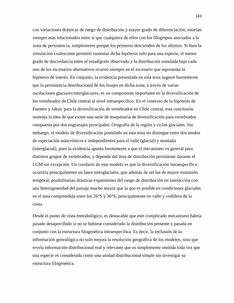
143

con variaciones drásticas de rango de distribución y mayor grado de diferenciación, estarían

siempre más relacionados entre sí que cualquiera de ellos con los filogrupos asociados a la

zona de persistencia, simplemente porque los primeros descienden de los últimos. Si bien la

simulación coalescente permitió sustentar dicha hipótesis solo para una especie, el menor

grado de discordancia entre el estadígrafo observado y la distribución simulada bajo cada

uno de los escenarios alternativos ocurrió siempre en el escenario que representa la

hipótesis de interés. En conjunto, la evidencia presentada en esta tesis sugiere fuertemente

que la persistencia distribucional de los linajes en dicha zona, a través de varias

oscilaciones glaciares/interglaciares, es un componente importante en la diversificación de

los vertebrados de Chile central al nivel intraespecífico. En el contexto de la hipótesis de

Fuentes y Jaksic para la diversificación de vertebrados en Chile central, esta conclusión

sustenta la idea de que existe una serie de maquinaria de diversificación para vertebrados

compuesta por dos engranajes principales: Orografía de la región y ciclos glaciales. Sin

embargo, el modelo de diversificación postulado en esta tesis no distingue entre dos modos

de especiación asincrónicos e independientes para el valle (glacial) y montaña

(interglacial), pues la evidencia apunta fuertemente a que el mecanismo es general para

distintos grupos de vertebrados, y depende del área de distribución persistente durante el

LGM sin excepción. Un corolario de este modelo es que la diversificación intraespecífica

ocurriría principalmente en fases interglaciales, que además de ser las de mayor extensión

temporal, posibilitarían drásticas expansiones del rango de distribución en interacción con

una heterogeneidad del paisaje mucho mayor que la que es posible en condiciones glaciales

en el área comprendida entre los 26°S y 36°S, principalmente en valle y codillera de la

costa.

Desde el punto de vista metodológico, es destacable que este complicado mecanismo habría

pasado desapercibido si no se hubiese considerado la distribución presente y pasada en

conjunto con la estructura filogenética intraespecífica. Es decir, la inclusión de la

información genealógica no solo mejora la resolución geográfica de los modelos, sino que

revela información distribucional real y relevante que es simplemente omitida toda vez que

una especie es considerada como una unidad distribucional simple sin investigar su

estructura filogenética.

144

Los vertebrados terrestres de Chile mediterráneo son un grupo que alberga una cantidad

importante de diversidad críptica intraespecífica. La identificación de estos linajes y su

historia biogeográfica no es un mero ejercicio teórico sino una necesidad real en el contexto

de la planificación de la conservación biológica en Chile. Por ejemplo, con los resultados

precedentes, es posible afirmar que los cordones montañosos del hotspot de Chile central

son importantes corredores biológicos en condiciones interglaciales. Una estrategia

razonada de conservación debiese por lo tanto priorizar la creación de numerosas reservas

de pequeña área pero alta conectividad a lo largo de los Andes y en los puntos en donde el

valle es más estrecho y la separación entre ambas cordilleras es mínima. Por otro lado,

existe suficiente evidencia que señala que el área entre los 33°S-36°S constituye un

importante centro de distribución persistente de linajes de vertebrados a través de

oscilaciones climáticas de gran escala, al menos desde el LGM hasta el presente, y muy

probablemente a través de varias transiciones glacial/interglacial durante el Pleistoceno. Se

debiese por tanto priorizar la presencia de áreas protegidas de gran extensión a lo largo de

la Cordillera de la Costa en dicho segmento latitudinal.

Finalmente, la evidencia expuesta permite proponer la discusión sobre la importancia de la

estructura filogenética en el contexto de las dinámicas de rango de distribución de las

especies; en consecuencia se propone la siguiente tesis:

Las especies con estructura filogenética intraespecífica a menudo presentan un mosaico

de respuestas distribucionales independientes, en donde cada linaje genealógico posee

dinámicas de distribución que son independientes de las variaciones en la distribución de

otros linajes de la misma especie, y frente a los mismos forzamientos climáticos.

145

Apéndices

Capítulo I

APPENDIX I.- List of individuals by catalog number, species, locality, initials, geographic

coordinates and GeneBank accession number.

Catalogue

Number

Species Locality Initial

s

Latitude

(S)

Longitude

(W)

Genebank accesion

number

NK 106069 Phyllotis

darwini

Cerro el Roble, Til-Til CR69 32°59´24´

´

71°1´12´´ JN226723

NK 106137 Phyllotis

darwini

Cerro el Roble, Til-Til CR37 32°59´24´

´

71°1´12´´ JN226724

NK 106141 Phyllotis

darwini

Cerro el Roble, Til-Til CR41 32°59´24´

´

71°1´12´´ JN226725

NK 106146 Phyllotis

darwini

Cerro el Roble, Til-Til CR46 32°59´24´

´

71°1´12´´ JN226726

NK 105341 Phyllotis

darwini

Cerro Santa Inés, Los Vilos CSI41 32°9´0´´ 71°28´48´´ JN226718

NK 105348 Phyllotis

darwini

Cerro Santa Inés, Los Vilos CSI48 32°9´0´´ 71°28´48´´ JN226719

NK 105349 Phyllotis

darwini

Cerro Santa Inés, Los Vilos CSI49 32°9´0´´ 71°28´48´´ JN226720

NK 95618 Phyllotis

darwini

Chillepín CH18 31°52’48´

´

70°47´24´´ JN226690

NK 95620 Phyllotis

darwini

Chillepín CH20 31°52’48´

´

70°47´24´´ JN226691

NK 95624 Phyllotis

darwini

Chillepín CH24 31°52’48´

´

70°47´24´´ JN226692

NK 120051 Phyllotis

darwini

Concepción, Tomé Agua

Tendida

Ate51 36°38´24´

´

72°47´24´´ JN226727

NK 120068 Phyllotis

darwini

Concepción, Tomé Agua

Tendida

Ate68 36°38´24´

´

72°47´24´´ JN226728

ER3 Phyllotis

magister

Desembocadura Río Loa Phm3 21°25´33´

´

70°33´36´´ JN226732

146

ER4 Phyllotis

magister

Desembocadura Río Loa Phm4 21°25´33´

´

70°33´36´´ JN226733

ER5 Phyllotis

magister

Desembocadura Río Loa Phm5 21°25´33´

´

70°33´36´´ JN226734

ER7 Phyllotis

magister

Desembocadura Río Loa Phm7 21°25´33´

´

70°33´36´´ JN226735

SSUC-Ma-

00451

Phyllotis

darwini

El Guanaco, Quirihue, Ñuble QUI5

1

36°24´0´´ 72°37´30´´ JN226683

SSUC-Ma-

00452

Phyllotis

darwini

El Guanaco, Quirihue, Ñuble QUI5

2

36°24´0´´ 72°37´30´´ JN226684

SSUC-Ma-

00453

Phyllotis

darwini

El Guanaco, Quirihue, Ñuble QUI5

3

36°24´0´´ 72°37´30´´ JN226685

SSUC-Ma-

00457

Phyllotis

darwini

El Guanaco, Quirihue, Ñuble QUI5

7

36°24´0´´ 72°37´30´´ JN226686

SSUC-Ma-

00458

Phyllotis

darwini

El Guanaco, Quirihue, Ñuble QUI5

8

36°24´0´´ 72°37´30´´ JN226687

SSUC-Ma-

00459

Phyllotis

darwini

El Guanaco, Quirihue, Ñuble QUI5

9

36°24´0´´ 72°37´30´´ JN226688

SSUC-Ma-

00460

Phyllotis

darwini

El Guanaco, Quirihue, Ñuble QUI6

0

36°24´0´´ 72°37´30´´ JN226689

NK 96868 Phyllotis

darwini

Fray Jorge FJ68 30°40´12´

´

71°37´48´´ JN226713

NK 96869 Phyllotis

darwini

Fray Jorge FJ69 30°40´12´

´

71°37´48´´ JN226714

NK 96871 Phyllotis

darwini

Fray Jorge FJ71 30°40´12´

´

71°37´48´´ JN226715

NK 96874 Phyllotis

darwini

Fray Jorge FJ74 30°40´12´

´

71°37´48´´ JN226716

NK 105515 Phyllotis

darwini

Fray Jorge FJ15 30°40´12´

´

71°37´48´´ JN226722

SSUC-Ma-

00426

Phyllotis

darwini

Las Tacas LT26 30°0´0´´ 71°22´26´´ JN226672

SSUC-Ma-

00427

Phyllotis

darwini

Las Tacas LT27 30°0´0´´ 71°22´26´´ JN226673

SSUC-Ma- Phyllotis Las Tacas LT28 30°0´0´´ 71°22´26´´ JN226674

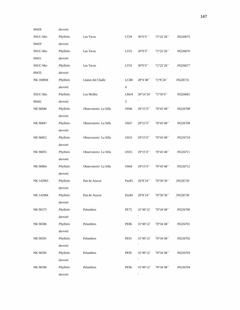
147

00428 darwini

SSUC-Ma-

00429

Phyllotis

darwini

Las Tacas LT29 30°0´0´´ 71°22´26´´ JN226675

SSUC-Ma-

00431

Phyllotis

darwini

Las Tacas LT31 30°0´0´´ 71°22´26´´ JN226676

SSUC-Ma-

00433

Phyllotis

darwini

Las Tacas LT33 30°0´0´´ 71°22´26´´ JN226677

NK 160004 Phyllotis

darwini

Llanos del Challe LCH0

4

28°4´48´´ 71°8´24´´ JN226731

SSUC-Ma-

00442

Phyllotis

darwini

Los Molles LMo4

2

30°14´24´

´

71°30´0´´ JN226681

NK 96846 Phyllotis

darwini

Observatorio La Silla OS46 29°15´0´´ 70°43´48´´ JN226708

NK 96847 Phyllotis

darwini

Observatorio La Silla OS47 29°15´0´´ 70°43´48´´ JN226709

NK 96852 Phyllotis

darwini

Observatorio La Silla OS52 29°15´0´´ 70°43´48´´ JN226710

NK 96855 Phyllotis

darwini

Observatorio La Silla OS55 29°15´0´´ 70°43´48´´ JN226711

NK 96864 Phyllotis

darwini

Observatorio La Silla OS64 29°15´0´´ 70°43´48´´ JN226712

NK 142983 Phyllotis

darwini

Pan de Azucar Paz83 26°8´24´´ 70°39´36´´ JN226729

NK 142984 Phyllotis

darwini

Pan de Azucar Paz84 26°8´24´´ 70°39´36´´ JN226730

NK 96575 Phyllotis

darwini

Pelambres PE75 31°49´12´

´

70°34´48´´ JN226700

NK 96586 Phyllotis

darwini

Pelambres PE86 31°49´12´

´

70°34´48´´ JN226701

NK 96591 Phyllotis

darwini

Pelambres PE91 31°49´12´

´

70°34´48´´ JN226702

NK 96595 Phyllotis

darwini

Pelambres PE95 31°49´12´

´

70°34´48´´ JN226703

NK 96596 Phyllotis

darwini

Pelambres PE96 31°49´12´

´

70°34´48´´ JN226704

148

NK 105381 Phyllotis

darwini

Llanos del Challe LCH8

1

28°4´48´´ 71°8´24´´ JN226721

SSUC-Ma-

00435

Phyllotis

darwini

Punta de Choros PCh35 29°15´0´´ 71°27´36´´ JN226678

SSUC-Ma-

00437

Phyllotis

darwini

Punta de Choros PCh37 29°15´0´´ 71°27´36´´ JN226679

SSUC-Ma-

00445

Phyllotis

darwini

Punta de Choros PCh45 29°15´0´´ 71°27´36´´ JN226682

SSUC-Ma-

00438

Phyllotis

darwini

Quebrada de la Plata PCh38 29°15´0´´ 71°27´36´´ JN226680

NK 96738 Phyllotis

darwini

Quebrada del Tigre QT38 32°33´36´

´

71°25´48´´ JN226705

NK 96754 Phyllotis

darwini

Quebrada del Tigre QT54 32°33´36´

´

71°25´48´´ JN226706

NK 95968 Phyllotis

darwini

Rinconada Huechún RHU6

8

33°0´36´´ 70°48´36´´ JN226693

NK 95973 Phyllotis

darwini

Rinconada Huechún RHU7

3

33°0´36´´ 70°48´36´´ JN226694

NK 96312 Phyllotis

darwini

San Carlos Apoquindo SA12 33°24´0´´ 70°28´48´´ JN226695

NK 96319 Phyllotis

darwini

San Carlos Apoquindo SA19 33°24´0´´ 70°28´48´´ JN226696

NK 96323 Phyllotis

darwini

San Carlos Apoquindo SA23 33°24´0´´ 70°28´48´´ JN226697

NK 96349 Phyllotis

darwini

San Carlos Apoquindo SA49 33°24´0´´ 70°28´48´´ JN226698

NK 96359 Phyllotis

darwini

San Carlos Apoquindo SA59 33°24´0´´ 70°28´48´´ JN226699

NK 96817 Phyllotis

darwini

San Carlos Apoquindo SA17 33°24´0´´ 70°28´48´´ JN226707

NK 105329 Phyllotis

darwini

San Carlos Apoquindo SA29 33°24´0´´ 70°28´48´´ JN226717

SSUC-Ma-

00416

Phyllotis

darwini

Tranque de relaves Barahona TrBa1

6

34°4´51´´ 70°31´12´´ JN226664

SSUC-Ma- Phyllotis Tranque de relaves Barahona TrBa1 34°4´51´´ 70°31´12´´ JN226665

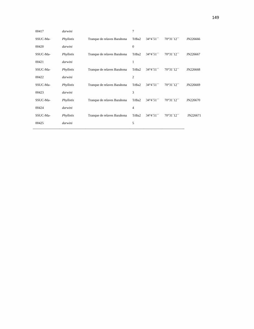
149

00417 darwini 7

SSUC-Ma-

00420

Phyllotis

darwini

Tranque de relaves Barahona TrBa2

0

34°4´51´´ 70°31´12´´ JN226666

SSUC-Ma-

00421

Phyllotis

darwini

Tranque de relaves Barahona TrBa2

1

34°4´51´´ 70°31´12´´ JN226667

SSUC-Ma-

00422

Phyllotis

darwini

Tranque de relaves Barahona TrBa2

2

34°4´51´´ 70°31´12´´ JN226668

SSUC-Ma-

00423

Phyllotis

darwini

Tranque de relaves Barahona TrBa2

3

34°4´51´´ 70°31´12´´ JN226669

SSUC-Ma-

00424

Phyllotis

darwini

Tranque de relaves Barahona TrBa2

4

34°4´51´´ 70°31´12´´ JN226670

SSUC-Ma-

00425

Phyllotis

darwini

Tranque de relaves Barahona TrBa2

5

34°4´51´´ 70°31´12´´ JN226671

150

APPENDIX II .- List of haplotypes with the number of individuals by locality that shares each haplotype. The proportion of haplotypes

by locality, the sample haplotype frequency and the proportional weighted frequency are listed.

Localities

Haplotype

Agua

Tendida

Cerro el

Roble

Cerro Santa

Inés

Chillepí

n

Fray

Jorge

Las

Tacas

Llanos de

Challe

Los

Molles

Obs. La

Silla

PN Pan de

Azúcar

Pelambr

es

TrBa16_21_24 0 0 0 0 0 0 0 0 0 0 0

TrBa17 0 0 0 0 0 0 0 0 0 0 0

TrBa20 0 0 0 0 0 0 0 0 0 0 0

TrBa22 0 0 0 0 0 0 0 0 0 0 0

TrBa23 0 0 0 0 0 0 0 0 0 0 0

TrBa25 0 0 0 0 0 0 0 0 0 0 0

LT26 0 0 0 0 0 1 0 0 0 0 0

LT27 0 0 0 0 0 1 0 0 0 0 0

LT28_29_31QPl38 0 0 0 0 0 3 0 0 0 0 0

LT33 0 0 0 0 0 1 0 0 0 0 0

DIV1 0 0 0 2 4 0 1 1 1 0 2

Qui51_53_57_58_59_60 0 0 0 0 0 0 0 0 0 0 0

Qui52 0 0 0 0 0 0 0 0 0 0 0

DIV2 0 0 1 1 1 0 0 0 0 0 0

RHu68 0 0 0 0 0 0 0 0 0 0 0

RHu73 0 0 0 0 0 0 0 0 0 0 0

SA12 0 0 0 0 0 0 0 0 0 0 0

151

SA19 0 0 0 0 0 0 0 0 0 0 0

SA23 0 0 0 0 0 0 0 0 0 0 0

SA49 0 0 0 0 0 0 0 0 0 0 0

PE75 0 0 0 0 0 0 0 0 0 0 1

PE91 0 0 0 0 0 0 0 0 0 0 1

PE95 0 0 0 0 0 0 0 0 0 0 1

SA17 0 0 0 0 0 0 0 0 0 0 0

OS46 0 0 0 0 0 0 0 0 1 0 0

OS47 0 0 0 0 0 0 0 0 1 0 0

OS55 0 0 0 0 0 0 0 0 1 0 0

OS64 0 0 0 0 0 0 0 0 1 0 0

CSI48_49 0 0 2 0 0 0 0 0 0 0 0

CR69 0 1 0 0 0 0 0 0 0 0 0

CR37_41_46 0 3 0 0 0 0 0 0 0 0 0

Ate51 1 0 0 0 0 0 0 0 0 0 0

Ate68 1 0 0 0 0 0 0 0 0 0 0

Paz83_84 0 0 0 0 0 0 0 0 0 2 0

LCh04 0 0 0 0 0 0 1 0 0 0 0

TOTAL 2 4 3 3 5 6 2 1 5 2 5

Proportion from the total of haplotypes by

locality 0.0294118 0.0588235 0.0441176

0.044117

6 0.0735294

0.0882

33 0.0294118

0.014705

9

0.073529

4 0.0294118

0.073529

4

APPENDIX II (CONTINUE).

152

Localiti

es

Haplotype

Punta de

Choros

Quebrada de

la plata

Quebada

del Tigre

Quiri

hue

Rinconada

Huechún

San Carlos de

Apoquindo

Tranque de

relaves Barahona

Total individuals

by haplotype

Frequ

ency

Weigthened

frequency

TrBa16_21_24 0 0 0 0 0 0 3 3

0.0441

176 0.0051903

TrBa17 0 0 0 0 0 0 1 1

0.0147

059 0.0017301

TrBa20 0 0 0 0 0 0 1 1

0.0147

059 0.0017301

TrBa22 0 0 0 0 0 0 1 1

0.0147

059 0.0017301

TrBa23 0 0 0 0 0 0 1 1

0.0147

059 0.0017301

TrBa25 0 0 0 0 0 0 1 1

0.0147

059 0.0017301

LT26 0 0 0 0 0 0 0 1

0.0147

059 0.0012976

LT27 0 0 0 0 0 0 0 1

0.0147

059 0.0012976

LT28_29_31QPl38 0 1 0 0 0 0 0 4

0.0588

235 0.0060554

LT33 0 0 0 0 0 0 0 1 0.0147 0.0012976

153

059

DIV1 3 0 2 0 0 0 0 16

0.2352

941 0.0934256

Qui51_53_57_58_59_60 0 0 0 6 0 0 0 6

0.0882

353 0.009083

Qui52 0 0 0 1 0 0 0 1

0.0147

059 0.0015138

DIV2 0 0 0 0 0 2 0 5

0.0735

294 0.0194637

RHu68 0 0 0 0 1 0 0 1

0.0147

059 0.0004325

RHu73 0 0 0 0 1 0 0 1

0.0147

059 0.0004325

SA12 0 0 0 0 0 1 0 1

0.0147

059 0.0015138

SA19 0 0 0 0 0 1 0 1

0.0147

059 0.0015138

SA23 0 0 0 0 0 1 0 1

0.0147

059 0.0015138

SA49 0 0 0 0 0 1 0 1

0.0147

059 0.0015138

PE75 0 0 0 0 0 0 0 1

0.0147

059 0.0010813

PE91 0 0 0 0 0 0 0 1 0.0147 0.0010813

154

059

PE95 0 0 0 0 0 0 0 1

0.0147

059 0.0010813

SA17 0 0 0 0 0 1 0 1

0.0147

059 0.0015138

OS46 0 0 0 0 0 0 0 1

0.0147

059 0.0010813

OS47 0 0 0 0 0 0 0 1

0.0147

059 0.0010813

OS55 0 0 0 0 0 0 0 1

0.0147

059 0.0010813

OS64 0 0 0 0 0 0 0 1

0.0147

059 0.0010813

CSI48_49 0 0 0 0 0 0 0 2

0.0294

118 0.0012976

CR69 0 0 0 0 0 0 0 1

0.0147

059 0.0008651

CR37_41_46 0 0 0 0 0 0 0 3

0.0441

176 0.0025952

Ate51 0 0 0 0 0 0 0 1

0.0147

059 0.0004325

Ate68 0 0 0 0 0 0 0 1

0.0147

059 0.0004325

Paz83_84 0 0 0 0 0 0 0 2 0.0294 0.0008651

155

118

LCh04 0 0 0 0 0 0 0 1

0.0147

059 0.0004325

TOTAL 3 1 2 7 2 7 8 68 1

Proportion from the total of

haplotypes by locality 0.0441176 0.0147059 0.0294118

0.1029

412 0.0294118 0.1029412 0.1176471

156

Capítulo II

APPENDIX I.- List of individuals by catalog number, species, locality, initials, geographic coordinates and GeneBank accession

number.

Species Catalogue Number Locality Initials Latitude (S) Longitude (W) Genebank accesion number

Abrothrix olivaceus NK95341 San Carlos de Apoquindo NK95341SCApoq 33˚ 24' 13" 70˚ 29' 01" Pending

Abrothrix olivaceus NK95549 San Carlos de Apoquindo NK95549SCApoq 33˚ 24' 13" 70˚ 29' 01" Pending

Abrothrix olivaceus NK95671 San Carlos de Apoquindo NK95671SCApoq 33˚ 24' 13" 70˚ 29' 01" Pending

Abrothrix olivaceus NK95672 San Carlos de Apoquindo NK95672SCApoq 33˚ 24' 13" 70˚ 29' 01" Pending

Abrothrix olivaceus NK95720 San Carlos de Apoquindo NK95720SCApoq 33˚ 24' 13" 70˚ 29' 01" Pending

Abrothrix olivaceus NK95812 San Carlos de Apoquindo NK95812SCApoq 33˚ 24' 13" 70˚ 29' 01" Pending

Abrothrix olivaceus NK96309 San Carlos de Apoquindo NK96309SCApoq 33˚ 24' 13" 70˚ 29' 01" Pending

Abrothrix olivaceus NK96348 San Carlos de Apoquindo NK96348SCApoq 33˚ 24' 13" 70˚ 29' 01" Pending

Abrothrix olivaceus NK104631 San Carlos de Apoquindo NK104631SCApoq 33˚ 24' 13" 70˚ 29' 01" Pending

Abrothrix olivaceus NK105427 San Carlos de Apoquindo NK105427SCApoq 33˚ 24' 13" 70˚ 29' 01" Pending

Abrothrix olivaceus NK106136 El Roble NK106136ElRoble 32˚ 58' 34" 71˚ 00' 50" Pending

Abrothrix olivaceus NK106138 El Roble NK106138ElRoble 32˚ 58' 34" 71˚ 00' 50" Pending

Abrothrix olivaceus NK106142 El Roble NK106142ElRoble 32˚ 58' 34" 71˚ 00' 50" Pending

Abrothrix olivaceus NK106143 El Roble NK106143ElRoble 32˚ 58' 34" 71˚ 00' 50" Pending

Abrothrix olivaceus NK106144 El Roble NK106144ElRoble 32˚ 58' 34" 71˚ 00' 50" Pending

Abrothrix olivaceus NK106145 El Roble NK106145ElRoble 32˚ 58' 34" 71˚ 00' 50" Pending

Abrothrix olivaceus NK106147 El Roble NK106147ElRoble 32˚ 58' 34" 71˚ 00' 50" Pending

Abrothrix olivaceus NK106148 El Roble NK106148ElRoble 32˚ 58' 34" 71˚ 00' 50" Pending

Abrothrix olivaceus NK106149 El Roble NK106149ElRoble 32˚ 58' 34" 71˚ 00' 50" Pending

Abrothrix olivaceus EP492 El Roble EP492ElRoble 32˚ 58' 34" 71˚ 00' 50" Pending

Abrothrix olivaceus EP554 El Roble EP554ElRoble 32˚ 58' 34" 71˚ 00' 50" Pending

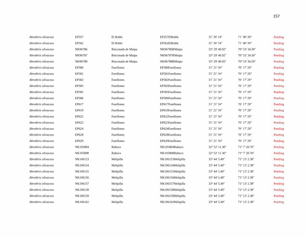
157

Abrothrix olivaceus EP557 El Roble EP557ElRoble 32˚ 58' 34" 71˚ 00' 50" Pending

Abrothrix olivaceus EP562 El Roble EP562ElRoble 32˚ 58' 34" 71˚ 00' 50" Pending

Abrothrix olivaceus NK96786 Rinconada de Maipu NK96786RMaipu 33° 29' 40.92" 70° 53' 34.50" Pending

Abrothrix olivaceus NK96787 Rinconada de Maipu NK96787RMaipu 33° 29' 40.92" 70° 53' 34.50" Pending

Abrothrix olivaceus NK96788 Rinconada de Maipu NK96788RMaipu 33° 29' 40.92" 70° 53' 34.50" Pending

Abrothrix olivaceus EP580 Farellones EP580Farellones 33˚ 21' 36" 70˚ 17' 28" Pending

Abrothrix olivaceus EP581 Farellones EP581Farellones 33˚ 21' 36" 70˚ 17' 28" Pending

Abrothrix olivaceus EP582 Farellones EP582Farellones 33˚ 21' 36" 70˚ 17' 28" Pending

Abrothrix olivaceus EP583 Farellones EP583Farellones 33˚ 21' 36" 70˚ 17' 28" Pending

Abrothrix olivaceus EP585 Farellones EP585Farellones 33˚ 21' 36" 70˚ 17' 28" Pending

Abrothrix olivaceus EP586 Farellones EP586Farellones 33˚ 21' 36" 70˚ 17' 28" Pending

Abrothrix olivaceus EP617 Farellones EP617Farellones 33˚ 21' 36" 70˚ 17' 28" Pending

Abrothrix olivaceus EP619 Farellones EP619Farellones 33˚ 21' 36" 70˚ 17' 28" Pending

Abrothrix olivaceus EP622 Farellones EP622Farellones 33˚ 21' 36" 70˚ 17' 28" Pending

Abrothrix olivaceus EP623 Farellones EP623Farellones 33˚ 21' 36" 70˚ 17' 28" Pending

Abrothrix olivaceus EP624 Farellones EP624Farellones 33˚ 21' 36" 70˚ 17' 28" Pending

Abrothrix olivaceus EP628 Farellones EP628Farellones 33˚ 21' 36" 70˚ 17' 28" Pending

Abrothrix olivaceus EP629 Farellones EP629Farellones 33˚ 21' 36" 70˚ 17' 28" Pending

Abrothrix olivaceus NK105804 Rabuco NK105804Rabuco 32° 52' 11.30" 71° 7' 20.70" Pending

Abrothrix olivaceus NK105808 Rabuco NK105808Rabuco 32° 52' 11.30" 71° 7' 20.70" Pending

Abrothrix olivaceus NK106153 Melipilla NK106153Melipilla 33° 44' 5.49" 71° 13' 2.38" Pending

Abrothrix olivaceus NK106154 Melipilla NK106154Melipilla 33° 44' 5.49" 71° 13' 2.38" Pending

Abrothrix olivaceus NK106155 Melipilla NK106155Melipilla 33° 44' 5.49" 71° 13' 2.38" Pending

Abrothrix olivaceus NK106156 Melipilla NK106156Melipilla 33° 44' 5.49" 71° 13' 2.38" Pending

Abrothrix olivaceus NK106157 Melipilla NK106157Melipilla 33° 44' 5.49" 71° 13' 2.38" Pending

Abrothrix olivaceus NK106158 Melipilla NK106158Melipilla 33° 44' 5.49" 71° 13' 2.38" Pending

Abrothrix olivaceus NK106159 Melipilla NK106159Melipilla 33° 44' 5.49" 71° 13' 2.38" Pending

Abrothrix olivaceus NK106162 Melipilla NK106162Melipilla 33° 44' 5.49" 71° 13' 2.38" Pending

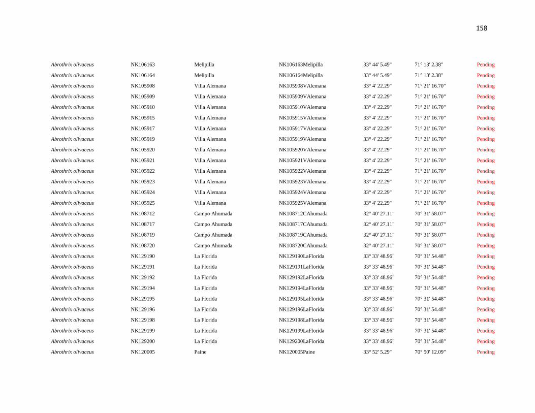
158

Abrothrix olivaceus NK106163 Melipilla NK106163Melipilla 33° 44' 5.49" 71° 13' 2.38" Pending

Abrothrix olivaceus NK106164 Melipilla NK106164Melipilla 33° 44' 5.49" 71° 13' 2.38" Pending

Abrothrix olivaceus NK105908 Villa Alemana NK105908VAlemana 33° 4' 22.29" 71° 21' 16.70" Pending

Abrothrix olivaceus NK105909 Villa Alemana NK105909VAlemana 33° 4' 22.29" 71° 21' 16.70" Pending

Abrothrix olivaceus NK105910 Villa Alemana NK105910VAlemana 33° 4' 22.29" 71° 21' 16.70" Pending

Abrothrix olivaceus NK105915 Villa Alemana NK105915VAlemana 33° 4' 22.29" 71° 21' 16.70" Pending

Abrothrix olivaceus NK105917 Villa Alemana NK105917VAlemana 33° 4' 22.29" 71° 21' 16.70" Pending

Abrothrix olivaceus NK105919 Villa Alemana NK105919VAlemana 33° 4' 22.29" 71° 21' 16.70" Pending

Abrothrix olivaceus NK105920 Villa Alemana NK105920VAlemana 33° 4' 22.29" 71° 21' 16.70" Pending

Abrothrix olivaceus NK105921 Villa Alemana NK105921VAlemana 33° 4' 22.29" 71° 21' 16.70" Pending

Abrothrix olivaceus NK105922 Villa Alemana NK105922VAlemana 33° 4' 22.29" 71° 21' 16.70" Pending

Abrothrix olivaceus NK105923 Villa Alemana NK105923VAlemana 33° 4' 22.29" 71° 21' 16.70" Pending

Abrothrix olivaceus NK105924 Villa Alemana NK105924VAlemana 33° 4' 22.29" 71° 21' 16.70" Pending

Abrothrix olivaceus NK105925 Villa Alemana NK105925VAlemana 33° 4' 22.29" 71° 21' 16.70" Pending

Abrothrix olivaceus NK108712 Campo Ahumada NK108712CAhumada 32° 40' 27.11" 70° 31' 58.07" Pending

Abrothrix olivaceus NK108717 Campo Ahumada NK108717CAhumada 32° 40' 27.11" 70° 31' 58.07" Pending

Abrothrix olivaceus NK108719 Campo Ahumada NK108719CAhumada 32° 40' 27.11" 70° 31' 58.07" Pending

Abrothrix olivaceus NK108720 Campo Ahumada NK108720CAhumada 32° 40' 27.11" 70° 31' 58.07" Pending

Abrothrix olivaceus NK129190 La Florida NK129190LaFlorida 33° 33' 48.96" 70° 31' 54.48" Pending

Abrothrix olivaceus NK129191 La Florida NK129191LaFlorida 33° 33' 48.96" 70° 31' 54.48" Pending

Abrothrix olivaceus NK129192 La Florida NK129192LaFlorida 33° 33' 48.96" 70° 31' 54.48" Pending

Abrothrix olivaceus NK129194 La Florida NK129194LaFlorida 33° 33' 48.96" 70° 31' 54.48" Pending

Abrothrix olivaceus NK129195 La Florida NK129195LaFlorida 33° 33' 48.96" 70° 31' 54.48" Pending

Abrothrix olivaceus NK129196 La Florida NK129196LaFlorida 33° 33' 48.96" 70° 31' 54.48" Pending

Abrothrix olivaceus NK129198 La Florida NK129198LaFlorida 33° 33' 48.96" 70° 31' 54.48" Pending

Abrothrix olivaceus NK129199 La Florida NK129199LaFlorida 33° 33' 48.96" 70° 31' 54.48" Pending

Abrothrix olivaceus NK129200 La Florida NK129200LaFlorida 33° 33' 48.96" 70° 31' 54.48" Pending

Abrothrix olivaceus NK120005 Paine NK120005Paine 33° 52' 5.29" 70° 50' 12.09" Pending

159

Abrothrix olivaceus NK120007 Paine NK120007Paine 33° 52' 5.29" 70° 50' 12.09" Pending

Abrothrix olivaceus NK120008 Paine NK120008Paine 33° 52' 5.29" 70° 50' 12.09" Pending

Abrothrix olivaceus EP410 Quebrada de Tarapacá EP410QTarapaca Outgroup Pending

Abrothrix olivaceus EP413 Quebrada de Tarapacá EP413QTarapaca Outgroup Pending

Abrothrix olivaceus EP435 Quebrada de Camarones EP435QCamarones Outgroup Pending

Abrothrix olivaceus EP438 Quebrada de Camarones EP438QCamarones Outgroup Pending

Phyllotis darwini NK95305 San Carlos de Apoquindo NK95305SCApoq 33˚ 24' 13" 70˚ 29' 01" Pending

Phyllotis darwini NK95336 San Carlos de Apoquindo NK95336SCApoq 33˚ 24' 13" 70˚ 29' 01" Pending

Phyllotis darwini NK96318 San Carlos de Apoquindo NK96318SCApoq 33˚ 24' 13" 70˚ 29' 01" Pending

Phyllotis darwini NK96359 San Carlos de Apoquindo NK96359SCApoq 33˚ 24' 13" 70˚ 29' 01" Pending

Phyllotis darwini NK95531 San Carlos de Apoquindo NK95531SCApoq 33˚ 24' 13" 70˚ 29' 01" Pending

Phyllotis darwini NK95544 San Carlos de Apoquindo NK95544SCApoq 33˚ 24' 13" 70˚ 29' 01" Pending

Phyllotis darwini NK120403 San Carlos de Apoquindo NK120403SCApoq 33˚ 24' 13" 70˚ 29' 01" Pending

Phyllotis darwini NK160855 San Carlos de Apoquindo NK160855SCApoq 33˚ 24' 13" 70˚ 29' 01" Pending

Phyllotis darwini EP493 El Roble EP493ElRoble 32˚ 58' 34" 71˚ 00' 50" Pending

Phyllotis darwini EP544 El Roble EP544ElRoble 32˚ 58' 34" 71˚ 00' 50" Pending

Phyllotis darwini EP546 El Roble EP546ElRoble 32˚ 58' 34" 71˚ 00' 50" Pending

Phyllotis darwini EP548 El Roble EP548ElRoble 32˚ 58' 34" 71˚ 00' 50" Pending

Phyllotis darwini EP553 El Roble EP553ElRoble 32˚ 58' 34" 71˚ 00' 50" Pending

Phyllotis darwini EP558 El Roble EP558ElRoble 32˚ 58' 34" 71˚ 00' 50" Pending

Phyllotis darwini EP560 El Roble EP560ElRoble 32˚ 58' 34" 71˚ 00' 50" Pending

Phyllotis darwini EP566 El Roble EP566ElRoble 32˚ 58' 34" 71˚ 00' 50" Pending

Phyllotis darwini EP567 El Roble EP567ElRoble 32˚ 58' 34" 71˚ 00' 50" Pending

Phyllotis darwini EP569 El Roble EP569ElRoble 32˚ 58' 34" 71˚ 00' 50" Pending

Phyllotis darwini EP571 El Roble EP571ElRoble 32˚ 58' 34" 71˚ 00' 50" Pending

Phyllotis darwini EP575 El Roble EP575ElRoble 32˚ 58' 34" 71˚ 00' 50" Pending

Phyllotis darwini NK106069 El Roble NK106069ElRoble 32˚ 58' 34" 71˚ 00' 50" Pending

Phyllotis darwini NK106137 El Roble NK106137ElRoble 32˚ 58' 34" 71˚ 00' 50" Pending

160

Phyllotis darwini NK106141 El Roble NK106141ElRoble 32˚ 58' 34" 71˚ 00' 50" Pending

Phyllotis darwini NK106146 El Roble NK106146ElRoble 32˚ 58' 34" 71˚ 00' 50" Pending

Phyllotis darwini EP563 Farellones EP563Farellones 33˚ 21' 36" 70˚ 17' 28" Pending

Phyllotis darwini EP587 Farellones EP587Farellones 33˚ 21' 36" 70˚ 17' 28" Pending

Phyllotis darwini EP588 Farellones EP588Farellones 33˚ 21' 36" 70˚ 17' 28" Pending

Phyllotis darwini EP606 Farellones EP606Farellones 33˚ 21' 36" 70˚ 17' 28" Pending

Phyllotis darwini EP614 Farellones EP614Farellones 33˚ 21' 36" 70˚ 17' 28" Pending

Phyllotis darwini EP621 Farellones EP621Farellones 33˚ 21' 36" 70˚ 17' 28" Pending

Phyllotis darwini EP625 Farellones EP625Farellones 33˚ 21' 36" 70˚ 17' 28" Pending

Phyllotis darwini EP626 Farellones EP626Farellones 33˚ 21' 36" 70˚ 17' 28" Pending

Phyllotis darwini EP630 Farellones EP630Farellones 33˚ 21' 36" 70˚ 17' 28" Pending

Phyllotis darwini EP633 Farellones EP633Farellones 33˚ 21' 36" 70˚ 17' 28" Pending

Phyllotis darwini NK108713 Campo Ahumada NK108713CAhumada 32° 40' 27.11" 70° 31' 58.07" Pending

Phyllotis darwini NK108714 Campo Ahumada NK108714CAhumada 32° 40' 27.11" 70° 31' 58.07" Pending

Phyllotis darwini NK108715 Campo Ahumada NK108715CAhumada 32° 40' 27.11" 70° 31' 58.07" Pending

Phyllotis darwini NK108716 Campo Ahumada NK108716CAhumada 32° 40' 27.11" 70° 31' 58.07" Pending

Phyllotis darwini NK108718 Campo Ahumada NK108718CAhumada 32° 40' 27.11" 70° 31' 58.07" Pending

Phyllotis darwini NK108721 Campo Ahumada NK108721CAhumada 32° 40' 27.11" 70° 31' 58.07" Pending

Phyllotis darwini NK108722 Campo Ahumada NK108722CAhumada 32° 40' 27.11" 70° 31' 58.07" Pending

Phyllotis darwini NK108723 Campo Ahumada NK108723CAhumada 32° 40' 27.11" 70° 31' 58.07" Pending

Phyllotis darwini EP539 La Campana EP539LaCampana 32˚ 57' 42" 71˚ 07' 37" Pending

Phyllotis darwini EP540 La Campana EP540LaCampana 32˚ 57' 42" 71˚ 07' 37" Pending

Phyllotis darwini EP542 La Campana EP542LaCampana 32˚ 57' 42" 71˚ 07' 37" Pending

Phyllotis darwini UCK156 Altos de Cantillana UCK156Cantillana 33˚ 55' 40.95" 70˚ 57' 49.9" Pending

Phyllotis darwini UCK157 Altos de Cantillana UCK157Cantillana 33˚ 55' 40.95" 70˚ 57' 49.9" Pending

Phyllotis darwini UCK158 Altos de Cantillana UCK158Cantillana 33˚ 55' 40.95" 70˚ 57' 49.9" Pending

Phyllotis darwini UCK159 Altos de Cantillana UCK159Cantillana 33˚ 55' 40.95" 70˚ 57' 49.9" Pending

Phyllotis darwini UCK160 Altos de Cantillana UCK160Cantillana 33˚ 55' 40.95" 70˚ 57' 49.9" Pending

161

Phyllotis darwini UCK162 Altos de Cantillana UCK162Cantillana 33˚ 55' 40.95" 70˚ 57' 49.9" Pending

Phyllotis darwini UCK163 Altos de Cantillana UCK163Cantillana 33˚ 55' 40.95" 70˚ 57' 49.9" Pending

Phyllotis darwini UCK164 Altos de Cantillana UCK164Cantillana 33˚ 55' 40.95" 70˚ 57' 49.9" Pending

Phyllotis darwini UCK165 Altos de Cantillana UCK165Cantillana 33˚ 55' 40.95" 70˚ 57' 49.9" Pending

Phyllotis darwini UCK166 Altos de Cantillana UCK166Cantillana 33˚ 55' 40.95" 70˚ 57' 49.9" Pending

Phyllotis darwini UCK167 Altos de Cantillana UCK167Cantillana 33˚ 55' 40.95" 70˚ 57' 49.9" Pending

Phyllotis darwini UCK168 Altos de Cantillana UCK168Cantillana 33˚ 55' 40.95" 70˚ 57' 49.9" Pending

Phyllotis darwini UCK177 Altos de Chicauma UCK177Chicauma 33˚ 16' 59" 70˚ 58' 14" Pending

Phyllotis darwini UCK178 Atos de Chicauma UCK178Chicauma 33˚ 16' 59" 70˚ 58' 14" Pending

Phyllotis darwini UCK181 Altos de Chicauma UCK181Chicauma 33˚ 16' 59" 70˚ 58' 14" Pending

Phyllotis darwini UCK183 Altos de Chicauma UCK183Chicauma 33˚ 16' 59" 70˚ 58' 14" Pending

Phyllotis darwini NK108791 El Canelo NK108791Elcanelo 33° 33' 21.89" 70° 27' 15.99" Pending

Phyllotis magister ER4 Desembocadura Rio Loa 4Pmagister Outgroup JN226733

Phyllotis magister ER5

Desembocadura Rio Loa 5Pmagister Outgroup JN226734

162

Capítulo III

APPENDIX I.- List of individuals by catalog number, species, locality, initials, geographic coordinates and GeneBank accession

number.

Species Catalogue Number Locality Initials Latitude (S) Longitude (W) Genebank

accesion number

Phyllotis darwini NK 106069 Cerro el Roble, Til-Til CR69 32°59´24´´ 71°1´12´´ JN226723

Phyllotis darwini NK 106137 Cerro el Roble, Til-Til CR37 32°59´24´´ 71°1´12´´ JN226724

Phyllotis darwini NK 106141 Cerro el Roble, Til-Til CR41 32°59´24´´ 71°1´12´´ JN226725

Phyllotis darwini NK 106146 Cerro el Roble, Til-Til CR46 32°59´24´´ 71°1´12´´ JN226726

Phyllotis darwini NK 105341 Cerro Santa Inés, Los Vilos CSI41 32°9´0´´ 71°28´48´´ JN226718

Phyllotis darwini NK 105348 Cerro Santa Inés, Los Vilos CSI48 32°9´0´´ 71°28´48´´ JN226719

Phyllotis darwini NK 105349 Cerro Santa Inés, Los Vilos CSI49 32°9´0´´ 71°28´48´´ JN226720

Phyllotis darwini NK 95618 Chillepín CH18 31°52’48´´ 70°47´24´´ JN226690

Phyllotis darwini NK 95620 Chillepín CH20 31°52’48´´ 70°47´24´´ JN226691

Phyllotis darwini NK 95624 Chillepín CH24 31°52’48´´ 70°47´24´´ JN226692

Phyllotis darwini NK 120051 Concepción, Tomé Agua Tendida Ate51 36°38´24´´ 72°47´24´´ JN226727

Phyllotis darwini NK 120068 Concepción, Tomé Agua Tendida Ate68 36°38´24´´ 72°47´24´´ JN226728

Phyllotis magister ER3 Desembocadura Río Loa Phm3 21°25´33´´ 70°33´36´´ JN226732

Phyllotis magister ER4 Desembocadura Río Loa Phm4 21°25´33´´ 70°33´36´´ JN226733

Phyllotis magister ER5 Desembocadura Río Loa Phm5 21°25´33´´ 70°33´36´´ JN226734

Phyllotis magister ER7 Desembocadura Río Loa Phm7 21°25´33´´ 70°33´36´´ JN226735

Phyllotis darwini SSUC-Ma-00451 El Guanaco, Quirihue, Ñuble QUI51 36°24´0´´ 72°37´30´´ JN226683

Phyllotis darwini SSUC-Ma-00452 El Guanaco, Quirihue, Ñuble QUI52 36°24´0´´ 72°37´30´´ JN226684

Phyllotis darwini SSUC-Ma-00453 El Guanaco, Quirihue, Ñuble QUI53 36°24´0´´ 72°37´30´´ JN226685

Phyllotis darwini SSUC-Ma-00457 El Guanaco, Quirihue, Ñuble QUI57 36°24´0´´ 72°37´30´´ JN226686

Phyllotis darwini SSUC-Ma-00458 El Guanaco, Quirihue, Ñuble QUI58 36°24´0´´ 72°37´30´´ JN226687

163

Phyllotis darwini SSUC-Ma-00459 El Guanaco, Quirihue, Ñuble QUI59 36°24´0´´ 72°37´30´´ JN226688

Phyllotis darwini SSUC-Ma-00460 El Guanaco, Quirihue, Ñuble QUI60 36°24´0´´ 72°37´30´´ JN226689

Phyllotis darwini NK 96868 Fray Jorge FJ68 30°40´12´´ 71°37´48´´ JN226713

Phyllotis darwini NK 96869 Fray Jorge FJ69 30°40´12´´ 71°37´48´´ JN226714

Phyllotis darwini NK 96871 Fray Jorge FJ71 30°40´12´´ 71°37´48´´ JN226715

Phyllotis darwini NK 96874 Fray Jorge FJ74 30°40´12´´ 71°37´48´´ JN226716

Phyllotis darwini NK 105515 Fray Jorge FJ15 30°40´12´´ 71°37´48´´ JN226722

Phyllotis darwini SSUC-Ma-00426 Las Tacas LT26 30°0´0´´ 71°22´26´´ JN226672

Phyllotis darwini SSUC-Ma-00427 Las Tacas LT27 30°0´0´´ 71°22´26´´ JN226673

Phyllotis darwini SSUC-Ma-00428 Las Tacas LT28 30°0´0´´ 71°22´26´´ JN226674

Phyllotis darwini SSUC-Ma-00429 Las Tacas LT29 30°0´0´´ 71°22´26´´ JN226675

Phyllotis darwini SSUC-Ma-00431 Las Tacas LT31 30°0´0´´ 71°22´26´´ JN226676

Phyllotis darwini SSUC-Ma-00433 Las Tacas LT33 30°0´0´´ 71°22´26´´ JN226677

Phyllotis darwini NK 160004 Llanos del Challe LCH04 28°4´48´´ 71°8´24´´ JN226731

Phyllotis darwini SSUC-Ma-00442 Los Molles LMo42 30°14´24´´ 71°30´0´´ JN226681

Phyllotis darwini NK 96846 Observatorio La Silla OS46 29°15´0´´ 70°43´48´´ JN226708

Phyllotis darwini NK 96847 Observatorio La Silla OS47 29°15´0´´ 70°43´48´´ JN226709

Phyllotis darwini NK 96852 Observatorio La Silla OS52 29°15´0´´ 70°43´48´´ JN226710

Phyllotis darwini NK 96855 Observatorio La Silla OS55 29°15´0´´ 70°43´48´´ JN226711

Phyllotis darwini NK 96864 Observatorio La Silla OS64 29°15´0´´ 70°43´48´´ JN226712

Phyllotis darwini NK 142983 Pan de Azucar Paz83 26°8´24´´ 70°39´36´´ JN226729

Phyllotis darwini NK 142984 Pan de Azucar Paz84 26°8´24´´ 70°39´36´´ JN226730

Phyllotis darwini NK 96575 Pelambres PE75 31°49´12´´ 70°34´48´´ JN226700

Phyllotis darwini NK 96586 Pelambres PE86 31°49´12´´ 70°34´48´´ JN226701

Phyllotis darwini NK 96591 Pelambres PE91 31°49´12´´ 70°34´48´´ JN226702

Phyllotis darwini NK 96595 Pelambres PE95 31°49´12´´ 70°34´48´´ JN226703

Phyllotis darwini NK 96596 Pelambres PE96 31°49´12´´ 70°34´48´´ JN226704

Phyllotis darwini NK 105381 Llanos del Challe LCH81 28°4´48´´ 71°8´24´´ JN226721

164

Phyllotis darwini SSUC-Ma-00435 Punta de Choros PCh35 29°15´0´´ 71°27´36´´ JN226678

Phyllotis darwini SSUC-Ma-00437 Punta de Choros PCh37 29°15´0´´ 71°27´36´´ JN226679

Phyllotis darwini SSUC-Ma-00445 Punta de Choros PCh45 29°15´0´´ 71°27´36´´ JN226682

Phyllotis darwini SSUC-Ma-00438 Quebrada de la Plata PCh38 29°15´0´´ 71°27´36´´ JN226680

Phyllotis darwini NK 96738 Quebrada del Tigre QT38 32°33´36´´ 71°25´48´´ JN226705

Phyllotis darwini NK 96754 Quebrada del Tigre QT54 32°33´36´´ 71°25´48´´ JN226706

Phyllotis darwini NK 95968 Rinconada Huechún RHU68 33°0´36´´ 70°48´36´´ JN226693

Phyllotis darwini NK 95973 Rinconada Huechún RHU73 33°0´36´´ 70°48´36´´ JN226694

Phyllotis darwini NK 96312 San Carlos Apoquindo SA12 33°24´0´´ 70°28´48´´ JN226695

Phyllotis darwini NK 96319 San Carlos Apoquindo SA19 33°24´0´´ 70°28´48´´ JN226696

Phyllotis darwini NK 96323 San Carlos Apoquindo SA23 33°24´0´´ 70°28´48´´ JN226697

Phyllotis darwini NK 96349 San Carlos Apoquindo SA49 33°24´0´´ 70°28´48´´ JN226698

Phyllotis darwini NK 96359 San Carlos Apoquindo SA59 33°24´0´´ 70°28´48´´ JN226699

Phyllotis darwini NK 96817 San Carlos Apoquindo SA17 33°24´0´´ 70°28´48´´ JN226707

Phyllotis darwini NK 105329 San Carlos Apoquindo SA29 33°24´0´´ 70°28´48´´ JN226717

Phyllotis darwini SSUC-Ma-00416 Tranque de relaves Barahona TrBa16 34°4´51´´ 70°31´12´´ JN226664

Phyllotis darwini SSUC-Ma-00417 Tranque de relaves Barahona TrBa17 34°4´51´´ 70°31´12´´ JN226665

Phyllotis darwini SSUC-Ma-00420 Tranque de relaves Barahona TrBa20 34°4´51´´ 70°31´12´´ JN226666

Phyllotis darwini SSUC-Ma-00421 Tranque de relaves Barahona TrBa21 34°4´51´´ 70°31´12´´ JN226667

Phyllotis darwini SSUC-Ma-00422 Tranque de relaves Barahona TrBa22 34°4´51´´ 70°31´12´´ JN226668

Phyllotis darwini SSUC-Ma-00423 Tranque de relaves Barahona TrBa23 34°4´51´´ 70°31´12´´ JN226669

Phyllotis darwini SSUC-Ma-00424 Tranque de relaves Barahona TrBa24 34°4´51´´ 70°31´12´´ JN226670

Phyllotis darwini SSUC-Ma-00425 Tranque de relaves Barahona TrBa25 34°4´51´´ 70°31´12´´ JN226671

Thylamys elegans NK95358 Rinconada de Maipú RMaipu58 33°29'40,92'' 70°53'34,5'' Pending

Thylamys elegans NK95677 San Carlos de Apoquindo SCApoq77 33°28'8,28'' 70°29'18,54'' KF164529

Thylamys elegans NK105407 Quebrada de Córdoba QCordoba07 33°26'18,06'' 71°39'14,76'' Pending

Thylamys elegans NK95435 Rinconada de Maipú RMaipu35 33°29'40,92'' 70°53'34,5'' Pending

Thylamys elegans NK95436 Rinconada de Maipú RMaipu36 33°29'40,92'' 70°53'34,5'' KF164526

165

Thylamys elegans NK108788 El Canelo Canelo88 33°33'21,9'' 70°27'16'' Pending

Thylamys elegans NK95673 San Carlos de Apoquindo SCApoq73 33°28'8,28'' 70°29'18,54'' Pending

Thylamys elegans NK96065 San Carlos de Apoquindo SCApoq65 33°28'8,28'' 70°29'18,54'' Pending

Thylamys elegans NK96096 San Carlos de Apoquindo SCApoq96 33°28'8,28'' 70°29'18,54'' Pending

Thylamys elegans NK96097 San Carlos de Apoquindo SCApoq97 33°28'8,28'' 70°29'18,54'' Pending

Thylamys elegans NK96306 San Carlos de Apoquindo SCApoq06 33°28'8,28'' 70°29'18,54'' Pending

Thylamys elegans NK105332 San Carlos de Apoquindo SCApoq32 33°28'8,28'' 70°29'18,54'' Pending

Thylamys elegans NK105336 San Carlos de Apoquindo SCApoq36 33°28'8,28'' 70°29'18,54'' Pending

Thylamys elegans NK95111 San Carlos de Apoquindo SCApoq11 33°28'8,28'' 70°29'18,54'' HM583378

Thylamys elegans SSUC-Ma-00519 Desembocadura Río Loa DLoa19 21°25'43,75'' 70°03'30,35'' KF164532

Thylamys elegans SSUC-Ma-00520 Desembocadura Río Loa DLoa20 21°25'43,75'' 70°03'30,35'' KF164533

Thylamys elegans NK96879 Fray Jorge FJorge79 30°38'18,276'' 71°39'16,596'' KF164531

Thylamys elegans NK27583 Fray Jorge FJorge83 30°38'18,276'' 71°39'16,596'' HM583376

Thylamys elegans NK95354 Rinconada de Maipú RMaipu54 33°29'40,92'' 70°53'34,5'' KF164527

Thylamys elegans NK96791 Rinconada de Maipú RMaipu91 33°29'40,92'' 70°53'34,5'' KF164530

Thylamys elegans NK27606 La Campana Campana06 32°57'42'' 71°07'37'' HM583377

Thylamys elegans EP538 La Campana Campana38 32°57'42'' 71°07'37'' Pending

Thylamys elegans EP543 La Campana Campana43 32°57'42'' 71°07'37'' Pending

Thylamys elegans NK108071 Cerro el Roble, Til-Til Roble71 33°0'37,44'' 71°0'46,08'' Pending

Thylamys elegans NK95971 Rinconada Huechún RHuechun71 33°1'3,9'' 70°49'1,31'' KF164530

Thylamys elegans NK95691 San Carlos de Apoquindo SCApoq91 33°28'8,28'' 70°29'18,54'' KF164528

Thylamys elegans NK160518 Vilches Vilches18 35°35'4,7'' 71°5'28'' KF164535

Thylamys elegans NK160526 Vilches Vilches26 35°35'4,7'' 71°5'28'' KF164534

Thylamys elegans NK160466 Tregualemu Tregualemu66 35°56'59,6'' 72°44'38,4'' KF164536

Thylamys elegans NK106178 Duao Duao78 34°52'55,56'' 72°09'15,08'' KF164537

Thylamys elegans NK160945 Lipimávida Lipimavida45 34°52'12,2'' 72°08'50,6'' KF164538

Thylamys elegans NK60947 Lipimávida Lipimavida47 34°52'12,2'' 72°08'50,6'' Pending

Thylamys elegans NK160970 Lipimávida Lipimavida70 34°52'12,2'' 72°08'50,6'' Pending

166

Thylamys elegans NK160971 Lipimávida Lipimavida71 34°52'12,2'' 72°08'50,6'' Pending

Thylamys elegans NK160972 Lipimávida Lipimavida72 34°52'12,2'' 72°08'50,6'' Pending

Thylamys elegans NK105928 Las Peñas LasPenas28 34°46' 70°46' KF164540

Thylamys elegans NK95963 Rinconada Huechún RHuechun63 33°1'3,9'' 70°49'1,31'' Pending

Thylamys elegans NK96571 Pelambres Pelambres71 31°49'13,7'' 70°34'56,1'' Pending

Thylamys elegans NK95622 Chillepín Chillepin22 31°53'12,12'' 70°47'47,04'' Pending

Thylamys elegans NK96763 Quebrada del Tigre QTigre63 32°33'36,396'' 71°26'18,672'' HM583379

Thylamys elegans SSUC-Ma-00522 Desembocadura Río Loa DLoa22 21°25'43,75'' 70°03'30,35'' Pending

Thylamys elegans SSUC-Ma-00523 Desembocadura Río Loa DLoa23 21°25'43,75'' 70°03'30,35'' Pending

Thylamys elegans SSUC-Ma-00525 Desembocadura Río Loa DLoa25 21°25'43,75'' 70°03'30,35'' Pending

Thylamys elegans SSUC-Ma-00524 Desembocadura Río Loa DLoa24 21°25'43,75'' 70°03'30,35'' Pending

Thylamys pallidior EP440 Quebrada de Camarones Arica40_pallidiorNorte 19°11'25,3" 70°16'07" Pending

Thylamys pallidior UP793 Establecimiento San Nicolás RioNegro93_pallidiorSur 41º43'50" 67º09'49" Pending

Thylamys sp HZP3576 Acho, Ayo, Valle de los Volcanes, Castilla HZP76_sp 15º39’47,67” 72º18’16,02’’ KF164541

Thylamys tatei MUSM23121 Pallasca, Pampas, 10 km to Pallasca MUSM21_tatei 8°13’45,984’’ 77°54’18,684’’ KF164555

Thylamys elegans NK106072 Hijuelas Hijuelas72 32°48'44,64'' 71°5'20,76'' Pending

Thylamys elegans NK106113 El Ingenio Ingenio13 33°47'9,96'' 70°14'51'' Pending

Thylamys elegans NK108881 Quebrada de Cordoba QCordoba81 33°26'18,06'' 71°39'14,76'' Pending

Thylamys elegans NK160924 Longotoma Longotoma24 32°16'38,9'' 71°14'13,3'' Pending

Thylamys elegans NK160927 Longotoma Longotoma27 32°16'38,9'' 71°14'13,3'' Pending

Thylamys elegans NK160925 Longotoma Longotoma25 32°16'38,9'' 71°14'13,3'' Pending

Thylamys elegans NK160926 Longotoma Longotoma26 32°16'38,9'' 71°14'13,3'' Pending

Thylamys elegans NK160932 Longotoma Longotoma32 32°16'38,9'' 71°14'13,3'' Pending

Thylamys elegans NK160933 Longotoma Longotoma33 32°16'38,9'' 71°14'13,3'' Pending

Thylamys elegans NK160934 Longotoma Longotoma34 32°16'38,9'' 71°14'13,3'' Pending

Thylamys elegans NK160935 Longotoma Longotoma35 32°16'38,9'' 71°14'13,3'' Pending

Thylamys elegans UCK807 Leyda Leyda1 33°34'08,1'' 71°22'22,3'' Pending

Thylamys elegans UCK808 Leyda Leyda2 33°34'08,1'' 71°22'22,3'' Pending

167

Thylamys elegans UCK809 El Mauro Mauro1 31°58'24,01'' 71°0'15,80'' Pending

Thylamys elegans UCK816 El Mauro Mauro7 31°58'24,01'' 71°0'15,80'' Pending

Thylamys elegans UCK810 El Mauro Mauro2 31°58'24,01'' 71°0'15,80'' Pending

Thylamys elegans UCK8 Los Patos LosPatos8 32°31'59,3'' 70°39'27,1'' Pending

Thylamys elegans UCK10 La Mora LaMora10 32°29'45,8'' 70°55'40,2'' Pending

Thylamys elegans RdeSilvaUCK9 Rinconada de Silva RSilva9 32°38'38,8'' 70°41'39,2'' Pending

Thylamys elegans UCK12 Puente Angeles LosAngeles5UCK12 32°30'51,5'' 70°48'06,8'' Pending

Thylamys elegans UCK14 Los Queñes LosQuenes14 35°00'14,8'' 70°49'54,9'' Pending

Thylamys elegans UCK15 Los Queñes LosQuenes15 35°00'14,8'' 70°49'54,9'' Pending

Thylamys elegans UCK16 Cantarrana Cantarrana16 34°23'22,7'' 71°03'16,9'' Pending

Thylamys elegans UCK17 San Enrique SanEnrique17 33°53'38,6'' 71°44'47,7'' Pending

Thylamys elegans UCK18 San Enrique SanEnrique18 33°53'38,6'' 71°44'47,7'' Pending

Thylamys elegans UCK19 San Enrique SanEnrique19 33°53'38,6'' 71°44'47,7'' Pending

Liolaemus monticola CUCH 1808 Petorca Petorca1808 32°17’ 71°02’ AY851704

Liolaemus monticola CUCH 1807 Petorca Petorca1807 32°17’ 71°02’ AY851704

Liolaemus monticola CUCH 2358 Mina Cerrillos MCerrillos2358 32°42’ 70°55’ AY851706

Liolaemus monticola CUCH 2359 Mina Cerrillos MCerrillos2359 32°42’ 70°55’ AY851707

Liolaemus monticola CUCH 2376 Cabrería Cabreria2376 32°49’ 71°05’ AY851708

Liolaemus monticola CUCH 2377 Cabrería Cabreria2377 32°49’ 71°05’ AY851709

Liolaemus monticola CUCH 2091 Rocín Rocin2091 32°28’ 70°27’ AY851710

Liolaemus monticola CUCH 2453 Saladillo Saladillo2453 32°55’ 70°10’ AY851711

Liolaemus monticola CUCH 2137 Río Blanco RBlanco2137 32°55’ 70°16’ AY851712

Liolaemus monticola CUCH 2551 Colorado Norte ColoradoN2551 32°50’ 70°24’ AY851713

Liolaemus monticola CUCH 2559 Colorado Sur ColoradoS2559 32°51’ 70°23’ AY851714

Liolaemus monticola CUCH 1386 La Campana Campana1386 32°57’ 71°07’ AY851715

Liolaemus monticola CUCH 2794 El Roble ElRoble2794 32°58’ 71°00’ AY851716

Liolaemus monticola CUCH 2688 La Dormida LDormida2688 33°03’ 71°02’ AY851717

Liolaemus monticola CUCH 2213 Cuesta Chacabuco Chacabuco2213 32°58’ 70°42’ AY851718

168

Liolaemus monticola CUCH 2211 Cuesta Chacabuco Chacabuco2211 32°58’ 70°42’ AY851719

Liolaemus monticola MZUC 28604 Lampa Lampa406 33°16’ 70°53’ AY851720

Liolaemus monticola MZUC 28606 Lampa Lampa404 33°16’ 70°53’ AY851721

Liolaemus monticola CUCH 2860 Yeso Norte YesoNorte2860 33°47’ 70°12’ AY850614

Liolaemus monticola CUCH 2858 Yeso Norte YesoNorte2858 33°47’ 70°12’ AY851722

Liolaemus monticola CUCH 2841 Alfalfal Sur AlfalfalS2841 33°32’ 70°16’ AY850615

Liolaemus monticola CUCH 2834 Alfalfal Norte AlfalfalN2834 33°32’ 70°16’ AY850616

Liolaemus monticola CUCH 1719 El Manzano Manzano1719 33°35’ 70°24’ AY850617

Liolaemus monticola MZUC 28609 El Canelo Canelo396 33°33’ 70°27’ AY851723

Liolaemus monticola CUCH 3030 Rinconada de Maipu RMaipu3030 33°29’ 70°53’ AY851724

Liolaemus monticola CUCH 1439 Arrayán Arrayan1439 33°20’ 70°28’ AY850618

Liolaemus monticola CUCH 1660 Yerba Loca YerbaLoca1660 33°19’ 70°20’ AY850619

Liolaemus monticola MZUC 28597 Farellones Farellones394 33°20’ 70°19’ AY851725

Liolaemus monticola CUCH 1457 Quebrada de Alvarado QAlvarado1457 33°07’ 71°07’ AY851726

Liolaemus monticola MZUC 28601 Baños Morales BMorales400 33°49’ 70°04’ AY851727

Liolaemus monticola CUCH 1646 Yeso Sur YesoSur1646 33°47’ 70°13’ AY850620

Liolaemus monticola CUCH 2763 Yeso Sur YesoSur2763 33°47’ 70°13’ AY851728

Liolaemus monticola CUCH 2762 Yeso Sur YesoSur2762 33°47’ 70°13’ AY851729

Liolaemus monticola CUCH 2758 Yeso Sur YesoSur2758 33°47’ 70°13’ AY851730

Liolaemus monticola CUCH 2759 Yeso Sur YesoSur2759 33°47’ 70°13’ AY851731

Liolaemus monticola CUCH 2661 Maipo Sur MaipoSur2661 33°48’ 70°09’ AY851732

Liolaemus monticola CUCH 2665 Maipo Sur MaipoSur2665 33°48’ 70°09’ AY851733

Liolaemus monticola CUCH 1379 Volcán Sur VolcanSur1379 33°48’ 70°09’ AY851734

Liolaemus monticola CUCH 1310 Cantillana Cantillana1310 33°57’ 70°56’ AY851735

Liolaemus monticola CUCH 1311 Cantillana Cantillana1311 33°57’ 70°56’ AY851736

Liolaemus monticola CUCH 2655 Rio Clarillo RClarillo2655 33°43’ 70°30’ AY851737

Liolaemus monticola MZUC 28603 San Fernando SFernando203 34°45’ 70°47’ AY851738

Liolaemus monticola CUCH 2638 Los Queñes LosQuenes2638 35°00’ 70°58’ AY851739

169

Liolaemus monticola CUCH 2384 Rio Lontué RLontue2384 35°10’ 71°10’ AY851740

Liolaemus monticola CUCH 2382 Rio Lontué RLontue2382 35°10’ 71°10’ AY851741

Liolaemus tenuis CUCH 2656 Outgroup AY850633

Liolaemus nigroviridis MZUC 26300 Outgroup AY173795

Rhinella arunco DBGUCH 1002003 Huentelauquén (río Choapa) Hue2003 31°35'16,6" 71°31'30,1" KC778247

Rhinella arunco DBGUCH 1002004 Huentelauquén (río Choapa) Hue2004 31°35'16,6" 71°31'30,1" KC778248

Rhinella arunco DBGUCH 1002005 Huentelauquén (río Choapa) Hue2005 31°35'16,6" 71°31'30,1" KC778249

Rhinella arunco DBGUCH 1002006 Huentelauquén (río Choapa) Hue2006 31°35'16,6" 71°31'30,1" KC778250

Rhinella arunco DBGUCH 1002007 Huentelauquén (río Choapa) Hue2007 31°35'16,6" 71°31'30,1" KC778251

Rhinella arunco DBGUCH 1002008 Huentelauquén (río Choapa) Hue2008 31°35'16,6" 71°31'30,1" KC778252

Rhinella arunco DBGUCH 0708002 Pupío Medio PM8002 31°51'55,0" 71°18'45,5" HQ132630

Rhinella arunco DBGUCH 0708004 Pupío Medio PM8004 31°51'55,0" 71°18'45,5" HQ132631

Rhinella arunco DBGUCH 0708006 Pupío Medio PM8006 31°51'55,0" 71°18'45,5" HQ132632

Rhinella arunco DBGUCH 0708007 Pupío Medio PM8007 31°51'55,0" 71°18'45,5" HQ132633

Rhinella arunco DBGUCH 0708008 Pupío Medio PM8008 31°51'55,0" 71°18'45,5" HQ132634

Rhinella arunco DBGUCH 0708009 Pupío Medio PM8009 31°51'55,0" 71°18'45,5" HQ132635

Rhinella arunco DBGUCH 0708010 Pupío Medio PM8010 31°51'55,0" 71°18'45,5" HQ132636

Rhinella arunco DBGUCH 0708011 Pupío Medio PM8011 31°51'55,0" 71°18'45,5" HQ132637

Rhinella arunco DBGUCH 0808027 Pupío Medio PM8027 31°51'55,0" 71°18'45,5" HQ132638

Rhinella arunco DBGUCH 0808028 Pupío Medio PM8028 31°51'55,0" 71°18'45,5" HQ132639

Rhinella arunco DBGUCH 0808031 Pupío Medio PM8031 31°51'55,0" 71°18'45,5" HQ132640

Rhinella arunco DBGUCH 0808030 Pupío Medio PM8030 31°51'55,0" 71°18'45,5" HQ132641

Rhinella arunco DBGUCH 0808029 Pupío Medio PM8029 31°51'55,0" 71°18'45,5" HQ132642

Rhinella arunco DBGUCH 0701210 Puente Pupío PP210 31°52'14,1" 71°23'55,2" HQ132616

Rhinella arunco DBGUCH 0701211 Puente Pupío PP211 31°52'14,1" 71°23'55,2" HQ132617

Rhinella arunco DBGUCH 0701212 Puente Pupío PP212 31°52'14,1" 71°23'55,2" HQ132618

Rhinella arunco DBGUCH 0701202 Puente Pupío PP202 31°52'14,1" 71°23'55,2" HQ132619

Rhinella arunco DBGUCH 0705005 Puente Pupío PP005 31°52'14,1" 71°23'55,2" HQ132620

170

Rhinella arunco DBGUCH 0701178 Puente Pupío PP178 31°52'14,1" 71°23'55,2" HQ132621

Rhinella arunco DBGUCH 0701199 Puente Pupío PP199 31°52'14,1" 71°23'55,2" HQ132622

Rhinella arunco DBGUCH 0808036 Puente Pupío PP8036 31°52'14,1" 71°23'55,2" HQ132623

Rhinella arunco DBGUCH 0808037 Puente Pupío PP8037 31°52'14,1" 71°23'55,2" HQ132624

Rhinella arunco DBGUCH 0908001 Puente Pupío PP8001 31°52'14,1" 71°23'55,2" HQ132625

Rhinella arunco DBGUCH 0908002 Puente Pupío PP8002 31°52'14,1" 71°23'55,2" HQ132626

Rhinella arunco DBGUCH 0908004 Puente Pupío PP8004 31°52'14,1" 71°23'55,2" HQ132627

Rhinella arunco DBGUCH 0908005 Puente Pupío PP8005 31°52'14,1" 71°23'55,2" HQ132628

Rhinella arunco DBGUCH 0908006 Puente Pupío PP8006 31°52'14,1" 71°23'55,2" HQ132629

Rhinella arunco DBGUCH 0810012 Quilimarí Medio QM0012 32°07'04,1" 71°19'25,3" KC778253

Rhinella arunco DBGUCH 0701227 Quilimarí Qui227 32°07'12,6" 71°28'10,6" HQ132643

Rhinella arunco DBGUCH 0701228 Quilimarí Qui228 32°07'12,6" 71°28'10,6" HQ132644

Rhinella arunco DBGUCH 0701246 Quilimarí LP246 32°07'12,6" 71°28'10,6" HQ132645

Rhinella arunco DBGUCH 0701247 Quilimarí LP247 32°07'12,6" 71°28'10,6" HQ132646

Rhinella arunco DBGUCH 0701243 Quilimarí LP1243 32°07'12,6" 71°28'10,6" HQ132647

Rhinella arunco DBGUCH 0701244 Quilimarí LP1244 32°07'12,6" 71°28'10,6" HQ132648

Rhinella arunco DBGUCH 0701245 Quilimarí Qui1245 32°07'12,6" 71°28'10,6" HQ132649

Rhinella arunco DBGUCH 0907001 Quilimarí Qui7001 32°07'12,6" 71°28'10,6" HQ132650

Rhinella arunco DBGUCH 0907002 Quilimarí Qui7002 32°07'12,6" 71°28'10,6" HQ132651

Rhinella arunco DBGUCH 0701221 Quilimarí Qui1221 32°07'12,6" 71°28'10,6" HQ132652

Rhinella arunco DBGUCH 0909011 Quilimarí Qui9011 32°07'12,6" 71°28'10,6" HQ132653

Rhinella arunco DBGUCH 0909012 Quilimarí Qui9012 32°07'12,6" 71°28'10,6" HQ132654

Rhinella arunco DBGUCH 0909013 Quilimarí Qui9013 32°07'12,6" 71°28'10,6" HQ132655

Rhinella arunco DBGUCH 0909014 Quilimarí Qui9014 32°07'12,6" 71°28'10,6" HQ132656

Rhinella arunco DBGUCH 0812047 Los Molles LM2047 32°13'28,4" 71°29'58,7" KC778264

Rhinella arunco DBGUCH 0812045 Los Molles LM2045 32°13'28,4" 71°29'58,7" KC778265

Rhinella arunco DBGUCH 0812046 Los Molles LM2046 32°13'28,4" 71°29'58,7" KC778266

Rhinella arunco DBGUCH 0810003 El Sobrante ES0003 32°13'44,7" 70°44'11,3" KC778271

171

Rhinella arunco DBGUCH 0701255 Palquico Pal255 32°14'28,5" 71°08'05,2" Pending

Rhinella arunco DBGUCH 0711001 Petorca PET001 32°15'05,6" 70°55'09,5" KC778276

Rhinella arunco DBGUCH 0711003 Petorca PET003 32°15'05,6" 70°55'09,5" KC778277

Rhinella arunco DBGUCH 0711002 Petorca Pet1002 32°15'05,6" 70°55'09,5" KC778278

Rhinella arunco DBGUCH 0701257 Santa Julia SJ257 32°18'21,2" 71°03'16,6" Pending

Rhinella arunco DBGUCH 0902011 Huaquén Hua2011 32°20'01,9" 71°25'01,2" KC778267

Rhinella arunco DBGUCH 0902012 Huaquén Hua2012 32°20'01,9" 71°25'01,2" KC778268

Rhinella arunco DBGUCH 0902014 Huaquén Hua2014 32°20'01,9" 71°25'01,2" KC778270

Rhinella arunco DBGUCH 0902021 El Trapiche ET2021 32°18'45,2" 71°16'38,6" HQ132657

Rhinella arunco DBGUCH 0902023 El Trapiche ET2023 32°18'45,2" 71°16'38,6" HQ132658

Rhinella arunco DBGUCH 0902025 El Trapiche ET2025 32°18'45,2" 71°16'38,6" HQ132659

Rhinella arunco DBGUCH 0902026 El Trapiche ET2026 32°18'45,2" 71°16'38,6" HQ132660

Rhinella arunco DBGUCH 0902022 El Trapiche ET2022b 32°18'45,2" 71°16'38,6" HQ132661

Rhinella arunco DBGUCH 0902024 El Trapiche ET2024b 32°18'45,2" 71°16'38,6" HQ132662

Rhinella arunco DBGUCH 0902007 El Trapiche ET2007 32°18'45,2" 71°16'38,6" KC778272

Rhinella arunco DBGUCH 0902009 El Trapiche ET2009 32°18'45,2" 71°16'38,6" KC778273

Rhinella arunco DBGUCH 0902010 El Trapiche ET2010 32°18'45,2" 71°16'38,6" KC778274

Rhinella arunco DBGUCH 0902008 El Trapiche ET2008 32°18'45,2" 71°16'38,6" KC778275

Rhinella arunco DBGUCH 0902018 Illalolén Illa2018 32°26'23,5" 71°14'10,0" KC778279

Rhinella arunco DBGUCH 0902020 Illalolén Illa2020 32°26'23,5" 71°14'10,0" KC778280

Rhinella arunco DBGUCH 0902019 Illalolén Illa2019 32°26'23,5" 71°14'10,0" KC778281

Rhinella arunco DBGUCH 1102001 Campo Ahumada bajo CAB2001 32°43'51,0" 70°34'01,5" KC778282

Rhinella arunco DBGUCH 1102002 Campo Ahumada bajo CAB2002 32°43'51,0" 70°34'01,5" KC778283

Rhinella arunco DBGUCH 1102003 Campo Ahumada bajo CAB2003 32°43'51,0" 70°34'01,5" KC778284

Rhinella arunco DBGUCH 0611002 Las Chilcas LCL1 32°52'04,7" 70°50'35,1" KC778285

Rhinella arunco DBGUCH 0611004 Las Chilcas LCh1004 32°52'04,7" 70°50'35,1" KC778286

Rhinella arunco DBGUCH 0909008 Las Chilcas LCh9008 32°52'04,7" 70°50'35,1" KC778287

Rhinella arunco DBGUCH 0611003 Las Chilcas LCh1003 32°52'04,7" 70°50'35,1" KC778288

172

Rhinella arunco DBGUCH 1002001 Las Chilcas LCh2001 32°52'04,7" 70°50'35,1" KC778289

Rhinella arunco DBGUCH 1002002 Las Chilcas LCh2002 32°52'04,7" 70°50'35,1" KC778290

Rhinella arunco DBGUCH 0909009 Las Chilcas LCh9009 32°52'04,7" 70°50'35,1" Pending

Rhinella arunco DBGUCH 1011021 Estero Puangue EP1021 33°15'26,7" 71°09'03,3" KC778300

Rhinella arunco DBGUCH 1011022 Estero Puangue EP1022 33°15'26,7" 71°09'03,3" KC778301

Rhinella arunco DBGUCH 1011023 Estero Puangue EP1023 33°15'26,7" 71°09'03,3" KC778302

Rhinella arunco DBGUCH 1011024 Estero Puangue EP1024 33°15'26,7" 71°09'03,3" KC778303

Rhinella arunco DBGUCH 1011025 Estero Puangue EP1025 33°15'26,7" 71°09'03,3" KC778304

Rhinella arunco DBGUCH 1011026 Estero Puangue EP1026 33°15'26,7" 71°09'03,3" KC778305

Rhinella arunco DBGUCH 1011027 Estero Puangue EP1027 33°15'26,7" 71°09'03,3" KC778306

Rhinella arunco DBGUCH 1102050 Río Molina RM2050 33°22'24,1" 70°23'47,3" KC778307

Rhinella arunco DBGUCH 1102051 Río Molina RM2051 33°22'24,1" 70°23'47,3" KC778308

Rhinella arunco DBGUCH 1102049 Río Molina RM2049 33°22'24,1" 70°23'47,3" KC778309

Rhinella arunco DBGUCH 1102048 Río Molina RM2048 33°22'24,1" 70°23'47,3" KC778310

Rhinella arunco DBGUCH 2096 Curacaví Bc2096Curacavi 33°24'42,7" 71°09'15,8" Pending

Rhinella arunco DBGUCH 2154 Curacaví Bchi45Curacavi2154 33°24'42,7" 71°09'15,8" Pending

Rhinella arunco DBGUCH 0611005 Quebrada de la Plata QP005 33°29'20,3" 70°53'38,2" KC778321

Rhinella arunco DBGUCH 2398 Quebrada de Cordoba Bc2398QuebradadeCord 33°26'27,6" 71°39'38,0" HQ132663

Rhinella arunco DBGUCH 2400 Quebrada de Córdova Bc2400QuebradadeCord 33°26'27,6" 71°39'38,0" HQ132664

Rhinella arunco DBGUCH 0610063 Quebrada de Córdova QC0063 33°26'27,6" 71°39'38,0" KC778311

Rhinella arunco DBGUCH 0610064 Quebrada de Córdova QC0064 33°26'27,6" 71°39'38,0" KC778312

Rhinella arunco DBGUCH 0611010 Camino a El Yeso SEY010 33°47'14,9" 70°11'03,1" KC778334

Rhinella arunco DBGUCH 0901001 Topocalma Top1001 34°06'54,1" 71°55'40,1" HQ132665

Rhinella arunco DBGUCH 0901002 Topocalma Top1002 34°06'54,1" 71°55'40,1" HQ132666

Rhinella arunco DBGUCH 0901003 Topocalma Top1003 34°06'54,1" 71°55'40,1" HQ132667

Rhinella arunco DBGUCH 0901004 Topocalma Top1004 34°06'54,1" 71°55'40,1" KC778335

Rhinella arunco DBGUCH 0910016 Los Cardos LCd0016 34°41'15,8" 71°26'29,8" KC778345

Rhinella arunco DBGUCH 0910015 Los Cardos LCd0015 34°41'15,8" 71°26'29,8" KC778346

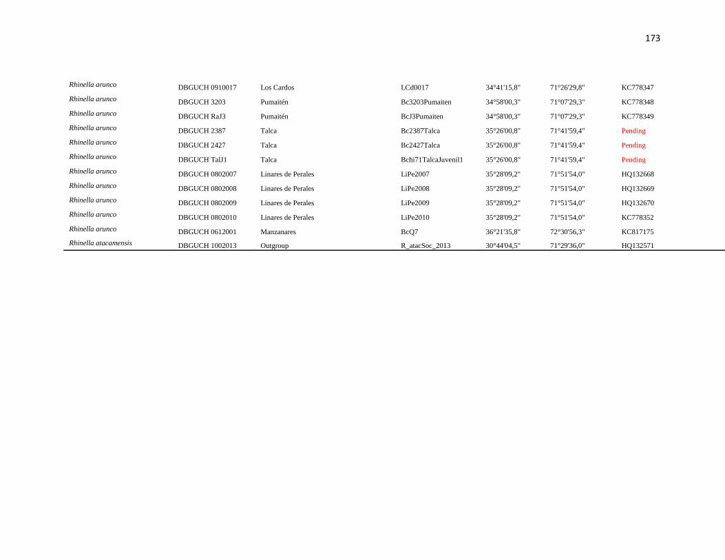
173

Rhinella arunco DBGUCH 0910017 Los Cardos LCd0017 34°41'15,8" 71°26'29,8" KC778347

Rhinella arunco DBGUCH 3203 Pumaitén Bc3203Pumaiten 34°58'00,3" 71°07'29,3" KC778348

Rhinella arunco DBGUCH RaJ3 Pumaitén BcJ3Pumaiten 34°58'00,3" 71°07'29,3" KC778349

Rhinella arunco DBGUCH 2387 Talca Bc2387Talca 35°26'00,8" 71°41'59,4" Pending

Rhinella arunco DBGUCH 2427 Talca Bc2427Talca 35°26'00,8" 71°41'59,4" Pending

Rhinella arunco DBGUCH TalJ1 Talca Bchi71TalcaJuvenil1 35°26'00,8" 71°41'59,4" Pending

Rhinella arunco DBGUCH 0802007 Linares de Perales LiPe2007 35°28'09,2" 71°51'54,0" HQ132668

Rhinella arunco DBGUCH 0802008 Linares de Perales LiPe2008 35°28'09,2" 71°51'54,0" HQ132669

Rhinella arunco DBGUCH 0802009 Linares de Perales LiPe2009 35°28'09,2" 71°51'54,0" HQ132670

Rhinella arunco DBGUCH 0802010 Linares de Perales LiPe2010 35°28'09,2" 71°51'54,0" KC778352

Rhinella arunco DBGUCH 0612001 Manzanares BcQ7 36°21'35,8" 72°30'56,3" KC817175

Rhinella atacamensis DBGUCH 1002013 Outgroup R_atacSoc_2013 30°44'04,5" 71°29'36,0" HQ132571