Observational constraints on methane emissions from Polish ...

Observational constraints on methane emissions from Polish coalmines using a ground-based remote sensing networkAndreas Luther1, Julian Kostinek8, Ralph Kleinschek1, Sara Defratyka6, Mila Stanisavljevic4,Andreas Forstmaier3, Alexandru Dandocsi5, Leon Scheidweiler1, Darko Dubravica2, NormanWildmann8, Frank Hase2, Matthias M. Frey7, Jia Chen3, Florian Dietrich3, Jarosław Necki4,Justyna Swolkien4, Christoph Knote 9, Sanam N. Vardag1,10, Anke Roiger8, and André Butz1,10,11

1Institute of Environmental Physics (IUP), Heidelberg University, Heidelberg, Germany2Karlsruhe Institute of Technology (KIT), Institute of Meteorology and Climate Research (IMK-ASF), Karlsruhe, Germany3Environmental Sensing and Modeling, Technical University of Munich (TUM), Munich, Germany4AGH - University of Science and Technology, Kraków, Poland5National Institute of Research and Development for Optoelectronics (INOE2000), Magurele, Romania6Laboratoire des sciences du climat et de l’environnement (LSCE-IPSL) CEA-CNRS-UVSQ Université Paris Saclay,Gif-sur-Yvette, France7National Institute for Environmental Studies, Tsukuba, Japan8Deutsches Zentrum für Luft- und Raumfahrt (DLR), Institut für Physik der Atmosphäre, Oberpfaffenhofen, Germany9Model-Based Environmental Exposure Science, University of Augsburg, Augsburg, Germany10Heidelberg Center for the Environment (HCE), Heidelberg University, Heidelberg, Germany11Interdisciplinary Center for Scientific Computing (IWR), Heidelberg University, Heidelberg, Germany

Correspondence: Andreas Luther ([email protected]), André Butz ([email protected])

Abstract. Given its abundant coal mining activities, the Upper Silesian Coal Basin (USCB) in southern Poland is one of

the largest sources for anthropogenic methane (CH4) emissions in Europe. Here, we report on CH4 emission estimates for

coal mine ventilation facilities in the USCB. Our estimates are driven by pair-wise upwind-downwind observations of the

column-average dry-air mole fractions of CH4 (XCH4) by a network of four portable, ground-based, sun-viewing Fourier

Transform Spectrometers of the type EM27/SUN operated during the CoMet campaign in May/June 2018. The EM27/SUN5

were deployed in the four cardinal directions around the USCB in approx. 50km distance to the center of the basin. We report

on six case studies for which we inferred emissions by evaluating the mismatch between the observed downwind enhancements

and simulations based on trajectory calculations releasing particles out of the ventilation shafts using the Lagrangian particle

dispersion model FLEXPART. The latter was driven by wind fields calculated by WRF (Weather Research and Forecasting

model) under assimilation of vertical wind profile measurements of three co-deployed wind lidars. For emission estimation,10

we use a Phillips-Tikhonov regularization scheme with the L-curve criterion. Diagnosed by the averaging kernels, we find

that, depending on the catchment area of the downwind measurements, our ad-hoc network can resolve individual facilities or

groups of ventilation facilities but that inspecting the averaging kernels is essential to detected correlated estimates. Generally,

our instantaneous emission estimates range between 80 and 133kt CH4 a−1 for the south-eastern part of the USCB and

between 414 and 790kt CH4 a−1 for various larger parts of the basin, suggesting higher emissions than expected from the15

https://doi.org/10.5194/acp-2021-978Preprint. Discussion started: 17 December 2021c© Author(s) 2021. CC BY 4.0 License.

annual emissions reported by the E-PRTR (European Pollutant Release and Transfer Register). Uncertainties range between

23 and 36% dominated by the error contribution from uncertain wind fields.

1 Introduction

The atmospheric abundance of methane (CH4) increased by a factor of 2.6 since pre-industrial times from roughly 720ppb

(parts-per-billion) to about 1879ppb in 2020 (Dlugokencky, 2021) mainly driven by anthropogenic influences (e.g. Bousquet20

et al., 2006; Loulergue et al., 2008; Kirschke et al., 2013; IPCC, 2013; Nisbet et al., 2014; Conley et al., 2016; Schwietzke

et al., 2016; Worden et al., 2017; Alvarez et al., 2018; Saunois et al., 2020; Hmiel et al., 2020). Roughly 20% of the total, global

anthropogenic CH4 emissions are caused by the fossil fuel industry (Bousquet et al., 2006; Schwietzke et al., 2016; Saunois

et al., 2020) and an extensive source of CH4 is hard coal mining. Poland is the largest hard coal producer in the European

Union with the Upper Silesian Coal Basin (USCB) as one of the largest hard coal producing regions in Europe. Several25

bottom-up inventories report on the total CH4 emissions for the USCB: According to the GESAPU database, the USCB

emitted a total of 405kt CH4 in 2010 (Bun et al., 2019). The E-PRTR (European Pollutant Release and Transfer Register,

http://prtr.ec.europa.eu/, 2018) collects emission reports of every individual mine yielding an aggregated total of 507kt CH4

a−1 for the USCB. Dreger (2021) reports hard coal mining emissions of 530kt CH4 for the USCB in 2018 and the Copernicus

Atmosphere Monitoring Service regional emission inventory (CAMS-REG-GHG/AP) lists 632kt CH4 a−1 (Granier et al.,30

2019; Fiehn et al., 2020). EDGAR v4.3.2 (Emission Database for Global Atmospheric Research) accounts emissions of 720kt

CH4 a−1 (Janssens-Maenhout et al., 2017) for the USCB in the year 2017.

In addition to the bottom-up inventories, top-down approaches examined the USCB emissions. During the CoMet mission

(Carbon dioxide and Methane mission 2018, from 23 May to 12 June 2018), several ground-based instruments and aircraft

measured the atmospheric CH4 abundance in the USCB. In our precursor study (Luther et al., 2019), we used stop-and-go35

measurements of the column-average dry-air mole fractions of CH4 (XCH4) by a mobile, ground-based Fourier Transform

Spectrometer (FTS) to evaluate the mining emissions of individual ventilation facilities, and found similar emissions as sug-

gested by the E-PRTR inventory. The total USCB emission estimates of Fiehn et al. (2020) and Kostinek et al. (2020), based

on airborne in situ measurements, are in broad agreement with the E-PRTR data for single flights. Using airborne imager data,

Krautwurst et al. (2021) found some discrepancies between their estimates and the E-PRTR inventory for small groups of ven-40

tilation facilities. The isotopic CH4 composition was measured by Menoud et al. (2021) with ground-based in situ instruments.

Swolkien (2020) discusses the short-term, shaft-wise CH4 release in the USCB.

Given the magnitude of emissions and the range of estimates, CH4 in the USCB warrants further investigation. Here, we

report on CH4 emission estimates derived from measurements of four stationary, sun-viewing FTS of the type EM27/SUN

arranged in a network-like pattern enclosing the USCB during the CoMet campaign activities. The setup largely mimics45

previous network deployments for quantifying urban greenhouse gas emissions in Berlin (Hase et al., 2015), Paris (Vogel

et al., 2019), St. Petersburg (Makarova et al., 2020), Munich (Dietrich et al., 2021), Indianapolis (Jones et al., 2021) and other

places. Our four EM27/SUN were positioned in the four cardinal directions at a distance of a few tens of kilometers to the

2


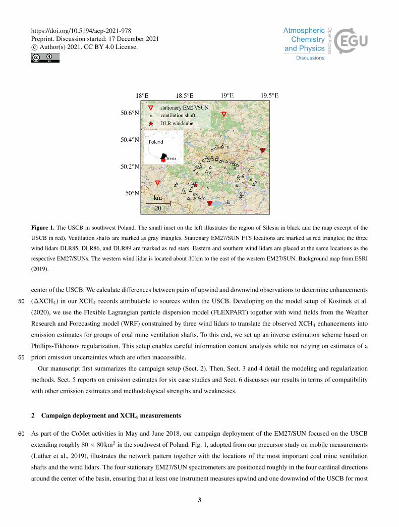
Figure 1. The USCB in southwest Poland. The small inset on the left illustrates the region of Silesia in black and the map excerpt of the

USCB in red). Ventilation shafts are marked as gray triangles. Stationary EM27/SUN FTS locations are marked as red triangles; the three

wind lidars DLR85, DLR86, and DLR89 are marked as red stars. Eastern and southern wind lidars are placed at the same locations as the

respective EM27/SUNs. The western wind lidar is located about 30km to the east of the western EM27/SUN. Background map from ESRI

(2019).

center of the USCB. We calculate differences between pairs of upwind and downwind observations to determine enhancements

(∆XCH4) in our XCH4 records attributable to sources within the USCB. Developing on the model setup of Kostinek et al.50

(2020), we use the Flexible Lagrangian particle dispersion model (FLEXPART) together with wind fields from the Weather

Research and Forecasting model (WRF) constrained by three wind lidars to translate the observed XCH4 enhancements into

emission estimates for groups of coal mine ventilation shafts. To this end, we set up an inverse estimation scheme based on

Phillips-Tikhonov regularization. This setup enables careful information content analysis while not relying on estimates of a

priori emission uncertainties which are often inaccessible.55

Our manuscript first summarizes the campaign setup (Sect. 2). Then, Sect. 3 and 4 detail the modeling and regularization

methods. Sect. 5 reports on emission estimates for six case studies and Sect. 6 discusses our results in terms of compatibility

with other emission estimates and methodological strengths and weaknesses.

2 Campaign deployment and XCH4 measurements

As part of the CoMet activities in May and June 2018, our campaign deployment of the EM27/SUN focused on the USCB60

extending roughly 80 × 80km2 in the southwest of Poland. Fig. 1, adopted from our precursor study on mobile measurements

(Luther et al., 2019), illustrates the network pattern together with the locations of the most important coal mine ventilation

shafts and the wind lidars. The four stationary EM27/SUN spectrometers are positioned roughly in the four cardinal directions

around the center of the basin, ensuring that at least one instrument measures upwind and one downwind of the USCB for most

3


wind situations. Due to mainly easterly wind conditions prevailing during our deployment, the eastern station (The Glade)65

functions as the upwind station for all case studies discussed here. The respective downwind stations are located in the south

(Pustelnik) and west (Raciborz) of the USCB. The northern station (Za Miastem) was identified neither upwind nor downwind

station for any of the cases.

The functioning of the EM27/SUN FTS and the data reduction techniques are described in detail by Gisi et al. (2012), Hase

et al. (2015) and Hase et al. (2016) and with a particular focus on our setup by Luther et al. (2019). Generally, the EM27/SUN70

observe spectra of direct sunlight in the shortwave infrared spectral range from which the total column concentrations of CH4,

carbon dioxide (CO2), water vapor (H2O), molecular oxygen (O2), carbon monoxide (CO), and other substances (Butz et al.,

2017) can be retrieved. CH4 and O2 are of relevance here. All EM27/SUN spectrometers participating in the campaign suc-

cessfully underwent the instrumental quality assurance tests required by the Collaborative Carbon Column Observing Network

(COCCON) and presented in Frey et al. (2019) before field deployment.75

We run the software package PROFFIT (Hase et al., 2004) to retrieve the column concentrations [O2] and [CH4] from the

7765 to 8005cm−1 and 5897 to 6145cm−1 spectral windows, respectively, using absorption line parameters by Toon (2017)

and Rothman et al. (2009). The respective column-averaged dry-air mole fractions of methane, XCH4, are calculated via nor-

malization through [CH4][O2]×0.2094 where the atmospheric O2 mole fraction is assumed 0.2094. The normalization is generally

recommended to lessen spurious artefacts due to pressure and solar zenith angle (SZA) dependencies. The SZAs during our80

measurements did not exceed 56◦ which is within the range which does not require airmass-dependent bias correction (Frey

et al., 2015). Slightly deviating from the processing recipe (Frey et al., 2019) and in line with our precursor study (Luther

et al., 2019), our CH4 retrievals only scale the CH4 concentrations in the layers below 1700m a.g.l. where we expect el-

evated methane due to the localized sources at the ground. Further, we extract the a priori CH4 profiles from a dedicated

ECHAM/MESSy Atmospheric Chemistry simulation described by Jöckel et al. (2016) and Nickl et al. (2020).85

For network deployments such as undertaken here, it is common practice to cross-calibrate the network nodes by side-by-

side measurements (Frey et al., 2015; Chen et al., 2016; Frey et al., 2019; Jones et al., 2021; Dietrich et al., 2021) in order to

exclude spurious gradients when conducting upwind-downwind analyses. We calibrated the four instruments through side-by-

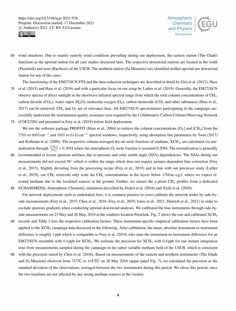
side measurements on 23 May and 26 May, 2018 at the southern location Pustelnik. Fig. 2 shows the raw and calibrated XCH4

records and Table 1 lists the respective calibration factors. These instrument-specific empirical calibration factors have been90

applied to the XCH4 campaign data discussed in the following. After calibration, the mean, absolute instrument-to-instrument

difference is roughly 1ppb which is compatible to Frey et al. (2019) who state the instrument-to-instrument difference for an

EM27/SUN ensemble with 0.8ppb for XCH4. We estimate the precision for XCH4 with 0.6ppb for one minute integration

time from measurements sampled during the campaign in the rather variable methane field of the USCB, which is consistent

with the precision stated by Chen et al. (2016). Based on measurements of the eastern and northern instruments (The Glade95

and Za Miastem) observed from 7UTC to 10UTC on 28 May 2018 (upper panel Fig. 7), we calculated the precision as the

standard deviation of the observations, averaged between the two instruments during this period. We chose this period, since

the two timelines are not affected by any strong methane sources in the vicinity.

4


In addition to the EM27/SUN network, we also operated three Leosphere Windcube 200S Doppler wind lidars (Vasiljevic

et al., 2016; Wildmann et al., 2018, 2020) marked as red stars in Fig. 1 and as detailed in Luther et al. (2019) and Kostinek et al.100

(2020). The measured wind profiles (10min time interval) reach up to 4km a.g.l. and are assimilated into the WRF simulations

to improve the modeled wind fields as discussed in Sect. 3.

Figure 2. Side-by-side measurements at station Pustelnik on 23 May 2018 on the first day of the deployment. The upper panel displays

unscaled data with an average instrument-to-instrument difference of 5ppb. The lower panel shows measured XCH4 after scaling with about

1ppb instrument-to-instrument difference. Note, that the instruments detected a plume like structure at the beginning of the measurements

and around 11:20UTC. The instrument The Glade measured side-by-side on 26 May with the Pustelnik instrument (data in A1).

Site Lat. ◦N Lon. ◦E m a.s.l XCH4 cal. O2 cal.

Za Miastem (N) 50.599 18.963 305 0.9949 1.0079

The Glade (E) 50.329 19.416 303 1.0002 0.9967

Pustelnik (S) 49.933 18.799 266 0.9989 1.0034

Raciborz (W) 50.083 18.192 223 1 1

Table 1. Calibration factors towards the western station Raciborz for each instrument and species, nominal geolocation in network.

5


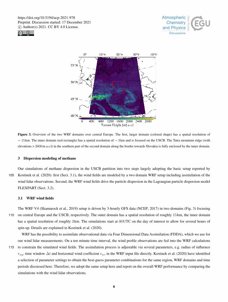
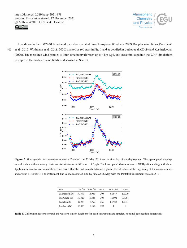
Figure 3. Overview of the two WRF domains over central Europe. The first, larger domain (colored shape) has a spatial resolution of

∼ 15km. The inner domain (red rectangle) has a spatial resolution of ∼ 3km and is focused on the USCB. The Tatra mountain ridge (with

elevations > 2000m a.s.l) in the southern part of the second domain along the border towards Slovakia is fully enclosed by the inner domain.

3 Dispersion modeling of methane

Our simulations of methane dispersion in the USCB partition into two steps largely adopting the basic setup reported by

Kostinek et al. (2020): first (Sect. 3.1), the wind fields are modeled by a two domain WRF setup including assimilation of the105

wind lidar observations. Second, the WRF wind fields drive the particle dispersion in the Lagrangian particle dispersion model

FLEXPART (Sect. 3.2).

3.1 WRF wind fields

The WRF V4 (Skamarock et al., 2019) setup is driven by 3-hourly GFS data (NCEP, 2017) in two domains (Fig. 3) focusing

on central Europe and the USCB, respectively. The outer domain has a spatial resolution of roughly 15km, the inner domain110

has a spatial resolution of roughly 3km. The simulations start at 00UTC on the day of interest to allow for several hours of

spin-up. Details are explained in Kostinek et al. (2020).

WRF has the possibility to assimilate observational data via Four Dimensional Data Assimilation (FDDA), which we use for

our wind lidar measurements. On a ten minute time interval, the wind profile observations are fed into the WRF calculations

to constrain the simulated wind fields. The assimilation process is adjustable via several parameters, e.g. radius of influence115

rxy , time window ∆t and horizontal wind coefficient cuv in the WRF input file directly. Kostinek et al. (2020) have identified

a selection of parameter settings to obtain the best-guess parameter combinations for the same region, WRF domains and time

periods discussed here. Therefore, we adopt the same setup here and report on the overall WRF performance by comparing the

simulations with the wind lidar observations.

6


Fig. 4 displays a comparison between modeled and observed wind speed (upper panel) and wind direction (lower panel)120

for altitude levels in the planetary boundary layer (PBL). PBL height is estimated by means of eddy dissipation rate gradients

calculated from the wind lidar observations directly. The observation levels of the wind lidar do not match the WRF grid levels

exactly. Thus, the comparison includes modeled and observed data if the WRF wind level is within the range of ±25m around

the level of observation. This represents all of the WRF wind levels but dismisses some of the wind lidar levels as the lidar

data has a finer vertical resolution. The comparison is restricted to the three days of the case studies to be discussed below125

(28 May; 6 June; 7 June, 2018). The prevailing wind directions were northeast to southeast and prevailing wind speeds range

from 2ms−1 to 9ms−1. The root-mean-square-error (RMSE) for the wind speed comparison calculates to 1.7ms−1. When

eliminating the top two levels, the wind direction RMSE reduces from 38◦ to 26◦ indicating model inaccuracies towards the

PBL top where wind shear effects are expected. Low wind speeds on 7 June are possibly deteriorating the wind direction bias,

as wind direction uncertainties are generally larger for low wind speeds. Further challenges for the wind direction estimation130

are the onset of convection during the observational morning hours with subsequent PBL rise and the calming winds towards

the end of the observational days. In general we observed most outliers for the top comparison levels for wind direction, which

could be related to a significant number of conspicuous low wind speed simulations and observations for these levels. This

might be related to model uncertainties when estimating the PBL height, leading to misinterpretation of actual above-PBL

observations with inside-PBL simulations and vice versa.135

3.2 Lagrangian methane dispersion via FLEXPART

WRF windfields drive the trajectory calculations in FLEXPART. The model simulates trajectories for 50000 particles for

every USCB coal mining shaft reported by the E-PRTR and the CoMet database (Gałkowski et al., 2021) with a total mass

of 105 kg CH4. The simulations do not consider background CH4. The model releases particles in a 10m ×10m ×10m box

on the ground. The modeling period starts at 00:10UTC the day of interest and continues until 17:50UTC which results140

in 17.7h simulation time. We chose the grid output option in FLEXPART with 100× 100 boxes and a spatial resolution of

roughly 1.3km stacked in 24 layers up to 3km altitude. The simulated XCH4 measurements are the sums of all boxes above

each pixel enclosing an EM27/SUN location. The 6min FLEXPART output is interpolated to the observational time interval

which generally is one measurement per minute. After unit conversion, the simulated methane enhancement is compared to the

measured upwind-downwind difference ∆XCH4.145

The FLEXPART simulations are iterated with slightly different meteorological parameters to provide an uncertainty analysis.

There are seven ensemble runs: the CONTROL run with best guess input, the WINDp5 run with +5◦ wind direction change of

the whole wind field, the WINDm5 run with −5◦ wind direction change of the whole wind field, the SPEEDp06 run with the

wind speed increased by 0.9ms−1, the SPEEDm06 run with the wind speed decreased by 0.9ms−1, the PBLp100 run with

the PBL height increased by 100m, and the PBLm100 run with the PBL height decreased by 100m. We use the same ensemble150

set up as discussed by Kostinek et al. (2020).

We further used the FLEXPART simulations for modeling the air mass travel time from the upwind to the downwind

instruments (Fig. 5). To this end, we implemented a virtual methane source at the upwind measurement location at the beginning

7


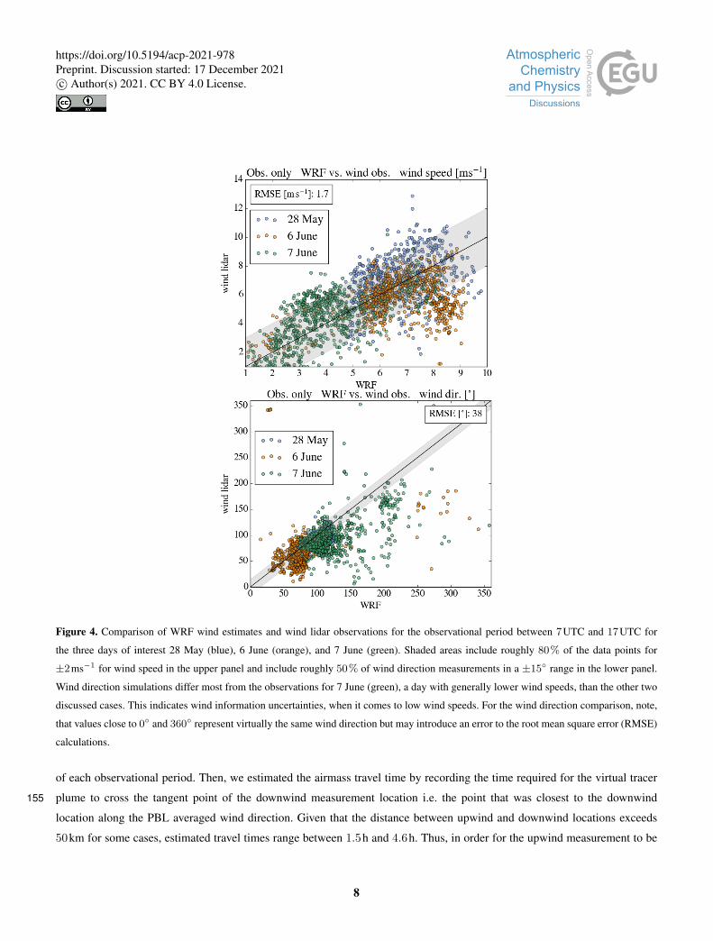
Figure 4. Comparison of WRF wind estimates and wind lidar observations for the observational period between 7UTC and 17UTC for

the three days of interest 28 May (blue), 6 June (orange), and 7 June (green). Shaded areas include roughly 80% of the data points for

±2ms−1 for wind speed in the upper panel and include roughly 50% of wind direction measurements in a ±15◦ range in the lower panel.

Wind direction simulations differ most from the observations for 7 June (green), a day with generally lower wind speeds, than the other two

discussed cases. This indicates wind information uncertainties, when it comes to low wind speeds. For the wind direction comparison, note,

that values close to 0◦ and 360◦ represent virtually the same wind direction but may introduce an error to the root mean square error (RMSE)

calculations.

of each observational period. Then, we estimated the airmass travel time by recording the time required for the virtual tracer

plume to cross the tangent point of the downwind measurement location i.e. the point that was closest to the downwind155

location along the PBL averaged wind direction. Given that the distance between upwind and downwind locations exceeds

50km for some cases, estimated travel times range between 1.5h and 4.6h. Thus, in order for the upwind measurement to be

8


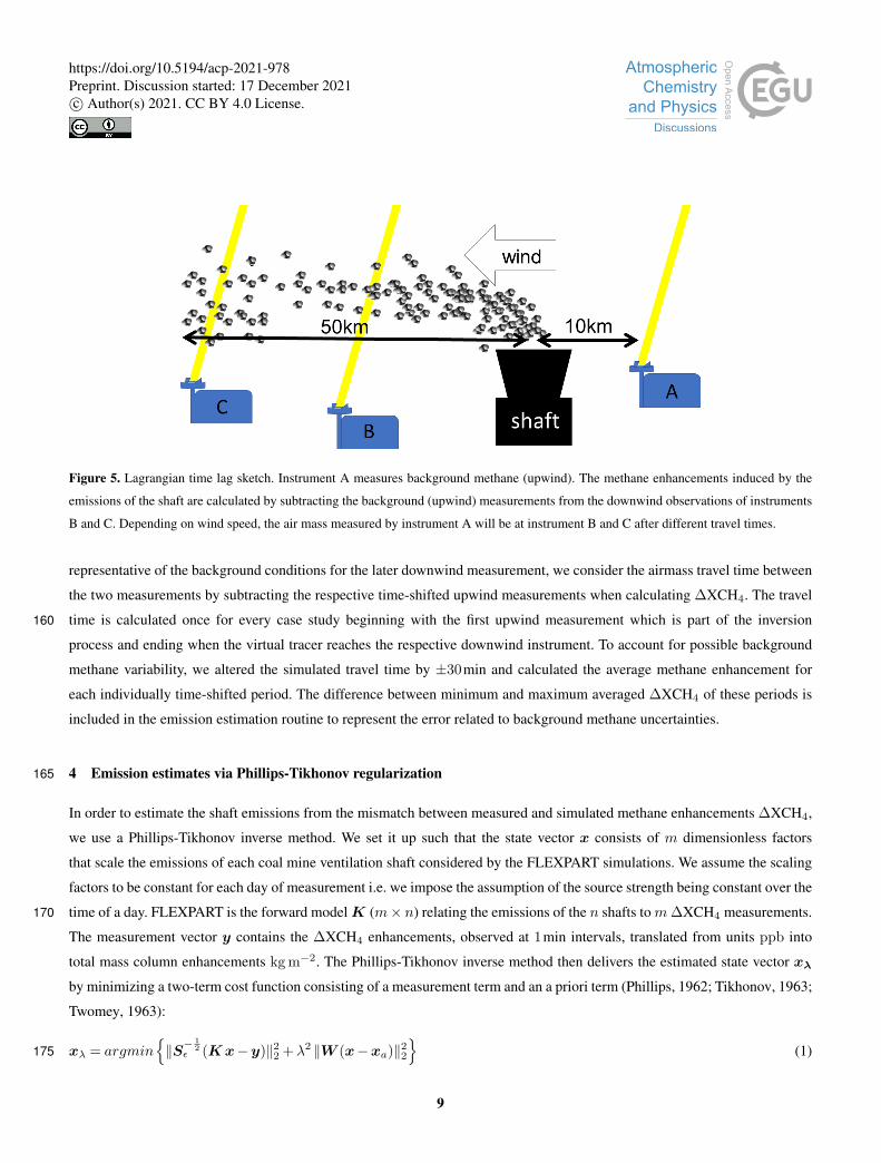
Figure 5. Lagrangian time lag sketch. Instrument A measures background methane (upwind). The methane enhancements induced by the

emissions of the shaft are calculated by subtracting the background (upwind) measurements from the downwind observations of instruments

B and C. Depending on wind speed, the air mass measured by instrument A will be at instrument B and C after different travel times.

representative of the background conditions for the later downwind measurement, we consider the airmass travel time between

the two measurements by subtracting the respective time-shifted upwind measurements when calculating ∆XCH4. The travel

time is calculated once for every case study beginning with the first upwind measurement which is part of the inversion160

process and ending when the virtual tracer reaches the respective downwind instrument. To account for possible background

methane variability, we altered the simulated travel time by ±30min and calculated the average methane enhancement for

each individually time-shifted period. The difference between minimum and maximum averaged ∆XCH4 of these periods is

included in the emission estimation routine to represent the error related to background methane uncertainties.

4 Emission estimates via Phillips-Tikhonov regularization165

In order to estimate the shaft emissions from the mismatch between measured and simulated methane enhancements ∆XCH4,

we use a Phillips-Tikhonov inverse method. We set it up such that the state vector x consists of m dimensionless factors

that scale the emissions of each coal mine ventilation shaft considered by the FLEXPART simulations. We assume the scaling

factors to be constant for each day of measurement i.e. we impose the assumption of the source strength being constant over the

time of a day. FLEXPART is the forward model K (m× n) relating the emissions of the n shafts tom∆XCH4 measurements.170

The measurement vector y contains the ∆XCH4 enhancements, observed at 1min intervals, translated from units ppb into

total mass column enhancements kg m−2. The Phillips-Tikhonov inverse method then delivers the estimated state vector xλ

by minimizing a two-term cost function consisting of a measurement term and an a priori term (Phillips, 1962; Tikhonov, 1963;

Twomey, 1963):

xλ = argmin{‖S−

12

ε (K x−y)‖22 +λ2 ‖W (x−xa)‖22}

(1)175

9


with Sε the error covariance matrix, λ the regularization parameter, W the weighting operator, xa the a priori state vector, and

|| · ||2 representing the L2 norm. Sε contains the averaged standard deviation of the FLEXPART simulation ensemble summed

in quadrature with the XCH4 background variability and the measurement noise. The latter is assumed to amount to 0.6ppb

which corresponds to the standard deviation of the averaged background measurements of two stationary instruments (The

Glade and Za Miastem) from 7UTC to 10UTC on 28 May 2018 (see top panel in Fig. 7). The estimated background variability180

ranges between 0.3ppb and 2.2ppb for the individual case studies, based on the differences of minimum and maximum average

∆XCH4 calculated under consideration of ±30min time shifts of the simulated methane travel times. W is a diagonal matrix

with elements 1xa,j

, j = 1, . . . ,m which renders the second cost term dimensionless (Butz et al., 2012). Technically, we trans-

form the Phillips-Tikhonov regularization problem into a plain least-squares fit using the definitions (Hansen and O’Leary,

1993; Hansen, 1999; Golub and Von Matt, 1997),185

C =

[S− 1

2ε K

λW

]and d =

[S− 1

2ε y

λW xa

](2)

which transforms equ. (1) to

xλ = argmin{‖C x−d‖22

}(3)

treatable by a standard least-squares solver (e.g. python module scipy.optimize.lsq_linear).

The a priori information xa for each ventilation shaft is taken from the annual E-PRTR emission inventory updated by190

Gałkowski et al. (2021). The a priori generally guides the minimization process towards physically reasonable solutions if

the inverse problem tends to be ill-posed e.g. when there is insufficient measurement information on some of the state vector

elements. However, the solution is dependent on the regularization parameter λ which has to be found by trading the propaga-

tion of measurement errors against influence of the a priori. Here, we use the L-curve criterion to determine the regularization

parameter λ for each individual case study (e.g. Hansen, 1999). The L-curve is a graphical representation of the the mismatch195

between measurements and simulations ‖K xλ−y‖2 plotted against the norm of the state vector ‖xλ‖2 evaluated for a range

of λ (cf. Fig. 9). The plot typically looks like an L. For small λ, the measurement term dominates the cost function, the estimate

xλ becomes noisy and drives large deviations from the a priori. For large λ, the a priori term dominates the cost function, the

estimate xλ ignores the measurements and produces a large norm of the measurement term. The corner of the L indicates a rea-

sonable regularization parameter for the given minimization problem and is graphically chosen. In addition, we found that the200

shape of the L-curve is sensitive to forward model errors e.g. when errors in the FLEXPART trajectories and the driving wind

fields suggest a spurious, erroneous link between emissions and methane enhancements. Obvious distortions of the L-curve

shape are used as a criterion to filter out periods, when the forward model does not represent the actual dispersion conditions.

Besides the L-curve, the regularized inversion approach holds another diagnostic measure: the averaging kernel matrix Aλ

with dimensions m × m. It is defined via the gain matrix Gλ (Rodgers, 2000; Butz et al., 2012; Borsdorff et al., 2014),205

Aλ = GλK (4)

Gλ =(KTS−1

ε K +λ2 ·W TW)−1

KTS−1ε (5)

10


The averaging kernel matrix, for a given regularization strength λ, diagnoses how information propagates from the true and a

priori states, xtrue and xa, into the emission estimate,

xλ = Aλxtrue + (W −Aλ)xa (6)210

The rows of Aλ are called the averaging kernels quantifying how an estimated state vector element calculates from the other

state elements and what portion comes from the prior. For our purposes, the averaging kernels quantify how the emission

estimate for a ventilation shaft is affected by the neighboring shafts and whether there is sufficient measurement information.

In the perfect case, the averaging kernel is unity for the shaft under consideration and zero for all other shafts indicating that

the shaft can be perfectly resolved and discriminated from neighboring sources and that it is well-constrained by measurement215

information. In reality, groups of neighboring sources and sources behind each other along the trajectory are not resolvable and

some shafts only marginally affect our measurements implying broader and smaller averaging kernels.

The errors due to measurement noise, background methane variability, and atmospheric transport incorporated in Sε are

propagated into the a posteriori error covariance for the emission estimates via

Sx,λ = GλSεGTλ (7)220

where we report the square-root of the diagonal as the error bars of the shaft-wise emission estimates and the square-

root of the sum of the entire covariance matrix as the error of the total emissions aggregated over all shafts. For the case

studies discussed in Sect. 5, the emission errors due to measurement noise range between 0.62kta−1 and 4.46kta−1 which is

small compared to the errors introduced by the dispersion modeling ensemble which range between 27kta−1 and 143kta−1.

Errors related to background methane variability introduced by a ±30min time shift of the airmass travel time range between225

0.83kta−1 and 8.5kta−1.

5 Case studies

We report on six case studies on three different days of the CoMet campaign. For the respective three days 28 May, 6 June and

7 June, 2018, Fig. 6 illustrates typical FLEXPART trajectories of air masses around midday dispersing out of the USCB coal

mine ventilation shafts. For all cases, easterly winds led to the southern station Pustelnik being influenced by a few southern230

shafts (red trajectories) and the western station Raciborz being influenced by many shafts in various parts of the basin (blue

trajectories). The eastern station The Glade provides the background measurements, the northern station Za Miastem was not

used here since The Glade was the better background station given the prevailing easterly winds.

Fig. 7 depicts the corresponding XCH4 measurements for all stations, indeed, pointing at significantly elevated concentra-

tions at the downwind sites typically amounting to ∆XCH4 on the order of 10 ppb with some diurnal and day-to-day variability.235

For 28 May, the maxima during the morning hours at Pustelnik and Raciborz are most likely connected to night-time methane

accumulation and subsequent transport with rising convection and mixing during the morning hours. When considering the

11


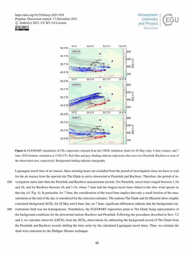
Figure 6. FLEXPART simulations of CH4 trajectories released from the USCB ventilation shafts for 28 May (top), 6 June (center), and 7

June, 2018 (bottom, simulation at 12:04 UT). Red, blue and grey shadings indicate trajectories that went over Pustelnik, Raciborz or none of

the observation sites, respectively. Background shading indicates topography.

Lagrangian travel time of air masses, these morning hours are excluded from the period of investigation since we have to wait

for the air masses from the upwind site The Glade to arrive downwind at Pustelnik and Raciborz. Therefore, the period of in-

vestigation starts later than the Pustelnik and Raciborz measurement records. For Pustelnik, travel times ranged between 1.3h240

and 2h, and for Raciborz between 3h and 5.5h, where 7 June had the longest travel times linked to the slow wind speeds on

that day (cf. Fig. 4). In particular, for 7 June, the consideration of the travel time implies that only a small fraction of the mea-

surements at the end of the day is considered for the emission estimates. The stations The Glade and Za Miastem show roughly

consistent background XCH4 for 28 May and 6 June, but, on 7 June, significant differences indicate that the background con-

centrations field was not homogeneous. Nonetheless, the FLEXPART trajectories point to The Glade being representative of245

the background conditions for the downwind stations Raciborz and Pustelnik. Following the procedures described in Sect. 3.2

and 4, we calculate observed ∆XCH4 from the XCH4 observations by subtracting the background record of The Glade from

the Pustelnik and Raciborz records shifting the time series by the calculated Lagrangian travel times. Then, we estimate the

shaft-wise emissions by the Philipps-Tikonov technique.

12


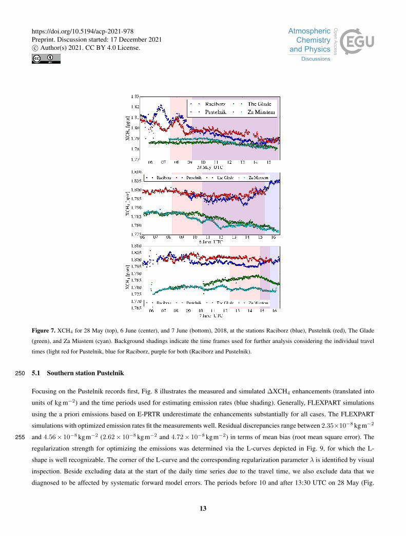
Figure 7. XCH4 for 28 May (top), 6 June (center), and 7 June (bottom), 2018, at the stations Raciborz (blue), Pustelnik (red), The Glade

(green), and Za Miastem (cyan). Background shadings indicate the time frames used for further analysis considering the individual travel

times (light red for Pustelnik, blue for Raciborz, purple for both (Raciborz and Pustelnik).

5.1 Southern station Pustelnik250

Focusing on the Pustelnik records first, Fig. 8 illustrates the measured and simulated ∆XCH4 enhancements (translated into

units of kg m−2) and the time periods used for estimating emission rates (blue shading). Generally, FLEXPART simulations

using the a priori emissions based on E-PRTR underestimate the enhancements substantially for all cases. The FLEXPART

simulations with optimized emission rates fit the measurements well. Residual discrepancies range between 2.35×10−8 kgm−2

and 4.56× 10−8 kgm−2 (2.62× 10−8 kgm−2 and 4.72× 10−8 kgm−2) in terms of mean bias (root mean square error). The255

regularization strength for optimizing the emissions was determined via the L-curves depicted in Fig. 9, for which the L-

shape is well recognizable. The corner of the L-curve and the corresponding regularization parameter λ is identified by visual

inspection. Beside excluding data at the start of the daily time series due to the travel time, we also exclude data that we

diagnosed to be affected by systematic forward model errors. The periods before 10 and after 13:30 UTC on 28 May (Fig.

13


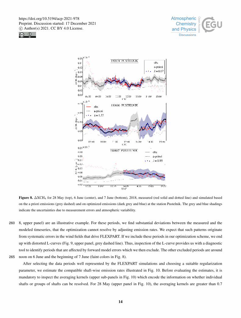
Figure 8. ∆XCH4 for 28 May (top), 6 June (center), and 7 June (bottom), 2018, measured (red solid and dotted line) and simulated based

on the a priori emissions (grey dashed) and on optimized emissions (dark grey and blue) at the station Pustelnik. The grey and blue shadings

indicate the uncertainties due to measurement errors and atmospheric variability.

8, upper panel) are an illustrative example. For these periods, we find substantial deviations between the measured and the260

modeled timeseries, that the optimization cannot resolve by adjusting emission rates. We expect that such patterns originate

from systematic errors in the wind fields that drive FLEXPART. If we include these periods in our optimization scheme, we end

up with distorted L-curves (Fig. 9, upper panel, grey dashed line). Thus, inspection of the L-curve provides us with a diagnostic

tool to identify periods that are affected by forward model errors which we then exclude. The other excluded periods are around

noon on 6 June and the beginning of 7 June (faint colors in Fig. 8).265

After selecting the data periods well represented by the FLEXPART simulations and choosing a suitable regularization

parameter, we estimate the compatible shaft-wise emission rates illustrated in Fig. 10. Before evaluating the estimates, it is

mandatory to inspect the averaging kernels (upper sub-panels in Fig. 10) which encode the information on whether individual

shafts or groups of shafts can be resolved. For 28 May (upper panel in Fig. 10), the averaging kernels are greater than 0.7

14


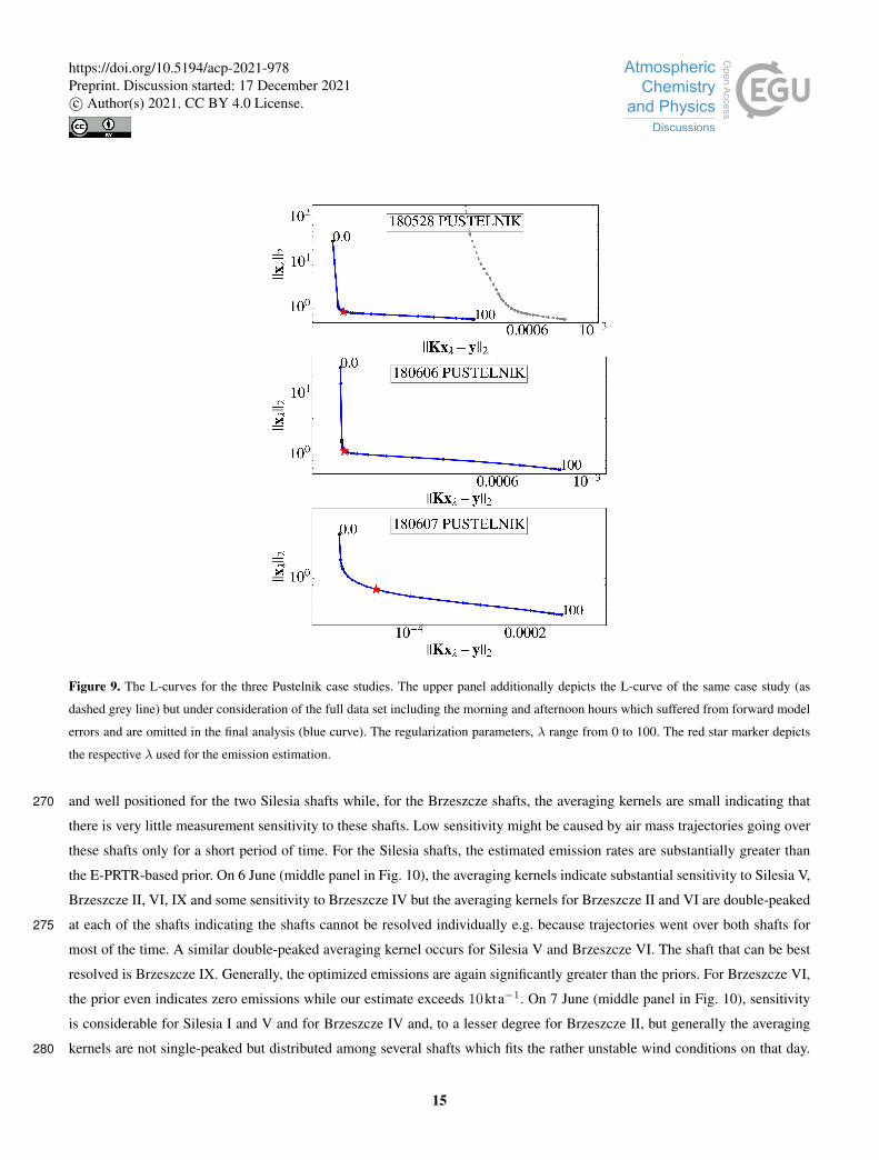
Figure 9. The L-curves for the three Pustelnik case studies. The upper panel additionally depicts the L-curve of the same case study (as

dashed grey line) but under consideration of the full data set including the morning and afternoon hours which suffered from forward model

errors and are omitted in the final analysis (blue curve). The regularization parameters, λ range from 0 to 100. The red star marker depicts

the respective λ used for the emission estimation.

and well positioned for the two Silesia shafts while, for the Brzeszcze shafts, the averaging kernels are small indicating that270

there is very little measurement sensitivity to these shafts. Low sensitivity might be caused by air mass trajectories going over

these shafts only for a short period of time. For the Silesia shafts, the estimated emission rates are substantially greater than

the E-PRTR-based prior. On 6 June (middle panel in Fig. 10), the averaging kernels indicate substantial sensitivity to Silesia V,

Brzeszcze II, VI, IX and some sensitivity to Brzeszcze IV but the averaging kernels for Brzeszcze II and VI are double-peaked

at each of the shafts indicating the shafts cannot be resolved individually e.g. because trajectories went over both shafts for275

most of the time. A similar double-peaked averaging kernel occurs for Silesia V and Brzeszcze VI. The shaft that can be best

resolved is Brzeszcze IX. Generally, the optimized emissions are again significantly greater than the priors. For Brzeszcze VI,

the prior even indicates zero emissions while our estimate exceeds 10kta−1. On 7 June (middle panel in Fig. 10), sensitivity

is considerable for Silesia I and V and for Brzeszcze IV and, to a lesser degree for Brzeszcze II, but generally the averaging

kernels are not single-peaked but distributed among several shafts which fits the rather unstable wind conditions on that day.280

15


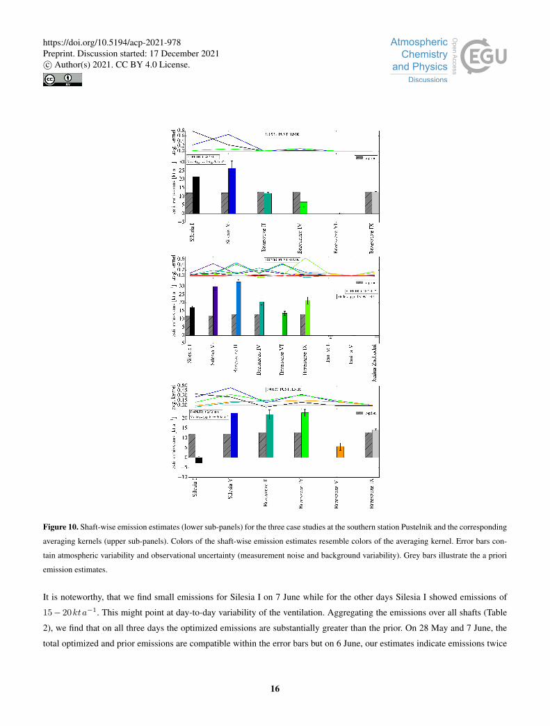
Figure 10. Shaft-wise emission estimates (lower sub-panels) for the three case studies at the southern station Pustelnik and the corresponding

averaging kernels (upper sub-panels). Colors of the shaft-wise emission estimates resemble colors of the averaging kernel. Error bars con-

tain atmospheric variability and observational uncertainty (measurement noise and background variability). Grey bars illustrate the a priori

emission estimates.

It is noteworthy, that we find small emissions for Silesia I on 7 June while for the other days Silesia I showed emissions of

15− 20kta−1. This might point at day-to-day variability of the ventilation. Aggregating the emissions over all shafts (Table

2), we find that on all three days the optimized emissions are substantially greater than the prior. On 28 May and 7 June, the

total optimized and prior emissions are compatible within the error bars but on 6 June, our estimates indicate emissions twice

16


as high than the prior, 133± 31kta−1 compared to 63kta−1. The difference of the total emission estimates to the other days285

is largely due to better sensitivity to all the Brzeszcze shafts and to the larger respective emission estimates.

5.2 Western station Raciborz

Figure 11. ∆XCH4 for 28 May (top), 6 June (center), and 7 June (bottom), 2018, measured (red solid and dashed line) and simulated based

on the a priori emissions (grey dashed) and on optimized emissions (dark grey and blue) at the station Raciborz. The grey and blue shadings

indicate the uncertainties due to measurement errors and atmospheric variability.

In contrast to the case studies for Pustelnik, the FLEXPART simulations indicate that the western station Raciborz is influ-

enced by a large and varying number of shafts (between 30 and 50 shafts for the three days discussed here). Figs. 11 and 12

show the fits to the ∆XCH4 observations for the prior and optimized emission estimates and the L-curves for the selection of290

the regularization parameter, respectively. For 6 June, we again find that the FLEXPART simulations could not represent our

measurements at the beginning and end of the time series and therefore, we excluded these periods based on visual inspection

of distortions of the L-curve. Overall, after optimization the simulated ∆XCH4 records fit the observations well, while simu-

17


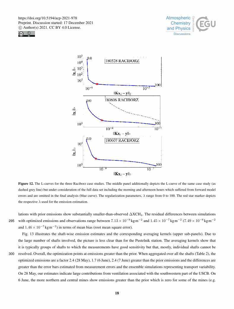
Figure 12. The L-curves for the three Raciborz case studies. The middle panel additionally depicts the L-curve of the same case study (as

dashed grey line) but under consideration of the full data set including the morning and afternoon hours which suffered from forward model

errors and are omitted in the final analysis (blue curve). The regularization parameters, λ range from 0 to 100. The red star marker depicts

the respective λ used for the emission estimation.

lations with prior emissions show substantially smaller-than-observed ∆XCH4. The residual differences between simulations

with optimized emissions and observations range between 7.13× 10−8 kgm−2 and 1.45× 10−7 kgm−2 (7.49× 10−8 kgm−2295

and 1.46× 10−7 kgm−2) in terms of mean bias (root mean square error).

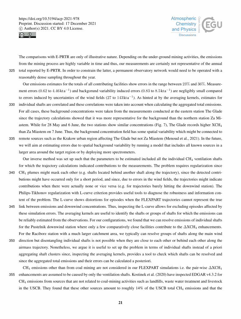
Fig. 13 illustrates the shaft-wise emission estimates and the corresponding averaging kernels (upper sub-panels). Due to

the large number of shafts involved, the picture is less clear than for the Pustelnik station. The averaging kernels show that

it is typically groups of shafts to which the measurements have good sensitivity but that, mostly, individual shafts cannot be

resolved. Overall, the optimization points at emissions greater than the prior. When aggregated over all the shafts (Table 2), the300

optimized emissions are a factor 2.4 (28 May), 1.7 (6 June), 2.4 (7 June) greater than the prior emissions and the differences are

greater than the error bars estimated from measurement errors and the ensemble simulations representing transport variability.

On 28 May, our estimates indicate large contributions from ventilation associated with the southwestern part of the USCB. On

6 June, the more northern and central mines show emissions greater than the prior which is zero for some of the mines (e.g.

18


Figure 13. Shaft-wise emission estimates (lower sub-panels) for the three case studies at the western station Raciborz and the corresponding

averaging kernels (upper sub-panels). Colors of the shaft-wise emission estimates resemble colors of the averaging kernel. Error bars con-

tain atmospheric variability and observational uncertainty (measurement noise and background variability). Grey bars illustrate the a priori

emission estimates.

19


Centrum Witczak/Staszic and Julian II/Rozbark Barbara). On 7 June, the number of contributing shafts is less than for the other305

days and the estimates point at large emissions from ventilation of Ziemowit, Janina and Chwałowicze V.

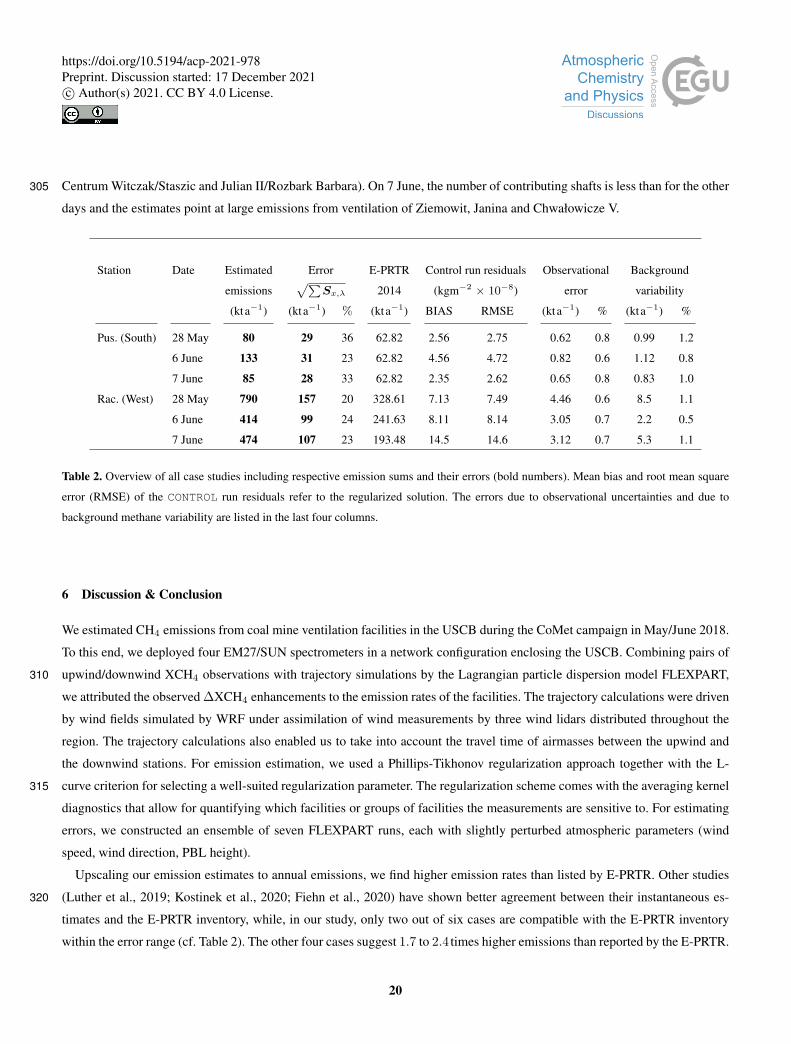
Station Date Estimated Error E-PRTR Control run residuals Observational Background

emissions√∑

Sx,λ 2014 (kgm−2 × 10−8) error variability

(kta−1) (kta−1) % (kta−1) BIAS RMSE (kta−1) % (kta−1) %

Pus. (South) 28 May 80 29 36 62.82 2.56 2.75 0.62 0.8 0.99 1.2

6 June 133 31 23 62.82 4.56 4.72 0.82 0.6 1.12 0.8

7 June 85 28 33 62.82 2.35 2.62 0.65 0.8 0.83 1.0

Rac. (West) 28 May 790 157 20 328.61 7.13 7.49 4.46 0.6 8.5 1.1

6 June 414 99 24 241.63 8.11 8.14 3.05 0.7 2.2 0.5

7 June 474 107 23 193.48 14.5 14.6 3.12 0.7 5.3 1.1

Table 2. Overview of all case studies including respective emission sums and their errors (bold numbers). Mean bias and root mean square

error (RMSE) of the CONTROL run residuals refer to the regularized solution. The errors due to observational uncertainties and due to

background methane variability are listed in the last four columns.

6 Discussion & Conclusion

We estimated CH4 emissions from coal mine ventilation facilities in the USCB during the CoMet campaign in May/June 2018.

To this end, we deployed four EM27/SUN spectrometers in a network configuration enclosing the USCB. Combining pairs of

upwind/downwind XCH4 observations with trajectory simulations by the Lagrangian particle dispersion model FLEXPART,310

we attributed the observed ∆XCH4 enhancements to the emission rates of the facilities. The trajectory calculations were driven

by wind fields simulated by WRF under assimilation of wind measurements by three wind lidars distributed throughout the

region. The trajectory calculations also enabled us to take into account the travel time of airmasses between the upwind and

the downwind stations. For emission estimation, we used a Phillips-Tikhonov regularization approach together with the L-

curve criterion for selecting a well-suited regularization parameter. The regularization scheme comes with the averaging kernel315

diagnostics that allow for quantifying which facilities or groups of facilities the measurements are sensitive to. For estimating

errors, we constructed an ensemble of seven FLEXPART runs, each with slightly perturbed atmospheric parameters (wind

speed, wind direction, PBL height).

Upscaling our emission estimates to annual emissions, we find higher emission rates than listed by E-PRTR. Other studies

(Luther et al., 2019; Kostinek et al., 2020; Fiehn et al., 2020) have shown better agreement between their instantaneous es-320

timates and the E-PRTR inventory, while, in our study, only two out of six cases are compatible with the E-PRTR inventory

within the error range (cf. Table 2). The other four cases suggest 1.7 to 2.4 times higher emissions than reported by the E-PRTR.

20


The comparisons with E-PRTR are only of illustrative nature. Depending on the under-ground mining activities, the emissions

from the mining process are highly variable in time and thus, our measurements are certainly not representative of the annual

total reported by E-PRTR. In order to constrain the latter, a permanent observatory network would need to be operated with a325

reasonably dense sampling throughout the year.

Our emissions estimates for the totals of all contributing facilities show errors in the range between 23% and 36%. Measure-

ment errors (0.62 to 4.46kta−1) and backgorund variability induced errors (0.83 to 8.5kta−1) are negligibly small compared

to errors induced by uncertainties of the wind fields (27 to 143kta−1). As hinted at by the averaging kernels, estimates for

individual shafts are correlated and these correlations were taken into account when calculating the aggregated total emissions.330

For all cases, these background concentrations were taken from the measurements conducted at the eastern station The Glade

since the trajectory calculations showed that it was more representative for the background than the northern station Za Mi-

astem. While for 28 May and 6 June, the two stations show similar concentrations (Fig. 7), The Glade records higher XCH4

than Za Miastem on 7 June. Thus, the background concentration field has some spatial variability which might be connected to

remote sources such as the Krakow urban region affecting The Glade but not Za Miastem (Menoud et al., 2021). In the future,335

we will aim at estimating errors due to spatial background variability by running a model that includes all known sources in a

larger area around the target region or by deploying more spectrometers.

Our inverse method was set up such that the parameters to be estimated included all the individual CH4 ventilation shafts

for which the trajectory calculations indicated contributions to the measurements. The problem requires regularization since

CH4 plumes might mask each other (e.g. shafts located behind another shaft along the trajectory), since the detected contri-340

butions might have occurred only for a short period, and since, due to errors in the wind fields, the trajectories might indicate

contributions when there were actually none or vice versa (e.g. for trajectories barely hitting the downwind station). The

Philips-Tikhonov regularization with L-curve criterion provides useful tools to diagnose the robustness and information con-

tent of the problem. The L-curve shows distortions for episodes when the FLEXPART trajectories cannot represent the true

link between emissions and downwind concentrations. Thus, inspecting the L-curve allows for excluding episodes affected by345

these simulation errors. The averaging kernels are useful to identify the shafts or groups of shafts for which the emissions can

be reliably estimated from the observations. For our configurations, we found that we can resolve emissions of individual shafts

for the Pustelnik downwind station where only a few comparatively close facilities contribute to the ∆XCH4 enhancements.

For the Raciborz station with a much larger catchment area, we typically can resolve groups of shafts along the main wind

direction but disentangling individual shafts is not possible when they are close to each other or behind each other along the350

airmass trajectory. Nonetheless, we argue it is useful to set up the problem in terms of individual shafts instead of a priori

aggregating shaft clusters since, inspecting the averaging kernels, provides a tool to check which shafts can be resolved and

since the aggregated total emissions and their errors can be calculated a posteriori.

CH4 emissions other than from coal mining are not considered in our FLEXPART simulations i.e. the pair-wise ∆XCH4

enhancements are assumed to be caused by only the ventilation shafts. Kostinek et al. (2020) have inspected EDGAR v4.3.2 for355

CH4 emissions from sources that are not related to coal-mining activities such as landfills, waste water treatment and livestock

in the USCB. They found that these other sources amount to roughly 14% of the USCB total CH4 emissions and that the

21


larger contributions stem form the northwest of the basin which our measurements are not sensitive to. The CoMet inventory

(Gałkowski et al., 2021) lists annual emission estimates for four from 16 landfills relevant for our case studies, which in total

amount to 0.97kta−1. We expect similar emission estimates for the other twelve landfills reported with undefined emissions.360

Thus, we assume that contributions from sources other than coal mining are small compared to our error bars.

Overall, our study shows that deploying sun-viewing spectrometers in an ad-hoc network configuration around the USCB

allows for estimating CH4 emissions from coal mine ventilation facilities with some resolution for individual facilities and

groups of them, depending on the deployment location. Given that the errors are dominated by uncertainties in the wind fields

driving the trajectory calculations, it is essential to validate model winds by local wind data or, as in our case, to assimilate365

local wind lidar measurements. In the view of developing such networks toward a monitoring capacity, priority should be put

on making the networks permanent for better temporal representativeness of the observations and on making the networks

denser in order to gain sensitivity to more shafts and to better quantify spatial variability in the background concentrations.

7 Data availability

The data are available from the author upon request.370

Author contributions. AL and AB wrote the paper. AL, JK, RK, LS, SW, SD, MS, AF, AD, and DD operated the EM27/SUN

spectrometers in the field during the campaign and collected and shared the data. NW provided the wind lidar data. AB, FH,

MF, JC, and FD supported preparations for the measurement campaign, contributed to the spectral retrievals, and assisted with

data postprocessing. JN and JS provided detailed information about coal mining and CH4 ventilation and functioned as local375

advisers. CK and JK provided the WRF and FLEXPART framework. SV contributed to the discussion. AB and AR developed

the research question.

Competing interest. The authors declare that they have no conflict of interest.

380

Acknowledgements. The Heidelberg team acknowledges support by the Heidelberg Center for the Environment and funding by

the Excellence Strategy - a funding programme of the Federal and State Governments of Germany. Further, we acknowledge

funding for the CoMet campaign by BMBF (German Federal Ministry of Education and Research) through AIRSPACE (grant

no. FKZ: 01LK1701A). We thank DLR VO-R for funding the young investigator research group “Greenhouse Gases”. This

work used resources of the Deutsches Klimarechenzentrum (DKRZ) granted by its Scientific Steering Committee (WLA) un-385

der project IDs 1104 and 1170.

22


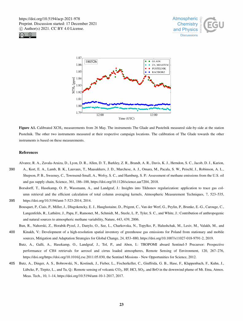
Figure A1. Calibrated XCH4 measurements from 26 May. The instruments The Glade and Pustelnik measured side-by-side at the station

Pustelnik. The other two instruments measured at their respective campaign locations. The calibration of The Glade towards the other

instruments is based on these measurements.

References

Alvarez, R. A., Zavala-Araiza, D., Lyon, D. R., Allen, D. T., Barkley, Z. R., Brandt, A. R., Davis, K. J., Herndon, S. C., Jacob, D. J., Karion,

A., Kort, E. A., Lamb, B. K., Lauvaux, T., Maasakkers, J. D., Marchese, A. J., Omara, M., Pacala, S. W., Peischl, J., Robinson, A. L.,390

Shepson, P. B., Sweeney, C., Townsend-Small, A., Wofsy, S. C., and Hamburg, S. P.: Assessment of methane emissions from the U.S. oil

and gas supply chain, Science, 361, 186–188, https://doi.org/10.1126/science.aar7204, 2018.

Borsdorff, T., Hasekamp, O. P., Wassmann, A., and Landgraf, J.: Insights into Tikhonov regularization: application to trace gas col-

umn retrieval and the efficient calculation of total column averaging kernels, Atmospheric Measurement Techniques, 7, 523–535,

https://doi.org/10.5194/amt-7-523-2014, 2014.395

Bousquet, P., Ciais, P., Miller, J., Dlugokencky, E. J., Hauglustaine, D., Prigent, C., Van der Werf, G., Peylin, P., Brunke, E.-G., Carouge, C.,

Langenfelds, R., Lathière, J., Papa, F., Ramonet, M., Schmidt, M., Steele, L. P., Tyler, S. C., and White, J.: Contribution of anthropogenic

and natural sources to atmospheric methane variability, Nature, 443, 439, 2006.

Bun, R., Nahorski, Z., Horabik-Pyzel, J., Danylo, O., See, L., Charkovska, N., Topylko, P., Halushchak, M., Lesiv, M., Valakh, M., and

Kinakh, V.: Development of a high-resolution spatial inventory of greenhouse gas emissions for Poland from stationary and mobile400

sources, Mitigation and Adaptation Strategies for Global Change, 24, 853–880, https://doi.org/10.1007/s11027-018-9791-2, 2019.

Butz, A., Galli, A., Hasekamp, O., Landgraf, J., Tol, P., and Aben, I.: TROPOMI aboard Sentinel-5 Precursor: Prospective

performance of CH4 retrievals for aerosol and cirrus loaded atmospheres, Remote Sensing of Environment, 120, 267–276,

https://doi.org/https://doi.org/10.1016/j.rse.2011.05.030, the Sentinel Missions - New Opportunities for Science, 2012.

Butz, A., Dinger, A. S., Bobrowski, N., Kostinek, J., Fieber, L., Fischerkeller, C., Giuffrida, G. B., Hase, F., Klappenbach, F., Kuhn, J.,405

Lübcke, P., Tirpitz, L., and Tu, Q.: Remote sensing of volcanic CO2, HF, HCl, SO2, and BrO in the downwind plume of Mt. Etna, Atmos.

Meas. Tech., 10, 1–14, https://doi.org/10.5194/amt-10-1-2017, 2017.

23


Chen, J., Viatte, C., Hedelius, J. K., Jones, T., Franklin, J. E., Parker, H., Gottlieb, E. W., Wennberg, P. O., Dubey, M. K., and

Wofsy, S. C.: Differential column measurements using compact solar-tracking spectrometers, Atmos. Chem. Phys., 16, 8479–8498,

https://doi.org/10.5194/acp-16-8479-2016, 2016.410

Conley, S., Franco, G., Faloona, I., Blake, D. R., Peischl, J., and Ryerson, T. B.: Methane emissions from the 2015 Aliso Canyon blowout in

Los Angeles, CA, Science, 351, 1317–1320, https://doi.org/10.1126/science.aaf2348, 2016.

Dietrich, F., Chen, J., Voggenreiter, B., Aigner, P., Nachtigall, N., and Reger, B.: MUCCnet: Munich Urban Carbon Column network,

Atmospheric Measurement Techniques, 14, 1111–1126, https://doi.org/10.5194/amt-14-1111-2021, 2021.

Dlugokencky, E.: NOAA/GML methane trends, https://esrl.noaa.gov/gmd/ccgg/trends_ch4/, accessed: 2021-07-09, 2021.415

Dreger, M.: Methane Emissions and Hard Coal Production in the Upper Silesian Coal Basin in Relation to the Greenhouse Effect Increase

in Poland in 1994-2018, Mining Science, 28, 59–76, https://doi.org/10.37190/msc212805, 2021.

ESRI: DeLorme World Base Map, http://server.arcgisonline.com/ArcGIS/rest/services/Specialty/DeLorme_World_Base_Map/MapServer/

export?bbox=465524.673242,223740.873843,484241.251687,238103.141466&bboxSR=2180&imageSR=2180&size=1500,1151&

dpi=96&format=png32&f=imageC, 2019.420

Fiehn, A., Kostinek, J., Eckl, M., Klausner, T., Gałkowski, M., Chen, J., Gerbig, C., Röckmann, T., Maazallahi, H., Schmidt, M., Korben,

P., Neçki, J., Jagoda, P., Wildmann, N., Mallaun, C., Bun, R., Nickl, A.-L., Jöckel, P., Fix, A., and Roiger, A.: Estimating CH4, CO2 and

CO emissions from coal mining and industrial activities in the Upper Silesian Coal Basin using an aircraft-based mass balance approach,

Atmospheric Chemistry and Physics, 20, 12 675–12 695, https://doi.org/10.5194/acp-20-12675-2020, 2020.

Frey, M., Hase, F., Blumenstock, T., Groß, J., Kiel, M., Mengistu Tsidu, G., Schäfer, K., Sha, M. K., and Orphal, J.: Calibration and425

instrumental line shape characterization of a set of portable FTIR spectrometers for detecting greenhouse gas emissions, Atmos. Meas.

Tech., 8, 3047–3057, https://doi.org/10.5194/amt-8-3047-2015, 2015.

Frey, M., Sha, M. K., Hase, F., Kiel, M., Blumenstock, T., Harig, R., Surawicz, G., Deutscher, N. M., Shiomi, K., Franklin, J. E., Bösch,

H., Chen, J., Grutter, M., Ohyama, H., Sun, Y., Butz, A., Mengistu Tsidu, G., Ene, D., Wunch, D., Cao, Z., Garcia, O., Ramonet, M.,

Vogel, F., and Orphal, J.: Building the COllaborative Carbon Column Observing Network (COCCON): long-term stability and ensemble430

performance of the EM27/SUN Fourier transform spectrometer, Atmos. Meas. Tech., 12, 1513–1530, https://doi.org/10.5194/amt-12-

1513-2019, 2019.

Gałkowski, M., Fiehn, A., Swolkien, J., Stanisavljevic, M., Korben, P., Menoud, M., Necki, J., Roiger, A., Röckmann, T., Gerbig, C., and

Fix, A.: Emissions of CH4 and CO2 over the Upper Silesian Coal Basin (Poland) and its vicinity, https://doi.org/10.18160/3K6Z-4H73,

2021.435

Gisi, M., Hase, F., Dohe, S., Blumenstock, T., Simon, A., and Keens, A.: XCO2-measurements with a tabletop FTS using solar absorption

spectroscopy, Atmos. Meas. Tech., 5, 2969–2980, https://doi.org/10.5194/amt-5-2969-2012, 2012.

Golub, G. H. and Von Matt, U.: Tikhonov regularization for large scale problems, Citeseer, 1997.

Granier, C., Darras, S., Denier Van Der Gon, H., Jana, d., Elguindi, N., Bo, g., Michael, g., Marc, g., Jalkanen, J.-P., Kuenen, J., Liousse, C.,

Quack, B., Simpson, D., and Sindelarova, K.: The Copernicus Atmosphere Monitoring Service global and regional emissions (April 2019440

version), Research report, Copernicus Atmosphere Monitoring Service, https://doi.org/10.24380/d0bn-kx16, 2019.

Hansen, P. C.: The L-curve and its use in the numerical treatment of inverse problems, 1999.

Hansen, P. C. and O’Leary, D. P.: The Use of the L-Curve in the Regularization of Discrete Ill-Posed Problems, SIAM Journal on Scientific

Computing, 14, 1487–1503, https://doi.org/10.1137/0914086, 1993.

24


Hase, F., Hannigan, J., Coffey, M., Goldman, A., Höpfner, M., Jones, N., Rinsland, C., and Wood, S.: Intercomparison of retrieval445

codes used for the analysis of high-resolution, ground-based FTIR measurements, J. Quant. Spectrosc. Radiat. Transfer, 87, 25 – 52,

https://doi.org/10.1016/j.jqsrt.2003.12.008, 2004.

Hase, F., Frey, M., Blumenstock, T., Groß, J., Kiel, M., Kohlhepp, R., Mengistu Tsidu, G., Schäfer, K., Sha, M. K., and Orphal, J.: Application

of portable FTIR spectrometers for detecting greenhouse gas emissions of the major city Berlin, Atmos. Meas. Tech., 8, 3059–3068,

https://doi.org/10.5194/amt-8-3059-2015, 2015.450

Hase, F., Frey, M., Kiel, M., Blumenstock, T., Harig, R., Keens, A., and Orphal, J.: Addition of a channel for XCO observations to a portable

FTIR spectrometer for greenhouse gas measurements, Atmos. Meas. Tech., 9, 2303–2313, https://doi.org/10.5194/amt-9-2303-2016, 2016.

Hmiel, B., Petrenko, V. V., Dyonisius, M. N., Buizert, C., Smith, A. M., Place, P. F., Harth, C., Beaudette, R., Hua, Q., Yang, B., Vimont,

I., Michel, S. E., Severinghaus, J. P., Etheridge, D., Bromley, T., Schmitt, J., Faïn, X., Weiss, R. F., and Dlugokencky, E.: Preindustrial

14CH4 indicates greater anthropogenic fossil CH4 emissions, Nature, 578, 409–412, https://doi.org/10.1038/s41586-020-1991-8, 2020.455

IPCC: Climate Change 2013: The Physical Science Basis. Contribution of Working Group I to the Fifth Assessment Report of the

Intergovernmental Panel on Climate Change, Cambridge University Press, Cambridge, United Kingdom and New York, NY, USA,

https://doi.org/10.1017/CBO9781107415324, 2013.

Janssens-Maenhout, G., Crippa, M., Guizzardi, D., Muntean, M., Schaaf, E., Dentener, F., Bergamaschi, P., Pagliari, V., Olivier, J. G. J.,

Peters, J. A. H. W., van Aardenne, J. A., Monni, S., Doering, U., and Petrescu, A. M. R.: EDGAR v4.3.2 Global Atlas of the three major460

Greenhouse Gas Emissions for the period 1970–2012, Earth System Science Data Discussions, 2017, 1–55, https://doi.org/10.5194/essd-

2017-79, 2017.

Jöckel, P., Tost, H., Pozzer, A., Kunze, M., Kirner, O., Brenninkmeijer, C. A. M., Brinkop, S., Cai, D. S., Dyroff, C., Eckstein, J., Frank, F.,

Garny, H., Gottschaldt, K.-D., Graf, P., Grewe, V., Kerkweg, A., Kern, B., Matthes, S., Mertens, M., Meul, S., Neumaier, M., Nützel, M.,

Oberländer-Hayn, S., Ruhnke, R., Runde, T., Sander, R., Scharffe, D., and Zahn, A.: Earth System Chemistry integrated Modelling (ES-465

CiMo) with the Modular Earth Submodel System (MESSy) version 2.51, Geosci. Model Dev., 9, 1153–1200, https://doi.org/10.5194/gmd-

9-1153-2016, 2016.

Jones, T. S., Franklin, J. E., Chen, J., Dietrich, F., Hajny, K. D., Paetzold, J. C., Wenzel, A., Gately, C., Gottlieb, E., Parker, H., Dubey,

M., Hase, F., Shepson, P. B., Mielke, L. H., and Wofsy, S. C.: Assessing urban methane emissions using column-observing portable

Fourier transform infrared (FTIR) spectrometers and a novel Bayesian inversion framework, Atmospheric Chemistry and Physics, 21,470

13 131–13 147, https://doi.org/10.5194/acp-21-13131-2021, 2021.

Kirschke, S., Bousquet, P., Ciais, P., Saunois, M., Canadell, J. G., Dlugokencky, E. J., Bergamaschi, P., Bergmann, D., Blake, D. R., Bruhwiler,

L., Cameron-Smith, P., Castaldi, S., Chevallier, F., Feng, L., Fraser, A., Heimann, M., Hodson, E. L., Houweling, S., Josse, B., Fraser, P. J.,

Krummel, P. B., Lamarque, J.-F., Langenfelds, R. L., Le Quéré, C., Naik, V., O’Doherty, S., Palmer, P. I., Pison, I., Plummer, D., Poulter,

B., Prinn, R. G., Rigby, M., Ringeval, B., Santini, M., Schmidt, M., Shindell, D. T., Simpson, I. J., Spahni, R., Steele, L. P., Strode, S. A.,475

Sudo, K., Szopa, S., van der Werf, G. R., Voulgarakis, A., van Weele, M., Weiss, R. F., Williams, J. E., and Zeng, G.: Three decades of

global methane sources and sinks, Nature Geoscience, 6, 813–823, https://doi.org/10.1038/ngeo1955, 2013.

Kostinek, J., Roiger, A., Eckl, M., Fiehn, A., Luther, A., Wildmann, N., Klausner, T., Fix, A., Knote, C., Stohl, A., and Butz, A.: Estimating

Upper Silesian coal mine methane emissions from airborne in situ observations and dispersion modeling, Atmospheric Chemistry and

Physics Discussions, 2020, 1–24, https://doi.org/10.5194/acp-2020-962, 2020.480

Krautwurst, S., Gerilowski, K., Borchardt, J., Wildmann, N., Galkowski, M., Swolkien, J., Marshall, J., Fiehn, A., Roiger, A., Ruhtz, T.,

Gerbig, C., Necki, J., Burrows, J. P., Fix, A., and Bovensmann, H.: Quantification of CH4 coal mining emissions in Upper Silesia by passive

25


airborne remote sensing observations with the MAMAP instrument during CoMet, Atmospheric Chemistry and Physics Discussions, 2021,

1–39, https://doi.org/10.5194/acp-2020-1014, 2021.

Loulergue, L., Schilt, A., Spahni, R., Masson-Delmotte, V., Blunier, T., Lemieux, B., Barnola, J.-M., Raynaud, D., Stocker, T. F.,485

and Chappellaz, J.: Orbital and millennial-scale features of atmospheric CH4 over the past 800,000 years, Nature, 453, 383–386,

https://doi.org/10.1038/nature06950, 2008.

Luther, A., Kleinschek, R., Scheidweiler, L., Defratyka, S., Stanisavljevic, M., Forstmaier, A., Dandocsi, A., Wolff, S., Dubravica, D.,

Wildmann, N., Kostinek, J., Jöckel, P., Nickl, A.-L., Klausner, T., Hase, F., Frey, M., Chen, J., Dietrich, F., Necki, J., Swolkien, J., Fix,

A., Roiger, A., and Butz, A.: Quantifying CH4 emissions from hard coal mines using mobile sun-viewing Fourier transform spectrometry,490

Atmospheric Measurement Techniques, 12, 5217–5230, https://doi.org/10.5194/amt-12-5217-2019, 2019.

Makarova, M. V., Alberti, C., Ionov, D. V., Hase, F., Foka, S. C., Blumenstock, T., Warneke, T., Virolainen, Y., Kostsov, V., Frey, M.,

Poberovskii, A. V., Timofeyev, Y. M., Paramonova, N., Volkova, K. A., Zaitsev, N. A., Biryukov, E. Y., Osipov, S. I., Makarov,

B. K., Polyakov, A. V., Ivakhov, V. M., Imhasin, H. K., and Mikhailov, E. F.: Emission Monitoring Mobile Experiment (EMME): an

overview and first results of the St. Petersburg megacity campaign-2019, Atmospheric Measurement Techniques Discussions, 2020, 1–45,495

https://doi.org/10.5194/amt-2020-87, 2020.

Menoud, M., van der Veen, C., Necki, J., Bartyzel, J., Szénási, B., Stanisavljevic, M., Pison, I., Bousquet, P., and Röckmann, T.:

Methane (CH4) sources in Krakow, Poland: insights from isotope analysis, Atmospheric Chemistry and Physics, 21, 13 167–13 185,

https://doi.org/10.5194/acp-21-13167-2021, 2021.

NCEP: NCEP GDAS/FNL 0.25 Degree Global Tropospheric Analyses and Forecast Grids, https://doi.org/10.5065/D65Q4T4Z, 2017.500

Nickl, A.-L., Mertens, M., Roiger, A., Fix, A., Amediek, A., Fiehn, A., Gerbig, C., Galkowski, M., Kerkweg, A., Klausner, T., Eckl, M.,

and Jöckel, P.: Hindcasting and forecasting of regional methane from coal mine emissions in the Upper Silesian Coal Basin using the

online nested global regional chemistry–climate model MECO(n) (MESSy v2.53), Geoscientific Model Development, 13, 1925–1943,

https://doi.org/10.5194/gmd-13-1925-2020, 2020.

Nisbet, E. G., Dlugokencky, E. J., and Bousquet, P.: Methane on the Rise – Again, Science, 343, 493–495,505

https://doi.org/10.1126/science.1247828, 2014.

Phillips, D. L.: A Technique for the Numerical Solution of Certain Integral Equations of the First Kind, J. ACM, 9, 84–97,

https://doi.org/10.1145/321105.321114, 1962.

Rodgers, C. D.: Inverse methods for atmospheric sounding: theory and practice, vol. 2, World scientific, 2000.

Rothman, L., Gordon, I., Barbe, A., Benner, D., Bernath, P., Birk, M., Boudon, V., Brown, L., Campargue, A., Champion, J.-P., Chance,510

K., Coudert, L., Dana, V., Devi, V., Fally, S., Flaud, J.-M., Gamache, R., Goldman, A., Jacquemart, D., Kleiner, I., Lacome, N., Lafferty,

W., Mandin, J.-Y., Massie, S., Mikhailenko, S., Miller, C., Moazzen-Ahmadi, N., Naumenko, O., Nikitin, A., Orphal, J., Perevalov, V.,

Perrin, A., Predoi-Cross, A., Rinsland, C., Rotger, M., Šimecková, M., Smith, M., Sung, K., Tashkun, S., Tennyson, J., Toth, R., Vandaele,

A., and Auwera, J. V.: The HITRAN 2008 molecular spectroscopic database, J. Quant. Spectrosc. Radiat. Transfer, 110, 533 – 572,

https://doi.org/10.1016/j.jqsrt.2009.02.013, 2009.515

Saunois, M., Stavert, A. R., Poulter, B., Bousquet, P., Canadell, J. G., Jackson, R. B., Raymond, P. A., Dlugokencky, E. J., Houweling, S.,

Patra, P. K., Ciais, P., Arora, V. K., Bastviken, D., Bergamaschi, P., Blake, D. R., Brailsford, G., Bruhwiler, L., Carlson, K. M., Carrol,

M., Castaldi, S., Chandra, N., Crevoisier, C., Crill, P. M., Covey, K., Curry, C. L., Etiope, G., Frankenberg, C., Gedney, N., Hegglin,

M. I., Höglund-Isaksson, L., Hugelius, G., Ishizawa, M., Ito, A., Janssens-Maenhout, G., Jensen, K. M., Joos, F., Kleinen, T., Krummel,

P. B., Langenfelds, R. L., Laruelle, G. G., Liu, L., Machida, T., Maksyutov, S., McDonald, K. C., McNorton, J., Miller, P. A., Melton,520

26


J. R., Morino, I., Müller, J., Murguia-Flores, F., Naik, V., Niwa, Y., Noce, S., O’Doherty, S., Parker, R. J., Peng, C., Peng, S., Peters, G. P.,

Prigent, C., Prinn, R., Ramonet, M., Regnier, P., Riley, W. J., Rosentreter, J. A., Segers, A., Simpson, I. J., Shi, H., Smith, S. J., Steele, L. P.,

Thornton, B. F., Tian, H., Tohjima, Y., Tubiello, F. N., Tsuruta, A., Viovy, N., Voulgarakis, A., Weber, T. S., van Weele, M., van der Werf,

G. R., Weiss, R. F., Worthy, D., Wunch, D., Yin, Y., Yoshida, Y., Zhang, W., Zhang, Z., Zhao, Y., Zheng, B., Zhu, Q., Zhu, Q., and Zhuang,

Q.: The Global Methane Budget 2000–2017, Earth System Science Data, 12, 1561–1623, https://doi.org/10.5194/essd-12-1561-2020,525

2020.

Schwietzke, S., Sherwood, O. A., Bruhwiler, L. M., Miller, J. B., Etiope, G., Dlugokencky, E. J., Michel, S. E., Arling, V. A., Vaughn,

B. H., White, J. W., and Tans, P. P.: Upward revision of global fossil fuel methane emissions based on isotope database, Nature, 538, 88,

https://doi.org/10.1038/nature19797, 2016.

Skamarock, W. C., Klemp, J. B., Dudhia, J., Gill, D. O., Barker, D. M., Duda, M. G., Huang, X.-Y., Wang, W., and Powers, J. G.: A description530

of the Advanced Research WRF version 4, in: NCAR Tech. Note NCAR/TN-556+ STR, https://doi.org/10.5065/1dfh-6p97, 2019.

Swolkien, J.: Polish underground coal mines as point sources of methane emission to the atmosphere, International Journal of Greenhouse

Gas Control, 94, 102 921, https://doi.org/https://doi.org/10.1016/j.ijggc.2019.102921, 2020.

Tikhonov, A. N.: On the solution of ill-posed problems and the method of regularization, in: Doklady Akademii Nauk, vol. 151, pp. 501–504,

Russian Academy of Sciences, 1963.535

Toon, G. C.: Atmospheric Line List for the 2014 TCCON Data Release, https://doi.org/10.14291/tccon.ggg2014.atm.r0/1221656, 2017.

Twomey, S.: On the Numerical Solution of Fredholm Integral Equations of the First Kind by the Inversion of the Linear System Produced by

Quadrature, J. ACM, 10, 97–101, https://doi.org/10.1145/321150.321157, 1963.

Vasiljevic, N., Lea, G., Courtney, M., Cariou, J.-P., Mann, J., and Mikkelsen, T.: Long-range WindScanner system, Remote Sens., 8, 896,

https://doi.org/10.3390/rs8110896, 2016.540

Vogel, F. R., Frey, M., Staufer, J., Hase, F., Broquet, G., Xueref-Remy, I., Chevallier, F., Ciais, P., Sha, M. K., Chelin, P., Jeseck, P., Janssen,

C., Té, Y., Groß, J., Blumenstock, T., Tu, Q., and Orphal, J.: XCO2 in an emission hot-spot region: the COCCON Paris campaign 2015,

Atmospheric Chemistry and Physics, 19, 3271–3285, https://doi.org/10.5194/acp-19-3271-2019, 2019.

Wildmann, N., Vasiljevic, N., and Gerz, T.: Wind turbine wake measurements with automatically adjusting scanning trajectories in a multi-

Doppler lidar setup, Atmospheric Measurement Techniques, 11, 3801–3814, https://doi.org/10.5194/amt-11-3801-2018, 2018.545

Wildmann, N., Päschke, E., Roiger, A., and Mallaun, C.: Towards improved turbulence estimation with Doppler wind lidar velocity-azimuth

display (VAD) scans, Atmospheric Measurement Techniques, 13, 4141–4158, https://doi.org/10.5194/amt-13-4141-2020, 2020.

Worden, J. R., Bloom, A. A., Pandey, S., Jiang, Z., Worden, H. M., Walker, T. W., Houweling, S., and Röckmann, T.: Reduced biomass

burning emissions reconcile conflicting estimates of the post-2006 atmospheric methane budget, Nature communications, 8, 2227,

https://doi.org/10.1038/s41467-017-02246-0, 2017.550

27


Observational constraints on methane emissions from Polish ...

Documents

Transcript of Observational constraints on methane emissions from Polish ...