Experiments and Simulations of Lean Methane Combustion

L I C� E N 1- I A T E T H E S I S

Experiments and Simulations of

Lean Methane Combustion

Jenny Lindberg

Lulea Uruvers1ty ot fechnology

Department of Applied Physics and Mechanical Engineering

Division of Energy Engineering

2004:61 I 1ssN: 1402-1757 I ISRN: uu-uc -- 041'61 -- SE

LULELTEKNISKA UNIVERSITET

Experiments and Simulations of Lean Methane Combustion

Jenny Lindberg

Division of Energy engineering Department of Applied Physics and Mechanical Engineering

Luleå University of Technology SE-97187 Luleå

Sweden

The thesis will be presented with permission of the Faculty Board at Luleå University of Technology in room E231 at Luleå University of Technology on Friday the 17th of December 2004 at 9.00.

Licentiate Thesis: 2004:61 ISSN: 1402-1757 ISRN: LTU-LIC-04/61—SE

PREFACE

The work presented in this thesis has been performed at the division of Energy Engineering at Luleå University of Technology. It deals with numerical simu-lations of gas phase combustion and the work has been funded by the Swedish energy agency and the program for small scale combustion.

The concept of learning is a central idea in the world inside a university, but sometimes we forget learning is not only about academic credits. This thesis is the fruit of my first journey as a graduate student and my first real contact with the field of research. It is a document of the academic learning process which I have undergone. But there is a larger and more important process of learning not to be seen in this document. A learning process initiated by the people who have shared this part of life's journey with me. I would here like to take the opportunity of addressing my gratitude towards some of the people which presence has made my life richer.

First, I would like to thank my supervisor, Dr. Roger Hermansson, for his time and guidance. Our collaboration have taught me to be more versatile in my way of expressing myself.

The experimental studies have been performed at the Energy Technology Center in Piteå and I want to thank Esbjörn Pettersson, for all time spent in the laboratory with experiments and gas analysis. I have learned the skill of accuracy from you.

To the Graduate school for Women (2000-2003), I am grateful for the open-ness in which you have shared your stories. You have taught me to be humble to life. A special thank you to Malin and Kristina, for your support and en-couragement. In our friendship I have found the strength to ask the difficult questions.

Ingegerd Palm& president of Luleå University of Technology, who has served as my mentor during one year (09/03-09/04), thank you for all the fruitful con-versations. In your company I have found the patients to follow the rhythm of life. My gratitude also goes to Marianne Åström, you have taught me the skill to listen not only to others but to myself and given me the tools to value the most important person in my life, me.

Mom and Dad, words seem insufficient, for giving me security and inspiring and encouraging me to learn. For always being there through good and bad. You have shown me the strength of man and given me the base for happiness. To you I am eternally grateful.

Finally I would like to thank my partner in life Jörgen, for pushing and encouraging me to be myself. I learn from you every day.

Jenny Lindberg, Luleå, November 2004

ABSTRACT

Computational fluid dynamics simulation of methane combustion using chem-ical kinetics is studied. Linear least squares data fit to measured concentrations and temperatures is used to modify reaction rate parameters in the Arrhenius rate equation for combustion of methane. The modification of reaction rate parameters influences the result of CFD-simulations to predict combustion at experimental conditions where the Fluent rate equation failed. This first test shows promising results. However, to further develop a global reaction model for combustion of methane and other more complex fuels, a more extensive experimental study is required. The reaction rate for combustion of methane is rapid making ordinary sampling techniques for measuring to crude to collect sufficient amount of data for modification.

An alternative method for assessing the space discretization error is pro-posed. Richardson extrapolation is the most common model used for assess-ment of solution accuracy but the rigidity of the method allows little variation in the results. For engineering purposes qualitative methods can be sufficient for error assessment. Here the space discretization error of a two-dimensional axisymmetric simulation of combustion of methane in turbulent flow is stud-ied. Profiles of temperature and carbon dioxide concentration are investigated and a second order polynomial fit is compared to the Richardson extrapolation. The profiles indicate grid independency of the solution but the Richardson method does not. The second order polynomial fit gives a better goodness-of-fit than obtained when using Richardson. By studying the first and second order terms of the polynomial fitted to the result of the simulations an estima-tion of the reaction order can be obtained.

Keywords: CFD, combustion, methane, rate parameters, error assessment

THESIS

This thesis consists of a theoretical survey and the two appended papers:

Paper I Lindberg, J. and Hermansson, R.; Modification of Reaction Rate Pa-rameters for Combustion of Methane based on Experimental Investi-gation at Furnace-like Conditions; Energy and Fuels, 18, 1482-1484, 2004.

Paper!! Lindberg, J. and Cervantes, M.J.; Space Discretization Error of Meth-ane Combustion Simulations in Turbulent Flow. To be submitted for publication.

During this process the work has lead me down many dead ends. How-ever, although these dead ends have not resulted in publishable material my understanding of the problem, its complexity and the tools for solution can not be ignored. Therefore, I have chosen to dedicate one chapter of the survey, section 8, to summarize the information and results on the subject that is not presented in the two papers of the thesis.

CONTENTS

1 INTRODUCTION 1 1.1 Background 1 1.2 CFD and combustion 1 1.3 Numerical errors 2 1.4 Scope of the thesis 3

2 THE DISCRETIZATION APPROACH 4

3 TURBULENCE/CHEMISTRY COUPLING 5 3.1 Eddy dissipation Concept model (EDC) 5 3.2 Finite rate/Eddy dissipation 6

4 MODIFICATION OF REACTION RATE PARAMETERS 7 4.1 Modification of reaction rate parameters for a one-step reac-

tion mechanism 7 4.2 Modification of rate parameters for multi-step reaction mech-

anisms 8

5 ASSESSMENT OF THE SPACE DISCRETIZATION ERROR ... 9

6 EXPERIMENTS 10

7 SUMMARY OF APPENDED PAPERS 13 7.1 Paper I 13 7.2 Paper II 15

8 REFLECTION ON KNOWLEDGE ACQUIRED 17

9 CONCLUSION 20

REFERENCES 21

APPENDED PAPERS

I Modification of Reaction Rate Parameters for Combustion of Methane based on Experimental Investigation at Furnace-like Conditions

II Space Discretization Error of Methane Combustion Simulations in Turbu-lent Flow


1 INTRODUCTION

1.1 Background

Research in reduction of pollutants and particle emissions has historically been based on experiments. Modification and development of new combustion equipment are an outcome of experimental trial and error techniques. Due to the increase in computer resources the solution of the equations of fluid mechanics on computers has become a wide spread and useful tool in fluid mechanics and there to related fields. The analysis of fluid flow involving heat transfer and associated phenomena such as chemical reactions by means of computer based simulations has opened up an alternative method in re-search and development and the field is known as computational fluid dynam-ics (CFD). Today CFD is finding its way into process, chemical, civil and envi-ronmental engineering. CFD opens up the opportunity of performing paramet-ric studies and optimizations faster and to a smaller cost than with techniques based solely on experiments.

CFD has several advantages over experimentally based approaches to fluid systems design, e.g. reduction of lead times and costs of new design, ability to study systems where controlled experiments are difficult or impossible to perform, ability to study systems under hazardous conditions at and beyond their normal performance limits and practically unlimited level of detail of results (Versteeg and Malalakesera, 1995).

1.2 CFD and combustion

CFD has become a commonly used tool in modelling the combustion process in a variety of applications in the field of energy engineering. Introducing chemistry into the CFD calculation requires two modelling choices. First, the model for coupling the chemical species to the fluid flow calculation. And second, the model for describing the chemistry of combustion. In this thesis the focus has been the Arrhenius reaction equation (Turns, 2000) for descrip-tion of the chemistry of combustion. Therefore the first modelling choice has been limited to the models implementing chemical species into the CFD code according to the principle of reaction kinetics. The choice of kinetic reaction model in its turn is limited by the computational resources. With the compu-tational resources available the model for describing the chemical process of combustion should to be limited to a maximum of five reaction steps.

Examples of such models are presented by Dryer and Glassman (1973); Westbrook and Dryer (1984); Jones and Lindstedt (1988); Dupont et al. (1993);

1

Jenny Lindberg

Nicol et al (1999). The conditions under which these models are developed are very different and do seldom correspond to conditions in ordinary boilers and furnaces. For example, in Dryer and Glassman (1973) energy release dur-ing experiment is lower than in an ordinary boiler. In Westbrook and Dryer (1984); Jones and Lindstedt (1988) the parameters used for optimization are for laminar flames where most combustion problems are turbulent and in Nicol et al (1999) the reaction model is developed using full chemical kinetic reactor model for optimization.

By modification of the Arrhenius reaction equation corresponding to these models they can be extended to a broader field of applications. Nicol (1995); Nicol et al (1999) presented a method based on linear lest squares data fit to temperatures and concentrations of a full chemical reactor model for modifi-cation of the reaction parameters of the reaction equations. Paper I presents the idea of extending this method of modification to measured temperatures and concentrations for obtaining a simple method for extending the reaction models to a broad set of combustion applications plausible (Lindberg and Her-mansson, 2004).

1.3 Numerical errors

When developing a new reaction model its predictability has to be tested. Preferably by running a CFD simulation on the combustion application of in-terest and comparing results with experimental data. Trustability of the results require an assessment of the numerical accuracy of the CFD solution, quali-tative or quantitative. There are three different types of errors to be aware of when working in the field of CFD, modelling errors, iterative errors and space discretization errors.

Modelling errors, are errors corresponding to the choice of model. Choosing a model that does not describe the physics of the problem of interest introduces an error into the solution. This error is difficult to quantify and the best way to minimize these types of errors is to choose models which performance is well studied for the application of interest.

Iterative errors, are errors introduced when the iterative procedure is inter-rupted to early before the solution is converged. To minimize this type of errors the iterative procedure should be continued until the reduction of residuals give the indication that the solution does not change from iteration to iteration.

Space discretization errors, are errors introduced as a result of too coarse grids. If the grid is too coarse some details of the underlying physics can be lost. The only way to eliminate errors due to coarseness of a grid is to perform a grid dependency study, which is a procedure of successive refinements of an

2


initially coarse grid until certain key results do not change. Then the solution can be considered grid independent (Versteeg and Malalakesera, 1995).

CFD simulation of a combustion problem in turbulent flow means solving approximately 12 equations in every iteration. This is very costly regarding computational resources and the engineer is therefore often limited to rela-tively coarse grids to obtain a solution within reasonable time. The discretiza-tion error plays an important role in the result of any combustion simulation and a systematic study of the grid dependence of the solution should be a part of all high quality CFD studies. In CFD studies on combustion there is little regarding to error estimation.

For CFD to work as an independent engineering tool it is necessary that the development of existing models and of new models continues. The ability to present a measure of the accuracy of the solution is important. A quantitative measure of the numerical uncertainty must be provided when the predictions are presented alone. Paper II presents a study of the discretization error of a two-dimensional axissymmetric combustion simulation.

1.4 Scope of the thesis

This work is meant to be a steppingstone in the path to make CFD a reliable and effective tool for studying combustion problems with chemical kinetics as the base for the description of the chemistry of combustion. The thesis is focusing on the combustion of methane and the software used is Fluent 5 and Fluent 6.

The thesis consists of two papers and a theoretical survey. Paper I presents a method for modification of the in Fluent 5 and 6 built-in kinetic two-step mechanism for combustion of methane based on measured concentrations and temperatures. The objective of Paper I is to investigate the contingency of finding a experimentally based method for modifying reaction rate parameters of the Arrhenius reaction equation for chemical kinetics. A simple method for modification increases the ability to extend today's reaction models to be valid for your application of choice.

Paper II presents an error assessment of the space discretization error of a turbulent combustion simulation. The objective is to give an indication of the convergence behavior of turbulent reactive flow simulations using chemical kinetics for modelling the chemistry of the combustion process. Being able to present an qualitative or quantitative error assessment of the results is essential if a new and improved reaction model based on the modification presented in Paper I is to be achieved.

3

Jenny Lindberg

Pw

1,0

my

0

w

0 w il 0

lo 0 0 0 I

,o 0 0 0 I

,o

Ili Ilk

0

.E.

0

II \

0 I

Ilk 41 IV

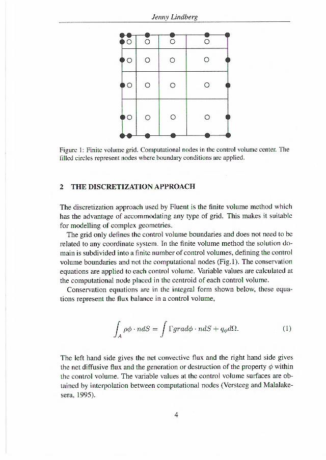
Figure 1: Finite volume grid. Computational nodes in the control volume center. The filled circles represent nodes where boundary conditions are applied.

2 THE DISCRETIZATION APPROACH

The discretization approach used by Fluent is the finite volume method which has the advantage of accommodating any type of grid. This makes it suitable for modelling of complex geometries.

The grid only defines the control volume boundaries and does not need to be related to any coordinate system. In the finite volume method the solution do-main is subdivided into a finite number of control volumes, defining the control volume boundaries and not the computational nodes (Fig.1). The conservation equations are applied to each control volume. Variable values are calculated at the computational node placed in the centroid of each control volume.

Conservation equations are in the integral form shown below, these equa-tions represent the flux balance in a control volume,

L pq5 • ndS = FgradO • ndS + q0d9. (1)

The left hand side gives the net convective flux and the right hand side gives the net diffusive flux and the generation or destruction of the property 0 within the control volume. The variable values at the control volume surfaces are ob-tained by interpolation between computational nodes (Versteeg and Malalake-

sera, 1995).

4


3 TURBULENCE/CHEMISTRY COUPLING

Mixing of reactants and products on a molecular level is one of the most im-portant components in combustion. Therefore in combustion modelling, the chemical reaction rate is closely coupled to the turbulence. This makes one of the most important factors in describing combustion the modelling of the turbulence chemistry coupling.

3.1 Eddy dissipation Concept model (EDC)

Eddy dissipation concept (Byggstol and Magnussen, 1985) is an expansion of the Eddy dissipation model (Magnussen and Hjertager, 1976). It is highly rec-ognized and has been used in this study. The EDC model presumes that chem-ical reactions occur in small turbulent structures so-called fine scales where the mixing is rapid. Chemical reactions occur when reactants are mixed on a molecular level at sufficiently high temperature. In turbulent flow the con-sumption of reactants is highly dependent on this mixing. The processes in micro scale that control the mixing on a molecular level as well as the transfor-mation of turbulent energy into heat are concentrated in small regions called Eddies. The volume of the Eddies corresponds to a small part of the total vol-ume of the fluid. These Eddies in their turn contain fine structures, called fine scales, which dimensions are small in two directions but not in the third. These fine scales are considered to be the source of transformation of turbulent en-ergy into heat and the reactants are here assumed to be mixed on a molecular level. The mixing is considered to be rapid and the fine scales can be viewed as perfectly stirred minireactors (Fig. 3.1 a and b). When modelling the chem-ical reactions in these fine scales the reaction volume and the mass transport between the fine scales and the surrounding gas has to be described.

The relationship between the residence time T* for the components of the fine scales and the time for the combustion reactions Tch contributes to a crite-rion for the combustion limit of the fine scales. When -ra j is small compared to T* the consumption of reactants is independent of the chemical kinetics of the reaction and is solely a factor of the mass transport between the fine scales. When the residence time is less than "rch the combustion will not be completed within the fine scales and the consumption of reactants will be dependent on the chemical kinetics of the reactions.

5

Small Eddy

Minireactor

Reactants Products

Surrounding fluid

Th

p C *fi,

T *

Jenny Lindberg

From mean Flow

Work transfer

Heat

(a) (b)

Figure 2: (a) Transference of turbulent energy. (b) Sketch of a reacting fine scale. Qrad, Cfu, Tand p is the energy resulting from radiation, concentration of fuel, tem-perature and density.

3.2 Finite rate/Eddy dissipation

During the work behind the thesis a few different models for integrating the chemistry of combustion into the fluid flow have been tested. One of them is the finite rate/eddy dissipation model (Fluent, 2001) where the eddy dissi-pation model (Magnussen and Hjertager, 1976) is used in combination with finite rate chemistry to account for the chemical kinetics of combustion. The reaction rate is calculated in two ways 1) as function of the chemical kinetics according to the Arrhenius equation (Turns, 2000), finite rate, and 2) as a func-tion of turbulence according to the eddy dissipation model. The reaction rate is then determined according to the "slowest rate governs". This means that in each control volume and each iteration both the mixing-controlled and the Arrhenius reaction rate are calculated and the lowest value is set to determine the reaction rate.

It should be noted that this model is designed to use the chemical kinetics as a switch to prevent combustion in front of the flame zone in the case of premixed gas; i.e. the kinetics should be set to limit the reaction rate where there is no energy source. Reaction rate parameters could be defined so that the chemical kinetics of reaction is controlling the reaction rate throughout the combustion. However, for this to be useful both the definition and the applica-tion of the model have to be performed on a highly turbulent case, i.e. reactants are perfectly mixed so the mass transport does not become the limiting factor of the reaction rate.

6


4 MODIFICATION OF REACTION RATE PARAMETERS

4.1 Modification of reaction rate parameters for a one-step reaction mech-anism

Modification of the reaction rate parameters in the Arrhenius equations of the reaction models can improve the fluid dynamics software's ability to predict the combustion process. The method described by Nicol et al (1999) for modi-fication of reaction rate parameters has been used on a one step global reaction for combustion of methane in Paper I,

CH4 + 202 -› CO2 + 21120. (I)

The reaction rate is given by

d[CH4] _ A. e — Ea/(RT)[CH4 ] 13 [02r, (2) dt -

where A is the Arrhenius constant describing the collision frequency of mole-cules, Ea is the activation energy in J/kmol, [CH4] and [02] are the concentra-tion of species in kmol/m3.

By a linear least squares data fit of the natural logarithm of the rate ex-pression the rate parameters in Eq. 2 can be modified as follows. The natural logarithm of the rate expression is given by

Ea 1 ln

d[CI14] ln A -I- B • ln[CH4] + C • ln[02] - —R T. (3)

dt The assumption of plug flow convey that the velocity, vx, of the gas in the

reactor at the different sampling locations can be calculated using the cross-sectional area of the tube and the ideal gas law according to

.1.7in Tx vx • —

A

(4)

Tin

where 1,./jr, is the flow rate through the inlet, Tir, is the measured inlet tem-perature and Tx is the measured temperature at each sampling location. The velocity, time and distance covered are related according to

ds dt= --(5)

v(s) ,

By integration of Eq. 5 between the first sampling location so and the fol-lowing 3, the time elapsed when a fluid particle passes from so to s, is given

by

7

Jenny Lindberg

sx ds t =

(6) v(s) •

By using the midpoint rule the integral in Eq. 6 is approximated. Further, the concentration of methane is described as a function of time, t. The reaction rate for methane corresponding to the sample locations is then obtained through numerical differentiation (Truncation error

A linear least squares data fit is performed on Eq. 3 according to the system

- ln d[cH4 ] i - dt

ln(A) i„ d[CH4]2

dt

R - • ,

d[CH4],i - dt -

1 ln[CH4] 111102] 1 ln[CH4]2 111[02]2

T2

, (7)

1 ln[CH]7 ln [02]n

where I ln RcH4 I, ln [CH4] and ln [02] are based on actual cubic meter at tem-perature Tx of measured concentrations. Data points where concentration of methane is zero are excluded since they do not contribute to the solution.

4.2 Modification of rate parameters for multi-step reaction mechanisms

The method for modification of reaction rate parameters presented in the pre-vious section can be expanded to a reaction mechanism consisting of multiple reactions. It is not possible to determine the global input parameters simul-taneously for a multi-step reaction mechanism since the reaction rate and the concentration of one specie affect the reaction rate and the concentration of an other. Therefore an iterative optimization procedure has to be applied when us-ing the method for modification of reaction parameters in a multi-step reaction model.

Consider the reaction mechanism

CH4 + —3

02 CO + 2H20 2 1

CO ± —02 --> CO2 2

(I)

1 CO2 --> CO -I- —

202

8


Consider the first reaction and optimize using the rate of methane destruc-tion, Rate(I). Once the rate of the first reaction is determined from measure-ments, using the method described in section 4.1, the rate of the second reac-tion, Rate(II), can be determined by optimizing using the rate of CO formation also determined from measurements. The rate of formation of CO is temporar-ily assumed to be given by the rate of the first reaction minus the rate of the second,

d[C0] =-- Rate(I) — Rate(II). (8)

dt Then the rate of the third reaction, Rate(III), can be determined by optimiz-

ing the CO2 formation using the reaction rate based on measurements. The rate of CO2 formation is given by the rate of the second reaction minus the rate of the third,

d[CO2] = Rate(II) — Rate(I I I). (9) dt

Once the rate of the third reaction has been approximated the rate of the second reaction can be revised so the CO formation is determined as the sum of the rates of the first and third reaction minus the rate of the second,

d[CO] =-- Rate(I) — Rate(II) + Rate(I I I). (10)

dt

With the revised rate of the second reaction, the rate of the third reaction can be modified again using the rate of CO2 formation for optimization. Thus through an iterative optimization procedure the final rate for the second and third reaction can be determined.

5 ASSESSMENT OF THE SPACE DISCRETIZATION ERROR

The grid has an important influence on the result of a simulation. Space dis-cretization error analysis is necessary to assess the quality of a simulation. Several approaches are at hand, both qualitative and quantitative. One way is to compare profiles obtained with different grids. If the profiles are similar in shape, grid independent solution is assumed and the grid error is assumed negligible.

The most widely used method for quantifying the grid convergence error seems to be the Richardson extrapolation method. Researchers like Roache (1994), Fertziger and Peri (1999), Celik and Zang (1995) and Nordlund and Lundström (2002) all used the method of Richardson extrapolation to estimate

9

Jenny Lindberg

the error in the solution. To perform the extrapolation, at least 3 simulations with different space discretizations are necessary. The results of the simula-tions have to be in the asymptotic region to be reliable. This means that there is a homogenous decrease in the error of the solution as the grid is homoge-nously refined. Unfortunately the asymptotic region can only be guessed, this is the main drawback of the method. The results of the simulations are fitted to the equation

y A + BP, (11)

where A is the solution obtained for an infinite number of cells, h is the inverse averaged cell edge size and a is the average order of the discretization scheme used. The stiffness involved in the determination of the equation parameters often gives unsatisfying results such as a scheme order of 10. Since the the-oretical order of the schemes involved in the simulation are known, a polyno-mial curve fit of the same order or higher could give a better estimation of the discretization order. A method for performing the estimation by studying the first-, second-, third order term, and so on, is proposed in Paper II. By investi-gating the dominating term in the function an estimation of the discretization order is found. However, the method need to be further investigated.

6 EXPERIMENTS

The work behind this thesis consists both of theoretical work and laboratory experiments. The laboratory work has been performed in the aim of retrieving data to use as a basis for modification of reaction rate parameters and for val-idation of reaction models. The experiments are performed on combustion of methane. Methane was chosen since it has a relatively simple composition and is the component almost always present in the case of incomplete combustion of biomass combustion.

The experimental setup of Paper I consisted of a mixing unit for primary and secondary gases such as the one used in Hermansson and Lundqvist (1999). The gas was ignited by inserting an acetylene flame through the ignition tube, and combustion proceeds in the circular duct, 10 cm in diameter, before the flue gas exited through a square chimney (Fig. 3). The combustion chamber was made of stainless steel, 253 MA, and it was insulated with 10 cm of mineral wool.

Gas from the combustion chamber was sampled using an air cooled probe of stainless steel. The tip of the probe consisted of a ceramic tube fitted with a thermocouple for temperature measurements.

10

Outlet Fuel inlet

Air Bed of steal sphereslicooled

Inletjet for air

robe

Micro GC

Ceramic tip with thermocou • le

Ignition tube Wall fitted

thermocou

air

les


Figure 3: Experimental setup in Paper I.

This experimental setup did not result in data sufficient for modification and validation of the reaction model. Since the experimental setup was constructed to achieve perfect mixing between the fuel and oxidizer the experiment was not optimized for retrieving data from the zone of combustion. As a result of the thorough mixing of fuel and oxidizer and the relatively low velocity in the combustion chamber the area where combustion occurs was limited to a narrow zone directly after the supply of oxidizer.

To retrieve data for modification the primary gas was diluted using nitrogen to extend the zone of reaction and to move it into the circular duct where mea-surements in plug flow could be performed. However, the dilution of the gases pushed the system very close to the combustion limit, and as the cooled probe was inserted into the combustion chamber the cooling of the surrounding gas lead to extinction of the flame. The cooling medium was switched from water to air and data from three sampling points in the combustion chamber could be collected.

The degree of turbulence in the experiment in Paper I cause problems in the modification of reaction rate parameters. The Reynolds number of the experiments in Paper I is approximately 1300. To isolate the chemical kinetics of a reaction, i.e. designing experiment so the mass transport does not affect the rate of reaction, the degree of turbulence has to be relatively high. The Dammköhler number is a measure of the degree of mixing and it gives an indication of which phenomenon is the rate controlling one. Dammköhler is the ratio between the turbulent and chemical time scales,

Da = —tt

. (12) tch

With a Da<1 the reactants can be assumed to be perfectly mixed and the chem-ical kinetics thereby controls the reaction rate. With the low Reynolds number of experiment presented in Paper I this was not the case and the mass transport

11

Jenny Lindberg

of species influenced the reaction rate and the chemical kinetics of the reaction were not isolated. Therefore optimization of the chemical kinetics of combus-tion based on these experiment were not satisfactory because the effect of mass transport was not included in the Arrhenius reaction equation (Turns, 2000).

Three sampling points are few to use for modification and validation and even if multiple experiments can be combined for modification the shortcom-ings above convey that the experiment has to be redesigned to give useful re-sults. In an attempt to extend the reaction zone without diluting the combustion gases a new design was tested.

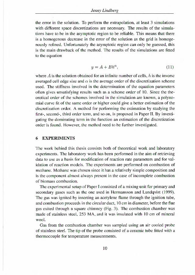
The aim of the second experiment was to stretch the zone of reaction without closing in on the combustion limit and at the same time increasing the degree of turbulence to isolate the chemical kinetics of the reaction. By stretching the reaction zone it could be possible to collect data for modification of reaction rate parameters using available sampling techniques. The second experimen-tal setup consisted of a vertical circular duct with a diameter of 0.035 m and a length of 3 m. The fuel and oxidizer were premixed and supplied through the inlet at the bottom at a velocity of approximately 6 m/s at 2CPC. The com-bustion gases exited through the top where an open flame incinerateed any products of incomplete combustion. The gas was continuously ignited through spark ignition before it passed through a stainless steel net that acted like flame holder.

The concentration of the combustion gases were measured approximately 35 cm above the flame holder where the probe from the experimental setup in Paper I was inserted horizontally into the combustion chamber. The probe was fitted with a ceramic tip with 3 mm in diameter closed at the end and with a hole for sampling of 1.5 mm in diameter facing the flow. The temperature was measured by three thermocouples centered in the cylindrical duct and placed 90 cm apart. The temperature of the wall was measured by three thermocou-ples placed in contact with the outside surface of the wall of the combustion chamber (Fig. 4).

Results from the second experiment indicated that the increase in turbulence isolated the chemical kinetics of combustion, Dammköhler number (Da) is 0.36. The extension of the reaction zone was not achieved in the way that was needed for successful collection of data for modification of reaction parame-ters. A measurable methane concentration was not detected at the sampling location, i.e. the zone of reaction was less than 35 cm and to narrow to collect required amount of data for modification of reaction rate parameters. The aim of the second experiment was to extend the zone of reaction as a result of in-creased velocity of the gas. The result was instead a decrease in Da, resulting

12

Flame holder Cooling water

Thermocouple Outlet

Wall mounted thermocou le

Micro GC

Sparc plug /


Figure 4: Experimental setup in Paper II.

in the desired isolation of the chemical kinetics. But the increase in mixing also increased the rate of combustion and the desired extension of the reaction zone was not achieved.

The conclusion to draw from the two experiments was that the combustion process of methane was too rapid to be studied using ordinary sampling tech-niques. To get required amount of data of temperatures and concentrations for modification of reaction rate parameters requires optical techniques that have the ability to collect a large number of data from a relatively small zone.

7 SUMMARY OF APPENDED PAPERS

All the simulations in the appended papers are performed using the software Fluent. Turbulence is modelled using the standard k-e model with wall func-tions in Paper I and enhanced wall treatment in Paper II. For radiation the discrete ordinate radiation model has been used. The computational domain has been discretized with a structured grid, three-dimensional in Paper I and two-dimensional in Paper II.

7.1 Paper I

The contingency of using the method described by Nicol (1995); Nicol et al (1999), on data from experiments under furnace-like conditions (i.e. moder-ate air factors and considerable heat release) for modification of reaction rate parameters in the Arrhenius equation is investigated. The reaction mechanism used to study the effect of modification of Arrhenius reaction rate parameters

13

3.5

3

2.5

-5 2 >

21" 1.5

1

0.5

00 Distance frgi?) front 0.3 0.45

Jenny Lindberg

Figure 5: [CH4] in volume percent: (*) measured [CH 4]; (-) mean value of [CH4] in the CFD simulation over cross section at each sampling location.

is a one-step global reaction mechanism for combustion of methane. Experiments are performed with the temperature of the primary and sec-

ondary gases at 296 K, 4,1% CH4 by volume, and two air factors, 1.9 and 1.6 respectively. Temperature and concentrations of hydrogen, oxygen, nitro-gen, carbon monoxide, methane, carbon dioxide, ethene, ethane and acetylene were measured. A numerical study of the combustion process is performed by simulating the experiments in Fluent. The geometry was discretized by a three-dimensional structured mesh consisting of 74 004 control volumes. The heat loss from the experiments was calculated using measured temperatures and concentrations at inlet and outlet conditions. The calculated heat loss was then applied to the simulations as a heat flux, 7.7 kW/m2 distributed over the wall of the reactor

The linear least-squares analysis results in A = 348, N, = 1.58.107 J/kmol, B = 0.62 and C = 0.51. The residuals are scattered stochastically and deviate from the fit by 0.6-3.2%. The results can be compared to the Fluent one-step reaction model for methane with A = 2.119 • 1011, E, = 2.027 • 108 J/kmol, B -= 0.2 and C = 1.3. The Dammköhler number indicates that the reactor is not perfectly stirred (Warnatz, 1999). This means that the modification of the reaction rate parameters compensates for both the mixing and the chemical kinetics, which might explain the large decrease in Arrhenius constant.

This first screening indicates that the method is plausible for implementation on experimental data, although a more detailed experimental investigation is required before an improved reaction model can be reached. Measurements are compared to results from simulation in Fig. 5.

Modification of the reaction rate parameters shifts the CFD simulation re-sults closer to measurements. Modelling results from CFD calculations, using

14


EDC on the system, with modified reaction parameters predicts combustion at experimental conditions where the Fluent rate equation fails.

Several difficulties did arise during the experiments, e.g. control of the heat loss from the experiments and to the cooled sampling probe, a limited num-ber of sampling locations in the combustion zone due to the limited flame thickness, and the relatively low degree of turbulence in the reactor. However, because the aim was to investigate the possibility of basing the method (Nicol et al, 1999) on measurements, the experiments were praised to give adequate results for this first study.

7.2 Paper II

Development of improved reaction models requires a measure of the accu-racy of the simulation used for validation of the model against experiments. Richardson extrapolation is the most common model used for assessment of solution accuracy but the rigidity of the method allows little variation in the results. For engineering purposes qualitative methods can be sufficient for er-ror estimation. The aim of Paper II is to assess the accuracy of solution of a turbulent methane combustion simulation terminated on the by Fluent recom-mended convergence criteria, using qualitative and quantitative techniques. An alternative method to Richardson extrapolation suitable for error assessment in engineering applications is proposed.

The space discretization error of a two-dimensional axisymmetric simula-tion of combustion of methane in turbulent flow is studied. Profiles of tem-perature and carbon dioxide concentration are investigated and second order polynomial fits are compared to the Richardson extrapolations.

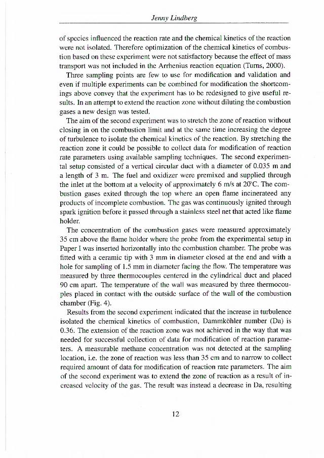
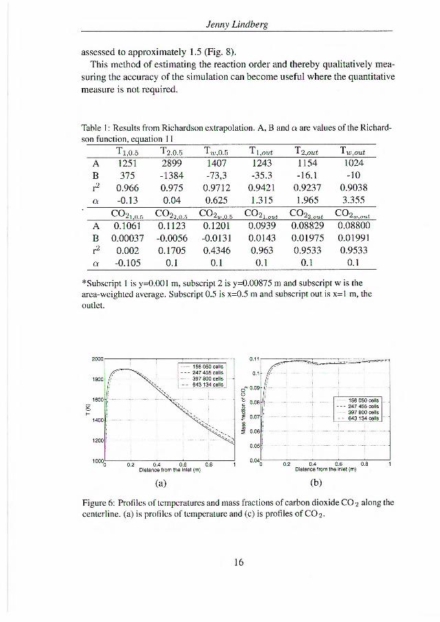
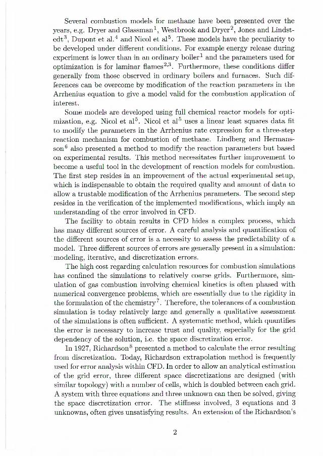
Profiles of temperature and CO2 concentration (Fig. 6) show little variation in the solution indicating grid independency. The results of the extrapolations give poor prediction of the theoretical discretization order. Values of a, Ta-ble 1, have a relevance for 3 of the extrapolations (T,0.5, Ttout, T2,0ut)• The second order polynomial fit gives a better goodness-of-fit than obtained us-ing Richardson (Fig. 7). If the fitted data are not in the asymptotic region the Richardson extrapolation can become unstable as h approaches zero, thereby explaining the sudden drop in Fig. 7

A method for estimating the reaction order from the polynomial fit is pro-posed. By studying the first and second order term of the solution together as function of the characteristic edge length, h, an estimation of the reaction order between one and two can be obtained and used to assess the accuracy of the solution. The second order term is dominant indicating that the order of the discretization scheme is closer to two than one for T and for CO2 the order is

15

2000 156 050 cells

247 455 cells 397 800 cells - - 643 134 cells

1800 -

1600

- 1400

1200

0.2 0.4 0.6 0.8 Distance from the inlet (m)

(a)

10000

- 156 050 cells - - - 247 455 cells 397 800 cells - - 643 134 cells

0.2 0.4 0.6 0.8 1 Distance from the inlet (m)

(b)

0.11

0.1

c>. 0.09-o

• 0.08

)13 • 0.07

0.06

0.05

0.04o

Jenny Lindberg

assessed to approximately 1.5 (Fig. 8). This method of estimating the reaction order and thereby qualitatively mea-

suring the accuracy of the simulation can become useful where the quantitative measure is not required.

Table 1: Results from Richardson extrapolation. A, B and a are values of the Richard-son function, equation 11

T1,03 T2,0.5 T,0.5 Ti,out T2,out Tw,out

A 1251 2899 1407 1243 1154 1024 B 375 -1384 -73,3 -35.3 -16.1 -10 r2 0.966 0.975 0.9712 0.9421 0.9237 0.9038

-0.13 0.04 0.625 1.315 1.965 3.355 CO21 0 5 CO2205 CO2w,05 CO21 ,out CO22 out CO2,, out

A 0.1061 0.11 b 0.1201 0.0939 0.08829 0.08800 B 0.00037 -0.0056 -0.0131 0.0143 0.01975 0.01991 1.2 0.002 0.1705 0.4346 0.963 0.9533 0.9533

-0.105 0.1 0.1 0.1 0.1 0.1

*Subscript 1 is y=0.001 m, subscript 2 is y=0.00875 m and subscript w is the area-weighted average. Subscript 0.5 is x=0.5 m and subscript out is x=1 m, the outlet.

Figure 6: Profiles of temperatures and mass fractions of carbon dioxide CO 2 along the centerline. (a) is profiles of temperature and (c) is profiles of CO 2.

16

2.5 0.5 1 1.5 2 Characteristic edge length, h

(a)

1040

1020:

g 960 -

940 -

920 -

900 -

88%

o Simulation — Richardson - - - Second orde

‘i Simulation — Richardson - - - Second order

0.5 1 1.5 2 2.5 Characteristic edge length, h

(b)

0.085 3 0

1000 -

980

0.115

0.11

00.105

8 0.1 co

.0.095 2

0.09

0.5 1 Characteristic edge length, h

(b)

2.5


Figure 7: Richardson extrapolation and second order polynomial fit to the area-weighted average of T and CO2 at x=0.5 m from results of simulations. (a) is the fit of T and (b) is the fit of CO2.

100

50

0.5 1 1.5 2

2.5 Characteristic edge length

(a)

Figure 8: First and second order term of the second order polynomial fit to the area-weighted average of T and CO2 at x=0.5 m. (a) are terms from fit of T and (b) are terms from fit of CO2.

8 REFLECTION ON KNOWLEDGE ACQUIRED

In the software Fluent there are two models for coupling chemical kinetics to the calculation of turbulent fluid flow, Finite Rate/Eddy dissipation (FR/ED) and the Eddy Dissipation Concept model (EDC) both described in chapter 3. Finite Rate/Eddy Dissipation uses the chemical kinetics as a switch to turn off combustion when the temperature is low, e.g. before the flame in the case of premixed gas. The reaction rate of the Eddy Dissipation model is described by

17

-50

-100

-150

-200

-250o

-0.005

-0.01

-0.0150 3

0.02

0.015

0.01

0.005

3

Jenny Lindberg

e YR = 11/1,, iAp— min(

' k vR,rMw,r)

EPYP Rz.,r = z,r 111 j AB P k j, EN O r

where v, v' and are stoichiometric constants and M„,,i is the molar weight. Yp is the mass fraction of product P, YR is the mass fraction of reactant R, A and B are empirical constants, here equal to 4.0 and 0.5 respectively.

The reaction rate equations of the Eddy dissipation model are not tempera-ture dependent and will predict reaction even when the energy available is not sufficient to sustain combustion.

Since the FR/ED only uses the chemical kinetics as a switch the predictabil-ity of the Arrhenius reaction equation on the combustion process becomes less important. Because the concept is that the slowest rate governs the Arrhenius equation is meant to limit the reaction rate as long as the reactants are cold. As soon as the temperature increases the exponential form of the equation con-tributes to a very rapid increase in the Arrhenius reaction rate. Very quickly the reaction rate for the Eddy dissipation equation will be the slowest and the one governing the rate of reaction until all fuel is consumed.

The EDC on the other hand integrates the chemical kinetics into the fluid flow making the chemical kinetics the only equation for calculation of the re-action rate and controlling the part of the flow where reaction can take place. By assuming chemical reaction only in the smallest eddies in the turbulent flow makes the overall reaction rate dependent on the relationship between residence times in these fine eddies and the chemical kinetic time scale. Eddy Dissipation Concept model is a model much more designed for the task of predicting the process of combustion than the FR/ED model is. On the other hand a correct description of the chemical kinetics of combustion becomes very important when using the EDC model to describe the combustion process as to where the chemical kinetics in the FR/ED model only have to result in a reaction rate high enough for the turbulence dependency to take over.

In order to make a modification of reaction rate parameters in the Arrhenius equation, based on conditions for the specific application in question, detailed experiments have to be performed. It is important to minimize the influence of mixing on the reaction rate. This to isolate the chemical kinetics of reaction and ensure that the data collected describes the chemical kinetics of combus-tion and not the mixing of reactants. A Dammköhler number<1 (see section 6) indicates that the mixing in the reactor is rapid and the chemical kinetics is the

18

(13)

(14)


limiting parameter on the reaction rate (Warnatz, 1999). Perfect mixing or Dammköhler<1 requires a Reynolds number of approximately 20 000,

vD Re = —. (15)

The high Reynolds number required for perfect mixing of reactants results in a velocity of 120 m/s at 1600°C for pipe flow like the setup described for exper-iment presented in Paper II. The viscosity is here approximated to 0.000179 kg/m.s.

An other difficulty in performing these experiments is the collection of data. Since the combustion process is very rapid the area in a reactive fluid flow of combustion where the consumption of fuel and production of flue gas can be observed is limited to a narrow band and therefore ordinary sampling tech-niques can be to crude. A common technique for gas analysis is the gas chro-matography. When using this technique a gas volume is let to pass through a column and depending on the compound the time to pass trough the col-umn differs and the species can be detected on the residence time. The sample should be isokinetic which introduces limitations on the sampling equipment. The narrow reaction zone makes it very difficult to collect multiple data points, which is required to perform the modification. Therefore, optical techniques are required to collect data for modification based on experimental concentra-tions and temperatures.

The idea to slow down the combustion process by cooling the system and thereby stretch the zone of reaction, has been tested and has little effect on the reaction zone. The time scale of the heat transfer from the bulk volume of the fluid is slower than the time scale of the reaction rate, and the result of exter-nal cooling is minimal. The effect of cooling has been studied in simulations and the position of the reaction zone is not influenced by the outside cooling (Fig. 9).

The modification of reaction rate parameters based on experiments during conditions representative for applications of interest, i.e. boilers and furnaces, will be difficult with sampling methods. However, with the use of optical measuring techniques the possibilities open up.

CFD calculations using the Arrhenius theory (Turns, 2000) on combustion is often faced with difficulties obtaining numerical convergence. This is a result of the stiffness of the chemical reaction rate equations (Norton and Vlachos, 2003). Perhaps other models, not persecuted with the same convergence diffi-culties, are more suited for modelling gas phase combustion.

19

-3

-4

-5

-6

-7

-8

-9

- - - Heat loss — Adiabatic

0.02 0.04 0.06 Distance from inlet (m)

_100 0.08

01

Jenny Lindberg

2000

1800 - - - Heat loss — Adiabatic

1600 2.• t; f-

1400 2 C-)

1200 -

0.2 0.4 0.6 0.8 100%

Distance from inlet (m)

(a) (b)

Figure 9: The effect of cooling of the reactor walls on the combustion process. (a) Temperature, and (b) concentration of CH 4 as a function of distance from the inlet.

9 CONCLUSION

Least square analysis of experimental measurements to modify the reaction rate parameters has the contingency to become very useful in further develop-ment of global rate equations. It is a relatively quick method which can pro-cess a large number of experimental data for each modification. The method requires that chemical kinetics of the reactions is isolated in the experiment. To achieve this the degree of turbulence has to be high enough to ensure per-fect mixing of the reactants. When the chemical kinetics of the reactions is isolated the rapid combustion reactions are completed in a narrow band in the combustion chamber making sampling techniques to crude for measuring. To perform detailed measurements in the zone of combustion optical measuring techniques are required.

Polynomial fit of an order equal to or higher than the discretization order has the potential of becoming a useful method for assessing the space discretiza-tion where the accuracy of a quantitative method is not required. Although, the study of profiles of the solutions indicates that the solution is grid independent variations in the solution can be too large for the Richardson method to present a quantitative measure. However, in many engineering applications the accu-racy of the Richardson method is not required. For these types of problems the polynomial fit in combination with the study of profiles can become a useful method in assessing the space discretization error of a simulation. However, further investigation of the method is necessary.

20


REFERENCES

Byggstøl, S., Magnussen, B. E A Model for Flame Extinction in Turbulent Flow, Turbulent shear flows 4, Springer: Berlin, 1985, pp 381-395.

Celik, I., Zang, W-M. Calculation of Numerical Uncertainty using Richard-son extrapolation: Application to some simple Turbulent Flow Calculations, Journal of Fluids Engineering, 1995, vol. 117, pp 439-445,.

Dryer, F. L., Glassman, I. High Temperature Oxidation of CO and CH4, Pro-ceedings of the 14th Symposium (International) on combustion, Combus-tion Institute, Pittsburgh, PA, 1973, pp 987-1003.

Dupont, V.; Pourkashanian, M.; Williams, A. Modelling of Process Heaters Fired by Natural Gas, J. Inst. Energy, 1993, vol. 66, pp 20-28.

Fretziger, J. H., Perid, M. Computational Methods for Fluid Dynamics, second edition; Springer: Berlin, 1996 and 1999, pp 68-84.

Fluent 6 Users Guide; Fluent Inc., Lebanon, NH, 2001, vol. 3, pp 13:10-13.

Hermansson, R., Lundqvist, M., Datorbaserade konstruktionshjälpmedel för miljövänligare biobränsleeldade pannor och kaminer, Swedish Energy Agency ER 8:1999, 1999.

Jones, W. P., Lindstedt, R. P. Global Reaction Schemes for Hydrocarbon Com-bustion, Combustion and Flame 1988, vol. 73, pp 233-249.

Lindberg, J., Hermansson, R. Modification of Reaction Rate Parameters for Combustion of Methane Based on Experimental Investigation at Furnace-like Conditions, Energy Sz Fuels 2004, vol. 18, pp 1482-1484.

Magnussen, B. F.; Hjertager, B. H. On Mathematical Modeling of Turbulent Combustion with Special Emphasis on Soot Formation and Combustion, Proceedings of the 16th Symposium on Combustion, The Combustion Insti-tute: Pittsburgh, PA, 1976, pp 719-729.

Nicol, D. G. A Chemical and Numerical Study of NO and Pollutant Forma-tion in Low-Emissions Combustion, PhD dissertation, 1995, University of Washington, St. Louis, MO.

Nicol, D. G., Malte, P. C., Hamer, A. J., Roby, R. J., Steele, R.C. Develop-ment of a Five-Step Global Methane Oxidation-NO Formation Mechanism for Lean-Premixed Gas Turbine Combustion, Journal of Engineering Gas Turbines Power 1999, vol. 121, pp 272-280.

21

Jenny Lindberg

Nordlund, M., Lundström, T. S., Numerical Simulation of the Permeability of Non-Crimp Fabrics, 14th International Conference on Composite Materials, July 14-18, 2003, San Diego, USA.

Norton, D.G. Vlachos, D.G. Combustion characteristics and flame stability at the micro scale: a CFD study of premixed methane/air mixtures, Chemical Engineering Science, 2003, vol. 58, pp 4871-4882.

Roache, P.J. Perspective: a method for uniform reporting of grid refinement studies, Journal of Fluids Engineering, vol. 116, pp 405-413.

Turns S.R., An Introduction to Combustion-Concepts and Applications, 2nd Edition, chapter 4, pp 111-147, 2000.

Warnatz, J., Maas, U., Dibble, R.W. Combustion: Physical and Chemical Fun-damentals, Modelling and Simulation, Experiments and Pollutant Forma-tion, Berlin: Springer, cop. 1999.

Versteeg, H. K., Malalakesera, W. An introduction to computational fluid dynamics-The finite volume method. Harlow, Longman Scientific Sz Tech-nical, New York, Wiley, 1995.

Westbrook C. K., Dryer F. L. Chemical Kinetic Modeling of Hydrocarbon Combustion, Prog. Energy Combust. and Sci. 1984, vol. 10, pp 1-57.

22

1482 Energy&Fuels2004, 18. 1482-1484

Modification of Reaction Rate Parameters for Combustion of Methane Based on Experimental

Investigation at Furnace-like Conditions

J. Lindberg* and R. Hermansson

Division of Energy Engineering. Luleå University of Technology, SE971 87 Luleå. Sweden

Received February 19, 2004

A method for modifying reaction rate parameters in the Arrhenius rate equation for combustion of methane is proposed. Linear least-squares data fit to measured concentrations and temperatures is used to modify reaction rate parameters in the Arrhenius rate equation for combustion of methane in one step. The modified equation is compared to the one provided by the software Fluent by implementing both into a three-dimensional Fluent simulation. The modification of reaction rate parameters influences the result of computational fluid dynamics simulations to predict combustion at experimental conditions where the Fluent rate equation failed. With modified parameters, the size of the reaction zone increases to give better agreement with experiments than that obtained using the Fluent rate equation. This first test indicates that the method has the contingency of becoming a useful tool for modification of reaction rate parameters though it still needs further development.

Introduction

Computational fluid dynamics (CFD) software is often used to mode) the combustion process in a variety of applications in the field of energy engineering. To keep the computational effort at a reasonable leve!. models used for describing chemical processes of combustion need to be relatively simple. i.e., one to five reaction steps.

Examples of such models for combustion of methane are presented by Dryer and Glassman. 1 Westbrook andDryer,2 Jones and Lindstedt,3 DuPont et al.,4 and Nicol et al.5 The conditions under which these models aredeveloped are very different, seldom similar to conditions in ordinary boilers and fumaces. For example, energy release during the experiment is Jower than that in an ordinary boiler, 1 and the parameters used for optimization are for laminar flames.2·3 Some models are developed using full chemical reactor models for optimization, e.g .. Nicol (1999).5 Nicol5 uses a linear leastsquares data fit to modify the parameters in the Arrhenius rate expression for a three-step reaction mechanism for combustion of methane. By an iterative optimization process, the rate parameters of the three reactions are related to each other. 6

Because the chemical reaction rate is closely coupled to the turbulence, one of the most important factors in

• E-mail: [email protected]. (I) Dryer, F. L.: Glassman. I. Proceedings of the 14th Symposium

(International) on Combustlorr, The Combustion lnstitute: Pittsburgh. PA. 1973: pp 987-!003.

(2) Westbrook. C. K.: Dryer. F. L. Prog. EnergyCombust. Sci. 1984. JO. l-57.

(3) Jones. W. P.: Lindstedt. R. P. Combust. Flame 1988. 73, 233-249.

(4) DuPont. V.: Pourkashanian, M.: Williams, A. J. Inse. Energy 1993. 66. 20

(5) Nicol. D. G.: Malte. P. C.: Hamer, A. J.: Roby, R. J.: Steele, R. C. J. Eng. Gas Turbines Power 1999. 121, 272-280.

describing combustion is modeling of the turbulence chemistry coupling. For turbulent flames, the eddy dissipation concept (EDC7) mode!, which is an expansion of the eddy dissipation model,8 is highly recognized and is used in this study. The EDC mode! presumes that chemical reactions occur in small turbulent structures, so-called fine scales, where the mixing is rapid. These fine scales can be viewed as perfectly stirred minireactors where reactants are mixed on a molecular leve!. The residence time of the components in the fine scales and the time of the chemical reactions together describe the reaction rate. EDC is available in Fluent 6 but has not been available in earlier versions of Fluent.

The eddy dissipation model can be used in combination with finite rate chemistry to account for the chemical kinetics of combustion. In this mode! the reaction rate is set according to the "slowest rate governs".9 This means that in each control volume and iteration both the mixing-controlled and the Arrhenius reaction rate are calculated and the lowest value is set to determine the reaction rate. It should be noted that this model is designed to use the chemical kinetics as a switch to prevent combustion in front of the flame zone in the case of a premixed gas; i.e., the kinetics is set to limit the reaction rate where there is no energy source. The effect of modification on this mode! is also studied. These results are not presented in this paper.

The objective of this work is to investigate the contingency of using the method described by Nicol5·6

(6) Nicol, D. G. Ph.D. Dissertation, University of Washington. St. Louis. MO. 1995.

(7) Byggstol, S.: Magnussen. B. F. Turbulent Shear Flows 4: Springer: Berlin. 1985: pp 381-395.

(8) Magnussen, B. F.: Hjertager. B. H. Proceedings of the 16th Symposium on Combusdon. The Combustion Institute: Pittsburgh. PA. 1976.

(9) Fluent 6 Users Guide: Fluent lnc.: Lebanon. NH, 2001: Vol. 3: pp 1-13.

i0.1021/efD40022x CCC: $27.50 © 2004 American Chemical Society Published an Web 07/29/2004

Combustion of Methane

Outlet Fle! kget 1 Air Bed of steal sphere cooled

Inletiet tor air ,probe

4,1.11.111.1111111P 11110111111011111111.1111.1110i

\ Ceramic tip with thermocouple

Ignition tube Wall fitted

\thermocouples

Figure 1. Experimental setup.

on data from experiments under furnace-like conditions (i.e., moderate air factors and considerable heat release) for modification of reaction rate parameters in the Arrhenius rate equation. To approach the question at issue, a global reaction mechanism for combustion of methane in one step is used to study the effect of modification of the Arrhenius reaction rate parameters. The modification, of reaction rate parameters, is per-formed by linear least-squares data fit of the experi-mental measurements, in Matlab 6.5. A three-dimen-sional CFD model is used to compare the modified equation to the one-step rate equation provided by the software Fluent.

Experiments The experimental setup consists of a mixing unit for primary

and secondary gases such as the one used in Hermansson and Lundqvist.'° The gas is ignited by inserting an acetylene flame through the ignition tube, and combustion proceeds in a circular duct, 10 cm in diameter, before the flue gas exits through a square chimney (Figure I). The combustion chamber is made of stainless steel, 253MA, and it is insulated with 10 cm of mineral wool.

Gas from the combustion chamber is sampled using an air-cooled probe of stainless steel. The tip of the probe consists of a ceramic tube fitted with a thermocouple for temperature measurement.

Experiments are performed with the temperature of the primary and secondary gases at 296 K, 4.1% CH., by volume, and two air factors, 1.9 and 1.6, respectively. For analysis of hydrogen, oxygen, nitrogen, carbon monoxide, methane, carbon dioxide, ethene, ethane, and acetylene, a two-column Micro gas chromatograph (CP-2002 P from Chrompack) with thermal conductivity detectors and argon as the carrier gas is used.

Modeling and Simulation A numerical study of the combustion process is

performed by simulating the experiments in Fluent. The experimental setup is discretized by a three-dimensional structured mesh consisting of 74 004 hexahedral control volumes using the software Fluent. To account for the heat losses from the flue gas, the heat loss from the experiments is calculated using measured temperatures and concentrations at inlet and outlet conditions. The inlet conditions are represented by measurements above the bed of steal spheres. The outlet conditions are represented by measurements using the probe posi-tioned as far back in the reactor as possible, where an area of 2 cm in diameter of the probe's cooled surface is visible to the gas 15 cm behind the sampling location.

(10) Hermansson, R.; Lundqvist, M. Swedish Energy Agency ER 8:1999, 1999.

Energy & Fuels, Vol. 18, No. 5, 2004 1483

X 10-4

0.05 0.1 0.15 02 t (s)

Figure 2. Measured concentration of methane in the combustion chamber as a function of t according to eq 5.

The calculated heat loss is then applied to the simula-tion as a heat flux, 7.7 kW/m2 distributed over the wall of the reactor.

The method for modification of reaction rate param-eters is tested using a global reaction mechanism for combustion of methane consisting of one reaction

CH4 + 202 — CO2 + 2H20

The reaction rate is given by

d (CH4)

dt = Ae-Ean9CH4] B1021 c (1)

where A is the Arrhenius constant describing the collision frequency of molecules, Ea is the activation energy in J/kmol, and [C1-14] and 1021 are the concentra-tions of species in kmol/m3. The natural logarithm of the rate expression is given by

d (CH4] Ea ln =

dt ln A + B ln (CH4] + C ln 102) --R- 7-

(2)

The assumption of plug flow conveys that the velocity of the gas in the reactor at the different sampling locations can be calculated using the cross-sectional area of the tube and the ideal gas law according to

(3)

where Vin is the flow rate through the inlet, Tin is the measured inlet temperature, and T„ is the measured temperature at each sampling location. The velocity, time, and distance covered are related according to

ds dt = — (4)

v(s)

The integral based on the distance between the first sampling location, so, and the following, s„, gives the time at each location related to so

ds t = f — s') v(s)

By using the midpoint rule, the integral in eq 5 is approximated. Further, the concentration of methane is plotted as a function of time t (Figure 2). The reaction rates for methane corresponding to the sample locations

Micro GC

Micro GC

/Cooling air

(5)

1484 Energy & Fuels. Vol. 18, No. 5, 2004

are then obtained through numerical differentiation [truncation error 0(h2)].

A linear least-squares data fit is performed on eq 2 according to the system

ln [CF14]1 In [02]1 1/ T1 ln ECH412 In 1021 2 1/ T2

ln(A) B C

In [CHI, ln [02],, 1/ T„ — Ea/RT dICH411

In dt

d [CH412 ln

dt (6)

d ECH41„

where Iln RcH4l, In ICH41, and In 1021 are based on actual cubic meters at temperature T for the data points in Figure 2. Data points where the concentration of methane is zero are excluded because they do not contribute to the solution.

The least-squares analysis results in A = 348, E. = 1.58 x 107 J/kmol, B= 0.62, and C= 0.51. The residuals are scattered stochastically and deviate from the fit by 0.6-3.2%. The results can be compared to the Fluent one-step reaction model for methane with A = 2.119 x 10", E. = 2.027 x 108 J/kmol, B = 0.2, and C = 1.3. The Damköhler number indicates that the reactor is not perfectly stirred." This means that the modification of the reaction rate parameters compensates for both the mixing and the chemical kinetics, which might explain the large decrease in the Arrhenius constant.

Results and Discussion

This first screening indicates that the method is plausible for implementation on experimental data, although a more detailed experimental investigation is required before an improved reaction model can be reached.

Modification of the reaction rate parameters shifts the CFD simulations results closer to measurements. Mod-eling results from CFD calculations, using EDC on the system, with modified reaction parameters predicts combustion at experimental conditions where the Fluent rate equation fails. The Fluent rate equation requires an increase in the inlet temperature of 300 °C to predict combustion. When combustion is simulated using the Fluent rate equation, the reaction zone is limited to a narrow zone around the inlet jets.

Visual observation through the ignition tube indicates that the flame irregularly wanders from side to side; this is not described by the steady-state simulation. Measurements were nonisokinetic and sampled over a time interval. Because of the unknown irregularities of the flame, the mean value of the methane concentration over the cylindrical cross section of the CFD model is used for comparison with the measurements in Figure

(11) Warnatz, J.; Maas, U.; Dibble, R. W. Combustion; Springer: Berlin, 1999.

Lindberg and Hermansson

Digiince frö:sig frontYreactölftm) 5 Figure 3. ICH4] in volume percent: (*) measured [CF14]; (—) mean value of [CF14] in the CFD simulation over a cross section at each sampling location.

3. For future work, isokinetic sampling is desired, which enables the use of point values from the CFD calculation for comparison. Figure 3 shows a reaction zone size comparable to the one observed in the measurements.

Several difficulties did arise during the experiments, e.g., control of the heat loss from the reactor and to the cooled sampling probe, a limited number of sampling locations in the combustion zone due to the limited flame thickness, and the relatively low degree of tur-bulence in the reactor. However, because the aim was to investigate the possibility of basing the method on measurements, the experiments were appraised to give adequate results for this first study.

Conclusions

Least-squares analysis of experimental measure-ments to modify the reaction rate parameters has the contingency to become very useful in the further devel-opment of global rate equations. It is a relatively quick method that can process a large number of experimental data for each modification. Therefore, improvements on the experimental setup are essential for this method to become reliable. First, the flow needs to be as close to fully turbulent as possible. By obtaining perfect mixing, i.e., keeping the Damköhler number < 1, the influence of mass and heat transfer due to mixing on the reaction rate is eliminated. Second, the number of sampling locations inside the flame zone needs to be increased. Third, the heat transfer in the experiment has to be measured and modeled in the CDF simulation to achieve a reliable description of the temperature during the reaction. The performed modification of the reaction rate parameters affects the CFD simulation to give a better agreement with experiments.

Modeling of the combustion chemistry using a one-step reaction model is found to be insufficient. The effect that the formation of carbon monoxide has on the reaction rate cannot be ignored and will in the future be included in the combustion model. The iterative optimization presented by Nicol8 will be used to extend the reaction model to multiple reaction steps. If the method shows further success in the development of a reaction model for combustion of methane, the model will be extended to describe the combustion of more complex fuels.

EF040022X

ln at

3.5

3

2.5

3, 2

2, 1.5

1

0.5

00

Space Discretization Error of Methane Combustion Simulations in Turbulent Flow

J. Lindberg* Div. of Energy Engineering

Luleå University of Technology

SE-97187 Luleå, Sweden Phone: +46 70 677 62 73

Fax: +46 920 491074

M.J Cervantest Div. of Fluid Mechanics

Luleå University of Technology

SE-97187 Luleå, Sweden

Phone: +46 920 492143

Fax: +46 920 491074

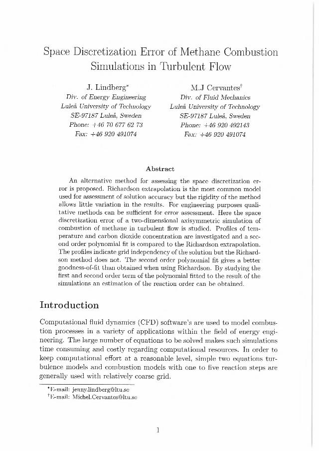
Abstract

An alternative method for assessing the space discretization er-ror is proposed. Richardson extrapolation is the most common model used for assessment of solution accuracy but the rigidity of the method allows little variation in the results. For engineering purposes quali-tative methods can be sufficient for error assessment. Here the space discretization error of a two-dimensional axisymmetric simulation of combustion of methane in turbulent flow is studied. Profiles of tem-perature and carbon dioxide concentration are investigated and a sec-ond order polynomial fit is compared to the Richardson extrapolation. The profiles indicate grid independency of the solution but the Richard-son method does not. The second order polynomial fit gives a better goodness-of-fit than obtained when using Richardson. By studying the first and second order term of the polynomial fitted to the result of the simulations an estimation of the reaction order can be obtained.

Introduction

Computational fluid dynamics (CFD) software's are used to model combus-tion processes in a variety of applications within the field of energy engi-neering. The large number of equations to be solved makes such simulations time consuming and costly regarding computational resources. In order to keep computational effort at a reasonable level, simple two equations tur-bulence models and combustion models with one to five reaction steps are generally used with relatively coarse grid.

*E-mail: jenny.lindbergaltu.se t E-mail: Michel.Cervantesültu.se

1

Several combustion models for methane have been presented over the years, e.g. Dryer and Glassman', Westbrook and Dryer2, Jones and Lindst-edt3, Dupont et al.4 and Nicol et al5. These models have the peculiarity to be developed under different conditions. For example energy release during experiment is lower than in an ordinary boiler' and the parameters used for optimization is for laminar flames2,3. Furthermore, these conditions differ generally from those observed in ordinary boilers and furnaces. Such dif-ferences can be overcome by modification of the reaction parameters in the Arrhenius equation to give a model valid for the combustion application of interest.

Some models are developed using full chemical reactor models for opti-mization, e.g. Nicol et al5. Nicol et al5 uses a linear least squares data fit to modify the parameters in the Arrhenius rate expression for a three-step reaction mechanism for combustion of methane. Lindberg and Hermans-son6 also presented a method to modify the reaction parameters but based on experimental results. This method necessitates further improvement to become a useful tool in the development of reaction models for combustion. The first step resides in an improvement of the actual experimental setup, which is indispensable to obtain the required quality and amount of data to allow a trustable modification of the Arrhenius parameters. The second step resides in the verification of the implemented modifications, which imply an understanding of the error involved in CFD.

The facility to obtain results in CFD hides a complex process, which has many different sources of error. A careful analysis and quantification of the different sources of error is a necessity to assess the predictability of a model. Three different sources of errors are generally present in a simulation: modeling, iterative, and discretization errors.

The high cost regarding calculation resources for combustion simulations has confined the simulations to relatively coarse grids. Furthermore, sim-ulation of gas combustion involving chemical kinetics is often phased with numerical convergence problems, which are essentially due to the rigidity in the formulation of the chemistry7. Therefore, the tolerances of a combustion simulation is today relatively large and generally a qualitative assessment of the simulations is often sufficient. A systematic method, which quantifies the error is necessary to increase trust and quality, especially for the grid dependency of the solution, i.e. the space discretization error.

In 1927, Richardson8 presented a method to calculate the error resulting from discretization. Today, Richardson extrapolation method is frequently used for error analysis within CFD. In order to allow an analytical estimation of the grid error, three different space discretizations are designed (with similar topology) with a number of cells, which is doubled between each grid. A system with three equations and three unknown can then be solved, giving the space discretization error. The stiffness involved, 3 equations and 3 unknowns, often gives unsatisfying results. An extension of the Richardson's

2

method to an ordinary polynomial will allow some variation in the results but still allow an estimation of the discretization order.

The objective of the paper is to investigate the solution of a methane combustion simulation using Nicol's5 reaction model with the standard k turbulence model. Special attention is given to the space discretization error through qualitative and quantitative methods such as profile comparison and Richardson's extrapolation. Then, the results are discussed in detail and compared to experiments and analytical solution.

Simulation of Methane combustion in a turbulent flow

The simulated flow consists of a mixture of methane, air, carbon dioxide (CO2) and water vapor (H20), which is supplied through the inlet of a pipe at a temperature of 1073 K. The pipe has a diameter of 0.035 m and is 1 m long. The calculations are initiated with a domain temperature at 1500 K to ensure combustion. The temperature of the pipe wall is kept constant at 323 K, simulating a cooled combustion chamber. Simulations were performed using the segregated solver of Fluent 6.

Models

Numerical simulations on combustion is demanding regarding the compu-tational resources due to the large number of differential equations to be solved. The axis-symmetry of the geometry allows 2-dimensional simula-tions, which substantially decreases the number of differential equations to be solved and the number of cells. The flow is modelled using the standard turbulence k — e model, the radiation heat transfer using the discrete or-dinates radiation model and the chemical process of combustion with the Arrhenius9 theory, see Table 1 for the different equations. The reaction model described by Nicol et al5 consisting of the three reaction equations,

, 3 Cn4 + —> lAJ 2H20

2 1

CO + —2

02 -> CO2

1 CO2 CO + —

202

is used. Since the chemical reaction rate is closely coupled to turbulence, the turbulence chemistry coupling is of great importance. For turbulent flames, the Eddy Dissipation Concept model (EDC) 19, which is an expansion of the Eddy Dissipation models'', is used in this study. The EDC-model presumes that chemical reaction occurs in small turbulent structures, so

3

a(k f g_) Y Py

a (k f

Continuity:

Momentum:

Energy:

Table 1: Conservation equations = a(pvx ) _L a (pvy)

at L Ps Py

a f ,17 a(pvxvx ) a (pv.voi Pp aTxx _L aTyx D-7 X 722 [ as -F 8Y -F as -F 8y

li(Ph) [a(PhVx) (phVy)1

ax ±

8 (hipDi,,e) Ei ax

a (hipDi fin ÇL

Py

a w9Yi) [a(pYiv.) a(pyv )] a (pDi,,,n a i-) Species: Ps + Ps x

P (pDi,„, 2h- + ay ) +R

Turbulence: ß(pk) + (pkui) = [(u+,) Pk i G k pE S

k

-17 (pe) + k(peui) = [(u + ±,§r, Gk 3

— C2E ± SE

*_viscosity; kf-thermal conductivity;Di diffusivities, k-turbulent kinetic energy, e-turbulent dissipation rate, Ck-generation of turbulent kinetic energy due to mean velocity gradients, C1,6 , C1,6 and C1,6 are constants, crk and a,- turbulent Prantl number and Sk and S, are user defined source terms.

called fine-scales, where the mixing is rapid. These fine-scales can be viewed as perfectly stirred mini-reactors where reactants are mixed on a molecular level. Residence-time of the components in the fine-scales and the time of the chemical reactions, together describe the reaction rate.

Fig. 1 illustrates the solution procedure of the segregated solver in Flu-ent 6.

Boundary conditions

At the inlet boundary, a gas mixture with a mass flow of 0.00685 kg/s is applied. The assortment contains the following gazes with the respective mass fraction: methane (CH4=0.023), carbon dioxide (CO2=0.047), water vapor (H20=0.0386), oxygen (02=0.15) and nitrogen (N2=0.7414). Tur-

4

Update properties

Solve momentum equation

• Solve pressure correction (continuity) equation

Update pressure, face mass flow rate

Solve energy, species, turbulence and other scalar equations

Converged Yes

Stop

Figure 1: Overview of the segregated solution method

bulence is specified using the hydraulic diameter and turbulence intensity. Outlet boundary is defined as pressure outlet, the wall temperature is fixed to 323 K and the internal emissivity is set to 0.7.

Grid and schemes

The domain, a 2-dimensional plane with a symmetry axis along the cen-ter line of the cylinder, was discretized using a two-dimensional structured mesh. Four grids have been investigated: 156 050, 247 455, 397 800 and 643 134 quadrilateral cells. Each grid is divided in two regions of different grid density. The finest region of the grid is found between the inlet and x=0.4 m with a density of 2.7 compared to the coarser part. The finer region is homogenous and aims to capture the large gradient generated close to the inlet due to the rapid changes in properties of the different variables describ-ing the process. The coarse region of the grid is located from x=0.4 m to the end of the pipe, where the combustion process is supposed to be completed and the gradients are therefore negligible. The cells of the coarser grid are elongated in the x-direction with a factor of 1.002 to minimize the number of cells.

Pressure is interpolated using the second order interpolation scheme and the SIMPLE algorithm is used for the pressure velocity coupling12. The second order scheme reconstructs the face pressure in the manner for second order accurate convection terms. Second order upwind discretization scheme is applied to the transport and conservation equations, see Table 1.

5

Assessment of the space discretization error

The grid has an important influence on the result of a simulation. Grid error analysis are necessary to assess the quality of a simulation. Several ways exist, qualitative and quantitative. One way is to compare profiles obtained with different grids. If the profiles are similar in shape, grid independent solution is assumed and the grid error is assumed negligible.

A way to quantify the grid error is to perform a Richardson extrapo-lation. To perform the extrapolation, at least 3 simulations with different spaces discretization are necessary. The result of the simulations has to be in the asymptotic region to get a reliable result. Unfortunately the asymp-totic region can only be guessed, the main drawback of the method. The results of the simulations are fitted to the equation

y -= A + MO, (1)

where A is the solution obtained for an infinite number of cells, h is the inverse averaged cell edge size and a is the average order of the discretization scheme used. The stiffness involved in the determination of the equation parameters often give unsatisfying results such as a scheme order of 10. Since the order of the schemes involved in the simulation is known, a curve fit to a polynomial of the same order or higher could give better results. This will be presented in the following section.

Results

The convergence criteria are first presented. Assessment of numerical error due to space discretization follows with discussion of the simulations results, which are compared to experiments and analytical solutions.

Convergence criteria

The scaled residual was used as a convergence criteria for the simulations. The scaled residual of a general variable cb is defined by

EcellsP I Enb anbOnb b- aP4P•1

EcellsP laPOPi (2)

where % is the center coefficient, ab is the influence coefficients for neigh-boring cells and b is the contribution of the constant part of the source term.

The convergence criteria for the scaled residual was set to 10-6 for the temperature and the D-0 intensity. The other parameters, i.e. mass, ve-locities, turbulent kinetic energy, turbulent dissipation and species concen-

6

Table 2: Scaled residual Grid 1 Grid 2 Grid 3 Grid 4

Continuity 7.33-10-6 7.63.10-6 2.39.10-5 3.09-10-6 x-Velocity 3.06.10-6 2.07.10-6 2.64.10-6 7.67.10-7 y-Velocity 4.98.10-7 2.00-10-7 1.6910-7 7.48.10-8 Energy 9.99-10-7 7.62.10-7 9.99-10-7 2.87-10-7 Turb. kinetic energy, k 6.94.10-6 5.69.10-6 7.35.10-6 2.77.10-6 Turb. Dissipation Rate, e 1.61.10-5 9.97-10-6 1.4310-5 4.82-10-6 D-0 intensity 7.59-10-7 9.96.10-7 9.10.10-7 9.96.10-7

CH4 2.36.10-5 1.13-10-5 1.0410-5 1.7040-4 02 4.24.10-6 3.10.10-6 2.05.10-6 8.13.10-6 CO2 5.99.10-6 4.58.10-6 3.04.10-6 3.44-10-6 CO 1.9140-4 1.3740-4 8.94-10-5 9.12-10-5 H20 2.69.10-7 1.3610-7 1.2310-7 3.29.10-6

*Grid 1 is the coarsest and Grid 4 is finest grid.

tration, had a limit of 10-3. The reached scaled residuals are presented in Table 2.

Space discretization error

Carbon dioxide is a product of complete combustion of hydrocarbons and is present at a large concentration in most part of the combustion chamber. The temperature is strongly connected to the combustion process and heat transfer to the wall. This makes these two parameters suited to study the space discretization error. The temperature and carbon dioxide along the centerline of the pipe and at x=0.5 m are presented in Fig. 2 (a-d). The profiles for the different grids are similar indicating a grid independent so-lution A regression analysis indicates a relatively good fit using Richardson extrapolation.

The result of the extrapolations gives poor prediction of the theoretical discretization order. Values of a, Table 3, have a relevance for 3 of the extrapolations (Tuo.5, T -1,out, T2,0„t)• The value of A represents the solution for an edge length h to equal zero.

A second order polynomial is fitted to the data, see Table 4. The cross correlation r2 indicates a better fit for the second order polynomial than with the Richardson extrapolation. Fig. 3 illustrates the Richardson ex-trapolation and a second order polynomial fit of the area-weighted average of the temperature and the mass fraction of carbon monoxide at x=0.5 m. If the fitted data are not in the asymptotic region the Richardson extrap-olation can become unstable as h approaches zero, thereby explaining the sudden drop in Fig. 3

7

0.11

0.1

0.09

8 C)

0.07

'5 0.08

0.06

0.05

— 156 050 cells - - - 247 455 cells 397 800 cells - - 643 134 cells

— 156 050 cells - 247 455 cells 397 800 cells - - 643 134 cells

0.005 0.01 0.015 0.02 Distance from the center (m)

(d)

0.102

0.10

1040

1020

1000

980

0.115

0.11

2.5 3

2 —960 I-

940-

920-

900

8800

o Simulation — Richardson - - - Second order

0.5 1 1.5 2 2 Characteristic edge length, h

(a)

0.085 0 0.5 1 1.5 2

Characteristic edge length, h

(b)

5 3

0.1 e 20.095

0.09

o Simulation — Richardson - - - Second order

Figure 3: Results of the simulation, Richardson extrapolation and second order polynomial fit: (a) fit T„,0.5 and (b) fit to

8

2000

1800

1600 2

1400

1200

10000 0.2 0.4 0.6 0.8 Distance from the inlet (m)

(a)

— 156 050 cells - - - 247 455 cells 397 800 cells

- 643 134 cells

0.2 0,4 0.6 0.8 Distance from the inlet (m)

(C)

1800

1600

1400

1200

— 1000

800

600

400

— 156 050 cells - - - 247 455 cells 397 800 cells - - 643 134 cells

200o 0.005 0.01 0.015 Distance from the center (m)

(b)

0.02

0.11

0.108

ö 0.106

• 0.104 - tt

Figure 2: Profiles of the temperature and mass fraction of carbon dioxide: (a) temperature profiles along the center line, (b) temperature profiles of the cross section at x=0.5 m, (c) CO2 profiles along the center line and (d) CO2 profiles of the cross section at x=0.5 m.

Table 3: Results from Richardson extrapolation. A, B and a are values of the Richardson function, equation 1, and r2 is the goodness-of-fit.

T1,0.5 T2,0.5 Tw,0,5 Ti,out T2,out Tw,OUt

A 1251 2899 1407 1243 1154 1024 B 375 -1384 -73,3 -35.3 -16.1 -10 r2 0.966 0.975 0.9712 0.9421 0.9237 0.9038

-0.13 0.04 0.625 1.315 1.965 3.355 CO21,0 5 CO22 05 COzo 05 CO21 out CO22,„ut CO2w 'out

A 0.1061 0.1123 0.1201 0.0939 0.08829 0.08800 B 0.00037 -0.0056 -0.0131 0.0143 0.01975 0.01991 r2 0.002 0.1705 0.4346 0.963 0.9533 0.9533

-0.105 0.1 0.1 0.1 0.1 0.1

*Subscript 1 is y=0.001 m, subscript 2 is y=0.00875 m and subscript w is the area-weighted average. Subscript 0.5 is x=0.5 m and subscript out is x=1 m, the outlet.

Table 4: Results from curve fitting of a second order polynomial. A, B and C are coefficients of the second order polynomial, and r2 is the goodness-of-fit.

T1,0.5 T2,0.5 T,0.5 Tl,out T2,0ut Tw,oUt A 1691 1586 1388 1251 1150 1010 B -80.2 -86 -60.9 -38.1 4.9 26.3 C 15.9 15.7 7 -4.8 -17.1 -22.4 r2 0.9719 0.9788 0.9723 0.9415 0.9238 0.9059

CO21,05 CO22 0 5 CO2,40 5 CO21,0u, CO22 out CO2w,out A 0.1107 0.116 0.1035 0.1059 0.10.42 0.1035 B -0.006 -0.0081 -0.1 0.0029 0.0049 0.0057 C 0.002 0.0026 0.003 -0.0006 -0.0011 -0.0014 r2 0.9881 0.777 0.7826 0.9736 0.9791 0.9991

*subscript 1 equals y=0.001 m, subscript 2 equals y=0.00875 m and subscript w equals the area-weighted average. Subscript 0.5 equals x=0.5 m and subscript out equals x=1 m, the outlet.

9

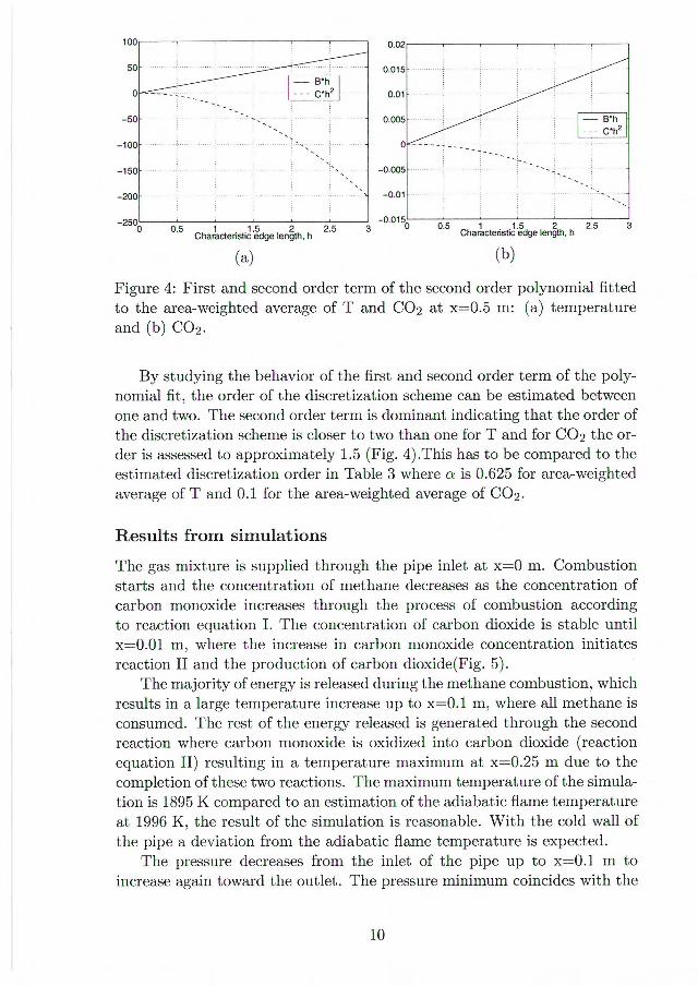
3 2.5 0.5 1 1.5 2 Characteristic edge length, fr

100

50

-50

-100

-150

-200

-25% 0.5 1 1.5 2 2.5

Characteristic edge length, h

(a)

3 0 -0015 .

(b)

0.02

0.015

0.01

0.005

0

-0.005

-0.01

Figure 4: First and second order term of the second order polynomial fitted to the area-weighted average of T and CO2 at x=0.5 m: (a) temperature and (b) CO2.

By studying the behavior of the first and second order term of the poly-nomial fit, the order of the discretization scheme can be estimated between one and two. The second order term is dominant indicating that the order of the discretization scheme is closer to two than one for T and for CO2 the or-der is assessed to approximately 1.5 (Fig. 4).This has to be compared to the estimated discretization order in Table 3 where a is 0.625 for area-weighted average of T and 0.1 for the area-weighted average of CO2.

Results from simulations

The gas mixture is supplied through the pipe inlet at x=0 m. Combustion starts and the concentration of methane decreases as the concentration of carbon monoxide increases through the process of combustion according to reaction equation I. The concentration of carbon dioxide is stable until x=0.01 m, where the increase in carbon monoxide concentration initiates reaction II and the production of carbon dioxide(Fig. 5).

The majority of energy is released during the methane combustion, which results in a large temperature increase up to x=0.1 m, where all methane is consumed. The rest of the energy released is generated through the second reaction where carbon monoxide is oxidized into carbon dioxide (reaction equation II) resulting in a temperature maximum at x=0.25 m due to the completion of these two reactions. The maximum temperature of the simula-tion is 1895 K compared to an estimation of the adiabatic flame temperature at 1996 K, the result of the simulation is reasonable. With the cold wall of the pipe a deviation from the adiabatic flame temperature is expected.

The pressure decreases from the inlet of the pipe up to x=0.1 m to increase again toward the outlet. The pressure minimum coincides with the

10

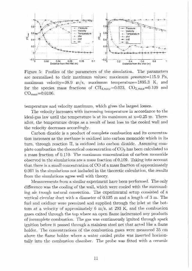
- Pressure - Velocity - e - Temperature - e - ch4 - co2

co

- Pressure - Velocity - - Temperature - e- ch4 - co2

co



0.1

Figure 5: Profiles of the parameters of the simulation. The parameters are normalized to their maximum values; maximum pressure=115.9 Pa, maximum velocity=38.9 m/s, maximum temperature=1895.3 K, and for the species mass fractions of CH4,7nas=0.023, CO2,max=-0.109 and COmax=0.0106.

temperature and velocity maximum, which gives the largest losses. The velocity increases with increasing temperature in accordance to the

ideal-gas law until the temperature is at its maximum at x=0.25 m. There-after, the temperature drops as a result of heat loss to the cooled wall and the velocity decreases accordingly.

Carbon dioxide is a product of complete combustion and its concentra-tion increases as the methane is oxidized into carbon monoxide which in its turn, through reaction II, is oxidized into carbon dioxide. Assuming com-plete combustion the theoretical concentration of CO2 has been calculated to a mass fraction of 0.110. The maximum concentration of carbon monoxide observed in the simulations are a mass fraction of 0.109. Taking into account that there is a small concentration of CO of a mass fraction of approximately 0.001 in the simulations not included in the theoretic calculation, the results from the simulations agree well with theory.

Measurements from a similar experiment have been performed. The only difference was the cooling of the wall, which were cooled with the surround-ing air trough natural convection. The experimental setup consisted of a vertical circular duct with a diameter of 0.035 m and a length of 3 m. The fuel and oxidizer were premixed and supplied through the inlet at the bot-tom at a velocity of approximately 6 m/s, at 293 K, and the combustion gases exited through the top where an open flame incinerated any products of incomplete combustion. The gas was continuously ignited through spark ignition before it passed through a stainless steel net that acted like a flame holder. The concentrations of the combustion gases were measured 35 cm above the flame holder where a water cooled probe was inserted horizon-tally into the combustion chamber. The probe was fitted with a ceramic

11

11_2Ut Cooling water

Flame holder

Wall mounted thermocou • le Micro

GC

Sparc plug /

Thermocouple Outlet

Figure 6: Experimental setup in Paper II.

tip with 3 mm in diameter closed at the end and with a hole for sampling of 1.5 mm in diameter facing the flow. The temperature was measured by three thermocouple centered in the cylindrical duct and placed 90 cm apart. The temperature of the wall was measured by three thermocouples place in contact with the outside surface of the wall of the combustion chamber (Fig. 6).

The measurements indicate a mass fraction of CO2 to 0.122., which corresponds to the extrapolated value using Richardson or second order method.

At high temperatures and high concentration of carbon dioxide the oxi-dized carbon monoxide can be reformed through dissociation(reaction III). When the carbon dioxide concentration is at its maximum at x=0.3 m and the temperature is at 1700 K an increase in carbon monoxide can be ob-served due to reaction equation III. As the number of molecules in the system increases as CO2 dissociates a slight increase in velocity corresponding to the change in volume can be observed. The change in concentration of CO in Fig. 5 should not be over estimated. As values are normalized with their maximum value a change in the concentration of CO will appear larger than the same change in CO2 concentration.

Discussion

A study of the temperature and carbon dioxide profiles the solution appears to be grid independent, and the observed differences between the different grids are only a few percent. However using a quantitative method such as the Richardson extrapolation to evaluate the solution the values obtained for the discretization order, a, indicates a solution far from the asymptotic range. Results from extrapolation using the Richardson theory also varies

12

depending on the parameter studied indicating that several parameter have to be studied when performing a Richardson extrapolation. The Richardson method is relatively rigid, i.e. it does not accept variations in the result before the goodness of fit becomes poor and result in unrealistic a.

The engineers evaluating combustion simulations are often limited to a qualitative assessment of the results. Here a second order polynomial fit can become a more useful tool in giving a qualitative assessment of the space discretization error. The fit of a second order polynomial always resulted in better goodness than with the Richardson extrapolation. The extrapolated solution for h=0 is more consequent than with the Richardson method. Further investigation of the method is necessary.

The extrapolated values for the mass fraction of CO2 at x=0.5 m are com-parable with the analytical solution and the experimental measurements. Comparison between the maximum temperature and the estimated adia-batic flame temperature also indicates that the results from the simulations are trustworthy.

Conclusion

Although the profiles of temperature and carbon dioxide agree well indicat-ing a qualitative grid independence the quantitative method of Richardson extrapolation does not produce results confirming the grid independence. This is a result of the stiffness of the Richardson method not allowing vari-ations in the results. A second order polynomial fit presents a better good-ness of fit to the data set than obtained using Richardson. For the problems where a qualitative assessment of the grid dependency is sufficient the study of the first and second order term of a second order polynomial fit can be used to assess the discretization order. However, further investigation of the method is necessary.

References

[1] Dryer, F. L., Glassman, I. Proceedings of the 14th Symposium (Inter-national) on combustion, Combustion Institute; Pittsburgh, PA, 1973, pp 987-1003.

[2] Westbrook C. K.; Dryer F. L. Prog. Energy Combust. and Sei. 1984, vol. 10, pp 1-57.

[3] Jones, W. P., Lindstedt, R. P. Combustion and Flame 1988, vol. 73, pp 233-249.

[4] Dupont, V., Pourkashanian, M.; Williams, A., J. Inst. Energy, 1993, vol. 66, pp 20-28.

13

[5] Nicol, D. G., Malte, P. C., Hamer, A. J., Roby, R. J., Steele, R.C., Journal of Engineering Gas Turbines Power 1999, 121, pp 272-280.

[6] Lindberg, J., Hermansson, R., Energy Sz Fuels 2004, 18, pp 1482-1484.

[7] Norton, D.G. Vlachos, D.G., Chemical Engineering Science, 2003, 58, pp 4871-4882.

[8] Richardson LF. The deferred approach to the limit, Trans. R. Soc. London, 1927, Ser. A. 226 pp 229-361.

[9] Turns S.R., An Introduction to Combustion-Concepts and Applica-tions, 2nd Edition, chapter 4, pp 111-147, 2000.

[10] Magnussen, B. F.; Hjertager, B. H., Proceedings of the 16th Sympo-sium on Combustion; The Combustion Institute: Pittsburgh, PA, 1976, pp 719-729.

[11] Byggstøl, S., Magnussen, B. F. Turbulent shear flows 4, Springer: Berlin, 1985, pp 381-395.

[12] Fretziger, J. H., Perk, M. Computational Methods for Fluid Dynamics, second edition; Springer: Berlin, 1996 and 1999.

14

LULE A1 UNIVERSITY

OF TECHNOLOGY

Universitetstryckeriet, Luleå

Experiments and Simulations of Lean Methane Combustion

Documents

Transcript of Experiments and Simulations of Lean Methane Combustion