Utilization Bounds for EDF Scheduling on

Real-Time Multiprocessor Systems

J.M. Lopez, J.L. Dıaz and D.F. GarcıaDepartamento de Informatica, Universidad de Oviedo, Gijon 33204, Spain

Abstract. The utilization bound for Earliest Deadline First scheduling is extendedfrom uniprocessors to homogeneous multiprocessor systems with partitioning strate-gies. First results are provided for a basic task model, which includes periodic andindependent tasks with deadlines equal to periods. Since the multiprocessor utiliza-tion bounds depend on the allocation algorithm, different allocation algorithms havebeen considered, ranging from simple heuristics to optimal allocation algorithms.

As multiprocessor utilization bounds for EDF scheduling depend strongly ontask sizes, all these bounds have been obtained as a function of a parameter whichtakes task sizes into account.

Theoretically, the utilization bounds for multiprocessor EDF scheduling can beconsidered a partial solution to the bin-packing problem, which is known to beNP-complete.

The basic task model is extended to include resource sharing, release jitter, dead-lines less than periods, aperiodic tasks, non-preemptive sections, context switchesand mode changes.

Keywords: multiprocessor scheduling, partitioning, bin-packing problem, EarliestDeadline First scheduling, multiprocessor utilization bounds

1. Introduction

Real-time systems theory supplies many results about uniprocessorsbut few about multiprocessors. One of the outstanding results aboutuniprocessors is the optimality of Earliest Deadline First (EDF) schedul-ing for any kind of tasks (Dertouzos, 1974). Unfortunately, EDF schedul-ing is not optimal on multiprocessor systems (Dertouzos and Mok,1989).

A new issue arises on multiprocessor scheduling; that is which pro-cessor executes each task at a given time. There are two major strategiesto deal with this problem: partitioning strategies, and global strate-

gies (Oh and Son, 1995). In a partitioning strategy, once a task isallocated to a processor, it is executed exclusively on that processor.In a global strategy, any instance of a task can be executed on anyprocessor, or even be preempted and moved to a different processorbefore it is completed.

Theoretically, global strategies provide in general higher schedulabil-ity than partitioning strategies. However, partitioning strategies have

c© 2003 Kluwer Academic Publishers. Printed in the Netherlands.

2003_rts.tex; 23/09/2003; 10:02; p.1

2

several advantages over global strategies. Firstly, the scheduling over-head associated with a partitioning strategy is lower than the overheadassociated with a global strategy. Secondly, partitioning strategies allowus to apply well-known uniprocessor scheduling algorithms to each pro-cessor. Furthermore, Earliest Deadline First (EDF) scheduling, whichis an optimal uniprocessor scheduling algorithm, perform poorly whenextended to global multiprocessor scheduling. The utilization boundassociated with global EDF multiprocessor scheduling is not higherthan one for any number of processors (Dall and Liu, 1978).

In this paper we follow the partitioning strategy, and assume thatall the tasks allocated to a processor are preemptively scheduled usingEDF, as this is the optimal scheduling algorithm for uniprocessors.Once the scheduler has been chosen, the only degree of freedom is theallocation algorithm.

The problem of allocating a set of tasks to a set of processors isanalogous to the bin-packing problem. In this case, the tasks are theobjects to pack, of size equal to their utilization factors. The bins areprocessors with a capacity of one for EDF scheduling (Liu and Layland,1973). The bin-packing problem is known to be NP-hard in the strongsense (Garey and Johnson, 1979). Thus, searching for optimal allo-cation algorithms is not practical. Several allocation algorithms havebeen proposed (Oh and Son, 1995; Garey and Johnson, 1979; Burchardet al., 1995; Dall and Liu, 1978; Saez et al., 1998).

Two different approaches are followed in the literature to estab-lish the schedulability associated with a given allocation algorithm:simulation approaches and theoretical approaches.

In the simulation approach, task sets are randomly generated. Next,the average number of processors required to allocate task sets of giventotal utilization is obtained. Uniprocessor exact tests (Saez et al., 1998),or uniprocessor sufficient tests (Lauzac et al., 1998) are commonlyused to decide whether a given group of tasks fits into one processor.Nevertheless, simulation results should be considered carefully, sincerandomly generated task sets may not be representative of those thatappear in practice.

The traditional theoretical approach focuses on the calculation ofthe metric (NAA/NOPT ), for pairs uniprocessor scheduling algorithm-

allocation algorithm (Oh and Son, 1995; Dall and Liu, 1978; Garey andJohnson, 1979; Burchard et al., 1995; Davari and Dhall, 1986a; Davariand Dhall, 1986b). This metric gives the relationship between the num-ber of processors required to schedule a task set using a given allocationalgorithm, AA, and the number of processors required using the optimalallocation algorithm,OPT. This metric is useful in order to compare

2003_rts.tex; 23/09/2003; 10:02; p.2

3

different allocation algorithms, but not to perform a schedulabilitytest (Lopez et al., 2003).

A new theoretical approach consists of calculating the utilizationbounds associated with scheduling algorithm-allocation algorithm pairs,analogous to those known for uniprocessors. This approach has severalinteresting features:

− Firstly, it allows us to carry out fast schedulability tests.

− Secondly, it allows us to quantify the influence of certain parame-ters, such as the number of processors, on schedulability.

The major disadvantage of this approach is the sufficient but not nec-essary character of the associated schedulability tests. This approachwas followed by Oh and Baker (1998) and Lopez et al. (2003) formultiprocessor RM scheduling.

Our work provides utilization bounds for multiprocessor EDF schedul-ing and deals with:

− Complex task models, including periodic and aperiodic tasks, re-lease jitter, arbitrary deadlines, resource sharing and mode changes.

− Arbitrary allocation algorithms, ranging from optimal allocationalgorithms to simple heuristics.

− Task sizes: by taking into account task sizes, the utilization boundscan be greatly incremented.

The rest of the paper is organized as follows. Section 2 defines thebasic system model dealt with. Section 3 provides limits on the utiliza-tion bounds for arbitrary allocation algorithms under the basic systemmodel. The utilization bounds for the basic system model and differentallocation algorithms are provided in Section 4. Section 5 analyzes theexpressions of the utilization bounds. Section 6 extends the basic sys-tem model, generalizing the task model, and calculates new utilizationbounds for the extensions. Finally, Section 7 presents our conclusionsand future work.

2. Basic system model

The task set consists of m independent and periodic tasks {τ1, . . . , τm},of computation times {C1, . . . , Cm}, periods {T1, . . . , Tm}, and harddeadlines equal to the task periods. The utilization factor ui of anytask τi, defined as ui = Ci/Ti, is assumed to be 0 < ui ≤ α ≤ 1, where

2003_rts.tex; 23/09/2003; 10:02; p.3

4

α is the maximum reachable utilization factor among all tasks. Thus, αis a parameter of the task set which takes the “task sizes” into account.The total utilization of the task set, denoted by U , is the sum of theutilization factors of the tasks that compose it.

Tasks are allocated to an array of n identical processors {P1, . . . , Pn},and are executed independently of each other. Once a task is allocatedto a processor, it is executed only on that processor. Within each pro-cessor, tasks are scheduled preemptively using EDF. The allocation iscarried out using Reasonable Allocation algorithms (RA). A reasonableallocation algorithm is one which fails to allocate a task only when thereis no processor in the system which can hold the task.

The uniprocessor utilization bound for EDF scheduling of periodicand independent tasks of periods equal to deadlines is 1.0 (Liu andLayland, 1973). This means that any subset of the tasks is schedulableon one processor if and only if U ≤ 1. Thus, a task of utilization factorui fits into processor Pj , which already has mj tasks allocated to itwith total utilization Uj, if the (mj + 1) tasks are schedulable, i.e, if1 − Uj ≥ ui.

Using the schedulability condition U ≤ 1, a reasonable allocationalgorithm is one which fails to allocate a task of utilization factor ui toa multiprocessor made up of n processors, only when the task does notfit into any processor, i.e,

1 − Uj < ui for j = 1, . . . , n (1)

Examples of reasonable allocation algorithms are First Fit (FF), BestFit (BF) and the optimal allocation algorithm (OPT).

Within the Reasonable Allocation (RA) algorithms we define a class,termed Reasonable Allocation Decreasing (RAD), made up of all thereasonable allocation algorithms fulfilling the following conditions:

− Tasks are ordered by decreasing utilization factors before makingthe allocation, i.e, u1 ≥ u2 ≥ · · · ≥ um.

− Tasks are allocated sequentially, that is, task τ1 is allocated first,next task τ2, and so on until task τm.

3. Limits on the utilization bounds

The multiprocessor utilization bound associated with any reasonableallocation algorithm, RA, and multiprocessor EDF scheduling is de-noted by UEDF-RA

wc . Any task set of total utilization U ≤ UEDF-RAwc is

schedulable using RA allocation and EDF scheduling on all processors,

2003_rts.tex; 23/09/2003; 10:02; p.4

5

while a task set of total utilization U > UEDF-RAwc may or may not be

schedulable. The multiprocessor utilization bound UEDF-RAwc depends

on the allocation algorithm, RA. Therefore, UEDF-RAwc is in the interval

[LEDF,HEDF], defined as follows:

LEDF = minRA

UEDF-RAwc

HEDF = maxRA

UEDF-RAwc

The calculation of this interval gives the worst and best utilizationbounds we can expect from all the reasonable allocation algorithms.

Before calculating the expressions of LEDF and HEDF, it is necessaryto introduce the parameter β. β is the maximum number of tasks ofutilization factor α which fit into one processor under EDF scheduling.β can be expressed as a function of α

β = ⌊1/α⌋

Any multiprocessor made up of n processors can allocate at least βntasks of arbitrary utilization factors (less than or equal to α). Thus, anytask set fulfilling m ≤ βn is trivially schedulable using EDF schedulingtogether with any reasonable allocation algorithm.

Figure 1 depicts β as a function of α, showing also the sufficientschedulability condition m ≤ βn. For example, if α is in the interval(1/3, 1/2] then β = 2. In this case, the task set is schedulable if it has2n tasks or less.

Henceforth, we will assume m > βn, as otherwise there would be nopoint in obtaining the utilization bounds.

Theorem 1 will provide a lower limit on the utilization bound as-sociated with any reasonable allocation algorithm and multiprocessorEDF scheduling. Section 4.1 will present the utilization bound forone reasonable allocation algorithm, the Worst Fit (WF) heuristic,which coincides with the previous lower limit. Therefore, LEDF andthe utilization bound for WF allocation coincide.

Theorem 2 will provide an upper limit on the utilization boundassociated with any allocation algorithm, reasonable or not, and multi-processor EDF scheduling. Section 4.2 will present the utilization boundassociated with some reasonable allocation algorithms, the heuristics inthe class RAD, which coincides with the previous upper limit. There-fore, HEDF and the utilization bound for the class RAD coincide. Fur-thermore, since the upper limit given by Theorem 2 applies to anyallocation algorithm, reasonable or not, HEDF is the maximum utiliza-tion bound among all the allocation algorithms.

2003_rts.tex; 23/09/2003; 10:02; p.5

6

1

2

3

4

5

6

7

8

9

1

2

1

3

1

4

1

5

1

6

1

7

m ≤ n

m ≤ 2n

m ≤ 3n

m ≤ 4n

· · ·

· · ·

Schedulability conditionm ≤ βn

α

β

Figure 1. Representation of the function β(α), and the associated schedulabilitycondition.

THEOREM 1. Let RA be any reasonable allocation algorithm. If m >βn then

UEDF-RAwc ≥ n − (n − 1)α

Proof. Let {τ1, . . . , τm} be a set of m tasks which does not fit intothe multiprocessor. There are tasks in the set which are allocated toprocessors, and tasks which are not. Let us change the indexes in theset, so that the tasks which were not allocated have the last indexes inthe set. Let τk be the first task in the set (after the change of indexes),which was not allocated to any processor. Since the allocation algorithmis reasonable, from (1) we get

Uj > 1 − uk for j = 1, . . . , n (2)

where Uj is the total utilization of the tasks previously allocated toprocessor Pj and uk is the utilization factor of task τk. The total

2003_rts.tex; 23/09/2003; 10:02; p.6

7

utilization of the whole set, U , fulfills

U =m

∑

i=1

ui ≥k

∑

i=1

ui =n

∑

j=1

Uj + uk (3)

From (2) we get

n∑

j=1

Uj >n

∑

j=1

(1 − uk) = n(1 − uk)

Substituting this inequality into (3)

U > n(1 − uk) + uk = n − (n − 1)uk

From the system definition, all the utilization factors are less than orequal to α, so uk ≤ α and

U > n − (n − 1)α

Any task set which does not fit into the multiprocessor fulfills theprevious expression. Consequently, any task set of total utilization lessthan or equal to n − (n − 1)α fits into the multiprocessor, and

UEDF-RAwc ≥ n − (n − 1)α �

We have found a lower limit on the utilization bound for any reason-able allocation algorithm. Section 4.1 will present the utilization boundfor a reasonable allocation algorithm, which coincides with this lowerlimit. Therefore, LEDF(n, α) = n − (n − 1)α.

Now we obtain an upper limit on the utilization bound for anyallocation algorithm, reasonable or not.

THEOREM 2. Let AA be an arbitrary allocation algorithm. If m > βnthen

UEDF-AAwc ≤

βn + 1

β + 1

Proof. We will prove that a set of m tasks {τ1, . . . , τm} exists, withutilization factors 0 < ui ≤ α for all i = 1, . . . ,m, and total utilizationU = (βn + 1)/(β + 1) + ǫ, with ǫ → 0+, which does not fit into nprocessors using any allocation algorithm and EDF scheduling on eachprocessor. The proof will be divided into three parts:

1. The task set is presented.

2003_rts.tex; 23/09/2003; 10:02; p.7

8

2. The utilization factors of the task set are proved to be valid, thatis, 0 < ui ≤ α.

3. The claim that the task set does not fit into the multiprocessor isproved.

Part 1. The set of m tasks is composed of two subsets: a first subsetwith (m − βn − 1) tasks, and a second subset with (βn + 1) tasks.

All the tasks of the first subset have the same utilization factor ofvalue

ui =ǫ

mfor i = 1, . . . , (m − βn − 1)

All the tasks of the second subset have the same utilization factorof value

ui =1

β + 1+

ǫ

mfor i = (m − βn), . . . ,m

It is simple to check that the task set is made up of m tasks of totalutilization (βn + 1)/(β + 1) + ǫ.

Part 2. It is also necessary to prove that the utilization factors ofboth subsets are valid, i.e, 0 < ui ≤ α for all i = 1, . . . ,m. On onehand, making ǫ low enough,

0 < ui =ǫ

m< α for i = 1, . . . , (m − βn − 1)

On the other hand, by definition of β, (β +1) tasks of utilization factorα do not fit into one processor, i.e, (β +1)α > 1. Making ǫ low enough,

α >1

β + 1+

ǫ

m= ui for i = (m − βn), . . . ,m

Part 3. There are (βn + 1) tasks in the second subset. Hence, atleast one processor of the n available should allocate (β +1) or more ofthese tasks. However, no processor can allocate (β+1) or more tasks ofthe second subset, since (β + 1) of these tasks have a utilization higherthan one in total.

We conclude that the proposed task set of total utilization (βn +1)/(β + 1) + ǫ does not fit into n processors when ǫ → 0+, so theutilization bound UEDF-AA

wc must be less than or equal to (βn+1)/(β +1).

Remark: the tasks of the first subset are necessary in the proof onlyto fulfill the restriction of having m tasks. �

We have found an upper limit on the utilization bound for anyallocation algorithm, reasonable or not. Section 4.2 will present the

2003_rts.tex; 23/09/2003; 10:02; p.8

9

utilization bound for some reasonable algorithms, which coincides withthis upper limit. Therefore, HEDF(n, α) = (βn + 1)/(β + 1).

4. Utilization bounds for reasonable allocation algorithms

The utilization bound for multiprocessor EDF scheduling depends onthe allocation algorithm. In this article, we focus on reasonable allo-cation algorithms, avoiding impractical allocation algorithms, whichwould only complicate the mathematical description of the problem.

Below, we present the utilization bounds for EDF multiprocessorscheduling, considering independent and periodic tasks of deadlinesequal to periods, and the following allocation algorithms:

− Worst Fit (WF).

− Reasonable allocation Decreasing (RAD). It includes First Fit De-creasing (FFD), Best Fit Decreasing (BFD), Worst Fit Decreasing(WFD), etc.

− First Fit (FF) and Best Fit (BF).

− Other allocation algorithms, including optimal allocation algorithms,First Fit Increasing (FFI), Best Fit Increasing (BFI), and WorstFit Increasing (WFI).

4.1. Worst fit allocation

The heuristic Worst Fit (WF) allocates tasks sequentially, i.e, one taskafter another. Each task is allocated to the processor in which it fitsthe worst. In other words, it is allocated to the processor Pj with thehighest free capacity, i.e, highest (1 − Uj), among those with enoughcapacity to hold the task.

THEOREM 3. If m > βn then

UEDF-WFwc (n, α) = n − (n − 1)α

Proof. Firstly, we will prove the existence of a set of m tasks, {τ1, . . . , τm},of utilization factors less than or equal to α, and total utilization

n − (n − 1)α + ǫ

with ǫ → 0+, which does not fit into the processors using the allocationalgorithm WF. The proof will be divided into three parts:

2003_rts.tex; 23/09/2003; 10:02; p.9

10

1. The task set is presented.

2. The utilization factors of the task set are proved to be valid, thatis, 0 < ui ≤ α.

3. The claim that the task set does not fit into the multiprocessor isproved.

Part 1. The set of m tasks is built as follows, strictly in the orderindicated. A first subset made up of (m − βn − 1) tasks of utilizationfactor

ui =ǫ

2(m − βn − 1)for i = 1, . . . ,m − βn − 1

A second subset made up of βn tasks of utilization factor

ui =1 − α

β+

ǫ

2βnfor i = (m − βn), . . . , (m − 1)

Finally, the last task has a utilization factor um = α.It can be proved that the task set is made up of m tasks, of total

utilization n − (n − 1)α.Part 2. It is necessary to prove that the utilization factors of all the

tasks are valid, i.e, 0 < ui ≤ α for i = 1, . . . ,m. Since ǫ → 0+, it isenough to prove that α > (1 − α)/β.

β is calculated from the expression β = ⌊1/α⌋, as indicated inSection 3. Therefore, it follows that

β >1

α− 1 =

1 − α

α, and

1 − α

β< α

Part 3. Next, we will prove that the task set does not fit into themultiprocessor using WF allocation.

The tasks of the first subset fit into the multiprocessor. They areequitatively allocated between all the processors, which means the dif-ference in the number of tasks between any pair of processors is notgreater than one.

The βn tasks of the second subset also fit into the multiprocessor.They are equitatively divided into the n processors, i.e, each proces-sor receives β of these tasks. Thus, the total utilization of the tasksallocated to any processor is higher than (1 − α) and the last task, ofutilization factor α, does not fit into any processor. Hence, UEDF-WF

wc ≤n − (n − 1)α.

Taking into account the lower limit on the utilization bound for anyreasonable allocation algorithm, given by Theorem 1, which includesWF, it follows that

UEDF-WFwc (n, α) = n − (n − 1)α

2003_rts.tex; 23/09/2003; 10:02; p.10

11�4.2. Reasonable allocation decreasing

The algorithms belonging to the class Reasonable Allocation Decreas-ing (RAD) order the tasks by decreasing utilization factors beforecarrying out the allocation (see Section 2). Examples of RAD algo-rithms are First Fit Decreasing (FFD), Best Fit Decreasing (BFD)and Worst Fit Decreasing (WFD).

All these algorithms share a common utilization bound, as will beproved in Theorem 4. In addition, this common utilization bound co-incides with the upper limit given by Theorem 2. Thus, not even theoptimal allocation algorithm can provide a higher utilization boundthan that of the allocation algorithms in the RAD class.

THEOREM 4. If m > βn then

UEDF-RADwc (n, α) =

βn + 1

β + 1

Proof. The proof for the case n = 1 is trivial. UEDF-RADwc (n = 1, α) =

1, so it coincides with the utilization bound for the uniprocessor case,which is independent of the “task sizes”. We will assume n > 1 in therest of the proof.

Let {τ1, . . . , τm} be a set of m tasks which does not fit into themultiprocessor. Let τk be the first task in the set which does not fit intothe multiprocessor. Since RAD allocation algorithms are reasonable,from (1) we get

Uj > 1 − uk for j = 1, . . . , n (4)

where Uj is the total utilization of the tasks allocated to processor Pj

and uk is the utilization factor of task τk. The total utilization of thefirst k tasks fulfills

k∑

i=1

ui =n

∑

j=1

Uj + uk (5)

From equation (4) we get

n∑

j=1

Uj >n

∑

j=1

(1 − uk) = n(1 − uk)

Substituting this expression into equation (5)

k∑

i=1

ui > n(1 − uk) + uk = n − (n − 1)uk (6)

2003_rts.tex; 23/09/2003; 10:02; p.11

12

Tasks are ordered by decreasing utilization factors before carrying outthe allocation, so

uk ≤

∑ki=1 ui

k

Substituting this inequality into (6)

k∑

i=1

ui > n − (n − 1)

∑ki=1 ui

k

Finding∑k

i=1 ui, it follows that

k∑

i=1

ui >kn

k + n − 1

The total utilization of the first k tasks is less than or equal to the totalutilization of the whole task set. Thus,

U =m

∑

i=1

ui ≥k

∑

i=1

ui >kn

k + n − 1(7)

Parameter k is restricted to βn < k ≤ m. If βn ≥ k, then the firstk tasks would fit into the multiprocessor, which would contradict thehypothesis stating that task τk does not fit into the multiprocessor. Inaddition, m is the number of tasks of the set, so k ≤ m. Next, we willcalculate the minimum value of

f(k, n) =kn

k + n − 1with βn < k ≤ m. (8)

Function f(k, n) fulfills

∂f(k, n)

∂k=

n(n − 1)

(k + n − 1)2> 0 for n > 1

Therefore, f(k, n) is increasing in the interval βn < k ≤ m and itsabsolute minimum corresponds to k = (βn + 1). Substituting k for(βn + 1) into (7)

U >βn + 1

β + 1

Therefore, a necessary condition to be fulfilled by the total utilizationof any task set which does not fit into the n processors is

U >βn + 1

β + 1

2003_rts.tex; 23/09/2003; 10:02; p.12

13

In other words, any task set of total utilization less than or equal to

βn + 1

β + 1

fits into n processors and

UEDF-RADwc ≥

βn + 1

β + 1

RAD algorithms are reasonable allocation algorithms, so applying The-orem 2

UEDF-RADwc ≤

βn + 1

β + 1

Therefore, we finally conclude

UEDF-RADwc (n, α) =

βn + 1

β + 1 �4.3. First Fit and Best Fit

The heuristic First Fit (FF) allocates tasks sequentially, i.e, one taskafter another. Each task is allocated to the first processor it fits into.Processors are visited in the order P1, . . . , Pn.

The heuristic Best Fit (BF) also allocates tasks sequentially. Eachtask is allocated to the processor into which it fits the best. In otherwords, it is allocated to the processor Pj with the lowest free capacity,i.e, lowest (1−Uj), among those with enough capacity to hold the task.

The utilization bounds for FF and BF allocation are the same, ofvalue

UEDF-FFwc (n, α) = UEDF-BF

wc (n, α) =βn + 1

β + 1

In addition, the proof is almost identical for both heuristics, so we willonly prove the multiprocessor utilization bound for FF allocation.

Next, we present the strategy in the proof of the multiprocessorutilization bound for FF allocation.

1. Lemma 1 is proved. This lemma is necessary in order to proveTheorem 5.

2. Theorem 5 proves an expression which relates the utilization for mtasks and n processors, with the utilization bound for (m−β) tasksand (n − 1) processors. This allows us to prove Theorem 6, goingfrom the case n = 1 (uniprocessor case) to a general multiprocessorcase with an arbitrary n.

2003_rts.tex; 23/09/2003; 10:02; p.13

14

3. From the result of Step 2 and the utilization bound for EDF schedul-ing on uniprocessors, Theorem 6 obtains the utilization bound forFF allocation.

The proof of Theorem 5 requires Lemma 1, which is proved below.It relates the utilization bounds for the same number of processors, butdifferent number of tasks.

LEMMA 1. Let UEDF-FFwc (m,n, α) be the multiprocessor utilization bound

for EDF scheduling and FF allocation on n processors of sets of m tasks

with utilization factors less than or equal to α. It follows that

UEDF-FFwc (q, n, α) ≥ UEDF-FF

wc (m,n, α) for q < m

Proof. Let us consider a task set made up of q tasks which does notfit into the multiprocessor. If we add (m−q) tasks of utilization factorsǫ → 0+ at the end of this task set, nor does the resulting task set fitinto n processors. Therefore, the utilization bound for q tasks and nprocessors can not be lower than the utilization bound for m tasks andn processors. �

Next, we prove an expression which relates the utilization boundof multiprocessors with n and (n − 1) processors. This will allow usto obtain a lower limit on the multiprocessor utilization bound, goingfrom the case n = 1 (uniprocessor case) to a general multiprocessorcase with an arbitrary n.

THEOREM 5. If m > βn then

UEDF-FFwc (m,n, α) ≥

β

β + 1+ UEDF-FF

wc (m − β, n − 1, α)

Proof. We will prove that any set of m tasks {τ1, . . . , τm}, withutilization factors 0 < ui ≤ α for all i = 1, . . . ,m, and total utilizationless than or equal to

β

β + 1+ UEDF-FF

wc (m − β, n − 1, α)

fits into n processors using EDF scheduling on each processor and FFallocation.There are two possible cases:

Case 1: The first (m− β) tasks have utilization factors less than or

equal to UEDF-FFwc (m − β, n − 1, α), that is,

∑m−βi=1 ui ≤ UEDF-FF

wc (m −β, n − 1, α). In this case, the whole set of m tasks always fits into nprocessors, because the first (m − β) tasks fit into the first (n − 1)

2003_rts.tex; 23/09/2003; 10:02; p.14

15

τ1 · · · τk−1 τk τk+1 · · · τm−β · · · τm

UEDF-FFwc (m − β, n − 1, α) ∆

uk,1

u1 uk−1 uk uk+1 um−β um

m∑

i=k

ui

m−β∑

i=1

ui

k−1∑

i=1

ui

Figure 2. General situation of case 2 of Theorem 5.

processors (since its utilization is below the bound), and the remainingβ tasks fit into the last processor, since the definition of β implies thatat least β tasks always fit into one processor.

Case 2: The first (m−β) tasks have a total utilization greater than

UEDF-FFwc (m−β, n−1, α), that is,

∑m−βi=1 ui > UEDF-FF

wc (m−β, n−1, α).In this case, we will prove that the whole set of m tasks still fits into nprocessors if the total utilization is equal to UEDF-FF

wc (m−β, n−1, α)+∆,provided ∆ ≤ β/(β + 1).

A task τk must exist, whose uk added to the previous utilizationsui, causes the bound UEDF-FF

wc (m − β, n − 1, α) to be exceeded. Thissituation is depicted in Figure 2, which is a graphical representation ofthe utilization factors of each task and the relationships between severalquantities and summations used throughout this proof. The value of kis obtained as the integer which fulfills:

k−1∑

i=1

ui ≤ UEDF-FFwc (m − β, n − 1, α) <

k∑

i=1

ui

Note that k ≤ m − β, because if k > m − β we would be dealing withCase 1.

Let us show that the first (k − 1) tasks fit into the first (n − 1)processors. The total utilization of the first (k − 1) tasks fulfills

k−1∑

i=1

ui ≤ UEDF-FFwc (m − β, n − 1, α)

2003_rts.tex; 23/09/2003; 10:02; p.15

16

Applying Lemma 1 with (m − β) > (k − 1), we get

UEDF-FFwc (m − β, n − 1, α) ≤ UEDF-FF

wc (k − 1, n − 1, α)

and thusk−1∑

i=1

ui ≤ UEDF-FFwc (k − 1, n − 1, α)

Therefore, the first (k−1) tasks fit into the first (n−1) processors. Wehave only to prove that the remaining (m−k+1) tasks fit into the lastprocessor.

The worst situation in terms of schedulability appears when all thetasks τi in {τk, . . . , τm} fulfill ui > uk,1, where

uk,1 = UEDF-FFwc (m − β, n − 1, α) −

k−1∑

i=1

ui

as shown in Figure 2. Note that if there is a task τi in {τk, . . . , τm}with ui ≤ uk,1, we can always allocate this task to the first (n − 1)processors (since the addition of this new task does not cause the totalutilization to exceed the bound), and the situation is analogous to thecurrent one, with k one unit greater. This reasoning can be repeateduntil no task τi with ui ≤ uk,1 exists among the last (m− k + 1) tasks.

In order to prove that the last (m − k + 1) tasks fit into the lastprocessor we have to prove that the total utilization of these tasks isnot greater than one, that is,

m∑

i=k

ui ≤ 1

Figure 2 shows thatm

∑

i=k

ui = uk,1 + ∆ (9)

As already stated, all the utilization factors ui in this summation aregreater than uk,1, so

(m − k + 1)uk,1 < uk,1 + ∆

≤ uk,1 +β

β + 1by the definition of ∆

and we can find uk,1.

uk,1 <β

(β + 1)(m − k)(10)

2003_rts.tex; 23/09/2003; 10:02; p.16

17

Substituting the value of uk,1 from (10) into (9) we obtain

m∑

i=k

ui <β

(β + 1)(m − k)+ ∆

<β

(β + 1)(m − k)+

β

(β + 1)by def. of ∆

=(m − k + 1)β

(β + 1)(m − k)

=1 + 1/(m − k)

1 + 1/β

We know that k ≤ m − β in case 2, so m − k ≥ β. Therefore,

m∑

i=k

ui ≤ 1

This equation shows that the last (m − k + 1) tasks meet the EDFuniprocessor schedulability condition, so they fit into the last processor.

We have proved that any task set with m tasks and a total utilization

UEDF-FFwc (m − β, n − 1, α) + ∆ ≤

UEDF-FFwc (m − β, n − 1, α) +

β

β + 1

fits into n processors. Therefore, the utilization bound UEDF-FFwc (m,n, α),

must be greater than or equal to UEDF-FFwc (m−β, n− 1, α)+β/(β +1),

and the theorem is proved. �Theorem 5 is also valid for BF allocation. Nevertheless, proving

the statement “the worst situation in terms of schedulability appearswhen all the tasks τi in {τk, . . . , τm} fulfill ui > uk,1”, requires someelaboration for BF allocation and is not shown for the sake of brevity.

The utilization bound for FF allocation is obtained in Theorem 6.

THEOREM 6. If m > βn then

UEDF-FFwc (n, α) =

βn + 1

β + 1(11)

Proof. First, we obtain a lower limit on the utilization bound for a setof m tasks on a multiprocessor with n processors, using FF allocation.

2003_rts.tex; 23/09/2003; 10:02; p.17

18

Theorem 5 relates the utilization bound of sets of m tasks on mul-tiprocessors of n processors, with utilization bound of sets of (m − β)tasks on multiprocessors with (n − 1) processors.

UEDF-FFwc (m,n, α) ≥

β

β + 1+ UEDF-FF

wc (m − β, n − 1, α)(12)

Theorem 5 also relates the utilization bound of sets of (m − β) taskson multiprocessors of (n − 1) processors, with the utilization bound ofsets of (m − 2β) tasks on multiprocessors of (n − 2) processors.

UEDF-FFwc (m − β, n − 1, α) ≥

β

β + 1+ UEDF-FF

wc (m − 2β, n − 2, α)(13)

Substituting (13) into (12) we get

UEDF-FFwc (m,n, α) ≥

2β

β + 1+ UEDF-FF

wc (m − 2β, n − 2, α)

This procedure can be repeated, until finally relating the utilizationbound of sets of m tasks on multiprocessors of n processors, with theutilization bound of sets of (m − (n − 1)β) tasks on a uniprocessor.

UEDF-FFwc (m,n, α) ≥

(n − 1)β

β + 1+ UEDF-FF

wc (m − (n − 1)β, 1, α)(14)

The utilization bound for (m − (n − 1)β) tasks and one processor isone, which does not depend on the values of m or α.

UEDF-FFwc (m − (n − 1)β, 1, α) = 1 (15)

Substituting (15) into (14), we obtain a lower limit on the utilizationbound of m tasks on n processors.

UEDF-FFwc (m,n, α) ≥

βn + 1

β + 1

Theorem 2 proved that

UEDF-RAwc (m,n, α) ≤

βn + 1

β + 1

and FF is a reasonable allocation algorithm. Hence,

UEDF-FFwc (m,n, α) =

βn + 1

β + 1

2003_rts.tex; 23/09/2003; 10:02; p.18

19

From this expression we observe that UEDF-FFwc does not depend on the

number of tasks, m, so our final conclusion is that

UEDF-FFwc = UEDF-FF

wc (n, α) =βn + 1

β + 1 �4.4. Other allocation algorithms

In this section we consider optimal allocation algorithms and the heuris-tics First Fit Increasing (FFI), Best Fit Increasing (BFI) and Worst FitIncreasing (WFI).

An optimal allocation algorithm (OPT) is one able to allocate anytask set whenever a feasible allocation exists.

The heuristics FFI, BFI and WFI are variants of the heuristics FF,BF and WF respectively. They order the tasks by increasing utilizationfactors before carrying out the allocation. Therefore, the task with thelowest utilization factor (the lowest “size”) is allocated first.

The utilization bound for an optimal allocation algorithm coincideswith HEDF, so it also coincides with the utilization bound for FF, BFand RAD allocation. Therefore,

UEDF-OPTwc (n, α) =

βn + 1

β + 1

The utilization bound for WFI allocation coincides with that of WFallocation. The task set defined in Theorem 3, in Section 4.1, was madeup of tasks ordered by increasing utilization factors and the task setwas proved not to fit into the multiprocessor using WF allocation.Therefore,

UEDF-WFIwc (n, α) = UEDF-WF

wc (n, α) = n − (n − 1)α

Let us calculate now the utilization bound for FFI allocation. Forany task set that can not be allocated using FFI allocation, there is an-other task set with the same total utilization that can not be allocatedusing FF allocation. This last task set can be obtained by ordering thetasks of the first task set by increasing utilization factors. Therefore,the utilization bound for FF allocation can not be higher than theutilization bound for FFI allocation, i.e, UEDF-FFI

wc ≥ UEDF-FFwc . Since

the utilization bound for FF allocation coincides with the maximumutilization bound, HEDF, it follows that

UEDF-FFIwc (n, α) = UEDF-FF

wc (n, α) =βn + 1

β + 1

2003_rts.tex; 23/09/2003; 10:02; p.19

20

Applying a similar reasoning for BFI allocation,

UEDF-BFIwc (n, α) = UEDF-BF

wc (n, α) =βn + 1

β + 1

5. Analysis of the theoretical results

All the utilization bounds for multiprocessor EDF scheduling presentedin the previous section fall into two categories:

− The utilization bounds for WF and WFI coincide with the mini-mum utilization bound, given by

LEDF(n, α) = n − (n − 1)α = n(1 − α) + α

− The utilization bounds for FF, BF, FFI, BFI and the class RADcoincide with the maximum utilization bound, given by

HEDF(n, α) =βn + 1

β + 1

Therefore, we will analyze only the expressions of LEDF and HEDF.Figure 3 depicts the function LEDF(n, α) as a function of the number

of processors, for different values of α. Although n is an integer, itis represented as a continuous function with the aim of improving itsvisualization. The representation is normalized by dividing LEDF by thenumber of processors, in order to show the average degree of utilizationof the processors.

LEDF(1, α) = 1, which corresponds to the bound for uniprocessorEDF scheduling. Every time we add a new processor to the system, theutilization bound is increased by (1 − α).

For high values of α, the utilization bound LEDF is too small tobe practical. It is close to 1.0, so LEDF/n nears 0, for any number ofprocessors. However, as α nears 0, the utilization bound LEDF becomesclose to n, so LEDF/n nears 1.0. In this case, the multiprocessor behavesapproximately like a uniprocessor n times faster.

Figure 4 depicts the function HEDF(n, α) as a function of the numberof processors for different values of α. Although n is an integer, it isagain represented as a continuous function to improve its visualization.The representation is normalized by dividing HEDF by the number ofprocessors. Each curve in Figure 4 corresponds to a different value ofβ, and therefore to different values of α.

2003_rts.tex; 23/09/2003; 10:02; p.20

21

0

0.25

0.5

0.75

1

1 5 10 15 20 25

α = 1

α = 0.75

α = 0.5

α = 0.25

α ≈ 0

Number of processors (n)

LEDF (n, α)

n

Figure 3. Plot of LEDF(n, α).

0

0.25

0.5

0.75

1

1 5 10 15 20 25

0.50 < α ≤ 1.00

0.33 < α ≤ 0.50

0.25 < α ≤ 0.33

0.09 < α ≤ 0.10

α ≈ 0

Number of processors (n)

HEDF (n, α)

n

Figure 4. Plot of HEDF(n, α).

2003_rts.tex; 23/09/2003; 10:02; p.21

22

HEDF(1, α) = 1, which corresponds to the bound for uniprocessorEDF scheduling. Every time we add a new processor to the system, theutilization bound is increased by β/(β + 1).

For α > 0.5, the utilization bound HEDF is equal to 0.5(n + 1). Asα nears 0, the utilization bound HEDF becomes close to n and HEDF/nclose to 1.0. In this case, the multiprocessor behaves approximately likea uniprocessor n times faster.

For example, the utilization bound associated with multiprocessorEDF scheduling and FF allocation in a multiprocessor made up of twoprocessors is 1.5, i.e, 0.75 per processor. If the tasks have utilizationfactors less than or equal to 0.25, then β = 4. In this case, the utilizationbound for FF allocation takes the value 1.8, i.e, 0.9 per processor, closeto the ideal 1.0 per processor.

Finally, it should be pointed out that the performance of any alloca-tion algorithm is not defined only by its utilization bound. Utilizationbounds consider only the worst-case. For example, any optimal allo-cation algorithm has the same EDF multiprocessor utilization boundas FFD allocation. However, optimal allocation algorithms are able toallocate task sets which can not be allocated using FFD allocation.

6. Task model extensions

All the results concerning multiprocessor utilization bounds provided inSection 4 were obtained using a basic task model, made up of periodicand independent tasks of deadlines equal to periods.

The objective of this section is to provide utilization bounds formore complex task sets. In some cases, the utilization bounds will betight and in other pessimistic.

Each of the following subsections introduces a different extensionwith regard to the basic task model. In any case, the results of all thesubsections may be merged to cover simultaneously all the extensions.

6.1. Arbitrary deadlines

The multiprocessor utilization bounds for EDF scheduling providedin Section 4 are valid even when some deadlines are higher than theperiods. The multiprocessor EDF utilization bounds depend on theuniprocessor EDF utilization bounds, which are 1.0 for deadlines equalto periods and for deadlines higher than the periods.

Let us consider the case of deadlines less than the periods. Assumingthat Di = ∆Ti for all the tasks, with ∆ ≤ 1, the new utilization bound

2003_rts.tex; 23/09/2003; 10:02; p.22

23

for EDF uniprocessor scheduling becomes

UEDF = ∆

Any task set Γ with utilization factors {u1, . . . , um} and deadlines{∆T1, . . . ,∆Tm} fits into the multiprocessor, if and only if, the task setΓ′ with utilization factors {u1/∆, . . . , um/∆} and deadlines {T1, . . . , Tm}fits into the multiprocessor. The proof is simple: the capacity of theprocessor for the task set Γ′ is 1, i.e, (1/∆) times higher than thecapacity for task set Γ, but the utilization factors of Γ′ are also (1/∆)times greater than those of Γ.

The multiprocessor utilization bound coincides with the total uti-lization of the worst-case task set (minus an ǫ), the worst-case task setbeing the one with the lowest utilization among those which do not fitinto the multiprocessor. Therefore, the worst-case task set for ∆ < 1can be obtained by multiplying the utilization factors of the worst-case task set for ∆ = 1 by the term ∆. Thus, the utilization boundsfor ∆ < 1 are obtained by multiplying the utilization bounds of theprevious sections by ∆.

To sum up, the utilization bounds for the case ∆ < 1 can be obtainedfollowing these steps:

1. Transform the original task set, Γ, with ∆ < 1, into a new task set,Γ′, with ∆ = 1, by multiplying the utilization factors and deadlinesby (1/∆). Therefore, it follows that α′ = α/∆, where α′ is themaximum reachable utilization factor of Γ′, and β′ = ⌊1/α′⌋ =⌊∆/α⌋. Note that if β′ is zero, Γ′ may have tasks with utilizationfactors greater than 1, and the task set is not schedulable.

2. Calculate the multiprocessor utilization bounds using β′ instead ofβ.

3. Multiply the utilization bound obtained for Γ′ by ∆ to obtain theutilization bound for the original task set, Γ.

For example, the multiprocessor utilization bound for FF allocationand ∆ = 0.5 becomes 0.5(β′n + 1)/(β′ + 1), with β′ = ⌊0.5/α⌋

The condition Di = ∆Ti is not common in practice. However, themultiprocessor utilization bounds assuming this condition give us in-sight into the schedulability variations against deadlines.

The same technique could be applied to any uniprocessor schedul-ing algorithm providing a fixed uniprocessor utilization bound. Forexample, a pessimistic (but close to the tight) utilization bound foruniprocessor RM scheduling is ln 2. Therefore, a pessimistic (but closeto the tight) multiprocessor utilization bound for RM scheduling andFF allocation is ln 2(β′n + 1)/(β′ + 1), with β′ = ⌊ln 2/α⌋.

2003_rts.tex; 23/09/2003; 10:02; p.23

24

6.2. Release jitter

The basic task model assume that the interarrival times of periodictasks are strictly constant, equal to the periods. However, it is commonto find some delay in the release times of the tasks called jitter (Tindelland Clark, 1994). Jitter is a source of unpredictability, which shouldbe bounded in some way. Frequently, a maximum jitter Ji is associatedto each task τi. Therefore, if a job of a periodic task τi is theoreticallyreleased at time λi,j, in practice the release time may be any instant in[λi,j, λi,j + Ji].

The jitter effect on the EDF uniprocessor bound can be taken intoaccount in a simple way if we admit some pessimism. If we artifi-cially increase the computation time of all the tasks by their jitters,the schedulability of the resulting task set (without jitter) implies theschedulability of the original task set (with jitter). The proof is notincluded for the sake of brevity.

Therefore, the multiprocessor utilization bounds for EDF schedulingof periodic tasks without jitter are totally valid for task sets with jitter,increasing the computation times of the tasks by their jitters.

Obviously this produces some pessimism, acceptable for low valuesof jitter.

6.3. Context switches

The cost of context switches should be accounted for in any realisticschedulability analysis. In the worst case, each time a job is released orcompleted, a context switch may occur. Therefore, the cost of contextswitches can be easily included in the analysis by adding the compu-tational cost of performing two context switches to the computationtime of all the tasks. Since the computational cost of context switchesis usually much lower than the computation times of the tasks, thepessimism introduced into the analysis is usually tolerable.

Therefore, multiprocessor utilization bounds are valid by simplyincreasing the computation times of the tasks by twice the cost of acontext switch.

6.4. Aperiodic tasks

Aperiodic tasks are characterized by soft deadlines and unpredictableinterarrival times. The objectives of systems running periodic and ape-riodic tasks together is to reduce the average response time of aperiodictasks without jeopardizing the schedulability of periodic tasks.

2003_rts.tex; 23/09/2003; 10:02; p.24

25

In order to meet these objectives, aperiodic tasks are scheduled usingaperiodic servers (Buttazzo, 1997; Bernat and Burns, 1999). Dependingon the aperiodic server, the interference with periodic tasks is different.

Those aperiodic servers that interfere on periodic tasks strictly likean equivalent periodic task, allow us to apply the utilization boundsprovided in Section 4. We need only substitute the aperiodic servers bytheir equivalent periodic tasks and ignore the aperiodic tasks. Examplesof these servers can be found in Buttazzo (1997).

Sporadic tasks are a special case of aperiodic tasks with interarrivaltimes bounded by a minimum value, and they are usually characterizedby hard deadlines. In the worst case, any sporadic task behaves like aperiodic task of period equal to its minimum interarrival time. Thus,assuming some pessimism, the multiprocessor utilization bounds fortask sets including sporadic tasks are identical to those provided forperiodic task sets.

6.5. Shared resources

The basic task model assumes independent tasks. However, tasks be-come dependent when they communicate through shared resources, likeshared memory areas.

Access to shared resources is controlled by protocols that avoid datainconsistencies and limit the blocking time. One of these protocols foruniprocessors is the Stack Resource Protocol (SRP). Assuming somepessimism, the uniprocessor schedulability of a task set using EDF andthis protocol can be tested by increasing the total utilization by theterm maxτi

(Bi/Ti), where Bi is the maximum blocking time of taskτi (Baker, 1991).

∑

ui + maxτi

(Bi/Ti) ≤ 1 (16)

We will assume that all the processors use EDF scheduling and theSRP protocol to access any shared resource. All the tasks linked eachother by shared resources make what we call a macrotask. In orderto clarify the concepts of dependency and macrotask, we will refer toFigure 5. Tasks τ1, τ2 and τ3 share a resource. In addition, task τ4 sharesanother resource with τ3. These four tasks are dependent (directly orindirectly) and make macrotask γ1. Task τ5 makes macrotask γ2. Tasksτ6 and τ7 share a resource and make macrotask γ3. Note that all themacrotasks are independent.

The utilization bounds for tasks, obtained in Section 4, can be ap-plied to macrotasks. A set of m dependent tasks {τi} is transformedinto a set of m independent macrotasks {γk} of utilization factors uk,

2003_rts.tex; 23/09/2003; 10:02; p.25

26

τ6

τ1

τ4τ3

τ5τ7

τ2

γ3

γ1

γ2

Figure 5. Concepts of dependency and macrotask.

given by equation (17).

uk =∑

τi∈γk

ui + maxτi∈γk

(B′

i/Ti) (17)

B′

i is the maximum blocking time of τi assuming that all the tasks inthe system were allocated to the same processor. If Bi is the maximumblocking time of τi considering only the tasks allocated to the sameprocessor as τi, it follows Bi ≤ B′

i. This is because adding more tasksincreases the number of possible blockings.

We have transformed a set of dependent tasks into a set of inde-pendent macrotasks. The schedulability of the macrotask set on themultiprocessor implies the schedulability of the task set on the multi-processor. Next we present a proof of this claim.

THEOREM 7. If a macrotask set {γk} can be allocated to a multipro-

cessor using a given allocation algorithm, the task set {τi}, from which

the macrotask set was derived, can also be allocated using the same

allocation algorithm.

Proof. If a macrotask set is schedulable, the m macrotasks of utiliza-tion factors {u1, . . . , um} can be allocated to the multiprocessor. Letus consider any processor Pj in the multiprocessor, which receives mj

macrotasks. It follows that∑mj

k=1uk ≤ 1. Therefore, from equation (17)

we getmj∑

k=1

∑

τi∈γk

ui +

mj∑

k=1

maxτi∈γk

(B′

i/Ti) ≤ 1

The previous equation is equivalent to

∑

τi∈Pj

ui +

mj∑

k=1

maxτi∈γk

(B′

i/Ti) ≤ 1 (18)

2003_rts.tex; 23/09/2003; 10:02; p.26

27

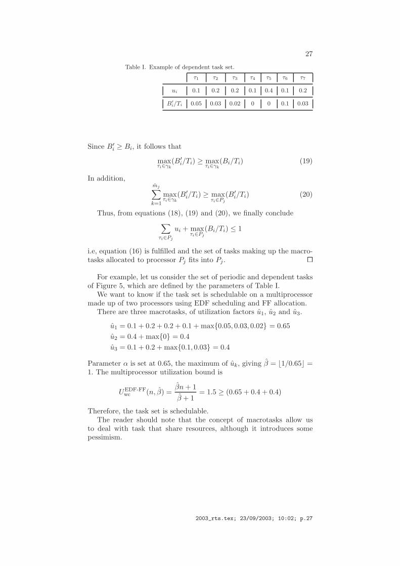
Table I. Example of dependent task set.

τ1 τ2 τ3 τ4 τ5 τ6 τ7

ui 0.1 0.2 0.2 0.1 0.4 0.1 0.2

B′

i/Ti 0.05 0.03 0.02 0 0 0.1 0.03

Since B′

i ≥ Bi, it follows that

maxτi∈γk

(B′

i/Ti) ≥ maxτi∈γk

(Bi/Ti) (19)

In addition,mj∑

k=1

maxτi∈γk

(B′

i/Ti) ≥ maxτi∈Pj

(B′

i/Ti) (20)

Thus, from equations (18), (19) and (20), we finally conclude∑

τi∈Pj

ui + maxτi∈Pj

(Bi/Ti) ≤ 1

i.e, equation (16) is fulfilled and the set of tasks making up the macro-tasks allocated to processor Pj fits into Pj . �

For example, let us consider the set of periodic and dependent tasksof Figure 5, which are defined by the parameters of Table I.

We want to know if the task set is schedulable on a multiprocessormade up of two processors using EDF scheduling and FF allocation.

There are three macrotasks, of utilization factors u1, u2 and u3.

u1 = 0.1 + 0.2 + 0.2 + 0.1 + max{0.05, 0.03, 0.02} = 0.65

u2 = 0.4 + max{0} = 0.4

u3 = 0.1 + 0.2 + max{0.1, 0.03} = 0.4

Parameter α is set at 0.65, the maximum of uk, giving β = ⌊1/0.65⌋ =1. The multiprocessor utilization bound is

UEDF-FFwc (n, β) =

βn + 1

β + 1= 1.5 ≥ (0.65 + 0.4 + 0.4)

Therefore, the task set is schedulable.The reader should note that the concept of macrotasks allow us

to deal with task that share resources, although it introduces somepessimism.

2003_rts.tex; 23/09/2003; 10:02; p.27

28

6.6. Non-preemptive sections

The system model presented in Section 2 assumes preemption. Thismeans, if one job of high priority is released while a low priority taskis executing, a context switch happens, moving the low priority job tothe pending queue and executing the high priority job.

Nevertheless, there are situations in which it is necessary to executea set of instructions atomically, i.e, without any kind of interruption.The set of instructions executed atomically is called a non-preemptivesection. The atomic execution can be accomplished by disabling in-terrupts at the beginning of the non-preemptive section and enablinginterrupts at the end. A non-preemptive section can be part of thecomputation of a job and invalidate the previous analysis, since theresponse times of the tasks may be higher than expected.

Let us focus on non-preemptive sections included in the computationof a low priority job, i.e, with a late absolute deadline under EDF.If the low priority job is executing within its non-preemptive sectionand a high priority job is released, the high priority job will sufferblocking. In the worst case, the blocking will be equal to the lengthof the non-preemptive section. The situation is analogous to that ofblocking while accessing protected shared resources. However, there isa basic difference: any job can be blocked at one non-preemptive sectionat most, and no protocol is necessary to enforce this property.

The multiprocessor utilization bounds provided in Section 6.5 canbe applied to the case of non-preemptive sections by increasing theblocking time B′

i of each task τi by the longest non-preemptive sectionof all the tasks except τi. Note that non-preemptive sections in τi arenot considered, because a task can not block itself.

This approach is pessimistic due to many factors, e.g., in the calcu-lation of the maximum blocking coming from non-preemptive sectionswe are assuming that all the tasks are allocated to the same processor.However, if non-preemptive sections are short, as in general they shouldbe, the pessimism introduced in the analysis is tolerable.

6.7. Mode changes

There are situations in which the environment of a real-time systemprogresses through well defined states, each state requiring a differenttask set. This scenario is called mode changes in the literature (Pedroand Burns, 1998).

Any mode change divide the timeline into three parts:

− A steady part before the mode change occurs.

− A transient part during the mode change.

2003_rts.tex; 23/09/2003; 10:02; p.28

29

τ1, τ3, τ4, τ5, τ7, τ8

τ4 τ5

τ1

τ3

MODE 1

τ4 τ5

τ1 τ6

τ3

τ1, τ3, τ4, τ5, τ6

MODE 3

τ4 τ5

τ8

τ1

τ3

MODE 2

τ7

τ4 τ5

τ6

τ1 τ2

τ3

τ1, τ2, τ3, τ4, τ5, τ6

MODE 1

τ1, τ2, τ3, τ4, τ5, τ6

τ6

τ2

Add τ7, τ8

Add τ2

Rem. τ2, τ6

Add τ6

Rem. τ7, τ8

Figure 6. Example of mode changes on multiprocessors.

− A steady part after the mode change.

Independently of the tasks involved in the mode change: old modecompleted, old mode aborted, wholly new, unchanged new tasks orchanged new tasks (Pedro and Burns, 1998); the steady parts beforeand after any mode change can be described by a process of removingand adding tasks. Every time a task is removed it leaves space in oneprocessor. Every time a new task is added to the system, it should beallocated to one processor. The rest of the tasks can not migrate toother processors, since it would require stopping and restarting themagain. Therefore, allocation algorithms such as FFD, which imply taskordering, can not be applied to dynamic situations such as changes.Quite the opposite, allocation algorithms such as FF, which do notrequire task ordering, can be applied to mode changes.

Figure 6 shows an example of three mode changes on a multiproces-sor using EDF scheduling and FF allocation. Each task is representedby a box of width equal to its utilization factor. Free space in eachprocessor is represented by a shaded area. The reader should observethat the system starts at Mode 1 with one allocation and ends up atthe same mode with the same tasks, but allocated differently.

2003_rts.tex; 23/09/2003; 10:02; p.29

30

On one hand, independently of the reasonable allocation algorithmwe use, the multiprocessor utilization bound can not be higher thanLEDF. The process of task removing during a mode change can drawthe system to the worst situation, presented in the proof of Theorem 3for WF allocation. For example, let us consider a multiprocessor madeup of two identical processors with EDF scheduling. Let us consider aninitial mode defined by four tasks {τ1, τ2, τ3, τ4} of utilization factors{ǫ, (1−ǫ), ǫ, (1−ǫ)}. These tasks are allocated using FF allocation. Eachprocessor allocates one task of utilization factor ǫ and another task ofutilization factor (1 − ǫ). Let us assume a mode change consisting ofremoving the tasks of utilization factor (1 − ǫ) and adding a new taskof utilization factor (1 − 0.5ǫ). This last task can not be allocated toany processor in the new mode. The situation coincides with the worstsituation for WF allocation. The total utilization of the task set in thenew mode is (1 + 1.5ǫ) which is below the utilization bound 1.5 for FFallocation on two processors, but not below the utilization bound 1.0for WF allocation on two processors.

On the other hand, independently of the reasonable allocation al-gorithm we use, the multiprocessor utilization bound can not be lowerthan LEDF, since the task allocation at any mode could be generatedusing a reasonable allocation algorithm.

Therefore, we conclude that the multiprocessor utilization boundfor any reasonable allocation algorithm under mode changes coincideswith LEDF(n, α) = n − (n − 1)α.

This utilization bound provides a global schedulability condition in-dependent of the task allocation. If we tried to apply local schedulabilityconditions in each processor, such as those based on response times, wewould have to analyze the schedulability for each processor for all thepossible allocations in each mode. For example, Figure 6 shows twodifferent task allocations for Mode 1. After a second repetition of thecycle Mode 1→Mode 2→Mode 3→Mode 1, the task allocation for thefinal Mode 1 may be different. Since the number of possible allocationsfor the same mode may be huge, local schedulability conditions are notapplicable.

Note that the utilization bound for mode changes is only valid inthe steady states, i.e, at times far enough from the instant of the modechange. Overloads are possible close to the mode change instant (Pedroand Burns, 1998), so the steady state utilization bound LEDF can notbe applied. In addition, if there is no restriction on the utilization factorof the tasks, then α = 1 and the utilization bound is 1.0, too low to beuseful in practice.

2003_rts.tex; 23/09/2003; 10:02; p.30

31

7. Conclusions and future work

The uniprocessor utilization bound for EDF scheduling on uniproces-sors has been extended to multiprocessors under a partitioning strategyand arbitrary (reasonable) allocation algorithms. The bound dependson the number of processors and the “task sizes”, limited by α, butdoes not depend on the number of tasks. For the case of tasks withlow utilization factors, the utilization bound is greatly raised, asymp-totically reaching the ideal value n, when all the utilization factors areclose to zero (α ≈ 0).

In general, the calculation of utilization bounds is a problem of im-portance real-time systems theory. Utilization bounds allow us not onlyto perform fast schedulability tests, but also to perform a schedulabilityanalysis. That is, utilization bounds allow us to establish the influenceof different parameters such as the number of tasks, task size, etc, on theschedulability of the system by considering the worst-case. Utilizationbounds indicate how far the system is from the ideal situation, in whichthe total utilization equals the number of processors in the system.Furthermore, multiprocessor utilization bounds allow us to performglobal schedulability tests for the whole multiprocessor. This is usefulin complex scenarios, like mode changes.

We have proved that the multiprocessor utilization bound for any(reasonable) allocation algorithm is in the interval

[

n − (n − 1)α,⌊1/α⌋ n + 1

⌊1/α⌋ + 1

]

When all the utilization factors near zero, α ≈ 0, and the EDFmultiprocessor utilization bound for any allocation algorithm is n.

The multiprocessor utilization bound for First Fit, First Fit Increas-ing, Best Fit, Best Fit Increasing and optimal allocation algorithms co-incide with the maximum. Furthermore, all the (reasonable) allocationalgorithms that order the tasks by decreasing utilization factors beforecarrying out the allocation, have a multiprocessor utilization boundequal to the maximum. This is the case of the allocation algorithmsFirst Fit Decreasing, Best Fit Decreasing and Worst Fit Decreasing.

The utilization bound for Worst Fit and Worst Fit Increasing allo-cation coincides with the minimum. When there is no restriction on theutilization factors of the tasks, then α = 1 and this minimum becomes1.0 for any number of processors.

All multiprocessor utilization bounds for the basic task model wereextended to deal with complex tasks, including aperiodic tasks, arbi-trary deadlines, release jitter, mode changes, context switches, non-preemptive sections and blocking in shared resources.

2003_rts.tex; 23/09/2003; 10:02; p.31

32

Future work will address the extension of the utilization bounds todistributed real-time systems through the use of jitter. One of the prob-lems is the pessimism of the jitter extension provided in Section 6.2,which is useful for low values of jitter, but too pessimistic for highvalues of jitter. In addition, an integral analysis of the communica-tions network and processors is necessary (Tindell et al., 1994), whichmay require obtaining two interrelated utilization bounds, one for thecommunications network and another for the processors.

2003_rts.tex; 23/09/2003; 10:02; p.32

33

References

Baker, T.: 1991, ‘Stack-Based scheduling of Real-Time Processes’. Real-Time

Systems 3(1), 301–324.Bernat, G. and A. Burns: 1999, ‘New Results on Fixed Priority Aperiodic Servers’.

In: Proceedings of the Real-Time Systems Symposium.Burchard, A., J. Liebeherr, Y. Oh, and S. Son: 1995, ‘New Strategies for Assigning

Real-Time Tasks to Multiprocessor Systems’. IEEE Transactions on Computers

44(12).Buttazzo, G.: 1997, Hard Real-Time Computing Systems. Predictable Scheduling

Algorithms and Applications, Chapt. 7. Boston/Dordrecht/London: KluwerAcademic Publishers.

Dall, S. and C. Liu: 1978, ‘On a Real-Time Scheduling Problem’. Operations

Research 6(1), 127–140.Davari, S. and S. Dhall: 1986a, ‘On a Periodic Real-Time Task Allocation problem’.

In: Annual international Conference on Systems Sciences. pp. 133–141.Davari, S. and S. Dhall: 1986b, ‘An on Line Algorithm for Real Time Tasks Al-

location’. In: Proceedings of the IEEE Real-Time Systems Symposium. pp.194–200.

Dertouzos, M. L.: 1974, ‘Control Robotics: The procedural Control of PhysicalProcesses’. Proceedings of IFIP Congress pp. 807–813.

Dertouzos, M. L. and A. K. Mok: 1989, ‘Multiprocessor On-Line Scheduling of Hard-Real-Time Tasks’. Transactions on Software Engineering 15(12), 1497–1506.

Garey, M. and D. Johnson: 1979, Computers and Intractability. New York: W.H.Freman.

Lauzac, S., R. Melhem, and D. Mosse: 1998, ‘An Efficient RMS Admission Con-trol and its Application to Multiprocessor Scheduling’. In: Proceedings of the

International Parallel Processing Symposium. pp. 511–518.Liu, C. and J. Layland: 1973, ‘Scheduling Algorithms for Multiprogramming in a

Hard-Real-time Environment’. Journal of the ACM 20(1), 46–61.Lopez, J., J. Dıaz, M. Garcıa, and D. Garcıa: 2003, ‘Utilization Bounds for

Multiprocessor Rate-Monotonic Scheduling’. Real-Time Systems 24(1), 5–28.Oh, D. and T. Baker: 1998, ‘Utilization Bounds for N-Processor Rate Monotone

Scheduling with Static Processor Assignment’. Real-Time Systems 15(2), 183–193.

Oh, Y. and S. Son: 1995, ‘Allocating Fixed-Priority Periodic Tasks on MultiprocessorSystems’. Real-Time Systems 9(3), 207–239.

Pedro, P. and A. Burns: 1998, ‘Schedulability Changes for Mode Changes in FlexibleReal-Time Systems’. In: Proceedings of the Euromicro Workshop on Real Time

Systems. pp. 172–179.Saez, S., J. Vila, and A. Crespo: 1998, ‘Using Exact Feasibility Tests for Allocating

Real-Time Tasks in Multiprocessor Systems’. Proceedings of the 10th Euromicro

Workshop on Real-Time Systems pp. 53–60.Tindell, K., A. Burns, and A. Wellings: 1994, ‘An extendible Approach for Analyzing

Fixed Priority Hard Real-Time Tasks’. Real-Time Systems 6(2), 133–151.Tindell, K. and J. Clark: 1994, ‘Holistic Schedulability Analysis for Distributed Hard

Real-Time Systems’. Microprocessing and Microprogramming 40, 117–134.

2003_rts.tex; 23/09/2003; 10:02; p.33