Using multilevel models to identify drivers oflandscape-genetic structure among management areas

RACHAEL Y. DUDANIEC,* 1 JONATHAN R. RHODES,*1 JESSICA WORTHINGTON WILMER,†

MITCHELL LYONS,* KRISTEN E. LEE,‡ CLIVE A. MCALPINE* and FRANK N. CARRICK‡

*School of Geography, Planning and Environmental Management, The University of Queensland, Brisbane, QLD 4072,

Australia, †Natural Environments Program, Queensland Museum, PO Box 3300, South Brisbane, QLD 4101, Australia,

‡Centre for Mined Land Rehabilitation, Sustainable Minerals Institute, The University of Queensland, Brisbane, QLD 4072,

Australia

Abstract

Landscape genetics offers a powerful approach to understanding species’ dispersal

patterns. However, a central obstacle is to account for ecological processes operating at

multiple spatial scales, while keeping research outcomes applicable to conservation

management. We address this challenge by applying a novel multilevel regression

approach to model landscape drivers of genetic structure at both the resolution of indi-

viduals and at a spatial resolution relevant to management (i.e. local government man-

agement areas: LGAs) for the koala (Phascolartos cinereus) in Australia. Our approach

allows for the simultaneous incorporation of drivers of landscape-genetic relationships

operating at multiple spatial resolutions. Using microsatellite data for 1106 koalas, we

show that, at the individual resolution, foliage projective cover (FPC) facilitates high

gene flow (i.e. low resistance) until it falls below approximately 30%. Out of six addi-

tional land-cover variables, only highways and freeways further explained genetic

distance after accounting for the effect of FPC. At the LGA resolution, there was

significant variation in isolation-by-resistance (IBR) relationships in terms of their

slopes and intercepts. This was predominantly explained by the average resistance

distance among LGAs, with a weaker effect of historical forest cover. Rates of recent

landscape change did not further explain variation in IBR relationships among LGAs.

By using a novel multilevel model, we disentangle the effect of landscape resistance

on gene flow at the fine resolution (i.e. among individuals) from effects occurring at

coarser resolutions (i.e. among LGAs). This has important implications for our ability

to identify appropriate scale-dependent management actions.

Keywords: habitat fragmentation, landscape genetics, mammal dispersal, multilevel model,

spatial scale, wildlife management

Received 22 November 2012; revision received 2 April 2013; accepted 5 April 2013

Introduction

Quantifying the mechanisms by which landscape

features impede or facilitate dispersal is important for

identifying ecological processes that govern species

distributions (sensu Slatkin 1993; Macdonald & Johnson

2001). The field of landscape genetics has rapidly

enhanced our ability to quantify the effects of landscape

features on species’ genetic dispersal (Manel et al. 2003;

Storfer et al. 2007). However, the challenge of linking

landscape and genetic data at different spatial and

temporal resolutions must be met (Landguth et al. 2010;

Lowe & Allendorf 2010), because mismatches in the

scale of observation and key processes can lead to

erroneous conclusions about a species’ sensitivity to

landscape features (Anderson et al. 2010). Therefore, it

is important to test for the underlying drivers of land-

scape-genetic relationships at multiple spatial scales, as

Correspondence: Rachael Y. Dudaniec, Fax +61 7 3365 6899;

Email: rachael.dudaniec@gmail.com1Joint first authors.

© 2013 John Wiley & Sons Ltd

Molecular Ecology (2013) 22, 3752–3765 doi: 10.1111/mec.12359

well as to incorporate variables that represent dynamic

landscape or demographic processes (e.g. Anderson

et al. 2010; Murphy et al. 2010).

Analysing data at spatial scales that are both biologi-

cally meaningful and of direct use for conservation

management is a further challenge that many molecular

ecological studies fail to meet (Taylor & Dizon 1999). To

develop useful models for managing landscape connec-

tivity for species, we must be able to statistically link

the spatial scales of relevance for understanding ecolog-

ical processes (e.g. species’ range, habitat patches) with

scales of management relevance (e.g. political, land use

or regional boundaries) (Taylor & Dizon 1999; Pelosi

et al. 2010). Complicating this further is that the

relationships between ecological and landscape patterns

can vary spatially, with this variation being mediated

by the scale at which these patterns are measured

(Whittingham et al. 2007; McAlpine et al. 2008; Rhodes

et al. 2008). Spatial heterogeneity in landscape-genetic

processes can also be influenced by a species’ popula-

tion size, dispersal capacity, life history and the

geographic area under study (e.g. Steele et al. 2009;

Landguth et al. 2010; Dudaniec et al. 2012; Rasic &

Keyghobadi 2012). Therefore, there is a need to explain

spatial heterogeneity in landscape-genetic patterns

across scales that are relevant to both ecology and

management.

A further challenge is that genetic population struc-

ture is a product of both past and contemporary pro-

cesses, such as changes in landscape characteristics or

demography (e.g. Chiucci & Gibbs 2010; Cushman &

Landguth 2010; Dudaniec et al. 2012). For species with

long generation times, or those subject to rapid frag-

mentation effects, genetic structure can change more

slowly than the landscape it inhabits, resulting in time

lags to detect landscape effects (Landguth et al. 2010;

Murphy et al. 2010). The majority of studies focus on

historical rather than contemporary landscape-change

effects on genetic structure, but in some cases, rapid

genetic responses to recent landscape change have been

detected (e.g. Balkenhol & Waits 2009; Zellmer &

Knowles 2009). Thus, the strength, rate and pattern of

past ‘legacy effects’ may determine the degree to which

current landscape influences on genetic dispersal can be

detected and explained. Quantifying to what extent

‘legacy effects’ determine landscape-genetic patterns at

scales relevant to management can therefore improve

conservation planning decisions by elucidating the

underlying mechanisms that drive species’ dispersal.

One approach to addressing these issues in landscape

genetics is to link multilevel (hierarchical) regression

with a spatial–temporal landscape-genetics approach.

Multilevel regression models provide a powerful frame-

work for representing relationships among variables

simultaneously at different resolutions based on the

specification of random effects to represent hierarchical

structure (McMahon & Diez 2007; Qian et al. 2010). As

such, they offer an elegant way to incorporate relation-

ships at resolutions relevant to both management and

ecological processes and to account for any mismatches

between them (Cumming et al. 2006; Pelosi et al. 2010).

However, to our knowledge, the teasing apart of spatial

and temporal elements using multilevel regression

has not previously been applied in landscape-genetic

studies.

Here, we apply a novel multilevel regression model-

ling approach (McMahon & Diez 2007) to the analysis

of landscape-genetic relationships while testing for the

effects of dynamic landscape change. We adopt a land-

scape resistance approach based on circuit theory

(McRae & Beier 2007) combined with microsatellite data

for the koala (Phascolarcotos cinereus), an arboreal marsu-

pial endemic to Australia that is under threat from mul-

tiple ecological stressors. Our study region spans eight

local government areas (LGAs) that are the spatial units

relevant to land-use planning and therefore representa-

tive of the scale of management for koalas. First, we test

hypotheses regarding land-cover effects on isolation by

resistance (IBR) at the individual resolution to derive a

landscape resistance model. Second, using multilevel

regression, we test for variation in IBR patterns at the

LGA resolution while continuing to account for IBR

relationships at the individual resolution. Third, we use

past and recent landscape data to test for drivers of

variation in IBR relationships among LGAs. In doing so,

this study provides a novel approach for simultaneously

analysing landscape-genetic patterns at multiple spatial

scales, while also incorporating landscape-change

effects.

Materials and methods

Study species

The koala, P. cinereus (Phascolarctidae), is an arboreal

folivore endemic to Australia and feeds on a small

number of Eucalyptus species (Ellis et al. 2002). Habitat

loss is a major factor causing population declines

(McAlpine et al. 2006a,b; Rhodes et al. 2008; Smith et al.

2013), which is further exacerbated by drought (Adams-

Hosking et al. 2011; Seabrook et al. 2011), disease, car

injuries and dog attacks (Dique et al. 2003b; Rhodes

et al. 2011). The area and configuration of forest habitat

are important determinants of koala distributions

(Rhodes et al. 2005; McAlpine et al. 2006b). Koalas

generally move via the ground and rarely via the canopy.

Dispersal is male-biased and typically 2–3 km from the

natal site; however, dispersal events of approximately

© 2013 John Wiley & Sons Ltd

MULTILEVEL MODELS AND LANDSCAPE GENETICS 3753

10 km have been observed (Dique et al. 2003b). The

koala is federally listed as Vulnerable in the states of

Queensland, New South Wales and the Australian

Capital Territory (Environment Protection and Biodiver-

sity Conservation Act 1999), and population sizes have

reduced by as much as 70% over the past 15 years in

some areas (Department of Environment and Natural

Resources 2009).

Study area and sampling

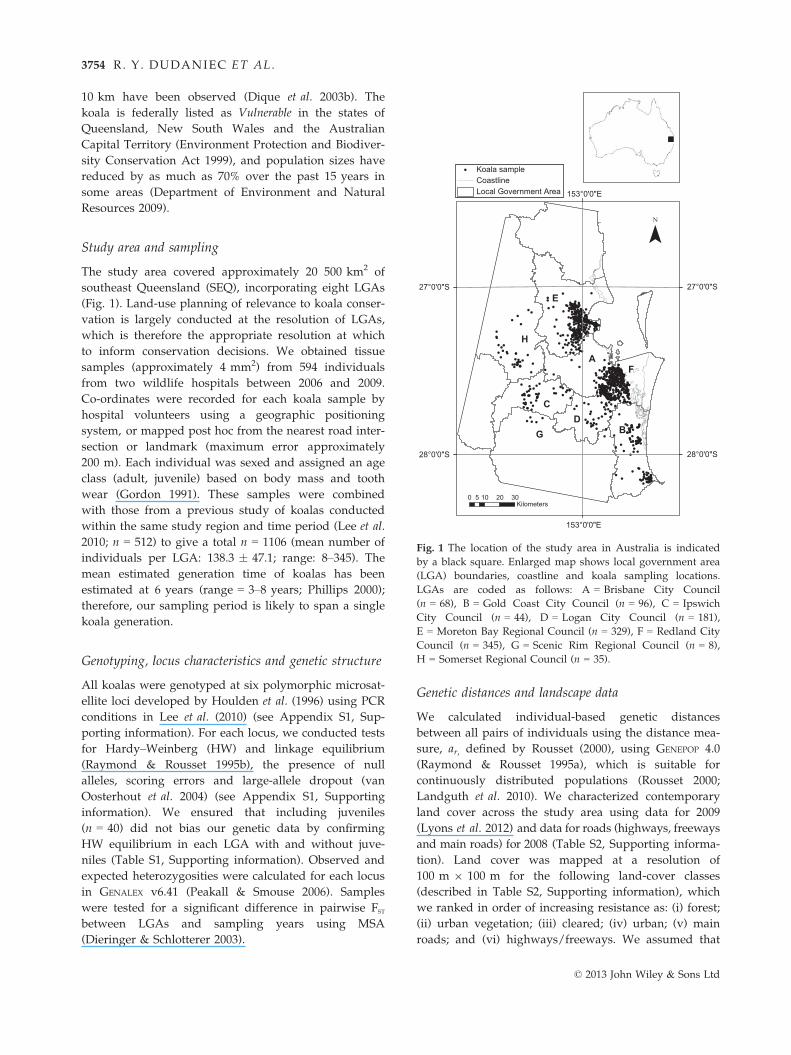
The study area covered approximately 20 500 km2 of

southeast Queensland (SEQ), incorporating eight LGAs

(Fig. 1). Land-use planning of relevance to koala conser-

vation is largely conducted at the resolution of LGAs,

which is therefore the appropriate resolution at which

to inform conservation decisions. We obtained tissue

samples (approximately 4 mm2) from 594 individuals

from two wildlife hospitals between 2006 and 2009.

Co-ordinates were recorded for each koala sample by

hospital volunteers using a geographic positioning

system, or mapped post hoc from the nearest road inter-

section or landmark (maximum error approximately

200 m). Each individual was sexed and assigned an age

class (adult, juvenile) based on body mass and tooth

wear (Gordon 1991). These samples were combined

with those from a previous study of koalas conducted

within the same study region and time period (Lee et al.

2010; n = 512) to give a total n = 1106 (mean number of

individuals per LGA: 138.3 � 47.1; range: 8–345). The

mean estimated generation time of koalas has been

estimated at 6 years (range = 3–8 years; Phillips 2000);

therefore, our sampling period is likely to span a single

koala generation.

Genotyping, locus characteristics and genetic structure

All koalas were genotyped at six polymorphic microsat-

ellite loci developed by Houlden et al. (1996) using PCR

conditions in Lee et al. (2010) (see Appendix S1, Sup-

porting information). For each locus, we conducted tests

for Hardy–Weinberg (HW) and linkage equilibrium

(Raymond & Rousset 1995b), the presence of null

alleles, scoring errors and large-allele dropout (van

Oosterhout et al. 2004) (see Appendix S1, Supporting

information). We ensured that including juveniles

(n = 40) did not bias our genetic data by confirming

HW equilibrium in each LGA with and without juve-

niles (Table S1, Supporting information). Observed and

expected heterozygosities were calculated for each locus

in GENALEX v6.41 (Peakall & Smouse 2006). Samples

were tested for a significant difference in pairwise FST

between LGAs and sampling years using MSA

(Dieringer & Schlotterer 2003).

Genetic distances and landscape data

We calculated individual-based genetic distances

between all pairs of individuals using the distance mea-

sure, ar, defined by Rousset (2000), using GENEPOP 4.0

(Raymond & Rousset 1995a), which is suitable for

continuously distributed populations (Rousset 2000;

Landguth et al. 2010). We characterized contemporary

land cover across the study area using data for 2009

(Lyons et al. 2012) and data for roads (highways, freeways

and main roads) for 2008 (Table S2, Supporting informa-

tion). Land cover was mapped at a resolution of

100 m 9 100 m for the following land-cover classes

(described in Table S2, Supporting information), which

we ranked in order of increasing resistance as: (i) forest;

(ii) urban vegetation; (iii) cleared; (iv) urban; (v) main

roads; and (vi) highways/freeways. We assumed that

153°0'0"E

153°0'0"E

27°0'0"S 27°0'0"S

28°0'0"S 28°0'0"S

A

B

CD

E

F

G

H

0 10 20 305Kilometers

Koala sampleCoastlineLocal Government Area

Fig. 1 The location of the study area in Australia is indicated

by a black square. Enlarged map shows local government area

(LGA) boundaries, coastline and koala sampling locations.

LGAs are coded as follows: A = Brisbane City Council

(n = 68), B = Gold Coast City Council (n = 96), C = Ipswich

City Council (n = 44), D = Logan City Council (n = 181),

E = Moreton Bay Regional Council (n = 329), F = Redland City

Council (n = 345), G = Scenic Rim Regional Council (n = 8),

H = Somerset Regional Council (n = 35).

© 2013 John Wiley & Sons Ltd

3754 R. Y . DUDANIEC ET AL.

large water bodies (>100 m in width) represent a complete

barrier, although there is some evidence for koalas

occasionally crossing water bodies (F. Carrick, personal

communication). We also mapped woody foliage pro-

jective cover (FPC) (a measure of canopy cover, Table

S2, Supporting information: Specht 1983) across the

study area for 2009 at the same resolution. A resolution

of 100 m 9 100 m was deemed to be fine enough given

that koalas can move several hundred metres in a given

movement event (Dique et al. 2003a; Rhodes et al. 2005).

We set the extent of the land-cover and FPC data so

that it included a buffer (as recommended by Koen

et al. 2010) of 10 km (using the land-cover data), which

is the estimated maximum dispersal distance for koalas

in the region (Dique et al. 2003a).

Modelling drivers of IBR relationships at theindividual resolution

We estimated resistance across the landscape extent

using an approach similar to Shirk et al. (2010), but we

used linear regression and the log-likelihood (sensu

Hilborn & Mangel 1997), rather than Mantel tests and

correlation coefficients to evaluate alternative resistance

models. We first assumed that resistance was a function

of both FPC and land cover as follows:

ri ¼ 1þ a100� Fi

100

� �c

þ bRLi

� 1

5

� �g

ð1Þ

where ri is the resistance of raster cell i; 0 � Fi � 100

is the percentage FPC of cell i; RLiis the rank of land-

cover type 1 � Li � 6 of cell i (with land-cover types

ranked from lowest to highest resistance); a > 0 and

b > 0 are parameters that determine the maximum pos-

sible resistance values; and c > 0 and g > 0 are parame-

ters that determine the shape of the relationship

between Fi and RLi, respectively, and ri. Equation (1)

explicitly assumes that resistance decreases as FPC

increases and that resistance increases as land-cover

rank increases.

The exponent c determines the shape of the relation-

ship between FPC and resistance, being linear when

c = 1 and nonlinear when c 6¼ 1 (Shirk et al. 2010).

Similarly, the exponent g determines the shape of the

relationship between land-cover rank and resistance.

The parameters a and b determine the maximum possible

resistance value, with 1 + a + b being the maximum

resistance value possible (i.e. when FPC is zero and

land cover is highways/freeways). We estimated the

parameters a, b, c, g from the individual-based genetic

distance data in two steps. First, we set b = 0 (i.e. no

effect of land cover) and chose a range of values for the

parameters a and c (i.e. the influence of FPC on

resistance). These values were 0, 2, 5, 10, 100, 1000 for aand 0.001, 0.01, 0.1, 0.2, 0.5, 1, 2, 5, 10, 100, 1000 for c.For each possible combination of these values, we

calculated the resistance value of each raster cell and

obtained pairwise resistance distances between all indi-

viduals using Circuitscape v3.5.7 (McRae & Beier 2007).

For each combination of a and c, we fitted a linear

regression model to the individual-based genetic dis-

tances, with resistance distance as the explanatory variable

(McRae 2006). To avoid problems with nonindependence

among samples, we used a modified bootstrap proce-

dure (without replacement) (Worthington-Wilmer et al.

2008) in which random sampling was constrained to

maintain independence between our pairwise distances

measures. We generated 1000 bootstrap replicates and

fitted a linear regression to each replicate. Our

estimated values for a and c where those that had the

highest mean log-likelihood across bootstrap replicates.

Second, we repeated the procedure for the b and gparameters while holding the best supported a and cparameters constant. We considered the same range of

values for b and g as for a and c. This allowed us to esti-

mate the parameters b and g (that link land cover to

resistance) conditional on the estimates of the parameters

a and c (that link percentage FPC to resistance).

Therefore, our model was constructed such that the

effect of land cover was considered after the effect of

FPC had been accounted for. We examined uncertainty

in our parameter estimates by examining the selection

frequency for each parameter value across bootstrap

replicates. Analyses were conducted in R version 2.14

(http://www.r-project.org/).

Incorporating drivers of IBR relationships at theLGA resolution

To test for and explain variation in the IBR relationship

at resolutions relevant to management (i.e. the LGA

resolution), we used mixed-effects, multilevel linear regres-

sion models (Pinheiro & Bates 2000) (Fig. 2). Based on the

estimated resistance surface at the individual resolution,

we modelled the relationship between genetic distance

and resistance distance using the linear mixed-effects

regression model:

arði;jÞ ¼ sj þ mjRi;j þ ei;j ð2Þ

where ar(i,j) is genetic distance for individual pair i in

LGA pair j; Ri,j is the resistance distance for individual

pair i in LGA pair j; τj is a normally distributed random

effect for LGA pair j with mean τ and variance r2s ; υj is

a normally distributed random effect for LGA pair j

with mean υ and variance r2m ; and ei,j are normally

distributed residuals with mean zero and variance r2.

We represented LGAs as ‘pairs’ to reflect that, for a pair

© 2013 John Wiley & Sons Ltd

MULTILEVEL MODELS AND LANDSCAPE GENETICS 3755

of individuals, each individual will be located in a spe-

cific LGA. Note that we consider all pairs simulta-

neously, although an LGA pair can be with itself or a

different LGA. We allowed for the intercept of the IBR

relationship to vary at the LGA resolution through τjand allowed for the slope to vary at the LGA resolution

through υj.We tested for the statistical significance of variation

in the intercept and slope of IBR relationships among

LGAs (i.e. significance of the random effects τj and υj)against a null hypothesis that there was no variation

in the intercept and/or slope among LGAs. This was

achieved using likelihood ratio tests based on simu-

lated values from the finite sample distribution (Crain-

iceanu & Ruppert 2004). We conducted these tests

using a stepwise procedure in which we first tested

for the significance of the intercept random effect, τj,and then tested for the significance of the slope ran-

dom effect, υj. For each test, we conducted significance

tests for each of 1000 bootstrap replicates of the

genetic distances. We rejected the null hypothesis if

the null hypothesis was rejected (at a significance level

of 0.05) in more than 5% of the individual bootstrap

replicates.

To test for variables measured at the resolution of

LGAs that explain variation in IBR relationships among

LGAs, we considered four predictor variables: (i)

proportion of the landscape that was forest in 1972 (rep-

resenting past habitat amount); (ii) recent rates of

change in the proportion of the landscape that was forest

(between 1988 and 2009); (iii) recent rates of change in

the proportion of the landscape that was urban

(between 1988 and 2009); and (iv) average resistance

distance between LGA pairs (representing a measure of

effective isolation due to the landscape between LGA

pairs). Predictor variable 1 tests whether, at equilib-

rium, LGAs with historically low amounts of habitat

have: (a) steeper IBR slopes due to lower population

densities and higher population divergence, and (b)

lower intercepts due to a smaller panmictic area (Peter-

son & Denno 1998; Novembre & Slatkin 2009). However,

rapid landscape change may create nonequilibrium

patterns (i.e. weaker IBR relationships) if there has

not been enough time for populations to achieve

equilibrium, although this will depend on the species’

generation time and dispersal behaviour relative to the

rate of landscape change (Anderson et al. 2010). To

test for landscape-change effects, we therefore examined

whether the rates of change in both forest (i.e.

representing habitat) and urban cover (i.e. representing

nonhabitat) were important predictors of variation in

IBR relationships among LGAs (predictor variables 2

and 3). Finally, as expected for isolation by distance, we

predict lower IBR slopes at high-resistance distances

than at low-resistance distances to be indicative of non-

equilibrium regional patterns, possibly due to genetic

drift (e.g. Slatkin 1993; Hutchison & Templeton

1999). Therefore, we examined whether IBR relation-

ships varied at the LGA resolution as a function of

the resistance distances separating them (predictor

variable 4).

For each pair of LGAs, we created a minimum con-

vex polygon around the koala sampling locations con-

tained in each LGA pair and buffered this by 3.5 km

(mean dispersal distance, Dique et al. 2003a). We then

calculated the amount of forest and urban cover within

INDIVIDUALRESOLUTION

Predictor variables ( j)

Regression coefficients

Random intercept ( j)

Regression coefficients

Variance of random-effect ( 2 ) Variance of random-effect ( 2 )

Random slope ( j)

Estimated genetic distance ( r (i, j))

Variance of residuals ( 2)

Measured genetic distance ( r (i, j))

Resistance (Ri,j)

LGA RESOLUTION

Residuals ( i,j)

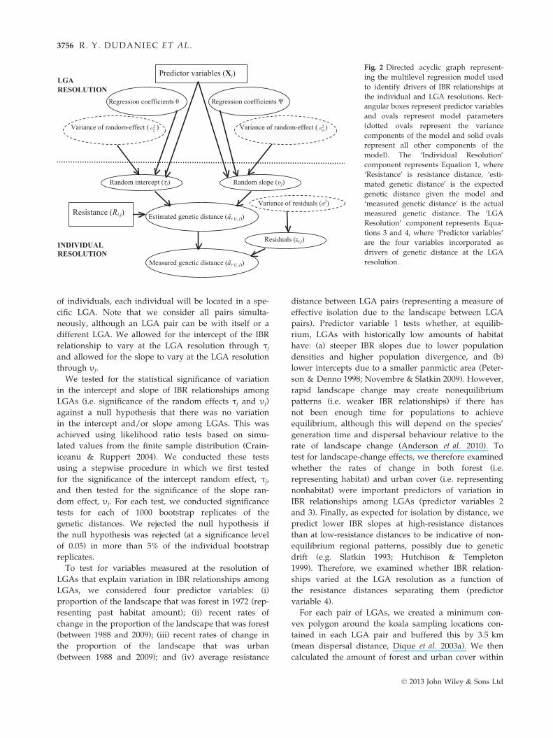
Fig. 2 Directed acyclic graph represent-

ing the multilevel regression model used

to identify drivers of IBR relationships at

the individual and LGA resolutions. Rect-

angular boxes represent predictor variables

and ovals represent model parameters

(dotted ovals represent the variance

components of the model and solid ovals

represent all other components of the

model). The ‘Individual Resolution’

component represents Equation 1, where

‘Resistance’ is resistance distance, ‘esti-

mated genetic distance’ is the expected

genetic distance given the model and

‘measured genetic distance’ is the actual

measured genetic distance. The ‘LGA

Resolution’ component represents Equa-

tions 3 and 4, where ‘Predictor variables’

are the four variables incorporated as

drivers of genetic distance at the LGA

resolution.

© 2013 John Wiley & Sons Ltd

3756 R. Y . DUDANIEC ET AL.

the buffered convex polygons for each LGA pair using

land-cover data from Lyons et al. (2012) for 1972 and

each year from 1988 to 2009. Rates of change in the

amount of forest and urban land cover were estimated

from the slope of a linear regression fitted to the

proportion of the area inside each buffered convex

polygon consisting of urban or forest cover for the

21 years between 1988 and 2009, with time as the

explanatory variable. The proportion of forest cover

within each convex polygon in 1972 was also calculated,

but these data were mapped at a coarser resolution

(60 m 9 60 m) than the data for 1988–2009 (25 m 9 25 m).

Therefore, we were unable to incorporate the 1972 data

into the calculation of rates of change, but instead used

these data to estimate variation among LGA pairs in

terms of past forest amount. Finally, for each LGA pair,

we calculated the average resistance distance (based on

our resistance surface) between all individuals in each

pair of LGAs (for all combinations of the eight LGAs,

n = 36 pairs). All variables were standardized to have a

mean of zero and standard deviation of one prior to

further analysis.

We tested whether the above four predictor variables

were important determinants of variation in IBR inter-

cepts and slopes at the LGA resolution by explicitly

incorporating them into our multilevel model as

predictors for the intercept, τj, and slope, υj, random

effects (sensu McMahon & Diez 2007). We did this by

redefining the intercept and slope random effects in

Equation (2) to be functions of the predictor variables

such that

sj ¼ h0Xj þ nj ð3ÞAnd

mj ¼ w0Xj þ xj ð4Þwhere τj and υj are the intercept and slope random

effects for local government pair j; h and w are vectors

of regression coefficients; Xj is a vector of the predictor

variables for local government pair j; and ξj and xj are

normally distributed random effects for local govern-

ment pair j, with means of zero and variances r2n and

r2x. This formulation allowed us to test explicitly for

drivers of IBR patterns at the LGA resolution, while still

accounting for patterns at the individual resolution. We

constructed 16 different models of all combinations of

the predictor variables assuming that, in every model,

the predictors for variation in the intercept were the

same as for those in the slope.

Each of the 16 regression models was fitted to the

1000 bootstrap replicates of the individual-based genetic

distances. We then conducted model selection within an

information theoretic framework to identify the relative

importance of each of the predictor variables in explaining

variation in IBR relationships among LGAs (Akaike

1998; Burnham & Anderson 2002). For each bootstrap

replicate, we identified the model with the lowest

Akaike’s Information Criterion (AIC) and then, for each

model, calculated the proportion of replicates in which

it was the best model (Burnham & Anderson 2002). This

provided a robust estimate of the probability that each

model is the most parsimonious model (Burnham &

Anderson 2002). We then calculated the 95% confidence

set of models, the relative importance of each variable

based on Akaike weights and model-averaged coeffi-

cients and unconditional standard errors based on the

bootstrap replicates (Burnham & Anderson 2002). For

each model, we also calculated the amount of variation

in the data explained by the explanatory variables and

random effects based on the measure r20 described in

Xu (2003). To assess the potential effect of differences in

sample sizes among LGAs we quantified the influence

of each LGA on model parameter estimates using

Cook’s Distance (Cook 1977). Cook’s Distance provides

a measure of the influence of a particular data point (or

set of data points) by estimating how much removing

that data point (or set of data points) changes the

parameter estimates in the model. We calculated the

mean and 95% confidence intervals of Cook’s Distance

for each LGA pair across bootstrap replicates for a

model containing the highest ranked variables. All

statistical analyses for the multilevel models were con-

ducted in R version 2.14 using the packages ‘lme4’,

‘RLRSim’ and ‘influence.ME’.

Results

Error-checking and locus characteristics

A complete set of genotypes for all six polymorphic loci

was obtained for 1106 individual koalas. There were no

significant differences in pairwise FST between years of

sampling within LGAs (all P > 0.05 following Bonfer-

roni correction), thus, years were pooled for all analy-

ses. None of the loci were consistently out of HW

equilibrium or consistently showed evidence for null

alleles across the eight LGAs (Table S1, Appendix S2,

Supporting information). Results of HW equilibrium

tests were almost identical when juveniles were

excluded (n = 40, Table S1, Supporting information).

There was no evidence for scoring error, stuttering

or large-allele dropout across loci. Genetic diversity of

koalas was high, with 8–19 alleles per locus (mean =13.3 � 1.6 SE) and observed heterozygosity ranged from

0.5 to 1.0 across loci and LGAs (Table S1, Supporting

information). Pairwise FST between LGAs ranged

between 0.002 and 0.107 (mean = 0.047 � 0.006, Table

S3, Supporting information).

© 2013 John Wiley & Sons Ltd

MULTILEVEL MODELS AND LANDSCAPE GENETICS 3757

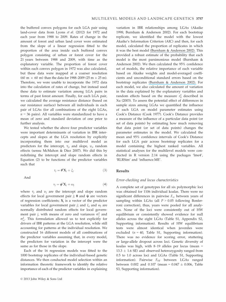
Landscape resistance parameterization

On average, across bootstrap replicates, the best-

supported model was considerably more parsimonious

than a model assuming no isolation by resistance, that

is, with a regression slope = 0, (mean ΔAIC = 45.89),

and a model assuming that all cells have the same resis-

tance value (mean ΔAIC = 7.66) (equivalent of isolation

by distance; McRae & Beier 2007). For the parameters aand c (determining the effect of % FPC on resistance),

the best-supported parameter values were a = 2 and

c = 10 (Fig. 3). This indicates that the resistance of cells

with 0% FPC is three times that of cells with 100% FPC

(Fig. 3), and that the rate of change in resistance with %

FPC is higher at lower percentages, all other things

being equal, due the nonlinear nature of the relation-

ship (Fig. 3). For the parameters b and g (determining

the effect of land cover on resistance, Appendix S2,

Supporting information), the best-supported parameter

combination was highly nonlinear, with b = 5 and

g = 1000. This represents a 33% increase in resistance

between highway/freeways and all other land-cover

types (Fig. 3). Thus, after accounting for the effect of %

FPC, the only land-cover type that has an important

effect on resistance is highways/freeways (Fig. 3).

Parameter value selection frequencies showed consider-

ably less uncertainty in the parameters for land cover

(b and g) than for % FPC (a and c) (Figs S1 and S2,

Supporting information), which may reflect the strong

effect of highways and freeways on resistance (Fig. 3).

The selection frequencies for the % FPC a parameter

indicated a bimodal distribution (Fig. S1A, Supporting

information), which suggests that the maximum resis-

tance due to % FPC is somewhat uncertain and could

be much larger.

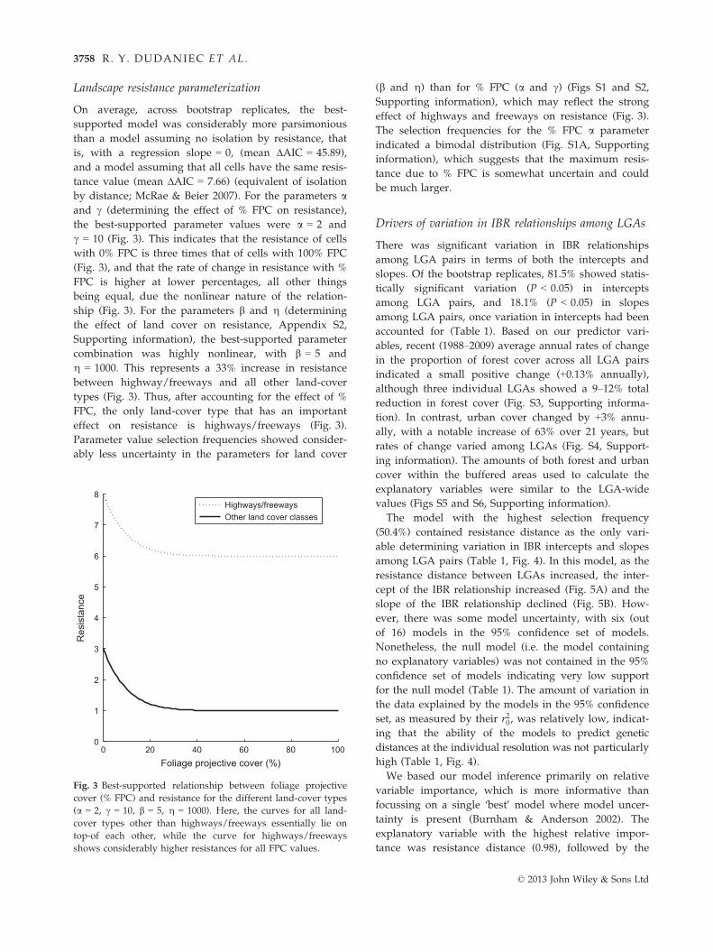
Drivers of variation in IBR relationships among LGAs

There was significant variation in IBR relationships

among LGA pairs in terms of both the intercepts and

slopes. Of the bootstrap replicates, 81.5% showed statis-

tically significant variation (P < 0.05) in intercepts

among LGA pairs, and 18.1% (P < 0.05) in slopes

among LGA pairs, once variation in intercepts had been

accounted for (Table 1). Based on our predictor vari-

ables, recent (1988–2009) average annual rates of change

in the proportion of forest cover across all LGA pairs

indicated a small positive change (+0.13% annually),

although three individual LGAs showed a 9–12% total

reduction in forest cover (Fig. S3, Supporting informa-

tion). In contrast, urban cover changed by +3% annu-

ally, with a notable increase of 63% over 21 years, but

rates of change varied among LGAs (Fig. S4, Support-

ing information). The amounts of both forest and urban

cover within the buffered areas used to calculate the

explanatory variables were similar to the LGA-wide

values (Figs S5 and S6, Supporting information).

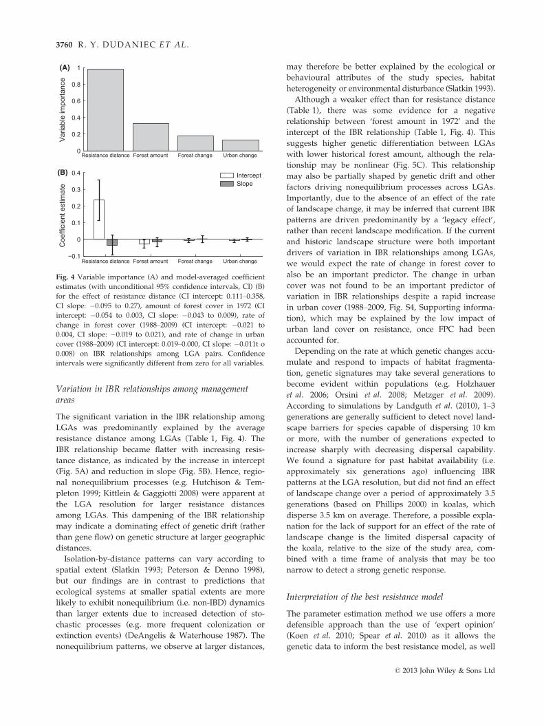
The model with the highest selection frequency

(50.4%) contained resistance distance as the only vari-

able determining variation in IBR intercepts and slopes

among LGA pairs (Table 1, Fig. 4). In this model, as the

resistance distance between LGAs increased, the inter-

cept of the IBR relationship increased (Fig. 5A) and the

slope of the IBR relationship declined (Fig. 5B). How-

ever, there was some model uncertainty, with six (out

of 16) models in the 95% confidence set of models.

Nonetheless, the null model (i.e. the model containing

no explanatory variables) was not contained in the 95%

confidence set of models indicating very low support

for the null model (Table 1). The amount of variation in

the data explained by the models in the 95% confidence

set, as measured by their r20, was relatively low, indicat-

ing that the ability of the models to predict genetic

distances at the individual resolution was not particularly

high (Table 1, Fig. 4).

We based our model inference primarily on relative

variable importance, which is more informative than

focussing on a single ‘best’ model where model uncer-

tainty is present (Burnham & Anderson 2002). The

explanatory variable with the highest relative impor-

tance was resistance distance (0.98), followed by the

0 20 40 60 80 1000

1

2

3

4

5

6

7

8

Foliage projective cover (%)

Res

ista

nce

Highways/freewaysOther land cover classes

Fig. 3 Best-supported relationship between foliage projective

cover (% FPC) and resistance for the different land-cover types

(a = 2, c = 10, b = 5, g = 1000). Here, the curves for all land-

cover types other than highways/freeways essentially lie on

top-of each other, while the curve for highways/freeways

shows considerably higher resistances for all FPC values.

© 2013 John Wiley & Sons Ltd

3758 R. Y . DUDANIEC ET AL.

amount of forest cover in 1972 (0.33), with the other

two variables having lower importance (Fig. 4A). If a

variable has an importance of above 0.5, then this can

be considered strong evidence that the variable has an

important effect (Barbieri & Berger 2004). Therefore,

there was strong evidence that resistance distance is

an important predictor of variation in IBR relationships

among LGA pairs, weaker evidence that the amount

of forest in 1972 was important, but little evidence that

the other variables were important. Model-averaged

coefficient estimates indicated that IBR intercepts were

positively related to resistance distance and negatively

related to the amount of forest in 1972, the rate of

change in forest cover and the rate of change in urban

cover (Fig. 4B). On the other hand, IBR slopes were

negatively related to all variables (Fig. 4B). However,

only the effect of resistance distance (for intercepts

and slopes) and the amount of forest cover in 1972

(for intercepts) had unconditional 95% confidence

intervals that did not contain zero and were thus iden-

tified as the key drivers of variation in IBR relation-

ships among LGA pairs (Fig. 5). When we averaged

Cook’s Distance by LGA, we found that those LGAs

with the largest samples sizes (i.e. E and F; Fig. 1)

exerted the highest influence on the model parameters

for resistance distance and forest amount in 1972. The

two LGAs with the lowest sample sizes (i.e. G and H;

Fig. 1) had the lowest influence (Fig. S7, Supporting

information), but apart from these, confidence intervals

all overlapped, indicating that differences in influence

among LGAs were not statistically significant despite

some unequal sample sizes (Fig. S7, Supporting

information).

Discussion

This study presents a novel use of multilevel statisti-

cal models to quantify the effect of landscape patterns

on genetic structure at multiple spatial resolutions

relevant to both management and ecological processes.

Our approach allowed us to quantify variation in IBR

relationships among management areas and explain

this variation in terms of broad resolution landscape

metrics, while still accounting for the effect of pat-

terns driving genetic structure at the finer individual

resolution. The use of multilevel regression models in

ecology is recognized as a robust method of dealing

objectively with the issue of scale dependencies (Qian

et al. 2010), but its application in landscape genetics

has been limited. By applying this framework to the

landscape genetics of the koala, we have demon-

strated important insights into the spatial drivers of

genetic structure at the resolution of management

areas.Table

1Forthe95%

confiden

cesetofmodels,

model

ranks,

model

selectionfreq

uen

cies,coefficien

testimates

and

stan

dard

errors

(inparen

theses)relatingto

theexplanatory

variablesfordeterminingvariationin

IBR

relationsh

ipsam

ongLGAsan

dr2 0.Rates

offorest

andurban

cover

chan

gewerecalculated1988–2009.

Blanksindicatethat

thevariable

isnotcontained

inthat

model

Model

rank

Selection

freq

uen

cy

(%)

Intercep

tCoefficien

ts(h)

SlopeCoefficien

ts(w)

r2 0

Resistance

distance

Forest

amount1972

Rateofch

ange

inforest

Rateofch

ange

inurban

Resistance

distance

Forest

amount1972

Rateofch

ange

inforest

Rateofch

ange

inurban

150.4

0.240(0.065)

�0.103

(0.053)

0.13

222.5

0.254(0.066)

�0.108

(0.053)

0.047(0.040)

�0.031

(0.049)

0.13

36.9

0.224(0.067)

�0.093

(0.056)

�0.035

(0.057)

0.003(0.056)

0.13

46.1

0.230(0.066)

�0.098

(0.057)

0.031(0.056)

0.009(0.056)

0.13

55.9

0.234(0.067)

�0.061

(0.062)

�0.024

(0.051)

0.061(0.043)

�0.097

(0.057)

�0.018

(0.060)

0.13

62.6

0.243(0.066)

0.038(0.056)

�0.037

(0.050)

0.048(0.040)

�0.099

(0.057)

0.007(0.056)

0.13

© 2013 John Wiley & Sons Ltd

MULTILEVEL MODELS AND LANDSCAPE GENETICS 3759

Variation in IBR relationships among managementareas

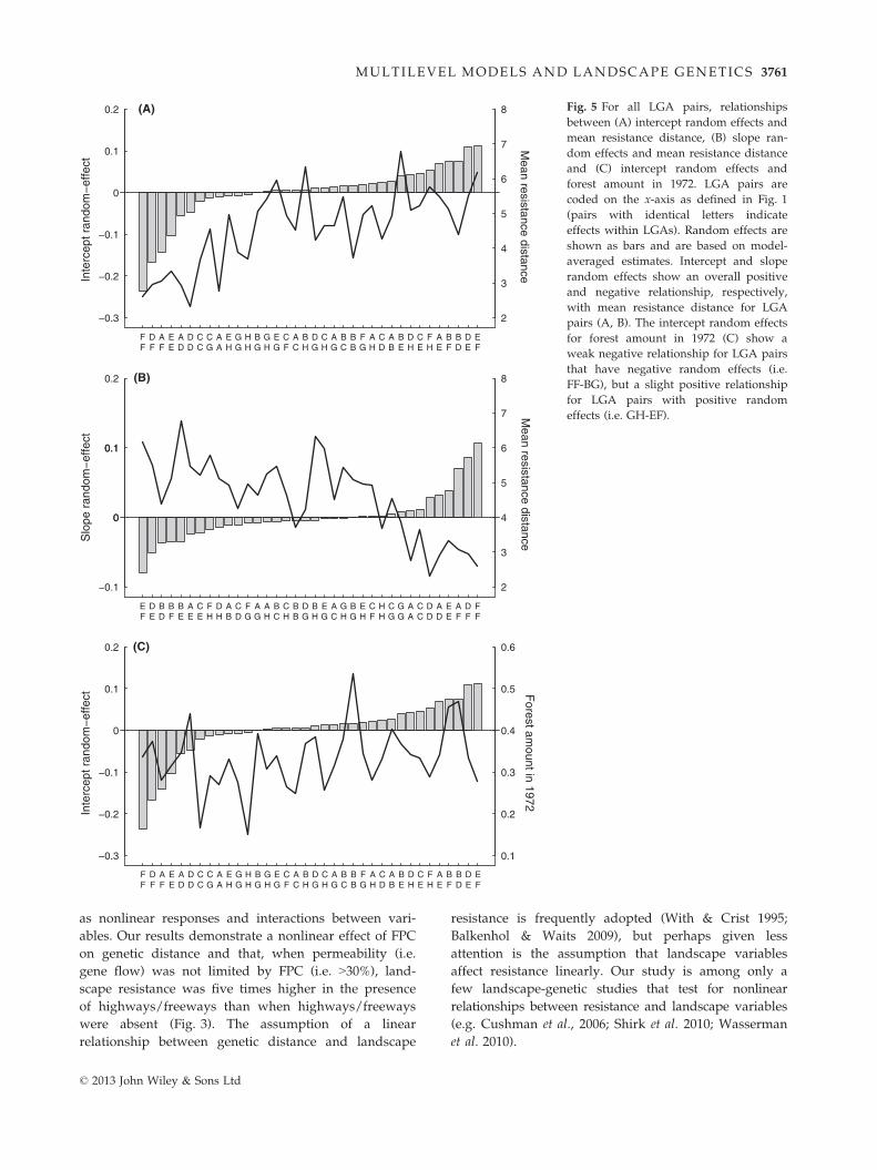
The significant variation in the IBR relationship among

LGAs was predominantly explained by the average

resistance distance among LGAs (Table 1, Fig. 4). The

IBR relationship became flatter with increasing resis-

tance distance, as indicated by the increase in intercept

(Fig. 5A) and reduction in slope (Fig. 5B). Hence, regio-

nal nonequilibrium processes (e.g. Hutchison & Tem-

pleton 1999; Kittlein & Gaggiotti 2008) were apparent at

the LGA resolution for larger resistance distances

among LGAs. This dampening of the IBR relationship

may indicate a dominating effect of genetic drift (rather

than gene flow) on genetic structure at larger geographic

distances.

Isolation-by-distance patterns can vary according to

spatial extent (Slatkin 1993; Peterson & Denno 1998),

but our findings are in contrast to predictions that

ecological systems at smaller spatial extents are more

likely to exhibit nonequilibrium (i.e. non-IBD) dynamics

than larger extents due to increased detection of sto-

chastic processes (e.g. more frequent colonization or

extinction events) (DeAngelis & Waterhouse 1987). The

nonequilibrium patterns, we observe at larger distances,

may therefore be better explained by the ecological or

behavioural attributes of the study species, habitat

heterogeneity or environmental disturbance (Slatkin 1993).

Although a weaker effect than for resistance distance

(Table 1), there was some evidence for a negative

relationship between ‘forest amount in 1972’ and the

intercept of the IBR relationship (Table 1, Fig. 4). This

suggests higher genetic differentiation between LGAs

with lower historical forest amount, although the rela-

tionship may be nonlinear (Fig. 5C). This relationship

may also be partially shaped by genetic drift and other

factors driving nonequilibrium processes across LGAs.

Importantly, due to the absence of an effect of the rate

of landscape change, it may be inferred that current IBR

patterns are driven predominantly by a ‘legacy effect’,

rather than recent landscape modification. If the current

and historic landscape structure were both important

drivers of variation in IBR relationships among LGAs,

we would expect the rate of change in forest cover to

also be an important predictor. The change in urban

cover was not found to be an important predictor of

variation in IBR relationships despite a rapid increase

in urban cover (1988–2009, Fig. S4, Supporting informa-

tion), which may be explained by the low impact of

urban land cover on resistance, once FPC had been

accounted for.

Depending on the rate at which genetic changes accu-

mulate and respond to impacts of habitat fragmenta-

tion, genetic signatures may take several generations to

become evident within populations (e.g. Holzhauer

et al. 2006; Orsini et al. 2008; Metzger et al. 2009).

According to simulations by Landguth et al. (2010), 1–3

generations are generally sufficient to detect novel land-

scape barriers for species capable of dispersing 10 km

or more, with the number of generations expected to

increase sharply with decreasing dispersal capability.

We found a signature for past habitat availability (i.e.

approximately six generations ago) influencing IBR

patterns at the LGA resolution, but did not find an effect

of landscape change over a period of approximately 3.5

generations (based on Phillips 2000) in koalas, which

disperse 3.5 km on average. Therefore, a possible expla-

nation for the lack of support for an effect of the rate of

landscape change is the limited dispersal capacity of

the koala, relative to the size of the study area, com-

bined with a time frame of analysis that may be too

narrow to detect a strong genetic response.

Interpretation of the best resistance model

The parameter estimation method we use offers a more

defensible approach than the use of ‘expert opinion’

(Koen et al. 2010; Spear et al. 2010) as it allows the

genetic data to inform the best resistance model, as well

Resistance distance Forest amount Forest change Urban change0

0.2

0.4

0.6

0.8

1V

aria

ble

impo

rtanc

e

Resistance distance Forest amount Forest change Urban change−0.1

0

0.1

0.2

0.3

0.4

Coe

ffici

ent e

stim

ate

InterceptSlope

(A)

(B)

Fig. 4 Variable importance (A) and model-averaged coefficient

estimates (with unconditional 95% confidence intervals, CI) (B)

for the effect of resistance distance (CI intercept: 0.111–0.358,

CI slope: �0.095 to 0.27), amount of forest cover in 1972 (CI

intercept: �0.054 to 0.003, CI slope: �0.043 to 0.009), rate of

change in forest cover (1988–2009) (CI intercept: �0.021 to

0.004, CI slope: �0.019 to 0.021), and rate of change in urban

cover (1988–2009) (CI intercept: 0.019–0.000, CI slope: �0.011t o

0.008) on IBR relationships among LGA pairs. Confidence

intervals were significantly different from zero for all variables.

© 2013 John Wiley & Sons Ltd

3760 R. Y . DUDANIEC ET AL.

as nonlinear responses and interactions between vari-

ables. Our results demonstrate a nonlinear effect of FPC

on genetic distance and that, when permeability (i.e.

gene flow) was not limited by FPC (i.e. >30%), land-

scape resistance was five times higher in the presence

of highways/freeways than when highways/freeways

were absent (Fig. 3). The assumption of a linear

relationship between genetic distance and landscape

resistance is frequently adopted (With & Crist 1995;

Balkenhol & Waits 2009), but perhaps given less

attention is the assumption that landscape variables

affect resistance linearly. Our study is among only a

few landscape-genetic studies that test for nonlinear

relationships between resistance and landscape variables

(e.g. Cushman et al., 2006; Shirk et al. 2010; Wasserman

et al. 2010).

−0.3

−0.2

−0.1

0

0.1

0.2

2

3

4

5

6

7

8

FF

DF

AF

EE

AD

DD

CC

CG

AA

EH

GG

HH

BG

GH

EG

CF

AC

BH

DG

CH

AG

BC

BB

FG

AH

CD

AB

BE

DH

CE

FH

AE

BF

BD

DE

EF

(A)

Mean resistance distanceIn

terc

ept r

ando

m−

effe

ct

−0.1

00

0.10.1

0.2

2

3

4

5

6

7

8

EF

DE

BD

BF

BE

AE

CE

FH

DH

AB

CD

FG

AG

AH

BC

CH

BB

DG

BH

EG

AC

GH

BG

EH

CF

HH

CG

GG

AA

CC

DD

AD

EE

AF

DF

FF

(B)

Mean resistance distanceS

lope

ran

dom

−ef

fect

−0.3

−0.2

−0.1

0

0.1

0.2

0.1

0.2

0.3

0.4

0.5

0.6

FF

DF

AF

EE

AD

DD

CC

CG

AA

EH

GG

HH

BG

GH

EG

CF

AC

BH

DG

CH

AG

BC

BB

FG

AH

CD

AB

BE

DH

CE

FH

AE

BF

BD

DE

EF

(C)

Forest am

ount in 1972

Inte

rcep

t ran

dom

−ef

fect

Fig. 5 For all LGA pairs, relationships

between (A) intercept random effects and

mean resistance distance, (B) slope ran-

dom effects and mean resistance distance

and (C) intercept random effects and

forest amount in 1972. LGA pairs are

coded on the x-axis as defined in Fig. 1

(pairs with identical letters indicate

effects within LGAs). Random effects are

shown as bars and are based on model-

averaged estimates. Intercept and slope

random effects show an overall positive

and negative relationship, respectively,

with mean resistance distance for LGA

pairs (A, B). The intercept random effects

for forest amount in 1972 (C) show a

weak negative relationship for LGA pairs

that have negative random effects (i.e.

FF-BG), but a slight positive relationship

for LGA pairs with positive random

effects (i.e. GH-EF).

© 2013 John Wiley & Sons Ltd

MULTILEVEL MODELS AND LANDSCAPE GENETICS 3761

The small number of spatial genetic studies on

nonflying, arboreal mammals show variable movement

sensitivities to forest fragmentation (e.g. in orang-utans:

Goossens et al. 2005; gliders: Taylor et al. 2007; lemurs:

Qu�em�er�e et al. 2010; and possums: Lancaster et al.

2011). Studies on the effect of canopy cover on gene

flow in terrestrial vertebrates show mostly positive rela-

tionships (e.g. Munshi-South 2012; Niedziałkowska et al.

2012), but the effect may be dominated by elevation

(e.g. Wasserman et al. 2010; Dudaniec et al. 2012) or

road cover (e.g. Crosby et al. 2009). Roads represent a

major movement barrier for many taxa (e.g. Balkenhol

& Waits 2009; Jackson & Fahrig 2011), and the impact

of major roads on koalas (via fatalities and injuries) is

well documented (Dique et al. 2003a,b; Rhodes et al.

2011). Notably, our results suggest that highways and

freeways confer much greater resistance to gene flow

than main roads, which were not distinguishable from

other land-cover variables. This may be related to dif-

ferences in traffic volume (e.g. as in Shirk et al. 2010), or

the presence of physical barriers bordering major roads.

Notably, urban areas appeared to have little influence

on resistance once FPC had been accounted for.

Limitations and future research

This study represents the largest sampling effort for

any regional genetic study on the koala (Houlden et al.

1996; Sherwin et al. 2000). Although greater resolution

in genetic patterns may have been obtained with more

loci, the high polymorphism of the six loci used, the

lack of missing genotypes and the large sample size of

individuals greatly increase the resolution of our data

(Landguth et al. 2012). Regarding the sampling of

LGAs, two points should be noted, (i) our inferences

are only well supported for the area where samples

were collected; and (ii) LGAs with small sample sizes

exerted little influence on our overall model because

their contributions to the model likelihood are small. In

addition, variation in sample sizes among LGAs does

not appear to be a major issue for inference, with little

significant variation in influence on parameter esti-

mates among LGAs (Fig. S7, Supporting information).

Further, our approach was designed to understand var-

iation in landscape-genetic relationships among LGAs,

rather than to make inferences about specific LGAs,

which would tend to be unreliable due to potentially

high levels of uncertainty in estimates of individual

LGA random effects (Link & Sauer 1996; Sauer & Link

2002). Although our model detected major landscape

effects, it is possible that we failed to detect other

land-cover effects due to a thematic resolution that was

too coarse (Cushman & Landguth 2010). Future

research may benefit from a finer habitat resolution, for

example, incorporating the distribution of koala-specific

Eucalyptus trees.

Management implications and conclusions

Evaluating different planning strategies to minimize the

impact of landscape change on species connectivity is

critical for conserving biodiversity (Epps et al. 2007).

The variations in IBR relationships identified in this

study provide several scale-dependent insights to guide

conservation decision-making for the koala. At a finer

resolution, targeting the preservation and restoration of

forest cover to a minimum 30% FPC (i.e. of food trees)

and facilitating movement across highways and

freeways are important. At the broader LGA resolution,

improving landscape connectivity within LGAs or

between geographically proximate LGAs may be more

important than among geographically distant LGAs.

This is because the effect of landscape resistance on

gene flow appears to give way to the effect of genetic

drift for LGAs that are separated by larger geographic

distances. Thus, improving connectivity may be best

directed towards resolutions at which gene flow

responds to landscape resistance. Generally increasing

the amount of forest within LGAs may also be an

important strategy for maintaining gene flow. The

choice of analysis scale can dramatically affect the infer-

ences we make about landscape-genetic processes

(Anderson et al. 2010). Multilevel models offer a robust

way to explicitly model landscape-genetic patterns at

resolutions appropriate to both genetic processes and

conservation management.

Acknowledgements

This project was conducted with approval from the Animal

Ethics Committee of the University of Queensland (approval

number GPA/359/09/ARC). The project was funded by the

Australian Research Council (ARC), the Queensland Museum,

Moreton Bay Regional Council, Redland City Council, Logan

City Council, Gold Coast City Council and the Queensland

Department of Environment and Heritage Protection. We

thank Matthew Warren for help with landscape data prepara-

tion, Camryn Allen for providing samples from Burbank and

Greg Simmons for providing Gold Coast samples collected

by Steve Phillips. We are grateful to the staff of the Austra-

lian Wildlife Hospital, Moggill Koala Hospital and the

Queensland Department of National Parks, Recreation, Sport

and Racing, for providing koala tissue samples and associ-

ated data.

References

Adams-Hosking C, Grantham HS, Rhodes JR, McAlpine CA,

Moss PT (2011) Modelling climate-change-induced shifts in

the distribution of the koala. Wildlife Research, 38, 122–130.

© 2013 John Wiley & Sons Ltd

3762 R. Y . DUDANIEC ET AL.

Akaike H (1998) Information theory as an extension of the

maximum likelihood principle. In: Selected Papers of Hirotugu

Akaike (eds Parzen E, Tanabe K & Kitagawa G), pp. 199–213.

Springer, New York.

Anderson CD, Epperson BK, Fortin M-J et al. (2010) Consider-

ing spatial and temporal scale in landscape-genetic studies

of gene flow. Molecular Ecology, 19, 3565–3575.

Balkenhol N, Waits LP (2009) Molecular road ecology: explor-

ing the potential of genetics for investigating transportation

impacts on wildlife. Molecular Ecology, 18, 4151–4164.Barbieri MM, Berger JO (2004) Optimal predictive model selec-

tion. Annals of Statistics, 32, 870–897.Burnham KP, Anderson DR (2002) Model Selection and Multi-

Model Inference: A Practical Information Theoretic Approach, 2nd

edn. Springer-Verlag, New York.

Chiucci JE, Gibbs HL (2010) Similarity of contemporary and

historical geneflow among highly fragmented populations of

an endangered rattlesnake. Molecular Ecology, 19, 5435–5358.Cook RD (1977) Detection of influential observation in linear

regression. Technometrics, 19, 15–18.Crainiceanu CM, Ruppert D (2004) Likelihood ratio tests in

linear mixed models with one variance component. Journal of

the Royal Statistical Society Series B - Statistical Methodology,

66, 165–185.Crosby MKA, Licht LE, Fu J (2009) The effect of habitat frag-

mentation on finescale population structure of wood frogs

(Rana sylvatica). Conservation Genetics, 10, 1707–1718.

Cumming GS, Cumming DHM, Redman CL (2006) Scale mis-

matches in social-ecological systems: causes, consequences,

and solutions. Ecology and Society, 11, 14.

Cushman SA, McKelvey KS, Hayden J, Schwartz MK (2006)

Gene flow in complex landscapes: testing multiple hypotheses

with causal modeling. The American Naturalist, 168, 486–499.Cushman SA, Landguth EL (2010) Scale dependent inference

in landscape genetics. Landscape Ecology, 25, 967–979.Department of Environment and Natural Resources (2009)

Decline of the Koala Coast population: Population Status in 2008.

Queensland Government, Brisbane, Australia.

DeAngelis DL, Waterhouse JC (1987) Equilibrium and nonequi-

librium concepts in ecological models. Ecological Monographs,

57, 1–21.Dieringer D, Schlotterer C (2003) Microsatellite analyser (MSA):

a platform independent analysis tool for large microsatellite

data sets. Molecular Ecology Notes, 3, 167–169.

Dique DS, Thompson J, Preece HJ, de Villiers DL, Carrick FN

(2003a) Dispersal patterns in a regional koala population in

south-east Queensland. Wildlife Research, 30, 281–290.Dique DS, Thompson J, Preece HJ et al. (2003b) Koala mortality

on roads in south-east Queensland: the koala speed-zone

trial. Wildlife Research, 30, 419–426.

Dudaniec RY, Spear SF, Storfer A (2012) Current and historical

drivers of landscape genetic structure differ in core and

peripheral salamander populations. PLoS ONE, 7, e36769.

Ellis W, Melzer A, Carrick F, Hasegawa M (2002) Tree use, diet

and home range of the koala (Phascolarctos cinereus) at Blair

Athol, central Queensland. Wildlife Research, 29, 303–311.

Environment Protection and Biodiversity Conservation Act

(1999) Australian Government, Canberra, Australia.

Epps CW, Wehausen JD, Bleich VC, Torres SG, Brashares JS

(2007) Optimizing dispersal and corridor models using land-

scape genetics. Journal of Applied Ecology, 44, 714–724.

Goossens B, Chikhi L, Jalil F et al. (2005) Patterns of genetic

diversity and migration in increasingly fragmented and

declining orang-utan (Pongo pygmaeus) populations from

Sabeh, Malaysia. Molecular Ecology, 14, 441–456.Gordon G (1991) Estimation of the age of the koala, Phascolarc-

tos cinereus (Marsupialia: Phascolarctidae) from tooth wear

and growth. Australian Mammalogy, 14, 5–12.

Hilborn R, Mangel M (1997) The Ecological Detective. Confronting

Models with Data. Princeton University Press, Princeton, New

Jersey.

Holzhauer SIJ, Ekschmitt K, Sander AC, Dauber J, Wolters V

(2006) Effect of historic landscape change on the genetic

structure of the bush-cricket Metrioptera roeseli. Landscape

Ecology, 21, 891–899.Houlden BA, England P, Eldridge MDB (1996) Paternity exclu-

sion in koalas (Phascolarctos cinereus) using hypervariable

microsatellite loci. Journal of Heredity, 87, 149–152.

Hutchison DW, Templeton AR (1999) Correlation of pairwise

genetic and geographic distance measures: inferring the rela-

tive influences of gene flow and drift on the distribution of

genetic variability. Evolution, 53, 1898–1914.

Jackson ND, Fahrig L (2011) Relative effects of road mortality

and decreased connectivity on population genetic diversity.

Biological Conservation, 144, 3143–3148.Kittlein MJ, Gaggiotti OE (2008) Interactions between envi-

ronmental factors can hide isolation by distance patterns: a

case study of Ctenomys rionegrensis and Uraguay. Proceed-

ings of the Royal Society B: Biological Sciences, 275, 2633–

2638.

Koen EL, Garroway CJ, Wilson PJ, Bowman J (2010) The effect

of map boundary on estimates of landscape resistance to animal

movement. PLoS ONE, 5, e11785.

Lancaster ML, Taylor AC, Cooper SJB, Carthew SM (2011) Lim-

ited ecological connectivity of an arboreal marsupial across a

forest/plantation landscape despite apparent resilience to

fragmentation. Molecular Ecology, 20, 2258–2271.

Landguth EL, Cushman SA, Schwartz MK et al. (2010) Quanti-

fying the lag time to detect barriers in landscape genetics.

Molecular Ecology, 19, 4179–4191.Landguth EL, Fedy BC, Oyler-McCance O et al. (2012) Effects

of sample size, number of markers, and allelic richness on

the detection of spatial genetic pattern. Molecular Ecology

Resources, 12, 276–284.Lee KE, Seddon JM, Corely SW et al. (2010) Genetic variation

and structuring in the threatened koala populations of

Southeast Queensland. Conservation Genetics, 11, 2091–2103.

Link W, Sauer J (1996) Extremes in ecology: avoiding the

misleading effects of sampling variation in summary analyses.

Ecology, 77, 1633–1640.Lowe WH, Allendorf FW (2010) What can genetics tell us

about population connectivity? Molecular Ecology, 19, 3038–3051.

Lyons M, Phinn SR, Roelfsema CM (2012) Long term land

cover and seagrass mapping using Landsat and object-based

image analysis from 1972 to 2010 in the coastal environment

of South East Queensland, Australia. ISPRS Journal of Photo-

grammetry and Remote Sensing, 71, 34–46.Macdonald DW, Johnson DDP (2001) Dispersal in theory and

practice: consequences for conservation biology. In: Dispersal

(eds Clobert J, Danchin E, Dhondt AA & Nichols JD), pp.

358–372. Oxford University Press, Oxford.

© 2013 John Wiley & Sons Ltd

MULTILEVEL MODELS AND LANDSCAPE GENETICS 3763

Manel S, Schwartz MK, Luikart G, Taberlet P (2003) Landscape

genetics: combining landscape ecology and population genet-

ics. Trends in Ecology & Evolution, 18, 189–197.

McAlpine CA, Bowen ME, Callaghan JG et al. (2006a) Testing

alternative models for the conservation of koalas in frag-

mented rural-urban landscapes. Austral Ecology, 31, 529–544.McAlpine CA, Rhodes JR, Bowen ME et al. (2006b) The impor-

tance of forest area and configuration relative to local habitat

factors for conserving forest mammals: a case study of koalas

in Queensland, Australia. Biological Conservation, 132,

153–165.

McAlpine CA, Rhodes JR, Bowen ME et al. (2008) Can multi-

scale models of species’ distribution be generalized from

region to region? A case study of the koala. Journal of Applied

Ecology, 45, 558–567.

McMahon SM, Diez JM (2007) Scales of association: hierarchi-

cal linear models and the measurement of ecological

systems. Ecology Letters, 10, 437–452.McRae BH (2006) Isolation by resistance. Evolution, 60, 1551–

1561.

McRae BH, Beier P (2007) Circuit theory predicts gene flow in

plant and animal populations. Proceedings of the National

Academy of Sciences, USA, 104, 19885–19890.

Metzger JP, Martensen AC, Dixo M et al. (2009) Time-lag in

biological response to landscape changes in a highly dynamic

Atlantic forest region. Biological Conservation, 142, 1166–1177.Munshi-South J (2012) Urban landscape genetics: canopy cover

predicts gene flow between white-footed mouse (Peromyscus

leucopus) populations from New York City. Molecular Ecology,

21, 1360–1378.

Murphy MA, Dezzani R, Pilliod DS, Storfer A (2010) Land-

scape genetics of high mountain frog metapopulations.

Molecular Ecology, 19, 3634–3649.Niedziałkowska M, Fontaine MC, Jezdrzejewska B (2012)

Factors shaping geneflow in red deer (Cervus elaphus) in

seminatural landscapes of central Europe. Canadian Journal of

Zoology, 90, 150–162.Novembre J, Slatkin M (2009) Likelihood-based inference in

isolation-by-distance models using the spatial distribution of

low-frequency alleles. Evolution, 63, 2914–2925.

van Oosterhout C, Hutchinson WF, Wills DPM, Shipley P

(2004) MICRO-CHECKER: software for identifying and

correcting genotyping errors in microsatellite data. Molecular

Ecology, 4, 535–538.

Orsini L, Corander J, Alasentie A, Hanski I (2008) Genetic

spatial structure in a butterfly metapopulation correlates better

with past than present demographic structure. Molecular

Ecology, 17, 2629–2642.

Peakall R, Smouse PE (2006) Genalex 6: genetic analysis in

Excel. Population genetic software for teaching and research.

Molecular Ecology Notes, 6, 288–295.Pelosi C, Goulard M, Balent G (2010) The spatial scale

mismatch between ecological processes and agricultural

management: do difficulties come from underlying theoretical

frameworks? Agriculture, Ecosystems and Environment, 139,

455–462.

Peterson MA, Denno RF (1998) The influence of dispersal and

diet breadth on patterns of genetic isolation by distance in

phytophagous insects. American Naturalist, 152, 428–446.Phillips SS (2000) Population trends and the koala conservation

debate. Conservation Biology, 14, 650–659.

Pinheiro J, Bates D (2000) Mixed Effects Models in S and S-Plus.

Springer-Verlag, New York.

Qian SS, Cuffney TF, Alameddine I, McMahon G, Reckhow

KH (2010) On the application of multilevel modeling in envi-

ronmental and ecological studies. Ecology, 91, 355–361.

Qu�em�er�e E, Crouau-Roy B, Rabarivola C, Louis EE, Chikhi L

(2010) Landscape genetics of an endangered lemur (Propithe-

cus tattersalli) within its entire fragmented range. Molecular

Ecology, 19, 1606–1621.

Rasic G, Keyghobadi N (2012) From broadscale patterns to

fine-scale processes: habitat structure influences genetic

differentiation in the pitcher plant midge across multiple

spatial scales. Molecular Ecology, 21, 223–236.

Raymond M, Rousset F (1995a) GENEPOP (Version 1.2): popu-

lation genetics software for exact tests and ecumenicism.

Journal of Heredity, 86, 248–249.Raymond M, Rousset F (1995b) GENEPOP (version 1.2): popu-

lation genetics software for exact tests and ecumenicism.

Journal of Heredity, 86, 248–249.

Rhodes JR, McAlpine CA, Lunney D, Possingham HP (2005) A

spatially explicit habitat selection model incorporating home

range behaviour. Ecology, 86, 1199–1205.Rhodes JR, Callaghan JG, McAlpine CA et al. (2008) Regional

variation in habitat-occupancy thresholds: a warning for con-

servation planning. Journal of Applied Ecology, 45, 549–557.

Rhodes JR, Ng CF, de Villiers DL et al. (2011) Using integrated

population modelling to quantify the implications of multi-

ple threatening processes for a rapidly declining population.

Biological Conservation, 144, 1081–1088.Rousset F (2000) Genetic differentiation between individuals.

Journal of Evolutionary Biology, 13, 58–62.Sauer J, Link W (2002) Hierarchical modeling of population

stability and species group attributes from survey data.

Ecology, 83, 1743–1751.

Seabrook L, McAlpine CA, Baxter G et al. (2011) Drought-driven

change in wildlife distribution and numbers: a case study

of koalas in south-west Queensland. Wildlife Research, 38,

509–524.

Sherwin WB, Timms P, Wilcken J, Houlden B (2000) Analysis

and conservation implications of koala genetics. Conservation

Biology, 14, 639–649.Shirk AJ, Wallin DO, Cushman SA, Rice CG, Warheit KI (2010)

Inferring landscape effects on gene flow: a new model selec-

tion framework. Molecular Ecology, 19, 3603–3619.

Slatkin M (1993) Isolation by distance in equilibrium and non-

equilibrium populations. Evolution, 47, 264–279.

Smith AG, McAlpine CA, Rhodes JR et al. (2013) At what

spatial scales does resource selection vary? A case study of

koalas in a semi-arid region. Austral Ecology, 38, 230–240.Spear SF, Balkenhol N, Fortin M-J, McRae BH, Scribner KIM

(2010) Use of resistance surfaces for landscape genetic

studies: considerations for parameterization and analysis.

Molecular Ecology, 19, 3576–3591.Specht R (1983) Foliage projective covers of overstorey and un-

derstorey strata of mature vegetation in Australia. Australian

Journal of Ecology, 8, 433–439.

Steele CA, Baumsteiger J, Storfer A (2009) Influence of life-history

variation on the genetic structure of two sympatric salamander

taxa.Molecular Ecology, 18, 1629–1639.Storfer A, Murphy MA, Evans JS et al. (2007) Putting the ‘land-

scape’ in landscape genetics. Heredity, 98, 128–142.

© 2013 John Wiley & Sons Ltd

3764 R. Y . DUDANIEC ET AL.

Taylor BL, Dizon AE (1999) First policy then science: why a

management unit based soley on genetic criteria cannot

work. Molecular Ecology, 8, S11–S16.

Taylor AC, Tyndale-Biscoe H, Lindenmayer DB (2007) Unex-

pected persistence on habitat islands: genetic signatures

reveal dispersal of a eucalypt-dependent marsupial through

a hostile pine matrix. Molecular Ecology, 16, 2655–2666.

Wasserman TN, Cushman SA, Schwartz MK, Wallin DO (2010)

Spatial scaling and multi-model inference in landscape

genetics: Martes americana in northern Idaho. Landscape Ecology,

25, 1601–1612.

Whittingham MJ, Krebs JR, Swetnam RD et al. (2007) Should

conservation strategies consider spatial generality? Farmland

birds show regional not national patterns of habitat associa-

tion. Ecology Letters, 10, 25–35.

With K, Crist T (1995) Critical thresholds in species’ responses

to landscape structure. Ecology, 76, 2446–2459.

Worthington-Wilmer J, Elkin C, Wilcox C et al. (2008) The

influence of multiple dispersal mechanisms and landscape

structure on population clustering and connectivity in frag-

mented artesian spring snail populations. Molecular Ecology,

17, 3733–3751.Xu RH (2003) Measuring explained variation in linear mixed

effects models. Statistics in Medicine, 22, 3527–3541.Zellmer AJ, Knowles L (2009) Disentangling the effects of historic

vs. contemporary landscape structure on population genetic

divergence.Molecular Ecology, 18, 3593–3602.

Data accessibility

Final microsatellite data set, koala sample coordinates,

genetic distance matrix, land-cover data, best resistance

layer and R scripts are uploaded as online supporting

information.

JRR, RYD, JWW and CAM designed the research, FNC

contributed to sample collection, JWW contributed

molecular analytical tools, KEL conducted laboratory

work and initial analysis, RYD performed the genetic

analyses, ML provided and processed the landscape

data, ML, RYD and JRR performed the geographical

analyses, JRR performed the statistical modelling, RYD

and JRR wrote the paper, JWW, ML, KEL, CAM and

FNC provided edits to the paper.

Supporting information

Additional supporting information may be found in the online ver-

sion of this article.

Table S1 Locus characteristics for the koala (Phascolarctos cinereus)

within each local government area (LGA, with map ID, Fig. 1)

with sample size (n), coordinates, number of alleles per locus (Na),

observed heterozygosity (Ho), and expected heterozygosity (He).

Table S2 Description of land cover (adapted from Lyons et al.

2012) and foliage projective cover (FPC) variables used in the

landscape genetic analysis for koalas.

Table S3 Pairwise Fst between eight Local Government Areas

(LGAs).

Appendix S1 DNA extraction, genotyping and locus characteris-

tics.

Appendix S2Microsatellite locus tests.

Fig. S1 Parameter value selection frequencies across bootstrap rep-

licates for the (A) a and (B) c parameters that control the relation-

ship between Foliage Projective Cover (FPC) and resistance.

Fig. S2 Parameter value selection frequencies across bootstrap rep-

licates for the (A) b and (B) g parameters that control the relation-

ship between land cover and resistance.

Fig. S3 Percentage of forest cover for the eight Local Government

Areas (LGAs) within the 3.5 km buffers around the sample points

between 1988 and 2009.

Fig. S4 Percentage of urban cover for the eight Local Government

Areas (LGAs) within the 3.5 km buffers around the sample points

between 1988 and 2009.

Fig. S5 Percentage of forest cover within each Local Government

Area (LGA) for 1972 calculated within 3.5 km buffers around sam-

pling points used to calculate predictor variables (grey) and for the

total extent of each LGA (black).

Fig. S6 Percentage urban cover within each Local Government

Area (LGA) for 2009 calculated within 3.5 km buffers around

sampling points used to calculate predictor variables (grey) and

for the total extent of each LGA (black).

Fig. S7 For each LGA, the mean and 95% confidence interval of

Cook’s Distances (Cook 1977; i.e. a measure of the influence

of data point(s) on parameter estimates of a model) across pairs of

LGAs where at least one of the pair is the LGA of interest.

© 2013 John Wiley & Sons Ltd

MULTILEVEL MODELS AND LANDSCAPE GENETICS 3765