
Users Guide v0.7 - TAU Nuclear Physics Pages
357
-
Upload
khangminh22 -
Category
Documents
-
view
0 -
download
0
Transcript of Users Guide v0.7 - TAU Nuclear Physics Pages

Users Guide v0.7 Draft, January 2001 Comments to: [email protected]

The ROOT User's Guide: Authors: René Brun/CERN, Fons Rademakers, Suzanne Panacek/FNAL, Damir Buskulic/Universite de Savoie/LAPP, Jörn Adamczewski/GSI, Marc Hemberger/GSI
Editor: Suzanne Panacek/FNAL
Special Thanks to: Philippe Canal/FNAL, Andrey Kubarovsky/FNAL

Preface Draft, January 2001 - version 0.7 i
Preface
In late 1994, we decided to learn and investigate Object Oriented programming and C++ to better judge the suitability of these relatively new techniques for scientific programming. We knew that there is no better way to learn a new programming environment than to use it to write a program that can solve a real problem. After a few weeks, we had our first histogramming package in C++. A few weeks later we had a rewrite of the same package using the, at that time, very new template features of C++. Again, a few weeks later we had another rewrite of the package without templates since we could only compile the version with templates on one single platform using a specific compiler. Finally, after about four months we had a histogramming package that was faster and more efficient than the well-known FORTRAN based HBOOK a histogramming package. This gave us enough confidence in the new technologies to decide to continue the development. Thus was born ROOT.
Since its first public release at the end of 1995, ROOT has enjoyed an ever-increasing popularity. Currently it is being used in all major High Energy and Nuclear Physics laboratories around the world to monitor, to store and to analyze data. In the other sciences as well as the medical and financial industries, many people are using ROOT. We estimate the current user base to be around several thousand people.
In 1997, Eric Raymond analyzed in his paper "The Cathedral and the Bazaar" the development method that makes Linux such a success. The essence of that method is: "release early, release often and listen to your customers". This is precisely how ROOT is being developed. Over the last five years, many of our "customers" became co-developers. Here we would like to thank our main co-developers and contributors:
Masaharu Goto who wrote the CINT C++ interpreter. CINT has become an essential part of ROOT. Despite being 8 time zones ahead of us, we often have the feeling he is sitting in the room next door.
Valery Fine who ported ROOT to Windows and who also contributed largely to the 3-D graphics and geometry packages.
Nenad Buncic who developed the HTML documentation generation system and integrated the X3D viewer in ROOT.
Philippe Canal who developed the automatic compiler interface to CINT. In addition to a large number of contributions to many different parts of the system, Philippe is also the ROOT support coordinator at FNAL.
Suzanne Panacek who is the main author of this manual. Suzanne is also very active in preparing tutorials and giving lectures about ROOT.
Further, we would like to thank the following people for their many contributions, bug fixes, bug reports and comments:

ii Draft, January 2001 - version 0.7 Preface
Maarten Ballintijn, Stephen Bailey, Damir Buskulic, Federico Carminati, Mat Dobbs, Rutger v.d. Eijk, Anton Fokin, Nick van Eijndhoven, George Heintzelman, Marc Hemberger, Christian Holm Cristensen, Jacek M. Holeczek, Stephan Kluth, Marcel Kunze, Christian Lacunza, Matthew D. Langston, Michal Lijowski, Peter Malzacher, Dave Morrison, Eddy Offermann, Pasha Murat, Valeriy Onuchin, Victor Perevoztchikov, Sven Ravndal, Reiner Rohlfs, Gunther Roland, Andy Salnikov, Otto Schaile, Alexandre V. Vaniachine, Torre Wenaus and Hans Wenzel, and many more who have also contributed
You all helped in making ROOT a great experience.
Happy ROOTing!
Rene Brun & Fons Rademakers
Geneva, August 2000.

Table of Contents Draft, January 2001 - version 0.7 iii
Table of Contents
Preface i
Table of Contents iii
1 Introduction 1 The ROOT Mailing List................................................................................ 2 Contact Information ...................................................................................... 2 Conventions Used in This Book ................................................................... 3 The Framework............................................................................................. 3
What is a Framework? .................................................................... 3 Why Object-Oriented?.................................................................... 4
Installing ROOT............................................................................................ 5 The Organization of the ROOT Framework ................................................. 6
$ROOTSYS/bin.............................................................................. 7 $ROOTSYS/lib............................................................................... 7 $ROOTSYS/tutorials ...................................................................... 9 $ROOTSYS/test ............................................................................. 9 $ROOTSYS/include ..................................................................... 10 $ROOTSYS/<library>.................................................................. 10
How to Find More Information................................................................... 11
2 Getting Started 13 Start and Quit a ROOT Session .................................................................. 13
Exit ROOT.................................................................................... 14 First Example: Using the GUI .................................................................... 15 Second Example: Building a Multi-pad Canvas ......................................... 19 The ROOT Command Line......................................................................... 20
CINT Extensions .......................................................................... 20 Helpful Hints for Command Line Typing .................................... 20 Multi-line Commands................................................................... 21
Conventions ................................................................................................ 21 Coding Conventions ..................................................................... 21 Machine Independent Types......................................................... 22 TObject ......................................................................................... 22
Global Variables ......................................................................................... 23 gROOT ......................................................................................... 23 ROOT's Housekeeping Lists......................................................... 23 gFile .............................................................................................. 23 gDirectory..................................................................................... 23 gPad .............................................................................................. 24 gRandom....................................................................................... 24 gEnv.............................................................................................. 24
History File ................................................................................................. 24 Environment Setup...................................................................................... 25

iv Draft, January 2001 - version 0.7 Table of Contents
The Script Path ............................................................................. 25 Logon and Logoff Scripts ........................................................................... 25 Converting HBOOK/PAW files.................................................................. 26
3 Histograms 27 The Histogram Classes................................................................................ 27 Creating Histograms ................................................................................... 28 Fixed or Variable Bin Size.......................................................................... 29
Bin numbering convention............................................................ 29 Re-binning .................................................................................... 30
Filling Histograms ...................................................................................... 30 Automatic Re-binning Option ...................................................... 30
Random Numbers and Histograms ............................................................. 31 Adding, Dividing, and Multiplying............................................................. 31 Projections .................................................................................................. 32 Drawing Histograms ................................................................................... 32
Setting the Style............................................................................ 32 Draw Options .............................................................................................. 34 Statistics Display......................................................................................... 35 Setting Line, Fill, Marker, and Text Attributes........................................... 36 Setting Tick Marks on the Axis .................................................................. 36 Giving Titles to the X, Y and Z Axis .......................................................... 36 The SCATter Plot Option ........................................................................... 37 The ARRow Option .................................................................................... 37 The BOX Option......................................................................................... 37 The ERRor Bars Options ............................................................................ 37 The COLor Option...................................................................................... 38 The TEXT Option ....................................................................................... 39 The CONTour Options................................................................................ 40 The LEGO Options ..................................................................................... 41 The SURFace Options ................................................................................ 42 The Z Option: Display the Color Palette on the Pad................................... 43
Setting the color palette ................................................................ 43 Drawing Options for 3-D Histograms......................................................... 43 Superimposing Histograms with Different Scales ...................................... 44 Making a Copy of an Histogram................................................................. 45 Normalizing Histograms ............................................................................. 45 Saving/Reading Histograms to/from a file.................................................. 45 Miscellaneous Operations ........................................................................... 45 Profile Histograms ...................................................................................... 46
The TProfile Constructor .............................................................. 46 Example of a TProfile................................................................... 48 Drawing a Profile without Error Bars........................................... 49 Create a Profile from a 2D Histogram .......................................... 49 Create a Histogram from a Profile ................................................ 49 Generating a Profile from a TTree................................................ 49 2D Profiles.................................................................................... 49 Example of a TProfile2D histogram............................................. 50
4 Graphs 51 TGraph........................................................................................................ 51
Creating Graphs ............................................................................ 51 Graph Draw Options..................................................................... 51 Continuous line, Axis and Stars (AC*)......................................... 52 Bar Graphs (AB)........................................................................... 53 Filled Graphs (AF)........................................................................ 53 Marker Options............................................................................. 54
Superimposing two Graph .......................................................................... 55 TGraphErrors .............................................................................................. 56

Table of Contents Draft, January 2001 - version 0.7 v
TGraphAsymmErrors.................................................................................. 57 TMultiGraph ............................................................................................... 58 Fitting a Graph ............................................................................................ 58 Setting the Graph's Axis Title ..................................................................... 59 Zooming a Graph ........................................................................................ 59
5 Fitting Histograms 61 The Fit Panel ............................................................................................... 61 The Fit Method ........................................................................................... 62 Fit with a Predefined Function.................................................................... 63 Fit with a User- Defined Function .............................................................. 63
Creating a TF1 with a Formula..................................................... 63 Creating a TF1 with Parameters ................................................... 63 Creating a TF1 with a User Function............................................ 64
Fitting Sub Ranges ...................................................................................... 65 Adding Functions to The List ..................................................................... 65 Combining Functions.................................................................................. 66 Access to the Fit Parameters and Results.................................................... 68 Fitting Between Parameter Bounds............................................................. 68 Associated Errors ........................................................................................ 69 Associated Function.................................................................................... 69 Fit Parameters ............................................................................................. 69 Fit Statistics................................................................................................. 69
6 A Little C++ 71 Classes, Methods and Constructors............................................................. 71 Inheritance and Data Encapsulation............................................................ 72 Creating Objects on the Stack and Heap..................................................... 74
7 CINT the C++ Interpreter 79 What is CINT? ............................................................................................ 79 The ROOT Command Line Interface ......................................................... 81 The ROOT Script Processor ....................................................................... 83
Un-named Scripts ......................................................................... 83 Named Scripts............................................................................... 84
Resetting the Interpreter Environment ........................................................ 86 A Script Containing a Class Definition....................................................... 87 Debugging Scripts....................................................................................... 89 Inspecting Objects....................................................................................... 90 ROOT/CINT Extensions to C++................................................................. 91 Interpreting and Compiling a Script............................................................ 92 ACLiC - The Automatic Compiler of Libraries for CINT.......................... 93
Usage ............................................................................................ 93 Intermediate Steps and Files ......................................................... 94 Moving between Interpreter and Compiler................................... 94 Setting the Include Path ................................................................ 95
8 Graphics and the Graphical User Interface 97 Drawing Objects ......................................................................................... 97 Interacting with Graphical Objects ............................................................. 97
Moving, Resizing and Modifying Objects.................................... 98 Selecting Objects .......................................................................... 99 Context Menus: the Right Mouse Button ................................... 100 Executing Events when a Cursor passes on top of an Object ..... 102
Graphical Containers: Canvas and Pad ..................................................... 104 The Coordinate Systems of a Pad ............................................... 106 Converting between Coordinates Systems.................................. 108

vi Draft, January 2001 - version 0.7 Table of Contents
Dividing a Pad into Sub-pads ..................................................... 108 Making a Pad Transparent .......................................................... 110 Setting the Log Scale is a Pad Attribute ..................................... 110
Graphical Objects...................................................................................... 111 Lines, Arrows, and Geometrical Objects.................................... 111 Text and Latex Mathematical Expressions ................................. 116 Example 1 ................................................................................... 119 Example 2 ................................................................................... 120 Example 3 ................................................................................... 121 Text in Labels and TPaves.......................................................... 122 Sliders ......................................................................................... 124
Axis........................................................................................................... 126 Axis Options and Characteristics................................................ 126 Axis Title .................................................................................... 127 Drawing Axis independently of Graphs or Histograms.............. 127 Orientation of tick marks on axis................................................ 127 Label Position ............................................................................. 128 Label Orientation ........................................................................ 128 Tick Mark Label Position ........................................................... 128 Label Formatting ........................................................................ 128 Optional Grid .............................................................................. 128 Axis Binning Optimization......................................................... 128 Time Format ............................................................................... 128 Axis Example 1: ......................................................................... 130 Axis Example 2: ......................................................................... 131
Graphical Objects Attributes..................................................................... 132 Text Attributes ............................................................................ 132 Line Attributes ............................................................................ 137 Fill Attributes.............................................................................. 138 Color and Color Palettes............................................................. 139
The Graphical Editor................................................................................. 143 Copy/Paste With DrawClone .................................................................... 145
Copy/Paste Programmatically..................................................... 146 Legends ..................................................................................................... 147 The PostScript Interface............................................................................ 148
Special Characters ...................................................................... 149 Multiple Pictures in a PostScript File: Case 1 ............................ 150 Multiple Pictures a PostScript File: Case 2................................. 151
Create or Modify a Style ........................................................................... 152
9 Input/Output 155 The Physical Layout of ROOT Files......................................................... 155
File Recovery.............................................................................. 158 Compression ............................................................................... 159
The Logical ROOT File: TFile and TKey................................................. 159 The Current Directory................................................................. 163 Objects in Memory and Objects on Disk.................................... 164 Saving Histograms to Disk ......................................................... 166 Histograms and the Current Directory........................................ 168 Saving Objects to Disk ............................................................... 169 Saving Collections to Disk ......................................................... 169 A TFile Object going Out of Scope ............................................ 170 Retrieving Objects from Disk ..................................................... 170 Subdirectories and Navigation.................................................... 170
Streamers .................................................................................................. 173 A Streamer Example................................................................... 174 Byte Count.................................................................................. 175 Writing Objects........................................................................... 176 Generated Streamers by rootcint................................................. 177

Table of Contents Draft, January 2001 - version 0.7 vii
Streamers and Arrays.................................................................. 179 Schema Evolution....................................................................... 180
The I/O System in ROOT Version 3......................................................... 181 Manual Class Schema Evolution ................................................ 185 Automatic Class Schema Evolution............................................ 185 How to use the new system......................................................... 186 Streamers with special additions................................................. 187 Support for more C++ constructs in the class definition ............ 187 The StreamerInfo saved in the Root file ..................................... 189 Automatic code generation from the StreamerInfo in a file ....... 189
Accessing ROOT Files Remotely via a rootd ........................................... 191 TNetFile URL............................................................................. 191 Remote Authentication ............................................................... 191 Using the General TFile::Open() Function ................................. 191 A Simple Session........................................................................ 192 The rootd Daemon ...................................................................... 192 Starting rootd via inetd ............................................................... 193 Command Line Arguments for rootd ...................................... 193
Reading ROOT Files via Apache Web Server.......................................... 194
10 Trees 195 Why should you Use a Tree? .................................................................... 195 A TNtuple Example .................................................................................. 196 The Tree Viewer ....................................................................................... 197 Creating and Saving Trees ........................................................................ 199 Branches.................................................................................................... 200
Autosave ..................................................................................... 200 Adding a TBranch to hold an Object .......................................... 200 Setting the Split-level ................................................................. 201 Adding a Branch to hold a List of Variables .............................. 203 References .................................................................................. 206
Five-Steps to Build A Tree ....................................................................... 207 Step 1: Create the TFile for writing ............................................ 207 Step 2: Create a TTree ................................................................ 207 Step 3: Adding Branches ............................................................ 208 Step 4: Filling the TTree............................................................. 208 Step 5: Write the TFile to Disk................................................... 208
Using Trees in Analysis ............................................................................ 210 Simple Analysis using TTree::Draw........................................... 210 Using Selection with TTree:Draw .............................................. 211 Using TCut Objects in TTree::Draw........................................... 212 Using Draw Options in TTree::Draw ......................................... 212 Setting the Range in TTree::Draw.............................................. 213 Using Accessor methods in TTree::Draw................................... 213 TTree::Draw with TClonesArray Branches................................ 214 More Complex Analysis using TTree::MakeClass ..................... 218 Analysis using Selectors ............................................................. 224
Chains ....................................................................................................... 225 References .................................................................................. 226
11 Adding a Class 227 Motivation................................................................................................. 227 The Default Constructor............................................................................ 228 rootcint: The CINT Dictionary Generator................................................. 229 Adding a Class With the Interpreter.......................................................... 233 Adding a Class with a Shared Library ...................................................... 234 Adding a Class with ACLiC ..................................................................... 236

viii Draft, January 2001 - version 0.7 Table of Contents
12 Collection Classes 237 Understanding Collections ........................................................................ 237 General Characteristics ............................................................................. 237 Determining the Class of Contained Objects ............................................ 238
Ordered Collections (Sequences)................................................ 239 Sorted Collection ........................................................................ 239 Unordered Collections ................................................................ 239
Iterators: Processing a Collection.............................................................. 239 Foundation Classes ................................................................................... 240
TCollection ................................................................................. 240 TIterator ...................................................................................... 240
A Collectable Class................................................................................... 241 The TIter Generic Iterator ......................................................................... 242 The TList Collection ................................................................................. 244 Iterating over a TList................................................................................. 245 The TObjArray Collection ........................................................................ 246 TClonesArray � An Array of Identical Objects ........................................ 247
The Idea Behind TClonesArray.................................................. 247 Template Containers and STL .................................................................. 248
13 Physics Vectors 251 The Physics Vector Classes ...................................................................... 251 TVector3 ................................................................................................... 252
Declaration / Access to the components ..................................... 252 Other Coordinates....................................................................... 253 Arithmetic / Comparison ............................................................ 253 Related Vectors........................................................................... 254 Scalar and Vector Products......................................................... 254 Angle between Two Vectors....................................................... 254 Rotation around Axes ................................................................. 254 Rotation around a Vector............................................................ 254 Rotation by TRotation ................................................................ 254 Transformation from Rotated Frame .......................................... 254
TRotation .................................................................................................. 255 Declaration, Access, Comparisons ............................................. 255 Rotation Around Axes ................................................................ 255 Rotation around Arbitrary Axis .................................................. 256 Rotation of Local Axes ............................................................... 256 Inverse Rotation.......................................................................... 256 Compound Rotations .................................................................. 256 Rotation of TVector3.................................................................. 257
TLorentzVector......................................................................................... 258 Declaration.................................................................................. 258 Access to Components................................................................ 258 Vector Components in non-Cartesian Coordinates..................... 259 Arithmetic and Comparison Operators ....................................... 260 Magnitude/Invariant mass, beta, gamma, scalar product ............ 260 Lorentz Boost ............................................................................. 260 Rotations..................................................................................... 261 Miscellaneous ............................................................................. 261
TLorentzRotation...................................................................................... 262 Declaration.................................................................................. 262 Access to the matrix Components/Comparisons ........................ 263 Transformations of a Lorentz Rotation....................................... 263 Transformation of a TLorentzVector.......................................... 264
Physics Vector Example ........................................................................... 264
14 The Tutorials and Tests 265

Table of Contents Draft, January 2001 - version 0.7 ix
$ROOTSYS/tutorials ................................................................................ 265 $ROOTSYS/test........................................................................................ 266
Event � An Example of a ROOT Application . .......................... 267 stress - Test and Benchmark ....................................................... 269 guitest � A Graphical User Interface .......................................... 272
15 Example Analysis 273 Explanation ............................................................................................... 273 Script......................................................................................................... 276
16 Networking 281 Setting up a Connection ............................................................................ 281 Sending Objects over the Network ........................................................... 282 Closing the Connection............................................................................. 283 A Server with Multiple Sockets ................................................................ 284
17 Writing a Graphical User Interface 285 The New ROOT GUI Classes ................................................................... 285 XClass'95 .................................................................................................. 285 ROOT Integration ..................................................................................... 286
Abstract Graphics Base Class TGXW ........................................ 286 Further changes: ......................................................................... 287
A Simple Example .................................................................................... 288 MyMainFrame .......................................................................... 288 Laying out the Frame.................................................................. 289 Adding Actions........................................................................... 290 The Result................................................................................... 290
The Widgets in Detail ............................................................................... 290 Example: Widgets and the Interpreter....................................................... 291 RQuant Example ....................................................................................... 292 References................................................................................................. 292
18 Automatic HTML Documentation 293
19 PROOF: Parallel Processing 295
20 Threads 297 Threads and Processes .............................................................................. 297
Process Properties....................................................................... 297 Thread Properties........................................................................ 298 The Initial Thread ....................................................................... 298
Implementation of Threads in ROOT ....................................................... 298 Installation .................................................................................. 298
Classes ...................................................................................................... 299 TThread for Pedestrians ............................................................................ 299
Loading:...................................................................................... 300 Creating: ..................................................................................... 300 Running: ..................................................................................... 300
TThread in More Detail ............................................................................ 301 Asynchronous Actions................................................................ 301 Synchronous Actions: TCondition.............................................. 301 Xlib connections ......................................................................... 302 Canceling a TThread................................................................... 303
Advanced TThread: Launching a Method in a Thread ............................. 304 Known Problems....................................................................................... 306 Glossary .................................................................................................... 306
Process........................................................................................ 306

x Draft, January 2001 - version 0.7 Table of Contents
Thread......................................................................................... 306 Concurrency................................................................................ 306 Parallelism .................................................................................. 306 Reentrant..................................................................................... 306 Thread-specific data.................................................................... 307 Synchronization .......................................................................... 307 Critical Section ........................................................................... 307 Mutex.......................................................................................... 307 Semaphore .................................................................................. 307 Readers/Writer Lock................................................................... 307 Condition Variable...................................................................... 307 Multithread safe levels................................................................ 308 Deadlock..................................................................................... 308 Multiprocessor ............................................................................ 308
List of Example files ................................................................................. 309 Example mhs3 ............................................................................ 309 Example conditions .................................................................... 309 Example TMhs3 ......................................................................... 309 Example CalcPiThread ............................................................... 309
21 Appendix A: Install and Build ROOT 311 ROOT Copyright and Licensing Agreement: ........................................... 311 Installing ROOT........................................................................................ 312 Choosing a Version................................................................................... 312 Installing Precompiled Binaries ................................................................ 313 Installing the Source ................................................................................. 313
More Build Options .................................................................... 314 Setting the Environment Variables ........................................................... 315 Documentation to Download .................................................................... 316
22 Appendix B: Event.h 319
23 Appendix C: SplitClass 323
24 Quizzes and Answers 327 Quiz on Root Files .................................................................................... 327 Quiz on Streamers..................................................................................... 329 Quiz on Trees............................................................................................ 331 Answers to Quiz on ROOT Files .............................................................. 333 Answers to Quiz on Streamers.................................................................. 334 Answers to Quiz on Root Trees: ............................................................... 335
25 Index 337

Table of Contents Draft, January 2001 - version 0.7 xi


Introduction Draft, January 2001 - version 0.7 1
1 Introduction
In the mid 1990's, René Brun and Fons Rademakers had many years of experience developing interactive tools and simulation packages. They had lead successful projects such as PAW, PIAF, and GEANT, and they knew the twenty-year-old FORTRAN libraries had reached their limits. Although still very popular, these tools could not scale up to the challenges offered by the Large Hadron Collider, where the data is a few orders of magnitude larger than anything seen before.
At the same time, computer science had made leaps of progress especially in the area of Object Oriented Design, and René and Fons were ready to take advantage of it.
ROOT was developed in the context of the NA49 experiment at CERN. NA49 has generated an impressive amount of data, around 10 Terabytes per run. This rate provided the ideal environment to develop and test the next generation data analysis.
One cannot mention ROOT without mentioning CINT its C++ interpreter. CINT was created by Masa Goto in Japan. It is an independent product, which ROOT is using for the command line and script processor.
ROOT was, and still is, developed in the "Bazaar style", a term from the book "The Cathedral and the Bazaar" by Eric S. Raymond. It means a liberal, informal development style that heavily leverages the diverse and deep talent of the user community. The result is that physicists developed ROOT for themselves, this made it specific, appropriate, useful, and over time refined and very powerful.
When it comes to storing and mining large amount of data, physics plows the way with its Terabytes, but other fields and industry follow close behind as they acquiring more and more data over time, and they are ready to use the true and tested technologies physics has invented. In this way, other fields and industries have found ROOT useful and they have started to use it also.
The development of ROOT is a continuous conversation between users and developers with the line between the two blurring at times and the users becoming co-developers.
In the bazaar view, software is released early and frequently to expose it to thousands of eager co-developers to pound on, report bugs, and contribute possible fixes. More users find more bugs, because more users add different ways of stressing the program. By now, after six years, many, many users have stressed ROOT in many ways, and it is quiet mature. Most likely, you will find the features you are looking for, and if you have found a hole, you are encouraged to participate in the dialog and post your suggestion or even implementation on roottalk, the ROOT mailing list.

2 Draft, January 2001 - version 0.7 Introduction
The ROOT Mailing List You can subscribe to roottalk, the ROOT Mailing list by registering at the ROOT web site: http://root.cern.ch/root/Registration.phtml.
This is a very active list and if you have a question, it is likely that it has been asked, answered, and stored in the archives. Please use the search engine to see if your question has already been answered before sending mail to root talk.
You can browse the roottalk archives at: http://root.cern.ch/root/roottalk/AboutRootTalk.html.
You can send your question without subscribing to: [email protected]
Contact Information This book was written by several authors. If you would like to contribute a chapter or add to a section, please contact us. This is the first and early release of this book, and there are still many omissions. However, we wanted to follow the ROOT tradition of releasing early and often to get feedback early and catch mistakes. We count on you to send us suggestions on additional topics or on the topics that need more documentation. Please send your comments, corrections, questions, and suggestions to [email protected].
We attempt to give the user insight into the many capabilities of ROOT. The book begins with the elementary functionality and progresses in complexity reaching the specialized topics at the end.
The new user wanting a quick start and just a taste of ROOT should read the Introduction, and the chapters: Getting Started, Histograms, Graphs, and Fitting Histograms.
The user interested in learning and using ROOT should read the Introduction, and the chapters on CINT, Input/Output, Graphics and the Graphical User Interface, and Trees.
The user with some experience will be interested in the chapters on Graphics and the Graphical User Interface, Collection Classes, and the Example Analysis.
The experienced user looking for special topics may find these chapters useful: Networking, Writing a Graphical User Interface, Threads, and PROOF: Parallel Processing.
Because this book was written by several authors, you may see some inconsistencies and a "change of voice" from one chapter to the next. We felt we could accept this in order to have the expert explain what they know best.

Introduction Draft, January 2001 - version 0.7 3
Conventions Used in This Book We tried to follow a style convention for the sake of clarity. Here are the few styles we used.
To show source code in scripts or source files:
{ cout << " Hello" << endl; float x = 3.; float y = 5.; int i = 101; cout <<" x = "<<x<<" y = "<<y<<" i = "<<i<< endl; }
To show the ROOT command line, we show the ROOT prompt without numbers. In the interactive system, the ROOT prompt has a line number (root [12]), for the sake of simplicity we left off the line number.
Bold monotype font indicates text for you to enter at verbatim.
root[] TLine l root[] l.Print() TLine X1=0.000000 Y1=0.000000 X2=0.000000 Y2=0.000000
Italic bold monotype font indicates a global variable, for example gDirectory.
We also used the italic bold font to highlight the comments in the code listing.
When a variable term is used, it is shown between angled brackets. In the example below the variable term <library> can be replaced with any library in the $ROOTSYS directory.
$ROOTSYS/<library>/inc
The Framework ROOT is an object-oriented framework aimed at solving the data analysis challenges of high-energy physics. There are two key words in this definition, object oriented and framework. First, we explain what we mean by a framework and then why it is an object-oriented framework.
What is a Framework? Programming inside a framework is a little like living in a city. Plumbing, electricity, telephone, and transportation are services provided by the city. In your house, you have interfaces to the services such as light switches, electrical outlets, and telephones. The details, for example the routing algorithm of the phone switching system, are transparent to you as the user. You do not care, your are only interested in using the phone to communicate with your collaborators to solve your domain specific problems.
Programming outside of a framework may be compared to living in the country. In order to have transportation and water, you will have to build a road and dig a well. To have services like telephone and electricity you will need to route the wires to your home. In addition, you cannot build some things yourself. For example, you cannot build a commercial airport on your patch of land. From a global perspective, it would make no sense for

4 Draft, January 2001 - version 0.7 Introduction
everyone to build their own airport. You see you will be very busy building the infrastructure (or framework) before you can use the phone to communicate with your collaborators and have a drink of water at the same time.
In software engineering, it is much the same way. In a framework the basic utilities and services, such as I/O and graphics, and are provided. In addition, ROOT being a HEP analysis framework, it provides a large selection of HEP specific utilities such as histograms and fitting. The drawback of a framework is that you are constrained to it, as you are constraint to use the routing algorithm provided by your telephone service. You also have to learn the framework interfaces, which in this analogy is the same as learning how to use a telephone.
If you are interested in doing physics, a good HEP framework will save you much work.
Below is a list of the more commonly used components of ROOT:
�� Command Line Interpreter �� Histograms and Fitting �� Graphic User Interface widgets �� 2D Graphics �� I/O �� Collection Classes �� Script Processor
There are also less commonly used components, these are:
�� 3D Graphics �� Parallel Processing (PROOF) �� Run Time Type Identification (RTTI) �� Socket and Network Communication �� Threads
Advantages of Frameworks The benefits of frameworks can be summarized as follows:
�� Less code to write: The programmer should be able to use and reuse the majority of the code. Basic functionality, such as fitting and histogramming are implemented and ready to use and customize.
�� More reliable and robust code: Code inherited from a framework has already been tested and integrated with the rest of the framework.
�� More consistent and modular code: Code reuse provides consistency and common capabilities between programs, no matter who writes them. Frameworks also make it easier to break programs into smaller pieces.
�� More focus on areas of expertise: Users can concentrate on their particular problem domain. They don't have to be experts at writing user interfaces, graphics, or networking to use the frameworks that provide those services.
Why Object-Oriented? Object-Oriented Programming offers considerable benefits compared to Procedure-Oriented Programming:
�� Encapsulation enforces data abstraction and increases opportunity for reuse.

Introduction Draft, January 2001 - version 0.7 5
�� Sub classing and inheritance make it possible to extend and modify objects.
�� Class hierarchies and containment hierarchies provide a flexible mechanism for modeling real-world objects and the relationships among them.
�� Complexity is reduced because there is little growth of the global state, the state is contained within each object, rather than scattered through the program in the form of global variables.
�� Objects may come and go, but the basic structure of the program remains relatively static, increases opportunity for reuse of design.
Installing ROOT The installation and building of ROOT is described in Appendix A: Install and Build ROOT. You can download the binaries (7 MB to 11 MB depending on the platform), or the source (about 3.4 MB). ROOT can be compiled by the GNU g++ compiler on most Unix platforms.
ROOT is currently running on the following platforms:
�� Intel x86 Linux (g++, egcs and KAI/KCC) �� Intel Itanium Linux (g++) �� HP HP-UX 10.x (HP CC and aCC, egcs1.2 C++ compilers) �� IBM AIX 4.1 (xlc compiler and egcs1.2) �� Sun Solaris for SPARC (SUN C++ compiler and egcs) �� Sun Solaris for x86 (SUN C++ compiler) �� Sun Solaris for x86 KAI/KCC �� Compaq Alpha OSF1 (egcs1.2 and DEC/CXX) �� Compaq Alpha Linux (egcs1.2) �� SGI Irix (g++ , KAI/KCC and SGI C++ compiler) �� Windows NT and Windows95 (Visual C++ compiler) �� Mac MkLinux and Linux PPC (g++) �� Hitachi HI-UX (egcs) �� LynxOS �� MacOS (CodeWarrior, no graphics)

6 Draft, January 2001 - version 0.7 Introduction
The Organization of the ROOT Framework Now we know in abstract terms what the ROOT framework is, let's look at the physical directories and files that come with the installation of ROOT.
You may work on a platform where your system administrator has already installed ROOT. You will need to follow the specific development environment for your setup and you may not have write access to the directories. In any case, you will need an environment variable called ROOTSYS, which holds the path of the top directory.
> echo $ROOTSYS /home/root
In the ROOTSYS directory are examples, executables, tutorials, header files, and if you opted to download the source it is also here. The directories of special interest to us are bin, tutorials, lib, test, and include. The diagram on the next page shows the contents of these directories.
*.h...
cintmakecintnewproofdproofservrmkdependrootroot.exerootcintroot-configrootd
bin
$ROOTSYS
libCint.solibCore.solibEG.so*libEGPythia.so*libEGPythia6.solibEGVenus.solibGpad.solibGraf.solibGraf3d.solibGui.solibGX11.so*libGX11TTF.solibHist.solibHistPainter.solibHtml.solibMatrix.solibMinuit.solibNew.solibPhysics.solibPostscript.solibProof.so*libRFIO.so*libRGL.solibRint.so*libThread.solibTree.solibTreePlayer.solibTreeViewer.so*libttf.solibX3d.solibXpm.a
Aclock.cxxAclock.hEvent.cxxEvent.hEventLinkDef.hHello.cxxHello.hMainEvent.cxxMakefileMakefile.inMakefile.win32READMETestVectors.cxxTetris.cxxTetris.heventa.cxxeventb.cxxeventload.cxxguitest.cxxhsimple.cxxhworld.cxxminexam.cxxstress.cxxtcollbm.cxxtcollex.cxxtest2html.cxxtstring.cxxvlazy.cxxvmatrix.cxxvvector.cxx
lib testtutorials include
* OptionalInstallation
EditorBar.CIfit.Canalyze.Carchi.Carrow.Cbasic.Cbasic.datbasic3d.Cbenchmarks.Ccanvas.Cclasscat.Ccleanup.Ccompile.Ccopytree.Ccopytree2.Cdemos.Cdemoshelp.Cdialogs.Cdirs.Cellipse.Ceval.Cevent.Cexec1.Cexec2.Cfeynman.Cfildir.Cfile.Cfillrandom.Cfirst.Cfit1.Cfit1_C.C
fitslicesy.Cformula1.Cframework.Cgames.Cgaxis.Cgeometry.Cgerrors.Cgerrors2.Cgraph.Ch1draw.Chadd.Chclient.Chcons.Chprod.Chserv.Chserv2.Chsimple.Chsum.ChsumTimer.Chtmlex.Cio.Clatex.Clatex2.Clatex3.Cmanyaxis.Cmultifit.Cmyfit.Cna49.Cna49geomfile.Cna49view.Cna49visible.C
ntuple1.Coldbenchmarks.Cpdg.datpsexam.Cpstable.Crootalias.Crootenv.Crootlogoff.Crootlogon.Crootmarks.Cruncatalog.sqlrunzdemo.Csecond.Cshapes.Cshared.Csplines.Csqlcreatedb.Csqlfilldb.Csqlselect.Cstaff.Cstaff.datsurfaces.Ctcl.Ctestrandom.Ctornado.Ctree.Ctwo.Cxyslider.CxysliderAction.Czdemo.Ch1analysis.C

Introduction Draft, January 2001 - version 0.7 7
$ROOTSYS/bin The bin directory contains several executables.
- root shows the ROOT splash screen and calls root.exe. - root.exe is the executable that root calls, if you use a debugger such
as gdb, you will need to run root.exe directly. - rootcint is the utility ROOT uses to create a class dictionary for CINT.
You will see how this utility is used in the chapter: Trees - rmkdepend is a modified version of makedepend that works for C++. It
is used by the ROOT build system. - root-config is a script returning the needed compile flags and
libraries for projects that compile and link with ROOT. - cint is the C++ interpreter executable that is independent of ROOT. - makecint is the pure CINT version of rootcint. It is used to generate
a dictionary. It is used by some of CINT's install scripts to generate dictionaries for external system libraries.
- proofd is a small daemon used to authenticate a user of ROOT's parallel processing capability (PROOF).
- proofserv is the actual PROOF process, which is started by proofd after a user, has successfully been authenticated.
- rootd is the daemon for remote ROOT file access (see TNetFile).
$ROOTSYS/lib There are several ways to use ROOT, one way is to run the executable by typing root at the system prompt another way is to link with the ROOT libraries and make the ROOT classes available in your own program.
Here is a short description for each library, the ones marked with a * are only installed when the options specified them.
- libCint.so is the C++ interpreter (CINT). - libCore.so is the Base classes - libEG.so is the abstract event generator interface classes - *libEGPythia.so is the Pythia5 event generator interface - *libEGPythia6.so is the Pythia6 event generator interface - libEGVenus.so is the Venus event generator interface - libGpad.so is the pad and canvas classes which depend on low level
graphics - libGraf.so is the 2D graphics primitives (can be used independent of
libGpad.so) - libGraf3d.so is the3D graphics primitives - libGui.so is the GUI classes (depend on low level graphics) - libGX11.so is the low level graphics interface to the X11 system - *libGX11TTF.so is an add on library to libGX11.so providing
TrueType fonts - libHist.so is the histogram classes - libHistPainter.so is the histogram painting classes - libHtml.so is the HTML documentation generation system - libMatrix.so is the matrix and vector manipulation - libMinuit.so - The MINUIT fitter - libNew.so is the special global new/delete, provides extra memory
checking and interface for shared memory (optional) - libPhysics.so is the physics quantity manipulation classes
(TLorentzVector, etc.)

8 Draft, January 2001 - version 0.7 Introduction
- libPostScript.so is the PostScript interface - libProof.so is the parallel ROOT Facility classes - *libRFIO.so is the interface to CERN RFIO remote I/O system. - *libRGL.so is the interface to OpenGL. - libRint.so is the interactive interface to ROOT (provides command
prompt). - *libThread.so is the Thread classes. - libTree.so is the TTree object container system. - libTreePlayer.so is the TTree drawing classes. - libTreeViewer.so is the graphical TTree query interface. - libX3d.so is the X3D system used for fast 3D display.
Library Dependencies The libraries are designed and organized to minimize dependencies, such that you can include just enough code for the task at hand rather than having to include all libraries or one monolithic chunk.
The core library (libCore.so) contains the essentials; it needs to be included for all ROOT applications. In the diagram, you see that libCore is made up of Base classes, Container classes, Meta information classes, Networking classes, Operating system specific classes, and the ZIP algorithm used for compression of the ROOT files.
The CINT library (libCint.so) is also needed in all ROOT applications, but libCint can be used independently of libCore, in case you only need the C++ interpreter and not ROOT. That is the reason these two are separate.
A program referencing only TObject only needs libCore and libCint. This includes the ability to read and write ROOT objects, and there are no dependencies on graphics, or the GUI.

Introduction Draft, January 2001 - version 0.7 9
A batch program, one that does not have a graphic display, which creates, fills, and saves histograms and trees, only needs the core (libCore and libCint), libHist and libTree. If other libraries are needed, ROOT loads them dynamically. For example if the TreeViewer is used, libTreePlayer and all the libraries the TreePlayer box below has an arrow to, are loaded also. In this case: GPad, Graf3d, Graf, HistPainter, Hist, and Tree. The difference between libHist and libHistPainter is that the former needs to be explicitly linked and the latter will be loaded automatically at runtime when needed. In the diagram, the dark boxes outside of the core are automatically loaded libraries, and the light colored ones are not automatic. Of course, if one wants to access an automatic library directly, it has to be explicitly linked also.
An example of a dynamically linked library is Minuit. To create and fill histograms you need to link libHist. If the code has a call to fit the histogram, the "Fitter" will check if Minuit is already loaded and if not it will dynamically load it.
$ROOTSYS/tutorials The tutorials directory contains many example scripts. They assume some basic knowledge of ROOT, and for the new user we recommend reading the chapters: Histograms and Input/Output before trying the examples. The more experienced user can jump to chapter The Tutorials and Tests to find more explicit and specific information about how to build and run the examples.
$ROOTSYS/test The test directory contains a set of examples that represent all areas of the framework. When a new release is cut, the examples in this directory are compiled and run to test the new release's backward compatibility.
We see these source files:
- hsimple.cxx - Simple test program that creates and saves some histograms
- MainEvent.cxx - Simple test program that creates a ROOT Tree object and fills it with some simple structures but also with complete histograms. This program uses the files Event.cxx, EventCint.cxx and Event.h. An example of a procedure to link this program is in bind_Event. Note that the Makefile invokes the d utility to generate the CINT interface EventCint.cxx.
- Event.cxx - Implementation for classes Event and Track - minexam.cxx - Simple test program to test data fitting. - tcollex.cxx - Example usage of the ROOT collection classes - tcollbm.cxx - Benchmarks of ROOT collection classes - tstring.cxx - Example usage of the ROOT string class - vmatrix.cxx - Verification program for the TMatrix class - vvector.cxx - Verification program for the TVector class - vlazy.cxx - Verification program for lazy matrices. - hworld.cxx - Small program showing basic graphics. - guitest.cxx - Example usage of the ROOT GUI classes - Hello.cxx - Dancing text example - Aclock.cxx - Analog clock (a la X11 xclock) - Tetris.cxx - The famous Tetris game (using ROOT basic graphics)

10 Draft, January 2001 - version 0.7 Introduction
- stress.cxx - Important ROOT stress testing program.
The $ROOTSYS/test directory is a gold mine of ROOT-wisdom nuggets, and we encourage you to explore and exploit it. However, we recommend that the new user read the chapters:. The chapter , has instructions on how to build all the programs and goes over the examples Event and stress.
$ROOTSYS/include The include directory contains all the header files, this is especially important because the header files contain the class definitions.
$ROOTSYS/<library> The directories we explored above are available when downloading the binaries or the source. When downloading the source you also get a directory for each library with the corresponding header and source files. Each library directory contains an inc and a src subdirectory. To see what classes are in a library, you can check the <library>/inc directory for the list of class definitions. For example, the physics library contains these class definitions:
> ls -m $ROOTSYS/physics/inc CVS, LinkDef.h, TLorentzRotation.h, TLorentzVector.h, TRotation.h, TVector2.h, TVector3.h

Introduction Draft, January 2001 - version 0.7 11
How to Find More Information The ROOT web site has up to date documentation. The ROOT source code automatically generates this documentation, so each class is explicitly documented on its own web page, which is always up to date with the latest official release of ROOT. The class index web pages can be found at http://root.cern.ch/root/html/ClassIndex.html. Each page contains a class description, and an explanation of each method. It shows the class it was derived from and lets you jump to the parent class page by clicking on the class name. If you want more detail, you can even see the source. In addition to this, the site contains tutorials, "How To's", and a list of publications and example applications.


Getting Started Draft, January 2001 - version 0.7 13
2 Getting Started
We begin by showing you how to use ROOT interactively. There are two examples to click through and learn how to use the GUI. We continue by using the command line, and explaining the coding conventions, global variables and the environment setup.
If you have not installed ROOT, you can do so by following the instructions in the appendix, or on the ROOT web site: http://root.cern.ch/root/Availability.html
Start and Quit a ROOT Session To start ROOT you can type root at the system prompt. This starts up CINT the ROOT command line C/C++ interpreter, and it gives you the ROOT prompt (root [0]).
% root ******************************************* * * * W E L C O M E to R O O T * * * * Version 2.25/02 21 August 2000 * * * * You are welcome to visit our Web site * * http://root.cern.ch * * * ******************************************* CINT/ROOT C/C++ Interpreter version 5.14.47, Aug 12 2000 Type ? for help. Commands must be C++ statements. Enclose multiple statements between { }. root [0]

14 Draft, January 2001 - version 0.7 Getting Started
It is possible to launch ROOT with some command line options, as shown below:
% root -/? Usage: root [-l] [-b] [-n] [-q] [file1.C ... fileN.C] Options: -b : run in batch mode without graphics -n : do not execute logon and logoff macros as specified in .rootrc -q : exit after processing command line script files -l : do not show the image logo (splash sceen)
�b: Run in batch mode, without graphics display. This mode is useful in case one does not want to set the DISPLAY or cannot do it for some reason.
�n: Usually, launching a ROOT session will execute a logon script and quitting will execute a logoff script. This option prevents the execution of these two scripts.
It is also possible to execute a script without entering a ROOT session. One simply adds the name of the script(s) after the ROOT command. Be warned: after finishing the execution of the script, ROOT will normally enter a new session.
�q: exit after processing command line script files. Retrieving previous commands and navigating on the Command Line.
ROOT's powerful C/C++ interpreter gives you access to all available ROOT classes, global variables, and functions via a command line. By typing C++ statements at the prompt, you can create objects, call functions, execute scripts, etc. For example:
root[] 1+sqrt(9) (double)4.000000000000e+00 root[]for (int i = 0; i<5; i++) cout << "Hello" << i << endl Hello 0 Hello 1 Hello 2 Hello 3 Hello 4 root[] .q
Exit ROOT To quit the command line type .q.
root[] .q

Getting Started Draft, January 2001 - version 0.7 15
First Example: Using the GUI In this example, we show how to use a function object, and change its attributes using the GUI. Again, start ROOT:
Note: The GUI on MS-Windows looks and works a little different from the one on UNIX. We are working on porting the new GUI class to Windows. Once they are available, the GUI will be changed to be identical to the one in UNIX. In this book, we used the UNIX GUI.
% root � root[] TF1 f1("func1", "sin(x)/x", 0, 10) root[] f1.Draw()
You should see something like this:
Drawing a function is interesting, but it is not unique to a function. Evaluating and calculating the derivative and integral are what one would expect from a function. TF1, the function class defines these methods for us.
root [] f1.Eval(3) (Double_t)4.70400026866224020e-02 root [] f1.Derivative(3) (Double_t)(-3.45675056671992330e-01) root [] f1.Integral(0,3) (Double_t)1.84865252799946810e+00 root [] f1.Draw()
Note that by default TF1::Paint, the method that draws the function, computes 100 equidistant points to draw it. You can set the number of points to a higher value with the TF1::SetNpx() method:
root[] f1.SetNpx(2000);

16 Draft, January 2001 - version 0.7 Getting Started
Classes, Methods and Constructors Object oriented programming introduces objects, which have data members and methods.
The line TF1 f1("func1", "sin(x)/x", 0, 10) creates an object named f1 of the class TF1 that is a one-dimensional function. The type of an object is called a class. The object is called an instance of a class. When a method builds an object, it is called a constructor.
TF1 f1("func1", "sin(x)/x", 0, 10)
In our constructor, we used sin(x)/x, which is the function to use, and 0 and 10 are the limits. The first parameter, func1 is the name of the object f1. Most objects in ROOT have a name. ROOT maintains a list of objects that can be searched to find any object by its given name (in our example func1).
The syntax to call an object's method, or if one prefers, to make an object do something is:
object.method_name(parameters)
This is the usual way of calling methods in C++. The dot can be replaced by " ->" if object is a pointer. In compiled code, the dot MUST be replaced by a "->" if object is a pointer.
object_ptr->method_name(parameters)
So now, we understand the two lines of code that allowed us to draw our function. f1.Draw() stands for �call the method Draw associated with the object f1 of class TF1�. We will see the advantages of using objects and classes very soon.
One point, the ROOT framework is an object oriented framework; however this does not prevent the user from calling plain functions. For example, most simple scripts have functions callable by the user.
User interaction If you have quit the framework, try to draw the function sin(x)/x again. Now, we can look at some interactive capabilities. Every object in a window (which is called a Canvas) is in fact a graphical object in the sense that you can grab it, resize it, and change some characteristics with a mouse click.
For example, bring the cursor over the x-axis. The cursor changes to a hand with a pointing finger when it is over the axis. Now, left click and drag the mouse along the axis to the right. You have a very simple zoom.

Getting Started Draft, January 2001 - version 0.7 17
When you move the mouse over any object, you can get access to selected methods by pressing the right mouse button and obtaining a context menu. If you try this on the function (TF1), you will get a menu showing available methods. The other objects on this canvas are the title a TPaveText, the x and y-axis, which are TAxis objects, the frame a TFrame, and the canvas a TCanvas. Try clicking on these and observe the context menu with their methods.
For the function, try for example to select the SetRange method and put -10, 10 in the dialog box fields. This is equivalent to executing the member function f1.SetRange(-10,10) from the command line prompt, followed by f1.Draw().
Here are some other options you can try. For example, select the DrawPanel item of the popup menu.
You will see a panel like this:

18 Draft, January 2001 - version 0.7 Getting Started
Try to resize the bottom slider and click Draw. You can zoom your graph. If you click on "lego2" and "Draw", you will see a 2D representation of your graph:
This 2D plot can be rotated interactively. Of course, ROOT is not limited to 1D graphs - it is possible to plot real 2D functions or graphs. There are numerous ways to change the graphical options/colors/fonts with the various methods available in the popup menu.
Line attributes Text attributes Fill attributes
Once the picture suits your wishes, you may want to see the code you should put in a script to obtain the same result. To do that, choose the "Save as canvas.C" option in the "File" menu. This will generate a script showing the various options. Notice that you can also save the picture in PostScript or GIF format.
One other interesting possibility is to save your canvas in native ROOT format. This will enable you to open it again and to change whatever you like, since all the objects associated to the canvas (histograms, graphs) are saved at the same time.

Getting Started Draft, January 2001 - version 0.7 19
Second Example: Building a Multi-pad Canvas Let�s now try to build a canvas (i.e. a window) with several pads. The pads are sub-windows that can contain other pads or graphical objects.
root[] TCanvas *MyC = new TCanvas("MyC","Test canvas",1) root[] MyC->Divide(2,2)
Once again, we called the constructor of a class, this time the class TCanvas. The difference with the previous constructor call is that we want to build an object with a pointer to it.
Next, we call the method Divide of the TCanvas class (that is TCanvas::Divide()), which divides the canvas into four zones and sets up a pad in each of them.
root[] MyC->cd(1) root[] f1->Draw()
Now, the function f1 will be drawn in the first pad. All objects will now be drawn in that pad. To change the active pad, there are three ways:
Click on the middle button of the mouse on an object, for example a pad. This sets this pad as the active one
Use the method TCanvas::cd with the pad number, as was done in the example above:
root[] MyC->cd(3)
Pads are numbered from left to right and from top to bottom.
Each new pad created by TCanvas::Divide has a name, which is the name of the canvas followed by _1, _2, etc. For example to apply the method cd() to the third pad, you would write:
root[] MyC_3->cd()
The third pad will be selected since you called TPad::cd() for the object MyC_3.
The obvious question is: what is the relation between a canvas and a pad? In fact, a canvas is a pad that spans through an entire window. This is nothing else than the notion of inheritance. The TPad class is the parent of the TCanvas class.

20 Draft, January 2001 - version 0.7 Getting Started
The ROOT Command Line We have briefly touched on how to use the command line, and you probably saw that there are different types of commands.
1.CINT commands start with �.�
root [].? //this command will list all the CINT commands root [].l <filename> //load [filename] root [].x <filename> //load [filename] and execute function [filename]
2.SHELL commands start with �.!� for example:
root [] .! ls
3. C++ commands follow C++ syntax (almost)
root [] TBrowser *b = new TBrowser()
CINT Extensions We can see that some things are not standard C++. The CINT interpreter has several extensions. See the section ROOT/CINT Extensions to C++ in chapter CINT the C++ Interpreter
Helpful Hints for Command Line Typing The interpreter knows all the classes, functions, variables, and user defined types. This enables ROOT to help the user complete the command line. For example we do not know yet anything about the TLine class. We can use the Tab feature to get help. Where <TAB> means type the <TAB> key. This lists all the classes starting with TL.
root [] l = new TL<TAB> TLeaf TLeafB TLeafC TLeafD TLeafF TLeafI TLeafObject TLeafS TLine TLatex TLegendEntry TLegend TLink TList TListIter TLazyMatrix TLazyMatrixD
This lists the different constructors and parameters for TLine.

Getting Started Draft, January 2001 - version 0.7 21
root [] l = new TLine(<TAB> TLine TLine() TLine TLine(Double_t x1, Double_t y1, Double_t x2, Double_t y2) TLine TLine(const TLine& line)
Multi-line Commands You can use the command line to execute multi-line commands. To begin a multi-line command you must type a single left curly bracket {, and to end it you must type a single right curly bracket }.
For example:
root[] { end with '}'> Int_t j = 0; end with '}'> for (Int_t i = 0; i < 3; i++) end with '}'> { end with '}'> j= j + i; end with '}'> cout <<"i = " <<i<<", j = " <<j<<endl; end with '}'> } end with '}'> } i = 0, j = 0 i = 1, j = 1 i = 2, j = 3
It is more convenient to edit scripts than the command line, and if your multi line commands are getting unmanageable you may want to start a script instead.
Conventions In this paragraph, we will explain some of the conventions used in ROOT source and examples.
Coding Conventions From the first days of ROOT development, it was decided to use a set of coding conventions. This allows a consistency throughout the source code. Learning these will help you identify what type of information you are dealing with and enable you to understand the code better and quicker. Of course, you can use whatever convention you want but if you are going to submit some code for inclusion into the ROOT sources you will need to use these. These are the coding conventions:
�� Classes begin with T: TTree, TBrowser �� Non-class types end with _t: Int_t �� Data members begin with f: fTree �� Member functions begin with a capital: Loop() �� Constants begin with k: kInitialSize, kRed �� Global variables begin with g: gEnv �� Static data members begin with fg: fgTokenClient �� Enumeration types begin with E: EColorLevel �� Locals and parameters begin with
a lower case: nbytes �� Getters and setters begin with
Get and Set: SetLast(), GetFirst()

22 Draft, January 2001 - version 0.7 Getting Started
Machine Independent Types Different machines may have different lengths for the same type. The most famous example is the int type. It may be 16 bits on some old machines and 32 bits on some newer ones.
To ensure the size of your variables, use these pre defined types in ROOT:
�� Char_t Signed Character 1 byte �� Uchar_t Unsigned Character 1 byte �� Short_t Signed Short integer 2 bytes �� UShort_t Unsigned Short integer 2 bytes �� Int_t Signed integer 4 bytes �� UInt_t Unsigned integer 4 bytes �� Long_t Signed long integer 8 bytes �� ULong_t Unsigned long integer 8 bytes �� Float_t Float 4 bytes �� Double_t Float 8 bytes �� Bool_t Boolean (0=false, 1=true)
If you do not want to save a variable on disk, you can use int or Int_t, the result will be the same and the interpreter or the compiler will treat them in exactly the same way.
TObject In ROOT, almost all classes inherit from a common base class called TObject. This kind of architecture is also used in the Java language. The TObject class provides default behavior and protocol for all objects in the ROOT system. The main advantage of this approach is that it enforces the common behavior of the derived classes and consequently it ensures the consistency of the whole system.
TObject provides protocol, i.e. (abstract) member functions, for:
�� Object I/O (Read(), Write()) �� Error handling (Warning(), Error(), SysError(), Fatal()) �� Sorting (IsSortable(), Compare(), IsEqual(), Hash()) �� Inspection (Dump(), Inspect()) �� Printing (Print()) �� Drawing (Draw(), Paint(), ExecuteEvent()) �� Bit handling (SetBit(), TestBit()) �� Memory allocation (operator new and delete, IsOnHeap()) �� Access to meta information (IsA(), InheritsFrom()) �� Object browsing (Browse(), IsFolder())

Getting Started Draft, January 2001 - version 0.7 23
Global Variables ROOT has a set of global variables that apply to the session. For example, gDirectory always holds the current directory, and gStyle holds the current style. All global variables begin with �g� followed by a capital letter.
gROOT The single instance of TROOT is accessible via the global gROOT and holds information relative to the current session. By using the gROOT pointer you get the access to basically every object created in a ROOT program. The TROOT object has several lists pointing to the main ROOT objects.
ROOT's Housekeeping Lists During a ROOT session, the system keeps a series of lists to maintain the environment. These can be accessed with the gROOT object. They are:
gROOT->GetListOfClasses() gROOT->GetListOfColors() gROOT->GetListOfTypes() gROOT->GetListOfGlobals() gROOT->GetListOfGlobalFunctions() gROOT->GetListOfFiles() gROOT->GetListOfMappedFiles() gROOT->GetListOfSockets() gROOT->GetListOfCanvases() gROOT->GetListOfStyles() gROOT->GetListOfFunctions() gROOT->GetListOfSpecials() // for example graphical cuts gROOT->GetListOfGeometries() gROOT->GetListOfBrowsers() gROOT->GetListOfMessageHandlers()
These methods return a TSeqCollection, meaning a collection of objects, and they can be used to do list operations such as finding an object, or traversing the list and calling a method for each of the members. See the TCollection class description for the full set of methods supported for a collection.
For example, to find a canvas called c1_n2:
root[] gROOT->GetListOfCanvases()->FindObject("c1_n2")
This returns a pointer to a TObject, and before you can use it as a canvas you will need cast it to a TCanvas*.
gFile gFile is the pointer to the current opened file.
gDirectory gDirectory is a pointer to the current directory. The concept and role of a directory is explained in chapter Input/Output.

24 Draft, January 2001 - version 0.7 Getting Started
gPad A graphic object is always drawn on the active pad. It is convenient to access the active pad, no matter what it is. For that we have gPad that is always pointing to the active pad. For example, if you want to change the fill color of the active pad to blue, but you do not know its name, you can use gPad.
root[] gPad->SetFillColor(38)
To get the list of colors, if you have an open canvas, click in the "View" menu, selecting the "Colors" entry.
gRandom gRandom is a pointer to the current random number generator. By default, it points to a TRandom object. Setting the seed to 0 implies that the seed will be generated from the time. Any other value will be used as a constant.
The following basic random distributions are provided: Gaus( mean, sigma) Rndm() Landau(mean, sigma) Poisson(mean) Binomial(ntot,prob)
You can customize your ROOT session by replacing the random number generator. You can delete gRandom and recreate it with your own:
root[] delete gRandom; root[] gRandom = new TRandom3(0); //seed=0
TRandom3 derives from TRandom and is a very fast generator with higher periodicity.
gEnv gEnv is the global variable (of type TEnv) with all the environment settings for the current session. This variable is set by reading the contents of a .rootrc file at the beginning of the session. See "Environment Setup" below for more information.
History File You can use the up and down arrow at the command line, to access the previous and next command. The commands are recorded in the history file $HOME/.root_hist. It contains the last 100 commands. It is a text file, and you can edit and cut and paste from it.
You can specify the history file in the system.rootrc (see below) file, by setting the Rint.History option. You can also turn off the command logging in the system.rootrc file with the option: Rint.History: -

Getting Started Draft, January 2001 - version 0.7 25
Environment Setup The behavior of a ROOT session can be tailored with the options in the rootrc file. At start-up, ROOT looks for a rootrc file in the following order:
�� ./.rootrc //local directory �� $HOME/.rootrc //user directory �� $ROOTSYS/system.rootrc //global ROOT directory
If more than one rootrc file is found in the search paths above, the options are merged, with precedence local, user, global.
While in a session, to see current settings, you can do
root[] gEnv->Print()
The rootrc file typically looks like:
# Path used by dynamic loader to find shared libraries Unix.*.Root.DynamicPath: .:~/rootlibs:$ROOTSYS/lib Unix.*.Root.MacroPath: .:~/rootmacros:$ROOTSYS/macros # Path where to look for TrueType fonts Unix.*.Root.UseTTFonts: true Unix.*.Root.TTFontPath: � # Activate memory statistics Rint.Root.MemStat: 1 Rint.Load: rootalias.C Rint.Logon: rootlogon.C Rint.Logoff: rootlogoff.C � Rint.Canvas.MoveOpaque: false Rint.Canvas.HighLightColor: 5
The various options are explained in $ROOTSYS/.rootrc.
The .rootrc file contents are combined. For example, if the flag to use true type fonts is set to true in one of the system.rootrc files, you have to explicitly overwrite it and set it to false. Removing the UseTTFonts statement in the local .rootrc file will not disable true fonts.
The Script Path ROOT looks for scripts in the path specified in the rootrc file in the Root.Macro.Path variable. You can expand this path to hold your own directories.
Logon and Logoff Scripts The rootlogon.C and rootlogoff.C files are script loaded and executed at start-up and shutdown. The rootalias.C file is loaded but not executed. It typically contains small utility functions. For example, the rootalias.C script that comes with the ROOT distributions and is in the $ROOTSYS/tutorials defines the function edit(char *file). This allows the user to call the editor from the command line. This particular

26 Draft, January 2001 - version 0.7 Getting Started
function will start the VI editor if the environment variable EDITOR is not set.
root [0] edit("c1.C")
For more details, see $ROOTSYS/tutorials/rootalias.C.
Converting HBOOK/PAW files ROOT has a utility called h2root that you can use to convert your HBOOK/PAW histograms or ntuples files into ROOT files. To use this program, you type the shell script command:
h2root <hbookfile> <rootfile>
If you do not specify the second parameter, a file name is automatically generated for you. If hbookfile is of the form file.hbook, then the ROOT file will be called file.root.
This utility converts HBOOK histograms into ROOT histograms of the class TH1F. HBOOK profile histograms are converted into ROOT profile histograms (see class TProfile). HBOOK row-wise and column-wise ntuples are automatically converted to ROOT Trees (see the chapter on Trees). Some HBOOK column-wise ntuples may not be fully converted if the columns are an array of fixed dimension(e.g. var[6]) or if they are a multi-dimensional array.
HBOOK integer identifiers are converted into ROOT named objects by prefixing the integer identifier with the letter "h" if the identifier is a positive integer and by "h_" if it is a negative integer identifier.
In case of row-wise or column-wise ntuples, each column is converted to a branch of a tree.
Note that h2root is able to convert HBOOK files containing several levels of sub-directories.
Once you have converted your file, you can look at it and draw histograms or process ntuples using the ROOT command line. An example of session is shown below:
// this connects the file hbookconverted.root root[] TFile f("hbookconverted.root"); //display histogram named h10 (was HBOOK id 10) root[] h10.Draw(); //display column "var" from ntuple h30 root[] h30.Draw("var");
You can also use the ROOT browser (see TBrowser) to inspect this file.
The chapter on trees explains how to read a Tree. ROOT includes a function TTree::MakeClass to automatically generate the code for a skeleton analysis function (see the chapter Example Analysis).
In case one of the ntuple columns has a variable length (e.g. px(ntrack)), h.Draw("px") will histogram the px column for all tracks in the same histogram. Use the script quoted above to generate the skeleton function and create/fill the relevant histogram yourself.

Histograms Draft, January 2001 - version 0.7 27
3 Histograms
This chapter covers the functionality of the histogram classes. We begin with an overview of the histogram classes and their inheritance relationship. Then we give instructions on the histogram features.
We have put this chapter ahead of the graphics chapter so that you can begin working with histograms as soon as possible. Some of the examples have graphics commands that may look unfamiliar to you. These are covered in the chapter Graphics and the Graphical User Interface .
The Histogram Classes ROOT supports the following histogram types:
1-D histograms:
�� TH1C: are histograms with one byte per channel. Maximum bin content = 255 �� TH1S: are histograms with one short per channel. Maximum bin content =
65,535 �� TH1F: are histograms with one float per channel. Maximum precision 7 digits �� TH1D: are histograms with one double per channel. Maximum precision 14 digits
2-D histograms:
�� TH2C: are histograms with one byte per channel. Maximum bin content = 255 �� TH2S: are histograms with one short per channel. Maximum bin content = 65535 �� TH2F: are histograms with one float per channel. Maximum precision 7 dig �� TH2D: are histograms with one double per channel. Maximum precision 14 digits
3-D histograms:
�� TH3C: are histograms with one byte per channel. Maximum bin content = 255 �� TH3S: are histograms with one short per channel. Maximum bin content = 65535 �� TH3F: are histograms with one float per channel. Maximum precision 7 digits �� TH3D: are histograms with one double per channel. Maximum precision 14 digits
Profile histograms:
�� TProfile: one dimensional profiles �� TProfile2D: two dimensional profiles
Profile histograms are used to display the mean value of Y and its RMS for each bin in X. Profile histograms are in many cases an elegant replacement of two-dimensional histograms. The inter-relation of two measured quantities X and Y can always be visualized with a two-dimensional histogram or

28 Draft, January 2001 - version 0.7 Histograms
scatter-plot. If Y is an unknown but single-valued approximate function of X, it will have greater precisions in a profile histogram than in a scatter plot.
All histogram classes are derived from the base class TH1. This image shows the class hierarchy of the histogram classes.
TH1
TH3 TH2
TH1C TH1S TH1F TH1D
TProfile
TH2C TH2S TH2F TH2DTH3S TH3F
TProfile2D
TH3C TH3D
The TH*C classes also inherit from the array class TArrayC. The TH*S classes also inherit from the array class TArrayS. The TH*F classes also inherit from the array class TArrayF. The TH*D classes also inherit from the array class TarrayD.
The histogram classes have a rich set of methods. Below is a list of what one can do with the histogram classes.
Creating Histograms Histograms are created with constructors:
TH1F *h1 = new TH1F("h1","h1 title",100,0,4.4); TH2F *h2 = new TH2F("h2","h2 title",40,0,4,30,-3,3);
The parameters to the TH1 constructor are: the name of the histogram, the title, the number of bins, the x minimum, and x maximum.
Histograms may also be created by:
�� Calling the Clone method of an existing histogram (see below) �� Making a projection from a 2-D or 3-D histogram (see below) �� Reading a histogram from a file
When a histogram is created, a reference to it is automatically added to the list of in-memory objects for the current file or directory. This default behavior can be disabled for an individual histogram or for all histograms by setting a global switch.

Histograms Draft, January 2001 - version 0.7 29
Here is the syntax to set the directory of a histogram:
// to set the in-memory directory for h the current histogram h->SetDirectory(0); // global switch to disable TH1::AddDirectory(kFALSE);
When the histogram is deleted, the reference to it is removed from the list of objects in memory. In addition, when a file is closed, all histograms in memory associated with this file are automatically deleted. See chapter Input/Output.
Fixed or Variable Bin Size All histogram types support fixed or variable bin sizes. 2-D histograms may have fixed size bins along X and variable size bins along Y or vice-versa. The functions to fill, manipulate, draw, or access histograms are identical in both cases.
To create a histogram with variable bin size one can use this constructor:
TH1(const char *name,const char *title,Int_t nbins,Float_t *xbins)
The parameters to this constructor are:
�� title: histogram title �� nbins: number of bins �� xbins: array of low-edges for each bin. This is an array of size nbins+1
Each histogram always contains three TAxis objects: fXaxis, fYaxis, and fZaxis. To access the axis parameters first get the axis from the histogram, and then call the TAxis access methods.
TAxis *xaxis = h->GetXaxis(); Double_t binCenter = xaxis->GetBinCenter(bin);
See class TAxis for a description of all the access methods. The axis range is always stored internally in double precision.
Bin numbering convention For all histogram types: nbins, xlow, xup
Bin# 0 contains the underflow. Bin# 1 contains the first bin with low-edge (xlow INCLUDED). The second to last bin (bin# nbins) contains the upper-edge (xup EXCLUDED). The Last bin (bin# nbins+1) contains the overflow.
In case of 2-D or 3-D histograms, a "global bin" number is defined. For example, assuming a 3-D histogram with binx, biny, binz, the function returns a global/linear bin number.

30 Draft, January 2001 - version 0.7 Histograms
Int_t bin = h->GetBin(binx,biny,binz);
This global bin is useful to access the bin information independently of the dimension.
Re-binning At any time, a histogram can be re-binned via the TH1::Rebin method. It returns a new histogram with the re-binned contents. If bin errors were stored, they are recomputed during the re-binning.
Filling Histograms A histogram is typically filled with statements like:
h1->Fill(x); h1->Fill(x,w); //with weight h2->Fill(x,y); h2->Fill(x,y,w); h3->Fill(x,y,z); h3->Fill(x,y,z,w);
The Fill method computes the bin number corresponding to the given x, y or z argument and increments this bin by the given weight. The Fill method returns the bin number for 1-D histograms or global bin number for 2-D and 3-D histograms. If TH1::Sumw2 has been called before filling, the sum of squares is also stored.
One can also increment a bin number directly by calling TH1::AddBinContent. Replace the existing content via TH1::SetBinContent, and access the bin content of a given bin via TH1::GetBinContent.
Double_t binContent = h->GetBinContent(bin);
Automatic Re-binning Option By default, the number of bins is computed using the range of the axis. You can change this to automatically re-bin by setting the automatic re-binning option:
h->SetBit(TH1::kCanRebin);
Once this is set, the Fill method will automatically extend the axis range to accommodate the new value specified in the Fill argument. The method used is to double the bin size until the new value fits in the range, merging bins two by two.
This automatic binning options is extensively used by the TTree::Draw function when drawing histograms of variables in TTrees with an unknown range. The automatic binning option is supported for 1-D, 2-D and 3-D histograms.
During filling, some statistics parameters are incremented to compute the mean value and root mean square with the maximum precision. In case of histograms of type TH1C, TH1S, TH2C, TH2S, TH3C, TH3S a check is made that the bin contents do not exceed the maximum positive capacity

Histograms Draft, January 2001 - version 0.7 31
(127 or 65535). Histograms of all types may have positive or/and negative bin contents.
Random Numbers and Histograms TH1::FillRandom can be used to randomly fill a histogram using the contents of an existing TF1 function or another TH1 histogram (for all dimensions). For example, the following two statements create and fill a histogram 10000 times with a default Gaussian distribution of mean 0 and sigma 1:
TH1F h1("h1","histo from a gaussian",100,-3,3); h1.FillRandom("gaus",10000);
TH1::GetRandom can be used to return a random number distributed according the contents of a histogram.
To fill a histogram following the distribution in an existing histogram you can use the second signature of TH1::FillRandom.
This code snipped assumes that h is an existing histogram (TH1).
root [] TH1F h2("h2","Random Histo",100,-3,3); root [] h2->FillRandom(h,1000);
The distribution contained in the histogram h (TH1) is integrated over the channel contents. It is normalized to 1. Getting one random number implies:
�� Generating a random number between 0 and 1 (say r1) �� Find the bin in the normalized integral for r1 �� Fill histogram channel
The second parameter (1000) indicates how many random numbers are generated.
Adding, Dividing, and Multiplying Many types of operations are supported on histograms or between histograms:
�� Addition of a histogram to the current histogram �� Additions of two histograms with coefficients and storage into the current
histogram �� Multiplications and Divisions are supported in the same way as
additions. �� The Add, Divide and Multiply functions also exist to add, divide or
multiply a histogram by a function.
If a histogram has associated error bars (TH1::Sumw2 has been called), the resulting error bars are also computed assuming independent histograms. In case of divisions, binomial errors are also supported.

32 Draft, January 2001 - version 0.7 Histograms
Projections One can:
�� Make a 1-D projection of a 2-D histogram or Profile. See functions TH2::ProjectionX, TH2::ProjectionY, TH2::ProfileX, TH2::ProfileY, TProfile::ProjectionX, TProfile2D::ProjectionXY
�� Make a 1-D, 2-D or profile out of a 3-D histogram see functions TH3::ProjectionZ, TH3::Project3D.
One can fit these projections via: TH2::FitSlicesX, TH2::FitSlicesY, TH3::FitSlicesZ.
Drawing Histograms
When you call the Draw method of a histogram (TH1::Draw) for the first time, it creates a THistPainter object and saves a pointer to painter as a data member of the histogram. The THistPainter class specializes in the drawing of histograms. It is separate from the histogram so that one can have histograms without the graphics overhead, for example in a batch program. The choice to give each histogram have its own painter rather than a central singleton painter, allows two histograms to be drawn in two threads without overwriting the painter's values.
When a displayed histogram is filled again, you do not have to call the Draw method again. The image is refreshed the next time the pad is updated. A pad is updated after one of these three actions:
�� A carriage control on the ROOT command line �� A click inside the pad �� A call to TPad::Update
By default, a call to TH1::Draw clears the pad of all objects before drawing the new image of the histogram. You can use the "SAME" option to leave the previous display in tact and superimpose the new histogram. The same histogram can be drawn with different graphics options in different pads.
When a displayed histogram is deleted, its image is automatically removed from the pad.
To create a copy of the histogram when drawing it, you can use TH1::DrawClone. This will clone the histogram and allow you to change and delete the original one without affecting the clone.
Setting the Style Histograms use the current style gStyle, which is the global object of class TStyle. To change the current style for histograms, the TStyle class provides a multitude of methods ranging from setting the fill color to the axis tick marks. Here are a few examples:

Histograms Draft, January 2001 - version 0.7 33
void SetHistFillColor(Color_t color = 1) void SetHistFillStyle(Style_t styl = 0) void SetHistLineColor(Color_t color = 1) void SetHistLineStyle(Style_t styl = 0) void SetHistLineWidth(Width_t width = 1)
When you change the current style and would like to propagate the change to a previously created histogram you can call TH1::UseCurrentStyle. You will need to call UseCurrentStyle on each histogram.
When reading many histograms from a file and you wish to update them to the current style you can use gROOT::ForceStyle and all histograms read after this call will be updated to use the current style (also see the chapter Graphics and Graphic User Interfaces).
When a histogram is automatically created as a result of a TTree::Draw, the style of the histogram is inherited from the tree attributes and the current style is ignored. The tree attributes are the ones set in the current TStyle at the time the tree was created. Currently there is no way to force an existing tree to use the current style, but this feature will be added shortly.

34 Draft, January 2001 - version 0.7 Histograms
Draw Options The following draw options are supported on all histogram classes:
�� "AXIS": Draw only the axis �� "HIST": Draw only the histogram outline (if the histogram has errors,
they are not drawn) �� "SAME": Superimpose on previous picture in the same pad �� "CYL": Use cylindrical coordinates �� "POL": Use polar coordinates �� "SPH": Use spherical coordinates �� "PSR": Use pseudo-rapidity/phi coordinates �� "LEGO": Draw a lego plot with hidden line removal �� "LEGO1": Draw a lego plot with hidden surface removal �� "LEGO2": Draw a lego plot using colors to show the cell contents �� "SURF": Draw a surface plot with hidden line removal �� "SURF1": Draw a surface plot with hidden surface removal �� "SURF2": Draw a surface plot using colors to show the cell contents �� "SURF3": Same as SURF with a contour view on the top �� "SURF4": Draw a surface plot using Gouraud shading
The following options are supported for 1-D histogram classes:
�� "AH": Draw the histogram, but not the axis labels and tick marks �� "B": Draw a bar chart �� "C": Draw a smooth curve through the histogram bins �� "E": Draw the error bars �� "E0": Draw the error bars including bins with 0 contents �� "E1": Draw the error bars with perpendicular lines at the edges �� "E2": Draw the error bars with rectangles �� "E3": Draw a fill area through the end points of the vertical error
bars �� "E4": Draw a smoothed filled area through the end points of the
error bars �� "L": Draw a line through the bin contents �� "P": Draw a (Poly) marker at each bin using the histogram's
current marker style �� "*H": Draw histogram with a * at each bin
The following options are supported for 2-D histogram classes:
�� "ARR": Arrow mode. Shows gradient between adjacent cells �� "BOX": Draw a box for each cell with surface proportional to contents �� "COL": Draw a box for each cell with a color scale varying with
contents �� "COLZ": Same as "COL" with a drawn color palette �� "CONT": Draw a contour plot (same as CONT0) �� "CONTZ": Same as "CONT" with a drawn color palette �� "CONT0": Draw a contour plot using surface colors to distinguish
contours �� "CONT1": Draw a contour plot using line styles to distinguish contours �� "CONT2": Draw a contour plot using the same line style for all contours �� "CONT3": Draw a contour plot using fill area colors

Histograms Draft, January 2001 - version 0.7 35
�� "CONT4": Draw a contour plot using surface colors (SURF option at theta = 0)
�� "LIST": Generate a list of TGraph objects for each contour �� "FB": To be used with LEGO or SURFACE, suppress the Front-
Box �� "BB": To be used with LEGO or SURFACE, suppress the Back-
Box �� "SCAT": Draw a scatter-plot (default)
Most options can be concatenated without spaces or commas, for example:
h->Draw("E1SAME");
The options are not case sensitive:
h->Draw("e1same");
The options BOX, COL and COLZ, use the color palette defined in the current style (see TStyle::SetPalette)
The options CONT, SURF, and LEGO have by default 20 equidistant contour levels, you can change the number of levels with TH1::SetContour.
You can also set the default drawing option with TH1::SetOption. To see the current option use TH1::GetOption.
For example:
h->SetOption("lego"); h->Draw(); // will use the lego option h->Draw("scat") // will use the scatter plot option
Statistics Display By default, drawing a histogram includes drawing the statistics box. To eliminate the statistics box use: TH1::SetStats(kFALSE).
If the statistics box is drawn, you can select the type of information displayed with gStyle->SetOptStat(mode). The mode has up to seven digits that can be set to on (1) or off (0). Mode = iourmen (default = 0001111)
�� n = 1 the name of histogram is printed �� e = 1 the number of entries printed �� m = 1 the mean value printed �� r = 1 the root mean square printed �� u = 1 the number of underflows printed �� o = 1 the number of overflows printed �� i = 1 the integral of bins printed
When trailing digits is left out, they are assumed 0. For example:
gStyle->SetOptStat(11);
This displays only the name of histogram and the number of entries.

36 Draft, January 2001 - version 0.7 Histograms
When the option "same" is used, the statistic box is not redrawn; and hence the statistics from the previously drawn histogram will still show. With the option "sames", you can rename a previous "stats" box and/or change its position with these lines:
root[ ]TPaveStats *st = (TPaveStats*)gPad->GetPrimitive("stats") root[ ]st->SetName(newname) root[ ]st->SetX1NDC(newx1); //new x start position root[ ]st->SetX2NDC(newx2); //new x end position root[ ]newhist->Draw("sames")
Setting Line, Fill, Marker, and Text Attributes The histogram classes inherit from the attribute classes: TAttLine, TAttFill, TAttMarker and TAttText. See the description of these classes for the list of options.
Setting Tick Marks on the Axis The TPad::SetTicks method specifies the type of tick marks on the axis. Assume tx = gPad->GetTickx() and ty = gPad->GetTicky().
�� tx = 1; tick marks on top side are drawn (inside) �� tx = 2; tick marks and labels on top side are drawn �� ty = 1; tick marks on right side are drawn (inside) �� ty = 2; tick marks and labels on right side are drawn �� By default only the left Y axis and X bottom axis are drawn (tx = ty =
0)
Use TPad::SetTicks(tx,ty) to set these options. See also The TAxis methods to set specific axis attributes. In case multiple color filled histograms are drawn on the same pad, the fill area may hide the axis tick marks. One can force a redraw of the axis over all the histograms by calling:
gPad->RedrawAxis();
Giving Titles to the X, Y and Z Axis Because the axis title is an attribute of the axis, you have to get the axis first and then call TAxis::SetTitle.
h->GetXaxis()->SetTitle("X axis title"); h->GetYaxis()->SetTitle("Y axis title");
The histogram title and the axis titles can be any TLatex string. The titles are part of the persistent histogram. For example if you wanted to write E with a subscript (T) you could use this:
h->GetXaxis()->SetTitle("E_{T}");
For a complete explanation of The Latex mathematical expressions see chapter "Graphics and Graphical User Interface".

Histograms Draft, January 2001 - version 0.7 37
The SCATter Plot Option By default, 2D histograms are drawn as scatter plots. For each cell (i, j) a number of points proportional to the cell content is drawn. A maximum of 500 points per cell are drawn. If the maximum is above 500 contents are normalized to 500.
The ARRow Option The ARR option shows the gradient between adjacent cells. For each cell (i,j) an arrow is drawn. The orientation of the arrow follows the cell gradient
The BOX Option For each cell (i,j) a box is drawn with surface proportional to contents.
The ERRor Bars Options �� 'E' Default. Draw only the error bars, without markers �� 'E0' Draw also bins with 0 contents �� 'E1' Draw small lines at the end of the error bars �� 'E2' Draw error rectangles �� 'E3' Draw a fill area through the end points of the vertical error
bars �� 'E4' Draw a smoothed filled area through the end points of the
error bars

38 Draft, January 2001 - version 0.7 Histograms
The COLor Option For each cell (i,j) a box is drawn with a color proportional to the cell content. The color table used is defined in the current style (gStyle). The color palette in TStyle can be modified with TStyle::SetPalette.

Histograms Draft, January 2001 - version 0.7 39
The TEXT Option For each cell (i, j) the cell content is printed. The text attributes are:
�� Text font = current TStyle font �� Text size = 0.02* pad-height * marker-size �� Text color = marker color

40 Draft, January 2001 - version 0.7 Histograms
The CONTour Options The following contour options are supported:
�� "CONT": Draw a contour plot (same as CONT0) �� "CONT0": Draw a contour plot using surface colors to distinguish contours �� "CONT1": Draw a contour plot using line styles to distinguish contours �� "CONT2": Draw a contour plot using the same line style for all contours �� "CONT3": Draw a contour plot using fill area colors �� "CONT4": Draw a contour plot using surface colors (SURF option at theta = 0)
The default number of contour levels is 20 equidistant levels and can be changed with TH1::SetContour.
When option "LIST" is specified together with option "CONT", the points used to draw the contours are saved in the TGraph object and are accessible in the following way:
TObjArray *contours = gROOT->GetListOfSpecials()->FindObject("contours") Int_t ncontours = contours->GetSize(); TList *list = (TList*)contours->At(i);
Where "i" is a contour number and list contains a list of TGraph objects. For one given contour, more than one disjoint poly-line may be generated. The number of TGraphs per contour is given by list->GetSize(). Here we show how to access the first graph in the list.
TGraph *gr1 = (TGraph*)list->First();

Histograms Draft, January 2001 - version 0.7 41
The LEGO Options In a lego plot, the cell contents are drawn as 3-d boxes, with the height of the box proportional to the cell content. A lego plot can be represented in several coordinate systems; the default system is Cartesian coordinates. Other possible coordinate systems are CYL, POL, SPH, and PSR.
�� "LEGO": Draw a lego plot with hidden line removal �� "LEGO1": Draw a lego plot with hidden surface removal �� "LEGO2": Draw a lego plot using colors to show the cell contents
See TStyle::SetPalette to change the color palette. We suggest you use palette 1 with the call
gStyle->SetColorPalette(1);

42 Draft, January 2001 - version 0.7 Histograms
The SURFace Options In a surface plot, cell contents are represented as a mesh. The height of the mesh is proportional to the cell content. A surface plot can be represented in several coordinate systems. The default is Cartesian coordinates, and the other possible systems are CYL, POL, SPH, and PSR.
�� "SURF": Draw a surface plot with hidden line removal �� "SURF1": Draw a surface plot with hidden surface removal �� "SURF2": Draw a surface plot using colors to show the cell contents �� "SURF3": Same as SURF with a contour view on the top �� "SURF4": Draw a surface plot using Gouraud shading
The following picture uses SURF1. See TStyle::SetPalette to change the color palette. We suggest you use palette 1 with the call:
gStyle->SetColorPalette(1);

Histograms Draft, January 2001 - version 0.7 43
The Z Option: Display the Color Palette on the Pad
For the options BOX, COL, CONT, SURF, and LEGO you can display the color palette with an axis indicating the value of the corresponding color.
Setting the color palette You can set the color palette with TStyle::SetPalette, e.g.
gStyle->SetPalette(ncolors,colors);
For example, the option COL draws a 2-D histogram with cells represented by a box filled with a color index, which is a function of the cell content. If the cell content is N, the color index used will be the color number in colors[N]. If the maximum cell content is greater than ncolors, all cell contents are scaled to ncolors.
If ncolors <= 0, a default palette (see below) of 50 colors is defined. This palette is recommended for pads, labels.
If ncolors == 1 && colors == 0, a pretty palette with a violet to red spectrum is created. We recommend you use this palette when drawing lego plots, surfaces, or contours.
If ncolors > 0 and colors == 0, the default palette is used with a maximum of ncolors.
The default palette defines:
�� Index 0 to 9: shades of gray �� Index 10 to 19: shades of brown �� Index 20 to 29: shades of blue �� Index 30 to 39: shades of red �� Index 40 to 49: basic colors
The color numbers specified in the palette can be viewed by selecting the item "colors" in the "VIEW" menu of the canvas toolbar. The color's red, green, and blue values can be changed via TColor::SetRGB.
Drawing Options for 3-D Histograms By default a 3-d scatter plot is drawn. If the "BOX" option is specified, a 3-D box with a volume proportional to the cell content is drawn.

44 Draft, January 2001 - version 0.7 Histograms
Superimposing Histograms with Different Scales
The following script creates two histograms; the second histogram is the bins integral of the first one. It shows a procedure to draw the two histograms in the same pad and it draws the scale of the second histogram using a new vertical axis on the right side.
void twoscales() { TCanvas *c1 = new TCanvas("c1","hists with different scales",600,400); //create, fill and draw h1 gStyle->SetOptStat(kFALSE); TH1F *h1 = new TH1F("h1","my histogram",100,-3,3); Int_t i; for (i=0;i<10000;i++) h1->Fill(gRandom->Gaus(0,1)); h1->Draw(); c1->Update(); //create hint1 filled with the bins integral of h1 TH1F *hint1 = new TH1F("hint1","h1 bins integral",100,-3,3); Float_t sum = 0; for (i=1;i<=100;i++) { sum += h1->GetBinContent(i); hint1->SetBinContent(i,sum); } //scale hint1 to the pad coordinates Float_t rightmax = 1.1*hint1->GetMaximum(); Float_t scale = gPad->GetUymax()/rightmax; hint1->SetLineColor(kRed); hint1->Scale(scale); hint1->Draw("same"); //draw an axis on the right side TGaxis *axis = new TGaxis(gPad->GetUxmax(),gPad->GetUymin(), gPad->GetUxmax(), gPad->GetUymax(),0,rightmax,510,"+L"); axis->SetLineColor(kRed); axis->SetTextColor(kRed); axis->Draw(); }

Histograms Draft, January 2001 - version 0.7 45
Making a Copy of an Histogram Like for any other ROOT object derived from TObject, one can use the Clone method. This makes an identical copy of the original histogram including all associated errors and functions:
TH1F *hnew = (TH1F*)h->Clone(); hnew->SetName("hnew"); // renaming is recommended, because otherwise you will // have 2 histograms with the same name.
Normalizing Histograms You can scale a histogram (TH1 *h) such that the bins integral is equal to the normalization parameter norm with:
Double_t scale = norm/h->Integral(); h->Scale(scale);
Saving/Reading Histograms to/from a file The following statements create a ROOT file and store a histogram on the file. Because TH1 derives from TNamed, the key identifier on the file is the histogram name:
TFile f("histos.root","new"); TH1F h1("hgaus","histo from a gaussian",100,-3,3); h1.FillRandom("gaus",10000); h1->Write();
To read this histogram in another ROOT session, do:
TFile f("histos.root"); TH1F *h = (TH1F*)f.Get("hgaus");
One can save all histograms in memory to the file by:
file->Write();
For a more detailed explanation, see chapter Input/Output
Miscellaneous Operations �� TH1::KolmogorovTest(): statistical test of compatibility in shape
between two histograms. �� TH1::Smooth(): smoothes the bin contents of a 1-d histogram �� TH1::Integral: returns the integral of bin contents in a given bin
range

46 Draft, January 2001 - version 0.7 Histograms
�� TH1::GetMean(int axis):returns the mean value along axis �� TH1::GetRMS(int axis):returns the Root Mean Square along axis �� H1::GetEntries (): returns the number of entries �� TH1::Reset(): resets the bin contents and errors of a histogram
Profile Histograms Profile histograms are in many cases an elegant replacement of two-dimensional histograms. The relationship of two quantities X and Y can be visualized by a two-dimensional histogram or a scatter-plot; its representation is not particularly satisfactory, except for sparse data. If Y is an unknown [but single-valued] function of X, it can be displayed by a profile histogram with much better precision than by a scatter-plot. Profile histograms display the mean value of Y and its RMS for each bin in X.
The following shows the contents [capital letters] and the values shown in the graphics [small letters] of the elements for bin j.
When you fill a profile histogram with TProfile.Fill[x,y]: E[j] will contain for each bin j the sum of the y values for this bin L[j] contains the number of entries in the bin j. e[j] or s[j] will be the resulting error depending on the selected option described in Build Options below.
E[j] = sum Y L[j] = number of entries in bin J h[j] = H[j] / L[j] s[j] = sqrt[E[j] / L[j] - h[j]**2] e[j] = s[j] / sqrt[L[j]]
In the special case where s[j] is zero, when there is only one entry per bin, e[j] is computed from the average of the s[j] for all bins. This approximation is used to keep the bin during a fit operation.
The TProfile Constructor The TProfile constructor takes up to six arguments. The first five parameters are similar to TH1D::TH1D.
TProfile(const char *name,const char *title,Int_t nbins,Axis_t xlow,Axis_t xup,Option_t *option)
The first five parameters are similar to TH1D::TH1D. All values of y are accepted at filling time. To fill a profile histogram, you must use TProfile::Fill function.
Note that when filling the profile histogram the method TProfile::Fill checks if the variable y is between fYmin and fYmax. If a minimum or maximum value is set for the Y scale before filling, then all values below ymin or above ymax will be discarded. Setting the minimum or maximum value for the Y scale before filling has the same effect as calling the special TProfile constructor above where ymin and ymax are specified.
Build Options
The last parameter is the build option. If a bin has N data points all with the same value Y, which is the case when dealing with integers, the spread in Y for that bin is zero, and the uncertainty assigned is also zero, and the bin is ignored in making subsequent fits. If SQRT(Y) was the correct error in the

Histograms Draft, January 2001 - version 0.7 47
case above, then SQRT(Y)/SQRT(N) would be the correct error here. In fact, any bin with non-zero number of entries N but with zero spread should have an uncertainty SQRT(Y)/SQRT(N).
Now, is SQRT(Y)/SQRT(N) really the correct uncertainty? That it is only in the case where the Y variable is some sort of counting statistics, following a Poisson distribution. This is the default case. However, Y can be any variable from an original NTUPLE, and does not necessarily follow a Poisson distribution.
The computation of errors is based on the parameter option:
Y = values of data points N = number of data points
' ' The default is blank, the Errors are: spread/SQRT(N) for a non-zero spread SQRT(Y)/SQRT(N) for a spread of zero and some data points 0 for no data points
's' Errors are: spread for a non-zero spread SQRT(Y) for a Spread of zero and some data points 0 for no data points
'i' Errors are:
spread/SQRT(N) for a non-zero spread 1/SQRT(12*N) for a Spread of zero and some data points 0 for no data points
'G' Errors are:
spread/SQRT(N) for a non-zero spread sigma/SQRT(N) for a spread of zero and some data points 0 for no data points
The third case (option 'i') is used for integer Y values with the uncertainty of +-0.5, assuming the probability that Y takes any value between Y-0.5 and Y+0.5 is uniform (the same argument for Y uniformly distributed between Y and Y+1). An example is an ADC measurement.
The 'G' option is useful, if all Y variables are distributed according to some known Gaussian of standard deviation Sigma. For example when all Y's are experimental quantities measured with the same instrument with precision Sigma.

48 Draft, January 2001 - version 0.7 Histograms
Example of a TProfile Here is a simple example of a profile histogram with its graphic output:
{ // Create a canvas giving the coordinates and the size TCanvas *c1 = new TCanvas ("c1","Profile example",200,10,700,500); // Create a profile with the name, title, the number of // bins, the low and high limit of the x-axis and the low // and high limit of the y-axis. No option is given so // the default is used. hprof = new TProfile ("hprof","Profile of pz versus px",100,-4,4,0,20); // Fill the profile 25000 times with random numbers Float_t px, py, pz; for ( Int_t i=0; i<25000; i++) { // Use the random number generator to get two // numbers following a gaussian distribution // with mean=0 and sigma=1 gRandom->Rannor(px,py); pz = px*px + py*py; hprof->Fill(px,pz,1); } hprof->Draw(); }

Histograms Draft, January 2001 - version 0.7 49
Drawing a Profile without Error Bars To draw a profile histogram and not show the error bars use the "HIST" option in the TProfile::Draw method. This will draw the outline of the TProfile.
Create a Profile from a 2D Histogram You can make a profile from a histogram using the methods TH2::ProfileX and TH2::ProfileY.
Create a Histogram from a Profile To create a regular histogram from a profile histogram, use the method TProfiel::ProjectionX. This example instantiates a TH1D object by copying the TH1D piece of a TProfile.
TH1D *sum = myProfile.ProjectionX()
You can do the same with a 2D profile with the TProfile2D::ProjectionXY method.
Generating a Profile from a TTree The 'prof' and 'profs' options in the TTree::Draw method (see the chapter on Trees) generate a profile histogram (TProfile), given a two dimensional expression in the tree.
2D Profiles The class for a 2D Profile is called TProfile2D. It is in many cases an elegant replacement of a three-dimensional histogram. The relationship of three measured quantities X, Y and Z can be visualized by a three-dimensional histogram or scatter-plot; its representation is not particularly satisfactory, except for sparse data. If Z is an unknown (but single-valued) function of X,Y, it can be displayed with a TProfile2D with better precision than by a scatter-plot.
A TProfile2D displays the mean value of Z and its RMS for each cell in X,Y. The following shows the cumulated contents (capital letters) and the values displayed (small letters) of the elements for cell I, J.
When you fill a profile histogram with TProfile2D.Fill[x,y,z]: E[i,j] will contain for each bin i,j the sum of the z values for this bin L[i,j] contains the number of entries in the bin j. e[j] or s[j] will be the resulting error depending on the selected option described in Build Options above.
E[i,j] = sum z L[i,j] = sum l h[i,j] = H[i,j ] / L[i,j]
s[i,j] = sqrt[E[i,j] / L[i,j]- h[i,j]**2] e[i,j] = s[i,j] / sqrt[L[i,j]]
In the special case where s[i,j] is zero, when there is only one entry per cell, e[i,j] is computed from the average of the s[i,j] for all cells. This approximation is used to keep the cell during a fit operation.

50 Draft, January 2001 - version 0.7 Histograms
Example of a TProfile2D histogram
{ // Creating a Canvas and a TProfile2D TCanvas *c1 = new TCanvas
("c1","Profile histogram example",200,10,700,500); hprof2d = new TProfile2D
("hprof2d","Profile of pz versus px and py" ,40,-4,4,40,-4,4,0,20);
// Filling the TProfile2D with 25000 points Float_t px, py, pz; for ( Int_t i=0; i<25000; i++) { gRandom->Rannor(px,py); pz = px*px + py*py; hprof2d->Fill(px,py,pz,1); } hprof2d->Draw(); }

Graphs Draft, January 2001 - version 0.7 51
4 Graphs
A graph is a graphics object made of two arrays X and Y, holding the x, y coordinates of n points. There are several graph classes, they are: TGraph, TGraphErrors, TGraphAsymmErrors, and TMultiGraph.
TGraph The TGraph class supports the general case with non equidistant points, and the special case with equidistant points.
Creating Graphs Graphs are created with the constructor. Here is an example. First we define the arrays of coordinates and then create the graph. The coordinates can be arrays of doubles or floats.
Int_t n = 20; Double_t x[n], y[n]; for (Int_t i=0;i<n;i++) { x[i] = i*0.1; y[i] = 10*sin(x[i]+0.2); } TGraph * gr1 = new TGraph (n, x, y);
An alternative constructor takes only the number of points (n). It is expected that the coordinates will be set later.
TGraph *gr2 = new TGraph(n);
Graph Draw Options The various draw options for a graph are explained in TGraph::PaintGraph. They are:
- "L" A simple poly-line between every points is drawn - "F" A fill area is drawn - "A" Axis are drawn around the graph - "C" A smooth curve is drawn - " * " A star is plotted at each point - "P" The current marker of the graph is plotted at each point - "B" A bar chart is drawn at each point

52 Draft, January 2001 - version 0.7 Graphs
The options are not case sensitive and they can be concatenated in most cases.
Let's look at some examples.
Continuous line, Axis and Stars (AC*)
{ Int_t n = 20; Double_t x[n], y[n]; for (Int_t i=0;i<n;i++) { x[i] = i*0.1; y[i] = 10*sin(x[i]+0.2); } // create graph TGraph *gr = new TGraph(n,x,y); TCanvas *c1 = new TCanvas ("c1","Graph Draw Options", 200, 10, 600, 400); // draw the graph with axis,contineous line, and // put a * at each point gr->Draw("AC*"); }

Graphs Draft, January 2001 - version 0.7 53
Bar Graphs (AB)
root [] TGraph *gr1 = new TGraph(n,x,y); root [] gr1->SetFillColor(40); root [] gr1->Draw("AB");
This code will only work if n, x, and y are defined. The previous example defines these.
You need to set the fill color, because by default the fill color is white and will not be visible on a white canvas. You also need to give it an axis, or the bar chart will not be displayed properly.
Filled Graphs (AF)
root [] TGraph *gr3 = new TGraph(n,x,y); root [] gr3->SetFillColor(45); root [] gr3->Draw("AF")
This code will only work if n, x, and y are defined. The first example defines these.
You need to set the fill color, because by default the fill color is white and will not be visible on a white canvas. You also need to give it an axis, or the bar chart will not be displayed properly.
Currently one can not specify the "CF" option.

54 Draft, January 2001 - version 0.7 Graphs
Marker Options
{ Int_t n = 20; Double_t x[n], y[n]; // build the arrays with the coordinate of points for (Int_t i=0;i<n;i++) { x[i] = i*0.1; y[i] = 10*sin(x[i]+0.2); } // create graphs TGraph *gr3 = new TGraph(n,x,y); TCanvas *c1 = new TCanvas ("c1","Graph Draw Options", 200,10, 600, 400); // draw the graph with the axis,contineous line, and put // a marker using the graph's marker style at each point gr3->SetMarkerStyle(21); c1->cd(4); gr3->Draw("APL"); // get the points in the graph and put them into an array Double_t *nx = gr3->GetX(); Double_t *ny = gr3->GetY(); // create markers of different colors for (Int_t j=2;j<n-1;j++) { TMarker *m = new TMarker(nx[j], 0.5*ny[j],22); m->SetMarkerSize(2); m->SetMarkerColor(31+j); m->Draw(); } }

Graphs Draft, January 2001 - version 0.7 55
Superimposing two Graphs To super impose two graphs you need to draw the axis only once, and leave out the "A" in the draw options for the second graph. Here is an example:
{ gROOT->Reset(); Int_t n = 20; Double_t x[n], y[n], x1[n], y1[n]; // create the blue graph with a cos function for (Int_t i=0;i<n;i++) { x[i] = i*0.5; y[i] = 5*cos(x[i]+0.2); x1[i] = i*0.5; y1[i] = 5*sin(x[i]+0.2); } TGraph *gr1 = new TGraph(n,x,y); TGraph *gr2 = new TGraph(n,x1,y1); TCanvas *c1 = new TCanvas ("c1","Two Graphs" , 200, 10, 600, 400); // draw the graph with axis,contineous line, and // put a * at each point gr1->SetLineColor(4); gr1->Draw("AC*"); // superimpose the second graph by leaving out // the axis option "A" gr2->SetLineWidth(3); gr2->SetMarkerStyle(21); gr2->SetLineColor(2); gr2->Draw("CP"); }

56 Draft, January 2001 - version 0.7 Graphs
TGraphErrors A TGraphErrors is a TGraph with error bars. The various format options to draw a TGraphErrors are the same for TGraph. In addition, it can be drawn with the "Z" option to leave off the small lines at the end of the error bars.
The constructor has four arrays as parameters. X and Y as in TGraph and X-errors and Y-errors the size of the errors in the x and y direction.
This example is in $ROOTSYS/tutorials/gerrors.C.
{ gROOT->Reset(); c1 = new TCanvas("c1","A Simple Graph with error bars",200,10,700,500); c1->SetFillColor(42); c1->SetGrid(); c1->GetFrame()->SetFillColor(21); c1->GetFrame()->SetBorderSize(12); // create the coordinate arrays Int_t n = 10; Float_t x[n] = {-.22,.05,.25,.35,.5,.61,.7,.85,.89,.95}; Float_t y[n] = {1,2.9,5.6,7.4,9,9.6,8.7,6.3,4.5,1}; // create the error arrays Float_t ex[n] = {.05,.1,.07,.07,.04,.05,.06,.07,.08,.05}; Float_t ey[n] = {.8,.7,.6,.5,.4,.4,.5,.6,.7,.8}; // create the TGraphErrors and draw it gr = new TGraphErrors(n,x,y,ex,ey); gr->SetTitle("TGraphErrors Example"); gr->SetMarkerColor(4); gr->SetMarkerStyle(21); gr->Draw("ALP"); c1->Update(); }

Graphs Draft, January 2001 - version 0.7 57
TGraphAsymmErrors A TGraphAsymmErrors is a TGraph with asymmetric error bars. The various format options to draw a TGraphAsymmErrors are as for TGraph.
The constructor has six arrays as parameters. X and Y as TGraph and low X-errors and high X-errors, low Y-errors and high Y-errors. The low value is the length of the error bar to the left and down, the high value is the length of the error bar to the right and up.
{ gROOT->Reset(); c1 = new TCanvas ("c1","A Simple Graph with error bars", 200,10,700,500); c1->SetFillColor(42); c1->SetGrid(); c1->GetFrame()->SetFillColor(21); c1->GetFrame()->SetBorderSize(12); // create the arrays for the points Int_t n = 10; Double_t x[n] = {-.22,.05,.25,.35,.5, .61,.7,.85,.89,.95}; Double_t y[n] = {1,2.9,5.6,7.4,9,9.6,8.7,6.3,4.5,1}; // create the arrays with high and low errors Double_t exl[n] = {.05,.1,.07,.07,.04,.05,.06,.07,.08,.05}; Double_t eyl[n] = {.8,.7,.6,.5,.4,.4,.5,.6,.7,.8}; Double_t exh[n] = {.02,.08,.05,.05,.03,.03,.04,.05,.06,.03}; Double_t eyh[n] = {.6,.5,.4,.3,.2,.2,.3,.4,.5,.6}; // create TGraphAsymmErrors with the arrays gr = new TGraphAsymmErrors(n,x,y,exl,exh,eyl,eyh); gr->SetTitle("TGraphAsymmErrors Example"); gr->SetMarkerColor(4); gr->SetMarkerStyle(21); gr->Draw("ALP"); }

58 Draft, January 2001 - version 0.7 Graphs
TMultiGraph A TMultiGraph is a collection of TGraph (or derived) objects. Use TMultiGraph::Add to add a new graph to the list. The TMultiGraph owns the objects in the list. The drawing options are the same as for TGraph.
{ // create the points Int_t n = 10; Double_t x[n] = {-.22,.05,.25,.35,.5,.61,.7,.85,.89,.95}; Double_t y[n] = {1,2.9,5.6,7.4,9,9.6,8.7,6.3,4.5,1}; Double_t x2[n] = {-.12,.15,.35,.45,.6,.71,.8,.95,.99,1.05}; Double_t y2[n] = {1,2.9,5.6,7.4,9,9.6,8.7,6.3,4.5,1}; // create the width of errors in x and y direction Double_t ex[n] = {.05,.1,.07,.07,.04,.05,.06,.07,.08,.05}; Double_t ey[n] = {.8,.7,.6,.5,.4,.4,.5,.6,.7,.8}; // create two graphs TGraph *gr1 = new TGraph(n,x2,y2); TGraphErrors *gr2 = new TGraphErrors(n,x,y,ex,ey); // create a multigraph and draw it TMultiGraph *mg = new TMultiGraph(); mg->Add(gr1); mg->Add(gr2); mg->Draw("ALP"); }
Fitting a Graph The Fit method of the graph works the same as the TH1::Fit (see Fitting Histograms).

Graphs Draft, January 2001 - version 0.7 59
Setting the Graph's Axis Title To give the axis of a graph a title you need to draw the graph first, only then does it actually have an axis object. Once drawn, you set the title by getting the axis and calling the TAxis::SetTitle method, and if you want to center it you can call the TAxis::CenterTitle method.
Assuming that n, x, and y are defined, this code sets the titles of the x and y axes.
root [] gr5 = new TGraph(n,x,y); root [] gr5->Draw() <TCanvas::MakeDefCanvas>: created default TCanvas with name c1 root [] gr5->Draw("ALP") root [] gr5->GetXaxis()->SetTitle("X-Axis") root [] gr5->GetYaxis()->SetTitle("Y-Axis") root [] gr5->GetXaxis()->CenterTitle() root [] gr5->GetYaxis()->CenterTitle() root [] gr5->Draw("ALP")
For more graph examples see: these scripts in the $ROOTSYS/tutorials directory graph.C, gerrors.C, zdemo.C, and gerrors2.C.
Zooming a Graph To zoom a graph you can create a histogram with the desired axis range first. Draw the empty histogram and then draw the graph using the existing axis from the histogram.
The example below is the same graph as above with a zoom in the x and y direction.

60 Draft, January 2001 - version 0.7 Graphs
{ gROOT->Reset(); c1 = new TCanvas("c1","A Zoomed Graph",200,10,700,500); // create a histogram for the axis range hpx = new TH2F ("hpx","Zoomed Graph Example",10, 0,0.5,10,1.0,8.0); // no statistics hpx->SetStats(kFALSE); hpx->Draw(); // create a graph Int_t n = 10; Double_t x[n] = {-.22,.05,.25,.35,.5,.61,.7,.85,.89,.95}; Double_t y[n] = {1,2.9,5.6,7.4,9,9.6,8.7,6.3,4.5,1}; gr = new TGraph(n,x,y); gr->SetMarkerColor(4); gr->SetMarkerStyle(20); // and draw it without an axis gr->Draw("LP"); }

Fitting Histograms Draft, January 2001 - version 0.7 61
5 Fitting Histograms
To fit a histogram you can use the Fit Panel on a visible histogram using the GUI, or you can use the TH1::Fit method. The Fit Panel, which is limited, is best for prototyping. The histogram needs to be drawn in a pad before the Fit Panel is available. The TH1::Fit method is more powerful and used in scripts and programs.
The Fit Panel To display the Fit Panel right click on a histogram to bring up the context menu, then select the menu option: FitPanel.
The first sets of buttons are the predefined functions of ROOT that can be used to fit the histogram. You have a choice of several polynomials, a gaussian, a landau, and an exponential function. You can also define a function and call it "user". It will be linked to the user button on this panel.
You have the option to specify Quiet or Verbose. This is the amount of feedback printed on the root command line on the result of the fit.
When a fit is executed the image of the function is drawn on the current pad. By default the image of the histogram is replaced with the image of the function. Select Same Picture to see the function drawn and the histogram on the same picture.
Select W: Set all weights to 1, to set all errors to 1.
Select E: Compute best errors to use the Minos technique to compute best errors.
When fitting a histogram, the function is attached to the histogram's list of functions. By default the
previously fitted function is deleted and replaced with the most recent one, so the list only contains one function. You can select + : Add to list of functions to add the newly fitted function to the existing list of functions for the histogram. Note that the fitted functions are saved with the histogram when it is written to a ROOT file.
By default, the function is drawn on the pad displaying the histogram. Select N: Do not store/draw function to avoid adding the function to the histogram and to avoid drawing it.
Select 0: Do not draw function to avoid drawing the result of the fit.

62 Draft, January 2001 - version 0.7 Fitting Histograms
Select L: Log Likelihood to use loglikelihood method (default is chisquare method).
The slider at the bottom of the panel allows you to set a range for the fit. Drag the edges of the slider towards the center to narrow the range. Draw the entire range to change the beginning and end.
To returns to the original setting, you need press Defaults.
To apply the fit, press the Fit button.
The Fit Method To fit a histogram programmatically, you can use the TH1::Fit method. Here is the signature of TH1::Fit and an explanation of the parameters:
void Fit(const char *fname , Option_t *option , Option_t *goption, Axis_t xxmin, Axis_t xxmax)
*fname:The name of the fitted function (the model) is passed as the first parameter. This name may be one of the of ROOT's pre-defined function names or a user-defined function.
The following functions are predefined, and can be used with the TH1::Fit method.
�� gaus: A gaussian function with 3 parameters: f(x) = p0*exp(-0.5*((x-p1)/p2)^2))
�� expo: An exponential with 2 parameters: f(x) = exp(p0+p1*x).
�� polN: A polynomial of degree N: f(x) = p0 + p1*x + p2*x^2 +...
�� landau: A landau function with mean and sigma. This function has been adapted from the CERNLIB routine G110 denlan.
*option: The second parameter is the fitting option. Here is the list of fitting options:
- "W" Set all errors to 1 - "I" Use integral of function in bin instead of value at bin center - "L" Use loglikelihood method (default is chisquare method) - "U" Use a user specified fitting algorithm - "Q" Quiet mode (minimum printing) - "V" Verbose mode (default is between Q and V) - "E" Perform better errors estimation using Minos technique - "M" Improve fit results - "R" Use the range specified in the function range - "N" Do not store the graphics function, do not draw - "0" Do not plot the result of the fit. By default the fitted function is
drawn unless the option "N" above is specified. - "+" Add this new fitted function to the list of fitted functions (by default,
the previous function is deleted and only the last one is kept)
*goption: The third parameter is the graphics option (goption), it is the same as in the TH1::Draw (see

Fitting Histograms Draft, January 2001 - version 0.7 63
Draw Options above) .
xxmin, xxmax: The fourth and fifth parameters specify the range over which to apply the fit
By default, the fitting function object is added to the histogram and is drawn in the current pad.
Fit with a Predefined Function To fit a histogram with a predefined function, simply pass the name of the function in the first parameter of TH1::Fit. For example, this line fits histogram object hist with a gaussian.
root[] hist.Fit("gaus");
For pre-defined functions, there is no need to set initial values for the parameters, it is done automatically.
Fit with a User- Defined Function You can create a TF1 object and use it in the call the TH1::Fit. The parameter in to the Fit method is the NAME of the TF1 object.
There are three ways to create a TF1.
1. Using C++ like expression using x with a fixed set of operators and functions defined in TFormula.
2. Same as #1, with parameters
3. Using a function that you have defined
Creating a TF1 with a Formula Let's look at the first case. Here we call the TF1 constructor by giving it the formula: sin(x)/x.
root[] TF1 *f1 = new TF1("f1", "sin(x)/x", 0,10)
You can also use a TF1 object in the constructor of another TF1.
root[] TF1 *f2 = new TF1("f2", "f1 * 2", 0,10)
Creating a TF1 with Parameters The second way to construct a TF1 is to add parameters to the expression. For example, this TF1 has 2 parameters:
root[] TF1 *f1 = new TF1("f1","[0]*x*sin([1]*x)",-3,3);
The parameter index is enclosed in square brackets. To set the initial parameters explicitly you can use the SetParameter method.

64 Draft, January 2001 - version 0.7 Fitting Histograms
root[] f1->SetParameter(0,10);
This sets parameter 0 to 10. You can also use SetParameters to set multiple parameters at once.
root[] f1->SetParameters(10,5);
This sets parameter 0 to 10 and parameter 1 to 5.
We can now draw the TF1:
root[] f1->Draw()
Creating a TF1 with a User Function The third way to build a TF1 is to define a function yourself and then give its name to the constructor. A function for a TF1 constructor needs to have this exact signature:
Double_t fitf(Double_t *x, Double_t *par)
The two parameters are:
�� Double_t *x: a pointer to the dimension array. Each element contains a dimension. For a 1D histogram only x[0] is used, for a 2D histogram x[0] and x[1] is used, and for a 3D histogram x[0], x[1], and x[2] are used. For histograms, only 3 dimensions apply, but this method is also used to fit other objects, for example a ntuple could have 10 dimensions.
�� Double_t *par: a pointer to the parameters array. This array contains the current values of parameters when it is called by the fitting function.
The following script $ROOTSYS/tutorials/myfit.C illustrates how to fit a 1D histogram with a user-defined function. First we declare the function.
// define a function with 3 parameters Double_t fitf(Double_t *x, Double_t *par) { Double_t arg = 0; if (par[2]) arg = (x[0] - par[1])/par[2]; Double_t fitval = par[0]*TMath::Exp(-0.5*arg*arg); return fitval; }

Fitting Histograms Draft, January 2001 - version 0.7 65
Now we use the function:
// this function used fitf to fit a histogram void fitexample() { // open a file and get a histogram TFile *f = new TFile("hsimple.root"); TF1 *hpx = (TF1*)f->Get("hpx"); // create a TF1 object using the function defined above. // The last 3 specifies the number of parameters // for the function. TF1 *func = new TF1 "fit",fitf,-3,3,3); // set the parameters to the mean and RMS of the histogram func->SetParameters(500,hpx->GetMean(),hpx->GetRMS()); // give the parameters meaningful names func->SetParNames ("Constant","Mean_value","Sigma"); // call TH1::Fit with the name of the TF1 object hpx->Fit ("fit"); }
Fitting Sub Ranges By default,TH1::Fit will fit the function on the defined histogram range. You can specify the option "R" in the second parameter of TH1::Fit to restrict the fit to the range specified in the TF1 constructor. In this example, the fit will be limited to �3 to 3, the range specified in the TF1 constructor.
root[] TF1 *f1 = new TF1("f1","[0]*x*sin([1]*x)",-3,3); root[] hist->Fit("f1", "R");
You can also specify a range in the call to TH1::Fit:
root[] hist->Fit("f1","","",-2,2)
For more complete examples, see $ROOTSYS/tutorials/myfit.C and $ROOTSYS/tutorials/multifit.C.
Adding Functions to The List The example $ROOTSYS/tutorials/multifit.C also illustrates how to fit several functions on the same histogram. By default a Fit command deletes the previously fitted function in the histogram object. You can specify the option "+" in the second parameter to add the newly fitted function to the existing list of functions for the histogram.
root[] hist->Fit("f1","+","",-2,2)
Note that the fitted function(s) are saved with the histogram when it is written to a ROOT file.

66 Draft, January 2001 - version 0.7 Fitting Histograms
Combining Functions You can combine functions to fit a histogram with their sum. Here is an example, the code is in $ROOTSYS/tutorials/FitDemo.C. We have a function that is the combination of a background and lorenzian peak. Each function contributes 3 parameters.
y(E) = a1 + a2E + a3E2 + AP (G / 2 p)/( (E-m)2 + (G/2)2)
background lorenzianPeak par[0] = a1 par[0] = AP
par[1] = a2 par[1] = G
par[2] = a3 par[2] = m
The combination function (fitFunction) has six parameters:
fitFunction = background (x, par ) + lorenzianPeak (x, &par[3]) par[0] = a1
par[1] = a2
par[2] = a3
par[3] = Ap
par[4] = G par[5] = m This script creates a histogram and fits the combination of the two functions. First we define the two functions and the combination function:
// Quadratic background function Double_t background(Double_t *x, Double_t *par) { return par[0] + par[1]*x[0] + par[2]*x[0]*x[0]; } // Lorenzian Peak function Double_t lorentzianPeak(Double_t *x, Double_t *par) { return (0.5*par[0]*par[1]/TMath::Pi()) / TMath::Max( 1.e-10, (x[0]-par[2])*(x[0]-par[2]) + .25*par[1]*par[1] ); } // Sum of background and peak function Double_t fitFunction(Double_t *x, Double_t *par) { return background(x,par) + lorentzianPeak(x,&par[3]); } // � continued on the next page

Fitting Histograms Draft, January 2001 - version 0.7 67
void FittingDemo() { // Bevington Exercise by Peter Malzacher, // modified by Rene Brun const int nBins = 60; Stat_t data[nBins] = { 6, 1,10,12, 6,13,23,22,15,21, 23,26,36,25,27,35,40,44,66,81, 75,57,48,45,46,41,35,36,53,32, 40,37,38,31,36,44,42,37,32,32, 43,44,35,33,33,39,29,41,32,44, 26,39,29,35,32,21,21,15,25,15}; TH1F *histo = new TH1F("example_9_1", "Lorentzian Peak on Quadratic Background",60,0,3); for(int i=0; i < nBins; i++) { // we use these methods to explicitly set the content // and error instead of using the fill method. histo->SetBinContent(i+1,data[i]); histo->SetBinError(i+1,TMath::Sqrt(data[i])); } // create a TF1 with the range from 0 to 3 // and 6 parameters TF1 *fitFcn = new TF1("fitFcn",fitFunction,0,3,6); // first try without starting values for the parameters // This defaults to 1 for each param. histo->Fit("fitFcn"); // this results in an ok fit for the polynomial function // however the non-linear part (lorenzian) does not // respond well. // second try: set start values for some parameters fitFcn->SetParameter(4,0.2); // width fitFcn->SetParameter(5,1); // peak histo->Fit("fitFcn","V+"); // improve the picture: TF1 *backFcn = new TF1("backFcn",background,0,3,3); backFcn->SetLineColor(3); TF1 *signalFcn = new TF1("signalFcn",lorentzianPeak,0,3,3); signalFcn->SetLineColor(4); Double_t par[6]; // writes the fit results into the par array fitFcn->GetParameters(par); backFcn->SetParameters(par); backFcn->Draw("same"); signalFcn->SetParameters(&par[3]); signalFcn->Draw("same"); }

68 Draft, January 2001 - version 0.7 Fitting Histograms
This is the result:
For another example see: http://root.cern.ch/root/html/examples/backsig.C.html
Access to the Fit Parameters and Results If the histogram (or graph) is made persistent, the list of associated functions is also persistent. Retrieve a pointer to the function with the TH1::GetFunction()method. Then you can retrieve the fit parameters from the function (TF1) with calls such as:
root[] TF1 *fit = hist->GetFunction(function_name); root[] Double_t chi2 = fit->GetChisquare(); // value of the first parameter root[] Double_t p1 = fit->GetParameter(0); // errro of the first parameter root[] Double_t e1 = fit->GetParError(0);
Fitting Between Parameter Bounds To set bounds for one parameter, use TF1::SetParLimits:
root[] func->SetParLimits(0, -1, 1);
Where func is the pointer to the function to be fitted. If you only have the function name, you can get the pointer to this function with:
root[] gROOT->GetFunction(func_name);

Fitting Histograms Draft, January 2001 - version 0.7 69
Associated Errors By default, for each bin, the sum of weights is computed at fill time. One can also call TH1::Sumw2 to force the storage and computation of the sum of the square of weights per bin. If Sumw2 has been called, the error per bin is computed as the sqrt(sum of squares of weights), otherwise the error is set equal to the sqrt (bin content). To return the error for a given bin number, do:
Double_t error = h->GetBinError(bin);
Associated Function One or more objects (typically a TF1*) can be added to the list of functions (fFunctions) associated to each histogram. When TF1::Fit is invoked, the fitted function is added to this list. Given a histogram h, one can retrieve an associated function with:
TF1 *myfunc = h->GetFunction("myfunc");
Fit Parameters Given a pointer (see above) to an associated function myfunc, one can retrieve the function/fit parameters with calls such as:
Double_t chi2 = myfunc->GetChisquare(); Double_t par0 = myfunc->GetParameter(0); // value of 1st parameter Double_t err0 = myfunc->GetParError(0); //error on first parameter
Fit Statistics You can change the statistics box to display the fit parameters with the TH1::SetOptFit(mode) method. This mode has four digits.
Mode = pcev (default = 0111)
�� v = 1 print name/values of parameters �� e = 1 print errors (if e=1, v must be 1) �� c = 1 print Chi-square/number of degrees of freedom �� p = 1 print probability
For example:
gStyle->SetOptFit(1011);
This prints the fit probability, parameter names/values, and errors.


A Little C++ Draft, January 2001 - version 0.7 71
6 A Little C++
This chapter introduces you to some useful insights into C++, to allow you to use of the most advanced features in ROOT. It is in no case a full course in C++.
Classes, Methods and Constructors C++ extends C with the notion of class. If you�re used to structures in C, a class is a struct, that is a group of related variables, which is extended with functions and routines specific to this structure (class). What is the interest? Consider a struct that is defined this way:
struct Line { float x1; float y1; float x2; float y2; }
This structure represents a line to be drawn in a graphical window. (x1,y1) are the coordinates of the first point, (x2,y2) the coordinates of the second point.
In standard C, if you want to effectively draw such a line, you first have to define a structure and initialize the points (you can try this):
Line firstline; firstline.x1 = 0.2; firstline.y1 = 0.2; firstline.x2 = 0.8; firstline.y2 = 0.9;
This defines a line going from the point (0.2,0.2) to the point (0.8,0.9). To draw this line, you will have to write a function, say LineDraw(Line l) and call it with your object as argument:
LineDraw(firstline);

72 Draft, January 2001 - version 0.7 A Little C++
In C++, we would not do that. We would instead define a class like this:
class TLine { Double_t x1; Double_t y1; Double_t x2; Double_t y2; TLine(int x1, int y1, int x2, int y2); void Draw(); }
Here we added two functions, that we will call methods or member functions, to the TLine class. The first method is used for initializing the line objects we would build. It is called a constructor.
The second one is the Draw method itself. Therefore, to build and draw a line, we have to do:
TLine l(0.2,0.2,0.8,0.9); l.Draw();
The first line builds the object l by calling its constructor. The second line calls the TLine::Draw() method of this object. You don�t need to pass any parameters to this method since it applies to the object l, which knows the coordinates of the line. These are internal variables x1, y1, x2, y2 that were initialized by the constructor.
Inheritance and Data Encapsulation Inheritance
We�ve defined a TLine class that contains everything necessary to draw a line. If we want to draw an arrow, is it so different from drawing a line? We just have to draw a triangle at one end. It would be very inefficient to define the class TArrow from scratch. Fortunately, inheritance allows a class to be defined from an existing class. We would write something like:
class TArrow : public TLine { int ArrowHeadSize; void Draw(); void SetArrowSize(int arrowsize); }
The keyword "public" will be explained later. The class TArrow now contains everything that the class TLine does, and a couple of things more, the size of the arrowhead and a function that can change it. The Draw method of TArrow will draw the head and call the draw method of TLine. We just have to write the code for drawing the head!
Method Overriding
Giving the same name to a method (remember: method = member function of a class) in the child class (TArrow) as in the parent (TLine) doesn't give any

A Little C++ Draft, January 2001 - version 0.7 73
problem. This is called overriding a method. Draw in TArrow overrides Draw in TLine. There is no possible ambiguity since, when one calls the Draw() method; this applies to an object which type is known. Suppose we have an object l of type TLine and an object a of type TArrow. When you want to draw the line, you do:
l.Draw()
Draw() from TLine is called. If you do:
a.Draw()
Draw() from TArrow is called and the arrow a is drawn.
Data Encapsulation
We have seen previously the keyword "public". This keyword means that every name declared public is seen by the outside world. This is opposed to "private" which means only the class where the name was declared private could see this name. For example, suppose we declare in TArrow the variable ArrowHeadSize private.
private : int ArrowHeadSize;
Then, only the methods (=member functions) of TArrow will be able to access this variable. Nobody else will see it. Even the classes that we could derive from TArrow will not see it. On the other hand, if we declare the method Draw() as public, everybody will be able to see it and use it. You see that the character public or private doesn't depend of the type of argument. It can be a data member, a member function, or even a class.
For example, in the case of TArrow, the base class TLine is declared as public:
class TArrow : public TLine {
This means that all methods of TArrow will be able to access all methods of TLine, but this will be also true for anybody in the outside world. Of course, this is true provided that TLine accepts the outside world to see it's methods/data members. If something is declared private in TLine, nobody will see it, not even TArrow members, even if TLine is declared as a public base class.
What if TLine is declared "private" instead of "public"? Well, it will behave as any other name declared private in TArrow: only the data members and methods of TArrow will be able to access TLine, it's methods and data members, nobody else.
This may seem a little bit confusing and readers should read a good C++ book if they want more details. Especially since, besides public and private, a member can be protected.
Usually, one puts private the methods that the class uses internally, like some utilities classes, and that the programmer doesn�t want to be seen in the outside world.
With "good" C++ practice (which we have tried to use in ROOT), all data members of a class are private. This is called data encapsulation and is one

74 Draft, January 2001 - version 0.7 A Little C++
of the strongest advantages of Object Oriented Programming (OOP). Private data members of a class are not visible, except to the class itself. So, from the outside world, if one wants to access those data members, one should use so called "getters" and "setters" methods, which are special methods used only to get or set the data members. The advantage is that if the programmers want to modify the inner workings of their classes, they can do so without changing what the user sees. The user doesn�t even have to know that something has changed (for the better, hopefully).
For example, in our TArrow class, we would have set the data member ArrowHeadSize private. The setter method is SetArrowSize(), we don�t need a getter method:
class TArrow : public TLine { private: int ArrowHeadSize; public: void Draw(); void SetArrowSize(int arrowsize); }
To define an arrow object you call the constructor. This will also call the constructor of TLine, which is the parent class of TArrow, automatically. Then we can call any of the line or arrow public methods such as SetArrowSize and Draw.
root[] TArrow* myarrow = new TArrow(1,5,89,124); root[] myarrow->SetArrowSize(10); root[] myarrow->Draw();
Creating Objects on the Stack and Heap To explain how objects are created on the stack and on the heap we will use the Quad class. You can find the definition in $ROOTSYS/tutorials/Quad.h and Quad.cxx.
The Quad class has four methods. The constructor and destructor, Evaluate which evaluates ax**2 + bx +c , and Solve which solves the quadratic equation ax**2 + bx +c = 0.
Quad.h:
class Quad { public: Quad(Float_t a, Float_t b, Float_t c); ~Quad(); Float_t Evaluate(Float_t x) const; void Solve() const; private: Float_t fA; Float_t fB; Float_t fC; };

A Little C++ Draft, January 2001 - version 0.7 75
Quad.cxx:
#include <iostream.h> #include <math.h> #include "Quad.h" Quad::Quad(Float_t a, Float_t b, Float_t c) { fA = a; fB = b; fC = c; } Quad::~Quad() { cout << "deleting object with coeffts: " << fA << "," << fB << "," << fC << endl; } Float_t Quad::Evaluate(Float_t x) const { return fA*x*x + fB*x + fC; } void Quad::Solve() const { Float_t temp = fB*fB - 4.*fA*fC; if ( temp > 0. ) { temp = sqrt( temp ); cout << "There are two roots: " << ( -fB - temp ) / (2.*fA) << " and " << ( -fB + temp ) / (2.*fA) << endl; } else { if ( temp == 0. ) { cout << "There are two equal roots: " << -fB / (2.*fA) << endl; } else { cout << "There are no roots" << endl; } } }
Let's first look how we create an object. When we create an object by
root[] Quad my_object(1.,2.,-3.);
We are creating an object on the stack. A FORTRAN programmer may be familiar with the idea; it's not unlike a local variable in a function or subroutine. Although there are still a few old timers who don't know it, FORTRAN is under no obligation to save local variables once the function or subroutine returns unless the SAVE statement is used. If not then it is likely that FORTRAN will place them on the stack and they will "pop off" when the RETURN statement is reached.
To give an object more permanence it has to be placed on the heap.
root[] .L Quad.cxx root[] Quad* my_objptr = new Quad(1., 2., -3.);
The second line declares a pointer to Quad called my_objptr. From the syntax point of view, this is just like all the other declarations we have seen

76 Draft, January 2001 - version 0.7 A Little C++
so far, i.e. this is a stack variable. The value of the pointer is set equal to new Quad(1., 2., -3.);
new, despite its looks, is an operator and creates an object or variable of the type that comes next, Quad in this case, on the heap. Just as with stack objects it has to be initialized by calling its constructor. The syntax requires that the argument list follow the type. This one statement has brought two items into existence, one on the heap and one on the stack. The heap object will live until the delete operator is applied to it.
There is no FORTRAN parallel to a heap object; variables either come and go as control passes in and out of a function or subroutine, or, like a COMMON block variables, live for the lifetime of the program. However, most people in HEP who use FORTRAN will have experience of a memory manager and the act of creating a bank is a good equivalent of a heap object. For those who know systems like ZEBRA, it will come as a relief to learn that objects don't move, C++ does not garbage collect, so there is never a danger that a pointer to an object becomes invalid for that reason. However, having created an object, it is the user's responsibility to ensure that it is deleted when no longer needed, or to pass that responsibility onto to some other object. Failing to do that will result in a memory leak, one of the most common and most hard-to-find C++ bugs.
To send a message to an object via a pointer to it, you need to use the "->" operator e.g.:
root[] my_objptr->Solve();
Although we chose to call our pointer my_objptr, to emphasize that it is a pointer, heap objects are so common in an OO program that pointer names rarely reflect the fact - you have to be careful that you know if you are dealing with an object or its pointer! Fortunately, the compiler won't tolerate an attempt to do something like:
root[] my_objptr.Solve();
Although this is a permitted by the CINT shortcuts, it is one that you are strongly advised not to follow!
As we have seen, heap objects have to be accessed via pointers, whereas stack objects can be accessed directly. They can also be accessed via pointers:
root[] Quad stack_quad(1.,2.,-3.); root[] Quad* stack_ptr = &stack_quad; root[] stack_ptr->Solve();
Here we have a Quad pointer that has been initialized with the address of a stack object. Be very careful if you take the address of stack objects. As we shall see soon, they get deleted automatically, which could leave you with an illegal pointer. Using it will corrupt and may well crash the program!
It is time to look at the destruction of objects. Just as its constructor is called when it is created, so its destructor is called when it is destroyed. The compiler will provide a destructor that does nothing if none is provided. We will add one to our Quad class so that we can see when it gets called.
The destructor is named by the class but with the prefix ~ which is the C++ one's complement i.e. bit wise complement, and hence has destruction overtones! We declare it in the .h file and define it in the .cxx file. It does not do much except print out that it has been called (still a useful debug technique despite today's powerful debuggers!). Now run root, load the Quad

A Little C++ Draft, January 2001 - version 0.7 77
class and create a heap object:
root[] .L Quad.cxx root[] Quad* my_objptr = new Quad(1., 2., -3.);
To delete the object:
root[] delete my_objptr; root[] my_objptr = 0;
You should see the print out from its destructor. Setting the pointer to zero afterwards isn't strictly necessary (and CINT does it automatically), but the object is no more, and any attempt to use the pointer again will, as has already been stated, cause grief.
So much for heap objects, but how do stack objects get deleted? In C++ a stack object is deleted as soon as control leaves the innermost compound statement that encloses it. So it is singularly futile to do something like:
root[] { Quad my_object(1.,2.,-3.); }
CINT does not follow this rule; if you type in the above line you will not see the destructor message. As explained in the Script lesson, you can load in compound statements, which would be a bit pointless if everything disappeared as soon as it was loaded! Instead, to reset the stack you have to type:
root[] gROOT->Reset();
This sends the Reset message via the global pointer to the ROOT object, which, amongst its many roles, acts as a resource manager. Start ROOT again and type in the following:
root[] .L Quad.cxx root[] Quad my_object(1.,2.,-3.); root[] Quad* my_objptr = new Quad(4., 5., -6.); root[] gROOT->Reset();
You will see that this deletes the first object but not the second. We have also painted ourselves into a corner, as my_objptr was also on the stack. This command will fail.
root[] my_objptr->Solve();
CINT no longer knows what my_objptr is. This is a great example of a memory leak; the heap object exists but we have lost our way to access it. In general, this is not a problem. If any object will outlive the compound statement in which it was created then it will be pointed to by a more permanent pointer, which frequently is part of another heap object. See Resetting the Interpreter Environment in the chapter CINT the C++ Interpreter


CINT the C++ Interpreter Draft, January 2001 - version 0.7 79
7 CINT the C++ Interpreter
The subject of this chapter is CINT, ROOT's command line interpreter and script processor. First, we explain what CINT is and why ROOT uses it. Then CINT as the command line interpreter, the CINT commands, and CINT's extensions to C++ are discussed. CINT as the script interpreter is also explained and illustrated with several examples.
What is CINT? CINT, which is pronounced C-int, is a C++ interpreter. An interpreter takes a program, in this case a C++ program, and carries it out by examining each instruction and in turn executing the equivalent sequence of machine language. For example, an interpreter translates and executes each statement in the body of a loop "n" times. It does not generate a machine language program. This may not be a good example, because most interpreters have become 'smart' about loop processing.
A compiler on the other hand, takes a program and makes a machine language executable. Once compiled the execution is very fast, which makes a compiler best suited for the case of "built once, run many times". For example, the ROOT executable is compiled occasionally and executed many times. It takes anywhere from 1 to 45 minutes to compile ROOT for the first time (depending on the CPU). Once compiled it runs very fast. On the average, a compiled program runs ten times faster than an interpreted one.
Because it takes much time to compile, using a compiler is cumbersome for rapid prototyping when one changes and rebuilds as often as every few minutes. An interpreter, optimized for code that changes often and runs a few times, is the perfect tool for this.
Most of the time, an interpreter has a separate scripting language, such as Python, IDL, and PERL, designed especially for interpretation, rather than compilation. However, the advantage of having one language for both is that once the prototype is debugged and refined, it can be compiled without translating the code to a compiled language.
CINT being a C++ interpreter is the tool for rapid prototyping and scripting in C++. It is a stand-alone product developed by Masaharu Goto. It's executable comes with the standard distribution of ROOT ($ROOTSYS/bin/cint), and it can also be installed separately from:
http://root.cern.ch/CINT.html
This page also has links to all the CINT documentation. The downloadable tar file contains documentation, the CINT executable, and many demo scripts, which are not included in the regular ROOT distribution.
Here is a list of CINT's main features:

80 Draft, January 2001 - version 0.7 CINT the C++ Interpreter
�� Supports K&R-C, ANSI-C, ANSI-C++ CINT covers 80-90% of the K&R-C, ANSI-C and C++ language constructs. It supports multiple inheritance, virtual function, function overloading, operator overloading, default parameter, template, and much more. CINT is robust enough to interpret its own source code. CINT is not designed to be a 100% ANSI/ISO compliant C++ language processor. It is a portable scripting language environment, which is close enough to the standard C++.
�� Interprets Large C/C++ source code CINT can handle huge C/C++ source code, and loads source files quickly. It can interpret its own, over 70,000 lines source code.
�� Enables mixing Interpretation & Native Code Depending on the need for execution speed or the need for interaction, one can mix native code execution and interpretation. "makeCINT" encapsulates arbitrary C/C++ objects as a precompiled libraries. A precompiled library can be configured as a dynamically linked library. Accessing interpreted code and precompiled code can be done seamlessly in both directions.
�� Provides a Single-Language solution CINT/makeCINT is a single-language environment. It works with any ANSI-C/C++ compiler to provide the interpreter environment on top of it.
�� Simplifies C++ CINT is meant to bring C++ to the non-software professional. C++ is simpler to use in the interpreter environment. It helps the non-software professional (the domain expert) to talk the same language as the software counterpart.
�� Provides RTTI and a Command Line CINT can process C++ statements from command line, dynamically define/erase class definition and functions, load/unload source files and libraries. Extended Run Time Type Identification is provided, allowing you to explore unthinkable way of using C++.
�� Has a Built-in Debugger and Class Browser CINT has a built-in debugger to debug complex C++ code. A text based class browser is part of the debugger.
�� Is Portable CINT works on number of operating systems: HP-UX, Linux, SunOS, Solaris, AIX, Alpha-OSF, IRIX, FreeBSD, NetBSD, NEC EWS4800, NewsOS, BeBox, Windows-NT, Windows-9x, MS-DOS, MacOS, VMS, NextStep, Convex.

CINT the C++ Interpreter Draft, January 2001 - version 0.7 81
The ROOT Command Line Interface Start up a ROOT session by typing ROOT at the system prompt.
hproot) [199] root ******************************************* * * * W E L C O M E to R O O T * * * * Version 2.25/02 21 August 2000 * * * * You are welcome to visit our Web site * * http://root.cern.ch * * * ******************************************* CINT/ROOT C/C++ Interpreter version 5.14.47, Aug 12 2000 Type ? for help. Commands must be C++ statements. Enclose multiple statements between { }.
Now create a TLine object:
root [] TLine l root [] l.Print() TLine X1=0.000000 Y1=0.000000 X2=0.000000 Y2=0.000000 root [] l.SetX1(10) root [] l.SetY1(11) root [] l.Print() TLine X1=10.000000 Y1=11.000000 X2=0.000000 Y2=0.000000 root [] .g ... 0x4038f080 class TLine l , size=40 0x0 protected: Double_t fX1 //X of 1st point 0x0 protected: Double_t fY1 //Y of 1st point 0x0 protected: Double_t fX2 //X of 2nd point 0x0 protected: Double_t fY2 //Y of 2nd point 0x0 private: static class TClass* fgIsA
Here we note:
�� Terminating ; not required (see the section ROOT/CINT Extensions to C++). �� Emacs style command line editing. �� Raw interpreter commands start with a . (dot).

82 Draft, January 2001 - version 0.7 CINT the C++ Interpreter
root [] .class TLine ================================================= class TLine //A line segment size=0x28 List of base class------------------------------- 0x0 public: TObject //Basic ROOT object 0xc public: TAttLine //Line attributes List of member variable-------------------------- Defined in TLine 0x0 protected: Double_t fX1 //X of 1st point 0x0 protected: Double_t fY1 //Y of 1st point 0x0 protected: Double_t fX2 //X of 2nd point 0x0 protected: Double_t fY2 //Y of 2nd point 0x0 private: static class TClass* fgIsA List of member function-------------------------- Defined in TLine filename line:size busy function type and name (compiled) 0:0 0 public: class TLine TLine(void); (compiled) 0:0 0 public: Double_t GetX1(void); (compiled) 0:0 0 public: Double_t GetX2(void); (compiled) 0:0 0 public: Double_t GetY1(void); (compiled) 0:0 0 public: Double_t GetY2(void); ... ... (compiled) 0:0 public: virtual void SetX1(Double_t x1); (compiled) 0:0 public: virtual void SetX2(Double_t x2); (compiled) 0:0 public: virtual void SetY1(Double_t y1); (compiled) 0:0 public: virtual void SetY2(Double_t y2); (compiled) 0:0 0 public: void ~TLine(void); root [] l.Print(); > test.log root [] l.Dump(); >> test.log root [] ?
Here we see:
�� Use .class as quick help and reference �� Unix like I/O redirection (; is required before >) �� Use ? to get help on all ``raw'' interpreter commands

CINT the C++ Interpreter Draft, January 2001 - version 0.7 83
Now lets execute a multi-line command:
root [] { end with '}'> TLine l; end with '}'> for (int i = 0; i < 5; i++) { end with '}'> l.SetX1(i); end with '}'> l.SetY1(i+1); end with '}'> l.Print(); end with '}'> } end with '}'> } TLine X1=0.000000 Y1=1.000000 X2=0.000000 Y2=0.000000 TLine X1=1.000000 Y1=2.000000 X2=0.000000 Y2=0.000000 TLine X1=2.000000 Y1=3.000000 X2=0.000000 Y2=0.000000 TLine X1=3.000000 Y1=4.000000 X2=0.000000 Y2=0.000000 TLine X1=4.000000 Y1=5.000000 X2=0.000000 Y2=0.000000 root [] .q
Here we note:
�� A multi-line command starts with a { and ends with a }. �� Every line has to be correctly terminated with a ; (like in "real'' C++). �� All objects are created in global scope. �� There is no way to back up, you are better off writing a script. �� Use .q to exit root.
The ROOT Script Processor ROOT script files contain pure C++ code. They can contain a simple sequence of statements like in the multi command line example given above, but also arbitrarily complex class and function definitions.
Un-named Scripts Lets start with a script containing a simple list of statements (like the multi-command line example given in the previous section). This type of script must start with a { and end with a }and is called an un-named script. Assume the file is called script1.C
{ #include <iostream.h> cout << " Hello" << endl; float x = 3.; float y = 5.; int i = 101; cout <<" x = "<<x<<" y = "<<y<<" i = "<<i<< endl; }
To execute the stream of statements in script1.C do:
root [] .x script1.C
This loads the contents of file script1.C and executes all statements in the interpreter's global scope.

84 Draft, January 2001 - version 0.7 CINT the C++ Interpreter
One can re-execute the statements by re-issuing ".x script1.C" (since there is no function entry point).
Scripts are searched for in the Root.MacroPath as defined in your .rootrc file. To check which script is being executed use:
root [] .which script1.C /home/rdm/root/./script1.C
Named Scripts Lets change the un-named script to a named script. Copy file script1.C to script2.C and add a function statement. Like this:
#include <iostream.h> int main() { cout << " Hello" << endl; float x = 3.; float y = 5.; int i= 101; cout <<" x = "<<x<<" y = "<<y<<" i = "<<i<<endl; return 0; }
Notice that no surrounding { } are required in this case. To execute function main() in script2.C do:
root [] .L script2.C // load script in memory root [] main() // execute entry point main Hello x = 3 y = 5 i = 101 (int)0 root [] main() // execute main() again Hello x = 3 y = 5 i = 101 (int)0 root [] .func // list all functions known by CINT filename line:size busy function type and name ... script2.C 4:9 0 public: int main();
The last command shows that main() has been loaded from file script2.C, that the function main() starts on line 4 and is 9 lines long. Notice that once a function has been loaded it becomes part of the system just like a compiled function.

CINT the C++ Interpreter Draft, January 2001 - version 0.7 85
Now we copy file script2.C to script3.C and change the function name from main() to script3(int j = 10):
#include <iostream.h> int script3(int j = 10) { cout << " Hello" << endl; float x = 3.; float y = 5.; int i = j; cout <<" x = "<<x<<" y = "<<y<<" i = "<<i<<endl; return 0; }
To execute script3() in script3.C type:
root [] .x script3.C(8)
This loads the contents of file script3.C and executes entry point script3(8). Note that the above only works when the filename (minus extension) and function entry point are both the same. Function script3() can still be executed multiple times:
root [] script3() Hello x = 3 y = 5 i = 10 (int)0 root [] script3(33) Hello x = 3 y = 5 i = 33 (int)0
In a named script, the objects created on the stack are deleted when the function exits. For example, this scenario is very common. You create a histogram in a named script on the stack. You draw the histogram, but when the function exits the canvas is empty and the histogram disappeared.
To avoid histogram from disappearing you can create it on the heap (by using new). This will leave the histogram object intact, but the pointer in the named script scope will be deleted.
Since histograms (and trees) are added to the list of objects in the current directory, you can always retrieve them to delete them if needed.
root[] TH1F *h = (TH1F*)gDirectory->Get("myHist");
or
root[] TH1F *h = (TH1F*)gDirectory->GetList()->FindObject("myHist");
In addition, histograms and trees are automatically deleted when the current directory is closed. This will automatically take care of the clean up. See chapter Input/Output.

86 Draft, January 2001 - version 0.7 CINT the C++ Interpreter
Resetting the Interpreter Environment Variables created on the command line and in un-named scripts are in the interpreter's global scope, which makes the variables created in un-named scripts available on the command line event after the script is done executing. This is the opposite of a named script where the stack variables are deleted when the function in which they are defined has finished execution.
When running an un-named script over again and this is frequently the case since un-named scripts are used to prototype, one should reset the global environment to clear the variables. This is done by calling gROOT->Reset(). It is good practice, and you will see this in the examples, to begin an un-named script with gROOT->Reset. It clears the global scope to the state just before executing the previous script (not including any logon scripts).
The gROOT->Reset() calls the destructor of the objects if the object was created on the stack. If the object was created on the heap (via new) it is not deleted, but the variable is no longer associated with it. Creating variables on the heap in un-named scripts and calling gROOT->Reset() without you calling the destructor explicitly will cause a memory leak.
This may be surprising, but it follows the scope rules. For example, creating an object on the heap in a function (in a named script) without explicitly deleting it will also cause a memory leak. Since when exiting the function only the stack variables are deleted.
The code below shows gROOT->Reset calling the destructor for the stack variable, but not for the heap variable. In the end, neither variable is available, but the memory for the heap variable is not released.
Here is an example.
root [] gDebug = 1 (const int)1 root [] TFile stackVar("stack.root","RECREATE") TKey Writing 86 bytes at address 64 for ID= stack.root Title= root [] TFile *heapVar = new TFile("heap.root", "RECREATE") TKey Writing 84 bytes at address 64 for ID= heap.root Title=
We turn on Debug to see what the subsequent calls are doing. Then we create two variables, one on the stack and one on the heap.
root [] gROOT->Reset() TKey Writing 48 bytes at address 150 for ID= stack.root Title= TKey Writing 54 bytes at address 198 for ID= stack.root Title= TFile dtor called for stack.root TDirectory dtor called for stack.root
When we call gROOT->Reset, CINT tells us that the destructor is called for the stack variable, but it doesn't mention the heap variable.
root [] stackVar Error: No symbol stackVar in current scope FILE:/var/tmp/faaa01jWe_cint LINE:1 *** Interpreter error recovered *** root [] heapVar Error: No symbol heapVar in current scope FILE:/var/tmp/gaaa01jWe_cint LINE:1 *** Interpreter error recovered ***
Neither variable is available in after the call to reset.

CINT the C++ Interpreter Draft, January 2001 - version 0.7 87
root [] gROOT->FindObject("stack.root") (class TObject*)0x0 root [] gROOT->FindObject("heap.root") (class TObject*)0x106bfb30
The object on the stack is deleted and shows a null pointer when we do a FindObject. However, the heap object is still around and taking up memory.
A Script Containing a Class Definition Lets create a small class TMyClass and a derived class TChild. The virtualTMyClass::Print() method is overridden in TChild . Save this in file called script4.C.
#include <iostream.h> class TMyClass { private: float fX; //x position in centimeters float fY; //y position in centimeters public: TMyClass() { fX = fY = -1; } virtual void Print() const; void SetX(float x) { fX = x; } void SetY(float y) { fY = y; } }; void TMyClass::Print() const // parent print method { cout << "fX = " << fX << ", fY = " << fY << endl; } //--------------------------------------------------------- class TChild : public TMyClass { public: void Print() const; }; void TChild::Print() const // child print metod { cout << "This is TChild::Print()" << endl; TMyClass::Print(); }

88 Draft, January 2001 - version 0.7 CINT the C++ Interpreter
To execute script4.C do:
root [] .L script4.C root [] TMyClass *a = new TChild root [] a->Print() This is TChild::Print() fX = -1, fY = -1 root [] a->SetX(10) root [] a->SetY(12) root [] a->Print() This is TChild::Print() fX = 10, fY = 12 root [] .class TMyClass ===================================================== class TMyClass size=0x8 FILE:script4.C LINE:3 List of base class----------------------------------- List of member variable------------------------------ Defined in TMyClass 0x0 private: float fX 0x4 private: float fY List of member function------------------------------ Defined in TMyClass filename line:size busy function type and name script4.C 16:5 0 public: class TMyClass TMyClass(void); script4.C 22:4 0 public: void Print(void); script4.C 12:1 0 public: void SetX(float x); script4.C 13:1 0 public: void SetY(float y); root [] .q
As you can see an interpreted class behaves just like a compiled class.
Note: Classes defined in a script cannot inherit from TObject. Currently the interpreter cannot patch the virtual table of compiled objects to reference interpreted objects.

CINT the C++ Interpreter Draft, January 2001 - version 0.7 89
Debugging Scripts A powerful feature of CINT is the ability to debug interpreted functions by means of setting breakpoints and being able to single step through the code and print variable values on the way. Assume we have script4.C still loaded, we can then do:
root [] .b TChild::Print Break point set to line 26 script4.C root [] a.Print() 26 TChild::Print() const 27 { 28 cout << "This is TChild::Print()" << endl; FILE:script4.C LINE:28 cint> .s 311 operator<<(ostream& ostr,G__CINT_ENDL& i) {return(endl(ostr)); FILE:iostream.h LINE:311 cint> .s } This is TChild::Print() 29 MyClass::Print(); FILE:script4.C LINE:29 cint> .s 16 MyClass::Print() const 17 { 18 cout << "fX = " << fX << ", fY = " << fY << endl; FILE:script4.C LINE:18 cint> .p fX (float)1.000000000000e+01 FILE:script4.C LINE:18 cint> .s 311 operator<<(ostream& ostr,G__CINT_ENDL& i) {return(endl(ostr)); FILE:iostream.h LINE:311 cint> .s } fX = 10, fY = 12 19 } 30 } 2 } root [] .q

90 Draft, January 2001 - version 0.7 CINT the C++ Interpreter
Inspecting Objects An object of a class inheriting from TObject can be inspected, with the Inspect method. The TObject::Inspect method creates a window listing the current values of the objects members. For example, this is a picture of TFile.
root[] TFile f("staff.root") root[] f.Inspect()
You can see the pointers are in red and can be clicked on to follow the pointer to the object. For example, here we clicked on fKeys, the list of keys in memory.

CINT the C++ Interpreter Draft, January 2001 - version 0.7 91
If you clicked on fList, the list of objects in memory and there were none, no new canvas would be shown.
On top of the page are the navigation buttons to see the previous and next screen.
ROOT/CINT Extensions to C++ In the next example, we demonstrate three of the most important extensions ROOT/CINT makes to C++. Start ROOT in the directory $ROOTSYS/tutorials (make sure to have first run ".x hsimple.C"):
root [] f = new TFile("hsimple.root") (class TFile*)0x4045e690 root [] f.ls() TFile** hsimple.root TFile* hsimple.root KEY: TH1F hpx;1 This is the px distribution KEY: TH2F hpxpy;1 py ps px KEY: THProfile hprof;1 Profile of pz versus px KEY: TNtuple ntuple;1 Demo ntuple root [] hpx.Draw() NULL Warning in <MakeDefCanvas>: creating a default canvas with name c1 root [] .q
The first command shows the first extension; the declaration of f may be omitted when "new" is used. CINT will correctly create f as pointer to object of class TFile.
The second extension is shown in the second command. Although f is a pointer to TFile we don't have to use the pointer de-referencing syntax "->" but can use the simple "." notation.

92 Draft, January 2001 - version 0.7 CINT the C++ Interpreter
The third extension is more important. In case CINT cannot find an object being referenced, it will ask ROOT to search for an object with an identical name in the search path defined by TROOT::FindObject(). If ROOT finds the object, it returns CINT a pointer to this object and a pointer to its class definition and CINT will execute the requested member function. This shortcut is quite natural for an interactive system and saves much typing. In this example, ROOT searches for hpx and finds it in simple.root.
The fourth is shown below. There is no need to put a semicolon at the end of a line. The difference between having it and leaving it off is that when you leave it off the return value of the command will be printed on the next line. For example:
root[] 23+5 // no semicolon prints the return value (int)28 root[] 23+5; // semicolon no return value is printed root[]
Be aware that these extensions do not work when the interpreter is replaced by a compiler. Your code will not compile, hence when writing large scripts, it is best to stay away from these shortcuts. It will save you from having problems compiling your scripts using a real C++ compiler.
Interpreting and Compiling a Script With some simple #ifdef's one can instrument a script so it can be either interpreted by root (the executable) or compiled and linked with ROOT (the libraries). CINT will ignore all statements between the "#ifndef __CINT__" and "#endif __CINT__".
#ifndef __CINT__ #include <stdio.h> #include "Root.h" #include "Class.h" #include "Method.h" #include "ClassTable.h" #include "Collection.h" #endif void listmemfun(char *cls = 0) { ... } #ifndef __CINT__ // Initialize the ROOT framework TROOT api("TestApi", "Test CINT API"); int main() { listmemfun("TObject"); listmemfun("TClassTable"); return 0; } #endif

CINT the C++ Interpreter Draft, January 2001 - version 0.7 93
ACLiC - The Automatic Compiler of Libraries for CINT
Instead of having CINT interpret your script there is a way to have your scripts compiled, linked and dynamically loaded using the C++ compiler and linker. The advantage of this is that your scripts will run with the speed of compiled C++ and that you can use language constructs that are not fully supported by CINT. On the other hand, you cannot use any CINT shortcuts (see CINT extensions) and for small scripts, the overhead of the compile/link cycle might be larger than just executing the script in the interpreter.
ACLiC will build a CINT dictionary and a shared library from your C++ script, using the compiler and the compiler options that were used to compile the ROOT executable. You do not have to write a makefile remembering the correct compiler options, and you do not have to exit ROOT.
Usage Before you can compile your interpreted script you need to add include statements for the classes used in the script. Once you did that, you can build and load a shared library containing your script. To load it, use the .L command and append the file name with a "+".
root [] .L MyScript.C+ root [] .files � � *file="/home/./MyScript.so"
The newly created shared library is named after the script file name and has a .so extension. If we execute a .files command we can see the newly created shared library is in the list of loaded files.
When a + command is executed as above the shared library is rebuilt if the date of the script file has changed. Note that it does not automatically check the time stamp of the include files. To ensure that the shared library is rebuilt you can use the ++ syntax:
root[] .L MyScript.C++
To build, load, and execute the function with the same name as the file you can use the .x command. This is the same as executing a named script. You can have parameters and use .x or .X. The only difference is you need to append a + or a ++.
root[] .x MyScript.C+ (4000) Creating shared library /home/./MyScript.so

94 Draft, January 2001 - version 0.7 CINT the C++ Interpreter
The alternative to .L is to use gROOT::LoadMacro. For example, in one script you can use ACLiC to compile and load another script.
gROOT->LoadMacro("MyScript.C+") gROOT->LoadMacro("MyScript.C++")
+ and ++ have the same meaning as described above. You can also use the gROOT::Macro method to load and execute the script.
gROOT->Macro("MyScript.C++")
NOTE: You should not call ACLiC with a script that has a function called main(). When ACLiC calls rootcint with a function called main it tries to add every symbol it finds while parsing the script and the header files to the dictionary. This includes the system header files and the ROOT header files. This will result in duplicate entries at best and crashes at worst, because some classes in ROOT needs special attention before they can be added to the dictionary.
Intermediate Steps and Files ACLiC executes two steps and a third one if needed. These are:
�� Calling rootcint to create a CINT dictionary. rootcint is a ROOT specific version of makecint, CINT's generic dictionary generator.
�� Calling the compiler to build the shared library from the script �� If there are errors, it calls the compiler to build a dummy executable to clearly
report unresolved symbols.
ACLiC makes a shared library with a CINT dictionary containing the classes and functions declared in the script. It also adds the classes and functions declared in included files with the same name as the script file and any of the following extensions: .h, .hh, .hpp, .hxx, .hPP, .hXX. This means you cannot combine scripts from different files into one library by using #include statements; you will need to compile each script separately. In a future release, we plan to add the global variables declared in the script to the dictionary also. If you are curious about the specific calls, you can raise the ROOT debug level (gDebug = 5). ACLiC will print the three steps.
Moving between Interpreter and Compiler The best way to develop portable scripts is to make sure you can always run them with both, the interpreter and with ACLiC. To do so, do not use the CINT extensions and program around the CINT limitations. When it is not possible or desirable to program around the CINT limitations, you can use the C preprocessor symbols defined for CINT and rootcint.
For example, the following will hide the declaration and initialization of the array gArray from both CINT and rootcint.
#if !defined(__CINT__) int gArray[] = { 2, 3, 4}; #endif
Because ACLiC calls rootcint to build a dictionary, the declaration of gArray will not be included in the dictionary, and consequently, gArray will not be available at the command line even if ACLiC is used. CINT and rootcint will

CINT the C++ Interpreter Draft, January 2001 - version 0.7 95
ignore all statements between the "#if !defined (__CINT__)" and "#endif". If you want to use gArray in the same script as its declaration, you can do so. However, if you want use the script in the interpreter you have to bracket the usage of gArray between #if's, since the definition is not visible.
If you add the following preprocessor statements, gArray will be visible to rootcint but still not visible to CINT. If you use ACLiC, gArray will be available at the command line and be initialized properly by the compiled code.
#if !defined(__CINT__) int gArray[] = { 2, 3, 4}; #elif defined(__MAKECINT__) int gArray[]; #endif
We recommend you always write scripts with the needed include statements. In most cases, the script will still run with the interpreter. However, a few header files are not handled very well by CINT. Rtypes.h is one of those header files. If you need to make it available to the compiler, you can use the following syntax:
#if !defined(__CINT__) || defined(__MAKECINT__) #include "Rtypes.h" #endif
In summary, the symbol __CINT__ is defined for both CINT and rootcint. The symbol __MAKECINT__ is only defined in rootcint.
Use !defined(__CINT__) || defined(__MAKECINT__)to bracket code that needs to seen by the compiler and rootcint, but invisible to the interpreter. The typical use is when a CINT dictionary entry is needed.
Use !defined(__CINT__) to bracket code that should be seen only by the compiler and not by CINT or rootcint.
Setting the Include Path You can get the include path by typing:
root [] .include
You can append to the include path by typing:
root [] .include "-I$HOME/mypackage/include "
In a script you can set the include path:
gSystem->SetIncludePath (" -I$HOME/mypackage/include ")
The $ROOTSYS/include directory is automatically appended to the include path, so you don't have to worry about including it, however if you have already added a path, this command will overwrite it.


Graphics and the Graphical User Interface Draft, January 2001 - version 0.7 97
8 Graphics and the Graphical User Interface
Graphical capabilities of ROOT range from 2D objects (lines, polygons, arrows) to various plots, histograms, and 3D graphical objects. In this chapter, we are going to focus on principals of graphics and 2D objects. Plots and histograms are discussed in a chapter of their own.
Drawing Objects In ROOT, most objects derive from a base class TObject. This class has a virtual method Draw() so all objects are supposed to be able to be "drawn".
The basic whiteboard on which an object is drawn is called a canvas (defined by the class TCanvas). If several canvases are defined, there is only one active at a time. One draws an object in the active canvas by using the statement:
object.Draw()
This instructs the object "object" to draw itself. If no canvas is opened, a default one (named "c1") is instantiated and drawn. Thy the following commands:
root [] TLine a (0.1,0.1,0.6,0.6) root [] a.Draw() <TCanvas::MakeDefCanvas>: created default TCanvas with name c1
The first statement defines a line and the second one draws it. A default canvas is drawn since there was no opened one.
Interacting with Graphical Objects When an object is drawn, one can interact with it. For example, the line drawn in the previous paragraph may be moved or transformed. One very important characteristic of ROOT is that transforming an object on the screen will also transform it in memory. One actually interacts with the real object, not with a copy of it on the screen. You can try for instance to look at the starting X coordinate of the line:
root[] a.GetX1() (double)1.000000000e-1

98 Draft, January 2001 - version 0.7 Graphics and the Graphical User Interface
X1 is the x value of the starting coordinate given in the definition above. Now move it interactively by clicking with the left mouse button in the line's middle and try to do again
root[] a.GetX1() (Double_t)1.31175468483816005e-01
You do not obtain the same result as before, the coordinates of 'a' have changed. As said, interacting with an object on the screen changes the object in memory.
Moving, Resizing and Modifying Objects Changing the graphic objects attributes can be done with the GUI or programmatically. First, let's see how it is done in the GUI.
The Left Mouse Button As was just seen moving or resizing an object is done with the left mouse button. The cursor changes its shape to indicate what may be done:
Point the object or one part of it:
Rotate:
Resize (exists also for the other directions):
Enlarge (used for text):
Move:
Here are some examples of
Moving: Resizing:
Rotating:

Graphics and the Graphical User Interface Draft, January 2001 - version 0.7 99
With C++ Statements (Programmatically) How would one move an object in a script? Since there is a tight correspondence between what is seen on the screen and the object in memory, changing the object changes it on the screen.
For example, try to do:
root[] a.SetX1(0.9)
This should change one of the coordinates of our line, but nothing happens on the screen. Why is that?
Updating the Canvas This is the expected behavior. Imagine the waste of processing power if the canvas was redrawn each time one of its elements changes. To avoid this waste, the canvas expects an explicit notification that something has changed. To see your change, you must inform the canvas that something has changed.
Since we did not create the canvas explicitly, it was created by default. Its name is also the default, which is "c1". There are several triggers to a redraw:
1. The explicit command:
root[] c1->Modified()
2. Touching the canvas with the mouse. For example resizing it.
3. The end of the execution of a script. If you just want to see the result of your script, you don�t have to manually update the canvas. But if you want to see some intermediate results, you will have to issue c1->Modified() in the script.
Selecting Objects
The Middle Mouse Button Objects in a canvas, as well as in a pad, are stacked on top of each other in the order they were drawn. Some objects may become "active" objects, which means they are reordered to be on top of the others. To interactively make an object "active", you can use the middle mouse button. In case of canvases or pads, the border becomes highlighted when it is active.
With C++ Statements (Programmatically) Frequently we want to draw in different canvases or pads. By default, the objects are drawn in the active canvas. To activate a canvas you can use the "TPad::cd()" method.
root[] c1->cd()

100 Draft, January 2001 - version 0.7 Graphics and the Graphical User Interface
Context Menus: the Right Mouse Button The context menus are a way to interactively call certain methods of an object. When designing a class, the programmer can add methods to the context menu of the object by making minor changes to the header file.
Using Context Menus On a ROOT canvas, you can right-click on any object and see the context menu for it. The script hsimple.C draws a histogram. The image below shows the context menus for some of the objects on the canvas.
This picture shows that drawing a simple histogram involves as many as seven objects.
When selecting a method from the context menu and that method has options, the user will be asked for numerical values or strings to fill in the option. For example, TAxis::SetTitle will prompt you for a string to use for the axis title.
Structure of the Context Menus The curious reader will have noticed that each entry in the context menu corresponds to a method of the class.
Look for example to the menu named TAxis::xaxis. xaxis is the name of the object and TAxis the name of its class. If we look at the list of TAxis methods, for example in http://www.root.ch/root/html/TAxis.html, we see the methods SetTimeDisplay and UnZoom, which appear also in the context menu.

Graphics and the Graphical User Interface Draft, January 2001 - version 0.7 101
There are several divisions in the context menu, separated by lines. The top division is a list of the class methods; the second division is a list of the parent class methods. The subsequent divisions are the methods of multiple parent classes in case of multiple inheritance.
For example, see the TPaveText::title context menu. A TPaveText inherits from TAttLine, which has the method SetLineAttributes().
Adding Context Menus for a Class For a method to in the context menu of the object it has to be marked by // *MENU* in the header file. Below is the line from TAttLine.h that adds the SetLineAttribute method to the context menu.
virtual void SetLineAttributes(); // *MENU*
Nothing else is needed, since CINT knows the classes and their methods. It takes advantage of that to create the context menu on the fly when the object is clicking on.
If you click on an axis, ROOT will ask the interpreter what are the methods of the TAxis and which ones are set for being displayed in a context menu.
Now, how does the interpreter know this? Remember, when you build a class that you want to use in the ROOT environment, you use rootcint that builds the so-called stub functions and the dictionary. These functions and the dictionary contain the knowledge of the used classes. To do this, rootcint parses all the header files.
ROOT has defined some special syntax to inform CINT of certain things, this is done in the comments so that the code still compiles with a C++ compiler.
For example, you have a class with a Draw() method, which will display itself. You would like a context menu to appear when on clicks on the image of an object of this class. The recipe is the following:
1. The class has to contain the ClassDef/ClassImp macros 2. For each method you want to appear in the context menu, put a
comment after the declaration containing *MENU* or *TOGGLE* depending on the behavior you expect. One usually uses Set methods (setters).
For example:
class MyClass : public TObject { private : int fV1; // first variable double fV2; // second variable public : int GetV1() {return fV1;} double GetV2() {return fV2;} void SetV1(int x1) { fV1 = x1;} // *MENU* void SetV2(double d2) { fV2 = d2;} // *MENU* void SetBoth(int x1, double d2) {fV1 = x1; fV2 = d2;} ClassDef (MyClass,1) }

102 Draft, January 2001 - version 0.7 Graphics and the Graphical User Interface
The *TOGGLE* comment is used to toggle a boolean data field. In that case, it is safe to call the data field fMyBool where MyBool is the name of the setter SetMyBool. Replace MyBool with your own boolean variable.
3. You can specify arguments and the data members in which to store the arguments.
For example:
void SetXXX(Int_t x1, Float_t y2); //*MENU* *ARGS={x1=>fV1}
This statement is in the comment field, after the *MENU*. If there is more than one argument, these arguments are separated by commas, where fX1 and fY2 are data fields in the same class.
void SetXXX(Int_t x1, Float_t y2); //*MENU* *ARGS={x1=>fX1,y2=>fY2}
If the arguments statement is present, the option dialog displayed when selecting SetXXXfield will show the values of variables. We indicate to the system which argument corresponds to which data member of the class.
Executing Events when a Cursor passes on top of an Object This paragraph is for class designers. When a class is designed, it is often desirable to include drawing methods for it. We will have a more extensive discussion about this, but drawing an object in a canvas or a pad consists in "attaching" the object to that pad. When one uses object.Draw(), the object is NOT painted at this moment. It is only attached to the active pad or canvas.
Another method should be provided for the object to be painted, the Paint() method. This is all explained in the next paragraph.
As well as Draw() and Paint(), other methods may be provided by the designer of the class. When the mouse is moved or a button pressed/released, the TCanvas function named HandleInput() scans the list of objects in all it's pads and for each object calls some standard methods to make the object react to the event (mouse movement, click or whatever).
The second one is DistanceToPrimitive(px,py). This function computes a "distance" to an object from the mouse position at the pixel position (px,py, see definition at the end of this paragraph) and returns this distance in pixel units. The selected object will be the one with the shortest computed distance. To see how this works, select the "Event Status" item in the canvas "Options" menu. ROOT will display one status line showing the picked object. If the picked object is, for example, a histogram, the status line indicates the name of the histogram, the position x,y in histogram coordinates, the channel number and the channel content.
It's nice for the canvas to know what is the closest object from the mouse, but it's even nicer to be able to make this object react. The third standard method to be provided is ExecuteEvent(). This method actually does the event reaction.
Its prototype is where px and py are the coordinates at which the event occurred, except if the event is a key press, in which case px contains the key code.

Graphics and the Graphical User Interface Draft, January 2001 - version 0.7 103
void ExecuteEvent(Int_t event, Int_t px, Int_t py);
Where event is the event that occurs and is one of the following (defined in Buttons.h):
kNoEvent, kButton1Down, kButton2Down, kButton3Down, kButton1Up, kButton2Up, kButton3Up, kButton1Motion, kButton2Motion, kButton3Motion, kButton1Locate, kButton2Locate, kButton3Locate, kButton1Double, kButton2Double, kButton3Double, kKeyDown, kKeyUp, kKeyPress, kMouseMotion, kMouseEnter, kMouseLeave.
We hope the names are self-explanatory.
Designing an ExecuteEvent method is not very easy, except if one wants very basic treatment. We will not go into that and let the reader refer to the sources of classes like TLine or TBox. Go and look at their ExecuteEvent method!
We can nevertheless give some reference to the various actions that may be performed. For example, one often wants to change the shape of the cursor when passing on top of an object. This is done with the SetCursor method:
gPad->SetCursor(cursor)
The argument cursor is the type of cursor. It may be:
kBottomLeft, kBottomRight, kTopLeft, kTopRight, kBottomSide, kLeftSide, kTopSide, kRightSide, kMove, kCross, kArrowHor, kArrowVer, kHand, kRotate, kPointer, kArrowRight, kCaret, kWatch.
They are defined in TVirtualX.h and again we hope the names are self-explanatory. If not, try them by designing a small class. It may derive from something already known like TLine.
Note that the ExecuteEvent() functions may in turn; invoke such functions for other objects, in case an object is drawn using other objects. You can also exploit at best the virtues of inheritance. See for example how the class TArrow (derived from TLine) use or redefine the picking functions in its base class.
The last comment is that mouse position is always given in pixel units in all these standard functions. px=0 and py=0 corresponds to the top-left corner of the canvas. Here, we have followed the standard convention in windowing systems. Note that user coordinates in a canvas (pad) have the origin at the bottom-left corner of the canvas (pad). This is all explained in the paragraph "Coordinate system of a pad".

104 Draft, January 2001 - version 0.7 Graphics and the Graphical User Interface
Graphical Containers: Canvas and Pad We have talked a lot about canvases, which may be seen as windows. More generally, a graphical entity that contains graphical objects is called a Pad. A Canvas is a special kind of Pad. From now on, when we say something about pads, this also applies to canvases.
A pad (class TPad) is a graphical container in the sense it contains other graphical objects like histograms and arrows. It may contain other pads (sub-pads) as well. More technically, each pad has a linked list of pointers to the objects it holds.
Drawing an object is nothing more than adding its pointer to this list. Look for example at the code of TH1::Draw(). It is merely ten lines of code. The last statement is AppendPad(). This statement calls a method of TObject that just adds the pointer of the object, here a histogram, to the list of objects attached to the current pad. Since this is a TObjects method, every object may be "drawn", which means attached to a pad.
We can illustrate this by the following figure.
The image correspond to this structure:
Pad1Arrow
Text
SubpadHistogram
Label
Polyline

Graphics and the Graphical User Interface Draft, January 2001 - version 0.7 105
When is the painting done then? The answer is: when needed. Every object that derives from TObject has a Paint() method. It may be empty, but for graphical objects, this routine contains all the instructions to effectively paint it in the active pad. Since a Pad has the list of objects it owns, it will call successively the Paint() method of each object, thus re-painting the whole pad on the screen. If the object is a sub-pad, its Paint() method will call the Paint() method of the objects attached, recursively calling Paint() for all the objects.
The Global Pad: gPad When an object is drawn, it is always in the so-called active pad. For every day use, it is comfortable to be able to access the active pad, whatever it is. For that purpose, there is a global pointer, called gPad. It is always pointing to the active pad. If you want to change the fill color of the active pad to blue but you don't know its name, do this.
root[] gPad->SetFillColor(38)
To get the list of colors, go to the paragraph "Color and color palettes" or if you have an opened canvas, click on the View menu, selecting the Colors item.
Finding an Object in a Pad Now that we have a pointer to the active pad, gPad and that we know this pad contains some objects, it is sometimes interesting to access one of those objects. The method GetPrimitive() of TPad, i.e. TPad::GetPrimitive(const char* name) does exactly this. Since most of the objects that a pad contains derive from TObject, they have a name. The following statement will return a pointer to the object myobjectname and put that pointer into the variable obj. As you see, the type of returned pointer is (TObject*).
root[] obj = gPad->GetPrimitive("myobjectname") (class TObject*)0x1063cba8
Even if your object is something more complicated, like a histogram TH1F, this is normal. A function cannot return more than one type. So the one chosen was the lowest common denominator to all possible classes, the class from which everything derives, TObject.
How do we get the right pointer then?
Simply do a cast of the function output that is transforming this output (pointer) into the right type. For example if the object is a TPaveLabel:
root[] obj = (TPaveLabel*)(gPad->GetPrimitive("myobjectname")) (class TPaveLabel*)0x1063cba8
This works for all objects deriving from TObject. However, a question remains. An object has a name if it derives from TNamed, not from TObject. For example, an arrow (TArrow) doesn't have a name. In that case, the "name" is the name of the class. To know the name of an object, just click with the right button on it. The name appears at the top of the context menu.

106 Draft, January 2001 - version 0.7 Graphics and the Graphical User Interface
Hiding an Object Hiding an object in a pad can be made by removing it from the list of objects owned by that pad. This list is accessible by the GetListOfPrimitives() method of TPad. This method returns a pointer to a TList. Suppose we get the pointer to the object, we want to hide, call it obj (see paragraph above). We get the pointer to the list:
root[] li = gPad->GetListOfPrimitives()
Then remove the object from this list:
root[] li->Remove(obj)
The object will disappear from the pad as soon as the pad is updated (try to resize it for example).
If one wants to make the object reappear:
root[] obj->Draw()
Caution, this will not work with composed objects, for example many histograms drawn on the same plot (with the option "same"). There are other ways! Try to use the method described here for simple objects.
The Coordinate Systems of a Pad Three coordinate systems may be used in a TPad: pixel coordinates, normalized coordinates (NDC), and user coordinates.
NDC coordinates
(0,0)
(0,1)
(1,0)
User coordinates
(0,0)
Pixel coordinates
(0,0)
The User Coordinate System The most common is the user coordinate system. Most methods of TPad use the user coordinates, and all graphic primitives have their parameters defined in terms of user coordinates. By default, when an empty pad is drawn, the user coordinates are set to a range from 0 to 1 starting at the lower left corner. At this point they are equivalent of the NDC coordinates (see below). If you draw a high level graphical object, such as a histogram or a function, the user coordinates are set to the coordinates of the histogram. Therefore, when you set a point it will be in the histogram coordinates
For a newly created blank pad, one may use TPad::Range to set the user coordinate system. This function is defined as:

Graphics and the Graphical User Interface Draft, January 2001 - version 0.7 107
void Range(float x1, float y1, float x2, float y2)
The arguments x1, x2 defines the new range in the x direction, and the y1, y2 define the new range in the y-direction.
root[] TCanvas MyCanvas ("MyCanvas") root[] gPad->Range(-100, -100, 100, 100)
This will set the active pad to have both coordinates to go from -100 to 100, with the center of the pad at (0,0). You can visually check the coordinates by viewing the status bar in the canvas. To display the status bar select Options:Event Status in the canvas menu.
The Normalized Coordinate System (NDC) Normalized coordinates are independent of the window size and of the user system. The coordinates range from 0 to 1 and (0,0) correspond to the bottom-left corner of the pad. Several internal ROOT functions use the NDC system (3D primitives, PostScript, log scale mapping to linear scale). You may want to use this system if the user coordinates are not known ahead of time.
The Pixel Coordinate System The least common is the pixel coordinate system, used by functions such as DistanceToPrimitive() and ExecuteEvent(). Its primary use is for cursor position, which is always given in pixel coordinates. If (px,py) is the cursor position, px=0 and py=0 corresponds to the top-left corner of the pad, which is the standard convention in windowing systems.
Using NDC for a particular Object Most of the time, you will be using the user coordinate system. But sometimes, you will want to use NDC. For example, if you want to draw text always at the same place over a histogram, no matter what the histogram coordinates are. There are two ways to do this. You can set the NDC for one object or may convert NDC to user coordinates. Most graphical objects offer an option to be drawn in NDC. For instance, a line (TLine) may be drawn in NDC by using DrawLineNDC(). A latex formula or a text may use TText::SetNDC() to be drawn in NDC coordinates.

108 Draft, January 2001 - version 0.7 Graphics and the Graphical User Interface
Converting between Coordinates Systems There are a few utility functions in TPad to convert from one system of coordinates to another. In the following table, a point is defined by (px,py) in pixel coordinates; (ux,uy) in user coordinates, (ndcx,ndcy) in NDC coordinates. Conversion Methods of TPad Returns
Pixel to User
PixeltoX(px)
PixeltoY(py)
PixeltoXY(px,py, &ux, &uy)
double
double
changes ux,uy
NDC to PixelUtoPixel(ndcx)
VtoPixel(ndcy)
int
int
User to Pixel
XtoPixel(ux)
YtoPixel(uy)
XYtoPixel(ux,uy,&px,&py)
int
int
changes px,py
Dividing a Pad into Sub-pads Dividing a pad into sub pads in order for instance to draw a few histograms, may be done in two ways. The first is to build pad objects and to draw them into a parent pad, which may be a canvas. The second is to automatically divide a pad into nxm sub pads.
Creating a Single Sub-pad The simplest way to divide a pad is to build sub-pads in it. However, this forces the user to explicitly indicate the size and position of those sub-pads. Suppose we want to build a sub-pad in the active pad (pointed by gPad). First, we build it, using a TPad constructor:
root[] subpad1 = new TPad("subpad1","The first subpad",.1,.1,.5,.5)
One gives the coordinates of the lower left point (0.1,0.1) and of the upper right one (0.5,0.5). These coordinates are in NDC. This means that they are independent of the user coordinates system, in particular if you have already drawn for example a histogram in the mother pad.
The only thing left is to draw the pad:
root[] subpad1->Draw()
If you want more sub-pads, you have to repeat this procedure as many times as necessary.

Graphics and the Graphical User Interface Draft, January 2001 - version 0.7 109
Dividing a Canvas into Sub-Pads The manual way of dividing a pad into sub-pads is sometimes very tedious. There is a way to automatically generate nxm sub-pads inside a given pad.
root[] pad1->Divide(3,2)
If pad1 is a pad then, it will divide the pad into 3 columns of 2 sub-pads:
The generated sub-pads get names pad1_i where i is 1 to nxm. In our case pad1_1, pad1_2... pad1_6:
The names pad1_1 etc� correspond to new variables in CINT, so you may use them as soon as the pad->Divide() was executed. However, in a compiled program, one has to access these objects. Remember that a pad contains other objects and that these objects may, themselves be pads. So we can use the GetPrimitive() method of TPad:
TPad* pad1_1 = (TPad*)(pad1->GetPrimitive("pad1_1"))
One question remains. In case one does an automatic divide, how can one set the default margins between pads? This is done by adding two parameters to Divide(), which are the margins in x and y:
root[] pad1->Divide(3,2,0.1,0.1)
The margins are here set to 10% of the parent pad width.

110 Draft, January 2001 - version 0.7 Graphics and the Graphical User Interface
Making a Pad Transparent As we will see in the paragraph "Fill attributes", a fill style (type of hatching) may be set for a pad.
root[] pad1->SetFillStyle(istyle)
This is done with the SetFillStyle method where istyle is a style number, defined in "Fill attributes".
A special set of styles allows handling of various levels of transparency. These are styles number 4000 to 4100, 4000 being fully transparent and 4100 fully opaque.
So, suppose you have an existing canvas with several pads. You create a new pad (transparent) covering for example the entire canvas. Then you draw your primitives in this pad.
The same can be achieved with the graphics editor.
For example:
root [] .x tutorials/h1draw.C root [] TPad *newpad=new TPad("newpad","a transparent pad,0,0,1,1); root [] newpad.SetFillStyle(4000); root [] newpad.Draw(); root [] newpad.cd(); root [] // create some primitives, etc
Setting the Log Scale is a Pad Attribute Setting the scale to logarithmic or linear is an attribute of the pad, not the axis or the histogram. The scale is an attribute of the pad because you may want to draw the same histogram in linear scale in one pad and in log scale in another pad. Frequently, we see several histograms on top of each other in the same pad. It would be very inconvenient to set the scale attribute for each histogram in a pad. Furthermore, if the logic were in the histogram class (or each object), one would have to test for the scale setting in each the Paint methods of all objects.
If you have a pad with a histogram, a right-click on the pad, outside of the histograms frame will convince you. The SetLogx(), SetLogy() and SetLogz() methods are there. As you see, TPad defines log scale for the two directions x and y plus z if you want to draw a 3D representation of some function or histogram.
The way to set log scale in the x direction for the active pad is:
root [] gPad->SetLogx(1)
To reset log in the z direction:
root [] gPad->SetLogz(0)
If you have a divided pad, you need to set the scale on each of the sub-pads. Setting it on the containing pad does not automatically propagate to the sub-pads. Here is an example of how to set the log scale for the x-axis on a canvas with four sub-pads:

Graphics and the Graphical User Interface Draft, January 2001 - version 0.7 111
root [] TCanvas MyCanvas("MyCanvas", "My Canvas") root [] MyCanvas->Divide(2,2) root [] MyCanvas->cd(1) root [] gPad->SetLogx() root [] MyCanvas->cd(2) root [] gPad->SetLogx() root [] MyCanvas->cd(3) root [] gPad->SetLogx()
Graphical Objects In this paragraph, we describe the various simple 2D graphical objects defined in ROOT. Usually, one defines these objects with their constructor and draws them with their Draw() method. Therefore, the examples will be very brief. Most graphical objects have line and fill attributes (color, width) that will be described in �Graphical objects attributes�.
If the user wants more information, the class names are given and he may refer to the online developer documentation. This is especially true for functions and methods that set and get internal values of the objects described here.
Lines, Arrows, and Geometrical Objects
Line: Class TLine The simplest graphical object is a line. It is implemented in the TLine class. The constructor is:
TLine(Double_t x1, Double_t y1, Double_t x2, Double_t y2)
The arguments x1, y1, x2, y2 are the coordinates of the first and second point.
This constructor may be used as in:
root [] l = new TLine(0.2,0.2,0.8,0.3) root [] l->Draw()
Arrows: Class TArrow Different arrow formats as show in the picture below are available.
Once an arrow is drawn on the screen, one can:

112 Draft, January 2001 - version 0.7 Graphics and the Graphical User Interface
�� click on one of the edges and move this edge. �� click on any other arrow part to move the entire arrow.
The constructor is:
TArrow(Double_t x1, Double_t y1,Double_t x2, Double_t y2, Float_t arrowsize, Option_t *option)
It defines an arrow between points x1,y1 and x2,y2. The arrow size is in percentage of the pad height.
The options are the following:
option = ">"
option = "<"
option = "|>"
option = "<|"
option = "<>"
option = "<|>"
If the fill colordefined if FillColor == 0, draw open triangle else draw full triangle with fill color. If ar is an arrow object, fill color is set with:
ar.SetFillColor(icolor);
Where icolor is the color defined in �Color and color palettes�.
The opening angle between the two sides of the arrow is 60 degrees. It can be changed with ar�>SetAngle(angle), where angle is expressed in degrees.
Poly-line: Class TPolyLine A poly-line is a set of joint segments. It is defined by a set of N points in a 2D space. Its constructor is:
TPolyLine(Int_t n, Double_t* x, Double_t* y, Option_t* option)
Where n is the number of points, and x and y are arrays of n elements with the coordinates of the points.
TPolyLine can be used by it self, but is also a base class for other objects, such as curly arcs.
Circles, Ellipses: Class TEllipse Ellipse is a general ellipse that can be truncated and rotated. An ellipse is defined by its center (x1,y1) and two radii r1 and r2. A minimum and maximum angle may be specified (phimin, phimax). The picture below

Graphics and the Graphical User Interface Draft, January 2001 - version 0.7 113
illustrates different types of ellipses:
The Ellipse may be rotated with an angle theta.
The attributes of the outline line and of the fill area are described in �Graphical objects attributes�
The constructor of a TEllipse object is:
TEllipse(Double_t x1, Double_t y1,Double_t r1,Double_t r2,Double_t phimin, Double_t phimax, Double_t theta)
An ellipse may be created with a statement like:
root [] e = new TEllipse(0.2,0.2,0.8,0.3) root [] e->Draw()
Rectangles: Classes TBox and TWbox A rectangle is defined by the class TBox since it is a base class for many different higher-level graphical primitives.
A box is defined by its bottom left coordinates x1, y1 and its top right coordinates x2, y2.
The constructor being:
TBox(Double_t x1, Double_t y1, Double_t x2, Double_t y2)
It may be used as in:
root [] b = new TBox(0.2,0.2,0.8,0.3) root [] b->Draw()

114 Draft, January 2001 - version 0.7 Graphics and the Graphical User Interface
A TWbox is a rectangle (TBox) with a border size and a border mode:
The attributes of the outline line and of the fill area are described in �Graphical Objects Attributes�
One Point, or Marker: Class TMarker A marker is a point with a fancy shape! The possible markers are the following:
One marker is build via the constructor:
TMarker(Double_t x, Double_t y, Int_t marker)
The parameters x and y are the coordinates of the marker and marker is the type, shown above.
Suppose ma is a valid marker. One can set the size of the marker with ma->SetMarkerSize(size), where size is the desired size. The available sizes are:
Sizes smaller than 1 may be specified.
Set of Points: Class TPolyMarker A TPolyMaker is defined by an array on N points in a 2-D space. At each point x[i], y[i] a marker is drawn. The list of marker types is shown in the previous paragraph.

Graphics and the Graphical User Interface Draft, January 2001 - version 0.7 115
The marker attributes are managed by the class TAttMarker and are described in �Graphical objects attributes�
The constructor for a TPolyMarker is:
TPolyMarker(Int_t n, Double_t *x, Double_t *y, Option_t *option)
Where x and y are arrays of coordinates for the n points that form the poly-marker.
Curly and Wavy Lines for Feynman Diagrams This is a peculiarity of particle physics, but we do need sometimes to draw Feynman diagrams. Our friends working in banking can skip this part.
A set of classes implements curly or wavy poly-lines typically used to draw Feynman diagrams. Amplitudes and wavelengths may be specified in the constructors, via commands or interactively from context menus. These classes are TCurlyLine and TCurlyArc.
These classes make use of TPolyLine by inheritance; ExecuteEvent methods are highly inspired from the methods used in TPolyLine and TArc.
The picture below has been generated by the tutorial feynman.C:
The constructors are:
TCurlyLine(Double_t x1, Double_t y1, Double_t x2, Double_t y2, Double_t wavelength, Double_t amplitude)
With the starting point (x1, y1), end point (x2, y2). The wavelength and amplitude are given in percent of the pad height
For TCurlyArc, the constructor is:
TCurlyArc(Double_t x1, Double_t y1, Double_t rad, Double_t phimin, Double_t phimax, Double_t wavelength, Double_t amplitude)
The center is (x1, y1) and the radius rad. The wavelength and amplitude are given in percent of the line length, phimin and phimax, which are the starting and ending angle of the arc, are given in degrees.
Refer to $ROOTSYS/tutorials/feynman.C for the script that built the picture above.

116 Draft, January 2001 - version 0.7 Graphics and the Graphical User Interface
Text and Latex Mathematical Expressions Text displayed in a pad may be embedded into boxes, called paves (such as PaveLabels), or titles of graphs or many other objects but it can live a life of its own. All text displayed in ROOT graphics is an object of class TText. For a physicist, it will be most of the time a TLatex expression (which derives from TText).
TLatex has been conceived to draw mathematical formulae or equations. Its syntax is very similar to the Latex one in mathematical mode.
Subscripts and Superscripts Subscripts and superscripts are made with the _ and ^ commands. These commands can be combined to make complicated subscript and superscript expressions. You may choose how to display subscripts and superscripts using the 2 functions SetIndiceSize(Double_t) and SetLimitIndiceSize(Int_t).
Examples of what can be obtained using subscripts and superscripts:
The expression Gives The expression Gives The expression Gives
x^{2y} yx 2
x^{y^{2}} 2yx x^{y}_{1} yx1
x_{2y} yx2 x^{y_{1}} 1yx x_{1}^{y} yx1
Fractions Fractions denoted by the / symbol are made in the obvious way. The #frac command is used for large fractions in displayed formula; it has two arguments: the numerator and the denominator. For example, this equation is obtained by following expression.
12/
2�
��
yzyx
x=#frac{y+z/2}{y^{2}+1}
Roots The #sqrt command produces the square ROOT of its argument; it has an optional first argument for other roots.
Example: #sqrt{10} #sqrt[3]{10}

Graphics and the Graphical User Interface Draft, January 2001 - version 0.7 117
Mathematical Symbols TLatex can make mathematical and other symbols. A few of them, such as + and >, are produced by typing the corresponding keyboard character. Others are obtained with the commands in the following table.
Delimiters You can produce three kinds of proportional delimiters.
#[]{....} or "a la" Latex #left[.....#right]: big square brackets
#{}{....} or #left{.....#right}: big curly brackets
#||{....} or #left|.....#right|: big absolute value symbol
#(){....} or #left(.....#right): big parenthesis

118 Draft, January 2001 - version 0.7 Graphics and the Graphical User Interface
Greek Letters The command to produce a lowercase Greek letter is obtained by adding a # to the name of the letter. For an uppercase Greek letter, just capitalize the first letter of the command name.
#alpha #beta #gamma #delta #epsilon #zeta #eta #theta #iota #kappa #lambda #mu #nu #xi #omicron #pi #varpi #rho #sigma #tau #upsilon #phi #varphi #chi #psi #omega #Gamma #Delta #Theta #Lambda #Xi #Pi #Sigma #Upsilon #Phi #Psi #Omega
Accents, Arrows and Bars Symbols in a formula are sometimes placed one above another. TLatex provides special commands for doing this.
#hat{a} = hat
#check = inverted hat
#acute = acute
#grave = accent grave
#dot = derivative
#ddot = double derivative
a Is obtained with #bar{a}
a� Is obtained with #vec{a}
Changing Style in Math Mode You can change the font and the text color at any moment using: #font[font-number]{...} and #color[color-number]{...}

Graphics and the Graphical User Interface Draft, January 2001 - version 0.7 119
Example 1 The following script ($ROOTSYS/tutorials/latex.C)
{ gROOT->Reset(); TCanvas c1("c1","Latex",600,700); TLatex l; l.SetTextAlign(12); l.SetTextSize(0.04); l.DrawLatex(0.1,0.8,"1) C(x) = d #sqrt{#frac{2}{#lambdaD}} #int^{x}_{0}cos(#frac{#pi}{2}t^{2})dt"); l.DrawLatex(0.1,0.6,"2) C(x) = d #sqrt{#frac{2}{#lambdaD}} #int^{x}cos(#frac{#pi}{2}t^{2})dt"); l.DrawLatex(0.1,0.4,"3) R = |A|^{2} = #frac{1}{2}(#[]{#frac{1}{2}+C(V)}^{2}+ #[]{#frac{1}{2}+S(V)}^{2})"); l.DrawLatex(0.1,0.2,"4) F(t) = #sum_{i= -#infty}^{#infty}A(i)cos#[]{#frac{i}{t+i}}"); }
The script makes this picture:

120 Draft, January 2001 - version 0.7 Graphics and the Graphical User Interface
Example 2 The following script ($ROOTSYS/tutorials/latex2.C):
{ gROOT->Reset(); TCanvas c1("c1","Latex",600,700); TLatex l; l.SetTextAlign(23); l.SetTextSize(0.1); l.DrawLatex(0.5,0.95,"e^{+}e^{-}#rightarrowZ^{0} #rightarrowI#bar{I}, q#bar{q}"); l.DrawLatex(0.5,0.75,"|#vec{a}#bullet#vec{b}|= #Sigmaa^{i}_{jk}+b^{bj}_{i}"); l.DrawLatex(0.5,0.5,"i(#partial_{#mu}#bar{#psi}#gamma^{#mu} +m#bar{#psi}=0 #Leftrightarrow(#Box+m^{2})#psi=0"); l.DrawLatex(0.5,0.3,"L_{em}=eJ^{#mu}_{em}A_{#mu} , J^{#mu}_{em}=#bar{I}#gamma_{#mu}I M^{j}_{i}=#SigmaA_{#alpha}#tau^{#alphaj}_{i}"); }
The result is the following picture:

Graphics and the Graphical User Interface Draft, January 2001 - version 0.7 121
Example 3 The following script ($ROOTSYS/tutorials/latex3.C):
{ gROOT->Reset(); TCanvas c1("c1"); TPaveText pt(.1,.5,.9,.9); pt.AddText("#frac{2s}{#pi#alpha^{2}} #frac{d#sigma}{dcos#theta} (e^{+}e^{-} #rightarrow f#bar{f} ) = "); pt.AddText("#left| #frac{1}{1 - #Delta#alpha} #right|^{2} (1+cos^{2}#theta"); pt.AddText("+ 4 Re #left{ #frac{2}{1 - #Delta#alpha} #chi(s) #[]{#hat{g}_{#nu}^{e}#hat{g}_{#nu}^{f} (1 + cos^{2}#theta) + 2 #hat{g}_{a}^{e} #hat{g}_{a}^{f} cos#theta) } #right}"); pt.SetLabel("Born equation"); pt.Draw(); }
The result is the following picture:

122 Draft, January 2001 - version 0.7 Graphics and the Graphical User Interface
Text in Labels and TPaves Text displayed in a pad may be embedded into boxes, called paves, or may be drawn alone. In any case, it is recommended to use a Latex expression, which is covered in the previous paragraph. Using TLatex is valid whether the text is embedded or not. In fact, you will use Latex expressions without knowing it since it is the standard for all the embedded text.
A pave is just a box with a border size and a shadow option. The options common to all types of paves and used when building those objects, are the following:
Option = "T" Top frame
Option = "B" Bottom frame
Option = "R" Right frame
Option = "L" Left frame
Option = "NDC" x1,y1,x2,y2 are given in NDC
Option = "ARC" corners are rounded
We will see the practical use of these options in the description of the more functional objects like TPaveLabels.
There are several categories of paves containing text:
TPaveLabels TPaveLabels are panels containing one line of text. They are used for labeling. The constructor is:
TPaveLabel(Double_t x1, Double_t y1,Double_t x2, Double_t y2, const char *label, Option_t *option)
Where (x1, y1) are the coordinates of the bottom left corner, (x2, y2) the coordinates of the upper right corner. �label� is the text to be displayed and �option� is the drawing option, described above. By default, the border size is 5 and the option is �br�.
If one wants to set the border size to some other value, one may use the SetBorderSize() method. For example, suppose we have a histogram, which limits are (-100, 100) in the x direction and (0,1000) in the y direction.
The following lines will draw a label in the center of the histogram, with no border. If one wants the label position to be independent of the histogram coordinates, or user coordinates, one can use the option �NDC�. See the paragraph about coordinate systems for more information.
root[] pl = new TPaveLabel(-50, 0, 50,200,�Some text�) root[] pl->SetBorderSize(0) root[] pl->Draw()

Graphics and the Graphical User Interface Draft, January 2001 - version 0.7 123
Here are examples of what may be obtained:
TPaveText A TPaveLabel can contain only one line of text. A TPaveText may contain several lines. This is the only difference. This picture illustrates and explains some of the points of TPaveText. Once a TPaveText is drawn, a line can be added or removed by brining up the context menu with the mouse.

124 Draft, January 2001 - version 0.7 Graphics and the Graphical User Interface
TPavesText A TPavesText is a stack of text panels (see TPaveText). One can set the number of stacked panels at building time. The constructor is:
TPavesText(Double_t x1, Double_t y1, Double_t x2, Double_t y2, Int_t npaves, Option_t* option)
By default, the number of stacked panels is 5 and option = �br�
Sliders Sliders may be used for showing the evolution of a process or setting the limits of an object�s value interactively. A TSlider object contains a slider box that can be moved or resized.
Slider drawing options include the possibility to change the slider starting and ending positions or only one of them.
The current slider position can be retrieved via the functions TSlider::GetMinimum() and TSlider::GetMaximum(). These two functions return numbers in the range [0,1].
One may set a C expression to be executed when the mouse button 1 is released. This is done with the TSlider::SetMethod() function.
It is also possible to reference an object. If no method or C expression has been set, and an object is referenced (SetObject has been called), while the slider is being moved/resized, the object ExecuteEvent function is called.

Graphics and the Graphical User Interface Draft, January 2001 - version 0.7 125
Let�s see an example using SetMethod. The script is called xyslider.C.
{ // Example of script featuring two sliders TFile *f = new TFile("hsimple.root"); TH2F *hpxpy = (TH2F*)f->Get("hpxpy"); TCanvas *c1 = new TCanvas("c1"); TPad *pad = new TPad("pad","lego pad",
0.1,0.1,0.98,0.98); pad->SetFillColor(33); pad->Draw(); pad->cd(); gStyle->SetFrameFillColor(42); hpxpy->SetFillColor(46); hpxpy->Draw("lego1"); c1->cd(); // Create two sliders in main canvas. When button1 // of the mouse will be released, action.C will be called TSlider *xslider = new TSlider ("xslider","x",.1,.02,.98,.08); xslider->SetMethod(".x action.C"); TSlider *yslider = new TSlider ("yslider","y",.02,.1,.06,.98); yslider->SetMethod(".x action.C"); }
The script that is executed when button 1 is released is the following (script action.C):
{ Int_t nx = hpxpy->GetXaxis()->GetNbins(); Int_t ny = hpxpy->GetYaxis()->GetNbins(); Int_t binxmin = nx*xslider->GetMinimum(); Int_t binxmax = nx*xslider->GetMaximum(); hpxpy->GetXaxis()->SetRange(binxmin,binxmax); Int_t binymin = ny*yslider->GetMinimum(); Int_t binymax = ny*yslider->GetMaximum(); hpxpy->GetYaxis()->SetRange(binymin,binymax); pad->cd(); hpxpy->Draw("lego1"); c1->Update(); }
The canvas and the sliders created in the above script are shown in the picture below.

126 Draft, January 2001 - version 0.7 Graphics and the Graphical User Interface
The second example uses SetObject (script xyslider.C) . Same example as above but using the SetMethod:
Myclass *obj = new Myclass(); // Myclass derived from TObject xslider->SetObject(obj); yslider->SetObject(obj);
When one of the sliders will be changed, Myclass::ExecuteEvent() will be called with px=0 and py = 0.
Axis The axis objects are automatically built by various high level objects such as histograms or graphs. Once build, one may access them and change their characteristics. It is also possible, for some particular purposes to build axis on their own. This may be useful for example in the case one wants to draw two axis for the same plot, one on the left and one on the right.
For historical reasons, there are two classes representing axis.
TAxis is the axis object, which will be returned when calling the TH1::GetAxis() method.
TAxis *axis = histo->GetXaxis()
Of course, you may do the same for Y and Z-axis.
The graphical representation of an axis is done with the TGaxis class. Instances of this class are generated by the histogram classes and TGraph. This is internal and the user should not have to see it.
Axis Options and Characteristics The axis options are most simply set with the styles. The available style options controlling specific axis options are the following:
SetAxisColor(Color_t color = 1, Option_t* axis = X) SetLabelColor(Color_t color = 1, Option_t* axis = X) SetLabelFont(Style_t font = 62, Option_t* axis = X) SetLabelOffset(Float_t offset = 0.005, Option_t* axis = X) SetLabelSize(Float_t size = 0.04, Option_t* axis = X) SetNdivisions(Int_t n = 510, Option_t* axis = X) SetTickLength(Float_t length = 0.03, Option_t* axis = X) SetTitleOffset(Float_t offset = 1, Option_t* axis = X) SetTitleSize(Float_t size = 0.02, Option_t* axis = X)
As one can see, the default is always for X-axis. As an example, if one wants the label size of all subsequent Y-axis to be 0.07, one may do:
gStyle->SetLabelSize(0.07,"Y");
Of course, getters corresponding to the described setters are available. Furthermore, the general options, not specific to axis, as for instance SetTitleTextColor() are valid and do have an effect on axis characteristics

Graphics and the Graphical User Interface Draft, January 2001 - version 0.7 127
Axis Title The axis title is set, as with all named objects, by
axis->SetTitle("Whatever title you want");
When the axis is embedded into a histogram or a graph, one has to first extract the axis object:
h->GetXaxis()->SetTitle("Whatever title you want")
Drawing Axis independently of Graphs or Histograms An axis may be drawn independently of a histogram or a graph. This may be useful to draw for example a supplementary axis for a graph. In this case, one has to use the TGaxis class, the graphical representation of an axis. One may use the standard constructor for this kind of objects:
TGaxis(Double_t xmin, Double_t ymin, Double_t xmax, Double_t ymax, Double_t wmin, Double_t wmax, Int_t ndiv = 510, Option_t* chopt, Double_t gridlength = 0)
The arguments xmin, ymin are the coordinates of the axis' start in the user coordinates system, and xmax, ymax are the end coordinates. The arguments wmin and wmax are the minimum (at the start) and maximum (at the end) values to be represented on the axis.
ndiv is the number of divisions and should be set to: ndiv = N1 + 100*N2 + 10000*N3
N1 = number of first divisions.
N2 = number of secondary divisions.
N3 = number of tertiary divisions.
For example:
ndiv = 0: no tick marks.
ndiv = 2: 2 divisions, one tick mark in the middle of the axis.
The options, given by the �chopt� string are the following:
�� chopt = 'G': logarithmic scale, default is linear. �� chopt = 'B': Blank axis. Useful to superpose the axis.
Orientation of tick marks on axis. Tick marks are normally drawn on the positive side of the axis, however, if xmin = xmax, then negative.
�� chopt = '+': tick marks are drawn on Positive side. (Default) �� chopt = '-': tick marks are drawn on the negative side. i.e.: '+-' --
> tick marks are drawn on both sides of the axis. �� chopt = 'U': Unlabeled axis, default is labeled.

128 Draft, January 2001 - version 0.7 Graphics and the Graphical User Interface
Label Position Labels are normally drawn on side opposite to tick marks. However, chopt = '=': on Equal side
Label Orientation Labels are normally drawn parallel to the axis. However, if xmin = xmax, then they are drawn orthogonal, and if ymin = ymax they are drawn parallel.
Tick Mark Label Position Labels are centered on tick marks. However, if xmin = xmax, then they are right adjusted.
�� chopt = 'R': labels are Right adjusted on tick mark (default is centered)
�� chopt = 'L': labels are left adjusted on tick mark. �� chopt = 'C': labels are centered on tick mark. �� chopt = 'M': In the Middle of the divisions.
Label Formatting Blank characters are stripped, and then the label is correctly aligned. The dot, if last character of the string, is also stripped. In the following, we have some parameters, like tick marks length and characters height (in percentage of the length of the axis, in user coordinates)
The default values are as follows:
�� Primary tick marks: 3.0 % �� Secondary tick marks: 1.5 % �� Third order tick marks: .75 % �� Characters height for labels: 4% �� Labels offset: 1.0 %
Optional Grid chopt = 'W': cross-Wire
Axis Binning Optimization By default, the axis binning is optimized.
�� chopt = 'N': No binning optimization �� chopt = 'I': Integer labeling
Time Format Axis labels may be considered as times, plotted in a defined time format. The format is set with SetTimeFormat().
chopt = 't': Plot times with a defined format instead of values
The format string for date and time use the same options as the one used in the standard strftime C function. For the date:

Graphics and the Graphical User Interface Draft, January 2001 - version 0.7 129
�� %a abbreviated weekday name �� %b abbreviated month name �� %d day of the month (01-31) �� %m month (01-12) �� %y year without century
For the time:
�� %H hour (24-hour clock) �� %I hour (12-hour clock) �� %p local equivalent of AM or PM �� %M minute (00-59) �� %S seconds (00-61) �� %% %
The start time of the axis will be wmin + time offset. This time offset is the same for all axes, since it is gathered from the active style. One may set the time offset:
gStyle->SetTimeOffset(time)
Where �time� is the offset time expressed in UTC (Universal Coordinated Time) and is the number of seconds since a standard date (1970), adjusted for some earth�s rotation drifting. Your computer time is using UTC as a reference.
Instead of the wmin,wmax arguments of the normal constructor, i.e. the limits of the axis, the name of a TF1 function can be specified. This function will be used to map the user coordinates to the axis values and ticks. The constructor is the following:
TGaxis(Double_t xmin, Double_t ymin, Double_t xmax, Double_t ymax, const char* funcname, Int_t ndiv = 510, Option_t* chopt, Double_t gridlength = 0)
In such a way, it is possible to obtain exponential evolution of the tick marks position, or even decreasing. In fact, anything you like.

130 Draft, January 2001 - version 0.7 Graphics and the Graphical User Interface
Axis Example 1: To illustrate all what was said before, we can show two scripts. This example creates this picture:
This script goes along with it::
{ gROOT->Reset(); c1 = new TCanvas("c1","Examples of Gaxis",10,10,700,500); c1->Range(-10,-1,10,1); TGaxis *axis1 = new TGaxis(-4.5,-0.2,5.5,-0.2,-6,8,510,""); axis1->SetName("axis1"); axis1->Draw(); TGaxis *axis2 = new TGaxis(4.5,0.2,5.5,0.2,
0.001,10000,510,"G"); axis2->SetName("axis2"); axis2->Draw(); TGaxis *axis3 = new TGaxis(-9,-0.8,-9,0.8,-8,8,50510,""); axis3->SetName("axis3"); axis3->Draw(); TGaxis *axis4 = new TGaxis(-7,-0.8,7,0.8,1,10000,50510,"G"); axis4->SetName("axis4"); axis4->Draw();
� the script is continued on the next page

Graphics and the Graphical User Interface Draft, January 2001 - version 0.7 131
TGaxis *axis5 = new TGaxis(-4.5,-.6,5.5,-.6,1.2,1.32,80506,"-+"); axis5->SetName("axis5"); axis5->SetLabelSize(0.03); axis5->SetTextFont(72); axis5->SetLabelOffset(0.025); axis5->Draw(); TGaxis *axis6 = new TGaxis(-4.5,0.6,5.5,0.6, 100,900,50510,"-"); axis6->SetName("axis6"); axis6->Draw(); TGaxis *axis7 = new TGaxis(8,-0.8,8,0.8,0,9000,50510,"+L"); axis7->SetName("axis7"); axis7->SetLabelOffset(0.01); axis7->Draw(); // one can make axis top->bottom. However because of a // problem, the two x values should not be equal TGaxis *axis8 = new TGaxis(6.5,0.8,6.499,-0.8, 0,90,50510,"-"); axis8->SetName("axis8"); axis8->Draw(); }
Axis Example 2: The second example shows the use of the second form of the constructor, with axis ticks position determined by a function TF1:
void gaxis3a() { gStyle->SetOptStat(0); TH2F *h2 = new TH2F("h","Axes",2,0,10,2,-2,2); h2->Draw(); TF1 *f1=new TF1("f1","-x",-10,10); TGaxis *A1 = new TGaxis(0,2,10,2,"f1",510,"-"); A1->SetTitle("axis with decreasing values"); A1->Draw(); TF1 *f2=new TF1("f2","exp(x)",0,2); TGaxis *A2 = new TGaxis(1,1,9,1,"f2"); A2->SetTitle("exponential axis"); A2->SetLabelSize(0.03); A2->SetTitleSize(0.03); A2->SetTitleOffset(1.2); A2->Draw(); TF1 *f3=new TF1("f3","log10(x)",0,800); TGaxis *A3 = new TGaxis(2,-2,2,0,"f3",505); A3->SetTitle("logarithmic axis"); A3->SetLabelSize(0.03); A3->SetTitleSize(0.03); A3->SetTitleOffset(1.2); A3->Draw(); }
This script produces the following picture:

132 Draft, January 2001 - version 0.7 Graphics and the Graphical User Interface
Graphical Objects Attributes
Text Attributes When a class contains text or derives from a text class, it needs to be able to set text attributes like font type, size, and color. To do so, the class inherits from the TAttText class (a secondary inheritance), which defines text attributes. TLatex and TText inherit from TAttText.
Setting Text Attributes Interactively When clicking on an object containing text, one of the last items in the context menu is SetTextAttributes. Selecting it makes the following window appear:
This canvas allows you to set:

Graphics and the Graphical User Interface Draft, January 2001 - version 0.7 133
The text alignment Font Color Size
Setting Text Alignment Text alignment may also be set by a method call. What is said here applies to all objects deriving from TAttText, and there are many. We will take an example that may be transposed to other types. Suppose "la" is a TLatex object. The alignment is set with:
root[] la->SetTextAlign(align)
The parameter align is a short describing the alignment: align = 10*HorizontalAlign + VerticalAlign
For Horizontal alignment the following convention applies:
�� 1 = left �� 2 = centered �� 3 = right
For Vertical alignment the following convention applies:
�� 1 = bottom �� 2 = centered �� 3 = top
For example
Align: 11 = left adjusted and bottom adjusted
Align: 32 = right adjusted and vertically centered
Setting Text Angle Use TAttText::SetTextAngle to set the text angle. The angle is the degrees of the horizontal.
root[] la->SetTextAngle(angle)
Setting Text Color Use TAttText::SetTextCoor to set the text color. The color is the color index. The colors are described in "Color and color palettes".

134 Draft, January 2001 - version 0.7 Graphics and the Graphical User Interface
root[] la->SetTextColor(color)
Setting Text Font Use TAttText::SetTextFont to set the font. The parameter font is the font code, combining the font and precision:
font = 10 * fontID + precision
root[] la->SetTextFont(font)
The table below lists the available fonts. The font IDs must be between 1 and 14.
The precision can be:
�� Precision = 0 fast hardware fonts (steps in the size) �� Precision = 1 scalable and rotate-able hardware fonts (see below) �� Precision = 2 scalable and rotate-able hardware fonts
When precision 0 is used, only the original non-scaled system fonts are used. The fonts have a minimum (4) and maximum (37) size in pixels. These fonts are fast and are of good quality. Their size varies with large steps and they cannot be rotated.
Precision 1 and 2 fonts have a different behavior depending if True Type Fonts (TTF) are used or not. If TTF are used, you always get very good quality scalable and rotate-able fonts. However, TTF are slow.
Precision 1 and 2 fonts have a different behavior for PostScript in case of TLatex objects:
�� With precision 1, the PostScript text uses the old convention (seeTPostScript) for some special characters to draw sub and superscripts or Greek text.
�� With precision 2, the "PostScript" special characters are drawn as such. To draw sub and superscripts it is highly recommended to use TLatex objects instead.
For example: font = 62 is the font with ID 6 and precision 2

Graphics and the Graphical User Interface Draft, January 2001 - version 0.7 135
The available fonts are: Font ID X11 True Type name is italic "boldness"
1 times-medium-i-normal "Times New Roman" Yes 4
2 times-bold-r-normal "Times New Roman" No 7
3 times-bold-i-normal "Times New Roman" Yes 7
4 helvetica-medium-r-normal
"Arial" No 4
5 helvetica-medium-o-normal
"Arial" Yes 4
6 helvetica-bold-r-normal "Arial" No 7
7 helvetica-bold-o-normal "Arial" Yes 7
8 courier-medium-r-normal "Courier New" No 4
9 courier-medium-o-normal
"Courier New" Yes 4
10 courier-bold-r-normal "Courier New" No 7
11 courier-bold-o-normal "Courier New" Yes 7
12 symbol-medium-r-normal
"Symbol" No 6
13 times-medium-r-normal "Times New Roman" No 4
14 "Wingdings" No 4
Here is an example of what the fonts look like:

136 Draft, January 2001 - version 0.7 Graphics and the Graphical User Interface
This script makes the image of the different fonts:
{ textc = new TCanvas("textc","Example of text",1); for (int i=1;i<15;i++) { cid = new char[8]; sprintf(cid,"ID %d :",i); cid[7] = 0; lid = new TLatex(0.1,1-(double)i/15,cid); lid->SetTextFont(62); lid->Draw(); l = new TLatex(.2,1-(double)i/15,
"The quick brown fox is not here anymore"); l->SetTextFont(i*10+2); l->Draw(); } }
How to use True Type Fonts You can activate the True Type Fonts by adding the following line in your .rootrc file.
Unix.*.Root.UseTTFonts: true
You can check that you indeed use the TTF in your Root session. When the TTF is active, you get the following message at the start of a session:
"Free Type Engine v1.x used to render TrueType fonts."
You can also check with the command:
gEnv->Print()
Setting Text Size Use TAttText::SetTextSize to set the text size.
root[] la->SetTextSize(size)
The size is the text size expressed in percentage of the current pad size. The text size in pixels will be:
�� If current pad is horizontal, the size in pixels = textsize * canvas_height
�� If current pad is vertical, the size in pixels = textsize * canvas_width

Graphics and the Graphical User Interface Draft, January 2001 - version 0.7 137
Line Attributes All classes manipulating lines have to deal with line attributes. This is done by using secondary inheritance of the class TAttLine.
Setting Line Attributes Interactively When clicking on an object being a line or having some line attributes, one of the last items in the context menu is SetLineAttributes. Selecting it makes the following window appear:
This canvas allows you to set:
The line color Style Width
Setting Line Color Line color may be set by a method call. What is said here applies to all objects deriving from TAttLine, and there are many (histograms, plots). We will take an example that may be transposed to other types. Suppose "li" is a TLine object. The line color is set with:
root[] li->SetLineColor(color)
The argument color is a color number. The colors are described in "Color and Color Palettes"
Setting Line Style Line style may be set by a method call. What is said here applies to all objects deriving from TAttLine, and there are many (histograms, plots). We will take an example that may be transposed to other types. Suppose "li" is a TLine object. The line style is set with:
root[] li->SetLineStyle(style)
The argument style is one of:
1=solid, 2=dash, 3=dash-dot, 4=dot-dot.

138 Draft, January 2001 - version 0.7 Graphics and the Graphical User Interface
Setting Line Width Line width may be set by a method call. What is said here applies to all objects deriving from TAttLine, and there are many (histograms, plots). We will take an example that may be transposed to other types. Suppose "li" is a TLine object. The line width is set with:
root[] li->SetLineWidth(width)
The width is the width expressed in pixel units.
Fill Attributes Almost all graphics classes have a fill area somewhere. These classes have to deal with fill attributes. This is done by using secondary inheritance of the class TAttFill.
Setting Fill Attributes interactively When clicking on an object having a fill area, one of the last items in the context menu is SetFillAttributes. Selecting it makes the following window appear:
This canvas allows you to set :
The fill color Style
Setting Fill Color Fill color may be set by a method call. What is said here applies to all objects deriving from TAttFill, and there are many (histograms, plots). We will take an example that may be transposed to other types. Suppose "h" is a TH1F (1 dim histogram) object. The histogram fill color is set with:
root[] h->SetFillColor(color)
The color is a color number. The colors are described in "Color and color palettes"

Graphics and the Graphical User Interface Draft, January 2001 - version 0.7 139
Setting Fill Style Fill style may be set by a method call. What is said here applies to all objects deriving from TAttFill, and there are many (histograms, plots). We will take an example that may be transposed to other types. Suppose "h" is a TH1F (1 dim histogram) object. The histogram fill style is set with:
root[] h->SetFillStyle(style)
The convention for style is:
0: hollow
1001: solid
2001: hatch style
3000 + pattern number: patterns
4000 to 4100: transparency, 4000 = fully transparent, 4100 = fully opaque.
The various patterns are represented here:
Color and Color Palettes At initialization time, a table of basic colors is generated when the first Canvas constructor is called. This table is a linked list, which can be accessed from the gROOT object (see TROOT::GetListOfColors()). Each color has an index and when a basic color is defined, two "companion" colors are defined:
- The dark version (color_index + 100)
- The bright version (color_index + 150)
The dark and bright colors are used to give 3-D effects when drawing various boxes (see TWbox, TPave, TPaveText, TPaveLabel, etc).

140 Draft, January 2001 - version 0.7 Graphics and the Graphical User Interface
If you have a black and white copy of the manual, here are the basic colors and their indices:
1 = black 2 = red 3 = bright green 4 = bright blue 5 = yellow 6 = hot pink 7 = aqua 8 = green 9 = blue
0 -> 9: basic colors 10 -> 19: shades of gray 20 -> 29: shades of brown 30 -> 39: shades of blue 40 -> 49: shades of red
The list of currently supported basic colors (here dark and bright colors are not shown) is shown in the picture below:
The color numbers specified in the basic palette, and the picture above, can be viewed by selecting the item "Colors" in the "View" menu of the canvas toolbar.
Other colors may be defined by the user. To do this, one has to build a new object of type TColor, which constructor is:
TColor(Int_t color, Float_t r, Float_t g, Float_t b, const char* name)
One has to give the color number and the three Red, Green, Blue values, each being defined from 0 (min) to 1(max). An optional name may be given. When built, this color is automatically added to the existing list of colors.
If the color number already exists, one has to extract it from the list and redefine the R, G, B values. This may be done for example with:
root[] color = (TColor*)(gROOT->GetListOfColors()->At(index_color)) root[] color->SetRGB(r,g,b)
Where r, g and b go from 0 to 1 and index_color is the color number you wish to change.

Graphics and the Graphical User Interface Draft, January 2001 - version 0.7 141
Color Palette (for Histograms) Defining one color at a time may be tedious. The color palette is used by the histogram classes (see

142 Draft, January 2001 - version 0.7 Graphics and the Graphical User Interface
Draw Options). For example, TH1::Draw("col") draws a 2-D histogram with cells represented by a box filled with a color CI function of the cell content. If the cell content is N, the color CI used will be the color number in colors[N]. If the maximum cell content is > ncolors, all cell contents are scaled to ncolors.
The current color palette does not have a class or global object of it�s own. It is defined in the current style as an array of color numbers. One may change the current palette with the TStyle::SetPalette(Int_t ncolors, Int_t* color_indexes) method.
By default, or if ncolors <= 0, a default palette (see above) of 50 colors is defined. The colors defined in this palette are good for coloring pads, labels, and other graphic objects.
If ncolors > 0 and colors = 0, the default palette is used with a maximum of ncolors. If ncolors == 1 && colors == 0, then a pretty palette with a spectrum Violet->Red is created. It is recommended to use this pretty palette when drawing legos, surfaces or contours.
For example, to set the current palette to the �pretty� one, one has to do:
root[] gStyle->SetPalette(1)
A more complete example is shown below. It illustrates the definition of a custom palette. You can adapt it to suit your needs. In case you use it for contour coloring, with the current color/contour algorithm, always define two more colors than the number of contours.
void palette() { // Example of creating new colors (purples) // and defining of a new palette const Int_t colNum = 10; Int_t palette[colNum]; for (Int_t i=0;i<colNum;i++) { // get the color and // if it does not exist create if (! gROOT->GetColor(230+i) ){ TColor *color = new TColor (230+i,1-(i/((colNum)*1.0)),0.3,0.5,""); } else { TColor *color = gROOT->GetColor(230+i); color->SetRGB(1-(i/((colNum)*1.0)),0.3,0.5); } palette[i] = 230+i; } gStyle->SetPalette(colNum,palette); TF2 *f2 = new TF2("f2","exp(-(x^2)-(y^2))",-3,3,-3,3); // two contours less than the // number of colors in palette f2->SetContour(colNum-2); f2->Draw("cont");
}

Graphics and the Graphical User Interface Draft, January 2001 - version 0.7 143
The Graphical Editor ROOT has a built-in graphics editor to draw and edit graphic primitives starting from an empty canvas or on top of a picture (e.g. histogram). The editor is started by selecting the �Editor� item in the canvas �Edit� menu. A menu appears into an independent window.
You can create the following graphical objects:
An arc or circle: Click on the center of the arc, and then move the mouse. A rubber band circle is shown. Click again with the left button to freeze the arc.
A line or an arrow: Click with the left button at the point where you want to start the arrow, then move the mouse and click again with the left button to freeze the arrow.
A Diamond: Click with the left button and freeze again with the left button. The editor draws a rubber band box to suggest the outline of the diamond.
An Ellipse: Proceed like for an arc. You can grow/shrink the ellipse by pointing to the sensitive points. They are highlighted. You can move the ellipse by clicking on the ellipse, but not on the sensitive points. If, with the ellipse context menu, you have selected a fill area color, you can move a filled-ellipse by pointing inside the ellipse and dragging it to its new position. Using the context menu, you can build an arc of ellipse and tilt the ellipse.
A Pad: Click with the left button and freeze again with the left button. The editor draws a rubber band box to suggest the outline of the pad.
A Pave Label: Proceed like for a pad. Type the text to be put in the box. Then type a carriage return. The text will be redrawn to fill the box.
A Pave Text or Paves Text: Proceed like for a pad. You can then click on the TPaveText object with the right mouse button
and select the option AddText.
A Poly Line: Click with the left button for the first point, move the moose, click again with the left button for a new point. Close the poly-line with a double click. To edit one vertex point, pick it with the left button and drag to the new point position.
A CurlyLine: Proceed as for the arrow/line. Once done, click with the third button to change the characteristics of the curly line, like transform it to wave, change the wavelength, etc�
A CurlyArc: Proceed like for the arrow/line. The first click is located at the position of the center, the second click at the position of the arc beginning. Once done, one obtains a curly ellipse, for which one can click with the third button to change the characteristics, like transform it to wavy, change the wavelength, set the minimum and maximum angle to make an arc that is not closed, etc�
A Text /Latex string: Click with the left button where you want to draw the text, then type in the text terminated by carriage return. All TLatex expressions are valid. To move the text or formula, point on it keeping the left mouse button pressed and drag the text to its new position. You can grow/shrink the text if you position the mouse to the first top-third part of the string, then move the mouse up or down to grow or shrink the text

144 Draft, January 2001 - version 0.7 Graphics and the Graphical User Interface
respectively. If you position the mouse near the bottom-end of the text, you can rotate it.
A Marker: Click with the left button where to place the marker. The marker can be modified by gStyle->SetMarkerStyle().
A Graphical Cut: Click with the left button on each point of a polygon delimiting the selected area. Close the cut by double clicking on the last point. A TCutG object is created. It can b e used as a selection for a TTree::Draw. You can get a pointer to this object with TCutG cut = (TCutG*) gPad->GetPrimitive("CUTG").
Once you are happy with your picture, you can select the Save as canvas.C item in the canvas File menu. This will automatically generate a script with the C++ statements corresponding to the picture. This facility also works if you have other objects not drawn with the graphics editor (histograms for example).

Graphics and the Graphical User Interface Draft, January 2001 - version 0.7 145
Copy/Paste With DrawClone You can make a copy of a canvas using TCanvas::DrawClonePad. This method is unique to TCanvas. It clones the entire canvas to the active pad. There is a more general method TObject::DrawClone, which all objects descendents of TObject, specifically all graphic objects inherit. Below are two examples, one to show the use of DrawClonePad and the other to show the use of DrawClone.
Example 1: TCanvas::DrawClonePad In this example we will copy an entire canvas to a new one with DrawClonePad.
Run the script draw2dopt.C.
root [] .x tutorials/h1draw.C
This creates a canvas with 1D histograms. To make a copy of the canvas follows these steps
Right-click on it to bring up the context menu.
Select DrawClonePad.
This copies the entire canvas and all its sub-pads to a new canvas. The copied canvas is a deep clone, and all the objects on it are copies and independent of the original objects. For instance, change the fill on one of the original histograms, and the cloned histogram retains its attributes.
DrawClonePad will copy the canvas to the active pad; the target does not have to be a canvas. It can also be a pad on a canvas.
Example 2: TObject::DrawClone If you want to copy and paste a graphic object from one canvas or pad to another canvas or pad, you can do so with DrawClone method inherited from TObject. The TObject::DrawClone method is inherited by all graphics objects.
In this example, we create a new canvas with one histogram from each of the canvases from the script draw2dopt.C.
1. Start a new ROOT session and execute the script draw2dopt.C 2. Select a canvas displayed by the script, and create a new canvas from
the File menu (c1). 3. Make sure that the target canvas (c1) is the active one by middle
clicking on it. If you do this step right after step 2, c1 will be active. 4. Select the pad with the first histogram you want to copy and paste. 5. Right click on it to show the context menu, and select DrawClone. 6. Leave the option blank and hit OK.
Repeat these steps for one histogram on each of the canvases created by the script, until you have one pad from each type.

146 Draft, January 2001 - version 0.7 Graphics and the Graphical User Interface
If you wanted to put the same annotation on each of the sub pads in the new canvas, you could use DrawClone to do so. Here we added the date to each pad. The steps to this are:
1. Create the label in on of the pads with the graphics editor. 2. Middle-click on the target pad to make it the active pad 3. Use DrawClone method of the label to draw it in each of the other
panels.
The option in the DrawClone method argument is the Draw option for a histogram or graph. A call to TH1::DrawClone can clone the histogram with a different draw option.
Copy/Paste Programmatically To copy and paste the four pads from the command line or in a script you would execute the following statements:
root [] .x tutorials/draw2dopt.C root [] TCanvas c1("c1","Copy Paste",200,200,800,600); root [] surfaces->cd(1); // get the first pad root [] TPad * p1 = gPad; root [] lego->cd(2); // get the next pad root [] TPad * p2 = gPad; root [] cont->cd(3); // get the next pad root [] TPad * p3 = gPad; root [] c2h->cd(4); // get the next pad root [] TPad * p4 = gPad; root [] // draw the four clones root [] c1->cd(); root [] p1->DrawClone(); root [] p2->DrawClone(); root [] p3->DrawClone(); root [] p4->DrawClone();
Note that the pad is copied to the new canvas in the same location as in the old canvas. For example if you were to copy the third pad of surf to the top

Graphics and the Graphical User Interface Draft, January 2001 - version 0.7 147
left corner of the target canvas you would have to reset the coordinates of the cloned pad.
Legends Legends for a graph are obtained with a TLegend object. This object points to markers/lines/boxes/histograms/graphs and represent their marker/line/fill attribute. Any object that has a marker or line or fill attribute may have an associated legend.
A TLegend is a panel with several entries (class TLegendEntry) and is created by the constructor
TLegend( Double_t x1, Double_t y1,Double_t x2, Double_t y2, const char *header, Option_t *option)
The legend is defined with default coordinates, border size and option x1,y1,x2,y2 are the coordinates of the legend in the current pad (in NDC coordinates by default). The default text attributes for the legend are:
�� Alignment = 12 left adjusted and vertically centered �� Angle = 0 (degrees) �� Color = 1 (black) �� Size = calculate when number of entries is known �� Font = helvetica-medium-r-normal scalable font = 42, and bold =
62 for title
The title It is a regular entry and supports TLatex. The default is no title (header = 0). The options are the same as for TPave; by default, they are "brNDC".
Once the legend box is created, one has to add the text with the AddEntry() method:
TLegendEntry* TLegend::AddEntry(TObject *obj, const char *label, Option_t *option)
The parameters are:
�� *obj: is a pointer to an object having marker, line, or fill attributes (for example a histogram, or graph)
�� label: is the label to be associated to the object �� option:
o �L� draw line associated with line attributes of obj if obj has them (inherits from TAttLine)
o �P� draw poly-marker associated with marker attributes of obj if obj has them (inherits from TAttMarker)
o �F� draw a box with fill associated with fill attributes of obj if obj has them (inherits TAttFill)
One may also use the other form of AddEntry:
TLegendEntry* TLegend::AddEntry(const char *name, const char *label, Option_t *option)
Where name is the name of the object in the pad. Other parameters are as in the previous case.

148 Draft, January 2001 - version 0.7 Graphics and the Graphical User Interface
Here's an example of a legend created with TLegend
The legend part of this plot was created as follows:
leg = new TLegend(0.4,0.6,0.89,0.89); leg->AddEntry(fun1,"One Theory","l"); leg->AddEntry(fun3,"Another Theory","f"); leg->AddEntry(gr,"The Data","p"); leg->Draw(); // oops we forgot the blue line... add it after leg->AddEntry(fun2, "#sqrt{2#pi} P_{T} (#gamma) latex formula","f"); // and add a header (or "title") for the legend leg->SetHeader("The Legend Title"); leg->Draw();
Where fun1,fun2,fun3 and gr are pre-existing functions and graphs. You can edit the TLegend by right clicking on it.
The PostScript Interface To generate a PostScript (or encapsulated PostScript) file for a single image in a canvas, you can:
Select the �Print PostScript� item in the canvas �File� menu. By default, a PostScript file called canvas.ps is generated.
Click in the canvas area, near the edges, with the right mouse button and select the �Print� item. You can select the name of the PostScript file. If the file name is xxx.ps, you will generate a PostScript file named xxx.ps. If the file name is xxx.eps, you generate an encapsulated Postscript file instead.
In your program (or script), you can type:
c1->Print("xxx.ps")
Or
c1->Print("xxx.eps")
This will generate a file of canvas pointed to by c1.

Graphics and the Graphical User Interface Draft, January 2001 - version 0.7 149
pad1->Print("xxx.ps")
This prints the picture in the pad pointed by pad1.
The TPad::Print method has a second parameter called option. Its value can be:
- 0 which is the default and is the same as "ps" - "ps" a Postscript file is produced - "eps" an Encapsulated Postscript file is produced - "gif" a GIF file is produced - "cxx" a C++ macro file is produced
You do not need to specify the second parameter, you can indicate by the filename extension what format you want to save a canvas in (i.e. canvas.ps, canvas.gif, canvas.C, etc).
The size of the PostScript picture, by default, is computed to keep the aspect ratio of the picture on the screen, where the size along x is always 20 cm.
You can set the size of the PostScript picture before generating the picture with a command such as:
TPostScript myps("myfile.ps",111) myps.Range(xsize,ysize); object->Draw(); myps.Close();
The first parameter in the TPostScript constructor is the name of the file. The second parameter is the format option.
- 111 - ps portrait - 112 - ps landscape - 113 - eps
You can set the default paper size with:
gStyle->SetPaperSize(xsize,ysize);
You can resume writing again in this file with myps.Open(). Note that you may have several Post Script files opened simultaneously.
Special Characters The following characters have a special action on the PostScript file:
`: Go to Greek
': Go to special
~: Go to Zapf Dingbats
? : Go to subscript
^: Go to superscript
!: go to normal level of script
&: Backspace one character
#: End of Greek or of Zapf Dingbats

150 Draft, January 2001 - version 0.7 Graphics and the Graphical User Interface
These special characters are printed as such on the screen. To generate one of these characters on the PostScript file, you must escape it with the escape character "@".
The use of these special characters is illustrated in several scripts referenced by the TPostScript constructor.
Multiple Pictures in a PostScript File: Case 1 The following script is an example illustrating how to open a PostScript file and draw several pictures. The generation of a new PostScript page is automatic when TCanvas::Clear is called by object->Draw().
{ TFile f("hsimple.root"); TCanvas c1("c1","canvas",800,600); //select PostScript output type Int_t type = 111; //portrait ps // Int_t type = 112; //landscape ps // Int_t type = 113; //eps //create a PostScript file and set the paper size TPostScript ps("test.ps",type); ps.Range(16,24); //set x,y of printed page //draw 3 histograms from file hsimple.root on separate pages hpx->Draw(); c1.Update(); //force drawing in a script hprof->Draw(); c1.Update(); hpx->Draw("lego1"); c1.Update(); ps.Close(); }

Graphics and the Graphical User Interface Draft, January 2001 - version 0.7 151
Multiple Pictures a PostScript File: Case 2 This example shows 2 pages. The canvas is divided. TPostScript::NewPage must be called before starting a new picture. object->Draw does not clear the canvas in this case because we clear only the pads and not the main canvas. Note that c1->Update must be called at the end of the first picture.
{ TFile *f1 = new TFile("hsimple.root"); TCanvas *c1 = new TCanvas("c1"); TPostScript *ps = new TPostScript("file.ps",112); c1->Divide(2,1); // picture 1 ps->NewPage(); c1->cd(1); hpx->Draw(); c1->cd(2); hprof->Draw(); c1->Update(); // picture 2 ps->NewPage(); c1->cd(1); hpxpy->Draw(); c1->cd(2); ntuple->Draw("px"); c1->Update(); ps->Close(); // invoke PostScript viewer gSystem->Exec("gs file.ps"); }

152 Draft, January 2001 - version 0.7 Graphics and the Graphical User Interface
Create or Modify a Style All objects that can be drawn in a pad inherit from one or more attribute classes like TAttLine, TAttFill, TAttText, TAttMarker. When the objects are created, their default attributes are taken from the current style. The current style is an object of the class TStyle and can be referenced via the global variable gStyle (in TStyle.h). See the class TStyle for a complete list of the attributes that can be set in one style. ROOT provides several styles called
�� "Default" The default style �� "Plain" The simple style (black and white) �� "Bold" Bolder lines �� "Video" Suitable for html output or screen viewing
The "Default" style is created by:
TStyle *default = new TStyle("Default","Default Style");
The "Plain" style can be used if you are working on a monochrome display or if you want to get a "conventional" PostScript output. As an example, these are the instructions in the ROOT constructor to create the "Plain" style.
TStyle *plain = new TStyle("Plain","Plain Style (no colors/fill areas)"); plain->SetCanvasBorderMode(0); plain->SetPadBorderMode(0); plain->SetPadColor(0); plain->SetCanvasColor(0); plain->SetTitleColor(0); plain->SetStatColor(0);
You can set the current style with:
gROOT->SetStyle(style_name);
You can get a pointer to an existing style with:
TStyle *style = gROOT->GetStyle(style_name);
You can create additional styles with:
TStyle *st1 = new TStyle("st1","my style"); st1->Set.... st1->cd(); // this becomes now the current style gStyle
In your rootlogon.C file, you can redefine the default parameters via statements like:

Graphics and the Graphical User Interface Draft, January 2001 - version 0.7 153
gStyle->SetStatX(0.7); gStyle->SetStatW(0.2); gStyle->SetLabelOffset(1.2); gStyle->SetLabelFont(72);
Note that when an object is created, its attributes are taken from the current style. For example, you may have created a histogram in a previous session, saved it in a file. Meanwhile, if you have changed the style, the histogram will be drawn with the old attributes. You can force the current style attributes to be set when you read an object from a file by calling ForceStyle before reading the objects from the file.
gROOT->ForceStyle();
Let's assume you have a canvas or pad with your histogram or any other object, you can force these objects to get the attributes of the current style with:
canvas->UseCurrentStyle();
The description of the style functions should be clear from the name of the TStyle setters or getters. Some functions have an extended description, in particular:
�� TStyle::SetLabelFont �� TStyle::SetLineStyleString: set the format of dashed lines. �� TStyle::SetOptStat �� TStyle::SetPalette to change the colors palette �� TStyle::SetTitleOffset


Input/Output Draft, January 2001 - version 0.7 155
9 Input/Output
This chapter covers the saving and reading of objects to and from ROOT files. It begins with an explanation of the physical layout of a ROOT file. It includes a discussion on compression, and file recovery. Then we explain the logical file, the class TFile and its methods. We show how to navigate in a file, how to save objects and read them back. We also include a discussion on Streamers. Streamers are the methods responsible to capture an objects current state to save it to disk or send it over the network. At the end of the chapter is a discussion on the two specialized ROOT files: TNetFile and TWebFile.
The Physical Layout of ROOT Files A ROOT file is like a UNIX file directory. It can contain directories and objects organized in unlimited number of levels. It also is stored in machine independent format (ASCII, IEEE floating point, Big Endian byte ordering).
To look at the physical layout of a ROOT file, we first create one. This example creates a ROOT file and 15 histograms, fills each histogram with 1000 entries from a gaussian distribution, and writes them to the file.
{ TFile f("demo.root","recreate"); char name[10], title[20]; for (Int_t i = 0; i < 15; i++) { sprintf(name,"h%d",i); sprintf(title,"histo nr:%d",i); TH1F *h = new TH1F(name,title,100,-4,4); h->FillRandom("gaus",1000); h->Write(); } f.Close(); }
The example begins with a call to the TFile constructor. TFile is the class describing the ROOT file. In the next section, when we discuss the logical file structure, we will cover TFile in detail. You can also see that the file has the extension ".root", this convention is encouraged, however ROOT does not depend on it.

156 Draft, January 2001 - version 0.7 Input/Output
The last line of the example closed the file. To view its contents it needs to be opened again, and once opened we can view the contents in the ROOT Object browser by creating a TBrowser object.
root [] TFile f("demo.root") root [] TBrowser browser;
In the browser, we can see the 15 histograms we created. Once we have the TFile object, we can call the TFile::Map() method to view the physical layout. The output of Map() prints the date/time, the start address of the record, the number of bytes in the record, the class name of the record, and the compression factor.
root [] f.Map() 20000719/093453 At:64 N=84 TFile 20000719/093453 At:148 N=353 TH1F CX = 2.42 20000719/093453 At:501 N=351 TH1F CX = 2.44 20000719/093453 At:852 N=340 TH1F CX = 2.52 20000719/093453 At:1192 N=345 TH1F CX = 2.48 20000719/093453 At:1537 N=343 TH1F CX = 2.50 20000719/093453 At:1880 N=358 TH1F CX = 2.39 20000719/093453 At:2238 N=342 TH1F CX = 2.50 20000719/093453 At:2580 N=355 TH1F CX = 2.41 20000719/093453 At:2935 N=356 TH1F CX = 2.40 20000719/093453 At:3291 N=346 TH1F CX = 2.47 20000719/093453 At:3637 N=347 TH1F CX = 2.48 20000719/093453 At:3984 N=353 TH1F CX = 2.44 20000719/093453 At:4337 N=355 TH1F CX = 2.42 20000719/093453 At:4692 N=344 TH1F CX = 2.50 20000719/093453 At:5036 N=345 TH1F CX = 2.49 20000719/093453 At:5381 N=732 TFile 20000719/093453 At:6113 N=53 TFile

Input/Output Draft, January 2001 - version 0.7 157
We see our fifteen histograms (TH1F's) with the first one starting at byte 148. We also see several entries for TFile. You may notice that the first entry starts at byte 64. The first 64 bytes are taken by the file header.
This table shows the file header information:
File Header Information
Byte Value Name Description
1 -> 4 "root" Root file identifier
5 -> 8 fVersion File format version
9 -> 12 fBEGIN Pointer to first data record
13 -> 16 fEND Pointer to first free word at the EOF
17 -> 20 fSeekFree Pointer to FREE data record
21 -> 24 fNbytesFree Number of bytes in FREE data record
25 -> 28 nfree Number of free data records
29 -> 32 fNbytesName Number of bytes in TNamed at creation time
33 -> 33 fUnits Number of bytes for file pointers
34 -> 37 fCompress Zip compression level
The first four bytes of the file header contain the string "root" which identifies a file as a ROOT file. Because of this identifier, ROOT is not dependent on the ".root" extension. It is still a good idea to use the extension, just for us to recognize them easier.
The nfree and value is the number of free records. A ROOT file has a maximum size of 2 gigabytes. This variable along with FNBytesFree keeps track of the free space in terms of records and bytes. This count also includes the deleted records, which are available again.
The 84 bytes after the file header contain the top directory description, including the name, the date and time it was created, and the date and time, it was last modified.
20000719/093453 At:64 N=84 TFile
What follows are the 15 histograms, in records of variable length.
20000719/093453 At:148 N=353 TH1F CX = 2.42 20000719/093453 At:501 N=351 TH1F CX = 2.44 � 20000719/093453 At:5036 N=345 TH1F CX = 2.49
The first four bytes of each record is an integer holding the number of bytes in this record. A negative number flags the record as deleted, and makes the space available for recycling in the next write. The rest of bytes in the header contain all the information to uniquely identify a data block on the file. This is followed by the object data.

158 Draft, January 2001 - version 0.7 Input/Output
This table explains the values in each individual record:
Record Information
Byte Value Name Description
1 -> 4 Nbytes Length of compressed object (in bytes)
5 -> 6 Version TKey version identifier
7 -> 10 ObjLen Length of uncompressed object
11 -> 14 Datime Date and time when object was written to file
15 -> 16 KeyLen Length of the key structure (in bytes)
17 -> 18 Cycle Cycle of key
19 -> 22 SeekKey Pointer to record itself (consistency check)
23 -> 26 SeekPdir Pointer to directory header
27 lname Number of bytes in the class name
28->.. ClassName Object Class Name
..->.. lname Number of bytes in the object name
..->.. Name lName bytes with the name of the object
..->.. lTitle Number of bytes in the object title
..->.. Title Title of the object
-----> DATA Data bytes associated to the object
You see a reference to TKey. It is explained in detail in the next section.
The last two entries on the output of TFile::Map() are also for TFile. When a file is closed, it writes a linked list of keys at the end of the file. This is what we see in the second to last entry. In our example, the list of keys is stored in 732 bytes beginning at byte# 5381.
The last entry is a list of free blocks. In our case, this starts at 6113 and is not very long, only 53 bytes, since we have not deleted any objects.
� 20000719/093453 At:5381 N=732 TFile 20000719/093453 At:6113 N=53 TFile
This is a picture of a ROOT file, showing the file header, record headers, and object data.
File Recovery A file may become corrupted or it may be impossible to write it to disk and close it properly. For example if the file is too large and exceeds the disk quota, or the job crashes or a batch job reaches its time limit before the file can be closed. In these cases, it is imperative to recover and retain as much information as possible. ROOT provides an intelligent and elegant file recovery mechanism using the redundant directory information in the record header.
If the file is not closed due to for example exceeded the time limit, and it is opened again, it is scanned and rebuilt according to the information in the record header. The recovery algorithm reads the file and creates the saved objects in memory according to the header information. It then rebuilds the directory and file structure.

Input/Output Draft, January 2001 - version 0.7 159
If the file is opened in write mode, the recovery makes the correction on disk when the file is closed; however if the file is opened in read mode, the correction can not be written to disk. You can also explicitly invoke the recovery procedure by calling the TFile::Recover() method.
You must be aware of the 2GB size limit before you attempt a recovery. If the file has reached this limit, you cannot add more data. You can still recover the directory structure, but you cannot save what you just recovered to the file on disk.
You can also explicitly invoke the recovery procedure by calling the TFile::Recover() method.
Here we interrupted and aborted the previous ROOT session, causing the file not to be closed. When we start a new session and attempt to open the file, it gives us an explanation and status on the recovery attempt.
root [] TFile f("demo.root") Warning in <TFile::TFile>: file demo.root probably not closed, trying to recoverWarning in <TFile::Recover>: successfully recovered 15 keys
Compression The last parameter in the TFile constructor is the compression level. By default, objects are compressed before being written to a file. Data in the records can be compressed or uncompressed, but the record headers are never compressed.
ROOT uses a compression algorithm based on the well-known gzip algorithm. This algorithm supports up to nine levels of compression, and the default ROOT uses is one. The level of compression can be modified by calling the TFile::SetCompressionLevel() method. If the level is set to zero, no compression is done. Experience with this algorithm indicates a
compression factor of 1.3 for raw data files and around two on most DST files is the optimum. The choice of one for the default is a compromise between the time it takes to read and write the object vs. the disk space savings. The time to uncompress an object is small compared to the compression time and is independent of the selected compression level. Note that the compression level may be changed at any time, but the new compression level will only apply to newly written objects. Consequently, a ROOT file may contain objects with different
compression levels.
The table shows four runs of the demo script that creates 15 histograms with different compression parameters.
The Logical ROOT File: TFile and TKey We saw that the TFile::Map() method reads the file sequentially and prints information about each record while scanning the file. It is not feasible to only support sequential access and hence ROOT provides random or direct access, i.e. reading a specified object at a time. To do so, TFile keeps a list of TKeys, which is essentially an index to the objects in the file. The TKey class describes the record headers of objects in the file. For example, we can get the list of keys and print them. To find a specific object on the file we can use the TFile::Get() method.
Compression Bytes
0 13797
1 6290
5 6103
9 5912

160 Draft, January 2001 - version 0.7 Input/Output
root [] TFile f("demo.root") root [] f.GetListOfKeys()->Print() TKey Name = h0, Title = histo nr:0, Cycle = 1 TKey Name = h1, Title = histo nr:1, Cycle = 1 TKey Name = h2, Title = histo nr:2, Cycle = 1 TKey Name = h3, Title = histo nr:3, Cycle = 1 TKey Name = h4, Title = histo nr:4, Cycle = 1 TKey Name = h5, Title = histo nr:5, Cycle = 1 TKey Name = h6, Title = histo nr:6, Cycle = 1 TKey Name = h7, Title = histo nr:7, Cycle = 1 TKey Name = h8, Title = histo nr:8, Cycle = 1 TKey Name = h9, Title = histo nr:9, Cycle = 1 TKey Name = h10, Title = histo nr:10, Cycle = 1 TKey Name = h11, Title = histo nr:11, Cycle = 1 TKey Name = h12, Title = histo nr:12, Cycle = 1 TKey Name = h13, Title = histo nr:13, Cycle = 1 TKey Name = h14, Title = histo nr:14, Cycle = 1 root [] TH1F *h9 = (TH1F*)f.Get("h9");
The TFile::Get() finds the TKey object with name "h9". Using the TKey info it will import in memory the object in the file at the file address #3352 (see the output from the TFile::Map above). This is done by the Streamer method that is covered in detail in a later section.
Since the keys are available in a TList of TKeys we can iterate over the list of keys:
{ TFile f("demo.root"); TIter next(f.GetListOfKeys()); TKey *key; while ((key=(TKey*)next())) { printf( "key: %s points to an object of class: %s at %d\n", key->GetName(), key->GetClassName(),key->GetSeekKey() ); } }
The output of this script is:
root [] .x iterate.C key: h0 points to an object of class: TH1F at 150 key: h1 points to an object of class: TH1F at 503 key: h2 points to an object of class: TH1F at 854 key: h3 points to an object of class: TH1F at 1194 key: h4 points to an object of class: TH1F at 1539 key: h5 points to an object of class: TH1F at 1882 key: h6 points to an object of class: TH1F at 2240 key: h7 points to an object of class: TH1F at 2582 key: h8 points to an object of class: TH1F at 2937 key: h9 points to an object of class: TH1F at 3293 key: h10 points to an object of class: TH1F at 3639 key: h11 points to an object of class: TH1F at 3986 key: h12 points to an object of class: TH1F at 4339 key: h13 points to an object of class: TH1F at 4694 key: h14 points to an object of class: TH1F at 5038

Input/Output Draft, January 2001 - version 0.7 161
In addition to the list of keys, TFile also keeps two other lists:
TFile::fFree is a TList of free blocks used to recycle freed up space in the file. ROOT tries to find the best free block. If a free block matches the size of the new object to be stored, the object is written in the free block and this free block is deleted from the list. If not, the first free block bigger than the object is used.
TFile::fListHead contains a sorted list (TSortedList) of objects in memory.
The diagram below illustrates the logical view of the TFile and TKey.

162 Draft, January 2001 - version 0.7 Input/Output
Viewing the Logical File Contents TFile is a descendent of TDirectory, which means it behaves like a TDirectory. We can list the contents, print the name, and create subdirectories. In a ROOT session, you are always in a directory and the directory you are in is called the current directory and is stored in the global variable gDirectory.
Let's look at a more detailed example of a ROOT file and its role as the current directory. First, we create a ROOT file by executing a sample script.
root [] .x $ROOTSYS/tutorials/hsimple.C
Now you should have hsimple.root in your directory. The file was closed by the script so we have to open it again to work with it.
We open the file with the intent to update it, and list its contents.
root [] TFile f ("hsimple.root", "UPDATE") root [] f.ls() TFile** hsimple.root TFile* hsimple.root KEY: TH1F hpx;1 This is the px distribution KEY: TH2F hpxpy;1 py vs px KEY: TProfile hprof;1 Profile of pz versus px KEY: TNtuple ntuple;1 Demo ntuple
It shows the two lines starting with TFile followed by four lines starting with the word "KEY". The four keys tell us that there are four objects on disk in this file. The syntax of the listing is:
KEY: <class> <variable>;<cycle number> <title>
For example, the first line in the list means there is an object in the file on disk, called hpx. It is of the class TH1F (one-dimensional histogram of floating numbers). The object's title is "This is the px distribution".
If the line starts with OBJ, the object is in memory. The <class> is the name of the ROOT class (T-something). The <variable> is the name of the object. The cycle number along with the variable name uniquely identifies the object. The <title> is the string given in the constructor of the object as title.

Input/Output Draft, January 2001 - version 0.7 163
This picture shows a TFile with five objects in the top directory (kObjA;1, kObjA;2, kObjB;1, kObjC;1 and kObjD;1). ObjA is on file twice with two different cycle numbers. It also shows four objects in memory (mObjE, mObjeF, mObjM, mObjL). It also shows several subdirectories.
The Current Directory If you have a ROOT session running, please quit and start fresh.
When you create a TFile object, it becomes the current directory. Therefore, the last file to be opened is always the current directory. To check your current directory you can type:
root[] gDirectory->pwd() Rint:/
This means that the current directory is the ROOT session (Rint). When you create a file, and repeat the command you will see the file becomes the current directory.
root[] TFile f1("AFile1.root"); root[] gDirectory->pwd() AFile1.root:/
If you create two files, the last becomes the current directory.
root[] TFile f2("AFile2.root"); root[] gDirectory->pwd() AFile2.root:/
To switch back to the first file, or to switch to any file in general, you can use the TDirectory::cd method. The next command changes the current directory back to the first file.

164 Draft, January 2001 - version 0.7 Input/Output
root [] f1.cd(); root [] gDirectory->pwd() AFile1.root:/
Note that even if you open the file in "READ" mode, it still becomes the current directory.
CINT also offers a shortcut for gDirectory->pwd() and gDirectory->ls(), you can type:
root [] .pwd AFile1.root:/ root [] .ls TFile** AFile1.root TFile* AFile1.root
To return to the home directory, the one we were in before we opened any files:
root [] gROOT->cd() (unsigned char)1 root [] gROOT->pwd() Rint:/
Objects in Memory and Objects on Disk The TFile::ls() method has an option to list the objects on disk ("-d") or the objects in memory ("-m"). If no option is given it lists both, first the objects in memory, then the objects on disk. For example:
root [] TFile *f = new TFile("hsimple.root"); root [] gDirectory->ls("-m") TFile** hsimple.root TFile* hsimple.root
Remember that gDirectory is the current directory and at this time is equivalent to "f". This correctly states that no objects are in memory. The next command lists the objects on disk in the current directory.
root [] gDirectory->ls("-d") TFile** hsimple.root TFile* hsimple.root KEY: TH1F hpx;1 This is the px distribution KEY: TH2F hpxpy;1 py vs px KEY: TProfile hprof;1 Profile of pz versus px KEY: TNtuple ntuple;1 Demo ntuple
To bring an object from disk into memory, we have to use it or "Get" it explicitly. When we use the object, CINT gets it for us. For example drawing hprof will read it from the file and create an object in memory. Here we draw the profile histogram, and then we list the contents.

Input/Output Draft, January 2001 - version 0.7 165
root [] hprof->Draw() <TCanvas::MakeDefCanvas>: created default TCanvas with name c1 root [] f->ls() TFile** hsimple.root TFile* hsimple.root OBJ: TProfile hprof Profile of pz versus px : 0 KEY: TH1F hpx;1 This is the px distribution KEY: TH2F hpxpy;1 py vs px KEY: TProfile hprof;1 Profile of pz versus px KEY: TNtuple ntuple;1 Demo ntuple
We now see a new line that starts with OBJ. This means that an object of class TProfile, called hprof has been added in memory to this directory. This new hprof in memory is independent from the hprof on disk. If we make changes to the hprof in memory, they are not propagated to the hprof on disk. A new version of hprof will be saved once we call Write.
You may wonder why hprof is added to the objects in the current directory. hprof is of the class TProfile that inherits from TH1D, which inherits from TH1. TH1 is the basic histogram. All histograms and trees are created in the current directory. The reference to "all histograms" includes objects of any class descending directly or indirectly from TH1. Hence, our TProfile hprof is created in the current directory f.
There was another side effect when we called the TH1::Draw method. CINT printed this statement:
<TCanvas::MakeDefCanvas>: created default TCanvas with name c1
It tells us that a TCanvas was created and it named it c1. This is where ROOT is being nice, and it creates a canvas for drawing the histogram if no canvas was named in the draw command, and if no active canvas exists.
The newly created canvas, however, is NOT listed in the contents of the current directory. Why is that? The canvas is not added to the current directory, because ONLY histograms and trees are added to the object list of the current directory. Actually, TEventList objects are also added to the current directory, but at this time, we don't have to worry about those.
If the canvas is not in the current directory then where is it? Because it is a canvas, it was added to the list of canvases. This list can be obtained by the command gROOT->GetListOfCanvases()->ls(). The ls() will print the contents of the list. In our list, we have one canvas called c1; it has a TFrame, a TProfile, a TPaveStats.
root [] gROOT->GetListOfCanvases()->ls() Canvas Name=c1 Title=c1 Option= TCanvas fXlowNDC=0 fYlowNDC=0 fWNDC=1 fHNDC=1 Name= c1 Title= c1 Option= TFrame X1= -4.000000 Y1=0.000000 X2=4.000000 Y2=19.384882 OBJ: TProfile hprof Profile of pz versus px : 0 TPaveText X1= -4.900000 Y1=20.475282 X2=-0.950000 Y2=21.686837 title TPaveStats X1= 2.800000 Y1=17.446395 X2=4.800000 Y2=21.323371 stats
Lets proceed with our example and draw one more histogram, and we see one more OBJ entry.

166 Draft, January 2001 - version 0.7 Input/Output
root [] hpx->Draw() root [] f->ls() TFile** hsimple.root TFile* hsimple.root OBJ: TProfile hprof Profile of pz versus px : 0 OBJ: TH1F hpx This is the px distribution : 0 KEY: TH1F hpx;1 This is the px distribution KEY: TH2F hpxpy;1 py vs px KEY: TProfile hprof;1 Profile of pz versus px KEY: TNtuple ntuple;1 Demo ntuple
TFile::ls() makes a loop over the list of objects in memory and another over the list of objects on disk. In both cases, it calls the ls() method of each object. The implementation of the ls method is specific to the class of the object, but since all of these objects are in a file, they are descendants of TObject and inherit the TObject::ls() implementation. The histogram classes are descendants of TNamed that in turn is a descent of TObject. In this case, TNamed::ls() is executed, and it prints the name of the class, and the name and title of the object.
Each directory keeps a list of its "in memory" objects. You can get this list by using TDirectory::GetList. To see the lists contents you need to call Print().
root [] gDirectory->GetList()->Print() TH1.Print Name= hprof, Entries= 10000, Total sum= 437.642 TH1.Print Name= hpx, Entries= 10000, Total sum= 10000
Since the file f is the current directory, this will yield the same result: root [] f->GetList()->Print() TH1.Print Name= hprof, Entries= 10000, Total sum= 437.642 TH1.Print Name= hpx, Entries= 10000, Total sum= 10000
Saving Histograms to Disk At this time, the objects in memory (OBJ) are identical to the objects on disk (KEY). Let's change that by adding a fit to the hpx we have in memory.
root [] hpx->Fit("gaus")
Now the hpx in memory is different from the histogram (hpx) on disk. The hpx in memory has a TF1 (or a function) added to its structure.
Only one version of the object can be in memory, however, on disk we can store multiple versions of the object. The TFile::Write method will write the list of objects in the current directory to disk. It will add a new version of hpx and hprof.

Input/Output Draft, January 2001 - version 0.7 167
root [] f->Write() root [] f->ls() TFile** hsimple.root TFile* hsimple.root OBJ: TProfile hprof Profile of pz versus px : 0 OBJ: TH1F hpx This is the px distribution : 0 KEY: TH1F hpx;2 This is the px distribution KEY: TH1F hpx;1 This is the px distribution KEY: TH2F hpxpy;1 py vs px KEY: TProfile hprof;2 Profile of pz versus px KEY: TProfile hprof;1 Profile of pz versus px KEY: TNtuple ntuple;1 Demo ntuple
The TFile::Write method wrote the entire list of objects in the current directory to the file. You see that it added two new keys: hpx;2 and hprof;2 to the file. Unlike memory, a file is capable of storing multiple objects with the same name. Their cycle number, the number after the semicolon, differentiates objects on disk with the same name.
This picture shows the file before and after the call to Write.
If you wanted to save only hpx to the file, but not the entire list of objects, you could use the TH1::Write method of hpx:
root [] hpx->Write()
A call to Write without any parameters will call GetName() to find the name of the object and use it to create a key with the same name. You can specify a new name by giving it as a parameter to the Write method.
root [] hpx->Write("newName")
If you want to re-write the same object, with the same key, use the overwrite option.

168 Draft, January 2001 - version 0.7 Input/Output
root [] hpx->Write("", TObject::kOverwrite)
If you give a new name and use the kOverwrite, the object on disk with the matching name is overwritten if such an object exists. If not, a new object with the new name will be created.
root [] hpx->Write("newName", TObject::kOverwrite)
The Write method did not affect the objects in memory at all. However, if the file is closed, the directory is emptied and the objects on the list are deleted.
root [] f->Close() root [] f->ls() TFile** hsimple.root TFile* hsimple.root
In the code snipped above you can see that the directory is now empty. If you followed along so far, you can see that c1 which was displaying hpx is now blank. Furthermore, hpx no longer exists.
root [] hpx->Draw() Error: No symbol hpx in current scope
This is important to remember, do not close the file until you are done with the objects or any attempt to reference the objects will fail.
Histograms and the Current Directory When a histogram is created, it is added by default to the list of objects in the current directory. You can get the list of histograms in a directory and retrieve a pointer to a specific histogram.
TH1F *h = (TH1F*)gDirectory->Get("myHist");
or
TH1F *h = (TH1F*)gDirectory->GetList()->FindObject("myHist");
The method TDirectory::GetList()returns a TList of objects in the directory.
h->SetDirectory(newDir)
You can change the directory to which a histogram will be added with the SetDirectory method.
h->SetDirectory(0)
You can also remove a histogram from its directory. Once a histogram is removed from the directory, it will no longer be deleted when the directory is closed. It is now your responsibility to delete this histogram object once you are finished with it.
To change the default that automatically adds the histogram to the current directory, you can call the static function:

Input/Output Draft, January 2001 - version 0.7 169
TH1::AddDirectory(kFALSE);
In this case, you will need to do all the bookkeeping for all the created histograms.
Saving Objects to Disk In addition to histograms and trees, you can save any object in a ROOT file provided it inherits from TObject. To save a canvas to the ROOT file you can use TCanvas::Write.
root [] TFile *f = new TFile("hsimple.root", "UPDATE") root [] hpx->Draw() <TCanvas::MakeDefCanvas>: created default TCanvas with name c1 root [] c1->Write() root [] f->ls() TFile** hsimple.root TFile* hsimple.root OBJ: TH1F hpx This is the px distribution : 0 KEY: TH1F hpx;2 This is the px distribution KEY: TH1F hpx;1 This is the px distribution KEY: TH2F hpxpy;1 py vs px KEY: TProfile hprof;2 Profile of pz versus px KEY: TProfile hprof;1 Profile of pz versus px KEY: TNtuple ntuple;1 Demo ntuple KEY: TCanvas c1;1 c1
Saving Collections to Disk All collection classes inherit from TCollection (see Chapter on Collection Classes) and hence inherit the TCollection::Write method. When you call TCollection::Write() each objects in the container is written individually into its own key in the file.
To write all objects into one key you can specify the name of the key and use the TObject::kSingleKey option. For example:
root[] TList * list = new TList; root[] TNamed * n1, * n2; root[] n1 = new TNamed("name1", "title1"); root[] n2 = new TNamed("name2", "title2"); root[] list->Add(n1); root[] list->Add(n2); root[] list->Write("list", TObject::kSingleKey);

170 Draft, January 2001 - version 0.7 Input/Output
A TFile Object going Out of Scope There is another important point to remember about TFile::Close and TFile::Write. When a variable is declared on the stack in a function such as in the code below, it will be deleted when it goes out of scope.
void foo() { TFile f("AFile.root", "RECREATE"); }
As soon as the function foo is finished executing, the variable f is deleted. When a TFile object is deleted an implicit call to TFile::Close is made. This will save the file to disk. However, it does not make a call to Write, which means that the object in memory will not be saved in the file.
You will need to make an explicit call to TFile::Write() to save the object in memory to file before the exit of the function.
void foo() { TFile f("AFile.root", "RECREATE"); � stuff � f->Write(); }
To prevent an object in a function from being deleted when it goes out of scope, you can create it on the heap instead of on the stack. This will create a TFile object f, that is available on a global scope, and it will still be available when exiting the function.
void foo() { TFile *f = new TFile("AFile.root", "RECREATE"); }
Retrieving Objects from Disk If you have a ROOT session running, please quit and start fresh.
We saw that multiple versions of an object with the same name can be in a ROOT file. In our example, we saved a second histogram hpx with a fit to the file, which resulted in two hpx's uniquely identified by the cycle number: hpx;1 and hpx;2. The question is how do we retrieve the right version of hpx.
When opening the file and using hpx, CINT retrieves the one with the highest cycle number.
To read the hpx;1 into memory, rather than the hpx:2 we would get by default, we have to explicitly get it and assign it to a variable.
root [] TFile *f1 = new TFile("hsimple.root") root [] TH1F *hpx1 = (TH1F*) f1->Get("hpx;1") root [] hpx1->Draw()
Subdirectories and Navigation The TDirectory class lets you organize its contents into subdirectories, and TFile being a descendent of TDirectory inherits this ability.

Input/Output Draft, January 2001 - version 0.7 171
Here is an example of a ROOT file with multiple subdirectories as seen in the ROOT browser.
Creating Subdirectories
To add a subdirectory to a file use Directory::mkdir. The example below opens the file for writing and creates a subdirectory called "Wed_03_29". Listing the contents of the file shows the new directory in the file and the TDirectory object in memory.
root [] TFile *f = new TFile("AFile.root","RECREATE") root [] f->mkdir("Wed_03_29") (class TDirectory*)0x1072b5c8 root [] f->ls() TFile** AFile.root TFile* AFile.root TDirectory* Wed_03_29 Wed_03_29 KEY: TDirectory Wed_03_29;1 Wed_03_29
Navigating to Subdirectories We can change the current directory by navigating into the subdirectory, and after changing directory; we can see that gDirectory is now "Wed_03_29".
root [] f->cd("Wed_03_29") root [] gDirectory->pwd() AFile.root:/Wed_03_29
In addition to gDirectory we have gFile, another global that points to the current file. In our example, gDirectory points to the subdirectory, and gFile points to the file (i.e. the files' top directory).
root [] gFile->pwd() AFile.root:/

172 Draft, January 2001 - version 0.7 Input/Output
To return to the file's top directory, use cd() without any arguments.
root [] f->cd() AFile.root:/
Change to the subdirectory again, and create a histogram. It is added to the current directory, which is the subdirectory "Wed_03_29".
root [] f->cd("Wed_03_29") root [] TH1F *histo=new TH1F("histo","histo",10,0, 10); root [] gDirectory->ls() TDirectory* Wed_03_29 Wed_03_29 OBJ: TH1F histo histo : 0
We write the file to save the histogram on disk, to show you how to retrieve it later.
root [] f->Write() root [] gDirectory->ls() TDirectory* Wed_03_29 Wed_03_29 OBJ: TH1F histo histo : 0 KEY: TH1F histo;1 histo
When retrieving an object from a subdirectory, you can navigate to the subdirectory first or give it the path name relative to the file. The read object is created in memory in the current directory.
In this first example the object will be in the top directory.
root [] TH1 *h = (TH1*) f->Get("Wed_03_29/histo;1")
In this, the second example histo will be in memory in the subdirectory. If the file is written, a copy of histo will be in the top directory. This is an effective way to copy an object from one directory to another.
root [] f->cd("Wed_03_29"); root [] TH1 *h = (TH1*) gDirectory->Get("histo;1")
Note that there is no warning if the retrieving was not successful. You need to explicitly check the value of h, and if it is null, the object could not be found. For example, if you did not give the path name the histogram cannot be found and 'h' is null:
root [] TH1 *h =(TH1*)gDirectory->Get("Wed_03_29/histo;1") root [] h (class TH1*)0x10767de0 root [] TH1 *h = (TH1*) gDirectory->Get("histo;1") root [] h (class TH1*)0x0
Removing Subdirectories To remove a subdirectory you need to use TDirectory::Delete. There is no TDirectory::rmdir. The Delete method takes a string containing the variable name and cycle number as a parameter.

Input/Output Draft, January 2001 - version 0.7 173
void Delete(const char *namecycle)
The namecycle string has the format name;cycle. Here are some rules to remember:
- name = * means all, but don't remove the subdirectories - cycle = * means all cycles (memory and file) - cycle = "" means apply to a memory object - cycle = 9999 also means apply to a memory object - namecycle = "" means the same as namecycle ="T*" - namecycle = T* delete subdirectories
For example to delete a directory from a file, you must specify the directory cycle,
root [] f->Delete("Wed_03_29;1")
Some other examples of namecycle format are:
�� foo: delete the object named foo from memory �� foo;1: delete the cycle 1 of the object named foo from the file �� foo;*: delete all cycles of foo from the file and also from memory �� *;2: delete all objects with cycle number 2 from the file �� *;*: delete all objects from memory and from the file �� T*;*: delete all objects from memory and from the file including all
subdirectories
Streamers To follow the discussion on streamers, you need to know what a simple data type is. A variable is of a simple data type if it cannot be decomposed into other types. Examples of simple data types are longs, shorts, floats, and chars. In contrast, a variable is of a composite data type if it can be decomposed. For example, classes, structures, and arrays are composite types. Simple types are also called primitive types, basic types, and CINT sometimes calls them fundamental types.
When we say, "writing an object to a file", we actually mean writing the current values of the data members. The most common way to do this is to decompose the object into its data members and write them to disk. The decomposition is the job of the streamer. Every class with ambitions to be stored in a file has a streamer that decomposes it and "streams" its members into a buffer.
To decompose the parent classes, the streamer calls the streamer of the parent classes. It moves up the inheritance tree until it reaches an ancestor without a parent.
To decompose the object data members it calls their streamer. They in turn move up their own inheritance tree and so forth.
The simple data members are written to the buffer directly. Eventually the buffer contains all simple data members of all the classes that make up this particular object.

174 Draft, January 2001 - version 0.7 Input/Output
A Streamer Example The Event class is defined in $ROOTSYS/test/Event.h. If you have a chance, open the file now and follow along. Looking at the class definition, we find that indeed it inherits from TObject. Event has four integer data members, one float, an EventHeader object, a pointer to an array of track objects, and a pointer to a histogram object. Note that fEvtHdr is an object, where fTracks and fH are pointers to objects.
class Event : public TObject { private: Int_t fNtrack; Int_t fNseg; Int_t fNvertex; UInt_t fFlag; Float_t fTemperature; EventHeader fEvtHdr; TClonesArray *fTracks; TH1F *fH; �
The implementation of Event is in $ROOTSYS/test/Event.cxx. Open Event.cxx and locate the Event::Streamer method. The Streamer method takes a pointer to a TBuffer as a parameter, and first checks to see if this is a case of reading or writing the buffer. Let's look at the case of writing the buffer.
void Event::Streamer(TBuffer &R__b) { � //reading part } else { // writing part R__c = R__b.WriteVersion(Event::IsA(), 1); TObject::Streamer(R__b); R__b << fNtrack; R__b << fNseg; R__b << fNvertex; R__b << fFlag; R__b << fTemperature; fEvtHdr.Streamer(R__b); fTracks->Streamer(R__b); fH->Streamer(R__b); R__b.SetByteCount(R__c, 1); } }
First, we see a call to TBuffer::WriteVersion. Class versioning is important and deserves a detailed discussion. It is covered a little later in the Schema Evolution section. For now, let's see how the object is decomposed.
A call to TObject::Streamer is made because it is the parent of Event. If Event were to inherit from multiple parents, its streamer would call each of the parent's Streamer method here.
TObject::Streamer(R__b);
Then each data member is added to the buffer. Simple data members are added directly.

Input/Output Draft, January 2001 - version 0.7 175
R__b << fNtrack; R__b << fNseg; R__b << fNvertex; R__b << fFlag; R__b << fTemperature;
Object data members are added by calling their Streamer. The Event class has three object data members: an Event Header (fEvtHdr), an array of tracks (fTracks), and a histogram (fH).
fEvtHdr.Streamer(R__b); fTracks->Streamer(R__b); fH->Streamer(R__b);
Note the difference in the syntax of the method call with an object versus making the call with a pointer to an object. The EventHeader fEvtHdr is an object and its streamer is called with the "." operator:
fEvtHdr.Streamer(R__b);
The variables fTracks and fH are pointer to objects. Their streamer is called with the "->" operator as in:
fTracks->Streamer(R__b); fH->Streamer(R__b);
The recursive nature of the streamers builds a buffer with only simple variables. The buffer will contain:
�� Data members of all inherited classes �� Data members of the class itself �� Data members of its object data members
Byte Count The last line in the streamer writes the byte count.
R__b.SetByteCount(R__c, 1);
When ROOT reads an object and it cannot find its streamer, ROOT has no way of interpreting the bytes and reassemble the object. In this case, ROOT skips the object and reads the next object. Root can do this because it reads the byte count at the beginning of each object. Root skips ahead by the number of bytes in the byte count. This allows for graceful recovery when reading undefined objects. It guarantees that even if an object is not readable, subsequent objects will still be read.
The byte count is also used to check that the number of bytes read matches the number of bytes expected.

176 Draft, January 2001 - version 0.7 Input/Output
Let's look at how the byte count is managed in the streamer.
void Event::Streamer(TBuffer &R__b) { // Stream an object of class Event. Uint_t R__s, R__c; if (R__b.IsReading()) { Version_t R__v = R__b.ReadVersion(&R__s, &R__c); if (R__v) {} � < stream in all data members > R__b.CheckByteCount(R__s, R__c, Event::IsA()); } else { R__c = R__b.WriteVersion(Event::IsA(), kTRUE); � < stream out all data members > R__b.SetByteCount(R__c, kTRUE); } }
In the writing part, WriteVersion returns the offset where the byte count should be placed. The variable is R__c now contains the location just before the version number.
R__c = R__b.WriteVersion(Event::IsA(), kTRUE);
SetByteCount writes the byte count at the reserved location.
R__b.SetByteCount(R__c, kTRUE);
Now, let's look at the reading part. ReadVersion returns the location of the current position in the input buffer. This spot is the beginning of the object description and is returned in the variable R__s. It also returns the expected byte count. The variable R__c now contains the number of bytes we expect the object to have.
Version_t R__v = R__b.ReadVersion(&R__s, &R__c);
After reading all data members, CheckByteCount is called to check, if the current position in the buffer matches the expected position by adding the byte count to the starting position.
R__b.CheckByteCount(R__s, R__c, Event::IsA());
If there is no match, an error is printed and the input buffer is positioned according to the byte count. This allows the system to correctly read the next object in the stream.
The byte count version of the streamer can read files generated by the streamer without a byte count. In addition, a standard streamer can read files produced with a byte count streamer.
Writing Objects The Streamer decomposes the objects into data members and writes them to a buffer. It does not write the buffer to a file, it simply populates a buffer with bytes representing the object. This allows us to write the buffer to a file or do anything else we could do with the buffer. For example, we can write it to a socket to send it over the network. This is beyond the scope of this

Input/Output Draft, January 2001 - version 0.7 177
chapter, but it is worthwhile to emphasize the need and advantage of separating the creation of the buffer from its use. Let's look how a buffer is written to a file.
A class needs to inherit from TObject to be saved to disk because it needs the TObject::Write method to write itself to the file. However, a class that is a data member of another class does not have to inherit from TObject, it only has to have a streamer. EventHeader is an example of such a case.
The TObject::Write method does the following:
1. Creates a TKey object in the current directory 2. Creates a TBuffer object which is part of the newly created TKey 3. Fills the TBuffer with a call to the class::Streamer method 4. Creates a second buffer for compression, if needed 5. Reserves space by scanning the TFree list. At this point, the size
of the buffer is known. 6. Writes the buffer to the file 7. Releases the TBuffer part of the key and returns a 60-byte key as
a reference to what was written to disk.
In other words, the TObject::Write calls the Streamer method of the class to build the buffer. The buffer is in the key and the key is written to disk. Once written to disk the memory consumed by the buffer part is released. The key part of the TKey is kept and returned as a parameter. The key consumes only 60 bytes, where the buffer since it contains the object data can be very large.
Generated Streamers by rootcint A streamer usually calls other streamers, the streamer of its parents and data members. This architecture depends on all objects having streamers, because eventually they will be called. To ensure that a class has a streamer, rootcint automatically creates one in the ClassDef macro which is defined in $ROOTSYS/include/RTypes.h. rootcint defines several methods for any class, and one of them is the streamer. The automatically generated streamer is complete and can be used as long as no customization is needed.
In our example, the Event class has a custom streamer that we just looked at. The EventHeader, Track, and HistogramManager classes (also defined in Event.h) have rootcint-generated streamers. They are in the file $ROOTSYS/test/EventDict.cxx.

178 Draft, January 2001 - version 0.7 Input/Output
Below is the automatically generated EventHeader::Streamer from EventDict.cxx.
Note: When you use rootcint to generate a dictionary, make sure you use a unique filename, because rootcint appends it to the name of static function ( see G__cpp_reset_tabableEventDict() and G__set_cpp_environmentEventDict () in EventDict.cxx) .
void EventHeader::Streamer(TBuffer &R__b) { // Stream an object of class EventHeader. if (R__b.IsReading()) { Version_t R__v = R__b.ReadVersion(); if (R__v) { } R__b >> fEvtNum; R__b >> fRun; R__b >> fDate; } else { R__b.WriteVersion(EventHeader::IsA()); R__b << fEvtNum; R__b << fRun; R__b << fDate; } }
The EventHeader class has only simple data members, but if we add a histogram, an object data member, it still works. The resulting streamer looks like this.
void EventHeader::Streamer(TBuffer &R__b) { // Stream an object of class EventHeader. if (R__b.IsReading()) { � R__b >> fH; } else { � R__b << (TObject*)fH; } }
At first it looks like the pointer is streamed out, but that is not so. The ">>" and "<<" operators are overwritten to call ReadObject and WriteObject respectively.
OK, now we know we have a choice to let rootcint make a streamer for us or to write our own. How do we let CINT know when to generate one and when not?
The input to the rootcint command (in the makefile) is a list of classes in a LinkDef.h file. For example, the list of classes for Event are listed in $ROOTSYS/test/EventLinkDef.h. The "-" at the end of the class name tells rootcint not to generate a streamer. In the example, you can see the Event class is the only one for which rootcint is instructed not to generate a streamer.

Input/Output Draft, January 2001 - version 0.7 179
#ifdef __CINT__ #pragma link off all globals; #pragma link off all classes; #pragma link off all functions; #pragma link C++ class EventHeader; #pragma link C++ class Event-; #pragma link C++ class HistogramManager; #pragma link C++ class Track; #endif
In ROOT version 1 and 2, you can tell rootcint to add the byte count check when generating a streamer, you need to add a "+" after the name of the class in the LinkDef.h file. For example to add the byte count check to the EventHeader streamer, add a "+" to the EventHeader entry (also see rootcint: The CINT Dictionary Generator).
IMPORTANT NOTE: In ROOT Version 3, a "+" after the class name will tell rootcint to use the new I/O system. The byte count check is always added. See: How To Use the New I/O System.
#pragma link C++ class EventHeader+;
We strongly recommend adding the byte count check. In case of an error in schema evolution the byte count, check will allow you to locate the problem.
Starting with ROOT version 3, you can instruct your class to ignore the TObject streamer with the MyClass::Class::IgnoreTObjectStreamer method. When the class kIgnoreTObjectStreamer bit is set (by calling the IgnoreTObjectStreamer method, the automatically generated Streamer will not call TObject::Streamer. This option saves the TObject space overhead on the file. However, the information (fBits, fUniqueID) of TObject is also eliminated.
Streamers and Arrays When the streamer comes across a data member that is a pointer to a simple type, it assumes it is an array. Somehow, rootcint has to find how many elements are in the array to reserve enough space in the buffer, and write out the appropriate number of elements. This is done in the definition of the class. For example, if we wanted to add an array of floats to the Event class we would add the following lines in the Event class definition.
class Event : public TObject { private: Int_t fNtrack; � Int_t fN; Float_t *fNArray; //[fN] �
The array fNArray is defined as a pointer of floats (Float_t is root's type for a float). Then a comment mark (//) , and the length of the array in square

180 Draft, January 2001 - version 0.7 Input/Output
brackets. In general the syntax is:
<simple type> *<name> //[<length>]
The length needs to be an integer, and it needs to be a data member defined in the class ahead of its use. It can also be defined in a base class. The length can be an expression, as long as the result is an integer.
Now we know how to write our own streamers, but why would you have to do that? The answer to that question is the subject of the next section on Schema Evolution.
Schema Evolution Schema evolution means we can use multiple versions of the same class. Somewhere in the software is a black box that takes care of mapping one version to another.
In the lifetime of a collaboration, the definition of a class is likely to change frequently. Not only can the class itself change, but any of its parent classes can also change. This makes the support for schema evolution necessary. To do so, ROOT uses class versions.
When a class is defined in ROOT, it must include the ClassDef macro as the last line in the header file inside the class definition. The syntax of that call is:
ClassDef (<ClassName>,<VersionNumber>)
The version number is what identifies this particular version of the class. The version number is written to the file in the streamer by the call TBuffer::WriteVersion. You, as the designer of the class, need to customize the streamer to write the appropriate data members for each version.
As an example, let's say our Event class has changed. It needs a new integer. We add the data member and bump the version number in the ClassDef to two:
class Event : public TObject { private: Int_t fNewInt; Int_t fNtrack; � ClassDef (Event,2) }

Input/Output Draft, January 2001 - version 0.7 181
To correctly read and write this second version of Event, we need to change the streamer to read fNewInt for all versions greater than version 1, but not expect it for version one. The streamer now looks like this:
void Event::Streamer(TBuffer &R__b) { if (R__b.IsReading()) { Version_t R__v = R__b.ReadVersion(); TObject::Streamer(R__b); // read the new data member for all versions // beyond the first one if (R__v > 1) { R__b >> fNewInt; } R__b >> fNtrack; � } else { R__b.WriteVersion(Event::IsA()); TObject::Streamer(R__b); R__b << fNewInt; � } }
In the writing part of the streamer, you will always want to write all members. This elegant and simple versioning mechanism allows your objects to evolve and be backward compatible.
Note that if you are declaring your own classes but are not interested in writing it to a file you can set the version number to zero and rootcint will generate an empty streamer.
The I/O System in ROOT Version 3 The version 3.0 of ROOT includes several enhancements in the I/O sub system, such as:
�� A new Automatic Class Schema Evolution system. �� The StreamerInfo saved to ROOT files. �� A self-describing object format. �� Full support for STL. �� An automatic code generator from the class StreamerInfo.
The new system is compatible with the current one. To use it, one must specify an option "+" in the pragma statement of the LinkDef.h file. To explain this new facility, we will use a simple example illustrating how I/O is done with the current version and what can be gained by selecting the new option.
To start, we will use the standard ROOT example in $ROOTSYS/test/Event.h. The same example will be used to also explain the new system.

182 Draft, January 2001 - version 0.7 Input/Output
class Event : public TObject { private: char fType[20]; Int_t fNtrack; Int_t fNseg; Int_t fNvertex; UInt_t fFlag; Float_t fTemperature; EventHeader fEvtHdr; TClonesArray *fTracks; TH1F *fH; Int_t fMeasures[10]; Float_t fMatrix[4][4]; Float_t *fClosestDistance; //[fNvertex] ClassDef(Event,1) //Event structure };
To write an instance of the class Event to a file, we can do:
TFile f("demo.root","new"); Event *event = new event(); event->Write("event0");
The statement "event->Write("event0")" writes the object to the file creating a key with name "event0". The Write function creates a TBuffer object and serializes all the members of the Event object to this buffer by invoking the Event::Streamer function. The Streamer function is generated automatically by the preprocessor rootcint.
rootcint -f EventDict.cxx -c Event.h EventLinkDef.h
where EventLinkDef.h contains the following statements:
#pragma link off all globals; #pragma link off all classes; #pragma link off all functions; #pragma link C++ class Event;
The file EventDict.cxx contains among other things the function Event::Streamer.

Input/Output Draft, January 2001 - version 0.7 183
void Event::Streamer(TBuffer &R__b) { // Stream an object of class Event. UInt_t R__s, R__c; if (R__b.IsReading()) { Version_t R__v = R__b.ReadVersion(&R__s, &R__c); if (R__v) { } TObject::Streamer(R__b); R__b.ReadStaticArray(fType); R__b >> fNtrack; R__b >> fNseg; R__b >> fNvertex; R__b >> fFlag; R__b >> fTemperature; fEvtHdr.Streamer(R__b); fTracks->Streamer(R__b); R__b >> fH; R__b.ReadStaticArray(fMeasures); R__b.ReadStaticArray((float*)fMatrix); delete []fClosestDistance; fClosestDistance = new Float_t[fNvertex]; R__b.ReadFastArray(fClosestDistance,fNvertex); R__b.CheckByteCount(R__s, R__c, Event::IsA()); } else { R__c = R__b.WriteVersion(Event::IsA(), kTRUE); TObject::Streamer(R__b); R__b.WriteArray(fType, 20); R__b << fNtrack; R__b << fNseg; R__b << fNvertex; R__b << fFlag; R__b << fTemperature; fEvtHdr.Streamer(R__b); fTracks->Streamer(R__b); R__b << (TObject*)fH; R__b.WriteArray(fMeasures, 10); R__b.WriteArray((float*)fMatrix, 16); R__b.WriteFastArray(fClosestDistance,fNvertex); R__b.SetByteCount(R__c, kTRUE); } }
The Streamer function above illustrates most of the I/O facilities in ROOT version 2.25.
�� The statement "R__b << fNtrack" writes the integer fNtrack to the buffer R__b, taking care of byte swapping if necessary.
�� The statement "fEvtHdr.Streamer(R__b)" invokes the Streamer function EventHeader::Streamer of the internal object fEvtHdr that in turn takes care of streaming all its members, etc.
�� The statement "fTracks->Streamer(R__b)" streams the object pointed by fTracks. In this particular case, fTracks points to a TClonesArray, a collection of Track objects. All the objects in the array are streamed to the buffer object R__b.
�� The statement "R__b << fH" is a variant of the case above. Here we assume that the pointer fH may be 0. In this case a special code is written to the buffer. if fH is not null, fH->Streamer is called.

184 Draft, January 2001 - version 0.7 Input/Output
�� A statement like "R__b.WriteArray(fMeasures, 10)" writes to the buffer the length of the array (10) of fMeasures followed by the 10 values of the array itself.
�� The statement "R__b.WriteFastArray(fClosestDistance,fNvertex)" writes only the fNvertex values of the array fClosestDistance to the buffer. In this case fNvertex may be null. This statement assumes that the variable fNvertex had already been written to the buffer. rootcint knows that the array fClosestDistance has a length fNvertex from the string [fNvertex] in the comment field of the data member declaration.
�� The statement "R__b.SetByteCount(R__c, kTRUE)" writes the total number of bytes written by this Streamer (including the bytes written by the called Streamers) into the word reserved at address R__c of the buffer, where R__c was returned by the call to the first function in the statement R__c = R__b.WriteVersion(Event::IsA(), kTRUE);
In a following session, to read the Event object from the file, one can do:
root[] TFile f("demo.root"); root[] Event *event = (Event*)f.Get("event0");
The TFile::Get function searches for the TKey key named "event0". Once the TKey object is found, the TKey::ReadObj function is called to de-serialize the Event object from the TKey buffer. TKey::ReadObj creates an instance of the Event class by calling its default constructor, then the Event::Streamer function is called. A short description of this operation is:
�� Find object TKey *key with name "event0" in the list of keys of the file. The TKey object knows that it is an instance of an object of a class named "Event" at a position filePos in the file.
�� TFile::Get calls key->ReadObj. The TKey::ReadObj creates a TBuffer object with a length sufficient to read the object from the file. The stream of bytes at filePos is read into the buffer.
�� TKey::ReadObj creates an instance of Event by executing: �� TClass *cl = gROOT->GetClass(key->GetClassName()); �� TObject *obj = cl->New();
The first statement gets a pointer to a TClass object that contains the full dictionary for the class specified in the key (here "Event"). The second statement creates a class object by calling its default constructor via the CINT interface.
�� Using the newly created (but empty) object, TKey::ReadObj calls obj->Streamer.
The Read part of the Streamer function simply performs the inverse operation of write by reading from the buffer R__b and restoring the class members. The statement "R__b.CheckByteCount(R__s, R__c, Event::IsA())" checks that the read position in the buffer is correct by comparing its actual value with the position at the start of the Streamer plus the byte count. In case of a mismatch, the pointer is set to the start position plus the byte count.

Input/Output Draft, January 2001 - version 0.7 185
Manual Class Schema Evolution When a data member is added or removed from a class, the Streamer function must be modified by hand. ROOT assumes that the user has increased the class version number in the ClassDef statement and introduced the relevant test in the read part of the Streamer. The Streamer function must be moved from the file generated by rootcint to the class implementation file. Because the Streamer function generated by rootcint is not any more adequate, one must now instruct rootcint to not generate this function. This is done by adding the character "-" at the end of the class name in the LinkDef file:
#pragma link C++ class Event-;
For example, if a new version of the Event class above includes a new member: "Int_t fNew;" the ClassDef statement should be changed to ClassDef(Event,2) and the following lines added to the read part of the Streamer:
if (R__v > 1) { R__b >> fNew; } else { fNew = 0; // set to some default value }
If, in the same new version 2 we remove the member fH, one has to add the following code to read the histogram object into some temporary object and delete it:
if (R__v) < 2 { TH1F *dummy = 0; R__b >> dummy; delete dummy; }
The experience so far with manual schema evolution shows that it is easy to make an error and frequent mismatches between Streamer writers and readers are observed when the number of classes increases.
Automatic Class Schema Evolution To reduce the number of problems caused by manual intervention in the Streamer functions, the new version of ROOT has a facility to automate it. To use this new facility, one must specify the "+" option in the LinkDef file:
#pragma link C++ class Event+;
The version id in the ClassDef statement must still be incremented by the user. In case the user forgets to increase this number, ROOT includes a class checksum algorithm that will issue a warning message in case one reads an object having the same class version than the current class but with a different definition. Instead of generating the style of Streamer function shown above, a shorter Streamer is generated. For example, in the case of the class Event above, the following code is generated:

186 Draft, January 2001 - version 0.7 Input/Output
void Event::Streamer(TBuffer &R__b) { // Stream an object of class Event. if (R__b.IsReading()) { Event::Class()->ReadBuffer(R__b, this); } else { Event::Class()->WriteBuffer(R__b, this); } }
All the I/O is now managed automatically by TClass::WriteBuffer and TClass::ReadBuffer. In turn these two functions invoke the services of a new class TStreamerInfo that is the real I/O manager of the new version of ROOT.
With this new scheme, one can change at will the class definition, for example:
�� change the order of data members in the class �� add new data members �� remove members �� move a member to a base class or vice-versa �� change the type of members if they are basic types or pointers to basic
types �� add or remove a base class
From ROOT version 3 onwards, it is possible:
�� to read old files (back compatibility) like now. �� to read files written by a new version of ROOT with an old version of
ROOT �� to read old versions of a class �� to read new versions of a class when using an old class
How To Use the New I/O System We will distinguish the following cases:
Case A: You have your own Streamer function in your class implementation file. This also means that you have specified MyClass- in the LinkDef.h file.
�� keep MyClass- unchanged �� Increment your class version id in ClassDef by 1, eg.
ClassDef(MyClass, 2) �� Change your Streamer function in the following way: The old write block
can be totally replaced by the new standard Write. The read block uses the new scheme for the new versions and the old code for the old versions.

Input/Output Draft, January 2001 - version 0.7 187
void MyClass::Streamer(TBuffer &R__b) { // Stream an object of class MyClass. if (R__b.IsReading()) { UInt_t R__s, R__c; Version_t R__v = R__b.ReadVersion(&R__s, &R__c); if (R__v > 1) { MyClass::Class()->ReadBuffer(R__b, this, R__v, R__s, R__c); return; } //====process old versions before automatic schema evolution R__b >> xxxx; R__b >> .. etc R__b.CheckByteCount(R__s, R__c, MyClass::IsA()); //====end of old versions } else { MyClass::Class()->WriteBuffer(R__b,this); } }
Case B: You use the automatic streamer in the dictionary file.
�� Move the old Streamer from the file generated by rootcint to your class implementation file, then modified the Streamer function as in case A above.
�� Increment your class version id in ClassDef by 1, for example ClassDef(MyClass, 2)
�� Add option "-" in the pragma line of LinkDef.
Case C: You use the automatic streamer in the dictionary file and you already use the option "+" in the LinkDef file. If the old automatic Streamer does not contain any statement using the function WriteArray, you have nothing to do, except running rootcint again to regenerate the new form of the Streamer function, otherwise proceed like for case B.
Streamers with special additions For some classes, it may be necessary to execute some code before or after the read or write blocks. For example after the execution of the read block, one can initialize some non persistent members.
Support for more C++ constructs in the class definition The new version supports all the C++ cases that were supported by the old version. In addition, a data member can be;
�� any STL container or pointer to an STL container (vector, list, deque, map, set, multimap, multiset.
�� more cases involving pointers to objects or pointers to pointers as illustrated in the evolution of Event.h shown below.

188 Draft, January 2001 - version 0.7 Input/Output
class Event : public TObject { private: enum {kSize=10}; char fType[20]; // array of 20 chars Int_t fNtrack; // number of tracks Int_t fNseg; // number of segments Int_t fNvertex; // number of vertices Int_t fMeasures[kSize]; // an array where dimension // is an enum UInt_t fFlag; // bit pattern event flag Float_t fMatrix[4][4]; // a two-dim array Float_t *fClosestDistance; //[fNvertex] pointer to an // array of floats of length // fNvertex Float_t fTemperature; // event temerature vector<int> fVectorint; // STL vector on ints vector<short> fVectorshort; // STL vector of shorts vector<double> fVectorD[4]; // array of STL vectors // of doubles vector<TObject> *fVectorTobject; // pointer to an STL vector vector<TNamed> *fVectorTnamed[6]; // array of pointers to // STL vectors deque<TAttLine> fDeque; // STL deque list<const TObject*> fVectorTobjectp; // STL list of pointers // to objects map<TNamed*,int> fMapTNamedp; // STL map map<TAxis*,int> *fMapTAxisp; // pointer to STL map set<TAxis*> fSetTAxis; // STL set set<TAxis*> *fSetTAxisp; // pointer to STL set multimap<TNamed*,int> fMultiMapTNamedp; // STL multimap multiset<TAxis*> *fMultiSetTAxisp; // pointer to STL multiset string fString; // C++ standard string string *fStringp; // pointer to standard C++ string TString *fTstringp; // [fNvertex] array of TString TString fNames[12]; // array of TString TAxis fXaxis; // example of class derived // from TObject TAxis fYaxis[3]; // array of objects TAxis *fVaxis[3]; // pointer to an array of TAxis TAxis *fPaxis; //[fNvertex] pointer to an array // of TAxis of length fNvertex TAxis **fQaxis; //[fNvertex] pointer to an array // of pointers to TAxis objs. EventHeader fEvtHdr; // example of class not derived // from TObject TClonesArray *fTracks; //-> array of tracks TH1F *fH; //-> pointer to an histogram
�� The character "!" when it is the first character of the comment field indicates a non persistent member. This is the case above for fTransient.
�� In the comment field of fClosestDistance, [fNvertex] indicates an array of length fNvertex. The index must be an integer defined before this member in the class itself or one of its base classes.

Input/Output Draft, January 2001 - version 0.7 189
�� The string "->" in the comment field of the members fH and fTracks instructs the automatic Streamer that it can assume that the objects fH and fTracks are never null pointers and that fH->Streamer can be used instead of the more expansive form R__b << fH.
The StreamerInfo saved in the ROOT file The StreamerInfo is a subset of the CINT class dictionary for persistent data members and base classes only.
All classes that have at least one object written to a file have their StreamerInfo saved to the file. Each file contains one record (a TKey object called StreamerInfo) describing the classes in the file. This StreamerInfo record is automatically written when a file is closed. Vice versa, when a file is connected, its StreamerInfo record is read in memory. One can see the classes StreamerInfo in a file with:
TFile f("demo.root"); f.ShowStreamerInfo();
The TFile::ShowStreamerInfo function prints a list of classes in the file and for each class a list of the data members with their description. When the StreamerInfo record is read in memory, the corresponding information is stored for each class into a linked list of TStreamerInfo objects. One can print the StreamerInfo for a class with:
gROOT->GetClass("Event")->GetStreamerInfo(classVersion)->ls();
if the argument classVersion is not specified, the StreamerInfo corresponding to the current class is shown. StreamerInfo corresponding to different class versions may exist in different files. When reading an object from a file, the system will use the StreamerInfo of the file to decode an object in the automatic Streamer. In this way, the system can support loops on files containing instances of a class generated with different versions of the class.
The StreamerInfo record in a file adds a small overhead of typically a few Kilobytes per file. In the current implementation, the StreamerInfo object is visible with functions such as TFile::ls. It is foreseen to hide this object from the list of keys in the final implementation.
Automatic code generation from the StreamerInfo in a file By using the two following statements:
TFile f("demo.root"); f.MakeProject("src");
one can generate a subdirectory (here called src) containing a header file for each class in the file. By default, TFile::MakeProject creates a header file for each class unknown to the current executable module. It is also possible to automatically generate a shared lib and link it with the running executable with:

190 Draft, January 2001 - version 0.7 Input/Output
f.MakeProject("src","*","new++);
When using the "new++" option (one can also specify "recreate++" or "update++"), TFile::MakeProject generates a small script called MAKE and executes it. The MAKE script calls rootcint to generate the class dictionary for all classes in the src directory, compile this file, create a shared lib and link it. For each header file generated, the original information of the data member part of the class is rebuilt, including the comment fields of the members. This makes possible the reading of any old ROOT file even when the code of the original classes is not available anymore. This facility is in particular useful to browse or analyze data in ROOT trees.
Currently TFile::MakeProject generates C++ code only. However, it would be trivial to extend this function to generate Java code instead.

Input/Output Draft, January 2001 - version 0.7 191
Accessing ROOT Files Remotely via a rootd Reading and writing ROOT files over the net can be done by creating a TNetFile object instead of a TFile object. Since the TNetFile class inherits from the TFile class, it has exactly the same interface and behavior. The only difference is that it reads and writes to a remote rootd daemon.
TNetFile URL TNetFile file names are in standard URL format with protocol "root". The following are valid TNetFile URL's:
root://hpsalo/files/aap.root root://hpbrun.cern.ch/root/hsimple.root root://pcna49a:5151/~na49/data/run821.root root://pcna49d.cern.ch:5050//v1/data/run810.root
The only difference with the well-known httpd URL's is that the root of the remote file tree is the remote user's home directory. Therefore an absolute pathname requires a // after the host or port (as shown in the last example above). Further the expansion of the standard shell characters, like ~, $, .., etc. is handled as expected. The default port on which the remote rootd listens is 1094 and this default port is assumed by TNetFile (actually by TUrl which is used by TNetFile). The port number has been allocated by the IANA and is reserved for ROOT.
Remote Authentication Connecting to a rootd daemon requires a remote user id and password. TNetFile supports three ways for you to provide your login information:
1. Setting it globally via the static TNetFile functions TNetFile::SetUser() and TNetFile::SetPasswd()
2. Via the ~/.netrc file (same format and file as used by ftp) 3. Via command line prompt
The different methods will be tried in the order given above. On machines with AFS, rootd will obtain an AFS token.
Using the General TFile::Open() Function To make life simple we provide a general function to open any type of file (except shared memory files of class TMapFile). This functionality is provided by the static TFile::Open() function:
TFile *TFile::Open(const Text_t *name, Option_t *option="", const Text_t *title="",
Depending on the name argument, the function returns a TFile, a TNetFile or a TWebFile object. In case a TNetFile URL specifies a local file, a TFile object will be returned (and of course no login information is needed). The arguments of the Open() function are the same as the ones for the TFile constructor.

192 Draft, January 2001 - version 0.7 Input/Output
A Simple Session
root [] TFile *f1 = TFile::Open("local/file.root", "update") root [] TFile *f2 = TFile::Open("root://pcna49a.cern.ch/data/file.root", "new") Name (pcna49a:rdm): Password: root [] TFile *f3 = TFile::Open("http://root.cern.ch/~rdm/hsimple.root") root [] f3.ls() TWebFile** http://root.cern.ch/~rdm/hsimple.root TWebFile* http://root.cern.ch/~rdm/hsimple.root KEY: TH1F hpx;1 This is the px distribution KEY: TH2F hpxpy;1 py vs px KEY: TProfile hprof;1 Profile of pz versus px KEY: TNtuple ntuple;1 Demo ntuple root [] hpx.Draw()
The rootd Daemon The rootd daemon works with the TNetFile class. It allows remote access to ROOT database files in read or read/write mode. The rootd daemon can be found in the directory $ROOTSYS/bin. It can be started either via inetd or by hand from the command line (no need to be super user). Its performance is comparable with NFS but while NFS requires all kind of system permissions to setup, rootd can be started by any user. The simplest way to start rootd is by starting it from the command line while being logged in to the remote machine. Once started rootd goes immediately in the background (no need for the &) and you can log out from the remote node. The only argument required is the port number (1094) on which your private rootd will listen. Using TNetFile you can now read and write files on the remote machine.
For example:
hpsalo [] telnet fsgi02.fnal.gov login: minuser Password: <fsgi02> rootd -p 1094 <fsgi02> exit hpsalo [] root root [] TFile *f = TFile::Open("root://fsgi02.fnal.gov:1094/file.root","new") Name (fsgi02.fnal.gov:rdm): minuser Password: root [] f.ls()
In the above example, rootd runs on the remote node under user id minuser and listens to port 1094. When creating a TNetFile object you have to specify the same port number 1094and use minuser (and corresponding password) as login id. When rootd is started in this way, you can only login with the user id under which rootd was started on the remote machine. However, you can make many connections since the original rootd will fork (spawn) a new rootd that will service the requests from the TNetFile. The original rootd keeps listening on the specified port for other connections. Each time a TNetFile makes a connection; it gets a new

Input/Output Draft, January 2001 - version 0.7 193
private rootd that will handle its requests. At the end of a ROOT, session when all TNetFiles are closed only the original rootd will stay alive ready to service future TNetFiles.
Starting rootd via inetd If you expect to often connect via TNetFile to a remote machine, it is more efficient to install rootd as a service of the inetd super daemon. In this way, it is not necessary for each user to run a private rootd. However, this requires a one-time modification of two system files (and super user privileges to do so). Add to /etc/services the line:
rootd 1094/tcp
To /etc/inetd.conf the line:
rootd stream tcp nowait root /usr/local/root/bin/rootd rootd -i
After these changes force inetd to reread, its config file with "kill -HUP <pid inetd>".
When setup in this way it is not necessary to specify a port number in the URL given to TNetFile. TNetFile assumes the default port to be 1094 as specified above in the /etc/services file.
Command Line Arguments for rootd rootd support the following arguments:
-i says we are started by inetd -p port# specifies port number to listen on -d level level of debug info written to syslogd 0 = no debug (default) 1 = minimum 2 = medium 3 = maximum

194 Draft, January 2001 - version 0.7 Input/Output
Reading ROOT Files via Apache Web Server By adding one ROOT specific module to your Apache web server, you can distribute ROOT files to any ROOT user. There is no longer a need to send your files via FTP and risking (out of date) histograms or other objects. Your latest up-to-date results are always accessible to all your colleagues.
To access ROOT files via a web server, create a TWebFile object instead of a TFile object with a standard URL as file name. For example:
root [] TWebFile f("http://root.cern.ch/~rdm/hsimple.root") root [] f.ls() TWebFile** http://root.cern.ch/~rdm/hsimple.root TWebFile* http://root.cern.ch/~rdm/hsimple.root KEY: TH1F hpx;1 This is the px distribution KEY: TH2F hpxpy;1 py vs px KEY: TProfile hprof;1 Profile of pz versus px KEY: TNtuple ntuple;1 Demo ntuple root [] hpx.Draw()
Since TWebFile inherits from TFile all TFile operations work as expected. However, due to the nature of a web server a TWebFile is a read-only file. A TWebFile is ideally suited to read relatively small objects (like histograms or other data analysis results). Although possible, you don't want to analyze large TTree's via a TWebFile.
Here follows a step-by-step recipe for making your Apache 1.1 or 1.2 web server ROOT aware:
1. Go to your Apache source directory and add the file ftp://root.cern.ch/root/mod_root.c or ftp://root.cern.ch/root/mod_root133.c when your Apache server is > 1.2 (rename the file mod_root.c).
2. Add to the end of the Configuration file the line: Module root_module mod_root.o
3. Run the Configure script 4. Type make 5. Copy the new httpd to its expected place 6. Go to the conf directory and add at the end of the srm.conf file the
line: AddHandler root-action root
7. Restart the httpd server

Trees Draft, January 2001 - version 0.7 195
10 Trees
In this chapter, we discuss the TTree class and its descendent class TNtuple. First, we go through an example and who how to analyze data in a TNtuple using ROOT's graphical user interface, the tree viewer. Then we explain how to build a TTree and add branches, and finally how to use a TTree programmatically in data analysis.
Why should you Use a Tree? In the chapter on Input/Output, we saw how objects can be saved in ROOT files. In case you want to save large quantities of the same objects, ROOT has designed the TTree and TNtuple classes specifically for that purpose. The TTree class is optimized to reduce disk space and enhance access speed. The TNtuple is a TTree that is limited to only hold floating-point numbers; a TTree on the other hand can hold all kind of data, such as objects or arrays in addition to all the simple types.
We can use an example to illustrate the difference in saving individual objects vs. filling a tree and saving the tree. Let's assume we have one million events and we write each one to a file, not using a tree. The TFile, being unaware that an event is always an event and the header information is always the same, will contain one million copies of the header. This header is about 60 bytes long, and contains information about the class, such as its name and title. For one million events, we would have 60,000,000 bytes of redundant information. For this reason, ROOT gives us the TTree class. A TTree is smart enough not to duplicate the object header, and is able to reduce the header information to about four bytes per object.
When using a TTree, we fill its branch buffers with data and the buffer is written to file when it is full. Branches and buffers are explained below. It is important to realize that not each object is written out individually, but rather collected and written a bunch at a time. In our example, we would fill the TTree with the million events and save the tree incrementally as we fill it.
The TTree is also used to optimize the data access. A tree uses a hierarchy of branches, and each branch can be read independently from any other branch. Now, assume that Px and Py are data members of the event, and we would like to compute Px2 + Py2 for every event and histogram the result. If we had saved the million events without a TTree we would have to: 1) read each event in its entirety into memory, 2) extract the Px and Py from the event, 3) compute the sum of the squares, and 4) fill a histogram. We would have to do that a million times! This is very time consuming, and we really do not need to read the entire event, every time. All we need are two little data members (Px and Py). On the other hand, if we use a tree with one branch containing Px and another branch containing Py, we can read all values of Px and Py by only reading the Px and Py branches. This makes the use of the TTree very attractive.

196 Draft, January 2001 - version 0.7 Trees
A TNtuple Example Here is an example, a script that builds a TNtuple from an ASCII file containing statistics about the staff at CERN. This script, staff.C and its input file staff.dat are in the $ROOTSYS/tutorials.
The script declares a structured called staff_t, which holds several floating-point numbers each representing the relevant attribute of a staff member. It opens the ASCII file, creates a ROOT file and a TNtuple. The TNtuple constructor names the columns to be filled. It then reads the data from the ACSII file into the staff_t structure and fills the ntuple by giving it the address of the staff structure. The ASCII file is closed, and the ROOT file is written to disk saving the ntuple. Remember, trees and histograms are created in the current directory, which is the file in our example. Hence an f->Write() saves the ntuple it being a child class of a tree.
{ gROOT->Reset(); struct staff_t { Float_t cat; Float_t division; Float_t flag; Float_t age; Float_t service; Float_t children; Float_t grade; Float_t step; Float_t nation; Float_t hrweek; Float_t cost; }; staff_t staff FILE *fp = fopen("staff.dat","r"); char line[81]; TFile *f = new TFile("staff.root","RECREATE"); TNtuple *ntuple = new TNtuple("ntuple","staff data from ascii file", "cat:division:flag:age:service:children:grade:step:nation:hrweek:cost"); while (fgets(&line,80,fp)) { sscanf(&line[0] ,"%f%f%f%f", &staff.cat,&staff.division,&staff.flag,&staff.age); sscanf(&line[17],"%f%f%f%f", &staff.service,&staff.children,&staff.grade,&staff.step); sscanf(&line[33],"%f%f%f", &staff.nation,&staff.hrweek,&staff.cost); ntuple->Fill(&staff.cat); } ntuple->Print(); fclose(fp); f->Write(); }

Trees Draft, January 2001 - version 0.7 197
The Tree Viewer You will have a chance to read in much detail how to create a tree, but for now let's see what we can do with the tree viewer. Display an object browser and click into it until the ntuple becomes visible. Now click on the ntuple and select Start Viewer. This pictures shows the ntuple created in staff.C . You can see a leaf for each of the floating-point numbers.
Alternatively, you can call the TTree::StartViewer method from the command line. root[] ntuple->StartViewer()
Here is what the tree viewer looks like.

198 Draft, January 2001 - version 0.7 Trees
Here is an explanation of the buttons:
Boxes/ Buttons
It's purpose is �
Draw Button To draw the active variable(s) that are placed in the X, Y, Z buttons
Scan Button To scan the tree rather than draw it.
Break Button To interrupt the current draw command
OList Box To create a new TEventList using the current selection
IList Box To activate a TEventList as an input selection
Hist Box To define the histogram (default = htemp)
Gopt Box To specify graphic options
X Box To select the X variable
Y Box To select the Y variable
Z Box To select the Z variable
Weight-Selection Box
To select the weight/Selection expression
REC Button To record the command in the history file
In addition, the vertical slider on the far left hand side can be used to select the minimum and maximum of an event range.
To draw a variable, just double click on it in the viewer. The histogram below shows the distribution of the age. To draw two variables, drag and drop one into the X box and the other into the Y box. In our example, we plotted cost vs. age in a scatter plot.

Trees Draft, January 2001 - version 0.7 199
Creating and Saving Trees To create a TTree we use its constructor. Then we design our data layout and add the branches.

200 Draft, January 2001 - version 0.7 Trees
Branches By now, you probably guessed that the class for a branch is called TBranch. The organization of branches allows the designer to optimize the data for the anticipated use.
If two variables are independent, and the designer knows the variables will not be used together, she would place them on separate branches. If, however, the variables are related, such as the coordinates of a point, it is most efficient to create one branch with both coordinates on it. A variable on a TBranch is called a leaf (yes - TLeaf).
Another point to keep in mind when designing trees is the branches of the same TTree can be written to separate files.
To add a TBranch to a TTree we call the TTree::Branch() method. Note that we DO NOT use the TBranch constructor. The TTree::Branch method has three signatures, one for each type. The branch type differs by what is stored in them. A branch can hold an entire object, a list of simple variables, or an array of objects. Let's see an example of each.
To follow along you will need the shared library libEvent.so. First, check if it is in $ROOTSYS/test. If it is, copy it to your own area. If it is not there, you have to build it, for instructions, see the chapter
Autosave Autosave gives the option to save all branch buffers every n bytes. We recommend using Autosave for large acquisitions. If the acquisition fails to complete, you can recover the file and all the contents since the last Autosave. To set the number of bytes between Autosave you can use the TTree::SetAutosave() method. You can also call TTree::Autosave in the acquisition loop every n entries.
Adding a TBranch to hold an Object To write a branch to hold an event object, we need to load the definition of the Event class, which is in $ROOTSYS/test/libEvent.so.
root [] .L libEvent.so
First, we need to open a file and create a tree.
root [] TFile *f = new TFile("AFile.root", "RECREATE") root [] TTree *tree = new TTree("T","A Root Tree")

Trees Draft, January 2001 - version 0.7 201
We need to create a pointer to an Event object that will be used as a reference in the TTree::Branch method. Then we create a branch with the TTree::Branch method.
root[] Event *event = new Event() root[] tree->Branch("EventBranch","Event", &event, 64000,1)
To add a branch to hold an object we use the signature above. The first parameter is the name of the branch. The second parameter is the name of the class of the object to be stored. The third parameter is the address of a pointer to the object to be stored.
Note that it is an address of a pointer to the object, not just a pointer to the object.
Keep in mind that the object needs to be a descendent of TObject to be written on a branch correctly.
The fourth parameter is the buffer size and is by default 32000.
The last parameter is the split-level, which is the topic of the next section.
Static class members are not part of an object and thus not written with the object. You could store them separately by collecting these values in a special "status" object or, if they make sense for each object, make them normal data members.
Setting the Split-level The split-level can be either one or zero, and the default is one. With the split-level of one, the object is split into a branch for each data member. The tree will look like the one on the left. It has a branch for each data member. Each branch has one leaf for the data member. The split is recursive for one level, which means if a data member is an object, it is also be split.
If the split-level is set to zero, the whole object is written in its entirety to one branch. The TTree will look like the one on the right, with one branch and one leaf holding the entire event object. When viewing a non-split branch in the tree viewer, the data members are not visible. Only the Event leaf will show.
A tree that is split A tree that is not split
Rules about Splitting When splitting a branch, variables of different types are handled differently. Here are the rules that apply:

202 Draft, January 2001 - version 0.7 Trees
�� If a data member is a basic type, it becomes one branch of class TBranch.
�� A data member can be an array of basic types (e.g. fTable[12]). In this case, one single branch is created for the array.
�� If a data member is an object of a class derived from TObject, the data members of this object are also split into branches (one level only). This is, for example the case for the data member fEvtHdr. However objects of the classes TArrayX are not supported.
�� If a data member is pointer to an object, a special branch of type TBranchObject is created. This is the case in our example for the data member fH, a pointer to a histogram. The fH branch will be filled by calling the class Streamer function to serialize this object into the branch buffer.
�� In split mode, a data member cannot be a pointer to an array of basic types. A variable size array must be encapsulated inside another object derived from TObject. Below is an example of the syntax:
class A : public TObject { B *b; // include the variable length array } class B : public TObject { Int_t n; //length of the array bytes Byte_t *bytes; //[n] array with variable num. of entries }
�� In split mode, a data member cannot be a TString or an array of chars. �� In split mode, a data member cannot be a C structure. �� In split mode, a data member cannot be an array of objects. �� If a data member is a non-ROOT container (e.g. STL), you must
implement the Streamer function for this class. It is our intention to modify rootcint to generate automatically the code to support STL containers.
�� If a data member is a pointer to a TClonesArray object, one super branch of class TBranchClones is created. In our example, this is the case for the data member fTracks. This super branch will have a buffer where to store the number of objects in the array. This super branch has the name of the data member. ROOT will also automatically generate additional branches, one branch for each data member of the class referenced by the array (Track in the example). Note that the data members of this class must be basic types only or arrays of basic types (e.g. fErrors[9]). Data members of this class cannot be pointers.
�� In split mode, a data member cannot be a TClonesArray. Only pointers to TClonesArray are accepted.
Note that splitting a branch can quickly generate many branches. Each branch has its own buffer in memory. In case of many branches (say more than 100), you should adapt the buffer size accordingly. A recommended buffer size is 32000 bytes if you have less than 50 branches. Around 16000 bytes if you have less than 100 branches and 4000 bytes if you have more than 500 branches. These numbers should be OK for existing computers with memory size ranging from 32MB to 256MB. If you have more memory, you should specify larger buffer sizes. However, in this case, do not forget that your file might be used on another machine with a smaller memory configuration.

Trees Draft, January 2001 - version 0.7 203
When to Split a Branch As a designer, you need to decide what split-level to use. These are some points to help you decide.
�� A split object is useful when the data members are to be used independently. A separate branch will allow the user of this tree to read selective branches.
�� A split object avoids a dependency on the class definition. If the object is split, only the primitive data types are used in the tree. This allows reading the class members without having the definition of the class. This is especially important for the longevity of the data, since over time the definition of the class may change or become unavailable.
�� A single branch, i.e. not splitting the object, is useful when the tree is used to process a subset of entries.
�� When an object is not split, the data members of the object are not visible in the browser. The data members are not accessible from the object browser or tree viewer. To make the data members "browse-able", the object must be split.
�� ROOT does not support splitting an object that has pointers as data members. Therefore, for objects containing pointers as data members the split-level needs to be 0.
Adding a Branch to hold a List of Variables Sometimes, the data we want to save is a list of simple variables, such as integers or floats. In this case, we use the following TTree::Branch signature:
tree->Branch ("Ev_Branch",&event,
"temp/F:ntrack/I:nseg:nvtex:flag/i ");
The first parameter is the branch name. The second parameter is the address of the first variable in the leaf list, and the third parameter is the description of the
leaf list. Let's look at the second and third parameter a little closer.
The second parameter is the address from which the first variable is to be read. In the code above, �event� is a structure with one float and three integers and one unsigned integer.
You should not assume that the compiler would align the elements of a structure without gaps. To avoid an alignment problem, we recommend specifying the largest variables first. If your structure cannot be rearranged, you will need to create one branch for each element of the structure.
The leaf name is NOT used to pick the variable out of the structure, but is only used the name for the leaf. This means that the list of variables needs to be in a structure in the order described in the third parameter.
This third parameter is a string describing the leaf list. Each leaf has a name and a type separated by a "/" and it is separated from the next leaf by a ":".
<Variable>/<type>:<Variable>/<type>
The example on the next line has two leafs: a floating-point number called temp and an integer named ntrack.

204 Draft, January 2001 - version 0.7 Trees
" temp/F:ntrack/I: "
The type can be omitted and if no type is given, the same type as the previous variable is assumed. This leaf list has three integers called ntrack, nseg, and nvtex.
"ntrack/I:nseg:nvtex"
There is one more rule: when no type is given for the very first leaf, it becomes a float (F). This leaf list has three floats called temp, mass, and px.
"temp:mass:px"
The symbols used for the type are:
C: a character string terminated by the 0 character. B: an 8 bit signed integer. b: an 8 bit unsigned integer. S: a 16 bit signed integer. s: a 16 bit unsigned integer. I: a 32 bit signed integer. i: a 32 bit unsigned integer. F: a 32 bit floating point. D: a 64 bit floating point.
The type is used for a byte count to decide how much space to allocate. The variable written is simply the block of bytes starting at the starting address given in the second parameter. It may or may not match the leaf list depending on whether or not the programmer is being careful when choosing the leaf address, name, and type.
By default, a variable will be copied with the number of bytes specified in the type descriptor symbol. However, if the type consists of two characters, the number specifies the number of bytes to be used when copying the variable to the output buffer. The line below describes ntrack to be written as a 16-bit integer (rather than a 32-bit integer).
"ntrack/I2"
With this Branch method, you can also add a leaf that holds an entire array of variables. To add an array of floats use the f[n] notation when describing the leaf.
Float_t f[10]; tree->Branch("fBranch",&f,"f[10]/F");
Adding a Branch to hold an Array of Objects In ROOT, two classes are designated to manage arrays of objects. The TObjArray that can manage objects of different classes, and the TClonesArray that specializes in managing objects of the same class (hence the name Clones Array). TClonesArray takes advantage of the constant size of each element when adding the elements to the array. Instead of allocating memory for each new object as it is added, it reuses the memory. Here is an example of the time a TClonesArray can save over a TObjArray.

Trees Draft, January 2001 - version 0.7 205
We have 100,000 events, and each has 10,000 tracks, which gives 1,000,000,000 tracks. If we use a TObjArray for the tracks, we implicitly make a call to new and a corresponding call to delete for each track. The time it takes to make a pair of new/delete calls is about 70 �s (10-6). If we multiply the number of tracks by 70 �s, (1,000,000,000 * 70 * 10-6) we calculate that the time allocating and freeing memory is about 19 hours. This is the chunk of time saved when a TClonesArray is used rather than a TObjArray. If you don't want to wait 19 hours for your tracks (or equivalent objects), be sure to use a TClonesArray for same-class objects arrays.
ROOT has a Branch method that lets you put a TClonesArray (not a TObjArray) on a branch. The syntax is:
tree->Branch( "Track_B",&Track,64000,1));
The first parameter is again the branch name. The second parameter is the address of a pointer to the TClonesArray. Note that this is again the address of a pointer to the array, not just a pointer to the array. The third
parameter is the branch buffer size, which defaults to 32000.
The last parameter is the split-level. The split-level is by default one and it will split the object into one sub-branch for each data member. The tree will look like the one in the cartoon. If the split-level is set to zero, the object in the array will be written as one leaf. This is the same principle as discussed above when adding a branch with an object (see setting the split level).
Branches with TClonesArrays have the following advantages compared to the other two branch types.
�� It minimizes the number of objects created/destroyed, which means faster access and memory savings.
�� Data members of the same type are consecutive in the buffer, which optimizes the compression algorithm, and will result in a smaller tree.
�� Array processing notation becomes possible when reading the tree data.
Note that the data members of the object in the array can only be basic types. The object cannot be saved correctly if it contains pointer data members.
Identical Branch Names When a top-level object (say event), has two data members of the same class the sub branches end up with identical names. To distinguish the sub branch we must associate them with the master branch by including a �.� (dot) at the end of the master branch name. This will force the name of the sub branch to be master.sub branch instead of simply sub branch.
For example, a tree has two branches FastTrack and SlowTrack, each containing an object of the same class (Track). To uniquely identify the sub branches we add the dot:

206 Draft, January 2001 - version 0.7 Trees
tree->Branch("FastTrack.","Track",&b1,8000,1); tree->Branch("SlowTrack.","Track",&b2,8000,1);
If Track has three members, Px, Py, Pz, the two instructions above will generate sub branches called: FastTrack.Px, FastTrack.Py , FastTrack.Pz, SlowTrack.Px, SlowTrack.Py , SlowTrack.Pz,
References This finishes the discussion of TTrees. You should now be able to create branches with an object, branches with a list of variables, and branches with an array. You should also have a good understanding when to use each type of branch, and when to split an object.
In this section, we covered the objects in the table below. To find more information about them, follow the links to the ROOT system page.
TTree http://root.cern.ch/root/html/TTree.html
TBranch http://root.cern.ch/root/html/TBranch.html
TLeaf http://root.cern.ch/root/html/TLeaf.html
TClonesArray http://root.cern.ch/root/html/TClonesArray.html
TObjArray http://root.cern.ch/root/html/TObjArray.html
A good example of building a tree with event objects is given in $ROOTSYS/test/MainEvent.cxx.

Trees Draft, January 2001 - version 0.7 207
Five-Steps to Build A Tree Now that we know what a TFile, a TTree, and a TBranch are, we can put them to use and build a tree to save our data to a file. We use a five-step recipe to do this:
1. Create the TFile for writing 2. Create the TTree 3. Add TBranches to the TTree 4. Fill the TTree 5. Write the TTree to the TFile
Step 1: Create the TFile for writing We create a TFile, by using the TFile constructor with the "RECREATE" option. The second line loads the shared library libEvent.so. We need the library, to provide the definition of the Event class that we will be saved in our tree (see building libEvent.so).
root [] TFile *f = new TFile("AFile.root", "RECREATE", "Example") root [] .L $ROOTSYS/test/libEvent.so
This creates a ROOT file with the name AFile.root. The "RECREATE" option requests the file to be overwritten if it already exists. The other options are:
"NEW" - if the file exists this will generate an error.
"CREATE" - same as new
"UPDATE" - update or append an existing file
"READ" - open the file for read only
Step 2: Create a TTree We now create an empty tree by using the TTree constructor. The listing of the directory (file) shows the new object, a TTree called "T". The TTree constructor takes up to four arguments. The first is the name of the tree, the second the title, and the third the total size of buffers kept in memory. This third parameter is called maxvirtualsize.
root [] TTree *tree = new TTree("T", "A Root tree"); root [] f->ls() TFile** AFile.root Example TFile* AFile.root Example OBJ: TTree T A Root tree : 0

208 Draft, January 2001 - version 0.7 Trees
Step 3: Adding Branches
In our case, we want to write a series of events to the tree. We have an event object and we would like to add a branch holding the event object. We split the branch, so that we can see each leaf in the browser.
The event object is defined in $ROOTSYS/test/Event.h. You may want to open $ROOTSYS/test/Event.h in your editor
now and note the data members and methods. If you are not on-line, there is a copy of Event.h in Appendix B: Event.h.
root[] Event *event = new Event(); root[] tree->Branch ("EventBranch","Event",&event,64000,1);
Step 4: Filling the TTree To fill the tree we need to assign values to the event object and call the Fill method. We set the data members of the event object in a for-loop, and fill the tree each time.
The TTree::Fill method uses the tree structure we designed by adding branches of the correct type. In our example, it will create a tree with one branch per data member, and write the value of the data member to the branch for each Fill.
In this cartoon, the 'fruit' are the values of one event, and the lines show the collection of 'fruit' that are added to the tree for each call to Fill.
for (Int_t ev = 0; ev < 200; ev++) { Float_t sigmat, sigmas; gRandom->Rannor(sigmat,sigmas); Int_t ntrack = Int_t (600 +600*sigmat/120.); Float_t random = gRandom->Rndm(1); event -> SetHeader(ev, 200, 960312, random); event -> SetNseg(Int_t (10*600+20*sigmas)); event -> SetNvertex(1); event -> SetFlag(UInt_t (random+0.5)); event -> SetTemperature(random+20.); for (Int_t t = 0; t < ntrack; t++) event->AddTrack(random); tree->Fill(); //fill the tree event->GetTracks()->Clear(); }
Step 5: Write the TFile to Disk We have created a tree, and we see it in the file as an object in memory when doing an ls().

Trees Draft, January 2001 - version 0.7 209
root [] hfile->ls() TFile** AFile.root An Example ROOT file TFile* AFile.root An Example ROOT file OBJ: TTree T A ROOT tree : 0 OBJ: TH1F hstat Event Histogram : 0
What would happen if we were to close the file now?
root [] hfile->Close()
The file would be saved, but it would be empty, because the objects in memory (TTree T, and TH1F hstat) were not written to the file. To save the tree and histogram to the file we need to call TFile::Write.
root [] hfile->Write()

210 Draft, January 2001 - version 0.7 Trees
Using Trees in Analysis In a collaboration only a few people will write the code that builds and saves trees. Many more will be using existing trees and run their analysis on the data. This section is for these people. We will show you two methods in TTree that are good tools for analysis on an existing tree. These are the TTree::Draw and TTree::MakeClass methods.
The TTree::Draw method is a powerful yet simple way to look and draw the trees contents. It enables you to plot a variable (a leaf) with just one line of code. However, the Draw method falls short once you want to look at each entry and design more sophisticated acceptance criteria for your analysis. For these cases, you can use TTree::MakeClass. It creates a class that loops over the trees entries one by one. You can then expand it to do the logic of your analysis.
Let us look at the Draw method first, with its powers and limitations. Then we will look at MakeClass.
Simple Analysis using TTree::Draw We will be using the trees and files we created in section three "Five Steps to Build a Tree". If you had a chance to complete these, you can now use AFile.root.
First, open the file and lists its contents.
root [] TFile *p = new TFile("AFile.root", "READ") root [] p->ls() TFile** AFile.root An Example ROOT file TFile* AFile.root An Example ROOT file KEY: TTree T;1 A ROOT tree KEY: TH1F hstat;1 Event Histogram
We see the tree "T" in the file. This tree we will use to learn what the Draw method can do for us, so let�s get it:
root [] TTree *MyTree = T
CINT allows us to simply get the object by using it. Here we define a pointer to a TTree object and assign it the value of T, the tree in the file. CINT looks for T and returns it.
To show the different Draw options, we create a canvas with four sub-pads. We will use one sub-pad for each Draw command.
root [] TCanvas *myCanvas = new TCanvas("c","C", 0,0,600,400) root [] myCanvas->Divide(2,2)
We activate the first pad with the cd statement:
root [] myCanvas->cd(1)
We then draw the variable fNtrack:

Trees Draft, January 2001 - version 0.7 211
root [] MyTree->Draw("fNtrack");
As you can see this signature of Draw has only one parameter. It is a string containing the leaf name.
When a histogram is automatically created as a result of a TTree::Draw, the style of the histogram is inherited from the tree attributes and the current style (gStyle) is ignored. The tree attributes are the ones set in the current TStyle at the time the tree was created. You can call the method TTree::useCurrentStyle to change the histogram to use the current style at the time the histogram is created (gStyle, see the Chapter Graphics and Graphic User Interfaces).
In this next segment we activate the second pad and use two variables : root [] myCanvas->cd(2) root [] MyTree->Draw("sqrt(fNtrack):fNtrack");
This signature still only has one parameter, but it now has two dimensions separated by a colon (�x:y�). The item to be plotted can be an expression not just a simple variable. In general, this parameter is a string that contains up to three expressions, one for each dimension, separated by a colon (�e1:e2:e3�).
Using Selection with TTree:Draw Change the active pad to 3, and add a selection to the list of parameters of the draw command.
root[] myCanvas->cd(3) root[] MyTree->Draw("sqrt(fNtrack):fNtrack","fTemperature > 20.8");
This will draw the fNtrack for the entries with a temperature above 20.8 degrees. In the selection parameter, you can use any C++ operator, plus some functions defined in TFormula.
The value of the selection is used as a weight when filling the histogram. If the expression includes only Boolean operations as in the example above, the result is 0 or 1. If the result is 0, the histogram is not filled. In general, the expression is:
Selection = "weight *(boolean expression)"
If the Boolean expression evaluates to true, the histogram is filled with a weight. If the weight is not explicitly specified it is assumed to be 1.
For example, this selection will add 1 to the histogram if x is less than y and the square root of z is less than 3.2.
"x<y && sqrt(z)>3.2"
On the other hand, this selection will add x+y to the histogram if the square root of z is larger than 3.2..
"(x+y)*(sqrt(z)>3.2)"
The Draw method has its own parser, and it only looks in the current tree for variables. This means that any variable used in the selection must be defined in the tree. You cannot use an arbitrary global variable in the TTree::Draw method.

212 Draft, January 2001 - version 0.7 Trees
Using TCut Objects in TTree::Draw The TTree::Draw method also accepts TCut objects. A TCut is a specialized string object used for TTree selections. A TCut object has a name and a title. It does not have any data members in addition to what it inherits from TNamed. It only adds a set of operators to do logical string concatenation. For example, assume:
cut1 = "x<1" and cut2 = "y>2"
then
cut1 && cut2 will be the string "(x<1)&&(y>2)"
Operators =, +=, +, *, !, &&, || are overloaded, here are some examples:
root[]TCut c1 = "x<1" root[]TCut c2 = "y<0" root[]TCut c3 = c1&&c2 root[]MyTree.Draw("x", c1) root[]MyTree.Draw("x", c1||"x>0") root[]MyTree.Draw("x", c1&&c2) root[]MyTree.Draw("x", "(x+y)"*(c1&&c2)
Using Draw Options in TTree::Draw The next parameter is the draw option for the histogram:
root [] myCanvas->cd(4) root [] MyTree->Draw("sqrt(fNtrack):fNtrack","fTemperature > 20.8", "surf2�);
The draw options are the same as for TH1::Draw, and they are listed in the section:

Trees Draft, January 2001 - version 0.7 213
Draw Options in the chapter on histograms. There is one additional draw option in the TTree::Draw; it is the "prof" option to generate a profile histogram from an expression with two variables rather than a regular 2D histogram.
You can combine them in a list separated by commas. If you specify the option "goff" no graphics will be generated.
After typing the lines above, you should now have a canvas that looks like this.
There is a case using the draw option "same" that is worth mentioning here. When superimposing two 2-D histograms inside a script with TTree::Draw and using the "same" option, you will need to update the pad between the calls to Draw. For example:
// superimpose two 2D scatter plots { // Create a 2D histogram and fill it with random numbers TH2 *h2 = new TH2D ("h2" ,"2D histo" ,40,0,4,30, 0,3); h2->FillRandom("gaus",10000); h2->Draw(); // Open the example file and get the tree TFile f("AFile.root"); TTree *myTree = (TTree*)f.Get("T"); // the update is needed for the next draw command to // work properly gPad->Update(); myTree->Draw("fTracks.fPy:fTracks.fPz", "","same",100,0); }
Setting the Range in TTree::Draw There are two more optional parameters to the Draw method: one is the number of entries and the second one is the entry to start with. We will show an example later. You can see the draw method is convenient.
Using Accessor methods in TTree::Draw We have been using a tree where the object was split when the tree was built, and consequentially there is one branch for each variable. If the object

214 Draft, January 2001 - version 0.7 Trees
was not split, and the entire event object is sitting on a branch, we can still use the draw method to plot a variable. However, the object has to provide an accessor method for the data member. In addition, the definition of the event object needs to be loaded into root. The syntax to draw with an accessor method is:
NonSplitTree->Draw("event->GetNtrack()")
We will show you later how to load the class and use the accessor method.
TTree::Draw with TClonesArray Branches We previously added a branch with a TClonesArray branch. In such a branch we have created another dimension in the tree. The tree has now an array of objects for each entry. The curious mind will wonder if the association of the array with its entry will be preserved.
Let�s take a hypothetical example (it is hypothetical because you will not be able to follow along). We have tree with 3 events and for each event we have a TClonesArray of tracks. Event #1 has 100 tracks, event #2 has 150 tracks, and event #3 has 200 tracks.
Each track has several data members as shown in the definition below:
class Track : public TObject { private: Float_t fPx; //X component of the momentum Float_t fPy; //Y component of the momentum Float_t fPz; //Z component of the momentum Float_t fRandom; //A random track quantity Float_t fMass2; //The mass square of this particle Float_t fBx; //X intercept at the vertex Float_t fBy; //Y intercept at the vertex Float_t fMeanCharge; //Mean charge deposition of all hits Float_t fXfirst; //X coordinate of the first point Float_t fXlast; //X coordinate of the last point Float_t fYfirst; //Y coordinate of the first point Float_t fYlast; //Y coordinate of the last point Float_t fZfirst; //Z coordinate of the first point Float_t fZlast; //Z coordinate of the last point Float_t fCharge; //Charge of this track Int_t fNpoint; //Number of points for this track Short_t fValid; //Validity criterion �
If we call the Draw method for the data member fPx, as follows:
Tree->Draw("fPx")
We will see a plot with all fPx values, which is: 100 + 150 + 200 = 450 tracks. We can limit the selection to just the tracks of the second event by using the conditional parameter of the Draw method.
Tree->Draw("fPx","","",1,2)
The plot drawn by this command will contain the fPx values from the 150 tracks in Event #2. Note that the middle two parameters are empty strings.
We can conclude that the association of the array and its entry is preserved in a TClonesArray branch.

Trees Draft, January 2001 - version 0.7 215
Draw Branches with Arrays as Leaves If you have a tree that has an array as a leaf, you can plot a specific index for all entries in the tree. Such a leaf looks like this when you issue the TTree::Print method:
*********************************************************** *Tree :MyTree : MyTree � *********************************************************** *Branch :CH : nch/I:chE[nch]/F:cheta[nch]/F:chphi[nch]/F
This tree, called MyTree has 1000 entries, and the first branch, the only one shown here is called CH. It contains an integer nch, and three floating point number arrays, chE, cheta, and chphi. Each array has nch elements. Here are some examples of the different Draw calls:
// draws all entries of chE (1000 * nch) root[] MyTree->Draw("chE"); root[] MyTree->Draw("CH.chE"); // draws all entries of the third element in che (1000) root[] MyTree->Draw("chE[3]"); // draws nch for all entries (1000) root[] MyTree->Draw("CH");
Creating an Event List The TTree::Draw method can also be used to build a list of the entries. When the first argument is preceded by ">>" ROOT knows that this command is not intended to draw anything, but to save the entries in a list with the name given by the first argument. The resulting list is a TEventList, and is added to the objects in the current directory.
For example, to create a TEventList of all entries with more than 600 tracks:
root [] TFile *f = new TFile("AFile.root") root [] T->Draw(">> myList", " fNtrack > 600")
This list contains the entry number of all entries with more than 600 tracks.
To see the entry numbers use the Print("all") command.
root [] myList->Print("all")
When using the ">>" whatever was in the TEventList is overwritten. The TEventList can be grown by using the ">>+" syntax.
For example to add the entries, with exactly 600 tracks:
root [] T->Draw(">>+ myList", " fNtrack == 600")
If the Draw command generates duplicate entries, they are not added to the list.

216 Draft, January 2001 - version 0.7 Trees
root [] T->Draw(">>+ myList", " fNtrack > 610")
This command does not add any new entries to the list because all entries with more than 610 tracks have already been found by the previous command for entries with more than 600 tracks.
Using an Event List The TEventList can be used to limit the TTree to the events in the list. The SetEventList method tells the tree to use the event list and hence limits all subsequent TTree methods to the entries in the list. In this example, we create a list with all entries with more than 600 tracks and then set it so the Tree will use this list. To reset the TTree to use all events use SetEventList(0).
1) Let�s look at an example. First, open the file and draw the fNtrack.
root [] TFile *f = new TFile("AFile.root")
root [] T->Draw("fNtrack ") 2) Now, put the entries with over 600 tracks into a TEventList called myList. We get the list from the current directory and assign it to a variable list.
root [] T->Draw(">>myList", " fNtrack >600") root [] TEventList *list = (TEventList*)gDirectory->Get("myList")
3) Instruct the tree T to use the new list and draw it again. Note that this is exactly the same Draw command. The list limits the entries.

Trees Draft, January 2001 - version 0.7 217
root [] T->SetEventList(list) root [] T->Draw("fNtrack ")
You should now see a canvas that looks like this one.
Creating a Histogram The TTree::Draw method can also be used to fill a specific histogram. The syntax is:
root [] TFile *f = new TFile("AFile.root") root [] T->Draw("fNtrack >> myHisto") root [] myHisto->Print() TH1.Print Name= myHisto, Total sum= 200
As we can see, this created a TH1, called myHisto. If you want to append more entries to the histogram, you can use this syntax:
root [] T->Draw("fNtrack >>+ myHisto")
If you do not construct a histogram ahead of time, ROOT will construct one at the time of the Draw command (as is the case above). If you would like to draw the variable into a specific histogram where you, for example, set the range and bin number, you can define the histogram ahead of time and use it in the Draw command. The histogram has to be in the same directory as the tree.
root[] TH1F *h1 = new TH1F("h1","h1",50, 0., 150.); root[] T -> Draw("fNtrack>> h1");
When you project a TTree into a histogram, the histogram inherits the TTree attributes and not the current style attributes. This allows you to project two Trees with different attributes into the same picture. You can call the method TTree::useCurrentStyle to change the histogram to use the current style (gStyle, see the Chapter Graphics and Graphic User Interfaces).
Projecting a Histogram If you would like to fill a histogram, but not draw it you can use the TTree::Project() method.
root [] T->Project("quietHisto","fNtrack")
Making a Profile Histogram In case of a two dimensional expression, you can generate a TProfile histogram instead of a two dimensional histogram by specifying the 'prof' or 'profs' option. The prof option is automatically selected when the output is redirected into a TProfile. For example y:x>>pf where pf is an existing TProfile histogram.
Tree Information Once we have drawn a tree, we can get information about the tree. These are the methods used to get information from a drawn tree:

218 Draft, January 2001 - version 0.7 Trees
�� GetSelectedRows: Returns the number of entries accepted by the selection expression. In case where no selection was specified, it returns the number of entries processed.
�� GetV1: Returns a pointer to the float array of the first variable. �� GetV2: Returns a pointer to the float array of second variable �� GetV3: Returns a pointer to the float array of third variable. �� GetW: Returns a pointer to the float array of Weights where the weight
equals the result of the selection expression.
To read the drawn values of fNtrack into an array, and loop through the entries follow the lines below. First, open the file and draw the fNtrack variable:
root [] TFile *f = new TFile("AFile.root") root [] T->Draw("fNtrack")
Then declare a pointer to a float and use the GetV1 method to retrieve the first dimension of the tree. In this example we only drew one dimension (fNtrack) if we had drawn two, we could use GetV2 to get the second one.
root [] Float_t *a root [] a = T->GetV1()
Loop through the first 10 entries and print the values of fNtrack:
root [] for (int i = 0; i < 10; i++) cout<<a[i]<< " " root [] cout << endl // need an endl to see the values 594 597 606 595 604 610 604 602 603 596
More Complex Analysis using TTree::MakeClass The Draw method is convenient and easy to use, however it falls short if you need to do some programming with the variable.
For example, for plotting the masses of all oppositely changed pairs of tracks, you would need to write a program that loops over all events, finds all pairs of tracks, and calculates the required quantities. We have shown how to retrieve the data arrays from the branches of the tree in the previous section, and you could just write that program from scratch. Since this is a very common task, ROOT provides a utility that generates a skeleton class designed to loop over the entries of the tree. This is the TTree::MakeClass method
We will now go through the steps of using MakeClass with a simplified example. The methods used here obviously work for much more complex event loop calculations.
These are our assumptions:
We would like to do selective plotting and loop through each entry of the tree and tracks. We chose a simple example: we want to plot fPx of the first 100 tracks of each entry.
We have a ROOT tree with one branch, containing the entire (un-split) "Event" object. To build this file and tree follow the instructions on how to build the examples in $ROOTSYS/test.
Execute Event and instruct it not to split the object with this command (from the Unix command line).

Trees Draft, January 2001 - version 0.7 219
> Event 400 1 0 1
This command creates an Event.root file with 400 events, compressed, not split, and filled. See $ROOTSYS/test/MainEvent.Cxx for more info.
The person who designed the tree makes a shared library available to you, which defines the classes needed. In this case, the classes are Event, EventHeader, and Track and they are defined in the shared library libEvent.so. The designer also gives you the Event.h file to see the definition of the classes. You can locate Event.h in $ROOTSYS/test, and if you have not yet built libEvent.so, please see the instructions of how to build it. If you have already built it, you can now use it again.
Creating a Class with MakeClass First, we load the shared library and open Event.root.
root [] .L libEvent.so root [] TFile *f = new TFile ("Event.root"); root [] f->ls(); TFile** Event.root TTree benchmark ROOT file TFile* Event.root TTree benchmark ROOT file KEY: TH1F htime;1 Real-Time to write versus time KEY: TTree T;1 An example of a ROOT tree KEY: TH1F hstat;1 Event Histogram
We can see there is a tree �T�, and just to verify that we are working with the correct one, we print the tree, which will show us the header and branches. From this we can see that we have one branch called event.
root [] T->Print(); ********************************************************* *Tree :T : An example of a ROOT tree *Entries : 400 : Total Size = 19321594 bytes � * : : Tree compression factor = 1.51 ********************************************************* *Branch :event : event *Entries : 400 : Total Size = 19319604 bytes � *Baskets : 80 : Basket Size = 256000 bytes � *........................................................
Now we can use the TTree::MakeClass method on our tree �T�. MakeClass takes one parameter, a string containing the name of the class to be made.
In the command below, the name of our class will be �MyClass�.
root [] T->MakeClass("MyClass") Files: MyClass.h and MyClass.C generated from Tree: T (Int_t)0
CINT informs us that it has created two files. MyClass.h, which contains the class definition and MyClass.C, which contains the MyClass::Loop method. MyClass has more methods than just Loop. The other methods are: a constructor, a destructor, GetEntry, LoadTree, Notify, and Show. The implementation of these methods is in the .h file. This division of methods was done intentionally. The .C file is kept as short as possible, and contains only code that is intended for you to customize. The .h file contains all the other methods.

220 Draft, January 2001 - version 0.7 Trees
To start with, it helps to understand both files, so lets start with MyClass.h and the class definition:
MyClass.h
class MyClass { public :
//pointer to the analyzed TTree or TChain TTree *fTree; //pointer to the current TTree TTree *fCurrent; //Declaration of leaves types Event *event; //List of branches TBranch *b_event; //Methods MyClass(TTree *tree=0); ~MyClass(); Int_t GetEntry(Int_t entry); Int_t LoadTree(Int_t entry); void Init(TTree *tree); void Loop(); void Notify(); void Show(Int_t entry = -1);
};
We can see four data members in the generated class. The first data member is fTree. Once this class is instantiated, fTree will point to the original tree this class was made from. In our case, this is �T� in �Event.root�. If the class is instantiated with a tree as a parameter to the constructor, fTree will point to the tree named in the parameter.
Next is fCurrent, which is also a pointer to the current tree. Its role is only relevant once we have multiple trees chained together in a TChain.
The class definition shows us that this tree has one branch and one leaf. In MyClass, the branch name is b_event and the leaf is called event and is of the Event class.

Trees Draft, January 2001 - version 0.7 221
If we had split the event branch when creating the tree, there would be one data member for each leaf, and one TBranch data member for each branch.
class SplitClass { � //Declaration of leaves types Int_t fNtrack; Int_t fNseg; Int_t fNvertex; UInt_t fFlag; � //List of branches TBranch *b_event; TBranch *b_fNtrack; TBranch *b_fNseg; TBranch *b_fNvertex; TBranch *b_fFlag; �
You can find the complete listing of �SplitClass� in the Appendix.
Let�s go back to the definition of MyClass, and go through the methods.
�� MyClass(TTree *tree=0): This constructor has an optional tree for a parameter. If you pass a tree, MyClass will use it rather than the tree from whitch it was created.
�� void Init(TTree *tree): Init is called by the constructor to initialize the tree for reading. It associates each branch with the corresponding leaf data member.
�� ~MyClass():This is the destructor, nothing special. �� Int_t GetEntry(Int_t entry): This loads the class with the entry
specified. Once you have executed GetEntry, the leaf data members in MyClass are set to the values of the entry. For example, GetEntry(12) loads the 13th event into the event data member of MyClass (note that the first entry is 0). GetEntry returns the number of bytes read.
�� Int_t LoadTree(Int_t entry) and void Notify(): These two methods are related to chains. LoadTree will load the tree containing the specified entry from a chain of trees. Notify is called by LoadTree to adjust the branch addresses.
�� void Loop(): This is the skeleton method that loops through each entry of the tree. This is interesting to us, because we will need to customize it for our analysis.
This covers MyClass.h; now open MyClass.C with your editor. Here we see the implementation of MyClass::Loop().
MyClass.C MyClass::Loop consists of a for-loop calling GetEntry for each entry. In the skeleton, the numbers of bytes are added up, but it does nothing else. If we were to execute it now, there would be no output.

222 Draft, January 2001 - version 0.7 Trees
void MyClass::Loop() { if (fTree == 0) return; Int_t nentries = Int_t(fTree->GetEntries()); Int_t nbytes = 0, nb = 0; for (Int_t i=0; i<nentries;i++) { if (LoadTree(i) < 0) break; nb = fTree->GetEntry(i); nbytes += nb; } }
At the beginning of the file are instructions about reading only selected branches. They are not reprinted here, but please read them from your own file. In our example, we only have one branch, so we can stick with GetEntry and read the entire entry.
Modifying MyClass::Loop Lets continue with the goal of going through the first 100 tracks of each entry and plot Px. To do this we change the Loop method.
Since we will be dealing with tracks, we need two temporary variables. We will need a pointer to a track and an integer to hold the number of tracks. We also need to create two histograms, one to hold fPx of the first 100 tracks and one to hold all values of fPx.
� if (fTree == 0) return; Track *track = 0; Int_t n_Tracks = 0; TH1F *myHisto = new TH1F("myHisto","fPx", 100, -5,5); TH1F *smallHisto = new TH1F("small","fPx", 100, -5,5); �
In the for-loop, we need to add another for-loop to go over all the tracks. In the outer for-loop, we get the entry and the number of tracks. In the inner for-loop, we fill the large histogram (myHisto) with all tracks and the small histogram (smallHisto) with the track if it is in the first 100.
� for (Int_t i=0; i<nentries;i++) {
if (LoadTree(i) < 0) break; GetEntry(i); n_Tracks = event->GetNtrack(); for (Int_t j = 0; j < n_Tracks; j++){ track = (Track*) event->GetTracks()->At(j); myHisto->Fill(track->GetPx()); if (j < 100){ smallHisto->Fill(track->GetPx()); } } } �
This statement could use some explanation.
track = (Track*) event->GetTracks()->At(j);
Remember that the tracks in the event are in a TClonesArray. The Event::GetTracks method returns the clones array of tracks for that event. The method TClonesArray::At(n) retrieves the nth element in the array. However, the return of At(n) is a pointer to TObject. So, for us to be of any use we have to cast the result to pointer to a Track object.

Trees Draft, January 2001 - version 0.7 223
Outside of the for-loop, we draw both histograms on the same canvas. � myHisto->Draw(); smallHisto->Draw("Same"); �
Save these changes to MyClass.C and start a fresh root session. We will now load MyClass and experiment with its methods.
Loading MyClass The first step is to load the library and the class file. Then we can instantiate a MyClass object.
root [] .L libEvent.so root [] .L MyClass.C root [] MyClass m
Now we can get a specific entry and populate the event leaf. In the code snipped below, we get entry 0, and print the number of tracks (594). Then we get entry 1 and print the number of tracks (597).
root [] m.GetEntry(0) (int)1 root [] m.event->GetNtrack() (Int_t)594 root [] m.GetEntry(1) (int)48045 root [] m.event->GetNtrack() (Int_t)597
Now we can call the Loop method, which will build and display the two histograms.
root [] m.Loop()
You should now see a canvas that looks like this.
To conclude the discussion on MakeClass let�s lists the steps that got us here.
�� Call TTree::MakeClass, which automatically creates a class to loop over the tree.
�� Modify the MyClass::Loop() method in MyClass.C to fit your task. �� Load and instantiate MyClass, and run MyClass::Loop().

224 Draft, January 2001 - version 0.7 Trees
Analysis using Selectors With a TTree we can make a selector and use it to process a limited set of entries. This is especially important in a parallel processing configuration where the analysis is distributed over several processors and we can specify which entries to send to each processors. The TTree::Process method is used to specify the selector and the entries.
Before we can use TTree::Process we need to make a selector. We can call the TTree::MakeSelector method. It creates two files similar to TTree::MakeClass. In the resulting files is a class that is a descendent of TSelector and implements the following methods:
�� TSelector::Begin: This function is called every time a loop over the tree starts. This is a convenient place to create your histograms.
�� TSelector::Notify(): This function is called at the first entry of a new tree in a chain.
�� TSelector::ProcessCut: This function is called at the beginning of each entry to return a flag true if the entry must be analyzed.
�� TSelector::ProcessFill: This function is called in the entry loop for all entries accepted by Select.
�� TSelector::Terminate: This function is called at the end of a loop on a TTree. This is a convenient place to draw and fit your histograms.
The TSelector, unlike the resulting class from MakeClass, separates the processing into a ProcessCut and ProcessFill, so that we can limit reading the branches to the ones we need.
To create a selector call:
root[] T->MakeSelector("MySelector");
Where T is the TTree and MySelector is the name of created class and the name of the .h and .C files.
The resulting TSelector is the argument to TTree::Process. The argument can be the file name or a pointer to the selector object.
root[] T->Process("MySelector.C",1000,100);
This call will interpret the class defined in MySelector.C and process 1000 entries beginning with entry 100. The file name can be appended with a "+" or a "++" to use ACLiC.
root[] T->Process("MySelector.C+",1000,100);
When appending one "+", the class will be compiled and loaded. The built binary file and shared library will be deleted at the end of the function.
root[] T->Process("MySelector.C++",1000,100);
When appending a "++", the class will be compiled and loaded. The built binary file and shared library is kept at the end of the function. When it is called again, it rebuilds the library only if the source file has changed since it was last compiled. If not it loads the existing library.
TTree::Process is aware of PROOF, ROOT's parallel processing facility. If PROOF is setup, it divides the processing amongst the slave CPUs.

Trees Draft, January 2001 - version 0.7 225
Please see the chapter Example Analysis for an example of using a selector on a large data set.
Chains A TChain object is a list of ROOT files containing the same tree. As an example, assume we have three files called file1.root, file2.root, file3.root. Each file contains one tree called "T". We can create a chain with the following statements:
TChain chain("T"); // name of the tree is the argument chain.Add("file1.root"); chain.Add("file2.root"); chain.Add("file3.root");
The name of the TChain will be the same as the name of the tree, in this case it will be "T". Note that two objects can have the same name as long as they are not histograms in the same directory, because there, the histogram names are used to build a hash table.
The class TChain is derived from the class TTree. For example, to generate a histogram corresponding to the attribute "x" in tree "T" by processing sequentially the three files of this chain, we can use the TChain::Draw method.
chain.Draw("x");
The following statements illustrate how to set the address of the object to be read and how to loop on all events of all files of the chain.
{ TChain chain("T"); // create the chain with tree "T" chain.Add("file1.root"); // add the files chain.Add("file2.root"); chain.Add("file3.root"); TH1F *hnseg = new TH1F("hnseg","Number of segments for selected tracks",5000,0,5000); // create an object before setting the branch address Event *event = new Event(); // Specify the address where to read the event object chain.SetBranchAddress("event", &event); // Start main loop on all events // In case you want to read only a few branches, use // TChain::SetBranchStatus to activate a branch. Int_t nevent = chain.GetEntries(); for (Int_t i=0;i<nevent;i++) { // read complete accepted event in memory chain.GetEvent(i); // Fill histogram with number of segments hnseg->Fill(event->GetNseg()); } // Draw the histogram hnseg->Draw(); }

226 Draft, January 2001 - version 0.7 Trees
References In this section, we covered the objects in the table below. To find more information about them, follow the links to the ROOT system page. TTree http://root.cern.ch/root/html/TTree.html
TBranch http://root.cern.ch/root/html/TBranch.html
TClonesArray http://root.cern.ch/root/html/TClonesArray.html
TEventList http://root.cern.ch/root/html/TEventList.html
TFormula http://root.cern.ch/root/html/TFormula.html
TCanvas http://root.cern.ch/root/html/TCanvas.html
TChain http://root.cern.ch/root/html/TChain.html

Adding a Class Draft, January 2001 - version 0.7 227
11 Adding a Class
Motivation If you want to integrate and use your classes with ROOT, to enjoy features like, extensive RTTI (Run Time Type Information) and ROOT object I/O and inspection, you have to add the following line to your class header files:
ClassDef (ClassName,ClassVersionID) //The class title
For example in TLine.h we have:
ClassDef (TLine,1) //A line segment
The ClassVersionID is used by the ROOT I/O system. It is written on the output stream and during reading you can check this version ID and take appropriate action depending on the value of the ID (see the section on Streamers in the Chapter Input/Output). Every time you change the data members of a class, you should increase its ClassVersionID by one. The ClassVersionID should be >=1. Set ClassVersionID=0 in case you don't need object I/O.
Similarly, in your implementation file you must add the statement:
ClassImp(ClassName)
For example in TLine.cxx:
ClassImp(TLine)
Note that you MUST provide a default constructor for your classes, i.e. a constructor with zero parameters or with one or more parameters all with default values in case you want to use object I/O. If not you will get a compile time error.
The ClassDef and ClassImp macros are necessary to link your classes to the dictionary generated by CINT.
The ClassDef and ClassImp macros are defined in the file Rtypes.h. This file is referenced by all ROOT include files, so you will automatically get them if you use a ROOT include file.

228 Draft, January 2001 - version 0.7 Adding a Class
The Default Constructor ROOT object I/O requires every class to have a default constructor. This default constructor is called whenever an object is being read from a ROOT database. Be sure that you don't allocate any space for embedded pointer objects in the default constructor. This space will be lost (memory leak) while reading in the object. For example:
class T49Event : public TObject { private: Int_t fId; TCollection *fTracks; ... ... public: // Error space for TList pointer will be lost T49Event() { fId = 0; fTrack = new TList; } // Correct default initialization of pointer T49Event() { fId = 0; fTrack = 0; } ... ... };
The memory will be lost because during reading of the object the pointer will be set to the object it was pointing to at the time the object was written.
Create the fTrack list when you need it, e.g. when you start filling the list or in a not-default constructor.
... if (!fTrack) fTrack = new TList; ...

Adding a Class Draft, January 2001 - version 0.7 229
rootcint: The CINT Dictionary Generator In the following example we walk through the steps necessary to generate a dictionary and I/O and inspect member functions.
Let start with a TEvent class, which contains a collection of TTracks:
#ifndef __TEvent__ #define __TEvent__ #include "TObject.h" class TCollection; class TTrack; class TEvent : public TObject { private: Int_t fId; // event sequential id Float_t fTotalMom; // total momentum TCollection *fTracks; // collection of tracks public: TEvent() { fId = 0; fTracks = 0; } TEvent(Int_t id); ~TEvent(); void AddTrack(TTrack *t); Int_t GetId() const { return fId; } Int_t GetNoTracks() const; void Print(Option_t *opt=""); Float_t TotalMomentum(); ClassDef (TEvent,1) //Simple event class };

230 Draft, January 2001 - version 0.7 Adding a Class
And the TTrack header:
#ifndef __TTrack__ #define __TTrack__ #include "TObject.h" class TEvent; class TTrack : public TObject { private: Int_t fId; //track sequential id TEvent *fEvent; //event to which track belongs Float_t fPx; //x part of track momentum Float_t fPy; //y part of track momentum Float_t fPz; //z part of track momentum public: TTrack() { fId = 0; fEvent = 0; fPx = fPy = fPz = 0; } TTrack(Int_t id, Event *ev, Float_t px,Float_t py,Float_t pz); Float_t Momentum() const; TEvent *GetEvent() const { return fEvent; } void Print(Option_t *opt=""); ClassDef (TTrack,1) //Simple track class }; #endif
The things to notice in these header files are:
�� The usage of the ClassDef macro �� The default constructors of the TEvent and TTrack classes �� Comments to describe the data members and the comment after the
ClassDef macro to describe the class
These classes are intended for you to create an event object with a certain id, and then add tracks to it. The track objects have a pointer to their event. This shows that the I/O system correctly handles circular references.

Adding a Class Draft, January 2001 - version 0.7 231
Next, the implementation of these two classes. Event.cxx:
#include <iostream.h> #include "TOrdCollection.h" #include "TEvent.h" #include "TTrack.h" ClassImp(TEvent) ... ...
and Track.cxx:
#include <iostream.h> #include "TMath.h" #include "Track.h" #include "Event.h" ClassImp(TTrack) ...
Now using rootcint we can generate the dictionary file.
Make sure you use a unique filename, because rootcint appends it to the name of static function (G__cpp_reset_tabableeventdict() and G__set_cpp_environmenteventdict ()) .
rootcint eventdict.cxx -c TEvent.h TTrack.h
Looking in the file eventdict.C we can see, besides the many member function calling stubs (used internally by the interpreter), the Streamer() and ShowMembers() methods for the two classes. Streamer() is used to stream an object to/from a TBuffer and ShowMembers() is used by the Dump() and Inspect() methods of TObject.

232 Draft, January 2001 - version 0.7 Adding a Class
Here is the TEvent::Streamer() method:
void TEvent::Streamer(TBuffer &R__b) { // Stream an object of class TEvent. if (R__b.IsReading()) { Version_t R__v = R__b.ReadVersion(); TObject::Streamer(R__b); R__b >> fId; R__b >> fTotalMom; R__b >> fTracks; } else { R__b.WriteVersion(TEvent::IsA()); TObject::Streamer(R__b); R__b << fId; R__b << fTotalMom; R__b << fTracks; } }
The TBuffer class overloads the operator<<() and operator>>() for all basic types and for pointers to objects. These operators write and read from the buffer and take care of any needed byte swapping to make the buffer machine independent. During writing the TBuffer keeps track of the objects that have been written and multiple references to the same object are replaced by an index. In addition, the object's class information is stored.
Both these cases need manual intervention. Cut and paste the generated Streamer() in the class' source file and modify as needed (e.g. add counter for array of basic types) and disable the generation of the Streamer() using the LinkDef.h file for next runs of rootcint.
To exclude a data member from the Streamer() add ! in comment field:
Int_t fTempVal; //! temp state value
To prevent generation of Streamer(), in case you don't want to do I/O (and not to prevent the generation of a Streamer() because you already have a customized version), do:
ClassDef (TEvent,0)

Adding a Class Draft, January 2001 - version 0.7 233
Adding a Class With the Interpreter To add your own class to ROOT from the interpreter you write a script containing your class. Below is the code that we save in a script called IClass.C:
#include <iostream.h> class IClass { private: float fX; //x position in centimeters float fY; //y position in centimeters public: IClass() { fX = fY = -1; } void Print()
{cout << "fX = " << fX << ", fY = " << fY << endl;} void SetX(float x) { fX = x; } void SetY(float y) { fY = y; } };
Now we can load the script and instantiate an IClass:
root [] .L IClass.C root [] IClass *ic = new IClass()
And we can use it.
root [] ic->Print() fX = -1, fY = -1 root [] ic->SetX(3) root [] ic->SetY(500) root [] ic->Print() fX = 3, fY = 500
But we can't save it � ouch!
root [] ic->Write() Error: Can't call IClass::Write() in current scope FILE:/var/tmp/daaa08MrC_cint LINE:1 Possible candidates are...

234 Draft, January 2001 - version 0.7 Adding a Class
Adding a Class with a Shared Library Step 1: Define your own class in SClass.h and implement it in SClass.cxx. You must provide a default constructor for your class.
#include <iostream.h> #include "TObject.h" class SClass : public TObject { private: float fX; //x position in centimeters float fY; //y position in centimeters public: SClass() { fX = fY = -1; } void Print() const; void SetX(float x) { fX = x; } void SetY(float y) { fY = y; } ClassDef (SClass, 1) };
Step 2: Add a call to the ClassDef macro to at the end of the class definition (i.e. in the SClass.h file). ClassDef(SClass,1). In case you don't need object I/O you could set ClassVersionID to 0.
Add a call to the ClassImp macro in the implementation file (SClass .cxx). ClassImp(SClass)
SClass.cxx:
#include "SClass.h" ClassImp (SClass); void SClass::Print() const { cout << "fX = " << fX << ", fY = " << fY << endl; }
You can add a class without using the ClassDef and ClassImp macros, however you will be limited. Specifically the object I/O features of ROOT will not be available to you for these classes.
The ShowMembers() and Streamer() method, as well as the >> operator overloads are implemented only if you use ClassDef and ClassImp.
See http://root.cern.ch/root/html/Rtypes.h for the definition of ClassDef and ClassImp.
Step 3: The LinkDef.h file tells rootcint for which classes the method interface stubs should be generated
#ifdef __CINT__ #pragma link off all globals; #pragma link off all classes; #pragma link off all functions; #pragma link C++ class SClass; #endif

Adding a Class Draft, January 2001 - version 0.7 235
Three options can trail the class name:
�� - : tells rootcint not to generate the Streamer() method for this class. This is necessary for those classes that need a customized Streamer() method.
#pragma link C++ class SClass+; // no streamer
�� ! : tells rootcint not to generate the operator>>(TBuffer &b, MyClass *&obj) method for this class. This is necessary to be able to write pointers to objects of classes not inheriting from TObject.
#pragma link C++ class SClass!; // no >> operator or #pragma link C++ class SClass-!; // no Streamer no >> operator
�� + : in ROOT version 1 and 2tells rootcint to generate a Streamer() with extra byte count information. This adds an integer to each object in the output buffer, but it allows for powerful error correction in case a Streamer() method is out of sync compared to the data on the file. The + option is mutual exclusive with both the - and ! options.
IMPORTANT NOTE: In ROOT Version 3, a "+" after the class name will tell rootcint to use the new I/O system. The byte count check is always added. See: How To Use the New I/O System.
#pragma link C++ class SClass+; // add byte count
For information on Streamers see the section on Streamers in the Input/Output chapter.
To get help on rootcint type: rootcint -? on the UNIX command line.
Step 4: Compile the class using the Makefile
In the Makefile call rootcint to make the dictionary for the class. Call it SClassDict.cxx. The rootcint utility generates the Streamer(), TBuffer &operator>>() and ShowMembers() methods for ROOT classes.
For more information on rootcint follow this link: http://root.cern.ch/root/RootCintMan.html
Also, see the $ROOTSYS/test directory Makefile, Event.cxx, and Event.h for an example.
gmake �f Makefile
Load the shared library:
root [] .L SClass.so root [] SClass *sc = new SClass() root [] TFile *f = new TFile("Afile.root", "UPDATE"); root [] sc->Write();

236 Draft, January 2001 - version 0.7 Adding a Class
Adding a Class with ACLiC Step 1. Define your class
#include "TObject.h" // define the ABC class and make it inherit // from TObject so that we can write ABC to a ROOT file class ABC : public TObject { public: Float_t a,b,c,p; ABC():a(0),b(0),c(0),p(0){}; // Define the class for the cint dictionary ClassDef (ABC,1) }; // Call the ClassImp macro to give the ABC class RTTI // and full I/O capabilities. #if !defined(__CINT__) ClassImp(ABC); #endif
Step 2: Load the ABC class in the script.
// Check if ABC is already loaded if (!TClassTable::GetDict("ABC")) { gROOT->Macro("ABCClass.C++"); } // Use the Class ABC *v = new ABC; v->p = (sqrt((v->a * v->a)+ (v->b * v->b)+(v->c * v->c)));

Collection Classes Draft, January 2001 - version 0.7 237
12 Collection Classes
Collections are a key feature of the ROOT system. Many, if not most, of the applications you write will use collections. If you have used parameterized C++ collections or polymorphic collections before, some of this material will be review. However, much of this chapter covers aspects of collections specific to the ROOT system. When you have read this chapter, you will know
�� How to create instances of collections �� The difference between lists, arrays, hash tables, maps, etc. �� How to add and remove elements of a collection �� How to search a collection for a specific element �� How to access and modify collection elements �� How to iterate over a collection to access collection elements �� How to manage memory for collections and collection elements �� How collection elements are tested for equality (IsEqual()) �� How collection elements are compared (Compare()) in case of sorted
collections �� How collection elements are hashed (Hash()) in hash tables
Understanding Collections A collection is a group of related objects. You will find it easier to manage a large number of items as a collection. For example, a diagram editor might manage a collection of points and lines. A set of widgets for a graphical user interface can be placed in a collection. A geometrical model can be described by colections of shapes, materials and rotation matrices. Collections can themselves be placed in collections. Collections act as flexible alternatives to traditional data structures of computers science such as arrays, lists and trees.
General Characteristics The ROOT collections are polymorphic containers that hold pointers to TObjects, so:
�� They can only hold objects that inherit from TObject �� They return pointers to TObjects, that have to be cast back to the
correct subclass
Collections are dynamic, they can grow in size as required.

238 Draft, January 2001 - version 0.7 Collection Classes
Collections themselves are descendants of TObject so can themselves be held in collections. It is possible to nest one type of collection inside another to any level to produce structures of arbitrary complexity.
Collections don�t own the objects they hold for the very good reason that the same object could be a member of more than one collection. Object ownership is important when it comes to deleting objects; if nobody owns the object it could end up as wasted memory (i.e. a memory leak) when no longer needed. If a collection is deleted, its objects are not. The user can force a collection to delete its objects, but that is the user�s choice.
Determining the Class of Contained Objects Most containers may hold heterogeneous collections of objects and then it is left to the user to correctly cast the TObject pointer to the right class. Casting to the wrong class will give wrong results and may well crash the program! So the user has to be very careful. Often a container only contains one class of objects, but if it really contains a mixture, it is possible to ask each object about its class using the InheritsFrom() method.
For example if myObject is a TObject pointer:
if (myObject->InheritsFrom("TParticle") { printf("myObject is a TParticle\n"); }
As the name suggests, this test works even if the object is a subclass of TParticle. The member function IsA() can be used instead of InheritsFrom() to make the test exact. The InheritsFrom() and IsA() methods use the extensive Run Time Type Information (RTTI) available via the ROOT meta classes.
Types of Collections
The ROOT system implements the following basic types of collections: unordered collections, ordered collections and sorted collections. This picture shows the inheritance hierarchy for the primary collection classes. All primary collection classes derive from the abstract base class TCollection.
TCollection
TSeqCollection
TList TObjArrayTOrdCollection
TSortedList
TMapTHashTable
THashList TClonesArray
TBtree

Collection Classes Draft, January 2001 - version 0.7 239
Ordered Collections (Sequences) Sequences are collections that are externally ordered because they maintain internal elements according to the order in which they were added. The following sequences are available:
�� TList �� THashList �� TOrdCollection �� TObjArray �� TClonesArray
The TOrdCollection, TObjArray as well as the TClonesArray can be sorted using their Sort() member function (if the stored items are sort able). Ordered collections all derive from the abstract base class TSeqCollection.
Sorted Collection Sorted collections are ordered by an internal (automatic) sorting mechanism. The following sorted collections are available:
�� TSortedList �� TBtree
The stored items must be sort able.
Unordered Collections Unordered collections don't maintain the order in which the elements were added, i.e. when you iterate over an unordered collection, you are not likely to retrieve elements in the same order they were added to the collection. The following unordered collections are available:
�� THashTable �� TMap
Iterators: Processing a Collection The concept of processing all the members of a collection is generic, i.e. independent of any specific representation of a collection. To process each object in a collection one needs some type of cursor that is initialized and then steps over each member of the collection in turn. Collection objects could provide this service but there is a snag: as there is only one collection object per collection there would only be one cursor. Instead, to permit the use of as many cursors as required, they are made separate classes called iterators. For each collection class there is an associated iterator class that knows how to sequentially retrieve each member in turn. The relationship between a collection and its iterator is very close and may require that the iterator has full access to the collection (i.e. it is a friend). In general iterators will be used via the TIter wrapper class.
For example:
�� TList TListIter �� TMap TMapIter

240 Draft, January 2001 - version 0.7 Collection Classes
Foundation Classes All collections are based on the fundamental classes: TCollection and TIterator. They are so generic that it is not possible to create objects from them; they are only used as base classes for other classes (i.e. they are abstract base classes).
TCollection The TCollection class provides the basic protocol (i.e. the minimum set of member functions) that all collection classes have to implement. These include:
�� Add() Adds another object to the collection. �� GetSize() Returns the number of objects in the collection. �� Clear() Clears out the collection, but does not delete the
removed objects. �� Delete() Clears out the collection and deletes the removed
objects. This should only be used if the collection owns its objects (which is not normally the case).
�� FindObject() Find an object given either its name or address. �� MakeIterator() Returns an iterator associated with the collection. �� Remove() Removes an object from the collection.
Coming back to the issue of object ownership. The code example below shows a class containing three lists, where the fTracks list is the owning collection and the other two lists are used to store a sub-set of the track objects. In the destructor of the class the Delete() method is called for the owning collection to delete correctly all its track objects.
class TEvent : public TObject { private: TList *fTracks; //list of all tracks TList *fVertex1; //subset of tracks part of vertex1 TList *fVertex2; //subset of tracks part of vertex2 ... }; TEvent::~TEvent() { fTracks->Delete(); delete fTracks; delete fVertex1; delete fVertex2; }
TIterator The TIterator class defines the minimum set of member functions that all iterators must support. These include:
�� Next() return the next member of the collection or 0 if no more members.
�� Reset() reset the iterator so that Next() returns the first object.

Collection Classes Draft, January 2001 - version 0.7 241
A Collectable Class By default, all objects of TObject derived classes can be stored in ROOT containers. However, the TObject class provides some member functions that allow you to tune the behavior of objects in containers. For example, by default two objects are considered equal if their pointers point to the same address. This might be too strict for some classes where equality is already achieved if some or all of the data members are equal. By overriding the following TObject member functions, you can change the behavior of objects in collections:
�� IsEqual() is used by the FindObject() collection method. By default, IsEqual() compares the two object pointers.
�� Compare() returns �1, 0 or 1 depending if the object is smaller, equal or larger than the other object. By default, a TObject has not a valid Compare() method.
�� IsSortable() returns true if the class is sort able (i.e. if it has a valid Compare() method). By default, a TObject is not sort able.
�� Hash() returns a hash value. It needs to be implemented if an object has to be stored in a collection using a hashing technique, like THashTable, THashList and TMap. By default, Hash() returns the address of the object. It is essential to choose a good hash function.
The example below shows how to use and override these member functions.
// TObjNum is a simple container for an integer. class TObjNum : public TObject { private: int num; public: TObjNum(int i = 0) : num(i) { } ~TObjNum() { } void SetNum(int i) { num = i; } int GetNum() const { return num; } void Print(Option_t *){ printf("num = %d\n", num); } Bool_t IsEqual(TObject *obj) { return num == ((TObjNum*)obj)->num; } Bool_t IsSortable() const { return kTRUE; } Int_t Compare(TObject *obj) { if (num < ((TObjNum*)obj)->num) return -1; else if (num > ((TObjNum*)obj)->num) return 1; else return 0; } ULong_t Hash() { return num; } };

242 Draft, January 2001 - version 0.7 Collection Classes
The TIter Generic Iterator As stated above, the TIterator class is abstract; it is not possible to create TIterator objects. However, it should be possible to write generic code to process all members of a collection so there is a need for a generic iterator object. A TIter object acts as generic iterator. It provides the same Next() and Reset() methods as TIterator although it has no idea how to support them! It works as follows:
�� To create a TIter object its constructor must be passed an object that inherits from TCollection. The TIter constructor calls the MakeIterator() method of this collection to get the appropriate iterator object that inherits from TIterator.
�� The Next() and Reset() methods of TIter simply call the Next() and Reset() methods of the iterator object.
So TIter simply acts as a wrapper for an object of a concrete class inheriting from TIterator.
To see this working in practice, consider the TObjArray collection. Its associated iterator is TObjArrayIter. Suppose myarray is a pointer to a TObjArray, i.e.
TObjArray *myarray;
Which contains MyClass objects. To create a TIter object called myiter:
TIter myiter(myarray);
As shown in the diagram, this results in several methods being called:
(1) The TIter constructor is passed a TObjArray
(2) TIter asks embedded TCollection to make an iterator
(3) TCollection asks TObjArray to make an iterator
(4) TObjArray returns a TObjArrayIter.
TObjArray
TIterTCollection
myarray myiter
TObjArrayIter
(1) TIter myiter(myarray)
(3) MakeIterator
(2) MakeIterator
(4)

Collection Classes Draft, January 2001 - version 0.7 243
Now define a pointer for MyClass objects and set it to each member of the TObjArray:
MyClass *myobject; while ((myobject = (MyClass *) myiter.Next())) { // process myobject }
The heart of this is the myiter.Next() expression which does the
following:
(1) The Next() method of the TIter object myiter is called
(2) The TIter forwards the call to the TIterator embedded in the TObjArrayIter
(3) TIterator forwards the call to the TObjArrayIter
(4) TObjArrayIter finds the next MyClass object and returns it
(5) TIter passes the MyClass object back to the caller
Sometimes the TIter object is called next, and then instead of writing:
next.Next()
Which is legal, but looks rather odd, iteration is written as: next()
This works because the function operator() is defined for the TIter class to be equivalent to the Next() method.
TObjArrayIter
TIter
TIterator
myiter
MyClass
(1) Next()
(3) Next()
(4)
(2) Next()
MyClass(5)

244 Draft, January 2001 - version 0.7 Collection Classes
The TList Collection A TList is a doubly linked list. Before being inserted into the list the object pointer is wrapped in a TObjLink object that contains, besides the object pointer also a previous and next pointer.
Objects are typically added using:
�� Add() �� AddFirst(), AddLast() �� AddBefore(), AddAfter()
Main features of TList: very low cost of adding/removing elements anywhere in the list.
Overhead per element: 1 TObjLink, i.e. two 4 (or 8) byte pointers + pointer to vtable = 12 (or 24) bytes.
The diagram below shows the internal data structure of a TList:
class TList : public TSeqCollection{private: TObjLink *fLast; TObjLink *fFirst; . . . . . .};
class TObjLink {friend class TList;private: TObjLink *fPrev; TObjLink *fNext; TObject *fObject; . . . . . .};
fPrev
fNext
fObject
obj
TObjLink
fPrev
fNext
fObject
obj
TObjLink
fPrev
fNext
fObject
obj
TObjLink

Collection Classes Draft, January 2001 - version 0.7 245
Iterating over a TList There are basically four ways to iterate over a TList:
(1) Using the ForEach script: GetListOfPrimitives()->ForEach(TObject,Draw)();
(2) Using the TList iterator TListIter (via the wrapper class TIter):
TIter next(GetListOfTracks()); while ((TTrack *obj = (TTrack *)next())) obj->Draw();
(3) Using the TObjLink list entries (that wrap the TObject*):
TObjLink *lnk = GetListOfPrimitives()->FirstLink(); while (lnk) { lnk->GetObject()->Draw(); lnk = lnk->Next(); }
(4) Using the TList's After() and Before() member functions:
TFree *idcur = this; while (idcur) { ... ... idcur = (TFree*)GetListOfFree()->After(idcur); }
Method 1 uses internally method 2.
Method 2 works for all collection classes. TIter overloads operator().
Methods 3 and 4 are specific for TList.
Methods 2, 3 and 4 can also easily iterate backwards using either a backward TIter (using argument kIterBackward) or by using LastLink() and lnk->Prev() or by using the Before() method.

246 Draft, January 2001 - version 0.7 Collection Classes
The TObjArray Collection A TObjArray is a collection which supports traditional array semantics via the overloading of operator[]. Objects can be directly accessed via an index. The array expands automatically when objects are added.
At creation time one specifies the default array size (default = 16) and lower bound (default = 0). Resizing involves a re-allocation and a copy of the old array to the new. This can be costly if done too often. If possible, set initial size close to expected final size. Index validity is always checked (if you are 100% sure and maximum performance is needed you can use UnCheckedAt() instead of At() or operator[]).
If the stored objects are sort able the array can be sorted using Sort(). Once sorted, efficient searching is possible via the BinarySearch() method.
Iterating can be done using a TIter iterator or via a simple for loop:
for (int i = 0; i < fArr.GetLast(); i++) if ((track = (TTrack*)fArr[i])) // or fArr.At(i) track->Draw();
Main features of TObjArray: simple, well known array semantics.
Overhead per element: none, except possible over sizing of fCont.
The diagram below shows the internal data structure of a TObjArray:
class TObjArray : public TSeqCollection {private: TObject **fCont; . . . . . .}; 0
0
0
objobj
objobj

Collection Classes Draft, January 2001 - version 0.7 247
TClonesArray � An Array of Identical Objects A TClonesArray is an array of identical (clone) objects. The memory for the objects stored in the array is allocated only once in the lifetime of the clones array. All objects must be of the same class and the object must have a fixed size (i.e. they may not allocate other objects). For the rest this class has the
same properties as a TObjArray.
The class is specially designed for repetitive data analysis tasks, where in a loop many times the same objects are created and deleted.
The diagram below shows the internal data structure of a TClonesArray:
The Idea Behind TClonesArray To reduce the very large number of new and delete calls in large loops like this (O(100000) x O(10000) times new/delete):
TObjArray a(10000); while (TEvent *ev = (TEvent *)next()) { // O(100000) for (int i = 0; i < ev->Ntracks; i++) { // O(10000) a[i] = new TTrack(x,y,z,...); ... ... } ... a.Delete(); }
class TClonesArray : public TObjArray {private: TObjArray *fKeep; TClass *fClass; . . . . . .};
fCont
space for identicalobjects of type fClass

248 Draft, January 2001 - version 0.7 Collection Classes
You better use a TClonesArray which reduces the number of new/delete calls to only O(10000):
TClonesArray a("TTrack", 10000); while (TEvent *ev = (TEvent *)next()) { // O(100000) for (int i = 0; i < ev->Ntracks; i++) { // O(10000) new(a[i]) TTrack(x,y,z,...); ... ... } ... a.Delete(); }
Considering that a pair of new/delete calls on average cost about 70 �s, O(109) new/deletes will save about 19 hours.
For the other collections see the class reference guide on the web and the test program $ROOTSYS/test/tcollex.cxx.
Template Containers and STL Some people dislike polymorphic containers because they are not truly �type safe�. In the end, the compiler leaves it the user to ensure that the types are correct. This only leaves the other alternative: creating a new class each time a new (container organization) / (contained object) combination is needed. To say the least this could be very tedious. Most people faced with this choice would, for each type of container:
1. Define the class leaving a dummy name for the contained object type.
2. When a particular container was needed, copy the code and then do a global search and replace for the contained class.
C++ has a built in template scheme that effectively does just this. For example:
template<class T> class ArrayContainer { private: T *member[10]; ... };
This is an array container with a 10-element array of pointers to T, it could hold up to 10 T objects. This array is flawed because it is static and hard-coded, it should be dynamic. However, the important point is that the template statement indicates that T is a template, or parameterized class. If we need an ArrayContainer for Track objects, it can be created by:
ArrayContainer<Track> MyTrackArrayContainer;
C++ takes the parameter list, and substitutes Track for T throughout the definition of the class ArrayContainer, then compiles the code so generated, effectively doing the same we could do by hand, but with a lot less effort. This produces code that is type safe, but does have different drawbacks:
�� Templates make code harder to read.

Collection Classes Draft, January 2001 - version 0.7 249
�� At the time of writing this documentation, some compilers can be very slow when dealing with templates.
�� It does not solve the problem when a container has to hold a heterogeneous set of objects.
�� The system can end up generating a great deal of code; each container/object combination has its own code, a phenomenon that is sometimes referred to as code bloat.
The Standard Template Library (STL) is part on ANSI C++, and includes a set of template containers.


Physics Vectors Draft, January 2001 - version 0.7 251
13 Physics Vectors
The physics vector classes describe vectors in three and four dimensions and their rotation algorithms. The classes were ported to root from CLHEP see: http://wwwinfo.cern.ch/asd/lhc++/clhep/manual/UserGuide/Vector/vector.html
The Physics Vector Classes There are four classes in this package. They are:
TVector3: A general tree-vector. A TVector3 may be expressed in Cartesian, polar, or cylindrical coordinates. Methods include dot and cross products, unit vectors and magnitudes, angles between vectors, and rotations and boosts. There are also functions of particular use to HEP, like pseudo-rapidity, projections, and transverse part of a TVector3, and kinetic methods on 4-vectors such as Invariant Mass of pairs or containers of particles.
TLorenzVector: a general four-vector class, which can be used either for the description of position and time (x, y, z, t) or momentum and energy (px, py, pz, E).
TRotation: a class describing a rotation of a TVector3 object.
TLorenzRotation: a class to describe the Lorentz transformations including Lorentz boosts and rotations.
There is also a TVector2, it is a basic implementation of a vector in two dimensions and not part of the CLHEP translation.

252 Draft, January 2001 - version 0.7 Physics Vectors
TVector3
TVector3 is a general three vector class, which can be used for description of different vectors in 3D. Components of three vector:
x ,y ,z - basic components � = azimuth angle � = polar angle magnitude = mag = sqrt(x2 + y2 + z2) transverse component = perp = sqrt(x2 + y2)
Using the TVector3 class you should remember that it contains only common features of three vectors and lacks methods specific for some particular vector values. For example, it has no translate function because translation has no meaning for vectors.
Declaration / Access to the components TVector3 has been implemented as a vector of three Double_t variables, representing the Cartesian coordinates. By default the values are initialized to zero, however you can change them in the constructor:
TVector3 v1; // v1 = (0,0,0) TVector3 v2(1); // v2 = (1,0,0) TVector3 v3(1,2,3); // v3 = (1,2,3) TVector3 v4(v2); // v4 = v2
It is also possible (but not recommended) to initialize a TVector3 with a Double_t or Float_t C array.
You can get the components by name or by index:
xx = v1.X(); or xx = v1(0); yy = v1.Y(); yy = v1(1); zz = v1.Z(); zz = v1(2);

Physics Vectors Draft, January 2001 - version 0.7 253
The methods SetX(), SetY(), SetZ() and SetXYZ() allows you to set the components:
v1.SetX(1.); v1.SetY(2.); v1.SetZ(3.); v1.SetXYZ(1.,2.,3.);
Other Coordinates To get information on the TVector3 in spherical (rho, phi, theta) or cylindrical (z, r, theta) coordinates, the following methods can be used.
Double_t m = v.Mag(); // get magnitude (=rho=Sqrt(x*x+y*y+z*z))) Double_t m2 = v.Mag2(); // get magnitude squared Double_t t = v.Theta(); // get polar angle Double_t ct = v.CosTheta();// get cos of theta Double_t p = v.Phi(); // get azimuth angle Double_t pp = v.Perp(); // get transverse component Double_t pp2= v.Perp2(); // get transverse squared
It is also possible to get the transverse component with respect to another vector:
Double_t ppv1 = v.Perp(v1); Double_t pp2v1 = v.Perp2(v1);
The pseudo-rapidity ( eta = -ln (tan (phi/2)) ) can be get by Eta() or PseudoRapidity():
Double_t eta = v.PseudoRapidity();
These setters change one of the non-Cartesian coordinates:
v.SetTheta(.5); // keeping rho and phi v.SetPhi(.8); // keeping rho and theta v.SetMag(10.); // keeping theta and phi v.SetPerp(3.); // keeping z and phi
Arithmetic / Comparison The TVector3 class has operators to add, subtract, scale and compare vectors:
v3 = -v1; v1 = v2+v3; v1 += v3; v1 = v1 - v3 v1 -= v3; v1 *= 10; v1 = 5*v2; if(v1 == v2) {...} if(v1 != v2) {...}

254 Draft, January 2001 - version 0.7 Physics Vectors
Related Vectors
v2 = v1.Unit(); // get unit vector parallel to v1 v2 = v1.Orthogonal(); // get vector orthogonal to v1
Scalar and Vector Products
s = v1.Dot(v2); // scalar product s = v1 * v2; // scalar product v = v1.Cross(v2); // vector product
Angle between Two Vectors
Double_t a = v1.Angle(v2);
Rotation around Axes
v.RotateX(.5); v.RotateY(TMath::Pi()); v.RotateZ(angle);
Rotation around a Vector
v1.Rotate(TMath::Pi()/4, v2); // rotation around v2
Rotation by TRotation TVector3 objects can be rotated by TRotation objects using the Transform() method, the operator *=, or the operator * of the TRotation class:
TRotation m; ... v1.transform(m); v1 = m*v1; v1 *= m; // Attention v1 = m*v1
Transformation from Rotated Frame This code transforms v1 from the rotated frame (z' parallel to direction, x' in the theta plane and y' in the xy plane as well as perpendicular to the theta plane) to the (x, y, z) frame.
TVector3 direction = v.Unit() v1.RotateUz(direction); // direction must be TVector3 of unit length

Physics Vectors Draft, January 2001 - version 0.7 255
TRotation The TRotation class describes a rotation of TVector3 object. It is a 3 * 3 matrix of Double_t:
| xx xy xz | | yx yy yz | | zx zy zz |
It describes a so-called active rotation, i.e. a rotation of objects inside a static system of coordinates. In case you want to rotate the frame and want to know the coordinates of objects in the rotated system, you should apply the inverse rotation to the objects. If you want to transform coordinates from the rotated frame to the original frame you have to apply the direct transformation.
A rotation around a specified axis means counterclockwise rotation around the positive direction of the axis.
Declaration, Access, Comparisons
TRotation r; // r initialized as identity TRotation m(r); // m = r
There is no direct way to set the matrix elements - to ensure that a TRotation always describes a real rotation. But you can get the values by with the methods XX()..ZZ() or the (,) operator:
Double_t xx = r.XX(); // the same as xx=r(0,0) xx = r(0,0); if (r==m) {...} // test for equality if (r!=m) {..} // test for inequality if (r.IsIdentity()) {...} // test for identity
Rotation Around Axes The following matrices describe counter-clockwise rotations around the coordinate axes and are implemented in: RotateX(), RotateY() and RotateZ():
| 1 0 0 | Rx(a) = | 1 cos(a) -sin(a) | | 0 sin(a) cos(a) |
| cos(a) 0 sin(a) | Ry(a) = | 0 1 0 | | -sin(a) 0 cos(a) |
| cos(a) -sin(a) 0 | Rz(a) = | cos(a) -sin(a) 0 | | 0 0 1 |

256 Draft, January 2001 - version 0.7 Physics Vectors
r.RotateX(TMath::Pi()); // rotation around the x-axis
Rotation around Arbitrary Axis The Rotate() method allows you to rotate around an arbitrary vector (not necessary a unit one) and returns the result.
r.Rotate(TMath::Pi()/3,TVector3(3,4,5));
It is possible to find a unit vector and an angle, which describe the same rotation as the current one:
Double_t angle; TVector3 axis; r.GetAngleAxis(angle,axis);
Rotation of Local Axes The RotateAxes()method adds a rotation of local axes to the current rotation and returns the result:
TVector3 newX(0,1,0); TVector3 newY(0,0,1); TVector3 newZ(1,0,0); a.RotateAxes(newX,newX,newZ);
Methods ThetaX(), ThetaY(), ThetaZ(), PhiX(), PhiY(),PhiZ() return azimuth and polar angles of the rotated axes:
Double_t tx,ty,tz,px,py,pz; tx= a.ThetaX(); ... pz= a.PhiZ();
Inverse Rotation
TRotation a,b; ... b = a.Inverse(); // b is inverse of a, a is unchanged b = a.Invert(); // invert a and set b = a
Compound Rotations The operator * has been implemented in a way that follows the mathematical notation of a product of the two matrices which describe the two consecutive rotations. Therefore the second rotation should be placed first:

Physics Vectors Draft, January 2001 - version 0.7 257
r = r2 * r1;
Rotation of TVector3 The TRotation class provides an operator * which allows to express a rotation of a TVector3 analog to the mathematical notation
| x' | | xx xy xz | | x | | y' | = | yx yy yz | | y | | z' | | zx zy zz | | z |
TVector3 v(1,1,1); v = r * v;
You can also use the Transform() method or the operator *= of the TVector3 class:
TVector3 v; TRotation r; v.Transform(r);

258 Draft, January 2001 - version 0.7 Physics Vectors
TLorentzVector TLorentzVector is a general four-vector class, which can be used either for the description of position and time (x, y, z, t) or momentum and energy (px, py, pz, E).
Declaration TLorentzVector has been implemented as a set a TVector3 and a Double_t variable. By default all components are initialized by zero.
TLorentzVector v1; // initialized by (0., 0., 0., 0.) TLorentzVector v2(1., 1., 1., 1.); TLorentzVector v3(v1); TLorentzVector v4(TVector3(1., 2., 3.),4.);
For backward compatibility there are two constructors from a Double_t and Float_t C array.
Access to Components There are two sets of access functions to the components of a LorentzVector: X(), Y(), Z(), T() and Px(), Py(), Pz() and E(). Both sets return the same values but the first set is more relevant for use where TLorentzVector describes a combination of position and time and the second set is more relevant where TLorentzVector describes momentum and energy:
Double_t xx =v.X(); ... Double_t tt = v.T(); Double_t px = v.Px(); ... Double_t ee = v.E();
The components of TLorentzVector can also accessed by index: |
xx = v(0); or xx = v[0]; yy = v(1); yy = v[1]; zz = v(2); zz = v[2]; tt = v(3); tt = v[3];
You can use the Vect() method to get the vector component of TLorentzVector:
TVector3 p = v.Vect();

Physics Vectors Draft, January 2001 - version 0.7 259
For setting components there are two methods: SetX(),.., SetPx(),..:
v.SetX(1.); or v.SetPx(1.); ... ... v.SetT(1.); v.SetE(1.);
To set more the one component by one call you can use the SetVect() function for the TVector3 part or SetXYZT(), SetPxPyPzE(). For convenience there is also a SetXYZM():
v.SetVect(TVector3(1,2,3)); v.SetXYZT(x,y,z,t); v.SetPxPyPzE(px,py,pz,e); v.SetXYZM(x,y,z,m); // v=(x,y,z,e=Sqrt(x*x+y*y+z*z+m*m))
Vector Components in non-Cartesian Coordinates There are a couple of methods to get and set the TVector3 part of the parameters in spherical coordinate systems:
Double_t m, theta, cost, phi, pp, pp2, ppv2, pp2v2; m = v.Rho(); t = v.Theta(); cost = v.CosTheta(); phi = v.Phi(); v.SetRho(10.); v.SetTheta(TMath::Pi()*.3); v.SetPhi(TMath::Pi());
or get information about the r-coordinate in cylindrical systems:
Double_t pp, pp2, ppv2, pp2v2; pp = v.Perp(); // get transvers component pp2 = v.Perp2(); // get transverse component squared ppv2 = v.Perp(v1); // get transvers component with // respect to another vector pp2v2 = v.Perp(v1);
for convenience there are two more set functions SetPtEtaPhiE(pt,eta,phi,e); and SetPtEtaPhiM(pt,eta,phi,m);

260 Draft, January 2001 - version 0.7 Physics Vectors
Arithmetic and Comparison Operators The TLorentzVector class provides operators to add, subtract or compare four-vectors:
v3 = -v1; v1 = v2+v3; v1+= v3; v1 = v2 + v3; v1-= v3; if (v1 == v2) {...} if(v1 != v3) {...}
Magnitude/Invariant mass, beta, gamma, scalar product The scalar product of two four-vectors is calculated with the (-,-,-,+) metric:
s = v1*v2 = t1*t2-x1*x2-y1*y2-z1*z2 The magnitude squared mag2 of a four-vector is therefore: mag2 = v*v = t*t-x*x-y*y-z*z If mag2 is negative mag = -Sqrt(-mag*mag).
The methods are:
Double_t s, s2; s = v1.Dot(v2); // scalar product s = v1*v2; // scalar product s2 = v.Mag2(); or s2 = v.M2(); s = v.Mag(); s = v.M();
Since in case of momentum and energy the magnitude has the meaning of invariant mass TLorentzVector provides the more meaningful aliases M2() and M();
The methods Beta() and Gamma() returns beta and gamma = 1/Sqrt(1-beta*beta).
Lorentz Boost A boost in a general direction can be parameterized with three parameters which can be taken as the components of a three vector b = (bx,by,bz). With x = (x,y,z) and gamma = 1/Sqrt(1-beta*beta), an arbitrary active Lorentz boost transformation (from the rod frame to the original frame) can be written as: x = x' + (gamma-1)/(beta*beta)*(b*x') * b + gamma * t'* b t = gamma (t'+ b*x).

Physics Vectors Draft, January 2001 - version 0.7 261
The Boost()method performs a boost transformation from the rod frame to the original frame. BoostVector() returns a TVector3 of the spatial components divided by the time component:
TVector3 b; v.Boost(bx,by,bz); v.Boost(b); b = v.BoostVector(); // b=(x/t,y/t,z/t)
Rotations There are four sets of functions to rotate the TVector3 component of a TLorentzVector:
Rotation around Axes v.RotateX(TMath::Pi()/2.); v.RotateY(.5); v.RotateZ(.99);
Rotation around an Arbitrary Axis v.Rotate(TMath::Pi()/4., v1); // rotation around v1
Transformation from Rotated Frame v.RotateUz(direction); // direction must be a unit TVector3
by TRotation (see TRotation) TRotation r; v.Transform(r); or v *= r; // Attention v = M*v
Miscellaneous
Angle Between Two Vectors Double_t a = v1.Angle(v2); // get angle between v1 and v2
Light-cone Components Methods Plus() and Minus() return the positive and negative light-cone components:
Double_t pcone = v.Plus(); Double_t mcone = v.Minus();

262 Draft, January 2001 - version 0.7 Physics Vectors
Transformation by TLorentzRotation A general Lorentz transformation see class TLorentzRotation can be used by the Transform() method, the *=, or * operator of the TLorentzRotation class:
TLorentzRotation l; v.Transform(l); v = l*v; or v *= l; // Attention v = l*v
TLorentzRotation The TLorentzRotation class describes Lorentz transformations including Lorentz boosts and rotations (see TRotation)
| xx xy xz xt | | | | yx yy yz yt | lambda = | | | zx zy zz zt | | | | tx ty tz tt |
Declaration By default it is initialized to the identity matrix, but it may also be initialized by an other TLorentzRotation, by a pure TRotation or by a boost:
TLorentzRotation l; // l is initialized as identity TLorentzRotation m(l); // m = l TRotation r; TLorentzRotation lr(r); TLorentzRotation lb1(bx,by,bz); TVector3 b; TLorentzRotation lb2(b);
The Matrix for a Lorentz boosts is:
| 1+gamma'*bx*bx gamma'*bx*by gamma'*bx*bz gamma*bx | | gamma'*bx*bz 1+gamma'*by*by gamma'*by*by gamma*by | | gamma'*bz*bx gamma'*bz*by 1+gamma'*bz*bz gamma*bz | | gamma*bx gamma*by gamma*bz gamma |
with the boost vector b=(bx,by,bz) and gamma=1/Sqrt(1-beta*beta) and gamma'=(gamma-1)/beta*beta.

Physics Vectors Draft, January 2001 - version 0.7 263
Access to the matrix Components/Comparisons Access to the matrix components is possible with the methods XX(), XY() .. TT(), and with the operator (int,int):
Double_t xx; TLorentzRotation l; xx = l.XX(); // gets the xx component xx = l(0,0); // gets the xx component if (l==m) {...} // test for equality if (l !=m) {...} // test for inequality if (l.IsIdentity()) {...} // test for identity
Transformations of a Lorentz Rotation
Compound transformations There are four possibilities to find the product of two TLorentzRotation transformations:
TLorentzRotation a,b,c; c = b*a; // product c = a.MatrixMultiplication(b); // a is unchanged a *= b; // Attention: a=a*b c = a.Transform(b) // a=b*a then c=a
Lorentz boosts
Double_t bx, by, bz; TVector3 v(bx,by,bz); TLorentzRotation l; l.Boost(v); l.Boost(bx,by,bz);
Rotations
TVector3 axis; l.RotateX(TMath::Pi()); // rotation around x-axis l.Rotate(.5,axis); // rotation around specified vector
Inverse transformation The matrix for the inverse transformation of a TLorentzRotation is as follows: | xx yx zx -tx | | | | xy yy zy -ty | | | | xz yz zz -tz | | | |-xt -yt -zt tt |
To return the inverse transformation keeping the current one unchanged, use the method Inverse(). Invert() inverts the current
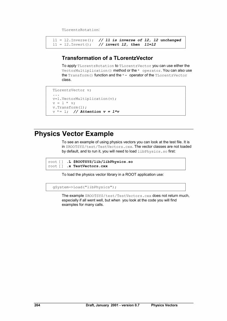
264 Draft, January 2001 - version 0.7 Physics Vectors
TLorentzRotation:
l1 = l2.Inverse(); // l1 is inverse of l2, l2 unchanged l1 = l2.Invert(); // invert l2, then l1=l2
Transformation of a TLorentzVector To apply TLorentzRotation to TLorentzVector you can use either the VectorMultiplication() method or the * operator. You can also use the Transform() function and the *= operator of the TLorentzVector class.
TLorentzVector v; ... v=l.VectorMultiplication(v); v = l * v; v.Transform(l); v *= l; // Attention v = l*v
Physics Vector Example To see an example of using physics vectors you can look at the test file. It is in $ROOTSYS/test/TestVectors.cxx. The vector classes are not loaded by default, and to run it, you will need to load libPhysics.so first:
root [] .L $ROOTSYS/lib/libPhysics.so root [] .x TestVectors.cxx
To load the physics vector library in a ROOT application use:
gSystem->Load("libPhysics");
The example $ROOTSYS/test/TestVectors.cxx does not return much, especially if all went well, but when you look at the code you will find examples for many calls.

The Tutorials and Tests Draft, January 2001 - version 0.7 265
14 The Tutorials and Tests
This chapter is a guide to the examples that come with the installation of ROOT. They are located in two directories: $ROOTSYS/tutorials and $ROOTSYS/test.
$ROOTSYS/tutorials The tutorials directory contains many example scripts. For the examples to work you must have write permission and you will need to execute hsimple.C first. If you do not have write permission in the $ROOTSYS/tutorials directory, copy the entire directory to your area.
The script hsimple.C displays a histogram as it is being filled, and creates a ROOT file used by the other examples. To execute it type:
> cd $ROOTSYS/tutorials > root ******************************************* * * * W E L C O M E to R O O T * * * * Version 2.25/02 21 August 2000 * * * * You are welcome to visit our Web site * * http://root.cern.ch * * * ******************************************* CINT/ROOT C/C++ Interpreter version 5.14.47, Aug 12 2000 Type ? for help. Commands must be C++ statements. Enclose multiple statements between { }. Welcome to the ROOT tutorials Type ".x demos.C" to get a toolbar from which to execute the demos Type ".x demoshelp.C" to see the help window root [] .x hsimple.C hsimple: Real Time =5.42 seconds Cpu Time = 3.92 seconds

266 Draft, January 2001 - version 0.7 The Tutorials and Tests
Now execute demos.C, which brings up the button bar shown on the left. You can click on any button to execute an other example. To see the source, open the corresponding source file (for example fit1.C). Once you are done, and want to quit the ROOT session, you can do so by typing .q.
root [] .x demos.C � root [] .q
$ROOTSYS/test The test directory contains a set of examples that represent all areas of the framework. When a new release is cut, the examples in this directory are compiled and run to test the new release's backward compatibility.
We see these source files:
- hsimple.cxx - Simple test program that creates and saves some histograms
- MainEvent.cxx - Simple test program that creates a ROOT Tree object and fills it with some simple structures but also with complete histograms. This program uses the files Event.cxx, EventCint.cxx and Event.h. An example of a procedure to link this program is in bind_Event. Note that the Makefile invokes the d utility to generate the CINT interface EventCint.cxx.
- Event.cxx - Implementation for classes Event and Track - minexam.cxx - Simple test program to test data fitting. - tcollex.cxx - Example usage of the ROOT collection classes. - tcollbm.cxx - Benchmarks of ROOT collection classes - tstring.cxx - Example usage of the ROOT string class. - vmatrix.cxx - Verification program for the TMatrix class. - vvector.cxx - Verification program for the TVector class. - vlazy.cxx - Verification program for lazy matrices. . - hworld.cxx - Small program showing basic graphics. . - guitest.cxx - Example usage of the ROOT GUI classes. - Hello.cxx - Dancing text example - Aclock.cxx - Analog clock (a la X11 xclock) - Tetris.cxx - The famous Tetris game (using ROOT basic graphics) . - stress.cxx - Important ROOT stress testing program.
The $ROOTSYS/test directory is a gold mine of root-wisdom nuggets, and we encourage you to explore and exploit it. These instructions will compile all programs in $ROOTSYS/test:
1. If you do not have write permission in the $ROOTSYS/test directory, copy the entire $ROOTSYS/test directory to your area.

The Tutorials and Tests Draft, January 2001 - version 0.7 267
2. The Makefile is a useful example of how ROOT applications are linked and built. Edit the Makefile to specify your architecture by changing the ARCH variable, for example, on an SGI machine type:
ARCH = sgikcc
3. Now compile all programs:
% gmake
This will build several applications and shared libraries. We are especially interested in Event, stress, and guitest.
Event � An Example of a ROOT Application . Event is created by compiling MainEvent.cxx, and Event.cxx. It creates a ROOT file with a tree and two histograms.
When running Event we have four optional arguments with defaults: Argument Default 1 Number of Events (1 ... n) 400 2 Compression level:
0: no compression at all. 1: event is compressed. 2: same as 1. In addition, the branches with
floats in the TClonesArray are also compressed.
1
3 Split or not Split 0: only one single branch is created and the
complete event is serialized in one single buffer
1: a branch per variable is created.
1 (Split)
4 Fill 0: read the file 1: write the file, but don't fill the histograms 2: don't write, don�t fill the histograms 10: fill the histograms, don't write the file 11: fill the histograms, write the file 20: read the file sequentially 25: read the file at random
1 (Write, no fill)
If we execute Event with the default arguments, we build a ROOT file with 400 events, with a tree "T" and one branch for each data member in the Event object, and we fill the histograms.
The code snipped below executes Event with the default arguments and starts a ROOT session. It opens the file Event.root created by the Event and starts a browser with which we can explore the contents (see the figure below).
%Event %root root [] TFile f("Event.root") root [] TBrowser browser

268 Draft, January 2001 - version 0.7 The Tutorials and Tests
We see that the size of the file we created is 17MB. When we run Event without splitting or compressing the size of the file is 23MB.

The Tutorials and Tests Draft, January 2001 - version 0.7 269
%ls -l Event.root -rw-r--r-- � 17549528 Jul 12 15:37 Event.root %Event 400 0 0 1 %ls -l Event.root -rw-r�r-- � 23209055 Jul 12 15:39 Event.root %root root [] TFile f("Event.root") root [] TBrowser T
We also notice only one branch; the individual data members of the Event object are no longer visible in the browser. They are contained in the event object on the event branch, because we specified no splitting.
Now we can run it once more and just read the file. This variation reads 400 events and prints the time it took.
%Event 400 0 0 20 event:0, rtime=0.500000 s event:100, rtime=0.960000 s event:200, rtime=0.900000 s event:300, rtime=0.910000 s 400 events and 21018404 bytes processed. RealTime=4.020000 seconds, CpuTime=3.040000 seconds You read 5.228459 Mbytes/Realtime seconds You read 6.913949 Mbytes/Cputime seconds
Let's see how the reading time compares with the compressed file:
%Event 400 1 1 1 %ls -l Event.root -rw-r--r-- 17549528 Jul 12 15:37 Event.root %Event 400 0 0 20 event:0, rtime=0.510000 s event:100, rtime=2.300000 s event:200, rtime=2.390000 s event:300, rtime=2.390000 s � 400 events and 21018404 bytes processed. RealTime=12.500000 seconds, CpuTime=10.760000 seconds compression level=1, split=1, arg4=1 You write 1.681472 Mbytes/Realtime seconds You write 1.953383 Mbytes/Cputime seconds
You can see that the compressed file reads much slower (4.02 seconds vs. 12.5 seconds).
stress - Test and Benchmark The executable stress is created by compiling stress.cxx. It completes sixteen tests covering the following capabilities of the ROOT framework.
1. Functions, Random Numbers, Histogram Fits 2. Size & compression factor of a ROOT file 3. Purge, Reuse of gaps in TFile 4. 2D Histograms, Functions, 2D Fits 5. Graphics & PostScript 6. Subdirectories in a ROOT file 7. TNtuple, Selections, TCut, TCutG, TEventList

270 Draft, January 2001 - version 0.7 The Tutorials and Tests
8. Split and Compression modes for Trees 9. Analyze Event.root file of stress 8 10. Create 10 files starting from Event.root 11. Test chains of Trees using the 10 files 12. Compare histograms of test 9 and 11 13. Merging files of a chain 14. Check correct rebuilt of Event.root in test 13 15. Divert Tree branches to separate files 16. CINT test (3 nested loops) with LHCb trigger
The program stress takes one argument, the number of events to process. The default is 1000 events. Be aware that executing stress with 1000 events will create several files consuming about 100 MB of disk space; running stress with 30 events will consume about 20 MB. The disk space is released once stress is done.
There are two ways to run stress:
From the system prompt or from the ROOT prompt using the interpreter. Start ROOT with the batch mode option (-b) to suppress the graphic output.
> cd $ROOTSYS/test > stress // default 1000 events > stress 30 // test with 30 events
> root -b root [] .x stress.cxx // default 1000 events root [] .x stress.cxx (30) // test with 30 events
The output of stress includes a pass/fail conclusion for each test, the total number of bytes read and written, and the elapsed real and CPU time. It also calculates a performance index for your machine relative to a reference machine a DELL Inspiron 7500 (Pentium III 600 MHz) with 256 MB of memory and 18 GBytes IDE disk in ROOTMARKS. Higher ROOTMARKS means better performance. The reference machine has 200 ROOTMARKS, so the sample run below with 53.7 ROOTMARKS is about four times slower than the reference machine.
Here is a sample run:
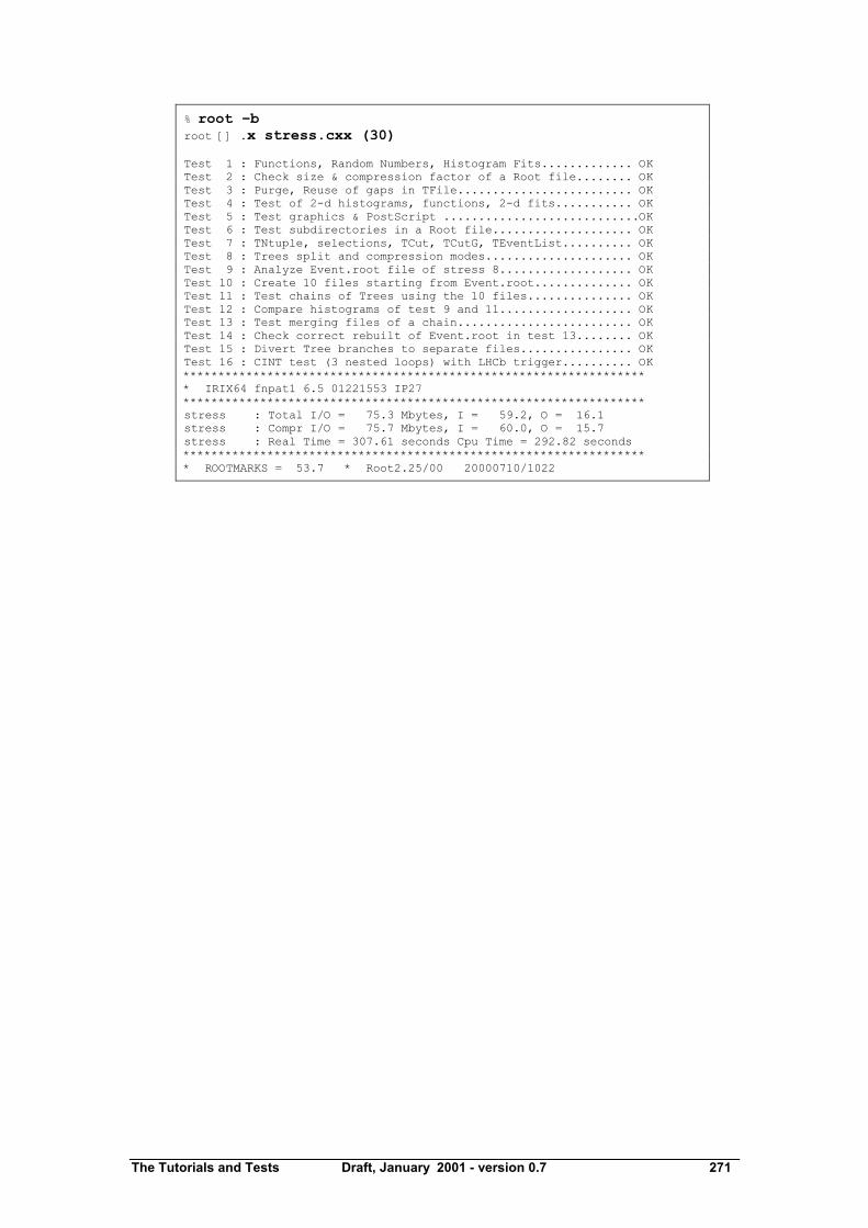
The Tutorials and Tests Draft, January 2001 - version 0.7 271
% root �b root [] .x stress.cxx (30) Test 1 : Functions, Random Numbers, Histogram Fits............. OK Test 2 : Check size & compression factor of a Root file........ OK Test 3 : Purge, Reuse of gaps in TFile......................... OK Test 4 : Test of 2-d histograms, functions, 2-d fits........... OK Test 5 : Test graphics & PostScript ............................OK Test 6 : Test subdirectories in a Root file.................... OK Test 7 : TNtuple, selections, TCut, TCutG, TEventList.......... OK Test 8 : Trees split and compression modes..................... OK Test 9 : Analyze Event.root file of stress 8................... OK Test 10 : Create 10 files starting from Event.root.............. OK Test 11 : Test chains of Trees using the 10 files............... OK Test 12 : Compare histograms of test 9 and 11................... OK Test 13 : Test merging files of a chain......................... OK Test 14 : Check correct rebuilt of Event.root in test 13........ OK Test 15 : Divert Tree branches to separate files................ OK Test 16 : CINT test (3 nested loops) with LHCb trigger.......... OK ****************************************************************** * IRIX64 fnpat1 6.5 01221553 IP27 ****************************************************************** stress : Total I/O = 75.3 Mbytes, I = 59.2, O = 16.1 stress : Compr I/O = 75.7 Mbytes, I = 60.0, O = 15.7 stress : Real Time = 307.61 seconds Cpu Time = 292.82 seconds ****************************************************************** * ROOTMARKS = 53.7 * Root2.25/00 20000710/1022

272 Draft, January 2001 - version 0.7 The Tutorials and Tests
guitest � A Graphical User Interface The guitest example, created by compiling guitest.cxx, tests and illustrates the use of the native GUI widgets such as cascading menus, dialog boxes, sliders and tab panels. It is a very useful example to study when designing a GUI. Below are some examples of the output of guitest, to run it type guitest at the system prompt in the $ROOTSYS/test directory.
We have included an entire chapter on this subject where we explore guitest in detail and use it to explain how to build our own ROOT application with a GUI (see Chapter Writing a Graphical User Interface).

Example Analysis Draft, January 2001 - version 0.7 273
15 Example Analysis
This chapter is an example of a typical physics analysis. Large data files are chained together and analyzed using the TSelector class.
Explanation This script uses four large data sets from the H1 collaboration at DESY Hamburg. One can access these data sets (277 Mbytes) from the ROOT web site at: ftp://root.cern.ch/root/h1analysis/
The physics plots generated by this example cannot be produced using smaller data sets.
There are several ways to analyze data stored in a ROOT Tree
�� Using TTree::Draw: This is very convenient and efficient for small tasks. A TTree::Draw call produces one histogram at the time. The histogram is automatically generated. The selection expression may be specified in the command line.
�� Using the TTreeViewer: This is a graphical interface to TTree::Draw with the same functionality.
�� Using the code generated by TTree::MakeClass: In this case, the user creates an instance of the analysis class. He has the control over the event loop and he can generate an unlimited number of histograms.
�� Using the code generated by TTree::MakeSelector: Like for the code generated by TTree::MakeClass, the user can do complex analysis. However, he cannot control the event loop. The event loop is controlled by TTree::Process called by the user. This solution is illustrated by the code below. The advantage of this method is that it can be run in a parallel environment using PROOF (the Parallel Root Facility).
A chain of four files (originally converted from PAW ntuples) is used to illustrate the various ways to loop on ROOT data sets. Each contains a ROOT Tree named "h42". The class definition in h1analysis.h has been generated automatically by the ROOT utility TTree::MakeSelector using one of the files with the following statement:

274 Draft, January 2001 - version 0.7 Example Analysis
h42->MakeSelector("h1analysis");
This produces two files: h1analysis.h and h1analysis.C. A skeleton of h1analysis.C file is made for you to customize. The h1analysis class is derived from the ROOT class TSelector. The following members functions of h1analyhsis (i.e. TSelector) are called by the TTree::Process method.
�� Begin: This function is called every time a loop over the tree starts. This is a convenient place to create your histograms.
�� Notify(): This function is called at the first entry of a new tree in a chain.
�� ProcessCut: This function is called at the beginning of each entry to return a flag true if the entry must be analyzed.
�� ProcessFill: This function is called in the entry loop for all entries accepted by Select.
�� Terminate: This function is called at the end of a loop on a TTree. This is a convenient place to draw and fit your histograms.
To use this program, try the following session.
First, turn the timer on to show the real and CPU time per command.
root[] gROOT->Time();
Step A: create a TChain with the four H1 data files. The chain can be created by executed this short script h1chain.C below. $H1 is a system symbol pointing to the H1 data directory.
{ TChain chain("h42"); chain.Add("$H1/dstarmb.root"); //21330730 bytes, 21920 events chain.Add("$H1/dstarp1a.root"); //71464503 bytes, 73243 events chain.Add("$H1/dstarp1b.root"); //83827959 bytes, 85597 events chain.Add("$H1/dstarp2.root");
//100675234 bytes, 103053 events }
Run the above script from the command line:
root[] .x h1chain.C
Step B: Now we have a d containing the four data files. Since a TChain is a descendent of TTree we can call TChain::Process to loop on all events in the chain. The parameter to the TChain::Process method is the name of the file containing the created TSelector class (h1analysis.C).
root[] chain.Process("h1analysis.C")
Step C: Same as step A, but in addition fill the event list with selected entries. The event list is saved to a file "elist.root" by the TSelector::Terminate method. To see the list of selected events, you

Example Analysis Draft, January 2001 - version 0.7 275
can do elist->Print("all"). The selection function has selected 7525 events out of the 283813 events in the chain of files. (2.65 per cent)
root[] chain.Process("h1analysis.C","fillList")
Step D: Process only entries in the event list. The event list is read from the file in elist.root generated by step C.
root[] chain.Process("h1analysis.C","useList")
Step E: The above steps have been executed with the interpreter. You can repeat the steps 2, 3, and 4 using ACLiC by replacing "h1analysis.C" by "h1analysis.C+" or "h1analysis.C++".
Step F: If you want to see the differences between the interpreter speed and ACLiC speed start a new session, create the chain as in step 1, then execute
root[] chain.Process("h1analysis.C+","useList")
The commands executed with the four different methods B, C, D and E produce two canvases shown below:

276 Draft, January 2001 - version 0.7 Example Analysis
Script This is the h1analsysis.C file that was generated by TTree::MakeSelector and then modified to perform the analysis.
#include "h1analysis.h" #include "TH2.h" #include "TF1.h" #include "TStyle.h" #include "TCanvas.h" #include "TLine.h" #include "TEventList.h" const Double_t dxbin = (0.17-0.13)/40; // Bin-width const Double_t sigma = 0.0012; TEventList *elist = 0; Bool_t useList, fillList; TH1F *hdmd; TH2F *h2; //_________________________________________________________ Double_t fdm5(Double_t *xx, Double_t *par) { Double_t x = xx[0]; if (x <= 0.13957) return 0; Double_t xp3 = (x-par[3])*(x-par[3]); Double_t res =
dxbin*(par[0]*TMath::Power(x-0.13957, par[1]) + par[2] / 2.5066 / par[4]*TMath::Exp(
xp3/2/par[4]/par[4])); return res; } //_________________________________________________________ Double_t fdm2(Double_t *xx, Double_t *par) { Double_t x = xx[0]; if (x <= 0.13957) return 0; Double_t xp3 = (x-0.1454)*(x-0.1454); Double_t res = dxbin*(par[0]*TMath::Power(x-0.13957, 0.25) + par[1] / 2.5066/sigma*TMath::Exp( xp3/2/sigma/sigma)); return res; } //_________________________________________________________ void h1analysis::Begin(TTree *tree) { // function called before starting the event loop // -it performs some cleanup // -it creates histograms // -it sets some initialization for the event list //initialize the Tree branch addresses Init(tree); //print the option specified in the Process function. TString option = GetOption(); printf("Starting h1analysis with process option:

Example Analysis Draft, January 2001 - version 0.7 277
%sn",option.Data()); //Some cleanup in case this function had //already been executed. //Delete any previously generated histograms or //functions gDirectory->Delete("hdmd"); gDirectory->Delete("h2*"); delete gROOT->GetFunction("f5"); delete gROOT->GetFunction("f2"); //create histograms hdmd = new TH1F("hdmd","dm_d",40,0.13,0.17); h2 = new TH2F
("h2","ptD0 vs dm_d",30,0.135,0.165,30,-3,6); //process cases with event list fillList = kFALSE; useList = kFALSE; fChain->SetEventList(0); delete gDirectory->GetList()->FindObject("elist"); // case when one creates/fills the event list if (option.Contains("fillList")) { fillList = kTRUE; elist = new TEventList
("elist","selection from Cut",5000); } // case when one uses the event list generated // in a previous call if (option.Contains("useList")) { useList = kTRUE; TFile f("elist.root"); elist = (TEventList*)f.Get("elist"); if (elist) elist->SetDirectory(0);
//otherwise the file destructor will delete elist fChain->SetEventList(elist); } } //_________________________________________________________ Bool_t h1analysis::ProcessCut(Int_t entry) { // Selection function to select D* and D0. //in case one event list is given in input, //the selection has already been done. if (useList) return kTRUE; // Read only the necessary branches to select entries. // return as soon as a bad entry is detected b_md0_d->GetEntry(entry); if (TMath::Abs(md0_d-1.8646) >= 0.04) return kFALSE; b_ptds_d->GetEntry(entry); if (ptds_d <= 2.5) return kFALSE; b_etads_d->GetEntry(entry); if (TMath::Abs(etads_d) >= 1.5) return kFALSE; b_ik->GetEntry(entry); ik--; //original ik used f77 convention starting at 1 b_ipi->GetEntry(entry); ipi--;

278 Draft, January 2001 - version 0.7 Example Analysis
b_ntracks->GetEntry(entry); b_nhitrp->GetEntry(entry); if (nhitrp[ik]*nhitrp[ipi] <= 1) return kFALSE; b_rend->GetEntry(entry); b_rstart->GetEntry(entry); if (rend[ik] -rstart[ik] <= 22) return kFALSE; if (rend[ipi]-rstart[ipi] <= 22) return kFALSE; b_nlhk->GetEntry(entry); if (nlhk[ik] <= 0.1) return kFALSE; b_nlhpi->GetEntry(entry); if (nlhpi[ipi] <= 0.1) return kFALSE; b_ipis->GetEntry(entry); ipis--; if (nlhpi[ipis] <= 0.1) return kFALSE; b_njets->GetEntry(entry); if (njets < 1) return kFALSE; // if option fillList, fill the event list if (fillList) elist->Enter (fChain->GetChainEntryNumber(entry)); return kTRUE; } //_________________________________________________________ void h1analysis::ProcessFill(Int_t entry) { // Function called for selected entries only // read branches not processed in ProcessCut b_dm_d->GetEntry(entry); //read branch holding dm_d b_rpd0_t->GetEntry(entry); //read branch holding rpd0_t b_ptd0_d->GetEntry(entry); //read branch holding ptd0_d //fill some histograms hdmd->Fill(dm_d); h2->Fill(dm_d,rpd0_t/0.029979*1.8646/ptd0_d); } //_________________________________________________________ void h1analysis::Terminate() { // Function called at the end of the event loop //create the canvas for the h1analysis fit gStyle->SetOptFit(); TCanvas *c1 = new TCanvas
("c1","h1analysis analysis",10,10,800,600); c1->SetBottomMargin(0.15); hdmd->GetXaxis()->SetTitle
("m_{K#pi#pi} - m_{K#pi}[GeV/c^{2}]"); hdmd->GetXaxis()->SetTitleOffset(1.4); //fit histogram hdmd with function f5 using

Example Analysis Draft, January 2001 - version 0.7 279
//the loglikelihood option TF1 *f5 = new TF1("f5",fdm5,0.139,0.17,5); f5->SetParameters(1000000, .25, 2000, .1454, .001); hdmd->Fit("f5","lr"); //create the canvas for tau d0 gStyle->SetOptFit(0); gStyle->SetOptStat(1100); TCanvas *c2 = new TCanvas("c2","tauD0",100,100,800,600); c2->SetGrid(); c2->SetBottomMargin(0.15); // Project slices of 2-d histogram h2 along X , // then fit each slice with function f2 and make a // histogram for each fit parameter. // Note that the generated histograms are added // to the list of objects in the current directory. TF1 *f2 = new TF1("f2",fdm2,0.139,0.17,2); f2->SetParameters(10000, 10); h2->FitSlicesX(f2,0,0,1,"qln"); TH1D *h2_1 = (TH1D*)gDirectory->Get("h2_1"); h2_1->GetXaxis()->SetTitle("#tau[ps]"); h2_1->SetMarkerStyle(21); h2_1->Draw(); c2->Update(); TLine *line = new TLine(0,0,0,c2->GetUymax()); line->Draw(); // save the event list to a Root file if one was // produced if (fillList) { TFile efile("elist.root","recreate"); elist->Write(); } }


Networking Draft, January 2001 - version 0.7 281
16 Networking
In this chapter, you will learn how to send data over the network using the ROOT socket classes.
Setting up a Connection On the server side, we create a TServerSocket to wait for a connection request over the network. If the request is accepted, it returns a full-duplex socket. Once the connection is accepted, we can communicate to the client that we are ready to go by sending the string "go", and we can close the server socket.
{ // server TServerSocket *ss = new TServerSocket(9090, kTRUE); TSocket *socket = ss->Accept(); socket->Send("go"); ss->Close(); }
On the client side, we create a socket and ask the socket to receive the string "go" as a signal for connecting successfully.
{ // client TSocket *socket = new TSocket("localhost", 9090); Char str[32]; Socket->Recv(str,32); }

282 Draft, January 2001 - version 0.7 Networking
Sending Objects over the Network We have just established a connection and you just saw how to send and receive a string with the example "go". Now let�s send a histogram.
To send an object (in our case on the client side) it has to derive from TObject because it uses the Streamers to fill a buffer that is then sent over the connection. On the receiving side, the Streamers are used to read the object from the message sent via the socket. For network communication, we have a specialized TBuffer, a descendant of TBuffer called TMessage. In the following example, we create a TMessage with the intention to store an object, hence the constant kMESS_OBJECT in the constructor. We create and fill the histogram and write it into the message. Then we call TSocket::Send to send the message with the histogram.
� // create an object to be sent TH1F *hpx = new TH1F("hpx","px distribution",100,-4,4); hpx->FillRandom("gaus",1000); // create a TMessage to send the object TMessage message(kMESS_OBJECT); // write the histogram into the message buffer message.WriteObject(hpx); // send the message socket->Send(message); �
On the receiving end (in our case the server side), we write a while loop to wait and receive a message with a histogram. Once we have a message, we call TMessage::ReadObject, which returns a pointer to TObject. We have to cast it to a TH1 pointer, and now we have a histogram. At the end of the loop, the message is deleted, and another one is created at the beginning.
� while (1) { TMessage *message; socket->Recv(message); TH1 *h = (TH1*)mess->ReadObject(mess->GetClass()); delete mess; } �

Networking Draft, January 2001 - version 0.7 283
Closing the Connection Once we are done sending objects, we close the connection by closing the sockets at both ends.
� Socket->Close(); }
This diagram summarizes the steps we just covered:
{TServerSocket *ss = new TServerSocket(9090, kTRUE);
TSocket *socket = ss->Accept();
socket->Send("go");ss->Close();
while (1) { TMessage *message; socket->Recv(message); TH1 *h = (TH1*)mess->ReadObject (mess->GetClass()); delete mess;}
socket->Close();}
{
TSocket *socket = new TSocket("localhost", 9090);
Char str[32]; Socket->Recv(str,32);
TH1F *hpx = new TH1F("hpx","px",100,-4,4); hpx->FillRandom("gaus",1000); // create a TMessage to send an object TMessage message(kMESS_OBJECT); // write the histogram into the message message.WriteObject(hpx); // send the message socket->Send(message)
socket->Close();}
connect
OK
send
Server Client

284 Draft, January 2001 - version 0.7 Networking
A Server with Multiple Sockets Chances are that your server has to be able to receive data from multiple clients. The class we need for this is TMonitor. It lets you add sockets and the TMonitor::Select method returns the socket with data waiting. Sockets can be added, removed, or enabled and disabled.
Here is an example of a server that has a TMonitor to manage multiple sockets:
{ TServerSocket *ss = new TServerSocket (9090, kTRUE); // Accept a connection and return a full-duplex // communication socket. TSocket *s0 = ss->Accept(); TSocket *s1 = ss->Accept(); // tell the clients to start s0->Send("go 0"); s1->Send("go 1"); // Close the server socket (unless we will use it // later to wait for another connection). ss->Close(); TMonitor *mon = new TMonitor; mon->Add(s0); mon->Add(s1); while (1) { TMessage *mess; TSocket *s; s = mon->Select(); s->Recv(mess); � }
The full code for the example above is in $ROOTSYS/tutorials/hserver.cxx and $ROOTSYS/tutorials/hclient.cxx.

Writing a Graphical User Interface Draft, January 2001 - version 0.7 285
17 Writing a Graphical User Interface
The ROOT GUI classes support an extensive and rich set of widgets. The widgets classes depend only on the X11 and Xpm libraries, eliminating the need for any other GUI engine such as Motif or QT, and they have the Windows look and feel. They are based on Hector Peraza's Xclass'95 widget library.
Although powerful and quite feature rich, we are missing extensive documentation. This will come eventually but for the time being you will have to "program by example". We start with a short tutorial followed by few non-trivial examples that will show how to use the different widget classes.
The New ROOT GUI Classes Features of the new GUI classes in a nutshell:
�� Originally based on Xclass'95 widget library (under a Lesser GNU Public License)
o A rich and complete set of widgets o Uses only X11 and Xpm (no Motif, Xaw, Xt, etc.) o Small (12000 lines of C++) o Win'95 look and feel
�� All X11 calls abstracted using in the "abstract" ROOT TGXW class �� Rewritten to use internally the ROOT container classes �� Completely scriptable via the C++ interpreter (fast prototyping) �� Full class documentation is generated automatically (as for all ROOT
classes)
XClass'95 Here are some highlights of the XClass'95. Hector Peraza is the original author of the XClass'95 class library.
The Xclass'95 comes with a complete set of widgets. These include:
�� Simple widgets, as labels and icons �� Push buttons, either with text or pix maps �� Check buttons �� Radio buttons �� Menu bars and popup menus

286 Draft, January 2001 - version 0.7 Writing a Graphical User Interface
�� Scroll bars �� Scrollable canvas �� List boxes �� Combo boxes �� Group frames �� Text entry widgets �� Tab widgets �� General-purpose composite widgets, for building toolbars and status
bars �� Dialog classes and top-level window classes
The widgets are shown in frames: frame, composite frame, main frame, transient frame, group frame
And arranged by layout managers: horizontal layout, vertical layout, row layout, list layout, tile layout, matrix layout, ...
Using a combination of layout hints: left, center x, right, top, center y, bottom, expand x, expand y and fixed offsets
Event handling by messaging (as opposed to callbacks): in response to actions widgets send messages (SendMessage()) to associated frames (ProcessMessage())
ROOT Integration Replace all calls to X11 by calls to the ROOT abstract graphics base class TGXW. Currently, implementations of TGXW exist X11 (TGX11) and Win32 (TGWin32). Thanks to this single graphics interface, porting ROOT to a new platform (BeOS, Rhapsody, etc.) requires only the implementation of TGXW (and TSystem).
Abstract Graphics Base Class TGXW
TGXW
TGX11 TGWin32 TGClient
rootdisp rootdisp
Unix Windows
Unix/Windows

Writing a Graphical User Interface Draft, January 2001 - version 0.7 287
Concrete implementations of TGXW are TGX11, for X Windows, TGWin32 for Win95/NT. The TGXClient implementation provides a network interface allowing for remote display via the rootdisp servers.
NOTE: the ROOT GUI classes are for the time being only supported on Unix/X11 systems. Work on a Win32 port is in progress and coming shortly
Further changes:
�� Changed internals to use ROOT container classes, notably hash tables for fast lookup of frame and picture objects
�� Added TObject inheritance to the few base classes to get access to the extended ROOT RTTI (type information and object inspection) and documentation system
�� Conversion to the ROOT naming conventions to provide a homogeneous and consistent environment for the user

288 Draft, January 2001 - version 0.7 Writing a Graphical User Interface
A Simple Example The code that uses the GUI classes is written in bold font.
#include <TROOT.h> #include <TApplication.h> #include <TGClient.h> extern void InitGui(); VoidFuncPtr_t initfuncs[] = { InitGui, 0 }; TROOT root("GUI", "GUI test environement", initfuncs); int main(int argc, char **argv) { TApplication theApp("App", &argc, argv); MyMainFrame mainWin(gClient->GetRoot(), 200, 220); theApp.Run(); return 0; }
MyMainFrame
#include <TGClient.h> #include <TGButton.h> class MyMainFrame : public TGMainFrame { private: TGTextButton *fButton1, *fButton2; TGPictureButton *fPicBut; TGCheckButton *fChkBut; TGRadioButton *fRBut1, *fRBut2; TGLayoutHints *fLayout; public: MyMainFrame(const TGWindow *p, UInt_t w, UInt_t h); ~MyMainFrame(); Bool_t ProcessMessage(Long_t msg, Long_t parm1, Long_t parm2); };

Writing a Graphical User Interface Draft, January 2001 - version 0.7 289
Laying out the Frame
MyMainFrame::MyMainFrame(const TGWindow *p, UInt_t w, UInt_t h): TGMainFrame(p, w, h) { // Create a main frame with a number of different buttons. fButton1 = new TGTextButton(this, "&Version", 1); fButton1->SetCommand("printf (\"This is ROOT version %s\\n\", gROOT->GetVersion());"); fButton2 = new TGTextButton(this, "&Exit", 2); fButton2->SetCommand(".q" ); fPicBut = new TGPictureButton( this, gClient->GetPicture("world.xpm"), 3); fPicBut->SetCommand("printf(\"hello world!\\n\");"); fChkBut = new TGCheckButton(this, "Check Button", 4); fRBut1 = new TGRadioButton(this, "Radio Button 1", 5); fRBut2 = new TGRadioButton(this, "Radio Button 2", 6); fLayout = new TGLayoutHints
(kLHintsCenterX | kLHintsCenterY); AddFrame(fButton1, fLayout); AddFrame(fPicBut, fLayout); AddFrame(fButton2, fLayout); AddFrame(fChkBut, fLayout); AddFrame(fRBut1, fLayout); AddFrame(fRBut2, fLayout); MapSubwindows(); Layout(); SetWindowName("Button Example"); SetIconName("Button Example"); MapWindow(); }

290 Draft, January 2001 - version 0.7 Writing a Graphical User Interface
Adding Actions
Bool_t MyMainFrame::ProcessMessage(Long_t msg, Long_t parm1, Long_t) { // Process events generated by the buttons in the frame. switch (GET_MSG(msg)) { case kC_COMMAND: switch (GET_SUBMSG(msg)) { case kCM_BUTTON: printf("text button id %ld pressed\n", parm1); break; case kCM_CHECKBUTTON: printf("check button id %ld pressed\n", parm1); break; case kCM_RADIOBUTTON: if (parm1 == 5) fRBut2->SetState(kButtonUp); if (parm1 == 6) fRBut1->SetState(kButtonUp); printf("radio button id %ld pressed\n", parm1); break; default: break; } default: break; } return kTRUE; }
The Result
The Widgets in Detail In this section we look at an example of using the widgets. The complete source code is in $ROOTSYS/test/guitest.C. Build the test directory with the appropriate makefile, and you will be able to run guitest. Here we present snippets of the code and the graphical output.

Writing a Graphical User Interface Draft, January 2001 - version 0.7 291
First the main program, which reveals that the functionality is in TestMainFrame.
TROOT root("GUI", "GUI test environement"); int main(int argc, char **argv) { TApplication theApp("App", &argc, argv); if (gROOT->IsBatch()) { fprintf(stderr,
"%s: cannot run in batch mode\n", argv[0]); return 1; } TestMainFrame mainWindow(gClient->GetRoot(), 400, 220); theApp.Run(); return 0; }
TestMainFrame has two subframes (TGCompositFrame), a canvas, a text entry field, a button, a menu bar, several popup menus, and layout hints. It has a public constructor, destructor and a ProcessMessage method to carry out the actions.
class TestMainFrame : public TGMainFrame { private: TGCompositeFrame *fStatusFrame; TGCanvas *fCanvasWindow; TGCompositeFrame *fContainer; TGTextEntry *fTestText; TGButton *fTestButton; TGMenuBar *fMenuBar; TGPopupMenu *fMenuFile, *fMenuTest, *fMenuHelp; TGPopupMenu *fCascadeMenu, *fCascade1Menu, *fCascade2Menu; TGLayoutHints *fMenuBarLayout, *fMenuBarItemLayout, *fMenuBarHelpLayout; public: TestMainFrame(const TGWindow *p, UInt_t w, UInt_t h); virtual ~TestMainFrame(); virtual void CloseWindow(); virtual Bool_t ProcessMessage(Long_t msg, Long_t parm1, Long_t); };
Example: Widgets and the Interpreter The script $ROOTSYS/tutorials/dialogs.C shows how the widgets can be used from the interpreter.

292 Draft, January 2001 - version 0.7 Writing a Graphical User Interface
RQuant Example This is an example of extensive use of the ROOT GUI classes. I include only a picture here, for the curious the full documentation or RQuant can be found at: http://svedaq.tsl.uu.se/~anton/rquant.htm
References http://home.cern.ch/~chytrace/xclasstut.html A basic introduction and mini tutorial on the Xclass by Hector Peraza's
ac.be/html-test/xclass.html The original Xclass'95 widget library documentation and source by Hector Peraza's.
http://svedaq.tsl.uu.se/~anton/rquant.htm An Example of an elaborate ROOT GUI application.

Automatic HTML Documentation Draft, January 2001 - version 0.7 293
18 Automatic HTML Documentation
The class descriptions on the ROOT website have been generated automatically by ROOT itself with the THtml class. With it, you can automatically generate (and update) a reference guide for your ROOT classes. Please read this class description and the paragraph on Coding Conventions.
The following illustrates how to generate an html class description using the MakeClass method. In this example class name is TBRIK.
root[] gHtml->MakeClass("TBRIK")
How to generate html code for all classes, including an index.
root[] gHtml->MakeAll();
This example also shows how to convert a script to html, including the generation of a "gif" file produced by the script. First execute the script.
root[] .x htmlex.C
Invoke the TSystem class to execute a shell script. Here we call the "xpick" program to capture the graphics window into a gif file.
root[] gSystem->Exec("xpick html/gif/shapes.gif")
Convert this script into html.
root[] gHtml->Convert("htmlex.C","Auto HTML document generation")
For more details see the documentation of the class THtml.


PROOF: Parallel Processing Draft, January 2001 - version 0.7 295
19 PROOF: Parallel Processing
Building on the experience gained from the implementation and operation of the PIAF system we have developed the parallel ROOT facility, PROOF. The main problems with PIAF were because its proper parallel operation depended on a cluster of homogenous equally performing and equally loaded machines. Due to PIAF's simplistic portioning of a job in N equal parts, where N is the number of processors, the overall performance was governed by the slowest node. The running of a PIAF cluster was an expensive operation since it required a cluster dedicated solely to PIAF. The cluster could not be used for other types of jobs without destroying the PIAF performance.
In the implementation of PROOF, we made the slave servers the active components that ask the master server for new work whenever they are ready. In the scheme the parallel processing performance is a function of the duration of each small job, packet, and the networking bandwidth and latency. Since the bandwidth and latency of a networked cluster are fixed the main tunable parameter in this scheme is the packet size. If the packet size is too small the parallelism will be destroyed by the communication overhead caused by the many packets sent over the network between the master and the slave servers. If the packet size is too large, the effect of the difference in performance of each node is not evened out sufficiently.
Another very important factor is the location of the data. In most cases, we want to analyze a large number of data files, which are distributed over the different nodes of the cluster. To group these files together we use a chain. A chain provides a single logical view of the many physical files. To optimize performance by preventing huge amounts of data being transferred over the network via NFS or any other means when analyzing a chain, we make sure that each slave server is assigned a packet, which is local to the node. Only when a slave has processed all its local data will it get packets assigned that cause remote access. A packet is a simple data structure of two numbers: begin event and number of events. The master server generates a packet when asked for by a slave server, taking into account t the time it took to process the previous packet and which files in the chain are local to the lave server. The master keeps a list of all generated packets per slave, so in case a slave dies during processing, all its packets can be reprocessed by the left over slaves.


Threads Draft, January 2001 - version 0.7 297
20 Threads
A thread is an independent flow of control that operates within the same address space as other independent flows of controls within a process. In most UNIX systems, thread and process characteristics are grouped into a single entity called a process. Sometimes, threads are called "lightweight processes''.
Note:This introduction is adapted from the AIX 4.3 Programmer's Manual.
Threads and Processes In traditional single-threaded process systems, a process has a set of properties. In multi-threaded systems, these properties are divided between processes and threads.
Process Properties A process in a multi-threaded system is the changeable entity. It must be considered as an execution frame. It has all traditional process attributes, such as:
�� Process ID, process group ID, user ID, and group ID �� Environment �� Working directory
A process also provides a common address space and common system resources:
�� File descriptors �� Signal actions �� Shared libraries �� Inter-process communication tools (such as message queues, pipes,
semaphores, or shared memory)

298 Draft, January 2001 - version 0.7 Threads
Thread Properties A thread is the schedulable entity. It has only those properties that are required to ensure its independent flow of control. These include the following properties:
�� Stack �� Scheduling properties (such as policy or priority) �� Set of pending and blocked signals �� Some thread-specific data (TSD)
An example of thread-specific data is the error indicator, errno. In multi-threaded systems, errno is no longer a global variable, but usually a subroutine returning a thread-specific errno value. Some other systems may provide other implementations of errno.
With respect to ROOT, a thread specific data is for example the gPad pointer, which is treated in a different way, whether it is accessed from any thread or the main thread.
Threads within a process must not be considered as a group of processes (even though in Linux each thread receives an own process id, so that it can be scheduled by the kernel scheduler). All threads share the same address space. This means that two pointers having the same value in two threads refer to the same data. Also, if any thread changes one of the shared system resources, all threads within the process are affected. For example, if a thread closes a file, the file is closed for all threads.
The Initial Thread When a process is created, one thread is automatically created. This thread is called the initial thread or the main thread. The initial thread executes the main routine in multi-threaded programs.
Note: At the end of this chapter is a glossary of thread specific terms
Implementation of Threads in ROOT The TThread class has been developed to provide a platform independent interface to threads for ROOT.
Installation For the time being, it is still necessary to compile a threaded version of ROOT to enable some very special treatments of the canvas operations. We hope that this will become the default later.
To compile ROOT, just do (for example on a debian Linux):
./configure linuxdeb2 --with-thread=/usr/lib/libpthread.so gmake depend gmake

Threads Draft, January 2001 - version 0.7 299
This configures and builds ROOT using /usr/lib/libpthread.so as the Pthread library, and defines R__THREAD. This enables the thread specific treatment of gPad, and creates $ROOTSYS/lib/libThread.so.
Note: The parameter linuxdeb2 has to be replaced with the appropriate ROOT keyword for your platform.
Classes TThread
This class implements threads. The platform dependent implementation is in the TThreadImp class and its descendant classes (e.g. TPosixThread). TMutex
This class implements mutex locks. A mutex is a mutually exclusive lock. The platform dependent implementation is in the TMutexImp class and its descendant classes (e.g. TPosixMutex) TCondition
This class implements a condition variable. Use a condition variable to signal threads. The platform dependent implementation is in the TConditionImp class and its descendant classes (e.g. TPosixCondition). TSemaphore
This class implements a counting semaphore. Use a semaphore to synchronize threads. The platform dependent implementation is in the TMutexImp and TConditionImp classes.
TThread for Pedestrians To run a thread in ROOT, follow these steps:
Initialization:
Add these lines to your rootlogon.C: { � // The next line may be unnecessary on some platforms gSystem->Load("/usr/lib/libpthread.so"); gSystem->Load("$ROOTSYS/lib/libThread.so"); � }
This loads the library with the TThread class and the pthread specific implementation file for Posix threads.
Coding:
Define a function (e.g. void* UserFun(void* UserArgs)) that should run as a thread. The code for the examples is at the web site of the authors (Jörn Adamczewski, Marc Hemberger). After downloading the code from this site, you can follow the example below.
www-linux.gsi.de/~go4/HOWTOthreads/howtothreadsbody.html#tth_sEc8

300 Draft, January 2001 - version 0.7 Threads
Loading: Start an interactive ROOT session
Load the shared library:
root [] gSystem->Load("mhs3.so");
Or
root [] gSystem->Load("CalcPiThread.so");
Creating: Create a thread instance (see also example RunMhs3.C or RunPi.C) with:
root [] TThread *th = new TThread(UserFun,UserArgs);
When called from the interpreter, this gives the name �UserFun� to the thread. This name can be used to retrieve the thread later. However, when called from compiled code, this method does not give any name to the thread. So give a name to the thread in compiled use:
root [] TThread *th = new TThread("MyThread", UserFun, UserArgs);
You can pass arguments to the thread function using the UserArgs-pointer. When you want to start a method of a class as a thread, you have to give the pointer to the class instance as UserArgs.
Running: root [] th->Run(); root [] TThread::Ps(); // like UNIX ps c.ommand;
With the mhs3 example, you should be able to see a canvas with two pads on it. Both pads keep histograms updated and filled by three different threads.
With the CalcPi example, you should be able to see two threads calculating Pi with the given number of intervals as precision.

Threads Draft, January 2001 - version 0.7 301
TThread in More Detail CINT is not thread safe yet, and it will block the execution of the threads until it has finished executing.
Asynchronous Actions Different threads can work simultaneously with the same object. Some actions can be dangerous. For example, when two threads create a histogram object, ROOT allocates memory and puts them to the same collection. If it happens at the same time, the results are undetermined. To avoid this problem, the user has to synchronize these actions with:
TThread::Lock() // Locking the following part of code ... // Create an object, etc... TThread::UnLock() // Unlocking
The code between Lock() and UnLock() will be performed uninterrupted. No other threads can perform actions or access objects/collections while it is being executed. The TThread::Lock() and TThread::UnLock() methods internally use a global TMutex instance for locking. The user may also define his own TMutex MyMutex instance and may locally protect his asynchronous actions by calling MyMutex.Lock() and MyMutex.UnLock().
Synchronous Actions: TCondition To synchronize the actions of different threads you can use the TCondition class, which provides a signaling mechanism.
The TCondition instance must be accessible by all threads that need to use it, i.e. it should be a global object (or a member of the class which owns the threaded methods, see below). To create a TCondition object, a TMutex instance is required for the Wait and TimedWait locking methods. One can pass the address of an external mutex to the TCondition constructor:
TMutex MyMutex; TCondition MyCondition(&MyMutex);
If zero is passed, TCondition creates and uses its own internal mutex:
TCondition MyCondition(0);

302 Draft, January 2001 - version 0.7 Threads
You can now use the following methods of synchronization:
�� TCondition::Wait() waits until any thread sends a signal of the same condition instance: MyCondition.Wait() reacts on MyCondition.Signal() or MyCondition.Broadcast(). MyOtherCondition.Signal() has no effect.
�� If several threads wait for the signal from the same TCondition MyCondition, at MyCondition.Signal() only one thread will react; to activate a further thread another MyCondition.Signal() is required, etc.
�� If several threads wait for the signal from the same TCondition MyCondition, at MyCondition.Broadcast() all threads waiting for MyCondition are activated at once.
In some tests of MyCondition using an internal mutex, Broadcast() activated only one thread (probably depending whether MyCondition had been signaled before).
�� MyCondition.TimedWait(secs,nanosecs) waits for MyCondition until the absolute time in seconds and nanoseconds since beginning of the epoch (January, 1st, 1970) is reached; to use relative timeouts ``delta'', it is required to calculate the absolute time at the beginning of waiting ``now''; for example:
Ulong_t now,then,delta; // seconds TDatime myTime; // root daytime class myTime.Set(); // myTime set to "now" now=myTime.Convert(); // to seconds since 1970 then=now+delta; // absolute timeout wait=MyCondition.TimedWait(then,0); // waiting
�� Return value wait of MyCondition.TimedWait should be 0, if MyCondition.Signal() was received, and should be nonzero, if timeout was reached.
The conditions example shows how three threaded functions are synchronized using TCondition: a ROOT script condstart.C starts the threads, which are defined in a shared library (conditions.cxx, conditions.h).
Xlib connections Usually Xlib is not thread safe. This means that calls to the X could fail, when it receives X-messages from different threads. The actual result depends strongly on which version of Xlib has been installed on your system. The only thing we can do here within ROOT is calling a special function XInitThreads() (which is part of the Xlib), which should (!) prepare the Xlib for the usage with threads.
To avoid further problems within ROOT some redefinition of the gPad pointer was done (that's the main reason for the recompilation). When a thread creates a TCanvas, this object is actually created in the main thread; this

Threads Draft, January 2001 - version 0.7 303
should be transparent to the user. Actions on the canvas are controlled via a function, which returns a pointer to either thread specific data (TSD) or the main thread pointer. This mechanism works currently only for gPad and will soon be implemented for other global Objects as e.g. gVirtualX, gDirectory, gFile.
Canceling a TThread Canceling of a thread is a rather dangerous action. In TThread canceling is forbidden by default. The user can change this default by calling TThread::SetCancelOn(). There are two cancellation modes:
Deferred Set by TThread::SetCancelDeferred() (default): When the user knows safe places in his code where a thread can be canceled without risk for the rest of the system, he can define these points by invoking TThread::CancelPoint(). Then, if a thread is canceled, the cancellation is deferred up to the call of TThread::CancelPoint() and then the thread is canceled safely. There are some default cancel points for pthreads implementation, e.g. any call of TCondition::Wait(), TCondition::TimedWait(), TThread::Join().
Asynchronous Set by TThread::SetCancelAsynchronous(): If the user is sure that his application is cancel safe, he could call:
TThread::SetCancelAsynchronous(); TThread::SetCancelOn(); // Now cancelation in any point is allowed. ... ... // Return to default TThread::SetCancelOff(); TThread::SetCancelDeferred();
To cancel a thread TThread* th call:
Th��Kill();
To cancel by thread name:
TThread::Kill(name);
To cancel a thread by ID:
TThread::Kill(tid);
To cancel a thread and delete th when cancel finished:
Th��Delete();
Deleting of the thread instance by the operator delete is dangerous. Use th->Delete() instead. C++ delete is safe only if thread is not running.

304 Draft, January 2001 - version 0.7 Threads
Often during the canceling, some clean up actions must be taken. To define clean up functions use:
void UserCleanUp(void *arg){ // here the user cleanup is done ... } TThread::CleanUpPush(&UserCleanUp,arg); // push user function into cleanup stack // �last in, first out� TThread::CleanUpPop(1); // pop user function out of stack // and execute it, // thread resumes after this call TThread::CleanUpPop(0); // pop user function out of stack // _without_ executing it
Note: CleanUpPush and CleanUpPop should be used as corresponding pairs like brackets; unlike pthreads cleanup stack (which is not implemented here), TThread does not force this usage.
Finishing thread When a thread returns from a user function the thread is finished. It also can be finished by TThread::Exit(). Then, in case of pthread-detached mode, the thread vanishes completely.
By default, on finishing TThread executes the most recent cleanup function (CleanUpPop(1) is called automatically once).
Advanced TThread: Launching a Method in a Thread
Consider a class Myclass with a member function void* Myclass::Thread0((void* arg) that shall be launched as a thread. To start Thread0 as a TThread, class Myclass may provide a method:
Int_t Myclass::Threadstart(){ if(!mTh){ mTh= new TThread("memberfunction", (void(*) (void *))&Thread0, (void*) this); mTh->Run(); return 0; } return 1; }
Here mTh is a TThread* pointer which is member of Myclass and should be initialized to 0 in the constructor. The TThread constructor is called as when we used a plain C function above, except for the following two differences.
First, the member function Thread0 requires an explicit cast to (void(*) (void *)). This may cause an annoying but harmless compiler warning:

Threads Draft, January 2001 - version 0.7 305
Myclass.cxx:98: warning: converting from "void (Myclass::*)(void *)" to "void *" )
Strictly speaking, Thread0 must be a static member function to be called from a thread. Some compilers, for example gcc version 2.95.2, may not allow the (void(*) (void*))s cast and just stop if Thread0 is not static. On the other hand, if Thread0 is static, no compiler warnings are generated at all.
Because the 'this' pointer is passed in 'arg' in the call to Thread0(void *arg), you have access to the instance of the class even if Thread0 is static. Using the 'this' pointer, non static members can still be read and written from Thread0, as long as you have provided Getter and Setter methods for these members.
For example:
Bool_t state = arg->GetRunStatus(); arg->SetRunStatus(state);
Second, the pointer to the current instance of Myclass, i.e. (void*) this, has to be passed as first argument of the threaded function Thread0 (C++ member functions internally expect the this pointer as first argument to have access to class members of the same instance). pthreads are made for simple C functions and do not know about Thread0 being a member function of a class. Thus, you have to pass this information by hand, if you want to access all members of the Myclass instance from the Thread0 function.
Note: Method Thread0 cannot be a virtual member function, since the cast of Thread0 to void(*) in the TThread constructor may raise problems with C++ virtual function table. However, Thread0 may call another virtual member function virtual void Myclass::Func0() which then can be overridden in a derived class of Myclass. (See example TMhs3).
Class Myclass may also provide a method to stop the running thread:
Int_t Myclass::Threadstop(){ if(mTh){ TThread::Delete(mTh); delete mTh; mTh=0; return 0; } return 1; }
Example TMhs3: Class TThreadframe (TThreadframe.h, TThreadframe.cxx) is a simple example of a framework class managing up to four threaded methods. Class TMhs3 (TMhs3.h, TMhs3.cxx) inherits from this base class, showing the mhs3 example 8.1 (mhs3.h, mhs3.cxx) within a class.
The Makefile of this example builds the shared libraries libTThreadframe.so and libTMhs3.so. These are either loaded or executed by the ROOT script TMhs3demo.C, or are linked against an executable: TMhs3run.cxx.

306 Draft, January 2001 - version 0.7 Threads
Known Problems Parts of the ROOT framework, like the interpreter, are not yet thread-safe. Therefore, you should use this package with caution. If you restrict your threads to distinct and `simple' duties, you will able to benefit from their use.
The TThread class is available on all platforms, which provide a POSIX compliant thread implementation. On Linux, Xavier Leroy's Linux Threads implementation is widely used, but the TThread implementation should be usable on all platforms that provide pthread.
Linux Xlib on SMP machines is not yet thread-safe. This may cause crashes during threaded graphics operations; this problem is independent of ROOT.
Object instantiation: there is no implicit locking mechanism for memory allocation and global ROOT lists. The user has to explicitly protect his code when using them.
Glossary The following glossary is adapted from the description of the Rogue Wave Threads.h++ package.
Process A process is a program that is loaded into memory and prepared for execution. Each process has a private address space. Processes begin with a single thread.
Thread A thread of control, or more simply, a thread, is a sequence of instructions being executed in a program. A thread has a program counter and a private stack to keep track of local variables and return addresses. A multithreaded process is associated with one or more threads. Threads execute independently. All threads in a given process share the private address space of that process.
Concurrency Concurrency exists when at least two threads are in progress at the same time. A system with only a single processor can support concurrency by switching execution contexts among multiple threads.
Parallelism Parallelism arises when at least two threads are executing simultaneously. This requires a system with multiple processors. Parallelism implies concurrency, but not vice-versa.
Reentrant A function is reentrant if it will behave correctly even if a thread of execution enters the function while one or more threads are already executing within the function. These could be the same thread, in the case of recursion, or different threads, in the case of concurrency.

Threads Draft, January 2001 - version 0.7 307
Thread-specific data Thread-specific data (TSD) is also known as thread-local storage (TLS). Normally, any data that has lifetime beyond the local variables on the thread's private stack are shared among all threads within the process. Thread-specific data is a form of static or global data that is maintained on a per-thread basis. That is, each thread gets its own private copy of the data.
Synchronization Left to their own devices, threads execute independently. Synchronization is the work that must be done when there are, in fact, interdependencies that require some form of communication among threads. Synchronization tools include mutexes, semaphores, condition variables, and other variations on locking.
Critical Section A critical section is a section of code that accesses a non-sharable resource. To ensure correct code, only one thread at a time may execute in a critical section. In other words, the section is not reentrant.
Mutex A mutex, or mutual exclusion lock, is a synchronization object with two states locked and unlocked. A mutex is usually used to ensure that only one thread at a time executes some critical section of code. Before entering a critical section, a thread will attempt to lock the mutex, which guards that section. If the mutex is already locked, the thread will block until the mutex is unlocked, at which time it will lock the mutex, execute the critical section, and unlock the mutex upon leaving the critical section.
Semaphore A semaphore is a synchronization mechanism that starts out initialized to some positive value. A thread may ask to wait on a semaphore in which case the thread blocks until the value of the semaphore is positive. At that time the semaphore count is decremented and the thread continues. When a thread releases semaphore, the semaphore count is incremented. Counting semaphores are useful for coordinating access to a limited pool of some resource.
Readers/Writer Lock A multiple-readers, single-writer lock is one that allows simultaneous read access by many threads while restricting write access to only one thread at a time. When any thread holds the lock for reading, other threads can also acquire the lock reading. If one thread holds the lock for writing, or is waiting to acquire the lock for writing, other threads must wait to acquire the lock for either reading or writing.
Condition Variable Use a condition variable in conjunction with a mutex lock to automatically block threads until a particular condition is true.

308 Draft, January 2001 - version 0.7 Threads
Multithread safe levels A possible classification scheme to describe thread-safety of libraries:
�� All public and protected functions are reentrant. The library provides protection against multiple threads trying to modify static and global data used within a library. The developer must explicitly lock access to objects shared between threads. No other thread can write to a locked object unless it is unlocked. The developer needs to lock local objects. The spirit, if not the letter of this definition requires the user of the library only to be familiar with the semantic content of the objects in use. Locking access to objects that are being shared due to extra-semantic details of implementation (for example, copy-on-write) should remain the responsibility of the library.
�� All public and protected functions are reentrant. The library provides protection against multiple threads trying to modify static and global data used within the library. The preferred way of providing this protection is to use mutex locks. The library also locks an object before writing to it. The developer is not required to explicitly lock or unlock a class object (static, global or local) to perform a single operation on the object. Note that even multithread safe level II hardly relieves the user of the library from the burden of locking.
Deadlock A thread suffers from deadlock if it is blocked waiting for a condition that will never occur. Typically, this occurs when one thread needs to access a resource that is already locked by another thread, and that other thread is trying to access a resource that has already been locked by the first thread. In this situation, neither thread is able to progress; they are deadlocked.
Multiprocessor A multiprocessor is a hardware system with multiple processors or multiple, simultaneous execution units.

Threads Draft, January 2001 - version 0.7 309
List of Example files Here is a list of the examples that you can find on the thread authors' web site (Jörn Adamczewski, Marc Hemberger) at:
www-linux.gsi.de/~go4/HOWTOthreads/howtothreadsbody.html#tth_sEc8
Example mhs3
�� Makefile.mhs3 �� mhs3.h �� mhs3LinkDef.h �� mhs3.cxx �� rootlogon.C �� RunMhs3.C
Example conditions
�� Makefile.conditions �� conditions.h �� conditionsLinkDef.h �� conditions.cxx �� condstart.C
Example TMhs3
�� Makefile.TMhs3 �� TThreadframe.h �� TThreadframeLinkDef.h �� TThreadframe.cxx �� TMhs3.h �� TMhs3LinkDef.h �� TMhs3.cxx �� TMhs3run.cxx �� TMhs3demo.C
Example CalcPiThread
�� Makefile.CalcPiThread �� CalcPiThread.h �� CalcPiThreadLinkDef.h �� CalcPiThread.cxx �� rootlogon.C �� RunPi.C


Appendix A: Install and Build ROOT Draft, January 2001 - version 0.7 311
21 Appendix A: Install and Build ROOT
ROOT Copyright and Licensing Agreement: This is a reprint of the copyright and licensing agreement of ROOT:
Copyright (C) 1995-2000, René Brun and Fons Rademakers. All rights reserved. ROOT Software Terms and Conditions The authors hereby grant permission to use, copy, and distribute this software and its documentation for any purpose, provided that existing copyright notices are retained in all copies and that this notice is included verbatim in any distributions. Additionally, the authors grant permission to modify this software and its documentation for any purpose, provided that such modifications are not distributed without the explicit consent of the authors and that existing copyright notices are retained in all copies. Users of the software are asked to feed back problems, benefits, and/or suggestions about the software to the ROOT Development Team ([email protected]). Support for this software - fixing of bugs, incorporation of new features - is done on a best effort basis. All bug fixes and enhancements will be made available under the same terms and conditions as the original software, IN NO EVENT SHALL THE AUTHORS OR DISTRIBUTORS BE LIABLE TO ANY PARTY FOR DIRECT, INDIRECT, SPECIAL, INCIDENTAL, OR CONSEQUENTIAL DAMAGES ARISING OUT OF THE USE OF THIS SOFTWARE, ITS DOCUMENTATION, OR ANY DERIVATIVES THEREOF, EVEN IF THE AUTHORS HAVE BEEN ADVISED OF THE POSSIBILITY OF SUCH DAMAGE. THE AUTHORS AND DISTRIBUTORS SPECIFICALLY DISCLAIM ANY WARRANTIES, INCLUDING, BUT NOT LIMITED TO, THE IMPLIED WARRANTIES OF MERCHANTABILITY, FITNESS FOR A PARTICULAR PURPOSE, AND NON-INFRINGEMENT. THIS SOFTWARE IS PROVIDED ON AN "AS IS" BASIS, AND THE AUTHORS AND DISTRIBUTORS HAVE NO OBLIGATION TO PROVIDE MAINTENANCE, SUPPORT, UPDATES, ENHANCEMENTS, OR MODIFICATIONS.

312 Draft, January 2001 - version 0.7 Appendix A: Install and Build ROOT
Installing ROOT To install ROOT you will need to go to the ROOT website at: http://root.cern.ch/root/Availability.html
You have a choice to download the binaries or the source. The source is quicker to transfer since it is only 3.4 MB, but you will need to compile and link it. The binaries range from 7.4 MB to 11 MB depending on the target platform.
Choosing a Version The ROOT developers follow the principle of "release early and release often", however a very large portion of a user base requires a stable product therefore generally three versions of the system is available for download � new, old and pro:
�� The new version evolves quickly, with weekly or bi-weekly releases. Use this to get access to the latest and greatest, but it may not be stable. By trying out the new version you can help us converge quickly to a stable version that can then become the new pro version. If you are a new user we would advice you to try the new version.
�� The pro (production) version is a version we feel comfortable with to exposing to a large audience for serious work. The change rate of this version is much lower than for the new version, it is about 3 to 6 months.
�� The old version is the previous pro version that people might need for some time before switching the new pro version. The old change rate is the same as for pro.
Supported Platforms
For each of the three versions the full source is available for these platforms. Precompiled binaries are also provided for most of them:
�� Intel x86 Linux (g++, egcs and KAI/KCC) �� Intel Itanium Linux (g++) �� HP HP-UX 10.x (HP CC and aCC, egcs1.1 C++ compilers) �� IBM AIX 4.1 (xlc compiler and egcs1.2) �� Sun Solaris for SPARC (SUN C++ compiler and egcs) �� Sun Solaris for x86 (SUN C++ compiler) �� Sun Solaris for x86 KAI/KCC �� Compaq Alpha OSF1 (egcs1.2 and DEC/CXX) �� Compaq Alpha Linux (egcs1.2) �� SGI Irix (g++, KAI/KCC and SGI C++ compiler) �� Windows NT and Windows95 (Visual C++ compiler) �� Mac MkLinux and Linux PPC (g++) �� Hitachi HI-UX (egcs) �� LynxOS �� MacOS (CodeWarrior, no graphics)

Appendix A: Install and Build ROOT Draft, January 2001 - version 0.7 313
Installing Precompiled Binaries The binaries are available for downloading from
root.cern.ch/root/Availability.html.
Once downloaded you need to unzip and de-tar the file. For example, if you have downloaded ROOT v2.25 for HPUX:
% gunzip root_v2.25.00.HP-UX.B.10.20.tar.gz % tar xvf root_v2.25.00.HP-UX.B.10.20.tar
This will create the directory root. Before getting started read the file README/README. Also, read the Introduction chapter for an explanation of the directory structure.
Installing the Source You have a choice to download a compressed (tar ball) file containing the source, or you can login to the source code change control (CVS) system and check out the most recent source. The compressed file is a one time only choice; every time you would like to upgrade you will need to download the entire new version. Choosing the CVS option will allow you to get changes as they are submitted by the developers and you can stay up to date.
Installing and Building the source from a compressed file To install the ROOT source you can download the tar file containing all the source files from the ROOT website. The first thing you should do is to get the latest version as a tar file. Unpack the source tar file, this creates directory �root�:
% tar zxvf root_v2.25.xx.source.tar.gz
Set ROOTSYS to the directory where you want root to be located:
% export ROOTSYS=<path>/root
Now type the build commands:
% ./configure --help % ./configure <target> % gmake % gmake install
Add $ROOTSYS/bin to PATH and $ROOTSYS/lib to LD_LIBRARY_PATH:
% export PATH=$ROOTSYS/bin:$PATH % export LD_LIBRARY_PATH=$ROOTSYS/lib:$LD_LIBRARY_PATH
Try running root:
% root
It is also possible to setup and build ROOT in a fixed location. Please check README/INSTALL for more a detailed description of this procedure.

314 Draft, January 2001 - version 0.7 Appendix A: Install and Build ROOT
Target directory By default, ROOT will be built in the $ROOTSYS directory. In that case the whole system (binaries, sources, tutorials, etc.) will be located under the $ROOTSYS directory.
Makefile targets The Makefile is documented in details in the README/BUILDSYSTEM file. It explains the build options and targets.
More Build Options To build the library providing thread support you need to define either the environment variable � THREAD=-lpthread � or the configure flag �--with-thread=-lpthread� (it is the default for the linuxegcs architecture). [Note: this is only tested on Linux for the time being.]
To build the library providing CERN RFIO (remote I/O) support you need to define either the environment variable � RFIO=<path>/libshift.a � or the configure flag �--with-rfio=<path>/libshift.a�. For pre-built version of libshift.a see ftp://root.cern.ch/root/shift/)
To build the PAW and Geant3 conversion programs h2root and g2root you need to define either the environment variable �CERNLIB=<cernlibpath>� or the configure flag �--with-cern-libdir=<cernlibpath>�.
To build the MySQL interface library you need to install MySQL first. Visit http://www.mysql.com/ for the latest versions.
To build the strong authentication module used by rootd, you first have to install the SRP (Secure Remote Password) system. Visit http://jafar.stanford.edu/srp/index.html.
To use the library you have to define either the environment variable � SRP=<srpdir> � or the configure flag �--with-srp=<srpdir>�.
To build the event generator interfaces for Pythia and Pythia6, you first have to get the pythia libraries available from ftp: ftp://root.cern.ch/root/pythia/.
To use the libraries you have to define either � PYTHIA=<pythiadir> � or the configure flag �--with-pythia=<pythiadir>�. The same applies for Pythia6.
Installing the Source from CVS This paragraph describes how to checkout and build ROOT from CVS for Unix systems. For description of a checkout for other platforms, please see ROOT installation web page (http://root.cern.ch/root/CVS.html).
(Note: The syntax is for ba(sh), if you use a t(csh) then you have to substitute export with setenv.)

Appendix A: Install and Build ROOT Draft, January 2001 - version 0.7 315
% export CVSROOT=:pserver:[email protected]:/user/cvs % cvs login % (Logging in to [email protected]) % CVS password: cvs % cvs �z3 checkout root U root/� U � % cd root % ./configure �-help % ./configure <platform> % gmake
If you are a part of a collaboration, you may need to use setup procedures specific to the particular development environment prior to running gmake.
You only need to run cvs login once. It will remember anonymous password in your $HOME/.cvspass file.
For more install instructions and options, see the file README/INSTALL.
CVS for Windows Although there exists a native version of CVS for Windows, we only support the build process under the Cygwin environment. You must have CVS version 1.10 or newer.
The checkout and build procedure is similar to that for Unix.
For detailed install instructions, see the file REAMDE/INSTALL.
Converting a tar ball to a working CVS sandbox You may want to consider downloading the source as a tar ball and converting it to CVS because it is faster to download the tar ball than checking out the entire source with CVS. Our source tar ball contains CVS information. If your tar ball is dated June 1, 2000 or later, it is already set up to talk to our public server (root.cern.ch). You just need to download and unpack the tar ball and then run following commands:
% cd root % cvs -z3 update -d -P % ./configure <platform>
Staying up-to-date To keep your local ROOT source up-to-date with the CVS repository you should regularly run the command:
% cvs -z3 update -d -P
Setting the Environment Variables Before you can run ROOT you need to set the environment variable ROOTSYS and change your path to include root/bin and library path variables to include root/lib. Please note: The syntax is for ba(sh), if you are running t(csh) you will have to use setenv and set instead of export.
1. Define the variable $ROOTSYS to the directory where you unpacked the ROOT:

316 Draft, January 2001 - version 0.7 Appendix A: Install and Build ROOT
% export ROOTSYS=/root
2. Add ROOTSYS/bin to your PATH:
% export PATH=$PATH:$ROOTSYS/bin
3. Set the Library Path
On HP-UX, before executing the interactive module, you must set the library path:
% export SHLIB_PATH=$SHLIB_PATH:$ROOTSYS/lib
On AIX, before executing the interactive module, you must set the library path:
% [ -z "$LIBPATH" ] && export LIBPATH=/lib:/usr/lib % export LIBPATH=$LIBPATH:$ROOTSYS/lib
On Linux, Solaris, Alpha OSF and SGI, before executing the interactive module, you must set the library path:
% export LD_LIBRARY_PATH=$LD_LIBRARY_PATH:$ROOTSYS/lib
On Solaris, in case your LD_LIBRARY_PATH is empty, you should set it like this:
% export LD_LIBRARY_PATH=$LD_LIBRARY_PATH:$ROOTSYS/lib:/usr/dt/lib
ROOTSYS is an environment variable pointing to the ROOT directory. For example, if you use the HPUX-10 AFS version you should set:
% export ROOTSYS=/afs/cern.ch/na49/library.4/ROOT/v2.23/hp700_ux102/root
To run the program just type: root
Documentation to Download PostScript Documentation The following PostScript files have been generated by automatically scanning the ROOT HMTL files. This documentation includes page numbers, table of contents and an index.
�� ROOT Overview: Overview of the ROOT system (365 KB, 81 pages) (ftp://root.cern.ch/root/ROOTMain.ps.gz)
�� ROOT Tutorials: The ROOT tutorials with graphics examples (320 KB, 81 pages) (ftp://root.cern.ch/root/ROOTTutorials.ps.gz)
�� ROOT Classes: Description of all the ROOT classes (1.47 MB, 661 pages) (ftp://root.cern.ch/root/ROOTClasses.ps.gz)

Appendix A: Install and Build ROOT Draft, January 2001 - version 0.7 317
HTML Documentation In case you only have access to a low-speed connection to CERN, you can get a copy of the complete ROOT html tree (24 MB):
ftp://root.cern.ch/root/ROOTHtmlDoc.ps.gz.


Appendix B: Event.h Draft, January 2001 - version 0.7 319
22 Appendix B: Event.h
class EventHeader { private: Int_t fEvtNum; Int_t fRun; Int_t fDate; Int_t fN; public: EventHeader() : fEvtNum(0), fRun(0), fDate(0) { } virtual ~EventHeader() { } void Set( Int_t i, Int_t r, Int_t d) { fEvtNum = i; fRun = r; fDate = d; } Int_t GetEvtNum() const { return fEvtNum; } Int_t GetRun() const { return fRun; } Int_t GetDate() const { return fDate; } ClassDef (EventHeader,1) //Event Header }; class Event : public TObject { private: Int_t fNtrack; Int_t fNseg; Int_t fNvertex; UInt_t fFlag; Float_t fTemperature; EventHeader fEvtHdr; TClonesArray *fTracks; TH1F *fH;
static TClonesArray *fgTracks; static TH1F *fgHist; public: Event(); virtual ~Event(); void Clear(Option_t *option =""); static void Reset(Option_t *option =""); void ResetHistogramPointer() {fH=0;} void SetNseg(Int_t n) { fNseg = n; } void SetNtrack(Int_t n) { fNtrack = n; } void SetNvertex(Int_t n) { fNvertex = n; } void SetFlag(UInt_t f) { fFlag = f; } void SetTemperature(Float_t t) { fTemperature = t; } void SetHeader( Int_t i, Int_t run, Int_t date, Float_t random); void AddTrack(Float_t random); Int_t GetNtrack() const { return fNtrack; } Int_t GetNseg() const { return fNseg; }

320 Draft, January 2001 - version 0.7 Appendix B: Event.h
Int_t GetNvertex() const { return fNvertex; } UInt_t GetFlag() const { return fFlag; } Float_t GetTemperature() const { return fTemperature; } EventHeader *GetHeader() { return &fEvtHdr; } TClonesArray *GetTracks() const { return fTracks; } TH1F *GetHistogram() const { return fH; } ClassDef (Event,1) //Event structure }; class Track : public TObject { private: Float_t fPx; //X component of the momentum Float_t fPy; //Y component of the momentum Float_t fPz; //Z component of the momentum Float_t fRandom; //A random track quantity Float_t fMass2; //The mass square of this particle Float_t fBx; //X intercept at the vertex Float_t fBy; //Y intercept at the vertex Float_t fMeanCharge; //Mean charge deposition of all hits Float_t fXfirst; //X coordinate of the first point Float_t fXlast; //X coordinate of the last point Float_t fYfirst; //Y coordinate of the first point Float_t fYlast; //Y coordinate of the last point Float_t fZfirst; //Z coordinate of the first point Float_t fZlast; //Z coordinate of the last point Float_t fCharge; //Charge of this track Int_t fNpoint; //Number of points for this track Short_t fValid; //Validity criterion public: Track() { } Track(Float_t random); virtual ~Track() { } Float_t GetPx() const { return fPx; } Float_t GetPy() const { return fPy; } Float_t GetPz() const { return fPz; } Float_t GetPt() const { return
TMath::Sqrt(fPx*fPx+ fPy*fPy); } Float_t GetRandom() const { return fRandom; } Float_t GetBx() const { return fBx; } Float_t GetBy() const { return fBy; } Float_t GetMass2() const { return fMass2; } Float_t GetMeanCharge() const { return fMeanCharge; } Float_t GetXfirst() const { return fXfirst; } Float_t GetXlast() const { return fXlast; } Float_t GetYfirst() const { return fYfirst; } Float_t GetYlast() const { return fYlast; } Float_t GetZfirst() const { return fZfirst; } Float_t GetZlast() const { return fZlast; } Float_t GetCharge() const { return fCharge; } Int_t GetNpoint() const { return fNpoint; } Short_t GetValid() const { return fValid; } virtual void SetValid(Int_t valid=1) { fValid = valid; } ClassDef (Track,1) //A track segment }; class HistogramManager { private: TH1F *fNtrack;

Appendix B: Event.h Draft, January 2001 - version 0.7 321
TH1F *fNseg; TH1F *fTemperature; TH1F *fPx; TH1F *fPy; TH1F *fPz; TH1F *fRandom; TH1F *fMass2; TH1F *fBx; TH1F *fBy; TH1F *fMeanCharge; TH1F *fXfirst; TH1F *fXlast; TH1F *fYfirst; TH1F *fYlast; TH1F *fZfirst; TH1F *fZlast; TH1F *fCharge; TH1F *fNpoint; TH1F *fValid; public: HistogramManager(TDirectory *dir); virtual ~HistogramManager(); void Hfill(Event *event); ClassDef (HistogramManager,1) //Manages all histograms }; #endif


Appendix C: SplitClass Draft, January 2001 - version 0.7 323
23 Appendix C: SplitClass
////////////////////////////////////////////////////////// // This class has been automatically generated // (Wed Apr 12 12:04:05 2000 by ROOT version 2.24/02) // from TTree T/An example of a ROOT tree // found on file: Event.root ////////////////////////////////////////////////////////// #ifndef SplitClass_h #define SplitClass_h #if !defined(__CINT__) || defined(__MAKECINT__) #include <TTree.h> #include <TFile.h> #endif const Int_t kMaxfTracks = 1000; class SplitClass { public : TTree *fTree; //pointer to the analyzed TTree or TChain TTree *fCurrent; //pointer to the current TTree //Declaration of leaves types Int_t fNtrack; Int_t fNseg; Int_t fNvertex; UInt_t fFlag; Float_t fTemperature; Int_t fEvtHdr_fEvtNum; Int_t fEvtHdr_fRun; Int_t fEvtHdr_fDate; Int_t fTracks_; Float_t fTracks_fPx[kMaxfTracks]; Float_t fTracks_fPy[kMaxfTracks]; Float_t fTracks_fPz[kMaxfTracks]; Float_t fTracks_fRandom[kMaxfTracks]; Float_t fTracks_fMass2[kMaxfTracks]; Float_t fTracks_fBx[kMaxfTracks]; Float_t fTracks_fBy[kMaxfTracks]; Float_t fTracks_fMeanCharge[kMaxfTracks]; Float_t fTracks_fXfirst[kMaxfTracks]; Float_t fTracks_fXlast[kMaxfTracks]; Float_t fTracks_fYfirst[kMaxfTracks]; Float_t fTracks_fYlast[kMaxfTracks]; Float_t fTracks_fZfirst[kMaxfTracks]; Float_t fTracks_fZlast[kMaxfTracks]; Float_t fTracks_fCharge[kMaxfTracks]; Int_t fTracks_fNpoint[kMaxfTracks]; Short_t fTracks_fValid[kMaxfTracks]; UInt_t fTracks_fUniqueID[kMaxfTracks]; UInt_t fTracks_fBits[kMaxfTracks];

324 Draft, January 2001 - version 0.7 Appendix C: SplitClass
TH1F *fH; UInt_t fUniqueID; UInt_t fBits; //List of branches TBranch *b_event; TBranch *b_fNtrack; TBranch *b_fNseg; TBranch *b_fNvertex; TBranch *b_fFlag; TBranch *b_fTemperature; TBranch *b_fEvtHdr_fEvtNum; TBranch *b_fEvtHdr_fRun; TBranch *b_fEvtHdr_fDate; TBranch *b_fTracks_; TBranch *b_fTracks_fPx; TBranch *b_fTracks_fPy; TBranch *b_fTracks_fPz; TBranch *b_fTracks_fRandom; TBranch *b_fTracks_fMass2; TBranch *b_fTracks_fBx; TBranch *b_fTracks_fBy; TBranch *b_fTracks_fMeanCharge; TBranch *b_fTracks_fXfirst; TBranch *b_fTracks_fXlast; TBranch *b_fTracks_fYfirst; TBranch *b_fTracks_fYlast; TBranch *b_fTracks_fZfirst; TBranch *b_fTracks_fZlast; TBranch *b_fTracks_fCharge; TBranch *b_fTracks_fNpoint; TBranch *b_fTracks_fValid; TBranch *b_fTracks_fUniqueID; TBranch *b_fTracks_fBits; TBranch *b_fH; TBranch *b_fUniqueID; TBranch *b_fBits; SplitClass(TTree *tree=0); ~SplitClass(); Int_t GetEntry(Int_t entry); Int_t LoadTree(Int_t entry); void Init(TTree *tree); void Loop(); void Notify(); void Show(Int_t entry = -1); }; #endif #ifdef SplitClass_cxx SplitClass::SplitClass(TTree *tree) { // if parameter tree is not specified (or zero),connect the // file used to generate this class and read the Tree. if (tree == 0) { TFile *f = (TFile*)gROOT->GetListOfFiles()->FindObject("Event.root"); if (!f) { f = new TFile("Event.root"); } tree = (TTree*)gDirectory->Get("T"); } Init(tree); } SplitClass::~SplitClass() {

Appendix C: SplitClass Draft, January 2001 - version 0.7 325
if (!fTree) return; delete fTree->GetCurrentFile(); } Int_t SplitClass::GetEntry(Int_t entry) { // Read contents of entry. if (!fTree) return 0; return fTree->GetEntry(entry); } Int_t SplitClass::LoadTree(Int_t entry) { // Set the environment to read one entry if (!fTree) return -5; Int_t centry = fTree->LoadTree(entry); if (centry < 0) return centry; if (fTree->GetTree() != fCurrent) { fCurrent = fTree->GetTree(); Notify(); } return centry; } void SplitClass::Init(TTree *tree) { // Set branch addresses if (tree == 0) return; fTree = tree; fCurrent = 0; fTree->SetBranchAddress("event",(void*)-1); fTree->SetBranchAddress("fNtrack",&fNtrack); fTree->SetBranchAddress("fNseg",&fNseg); fTree->SetBranchAddress("fNvertex",&fNvertex); fTree->SetBranchAddress("fFlag",&fFlag); fTree->SetBranchAddress("fTemperature",&fTemperature); fTree->SetBranchAddress("fEvtHdr.fEvtNum",&fEvtHdr_fEvtNum); fTree->SetBranchAddress("fEvtHdr.fRun",&fEvtHdr_fRun); fTree->SetBranchAddress("fEvtHdr.fDate",&fEvtHdr_fDate); fTree->SetBranchAddress("fTracks_",&fTracks_); fTree->SetBranchAddress("fTracks.fPx",fTracks_fPx); fTree->SetBranchAddress("fTracks.fPy",fTracks_fPy); fTree->SetBranchAddress("fTracks.fPz",fTracks_fPz); fTree->SetBranchAddress("fTracks.fRandom",fTracks_fRandom); fTree->SetBranchAddress("fTracks.fMass2",fTracks_fMass2); fTree->SetBranchAddress("fTracks.fBx",fTracks_fBx); fTree->SetBranchAddress("fTracks.fBy",fTracks_fBy); fTree->SetBranchAddress("fTracks.fMeanCharge",fTracks_fMeanCharge); fTree->SetBranchAddress("fTracks.fXfirst",fTracks_fXfirst); fTree->SetBranchAddress("fTracks.fXlast",fTracks_fXlast); fTree->SetBranchAddress("fTracks.fYfirst",fTracks_fYfirst); fTree->SetBranchAddress("fTracks.fYlast",fTracks_fYlast); fTree->SetBranchAddress("fTracks.fZfirst",fTracks_fZfirst); fTree->SetBranchAddress("fTracks.fZlast",fTracks_fZlast); fTree->SetBranchAddress("fTracks.fCharge",fTracks_fCharge); fTree->SetBranchAddress("fTracks.fNpoint",fTracks_fNpoint); fTree->SetBranchAddress("fTracks.fValid",fTracks_fValid); fTree->SetBranchAddress("fTracks.fUniqueID",fTracks_fUniqueID); fTree->SetBranchAddress("fTracks.fBits",fTracks_fBits); fTree->SetBranchAddress("fH",&fH); fTree->SetBranchAddress("fUniqueID",&fUniqueID); fTree->SetBranchAddress("fBits",&fBits); } void SplitClass::Notify() {

326 Draft, January 2001 - version 0.7 Appendix C: SplitClass
// called by LoadTree when loading a new file // get branch pointers b_event = fTree->GetBranch("event"); b_fNtrack = fTree->GetBranch("fNtrack"); b_fNseg = fTree->GetBranch("fNseg"); b_fNvertex = fTree->GetBranch("fNvertex"); b_fFlag = fTree->GetBranch("fFlag"); b_fTemperature = fTree->GetBranch("fTemperature"); b_fEvtHdr_fEvtNum = fTree->GetBranch("fEvtHdr.fEvtNum"); b_fEvtHdr_fRun = fTree->GetBranch("fEvtHdr.fRun"); b_fEvtHdr_fDate = fTree->GetBranch("fEvtHdr.fDate"); b_fTracks_ = fTree->GetBranch("fTracks_"); b_fTracks_fPx = fTree->GetBranch("fTracks.fPx"); b_fTracks_fPy = fTree->GetBranch("fTracks.fPy"); b_fTracks_fPz = fTree->GetBranch("fTracks.fPz"); b_fTracks_fRandom = fTree->GetBranch("fTracks.fRandom"); b_fTracks_fMass2 = fTree->GetBranch("fTracks.fMass2"); b_fTracks_fBx = fTree->GetBranch("fTracks.fBx"); b_fTracks_fBy = fTree->GetBranch("fTracks.fBy"); b_fTracks_fMeanCharge = fTree->GetBranch("fTracks.fMeanCharge"); b_fTracks_fXfirst = fTree->GetBranch("fTracks.fXfirst"); b_fTracks_fXlast = fTree->GetBranch("fTracks.fXlast"); b_fTracks_fYfirst = fTree->GetBranch("fTracks.fYfirst"); b_fTracks_fYlast = fTree->GetBranch("fTracks.fYlast"); b_fTracks_fZfirst = fTree->GetBranch("fTracks.fZfirst"); b_fTracks_fZlast = fTree->GetBranch("fTracks.fZlast"); b_fTracks_fCharge = fTree->GetBranch("fTracks.fCharge"); b_fTracks_fNpoint = fTree->GetBranch("fTracks.fNpoint"); b_fTracks_fValid = fTree->GetBranch("fTracks.fValid"); b_fTracks_fUniqueID = fTree->GetBranch("fTracks.fUniqueID"); b_fTracks_fBits = fTree->GetBranch("fTracks.fBits"); b_fH = fTree->GetBranch("fH"); b_fUniqueID = fTree->GetBranch("fUniqueID"); b_fBits = fTree->GetBranch("fBits"); } void SplitClass::Show(Int_t entry) { // Print contents of entry. // If entry is not specified, print current entry if (!fTree) return; fTree->Show(entry); } #endif // #ifdef SplitClass_c

Quizzes and Answers Draft, January 2001 - version 0.7 327
24 Quizzes and Answers
Quiz on Root Files 1.What is the value of gDirectory->pwd() after this code is executed?
root [1] TFile *f1=new TFile("AFile1.root","RECREATE") root [2] TFile *f2=new TFile("AFile2.root","RECREATE") root [3] TFile *f3=new TFile("AFile3.root","RECREATE") root [4] f2->cd()
a) Rint
b) AFile1.root
c) AFile2.root
d) AFile3.root
2. The hsimple.root file contains four histograms: hpx, hprof, ntuple, and hpxpy. After executing these lines what objects are named when the command gDirectory->GetList()->Print() is executed? Hint: the GetList command builds a list of "in-memory" objects of the directory.
root [0] TFile *f1 = new TFile("hsimple.root","UPDATE"); root [1] gDirectory->GetList()->Print()
a) hpx, hprof, ntuple, hpxpy
b) None
c) hpx
d) f1

328 Draft, January 2001 - version 0.7 Quizzes and Answers
3. We now add a call to the Draw method as below. What objects are listed by gDirectory->GetList()->Print() after the Draw command?
root [2] hpx->Draw(); root [3] gDirectory->GetList()->Print()
a) hpx, hprof, ntuple, hpxpy
b) None
c) hpx
d) f1
4. Now, we add another Draw command and a Write command. After executing this code, what would you expect the on-disk contents of f1 to be?
root [3] hprof->Draw(); root [4] hprof->Write();
a) hpx;1, hpxpy;1, hprof;1, ntuple;1,
b) hpx;2, hpx;1, hpxpy;1, hprof;2, hprof;1, ntuple;1, hpx;1, hprof;1, ntuple;1, c1;1
c) hpx;1, hpxpy;1, hprof;2, hprof;1, ntuple;1
d) hpx;2, hpx;1, hpxpy;2, hpxpy;1, hprof;2, hprof;1, ntuple;2, ntuple;1,
e) hpx;1, hpxpy;1, hprof;2, hprof;1, ntuple;1,c1;1
f) None of the above
5. After executing this line after the lines in the previous question, what would you expect f1->ls() to list?
root [5] f1->Write();
a) hpx;1, hpxpy;1, hprof;1, ntuple;1,
b) hpx;2, hpx;1, hpxpy;1, hprof;3, hprof;2, hprof;1, ntuple;1, hpx;1, hprof;1, ntuple;1, c1;1
c) hpx;2, hpx;1, hpxpy;2, hpxpy;1 hprof;2, hprof;1, ntuple;2, ntuple;1
d) hpx;2, hpx;1, hpxpy;1, hprof;3, hprof;2, hprof;1, ntuple;1
e) hpx;2, hpx;1, hpxpy;1, hprof;3, hprof;2, hprof;1, ntuple;1
f) None of the above

Quizzes and Answers Draft, January 2001 - version 0.7 329
6. After this line, what would you expect gDirectory->ls() to list?
root [6] f1->Close();
a) hpx;1, hprof;1, ntuple;1, hpxpy;1
b) hpx;1, hpx;2, hprof;1, hprof;2, ntuple;1, hpxpy;1
c) hpx;1, hprof;1, ntuple;1, hpxpy;1, c1;1
d) hpx;1, hpx;2, hprof;1, hprof;2, ntuple;1, ntuple;2, hpxpy;1,hpxpy;2
e) hpx;1, hpx;2, hprof;1, hprof;2, ntuple;1, ntuple;2, hpxpy;1,hpxpy;2,c1;1
f) None of the above
Quiz on Streamers Note that in this quiz more than one answer may be correct. Choose all the choices that apply.
1. A streamers job is to:
a) Write an object to a file
b) Decompose an object into simple data types and write them to a buffer
c) Decompose an object into simple data types and write them to a file
2. A streamer is:
a) Responsible for calling the streamers of all its parents
b) Responsible for calling the streamers of all its object data members
c) Streaming simple data members
d) Responsible for checking the byte count
3. What class contains the TBuffer with the streamed object when the object is written to a file in the TObject::Write method?
a) The Object's class (i.e. Event)
b) TKey
c) TObject
4. How would you modify the EventLinkDef.h file to let rootcint know NOT to generate a streamer for the EventHeader class?
a) #pragma link C++ class EventHeader*; b) #pragma link C++ class EventHeader-; c) #pragma link C++ class EventHeader+; d) #pragma link C++ class EventHeader;
5. How would you modify the EventLinkDef.h file to tell rootcint to include the byte count check in the automatically generated streamer (in

330 Draft, January 2001 - version 0.7 Quizzes and Answers
ROOT version 2.25)?
a) #pragma link C++ class EventHeader*; b) #pragma link C++ class EventHeader-; c) #pragma link C++ class EventHeader+; d) #pragma link C++ class EventHeader;
6. Assuming the EventLinkDef.h file contains this line:
#pragma link C++ class EventHeader+;
What statements below apply when this call to ClassDef is made?
ClassDef (Event,0)
a) Writes the class version number 0 in the streamer
b) Generates an empty streamer
c) No streamer is generated
d) A streamer with a byte count check is generated
7. Why would you write your own streamer?
a) Because you need to read/write multiple versions of your class
b) Because you have an array of integers data member and an older version of root
c) Because the streamer generated by rootcint does not stream the parent classes and your class inherits from multiple classes.
8. How does ROOT react when reading objects without streamers?
a) Using a default streamer
b) Skipping the object by using the byte count
c) Stop reading and print an error message
9. What does the StreamerInfo string tell us about the class? |
"TNamed;TAttLine;TAttFill;TAttMarker;Int_t fScanField;Int_t fUpdate;Int_t fMaxEntryLoop;Int_t fMaxVirtualSize"
a) It inherits from TObject
b) It inherits from TNamed, TAttLine, and TattFill
c) It has an array of integers.
10. Why do you need to write your own StreamerInfo when you have a customized streamer?
a) Because ROOT will give a segmentation fault if you don't
b) Because ROOT will otherwise generate an empty string
c) Because the string needs to match the order and contents of what is streamed out in the streamer method.

Quizzes and Answers Draft, January 2001 - version 0.7 331
Quiz on Trees 1. We have a class called Event with these data members:
class Event : public TObject { Int_t fNtrack; Int_t fNseg; Float_t fTemperature; EventHeader fEvtHdr; TClonesArray *fTracks; class Track : public TObject { Int_t Px; Int_t Py; Float_t Pz;
Creating a branch with this call, how many branches will be crated?
Event *event = new Event(); tree->Branch("EventBranch", "Event", &event);
a) 1
b) 5
c) 6
d) 7
e) Error
2. With this command, how many branches will be created?
Event *event = new Event(); tree->Branch("EventBranch", "Event", &event, 64000,0);
a) 0
b) 1
c) 4
d) 5
e) 6
f) Error
3. With this command, how many branches will be created?
Event *event = new Event(); tree->Branch("EventBranch", "Event", event, 64000,1);
a) 0
b) 1
c) 4
d) error

332 Draft, January 2001 - version 0.7 Quizzes and Answers
4. How many branches will this tree have?
tree->Branch ("Ev_Branch",&event, "ntrack/I2:nseg:nvtex:flag/i:temp/F");
a) One branch, with five leaves
b) Five branches with one leaf each
c) No branch, no leaves
d) Error
5. What type of leaves is on the branch of the tree above?
a) 3- 32 bit signed integer, 1- 32 bit unsigned integer, 1- 32 bit floating point number.
b) 1- 16 bit signed integer, 3- 32 bit unsigned integer, 1- 32 bit floating point number.
c) 1- 32 bit signed integer, 3- 32 bit unsigned integer, 1- 32 bit floating point number.
d) 3 - 16 bit signed integer, 1- 32 bit unsigned integer, 1 - 32 bit floating point number.
6. Assuming we have a structure defined below:
typedef struct { Int_t a,b,c; Float_t p; } MyStructure; MyStructure mst;
How many branches and what type of leaves will this call to Branch create?
tree->Branch ("ABranch",&mst,"b/i:c:p/F");
a) One Branch with three leaves: two integers and one float.
b) Three branches with one leaf each. One integer, and two floats.
c) One branch with three leaves: one integer and two floats.
7. In the question above, what variable in the structure will be in the leaf called "b"?
a) mst.a
b) mst.b
c) mst.c
d) mst.p
8. Which of the cases below are candidates for a branch of TClonesArrays:
a) An array of events
b) An array of tracks for one event
c) An array of hits for one event

Quizzes and Answers Draft, January 2001 - version 0.7 333
Answers to Quiz on ROOT Files C - is correct. The last command sets the current directory to f2, which is AFile2.root.
B - is correct. At this time, there are no objects in memory. The list that gDirectory->GetList() returns is empty.
C - is correct. The call to the Draw method brought the object hpx into memory.
C - is correct. The call hprof->Write() added another version of hprof to the file. It did not add anything else.
E - is correct. The f1->Write() command added yet another hprof object and a hpx object to the file.
F- is correct. After the file is closed, gDirectory no longer points to it.

334 Draft, January 2001 - version 0.7 Quizzes and Answers
Answers to Quiz on Streamers B is correct. The streamer does not write the buffer or the object to a file. It only streams the object into the buffer.
A, B, C, and D are correct.
B is correct. TObject::Write creates a TKey, which has a buffer
B is correct
C is correct
B is correct. The zero in the version parameter is a special case and instructs CINT to generate an empty streamer.
A and B are correct.
B is correct
B is correct
C is correct

Quizzes and Answers Draft, January 2001 - version 0.7 335
Answers to Quiz on Root Trees: 1. E - is correct. The branch is split by default to one branch for each member function. The split is recursive, so the track in the clones array is also split into one branch per data member of the track class. This adds up to 7
2. B - is correct. The split-level is 0 and there is only one branch with one leaf of type Event created.
3. D - is correct. The third parameter is not a pointer to an Event object, not the address of a pointer.
4. A- is correct. The second parameter is the description of the leaf list in the branch.
5. D - is correct. The type qualifier "I2" means a signed integer that is 2 bytes (i.e. 16 bits" long. When no type is given as in nseg and nvtex the type of the previous leaf is assumed.
6. A - is correct.
7. A - is correct. The second parameter is the address of the first leaf. The address in this statement is of the first variable in the structure which is "a". The leaf list string names the first leaf b. Hence the value a will be in the leaf b.
8. B and C. Both of these cases are an array per entry.


Index Draft, January 2001 - version 0.7 337
25 Index
A accent symbols............................................118 ACLiC.......................93, 94, 95, 224, 236, 275 active pad .19, 24, 97, 102, 105, 107, 108, 110,
145, 146, 211 adding a class ..............................................227
ACLiC......................................................236 interpreter.................................................233 shared library ...........................................234
analysis .......................................................210 arc 143 arrays ..................................................179, 204 arrow...................................................111, 143
angle.........................................................112 color .........................................................112 options......................................................112
asymmetric errors in graphs..........................57 automatic class descriptions........................293 Automatic Class Schema Evolution............185 Automatic code generation .........................189 181 Autosave .....................................................200 axis 126
binning .....................................................128 label..................................................126, 128 options......................................................126 tick marks.....................34, 36, 127, 128, 129 time format...............................................128 title .............................................36, 100, 127
B bar graph .......................................................53 benchmark...................................................269 branch .........................................................200 browser .80, 156, 171, 197, 203, 208, 267, 269 byte count............175, 176, 179, 181, 204, 235
C canvas..............................................16, 97, 104
automatically created................................165 copy/paste.................................................145 dividing...............................................19, 108 list of cavases............................................165 transparent ................................................110 updating................................................32, 99
chain ...221, 224, 225, 270, 271, 273, 274, 275, 295
name .........................................................225 change directory ..........................................168 check buttons...............................................285 CINT .............................................................79
commands...................................................20 debugger ...........................................7, 80, 89 dictionary................................93, 94, 95, 229 dictonary...................................................231 extensions .............................................20, 91 library ...........................................................8
circles ..........................................................112 class 71 class index .....................................................11 class versioning ...........................................174 ClassDef ......101, 177, 180, 227, 230, 234, 330 ClassVersionID ...........................................227 client............................................................281 coding conventions........................................21 collections ...................................................237
ordered......................................................239 sorted ........................................................239 unordered..................................................239
color 139 color palettes ...............................................139 column-wise ntuples......................................26 combo boxes................................................286 command line ..........................................20, 81

338 Draft, January 2001 - version 0.7 Index
history ........................................................24 multi-line command .............................21, 83 quit .............................................................14 short cuts ....................................................20
command options..........................................14 constructor ..............................................16, 74 contact
comments .....................................................2 mailing list ...................................................2
context menu 17, 100, 101, 105, 123, 132, 137, 138, 143, 145
adding.......................................................101 toggle .......................................................101
contour ........................................34, 35, 40, 42 copy/paste ...................................................145 core library......................................................8 curly arc ..............................................115, 143 curly lines............................................115, 143 current directory.....23, 85, 162, 167, 168, 171,
172, 196, 215, 216, 333 current style ................................................152 cursor ............................................................98 cut 211 CVS 314 cycle number...............................................163
D data encapsulation.........................................73 debugging .....................................................89 default constructor ......................227, 228, 234 destructor ......................................................76 diamond ......................................................143 documentation.............................................316 draw options for graphs ................................51 draw options for histograms..........................34 draw panel
slider...........................................................18 DrawClonePad ............................................145 drawing objects .............................................97
E ellipse..........................................................143 ellipses ........................................................112 environment settings ...............................24, 25 errors in graphs .............................................56 event list......................................................215 example...........................................9, 265, 266
analysis.....................................................273 axis ...................................................130, 131 bar graph ....................................................53 basic graphics...........................................266 collection classes......................................266 copy/paste ................................................145 creating a file............................................155 creating a tree...........................................266 creating histogram....................................266 fitting..................................................66, 266 fitting subranges.........................................65
fitting with user defined function ...............64 graph...........................................................51 graph with contineour line..........................52 GUI actions ..............................................290 GUI application ........................................272 GUI classes...............................................288 GUI frame layout......................................289 GUI widgets .............................................290 latex ..................................................120, 121 lazy application.........................................267 lazy GUI classes .......................................266 lazy matrix................................................266 mathematical experssion ..........................119 matrix .......................................................266 ntuple........................................................196 physics vector ...........................................264 PostScript .........................................150, 151 remote access to a file...............................192 streamer ....................................................174 string classes.............................................266 tetris..........................................................266 threads ..............................................305, 309 tree with an event list................................216 vectors ......................................................266
exit 14 exponential ....................................................62
F Feynman......................................................115 file 155
close..........................................................170 compression..............................................159 current directory .......................................163 cycle numbers...........................................163 free block..................................................158 header .......................................................157 list of objects ............................................168 logical .......................................................159 logical view ..............................................161 navigating .................................................171 objects in memory ....................................164 objects on disk ..........................................164 out of scope ..............................................170 physical layout..........................................155 read mode .................................................164 record........................................................158 recovery....................................................158 retrieving objects ......................................170 saving collections .....................................169 saving histograms .....................................166 saving objects ...........................................169 subdirectories............................................170 subdirectory
removing................................................172 write..........................................166, 170, 208
files access via web server ...............................194
fill attributes ................................................138 Fit Panel ........................................................61

Index Draft, January 2001 - version 0.7 339
fitting ............................... See histogram fitting draw options...............................................63 exponential.................................................62 function ......................................................62 gaussian......................................................62 histogram ...................................................61 initial parameters........................................63 landau.........................................................62 options........................................................62 polynomial .................................................62 predefined function ....................................63 quiet ...........................................................62 range...........................................................62 verbose .......................................................62
fonts 134 fractions ......................................................116 frame ...........................................................286 framework.......................................................3
advantages....................................................4 components ..................................................4 organization .................................................6
function derivative ...................................................15 integral .......................................................15 number of points ........................................15
G gaussian.........................31, 45, 61, 62, 63, 155 gDirectory ..3, 23, 85, 162, 163, 164, 166, 168,
171, 172, 216, 277, 303, 324, 327, 328, 329, 333
gEnv 21, 24, 25, 136 gFile 23, 171, 303 gHtml ..........................................................293 global variables .............................................23 gPad 24, 36, 44, 103, 105, 106, 107, 108, 110,
111, 144, 146, 298, 299, 302 gRandom.................................................24, 44 graph .............................................................51
asymmetric errors.......................................57 axis .............................................................52 axis titles ....................................................59 bar graph ....................................................53 collection....................................................58 draw options...............................................51 errors ..........................................................56 filling..........................................................53 fitting..........................................................58 markers.......................................................54 superimposing ............................................55 zoom...........................................................59
graphical cut................................................ See graphical editor ...........................................143 graphical objects
adding events ...........................................102 coordinate system
conversion .............................................108 global setting .........................................106 pixel coordinates ...................................107
moving..................................................98, 99 resizing .......................................................98 selecting......................................................99
greek font ............................................118, 149 gROOT...23, 33, 40, 77, 86, 94, 119, 120, 121,
130, 139, 140, 152, 153, 164, 165, 196, 236, 274, 277, 289, 291, 324
gROOT->Reset .......................................77, 86 GUI actions .................................................290 GUI Application..........................................272
H h2root ....................................................26, 314 HBOOK.........................................................26 heap 74, 85, 86, 170 histogram.......................................................27
1-D histograms ...........................................27 2-D histograms ...........................................27 3-D histograms ...........................................27 addition.......................................................31 axis title ......................................................36 change default directory ...........................168 clone ...........................................................45 color palette ........................................43, 141 contour........................................................40 coordinate systems .....................................41 division .......................................................31 draw options ...............................................34 drawing.......................................................32
draw options ............................................34 setting default ....................................35
refreshing.................................................32 superimpose.............................................32
error bars ....................................................31 filling ..........................................................30
with random numbers ..............................31 first bin .......................................................29 Fit Panel......................................................61 fitting ....................................................61, 62
combining functions ................................66 errors........................................................69 function....................................................62 function list ..............................................65 initial parameters .....................................63 options .....................................................62 parameter bounds.....................................68 parameters .........................................68, 69 range ........................................................65 statistics ...................................................69 user defined function .........................63, 64
last bin ........................................................29 legend .......................................................147 lego plot......................................................41 list of functions...........................................62 log scale....................................................110 multiplication .............................................31 profile histograms.......................................27 projection....................................................32 reading........................................................45

340 Draft, January 2001 - version 0.7 Index
re-binning...................................................30 automatic re-binning ...............................30
remove from directory .............................168 saving to file.............................................166 scatter plot..................................................37 second bin ..................................................29 second to lastf bin ......................................29 style ............................................................32 superimpose ...............................................44 surface plot.................................................42 variable bin sizes........................................29 writing........................................................45
history file .............................................24, 198 home directory ............................................164
I I/O redirection...............................................82 icons 285 in memory objects.......................................166 include path...................................................95 Inheritance ....................................................72 input/output.................................................155 inspecting......................................................90 install ROOT...............................................312 interpreter......................................................79 Iterator.........................................................242 iterators .......................................................239
K key 158, 160, 167, 169, 177, 237 KEY 162 kOverwrite ..................................................168
L label 143 labels ...........................................................122 landau............................................................62 latex 116, 143 layout managers ..........................................286 legends ........................................................147 lego plot ........................................................41 libraries ...........................................................8
CINT ............................................................8 core...............................................................8 dependencies ................................................8
licens ...........................................................311 line 111, 143 line attributes ..............................................137 LinkDef.................10, 178, 179, 181, 232, 234
options......................................................235 list boxes .....................................................286 logarithmic scale .........................................110 Lorenz vector ..............................................258
M macro path ....................................................25
mailing list.......................................................2 marker .................................................114, 144 markers..........................................................54 mathematical expressions............................116 mathematical symbols .................................117 menu bars ....................................................285 method overriding .........................................72 methods .........................................................72 mouse
left button ...................................................98 multi-line command ......................................21 multi-pad canvas ...........................................19 multiple sockets...........................................284 mutex..................................................299, 301
N NDC 107 networking...................................................281 New IO system............................................181 normalized coordinate system .....................107 ntuple...........................................................195
example ....................................................196
O OBJ 162, 165 objects in memory .......................................164 objects on disk.............................................164 ordered collections ......................................239
P pad 143. See canvas
coordinate system .....................................106 copy/paste.................................................145 dividing.....................................................108 find an object ............................................105 hide an object............................................106 transparent ................................................110 updating......................................................32
palette ..........................................................139 pave 143 PAW..........................................1, 26, 273, 314 physics vector..............................................251 pixel coordinate ...........................................107 pixel coordinate system...............................107 point 114 poly-line ..............................................112, 143 poly-marker .................................................114 polynomial.....................................................62 popup menus ...............................................285 PostScript ....................................................148 private............................................................73 profile histograms
from a tree ................................................213 PROOF........................................................295 public.............................................................73

Index Draft, January 2001 - version 0.7 341
R radio buttons ...............................................285 ramdom numbers ..........................................24 rectangles ....................................................113 reset 77, 86 Rint 163 rootalias.C...............................................25, 26 rootcint7, 94, 95, 101, 177, 178, 179, 181, 231,
232, 234, 235 help...........................................................235
rootd 7, 191, 192, 314 command line arguments .........................193
rootlogoff.C ..................................................25 rootlogon.C ...........................................25, 152 rootrc...................................14, 24, 25, 84, 136 rotation of TVector3 ...................................255 row-wise ntuples ...........................................26 RTTI .................................4, 80, 227, 238, 287 Rtypes.h ......................................................227
S saving collections to disk ............................169 scatter plot.....................................................37 schema evolution ........................................180 Schema Evolution .......................................185 scope .................83, 85, 86, 168, 170, 176, 233 script .............................................................83
compiling ...................................................93 debugger.....................................................89 named.......................................84, 85, 86, 93 un-named .......................................83, 84, 86
script compiler ................................See ACLiC script path......................................................25 scroll bars....................................................286 selectors ......................................................224 semaphore ...................................................299 server ..........................................................281 ShowMembers()..........................................231 sliders..........................................................124 socket ..........................................................281 sorted collections ........................................239 special characters ........................................149 split-level ....................................................201 square root symbol......................................116 stack 74, 85, 86, 124, 170, 304, 306, 307 statistics
fitting..........................................................69 STL 187, 248 streamer...............................................173, 282
arrays........................................................179 exclude a data member.............................232 exclude TObject .......................................179 generated by rootcint................................177 turn off automatic creation.......................178 writing objects..........................................176
StreamerInfo ...............................................189 style 152 subdirectories ..............................................170 superimposing graphs ...................................55
superscripts..................................................116 supported platforms.................................5, 312 surfacce plot ..................................................42
T tab completion...............................................20 TBrowser...................20, 21, 26, 156, 267, 269 TChain............................................... See chain TClonesArray..............................................247 TCondition ..................................................299 template containers......................................248 test 269 text attributes ...............................................132 TGraph ........................................ 51. See graph TGraphAsymmErrors....................................57 TGraphErrors ................................................56 TH1::Fit.........................................................62 thread...........................................................297 threads .........................................................306
asynchronous action .................................301 cancelling .................................................303 concurrency ..............................................306 condition variable .....................................307 deadlock ...................................................308 examples...................................................309 lock...........................................................307 mutex........................................................307 reentrant code ...........................................306 semaphore.................................................307 synchronization ........................................307
THtml ..........................................................293 TIterator.......................................................240 TList ............................................................244 TLorentzVector ...........................................258 TMessage ....................................................282 TMultiGraph .................................................58 TObjArray ...................................................246 TObject..........................................................22
write..........................................................177 TPaves .........................................................122 treads
initialization..............................................299 installation ................................................298
tree viewer ...................................................197 trees 195
analysis .....................................................210 Autosave...................................................200 branches....................................................200
adding ....................................................208 array of objects ......................................204 array of variables ...................................204 identical names ......................................205 list of variables ......................................203 objects....................................................200 split-level ...............................................201
creating .............................................199, 207 creating a profile histogram..............213, 217 creating histograms...................................217 cut 211

342 Draft, January 2001 - version 0.7 Index
draw .........................................................210 draw options.............................................212 event list ...................................................215 filling........................................................208 histogram style .................................211, 217 information...............................................217 MakeClass........210, 218, 219, 223, 224, 273 saving .......................................................199 selection ...................................................211 selectors ...................................................224 static class memebers ...............................201 TClones Array..........................................214 tree viewer................................................197 using TCut................................................212
true type fonts .............................................136 tutorials ...........................................................9 TVector3 .....................................................252 types 22
U unordered collections ..................................239 user coordinate system ................................106
W web server ...................................................194 web site..........................................................11 widgets ................................................285, 290
X X11 285 Xclass'95 .....................................................285
Z zoom..................................................16, 18, 59

Index Draft, January 2001 - version 0.7 343