User's Guide. The SEEM-model Version 2.0
122
Pål Boug User's Guide The SEEM-model Version 2.0 95/6 August 1995 Documents Statistics Norway Research Department
-
Upload
khangminh22 -
Category
Documents
-
view
0 -
download
0
Transcript of User's Guide. The SEEM-model Version 2.0

Pål Boug
User's GuideThe SEEM-model Version 2.0
95/6 August 1995 Documents
Statistics NorwayResearch Department
Table of Contents
1 Introduction 3
2 Overview of Files and Directories 42.1 Directories 42.2 Files for SEEM 52.3 Country Files: Germany 5
3 The Implemented SEEM -model 83.1 The Household Model 83.2 The Industry Model 103.3 The Service Model 133.4 The Electricity Generating Model 153.5 The Transport Model 223.6 The Price Model 31
4 Extrapolation and Simulation 364.1 Troll Macros for Extrapolation 364.1.1 The Reference and IS Scenario 364.1.2 The FS Scenario 424.1.3 A Translation Macro 484.2 Troll Input Files for Simulation 504.2.1 The Reference Scenario 504.2.2 The IS Scenario 554.2.3 The FS Scenario 604.3 A Summary of Files and Their Linkages 644.3.1 The Reference Scenario 644.3.2 The IS Scenario 664.3.3 The FS Scenario 674.4 The Procedure for Simulation 68
5 Aggregate Energy Demand and CO 2-emission 715.1 Description of the Troll Macro seemsum 715.2 Presentation of the Troll Macro seemsum 72
6 Concluding Remarks 85
AppendixAl Troll Errors and Warning Messages. 86A2 List of Variables and Parameters 89
References 119
1

1. Introduction*
The Sectoral European Energy Model, abbreviated SEEM, calculates future demand for fossil fuelsand electricity in the following five sectors: households, industry, service, electricity generation, andtransport in each of thirteen Western European countries'. The model is programmed in the PortableTroll software2, and is an efficient and user friendly tool in order to study energy demand in thecontinously changing Western Europe.
This document is a user's guide for extrapolating and simulating the implemented SEEM-modelversion 2.0 by means of the Portable Troll software. The purpose of the user's guide is to make theuser familiar with the model as it is implemented in Troll, and to make her able to extrapolate andsimulate the model according to various scenarios.
In this user's guide, the model user is guided through the extrapolation and simulation routine in thecases of the reference scenario, the integration scenario, and the fragmentation scenario for Germanyas illustrative examples. These scenarios have been defined by the project «Energy scenarios for achanging Europe», which was jointly carried out by the Netherlands Energy Research Foundation(ECN) and Statistics Norway in 1994 and 1995 3 . The present document also guides the model userthrough a summation routine which summarises simulated energy demand for each country, and forthe total of a group of countries. Moreover, the user's guide explains the calculation routine for CO 2
-emissions as it is implemented in a separate submodel of the SEEM-model.
The user's guide is organised as follows. Chapter 2 gives an overview of how the SEEM-model isorganised in directories and files on the personal computer. Chapter 3 provides an outline of how theSEEM-model for Germany is implemented in the Portable Troll software. Chapter 4 is concerned withthe procedure for extrapolating and simulating the model for Germany in the scenarios refered toabove. Chapter 5 describes and presents the summation routine of energy demand and the calculationroutine of CO2-emissions. Finally, chapter 6 ends this user's guide by giving some concludingremarks.
If you as a model user have any questions regarding parts of the user's guide, spot type errors or findthings missing, please do not hesitate to contact the author:
Pal BougStatistics NorwayResearch Departmenttlf.: 22864877, e-mail: [email protected]
* Chapter 5 is written by Dag Kolsrud, Statistics Norway, Research Department. The author is indebted toMorten Aaserud. Leif Brubakk, and Snorre Kverndokk for useful comments and suggestions.1 For further information about the SEEM-model, consult the model documentation by Brubakk et. al (1995).2 c.f. Hollinger and Sivatovsky (1993).3 This project was partly funded by Statoil and the Dutch Ministry of Planning. A detailed description of therefered scenarios is given in Aaserud et. al. (1995).
3
basisbr.txtbrexpl.txtbrinn.txtcurrent.modelinbr.txtemodbr.inpframskr.prgframskr.srchmodbr.inp
imodbr.inpmodbr.modoutfsbr.txtoutisbr.txtpmodbr.inpscenfsbr.prgscenfsbr.srcscenisbr.prgscenisbr.src
scfsbr.txt troll.logscisbr.txtsimbisbr.inpsimexpl.txtsimfsbr.inpsimisbr.inpsmodbr.inptmodbr.inptpinbr.txt
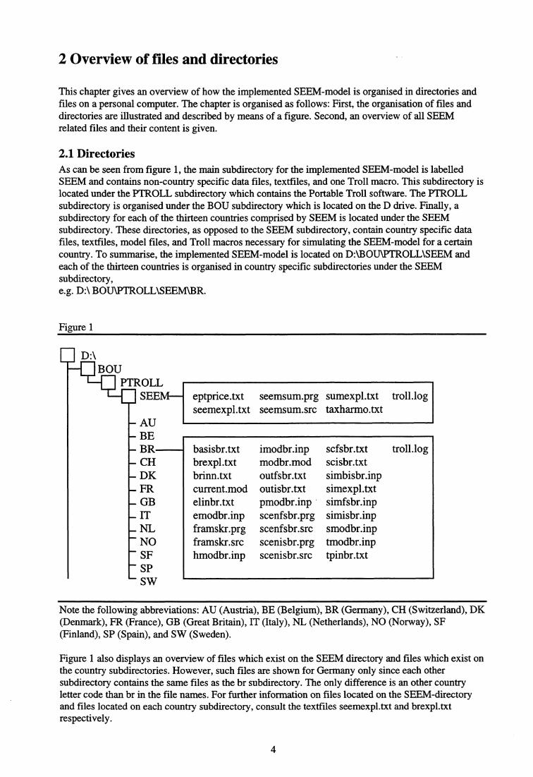
E D:\BOU
PTROLL■ SEEM- eptprice.txt seemsum.prg sumexpl.txt troll.log
seemexpl.txt seemsum.src taxharmo.txt—AU
BEBR
—CH— DK—FR
GB— IT_ NL—NO
SFSP
- SW
2 Overview of files and directories
This chapter gives an overview of how the implemented SEEM-model is organised in directories andfiles on a personal computer. The chapter is organised as follows: First, the organisation of files anddirectories are illustrated and described by means of a figure. Second, an overview of all SEEMrelated files and their content is given.
2.1 DirectoriesAs can be seen from figure 1, the main subdirectory for the implemented SEEM-model is labelledSEEM and contains non-country specific data files, textfiles, and one Troll macro. This subdirectory islocated under the PTROLL subdirectory which contains the Portable Troll software. The PTROLLsubdirectory is organised under the BOU subdirectory which is located on the D drive. Finally, asubdirectory for each of the thirteen countries comprised by SEEM is located under the SEEMsubdirectory. These directories, as opposed to the SEEM subdirectory, contain country specific datafiles, textfiles, model files, and Troll macros necessary for simulating the SEEM-model for a certaincountry. To summarise, the implemented SEEM-model is located on D:\BOU\PTROLL\SEEM andeach of the thirteen countries is organised in country specific subdirectories under the SEEMsubdirectory,e.g. D:\ BOU\PTROLL\SEEM\BR.
Figure 1
Note the following abbreviations: AU (Austria), BE (Belgium), BR (Germany), CH (Switzerland), DK(Denmark), FR (France), GB (Great Britain), IT (Italy), NL (Netherlands), NO (Norway), SF(Finland), SP (Spain), and SW (Sweden).
Figure 1 also displays an overview of files which exist on the SEEM directory and files which exist onthe country subdirectories. However, such files are shown for Germany only since each othersubdirectory contains the same files as the br subdirectory. The only difference is an other countryletter code than br in the file names. For further information on files located on the SEEM-directoryand files located on each country subdirectory, consult the textfiles seemexpl.txt and brexpl.txtrespectively.
4
2.2 Files for SEEMThe textfile seemexpl.txtThis textfile, called seemexpl.txt, provides an overview of files and their content which exist on theSEEM subdirectory, i.e. on d:\bou\ptroll\seem. Below these files are listed in alphabetic order as theyare listed on the SEEM subdirectory.
1) eptprice.txtAn ASCII textfile in the Troll format «formdata» and contains values of fuel import prices, margins,energy taxes, and value added taxes for all fuels, sectors, and countries comprised in the SEEM-model.Since the data are valid for all countries, the file is located directly on the SEEM directory, and notunder each country subdirectory. For information on the data sources, consult Brubakk et. al. (1995).
2)seemexpl.txtA textfile which provides an overview of files and their content existing on the SEEM directory, i.e.on d:\bou\ptroll\seem.
3)seemsum.prgA compiled version of the Troll macro file seemsum.src. The extension .prg denotes a Trollprogramme and the file is thus an executable version of seemsum.src.
4)seemsum.srcA Troll macro which summarises simulated fuel demand across sectors and/or countries. Additionally,the macro also calculates CO2-emissions by fuel, sector, and country based on simulated fuel demandand CO2-coefficients. Since the macro is general for all countries, the file is located directly on theSEEM directory, and not under each country subdirectory. The macro is programmed by Dag Kolsrud,Statistics Norway.
5)sumexpl.txtA textfile which explains how to use the macro seemsum.src. In addition, sumexpl.txt providescomments and explanations to each command in the Troll macro.
6)taxharmo.txtAn ASCII textfile in the Troll format «formdata» and contains harmonisation projections of fuel taxesfor all fuels, sectors, and countries comprised by the SEEM-model. Since the data are common for allcountries, the file is located directly on the SEEM directory, and not under each country subdirectory.This file is relevant for the reference scenario and the integration scenario, since these scenariosassume harmonisation of energy taxes in the period from 2000 to 2010.
7) troll.logA Troll file which logs the latest simulation results from running a Troll macro or simulating a model.This file also contains any errors or warning messages made by Troll during a simulation.
2.3 Country Files: GermanyThe textfile brexpl.txtThis textfile, called brexpl.txt, provides an overview of files and their content which exist on theGerman (br) directory, i.e. on d:\bou\ptroll\seem\br. Below these files are listed in alphabetic order asthey are listed on the br subdirectory. Generally speaking, all the other country subdirectories containthe same files as the br subdirectory.
1) basisbr.txtAn ASCII textfile in the Troll format «formdata» and contains historical and simulated data on allvariables and parameters in the SEEM-model from 1960 to 2020 for the reference scenario (basisscenario) for Germany. This datafile may serve as input when simulating the SEEM-model in the caseof other scenarios.
5
2) brexpl.txtA textfile which provides an overview of files and their content existing on the German (br) directory,i.e. on d:\bou\ptroll\seem\br.
3) brinn.txtAn ASCII textfile in the Troll format «formdata» and contains all data needed for extrapolation ofinput variables and simulation of the household, the industry, and the service sector models forGermany in the base year 1991.
4) current.mod The latest version of the Troll model used for simulation of Germany.
5) elinbr.txtAn ASCII textfile in the Troll format «formdata» and contains all data needed for extrapolation ofinput variables and simulation of the electricity generating sector model for Germany in the base year1991.
6) emodbr.inpA Troll input file which defines and establishes the model for the electricity generating sector inGermany. The file includes all equations and provides comments and descriptions to these. Theelectricity generating model is programmed by Wilma Pellekaan, ECN Netherlands.
7) framskr.DrgA compiled version of the Troll macro file framskr.src. The extension .prg denotes a Troll programmeand the file is thus an executable version of framskr.src.
8) framskr.srcA Troll macro which translates the commands in the scenfsbr.src and the scenisbr.src (see below)macros into Troll syntax. The macro is programmed by Rune Johansen, Statistics Norway.
9) hmodbr.inp A Troll input file which defines and establishes the model for the household sector in Germany. Thefile includes all equations and provides comments and descriptions to these. The household model isprogrammed by Leif Brubakk, Statistics Norway.
10) imodbr.inpA Troll input file which defines and establishes the model for the industry sector in Germany. The fileincludes all equations and provides comments and descriptions to these. The industry model isprogrammed by Leif Brubakk, Statistics Norway.
11) modbr.mod The compiled SEEM-model for Germany, including the household model, the industry model, theservice model, the electricity generating model, the transport model, and the price model
12) outfsbr.txtAn ASCII textfile in the Troll format «formdata» and contains simulation results from thefragmentation scenario for Germany.
13) outisbr.txtAn ASCII textfile in the Troll format «formdata» and contains simulation results from the integrationscenario for Germany.
14) pmodbr.inp A Troll input file which defines and establishes the fuel end user price model in Germany. The fileincludes all equations and provides comments and descriptions of these. The price model isprogrammed by Morten Aaserud, Statistics Norway and Wilma Pellekaan, ECN Netherlands.
6

15) scenfsbr.prgA compiled version of scenfsbr.src. The extension .prg denotes a Troll programme and the file is thusan executable version of scenfsbr.src.
16) scenfsbr.src A Troll macro which consists of Troll commands extrapolating input variables according to thefragmentation scenario assumptions for Germany. This macro is called upon from the simfsbr.inp file,and the macro works together with the framskr.prg macro.
17) scenisbnprgA compiled version of scenisbr.src. The extension .prg denotes a Troll programme and the file is thusan executable version of scenisbr.src.
18) scenisbr.srcA Troll macro which consists of Troll commands extrapolating input variables according to theintegration scenario assumptions for Germany. This macro is called upon from the simisbr.inp file, andthe macro works together with the framskr.prg macro. Note that the is scenario is based on the sameinput assumptions as the reference scenario assumptions.
19) scfsbr.txtAn ASCII textfile in the Troll format 4ormdata» and contains the input extrapolated according to thefragmentation scenario assumptions for Germany. This file is a result of the scenfsbr.src macro.
20) scisbr.txtAn ASCII textfile in the Troll format <dormdata» and contains the input extrapolated according to theintegration scenario assumptions for Germany. This file is a result of the scenisbr.src macro.
21) simbisbr.inpA Troll input file which gives access and search lists to all data needed for simulating the SEEM-model for the reference (basis) scenario in Germany. The file also defines and establishes the model bystarting the input files hmodbr.inp, imodbr.inp, smodbr.inp, tmodbr.inp, emodbr.inp, and pmodbr.inp.Finally, the file simulates the SEEM-model for Germany and saves the scenario results.
22) simexpl.txtA textfile which explains the procedure of making a simulation of the SEEM-model.
23) simfsbr.inp A Troll input file which gives access and search lists to all data needed for simulating the SEEMmodel for the fragmentation scenario in Germany. The file also defines and establishes the model bystarting the input files hmodbring, imodbr.inp, smodbr.inp, tmodbr.inp, emodbr.inp, and pmodbr.inp.Finally, the file simulates the SEEM-model for Germany and saves the scenario results.
24) simisbr.inpA Troll input file which gives access and search lists to all data needed for simulating the SEEMmodel for the integration scenario in Germany. The file also defines and establishes the model bystarting the input files hmodbr.inp, imodbr.inp, smodbr.inp, tmodbr.inp, emodbr.inp, and pmodbr.inp.Finally, the file simulates the SEEM-model for Germany and saves the scenario results. Note that theintegration scenario is identical to the reference (basis) scenario.
25) smodbr.inp A Troll input file which defines and establishes the model for the service sector in Germany. The fileincludes all equations and provides comments and descriptions to these. The service model isprogrammed by Leif Brubakk, Statistics Norway.

26) tmodbr.inpA Troll input file which defines and establishes the model for the transport sector in Germany. The fileincludes all equations and provides comments and descriptions to these. The transport model isprogrammed by Wilma Pellekaan, ECN Netherlands.
27) tpinbr.txtAn ASCII textfile in the Troll format «formdata» and contains all data needed for extrapolation ofinput variables and simulation of the transport sector model for Germany in the base year 1991.
28) troll.logA Troll file which logs the latest simulation results from running a Troll macro or simulating a model.This file also contains any errors or warning messages made by Troll during a simulation.
3. The Implemented SEEM-model
This chapter provides an outline of how the SEEM-model for Germany is implemented in the PortableTroll software. The reason for the choice of the implemented model for Germany as an illustrativeexample, lies in the fact that this model is the most general one compared to other country models. Allthe other country models are special cases of the more general German model specification. Thedifferences relate to the existing structure of fossil fuel demand in each country. The present chapterpresents and describes each sector model and the end user fuel price model for Germany as they areimplemented in Troll input files. For a more comprehensive and detailed theoretical explanation oneach model, consult Brubakk et. al. (1995).
It is worthwhile to notice in the Troll input files presented below, that the Troll syntax for a commentbegins with a 4*». Note also that the Troll commands in each input file are emphasised with italicletters.
3.1 The Household Model/* The Troll Input File hmodbr.inp1* This Troll input file, called hmodbr.inp, defines and establishes the model for the1* household sector (ho) in Germany (br). The hmodbr.inp file also provides1* descriptions and comments to this sector model. For easy references the equation1* numbers in the brackets below correspond to the equation numbers in the appendix in1* Brubakk et. al. (1995). As far as variable names and parameter names used in the1* household model are concerned, consult the appendix to this user's guide. The other1* sector models for Germany, namely for the industry sector (in), the service sector1* (se), the electricity generating sector (el), and the transport sector (tp) are established1* and described in the files with corresponding names imodbr.inp, smodbr.inp,1* emodbr.inp, and tmodbr.inp respectively. The end user fuel price calculation routine1* is implemented in the file named pmodbr.inp.
/* The Household Sector/* 1* The following model calculates fuel demand and aggregate fuel price indices in the1* household sector. First, the aggregate fuel price indices are determined. Second, the1* demand for the electricity aggregate and the fossil fuel aggregate (consisting of all1* three fossil fuels) are calculated at the upper level. Third, the fossil fuel aggregate is1* divided into a subaggregate (consisting of two fuels) and the remaining fuel at the/* intermediate level. Finally, demand for each of the two fuels constituting the1* subaggregate is determined at the lower level. In countries where only two types of1* fossil fuels are used, the lower level is omitted in the model. Similarly, only the upper
8
/* level applies to countries where only one type of fossil fuel is demanded.
/* Troll Commands1* 1* This Troll command specifies the endogenous variables in the household model.
addsym endogenousocprihobrcogprihobr1* start part 11* Note that the electricity consumption (eleconhobr) is set to be exogenous here due to1* the fact that it is set to be endogenous in the electricity generation part of the SEEM-1* model, named emodbr.inp.1* eleconhobrcogconhobrocconhobrngsconhobroilconhobrcoaconhobr/* end part 11* When recalibrating the model for the household sector, the endogenous variables1* above should be specified as exogenous and the calibration parameters below should1* be specified as endogenous.1* start part 21* a0elehobr1* a0coghobr1* a0ochobr1* a0oilhobr1* a0coahobr1* aOngshobr1* end part 2
/* This Troll command adds equations to the household model.
addeq bottom
I* Calculation of Aggregate Fuel Price Indices1* 1* Equation 1 and 2 calculates the oil-coal aggregate price index (ocpri) and the coal-oil-1* gas aggregate price index (cogpri) respectively, based on CES-functions.
1* Equation 1 (A2.4) ocprihobr=(a3dochobr*oilprihobr**( 1 -al sochobr)+( 1 -a3dochobr)*
coaprihobr**( 1 -al sochobr))**( 1/( 1 -a 1 sochobr))
1* Equation 2 (A2.4) cogprihobr.(a3dcoghobr*ngsprihobr**( I -al scoghobr)+ ( 1 -a3dcoghobr)*
ocprihobr**( 1-a1 scoghobr))**( 1/( 1 -al scoghobr))
1* Calculation of Fuel Demand at the Upper Level1* 1* Equation 3 and 4 calculates the aggregate demand for electricity (elecon) and the1* aggregate demand for fossil fuels (cogcon) respectively, based on Cobb-Douglas1* functions. The fossil fuel aggregate consists of coal, oil, and natural gas, named cog.

1* Equation 3 (A2.5) eleconhobr=a0elehobr*eleprihobr**al elehobr*cogprihobr**al cogelehobr*
conhobr**a2elehobr*eleconhobr( -1 )**a3lelehobr1* Equation 4 (A2.5) cogconhobr=a0coghobr*cogprihobr**a3coghobr*eleprihobr**a3elecoghobr*
conhobr**a2coghobr*cogconhobr(-1)**a3lcoghobr
/* Calculation of Fuel Demand at the Intermediate Level/* 1* Equation 5 and 6 calculates the subaggregate demand for fossil fuel (occon) and the1* demand for natural gas (ngscon) respectively, based on CES-functions. The1* subaggregate consists of oil and coal, named oc.
1* Equation 5 (A2.6) occonhobr=a0ochobr*cogconhobr*( 1 -a3dcoghobr)*(( 1 -a3dcoghobr)+
a3dcoghobr*((ngsprihobriocprihobr)**( 1 -a3lagcoghobr)*(((ngsconhobr( -1 )/occonhobr( -1 ))+cogrehobrY(a3dcoghobr/( 1 -a3dcoghobr)))**(( -1 )*(a3lagcoghobrial scoghobr)))**(1-al scoghobr))**(a I scoghobr/( 1 -al scoghobr))
1* Equation 6 (A2.6) ngsconhobr=a0ngshobr*cogconhobr*a3dcoghobr*(a3dcoghobr+
( 1 -a3dcoghobr)*((ngsprihobr/ocPRIhobr)**(( -I )*( 1 -a3lagcoghobr))*(((ngsconhobr( -1 )/occonhobr( -1 ))+cogrehobrY(a3dcoghobr/( 1 -a3dcoghobr)))**(a3lagcoghobrial scoghobr))**( 1-al scoghobr))**(al scoghobr/( 1-al scoghobr))
/* Calculation of Fuel Demand at the Lower Level/* 1* Equation 7 and 8 calculates the demand for oil (oilcon) and coal (coacon)/* respectively, based on CES-functions.
1* Equation 7 (A2.6) oilconhobr=a0oilhobr*occonhobr*a3dochobr*(a3dochobr+
( 1 -a3dochob r)*(( oilprihobricoaprihobr)**((-1 )*( 1 -a3lagochobr))*( (( oilconhobr( -1 )/coaconhobr(-1 ))+ocrehobrY(a3dochobri( 1 -a3dochobr)))**(a3lagochobrial sochobr))**( I -al sochobr))**(al sochobr/( 1-al sochobr))
1* Equation 8 (A2.6) coaconhobr=a0coahobr*occonhobr*( 1 -a3dochobr)*(( 1 -a3dochobr)+
a3dochobr*((oilprihobricoaprihobr)**( 1 -a3lagochobr)*( (( oilconhobr( -1 )/coaconhobr( -1 ))+ocrehobrY(a3dochobr/( 1 -a3dochobr)))**(( -1 )*(a3lagochobrial sochobr)))**( 1 -al sochobr))**(al sochobri( 1 -a I sochobr))
/* End of the household model.
3.2 The Industry Model1* The Troll Input File imodbr.inp1* This Troll input file, called imodbr.inp, defines and establishes the model for the1* industry sector (in) in Germany (br). The file imodbr.inp also provides descriptions/* and comments to this sector model. For easy references the equation numbers in the
10

1* brackets below correspond to the equation numbers in the appendix in Brubakk et. al.1* (1995). As far as variable names and parameter names used in the industry model are1* concerned, consult the appendix to this user's guide. The other sector models for1* Germany, namely for the household sector (ho), the service sector (se), the electricity1* generating sector (el), and the transport sector (tp), are established and described in1* the files with corresponding names hmodbr.inp, smodbr.inp, emodbr.inp, and1* tmodbr.inp respectively. The end user fuel price calculation routine is implemented in1* the file named pmodbr.inp.
1* The Industry Sector1* 1* The following model calculates the energy price index and the desired and realised1* fuel consumption in the industry sector. In the first part of the model the energy price1* index is determined. In the second and third part of the model desired and realised1* consumption of each of the fuel carriers is calculated.
1* Troll Commands1* 1* This Troll command specifies the endogenous variables in the industry model.
addsym endogenous
eenrpriinbrecoaconinbreoilconinbrengsconinbreeleconinbr1* start part 1coaconinbroilconinbrngsconinbr1* Note that the electricity consumption (eleconinbr) is set to be exogenous here due to1* the fact that it is set to be endogenous in the electricity generation part of the SEEM-1* model, named emodbr.inp.1* eleconinbr1* end part 11* When recalibrating the model for the industry sector, the endogenous variables above1* should be specified as exogenous and the calibration parameters below should be1* specified as endogenous.1* end part 21* a0coainbr1* a0oilinbr1* aOngsinbr1* a0eleinbr1* slutt del 2
/* This Troll command adds equations to the industry model.
addeq bottom
1* Calculation of the Energy Price Index1* 1* Equation 1 calculates the energy price index (eenrpri), based on a Cobb-Douglas1* function.
11

1* Equation 1 (A2.1) eempriinbr=coapriinbr**al coainbr*oilpriinbr**a 1 oilinbr*
ngspriinbr**al ngsinbr*elepriinbr**al eleinbr
/* Calculation of Desired Fuel Consumption/* 1* Equation 2, 3, 4, and 5 calculates desired consumption of coal (ecoacon), oil/* (eoilcon), natural gas (engscon), and electricity (eelecon) respectively, based on/* Cobb-Douglas functions.
/* Equation 2 (A2.2) ecoaconinbr=proinbr**a2proinbr*cappriinbr**alcapinbr*labpriinbr**
a1 waginbr*eenrpriinbr**al enrinbr*coapriinbr**( -1 )*coapriinbr**a 1 coainbr*oilpriinbr**al oilinbr*ngspriinbr**al ngsinbr*elepriinbr* *al eleinbr
/* Equation 3 (A2.2) eoilconinbr=proinbr**a2proinbr*cappriinbr**alcapinbr*labpriinbr**
al waginbr*eenrpriinbr**al enrinbr*oilpriinbr**( - 1 )*coapriinbr**al coainbr*oilpriinbr**al oilinbr*ngspriinbr**al ngsinbr*elepriinbr**a I eleinbr
/* Equation 4 (A2.2) engsconinbr=proinbr**a2proinbr*cappriinbr**alcapinbr*labpriinbr**
alwaginbr*eenrpriinbr**al enrinbr*ngspriinbr**( -I )*coapriinbr**al coainbr*oilpriinbr**al oilinbr*ngspriinbr**al ngsinbr*elepriinbr**al eleinbr
/* Equation 5 (A2.2) eeleconinbr=proinbr**a2proinbr*cappriinbr**a 1 capinbr*labpriinbr**
alwaginbr*eenrpriinbr**al enrinbr*elepriinbr**( -1 )*coapriinbr**alcoainbr*oilpriinbr**al oilinbr*ngspriinbr**al ngsinbr*elepriinbr**al eleinbr
/* Calculation of Realised Consumption/* /* Equation 6, 7, 8, and 9 calculates realised consumption of coal (coacon), oil (oilcon),/* natural gas (ngscon), and electricity (elecon) respectively, based on Cobb-Douglas/* functions.
/* Equation 6 (A2.3) coaconinbr=a0coainbr*( ecoaconinbr)**( 1 -a3laginbr)*
(coaconinbr( - 1 )-rcoainbr)**a3laginbr
1* Equation 7 (A2.3) oilconinbr=a0oilinbr*(eoilconinbr)**( 1 -a3laginbr)*
(oilconinbr( -1 )-roilinbr)**a3laginbr
/* Equation 8 (A2.3) ngsconinbr=a0ngsinbr*( engsconinbr)**( 1 -a3laginbr)*
(ngsconinbr( -1 )-mgsinbr)**a3laginbr
1* Equation 9 (A2.3) eleconinbr=a0eleinbr*(eeleconinbr)**( 1 -a3laginbr)*
( eleconinbr( -1 )-releinbr)**a3laginbr
12

1* End of the industry model.
3.3 The Service Model1* The Troll Input File smodbr.inp1* This Troll input file, called smodbr.inp, defines and establishes the model for the1* service sector (se) in Germany (br). The file smodbr.inp also provides descriptions1* and comments to this sector model. For easy references the equation numbers in the1* brackets below correspond to the equation numbers in the appendix in Brubakk et. al.1* (1995). As far as variable names and parameter names used in the service model are1* concerned, consult the appendix to this user's guide. The other sector models for1* Germany, namely for the household sector (ho), the industry sector (in), the1* electricity generating sector (el), and the transport sector (tp) are established and1* described in the files with corresponding names hmodbr.inp, imodbr.inp, emodbr.inp,1* and tmodbr.inp respectively. The end user fuel price calculation routine is1* implemented in the file named pmodbr.inp.
/* The Service Sector/* 1* The following model calculates fuel demand and aggregate fuel price indices in the1* service sector. First, the aggregate fuel price indices are determined. Second, the1* demand for the electricity aggregate and the fossil fuel aggregate (consisting of all1* three fossil fuels) are calculated at the upper level. Third, the fossil fuel aggregate is1* divided into a subaggregate (consisting of two fuels) and the remaining fuel at the1* intermediate level. Finally, demand for each of the two fuels constituting the1* subaggregate is determined at the lower level. In countries where only two types of1* fossil fuels are used, the lower level is omitted in the model. Similarly, only the upper1* level applies to countries where only one type of fossil fuel is demanded.
/* Troll Commands/* 1* This Troll command specifies the endogenous variables in the service model.
addsym endogenous
ogprisebrcogprisebr1* start part 1cogconsebr1* Note that the electricity consumption (eleconsebr) is set to be exogenous here due to1* the fact that it is set to be endogenous in the electricity generation part of the SEEM-1* model, named emodbr.inp.1* eleconsebrogconsebroilconsebrngsconsebrcoaconsebr1* end part 11* When recalibrating the model for the service sector the endogenous variables above1* should be specified as exogenous and the calibration parameters below should be1* specified as endogenous.1* end part 21* a0cogsebr1* a0elesebr1* a0ogsebr
13
1* a0coasebr1* a0oilsebr1* aOngssebr1* slutt del 2
1* This Troll command adds equations to the service model.
addeq bottom
I* Calculation of Aggregate Fuel Price Indices/*1* Equation 1 and 2 calculates the oil-gas aggregate price index (ogpri) and the coal-oil-1* gas aggregate price index (cogpri) respectively, based on CES-functions.
1* Equation 1 (A2.7) ogprisebr.(a3dogsebr*ngsprisebr**(1 -al sogsebr)+ (1 -a3dogsebr)*
oilprisebr**( 1 -al sogsebr))**(1/( 1 -al sogsebr))
1* Equation 2 (A2.7) cogprisebr.(a3dcogsebr*coaprisebr**( I -al scogsebr)+( 1 -a3dcogsebr)*
ogprisebr**( 1 -al scogsebr)) **( 1/( 1 -al scogsebr))
1* Calculation of Fuel Demand at the Upper Level1* 1* Equation 3 and 4 calculates the aggregate demand for electricity (elecon) and the1* aggregate demand for fossil fuel (cogcon) respectively, based on Cobb-Douglas/* functions. The fossil fuel aggregate consists of coal, oil, and natural gas, named cog.
1* Equation 3 (A2.8) eleconsebr=a0elesebr*prosebr**a2elesebr*
capprisebr**al capelesebr*labprisebr**allabelesebr*cogprisebr**al cogelesebr*eleprisebr**al elesebr*eleconsebr(-1)**a3lelesebr
1* Equation 4 (A2.8) cogconsebr=a0cogsebr*prosebr**a2cogsebr*
capprisebr**alcapcogsebr*labprisebr**allabcogsebr*cogprisebr**al cogsebr*eleprisebr**a 1 elecogsebr*co gconsebr(-1 )**a3kogsebr
1* Calculation of Fuel Demand at the Intermediate Level1* 1* Equation 5 and 6 calculates the subaggregate demand for fossil fuel (ogcon) and the1* demand for coal (coacon) respectively, based on CES-functions. The subaggregate1* consists of oil and natural gas, named og.
1* Equation 5 (A2.9) ogconsebr=a0ogsebr*cogconsebr*( 1 -a3dcogsebr)*(( 1 -a3dcogsebr)+
a3dcogsebr*((ogprisebricoaprisebr)**((-1)*(1-a3lagcogsebr))*(((ogconsebr( -1 )/coaconsebr(-1 ))+cogresebrY(( 1 -a3dcogsebrYa3dcogsebr))**(a3lagcogsebrialscogsebr))**(1 -al scogsebr))**(al scogsebr/(1-al scogsebr))
14

1* Equation 6 (A2.9) coaconsebr=a0coasebr*cogconsebr*a3dcogsebr*(a3dcogsebr+
( I -a3dcogsebr)*(( ogprisebricoaprisebr)**( 1 -a3lagcogsebr)*((( ogconsebr( -1 )/coaconsebr(-1 ))+ cogresebrY(( 1 -a3dcogsebr)/a3dcogsebr))**((-1 )*(a3lagcogsebrial scogsebr)))**
(1-al scogsebr))**(al scogsebr/(1 -al scogsebr))
1* Calculation of Fuel Demand at the Lower Level1* 1* Equation 7 and 8 calculates the demand for oil (oilcon) and natural gas (ngscon)1* respectively, based on CES-functions.1* Equation 7 (A2.9) oilconsebr=a0oilsebr*ogconsebr*( 1 -a3dogsebr)*(( 1 -a3dogsebr)+
a3dogsebrVoilprisebringsprisebr)**(( -1 )*( 1 -a3lagogsebr))*(ffoilconsebr(-1)/ngsconsebr(-1 ))+ogresebrY(( 1 -a3dogsebr)/a3dogsebr))**(a3lagogsebrialsogsebr))**
(1-al sogsebr)) **(al sogsebri( 1 -al sogsebr))
1* Equation 8 (A2.9) ngsconsebr=a0ngssebr*ogconsebr*a3dogsebr*(a3dogsebr+
(1 -a3dogsebr)*(( oilprisebringsprisebr)**( 1 -a3lagogsebr)*( (( oilconsebr(-1 )/ngsconsebr(-1))+ogresebrY(( 1 -a3dogsebrYa3dogsebr))**((-1 ) *(a3lagogsebr/al sogsebr)))**( I -al sogsebr)) **(al sogsebri( 1 -al sogsebr))
1* End of the service model.
3.4 The Electricity Generating Model1* The Troll Input file emodbr.inp1* This Troll input file, called emodbr.inp, defines and establishes the model for the1* electricity generating sector (el) in Germany (br).The file emodbr.inp also provides1* descriptions and comments to this sector model. For easy references the equation1* numbers in the brackets below correspond to the equation numbers in the appendix in1* Brubakk et. al. (1995). As far as variable names and parameter names used in the1* electricity generating model are concerned, consult the appendix to this user's guide.1* The other sector models for Germany, namely for the household sector (ho), the1* industry sector (in), the service sector (se), and the transport sector (tp) are1* established and described in the files with corresponding names hmodbr.inp,1* imodbr.inp, smodbr.inp, and tmodbr.inp respectively. The end user fuel price1* calculation routine is implemented in the file named pmodbr.inp.
1* The Electricity Generating Sector1* 1* The following model calculates fuel demand in the electricity generating sector. In1* the first part of the model the shares of the old, new, and best available technologies1* (bat) technologies are calculated, using a linear penetration path. Based on these/* shares the average production costs and efficiencies for each type of production (coal,1* gas, oil, nuclear and renewable) are determined. These production costs and1* efficiencies serve in turn as input in the Cobb-Douglas functions which calculate the/* overall shares of electricity production for each type of fuel based production. These1* shares multiplied with their respective efficiencies and the total average production1* cost of electricity yield the fuel demand in the electricity generating sector.
15

/* Troll Commands/* /* This Troll command specifies the endogenous variables in the electricity generating/* model.
addsym endogenouscoasha0belbrngssha0belbroilsha0belbrnucsha0belbrrensha0belbrcoashanelbrcoashafelbrcoashabelbrcoashaoelbrngsshanelbrngsshabelbrngsshaoelbroilshanelbroilshabelbroilshaoelbrnucshanelbrnucshabelbrnucshaoelbrrenshanelbrrenshabelbrrenshaoelbrcoacstelbrngscstelbroilcstelbrnuccstelbrrencstelbrcoaeffelbrngseffelbroileffelbrnuceffelbrreneffelbrcoashal elbrngsshal elbroilshal elbrnucshal elbrrenshal elbrcoashaelbrngsshaelbroilshaelbrnucshaelbrrenshaelbrcoaconelbrngsconelbroilconelbrnucconelbrrenconelbr1* Note that the electricity generating price (elegenpribr) is set to be exogenous here due1* to the fact that it is set to be endogenous in the end user fuel price model, named1* pmodbr.inp.

1* elegenpribrtotdemelbreleconhobreleconsebreleconinbrrailcontotbr
1* This Troll command adds equations to the electricity generating model.
addeq bottom
/* Calculation of Shares of Old, New, and Bat Technology
1* Equation 1 to 16 calculates the share of old, new, and bat technology based on a1* linear penetration path. Note that the share of future technology is calculated for coal-/4' technology only.
1* The different shares of bat fuel technology are set equal to zero in the base year.
coasha0belbr=0
ngssha0belbr=0
oilsha0belbr=0
nucsha0belbr=0
rensha0belbr=0
/*1* Equation 1, 2, 3, and 4 calculates the share of new, future, bat, and old coal1* technology respectively.1*
1* Equation 1 coashanelbr=(if time > 15 then dumnbr*coashalnelbr
else coashaOnelbr+((dumnbr*coashalnelbr-coashaOnelbr)/15)*time)
/* Equation 2coashafelbr=(if time > 15 then dumnbr*coashalfelbr
else coashaOfelbr+((dumnbr*coashalfelbr-coashaOfelbr)/15)*time)
/* Equation 3 coashabelbr.(if time > 15 then dumbbr*coashalbelbr
else coasha0belbr+((dumbbr*coashalbelbr-coasha0belbr)/15)*time)
1* Equation 4 coashaoelbr= 1-coashanelbr-coashafelbr-coashabelbr
1* 1* Equation 5, 6, and 7 calculates the share of new, bat, and old natural gas technology1* respectively.1*
1* Equation 5 ngsshanelbr.(if time > 15 then dumnbr*ngsshalnelbr
else ngsshaOnelbr+((dumnbr*ngsshalnelbr-ngsshaOnelbr)/15)*time)
1* Equation 6 ngsshabelbr.(if time > 15 then dumbbr*ngsshalbelbr
else ngssha0belbr+((dumbbr*ngsshalbelbr-ngssha0belbr)/15)*time)
1* Equation 7 ngsshaoelbr= 1 -ngsshanelbr-ngsshabelbr
1* 1* Equation 8, 9, and 10 calculates the share of new, bat, and old oil technology1* respectively.1*
1* Equation 8 oilshanelbr.(if time > 15 then dumnbr*oilshalnelbr
else oilshaOnelbr+((dumnbr*oilshalnelbr-oilshaOnelbr)/15)*time)
1* Equation 9 oilshabelbr.(if time > 15 then dumbbr*oilshalbelbr
else oilsha0belbr+((dumbbr*oilshalbelbr-oilsha0belbr)/15)*time)
1* Equation 10oilshaoelbr= 1 -oilshanelbr- oilshabelbr
1* 1* Equation 11, 12, and 13 calculates the share of new, bat, and old nuclear technology1* respectively.1*
1* Equation 11 nucshanelbr.(if time > 15 then dumnbr*nucshalnelbr
else nucshaOnelbr+((dumnbr*nucshalnelbr-nucshaOnelbr)/15)*time)
1* Equation 12nucshabelbr=fif time > 15 then dumbbr*nucshalbelbr
else nucsha0belbr+((dumbbr*nucshalbelbr-nucsha0belbr)/15)*time)
1* Equation 13 nucshaoelbr=1 -nucshanelbr-nucshabelbr
1* 1* Equation 14, 15, and 16 calculates the share of new, bat, and old renewable1* technology respectively.1*
18
1* Equation 14 renshanelbr.(if time > 15 then dumnbr*renshalnelbr
else renshaOnelbr+((dumnbr*renshalnelbr-renshaOnelbr)/15)*time)
/* Equation 15 renshabelbrqif time > 15 then dumbbr*renshalbelbr
else rensha0belbr+((dumbbr*renshalbelbr-renshaObelbr)/15)*time)
/* Equation 16 renshaoelbr= I -renshanelbr-renshabelbr
1* Determination of Average Production Costs of Electricity1* 1* Equation 17, 18, 19, 20, and 21 determines the average production costs of electricity1* when using coal, gas, oil, nuclear, and renewable as input respectively. These1* calculations are based on the foregoing share calculations.
1* Equation 17 (A5.4) coacstelbr=coashaoelbr*(coaprcstoelbr+coaprielbricoaeffoelbr)
+coashanelbr*(coaprcstnelbr+coaprielbricoaeffnelbr)+coashafelbr*(coaprcsYselbr+coaprielbricoaeffelbr)+coashabelbr*(coaprcstbelbr+coaprielbricoaelibelbr)
1* Equation 18 (A5.4) ngscstelbr.ngsshaoelbr*(ngsprcstoelbr+ngsprielbr/ngseffoelbr)
+ngsshanelbr*(ngsprcstnelbr+ngsprielbringseffnelbr)+ngsshabelbr*(ngsprcstbelbr+ngsprielbringseffbelbr)
1* Equation 19 (A5.4) oilcstelbr=oilshaoelbr*(oilprcstoelbr+oilprielbrioileffoelbr)
+oilshanelbr*(oilprcstnelbr+oilprielbrioileffnelbr)+oilshabelbr*(oilprcstbelbr+oilprielbrioileffbelbr)
1* Equation 20 (A5.4) nuccstelbr=nucshaoelbr*(nucprcstoelbr+nucprielbrinuceffoelbr)
+nucshanelbr*(nucprcstnelbr+nucprielbrinuceffnelbr)+nucshabelbr*(nucprcstbelbr+nucprielbrinuceffbelbr)
1* Equation 21 (A5.4) rencstelbr=renshaoelbr*(renprcstoelbr+renprielbrireneffoelbr)
+renshanelbr*(renprcstnelbr+renprielbrireneffnelbr)+renshabelbr*(renprcstbelbr+renprielbrireneffbelbr)
1* Determination of Average Efficiency in Electricity Production1* 1* Equation 22, 23, 24, 25, and 26 determines the average efficiency per unit coal,1* natural gas, oil, nuclear, and renewable as input respectively, when producing1* electricity. These calculations are based on the foregoing share calculations.
/* Equation 22 (A5.1) coaeffelbr=coashaoelbr*coaeffoelbr+coashanelbr*coaeffnelbr
+coashafelbr*coaeffelbr+coashabelbr*coaeffbelbr
19
1* Equation 23 (A5.1) ngseffelbr=ngsshaoelbr*ngseffoelbr+ngsshanelbr*ngseffnelbr
+ngsshabelbr*ngseffbelbr
1* Equation 24 (A5.1) oileffelbr=oilshaoelbr*oileffoelbr+oilshanelbr*oileffnelbr
+oilshabelbr*oileffbelbr
1* Equation 25 (A5.1) nuceffelbr=nucshaoelbr*nuceffoelbr+nucshanelbr*nuceffnelbr
+nucshabelbr*nucelibelbr
1* Equation 26 (A5.1) reneffelbr=renshaoelbr*reneffoelbr+renshanelbr*reneffnelbr
+renshabelbr*reneffbelbr
1* Calculation of Overall Fuel Based Shares of Electricity Production1* 1* Equation 27, 28, 29, 30, and 31 calculates the coal, natural gas, oil, nuclear, and1* renewable based production shares of total electricity produced respectively. These1* share calculations are based on Cobb-Douglas functions.
1* Equation 27 (A2.20) coashal elbr=a0coaconelbr*( coacstelbr)**( -I )*(coacstelbr)**(alcoaconelbr)*
(ngscstelbr)**(alngsconelbr)*(oilcstelbr)**(al oilconelbr)*(nuccstelbr)**( al nucconelbr)*(rencstelbr)**(alrenconelbr)
1* Equation 28 (A2.20) ngsshal elbr=a0ngsconelbr*(ngscstelbr)**(-1 )*(coacstelbr)**(alcoaconelbr)*
(ngscstelbr)**(alngsconelbr)*(oilcstelbr)**(al oilconelbr)*(nuccstelbr)**(alnucconelbr)*(rencstelbr)**(alrenconelbr)
/* Equation 29 (A2.20) oilshal elbr=a0oilconelbr*( oilcstelbr)**(- 1 )*(coacstelbr)**(al coaconelbr)*
(ngscstelbr)**( al ngsconelbr)*(oilcstelbr)**(al oilconelbr)*(nuccstelbr)**( al nucconelbr)*(rencstelbr)**(alrenconelbr)
1* Equation 30 (A2.20) nucshal elbr=a0nucconelbr*(nuccstelbr)**( -1 )*(coacstelbr)**(al coaconelbr)*
(ngscstelbr)**(alngsconelbr)*(oilcstelbr)**(al oikonelbr)*(nuccstelbr)**(al nucconelbr)*(rencstelbr)**(al renconelbr)
1* Equation 31 (A2.20) renshal elbr=a0renconelbr*( rencstelbr)**( -1 )*(coacstelbr)**(al coaconelbr)*
(ngscstelbr)**(alngsconelbr)*( oilcstelbr)**( al oikonelbr)*(nuccstelbr)**(alnucconelbr)*(rencstelbr)**(alrenconelbr)
1* Calculation of Normalized Fuel Based Shares of Electricity Production1* /* Equation 32, 33, 34, 35, and 36 calculates the normalized coal, natural gas, oil,1* nuclear, and renewable based production shares of total electricity produced1* respectively.
20

1* Equation 32 (A2.21) coashaelbr=coashalelbr/(coashal eibr+ngsshal elbr+ oilshal elbr+nucshal elbr
+renshalelbr)
/* Equation 33 (A2.21) ngsshaelbr=ngsshal elbrficoashal elbr+ngsshal elbr+oilshalelbr+nucshal elbr
+renshal elbr)
1* Equation 34 (A2.21) oilshaelbr=oilshal elbr/(coashal elbr+ngsshal elbr+ oilshal elbr+nucshalelbr
+renshalelbr)
/* Equation 35 (A2.21)nucshaelbr=nucshal elbr/(coashal elbr+ngsshal elbr+ oilshal elbr+nucshal elbr
+renshalelbr)
1* Equation 36 (A2.21) renshaelbr=renshal elbr/(coashal elbr+ngsshalelbr+oilshal elbr+ nucshal elbr
+renshal elbr)
1* Calculation of Total Average Production Costs (i.e. price) of Electricity1* 1* Equation 37 calculates the electricity generation price based on foregoing calculation1* of normalized fuel based production shares and average production costs. Note that1* the divisor 1.66 at the end of the equation, is the exchange rate in the base year.
1* Equation 37 (A2.23) elegenpribr= (coashaelbr*coacstelbr+ngsshaelbr*ngscstelbr+ oilshaelbr*oilcstelbr
+nucshaelbr*nuccstelbr+renshaelbr*rencstelbr)/1 .66
1* Calculation of Total Domestic Electricity Production1* 1* Equation 38 calculates total requirement of electricity production based on calculated1* electricity consumption in the other sectors, net electricity export, and the distribution1* losses of electricity.
/* Equation 38 (A2.19) totdemelbr=(eleconhobr+eleconsebr+eleconinbr+railcontotbr+eleconexbr)*
( 1 +elelossbr/100)
1* Calculation of Fuel Demand1* 1* Equation 39, 40, 41, 42, and 43 calculates demand for coal, natural gas, oil, nuclear,1* and renewable respectively in the electricity generating sector.
1* Equation 39 (A2.22) coaconelbr=coashaelbr*totdemelbr*( 1/coaeffelbr)*a3coacalelbr
1* Equation 40 (A2.22) ngsconelbr=ngsshaelbr*totdemelbr*( 1/ngseffelbr)*a3ngscalelbr

1* Equation 41 (A2.22) oilconelbr=oilshaelbr*totdemelbr*(1/oileffelbr)*a3oilcalelbr
1* Equation 42 (A2.22) nucconelbr=nucshaelbr*totdemelbr*(1/nuceffelbr)*a3nuccalelbr
1* Equation 43 (A2.22) renconelbr=renshaelbr*totdemelbr*(1/reneffelbr)*a3rencalelbr
1* End of the electricity generating model.
3.5 The Transport Model1* The Troll Input File tmodbr.inp1* This Troll input file, called tmodbr.inp, defines and establishes the model for the1* transport sector (tp) in Germany (br). The file tmodbr.inp also provides descriptions1* and comments to this sector model. For easy references the equation numbers in the1* brackets below correspond to the equation numbers in the appendix in Brubakk et. al.1* (1995). As far as variable names and parameter names used in the transport model are1* concerned, consult the appendix to this user's guide. The other sector models for1* Germany, namely for the household sector (ho), the industry sector (in), the service1* sector (se), and the electricity generating sector (el) are established and described in1* the files with the corresponding names hmodbr.inp, imodbr.inp, smodbr.inp, and1* emodbr.inp respectively. The end user fuel price calculation routine is implemented1* in the file named pmodbr.inp.
/* The Transport Sector/* 1* In general, the transport sector is divided into passenger, transport, freight transport,1* and air transport as subsectors. The following model calculates separately fuel1* demand in each of these subsectors.
1* Passenger Transport1* When it comes to passenger transport the shares of old, new, and bat technologies are1* calculated using a linear penetration path. Based on these shares the average prices1* and efficiencies for each type of transport mode options (i.e. gasoline car, diesel car,1* 1pg car, electricity train, diesel train, and diesel bus) are determined. These average1* prices and efficiencies serve in turn as input in the Cobb-Douglas functions which1* calculate the optimal share for each type of transport mode option. Finally, these1* optimal shares multiplied with their respective efficiencies and the total demand for1* passenger kilometers yield the total fuel demand in the passenger transport sector.
1* Freight Transport1* The freight transport sector is modelled in a similar way as the passenger transport1* sector. However, the optimal share of each type of transport mode option (i.e. road,1* rail, and water) are assumed exogenously given in the freight transport sector as1* opposed to the passenger transport sector. Based on the level of domestic production,1* total demand for tonkilometers are determined. Given total demand for tonkilometers1* and the share for each type of transport mode, the optimal distribution of total freight1* transport on the three modes is calculated. This in turn determines the final demand/* for the different fuels in the freight transport sector given some efficiency parameters.

/* Air Transport1* The air transport sector is modelled somewhat simplier than both the passanger and1* the freight transport sector. The submodel for air transport abstracts from substitution1* possibilities between air and other transport modes. Additionally, the model does not1* distinguish between passenger transport and freight transport. Hence, demand for air1* fuel is determined directly as a function of the price of kerosene and the activity level1* (GDP). Finally, total demand for the different fuels is computed in the transport1* model.
1* Troll Commands1* 1* This Troll command specifies the endogenous variables in the transport model.
addsym endogenous
totdemindtpbrtotdemtpbrgoshantpbrgoshabtpbrgoshaotpbrdishantpbrdishabtpbrdishaotpbrgashantpbrgashabtpbrgashaotpbrreshantpbrreshabtpbrreshaotpbrrdshantpbrrdshabtpbrrdshaotpbrbdshantpbrbdshabtpbrbdshaotpbrgocsttpbrdicsttpbrgacsttpbrrecsttpbrrdcsttpbrbdcsttpbrgoefftpbrdieffipbrgaefftpbrreefftpbrrdefftpbrbdeffipbrgoshaltpbrdishaltpbrgashaltpbrreshaltpbrrdshaltpbrbdshaltpbrgoshatpbrdishatpbrgashatpbr
23

reshatpbrrdshatpbrbdshatpbrgocontpbrdicontpbrgacontpbrrecontpbrrdcontpbrbdcontpbrtppribrtotdemindOrtotdembrrotkmbrratkmbrwatkmbrdiconOrelconOroilcontfbroilconindfabroilconfabraircontotbrroadcontotbr1* Note that the total electricity consumption in the transport sector (railcontotbr) is set1* to be exogenous here due to the fact that it is set to be endogenous in the electricity/* generation part of the SEEM-model, named emodbr.inp.1* railcontotbrrailcondiebrwatcontotbrnsharofflyrnsharaOrnshawaOr
1* This Troll command adds equations to the transport model.
addeq bottom
I* The Passenger Transport Sector
1* Calculation of shares of New, Bat, and Old Technology1* 1* Equation 1 to 18 calculates the share of new, bat, and old technology for the different1* transport modes (car, train, and bus) based on a linear penetration path.
1* Equation 1, 2, and 3 calculates the share of new, bat, and old technology respectively1* for gasoline cars.
1* Equation 1 goshantpbr=dumntpbr*( goshaOntpbr+ (( 1 - goshaOntpbr)/29)*time)
1* Equation 2goshabtpbr=dumbtpbr*( goshaObtpbr+ (( 1 -goshaObtpbr)/29)*time)
1* Equation 3 goshaotpbr= 1- goshantpbr- goshabtpbr

/* Equation 4, 5, and 6 calculates the share of new, bat, and old technology respectively1* for diesel cars.
1* Equation 4 dishantpbr=dumntpbr*(dishaOntpbr+(( 1 -dishaOntpbr)/29)*time)
1* Equation 5 dishabtpbr=dumbtpbr*(dishaObtpbr+(( 1 -dishaObtpbr)/29)*time)
1* Equation 6 dishaotpbr=1 -dishantpbr-dishabtpbr
1* Equation 7, 8, and 9 calculates the share of new, bat, and old technology respectively1* for gas cars.
1* Equation 7 gashantpbr=dumntpbr*( gashaOntpbr+(( 1 - gashaOntpbr)/29)*time)
/* Equation 8 gashabtpbr=dumbtpbr*( gashaObtpbr+(( 1 -gashaObtpbr)/29)*time)
1* Equation 9 gashaotpbr= 1 - gashantpbr- gashabtpbr
1* Equation 10, 11, and 12 calculates the share of new, bat, and old technology1* respectively for electricity trains.
1* Equation 10reshantpbr=dumntpbr*(reshaOntpbr+(( 1 - reshaOntpbr)/29)*time)
1* Equation 11 reshabtpbr=dumbtpbr*(reshaObtpbr+((1 - reshaObtpbr)/29)*time)
1* Equation 12reshaotpbr= I - reshantpbr- reshabtpbr
/* Equation 13, 14, and 15 calculates the share of new, bat, and old technology1* respectively for diesel trains.
1* Equation 13 rdshantpbr=dumntpbr*(rdshaOntpbr+(( 1 - rdshaOntpbr)/29)*time)
1* Equation 14rdshabtpbr= dumbtpbr*( rdshaObtpbr+ (( 1 - rdsha0bipbr)/29)*time)
1* Equation 15 rdshaotpbr= 1 - rdshantpbr- rdshabtpbr
1* Equation 16, 17, and 18 calculates the share of new, bat, and old technology1* respectively for diesel buses.
1* Equation 16 bdshantpbr=dumntpbr*(bdshaOntpbr+(( 1-bdshaOntpbr)/29)*time)
/* Equation 17 bdshabtpbr=dumbtpbr*(bdshaObtpbr+(( 1 -bdshaObtpbr)/29)*time)
1* Equation 18 bdshaotpbr= 1 -bdshantpbr-bdshabtpbr
1* Determination of Average Price (or cost) of Transport Mode1* /* Equation 19 to 24 determines the average price per person kilometre (pkm) of1* transport mode gasoline car, diesel car, gas car, electricity train, diesel train, and1* diesel bus respectively. These calculations are based on the foregoing share1* calculations.
1* Equation 19 (A5.3) gocsttpbr=goshaotpbr*( goprcstotpbr+ gopritpbr/goeffotpbr)
+ goshantpbr*( goprcstntpbr+ gopritpbr/goeffntpbr)+ goshabtpbr*( goprcstbtpbr+ gopritpbr/goeffbtpbr)
/* Equation 20 (A5.3) dicsupbr=dishaotpbr*(diprcstotpbr+dipritpbr/dieffotpbr)
+dishantpbr*(diprcsintpbr+dipritpbr/dieffntpbr)+dishabtpbr*(diprcstbtpbr+dipritpbrklieffbtpbr)
1* Equation 21 (A5.3)gacsttpbr=gashaotpbr*( gaprcstotpbr+ gapritpbr/gaeffotpbr)
+ gashantpbr*( gaprcstntpbr+ gapritpbr/gaeffntpbr)+ gashabtpbr*( gaprcstbtpbr+ gapritpbrigaelibtpbr)
1* Equation 22 (A5.3) recsttpbr=reshaotpbr*(reprcstotpbr+ repritpbr/reeffotpbr)
+reshantpbr*(reprcstntpbr+ repritpbr/reeffntpbr)+reshabtpbr*( reprcstbtpbr+repritpbr/reebtpbr)
/* Equation 23 (A5.3) rdcsttpbr=rdshaotpbr*(rdprcstotpbr+ rdpritpbr/rdeffotpbr)
+rdshantpbr*(rdprcstntpbr+rdpritpbr/rdeffntpbr)+rdshabtpbr*(rdprcstbtpbr+rdpritpbrirdeffimpbr)
/* Equation 24 (A5.3) bdcsupbr=bdshaotpbr*(bdprcstotpbr+bdpritpbribdeffotpbr)
+bdshantpbr*(bdprcstntpbr+bdpritpbribdeffntpbr)+bdshabtpbr*(bdprcstbtpbr+bdpritpbribdelibtpbr)
1* Determination of Average Efficiency of Transport Mode1* /* Equation 25 to 30 determines the average efficiency per unit of gasoline (car), diesel1* (car), gas (car), electricity (train), diesel (train), and diesel (bus) respectively. These1* calculations are based on the foregoing share calculations.
1* Equation 25 (A5.1) goefftpbr= goshaotpbr* goeffotpbr+ goshantpbr* goeffntpbr
+ goshabtpbr* goeffbtpbr
26

1* Equation 26 (A5.1) dieffipbr=dishaotpbr*dieffotpbr+dishantpbr*dieffntpbr
+dishabtpbr*dieffbtpbr
1* Equation 27 (A5.1) gaefftpbr=gashaotpbr*gaeffotpbr+gashantpbr*gaeffntpbr
+ gashabtpbr*gaeffbtpbr
1* Equation 28 (A5.1) reefftpbr=reshaotpbr*reeffotpbr+reshantpbr*reeffntpbr
+reshabtpbr*reefflytpbr
1* Equation 29 (A5.1) rdeffipbr=rdshaotpbr*rdeffotpbr+rdshantpbr*rdeffntpbr
+rdshabtpbr*rdeffbtpbr
1* Equation 30 (A5.1) bdeffipbr=bdshaotpbr*bdeffotpbr+bdshantpbr*bdeffntpbr
+bdshabtpbr*bdeffbtpbr
/* Calculation of Optimal Share of Transport Mode/* /* Equation 31 to 36 calculates the optimal share of transport mode gasoline car, diesel1* car, gas car, electricity train, diesel train, and diesel bus respectively. These share1* calculations are based on Cobb-Douglas functions.
1* Equation 31 (A2.12) goshaltpbr=a0gocontpbr*( gocsttpbr)**( -1 )*(gocsttpbr)**(al gocontpbr)*
(dicsttpbr)**(al dicontpbr)*( gacsttpbr)**(al gacontpbr)*(recsttpbr)**(alrecontpbr)*(rdcsttpbr)**(alrdcontpbr)*(bdcsttpbr)**(albdcontpbr)
1* Equation 32 (A2.12) dishaltpbr=a0dicontpbr*(dicsupbr)**(-1)*(gocsttpbr)**(al gocontpbr)*
(dicsttpbr)**(al dicontpbr)*( gacsttpbr)**(al gacontpbr)*(recsttpbr)**(alrecontpbr)*(rdcsttpbr)**(alrdcontpbr)*(bdcsttpbr)**(albdcontpbr)
1* Equation 33 (A2.12) gashaltpbr=a0gacontpbr*( gacsttpbr)**( -1 )*(gocsttpbr)**(al gocontpbr)*
(dicsttpbr)**(aldicontpbr)*(gacsttpbr)**(al gacontpbr)*(recsttpbr)**(alrecontpbr)*(rdcsttpbr)**(alrdcontpbr)*(bdcsttpbr)**(albdcontpbr)
1* Equation 34 (A2.12) reshal tpbr=a0recontpbr*(recsttpbr)**( -1 )*( gocsttpbr)**(al gocontpbr)*
(dicsttpbr)**(al dicontpbr)*( gacsttpbr)**(al gacontpbr)*(recsttpbr)**(alrecontpbr)*(rdcsttpbr)**(al rdcontpbr)*(bdcsttpbr)**(albdcontpbr)
1* Equation 35 (A2.12) rdshal tpbr=a0rdcontpbr*(rdcsttpbr)**( -1 )*( gocsttpbr)**(al gocontpbr)*
(dicsttpbr)**(aldicontpbr)*( gacsttpbr)**(al gacontpbr)*(recsttpbr)**(alrecontpbr)*(rdcsttpbr)**(alrdcontpbr)*
27

(bdcsttpbr)**(albdcontpbr)
1* Equation 36 (A2.12) bdshaltpbr=a0bdcontpbr*(bdcsttpbr)**( -1 )*( gocsttpbr)**(al gocontpbr)*
(dicsttpbr)**(aldicontpbr)*( gacsttpbr)**(al gacontpbr)*(recsttpbr)**(al recontpbr)*(rdcsttpbr)**(alrdcontpbr)*(bdcsttpbr)**(albdcontpbr)
1* Calculation of Normalized Share of Transport Mode1* 1* Equation 37 to 42 calculates the normalized share of transport mode gasoline car,1* diesel car, gas car, electricity train, diesel train, and diesel bus respectively.
/* Equation 37 (A2.13) goshatpbr= goshal tpbrA goshaltpbr+dishaltpbr+gashaltpbr+reshaltpbr
+rdshaltpbr+bdshaltpbr)
1* Equation 38 (A2.13) dishatpbr=dishal tpbrA goshaltpbr+dishaltpbr+ gashal tpbr+reshaltpbr
+rdshaltpbr+bdshaltpbr)
1* Equation 39 (A2.13) gashatpbr= gashal tpbrA goshaltpbr+dishaltpbr+gashaltpbr+reshaltpbr
+rdshaltpbr+bdshaltpbr)
1* Equation 40 (A2.13) reshatpbr=reshaltpbr/(goshaltpbr+dishaltpbr+gashalipbr+reshaltpbr
+rdshaltpbr+bdshaltpbr)
/* Equation 41 (A2.13) rdshatpbr=rdshal tpbrA goshaltpbr+dishaltpbr+ gashal tpbr+resha I tpbr
+rdshaltpbr+bdshaltpbr)
1* Equation 42 (A2.13) bdshatpbr=bdshaltpbrAgoshaltpbr+disluzltpbr+gashaltpbr+reshaltpbr
+rdshaltpbr+bdshaltpbr)
1* Calculation of the Price Index (cost) per Passenger Kilometer1* 1* Equation 43 calculates the price index per passenger kilometer based on foregoing1* calculations of average price of each transport mode. The underlying function is of a/* Cobb-Douglas spesification. Note that tppri9lbr denotes a calibration constant in the1* base year 1991.
/* Equation 43 (A2.10) tppribr=(( gocsttpbr)**(al gocontpbr)*(dicsttpbr)**(al dicontpbr)*( gacsttpbr)**
(al gacontpbr)*(recsttpbr)**(al recontpbr)*(rdcsttpbr)**(a I rdcontpbr)*(bdcsttpbr)**(albdcontpbr))/tppri9lbr
1* Calculation of Total Demand for Passenger Kilometres/* 1* Equation 44 calculates total demand for passenger kilometres based on foregoing/* calculation of the price index per passenger kilometres as well as the consumer/* expenditure (income). The underlying function is of a Cobb-Douglas spesification.
28
/* Equation 45 is equation 44 multiplied with a calibration constant in the base year1* 1991(totdemtp9lbr).
/* Equation 44 (A2.11) totdemindtpbr=incomebr**b pkmbr*tppribr**b2pkmbr
/* Equation 45 (A2.11) totdemtpbr=totdemindtpbr*totdemtp9 1 br
1* Calculation of Fuel Demand in Passenger Transport1* /* Equation 46 to 51 calculates demand (ktoe) for gasoline (car), diesel (car), gas (car),1* electricity (train), diesel (train), and diesel (bus) respectively in the passenger1* transport sector. Note that each equation is multiplied with a calibration constant/* labelled aOcalplcmbr
1* Equation 46 (A2.14) gocontpbr= 1 000*( aOcalpkmbr* goshatpbr*totdemtpbr*( ligoefftpbr))
1* Equation 47 (A2.14) dicontpbr= 1000*( aOcalpkmbr*dishatpbr*totdemtpbr*( 1/diefftpbr))
1* Equation 48 (A2.14) gacontpbr= 1000*( aOcalpkmbr* gashatpbr*totdemtpbr*( 1/gaefftpbr))
/* Equation 49 (A2.14) recontpbr= 1000*( aOcalrelbr*reshatpbr*totdemtpbr*( 1/reefftpbr))
/* Equation 50 (A2.14) rdcontpbr= 1000*( aOcalrdibr*rdshatpbr*totdemtpbr*( lirdeffipbr))
1* Equation 51 (A2.14) bdconipbr= 1000*( aOcalpkmbr*bdshatpbr*totdemtpbr*( llbdefftpbr))
1* The Freight Transport Sector1*
1* Calculation of Total Demand for Tonkilometers1* 1* Equation 52 calculates total demand for tonkilometers in the freight transport sector/* based on the level of domestic production (GDP). Equation 53 is equation 521* multiplied with a calibration constant in the base year 1991 (totdemtf9lbr).
1* Equation 52 (A2.15) totdemindfflyr= gdpindbr**( dumifflyr*b 1 itlanbr+ dumftfbr*b lftkmbr)
1* Equation 53 (A2.15) totdemfflyr=totdemindbr*totdemy9 1 br
1* Distribution of Total Freight Transport Demand on Modes1* /* Equation 54, 55, and 56 calculates the normalised road mode share, the rail mode1* share, and the water mode share respectively of total demand for tonkilometers. Note
29

/* that the calculated shares are exogenously determined in the model. Equation 57, 58,1* and 59 multiplies these shares with the total demand for tonkilometers to obtain the1* distribution of total freight transport in tonkilometers on the three modes road, rail,1* and water resepctively.
1* Equation 54nsharofflyr=sharoOr4 sharoOr+shar4br+shawa0r)
1* Equation 55 nsharaOr=sharaOrA sharofflyr+ sharafflyr+shawafflyr)
1* Equation 56nshawa0r=shawafflyr/(sharofflyr+sharafflyr+shawaYbr)
1* Equation 57 (A2.16) rotkmbr=nsharofflyr*totdemOr
/* Equation 58 (A2.16) ratkmbr=(nsharaOr*( 1 -sharadifflyr)+nsharafflyr*sharadifflyr)*totdemOr
1* Equation 59 (A2.16) watkmbr=nshawafflyr*totdemOr
/* Calculation of Fuel Demand in Freight Transport/* 1* Equation 60, 61, and 62 calculates demand (ktoe) for diesel (road), electricity (rail),/* and oil (water) respectively in the freight transport sector. These calculations are1* based on foregoing distribution of total freight transport demand on modes.
1* Equation 60 (A2.17) diconOr=a0calpkmbr*1000*(rotkmbrlroefftibr)*exp(a3dir*time)
1* Equation 61 (A2.17) elconOr=a0calrelbr*1000*((ratkmbr*( 1 -sharadifflyr))/raefftibr)*exp(a3eleObr*time)
1* Equation 62 (A2.17) oilconOr=a0calwkmbr*1000*(watkmbriwaefftibr)*exp(a3oilbr*time)
/* The Air Transport Sector/* /* Equation 63 calculates demand for air fuel (kerosene) in the air transport sector based1* on a Cobb-Douglas function in which the price of kerosene and the activity measure1* (GDP) are arguments in the function. Equation 64 is equation 63 multiplied with a1* calibration constant in the base year 1991 (oilconfa9lbr).
1* Equation 63 (A2.18) oilconindfabr= gdpindbr**b 1 tabr*oilpritabr**b2tabr*exp(a3oWabr*time)
1* Equation 64 (A2.18) oilconfab r=oilconindfabr*oilconfa9 1 br

1* Calculation of Total Fuel Demand in the Transport Sector/* 1* Equation 65, 66, 67, 68, and 69 calculates total demand for air fuel (kerosene), road1* fuel (sum of gasoline car, diesel car, gas car, diesel bus, and diesel rail freight),1* electricity (sum of rail passenger and rail freight transport), rail fuel (diesel train1* passenger transport), and oil (freight transport) respectively.
1* Equation 65 aircontotbr=oilconfabr
1* Equation 66 roadcontotbr=gocontpbr+dicontpbr+gacontpbr+bdcontpbr+diconYbr
1* Equation 67 railcontotbr=recontpbr+elconYbr
1* Equation 68 railcondiebr=rdcontpbr -FaOcalrdibr*1000*((ratkmbr*sharadiYbr)/raefftfbr)
1* Equation 69 watcontotbr=oilconOr
1* End of the transport model.
3.6 The Price Model/* The Troll Input File pmodbr.inp1* This Troll input file, called pmodbr.inp, defines and establishes the model for the end1* user prices in each sector in Germany. The file pmodbr.inp also provides descriptions1* and comments to this price model. For easy references the equation numbers in the1* brackets below correspond to the equation numbers in the appendix in Brubakk et. al.1* (1995). As far as variable names and parameter names used in the price model are1* concerned, consult the appendix to this user's guide. The sector models for Germany,1* namely for the household sector (ho), the industry sector (in), the service sector (se),1* the electricity generating sector (el), and the transport sector (tp) are established and1* described in the files with the corresponding names hmodbr.inp, imodbr.inp,1* smodbr.inp, emodbr.inp, and tmodbr.inp respectively.
1* The Price Model1* 1* The following model calculates the fuel end user prices to be used in the SEEM-1* model simulation. For each fuel the calculations consist of two equations. In the first1* equation end user prices in USD per toe is computed, based on exogenous inputs for1* import prices, margins and taxes. In the second equation the end user price in USD1* per toe for each fuel is multiplied with a coefficient. This coefficient consists of i) the1* base year value of the end user price used when calibrating the SEEM-model and ii)1* the base year value of the end user price in USD per toe. Note that the figures1* constituting the coefficient have to be inserted by hand in the price equations below.
1* Troll Commands1* 1* This Troll command specifies the endogenous variables in the price model.
addsym endogenous

elegenpribrcoaprisinbrcoapriinbrcoaprissebrcoaprisebrcoaprishobrcoaprihobrcoapriselbrcoaprielbroilprisinbroilpriinbroilprissebroilprisebroilprishobroilprihobroilpriselbroilprielbrngsprisinbrngspriinbrngsprissebrngsprisebrngsprishobrngsprihobrngspriselbrngsprielbreleprisinbrelepriinbreleprissebreleprisebreleprishobreleprihobrgopristpbrgopritpbrdipristpbrdipritpbrrdpritpbrbdpritpbrgapritpbrrepritpbroilpriinbr
/* This Troll command adds equations to the price model.
addeq bottom
I* End User Fuel Prices in the Stationary Sectors1* /* Equation 1 to 30 calculates end user fuel prices in the stationary sectors, i.e. in the/* industry sector, the service sector, the household sector, and the electricity generating/* sector.
1* Coal End User Prices1* /* Equation 1 to 8 calculates coal end user price in the industry sector, the service/* sector, the household sector, and the electricity generating sector respectively.
32
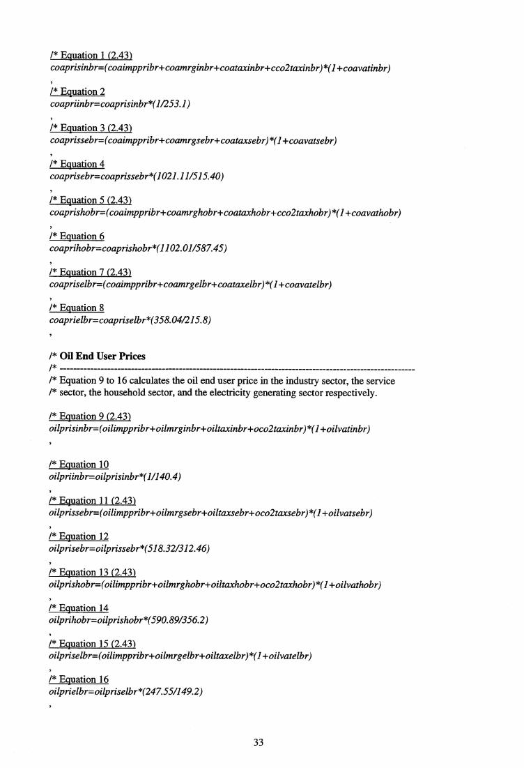
1* Equation 1 (2.43) coaprisinbr=(coaimppribr+coamrginbr+coataxinbr+cco2taxinbr)*(1+coavatinbr)
1* Equation 2 coapriinbr=coaprisinbr*(1/253.1)
1* Equation 3 (2.43) coaprissebr=(coaimppribr+coamrgsebr+coataxsebr)*(1+coavatsebr)
1* Equation 4coaprisebr=coaprissebr*(1021.11/515.40)
1* Equation 5 (2.43) coaprishobr=(coaimppribr+coamrghobr+coataxhobr+cco2taxhobr)*(1+coavathobr)
1* Equation 6coaprihobr=coaprishobr*(1102.01/587.45)
/* Equation 7 (2.43) coapriselbr=(coaimppribr+coamrgelbr+coataxelbr)*(1+coavatelbr)
/* Equation 8 coaprielbr=coapriselbr*(358.04/215.8)
1* Oil End User Prices1* /* Equation 9 to 16 calculates the oil end user price in the industry sector, the service1* sector, the household sector, and the electricity generating sector respectively.
1* Equation 9 (2.43) oilprisinbr=(oilimppribr+oilmrginbr+oiltaxinbr+oco2taxinbr)*(1+oilvatinbr)
/* Equation 10 oilpriinbr=oilprisinbr*(1/140.4)
1* Equation 11 (2.43) oilprissebr=(oilimppribr+oilmrgsebr+oiltaxsebr+oco2taxsebr)*(1+oilvatsebr)
1* Equation 12oilprisebr=oilprissebr*(518.32/312.46)
1* Equation 13 (2.43) oilprishobr=(oilimppribr+oilmrghobr+oiltaxhobr+oco2taxhobr)*(1+oilvathobr)
1* Equation 14oilprihobr=oilprishobr*(590.89/356.2)
/* Equation 15 (2.43) oilpriselbr=(oilimppribr+oilmrgelbr+oiltaxelbr)*(1 +oilvatelbr)
1* Equation 16 oilprielbr=oilpriselbr*(247.55/149.2)
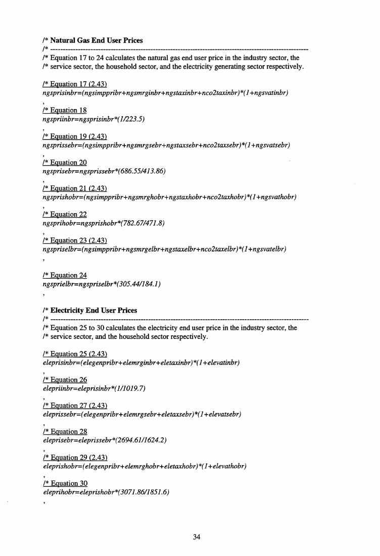
1* Natural Gas End User Prices1* 1* Equation 17 to 24 calculates the natural gas end user price in the industry sector, the1* service sector, the household sector, and the electricity generating sector respectively.
1* Equation 17 (2.43) ngsprisinbr=(ngsimppribr+ngsmrginbr+ngstaxinbr+nco2taxinbr)*( l+ngsvatinbr)
1* Equation 18 ngspriinbr=ngsprisinbr*( 1/223.5)
1* Equation 19 (2.43) ngsprissebr=(ngsimppribr+ngsmrgsebr+ngstaxsebr+nco2taxsebr)*( 1 +ngsvatsebr)
/* Equation 20ngsprisebr=ngsprissebr*(686.55/4 13 .86)
1* Equation 21 (2.43) ngsprishobr=(ngsimppribr+ngsmrghobr+ngstaxhobr+nco2taxhobr)*( 1 +ngsvathobr)
1* Equation 22ngsprihobr=ngsprishobr*(782.67/471.8)
/* Equation 23 (2.43) ngspriselbr=(ngsimppribr+ngsmrgelbr+ngstaxelbr+nco2taxelbr)*( I +ngsvatelbr)
1* Equation 24 ngsprielbr=ngspriselbr*( 305 .44/184.1)
1* Electricity End User Prices1* /* Equation 25 to 30 calculates the electricity end user price in the industry sector, the1* service sector, and the household sector respectively.
1* Equation 25 (2.43) eleprisinbr=(elegenpribr+elemrginbr+eletaxinbr)*( 1 + elevatinbr)
1* Equation 26elepriinbr=eleprisinbr*( 1/1019.7)
1* Equation 27 (2.43) eleprissebr=(elegenpribr+elemrgsebr+eletaxsebr)*( 1 + elevatsebr)
1* Equation 28eleprisebr=eleprissebr*(2694.61/1624.2)
1* Equation 29 (2.43) eleprishobr=(elegenpribr+elemrghobr+eletaxhobr)*( 1 + elevathobr)
1* Equation 30eleprihobr=eleprishobr*( 3071.86/185 1.6)

/* End User Fuel Prices in the Transport Sector/* 1* Equation 31 to 39 calculates the end user price for gasoline (car), diesel (car), diesel1* (rail), diesel (bus), gas (car), electricity (rail), and oil (air) respectively.
1* Equation 31 (2.43) gopristpbr=( goimppribr+ gomrgtpbr+ gotaxtpbr+ goco2taxtpbr)*( 1 + govattpbr)
1* Equation 32gopritpbr=gopristpbr*( 1783.5/1074.4)
/* Equation 33 (2.43) dipristpbr=(diimppribr+dimrgtpbr+ditaxtpbr+dico2tampbr)*( 1 +divattpbr)
1* Equation 34dipritpbr=dipristpbr*( 1261/759.6)
1* Equation 35 rdpritpbr=dipritpbri( 1 +divattpbr)
1* Equation 36 bdpritpbr=dipritpbr/( I +divattpbr)
1* Equation 37 gapritpbr=dipritpbr*( 1070/1261)
1* Equation 38 ,
repritpbr= eleprissebr
1* Equation 39 oilpritabr=oilprishobr*( 1/3 56.2)
/* End of the price model.

4. Extrapolation and Simulation
This chapter is concerned with the procedure for extrapolating and simulating the implementedSEEM-model in Troll. The chapter is organised as follows: Part one presents and describes macrosneccessary for extrapolating input variables. Part two presents and describes input files neccessary forsimulating the SEEM-model. Part three gives an overview of files and their linkages when extra-polating and simulating the SEEM-model. Finally, the fourth part of this chapter explains theprocedure of making a scenario specific simulation of the SEEM-model.
The following scenarios with related Troll files are considered in this chapter: The reference scenario,the integration scenario (is) which is the same scenario as the reference scenario, and the fragmen-tation scenario (fs). For further information on these scenarios and their underlying assumptions,consult Aaserud et. al. (1995).
It is worthwhile to notice in the Troll macros and input files presented below that the Troll syntax for acomment begins with «/*». Note also that the Troll commands in each macro and input file areemphasised with italic letters.
4.1 Troll Macros for Extrapolation4.1.1 The Reference and IS Scenario1* The Troll Macro File scenisbr.src1* This macro file, called scenisbr.src, consists of Troll commands which extrapolate1* input variables according to the reference and the is scenario assumptions for1* Germany. In what follows, a description of how to use this macro is given. Note1* that scenario assumptions on the growth rates for input variables have to be inserted1* manually. The file is divided into two parts. Part A consists of dummy variable1* extrapolations and part B consists of growth rates assumptions on input variables1* according to the reference and is scenario.
addfun main;procedure main()begin;
1* Part A: Dummy Variable Extrapolations1* 1* Dummy variables in the electricity generating sector
> >dofile dumnbr= 1 + dumnbr*0 ;> >dofile dumbbr=dumbbr*O;
1* Dummy variables in the transport sector
>>dofile dumntpbr=l+dumntpbr*O;>>dofile dumbtpbr=dumbtpbr*O;
1* Dummy variables in the freight transport
>>dofile dumiOr=dumiOr*O;>>dofile dumftfbr=l+dumfifbr*O;
1* Part B: Growth Rates Assumptions1* /* The following consists of sequences like
36
1* &framskr;1* >>variabel name start year growth factor start year (for next growth period)1* growth factor ... *.
1* The model user might change the variable names, years, and growth factors. Note that1* the growth rate sequence must end with «*».
1* Example:1* >>conhobr 1991A 1.020 2000A 1.030 2010A 1.000 * means that the variable1* conhobr grows by 2.0 per cent annually from 1991 to 2000, then by 3.0 per cent1* annually from 2000 to 2010 and finally by 0 per cent the rest of the simulation period.
1* Part Bl: Growth Rates Assumptions on some Exogenous Fuel Use Variables/* 1* The term «x» in the variable names below is used because these variables represent1* <<he1p variables in the sector models for some countries. These variables are however1* endogenous in the SEEM-model, and the extrapolations will thus be overwritten by1* the model simulations.
&framskr;>>coaconxsebr 1991A 1.000 2000A 1.000 2010A 1.000 *
&framskr;>>coaconxhobr 1991A 1.000 2000A 1.000 2010A 1.000 *
&framskr;>>oikonxsebr 1991A 1.000 2000A 1.000 2010A 1.000 *
&framskr;>>oilconxhobr 1991A 1.000 2000A 1.000 2010A 1.000 *
&framskr;> >ngsconxinbr 1991A 1.000 2000A 1.000 2010A 1.000 *
&framskr;>>ngsconxsebr 1991A 1.000 2000A 1.000 2010A 1.000 *
&framskr;>>ngsconxhobr 1991A 1.000 2000A 1.000 2010A 1.000 *
1* Part B2: Growth Rates Assumptions for other Variables1* 1* The following equations expand the scenario-dependent variables for the household I* sector.
&framskr;>>conhobr 1991A 1.022 2000A 1.025 2010A 1.025 *
&framskr;>>a0elehobr 1991A 0.996 2000A 0.996 2010A 0.996 *
&framskr;>>a0coghobr 1991A 0.996 2000A 0.996 2010A 0.996 *
/*&framskr;1* >>ngsimppribr 1991A 0.979 2000A 0.998 2010A 1.024 *&framskr;>>ngsmrghobr 1991A 1.000 2000A 1.000 2010A 1.000 *
&framskr;>>ngstaxhobr 1991A 1.000 2000A 1.000 2010A 1.000 *
&framskr;>>nco2taxhobr 1991A 1.000 2000A 1.000 2010A 1.000 *
&framskr;> >ngsvathobr 1991A 1.000 2000A 1.000 2010A 1.000 *
&framskr;
37
>>elemrghobr 1991A 1.000 2000A 1.000 2010A 1.000 *&framskr;>>eletaxhobr 1991A 1.000 2000A 1.000 2010A 1.000 *
&framskr;>>eco2taxhobr 1991A 1.000 2000A 1.000 2010A 1.000 *
&framskr;>>elevathobr 1991A 1.000 2000A 1.000 2010A 1.000 *
&framskr;>>coamrghobr 1991A 1.000 2000A 1.000 2010A 1.000 *
&framskr;>>coataxhobr 1991A 1.000 2000A 1.000 2010A 1.000 *
&framskr;>>cco2taxhobr 1991A 1.000 2000A 1.000 2010A 1.000 *
&framskr;>>coavathobr 1991A 1.000 2000A 1.000 2010A 1.000 *
&framskr;>>oilmrghobr 1991A 1.000 2000A 1.000 2010A 1.000 *
&framskr;>>oiltaxhobr 1991A 1.000 2000A 1.000 2010A 1.000 *
&framskr;>>oco2taxhobr 1991A 1.000 2000A 1.000 2010A 1.000 *
&framskr;>>oilvathobr 1991A 1.000 2000A 1.000 2010A 1.000 *
/* The following equations expand the scenario-dependent variables for the service/* sector.
&framskr;>>prosebr 1991A 1.023 2000A 1.026 2010A 1.023 *
&framskr;>>a0elesebr 1991A 0.9974 2000A 0.9974 2010A 0.9974 *
&framskr;>>a0cogsebr 1991A 0.9976 2000A 0.9976 2010A 0.9976 *
&framskr;>>capprisebr 1991A 1.002 2000A 1.002 2010A 1.002 *
&framskr;>>labprisebr 1991A 1.016 2000A 1.016 2010A 1.016 *
&framskr;>>ngsmrgsebr 1991A 1.000 2000A 1.000 2010A 1.000 *
&framskr;>>ngstaxsebr 1991A 1.000 2000A 1.000 2010A 1.000 *
&framskr;>>nco2taxsebr 1991A 1.000 2000A 1.000 2010A 1.000 *
&framskr;>>ngsvatsebr 1991A 1.000 2000A 1.000 2010A 1.000 *
&framskr;>>elemrgsebr 1991A 1.000 2000A 1.000 2010A 1.000 *
&framskr;>>eletaxsebr 1991A 1.000 2000A 1.000 2010A 1.000 *
&framskr;>>eco2taxsebr 1991A 1.000 2000A 1.000 2010A 1.000 *
&framskr;>>elevatsebr 1991A 1.000 2000A 1.000 2010A 1.000 *
&framskr;
38

>>oilmrgsebr 1991A 1.000 2000A 1.000 2010A 1.000 *&framskr;>>oiltaxsebr 1991A 1.000 2000A 1.000 2010A 1.000 *
&framskr;>>oco2taxsebr 1991A 1.000 2000A 1.000 2010A 1.000 *
&framskr;>>oilvatsebr 1991A 1.000 2000A 1.000 2010A 1.000 *
&framskr;>>coamrgsebr 1991A 1.000 2000A 1.000 2010A 1.000 *
&framskr;>>coataxsebr 1991A 1.000 2000A 1.000 2010A 1.000 *
&framskr;>>cco2taxsebr 1991A 1.000 2000A 1.000 2010A 1.000
&framskr;>>coavatsebr 1991A 1.000 2000A 1.000 2010A 1.000 *
1* The following equations expand the scenario-dependent variables for the industry1* sector.
&framskr;>>proinbr 1991A 1.022 2000A 1.025 2010A 1.022 *
&framskr;>>a0eleinbr 1991A 0.9988 2000A 0.9988 2010A 0.9988 *
&framskr;>>a0coainbr 1991A 0.9988 2000A 0.9988 2010A 0.9988 *
&framskr;>>a0oilinbr 1991A 0.9988 2000A 0.9988 2010A 0.9988 *
&framskr;>>aOngsinbr 1991A 0.9988 2000A 0.9988 2010A 0.9988 *
&framskr;>>cappriinbr 1991A 1.002 2000A 1.002 2010A 1.002 *
&framskr;>>labpriinbr 1991A 1.016 2000A 1.016 2010A 1.016 *
&framskr;>>ngsmrginbr 1991A 1.000 2000A 1.000 2010A 1.000 *
&framskr;>>ngstaxinbr 1991A 1.000 2000A 1.000 2010A 1.000 *
&framskr;> >nco2taxinbr 1991A 1.000 2000A 1.000 2010A 1.000 *
&framskr;>>ngsvatinbr 1991A 1.000 2000A 1.000 2010A 1.000 *
&framskr;>>elemrginbr 1991A 1.000 2000A 1.000 2010A 1.000 *
&framskr;> >eletaxinbr 1991A 1.000 2000A 1.000 2010A 1.000 *
&framskr;>>eco2taacinbr 1991A 1.000 2000A 1.000 2010A 1.000 *
&framskr;>>elevatinbr 1991A 1.000 2000A 1.000 2010A 1.000 *
1*&framskr,1* >>oilimppribr 1991A 0.983 2000A 0.975 2010A 1.000&framskr;>>oilmrginbr 1991A 1.000 2000A 1.000 2010A 1.000 *
&framskr;
39

> >oiltaxinbr 1991A 1.000 2000A 1.000 2010A 1.000 *&framskr;>>oco2taxinbr 1991A 1.000 2000A 1.000 2010A 1.000 *
&framskr;>>oilvatinbr 1991A 1.000 2000A 1.000 2010A 1.000 *
&framskr;>>coaimppribr 1991A 1.000 2000A 1.000 2010A 1.000 *
&framskr;>>coamrginbr 1991A 1.000 2000A 1.000 2010A 1.000 *
&framskr;>>coataxinbr 1991A 1.000 2000A 1.000 2010A 1.000 *
&framskr;>>cco2taxinbr 1991A 1.000 2000A 1.000 2010A 1.000 *
&framskr;> >coavatinbr 1991A 1.000 2000A 1.000 2010A 1.000 *
/* The following equations expand the scenario-dependent variables for the transport/* sector.
&framskr;>>incomebr 1991A 1.022 2000A 1.025 2010A 1.025 *
&framskr;>>gdpindbr 1991A 1.022 2000A 1.025 2010A 1.022 *
&framskr;>>goimppribr 1991A 0.966 2000A 1.002 2010A 1.001 *
&framskr;>>gomrgtpbr 1991A 1.000 2000A 1.000 2010A 1.000 *
&framskr;>>gotaxtpbr 1991A 1.000 2000A 1.000 2010A 1.000 *
&framskr;>>goco2taxtpbr 1991A 1.000 2000A 1.000 2010A 1.000 *
&framskr;>>govattpbr 1991A 1.000 2000A 1.000 2010A 1.000 *
&framskr;>>diimppribr 1991A 0.966 2000A 1.002 2010A 1.001 *
&framskr;>>dimrgtpbr 1991A 1.000 2000A 1.000 2010A 1.000 *
&framskr;>>ditaxtpbr 1991A 1.000 2000A 1.000 2010A 1.000 *
&framskr;>>dico2taxtpbr 1991A 1.000 2000A 1.000 2010A 1.000 *
&framskr;>>divattpbr 1991A 1.000 2000A 1.000 2010A 1.000 *
&framskr;>>dumntpbr 1991A 1.000 2000A 1.000 2010A 1.000 *
&framskr;>>dumbtpbr 1991A 1.000 2000A 1.000 2010A 1.000 *
&framskr;>>a3d4br 1991A 1.000 2000A 1.000 2010A 1.000 *
&framskr;>>a3elebr 1991A 1.000 2000A 1.000 2010A 1.000 *
&framskr;>>a3oilObr 1991A 1.000 2000A 1.000 2010A 1.000 *
&framskr;
40
>>a3oWabr 1991A 1.000 2000A 1.000 2010A 1.000 *
1* Constant: ?/* &framskr;1* >>bltkmbr 1991A 1.000 2000A 1.000 2010A 1.000 *
1* Endogenous: ?&framskr;>>shar4br 1991A 1.000 2000A 1.003 2010A 1.003 *
&framskr;>>sharaOr 1991A 1.050 2000A 1.018 2010A 0.980 *
&framskr;>>shawaOr 1991A 0.990 2000A 0.985 2010A 1.000 *
&framskr;>>roeffifbr 1991A 1.005 2000A 1.005 2010A 1.005 *
&framskr;>>raefftfbr 1991A 1.010 2000A 1.010 2010A 1.010 *
&framskr;>>waefftibr 1991A 1.010 2000A 1.010 2010A 1.010 *
1* The following equations expand the scenario-dependent variables for the electricity1* generating sector.
&framskr;>>ngsmrgelbr 1991A 1.000 2000A 1.000 2010A 1.000 *
&framskr;> >ngstaxelbr 1991A 1.000 2000A 1.000 2010A 1.000 *
&framskr;>>nco2taxelbr 1991A 1.000 2000A 1.000 2010A 1.000 *
&framskr;>>ngsvatelbr 1991A 1.000 2000A 1.000 2010A 1.000 *
&framskr;>>oilmrgelbr 1991A 1.000 2000A 1.000 2010A 1.000 *
&framskr;>>oiltaxelbr 1991A 1.000 2000A 1.000 2010A 1.000 *
&framskr;>>oco2taxelbr 1991A 1.000 2000A 1.000 2010A 1.000 *
&framskr;>>oilvatelbr 1991A 1.000 2000A 1.000 2010A 1.000 *
&framskr;>>coamrgelbr 1991A 1.000 2000A 1.000 2010A 1.000 *
&framskr;>>coataxelbr 1991A 1.000 2000A 1.000 2010A 1.000 *
&framskr;>>cco2taxelbr 1991A 1.000 2000A 1.000 2010A 1.000 *
&framskr;>>coavatelbr 199IA 1.000 2000A 1.000 2010A 1.000 *
/* &framskr;1* >>nucprielbr 1991A 1.000 2000A 1.000 2010A 1.000 *&framskr;>>renprielbr 1991A 1.000 2000A 1.000 2010A 1.000 *
1* &framskr;1* >>dumnbr 1991A 1.000 2000A 1.000 2010A 1.000 *
41

1* &framskr;1* >>dumbbr 1991A 1.000 2000A 1.000 2010A 1.000 *
&framskr;>>coashalnelbr 1991A 1.000 2000A 1.000 2010A 1.000 *
&framskr;>>coashalfelbr 1991A 1.000 2000A 1.000 2010A 1.000 *
&framskr;>>coashalbelbr 1991A 1.000 2000A 1.000 2010A 1.000 *
&framskr;>>ngsshalnelbr 1991A 1.000 2000A 1.000 2010A 1.000 *
&framskr;>>ngsshalbelbr 1991A 1.000 2000A 1.000 2010A 1.000 *
&framskr;>>oilshalnelbr 1991A 1.000 2000A 1.000 2010A 1.000 *
&framskr;>>oilshalbelbr 1991A 1.000 2000A 1.000 2010A 1.000 *
&framskr;>>nucshalnelbr 1991A 1.000 2000A 1.000 2010A 1.000 *
&framskr;>>nucshalbelbr 1991A 1.000 2000A 1.000 2010A 1.000 *
&framskr;>>renshalnelbr 1991A 1.000 2000A 1.000 2010A 1.000 *
&framskr;>>renshalbelbr 1991A 1.000 2000A 1.000 2010A 1.000 *
&framskr;>>ngsimppribr 1991A 0.939 1995A 0.991 2000A 0.963 2005A 1.035 2010A 1.021 2015A 1.027 *
&framskr;>>oilimppribr 1991A 0.973 1995A 1.021 2000A 0.966 2005A 0.985 2010A 1.000 2015A 1.000 *
end;
4.1.2 The FS Scenario/* The Troll Macro File scenfsbr.src1* This macro file, called scenfsbr.src, consists of Troll commands which extrapolate1* input variables according to the fs scenario assumptions for Germany. In what1* follows, a description of how to use this macro is given. Note that scenario1* assumptions on the growth rates for input variables have to be inserted manually. The1* file is divided into two parts. Part A consists of dummy variable extrapolations and1* part B consists of growth rates assumptions on input variables according to the fs1* scenario.
addfun main;procedure main()begin;
/* Part A: Dummy Variable Extrapolations/* 1* Dummy variables in the electricity generating sector
>>dofile dumnbr=l+dumnbr*O;>>dofile dumbbr=dumbbr*O;
42

1* Dummy variables in the transport sector
>>dofile dumntpbr=l+dumntpbr*O;>>dofile dumbtpbr=dumbtpbr*O;
1* Dummy variables in the freight transport
>>dofile dum4br=dumi4br*O;>>dofile dumftfbr=l+dumftfbr*0;
1* Part B: Growth Rates Assumptions1* 1* The following consists of sequences like/* &framskr;1* >>variabel name start year growth factor start year (for next growth period)1* growth factor... *.
1* The model user might change the variable names, years, and growth factors. Note that1* the growth rate sequence must end with «*».
1* Example:1* >>conhobr 1991A 1.020 2000A 1.030 2010A 1.000 * means that the variable1* conhobr grows by 2.0 per cent annually from 1991 to 2000, then by 3.0 per cent1* annually from 2000 to 2010 and finally by 0 per cent the rest of the simulation period.
1* Part Bi: Growth Rates Assumptions on some Exogenous Fuel Use Variables1* /* The term «x» in the variable names below is used because these variables represent1* <<he1p» variables in the sector models for some countries. These variables are however/* endogenous in the SEEM-model, and the extrapolations will thus be overwritten by/* the model simulations.
&framskr;>>coaconxsebr 1991A 1.000 2000A 1.000 2010A 1.000 *
&framskr;>>coaconxhobr 1991A 1.000 2000A 1.000 2010A 1.000 *
&framskr;>>oilconxsebr 1991A 1.000 2000A 1.000 2010A 1.000 *
&framskr;> >oilconxhobr 1991A 1.000 2000A 1.000 2010A 1.000 *
&framskr;>>ngsconxinbr 1991A 1.000 2000A 1.000 2010A 1.000 *
&framskr;>>ngsconxsebr 1991A 1.000 2000A 1.000 2010A 1.000 *
&framskr;>>ngsconxhobr 1991A 1.000 2000A 1.000 2010A 1.000 *
1* Part B2: Growth Rates Assumptions for other Variables1* 1* The following equations expand the scenario-dependent variables for the household /* sector.
&framskr;>>conhobr 1991A 1.020 2000A 1.020 2010A 1.020 *
43

&framskr;>>a0elehobr 1991A 0.998 2000A 0.998 2010A 0.998 *
&framskr;>>a0coghobr 1991A 0.998 2000A 0.998 2010A 0.998 *
/* &framskr;1* >>ngsimppribr 1991A 0.985 2000A 1.038 2010A 1.006 *&framskr;>>ngsmrghobr 1991A 1.000 2000A 1.000 2010A 1.000 *
&framskr;>>ngstaxhobr 1991A 1.000 2000A 1.000 2010A 1.000 *
&framskr;>>nco2taxhobr 1991A 1.000 2000A 1.000 2010A 1.000 *
&framskr;>>ngsvathobr 1991A 1.000 2000A 1.000 2010A 1.000 *
&framskr;>>elemrghobr 1991A 1.000 2000A 1.000 2010A 1.000 *
&framskr;>>eletaxhobr 1991A 1.000 2000A 1.000 2010A 1.000 *
&framskr;>>eco2taxhobr 1991A 1.000 2000A 1.000 2010A 1.000 *
&framskr;>>elevathobr 1991A 1.000 2000A 1.000 2010A 1.000 *
&framskr;>>coamrghobr 1991A 1.000 2000A 1.000 2010A 1.000 *
&framskr;>>coataxhobr 1991A 1.000 2000A 1.000 2010A 1.000 *
&framskr;>>cco2taxhobr 1991A 1.000 2000A 1.000 2010A 1.000 *
&framskr;>>coavathobr 1991A 1.000 2000A 1.000 2010A 1.000 *
&framskr;>>oilmrghobr 1991A 1.000 2000A 1.000 2010A 1.000 *
&framskr;>>oiltaxhobr 1991A 1.000 2000A 1.000 2010A 1.000 *
&framskr;>>oco2taxhobr 1991A 1.000 2000A 1.000 2010A 1.000 *
&framskr;>>oilvathobr 1991A 1.000 2000A 1.000 2010A 1.000 *
1* The following equations expand the scenario-dependent variables for the service1* sector.
&framskr;>>prosebr 1991A 1.022 2000A 1.022 2010A 1.022 *
&fratnskr;>>a0elesebr 1991A 0.9987 2000A 0.9987 2010A 0.9987
&framskr;>>a0cogsebr 1991A 0.9988 2000A 0.9988 2010A 0.9988 *
&framskr;>>capprisebr 1991A 1.002 2000A 1.002 2010A 1.002 *
&framskr;>>labprisebr 1991A 1.016 2000A 1.016 2010A 1.016 *
&framskr;>>ngsmrgsebr 1991A 1.000 2000A 1.000 2010A 1.000 *
&framskr;

> >ngstaxsebr 1991A 1.000 2000A 1.000 2010A 1.000 *&framskr;>>nco2taxsebr 1991A 1.000 2000A 1.000 2010A 1.000 *
&framskr;>>ngsvatsebr 1991A 1.000 2000A 1.000 2010A 1.000 *
&framskr;>>elemrgsebr 1991A 1.000 2000A 1.000 2010A 1.000 *
&framskr;>>eletaxsebr 1991A 1.000 2000A 1.000 2010A 1.000 *
&framskr;>>eco2taxsebr 1991A 1.000 2000A 1.000 2010A 1.000 *
&framskr;> >elevatsebr 1991A 1.000 2000A 1.000 2010A 1.000 *
&framskr;>>oilmrgsebr 1991A 1.000 2000A 1.000 2010A 1.000 *
&framskr;>>oiltaxsebr 1991A 1.000 2000A 1.000 2010A 1.000 *
&framskr;>>oco2taxsebr 1991A 1.000 2000A 1.000 2010A 1.000 *
&framskr;>>oilvatsebr 1991A 1.000 2000A 1.000 2010A 1.000 *
&framskr;>>coamrgsebr 1991A 1.000 2000A 1.000 2010A 1.000 *
&framskr;>>coataxsebr 1991A 1.000 2000A 1.000 2010A 1.000 *
&framskr;>>cco2taxsebr 1991A 1.000 2000A 1.000 2010A 1.000 *
&framskr;> >coavatsebr 1991A 1.000 2000A 1.000 2010A 1.000 *
/* The following equations expands the scenario-dependent variables for the industry/* sector.
&framskr;>>proinbr 1991A 1.021 2000A 1.021 2010A 1.021 *
&framskr;>>a0eleinbr 1991A 0.9994 2000A 0.9994 2010A 0.9994 *
&framskr;>>a0coainbr 1991A 0.9994 2000A 0.9994 2010A 0.9994 *
&framskr;>>a0oilinbr 1991A 0.9994 2000A 0.9994 2010A 0.9994 *
&framskr;>>aOngsinbr 1991A 0.9994 2000A 0.9994 2010A 0.9994 *
&framskr;>>cappriinbr 1991A 1.002 2000A 1.002 2010A 1.002 *
&framskr;>>labpriinbr 1991A 1.016 2000A 1.016 2010A 1.016 *
&framskr;>>ngsmrginbr 1991A 1.000 2000A 1.000 2010A 1.000 *
&framskr;> >ngstaxinbr 1991A 1.000 2000A 1.000 2010A 1.000 *
&framskr;> >nco2taxinbr 1991A 1.000 2000A 1.000 2010A 1.000 *
&framskr;
45

>>ngsvatinbr 1991A 1.000 2000A 1.000 2010A 1.000 *&framskr;>>elemrginbr 1991A 1.000 2000A 1.000 2010A 1.000 *
&framskr;>>eletaxinbr 1991A 1.000 2000A 1.000 2010A 1.000 *
&framskr;>>eco2taxinbr 1991A 1.000 2000A 1.000 2010A 1.000 *
&framskr;>>elevatinbr 1991A 1.000 2000A 1.000 2010A 1.000 *
/*&framskr;/* >>oilimppribr 1991A 0.989 2000A 1.027 2010A 1.000&framskr;>>oilmrginbr 1991A 1.000 2000A 1.000 2010A 1.000 *
&framskr;> >oiltaxinbr 1991A 1.000 2000A 1.000 2010A 1.000 *
&framskr;> >oco2taxinbr 1991A 1.000 2000A 1.000 2010A 1.000 *
&framskr;> >oilvatinbr 1991A 1.000 2000A 1.000 2010A 1.000 *
&framskr;>>coaimppribr 1991A 1.000 2000A 1.000 2010A 1.000 *
&framskr;>>coamrginbr 1991A 1.000 2000A 1.000 2010A 1.000 *
&framskr;>>coataxinbr 1991A 1.000 2000A 1.000 2010A 1.000 *
&framskr;>>cco2taxinbr 1991A 1.000 2000A 1.000 2010A 1.000 *
&framskr;>>coavatinbr 1991A 1.000 2000A 1.000 2010A 1.000 *
1* The following equations expand the scenario-dependent variables for the transport1* sector.
&framskr;>>incomebr 1991A 1.020 2000A 1.020 2010A 1.020 *
&framskr;>>gdpindbr 1991A 1.021 2000A 1.021 2010A 1.021 *
&framskr;> >goimppribr 1991A 0.982 2000A 1.045 2010A 1.021 *
&framskr;>>gomrgtpbr 1991A 1.000 2000A 1.000 2010A 1.000 *
&framskr;>>gotaxtpbr 1991A 1.000 2000A 1.000 2010A 1.000 *
&framskr;>>goco2taxtpbr 1991A 1.000 2000A 1.000 2010A 1.000 *
&framskr;>>govattpbr 1991A 1.000 2000A 1.000 2010A 1.000 *
&framskr;>>diimppribr 1991A 0.979 2000A 1.044 2010A 1.021 *
&framskr;>>dimrgtpbr 1991A 1.000 2000A 1.000 2010A 1.000 *
&framskr;> >ditaxtpbr 1991A 1.000 2000A 1.000 2010A 1.000 *
&framskr;>>dico2taxtpbr 1991A 1.000 2000A 1.000 2010A 1.000 *
46

&framskr;>>divattpbr 1991A 1.000 2000A 1.000 2010A 1.000
&framskr;>>dumntpbr 1991A 1.000 2000A 1.000 2010A 1.000 *
&framskr;>>dumbtpbr 1991A 1.000 2000A 1.000 2010A 1.000 *
&framskr;>>a3d4tbr 1991A 1.000 2000A 1.000 2010A 1.000 *
&framskr;>>a3elebr 1991A 1.000 2000A 1.000 2010A 1.000 *
&framskr;>>a3oi10-br 1991A 1.000 2000A 1.000 2010A 1.000 *
&framskr;>>a3oWabr 1991A 1.000 2000A 1.000 2010A 1.000 *
1* Constant: ?1* &framskr;1* >>b ltkmbr 1991A 1.000 2000A 1.000 2010A 1.000 *
/* Endogenous: ?&framskr;>>sharo4lor 1991A 1.001 2000A 1.005 2010A 1.005 *
&framskr;>>shara4br 1991A 1.029 2000A 0.972 2010A 1.000 *
&fra►skr;>>shawaqbr 1991A 1.009 2000A 0.985 2010A 0.977 *
&framskr;>>roefftfbr 1991A 1.000 2000A 1.000 2010A 1.000 *
&framskr;>>raefftfbr 1991A 1.000 2000A 1.000 2010A 1.000 *
&framskr;>>waefftfbr 1991A 1.000 2000A 1.000 2010A 1.000 *
1* The following equations expands the scenario-dependent variables for the electricity/* generating sector.
&framskr;>>ngsmrgelbr 1991A 1.000 2000A 1.000 2010A 1.000 *
&framskr;>>ngstaxelbr 1991A 1.000 2000A 1.000 2010A 1.000 *
&framskr;>>nco2taxelbr 1991A 1.000 2000A 1.000 2010A 1.000 *
&framskr;>>ngsvatelbr 1991A 1.000 2000A 1.000 2010A 1.000 *
&framskr;>>oilmrgelbr 1991A 1.000 2000A 1.000 2010A 1.000 *
&framskr;>>oiltaxelbr 1991A 1.000 2000A 1.000 2010A 1.000 *
&framskr;>>oco2taxelbr 1991A 1.000 2000A 1.000 2010A 1.000 *
&framskr;>>oilvatelbr 1991A 1.000 2000A 1.000 2010A 1.000 *
&framskr;>>coamrgelbr 1991A 1.000 2000A 1.000 2010A 1.000 *
&framskr;
47

>>coataxelbr 1991A 1.000 2000A 1.000 2010A 1.000 *&framskr;>>cco2taxelbr 1991A 1.000 2000A 1.000 2010A 1.000
&framskr;>>coavatelbr 1991A 1.000 2000A 1.000 2010A 1.000 *
&framskr;> >nucprielbr 1991A 1.000 2000A 1.000 2010A 1.000 *
&framskr;>>renprielbr 1991A 1.000 2000A 1.000 2010A 1.000 *
1* &framskr;1* >>dumnbr 1991A 1.000 2000A 1.000 2010A 1.000 *1* &framskr;1* >>dumbbr 1991A 1.000 2000A 1.000 2010A 1.000 *
&framskr;>>coashalnelbr 1991A 1.000 2000A 1.000 2010A 1.000 *
&framskr;>>coashalfelbr 1991A 1.000 2000A 1.000 2010A 1.000 *
&framskr;>>coashalbelbr 1991A 1.000 2000A 1.000 2010A 1.000 *
&framskr;>>ngsshalnelbr 1991A 1.000 2000A 1.000 2010A 1.000 *
&framskr;>>ngsshalbelbr 1991A 1.000 2000A 1.000 2010A 1.000 *
&framskr;>>oilshalnelbr 1991A 1.000 2000A 1.000 2010A 1.000 *
&framskr;>>oilshalbelbr 1991A 1.000 2000A 1.000 2010A 1.000 *
&framskr;>>nucshalnelbr 1991A 1.000 2000A 1.000 2010A 1.000 *
&framskr;>>nucshalbelbr 1991A 1.000 2000A 1.000 2010A 1.000 *
&framskr;>>renshalnelbr 1991A 1.000 2000A 1.000 2010A 1.000 *
&framskr;>>renshalbelbr 1991A 1.000 2000A 1.000 2010A 1.000 *
&framskr;>>ngsimppribr 1991A 0.913 1995A 1.026 2000A 1.053 2005A 1.023 2010A 1.012 2015A 1.000 *
&framskr;>>oilimppribr 1991A 0.946 1995A 1.057 2000A 1.039 2005A 1.015 2010A 1.000 2015A 1.000 *
end;
4.1.3 A Translation Macro/* The Troll Macro File framskr.src1* The macro, called framskr.src, translates the commands in the scenisbr.src and the1* scenfsbr.src files presented and described above into Troll syntax. Hence, the macro1* works together with the two mentioned Troll macros for extrapolating input variables1* according to the integration (and reference) and fragmentation scenario respectively.1* The framskr.src macro is written in the Troll programming language by Rune1* Johansen, The Research Department, Statistics Norway, email: [email protected]. Latest
48
1* updated 28. November 1994. In what follows, a description on how this macro works1* and how to use it is given.
1* How to use this macro:1* 1* A call to this macro is done in the following way:
1* &framskr;1* >>series yearl fac 1 year2 fac2 *
1* The parameter «series» is the name of the time series to be extrapolated. The1* parameters «year» and «fac» always occur pairwise. «year» specifies the starting year1* of a extrapolation and the «fac» represents the extrapolation factor or the growth rate1* of the time series. WARNING: Due to the general design of the «autocum»-function1* in Troll, it starts the extrapolation in year number «year+1», in the sense that the1* value in «year» is not changed, and the value in «year+1» is set equal to the value in1* «year» multiplied with the factor «fac». The model user may specify as many pairs/* «year-fac» as wanted, but the parameter sequence must always end with a «*».
addfun main;procedure main()addsym fac, pl, series, year, num;begin;>>do;dekore all;get series «name of time series to be extrapolated: »;
/* The variable «num» decides how far beyond the end date of the original series the/* model user wants to extrapolate. If the model user does not want to extrapolate1* beyond the end date of the original series, «num» may be set equal to zero.
num = 0;
1* The parameter «temp» is a temporary time series where subsequent extrapolated parts/* of the original series are stored. First the model user creates «temp» as an extension1* of the original series decided by the variable «num».
on warning nomsg;on error nomsg;> >docore temp = reshape(seq(&(num)+1)*0,enddate(kseries)));on warning nomsg;on error nomsg;> >docore temp = overlay(&(series), temp);get pl 'first year (or '*' if finished)
1* The macro is running in a loop until the parameter is a «*».
while(pl <> "*")begin;year = pl;get number fac"extrapolating factor";on warning nomsg;on error nomsg;

1* The extrapolation is done by the «autocum»-function
>>docore temp = autocum(temp,0,&(year),0,&(fac));on error nomsg;get pl "next year (or '*')",-
end;
1* The extrapolation is completed and the temporary series is copied to a new series1* with the same name as the original series, but belonging to a database specified by the1* search-statement
on error nomsg;>>dofile &(series) = temp;>>delcore all;
end;
4.2 Troll Input Files for Simulation4.2.1 The Reference Scenario1* The Troll Input File simbisbr.inp1* The Troll input file, called simbisbr.inp, contains a collection of Troll commands1* which extrapolates input variables according to the reference scenario assumptions,1* and establishes and simulates the SEEM-model for Germany. The file simbisbr.inp1* makes simulation results for the reference scenario on basis of the is scenario, and the1* simulation results is saved in a data output file named basisbr.txt. This data file1* includes historical and simulated data on all variables and parameters for all energy1* using sectors from 1960 to 2020, and may serve as input when simulating the SEEM-1* model for other scenarios. In what follows, some comments and explanations1* connected to each Troll command are given. The file is divided into two parts. Part A1* consists of Troll commands for implementation of scenario assumptions for input1* variables and part B consists of Troll commands for establishing, simulating and/* filing the SEEM-model.
/* Part A: Troll Commands for Implementation of Scenario Assumptions/*
1* Access and Search Lists Commands1* 1* The two Troll commands below delete all existing accesses and search lists to data1* files in Troll in order to clear old search paths no longer relevant.
delaccess all;delsearch all;
1* Access Commands1* 1* The Troll commands below provide access to all data for input variables to be1* extrapolated in the reference scenario. The access commands are as follows: «access»1* «alias name of data file» «type» «data file type» «id» «data file name» «mode»1* «mode type». «access» is a single Troll command. «alias name of data file» is an1* abbreviated name, made by the model user, of the data file which is accessed. «type»1* is a Troll command. «data file type» spesifies the type of the datafile to be accessed.1* In the case of a textfile with extension .txt, «data file type» is Troll's readable format1* formdata. «id» is a Troll command. «data file name» represents the entire name of the1* data file to be accessed. Note that the data file name has to be indicated by the whole
50

1* path on which the file exists in addition to the data file name itself if the data file1* exists on another directory than this Troll input file does (simbisbr.inp). The1* extension in the data file name is .txt. «mode» is a Troll command. Finally, «mode1* type» specifies the type of mode of the datafile to be accesed, and could be either r/* (i.e. read) or create.
1* The three commands below provide access to the input data files for each sector in1* the SEEM-model, that is for the household sector, the industry sector, and the service1* sector with alias name his, the transport sector with alias name tp, and the electricity1* generating sector with alias name el.
access his type formdata id brinn.txt mode r;access tp type formdata id tpinbr.txt mode r;access el type formdata id elinbr.txt mode r;
1* The command below provides access to the input data file consisting of data for fuel1* prices, margins and energy taxes.
access pinnbr type formdata id dAbou\ptrolAseem\eptprice.txt mode r;
1* The command below provides access to the output data for the input extrapolations to1* be created.
access scinnbr type formdata id scisbr.txt mode create;
1* Search Lists Commands/*1* The commands below provide search lists for the data which have been accessed1* above. The order of the search list is important. If a variable exists in two data files,/* but with different values, first search should be on the file with the right value of the1* variable. The search syntax for input data files is as follows: «search data» «alias/* name of data file», where «search data» is a Troll command and «alias name of data/* file» is an abbreviated name, made by the model user, for the data file to be searched./* The search syntax for output data files is as follows: «search data» «alias name of/* data file» «w» where «w» denotes write.
1* The five commands below provide a search list for all data files, both the data input1* files and the data output file, accessed above.
search data his;search data tp;search data el;search data pinnbr;search data scinnbr w;
1* Command for Extrapolation of Input Variables1* 1* The command below starts the programme called scenisbr.prg for extrapolating the1* input variables with annual growth rates according to the reference scenario1* assumptions. Note that the growth rates have to be inserted manually in the file1* scenisbr.src. This file has to be compiled in Troll in order to make the programme1* executable. For further information on this, consult the textfile simexpl.txt which1* explains the procedure of making a simulation with the SEEM-model.
&scenisbr;
51

1* Output from Extrapolation of Input Variables1* 1* The extrapolations of input variables are saved under the data file name indicated in1* the above access command line ending by create, i.e. under the data file scisbr.txt.1* This output data file consisting of scenario assumptions on input variables may then1* be used as an input data file in the simulation initiated by the commands below.
/* Part B: Troll Commands for Establishing and Simulating the SEEM-model1*
1* Access and Search Lists Commands1* /* The two commands below delete all existing accesses and search lists to data files in1* order to clear any old search paths no longer valid.
delaccess all;delsearch all;
1* Access Commands1* /* The commands below provide access to all data files required for simulation of the/* SEEM-model in the case of the reference scenario. The access commands are as1* follows: «access» «alias name of data file» «type» «data file type» «id» «data file1* name» «mode» «mode type». «access» is a single Troll command. «alias name of1* data file» is an abbreviated name, made by the model user, of the data file which is1* accessed. «type» is a Troll command. «data file type» spesifies the type of the datafile1* to be accessed. In the case of a textfile with extension .txt, «data file type is Troll's1* readable format formdata. «id» is a Troll command. «data file name» represents the1* entire name of the data file to be accessed. Note that the data file name has to be/* indicated by the whole path on which the file exists in addition to the data file name1* itself if the data file exists on another directory than this Troll input file does1* (simbisbr.inp). The extension in the data file name is .txt. «mode» is a Troll1* command. Finally, «mode type» specifies the type of mode of the datafile to be1* accesed, and could be either r (i.e. read) or create.
1* The Troll command below provides access to a reference scenario specific data file.1* In this case the scenario specific data file, called taxharmo.txt, is a file with1* harmonisation of energy taxes in the period from 2000 to 2010. Note that the data file1* has been established in advance and made executable for Troll in a Fame routine.
access taxbr type formdata id dAbou\ptrolAseem\taxharmo.txt mode r;
1* The command below provides access to the data file which contains extrapolations of1* the input variables. This data file was created under part A.
access scinnbr type formdata id scisbr.txt mode r;
1* The four commands below provide access to all other input data (also start values for1* the endogenous variables) required for simulation of the different sector models as1* well as the price model.
access his type formdata id brinn.txt mode r;access tp type formdata id tpinbr.txt mode r;access el type formdata id elinbr.txt mode r;access pinnbr type formdata id dAbou\ptrolAseem\eptprice.txt mode r;
52

1* The command below provides access to the scenario output data to be created. In this1* case the alias name of the data file is just called Alename». Hence the alias name/* will be the same name as the data file which it is provided access to (basisbr.txt).
access filename type formdata id basisbr.txt mode create;
1* Search Lists Commands/* 1* The commands below provide search lists for the data which have been accessed1* above. The order of the search list is important. If a variable exists in two data files,/* but with different values, first search should be on the file with the right value of the1* variable. The search syntax for input data files is as follows: «search data» «alias1* name of data file», where «search data» is a command and «alias name of data file»1* is an abbreviated, made by the model user, for the data file to be searched. The search1* syntax for output data files is as follows: «search data» «alias name of data file» «w»1* where «w» denotes write.
search data taxbr;search data scinnbr;search data his;search data tp;search data el;search data pinnbr;search data filename w;
1* Commands for Establishing the SEEM-model/* 1* In this Troll sequence the SEEM model for Germany is established. That is, all five1* sector models as well as the price model for Germany are added to and linked1* together in the modbr model by this sequence. The Troll syntax for establishing the1* model is as follows:
1* usemod «model name»; (without the extension .mod)1* modedit «model name»; (edits the model)1* input «input model file name», (sector and price models without extension .inp)1* filemod; (files the model)
1* Note that the sector model input files have to be specified in a certain order due to the1* link structure between the sector models and the price model for some of the1* variables. The order should be as follows: First, the fuel end user price model1* (pmodbr). Then, the electricity generating model (emodbr). Finally, the household,1* the industry, and the service models (hmodbr, imodbr, and smodbr respectively), and1* the transport model (tmodbr).
usemod modbr;modedit modbr;input pmodbr;input emodbr;input hmodbr;input imodbr;input smodbr;input tmodbr;filemod;
1* Note also that if the model already exists, the model user may do one of the following
53

1* two alternatives before simulating the SEEM-model: i) Skip the commands above by1* means of a text string represented by «/*» at the beginning of each command or ii)/* delete the existing models named modbr.mod and current.mod under the br directory,1* i.e. under d:\bou\ptroll\seem\br , for instance in MS-DOS .
1* Commands for Simulating and Filing the SEEM-model1* 1* Now, the model user may simulate and file the established SEEM-model by means of1* the Troll commands below. First, a command telling which model to use.
usemod modbr;
1* Simulation Commands/* 1* The following sequence of Troll commands simulates the SEEM-model from 1960 to1* 2020 anually for Germany in the case of the reference scenario.
simulate;simstart 1991a from 1960a;dotil 2020a;simstart;
1* If the model user does not want to include historical variable values before 1991 in/* the simulation period, the command «simstart 1991a from 1960a» may be substituted1* with the command «simstart 1991a».
1* Filing Commands1* 1* The Troll command below files the output data file containing the simulation results1* from the reference scenario.
filesim filename;
/* Here all simulated variables and parameters for all energy using sectors are specified1* to be included in the output data file. Note that the output will be saved under the data1* file name indicated after the «filesim» command. In this case «basisbr.txt» with alias1* name «filename» is the name of the output file, which was created under the access1* command above. If nothing else is commanded the output file is saved under the1* same directory as the model user is running this input file from. Thus, the1* output data file in this case will be saved on the following subdirectory:1* d:\bou\ptroll\seem\br.
1* Furthermore, if only some special variables are to be included in the output1* data file, the model user may specify the «filesim» command with the following1* syntax: «filesim» «filename» : «variable name» «variable name»; «filename»1* represents the alias name of the output data file and «variable name» represents the/* particular variable the model user wants to include in the output data file.
1* Example: 1* filesim filename : ngsconhobr oilconhobr coaconhobr eleconhobr;
1* If only endogenous variables are to be included in the output data file, the1* model user may write as follows: filesim filename : endogenous;
54

1* Command for Leaving Troll1* 1* Now, the simulation of the reference scenario for Germany is accomplished. The1* model user may want to use the output file for instance in a spreadsheet programme1* for further analysis of the output data.
1* The two commands below delete all existing accesses and search lists to data1* files in Troll in order to clear old search paths no longer relevant.
delsearch all;delaccess all;
/* This final Troll command leaves Troll.
trexit
4.2.2 The IS Scenario1* The Troll Input File simisbr.inp1* The input file, called simisbr.inp, contains a collection of Troll commands1* which extrapolate input variables according to the integration scenario assumptions,1* and establish and simulate the SEEM-model for Germany. Since the integration1* scenario is the reference scenario, simisbr.inp will make identical simulation results1* as the simbisbr.inp file. In what follows, some comments and explanations connected1* to each Troll command are given. The file is divided into two parts. Part A consists of1* Troll commands for implementation of scenario assumptions for input variables and1* part B consists of Troll commands for establishing, simulating and filing the SEEM-1* model.
1* Part A: Troll Commands for Implementation of Scenario Assumptions1*
1* Access and Search Lists Commands1* 1* The two Troll commands below delete all existing accesses and search lists to data1* files in order to clear search paths no longer relevant.
delaccess all;delsearch all;
1* Access Commands1* /* The Troll commands below provide access to all data for input variables to be1* extrapolated in the integration scenario. The access commands are as follows:/* «access» «alias name of data file «type» «data file type» «id» «data file name»1* «mode» «mode type». «access» is a single Troll command. «alias name of data file»/* is an abbreviated name, made by the model user, for the data file which is accessed.1* «type» is a Troll command. «data file type» spesifies the type of the datafile to be/* accessed. In the case of a textfile with extension .txt, «data file type» is Troll's/* readable format formdata. «id» is a Troll command. «data file name» represents the1* entire name of the data file to be accessed. Note that the data file name has to be1* indicated by the whole path on which the file exists in addition to the data file name1* itself if the data file exists on another directory than this Troll input file does/* (simisbr.inp).The extension in the data file name is .txt. «mode» is a Troll command.1* Finally, «mode type» specifies the type of mode of the datafile to be accesed, and1* could be either r (i.e. read) or create.
55
1* The command below provides access to the input data file basisbr.txt, with alias1* name innbr, which consists of energy demand and fuel prices for all energy using1* sectors in the SEEM-model. Note that this input data file has been created in the1* reference scenario which is based on the is scenario (c.f. simbisbr.inp).
access innbr type formdata id basisbr.txt mode r;
1* The Troll command below provides access to the output data for the input1* extrapolations to be created.
access scinnbr type formdata id scisbr.txt mode create;
1* Search Lists Commands1* 1* The Troll commands below provide search lists for the data which have been1* accessed above. The order of the search list is important. If a variable1* exists in two data files, but with different values, first search should be on the file1* with the right value of the variable. The search syntax for input data files is as1* follows: «search data» «alias name of data file», where «search data» is a Troll1* command and «alias name of data file» is an abbreviated name, made by the model1* user, for the data file to be searched. The search syntax for output data files is as1* follows: «search data» «alias name of data file» «w», where «w» denotes write.
1* The two Troll commands below provide search list for all data files, both the data1* input file and the data output file, which are accessed above.
search data innbr;search data scinnbr w;
1* Command for Extrapolation of Input Variables1* 1* The command below starts the programme called scenisbr.prg for extrapolating the1* input variables with annual growth rates according to the integration scenario1* assumptions. Note that the growth rates have to be inserted manually in the file1* scenisbr.src. This file has to be compiled in Troll in order to make the programme1* executable. For further information on this, consult the textfile simexpl.txt which1* explains the procedure of making a simulation with the SEEM-model.
&scenisbr;
1* Output from Extrapolation of Input Variables1* 1* The output from extrapolations of input variables is saved under the data file name1* indicated in the above access command line ending by create, i.e. under the data file/* scisbr.txt. This output data file consisting of scenario assumptions on input variables1* may then be used as an input data file in the simulation initiated by the commands1* below.
1* Part B: Troll Commands for Establishing and Simulating the SEEM-model1*
1* Access and Search Lists Commands1* 1* The two Troll commands below delete all existing accesses and search lists to data1* files in order to clear any search lists no longer valid.
56
delaccess all;delsearch all;
/* Access Commands/* 1* The Troll commands below provide access to all data files required for simulation of1* the SEEM-model in the case of the integration scenario. The access commands are as1* follows: «access» «alias name of data file» «type» «data file type «id» «data file/* name» «mode» «mode type». «access» is a single Troll command. «alias name of1* data file» is an abbreviated name, made by the model user, for the data file which is1* accessed. «type» is a Troll command. «data file type» specifies the type of the datafile1* to be accessed. In the case of a textfile with extension .txt, «data file type» is Troll's1* readable format formdata. «id» is a Troll command. «data file name» represents the/* entire name of the data file to be accessed. Note that the data file name has to be1* indicated by the whole path on which the file exists in addition to the data file name1* itself if the data file exists on another directory than this Troll input file does1* (simisbr.inp). The extension in the data file name is .txt. «mode» is a Troll command.1* Finally, «mode type» specifies the type of mode of the datafile to be accesed, and/* could be either r (i.e. read) or create.
1* The Troll command below provides access to a integration scenario specific data file.1* In this case the scenario specific data file, called taxharmo.txt, is a file with1* harmonisation of energy taxes in the period from 2000 to 2010. Note that the data file1* has been established in advance and made executable for Troll in a Fame routine.
access taxbr type formdata id clAbotAptrolAseem\taxharmatxt mode r;
/* The Troll command below provides access to the data file which contains1* extrapolations of the input variables. This data file was created under part A.
access scinnbr type formdata id scisbr.txt mode r;
/* The Troll command below provides access to all other input data (also start values for1* the endogenous variables) required for simulation of the different sector models as/* well as the price model.
access innbr type formdata id basisbr.txt mode r;
1* The Troll command below provides access to the scenario output data to be created./* In this case the alias name of the data file is just called «filename». Hence the alias1* name will be the same name as the data file which is accessed (outisbr.txt).
access filename type formdata id outisbr.txt mode create;
/* Search Lists Commands/* /* The Troll commands below provide search lists for the data which have been/* accessed above. The order of the search list is important. If a variable1* exists in two data files, but with different values, first search should be on the file/* with the right value of the variable. The search syntax for input data files is as/* follows: «search data» «alias name of data file», where «search data» is a Troll/* command and «alias name of data file» is an abbreviated, made by the model user,1* for the data file to be searched. The search syntax for output data files is as follows:/* «search datao «alias name of data file» «w», where «w» denotes write.
57
search data taxbr;search data scinnbr;search data innbr;search data filename w;
1* Commands for Establishing the SEEM-model1* 1* In this Troll sequence the SEEM model for Germany is established. That is, all five1* sector models as well as the price model for Germany are added to and linked1* together in the modbr model by this sequence. The Troll syntax for establishing the1* model is as follows:
1* usemod «model name»; (without the extension .mod)1* modedit «model name»; (edits the model)1* input «input model file name»; (sector and price models without extension .inp)1* filemod; (files the model)
1* Note that the sector model input files have to be specified in a certain order due to the1* link structure between the sector models and the price model for some of the1* variables. The order should be as follows: First, the fuel end user price model1* (pmodbr). Then, the electricity generating model (emodbr). Finally, the household,1* the industry, and the service models (hmodbr, imodbr, and smodbr respectively), and1* the transport model (tmodbr).
1* usemod modbr;1* modedit modbr;1* input pmodbr;1* input emodbr;1* input hmodbr;1* input imodbr;1* input smodbr;1* input tmodbr;1* filemod;
1* Note also that if the model already exists, the model user may do one of the following1* two alternatives before simulating the SEEM-model: i) Skip the Troll commands/* above by means of a text string represented by «/*» at the beginning of each1* command or ii) delete the existing models named modbr.mod and current.mod under1* the br directory, i.e. under d:\bou\ptroll\seem\br , for instance in MS-DOS. In this case/* text strings are used, since the model already exists from the reference scenario(c.f.1* simbisbr.inp).
1* Commands for Simulating and Filing the SEEM-model1* 1* Now, the model user may simulate and file the established SEEM-model by means of1* the Troll commands below. First, a command telling which model to use.
usemod modbr;
1* Simulation Commands1* 1* The following sequence of Troll commands simulates the SEEM-model from 1991 to1* 2020 anually for Germany in the case of the integration scenario.
simulate;
58

simstart 1991a;dotil 2020a;simstart;
/* If the model user wants to include historical variable values before 1991 in the1* simulation period, the command «simstart 1991a» may be substituted with the1* command «simstart 1991a from 1960a».
1* Filing Commands1* 1* The Troll command below files the output data file containing the simulation results1* from the integration scenario.
filesim filename;
1* Here all simulated variables and parameters for all energy using sectors are specified1* to be included in the output data file. Note that the output will be saved under the data1* file name indicated after the «filesim» command. In this case «outisbr.txt» with alias1* name «filename» is the name of the output file, which was created under the access1* command above. If nothing else is commanded the output file is saved under the1* same directory as the model user is running this Troll input file from. Thus, the1* output data file in this case will be saved on the following subdirectory:1* d:\bou\ptroll\seem\br.
1* Furthermore, if only some special variables are to be included in the output1* data file, the model user may specify the «filesim» command with the following1* syntax: «filesim» «fflenameo : «variable namel» «variable name 2», «filename»1* represents the alias name of the output data file and «variable name» represents the1* particular variable the model user wants to include in the output data file.
1* Example: 1* filesim filename : ngsconhobr oilconhobr coaconhobr eleconhobr;
1* If only endogenous variables are wanted to be included in the output data file, the1* model user may write as follows: filesim filename : endogenous;
1* Command for Leaving Troll1* 1* Now, the simulation of the integration scenario for Germany is accomplished and the1* model user may use the data output file for instance in a spreadsheet programme for1* further analysis of the output data.
1* The two Troll commands below delete all existing accesses and search lists to data1* files in order to clear any serach lists no longer valid.
delsearch all;delaccess all;
1* This final Troll command leaves Troll.
trexit

4.2.3 The FS Scenario1* The Troll Input File simfsbr.inp1* The input file, called simfsbr.inp, contains a collection of Troll commands which1* extrapolate input variables according to the fragmentation scenario assumptions, and1* establishes and simulates the SEEM-model for Germany. In what follows, some1* comments and explanations connected to each Troll command are given. The file is1* divided into two parts. Part A consists of Troll commands for implementation of1* scenario assumptions for input variables and part B consists of Troll commands for1* establishing, simulating and filing the SEEM-model.
1* Part A: Troll Commands for Implementation of Scenario Assumptions1*
1* Access and Search Lists Commands1* /* The two Troll commands below delete all existing accesses and search lists to data1* files in order to clear search paths no longer relevant.
delaccess all;delsearch all;
1* Access Commands1* 1* The Troll commands below provide access to all data for input variables to be1* extrapolated in the fragmentation scenario. The access commands are as follows:1* «access» «alias name of data file» «type» «data file type» «ich> «data file name»1* «mode» «mode type». «access» is a single Troll command. «alias name of data file»1* is an abbreviated name, made by the model user, of the data file which is accessed.1* «type» is a Troll command. «data file type» spesifies the type of the datafile to be1* accessed. In the case of a textfile with extension .txt, «data file type» is Troll's1* readable format formdata. «id» is a Troll command. «data file name» represents the1* entire name of the data file to be accessed. Note that the data file name has to be1* indicated by the whole path on which the file exists in addition to the data file name1* itself if the data file exists on another directory than this Troll input file does1* (simfsbr.inp). The extension in the data file name is .txt. «mode» is a Troll command.1* Finally, «mode type» specifies the type of mode of the datafile to be accesed, and1* could be either r (i.e. read) or create.
1* The command below provides access to the input data file basisbr.txt, with alias1* name innbr, which consists of energy demand and fuel prices for all energy using1* sectors in the SEEM-model. Note that this input data file has been created in the1* reference scenario which is based on the is scenario (c.f. simbisbr.inp).
access innbr type formdata id basisbr.txt mode r;
1* The Troll command below provides access to the output data for the input1* extrapolations to be created
access scinnbr type formdata id scfsbr.txt mode create;
1* Search Lists Commands1* 1* The Troll commands below provide search lists for the data which have been1* accessed above. The order of the search list is important. If a variable
60

1* exists in two data files, but with different values, first search should be on the file1* with the right value of the variable. The search syntax for input data files is as1* follows: «search data» «alias name of data file» where «search data» is a Troll1* command and «alias name of data file» is an abbreviated name, made by the model/* user, of the data file to be searched. The search syntax for output data files is as1* follows: «search data>› «alias name of data file» ow» where «w» denotes write.
1* The two Troll commands below provide search list for all data files, both the data/* input file and the data output file, which are accessed above.
search data innbr;search data scinnbr w;
/* Command for Extrapolation of Input Variables1* 1* The command below starts the programme called scenfsbr.prg for extrapolating the/* input variables with annual growth rates according to the fragmentation scenario1* assumptions. Note that the growth rates have to be inserted manually in the file1* scenfsbr.src. This file has to be compiled in Troll in order to make the programme1* executable. For further information on this, consult the textfile simexpl.txt which1* explains the procedure of making a simulation with the SEEM-model.
&scenfsbr;
1* Output from Extrapolation of Input Variables1* 1* The output from extrapolations of input variables is saved under the data file name1* indicated in the above access command line ending by create, i.e. under the data file1* scfsbr.txt. This output data file consisting of scenario assumptions on input variables1* may then be used as an input data file in the simulation initiated by the commands/* below.
1* Part B: Troll Commands for Establishing and Simulating the SEEM-model1*
1* Access and Search Lists Commands1* 1* The two Troll commands below delete all existing accesses and search lists to data1* files in order to clear any search lists no longer valid.
delaccess all;delsearch all;
1* Access Commands1* 1* The Troll commands below provide access to all data files required for simulation of1* the SEEM-model in the case of the fragmentation scenario. The access commands are1* as follows: «access» «alias name of data file» «type» «data file type» «id» «data file1* name» «mode» «mode type». «access» is a single Troll command. «alias name of1* data file» is an abbreviated name, made by the model user, for the data file which is1* accessed. «type» is a Troll command. «data file type» spesifies the type of the datafile/* to be accessed. In the case of a textfile with extension .txt, «data file type» is Troll's/* readable format formdata. «id» is a Troll command. «data file name» represents the/* entire name of the data file to be accessed. Note that the data file name has to be
61

1* indicated by the whole path on which the file exists in addition to the data file name/* itself if the data file exists on another directory than this Troll input file does1* (simfsbr.inp). The extension in the data file name is .txt. «mode» is a Troll command./* Finally, «mode type» specifies the type of mode of the datafile to be accessed, and1* could be either r (i.e. read) or create.
1* As in the reference scenario and the integration scenario, fragmentation scenario/* specific data files could be provided access to in this section of the Troll input file./* However, no such scenario specific data files are established in the fragmentation/* case, and thus no Troll commands for accessing such files are required here.
/* The Troll command below provides access to the data file which contains1* extrapolations of the input variables. This data file was created under part A.
access scinnbr type formdata id scfsbr.txt mode r;
/* The Troll command below provides access to all other input data (also start values for1* endogenous variables) required for simulation of the different sector models as well1* as the price model.
access innbr type formdata id basisbr.txt mode r;
1* The Troll command below provides access to the scenario output data to be created.1* In this case the alias name of the data file is just called «filename». Hence the alias1* name will be the same name as the data file which is accessed (outfsbr.txt).
access filename type formdata id outfsbr.txt mode create;
/* Search Lists Commands1* 1* The Troll commands below provide search lists for the data which have been/* accessed above. The order of the search list is important. If a variable1* exists in two data files, but with different values, first search should be on the file1* with the right value of the variable. The search syntax for input data files is as/* follows: «search data» «alias name of data file» where «search data» is a Troll1* command and «alias name of data file» is an abbreviated, made by the model user, of/* the data file to be searched for. The search syntax for output data files is as follows:/* «search data» «alias name of data file» «w» where «w denotes write.
search data scinnbr;search data innbr;search data filename w;
1* Commands for Establishing the SEEM-model/* /* In this Troll sequence the SEEM model for Germany is established. That is, all five/* sector models as well as the price model for Germany are added to and linked/* together in the modbr model by this sequence. The Troll syntax for establishing the1* model is as follows:
/* «usemoth «model name»; (without the extension .mod)/* «modedit» «model name»; (edits the model)/* «input» «input model file name»; (sector and price models without extension .inp)/* dilemod», (files the model)
62

/* Note that the sector model input files have to be specified in a certain order due to the1* link structure between the sector models and the price model for some of the1* variables. The order should be as follows: First, the fuel end user price model1* (pmodbr). Then, the electricity generating model (emodbr). Finally, the household,1* the industry, and the service models (hmodbr, imodbr, and smodbr respectively), and1* the transport model (tmodbr).
1* usemod modbr;1* modedit modbr;1* input pmodbr;1* input emodbr;1* input hmodbr;1* input imodbr;1* input smodbr;1* input tmodbr;1* filemod;
1* Note also that if the model already exists, the model user may do one of the following1* two alternatives before simulating the SEEM-model: i) Skip the Troll commands1* above by means of a text string represented by o/*» at the beginning of each1* command or ii) delete the existing models named modbr.mod and current.mod under1* the br directory, i.e. under d:\bou\ptroll\seem\br, for instance in MS-DOS. In this case1* text strings are used, since the model already exists from the reference scenario(c.f.1* simbisbr.inp).
1* Commands for Simulating and Filing the SEEM-model1* 1* Now, the model user may simulate and file the established SEEM-model by means of1* the Troll commands below. First, a command telling which model to use.
usemod modbr;
1* Simulation Commands1* 1* The following sequence of Troll commands simulates the SEEM-model from 1991 to1* 2020 anually for Germany in the case of the fragmentation scenario.
simulate;simstart 1991a;dotil 2020a;simstart;
1* If the model user wants to include historical variable values before 1991 in the1* simulation period, the command «simstart 1991a» may be substituted with the1* command «simstart 1991a from 1960a».
1* Filing Commands1* 1* The Troll command below files the output data file containing the simulation results1* from the fragmentation scenario.
filesim filename;
1* Here all simulated variables and parameters for all energy using sectors are specified1* to be included in the output data file. Note that the output will be saved under the data
63
1* file name indicated after the «filesim» command. In this case «outfsbr.txt>> with alias1* name «filename» is the name of the output file, which was created under the access1* command above. If nothing else is commanded the output file is saved under the1* same directory as the model user is running this Troll input file from. Thus, the/* output data file in this case will be saved on the following subdirectory:/* d:\bou\ptroll\seem\br.
1* Furthermore, if only some special variables are to be included in the output1* data file, the model user may specify the «filesim» command with the following1* syntax: «filesim» «filename» : «variable name 1» «variable name 2»; «filename»1* represents the alias name of the output data file and «variable name» represents the1* particular variable the model user wants to include in the output data file.
/* Example: /* filesim filename : ngsconhobr oilconhobr coaconhobr eleconhobr;
/* If only endogenous variables are wanted to be included in the output data file, the1* model user may write as follows: filesim filename : endogenous;
1* Command for Leaving Troll1* 1* Now, the simulation of the fragmentation scenario for Germany is accomplished and1* the model user may use the data output file for instance in a spreadsheet programme1* for further analysis of the output data.
1* The two Troll commands below delete all existing accesses and search lists to data1* files in order to clear any search lists no longer valid.
delsearch all;delaccess all;
1* This final Troll command leaves Troll.
trexit
4.3 A Summary of Files and Their Linkages4.3.1 The Reference ScenarioFigure 2 depicts an overview of files in terms of input files and Troll macro/programmes neccessaryfor extrapolating input variables as well as simulating the SEEM-model according to the referencescenario. Additionally, figure 2 provides an overview of output files created from both theextrapolation and the simulation routines. The arrows indicate a link between these files. Below a briefdescription of the figure is given. For further information of the files and their content, consult thetextfile brexpl.txt.
64

ReferenceScenario:
Macro/Programme Output FilesInput Files
Exogenousextrapolation:
scenisbr.src
scenisbr.prg scisbr.txt
framskr.prg
framskr.src
troll.log
Simulation: taxharmo.txtscisbr.txtbrinn.txttpinbr.txtelinbr.txteptprice.txt
simbisbr.inp modbr.modcurrent.mod
basisbr.txt
troll.log
pmodbr.inpemodbr.inphmodbr.inpimodbr.inpsmodbr,inptmodbr.inp
brinn.txttpinbr.txtelinbr.txteptprice.txt
Figure 2:
Exogenous extrapolation Based on the input files containing historical data for all energy using sectors as well as end user fuelprices, exogenous variables are extrapolated and saved in the output file scisbr.txt by means of theprogramme scenisbr.prg. This programme works together with the executable framskr. prg, and iscalled upon from the simulation programme simbisbr.inp (not shown in the figure). Any errors orwarning messages made by Troll during the extrapolations are saved in the file troll.log.
Simulation: The programme simbisbr.inp establishes and simulates the SEEM-model based on all input filesrequired for simulation in the case of the reference scenario. The established model is saved inmodbr.mod as well as in current.mod, and the output of the simulation is saved in basisbr.txt. Anyerrors or warning messages made by Troll during the establishing and simulation of the model aresaved in the file troll.log.
65
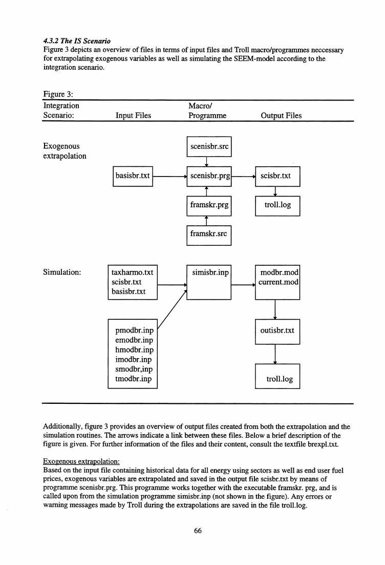
basisbr.txt
framskr.src
Integration
Macro/Scenario:
Input Files
Programme
Output Files
Exogenousextrapolation
scenisbr.src
scenisbr.prg
framskr.prg
scisbr.txt
troll.log
taxharmo.txtscisbr.txtbasisbr.txt
simisbr.inp
4.3.2 The IS ScenarioFigure 3 depicts an overview of files in terms of input files and Troll macro/programmes neccessaryfor extrapolating exogenous variables as well as simulating the SEEM-model according to theintegration scenario.
Figure 3:
modbr.modcurrent.mod
Simulation:
pmodbr.inpemodbr.inphmodbr.inpimodbr.inpsmodbr,inptmodbr.inp
outisbr.txt
troll.log
Additionally, figure 3 provides an overview of output files created from both the extrapolation and thesimulation routines. The arrows indicate a link between these files. Below a brief description of thefigure is given. For further information of the files and their content, consult the textfile brexpl.txt.
Exogenous extrapolation: Based on the input file containing historical data for all energy using sectors as well as end user fuelprices, exogenous variables are extrapolated and saved in the output file scisbr.txt by means ofprogramme scenisbr.prg. This programme works together with the executable framskr. prg, and iscalled upon from the simulation programme simisbr.inp (not shown in the figure). Any errors orwarning messages made by Troll during the extrapolations are saved in the file troll.log.
66

Simulation: The programme simisbr.inp establishes and simulates the SEEM-model based on all input filesrequired for simulation in the case of the integration scenario. The established model is saved inmodbr.mod as well as in current.mod, and the output of the simulation is saved in outisbr.txt. Anyerrors or warning messages made by Troll during the establishing and simulation of the model aresaved in the file troll.log.
4.3.3 The FS ScenarioFigure 4 depicts an overview of files in terms of input files and macro/programmes neccessary forextrapolating exogenous variables as well as simulating the SEEM-model according to thefragmentation scenario. Additionally, figure 4 provides an overview of output files created from boththe extrapolation and the simulation routines. The arrows indicate a link between these files. Below abrief description of the figure is given. For further information of the files and their content, consultthe textfile brexpl.txt.
Exogenous extrapolation: Based on the input file containing historical data for all energy using sectors as well as end user fuelprices, exogenous variables are extrapolated and saved in the output file scfsbr.txt by means of theprogramme scenfsbr.prg. This programme works together with the executable framskr. prg, and iscalled upon from the simulation programme simfsbr.inp (not shown in the figure). Any errors orwarning messages made by Troll during the extrapolations are saved in the file troll.log.
Simulation -. The programme simfsbr.inp establishes and simulates the SEEM-model based on all input filesrequired for simulation in the case of the fragmentation scenario. The established model is saved inmodbr.mod as well as in current.mod, and the output of the simulation is saved in outfsbr.txt. Anyerrors or warning messages made by Troll during the establishing and simulation of the model aresaved in the file troll.log.
67

Input FilesMacro/Programme Output Files
FragmentationScenario:
Exogenousextrapolation:
scenfsbr.prg scfsbr.txt
troll.log
Simulation: scfsbr.txtbasisbr.txt
simfsbr.inp modbr.modcurrent.mod
outfsbr.txt
framskr.prg
scenfsbr.src
basisbr.txt
pmodbr.inpemodbr.inphmodbr.inpimodbr.inpsmodbr,inptmodbr.inp
framskr.src
Figure 4:
4.4 The Procedure for SimulationThe Textfile simexpl.txtThe textfile, called simexpl.txt, explains the procedure of making a simulation with the SEEM-modelfor a given scenario and country. In what follows, the simulation procedure for the fragmentationscenario for Germany is used as an example.
General InformationGenerally speaking, the model user needs the following in order to accomplish a simulation: acompiled SEEM-model and a data file with scenario spesific data necessary for simulation. However,before any simulation can be accomplished, the model user has to make sure that no output files of anykind already exist, that is no data output file with extension .txt and no model file with extension .modshould already exist before simulation. In the fs scenario case such output files include the following:
outfsbr.txt, scfsbr.txt, modbr.mod, and current.mod
A Simulation ExampleThis is an example of the simulation procedure for the fragmentation scenario for Germany. Thefragmentation scenario has the identification letters «fs», and is based on the reference scenario whichis represented by the datafile basisbr.txt. The fs scenario differs from the reference scenario only when
68

it comes to assumed growth rates in GDP, private consumption, sectoral production, and import fuelprices among others.
Simulation Procedure1) Go to the br country subdirectory under the SEEM-directory in MS-DOS, i.
d:\bou\ptroll\seem\br.
2) Copy scenfsbr.src to scenfsbr.src, and start editing scenfsbr.src. In scenfsbr.src, change the annualgrowth rates manually according to the fs scenario input assumptions. That is, insert the newgrowth rates for the following variables and save the file scenfsbr.src:
The Household Sector: conhobra0elehobra0coghobrngsimppribr
The Service Sector: prosebra0elesebra0cogsebr
The Industry SectorproinbraDeleinbra0coainbra0oilinbraOngsinbroilimppribr
The Transport Sector: incomebrgdpindbrgoimppribrdiimppribrshar4brsharatfbrshawa0brroefftfbrraefftfbrwaefftfbr
The Electricity Generating Sector: ngsimppribroilimppribr
3) Start Troll by writing troll from the br subdirectory
d:\bou\ptroll\seem\br\troll
and Troll command will be shown on the screen. PC-Troll is now ready for commands.Then, compile the scenfsbr.src file and the framskr.src file by writing
Troll command: compile scenfsbrTroll command: compile framskr
69

Note that no file extension is neccessary. The compiled or executable version of the scenfsbr.src fileand the framskr.src file are now made, and they are called scenfsbr.prg and framskr.prg respectively.The extension .prg denotes a programme. Leave Troll by writing
Troll command: trexit
4) Copy the Troll input file for simulation, simisbr.inp to simfsbr.inp, and start editing simfsbr.inp.Simfsbr.inp contains a set of Troll commands which starts scenfsbr.prg, establishes the SEEM-model for Germany (if the model does not exist already), and simulates the model. Sincesimfsbr.inp is a copy of simisbr.inp, it has to be edited and adjusted to the fs scenario beforesimulation. In principle all «is» in the file names referred to in simisbr.inp should be changed to«fs» in order to avoid any overwriting of old scenario results. That is the model user has to specifythe name of the output files which keep the extrapolations of the input variables as well as thesimulation results of the fs scenario. Furthermore, the model user should check that only the datainput files relevant for the fs scenario is accessed to and searched for. Additionally, the model userhas to make sure that none of the output files (or eventually models) which will be created byrunning simfsbr.inp, exist already. If such files do exist already, the model user has to delete thosefiles before starting the chosen scenario simulation. When simfsbr.inp has been edited, save the file.
5) Start Troll again (see item 3) from the br subdirectory and write
Troll command: input simfsbr
Note that no file extension is necessary. With this Troll command the file simulates the model, savesthe output file with simulation results, and leaves Troll.
6) Check if the simulation has succeeded by looking at the file list under the br subdirectory.Theoutput file should be in the br subdirectory, with the right name, the right size (compare with otheroutput files), and it should have been established at the right time. To check the simulation resultsfurther, the model user should make a hard copy of values and annual growth rates for main inputand output variables (for instance by means of a spreadsheet table).
If something has gone wrong when running the simulation input file simfsbr.inp, the model user mayread and check the troll.log text file. This file contains any warnings or error messages made by Trollduring the simulation. A list of all possible Troll errors or warning messages with explanations isattached to this user's guide. Note that the troll.log file is overwritten when running the next Trollinput or macro file.
7) The fs scenario simulation for Germany is accomplished
70

Ef,c (t) =le c,5,1 (t),
Es (t) (t),c f
E 5 ,c (t) = ec , s , f (t),
Ec (t) c,s,f (t),
s f
E(t) = e c,s,f (t).c s f
E (t) = c,5,1 (t),
E f (t) =Eli e (t),c s
5. Aggregate Energy Demand and CO2-emission
This chapter describs and presents the summation routine for summarising simulated energy demandfrom the different scenarios for each country, or for a total of a group of countries. Moreover, thechapter presents the calculation routine of CO2-emissions as it is implemented in a submodel of theSEEM-model.
It is worthwhile to notice in the Troll macro presented below that the Troll syntax for a commentbegins with a «/*».
5.1 Description of the Troll Macro seemsumThe textfile, called sumexpl.txt, explains how to use the Troll macro seemsum.src. In addition, thetextfile provides comments and explanations related to each Troll command in the Troll macro justmentioned.
The SEEM-model outputs disaggregated energy consumption figures. For each single fuel f in eachsingle sector s within each single country c, the SEEM model outputs a simulated time series of energyconsumption figures xc,s,f(t). The seemsum.src macro does either
(i) aggregate the energy consumption figures over the three dimensions of fuel, sector and/orcountry, that is calculate the different aggregates
xs,c (t)= (t),
Xc (t) = 1,EXc,s,f (t),s f
X(t)= 1,11, X c, s f (t),
XS (t) = I Xc,s,f (t), X (t) XcAf (t),c I c s
Xf ,c (t) =EX c,5,1 (t), X ,s (t)=Ex c,s,f (t),
s f
and in addition a few special category aggregates over subsets of the fuels and subsets of thesectors,
or(ii) calculate disaggregated CO2 emissions: ec,sj (t) = xc,sff. (t) afi where ocf is a CO2 emissioncoefficient specific to the fuel f before calculateing the corresponding aggregates
In addition come the few special category aggregates over subsets of the fuels and subsets of thesectors.
The SEEM model contains 13 countries, 7 sectors and 14 fuels, which imply that the seemsummacro either calculates more than 400 aggregated energy series or about 600 disaggregated andaggregated emission series. Consult the documentation of the SEEM model for more details on thecountries, sectors and fuels, or read the comments to the macro code on the following pages.
The tasks (i) and (ii) are performed by the same macro by multiplying each disaggregated energyconsumption figure output from SEEM by either 1 or a fuel specific CO2 emission coefficient before
71

aggregation. In the latter case (ii) the calculated disaggregated emission figures are also saved to diskalong with the aggregates.
The macro performs the calculations in nested loops. It runs through all fuels within all sectors withinall countries, initializing and updating aggregation variables, and storing them on disk after finalupdate. To make the macro readable and understandable we name each variable according to itscontent. But, amounting to more than half a thousand in number motivates a scheme of automaticnaming of the individual variables. The names are constructed by concatenating the contents of a fewvariables. Let us say that the variables named oil, sector and country at a certain stage contain thenames "oil", "in" (short for industry) and "nor" (short for Norway). By concatenating (the content of)the three variables and an explicit text string, like name = fuel II "co2" II sector II country, we get name= "oilco2innor". In TROLL the construct &name returns the content of the variable name. Hence themacro command >>DOFILE &name = ... here equals the TROLL command "DOFILE oilco2innor =...", which files the right hand side of the equation as the disaggregated CO2 emission from oilconsumption in Norwegian industries in a disk variable named "oilco2innor". The alternative of anindexed variable (e.g. etnissionc,sf) would not reveal its content, thus yielding an incomprehensiblecode. This would hamper or effectively block code maintenace. Besides, it would create a problem ofnaming the disk variable.
The macro is extensively commented, to such an extent that we only sketch an outline:
1. User interface and initialization,2. For c = first_country to last_country
for s first sector to last sectorfor f = first_fuel_within_sector to last_fuel_within_sector
update relevant variables;if final update store variables;
3. Store rest of the variables.
5.2 Presentation of the Troll Macro seemsum1* The Portable TROLL macro: SEEMSUM.
/* Programmed by: Dag Kolsrud, SRM, Research Department, Statistics Norway/* Updates: Version 1 in December 1994 by Dag Kolsrud
/* Purpose: Either to (1) sum up energy consumption figures or (2) calculate and sum up CO2-emission figures for/* several European countries. A third task of calculating and summing up fuel expenditure can be implemented the same/* way as the CO2-emission.
/* Short description: This macro does the following:/* - decides whether to calculate (1) consumption or (2) emmision figures from user's choice input,1* - reads from a TROLL FORMDATA file disaggregated energy consumption figures for various fuel-sector-country,/* - initializes and updates aggregates with disaggregates in single and nested loops through fuels, sectors and countries,
- stores the aggregates in an ouput FORMDATA file after final updates.
/* Details: The calculations are performed by traversing the 3 "dimensions" of country-, sector- and fuel specific energy/* consumption figures, calculating disaggregated and/or aggregated figures. The structure of the calculations are the same/* in both cases (1) and (2), hence the two tasks of aggregating energy consumption figures and calculating and aggregating/* emission figures can be gathered into one single macro. The macro prompts the user to choose between the two tasks/* (1) and (2), which are independent of each other. The user also has to provide a number for the scenario for which the/* consumption or emission aggregates are to be calculated./*
/* The SEEM model has 13 countries:AUstria, BElgium, BundesRepublik, Canton Helvetica, DenmarK, FRance, Great Britain, *//* ITaly, NetherLands, NOrway, Suomi Finland, SPain and SWeden: (AU, BE, BR, CH, DK, FR, GB, IT, NL, NO, SF, SP, SW). *//* There are 4 STationary sectors: ELectricity, HOseholds, INdustry and SErvices: (EL, HO, IN, SE), and 3 MObile sectors: *//* Transport Passengers, Transport Freigth and Freight Air: (TP, TF, FA). The stationary sectors use 6 fuels: NUClear power, */
72

/* RENewables, COAT, OIL, Natural GaS and ELEctricity: (NEC, REN, COA, OIL, NGS, ELE), while the mobile sectors use *//* 8 fuels: Bus Diesel, GAs, GasOline, Rail Electricity, Rail Diesel, Diesel, ELectricity and 011: (BD, GA, GO, RE, RD, BD, DI, *//* EL, 01). TROLL FORMDATA files output from the SEEM model contain disaggregated country-sector-fuel specific energy *//* consumption data in the form of time series. Some series may be equal to zero. Not all fuels and sectors combine, e.g. *//* there is no use of ELEctricity in the production of ELectricity, and some fuels are transport specific, e.g. Rail Diesel in the *//* sector Transport Passengers. */
/* For the STationary sources this macro calculates (2) disaggregated CO2-emissions from each of *//* 1: #countries x 4 x 3 = #countries x 12 <= 156 country-sector-fuel combinations, contained in the TROLL variables *//* fuel_CO2_sector country (see below for explanations of the composition of names), *//* and/or (2 or 1) it sums up disaggregated energy consumption figures or the calculated emission figures for/* 2: #countries x 4 <= 52 totals for the country-sector combinations (aggregating over all STationary fuels), named *//* ENR _{CON or CO2}_sector_country, *//* 3: #countries x (6 or 3) <= 78 or 39 totals for the country-fuel combinations (aggregating over ST sectors), named */
1* fuel _{CON or CO2}_ST_country, (= fuel_{CON or CO2)_TO_country (except for NGS, cf 31), which is omitted) *//* 4: (5 or 3) + 3 x (4 or 3) = (17 or 12) totals for the fuel in sector combinations (aggregating over all countries), named *//* fuel_{CON or CO2}_sector_EU (or country-aggregate codes - C#countries, e.g. C3 - if a subset of countries), *//* 5: #countries <= 13 totals for the countries (aggregating over all STationary fuels and sectors), named *//* ENR _{CON or CO2}_ST_country, *//* 6: 4 totals for the sectors (aggregating over all STationary fuels and all countries), named *//* ENR_{CON or CO2Lsector_EU, *//* 7: 6 or 3 totals for the fuels (aggregating over all STationary sectors and all countries), named *//* fuel_{CON or CO2}_ST_EU, (= fueL{CON or CO2)_TO_EU (except for NGS, cf 32), which is omitted) *//* 8: 1 total for the STationary sources (aggregating over all STationary country-sector-fuel combinations), named *//* ENR _ICON or CO2}_ST_EU, *1
/* where 4 or 3 refers to 4 CONsumption or 3 CO2 aggregates, since the fuel ELE emits no CO2. The numbering corresponds *//* to the numbered TROLL code statements in the macro. This sums up to (1) #countries x 11 + 28 <= 171 consumption *//* aggregates or (2) #countries x 12 <= 156 disaggregated and #countries x 8 + 20 <= 124 aggregated emissions in the */
/* STationary sectors. */
/*/* For the MObile sources this macro calculates (2) disaggregated CO2-emissions from each of *//* 9: #countries x (5 + 2 + 1) = #countries x 8 <= 104 country-fuel in sector combinations, named *//* fuel_{CON or CO2}_sector country, *//* and/or (2 or 1) it sums up disaggregated energy consumption figures or the calculated emission figures for/* 10: #countries x 2 <= 26 totals for the country-sector (TP and TF only, since FA sector uses only one single fuel) */
/* combinations (aggregating over all MObile fuels), named ENR_{CON or CO2}_sector country, *//* 11: #countries x 2 <= 26 totals for the country-fuel (DI and 01 only, since the other MObile sectors each uses only *//* one single fuel) combinations (aggregating over all MObile sectors), *//* named fuel_ICON or CO2)_MO_country, (= fuel _{CON or CO2)_TO_country, which is omitted) *//* 12: (6 or 5) + (3 or 2) + 1= (10 or 8) totals for each fuel-sector combination (aggregating over all countries), named *//* fuel_{CON or CO2}_sector_EU, */
/* 13: #countries <= 13 totals for the countries (aggregating over all MObile fuels and sectors), named */
/* ENR _{CON or CO2}_MO_country, *//* 14: 2 totals for sectors TP and TF (FA uses only 01, aggregating over all MObile fuels and all countries), named *//* ENR _{CON or CO2}_sector_EU, *//* 15: 2 totals for the fuels DI and 01, cf. 11 (aggregating over all MObile sectors and all countries), named/* fuel_{CON or CO2}_MO_EU, (= fuel _{CON or CO2)_TO_EU, which is omitted) *//* 16: 1 total for the MObile sources (aggregating over all MObile country-sector-fuel combinations), named *//* ENR_{CON or CO2}_MO_EU./* This sums up to (1) #countries x 5 + 15 <= 80 consumption aggregates or (2) #countries x 8 <= 104 disaggregated *//* and #countries x 5 + 13 <= 78 aggregated emissions in the MObile sectors. *//* *//* The STationary and the MObile sectors together are summed up by the following: *//* 17: #countries totals for each country (the sum of STationary total and MObile total in each country), named */
/* ENR ACON or CO2}_TO_country, *//* 18: 1 total for all STationary and MObile sources (aggregating over everything), named *//* ENR_{CON or CO2}TO_EU, */
/* This sums up to #countries + 1 <= 14 consumption or emission aggregates. Since each fuel is specific to the STationary *//* and the MObile sectors there is no fuel TOtal (which would equal the ST and MO total). */
73

/* *//* In addition come some special aggregates. First, the sector aggregate called Final Consumption = TOtal - ELctricity *//* producing STationary sector yields the extra aggregates: *1
/* 19: #countries x (3 or 2) <= (39 or 26) FC totals for the country-fuel combinations (aggregating over the fuels *//* COA, NGS (and ELE if not CO2 calculations) in ST sectors HO, IN and SE. The FC total for OIL containing oil *//* fuels in MO sectors is calculated in 25), named fuelACON or CO2LFCcountry, *//* 20: 3 or 2 FC totals for the fuels (aggregating over the fuels COA, NGS (and ELE if not CO2 calculations) in ST *//* sectors HO, IN and SE. The FC total for OIL containing oil fuels in MO sectors is calculated in 28), named *//* fuel_{CON or CO2}_FC_EU, *//* 21: #countries <= 13 FC totals for the countries (aggregating over all ST fuels and FC sectors), named *//* ENR_{CON or CO2)_FC_country, (= ENFUCON or CO2)_TO_country - ENR_{CON or CO2}_EL_country), *//* 22: 1 total for the FC sectors (aggregating over all country-FC sector-ST fuel combinations), named *//* ENR_{CON or CO2}_FC_EU, (= ENR _{CON or CO2}TO_EU - ENR _{CON or CO2}_EL_EU). *//* This sums up to #countries x 4 + 4 <= 56 consumption or #countries x 3 + 3 <= 42 emission aggregates. *//* *//* Second, the fuel aggregates OIL = BD+GO+RD+DI+01 in MO sectors (not RE and EL in MO sectors) plus OIL in */
/* ST sectors. This yields the extra aggregates: *//* 23: #countries x 2 <= 26 OIL totals for the country-TP and -TF sector specific combinations, named *//* OIL _{CON or CO2}_{TP and TFLcountry, *1
/* 24: #countries <= 13 OIL totals for the country-MO sectors specific combinations, named */
/* OIL_{CON or CO2)_MO_country, *//* 25: #countries x 2 <= 26 OIL totals for the country-FC and -TO sector specific combinations, named *//* OIL_{CON or CO2}_{FC and TOLcountry, */
/* 26: 2 OIL totals for the TP and TF sectors (aggregating over all countries), named */
/* OIL_{CON or CO2UTP and TFLEU, *//* 27: 1 OIL totals for the MObile sectors (aggregating over all countries), named */
/* OIL _{CON or CO2}_MO_EU, *//* 28: 2 totals for the FC and TO sectors (aggregating over all countries), named *//* OIL_{CON or CO2}_{FC and TO}_EU. *1/* This sums up to #countries x 5 + 5 <= 70 consumption or emission aggregates. Since FA sector uses only one OIL product *//* 01, it is not included in the fuel-sector aggregates (i.e. in 23 and 26). */
/* Third, the fuel consumption aggregate ELE = RE+EL in MO sectors and ELE in ST sectors, yielding the extra aggregates: *//* 29: #countries x 2 <= 26 OIL totals for the country-MO and -TO sector specific combinations, named *//* ELE_CON_{MO and TO}_country, *//* 30: 2 ELE totals for the MO and TO sectors, (aggregating over all countries), named *//* ELE_CON _{MO and TO}_EU. *//* This sums up to #countries x 2 + 2 <= 28 consumption aggregates. There is no calculation of ELEctricity aggregate if "I//* CO2 emissions are calculated, since ELEctricity emits no CO2. */1" *1
/* Fourth, the fuel aggregate NGS = GA in MO sectors and NGS in ST sectors, yielding the extra aggregates: */
/* 31: #countries <= 13 gas totals for the country (aggregating over all ST sectors and TP sectors), named */
/* NGS_{CON or CO2)_TO_country, *//* 32: 1 NGS total (aggregating over all countries) named *//* NGS _{CON or CO2}TO_EU. */
/* This sums up to #countries + 1 <= 14 consumption or CO2 aggregates. *1
1* */
/* The total number of calculated new series are (1) #countries x 29 + 56 <= 433 consumption aggregates or *//* (2) #countries x 43 + 43 <= 602 emission variables. */
/* Macro programming: The macro uses local variables to hold both scalar constants and strings that are letter codes for/* the fuels, sectors and countries. Looping through the fuels, sectors and countries the letter codes are concatenatedr into names of temporary TROLL variables. These memory (not disk) variables are initialized to zero and then updated with/* disaggregated figures in (nested) loops. The disaggregated figures are read from FORMDATA output files from simulations/* of the SEEM model. In the case of calculating emmision figures, the consumption disaggregates are first multiplied with/* emission coefficients. (Fuel expenditurs can be calculated the same way, by multiplying consumption figures with fuel/* prices (and exchange rates)). After final updates the temporary TROLL variables are written into an output FORMDATA/* file. The number of the input scenario is used for naming both the input files and the single output file.
74

1* Names of the aggregate energy consumption or CO2-emission variables written to the output FORMDATA filer are all concatenations of 4 components:
1: a disaggregated fuel code or the all fuels aggregated code ENR,2: the energy consumption code CON or the CO2-emission code CO2,3: a single sector code or one of the sector aggregation codes ST, MO, FC or TO,4: a single country code or the code for the number of countries included in the summation C# or EU.
r A disaggregated output variable may e.g. be named OIL_CO2_HO_NO, while a most aggregated variable may ber named ENR_CON_TO_EU, where the _ separating the different components of the names is dropped when storingr the files in the FORMDATA file on disk.
ADDFUN MAIN;PROCEDURE MAIN()BEGIN;
1*
USER INTERFACE AND INITIALIZING
r First the user decides whether the macro should calculate emission figures or only sum up the energy consumption 1r figures already simulated. Later, the, boolean variables will decide whether energy consumption figures have to be */
multipied with CO2-emission coefficients:
GET FROM TERMINAL NUMBER task "\n Answer 1 for summing energy consumption or 2 for \n for calculating andsumming CO2-emission figures. \n Any other answer terminates the macro: ";
co2_emission = task == 2; r TRUE implies calculating CO2-emissions and all their aggregates 1energy_summation = task == 1; P TRUE implies calculating all aggregates of energy consumptions 1
r Electricity, nuclear power and renewables count when summing up energy consumption, but not when calculatingCO2-emission. Hence the difference in (the numbers of) STationary fuels in the two cases. For the STationary
1* sectors we have thatr EL sector uses NUC, REN, COA, OIL, NGS, i.e. fuel no. 1 to 5, while emitting from COA, OIL NGS,r HO, SE and IN sector uses COA, OIL, NGS, ELE, i.e. fuel no. 3 to 6, while emitting from COA, OIL NGS, 1
1* Rail Electricity and ELectricity count when summing up energy consumption, but not when calculating CO2-emmision.r For the MObile sectors we have that
TP sector uses BD, GA, GO, RE, RD, DI, i.e. fuel no. 1 to 6, while emitting from all but RE,TF sector uses DI, EL, 01, i.e. fuel no. 6 to 8, while emitting from DI and 01,
r FA sector uses and emits from 01, i.e. fuel no. 8.
IF (energy_summation) THEN BEGIN; r The consumption of hydroelectric energy (ELE and RE and EL) counts 1summ = "CON"; 1* Name postfix reflecting summation of energy consumption figures 1ST_fuel = COMBINE("NUC", "REN", "COA", "OIL", "NGS", "ELE");final_ST_fuel = 6;MO fuel = COMBINE("BD", "GA", "GO", "RE", "RD", "DI", "EL", "Or);final_MO_fuel = 8;final_TP_fuel = 6; TP uses the first 6 fuels 1
END; Pe IF energy_consumptionELSE IF (co2_emission) THEN BEGIN; r Hydroelectric energy does not contribute to any CO2-emission
summ = "CO2"; r Name postfix reflecting calculation of emmision consumption figures */coef_NGS = 0.0024; r Amount of CO2-emission pr energy unit of the various fuels */coef_GA = 0.0024;coef_OIL = 0.0031;coef_BD = 0.0031;coef_GO = 0.0031;coef_RD = 0.0031;coef_D1 = 0.0031;coef_COA = 0.0039;ST_coef = COMBINE(coef_COA, coef_OIL, coef_NGS); r Array corresponding to the array ST_fuel */
ST_fuel COMBINE("COA", "OIL", "NGS"); NUC, REN and ELE is ommited due to zero CO2 emission */
75

final_ST_fuel = 3;MO_coef = COMBINE(coef_BD, coefGA, coef_GO, coefRD, coef_DI, coef_01L);MO_fuel = COMBINE("BD", "GA", "GO", "RD", "DI", "Or); r RE and EL is ommited due to zero CO2 emission */final_MO_fuel = 6;final_TP_fuel = 5; TP uses the first 5 fuels (which all emit CO2) */
END; /* IF CO2_emissionELSE BEGIN; PRINT("\n Wrong answer, ending macro! "); EXIT(); END; r Error message and exit */
/* The user then decides whether to sum up for a single country, a few countries or for all 13 countries: ./
GET FROM TERMINAL choice ''\n Decide what countries to sum up. Answer the letter S \n for a singel country, the letter Mfor many (or a few) countries \n or the letter A for all 13 countries. \n Any other answer terminates the macro: ";
choice = UPPER(choice);
/* User's choice = S, M or A */single_country = choice = "S";many_countries = choice = "M";all_countries = choice == "A";
IF (single_country) THEN BEGIN; /* Construct a single entry array */GET FROM TERMINAL answer "\n Give ONE SINGLE country code from the following: AU, BE, \n BR, CH, DK, FR,
GB, IT, NL, NO, SF, SP or SW: ";all_country = COMBINE(UPPER(answer)); P Single country code */final_country = 1;geo = "C1"; /* Code for country aggregation */
END; r IF single_country */
ELSE IF (many_countries) THEN BEGIN;
it Construct an array with user's country codes as entries */all_country = COMBINE();
/* Empty array of zero length */
final_country = 0;
/* Initializing */GET FROM TERMINAL answer "\ri List countries by the following codes: \n AU, BE, BR, CH, DK, FR, GB, IT, NL, NO,
SF, SP or SW \n separated by blanks and terminated bya blank and \n a semicolon (e.g. like NO SF SW ;): ";WHILE (answer <> ";") BEGIN; /* Not finnished country input */
all_country = COMBINE(aIl_country, UPPER(answer)); /* Adding next country to the array */final_country = final_country + 1;GET FROM TERMINAL answer;
END; r WHILE answer */geo = "C" II CONVERT(final_country); /* CONVERT changes number to string */IF (final_country == 0) THEN BEGIN; PRINT("\n Wrong option, ending macro! "); EXIT(); END; /* Error message, exit */
END; r IF many_countries
ELSE IF (all_countries) THEN BEGIN;all_country = COMBINE("AU", "BE", "BR", "CH", "DK", "FR", "GB", "IT", "NL", "NO", "Sr, 'SP", "SW");final_country = 13;geo = "EU"; 1* Code for country aggregation */
END; r IF all_countries */
ELSE BEGIN; PRINT("\n Wrong option, ending macro! "); EXIT(); END; /* Error message and exit */
/* Then the SEEM simulation scenario on which to base the calculations have to be input. Later the scenario number goes at/1* into the name of the FORMDATA or FAME file containing the individual TROLL files (variables). The user chooses */
/* between storing the output in a FORMDATA or FAME database: */
GET FROM TERMINAL scenario "\n Give the name code (is or fs) of the scenario which data to calculate/summarize: ";GET FROM TERMINAL format "\n Write FORM for FORMDATA output or FAME for FAMEDATA output: ";
CALCULATING, UPDATING AND STORING */
/* Putting sector codes into vectors. The sectors are the same no matter what the user answers:
ST sector = COMBINE("EL", "HO", "IN", "SE");final_ST_sector = 4;
76

MO_sectorfinal_MO_sector
= COMBINE("TP", "TF", "FA"); /* Vital order of MO sectors *1=3;
r The calculated TROLL DATA files will be written into one single FORMDATA or FAME file (for all countries), containing *//* disaggregated and aggregated emissions or aggregated energy use. The filename is converted to lowercase letters, *//* being common in the UNIX environment: */
IF (UPPER(format) = "FAME" ) THEN /* The (name of the) FORMDATA file to be written does already exist */out_file = LOWER("sum" II scenario II summ II ".db"); P Concatenating name of FAMEDATA file to write */
ELSEout_file = LOWER("sum" II scenario II summ); /* Concatenating name of FORMDATA file to write */
IF (HOSTEXIST(out_file)) THEN BEGIN; /* The (name of the) FORMDATA file to be written does already exist */PRINT("Deleting existing formdata file: ", out_file); /* Informing user of macro */» HOST "rrn -f &out_file"; /* Unix command to delete any existing file by the same name */
END;
» ACCESS outfile TYPE &(format)DATA ID Cout_file) MODE CREATE; r Creating new FORM- or FAMEDATA file */» SEARCH DATA outfile W; P Set up to write results to the accessed outpuffile */
/* Main loop through the 13 countries. Both the STationary and the MObile sources are dealt with in this loop:
FOR (i = 1; i <= final_country; i = i + 1) BEGIN;
/* Looping through the countries "/first c
-
ountry = i == 1; /* =TRUE or FALSE */last c
-
ountry = i == final_country; /* =TRUE or FALSE */country = all_country[i];
/* Getting country name from vector */
/* The TROLL DATA files containing the simulation results for the specified scenario are read from a single *1
/* FORMDATA file for each country. All disaggregated energy consumption figures are read from this file:
informfile = LOWER(country11"/"Ilcountry II "out" II scenario II ".txt"); /* Name of FORMDATA file to read */IF (NOT HOSTEXIST(informfile)) THEN BEGIN; PRINT("Does not find the formdata file: ", informfile); EXIT(); END;» ACCESS infile TYPE FORMDATA ID &informfile MODE R;» SEARCH FIRST DATA infile; /* Ready to read energy use in current country */
/* STATIONARY SOURCES
/* For each country looping through 4 or 3 fuels within 4 sectors calculating all CO2-emissions or energy-use/* aggregates for the STationary sources:
FOR (j = 1; j <= final_ST_sector; j = j + 1) BEGIN;first_ST_sector j == 1;second_ST_sector = j == 2;last_ST_sector = j == final_ST_sector;sector = ST_sector[j];
/* Looping through 4 sectors: EL, HO, IN and SE *//* =TRUE or FALSE */
/* =TRUE if first Final Consumption sector else FALSE *//* = FALSE or TRUE */
/* Getting sector name from vector */
/* Deciding which fuels to scan depending on type of calculation (CO2 or not) and current sector. Then scan:
first = 1;last = final_ST_fuel;IF (energy_summation) THEN
IF (sector == "EL") THENlast = 5;
ELSE first = 3;
/* Default start index *//* Default end index */
/* only first or last has to be altered (ELSE first and last are correct) *//* If calculating CO2-emission no emission from NUC, REN and ELE fuel */
/* last = 5 since EL sector uses no ELE fuel *//* first = 3 since NUC and REN only in EL sector */
FOR (k = first; k <= last; k = k + 1) BEGIN; r Looping through 3 fuels: COA, OIL, NGS (and ELE), with ELE only... */first_ST_fuel = k == first;last_ST _fuel = k = last; /* = FALSE or TRUE */fuel = ST_fuel[k]; /* Getting country name from vector */variable = fuel II "CON" II sector II country; /* Concatenating filename */
77
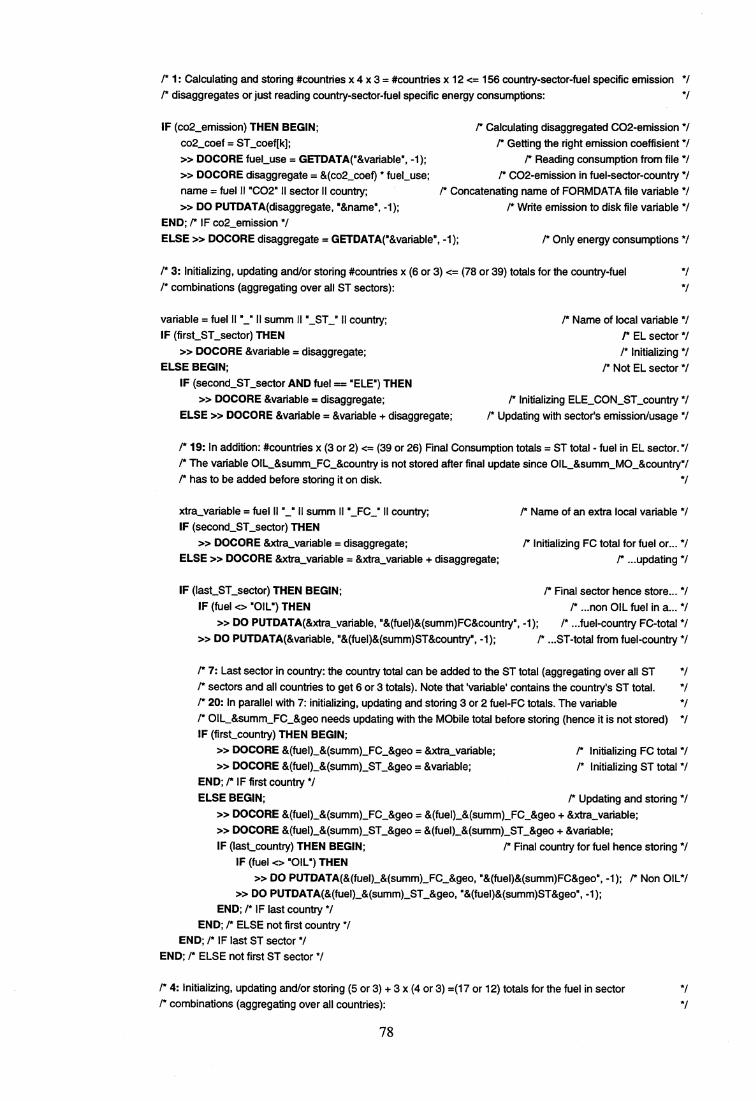
/* 1: Calculating and storing #countries x 4 x 3 = #countries x 12 <= 156 country-sector-fuel specific emission *//* disaggregates or just reading country-sector-fuel specific energy consumptions: */
IF (co2_emission) THEN BEGIN;co2_coef = ST_coef[k];» DOCORE fuel_use = GETDATA("&variable", -1);» DOCORE disaggregate = &(co2_coef) * fuel_use;name = fuel II "CO2" II sector II country;
DO PUTDATA(disaggregate, "&name", -1);END; r IF co2_emission */ELSE » DOCORE disaggregate = GETDATA("&variable", -1); /* Only energy consumptions */
/* Calculating disaggregated CO2-emission *//* Getting the right emission coeffisient */
/* Reading consumption from file *//* CO2-emission in fuel-sector-country */
/* Concatenating name of FORMDATA file variable *//* Write emission to disk file variable */
/* 3: Initializing, updating and/or storing #countries x (6 or 3) <= (78 or 39) totals for the country-fuel/* combinations (aggregating over all ST sectors):
variable = fuel II "_" II summ II "_ST_" II country;IF (first_ST_sector) THEN
» DOCORE &variable = disaggregate;ELSE BEGIN;
IF (second_ST_sector AND fuel == "ELE") THEN» DOCORE &variable = disaggregate;
ELSE » DOCORE &variable = &variable + disaggregate;
/* Name of local variable */1* EL sector *//* Initializing */
/* Not EL sector */
/* Initializing ELE_CON_ST_country *//* Updating with sector's emission/usage */
r 19: In addition: #countries x (3 or 2) <= (39 or 26) Final Consumption totals = ST total - fuel in EL sector. *//* The variable OIL_&summ_FC_&country is not stored after final update since OIL_&summ_MO_&country*//* has to be added before storing it on disk.
xtra_variable = fuel II "_" II summ II "_FC_" II country; /* Name of an extra local variable */IF (second_ST_sector) THEN
» DOCORE &xtra_variable = disaggregate; /* Initializing FC total for fuel or... */ELSE » DOCORE &xtra_variable = &xtra_variable + disaggregate; /* ...updating */
IF (last_ST_sector) THEN BEGIN; r Final sector hence store... */IF (fuel <> "OIL") THEN r ...non OIL fuel in a... */
» DO PUTDATA(&xtra_variable, "&(fuel)&(summ)FC&country", -1); /* ...fuel-country FC-total */» DO PUTDATA(&variable, "&(fuel)&(summ)ST&country", -1); 1* ...ST-total from fuel-country */
/* 7: Last sector in country: the country total can be added to the ST total (aggregating over all ST/* sectors and all countries to get 6 or 3 totals). Note that 'variable' contains the country's ST total./* 20: In parallel with 7: initializing, updating and storing 3 or 2 fuel-FC totals. The variable/* OIL_&summ_FC_&geo needs updating with the MObile total before storing (hence it is not stored)IF (first country) THEN BEGIN;
» DOCORE &(fuel)_&(summ)_FC_&geo = &xtra_variable; P Initializing FC total */» DOCORE &(fuel)_&(summ)_ST_&geo = &variable; r Initializing ST total */
END; /* IF first country */ELSE BEGIN; r Updating and storing */
DOCORE &(fuel)_&(summ)_FC_&geo = &(fuel)_&(summ)_FC_&geo + &xtra_variable;» DOCORE &(fuel)_&(summ)_ST_&geo = &(fuel)_&(summ)_ST_&geo + &variable;IF (last country) THEN BEGIN; r Final country for fuel hence storing */
IF (fuel <> "OIL") THENDO PUTDATA(&(fuel)_&(summ)_FC_&geo, "Cfuel)&(summ)FC&geo", -1); /* Non OIL*/
» DO PUTDATA(&(fuel)_&(summ)_ST_&geo, "&(fuel)&(surnm)ST&geo", -1);END; /* IF last country */
END; /* ELSE not first country */END; /* IF last ST sector */
END; r ELSE not first ST sector */
/* 4: Initializing, updating and/or storing (5 or 3) + 3 x (4 or 3) =(17 or 12) totals for the fuel in sector/* combinations (aggregating over all countries):
78

variable = fuel II "_" II summ II 11_," II sector II geo; /* Name of local variable */IF (first_country) THEN
» DOCORE &variable = disaggregate; /* Initializing or... */ELSE BEGIN;
» DOCORE &variable = &variable + disaggregate; /* ...updating with country's emission/fuel */IF (last_country) THEN
/* Final country: store... */» DO PUTDATAMvariable, "&(fuel)&(summ)&(sector)&geo", -1); /* ...total from fuel in sector */
END; /* ELSE not first country */
/* 2: Initializing or updating (and storing immediately after the fuel-loop) *countries x 4 <= 52 totals for the *//* country-sector combinations (aggregating over all STationary fuels): */
variable = 'ENR_" II summ II "_" II sector II "_" II country;IF (first_ST_fuel) THEN
» DOCORE &variable = disaggregate;ELSE » DOCORE &variable = &variable + disaggregate;
END; /* fuel-loop */» DO PUTDATA(&variable, "ENR&(summ)&(sector)&country", -1);
/* Name of local variable */
/* Initializing or... *//* ...updating with fuel -emission/consumption */
/* Storing total from sector-country */
/* 6: Initializing, updating and/or storing 4 totals for the sectors (aggregating over all STationary fuels and all/* countries). Note that variable = ENR_&(summ)_&(sector)_&country from above:
xtra_variable = "ENR_" II summ II "" II sector II "_" II geo; /* Name of local variable */IF (first_country) THEN
» DOCORE &xtra_variable = &variable; /* Initializing with first country's sector total or... */ELSE BEGIN;
» DOCORE &xtra_variable = &xtra_variable + &variable; /* ... updating with it */IF (last_country) THEN
/* Final country for sector... */» DO PUTDATA(&xtra_variable, "ENR&(summ)&(sector)&geo", -1); /* ...storing total from sector */
END; /* ELSE not first country *//* 5: Initializing or updating (and storing immediately after the sector-loop) *countries <= 13 totals for the countries */1* (aggregating over all STationary fuels and sectors). Note that from above we have *//* variable = ENR_&(summ)_&(sector)_&country:
xtra_variable = "ENR_" II summ II "_ST_" II country;IF (first_ST_sector) THEN
» DOCORE &xtra_variable = &variable;ELSE » DOCORE &xtra_variable = &xtra_variable + &variable;
END; /* sector-loop */» DO PUTDATA(&xtra_variable, "ENR&(summ)ST&country", -1);
/* Name of local variable */
/* Initializing with first country's sector total or... *//* ...or updating with it */
/* Storing total ST-country */
/* 8: Initializing and updating (and storing after the country-loop) 1 total for from STationary sources (aggregating/* over all STationary country-sector-fuel combinations). Update ST total with country-ST total. Note that we have
xtra_variable = ENR_&(summ)_ST_&country from above:
variable = "ENR_" II summ II ft_ST_" II geo;IF (first_country) THEN
» DOCORE &variable = &xtra_variable;ELSE» DOCORE &variable = &variable + &xtra_variable;
MOBILE SOURCES
/* Name of local variable */
/* Initializing total ST *//* updating total ST with country */
*/
/* For each country looping through different fuel subset within the 3 sectors TP, TF and FA calculating all/* CO2-emissions or energy-use aggregates for the MObile sources:
FOR (j =1; j final_MO_sector; j = j + 1) BEGIN; 1* Looping through 3 MObile sectors: TP and TF and FA */first_MO_sector = j =1; /* = TRUE or FALSE */last_MO_sector = j == final_MO_sector; /* = FALSE or TRUE */sector = MO_sector[j];
79

/* Deciding which fuels to loop through for the current sector, as different MObile sectors use different fuels:
IF (sector == "TP") THEN BEGIN;first_fuel = 1;last_fuel = final_TP_fuel;
END; /* IF TP-sector */ELSE IF (sector == "TF") THEN BEGIN;
first_fuel = final_TP_fuel;last_fuel = final_MO_fuel,
END; /* IF TF-sector */ELSE BEGIN;
first_fuel = final_MO_fuel;last_fuel = first_fuel;
END; /* IF FA-sector */
/* TP uses the 5/6 first fuels BD, GA, GO, (RE), RD and DI*/
/*=6or5*/
/* TF uses the 3/2 next fuels DI, (EL) and the oil product 01 *//* = 6 if CONsumption or 5 if CO2 */1* = 8 if CONsumption or 6 if CO2 */
/* FA sector uses only the oil product 01 *//* = 8 if CONsumption or 6 if CO2 */
/* For each sector in each country loop through a subset of BD, GA, GO, (RE,) RD, DI, (EL) and 01:
FOR (k = first_fuel; k <= last_fuel; k = k + 1) BEGIN;first_sector_fuel = k == first_fuel;last_sector_fuel = k == last_fuel;first_MO_fuel = k == 1;last_MO_fuel = k == final_MO_fuel;fuel = MO_fuel[k];IF (fuel == "01") THEN
SEEM_fuel = "OIL";ELSE SEEM_fuel = fuel;variable = SEEM_fuel II "CON" 11 sector II country;
/* 9: Calculating *countries x 8 <= 104 emissions or reading energy disaggregates in sector-country:
/* Looping through 6 or 5 and 3 or 2 and finally just 1 fuel *//* = TRUE or FALSE *//* = FALSE or TRUE *//* = TRUE or FALSE */1* = FALSE or TRUE */
/* Getting fuel name from vector */
/* SEEM output fuel name = OIL different from macro output fuel name = 01 *//* SEEM output fuel name = macro output fuel name */
/* Concatenating name of SEEM output variable */
IF (co2_emission) THEN BEGIN;co2_coef = MO_coef[k];» DOCORE fuel_use = GETDATA("&variable", -1);» DOCORE disaggregate = &(co2_coef) * fuel_use;name = fuel II "CO2" II sector II country;» DO PUTDATA(disaggregate, "&name", -1);
END; r IF co2_emission */ELSE BEGIN;
» DOCORE disaggregate = GETDATA("&variable", -1);/* Energy consumption is... */
/*... fuel-sector-country specific */
/* Calculating disaggregated CO2-emission *//* Getting the right emission coeffisient */
/* Reading consumption from file *//* CO2-emission in fuel-sector-country */
/* Concatenating name of FORMDATA file variable *//* Writing emission to disk file variable */
/* 29: If fuel is electricity, calculating *countries x 2 <= 26 ELE-CON totals for MO and TOT country. The 2 *//* ELE fuels in the MO sectors are visited once, hence we do the storing once in the fuel-sector loop:
IF (fuel == "RE") THEN
/* El-consumption in TP sector */» DOCORE ELE_CON_MO_&country = disaggregate;
/* initializing El aggregate for country */
ELSE IF (fuel == "EL") THEN BEGIN; /* El-consumption in TF sector */variable = "ELE_CON_MO",
/* Updating El aggregate for country with consumption in ... */
» DOCORE &(variable)_&country = &(variable)_&country + disaggregate; /* ...TF sector */» DO PUTDATA(&(variable)_&country, "ELECONMO&country", -1); /* ...and storing total */xtra_variable = "ELE_CON_TOT"; /* Total ELEctricity consumption */» DOCORE &(xtra_variable)_&country = &(variable)_&country + ELE_CON_ST_&country;» DO PUTDATA(&(xtra_variable)_&country, "ELECONTOT&country", -1); /* ...and storing */
/* 30: Initializing and updating 2 ELEctricity consumption MO and TOT total:
IF (first country) THEN /*Initializing total MObile ELE-consumption */» DOCORE &(variable)_&geo = &(variable)_&country; /* ...with consumption in country... */
ELSE BEGIN; r ...or updating... */
80
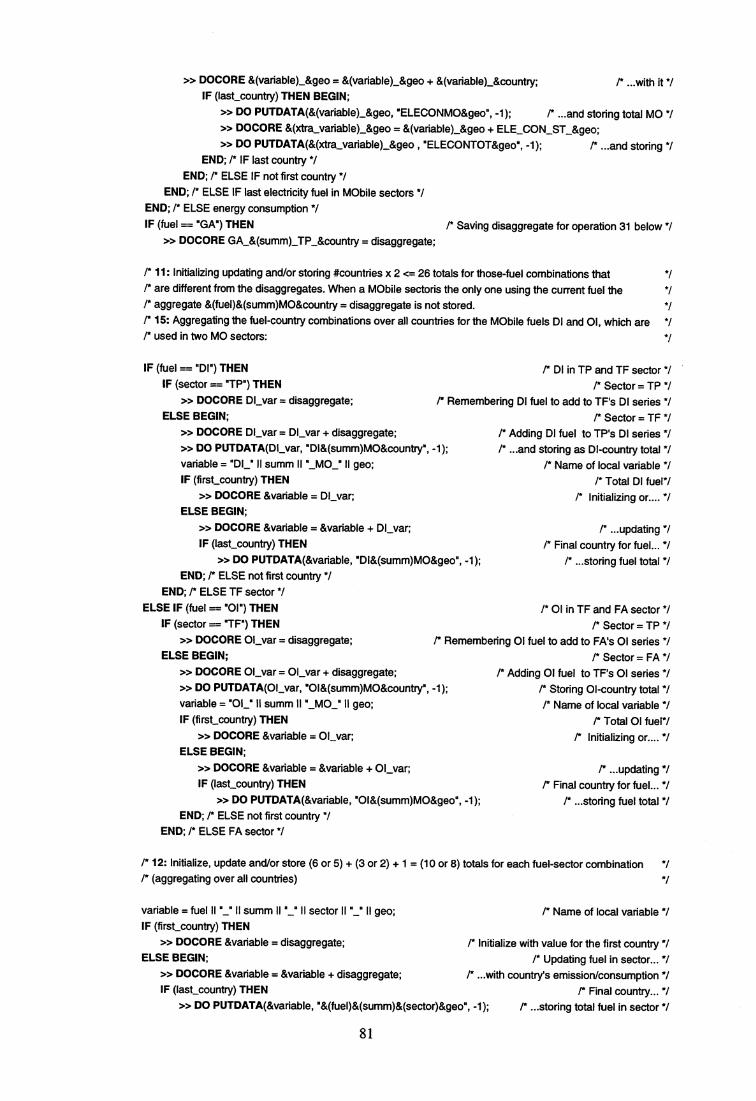
» DOCORE &(variable)_&geo = &(variable)_&geo + &(variable)_&country; r ...with it */IF (last_country) THEN BEGIN;
» DO PUTDATA(&(variable)_&geo, "ELECONMO&geo", -1); r ...and storing total MO */» DOCORE &(xtra_variable)_&geo = kvariable)_&geo + ELE_CON_ST_&geo;» DO PUTDATA(&(xtra_variable)_&geo , "ELECONTOT&geo", -1); /* ...and storing */
END; /* IF last country */END; r ELSE IF not first country */
END; /* ELSE IF last electricity fuel in MObile sectors */END; r ELSE energy consumption */IF (fuel == "GA") THEN Pe Saving disaggregate for operation 31 below */
» DOCORE GA_&(summ)TP_&country = disaggregate;
r 11: Initializing updating and/or storing #countries x 2 <= 26 totals for those-fuel combinations that/* are different from the disaggregates. When a MObile sectoris the only one using the current fuel the/* aggregate &(fuel)&(summ)MO&country = disaggregate is not stored./* 15: Aggregating the fuel-country combinations over all countries for the MObile fuels DI and 01, which are/* used in two MO sectors:
IF (fuel == "Dr) THEN
/* DI in TP and TF sector */IF (sector = "TP") THEN
/* Sector = TP */
» DOCORE Dl_var = disaggregate; /* Remembering DI fuel to add to TF's DI series */ELSE BEGIN; /* Sector = TF */
» DOCORE Dl_var = Dl_var + disaggregate; /* Adding DI fuel to TP's DI series */» DO PUTDATA(Dl_var, "DI&(summ)MO&country", -1); /* ...and storing as DI-country total */variable = "DI_" II summ II "_MO_" II geo; /* Name of local variable */IF (first country) THEN
/* Total DI fuel*/
» DOCORE &variable = Dl_var; /* Initializing or.... */ELSE BEGIN;
» DOCORE &variable = &variable + Dl_var; r ...updating */IF (last_country) THEN
p Final country for fuel... */
» DO PUTDATA(&variable, "Dlksumm)MO&geo", -1); 1* ...storing fuel total */END; r ELSE not first country */
END; /* ELSE TF sector */ELSE IF (fuel == "Or) THEN
/* 01 in TF and FA sector */
IF (sector == "TF") THEN
/* Sector = TP */» DOCORE Ol_var = disaggregate;
/* Remembering 01 fuel to add to FA's 01 series */
ELSE BEGIN; /* Sector = FA */» DOCORE Ol_var = Ol_var + disaggregate; /* Adding Cl fuel to TF's 01 series */» DO PUTDATA(OI_var, "01&(summ)MO&country", -1); /* Storing 01-country total */variable = "012 II summ 11 N_MO_R 11 geo; /* Name of local variable */IF (first country) THEN
/* Total 01 fuel*/
» DOCORE &variable = Ol_var; p Initializing or.... */ELSE BEGIN;
» DOCORE &variable = &variable + Ol_var; /* ...updating */IF (last_country) THEN
/* Final country for fuel... */
» DO PUTDATA(&variable, "01&(summ)MO&geou, -1); /* ...storing fuel total */END; P ELSE not first country */
END; /* ELSE FA sector */
/* 12: Initialize, update and/or store (6 or 5) + (3 or 2) + 1 = (10 or 8) totals for each fuel-sector combination *//* (aggregating over all countries)
variable = fuel II "_" II summ II "_" II sector II "2 11 geo; /* Name of local variable */IF (first_country) THEN
» DOCORE &variable = disaggregate; /* Initialize with value for the first country */ELSE BEGIN; /* Updating fuel in sector... */
» DOCORE &variable = &variable + disaggregate; /* ...with country's emission/consumption */IF (last_country) THEN
/* Final country... */
» DO PUTDATA(&variable, "&(fuel)&(summ)&(sector)&geo", -1); /* ...storing total fuel in sector */
81

END; r ELSE not first country */
/* 23: TP and TF sectors use several oil products, hence initializing, updating and storing the *countries x 2 *//* <= 26 oil aggregates in TP and TF sector. FA sector is not included since it uses only 01:
IF (fuel <> "GA" AND fuel <> "RE" AND fuel <> "EL") THEN BEGIN; r OIL fuel in sector */
IF (sector <> ''FA") THEN BEGIN; P IF or TP sector */
variable = "OIL_" II summ II 11_11 II sector II "_" II country; P. Name of local variable */IF (first_sector_fuel) THEN r Initializing oil aggregate for sector in country... */
» DOCORE &variable = disaggregate; /* ...with fuel consumption/emission */
ELSE BEGIN; P Updating oil aggregate for sector in country... */» DOCORE &variable = &variable + disaggregate; r ...with fuel consumption/emission */
IF (last sector fuel) THEN BEGIN; /* Final update hence... */
» DO PUTDATA(&variable, "OlL&(summ)&(sector)&country's, -1); /* ...storing total */
/* 26: Updating 2 OIL aggregates in TP and TF sector */
xtra_variable = "OIL" II summ II "2 II sector II "2 II geo; /* Name of local variable */IF (first_country) THEN
» DOCORE &(xtra_variable) = &variable; r Initializing oil aggregate for sector */ELSE BEGIN;
» DOCORE &(xtra_variable) = &(xtra_variable) + &variable;/* Updating sector aggregate */IF (last_country) THEN
» DO PUTDATA(&(xtra_variable), uOIL&(summ)&(sector)&geoft, -1); re ...storing total */END; /* ELSE not first country */
END; /* IF last sector fuel */END; /* ELSE not first sector fuel */
END; /* IF not FA sector */
/* 24: Initializing, updating and/or storing *countries <= 13 total OIL aggregates in MO sectors in country: */
variable = *OIL! II summ II "_MO_" II country;IF (first_MO_sector AND first_MO_fuel) THEN r Initializing oil aggregate for MO in country... */
» DOCORE &variable = disaggregate; /* ...with consumption/emission in sector */ELSE BEGIN; r Updating oil aggregate for MO in country... */
» DOCORE &variable = &variable + disaggregate; /* ...with consumption/emission in sector */
IF (last_MO_sector AND last_MO_fuel) THEN BEGIN; r Final sector update... */» DO PUTDATA(&variable, NOIL&(summ)MO&countryu, -1); 1* storing total OIL in MO-country */» DOFILE OIL&(summ)FC&country = OIL_&(summ)_FC_&country + &variable; r FC i ST + MO */
/* 27: Initializing, updating and/or storing 1 total OIL consumption/emission in all MObile sectors: */
xtra_variable = II summ II "_MO...! II geo; /* Name of local variable */IF (first_country) THEN
» DOCORE &(xtra_variable) = &variable; r Initializing total oil in MO sectors */ELSE BEGIN;
» DOCORE &(xtra_variable) = &(xtra_variable) + &variable; /* Updating total oil... */IF (last_country) THEN BEGIN;
» DO PUTDATA(&(xtra_variable), NOIL&(summ)MO&geoN, -1); /* Storing total in sector */» DOFILE OIL&(summ)FC&geo = OIL_&(summ)_FC_&geo + &(xtra_variable);
END; /* IF last country */END; /* ELSE not first country */
END; /* IF last.... */END; r ELSE not first MO sector */
END; /* IF OIL fuel */
/* 10: Updating and storing *countries x 2 <= 26 totals for the country-sector combination (aggregating over *//* all MObile fuels). Since FA uses the single 01 fuel, only TP and TF are included:
82

variable = "ENR_" II summ II "_" II sector II "_" II country; r Name of local variable */IF (sector <> "FA") THEN 1* TP or TF sector */
IF (firstsector_fuel) THEN /* Initializing fuel total with ... */» DOCORE &variable = disaggregate; /* ...sector's first fuel's emission/consumption */
ELSE BEGIN; r Updating fuel total with ... */» DOCORE &variable = &variable + disaggregate; /* ...with fuel's emission/consumption */IF (last_sector fuel) THEN» DO PUTDATA(&variable, "ENR&(summ)&(sector)&country", -1); /* Storingsector-country total */
END; /* ELSE not first fuel in sector */ELSE » DOCORE &variable = disaggregate; r variable = 01_&(summ)_FA_&country */
END; /* fuel-loop */
1* 14: Initializing, updating and storing 2 totals for the sectors TP and TF (aggregating over all MObile fuels and all: *//* countries). Since sector FA uses only one fuel 01, there is no fuel aggregation (ENR = 01): */
IF (sector <> "FA") THEN BEGIN;xtra_variable = "ENR_" II summ II II sector II "2 II geo; /* Name of local variable */IF (first_country) THEN
» DOCORE &xtra_variable = &variable; /* Initializing with first country's sector total */ELSE BEGIN;
» DOCORE &xtravariable = &xtra_variable + &variable; r Updating with country's sector total */IF (last country) THEN
» DO PUTDATA(&xtra_variable, "ENR&(summ)&(sector)&geoH, -1); /* Storing total from sector */END; /* ELSE not first country */
END; r IF sector not FA */
/* 13: Initializing and updating (but storing immediately after the sector-loop) *countries <= 13 totals for all MObile *//* sectors in the country, aggregating over all MObile fuels and sectors:
xtra_variable = "ENR_" II summ II "_MO_" II country;IF (first_MO_sector) THEN
» DOCORE &xtra_variable = &variable;ELSE » DOCORE &xtra_variable = &xtra_variable + &variable;
END; /* sector-loop */» DO PUTDATA(&xtra_variable, "ENR&(summ)MO&country", -1);
/* Name of local variable */
/* Initializing with first country's sector total *//* Updating with it */
/* Storing total in MO sectors in country */
/* 16: Initializing and updating (but storing after the country-loop) 1 total for MObile sources (aggregating over all *//* MObile sector-fuel combinations in all countries) with country's MO total. Note that we have xtra_variable holding *//* the string ENR_&(summ)_MO_&country from above, while variable is given a new string: */
variable = "ENR_" II summ II "_MO_" II geo; /* Name of local variable */IF (first_country) THEN
» DOCORE &variable = &xtra_variable; /* Initializing or */ELSE » DOCORE &variable = &variable + &xtra_variable; /* Updating with country */
/* 17: Adding MObile sector totals to Stationary sector totals and storing as *countries <= 13 country-TOtals:
» DOCORE ENR_&(summ)TOT_&country = ENR_&(summ)_ST_&country + ENR_&(summ)_MO_&country;» DO PUTDATA(ENR_&(summ)TOT_&country, "ENR&(summ)TOT&country", -1);
r 21: Storing *countries <= 13 totals for FC sectors, aggregated over all fuels and sectors but EL:
» DOFILE ENR&(summ)FC&country = ENR_Csumm)_TOT_&country - ENR_&(summ)_EL_&country;
r 25: Calculating *countries x 2 <= 26 TOtal and Final Consumptions or CO2-emissions from oil products in each *//* country, aggregated over all fuels and all sectors and FC = all sectors but EL: */
» DOCORE OIL_Csumm)TOT_&country = OIL_&(summ)_ST_&country + OIL_&(summ)_MO_&country;» DO PU'TDATA(01L_&(summ)_TOT_&country, "OlL&(summ)TOT&country", -1);
83
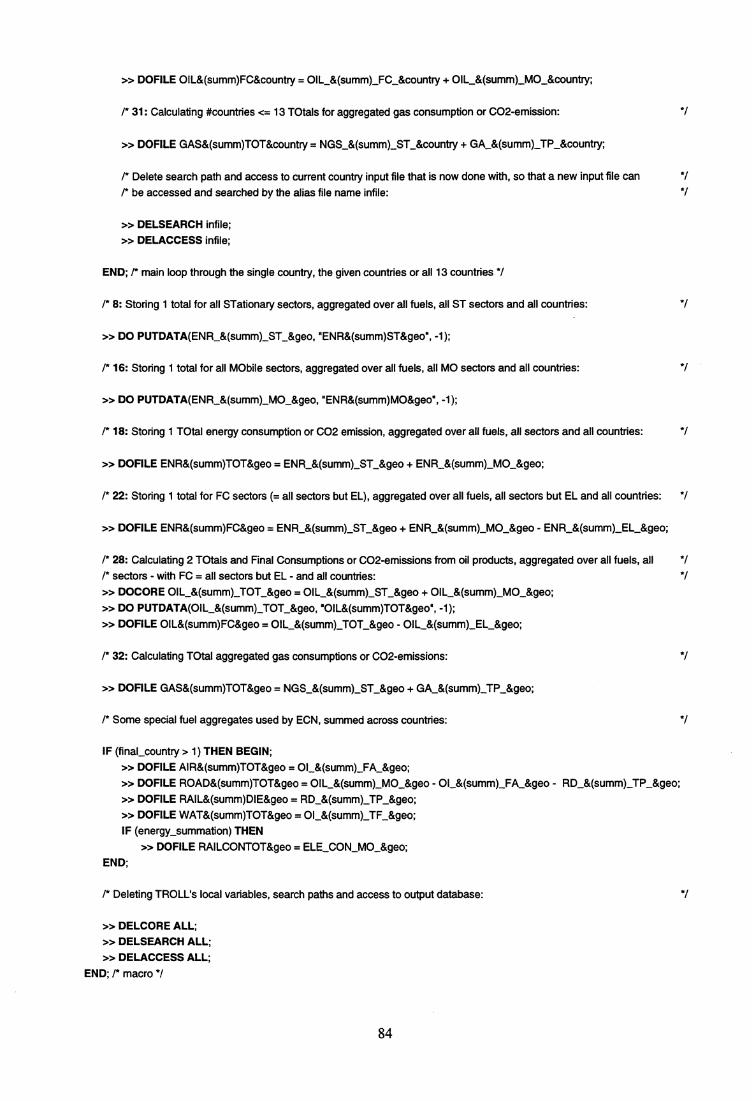
» DOFILE OIL&(summ)FC&country = OIL_&(summ)_FC_&country + OIL_&(summ)_MO_&country;
/* 31: Calculating #countries <= 13 TOtals for aggregated gas consumption or CO2-emission: */
» DOFILE GAS&(summ)TOT&country = NGS_&(summ)_ST_&country + GA_&(summ)TP_&country;
/* Delete search path and access to current country input file that is now done with, so that a new input file can *//* be accessed and searched by the alias file name infile: *1
» DELSEARCH infile;» DELACCESS infile;
END; /* main loop through the single country, the given countries or all 13 countries */
/* 8: Storing 1 total for all STationary sectors, aggregated over all fuels, all ST sectors and all countries:
» DO PUTDATA(ENR_&(summ)_ST_&geo, "ENR&(summ)ST&geo*, -1);
/* 16: Storing 1 total for all MObile sectors, aggregated over all fuels, all MO sectors and all countries:
» DO PUTDATA(ENR_&(summ)_MO_&geo, HENR&(summ)MO&geo", -1);
/* 18: Storing 1 TOtal energy consumption or CO2 emission, aggregated over all fuels, all sectors and all countries:
» DOFILE ENR&(summ)TOT&geo = ENR_&(summ)_ST_&geo + ENR_&(summ)_MO_&geo;
/* 22: Storing 1 total for FC sectors (= all sectors but EL), aggregated over all fuels, all sectors but EL and all countries: */
» DOFILE ENR&(summ)FC&geo = ENR_&(summ)_ST_&geo + ENR_&(summ)_MO_&geo - ENR_&(summ)_EL_&geo;
/* 28: Calculating 2 TOtals and Final Consumptions or CO2-emissions from oil products, aggregated over all fuels, all *//* sectors - with FC = all sectors but EL - and all countries: */» DOCORE OIL_&(summ)TOT_&geo = OIL_&(summ)_ST_&geo + OIL_&(summ)_MO_&geo,» DO PUTDATA(01L_&(summ)TOT_&geo, *OIL&(summ)TOT&geo", -1);» DOFILE OIL&(summ)FC&geo = OIL_&(summ)TOT_&geo - OIL_&(summ)_EL_&geo;
/* 32: Calculating TOtal aggregated gas consumptions or CO2-emissions: */
» DOFILE GAS&(summ)TOT&geo = NGS_&(summ)_ST_&geo + GA_&(summ)TP_&geo;
/* Some special fuel aggregates used by ECN, summed across countries: */
IF (final_country > 1) THEN BEGIN;» DOFILE AIR&(summ)TOT&geo = 01_&(summ)_FA_&geo;» DOFILE ROAD&(summ)TOT&geo = OIL_&(summ)_MO_&geo - 01_&(summ)_FA_&geo - RD_&(summ)_TP_&geo;» DOFILE RAIL&(summ)DIE&geo = RD_&(summ)TP_&geo;» DOFILE WAT&(summ)TOT&geo = 01_&(summ)TF_&geo;IF (energy_summation) THEN
» DOFILE RAILCONTOT&geo = ELE_CON_MO_&geo;END;
/* Deleting TROLL's local variables, search paths and access to output database:
» DELCORE ALL;» DELSEARCH ALL;» DELACCESS ALL;
END; /* macro */
84

6. Concluding Remarks
This user's guide has fully documented the implemented SEEM-model version 2.0 and how a modeluser can extrapolate and simulate the model by means of the Portable Troll software. The model useris guided through various SEEM related Troll macros and input files necessary for extrapolating andsimulating the model according to certain scenarios for Germany as an illustrative example. Thesescenarios include the so called reference scenario, the integration scenario, and the fragmentationscenario defined by the project «Energy scenarios for a changing Europe».
This user's guide has also offered one chapter on the procedure for summarising simulated energydemand for each country, and for the total of a group of countries. Moreover, the user's guide hasexplained the calculation routine for CO2-emissions as it is implemented in a separate submodel of theSEEM-model.
Finally, the author would like to emphasise that this document may be used as a guideline forextrapolating and simulating scenarios other than the above mentioned ones when the aim is to studyenergy demand in Western Europe.
85

Appendix
Al Troll Errors and Warning Messages
Recall from section 4.4, «The Procedure for Simulation», that the «troll.lop file contains errors orwarning messages when something goes wrong during a simulation of the SEEM-model. All possibleerrors or warnings are listed below as the model user may meet them in the «trollop file. This listmay also be found in the <droll.err» file located on the following subdirectory: d:\bou\ptroll.
Portable TROLL error messages
#00002 System file missing or corrupted.#00101 Not a command:#00102 Internal program error: invalid subtask.#00160 Internal program error -- report to TROLL maintenance staff.#00161 Command or option not available:#00193 HOST command processor returned a non-zero code:#00500 Not an option:#00501 Incorrect input:#00502 Name not found:#00700 Not enough memory.#01000 Invalid date.
#01001 Parser error.#01004 Evaluating error.#01006 Parser redefinition.
#02047 OLS Message.#02048 Ols statistics message.#02049 Ols statistics message.#02050 Datamatrix is extremely ill-conditioned.#02051 SCC Message.#02052 REGOPT message#02053 TSLS Message.#02054 NLS Message.#02055 Gremlin Message.
*** Gremlin messages ***
#02056 There are no coefficients in the current model.#02057 There are no equations in the current model.#02058 The number of equations does not match the number of endogenous variables.#02059 Negative subscript#02060 SFILLIN_XFILLIN error.#02222 Evaluating error.
#03001 Input/output - error.#03102 The string to be changed was not found.#03106 Invalid equation position:#03202 DEFINITION variable used before it is defined:#03203 ENDOGENOUS or DEFINITION variable has a lead:#03204 A lag or subscript cannot be calculated in equation:#03205 Subscripts are nested, or a symbol has more than one subscript, in eqn:#03206 Nested SUMs or PRODUCTs were found in equation:
86

#03207 The incidence matrix cannot be created due to problems with lags.#03208 Symbol not used in any equation (it will be ignored):#03209 The number of equations does not equal the number of variables.#03210 Some variables cannot be assigned to any equation:#03211 There are no assignable variables in some equations:#03212 The model cannot be block-ordered due to problems with the incidence matrix.#03213 It was not possible to normalize all equations.#03214 The CURRENT model has no equations.#03302 Not a symboltype:#03303 Not a symbolname, symboltype or suffix:#03304 Equation label already used:#03308 Suffixes may not be declared; ignoring:#03309 Wrong symboltype:#03333 Compile Error:#03401 Not a symbolname in the model:#03403 Missing comma before new symboltype:#03405 Symbol(s) used in equations cannot be deleted:#03503 The current model has no name, so you must give a name in this case.#03504 Not a valid model name:#03507 No CURRENT model can be found.#03599 GETXREF problem:
#04005 Run-Time error.
#05000 Problem trying to write data file:#05001 Problem trying to read data file:#05002 Problem trying to read program file:#05003 Problem trying to write program file:#05004 Problem trying to open file:#05005 Problem trying to close file:#05006 Disk file has incorrect contents:#05010 Search error:
#06000 Invalid argument(s) to a function.#06001 NA(s) returned where operand values did not allow an operation.#06010 Regression error.#06011 DLAG command error.
#07001 Input/Output Error.#07010 Modedit error
#08000 Macro error
#09002 No simulation dates are possible with the available data.#09003 No data was found for:#09010 The periodicity did not match that of the previous data for:#09012 The available data did not cover the lead/lag horizons for:#09013 Variables must be scalar or scalar timeseries; space dimension found for:#09016 Non-numeric data was found for:#09017 Timeseries data was found for constant symbol(s):#09018 Function(s) not supported in SIMULATE:#09019 Initial constant subscript not 1 (will be treated as 1) for:#09020 NEWVALS assumes date-range is ALL for constant symbols:
#15000 The current model cannot be simulated (check identities, lags, SUMs etc).
87

#15005 You must issue SIMSTART first.#15007 Not a date:#15008 An 'NA' was encountered:#15010 Date too early or late:#15011 Divergence occured:#15030 These variables were not on the DROP list:#15041 'FROM' option ignored in SIMRESID#15042 No simulation output to store. Use SIMSTART, then DOSIM or DOTIL.#15045 Iteration limit has been reached at iteration:#15046 Expression cannot be evaluated.#15049 You have already simulated the model through this date:#15050 The Jacobian matrix is singular or extremely ill-conditioned:#15070 Date has wrong periodicity:#15081 'STACK' not specified for Forward-Looking simulation 'NOFL' assumed.#15082 'STACK' is only intended for forward-looking models.#15083 STACKing only 1 time period has no effect.#15084 The number of periods you simulate must be a multiple of the number youSTACKed.
#24204 Input format error in bounds:#24207 Regression bounds have not yet been set.

coa con ho br
households
A2 List of Variables and Parameters
This appendix presents a complete list of variable names and parameter names used in the sectormodels as well as the price model for Germany (c.f. chapter 3). Since the names are constructedaccording to a general pattern of codes, the list may be applied as an illustrative example for othercountries as well. This general pattern of names is illustrated by means of figure 5.
Figure 5
a0coa con ho br
As can be seen from the figure, the variable «coaconhobr» denotes coal consumption in the householdsector in Germany. The parameter «a0coaconhobr» likewise denotes a calibration constant for the coalconsumption in the household sector in Germany. Hence, the names of the variables and theparameters consist of four separate letter/figure codes.
The first part of the names indicates the «type» of variable or parameter. Some of these «types»include the following: coa = coal, oil = oil, ngs = natural gas, ele = electricity, cog = coal-oil-gasaggregate, cap = capital, lab = labour. The first two symbols in the parameter names indicate whetherthe parameter is a calibration constant (a0), a price or a substitution elasticity (al), an incomeelasticity (a2) or other parameters such as a lag parameter and a technological progress parameter (a3).
The second part indicates a consumption (con), a price (pri), or a cost (cst) variable or parameter.Finally, the third and fourth part of the names indicates the sector and the country, respectively, inwhich the variable or the parameter belongs to. The sector codes are as follows: ho = the householdsector, in = the industry sector, se = the service sector, el = the electricity generating sector, and tp =the transport sector. The country codes are as follows: au = Austria, be = Belgium, br = Germany, ch= Switzerland, dk = Denmark, fr = France, gb = Great Britain, it = Italy, nl = Netherlands, no =Norway, sf = Finland, sp = Spain, and sw = Sweden.
Applying this general pattern of codes for the variable oil consumption in the service sector inGermany, we obtain the following variable name: oilconsebr. Similarly, by changing con with pri weget the variable oilprisebr, which is the end user oil price in the service sector in Germany.
In the tables below, the numbers in the first column correspond to the equation numbers in the modelspresented in chapter 3 and the equation numbers in Brubakk et.al. (1995).
89
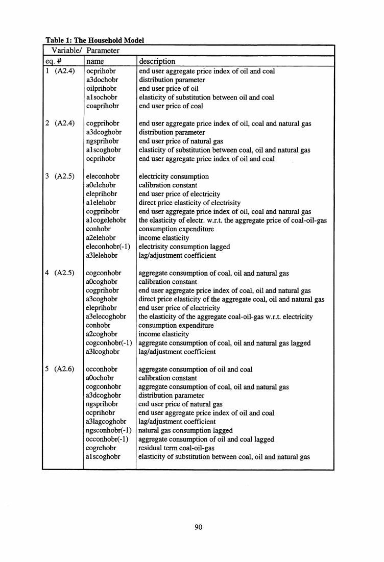
Table 1: The Household ModelVariable/ Parameter
eq. # name description1 (A2.4) ocprihobr end user aggregate price index of oil and coal
a3dochobr distribution parameteroilprihobr end user price of oilal sochobr elasticity of substitution between oil and coalcoaprihobr end user price of coal
2 (A2.4) cogprihobr end user aggregate price index of oil, coal and natural gasa3dcoghobr distribution parameterngsprihobr end user price of natural gasal scoghobr elasticity of substitution between coal, oil and natural gasocprihobr end user aggregate price index of oil and coal
3 (A2.5) eleconhobr electricity consumptiona0elehobr calibration constanteleprihobr end user price of electricityalelehobr direct price elasticity of electrisitycogprihobr end user aggregate price index of oil, coal and natural gasal cogelehobr the elasticity of electr. w.r.t. the aggregate price of coal-oil-gasconhobr consumption expenditurea2elehobr income elasticityeleconhobr(-1) electrisity consumption laggeda3lelehobr lag/adjustment coefficient
4 (A2.5) cogconhobr aggregate consumption of coal, oil and natural gasa0coghobr calibration constantcogprihobr end user aggregate price index of coal, oil and natural gasa3coghobr direct price elasticity of the aggregate coal, oil and natural gaseleprihobr end user price of electricitya3elecoghobr the elasticity of the aggregate coal-oil-gas w.r.t. electricityconhobr consumption expenditurea2coghobr income elasticitycogconhobr(-1) aggregate consumption of coal, oil and natural gas laggeda3lcoghobr lag/adjustment coefficient
5 (A2.6) occonhobr aggregate consumption of oil and coala0ochobr calibration constantcogconhobr aggregate consumption of coal, oil and natural gasa3dcoghobr distribution parameterngsprihobr end user price of natural gasocprihobr end user aggregate price index of oil and coala3lagcoghobr lag/adjustment coefficientngsconhobr(-1) natural gas consumption laggedocconhobr(-1) aggregate consumption of oil and coal laggedcogrehobr residual term coal-oil-gasal scoghobr elasticity of substitution between coal, oil and natural gas
90

Table 1 (continuedVariable/ Parameter
eq. # name description6 (A2.6) ngsconhobr natural gas consumption
aOngshobr calibration constantcogconhobr aggregate consumption of coal, oil and natural gasa3dcoghobr distribution parameterngsprihobr end user price of natural gasocprihobr end user aggregate price index of oil and coala3lagcoghobr lag/adjustment coefficientngsconhobr(-1) natural gas consumption laggedocconhobr(-1) aggregate consumption of oil and coal laggedcogrehobr residual term coal-oil-gasal scoghobr elasticity of substitution between coal, oil and natural gas
7 (A2.6) oilconhobr oil concumptiona0oilhobr calibration constantocconhobr aggregate consumption of oil and coala3dochobr distribution parameteroilprihobr end user price of oilcoaprihobr end user price of coala3lagochobr lag/adjustment coefficientoilconhobr(-1) oil concumption laggedcoaconhobr(-1) coal concumption laggedocrehobr residual term oil-coalal sochobr elasticity of substitution between oil and coal
8 (A2.6) coaconhobr coal concumptiona0coahobr calibration constantocconhobr aggregate consumption of oil and coala3dochobr distribution parameteroilprihobr end user price of oilcoaprihobr end user price of coala3lagochobr lag/adjustment coefficientoilconhobr(-1) oil concumption laggedcoaconhobr(-1) coal concumption laggedocrehobr residual term oil-coalal sochobr elasticity of substitution between oil and coal
91

Table 2: The Industry ModelVariable/ Parameter
eq. # name description1 (A2.1) eenrpriinbr end user price index of energy
coapriinbr end user price of coalalcoainbr cost-share coaloilpriinbr end user price of oilaloilinbr cost-share oilngspriinbr end user price of natural gasal ngsinbr cost-share natural gaselepriinbr end user price of electricityaleleinbr cost-share electricity
2 (A2.2) ecoaconinbr desired coal consumptionproinbr production/activity levela2proinbr elasticity of energy w.r.t. industry productioncapriinbr price of capitalalcapinbr cross price elasticity of energy w.r.t. capital pricelabpriinbr price of labouralwaginbr cross price elasticity of energy w.r.t. labour priceeenrpriinbr end user price index of energyalenrinbr price elasticity of energy w.r.t. energy pricecoapriinbr end user price of coalalcoainbr cost-share coaloilpriinbr end user price of oilaloilinbr cost-share oilngspriinbr end user price of natural gasalngsinbr cost-share natural gaselepriinbr end user price of electricityaleleinbr cost-share electricity
3 (A2.2) eoilconinbr desired oil consumptionproinbr production/activity levela2proinbr elasticity of energy w.r.t. industry productioncapriinbr price of capitalalcapinbr cross price elasticity of energy w.r.t. capital pricelabpriinbr price of labouralwaginbr cross price elasticity of energy w.r.t. labour priceeenrpriinbr end user price index of energyalenrinbr price elasticity of energy w.r.t. energy pricecoapriinbr end user price of coalalcoainbr cost-share coaloilpriinbr end user price of oilaloilinbr cost-share oilngspriinbr end user price of natural gasal ngsinbr cost-share natural gaselepriinbr end user price of electricityaleleinbr cost-share electricity
92
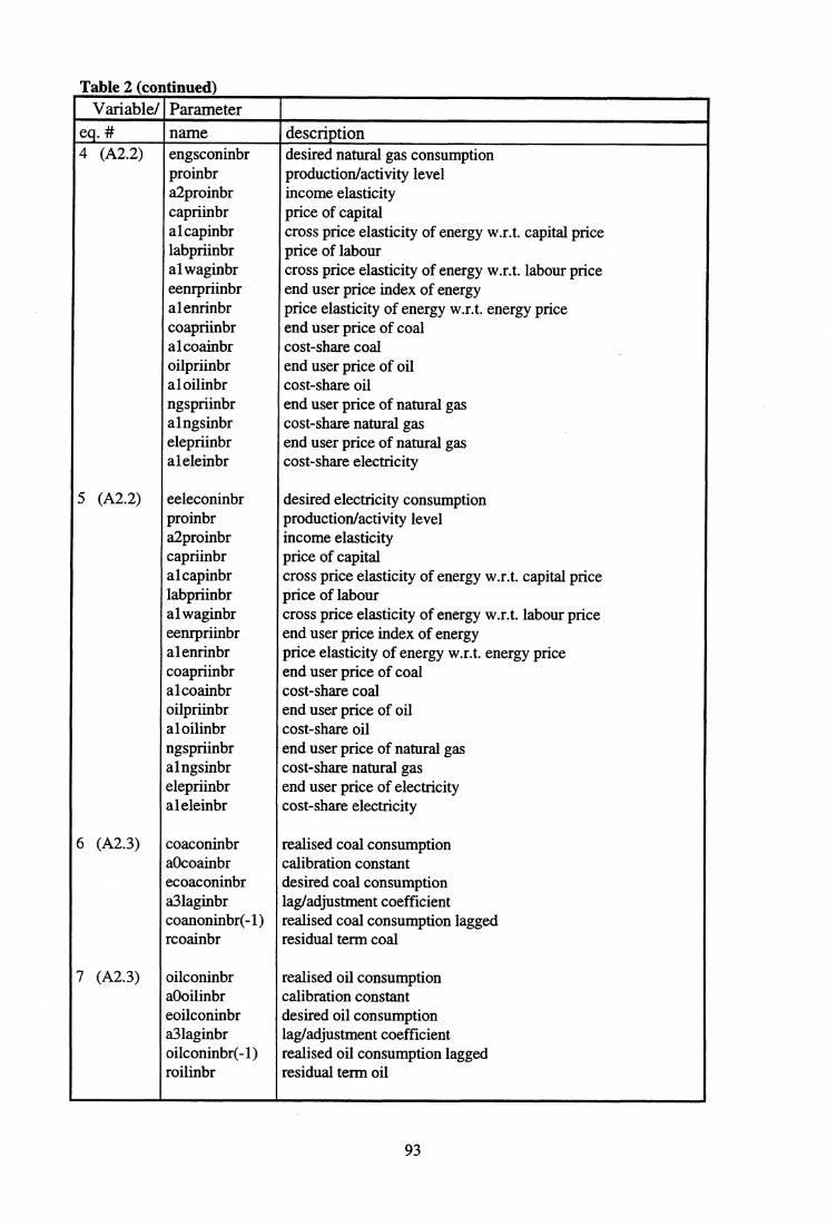
Table 2 (continued)Variable/ Parameter
eq. # name description4 (A2.2) engsconinbr desired natural gas consumption
proinbr production/activity levela2proinbr income elasticitycapriinbr price of capitalalcapinbr cross price elasticity of energy w.r.t. capital pricelabpriinbr price of labouralwaginbr cross price elasticity of energy w.r.t. labour priceeenrpriinbr end user price index of energyalenrinbr price elasticity of energy w.r.t. energy pricecoapriinbr end user price of coalalcoainbr cost-share coaloilpriinbr end user price of oilal oilinbr cost-share oilngspriinbr end user price of natural gasalngsinbr cost-share natural gaselepriinbr end user price of natural gasaleleinbr cost-share electricity
5 (A2.2) eeleconinbr desired electricity consumptionproinbr production/activity levela2proinbr income elasticitycapriinbr price of capitalalcapinbr cross price elasticity of energy w.r.t. capital pricelabpriinbr price of labouralwaginbr cross price elasticity of energy w.r.t. labour priceeenrpriinbr end user price index of energyalenrinbr price elasticity of energy w.r.t. energy pricecoapriinbr end user price of coalalcoainbr cost-share coaloilpriinbr end user price of oilal oilinbr cost-share oilngspriinbr end user price of natural gasalngsinbr cost-share natural gaselepriinbr end user price of electricityaleleinbr cost-share electricity
6 (A2.3) coaconinbr realised coal consumptiona0coainbr calibration constantecoaconinbr desired coal consumptiona3laginbr lag/adjustment coefficientcoanoninbr(-1) realised coal consumption laggedrcoainbr residual term coal
7 (A2.3) oilconinbr realised oil consumptiona0oilinbr calibration constanteoilconinbr desired oil consumptiona3laginbr lag/adjustment coefficientoilconinbr(-1) realised oil consumption laggedroilinbr residual term oil
93

Table 2 (continued)Variable/ Parameter
eq. # name description8 (A2.3) ngsconinbr realised natural gas consumption
aOngsinbr calibration constantengsconinbr desired natural gas consumptiona3laginbr lag/adjustment coefficientngsconinbr(-1) realised natural gas consumption laggedmgsinbr residual term natural gas
9 (A2.3) eleconinbr realised electricity consumptiona0eleinbr calibration constanteeleconinbr desired electricity consumptiona3laginbr lag/adjustment coefficienteleconinbr(-1) realised electrisity consumption laggedreleinbr residual term electrisity
Table 3: The Service ModelVariable/ Parameter
eq. # name description1 (A2.7) ogprisebr end user aggregate price index of oil and natural gas
a3dogsebr distribution parameter oil-gasngsprisebr end user price of natural gasal sogsebr elasticity of substitution between oil and natural gasoilprisebr end user price of oil
2 (A2.7) cogprisebr end user aggregate price index of coal, oil and natural gasa3dcogsebr distribution parameter coal-oil-gascoaprisebr end user price of coalal scogsebr elasticity of substitution between coal, oil and natural gasogprisebr end user aggregate price index of oil and natural gas
3 (A2.8) eleconsebr electricity consumptiona0elesebr calibration constantprosebr production/activity levela2elesebr income elasticitycapprisebr price of capitalal capelesebr capital factor elasticitylabprisebr price of laboural labelesebr labour factor elasticitycogprisebr end user aggregate price index of coal, oil and natural gasal cogelesebr the elasticity of electricity w.r.t. the aggr. price of coal-oil-gaseleprisebr end user price of electricityalelesebr direct price elasticity of electrisityeleconsebr(-1) electrisity consumption laggeda3lelesebr lag/adjustment coefficient
94

Table 3 (continued)Variable/ Parameter
eq. # name description4 (A2.8) cogconsebr aggregate consumption of coal,oil and gas
a0cogsebr calibration constantprosebr production/activity levela2cogsebr income elasticitycapprisebr price of capitalal capcogsebr capital factor elasticitylabprisebr price of laboural labcogsebr labour factor elasticitycogprisebr end user aggregate price index of coal, oil and natural gasal cogsebr direct price elasticity of the aggregate coal-oil-gaseleprisebr end user price of electricityalelecogsebr elasticity of the aggr. coal, oil and natural gas w.r.t electricitycogconsebr(-1) aggregate consumption of coal,oil and gas laggeda3lcogsebr lag/adjustment coefficient
5 (A2.9) ogconsebr aggregate consumption of oil and natural gasa0ogsebr calibration constantcogconsebr aggregate consumption of coal,oil and gasa3dcogsebr distribution parameterogprisebr end user aggregate price index of oil and natural gascoaprisebr end user price of coala3lagcogsebr lag/adjustment coefficientogconsebr(-1) aggregate consumption of oil and natural gas laggedcoaconsebr(-1) coal consumption laggedcogresebr residual term coal-oil-gasal scogsebr elasticity of substitution between coal, oil and natural gas
6 (A2.9) coaconsebr coal consumptiona0coasebr calibration constantcogconsebr aggregate consumption of coal, oil and gasa3dcogsebr distribution parameterogprisebr end user aggregate price index of oil and natural gascoaprisebr end user price of coala3lagcogsebr lag/adjustment coefficientogconsebr(-1) aggregate consumption of oil and natural gas laggedcoaconsebr(-1) coal consumption laggedcogresebr residual term coal-oil-gasal scogsebr elasticity of substitution between coal, oil and natural gas
95

Table 3 (continued)Variable/ Parameter
eq. # name description7 (A2.9) oilconsebr oil consumption
a0oilsebr calibration constantogconsebr aggregate consumption of oil and natural gasa3dogsebr distribution parameteroilprisebr end user price of oilngsprisebr end user price of natural gasa3lagogsebr lag/adjustment coefficientoilconsebr(-1) oil consumption laggedngsconsebr(-1) natural gas consumption laggedogresebr residual term oil-gasal sogsebr elasticity of substitution between oil and natural gas
8 (A2.9) ngsconsebr natural gas consumptionaOngssebr calibration constantogconsebr aggregate consumption of oil and natural gasa3dogsebr distribution parameteroilprisebr end user price of oilngsprisebr end user price of natural gasa3lagogsebr lag/adjustment coefficientoilconsebr(-1) oil consumption laggedngsconsebr(-1) natural gas consumption laggedogresebr residual term oil-gasal sogsebr elasticity of substitution between oil and natural gas
Table 4: The Electrisity Generating ModelVariable/ Parameter
eq. # name description1 coashanelbr share of new coal technology
dumnbr dummy variable new technologycoashalnelbr share of new coal technology later than the base yearcoashaOnelbr share of new coal technology in the base year
2 coashafelbr share of future coal technologydumnbr dummy variable new technologycoashalfelbr share of future coal technology later than the base yearcoashaOfelbr share of future coal technology in the base year
3 coashabelbr share of bat coal technologydumbbr dummy variable bat technologycoashalbelbr share of bat coal technology later than the base yearcoasha0belbr share of bat coal technology in the base year
4 coashaoelbr share of old coal technologycoashanelbr share of new coal technologycoashafelbr share of future coal technologycoashabelbr share of bat coal technology
96
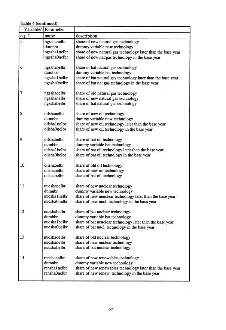
Table 4 (continuedVariable/ Parameter
eq. # name description5 ngsshanelbr share of new natural gas technology
dumnbr dummy variable new technologyngsshalnelbr share of new natural gas technology later than the base yearngsshaOnelbr share of new nat.gas technology in the base year
6 ngsshabelbr share of bat natural gas technologydumbbr dummy variable bat technologyngsshalbelbr share of bat natural gas technology later than the base yearngssha0belbr share of bat nat.gas technology in the base year
7 ngsshaoelbr share of old natural gas technologyngsshanelbr share of new natural gas technologyngsshabelbr share of bat natural gas technology
8 oilshanelbr share of new oil technologydumnbr dummy variable new technologyoilshalnelbr share of new oil technology later than the base yearoilshaOnelbr share of new oil technology in the base year
9 oilshabelbr share of bat oil technologydumbbr dummy variable bat technologyoilshalbelbr share of bat oil technology later than the base yearoilsha0belbr share of bat oil technology in the base year
10 oilshaoelbr share of old oil technologyoilshanelbr share of new oil technologyoilshabelbr share of bat oil technology
11 nucshanelbr share of new nuclear technologydumnbr dummy variable new technologynucshalnelbr share of new neuclear technology later than the base yearnucshaOnelbr share of new nucl. technology in the base year
12 nucshabelbr share of bat nuclear technologydumbbr dummy variable bat technologynucshalbelbr share of bat neuclear technology later than the base yearnucsha0belbr share of bat nucl. technology in the base year
13 nucshaoelbr share of old nuclear technologynucshanelbr share of new nuclear technologynucshabelbr share of bat nuclear technology
14 renshanelbr share of new renewables technologydumnbr dummy variable new technologyrenshalnelbr share of new renewables technology later than the base yearrenshaOnelbr share of new renew. technology in the base year
97

Table 4 (continued)Variable/ Parameter
eq. # name description15 renshabelbr share of bat renewables technology
dumbbr dummy variable bat technologyrenshalbelbr share of bat renewables technology later than the base yearrensha0belbr share of bat renew. technology in the base year
16 renshaoelbr share of old renewables technologyrenshabelbr share of new renewables technologyrenshabelbr share of bat renewables technology
17 (A5.4) coacstelbr average production cost of electricity using coalcoashaoelbr share of old coal technologycoaprcstoelbr fixed production cost using old coal technologycoaprielbr end user price of coalcoaeffoelbr efficiency per unit of coal old technologycoashaoelbr share of new coal technologycoaprcstnelbr fixed production cost using new coal technologycoaeffnelbr efficiency per unit of coal new technologycoashafelbr share of future coal technologycoaprcstfelbr fixed production cost using future coal technologycoaefffelbr efficiency per unit of coal future technologycoashabelbr share of bat coal technologycoaprcstbelbr fixed production cost using bat coal technologycoaeffbelbr efficiency per unit of coal bat technology
18 (A5.4) ngscstelbr average production cost of electricity using gasngsshaoelbr share of old gas technologyngsprcstoelbr fixed production cost using old gas technologyngsprielbr end user price of natural gasngseffoelbr efficiency per unit of gas old technologyngsshanelbr share of new gas technologyngsprcstnelbr fixed production cost using new gas technologyngseffnelbr efficiency per unit of gas new technologyngsshabelbr share of bat gas technologyngsprcstbelbr fixed production cost using bat gas technologyngseffbelbr efficiency per unit of gas bat technology
19 (A5.4) oilcstelbr average production cost of electricity using oiloilshaoelbr share of old oil technologyoilprcstoelbr fixed production cost using old oil technologyoilprielbr end user price of oiloileffoelbr efficiency per unit of oil old technologyoilshanelbr share of new oil technologyoilprcstnelbr fixed production cost using new oil technologyoileffnelbr efficiency per unit of oil new technologyoilshabelbr share of bat oil technologyoilprcstbelbr fixed production cost using bat oil technologyoileffbelbr efficiency per unit of oil bat technology
98
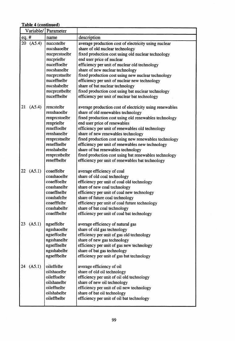
Table 4 (continuedVariable/ Parameter
eq. # name description20 (A5.4) nuccstelbr average production cost of electricity using nuclear
nucshaoelbr share of old nuclear technologynucprcstoelbr fixed production cost using old nuclear technologynucprielbr end user price of nuclearnuceffoelbr efficiency per unit of nuclear old technologynucshanelbr share of new nuclear technologynucprcstnelbr fixed production cost using new nuclear technologynuceffnelbr efficiency per unit of nuclear new technologynucshabelbr share of bat nuclear technologynucprcstbelbr fixed production cost using bat nuclear technologynuceffbelbr efficiency per unit of nuclear bat technology
21 (A5.4) rencstelbr average production cost of electricity using renewablesrenshaoelbr share of old renewables technologyrenprcstoelbr fixed production cost using old renewables technologyrenprielbr end user price of renewablesreneffoelbr efficiency per unit of renewables old technologyrenshanelbr share of new renewables technologyrenprcstnelbr fixed production cost using new renewables technologyreneffnelbr efficiency per unit of renewables new technologyrenshabelbr share of bat renewables technologyrenprcstbelbr fixed production cost using bat renewables technologyreneffbelbr efficiency per unit of renewables bat technology
22 (A5.1) coaeffelbr average efficiency of coalcoashaoelbr share of old coal technologycoaeffoelbr efficiency per unit of coal old technologycoashanelbr share of new coal technologycoaeffnelbr efficiency per unit of coal new technologycoashafelbr share of future coal technologycoaefffelbr efficiency per unit of coal future technologycoashabelbr share of bat coal technologycoaeffbelbr efficiency per unit of coal bat technology
23 (A5.1) ngseffelbr average efficiency of natural gasngsshaoelbr share of old gas technologyngseffoelbr efficiency per unit of gas old technologyngsshanelbr share of new gas technologyngseffnelbr efficiency per unit of gas new technologyngsshabelbr share of bat gas technologyngseffbelbr efficiency per unit of gas bat technology
24 (A5.1) oileffelbr average efficiency of oiloilshaoelbr share of old oil technologyoileffoelbr efficiency per unit of oil old technologyoilshanelbr share of new oil technologyoileffnelbr efficiency per unit of oil new technologyoilshabelbr share of bat oil technologyoileffbelbr efficiency per unit of oil bat technology
99

Table 4 (continued)Variable/ Parameter
es. # _ name description25 (A5.1) nuceffelbr average efficiency of nuclear
nucshaoelbr share of old nuclear technologynuceffoelbr efficiency per unit of nuclear old technologynucshanelbr share of new nuclear technologynuceffnelbr efficiency per unit of nuclear new technologynucshabelbr share of bat nuclear technologynuceffbelbr efficiency per unit of nuclear bat technology
26 (A5.1) reneffelbr average efficiency of renewablesrenshaoelbr share of old renewables technologyreneffoelbr efficiency per unit of renewables old technologyrenshanelbr share of new renewables technologyreneffnelbr efficiency per unit of renewables new technologyrenshabelbr share of bat renewables technologyreneffbelbr efficiency per unit of renewables bat technology
27 (A2.20) coashalelbr share of electicity produced using coala0coaconelbr calibration constantcoacstelbr average production cost of electricity using coalalcoaconelbr cost share of coal consumptionngscstelbr average production cost of electricity using gasalngsconelbr cost share of gas consumptionoilcstelbr average production cost of electricity using oilaloilconelbr cost share of oil consumptionnuccstelbr average production cost of electricity using nuclearalnucconelbr cost share of nuclear consumptionrencstelbr average production cost of electricity using renewablesalrenconelbr cost share of renewables consumption
28 (A2.20) ngsshalelbr share of electricity produced using gasa0ngsconelbr calibration constant.ngscstelbr average production cost of electricity using gascoacstelbr average production cost of electricity using coalalcoaconelbr cost share of coal consumptionalngsconelbr cost share of gas consumptionoilcstelbr average production cost of electricity using oilaloilconelbr cost share of oil consumptionnuccstelbr average production cost of electricity using nuclearalnucconelbr cost share of nuclear consumptionrencstelbr average production cost of electricity using renewablesalrenconelbr cost share of renewables consumption
100

Table 4 (continued)Variable/ Parameter
eq. # name , description29 (A2.20) oilshalelbr share of electricity produced using oil
a0oilconelbr calibration constantoilcstelbr average production cost of electricity using oilcoacstelbr average production cost of electricity using coalalcoaconelbr cost share of coal consumptionngscstelbr average production cost of electricity using gasalngsconelbr cost share of gas consumptionaloilconelbr cost share of oil consumptionnuccstelbr average production cost of electricity using nuclearalnucconelbr cost share of nuclear consumptionrencstelbr average production cost of electricity using renewablesalrenconelbr cost share of renewables consumption
30 (A2.20) nucshalelbr share of electricity produced using nucleara0nucconelbr calibration constant.nuccstelbr average production cost of electricity using nuclearcoacstelbr average production cost of electricity using coalalcoaconelbr cost share of coal consumptionngscstelbr average production cost of electricity using gasalngsconelbr cost share of gas consumptionoilcstelbr average production cost of electricity using oilaloilconelbr cost share of oil consumptionalnucconelbr cost share of nuclear consumptionrencstelbr average production cost of electricity using renewablesalrenconelbr cost share of renewables consumption
31 (A2.20) renshalelbr share of electricity produced using renewablesaOrenconelbr calibration constant.rencstelbr average production cost of electricity using renewablescoacstelbr average production cost of electricity using coalalcoaconelbr cost share of coal consumptionngscstelbr average production cost of electricity using gasalngsconelbr cost share of gas consumptionoilcstelbr average production cost of electricity using oilaloilconelbr cost share of oil consumptionnuccstelbr average production cost of electricity using nuclearalnucconelbr cost share of nuclear consumptionalrenconelbr cost share of renewables consumption
32 (A2.21) coashaelbr normalised share of electricity produced using coalcoashalelbr share of electricity produced using coalngsshalelbr share of electricity produced using gasoilshalelbr share of electricity produced using oilnucshalelbr share of electricity produced using nuclearrenshalelbr share of electricity produced using renewables
101

Table 4 (continuedVariable/ Parameter
eq. # name description33 (A2.21) ngsshaelbr normalised share of electricity produced using gas
ngsshalelbr share of electricity produced using gascoashalelbr share of electricity produced using coaloilshalelbr share of electricity produced using oilnucshalelbr share of electricity produced using nuclearrenshalelbr share of electricity produced using renewables
34 (A2.21) oilshaelbr normalised share of electricity produced using oiloilshalelbr share of electricity produced using oilcoashalelbr share of electricity produced using coalngsshalelbr share of electricity produced using gasnucshalelbr share of electricity produced using nucl.renshalelbr share of electricity produced using ren.
35 (A2.21) nucshaelbr normalised share of electricity produced using nuclearnucshalelbr share of electricity produced using nuclearcoashalelbr share of electricity produced using coalngsshalelbr share of electricity produced using gasoilshalelbr share of electricity produced using oilrenshalelbr share of electricity produced using renewables
36 (A2.21) renshaelbr normalised share of electricity produced using renewablesrenshalelbr share of electricity produced using renewablescoashalelbr share of electricity produced using coalngsshalelbr share of electricity produced using gasoilshalelbr share of electricity produced using oilnucshalelbr share of electricity produced using nuclear
37 (A2.23) elegenpribr electricity generation pricecoashaelbr normalised share of electricity produced using coalcoacstelbr average production cost of electricity using coalngsshaelbr normalised share of electricity produced using gasngscstelbr average production cost of electricity using gasoilshaelbr normalised share of electricity produced using oiloilcstelbr average production cost of electricity using oilnucshaelbr normalised share of electricity produced using nuclearnuccstelbr average production cost of electricity using nuclearrenshaelbr normalised share of electricity produced using renewablesrencstelbr average production cost of electricity using renewables
38 (A2.19) totdemelbr total domestic electricity productioneleconhobr electricity consumption in the household sectoreleconsebr electricity consumption in the service sectoreleconinbr electricity consumption in the industry sectorrailcontotbr electricity consumption in the rail transporteleconexbr net electricity exportselelossbr distribution loss of electricity
102
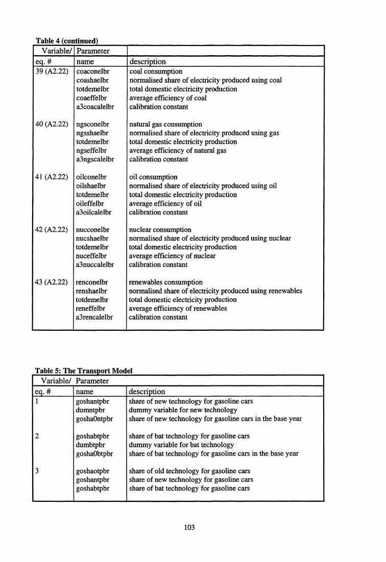
Table 4 (continued)Variable/
,Parameter
eq. # name description39 (A2.22) - coaconelbr coal consumption
coashaelbr normalised share of electricity produced using coaltotdemelbr total domestic electricity productioncoaeffelbr average efficiency of coala3coacalelbr calibration constant
40 (A2.22) ngsconelbr natural gas consumptionngsshaelbr normalised share of electricity produced using gastotdemelbr total domestic electricity productionngseffelbr average efficiency of natural gasa3ngscalelbr calibration constant
41 (A2.22) oilconelbr oil consumptionoilshaelbr normalised share of electricity produced using oiltotdemelbr total domestic electricity productionoileffelbr average efficiency of oila3oilcalelbr calibration constant
42 (A2.22) nucconelbr nuclear consumptionnucshaelbr normalised share of electricity produced using nucleartotdemelbr total domestic electricity productionnuceffelbr average efficiency of nucleara3nuccalelbr calibration constant
43 (A2.22) renconelbr renewables consumptionrenshaelbr normalised share of electricity produced using renewablestotdemelbr total domestic electricity productionreneffelbr average efficiency of renewablesa3rencalelbr calibration constant
Table 5: The Trans ort ModelVariable/ Parameter
eq. # name description1 goshantpbr share of new technology for gasoline cars
dumntpbr dummy variable for new technologygoshaOntpbr share of new technology for gasoline cars in the base year
2 goshabtpbr share of bat technology for gasoline carsdumbtpbr dummy variable for bat technologygoshaObtpbr share of bat technology for gasoline cars in the base year
3 goshaotpbr share of old technology for gasoline carsgoshantpbr share of new technology for gasoline carsgoshabtpbr share of bat technology for gasoline cars
103
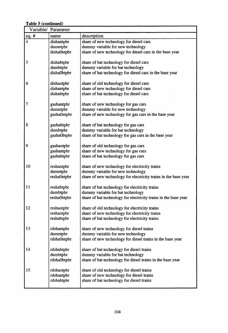
Table 5 (continued)Variable/ Parameter
eq. # name description4 dishantpbr share of new technology for diesel cars
dumntpbr dummy variable for new technologydishaOntpbr share of new technology for diesel cars in the base year
5 dishabtpbr share of bat technology for diesel carsdumbtpbr dummy variable for bat technologydisha0btpbr share of bat technology for diesel cars in the base year
6 dishaotpbr share of old technology for diesel carsdishantpbr share of new technology for diesel carsdishabtpbr share of bat technology for diesel cars
7 gashantpbr share of new technology for gas carsdumntpbr dummy variable for new technologygashaOntpbr share of new technology for gas cars in the base year
8 gashabtpbr share of bat technology for gas carsdumbtpbr dummy variable for bat technologygasha0btpbr share of bat technology for gas cars in the base year
9 gashaotpbr share of old technology for gas carsgashantpbr share of new technology for gas carsgashabtpbr share of bat technology for gas cars
10 reshantpbr share of new technology for electricity trainsdumntpbr dummy variable for new technologyreshaOntpbr share of new technology for electricity trains in the base year
11 reshabtpbr share of bat technology for electricity trainsdumbtpbr dummy variable for bat technologyreshaObtpbr share of bat technology for electricity trains in the base year
12 reshaotpbr share of old technology for electricity trainsreshantpbr share of new technology for electricity trainsreshabtpbr share of bat technology for electricity trains
13 rdshantpbr share of new technology for diesel trainsdumntpbr dummy variable for new technologyrdshaOntpbr share of new technology for diesel trains in the base year
14 rdshabtpbr share of bat technology for diesel trainsdumbtpbr dummy variable for bat technologyrdshaObtpbr share of bat technology for diesel trains in the base year
15 rdshaotpbr share of old technology for diesel trainsrdshantpbr share of new technology for diesel trainsrdshabtpbr share of bat technology for diesel trains
104
Table 5 (continuedVariable/ Parameter
eq. # name description16 bdshantpbr share of new technology for diesel buses
dumntpbr dummy variable for new technologybdsha0ntpbr share of new technology for diesel buses in the base year
17 bdshabtpbr share of bat technology for diesel busesdumbtpbr dummy variable for bat technologybdshaObtpbr share of bat technology for diesel buses in the base year
18 bdshaotpbr share of old technology for diesel busesbdshantpbr share of new technology for diesel busesbdshabtpbr share of bat technology for diesel buses
19 (A5.3) gocsttpbr average cost of gasoline cars per pkmgoshaotpbr share of old technology for gasoline carsgoprcstotpbr variable cost of old technology for gasoline carsgopritpbr gasoline price for carsgoeffotpbr average efficiency of gasoline cars using old technologygoshantpbr share of new technology for gasoline carsgoprcstntpbr variable cost of new technology for gasoline carsgoeffntpbr average efficiency of gasoline cars using new technologygoshabtpbr share of bat technology for gasoline carsgoprcstbtpbr variable cost of bat technology for gasoline carsgoeffbtpbr average efficiency of gasoline cars using bat technology
20 (A5.3) dicsttpbr average cost of diesel cars per pkmdishaotpbr share of old technology for diesel carsdiprcstotpbr variable cost of old technology for diesel carsdipritpbr diesel price for carsdieffotpbr average efficiency of diesel cars using old technologydishantpbr share of new technology for diesel carsdiprcstntpbr variable cost of new technology for diesel carsdieffntpbr average efficiency of diesel cars using new technologydishabtpbr share of bat technology for diesel carsdiprcstbtpbr variable cost of bat technology for diesel carsdieffbtpbr average efficiency of diesel cars using bat technology
21 (A5.3) gacsttpbr average cost of gas cars per pkmgashaotpbr share of old technology for gas carsgaprcstotpbr variable cost of old technology for gas carsgapritpbr gas price for carsgaeffotpbr average efficiency of gas cars using old technologygashantpbr share of new technology for gas carsgaprcstntpbr variable cost of new technology for gas carsgaeffntpbr average efficiency of gas cars using new technologygashabtpbr share of bat technology for gas carsgaprcstbtpbr variable cost of bat technology for gas carsgaeffbtpbr average efficiency of gas cars using bat technology
105
Table 5 (continued)Variable/ Parameter
eq. # name description22 (A5.3) recsttpbr average cost of electricity train per pkm
reshaotpbr share of old technology for electricity trainreprcstotpbr variable cost of old technology for electricity trainrepritpbr electricity price for trainreeffotpbr average efficiency of electricity train using old technologyreshantpbr share of new technology for electricity trainreprcstntpbr variable cost of new technology for electricity trainreeffntpbr average efficiency of electricity train using new technologyreshabtpbr share of bat technology for electricity trainreprcstbtpbr variable cost of bat technology for electricity trainreeffbtpbr average efficiency of electricity train using bat technology
23 (A5.3) rdcsttpbr average cost of diesel train per pkmrdshaotpbr share of old technology for diesel trainrdprcstotpbr variable cost of old technology for diesel trainrdpritpbr diesel price for trainrdeffotpbr average efficiency of diesel train using old technologyrdshantpbr share of new technology for diesel trainrdprcstntpbr variable cost of new technology for diesel trainrdeffntpbr average efficiency of diesel train using new technologyrdshabtpbr share of bat technology for diesel trainrdprcstbtpbr variable cost of bat technology for diesel trainrdeffbtpbr average efficiency of diesel train using bat technology
24 (A5.3) bdcsttpbr average cost of diesel bus per pkmbdshaotpbr share of old technology for diesel busbdprcstotpbr variable cost of old technology for diesel busbdpritpbr diesel price for busbdeffotpbr average efficiency of diesel bus using old technologybdshantpbr share of new technology for diesel busbdprcstntpbr variable cost of new technology for diesel busbdeffntpbr average efficiency of diesel bus using new technologybdshabtpbr share of bat technology for diesel busbdprcstbtpbr variable cost of bat technology for diesel busbdeffbtpbr average efficiency of diesel bus using bat technology
25 (A5.1) goefftpbr average efficiency of gasoline carsgoshaotpbr share of old technology for gasoline carsgoeffotpbr average efficiency of gasoline cars using old technologygoshantpbr share of new technology for gasoline carsgoeffntpbr average efficiency of gasoline cars using new technologygoshabtpbr share of bat technology for gasoline carsgoeffbtpbr average efficiency of gasoline cars using bat technology
106
Table 5 (continued )
Variable/ Parametereq. # name description26 (A5.1) diefftpbr average efficiency of diesel cars
dishaotpbr share of old technology for diesel carsdieffotpbr average efficiency of diesel cars using old technologydishantpbr share of new technology for diesel carsdieffntpbr average efficiency of diesel cars using new technologydishabtpbr share of bat technology for diesel carsdieffbtpbr average efficiency of diesel cars using bat technology
27 (A5.1) gaefftpbr average efficiency of gas carsgashaotpbr share of old technology for gas carsgaeffotpbr average efficiency of gas cars using old technologygashantpbr share of new technology for gas carsgaeffntpbr average efficiency of gas cars using new technologygashabtpbr share of bat technology for gas carsgaeffbtpbr average efficiency of gas cars using bat technology
28 (A5.1) reefftpbr average efficiency of electricity trainreshaotpbr share of old technology for electricity trainreeffotpbr average efficiency of electricity train using old technologyreshantpbr share of new technology for electricity trainreeffntpbr average efficiency of electricity train using new technologyreshabtpbr share of bat technology for electricity trainreeffbtpbr average efficiency of electricity train using bat technology
29 (A5.1) rdefftpbr average efficiency of diesel trainrdshaotpbr share of old technology for diesel trainrdeffotpbr average efficiency of diesel train using old technologyrdshantpbr share of new technology for diesel trainrdeffntpbr average efficiency of diesel train using new technologyrdshabtpbr share of bat technology for diesel trainrdeffbtpbr average efficiency of diesel train using bat technology
30 (A5.1) bdefftpbr average efficiency of diesel busbdshaotpbr share of old technology for diesel busbdeffotpbr average efficiency of diesel bus using old technologybdshantpbr share of new technology for diesel busbdeffntpbr average efficiency of diesel bus using new technologybdshabtpbr share of bat technology for diesel busbdeffbtpbr average efficiency of diesel bus using bat technology
107

Table 5 (continued)Variable/ Parameter
eq. # name description31 (A2.12) goshaltpbr optimal share of gasoline cars
aOgocontpbr calibration constantgocsttpbr average cost of gasoline cars per pkmalgocontpbr cost share of gasoline consumption, carsdicsttpbr average cost of diesel cars per pkmaldicontpbr cost share of diesel consumption, carsgacsttpbr average cost of gas cars per pkmalgacontpbr cost share of gas consumption, carsrecsttpbr average cost of electricity train per pkmalrecontpbr cost share of electricity consumption, trainrdcsttpbr average cost of diesel train per pkmalrdcontpbr cost share of diesel consumption, trainbdcsttpbr average cost of diesel bus per pkmalbdcontpbr cost share of diesel consumption, bus
32 (A2.12) dishaltpbr optimal share of diesel carsa0dicontpbr calibration constantdicsttpbr average cost of diesel cars per pkmgocsttpbr average cost of gasoline cars per pkmalgocontpbr cost share of gasoline consumption, carsaldicontpbr cost share of diesel consumption, carsgacsttpbr average cost of gas cars per pkmalgacontpbr cost share of gas consumption, carsrecsttpbr average cost of electricity train per pkmalrecontpbr cost share of electricity consumption, trainrdcsttpbr average cost of diesel train per pkmalrdcontpbr cost share of diesel consumption, trainbdcsttpbr average cost of diesel bus per pkmalbdcontpbr cost share of diesel consumption, bus
33 (A2.12) gashaltpbr optimal share of gas carsa0gacontpbr calibration constantgacsttpbr average cost of gas cars per pkmgocsttpbr average cost of gasoline cars per pkmalgocontpbr cost share of gasoline consumption, carsdicsttpbr average cost of diesel cars per pkmaldicontpbr cost share of diesel consumption, carsalgacontpbr cost share of gas consumption, carsrecsttpbr average cost of electricity train per pkmalrecontpbr cost share of electricity consumption, trainrdcsttpbr average cost of diesel train per pkmalrdcontpbr cost share of diesel consumption, trainbdcsttpbr average cost of diesel bus per pkmalbdcontpbr cost share of diesel consumption, bus
108

Table 5 (continuedVariable/ Parameter
eq. # name description34 (A2.12) reshaltpbr optimal share of electricity train
aOrecontpbr calibration constantrecsttpbr average cost of electricity train per pkmgocsttpbr average cost of gasoline cars per pkmalgocontpbr cost share of gasoline consumption, carsdicsttpbr average cost of diesel cars per pkmaldicontpbr cost share of diesel consumption, carsgacsttpbr average cost of gas cars per pkmalgacontpbr cost share of gas consumption, carsalrecontpbr cost share of electricity consumption, trainrdcsttpbr average cost of diesel train per pkmalrdcontpbr cost share of diesel consumption, trainbdcsttpbr average cost of diesel bus per pkmalbdcontpbr cost share of diesel consumption, bus
35 (A2.12) rdshaltpbr optimal share of diesel trainaOrdcontpbr calibration constantrdcsttpbr average cost of diesel train per pkmgocsttpbr average cost of gasoline cars per pkmalgocontpbr cost share of gasoline consumption, carsdicsttpbr average cost of diesel cars per pkmaldicontpbr cost share of diesel consumption, carsgacsttpbr average cost of gas cars per pkmalgacontpbr cost share of gas consumption, carsrecsttpbr average cost of electricity train per pkmalrecontpbr cost share of electricity consumption, trainalrdcontpbr cost share of diesel consumption, trainbdcsttpbr average cost of diesel bus per pkmalbdcontpbr cost share of diesel consumption, bus
36 (A2.12) bdshaltpbr optimal share of diesel busa0bdcontpbr calibration constantbdcsttpbr average cost of diesel bus per pkmgocsttpbr average cost of gasoline cars per pkmal gocontpbr cost share of gasoline consumption, carsdicsttpbr average cost of diesel cars per pkmaldicontpbr cost share of diesel consumption, carsgacsttpbr average cost of gas cars per pkmalgacontpbr cost share of gas consumption, carsrecsttpbr average cost of electricity train per pkmalrecontpbr cost share of electricity consumption, trainrdcsttpbr average cost of diesel train per pkmalrdcontpbr cost share of diesel consumption, trainalbdcontpbr cost share of diesel consumption, bus
109

Table 5 (continued)Variable/ Parameter
eq. # name description37 (A2.13) goshatpbr normalised share of gasoline cars
goshaltpbr optimal share of gasoline carsdishaltpbr optimal share of diesel carsgashaltpbr optimal share of gas carsreshaltpbr optimal share of electricity trainrdshaltpbr optimal share of diesel trainbdshaltpbr optimal share of diesel bus
38 (A2.13) dishatpbr normalised share of diesel carsdishaltpbr optimal share of diesel carsgoshaltpbr optimal share of gasoline carsgashaltpbr optimal share of gas carsreshaltpbr optimal share of electricity trainrdshaltpbr optimal share of diesel trainbdshaltpbr optimal share of diesel bus
39 (A2.13) gashatpbr normalised share of gas carsgashaltpbr optimal share of gas carsgoshaltpbr optimal share of gasoline carsdishaltpbr optimal share of diesel carsreshaltpbr optimal share of electricity trainrdshaltpbr optimal share of diesel trainbdshaltpbr optimal share of diesel bus
40 (A2.13) reshatpbr normalised share of electricity trainreshaltpbr optimal share of electricity traingoshaltpbr optimal share of gasoline carsdishaltpbr optimal share of diesel carsgashaltpbr optimal share of gas carsrdshaltpbr optimal share of diesel trainbdshaltpbr optimal share of diesel bus
41 (A2.13) rdshatpbr normalised share of diesel trainrdshaltpbr optimal share of diesel traingoshaltpbr optimal share of gasoline carsdishaltpbr optimal share of diesel carsgashaltpbr optimal share of gas carsreshaltpbr optimal share of electricity trainbdshaltpbr optimal share of diesel bus
42 (A2.13) bdshatpbr normalised share of diesel busbdshaltpbr optimal share of diesel busgoshaltpbr optimal share of gasoline carsdishaltpbr optimal share of diesel carsgashaltpbr optimal share of gas carsreshaltpbr optimal share of electricity trainrdshaltpbr optimal share of diesel train
110

Table 5 (continuedVariable/ Parameter
eq. # name description43 (A2.10) tppribr price index for passenger transport
gocsttpbr average cost of gasoline cars per pkmalgocontpbr cost share of gasoline consumption, carsdicsttpbr average cost of diesel cars per pkmaldicontpbr cost share of diesel consumption, carsgacsttpbr average cost of gas cars per pkmal gacontpbr cost share of gas consumption, carsrecsttpbr average cost of electricity train per pkmalrecontpbr cost share of electricity consumption, trainrdcsttpbr average cost of diesel train per pkmalrdcontpbr cost share of diesel consumption, trainbdcsttpbr average cost of diesel bus per pkmalbdcontpbr cost share of diesel consumption, bustppri9lbr calibration constant
44 (A2.11) totdemindtpbr total demand for passenger transportincomebr consumption expenditure (income)blpkmbr income elasticity for passenger transporttppribr price index for passenger transportb2pkmbr price elasticity fot passenger transport
45 (A2.11) totdemtpbr total demand for passenger transporttotdemindtpbr total demand for passenger transporttotdemtp9lbr calibration constant
46 (A2.14) gocontpbr demand for gasoline (car) in passenger transportaOcalpkmbr calibration constantgoshatpbr normalised share of gasoline carstotdemtpbr total demand for passenger transportgoefftpbr average efficiency of gasoline cars
47 (A2.14) dicontpbr demand for diesel (car) in passenger transportaOcalpkmbr calibration constantdishatpbr normalised share of diesel carstotdemtpbr total demand for passenger transportdiefftpbr average efficiency of diesel cars
48 (A2.14) gacontpbr demand for gas (car) in passenger transportaOcalpkmbr calibration constantgashatpbr normalised share of gas carstotdemtpbr total demand for passenger transportgaefftpbr average efficiency of gas cars
49 (A2.14) recontpbr demand for electricity (train) in passenger transportaOcalpkmbr calibration constantreshatpbr normalised share of electricity traintotdemtpbr total demand for passenger transportreefftpbr average efficiency of electricity train
111

Table 5 (continuedVariable/ Parameter
eq. # name description50 (A2.14) rdcontpbr demand for diesel (train) in passenger transport
aOcalpkmbr calibration constantrdshatpbr normalised share of diesel traintotdemtpbr total demand for passenger transportrdefftpbr average efficiency of diesel train
51 (A2.14) bdcontpbr demand for diesel (bus) in passenger transportaOcalpkmbr calibration constantbdshatpbr normalised share of diesel bustotdemtpbr total demand for passenger transportbdefftpbr average efficiency of diesel bus
52 (A2.15) totdemindtfbr total demand for freight transportgdpindbr gross domestic production (GDP)dumitfbr dummy variable for the integration scenarioblitkmbr income elasticity in the case of the integration scenariodumftfbr dummy variable for the fragmentation scenarioblftkmbr income elasticity in the case of the fragmentation scenario
53 (A2.15) totdemtfbr total demand for freight transporttotdemindtfbr total demand for freight transporttotdemtf9lbr calibration constant
54 nsharotfbr normalised road transport sharesharotfbr road transport sharesharatfbr rail transport shareshawatfbr water transport share
55 nsharatfbr normalised rail transport sharesharatfbr rail transport sharesharotfbr road transport shareshawatfbr water transport share
56 nshawatfbr normalised water transport shareshawatfbr water transport sharesharotfbr road transport sharesharatfbr rail transport share
57 (A2.16) rotkmbr demand for road transportnsharotfbr normalised road transport sharetotdemtfbr total demand for freight transport
58 (A2.16) ratkmbr demand for rail transportnsharatfbr normalised rail transport sharesharaditfbr dummy variable for the integration scenariototdemptfbr total demand for freight transport
112
Table 5 (continued)Variable/ Parameter
eq. # name description59 (A2.16) watkmbr demand for water transport
nshawatfbr normalised water transport sharetotdemtfbr total demand for freight transport
60 (A2.17) dicontfbr demand for diesel in road transportaOcalplanbr calibration constantrotkmbr demand for road transportroefftfbr average efficiency of diesel used in road transporta3ditftbr coefficient for technological improvement
61 (A2.17) elcontfbr demand for electricity in rail transportaOcalrelbr calibration constantratkmbr demand for rail transportsharaditfbr dummy variable for the integration scenarioraefftfbr average efficiency of electricity used in rail transporta3eletftbr coefficient for technological improvement
62 (A2.17) oilcontfbr demand for oil in water transportaOcalwkmbr calibration constantwatkmbr demand for water transportwaefftfbr average efficiency of oil used in water transporta3oiltftbr coefficient for technological improvement
63 (A2.18) oilconindfabr demand for air fuel (kerosene)gdpindbr gross domestic production (GDP)bltabr income elasticityoilpritabr price of keroseneb2tabr price elasticitya3oiltfabr lag/adjustment coefficient
64 (A2.18) oilconfabr demand for air fuel (kerosene)oilconindfabr demand for air fuel (kerosene)oilconfa9lbr calibration constant
65 aircontotbr total demand for air fuel (kerosene)oilconfabr demand for air fuel (kerosene)
66 roadcontotbr total demand for fuel in road transportgocontpbr demand for gasoline (car) in passenger transportdicontpbr demand for diesel (car) in passenger transportgacontpbr demand for gas (car) in passenger transportbdcontpbr demand for diesel (bus) in passenger transportdicontfbr demand for diesel in road transport
67 railcontotbr total demand for electricity in rail transportrecontpbr demand for electricity (train) in passenger transportelcontfbr demand for electricity in rail transport
113
Table 5 (continued)Variable/ Parameter
eq. # name description68 railcondiebr demand for diesel in rail transport
rdcontpbr demand for diesel (train) in passenger transportaOcalrdibr calibration constantratkmbr demand for rail transportsharaditfbr dummy variable for the integration scenarioraefftfbr average efficiency of electricity used in rail transport
69 watcontotbr total demand for fuel in water transportoilcontfbr demand for oil in water transport
Table 6: The Price ModelVariable/ Parameter
eq. # name description1 (2.43) coaprisinbr end user price of coal in the industry sector, USD per toe
coaimppribr import price of coal in Germanycoamrginbr price margin on coal in the industry sectorcoataxinbr excise tax on coal in the industry sectorcco2taxinbr co2 tax on coal in the industry sectorcoavatinbr value added tax on coal in the industry sector
2 coapriinbr end user price of coal in the industry sectorcoaprisinbr end user price of coal in the industry sector, USD per toe
3 (2.43) coaprissebr end user price of coal in the service sector, USD per toecoaimppribr import price of coal in Germanycoamrgsebr price margin on coal in the service sectorcoataxsebr excise tax on coal in the service sectorcoavatsebr value added tax on coal in the service sector
4 coaprisebr end user price of coal in the service sectorcoaprissebr end user price of coal in the service sector, USD per toe
5 (2.43) coaprishobr end user price of coal in the household sector, USD per toecoaimppribr import price of coal in Germanycoamrghobr price margin on coal in the household sectorcoataxhobr excise tax on coal in the household sectorcco2taxhobr co2 tax on coal in the household sectorcoavathobr value added tax on coal in the household sector
6 coaprihobr end user price of coal in the household sectorcoaprishobr end user price of coal in the household sector, USD per toe
114

Table 6 (continuedVariable/ Parameter
eq. # name description7 (2.43) coapriselbr end user price of coal in the electricity sector, USD per toe
coaimppribr import price of coal in Germanycoamrgelbr price margin on coal in the electricity sectorcoataxelbr excise tax on coal in the electricity sectorcoavatelbr value added tax on coal in the electricity sector
8 coaprielbr end user price of coal in the electricity sectorcoapriselbr end user price of coal in the electricity sector, USD per toe
9 (2.43) oilprisinbr end user price of oil in the industry sector, USD per toeoilimppribr import price of oil in Germanyoilmrginbr price margin on oil in the industry sectoroiltaxinbr excise tax on oil in the industry sectoroco2taxinbr co2 tax on oil in the industry sectoroilvatinbr value added tax on oil in the industry sector
10 oilpriinbr end user price of oil in the industry sectoroilprisinbr end user price of oil in the industry sector, USD per toe
11 (2.43) oilprissebr end user price of oil in the service sector, USD per toeoilimppribr import price of oil in Germanyoilmrgsebr price margin on oil in the service sectoroiltaxsebr excise tax on oil in the service sectoroco2taxsebr co2 tax on oil in the service sectoroilvatsebr value added tax on oil in the service sector
12 oilprisebr end user price of oil in the service sectoroilprissebr end user price of oil in the service sector, USD per toe
13 (2.43) oilprishobr end user price of oil in the household sector, USD per toeoilimppribr import price of oil in Germanyoilmrghobr price margin on oil in the household sectoroiltaxhobr excise tax on oil in the household sectoroco2taxhobr co2 tax on oil in the household sectoroilvathobr value added tax on oil in the household sector
14 oilprihobr end user price of oil in the household sectoroilprishobr end user price of oil in the household sector, USD per toe
15 (2.43) oilpriselbr end user price of oil in the electricity sector, USD per toeoilimppribr import price of oil in Germanyoilmrgelbr price margin on oil in the electricity sectoroiltaxelbr excise tax on oil in the electricity sectoroilvatelbr value added tax on oil in the electricity sector
16 oilprielbr end user price of oil in the electricity sectoroilpriselbr end user price of oil in the electricity sector, USD per toe
115
Table 6 (continued)Variable/ Parameter
eq. # name description17 (2.43) ngsprisinbr end user price of gas in the industry sector, USD per toe
ngsimppribr import price of gas in Germanyngsmrginbr price margin on gas in the industry sectorngstaxinbr excise tax on gas in the industry sectornco2taxinbr co2 tax on gas in the industry sectorngsvatinbr value added tax on gas in the industry sector
18 ngspriinbr end user price of gas in the industry sectorngsprisinbr end user price of gas in the industry sector, USD per toe
19 (2.43) ngsprissebr end user price of gas in the service sector, USD per toengsimppribr import price of gas in Germanyngsmrgsebr price margin on gas in the service sectorngstaxsebr excise tax on gas in the service sectornco2taxsebr co2 tax on gas in the service sectorngsvatsebr value added tax on gas in the service sector
20 ngsprisebr end user price of gas in the service sectorngsprissebr end user price of gas in the service sector, USD per toe
21 (2.43) ngsprishobr end user price of gas in the household sector, USD per toengsimppribr import price of gas in Germanyngsmrghobr price margin on gas in the household sectorngstaxhobr excise tax on gas in the household sectornco2taxhobr co2 tax on gas in the household sectorngsvathobr value added tax on gas in the household sector
22 ngsprihobr end user price of gas in the household sectorngsprishobr end user price of gas in the household sector, USD per toe
23 (2.43) ngspriselbr end user price of gas in the electricity sector, USD per toengsimppribr import price of gas in Germanyngsmrgelbr price margin on gas in the electricity sectorngstaxelbr excise tax on gas in the electricity sectornco2taxelbr co2 tax on gas in the electricity sectorngsvatelbr value added tax on gas in the electricity sector
24 ngsprielbr end user price of gas in the electricity sectorngspriselbr end user price of gas in the electricity sector, USD per toe
25 (2.43) eleprisinbr end user price of electricity in the industry sector , USD per toeelegenpribr electricity generation price (cost)elemrginbr price margin on electricity in the industry sectoreletaxinbr excise tax on electricity in the industry sectorelevatinbr value added tax on electricity in the industry sector
26 elepriinbr end user price of electricity in the industry sectoreleprisinbr end user price of electricity in the industry sector , USD per toe
116

Table 6 (continuedVariable/ Parameter
eq. # name description27 (2.43) eleprissebr end user price of electricity in the service sector , USD per toe
elegenpribr electricity generation price (cost)elemrgsebr price margin on electricity in the service sectoreletaxsebr excise tax on electricity in the service sectorelevatsebr value added tax on electricity in the service sector
28 eleprisebr end user price of electricity in the service sectoreleprissebr end user price of electricity in the service sector , USD per toe
29 (2.43) eleprishobr end user price of electr. in the household sector , USD per toeelegenpribr electricity generation price (cost)elemrghobr price margin on electricity in the household sectoreletaxhobr excise tax on electricity in the household sectorelevathobr value added tax on electricity in the household sector
30 eleprihobr end user price of electricity in the household sectoreleprishobr end user price of electr. in the household sector, USD per toe
31 (2.43) gopristpbr end user price of gasoline in the passenger transp., USD per toegoimppribr import price of gasoline in Germanygomrgtpbr price margin on gasoline in the passenger transportgotaxtpbr excise tax on gasoline in the passenger transportgoco2taxtpbr co2 tax on gasoline in the passenger transportgovattpbr value added tax on gasoline in the passenger transport
32 gopritpbr end user price of gasoline in the passenger transportgopristpbr end user price of gasoline in the passenger transp., USD per toe
33 (2.43) dipristpbr end user price of diesel in the passenger transport, USD per toediimppribr import price of diesel in Germanydimrgtpbr price margin on diesel in the passenger transportditaxtpbr excise tax on diesel in the passenger transportdico2taxtpbr co2 tax on diesel in the passenger transportdivattpbr value added tax on diesel in the passenger transport
34 dipritpbr end user price of diesel in the passenger transportdipristpbr end user price of diesel in the passenger transport, USD per toe
35 rdpritpbr end user price of diesel in the rail passenger transportdipritpbr end user price of diesel in the passenger transportdivattpbr value added tax on diesel in the passenger transport
36 bdpritpbr end user price of diesel in the bus passenger transportdipritpbr end user price of diesel in the passenger transportdivattpbr value added tax on diesel in the passenger transport
37 gapritpbr end user price of gas in the passenger transportdipritpbr end user price of diesel in the passenger transport
117

Table 6 (continuedVariable/ Parameter
eq. # name description38 repritpbr end user price of electricity in the rail passenger transport
eleprissebr end user price of electricity in the service sector , USD per toe
39 oilpritabr end user price of oil (kerosene) in the air transportoilprishobr end user price of oil in the household sector, USD per toe
118
References
Brubakk, L., Aaserud, M., Hammelen, T.V., Pellekaan, W., and Ostvoorn, F.V. (1995): SEEM- Amodel documentation Version 2.0, forthcoming in the series Rapporter, Statistics Norway, and in thereport series of ECN (The Netherlands Energy Research Foundation).
Aaserud, M., Brubakk, L., Ostvoorn, F.V., and Pellekaan, W. (1995): Energy scenarios for aChanging Europe, unpublished executive summary.
Hollinger, P. and Spivatovsky, L. (1993): Portable Troll Reference Manual, Latex Solutions, Inc.
119

Issued in the series Documents
94/1 Haakon Vennemo (1994): Welfare and theEnvironment. Implications of a Recent TaxReform in Norway.
94/2 Knut H. Alfsen (1994): Natural ResourceAccounting and Analysis in Norway.
94/3 Olav Bjerkholt (1994): Ragnar Frisch 1895-1995.
95/1 Anders Rygh Swensen (1995): SimpleExamples on Smoothing MacroeconomicTime Series.
95/2 Eystein Gjelsvik, Torgeir Johnsen, HansTerje Mysen and Asgeir Valdimarsson(1995): Energy Demand in Iceland
95/3 Chunping Zhao, Olav Bjerkholt, ToreHalvorsen and Yu Zhu (1995): The Flow ofFunds Accounts in China
95/4 Nordic Indicator Group (1995): NordicEnvironmental Indicators. Draft document.English version with main points fromcomments received.
95/5 Hanne A. Gravningsmyhr (1995): AnalysingEffects of Removing Survivors' Pensions,Using the Microsimulation Model LO
95/6 Pal Boug (1995): User's Guide. The SEEM-model Version 2.0.
120
Documents
Statistics NorwayResearch DepartmentP.O.B. 8131 Dep.N-0033 Oslo
Tel.: + 47 - 22 86 45 00Fax: + 47 - 22 11 12 38
ISSN 0805-9411
0040 Statistics NorwayResearch Department