Bulletin of Mathematical Biology VoL 51, No. 3, pp. 325--335, 1989. Printed in Gte.at Britain.

0092-8240/8953.00 + 0.00 Pergamon ~ pie

�9 1989 Society for Mathematical Biology

U P P E R AND LOWER B OUNDS F R O M THE M A X I M U M PRINCIPLE. INTRACELLULAR D I F F U S I O N WITH M I C H A E L I S - M E N T E N KINETICS

M6NICA C. REGALBUTO, WILLIAM STRIEDER* and ARVIND VARMA Department of Chemical Engineering University of Notre Dame Notre Dame, IN 46556, U.S.A.

Analytical bounding functions for diffusion problems with Michaelis-Menten kinetics were recently presented by Anderson and Arthurs, 1985 (Bull. math. Biol. 47, 145-153). Their method, successful to some extent for a small range of parameters, has the disadvantage of providing a weak upper bound. The optimal approach for the use of one-line bounding kinetics is presented. The use of two-line bounding kinetics is also shown, in order to give sufficient accuracy in those cases where the one-line approach does not provide satisfactory results. The bounding functions provide excellent upper and lower bounds on the true solution for the entire range of kinetic and transport parameters.

1. In t roduc t ion . Steady-state intracellular oxygen diffusion within a spherical cell (Lin, 1976; McElwain, 1978) can be represented by the following equation:

d2u t_ ! ~rU +f(u)=0, dr 2 O < r < l , (1)

with Michaelis-Menten uptake kinetics,

f ( u ) = - ~u/(u + gm) , (2)

and the two boundary conditions,

u'(0) =0, u'(1)=H{1 --u(1)}. (3)

The variable u is a measure of the oxygen tension, whose value, from equations (1)-(3), is unique and positive (Hiltmann and Lory, 1983). The primes in equation (3) represent differentiation of the function with respect to its independent variable; in the case of u(r), the radial coordinate r. The positive constants ~, H, and K m involve the reaction rate, cell wall permeability, and Michaelis constant.

Although equations (1) to (3) above are presented in the context of transport and uptake of oxygen in a spherical cell, they in fact have wider biological

* Author to whom correspondence should be addressed.

325

326 M . C . R E G A L B U T O et al.

applicability. It is well-known that the apparent behavior of many biological and biochemical processes is well represented by diffusive mass transport coupled with the Michaelis-Menten reaction rate expression (cf. Bailey and Ollis, 1986). Thus these equations are appropriate for a wide variety of biological applications, ranging from applied enzyme catalysis to cellular reactions. Furthermore, the simple methods presented in this work could also be used with advantage to estimate kinetic parameters from experimental data in diffusionally influenced biological systems.

In previous publications (Aris, 1975; Villadsen and Michelsen, 1978; Oh et al., 1978; Varma and Strieder, 1985; Anderson and Arthurs, 1985; Regalbuto et al., 1988), it was shown that the construction of bounding kinetics:

f (u) (u) <.f (u), (4)

can be used to generate upper and lower solutions for equations of the type (1)-(3) from the Maximum Principle. In l~articular if f is used in place of f i n equation (1), a lower bound solution ti(r;f) and iffis used in equation (1), an upper bound solution t~(r;f) is generated:

a(r; f ) a(r; f). (5)

It was also suggested that a direct variation of f and fcould be applied to tighten the rigorous bounds on u(r). It is of practical interest to develop efficient optimization schemes in order to provide the best bounds that can be obtained by using 1, 2, or more lines to construct upper and lower bounding kinetics. Anderson and Arthurs (1985) have recently provided upper and lower bounds on u(r) using one-line bounding kinetics. Even using only one line, their upper bound can be improved, and the optimal upper bound is thus developed here. For some combinations of the kinetic and transport parameters 0~, H and K m, one-line bounding kinetics do not produce accurate results. In such cases, the use of two lines with appropriate optimization is shown to provide sufficient accuracy without much additional work.

2. One-Line Bounding Kinetics. For the one-line case (see Fig. 1) both the lower and upper bounding kinetics can always be expressed in terms of slope - m and intercept " b as:

f ( o r / . ) = - - m u - - b , (6)

where m and b are both non-negative. The analytical form that will bound the solution u both from below and above can be obtained in terms of m and b, by replacing equation (2) with equation (6) and solving equations (1) and (3):

ti(or fi) = 6r - ' sinh(x/~ r ) - b/m, (7)

M I C H A E L I S - - M E N T E N K I N E T I C S 327

where:

G= H{ 1 + b/m}/{w/-m cosh(~jFm) + (H- - 1)sinh(~/-m)}.

A plot of the reaction kinetics (2) in Fig. 1 shows that the function f is concave up. A single line drawn tangent t o fwi th a slope:

f ' (u) = -- aKm/(U + K~) 2, (8)

at the tangent point ti" provides a lower bounding kineticsfwith:

fit= --f'((t'), g= --rha'--f(~'). (9)

Substitution of equation (9) into equation (7) generates a lower bound ti(r) for any r. For each r value the tangent point can be varied between 0 and 1, and a value tiop t selected that gives the best lower bound tiopt(r ) which can be obtained with a single line. Anderson and Arthurs (1985) have done this and in particular for the case r = 0 list two values: Ziopt(0)=0.828471 for a=0.76129, H = 5 , Km =0.03119 and tiopt(0)=0.278878 for a = 10, H = 5 , Kin= 1.

0 u

fl .

f (u) f2

1 I I I i I I l

- ~ I

1 +Kin I I

~opl(O) ~1" 0..(1) fi~ (1

Figure 1. Reaction kinetics f(u) for K m > 0 and the various constructed one-line upper and lower bounding kinetics. Included in the figure is the lower bound- ing kinetics fwith associated tangent point a" and optimum global lower bound aopt(0 ). Also shown are the members of the upper bounding kinetics sequencer 1 ,f2,

fo~, along with the associated global upper bounds ~a(1), and t~(1)i

328 M.C. REGALBUTO et al.

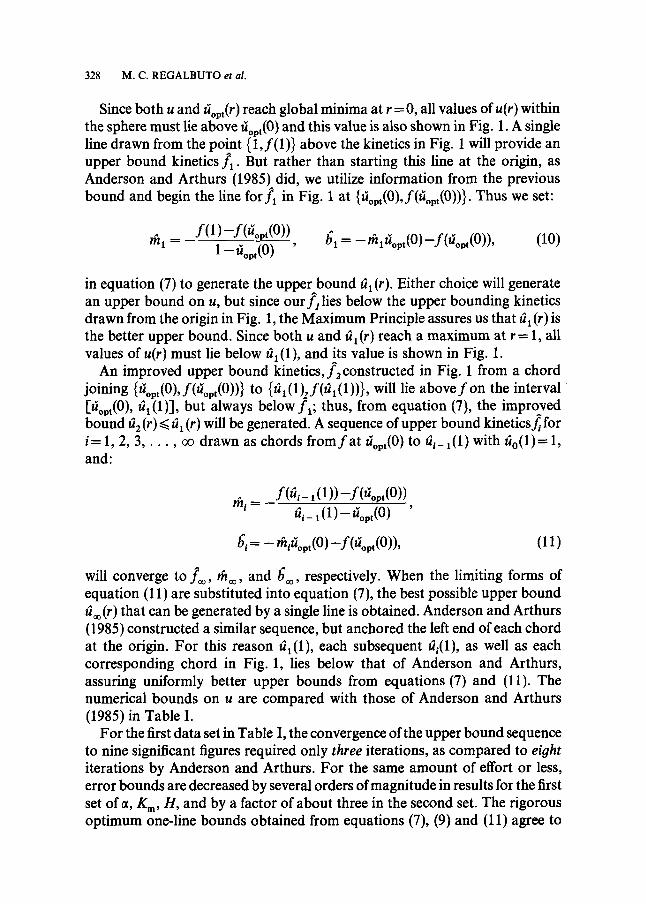
Since both u and t~opt(r ) reach global minima at r = 0, all values of u(r) within the sphere must lie above tioot(0 ) and this value is also shown in Fig. 1. A single line drawn from the point {1,f(1)} above the kinetics in Fig. 1 will provide an upper bound kinetics f l . But rather than starting this line at the origin, as Anderson and Arthurs (1985) did, we utilize information from the previous bound and begin the line forf~ in Fig. 1 at {l~opt(0),f(l~opt(0)) } . Thus we set:

rh 1 = _f(1)--f(Uopt(0)) 1 -t iopt(O ) '

~1 ~'= -- }~ll/~opt(0) --f(/~opt(0)), (10)

in equation (7) to generate the upper bound ti 1 (r). Either choice will generate an upper bound on u, but since our f l lies below the upper bounding kinetics drawn from the origin in Fig. 1, the Maximum Principle assures us that til(r) is the better upper bound. Since both u and adr) reach a maximum at r = 1, all values of u(r) must lie below a~(1), and its value is shown in Fig. 1.

An improved upper bound kinetics, f2constructed in Fig. 1 from a chord joining {/~opt (0), f(t~op t (0))} to { ti I (1), f (a I (1))}, will lie above f on the interval [tiovt(0 ), t~l(1)], but always below ff i thus, from equation (7), the improved bound a 2 (r)~< ti 1 (r) will be generated. A sequence of upper bound kinetics~ for i= 1, 2, 3, . . . , ~ drawn as chords from f a t tiopt(0 ) to ti,_ 1(1 ) with ao(1)= 1, and:

th i = _ f (fii- , (1)) --f(5opt(O)) /~i_ 1 (1) __ ~opt(0 ) '

/~/= --/~l/aopt (0) --f(t~opt (0)) , (11 )

will converge to foo, rho0, and 600, respectively. When the limiting forms of equation (11) are substituted into equation (7), the best possible upper bound aoo(r) that can be generated by a single line is obtained. Anderson and Arthurs (1985) constructed a similar sequence, but anchored the left end of each chord at the origin. For this reason tix(1 ), each subsequent ai(1), as well as each corresponding chord in Fig. 1, lies below that of Anderson and Arthurs, assuring uniformly better upper bounds from equations (7) and (11). The numerical bounds on u are compared with those of Anderson and Arthurs (1985) in Table I.

For the first data set in Table I, the convergence of the upper bound sequence to nine significant figures required only three iterations, as compared to eight iterations by Anderson and Arthurs. For the same amount of effort or less, error bounds are decreased by several orders of magnitude in results for the first set of a, K m, H, and by a factor of about three in the second set. The rigorous optimum one-line bounds obtained from equations (7), (9) and (11) agree to

MICHAELIS-MENTEN KINETICS 329

TABLE I Upper and Lower Bounds on u for a=0.76129, H - 5 and Kin=0.03119

Anderson Hiltmann Optimum one-line and Arthurs and Lory bounds Two-line bounds

(1985) (1983) equation (7) equation (14)

0.0 0.834537 + 0.006066 0.828483 0.2 0.839153+0.005789 0.833375 0.4 0.853045 + 0.005001 0.848053 0.6 0.876338+0.003815 0.872528 0.8 0.909248+0.002433 0.906819 1.0 0.952080+0.001136 0.950946

0.828488-t-0.000012 0.833380 + 0.000012 0.848058 + 0.000011 0.872534 + 0.000009 0.906822__+ 0.000007 0.950947 + 0.000003

0.828483 + 0.000004 0.833375 +0.000004 0.848053 _ 0.000004 0.872528 + 0.000003 0.906819 + 0.000002 0.950946 ___ 0.000001

Upper and Lower Bounds on u for a = 10, H = 5, K m = 1

Anderson and Arthurs Optimum one-line Two-line bounds (1985) bounds equation (7) equation (14)

0.0 0.313680+0.034802 0.289000+0.010122 0.284954+0.003723 0.2 0.327882-t-0.033801 0.304236+0.010155 0.300154+0.003569 0.4 0.372309___+0.030786 0.351856+0.009976 0.347617+0.003146 0.6 0A52719 +0.025715 0.437508+__0.009065 0.433199+0.002583 0.8 0.581185__+0.017087 0.571059+0.006823 0.567562+0.002094 1.0 0.771563___0.008209 0.766861+0.003507 0.765354+0.001082

five significant figures with the numerical calculations of Hil tmann and Lory (1983); these authors performed computat ions using the multiple shooting method, and their results are also listed in Table I.

3. Two-Line Bounding Kinetics. The use of a one-line optimization will produce quite accurate results when the kinetic and transport parameters ~, H and K m are such that 5opt(0) and a~(1) are relatively close. However, when the parameters are such that the interval between aop,(0 ) and a~(1) is wide, the one-line bounds produce less accurate results, and a two-line approach (Regalbuto et al., 1988) may become necessary. For the case in which l o w e r f and upper f b o u n d i n g kinetics are formed by two straight lines, they can be represented in terms of the intercept u*:

f-(orf-)= - m - u - b - u~u* (12a)

f+(orf§ - m + u - b + u>~u*, (12b)

and:

330 M.C. REGALBUTO e t a l .

u*=(b + - b - ) / ( m - - m +) (13)

where m • and b • are non-negative. A direct substitution of these f - a n d f § into equations (1) and (3) analytically gives the upper or lower bound on u. The solution requires the continuity of fi (or ti) and its derivative at the point r*, the radial position coordinate where the analytical bound equals u*, i.e. at the radial position that divides f - and f + . Note that the same analytical form applies without modification to both upper and lower bounds; only the values of m • and b • need to be changed.

- 2 A s i n h ( x / ~ r) b -

r m

a(or a)= B exp(x/~ + r) + C e x p ( - x / ~ r)

?" r

b +

m +,

(14a)

r>r*. (14b)

The values of the constants A, B and C are given in Table II in terms of m- , b - , m +, b § and r*. The value of r* can be calculated as the root of:

u* -+ 2A sinh,v .. - r r*) ~- b - = 0, (16) r* m -

where u* is given in terms of the geometrical parameters m - , b - , m + and b + for either of the bounding kinetics from equation (13).

The two-line approach can use as a starting u interval either [tiopt(0 ), ~oo(1)] for cases where the one-line bounds have been calculated, or [0, 1-l. In general, u values may be restricted to some subinterval from tiao up to t~o, and these values along with the kinetics f a r e shown in Fig. 2. A two-line lower bounding kinetics f ~ which can be constructed within this interval [ti~o, a,o ] from straight line segments--the first drawn tangent from f a t fiao to the intersection uaa ~* , and the second drawn tangent to f a t the point ti:~ from tiao up to ti*~--is also shown in Fig. 2. A sequential motion of ti~, t to variationally maximize the lower bound (14) for every r guarantees an improvement and would give the best bound, but this requires a numerical sequence of repeated calculations. An alternative simpler procedure, which gives satisfactory accuracy (Regalbuto, 1988), selects the specific tangent point ti: 1 that minimizes the area in Fig. 2 b e t w e e n f ~ a n d f f r o m ti ~otO a ~d

v o m 1 v v 2 ual-g[Uao-3Km+x/U~o + lOKm~O+8fi,o(Km+~,o)+9K2]. (17)

MICHAELIS-MENTEN KINETICS 331

TABLE II Values for the Constants A, B, and C Used in equations (14a), (14b) and

(16)

,4 - OSa) 2 sinh(x/~ ~ r*)

- b2bar* r x / ~ r*) + babsr* (b + B=

bab6 r* e x p ( x / ~ r*)+blbar* exp(- x / / ~ - r*)

C = (b 1 B+b2) /b 3

b x = ( H - 1 + x / ~ ) e x p ( x / ~ )

b 2 = --H(1 +b+/m +)

ba= ( - H + l + x ~ ) e x p ( - x / - ~ )

b, = x/'-m 7 sinh(x/'m -~- r*)+ ~ c o s h ( x ~ r*)

b s = - s i nh (x /~ r*) + x/-m z r* eosh (x /~ r*)

(15b)

(15c)

(lSd)

(15e)

05f)

(15g)

(15h)

(15i)

Withfalas shown in Fig. 2, instead of f i n equations (1) and (3), a lower bound fiaa of the form of equation (14) is obtained. The slope and intercept of the bounding kinetics as defined by equation (12) can be taken from Fig. 2:

m~ = - f ' ( a h ) ,

b\~ = - " ~ a h - f ( a h ) ,

.~5 = - f ' (a .o ) ,

b\] = - m5 a .o - f (a .o ) ,

with:

(18a)

(18b)

(18c)

(18d)

v , v + u.1 = (b.1 - / ~ )t(rh~ - rh + ). (19)

The kinetic expressionf(u) and its derivativef'(u) with respect to u are given respectively by equations (2) and (8). A substitution of equations (17)-(18d)

332 M . C . R E G A L B U T O et al.

into equations (15a)-(15i) of Table II gives the coefficients of equations (14) and (16) in terms of r*. The combination of equation (16) with equation (19) provides a root equation for r*, which requires an iterative numerical calculation. Once r* is determined, the analytical lower bound a,~ (r) is given by equations (14a) and (b). As both t~,l(r ) and u(r) reach global minimum values at r = 0, all values of u must lie above aa~ (0) and its value is indicated in Fig. 2.

0 u

f (u)

I ^ a I f a l

I I

I + K ~ I ' I i

a0 I]a0

Figure 2. Reaction kinetics f(u) for Km> 0 and the various constructed two-line upper and lower bounding kinetics over the u interval ti.o to aao. Included on the figure is the area optimized lower bounding kinetics./. 1 with the associated tangent point ti~x, intercept point u.l"* and the global ̂lower bound a,,l (0). Also shown are the area optimum upper bounding kineticsf,~, the intercept u*l, and the global upper

bound a,l(1) on u.

Two-line upper bounding kinetics fal, constructed (Fig. 2) by two con- "* "* the fcurve with nected straight line segments joining the point {%1 ,f(u,1)} on

{a,l(0), f(t~l(0))} and {a,o, f (a ,o )} , will lie below a one-line kinetics l a n d generate an upper bound t~a~ (r). Numerical minimization of the upper bound over a sequence of a* 1 values between ti~l(0) and aao for every u(r) will give the best upper bound function, but area-optimal kinetics again require only a single calculation. The point a*~, that minimizes the area between f and fa~, over the interval ~,~(0) to ti,o, can be obtained by analytical manipulations:

"* = J K + a . (o) a.o + K,.a. (0)+ K.a.o -Kin. Ual (20)

The slope and intercept of the upper bound kinetics as defined by equation (12) can be obtained from examination of Fig. 2:

M I C H A E L I S - M E N T E N K I N E T I C S 333

f i t_= (21a) '

g - = - - m u,.1--f(ual), (21b)

and:

fi t+= f(a~~ (21c) A All t ,

U a o - - Ua I

6 + = - - m u.t--f(u.l ). (21d)

In a manner similar to the two-line lower bound, when the geometrical parameters (20) and (21) are substituted into equations (14)-(16), an upper bound u~l (r), and a global maximum u~l (1) on all values of u, is obtained. The value of ~31(1) is shown in Fig. 2. As in the lower bound calculation, the solution of equation (16) for r* in the upper bound calculation also requires a single root calculation. Now beginning with t~l(1) and ti~l(0), the entire cycle for the two-line bounding kinetics can be repeated, generating a new tangent a~2 forf,2with global minimum a~2(0 ), a new intersection point 0a* for~2, and new improved bounds t~a2(r ) with global maximum a.2(1) for the price of two root calculations.

Numerical values and error bounds for the two-line method are listed in Table I for comparison with Anderson and Arthurs (1985) and the optimum one-line results. In the first data set, convergence following the two-line procedure introduced in Fig. 2 was achieved in only two cycles to nine decimal places, and all six figures now agree with Hiltmann and Lory (1983).

It is a common practice to express solution accuracy and convergence (Sawyer, 1978) in terms of the norm of the error e:

[ [El i=If ~ e 2 dr ] 1/2. (22)

The values in Table I provide a point-wise maximum on the error:

e(r) <~ a(r)- a(r) (23) 2 '

and with equations (22) and (23) the maximum principle results for the optimum one-line and two-line methods inherently give a maximum norm Ilgmaxll of the error. For the first set of bounds in Table I, IIEmJ for the Anderson and Arthurs results is 4.43 x 10-3, the optimum one-line kinetics is 1.03 x 10 -5, and the two-line area optimum kinetics is 3.32 x 10 -6. For the

334 M.C. REGALBUTO et al.

second set of bounds, the maximum error norms are 2.72 x 10-2, 8.84 x 10-3 and 2.88 x 10 -a, respectively.

Reciprocal bounds were computed for a wide range of parameter values, 2 ~< H~< 100, 0.01 ~< K,, ~< 5, and 0.01 ~< �9 ~< 100. The one-line approach was used when IgmaxII was less than 0.001, and two lines when it was greater. Plots of IIE a [for the case H - 5, and for various K m from 0.1 up to 2, are shown vs the variable ~/(1 + K~) in Fig. 3. For either large or small extremes of ~/(1 + Kin), the u(r) range from r = 0 to r = 1 is small. In such cases, only a small fraction of the fcu rve is used, and very accurate u bounds can be obtained with a single line. Dividing the reaction rate constant 0~ by (1 + K~) shifts the maxima of the various K~ curves to a narrow region on the plot for easy representation. An absolute maximum for all Km occurs near ~/(1 + Kin) = 6.

0.025 H = 5

t ' t 0 .020 I,.,~.~'- km= 0.1

i 005 I ~ 0.02

0.015

Ir Emax II 0.5 0.010

0.005

t . I I I I O0 20 40 60 80 1 O0

I + K m

Figure 3. Maxima in the norm of the error [IEm,,[[ vs •/(1 + Kin) for H = 5 and various values o f K m. Note that an absolute maximum of 0.023 is attained at Km =0.1 and

~/(1 + Kin)= 6.25.

The error's norm curves in Fig. 3 for H = 5 are typical of those for the other H values we considered. A maximum was always observed in the same region on the abscissa. The maximum value of the error's norm for the full range of H, K~ and ~ was 0.03, and it occurred at H = 100. Typically 2 cycles were required to obtain three-figure accuracy, and in the worst case at H = 50, ~ = 10.8, K~ = 0.2, convergence was attained in 4 cycles. Additional improvements could be included in the two-line calculation, for example the right hand segment o f~ l in Fig. 2 could be iterated as fwas in Fig. 1. However, the one-and two-line methods as presented seem to have the proper balance of ease of application along with sufficient accuracy.

MICHAELIS-MENTEN KINETICS 335

L I T E R A T U R E

Anderson, N. and A. M. Arthurs. 1985. "Analytical Bounding Functions for Diffusion Problems with Michaelis-Menten Kinetics." Bull. math. Biol. 47, 145-153.

Aris, R. 1975. The Mathematical Theory of Diffusion and Reaction in Permeable Catalysts, Vols I and II. Oxford: Clarendon Press.

Bailey, J. E. and D. F. Ollis. 1986. Biochemical Engineering Fundamentals (Second edn). New York: McGraw-Hill.

Hiltmann, P. and P. Lory. 1983. "On Oxygen Diffusion in a Spherical Cell with Michaelis-Menten Oxygen Uptake Kinetics." Bull. math. Biol. 45, 661~64.

Lin, S. H. 1976. "Oxygen Diffusion in a Spherical Cell with Nonlinear Oxygen Uptake Kinetics." J. theor. Biol. 60, 449-457.

McElwain, D. L. S. 1978. "A Re-examination of Oxygen Diffusion in a Spherical Cell with Michaelis-Menten Oxygen Uptake Kinetics." J. theor. Biol. 71,255-263.

Oh, S. H., L. L. Hegedus and R. Aris. 1978. "Temperature Gradients in Porous Catalyst Pellets." Ind. Engng. Chem. Fundam. 17, 309-313.

Regalbuto, M. 1988. PhD Thesis, University of Notre Dame. , W. Strieder and A. Varma. 1988. "Approximate Solutions for Nonlinear Diffusion-

Reaction Equations from the Maximum Principle." Chem. Engng Sci. 43, 513-518. Sawyer, W. W. 1978. A First Look at Numerical Functional Analysis. Oxford: Clarendon Press. Varma, A., and W. Strieder. 1985. "Approximate Solutions of Non-linear Boundary-Value

Problems." IMA J. appl. Math. 34, 165-171. Villadsen, J. and M. L. Michelsen. t978. Solution of Differential Equation Models by Polynomial

Approximation. Englewood Cliffs, NJ: Prentice-Hall.

Received 17 M a r c h 1988 Revised 10 N o v e m b e r 1988