Untitled - Journal of Mechanical Engineering - Universiti Teknologi ...
231
-
Upload
khangminh22 -
Category
Documents
-
view
1 -
download
0
Transcript of Untitled - Journal of Mechanical Engineering - Universiti Teknologi ...


JOURNAL OF MECHANICAL ENGINEERING
An International Journal
Vol 18 (2) 15 April 2021 ISSN 1823-5514 eISSN 2550-164X 1 Computational Analysis of Soft Polymer Lattices for 3D Wound Dressing
Materials Muhammad Hanif Nadhif , Muhammad Irsyad, Muhammad Satrio Utomo, Muhammad Suhaeri, and Yudan Whulanza*
1
2 Sustainable Surface Water Dissolved Oxygen Monitoring at Lake 7/1F, Shah Alam, Selangor Norashikin M. Thamrin*, Megat Syahirul Amin Megat Ali, Mohamad Farid Misnan, Nik Norliyana Nik Ibrahim, and Navid Shaghaghi
13
3 Heat Transfer Simulation of Various Material for Polymerase Chain Reaction Thermal Cycler Kenny Lischer*, Ananda Bagus Richky Digdaya Putra, Muhamad Sahlan, Apriliana Cahya Khayrani, Mikael Januardi Ginting, Anondho Wijanarko, Yudan Whulanza, and Diah Kartika Pratami
27
4 COVID-19 and Effective Management of Public Transport: Perspective from the Philippines G U Nnadiri, and N S Lopez*
39
5 Microstructure and Microhardness Alterations of Inconel 718 under Cryogenic Cutting Che Hassan Che Haron, Jaharah Abdul Ghani, Muammar Faiq Azhar, and Nurul Hayati Abdul Halim*
51
6 Effect of Spindle Speed and Feed Per Tooth in Feed Rate Perspective on Inconel HX Cutting Force N. A. Mohd Nor*, N. F. Kamarulzaman, N. A. S. Zakaria, and N. Awang, B. T. H. T. Baharudin, M. K. A. Mohd Ariffin, and Z. Leman
65
7 Evaluation of Tabular Leg Structure of Mobile Offshore Production Unit (MOPU) Life Extension using Condition Assessment Method Emi Hafizzul Jamaluddin, Azli Abd Razak*, Mohd Shahriman Adenan, and Mohd Faizal Mohamad
77
8 Design for Additive Manufacturing and Finite Element Analysis for High Flexion Total Knee Replacement (TKR) Solehuddin Shuib*, Mohammad Arsyad Azemi, Iffa Mohd Arrif, and Najwa
97

Syakirah Hamizan
9 Comparative Investigation of Worm Positions for Worm Gear-box Performance under No-Load Condition Hardik G Chothani*, and Kalpesh D Maniya
111
10 Pressure Drop and Flow Characteristics in a Diffuser with a Dimpled Tube Ehan Sabah Shukri Askari*, and Wirachman Wisnoe
125
11 Heat Transfer and Pressure Drop Characteristics of Hybrid Al2O3-SiO2 Muyassarah Syahirah Mohd Yatim, Irnie Azlin Zakaria*, Mohamad Fareez Roslan, Wan Ahmad Najmi Wan Mohamed, and Mohd Faizal Mohamad
145
12 Optimization of Machining Parameters using Taguchi Coupled Grey Relational Approach while Turning Inconel 625 Chinmaya Padhy*, and Pariniti Singh
161
13 Effect of Fiber Misalignment on Mechanical and Failure Response of Kenaf Composite under Compressive Loading M. F. Razali, S.A.H.A. Seman*, and T. W. Theng
177
14 Flexible Pavement Crack’s Severity Identification and Classification using Deep Convolution Neural Network A. Ibrahim*, N. A. Z. M. Zukri, B. N. Ismail, M. K. Osman, N. A. M. Yusof, M. Idris, A. H. Rabian, and I. Bahri
193
15 Severity Effect of Methanol Toxicity from High Pressure Reactor Z A Rashid*, M A Subri, M A Ahmad, M F I Ahmad Fuad, and N S Japperi
203
16 Artificial Neural Network Predictive Modelling of Laser Micro-Grooving for Commercial Pure Titanium (CP Ti) Grade 2 Sivaraos*, A.K Zuhair, M.S. Salleh, M.A.M. Ali, Kadirgama, Satish Pujari, and L.D. Sivakumar
217
Journal of Mechanical Engineering Vol 18(2), 1-11, 2021
___________________
ISSN 1823-5514, eISSN 2550-164X © 2021 College of Engineering,
Universiti Teknologi MARA (UiTM), Malaysia.
Received for review: 2020-11-16 Accepted for publication: 2021-02-04
Published: 2021-04-15
Computational Analysis of Soft Polymer Lattices for 3D Wound
Dressing Materials
Muhammad Hanif Nadhif 1,2, Muhammad Irsyad2, Muhammad Satrio
Utomo1,2 , Muhammad Suhaeri2,4, Yudan Whulanza* 5,6
1Department of Medical Physics, Faculty of Medicine,
Universitas Indonesia, Indonesia
2Medical Technology Cluster,
Indonesia Medical Education and Research Institute (IMERI), Indonesia
3Research Center for Metallurgy and Material,
Indonesia Institute of Science (LIPI), Indonesia
4Indonesia Unit of Education, Research, and Training,
Universitas Indonesia Hospital, Universitas Indonesia, Indonesia
5Department of Mechanical Engineering,
Faculty of Engineering, Universitas Indonesia
6Research Center on Biomedical Engineering (RCBE),
Faculty of Engineering, Universitas Indonesia
ABSTRACT
One of the wound treatments was negative pressure wound therapy (NPWT),
which used wound dressings on the wound bed to ameliorate the wound
healing. Unfortunately, most wound dressings were two dimensional (2D),
lacking the ability to cover severe wounds with a straightforward procedure.
The sheets needed to be stacked following the wound curvature, which might
be problematic since improper stacking could hinder the wound healing.
Regarding the mentioned problems, our group develop 3D wound dressings,
which are made using 3D printers. The wound dressings are made of
polycaprolactone (PCL), polyurethane (PU), and polyvinyl alcohol (PVA). As
the initial stage, the mechanical integrity of the soft polymers was investigated

M. Hanif Nadhif et al.
2
under uniaxial tensile and uniaxial compressive stress using computational
methods. The polymers were defined as 3D lattices following the dimension of
existing wound dressings. Based on the simulation results of displacement and
von Mises stress, the three polymers are mechanically safe to be used as wound
dressing materials.
Keywords: Computational analysis; Lattice; Soft polymer; Wound dressing
Introduction
Chronic ulcers affected 1% of the world population with various causes [1]. At
least three types of chronic ulcer were known, venous leg ulcer, diabetic ulcer,
and pressure ulcer. In Germany, 37% - 80% of leg ulcer cases had an aetiology
of chronic venous insufficiency [2]. In the UK, venous ulcer prevalence could
reach 1.2 – 3.2 per 1,000 people [3]. Apart from venous leg ulcers, diabetic
foot ulcers also showed high prevalence. The incidence of diabetic foot ulcers
also grown globally [4], along with the increase in the prevalence of diabetic
mellitus all over the world. This type of ulcer was responsible for more
hospitalization than other diabetic complications. This ulcer also increased the
chance of the patient experiencing pressure ulcers [5]. Regardless of the
diabetic co-factor, pressure ulcers also presented high prevalence, particularly
in immobilized patients. It was reported that 18.1% of hospitalized patients in
Europe were affected by pressure ulcers4. Both diabetic and pressure ulcers
spent a high expenditure on national healthcare [4], [6].
The treatment of abovementioned ulcers varied. For the initial stage,
the ulcer was cleansed using irrigation to remove debris and prevent premature
surface healing [7]. The shallow ulcer usually only required wound dressing to
close the ulcer and prevent contamination. However, higher-stage ulcers
required a negative pressure wound therapy (NPWT) to accelerate the wound
healing process by providing an electrically powered vacuum condition in the
wound vicinity [8]. The vacuum condition enabled humidity maintenance,
allowed for epithelization, and prevented tissue desiccation [9]. Due to the
vacuum condition, the exudate could also be removed, thereby preventing
contamination and lowering the risk of hematoma and seroma formation [10].
The selection of wound dressing for NPWT devices was crucial. Ulcers
could react differently to different materials of wound dressing. To date,
polycaprolactone (PCL), polyurethane (PU) dan polyvinyl alcohol (PVA) were
regularly used as building blocks of wound dressings due to the
biocompatibility [11]–[14]. Besides that, the use of materials was based on the
softness since the materials interacted with damage skins (ulcers) [15], [16].
The available wound dressing materials, nonetheless, are mostly two
dimensional (2D), in the form of sheet. For Stage III or Stage IV ulcers, the
Computational Analysis of Soft Polymer Lattices for 3D Wound Dressing Materials
3
2D wound dressing sheets have to be stacked to fill the gap in the wound cavity
since every chronic ulcer had its own curvature. Sometimes, the wound
dressing sheet was not able to fit properly in the wound bed, which caused the
air leakage [17]. A loose stacking might cause a partially covered wound bed,
while a tight stacking might induce pain to the wound bed. An improper
stacking might also interfere with the vacuum perseverance of the NPWT.
Regarding this problem, our group developed a three-dimensional (3D) wound
dressing made of soft polymers. The 3D curvature of the wound dressing was
extracted from medical imaging (i.e., magnetic resonance imaging, 3D
scanning). The medical images were subsequently modified to generate a
lattice pattern in the wound dressing, following the size of the existing wound
dressing. The modified lattice-structured wound dressing was subsequently
realized using rapid prototyping technology, as known as 3D printing.
Before the wound dressing realization, one of the crucial steps is the
computational and experimental characterization of the wound dressing
materials. This study aims to investigate the mechanical integrity of the
materials using computational methods under several modes of stress. The
materials were as 3D lattices made of soft polymers: PCL, PU, and PVA.
Methods
3D soft polymer lattice model The model of the three lattices (PCL, PU, and PVA) was designed with the
pore-strut configuration using an Autodesk Inventor Professional 2020
modelling software. The strut dimension was based on the maximum
resolution of the 3D printer [18] and the setting in the slicer software. Low-
cost fused deposition modelling (FDM) 3D printers commonly used a nozzle
with a diameter of 0.4 mm [18]. The nozzle diameter determined the extrusion
width (strut width), which had the same value as the nozzle diameter. The strut
height, on the other hand, could be altered using a slicer software by choosing
the 3D printing quality, which was the layer height per print. Commonly, the
slightest dimension of the layer was 0.1 mm [18], thereby the strut height.
From the mentioned considerations, the strut width and height were 0.4 mm
and 0.1 mm, respectively. Different from the strut, which size was fixed, the
pore dimension varied following the wound dressing specification applied in
the NPWT device. There were three sizes of pore in literature: 0.4 mm [19],
0.5 mm [19], and 0.68 mm [20], thus generating three samples for each
material, which had the same strut dimension, as well as the number of pores
and struts. As a result, there were 9 samples: PCL0.68, PCL0.5, PCL0.4,
PU0.68, PU0.5, PU0.4, PVA0.68, PVA0.5, and PVA0.4 The illustration of the
3D lattice is presented in Figure 1.
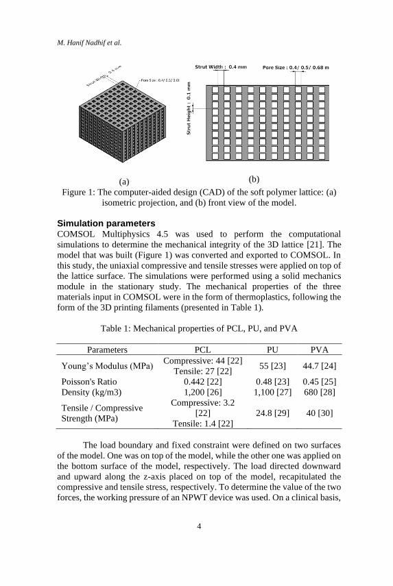
M. Hanif Nadhif et al.
4
(a)
(b)
Figure 1: The computer-aided design (CAD) of the soft polymer lattice: (a)
isometric projection, and (b) front view of the model.
Simulation parameters COMSOL Multiphysics 4.5 was used to perform the computational
simulations to determine the mechanical integrity of the 3D lattice [21]. The
model that was built (Figure 1) was converted and exported to COMSOL. In
this study, the uniaxial compressive and tensile stresses were applied on top of
the lattice surface. The simulations were performed using a solid mechanics
module in the stationary study. The mechanical properties of the three
materials input in COMSOL were in the form of thermoplastics, following the
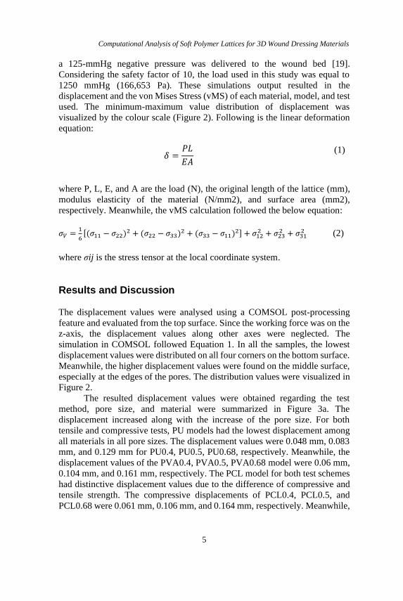
form of the 3D printing filaments (presented in Table 1).
Table 1: Mechanical properties of PCL, PU, and PVA
Parameters PCL PU PVA
Young’s Modulus (MPa) Compressive: 44 [22]
Tensile: 27 [22] 55 [23] 44.7 [24]
Poisson's Ratio 0.442 [22] 0.48 [23] 0.45 [25]
Density (kg/m3) 1,200 [26] 1,100 [27] 680 [28]
Tensile / Compressive
Strength (MPa)
Compressive: 3.2
[22]
Tensile: 1.4 [22]
24.8 [29] 40 [30]
The load boundary and fixed constraint were defined on two surfaces
of the model. One was on top of the model, while the other one was applied on
the bottom surface of the model, respectively. The load directed downward
and upward along the z-axis placed on top of the model, recapitulated the
compressive and tensile stress, respectively. To determine the value of the two
forces, the working pressure of an NPWT device was used. On a clinical basis,
Computational Analysis of Soft Polymer Lattices for 3D Wound Dressing Materials
5
a 125-mmHg negative pressure was delivered to the wound bed [19].
Considering the safety factor of 10, the load used in this study was equal to
1250 mmHg (166,653 Pa). These simulations output resulted in the
displacement and the von Mises Stress (vMS) of each material, model, and test
used. The minimum-maximum value distribution of displacement was
visualized by the colour scale (Figure 2). Following is the linear deformation
equation:
𝛿 =𝑃𝐿
𝐸𝐴
(1)
where P, L, E, and A are the load (N), the original length of the lattice (mm),
modulus elasticity of the material (N/mm2), and surface area (mm2),
respectively. Meanwhile, the vMS calculation followed the below equation:
𝜎𝑉 =1
6[(𝜎11 − 𝜎22)
2 + (𝜎22 − 𝜎33)2 + (𝜎33 − 𝜎11)
2] + 𝜎122 + 𝜎23
2 + 𝜎312 (2)
where σij is the stress tensor at the local coordinate system.
Results and Discussion
The displacement values were analysed using a COMSOL post-processing
feature and evaluated from the top surface. Since the working force was on the
z-axis, the displacement values along other axes were neglected. The
simulation in COMSOL followed Equation 1. In all the samples, the lowest
displacement values were distributed on all four corners on the bottom surface.
Meanwhile, the higher displacement values were found on the middle surface,
especially at the edges of the pores. The distribution values were visualized in
Figure 2.
The resulted displacement values were obtained regarding the test
method, pore size, and material were summarized in Figure 3a. The
displacement increased along with the increase of the pore size. For both
tensile and compressive tests, PU models had the lowest displacement among
all materials in all pore sizes. The displacement values were 0.048 mm, 0.083
mm, and 0.129 mm for PU0.4, PU0.5, PU0.68, respectively. Meanwhile, the
displacement values of the PVA0.4, PVA0.5, PVA0.68 model were 0.06 mm,
0.104 mm, and 0.161 mm, respectively. The PCL model for both test schemes
had distinctive displacement values due to the difference of compressive and
tensile strength. The compressive displacements of PCL0.4, PCL0.5, and
PCL0.68 were 0.061 mm, 0.106 mm, and 0.164 mm, respectively. Meanwhile,
M. Hanif Nadhif et al.
6
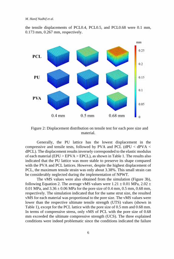
the tensile displacements of PCL0.4, PCL0.5, and PCL0.68 were 0.1 mm,
0.173 mm, 0.267 mm, respectively.
Figure 2: Displacement distribution on tensile test for each pore size and
material.
Generally, the PU lattice has the lowest displacement in the
compressive and tensile tests, followed by PVA and PCL (dPU < dPVA <
dPCL). The displacement results inversely corresponded to the elastic modulus
of each material (EPU > EPVA > EPCL), as shown in Table 1. The results also
indicated that the PU lattice was more stable to preserve its shape compared
with the PVA and PCL lattices. However, despite the highest displacement of
PCL, the maximum tensile strain was only about 3.38%. This small strain can
be considerably neglected during the implementation of NPWT.
The vMS values were also obtained from the simulation (Figure 3b),
following Equation 2. The average vMS values were 1.21 ± 0.01 MPa, 2.02 ±
0.01 MPa, and 3.36 ± 0.06 MPa for the pore size of 0.4 mm, 0.5 mm, 0.68 mm,
respectively. The simulation indicated that for the same strut size, the resulted
vMS for each material was proportional to the pore size. The vMS values were
lower than the respective ultimate tensile strength (UTS) values (shown in
Table 1), except for the PCL lattice with the pore size of 0.5 mm and 0.68 mm.
In terms of compressive stress, only vMS of PCL with the pore size of 0.68
mm exceeded the ultimate compressive strength (UCS). The three explained
conditions were indeed problematic since the conditions indicated the failure

Computational Analysis of Soft Polymer Lattices for 3D Wound Dressing Materials
7
of materials. However, the safety factor used in the simulation was
overestimated, 10. When the safety factor was lowered to 5 (P= 83, 326 Pa),
the vMS of the PCL lattice with the pore size of 0.5 mm was lower than the
UTS. When the safety factor was even decreased to 4 (P= 66, 661 Pa), the PCL
lattice with the pore size of 0.68 mm did not experience failure due to either
tensile or compressive stress. These results are of importance for the future
design of 3D wound dressings made of PCL. Instead of 10, the safety factor
used for PCL wound dressings can be 4. The safety factor of 4 is still tolerable.
(a)
(b)
Figure 3: Displacement (a) von Mises Stress, and (b) along the z-axis.

M. Hanif Nadhif et al.
8
Based on the mechanical simulation results, the 3D PU lattice was
superior compared to the other two lattices. However, the strain of all lattices
was very small (Table 2). The vMS of all materials was below the UTS, except
for PCL with certain pore sizes. Nonetheless, when the safety factor was
lowered to 4, PCL lattices were still safe and applicable for NPWT. It means
that the other two materials (PVA and PCL) can still be considered as
compatible materials for NPWT wound dressings. Therefore, three options of
3D wound dressing material are still available for plastic surgeons to use. For
instance, if the surgeons would like to incorporate a biodegradable wound
dressing, they can select 3D PVA-based and PCL-based wound dressings
[31]–[33]. Meanwhile, when the surgeons want to keep the structural integrity
of the 3D wound dressing material, they can choose 3D PU-based wound
dressing since thermoplastic PU is not degradable in the body [13].
Table 2: The strain for each pore size and material
Material Pore Size
0.4 mm 0.5 mm 0.68 mm
PCL (%) 1.95 2.84 3.39
PU (%) 0.95 1.37 1.64
PVA (%) 1.18 1.71 2.04
Conclusion
The computational analysis was successfully executed. From the results, it can
be concluded that the 3D lattices made of PCL, PU, and PVA, were safe and
feasible to be used as wound dressing materials. The von Mises stress resulted
from the equivalent stress produced by NPWT devices on a wound bed did not
exceed the ultimate tensile strength of all materials. The maximum strain rate
due to the compressive and tensile stress was also considerably low. In terms
of biodegradability, surgeons can take 3D PVA- and PCL-based wound
dressings. On the other hand, the perseverance of 3D wound dressing structural
integrity can be achieved using PU-based wound dressings. Finally, the results
of this study provide the readers the finite element analysis of 3D lattices for
wound dressing applications. However, this study hopefully will become a
cornerstone of the development of 3D wound dressing materials,
experimentally and clinically, since a one-piece dressing product was desired
by burn wound specialists around the world [34].
Computational Analysis of Soft Polymer Lattices for 3D Wound Dressing Materials
9
Acknowledgement
This research was supported by the Universitas Indonesia through the PUTI
Saintekes Grant NKB-2444/UN2.RST/HKP.05.00/2020.
References
[1] L. Martinengo et al., “Prevalence of chronic wounds in the general
population: systematic review and meta-analysis of observational
studies,” Ann. Epidemiol., vol. 29, pp. 8–15, 2019.
[2] K. Heyer, K. Protz, G. Glaeske, and M. Augustin, “Epidemiology and use
of compression treatment in venous leg ulcers: nationwide claims data
analysis in Germany: Compression treatment in venous leg ulcers,” Int.
Wound J., vol. 14, no. 2, pp. 338–343, 2017.
[3] A. H. Davies, J. M. Mora, M. S. Gohel, F. Heatley, and K. Dhillon, “Early
referral of venous leg ulcers: lessons from the EVRA trial,” Nurs. Resid.
Care, vol. 22, no. 1, pp. 31–36, 2020.
[4] P. Zhang, J. Lu, Y. Jing, S. Tang, D. Zhu, and Y. Bi, “Global
epidemiology of diabetic foot ulceration: a systematic review and meta-
analysis,” Ann. Med., vol. 49, no. 2, pp. 106–116, 2017.
[5] Z.-Q. Kang and X.-J. Zhai, “The Association between Pre-existing
Diabetes Mellitus and Pressure Ulcers in Patients Following Surgery: A
Meta-analysis,” Sci. Rep., vol. 5, no. 1, pp. 13007, 2015.
[6] B. K. Lal, “Venous ulcers of the lower extremity: Definition,
epidemiology, and economic and social burdens,” Semin. Vasc. Surg., vol.
28, no. 1, pp. 3–5,. 2015.
[7] J. C. Lawrence, “Wound irrigation,” J. Wound Care, vol. 6, no. 1, pp. 4,
1997.
[8] A. Gabriel, “Integrated negative pressure wound therapy system with
volumetric automated fluid instillation in wounds at risk for compromised
healing,” Int. Wound J., vol. 9, pp. 25–31, 2012.
[9] N. A. Kantak, R. Mistry, D. E. Varon, and E. G. Halvorson, “Negative
Pressure Wound Therapy for Burns,” Clin. Plast. Surg., vol. 44, no. 3, pp.
671–677, 2017.
[10] S. Gupta, “Optimal use of negative pressure wound therapy for skin
grafts,” Int. Wound J., vol. 9, pp. 40–47, 2012.
[11] M. Mir et al., “Synthetic polymeric biomaterials for wound healing: a
review,” Prog. Biomater., vol. 7, no. 1, pp. 1–21, 2018.
[12] J. Kucińska-Lipka, “Polyurethanes Crosslinked with Poly(vinyl alcohol)
as a Slowly-Degradable and Hydrophilic Materials of Potential Use in
Regenerative Medicine,” Materials, vol. 11, no. 3, pp. 352, 2018.
M. Hanif Nadhif et al.
10
[13] R. R. M. Vogels et al., “Biocompatibility and biomechanical analysis of
elastic TPU threads as new suture material,” J. Biomed. Mater. Res. B
Appl. Biomater., vol. 105, no. 1, pp. 99–106, 2017.
[14] D. Lupuleasa, “biocompatible polymers for 3d printing,” FARMACIA,
vol. 66, no. 5, pp. 737–746, 2018.
[15] A. Krishna, A. Kumar, and R. K. Singh, “Effect of Polyvinyl Alcohol on
the Growth, Structure, Morphology, and Electrical Conductivity of
Polypyrrole Nanoparticles Synthesized via Microemulsion
Polymerization,” ISRN Nanomater., vol. 2012, pp. 1–6, 2012.
[16] D. Garcia-Garcia, J. M. Ferri, T. Boronat, J. Lopez-Martinez, and R.
Balart, “Processing and characterization of binary poly(hydroxybutyrate)
(PHB) and poly(caprolactone) (PCL) blends with improved impact
properties,” Polym. Bull., vol. 73, no. 12, pp. 3333–3350, 2016.
[17] D. A. Hudson, K. G. Adams, A. Van Huyssteen, R. Martin, and E. M.
Huddleston, “Simplified negative pressure wound therapy: clinical
evaluation of an ultraportable, no-canister system,” Int. Wound J., vol. 12,
no. 2, pp. 195–201, 2015.
[18] J. Cantrell et al., “Experimental Characterization of the Mechanical
Properties of 3D-Printed ABS and Polycarbonate Parts,” Rapid Prototyp.
J., vol. 23, no. 4, pp. 811–824, 2017.
[19] T. O. H. Prasetyono, I. S. Rini, and C. Wibisono, “EASEPort NPWT
System to Enhance Skin Graft Survival – A Simple Assembly,” Int. Surg.,
vol. 100, no. 3, pp. 518–523, 2015.
[20] V. Milleret, A. G. Bittermann, D. Mayer, and H. Hall, “Analysis of
Effective Interconnectivity of DegraPol-foams Designed for Negative
Pressure Wound Therapy,” Materials, vol. 2, no. 1, pp. 292–306, 2009.
[21] M. S. Utomo, Y. Whulanza, F. P. Lestari, A. Erryani, I. Kartika, and N.
A. Alief, “Determination of compressive strength of 3D polymeric lattice
structure as template in powder metallurgy,” IOP Conf. Ser. Mater. Sci.
Eng., vol. 541, pp. 012042, 2019.
[22] L. Lu et al., “Mechanical study of polycaprolactone-hydroxyapatite
porous scaffolds created by porogen-based solid freeform fabrication
method,” J. Appl. Biomater. Funct. Mater., vol. 12, no. 3, pp. 145–154,
2014.
[23] H. J. Qi and M. C. Boyce, “Stress–strain behavior of thermoplastic
polyurethanes,” Mech. Mater., vol. 37, no. 8, pp. 817–839, 2005.
[24] W. Zhang, X. Yang, C. Li, M. Liang, C. Lu, and Y. Deng,
“Mechanochemical activation of cellulose and its thermoplastic polyvinyl
alcohol ecocomposites with enhanced physicochemical properties,”
Carbohydr. Polym., vol. 83, no. 1, pp. 257–263, 2011.
[25] F. Chen, D. J. Kang, and J. H. Park, “New measurement method of
Poisson’s ratio of PVA hydrogels using an optical flow analysis for a
digital imaging system,” Meas. Sci. Technol., vol. 24, no. 5, 2013.
Computational Analysis of Soft Polymer Lattices for 3D Wound Dressing Materials
11
[26] M. Labet and W. Thielemans, “Synthesis of polycaprolactone: A review,”
Chem. Soc. Rev., vol. 38, no. 12, pp. 3484–3504, 2009.
[27] M. Al Minnath, G. Unnikrishnan, and E. Purushothaman, “Transport
studies of thermoplastic polyurethane/natural rubber (TPU/NR) blends,”
J. Membr. Sci., vol. 379, no. 1–2, pp. 361–369, 2011.
[28] K. Wahyuningsih, E. S. Iriani, and F. Fahma, “Utilization of Cellulose
from Pineapple Leaf Fibers as Nanofiller in Polyvinyl Alcohol-Based
Film,” Indones. J. Chem., vol. 16, no. 2, p. 181, 2018.
[29] Y. Kanbur and U. Tayfun, “Development of multifunctional polyurethane
elastomer composites containing fullerene: Mechanical, damping,
thermal, and flammability behaviors,” J. Elastomers Plast., vol. 51, no. 3,
pp. 262–279, 2019.
[30] V. Goodship and D. K. Jacobs, Polyvinyl Alcohol: Materials, Processing
and Applications, vol. 16. Shrewsbury, Shropshire: Smithers Rapra
Technology, 2009.
[31] M. Sabino et al., “In vitro biocompatibility study of biodegradable
polyester scaffolds constructed using Fused Deposition Modeling
(FDM),” IFAC Proc. Vol., vol. 46, no. 24, pp. 356–360, 2013.
[32] S. Mohanty et al., “Fabrication of scalable and structured tissue
engineering scaffolds using water dissolvable sacrificial 3D printed
moulds,” Mater. Sci. Eng. C, vol. 55, pp. 569–578, 2015.
[33] N. Thuaksuban, R. Pannak, P. Boonyaphiphat, and N. Monmaturapoj, “In
vivo biocompatibility and degradation of novel Polycaprolactone-
Biphasic Calcium phosphate scaffolds used as a bone substitute,” Biomed.
Mater. Eng., vol. 29, no. 2, pp. 253–267, 2018.
[34] H. F. Selig, D. B. Lumenta, M. Giretzlehner, M. G. Jeschke, D. Upton,
and L. P. Kamolz, “The properties of an ‘ideal’ burn wound dressing –
What do we need in daily clinical practice? Results of a worldwide online
survey among burn care specialists,” Burns, vol. 38, no. 7, pp. 960–966,
2012.
Journal of Mechanical Engineering Vol 18(2), 13-26, 2021
___________________
ISSN 1823-5514, eISSN 2550-164X © 2021 College of Engineering,
Universiti Teknologi MARA (UiTM), Malaysia.
Received for review: 2020-09-08 Accepted for publication: 2021-03-18
Published: 2021-04-15
Sustainable Surface Water Dissolved Oxygen Monitoring at Lake 7/1F, Shah Alam, Selangor
Norashikin M. Thamrin*, Megat Syahirul Amin Megat Ali
College of Engineering, Universiti Teknologi MARA,
40450 Shah Alam, Selangor, Malaysia
Mohamad Farid Misnan
Faculty of Electrical Engineering, Universiti Teknologi MARA,
Pasir Gudang, Johor, Malaysia
Nik Norliyana Nik Ibrahim
Department of Chemical and Environmental Engineering,
Universiti Putra Malaysia, Serdang, Selangor, Malaysia
Navid Shaghaghi
EPIC (Ethical, Pragmatic, and Intelligent Computing) Laboratory,
Departments of Mathematics and Computer Science (MCS) and
Computer Science and Engineering (CSE)
Santa Clara University (SCU), Santa Clara, USA
ABSTRACT
Shah Alam is in Selangor, Malaysia and symbolized with several lakes that
are popular among local communities and visitors for leisure and
recreational activities. Among of these lakes, few lakes need management to
look after its hygienic and well-being to serve its purpose as the recreational
lake for the nearby community, such as Lake 7/1F, Shah Alam, Selangor. The
secluded location of this water reservoir has made it unpopular, and
improper management of it could invite an imbalance environment to its
surrounding. Therefore, to initiate the effort, an Internet-of-Thing (IoT) water
monitoring system is deployed at this lake to study the dissolved oxygen (DO)
level in the water that could indicate the health status of this lake. The system
consists of a DO sensor, embedded controller, self-charging power supply,
wireless data transmission, and IoT dashboard for in-situ DO measurement.
From the analysis, the lake has the normal cycle of DO production, but a

Norashikin et al.
14
dangerous condition is detected when the concentrated DO in the lake water
is mostly below the saturation value.
Keywords: Water Quality; Surface Water; Dissolved Oxygen; IoT System;
Lake Water
Introduction
Recreational lakes are becoming increasingly popular with local communities
for leisure and social activities. Shah Alam is a city and the state capital of
Selangor, Malaysia and was the first planned city in this country after the
Independence Day in 1957. This well-designed plan has set up a few
recreational areas in a walking distance from surrounding residential areas,
such as catchment ponds and artificial lakes. Furthermore, the presence of
well-developed parks with ponds and lakes has a positive impact on the
perception of the historical, cultural, environmental, and recreational
functions that can surely develop the domestic and international tourism [1].
On top of that, these lakes’ aquatic systems can improve the urban
microclimate problem by absorbing solid pollutants, increasing air humidity,
and reducing the adverse thermal radiation during the hot season [2-3].
Besides, with these aesthetic and scenic values, they are enticing the
attractive water resources, which are capitalized into property prices [4-5].
However, climate change and rapid developments around the lake
have modified the ecological character of the lake. Climate change affects
the levels of dissolved oxygen level and aquatic species in lake water. With
the increase in surface water temperature, the concentration of dissolved
oxygen in the water decreased [6]. The prolonged dry season also reduces the
volume of lake water that affects the health of Urmia Lake, Iran. When the
climate has changed the character of this lake water over the last few
decades, its use for irrigation should be supplemented by other groundwater
sources, further reducing the depletion of that lake [7]. There is also
environmental concern regarding the relationship between nutrient runoff and
biological growth, including harmful algal blooms and hypoxic conditions
caused by the entry of untreated wastewater into the water, littering, and
eutrophication [1,5]. If lake water cannot be self-purified, it loses its
recreation and may be unfit to be used by the local communities.
The excessive presence of nitrate and phosphate in the water may
invite unwanted weeds to cover the lake, which leads to the lake
eutrophication. This condition can pose a threat to the public with dangerous
diseases such as malaria, dengue and cholera, and other parasitic infections
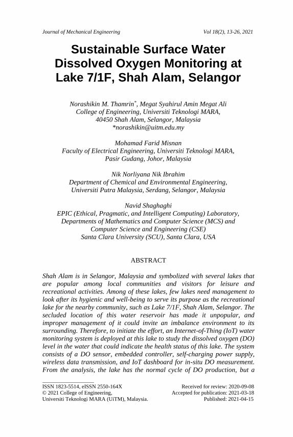
[1,8]. Figure 1 shows the Lake 7/1F condition with the growing weeds in the
water.
Sustainable Surface Water Dissolved Oxygen Monitoring at Lake 7/1F, Shah Alam, Selangor
15
Figure 1: The growing weeds on the banks of the Lake 7/1F, Shah
Alam, Selangor.
The vast majority of studies included in the review suggest that the
concentration of the dissolved oxygen in the lake water can determine the
health of its ecosystem [6-10]. The dissolved oxygen concentration needs
regular monitoring to observe any sudden and extreme changes in the data.
Traditional in-situ measurements have too limited time and spatial resolution
to make such a numerical model accurate. Efforts needed to use innovative
tools to solve these limitations [11]. Consequently, a faster approach in
monitoring the concentration of the dissolved oxygen level in the lake water
is desired. Previous researchers in the literature have proposed a range of
techniques. This approach incorporates two essential techniques, namely (1)
in-situ measurement of the dissolved oxygen concentration, and (2) remote
monitoring access. In-situ measurement is the critical element of
continuously monitoring the water parameter in the lake. The sensor is
attached to a self-power embedded system that contains a controller for a
sustainable water monitoring system. A continuous dissolved oxygen
monitoring data allow prediction on the health of the lake water and fish
habitats by integrating it with the numerical analysis and prediction algorithm
[6,10,11]. The changes in the dissolved oxygen concentration assessed
through the computers and smartphones by using the intelligent sensor
network implementation or the Internet-of-Thing (IoT) approach, which is
one of the advantages of the automated monitoring system can provide to the
local authorities and community. For this purpose, the system equipped with
the wireless data transmission by using several IoT protocols such as
Message Queue Telemetry Transport (MQTT), Hypertext Transfer Protocol
(HTTP), and others [12-15] to display the monitored dissolved oxygen
concentration level in the IoT dashboard. The use of IoT technology
supported by the data retrieval method using sensors, embedded systems and
remote communication technology can, therefore, help to simplify the
assessment of lake water quality.

Norashikin et al.
16
Research Methodology
This project developed a Buoy water monitoring to gather a broad data set of
the water parameter. This system involves the design and development of the
floating Water Quality Monitoring Platform, Sustainable Power Supply
System, Sensor Network, IoT Mobile Dashboard & Cloud Data Storage
System. This system installed at Lake 7/1F, Shah Alam, Selangor, as shown
in Figure 2.
Figure 2: The research location at Lake 7/1F Shah Alam, Selangor.
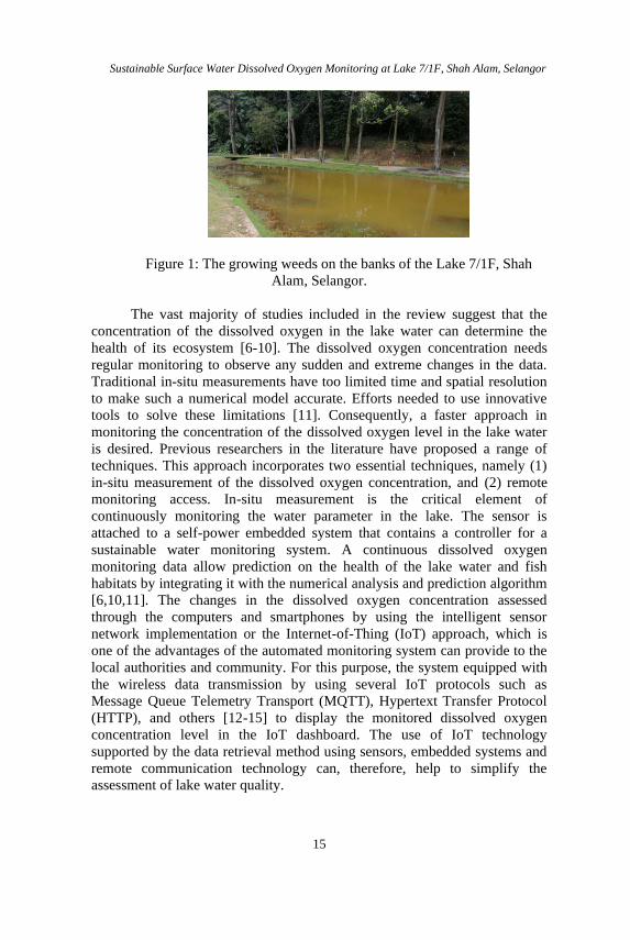
Development of IoT-based water Qquality monitoring system Five components involve in this development, namely, are the floating
platform (buoy), sustainable power supply management unit, embedded
controller unit, sensor network system, IoT dashboard, and physical data
storage for the backup system during failure. Each component includes the
mechanical and electrical/ electronic components, has been weatherproofed
to be placed in the lake water. The overall architecture diagram of the system
is shown in Figure 3 and Figure 4, respectively.
Sustainable Surface Water Dissolved Oxygen Monitoring at Lake 7/1F, Shah Alam, Selangor
17
GPS
Dissolved Oxygen
Sensor Network
Analog
Serial
Process
Control
GPS Serial Data
Analog Signal
ESP Wireless
ModuleSerial
Sensor
Data
JSON
Payload
Wireless
Data Transfer
Data Storage
Serial SD Card
Module
ATMega328p
Solar
Panel
Solar
Charger
Lead Acid
Battery
Voltage
Regulator
5Vdc
Power Supply Management System
Control Process
Internet of Things
Platform
Sensor
Data
SPI
Figure 3: Block diagram of the floating water quality monitoring system.
Dissolved
Oxygen
Solar
Power
Supply
IoT Dashboard
Monitoring Platform
Wifi Module
Embedded
Controller
Data storage
DesktopMobile phone
Cloud data
SD card Module
Lake / Pond
Seksyen 7/1F
Shah Alam
GPS Module
Sensor
Network
Sensor
Signal
GPS data
AT command
Low
Power
Voltage
Wireless
data transfer
Serial Data
Figure 4: The architecture of the Floating Water Quality Monitoring using
IoT System.
Norashikin et al.
18
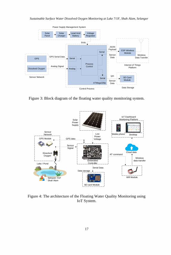
The Design of the Floating Platform for Water Monitoring System
The system used a buoy to float the water monitoring system platform on the
lake while measuring the DO parameter. The size of the buoy used is
approximately 750 mm outer diameter and 450 mm inner diameter with a
load capacity of 14.5 kg above water, which is suitable to be used as the total
weight of the water monitoring system is 4 kg as depicted in Figure 5(a). The
required floating platform must then be larger than the hardware mounted on
the platform. The buoy platform frame made of aluminium steel to prevent
rust from occurring due to the oxidation process. An opening is made in the
middle of the buoy platform to allow trouble-free water flow and exchange,
and therefore, avoid the stagnant water which can interrupt the precise
measurement. The buoy platform was anchored via the nylon cable on the
lake to prevent it from drifting into the middle of the lake, as shown in Figure
5(b). The electrical/electronic components and sensor network are installed at
this frame using the grey polycarbonate boxes fitted with a standard IP67
waterproof compliance [16]. The external dimensions of the IP67 boxes were
about 300 mm (H) x 200 mm (L) x 80 mm (W) and were equipped with the
stainless-steel screws to avoid corrosion. A solar panel is placed on top of the
aluminium frame, as shown in Figure 5(a).
(a)
(b) Figure 5: (a) Buoy monitoring system platform, (b) The floating buoy
platform in the Lake 7/1F, Shah Alam, Selangor.
Sustainable solar power supply system The buoy platform is fitted with 1000 mm x 670 mm solar panels which
mounted horizontally on the buoy platform [16]. The installed system
hardware powered by a solar power supply system with 30W small solar
panel, 12V solar charger, 12V 7AH lead-acid rechargeable battery and a low
voltage converter [17-19]. The voltage regulator is used to supply different

Sustainable Surface Water Dissolved Oxygen Monitoring at Lake 7/1F, Shah Alam, Selangor
19
voltage to different components, which is 5Vdc to the embedded controller
and 9Vdc to the sensor network. The solar panel is mounted facing higher
solar exposure to get the optimum solar energy to charge the rechargeable
battery. As an estimate, the power storage could provide enough for the entire
system to operate with optimum voltage and current for 24 hours operation.
Embedded control unit Embedded controller AtMega328p used as the central controller for this
project to process all the sensor data parameters [19-20]. Appropriately, C
program with Arduino IDE software used to read the analog sensor value
data via the ADC at setup time intervals to digitize the required parameter
value to the exact unit value. The controller also integrated with the offline
data storage SD card module to gather all sensor data parameters via the
Serial I2C data transfer. It is also integrated with the ESP wireless module for
transmitting all the necessary parameter data to the cloud storage to the IoT
dashboard platform for Big Data Analysis and data visualization [19-20]. All
water parameters instantaneously and wirelessly updated in a requisite setup
period, which can be monitored at anytime and anywhere by the authorized
person [19].
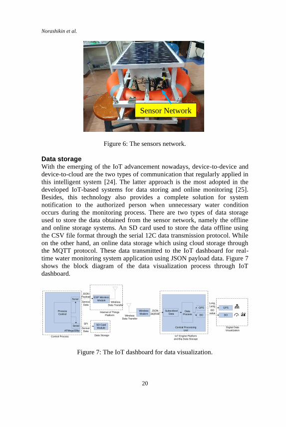
Water sensors The water parameter sensor network comprises two sensors, namely the DO
sensor and Global Positioning System (GPS) as shown in Figure 6. The
former is a sensor used to measure the chemical parameter, which is the
dissolved oxygen in the water. The latter used to read the location of the
water monitoring system at the lake [16, 21]. An Industrial DO sensor
module used to obtain precise oxygen level information from the water [17,
22]. The DO sensor is immersed approximately 30 cm from the surface of the
water, beneath the buoy platform [23]. The selected location of the sensors in
the buoy is to keep them protected from shock and other problems. The
integrated real-time clock (RTC) in the SD card module used to record data
using pre-loaded sampling time.
Norashikin et al.
20
Figure 6: The sensors network.
Data storage With the emerging of the IoT advancement nowadays, device-to-device and
device-to-cloud are the two types of communication that regularly applied in
this intelligent system [24]. The latter approach is the most adopted in the
developed IoT-based systems for data storing and online monitoring [25].
Besides, this technology also provides a complete solution for system
notification to the authorized person when unnecessary water condition
occurs during the monitoring process. There are two types of data storage
used to store the data obtained from the sensor network, namely the offline
and online storage systems. An SD card used to store the data offline using
the CSV file format through the serial 12C data transmission protocol. While
on the other hand, an online data storage which using cloud storage through
the MQTT protocol. These data transmitted to the IoT dashboard for real-
time water monitoring system application using JSON payload data. Figure 7
shows the block diagram of the data visualization process through IoT
dashboard.
Wireless
ModemWireless
Data Transfer
Subscribed
DataData
Process
GPS
Digital Data
Visualization
Central Processing
Unit
DO
GPS
DO
IoT Engine Platform
and Big Data Storage
JSON
payload
Long,
Lang
DO
valueProcess
Control
ESP Wireless
ModuleSerial
Sensor
Data
JSON
Payload
Wireless
Data Transfer
Data Storage
Serial SD Card
ModuleATMega328p
Control Process
Internet of Things
Platform
Sensor
Data
SPI
Figure 7: The IoT dashboard for data visualization.
Sensor Network

Sustainable Surface Water Dissolved Oxygen Monitoring at Lake 7/1F, Shah Alam, Selangor
21
Result and Discussion
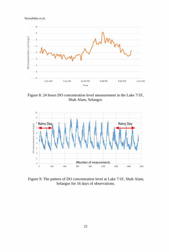
In this section, the concentration of DO in Lake 7/1F, Shah Alam, is analyzed
and summarized in Figure 8 and Figure 9. The data is sampled from 18
February 2020 to 3 March 2020 to monitor the DO concentration level
pattern in this lake. Figure 8 shows the output trend obtained from the DO
sensor for 24 hours. The concentration of the DO varies in the lake during the
day, and night time is analyzed. The DO concentration level inclines after
sunrise and approaching the noon. The minimum oxygen concentrations in
the water occurred during sunrise (2.8 mg/L–3.0 mg/L) after a full respiration
process by the aquatic life at night [26]. The Sediment denitrification in the
sallowed vegetated lake water can also reduce the dissolved oxygen
concentration, which can be the first sign of nitrogen pollution in the lake
ecosystem [27]. The highest DO value of 7.11 mg/L obtained during the
afternoon, around 4.40 PM. During the night, the DO level declines to 2.68
mg/L. When the DO level in the surface water is less than 5 mg/L, it
indicates a distressed environment to the aquatic lives such as fish [28]. It
also indicates the appearance of sediment oxygen demand (SOD) caused by
the algae in the water as well [29]. This value indicates an alarming sign as
growth of aquaculture will be slow due to low exposure of dissolved oxygen.
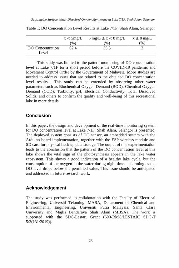
The broad range of DO value is indirectly proposing the lake has
excessive algae and phytoplankton which high oxygen consumption by the
photosynthetic organisms in the lake. However, more studies are needed to
confirm this condition. Correlation between different parameters needs to be
determined and measured for further studies. The temperature of the lake
water also plays a prominent role in dissolved oxygen levels. During this
monitoring period, the range of the water temperature at Lake 7/1F Shah
Alam is from 29 ⁰C to 33 ⁰C, which is considered high [12]. The rain also
contributes to the DO concentration level in the lake water. Figure 9 shows
the scenario explained. A plausible and useful theory behind the situation is
that the cloudy day affects the rate of photosynthesis by aquatic life. During
the dry season, the DO concentration is higher compared to the wet season
[30]. During rainy days, the highest DO concentration level at this lake
ranges from 6.63 mg/L to 7.75 mg/L. Table 1 summarizes the percentage of
the DO level distribution during the monitoring period. From this table,
62.4% of the DO concentration levels are below 5 mg/L, which is not a good
sign for a healthy lake ecosystem. Only 2% obtain more than 8 mg/L during
the peak of hot weather.
Norashikin et al.
22
Figure 8: 24 hours DO concentration level measurement in the Lake 7/1F,
Shah Alam, Selangor.
Rainy Day Rainy Day
#Number of measurements
Figure 9: The pattern of DO concentration level at Lake 7/1F, Shah Alam,
Selangor for 16 days of observations.
Sustainable Surface Water Dissolved Oxygen Monitoring at Lake 7/1F, Shah Alam, Selangor
23
Table 1: DO Concentration Level Results at Lake 7/1F, Shah Alam, Selangor
x < 5mg/L
(%)
5 mg/L ≤ x < 8 mg/L
(%)
x ≥ 8 mg/L
(%)
DO Concentration
Level
62.4 35.6 2
This study was limited to the pattern monitoring of DO concentration
level at Lake 7/1F for a short period before the COVID-19 pandemic and
Movement Control Order by the Government of Malaysia. More studies are
needed to address issues that are related to the obtained DO concentration
level results. This study can be extended by observing other water
parameters such as Biochemical Oxygen Demand (BOD), Chemical Oxygen
Demand (COD), Turbidity, pH, Electrical Conductivity, Total Dissolved
Solids, and others to confirm the quality and well-being of this recreational
lake in more details.
Conclusion
In this paper, the design and development of the real-time monitoring system
for DO concentration level at Lake 7/1F, Shah Alam, Selangor is presented.
The deployed system consists of DO sensor, an embedded system with the
Arduino board implementation, together with the ESP wireless module and
SD card for physical back up data storage. The output of this experimentation
leads to the conclusion that the pattern of the DO concentration level at this
lake shows the vital sign of the photosynthesis appears in the lake water
ecosystem. This shows a good indication of a healthy lake cycle, but the
consumption of the oxygen in the water during night time is alarming as the
DO level drops below the permitted value. This issue should be anticipated
and addressed in future research work.
Acknowledgement
The study was performed in collaboration with the Faculty of Electrical
Engineering, Universiti Teknologi MARA, Department of Chemical and
Environmental Engineering, Universiti Putra Malaysia, Santa Clara
University and Majlis Bandaraya Shah Alam (MBSA). The work is
supported with the SDG-Lestari Grant (600-RMC/LESTARI SDG-T
5/3(131/2019)).

Norashikin et al.
24
References
[1] A. Ishbirdin, M. Ishmuratova, G. Gabidullina, & Z. Baktybaeva,
“Ecological and Hygienic Assessment of the State of the Recreational
Lake in the City of Ufa,” in Ecological-Socio-Economic Systems:
Models of Competition and Cooperation (ESES 2019), pp. 104-109,
2020.
[2] C.Y. Zhu “Effects of urban lake wetland on temperature and humidity:
A case study of Wuhan City,” Acta Ecologica Sinica, vol. 35, no. 16,
pp. 5518-5527, 2015.
[3] D. Zhu and X.F. Zhou, “Effect of urban water bodies on distribution
characteristics of particulate matters and NO2,” Sustainable Cities and
Society, vol. 50, pp. 101679, 2019.
[4] S. Nicholls, & J. L. Crompton, “The contribution of scenic views of,
and proximity to, lakes and reservoirs to property values,” Lakes &
Reservoirs: Research & Management, vol. 23, no. 1, pp. 63-78, 2018.
[5] M. R. Moore, J. P. Doubek, H. Xu, & B. J. Cardinale, “Hedonic Price
Estimates of Lake Water Quality: Valued Attribute Instrumental
Variables, and Ecological-Economic Benefits,” Ecological Economics,
vol. 176, pp. 106692, 2020.
[6] S. Missaghi, M. Hondzo, & W. Herb, “Prediction of lake water
temperature, dissolved oxygen, and fish habitat under changing
climate,” Climatic Change, vol. 141, no. 4, pp. 747-757, 2017.
[7] S. Shadkam, F. Ludwig, P. van Oel, Ç. Kirmit, & P. Kabat, “Impacts of
climate change and water resources development on the declining
inflow into Iran’s Urmia Lake,” Journal of Great Lakes Research, vol.
42, no. 5, pp. 942–952, 2016.
[8] M. F. Khan, “Physico-Chemical and Statistical Analysis of Upper Lake
Water in Bhopal Region of Madhya Pradesh, India,” International
Journal of Lakes and Rivers, vol. 13, no. 1, pp. 1-16, 2020.
[9] R. Bhateria, & D. Jain, “Water quality assessment of lake water: a
review,” Sustainable Water Resources Management, vol. 2, no. 2, pp.
161-173, 2016.
[10] T. Fukushima, T. Inomata, E. Komatsu, & B. Matsushita, “Factors
explaining the yearly changes in minimum bottom dissolved oxygen
concentrations in Lake Biwa, a warm monomictic lake,” Scientific
reports, vol. 9, no. 1, pp. 1-10, 2019.
[11] Y. Hong, F. Soulignac, A. Roguet, F.Piccioni, P. Dubois, B. J. Lemaire,
& B. Vinçon-Leite, “An automatic warning system for face al
contamination in urban recreational lake,” in Novatech 2019, pp. 3B82-
274HON, 2019.

Sustainable Surface Water Dissolved Oxygen Monitoring at Lake 7/1F, Shah Alam, Selangor
25
[12] R. F. Rahmat, M. F. Syahputra, & M. S. Lydia, “Real time monitoring
system for water pollution in Lake Toba,” in 2016 International
Conference on Informatics and Computing (ICIC), pp. 383-388, 2016.
[13] L. F. M. Vieira, M. A. M. Vieira, J. A. M. Nacif, & A. B. Vieira,
“Autonomous wireless lake monitoring,” Computing in Science &
Engineering, vol. 20, no. 1, pp. 66-75, 2018.
[14] J. Huan, H. Li, F. Wu, & W. Cao, “Design of water quality monitoring
system for aquaculture ponds based on NB-IoT,” Aquacultural
Engineering, vol. 90, pp. 102088, 2020.
[15] R. P. N. Budiarti, A. Tjahjono, M. Hariadi, & M. H. Purnomo,
“Development of IoT for Automated Water Quality Monitoring
System,” in 2019 International Conference on Computer Science,
Information Technology, and Electrical Engineering (ICOMITEE) pp.
211-216, 2019.
[16] A. Hegarty, G. Westbrook, D. Glynn, D. Murray, E. Omerdic, & D. A
Toal, “Low-Cost Remote Solar Energy Monitoring System for a
Buoyed IoT Ocean Observation Platform,” in 2019 IEEE 5th World
Forum on Internet of Things (WF-IoT). pp. 386-391, 2019.
[17] T. Li, M. Xia, J. Chen, Y. Zhao, & C. de Silva, “Automated Water
Quality Survey and Evaluation Using an IoT Platform with Mobile
Sensor Nodes,” Sensors, vol. 17, no. 8, pp. 1735, 2017.
[18] R. Venkatesan, N. Vedachalam, M. A. Muthiah, B. Kesavakumar, R.
Sundar, & M. A. Atmanand, “Evolution of Reliable and Cost-Effective
Power Systems for Buoys Used in Monitoring Indian Seas,” Marine
Technology Society Journal, vol. 49, no. 1, pp. 71–87, 2015.
[19] P. V. Vimal, & K. S. Shivaprakasha, “IoT based Greenhouse
Environment Monitoring and Controlling System Using Arduino
Platform,” in 2017 International Conference on Intelligent Computing,
Instrumentation and Control Technologies (ICICICT), pp. 1514 – 1519,
2017.
[20] T. Perumal, M. N. Sulaiman, & C. Y Leong, “Internet of Things (IoT)
Enabled Water Monitoring System,” in 2015 IEEE 4th Global
Conference on Consumer Electronics (GCCE), pp. 86-87, 2015.
[21] H. Apel, N. G. Hung, H. Thoss, & T. Schöne, “GPS buoys for stage
monitoring of large rivers,” Journal of Hydrology, vol. 412-413, pp.
182–192, 2012.
[22] R. Arridha, S. Sukaridhoto, D. Pramadihanto, & N. Funabiki,
“Classification extension based on IoT-big data analytic for smart
environment monitoring and analytic in real-time system,” International
Journal of Space-Based and Situated Computing, vol. 7, no. 2, pp. 82,
2017.
[23] S. Sendra, L. Parra, J. Lloret, & J. M. Jiménez, “Oceanographic
Multisensor Buoy Based on Low Cost Sensors for Posidonia Meadows
Norashikin et al.
26
Monitoring in Mediterranean Sea,” Journal of Sensors, vol. 2015, pp.
1–23, 2015.
[24] A. N. Prasad, K. A. Mamun, F. R. Islam, & H. Haqva, “Smart Water
Quality Monitoring System,” in 2015 2nd Asia-Pacific World Congress
on Computer Science and Engineering (APWC on CSE). pp.1-6, 2015.
[25] K. H. Kamaludin, & W. Ismail, “Water Quality Monitoring with
Internet of Things (IoT),” in 2017 IEEE Conference on Systems,
Process and Control (ICSPC), pp. 18-23, 2017.
[26] M. R. Andersen, T. Kragh, & K. Sand-Jensen, “Extreme diel dissolved
oxygen and carbon cycles in shallow vegetated lakes,” Proceedings of
the Royal Society B: Biological Sciences, vol. 284, no. 1862,
20171427, 2017.
[27] P. Hong, S. Gong, C. Wang, Y. Shu, X. Wu, C. Tian, & B. Xiao,
“Effects of organic carbon consumption on denitrifier community
composition and diversity along dissolved oxygen vertical profiles in
lake sediment surface,” Journal of Oceanology and Limnology, vol. 38,
pp. 733-744, 2020.
[28] H. L. Koh, W. K. Tan, S. Y. Teh, & C. J. Tay, “Water Quality
Simulation for Rehabilitation Of A Eutrophic Lake In Selangor,
Malaysia,” in IOP Conference Series: Earth and Environmental Science
vol. 380, no. 1, 012006, 2019.
[29] L. D. Dien, S. J. Faggotter, C. Chen, J. Sammut, & M. A. Burford,
“Factors driving low oxygen conditions in integrated rice-shrimp
ponds,” Aquaculture, vol. 512, 734315, 2019.
[30] R. Yang, H. Sun, B. Chen, M. Yang, Q. Zeng, C. Zeng, & D. Lin,
“Temporal Variations In Riverine Hydrochemistry And Estimation Of
The Carbon Sink Produced By Coupled Carbonate Weathering With
Aquatic Photosynthesis On Land: An Example From The Xijiang
River, A Large Subtropical Karst-Dominated River In China,”
Environmental Science and Pollution Research, vol. 27, pp. 13142-
13154, 2020.
Journal of Mechanical Engineering Vol 18(2), 27-37, 2021
___________________
ISSN 1823-5514, eISSN 2550-164X © 2021 College of Engineering,
Universiti Teknologi MARA (UiTM), Malaysia.
Received for review: 2020-11-16 Accepted for publication: 2020-12-22
Published: 2021-04-15
Heat Transfer Simulation of Various Material for Polymerase Chain
Reaction Thermal Cycler
Kenny Lischer*, Ananda Bagus Richky Digdaya Putra, Muhamad Sahlan,
Apriliana Cahya Khayrani, Mikael Januardi Ginting, Anondho Wijanarko
Department of Chemical Engineering, Faculty of Engineering,
Universitas Indonesia, Depok, West Java, 16424, Indonesia
Yudan Whulanza
Department of Mechanical Engineering, Faculty of Engineering,
Universitas Indonesia, Depok, West Java, 16424, Indonesia
Diah Kartika Pratami
Lab of Pharmacognosy and Phytochemistry, Faculty of Pharmacy, Pancasila University, Jakarta 12640, Indonesia
ABSTRACT
Medical diagnosis is the initial stage in identifying a person's condition,
disease or injury from its signs and symptoms. The diagnostic method is
carried out quantitatively by using a diagnostic kit which measures data such
as blood pressure, heart rate frequency and blood cell concentration. These
diagnostic kits are available in their respective capabilities and their
activities require medical facilities and logistical readiness to function.
Furthermore, Indonesia's geographical condition which consists of many
islands and mountains causes uneven distribution of health facilities and
laboratories in each region. Therefore, resulting in problems such as
inadequate access and availability of these diagnostic kit in each region.
Presently, one of the most widely used diagnostic methods is the Polymerase
Chain Reaction (PCR) which allows the amplification of specific fragments
from complex DNA. In PCR, only a small amount of DNA is needed to
produce enough replication copies which were further analyzed by
microscopic examination. This process begins with thermal cycling, which is
the reactant's exposure to the heating cycle and repetitive repairs to produce
reactions to different temperatures. This study aims to examine the material
used for thermal cyclers which is an essential aspect of the heat transfer
Kenny Lischer et al.
28
needed by the PCR process. In this study, heat transfer from several
materials were simulated and analyzed by COMSOL Multiphysics 5.3
Software. The following results were obtained from the simulation: the
saturation time for heating aluminum, copper and nickel were 29,37 and 51
seconds, respectively. Meanwhile, the cooling time was 26, 35 and 55
seconds, respectively. In addition, the saturation time for heating and cooling
silver and Polydimethylsiloxane (PDMS) were 26 and 1480 seconds,
respectively.
Keywords: COMSOL Multiphysics 5.3; Material; Heat Transfer Simulation;
Polymerase Chain Reaction; Portable Thermal Cycler
Introduction
Medical diagnosis is the initial stage in identifying a person's condition,
disease or injury from its signs and symptoms. Furthermore, the diagnostic
method is carried out quantitatively by using a diagnostic kit which measures
data such as blood pressure, heart rate frequency and blood cell
concentration. These diagnostic kits are available in various capabilities,
ranging from blood pressure measuring devices to devices that require
laboratory treatment such as blood cell checking devices. All of these
diagnostic activities require the readiness of facilities and medical logistics to
function.
Presently, one of the most widely used diagnostic methods is the
Polymerase Chain Reaction (PCR) which allows the amplification of specific
DNA fragments from complex DNA. In PCR, only a small amount of DNA
is needed to produce enough replication copies which were further analyzed
by microscopic examination [1]. It requires a thermal cycle or repeated
temperature changes between two or three separate temperatures to amplify
the specific nucleic acid target sequence [2]. Thermal cyclers with metal
heating blocks powered by Peltier elements are widely used commercially by
researchers in this field [3].
Furthermore, in making a thermal cycler machine, the material used as
a container for heat transfer is of great importance because the use of PCR
thermal cycler device material affects the time needed in the reaction process
[4]. Some PCR thermal cycler devices are used commercially and have been
patented using several materials such as Aluminum [5] – [8], Copper [9, 10],
Nickel [8, 9, 11] and Silver [6, 12].
In general, the size of a commercial PCR machine is quite large and
heavy therefore, it only allows PCR reactions to be carried out in a fully
equipped laboratory [13]. However, the geographical condition of Indonesia,
which consists of many islands and mountains, has resulted in an uneven

Heat Transfer Simulation of Various Material for PCR Thermal Cycler
29
distribution of health facilities and laboratories in each region. There are
2820 hospitals spread across Indonesia which are unevenly distributed, with
1345 hospitals in region 1 (DKI Jakarta, West Java, Central Java, DI
Yogyakarta, East Java, and Banten). This is inversely proportional to the
number of hospitals in region 5 (NTT, Maluku, North Maluku, Papua, and
West Papua), where the number of hospitals is 159 for the entire region [14].
This results in problems such as inadequate access and availability of health
facilities for underdeveloped areas.
Modeling and simulation is one of the methods used in testing the
effectiveness of a material as a conductor in the PCR reaction. In this study,
several materials and thermal cycler designs will be simulated if used as heat
transfer containers to carry out the PCR reaction.
The expected results were obtained by applying simulation and
modeling the conduction heat transfer equation in order to obtain the heat
transfer profile during the PCR reaction as well as the saturation time of each
material and the heat transfer process.
Methods
In this study, Modeling discussed the uses and stages of work carried out
using COMSOL Multiphysics 5.3. In the PCR reaction chamber, the heat
comes from the heating element of the Al2O3 ceramic Peltier which
experiences conduction passing through the material (PCR reaction chamber
material). The geometry of the first model was done using a PCR tube, which
became a container for placing samples for PCR reactions.
Determining models limitation and modeling The modeling stages were carried out by the COMSOL Multiphysics 5.3
application using the HP 14-an002ax computer specifications with an AMD
Quad-Core A8-7410 APU processor with Radeon™ R5 Graphics (2.2 GHz,
up to 2.5 GHz, 2 MB cache) with 4 GB DDR3L memory -1600 SDRAM (1 x
4 GB) and AMD Radeon™ R5 M430 Graphics (2 GB DDR3 Video
Memory) graphics card.
Conduction heat transfer equation:
𝜌𝐶𝑝𝜕𝑇
𝜕𝑡+ 𝜌𝐶𝑝𝑢. ∇𝑇 + ∇. 𝑞 = 𝑄 + 𝑄𝑡𝑒𝑑 (1)
where, q = -k∇T
Convection heat transfer equation:
𝜌𝐶𝑝𝜕𝑇
𝜕𝑡+ 𝜌𝐶𝑝𝑢. ∇𝑇 + ∇. 𝑞 = 𝑄 + 𝑄𝑝 + 𝑄𝑣 (2)

Kenny Lischer et al.
30
where, 𝑞 = −𝑘A𝑑𝑇
𝑑𝑥
𝜌 is the density of the fluid in units (kg/m3), 𝐶𝑝 is the Heat Capacity in units
(J.kg/K) and k is the Heat Conductivity in unit (W/m.K). Furthermore, Q is
the heat source that comes from the heating carried out by the Peltier element
in units (W/m3). Meanwhile, Qted is thermoelastic damping which is the result
of the irreversible heat flow across a temperature gradient produced by
inhomogeneous compression and expansion of the resonating structure with
units (W/m3). In addition, 𝑄𝑝 is the pressure works in units (W/m3).
There are also model limitations set as follows,
Thermal Insulation,
−𝑛 ∙ 𝑞 = 0 (3)
Temperature,
𝑇 = 𝑇0 (4)
Heat Source,
𝑄 = 𝑄0 (5)
Geometrical design The heat transfer event that occurs in the PCR reaction using a PCR tube is
conduction through the chamber material. The heat moves to the PCR tube
and the convectional heat is transferred to the PCR reagent solution. The size
of the Peltier element used for heating was 80 mm x 40 mm x 4 mm figured
in Figure 1.
Figure 1: Geometry of Peltier element.

Heat Transfer Simulation of Various Material for PCR Thermal Cycler
31
A geometry with the shape of a block was made for the PCR chamber
having a size of 81 mm x 40 mm x 15 mm [15]. The chamber had an upper
outer diameter of 10.7 mm, an inner diameter of 6.7 mm, a height of 10.5
mm and a radius of 1.5 mm. The distance between the chambers was
designed to be 10 mm and 22 mm. This geometric shape was used as a
material in the simulation stage until the PCR reaction stage figured in Figure
2.
Figure 2: Geometry of PCR block.
The next step was to add the geometry of the PCR tube and the PCR
reagent solution to the geometry of the Peltier element. The PCR tube was
shaped like a chamber made with a height of 2 mm above the surface of the
PCR chamber hole. This geometry was used to simulate heating in the PCR
tube and the PCR reaction reagent solution figured in Figure 3.
Figure 3: Geometry of PCR block, with PCR tube and reagents.
Kenny Lischer et al.
32
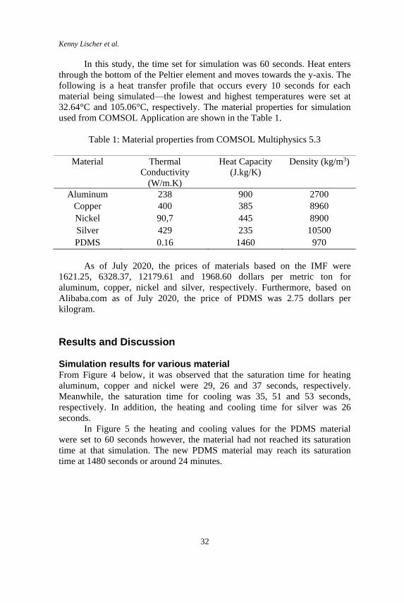
In this study, the time set for simulation was 60 seconds. Heat enters
through the bottom of the Peltier element and moves towards the y-axis. The
following is a heat transfer profile that occurs every 10 seconds for each
material being simulated—the lowest and highest temperatures were set at
32.64°C and 105.06°C, respectively. The material properties for simulation
used from COMSOL Application are shown in the Table 1.
Table 1: Material properties from COMSOL Multiphysics 5.3
Material Thermal
Conductivity
(W/m.K)
Heat Capacity
(J.kg/K)
Density (kg/m3)
Aluminum 238 900 2700
Copper 400 385 8960
Nickel 90,7 445 8900
Silver 429 235 10500
PDMS 0.16 1460 970
As of July 2020, the prices of materials based on the IMF were
1621.25, 6328.37, 12179.61 and 1968.60 dollars per metric ton for
aluminum, copper, nickel and silver, respectively. Furthermore, based on
Alibaba.com as of July 2020, the price of PDMS was 2.75 dollars per
kilogram.
Results and Discussion
Simulation results for various material From Figure 4 below, it was observed that the saturation time for heating
aluminum, copper and nickel were 29, 26 and 37 seconds, respectively.
Meanwhile, the saturation time for cooling was 35, 51 and 53 seconds,
respectively. In addition, the heating and cooling time for silver was 26
seconds.
In Figure 5 the heating and cooling values for the PDMS material
were set to 60 seconds however, the material had not reached its saturation
time at that simulation. The new PDMS material may reach its saturation
time at 1480 seconds or around 24 minutes.

Heat Transfer Simulation of Various Material for PCR Thermal Cycler
33
(a) (b) Figure 4: Temperature curve for each material for 60 seconds (a) heating (b)
cooling.
Figure 5: Saturation time for each material.
Considering that each type of material was tested in the same
geometry, the factors affecting the time difference based on Equation (1)
were density, thermal conductivity and thermal capacity values. The thermal
conductivity value in Equation (1) also appeared in Equation (2) namely
Fourier's law, where q is the heat transfer rate influenced by k which is the
thermal conductivity and ∇T is the temperature gradient.
In Equation (1), the multiplication value of thermal density and
capacity is also known as thermal mass. This is an energy requirement
needed to increase the temperature at a specific volume [17]. Therefore, these
two valueshave an effect on the heat transfer that will occur in the PCR
thermal cycler [18].
Thermal conductivity is one of the crucial factors in the conduction of
material. Therefore, a good thermal conductivity value determines the quality
of a good conductor material [19]. It was observed that silver had the highest
thermal conductivity value of 429 W/mK. Meanwhile, copper, aluminum,
0
20
40
60
80
100
120
0 20 40 60
Tem
per
atu
re(°
C)
Time (s)
Aluminum
Copper
Nickel
Silver
PDMS
0
20
40
60
80
100
120
0 20 40 60
Tem
per
atu
re(°
C)
Time (s)
Aluminum
Copper
Nickel
Silver
PDMS
29 3751
2660
26 3553
2660
0
50
100
Aluminum Copper Nickel Silver PDMS*
Satu
rati
on
Tim
e (S
)
Used Material
Heating Cooling

Kenny Lischer et al.
34
nickel and PDMS had thermal conductivity values of 400, 238, 90.7 and 0.16
W/mK, respectively. Based on thermal conductivity alone, the order for
selecting the best materials for producing a portable thermal cycler design is
silver, copper, aluminum, nickel and PDMS.
However, study carried out by [16] used thermal mass as the basis for
selecting a material to be developed as a portable thermal cycler design.
Therefore, in addition paying attention to the conductivity value, it is
necessary to pay attention to the value of the thermal mass of each material
used. The higher the thermal mass value of a material, the higher the heat
required for the material to raise the temperature. Therefore, much longer
time would be required. Thermal mass is obtained by multiplying the density
value of the material by its heat capacity. For materials with high thermal
conductivity, aluminum had the smallest value of 2430000 J/K m3, silver,
copper and nickel had values of 2467500, 344960 and 3960 500 J/K m3,
respectively. Meanwhile, the PDMS material had a thermal mass of 1416200
J/K m3.
In the saturation time graph, it was observed that the combination of
thermal capacity and thermal mass significantly affects the saturation time of
each material. For example, although silver and copper have close thermal
capacity values with differences in thermal mass values, the saturation times
differ quite significantly. In addition, although aluminum has a low calorific
capacity value compared to silver and copper, with a smaller heat mass the
transfer of heat is faster than in copper but differs slightly when compared to
silver. Aluminum benefits from its low density even though it has a high
heating capacity and an average high thermal conductivity. Conversely, silver
and copper have high thermal conductivity and low heat capacity. However,
the density of the two materials is high enough that there is a little difference
between these materials and aluminum.
For nickel and PDMS, with a conductivity value that is not too high,
the results obtained were not very satisfying however, the nickel material still
managed to reach its saturation time in 60 seconds. Meanwhile, the PDMS
material was unable to reach its saturation time in 60 seconds at such a
thickness condition. Therefore, the next study will focus on aluminum,
copper and silver.
Furthermore, from the economic perspective, the market price of
aluminum is low compared to copper and silver. This was reinforced by the
statement of the company producing PCR, Eppendorf which stated that
aluminum is widely used as a base material for commercial PCR thermal
cycler blocks. In addition, they stated the use of other stuff as a coating on
aluminum or as an alloy. However, there are also commercial PCR thermal
cycler manufacturers that use pure silver as the primary material because of
its effectiveness [20].

Heat Transfer Simulation of Various Material for PCR Thermal Cycler
35
Aluminum is the best material that may be used as a portable design
for thermal cycler PCR as a result of its low price and performance which is
slightly different from silver. This material is also used by several methods of
low-cost microfabrication [21].
Heat transfer to reagents From the Figure 6, it was observed that the saturation time for heating the
chamber material, PCR tube and PCR solution were 29, 30 and 32 seconds,
respectively. Meanwhile for cooling, the saturation time was 26, 30 and 35
seconds, respectively.
Figure 6: Saturation time for each heat transfer process.
The phenomenon that occurs is the transfer of heat to PCR tubes
made of polypropylene [22]. The difference observed in saturation time
was 1 second for heating and 4 seconds for cooling. This is the time
required for conduction from aluminum to the PCR tube. The heat moves
from the PCR tube to the PCR reagent and takes 2 seconds to warm up and
5 seconds to cool down. Therefore, with a total time of 32 seconds for
heating and 35 seconds for cooling, the time required for heat to move
from the metal to the reagent is 3 seconds for heating and 9 seconds for
cooling. This is because a thermal cycler with static heater has more
constant heat flux and gives good temperature uniformity [23].
Conclusions
From this study, the following conclusions were drawn. The heat transfer rate
on a thermal cycler PCR machine may be influenced by the thermal
conductivity and thermal mass values of the material used. The saturation
time obtained in this design for heating was 29, 37 and 51 seconds for
aluminum, copper and nickel, respectively. Meanwhile, the saturation time
29 30 3226 30 35
0
20
40
Material Chamber PCR Tube PCR Reagent
Satu
rati
on
Tim
e (S
)
Location of Heating Process
Heating Cooling
Kenny Lischer et al.
36
obtained for cooling were 26, 35 and 53 seconds for aluminum, copper and
nickel, respectively. In addition, the saturation time for heating and cooling
were 26 seconds and 1480 seconds for silver and PDMS, respectively. In this
design, the saturation time obtained to heat and cool the reagent when using
aluminum was 32 seconds and 35 seconds, respectively after the heat had
passed through the thermal block and the PCR tube
Acknowledgement
We acknowledge that the study is made as an output for PUTI Q2 with
number NKB-1082/UN2.RST/HKP.05.00/2020.
References
[1] L. Garibyan and N. J. T. J. Avashia, “Research techniques made simple:
polymerase chain reaction (PCR),” J. Investigative Dermatology, vol.
133, no. 3, pp. 1 – 8, 2013.
[2] H. Nagai, Y. Murakami, K. Yokoyama, and E. Tamiya, “High-
throughput PCR in silicon based microchamber array,” Biosensor
Bioelectronic, vol. 133, no. 9, pp. 1015 – 1019, 2001.
[3] S. Yamaguchi, T. Suzuki, K. Inoue, and Y. Azumi, “DC-driven
thermoelectric peltier device for precise DNA amplification,” Japanese
J. Applied Physics, vol. 54, no. 5, pp. 057001, 2015.
[4] S. Jeong, J. Lim, M. Y. Kim, J. Yeom, H. Cho, H. Lee, and J. H. Lee,
“Portable low-power thermal cycler with dual thin-film Pt heaters for a
polymeric PCR chip” Biomedical microdevices, vol. 2, no. (1), pp. 14,
2018.
[5] T. Reid, R. Taylor, and L. Brown, U.S. Patent No. 7,459,302,
Washington, DC: U.S. Patent and Trademark Office, 2 December 2008.
[6] M. J. Mortillaro, and D. A. Cohen, U.S. Patent No. 9,604,219,
Washington, DC: U.S. Patent and Trademark Office. 28 March 2017.
[7] W. J. Benett, J. T. Andreski, J. M. Dzenitis, A. J. Makarewicz, D. R.
Hadley, and S. S. Pannu, U.S. Patent No. 8,778,663, Washington, DC:
U.S. Patent and Trademark Office, 15 July 2014.
[8] J. L. Danssaert,, R. J. Shopes,, and D. D. Shoemaker, U.S. Patent No.
5,525,300, Washington, DC: U.S. Patent and Trademark Office, 11 June
1996.
[9] T. C. Gubatayao, K. Handique, K. Ganesan, and D. M. Drummond, U.S.
Patent No. 9,765,389, Washington, DC: U.S. Patent and Trademark
Office. 19 September 2017.
[10] H. Koeda, U.S. Patent No. 9,144,800, Washington, DC: U.S. Patent and
Trademark Office, 29 September 2015.
Heat Transfer Simulation of Various Material for PCR Thermal Cycler
37
[11] R. M. F. Jones, & E. T. McDevitt, U.S. Patent No. 9,869,003,
Washington, DC: U.S. Patent and Trademark Office, 16 January 2018.
[12] J. Courtney, U.S. Patent No. 10,307,762. Washington, DC: U.S. Patent
and Trademark Office, 4 June 2019.
[13] S. A. B. Hermsen, B. R. Roszek, A. W. van Drongelen, and R. E.
Geertsma, “Lab-on-a-chip devices for clinical diagnostics: Measuring
into a new dimension”, 2014.
[14] O. O'Donnell, E. Van Doorslaer, R. P. Rannan-Eliya, A. Somanathan,, S.
R. Adhikari, D. Harbianto, and G. M. Leung, “The incidence of public
spending on healthcare: comparative evidence from Asia”, The World
Bank Economic Review, vol. 21, no. (1), pp. 93-123, 2007.
[15] K. S. Chong, K. B. Gan, and S. M. Then, “Development of a portable
low-cost real-time PCR system”, In 2017 International Conference on
Robotics, Automation and Sciences (ICORAS) (pp. 1-5). IEEE, 2017.
[16] S. Jeong, J. Lim, M. Y. Kim, J. Yeom, H. Cho, H. Lee, and J. H. Lee,
“Portable low-power thermal cycler with dual thin-film Pt heaters for a
polymeric PCR chip”, Biomedical microdevices, vol. 20, no. (1), pp. 14,
2018.
[17] G. Wong, I. Wong, K. Chan, Y. Hsieh, and S. Wong, “A rapid and low-
cost PCR thermal cycler for low resource settings” PLoS one, vol. 10,
no. (7), pp. 0131701, 2015.
[18] Q. Zou, Y. Miao, Y. Chen, U. Sridhar, C. S. Chong, T. Chai, and C.
Heng, “Micro-assembled multi-chamber thermal cycler for low-cost
reaction chip thermal multiplexing”, Sensors and Actuators A:
Physical, vol. 102, no. (1-2), pp. 114-121, 2002.
[19] K. S. Chong,, and K. B. Gan, “Portable polymerase chain reaction
(PCR): thermal ramping rate performance evaluation”. In 2016 IEEE
EMBS Conference on Biomedical Engineering and Sciences
(IECBES) (pp. 447-449). IEEE, 2016.
[20] J. G. Atwood, A. Fawcett, K. S. Ferrara, P. M. Hetherington, R. W.
Noreiks, D. E. Olsen, and C. M. Wittmer, U.S. Patent No. 7,537,377.
Washington, DC: U.S. Patent and Trademark Office, 26 May 2009.
[21] J. Charmet, R. Rodrigues, E. Yildirim, P. K. Challa, B. Roberts, R.
Dallmann, & Y. Whulanza, Low-Cost Microfabrication Tool
Box. Micromachines, vol. 11, no. (2), pp. 135, 2020.
[22] X. Huang, L. Hou, X. Xu, H. Chen, H. Ji, and S. Zhu, “One-PCR-tube
approach for in situ DNA isolation and detection”, Analyst, vol. 136, no.
(20), pp. 4254-4259, 2011.
[23] V. S. Duryodhan, S. G. Singh, & A. Agrawal. (2020). The Concept of
Making On-Chip Thermal Cycler for RT-PCR Using Conjugate Heat
Transfer in Diverging Microchannel. Transactions of the Indian
National Academy of Engineering, 1.

Journal of Mechanical Engineering Vol 18(2), 39-50, 2021
___________________
ISSN 1823-5514, eISSN 2550-164X © 2021 College of Engineering,
Universiti Teknologi MARA (UiTM), Malaysia.
Received for review: 2020-09-08 Accepted for publication: 2021-03-18
Published: 2021-04-15
COVID-19 and Effective Management of Public Transport: Perspective from the Philippines
G U Nnadiri, N S Lopez*
Mechanical Engineering Department, De La Salle University,
Manila, Philippines
ABSTRACT
The fight of COVID-19 resulted to the suspension of main public
transportation services in the Philippines to avoid the spread of the virus on
March 16, 2020. This raised questions on how people can travel to access
essential services. A study estimated that there can be 7 billion infections and
40 million deaths globally this year in the absence of interventions. Thus, in
this paper, the authors reflect on key transport-related issues arising from the
pandemic and analyse potential policy recommendations. Particularly, the
paper provides a focus on public transport services. The authors recommend
focusing on reducing virus transmission in surfaces found in public transport
vehicles, use of digital technology to speed up information generation and
distribution for contact tracing, and exertion of efforts to reduce transport
demand by incentivizing and supporting telecommuting among companies. In
conclusion, the authors believe that the central government should be on top
of this COVID-19 response. Though delegating the management to local
government units and various sectors has its benefits, one wrong decision from
a certain unit can lead to a ripple of infections. Standards and protocols,
especially on how public transport should operate, must be scientifically
commissioned to avoid one big trial and error experiment considering the
wealth of information already available in literature.
Keywords: Covid-19; Public transport; Philippines; Policy
Introduction
The intensity and speed Covid-19 spread vary by locations and is now planet-
wide. A study [1] estimates 7.0 billion infections and 40 million death globally
G U Nnadiri and N S Lopez
40
this year in the absence of interventions. As of 25th of July 2020, there has
been 15,581,009 confirmed cases, 635,173 deaths globally according to World
Health Organization [2]. While the Centers for Disease Control and Prevention
[3] claims that most coronaviruses will not survive high temperatures and
humidity levels, the recent summer in Southeast Asia make it seem otherwise.
This is explained in [4] where they estimated that the 2019-nCov only rapidly
inactivated when exposed to 70 °C. In recent times, the hottest summer in the
Philippines only reached a record high of 36.6 °C in April 2019 [5], while
historically, the highest temperature recorded in the Philippines was 42.2 °C
in Tuguegarao in 1969 [6].
To fight COVID-19, the Philippine government suspended public
transportation on March 16, 2020. This decision has met significant
disagreement from the public [7]. As a result of the travel ban, workers were
forced to walk back to their homes outside of Metro Manila. Particularly, these
were mostly the blue-collar workers who were not able to catch the last bus
trips when the quarantine order was immediately raised. Without public
transport, the public can only rely to private vehicles, bicycles, and when
possible, walking. The vital role of public transport in the daily tasks of the
public is undeniable and can never be met fully by private vehicles. People
living in areas that are only accessible by tricycles and jeepneys are particularly
affected the most [8].
Temporarily, the emphasis ought to be on demand control, and this will
incorporate the exacting execution of physical distancing measures, regular
transportation disinfection, implementation of safety rules in every single
casual method of transport and control of travel demand. In the medium-term,
there should be an emphasis on public transport improvement including
interjurisdictional coordination of public travel and better administration of
informal transport providers. This can be accomplished by acquiring multi-
modular arrangements, for example, mass travel frameworks like Metro and
bus transport and begin considering elective arrangements like bikes and e-
vehicles to offer different versatility answers for individuals [9]. A study [10]
reported the financial implications brought about by the pandemic.
Manufacturing may lose PhP 82.1 billion to PhP 855.2 billion; wholesale and
retail trade may suffer a loss of at least PhP 93.2 billion to PhP 724.8 billion;
and transport, storage, and communication due to expected declines in tourism
may lose between PhP 11.7 billion to PhP 124.3 billion. Those are among the
expected worst-hit sectors. Philippines on the other hand is not expected to
recover in the third quarter because of the long strict lockdown aimed to
contain the outbreak of the virus. The country is the only country in the Asia-
Pacific (APAC) region to implement the longest lockdown [11]. In addition,
COVID-19 has become a devastating world-wide human catastrophe and has
disrupted lives and livelihoods. The degree of change will affect the way
people work and interact daily with several companies and organizations
COVID-19 and Effective Management of Public Transport: Perspective from the Philippines
41
imposing a telecommuting (work-from-home) setup for their employees who
can still be productive while working from home. This new trend of mobility
may present a unique opportunity to innovate for different sectors [12].
Given that mobility is almost front and centre in this pandemic, the
authors recognize the need for governments to act swiftly and make key
mobility-related decisions that would minimize further impacts to the economy
and well-being of the people. Thus, in this paper, the authors reflect on key
transport-related issues arising from the pandemic and analyse potential policy
recommendations. Particularly, the paper provides a focus on public transport
services. Moreover, the authors will be interchanging between COVID-19,
SARS-CoV-2, and 2019-nCov throughout the manuscript as other published
literature are cited. To clarify, 2019-nCov will be used to refer to the virus
itself, COVID-19 to refer to the disease obtained from the virus, and SARS-
CoV-2 to refer to the virus as part of a larger family of viruses.
Immediate issues for public transport In this section, three key immediate issues are discussed: (1) the need to reduce
virus transmission within the vehicles; (2) speeding up information generation
and distribution in light of non-compliance reporting and contact tracing; and
(3) keeping up with the demand.
Reducing virus transmission within the vehicles Findings in literature about the transmission of the 2019-nCOv through
aerosols vary. However, a computational fluid dynamics simulation by [13]
showed that 85% to 100% of virus-carrying droplets deposit on surfaces or fall
to the floor, instead of getting directly inhaled. Moreover, [14] noted that the
residence of SARS-CoV-2 in the air is not long. [15] did not find SARS-CoV-
2 in air samples obtained from the rooms of COVID-19 hospitalized patients.
Furthermore, it has been observed that the disease is not transmitted to
healthcare workers directly in contact with COVID-19 patients when they are
wearing simple surgical masks [16]. Thus, the focus now should likely be on
how the virus spreads through contact with infected surfaces. For public
transport patrons, there is a huge chance that they can bring home the virus to
unsuspecting family members through their clothing, bank notes (i.e. paper
money) and unwashed arms or hands after getting into contact with various
surfaces in public transport.
Most cases of COVID-19 are reported to be mild, but the infection tends
to be transmitted quickly. Tiny droplets from coughing and sneezing can carry
the virus by as far as one to two meters. If they happen to make it into another
person’s airways, they could become infected, but the virus can also live on
surfaces where these droplets land [17].
A comprehensive report by [18] and [4] evaluated the survival of 2019-
nCov on different sorts of surfaces (see Table 1). They analysed the aerosol
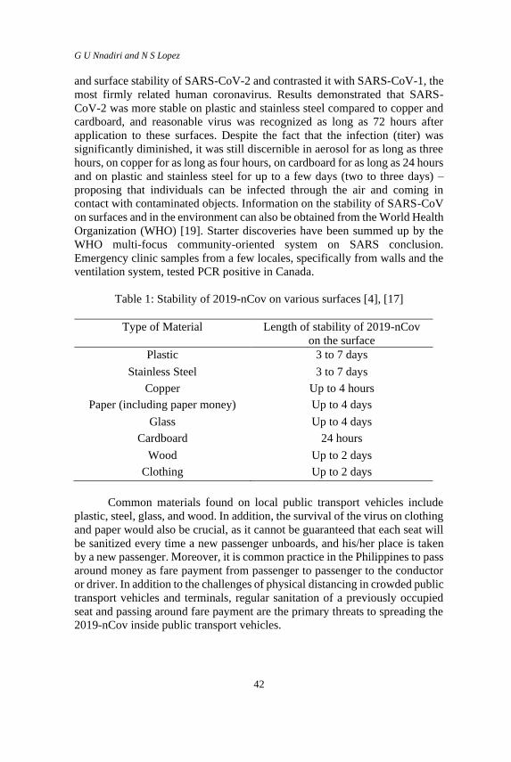
G U Nnadiri and N S Lopez
42
and surface stability of SARS-CoV-2 and contrasted it with SARS-CoV-1, the
most firmly related human coronavirus. Results demonstrated that SARS-
CoV-2 was more stable on plastic and stainless steel compared to copper and
cardboard, and reasonable virus was recognized as long as 72 hours after
application to these surfaces. Despite the fact that the infection (titer) was
significantly diminished, it was still discernible in aerosol for as long as three
hours, on copper for as long as four hours, on cardboard for as long as 24 hours
and on plastic and stainless steel for up to a few days (two to three days) –
proposing that individuals can be infected through the air and coming in
contact with contaminated objects. Information on the stability of SARS-CoV
on surfaces and in the environment can also be obtained from the World Health
Organization (WHO) [19]. Starter discoveries have been summed up by the
WHO multi-focus community-oriented system on SARS conclusion.
Emergency clinic samples from a few locales, specifically from walls and the
ventilation system, tested PCR positive in Canada.
Table 1: Stability of 2019-nCov on various surfaces [4], [17]
Type of Material Length of stability of 2019-nCov
on the surface
Plastic 3 to 7 days
Stainless Steel 3 to 7 days
Copper Up to 4 hours
Paper (including paper money) Up to 4 days
Glass Up to 4 days
Cardboard 24 hours
Wood Up to 2 days
Clothing Up to 2 days
Common materials found on local public transport vehicles include
plastic, steel, glass, and wood. In addition, the survival of the virus on clothing
and paper would also be crucial, as it cannot be guaranteed that each seat will
be sanitized every time a new passenger unboards, and his/her place is taken
by a new passenger. Moreover, it is common practice in the Philippines to pass
around money as fare payment from passenger to passenger to the conductor
or driver. In addition to the challenges of physical distancing in crowded public
transport vehicles and terminals, regular sanitation of a previously occupied
seat and passing around fare payment are the primary threats to spreading the
2019-nCov inside public transport vehicles.
COVID-19 and Effective Management of Public Transport: Perspective from the Philippines
43
Speeding up information generation and distribution in public transport The speed of information generation and distribution is crucial in controlling
the spread of a virus like the 2019-nCov. Countries which have implemented
strict contact tracing measures have been seen to beat COVID-19 faster than
others [20]. Contact tracing, including case investigations, are part of the
process of warning individuals who may have been exposed to the virus and
have potentially contracted the disease as well. Countries such as South Korea
and New Zealand [21] have shown that good contact tracing and case
investigation strategies can stop chains of transmission of the virus. However,
contact tracing is a specialized skill and time is of the essence [22].
The problem now is, how can contact tracing be implemented in public
transport? A person would roughly get into close physical contact with at least
5 people in public transport. Additionally, these interactions are multiplied by
the multi-modal nature of public transport. A person can take jeepney route A,
and then transfer to rail route B, before finally taking jeepney route C to the
final destination.
Recently, public transport operators in the Philippines have
implemented their own approaches, such as requiring passengers to fill out
information sheets before getting on board the vehicle [23]. However, though
this is possible in terminal-based services, this will be challenging to
implement in fast-paced services which implement road-side loading and
unloading such as jeepneys. Moreover, given the paper-based system, how
fast can contact tracing be done and who will be responsible to do the tracing?
Will it be faster than the speed of transmission of the disease?
Furthermore, non-compliance among public transport operators and
drivers must be promptly reported and acted on. Non-compliance to safety
protocols put in place by policymakers carelessly spread the virus. Thus, the
rapid generation and distribution of information among public transport
stakeholders (i.e. operators, drivers, and commuters) would facilitate timely
testing of potential virus carriers and stop random transmission of the virus.
Contact tracing is the weakest link in the Philippine COVID-19 response. The
adequacy of resources to identify people exposed to the virus, especially those
who are asymptomatic can help manage the spread of the virus in public
transport.
Keeping up with the demand After the first phase of the quarantine order, the gradual reopening of shopping
malls, public transit, and other selected services were proposed, should the
government lift or extend the enhanced community quarantine (ECQ). The
transportation department is looking into the possibility of allowing 30%
capacity resumption of public transportation, mostly buses and trains, to allow
the observation of physical distancing measures. In line with the resumption

G U Nnadiri and N S Lopez
44
and reduction of public transportation capacity, [24] reported the guidelines
for public transportation in areas deemed at low risk for transmission of the
virus (COVID-19). This guideline requires a special permit for public utility
vehicles (PUV) to operate and the reduction of passenger capacity for buses,
jeeps, and UV Express to 50% in adherence to a 1 meter physical distancing
rule. A report retrieved from [25] on April 30, 2020 during the transition of
Metro Manila from ECQ to general community quarantine (GCQ) stated that
all allowed PUVs and transport terminals and administrators must stick to all
three basic parts directed - Safety, Capacity and Coverage or Scope. Safety as
expressed refers to the rules to decrease contact, transmission and spread of
the virus through obligatory utilization of face cover and gloves by drivers,
careful sanitation of vehicles, terminals, and even among travellers are
likewise required. The admissible capacity is 50%, excluding driver and
conductor to guarantee distancing in public utility buses (PUBs) and public
utility jeepneys (PUJs). For utility vans and taxis, passengers ought to not
surpass two persons for every row, aside from the driver's row where just a
single passenger is permitted. Tricycles must not exceed one person in the
sidecar, while back riding will not be permitted. With respect to private vehicle
and motorcycle owners, they will be permitted to operate on essential purposes
as approved by the Inter-Agency Task Force (IATF). Private vehicles will be
permitted one person in the front row, while the rear seats should not surpass
two persons for each row. Motorcycles are restricted from having back-riding
travellers. The utilization of bicycles and comparative modes are likewise
profoundly empowered, and local government units (LGUs) are additionally
urged to identify dedicated bicycle paths or lanes.
This guideline was further amended, allowing motorcycles to have
back-riding passengers with the use of barriers to demarcate the back-rider.
While people are trying to observe physical distancing in public transport,
there will be a rise on personal transport modes like bicycle, electric scooters,
and other forms which are expected to gain popularity following this
pandemic.
Possible issues of reducing transportation capacity by 50% will be the
rise of more private vehicle trips thereby resulting to traffic congestion;
stranded passengers at vehicles terminals; and loss of time. Similarly, the
proposed barrier used for motorcycles may not be the best. This may lead to
potential accidents and fatal injuries for both the motorist and the back-rider
when driving on free roads where high speeds are inevitable.
On 11th and 14th of September 2020, the Philippine government planned
the easing of physical distancing in public transports. This will be done with
strict monitoring of the daily reported cases after its implementation to know
the effects of the adjustments from the approved one-meter distance by WHO
to a reduced distance of 0.75 meters. This will be further reduced to 0.5 meters
and then 0.3 meters with two-weeks progressive monitoring of each
COVID-19 and Effective Management of Public Transport: Perspective from the Philippines
45
implemented reduced physical distancing, and if there are no issues then the
policy will remain [26,27]. Furthermore, DOTr noted that with full compliance
of the use of face masks and face shields in public transport, the one-meter
distancing can successfully be reduced to 0.3 meters. A report from the
International Union of Railways (UIC) further explained that the use of a face
mask and face shield is 100 percent safe even if you come in contact with
someone who is the carrier of the virus [28]. With this at hand, there has been
complaints from the masses noting that the reduced physical distancing should
only be encouraged when the number of reported cases and active cases flatten.
With regards to this, there are a lot of oppositions to the implementation of
reduced physical social distancing, mostly medical practitioners who have
criticized and noted that the reduced spacing among commuters will further
increase the spread of the virus [29]. Due to the strong opposition from the
masses, the government decided to suspend this new policy on 17th September
2020 [30].
Policy Recommendations
Considering the key issues raised in the previous section, the authors would
like to propose the following policy implications.
• Provide standards. The government should provide scientific and data-
driven standards, rather than allowing local government units and sectors
to implement their own strategies. The minimum requirements should at
least come from the centralized government. For example, what safety
features should be found in jeepneys at the minimum? Some operators are
installing plastic sheets to shield passengers away from each other. Instead
of helping, that can even help spread the virus further because it will add
more surfaces for the virus to live on to. If the government does not
publish standards about this, operators will just implement what they
want, and our pandemic response will become one big experiment. There
is enough information in literature now to narrow down the options and
help the country develop minimum standards now. Standards should be
developed scientifically and in consultation with academics.
• Manage the demand. You cannot expect a service to run smoothly when
you decrease its capacity (supply) by half without creating a similar
reduction in demand. To reduce demand, it is recommended that the
government encourage companies to maintain their telecommuting (work-
from-home) setups until after a viable vaccine becomes available. This
can be done by providing fiscal and non-fiscal incentives to companies
willing to do telecommuting. Without this kind of support, companies
might be forced to risk their employees commuting or opt to suspend
operations, which will be detrimental to the economy. In addition to the
G U Nnadiri and N S Lopez
46
said incentives, this is also prime time to improve the internet
infrastructure of the country and strengthen our data security policies and
protocols. It is also recommended to encourage schools capable of
distance-learning to keep doing this until after a viable vaccine becomes
available.
• Improve the supply. Supply can be improved by allowing modern jeepney
fleets to operate and co-exist with conventional jeepneys. Modern
jeepneys are more spacious, which could make physical distancing easier
to implement. This can be a good opportunity to accelerate the
implementation of the Public Utility Vehicle Modernization Program of
the government. However, the welfare and livelihood of conventional
jeepney operators and drivers should be put first and foremost. Social
programs need to be set up for them.
• Improve the services. This can be done by leveraging and promoting
digital technologies in transportation. The government should fund the
development of fleet management systems, which would speed up
information generation and distribution in public transport. This would
manage non-compliance among operators and drivers. Also, the fleet
management system should provide an efficient means to keep record of
which vehicles each commuter takes and at which date and time to enable
fast contact tracing in public transport. This can be done by creating an
end-user app that commuters can use to book seats in advance, or just to
log their vehicle boarding and unboarding activities.
Conclusions
In conclusion, the authors believe that the central government should be on top
of this COVID-19 response. Though delegating the management to local
government units and various sectors has its benefits, one wrong decision from
a certain unit can lead to a ripple of infections. Standards and protocols,
especially on how public transport should operate, must be scientifically
commissioned. The country’s COVID-19 response does not have to be a one
big trial and error experiment considering the wealth of information already
available in literature, especially when the lives of many people are on the line.
This is also a good time to embrace innovation, not only
technologically but also on how certain business processes are carried out. The
country should leverage on the telecommuting experience it has obtained
during this time, including distance learning. These alternatives are better
maintained even beyond the pandemic from a sustainability perspective.
Based on literature, the best protection for commuters, public transport
operators and drivers are plain and simple wearing of face masks, good
personal hygiene, and regular sanitation of surfaces which get into contact with
COVID-19 and Effective Management of Public Transport: Perspective from the Philippines
47
passengers. Thus, additional structures (e.g. shielding) might not be necessary
after all. Proper management of supply and demand, the use of digital
technology to speed up information generation and distribution, and the
implementation of scientific safety standards should allow our commuters to
use public transport safely and comfortably.
Acknowledgements
The authors would like to thank the ASEAN Foundation and USAID for their
invaluable support to the ASEAN Science and Technology Fellows of the year
2019-2020. Gratitude is also expressed to the Office of the Vice Chancellor for
Research and Innovation and the Science Foundation of De La Salle University
for the financial support provided in the publishing of this work.
References
[1] P. Walker, C. Whittaker, O. Watson, M. Baguelin, K. Ainslie, S. Bhatia
and P. Z. Cucunuba, “The impact of COVID-19 and strategies for
mitigation and suppression in low- and middle-income countries,”
Science, vol. 369, no. 6502, pp. 413-422, 2020.
[2] World Health Organization, “Coronavirus Diseases (COVID-19)
Dashboard,” July 25, 2020. [Online]. Available:
https://covid19.who.int/?gclid=Cj0KCQjwgo_5BRDuARIsADDEntSiB
wc0wVE_m816mOuxm98W4of1C3PLXEZstZscG48yYBwVw6_1aZM
aAueNEALw_wcB. [Accessed July 25, 2020].
[3] Centers for Disease Control and Prevention, “Coronavirus Disease 2019
(COVID-19),” Frequently Asked Questions. [Online]. Available:
https://www.cdc.gov/coronavirus/2019-ncov/faq.html. [Accessed July
30, 2020].
[4] A. W. H. Chin, J. T. S. Chu, M. R. A. Perera, K. P. Y. Hui, H. Yen, M. C.
W. Chan, M. Peiris and L. L. M. Poon, “Stability of SARS-CoV-2 in
different environmental conditions,” The Lancet, Microbe, vol. 1, no. 1,
e10, 2020.
[5] CNN Philippines, “Metro Manila records highest temperature for 2019,”
July 31, 2020. [Online]. Available: https://www.cnnphilippines.com/
news/2019/4/22/Metro-Manila-temperature-record-high-2019.html.
[Accessed July 31, 2020].
[6] Inquirer, “Tuguegarao City records hottest temperature–Pagasa,” April
26, 2014. [Online]. Available: https://newsinfo.inquirer.net/597474/
tuguegarao-city-records-hottest-temperature-pagasa. [Accessed July 31,
2020].
G U Nnadiri and N S Lopez
48
[7] R. De Silva, “COVID-19: Its Impact on the Philippines – FINAL,” Europe
Solidaire Sans Frontières, July 25, 2020. [Online]. Available:
http://www.europe-solidaire.org/spip.php?article52772. [Accessed July
25, 2020].
[8] EcoMobility, “COVID-19: Focus on cities and transport responses—
South East Asia,” July 25, 2020. [Online]. Available:
https://sustainablemobility.iclei.org/covid-19-focus-on-cities-and-
transport-responses-south-east-asia/. [Accessed July 25, 2020].
[9] R. Madhu, “Building safer and more resilient cities in Philippines,” World
Bank Blogs, May 14, 2020. [Online]. Available:
https://blogs.worldbank.org/eastasiapacific/building-safer-and-more-
resilient-cities-philippines?fbclid=IwAR0fJ4YXjW3VVBuwgLdl7LW_
AjVHJ6Lbj9PXU2_JaHjVF3yo4RqyDJI9qtk. [Accessed July 25, 2020].
[10] C. M. Ramos, “Covid-19 impact study: Losses may hit P2.5 trillion; ease
economic restrictions,” Inquirer, April 17, 2020. [Online]. Available:
https://newsinfo.inquirer.net/1260203/ph-economy-may-lose-up-to-p2-5-
trillion-due-to-covid-19-pandemic-pids-study. [Accessed July 25, 2020].
[11] S. Cochrane, “No growth for Philippines in Q3, says Moody’s unit,”
Philstar Global, July 25, 2020. [Online]. Available:
https://www.philstar.com/business/2020/07/25/2030363/no-growth-
philippines-q3-says-moodys-unit?fbclid=IwAR2g_zL0JCBqRwsym4
YVSnt2b26hgiXWRoGGGTCoQXfNrbe3Eyy0oFG94-0. [Accessed July
25, 2020].
[12] L. Wright, “Let’s use the pandemic to expand our transport options,”
Asian Development Blog, April 3, 2020. [Online]. Available:
https://blogs.adb.org/let-s-use-the-pandemic-to-expand-our-transport-
options?fbclid=IwAR0w4wXVhPudpo-kjNKCCceeES9_ThA7FLwb
R6K2Dg7Uw1YKjXb5xGS6km8. [Accessed July 28, 2020].
[13] X. Yang, C. Ou, H. Yang, L. Liu, T. Song, M. Kang, H. Lin and J. Hang,
“Transmission of pathogen-laden expiratory droplets in a coach bus,”
Journal of Hazardous Materials, vol. 397, pp. 122609, 2020.
[14] J. H. Rubens, P. C. Karakousis and S. K. Jain, “Stability and Viability of
SARS-CoV-2,” The New England Journal of Medicine, vol. 382, pp.
1962-1966, 2020.
[15] S. W. X. Ong, Y. K. Tan, P. Y. Chia, T. H. Lee, O. T. Ng, M. S. Y. Wong
and K. Marimuthu, “Air, surface environmental, and personal protective
equipment contamination by severe acute respiratory syndrome
coronavirus 2 (SARS-CoV-2) from a symptomatic patient,” JAMA, vol.
323, no. 16, pp.1610-1612, 2020.
[16] K. Ng, B. H. Poon, T. H. Kiat Puar, J. L. Shan Quah, W. J. Loh, Y. J.
Wong, T. Y. Tan and J. Raghuram, “COVID-19 and risk to health care
workers: a case report,” Annuals of Internal Medicine, vol. 172, no. (11),
pp. 766-767, 2020.
COVID-19 and Effective Management of Public Transport: Perspective from the Philippines
49
[17] K. E. Foley, “The novel coronavirus can likely live up to 96 hours on
phone screens,” Quartz, February 29, 2020. [Online]. Available:
https://qz.com/1810508/covid-19-can-likely-live-up-to-96-hours-on-
your-phone/. [Accessed July 28, 2020].
[18] N. Van Doremalen, T. Bushmaker, D. H. Morris, M. G. Holbrook, A.
Gamble, B. N. Williamson and J. O. Lloyd-Smith, “Aerosol and surface
stability of SARS-CoV-2 as compared with SARS-CoV-1,” The New
England Journal of Medicine, vol. 382, pp. 1564-1567, 2020.
[19] World Health Organization, “Consensus document on the epidemiology of
severe acute respiratory syndrome (SARS) (No. WHO/CDS/
CSR/GAR/2003.11),” May 17, 2003. [Online]. Available:
https://apps.who.int/iris/handle/10665/70863. [Accessed July 28, 2020].
[20] Bloomberg, “These elite contact tracers show the world how to beat
COVID-19,” July 25, 2020. [Online]. Available: https://www.
bloomberg.com/news/articles/2020-07-25/these-elite-contact-tracers-
show-the-world-how-to-beat-covid-19. [Accessed July 31, 2020].
[21] World Health Organization, “New Zealand takes early and hard action to
tackle COVID-19,” July 15, 2020. [Online]. Available: https://www.
who.int/westernpacific/news/feature-stories/detail/new-zealand-takes-
early-and-hard-action-to-tackle-covid-19. [Accessed July 31, 2020].
[22] Centers for Disease Control and Prevention, “Case investigation and
contact tracing: Part of a multipronged approach to fight the COVID-19
pandemic,” December 3, 2020. [Online]. Available: https://www.cdc.gov
/coronavirus/2019-ncov/php/principles-contact-tracing.html. [Accessed
July 31, 2020].
[23] Manila Times, “LTFRB: Commuters may be asked to give personal info
to PUVs for virus contact tracing,” May 19, 2020. [Online]. Available:
https://www.manilatimes.net/2020/05/19/second-headline/ltfrb-
commuters-may-be-asked-to-give-personal-info-to-puvs-for-virus-
contact-tracing/725813/. [Accessed July 31, 2020].
[24] Philippine News Agency, “DOTr sets guidelines for public transport in
GCQ areas,” May 1, 2020. [Online]. Available: https://www.pna.gov.ph
/articles/1101544. [Accessed July 26, 2020].
[25] Department of Transportation, “DOTr issued guideline for road transport
sector in areas under GCQ,” May 1, 2020. [Online]. Available:
https://dotr.gov.ph/55-dotrnews/1315-dotr-issues-guidelines-for-road-
transport-sector-in-areas-under-gcq.html. [Accessed July 26, 2020].
[26] CNN Philippines, “DOTr: Possible to recall new public transport
distancing policy,” September 14, 2020. [Online]. Available:
https://www.cnnphilippines.com/news/2020/9/14/DOTr-reduced-
physical-distancing-public-transport-study.html? fbclid=IwAR2mon-
aotP96nZd7FE_A9R4ABNpsPzJyYbul7l-wZFEl-pZLZEd9D9_gXM.
[Accessed September 17, 2020].
G U Nnadiri and N S Lopez
50
[27] CNN Philippines, “Gov't approves easing of physical distancing rules in
public transport,” September 11, 2020. [Online]. Available:
https://cnnphilippines.com/news/2020/9/11/Public-transportation-
physical-distancing-rules-Philippines.html?fbclid=IwAR1Q0-
vuy9YnenkSWz2DHqFmj22jzFnNZz4YyldAYrV28uAgcu jLT5os7LI.
[Accessed September 17, 2020].
[28] International Union of Railways, "Masks ventilation and social
distancing,” September 17, 2020. [Online]. Available:
https://uic.org/IMG/pdf/railsilience_masks_ventilation.pdf. [Accessed
September 17, 2020].
[29] M. Vacas, “Reduced commuter distancing up for review; DILG agrees
more public transportation must be deployed,” One News, September 15,
2020. [Online]. Available: https://www.onenews.ph/reduced-commuter-
distancing-up-for-review-dilg-agrees-more-public-transportation-must-
be-deployed. [Accessed September 17, 2020].
[30] P. Ranada, “Gov’t suspends reduced physical distancing in public
transportation,” Rappler, September 17, 2020. [Online]. Available:
https://www.rappler.com/nation/government-suspends-reduced-physical-
distancing-public-transportation. [Accessed September 29, 2020].
Journal of Mechanical Engineering Vol 18(2), 51-64, 2021
___________________
ISSN 1823-5514, eISSN 2550-164X Received for review: 2021-01-22
© 2021 College of Engineering, Accepted for publication: 2021-03-08
Universiti Teknologi MARA (UiTM), Malaysia. Published: 2021-04-15
Microstructure and Microhardness Alterations of Inconel 718 under
Cryogenic Cutting
Che Hassan Che Haron, Jaharah Abdul Ghani, Muammar Faiq Azhar
Centre for Engineering Materials and Smart Manufacturing (MERCU),
Faculty of Engineering and Built Environment,
Universiti Kebangsaan Malaysia, 43600 Bangi, MALAYSIA
Nurul Hayati Abdul Halim*
School of Mechanical Engineering, College of Engineering,
Universiti Teknologi MARA, 40450, Shah Alam, Malaysia.
N. Badroush
Center of Human Resource Development and Quality,
Academy of Maritime Studies, Tripoli, Libya
ABSTRACT
This paper presents the experimental investigations to identify the effect of
different machining parameters on the microstructure and microhardness
alterations beneath the machined surface of Inconel 718. The high-speed
milling experiments were conducted using PVD multi-coated ball nose carbide
inserts, under cryogenic CO2 condition at controlled cutting speed of 120-140
m/min, feed rate of 0.15-0.25 mm/tooth, depth of cut of 0.3–0.7 mm and a fixed
width of cut at 0.4 mm. The experimental results discovered that the formation
of plastic deformation could only be observed when cutting with the highest
value of feed rate and depth of cut, deepened until 8.87 µm from the machined
surface. At the same time, those factors also significantly increased machined
surface hardness, made the workpiece harder than its bulk hardness. However,
the hardness values were found reduced towards the sub-surface and back to
its bulk hardness approximately 250 - 300 µm from the top surface. This study
suggests that the finishing milling process of Inconel 718 under cryogenic CO2
condition and at predetermined parameters can be performed at a depth of cut
less than 0.3 mm as its machined sub-surface microhardness and
microstructure alteration were observed to be inconsequential. Thus, a more
economical machining process can be performed.

C.H.C.Haron et al.
52
Keywords: Cryogenic Machining; Coated Tungsten Carbide; Inconel 718;
Microstructure alteration; Microhardness
Introduction
Super alloy Inconel 718 is one of the Nickel-based super-alloys. It is widely
applied in aerospace industries due to its high strength at elevated temperatures
and high resistance to corrosion. However, when cutting this difficult-to-
machine material at high-speed, its low thermal conductivity caused the heat
that inherently generated accumulating in the cutting zone to extreme levels.
Researchers such as Musfirah et al. [1], Kasim [2], and Sonawane and Joshi
[3] reported there were microstructure and microhardness changes beneath the
machined surface when high-speed milling Inconel 718 under cryogenic,
minimum quantity lubrication (MQL) and dry conditions, respectively. As
reported, the combination of elevated cutting temperatures and the mechanical
shock from the intermittent cutting of milling process accelerates wear rate
which then facilitates sub-surface defects like plastic deformation and the
tendency of the machined surface to work-harden [4]. These undesirable
changes reduce its surface integrity while increasing its difficulty to be
machined.
The correlation between different machining conditions and the levels
of microstructure and microhardness alteration at machined sub-surface have
been numerously examined by previous studies. Cutting speed, feed rate, depth
of cut, tool type, geometry, as well as lubrication or cooling conditions, are
some of the common factors that have been investigated [5]. The finding is
important as the alterations affect the fatigue life, functionality, and durability
of the final products, mainly the one serviced in high temperatures or stress
loads and aggressive environments [6]. Meanwhile, Grzesik et al. [7] used
terms abusive, conventional, and gentle machining processes which related to
the level of heat and strain rates generated during cutting to demonstrate their
influence on machined surface integrity.
Generally, the depth of plastic deformation below the machined surface
to which it extends significantly influenced by the tool geometry, depth of cut,
machining conditions as well as the absence or presence of coolant or lubricant
during cutting [7]. For instance, Sharman et al. [8] found that the worn tool
produced greater degree of grain boundary microstructural plastic deformation
than the new tool in turning of Inconel 718. Meanwhile, a study by Musfirah
et al. [1] revealed obvious grain structure deformation near the machined
surface in dry milling of Inconel 718 rather than in cryogenic condition using
liquid nitrogen (LN2). This is apparently related to the elevated temperature of
dry milling due to the absence of any coolant or lubricants during cutting [9].
However, the extremely low temperature of cryogenic LN2 at -196 ºC tends to
work-harden Inconel 718, thus increase its microhardness. As also found by
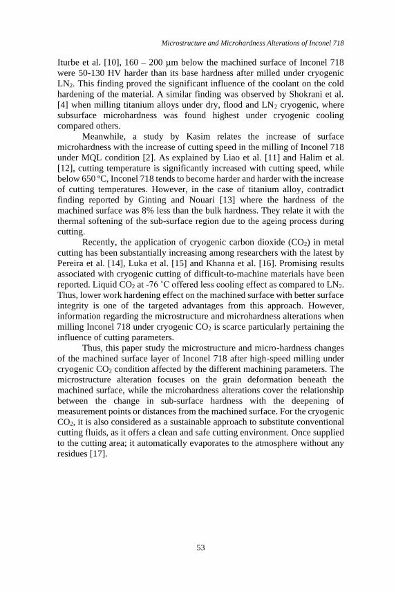
Microstructure and Microhardness Alterations of Inconel 718
53
Iturbe et al. [10], 160 – 200 µm below the machined surface of Inconel 718
were 50-130 HV harder than its base hardness after milled under cryogenic
LN2. This finding proved the significant influence of the coolant on the cold
hardening of the material. A similar finding was observed by Shokrani et al.
[4] when milling titanium alloys under dry, flood and LN2 cryogenic, where
subsurface microhardness was found highest under cryogenic cooling
compared others.
Meanwhile, a study by Kasim relates the increase of surface
microhardness with the increase of cutting speed in the milling of Inconel 718
under MQL condition [2]. As explained by Liao et al. [11] and Halim et al.
[12], cutting temperature is significantly increased with cutting speed, while
below 650 ºC, Inconel 718 tends to become harder and harder with the increase
of cutting temperatures. However, in the case of titanium alloy, contradict
finding reported by Ginting and Nouari [13] where the hardness of the
machined surface was 8% less than the bulk hardness. They relate it with the
thermal softening of the sub-surface region due to the ageing process during
cutting.
Recently, the application of cryogenic carbon dioxide (CO2) in metal
cutting has been substantially increasing among researchers with the latest by
Pereira et al. [14], Luka et al. [15] and Khanna et al. [16]. Promising results
associated with cryogenic cutting of difficult-to-machine materials have been
reported. Liquid CO2 at -76 ˚C offered less cooling effect as compared to LN2.
Thus, lower work hardening effect on the machined surface with better surface
integrity is one of the targeted advantages from this approach. However,
information regarding the microstructure and microhardness alterations when
milling Inconel 718 under cryogenic CO2 is scarce particularly pertaining the
influence of cutting parameters.
Thus, this paper study the microstructure and micro-hardness changes
of the machined surface layer of Inconel 718 after high-speed milling under
cryogenic CO2 condition affected by the different machining parameters. The
microstructure alteration focuses on the grain deformation beneath the
machined surface, while the microhardness alterations cover the relationship
between the change in sub-surface hardness with the deepening of
measurement points or distances from the machined surface. For the cryogenic
CO2, it is also considered as a sustainable approach to substitute conventional
cutting fluids, as it offers a clean and safe cutting environment. Once supplied
to the cutting area; it automatically evaporates to the atmosphere without any
residues [17].
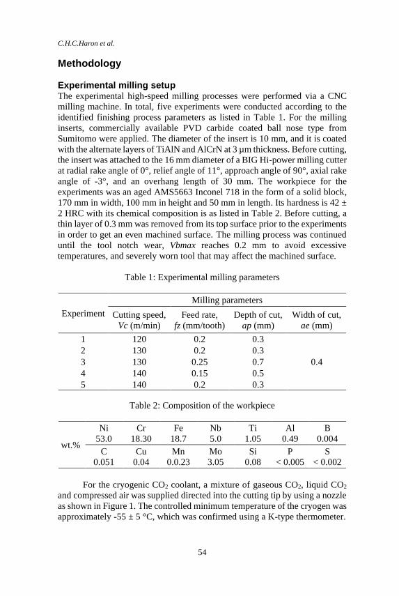
C.H.C.Haron et al.
54
Methodology
Experimental milling setup The experimental high-speed milling processes were performed via a CNC
milling machine. In total, five experiments were conducted according to the
identified finishing process parameters as listed in Table 1. For the milling
inserts, commercially available PVD carbide coated ball nose type from
Sumitomo were applied. The diameter of the insert is 10 mm, and it is coated
with the alternate layers of TiAlN and AlCrN at 3 µm thickness. Before cutting,
the insert was attached to the 16 mm diameter of a BIG Hi-power milling cutter
at radial rake angle of 0°, relief angle of 11°, approach angle of 90°, axial rake
angle of -3°, and an overhang length of 30 mm. The workpiece for the
experiments was an aged AMS5663 Inconel 718 in the form of a solid block,
170 mm in width, 100 mm in height and 50 mm in length. Its hardness is 42 ±
2 HRC with its chemical composition is as listed in Table 2. Before cutting, a
thin layer of 0.3 mm was removed from its top surface prior to the experiments
in order to get an even machined surface. The milling process was continued
until the tool notch wear, Vbmax reaches 0.2 mm to avoid excessive
temperatures, and severely worn tool that may affect the machined surface.
Table 1: Experimental milling parameters
Experiment
Milling parameters
Cutting speed,
Vc (m/min)
Feed rate,
fz (mm/tooth)
Depth of cut,
ap (mm)
Width of cut,
ae (mm)
1 120 0.2 0.3
0.4
2 130 0.2 0.3
3 130 0.25 0.7
4 140 0.15 0.5
5 140 0.2 0.3
Table 2: Composition of the workpiece
wt.%
Ni
53.0
Cr
18.30
Fe
18.7
Nb
5.0
Ti
1.05
Al
0.49
B
0.004
C
0.051
Cu
0.04
Mn
0.0.23
Mo
3.05
Si
0.08
P
< 0.005
S
< 0.002
For the cryogenic CO2 coolant, a mixture of gaseous CO2, liquid CO2
and compressed air was supplied directed into the cutting tip by using a nozzle
as shown in Figure 1. The controlled minimum temperature of the cryogen was
approximately -55 ± 5 °C, which was confirmed using a K-type thermometer.
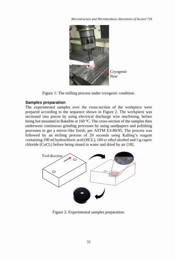
Microstructure and Microhardness Alterations of Inconel 718
55
Figure 1: The milling process under cryogenic condition.
Samples preparation The experimental samples over the cross-section of the workpiece were
prepared according to the sequence shown in Figure 2. The workpiece was
sectioned into pieces by using electrical discharge wire machining, before
being hot mounted in Bakelite at 160 ºC. The cross-section of the samples then
underwent continuous grinding processes by using sandpapers and polishing
processes to get a mirror-like finish, per ASTM E3-80/95. The process was
followed by an etching process of 20 seconds using Kalling’s reagent
containing 100 ml hydrochloric acid (HCL), 100 cc ethyl alcohol and 5 g cupric
chloride (CuCl2) before being rinsed in water and dried by air [18].
Figure 2: Experimental samples preparation.
Cryogenic
flow

C.H.C.Haron et al.
56
Microstructure and microhardness observation The changes in microhardness along the cross-section of the machined surfaces
were measured using a Vickers microhardness tester. The measurements were
conducted at depths of up to 600 µm with 100 µm intervals between successive
readings from the edge of the sample. At each interval, three readings were
taken from three different spots to get the average hardness for that particular
depth. The indentation mark on the surface was generated by a diamond
indenter in a pyramid form under a consistent load of 98.07 N (10 Kp) with 15
seconds dwell time. For the indentation mark, the angle between opposites was
136º. This approach was in parallel with that of researchers like Devillez et al.
[19], Kenda et al. [5] and Kasim [2] which used 50-500 gf of indentation load
and 10-15 seconds of holding time for Inconel 718. For microstructure
observation, an Olympus optical microscope model BX51M at 10X
magnification was used.
Results and Discussions
Figure 3 shows the microstructure of aged-hardened Inconel 718 before the
machining process. As can be seen, the presences of micro-twinning structures
known as annealing twins were found in the microstructure. These needle
shapes were believed to have been created due to re-crystallization and growth
of new grains during heat treatment process [20]. According to Ramirez [21],
these structures made the material stronger in withstanding any plastic
deformation due to the shearing force of the cutting process. Due that, the
hardness of the aged-hardened Inconel 718 was found to be 65% higher as
compared to its initial hardness before the heat treatment process. The heat-
treated material is believed offer consistent thermal shock and creep properties
at higher cutting temperatures as in high-speed machining.
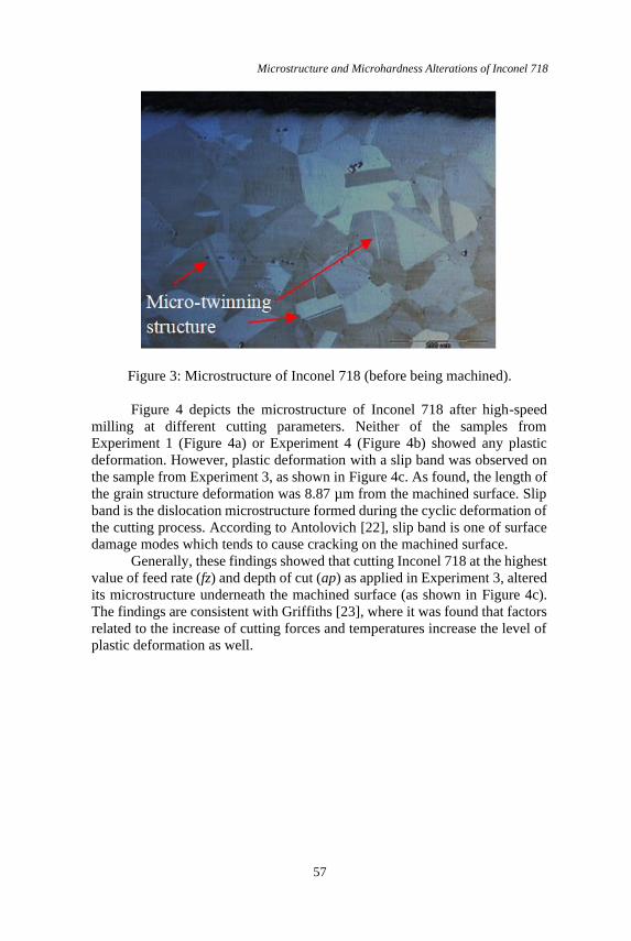
Microstructure and Microhardness Alterations of Inconel 718
57
Figure 3: Microstructure of Inconel 718 (before being machined).
Figure 4 depicts the microstructure of Inconel 718 after high-speed
milling at different cutting parameters. Neither of the samples from
Experiment 1 (Figure 4a) or Experiment 4 (Figure 4b) showed any plastic
deformation. However, plastic deformation with a slip band was observed on
the sample from Experiment 3, as shown in Figure 4c. As found, the length of
the grain structure deformation was 8.87 µm from the machined surface. Slip
band is the dislocation microstructure formed during the cyclic deformation of
the cutting process. According to Antolovich [22], slip band is one of surface
damage modes which tends to cause cracking on the machined surface.
Generally, these findings showed that cutting Inconel 718 at the highest
value of feed rate (fz) and depth of cut (ap) as applied in Experiment 3, altered
its microstructure underneath the machined surface (as shown in Figure 4c).
The findings are consistent with Griffiths [23], where it was found that factors
related to the increase of cutting forces and temperatures increase the level of
plastic deformation as well.
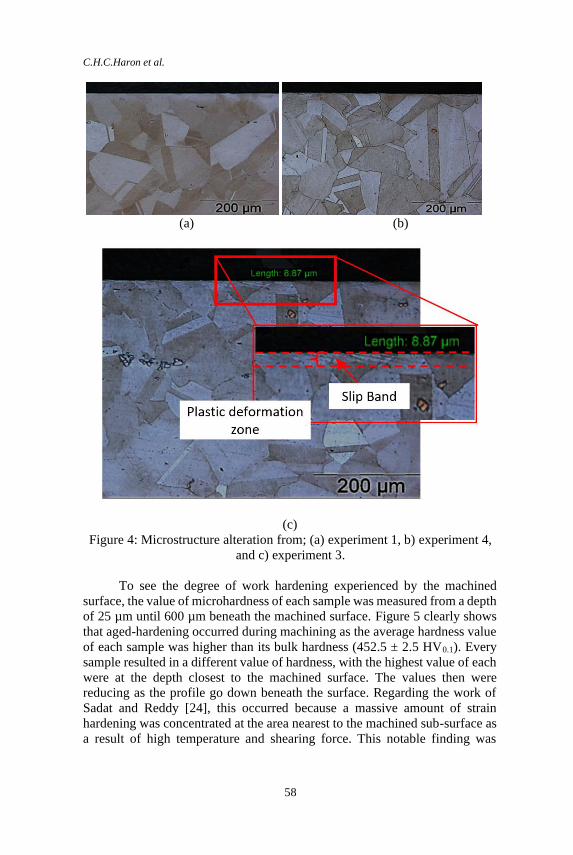
C.H.C.Haron et al.
58
(a) (b)
(c)
Figure 4: Microstructure alteration from; (a) experiment 1, b) experiment 4,
and c) experiment 3.
To see the degree of work hardening experienced by the machined
surface, the value of microhardness of each sample was measured from a depth
of 25 µm until 600 µm beneath the machined surface. Figure 5 clearly shows
that aged-hardening occurred during machining as the average hardness value
of each sample was higher than its bulk hardness (452.5 ± 2.5 HV0.1). Every
sample resulted in a different value of hardness, with the highest value of each
were at the depth closest to the machined surface. The values then were
reducing as the profile go down beneath the surface. Regarding the work of
Sadat and Reddy [24], this occurred because a massive amount of strain
hardening was concentrated at the area nearest to the machined sub-surface as
a result of high temperature and shearing force. This notable finding was

Microstructure and Microhardness Alterations of Inconel 718
59
consistent with Hadi [25], Kasim [2] and Pusavec et al. [26], who were also
concentrated on high-speed cutting of Inconel 718.
In this analysis, the highest value of hardness was obtained in
Experiment 3 with an average value of 474 HV0.1, 4.2% higher than its bulk
hardness. In comparison, Hadi [25] and Kasim [2] recorded an increase in
hardness of 8.9% and 8.8% in LN2 cryogenic and MQL, respectively. Clearly,
the effects of controlled cryogenic cooling and the use of a cutting tool with a
maximum wear rate Vbmax ≥ 0.2 mm helped to reduce the effects of heat and
work hardening on the machined surface. The hardness values were found to
decrease with the deepening of the measurement point from the sub-surface
until it almost approached the bulk hardness approximately 0.3 mm from the
machined surface. This was consistent with the findings of Devillez et al. [19],
Hadi [25], Kasim [2], and Pusavec et al. [27]. The zone where age-hardening
occurred is known as the machining affected zone, MAZ as proposed by
Sonawane and Joshi [3]. MAZ results from work hardening during machining,
which forms a plastic deformation layer at a certain distance from the
machined surface. Ginting and Nouari [13] defined these two zones as the hard
sub-surface region and the bulk material region as also adopted in Figure 5.
Figure 5: Micro-hardness at the sub-surface of the machined area.
Figure 6a shows the effects of a feed rate (fz) and depth of cut (ap) on
micro-hardness in Experiment 3, Experiment 4 and Experiment 5. It is shown
that the microhardness (starting at 50 µm beneath the machined surface)
increased with the depth of cut. The highest value of feed rate also resulted
with the highest microhardness. This result is consistent with the findings of
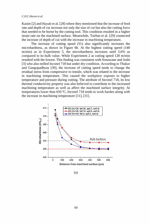
C.H.C.Haron et al.
60
Kasim [2] and Hayati et al. [28] where they mentioned that the increase of feed
rate and depth of cut increase not only the size of cut but also the cutting force
that needed to be borne by the cutting tool. This condition resulted in a higher
strain rate on the machined surface. Meanwhile, Tsirbas et al. [29] connected
the increase of depth of cut with the increase in machining temperature.
The increase of cutting speed (Vc) also significantly increases the
microhardness, as shown in Figure 6b. At the highest cutting speed (140
m/min) as in Experiment 5, the microhardness increases until 3.6% as
compared to its bulk value. While Experiment 2 at cutting speed 120 m/min
resulted with the lowest. This finding was consistent with Sonawane and Joshi
[3] who also milled Inconel 718 but under dry condition. According to Thakur
and Gangopadhyay [30], the increase of cutting speed tends to change the
residual stress from compressive to tensile, which was related to the increase
in machining temperature. This caused the workpiece exposes to higher
temperature and pressure during cutting. The attribute of Inconel 718, its low
thermal conductivity property was also believed to contribute to the increased
machining temperature as well as affect the machined surface integrity. At
temperatures lower than 650 ºC, Inconel 718 tends to work harden along with
the increase in machining temperature [11], [31].
(a)
Bulk hardness

Microstructure and Microhardness Alterations of Inconel 718
61
(b)
Figure 6: Micro-hardness; (a) effects of feed rate (fz) and depth of cut (ap);
and (b) effects of cutting speed (Vc).
Conclusion
Microstructure and microhardness alterations on the sub-surface of Inconel
718 after high-speed cutting Inconel 718 under cryogenic CO2 condition using
PVD carbide coated ball nose milling insert were analyzed. In was found that
the depth of plastic deformation depends greatly on the machining parameters.
The highest value of feed rate and depth of cut resulted with obvious grain
structure deformation, deepening until 8.87 µm from the machined surface. At
the same time, those factors also significantly increase the sub-surface
microhardness, made the machined surface harder and more difficult to be
machined. Cutting speed also plays an important role in increasing the
subsurface microhardness. At the highest cutting speed, the machined sub-
surface microhardness was 3.6% harder than bulk hardness. Also found that
the depth of machined affected zone was reduced as the profile go down
beneath the surface. The workpiece’s hardness was back to its bulk hardness
approximately 300 µm from the top surface. Thus, it can be suggested that the
finishing process of Inconel 718 under cryogenic condition can be performed
at a depth of cut lower than 0.3 mm to remove any hardening effect on the
machined surface.
Bulk hardness

C.H.C.Haron et al.
62
Acknowledgements
This research was founded by the UKM-DIP-2017-023 grant.
References [1] A. H. Musfirah, J. A. Ghani, and C. H. C. Haron, “Tool wear and surface
integrity of Inconel 718 in dry and cryogenic coolant at high cutting
speed,” Wear, vol. 376–377, pp. 125–133, 2017.
[2] M. S. Kasim, “Prestasi Perkakas Pemotong Karbida Bersalut Semasa
Pengisaran Inkonel 718 Dalam Keadaan Kuantiti Pelincir Minimum,”
Universiti Kebangsaan Malaysia, Ph.D thesis, 2014.
[3] H. A. Sonawane and S. S. Joshi, “Analysis of machined surface quality in
a single-pass of ball-end milling on Inconel 718,” J. Manuf. Process., vol.
14, no. 3, pp. 257–268, Aug. 2012.
[4] A. Shokrani, V. Dhokia, and S. T. Newman, “Investigation of the effects
of cryogenic machining on surface integrity in CNC end milling of Ti-
6Al-4V titanium alloy,” J. Manuf. Process., vol. 21, no. 1, pp. 172–179,
2016.
[5] J. Kenda, F. Pusavec, and J. Kopac, “Analysis of Residual Stresses in
Sustainable Cryogenic Machining of Nickel Based Alloy—Inconel 718,”
J. Manuf. Sci. Eng., vol. 133, no. 4, pp. 041009-1-041009–7, 2011.
[6] X. Liang, Z. Liu, and B. Wang, “State-of-the-art of surface integrity
induced by tool wear effects in machining process of titanium and nickel
alloys: A review,” Measurement, vol. 132, pp. 150–181, 2018.
[7] W. Grzesik, Z. Zalisz, S. Krol, and P. Nieslony, “Investigations on friction
and wear mechanisms of the PVD-TiAlN coated carbide in dry sliding
against steels and cast iron,” Wear, vol. 261, no. 11–12, pp. 1191–1200,
2006.
[8] A. R. C. Sharman, J. I. Hughes, and K. Ridgway, “Workpiece surface
integrity and tool life issues when turning Inconel 718TM nickel based
superalloy,” Mach. Sci. Technol., vol. 8, no. 3, pp. 399–414, 2004.
[9] N. H. A. Halim, C. H. C. Haron, J. A. Ghani, and M. F. Azhar, “Tool wear
and chip morphology in high-speed milling of hardened Inconel 718 under
dry and cryogenic CO <inf>2</inf> conditions,” Wear, vol. 426–427,
2019.
[10] A. Iturbe, E. Hormaetxe, A. Garay, and P. J. Arrazola, “Surface integrity
analysis when machining Inconel 718 with conventional and cryogenic
cooling,” Procedia CIRP, vol. 45, no. Table 1, pp. 67–70, 2016.
[11] Y. S. Liao, H. M. Lin, and J. H. Wang, “Behaviors of end milling Inconel
718 superalloy by cemented carbide tools,” J. Mater. Process. Technol.,
vol. 201, no. 1–3, pp. 460–465, May 2008.
[12] N. H. Abdul Halim, C. H. C. Haron, J. A. Ghani, and M. F. Azhar,
Microstructure and Microhardness Alterations of Inconel 718
63
“Machining-induced microstructure of Inconel 718 in cryogenic
environment,” Prog. Ind. Ecol. An Int. J., vol. 12, no. 3, p. 234, 2018.
[13] A. Ginting and M. Nouari, “Surface integrity of dry machined titanium
alloys,” Int. J. Mach. Tools Manuf., vol. 49, no. 3–4, pp. 325–332, 2009.
[14] O. Pereira, A. Celaya, G. Urbikaín, A. Rodríguez, A. Fernández-
Valdivielso, and L. Noberto López de Lacalle, “CO2 cryogenic milling of
Inconel 718: Cutting forces and tool wear,” J. Mater. Res. Technol., vol.
9, no. 4, pp. 8459–8468, 2020.
[15] L. Sterle, D. Mallipeddi, P. Krajnik, and F. Pušavec, “The influence of
single-channel liquid CO2 and MQL delivery on surface integrity in
machining of Inconel 718,” Procedia CIRP, vol. 87, pp. 164–169, 2020.
[16] N. Khanna, P. Shah, and Chetan, “Comparative analysis of dry, flood,
MQL and cryogenic CO2 techniques during the machining of 15-5-PH SS
alloy,” Tribol. Int., vol. 146, no. January, p. 106196, 2020.
[17] T. Stefansson, “Application of Cryogenic Coolants in Machining
Processes,” Royal Institute of Technology, 2014.
[18] S. Kumar, G. Sudhakar Rao, K. Chattopadhyay, G. S. Mahobia, N. C.
Santhi Srinivas, and V. Singh, “Effect of surface nanostructure on tensile
behavior of superalloy IN718,” Mater. Des., vol. 62, no. 3, pp. 76–82,
2014.
[19] A. Devillez, G. Le Coz, S. Dominiak, and D. Dudzinski, “Dry machining
of Inconel 718, workpiece surface integrity,” J. Mater. Process. Technol.,
vol. 211, no. 10, pp. 1590–1598, 2011.
[20] M. Moiz, “The influence of grain size on the mechanical properties of
Inconel 718,” Linköping University, 2013.
[21] A. C. Ramirez, “Microstructural Properties Associated with Adiabatic
Shear Bands in Titanium-aluminum-vanadium Deformed by Ballistic
Impact,” The University of Texas at El Paso, 2008.
[22] S. D. Antolovich, “Microstructural aspects of fatigue in Ni-base
superalloys,” Philos. Trans. R. Soc. A Math. Phys. Eng. Sci., vol. 373, no.
2038, pp. 1–36, 2015.
[23] B. Griffiths, Manufacturing Surface Technology: Surface Integrity and
Functional Performance (Manufacturing Engineering Modular), Ed. ke-
4. New York: Elsevier, 2001.
[24] A. B. Sadat and M. Y. Reddy, “Surface integrity of inconel-718 nickel-
base superalloy using controlled and natural contact length tools. Part II:
Unlubricated,” Exp. Mech., vol. 33, no. 4, pp. 343–348, 1993.
[25] M. B. A. Hadi, “Pencirian dan analisa pemesinan laju tinggi kriogenik
menggunakan mata alat kisar hujung bebola bersalut karbida ke atas
Inkonel 718,” Universiti Kebangsaan Malaysia, 2016.
[26] F. Pusavec, H. Hamdi, J. Kopac, and I. S. Jawahir, “Surface integrity in
cryogenic machining of nickel based alloy — Inconel 718,” J. Mater.
Process. Tech., vol. 211, no. 4, pp. 773–783, 2011.
[27] F. Pusavec, H. Hamdi, J. Kopac, and I. S. Jawahir, “Surface integrity in
C.H.C.Haron et al.
64
cryogenic machining of nickel based alloy—Inconel 718,” J. Mater.
Process. Technol., vol. 211, no. 4, pp. 773–783, 2011.
[28] N. Hayati, A. Halim, C. Hassan, C. Haron, J. A. Ghani, and M. F. Azhar,
“Prediction of Cutting Force for Milling of Inconel 718 under Cryogenic
Condition by Response Surface Methodology,” vol. 16, no. 1, pp. 1–16,
2019.
[29] K. Tsirbas, G. Chryssolouris, and D. Mourtzis, “Grind-hardening
modeling with the use of neural networks,” in Conference: 5th
International Conference on Advanced Manufacturing Systems and
Technology (AMST)At: Undine, Italy, 1999, pp. 197–206.
[30] A. Thakur and S. Gangopadhyay, “State-of-the-art in surface integrity in
machining of nickel-based super alloys,” Int. J. Mach. Tools Manuf., vol.
100, pp. 25–54, 2016.
[31] M. N. Sharif, S. Pervaiz, and I. Deiab, “Potential of alternative lubrication
strategies for metal cutting processes : A review,” Int. J. Adv. Manuf.
Technol., vol. 89, no. 5–8, pp. 2447–2479, 2016.
Journal of Mechanical Engineering Vol 18(2), 65-76, 2021
___________________
ISSN 1823-5514, eISSN 2550-164X Received for review: 2020-12-01 © 2021 College of Engineering, Accepted for publication: 2021-03-18
Universiti Teknologi MARA (UiTM), Malaysia. Published: 2021-04-15
Effect of Spindle Speed and Feed Per Tooth in Feed Rate Perspective
on Inconel HX Cutting Force
N. A. Mohd Nor*, N. F. Kamarulzaman, N. A. S. Zakaria, N. Awang
Department of Mechanical Engineering, School of Engineering,
Manipal International University, 71800 Putra Nilai, Malaysia.
B. T. H. T. Baharudin, M. K. A. Mohd Ariffin, Z. Leman
Department of Mechanical and Manufacturing Engineering,
Faculty of Engineering, Universiti Putra Malaysia,
43400 Serdang, Malaysia.
ABSTRACT
Reducing feed rate during end-milling of nickel-based superalloys for low-
cutting force has always been a common approach. This is due to these
alloys having superior properties, making them widely regarded as difficult-
to-machine materials. As feed rate is tied to spindle speed and feed per tooth,
it is crucial to comprehend whether spindle speed, feed per tooth or the
interaction between spindle speed and feed per tooth has a significant factor
on cutting force reduction when increasing the feed rate. Accordingly, this
manuscript presents an effect of spindle speed and feed per tooth in feed rate
perspective on Inconel HX cutting force. Half-immersion down-milling and
full-immersion down-milling was conducted experimentally using solid
ceramic end-mill cutter. The results indicate that cutting force decreases and
then increases after further increase in spindle speed, while cutting force
increases with an increase in feed per tooth. Optimum spindle speed and
optimum feed per tooth for low-cutting force were 21,400 rpm and 0.013
mm/tooth. Furthermore, feed per tooth was the significant factor which
influenced the cutting force, whereas spindle speed, and the interaction
between spindle speed and feed per tooth were not significant.
Keywords: Spindle speed; feed per tooth; down-milling; Inconel HX; cutting
force
N. A. Mohd Nor et al.
66
Introduction
Cutting force or resultant force in end-milling is conveniently resolved into
three cutting force components in the X, Y and Z axis. Firstly, the cutting
force projection that acts along the feed direction or X-axis is defined as the
feed force. Secondly, the cutting force projection in the Y-axis is called the
normal force. Finally, the cutting force projection that acts in a perpendicular
direction to the feed direction or Z-axis is called the axial force. On the other
side, the findings from cutting force research have positively contributed to
extending cutting tool life [1, 2], improved quality of machined material [2],
reduction in production cost [3] and increase in production rate [4, 5].
Cutting force research findings are also key to curb carbon emissions due to
climate change which is seen as top global threat. This is due to decrease in
cutting force indirectly consumes less power for milling machine and can
cause reduction in carbon emissions. As indicated by Hidayah et al. [6],
approximately more than 70% of machining process is applied in the
production sector in the world, and this sector has contributed about 36% of
carbon emissions [7], thus reducing cutting force in end-milling can help in
reducing the percentage of carbon emissions.
Apart from cutting force research findings, reducing feed rate and
increasing cutting speed during end-milling of nickel-based superalloys have
long been used for low-cutting force, as this difficult-to-machine material
tends to be hard to end-mill [8, 9] which leads to high-cutting force due to its
superior mechanical properties [8, 10]. The decrease in cutting force during
reduction of feed rate is due to decrease in speed at which cutting tool
engages the machined material [1]. Meanwhile, decrease in cutting force
during increasing cutting speed is associated with increase in cutting
temperature in the shear zone, and consequently softening the machined
material due to drop in mechanical properties [11, 12]. In end-milling, feed
rate is tied to spindle speed and feed per tooth, while cutting speed is tied to
spindle speed. Decrease in feed per tooth indirectly decreases feed rate, and
subsequently decreases cutting force. Whereas, increase in spindle speed not
only increases cutting speed, but also increases feed rate. Therefore, a precise
understanding whether spindle speed, feed per tooth or the interaction
between spindle speed and feed per tooth is a significant factor on cutting
force reduction when decreasing the feed rate is crucial.
In this manuscript, Inconel HX is selected as a specimen to study the
effect of spindle speed and feed per tooth on cutting force in the feed rate
perspective. It is one of the nickel-based superalloys and commonly used as a
material for gas turbine engine applications [13] as it has high-strength at
elevated temperatures [14] and outstanding oxidation resistance [15].
Besides, end-milling test performed experimentally by half-immersion down-
milling and full-immersion down-milling as down-milling has been
Effect of Spindle Speed and Feed Per Tooth in Feed Rate Perspective on Inconel HX
67
recognised as the preferred method to end-mill difficult-to-machine materials
compared to up-milling, since it reduces the load from the end-mill cutter
edge, improves end-mill cutter life and leaves a better machined material
surface quality. Solid ceramic end-mill cutter is used as it is an ideal solution
to eliminate the role of cutting fluid due to its negative effect towards human
health and environment [16], since this end-mill cutter has the ability to
withstand high-cutting temperature during dry end-milling. The effect of
spindle speed, feed per tooth and the interaction between spindle speed and
feed per tooth are analysed systematically, therefore the optimum spindle
speed and optimum feed per tooth for achieving low-cutting force is
simultaneously proposed.
Experimental Setup
Experimental test for this research was carried out on a vertical machining
centre model Mori Seiki NV 4000 DCG. Its maximum spindle speed is
30,000 rpm. The experimental set-up is illustrated in Table 1 where spindle
speed and feed per tooth are divided into three levels. Since this research is
focused on spindle speed and feed per tooth in feed rate perspective, there is
no correlation between axial depth of cut and feed rate, thus axial depth of
cut is held constant at 0.2 mm.
Table 1: Experimental setup
Cutting parameter Level
Spindle speed (rpm)
Feed per tooth (mm/tooth)
16,000, 21,400 and 26,800
0.013, 0.016 and 0.019
Axial depth of cut (mm) 0.2
Dry end-milling of Inconel HX was performed by half-immersion
down-milling and full-immersion down-milling using KYS40 solid ceramic
end-mill diameter of 6 mm with 4 flutes from Kennametal. The dimension of
Inconel HX specimen was 90 mm × 40 mm × 10 mm with original hardness
92 HRB. Figure 1 and Figure 2 illustrate half-immersion down-milling and
full-immersion down-milling performed in this experimental test. The cutting
length was set at 22 mm per run. In addition, fresh KYS40 solid ceramic end-
mill cutter was used at each run.
N. A. Mohd Nor et al.
68
Figure 1: Half-immersion down-milling.
Figure 2: Full-immersion down-milling.
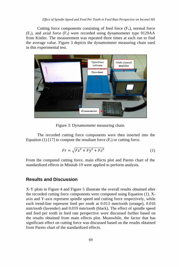
Effect of Spindle Speed and Feed Per Tooth in Feed Rate Perspective on Inconel HX
69
Cutting force components consisting of feed force (Fx), normal force
(Fy), and axial force (Fz) were recorded using dynamometer type 9129AA
from Kistler. The measurement was repeated three times at each run to find
the average value. Figure 3 depicts the dynamometer measuring chain used
in this experimental test.
Figure 3: Dynamometer measuring chain.
The recorded cutting force components were then inserted into the
Equation (1) [17] to compute the resultant force (Fr) or cutting force.
𝐹𝑟 = √𝐹𝑥² + 𝐹𝑦² + 𝐹𝑧² (1)
From the computed cutting force, main effects plot and Pareto chart of the
standardized effects in Minitab 19 were applied to perform analysis.
Results and Discussion
X-Y plots in Figure 4 and Figure 5 illustrate the overall results obtained after
the recorded cutting force components were computed using Equation (1). X-
axis and Y-axis represent spindle speed and cutting force respectively, while
each trend-line represent feed per tooth at 0.013 mm/tooth (orange), 0.016
mm/tooth (lavender) and 0.019 mm/tooth (black). The effect of spindle speed
and feed per tooth in feed rate perspective were discussed further based on
the results obtained from main effects plot. Meanwhile, the factor that has
significant effect on cutting force was discussed based on the results obtained
from Pareto chart of the standardized effects.
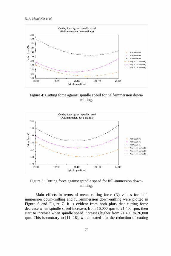
N. A. Mohd Nor et al.
70
Figure 4: Cutting force against spindle speed for half-immersion down-
milling.
Figure 5: Cutting force against spindle speed for full-immersion down-
milling.
Main effects in terms of mean cutting force (N) values for half-
immersion down-milling and full-immersion down-milling were plotted in
Figure 6 and Figure 7. It is evident from both plots that cutting force
decrease when spindle speed increases from 16,000 rpm to 21,400 rpm, then
start to increase when spindle speed increases higher from 21,400 to 26,800
rpm. This is contrary to [11, 18], which stated that the reduction of cutting
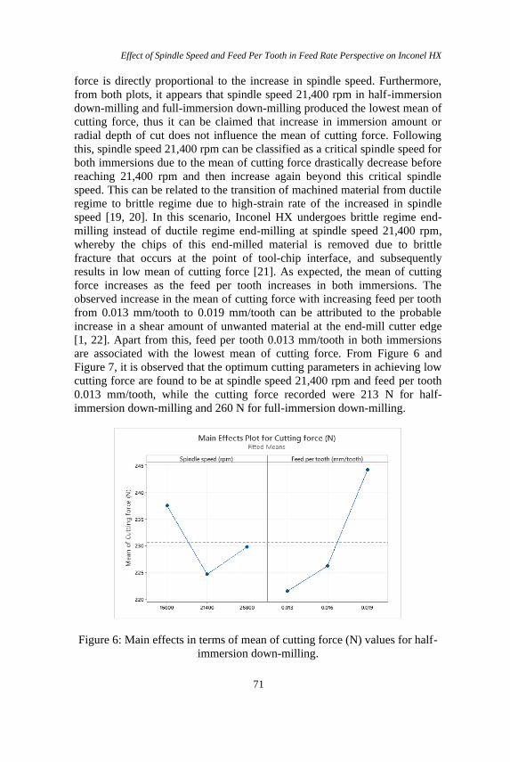
Effect of Spindle Speed and Feed Per Tooth in Feed Rate Perspective on Inconel HX
71
force is directly proportional to the increase in spindle speed. Furthermore,
from both plots, it appears that spindle speed 21,400 rpm in half-immersion
down-milling and full-immersion down-milling produced the lowest mean of
cutting force, thus it can be claimed that increase in immersion amount or
radial depth of cut does not influence the mean of cutting force. Following
this, spindle speed 21,400 rpm can be classified as a critical spindle speed for
both immersions due to the mean of cutting force drastically decrease before
reaching 21,400 rpm and then increase again beyond this critical spindle
speed. This can be related to the transition of machined material from ductile
regime to brittle regime due to high-strain rate of the increased in spindle
speed [19, 20]. In this scenario, Inconel HX undergoes brittle regime end-
milling instead of ductile regime end-milling at spindle speed 21,400 rpm,
whereby the chips of this end-milled material is removed due to brittle
fracture that occurs at the point of tool-chip interface, and subsequently
results in low mean of cutting force [21]. As expected, the mean of cutting
force increases as the feed per tooth increases in both immersions. The
observed increase in the mean of cutting force with increasing feed per tooth
from 0.013 mm/tooth to 0.019 mm/tooth can be attributed to the probable
increase in a shear amount of unwanted material at the end-mill cutter edge
[1, 22]. Apart from this, feed per tooth 0.013 mm/tooth in both immersions
are associated with the lowest mean of cutting force. From Figure 6 and
Figure 7, it is observed that the optimum cutting parameters in achieving low
cutting force are found to be at spindle speed 21,400 rpm and feed per tooth
0.013 mm/tooth, while the cutting force recorded were 213 N for half-
immersion down-milling and 260 N for full-immersion down-milling.
Figure 6: Main effects in terms of mean of cutting force (N) values for half-
immersion down-milling.
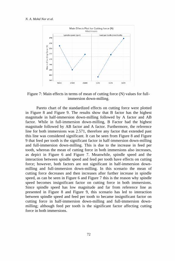
N. A. Mohd Nor et al.
72
Figure 7: Main effects in terms of mean of cutting force (N) values for full-
immersion down-milling.
Pareto chart of the standardized effects on cutting force were plotted
in Figure 8 and Figure 9. The results show that B factor has the highest
magnitude in half-immersion down-milling followed by A factor and AB
factor. While in full-immersion down-milling, B Factor had the highest
magnitude followed by AB factor and A factor. Furthermore, the reference
line for both immersions was 2.571, therefore any factor that extended past
this line was considered significant. It can be seen from Figure 8 and Figure
9 that feed per tooth is the significant factor in half-immersion down-milling
and full-immersion down-milling. This is due to the increase in feed per
tooth, whereas the mean of cutting force in both immersions also increases,
as depict in Figure 6 and Figure 7. Meanwhile, spindle speed and the
interaction between spindle speed and feed per tooth have effects on cutting
force; however, both factors are not significant in half-immersion down-
milling and full-immersion down-milling. In this scenario the mean of
cutting force decreases and then increases after further increase in spindle
speed, as can be seen in Figure 6 and Figure 7 this is the reason why spindle
speed becomes insignificant factor on cutting force in both immersions.
Since spindle speed has low magnitude and far from reference line as
presented in Figure 8 and Figure 9, this scenario has led to interaction
between spindle speed and feed per tooth to became insignificant factor on
cutting force in half-immersion down-milling and full-immersion down-
milling; although feed per tooth is the significant factor affecting cutting
force in both immersions.
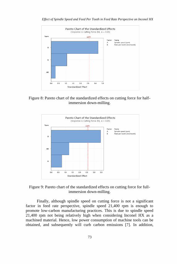
Effect of Spindle Speed and Feed Per Tooth in Feed Rate Perspective on Inconel HX
73
Figure 8: Pareto chart of the standardized effects on cutting force for half-
immersion down-milling.
Figure 9: Pareto chart of the standardized effects on cutting force for full-
immersion down-milling.
Finally, although spindle speed on cutting force is not a significant
factor in feed rate perspective, spindle speed 21,400 rpm is enough to
promote low-carbon manufacturing practices. This is due to spindle speed
21,400 rpm not being relatively high when considering Inconel HX as a
machined material. Hence, low power consumption of machine tools can be
obtained, and subsequently will curb carbon emissions [7]. In addition,

N. A. Mohd Nor et al.
74
production sectors can reduce production cost due to low power consumption
by using this spindle speed during end-milling of Inconel HX. Therefore,
increasing spindle speed higher than 21,400 rpm or to its highest level for
low-cutting force [11, 18], becomes unnecessary. Although Inconel HX had
once been considered impractical to machine under dry condition, the use of
KYS40 solid ceramic end-mill cutter in this experimental test proves that dry
end-milling is practicable. Harmful effects of cutting fluid are becoming
more apparent, mainly on human well-being and environment [23, 24].
Considering this issue, dry end-milling of Inconel HX using KYS40 solid
ceramic end-mill cutter is the key for sustainable development.
Conclusion
In present research, the effects of spindle speed and feed per tooth in feed
rate perspective on Inconel HX cutting force are studied. The following
conclusions can be drawn from this research:
• Cutting force decreased when spindle speed is increased between 16,000
rpm and 21,400 rpm, and increased when using a spindle speed higher
than 21,400 rpm.
• Cutting force increased with the increasing in feed per tooth.
• Spindle speed 21,400 rpm and feed per tooth 0.013 mm/tooth were an
optimum cutting parameters as it was found to achieve low-cutting force.
• Feed per tooth was the significant factor affecting cutting force. Likewise,
the effect of the spindle speed and the interaction between spindle speed
and feed per tooth were not statistically significant.
• Future work should be focused on tool life and economical aspect of
KYS40 solid ceramic end-mill cutter.
Acknowledgements The results presented in this manuscript are part of the research project GP-
IPS/2017/9539900 financed by Universiti Putra Malaysia. The authors would
like to acknowledge Mr. Mohd Nor Bin Puteh, Mdm. Hatijah Binti Kassim,
Mdm. Dyg. Siti Quraisyah Bt. Abg. Adenan and Mr. Nor Iman Ziqri Bin Nor
Aznan for their support and encouragement.
References
[1] G. Bolar, A. Das, and S. N. Joshi, “Measurement and analysis of cutting

Effect of Spindle Speed and Feed Per Tooth in Feed Rate Perspective on Inconel HX
75
force and product surface quality during end-milling of thin-wall
components,” Meas. J. Int. Meas. Confed., vol. 121, no. November 2017,
pp. 190–204, 2018.
[2] J. Ma, D. Song, Z. Jia, G. Hu, W. Su, and L. Si, “Tool-path planning
with constraint of cutting force fluctuation for curved surface
machining,” Precis. Eng., vol. 51, pp. 614–624, 2018.
[3] Z. Xie, Y. Lu, and J. Li, “Development and testing of an integrated smart
tool holder for four-component cutting force measurement,” Mech. Syst.
Signal Process., vol. 93, pp. 225–240, 2017.
[4] M. Wan, W. Yin, and W.-H. Zhang, “Study on the Correction of cutting
force measurement with table dynamometer,” Procedia CIRP, vol. 56,
pp. 119–123, 2016.
[5] M. Wan, W. Yin, W.-H. Zhang, and H. Liu, “Improved inverse filter for
the correction of distorted measured cutting forces,” Int. J. Mech. Sci.,
vol. 120, pp. 276–285, 2017.
[6] M. T. Hidayah, J. A. Ghani, M. Z. Nuawi, and C. H. C. Haron, “A
review of utilisation of cutting force analysis in cutting tool condition
monitoring,” Int. J. Eng. Technol. IJET-IJENS, vol. 15, no. 28, pp.
150203–4848, 2015.
[7] C. Tian, G. Zhou, J. Zhang, and C. Zhang, “Optimization of cutting
parameters considering tool wear conditions in low-carbon
manufacturing environment,” J. Clean. Prod., vol. 226, pp. 706–719,
2019.
[8] A. Pleta and L. Mears, “Cutting Force Investigation of Trochoidal
milling in Nickel-based superalloy,” Procedia Manuf., vol. 5, pp. 1348–
1356, 2016.
[9] D. Grguraš, M. Kern, and F. Pušavec, “Suitability of the full body
ceramic end milling tools for high speed machining of nickel based alloy
Inconel 718,” Procedia CIRP, vol. 77, no. Hpc, pp. 630–633, 2018.
[10] D. Finkeldei, M. Sexauer, and F. Bleicher, “End milling of inconel 718
using solid Si3N4 ceramic cutting tools,” Procedia CIRP, vol. 81, pp.
1131–1135, 2019.
[11] N. Masmiati, A. A. D. Sarhan, M. A. N. Hassan, and M. Hamdi,
“Optimization of cutting conditions for minimum residual stress, cutting
force and surface roughness in end milling of S50C medium carbon
steel,” Meas. J. Int. Meas. Confed., vol. 86, pp. 253–265, 2016.
[12] H. Çalışkan and M. Küçükköse, “The effect of aCN/TiAlN coating on
tool wear, cutting force, surface finish and chip morphology in face
milling of Ti6Al4V superalloy,” Int. J. Refract. Met. Hard Mater., vol.
50, pp. 304–312, 2015.
[13] Q. Han, Y. Gu, S. Soe, F. Lacan, and R. Setchi, “Effect of hot cracking
on the mechanical properties of Hastelloy X superalloy fabricated by
laser powder bed fusion additive manufacturing,” Opt. Laser Technol.,
N. A. Mohd Nor et al.
76
vol. 124, p. 105984, 2020.
[14] A. R. K. Chennamsetty, J. Leblanc, S. Abotula, P. N. Parrikar, and A.
Shukla, “Dynamic response of Hastelloy® X plates under oblique
shocks: Experimental and numerical studies,” Int. J. Impact Eng., vol.
92, pp. 75–88, 2016.
[15] M. Esmaeilzadeh, F. Qods, H. Arabi, and B. M. Sadeghi, “An
investigation on crack growth rate of fatigue and induction heating
thermo-mechanical fatigue (TMF) in Hastelloy X superalloy via LEFM,
EPFM and integration models,” Int. J. Fatigue, vol. 97, pp. 135–149,
2017.
[16] A. Iturbe, E. Hormaetxe, A. Garay, and P. J. Arrazola, “Surface integrity
analysis when machining Inconel 718 with conventional and cryogenic
cooling,” Procedia CIRP, vol. 45, no. Table 1, pp. 67–70, 2016.
[17] W. Shixiong, M. Wei, L. Bin, and W. Chengyong, “Trochoidal
machining for the high-speed milling of pockets,” J. Mater. Process.
Technol., vol. 233, pp. 29–43, 2016.
[18] A. Mebrahitom, W. Choon, and A. Azhari, “Side milling machining
simulation using finite element analysis: Prediction of Cutting Forces,”
Mater. Today Proc., vol. 4, no. 4, Part D, pp. 5215–5221, 2017.
[19] B. Wang, Z. Liu, G. Su, Q. Song, and X. Ai, “Investigations of critical
cutting speed and ductile-to-brittle transition mechanism for workpiece
material in ultra-high speed machining,” Int. J. Mech. Sci., vol. 104, pp.
44–59, 2015.
[20] N. A. Mohd Nor, B. T. H. T. Baharudin, J. A. Ghani, Z. Leman, and M.
K. A. Mohd Ariffin, “Effect of chip load and spindle speed on cutting
force of Hastelloy X,” J. Mech. Eng. Sci., vol. 14, no. 1, pp. 6497–6503,
2020.
[21] B. Wang, Z. Liu, G. Su, and X. Ai, “Brittle removal mechanism of
ductile materials with Ultrahigh-speed machining,” J. Manuf. Sci. Eng.
Trans. ASME, vol. 137, no. 6, 2015.
[22] V. Gaikhe, J. Sahu, and R. Pawade, “Optimization of cutting parameters
for cutting force minimization in helical ball end milling of inconel 718
by using genetic algorithm,” Procedia CIRP, vol. 77, no. Hpc, pp. 477–
480, 2018.
[23] N.A. Mohd Nor, S.S. Mohd Alisjabana, G. Seloraji, Y. M. Tee, J. X.
Teh, B.T.H.T. Baharudin, M.K.A. Mohd Ariffin, and Z. Leman, “Effect
and optimization of cutting speed and depth of cut in half-immersion up-
milling of 6061 aluminium alloy,” J. Mech. Eng., vol. 16, no. 1, pp. 17–
27, 2019.
[24] N. A. Mohd Nor, B. T. H. T. Baharudin, M. K. A. Mohd Ariffin, and Z.
Leman, “Effect of compressed air and cutting speed on surface
roughness of 6061 aluminium alloy,” J. Mech. Eng., vol. 16, no. 2, pp.
53–62, 2019.
Journal of Mechanical Engineering Vol 18(2), 77-96, 2021
___________________
ISSN 1823-5514, eISSN 2550-164X Received for review: 2020-11-03
© 2021 College of Engineering, Accepted for publication: 2021-01-18
Universiti Teknologi MARA (UiTM), Malaysia. Published: 2021-04-15
Evaluation of Tabular Leg Structure of Mobile Offshore Production Unit
(MOPU) Life Extension using Condition Assessment Method
Emi Hafizzul Jamaluddin, Azli Abd Razak*, Mohd Shahriman Adenan,
Mohd Faizal Mohamad
Faculty of Mechanical Engineering, Universiti Teknologi MARA,
40450, Shah Alam, Malaysia
ABSTRACT
A Mobile Offshore Production Unit (MOPU) is any type of portable structure
that can be reused when procuring oil and gas from the seabed. There are few
reasons why MOPU is chosen over the conventional fixed offshore platforms,
mainly due to its ability to be installed and relocated in a short period, low
installation, and abandonment cost, and providing adequate time to evaluate
new reservoirs properly. In certain circumstances, MOPU may be required to
remain at the same location for a more extended period beyond its designed
life. This paper explains the method of life extension (LE) assessment to extend
the useful life of the MOPU. A MOPU with a three-legged jack-up rig in
cruciform shape designed and constructed based on the American Bureau of
Shipping (ABS) Classification requirement with a design life of 5 years, which
currently in laid-up mode after 14 years in operation. The legs will be the focus
of the condition assessment for the LE of the MOPU. The MOPU was
constructed with 3 tabular legs with each 92200 mm length, 3500 mm
diameter, and 55 mm thickness operate under tensile and shear stress,
standing with simply supported at the one-end with hull hanged at the tabular
using jacking-pin at the equal elevation of 77,600 mm. The method of
assessment used is Non-destructive Tests (NDT). No severe defects or cracks
were recorded at the identified stress concentration points. All NDT
measurements were found within the acceptable ranges with no recorded
anomalies.
Keywords: Condition Assessment; Life Extension; MOPU; Tabular Leg; NDT
E. H. Jamaluddin et al.
78
Introduction
Mobile Offshore Production Unit (MOPU) is a primary candidate for shallow
water early production applications. MOPU offer a cost-efficient solution for
short life fields, compared with conventional jacket structure. Advantages in
terms of mobility enable ease of installation, hook up, and commissioning and
decommissioning costs, in comparison with a traditional jacket structure [1].
For a newly build MOPU, the cost must be weighed against the cost of
installation, hook-up, commissioning, and decommissioning. For an existing
jackups as a MOPU conversion candidate, the cost is not as much of an issue
as the cost of acquisition. MOPU has the added advantage of relocation and
re-use at less cost [2, 3].
MOPU has proven its ability to accelerate the monetization of the newly
discovered oil field. The first MOPU was installed in the Ekofisk Field in
Norway, utilizing the Gulftide type (Figure 1) jackups as an early production
system. Production began in 1971, in just 18 months after discovery while
permanent were being designed and build. The Gulftide remained a MOPU
until the permanent production facilities were installed in 1975, at which time
it returned to drilling [4].
Offshore structures are subject to very harsh marine environment [5].
Deterioration of offshore structure commonly caused by forces such as wind,
ocean wave’s buoyant forces, current loading, and marine growth [6]. The
most critical component in MOPU to ensure it can stand at the location safely
is the legs, where it can directly affect the overall performance of the unit.
There are 2 types of leg construction, as shown in Figure 2 [7].
In offshore oil and gas operation, a temporary or permanent structure
equipped with necessary operational equipment is required before the
commencement of the production. The living quarter module is part of the
facility attached to the structure to man the structure for operational and
maintenance purposes. In certain cases, the unmanned structure was installed,
which operates remotely. The design of the structure deployed is depending on
the depth of the seawater and as per the requirement [8].
Offshore exploration and production require a massive amount of
investment. An optimal solution is always a desirable option in making sure of
a profitable investment. There are three main economic reasons that usually
taken into consideration to decide the use of MOPU: schedule, cost, and risk
[3, 9, 10]. MOPU has limitations in terms of operational conditions. It is
suitable to operate only at shallow water with a water depth of less than 152.4
meters [6]. To optimize the useful life of the structure, it has to be maintained
and inspected as per Class guideline such as American Bureau of Shipping
(ABS), Bureau Veritas (BV), China Classification Society (CCS), Croatian
Register of Shipping (CRS), DNV GL (DNV GL), Indian Register of Shipping
(IRS), Korean Register of Shipping (KR), Lloyd's Register of Shipping (LR),
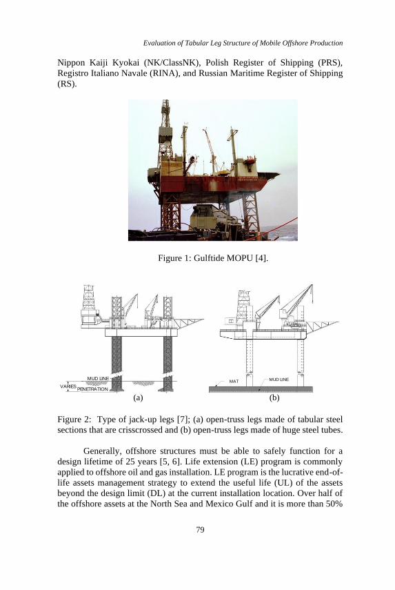
Evaluation of Tabular Leg Structure of Mobile Offshore Production
79
Nippon Kaiji Kyokai (NK/ClassNK), Polish Register of Shipping (PRS),
Registro Italiano Navale (RINA), and Russian Maritime Register of Shipping
(RS).
Figure 1: Gulftide MOPU [4].
Figure 2: Type of jack-up legs [7]; (a) open-truss legs made of tabular steel
sections that are crisscrossed and (b) open-truss legs made of huge steel tubes.
Generally, offshore structures must be able to safely function for a
design lifetime of 25 years [5, 6]. Life extension (LE) program is commonly
applied to offshore oil and gas installation. LE program is the lucrative end-of-
life assets management strategy to extend the useful life (UL) of the assets
beyond the design limit (DL) at the current installation location. Over half of
the offshore assets at the North Sea and Mexico Gulf and it is more than 50%
MUD LINEMAT MUD LINE
(a) (b)
VARIESPENETRATION
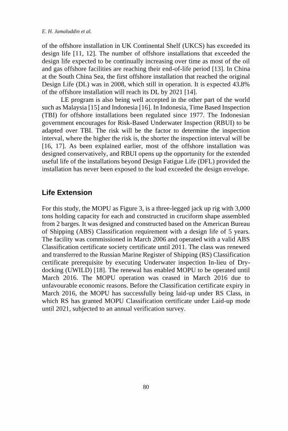
E. H. Jamaluddin et al.
80
of the offshore installation in UK Continental Shelf (UKCS) has exceeded its
design life [11, 12]. The number of offshore installations that exceeded the
design life expected to be continually increasing over time as most of the oil
and gas offshore facilities are reaching their end-of-life period [13]. In China
at the South China Sea, the first offshore installation that reached the original
Design Life (DL) was in 2008, which still in operation. It is expected 43.8%
of the offshore installation will reach its DL by 2021 [14].
LE program is also being well accepted in the other part of the world
such as Malaysia [15] and Indonesia [16]. In Indonesia, Time Based Inspection
(TBI) for offshore installations been regulated since 1977. The Indonesian
government encourages for Risk-Based Underwater Inspection (RBUI) to be
adapted over TBI. The risk will be the factor to determine the inspection
interval, where the higher the risk is, the shorter the inspection interval will be
[16, 17]. As been explained earlier, most of the offshore installation was
designed conservatively, and RBUI opens up the opportunity for the extended
useful life of the installations beyond Design Fatigue Life (DFL) provided the
installation has never been exposed to the load exceeded the design envelope.
Life Extension
For this study, the MOPU as Figure 3, is a three-legged jack up rig with 3,000
tons holding capacity for each and constructed in cruciform shape assembled
from 2 barges. It was designed and constructed based on the American Bureau
of Shipping (ABS) Classification requirement with a design life of 5 years.
The facility was commissioned in March 2006 and operated with a valid ABS
Classification certificate society certificate until 2011. The class was renewed
and transferred to the Russian Marine Register of Shipping (RS) Classification
certificate prerequisite by executing Underwater inspection In-lieu of Dry-
docking (UWILD) [18]. The renewal has enabled MOPU to be operated until
March 2016. The MOPU operation was ceased in March 2016 due to
unfavourable economic reasons. Before the Classification certificate expiry in
March 2016, the MOPU has successfully being laid-up under RS Class, in
which RS has granted MOPU Classification certificate under Laid-up mode
until 2021, subjected to an annual verification survey.
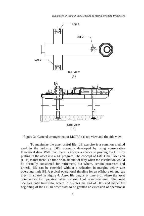
Evaluation of Tabular Leg Structure of Mobile Offshore Production
81
Figure 3: General arrangement of MOPU; (a) top view and (b) side view.
To maximize the asset useful life, LE exercise is a common method
used in the industry. DFL normally developed by using conservative
theoretical data. With that, there is always a chance to prolong the DFL by
putting in the asset into a LE program. The concept of Life Time Extension
(LTE) is that there is a time or an amount of duty when the installation would
be normally considered for retirement, but where, certain processes and
criteria, life can be extended without a reduction in margins below safe
operating limit [8]. A typical operational timeline for an offshore oil and gas
asset illustrated in Figure 4. Asset life begins at time t=0, where the asset
commences for operation after successful of commissioning. The asset
operates until time t=lo, where lo denotes the end of DFL and marks the
beginning of the LE. In order asset to be granted an extension of operational
Leg 1
Leg 2
Leg 3
Top View
Sid e View
(a)
(b)
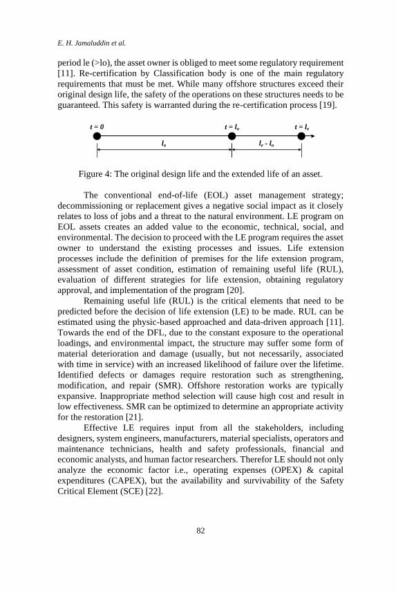
E. H. Jamaluddin et al.
82
period le (>lo), the asset owner is obliged to meet some regulatory requirement
[11]. Re-certification by Classification body is one of the main regulatory
requirements that must be met. While many offshore structures exceed their
original design life, the safety of the operations on these structures needs to be
guaranteed. This safety is warranted during the re-certification process [19].
Figure 4: The original design life and the extended life of an asset.
The conventional end-of-life (EOL) asset management strategy;
decommissioning or replacement gives a negative social impact as it closely
relates to loss of jobs and a threat to the natural environment. LE program on
EOL assets creates an added value to the economic, technical, social, and
environmental. The decision to proceed with the LE program requires the asset
owner to understand the existing processes and issues. Life extension
processes include the definition of premises for the life extension program,
assessment of asset condition, estimation of remaining useful life (RUL),
evaluation of different strategies for life extension, obtaining regulatory
approval, and implementation of the program [20].
Remaining useful life (RUL) is the critical elements that need to be
predicted before the decision of life extension (LE) to be made. RUL can be
estimated using the physic-based approached and data-driven approach [11].
Towards the end of the DFL, due to the constant exposure to the operational
loadings, and environmental impact, the structure may suffer some form of
material deterioration and damage (usually, but not necessarily, associated
with time in service) with an increased likelihood of failure over the lifetime.
Identified defects or damages require restoration such as strengthening,
modification, and repair (SMR). Offshore restoration works are typically
expansive. Inappropriate method selection will cause high cost and result in
low effectiveness. SMR can be optimized to determine an appropriate activity
for the restoration [21].
Effective LE requires input from all the stakeholders, including
designers, system engineers, manufacturers, material specialists, operators and
maintenance technicians, health and safety professionals, financial and
economic analysts, and human factor researchers. Therefor LE should not only
analyze the economic factor i.e., operating expenses (OPEX) & capital
expenditures (CAPEX), but the availability and survivability of the Safety
Critical Element (SCE) [22].
lo le - lo
t = 0 t = lo t = le

Evaluation of Tabular Leg Structure of Mobile Offshore Production
83
LE requires regular inspection, assessment and maintenance, which
fatigue, and fracture degradation are the main elements that need to be well
understood. RUL can be predicted with S-N Curve approach, which conducted
during the design stage and Fracture mechanic (FM) approach can predict RUL
when S-N Curve analysis gives a low RUL to components. Inspection interval
developed based on the prediction to detect crack that grows to a critical level
and caused a catastrophic failure [23].
Condition Assessment
Condition assessment is a vital part of the marine industry, regulated by the
United Nation (UN) under the supervision of IMO and being adopted by the
marine industry worldwide. As a specialized agency of the United Nations,
IMO is the global standard-setting authority for the safety, security, and
environmental performance of international shipping. Its primary role is to
create a regulatory framework for the shipping industry that is fair and
effective, universally adopted and universally implemented.
Inspection activity includes coverage above and underwater locations at
specified points. It is focusing on the effectiveness of structure protection
system, i.e., cathodic protection, coating system and measuring the
deterioration of the legs. The inspection categorization:
i. General visual inspection (GVI); As found visual inspection, video &
photo.
ii. Close visual inspection (CVI); Surface cleaning, Non-destructive Test
(NDT) & measurement.
iii. These surveys were conducted to find any defects and correctly and
accurately record:
iv. the type of defect
v. the location of the defect
vi. the dimension of the defect
The leg comprises of 3 main components; tabular, tabular-to-spud can
flange, and spud can as shown in Figure 5. Critical hotspots or stress
concentration points for MOPU has been pre-identified during the design stage
as per below; however, the inspection location is not limited to the hotspot’s
points:
i. Pin holes near lower guide
ii. Lowest pin holes near to mud line
iii. Welding connection at flange to the tubular pipe
iv. Flange and bolt connection
v. Spudcan
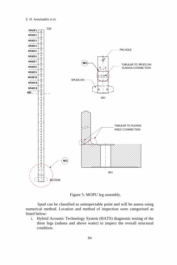
E. H. Jamaluddin et al.
84
Figure 5: MOPU leg assembly.
Spud can be classified as uninspectable point and will be assess using
numerical method. Location and method of inspection were categorised as
listed below:
i. Hybrid Acoustic Technology System (HATS) diagnostic testing of the
three legs (subsea and above water) to inspect the overall structural
condition.
TABULAR TO FLANGE
WELD CONNECTION
B01
MSL
SPLICE 12
SPLICE 11
SPLICE 10
SPLICE 9
SPLICE 8
SPLICE 7
SPLICE 6
SPLICE 5
SPLICE 4
SPLICE 3
SPLICE 2
SPLICE 1
BOTTOM
TOP
A01
A01
SPUDCAN
TUBULAR TO SPUDCAN
FLANGE CONNECTION
B01
PIN HOLE

Evaluation of Tabular Leg Structure of Mobile Offshore Production
85
ii. General Visual Inspections (GVI), Close Visual Inspections (CVI), and
Eddy Current Inspections (ECI) of above water weld joints and pinholes
in all three of the MOPU’s legs.
iii. General Visual Inspections (GVI), Close Visual Inspections (CVI)
inspections of the underwater weld joints and pinholes in all three
MOPU’s legs.
iv. Alternating Current Field Measurement (ACFM) inspections of the
underwater
v. Weld joints and pinholes in MOPU’s legs number 2.
vi. CVI or voltage measurement of the MOPU’s Cathodic Protection (CP)
System.
Assessment Method
The proposed method for life extension, as shown in Figure 6 comprises of 2
phases: 1) preparation and 2) implementation. The critical tasks in each of the
three phases are described in the following subsections.
Phase 1: Preparation The first phase in the LE process is the preparation stage which includes two
tasks of data gathering and development of essential criteria.
Data gathering The operational integrity of the MOPU legs LE depends on the accuracy and
quality of the data from how it has been designed, constructed, commissioned,
operated, and maintained over the original lifetime [22]. Design Fatigue Life
(DFL) study carried out during the design stage used as a basis to determine
the highest stress concentration points. Maintenance history of the MOPU
inclusive of incident reports were analyzed to identify any significant incident
that may have to the structural integrity and affects the stress concentration
points. Pass inspection reports were analyzed to develop the inspection plan.
Method of inspection determined by the defects that prone to be happening on
the legs i.e., loss of metallic area, surface crack, sub-surface crack, and
insufficient voltage for the Cathodic Protection for locations at above and
underwater.
Development of essential criteria Essential criteria developed based on the Classification guidelines. In this
study the classification guideline used are from American Bureau of Shipping
(ABS) and Russian Marine Register of Shipping (RS). Classification guideline
provides the acceptance criteria such as allowable percentage of general metal
loss, localized metal loss and coating breakdown [18].
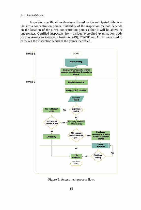
E. H. Jamaluddin et al.
86
Inspection specifications developed based on the anticipated defects at
the stress concentration points. Suitability of the inspection method depends
on the location of the stress concentration points either it will be above or
underwater. Certified inspectors from various accredited examination body
such as American Petroleum Institute (API), CSWIP and ASNT were used to
carry out the inspection works at the points identified.
PHASE 1
PHASE 2
START
Data Gathering
Development of essential criteria:
Inspection specifications & Acceptance
criteria.
Inspection
Result
Remaining useful life
(RUL) analysis
RUL exceeds
Design fatigue life
(DFL)
Site rectification
works
Risk based
management (RBM) to
establish inspection
interval
Significant
findingYes
No
Successfully
rectified at siteYes
Dry-docking
No
Life
extension
Yes
No
END
Significant
findingNo
Periodic
inspection
Regulatory approval
Inspection work execution
Yes
Figure 6: Assessment process flow.

Evaluation of Tabular Leg Structure of Mobile Offshore Production
87
Phase 2: Approval and implementation The second stage of the LE process focuses on regulatory approval process and
implementation measures.
Regulatory approval Main regulatory body that oversees the marine activity is the Flag State Marine
Administration (FSMA) who responsible to issue the final approval for the
MOPU to operate within their water territory. Classification body is
responsible to ensure the integrity of the MOPU is intact to continue operation.
Inspection work execution All the surveys and inspections of the MOPU were conducted considering that
the facility is in “Laid-Up” mode as classed by RS, non-operational and clear
of hydrocarbons. The inspection divided to two; above water and underwater.
Based on the anticipated defects and inspection parameter, method of
inspection as shown in Table 1.
Table 1: Method of inspection
Anticipated Defect /
Inspection Parameter
Method of Inspection
Above Water Underwater
General metal loss UT UT
Localize metal loss UT UT
Coating breakdown Visual Visual
Surface crack Visual, EC ACFM
Sub-surface crack EC ACFM
Depletion of anode Visual Visual
CP voltage measurement Voltmeter N/A
Area/Surrounding survey N/A Visual/ROV
Overall thickness screening HATS HATS
Site rectification work Found defects that exceeded the allowable limit require rectification.
Rectification at the site is a preferred method aligned with the LE intention to
maintain the MOPU location beyond design life.
Remaining useful life (RUL) analysis There are few methods used to determine the remaining period for MOPU to
safely stand at the existing location. RUL will be based on the DFL calculation
where the safety factor may be reduced depending on the inspection result [24].
E. H. Jamaluddin et al.
88
Risk-based management Risk-Based Management (RBM) on assets consists of the execution of risk
assessment and the development of an inspection plan. The assessment and the
inspection may cover the whole assets or only focus on certain equipment or
component. Risk ranking was developed to define the requirement of the
inspection requirement and the intervals [25].
Dry-docking Dry-docking is a term used for repairs or when a ship is taken to the service
yard. During dry docking, the whole ship is brought to dry land so that the
submerged portions of the hull can be cleaned or inspected. In the event where
site rectification work is not doable, dry-docking is the only method for the
rectification works to be executed.
Result and Discussion
The topsides and underwater leg surveys found minor weld bulges, anode
depletion, and coating variations on all three legs. However, no severe defects
or cracks were recorded at the jacking pinholes or indeed anywhere else.
Ultrasonic Testing (UT) and Cathodic Protection (CP) surveys of each leg
were carried out. All readings for ultrasonic thickness gauging and cathodic
potential were found to be within acceptable ranges with no recorded
anomalies.
Condition assessment Critical hotspots or stress concentrations as identified by the analyses and
recommended to be inspected have been inspected in accordance with the
schedule of inspections and resulted in no significant findings other than
corrosion. The hotspots remain unchanged due to no excessive load or forces
being applied to the structure i.e.: collation with vessels, earthquakes, etc.
Hybrid acoustic technology system survey
Hybrid Acoustic Technology System (HATS) can detect and record an
anomaly’s size, severity, and number and then classifies it according to the
type of anomaly, e.g., corrosion, metal loss, crack. HATS diagnostics were
conducted to the entire length of the legs and recorded the relevant data.
Dormant cracks cannot be detected with the HATS diagnostics (such as
fatigue cracks which have stopped propagating, i.e., remain the same in time,
and therefore have no significant effect on the overall integrity of the structural
member). However, active defects including fatigue cracks that are still
developing in time can and would have been detected by this methodology.
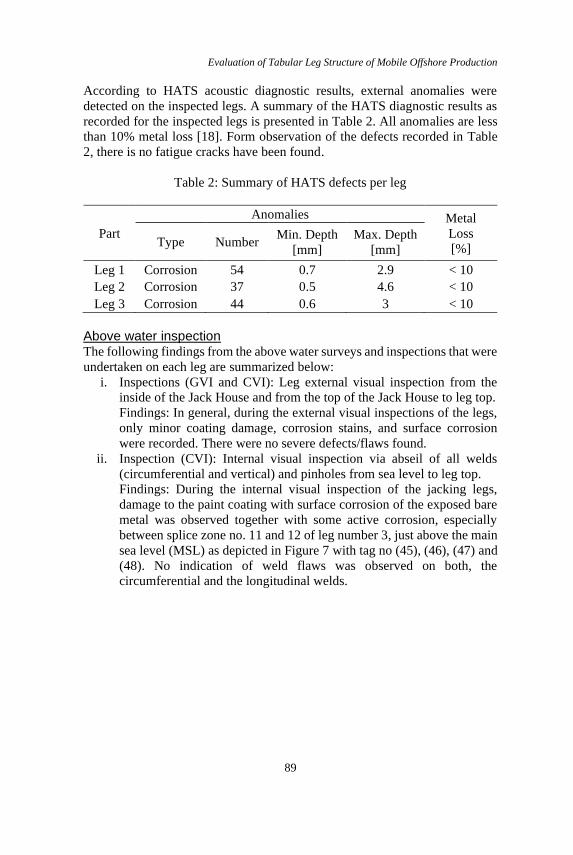
Evaluation of Tabular Leg Structure of Mobile Offshore Production
89
According to HATS acoustic diagnostic results, external anomalies were
detected on the inspected legs. A summary of the HATS diagnostic results as
recorded for the inspected legs is presented in Table 2. All anomalies are less
than 10% metal loss [18]. Form observation of the defects recorded in Table
2, there is no fatigue cracks have been found.
Table 2: Summary of HATS defects per leg
Part
Anomalies Metal
Loss
[%] Type Number
Min. Depth
[mm]
Max. Depth
[mm]
Leg 1 Corrosion 54 0.7 2.9 < 10
Leg 2 Corrosion 37 0.5 4.6 < 10
Leg 3 Corrosion 44 0.6 3 < 10
Above water inspection
The following findings from the above water surveys and inspections that were
undertaken on each leg are summarized below:
i. Inspections (GVI and CVI): Leg external visual inspection from the
inside of the Jack House and from the top of the Jack House to leg top.
Findings: In general, during the external visual inspections of the legs,
only minor coating damage, corrosion stains, and surface corrosion
were recorded. There were no severe defects/flaws found.
ii. Inspection (CVI): Internal visual inspection via abseil of all welds
(circumferential and vertical) and pinholes from sea level to leg top.
Findings: During the internal visual inspection of the jacking legs,
damage to the paint coating with surface corrosion of the exposed bare
metal was observed together with some active corrosion, especially
between splice zone no. 11 and 12 of leg number 3, just above the main
sea level (MSL) as depicted in Figure 7 with tag no (45), (46), (47) and
(48). No indication of weld flaws was observed on both, the
circumferential and the longitudinal welds.

E. H. Jamaluddin et al.
90
Figure 7: Observed paint damage and surface corrosion at leg 3.
iii. Inspection: Ultrasonic thickness measurements of the legs were carried
out at four main areas namely, within their splash zone area, at points
below the shear pin location of leg 1 and 3, and areas above the shear
pin location of leg 2.
Findings: No significant reductions of the wall thicknesses were
observed during the measurements. Thickness measurements were
within the range 53.9 mm to 56.2 mm. The design thickness is 55 mm.
Table 3 provides the thickness measurements for all three legs.
Table 3: Leg thicknesses (above water)
Part
Thickness [mm]
Design
Value
Min.
Measured
Max.
Measured
Average
Measured
Leg 1 55.00 53.90 56.20 55.56
Leg 2 55.00 54.70 56.00 55.41
Leg 3 55.00 54.10 55.90 55.57
iv. Inspection: Eddy Current Inspection of the legs at designated areas of
the jacking holes circumferential and longitudinal welds.
Findings: No significant flaws/defects were observed during the ECI.
v. Inspection (UFD): Ultrasonic Flaw Detection to be carried out on
MOPU legs at designated areas of Jacking holes, circumferential and
longitudinal welds.
SPLICE 12
SPLICE 11
SPLICE 10
SPLICE 9
MSL

Evaluation of Tabular Leg Structure of Mobile Offshore Production
91
Findings: No recordable Indications were observed during the
inspection.
Under water inspection
The GVI to the subsea parts of the legs was carried out by divers aiming at
inspecting the coating condition and at finding any abnormalities such as
cracks and other defects. The following findings from the underwater surveys
and inspections that were undertaken on each leg are summarized below:
i. General Visual Inspection of the legs, the full leg length (from MSL to
seabed) was reported to be covered with hard marine growth. No
cracks/flaws were found. The CVI of the subsea parts of the legs has
been carried out by divers on the jacking holes of the splash zone area
all the way to the lowest reachable jacking holes (No 52) to identify
cracks (if any present) on all three legs. Prior to the commencement of
CVI, cleaning of all jacking holes was carried out using HP water jet,
hand scraper, and wire brush. No crack initiation indications were
reported during the Close Visual Inspection of the jacking pinholes. A
considerable amount of metallic debris was found in close vicinity of
leg 1 and 3 which can compromise the cathodic protection of the
underwater leg structure by creating overprotection or under-protection
voltages of the legs. This concern, however, has been assessed and
eliminated on the grounds provided by the following facts:
a. The debris has been in the same location for several years as
recorded from previous surveys.
b. The cathodic protection (CP) measurements recorded by the
surveys of the years 2013, 2014, 2015 and 2017 have been
consistent and with voltage values within the normal range of
protection.
c. No active corrosion has been recorded at these locations.
ii. Marine growth thickness was measured by a mechanical measurement
technique which recorded an average thickness of 25 mm and 41 mm
at depths of 48.5 m and 10 m below the MSL respectively.
iii. Ultrasonic thickness measurements of the legs were carried out for four
measurement points at specified underwater areas. No significant
reduction in the wall thickness was observed during these
measurements. Thickness measurements were within the range 53.9
mm to 56.0 mm. The design thickness is 55 mm. The thickness
measurements for all the legs are given in Table 4.
iv. Alternating current field measurement (ACFM) was employed on leg 2
to determine the weld presence in the joint as well as determine
underwater crack sizing. The ACFM underwater survey of weldments
and jacking pinholes was performed by divers. No crack initiation
indications were recorded while carrying out ACFM.
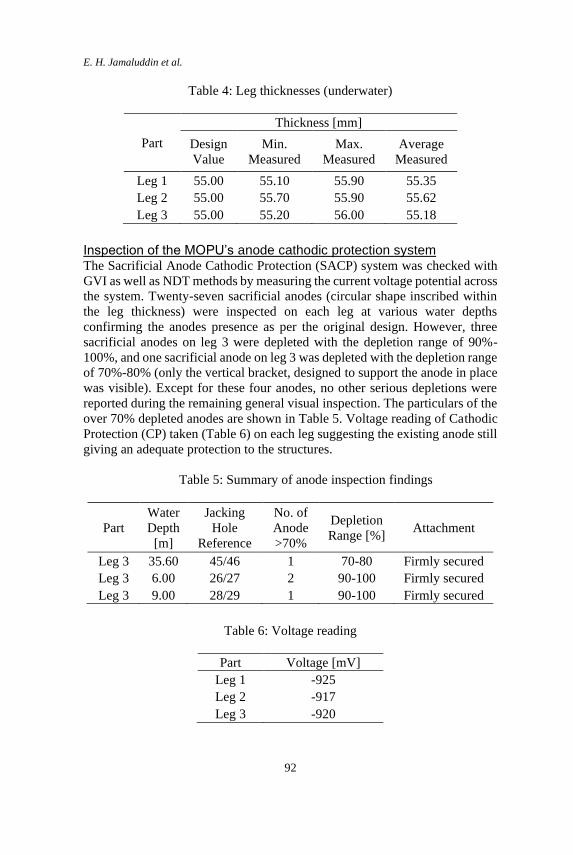
E. H. Jamaluddin et al.
92
Table 4: Leg thicknesses (underwater)
Part
Thickness [mm]
Design
Value
Min.
Measured
Max.
Measured
Average
Measured
Leg 1 55.00 55.10 55.90 55.35
Leg 2 55.00 55.70 55.90 55.62
Leg 3 55.00 55.20 56.00 55.18
Inspection of the MOPU’s anode cathodic protection system The Sacrificial Anode Cathodic Protection (SACP) system was checked with
GVI as well as NDT methods by measuring the current voltage potential across
the system. Twenty-seven sacrificial anodes (circular shape inscribed within
the leg thickness) were inspected on each leg at various water depths
confirming the anodes presence as per the original design. However, three
sacrificial anodes on leg 3 were depleted with the depletion range of 90%-
100%, and one sacrificial anode on leg 3 was depleted with the depletion range
of 70%-80% (only the vertical bracket, designed to support the anode in place
was visible). Except for these four anodes, no other serious depletions were
reported during the remaining general visual inspection. The particulars of the
over 70% depleted anodes are shown in Table 5. Voltage reading of Cathodic
Protection (CP) taken (Table 6) on each leg suggesting the existing anode still
giving an adequate protection to the structures.
Table 5: Summary of anode inspection findings
Part
Water
Depth
[m]
Jacking
Hole
Reference
No. of
Anode
>70%
Depletion
Range [%] Attachment
Leg 3 35.60 45/46 1 70-80 Firmly secured
Leg 3 6.00 26/27 2 90-100 Firmly secured
Leg 3 9.00 28/29 1 90-100 Firmly secured
Table 6: Voltage reading
Part Voltage [mV]
Leg 1 -925
Leg 2 -917
Leg 3 -920
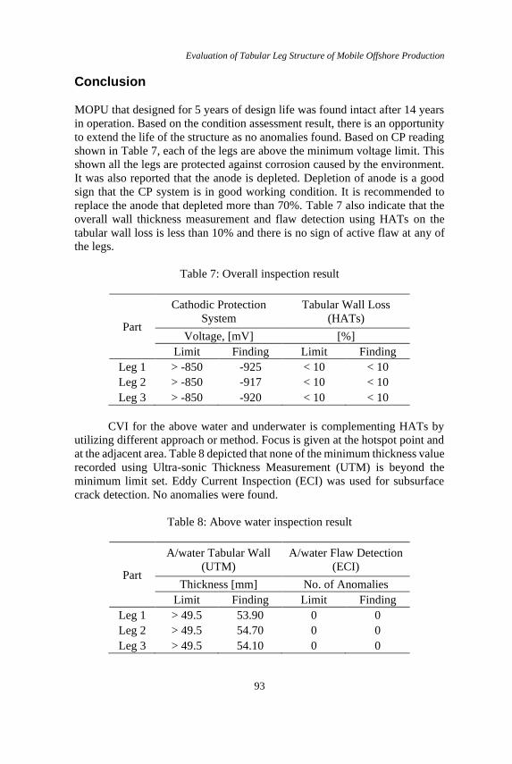
Evaluation of Tabular Leg Structure of Mobile Offshore Production
93
Conclusion
MOPU that designed for 5 years of design life was found intact after 14 years
in operation. Based on the condition assessment result, there is an opportunity
to extend the life of the structure as no anomalies found. Based on CP reading
shown in Table 7, each of the legs are above the minimum voltage limit. This
shown all the legs are protected against corrosion caused by the environment.
It was also reported that the anode is depleted. Depletion of anode is a good
sign that the CP system is in good working condition. It is recommended to
replace the anode that depleted more than 70%. Table 7 also indicate that the
overall wall thickness measurement and flaw detection using HATs on the
tabular wall loss is less than 10% and there is no sign of active flaw at any of
the legs.
Table 7: Overall inspection result
Part
Cathodic Protection
System
Tabular Wall Loss
(HATs)
Voltage, [mV] [%]
Limit Finding Limit Finding
Leg 1 > -850 -925 < 10 < 10
Leg 2 > -850 -917 < 10 < 10
Leg 3 > -850 -920 < 10 < 10
CVI for the above water and underwater is complementing HATs by
utilizing different approach or method. Focus is given at the hotspot point and
at the adjacent area. Table 8 depicted that none of the minimum thickness value
recorded using Ultra-sonic Thickness Measurement (UTM) is beyond the
minimum limit set. Eddy Current Inspection (ECI) was used for subsurface
crack detection. No anomalies were found.
Table 8: Above water inspection result
Part
A/water Tabular Wall
(UTM)
A/water Flaw Detection
(ECI)
Thickness [mm] No. of Anomalies
Limit Finding Limit Finding
Leg 1 > 49.5 53.90 0 0
Leg 2 > 49.5 54.70 0 0
Leg 3 > 49.5 54.10 0 0

E. H. Jamaluddin et al.
94
As per Table 9, none of the minimum thickness value recorded using
Ultra-sonic Thickness Measurement (UTM) is beyond the minimum limit set.
Alternating Current Field Measurement (ACFM) was used for subsurface
crack detection. No anomalies was found. Based on the design, Leg 2 received
the highest loads compared to others. Thus, only Leg 2 has been considered
for ACFM. In case of any flaw detected at Leg 2, ACFM will be expand to the
other legs.
Table 9: Underwater inspection result
Part
U/water Tabular Wall
(UTM)
U/water Flaw Detection
(ACFM)
Thickness [mm] No. of Anomalies
Limit Finding Limit Finding
Leg 1 > 49.5 55.10 N/A N/A
Leg 2 > 49.5 55.70 0 0
Leg 3 > 49.5 55.20 N/A N/A
Recommendation
For MOPU useful life to be extended, there is an engineering assessment that
required to take place such as: i) Remaining Useful Life (RUL) Assessment
and ii) Risk Assessment. RUL at each of the hotspot has to be calculated to
establish the inspection interval based on the remaining years of life. Based on
the condition assessment result that shows no significant anomalies, thus
Reduced Fatigue Design Factor (FDF) can be applied in the RUL calculation
[24]. Hotspots that have exceeded the RUL require further extensive
engineering assessment i.e.: Finite Element Analysis to predict the
deterioration rate or pattern. The risk on each hotspot has to be assessed to firm
up the inspection interval. A risk-based structural assessment considers that
structures of a higher risk require more frequent and more detailed levels of
inspection than those with a lower risk.
Acknowledgement
The authors of this work would like to express their sincere gratitude to Faculty
of Mechanical Engineering, Universiti Teknologi MARA (UiTM) for
facilitating this research.

Evaluation of Tabular Leg Structure of Mobile Offshore Production
95
References
[1] W. P. Stewart and M. Ooley, "The Maleo MOPU Project-Overview and
Keynote Introduction to Session," in Offshore Technology Conference,
2008.
[2] Z. Alwi, "Decommissioning of Kapal Wellbay Module, its Support
Structure and MOPU Mobile Producer 1," in SPE Symposium:
Decommissioning and Abandonment, 2018.
[3] M. J. Kaiser and M. Liu, "Decommissioning cost estimation for deepwater
floating structures in the US Gulf of Mexico," Ships and Offshore
Structures, vol. 10, no. 4, pp. 436-455, 2015. [4] B. Crager, F. Shumaker, and C. McCabe, "Mobile Offshore Production
Systems: An Analysis of Technical and Commercial Trends," in Offshore
Technology Conference, 1996.
[5] M. Abbas and M. Shafiee, "An overview of maintenance management
strategies for corroded steel structures in extreme marine environments,"
Marine Structures, vol. 71, pp. 102718, 2020. [6] A. Kharade and S. Kapadiya, "Offshore engineering: an overview of types
and loadings on structures," International Journal of Structural and Civil
Engineering Research, vol. 3, no. 2, pp. 16-28, 2014. [7] Y. M. Welaya, A. Elhewy, and M. Hegazy, "Investigation of jack-up leg
extension for deep water operations," International Journal of Naval
Architecture and Ocean Engineering, vol. 7, no. 2, pp. 288-300, 2015. [8] A. Nezamian, D. Vuckovic, and R. J. Nicolson, "Integrity Assessment and
Redeployment of Existing Mobile Offshore Production Unit for a
Marginal Field Development," in The 26th International Ocean and Polar
Engineering Conference, 2016.
[9] J. Van Meter, "Deciding when to use a MOPU for field development,"
Offshore, vol. 55, no. 5) pp. 112-114, 1995. [10] M. Shafiee and I. Animah, "An integrated FMEA and MCDA based risk
management approach to support life extension of subsea facilities in
high-pressure–high-temperature (HPHT) conditions," Journal of Marine
Engineering & Technology, pp. 1-16, 2020. [11] I. Animah and M. Shafiee, "Condition assessment, remaining useful life
prediction and life extension decision making for offshore oil and gas
assets," Journal of loss prevention in the process industries, vol. 53, pp.
17-28, 2018. [12] A. Stacey, M. Birkinshaw, and J. Sharp, "Life extension issues for ageing
offshore installations," in International Conference on Offshore
Mechanics and Arctic Engineering, 2008, pp. 199-215.
[13] E. Tveit, H. Sivertsen, and S. Hernæs, "Experience from field life
extension," in Offshore Technology Conference, 2014.
E. H. Jamaluddin et al.
96
[14] H. Liu, X. Shi, X. Chen, and Y. Liu, "Management of life extension for
topsides process system of offshore platforms in Chinese Bohai Bay,"
Journal of Loss Prevention in the Process Industries, vol. 35, pp. 357-365,
2015. [15] S. M. Ng, R. Khan, B. Isnadi, L. A. Lee, and S. N. Saminal, "A Holistic
Approach to Life Extension of Fixed Offshore Platforms in Malaysian
Waters," in International Petroleum Technology Conference, 2019.
[16] R. Tawekal et al., "Risk based underwater inspection (RBUI) for existing
fixed platforms in Indonesia," International Journal of Research in
Engineering and Science (IJRES), vol. 5, no. 7, 2017. [17] R. L. Tawekal, F. D. Purnawarman, and Y. Muliati, "Development of
Risk-Reliability Based Underwater Inspection for Fixed Offshore
Platforms in Indonesia," in MATEC Web of Conferences, 2018, pp. 05002.
[18] Rules for the Classification Surveys of Ship in Service, R. M. R. o.
Shipping, St Petersburg, 2018.
[19] B. Nagesh and I. Niranjan Kumar, "Investigation on the Overturning
Stability of a Jack up Mobile Offshore Production Unit by Site-Specific
Analysis to Find a Solution to Avoid the Failure of Its Leg Lattice
Structure," IJRASET, vol. 10, 2016. [20] M. Shafiee and I. Animah, "Life extension decision making of safety
critical systems: an overview," Journal of Loss Prevention in the Process
Industries, vol. 47 pp. 174-188, 2017. [21] S. M. Samarakoon and R. C. Ratnayake, "Strengthening, modification and
repair techniques’ prioritization for structural integrity control of ageing
offshore structures," Reliability Engineering & System Safety, vol. 135,
pp. 15-26, 2015. [22] M. Shafiee, I. Animah, and N. Simms, "Development of a techno-
economic framework for life extension decision making of safety critical
installations," Journal of Loss Prevention in the Process Industries, vol.
44, pp. 299-310, 2016. [23] A. Keprate and R. C. Ratnayake, "Fatigue and fracture degradation
inspection of offshore structures and mechanical items: the state of the
art," in International Conference on Offshore Mechanics and Arctic
Engineering, 2015, pp. V004T03A018.
[24] Guide for Fatigue Assessment of Offshore Structures, A. B. o. Shipping,
Houston, 2003.
[25] F. Guédé, "Risk-based structural integrity management for offshore jacket
platforms," Marine Structures, vol. 63, pp. 444-461, 2019.

Journal of Mechanical Engineering Vol 18(2), 97-110, 2021
___________________
ISSN 1823-5514, eISSN 2550-164X Received for review: 2020-11-02 © 2021 College of Engineering, Accepted for publication: 2021-02-19
Universiti Teknologi MARA (UiTM), Malaysia. Published: 2021-04-15
Design for Additive Manufacturing and Finite Element Analysis for
High Flexion Total Knee Replacement (TKR)
Solehuddin Shuib*, Mohammad Arsyad Azemi, Iffa Binti Mohd Arrif,
Najwa Syakirah Hamizan
Faculty of Mechanical Engineering, Universiti Teknologi MARA,
40450 Shah Alam, Selangor, Malaysia.
ABSTRACT
The patient from the Asian region always demanded a fully functional knee
implant, which implied a high-flexion range of motion. Most of their daily life
activities utilized the deep knee flexion which flexed until 165° such as the
Japanese proper sitting style and Muslim prayer position. The problem of the
study is extending the range of motion or achieving the high flexion of total
knee replacement as the traditional total knee replacement was incapable to
achieve more than 115°. Hence, the purpose of this study is to achieve a
modified design of a knee implant that can flex up to 165° by carried out a
static structural analysis in the ANSYS R16. There are 0°, 90°, 135°, and
165° angles of flexion with a different net force based on the percentage of
body weight implemented on the knee implant. The analysis includes total
deformation, Von Mises stress, shear stress, and contact pressure on knee
implant were observed and compared to find better modification design. The
total deformation had been decreased by about 69% at 0° flexion, 58.5% at
90° flexion, 90.93% at 135° flexion. The contact pressure also had been
decreased by about 99.2%, 22.2%, 99.98% at angle flexion of 0, 90, and 135,
respectively. The same declination happened to von Mises stress at about
85.05%, 9.52%, and 88.04% at the same angle of 0, 90, and 135,
respectively.
Keywords: Total knee replacement; High flexion; Finite element analysis;
Additive manufacturing
Solehuddin Shuib et al.
98
Introduction
The human knee joint is some of the most complex joints in the human body
that can be divided into soft tissues and body structure. The soft tissues
consist of tendons, menisci, muscles, and articular cartilages. While the bony
structure includes the femur, tibia, fibula, and patella [1]. The knee joint
bearing remarkably high loads as mostly human body weight are supported
by it to do active movement such as walking, sitting, running, and kneeling
for daily activities. Injury and damage to knee joints are bound to happen
because of an accident and playing sports that can cause fractures,
dislocations, and posterior cruciate ligament tears. Besides that, there is also
disease due to inflammation of the knee joint namely arthritis. If nonsurgical
treatment such as taking medications and walking using supports are no
longer bearable, total knee replacement surgery should be considered [2].
Total knee replacement (TKR) is to replace a knee joint with artificial
material by conducting a surgical procedure. This surgery and post-treatment
are needed to relieve pain and to restore knee functionality. Squatting and
kneeling are common activities that require normal flexion beyond 90°. As
the development of surgical technique, implant designs, and available
biomaterials have improved through the years, patients who undergo total
knee replacement can achieve more than 100° of knee flexion and sometimes
able to do squatting and kneeling [3]. However, the extent of the range of
motion for deep flexion is required in young and active individuals in Asian
countries. Besides, mostly Asian and Middle Eastern countries are required
to bend their knee up to 165° for deep flexion to do their cultural and
religious activities [4][5]. For instance, in Japanese culture, Seiza-sitting is a
traditional practice of sitting in attending a tea ceremony. While for the
Muslim religion, several positions required deep flexion to perform prayer.
Nevertheless, additive manufacturing (3D printing) is necessary to
develop a knee joint with deep flexion as it is cost-effective and time-
efficient to produce low volume and complex 3D implants [6]. This recent
technology can assist in developing deep flexion of the knee joint with
several modifications of designs and analysis. Besides that, additive
manufacturing also helps to guide orthopedic surgeons to understand and
plan their approach before beginning the operations as it can produce bone
models rapidly [6].
Therefore, a suitable design of total knee replacement should be
considered to fabricate and assist by additive manufacturing as well as to
ensure the knee implant is fully functional in flexing to different angles. The
main objective was to achieve a modified design of deep flexion of total knee
replacement by implementing finite element analysis and fabricate the
prototype of the 3D implant by using additive manufacturing such as fused
deposition modeling (FDM).
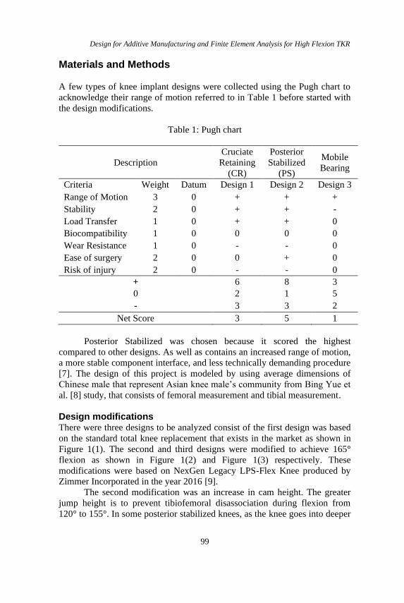
Design for Additive Manufacturing and Finite Element Analysis for High Flexion TKR
99
Materials and Methods
A few types of knee implant designs were collected using the Pugh chart to
acknowledge their range of motion referred to in Table 1 before started with
the design modifications.
Table 1: Pugh chart
Description
Cruciate
Retaining
(CR)
Posterior
Stabilized
(PS)
Mobile
Bearing
Criteria Weight Datum Design 1 Design 2 Design 3
Range of Motion 3 0 + + +
Stability 2 0 + + -
Load Transfer 1 0 + + 0
Biocompatibility 1 0 0 0 0
Wear Resistance 1 0 - - 0
Ease of surgery 2 0 0 + 0
Risk of injury 2 0 - - 0
+ 6 8 3
0 2 1 5
- 3 3 2
Net Score 3 5 1
Posterior Stabilized was chosen because it scored the highest
compared to other designs. As well as contains an increased range of motion,
a more stable component interface, and less technically demanding procedure
[7]. The design of this project is modeled by using average dimensions of
Chinese male that represent Asian knee male’s community from Bing Yue et
al. [8] study, that consists of femoral measurement and tibial measurement.
Design modifications There were three designs to be analyzed consist of the first design was based
on the standard total knee replacement that exists in the market as shown in
Figure 1(1). The second and third designs were modified to achieve 165°
flexion as shown in Figure 1(2) and Figure 1(3) respectively. These
modifications were based on NexGen Legacy LPS-Flex Knee produced by
Zimmer Incorporated in the year 2016 [9].
The second modification was an increase in cam height. The greater
jump height is to prevent tibiofemoral disassociation during flexion from
120° to 155°. In some posterior stabilized knees, as the knee goes into deeper
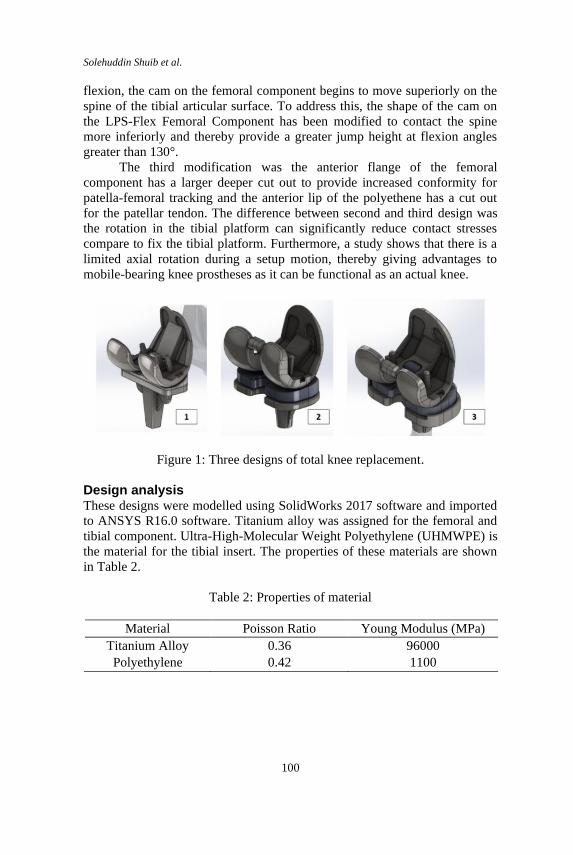
Solehuddin Shuib et al.
100
flexion, the cam on the femoral component begins to move superiorly on the
spine of the tibial articular surface. To address this, the shape of the cam on
the LPS-Flex Femoral Component has been modified to contact the spine
more inferiorly and thereby provide a greater jump height at flexion angles
greater than 130°.
The third modification was the anterior flange of the femoral
component has a larger deeper cut out to provide increased conformity for
patella-femoral tracking and the anterior lip of the polyethene has a cut out
for the patellar tendon. The difference between second and third design was
the rotation in the tibial platform can significantly reduce contact stresses
compare to fix the tibial platform. Furthermore, a study shows that there is a
limited axial rotation during a setup motion, thereby giving advantages to
mobile-bearing knee prostheses as it can be functional as an actual knee.
Figure 1: Three designs of total knee replacement.
Design analysis These designs were modelled using SolidWorks 2017 software and imported
to ANSYS R16.0 software. Titanium alloy was assigned for the femoral and
tibial component. Ultra-High-Molecular Weight Polyethylene (UHMWPE) is
the material for the tibial insert. The properties of these materials are shown
in Table 2.
Table 2: Properties of material
Material Poisson Ratio Young Modulus (MPa)
Titanium Alloy 0.36 96000 Polyethylene 0.42 1100
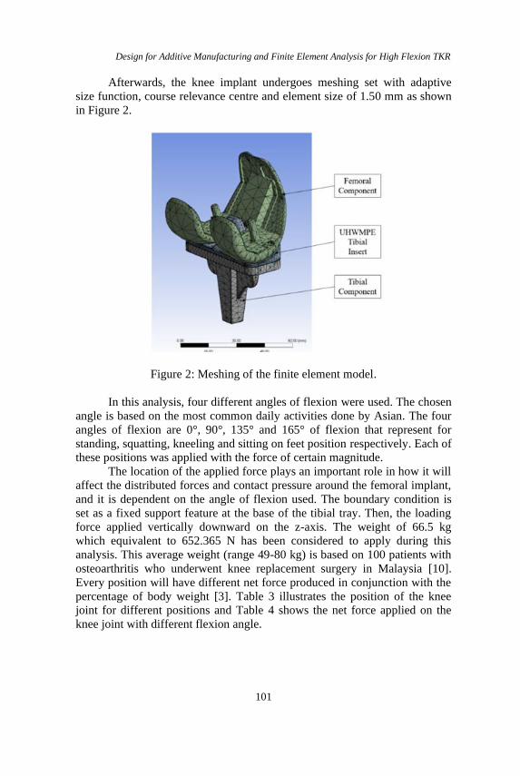
Design for Additive Manufacturing and Finite Element Analysis for High Flexion TKR
101
Afterwards, the knee implant undergoes meshing set with adaptive
size function, course relevance centre and element size of 1.50 mm as shown
in Figure 2.
Figure 2: Meshing of the finite element model.
In this analysis, four different angles of flexion were used. The chosen
angle is based on the most common daily activities done by Asian. The four
angles of flexion are 0°, 90°, 135° and 165° of flexion that represent for
standing, squatting, kneeling and sitting on feet position respectively. Each of
these positions was applied with the force of certain magnitude.
The location of the applied force plays an important role in how it will
affect the distributed forces and contact pressure around the femoral implant,
and it is dependent on the angle of flexion used. The boundary condition is
set as a fixed support feature at the base of the tibial tray. Then, the loading
force applied vertically downward on the z-axis. The weight of 66.5 kg
which equivalent to 652.365 N has been considered to apply during this
analysis. This average weight (range 49-80 kg) is based on 100 patients with
osteoarthritis who underwent knee replacement surgery in Malaysia [10].
Every position will have different net force produced in conjunction with the
percentage of body weight [3]. Table 3 illustrates the position of the knee
joint for different positions and Table 4 shows the net force applied on the
knee joint with different flexion angle.
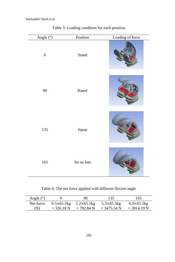
Solehuddin Shuib et al.
102
Table 3: Loading condition for each position
Angle (°) Position Loading of force
0 Stand
90 Kneel
135 Squat
165 Sit on feet
Table 4: The net force applied with different flexion angle
Angle (°) 0 90 135 165
Net force
(N) 0.5×65.5kg
= 326.18 N 1.2×65.5kg
= 782.84 N 5.3×65.5kg
= 3475.54 N
6.0×65.5kg
= 3914.19 N
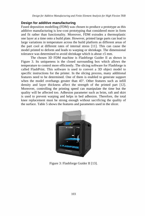
Design for Additive Manufacturing and Finite Element Analysis for High Flexion TKR
103
Design for additive manufacturing Fused deposition modelling (FDM) was chosen to produce a prototype as this
additive manufacturing is low-cost prototyping that considered more in form
and fit rather than functionality. Moreover, FDM extrudes a thermoplastic
one layer at a time onto a build plate. However, printed large parts can lead to
large variations in temperature across the build platform as different areas of
the part cool at different rates of internal stress [11]. This can cause the
model printed to deform and leads to warping or shrinkage. The dimensional
tolerance was determined to avoid shrinkage which is about ±5 mm.
The chosen 3D FDM machine is Flashforge Guider II as shown in
Figure 3. Its uniqueness is the closed surrounding box which allows the
temperature to control more efficiently. The slicing software for Flashforge is
called FlashPrint. This software is used to convert a 3D object model to
specific instructions for the printer. In the slicing process, many additional
features need to be determined. One of them is enabled to generate support
when the model overhangs greater than 45°. Other features such as infill
density and layer thickness affect the strength of the printed part [12].
Moreover, controlling the printing speed can manipulate the time but the
quality will be affected too. Adhesion parameter such as brim, raft and skirt
is used to prevent warping and helps in bed adhesion. Therefore, the total
knee replacement must be strong enough without sacrificing the quality of
the surface. Table 5 shows the features and parameters used in the slicer.
Figure 3: Flashforge Guider II [13].
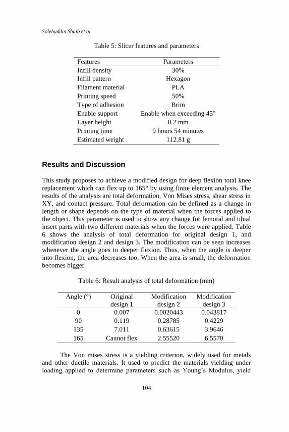
Solehuddin Shuib et al.
104
Table 5: Slicer features and parameters
Features Parameters
Infill density 30% Infill pattern Hexagon Filament material PLA Printing speed 50% Type of adhesion Brim Enable support Enable when exceeding 45° Layer height 0.2 mm Printing time 9 hours 54 minutes
Estimated weight 112.81 g
Results and Discussion
This study proposes to achieve a modified design for deep flexion total knee
replacement which can flex up to 165° by using finite element analysis. The
results of the analysis are total deformation, Von Mises stress, shear stress in
XY, and contact pressure. Total deformation can be defined as a change in
length or shape depends on the type of material when the forces applied to
the object. This parameter is used to show any change for femoral and tibial
insert parts with two different materials when the forces were applied. Table
6 shows the analysis of total deformation for original design 1, and
modification design 2 and design 3. The modification can be seen increases
whenever the angle goes to deeper flexion. Thus, when the angle is deeper
into flexion, the area decreases too. When the area is small, the deformation
becomes bigger.
Table 6: Result analysis of total deformation (mm)
Angle (°) Original
design 1
Modification
design 2
Modification
design 3
0 0.007 0.0020443 0.043817
90 0.119 0.28785 0.4229
135 7.011 0.63615 3.9646
165 Cannot flex 2.55520 6.5570
The Von mises stress is a yielding criterion, widely used for metals
and other ductile materials. It used to predict the materials yielding under
loading applied to determine parameters such as Young’s Modulus, yield
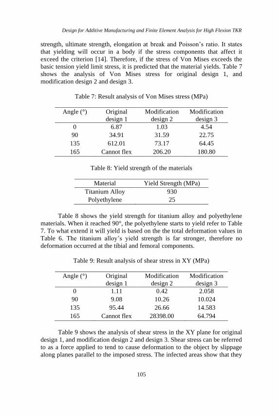
Design for Additive Manufacturing and Finite Element Analysis for High Flexion TKR
105
strength, ultimate strength, elongation at break and Poisson’s ratio. It states
that yielding will occur in a body if the stress components that affect it
exceed the criterion [14]. Therefore, if the stress of Von Mises exceeds the
basic tension yield limit stress, it is predicted that the material yields. Table 7
shows the analysis of Von Mises stress for original design 1, and
modification design 2 and design 3.
Table 7: Result analysis of Von Mises stress (MPa)
Angle (°) Original
design 1
Modification
design 2
Modification
design 3
0 6.87 1.03 4.54
90 34.91 31.59 22.75
135 612.01 73.17 64.45
165 Cannot flex 206.20 180.80
Table 8: Yield strength of the materials
Material Yield Strength (MPa)
Titanium Alloy 930 Polyethylene 25
Table 8 shows the yield strength for titanium alloy and polyethylene
materials. When it reached 90°, the polyethylene starts to yield refer to Table
7. To what extend it will yield is based on the the total deformation values in
Table 6. The titanium alloy’s yield strength is far stronger, therefore no
deformation occurred at the tibial and femoral components.
Table 9: Result analysis of shear stress in XY (MPa)
Angle (°) Original
design 1
Modification
design 2
Modification
design 3
0 1.11 0.42 2.058
90 9.08 10.26 10.024
135 95.44 26.66 14.583
165 Cannot flex 28398.00 64.794
Table 9 shows the analysis of shear stress in the XY plane for original
design 1, and modification design 2 and design 3. Shear stress can be referred
to as a force applied to tend to cause deformation to the object by slippage
along planes parallel to the imposed stress. The infected areas show that they
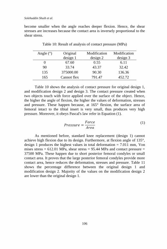
Solehuddin Shuib et al.
106
become smaller when the angle reaches deeper flexion. Hence, the shear
stresses are increases because the contact area is inversely proportional to the
shear stress.
Table 10: Result of analysis of contact pressure (MPa)
Angle (°) Original
design 1
Modification
design 2
Modification
design 3
0 67.60 0.55 6.11
90 33.74 43.37 32.42
135 375000.00 90.30 136.36
165 Cannot flex 791.47 452.72
Table 10 shows the analysis of contact pressure for original design 1,
and modification design 2 and design 3. The contact pressure created when
two objects touch with force applied over the surface of the object. Hence,
the higher the angle of flexion, the higher the values of deformation, stresses
and pressure. These happen because, at 165° flexion, the surface area of
femoral intact to the tibial insert is very small, thus produces very high
pressure. Moreover, it obeys Pascal's law refer in Equation (1).
𝑃𝑟𝑒𝑠𝑠𝑢𝑟𝑒 =𝐹𝑜𝑟𝑐𝑒
𝐴𝑟𝑒𝑎
(1)
As mentioned before, standard knee replacement (design 1) cannot
achieve high flexion due to its design. Furthermore, at flexion angle of 135°,
design 1 produces the highest values in total deformation = 7.011 mm, Von
mises stress = 612.01 MPa, shear stress = 95.44 MPa and contact pressure =
37500 MPa. These happen due to short posterior femoral condyles or small
contact area. It proves that the large posterior femoral condyles provide more
contact area, hence reduces the deformation, stresses and pressure. Table 11
shows the percentage difference between the original design 1 and
modification design 2. Majority of the values on the modification design 2
are lower than the original design 1.
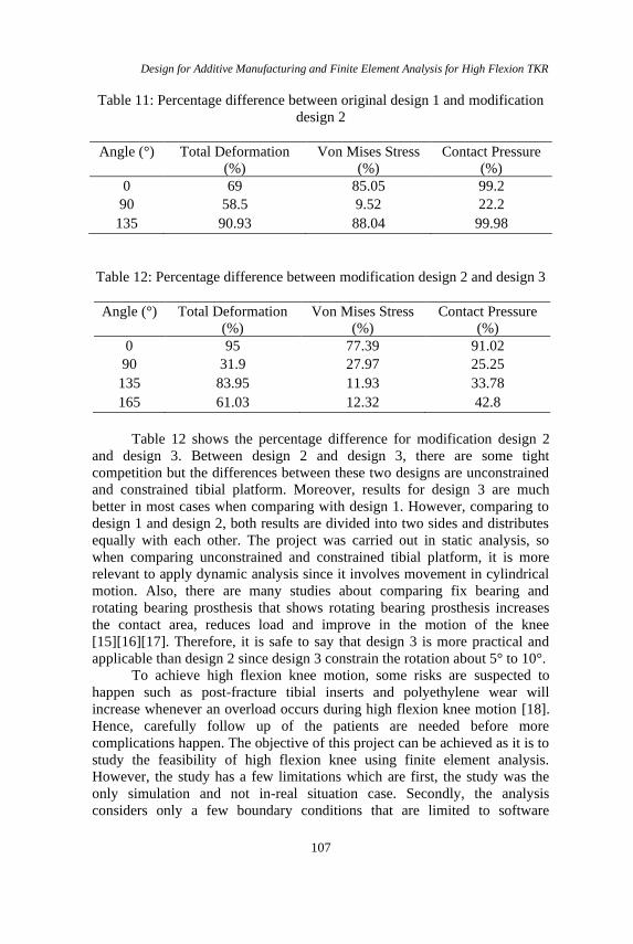
Design for Additive Manufacturing and Finite Element Analysis for High Flexion TKR
107
Table 11: Percentage difference between original design 1 and modification
design 2
Angle (°) Total Deformation
(%)
Von Mises Stress
(%)
Contact Pressure
(%)
0 69 85.05 99.2
90 58.5 9.52 22.2
135 90.93 88.04 99.98
Table 12: Percentage difference between modification design 2 and design 3
Angle (°) Total Deformation
(%)
Von Mises Stress
(%)
Contact Pressure
(%)
0 95 77.39 91.02
90 31.9 27.97 25.25
135 83.95 11.93 33.78
165 61.03 12.32 42.8
Table 12 shows the percentage difference for modification design 2
and design 3. Between design 2 and design 3, there are some tight
competition but the differences between these two designs are unconstrained
and constrained tibial platform. Moreover, results for design 3 are much
better in most cases when comparing with design 1. However, comparing to
design 1 and design 2, both results are divided into two sides and distributes
equally with each other. The project was carried out in static analysis, so
when comparing unconstrained and constrained tibial platform, it is more
relevant to apply dynamic analysis since it involves movement in cylindrical
motion. Also, there are many studies about comparing fix bearing and
rotating bearing prosthesis that shows rotating bearing prosthesis increases
the contact area, reduces load and improve in the motion of the knee
[15][16][17]. Therefore, it is safe to say that design 3 is more practical and
applicable than design 2 since design 3 constrain the rotation about 5° to 10°.
To achieve high flexion knee motion, some risks are suspected to
happen such as post-fracture tibial inserts and polyethylene wear will
increase whenever an overload occurs during high flexion knee motion [18].
Hence, carefully follow up of the patients are needed before more
complications happen. The objective of this project can be achieved as it is to
study the feasibility of high flexion knee using finite element analysis.
However, the study has a few limitations which are first, the study was the
only simulation and not in-real situation case. Secondly, the analysis
considers only a few boundary conditions that are limited to software
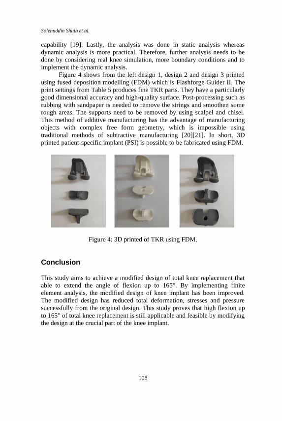
Solehuddin Shuib et al.
108
capability [19]. Lastly, the analysis was done in static analysis whereas
dynamic analysis is more practical. Therefore, further analysis needs to be
done by considering real knee simulation, more boundary conditions and to
implement the dynamic analysis.
Figure 4 shows from the left design 1, design 2 and design 3 printed
using fused deposition modelling (FDM) which is Flashforge Guider II. The
print settings from Table 5 produces fine TKR parts. They have a particularly
good dimensional accuracy and high-quality surface. Post-processing such as
rubbing with sandpaper is needed to remove the strings and smoothen some
rough areas. The supports need to be removed by using scalpel and chisel.
This method of additive manufacturing has the advantage of manufacturing
objects with complex free form geometry, which is impossible using
traditional methods of subtractive manufacturing [20][21]. In short, 3D
printed patient-specific implant (PSI) is possible to be fabricated using FDM.
Figure 4: 3D printed of TKR using FDM.
Conclusion This study aims to achieve a modified design of total knee replacement that
able to extend the angle of flexion up to 165°. By implementing finite
element analysis, the modified design of knee implant has been improved.
The modified design has reduced total deformation, stresses and pressure
successfully from the original design. This study proves that high flexion up
to 165° of total knee replacement is still applicable and feasible by modifying
the design at the crucial part of the knee implant.
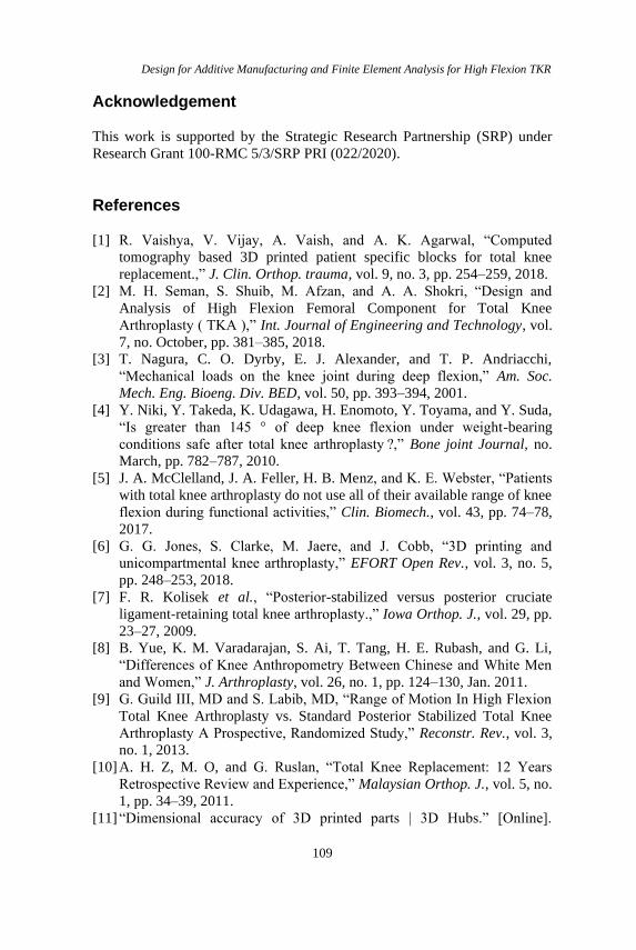
Design for Additive Manufacturing and Finite Element Analysis for High Flexion TKR
109
Acknowledgement
This work is supported by the Strategic Research Partnership (SRP) under
Research Grant 100-RMC 5/3/SRP PRI (022/2020).
References
[1] R. Vaishya, V. Vijay, A. Vaish, and A. K. Agarwal, “Computed
tomography based 3D printed patient specific blocks for total knee
replacement.,” J. Clin. Orthop. trauma, vol. 9, no. 3, pp. 254–259, 2018.
[2] M. H. Seman, S. Shuib, M. Afzan, and A. A. Shokri, “Design and
Analysis of High Flexion Femoral Component for Total Knee
Arthroplasty ( TKA ),” Int. Journal of Engineering and Technology, vol.
7, no. October, pp. 381–385, 2018.
[3] T. Nagura, C. O. Dyrby, E. J. Alexander, and T. P. Andriacchi,
“Mechanical loads on the knee joint during deep flexion,” Am. Soc.
Mech. Eng. Bioeng. Div. BED, vol. 50, pp. 393–394, 2001.
[4] Y. Niki, Y. Takeda, K. Udagawa, H. Enomoto, Y. Toyama, and Y. Suda,
“Is greater than 145 ° of deep knee flexion under weight-bearing
conditions safe after total knee arthroplasty ?,” Bone joint Journal, no.
March, pp. 782–787, 2010.
[5] J. A. McClelland, J. A. Feller, H. B. Menz, and K. E. Webster, “Patients
with total knee arthroplasty do not use all of their available range of knee
flexion during functional activities,” Clin. Biomech., vol. 43, pp. 74–78,
2017.
[6] G. G. Jones, S. Clarke, M. Jaere, and J. Cobb, “3D printing and
unicompartmental knee arthroplasty,” EFORT Open Rev., vol. 3, no. 5,
pp. 248–253, 2018.
[7] F. R. Kolisek et al., “Posterior-stabilized versus posterior cruciate
ligament-retaining total knee arthroplasty.,” Iowa Orthop. J., vol. 29, pp.
23–27, 2009.
[8] B. Yue, K. M. Varadarajan, S. Ai, T. Tang, H. E. Rubash, and G. Li,
“Differences of Knee Anthropometry Between Chinese and White Men
and Women,” J. Arthroplasty, vol. 26, no. 1, pp. 124–130, Jan. 2011.
[9] G. Guild III, MD and S. Labib, MD, “Range of Motion In High Flexion
Total Knee Arthroplasty vs. Standard Posterior Stabilized Total Knee
Arthroplasty A Prospective, Randomized Study,” Reconstr. Rev., vol. 3,
no. 1, 2013.
[10] A. H. Z, M. O, and G. Ruslan, “Total Knee Replacement: 12 Years
Retrospective Review and Experience,” Malaysian Orthop. J., vol. 5, no.
1, pp. 34–39, 2011.
[11] “Dimensional accuracy of 3D printed parts | 3D Hubs.” [Online].
Solehuddin Shuib et al.
110
Available: https://www.3dhubs.com/knowledge-base/dimensional-
accuracy-3d-printed-parts/. [Accessed: 16-Jun-2020].
[12] J. Fernandes, A. M. Deus, L. Reis, M. F. Vaz, and M. Leite, “Study of
the influence of 3D printing parameters on the mechanical properties of
PLA,” Proc. Int. Conf. Prog. Addit. Manuf., vol. 2018-May, no. August,
pp. 547–552, 2018.
[13] “Guider Ⅱs - FlashForge.” [Online]. Available:
https://www.flashforge.com/product-detail/11. [Accessed: 28-Oct-2020].
[14] H. Altenbach, “Book Review: Armenàkas, A. E., Advanced Mechanics
of Materials and Applied Elasticity,” J. Appl. Mathematics Mech., no.
86(9), pp. 681–681, 2006.
[15] E. H. Garling, B. L. Kaptein, R. G. H. H. Nelissen, and E. R. Valstar,
“Limited rotation of the mobile-bearing in a rotating platform total knee
prosthesis,” J. Biomech., vol. 40, no. SUPPL. 1, 2007.
[16] G. Solarino, M. Carrozzo, G. Vicenti, and B. Moretti, "Joints Long-term
outcome of low contact stress total knee arthroplasty with different
mobile-bearing designs," Joint, vol. 2, no. 3, pp. 109–114, 2014.
[17] A. Causero, P. Di Benedetto, A. Beltrame, R. Gisonni, V. Cainero, and
M. Pagano, “Design evolution in total knee replacement: which is the
future?,” Acta Biomed., vol. 85, pp. 5–19, 2014.
[18] J. Victor, J. K. P. Mueller, R. D. Komistek, A. Sharma, M. C. Nadaud,
and J. Bellemans, “In vivo kinematics after a cruciate-substituting
TKA,” Clin. Orthop. Relat. Res., vol. 468, no. 3, pp. 807–814, 2010.
[19] C. K. Cheng et al., “Biomechanical considerations in the design of high-
flexion total knee replacements,” Sci. World J., vol. 2014, 2014.
[20] M. J. Rowe and M. Crane, “3D-printed patient-specific applications,”
Orthop. Res. Rev., no. August, pp. 57–66, 2008.
[21] M. Javaid and A. Haleem, “Additive manufacturing applications in
medical cases: A literature based review,” Alexandria J. Med., vol. 54,
no. 4, pp. 411–422, 2018.

Journal of Mechanical Engineering Vol 18(2), 111-124, 2021
___________________
ISSN 1823-5514, eISSN 2550-164X Received for review: 2020-03-18 © 2021 College of Engineering, Accepted for publication: 2020-10-16
Universiti Teknologi MARA (UiTM), Malaysia. Published: 2021-01-15
Comparative Investigation of Worm Positions for Worm Gear-box Performance under No-Load
Condition
Hardik G Chothani*
Mechanical Engineering Department,
Government Engineering College, Bhavanagar, India
Kalpesh D Maniya
Mechanical Engineering Department,
C.K.Pithawala College of Engineering & Technology,
Surat, Gujarat, India
ABSTRACT
The Worm Gear drive is a gear arrangement where the worm shaft meshes
with a worm wheel (gear). The worm shaft plays an important role in
reduction ratio & efficiency. This worm shaft can be used at the top and
the bottom in the gearbox. This technical research paper provides
a comprehensive comparative evaluation of Input torque analysis &
heating rate of lubricant inside the gearbox for two positions of the worm
shaft in the worm gearbox under no-load condition. Worm shaft at the top
and worm shaft at the bottom were assessed at variable speed (1000-1400
rpm), the different splashed volume of lubricant (1.5-2.7 liter), and
variable temperature of lubricant (30-50 ºC). Input torque was measured
with the help of a direct torque measurement technique. Similarly, the
heating rate of the lubricant was also measured with a temperature sensor
for both orientations of the worm shaft. Full factorial experiments were
performed on a specially designed and fabricated worm gear test rig. The
experiments showed that the input torque requirement for the worm at the
bottom position is 20 -25% higher than the worm at the top position at an
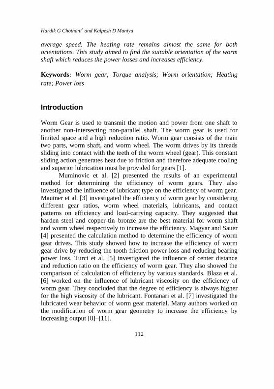
Hardik G Chothani* and Kalpesh D Maniya
112
average speed. The heating rate remains almost the same for both
orientations. This study aimed to find the suitable orientation of the worm
shaft which reduces the power losses and increases efficiency.
Keywords: Worm gear; Torque analysis; Worm orientation; Heating
rate; Power loss
Introduction
Worm Gear is used to transmit the motion and power from one shaft to
another non-intersecting non-parallel shaft. The worm gear is used for
limited space and a high reduction ratio. Worm gear consists of the main
two parts, worm shaft, and worm wheel. The worm drives by its threads
sliding into contact with the teeth of the worm wheel (gear). This constant
sliding action generates heat due to friction and therefore adequate cooling
and superior lubrication must be provided for gears [1].
Muminovic et al. [2] presented the results of an experimental
method for determining the efficiency of worm gears. They also
investigated the influence of lubricant type on the efficiency of worm gear.
Mautner et al. [3] investigated the efficiency of worm gear by considering
different gear ratios, worm wheel materials, lubricants, and contact
patterns on efficiency and load-carrying capacity. They suggested that
harden steel and copper-tin–bronze are the best material for worm shaft
and worm wheel respectively to increase the efficiency. Magyar and Sauer
[4] presented the calculation method to determine the efficiency of worm
gear drives. This study showed how to increase the efficiency of worm
gear drive by reducing the tooth friction power loss and reducing bearing
power loss. Turci et al. [5] investigated the influence of center distance
and reduction ratio on the efficiency of worm gear. They also showed the
comparison of calculation of efficiency by various standards. Blaza et al.
[6] worked on the influence of lubricant viscosity on the efficiency of
worm gear. They concluded that the degree of efficiency is always higher
for the high viscosity of the lubricant. Fontanari et al. [7] investigated the
lubricated wear behavior of worm gear material. Many authors worked on
the modification of worm gear geometry to increase the efficiency by
increasing output [8]–[11].
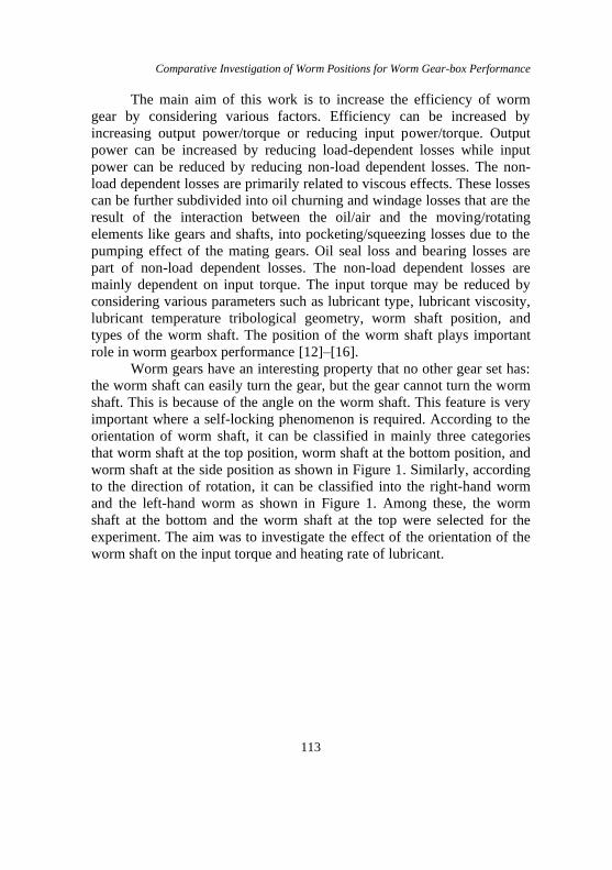
Comparative Investigation of Worm Positions for Worm Gear-box Performance
113
The main aim of this work is to increase the efficiency of worm
gear by considering various factors. Efficiency can be increased by
increasing output power/torque or reducing input power/torque. Output
power can be increased by reducing load-dependent losses while input
power can be reduced by reducing non-load dependent losses. The non-
load dependent losses are primarily related to viscous effects. These losses
can be further subdivided into oil churning and windage losses that are the
result of the interaction between the oil/air and the moving/rotating
elements like gears and shafts, into pocketing/squeezing losses due to the
pumping effect of the mating gears. Oil seal loss and bearing losses are
part of non-load dependent losses. The non-load dependent losses are
mainly dependent on input torque. The input torque may be reduced by
considering various parameters such as lubricant type, lubricant viscosity,
lubricant temperature tribological geometry, worm shaft position, and
types of the worm shaft. The position of the worm shaft plays important
role in worm gearbox performance [12]–[16].
Worm gears have an interesting property that no other gear set has:
the worm shaft can easily turn the gear, but the gear cannot turn the worm
shaft. This is because of the angle on the worm shaft. This feature is very
important where a self-locking phenomenon is required. According to the
orientation of worm shaft, it can be classified in mainly three categories
that worm shaft at the top position, worm shaft at the bottom position, and
worm shaft at the side position as shown in Figure 1. Similarly, according
to the direction of rotation, it can be classified into the right-hand worm
and the left-hand worm as shown in Figure 1. Among these, the worm
shaft at the bottom and the worm shaft at the top were selected for the
experiment. The aim was to investigate the effect of the orientation of the
worm shaft on the input torque and heating rate of lubricant.

Hardik G Chothani* and Kalpesh D Maniya
114
Figure 1: Classification of worm gear drive according to the position of
worm shaft [17].
Material and Methodology
The experimental studies were performed on a specially designed torque
measurement test machine. The schematic representation of this developed
test machine is given in Figure 2. The test machine is composed of a
motor, torque sensor, temperature sensor, variable frequency drive (VFD),
shaft, Bearings, couplings, testbed, and data collector.
Figure 2: Schematic representation of the test machine for worm gear [18].
Comparative Investigation of Worm Positions for Worm Gear-box Performance
115
The test stand is built with an electric motor controlled by the
variable frequency drive to enable the variation in rotational speed. The
gearbox containing the test gear pair is connected to the motor through the
shaft, torque sensor, and couplings. The gearbox is rigidly mounted at the
end of the test-bed and similarly, the motor is mounted on the other end of
the test-bed. The input torque of the test gear is measured with the torque
sensor. The temperature of oil inside the gearbox and pressure of the air
inside the gearbox can be measured with the help of a temperature sensor
and pressure gauge respectively. This test rig is designed to perform the
experiment based on the direct torque measurement technique. The same
test rig is used for both orientations of the worm gearbox. The complete
test rig with different views are shown in Figure 3(a) and (b). The selected
test worm gearbox is shown in Figure 3(c) and its inside volume of the
gearbox was kept constant (180 mm×180 mm×280 mm). In the same
gearbox, the worm shaft can be used at the top and bottom positions.
The purpose of this study was to analyze the influence of the worm
shaft of non-throated worm gearbox on input torque and heating rate of
lubricant under the different speed, and different oil conditions. The range
for control factors for various experiments was selected through various
pilot experiments. The test matrix is given in Table 1.
1-Pressure Gauge, 2-Worm gearbox,
3-Provision for oil level indicator,
4-Jaw type coupling, 5-Foot mounted bearing,
6-Variable frequency drive (VFD),
7-Torque sensor, 8-VFD regulator,
9-Temperature indicator,
10-Digital controller for Torque sensor
11-AC motor
(a)
Hardik G Chothani* and Kalpesh D Maniya
116
(b)
(c)
Figure 3: Test machine to measure the input torque and heating rate of
worm gearbox. (a) Front view of the test rig, (b) Top view of test rig (c)
Detailed arrangement of test gearbox.
Table 1: Test matrix
Control factors Unit Values
Speed of worm rpm 1000, 1200, 1400
Oil volume liter 1.5, 2.1, 2.7
Temperature ºC 30, 40, 50
Orientation of worm - The worm at the top, worm at
the bottom
The speed of the driving shaft was selected as 1000 rpm minimum
speed and 1400 rpm maximum speed [18]. Static oil levels were selected
based on the capacity of the gearbox and worm gear manufacturer report
[19]. The gearbox was operated at various lubricant volumes which are
shown in Figure 4. The experiments were tested at three temperature levels
of 30 ºC, 40 ºC and 50 ºC [18].
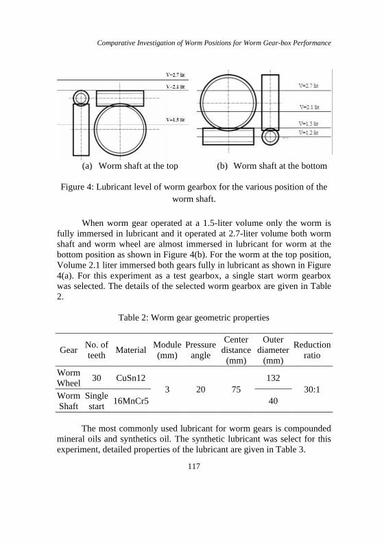
Comparative Investigation of Worm Positions for Worm Gear-box Performance
117
(a) Worm shaft at the top (b) Worm shaft at the bottom
Figure 4: Lubricant level of worm gearbox for the various position of the
worm shaft.
When worm gear operated at a 1.5-liter volume only the worm is
fully immersed in lubricant and it operated at 2.7-liter volume both worm
shaft and worm wheel are almost immersed in lubricant for worm at the
bottom position as shown in Figure 4(b). For the worm at the top position,
Volume 2.1 liter immersed both gears fully in lubricant as shown in Figure
4(a). For this experiment as a test gearbox, a single start worm gearbox
was selected. The details of the selected worm gearbox are given in Table
2.
Table 2: Worm gear geometric properties
Gear No. of
teeth Material
Module
(mm)
Pressure
angle
Center
distance
(mm)
Outer
diameter
(mm)
Reduction
ratio
Worm
Wheel 30 CuSn12
3 20 75
132
30:1 Worm
Shaft
Single
start 16MnCr5 40
The most commonly used lubricant for worm gears is compounded
mineral oils and synthetics oil. The synthetic lubricant was select for this
experiment, detailed properties of the lubricant are given in Table 3.
Hardik G Chothani* and Kalpesh D Maniya
118
Table 3: Lubricant properties
Sr.
No
Name of
oil
Kinematic
Viscosity
(cSt)
@ 40 ºC
Kinematic
Viscosity
(cSt)
@ 100 ºC
Viscosity
Index
Density
(Kg/m3)
@ 15 ºC
1 Synthetic
oil 330 35.50 162 790
Before any test, the machine was operated for at least 30 minutes
with heated lubricant in circulation to bring the entire gearbox up to the
steady-state test temperature. The experiments were operated from 2 ºC to
5 ºC before the starting temperature to avoid the previous experiment
effect. The test machine was operated with different positions of the worm
shaft at various controlling factors as per the test matrix. The input torque
and temperature of the lubricant were measured at every interval of time.
Results and Discussion
According to the orientation of a worm, it can be classified in mainly three
categories: worm on the top, worm on the bottom, and worm on the side.
Among these three categories, two categories were tested on the designed
test rig, worm at the bottom and worm at the top. The experiment test was
conducted for at least a prior 5 ºC temperature of the basic starting
temperature of the test. Time was not bounded for the test but the test was
going on till the desired temperature was reached. This test was designed
to describe the influence of the orientation of the worm shaft on multiple
responses: 1) influence of Position of worm shaft on input torque, and 2)
influence of position of worm shaft on lubricant heating rate.
Influence of worm orientation on input torque The input torque at various operating conditions was recorded in the
digital controller of the torque sensor. To investigate the effect of the
position of the worm shaft on input torque, the input torque obtained from
the experiments was plotted in the form of a graph. The influence of worm
position on input torque at different volume for speed 1000 and
temperature 40 ºC is shown in Figure 5. At 1.5-liter volume, there is no
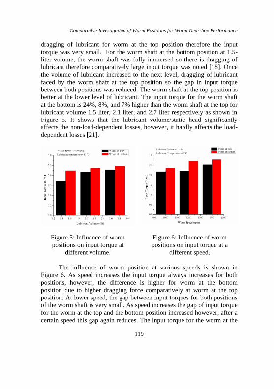
Comparative Investigation of Worm Positions for Worm Gear-box Performance
119
dragging of lubricant for worm at the top position therefore the input
torque was very small. For the worm shaft at the bottom position at 1.5-
liter volume, the worm shaft was fully immersed so there is dragging of
lubricant therefore comparatively large input torque was noted [18]. Once
the volume of lubricant increased to the next level, dragging of lubricant
faced by the worm shaft at the top position so the gap in input torque
between both positions was reduced. The worm shaft at the top position is
better at the lower level of lubricant. The input torque for the worm shaft
at the bottom is 24%, 8%, and 7% higher than the worm shaft at the top for
lubricant volume 1.5 liter, 2.1 liter, and 2.7 liter respectively as shown in
Figure 5. It shows that the lubricant volume/static head significantly
affects the non-load-dependent losses, however, it hardly affects the load-
dependent losses [21].
Figure 5: Influence of worm
positions on input torque at
different volume.
Figure 6: Influence of worm
positions on input torque at a
different speed.
The influence of worm position at various speeds is shown in
Figure 6. As speed increases the input torque always increases for both
positions, however, the difference is higher for worm at the bottom
position due to higher dragging force comparatively at worm at the top
position. At lower speed, the gap between input torques for both positions
of the worm shaft is very small. As speed increases the gap of input torque
for the worm at the top and the bottom position increased however, after a
certain speed this gap again reduces. The input torque for the worm at the

Hardik G Chothani* and Kalpesh D Maniya
120
bottom position is 0.2 Nm, 0.5 Nm, and 0.25 Nm higher than the worm at
the top position for worm speed 1000, 1200, and 1400 respectively. The
theoretical reason behind it, When the worm shaft at the top, the least
amount of oil is likely to be forced compared to the worm at the bottom
[14]. It reduces the churning power loss.
Figure 7 shows the influence of worm position on input torque at
different lubricant temperature. The temperature range is selected from 30
to 50 ºC. As temperature increases viscosity of lubricant goes down, this
reduces the dragging force of lubricant [14]. Due to static head, dragging
forces are high for worm shaft at the bottom and less for worm at the top
so input torque for worm at top position is less for every temperature
condition [18]. Input torque required for the bottom position of the worm
shaft reduces as temperature increases, however, the gap was remained
almost the same for temperature range from 30 ºC to 50 ºC. The constant
gap suggests that there is no influence of the worm shaft position on input
torque based on lubricant temperature.
(a) 1.5 litre volume and 1000
rpm
(b) 2.7 litre volume and 1400
rpm
Figure 7: Influence of worm position on input torque at different
temperature.
Influence of worm orientation on heating rate of lubricant Lubricant is not essential only for the friction of gear and bearing but it is
also useful to dissipate the heat during the operating condition [18]. Figure
8(a) shows the heating rate of lubricant for both operating conditions at
volume 2.1 liter and speed of worm 1000 rpm. The lubricant heating rate
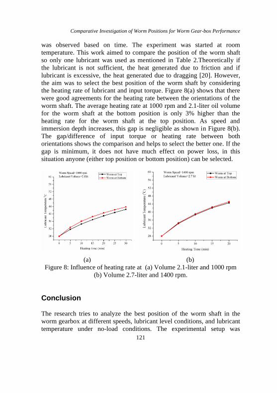
Comparative Investigation of Worm Positions for Worm Gear-box Performance
121
was observed based on time. The experiment was started at room
temperature. This work aimed to compare the position of the worm shaft
so only one lubricant was used as mentioned in Table 2.Theoretically if
the lubricant is not sufficient, the heat generated due to friction and if
lubricant is excessive, the heat generated due to dragging [20]. However,
the aim was to select the best position of the worm shaft by considering
the heating rate of lubricant and input torque. Figure 8(a) shows that there
were good agreements for the heating rate between the orientations of the
worm shaft. The average heating rate at 1000 rpm and 2.1-liter oil volume
for the worm shaft at the bottom position is only 3% higher than the
heating rate for the worm shaft at the top position. As speed and
immersion depth increases, this gap is negligible as shown in Figure 8(b).
The gap/difference of input torque or heating rate between both
orientations shows the comparison and helps to select the better one. If the
gap is minimum, it does not have much effect on power loss, in this
situation anyone (either top position or bottom position) can be selected.
(a)
(b)
Figure 8: Influence of heating rate at (a) Volume 2.1-liter and 1000 rpm
(b) Volume 2.7-liter and 1400 rpm.
Conclusion
The research tries to analyze the best position of the worm shaft in the
worm gearbox at different speeds, lubricant level conditions, and lubricant
temperature under no-load conditions. The experimental setup was
Hardik G Chothani* and Kalpesh D Maniya
122
specially developed for the research study. Various experiments were
conducted with the worm shaft at the top position and the worm shaft at
the bottom position. Input torque and heating rate of lubricant were noted
and plotted to understand the variations concerning worm positions. With
the increase in the volume of lubricant, gear gets more dragged which
increases the input torque. At 1.5 liter volume, 23.31% higher input torque
is required for the worm at the bottom position, similarly, 10.9% and 7.9%
higher input torque is required at 2.1 liter and 2.7 liter volume for the
worm at the bottom position compares to the worm at the top position. As
volume increases the gap between input torque for both positions reduces.
The worm at the top condition for lower volume is quite preferable. With
the increase in the temperature of the lubricant, input torque reduces. As
volume increases at the same speed heating rate of lubricant reduce and as
speed increases at the same volume heating rate of lubricant increases.
However, it was applicable for both conditions of the shaft so the
Influence of the position of the worm shaft cannot be evaluated based on
lubricant temperature only. With the increase in speed, higher input torque
was noted for both positions of the worm shaft however increasing input
rate is quite higher for the worm at the bottom position. For worm at
bottom position at 1000 rpm 12% input torque is more compare to worm
at the top position. Based on the speed, the worm shaft at the top position
required less input torque compare to the worm at the bottom position. It is
concluded that the worm shaft at the top position is more preferable to the
bottom position for non-load dependent losses.
References [1] V. Fontanari, M. Benedetti, G. Straffelini, C. Girardi, and L.
Giordanino, “Tribological behavior of the bronze-steel pair for worm
gearing,” Wear, vol. 302, no. 1–2, pp. 1520–1527, 2013.
[2] Muminovic Adil, R. Nedzad, and D. Zezelj, “The Efficiency of Worm
Gears Lubricated with Oil of Mineral and Synthetic Bases,”
Transactions of Famena, vol. 70, no. 4, pp. 65–72, 2013.
[3] E.-M. Mautner, W. Sigmund, J.-P. Stemplinger, K. Stahl, and
Experimental, “Investigations on the Efficiency of Worm Gear
Drives,” Gear Solution, pp. 33–45, 2016.
[4] B. Magyar and B. Sauer, “Calculation of the efficiency of worm gear
Comparative Investigation of Worm Positions for Worm Gear-box Performance
123
drives,” in International Gear Conference 2014: 26th–28th August
2014, Lyon, 2014, no. June, pp. 15–23.
[5] M. Turci, E. Ferramola, F. Bisanti, and G. Giacomozzi, “Worm Gear
Efficiency Estimation and Optimization,” Gear Technology, vol. 92,
pp. 46–53, 2016.
[6] Blaza Stojanovic, Sasa Radosavljevic, V. Sandra, and M. Slavica,
“The influence of lubricant viscosity on the efficiency of worm gear
reducer,” in 8th International Scientific Conference IRMES, 2017, no.
September, pp. 219–224.
[7] V. Fontanari, M. Benedetti, C. Girardi, and L. Giordanino,
“Investigation of the lubricated wear behavior of ductile cast iron and
quenched and tempered alloy steel for possible use in worm gearing,”
Wear, vol. 350–351, pp. 68–73, 2016.
[8] A. T. Alexandru, “Worm gears with optimized main geometrical
parameters and their efficiency,” Mechanika, vol. 81, no. 1, pp. 62–
65, 2010.
[9] H. Winter and H. Wilkesmann, “Calculation of Cylindrical Worm
Gear Drives of Different Tooth Profiles.,” Journal of Mechanical
Design, vol. 103, no. 4, pp. 73–82, 1981.
[10] K. Yukishima, I. Gonzalez-perez, A. Fuentes, and F. L. Litvin,
“Geometry and Investigation of Klingelnberg-TypeWorm Gear
Drive,” Journal of Mechanical Design, vol. 129, no. January 2007,
pp. 17–22, 2017.
[11] V. V. Simon, “Influence of tooth errors and shaft misalignments on
loaded tooth contact in cylindrical worm gears,” Mechanism and
Machine Theory, vol. 41, no. 6, pp. 707–724, 2006.
[12] S. Seetharaman and A. Kahraman, “Load-Independent Spin Power
Losses of a Spur Gear Pair: Model Formulation,” Journal of
Tribology, vol. 131, no. 2, pp. 022201, 2009.
[13] P. Luke and a. V. Olver, “A study of churning losses in dip-lubricated
spur gear,” Proceedings of the Institution of Mechanical Engineers,
Part G: Journal of Aerospace Engineering, vol. 82, no. 1, pp. 337–
346, 1999.
[14] J. Polly, D. Talbot, A. Kahraman, A. Singh, and H. Xu, “An
Experimental Investigation of Churning Power Losses of a Gearbox,”
Journal of Tribology, vol. 140, no. 6, pp. 1–8, 2018.
[15] C. Changenet and P. Velex, “Housing Influence on Churning Losses
in Geared Transmissions,” Journal of Mechanical Design, vol. 130,
Hardik G Chothani* and Kalpesh D Maniya
124
no. June 2008, pp. 062603, 2008.
[16] H. G. Chothani and K. D. Maniya, “Experimental investigation of
churning power loss of single start worm gear drive through
optimization technique,” Materials Today: Proceedings-Journal-
Elseiver, vol. 28, pp. 2031-2038, 2020.
[17] O. Mohammed, Mechanical Design Engineering Handbook., no. July.
2014.
[18] H. G. Chothani and K. D. Maniya, “Determination of optimum
working parameters for multiple response characteristics of worm
gearbox,” International Journal of Recent Technology and
Engineering, vol. 8, no. 3, pp. 1858–1862, 2019.
[19] KHK Stock gears, “Lubrication of Gears,” KHK Stock gears, 2015.
[Online]
[20] M. C. Brown, “Machinery Lubrication,” Noria corporation, 2011.
[21] B. R. Höhn, K. Michaelis, and H. P. Otto, “Influence of Immersion
Depth of Dip Lubricated Gears on Power Loss, Bulk Temperature and
Scuffing Load Carrying Capacity,” International Journal of
Mechanics and Materials in Design, vol. 4, no. 2, pp. 145–156, 2008.

"Journal of Mechanical Engineering” Vol 18(2), 125-144, 2021
___________________
“ISSN 1823-5514, eISSN 2550-164X” “Received for review: 2020-08-28”
“© 2021 College of Engineering, “ Accepted for publication: 2021-01-21
“Universiti Teknologi MARA (UiTM), Malaysia.” “ Published: 2021-04-15”
Pressure Drop and Flow Characteristics in a Diffuser with a
Dimpled Tube
Ehan Sabah Shukri Askari*
Institute of Technology Baghdad, Middle Technical University (MTU),
Baghdad, Iraq,
Wirachman Wisnoe
“Faculty of .Mechanical Engineering, Universiti Teknologi. MARA (UiTM),
Shah Alam, Selangor, Malaysia
“ABSTRACT”
The pressure drops and flow characteristics in a diffuser fitted with a semi-
dimpled tube are numerically studied. Air is selected as a working fluid and
its physical properties are modelled using pressure and velocity distribution.
The study reveals that every semi-dimple act as a vortex generator. They
provide the flow with intensive vortices between the dimpled surface and the
diffuser wall. Therefore, they cause an enhancement in the pressure drop
inside the diffuser. The performance of the dimples consisting of sphere type
dimples with 5 mm in diameter. Three “Reynolds number” operated in the
range of 25000 ˂Re˂ 50000 that is based on the hydraulic diameter of the
diffuser Dh. The variation in Reynolds number is examined to further
investigations of the pressure drop and flow characteristics of the diffuser.
The numerical simulations are conducted using incompressible steady-state
Reynolds Averaged Navier Stokes equations and the turbulence model “RNG
k-e is utilized in the current study. The flow characteristics of the diffuser
with semi-dimpled tube are analysed and compared in terms of pressure
contour, velocity profile, and velocity vectors, at the operating range of
Reynolds numbers. The results are discussed to point out the flow structure
mechanisms. It is found that equipping the diffuser with a semi-dimpled tube
leads to an increase in the recirculation and vortices inside and near the
dimples area. Therefore, they have a considerable influence on the flow field.
For the diffuser equipped with a semi-dimpled tube, it is noted that the flow
characteristics depend on the Reynolds number. The pressure drop in the
flow direction becomes lower with increasing Reynolds number. The findings

Ehan . Sabah Shukri Askari and Wirachman Wisnoe
126
indicate that for the semi-dimples, increasing Reynolds number increases the
velocity distribution significantly due to better mixing of the air.
Keywords: CFD; annular diffuser; dimpled tube; pressure drop; velocity
distribution
Nomenclature
Di
Do
L
dt
Lt
dm
P
u
ρ
Re
Inlet diameter of the diffuser, mm
Outlet diameter of the diffuser, mm
Length of the diffuser, mm
The diameter of the tube, mm
Length of the tube, mm
The diameter of the dimple, mm
The pressure at the inlet, bar
The velocity at the inlet, m.s-1
Air density, kg.m-3
“Reynolds Number”
k
ε
l
I
Cμ
λ
Cp
Greek Symbols
Turbulent1 kinetic energy
Turbulence. dissipation
Turbulence. length scale
Initial turbulence intensity
k-ε model parameter
Thermal conductivity
Specific heat capacity, kJ.kg-1 K-1
Introduction
There are many engineering applications where flow mixing, and
recirculation is a necessary part. The classic types of flow characteristics
enhancements such as fins, helical screw tape, dimples, etc., always increase
turbulence and recirculation. Gas turbine engines are one of the most popular
kinds of applications. In such engines, the product of power and efficiency
increases as these types of enhancement is added. One of the important gas
turbine engine components is the combustor. It directly affects engine
performance. The most serious problems of the combustors are the high-
pressure air coming from the compressor and the other highlighted problem
how good is the mixing between the fuel and the compressed air. These two
facts may cause serious problems on combustion uniformity and total
pressure loss coefficient. Utilizing pre-diffuser can reduce the effects of
previous problems. It is used to decelerate the flow and distribute the air
around the combustor uniformly and stably. This process should be
completed with a minimum total pressure loss.
To enhance efficiency and save energy with less loss, enhancement
techniques are required to improve mixing and increase turbulence. Dimples
are selected to generate turbulence and surfaces with dimples are easy to
fabricate. The existence of dimples enhances the character of the flow. In
recent years, numerous studies with numerical and experimental methods
have been carried out to improve the mixing and the performance of the heat
transfer by using different types of turbulence generators systems such as
Pressure Drop and Flow Characteristics in a diffuser with a dimpled tube
127
helical screw tapes [1]-[6], pin-fins [7]-[9], and dimples [10]-[18]. In the
recent decade, many researchers used pimples as a mixing method and it
could enhance the characteristics of the flow including temperature, velocity
profile, etc. Zhou et al. [18] pointed out that the performance of the heat
transfer in a dimpled surface is affected by the dimple geometries, including
dimple shape, dimple depth ratio, and dimple diameter. They completed an
experimental enquiry to search about the turbulent boundary layer
characteristics when it flows over a dimpled surface and compares the results
with a plain flat plate. “The results found that the flow characteristics of the
turbulent boundary layer flow over the dimpled surface were more
complicated with much stronger near-wall Reynolds stress and higher
turbulence kinetic energy, especially in the region near the back rims of the
dimples”.
Aroonrat and Wongwises [19] investigated the advantage of the
refrigerant (R-134a) on the heat transfer and pressure drop characteristics. In
a double-tube heat exchanger, the refrigerant (R-134a) was flowing into the
inner tube and in the annulus, the cold water was flowing. The study focused
on the inner tube with a dimpled tube and a plain tube. At the results, they
found that with the dimpled tube, the heat transfer coefficient and frictional
pressure drop were higher than that of the plain tube and as the Reynolds
number increases, it increased Nusselt number.
To improve heat transfer by using dimples and protrusions, Xie et al.
[20] suggested a modern design of an enhanced tube with dimples and
protrusions to induce swirl flow. From this investigation, it is found that the
geometries parameters of the dimples and the protrusions play an important
role to improve the thermal-hydraulic characterizes and heat transfer rate
compared with the plain tube, due to improved flow mixing. Xie et al. [21]
carried out numerical research using cross-ellipsoidal dimples inside an
enhanced tube to construe the mechanisms of the flow field method and heat
transfer. In their research, they used longitudinal and transverse dimples. The
effects of the dimple geometries (depth pitch and axis ratio) on thermal-
hydraulic performance were discussed and the simulations were employed
with the Re range from 5000 to 30,000. The results got that the flow mixing
was improved by the downward flow of the transverse and longitudinal
dimples. And the geometric parameter had been affected by the thermal-
hydraulic performance significantly.
Recently, many industrial and thermal applications required new
techniques to enhance heat transfer and increased thermal efficiency Wang et
al. [22] applied a numerical study in a square channel with dimples. The aim
was to test the bleed hole installation angle effect on the heat transfer and the
flow structure. They found that utilizing a bleed hole in this channel
significantly improved the thermal performance of the flow. Recently,
dimples were utilized as one kind of concavity that has a significant effect on
energy conservation augmentations. Qu et al. [23] investigated heat transfer
Ehan . Sabah Shukri Askari and Wirachman Wisnoe
128
and flow features in arrays of dimples inside a rectangular channel at a
transitional Reynolds number. In this investigation, they used the SST
turbulent model coupled with the Gamma-Theta transition model to indicate
the effect of different dimple depth and different Reynolds numbers on the
heat transfer performance and Nusselt number. The results displayed that
under the laminar condition the average Nusselt number decreases in the flow
direction while it increased when the flow became turbulent. Moreover, the
study obtained heat transfer enhancement during the turbulent flow and
became worse during the laminar flow. The numerical findings showed that
the heat transfer performance increased with the dimples depth increases
because of the induction of the turbulence kinetic energy into the main flow.
Abdulwahid et al. [24] studied the effect of an oval cross-section tube
with an oval dimpled surface in a laminar flow experimentally. The non-
Newtonian fluid was assumed with a constant heat flux condition and water
as a working fluid. This kind of passive technique showed good results in
terms of Nusselt number enhancement.
Most of the above works investigated flow features and heat transfer
improvement in channels and pipes with dimples. The present research
conducts numerical simulations to study pressure drop and flow
characteristics in a diffuser with a dimpled tube. The study is employed
sphere type dimples of 5 mm diameter and different Reynolds numbers based
on the diffuser hydraulic diameter in the range of 25000 ˂Re˂ 50000. The
pressure contour, velocity streamlines, and velocity vectors are numerically
investigated to indicate the flow mixing mechanisms.
Setup Design Methods
Model mechanism descriptions In the present research, a numerical method is used to be carried out to learn
about the impact of dimples on the flow attribute and pressure drop in a
diffuser geared up with a dimpled tube. Air is used as the working fluid in
this investigation to show the effect of dimples insert. The study considers all
the numerical simulations under the same inlet condition. In this research,
(L=80 mm) is the diffuser length, (Di=20 mm) is the diffuser inlet diameter,
and (Do=40 mm) is the diffuser outlet diameter. The tube diameter (dt) is
(10 mm) and a length (Lt) is (60 mm), [25]. The spherical dimples have a
diameter (ds=5 mm). The model geometries are illustrated in Figure 1.
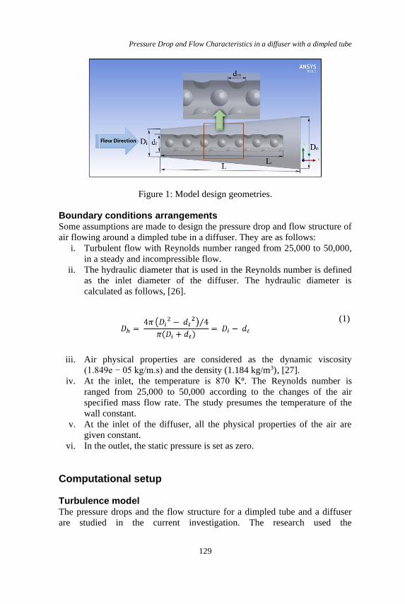
Pressure Drop and Flow Characteristics in a diffuser with a dimpled tube
129
Figure 1: Model design geometries.
Boundary conditions arrangements Some assumptions are made to design the pressure drop and flow structure of
air flowing around a dimpled tube in a diffuser. They are as follows:
i. Turbulent flow with Reynolds number ranged from 25,000 to 50,000,
in a steady and incompressible flow.
ii. The hydraulic diameter that is used in the Reynolds number is defined
as the inlet diameter of the diffuser. The hydraulic diameter is
calculated as follows, [26].
(1)
iii. Air physical properties are considered as the “dynamic viscosity
(1.849e − 05 kg/m.s) and the density (1.184 kg/m3)”, [27].
iv. At the inlet, the temperature is 870 K⁰. The “Reynolds number ” is
ranged from 25,000 to 50,000 according to the changes of the air
specified mass flow rate. The study presumes the temperature of the
wall constant.
v. At the inlet of the diffuser, all the physical properties of the air are
given constant.
vi. In the outlet, the static pressure is set as zero.
Computational setup
Turbulence model The pressure drops and. the flow structure for a dimpled tube and a diffuser
are studied in the current investigation. The research used the
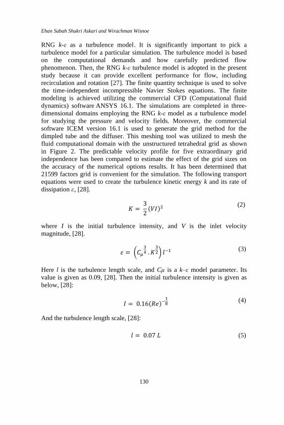
Ehan . Sabah Shukri Askari and Wirachman Wisnoe
130
RNG. k-ε as a “turbulence model ”. It is significantly important to pick a
turbulence model for a particular simulation. The turbulence model is based
on the computational demands and how carefully predicted flow
phenomenon. Then, the RNG. k-ε turbulence model is adopted in the present
study because it can provide excellent performance for flow, including
recirculation and rotation [27]. The finite quantity technique is used to solve
“the time-independent incompressible Navier Stokes equations ”. The finite
modeling is achieved utilizing the commercial .CFD .(Computational fluid .
dynamics) .software. ANSYS 16.1. The simulations are completed in three-
dimensional domains employing the RNG k-ε model as a turbulence model”
for studying the pressure and velocity fields. Moreover, the commercial
software ICEM .version 16.1 is used to generate the grid method for the
dimpled tube and the diffuser. This meshing tool was utilized to mesh the
fluid computational domain with the .unstructured tetrahedral grid . as shown
in Figure 2. The predictable velocity profile for five extraordinary grid
independence has been compared to estimate the effect of the grid sizes on
the accuracy of the numerical options results. It has been determined that
21599 factors grid is convenient for the simulation. The following transport .
equations were used to create “the turbulence kinetic energy k and its rate of
dissipation ε”, [28].
𝐾 = 3
2(𝑉𝐼)2
(2)
where I is the initial turbulence intensity, and V is the inlet velocity
magnitude, [28].
𝜀 = (𝐶𝜇
34 . 𝐾
32) 𝑙−1
(3)
Here l is the turbulence length scale, and Cμ is a k–ε model parameter. Its
value is given as 0.09, [28]. Then the initial turbulence intensity is given as
below, [28]:
𝐼 = 0.16(𝑅𝑒)−18
(4)
And the turbulence length scale, [28]:
𝑙 = 0.07 𝐿 (5)
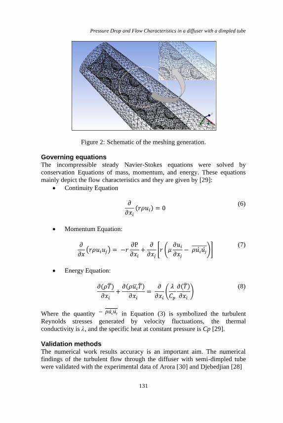
Pressure Drop and Flow Characteristics in a diffuser with a dimpled tube
131
Figure 2: Schematic of the meshing generation.
Governing equations The incompressible steady Navier-Stokes equations were solved by
conservation . Equations of mass, momentum, and energy. These equations
mainly depict the flow .characteristics and they are given by [29]:
• Continuity Equation
𝜕
𝜕𝑥𝑖
(𝑟𝜌𝑢𝑖) = 0 (6)
• Momentum Equation:
𝜕
𝜕𝑥(𝑟𝜌𝑢𝑖𝑢𝑗) = −𝑟
𝜕P
𝜕𝑥𝑖
+𝜕
𝜕𝑥𝑗
[𝑟 (𝜇𝜕𝑢𝑖
𝜕𝑥𝑗
− 𝜌𝑢𝑖́ 𝑢�́�)] (7)
• Energy Equation:
𝜕(𝜌�̅�)
𝜕𝑥𝑖
+𝜕(𝜌𝑢�̅��̅�)
𝜕𝑥𝑖
= 𝜕
𝜕𝑥𝑖
(𝜆
𝐶𝑝
𝜕(�̅�)
𝜕𝑥𝑖
) (8)
Where the quantity in Equation (3) is symbolized the turbulent
Reynolds stresses generated by velocity fluctuations, “the thermal
conductivity is λ”, and the specific heat at constant pressure is Cp [29].
Validation methods The numerical work results accuracy is an important aim. The numerical
findings of the turbulent flow through the diffuser with semi-dimpled tube
were validated with the experimental data of Arora [30] and Djebedjian [28]
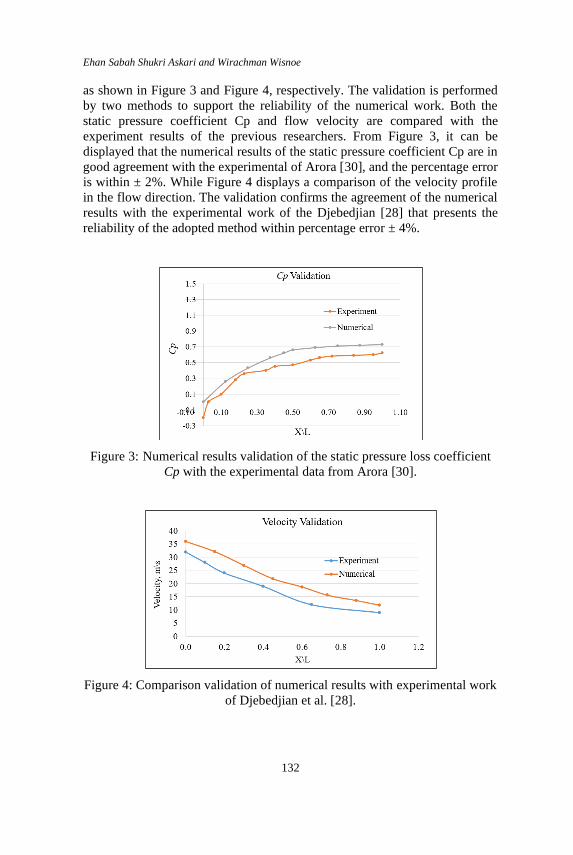
Ehan . Sabah Shukri Askari and Wirachman Wisnoe
132
as shown in Figure 3 and Figure 4, respectively. The validation is performed
by two methods to support the reliability of the numerical work. Both the
static pressure coefficient Cp and flow velocity are compared with the
experiment results of the previous researchers. From Figure 3, it can be
displayed that the numerical results of the static pressure coefficient Cp are in
good agreement with the experimental of Arora [30], and the percentage error
is within ± 2%. While Figure 4 displays a comparison of the velocity profile
in the flow direction. The validation confirms the agreement of the numerical
results with the experimental work of the Djebedjian [28] that presents the
reliability of the adopted method within percentage error ± 4%.
Figure 3: Numerical results validation of the static pressure loss coefficient
Cp with the experimental data from Arora [30].
Figure 4: Comparison validation of numerical results with experimental work
of Djebedjian et al. [28].
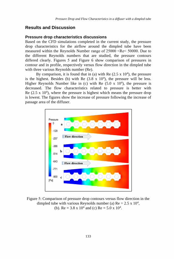
Pressure Drop and Flow Characteristics in a diffuser with a dimpled tube
133
Results and Discussion
Pressure drop characteristics discussions Based on the CFD simulations completed in the current study, the pressure
drop characteristics for the airflow around the dimpled tube have been
measured within the “Reynolds. Number1 range of 25000 ˂Re˂ 50000. Due to
the different Reynolds . numbers that are studied, the pressure contours
differed clearly. Figures 5 and Figure 6 show comparison of pressures in
contour and in profile, respectively versus flow direction in the dimpled tube
with three various Reynolds number (Re).
By comparison, it is found that in (a) with Re (2.5 x 10⁴), the pressure
is the highest. Besides (b) with Re (3.8 x 10⁴), the pressure will be less.
Higher Reynolds. Number like in (c) with Re (5.0 x 10⁴), the pressure is
decreased. The flow characteristics related to pressure is better with
Re (2.5 x 10⁴), where the pressure is highest which means the pressure drop
is lowest. The figures show the increase of pressure following the increase of
passage area of the diffuser.
Figure 5: Comparison of pressure drop contours versus flow direction in the
dimpled tube with various Reynolds number (a) Re = 2.5 x 10⁴,
(b). Re = 3.8 x 10⁴ and (c) Re = 5.0 x 10⁴.

Ehan . Sabah Shukri Askari and Wirachman Wisnoe
134
Figure 6: Comparison of pressure drop profile versus flow direction in a
dimpled tube with various Reynolds number (Re = 2.5 x 10⁴, 3.8 x 10⁴ and
5.0 x 10⁴).
Velocity distribution characteristics discussions The following simulations are utilized to study the velocity profile
characteristics in a dimpled tube during turbulence. flow. The effect of
Reynolds number on the velocity profile through the dimpled tube is
examined. Figures 7, 8 and 9 show the velocity vectors for three different
Reynolds. numbers (2.5 x 10⁴, 3.8 x 10⁴, and 5.0 x 10⁴) along the flow
direction.
In terms of the effect of Reynolds number on the velocity feature, the
recirculation and the tangential velocity component near the dimples area
increases as the Reynolds number increased. The figures reveal that the air
near the dimples area is mixed with the additional air that flowing around the
dimpled tube and enhances the distributions of the velocity.
More explanations for the effect of dimples on the flow characteristics
can be depicted in Figure 10, Figure 11, and Figure 12. The figures show
clearly the presence of flow recirculation at the dimples area. The colour of
the blue balls shows the velocity magnitude. For the three tested Reynolds
numbers, recirculation and vortices are conducted at the dimples area but in
different manners. The recirculation remains at the three tests but became
weak with Reynolds number (5.0 x 10⁴). This means that dimples can
produce tangential velocities and provide the flow with high distribution
intensity. However, the high distribution intensity also increases the pressure
drop. It is obvious that the dimple hole cause to change the direction of the
velocity inside the dimple. Thus, the cross-sectional area of the flow is
increased. Songtao . Wang explained this fact, as when the main flow accesses
the dimple, it will be divided into two parts. The flow in some parts of the
dimple has a high velocity and it makes a low velocity recirculation-zone in
other parts. When the flow impinged the dimples area, the flow .streamlines.
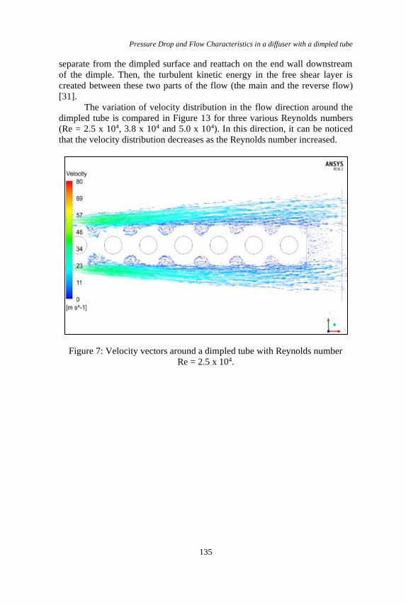
Pressure Drop and Flow Characteristics in a diffuser with a dimpled tube
135
separate from the dimpled surface and reattach on the end wall downstream
of the dimple. Then, the turbulent kinetic energy in the free shear layer is
created between these two parts of the flow (the main and the reverse flow)
[31].
The variation of velocity distribution in the flow direction around the
dimpled tube is compared in Figure 13 for three various Reynolds. numbers
(Re = 2.5 x 10⁴, 3.8 x 10⁴ and 5.0 x 10⁴). In this direction, it can be noticed
that the velocity distribution decreases as the Reynolds number increased.
Figure 7: Velocity vectors around a dimpled tube with Reynolds number
Re = 2.5 x 10⁴.
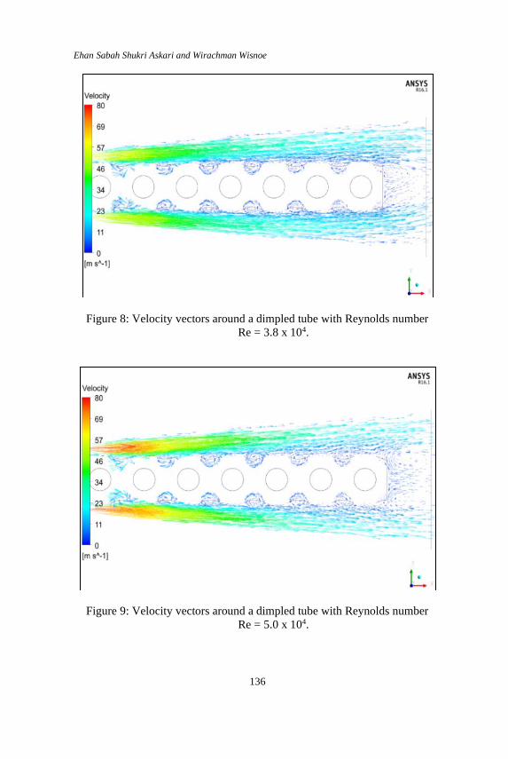
Ehan . Sabah Shukri Askari and Wirachman Wisnoe
136
Figure 8: Velocity vectors around a dimpled tube with Reynolds number
Re = 3.8 x 10⁴.
Figure 9: Velocity vectors around a dimpled tube with Reynolds number
Re = 5.0 x 10⁴.
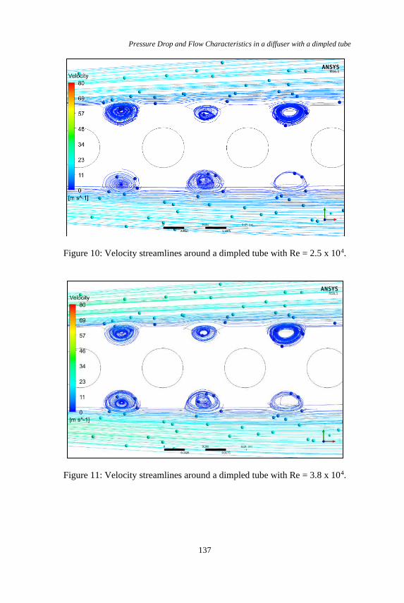
Pressure Drop and Flow Characteristics in a diffuser with a dimpled tube
137
Figure 10: Velocity streamlines around a dimpled tube with Re = 2.5 x 10⁴.
Figure 11: Velocity streamlines around a dimpled tube with Re = 3.8 x 10⁴.

Ehan . Sabah Shukri Askari and Wirachman Wisnoe
138
Figure 12: Velocity streamlines around a dimpled tube with Re = 5.0 x 10⁴.
Figure 13: Comparison of velocity distribution versus flow direction in a
dimpled tube with various Reynolds number (Re = 2.5 x 10⁴, 3.8 x 10⁴
and 5.0 x 10⁴).

Pressure Drop and Flow Characteristics in a diffuser with a dimpled tube
139
Velocity and pressure profile comparison in the outlet To test the effect of dimples insertion on the outlet flow characteristics, an
outlet plane is used.
The streamline velocity, the velocity profile and the pressure variation
comparison with three different “Reynolds numbers” (Re = 2.5 x 10⁴, 3.8 x 10⁴,
and 5.0 x 10⁴) are depicted in Figure 14, 15 and 16, respectively. Figure 14
presents the velocity streamlines . for different Reynolds numbers (Re) near
the outlet of the diffuser. For a plane at the outlet of the annular diffuser
behind the dimpled tube, the distribution . of the velocity . increased with
higher Reynolds. numbers. In Figure . 15, it is displayed . that. the distribution of
the velocity increases at the outlet as the “Reynolds number ” increases because
that increase disturbs the entire flow and cause more swirl flow and
recirculation. At the same time, the pressure variation decreases with a high
Reynolds number as shown . in Figure 16.
Figure 14: Streamline velocity comparison in the flow direction around a dimpled tube with various Reynolds number (Re = 2.5 x 10⁴, 3.8 x 10⁴
and 5.0 x 10⁴).
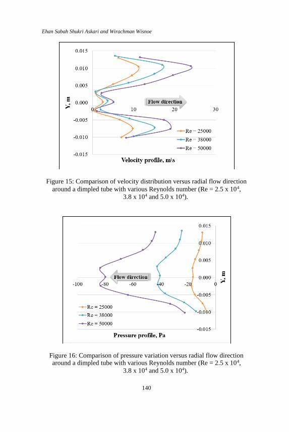
Ehan . Sabah Shukri Askari and Wirachman Wisnoe
140
Figure 15: Comparison of velocity distribution versus radial flow direction
around a dimpled tube with various Reynolds number (Re = 2.5 x 10⁴,
3.8 x 10⁴ and 5.0 x 10⁴).
Figure 16: Comparison of pressure variation versus radial flow direction around a dimpled tube with various Reynolds number (Re = 2.5 x 10⁴,
3.8 x 10⁴ and 5.0 x 10⁴).
Pressure Drop and Flow Characteristics in a diffuser with a dimpled tube
141
Conclusions
In this paper, a numerical analysis was performed to investigate the pressure
drop and flow structure of air flowing around a dimpled . tube in an annular
diffuser. The research is considered the boundary condition as a steady and
incompressible flow. The results were obtained by using different Reynolds
numbers ranging as 25000 <Re< 50000. Based on these assumptions, the
following conclusion is made.
1. The numerical analyses were performed to differ the pressure . drop
around the dimpled . tube. From the comparative analysis of pressure
drop contours versus flow direction, the air pressure decreases with
the increase ... of Reynolds number because of the .increases in the
flow passage area in the diffuser and the pressure losses increases
due to the existence of the dimples that create recirculation and
vortices causes to increase the losses.
2. Velocity simulations are utilized to study the velocity profile
characteristics in a dimpled tube during the turbulent flow. It is
found that the air near the dimples area is mixed with the additional
air that flowing around the dimpled tube and enhances the
distributions of the velocity that means more tangential velocity
components. This fact leads to enhance the flow mixing through the
diffuser area.
3. The recirculation and the tangential velocity component intensity
near the dimples . area increase as the Reynolds. number increase.
4. In the flow direction, it can be noticed that with the .increase. of
Reynolds.. number, the velocity profile decreases.
5. At the outlet, the velocity distribution increases . as the Reynolds..
number increases and the pressure . rate .decreases. with the .increase
of Reynolds.. number. The increase in Reynolds. number disturbs the
flow and creates more swirl flow and recirculation.
References
[1] P. R. Ingole and S. L. Kolhe, “Analysis of coiled-tube heat exchangers to
improve heat transfer rate with spirally corrugated wall,” International
Journal of Modern Engineering Research (IJMER), vol. 4, pp. 196-175,
2014.
[2] S. Naga Sarada, A.V. Sita Rama Raju, K. Kalyani Radha and L. Shyam
Sunder, “Enhancement of heat transfer using varying width twisted tape
inserts,” International Journal of Engineering, Science and Technology,
vol. 2, pp. 107-118, 2007.
Ehan . Sabah Shukri Askari and Wirachman Wisnoe
142
[3] F. A. Saleh, “Computational and experimental investigations on thermal
and fluid flow characteristics for different models of tapes inserts with
TiO2/water nanofluid under turbulent conditions,” International Journal
of Mechanical & Mechatronics Engineering IJMME-IJENS, vol. 18,
pp. 1-14, 2018.
[4] E. S. Shukri and W. Wisnoe, “Temperature distribution enhancement in
a conical diffuser fitted with helical screw-tape with and without
center-rod,” International Journal of Mechanical, Aerospace, Industrial,
Mechatronic and Manufacturing Engineering, vol. 10, pp. 439-444,
2016.
[5] E. S. Shukri, “Numerical comparison of temperature distribution in an
annular diffuser fitted with helical screw-tape hub and pimpled hub,” 4th
International Conference on Power and Energy Systems Engineering,
CPESE 2017, 25-29 September 2017, Berlin, Germany, Procedia
Engineering, vol. 141, pp. 625-629, 2017.
[6] V. Arunprasad, P. Murugesan and S. Jaisankar, “Experimental studies on
natural circulation solar water heating system fitted with helical screw
tape inserts,” Asian Journal of Research in Social Sciences and
Humanities, vol. 6, pp. 1703-1716, 2016.
[7] A. Soni, “Study of thermal performance between plate-fin, pin-fin and
elliptical fin heat sinks in closed enclosure under natural convection,”
International Advanced Research Journal in Science, Engineering and
Technology, ISO 3297:2007 Certified, ISSN 2394-1588, vol. 3, no. 11,
pp. 133-139, 2016.
[8] Y. S. Tomar and M. M. Sahu, “Comparative study of performance of pin
fin under forced convection heat transfer,” International Journal of
Engineering Research & Technology (IJERT), ISSN: 2278 – 0181, vol. 2
no. 9, pp. 364-374, 2013.
[9] R. J. Moitsheki and C. Harley, “Steady thermal analysis of two-
dimensional cylindrical pin fin with a nonconstant base temperature,”
Hindawi Publishing Corporation Mathematical Problems in
Engineering, 2011, Article ID 132457, DOI:10.1155/2011/132457,
2011, pp. 1-17.
[10] F. Sangtarash and H. Shokuhmand, “Experimental and numerical
investigation of the heat transfer augmentation and pressure drop in
simple dimpled and perforated dimpled louver fin banks with an in-line
or staggered arrangement,” Applied Thermal Engineering, vol. 82,
pp. 194-205, 2015.
[11] A. A. Tsynaeva and M. N. Nikitin, “Study of the flow in a channel with
dumbbell-shaped dimples,” International Conference on Industrial
Engineering, ICIE 2016, Procedia Engineering, vol. 150, pp. 2340-2344,
2016.
Pressure Drop and Flow Characteristics in a diffuser with a dimpled tube
143
[12] J. Abraham and R. Maki, “Hydrodynamics of laminar flow through
dimpled pipes,” MOJ Civil Engineering, vol. 4, no. 3, pp. 150-154, 2018.
[13] K. A. Amsha, “Turbulence modelling of the flow and heat transfer in
dimpled channels,” A thesis submitted to The University of Manchester
for the degree of Doctor of Philosophy (Ph.D.) in the Faculty of Science
and Engineering, School of Mechanical, Aerospace and Civil
Engineering, 2017.
[14] S. Shin, K. S. Lee, S. D. Park and J. S. Kwak, “Measurement of the heat
transfer coefficient in the dimpled channel: effects of dimple
arrangement and channel height,” Journal of Mechanical Science and
Technology, vol. 23, pp. 624- 630, 2009.
[15] E. S. Shukri, “Thermal flow analysis for annular diffuser equipped with
pimpled hub,” Journal of Mechanical Engineering, JMechE, vol. 15, no.
1, pp. 115-134, 2018.
[16] J.Sathees Babu, “Analysis of heat transfer and fluid flow characteristics
of concentric tube heat exchanger with dimpled tube,” Journal of Xi'an
University of Architecture & Technology, vol. 13, pp. 508-516, 2020.
[17] E. S. Shukri, “Performance analysis of annulus diffusing area with
divergent dimpled tube,” The 6th International Conference on Power
and Energy Systems Engineering (CPESE 2019), September 20 – 23,
2019, Okinawa, Japan, vol. 6, pp. 11-18, 2020.
[18] W. Zhou, Y. Rao and H. Hu, “An experimental investigation on the
characteristics of turbulent boundary layer flow over a dimpled surface,”
Journal of Fluids Engineering ASME, vol. 138, pp. 021204-1-021204-
13, 2016.
[19] K. Aroonrat and S. Wongwises, “Experimental study on two-phase
condensation heat transfer and pressure drop of R-134a flowing in a
dimpled tube,” International Journal of Heat and Mass Transfer, vol.
106, pp. 437-448, 2017.
[20] S. Xie, Z. Liang, L. Zhang, Y. Wang, H. Ding and J. Zhang, “Numerical
investigation on heat transfer performance and flow characteristics in
enhanced tube with dimples and protrusions,” International Journal of
Heat and Mass Transfer, vol. 122, pp. 602- 613, 2018.
[21] S. Xie, Z. Liang, L. Zhang and Y. Wang, “A numerical study on heat
transfer enhancement and flow structure in enhanced tube with cross
ellipsoidal dimples,” International Journal of Heat and Mass Transfer,
vol. 125, pp. 434- 444, 2018.
[22] S. Wang, W. Du, L. Luo, D. Qiu, X. Zhang and S. Li, “Flow structure
and heat transfer characteristics of a dimpled wedge channel with a bleed
hole in dimple at different orientations and locations,” International
Journal of Heat and Mass Transfer, vol. 117, pp. 1216-1230, 2018.
[23] H. Qu, Z. Shen and Y. Xie, “Numerical investigation of flow and heat
transfer in a dimpled channel among transitional Reynolds numbers,”
Ehan . Sabah Shukri Askari and Wirachman Wisnoe
144
Hindawi Publishing Corporation Mathematical Problems in
Engineering, 2013, pp. 1-10.
[24] Ammar F. Abdulwahid, Hyder H. Balla and Reyadh Ch. Al-Zuhairy,
“Experimental heat transfer enhancement in oval dimpled tube,” Journal
of Mechanical Engineering Research and Developments, ISSN: 1024-
1752, vol. 43, pp. 400-408, 2020.
[25] Y. Eldrainy, J. Jeffrie and M. Ridzwan, “Prediction of the flow inside a
micro gas turbine combustor,” Jurnal Mecchanikal, no. 25, pp. 50–63,
2008.
[26] P. Promvonge, S. Suwannapan, M. Pimsarn and C. Thianpong,
“Experimental study on heat transfer in square duct with combined
twisted-tape and winglet vortex generators,” International
Communications in Heat and Mass Transfer, vol. 59, pp. 158-165, 2014.
[27] E. S. Shukri, B. H. Abdullah, O. M. Ali, “Velocity distribution in an
annular diffuser fitted with twisted hub for different area ratios,” 4th
International Conference on Power and Energy Systems Engineering,
CPESE 2017, 25-29 September 2017, Berlin, Germany, vol. 141,
pp. 639-643, 2018.
[28] B. Djebedjian, M. Giat, J. P. Renaudeaux and M. A Rayan, “Numerical
study of turbulent flow through equiangular annular diffusers,”
Proceeding of Fifth International Conference of Fluid Mechanics, Cairo,
pp.719-729, 1995.
[29] D. Flórez-Orrego, W. Arias, D. López, and H. Velásquez, “Experimental
and CFD study of a single-phase cone-shaped helical coiled heat
exchanger: an empirical correlation,” Proceedings of the 25th
International Conference on Efficiency, Cost, Optimization, Simulation
and Environmental Impact of Energy Systems, pp. 375-394, 2012.
[30] B. B. Arora and B. D. Pathak, “Effect of geometry on the performance of
annular diffuser,” International Journal of Applied Engineering
Research, vol. 4, pp. 2639-2652, 2009.
[31] S. Wang, W. Du, L. Luo, D. Qiu, X. Zhang and S. Li, “Flow structure
and heat transfer characteristics of a dimpled wedge channel with a bleed
hole in dimple at different orientations and locations,” International
Journal of Heat and Mass Transfer, vol. 117, pp. 1216-1230, 2018.
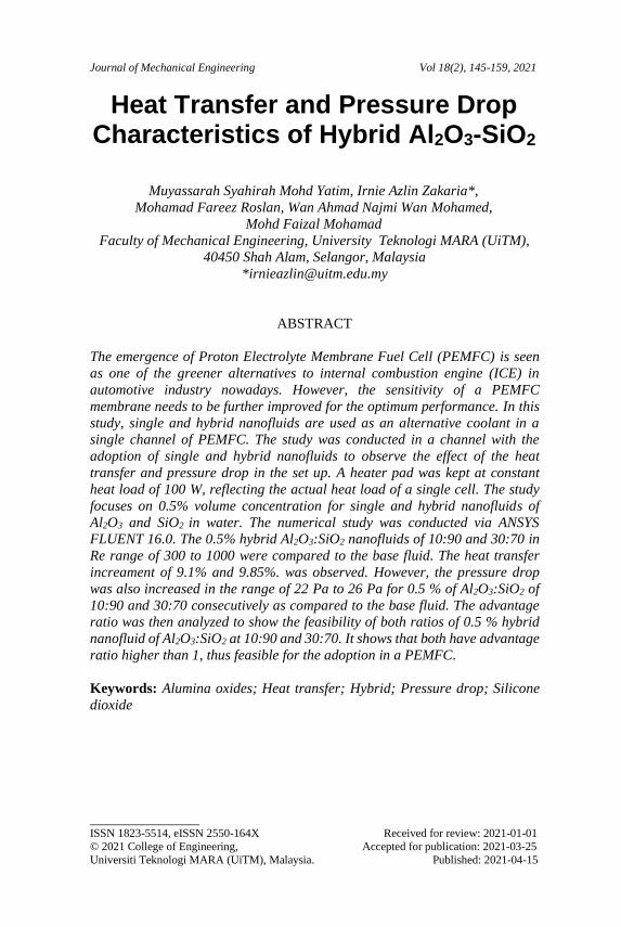
Journal of Mechanical Engineering Vol 18(2), 145-159, 2021
___________________ ISSN 1823-5514, eISSN 2550-164X Received for review: 2021-01-01
© 2021 College of Engineering, Accepted for publication: 2021-03-25
Universiti Teknologi MARA (UiTM), Malaysia. Published: 2021-04-15
Heat Transfer and Pressure Drop Characteristics of Hybrid Al2O3-SiO2
Muyassarah Syahirah Mohd Yatim, Irnie Azlin Zakaria*,
Mohamad Fareez Roslan, Wan Ahmad Najmi Wan Mohamed,
Mohd Faizal Mohamad
Faculty of Mechanical Engineering, University Teknologi MARA (UiTM),
40450 Shah Alam, Selangor, Malaysia
ABSTRACT
The emergence of Proton Electrolyte Membrane Fuel Cell (PEMFC) is seen
as one of the greener alternatives to internal combustion engine (ICE) in
automotive industry nowadays. However, the sensitivity of a PEMFC
membrane needs to be further improved for the optimum performance. In this
study, single and hybrid nanofluids are used as an alternative coolant in a
single channel of PEMFC. The study was conducted in a channel with the
adoption of single and hybrid nanofluids to observe the effect of the heat
transfer and pressure drop in the set up. A heater pad was kept at constant
heat load of 100 W, reflecting the actual heat load of a single cell. The study
focuses on 0.5% volume concentration for single and hybrid nanofluids of
Al2O3 and SiO2 in water. The numerical study was conducted via ANSYS
FLUENT 16.0. The 0.5% hybrid Al2O3:SiO2 nanofluids of 10:90 and 30:70 in
Re range of 300 to 1000 were compared to the base fluid. The heat transfer
increament of 9.1% and 9.85%. was observed. However, the pressure drop
was also increased in the range of 22 Pa to 26 Pa for 0.5 % of Al2O3:SiO2 of
10:90 and 30:70 consecutively as compared to the base fluid. The advantage
ratio was then analyzed to show the feasibility of both ratios of 0.5 % hybrid
nanofluid of Al2O3:SiO2 at 10:90 and 30:70. It shows that both have advantage
ratio higher than 1, thus feasible for the adoption in a PEMFC.
Keywords: Alumina oxides; Heat transfer; Hybrid; Pressure drop; Silicone
dioxide

M S M Yatim et al.
146
Introduction
The Proton-exchange membrane fuel cells (PEMFC) is one of the fuel cells
categories which is favorable for automotive sector. The PEMFC has an
advantage of high-power density, rapid response to change in loads, low
operating temperature of 60 to 80 C and its rapid start up [1]. The effective
cooling is important to ensure that the proton exchange membrane fuel cell
(PEMFC) is safe and operate efficiently, particularly when it comes to the
higher fuel cell stack capacity. However, there are still some issues in the
thermal management of PEMFC adoption which need to be resolved critically
due to the sensitivity of its membrane as one of the vital components in its
operation [2]. Besides the improvement in thermal management, many
researchers nowadays are exploring possibilities to miniaturize the PEMFC
cooling system in order to make it more attractive for commercialization [1].
Among the advancement are optimizing the design of the cooling path, the
flow field and enhancing the heat transfer coefficient of its cooling medium
[2]. The passive way of improving the PEMFC cooling medium property is
through the adoption of nanofluids which seems to be a better way of thermal
management without having to sacrifice the size of the cooling system of fuel
cells [2-3].
Nanofluids is an engineered fluid which comprises of nano sized
particles dispersed in its base fluid [3]. Nanofluids are primarily a dispersion
of both metallic and non-metallic solids which is magnitudes higher in thermal
conductivity as compared to base fluid [4]. Nanofluids is also capable of
increasing the thermal conductivity of its base fluid due to increase in the total
surface area of the nanoparticles [5]. In comparison to distilled water, a
significant heat transfer coefficient improvement of 18 % was achieved
through the nanofluids [6]. However, unlike adoption of nanofluids in other
heat transfer application, PEMFC cooling fluids not only has to be high in
thermal conductivity but at the same time maintaining the strict limit of its
electrical conductivity value of 5 µS/cm [4]. This is required as to avoid shunt
current while operating the stack and also power leakage to the conductive
coolant [7]. There are a lot of heat transfer improvement performed utilizing
different types of nanofluids such as ZnO, TiO2, SiO2 and Al2O3 [8–10].
A lot of research works has been established in the adoption of
nanofluids to PEMFC. Zakaria et al. [11] was among the pioneer in the study
and managed to established a correlation between thermal conductivity and
electrical conductivity of Al2O3 in PEMFC. The study reported that there was
an increment of 12.8 % in thermal conductivity and 14.8 % increment in
electrical conductivity. There are various numerical and experimental works
conducted to justify the feasibility of nanofluids adoption in PEMFC [10-12].
The performance of nanofluids was also studied in both plate and stack level
of PEMFC [12–15]. It was reported that nanofluids has managed to improve
Heat Transfer and Pressure Drop of Hybrid Nanofluids
147
the heat transfer in a 1.5 kWe Ballard PEMFC with almost negligible power
drop with due to higher value in electrical conductivity nanofluids but is still
acceptable with respect to overall stack output [14].
Research in nanofluids has evolved from a single nanofluids to both
hybrid and tri-hybrid nanofluids in which the thermal conductivity was
observed to be further improved [16-17]. Nabil et. al [20] has reported an
increase of 22.8 % in thermal conductivity of TiO2-SiO2 hybrid nanofluids as
compared to the base fluid. Saifudin et. al [5] on the other hand has managed
to establish a performance enhancement ratio termed as PER for Al2O3-SiO2
hybrid nanofluids in both thermal conductivity enhancement over electrical
conductivity and viscosity penalty in PEMFC application. The study reported
that the most feasible Al2O3-SiO2 hybrid nanofluids mixture ratio was 10:90
and 30:70 for PEMFC application.
In this study, the established work of Saifudin et. al [5] is further
investigated numerically. This work complemented the thermo-physical
properties level of the study through the adoption of the Al2O3-SiO2 hybrid
nanofluids in a channel. This study add application value to the thermo-
physical characterization done by Saifudin et. al [5]. The stainless steel channel
was used to simulate a single channel in the PEMFC cooling plate. The channel
was then subjected to a constant heat flux to replicate the heat released during
the reaction in the bipolar plates of PEMFC. Two recommended mixture ratios
as proposed in the previous work was studied which were 10:90 and 30:70
Al2O3-SiO2 hybrid nanofluids in water. The base fluid of water, single
nanofluids of Al2O3 and SiO2 were also simulated as a cooling medium in the
channel. At the end of the study, and advantage ratio was established to justify
the feasibility of the adoption in PEMFC channel.
Methodology
Nanofluid thermo physical properties measurements Thermal conductivity and viscosity of the nanofluid and base fluid used in this
simulation were calculated at 30°C.
The density of nanofluid is calculated by using Equation (1):
𝜌𝑛𝑓 = (1 − 𝜙)𝜌𝑓 + 𝜙𝜌𝑝 (1)
The density of hybrid nanofluid is calculated by using Equation (2):
𝜌𝑛𝑓 = (1 − 𝜙)𝜌𝑓 + 𝜙𝜌𝑝1 + 𝜙𝜌𝑝2 (2)
The specific heat of nanofluid is calculated by using Equation (3):
M S M Yatim et al.
148
𝐶𝑝,𝑛𝑓 =(1−𝜙)𝜌𝑓𝐶𝑓+𝜙𝜌𝑝𝐶𝑝
𝜌𝑛𝑓 (3)
The specific heat of hybrid nanofluid is calculated by using Equation (4):
𝐶𝑝,ℎ𝑛𝑓 =(1−𝜙)𝜌𝑓𝐶𝑓+𝜙𝑝1𝜌𝑝1𝐶𝑝1+𝜙𝑝2𝜌𝑝2𝐶𝑝2
𝜌ℎ𝑛𝑓 (4)
Where 𝜙 was alluded as the proportion of particles by volume and the
addendums f, p1, p2, bf and hnf were alluded as base liquid (water), Al2O3 and
SiO2 nanofluids and mixture nanofluid. Table 1 lists the nanofluid properties
that were measured and determined.
Table 1: Nanofluid and base fluid properties used in numerical analysis
Fluid
Name
Thermal
Conductivity,K
(W/mk)
Specific
Heat,Cp
(J/kg.k)
Viscosity,μ
(Pa.s)
Density,ρ
(kg/m3) References
Al2O3
0.5%
conc.
36 765 - 4000 [11]
SiO2
0.5%
conc.
1.4 745 - 2220 [12]
Water 0.615 4180 0.000854 999 [11]
PEMFC channel mathematical model A 3D Computational Fluid Dynamic (CFD) was established on the basis of a
channel dimension as shown in Figure 1. As for the channel, the material used
is stainless steel to imitate the channel of PEMFC. The dimension of channel
is 20 mm x 10 mm x 380 mm. A consistent heat source of 100 W was
implemented to the channel. There have only been a few assumptions [21]:
i. Incompressible, laminar and steady state flow.
ii. Body force effect is neglected.
iii. Viscous dissipation is neglected.
iv. With a relative velocity of zero, the fluid and nanoparticles are thermally
balanced.
Heat Transfer and Pressure Drop of Hybrid Nanofluids
149
For computing in modelling, the channel has the same heat transfer and fluid
flow characteristics.
Figure 1: The schematic diagram of channel in PEMFC.
The following are the governing equations for the assumptions:
Equation for continuity:
𝛻. (𝜌𝑛𝑓 . 𝑉𝑚) = 0 (5)
Equation for momentum:
𝛻. (𝜌𝑛𝑓 . 𝑉𝑚 . 𝑉𝑀) = −𝛻𝑃 + 𝛻(µ𝑛𝑓 . 𝛻𝑉𝑚 (6)
Coolant energy equation:
𝛻. (𝜌𝑛𝑓 . 𝐶. 𝑉𝑚. 𝑇) = 𝛻. (𝑘𝑛𝑓 . 𝛻𝑇) (7)
Conduction of heat through a solid wall:
0 = 𝛻. (𝑘𝑠. 𝛻𝑇𝑠) (8)
At the wall, there is a no-slip boundary:
�⃗� = 0 (Walls) (9)
The following boundary conditions were assumed at the channel inlet:
�⃗� = 𝑉𝑚 (𝑖𝑛𝑙𝑒𝑡) (10)
𝑃 = 𝑎𝑡𝑚𝑜𝑠𝑝ℎ𝑒𝑟𝑖𝑐 𝑝𝑟𝑒𝑠𝑠𝑢𝑟𝑒 (𝑜𝑢𝑡𝑙𝑒𝑡) (11)

M S M Yatim et al.
150
Heat is transmitted through the solid and distributed through the channel by
forced convection of cooling liquid.
−𝑘𝑛𝑓 . 𝛻𝑇 = 𝑞 (Bottom of channel) (12)
−𝑘𝑛𝑓 . 𝛻𝑇 = 0 (Top of channel) (13)
The analysis of heat transfer and fluid flow Using this equation, heat transfer coefficient can be determined (14):
ℎ =𝑞
𝛥𝑇 (14)
The Nusselt number can be calculated by using this Equation (15):
𝑁𝑢 =ℎ𝑙
𝑘 (15)
The pressure drop can be calculated by using this Equation (16):
𝛥𝑃 = 𝑃𝑖 − 𝑃𝑜 (16)
The pumping power can be calculated by using this Equation (17):
𝑊𝑝 = �̇�. 𝛥𝑃 (17)
The advantage ratio can be calculated by using this Equation (18):
𝐴𝑅 =ℎ
𝛥𝑃 (18)
Results and Discussion Validation of the study Prior to analysing the heat transfer and pressure drop effect of hybrid
nanofluids, the simulation was first validated to ensure its accuracy against
experimental data. The simulation data shows an acceptable accuracy value
which was in the range of 2.47 % 2.82 % as shown in Figure 2. The small
deviation shows that the simulation was reliable and further analysis then can
be carried out.
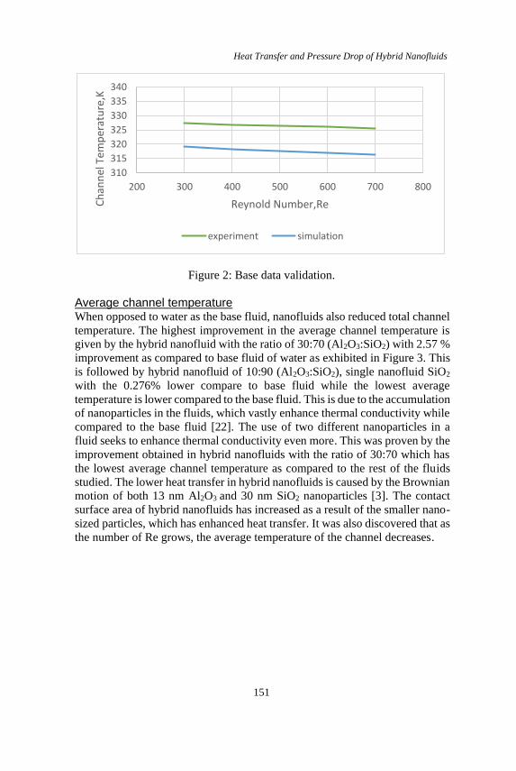
Heat Transfer and Pressure Drop of Hybrid Nanofluids
151
Figure 2: Base data validation.
Average channel temperature When opposed to water as the base fluid, nanofluids also reduced total channel
temperature. The highest improvement in the average channel temperature is
given by the hybrid nanofluid with the ratio of 30:70 (Al2O3:SiO2) with 2.57 %
improvement as compared to base fluid of water as exhibited in Figure 3. This
is followed by hybrid nanofluid of 10:90 (Al2O3:SiO2), single nanofluid SiO2
with the 0.276% lower compare to base fluid while the lowest average
temperature is lower compared to the base fluid. This is due to the accumulation
of nanoparticles in the fluids, which vastly enhance thermal conductivity while
compared to the base fluid [22]. The use of two different nanoparticles in a
fluid seeks to enhance thermal conductivity even more. This was proven by the
improvement obtained in hybrid nanofluids with the ratio of 30:70 which has
the lowest average channel temperature as compared to the rest of the fluids
studied. The lower heat transfer in hybrid nanofluids is caused by the Brownian
motion of both 13 nm Al2O3 and 30 nm SiO2 nanoparticles [3]. The contact
surface area of hybrid nanofluids has increased as a result of the smaller nano-
sized particles, which has enhanced heat transfer. It was also discovered that as
the number of Re grows, the average temperature of the channel decreases.
310
315
320
325
330
335
340
200 300 400 500 600 700 800
Ch
ann
el T
emp
erat
ure
,K
Reynold Number,Re
experiment simulation

M S M Yatim et al.
152
Figure 3: Average channel temperature with the adoption of nanofluids.
Heat transfer coefficient effect The channel temperature was then converted to a heat transfer coefficient to
determine a moving fluid's convective heat transfer ability. The higher
convective heat transfer will give better heat transfer result. The highest heat
transfer coefficient at Re 1000 is shown in Figure 4, was given by 0.5% of
hybrid 30:70 Al2O3:SiO2 nanofluid with 9.851% higher than the base fluid. As
the ratio of nanofluids changed and Reynold number increased for all hybrid
Al2O3:SiO2 nanofluids, the heat transfer coefficient also increases. The
addition of two nanofluids between Al2O3 and SiO2 has enhanced
thermophysical properties such thermal conductivity, specific heat capacity
and others [6].
40
41
42
43
44
45
46
47
0 500 1000 1500
Ch
ann
el T
emp
erat
ure
,(K
)
Reynold Number, Re
water
Al₂O₃
SiO₂
10:90(Al₂O₃:SiO₂)
30:70(Al₂O₃:SiO₂)
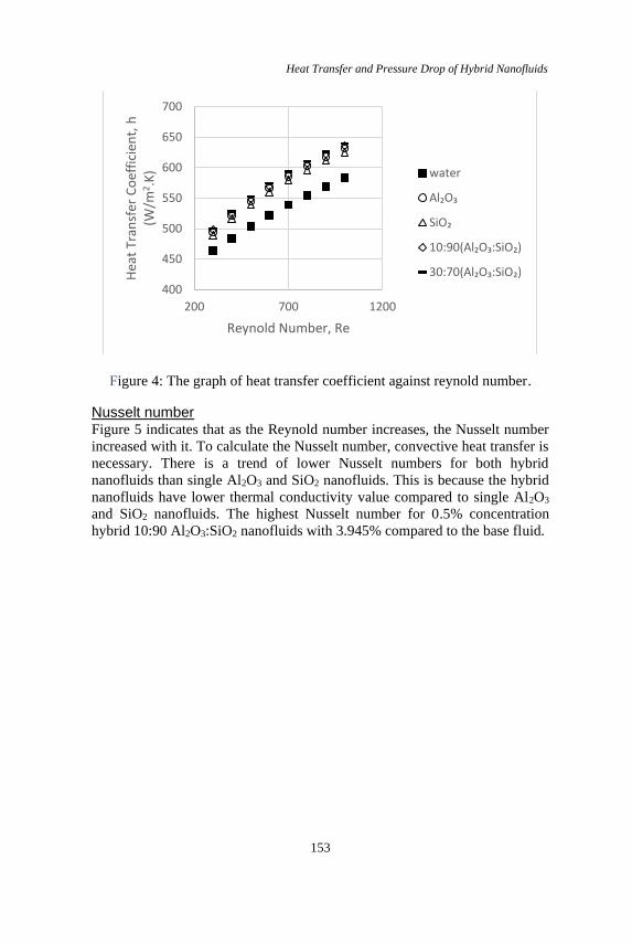
Heat Transfer and Pressure Drop of Hybrid Nanofluids
153
Figure 4: The graph of heat transfer coefficient against reynold number.
Nusselt number Figure 5 indicates that as the Reynold number increases, the Nusselt number
increased with it. To calculate the Nusselt number, convective heat transfer is
necessary. There is a trend of lower Nusselt numbers for both hybrid
nanofluids than single Al2O3 and SiO2 nanofluids. This is because the hybrid
nanofluids have lower thermal conductivity value compared to single Al2O3
and SiO2 nanofluids. The highest Nusselt number for 0.5% concentration
hybrid 10:90 Al2O3:SiO2 nanofluids with 3.945% compared to the base fluid.
400
450
500
550
600
650
700
200 700 1200
Hea
t Tr
ansf
er C
oef
fici
ent,
h
(W/m
2 .K
)
Reynold Number, Re
water
Al₂O₃
SiO₂
10:90(Al₂O₃:SiO₂)
30:70(Al₂O₃:SiO₂)
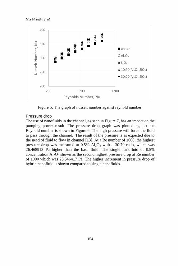
M S M Yatim et al.
154
Figure 5: The graph of nusselt number against reynold number.
Pressure drop The use of nanofluids in the channel, as seen in Figure 7, has an impact on the
pumping power result. The pressure drop graph was plotted against the
Reynold number is shown in Figure 6. The high-pressure will force the fluid
to pass through the channel. The result of the pressure is as expected due to
the need of fluid to flow in channel [13]. At a Re number of 1000, the highest
pressure drop was measured at 0.5% Al2O3 with a 30:70 ratio, which was
26.468913 Pa higher than the base fluid. The single nanofluid of 0.5%
concentration Al2O3 shown as the second highest pressure drop at Re number
of 1000 which was 25.546417 Pa. The higher increment in pressure drop of
hybrid nanofluid is shown compared to single nanofluids.
200
250
300
350
400
200 700 1200
Nu
ssel
t N
um
ber
, Nu
Reynolds Number, Nu
water
Al₂O₃
SiO₂
10:90(Al₂O₃:SiO₂)
30:70(Al₂O₃:SiO₂)
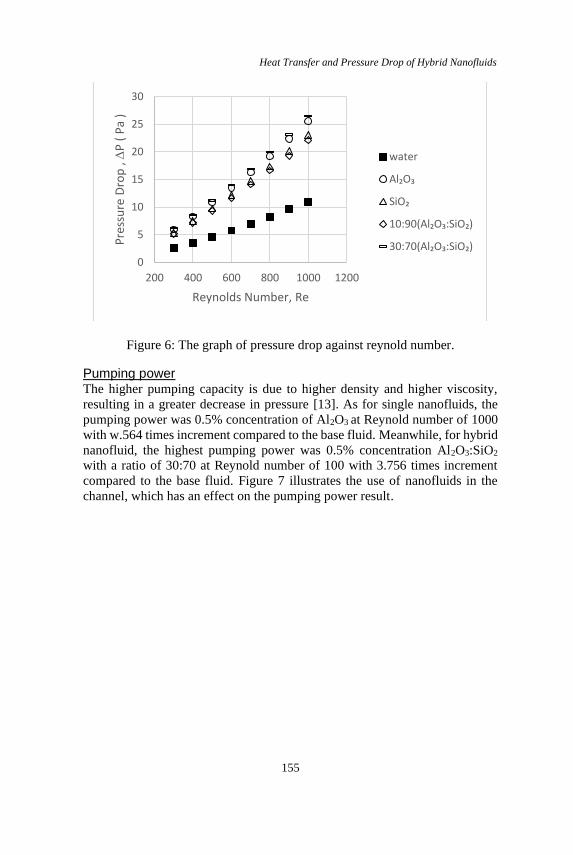
Heat Transfer and Pressure Drop of Hybrid Nanofluids
155
Figure 6: The graph of pressure drop against reynold number.
Pumping power The higher pumping capacity is due to higher density and higher viscosity,
resulting in a greater decrease in pressure [13]. As for single nanofluids, the
pumping power was 0.5% concentration of Al2O3 at Reynold number of 1000
with w.564 times increment compared to the base fluid. Meanwhile, for hybrid
nanofluid, the highest pumping power was 0.5% concentration Al2O3:SiO2
with a ratio of 30:70 at Reynold number of 100 with 3.756 times increment
compared to the base fluid. Figure 7 illustrates the use of nanofluids in the
channel, which has an effect on the pumping power result.
0
5
10
15
20
25
30
200 400 600 800 1000 1200
Pre
ssu
re D
rop
,
P (
Pa
)
Reynolds Number, Re
water
Al₂O₃
SiO₂
10:90(Al₂O₃:SiO₂)
30:70(Al₂O₃:SiO₂)
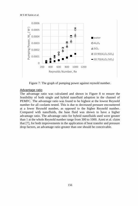
M S M Yatim et al.
156
Figure 7: The graph of pumping power against reynold number.
Advantage ratio The advantage ratio was calculated and shown in Figure 8 to ensure the
feasibility of both single and hybrid nanofluid adoption in the channel of
PEMFC. The advantage ratio was found to be highest at the lowest Reynold
number for all coolants tested. This is due to decreased pressure encountered
at a lower Reynold number, as opposed to the higher Reynold number.
Compared with nanofluids, the base fluid was shown to have a higher
advantage ratio. The advantage ratio for hybrid nanofluids used were greater
than 1 at the whole Reynold number range from 300 to 1000. Azmi et al. claim
that [7], for both improvements in the application of heat transfer and pressure
drop factors, an advantage ratio greater than one should be conceivable.
0
0.0001
0.0002
0.0003
0.0004
0.0005
0.0006
200 400 600 800 1000 1200
Pu
mp
ing
Po
wer
, Wp
( W
)
Reynolds Number, Re
water
Al₂O₃
SiO₂
10:90(Al₂O₃:SiO₂)
30:70(Al₂O₃:SiO₂)
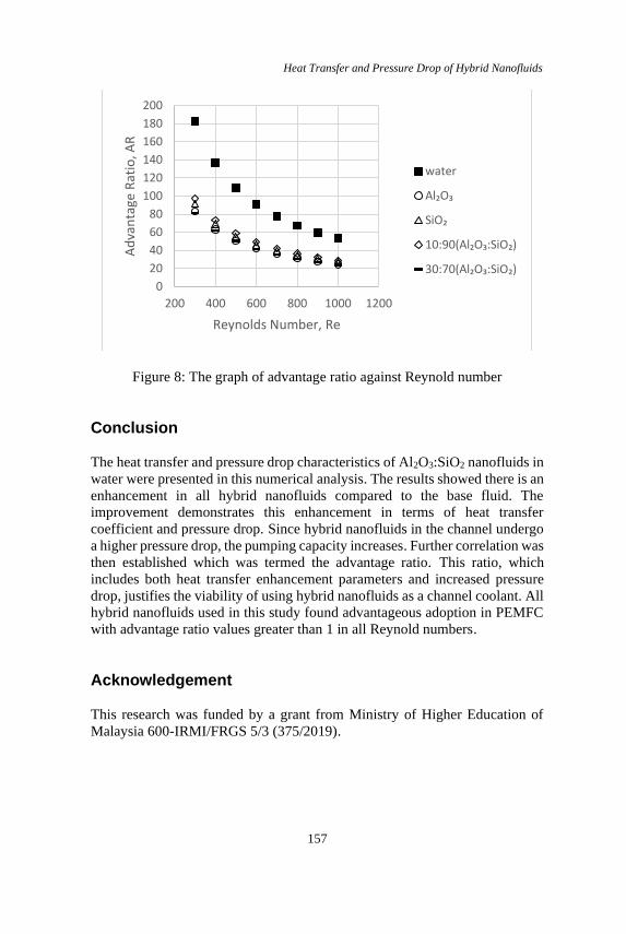
Heat Transfer and Pressure Drop of Hybrid Nanofluids
157
Figure 8: The graph of advantage ratio against Reynold number
Conclusion
The heat transfer and pressure drop characteristics of Al2O3:SiO2 nanofluids in
water were presented in this numerical analysis. The results showed there is an
enhancement in all hybrid nanofluids compared to the base fluid. The
improvement demonstrates this enhancement in terms of heat transfer
coefficient and pressure drop. Since hybrid nanofluids in the channel undergo
a higher pressure drop, the pumping capacity increases. Further correlation was
then established which was termed the advantage ratio. This ratio, which
includes both heat transfer enhancement parameters and increased pressure
drop, justifies the viability of using hybrid nanofluids as a channel coolant. All
hybrid nanofluids used in this study found advantageous adoption in PEMFC
with advantage ratio values greater than 1 in all Reynold numbers.
Acknowledgement
This research was funded by a grant from Ministry of Higher Education of
Malaysia 600-IRMI/FRGS 5/3 (375/2019).
0
20
40
60
80
100
120
140
160
180
200
200 400 600 800 1000 1200
Ad
van
tage
Rat
io, A
R
Reynolds Number, Re
water
Al₂O₃
SiO₂
10:90(Al₂O₃:SiO₂)
30:70(Al₂O₃:SiO₂)
M S M Yatim et al.
158
References
[1] H. Tamura and M. Matsumoto, “Fuel Cell Vehicles: Technology
Development Status and Popularization Issues,” Converg. Int. Congr.
Expo. Transp. Electron., no. 2002-21–0036, pp. 1-8, 2002.
[2] M. Imazeki and T. Ushio, “Cooling system for fuel cell,” ed Google
Patents, 2004.
[3] U. C. and T. Tran, “Experimental studies of the effects of non-Newtonian
surfactant solutions on the performance of a shell-and-tube heat
exchanger,” in American Society of Mechanical Engineers, Fluids
Engineering Division (Publication), pp. 47–52, 1991
[4] E. D. P. McMullen, S. Mohapatra, “Advances in PEM Fuel Cell Nano-
Coolant,” in Fuel Cell Seminar & Energy Exposition, pp. 344, 2013
[5] S. Khalid, I. Zakaria, W. H. Azmi, and W. A. N. W. Mohamed, “Thermal–
electrical–hydraulic properties of Al2O3–SiO2 hybrid nanofluids for
advanced PEM fuel cell thermal management,” J. Therm. Anal. Calorim.,
2020.
[6] M. R. Sohel, S. S. Khaleduzzaman, R. Saidur, A. Hepbasli, M. F. M. Sabri,
and I. M. Mahbubul, “An experimental investigation of heat transfer
enhancement of a minichannel heat sink using Al2O3-H2O nanofluid,”
Int. J. Heat Mass Transf., vol. 74, pp. 164–172, 2014.
[7] H.Egawa, “Fuel Cell Coolant,” US 8187763B2, May 29, 2012.
[8] A. Abdollahi, H. A. Mohammed, S. M. Vanaki, A. Osia, and M. R.
Golbahar Haghighi, “Fluid flow and heat transfer of nanofluids in
microchannel heat sink with V-type inlet/outlet arrangement,” Alexandria
Eng. J., vol. 56, no. 1, pp. 161–170, 2017.
[9] R. Islam and B. Shabani, “Prediction of electrical conductivity of TiO2
water and ethylene glycol-based nanofluids for cooling application in low
temperature PEM fuel cells,” Energy Procedia, vol. 160, no. 2018, pp.
550–557, 2019.
[10] N. M. Muhammad, N. A. C. Sidik, A. Saat, and B. Abdullahi, “Effect of
nanofluids on heat transfer and pressure drop characteristics of diverging-
converging minichannel heat sink,” CFD Lett., vol. 11, no. 4, pp. 105–
120, 2019.
[11] I. Zakaria, W. H. Azmi, W. A. N. W. Mohamed, R. Mamat, and G. Najafi,
“Experimental Investigation of Thermal Conductivity and Electrical
Conductivity of Al2O3 Nanofluid in Water - Ethylene Glycol Mixture for
Proton Exchange Membrane Fuel Cell Application,” Int. Commun. Heat
Mass Transf., vol. 61, pp. 61–68, 2015.
[12] I. Zakaria et al., “Thermal analysis of Al2O3-water ethylene glycol
mixture nanofluid for single PEM fuel cell cooling plate: An experimental
study,” Int. J. Hydrogen Energy, vol. 41, no. 9, pp. 5096–5112, 2016.
[13] I. A. Zakaria, W. A. N. W. Mohamed, A. M. I. Mamat, K. I. Sainan, and
Heat Transfer and Pressure Drop of Hybrid Nanofluids
159
S. F. A. Talib, “Thermal performance of Al2O3 in water - Ethylene glycol
nanofluid mixture as cooling medium in mini channel,” AIP Conf. Proc.,
vol. 1674, 2015.
[14] I. Zakaria, W. A. N. W. Mohamed, W. H. Azmi, A. M. I. Mamat, R.
Mamat, and W. R. W. Daud, “Thermo-electrical performance of PEM fuel
cell using Al2O3 nanofluids,” Int. J. Heat Mass Transf., vol. 119, pp. 460–
471, 2018.
[15] I. A. Zakaria, W. A. N. W. Mohamed, M. B. Zailan, and W. H. Azmi,
“Experimental analysis of SiO2-Distilled water nanofluids in a Polymer
Electrolyte Membrane fuel cell parallel channel cooling plate,” Int. J.
Hydrogen Energy, vol. 44, no. 47, pp. 25850–25862, 2019.
[16] R. Islam, B. Shabani, J. Andrews, and G. Rosengarten, “Experimental
investigation of using ZnO nanofluids as coolants in a PEM fuel cell,” Int.
J. Hydrogen Energy, vol. 42, no. 30, pp. 19272–19286, 2017.
[17] W. A. N. W. Mohamed, S. F. A. Talib, I. A. Zakaria, A. M. I. Mamat, and
W. R. W. Daud, “Effect of dynamic load on the temperature profiles and
cooling response time of a proton exchange membrane fuel cell,” J.
Energy Inst., vol. 91, no. 3, pp. 349–357, 2018.
[18] A. I. Ramadhan, W. H. Azmi, R. Mamat, K. A. Hamid, and S. Norsakinah,
“Investigation on stability of tri-hybrid nanofluids in water-ethylene
glycol mixture,” IOP Conf. Ser. Mater. Sci. Eng., vol. 469, no. 1, 2019.
[19] S. Salman, A. R. A. Talib, S. Saadon, and M. T. H. Sultan, “Hybrid
nanofluid flow and heat transfer over backward and forward steps: A
review,” Powder Technol., vol. 363, pp. 448–472, 2020.
[20] M. F. Nabil, W. H. Azmi, K. A. Hamid, N. N. M. Zawawi, G. Priyandoko,
and R. Mamat, “Thermo-physical properties of hybrid nanofluids and
hybrid nanolubricants: A comprehensive review on performance,” Int.
Commun. Heat Mass Transf., vol. 83, pp. 30–39, 2017.
[21] I. A. Zakaria, W. A. N. W. Mohamed, A. M. I. Mamat, K. I. Sainan, M.
R. M. Nawi, and G. H. Najafi, “Numerical analysis of Al2O3 nanofluids
in serpentine cooling plate of PEM fuel cell,” J. Mech. Eng., vol. 5, no.
Special issue1, pp. 1–13, 2018.
[22]K. S. Arjun and K. Rakesh, “Heat transfer enhancement using alumina
nanofluid in circular micro channel,” J. Eng. Sci. Technol., vol. 12, no. 1,
pp. 265–279, 2017.
Journal of Mechanical Engineering Vol 18(2), 161-176, 2021
__________________ ISSN 1823-5514, eISSN 2550-164X Received for review: 2020-03-18
© 2021 College of Engineering, Accepted for publication: 2021-02-26
Universiti Teknologi MARA (UiTM), Malaysia. Published: 2021-04-15
Optimization of Machining Parameters using Taguchi Coupled
Grey Relational Approach while Turning Inconel 625
Chinmaya Padhy*, Pariniti Singh
Center for Manufacturing Excellence, Dept. of Mechanical Engineering,
School of Technology, GITAM University,
Hyderabad, 502329, India.
ABSTRACT
In manufacturing industries preparation of quality surfaces is very important.
The surface roughness will influence the quality and effectiveness of the
subsequent coatings for protection against corrosion, wear resistance etc. For
achieving desired surface roughness, factors like cutting force (N) and
material removal rate (mm3/sec) plays an important role towards final product
optimization. This study helps to determine the contribution of each machining
parameters [cutting speed (v), feed rate (f) and depth-of-cut (d)] and their
interaction to investigate their optimum values during dry turning of Inconel
625 with the objective of enhancing the productivity (optimum production) by
minimizing surface roughness (Ra), cutting forces (Fc), whereas maximizing
material removal rate (MRR). This kind of multi response process variable
(MRP) problems usually known as multi-objective optimizations (MOOs) are
resolved with the help of Taguchi and Grey relation approach (T-GRA). As a
result, the attained optimum cutting parameters are viz. cutting speed (60
m/min), feed rate (0.3 mm/rev), depth-of-cut (0.25 mm) lead to value of desired
variables - cutting forces (340 N), surface roughness (0.998 μm) and material
removal rate (0.786 mm3/min).
Keywords: Cutting force; Cutting parameters; Dry turning; Material removal
rate; Minitab 17; Optimization; Surface roughness
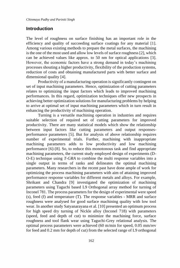
Chinmaya Padhy and Pariniti Singh
162
Introduction
The level of roughness on surface finishing has an important role in the
efficiency and quality of succeeding surface coatings for any material [1].
Among various existing methods to prepare the metal surfaces, the machining
is the one of the most used and allow low levels of surface roughness [2], which
can be achieved values like approx. to 50 nm for optical applications [3].
However, the economic factors have a strong demand in today’s machining
processes shouting a higher productivity, flexibility of the production systems,
reduction of costs and obtaining manufactured parts with better surface and
dimensional quality [4].
Productivity of a manufacturing operation is significantly contingent on
set of input machining parameters. Hence, optimization of cutting parameters
relates to optimizing the input factors which leads to improved machining
performances. In this regard, optimization techniques offer new prospects in
achieving better optimization solutions for manufacturing problems by helping
to arrive at optimal set of input machining parameters which in turn result in
enhancing the productivity of machining operation.
Turning is a versatile machining operation in industries and requires
suitable selection of required set of cutting parameters for improved
productivity. There are many statistical models which show the relationship
between input factors like cutting parameters and output responses-
performance parameters [5]. But for analysis of above relationship requires
number of experimental trials. Further, machining with inappropriate
machining parameters adds to low productivity and low machining
performance [6]-[8]. So, to reduce this monotonous task and find appropriate
machining parameters, the current study employed design of experiments (D-
O-E) technique using T-GRA to combine the multi response variables into a
single output in terms of ranks and delineates the optimal machining
parameters. Many researchers in the recent past have done ample of work for
optimizing the process machining parameters with aim of attaining improved
performance response variables for different metals and alloys. For example,
Shrikant and Chandra [9] investigated the optimization of machining
parameters using Taguchi based L9 Orthogonal array method for turning of
Inconel 781. The process parameters for the design of experimental were speed
(s), feed (f) and temperature (T). The response variables - MRR and surface
roughness were analysed for good surface machining quality with low tool
wear. In another study Satyanarayana et al. [10] presented an optimum process
for high speed dry turning of Nickle alloy (Inconel 718) with parameters
(speed, feed and depth of cut) to minimize the machining force, surface
roughness and tool flank wear using Taguchi-Grey relational analysis. The
optimal process parameters were achieved (60 m/min for speed, 0.05 mm/rev
for feed and 0.2 mm for depth of cut) from the selected range of L9 orthogonal
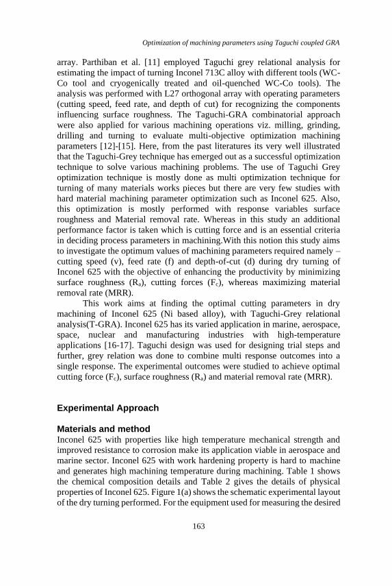
Optimization of machining parameters using Taguchi coupled GRA
163
array. Parthiban et al. [11] employed Taguchi grey relational analysis for
estimating the impact of turning Inconel 713C alloy with different tools (WC-
Co tool and cryogenically treated and oil-quenched WC-Co tools). The
analysis was performed with L27 orthogonal array with operating parameters
(cutting speed, feed rate, and depth of cut) for recognizing the components
influencing surface roughness. The Taguchi-GRA combinatorial approach
were also applied for various machining operations viz. milling, grinding,
drilling and turning to evaluate multi-objective optimization machining
parameters [12]-[15]. Here, from the past literatures its very well illustrated
that the Taguchi-Grey technique has emerged out as a successful optimization
technique to solve various machining problems. The use of Taguchi Grey
optimization technique is mostly done as multi optimization technique for
turning of many materials works pieces but there are very few studies with
hard material machining parameter optimization such as Inconel 625. Also,
this optimization is mostly performed with response variables surface
roughness and Material removal rate. Whereas in this study an additional
performance factor is taken which is cutting force and is an essential criteria
in deciding process parameters in machining.With this notion this study aims
to investigate the optimum values of machining parameters required namely –
cutting speed (v), feed rate (f) and depth-of-cut (d) during dry turning of
Inconel 625 with the objective of enhancing the productivity by minimizing
surface roughness (Ra), cutting forces (Fc), whereas maximizing material
removal rate (MRR).
This work aims at finding the optimal cutting parameters in dry
machining of Inconel 625 (Ni based alloy), with Taguchi-Grey relational
analysis(T-GRA). Inconel 625 has its varied application in marine, aerospace,
space, nuclear and manufacturing industries with high-temperature
applications [16-17]. Taguchi design was used for designing trial steps and
further, grey relation was done to combine multi response outcomes into a
single response. The experimental outcomes were studied to achieve optimal
cutting force (Fc), surface roughness (Ra) and material removal rate (MRR).
Experimental Approach
Materials and method Inconel 625 with properties like high temperature mechanical strength and
improved resistance to corrosion make its application viable in aerospace and
marine sector. Inconel 625 with work hardening property is hard to machine
and generates high machining temperature during machining. Table 1 shows
the chemical composition details and Table 2 gives the details of physical
properties of Inconel 625. Figure 1(a) shows the schematic experimental layout
of the dry turning performed. For the equipment used for measuring the desired

Chinmaya Padhy and Pariniti Singh
164
output variables, i.e. measuring material removal rate (MRR)- weight scale
device is used, refer Figure 1(b). For measuring surface roughness-Mitutoyo
surface roughness tester is used, refer Figure 2(a) and for measurement of
cutting forces-lathe tool dynamometer is used, refer Figure 2(b).
Table 1: Chemical Composition (wt %) of Inconel 625 [18]
C Mn S Si Cr Fe Mo Co-
Ta Ti Al P
Ni
.05 .30 .003 .25 20-
23
4 9 3.5 .30 .30 .15 Balance
Table 2: Physical Properties of Inconel 625 [18]
Alloy Density Melting Point Tensile
Strength
Brinell
Hardness
Inconel
625
8.4 g/cm3
1290 – 1350 0C
760
N/mm2
240 HB
The experiment was conducted on Inconel 625 work piece of
dimensions [diameter (Ø)-40 mm, length (L)-350 mm], purchased from
Mishra Dhatu Nigam Ltd., on NAGMATI 175 model lathe with maximum
cutting speed 1200 rpm, 3HP motor, along with Korloy insert -model: PC9030
carbide tool inserts, designation: CCMT09T308.
The study optimizes the machining parameters- speed (v), feed (f) and
depth-of-cut (d) with T-GRA. Each parameter has three levels – namely low,
medium and high, respectively. According to the Taguchi method, if three
parameters and 3 levels for each parameters L9 orthogonal array should be
employed for the experimentation. The optimization parameters are designed
for maximizing MRR and for minimizing the surface roughness and cutting
forces. Figure 3 shows procedural steps used to follow for T-GRA [19]. The
selected levels of machining parameters and attained experimental test results
for corresponding set of arrays are tabulated in Table 3 and Table 4
respectively.
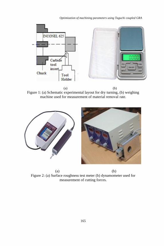
Optimization of machining parameters using Taguchi coupled GRA
165
(a) (b)
Figure 1: (a) Schematic experimental layout for dry turning, (b) weighing
machine used for measurement of material removal rate.
(a) (b)
Figure 2: (a) Surface roughness test meter (b) dynamometer used for
measurement of cutting forces.

Chinmaya Padhy and Pariniti Singh
166
Figure 3: Flow chart of Taguchi-Grey relation method [19].
Multiple Objective Optimization-
Taguchi-Grey Method
Determine and select the process control factors and
response variables
Select an appropriate orthogonal experiment array
(OA)
Calculate the average of process response variables
Conduct of experiments to obtain multi-responses
Normalization of the multi response sequence
Calculation of GRC/ GRG (Grey Relation
Coefficient and Grey Gelation Grade)
Prediction of optimal response variable
Validation of
results
No
Yes
Result accepted
Taguchi
Technique
Grey Relation
Approach
Stop
Start

Optimization of machining parameters using Taguchi coupled GRA
167
Table 3: Input parameters with Taguchi design
Machining Parameters Levels of Parameters
1 (low) 2 (medium) 3 (high)
Cutting speed (v) m/min 42 60 108
Feed rate (f) mm/rev 0.1 0.2 0.3
Depth-of-cut (d) mm 0.25 0.5 0.75
Evaluation of optimal cutting parameters
Taguchi and Grey relational analysis (T-GRA) Taguchi design of experiments is a process of optimization which deals with
eight steps of planning, conducting and evaluating matrix experiments to
determine the best level of control factors. Wheras, Taguchi robust design
finds the appropriate control factor levels to give a robust experimental design
approach. There are many factors which affect the performance parameters
among which few can be controlled and are called control factors and rest are
impossible control and are called “noise factors”. This experimental approach
leads to the development of designs with enhanced quality and shorter design
and cost. They allow to understand and provide the interaction of factors
affecting the output parameters. Taguchi analysis uses orthogonal array (OA)
of experiments that give set of appropriate number of experimental trials.
Taguchi design gives well defined standard orthogonal arrays which are made
for a precise level of independent designs. These orthogonal arrays reduce the
number of trial experiments. In current study the machining parameters- speed
(v), feed (f) and depth-of-cut (d), each parameter has three levels – namely
low, medium and high, respectively. According to the Taguchi method, if three
parameters and 3 levels for each parameters L9 orthogonal array should be
employed for the experimentation. Further, on coupling with Grey relation a
multi response optimization gets converted into a single response optimizing
problem. S/N (signal to noise ratio) for each machining parameter level is
evaluated for each performance function and the highest S/N ratio indicates an
optimal level of machining. Multi response is associated with more than one
performance criteria/responses (surface roughness, material removal rate, tool
wear, cutting forces) simultaneously. These responses follow either larger the
better equations such as for material removal rate, or for some characteristics
are required to be less and are followed as smaller the better. Figure 4 shows
detailed experimental stages for T-GRA used during this study [20].
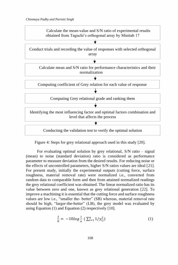
Chinmaya Padhy and Pariniti Singh
168
Figure 4: Steps for grey relational approach used in this study [20].
For evaluating optimal solution by grey relational, S/N ratio – signal
(mean) to noise (standard deviation) ratio is considered as performance
parameter to measure deviation from the desired results. For reducing noise or
the effects of uncontrolled parameters, higher S/N ratios values are ideal [21].
For present study, initially the experimental outputs (cutting force, surface
roughness, material removal rate) were normalized i.e., converted from
random data to comparable form and then from attained normalized readings
the grey relational coefficient was obtained. The linear normalized ratio has its
value between zero and one, known as grey relational generation [22]. To
improve a machining it is essential that the cutting force and surface roughness
values are low i.e., “smaller the- better” (SB) whereas, material removal rate
should be high, “larger-the-better” (LB), the grey model was evaluated by
using Equation (1) and Equation (2) respectively [10].
𝑆
𝑁= −10𝑙𝑜𝑔
1
𝑛 ( ∑ 1/𝑦𝑖𝑗
2𝑛𝑖=1 ) (1)
Conduct trials and recording the value of responses with selected orthogonal
array
Calculate mean and S/N ratio for performance characteristics and their
normalization
Computing coefficient of Grey relation for each value of response
Computing Grey relational grade and ranking them
Identifying the most influencing factor and optimal factors combination and
level that affects the process
Conducting the validation test to verify the optimal solution
Calculate the mean-value and S/N ratio of experimental results
obtained from Taguchi’s orthogonal array by Minitab 17
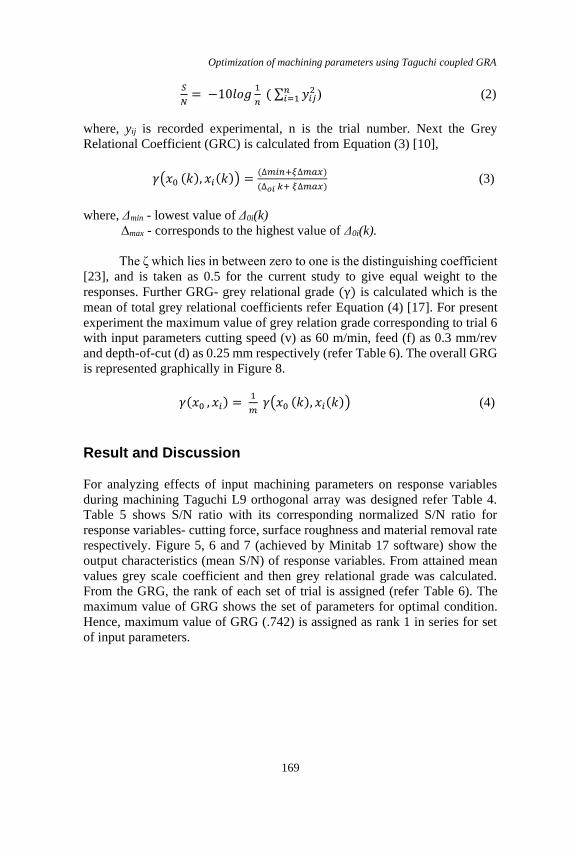
Optimization of machining parameters using Taguchi coupled GRA
169
𝑆
𝑁= −10𝑙𝑜𝑔
1
𝑛 ( ∑ 𝑦𝑖𝑗
2𝑛𝑖=1 ) (2)
where, yij is recorded experimental, n is the trial number. Next the Grey
Relational Coefficient (GRC) is calculated from Equation (3) [10],
𝛾(𝑥0 (𝑘), 𝑥𝑖(𝑘)) =(∆𝑚𝑖𝑛+𝜉∆𝑚𝑎𝑥)
(∆𝜊𝑖 𝑘+ 𝜉∆𝑚𝑎𝑥) (3)
where, Δmin - lowest value of Δ0i(k)
Δmax - corresponds to the highest value of Δ0i(k).
The ζ which lies in between zero to one is the distinguishing coefficient
[23], and is taken as 0.5 for the current study to give equal weight to the
responses. Further GRG- grey relational grade (γ) is calculated which is the
mean of total grey relational coefficients refer Equation (4) [17]. For present
experiment the maximum value of grey relation grade corresponding to trial 6
with input parameters cutting speed (v) as 60 m/min, feed (f) as 0.3 mm/rev
and depth-of-cut (d) as 0.25 mm respectively (refer Table 6). The overall GRG
is represented graphically in Figure 8.
𝛾(𝑥0 , 𝑥𝑖) = 1
𝑚 𝛾(𝑥0 (𝑘), 𝑥𝑖(𝑘)) (4)
Result and Discussion
For analyzing effects of input machining parameters on response variables
during machining Taguchi L9 orthogonal array was designed refer Table 4.
Table 5 shows S/N ratio with its corresponding normalized S/N ratio for
response variables- cutting force, surface roughness and material removal rate
respectively. Figure 5, 6 and 7 (achieved by Minitab 17 software) show the
output characteristics (mean S/N) of response variables. From attained mean
values grey scale coefficient and then grey relational grade was calculated.
From the GRG, the rank of each set of trial is assigned (refer Table 6). The
maximum value of GRG shows the set of parameters for optimal condition.
Hence, maximum value of GRG (.742) is assigned as rank 1 in series for set
of input parameters.
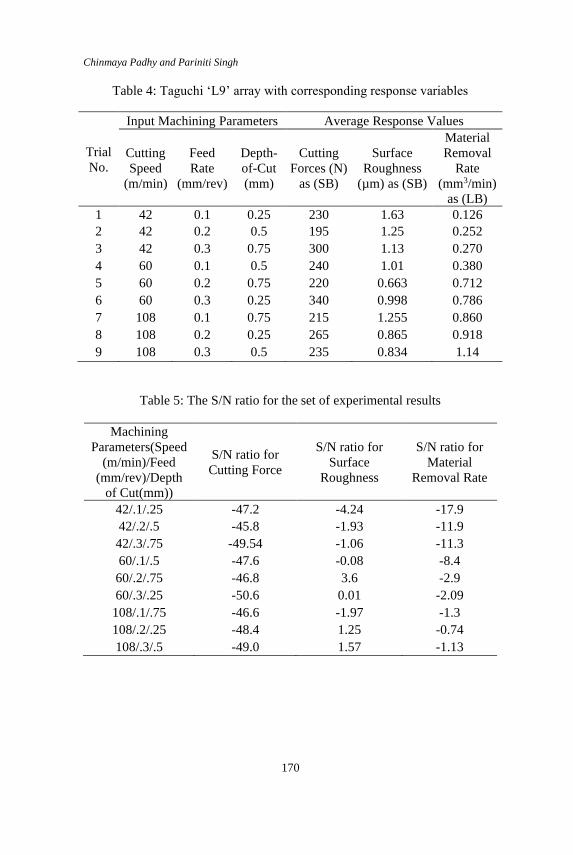
Chinmaya Padhy and Pariniti Singh
170
Table 4: Taguchi ‘L9’ array with corresponding response variables
Trial
No.
Input Machining Parameters Average Response Values
Cutting
Speed
(m/min)
Feed
Rate
(mm/rev)
Depth-
of-Cut
(mm)
Cutting
Forces (N)
as (SB)
Surface
Roughness
(µm) as (SB)
Material
Removal
Rate
(mm3/min)
as (LB)
1 42 0.1 0.25 230 1.63 0.126
2 42 0.2 0.5 195 1.25 0.252
3 42 0.3 0.75 300 1.13 0.270
4 60 0.1 0.5 240 1.01 0.380
5 60 0.2 0.75 220 0.663 0.712
6 60 0.3 0.25 340 0.998 0.786
7 108 0.1 0.75 215 1.255 0.860
8 108 0.2 0.25 265 0.865 0.918
9 108 0.3 0.5 235 0.834 1.14
Table 5: The S/N ratio for the set of experimental results
Machining
Parameters(Speed
(m/min)/Feed
(mm/rev)/Depth
of Cut(mm))
S/N ratio for
Cutting Force
S/N ratio for
Surface
Roughness
S/N ratio for
Material
Removal Rate
42/.1/.25 -47.2 -4.24 -17.9
42/.2/.5 -45.8 -1.93 -11.9
42/.3/.75 -49.54 -1.06 -11.3
60/.1/.5 -47.6 -0.08 -8.4
60/.2/.75 -46.8 3.6 -2.9
60/.3/.25 -50.6 0.01 -2.09
108/.1/.75 -46.6 -1.97 -1.3
108/.2/.25 -48.4 1.25 -0.74
108/.3/.5 -49.0 1.57 -1.13
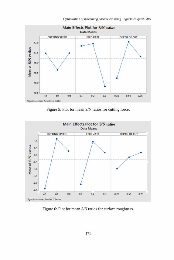
Optimization of machining parameters using Taguchi coupled GRA
171
Figure 5: Plot for mean S/N ratios for cutting force.
Figure 6: Plot for mean S/N ratios for surface roughness.
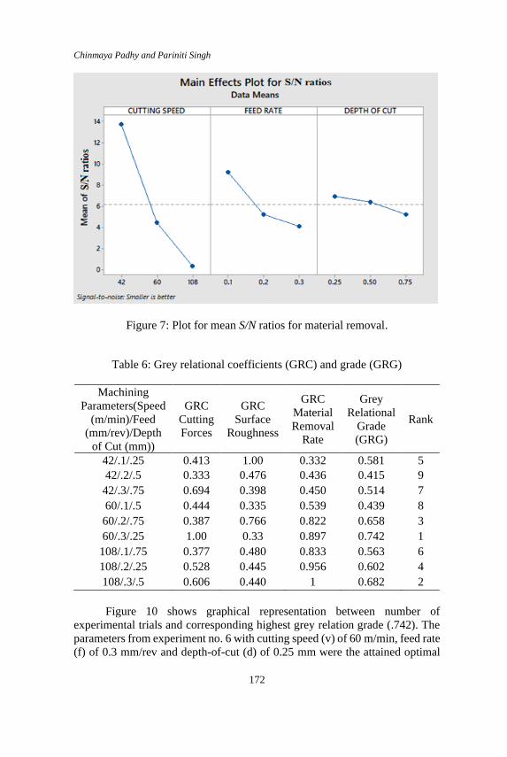
Chinmaya Padhy and Pariniti Singh
172
Figure 7: Plot for mean S/N ratios for material removal.
Table 6: Grey relational coefficients (GRC) and grade (GRG)
Machining
Parameters(Speed
(m/min)/Feed
(mm/rev)/Depth
of Cut (mm))
GRC
Cutting
Forces
GRC
Surface
Roughness
GRC
Material
Removal
Rate
Grey
Relational
Grade
(GRG)
Rank
42/.1/.25 0.413 1.00 0.332 0.581 5
42/.2/.5 0.333 0.476 0.436 0.415 9
42/.3/.75 0.694 0.398 0.450 0.514 7
60/.1/.5 0.444 0.335 0.539 0.439 8
60/.2/.75 0.387 0.766 0.822 0.658 3
60/.3/.25 1.00 0.33 0.897 0.742 1
108/.1/.75 0.377 0.480 0.833 0.563 6
108/.2/.25 0.528 0.445 0.956 0.602 4
108/.3/.5 0.606 0.440 1 0.682 2
Figure 10 shows graphical representation between number of
experimental trials and corresponding highest grey relation grade (.742). The
parameters from experiment no. 6 with cutting speed (v) of 60 m/min, feed rate
(f) of 0.3 mm/rev and depth-of-cut (d) of 0.25 mm were the attained optimal
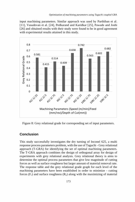
Optimization of machining parameters using Taguchi coupled GRA
173
input machining parameters. Similar approach was used by Parthiban et al.
[11], Vasudevan et al. [24], Pedkarand and Karidkar [25], Pawade and Joshi
[26] and obtained results with their study were found to be in good agreement
with experimental results attained in this study.
Figure 8: Grey relational grade for corresponding set of input parameters.
Conclusion
This study successfully investigates the dry turning of Inconel 625, a multi
response process parameters problem, with the use of Taguchi - Grey relational
approach (T-GRA) for identifying the set of optimal machining parameters.
The T-GRA approach combines the design of orthogonal array for design of
experiments with grey relational analysis. Grey relational theory is aims to
determine the optimal process parameters that give low magnitude of cutting
forces as well as surface roughness but larger amount of material removal rate.
The response table and the grey relational grade graph for each level of the
machining parameters have been established in order to minimize - cutting
forces (Fc) and surface roughness (Ra) along with the maximizing of material
0.581
0.415
0.514
0.439
0.658
0.742
0.5630.602
0.682
0
0.1
0.2
0.3
0.4
0.5
0.6
0.7
0.8
Gre
y R
elat
ion
al G
rad
e
Machining Parameters (Speed (m/min)/Feed (mm/rev)/Depth of Cut(mm))
Chinmaya Padhy and Pariniti Singh
174
removal rate (MRR). Grey relation analysis is applied to the results obtained
from Taguchi technique for establishing process parameters which provide
optimal solution between the multi performance responses. Based on the
experimental analysis, the results obtained for optimal machining conditions
were found out viz. (i) cutting speed (v) as 60 m/min, (ii) feed (f) as 0.3 mm/rev
and (iii) depth-of-cut (d) as 0.25 mm respectively. Hence, this study concludes
that turning with these set of combinations maximizes the performance of
response variables (Fc, Ra, MRR), ultimately which increases the overall
machining efficiency (machinability) of Inconel 625. The machining
parameters obtained can be used further for analyzing the machining
performances (with different lubricating environment) at this optimal
machining conditions, which can be extended for surface engineering study of
Inconel 625.
References
[1] T. Thomas, 2014. “Roughness and function. Surface Topography”,
Metrology and Properties, vol. 2, 014001
[2] P. Benardos, G. Vosniakos, “Predicting surface roughness in machining:
a review”, International Journal of Machine Tools and Manufacture, vol.
43, pp. 833-844, 2003.
[3] K. Guenther, P. Wierer, J. Bennett, “Surface roughness measurements of
low-scatter mirrors and roughness standards” Applied Optics, vol. 23, pp.
3820–3836, 1984.
[4] G. Besseris, “Product Screening to Multicustomer Preferences:
Multiresponse Unreplicated Nested Super-ranking”, International
Journal of Quality, Statistics, and Reliability, pp. 1-16, 2008.
[5] D. P. Selvaraj, “Optimization of cutting force of duplex stainless steel in
dry milling operation’, Materials Today: Proceedings, vol. 4, no. 10, pp.
11141–11147, 2017.
[6] Julie Z. Zhang, Joseph C. Chen, E. Daniel Kirby, “Surface roughness
optimization in an end-milling operation using the Taguchi design
method”, Journal of Materials Processing Technology, vol. 184, pp. 233-
239, 2007.
[7] Muammer Nalbant, Abdullah Altin, Hasan Gokkaya, “The effect of
coating material and geometry of cutting tool and cutting speed on
machinability properties of Inconel 718 super alloys”, Materials and
Design, vol. 28, pp. 1719-1724, 2007.
[8] S.M. Darwish, “The impact of tool material and cutting parameters on
surface roughness of supermet 718 nickel super alloy, s”, Journal of
Materials Processing Technology”, 97, pp 10-18, 2000.
[9] V. Srikanth, M. K. Chandra, “Parametric Optimization of Inconel 718
Optimization of machining parameters using Taguchi coupled GRA
175
With Carbide Inserts in Turning Using Taguchi L-9 Orthogonal Array
Method”, COJ Tech Sci Res, vol. 1, no. 4, COJTS.000521, 2019.
[10] Satyanarayana, B. Janardhana, G. Ranga Rao, D. Hanumantha,
“Optimized high speed turning on Inconel 718 using Taguchi method
based Grey relational analysis”, IJEM, vol. 20, no. 4, pp. 269-275, 2013.
[11] V. Parthiban, S. Vijayakumar, M. Sakthivel, “Optimization of high- speed
turning parameters for inconel 713C based on Taguchi grey relational
analysis (TGRA)”, Transactions of the Canadian Society for Mechanical
Engineering, vol. 43, no. 3, pp. 0221, 2019.
[12] E. Kuram, B. Ozcelik, “Multi-objective optimization using Taguchi based
grey relational analysis for micro-milling of Al 7075 material with ball
nose end mill”, Measurement, vol. 46, pp. 1849–1864, 2013.
[13] M. Kurt, S. Hartomac, B. Mutlu, U. Köklü, “Minimization of the Surface
Roughness and Form Error on the Milling of Free-Form Surfaces using a
Grey Relational Analysis”, Mater. Technol, vol.46, pp. 205–213, 2012.
[14] S.J. Raykar, D.M.D. Addona, A.M. Mane, “Multi-objective optimization
of high speed turning of Al 7075 using grey relational analysi,s”, Procedia
CIRP, vol. 33, pp. 293–298, 2015.
[15] S, Pariniti P, Chinmaya “Influence of nano (h-BN) cutting fluid on
machinability of Inconel 625”, Jour. of physics: conf. series, vol. 1355,
(012033), pp. 1-7, 2019.
[16] A.N., Siddiquee, Z.A. Khan, Z. Mallick, “Grey relational analysis coupled
with principal component analysis for optimization design of the process
parameters in in-feed centerless cylindrical grinding”, Int. J. Adv. Manuf.
Technol, vol. 46, pp. 983–992, 2010.
[17] I.A. Choudhury, M.A. El-Baradie, “Machinability of nickel-base super
alloys: a general review”, Journal of Materials Processing Technology,
vol. 77, pp. 278-284, 1998.
[18] C. V. Yıldırım, T. Kıvak. M. Sarıkaya, S. Sirin, “Evaluation of tool wear,
surface roughness/topography and chip morphology when machining of
Ni-based alloy 625 under MQL, cryogenic cooling and CryoMQL”.
Journal of Materials Research and Technology, vol. 9, no. 2, p. 2079–
2092, 2020.
[19] M. Mathew, P. K. Rajendrakumar, “Optimization of process parameters
of boro-carburized low carbon steel for tensile strength by Taquchi
method with grey relational analysis”, Materials & Design, vol. 32, no. 6,
pp 3637–3644, 2011.
[20] R.S. Pawade, S.B. Bhosele, “Grey Relation Parameter Optimization in
ultrasonic machining of ceramic composite (Al2O3/ZrO2)”, Journal of the
Association of Engineers, vol. 83, no. 2, pp. 63-77, 2013.
[21] F. Puh, Z. Jurkovic, M. Perinic, M. Brezocnik, S. Buljan, “Optimization
of machining parameters for turning operation with multiple quality
characteristics using Grey relational analysis”, Tehnički vjesnik, vol. 23,
Chinmaya Padhy and Pariniti Singh
176
no. 2, pp. 377-382, 2016.
[22] Nihat Tosun, “Determination of optimum parameters for multi-
performance characteristics in drilling by using grey relational analysis”,
International Journal of Advanced manufacturing Technology, vol. 28,
pp. 450-455, 2006.
[23] K.W. Ng David, “Grey system and grey relational model”, ACM SIGICE
Bulletin, vol. 20, no. 2, pp.1–9,1994.
[24] H. Vasudevan, R. Rajguru, M. Shaikh, & A. Shaikh, “Optimization of
Process Parameters in the Turning Operation of Inconel 625”. Materials
Science Forum, vol. 969, pp. 756–761, 2019.
[25] Pooja Petkar, S. S. Karidkar, “Optimization of Machining Parameters for
Turning on CNC Machine of Inconel-718 alloy”, International Journal of
Engineerig Research and Technology, vol. 08, pp. 06, 2019.
[26] Pawade, R. S., & Joshi, S. S., “Multi-objective optimization of surface
roughness and cutting forces in high-speed turning of Inconel 718 using
Taguchi grey relational analysis (TGRA)”, The International Journal of
Advanced Manufacturing Technology, vol. 56, pp. 47–62, 2011.

Journal of Mechanical Engineering Vol 18(2), 177-191, 2021
___________________
ISSN 1823-5514, eISSN 2550-164X Received for review: 2021-01-02
© 2021 College of Engineering, Accepted for publication: 2021-03-09
Universiti Teknologi MARA (UiTM), Malaysia. Published: 2021-04-15
Effect of Fiber Misalignment on Mechanical and Failure Response
of Kenaf Composite under Compressive Loading
M. F. Razali, S.A.H.A. Seman*, T. W. Theng
School of Mechanical Engineering, Engineering Campus,
Universiti Sains Malaysia,
14300 Nibong Tebal, Pulau Pinang, Malaysia
ABSTRACT
The use of kenaf fibres has grown unexpectedly in the world as they help to
establish green materials in automobile, sports and food packaging industries. Over the past few decades, unidirectional fiber-reinforced composites have
been extensively used in industry due to their high specific strength
characteristics. During manufacturing process, several defects especially
fiber misalignment might exist in the unidirectional composite structure. This
kind of deviation from its optimal parallel packing in a unidirectional fibre
reinforced composite would influence its overall load-bearing efficiency. Performance data of kenaf composite due to this imperfection, however, is very
limited in the literature. In this regard, the effects of fibre misalignments on
the unidirectional kenaf composite compressive reaction have been studied.
For this reason, pultruded kenaf composite specimens with different fibre
alignment from 00 to 20 at 2.1 and 8.4 mm/s strain rates were subjected to a
range of compression measures. The findings revealed that, the failure strain
seems to be almost constant at value of 0.05 and 0.063 while the failure stress
decreases from 140Mpa until 120MP when the fibre alignment increases when
loaded within a range of 2.1~8.4s-1. Additionally, under increased fiber
misalignment and strain rate, fibre plastic microbuckling, fibre breakage, fibre
splitting and fibre matrix debonding was progressively formed on the
specimen.
Keywords: Kenaf composite; Fiber misalignment; Damage behavior
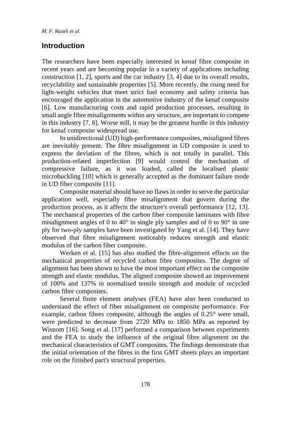
M. F. Razali et al.
178
Introduction
The researchers have been especially interested in kenaf fibre composite in
recent years and are becoming popular in a variety of applications including
construction [1, 2], sports and the car industry [3, 4] due to its overall results,
recyclability and sustainable properties [5]. More recently, the rising need for
light-weight vehicles that meet strict fuel economy and safety criteria has
encouraged the application in the automotive industry of the kenaf composite
[6]. Low manufacturing costs and rapid production processes, resulting in
small angle fibre misalignments within any structure, are important to compete
in this industry [7, 8]. Worse still, it may be the greatest hurdle in this industry
for kenaf composite widespread use.
In unidirectional (UD) high-performance composites, misaligned fibres
are inevitably present. The fibre misalignment in UD composite is used to
express the deviation of the fibres, which is not totally in parallel. This
production-related imperfection [9] would control the mechanism of
compressive failure, as it was loaded, called the localised plastic
microbuckling [10] which is generally accepted as the dominant failure mode
in UD fiber composite [11].
Composite material should have no flaws in order to serve the particular
application well, especially fibre misalignment that govern during the
production process, as it affects the structure's overall performance [12, 13].
The mechanical properties of the carbon fiber composite laminates with fibre
misalignment angles of 0 to 40° in single ply samples and of 0 to 90° in one
ply for two-ply samples have been investigated by Yang et al. [14]. They have
observed that fibre misalignment noticeably reduces strength and elastic
modulus of the carbon fiber composite.
Werken et al. [15] has also studied the fibre-alignment effects on the
mechanical properties of recycled carbon fibre composites. The degree of
alignment has been shown to have the most important effect on the composite
strength and elastic modulus. The aligned composite showed an improvement
of 100% and 137% in normalised tensile strength and module of recycled
carbon fibre composites.
Several finite element analyses (FEA) have also been conducted to
understand the effect of fiber misalignment on composite performance. For
example, carbon fibres composite, although the angles of 0.25° were small,
were predicted to decrease from 2720 MPa to 1850 MPa as reported by
Wisnom [16]. Song et al. [17] performed a comparison between experiments
and the FEA to study the influence of the original fibre alignment on the
mechanical characteristics of GMT composites. The findings demonstrate that
the initial orientation of the fibres in the first GMT sheets plays an important
role on the finished part's structural properties.
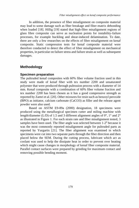
Fiber misalignment effect on kenaf composite performance
179
In addition, the presence of fiber misalignment on composite material
may lead to some damage such as fiber breakage and fiber-matrix debonding
when loaded [18]. Hillig [19] stated that high-fibre misalignment regions of
glass fibre composite can serve as nucleation points for instability-failure
processes, for example buckling and shear-induced delamination. To date,
there are only a few researches on the effects of fibre misalignment on kenaf
composite. Static compression tests for kenaf composite material were
therefore conducted to detect the effect of fiber misalignment on mechanical
properties, in particular on failure stress and failure strain as well as subsequent
damages.
Methodology
Specimen preparation The pultruded kenaf composites with 60% fiber volume fraction used in this
study were made of kenaf fiber with tex number 2200 and unsaturated
polyester that were produced through pultrusion process with a diameter of 14
mm. Kenaf composite with a combination of 60% fiber volume fraction and
tex number 2200 has been chosen as it has a good compressive strength as
reported by Zamri et al. [20]. Other mixtures for resin such as benzoyl peroxide
(BPO) as initiator, calcium carbonate (CaCO3) as filler and the release agent
powder were also used.
Based on ASTM E9-89a (2000) designation, 18 specimens were
produced using the metallurgical specimen cutter and miling machine with
length/diameter (L/D) of 1.5 and 3 different alignment angles of 0°, 1° and 2°
as illustrated in Figure 1. For each strain rate and fiber misalignment tested, 3
samples have been used. The fiber angle was selected between 1-20 because it
was the most commonly reported misalignment angle for pultruded parts as
reported by Yurgartis [21]. The fiber alignment was examined in which
specimens were cut into two separate parts through the fiber direction and then
placed below the SEM. During the cutting process, lubricant which act as
coolant was used to help the dissipate heat in order to prevent over heating
which might cause changes in morphology of kenaf fiber composite material.
Parallel contact surfaces were prepared by grinding for maximum contact and
removing possible bending moment.
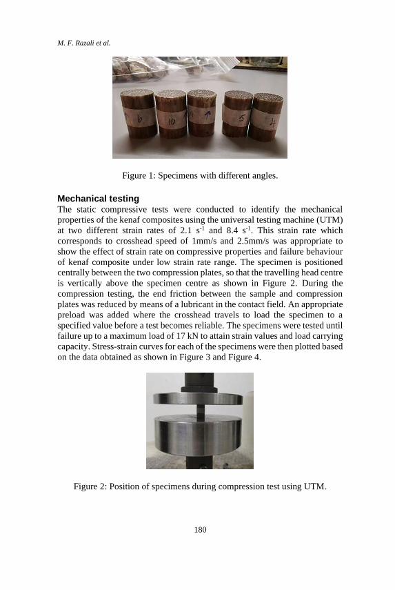
M. F. Razali et al.
180
Figure 1: Specimens with different angles.
Mechanical testing The static compressive tests were conducted to identify the mechanical
properties of the kenaf composites using the universal testing machine (UTM)
at two different strain rates of 2.1 s-1 and 8.4 s-1. This strain rate which
corresponds to crosshead speed of 1mm/s and 2.5mm/s was appropriate to
show the effect of strain rate on compressive properties and failure behaviour
of kenaf composite under low strain rate range. The specimen is positioned
centrally between the two compression plates, so that the travelling head centre
is vertically above the specimen centre as shown in Figure 2. During the
compression testing, the end friction between the sample and compression
plates was reduced by means of a lubricant in the contact field. An appropriate
preload was added where the crosshead travels to load the specimen to a
specified value before a test becomes reliable. The specimens were tested until
failure up to a maximum load of 17 kN to attain strain values and load carrying
capacity. Stress-strain curves for each of the specimens were then plotted based
on the data obtained as shown in Figure 3 and Figure 4.
Figure 2: Position of specimens during compression test using UTM.
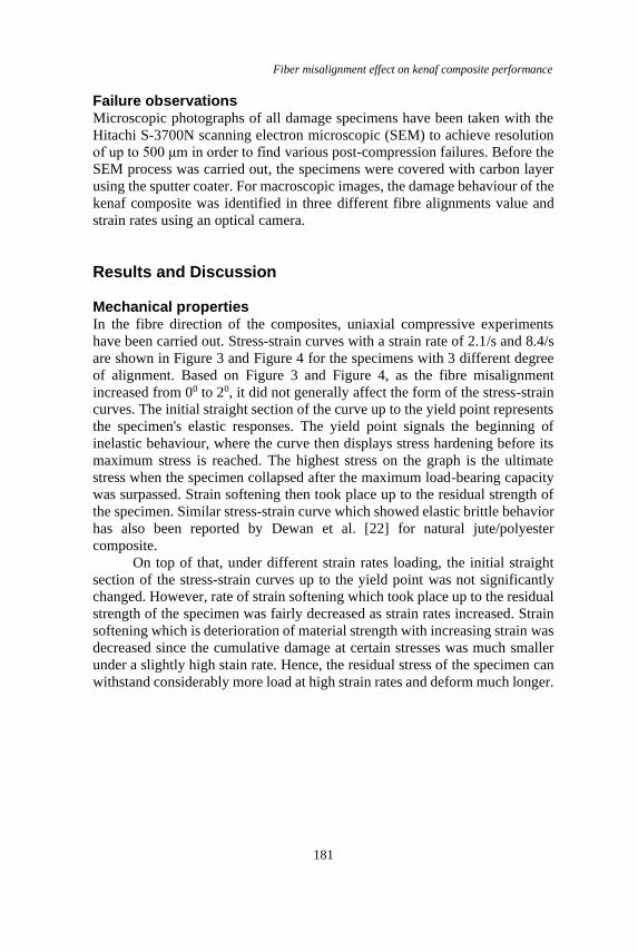
Fiber misalignment effect on kenaf composite performance
181
Failure observations Microscopic photographs of all damage specimens have been taken with the
Hitachi S-3700N scanning electron microscopic (SEM) to achieve resolution
of up to 500 μm in order to find various post-compression failures. Before the
SEM process was carried out, the specimens were covered with carbon layer
using the sputter coater. For macroscopic images, the damage behaviour of the
kenaf composite was identified in three different fibre alignments value and
strain rates using an optical camera.
Results and Discussion
Mechanical properties In the fibre direction of the composites, uniaxial compressive experiments
have been carried out. Stress-strain curves with a strain rate of 2.1/s and 8.4/s
are shown in Figure 3 and Figure 4 for the specimens with 3 different degree
of alignment. Based on Figure 3 and Figure 4, as the fibre misalignment
increased from 00 to 20, it did not generally affect the form of the stress-strain
curves. The initial straight section of the curve up to the yield point represents
the specimen's elastic responses. The yield point signals the beginning of
inelastic behaviour, where the curve then displays stress hardening before its
maximum stress is reached. The highest stress on the graph is the ultimate
stress when the specimen collapsed after the maximum load-bearing capacity
was surpassed. Strain softening then took place up to the residual strength of
the specimen. Similar stress-strain curve which showed elastic brittle behavior
has also been reported by Dewan et al. [22] for natural jute/polyester
composite.
On top of that, under different strain rates loading, the initial straight
section of the stress-strain curves up to the yield point was not significantly
changed. However, rate of strain softening which took place up to the residual
strength of the specimen was fairly decreased as strain rates increased. Strain
softening which is deterioration of material strength with increasing strain was
decreased since the cumulative damage at certain stresses was much smaller
under a slightly high stain rate. Hence, the residual stress of the specimen can
withstand considerably more load at high strain rates and deform much longer.
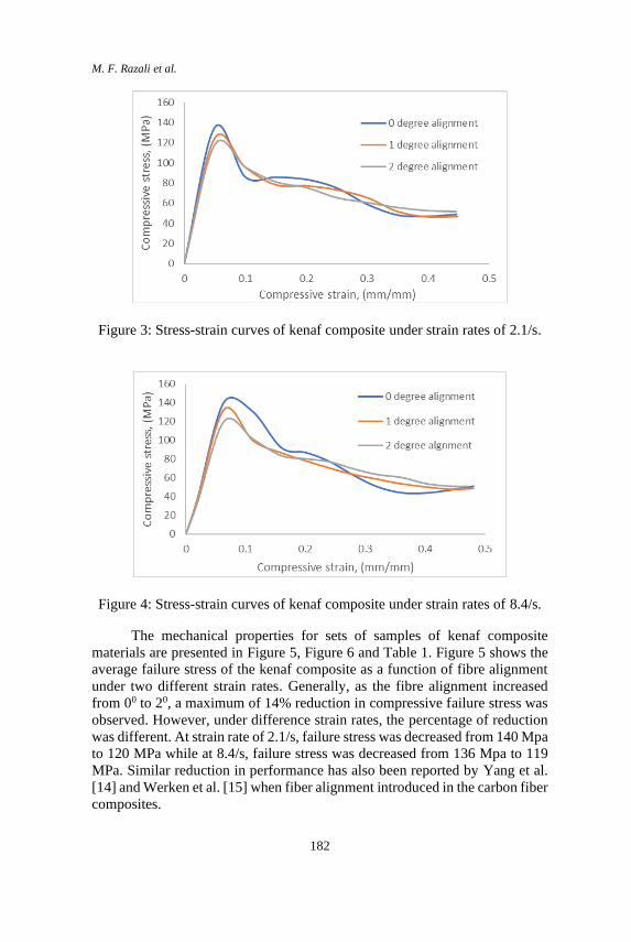
M. F. Razali et al.
182
Figure 3: Stress-strain curves of kenaf composite under strain rates of 2.1/s.
Figure 4: Stress-strain curves of kenaf composite under strain rates of 8.4/s.
The mechanical properties for sets of samples of kenaf composite
materials are presented in Figure 5, Figure 6 and Table 1. Figure 5 shows the
average failure stress of the kenaf composite as a function of fibre alignment
under two different strain rates. Generally, as the fibre alignment increased
from 00 to 20, a maximum of 14% reduction in compressive failure stress was
observed. However, under difference strain rates, the percentage of reduction
was different. At strain rate of 2.1/s, failure stress was decreased from 140 Mpa
to 120 MPa while at 8.4/s, failure stress was decreased from 136 Mpa to 119
MPa. Similar reduction in performance has also been reported by Yang et al.
[14] and Werken et al. [15] when fiber alignment introduced in the carbon fiber
composites.
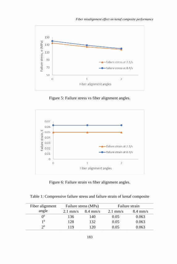
Fiber misalignment effect on kenaf composite performance
183
Figure 5: Failure stress vs fiber alignment angles.
Figure 6: Failure strain vs fiber alignment angles.
Table 1: Compressive failure stress and failure strain of kenaf composite
Fiber alignment
angle
Failure stress (MPa) Failure strain
2.1 mm/s 8.4 mm/s 2.1 mm/s 8.4 mm/s
00 136 140 0.05 0.063
10 128 132 0.05 0.063
20 119 120 0.05 0.063
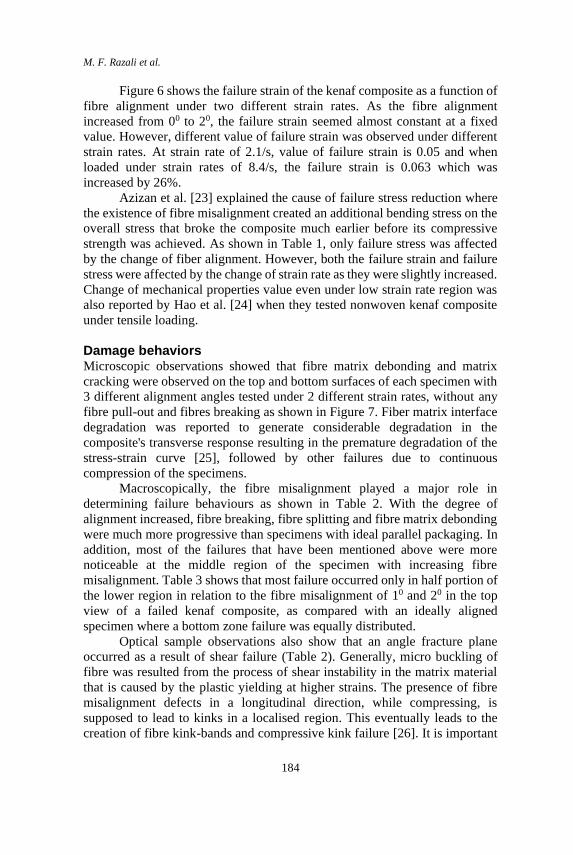
M. F. Razali et al.
184
Figure 6 shows the failure strain of the kenaf composite as a function of
fibre alignment under two different strain rates. As the fibre alignment
increased from 00 to 20, the failure strain seemed almost constant at a fixed
value. However, different value of failure strain was observed under different
strain rates. At strain rate of 2.1/s, value of failure strain is 0.05 and when
loaded under strain rates of 8.4/s, the failure strain is 0.063 which was
increased by 26%.
Azizan et al. [23] explained the cause of failure stress reduction where
the existence of fibre misalignment created an additional bending stress on the
overall stress that broke the composite much earlier before its compressive
strength was achieved. As shown in Table 1, only failure stress was affected
by the change of fiber alignment. However, both the failure strain and failure
stress were affected by the change of strain rate as they were slightly increased.
Change of mechanical properties value even under low strain rate region was
also reported by Hao et al. [24] when they tested nonwoven kenaf composite
under tensile loading.
Damage behaviors Microscopic observations showed that fibre matrix debonding and matrix
cracking were observed on the top and bottom surfaces of each specimen with
3 different alignment angles tested under 2 different strain rates, without any
fibre pull-out and fibres breaking as shown in Figure 7. Fiber matrix interface
degradation was reported to generate considerable degradation in the
composite's transverse response resulting in the premature degradation of the
stress-strain curve [25], followed by other failures due to continuous
compression of the specimens.
Macroscopically, the fibre misalignment played a major role in
determining failure behaviours as shown in Table 2. With the degree of
alignment increased, fibre breaking, fibre splitting and fibre matrix debonding
were much more progressive than specimens with ideal parallel packaging. In
addition, most of the failures that have been mentioned above were more
noticeable at the middle region of the specimen with increasing fibre
misalignment. Table 3 shows that most failure occurred only in half portion of
the lower region in relation to the fibre misalignment of 10 and 20 in the top
view of a failed kenaf composite, as compared with an ideally aligned
specimen where a bottom zone failure was equally distributed.
Optical sample observations also show that an angle fracture plane
occurred as a result of shear failure (Table 2). Generally, micro buckling of
fibre was resulted from the process of shear instability in the matrix material
that is caused by the plastic yielding at higher strains. The presence of fibre
misalignment defects in a longitudinal direction, while compressing, is
supposed to lead to kinks in a localised region. This eventually leads to the
creation of fibre kink-bands and compressive kink failure [26]. It is important
Fiber misalignment effect on kenaf composite performance
185
to note that fibre misalignment is very sensitive to kinking stresses. Outcome
of this study are in line with what reported by where the 0.8–2.3° angle of
misalignment was sufficient to cause a kink [27].
As shown in Table 2 and Table 3, the failure progression of the
specimens with higher fiber misalignment is gradual compared to ideally
aligned specimens. As previously discussed, main failure under compression
loading of unidirectional composites was plastic kinking due to the existence
of fiber misalignment and subsequent occurrence of matrix’s shear instability.
In Table 2, fiber kinking was a first failure initiated and visible prior to an
inclined shear crack and fiber splitting. However, for specimens of high fibre
misalignment, the gradual formation of the kink band and the associated fibre
kink failure mode are more obvious.
Decohesion at the interface and shear band formation in the matrix are
the two dominant damage mechanisms in controlling the composite strength
[28]. In condition where decohesion is constricted, matrix’s shear bands would
occur at angle of ±450 from the compression axis [29]. The angle between the
failure plane and the in-plane load direction is slightly higher than 45° and
typical values are reported between 50-56° for certain composites which may
be more susceptible to shear bands formation [30]. For kenaf composite’s
compressive strength reported here, it was controlled by the visible decohesion
of fiber and matrix at the interface as no shear bands failure occurred. As fiber
misalignment increased, decohesion of fiber and matrix at the interface was
more obvious (Table 2 and Table 3) which contribute to the reduction of
compressive strength.
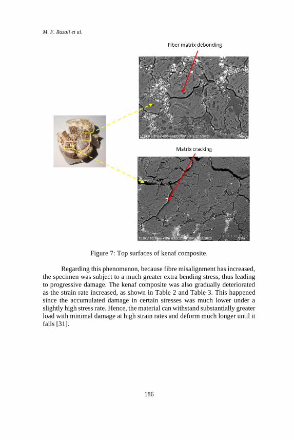
M. F. Razali et al.
186
Figure 7: Top surfaces of kenaf composite.
Regarding this phenomenon, because fibre misalignment has increased,
the specimen was subject to a much greater extra bending stress, thus leading
to progressive damage. The kenaf composite was also gradually deteriorated
as the strain rate increased, as shown in Table 2 and Table 3. This happened
since the accumulated damage in certain stresses was much lower under a
slightly high stress rate. Hence, the material can withstand substantially greater
load with minimal damage at high strain rates and deform much longer until it
fails [31].
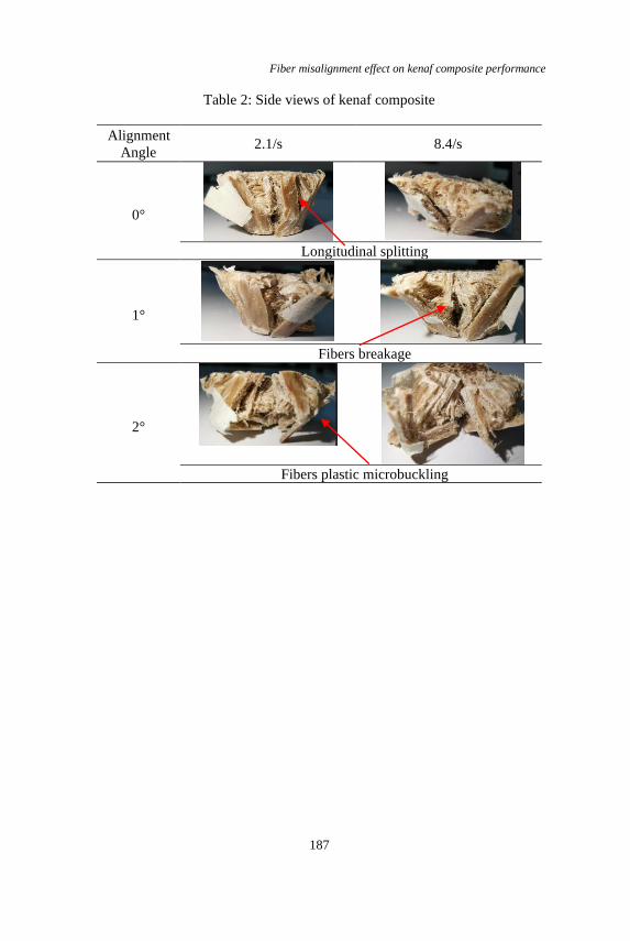
Fiber misalignment effect on kenaf composite performance
187
Table 2: Side views of kenaf composite
Alignment
Angle 2.1/s 8.4/s
0°
Longitudinal splitting
1°
Fibers breakage
2°
Fibers plastic microbuckling
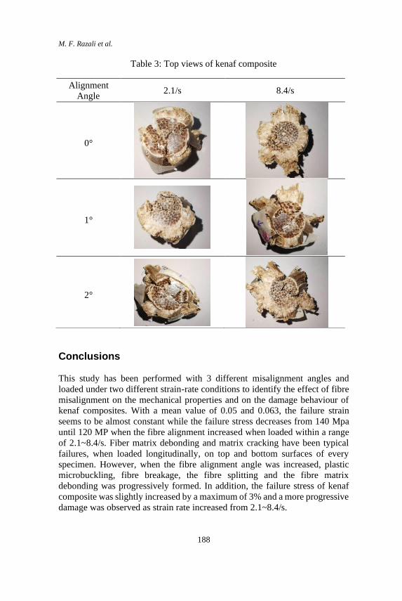
M. F. Razali et al.
188
Table 3: Top views of kenaf composite
Conclusions
This study has been performed with 3 different misalignment angles and
loaded under two different strain-rate conditions to identify the effect of fibre
misalignment on the mechanical properties and on the damage behaviour of
kenaf composites. With a mean value of 0.05 and 0.063, the failure strain
seems to be almost constant while the failure stress decreases from 140 Mpa
until 120 MP when the fibre alignment increased when loaded within a range
of 2.1~8.4/s. Fiber matrix debonding and matrix cracking have been typical
failures, when loaded longitudinally, on top and bottom surfaces of every
specimen. However, when the fibre alignment angle was increased, plastic
microbuckling, fibre breakage, the fibre splitting and the fibre matrix
debonding was progressively formed. In addition, the failure stress of kenaf
composite was slightly increased by a maximum of 3% and a more progressive
damage was observed as strain rate increased from 2.1~8.4/s.
Alignment
Angle 2.1/s 8.4/s
0°
1°
2°
Fiber misalignment effect on kenaf composite performance
189
References
[1] A. Elsaid, M. Dawood, R. Seracino, and C. Bobko, "Mechanical properties
of kenaf fiber reinforced concrete," Construction and Building Materials,
vol. 25, no. 4, pp. 1991-2001, 2011.
[2] C. Zhou, L. Cai, Z. Chen, and J. Li, "Effect of kenaf fiber on mechanical
properties of high-strength cement composites," Construction and
Building Materials, vol. 263, no. 1, pp. 121007, 2020.
[3] N. Saba, M.T. Paridah, and M. Jawaid, "Mechanical properties of kenaf
fibre reinforced polymer composite: A review," Construction and
Building Materials, vol. 76, no., pp. 87-96, 2015
[4] M.F. Omar, H. Jaya, and N.N. Zulkepli, "Kenaf Fiber Reinforced
Composite in the Automotive Industry", In Encyclopedia of Renewable
and Sustainable Materials. Elsevier, Oxford, 2020. pp. 95-101.
[5] V. Fiore, G. Di Bella, and A. Valenza, "The effect of alkaline treatment on
mechanical properties of kenaf fibers and their epoxy composites,"
Composites Part B: Engineering, vol. 68, no., pp. 14-21, 2015.
[6] H.T. Sreenivas, N. Krishnamurthy, and G.R. Arpitha, "A comprehensive
review on light weight kenaf fiber for automobiles," International Journal
of Lightweight Materials and Manufacture, vol. 3, no. 4, pp. 328-337,
2020.
[7] L.T. Harper, T. Turner, J.R.B. Martin, and N. Warrior, "Fiber Alignment
in Directed Carbon Fiber Preforms — A Feasibility Study," Journal of
Composite Materials vol. 43, no. 1, pp. 57-74, 2009.
[8] K. Potter, B. Khan, M. Wisnom, T. Bell, and J. Stevens, "Variability, fibre
waviness and misalignment in the determination of the properties of
composite materials and structures," Composites Part A: Applied Science
and Manufacturing, vol. 39, no. 9, pp. 1343-1354, 2008.
[9] G.M. Martinez, M.R. Piggott, D.M.R. Bainbridge, and B. Harris, "The
compression strength of composites with kinked, misaligned and poorly
adhering fibres," Journal of Materials Science, vol. 16, no. 10, pp. 2831-
2836, 1981.
[10] K.K. Kratmann, M.P.F. Sutcliffe, L.T. Lilleheden, R. Pyrz, and O.T.
Thomsen, "A novel image analysis procedure for measuring fibre
misalignment in unidirectional fibre composites," Composites Science and
Technology, vol. 69, no. 2, pp. 228-238, 2009.
[11] B. Budiansky, and N.A. Fleck, "Compressive failure of fibre composites,"
Journal of the Mechanics and Physics of Solids, vol. 41, no. 1, pp. 183-
211, 1993.
[12] Y. Li, B. Stier, B. Bednarcyk, J.-W. Simon, and S. Reese, "The effect of
fiber misalignment on the homogenized properties of unidirectional fiber
reinforced composites," Mechanics of Materials, vol. 92, no., pp. 261-274,
2016.
M. F. Razali et al.
190
[13] S.C. Barwick, and T.D. Papathanasiou, "Identification of fiber
misalignment in continuous fiber composites," Polymer Composites, vol.
24, no. 3, pp. 475-486, 2003.
[14] X. Yang, A. Nanni, S. Haug, and C. Sun, "Strength and Modulus
Degradation of Carbon Fiber-Reinforced Polymer Laminates from Fiber
Misalignment," Journal of Materials in Civil Engineering vol. 14, no.,
2002.
[15] N. Werken, M.S. Reese, M.R. Taha, and M. Tehrani, "Investigating the
effects of fiber surface treatment and alignment on mechanical properties
of recycled carbon fiber composites," Composites Part A: Applied Science
and Manufacturing, vol. 119, no., pp. 38-47, 2019.
[16] M.R. Wisnom, "The effect of fibre misalignment on the compressive
strength of unidirectional carbon fibre/epoxy," Composites, vol. 21, no. 5,
pp. 403-407, 1990.
[17] Y. Song, U. Gandhi, A. Koziel, S. Vallury, and A. Yang, "Effect of the
initial fiber alignment on the mechanical properties for GMT composite
materials," Journal of Thermoplastic Composite Materials, vol. 31, no. 1,
pp. 91-109, 2017.
[18] H. Ahmadian, M. Yang, A. Nagarajan, and S. Soghrati, "Effects of shape
and misalignment of fibers on the failure response of carbon fiber
reinforced polymers," Computational Mechanics, vol. 63, no. 5, pp. 999-
1017, 2019.
[19] W.B. Hillig, "Effect of fibre misalignment on the fracture behaviour of
fibre-reinforced composites," Journal of Materials Science, vol. 29, no. 2,
pp. 419-423, 1994.
[20] M.H. Zamri, H.M. Akil, and Z.A. MohdIshak, "Pultruded Kenaf Fibre
Reinforced Composites: Effect of Different Kenaf Fibre Yarn Tex,"
Procedia Chemistry, vol. 19, no., pp. 577-585, 2016.
[21] S.W. Yurgartis, "Measurement of small angle fiber misalignments in
continuous fiber composites," Composites Science and Technology, vol.
30, no. 4, pp. 279-293, 1987.
[22] M.W. Dewan, M.K. Hossain, M. Hosur, and S. Jeelani,
"Thermomechanical properties of alkali treated jute-polyester/nanoclay
biocomposites fabricated by VARTM process," Journal of Applied
Polymer Science, vol. 128, no. 6, pp. 4110-4123, 2013.
[23] A. Azizan, H.A. Israr, and N. Tamin, "Effect of Fiber Misalignment on
Tensile Response of Unidirectional CFRP Composite Lamina," Journal of
Advanced Research in Applied Sciences and Engineering Technology, vol.
11, no. 1, pp. 23-30, 2018.
[24] A. Hao, H. Zhao, W. Jiang, L. Yuan, and J.Y. Chen, "Mechanical
Properties of Kenaf/Polypropylene Nonwoven Composites," Journal of
Polymers and the Environment, vol. 20, no. 4, pp. 959-966, 2012.
Fiber misalignment effect on kenaf composite performance
191
[25] W.S. Johnson, S.J. Lubowinski, and A.L. Highsmith, "Mechanical
Characterization of Unnotched SCS 6 /Ti-15-3 Metal Matrix Composites
at Room Temperature", In. ASTM International, West Conshohocken,
PA, 1990. pp. 193-218.
[26] B. Budiansky, and N.A. Fleck, "Compressive Kinking of Fiber
Composites: A Topical Review," Applied Mechanics Reviews, vol. 47, no.
6S, pp. S246-S250, 1994.
[27] J. Lee, and C. Soutis, "A study on the compressive strength of thick carbon
fibre–epoxy laminates," Composites Science and Technology, vol. 67, no.
10, pp. 2015-2026, 2007.
[28] S. Ghaffari, A. Makeev, G. Seon, D.P. Cole, D.J. Magagnosc, and S.
Bhowmick, "Understanding compressive strength improvement of high
modulus carbon-fiber reinforced polymeric composites through fiber-
matrix interface characterization," Materials & Design, vol. 193, no., pp.
108798, 2020.
[29] C. González, and J. Llorca, "Mechanical behavior of unidirectional fiber-
reinforced polymers under transverse compression: Microscopic
mechanisms and modeling," Composites Science and Technology, vol. 67,
no. 13, pp. 2795-2806, 2007.
[30] M.M. Shokrieh, M.A. Torabizadeh, and A. Fereidoon, "Progressive failure
analysis of glass/epoxy composites at low temperatures," Strength of
Materials, vol. 44, no. 3, pp. 314-324, 2012.
[31] S. Abrate, "Impact on Laminated Composite Materials," Applied
Mechanics Reviews, vol. 44, no. 4, pp. 155-190, 1991.

Journal of Mechanical Engineering Vol 18(2), 193-201, 2021
___________________
ISSN 1823-5514, eISSN 2550-164X Received for review: 2020-09-13
© 2021 College of Engineering, Accepted for publication: 2021-03-18
Universiti Teknologi MARA (UiTM), Malaysia. Published: 2021-04-15
Flexible Pavement Crack’s Severity Identification and Classification using Deep Convolution Neural
Network
A. Ibrahim*, N. A. Z. M. Zukri, B. N. Ismail
Faculty of Civil Engineering, UiTM Cawangan Pulau Pinang, Malaysia
M. K. Osman, N. A. M. Yusof, M. Idris
Faculty of Electrical Engineering, UiTM Cawangan Pulau Pinang, Malaysia
A. H. Rabian
THB Maintenance Sdn. Bhd. Malaysia
I. Bahri
Unitec Institute of Technology, Auckland, New Zealand.
ABSTRACT
Effective road maintenance program is vital to ensure traffic safety,
serviceability, and prolong the life span of the road. Maintenance will be
carried out on pavements when signs of degradation begin to appear and
delays may also lead to increased maintenance costs in the future, when more
severe changes may be required. In Malaysia, manual visual observation is
practiced in the inspection of distressed pavements. Nonetheless, this method
of inspection is ineffective as it is more laborious, time consuming and poses
safety hazard. This study focuses in utilizing an Artificial Intelligence (AI)
method to automatically classify pavement crack severity. Field data
collection was conducted to allow meaningful verification of accuracy and
reliability of the crack’s severity prediction based on AI. Several important
phases are required in research methodology processes including data
collection, image labelling, image resizing, image enhancement, deep
convolution neural network (DCNN) training and performance evaluation.
Throughout the analysis of image processing results, the image output was
successfully classified using MATLAB software. The good agreement between
field measurement data and DCNN prediction of crack’s severity proved the

A.Ibrahim et.al
194
reliability of the system. In conclusion, the established method can classify the
crack’s severity based on the JKR guideline of visual assessment.
Keywords: Road maintenance; DCNN; Crack severity; Flexible pavement
Introduction
Road networks are crucial infrastructures that provide transport services, and
a catalyst for the economic development of a nation. A large part of the current
road infrastructure is approaching the end of its service life, which is placing
even more pressure on the budgets in the coming years [1]. Road maintenance
involves monitoring road performance and repairing defects such as potholes,
pavement cracks and rutting. Some examples of pavement defect treatments
are pothole patching, crack sealing, mill and pave and road reconstruction [2].
Manual pavement distress survey is inefficient and lead to low productivity in
road maintenance. For example, one pavement inspector can only inspect less
than 10 km per day [3]. The goal of this study is to improve pavement
maintenance survey using an AI by measuring the level of severity of
distressed pavement. AI is an area of computer science that accentuates the
development of smart machines that function and respond like humans. AI
performs frequent, high-volume, computerized tasks reliably and without
fatigue rather than automating manual tasks. This work introduces a
customized image processing algorithm for high-speed, real-time inspection of
pavement cracking [4]. Traditionally, it requires engineers working on busy
roads, which is dangerous, costly, time-consuming, and inefficient [5]-[7].
Several attempts have been made in the past to automate the pavement
distress survey using image processing techniques. Among them are based on
image segmentation [8], seed growing [9], local optimal thresholding [10] and
matched filtering algorithm [11]. However, these methods suffer from problem
of intensity variation in pavement images due to shadow, oily, complex, and
rough pavement surfaces. To overcome these problems, recent researches have
integrated artificial intelligence such as random decision forest [12], support
vector machine (SVM) [13]-[14], artificial neural network [14]-[15] and fuzzy
inference system [16]. This study utilises MATLAB software to develop an AI
system based on deep convolutional neural network to analyse pavement
distress images automatically. The AI system will automate the classification
of crack severity of flexible asphalt pavement. To further advance the system,
the automated crack detection was moved to the next stage of computer vision
where utilizing machine learning approach that can be found in many studies.
Machine learning is a subset of AI, where it uses algorithms to analyse and
learn from a sample dataset, and then decide or make new predictions about
other datasets. This is compatible with the objective of machine learning which

Flexible Pavement Crack’s Severity Identification
195
is to allow the system to learn automatically without human intervention.
Consequently, the main aim of this project is to develop an intelligent system
based on DCNN to detect and classify pavement cracks of asphalt pavement.
To achieve that, this project focuses on developing an AI system for flexible
pavement crack’s severity classification. The system is then tested using field
datasets to verify its accuracy and reliability.
Research Methodology
The methodology adopted in this project involves four major steps starting
with the data collection, image processing and labelling, Deep Convolution
Neural Network (DCNN) training and evaluation of the system’s performance.
The prediction data of pavement crack’s severity will be compared with the
field measurement data to ensure its accuracy and reliability of the AI system.
Data collection of pavement crack and its severity The images of asphalt pavement crack were acquired from various location in
Penang and Terengganu. Generally, there are three main types of pavement
cracks which are longitudinal, alligator and transverse cracks. For this study,
the focus is on pavement cracks with various level of severity. Photos were
taken using a mobile phone camera with its optical perpendicular to the road
surface. The data collection can be carried out with any device that can take
pictures downwards [17]. The camera is mounted on a phone holder with a
consistent height of 100 cm from the pavement surface to achieve accurate,
reliable, and efficient image collection. For every captured image, Vernier
calliper is used to directly measure the width of the crack for field data
collection
Image labelling, resizing, and enhancing Pavement crack images obtained from field were labelled based on the
measurement of the average width of the pavement’s crack. Images will be
classified into low, moderate, and high severity of crack based on [18]
guideline of visual assessment of flexible pavement surface condition as
shown in Figure 1. Low severity of asphalt pavement crack’s width is below
than 6 mm, moderate severity’s width is between 6 mm to 19 mm, and high
severity’s width is 19 mm and above.
Resizing images is compulsory because if the size is too big, it will slow
down the process in training process in Deep Convolutional Neural Network
operation. For this research, 64 x 64 is found to be the optimal image size. For
resizing images, using photoshop is preferred and easier method.

A.Ibrahim et.al
196
Figure 1: Classification of crack’s severity from low, moderate to high (left
to right).
Image enhancing is performed to increase the number of images. To
achieve this, images were edited into 90° anti-clockwise, 90° clockwise,
perpendicular, and vertical rotation form. Higher number in images from data
collection will allow better accuracy in the training process of DCNN system.
DCNN data training and testing The network prepares two sets of training and testing dataset: types of crack
classification consists of transverse, longitudinal and alligator [19]. To achieve
the objective, Deep Convolutional Neural Network (DCNN) must be train
first. Divide the data into datasets for the testing and validation. Using 70% of
the photos for processing, and 30% for validation. After succeeding with the
when training the coding in MATLAB, run the other codes to test the pavement
crack images. When running the codes, it will ask to input the images we want
to test. After selecting the image, MATLAB will state the severity of pavement
cracks in the images.
Performance evaluation The performance of the DCNN was tested based on testing patches that have
not been used in the training process. The value of prediction and actual labels
in this study uses of matrix analysis which is called confusion matrix. Figure
2 shows that the confusion matrix represents all the parameters that have been
mention before. The predicted labels are relayed on the horizontal axis while
for the actual labels is relayed on the vertical axis. Usually, training data has
higher accuracy than the validation data. For this research, confusion matrix
shows the accuracy for each classified data which are low, moderate, and high
data.

Flexible Pavement Crack’s Severity Identification
197
80(19.2%)
0(0%)
0(0%)
0(0%)
80(19.2%)
0(0%)
0(0%)
0(0%)
256(61.5%)
100% 100% 100%
100%
100%
100%
100%
Target class
Ou
tpu
t cl
ass
High
High
Low
Low
Medium
Medium
14(13.5%)
0(0%)
0(0%)
0(0%)
19(18.3%)
0(0%)
6(5.8%)
1(1%)
64(61.5%)
70% 95% 100%
100%
100%
90.1%
93.3%
Target class
Outp
ut
clas
s
High
High
Low
Low
Medium
Medium
Training Validation
Figure 2: Training confusion matrix (left) and validation confusion matrix
(right).
Result and Discussion
The results of prediction from DCNN and validation based on field data
collection were discussed to ensure the main objective of this study is
achieved. This project aims to have an AI that will enable auto classification
of crack’s severity of flexible pavement.
Flexible pavement crack’s severity using artificial intelligence system result Figure 3 shows the training process for DCNN. Deep learning models of the
neural network learn to map inputs to outputs given an example collection of
training data. The training method includes finding in the network a set of
weights that proves to be sufficient or sufficient to solve the problem. A
validation set is used to evaluate the model during the training [20]. The
developed system managed to achieve 93.27 % accuracy for all data.
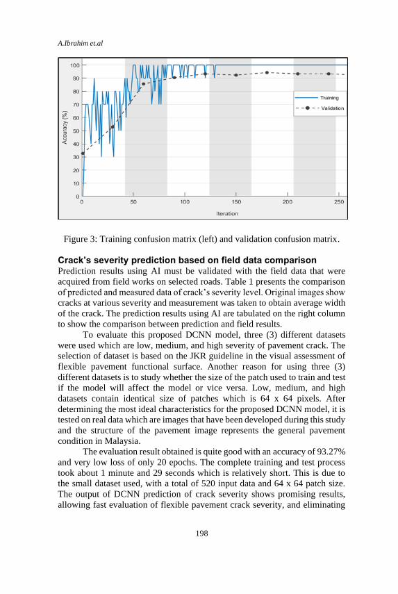
A.Ibrahim et.al
198
Figure 3: Training confusion matrix (left) and validation confusion matrix.
Crack’s severity prediction based on field data comparison Prediction results using AI must be validated with the field data that were
acquired from field works on selected roads. Table 1 presents the comparison
of predicted and measured data of crack’s severity level. Original images show
cracks at various severity and measurement was taken to obtain average width
of the crack. The prediction results using AI are tabulated on the right column
to show the comparison between prediction and field results.
To evaluate this proposed DCNN model, three (3) different datasets
were used which are low, medium, and high severity of pavement crack. The
selection of dataset is based on the JKR guideline in the visual assessment of
flexible pavement functional surface. Another reason for using three (3)
different datasets is to study whether the size of the patch used to train and test
if the model will affect the model or vice versa. Low, medium, and high
datasets contain identical size of patches which is 64 x 64 pixels. After
determining the most ideal characteristics for the proposed DCNN model, it is
tested on real data which are images that have been developed during this study
and the structure of the pavement image represents the general pavement
condition in Malaysia.
The evaluation result obtained is quite good with an accuracy of 93.27%
and very low loss of only 20 epochs. The complete training and test process
took about 1 minute and 29 seconds which is relatively short. This is due to
the small dataset used, with a total of 520 input data and 64 x 64 patch size.
The output of DCNN prediction of crack severity shows promising results,
allowing fast evaluation of flexible pavement crack severity, and eliminating
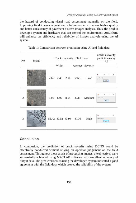
Flexible Pavement Crack’s Severity Identification
199
the hazard of conducting visual road assessment manually on the field.
Improving field images acquisition in future works will allow higher quality
and better consistency of pavement distress images analysis. Thus, the need to
develop a system and hardware that can control the environment conditions will enhance the efficiency and reliability of images analysis using the AI
system.
Table 1: Comparison between prediction using AI and field data
No Image Crack’s severity of field data
Crack’s severity
prediction using
AI
Width Average Severity
1
2.66 2.43 2.96 2.68 Low
2
5.06 6.02 8.04 6.37 Medium
3
58.42 40.92 43.94 47.76 High
Conclusion
In conclusion, the prediction of crack severity using DCNN could be
effectively conducted without relying on operator judgement on the field
assessment. Throughout the analysis of processing images, the objectives were
successfully achieved using MATLAB software with excellent accuracy of
output data. The predicted results using the developed system indicated a good
agreement with the field data, which proved the reliability of the system.
A.Ibrahim et.al
200
Acknowledgement
The authors would like to thank to all parties that support and involve directly
or indirectly into this research especially to Advanced Rehabilitation
Engineering in Diagnostic and Monitoring Research Group (AREDiM),
Universiti Teknologi MARA, Pulau Pinang and Universiti Teknologi MARA,
Shah Alam. This research is supported by the Fundamental Research Grant
Scheme (FRGS), Grant No: FRGS/1/2019/TK04/UITM/02/30. Also,
appreciation goes to the Ministry of Higher Education (MOHE) for giving
great privilege in providing scholarship as inspiring encouragement for the
success of this research.
References
[1] R. Salini, B. Xu and P. Paplauskas, “Pavement distress detection with
picucha methodology for area-scan cameras and dark images,” Civ. Eng.
J., vol. 1 no. 1 pp. 34 - 45, April 2017.
[2] A. Cubero-Fernandez, F. J. Rodriguez-Lozano, R. Villatoro, J. Olivares
and J. M. Palomares, “Efficient pavement crack detection and
classification,” EURASIP Journal on Image and Video Processing, vol.
39, June 2017.
[3] N. D. Hoang, “An artificial intelligence method for asphalt pavement
pothole detection using least squares support vector machine and neural
network with steerable filter-based feature extraction,” Advances in Civil
Engineering, pp. 1 – 12, June 2018.
[4] Y. Huang and B. Xu, “Automatic inspection of pavement cracking
distress,” Journal of Electronic Imaging, vol. 15, no. 1, January 2006.
[5] M. A. Qurishee, “Low-cost deep learning UAV and Raspberry Pi solution
to real time pavement condition assessment,” Department of Civil and
Chemical Engineering, University of Tennessee, 2019.
[6] S. Bhat, S. Naik, M. Gaonkar, P. Sawant, S. Aswale, and P. Shetgaonkar,
"A Survey on Road Crack Detection Techniques," 2020 International
Conference on Emerging Trends in Information Technology and
Engineering (ic-ETITE), Vellore, India, pp. 1-6, 2020.
[7] C. O. Tayo, N. B. Linsangan and R. V. Pellegrino, "Portable Crack Width
Calculation of Concrete Road Pavement Using Machine Vision," 2019
IEEE 11th International Conference on Humanoid, Nanotechnology,
Information Technology, Communication and Control, Environment, and
Management (HNICEM), Laoag, Philippines, pp. 1-5, 2019.
[8] Y. C. Tsai, V. Kaul, and R. M. Mersereau, “Critical Assessment of
Pavement Distress Segmentation Methods,” J. Transp. Eng., vol. 136, pp.
11-19, 2010.
Flexible Pavement Crack’s Severity Identification
201
[9] Q. Li, L. Zou, D. Zhang and Q. Mao, “FoSA: F* Seed-growing Approach
for crack-line detection from pavement images,” Image and Vision
Computing, vol. 29, no. 12, pp. 861-872, 2011.
[10] S. Wang, and W. Tang, “Pavement Crack Segmentation Algorithm
Based on Local Optimal Threshold of Cracks Density Distribution,” In:
Huang DS., Gan Y., Bevilacqua V., Figueroa J.C. (eds) Advanced
Intelligent Computing. ICIC 2011, Lecture Notes in Computer Science,
vol. 6838. Springer, Berlin, Heidelberg.
[11] A. Zhang, Q. Li, K. C. P. Wang and S. Qiu, “Matched Filtering Algorithm
for Pavement Cracking Detection,” Transportation Research Record, vol.
236, no. 1, pp. 30-42. 2013.
[12] L. Cui, Z. Qi, Z. Chen, F. Meng and Y. Shi, “Pavement Distress Detection
Using Random Decision Forests,” In: Zhang C. et al. (eds) Data Science.
ICDS 2015, Lecture Notes in Computer Science, vol. 9208.
[13] G. M. Hadjidemetriou, P. A. Vela and S. E. Christodoulou, “Automated
Pavement Patch Detection and Quantification Using Support Vector
Machines,” Journal of Computing in Civil Engineering, vol. 32 no. 1, pp.
1-11, 2018.
[14] N. D. Hoang and Q. L. Nguyen, “A novel method for asphalt pavement
crack classification based on image processing and machine learning,”
Engineering with Computers, vol. 35, pp. 487–498, 2019.
[15] N. D. Hoang, "An Artificial Intelligence Method for Asphalt Pavement
Pothole Detection Using Least Squares Support Vector Machine and
Neural Network with Steerable Filter-Based Feature Extraction,"
Advances in Civil Engineering, vol. 2018.
[16] M. Abambres and A Ferreira, “Application of ANN in pavement
engineering: State-of-Art,” SSRN Electronic Journal, 2017.
[17] Pavement Research Unit, “A Guide to the Visual Assessment of Flexible
Pavement Surface Conditions,” Jabatan Kerja Raya Malaysia, JKR
20709-2060-92, 1992.
[18] A. Ibrahim, M. K. Osman, N. A. Yusof, K. A. Ahmad, N. H. Harun, and
R. A. Raof, “Characterization of cracking in pavement distress using
image processing techniques and k-Nearest neighbour,” Indonesian
Journal of Electrical Engineering and Computer Science, vol. 14, no. 2.
2019.
[19] R. Yamashita, M. Nishio, R. K. Do and K. Togashi, “Convolutional neural
networks: an overview and application in radiology, Insights into
imaging,” vol. 9, issue 4, pp. 611-629, 2018.
[20] A. T. Azeez and N. Anupama, “Crack Pavement Detection Utilizing
Fuzzy Inference System,” Int. Journal of Scientific Engineering and
Technology Research, vol. 5, no. 7, pp. 1400-1404, 2016.
Journal of Mechanical Engineering Vol 18(2), 203-215, 2021
___________________
ISSN 1823-5514, eISSN 2550-164X Received for review: 2020-09-16
© 2021 College of Engineering, Accepted for publication: 2021-03-18
Universiti Teknologi MARA (UiTM), Malaysia. Published: 2021-04-15
Severity Effect of Methanol Toxicity from High Pressure Reactor
Z A Rashid*, M A Subri, M A Ahmad, M F I Ahmad Fuad, N S Japperi
Faculty of Chemical Engineering, Universiti Teknologi MARA,
40450 Shah Alam, Selangor, Malaysia
ABSTRACT
CO2 hydrogenation to methanol synthesis is one of the effective solutions to
mitigate the climate changes and the greenhouse gas emissions. However, the
drawbacks of this process needed it to operate at high pressure condition
where the possibility of leakage and fatality occur is possible. The simulation
of this process was simulated using Aspen HYSYS, ALOHA and Google Earth
to analyse the methanol toxicity severity from the high-pressure reactor. The
probit will determine the level of the severity. It shows that higher pressure
with bigger leakage size may experience high severity for the methanol is
achieved the highest severity at 400 bar with the bigger leakage size. As the
leakage size and pressure is increasing the exposure of the chemical is
increasing, thus increasing the severity to the surrounding.
Keywords: Risk Assessment; Severity; Consequence Modelling; Toxicity
Introduction
Methanol has a characteristic which are very toxic and very flammable.
Methanol is toxic when it enters the body by ingestion, inhalation, or
absorption through the skin and can be fatal due to depression of the central
nervous system which can lead to decreased respiratory rate, decreased heart
rate, and suppressed brain activity [1]. Methanol has colourless appearance,
hygroscopic and methanol is miscible or mixable with water completely. The
demand of methanol has increasing as fuel at global competition where the
needs to search the new alternatives of producing the chemical bulk is varied
[2]. Methanol is a feasible substitute for the energy source which offering a
suitable solution on large scale for the efficient energy storage, while it plays
a significant part in economy and sustainability by captured the carbon dioxide
from power plant and convert it into the methanol [3]. One of the alternatives

Z A Rashid et al.
204
is the methanol synthesis from hydrogen (H2) and carbon dioxide where carbon
dioxide is hydrogenated to methanol which has greater attention recently
because of the global warming such as greenhouse gas emission from the
industrial activities [4]. The importance of CO2 hydrogenation to methanol was
highlighted in the work using electricity and electrolysis for methanol
production [5], and study on power to fuel technologies [6].
Since 1920’s until 1960’s the methanol synthesis from syngas was
operated at pressure range from 250 bar to 350 bar and 320 oC to 450 oC. Then,
at 1970 the reaction operating condition switched to 50–100 bar and 200–300 oC due to present catalyst that more active [7]. However, the methanol
conversion percentage is still low (less 60%). Recently, advantage of using
high pressure has been discovered by several researchers [8]–[11]. In 2016,
based on experiment done by Gaikward et. al, have shown that under high-
pressure condition above a threshold temperature, the reaction overcomes
kinetic control, entering thermodynamically controlled regime. 90% CO2
conversion and >95% methanol selectivity was achieved with a very good
yield (0.9-2.4 gMeOH gcat -1h-1) at 442 bar [10]. In view of this fact, it can be
concluded that CO2 hydrogenation methanol synthesis process introduced is
operated at the high-pressure condition which is more than 100 bars, when the
experimental results show a 76.4 bar with recycle pressurized CO2
hydrogenation reactor, at a temperature of 288 oC, is able to produce a
conversion to methanol product of 24%. This methanol conversion percentage
increased to 35% (200 bar), 54% (300 bar), 87% (400 bar) and exceeded 90%
(500bar). However, this condition is possibly can lead to the leaking of the
reactor due to the high-pressure condition [12]. Furthermore, high temperature
combine with high pressure have more energy, lead to higher risk compare to
lower pressure [13]. The exposure of chemical from the reactor such as
methanol may lead to fatality to the human and environment. Based on past
incident, methanol has poison effect that can cause severe metabolic
disturbances, loss of sight, permanent neurologic dysfunction and also lead to
death [14]. This study aims to analyse the leakage from CO2 hydrogenation to
methanol synthesis reactor that operating at high pressure and determine the
severity effect from the CO2 hydrogenation to methanol synthesis process
which is methanol toxicity. The risk assessment analyses the severity of the
incident towards the human and environment if the methanol leakage occurred
in the plant. Currently, only few author works on high-pressure methanol plant
such as study on fatalities comparing pressure 76 bar and 442 bar [15], work
using artificial intelligent to predict percentage fatalities for methanol jet fire
[16], where other works not focus on risk assessment study for CO2
hydrogenation to methanol such as study on energy analysis for methanol plant
up to 950 bar and 1000 bar [17, 18], study on the thermodynamic equilibrium
using high-pressure methanol process [19], design and simulation CO2
hydrogenation to produce methanol for CO2 capture and energy analysis [20],
Severity Effect of Methanol Toxicity from High Pressure Reactor
205
works on CO2 and H2 different ratio to produce high yield methanol [21, 22],
works on CO2 and H2 1:3 ratio at high-pressure as high as 442 bar to produce
more methanol [10] [23].
Methodology
The assessment is focussed on severity effect of methanol plant in high
pressure condition. The reactor of the methanol is modelled to determine the
methanol produce based on 100, 200, 300, 400 and 500 bar. The volume of
reactor used was 7.6 m3, refer to the work by Mar Perez-Fortes et al. [24]. In
this study, mass flow rate into reactor was 91,500 kg/h, combining 80,500 kg/h
of CO2 and 11,000 kg/h of H2, while simulation study by Mar Perez-Fortes et
al. used 91,500 kg/h at inlet combined with recycle flow rate of 376, 200 kg/h,
to have 467,600 kg/h flow rate into reactor. Mar Perez-Fortes et al. using 42
m3 to contain 515 gas hourly space volume (GHSV), then this GHSV value
was used to get reactor volume of 7.6 m3 for this study. The severity effects of
methanol are determined based on the leakages and pressure simulations.
Modelling simulation The study is conducted by using the computer aided such as Aspen HYSYS,
ALOHA and Google Earth. The suitable fluid package for carbon dioxide
(CO2) process used is The Peng-Robinson equation of state. Peng Robinson
equation is suitable for mixtures of nonpolar and slightly polar compounds and
most widely used thermodynamic package as it applies to all applications
involving hydrocarbons [25]. The ALOHA is simulated to determine the radius
affected and downwind concentration which the location is located at Port
Kalama, WA. The coordinate location is 46o 01’18” N 122o 51’ 30.07” and has
elevation about 8 meters. The windspeed modelled is 1.6 m/s, temperature is
51.5 oF, surface roughness is 1 meter, class B, no inversion and humidity level
at 71%. All these data extracted from QRA report on Methanol Plant produced
by AcuTech Consulting Group [26]. The Google Earth is applied in order to
get affected mapping areas from consequence simulation. Figure 1 shows the
process diagram of reactor modelled in this analysis.

Z A Rashid et al.
206
Figure 1: Reactor’s process flow diagram.
Release rate formulation
The choked pressure is the maximum downstream pressure resulting in
maximum flow through the hole or pipe.
𝑃𝑐ℎ𝑜𝑘𝑒𝑑
𝑃1= (
2
𝛾+1)(𝛾𝛾−1⁄ )
(1)
Where Pchoked is maximum downstream pressure resulting in maximum flow,
P1 is upstream pressure (bar abs) and k is heat capacity ratio (1.2 for methanol).
𝑄𝑚,𝑐ℎ𝑜𝑘𝑒𝑑 = 𝐶𝑜𝐴𝑃𝑜√𝛾𝑔𝑐𝑀
𝑅𝑔𝑇𝑜(
2
𝛾+1)(𝛾+1)(𝛾−1)
(2)
Where Qm,choked is gas discharge rate, choked flow (kg/s) ,Co is discharge
coefficient (approximately 1.0 for gases) , A is hole cross-section area (m2), Po
is upstream pressure (N/m2), M is molecular weight (kg/kg-mol) (for methanol
1.2), Rg is gas constant (8314 J/kg-mole/°K) and T is upstream temperature
(K). Equation (1) and Equation (2) is referred in published Purple book [27].
𝑌 = 𝐾1 + 𝐾2 ln 𝑉 (3)
Where V is dose and Y is probit variable. Equation (3) provided by author in
QRA book [28].
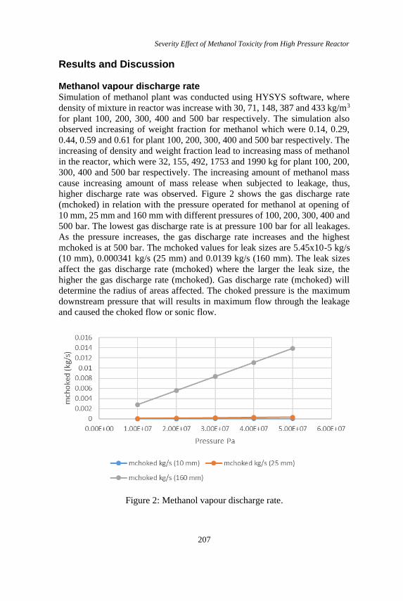
Severity Effect of Methanol Toxicity from High Pressure Reactor
207
Results and Discussion
Methanol vapour discharge rate Simulation of methanol plant was conducted using HYSYS software, where
density of mixture in reactor was increase with 30, 71, 148, 387 and 433 kg/m3
for plant 100, 200, 300, 400 and 500 bar respectively. The simulation also
observed increasing of weight fraction for methanol which were 0.14, 0.29,
0.44, 0.59 and 0.61 for plant 100, 200, 300, 400 and 500 bar respectively. The
increasing of density and weight fraction lead to increasing mass of methanol
in the reactor, which were 32, 155, 492, 1753 and 1990 kg for plant 100, 200,
300, 400 and 500 bar respectively. The increasing amount of methanol mass
cause increasing amount of mass release when subjected to leakage, thus,
higher discharge rate was observed. Figure 2 shows the gas discharge rate
(mchoked) in relation with the pressure operated for methanol at opening of
10 mm, 25 mm and 160 mm with different pressures of 100, 200, 300, 400 and
500 bar. The lowest gas discharge rate is at pressure 100 bar for all leakages.
As the pressure increases, the gas discharge rate increases and the highest
mchoked is at 500 bar. The mchoked values for leak sizes are 5.45x10⁻⁵ kg/s
(10 mm), 0.000341 kg/s (25 mm) and 0.0139 kg/s (160 mm). The leak sizes
affect the gas discharge rate (mchoked) where the larger the leak size, the
higher the gas discharge rate (mchoked). Gas discharge rate (mchoked) will
determine the radius of areas affected. The choked pressure is the maximum
downstream pressure that will results in maximum flow through the leakage
and caused the choked flow or sonic flow.
Figure 2: Methanol vapour discharge rate.
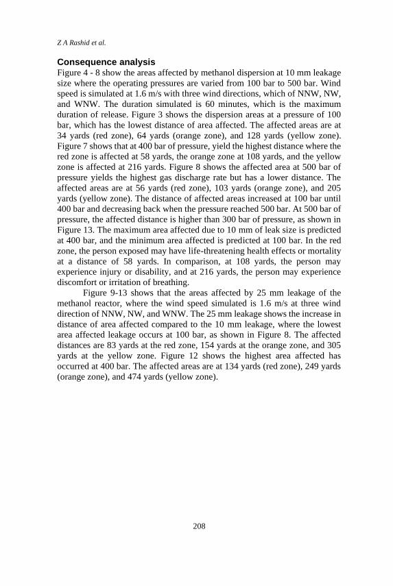
Z A Rashid et al.
208
Consequence analysis Figure 4 - 8 show the areas affected by methanol dispersion at 10 mm leakage
size where the operating pressures are varied from 100 bar to 500 bar. Wind
speed is simulated at 1.6 m/s with three wind directions, which of NNW, NW,
and WNW. The duration simulated is 60 minutes, which is the maximum
duration of release. Figure 3 shows the dispersion areas at a pressure of 100
bar, which has the lowest distance of area affected. The affected areas are at
34 yards (red zone), 64 yards (orange zone), and 128 yards (yellow zone).
Figure 7 shows that at 400 bar of pressure, yield the highest distance where the
red zone is affected at 58 yards, the orange zone at 108 yards, and the yellow
zone is affected at 216 yards. Figure 8 shows the affected area at 500 bar of
pressure yields the highest gas discharge rate but has a lower distance. The
affected areas are at 56 yards (red zone), 103 yards (orange zone), and 205
yards (yellow zone). The distance of affected areas increased at 100 bar until
400 bar and decreasing back when the pressure reached 500 bar. At 500 bar of
pressure, the affected distance is higher than 300 bar of pressure, as shown in
Figure 13. The maximum area affected due to 10 mm of leak size is predicted
at 400 bar, and the minimum area affected is predicted at 100 bar. In the red
zone, the person exposed may have life-threatening health effects or mortality
at a distance of 58 yards. In comparison, at 108 yards, the person may
experience injury or disability, and at 216 yards, the person may experience
discomfort or irritation of breathing.
Figure 9-13 shows that the areas affected by 25 mm leakage of the
methanol reactor, where the wind speed simulated is 1.6 m/s at three wind
direction of NNW, NW, and WNW. The 25 mm leakage shows the increase in
distance of area affected compared to the 10 mm leakage, where the lowest
area affected leakage occurs at 100 bar, as shown in Figure 8. The affected
distances are 83 yards at the red zone, 154 yards at the orange zone, and 305
yards at the yellow zone. Figure 12 shows the highest area affected has
occurred at 400 bar. The affected areas are at 134 yards (red zone), 249 yards
(orange zone), and 474 yards (yellow zone).
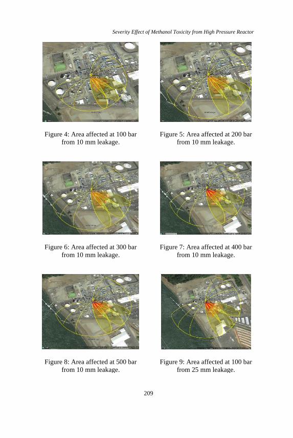
Severity Effect of Methanol Toxicity from High Pressure Reactor
209
Figure 4: Area affected at 100 bar
from 10 mm leakage.
Figure 5: Area affected at 200 bar
from 10 mm leakage.
Figure 6: Area affected at 300 bar
from 10 mm leakage.
Figure 7: Area affected at 400 bar
from 10 mm leakage.
Figure 8: Area affected at 500 bar
from 10 mm leakage.
Figure 9: Area affected at 100 bar
from 25 mm leakage.
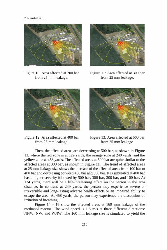
Z A Rashid et al.
210
Figure 10: Area affected at 200 bar
from 25 mm leakage.
Figure 11: Area affected at 300 bar
from 25 mm leakage.
Figure 12: Area affected at 400 bar
from 25 mm leakage.
Figure 13: Area affected at 500 bar
from 25 mm leakage.
Then, the affected areas are decreasing at 500 bar, as shown in Figure
13, where the red zone is at 129 yards, the orange zone at 240 yards, and the
yellow zone at 458 yards. The affected areas at 500 bar are quite similar to the
affected areas at 300 bar, as shown in Figure 11. The trend of affected areas
at 25 mm leakage size shows the increase of the affected areas from 100 bar to
400 bar and decreasing between 400 bar and 500 bar. It is simulated at 400 bar
has a higher severity followed by 500 bar, 300 bar, 200 bar, and 100 bar. At
134 yards, there will be a life-threatening effect on the person in the area
distance. In contrast, at 249 yards, the person may experience severe or
irreversible and long-lasting adverse health effects or an impaired ability to
escape the area. At 458 yards, the person may experience the discomfort of
irritation of breathing.
Figure 14 - 18 show the affected areas at 160 mm leakage of the
methanol reactor. The wind speed is 1.6 m/s at three different directions:
NNW, NW, and WNW. The 160 mm leakage size is simulated to yield the
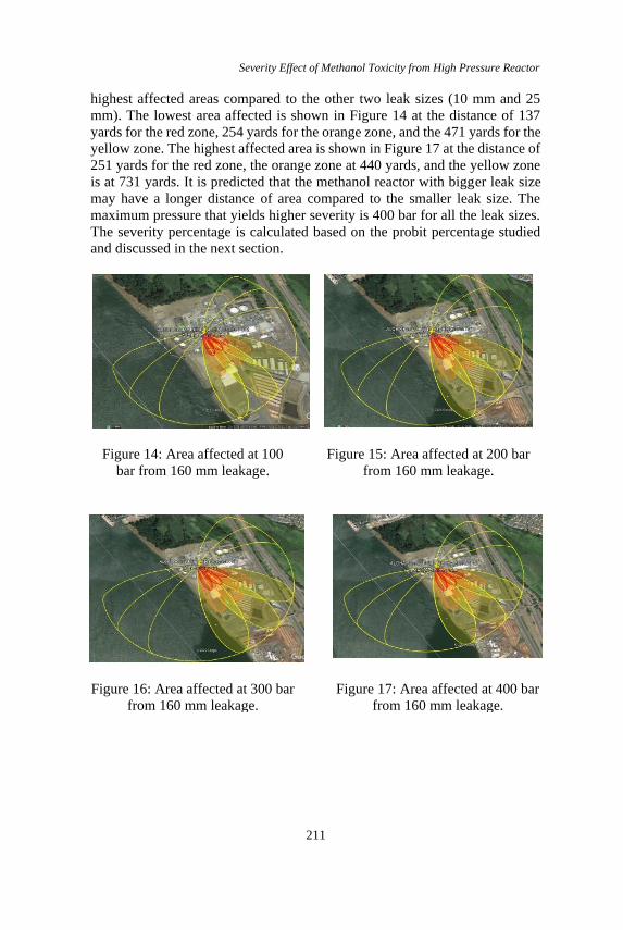
Severity Effect of Methanol Toxicity from High Pressure Reactor
211
highest affected areas compared to the other two leak sizes (10 mm and 25
mm). The lowest area affected is shown in Figure 14 at the distance of 137
yards for the red zone, 254 yards for the orange zone, and the 471 yards for the
yellow zone. The highest affected area is shown in Figure 17 at the distance of
251 yards for the red zone, the orange zone at 440 yards, and the yellow zone
is at 731 yards. It is predicted that the methanol reactor with bigger leak size
may have a longer distance of area compared to the smaller leak size. The
maximum pressure that yields higher severity is 400 bar for all the leak sizes.
The severity percentage is calculated based on the probit percentage studied
and discussed in the next section.
Figure 14: Area affected at 100
bar from 160 mm leakage.
Figure 15: Area affected at 200 bar
from 160 mm leakage.
Figure 16: Area affected at 300 bar
from 160 mm leakage.
Figure 17: Area affected at 400 bar
from 160 mm leakage.

Z A Rashid et al.
212
Figure 18: Area affected at 500 bar from
160 mm leakage. Methanol probit toxic release Table 1 shows the value of probit for each duration, from 10 minutes to 60
minutes, and categorized by three different types of exposure-response of
Acute Exposure Guideline Levels for Airborne Chemicals (AEGL). Each
level of AEGL has each concentration limit to methanol exposure, AEGL-3 at
7200 ppm, AEGL-2 at 2100 ppm, and AEGL-1 at 530 ppm. The severity of
methanol from the exposure of 10 minutes is 1.1% of people will suffer to the
exposure of AEGL-1, 0.3% of people will suffer to the exposure of AEGL-2,
and there will be no injury or exposure to people in AEGL-3 as the probit is
negative in values. At a duration of 20 minutes, the exposure from AEGL-1
will suffer about 1.5%, whereas AEGL-2 will expose the chemical to people
about 0.7% and no injury or any suffering at AEGL-3. At the duration of 30
minutes, the probit percentage increases, where about 1.8% of people will
suffer from exposure to AEGL-1. While 1% of people will experience at
AEGL-2, and 0.08% will suffer life-threatening effects at AEGL-3. As the
duration reached 40 minutes, 2% of people will suffer from AEGL-1, 1.2%
will suffer from AEGL-2, and 0.3% will suffer at an exposure of AEGL-3,
which can lead to mortality. In the duration of 50 minutes, the severity
increases as the people will experience 2.1% from AEGL-1, 1.3% will suffer
from the AEGL-2, and 0.4% will be exposed to AEGL-3. The highest score of
probit will be at duration 60 minutes, where 2.3% of people will suffer
irritation or discomfort of breathing, while 1.5% of people will suffer long-
lasting adverse health effects or an impaired ability to escape and 0.5% of
people surrounding may suffer which can lead to mortality. Figure 19 shows
most of the people surrounding will have higher exposure from AEGL-1.
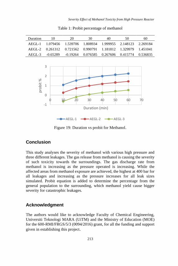
Severity Effect of Methanol Toxicity from High Pressure Reactor
213
Table 1: Probit percentage of methanol
Duration 10 20 30 40 50 60
AEGL-1 1.079456 1.539706 1.808934 1.999955 2.148123 2.269184
AEGL-2 0.261312 0.721562 0.990791 1.181812 1.329979 1.451041
AEGL-3 -0.65289 -0.19264 0.076585 0.267606 0.415774 0.536835
Figure 19: Duration vs probit for Methanol.
Conclusion This study analyses the severity of methanol with various high pressure and
three different leakages. The gas release from methanol is causing the severity
of such toxicity towards the surroundings. The gas discharge rate from
methanol is increasing as the pressure operated is increasing. While the
affected areas from methanol exposure are achieved, the highest at 400 bar for
all leakages and increasing as the pressure increases for all leak sizes
simulated. Probit equation is added to determine the percentage from the
general population to the surrounding, which methanol yield cause bigger
severity for catastrophic leakages.
Acknowledgment
The authors would like to acknowledge Faculty of Chemical Engineering,
Universiti Teknologi MARA (UiTM) and the Ministry of Education (MOE)
for the 600-RMI/FRGS/5/3 (0094/2016) grant, for all the funding and support
given in establishing this project.
-1
0
1
2
3
0 10 20 30 40 50 60 70
pro
bit
%
Duration (min)
AEGL-1 AEGL-2 AEGL-3
Z A Rashid et al.
214
References [1] J. V Ashurst and T. M. Nappe, “Methanol toxicity,” StatPearls [Internet],
2019.
[2] R. Kajaste, M. Hurme, and P. Oinas, “Methanol-Managing greenhouse
gas emissions in the production chain by optimizing the resource base,”
AIMS Energy, vol. 6, no. 6, pp. 1074–1102, 2018.
[3] A. A. Kiss, J. J. Pragt, H. J. Vos, G. Bargeman, and M. T. De Groot,
“Novel efficient process for methanol synthesis by CO2 hydrogenation,”
Chem. Eng. J., vol. 284, pp. 260–269, 2016.
[4] T. Kakumoto and T. Watanabe, “A theoretical study for methanol
synthesis by CO2 hydrogenation,” Catal. today, vol. 36, no. 1, pp. 39–44,
1997.
[5] C. Bergins, K. C. Tran, E. I. Koytsoumpa, E. Kakaras, T. Buddenberg,
and Ó. Sigurbjörnsson, “Power to methanol solutions for flexible and
sustainable operations in power and process industries,” Power-Gen Eur,
2015.
[6] S. Schemme, R. C. Samsun, R. Peters, and D. Stolten, “Power-to-fuel as
a key to sustainable transport systems–An analysis of diesel fuels
produced from CO2 and renewable electricity,” Fuel, vol. 205, pp. 198–
221, 2017.
[7] B. Tidona, C. Koppold, A. Bansode, A. Urakawa, and P. R. von Rohr,
“CO2 hydrogenation to methanol at pressures up to 950 bar,” J. Supercrit.
Fluids, vol. 78, pp. 70–77, 2013.
[8] R. Gaikwad, A. Bansode, and A. Urakawa, “High-pressure advantages in
stoichiometric hydrogenation of carbon dioxide to methanol,” J. Catal.,
vol. 343, pp. 127–132, 2016.
[9] S. Li, L. Guo, and T. Ishihara, “Hydrogenation of CO2 to methanol over
Cu/AlCeO catalyst,” Catal. Today, vol. 339, pp. 352–361, 2020.
[10] R. Gaikwad, A. Bansode, and A. Urakawa, “High-pressure advantages in
stoichiometric hydrogenation of carbon dioxide to methanol,” J. Catal.,
vol. 343, no. April, pp. 127–132, 2016.
[11] R. Gaikwad, H. Reymond, N. Phongprueksathat, P. R. von Rohr, and A.
Urakawa, “From CO or CO2?: space-resolved insights into high-pressure
CO2 hydrogenation to methanol over Cu/ZnO/Al2O3,” Catal. Sci.
Technol., vol. 10, no. 9, pp. 2763–2768, 2020.
[12] A.-M. Heikkilä, “Inherent safety in process plant design,” VTT Publ, pp.
1–132, 1999.
[13] R. Srinivasan and N. T. Nhan, “A statistical approach for evaluating
inherent benign-ness of chemical process routes in early design stages,”
Process Saf. Environ. Prot., vol. 86, no. 3, pp. 163–174, 2008.
[14] N. Yayci, H. Ağritmiş, A. Turla, and S. Koç, “Fatalities due to methyl
alcohol intoxication in Turkey: an 8-year study,” Forensic Sci. Int., vol.
Severity Effect of Methanol Toxicity from High Pressure Reactor
215
131, no. 1, pp. 36–41, 2003.
[15] M. Aizad and A. Rashid, “Fatality assessment for high pressure reactor of
methanol production plants from CO2 hydrogenation,” Malaysian J.
Chem. Eng. Technol., vol. 2, pp. 26–40, 2019.
[16] M. A. Ahmad and Z. A. Rashid, “Adaptive neuro-fuzzy inference system
prediction method for percentage fatalities of jet fire incident in methanol
production plant,” Int. J. Eng. Adv. Technol., vol. 9, no. 1, pp. 5766–5772,
2019.
[17] P. R. Tidona, B., Koppold, C., Bansode, A., Urakawa, A., & von Rohr,
“CO2 hydrogenation to methanol at pressures up to 950 bar,” J. Supercrit.
Fluids, vol. 78, pp. 70–77, 2013.
[18] B. Tidona, “Hydrogenation of carbon dioxide in a flow microreactor at
pressures up to 1000 bar.” ETH Zurich, 2013.
[19] J. G. Van Bennekom et al., “Methanol synthesis beyond chemical
equilibrium,” Chem. Eng. Sci., vol. 87, pp. 204–208, 2013.
[20] É. S. Van-Dal and C. Bouallou, “Design and simulation of a methanol
production plant from CO2 hydrogenation,” J. Clean. Prod., vol. 57, pp.
38–45, 2013.
[21] A. B. Bansode, “Exploiting high pressure advantages in catalytic
hydrogenation of carbon dioxide to methanol.” Universitat Rovira i
Virgili, 2014.
[22] A. Bansode and A. Urakawa, “Towards full one-pass conversion of
carbon dioxide to methanol and methanol-derived products,” J. Catal.,
vol. 309, pp. 66–70, 2014.
[23] R. Gaikwad, “Carbon dioxide to methanol: stoichiometric catalytic
hydrogenation under high pressure conditions.” Universitat Rovira i
Virgili, 2018.
[24] M. Pérez-Fortes, J. C. Schöneberger, A. Boulamanti, and E. Tzimas,
“Methanol synthesis using captured CO2 as raw material: Techno-
economic and environmental assessment,” Appl. Energy, vol. 161, pp.
718–732, 2016.
[25] R. Stryjek and J. H. Vera, “PRSV: An improved Peng—Robinson
equation of state for pure compounds and mixtures,” Can. J. Chem. Eng.,
vol. 64, no. 2, pp. 323–333, 1986.
[26] AcuTech Consulting Group, “Quantitative risk assessment final report
prepared for : NW Innovation Works, Port of Kalama,” February, 2016.
[27] P. G. Stoffen, “Guidelines for quantitative risk assessment,” Minist. van
Volkshuisv. Ruimtelijke Ordening en Milieu. CPR E, vol. 18, 2005.
[28] J. Casal, 2nd Ed., Evaluation of the effects and consequences of major
accidents in industrial plants. Amsterdam: Elsevier, 2017.
Journal of Mechanical Engineering Vol 18(2), 217-234, 2021
___________________ ISSN 1823-5514, eISSN 2550-164X Received for review: 2020-04-30
© 2021 College of Engineering, Accepted for publication: 2021-03-09
Universiti Teknologi MARA (UiTM), Malaysia. Published: 2021-04-15
Artificial Neural Network Predictive Modelling of Laser Micro-
Grooving for Commercial Pure Titanium (CP Ti) Grade 2
Sivaraos*, A.K Zuhair, M.S. Salleh, M.A.M. Ali
Faculty of Manufacturing Engineering,
Universiti Teknikal Malaysia Melaka (UTeM), Malaysia
Kadirgama
Faculty of Engineering Technology Mechanical and Automotive,
Universiti Malaysia Pahang, Malaysia
U.K. Dubey
Amity University, Uttar Pradesh, India
Satish Pujari
Lendi Institute of Engineering and Technology,
Vizianagaram, Andhra Pradesh, India
L.D. Sivakumar
Faculty of Mechanical Engineering,
Universiti Teknikal Malaysia Melaka (UTeM), Malaysia
ABSTRACT
Grooving is the process of making a narrow channel on a surface of flat or
cylindrical workpiece. Groove is precisely made to parts used in automotive,
biomedical, and electronics industries. In automotive industries, groove plays
an important role especially on mechanical parts to precisely locate seal (o-
ring) to prevent gas/oil leakage between dynamic mating parts. On the other
hand, artificial neural network (ANN) has been widely used in developing
predictive models of various manufacturing processes to save huge amount of
production time and money for industries. Unfortunately, very limited research
has been investigated on micro groove quality employing ANN predictive
models. Therefore, this research work presents on how the Artificial Neural
Network (ANN) predictive model has been established, optimised and utilised
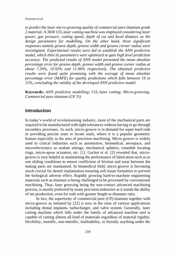
Sivaraos et al.
218
to predict the laser micro-grooving quality of commercial pure titanium grade
2 material. A 3KW CO2 laser cutting machine was employed considering laser
power, gas pressure, cutting speed, depth of cut and focal distance as the
design parameters for modelling. On the other hand, three significant
responses namely groove depth, groove width and groove corner radius were
investigated. Experimental results were fed to establish the ANN predictive
model, which then its parameters were optimized to gain high level prediction
accuracy. The predicted results of ANN model presented the mean absolute
percentage error for groove depth, groove width and groove corner radius at
about 7.29%, 10.93% and 11.96% respectively. The obtained predictive
results were found quite promising with the average of mean absolute
percentage error (MAPE) for quality predictions which falls between 10 to
15%, concluding the validity of the developed ANN predictive model.
Keywords: ANN predictive modelling; CO2 laser cutting; Micro-grooving;
Commercial pure titanium (CP Ti)
Introduction
In today’s world of revolutionising industry, most of the mechanical parts are
required to be manufactured with tight tolerances without having to go through
secondary processes. As such, micro-groove is in demand for super-hard rods
in providing precise seats to locate seals, where it is a popular geometric
feature especially in the area of precision machining. Micro groove is widely
used in critical industries such as automotive, biomedical, aerospace, and
microelectronics as sealant sittings, mechanical splitters, rotatable locating
rings, micro-sprue actuators, etc. [1]. Gachot et al. [2] revealed that, micro-
groove is very helpful in maintaining the performance of lubrication such as in
wet sliding conditions to ensure coefficient of friction and wear between the
mating parts are maintained. In biomedical field, micro-groove is becoming
much crucial for dental implantation ensuring soft tissue formation to prevent
the biological adverse effect. Rapidly growing hard-to-machine engineering
materials such as titanium is being challenged to be processed by conventional
machining. Thus, laser grooving being the non-contact advanced machining
process, is mostly preferred by many precision industries as it stands the ability
of net production, even for rods with greater length to diameter ratio.
In fact, the superiority of commercial pure (CP) titanium together with
micro-groove as initiated by [22] is now in the raise of various applications
including dental implants, turbocharger, and valve system. Generally, laser
cutting machine which falls under the family of advanced machine tool is
capable of cutting almost all kind of materials regardless of material rigidity,
flexibility, metallic, non-metallic, malleability, or literally anything under the
ANN Predictive Modeling of Laser Micro-Grooving for Titanium Grade 2
219
sky for the matter. Thus, laser cutting is often used as precision machining
preference which is also able to produce micro level grooves, holes, and
corners with tight tolerances due to its excellent kerf width and narrower heat
affected zone [3]. But then, practical applications of the laser advancements by
newly exploring industries often spend huge amount of production time and
materials which leads into unnecessary money spending before arriving at the
final decision of the process parameters setting. In conjunction to that, the
machinability investigation of titanium alloy (Ti-6Al-4V) using laser
machining has been successfully performed by controlling the material
removal rate to attain desired surface roughness [4]. The micro grooving of Ti-
6Al-4V alloys conducted by [5] reveals that, a good quality of 8-12 μm groove
depth and width was achieved by controlling the pulse frequency, scan speed,
and focal length which have direct control over the laser spot size. Taweeporn
et al. [6] performed underwater laser micromachining of titanium alloy with
different sets of temperatures. It was found that, the effect of laser power,
traverse speed and numbers of laser passes are much significant for deep
grooving. In fact, to have the laser processing phenomenon be well understood,
[7] has modelled the micro-grooving process by employing Artificial Neural
Network (ANN).
ANN multi-objective model was developed to optimize the process
parameters of yttrium aluminium garnet (YAG) laser for minimum depth
investigation of micro-turning by [8]. ANN model developed by [9] was
capable to accurately predict the surface quality of CNC turning processes as
compared to Taguchi model. Sathish et al., [10] investigated the ANN
predicted of methane yield by different parameters selection and the model
was proven to be efficient within the settings of feed forward network (FFN)
with one hidden layer was a better approach over other common types for
methane content prediction. Ming-Jong [11] has investigated the cut quality
measurements of Quad Flat Non-lead (QFN) package which is depth of cutting
line, width of heat affected zone, cutting line of epoxy, and copper-
compounded using back propagation neural network model. On top of that,
four algorithms including broyden fletcher goldfarb shanno quasi-newton
(BFG), scaled conjugate gradient (SCG), gradient descent (GD), and
lavenberg-marquardt (LM) were also used to simulate the model. Ming-Jong
concluded that, LM algorithm is an optimal algorithm which yields much
lower error predictions as compared to other optimised algorithms.
On the other hand, optimization of surface roughness has been studied
and modelled employing ANN by [12]. The model shows that, 4-7-1 structure
predicts best cut quality of surface roughness with properly controlled three
design parameters which are cutting speed, power, and assist gas pressure. It
has been summarised that, cutting speed plays an important role as compared
to other tested parameters. The optimized model of hybrid Taguchi artificial
Sivaraos et al.
220
neural network hybrid with genetic algorithm based model was developed by
[13] to predict the CO2 laser cut quality. The model succeeded to predict the
cut quality accuracy with the prediction error of not more than 10%. ANN
modelling is able to reduce the production cost particularly in precision
industries which often waste a lot of experimental time and raw materials to
arrive into the optimal settings, especially if it involves new material or new
processing [15]. Properly designed ANN model architecture with optimised
parameters will be powerful enough to capture the relationship between input
and output parameters. The pattern learning ability of ANN makes it a very
powerful predictive modelling tool. In other words, artificial neural network
can be classified as a black box model which provides information behind the
processing physics explicitly [16].
ANN model is often adopted for prediction and optimization of many
processes including laser micro-grooving process as it has the ability to
compute the very non-linear process phenomenon including laser machining.
According to [17], the artificial neural network model can be simplified using
mathematical expression as shown in Equation (1).
+=
=
bkwFkym
i
i )()(0
(1)
where;
xi (k) is input value in discrete time k where i goes to 0 to m
wi (k) is weight value in discrete time k where i goes from 0 to m
b is bias
F is a transfer function
yi (k) is output value in discrete time k
As to achieve the primary objective of this research which is to predict
laser grooving quality of commercial pure titanium grade 2, various critical
steps have been performed towards developing a sound ANN model to ensure
that the attainable values are within desired values.
Experimental setup and procedures
The aim of this experimental based modelling research is to develop, optimise
and validate ANN model to predict and experimentally validate micro-groove
quality of laser processed commercial pure (CP) titanium grade 2 rods. The
material was selected based on high demand of wide applications in the area
of aerospace, architecture, power generation, medical industry, hydro-carbon
processing, marine industry and so on [27]. The CP titanium grade 2 is well
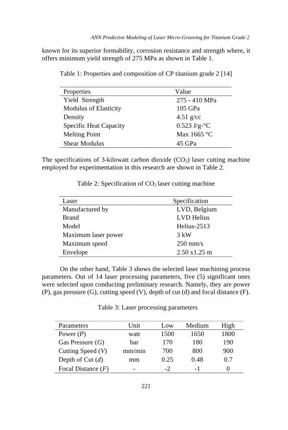
ANN Predictive Modeling of Laser Micro-Grooving for Titanium Grade 2
221
known for its superior formability, corrosion resistance and strength where, it
offers minimum yield strength of 275 MPa as shown in Table 1.
Table 1: Properties and composition of CP titanium grade 2 [14]
The specifications of 3-kilowatt carbon dioxide (CO2) laser cutting machine
employed for experimentation in this research are shown in Table 2.
Table 2: Specification of CO2 laser cutting machine
On the other hand, Table 3 shows the selected laser machining process
parameters. Out of 14 laser processing parameters, five (5) significant ones
were selected upon conducting preliminary research. Namely, they are power
(P), gas pressure (G), cutting speed (V), depth of cut (d) and focal distance (F).
Table 3: Laser processing parameters
Properties Value
Yield Strength
275 - 410 MPa
Modulus of Elasticity
105 GPa
Density
4.51 g/cc
Specific Heat Capacity
0.523 J/g-°C
Melting Point
Max 1665 °C
Shear Modulus 45 GPa
Laser Specification
Manufactured by
LVD, Belgium
Brand
LVD Helius
Model
Helius-2513
Maximum laser power
3 kW
Maximum speed
250 mm/s
Envelope 2.50 x1.25 m
Parameters Unit Low Medium High
Power (P)
watt
1500
1650
1800
Gas Pressure (G)
bar
170
180
190
Cutting Speed (V)
mm/min
700
800
900
Depth of Cut (d)
mm
0.25
0.48
0.7
Focal Distance (F) - -2 -1 0
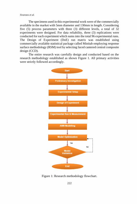
Sivaraos et al.
222
The specimens used in this experimental work were of the commercially
available in the market with 5mm diameter and 130mm in length. Considering
five (5) process parameters with three (3) different levels, a total of 32
experiments were designed. For data reliability, three (3) replications were
conducted for each experiment which sums into the total 96 experimental runs.
The Design of Experiment (DoE) run matrix was established using
commercially available statistical package called Minitab employing response
surface methodology (RSM) tool by selecting faced cantered central composite
design (CCD).
The entire research was carefully design and conducted based on the
research methodology established as shown Figure 1. All primary activities
were strictly followed accordingly.
Figure 1: Research methodology flowchart.

ANN Predictive Modeling of Laser Micro-Grooving for Titanium Grade 2
223
The laser grooving process was performed onto the CP titanium grade
2 rod(s) by securing within a three-jaw chuck attached onto a specially
designed speed-controlled spinning device. The spinner was properly aligned
in the transverse direction laser bean to provide lathe alike interaction. Figure
2 shows how the spinner was mounted and used for laser grooving. The laser
machine used in the experimental work was a 2.5 x 1.25 meter flatbed where
the interaction of the linearly moving bed axes with spinning speed
controllable device enabled the development of a cost effective 3D laser
grooving possibility.
Figure 2: Flatbed Laser with integrated spinner chuck.
The depth, width, and corner radius of the produced micro-groove by
laser machine was precisely measured using 20-4600 series model optical
comparator made by Scherr-Tumico as shown in Figure 3.
Figure 3: Measuring of micro-groove with optical comparator.
Rotating Glass Screen
Kerf Width Image
Digital Readout (DRO)
Specimen
Tungsten Halogen Ray
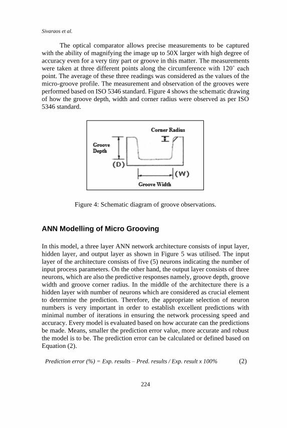
Sivaraos et al.
224
The optical comparator allows precise measurements to be captured
with the ability of magnifying the image up to 50X larger with high degree of
accuracy even for a very tiny part or groove in this matter. The measurements
were taken at three different points along the circumference with 120˚ each
point. The average of these three readings was considered as the values of the
micro-groove profile. The measurement and observation of the grooves were
performed based on ISO 5346 standard. Figure 4 shows the schematic drawing
of how the groove depth, width and corner radius were observed as per ISO
5346 standard.
Figure 4: Schematic diagram of groove observations.
ANN Modelling of Micro Grooving
In this model, a three layer ANN network architecture consists of input layer,
hidden layer, and output layer as shown in Figure 5 was utilised. The input
layer of the architecture consists of five (5) neurons indicating the number of
input process parameters. On the other hand, the output layer consists of three
neurons, which are also the predictive responses namely, groove depth, groove
width and groove corner radius. In the middle of the architecture there is a
hidden layer with number of neurons which are considered as crucial element
to determine the prediction. Therefore, the appropriate selection of neuron
numbers is very important in order to establish excellent predictions with
minimal number of iterations in ensuring the network processing speed and
accuracy. Every model is evaluated based on how accurate can the predictions
be made. Means, smaller the prediction error value, more accurate and robust
the model is to be. The prediction error can be calculated or defined based on
Equation (2).
Prediction error (%) = Exp. results – Pred. results / Exp. result x 100% (2)
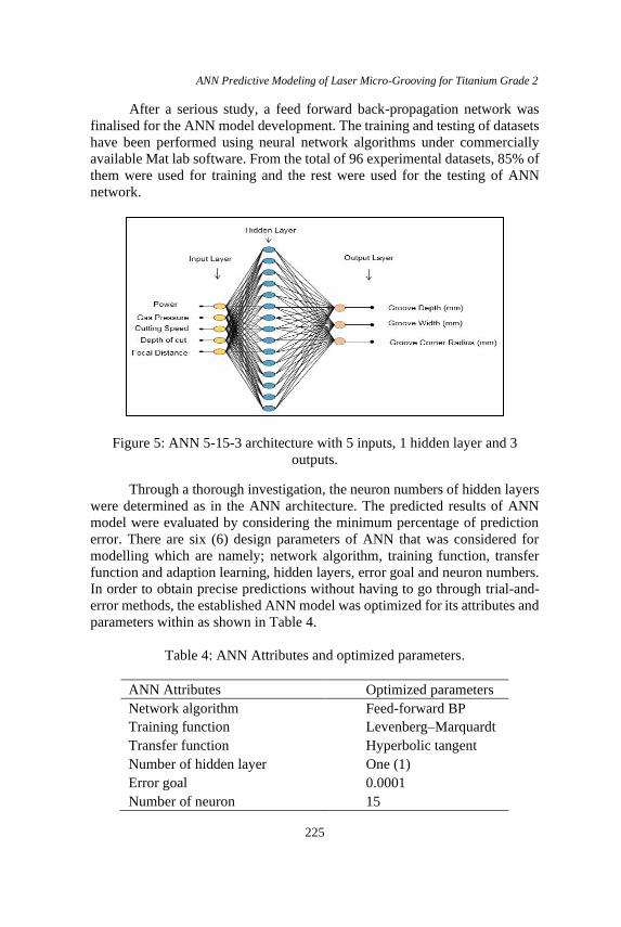
ANN Predictive Modeling of Laser Micro-Grooving for Titanium Grade 2
225
After a serious study, a feed forward back-propagation network was
finalised for the ANN model development. The training and testing of datasets
have been performed using neural network algorithms under commercially
available Mat lab software. From the total of 96 experimental datasets, 85% of
them were used for training and the rest were used for the testing of ANN
network.
Figure 5: ANN 5-15-3 architecture with 5 inputs, 1 hidden layer and 3
outputs.
Through a thorough investigation, the neuron numbers of hidden layers
were determined as in the ANN architecture. The predicted results of ANN
model were evaluated by considering the minimum percentage of prediction
error. There are six (6) design parameters of ANN that was considered for
modelling which are namely; network algorithm, training function, transfer
function and adaption learning, hidden layers, error goal and neuron numbers.
In order to obtain precise predictions without having to go through trial-and-
error methods, the established ANN model was optimized for its attributes and
parameters within as shown in Table 4.
Table 4: ANN Attributes and optimized parameters.
ANN Attributes Optimized parameters
Network algorithm Feed-forward BP
Training function Levenberg–Marquardt
Transfer function Hyperbolic tangent
Number of hidden layer One (1)
Error goal 0.0001
Number of neuron 15
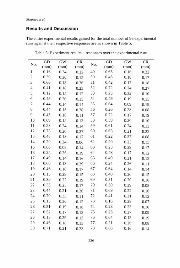
Sivaraos et al.
226
Results and Discussion
The entire experimental results gained for the total number of 96 experimental
runs against their respective responses are as shown in Table 5.
Table 5: Experiment results – responses over the experimental runs
No. GD
(mm)
GW
(mm)
CR
(mm) No.
GD
(mm)
GW
(mm)
CR
(mm)
1 0.16 0.34 0.12 49 0.65 0.16 0.22
2 0.39 0.20 0.15 50 0.45 0.18 0.17
3 0.66 0.18 0.26 51 0.42 0.17 0.18
4 0.41 0.18 0.23 52 0.72 0.24 0.27
5 0.12 0.15 0.12 53 0.25 0.32 0.10
6 0.43 0.20 0.15 54 0.49 0.19 0.15
7 0.44 0.14 0.14 55 0.64 0.09 0.19
8 0.44 0.15 0.28 56 0.26 0.28 0.08
9 0.45 0.16 0.11 57 0.72 0.17 0.19
10 0.69 0.15 0.13 58 0.59 0.20 0.10
11 0.23 0.24 0.14 59 0.61 0.24 0.13
12 0.73 0.20 0.27 60 0.63 0.21 0.22
13 0.48 0.18 0.17 61 0.22 0.27 0.08
14 0.20 0.24 0.06 62 0.20 0.23 0.15
15 0.68 0.08 0.14 63 0.23 0.29 0.17
16 0.24 0.26 0.19 64 0.48 0.17 0.12
17 0.49 0.14 0.16 66 0.49 0.21 0.12
18 0.66 0.13 0.29 66 0.24 0.26 0.11
19 0.46 0.18 0.17 67 0.64 0.14 0.14
20 0.13 0.29 0.15 68 0.48 0.20 0.15
21 0.39 0.22 0.19 69 0.51 0.20 0.16
22 0.35 0.25 0.17 70 0.30 0.29 0.08
23 0.44 0.21 0.20 71 0.69 0.22 0.16
24 0.20 0.33 0.11 72 0.41 0.21 0.12
25 0.13 0.30 0.12 73 0.16 0.28 0.07
26 0.51 0.19 0.18 74 0.23 0.23 0.10
27 0.52 0.17 0.13 75 0.25 0.27 0.09
28 0.18 0.29 0.13 76 0.64 0.13 0.19
29 0.46 0.18 0.15 77 0.21 0.26 0.08
30 0.71 0.21 0.23 78 0.66 0.16 0.14

ANN Predictive Modeling of Laser Micro-Grooving for Titanium Grade 2
227
Based on the experimental results, ANN model with multiple outputs
has been developed. Various architectures were designed, optimised and tested
where in this case, 5-15-3 architecture was seen to be fitting best and therefore
it is selected for this modelling process. Table 6 shows the optimised neural
network parameters within the 5-15-3 network architecture.
Table 6: ANN parameters for 5-15-3 architecture
ANN Parameter Value
Network Architecture
5-15-3
Training/Testing Data
83/13
Network
Feed forward back Propagation
Performance
MSE
Training Function
Trainlm
Transfer Function
Tansig/Tansig
Learning Function LearnGDM
Figure 6 shows the performance simulation of the developed model for
training environment. The ANN model training performance was determined
based on the lowest Mean Square Error (MSE) gained. The training curve
31 0.73 0.14 0.24 79 0.67 0.12 0.18
32 0.44 0.21 0.15 80 0.20 0.25 0.08
33 0.41 0.22 0.12 81 0.48 0.23 0.10
34 0.21 0.31 0.10 82 0.49 0.24 0.11
35 0.15 0.27 0.14 83 0.49 0.20 0.12
36 0.40 0.13 0.15 84 0.23 0.26 0.10
37 0.22 0.37 0.15 85 0.17 0.21 0.10
38 0.72 0.12 0.14 86 0.7 0.17 0.16
39 0.37 0.19 0.17 87 0.66 0.15 0.14
40 0.61 0.18 0.24 88 0.52 0.16 0.15
41 0.22 0.35 0.15 89 0.50 0.23 0.19
42 0.38 0.26 0.16 90 0.71 0.14 0.16
43 0.43 0.19 0.22 91 0.48 0.19 0.13
44 0.58 0.14 0.16 92 0.44 0.20 0.10
45 0.43 0.19 0.14 93 0.65 0.20 0.13
46 0.40 0.19 0.13 94 0.47 0.22 0.14
47 0.48 0.22 0.14 95 0.49 0.17 0.15
48 0.47 0.21 0.16 96 0.60 0.15 0.16
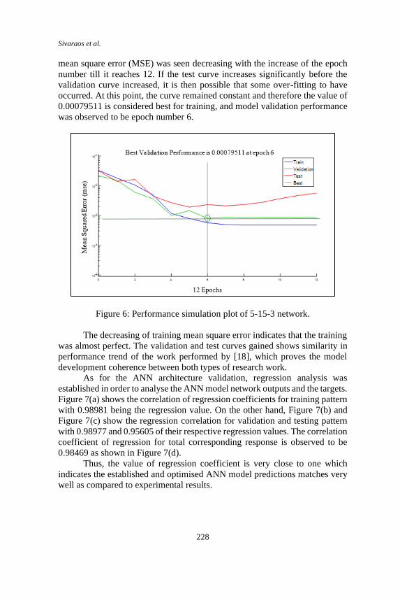
Sivaraos et al.
228
mean square error (MSE) was seen decreasing with the increase of the epoch
number till it reaches 12. If the test curve increases significantly before the
validation curve increased, it is then possible that some over-fitting to have
occurred. At this point, the curve remained constant and therefore the value of
0.00079511 is considered best for training, and model validation performance
was observed to be epoch number 6.
Figure 6: Performance simulation plot of 5-15-3 network.
The decreasing of training mean square error indicates that the training
was almost perfect. The validation and test curves gained shows similarity in
performance trend of the work performed by [18], which proves the model
development coherence between both types of research work.
As for the ANN architecture validation, regression analysis was
established in order to analyse the ANN model network outputs and the targets.
Figure 7(a) shows the correlation of regression coefficients for training pattern
with 0.98981 being the regression value. On the other hand, Figure 7(b) and
Figure 7(c) show the regression correlation for validation and testing pattern
with 0.98977 and 0.95605 of their respective regression values. The correlation
coefficient of regression for total corresponding response is observed to be
0.98469 as shown in Figure 7(d).
Thus, the value of regression coefficient is very close to one which
indicates the established and optimised ANN model predictions matches very
well as compared to experimental results.
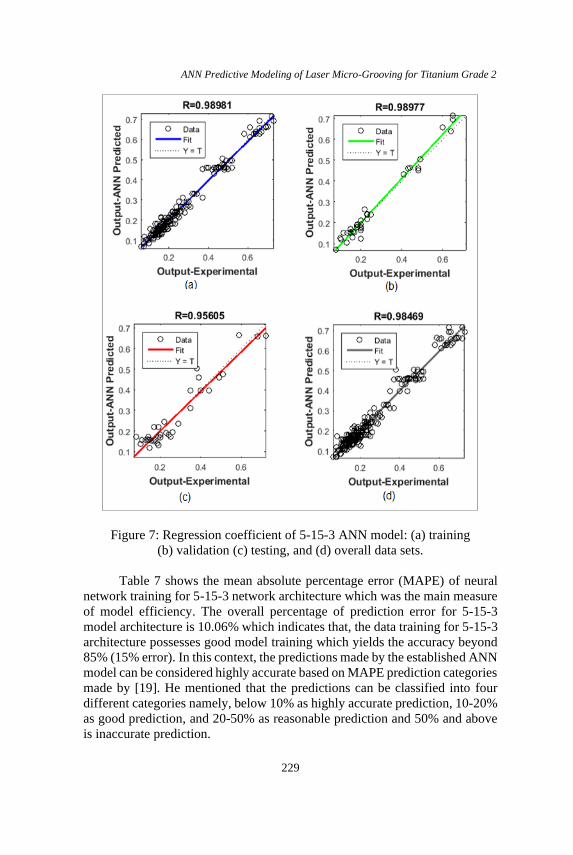
ANN Predictive Modeling of Laser Micro-Grooving for Titanium Grade 2
229
Figure 7: Regression coefficient of 5-15-3 ANN model: (a) training
(b) validation (c) testing, and (d) overall data sets.
Table 7 shows the mean absolute percentage error (MAPE) of neural
network training for 5-15-3 network architecture which was the main measure
of model efficiency. The overall percentage of prediction error for 5-15-3
model architecture is 10.06% which indicates that, the data training for 5-15-3
architecture possesses good model training which yields the accuracy beyond
85% (15% error). In this context, the predictions made by the established ANN
model can be considered highly accurate based on MAPE prediction categories
made by [19]. He mentioned that the predictions can be classified into four
different categories namely, below 10% as highly accurate prediction, 10-20%
as good prediction, and 20-50% as reasonable prediction and 50% and above
is inaccurate prediction.
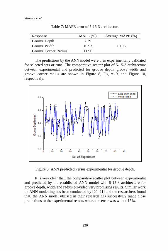
Sivaraos et al.
230
Table 7: MAPE error of 5-15-3 architecture
Response MAPE (%) Average MAPE (%)
Groove Depth 7.29
10.06 Groove Width 10.93
Groove Corner Radius 11.96
The predictions by the ANN model were then experimentally validated
for selected sets or runs. The comparative scatter plot of 5-15-3 architecture
between experimental and predicted for groove depth, groove width and
groove corner radius are shown in Figure 8, Figure 9, and Figure 10,
respectively.
Figure 8: ANN predicted versus experimental for groove depth.
It is very clear that, the comparative scatter plot between experimental
and predicted by the established ANN model with 5-15-3 architecture for
groove depth, width and radius provided very promising results. Similar work
on ANN modelling has been conducted by [20, 21] and the researchers found
that, the ANN model utilised in their research has successfully made close
predictions to the experimental results where the error was within 15%.

ANN Predictive Modeling of Laser Micro-Grooving for Titanium Grade 2
231
Figure 9: ANN predicted versus experimental for groove width.
Figure 10: ANN predicted versus experimental for groove corner radius.
Sivaraos et al.
232
The exact overlapping of almost 85% of the signature graph spikes
between experimental and predicted values proves that, a properly designed
and optimised ANN model is capable of capturing the pattern and processing
behaviour of even a complex and non-linear parametric relationship, in this
case even for non-linear laser machining process.
Conclusions
Developing an artificial intelligence neural network model to understand the
phenomena of a complex and non-linear laser processing to predict micro-
grooving quality of CP Titanium Grade 2 has been successfully conducted
besides attaining efficient predictions. Perhaps, a flatbed laser machine was
modified by integrating a controllable spinning device to perform laser micro-
grooving on a cylindrical part. Transforming the flat to 3D machining is
primary contribution of this work where, it would be a cost effective solution
for most precision metal machining industries. Secondly, the developed and
optimised ANN model with 5-15-3 architecture was able to precisely predict
the machining accuracy and cut geometry quality. The model stands to
contribute in terms of cost and time saving to most industries employing laser
lathing as their primary businesses. As to improve the parameter selection of
laser cutting accuracy, an effective ANN model selection has been developed
in this research to model the experiment before bringing it into actual
environment. The results show that, the ANN model was able to predict the
desired responses; groove depth, groove width, and corner radius. The
achieved mean absolute percentage error (MAPE) for groove depth, width and
corner radius was about 10% in average, where each of them yields with
7.29%, 10.93% and 11.96% respectively. This indicates the model robustness
allowing the predictions to achieve as high as 90% in accuracy. As overall, the
development of ANN model and the validation between predictive model and
experiment shows an excellent agreement. To move forward and explore ahead
within the field and further enhance the prediction accuracy, it is strongly
recommended to develop Adapted Neuro-Fuzzy Inference System (ANFIS)
predictive model where the attained results can be directly compared with the
attained results.
Acknowledgement
The authors would like to thank the top management of Universiti Teknikal
Malaysia Melaka, as well as Faculty of manufacturing Engineering for their
continuous support in having this research completed as scheduled.
Prediction of Micro-Grooving for Titanium Grade 2 using ANN
References
[1] C. Chen, J. Li, S. Zhan, Z. Yu, and W. Xu, “Study of micro groove
machining by micro ECM,” Proc. CIRP, vol. 42, pp. 418-422, 2016.
[2] C. Gachot, A. Rosenkranz, S.M Hsu, and H.L Costa, “A critical
assessment of surface texturing for friction and wear improvement,” Wear
vol. 372–373, pp. 21–41, 2017.
[3] S. Sivarao, P. Brevern, N.S.M El-Tayeb, and V.C Vengkatesh, “GUI
based mamdani fuzzy inference system modeling to predict surface
roughness in laser machining,” Int. J. of Elec. & Comp. Sci. IJECS-IJENS,
vol. 09, no. 09, pp. 37-43, 2009.
[4] N. Ahmed, S. Ahmad, S. Anwar, A. Hussain, M. Rafaqat, M. Zaindin,
“Machinability of titanium alloy through laser machining: material
removal and surface roughness analysis,” Int. J. Adv. Manuf. Technol.,
vol. 105, pp. 3303–3323, 2019.
[5] A.Y. Fasasi, S. Mwenifumbo, N. Rahbar, J. Chen, M. Li, A.C. Beye, C.B.
Arnold, W.O. Soboyejo, “Nano-second UV laser processed micro-
grooves on Ti6Al4V for biomedical applications,” Mat. Sci. and Eng. C,
vol. 29, pp. 5-13, 2009.
[6] W. Taweeporn, T. Viboon, D. Chaiya, “Laser micromachining of titanium
alloy in water with different temperatures,” Key Eng. Mat., vol. 777, pp.
333-338, 2018.
[7] M.F.M Yunoh, S. Abdullah, M.H.M Saad, Z.M Nopiah, M.Z Nuawi, A.
Ariffin, “Classification of fatigue damaging segments using artificial
neural network,” J. of Mech. Eng. SI 5, no. 3, pp. 61-72, 2018.
[8] G. Kbria1, B. Doloi, and B. Bhattacharyya, “Modelling and optimization
of Nd:YAG laser micro-turning process during machining of aluminum
oxide (Al2O3) ceramics using response surface methodology and artificial
neural network,” Manuf. Rev., vol. 1, no. 12, pp. 1-8, 2014.
[9] V.C Boppana, J. Riaz, A. Fahraz, G. Trishel, “Optimisation of surface
roughness when CNC turning of Al-6061: application of taguchi design
of experiments and ANN algorithm optimization,” J. of Mech. Eng., vol.
16, no. 2, pp. 77-91, 2019.
[10] S. Sathish A. Parthiban, R. Balakrishna, and R. Anandan, “Development
of ANN models for optimization of methane yield from floating dome
digester,” Int. J. of Eng. & Technol., vol. 7, no. 2.21, pp. 316-318, 2018.
[11] T. Ming-Jong, L. Chen-Hao, and C. Cheng-Che, “Optimal laser cutting
parameters for QFN packages by utilizing artificial neural networks and
genetic algorithm,” J. of Mat. Proc. Technol., vol. 208, pp. 270-283, 2008.
[12] B.J Ranaganth, and G. Viswanath, “Application of artificial neural
network for optimising cutting variables in laser cutting of 304 Grade
stainless steel,” Int. J. of Appl. Eng. and Technol., vol. 1, no. 1, pp. 106-
112, 2011.
[13] Y. Nukman, M.A Hassan, and M.Z Harizam, “Optimization of prediction

Sivaraos et al.
234
error in CO2 laser cutting process by Taguchi artificial neural network
hybrid with genetic algorithm,” Appl. Math. & Info. Sci., vol. 7, no. 1, pp.
363-370, 2013.
[14] Titanium Grade 2, Aerospace specification metals Inc., n.d. [Online]
Available at http://asm.matweb.com/search/ SpecificMaterial.asp?
bassnum=MTU020.
[15] K.D Chinmay, and S. Abdulhafiz, “Prediction of depth of cut for single-
pass laser micro-milling process using semi-analytical, ANN and GP
approaches,” Int. J. Adv. Manuf. Technol., vol. 60, pp. 865–882, 2012.
[16] I.T Moghaddam, M. Ayati, A. Taghavipour, J. Marzbanrad, “Modeling
and prediction of driver-vehicle-unit velocity using adaptive neuro-fuzzy
inference system in real traffic flow,” J. of Mech. Eng., vol. 16, no. 3, pp.
105-122, 2019.
[17] Introduction to the Artificial Neural Networks, in Artificial Neural
Networks, Methodological Advances and Biomedical Applications, 2011.
[Online]. Available: http:// www. intechopen. com /books/ artificial -
neural networks methodological-advances –and –biomedical -
applications/ introduction-to-the-artificial-neural-networks
[18] W. Saleem, M. Zain-ul-abdein, H. Ijaz, A.S Abdullah Salmeen Mahfouz,
A. Ahmed, M. Asad, T. Mabrouki, “Computational analysis and artificial
neural network optimization of dry turning parameters-AA2024-T351,”
Appl. Sci., vol. 7, pp. 1-21, 2017.
[19] A. Gokhan, K. Izzet, H. Coskun, “Artificial neural network and regression
models for performance prediction of abrasive waterjet in rock cutting,”
Int. J. Adv. Manuf. Technol., vol. 75, pp. 1321–1330, 2014.
[20] D. Dhupal, B. Doloi, B. Bhattacharyya, “Optimization of process
parameters of Nd:YAG laser micro-grooving of Al2TiO5 ceramic
material by response surface methodology and artificial neural network
algorithm,” Proc. of the Inst. of Mech. Eng. Part B: J. of Eng. Manuf., vol.
221, pp. 1341-1351, 2007.
[21] G. Kibria, B. Doloi, B. Bhattacharyya, “Modelling and optimization of
Nd:YAG laser micro-turning process during machining of aluminum
oxide (Al2O3) ceramics using response surface methodology and artificial
neural network,” Manuf. Rev., vol. 1, no. 12, pp. 1-8, 2014.
[22] Yoji Kosaka, Stephen P. Fox, Kurt Faller, “Recent Development of
Titanium and Its Alloys in Automotive and Motorcycle Applications,”
Titanium Science and Technology, The Japan Institute of Metals, pp.
1383-1386, 2007.