
San Diego Regional Decarbonization ... - County of San Diego
Upload
khangminh22Category
view
2download
0
UNIVERSITY OF CALIFORNIA, SAN DIEGO
Developing a Multi-Scale Understanding of the B Cell Immune Response
A dissertation submitted in partial satisfaction of the requirements for the degree Doctor of Philosophy
in
Bioinformatics and Systems Biology
by
Maxim Nikolaievich Shokhirev
Committee in charge:
Professor Alexander Hoffmann, Chair Professor Andrew McCulloch, Co-Chair Professor Robert Rickert Professor Scott Rifkin Professor Ruth Williams
2014

Copyright
Maxim Nikolaievich Shokhirev, 2014
All rights reserved.

iii
The Dissertation of Maxim Nikolaievich Shokhirev is approved, and it is acceptable in
quality and form for publication on microfilm and electronically:
Co-Chair
Chair
University of California, San Diego
2014

iv
DEDICATION
To my dear parents Nikolai and Tatiana for taking me along with them to the lab and nurturing my love for science.
To my wiser older brother Kirill for paving the way and lending a knowin ear.
To my brilliant childhood friends Adiv, Boris, Jordan, and Yan for throwing gasoline on the fire of creativity.
To my outstanding group of friends in the Signaling Systems Lab for suffering along with me and making this experience an absolute pleasure.
To my mentor Professor Ann Walker, for inviting my family to the US and giving me the chance to succeed early.
To Alex, for accepting me into the lab with a smile, and giving me the opportunity and freedom to work on these fascinating biological challenges.
Most importantly, to my beautiful fiancée Ella, for loving and supporting me despite the late nights and weekends in the lab.

v
EPIGRAPH
“Bottomless wonders spring from simple rules, which are repeated without end.”
- Benoit Mandelbrot
Fractals and the Art of Roughness

vi
TABLE OF CONTENTS
SIGNATURE PAGE ........................................................................................................ iii
DEDICATION ................................................................................................................. iv
EPIGRAPH ...................................................................................................................... v
TABLE OF CONTENTS.................................................................................................. vi
LIST OF ABBREVIATIONS ............................................................................................ xi
LIST OF SUPPLEMENTAL FILES .................................................................................xiii
LIST OF FIGURES ....................................................................................................... xiv
LIST OF TABLES ......................................................................................................... xvi
ACKNOWLEDGEMENTS .............................................................................................xvii
VITA ............................................................................................................................. xxi
ABSTRACT OF THE DISSERTATION .........................................................................xxii
Chapter 1 Introduction ..................................................................................................... 1
1.1. Overview of B cell development and function ........................................... 2
1.2. Stochastic cellular behavior orchestrates the response ............................ 7
1.3. The role of NFκB signaling in the B cell response .................................. 10
1.4. NFκB, Myc, an mTOR in B cell division and death ................................. 14
1.5. Interpreting B cell CFSE population dynamics ........................................ 18
1.6. Time-lapse imaging and cell tracking approaches .................................. 22
1.7. Single-cell RNA sequencing and immunofluorescence ........................... 24
1.8. Computational modeling across scales .................................................. 27
1.9. Motivation ............................................................................................... 29
Chapter 2 FlowMax: a computational tool for maximum likelihood deconvolution of CFSE time courses .................................................................................................................. 31

vii
2.1. Introduction ............................................................................................ 32
2.2. Results ................................................................................................... 34
2.2.1. Evaluating the accuracy of cell fluorescence model fitting ........... 36
2.2.2. Evalutating the accuracy of cell population model fitting ............. 38
2.2.3. Evaluating the accuracy when both model fitting steps are incorporated ................................................................................ 40
2.2.4. Developing solution confidence and comparison to the more recent tool ................................................................................... 51
2.2.5. Investigating how data quality affects solution sensitivity and redundancy ................................................................................. 58
2.2.6. Phenotyping B lymphocytes lacking NFκB family members ........ 61
2.3. Discussion .............................................................................................. 69
2.4. Models and Methods .............................................................................. 74
2.4.1. Ethics Statement ......................................................................... 74
2.4.2. Modleing experimental fluorescence variability ........................... 74
2.4.3. Modeling Population Dynamics ................................................... 75
2.4.4. Testing model accuracy with generation CFSE fluorescence time courses ....................................................................................... 77
2.4.5. Developing measures of confidence for parameter fits ................ 79
2.4.6. Comparing Flowmax to the Cyton Calculator .............................. 89
2.4.7. Testing how our methodology is affected by the choise of objective function ........................................................................ 89
2.4.8. Generating chimeric solutions from two phenotypes ................... 90
2.4.9. Visualizing solution clusters ........................................................ 91
2.4.10. Using FlowMax to phenotype CFSE time courses....................... 91
2.4.11. Experimental Methods ................................................................ 92
2.4.12. Description of CFSE time courses .............................................. 93

viii
2.4.13. Fitting the cell fluorescence model .............................................. 93
2.4.14. Peak weight calculations during cell fluorescence model fitting ... 96
2.4.15. Fitting the fcyton model to cell counts derived from fluorescence histograms .................................................................................. 99
2.4.16. Fitting the fcyton models to fluorescence histograms directly .... 101
2.5. Acknowledgements .............................................................................. 103
Chapter 3 Observing cell-to-cell variability in fate decision and timing ......................... 104
3.1. Introduction .......................................................................................... 105
3.2. Results ................................................................................................. 107
3.2.1. Time-lapse microscopy reveals generation specific single-cell behavior .................................................................................... 107
3.2.2. B cell fate is decided: growing B cells are protected from death 112
3.2.3. A molecular race cannot recapitulate progenitor death timing ... 115
3.3. Discussion ............................................................................................ 118
3.4. Methods ............................................................................................... 120
3.4.1. B cell purification and incubation ............................................... 120
3.4.2. CFSE flow cytometry and FlowMax analysis ............................. 120
3.4.3. Time-lapse microscopy ............................................................. 121
3.4.4. Cell tracking .............................................................................. 121
3.4.5. Calculating the expected probability that a dying cell would have started growing ......................................................................... 122
3.5. Acknowledgements .............................................................................. 126
Chapter 4 Molecular Determinants of Fate Decision and Timing ................................. 128
4.1. Introduction .......................................................................................... 129
4.2. Results ................................................................................................. 130
4.2.1. Single-cell transcriptome sequencing reveals NFκB signatures in big cells..................................................................................... 130

ix
4.2.2. NFκB cRel mediates growth and survival in B cells................... 133
4.2.3. Time-lapse microscopy confirms NFκB cRel as a decision enforcer .................................................................................... 137
4.3. Discussion ............................................................................................ 140
4.4. Methods ............................................................................................... 141
4.4.1. Single-Cell RNAseq .................................................................. 141
4.4.2. Western blot analysis ................................................................ 144
4.4.3. RT PCR .................................................................................... 145
4.5. Acknowledgements .............................................................................. 145
Chapter 5 Multi-scale agent-based modeling of B-cell population dynamics ................ 146
5.1. Introduction .......................................................................................... 147
5.2. Results ................................................................................................. 152
5.2.1. Multi-scale models integrate obsevationand predict population dynamics .................................................................................. 152
5.2.2. Predicting population behavior .................................................. 159
5.2.3. Testing how extrinsic variabilitiy affects the population respose 161
5.3. Discussion ............................................................................................ 163
5.4. Methods ............................................................................................... 165
5.4.1. Multi-scale agent-based modeling ............................................. 165
5.5. Acknowledgements .............................................................................. 167
Chapter 6: Conclusion ................................................................................................. 168
6.1. Chapter 2 ............................................................................................. 168
6.2. Chapter 3 ............................................................................................. 172
6.3. Chapter 4 ............................................................................................. 175
6.4. Chapter 5 ............................................................................................. 178

x
APPENDICIES ............................................................................................................ 183
A. Integrated B-cell model species ................................................................. 183
B. Integrated B-cell model parameters............................................................ 184
C. Integrated B-cell model fluxes .................................................................... 193
D. Integrated B-cell model reactions ............................................................... 197
E. Other simulation parameters ...................................................................... 200
Bibliography................................................................................................................. 201

xi
LIST OF ABBREVIATIONS
ABM Agent based model
BclXL B-cell lymphoma-extra large
BCR B cell receptor
BAFFR B cell activating factor receptor
BAFF B cell activating factor
CD40L TNF superfamily member 5 ligand
CFSE Carboxyfluorescein succimidyl ester
CpG unmethylated C-G rich DNA
cRel Rel reticuloendotheliosis oncogene
CyclinD Cyclin D2 or Cyclin D3 transcription factors
EMSA Electrophoretic mobility shift assay
FAST Force Algorithm Semi-automated Tracker
FO Follicular Mature
IF Immunofluorescence
RT PCR Real time polymerase chain reaction
TRAIL TNF-related apoptosis-inducing ligand
NFκB Nuclear Factor kappaB
TNF Tumor necrosis factor
LPS Lipopolysaccharide
Ig Immunoglobulin
IgM Immunoglobulin M
IκBα Inhibitor of kappaB alpha
IκBβ Inhibitor of kappaB beta
xii
IκBδ Inhibitor of kappaB delta
IκBε Inhibitor of kappaB epsilon
IKK1 Inhibitor of kappaB kinase alpha
IKK2 Inhibitor of kappaB kinase beta
mTOR Mammalian Target of Rapamycin
Myc c-myc transcription factor
MZ Marginal Zone
NLR Nod-like receptor
ODE Ordinary differential equation
PAMP Pathogen Associated Molecular Pattern
PLoS Public Library of Science
RelA v-rel reticuloendotheliosis viral oncogene homolog A
RelB v-rel reticuloendotheliosis viral oncogene homolog B
RLR Rig-I-like receptor
T1 Transitional-1 B cells
T2 Transitional-2 B cells
TLR Toll-like receptor
TLR9 DNA sensing Toll-like receptor 9
UCSD University of California San Diego
WT wildtype

xiii
LIST OF SUPPLEMENTAL FILES
FlowMax.zip The FlowMax source code, executables, and tutorial
CFSEdatasets.zip FCS3.0 flow cytometry files used in Chapter 2
CFAnalyzer.zip Program for analyzing immunofluorescence images
IFImages.zip PNG images quantified with CFAnalyzer
SeqAnalysis.zip Spreadsheet containing all normalized gene counts
WT250nM.mpg Video of tracked wildtype 250 nM CpG B cells
CKO250nM.mpg Video of tracked NFκB cRel deficient 250 nM CpG B cells
WT10nM.mpg Video of tracked wildtype 10 nM CpG B cells
Rap250nM.mpg Video of tracked wildtype 250 nM CpG B cells + rapamycin
FAST.jar Force Algorithm Semi-automated Tracker program
MultiScale.zip Matlab files for simulating the multi-scale B cell model

xiv
LIST OF FIGURES
Figure 1.1. Diagram summarizing the development and activation of B cells ................... 6
Figure 1.2. The B cell population response is compsed of heterogeneous single-cell behaviors ......................................................................................................................... 9
Figure 1.3. Components of the NFκB signal transduction system .................................. 12
Figure 1.4. NFκB signaling pathway in B cells ............................................................... 13
Figure 1.5. The NFκB, Myc, mTOR interplay in B cell division and death ...................... 14
Figure 1.6. Summary of the approach............................................................................ 30
Figure 2.1. Proposed integrated phenotyping approach (FlowMax) ............................... 35
Figure 2.2. The cell fluorescence model ........................................................................ 37
Figure 2.3. The fcyton cell proliferation model ............................................................... 39
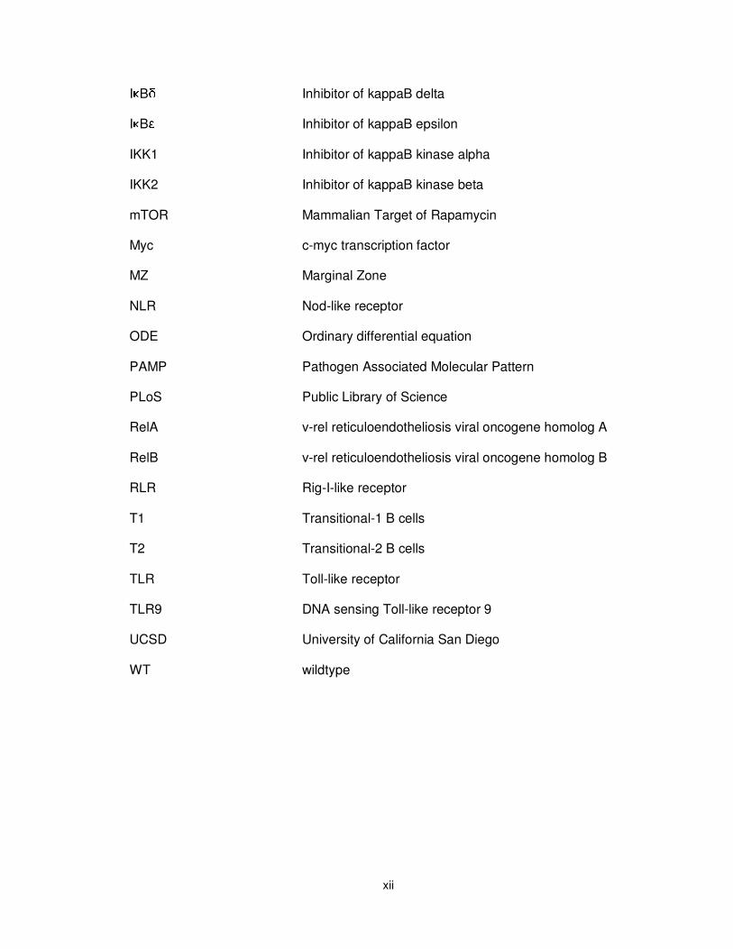
Figure 2.4. Accuracy of fitting the population model to generated fitted generation cell counts............................................................................................................................ 41 Figure 2.5. Accuracy of pheotyping generated datasets in a sequential or integrated manner .......................................................................................................................... 44 Figure 2.6. Comparsion of the integrated model fitting approach to training each model independently ................................................................................................................ 45 Figure 2.7. Anlysis of the phenotyping accuracy as a function of the number of fit attempts (trials) .............................................................................................................. 48 Figure 2.8. Analysis of the fitting accuracy when using fewer experimental timepoints .. 49
Figure 2.9. Analysis of the fitting accuracy as a function of bjective function choice ...... 50
Figure 2.10. Comparison of FlowMax to the Cyton Calculator ...................................... 56
Figure 2.11. Testing the accuracy of the propsed approach as a function of data quality ............................................................................................................................ 59 Figure 2.12. Phenotyping WT, nfkb1-/-, and rel-/- B cells stimulated with anti-IgM and LPS ............................................................................................................................... 63 Figure 2.13. Best-fit fcyton solution overlays for stimulated wildtype, nfkb1-/-, and rel-/- B cell CFSE time courses ................................................................................................. 65

xv
Figure 2.14. Using chimeric model solutions to identify key fcyton parameters .............. 67
Figure 3.1. Time-lapse microscopy reveals two distinct generation-dependent growth patterns for B cells. ..................................................................................................... 109 Figure 3.2. The minimum biologically-relevant death time in progenitor cells is distinct ......................................................................................................................... 111 Figure 3.3. B cells decide to divide or die and are protected from the alternate fate .... 113
Figure 3.4. Cells typically grow less prior to the last dvision ......................................... 114
Figure 3.5. FlowMax deconvolution of WT 250 nM CpG stimulated CFSE time series 116
Figure 3.6. The decision, division, an death times are correlated between siblings and cousins ........................................................................................................................ 118
Figure 4.1. Molecular assays suggest that NFκB enorces an upstream fate ................ 132
Figure 4.2. NFκB mediates growth and survival .......................................................... 135
Figure 4.3. Immunofluoresnce control experiments ..................................................... 136
Figure 4.4. Time-lapse microscopy confirms NFκB cRel as an enforces of cell decision making......................................................................................................................... 138
Figure 5.1. Biological processes are complex and non-linear ...................................... 150
Figure 5.2. Data-driven probabilistic vs physicokinetic modeling.................................. 151
Figure 5.3. Extrinsic noise results in cell-to-cell NFκB, division, and death variability .. 153
Figure 5.4. Multi-scale agent-based modeling of the B cell response .......................... 157
Figure 5.5. The multi-scale model predicts the effect of low stimulus, cRel deficiency, and rapamycin treatment ............................................................................................. 160
Figure 5.6. NFκB levels determine fate, while protein variability affects both timing variability and fate........................................................................................................ 162
Figure 6.1. Diagram showing how FlowMax phenotyping may be used to characterize the mechanics of B cell tumors for specific individuals. ................................................ 172
Figure 6.2. Early iteration of the integrated cell-cycle/apoptosis model ........................ 180
Figure 6.3. The multi-scale receptor-specific population model.................................... 182

xvi
LIST OF TABLES
Table 1.1. Sumary of TLRs and their abundance in mice and humans ............................ 5
Table 1.2. Summary of recent cell population models for interpreting CFSE datasets ... 21
Table 2.1. Analysis of fit running time dependence on the number of time points and generations.................................................................................................................... 51
Table 2.2. Starting and fitted cyton model parameters for four successful Cyton Calculator fitting trials .................................................................................................... 53
Table 2.3. Cell fluorescence and population parameter ranges used to generate realistic CFSE time courses........................................................................................................ 54
Table 2.4. Time points considered for analysis of generated time courses .................... 55
Table 4.1. Correlations between cell transcriptomes .................................................... 143
Table 4.2. NFκB target genes that are transcriptional regulators ................................. 144
Appendix A. Integrated B cell model species ............................................................... 183
Appendix B. Integrated B cell model parameters ......................................................... 184
Appendix C. Integrated B cell model fluxes ................................................................. 193
Appendix D. Integrated B cell model reactions ............................................................ 197
Appendix E. Other simulation parameters ................................................................... 200

xvii
ACKNOWLEDGEMENTS
I am very fortunate to have been supported by many friends and loved ones over
the years. Without their inspiration, knowledge, wisdom, and love this dissertation would
not be possible.
My fiancée, Ella Trubman, provided day-to-day unwavering support, friendship,
and love and made sure to keep me well-grounded and focused over the years. She was
always a happy thought in the back of my mind even when I had to stay in the lab
overnight, or face stubborn reviewers.
Drs. Nikolai, Tatiana, and Kirill Shokhirev have been an inspiration and role
models for my aspirations. Having grown up in a household of scientists, I was fortunate
to be exposed to critical thinking, scientific ideas, and a hard-working attitude, without
which I would not have had a chance among my peers. They were always there to
provide advice, voice their concerns, and give me pointers on chemistry, physics,
computer science, mathematics, statistics …
The Signaling Systems Lab at UCSD has grown to a whole community of
supportive friends over the years. I could always count on them to drop what they were
doing to go grab a beer, teach me a new technique, get me a mouse from the mouse
house, or explain the ins and outs of an algorithm or assay. I would like to especially
acknowledge Jeremy Davis-Turak, Jon Almaden, Bryce Alves, Harry Birnbaum, Kim
Ngo, and Jesse Vargas, who have provided expert training, and both experimental and
computational expertise to make chapters 3, 4, and 5 of this thesis a success. In
addition, I will always keep several previous lab members Paul Loriaux, Tony Yu, Jenny
Huang, and Krystin Feldman close to heart for their friendship. BacT 4 life! Diana Rios,
Rachel Tsui, Karen Fortman, Brooks Taylor and honorary lab member Romila Mukerjea

xviii
were always there to provide a sympathetic ear and a witty retort. I wish all the labbies
all the best!
My dear and brilliant childhood friends and collaborators Adiv, Boris, Jordan, and
Yan have supported me over the decades, challenged my viewpoints, and fuelled my
creativity, whether we were publishing papers together, writing stories, designing card
games, or creating the next big computer game.
Alexander Hoffmann, has provided invaluable training and wisdom over the
years. His enthusiasm and friendly welcoming nature and expert knowledge in diverse
fields cultured an easy-going and supportive environment in the lab. Furthermore, it was
Alex’s excellent ideas for research on the heterogeneity of the B cell response that first
got me interested in his lab and led to a successful application for the NSF Graduate
Research Fellowship. He supported my own ideas and gave me the latitude to work on
time-lapse imaging, multi-scale modeling, and other projects, even when it wasn’t clear
that the problems were surmountable.
Regents Professor Emerita Ann Walker invited our family to the states and gave
me my first taste of scientific research when she hired me out of high-school to work on
Nitrophorin proteins in her lab alongside my parents and under the guidance of an awe-
inspiring graduate student, Lillya Yatsunik (now Professor) and brilliant post-doctorate
researchers Robert Berry and Igor Filippov.
Dr. Osamu Miyashita was my undergraduate thesis advisor in biochemistry and
first got me interested in physics-based simulations which I have taken with me to San
Diego and applied to the study of miRNA structures and B-cell tracking.
Finally, the support, helpful discussions, and time that my Ph.D. committee
provided freely made this entire process as painless as possible.

xix
Chapter 2, in full, is a reprint of the material as it appears in PLoS One 2013.
Maxim N. Shokhirev and Alexander Hoffmann, A. Public Library of Science, 2013.
Alexander Hoffmann is the corresponding author. The dissertation author was the
primary investigator and author of this paper.
Chapter 3, in part, is currently being prepared for submission for publication of
the material and may appear as Maxim N. Shokhirev, Jonathan Almaden, Jeremy Davis-
Turak, Harry Birnbaum, Theresa M. Russell, Jesse A.D. Vargas, Alexander Hoffmann.
“A multi-scale approach reveals that NFκB enforces a decision to divide or die in B
cells.” Jesse A.D. Vargas helped train me to run single-cell microscopy experiments. The
dissertation author was the primary investigator and author of this paper.
Chapter 4, in part, is currently being prepared for submission for publication of
the material and may appear as Maxim N. Shokhirev, Jonathan Almaden, Jeremy Davis-
Turak, Harry Birnbaum, Theresa M. Russell, Jesse A.D. Vargas, Alexander Hoffmann.
“A multi-scale approach reveals that NFκB enforces a decision to divide or die in B
cells.” Jonathan Almaden helped with B-cell purification, western blotting, and RT-PCR.
Jeremy Davis-Turak and Harry Birnbaum collaborated to align and map single-cell
RNAseq results. Theresa M. Russell and I collaborated to produce the single-cell RNA
sequencing datasets. Jesse A.D. Vargas devised the immunofluorescence protocol and
trained me to run immunofluorescence and single-cell microscopy experiments. The
dissertation author was the primary investigator and author of this paper.
Chapter 5, in part, is currently being prepared for submission for publication of
the material and may appear as Maxim N. Shokhirev, Jonathan Almaden, Jeremy Davis-
Turak, Harry Birnbaum, Theresa M. Russell, Jesse A.D. Vargas, Alexander Hoffmann.
“A multi-scale approach reveals that NFκB enforces a decision to divide or die in B

xx
cells.” Jonathan Almaden helped with B-cell purification. The dissertation author was the
primary investigator and author of this paper.

xxi
VITA
2003-2008 Undergraduate Researcher, University of Arizona
2008 Bachelor of Science, University of Arizona
2010-2011 ScienceBridge Scientist Lecturer, Correia Middle School, San Diego
2010-2013 NSF Graduate Research Fellow, University of California, San Diego
2011-2012 Independent Contractor, NanoCellect Biomedical Inc. San Diego, CA.
2014 Doctor of Philosophy, University of California, San Diego
SELECTED PUBLICATIONS
“Effect of mutation of carboxyl side-chain amino acids near the heme on the midpoint potentials and ligand binding constants of nitrophorin 2 and its NO, histamine, and imidazole complexes.” J Am Chem Soc. 2009.
“Biased coarse-grained molecular dynamics simulation approach for flexible fitting of X-ray structure into cryo electron microscopy maps.” J Struct Biol. 2010.
“Paternal RLIM/Rnf12 is a survival factor for milk-producing alveolar cells.” Cell. 2012.
“FlowMax: A Computational Tool for Maximum Likelihood Deconvolution of CFSE Time Courses.” PLoS One. 2013.
“Effects of extrinsic mortality on the evolution of aging: a stochastic modeling approach.” PLoS One. 2014.
“IκBε Is a Key Regulator of B Cell Expansion by Providing Negative Feedback on cRel and RelA in a Stimulus-Specific Manner” The Journal of Immunology. 2014.
“BAFF engages distinct NFκB effectors in maturing and proliferating B cells.” In press.
“Sequence Signatures and Polymerase Dynamics Favor Co-transcriptional Splicing Genome-wide.” In press.
“A multi-scale approach reveals that NFκB enforces a decision to divide or die in B cells.” In preparation.

xxii
ABSTRACT OF THE DISSERTATION
Developing a Multi-Scale Understanding of the B Cell Immune Response
by
Maxim Nikolaievich Shokhirev
Doctor of Philosophy in Bioinformatics and Systems Biology
University of California, San Diego, 2014
Professor Alexander Hoffmann, Chair Professor Andrew McCulloch, Co-Chair
The immune system is composed of hundreds of highly-specialized cell types
that collaboratively orchestrate an efficient response to pathogens and damage. Central
to immune function, B lymphocytes participate in both the fast but non-specific innate,
and persistent adaptive immune responses by sensing conserved pathogen-associated
molecular patterns such as bacterial or viral CpG DNA as well as pathogen-specific
patterns recognized by uniquely generated B-cell receptors. Upon activation, B cells

xxiii
undergo rapid expansion in number, deal with the threat by carrying out specific effector
functions, and eventually die by programmed cell death or become long-lived memory
cells. As a result, B-cell dynamics dictate vaccine efficiency, while aberrant proliferation
and/or survival is the hallmark of autoimmune disorders, immune deficiency, and cancer.
Decades of Nobel-worthy studies have characterized the key molecular players, cellular
behaviors, and population dynamics of B cells, but the implicit heterogeneity and multi-
scale nature of the B-cell response pose fundamental challenges to meaningful
interpretation in specific contexts. A multi-scale understanding has only recently become
possible with the advent of single-cell assays and the advancement of computational
methods. To better-understand how individual cells orchestrate the population response,
we developed CFSE flow cytometry deconvolution of cell populations, time-lapse cell
tracking, and agent-based multi-scale computational modeling methods which we
combined with single-cell and traditional biochemical assays and literature mining to
develop a mechanistic understanding of the B cell immune response from the molecular
pathways governing NFκB signaling, growth, cell-cycling, and apoptosis to cellular
behavior and ultimately the population dynamics. We find that 1)the population behavior
is best explained by individual B cells making decisions to either grow and divide, or die
2)that NFκB signaling serves as a central enforcer of B cell decision making by
promoting division and survival and 3)that a multi-scale model can accurately predict
population behavior with a lower dose of the stimulus, when NFκB cRel missing, and
when pretreated with the drug rapamycin. The methods and models developed as part
of this dissertation serve as predictive frameworks for future hypothesis-driven discovery
and model-driven analysis, enabling meaningful interpretation of patient data, and drug
target prediction across biological scales.

1
Chapter 1
Introduction
Developing an understanding of the multi-scale B-cell immune response requires
a diverse background in the underlying biological processes as well as a working
knowledge of various experimental and computational techniques. In the following
sections I provide an overview of B-cell biology, the stochastic multi-scale dynamics of
the B-cell immune response, the role of NFκB signaling, an overview of the interplay
between NFκB, Myc, and mTOR, as well as highlighting the current state of the art
approaches to time-lapse microscopy, cell tracking, single-cell molecular assays,
stochastic modeling of CFSE flow cytometry datasets, and multi-scale agent based
modeling. My aim is to provide a general overview of these topics and to highlight the
findings pertinent to these studies, while referring readers to more in-depth reviews.

2
1.1. Overview of B cell development and function
The immune system is a collection of diverse cells that are typically dormant but
can rapidly respond to pathogens, inflammatory signals, and other stresses by
upregulating metabolism, proliferating, traveling to the source of infection, producing
secondary messenger molecules, differentiating into specialized cell types and ultimately
dying or resuming a quiescent steady state [1,2]. First characterized in the middle 1960’s
and early 1970’s [3-5], B cells serve important roles in both the adaptive and innate
immune responses and so it is not surprising that their homeostasis is under control at
multiple development and functional checkpoints [6]. B lymphocytes are continuously
being produced from a stem-cell pool in the bone marrow, where they undergo a
stringent vetting process that removes auto-reactive, and potentially dangerous clones.
The remaining ~10% migrate to the secondary lymphoid tissues (spleen, lymph nodes),
where they undergo further maturation into naïve mature B cells, and are primed to
rapidly respond to pathogens and inflammatory signals [5-9]. B cells that pass the
necessary checkpoints during development and differentiation receive tonic survival
signals allowing them to survive for weeks and providing plenty of opportunity for them to
sample the blood (spleen), gut (Payer’s Patches), and periphery (lymph nodes) for
potential pathogens [4,10].
Unlike most other immune cells, B cells play important roles in both the innate
and adaptive immune responses [11]. Adaptive immunity is achieved through
diversification followed by rapid clonal selection and the establishment of immune
memory. During B cell development, B cells recombine immunoglobin (Ig) heavy and
light chains via a specialized genetic editing mechanism that is able to generate
incredible receptor diversity, thereby ensuring that any potential pathogen will be
recognized [12,13]. Furthermore, since B-cells are clonal, rapid proliferation upon

3
pathogen recognition will produce a geometrically increasing population of B-cells that
recognize the specific pathogen [6]. B cell receptor binding is further optimized during
clonal expansion in germinal centers (GC) due to somatic hyper-mutation of the Ig genes
[14]. After the threat is neutralized, most of the proliferating B cells die, leaving a
population of long-lived memory B-cells that are poised to rapidly reactivate in the event
of a subsequent reinfection by the same pathogen potentially decades later. This
adaptability comes at the cost of speed as the response ramps up over the span of days
and even weeks, requiring the presence of the right B cell that is expressing the right
antigen-specific receptor, secondary signaling from other immune cells, and clonal
selection prior to full activation. On the other hand, the more ancient innate immune
response results in the immediate activation of B cells expressing sets of highly-
conserved receptors that recognize specific pathogen-associated molecular patterns
(PAMPS) [15]. There are three main classes of pattern recognition receptors (PRRs) that
have evolved to recognize various pathogen-specific structures [16]. In addition to Nod-
like receptors (NLRs) and RIG-I-like receptors (RLRs) which sense viruses and other
pathogens in the cytosol, Toll-like receptors (TLRs) span the cell membrane or
internalized endosomes and recognize structures indicative of bacteria, viruses, or fungi
outside of the cell [17]. There are at least 13 different TLRs known to exist, however the
specific combination of TLRs expressed differs between species (Table 1.1). Of
particular interest, TLR9, which recognizes bacterial and viral unmethylated CG-rich
sequences, is found in both mice an humans, and leads to T-cell independent B-cell
expansion and cytokine/chemokine/growth-factor production when exposed to nM
concentrations of CpG [18-20]. Furthermore, cells stimulated with CpG are not self-
adherent, enabling direct imaging and tracking of stimulated B cells with a microscope
[21]. Figure 1.1 shows an overview of B cell development and activation.

4
An efficient B-cell immune response is essential for survival while dysregulation
is the hallmark of B-cell cancers, autoimmunty, and immune deficiency. B-cell
lymphomas, like other types of cancers, occur due to a loss of proliferative/death checks
and balances in B cells, causing uncontrolled accumulation of lymphocytes. Lymphomas
are the fifth most common type of cancer in the United States and are the sixth deadliest
causing an estimated 21,530 deaths in 2010 [22]. B cell lymphomas typically arise
during an error in V(D)J recombination, somatic hyper mutation during the germinal
center (GC) expansion, or class-switch recombination [23]. For example, the anti-
apoptotic Bcl2 regulator is found to be translocated into the heavy chain Ig locus in 90%
of follicular lymphomas, promoting its constitutive transcription and immortality. Other
types of lymphomas arise from similar translocations of growth and cell-cycle regulators
such as Myc and Cyclin D. Importantly, cancerous transformation results in considerable
cell-to-cell heterogeneity within even clonal sub-sets of cells, posing significant
challenges for drug-based treatment [24-30]. In addition to B cell cancers, buildup of
constitutively active B cells can lead to autoimmune disorders and chronic inflammation,
due to excess proliferation, cytokine production, or antigen presentation to auto-reactive
T-cells [31]. Excessive B-cell activation can be caused by defects in the B-cell ablation
mechanisms during Ig maturation in the bone marrow or caused by somatic hyper
mutation in the GC, as well as due to aberrant signaling through pro-survival BAFF
receptor and defective TLR signaling as reviewed in recent works [31-33].
Unfortunately, since B-cell activation and survival are hallmarks of cancer, autoimmune
diseases often predispose individuals to B cell cancers [34]. While out of control B cell
activation can lead to autoimmunity, chronic inflammation, and lymphomas,
developmental blocks caused by dysfunctional Ig production and problems with
activation or survival result in immune deficiency and susceptibility to diseases [35] .

5
Interestingly, a shift in B cell subsets caused by developmental blocks can result in
autoimmunity [36] and further highlights the complexity of the immune system as well as
a need for stringent regulation for proper function. Thus, the complexity, heterogeneity,
and dynamic nature of B cell homeostasis and function demands stringent regulation at
all points during B cell development and activation. The potential for malignancy cannot
be overstated as activated B-cells essentially resemble specialized “cancer” cells due to
their fast proliferation, anaerobic metabolism, and the upregulation of potentially
mutagenic processes (i.e. V(D)J recombination, somatic hyper-mutation, class-switch
recombination).
Table 1.1. Summary of various TLRs and their abundance in mice and humans. Compiled from various sources [16,17,37-42].
TLR PAMPS recognized Mouse Human
1/2 Triacyl lipopeptides + +
2 Peptidoglycan, LAM, Hemagglutinin, phospholipomannan,
Glycosylphosphophatidyl inositol mucin + +/-
3 ssRNA virus, dsRNA virus, RSV, MCMV +/- +/-
4 Lipopolysaccharides, Mannan, Glycoinositolphospholipids,
Envelope proteins + -
5 Flagellin + +
6/2 Diacyl lipopeptides, LTA, Zymosan + +
7 ssRNA viruses + +
8 ssRNA from RNA virus - +
9 dsDNA viruses, CpG motifs from bacteria and viruses,
Hemozoin +* +
10 Bacterial peptidoglycan - +
11 Uropathogenic bacteria, profillin-like molecule + -
12 Profilin + -
13 Bacterial RNA + -
*-TLR9 is expressed in B1, marginal zone, and follicular murine B-cells

6
Figure 1.1. Diagram summarizing the development and activation of B cells. B cells develop from lymphoid progenitors in the bone marrow, undergo selection for self-tolerance, and finish maturation in the spleen. Quiescent mature naïve B cells undergo rapid population expansion and differentiate into long- or short-lived antibody producing plasma cells, or memory cells. Innate toll-like receptors (red), membrane-bound and excreted IgM (green), class-switched IgD (blue), and somatically hypermutated Igs (purple) are depicted on cell membranes. Recently reviewed in [4-6,9].

7
1.2. Stochastic cellular behavior orchestrates the response
Given the complexity of B cell signaling, presence of numerous B cell subtypes,
and inherent randomization of Igs during development, it is clear that heterogeneity is a
central theme of the B-cell immune response. Strikingly, the apparent stochasticity is
most evident when observing individual B-cells stimulated with mitogenic signals such as
unmethylated bacterial or viral CpG DNA (Figure 1.2). Individual B cells interpret these
signals by undergoing 1-6 rounds of cell cycling, followed by cell cycle exit, and death by
programmed cell death [21]. The population response is the sum of these single-cell
decisions and characteristically lasts several days to a week by first producing a
dramatic increase in the number of activated B cells for several days, followed by a
return to starting cell counts [43]. While the population response is robust (i.e.
reproducible total cell coun dynamics), the behavior of individual cells is seemingly
stochastic since only a fraction of cells respond in each generation and because the
timing of division and death is highly variable between these genetically identical
synchronized cells. In fact, the timing of division and death is well-modeled by long-tailed
distributions (e.g. log-normal) as a function of cell age, resulting in a distribution of cells
across many generations after only a few days of stimulation [21,44]. Furthermore,
progenitor cells (generation 0) typically take much longer to divide or die, while dividing
cells (generation 1+) divide again within six to twelve hours [21,45]. After several days of
intense proliferation, the population response returns back to basal levels which is
caused primarily by cell-cycle exit followed by programmed cell death [21]. In fact, the
fraction of cells that progress to the next generation (i.e. the fraction that divides)
decreases approximately sigmoidally with each generation such that the final division
number, or “division destiny” of a cells is approximately normally distributed as a function
of generation [20,21,44].

8
But what gives rise to this variability in cell fate and timing? Previous studies offer
evidence that the inherent variability in timing of the apoptosis is caused primarily by
cell-to-cell protein abundance variability [24] and presumably variability in cell-cycle
regulators generate cell-to-cell variability in cell-cycle duration, however, it is still unclear
if variability in timing of competing division/death processes determine fate. There are
competing theories for how fate (division/death) is determined. On one hand there is
recent support for a molecular race hypothesis, which posits that cell-cycle and
apoptosis processes are proceeding concurrently within cells, and that fate is
determined by the faster of these mutually exclusive outcomes [44,46]. Specifically, an
age-structured population model, the cyton model, which incorporates competition
between division and death fates can reproduce the major population features and
produces excellent fits to experimental datasets [44]. Furthermore, a recent study [46]
demonstrated that a probabilistic model that assumes correlation of fate timing between
siblings and mutual censorship between competing processes (e.g. division and death)
can reproduce the correlations between non-concordant fates as well as the observed
censored distributions for the time to divide, time to isotype switch, and time to
plasmablast differentiation (although the best-fit censored model death time distributions
were typically earlier than the observed death distributions). On the other hand, there is
also evidence that cells decide their fate early and are protected from the alternate
outcome. Single-cell time-lapse videos of stimulated B cells revealed that cells that died
did not grow, while cells grew prior to dividing in all except the last and pen-ultimate
generations, indicative of a lack of fate competition [21]. Furthermore, the authors found
that the size of the progenitor cells was predictive of the number of divisions suggesting
that fate is decided in the initial generation. As a result, we described the fcyton model,
which unlike the cyton model, commits responding cells to division, and showed that cell

9
commitment to a specific fate nevertheless resulted in excellent model fits for all
experimental datasets [47]. Further support for a molecular decision comes from a
recent study, demonstrating that levels of cell cycle inhibitor p21, which directly inhibits
CDK2 activity is sufficient for promoting cell-cycle reentry in cell lines and human primary
cells [48]. Therefore, while extrinsic variation in initial protein levels determines timing of
cell death (and presumably cell-cycle timing), cell fate may be a function of competing
mutually exclusive processes or stochastic variation in the concentrations of key
regulators. Knowing whether cells make decisions will determine how we model cell fate
determination on the molecular level and in turn informs experimental and drug design.
Figure 1.2. The B cell population response is composed of heterogeneous single-cell behaviors. While the population response is robust with a period of expansion followed by programmed cell death, timing and fate of individual cells is heterogeneous. Results were obtained from fitting mixed Gaussian distributions to CFSE log-fluorescence histograms measured by flow cytometry after the indicated times of 250 nM CpG stimulation.

10
1.3. The role of NFκB signaling in the B cell response
While it is unclear how B cell fate is ultimately determined, the underlying
biochemical processes involved in transducing receptor signals, cell growth, cell cycling,
and programmed cell death by apoptosis are known and well-studied (recently reviewed
in [4,17], [49], [50], respectively). In B cells, which remain small and in an actively
maintained quiescent state (G0 phase of the cell-cycle), activation can be achieved
through TLR signaling as well as through the BCR resulting in the activation of growth,
cell-cycling, and apoptosis pathways through various signaling networks. As mentioned
previously, signaling through TLR9 by adding nM-uM concentrations of non-methylated
CpG independently leads to dramatic non-self-adherent B cell activation, providing a
convenient window into the behavior of proliferating B cells. Importantly, CpG robustly
activates the canonical branch of the well-studied and essential NFκB signaling pathway
(Figure 1.3) [51], resulting in the upregulation of hundreds of genes associated with
survival and proliferation, providing a natural molecular connection between signaling
and cell fate [52]. Specifically, activation of TLR9 by CpG results in the activation of the
kinase IKK2, which rapidly phosphorylates NFκB inhibitor proteins, the IkBs, which
sequester NFκB dimers in the cytoplasm. Phosphorylation of IkBs results in their
ubiquitination and degradation, releasing NFκB dimers (primarily RelA:p50 and cRel:p50
in B cells [4]) and allowing them to enter the nucleus where they bind to promoters of
genes containing the NFκB motif, and activate gene expression. Importantly, the genes
coding for cRel [53] and p50 [54] as well as the inhibitors IkBα [55] and IkBε [56] are
themselves target genes, resulting in waves of NFκB activation lasting potentially
several days (Figure 1.4). Therefore, many essential molecular players involved in the B
cell immune response have been identified but it remains unknown how their dynamics

11
lead to the observed cell fate and timing variability and in turn the B cell population
response.

12
Figure 1.3. Components of the NFκB signal transduction system. Receptors lead to
the downstream activation of kinases, the IKKs, which phosphorylate inhibitors of NFκB, the IkBs, targeting them for ubiquitin-mediated protease degradation. IkB degradation
leads to release of NFκB dimers that are free to enter the nucleus and upregulate gene expression programs. While RelA:p50 is the canonical dimer responsible for signaling in most cells, in B-cells both RelA:p50 and cRel:p50 can activate growth, cell-cycle progression, and survival programs. Recently reviewed by [57] and [4].

13
Figure 1.4. NFκB signaling pathway in B-cells. The canonical and non-canonical
branches of the NFκB signaling pathway are shown. Receptors initiate downstream signaling through the canonical or non-canonical branches by activating kinases IKK1 and IKK2. Canonical signaling results in IKK2-mediated degradation of IkBs which serve
to sequester NFκB dimers in the cytoplasm, whereas non-canonical activation of NIK
results in processing of p100 precursor to p52. Free NFκB dimers that contain transactivation domains (A,B, or C) bind to kB elements in the promoters of genes and
promote activation of growth/cell-cycle and survival genes. Importantly, NFκB can
upregulate the production of IkBα and IkBε as well as p105, p100, RelB, and cRel proteins, leading to waves of NFκB activation. Recently reviewed by [57] and [4].

14
1.4. NFκB, Myc, and mTOR in B cell division and death
While NFκB can activate survival and proliferative genetic programs, the exact
mechanisms leading to cell growth, cell-cycle progression, and survival, as well as the
roles that central regulators myc and mTOR play are still not fully understood.
Like NFκB, myc is a central transcription factor that promotes growth and
proliferation by promoting the production of cellular machinery (e.g. ribosomes)[4,49].
Whereas, myc has traditionally been traditionally associated with the control of growth in
cells, recently, it has been shown that myc is best thought of as a global regulator of
transcriptional activation in lymphocytes, a central regulator of cell activation [58].
Unsurprisingly, myc dysfunction is prevalent in cancers which exist in a perpetually
active state [49]. Importantly, myc is a direct downstream target of NFκB activation,
providing a direct link between NFκB signaling to cell growth and activation [59]. In
addition to being NFκB target genes, genetic knockout of NFκB cRel and p105/p50
(leading to effective removal of canonical gene-inducing NFκB dimers cRel:p50 and
RelA:p50) results in B cells that are unable to grow and proliferate due to a failure to
upregulate myc, showing that at least in B cells, signaling through NFκB is essential for
activation and function [60]. NFκB-dependent regulation of myc has also been observed
in T-cells further enforcing an NFκB regulation in myc activity.
Mammalian target of rapamycin (mTOR) is another key regulator of metabolism
in cells, and acts to promote growth and proliferation by inducing general cellular
machinery required for metabolite uptake, protein synthesis, and DNA replication
[61,62]. Importantly, mTOR is activated by the presence of metabolites as well as by
general mitogenic signals, enabling it to serve as a general sensor and regulator of
metabolism. As with NFκB and myc, mTOR dysfunction is a hallmark of cancer and

15
inhibitors of mTOR such as rapamycin, hold promise for cancer treatment [63-65].
However, the interplay between Myc or NFκB with mTOR signaling in lymphocytes
remains poorly understood. Myc and mTOR signaling seem to form a mutual feedback
loop, as depeletion of myc leads to lower mTOR, while inhibition of mTOR function leads
to lower Myc [66]. The crosstalk between NFκB and mTOR remains uncertain.
Signaling through the Akt/mTOR axis has been shown to activate NFκB via IKK in a
prostate cancer cell line [67]. On the other hand, in myocytes NFκB and mTOR impose a
mutual bidirectional control [68]. Finally, NFκB and mTOR may be activated in parallel
through IKK signaling to mTOR and NFκB in a cancer cell line [69].
How can NFκB, Myc, and mTOR control cell growth, cell-cycle progression and
survival in B cells? In addition to NFκB control of myc, the genes coding for CyclinD [70-
72], E2F3 [73], and BclXL [74], which are essential for cell-cycle progression and survival,
are all known to be NFκB target genes. Cyclins D1-3, are cell-cycle regulator
responsible for G1-S checkpoint progression by phosphorylating and thereby inactivating
retinoblastoma protein [75], however only Cyclin D2 and D3 have been shown to be
important for G1-S checkpoint progression in B cells[76-78] and reviewed in [79].
Inhibition of NFκB signaling in lymphoma cell lines resulted in cell-cycle arrest in the G1
phase due to downregulation of Cyclin D1 expression, further supporting a direct link
between NFκB signaling and cyclin D1 driven cell-cycle progression in B cells [80].
Furthermore, NFκB promotes the activation of transcription factor E2F3 which helps
drive cell-cycle progression in the G1 phase of the cell cycle. E2F3 is a transcription
factor that is typically bound to the retinoblastoma protein (Rb) in quiescent cells, and
upon Rb hyperphosphorylation can activate the transcription of other cyclins [81,82]. In
addition to its role in growth and cell-cycle progression, there is a direct link between

16
NFκB signaling and survival in B cells. NFκB is known to promote the expression of anti-
apoptotic BCL family members BclXL [73] as well as A1[83]. A1 is thought to serve an
early survival function, while BclXL builds up to provide prolonged survival [73,83].
Furthermore, NFκB signaling contributes to the ERK-dependent degradation of the pro-
apoptotic BH3-only protein Bim, via the IKK/p105/Tpl2 axis[84-87]. Both myc and mTOR
are important for turning on general machinery and show bi-directional regulation. In
addition, myc and mTOR play indirect roles in survival as gene expression and protein
synthesis are required for programmed cell death. As such, quiescent cells are protected
from death as compared to actively growing and metabolically active cells. Whereas
NFκB can control myc expression directly, its role in mTOR signaling is currently poorly
understood. These interdependencies are summarized in Figure 1.5.

17
Figure 1.5. The NFκB, Myc, mTOR interplay in B cell division and death. NFκB signaling promotes the expression of Myc, cell-cycle progression genes, and anti-apoptotic Bcl proteins. Myc serves to upregulate global gene expression programs as well as general machinery proteins which are required for cell growth and subsequently for B cell progression through the cell-cycle. In addition, mTOR is important for ribosome activation and protein synthesis. Cell death is caused by the oligomerization of Bax protein on the mitochondria leading to pore formation, release of cytochrome c and subsequent apoptosome-mediated executioner caspase activation and death. Interplay
between NFκB, Myc, and mTOR is poorly understood with possible cross-talk between NFκB and mTOR as well as Myc.

18
1.5. Interpreting B cell CFSE population dynamics
A current experimental approach for tracking lymphocyte population dynamics
involves flow cytometry of carboxyfluorescein succimidyl ester (CFSE)-stained cells.
First introduced in 1990 [88], CFSE tracking relies on the fact that CFSE is irreversibly
bound to proteins in cells, resulting in progressive halving of cellular fluorescence with
each cell division. By measuring the fluorescence of thousands of cells at various points
in time after stimulation, fluorescence histograms with peaks representing divisions are
obtained. However, interpreting CFSE data confronts two challenges. In addition to
intrinsic biological complexity arising from generation- and cell age-dependent variability
in cellular processes, fluorescence signals for a specific generation are not truly uniform
due to heterogeneity in (i) staining of the founder population, (ii) partitioning of the dye
during division, and (iii) dye clearance from cells over time. Thus, while high-throughput
experimental approaches enable population-level measurements, deconvolution of
CFSE time courses into biologically-intuitive cellular parameters objectively remains a
major challenge and is susceptible to misinterpretation [89].
To address the experimental and biological variability associated with CFSE time
courses, a number of theoretical models have been developed (see [90,91] for recent
reviews) and some of the most recent are summarized in Table 1. Early models adopted
the ordinary differential equation (ODE) approach, modeling division [92-99] and death
[92-95,97-105] as first-order processes. As experimental information about cellular
processes became available, models were updated to account for the non-exponential
nature of division, imposing a delay, or skewed distribution for the interdivision time
[44,92,100-109]. While both the time to divide and time to die are well-modeled by
skewed distributions, only several models allow arbitrary distributions for cell death times
[44,107-111].To account for the large difference in the division and death times between

19
undivided and dividing cells, most recent models have explicit generation structure or
heterogeneity [44,100-102,104-109,111,112]. Also, some models explicitly incorporate
mechanisms that can account for the decrease in cell numbers after an initial period of
population expansion [44,93,95,101,104,105,107-109,111]. In addition, a few models
incorporate fractional progression of cells to the next division [44,101,104-106,109,111].
Finally, more recent models are formulated to account for both sources of variability,
modeling population dynamics and fluorescence effects in an integrated manner
[98,99,107,108], while others account for cell fluorescence with a time-independent
mixture of Gaussians models [107,111,112]. Modeling the population fluorescence
dynamics is advantageous as models can be compared to the experimental data directly
during fitting, but this approach typically suffers from computational intractability. While
the computational complexity has been shown to be greatly reduced by decoupling dye
intrinsic effects from population dynamics and employing approximations [107],
potentially important biological features such as cell age-dependent rates for division
and death and late-phase population contraction (in the form of decreasing fractions of
responding cells) must be taken into account. Several extensions of the DLSP model
[107] incorporating age-structure and fractional responses of cell populations have
recently been proposed which incorporate cell age structure [108], or fractional response
to stimulus [109], however there is no label-structured model available that incorporates
all of the important biological features. Of note, the Hyrien-Chen-Zand general branching
process model [111] can be adopted to include all desired biological features, however,
efficient computation is not straightforward, and a late-phase contraction mechanism is
not explicitly shown. Upon comparing recent models (Table 1.2), only the generalized
cyton model explicitly accounts for all of the essential biological features: age- and
generation-structured division and death, fractional response to stimulus, and late-phase

20
contraction of the population [44]. A competition between independent division and
death pathways in responding cells is at the heart of the cyton model. Responding cells
have a non-zero probability of dying before division. However, more recent single-cell
microscopy studies have shown that growing cells are protected from death [21].
Therefore, the cyton model was recently reformulated to include an explicit decoupling of
the division and death pathways [113]. In the reformulated fcyton model responding cells
are committed to age-dependent division, while non-responding cells are committed to
age-dependent death. This model is covered in depth in chapter 2.
The biggest challenge for interpreting heterogeneous CFSE datasets is the
availability of validated computational tools for deriving biological insights. To date, only
two freely available user-friendly computational tools for interpreting CFSE datasets are
available. The Cellular Calculator (Cyton Calculator) is a free polished computational tool
that relies on user-provided generational cell counts and manual estimates of cyton
model parameters to find the a local optimum set of cyton model parameters [44,45].
The problem with this approach is that it confidence in the solution was not known. First,
any computational tool requires a characterization of its performance to establish how
the solution accuracy, sensitivity, and redundancy will depend on the underlying data.
Second, solutions were provided as is, leaving the user without a measure of solution
confidence. Third, the tool found a local optimum, precluding multiple solutions. Finally,
the source code for the tool was not provided, severely limiting its expandability. Our
approach was to create, validate, and use a user-friendly open-source computational
tool for fitting population model parameters to CFSE datasets with measures of
confidence [47]. This tool is the subject of chapter 2 of this thesis.

21
Table 1.2 Summary of recent cell population models for interpreting CFSE
datasets.
Reference Cell Cycle Cell Death Late-phase contraction
Fractional activation
Fl. Dyn.
Gett et al (2000) [100]
Tdiv0 ~normal. Tdiv1 const. Exponential decay.
Generation-invariant. N/A N/A N/A
De Boer et al
(2001) [93] Piece-wise constant division
rate of activated cells Piece-wise constant
generation-invariant rate. Fate = f(t) N/A N/A
Revy et al
(2001) Constant division rate.
Exponential decay. Generation-invariant.
N/A N/A N/A
De Boer et al (2003) [95]
Constant division rate for activated cells
Constant death rate. Differs between active/resting cells
Cells inactivate at constant rate
N/A N/A
Deenick et al (2003) [106]
Age-dependent division rate for responding undivided cells. Constant division time for
dividing cells
Constant death rate for undivided cells, constant
fractional survival of divided cells.
N/A Undivided cells only
N/A
Pilyugin et al (2003) [96]
Average cell cycle time and variance of generation times
can be calculated
Prob. dying during each division can be calculated. Death is generation- and
time-invariant.
N/A N/A N/A
Leon et al (2004)
R. G-H [101]
Gamma-distributed division rates. Dif. parameters for gen 0
and gen 1+ cells.
Exponential decay. Generation-invariant.
N/A N/A N/A
Leon et al (2004)
E Nordon [101]
Delayed exponential division for undivided cells. Gen 1+
have constant division times.
Exponential decay of resting cells. Generation-invariant.
Active cells inactivate with constant prob.
Prob. to continue cycling
N/A
Ganusov et al (2005) [103]
Delayed exponential Tdiv0. Rate is generation-invariant
Exponential decay with different rates: resting/cycling
N/A N/A N/A
De Boer et al (2005) [102]
Delayed exponential division that differs for dividing cells.
Constant death rates specific to resting and
cycling cells. N/A N/A N/A
De Boer et al (2006) [104]
Tdiv0 ~ delayed log-normal. Tdiv1 ~ const.
Exponential decay with death rate dependent on
generation
Gen. dependent exponential
decay
Undivided cells only
N/A
Luzyanina et al (2007a) [97]
Constant generation-dependent rates for div.
Constant generation-dependent rates for death.
N/A N/A N/A
Luzyanina et al (2007b) [98]
Constant generation-independent rates for division.
Constant generation-independent rates for death.
N/A N/A Dye decay, and dilution.
Hawkins et al (2007) [44]
Age- and generation-dependent Tdiv. Tdiv0 different
from Tdiv1+
Age- and generation-dependent Tdie. Tdie0 different from Tdiv1+. Responders can die.
Number of divisions ~
normal.
Gen 0 const. Gen 1+ decays.
N/A
Lee et al (2008) [105]
Tdiv0 follows delayed Gamma distribution, then generation-
dependent constant Tdiv.
Exponential decay with different rates for dividing vs
undivided cells.
Linearly-increasing
Tdivs.
Undivided cells only.
N/A
Banks et al (2011) [99]
Constant generation-independent rates for division.
Constant generation-independent rates for death.
N/A N/A Gompertz
decay, auto-fluroescence
Hasenauer et al (2012) [110]
Age- and generation-specific rates for division*.
Age- and generation-specific rates for death*.
Not explicitly but framework
general N/A
Dye decay, auto fl, and
dilution.
Shokhirev and Hoffmann
(2013) [113]
Age- and generation-dependent Tdiv. Tdiv0 different from Tdiv1+. Non-responders
do not divide.
Age- and generation-dependent Tdie. Tdie0 different from Tdiv1+.
Responders do not die.
Number of divisions ~
normal.
Gen 0 const. Gen 1+ decays
Manual input and auto fl.
*- optimized computation method for age-independent division and death only [110].

22
1.6. Time-lapse imaging and cell tracking approaches
The dynamics of individual cells are lost when using traditional bulk biochemical
assays (e.g. western blot, real-time PCR, gel-electrophoresis, and etc.). Flow cytometry
and classical microscopy experiments provide snapshots of cell populations.
Unfortunately the assayed cells are typically fixed or lost after measurement, making it
impossible to analyze single-cell behavior across time. An alternative approach is to
culture cells on an incubated microscope and take periodic images, making it possible to
track single-cell behavior over long periods. This was recently performed using primary
B cells stimulated with the TLR9 agonist CpG [21]. To avoid issues with cell motility and
to simplify cell tracking, microfluidic devices that confine cells to small compartments
have also been used with success [46,114,115], although paracrine signaling maybe
disrupted if cells are forced to grow in micro-wells. After cell growth on microscopes has
been optimized, the challenge of digitizing cell behavior (tracking) remains. Tracking B
cells is especially challenging because B cells are non-adherent, motile, and divide or
die. This problem is further compounded by the fact that primary B cells are difficult to
manipulate ex vivo, as they readily die and are resistant to viral transduction.
Approaches to tracking cells in images are diverse but can be placed into three
main categories (recently reviewed in [116,117]: fully automated, semi-automated, and
manual. Each approach has associated benefits and drawbacks. Automated approaches
maximize throughput while minimizing human labor at the cost of accuracy. Numerous
algorithms for automated cell tracking have been described, but are not implemented or
readily available to the public [118-124]. Other tools are freely available for automated
tracking [125-127] but typically do not allow for track curation in real-time and/or do not
handle cell division/death events, making them ill-suited for accurate tracking of dividing
and dying B-cell contours over time. Furthermore, the accuracy of extant automated

23
tracking tools is typically low (especially if only phase-contrast images are
available)[120], necessitating track curation. On the other hand, manual approaches
provide the best tracking accuracy at the high cost of human labor and therefore
throughput/statistical power [21,46,128,129]. Semi-automated approaches, which strive
to automate as much as possible, while relying on human input for error-prone tasks (i.e.
track curation), represent a compromise between throughput and accuracy. Since
curation of cell-tracks is essential to avoid runaway error propagation [124], tools that
enable the identification and correction of errors are a pre-requisite for accurate lineage
tracking. An automated error identification and correction methodology was recently
developed, however it does not handle apoptosis events and has not been integrated
into freely available tools [124]. Specialized tools for tracking embryogenesis and which
allow track curation have been developed, but are not applicable to studies where cells
are motile and dying [130,131]. Of particular note, the recently-developed tracking tool:
TrackAssist [116] allows for semi-automated tracking of B-cells by providing automated
cell detection and tracking in addition to manual track curation tools. A pre-requisite of
the tool is that cells must be easily discernable in all images, which requires the use of
transgenic mice expressing fluorescently-labeled cells, or manually identification of all
cells in all images (i.e. manual tracking). Nevertheless, this tool highlights the importance
of semi-automated approaches for deriving meaningful information from B-cell time
lapse microscopy datasets.
In summary, automated tracking remains inaccurate (as even a miniscule error
rate rapidly propagates), while manual tracking is intractable for more than a few dozen
cells [116]. Semi-automated methods promise a viable alternative as long as tracks can
be easily curated, however most tools do not offer real-time track curation. Time-lapse

24
microscopy imaging of B cells and the semi-automated tracking tool, FAST, are the topic
of the third chapter of this thesis.
1.7. Single-cell RNA sequencing and immunofluorescence
Single-cell molecular assays are useful for correlating cellular features (e.g. size)
to molecular pathways. Specifically, immunofluorescence (IF) allows for quantitative
measurement of fluorescently-labeled proteins in hundreds of individual cells [132,133].
This is accomplished by fixing cell samples with formaldehyde or other fixatives, followed
by permeabilization of the cell membrane, and “staining” via introduction of antibodies
raised against the protein of interest. Typically, this is followed by secondary staining
with an antibody raised against the particular species that produced the first antibody.
The secondary “detector” antibody is conjugated to a fluorescent marker which enables
visualization of the proteins of interest by flow cytometry or microscopy. Alternatively, a
fluorescently-labeled primary antibody specific for the protein of interest may be used
bypassing the secondary staining step. Unfortunately, antibody specificity is often an
issue, resulting in non-specific binding. Therefore, each experiment must include control
experiments which show that the antibody is binding only to the protein of interest.
Furthermore, staining/measurement conditions may change from sample to sample,
requiring that all samples are measured simultaneously and compared to baseline
controls (e.g. a 0 h control measured at the same time). Finally, IF requires chemical
crosslinking, resulting in cell death and making single-cell tracking impossible. The
upside is that IF provides high-throughput measurements of individual cells in a
population, enabling the simultaneous measurement of several proteins as well as the
cell size.

25
On the other hand, single-cell RNA sequencing can be used to quantify whole
transcriptomes of individual cells [134-138]. A relatively new technology, single cell
RNAseq uses microfluidic devices to trap individual cells and perform the necessary
chemistry to lyse cells, and reverse transcribe transcripts into cDNA for library
preparation (purification, segmentation, barcoding, normalization, and etc.) and
sequencing. Furthermore, captured cells can be stained and measured under the
microscope prior to lysis, allowing for filtering of transcriptomes by cell size, surface
markers, and viability. This allows for the unbiased whole-genome testing of differential
gene expression between individual cells. There are several considerations associated
with single-cell RNA sequencing. First, since the amount of RNA fluctuates between
individual cells due to differences in cell-cycle phase, activation, as well as extrinsic cell
state, RNA spike-in controls are required to provide an accurate normalization of
transcript counts, this is achieved by addition of RNA spike-ins directly into microfluidics
chip prior to lysis, ensuring that each cell receives approximately equal amounts of the
spike-in RNA[138]. Furthermore, since cell size is typically used to isolate cells in the
microfluidics chambers, cells with particular sizes and geometries may be captured with
different efficiencies. Finally, since there is considerable cell-to-cell biological variability,
the number of cells analyzed should be significantly high to avoid artifacts and sample
bias (typically dozens of cells in each tested category).
Analysis of IF and single-cell RNAseq datasets requires software tools.
Fluorescence can be measured by flow cytometry, or by taking fluorescence microscopy
images. Flow cytometry datasets are then typically analyzed with commercial third-party
software such as FlowJo (TreeStar Inc.), or FCS Express (De Novo Software), however,
fluorescence localization within cells cannot be accurately measured by flow cytometry,
and fixing cells often diminishes the forward scatter characteristics of cells [139], making

26
cell size quantification potentially problematic. Alternatively, fixed and stained cells may
be quantified by fluorescence microscopy. On the other hand, fluorescence microscopy
provides direct measurements of cell size and protein localization, but requires image
processing techniques for identifying cells in images (segmentation), and as such is
more labor intensive. Single-cell RNA sequencing results in the quantification of global
gene expression for individual cells. Typically, bar-coded libraries are pooled and
sequenced in parallel, with outputs comprising several hundred million read-barcode
pairs. Software for aligning the reads to a reference genome, and associating the read
with a genomic feature (e.g. gene) is freely available (recently reviewed in [140]). Of
particular interest, the STAR algorithm was implemented and characterized recently
which shows advances in both alignment sensitivity and speed as it aligns reads directly
to the genome [141]. After reads are aligned and associated with genomic features (i.e.
genes), read counts are normalized using counts from artificial spike-in sequences and
counts from different conditions are evaluated for differential expression using statistical
software such as Homer [142] or WebGestalt [143] among others (reviewed in
[134,144]). Immunofluorescence and single-cell RNA sequencing are used to interrogate
individual B cells in chapter 4 of the thesis.

27
1.8. Computational modeling across scales
Systems biology offers an understanding of how simple rules lead to the
emergent complexity as one zooms out from macromolecules to biochemical pathways
to cells to organs and indeed to entire organisms [145,146]. Typically, computational
models connect two scales. For example, biochemical interactions can be modeled to
produce cellular outcomes such as NFκB activation [147-150], cell-cycle progression
[151-154], and apoptosis [24,155,156]. This is typically done using the law of mass
action, which assumes under the limiting conditions of perfectly mixed infinite systems,
biochemical reactions are proportional to the product of the reaction concentrations
[157], while rule-based models naturally abstract reactions between related
reactants[158], and stochastic Gillespie-type models [159] enable modeling of low copy
number species (e.g. individual allele activities, chromatin rearrangements, or the
dynamics of relatively scarce proteins in non-mammalian cells). Alternatively, cell
populations have been modeled as stochastic processes incorporating cellular
parameters (such as the distribution of division and death times) to predict population
dynamics [44,93,95-106,110,113]. However, since the cellular decisions are themselves
the product of the underlying biochemical connections, predicting the effects of drug
targets require an ability to directly model the molecular interactions occurring inside
heterogeneous cells [160].
Bridging the scale gap requires alternate modeling strategies. Kinetic models
consisting of multiple compartments or multiple models operating on multiple scales
provide link scales with logical/event-driven rules [153,161,162]. For example, the Basic
Immune Simulator models tissues comprised of autonomous agents existing in a two
dimensional plane, enabling rule-based modeling of cells and tissues during an infection
[163]. In a more recent example, angiogenesis was modeled using a combination of

28
agent-based cellular agents, algebraic equations, and partial differential equations for
oxygen diffusion and blood flow [164]. Finally, agent-based models have been used to
simulate the evolution of murine populations under specific selective genetic pressures
[165,166].
As the B-cell immune response is comprised of a heterogeneous population of
individual B-cells making seemingly-stochastic decisions to divide and die, multi-scale
agent-based models, consisting of cellular agents simulating the biochemical processes
driving signaling, growth, cell-cycle progression, and death are required to bridge the
gap. A mechanistic framework for exploring the effects of molecular perturbations on the
population response enables in silico hypothesis testing and clinical trials, facilitating an
era of personalized medicine [167,168].

29
1.9. Motivation
The B-cell immune response is a multi-scale process with key molecular plays
controlling heterogeneous cellular processes which interleave from generation to
generation to produce a robust population response to pathogens. While B-cell immune
response is essential for vaccine design whereas dysregulation leads to autoimmune
disorders, immune deficiencies, and cancers, a multi-scale mechanistic understanding of
this essential process is still an outstanding problem. To date, the B-cell immune
response has been studied using traditional bulk biochemical assays, flow cytometric
assays that quantify snapshots of populations, time-lapse microscopy studies, as well as
ordinary differential equation and stochastic process models. These studies have
amassed a wealth of observations about the biochemical, cellular, and population level
characteristics of the response, but the complexity and heterogeneity of B cells make
meaningful interpretation in specific contexts challenging. Therefore, we developed
experimental and computational pipelines and tools for deriving mechanistic insights
which we used to construct, calibrate, and validate a multi-scale agent-based predictive
model, utilizing established ODE-based models of NFκB signaling, growth, cell-cycle
progression, and apoptosis (Figure 1.6). The methods and tools developed as part of
these studies were designed to enable model-driven derivation of meaningful biological
insights in the lab and clinic and are provided free-of charge in the supplementary files.

30
Figure 1.6. Summary of the approach. The first task is to develop, characterize, and validate a methodology and tool for deconvoluting CFSE histograms into cellular parameters. Next, an experimental and computational pipeline must be designed for extracting single-cell B-cell behavior directly. Next, single-cell molecular assays are used to test key molecular plays associated with B-cell decision enforcement. Finally, the multi-scale observations are combined into a multi-scale agent based model which is used to predict molecular perturbations.

31
Chapter 2
FlowMax: a computational tool for
maximum likelihood deconvolution of
CFSE time courses
The immune response is a concerted dynamic multi-cellular process. Upon
infection, the dynamics of lymphocyte populations are an aggregate of molecular
processes that determine the activation, division, and longevity of individual cells. The
timing of these single-cell processes is remarkably widely distributed with some cells
undergoing their third division while others undergo their first. High cell-to-cell variability
and technical noise pose challenges for interpreting popular dye-dilution experiments
objectively. It remains an unresolved challenge to avoid under- or over-interpretation of
such data when phenotyping gene-targeted mouse models or patient samples. Here we
develop and characterize a computational methodology to parameterize a cell population
model in the context of noisy dye-dilution data. To enable objective interpretation of
model fits, our method estimates fit sensitivity and redundancy by stochastically
sampling the solution landscape, calculating parameter sensitivities, and clustering to
determine the maximum-likelihood solution ranges. Our methodology accounts for both
technical and biological variability by using a cell fluorescence model as an adaptor
during population model fitting, resulting in improved fit accuracy without the need for ad
hoc objective functions. We have incorporated our methodology into an integrated

32
phenotyping tool, FlowMax, and used it to analyze B cells from two NFκB knockout mice
with distinct phenotypes; we not only confirm previously published findings at a fraction
of the expended effort and cost, but reveal a novel phenotype of NFκB1/p105/50 in
limiting the proliferative capacity of B cells following B-cell receptor stimulation. In
addition to complementing experimental work, FlowMax is suitable for high throughput
analysis of dye dilution studies within clinical and pharmacological screens with objective
and quantitative conclusions.
2.1. Introduction
Lymphocyte population dynamics within the mammalian immune response have
been extensively studied, as they are a predictor of vaccine efficacy, while their
misregulation may lead to cancers or autoimmunity [1]. Lymphocyte population
dynamics involve seemingly stochastic cellular parameters describing the decision to
respond to the stimulus, the time spent progressing through the cell cycle, the time until
programmed cell death, and the number of divisions progenitor cells undergo [44].
Specifically, experimental observations show that population dynamics are well modeled
at the cellular level by skewed distributions for the time to divide and die, that these
distributions are different for undivided and dividing cells, and that the proliferative
capacity is limited [21]. Recently, Hawkins et al showed that cells, that exhibit growth in
size invariably divide (though at highly variable times), while cells that do not are
committed to cell death, albeit at highly variable times [21]. A high degree of biological
variability may ensure that population-level immune responses are robust [44,169], but
renders the deconvolution of experimental data and their subsequent interpretation
challenging.

33
A current experimental approach for tracking lymphocyte population dynamics
involves flow cytometry of carboxyfluorescein succimidyl ester (CFSE)-stained cells.
First introduced in 1990 [88], CFSE tracking relies on the fact that CFSE is irreversibly
bound to proteins in cells, resulting in progressive halving of cellular fluorescence with
each cell division. By measuring the fluorescence of thousands of cells at various points
in time after stimulation, fluorescence histograms with peaks representing generations of
divided cells are obtained. However, interpreting CFSE data confronts two challenges.
In addition to intrinsic biological complexity arising from generation- and cell age-
dependent variability in cellular processes, fluorescence signals for a specific generation
are not truly uniform due to heterogeneity in (i) staining of the founder population, (ii)
partitioning of the dye during division, and (iii) dye clearance from cells over time. Thus,
while high-throughput experimental approaches enable population-level measurements,
deconvolution of CFSE time courses into biologically-intuitive cellular parameters is
susceptible to misinterpretation [170].
To recapitulate lymphocyte population dynamics a number of theoretical models
have been developed (see [90,91] for recent reviews). However, the available
computational methodologies to utilize them for analyzing CFSE time series data remain
cumbersome, and these are prone to under- or over- interpretation. First, commercial
software such as FlowJo (Tree Star Inc.) and FCExpress (De Novo Software) is typically
used to fit Gaussian distributions to log-fluorescence data on a histogram-by-histogram
basis to determine cell counts at each generation, but these do not provide an objective
measure of fit quality. Then mathematical models of population dynamics must be
employed to fit cell cycle and cell death parameters to the fitted generational cell counts
[45,104]; however, they also do not provide a measure of fit quality, and they are
affected by errors in cell-counts determined by aforementioned software tools. Without

34
an estimate of solution sensitivity and redundancy in the quantitative conclusions,
computational tools do not give a sense of whether the information contained in CFSE
data is used appropriately (or whether it is under- or over-interpreted). This may be the
underlying reason for why population dynamic models have not yet impacted
experimental or clinical research for the interpretation of ubiquitous CFSE data.
Here, we introduce an integrated computational methodology for phenotyping
lymphocyte expansion in terms of single-cell parameters. We first evaluate the
theoretical accuracy of each module in the phenotyping process by fitting generated
data. We then show that implementing them in an integrated, rather than sequential,
workflow reduces expected parameter error. Next, we describe our approach to
estimating the quality of the fit and demonstrate the advantages of using our integrated
methodology compared to phenotyping with the current state-of-the-art approach, the
Cyton Calculator [45]. We then evaluate how different types of imperfections in data
quality affect performance. Finally, we demonstrate the method’s utility in phenotyping B
cells from NFκB1-/- and rel-/- mice stimulated with anti-IgM and LPS, extending the
conclusions of previously published studies [60,171] and disaggregating the role of
distinct cellular parameters by using the model simulation capabilities. FlowMax, a Java
tool implementation of our methodology as well as the experimental datasets are
available for download from http://signalingsystems.ucsd.edu/models-and-code/. The
FlowMax code and program is provided as FlowMax.zip in the supplementary materials,
while the FCS 3.0 flow cytometry datasets are available as CFSEdatasets.zip.
2.2. Results
To enable objective interpretation of dye dilution lymphocyte proliferation studies,
we constructed a suite of integrated computational modules (Figure 2.1). Given a CFSE

35
dye-dilution time course, the first step involves fitting the cell fluorescence model to
CFSE fluorescence histograms recorded at various times, accounting for dye dilution
from cell division and intrinsic variability from biological and technical sources. In a
second step, a cell population model, describing the fraction of responding cells in each
generation and times to cell division or death, is fit to the CFSE time series data directly,
using the best-fit cell fluorescence parameters as adaptors during fitting. Repeating the
second fitting step numerous times allows for a critical third step: estimating the
sensitivity and degeneracy of the best fit parameter set, providing the maximum
likelihood non-redundant solutions ranges.
Figure 2.1. Proposed integrated phenotyping approach (FlowMax). CFSE flow-
cytometry time series are preprocessed to create one-dimensional fluorescence
histograms that are used to determine the cell proliferation parameters for each time
point, using the parameters of the previous time points as added constraints (step 1).
Fluorescence parameters are then used to extend a cell population model and allow for
direct training of the cell population parameters on the fluorescence histograms (step 2).
To estimate solution sensitivity and redundancy, step 2 is repeated many times,
solutions are filtered by score, parameter sensitivities are determined for each solution,
non-redundant maximum-likelihood parameter ranges are found after clustering, and a
final filtering step eliminates clusters representing poor solutions (step 3).

36
2.2.1. Evaluating the accuracy of cell fluorescence model fitting
The first computational module addresses the challenge of converting
fluorescence histograms of CFSE data into generation-specific cell counts and
experimental dye parameters. We selected a simple time-independent cell fluorescence
model (Figure 2.2A) similar to the models used in current flow cytometry analysis tools
(TreeStar Inc., De Novo Software) and recent studies [107,111,112]. We assume that
the log-transformed fluorescence of populations of cells is well-modeled by a mixture of
Gaussians, as observed previously [45]. We selected this simple model because recent
models [98,99,107,108], which incorporate both cell dynamics and dye dynamics, do not
naturally account for both cell age-dependent death and division rates, as well as for the
observation that only a fraction of lymphocytes choose to respond to the stimulus. While
the cell fluorescence model does not explicitly account for time-dependent dye
catabolism, the model allows for the fluorescence of the initial population, 0µ , to be
manually specified for each time point when log-fluorescence histograms are
constructed.
In order to quantify the cell fluorescence model fitting accuracy, we tested it with
a panel of generated realistic CFSE time courses. Specifically, the cell fluorescence
model was fitted to the generated histograms and the average normalized % error
between generated and fitted peak counts as a function of time point (Figure 2.2B). As
expected, the average error in generation counts was highest for early time points due to
absence of a second peak, which may help constrain parameter fitting. However, the %
error between generated and fitted peak counts (Figure 2.2B) suggested that the
fluorescence model fitting was on average quite successful as the maximum average
normalized error was 7.1%. Finally, direct comparison of cell fluorescence model fits to

37
experimental data showed good agreement throughout the entire time course, even
when late generation peaks are poorly resolved (Figure 2.2C).
Figure 2.2. The cell fluorescence model. (A) Noisy log-transformed cell fluorescence is modeled by a weighted mixture of Gaussian distributions for each cell division:
( , )g ggw N µ σ
∑
, parameterized according to equations describing variability in staining
(CV), background fluorescence (b), dye dilution (r), and a small correction for the fluorescence of the initial population of cells (s). Weights for each Gaussian correspond to cell counts in each generation. (B) Analysis of the cell fluorescence model fitting accuracy for 1,000 generated CFSE fluorescence time courses (see also Tables 2.3 and 2.4). Average percent error in generational cell counts normalized to the maximum
generational cell count for each time course. Numbers indicate an error ≥ 0.5%. (C) Representative cell fluorescence model fitting to experimental data from wildtype B cells at indicated time points after start of lipopolysaccharides (LPS) stimulation (red lines indicate undivided population).

38
2.2.2. Evaluating the accuracy of cell population model fitting
Employing the fcyton model described above (Figure 2.3A), we examined the
accuracy associated with fitting the fcyton population model with the generated panel of
datasets directly to the known generational cell counts, and calculated both the average
normalized cell count error (Figure 2.3B) as well as the error distributions associated
with fitting particular fcyton parameters (Figure 2.3C). Fitting the fcyton model to given
counts resulted in very low generational cell count errors : the maximum average
normalized error was 3.5%, while the maximum average normalized error for all time
points ≤ 120 h was always less than 2%. The median errors in the key parameters N, F0,
E[Tdiv0], E[Tdie0], E[Tdiv1+]) were small: 1.2%, 0.02, 5.8%,4.0%, and 2.6%, respectively.
However, interestingly, even with perfect knowledge of generational cell counts and a
large number of time points, not all cellular parameters were accurately determined. This
is illustrated by a median % error value of about 18% for E[Tdie1+] and a median error of
about 1 generation for Dµ, the average number of divisions a divided cell will undergo,
and suggests that these parameters do not contribute substantially to the cell count data
within the physiologically relevant parameter regime.

39
Figure 2.3. The fcyton cell proliferation model. (A) A graphical representation summarizing the model parameters required to calculate the total number of cells in each generation as a function of time. Division and death times are assumed to be log-normally distributed and different between undivided and dividing cells. Progressor fractions (Fs) determine the fraction of responding cells in each generation committed to division and protected from death. (B,C) Analysis of the accuracy associated with fitting fcyton parameters for a set of 1,000 generated realistic datasets of generational cell counts assuming perfect cell counts and an optimized ad hoc objective function (see Text 2.1 and Tables 2.3 and 2.4). (B) Average percent error in generational cell counts normalized to the maximum generational cell count for each time course. Numbers
indicate an error ≥ 0.5%. (C) Analysis of the error associated with determining key fcyton parameters. Box plots represent 5, 25, 50, 75, and 95 percentile values. Outliers are not shown. For analysis of all fcyton parameter errors see also Figure 2.9 (green).

40
2.2.3. Evaluating the accuracy when both model fitting steps are incorporated
Interpreting the population dynamics provided by dye dilution data in terms of
cellular parameters requires both computational modules: the cell fluorescence model
describes variability in experimental staining, while cell proliferation modeling explains
evolution of the population through time. We first assessed their performance when
linked sequentially, fitting the population model to best-fit cell counts, using the above-
described generated dataset. Since the objective function that determines the fit of
model output to experimental cell counts is a key determinant of the performance, we
compared a simple squared deviation scoring function (SD) with a more complex,
manually-optimized objective function which takes into account multiple measures of
similarity (Equations 46 and 47). The results showed that a complex ad hoc optimized
scoring function drastically outperformed the simpler SD-based scoring function with all
fcyton parameter error distributions significantly (each p-value < 1E-12; Mann-Whitney U
test) shifted toward zero (Figure 2.4).

41
Figure 2.4. Accuracy of fitting the population model to generated fitted generational cell counts. The simple squared deviation (grey) and ad hoc optimized (blue) scoring functions were used to fit the fcyton model to fitted generational cell counts for 1,000 sets of randomly generated CFSE time courses with parameters sampled uniformly from ranges in Table 2.3, and evaluated at times described in Table 2.4. (A) Average percent error in fitted generational cell counts normalized to the maximum generational cell count for each generated time course. Numbers indicate an
error ≥ 0.5%. (B) Analysis of the error associated with determining all fcyton cellular parameters. Box plots represent 5, 25, 50, 75, and 95 percentile values. Outliers are not shown.

42
Next, we integrated the two modules (Figure 2.1) and characterized the resulting
performance. This integrated approach uses the best-fit cell fluorescence parameters to
represent the cell population solutions as fluorescence histograms, enabling direct
comparison to the experimental data, and obviating the need for an ad hoc objective
function during population model fitting (compare Equations 47 and 48). After applying
each approach to the panel of generated datasets, we calculated the generational
average normalized percent count errors (Figure 2.5A), as well as parameter error
distributions (Figure 2.5B). Both the sequential and integrated approaches resulted in
relatively low generational cell count errors on average, however, the integrated
approach outperformed sequential model fitting for predicting the generational cell
counts at late time points (Figure 2.5A). The improvement was more readily apparent in
the distribution of parameter fit errors: all parameter error distributions were shifted
toward zero when the integrated rather than the sequential model fitting approach was
used (p-values for each parameter distribution ≤ 1E-5, Mann-Whitney U test). In fact, all
but the Tdie1+ parameter errors showed a very dramatic improvement (p-value ≤ 1E-10,
Mann-Whitney U test). To determine if the improvement was due to a propagation of fit
errors caused by sequential fitting steps, we compared both the sequential and
integrated method when the population model was fitted to perfect counts or when
perfect fluorescence parameters were used, respectively. (Figure 2.6) When comparing
both approaches under ideal conditions, integrated fitting resulted in overall better cell
count errors at later time points (Figure 2.6A.), and improved error distributions for fcyton
parameters F0 and N (p-value ≤ 0.05, Mann-Whitney U test). Next, by comparing the
integrated approach to individual computational modules, we found that the accuracy of
the integrated approach was comparable to the accuracy associated with fitting the
fcyton model cell counts to known counts using the ad hoc optimized objective function,

43
as well as when the integrated method was used with known cell fluorescence
parameters (Figure 2.6). This suggests that the integrated method minimizes the
propagation of errors, as it is comparable to fitting to the original generated cell counts
using a complex optimized objective function, and because eliminating the fluorescence
model fitting error did not significantly improve the fit.
44
Figure 2.5. Accuracy of phenotyping generated datasets in a sequential or integrated manner. The accuracy associated with sequential fitting Gaussians to fluorescence data to obtain cell counts for each generation (blue) and integrated fitting of the fcyton model to fluorescence data directly using fitted fluorescence parameters as adaptors (purple) was determined for 1,000 sets of randomly generated realistic CFSE time courses (see also Tables 2.3 and 2.4). (A) Average percent error in generational cell counts normalized to the maximum generational cell count for each time course.
Numbers indicate an error ≥ 0.5%. (B) Analysis of the error associated with determining key fcyton cellular parameters. Box plots represent 5,25,50,75, and 95 percentile values. Outliers are not shown. For a comparison of all 12 parameters see Figure 2.4 (blue) and Figure 2.6 (purple).

45
Figure 2.6. Comparison of the integrated model fitting approach to training each model independently. A collection of 1,000 randomly generated sets of CFSE time courses was used to analyze the errors associated with training the cell fluorescence model only (red), training the fcyton model on known cell counts (green), training the fcyton model using the known (orange) or fitted (purple) cell fluorescence parameters as adaptors during fcyton population model fitting. See also Tables 2.3, and 2.4. (A) Average percent error in fitted generational cell counts normalized to the maximum
generational cell count for each generated time course. Numbers indicate an error ≥ 0.5%. (B) Analysis of the error associated with determining all fcyton cellular parameters. Box plots represent 5, 25, 50, 75, and 95 percentile values. Outliers are not shown.
45

46

47
To develop best practices for employing integrated fitting, we examined how the
number of experimental time points, the number of computational fit attempts, and
selection of the objective function would affect fitting accuracy. We found that using the
best of eight, three or one computational fit attempts decreased the average normalized
generational cell count errors and asymptotically improved the distributions of parameter
errors (Figure 2.7). Since choice of time points can also affect solution quality, we
repeated our error analysis with fewer time points. While more frequent sampling
improved the median and variance of the error distributions, key time points turned out to
be those close to the start of the experiment, just when the first cell divisions have
occurred, and when the founding generation has all but disappeared, affecting fcyton
parameters F0, N, and Tdie0 to a higher degree (Figure 2.8). To test which objective
function to use for integrated model fitting, we tested three objective functions of
increasing complexity: simple mean sum of absolution deviations (MAD), mean root sum
of squared deviations (MRSD), and mean root sum of squared deviations with Pearson
correlation (MRSD+). We fitted sets of 1,000 generated time courses (see Methods) with
each of the three objective functions (Figure 2.9B) and we calculated the generational
average normalized percent count errors (Figure 2.9A), as well as parameter error
distributions (Figure 2.9C). The results showed that using the MRSD+ objective function
resulted in the lowest average normalized generation percent count errors, however all
three objective functions resulted in comparable fcyton parameter error distributions (p-
value>0.05, Mann-Whitney U test), except error in N for MAD was significantly higher
compared to MRSD/MRSD+ (p-value < 1E-10, Mann-Whitney U test).

48
Figure 2.7. Analysis of the phenotyping accuracy as a function of the number of fit attempts (trials). For each experiment, 1,000 CFSE time courses were generated with model parameters within ranges described in Table 2.3 and times described in Table 2.4. Generated time courses were used to fit the fcyton population model using the fitted cell fluorescence parameters as adaptors, using the best of one (light), three (medium), or eight (dark) fit trials. (A) Average percent error in fitted generational cell counts normalized to the maximum generational cell count for each generated time course.
Numbers indicate an error ≥ 0.5%. (B) Analysis of the error associated with determining all fcyton cellular parameters. Box plots represent 5, 25, 50, 75, and 95 percentile values. Outliers are not shown.

49
Figure 2.8. Analysis of the fitting accuracy when using fewer experimental time points. For each experiment, three (light), five (medium), or ten (dark) time points were considered from a collection of 1,000 generated CFSE time courses with parameters sampled uniformly from ranges in Table 2.3, and evaluated at times described in Table 2.4. Generated time courses were then phenotyped using the integrated computational method (cell fluorescence parameters used as adaptors during fcyton fitting). (A) Average percent error in fitted generational cell counts normalized to the maximum
generational cell count for each generated time course. Numbers indicate an error ≥ 0.3%. (B) Box plots represent 5, 25, 50, 75, and 95 percentile error values. Outliers are not shown.

50
Figure 2.9. Analysis of the fitting accuracy as a function of objective function choice. For each experiment, a mean absolute deviation (ObjMAD, light), a mean root square deviation (ObjMRSD, medium), and a mean root square deviation with correlation (ObjMRSD+, dark) were used to phenotype a collection of 1,000 generated CFSE time courses with parameter sampled uniformly from ranges in Table 2.3, and evaluated at times described in Table 2.4, using the integrated computational method (cell fluorescence parameters used as adaptors during fcyton fitting). (A) Average percent error in fitted generational cell counts normalized to the maximum generational cell count
for each generated time course. Numbers indicate an error ≥ 0.5%. (B) Mathematical description of the objective functions used. (C) Analysis of the error associated with determining all fcyton cellular parameters. Box plots represent 5, 25, 50, 75, and 95 percentile values. Outliers are not shown.

51
Finally, we tested how the length of time needed to fit both of the models
depends on the number of time points and cell generations used. As expected, the
running time increased approximately linearly with the number of time points fitted and
number of generations modeled, with typical time courses (9 generations, 7 time points)
taking on average 2.11 minutes to fit (Table 2.1).
Table 2.1. Analysis of fit running time dependence on the number of time points and generations. The average running time for fitting the cell fluorescence followed by fitting the fcyton cell population model using the best-fit cell fluorescence parameters to 300 generated time courses with four, seven, and ten time points is shown. Fitting was carried out using an assumed 6, 9, or 12 generations during fitting. Times are in minutes and errors are SEM. See also Table 2.3 and 2.4
Generations Four Time Points Seven Time Points Ten Time Points
6 0.86±0.01 1.37±0.01 1.62±0.01
9 1.43±0.01 2.11±0.02 2.54±0.02
12 1.84±0.01 2.82±0.02 3.52±0.02
2.2.4. Developing solution confidence and comparison to the most recent tool
As part of a crucial third step, we developed a computational pipeline for
estimating both the sensitivity and redundancy of solutions. At the end of population
model fitting, multiple candidate best-fit parameter sets are found (Figure 2.1, step 2). To
enable objective evaluation of solutions, we estimate parameter sensitivities for
candidate fits with particularly low ending objective function values and use an
agglomerative clustering approach to combine pairs of candidate solutions until only
disjoint clusters remain, representing non-redundant maximum-likelihood parameter
ranges (Figure 2.10A and see Methods). To demonstrate the benefit of using our
solution sensitivity and redundancy estimation procedure, we compared our approach to
the most recent phenotyping tool, the Cyton Calculator [45]. The Cyton Calculator was
designed for fitting the cyton model [44] to generational cell counts determined using

52
flow cytometry analysis tools. The cyton model incorporates most of the key biological
features of proliferating lymphocytes, with the exception that responding cells are subject
to competing death and division processes. We demonstrated the utility of our method,
by phenotyping a CFSE time course of wildtype B cells stimulated with bacterial
lipopolysaccharides (LPS) with both the Cyton Calculator as well as FlowMax, a tool
implementing our methodology. While several qualitatively good solutions were found
using the Cyton Calculator for four different starting combinations of parameters (Table
2.2), we could not objectively determine if the best-fit solutions were representative of
one solution with relatively insensitive parameters, or four unique solutions (Figure 2.10B
blue dots). As a comparison, we repeated the fitting using FlowMax under identical fitting
conditions (Figure 2.10B, red individual solutions and clustered averages in green).
Best-fit clustered FlowMax cyton parameters yielded one unique quantitatively excellent
average fit (3.01% difference in normalized percent histogram areas). The best-fit
parameter ranges showed that the division times and the propensity to enter the first
round of division are important for obtaining a good solution, while predicted death times
can be more variable without introducing too much fit error (Figure 2.10C). Plotting cell
count trajectories using parameters sampled uniformly from maximum-likelihood
parameter sensitivity ranges revealed that while the early B cell response is constrained,
the peak and late response is more difficult to determine accurately (Figure 2.10D).

53
Table 2.2. Starting and fitted cyton model parameters for four successful Cyton Calculator fitting trials. Starting cyton model parameter values that resulted in successful fits of our CFSE LPS-stimulated wildype B cell time course (columns 2-5) were chosen manually within ranges specified in Table 2.3. Corresponding Cyton Calculator [45] best-fit parameters are shown in columns 6-9. The data for experimental replicates is shown in Figure 2.13 (WT LPS).
Parameter Starting Value 1
Starting Value 2
Starting Value 3
Starting Value 4
Fitted Value 1
Fitted Value 2
Fitted Value 3
Fitted Value 4
F0 0.001 1 0.57 0.72 0.41 0.67 0.47 0.37 E[Tdiv
0] 30.6 80.8 41.2 33.8 39.3 45.1 43 38.6
s.d.[Tdiv0] 0.21 0.33 0.68 0.22 7.58 19.9 14.1 8.54
E[Tdiv1+
] 17.6 49 20.7 14.5 14 17.7 9.43 8.96
s.d.[Tdiv1+
] 0.18 0.35 0.36 0.35 13.3 11.6 0.48 2.2
E[Tdie0] 110 94.7 200 130 130 275 137 119
s.d.[Tdie0] 0.57 0.42 0.8 0.6 123 260 129 113
E[Tdie1+
] 32.9 52.3 66.3 51.6 45.2 18.7 49.5 69.6
s.d.[Tdie1+
] 0.8 0.5 0.17 0.8 42.7 0.95 46.8 47.2
D µµµµ 1.04 1.16 2.37 4.7 3.16 1.37 1.57 1.23
D σσσσ 1.28 0.53 4.91 5.7 1.53 5.9 1.95 1.95

54
Table 2.3. Cell fluorescence and population parameter ranges used to generate
realistic CFSE time courses. Selected ranges were chosen to exclude biologically
implausible scenarios. Parameters were sampled evenly from the specified ranges
whenever generating 1,000 time courses. The standard deviation parameters for the log-
normal distributions: Tdiv0, Tdiv1+, Tdie0, Tdie1+ were further restricted to be less than or
equal to their corresponding log-normal expected value parameters (e.g. s.d[Tdiv0] ≤
E[Tdiv0]). Model fitting was restricted within these parameter ranges. Refer to Table 2.4
for the specific time points used.
Cell Fluorescence Parameter Minimum Maximum
Peak width(CV) 0.015 0.021
Dye Dilution Ratio 0.45 0.5
Background Fluorescence 0 1000
Fluorescence Shift -0.001 0.001
Population Parameter Minimum Maximum
E[Tdiv0] 6 h 72 h
E[Tdie0] 6 h 192 h
E[Tdiv1+
] 6 h 48 h
E[Tdie1+
] 6 h 96 h
s.d.[Tdiv0] 0.001 h 72 h
s.d.[Tdie0] 0.001 h 192 h
s.d.[Tdiv1+
] 0.001 h 48 h
s.d.[Tdie1+
] 0.001 h 96 h
D µ -3 generations 8 generations
D σ 0.001 generations 10 generations
F0 0.001 1
Start Cells (N) 10,000 cells 200,000 cells
K mech death 0 0
Fraction mech death 0 0

55
Table 2.4. Time points considered for analysis of generated time courses. For generated time courses, model solutions were sampled according to these time course schedules. Three, five, and ten time points were used in Figure 2.8. Four, four early, and eight time points were used in Figure 2.11. Four, seven, and ten time points were used when generating Table 2.1. Otherwise 10 time points were sampled from generated datasets. See also Table 2.3.
Time Point
3 Time points
4 Time points
4 early time
points
5 Time Points
7 Time Points
8 Time Points
10 Time
Points
1 48 h 24 h 12 h 24 h 24 h 24 h 6 h
2 96 h 60 h 24 h 48 h 48 h 32 h 24 h
3 144 h 96 h 36 h 72 h 60 h 48 h 36 h
4 144 h 48 h 96 h 72 h 60 h 48 h
5 144 h 96 h 80 h 60 h
6 144 h 100 h 72 h
7 180 h 144 h 96 h
8 192 h 120 h
9 144 h
10 192 h

56
Figure 2.10. Comparison of FlowMax to the Cyton Calculator. The Cyton Calculator [45] and a computational tool implementing our methodology, “FlowMax,” were used to train the cyton model with log-normally distributed division and death times on a CFSE time course of wildtype B cells stimulated with lipopolysaccharides (LPS). The best-fit generational cell counts were input to the Cyton Calculator. (A) Visual summary of solution quality estimation pipeline implemented as part of FlowMax. Candidate parameter sets are filtered by the normalized % area difference score, parameter sensitivity ranges are calculated, parameter sensitivity ranges are clustered to reveal non-redundant maximum-likelihood parameter ranges (red ranges). Jagged lines represent the sum of uniform parameter distributions in each cluster. (B) Best fit cyton model parameters determined using the Cyton Calculator (blue dots) and our phenotyping tool, FlowMax (square red individual fits with sensitivity ranges represented by error bars and square green weighted cluster averages with error bars representing the intersection of parameter sensitivity ranges for 41 solutions in the only identified cluster). (C) Plots of Fs (the fraction of cells dividing to the next generation), and log-normal distributions for the time to divide and die of undivided and dividing cells sampled uniformly from best-fit cluster ranges in (B). (D) Generational (colors) and total cell counts (black) are plotted as a function of time for 250 cyton parameter sets sampled uniformly from the intersection of best-fit cluster parameter ranges. Red dots show average experimental cell counts for each time point. Error bars show standard deviation for duplicate runs.
56

57

58
2.2.5. Investigating how data quality affects solution sensitivity and redundancy
We tested how sources of imperfections in typical experimental CFSE data
affected the outcome of our integrated fitting procedure. Starting with the best fit average
wildtype B cell time course stimulated with bacterial lipopolysaccharides (LPS), we
generated in silico CFSE datasets. Specifically, we wanted to test the effect of time point
frequency, increased fluorescence CV (e.g. due to poor CFSE staining), increased
Gaussian noise in generational counts (e.g. mixed populations), and increased Gaussian
noise in the total number of cells collected during each time point (e.g.
mixing/preparation noise) (Figure 2.11). For each generated dataset, we fitted cell
fluorescence parameters, used the best-fit fluorescence parameters as adaptors during
a subsequent 100 rounds of population model fitting, filtered poor solutions, calculated
parameter sensitivities, and clustered the solution ranges to obtain maximum-likelihood
non-redundant solution ranges (Figure 2.1).
Results show that increasing CV or using only four, albeit well positioned time
points, does not significantly impact the quality of the fit, with all parameters still
accurately recovered (blue triangles, pink crosses). On the other hand, adding random
noise in the number of cells per peak or per time point results in increased error in fcyton
parameters F0, Tdie0 and to a lesser degree s.d.[Tdiv0] and s.d.[Tdiv1+] (Figure 2.11
green circles and purple bars). However, only using early time points resulted in
egregious errors with most parameters displaying diminished sensitivity and higher
deviation from the actual parameter value. Indeed, our method identified four non-
redundant solutions when fitting the early time point only time course (Figure 2.11,
orange).

59
Figure 2.11. Testing the accuracy of the proposed approach as a function of data quality. Six typical CFSE time courses of varying quality were generated and fitted using our methodology (Figure 2.1). (A-F) The best-fit cluster solutions are shown as overlays on top of black histograms for indicated time points. Conditions tested were (A) low CV, (B) high CV (e.g. poor staining), (C) 10% Gaussian count noise (e.g. mixed populations), (D) 10% Gaussian scale noise (poor mixing of cells), (E) four distributed time points (e.g. infrequent time points), (F) four early time points from the first 48 hours (see Methods for full description). (G) Parameter sensitivity ranges for each solution in each non-redundant cluster next to the maximum likelihood parameter ranges are shown for fcyton fitting. The actual parameter value is shown first (black dot).
59

60

61
2.2.6. Pheotyping B lymphocytes lacking NFκB family members
We next applied the integrated phenotyping tool, FlowMax, to a well-studied
experimental system: the dynamics of B cell populations triggered by ex vivo stimulation
with pathogen-associated molecular patterns (PAMPs) or antigen-receptor agonists. B
cell expansion is regulated by the transcription factor NFκB, which may control cell
division and/or survival. Indeed, mice lacking different NFκB family members have been
shown to have distinct B cell expansion phenotypes in response to different mitogenic
stimuli [33].
Using published studies as a benchmark, we tested the utility of FlowMax. Using
purified naïve B lymphocytes from WT, nfkb1-/-, and rel-/- mice, stained with CFSE, we
obtained flow-cytometry data following LPS and anti-IgM stimulation over a six day time
course. We then used FlowMax to arrive at the best-fit single-cell representation of the
CFSE population data for each experimental condition tested (Figure 2.12A and Figure
2.13) and tabulated the cellular parameter values from the best family of clustered
solutions for all conditions tested alongside our summary of the previously-published
results (Figure 2.12B). The best-fit solution clusters fit the time courses well (11.95%
median normalized percent area error), with the larger errors naturally biased toward
weekly proliferating populations (Figure 2.13). Our analysis revealed that in response to
anti-IgM cRel-deficient B cells are unable to enter the cell division program, as
evidenced by a low F0 value. However, in response to LPS, rel-/- and nfkb1-/- B-cells
show both cell survival and activation phenotypes, suggesting the involvement of other
nfkb1 functions downstream of the receptor TLR4 (Figure 2.14). These computational
phenotyping results are in agreement with the conclusions reached in prior studies using
traditional methods such as tritiated thymidine incorporation, as well as staining for DNA
content or membrane integrity (propidium iodide) to measure cell population growth as

62
well as the fractions of cycling and dying cells, respectively [171]. In particular, in
response to LPS, the nfkb1 gene product p105 (rather than p50) was shown to mediate
B-cell survival via the Tpl2/ERK axis [60]. However, our results extend the published
analysis by quantifying the contributions of the cell survival and decision making
functions of these genes to B lymphocyte expansion. For example, whereas NFκB1 and
rel appear to equally contribute to cell cycle and survival, rel has a more critical role in
the cellular decision to enter the cell division program (Figure 2.12 and Figure 2.14).
Interestingly, in response to anti-IgM, our analysis reveals a previously unknown
suppressive role for nfkb1 of limiting the number of divisions that cells undergo (Figure
2.12, compare Dµ and Dσ). In response to LPS, Fs are reduced in nfkb1-/- B cells, but
they are higher in response to anti-IgM. This affects mostly the later progressor fractions,
e.g. F1, F2. To examine the contribution of each parameter type (decision making, cell
cycle times, death times) we developed a solution analysis tool, which allows for model
simulations with mixed knockout- and wildtype-specific parameters to illustrate which
parameter or combination of cellular processes substantially contribute to the knockout
phenotype. In the case of IgM-stimulated nfkb1-/-, this analysis reveals that the later cell
decision parameters (e.g. F1,2,...) are necessary and largely sufficient to produce the
observed phenotype (Figure 2.12C, Figure 2.14).
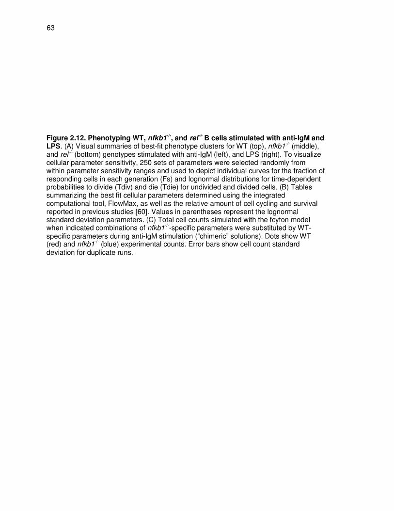
63
Figure 2.12. Phenotyping WT, nfkb1-/-, and rel
-/- B cells stimulated with anti-IgM and LPS. (A) Visual summaries of best-fit phenotype clusters for WT (top), nfkb1-/- (middle), and rel-/- (bottom) genotypes stimulated with anti-IgM (left), and LPS (right). To visualize cellular parameter sensitivity, 250 sets of parameters were selected randomly from within parameter sensitivity ranges and used to depict individual curves for the fraction of responding cells in each generation (Fs) and lognormal distributions for time-dependent probabilities to divide (Tdiv) and die (Tdie) for undivided and divided cells. (B) Tables summarizing the best fit cellular parameters determined using the integrated computational tool, FlowMax, as well as the relative amount of cell cycling and survival reported in previous studies [60]. Values in parentheses represent the lognormal standard deviation parameters. (C) Total cell counts simulated with the fcyton model when indicated combinations of nfkb1-/--specific parameters were substituted by WT-specific parameters during anti-IgM stimulation (“chimeric” solutions). Dots show WT (red) and nfkb1-/- (blue) experimental counts. Error bars show cell count standard deviation for duplicate runs.
63

64

65
Figure 2.13. Best-fit fcyton solution overlays for stimulated wildtype, nfkb1-/-, and
rel-/- B cell CFSE time courses. CFSE fluorescence data was collected and
phenotyped using FlowMax, a computational tool that implements our integrated methodology. Green overlays show the weighted average best-fit model solutions for six duplicate log-fluorescence CFSE time courses (filled histograms). Columns represent individual time points. Histograms are normalized to the highest count for each time course across experimental duplicates. X-axes are in log-fluorescence units and automatically chosen to encompass all fluorescence values across all time-points and experimental runs. Red line shows manually selected position of the undivided population. Times of collection are indicated next to each histogram. Background indicates stimulus (blue = LPS, purple = anti-IgM). See also Figure 2.12.
65

66

67
Figure 2.14. Using chimeric model solutions to identify key fcyton parameters. Total model cell counts determined when combinations of best-fit wildtype parameters were replaced by nfkb1-/- -specific (rows 1 and 3) and rel-/--specific (rows 2 and 4) best-fit maximum-likelihood parameter ranges for anti-IgM (rows 1 and 2) and LPS (rows 3 and 4) stimulation. Dots show wildtype (red) and knockout (blue) experimental counts. Error bars show standard deviation of cell counts from duplicate runs. Poor fitting indicates that the indicated parameters do not sufficiently describe the mutant phenotype.
67

68

69
2.3. Discussion
Recent advances in flow cytometry and mathematical modeling have made it
possible to study cell population dynamics in terms of stochastic cellular processes that
describe cell response, cell cycle, and life span. Interpreting CFSE dye dilution
population experiments in terms of biologically intuitive cellular parameters remains a
difficult problem due to experimental and biological heterogeneity on the cellular level.
While available population models may be fitted to generational cell counts, a remaining
challenge lies in determining the redundancy and size of the solution space, a
requirement for developing confidence in the quantitative deconvolution of CFSE data.
Developing a methodology for objective interpretation of CFSE data may lead to
quantitative mechanism-oriented insights about cellular decision-making, and allow for
improved and automated diagnosis of such data in the clinic.
In this study we present an integrated phenotyping methodology, exemplified by
the computational tool FlowMax, which addresses these challenges. FlowMax
comprises the tools needed to construct CFSE histograms from flow cytometry data, fit a
fluorescence model to each histogram, determine sets of best fit cellular parameters that
best describe the CFSE fluorescence time series, and estimate the sensitivity and
redundancy of the best fit parameters (Figure 2.1). By using the cell fluorescence model
to translate between generation-specific cell counts of the cell population model and the
CFSE fluorescence profiles, the method ensures that the population dynamics model is
trained directly on the experimental fluorescence data, without relying on ad hoc scoring
functions. While our general methodology can be relatively easily adopted for use with
any population dynamics and cell fluorescence models (including population models that
incorporate both CFSE label and population dynamics [98,99,107,108]), we adopted a
version of the cyton model because it explicitly incorporates most features of

70
proliferating lymphocytes in an intuitive manner, forms the basis of the Cyton Calculator
tool, and could be easily adapted to include new observations from single-cell studies.
While, the cyton model is over-determined and it is possible that minimal alternative
models may describe the noisy CFSE data equally-well [90]. For example, it is possible
that models with exponential distributions for the time to divide and die, or models which
do not include generational dependence for division/death may be able to describe the
data. However, independent studies have shown that lymphocyte cycling and
programmed cell death show delay times and conform to log-normal distributions, and
that the fraction of lymphocytes exiting the cell cycle as well as the timing for division
and death of lymphocytes are generation-dependent [21,44,46]. Our attempts at fitting a
typical experimental dataset using minimal models confirmed that to model B cell
dynamics both a delay in division/death timing (e.g. using log-normal distributions) as
well as distinguishing between generations (e.g. undivided/divided) is essential
(unpublished data). Within FlowMax we chose to decouple treatment of cell fluorescence
from population dynamics and allow for manual compensation for general fluorescence
changes such as dye catabolism (supplementary file FlowMax.zip). Treating such
experimental heterogeneity separately from biological variability was essential for
computational tractability of solution finding via repeated fitting.
Fitting generated datasets allowed us to evaluate individual fitting steps, and
when these were combined in an integrated or sequential manner. While, the cell
fluorescence model is readily trained on the generated data, especially if multiple peaks
are present (Figure 2.2B-C), not all fcyton model parameters are equally determinable,
as parameters for Tdie1+ and Dµ were associated with significant median errors (Figure
2.3C and Figure 2.6). When both models were fitted, doing so in an integrated manner
(using the fitted cell fluorescence parameters as adaptors during population model

71
optimization) outperformed doing so sequentially in terms of both solution statistical
significance (Figure 2.5A) and fcyton parameter error distributions (Figure 2.5B and
Figure 2.4). This is not surprising as the integrated method avoids errors introduced
during fluorescence model fitting, by optimizing the cell population model on the
fluorescence histograms directly (Figure 2.6). Furthermore, by using the fluorescence
model as an adaptor, contributions from each fluorescence intensity bin are
automatically given appropriate weight during population model fitting, while the
sequential approach must rely on ad hoc scoring functions to achieve reasonable, albeit
worse, fits. The accuracy of the integrated fitting approach improves asymptotically with
the number of fit points used (Figure 2.7), and is dependent on the choice of time points
used, with errors in key fcyton model early F0, N, and late Tdie0 parameters especially
sensitive to sufficiently early and late time points, respectively (Figure 2.8). Testing
potential scoring functions demonstrated that while the methodology is relatively robust
to specific objective function selection, an objective function including both a mean root
sum of squared deviations as well as a correlation term resulted in lower errors in
average fitted generational counts (Figure 2.9). Finally, fitting both the cell fluorescence
and fcyton model typically requires only a few minutes on a modern computer (Table
2.1), suggesting that our methodology and tool can be used to process a long duplicate
time course in about a day.
The analysis of our fitting methodology revealed a limit on the accuracy of fitted
model parameters, even under idealized conditions of perfect knowledge of experimental
heterogeneity and assuming the fcyton model is a perfect description of B cell dynamics
(Figure 2.3), suggesting that objective interpretation requires solution sensitivity and
redundancy estimation. We compared several qualitatively good model fits obtained with
the Cyton Calculator [45] to our phenotyping tool FlowMax (Table 2.2 and Figure 2.10).

72
Using the Cyton Calculator, best-fit parameter sets (Figure 2.10B blue dots) are subject
to choice of initial parameters (Table 2.2). Repeated fitting with different fitting
conditions yielded qualitatively good solutions with different parameter values.
Conversely, the solution quality estimation integrated into our methodology (Figure
2.10A) revealed that only one set of parameters best describes the dataset, and that
only a relatively small range of maximum-likelihood parameter values was common to
good fits (Figure 2.10B green dots and ranges). Interestingly, most of the fitted
parameters are in approximate quantitative agreement between the two methods,
however, the maximum-likelihood parameter ranges determined by our methodology
usually showed agreement with outlying parameter values determined by the Cyton
Calculator, suggesting that picking a specific or average solution may be inappropriate
(Figure 2.10B).
Testing how data quality affects solution redundancy and sensitivity reveals that
the methodology is relatively robust to poor CFSE staining (high CV) as well as the
frequency of time points used for fitting, assuming they are spaced throughout the time
course (Figure 2.11). However, this is only true if time points are selected such that they
capture the population behavior throughout the response, as picking only early time
points resulted in global parameter insensitivity, degeneracy, and large parameter errors.
Furthermore, poor mixing/preparation of cells (scale noise) or the presence of other cell
populations (count noise) resulted in qualitatively good fits at the cost of some errors in
perceived population parameters, highlighting the importance of fitting to two or more
replicate time courses and working with a single cell type.
Finally, to demonstrate that our computational tool can provide valuable insights
into the cellular processes underlying lymphocyte dynamics, we used FlowMax to
phenotype B cells from NFκB-deficient mice, which show strong proliferative and

73
survival phenotypes when stimulated with anti-IgM and LPS mitogenic signals (Figure
2.13). Our analysis of these cells confirmed the previously published data [60,171] and
extended the analysis to specific cellular processes in a quantitative manner. We found
for example that the phenotype of NFκB1-/- and rel-/- is similar in the proliferation and
survival of B-cells, except in the ability of resting B cells to exit the G0 stage, which is
more critically controlled by rel gene product cRel (Figure 2.12A). This may reflect that
while cRel is activated early and required for all aspects of B-cell proliferation, the
NFκB1 gene product p105 is thought to provide for lasting ERK1 activity [86] that may
facilitate primarily later stages of B-cell proliferation. Furthermore, our analysis revealed
a previously unappreciated anti-proliferative role for NFκB gene NFκB1 during anti-IgM
stimulation (Figure 2.12B). Although more subtle, this phenotype was revealed because
we were able to distinguish between early pro-proliferative cellular processes (F0, Tdiv0,
Tdie0) and later ones (F1+, Tdiv1+, Tdie1+), which may otherwise be overshadowed by
early parameters that more prominently determine bulk population dynamics, but
importantly determine the proliferative capacity of B cells. We confirmed the importance
of the later parameters by modeling population dynamics with “chimeric” parameter sets
derived from wildtype and knockout model fits (Figure 2.12C and Figure 2.14). How
NFκB1 may dampen late proliferative functions in response to anti-IgM but not LPS
remains to be investigated. Preliminary results indicate that the NFκB1 gene product
p50, which may have repressive effects as homodimers, is actually less abundant
following anti-IgM than LPS stimulation. Conversely the NFκB1 gene product p105 is
more abundant following anti-IgM than LPS stimulation and could inhibit signaling in two
ways. Induced expression of p105 may block MEK1/ERK activation by Tpl2 [85], or it
may function to provide negative feedback on NFκB activity, as a component of the

74
inhibitory IκBsome complex [148,172]. Future studies may distinguish between these
mechanisms and examine the role of the IκBsome in limiting the proliferative capacity of
antigen-stimulated B cells.
2.4. Models and Methods
FlowMax source code, executable, and a short tutorial can be found in
supplementary file FlowMax.zip. CFSE datasets used are provided as CFSEdatasets.zip
supplementary file.
2.4.1. Ethics Statement
Wildtype and gene-deficient rel and NFκB1 mice were maintained in ventilated
cages. Animal studies were approved by the Institutional Animal Care and Use
Committee of the University of California, San Diego.
2.4.2. Modeling experimental fluorescence variability
For the cell fluorescence model, we adopted a mixture of Gaussians model for
representing log-fluorescence CFSE histograms. The mean, µ, and standard deviation,
σ, for a Gaussian distribution of cellular fluorescence in a specific generation, g, is
calculated as
0
10log (10 )g
gr b s
µµ = ⋅ + + , (1)
0 g CVµσ σ= ⋅= , (2)

75
where r represents the halving ratio (~0.5), b the background (autofluorescence) [173], s
is a shift parameter used to adjust the fluorescence of the whole distribution during
fitting, and CV is the generation-invariant Gaussian coefficient of variation. While the CV
is generation-invariant, fluorescence parameters are allowed to vary from time point to
time point during fitting. These fluorescence parameters must be combined with
generation-specific cell counts to describe a weighted fluorescence histogram that
resembles typical CFSE data. Recent studies have shown that a mixture of Gaussians
closely approximates experimental CFSE log-fluorescence histograms [45,111,112]. Our
model is based on those suggested by Hodgkin et al [45]. In addition, Hasenauer et al
suggest a mixture of log-normal distributions to approximate the combined heterogeneity
in CFSE staining and autofluorescence [107]. A description of our model fitting strategy
can be found below.
2.4.3. Modeling Population Dynamics
For modeling population dynamics, we started with the generalized cyton model,
which straightforwardly incorporates most biological features of lymphocyte proliferation
[44], and forms the basis of the Cyton Calculator [45], the current state-of-the-art
computational tool for interpreting CFSE-derived generational cell count data. To reflect
the recent experimental finding that growing (i.e. responding) cells are resistant to death
[21] we logically decoupled the division and death processes by explicitly removing the
cell fate competition. In the so called, fcyton model, the fraction of responding cells in
each generation (the Fs) control cell fate by ensuring that responding cells are protected
from death, however the timing to the chosen fate (division or death) is still stochastically
distributed. Specifically, the number of cells that divide and die for each cell generation,
g, as a function of time, t, is found using

76
( ) ( )0 0 0
div
gn t F N tφ= = ⋅ ⋅ , (3)
( )0 0 0(1 ) ( )die
gn t F N tψ= = − ⋅ ⋅ , (4)
( ) ( ) ( )' ' '
0 1 1
0
2 ,
t
div div
g g gn t F n t t t dtφ> − += ⋅ ⋅ −
∫
(5)
( ) ( ) ( ) ( )' ' '
0 1 1
0
2 1 .
t
die div
g g gn t F n t t t dtψ> − += ⋅ − ⋅ ⋅ −
∫
(6)
In equations (3-6) ( )0 tφ , ( )1 tφ + , 0 ( ), tψ and 1 ( )tψ + represent the cell age-dependent
probability density functions that undivided cells will divide, divided cells will divide,
undivided cells will die, and divided cells will die, respectively. The parameters N and iF ,
represent the starting cell count, and fraction of cells responding in generation i,
respectively. The total number of cells, ( )gN t at time t and generation g is given by
( ) ( ) ( )( )' ' '
0 0 0
0
,
t
div die
gN t N n t n t dt= = − +
∫
(7)
( ) ( ) ( ) ( )( )' ' ' '
0 1
0
2 .
t
div div die
g g g gN t n t n t n t dt> −= − −
∫
(8)
The progressor fractions, 1iF≥ , are calculated using a truncated Gaussian distribution
similar to the “division destiny” curve suggested by Hawkins et al in the cyton model [44]:

77
1
1 ( ), ( 1) 1
1 ( 1)
0, ( 1) 1
i
cdf icdf i
cdf iF
cdf i
≥
−
− <
− −=
− =
, (9)
where ( )cdf i is the cumulative normal distribution with mean Dµ and standard deviation
Dσ . Since lymphocyte inter-division and death times are well-approximated by log-
normal distributions [44], a total of 12 parameters are required to determine the cell
count at any point in time in each generation: N, 0F , Dµ , Dσ , and eight parameters
specifying the log-normal division and death distributions. For a full list of parameters
and the ranges used during fitting, refer to Table 2.3.
2.4.4. Testing model accuracy with generated CFSE fluorescence time courses
A total of 1,000 sets of randomized fcyton and fluorescence parameters within
realistic ranges [21,44,45,174], were generated (Table 2.3). The randomized fcyton
parameters were applied to construct cell counts for eight generations ten time points up
to192 hours (Table 2.4). The randomly chosen fluorescence parameters were then
applied to construct weighted fluorescence histograms (Figure 2.2A). To test the
accuracy of cell fluorescence model fitting, we trained the fluorescence model on the
generated histogram time courses one histogram at a time. During fitting, peak weights
were calculated analytically using a non-linear regression approach (see below).
Resulting best-fit model histogram areas under each peak were compared to their
generated counterparts and the average percent errors of the counts normalized to the
maximum generational count for each parameter set were plotted (Figure 2.2B, 2.3B,
2.4A, 2.5A, 2.6A, 2.7A, 2.8A, and 2.9A). To test the fcyton cell population model, we

78
trained the model on known generational cell counts from the generated datasets.
Resulting best-fit model generational counts and fcyton parameters were compared to
their generated counterparts (Figure 2.2). To evaluate the accuracy of sequential model
fitting, the generated datasets were used to first train the cell fluorescence model
followed by a round of fcyton model fitting on the resulting best-fit generational cell
counts using a simple squared deviation and a more complex ad hoc objective function
(Figure 2.5 (blue) and Figure 2.4). Next, the generated datasets were used to first train
the cell fluorescence model followed by a round of fcyton model fitting to the
fluorescence histograms using the best-fit cell fluorescence parameters to generate log-
fluorescence histograms with peak weights determined by the population model, which
were compared to generated histograms directly (proposed integrated fitting
methodology). Different time point schedules were used when testing three or five time
point time courses (see Table 2.4). For demonstrating how data quality affects fitting of
typical time courses, we used the fitted experimental wildtype LPS cluster solutions to
generate six separate in silico time courses: a low CV time course (8 time points,
CV=0.18, ratio=0.5, background=100,shift=0), a high CV time course (8 time points,
CV=0.23, ratio=0.5, background = 100, shift = 0), a generation count noise time course
(8 time points, CV=0.18, ratio=0.5, background = 100, shift = 0, each peak count scaled
randomly by 1+N(µ=0,σ=0.1)), a scaled noise time course (8 time points, CV=0.18,
ratio=0.5, background=100, shift=0, number of cells in histogram scaled randomly by
1+N(µ=0,σ=0.1)), an infrequent time point time course (4 time points from 24-144 h,
CV=0.18, ratio=0.5, background=100, shift=0), and an early time point time course (4
time points from 12-48 h, CV=0.18, ratio=0.5, background=100, shift=0). Each time
course was fitted 100 times using our full methodology (Figure 2.1), and parameter

79
solution clusters were plotted (Figure 2.11). Refer to Table 2.4 for specific time point
schedules used.
2.4.5. Developing measures of confidence for parameter fits
We implemented a computational pipeline for estimating the redundancy and
sensitivity of model solutions (Figure 2.1 step 3). A stochastic simulated annealing fitting
procedure [175] was used to determine multiple best-fit solutions with random initial
parameters (see below). Next, we used a normalized percent area error (NPAE) metric
for solution quality estimation which ranges between 0% and 100% difference in
histogram areas:
[ ] [ ]1 1 1
1 1
50
t r mj j
i i ii j k
t r j
ii j
Cells H kN
M kPAE
Cells
= = =
= =
⋅ −= ⋅
∑ ∑ ∑
∑ ∑
,
(10)
where i and j represent time point i, and experimental run j, and Cells, H, and M
represent total cell counts, experimental discrete histogram density, and model discrete
histogram density with m total bins, respectively. Solution candidates with NPAE within
0.1 of the top were kept for quality estimation:
1 2{ , , , }nCandidates S S S= …, (11)
where xS represents the xth set of best-fit parameters. These fits were subjected to one-
dimensional parameter sensitivity estimation, which establishes an upper and lower
bound on each parameter value that would result in the weighted percent histogram area
error (NPAE) to, increase by 1 (1% normalized area difference increase), yielding two
sets of sensitivity values for each parameter:
1 1 2 2{ , , , , , , }n nSensitivities L H L H L H= < > < > … < >, (12)

80
where ,x xL H< > represents a 2-tuple consisting of sets of lower and upper parameter
sets for xS , respectively. Since more than one non-redundant set of parameters may
exist, we developed an agglomerative clustering algorithm which is designed to combine
clusters with the highest parameter sensitivity overlap, arriving at sets of non-redundant
maximum likelihood parameter ranges. Briefly, the solutions are clustered by continually
agglomerating pairs of clusters xC , yC with highest total normalized overlap ,x yD between
parameters:
[ ] [ ]( ) [ ]
[ ]
[ ] [ ]( ) [ ]
[ ]
,
( [ ]),
| [ ] | | [ ] [ ] |
( [ ]),
| [ ] | |
,
[ ] [ ] |
y y x
x
x x y y
x y y
x y
x
x
yparams
x y i i
i
y y
x
x
A i H i A i L iif A A
A i H i A i H i
A i H i A i L iif A A
A i H
D
i A i H
d d
i
+ − − >
+ + +
+
= =
− −
+
≤+ +
∑ ,
(13)
where xA and yA are weighted parameter averages for clusters xC and yC , respectively.
The agglomerated parameter sensitivity ranges are defined to be the intersection of
ranges supported by all candidate solutions in the cluster, resulting in increasingly tighter
estimates of the maximum likelihood parameter sensitivity ranges as more solutions are
incorporated into the cluster. Clustering is terminated when cluster pairs for which
parameter ranges are overlapping for all parameters no longer exist. When clustering
parameter ranges, we keep track of a weighted average value that is guaranteed to be
within the overlap between ranges being clustered, however its position is weighted
according to the relative maximum distance from the average of each of the starting
cluster averages:

81
[ ] [ ]
,
,
,
a c a
b b c
b ac c c c c c c
a b a b
d H A
d A L
d dA H L L H H L
d d d d
= −
= −
= − + = − −+ +
(14)
where the distance ( d ), high( H ), average ( A ), and low ( L ) values are used to
agglomerate clusters a and b into cluster c and letting aA < bA . Finally, since solution
clusters represent linear independent combinations of parameters, solution clusters are
sampled uniformly (n=1,000) within the clustered maximum- likelihood parameter ranges
for all parameters simultaneously and clusters with median NPAE within 1% of the top
cluster’s NPAE are kept to ensure that unrealistic parameter combinations were
removed.
A simple divide-and-conquer algorithm was chosen for calculating the parameter
sensitivity ranges which operates on the best-fit fcyton model parameters, X = { , 0F ,
, , , , , , , , , }, and
a constant values for the fit tolerance,ε :
ALGORITHM CalParamSensitivities (X, ε)
( )MinScore AreaDiff X←
Define array Upper of size |X|
Define array Lower of size |X|
FOREACH parameter ix X∈ :
iOriginal x=
| max( ) |
1000
i ix x
StepSize−
←
WHILE | max( ) |
10000
i ix x
StepSize−
>
N
Dµ Dσ0Tdiv µ 0Tdiv σ 0Tdie µ 0Tdie σ 1Tdiv µ+ 1Tdiv σ+ 1Tdie µ+ 1Tdie σ+

82
i ix x StepSize← +
( )CurrScore AreaDiff X←
IF (1 )CurrScore MinScore ε< ⋅ +
i ix x StepSize← −
2
StepSizeStepSize ←
ELSE
min( 2, max( ) )i iStepSize StepSize x x← ⋅ −
ENDIF
ENDWHILE
i iUpper x←
ix Original=
ENDFOREACH
FOR EACH parameter ix X∈ :
iOriginal x=
| min( ) |
1000
i ix x
StepSize−
←
WHILE | min( ) |
10000
i ix x
StepSize−
>
i ix x StepSize← −
( )CurrScore AreaDiff X←
IF (1 )CurrScore MinScore ε< ⋅ +
i ix x StepSize← +

83
2
StepSizeStepSize ←
ELSE
min( 2, min( ))i iStepSize StepSize x x← ⋅ −
ENDIF
ENDWHILE
i iLower x←
ix Original=
ENDFOREACH
RETURN Upper and Lower
Since the value of the tolerance parameter ε, or the maximum percent increase
in the overall normalized percent area error (NPAE), is an important implicit parameter
for sensitivity analysis, an appropriate value must be used. In our experience, a value
that is too small resulted in small sensitivity ranges for each parameter tested and a
large number of non-overlapping solutions. Conversely, high tolerance resulted in large
acceptable parameter sensitivity ranges, increasing the chance that linear sampling of
parameters introduced errors into sensitivity estimation and underestimating the
sensitivity of the solution to model parameters. The parameter ε was set to 1%
normalized percent area error (NPAE) empirically because this resulted in parameter
sensitivities of approximately ±10% of the best-fit parameter value for the determinable
parameters such as F0, Tdiv0, and Tdiv1+. In addition, this resulted in fewer than three
solution clusters for experimental datasets. Conversely, values of ε smaller than 1%
resulted in more than five solution clusters for the experimental datasets.

84
The main motivation for clustering parameters is to identify solution uniqueness
since more than one set of model parameters can sufficiently describe the data. To
determine if more than one solution space can fit the data, we perform a parameter
sensitivity analysis for each best-fit solution then successively combine solutions with the
largest overlap in the solution space until only non-disjoint solutions remain. By doing
this we guarantee that the clustered solution space(s) are non-redundant.
Since parameter fits are obtained using a non-deterministic fitting procedure, the
best-fit parameter solution is only an estimate of the true solution. Furthermore, we
established that parameters exhibit widely varying degrees of sensitivity that is heavily
determined by the underlying dataset. Therefore, we first estimate the sensitivity of each
best-fit parameter in a solution, obtaining a set of independent lower and higher
parameter values for each parameter, p. Repeating the fitting n times we get the set of
best-fit parameter ranges for parameter p:
. { },1 ,1 ,2 ,2 , ,[ , ],[ , ], ,[ , ] .p p p p p p n p nS L H L H L H= …
We assume that each distribution of p found is equally likely and therefore the probability
of p is modeled as:
, ,
1 , ,
( )1( | ) ,
nx p i p i
p p
i p i p i
I L x Hf p x S
n H Lφ
=
≤ ≤= = =
−∑
Where , ,( )p i p iI L x H≤ ≤ is the indicator function and returns 1 if p is within the ith range.
In other words, p
φ assumes a linear combination of uniform distributions for , which
comes about if one marginalizes the distribution on all other model parameters. Since
represents the probability distribution model of the parameter p given the observed
best-fit ranges, the region of maximum likelihood is the range of parameter values such
that the overlap count is maximized. Furthermore, by ensuring that only overlapping
p
pφ

85
parameter ranges are clustered together, we guarantee that only one such maximum
region exists for each cluster:
{ }
{ }
,max
,1 ,2 ,
,1 ,2 ,
( | ) [ , ],
max , , ,
min , , ,
p p p p
p p p p n
p p p p n
f p x S x L H
L L L L
H H H H
φ∧ ∧
∧
∧
= = ∀ ∈
=
=
…
…
(15)
The maximum likelihood estimator for are all values of within the range [ , ]p p
L H∧ ∧
or the intersection of all of the parameter ranges in p
S . In other words, p
L∧
and p
H∧
are
the maximum likelihood estimators of the lower and upper value of , due to the
resolution of the data and methodology (i.e. the probability of is uniform for any ith
best-fit sensitivity range , ,[ , ]p i p i
L H ). We report the region of defined by and for
which is maximized, or the mode of .
An added potential benefit of clustering is to minimize bias in how we calculate
the sensitivity of each solution. Since solution spaces are created by varying parameters
around the best-fit value, an implicit parameter is the amount by which a solution can
worsen as we vary each parameter independently. If the allowed error is inappropriate,
the clustering will either return too many similar solutions (error tolerance too low) or
both clusters with poor and good fits (tolerance is too high). The later happens because
only the intersection of parameter spaces is kept during the agglomeration process,
which means that an overestimate of the parameter range for solutions about a region
containing a local minimum will still only contain good fits, while an over estimate of the
parameter range for solutions about a region containing poor fits will contain poor
solutions. A subsequent filtering of the solution clusters can be used to remove these
p p
p
p
p pL∧
pH∧
pφ
pφ

86
“artifact” clusters containing poor solutions and we can alleviate the bias in selecting the
error tolerance parameter.
Choosing the representative parameter value (the cluster “average”) for a
specific cluster is somewhat arbitrary as the probability of the parameter within a range
was assumed to be uniform during clustering. In reality, the probability of any parameter
is likely to decrease with the distance from a best-fit value. Therefore when clustering
parameter ranges, we keep track of a weighted average value of that is guaranteed
to be within the overlap between ranges being clustered, but its position is weighted
according to the relative maximum distance from the average of each of the starting
cluster averages:
[ ] [ ]
,
,
,
a c a
b b c
b ac c c c c c c
a b a b
d H A
d A L
d dA H L L H H L
d d d d
= −
= −
= − + = − −+ +
(16)
where the distance ( d ), high( H ), average ( A ), and low ( L ) values are used to
agglomerate clusters a and b into cluster c and letting aA < bA .
The pseudo code for clustering the candidates by maximizing the parameter sensitivity
overlap given the set of candidate best-fit fcyton parameter values and their
corresponding lower and upper bound sensitivity ranges is shown below:
ALGORITHM: ClusterBySensitivityAgglomeration (Candidates, Sensitivities)
Define { } { } { }1 1 2 2{ , , , }n nClusters C S C S C S= = = … =
Define 1 1 2 2{ , , , }n nAverages A S A S A S= = = … =
Define 1 1 2 2{ , , , }n nLows D L D L D L= = = … =
Define 1 1 2 2{ , , , }n nHighs U H U H U H= = = … =
p
p

87
Define best_c1 = best_c2 = -1
Define largestOverlap =0
Define clustering = true
WHILE clustering = true
FOR , , a bA Averages A Averages a b∈ ∈ ≠
Define dist = 0
FOREACH parameter, i
Define
[ ] [ ]( ) [ ]
[ ]
[ ] [ ]( ) [ ]
[ ]
( [ ]),
| [ ] | | [ ] [ ] |
( [ ]),
| [ ] | | [ ] [ ] |
b b a
a
a a b b
a b b
a b
a
b
i
a a b b
a
A i U i A i D iif A A
A i U i A i U i
A i U i A i D iif A A
A i U i A i U i
d
+ − − >
+ + +
+ − − ≤
=
+ + +
dist = dist+di
ENDFOREACH
IF dist > 0 and dist > largestOverlap
largestOverlap =dist
best_c1 = a
best_c2 = b
ENDIF
ENDFOR
IF best_c1 ≠ -1 and best_c2 ≠ -1
Define , ,newA newD newU
FOREACH parameter, i
Define x = y=z=0
IF _ 1[ ]best c
A i < _ 2[ ]best c
A i

88
_ 2[ ]best c
x D i=
_ 1[ ]best c
y U i=
_ 2 _ 1[ ] [ ]best c best c
z A i A i= −
ELSE
_ 1[ ]best c
x D i=
_ 2[ ]best c
y U i=
_ 1 _ 2[ ] [ ]best c best c
z A i A i= −
ENDIF
Define int
z yx
y x
⋅=
+
[ ]newA i = _ 1 int[ ]best c
A i x+
[ ]newD i =
_ 1 _ 1 _ 2 _ 2[ ] max( [ ] [ ], [ ] [ ])best c best c best c best c
newA i A i L i A i L i− − −
_ 1 _ 1 _ 2 _ 2[ ] min( [ ] [ ], [ ] [ ]) [ ]best c best c best c best c
newU i A i U i A i U i newA i= + + −
ENDFOREACH
c1 2best ( / {A , }
cbestAverages Averages A= )∪ newA
(Lows Lows= /{ _ 1best cD , _ 2best c
D })∪ newD
(Highs Highs= /{ _ 1best cU , _ 2best c
U })∪ newU
(Clusters Clusters= /{ _ 1best cC , _ 2best c
C })∪ _ 1 _ 2(best c best c
C C )
ELSE

89
clustering = false
ENDIF
ENDWHILE
RETURN < , , ,Averages Lows Highs Clusters >
END
2.4.6. Comparing FlowMax to the Cyton Calculator
We used counts derived after fitting the cellular fluorescence model to the
experimental wildtype B cell proliferation time courses stimulated with LPS (Figure 2.13),
to repeatedly fit the cyton model using the Cyton Calculator [45] and compared to results
from fitting the cyton model using FlowMax, a tool that implements our methodology and
solution quality estimation procedure (Figure 2.10A). For the Cyton Calculator we used
counts derived from fitting the cellular fluorescence model as input, while for FlowMax,
we used the fluorescence data directly. To find Cyton Calculator solutions, we carried
out Cyton Calculator fitting multiple times using varied starting parameters values
sampled from ranges in Table 2.3, as suggested. Most-parameter combinations yielded
qualitatively poor fits (determined visually by comparing total and generation cell counts
to experimental data), and were discarded. Four qualitatively good solutions, determined
visually by comparing total and generational cell counts to experimental data, were
found using starting parameters listed in Table 2.2 (Figure 2.10B, blue dots). Using
FlowMax involved 1,000 fits, automated solution filtering, parameter sensitivity
estimation, and solution clustering. This allowed visualization of a family of solutions
sampled from the maximum-likelihood sensitivity ranges for the only solution cluster
identified.

90
2.4.7. Testing how our methodology is affected by the choice of objective
function
To analyze how our methodology is affected by choice of objective function
during fitting, we used 1,000 generated time courses to fit the fcyton model using best-fit
cell fluorescence parameters as adaptors (our proposed integrated methodology). We
tested three objective functions for comparing the model histograms to generated
histograms: a simple mean sum of absolute deviations (MAD):
[ ] [ ], ,1 1 1
,1 1
t r m
i j i j ii j k
MAD t r
i ji j
Cells H k M kObj
Cells
= = =
= =
⋅ −=∑ ∑ ∑
∑ ∑
,
(17)
a mean root sum of squared deviations (MRSD) objective function:
[ ] [ ]( )2
, ,1 1 1
,1 1
t r m
i j i j ii j k
MRSD t r
i ji j
Cells H k M kObj
Cells
= = =
= =
⋅ −=∑ ∑ ∑
∑ ∑
,
(18)
and a mean root sum of squared deviations with Pearson correlation (MRSD+) objective
function:
[ ] [ ]( )
( )
2
,1
, 21 1
,
,1 1
,
m
i j it r k
i ji j
i j i
MRSD t r
i ji j
H k M kCells
cor H MObj
Cells
=
= =
+
= =
−⋅
=
∑
∑ ∑
∑ ∑
.
(19)
In the above equations,
j
iCells is the total cell count in run j for time point i, and cor(x,y)
represents the Pearson correlation coefficient between the experimental histogram, j
iH ,
and modeled histogram, iM . See also Figure 2.10.
2.4.8. Generating chimeric solutions from two phenotypes

91
To dissect the contributions of several components of complex phenotypes, we
used two sets of parameters (i.e. wildtype and mutant) and generated a “chimeric” set of
parameters with combinations of F0, F1+ (Dµ, Dσ), Tdivs (E[Tdiv0], s.d.[Tdiv0],E[Tdiv1+],
s.d.[Tdiv1+]), and Tdies (E[Tdie0], s.d.[Tdie0],E[Tdie1+], s.d.[Tdie1+]), copied from either
set. The generated “chimeric” phenotypes were visualized (see below) and qualitatively
compared to visualizations from the two originating phenotypes. In the case of NFκB1-/-
anti-IgM stimulated B cells, this analysis confirmed that misregulation of the late
progressor fractions (F1+) constituted the primary phenotype (Figure 2.12C).
2.4.9. Visualizing solution clusters
Solution clusters were defined as sets of maximum-likelihood parameter
sensitivity ranges that are overlapping between all solutions in a cluster. To visualize
these solutions, parameter sets were sampled uniformly from within the clustered
maximum-likelihood parameter sensitivity ranges independently for each parameter. For
parameter visualization, the sampled parameters were used to plot the four lognormal
distribution probability density functions (Tdiv0, Tdie0, Tdiv1+, Tdie1+), normalizing by the
maximum probability per distribution. The fraction of responding cells in each generation
(Fs) are plotted using connected dots on a scale between 0 and 1 for each generation (x
axis), with the larger dot representing the independent F0 parameter (Figure 2.12). For
population count visualization, the sampled parameter values were used to calculate cell
count time series data by solving the fcyton model with the sampled parameters (Figure
2.12C and Figure 2.14). FlowMax provides options for plotting either the sampled
solutions or the best-fit solutions found during model fitting. The best-fit cluster average
solution is shown as an overlay for each experimental dataset (Figure 2.13).

92
2.4.10. Using FlowMax to phenotype CFSE time courses
We used a computational tool, which implements all of the steps for fitting
experimental CFSE B cell datasets. A succinct tutorial is included in the supplementary
text (Supplementary File 2.3). In brief, we used our computational tool to construct log-
fluorescence CFSE histograms of viable B cells from raw CFSE data (see experimental
methods below). For each log fluorescence histogram, the average fluorescence of
undivided cells was selected manually based on previous time points. Then the cell
fluorescence parameters were automatically determined for each time course subject to
user constraints for the coefficient of variation, background autofluorescence, and die
halving ratio, and shift of the undivided peak as well as an estimate of the maximum
number of generations to be fitted to each time course (The default is set to eight
[45]).The fitted cell fluorescence parameters were then used during the population
dynamics fitting step to represent generational cell counts derived from the fcyton model.
The population dynamics fitting step was repeated 1,000 times, poor results were
removed from consideration, parameter sensitivity ranges were calculated and solutions
were clustered to estimate solution redundancy. The resulting best-fit families of
solutions (determined by average error in histogram area sampled from parameter
sensitivity ranges) for each experimental condition were compared.
2.4.11. Experimental Methods
Primary splenocytes were isolated from 6-8 week old mice, naïve B cells purified
using magnetic bead separation (Miltenyi Biotec), labeled with 4 µM 5(6)-
Carboxyfluorescein diacetate, N-succinimidyl ester (CFSE) dye (Axxora) for 5 minutes at
room temperature, and stimulated with 10 µg/mL LPS (Sigma) or 10 µg/mL goat anti-
mouse IgM (Jackson Immunoresearch Inc.) B cells were grown in fresh media with 1%

93
penicillin streptomycin solution (Mediatech Inc.), 5 mM L-glutamine (Mediatech Inc.), 25
mM HEPES buffer (Mediatech Inc.), 10% FCS and 2 µL/500 mL BME (Fisher Scientific)
at a concentration of 2.5x10⁵ cells/mL in 48 well plates at 37oC for a period of 6
days.Cells were removed from media, stained with 10 ng/mL propidium iodide, and
measured using an Accuri C6 Flow Cytometer (Accuri Inc.) at 28, 40, 43, 54, 59.5, 67.5,
74.5, 89, and 145 hours post stimulation. CFSE histograms were constructed after
software compensation for fluorescence spillover and manual gating on viable (PI-
negative) B cells using the FlowMax software. All measurements were performed in
duplicate (B cells from the same spleen were cultured in separate wells, two wells per
time point to ensure that each time course represented a single population of cells
subject to only experimental variability).
2.4.12. Description of CFSE time courses
A typical CFSE time course consists of a set of time points. Each time point
consists of one or more experimental bulk CFSE fluorescence measurements
(experimental runs/replicates). Each experimental run consists of a set of CFSE
fluorescence measurements which are typically represented by 2D log-transformed (or
log-fluorescence) histograms. We assume that the total number of cells per run is also
known.
2.4.13. Fitting the cell fluorescence model
The simulated annealing approach [176] was used to arrive at the set of cell
fluorescence parameters (CV, Ratio, Background, and Shift) that best describe a log-
fluorescence histogram. Each simulated annealing optimization routine was initialized
such that for time {1,2, , }t n∈ … :

94
1
1 min
t
t
CV if tCV
CV −
=
=
,
(20)
t maxRatio Ratio=, (21)
t maxBackground Background=, (22)
0tShift =, (23)
1
1
1
*(1 0.5 )
min
min t
t
CV if tCV
CV −−
=
=
− ,
(24)
1
1
1
*(1 0.5 )
max
max t
t
CV if tCV
CV −−
=
=
+
. (25)
where the subscripts “min” and “max” signify the given lower and upper limit for a
parameter, respectively. We used the best-fit CV parameters from each time point to
constrain the CV parameter range for the subsequent time point. This was useful for
fitting later time points for which individual peaks were harder to discern without some
prior knowledge of the approximate CV from previous time points.
In summary, if both early and late time points are available, FlowMax uses
information from fitting the early time points to constrain the cell fluorescence
parameters for later time points (described in the supplementary section “Fitting the cell
fluorescence model”). In this way, if the CV or dye halving ratio “drifts” between time
points, the early time points can be used to guide the fitting of these parameters for later
time points. However, the position of the undivided population is one of the parameters
supplied by the user for each histogram as it depends on the experimental conditions
(cell staining conditions, cell type, dye catabolism, cytometer setup, etc.). Instead of
trying to model how these factors affect the position of the undivided peak across
time/generations (which is computationally intractable [98,99] and outside of the scope

95
of this study), we rely on the user to specify the approximate position of the undivided
peak based on the location from previous time points. To help with this, we include a
fourth “shift” term in the model to find the optimal peak placement.
A score-based annealing schedule was used during simulated annealing. Initial
temperature was set to half of the fit score of the initial random parameter set. The
minimum temperature was set to 1/1,000 of that value. Temperature was multiplied by
0.99 at the end of each iteration. In addition, if a better solution was found, the
temperature was set to the minimum of the initial temperature or the current temperature
multiplied by 1.1. This “heating” was used to discourage local trapping of the solution. In
practice, this artificial heating helped in cases where solutions were stuck for many
iterations in a high score parameter space but proceeded toward a better solution toward
the end of the optimization, in which case, the sudden frequent improvement in the
solution “reheated” the system and allowed for optimization to finish. While this approach
resulted in satisfactory optimization, other optimization schemes of equal or better
efficiency may be possible.
A scoring function which penalized both the squared distance as well as the
difference in correlation between the fluorescence histograms for a particular time point,
t, and experimental run, r
[ ] [ ]( )( )
( )
2
1
, (1 , )
m
normali
t r normal
n H i M iScore n cor H M
m
=⋅ −
= + ⋅ −∑
,
(26)
was used where normalH is the histogram of d observed fluorescence values, M is the
model histogram of fluorescence values, n is the number of cells measured
experimentally, and cor(x,y) represents the Pearson correlation coefficient between the
histograms of x and y. The average run score was used as the time point score, and the

96
average time point score was used as the overall objective function during fitting. The
scoring function was manually optimized for experimental data fitting: correlation was
included to help guide initial optimization toward a suitable histogram shape.
While the choice of algorithm for fitting the cell-fluorescence model did not
qualitatively affect the conclusions, we desired a fitting algorithm which would allow us to
quickly find appropriate cell fluorescence model parameters (i.e. peak CV, ratio between
peaks, autofluorescence, and offset from user-specified µ0), while taking into account
solutions from previous time points. We also wanted to exclude solutions that were
outside of user-specified ranges. In addition, we wanted a fitting approach which dealt
with solution trapping in local minima, as is often the case with noisy experimental data.
We are not aware of a conventional method for achieving this efficiently. Therefore, we
selected the stochastic simulated annealing approach for fitting the model parameters,
while explicitly solving for peak weights during each step (using a conventional non-
linear regression approach described above), and allowing for information from earlier
time points to contribute to the fit. Our evaluation of the fitting methodology suggests
good agreement between fitted and generated data (see Figure 2.2); however other
methods for fitting may also be appropriate. In addition, our methodology can be
adapted to incorporate other models for cell fluorescence and/or fitting approaches if
desired by changing the cell fluorescence computational module.
2.4.14. Peak weight calculations during cell fluorescence model fitting
The problem of solving for the optimal model weights given the cell fluorescence
parameters can be formulated as a nonlinear least squares regression problem. Given a
log-fluorescence histogram with fluorescence, x , and bin size ∆ x :

97
i( ) Pr( | )iH x x X x x X Data= < ≤ + ∆ ∈ (27)
Defining the cellular fluorescence model solution, ( )F x , as a weighted sum of Gaussian
distributions, ( )g
G x :
( )1
( )G
g g
g
F x w G x=
=∑
, (28)
where w represents a weight multiplier and ( , )g g g
G G µ σ= . Then the sum of squared
errors is:
( ) ( )2
1
iI
i i x
E H i F x dx= −∆
= −
∑
∫
.
(29)
To solve for the optimal set of weights, minimize E. Rewriting E:
( ) ( )2
1 1
iI G
g g
i gi x
E H i w G x dx= =−∆
= −
∑ ∑
∫
(30)
( ) ( )2
1 1
iI G
g g
i g i x
w G x dx H i= = −∆
= −
∑ ∑
∫
(31)
( )2
1 1
I G
g ig
i g
w J H i= =
= −
∑ ∑
.
(32)
To solve the minimization problem, solve:
0 b
E
w
∂=
∂
(33)
where:
1,
, 0,
g
gb gb
b
w g b
g bwδ δ
∂ =
= =
≠∂ ,
(34)

98
1 1 1
0 2 ( )I G G
g ig gb ig
i g g
w J H i Jδ= = =
= −
∑ ∑ ∑
,
(35)
( )1 1
0 2 ( )I G
g ig ib
i g
w J H i J= =
= −
∑ ∑
,
(36)
( )1 1 1
0G I I
g ig ib ib
g i i
w J J H i J= = =
= −
∑ ∑ ∑
,
(37)
( )1 1 1
G I I
ig ib g ib
g i i
J J w H i J= = =
=
∑ ∑ ∑
,
(38)
Mw c=� �
. (39)
M is a G x G matrix and both c�
and w�
are vectors of size G, where G is the number of
generations being modeled. To calculate each element of M, and c�
:
( ) ( )1
i iI
ba a b
i i x i x
M G x dx G x dx= −∆ −∆
=∑
∫ ∫
,
(40)
( )1
( )*
iI
j j
i i x
c H i G x dx= −∆
=∑
∫
,
(41)
where xG is the Gaussian distribution ( , )x x xG representing fluorescence distributions
for cells in division class x from equations (1) and (2). Solving for the optimal weights, ,w�
associated with each Gaussian distribution:
1 w M c−=
� �
, (42)
we further ensure that the weights are non-negative and sum to 1:
0 g gw w w> ∀ ∈�
,
1
1G
g
g
w=
=∑
.
(43)
(44)

99
By solving for the weights at the end of each iteration of fluorescence model optimization
(see above), excellent fluorescence model parameters were found relatively quickly.
Furthermore, solving explicitly for the peak weights subjected only the cell fluorescence
model parameters to optimization, minimizing fitting bias that could arise due to errors in
weight optimization.
2.4.15. Fitting the fcyton model to cell counts derived from fluorescence
histograms
In order to fit the fcyton cell population model parameters ( N , 0F , Dµ , Dσ ,
0Tdiv µ , 0Tdiv σ , 0Tdie µ , 0Tdie σ , 1Tdiv µ+ , 1Tdiv σ+ , 1Tdie µ+ , 1Tdie σ+ ) to sets of
division specific cell counts, a simulated annealing [176] approach was used.
Specifically, fitting started with 4,000 iterations of randomized guess and check trials to
establish a coarse approximation of the parameters. Then the best parameter set out of
the 4,000 randomly selected parameter sets was used as the starting point for simulated
annealing. Prior to the first round of optimization by simulated annealing, the
temperature, T, was set to the current best-fit score, and Tmin, or the stopping
temperature, was initialized to 1/100,000 of T. Each simulated annealing iteration
consisted of three steps: the current parameters were modified slightly (Gaussian
sampling with sigma = 1% of the current value), the fit score was calculated for the new
parameter set, and the new parameter set was adopted with probability p such that:
1,
, diff k
T
if thenewscore was lower
p
e otherwise⋅
−
=
.
(45)
where diff is the new score minus the previous score and k is a score scaling factor.
Similarly to the optimization process used to fit the fluorescence model, if the
new score was an improvement over the current global best fit score, the temperature

100
was set to the minimum of the current temperature*1.1 or the initial temperature. This
artificial “heating” was implemented to ensure that all improving parameter sets find a
local minimum after leaving a parameter space of relatively poor fit scores. The
annealing factor was 0.9995.
Two objective functions were used during this optimization process: a simple
objective function consisting of the square deviation between the model and generated
counts, and a more complex optimized objective function that takes into account multiple
difference measures:
[ ] [ ] [ ] [ ]( )2
1 1
* , * ,n G
SD data data model model
t i
Obj Count t Prop i t Count t Prop i t= =
= −∑∑
(46)
[ ] [ ]( )
[ ][ ] [ ]
[ ][ ] [ ]
[ ] [ ]( )
2
1
2
1
,2*
, ,5*
2* ( , )
data model
ndata model
tOPT data model data model
Gdata model
i
data model
cor Prop t Prop t
n
Count t Count t
Obj Count t Count t Count t Count t
Prop i t Prop i t
n
cor Count Count
=
=
+
− + +
= + +
−
∑
∑
(47)
where Count[t] represents the total cell count at time point t, and Prop[i,t] is the
proportion of cells at time point t in generation i. The cor(x,y) function represents the
Pearson correlation coefficient between the functions x and y. In the optimized scoring
function, G is defined as the maximum number of division classes at time point t such
that Countdata[G+1] = 0 and G > 6. Therefore, all cells in division classes > 6 are treated
as one population in order to reduce the penalty for cells assigned to division classes 7
and higher. This was implemented due to an increased difficulty in discriminating CFSE
peaks after 6 divisions experimentally. This complex objective function was developed in
a step-by-step manner, starting with a basic sum of squared differences objective

101
function (46), followed by the addition of correlations, and the use of ad hoc weights for
each part of the scoring function. The annealing schedule was optimized to allow for
efficient optimization of both fit scores.
After an initial round of simulated annealing, a subsequent fast round of localized
simulated annealing centered on the optimal solution was carried out. Analogously to the
first round, the temperature was set equal to the fit score for the current optimal solution
and annealing continued until the temperature dropped below 1/1,000 of this
temperature. At the beginning of each iteration a new set of parameters was generated
randomly by modifying the best parameter set (Gaussian sampling with sigma = 0.1% of
the current value). This limited the search to the local parameter space around the best-
fit solution. In practice this often only yielded minor improvements to the fit, but on rare
occasions, allowed a very poor solution to be improved significantly before it was used in
the post-processing steps following model parameterization.
2.4.16. Fitting the fcyton models to fluorescence histograms directly
Analogously to the fitting approach used to fit the fcyton models to generational
cell counts, a stochastic method was used to fit the models to experimental
fluorescence histograms directly. The fluorescence model was used to adapt the derived
model cell counts to log-fluorescence histograms. Specifically, for each set of predicted
division-specific cell counts a fluorescence histogram was generated using the
previously fitted cell fluorescence parameters and generational cell counts as weights
(see Figure 2.2A). This facilitated the use of a relatively simple objective function for
calculating the difference between the model fluorescence histograms and the
experimental fluorescence histograms. A manually optimized objective function which
accounted for the difference between the fluorescence histograms, the correlation

102
between the fluorescence histograms, and the proportion of the total cells represented in
each histogram was used:
[ ] [ ]( )
( )
2
,1
, 21 1
,
,1 1
,
m
i j it r k
i ji j
i j i
MRSD t r
i ji j
H k M kCells
cor H MObj
Cells
=
= =
+
= =
−⋅
=
∑
∑ ∑
∑ ∑
.
(48)
where j
iCells is the total cell count in run j for time point i, and cor(x,y) represents the
Pearson correlation coefficient between the experimental histogram, j
iH , and modeled
histogram, iM . We also tested if simpler scoring functions were sufficient for fitting
generated datasets. Specifically we tried a simple mean absolute deviation objective
function (MAD):
[ ] [ ], ,1 1 1
,1 1
t r m
i j i j ii j k
MAD t r
i ji j
Cells H k M kObj
Cells
= = =
= =
⋅ −=∑ ∑ ∑
∑ ∑
,
(49)
as well as a mean root square deviation objective function:
[ ] [ ]( )2
, ,1 1 1
,1 1
t r m
i j i j ii j k
MRSD t r
i ji j
Cells H k M kObj
Cells
= = =
= =
⋅ −=∑ ∑ ∑
∑ ∑
,
(50)
While even the simplest scoring function we tried produced similar results, the more
complex objective function produced lower average errors in generational counts and
outperformed the simplest (MAD) objective function when fitting the fcyton N parameter
(see Figure 2.9). Therefore, we decided that the more complex objective function
(MRSD+) was justified.

103
2.5. Acknowledgements
We thank N. V. Shokhirev, M. Behar, P. Loriaux, and J. Davis-Turak, for
insightful discussions and critical reading of the manuscript. J. Almaden and B. Alves
provided experimental training.
Chapter 2, in full, is a reprint of the material as it appears in PLoS One 2013.
Maxim N. Shokhirev and Alexander Hoffmann. Public Library of Science, 2013.
Alexander Hoffmann is the corresponding author. The dissertation author was the
primary investigator and author of this paper.

104
Chapter 3
Observing cell-to-cell variability in fate
decisions and timing
B lymphocyte population dynamics dictate the veracity of the immune response
and vaccine effectiveness. Yet individual cells appear to undergo division or death
stochastically possibly as a result of a race of the two processes running in parallel. To
characterize the behaviors of hundreds of cells under various conditions, we developed
a time-lapse microscopy experimental and semi-automated tracking pipeline which
enabled the accurate measurement of cell size trajectories and lineages across six days
and eight generations. Strikingly, we found that cells decide early whether to enter a
rapid growth phase during which they are protected from death. This was verified using
three different approaches: direct measurement of cell death in growing cells within a 24
h period, using the observed time to growth, time to division, and time to death
distributions to predict the expect fraction of dying cells that grow, and by using two
different population models (one assuming a race, and another that assumes
commitment to decision) to fit CFSE time courses. All three approaches showed that a
decision is more congruent with the observed behavior, while a molecular race between
division and death is not.

105
3.1. Introduction
B cells are immune cells that are central to both the innate and adaptive immune
response. When B cells encounter pathogens, a specific class of TOL-like receptors
(TLRs) recognizes specific pathogen associated molecular patterns (PAMPS) such as
unmethylated bacterial DNA (CpG), and initiates a dynamic cellular response [1].
Individual B cells interpret these signals by undergoing 1-6 rounds of cell cycling,
followed by cell cycle exit, and death by programmed cell death [21]. Individual cells
make up the populations response, which characteristically lasts several days to a week
and produces a dramatic increase in the number of activated B cells for several days,
followed by a return to starting cell counts [43]. Importantly, while the population
response is robust, the behavior of individual cells is seemingly stochastic since only a
fraction of cells respond in each generation and because the timing of division and death
is highly variable between these genetically identical synchronized cells. In fact, the
timing of division and death is well-modeled by long-tailed distributions (e.g. log-normal)
as a function of cell age, resulting in a distribution of cells across many generations after
only a few days of stimulation [21,44]. Furthermore, progenitor cells (generation 0)
typically take much longer to divide or die, while dividing cells (generation 1+) divide
again within six to twelve hours [21,45]. Understanding this stochastic multi-scale
process is of paramount importance as it is essential for vaccine design and
dysregulated in B cell lymphomas and can lead to autoimmune diseases, and immune
deficiency.
Previous studies offer evidence that the inherent variability in timing of the
apoptosis is caused primarily by cell-to-cell protein abundance [24] and presumably
variability in cell-cycle regulators generate cell-to-cell variability in cell-cycle duration,
however, it is still unclear if variability in timing of competing division/death processes

106
determine fate. There are competing theories for how fate (i.e. whether the cell divides
or dies) is determined. Recent studies support a molecular race hypothesis, which posits
that cell-cycle and apoptosis processes are proceeding concurrently within cells, and
that fate is determined by the faster of these mutually exclusive outcomes. Specifically,
an age-structured population model, the cyton model, which incorporates competition
between division and death fates can reproduce the major population features and
produces excellent fits to experimental datasets[44]. Furthermore, a recent study [46]
demonstrated that a probabilistic model that assumes correlation of fate timing between
siblings and mutual censorship between competing processes (e.g. division and death)
can reproduce the correlations between non-concordant fates as well as the observed
censored distributions for the time to divide, time to isotype switch, and time to
plasmablast differentiation (although the best-fit censored model death time distributions
were typically earlier than the observed death distributions). On the other hand, there is
also evidence that cells decide their fate early and are protected from the alternate
outcome. Single-cell time-lapse videos of stimulated B cells revealed that cells that died
did not grow, while cells grew prior to dividing in all except the last and pen-ultimate
generations, indicative of a lack of fate competition [21]. Furthermore, the authors found
that the size of the progenitor cells was predictive of the number of divisions suggesting
that fate is decided in the initial generation. As a result, we described the fcyton model,
which unlike the cyton model, commits responding cells to division, and showed that cell
commitment to a specific fate nevertheless resulted in excellent model fits for all
experimental datasets [47]. Providing further support for a molecular decision, levels of
cell cycle inhibitor p21, which directly inhibits CDK2 activity was recently shown to be
sufficient for promoting cell-cycle reentry in cell lines and human primary cells[48].

107
Knowing whether cells make decisions will determine how we model cell fate
determination on the molecular level and in turn informs experimental and drug design.
3.2. Results
3.2.1. Time-lapse microscopy reveals generation specific single-cell behavior
First, in order to determine the key cellular behaviors of the response, we tracked
1,295 live primary B cells using a time-lapse microscopy pipeline (Figure 3.1A). Since
manually tracking hundreds of individual cells is impractical, while automated tracking
suffers from rapid error accumulation, we developed a semi-automated computational
tool which leverages human input to minimize errors, while ensuring tractability. Analysis
of wildtype B cells growing under high CpG stimulation, confirmed the expected
population expansion followed by a contraction period during which most cells died by
programmed cell death (Figure 3.1B). After cells that died from mechanical death were
filtered out (Figure 3.2), we see that approximately 38% of the progenitor cells divided
while subsequent generations showed a steady decrease in the fraction of cells dividing
in each generation with approximately 85% cells dividing in generation 1 but just 9% of
cells dividing in generation 6 (Figure 3.1C). To quantify cell response, we classified cell
size trajectories into two categories: a) cells that grew by at least 350 µM3 or reached a
final size of at least 800 µM3 by the time of their division or death, dubbed “growers” and
b) cells that did not which we labeled as “non-growers” (Figure 3.1D). Averaging the
growth trajectories of “growers” (Figure 3.1E) and “non-growers” (Figure 3.1F) in each
generation normalized by percent cell lifespan revealed that progenitors (generation 0)
that grew exhibited a growth delay followed by rapid growth to ~ 5 fold their starting size,
while “non-growers” by did not exhibit the delay phase, and started growing immediately

108
after mitosis. Furthermore, “grower” cells grew to the same size on average in all but
perhaps the last generation. While “non-growers” by definition did not exhibit significant
growth, they nevertheless typically exhibited some growth on average, especially in
generation 1.

109
Figure 3.1. Time-lapse microscopy reveals two distinct generation-dependent growth patterns for B cells. A) Overview of the time-lapse microscopy experimental and analysis pipeline. B cells were purified from mouse spleen, stimulated with TLR9 agonist CpG, imaged on an environmentally controlled microscope for six days and tracked using a semi-automated tracking tool to quantify generation-dependent cell statistics. B) Generational cell counts relative to initial count. C) The observed fraction of cells dividing or dying in each generation. Error bars = 1/n D) Growth trajectories of
generation 0 cells that grew by more than 350 µM3 or ended with a volume of at least
800 µM3 (blue) and trajectories of generation 0 cells that did not end with a large volume (black). E) Cell size trajectories as a function of % lifetime for growers in each generation (colors as in B). F) Cell size trajectories as a function of % lifetime for non-growers in each generation (colors as in B).
109

110
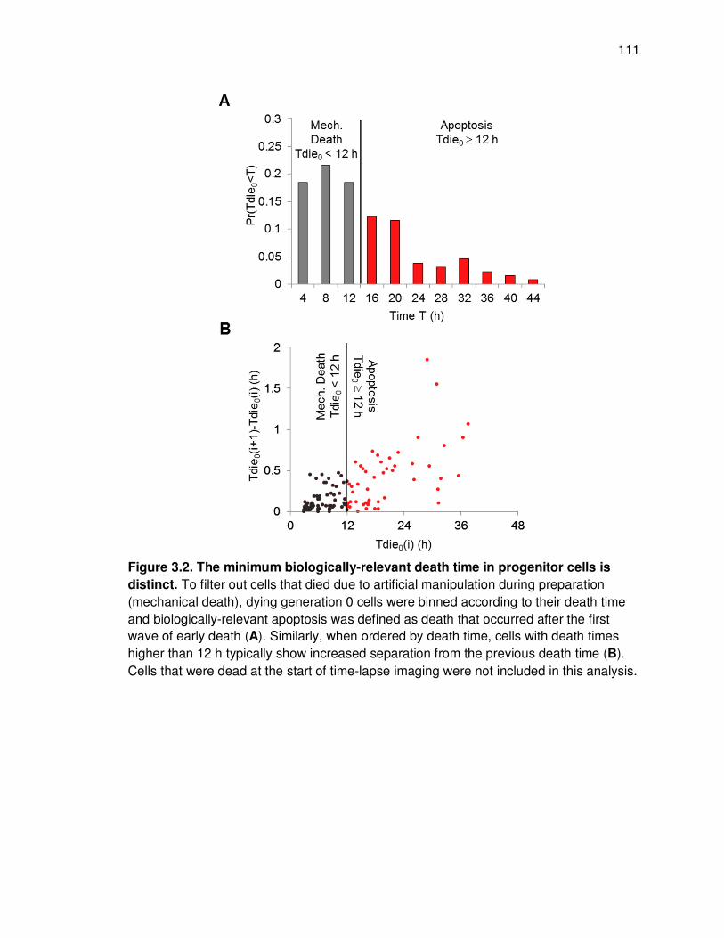
111
Figure 3.2. The minimum biologically-relevant death time in progenitor cells is
distinct. To filter out cells that died due to artificial manipulation during preparation
(mechanical death), dying generation 0 cells were binned according to their death time
and biologically-relevant apoptosis was defined as death that occurred after the first
wave of early death (A). Similarly, when ordered by death time, cells with death times
higher than 12 h typically show increased separation from the previous death time (B).
Cells that were dead at the start of time-lapse imaging were not included in this analysis.

112
3.2.2. B cell fate is decided: growing B cells are protected from death
To further establish the fundamental cellular mechanisms, we next tested if the
cell-cycle and apoptosis were indeed parallel racing processes (Figure 3.3A), or if
growth was predictive of fate (Figure 3.3B). Intuitively, if cells “decide” their fate early,
one would expect most growing cells to divide, and vise-versa. We tallied the fraction of
“growers” that divided and died within the first 36 (generation 0) or 24 hours (generations
1+) for each generation (Figure 3.3C) as well as the fraction of “non-growers” that
divided and died within the same periods for each generation (Figure 3.3D). Our results
indicate that almost all “growers” divided in the first four generations, followed by loss of
decision robustness in the last two generations, indicative of an early decision that
predisposed B cells to a particular fate (Figure 3.3B). Interestingly, except in the first
generation, there was a significant fraction of “non-growers” that divided, due to primarily
poor growth prior to the last division (Figure 3.4). To further test this important
distinction, we used the observed time to decide (start of growth), time to division, and
time to death of progenitor cells, and calculated the expected lower bound probability
that a dying cell would have grown, given the molecular race (Figure 3.3A), and decision
(Figure 3.3B) models (Figure 3.3E-F). Our analysis revealed that even under relatively
relaxed assumptions, the data are inconsistent with both processes occurring
simultaneously in cells (i.e. race). On the other hand, a decision which commits cells to
either fate is more appropriate as grown dead cells are rare. In other words, because
time to death is typically earlier than time to division, and because time to decision (i.e.
growth start) is typically much earlier than division or death our analysis predicts most
cells to start growing prior to death if the two processes were indeed running in parallel
within B cells.

113
Figure 3.3. B cells decide to divide or die and are protected from the alternate fate A) Flowchart depicting activated cell fate determined by a race between division (green) and death (red) as well as hypothetical division and death time distributions before and after mutual censorship B) Flowchart showing an early commitment to one fate, and the independent division (green) and death (red) time distributions. C-F) Analysis of response (growth), division, and death statistics for WT B cells. Error bars = 1/n. C) Measured generational probabilities that a growing (C) or non-growing (D) cell divided (green) or died (red) within a 24 hour period (12-36 h for gen 0). E) Measured cumulative distributions for the time to start growing (blue), time to divide (green), and time to die (red) of generation 0 cells. Distributions were used to calculate the lower bound expected probability that a dying cell had started to grow (F) assuming a molecular race between fates or an early commitment to one fate, as compared to the measured probability. For further details please see supplementary materials.

114
Figure 3.4. Cells typically grow less prior to the last division. Wildtype purified naïve
B cells were stimulated with 250 nM CpG and tracked by time lapse microscopy. The
fraction of “non-growing” cells that divided (A green) or died (A red) are shown for each
generation. Error bars = 1/n. The quantification was repeated with penultimate dividing
cells removed from consideration (B).

115
3.2.3. A molecular race cannot recapitulate progenitor death timing
Alternatively, if the CFSE deconvolution methodology developed in chapter 2
(Figure 3.5A) can be used to test the decision and molecular race hypothesis. To do
this, we obtained CFSE fluorescence histograms for populations of B cells from the
same mouse by flow cytometry. FlowMax deconvolution of the datasets into the
maximum-likelihood cyton (Figure 3.5B) model and fcyton model (Figure 3.5C)
parameters allowed us to test which hypothesis best agrees with the cellular parameters
observed by time-lapse microscopy (Figure 3.5D), as the cyton model assumes that
responding cells may die, while the fcyton model does not. While both models accurately
fit the CFSE time course (Figure 3.5E), the molecular race model requires a much later
Tdie0 (Figure 3.5F), while the fcyton model, which assumes independence between
fates, allows for a much earlier Tdie0 concordant with the experimental microscopy
dataset. Interestingly, both models were able to capture the experimentally observed
fraction of dividing cells in each generation (Fs), but largely failed to predict the relatively
late division time experienced by generation 0, and 1+ cells (Figure 3.5D green and blue
distributions).
116
Figure 3.5. FlowMax deconvolution of WT 250 nM CpG stimulated CFSE time series. CFSE-stained purified murine B cells were stimulated with 250 nM CpG, assayed by flow cytometry and a computational tool, FlowMax, was applied to determine non-redundant sets of maximum-likelihood population model parameters (A).To test if a molecular race or a decision are more appropriate, the cyton model, which assumes a race between division and death, (B) and fcyton decision-based model (C) were used as part of the FlowMax phenotyping. Maximum-likelihood parameter sets obtained from fitting each model to the experimental CFSE time courses were sampled using a Monte-Carlo approach to expose the fraction of responding cells in each generation (Fs), as well as division and death time distributions for undivided (Tdiv0,Tdie0) and dividing cells (Tdiv1+,Tdie1+) expected to be observed after any potential censorship and compared to the actual cellular distributions measured by time-lapse microscopy (D). The best-fit modeled CFSE histograms from the best-fit cluster of cyton (E purple) or fcyton (E blue) model parameters overlaid on experimental CFSE histograms collected in duplicate across six days at the indicated time points.
116
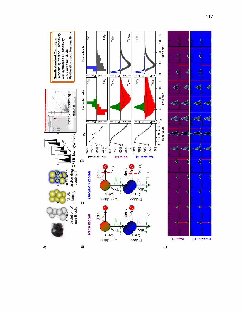
117

118
While our results suggest that cell fate is determined early, variability in the
decision and fate timing is consistent with extrinsic cell-to-cell protein heterogeneity. To
check this, we measured the correlation in the timing of the decision process (i.e. time to
growth), the time to division, and the time to death in between sister and cousin cells
(Figure 3.6). The timing of the decision process, interdivision time, and to a smaller
extent lifespan were significantly correlated between sister cells: Pr(∆Tdecide≤ 4
h)=0.90, R2=0.74, and R2=0.39, respectively. Furthermore, the correlations decreased
with a subsequent division (i.e. between cousins): Pr(∆Tdecide≤ 4 h)=0.77, R2=0.44, and
R2=0.38, respectively, consistent with mixing times on the order of hours to days, ruling
out genetic and epigenetic sources of cell-to-cell variability [Sorger 2011, 2009].
Figure 3.6. The decision, division, and death times are correlated between siblings and cousins. B cell lineages from WT 250 nM CpG time-lapse microscopy video were determined by semi-automated tracking. Correlations in timing to the start of growth, division, or death of sister cells (blue) and cousins (red) were calculated. Histogram of the differences between the times to decide to start growing (A) is shown. Division (B) and death (C) times are plotted between sister and cousin cells across all generations. Colored lines represent the linear fit through the origin with r-squared values for sisters (top) and cousins (bottom) as indicated. 3.3. Discussion
Key to parameterizing a multi-scale response was the development of a B cell live
cell microscopy experimental and computational tracking pipeline, which we used to
obtain accurate cell-size trajectories and lineages for hundreds of cells across a six day

119
period (Figure 3.1). Tracking wildtype B cells revealed several key properties of the
response. B cells undergo 1-7 divisions, increasing total cell counts several fold and then
most cells die by apoptosis (Figure 3.1B-C).There is a noticeable but variable delay in
growth initiation prior to the first division, while generation 1+ cells start growing
immediately (Figure 3.1D). This is consistent with a model in which activated generation
0 cells must prepare for several rounds of rapid divisions by simultaneously deactivating
quiescence [21,177] and activating the appropriate growth pathways such as Myc and
mTOR [66,178]. Tracking cell size trajectories and their eventual fate allowed us to
confirm that B cells that grow are protected from death, suggesting that B cells have
underlying molecular mechanisms for upregulating both survival and the cell-cycle
(Figure 3.3). Furthermore, even in the absence of cell growth trajectories, a
mathematical model which assumed a race between division and death [44] could not
account for the typically early death we see with microscopy experiments (Figure 3.5),
especially considering that we filter out death that occurs within the first 12 h caused by
the experimental process (Figure 3.2) We were also able to confirm that both division
and death are correlated between sibling cells (Figure 3.6), which is consistent with
differences in protein turnover processes [24,25] resulting in distributions of single-cell
proteomes within a population. Taken together, these data suggest an upstream
decision to divide or die, while the variability in timing is caused by cell-to-cell variability
in protein turnover (protein remixing).

120
3.4. Methods
A video showing the tracking of wildtype B cells, WT250nM.mpg can be found in
the supplementary files along with FAST.jar, the tracker code and executable used to
perform semi-automated tracking.
3.4.1. B cell purification and incubation
Primary splenocytes were isolated from 6-8 week old mice, naïve B cells purified
using magnetic bead separation (Miltenyi Biotec), and stimulated with 250 ng/mL, or 10
ng/mL CpG ODN 1668 (Invivogen). mTORc1 inhibition was achieved by 1 hr
pretreatment of 1 ng/mL Rapamycin (Sigma) prior to addition of stimulus. B cells were
grown in fresh media with 1% penicillin streptomycin solution (Mediatech Inc.), 5 mM L-
glutamine (Mediatech Inc.), 25 mM HEPES buffer (Mediatech Inc.), 10% FCS and 55 uM
2-ME (Fisher Scientific) at a concentration of 5x10⁴ cells/mL in 48 well plates, or 1536
flat-bottom tissue-culture plates at 37oC for a period of 1-6 days.
3.4.2. CFSE flow cytometry and FlowMax analysis
Cells were removed from media, stained with 10 ng/mL propidium iodide, and
measured using an Accuri C6 Flow Cytometer (Accuri Inc.) over a six day time course.
CFSE histograms were constructed after software compensation for fluorescence
spillover and manual gating on viable (PI-negative) B cells using FlowMax software. All
measurements were performed in duplicate (B cells from the same spleen were cultured
in separate wells, two wells per time point to ensure that each time course represented a
single population of cells subject to only experimental variability). The FlowMax
computational tool [47] was used to construct 1D log-transformed CFSE histograms of
viable cells. After specifying the fluorescence of the undivided peak manually for each

121
time point, maximum-likelihood fcyton model parameter ranges were determined by
filtering, and clustering 1000 best-fit solutions and their corresponding sensitivity ranges.
The top solution cluster was plotted by randomly sampling parameters from within the
maximum-likelihood parameter ranges. To account for potential censorship of the
fraction of dividing cells or division and death time distributions when both division and
death processes were active simultaneously (i.e. cyton model), Monte-Carlo sampling of
cell populations was used to approximate population model parameters directly.
3.4.3. Time-lapse microscopy
Purified naïve B cells were grown in 1536 flat-bottom tissue-culture treated
microwells (Greiner Bio-One). Images were acquired on an Axio Observer Z1 inverted
microscope (Carl Zeiss Microscopy GmbH, Germany) with a 10x, 0.3 NA air immersion
objective to a Coolsnap HQ2 CCDcamera (Photometrics, Canada) using ZEN imaging
software (Carl Zeiss Microscopy GmbH, Germany). Environmental conditions were
maintained at 37º C, 10% CO2 with a heated enclosure and CO2 controller (Pecon,
Germany). Phase contrast images were taken every minute for six days.
3.4.4. Cell tracking
A semi-automated computational approach was used to track B cells in phase-
contrast images. First, image intensities were normalized to maximize contrast. Next,
edges were identified using a Sobel transformation and global thresholding. Cells were
identified using a customized Hough transformation assuming cells were approximately
circular. Next, approximate linear paths were manually drawn for each cell until the cell
was observed to divide, die, or leave the field of view. Cells entering the field of view
after 24 hours (i.e. potentially after the first division), and debris were tracked but

122
removed from the subsequent analysis. After all paths were drawn, all cell boundaries
were optimized simultaneously from frame to frame. During automatic optimization, cells
were modeled as deformable two-dimensional polygons with forces acting upon each
vertex that ensured the polygons did not grow/shrink too quickly, did not overlap other
polygons, were attracted to edges in the image, and were attracted to their respective
manually-curated path. The relative magnitudes of the forces were manually calibrated
to ensure appropriate behavior. Cell size trajectories were fitted using a piece-wise
function consisting of a linear no-growth period, followed by exponential growth:
0
( )
0
( )decide
decide
k t t
decide
V t tV t
V e t t−
≤
=
>
The quality of individual cell tracks were assessed by calculating RMSD from ( )V t , and
the decidet value was assumed to be the fitted inflection point in this function (i.e. when
cells were predicted to start exponential growth). Growing cells were defined as having
an average ending volume at least 350 µM3 above the average starting volume, or if the
final volume was at least 800 µM3. Cells that grew but then decreased in size, or that
didn’t meet any of these conditions were labeled as non-growing. For implementation
details please see Supplementary File CellTracker.zip. A video showing the output of
tracking for the WT 250 nM CpG condition is provided as Supplementary File
WT250nM.mpg.
3.4.5. Calculating the expected probability that a dying cell would have started
growing
In order to test if the molecular race (Figure 3.3A) and/or the molecular decision
(Figure 3.3B) hypotheses are consistent with our datasets, we used the observed

123
0
0 ( )growT t , 0
0 ( )div
T t , and 0
0 ( )die
T t distributions (Figure 3.3E), designed with a superscript “o”,
to determine a lower bound on the fraction of dying cells that are expected to grow under
the race or decision hypothesis. While under the decision hypothesis we would expect
that all responding cells are subject only to eventual division, while non-responders will
not grow or divided, the fraction of growing cells that will die, or vise-versa are not readily
apparent. Therefore, we derived a lower limit on the expected probability that a dying (
fate death= ) cell will grow under the race hypothesis in terms of observed distributions,
and show that the observed probability of this happening is inconsistent. We are
interested in the probability that progenitors (generation 0) cells started growing and
died:
0 0 0Pr( , | )grow die
T T F fate death< = , (51)
where 0dieT and 0growT are the true probability distributions for the time to die or start
growing, and 0F is the true fraction of cells that respond to the stimulus and start growing
(still subject to death) in the race model. We define the probability censoring of some
probability distribution ( )f t by a competing probability distribution ( )g t as:
( )( )
( ) |
( ) 1 ( )
( | ( )) ( ) 1 ( )
( ) 1 ( )
t
t
f gt
f t g t dt
f t g t f t g t dt w
f t g t dt dt
−∞
∞ −∞
−∞ −∞
′ ′−′ ′= = −
′ ′−
∫
∫
∫ ∫
,
(52)
where ( | ( ))f t g t represents ( )f t given that a competing mutually explosive event has
probability distribution ( )g t , and |f gw is a rescaling constant. From this definition it
follows that
( | ( )) ( ) , , ( )t t
f t g t dt f t dt t g t−∞ −∞
≥ ∀ ∀∫ ∫
. (53)

124
Furthermore, since under the race hypothesis, all cells are subject to age-dependent
death, 0 ( )dieT t , and since 0 ( )dieT t is typically earlier than 0 ( )divT t , then for each cell that
divided, there must have been at least another cell that would have divided but died, or
in terms of the fraction of observed generation 0 responders:
0 02 oF F≤ . (54)
Using (53) the observed 0 ( )grow
T t , 0 ( )div
T t , and 0 ( )die
T t distributions are biased toward
earlier values, since death will censor decision and division fates, while division will
censor late death fates:
0 0( ) ( ) ,t t
o
grow growT t dt T t dt t
−∞ −∞≥ ∀
∫ ∫
,
0 0( ) ( ) ,t t
o
die dieT t dt T t dt t
−∞ −∞≥ ∀
∫ ∫
.
(55)
However, of the cells for which both division and death are running in parallel (at least
twice as many as had been observed to divide from equation (54)) a fraction would not
have started measurably growing prior to dying (i.e. died before growth decision was
reached and observed). Therefore, to calculate the true fraction of dying cells that are
expected to start growing we first calculated the probability that a cell will start
measurably growing prior to dying:
( )0 0 0 0Pr( ) ( ) 1 ( )t
grow die grow dieT T T t T t dt dt
∞
−∞ −∞′ ′< = −
∫ ∫
. (56)
To do this, we used (55) to show that
0 0 0 0Pr( ) Pr( )o
grow die grow dieT T T T< ≥ < . (57)
Furthermore, we can define a new function *
0 ( )growT t in terms of observed distributions:
*
0 0 0( ) ( | ( ))o o
grow grow dieT t T t T t= . (58)
Since by definition of function censorship:

125
0 0 0( ) ( | ( ))o
grow grow dieT t T t T t= . (59)
and since from (55) the 0 ( )o
dieT t distribution is shifted toward lower values compare to
0 ( )dieT t , it follows that *
0 ( )growT t is typically shifted toward later values when compared to
the true 0 ( )growT t :
*
0 0( ) ( ) ,t t
grow growT t dt T t dt t
−∞ −∞≤ ∀
∫ ∫
. (60)
Therefore, from eq. (57) and (60) we can establish a lower bound on 0 0Pr( )grow dieT T< :
*
0 0 0 0 0 0Pr( ) Pr( ) Pr( )o o
grow die grow die grow dieT T T T T T< ≥ < ≥ < . (61)
Since both *
0 ( )growT t , and 0 ( )o
dieT t are defined in terms of observed continuous probability
functions, we next developed an expression for calculating *
0 0Pr( )o
grow dieT T< using a
collection of discrete observations. Specifically, to calculate *
0 ( )grow
cdf t from 0 ( )o
growcdf t
we reweighed the contribution of each, ith, observed 0growT value according to the
observed 0
o
diecdf :
0 0,*
0 0,
( )( )
o
grow grow i i
grow grow i m
i
i
cdf T wcdf T
w
⋅=
∑
,
0 0,
1
1 ( )i o
die grow i
wcdf T
=−
.
(62)
Finally, we used (62) with (54) to obtain an expression on the lower bound for (51) given
m observed 0growT values, and n observed 0dieT values:

126
( )
* 0
0 0 0 0 0 0
, ,
0
Pr( , | ) 2 Pr( )
2 ,
o
grow die grow die
n
grow i die j im mjo
ii i
T T F fate death F T T
T T kF Z k
< = ≥ < =
Ι < = Ζ
∑
∑ ∑
.
(63)
In essence, we used the observed 0dieT distribution to obtain a 0growT distribution that is
guaranteed to be equal to or more biased toward later values than the true 0growT
distribution. Combined with the fact that under the race hypothesis, the observed fraction
of dividing cells is at least twice as small as the true fraction of responders, this allowed
us to calculate a lower bound on the probability that a dying cell would start growing prior
to actually dying (Figure 3.3F). Under the molecular decision model, cells commit to
either division or death early, and are therefore protected from the alternative (growth
and division for cells committed to death, and death for cells committed to growth and
division). The fraction of dying cells that are expected to be also growing under the
molecular decision hypothesis is zero. To test which hypothesis is best supported, we
measured the fraction of dying generation 0 cells that were growing at the time of death
defined as:
max 0 max, ( , ) ( ) 350 | ( , ) 800
,i
true V i t V i m V i t mGrowing
false otherwise
µ µ> + >
=
, (64)
where max( , )V i t and 0 ( )V i are the average final 30 volumes and the average first 30
volume measurements for cell i, respectively.
3.5. Acknowledgements
Chapter 3, in part, is currently being prepared for submission for publication of
the material and may appear as Maxim N. Shokhirev, Jonathan Almaden , Jeremy

127
Davis-Turak, Harry Birnbaum, Theresa M. Russell, Jesse A.D. Vargas, Alexander
Hoffmann. “A multi-scale approach reveals that NFκB enforces a decision to divide or
die in B cells.” Jesse A.D. Vargas helped train me to run single-cell microscopy
experiments. The dissertation author was the primary investigator and author of this
paper.

128
Chapter 4
Molecular Determinants of Fate
Decision and Timing
In Chapter 3, we established that B cells indeed make decisions, as growing B
cells are protected from death. However, it remains unclear how fate is determined and
enforced on the molecular level. Therefore, we performed a single-cell transcriptome
analysis revealing an NFκB signature in growing cells. This is concordant with decades
of studies establishing NFκB signaling as essential for B-cell proliferation and survival;
however it remained unclear whether NFκB signaling played a direct role in the decision
enforcement. Therefore, we applied an immunofluorescence and traditional biochemical
assays to characterize the abundance of key molecular players in individual cells after
24 h of stimulation. We found that both NFκB RelA and cRel are upregulated at 24 h.
Furthermore, mammalian target of rapamycin (mTORc1) abundance was upregulated
approximately 4.5-fold in wildtype and only approximately 1.5 fold in cells deficient in
NFκB cRel 24 h post stimulation. Rapamycin pretreatment resulted in reduced cell size
while the abundance of cRel remained high; suggesting that cell growth is mediated by
NFκB cRel activity. In addition to cell growth, NFκB is essential for the upregulation of
the anti-apoptotic regulator BclXL at 24 h as NFκB cRel deficient cells have dramatically
reduced BclXL mRNA and protein levels. These findings suggest that NFκB cRel serves

129
to enforce the B-cell decision to grow and survive by simultaneously upregulating growth
and survival programs.
4.1. Introduction
TLR9 robustly activates the well-studied and essential NFκB signaling pathway
[51], resulting in the upregulation of hundreds of genes associated with survival and
proliferation, providing a natural molecular connection between signaling and cell fate
[52]. Specifically, activation of TLR9 by CpG results in the activation of the kinase IKKb,
which rapidly phosphorylates NFκB inhibitor proteins, the IkBs, which sequester NFκB
dimers in the cytoplasm. Phosphorylation of IkBs results in their ubiquitination and
degradation, releasing NFκB dimers (primarily RelA:p50 and cRel:p50 in B cells [4]) and
allowing them to enter the nucleus where they bind to promoters of genes containing the
NFκB motif, and activate gene expression. Importantly, the genes coding for cRel[53]
and p50[54] as well as the inhibitors IkBα[55] and IkBε[56] are themselves target genes,
resulting in waves of NFκB activation lasting potentially several days. Furthermore the
genes coding for CyclinD [70-72], Myc [59], and BclXL [74], which are essential for cell-
cycle progression, growth, and survival, respectively, are all known to be NFκB target
genes. Therefore, many essential molecular players involved in the B cell immune
response have been identified but it remains unknown how their dynamics lead to the
observed cell fate and timing variability and in turn the B cell population response.
Finally, single-cell molecular assays are useful for correlating cellular features
(e.g. size) to molecular pathways. Specifically, immunofluorescence (IF) allows for
quantitative measurement of fluorescently-labeled proteins in hundreds of individual
cells. On the other hand, IF requires chemical crosslinking, which makes single-cell

130
tracking impossible. While IF can provide high-throughput single-cell results for specific
proteins of interest, single-cell RNA sequencing can be used to quantify whole
transcriptomes of individual cells [134]. A relatively new technology, single cell RNAseq
uses microfluidic devices to trap individual cells and perform the necessary chemistry.
Furthermore, captured cells can be stained and measured under the microscope prior to
lysis, allowing for filtering of transcriptomes by the cell size and viability. This allows for
the unbiased whole-genome testing of differential gene expression between individual
cells.
4.2. Results
4.2.1. Single-cell transcriptome sequencing reveals NFκB signatures in big cells
We next turned to single-cell molecular assays to test the importance of key
molecular players in determining fate and timing. Specifically, we stimulated purified
primary naïve murine B cells, stimulated with a high dose of CpG for 24 hours and
performed both single-cell RNA sequencing, as well as multi-channel
immunofluorescence experiments (Figure 4.1A). We sequenced the transcriptomes of
five large and small cells using the single-cell autoprep system, which allowed us to
image and measure the size of individual B cells trapped inside of a microfluidics chip
(Figure 4.1B). After preparing and sequencing oligomer cDNA libraries, we normalized
transcript counts to RNA spikein controls, and identified 369 and 121 genes upregulated
or downregulated in large cell, respectively (Figure 4.1C). We next identified and
summarized the pathways that were significantly upregulated in large or small cells
(Figure 4.1D). Next, since the NFκB signal transduction systems is known to be
essential for the B cell immune response and because NFκB signaling was one of the

131
upregulated pathways in B cells, we checked if big cells had an NFκB gene expression
signature compared to small cells. To do this, we performed a transcription factor
enrichment analysis on the upregulated and downregulated gene sets, and tallied the
transcription factors that are themselves known to be NFκB targets (Figure 4.1E). Our
analysis revealed the signature of nine transcription factors that are known NFκB target
genes, as well as NFκB itself among the genes upregulated in big cells (Figure 4.1E
red), while we only identified p53 as a known NFκB target gene transcription factor in the
set of genes downregulated in big cells, suggesting that large B cells tended to
upregulate NFκB activity.

132
Figure. 4.1. Molecular assays suggest that NFκB enforces an upstream fate decision. Naïve purified B cells were stimulated with 250 nM CpG for 24 h, and analyzed using single-cell RNA sequencing (A top). Five small and five large B cells were captured in a microfluidics chip (B) and their transcriptomes were sequenced to reveal sets of genes typically upregulated in big cells (C, red) or small cells (C, green). Pathway analysis on genes upregulated in large B cells (D, top) and small cells (D, bottom) was performed. E) Transcription factor motif enrichment analysis on the genes upregulated in large cells (E, top) and small cells (E, bottom) was performed and
filtered to show only significantly upregulated (p-value < 0.05) and known NFκB target
genes or NFκB itself.

133
4.2.2. NFκB cRel mediates growth and survival in B cells
Next, we stained fixed B cells which were stimulated for 24 hours (Figure 4.2A),
and measured average NFκB cRel fluorescence as a function of cell area by microscopy
(Figure 4.2B). We found that compared to a 0 h control, B cells were larger (63% of
cells) and had higher cRel fluorescence (63% of cells) after 24 h of stimulation.
Furthermore, 68% of large cells had upregulated cRel at 24 h. To test the specificity of
our immunofluorescence methodology, we showed that NFκB cRel deficient B cells had
no detectable cRel fluorescence at 24 h (Figure 4.3A). Similarly to NFκB cRel, 50% of
cells showed significantly increased levels of NFκB RelA after 24 h, with 70% of large
cells showing increased NFκB RelA abundance after 24 h of stimulation (Figure 4.3B). In
addition, we tested the role of NFκB cRel in cell growth by repeating the
immunofluorescence analysis in the presence of 1 ng/mL rapamycin, the mTORc1
inhibitor (Figure 4.3C). We found that while the same fraction of cells had upregulated
cRel abundance after 24 h of stimulation, the fraction of large cells was reduced,
suggesting that cRel is independent of mTORc1. Furthermore, we tested the role of
NFκB cRel on regulating mTORc1 directly, by measuring the abundance of p-S6, an
indicator of mTORc1 activity, by western blot in wildtype and NFκB cRel deficient mice
(Figure 4.2C). The data suggest that in the absence of NFκB cRel the signal is reduced
by approximately a factor of 2. We also, checked the dependence of BcLXL a known
NFκB cRel target gene and anti-apoptotic regulator by measuring average BcLXL
abundance (Figure 4.2D) as well as by measuring BcLXL mRNA levels by qPCR at
several time points in wildtype and NFκB cRel deficient B cells (Figure 4.3E). The results
show that 84% of all cells upregulated BcLXL and that NFκB cRel deficient results in
three-fold decrease in BcLXL expression at 20 h suggesting that NFκB cRel contributes

134
to roughly 2/3 of the BcLXL expression at 20 h. Concurrently, immunofluorescence
analysis reveals that only 8% of cells upregulate BcLXL in the absence of NFκB cRel and
that only 8% of large cells have an upregulated BcLXL abundance (Figure 4.3D).

135
Figure 4.2. NFκB mediates growth and survival. NFκB cRel abundances of purified naïve B cells stimulated with 250 nM CpG for 24 h were obtained by quantifying average fluorescence in fixed B cells in the presence of fluorescently-labeled antibodies (A).
NFκB cRel fluorescence as a function of cell area at 0 h and 24 h (B). Quantification of pS6, a downstream target of mTORc1 after 24 h by western blot normalized to tubulin control in WT and cRel deficient B cells (C). Anti-apoptotic BclXL fluorescence as a function of cell size at 0 h and 24 h (D). BclXL mRNA levels were measured by
quantitative PCR at 0, 1, 6, and 20 h in wildtype and NFκB cRel deficient B cells (E). Significant fluorescence in (B) and (D) determined using 0 h fluorescence distribution. Large cells empirically defined as > 100 pixels. Error bars=s.d.

136
Figure. 4.3. Immunofluorescence control experiments. Immunofluorescence control experiments were performed in wildtype and cRel deficient B cells stimulated with 250
nM CpG. Average NFκB cRel fluorescence at 0 h and 24 h in NFκB cRel deficient cells
(A). Analogously to NFκB cRel, NFκB RelA average fluorescence was quantified at 0 h and 24 h post stimulation (B). Average cRel fluorescence at 0 h and 24 h and 1 h pretreatment with 1 ng/mL rapamycin (C). Average BcLXL fluorescence at 0 h and 24 h in
NFκB cRel deficient B cells (D). Quadrants delineate significance at 24 h compared to 0 h.

137
4.2.3. Time-lapse microscopy confirms NFκB cRel as a decision enforcer
Since our data implicated NFκB cRel as an essential driver of the decision in B
cells, we tracked NFκB cRel deficient B cells and compared the dataset against the
wildtype dataset (Figure 4.4). We find that the population result is noticeably decreased
in the cRel deficient dataset (Figure 4.4A) with most cell only undergoing two or three
divisions compared to at least seven observed generations in wildtype cells (Figure
4.4B). Nevertheless, the growth trajectories of responding and non-responding cells
remained nearly-identical with responding cells growing to approximately 1000 µM3
before division on average (Figure 4.4C), while “non-growing” cells remained largely the
same size on average (Figure 4.4D). Concomitant with the molecular observations that
NFκB cRel is important for enforcing the decision, we see an elevated fraction of
growing cells dying in cRel deficient cells (Figure 4.4E). In fact, we observe 40% of
growing cells dying in generation 0 when NFκB cRel is knocked out, while just 12.5% of
growing cells were observed to die under wildtype conditions. On the other hand, we see
that non-growing cells almost never divided in the cRel knockout condition, while this
was relatively common for wildtype B cells (Figure 4.4F) due to poor growth prior to the
last division (Figure 3.4). Furthermore, while there wasn’t a significant fate timing
phenotype in NFκB cRel deficient cells (Figure 4.4G), the fraction of dying cells which
grew was elevated (31%±1% compare to 8%±2% for wildtype) under knockout
conditions (Figure 4.4H).
Therefore, NFκB seems to play a role in enforcing the decision to survive and
progress through the cell cycle, while the timing of the cell-cycle and apoptosis remains
largely independent.

138
Figure 4.4. Time-lapse microscopy confirms NFκB cRel as an enforcer of cell decision making. Time-lapse microscopy experiments were performed on wildtype and cRel deficient B cells stimulated with 250 nM CpG and cell size trajectories and lineages were tracked using a semi-automated approach. Cellular statistics are shown for wildtype (left column) and cRel deficient cells (right column). Generation cell counts normalized to starting cell count (A). Fractional division and death probabilities are shown for each generation (B). Error bars are 1/n. Cell size trajectories as a function of percent lifetime for growing (C) and non-growing (D) cells are plotted for each generation (blue to orange curves). Error bars show SEM. Fraction of growing (E) and non-growing (D) cells that divided or died within a 24 h period (12-36 h after stimulation) in each generation. Error bars show 1/n. Cumulative density functions for the observed progenitor time to decide to grow (blue), time to die (red), and time to divide (green) are shown (G). The observed cumulative distributions and fraction of dividing cells in generation 0 were used to calculate the minimum probability that dying cells were also grower cells under the molecular race or decision scenarios and compared to the fraction measured from time-lapse cell tracking.
138

139

140
4.3. Discussion
So what enforces the decision to divide and survive? Previous studies have
shown that in B cells, the NFκB signaling system plays a central role in the determining
fate of stimulated B cells for a wide assortment of mitogenic signals [60], therefore, we
characterized key molecular players in individual cells by IF and by sequencing the
transcriptomes of small and large cells after the cells have had a chance to grow, but
have not yet divided. While, there was significant cell-to-cell transcriptome variability
(Table 4.1), there was nevertheless an NFκB signaling signature readily apparent in
large cells (Figure 4.1). Taking advantage of other molecular assays, we showed that
NFκB cRel, and RelA are upregualted after 24 h of stimulation and large cells show
increased NFκB abundance as compared to 0 h (Figure 4.2B and Figure 4.3B).
Furthermore, inhibition of mTORc1 by rapamycin resulted in an appreciable growth
defect at 24 h, while maintaining nearly identical proportions of NFκB cRel positive cells
(Figure 4.3C), confirming that mTORc1 is downstream or independent of NFκB
signaling. We confirmed that mTORc1 is downstream of cRel by western blot and
showed that in the absence of NFκB cRel, mTORc1 activity is roughly halved (Figure
4.2C). Analogously, the anti-apoptotic regulator BclXL was dramatically upregulated after
24 h and correlated with cell size (Figure 4.2D). Furthermore, BclXL levels were
dramatically reduced in the NFκB cRel knockout, suggesting that NFκB cRel is required
for roughly 2/3 of the BclXL transcripts at 24 h (Figure 4.2E). Therefore, molecular assays
suggest that NFκB acts as an enforcer of an upstream decision by simultaneously
upregulating cell growth (via mTOR), as well as survival in B cells (via BclXL). However, it
remained unclear how cRel deficiency is manifested on the population scale.

141
To test this, we repeated the time-lapse microscopy experiments with B cells
missing NFκB cRel, and quantified the degree to which cRel is important for promoting
an efficient response. Cell growth trajectories and fate time distributions were similar to
wildtype, but we saw a dramatic decrease in the population response caused primarily
by a failure to commit to more than a few rounds of division (Figure 4.4B). Critically, we
see that NFκB cRel deficient cells were having trouble enforcing their fate, with the
fraction of grown dying cells increasing four-fold (Figure 4.4H). Thus, time-lapse
microscopy confirms that NFκB cRel enforces decisions during the B cell immune
response.
Taken together, these results suggest that the early commitment to one fate in B
cells is driven by NFκB-mediated activation of survival and cell-cycle activation.
4.4. Methods
The single-cell RNA sequencing analysis (CSV format), pertinent
immunofluorescence images, and CFAnalyzer, the tool we developed for quickly
quantifying fluorescence in IF images are part of the supplementary materials as
IFAnalysis.csv, IFImages.zip, and CFAnalyzer.zip, respectively.
4.4.1. Single-Cell RNAseq
Stimulated wildtype B cells were collected at 24 h post stimulation and
concentrated to 5x10⁵ cells per mL. Cells were loaded onto a 10-17 uM primed C1
single-cell auto prep array IFC (Fluidigm), and phase contrast images were taken of all
viable cells as determined by the Live/Dead® Viability/Cytotoxicity Kit (Invitrogen).
ERCC RNA spikein controls (LifeTechnologies) were added to the lysis mix at a 1:200
dilution. Tube controls (bulk cell positive control, and no cell negative control) were also

142
prepared according to the Fluidigm protocol. Lysis, reverse transcription, and PCR were
performed using the SMARTer Ultra Low RNA Kit (CloneTech) and Advantage® 2 PCR
Kit (CloneTech) on individual cells using the C1 Single-Cell Auto Prep System (Fluidigm).
Cell size was manually determined from images using ImageJ software. Sample libraries
for the five smallest and five largest cells along with the controls were prepared using the
Nextera XT DNA Sample Preparation (Illumina), and library quality was assayed using
the Quant-iT PicoGreen dye (Life Technologies) quantification on a Qubit® 2.0
Fluorometer (LifeTechnologies) and by gel electrophoresis. Libraries were sequenced by
the UCLA Broad Stem Cell Research Center High Throughput Sequencing Core on
Illumina HiSeq 2000 sequencers according to manufacturer recommendations. Reads
were aligned to the ENSEMBL NCBI m37 genome [179] using rna-STAR [141]. To
compute spikein concentrations for normalization purposes, the 23 most abundant RNA
spikein concentrations (at least one read in all samples) were compared to the expected
concenrations in log-log space, and the y-intercept in log-space was used to compute a
normalized spike in concentrations for each sample, *[ ]jSpikein . The normalized
expression of gene i, in sample j was then computed as:
,
, *100
[ ]
i j
i j
j
GeneGene
Spikein= +
,
where *[ ]jSpikein is the normalized spikein concentration that is ≥ 1. A constant count of
100 was added because Spikeins with counts with counts < 100 were variable across
samples. To assess the overall quality of each cell, we correlated their transcriptomes to
the average across all cells as well as to the positive tube control. We found that one
large cell had significantly lower correlation, so we omitted it from further analysis (Table

143
4.1). To determine if a particular gene was upregulated in big cells, we computed an
expression score:
( 300) ( 300)
# #
i ibig small
i
big small
I gene I gene
Escorecells cells
> >
= −∑
∑
,
where ( 300)iI gene > is 1 if gene i has above 300 read count in a particular sample. A
gene with an expression score ≥ 0.5 was considered upregulated in big cells, while a
gene with an expression score ≤ -0.5 was considered downregulated in big cells. These
sets of upregulated and downregulated genes were analyzed for pathway enrichment
and transcription factor motif enrichment using WebGestalt [143]. Significant
transcription factors were further filtered to remove non-NFκB downstream targets as
defined in Table 4.2.
Table 4.1: Correlations between cell transcriptomes. Transcriptomes of five large and five small cells were sequenced and aligned to the mouse genome. Gene counts were normalized to RNA spike in pseudo-counts and a constant positive count of 100 was added to all genes to represent experimental sensitivity as seen in the variability in spikein counts between samples (see methods). Colors represent degree of correlation (Pearson’s r). The second large cell was removed from further analysis due to poor correlation with all other cells (similar to negative).
Small 1 Small 2 Small 3 Small 4 Small 5 Large 1 Large 2 Large 3 Large 4 Large 5 Neg. bulk +
Small 1 1.00 0.77 0.58 0.63 0.63 0.65 0.40 0.65 0.67 0.59 0.27 0.61
Small 2 0.77 1.00 0.70 0.64 0.65 0.65 0.45 0.71 0.70 0.66 0.33 0.65
Small 3 0.58 0.70 1.00 0.59 0.73 0.67 0.49 0.63 0.72 0.74 0.34 0.62
Small 4 0.63 0.64 0.59 1.00 0.73 0.83 0.45 0.81 0.79 0.61 0.41 0.82
Small 5 0.63 0.65 0.73 0.73 1.00 0.82 0.49 0.76 0.87 0.77 0.39 0.73
Large 1 0.65 0.65 0.67 0.83 0.82 1.00 0.46 0.82 0.84 0.66 0.37 0.81
Large 2 0.40 0.45 0.49 0.45 0.49 0.46 1.00 0.44 0.51 0.51 0.30 0.44
Large 3 0.65 0.71 0.63 0.81 0.76 0.82 0.44 1.00 0.83 0.62 0.40 0.80
Large 4 0.67 0.70 0.72 0.79 0.87 0.84 0.51 0.83 1.00 0.71 0.43 0.75
Large 5 0.59 0.66 0.74 0.61 0.77 0.66 0.51 0.62 0.71 1.00 0.35 0.64
Negative 0.27 0.33 0.34 0.41 0.39 0.37 0.30 0.40 0.43 0.35 1.00 0.37
bulk + 0.61 0.65 0.62 0.82 0.73 0.81 0.44 0.80 0.75 0.64 0.37 1.00

144
Table 4.2: NFκB target genes that are transcriptional regulators. This list was adapted from [180]. Transcription factors with motifs upregulated in large (red) or small (green) cells have been highlighted. Name Description Name Description Androgen receptor Hormone receptor IRF-2 Interferon regulatory factor-2 Bcl-3 Coactivator for NF-kB p50 and p52 IRF-4 Interferon regulatory factor-4
BMI-1 Polycomb chromatin modifier IRF-7 Interferon regulatory factor -7
CDX1 Homeobox protein junB Proto-oncogene
c-fos Proto-oncogene Lef1 Transcription factor in Wnt/b-catenin pathway
c-myb Proto-oncogene LZIP Leukocyte cell mobility
c-myc Proto-oncogene NLRP2 NF-kB pathway inhibitor c-rel Proto-oncogene NURR1 Nuclear orphan receptor C/EBPdelta Transcription factor Osterix Bone transcription factor
DC-SCRIPT Dendritic cell zinc finger protein p53 TF, Tumor suppressor
Dmp1 Myb-like transcription factor Progesterone receptor
Transcription factor
E2F3a Cell cycle regulator PU.1 Transcription factor Elf3 Ets family transcription factor relb Transcription factor
ELYS Embryonic large molecule derived from yolk sac
Snail Transcription factor
Egr-1 Mitogen-induced early response gene; zinc finger
Sox9 Transcription factor
ETR101 TPA-inducible, Jun-like transcription factor
Stat5a Transcription factor
Gata-3 T-cell differentiation Factor Tfec Transcription factor Glucocorticoid receptor
Promoter 1B of the GR Twist Transcription repressor
HIF-1alpha Hypoxia-inducible factor WT1 Zinc finger transcription factor
HOXA9 Homeobox protein YY1 Transcription factor
IRF-1 Interferon regulatory factor-1
4.4.2. Western blot analysis
Whole cell lysates were prepared using RIPA buffer lysis of B cells. The resulting
lysates were resolved on a 10% SDS-PAGE, proteins detected using the Bio-Rad
ChemiDoc XRS System and SuperSignal west femto substrate (Thermo Scientific).
Antibodies used to identify the protein of interest: S6 Ribosomal Protein (Cell signaling
#2217) and αtubulin (Santa Cruz sc-5286).

145
4.4.3. RT PCR
RNA extraction was performed using RNAeasy Mini Kit (Qiagen). cDNA
synthesis of purified RNA was done with iScript cDNA Synthesis kit (Bio-Rad).
Quantitative RT-PCR was performed with SYBR Green PCR Master Mix reagent
(Stratagene) and Eppendorf Mastercycler realplex system using the ∆(∆Ct) method with
β-actin as normalization control.
4.5. Acknowledgements
Reagents, training, and expertise for single-cell RNA sequencing was provided
by Fluidigm Corp. and Theresa Russell. The anti-cRel antibody conjugated to PE used in
IF studies was a generous gift from Ananda Goldrath. Andrew Doedens provided
training on its use.
Chapter 4, in part, is currently being prepared for submission for publication of
the material and may appear as Maxim N. Shokhirev, Jonathan Almaden , Jeremy Davis-
Turak, Harry Birnbaum, Theresa M. Russell, Jesse A.D. Vargas, Alexander Hoffmann.
“A multi-scale approach reveals that NFκB enforces a decision to divide or die in B
cells.” Jonathan Almaden helped with B-cell purification, western blotting, and RT-PCR.
Jeremy Davis-Turak and Harry Birnbaum collaborated to align and map single-cell
RNAseq results. Theresa M. Russell and I collaborated to produce the single-cell RNA
sequencing datasets. Jesse A.D. Vargas devised the immunofluorescence protocol and
trained me to run immunofluorescence and single-cell microscopy experiments. The
dissertation author was the primary investigator and author of this paper.

146
Chapter 5
Multi-scale agent-based modeling of B-
cell population dynamics
In chapters 3 and 4 we determined that B cells make decisions to survive and
divide or remain quiescent and die by programmed cell death and that NFκB cRel
enforces this decision by promoting the production of growth and survival processes. In
fact, deficiency in NFκB cRel results in premature contraction, with cells exiting the cell
cycle and dying after just a few divisions (Figure 4.4). Presumably, variability in the
extrinsic state of a cell at the time of stimulation determines if a cell will respond to the
stimulus as well as the observed variability in the timing until division or death. Given the
complexity and non-linearity of the biochemical pathways leading to decision making,
division, and apoptosis it is not apparent how the interplay between these pathways
leads to the observed variability in cell fate, fate timing, and ultimately the population
response. Therefore, we constructed an agent-based multi-modular computational
model to simulate lymphocyte population dynamics in terms of the molecular networks
that control NFκB signaling, apoptosis, and cell-cycle. Testing genetic perturbations by
modeling and subsequent experimentation, we found that NFκB cRel enhancement of
survival and cell-cycle progression allows it to play an essential role in enforcing the
execution of the cellular decision of mutually exclusive fates. Our work demonstrates
how a multi-scale modeling approach allows the harnessing of molecular mechanistic
knowledge to an understanding of dynamic organ level physiology.

147
5.1. Introduction
At first glance, the complexity of biological systems is daunting (Figure 5.1).
Coupled with the fact that hundreds of different cell types exist, and that even clonal
cells of one type can have discordant fates (e.g. division vs. death in B cells) in response
to the same stimuli, it is unclear how multi-cellular organisms can function. Nonetheless,
multi-cellular heterogeneity and population robustness are hallmarks of the immune
response and are essential for proper function [44]. Fortunately, there are fundamental
rules governing biological function, making a bottom-up systems biology an attractive
avenue. The central tenant of bottom up systems biology is the mechanistic description
of the complex behavior of organisms, organs, and tissues in terms of underlying basic
rules enabling targeted disease intervention [168,181]. Scaling from biochemical
networks up to cells and ultimately organs, requires a method for connecting the output
of biochemical reactions to cellular outcomes as well as a way to predict population
behavior given the cellular parameters. Computational modeling provides a
mathematically rigorous and powerful methodology for testing multi-scale hypothesis,
enabling meaningful interpretation and iterative rounds of hypothesis generation.
Fortunately we can stand on the shoulders of giants that have successfully
pioneered models connecting the interactions of macromolecules to cellular outcomes in
mammalian cells. Specifically, kinetic models for NFκB signaling are well
established[149,150,182-187] and recently reviewed in [188] and a recent iteration has
been specifically trained on experimental data from stimulated B cells [150], which unlike
most cells has mostly cRel-containg NFκB dimers [4]. Also, ODE models of the cell-
cycle are abundant [152,153] and recently reviewed by [189]. Computational models of
apoptosis are also available and experimentally validated in single-cells [24,155]. Of
note, Loriaux and coworkers have recently published an updated version of these well-

148
established models that incorporates protein turnover dynamics and can allow for cell
survival given extrinsic protein turnover variability [156]. Therefore, the filed is set for an
integrated modeling approach, combining extant models of NFκB signaling, cell-cycle
progression, and apoptosis.
What is required to bridge the cell-population divide? Since population models
have already been established that map cellular parameters to population dynamics
(e.g. cyton-like models that are the topic of chapter 2), one approach is to reduce the
complex dynamics of the biochemical networks to a probabilistic mapping from a set to
features to the parameters dictating distributions of the population network (Figure 5.2A).
However, this results in essentially a parameterized black box which cannot be used to
predict output under novel (i.e. unseen) conditions as the underlying mechanisms
mapping inputs to output are ad hoc. On the other hand, physicochemical models which
assume mass-action kinetics [157] and concentration-proportional rates for biochemical
interactions between reactants and products can be used to test specific biologically-
meaningful hypothesis a priori (Figure 5.2B).
Unfortunately, there is no elegant and efficient strategy for employing
physicochemical models to model entire populations of cells. Each reaction in each cell
must be modeled explicitly since a minimum of approximately 100 reactants must be
simulated with slightly different starting conditions/reactions rates within each of at least
several hundred in silico cells, with each generation depending on the behavior of
previous generations. Typically, this is done by encapsulating each in silico cell into an
autonomously-operating computational agent, which is responsible for the accurate
bookkeeping and model iteration. Agent-based models have enjoyed popularity as
hypothesis testing tools in the recent past [163-166,190,191], with the added benefit of

149
allowing one to test biological systems across scales even when much of the biological
details are poorly understood.
In this chapter we used extant ODE models describing NFκB signaling,
apoptosis, and cell-cycling to construct a multi-scale agent-based model of the
population response. We parameterize the connections between these modules using
results from time-lapse microscopy and molecular assays described in chapters 3 and 4.
We show that the model can predict the observed behavior of cell stimulated with a
lower dose of the stimulus, cells deficient in NFκB cRel, and cells pre-treated with
rapamycin. Furthermore, we use the model to explore the propagation of extrinsic
variability across scales.

150
Figure 5.1 Biological processes are complex non-linear processes. The current metabolic pathway map in the Kyoto Encyclopedia of Genes and Genomes [192].

151
Figure 5.2. Data-driven probabilistic vs physicokinetic modeling. An example of a probabilistic model that assumes ad hoc dependence of variables comprising a belief network. Data is used to parameterize the probabilities associated with the connections as well as the state of unobserved variables (A). If information about the components are known (e.g. the interactions and reaction rates), pharmacokinetic models can be used to mechanistically describe the abundances of all species as a function of time. An example biochemical model is shown under the assumption of mass-action kinetics and a condition governing the occurrence of some “event” (B).

152
5.2. Results
5.2.1. Multi-scale models integrate observations and predict population dynamics
Results from CFSE time courses, time-lapse microscopy, and molecular studies
demonstrated the intricate behavior of B cells across biological scales, however, the
mechanics of how biochemical variability leads to the observed single-cell behavior and
ultimately the robust population response remained untested. Our strategy for doing this
was to first implement established ordinary differential equation kinetic models of the
NFκB signaling system, apoptosis, and the cell-cycle (Figure 5.3A), and introduce
sources of extrinsic variability to determine if these models were sufficient for generating
the variability in decision and timing we observed in our microscopy datasets. We found
that, variability in protein levels alone was sufficient for producing cell-to-cell variability in
nuclear NFκB concentration, cell-cycle duration, and lifetime typically observed (Figure
5.3B). Importantly, the cell-cycle model with added sources of extrinsic noise produces
relatively short cell-cycle durations of ~ 10-20 h, similar to generation1+ cells, but cannot
readily account for the increased delay and the six-fold increase in size (Figure 2.2).
Furthermore, we found that introducing extrinsic protein variability resulted in significant
cell death timing variability, with a significant fraction of cells surviving after 144 h of
death stimulation as expected in heterogeneous populations of cells.

153
Figure. 5.3. Extrinsic noise results in cell-to-cell NFκκκκB, division, and death
variability. Models for NFκB signaling, cell-cycling, and apoptosis are summarized (A). Bolded species represent the input (active IKK), and output event nodes (cleaved PARP signals death, cdh1 accumulation signals cytokinesis). Extrinsic noise in the form of protein synthesis and degradation rate variability (~normal(rate,rate*0.1)), total protein abundance (~log-normal([protein], [protein]*0.25)), and initial cell size (~normal(1,0.07)) was introduced to each module and 100 simulations were carried out. Active IKK (B), nuclear RelA:p50 and nuclear cRel:p50 (C), cyclin and cdh1 (F), cell mass (G), BclXL (H) and cleaved PARP (I) are shown. The published cell-cycle model [152] which does not include cell growth control (D) and the results for solving 100 independently-distributed simulations (E) are shown for reference. Overlapping histograms indicate division (green) and death (red) events. Error bars in (B,C) represent s.d.
153

154

155
Confident that these models could be combined to model NFκB driven B cell
division and death, we constructed an integrated ODE model (Figure 5.4A) with NFκB-
controlled synthesis of anti-apoptotic BclXL, a key protein in the apoptosis model, as well
as NFκB-controlled synthesis of CycD, which is explicitly modeled in the cell-cycle
model. Furthermore, in the cell-cycle model, growth is controlled by general machinery,
GM, which represents the ribosomes and all other cellular components that promote the
accumulation of cell mass. Mass in turn promotes the growth of general machinery,
creating a positive feedback loop that results in exponential growth and cellular
progression through the cell cycle. However, since we observed B cells to delay growth
prior to the first division (Figure 2.2), we needed to model the control of general cell
machinery in more detail. To do this, we incorporated NFκB-controlled synthesis of c-
Myc, a transcription factor that promotes cell growth, which is typically low in quiescent
cells prior to activation, and which is a known NFκB target gene. To obtain population
dynamics, the integrated ODE model was incorporated into cellular agents (Figure 5.4B),
which kept track of their generation, age, and independent set of starting
synthesis/degradation or total protein concentrations, which were draw from normal or
log-normal distributions, respectively. The models were solved until the agent died
(defined as [cPARP]>25,000 molecules/cell) or finished mitosis ([cdh6]>0.2), at which
point it was either removed or two new daughter agents were created, respectively.
Daughter agents we subject to extrinsic re-mixing noise to account for loss of correlation
with successive generations. When training the model on our results from the wildtype
condition, we left all NFκB, cell-cycle, and apoptosis parameters largely intact leaving a
set of free parameters involving the control of BclXL, CycD, and Myc transcript synthesis
and degradation, as well as parameters controlling the growth of cells (Appendix ).
Importantly, we were able to recapitulate the population dynamics (Figure 5.4C), the

156
fraction of cells dividing or dying in each generation (Figure 5.4D), as well as the growth
curves of growing and non-growing cells in each generation.

157
Figure 5.4. Multi-scale agent-based modeling of the B cell response. Established ordinary
differential equation models for NFκB signaling (Almaden, in press), apoptosis [193], and the cell cycle [152] were implemented and combined into one integrated model (A). Blue, green,
and red colors represent NFκB, apoptosis, and cell-cycle modules, respectively, while bolded species represent active IKK (input), cleaved PARP (death readout), and cdh1 abundance (mitosis readout). Instances of the integrated model were incorporated into cellular agents, extrinsic noise was introduced to mimic cell-to-cell variability, and the agent-based model was solved one generation at a time, with division resulting in the creation of two new agents, and death resulting in the removal of the agent from the population (B). A comparison of agent-based modeling solutions to the time-lapse microscopy dataset is shown (C-F). Cell counts normalized to start count (C), fraction of cells dividing or dying in each generation (D), average size of growers in each generation as a function of % lifetime (E), and average size of non-growers in each generation as a function of % lifetime (F) are compared. Error bars represent SEM or 1/n.
157

158

159
5.2.2. Predicting population behavior
Next we used the model to predict the population behavior in B cells missing
NFκB cRel, in cells exposed to lower concentrations of the stimulus, and in cells treated
with rapamycin. This was achieved by increasing the IKK activity decay, removal of cRel
monomer production, and a 30% decrease in translation rates, respectively. Time lapse
imaging showed that NFκB cRel deficient cells had reduced cell counts caused by
premature cell-cycle exit (Figure 4.4A-B) as well as a commitment defect (Figure
4.4E,H), while cell growth remained largely the same (Figure 4.4C). Importantly, the
multi-scale model predicts exactly this behavior (Figure 5.5 B-F; red vs blue), although
the decrease in cell-cycle commitment is not predicted to be as pronounced (Figure
5.5C). Importantly, the model also predicts an increased tendency for progenitor cells to
start growing and then die, demonstrating a decision enforcement phenotype for NFκB
cRel (Figure 5.5D). Furthermore, the model readily predicted the population response for
cells stimulated with a lower dose of CpG (Figure 5.5, green), as well as the effects of
rapamycin pre-treatment (Figure 5.5, purple). Specifically, the model predicts that a
lower concentration of the mitogen should decrease the fraction of cells that divide in
generations 3+ (Figure 5.5C, green), which adds up to a dramatic decrease in the total B
cell population (Figure 5.5B, green). Rapamycin pre-treatment, which results in defective
cell growth and ribosome biosynthesis, as well as a dramatic decrease in cells that
divide more than once, can be recapitulated accurately by simply decreasing the protein
translation rate by 30% (Figure 5.5, purple). Importantly, this also results in longer delays
prior to death in both simulations and time-lapse microscopy datasets (Figure 5.5D,
purple lines). Cell growth remained constant with respect to % cell lifetime under all
conditions in both experiment and model simulations (Figure 5.5 F,G), suggesting that
cell size is correlated with cell-cycle progression.

160
Figure. 5.5. The multi-scale model predicts the effects of low stimulus, cRel knockout, and rapamycin treatment. After parameterizing the multi-scale model using results from wildtype B cells stimulated with 250 nM CpG (red), we predicted the effects
of decreasing IKK duration (green), lack of NFκB cRel (blue), and decreased protein synthesis (purple) in silico, and compared the results to those from analogous time-lapse microscopy experiments where we stimulated with only 10 nM CpG, used cRel deficient cells, or pretreated with 1 ng/mL rapamycin (A). B-F) Side-by-side comparison of modeling and experimental results: total cell counts (B), fraction of dividing cells in each generation (C), cumulative distribution of progenitor death times (D),fraction of growing progenitors that died (E), average growth trajectories for growing (F) and non-growing (G) generation 0 and 1 cells as a function of % lifetime. Error bars = 1/n.

161
5.2.3. Testing how extrinsic variability affects the population response
Given that our model incorporates parameters for various sources of extrinsic
noise, NFκB induction strength, and total IKK protein levels, we concluded our study by
simulating how protein variability, and the strength of NFκB signaling affects the
population response (Figure 5.6). We found that protein variability plays a dramatic role
in controlling both the fraction of responding cells in each generation as well as the
duration of the cell-cycle and death pathways. Specifically, doubling the coefficient of
variation associated with protein synthesis/degradation kinetics, or total protein amounts
resulted in a dramatic increase in the total population of cells caused by a sustained cell-
cycling, faster interdivision times, and longer survival times (Figure 5.6, red). The
opposite is true if protein variability is halved (Figure 5.6, blue). Interestingly, increasing
the variability of the total IKK between cells resulted in a nearly identical outcome,
however increasing the induction strength of NFκB cRel, and p50 as well as the amount
of IKK resulted in ~2.5 fold increase in the population response, while leaving division
and death timing intact. This was caused by an increase in the fraction of dividing cells
for all generations, however increase NFκB induction had a large effect on late activation
(generations 4+), while increased IKK tended to upregulate early activation (generation
0).

162
Figure 5.6. NFκB levels determine fate, while protein variability affects both timing variability and fate. Simulations were repeated with lower protein variability (blue),
higher protein variability (red), higher IKK abundance variability (green), increased NFκB cRel and p50 induction (purple), and increased IKK abundance (yellow). Population count dynamics (A), fraction of dividing cells in each generation (B), and generation 1+ division (C), and death (D) times are shown. Insets summarize mean and standard deviation of the fate time distributions.

163
5.3. Discussion
Agent-based models (ABMs) explicitly model autonomous entities within a
system and provide a natural computational framework for modeling immune processes
(recently reviewed in [145,146]). As such, ABMs have been successfully utilized to
provide insights into molecular dynamics of the NFκB signaling system [191], wound
healing [190], the multi-scale effects of acute inflammation [194], as well as the
implications of transgenerational epigenetic inheritance [165], and even the evolution of
aging [166]. We constructed a multi-scale agent-based model to test if NFκB
enforcement of the decision, coupled with extrinsic heterogeneity in the cellular state
could describe the observed time-lapse cellular dynamics an population response. Since
the number of parameters typically scales non-linearly with the size of the model, our
strategy was to use previously established models, and manually parameterize just the
connections between them based on the aforementioned experimental observations.
Surprisingly, we were able to recapitulate all of the major features of the cellular and
population responses (Figure 5.4) by imposing reasonable NFκB driven BclXL, Myc,
cyclinD transcription, and Myc-dependent general machinery production (general
machinery synthesis was originally controlled by mass, which was in turn controlled by
the general machinery forming a positive feedback loop [152]). To simulate the
population response, we encapsulated the integrated B cell model into cellular agents
which were initialized with differences in starting protein concentrations or
synthesis/degradation rates analogously to previous studies [193,195]. It is important to
note, that we did not explicitly bias cells toward one fate or the other in our simulations,
instead allowing both processes to run simultaneously, however in practice fate was
biased by the nuclear dynamics of NFκB, which promoted transcription of anti-apoptotic
BclXL as well as growth via the upregulation of Myc, and cell-cycle progression by

164
enhancing transcription of cyclinD. Furthermore, in silico knockout of NFκB cRel, which
can promote its own transcription, essentially halves the population response as NFκB
RelA, the only remaining NFκB family member that is able to trans-activate gene
expression, drops to levels that are insufficient for promoting growth/cell-cycle progress
and survival after only a few generations (Figure 5.5). Decreasing the duration of the IKK
input faithfully captured the population and cellular behavior of cells stimulated with a
decreased concentration of the CpG stimulus, suggesting that a graded response to the
intensity of the stimulus may be achieved on the population level by modulating the
duration that upstream kinases remain active. Simulations suggest that further gradation
may be achieved by modulating the amount of upstream kinases (Figure 5.6, yellow), or
the strength of NFκB induction (Figure 5.6, purple), affecting the fraction of cells that
divide in early or late generations, respectively. Interestingly, simulations reveal that the
amount of extrinsic protein variability controlled both the fraction of cells dividing in later
generations, as well as the timing of division and apoptosis in cells. Higher protein
variability alone led to out of control growth and prolonged survival of B cell populations,
indicative of a tumor state. Treatment with rapamycin, which results in slowed growth
and cell-cycle exit after just one division (Figure 5.6, purple), can be modeled by simply
decreasing the protein translation rate by 30%, indicating that even a modest decrease
in general cellular machinery or metabolism can dramatically decrease the population
dynamics of rapidly dividing cell populations.

165
5.4. Methods
The multi-scale modeling Matlab 2012b files are included as MultiScale.zip in the
supplementary files. Videos of tracked B cells stimulated with 10 nM CpG, missing NFκB
cRel, or treated with rapamycin, are included in the supplemental files as WT10nM.mpg,
CKO250nM.mpg, and Rap250nM.mpg.
5.4.1. Multi-scale agent-based modeling
Ordinary differential equation models of the cell-cycle [152], apoptosis [193] and
NFκB signaling (Almaden, in press) were implemented in Matlab (Mathworks), using the
ode15s solver for stiff problems. The modules were connected by imposing cooperative
Hill activation of the CyclinD, Myc, and BclXL promoters:
( )
( )
2
50 50
, , 1
2
50 50
[ 50 ] [ 50 ]
[ ](1 ) [ ]
[ 50 ] [ 50 ]1
A n C n
X CycD Myc BclXL x
x x x x
A n C n
x
k A k C
d tX ka b b a tX
dt k A k C
k
= −
+
= − + −
+ +
,
where 50Ak and 50Ck are constants determining the relative activation strength of nuclear
RelA:p50 heterodimer and cRel:p50 heterodimer, respectively. The constants xa , 1
xa− ,
xb
and x
k determine the transcription rate, transcript degradation rate, the degree of basal
activation and the concentration resulting in half-maximal activation of the promoter for
gene x, respectively. Our molecular assays revealed that cRel deficient cells had
approximately half the mTORc activity and approximately one third the BclXL activity,
therefore we set and to 0.5 for all promoters except for the BclXL promoter for
which we decreased to 0.333, while increasing to 0.666. For simplicity, we also
assumed that the growth of general cellular machinery, the model species representing
50Ak 50C
k
50Ak 50C
k

166
catabolism and protein synthesis in the cell, was dependent on the current mass, and
the concentration of Myc:
( )
( )( )2
2
[ ]2 1
2
[ / ] /[ ](1 ) [ ] [ ]
1 [ / ] /
GMGM d Mass
GM GM GM GM GM
GM
Myc TOR kd GMa b c Mass e b a GM
dt Myc TOR k
− −
= − + −
+
,
where GMa , 1
GMa− ,
GMb ,
GMc ,
GMd , and
GMk are constants that normalize for synthesis rate,
degradation rate, basal activity, early mass-dependent growth rate, and maximum cell
size, respectively. The integrated model consisting of these three modules constituted
one cellular agent, and was solved independently in a generation-by-generation fashion
until the simulation time limit was reached, the cell divided ([cdh20] >0.2), or the cell died
([cPARP] ≥ 25,000 molecules/cell). Upon division, two new copies of the model were
generated with half the mass and general machinery (we assumed that the
concentration of all other species was unchanged). If daughter volume variability was
modeled, the mass and general machinery were multiplied by a constant a
r or b
r such
that ~ (1.0, )a partition
r CVΝ and 1b a
r r= − , where partition
CV is a the coefficient of variability
of daughters measured from wildtype microscopy. In addition, to mimic protein
concentration remixing which leads to the loss of correlation with subsequent divisions,
we generated independent log-normally distributed (if not modeling synthesis and
degradation), or normally distributed protein synthesis and degradation reactions
concentrations as well as log-normally distributed total IKK concentrations and set the
daughter values to the average of the newly generated and the value inherited from the
mother. This ensured that the daughter cells had correlated protein dynamics, but that
the correlation decreased with each generation. At the time of division, nuclear proteins
were redistributed evenly among the nucleus and cytoplasm to mimic nuclear envelope

167
breakdown. Models that ended in death were removed from the pool of running models.
Multi-scale models, which consisted of many such cellular agents, were initialized at
generation 0 to contain n independent integrated models. To model cell-to-cell protein
abundances, we initialized each model with initial protein concentrations sampled from
lognormal distributions if the total protein concentration was fixed, or with normally-
distributed protein synthesis and degradation rates if the protein had explicit synthesis
and degradation reactions defined. In addition, the total amount of IKK, the upstream
signal responsible for NFκB activation, was also assumed to be log-normally distributed.
Finally, we assumed that the initial mass and general machinery of cells was normally
distributed as determined by microscopy. After an initial equilibration phase with only
basal IKK signaling to NFκB, a quiescent steady state was achieved as defined by lack
of cell-cycle progression and species stabilization. Then, all models were solved
independently for each generation until the simulation time was elapsed. For a full
description of model reactants, parameters, fluxes, and species, please see refer to the
appendices.
5.5. Acknowledgements
Chapter 5, in part, is currently being prepared for submission for publication of
the material and may appear as Maxim N. Shokhirev, Jonathan Almaden, Jeremy Davis-
Turak, Harry Birnbaum, Theresa M. Russell, Jesse A.D. Vargas, Alexander Hoffmann.
“A multi-scale approach reveals that NFκB enforces a decision to divide or die in B
cells.” Jonathan Almaden helped with B-cell purification. The dissertation author was the
primary investigator and author of this paper.

168
Chapter 6
Conclusion
In this chapter I would like to briefly and informally provide a historic context for
each chapter, summarize major findings, discuss the possible implications of the results,
and elaborate on how these studies can be extended in the future.
6.1. Chapter 2
Chapter 2 is the culmination of four-year effort to develop and publish a tool for
interpreting CFSE flow cytometry time courses. This began as a rotation project in the
summer of 2009, when my thesis advisor, Alex, showed me a then recently published
paper detailing the cyton model [44], which introduced me to the complexity and
heterogeneity of the B-cell immune response. I spent the next few days implementing
the model and experimenting with the parameters. My rotation project culminated in a
computational tool for fitting generation cell counts using various algorithms. I drafted the
first outline for the paper in September of 2010 and began to write it up soon after. One
of the goals of the study was to account for the inherent measurement noise by
repeatedly fitting generational cell counts fitted using a third-party software called FlowJo
(TreeStar). This seemed very ad hoc to me as the solutions depended on a very
complex objective function and the quality of the FlowJo fitting, making quantitative
validation of the tool challenging. Therefore, I decided to try to fit the CFSE data directly,
thereby eliminating the middle man (FlowJo). Unfortunately, this turned out to be a major
programming challenge as the interpretation of CFSE datasets requires user input in the
form of manual gating, channel compensation, and peak calling. This resulted in the

169
development of FlowMax, a computational suite that incorporates all of the necessary
function for flow cytometry analysis as well as peak calling, and cyton model fitting tools
(see supplementary files for source code and succinct tutorial). In late 2009, the group
that published the cyton model published the most influential paper of my Ph.D. career
[21], in which they detailed a single-cell time-lapse microscopy study of stimulated
primary B cells. The results indicated that B cells did not grow in their last division,
suggesting that instead of a race, B cells may in fact be “deciding” their fate. This
prompted us to reformulate the original cyton model, in which dividing cells can still die,
to the fcyton model in which growing B cells can only divide, while non-responding cells
can only die. With FlowMax as my sandbox, and the reformulated fcyton model in hand,
I spent the next two years characterizing the FlowMax methodology (Figure 2.1),
applying the tool to CFSE time courses of wildtype and NFκB deficient B cells, and
periodically resubmitting the manuscript.
There were several key results that surfaced during the course of our
investigations. First, it became apparent that some parameters were always accurately
determined, while others could not be systematically determined even in the presence of
perfect datasets. This suggests that some parameters have a large impact on the
solution (e.g. the fraction of responding progenitors), while other parameters could be
typically be kept random without significant loss of concordance (e.g. the average death
time of responding cells). Furthermore, we found that solution accuracy was robust to
poor CFSE staining (wide peaks), but sensitive to the quality of the initial purification
process. In addition, the number of time points is not as crucial as long as the population
dynamics can be sampled at early, intermediate, and late times. Therefore, it is generally
better to sample at say 24 h, 72 h, and 120 h post stimulation than at 48 h, 60 h, 72 h,
84 h, 96 h post stimulation as the later time course is likely to miss both the initial

170
divisions and late-phase contraction of a typical B-cell response. Together, these results
demonstrate that a single-set of “best-fit” solutions is meaningless without some
measure of sensitivity and degeneracy, which is achieved during FlowMax fitting using
sensitivity estimation, and subsequent agglomerative clustering of the sensitivity ranges
until only disjoint solution spaces remain. Finally, when we turned FlowMax to
phenotyping of NFκB deficient B-cells stimulated with LPS and anti-Igm, we confirmed
that cRel is essential for BCR signaling and important for TLR4 signaling, affecting
primarily the fraction of cells that respond, as well as survival in TLR4 stimulated cells.
On the other hand, NFκB1, the gene encoding NFκB p105/p50 plays a repressive role
during BCR signaling by turning down late cell-cycle reentry, while playing a role similar
to cRel in the enforcement of B-cell activation and survival during TLR4 stimulation.
While the tool has already been used subsequent studies [150] and (Almaden, in
press; and Chapter 3), it took several years of resubmissions (from PNAS, to Immunity,
PLoS Comp. Biology, and finally to PLoS One), before it was finally accepted for
publication. In hindsight, a better approach may have been to focus on characterizing
other CFSE datasets, while devoting only several figures to the description and
characterization of the tool, which resulted in a long and technical paper that generated
considerable friction with reviewers. Instead, we could have focused on analyzing CFSE
datasets from B cells treated with various NFκB, cell-cycle, and apoptosis inhibitors to
characterize the effect that pharmalogical perturbation has on the distributions of cellular
outcomes (e.g. how do specific inhibitors affect division timing, the fraction of
responders, etc.). In addition, it would have been interesting to see how the proliferative
patterns changed when various cell types were mixed, as populations could be
distinguished with the help of fluorescently labeled antibodies specific for B cells, such
as B220. By tracking two populations simultaneously and comparing the behavior to that

171
of purified subsets alone, it should be possible to determine the contributions that
cohabitation has on specific cellular parameters (such as the fraction of responding
cells). Importantly, since the population response is robust, FlowMax can be used as a
fast user-friendly tool for the characterization of patient samples. For example,
lymphomas may be characterized in the presence of chemotherapeutic drugs targeting
specific components of the cell death, signaling, or cell-cycle pathways followed by
FlowMax analysis to test if the target pathway was indeed affected (Figure 6.1). Tumor
characterization is typically done using gene expression profiling, however, due to the
extreme heterogeneity of tumor samples, a better approach may be to phenotype the
collective population dynamics of the tumor, resulting in potentially more robust
classification, personalized treatment, and improved survival [22,168,196] FlowMax is
available free of charge as a supplemental file, and its source may be adapted as better
population models become available, thereby serving as a general computational
framework for analyzing ubiquitous CFSE flow cytometry datasets. At a minimum it can
be used in lieu of costly commercial packages for routine flow cytometry analysis and
quantification.

172
Figure 6.1 Diagram showing how FlowMax phenotyping may be used to characterize the mechanics of B cell tumors from specific individuals. 6.2. Chapter 3
In this chapter, we developed a time-lapse microscopy and cell-tracking pipeline
to characterize the growth pattern and genealogy of hundreds of individual B cells. I first
proposed using time-lapse microscopy to characterize the behavior of B cells shortly

173
after reading the study by Hawkins and coworkers which showed that it is feasible and
highly informative [21]. In addition, a recent paper by the Covert group showed that
NFκB signaling is heterogeneous on the single-cell level [197], reinforcing the idea that
microscopy can be used to tie together molecular and cellular scales. In fact, I
suggested measuring single-cell NFκB dynamics in B-cells as part of my second year
qualifying exam. This was a risky venture at the time, as I had no prior experience with
microscopy and our lab had just started to look into purchasing a microscope.
Nevertheless, I started to routinely take videos of B cells as soon as we purchased our
first microscope. To say that this was a daunting challenge would be an understatement.
In fact, it took over a year before I could find the optimal conditions under which B cells
would not immediately die, get swept away by convection currents, or die from dried out
well conditions. After trying everything from 3D printing of custom designed micro grids,
application of various coatings to the bottom of the well, etc. I ended up finding that B-
cells at a concentration of ~ 50,000 per/mL stimulated with 10-250 nM CpG, and seeded
into 1536-well clear-bottom uncoated plastic micro plates resulted in minimal convection,
typical cell proliferation of 7-8 division rounds, and typically at least 120 h of imaging
time before the wells started to appreciable dry out.
After successfully taking 8,000 images of hundreds of cells, I quickly became
overwhelmed with data, and had to find methods for reliably quantifying cellular behavior
in the images. At the time, no freely available tools were available for accurately tracking
B cells, which are highly mobile, deformable, growing, dividing, and dying. In the first
year, I attempted to automate cell tracking with modest results obtained when B cell
boundaries were easy to discern. Unfortunately, automated tracking of B cell dynamics
turns out to be a computationally hard problem and my automated methods ultimately
ended in disaster after tracking cells for just several hours due to runaway error

174
accumulation. In desperation, I turned to a semi-automated approach which relied on
human input to tackle the challenging problem of resolving ambiguous tracks. I spent the
next year building training and utilizing a software tool that used a modified Hough
transform [198] to detect cells, followed by an active-contour approach [118,199] for
predicting cell shape from one frame to the next by taking into account nearby edges,
cell shape, size, and rough paths laid out by the curator. When parameterized, this
approach allowed me to track arbitrarily difficult cell paths as fast as my own mind could
solve the problem, reducing the time to track a single cell from many hours to several
minutes on average. The tracking tool dubbed Force-based Algorithm Semi-automated
Tracker (FAST), is provided as a supplemental file along with videos of tracked cells
from wildtype, NFκB cRel deficient, and drug-treated cells.
Tracking wildtype B cells revealed that B cells can be described as either
growing and dividing, or poorly growing and dying, suggesting that only one process is
active in the cells at the same time. This was also shown using the observed time to
decision (start of growth), time to death, and time to division distributions, which predict
that most cells would start to grow and then die if division and death processes were
occurring in simultaneously in cells. In fact, we observe the opposite as almost all
growing cells are protected from death especially since death typically occurs earlier
than division in generation 0 cells. This prompted us to explore the molecular drivers of
this decision making process using molecular assays.
Having established the experimental and computational pipeline for tracking
populations of dividing and dying B cells, and having applied it to four particular datasets
of interest, it is clear that the stage is set to characterize the single-cell behavior of
lymphocytes under other conditions. For example, cell-cycle and apoptosis inhibitors can
be used to further phenotype the mechanistic roles of cyclins (primarily cyclin E which is

175
implicated in controlling cell cycle reentry in proliferating cells [25]), and cell cycle
inhibitors p21cip and p27kip. Furthermore, it would be great to test if B cells treated with
apoptosis blockers were indeed quiescent, as it entirely possible that decision
enforcement is not permanent, but acts transiently in the first several division rounds to
ensure rapid expansion. Indeed, we observed that decision enforcement is typically lost
after the first few rounds of division even when NFκB cRel is present to act as enforcer,
reinforcing the general theme that NFκB cRel is important for keeping cells committed
for at least several cell-cycles. Under this hypothesis, tracking IkBδ deficient cells should
reveal a prolonged response caused by late-phase loss of NFκB inhibition and
prolonged decision enforcement provided the upstream signaling mediators remain
activated by receptor activity for sufficiently long periods. Finally, it would be informative
to see if B cells that have decreased receptor turnover rates experience a prolonged
response, as receptor signaling to IKK drives NFκB activation, and tapers off as
receptors and mediators are recycled.
6.3. Chapter 4
Single cell molecular assays are the subject of Chapter 4 and are the culmination
of several fruitful collaborative efforts between myself various members of the signaling
systems lab and the Fluidigm Corp. which provided training, materials, and live expertise
for performing the single-cell RNA sequencing experiments. Andrew Doedens, a post-
doctoral scholar in Ananda Goldraths lab generously lent us a fluorescently labeled anti-
NFκB cRel antibody to use in immunofluorescence studies, which was useful for
determining the abundance of cRel in single cells. Jesse Vargas helped design the IF
experiments and trained me to carry out the protocol. Jon Almaden ran a series of
western blots testing for mTORc1 activation and an RT-PCR analysis of BclXL

176
transcription. Finally, Jeremy Davis-Turak, and Harry Birnbaum collaborated together to
align, map, and normalize the single-cell RNA sequencing dataset.
This project was first developed in the fall of 2013 as it became clear that we did
not know how the B-cell decision was determined on the molecular level. Single-cell
RNA sequencing and immunofluorescence studies were carried out simultaneously in an
attempt to characterize the global transcriptome signature of large (i.e decided to
respond) and small cells (i.e. failed to respond). As single-cell transcriptome sequencing
was still brand new at the time and required considerable investment of time and money
to optimize, we decided to take advantage of a live demonstration to facilitate discovery,
while avoiding early mistakes that typically pop up when first starting to optimize a new
experimental methodology. Luckily, we were able to capture several dozen B cells and
proceeded to prepare oligonucleotide libraries for the five smallest and five largest cells
as well as bulk positive, bulk 0 h, and negative controls. Analyzing the results, we found
that there was high cell-to-cell variability in transcript levels even within groups of large
and small cells. Nevertheless when we scored each gene using a metric that took into
account significant counts for all cells within a group a familiar pattern arose. Big cells
tended to upregulate gene regulation, metabolism, cell-cycle, and apoptosis genes,
while down-regulating adhesion and autophagy/senescence pathways. Furthermore, the
NFκB signaling pathway was significantly upregulated in large cells. This prompted us to
probe for specific NFκB monomers and relevant downstream targets of NFκB by
immunofluorescence and traditional biochemical studies confirming that NFκB cRel
mediates growth and survival in B cells.
In the immediate future, it would be great to confirm the effect of NFκB cRel on
the abundance of Myc, and Cyclin D2/3 in B cells by RT-PCR and western blot, The
relative magnitude of the change would help to further constrain the multi-scale model

177
presented in chapter 5. In addition, looking at several time points prior to 24 h (at 2 h and
8 h post stimulation) could help trace the dynamics of essential molecular players
providing temporal constraints for the multi-scale modeling effort. This work could be
carried out in the span of a few weeks or months by the next generation of
undergraduate and graduate students.
Future single-cell assays promise exciting revelations of single cell behaviors.
Clearly, being able to directly link readouts for several proteins and cell size in individual
cells is key to deciphering molecular relationships in the context of dramatic
heterogeneity caused by variability in extrinsic cell states (e.g. tumors and organs). The
challenge will be in proper sampling. Single-cell transcriptome sequencing is expensive
and at best currently yields 96 cell samples per microfluidic chip, making studies of low-
abundance cell subsets laborious and exceedingly expensive. Nevertheless, this is a
powerful method for studying cellular processes that are driven by heterogeneous
cellular states. As these data quantify the abundance of tens of thousands of transcripts
within each cell, data analysis will continue to dominate experimental workflow. Given
the chance and resources, it would be interesting to scale up the experiment we
performed in this chapter tenfold to obtain transcriptome information on approximately
50 small and 50 large cells for both wildtype and aberrant B cells at 2 h, 8h, an 24 h post
stimulation with CpG, BAFF, and CD40L, which signal through the canonical, non-
canonical, and both NFκB pathways, respectively, providing a wealth of data on cell-to-
cell variability, dynamics, disease mechanisms, and signaling crosstalk. The future of
single-cell fluorescence in B-cells likely lies in live-cell microscopy of B cells from
genetically engineered mice expressing fluorescently-labeled NFκB cRel, Myc, BclXL and
Cyclins D2/3 and E. As it is possible to reconstruct B-cell genealogical trees, concurrent
measurements of key molecular players will provide essential clues to how dynamics

178
dictate decision making, as the history of signaling molecules provides more information
content than individual snapshots. Furthermore, as the timing of division and death
processes varies considerably between cells, dynamic observations of key molecular
regulators can be directly compared to the timing of events in individual cells.
6.4. Chapter 5
The culmination of the dissertation lies with the construction and
parameterization of a multi-scale agent-based model consisting of a population of
integrated ODE models running in parallel, thereby simulating the population response
as a function of the biochemical reactions governing NFκB signaling, apoptosis, and cell-
cycling. The first step in model construction was the reimplementation of the established
Conradie/Tyson model [152] of the mammalian cell cycle into a common language
(Matlab). Matlab was selected for two main reasons. First, the NFκB signaling models
developed in our lab are all implemented in Matlab, second Matlab offers convenient and
efficient solvers for inherently stiff systems of ODEs (all three of these models are
inherently stiff) as well as conventions for parallelizing computation across up to 12
cores, essentially speeding up the computation by another order of magnitude (essential
considering the size the model and the fact that hundreds of copies of the model will
need to be simulated in parallel to obtain a single multi-scale solution). In the early days,
I even considered implementing a GPU-based solver, but luckily realized that this is not
feasible for models of this size (not to mention the complexity of implementing an ODE
solver). Model integration proceeded in three steps over the next year. First, the cell-
cycle model was implemented in Matlab and tested for solution accuracy. Next, the cell-
cycle model was combined with the xEARM model that was being developed by Paul
Loriaux in the lab [156] and a basic population consisting of competing outcomes could

179
be modeled for the first time. At this time, the sensitivity of various parameters on the
timing of division and death was performed (Figure 5.2). Finally, the NFκB model was
incorporated and implicated in the production of Myc, CyclinD, and BclXL. By
encompassing each integrated model within autonomous agents, we could readily
account for cell-to-cell extrinsic variability by distributing the starting protein
concentrations (or synthesis an degradation rates which are themselves functions of
proteasome and ribosome abundance variability), the initial size of cells, and the
variability associated with uneven distribution of cell mass at the time of division.
Furthermore, this enabled us to explicitly account for correlations in the timing of
processes between sister and cousin cells by implementing remixing of protein
abundances inherited from the mother cell.

180
Figure 6.2. Early iteration of the integrated cell-cycle/apoptosis models. A) Variability in the timing of the first division. B) Variability in the timing of the subsequent division. C) Variability in the timing of cell death (notice that many cells survived indefinitely). D) Population counts of agents in each generation. Notice that cell populations increased indefinitely as there was no mechanism for controlling division/death rates as a function of generation or time.

181
Upon completing chapters 3 and 4, we were finally poised to parameterize the
model, with NFκB-driven synthesis of pro-survival BclXL, Myc, and CyclinD using the
results from the molecular assays and time-lapse imaging studies to ensure that the
model could accurately recapitulate the observed doubling in total cell count during peak
response, an initial ~35% of progenitors dividing, monotonically decreasing fractions of
cells that divide in subsequent divisions starting with a high fraction of cells dividing
again after the first division, as well as the characteristic observed size trajectories of
growing and non-growing cells, and observed Tdiv and Tdie distributions. The resulting
model was then used to predict the effects decreased stimulation (faster decaying IKK
activity), cRel deficiency, and rapamycin pretreatment (30% drop in protein synthesis).
Subsequent time-lapse imaging experiments showed remarkably similar responses,
suggesting that the model was generally applicable to many different situations. Finally,
we used the model to demonstrate that protein variability is expected to affect both
timing variability as well as the magnitude of the population response, while increased
average IKK levels and NFκB cRel transcription resulted in increased population
responses but unchanged variability in the timing of division or death.
While the multi-scale model will undoubtedly be continuously modified as new
parameters and molecular players come to light, an exciting next step would be to
explicitly model the activation of various TLRs and the BCR, enabling the prediction of
pathogen specific immunity different pathogens will activate specific receptors with
varied strengths. Furthermore, by explicitly modeling receptor dynamics, we can predict
how receptor, and receptor-proximal components will affect the population response.
Finally, since the B cell receptor is unique and undergoes class-switching and somatic
hyper mutation, an agent-based model could be readily extended to study the population

182
dynamics of the GC reaction and adaptive immunity providing insights into both
branches of the immune response (Figure 6.3).
Figure 6.3. The multi-scale receptor-specific population model. By incorporating modules for TLR and BCR mediated activation of Kinases via TRIF and/or MyD88, we can expand the multi-scale model to explore pathogen specificity, receptor editing, as well as paracrine/autocrine signaling across scales.

183
Appendices These appendices tabulate the various reactants, reactions, parameters, fluxes,
and extrinsic variability coefficients required for modeling the integrated B cell multi-scale
model. Matlab model files are included as MultiScale.zip in the supplementary files.
A. Integrated B-cell model species. Prior to simulation, the model was equilibrated
starting from initial concentrations, x0, with basal IKK signaling and no death signal (L=0)
for a period of 24 h. Due to relatively high initial cyclin levels, the equilibration was
repeated until the cell divided ([Mass] and [GM] was halved as usual).
# Species x0 # Species x0 # Species x0 # Species x0
1 tIkBa 0 37 IkBbA50n 0 73 pC3 10000 109 CytoC 0
2 IkBa 0 38 IkBeA50 0 74 C8-pC3 0 110 Apaf 100000
3 IkBan 0 39 IkBeA50n 0 75 C3 0 111 Apaf-CytoC 0
4 tIkBb 0 40 IkBdA50 0 76 pC6 10000 112 act_Apaf 0
5 IkBb 0 41 IkBdA50n 0 77 C3-pC6 0 113 pC9 100000
6 IkBbn 0 42 5050 0 78 C6 0 114 Apop 0
7 tIkBe 0 43 5050n 0 79 C6-pC8 0 115 Apop-pC3 0
8 IkBe 0 44 IkBa5050 0 80 XIAP 100000 116 cSmac 0
9 IkBen 0 45 IkBa5050n 0 81 XIAP-C3 0 117 Apop-XIAP 0
10 tIkBd 0 46 IkBb5050 0 82 PARP 1000000 118 cSmac-XIAP 0
11 IkBd 0 47 IkBb5050n 0 83 C3-PARP 0 119 C3_Ub 0
12 IkBdn 0 48 IkBe5050 0 84 CPARP 0 120 CycA 0.014254
13 tRelA 0 49 IkBe5050n 0 85 Bid 60000 121 CycB 2.228995
14 RelA 0 50 IkBd5050 0 86 C8-Bid 0 122 CycD 0.411217
15 RelAn 0 51 IkBd5050n 0 87 tBid 0 123 CycE 0.170235
16 tP50 0 52 C50 0 88 Mcl1 20000 124 tCycD 0
17 P50 0 53 C50n 0 89 Mcl1-tBid 0 125 tBclXL 1000
18 P50n 0 54 IkBaC50 0 90 Bax 80000 126 Cdh1 1
19 tcRel 0 55 IkBaC50n 0 91 tBid-Bax 0 127 CA 0.001343
20 cRel 0 56 IkBbC50 0 92 act_Bax 0 128 CD 0.039049
21 cReln 0 57 IkBbC50n 0 93 Baxm 0 129 CDc20 0.610581
22 AA 0 58 IkBeC50 0 94 BclXL 30000 130 CDc20T 2.967532
23 AAn 0 59 IkBeC50n 0 95 Baxm-Bcl2 0 131 CE 0.016231
24 IkBaAA 0 60 IkBdC50 0 96 Bax2 0 132 GM 0.747611
25 IkBaAAn 0 61 IkBdC50n 0 97 Bax2-Bcl2 0 133 IEP 0.791894
26 IkBbAA 0 62 L 0 98 Bax4 0 134 Mass 0.930762
27 IkBaAAn 0 63 R 1000 99 Bax4-Bcl2 0 135 p27 0.024804
28 IkBeAA 0 64 L-R 0 100 M 500000 136 PPX 1
29 IkBeAAn 0 65 DISC 0 101 Bax4-M 0 137 pp-Rb 9.859403
30 IkBdAA 0 66 flip 2000 102 AMito 0 138 E2F 1.2212
31 IkBdAAn 0 67 flip-DISC 0 103 mCytoC 500000 139 p-E2F 3.639173
32 A50 0 68 pC8 10e4 104 AMito-mCytoC 0 140 Rb 0.000975
33 A50n 0 69 DISC-pC8 0 105 aCytoC 0 141 E2F-Rb 0.035082
34 IkBaA50 0 70 C8 0 106 mSmac 100000 142 p-E2F-Rb 0.104543
35 IkBaA50n 0 71 Bar 1000 107 AMito-mSmac 0 143 Myc 0
36 IkBbA50 0 72 Bar-C8 0 108 aSmac 0 144 tMyc 0

184
B. Integrated B-cell model parameters. # Parameter Description Value Units Justification
1
ki(1,αααα) →tIkbα 0.0009 nM min-1
Parameter value chosen to fit mRNA and protein Expression profiles as measure by RNase Protection (RPA) and Western blot assays, reformulated from [147]to fit a Hill function where Hill coefficient = 1.1
2 ki(2,αααα) tIkbα→ 0.0438 min-1
[148]
3
ki(3,αααα) tIkbα→Ikbα 12 Proteins/ mRNA min
-1
Derived from the elongation rate of the ribosome and corrected for th nucleotide spacing between adjacent ribosomes on the same transcript: 30 nt sec
-1/150 nt = 12
min-1
4 ki(4,αααα) Ikbα→ 0.12 min-1
As in #2
5 ki(5,αααα) nIkbα→ 0.12 min-1
As in #2
6 ki(6,αααα) Ikbα→ nIkbα 0.06 min-1
As in #2
7 ki(7,αααα) nIkbα→ Ikbα 0.012 min-1
As in #2
8 ki(8,αααα) transcription delay 0 min As in #1
9 ki(9,αααα) Hill c for inducible txn. 1.1 [150]
10 ki(10,αααα) Hill Kd 150 nM As in #1
11 ki(11,αααα) Ikbα+IKK→IKK 0.00135 nM
-1 min
-1
Based on measured IkB degradation time courses given numerical input
12 ki(12,αααα) Ikbα:NFκB+IKK→IKK 0.00135 nM-1
min-1
As in #11
13 ki(13,αααα) Ikbα:NFκB→ 0.00024 min-1
Based on estimated 48 h half-life
14 ki(14,αααα) nIkbα:NFκB→ 0.00024 min-1
As in #13
15 ki(1,ββββ) →tIkbβ 0.0006 nM min-1
As in #1
16 ki(2,ββββ) tIkbβ→ 0.00288 min-1
As in #2
17 ki(3,ββββ) tIkbβ→Ikbβ 12
Proteins/ mRNA min
-1
As in #3
18 ki(4,ββββ) Ikbβ→ 0.12 min-1
As in #2
19 ki(5,ββββ) nIkbβ→ 0.12 min-1
As in #2
20 ki(6,ββββ) Ikbβ→ nIkbβ 0.009 min-1
As in #2
21 ki(7,ββββ) nIkbβ→ Ikbβ 0.012 min-1
As in #2
22 ki(8,ββββ) transcription delay 45 min As in #1
23 ki(9,ββββ) Hill c for inducible txn. 1.1 As in #9
24 ki(10,ββββ) Hill Kd 150 nM As in #1
25 ki(11,ββββ) Ikbβ+IKK→IKK 0.00045 nM-1
min-1
As in #11
26 ki(12,ββββ) Ikbβ:NFκB+IKK→IKK 0.00045 nM-1
min-1
As in #11
27 ki(13,ββββ) Ikbβ:NFκB→ 0.00024 min-1
As in #13
28 ki(14,ββββ) nIkbβ:NFκB→ 0.00024 min-1
As in #13
29 ki(1,εεεε) →tIkbε 7.20E-05 nM min-1
As in #1
30 ki(2,εεεε) tIkbε→ 0.00384 min-1
As in #2
31 ki(3,εεεε) tIkbε→Ikbε 12
Proteins/ mRNA min
-1
As in #3
32 ki(4,εεεε) Ikbε→ 0.01155 min
-1
Schuerenberg and Hoffmann, in preparation
33 ki(5,εεεε) nIkbε→ 0.01155 min-1
As in #32
34 ki(6,εεεε) Ikbε→ nIkbε 0.045 min-1
As in #2
35 ki(7,εεεε) nIkbε→ Ikbε 0.012 min-1
As in #2
36 ki(8,εεεε) transcription delay 45 min As in #1
37 ki(9,εεεε) Hill c for inducible txn. 1.1 As in #9
38 ki(10,εεεε) Hill Kd 150 nM As in #1
39 ki(11,εεεε) Ikbε+IKK→IKK 0.0003375 nM-1
min-1
As in #11
40 ki(12,εεεε) Ikbε:NFκB+IKK→IKK 0.0003375 nM-1
min-1
As in #11
41 ki(13,εεεε) Ikbε:NFκB→ 0.00024 min-1
As in #13
42 ki(14,εεεε) nIkbε:NFκB→ 0.00024 min-1
As in #13
43 km(1,RelA) →tRelA 7.20E-05 nM min-1
As in #1

185
# Parameter Description Value Units Justification
44 km(2,RelA) tRelA→ 0.00288 min-1
As in #2
45 km(3,RelA) tRelA→RelA 12 Proteins/
mRNA min As in #3
46
km(4,RelA) RelA→ 0.0231 min
-1
Based on estimated 30 min half-life
of NFκB monomers
47 km(5,RelA) nRelA→ 0.0231 min-1
As in #46
48 km(6,RelA) transcription delay 60
min Based on estimated 1 h delay from RPA experiments
49 km(7,RelA) Hill c for inducible txn. 1 Assumed to be similar to #9
50 km(8,RelA) Hill Kd 150 nM As in #1
51
km(1,p50) →tp50 4.68E-05 nM min-1
Reduced to account for induced expression and a basal steady state of 4 nM RelA:p50 and 2 nM cRel:p50 in the nucleus.
52 km(2,p50) tp50→ 0.00288 min-1
As in #2
53 km(3,p50) tp50→p50 12 Proteins/
mRNA min As in #3
54 km(4,p50) p50→ 0.0231 min-1
As in #46
55 km(5,p50) np50→ 0.0231 min-1
As in #46
56 km(6,p50) transcription delay 60 min As in #48
57 km(7,p50) Hill c for inducible txn. 1 As in #49
58 km(8,p50) Hill Kd 150 nM As in #1
59 km(1,cRel) →tcRel 4.68E-05 nM min-1
As in #51
60 km(2,cRel) tcRel→ 0.00288 min-1
As in #2
61 km(3,cRel) tcRel→cRel 12 Proteins/
mRNA min As in #3
62 km(4,cRel) cRel→ 0.0231 min-1
As in #46
63 km(5,cRel) ncRel→ 0.0231 min-1
As in #46
64 km(6,cRel) transcription delay 60 min As in #48
65 km(7,cRel) Hill c for inducible txn. 1 As in #49
66 km(8,cRel) Hill Kd 150 nM As in #1
67 kd(1,AA) RelA+RelA→AA 0.0006 nM-1
min-1
Tsui et al. in press
68 kd(2,AA) nRelA+nRelA→nAA 0.0006 nM-1
min-1
As in #67
69 kd(3,AA) AA→ RelA+RelA 0.48 min-1
As in #67
70 kd(4,AA) nAA→nRelA+nRelA 0.048 min-1
As in #67
71 kd(5,AA) AA→nAA 5.4 min-1
As in #2
72 kd(6,AA) nAA→AA 0.0048 min-1
As in #2
73 kd(7,AA) AA→ 0.00024 min-1
Based on estimated 48 hour half-life
74 kd(8,AA) nAA→ 0.00024 min-1
As in #73
75 kd(9,AA) IkB:AA→IkB 0.00024 min-1
See #13
76 kd(10,AA) nIkB:AA→nIkB 0.00024 min-1
See #13
77 kd(1,A50) RelA+p50→A50 0.001896 nM-1
min-1
As in #67
78 kd(2,A50) nRelA+np50→nA50 0.001896 nM-1
min-1
As in #67
79 kd(3,A50) A50→ RelA+p50 0.01896 min-1
As in #67
80 kd(4,A50) nA50→nRelA+np50 0.001896 min-1
As in #67
81 kd(5,A50) A50→nA50 5.4 min-1
As in #2
82 kd(6,A50) nA50→A50 0.0048 min-1
As in #2
83 kd(7,A50) A50→ 0.00024 min-1
As in #73
84 kd(8,A50) nA50→ 0.00024 min-1
As in #73
85 kd(9,A50) IkB:A50→IkB 0.00024 min-1
See #13
86 kd(10,A50) nIkB:A50→nIkB 0.00024 min-1
See #13
87 kd(1,5050) p50+p50→A50 0.0018 nM-1
min-1
As in #67
88 kd(2,5050) np50+np50→nA50 0.0018 nM-1
min-1
As in #67
89 kd(3,5050) 5050→ p50+p50 0.054 min-1
As in #67

186
# Parameter Description Value Units Justification
90 kd(4,5050) N5050→np50+np50 0.0054 min-1
As in #67
91 kd(5,5050) 5050→n5050 5.4 min-1
As in #2
92 kd(6,5050) N5050→5050 0.0048 min-1
As in #2
93 kd(7,5050) 5050→ 0.00024 min-1
As in #73
94 kd(8,5050) N5050→ 0.00024 min-1
As in #73
95 kd(9,5050) IkB:5050→IkB 0.00024 min-1
See #13
96 kd(10,5050) nIkB:5050→nIkB 0.00024 min-1
See #13
97 kd(1,C50) cRel+p50→A50 0.0018 nM-1
min-1
As in #67
98 kd(2,C50) ncRel +np50→nA50 0.0018 nM-1
min-1
As in #67
99 kd(3,C50) C50→ cRel +p50 0.054 min-1
As in #67
100 kd(4,C50) nC50→ncRel+np50 0.0054 min-1
As in #67
101 kd(5,C50) C50→nC50 5.4 min-1
As in #2
102 kd(6,C50) nC50→C50 0.0048 min-1
As in #2
103 kd(7,C50) C50→ 0.00024 min-1
As in #73
104 kd(8,C50) nC50→ 0.00024 min-1
As in #73
105 kd(9,C50) IkB:C50→IkB 0.00024 min-1
See #13
106 kd(10,C50) nIkB:C50→nIkB 0.00024 min-1
See #13
107
kdm(AA,A) Monomer induction 0 RelA is not induced by NFκB
dimers.
108
kdm(AA,50) Monomer induction 0 Set to 0 since RelA homodimer is 1000 fold less than RelA:p50 or cRel:p50 heterodimers in the nucleus.
109 kdm(AA,C) Monomer induction. 0 As in #108
110 kdm(A50,A) Monomer induction 0 As in #107
111
kdm(A50,50) Monomer induction 10 Manually calibrated to ensure late-phase signaling of cRel:p50 heterodimer.
112 kdm(A50,C) Monomer induction. 10 As in #111
113 kdm(5050,A) Monomer induction 0 As in #107, also p50 homodimer
does not induce gene expression.
114 kdm(5050,50) Monomer induction 0 As in #113
115 kdm(5050,C) Monomer induction. 0 As in #113
116 kdm(C50,A) Monomer induction 0 As in #107
117 kdm(C50,50) Monomer induction 10 As in #111
118 kdm(C50,C) Monomer induction. 10 As in #111
119 kp(1,AA,αααα) AA+IkBα→AA:IkBα 0.001344 nM-1
min-1
As in #67
120 kp(2,AA,αααα) AA:IkBα→ AA+IkBα 0.001344 min-1
As in #67
121 kp (3,AA,αααα) nAA+nIkBα→nAA:IkBα 2.68E-05 nM-1
min-1
As in #67
122 kp(4,AA,αααα) nAA:IkBα→ nAA+IkBα 2.68E-05 min-1
As in #67
123 kp(5,AA,αααα) AA:IkBα→ nAA:IkBα 0.276 min-1
As in #2
124 kp(6,AA,αααα) nAA:IkBα→ AA:IkBα 0.84 min-1
As in #2
125 kp(7,AA,αααα) Induction strength 25 As in #1
126 kp(1,AA,ββββ) AA+IkBβ→AA:IkBβ 0.3 nM-1
min-1
As in #67
127 kp(2,AA,ββββ) AA:IkBβ→ AA+IkBβ 0.3 min-1
As in #67
128 kp (3,AA,ββββ) nAA+nIkββ→nAA:IkBβ 0.0012 nM-1
min-1
As in #67
129 kp(4,AA,ββββ) nAA:IkBβ→ nAA+IkBβ 0.0012 min-1
As in #67
130 kp(5,AA,ββββ) AA:IkBβ→ nAA:IkBβ 0.0276 min-1
As in #2
131 kp(6,AA,ββββ) nAA:IkBβ→ AA:IkBβ 0.42 min-1
As in #2
132 kp(7,AA,ββββ) Induction strength 1 As in #1
133 kp(1,AA,εεεε) AA+IkBε→AA:IkBε 0.000213 nM-1
min-1
As in #67
134 kp(2,AA,εεεε) AA:IkBε→ AA+IkBε 0.000213 min-1
As in #67
135 kp (3,AA,εεεε) nAA+nIkβε→nAA:IkBε 0.01692 nM-1
min-1
As in #67
136 kp(4,AA,εεεε) nAA:IkBε→ nAA+IkBε 0.01692 min-1
As in #67
137 kp(5,AA,εεεε) AA:IkBε→ nAA:IkBε 0.138 min-1
As in #2
138
kp(6,AA,εεεε) nAA:IkBε→ AA:IkBε 0.42 min-1
As in #2

187
# Parameter Description Value Units Justification
139 kp(7,AA,εεεε) Induction strength 25 As in #1
140 kp(1,A50,αααα) A50+IkBα→A50:IkBα 0.004806 nM-1
min-1
As in #67
141 kp(2,A50,αααα) A50:IkBα→ A50+IkBα 0.004806 min-1
As in #67
142 kp (3,A50,αααα) nA50+nIkBα→nA50:IkBα 0.0006 nM-1
min-1
As in #67
143 kp(4,A50,αααα) nA50:IkBα→ nA50+IkBα 0.0006 min-1
As in #67
144 kp(5,A50,αααα) A50:IkBα→ nA50:IkBα 0.276 min-1
As in #2
145 kp(6,A50,αααα) nA50:IkBα→ A50:IkBα 0.84 min-1
As in #2
146 kp(7,A50,αααα) Induction strength 200 As in #1
147 kp(1,A50,ββββ) A50+IkBβ→A50:IkBβ 0.000213 nM-1
min-1
As in #67
148 kp(2,A50,ββββ) A50:IkBβ→ A50+IkBβ 0.000213 min-1
As in #67
149 kp (3,A50,ββββ) nA50+nIkββ→nA50:IkBβ 0.01692 nM-1
min-1
As in #67
150 kp(4,A50,ββββ) nA50:IkBβ→ nA50+IkBβ 0.01692 min-1
As in #67
151 kp(5,A50,ββββ) A50:IkBβ→ nA50:IkBβ 0.0276 min-1
As in #2
152 kp(6,A50,ββββ) nA50:IkBβ→ A50:IkBβ 0.42 min-1
As in #2
153 kp(7,A50,ββββ) Induction strength 1 As in #1
154 kp(1,A50,εεεε) A50+IkBε→A50:IkBε 0.001344 nM-1
min-1
As in #67
155 kp(2,A50,εεεε) A50:IkBε→ A50+IkBε 0.001344 min-1
As in #67
156 kp (3,A50,εεεε) nA50+nIkβε→nA50:IkBε 0.006 nM-1
min-1
As in #67
157 kp(4,A50,εεεε) nA50:IkBε→ nA50+IkBε 0.006 min-1
As in #67
158 kp(5,A50,εεεε) A50:IkBε→ nA50:IkBε 0.138 min-1
As in #2
159 kp(6,A50,εεεε) nA50:IkBε→ A50:IkBε 0.42 min-1
As in #2
160 kp(7,A50,εεεε) Induction strength 25 As in #1
161 kp(1,5050,αααα) 5050+IkBα→5050:IkBα 0 nM-1
min-1
As in #67
162 kp(2,5050,αααα) 5050:IkBα→ 5050+IkBα 0 min-1
As in #67
163 kp (3,5050,αααα) n5050+nIkBα→n5050:IkBα 0 nM-1
min-1
As in #67
164 kp(4,5050,αααα) n5050:IkBα→ n5050+IkBα 0 min-1
As in #67
165 kp(5,5050,αααα) 5050:IkBα→ n5050:IkBα 0 min-1
As in #2
166 kp(6,5050,αααα) n5050:IkBα→ 5050:IkBα 0 min-1
As in #2
167 kp(7,5050,αααα) Induction strength 0 As in #1
168 kp(1,5050,ββββ) 5050+IkBβ→5050:IkBβ 0 nM-1
min-1
As in #67
169 kp(2,5050,ββββ) 5050:IkBβ→ 5050+IkBβ 0 min-1
As in #67
170 kp (3,5050,ββββ) n5050+nIkββ→n5050:IkBβ 0 nM-1
min-1
As in #67
171 kp(4,5050,ββββ) n5050:IkBβ→ 50A50+IkBβ 0 min-1
As in #67
172 kp(5,5050,ββββ) 5050:IkBβ→ 50A50:IkBβ 0 min-1
As in #2
173 kp(6,5050,ββββ) n5050:IkBβ→ 5050:IkBβ 0 min-1
As in #2
174 kp(7,5050,ββββ) Induction strength 0 As in #1
175 kp(1,5050,εεεε) 5050+IkBε→5050:IkBε 0 nM-1
min-1
As in #67
176 kp(2,5050,εεεε) 5050:IkBε→ 5050+IkBε 0 min-1
As in #67
177 kp (3,5050,εεεε) n5050+nIkβε→n5050:IkBε 0 nM-1
min-1
As in #67
178 kp(4,5050,εεεε) n5050:IkBε→ n5050+IkBε 0 min-1
As in #67
179 kp(5,5050,εεεε) 5050:IkBε→ n5050:IkBε 0 min-1
As in #2
180 kp(6,5050,εεεε) n5050:IkBε→ 5050:IkBε 0 min-1
As in #2
181 kp(7,5050,εεεε) Induction strength 0 As in #1
182 kp(1,C50,αααα) C50+IkBα→A50:IkBα 0.003006 nM-1
min-1
As in #67
183 kp(2,C50,αααα) C50:IkBα→ A50+IkBα 0.003006 min-1
As in #67
184 kp (3,C50,αααα) nC50+nIkBα→nA50:IkBα 0.0048 nM-1
min-1
As in #67
185 kp(4,C50,αααα) nC50:IkBα→ nA50+IkBα 0.0048 min-1
As in #67
186 kp(5,C50,αααα) C50:IkBα→ nA50:IkBα 0.276 min-1
As in #2
187 kp(6,C50,αααα) nC50:IkBα→ A50:IkBα 0.84 min-1
As in #2
188 kp(7,C50,αααα) Induction strength 1 As in #1
189 kp(1,C50,ββββ) C50+IkBβ→C50:IkBβ 0.000213 nM-1
min-1
As in #67
190 kp(2,C50,ββββ) C50:IkBβ→ C50+IkBβ 0.000213 min-1
As in #67
191 kp (3,C50,ββββ) nC50+nIkββ→nC50:IkBβ 0.01692 nM-1
min-1
As in #67
192 kp(4,C50,ββββ) nC50:IkBβ→ nC50+IkBβ 0.01692 min-1
As in #67
193 kp(5,C50,ββββ) C50:IkBβ→ nC50:IkBβ 0.0276 min-1
As in #2
194 kp(6,C50,ββββ) nC50:IkBβ→ C50:IkBβ 0.42 min-1
As in #2
195 kp(7,C50,ββββ) Induction strength 1 As in #1
196 kp(1,C50,εεεε) C50+IkBε→C50:IkBε 0.001344 nM-1
min-1
As in #67
197 kp(2,C50,εεεε) C50:IkBε→ C50+IkBε 0.001344 min
-1 As in #67

188
# Parameter Description Value Units Justification
198 kp (3,C50,εεεε) nC50+nIkβε→nC50:IkBε 2.68E-05 nM-1
min-1
As in #67
199 kp(4,C50,εεεε) nC50:IkBε→ nC50+IkBε 2.68E-05 min-1
As in #67
200 kp(5,C50,εεεε) C50:IkBε→ nC50:IkBε 0.138 min-1
As in #2
201 kp(6,C50,εεεε) nC50:IkBε→ C50:IkBε 0.42 min-1
As in #2
202 kp(7,C50,εεεε) Induction strength 250 As in #1
203 ka(1)
L+R→L:R
2.40E-05
mol-1
min-1
Constants were derived using py-substitution to achieve similar steady state concentrations of species as described in an extant model of mammalian apoptosis [155], while also allowing cells to survive low doses of stimuluation. See [156].
204 ka(2) L:R→L+R 6.00E-05 min-1 As in #203
205 ka(3) L:R→DISC (R*) 0.6 min-1 As in #203
206 ka(4) flip + DISC → flip:DISC 6.00E-05 mol-1
min-1
As in #203
207 ka(5) flip:DISC → flip + DISC 0.06 min-1
As in #203
208 ka(6) pC8 + DISC → DISC:pC8 6.00E-06 mol-1
min-1
As in #203
209 ka(7) DISC:pC8 → pC8 + DISC 0.06 min-1
As in #203
210 ka(8) DISC:pC8 → C8 + DISC 60 min-1
As in #203
211 ka(9) C8 + BAR → BAR:C8 6.00E-05 mol-1
min-1
As in #203
212 ka(10) BAR:C8 → C8 + BAR 0.06 min-1
As in #203
213 ka(11) pC3 + C8 → pC3:C8 6.00E-06 mol-1
min-1
As in #203
214 ka(12) pC3:C8 → pC3 + C8 0.06 min-1
As in #203
215 ka(13) pC3:C8 → C3 + C8 60 min-1
As in #203
216 ka(14) pC6 + C3 → pC6:C3 6.00E-06 mol-1
min-1
As in #203
217 ka(15) pC6:C3 → pC6 + C3 0.06 min-1
As in #203
218 ka(16) pC6:C3 → C6 + C3 60 min-1
As in #203
219 ka(17) pC8 + C6 →pC8:C6 6.00E-06 mol-1
min-1
As in #203
220 ka(18) pC8:C6 → pC8 + C6 0.06 min-1
As in #203
221 ka(19) pC8:C6 → C8 + C6 60 min-1
As in #203
222 ka(20) XIAP + C3 → XIAP:C3 0.00012 mol-1
min-1
As in #203
223 ka(21) XIAP:C3 →XIAP + C3 0.06 min-1
As in #203 224 ka(22) XIAP:C3 →XIAP + C3_U 6 min
-1 As in #203
225 ka(23) PARP + C3 → PARP:C3 6.00E-05 mol-1
min-1
As in #203 226 ka(24) PARP:C3 → PARP + C3 0.06 min
-1 As in #203
227 ka(25) PARP:C3 → CPARP + C3 1200 min-1
As in #203 228 ka(26) Bid + C8 → Bid:C8 6.00E-06 mol
-1 min
-1 As in #203
229 ka(27) Bid:C8 → Bid + C8 0.06 min-1
As in #203 230 ka(28) Bid:C8→ tBid + C8 60 min
-1 As in #203
231 ka(29) tBid + Bcl2c → tBid:Bcl2c 6.00E-05 mol-1
min-1
As in #203
232 ka(30) tBid:Bcl2c → tBid + Bcl2c 0.06 min-1
As in #203
233 ka(31) Bax + tBid →Bax:tBid 6.00E-06 mol-1
min-1
As in #203 234 ka(32) Bax:tBid → Bax + tBid 0.06 min
-1 As in #203
235 ka(33) Bax:tBid → aBax + tBid 60 min-1
As in #203 236 ka(34) aBax → MBax 0.6 min
-1 As in #203
237 ka(35) MBax → aBax 60 min-1
As in #203 238 ka(36) MBax + BclXL → MBax:BclXL 6.00E-05 mol
-1 min
-1 As in #203
239 ka(37) MBax:BclXL → MBax + BclXL 0.06 min-1
As in #203 240 ka(38) MBax + MBax → Bax2 6.00E-05 min
-1 As in #203
241 ka(39) Bax2 → MBax + MBax 0.06 min-1
As in #203 242 ka(40) Bax2 + Bcl2 → MBax2:Bcl2 6.00E-05 mol
-1 min
-1 As in #203
243 ka(41) MBax2:Bcl2 →Bax2 + Bcl2 0.06 min-1
As in #203 244 ka(42) Bax2 + Bax2→ Bax4 6.00E-05 mol
-1 min
-1 As in #203
245 ka(43) Bax4 → Bax2 + Bax2 0.06 min-1
As in #203 246 ka(44) Bax4 + Bcl2 → MBax4:Bcl2 6.00E-05 mol
-1 min
-1 As in #203
247 ka(45) MBax4:cl2→Bax4 + Bcl2 0.06 min-1
As in #203 248 ka(46) Bax4 + Mito → Bax4:Mito 6.00E-05 mol
-1 min
-1 As in #203
249 ka(47) Bax4:Mito →Bax4 + Mito 0.06 min-1
As in #203 250 ka(48) Bax4:Mito → AMito 60 min
-1 As in #203

189
# Parameter Description Value Units Justification
251 ka(49) AMito + mCytoC → AMito:mCytoC 0.00012 mol-1
min-1
As in #203
252 ka(50) AMito:mCytoC → AMito + mCytoC 0.06 min-1
As in #203
253 ka(51) AMito:mCytoC → AMito + ACytoC 600 min-1
As in #203
254 ka(52) AMito + mSMac → AMito:mSmac 0.00012 mol-1
min-1
As in #203
255 ka(53) AMito:mSMac →AMito + mSmac 0.06 min-1
As in #203
256 ka(54) AMito + mSMac→ AMito + ASmac 600 mol-1
min-1
As in #203
257 ka(55) ACytoC → cCytoC 60 min-1
As in #203
258 ka(56) cCytoC → ACytoC 0.6 min-1
As in #203
259 ka(57) Apaf + cCytoC → Apaf:cCytoC 3.00E-05 mol-1
min-1
As in #203 260 ka(58) Apaf:cCytoC → Apaf + cCytoC 0.06 min
-1 As in #203
261 ka(59) Apaf:cCytoC → Apaf* + cCytoC 60 min-1
As in #203
262 ka(60) Apaf* + Procasp9→ Apoptosome 3.00E-06 mol-1
min-1
As in #203
263 ka(61) Apoptosome →Apaf* + Procasp9 0.06 min-1
As in #203
264 ka(62) Apop + pC3→Apop:pC3 3.00E-07 mol-1
min-1
As in #203
265 ka(63) Apop:pC3 → Apop + pC3 0.06 min-1
As in #203
266 ka(64) Apop:pC3→Apop + C3 60 min-1
As in #203
267 ka(65) ASmac →cSmac 60 min-1
As in #203
268 ka(66) cSmac →ASmac 0.6 min-1
As in #203
269 ka(67) Apop + XIAP→Apop:XIAP 0.00012 mol-1
min-1
As in #203
270 ka(68) Apop:XIAP → Apop + XIAP 0.06 min-1
As in #203
271 ka(69) cSmac + XIAP→ cSmac:XIAP 0.00042 mol-1
min-1
As in #203
272 ka(70) cSmac:XIAP→cSmac + XIAP 0.06 min-1
As in #203
273 ka(71) →R 2.312439 mol/min As in #203
274 ka(72) R → 0.01155245 min-1
As in #203
275 ka(73) →flip 1.15719366 mol/min As in #203
276 ka(74) flip→ 0.01155245 min-1
As in #203
277 ka(75) flip:DISC→ 0.01155245 min-1
As in #203
278 ka(76) →pC8 233.519067 mol/min As in #203
279 ka(77) pC8→ 0.01155245 min-1
As in #203
280 ka(78) → BAR 21.1716068 mol/min As in #203
281 ka(79) BAR→ 0.03465736 min-1
As in #203
282 ka(80) BAR:C8→ 0.11552453 min-1
As in #203
283 ka(81) →Bid 477.094542 mol/min As in #203
284 ka(82) Bid→ 0.01155245 min-1
As in #203
285 ka(83) →Mcl1 246.045482 mol/min As in #203
286 ka(84) Mcl1→ 0.01155245 min-1
As in #203
287 ka(85) tBid:Bcl2c → 0.01155245 min-1
As in #203
288 ka(86) →Bax 1201.64059 mol/min As in #203
289 ka(87) Bax → 0.01155245 min-1
As in #203
290 ka(88) BclXLt →BclXL .307
min-1
Value was derived such that the steady-state flux was identical to the original BclXL production flux, which did not explicitly model translation from transcript.
291 ka(89) BclXL→ 0.01155245 min-1
As in #203
292 ka(90) Baxm:BclXL → 0.01155245 min-1
As in #203
293 ka(91) Bax2:BclXL→ 0.01155245 min-1
As in #203
294 ka(92) Bax4:BclXL→ 0.01155245 min-1
As in #203
295 ka(93) AMito→Mito 0.11552453 min-1
As in #203
296 ka(94) Apaf*→Apaf 0.11552453 min-1
As in #203
297 ka(95) →XIAP 69320.9971 mol/min As in #203
298 ka(96) XIAP→ 0.01155245 min-1
As in #203
299 ka(97) →mSmac 69315.2463 mol/min As in #203

190
# Parameter Description Value Units Justification
300 ka(98) mSmac → 0.01155245 min-1
As in #203
301 ka(99) cSmac → 0.01155245 min-1
As in #203
302 ka(100) cSmac:XIAP→ 0.01155245 min-1
As in #203
303 ka(101) → pC3 7156.42702 mol/min As in #203
304 ka(102) pC3 → 0.01155245 min-1
As in #203
305 ka(103) C3_U → 0.01155245 min-1
As in #203
306 ka(104) →pC6 6942.8207 mol/min As in #203
307 ka(105) pC6→ 0.01155245 min-1
As in #203
308 ka(106) C6 → 0.11552453 min-1
As in #203
309 ka(107) Apop:XIAP → Apop 0.01155245 min-1
As in #203
310 ka(108) →Parp 11571.1993 mol/min As in #203
311 ka(109) Parp→ 0.01155245 min-1
As in #203
312 ka(110) cParp→ 0.06931472 min-1
As in #203
313 ka(111) →L 0 mol/min
Set to zero to synchronize ligand abundance across cells (i.e. the ligand concentration is assumed to be constant)
314 ka(112) L → 0 min-1
As in #313
315 ka(113) →mCytoC 5776.27053 mol/min As in #203
316 ka(114) mCytoC → 0.01155245 min-1
As in #203
317 ka(115) cCytoC→ 0.11552453 min-1
As in #203
399 PP1A kcc(44)/(kcc(43)*(kcc(45)*([CycA]+[CycE])+kcc(46)*[CycB])+1) As in #318
318 kcc(1)
Early and Delayed Response Genes (ERG/DERG) parameters in the original model that have been
replaced with NFκB-mediated
activation of CyclinD 0.004167
Units are arbitrary and non-biological. All rate constants are per min as with the
NFκB and
apoptosis models.
Refer to [152] for details.
319 kcc(2) 0.004167 As in #318 As in #318
320 kcc(3) 0.1 As in #318 As in #318
321 kcc(4) 0.005833 As in #318 As in #318
322 kcc(5) 0.000833 As in #318 As in #318
323 kcc(6) 0.3 As in #318 As in #318
324 kcc(7) 0.166667 As in #318 As in #318
325 kcc(8) kcc(77)kcc(8)[tCycD] 0.833333
As in #318 As in #318
326 kcc(9) kcc(9)[CD] kcc(9)[CycD] 0.083333
As in #318 As in #318
327 kcc(10) kcc(10)[p27][CycD] 16.66667
As in #318 As in #318
328 kcc(11) kcc(11)[CD] 0.166667 As in #318 As in #318
329 kcc(12) kcc(77)(kcc(12)+kcc(13)[E2F])
0 As in #318 As in #318
330 kcc(13) 0.01 As in #318 As in #318
331 kcc(14) V8 0.001667 As in #318 As in #318
332 kcc(15) V8 0.033333 As in #318 As in #318
333 kcc(16) kcc(16)[p27][CycE] kcc(16)[p27][CycA] 16.66667
As in #318 As in #318
334 kcc(17) kcc(17)[CE] kcc(17)[CA] 0.166667
As in #318 As in #318
335 kcc(18) V8
0.1 As in #318 As in #318
336 kcc(19) 1 As in #318 As in #318
337 kcc(20) 0.05 As in #318 As in #318
338 kcc(21) kcc(77)kcc(21)[E2F]max(0,GMAct*(vcc(33)-vcc(55))*300)) if [Mass] > 0.5, 0 otherwise
0.008333 As in #318 As in #318
339 kcc(22)
kcc(22)[CDc20][CycA] kcc(22)[CDc20][CA] 0.333333
As in #318 As in #318

191
# Parameter Description Value Units Justification
340 kcc(23) kcc(77)(kcc(24)*(([CycB]/kcc(25))^2/([CycB]/kcc(25))^2+1))+kcc(23)
0.001667 As in #318 As in #318
341 kcc(24) 0.01 As in #318 As in #318
342 kcc(25) 0.1 As in #318 As in #318
343 kcc(26)
V2
0.000833 As in #318 As in #318
344 kcc(27) 0.333333 As in #318 As in #318
345 kcc(28) 0.016667 As in #318 As in #318
346 kcc(29) kcc(77)kcc(29) 0.333333 As in #318 As in #318
347 kcc(30)
V6
0.166667 As in #318 As in #318
348 kcc(31) 1.666667 As in #318 As in #318
349 kcc(32) 0.5 As in #318 As in #318
350 kcc(33) 1 As in #318 As in #318
351 kcc(34) 0.5 As in #318 As in #318
352 kcc(35) RB total (not used) 1.666667 As in #318 As in #318
353 kcc(36) [E2F-Rb](kcc(40) (([CycD]+[CD])kcc(36)+kcc(39)[CycA]+kcc(38)[CycB]+kcc(37)[CycD])) [p-E2F-Rb](kcc(40) (([CycD]+[CD])kcc(36)+kcc(39)[CycA]+kcc(38)[CycB]+kcc(37)[CycD]))
3.3 As in #318 As in #318
354 kcc(37) 5 As in #318 As in #318
355 kcc(38) 5 As in #318 As in #318
356 kcc(39) 3 As in #318 As in #318
357 kcc(40) 0.166667 As in #318 As in #318
358 kcc(41) [pp-Rb](kcc(41)(kcc(44)-PP1A)+kcc(42)PP1A)
0 As in #318 As in #318
359 kcc(42) 0.333333 As in #318 As in #318
360 kcc(43) PP1A 1 As in #318 As in #318
361 kcc(44) [pp-Rb](kcc(41)(kcc(44)-PP1A)+kcc(42)PP1A) 1
As in #318 As in #318
362 kcc(45) PP1A 25 As in #318 As in #318
363 kcc(46) PP1A 2 As in #318 As in #318
364 kcc(47) ((kcc(47)+kcc(48)[CDc20](1-[Cdh1]))/(kcc(49)-[Cdh1]+1) if [Cdh1] <=1 else 0
0.125 As in #318 As in #318
365 kcc(48) 2.333333 As in #318 As in #318
366 kcc(49) 0.01 As in #318 As in #318
367 kcc(50) V4[Cdh1])/(kcc(50)+[Cdh1]) 0.01 As in #318 As in #318
368 kcc(51)
V4
0.666667 As in #318 As in #318
369 kcc(52) 0 As in #318 As in #318
370 kcc(53) 1 As in #318 As in #318
371 kcc(54) 0.3 As in #318 As in #318
372 kcc(55) kcc(77)kcc(55) 0.000833 As in #318 As in #318
373 kcc(56) kcc(56)[PPX] 0.000833 As in #318 As in #318
374 kcc(57) (kcc(57)[CycB](1-[IEP]))/(kcc(59)-[IEP]+1)
0.011667 As in #318 As in #318
375 kcc(58) (kcc(58)[PPX][IEP])/(kcc(60)+[IEP]) 0.03 As in #318 As in #318
376 kcc(59) (kcc(57)[CycB](1-[IEP]))/(kcc(59)-[IEP]+1) 0.01
As in #318 As in #318
377 kcc(60) (kcc(58)[PPX][IEP])/(kcc(60)+[IEP]) 0.01 As in #318 As in #318
378 kcc(61) kcc(77)(kcc(61)+kcc(62)[CycB])
0 As in #318 As in #318
379 kcc(62) 0.025 As in #318 As in #318
380 kcc(63) kcc(63)[CDc20T] kcc(63)[CDc20] 0.025 As in #318 As in #318
381 kcc(64) (kcc(64)[IEP]([CDc20T]-[CDc20]))/(kcc(66)-[CDc20]+[CDc20T])
0.083333 As in #318 As in #318
382 kcc(65) kcc(65)[CDc20]/(kcc(67)+[CDC20]) 0.041667 As in #318 As in #318
383 kcc(66) (kcc(64)[IEP]([CDc20T]-[CDc20]))/(kcc(66)-[CDc20]+[CDc20T])
0.005 As in #318 As in #318
384 kcc(67) kcc(65)[CDc20]/(kcc(67)+[CDC20]) 0.005 As in #318 As in #318
385 kcc(68) E2F Total (not used) 0.833333 As in #318 As in #318
386 kcc(69) [p-E2F]kcc(69) 0.016667 As in #318 As in #318
387 kcc(70) [E2F](kcc(70)+kcc(71) *([CycA]+[CycB])))
8.33E-05 As in #318 As in #318
388 kcc(71) 0.016667 As in #318 As in #318
389 kcc(72) [E2F][Rb]kcc(72) [Rb][p-E2F]kcc(72) 166.6667
As in #318 As in #318
390 kcc(73) [p-E2F-Rb]kcc(73) 3.333333 As in #318 As in #318
391 kcc(74) kcc(74)(0.01+0.99*GMAct*GMSize) if RbFrac < 0.8, kcc(74)*0.01 else
0.002 As in #318 As in #318

192
# Parameter Description Value Units Justification
392 kcc(75) kcc(75)[GM] 0.00015 As in #318 As in #318
393 kcc(76) kcc(77)kcc(76)[GM] 0.0045 As in #318 As in #318
394 kcc(77) Eps, the efficiency of protein translation reactions.
1 or 0.7 when simulating rapamycin
As in #318 As in #318 0.7 was manually derived.
395 kcc(78) kcc(78)CycDAct 0.003 As in #318 Free parameters with values∈ [0.001-0.01]
396 kcc(79) kcc(79)[tCycD] 0.002 As in #318 As in #395
397 kcc(80) max(kcc(80)BclAct,0.01kcc(80) 8 As in #318 Free parameters with values∈ [1-10]
398 kcc(81) kcc(81)[tBcl2] 0.005 As in #318 As in #395
399 kcc(82) kcc(82)[tMycTor] 0.0035 As in #318 As in #395
400 kcc(83) kcc(83)[MycTor] 0.0025 As in #318 As in #395
401 kcc(84) kcc(84)[Mass] 0.0025 As in #318 As in #395
402 kcc(85) kcc(85)MycAct 1 As in #318 As in #397
403 kcc(86) kcc(86)[tMycTor] 0.0231 As in #318 Given 30 min half-life [200]
404 V2 kcc(28)*[CDc20]+kcc(26)*(1-[Cdh1])+kcc(27)*[Cdh1] As in #318 405 V4 kcc(51)*(kcc(54)[CycA]+kcc(53)[CycB]+kcc(52)[CycE]) As in #318 406 V6 kcc(30)+kcc(31)*(kcc(34)[CycA]+kcc(33)[CycB]+kcc(32)[CycE] As in #318 407 V8 ((kcc(19)*([CycA]+[CycE])+kcc(20)[CycB]))*kcc(15))/
([CycE]+[CE]_kcc(18))+kcc(14) As in #318
408 H Hill coefficient for Myc/Bcl/CycD/GM promoter activation
2 Manually fitted to ensure delayed dynamics in generation 0 cells as observed in this study.
409 k(1,Myc/TOR) d[tMyc]/dt parameter 0.45 Derived from [178] and from pS6/IF measurements in this study
410 k(2,Myc/TOR) d[tMyc]/dt parameter 0.45 As in #409
411 k(3,Myc/TOR) d[tMyc]/dt parameter 0.1 NFκB independent activity assumed
to be low As in #409
412 k(4,Myc/TOR) d[tMyc]/dt parameter 1 Scaling factor
413 k(5,Myc/TOR) d[tMyc]/dt parameter 0.01 Basal transcription
413 k(1,Bcl) d[tBclXL]/dt parameter 0.3 Derived from IF and RT-PCR in this study
414 k(2,Bcl) d[tBclXL]/dt parameter 0.6 As in #413
415 k(3,Bcl) d[tBclXL]/dt parameter 0.1 NFκB independent activity assumed
to be low
416 k(4,Bcl) d[tBclXL]/dt parameter 1 As in #412
417 k(5,Bcl) d[tBclXL]/dt parameter 0.01 As in #413
418 k(1,CycD) d[tCycD]/dt parameter 0.45 We assumed equal NFκB RelA and
cRel dependence for Cyclin D transcription as it is unclear how each monomer contributes to cyclin D2 or 3 mediated cell-cycle progression.[79]
419 k(2,CycD) d[tCycD]/dt parameter 0.45
420 k(3,CycD) d[tCycD]/dt parameter 0.1 NFκB independent activity assumed
to be low to ensure the observed dynamics.
421 k(4,CycD) d[tCycD]/dt parameter 1 As in #412
422 k(5,CycD) d[tCycD]/dt parameter 0.01 As in #413
423 MycTor Kd NFκB scaling parameter that determines
NFκB-mediated Myc/TOR activation
40 nM Manually fitted to ensure wildtype B cell population dynamics.
424 BclXLKd NFκB scaling parameter that determines
NFκB-mediated BclXL activation
40 nM As in #423
425 CycDKd NFκB scaling parameter that determines
NFκB-mediated CycD activation
40 nM As in #423
426 GMKd Myc/TOR scaling parameter that determines Myc/TOR-mediated GM growth
40 nM As in #423

193
# Parameter Description Units Justification
427 MycTORAct (((k(1,Myc)[nA50]+k(2,Myc)[nC50]+k(3,Myc)[IKK*])/MycTorKd)^H)/(k(4,Myc)+ ((k(1,Myc)[nA50]+k(2,Myc)[nC50]+k(3,Myc)[IKK*])/MycTorKd)^H)*(1-k(5,Myc))+k(5,Myc)
Unitless 0-1 Hill-based expression of Myc/TOR transcription activity. See #408-413
428 BclAct (((k(1,Bcl)[nA50]+k(2, Bcl)[nC50]+k(3, Bcl)[IKK*])/ Bcl XLKd)^H)/(k(4, Bcl)+ ((k(1, Bcl)[nA50]+k(2, Bcl)[nC50]+k(3, Bcl)[IKK*])/ BclXL Kd)^H)*(1-k(5,Bcl))+k(5,Bcl)
Unitless 0-1 Hill-based expression of BclXL transcription activity. See #413-417
429 CycDAct (((k(1,CycD)[nA50]+k(2,CycD)[nC50]+k(3,CycD)[IKK*])/CycDKd)^H)/(k(4,CycD)+ ((k(1,CycD)[nA50]+k(2,CycD)[nC50]+k(3,CycD)[IKK*])/CycDKd)^H)*(1-k(5,CycD))+k(5,CycD)
Unitless 0-1 Hill-based expression of CycD transcription activity. See #418-422
430 GMAct ([Myc/TOR]/GMKd)^H/(1+([Myc/TOR]/GMKd)^H)
Unitless 0-1 Assume basic Hill relationships between Myc/TOR and the accumulation of general machinery in the cell. See [49,58,66] and [61,62] reviewing myc and mTOR in the context of B-cell growth.
431 RbFrac ([Rb]+[E2F-Rb]+[p-E2F-Rb])/( [Rb]+[E2F-Rb]+[p-E2F-Rb]+[pp-Rb])
Unitless 0-1 As in #318
C. Integrated B-cell model fluxes # Name Flux equation Justification
1-4 vd(1,d∈{AA,A50,5050,C50}) kd(1,d)[m∈{RelA,RelA,p50,cRel}][ n∈{RelA,p50,p50,p50}] See [150]
5-8 vd(2, d∈{AA,A50,5050,C50}) kd(2,d) [m∈{nRelA,nRelA,np50,ncRel}][
n∈{nRelA,np50,np50,np50}]
As in #1
9-12 vd(3,d∈{AA,A50,5050,C50}) kd(3,d)[d] As in #1 13-16
vd(4,d∈{AA,A50,5050,C50}) kd(4,d)[ e∈{nAA,nA50,n5050,nC50}] As in #1
17-20
vd(5,d∈{AA,A50,5050,C50}) kd(5,d)[d] As in #1
21-24
vd(6,d∈{AA,A50,5050,C50}) kd(6,d)[ e∈{nAA,nA50,n5050,nC50}] As in #1
25-28
vd(7,d∈{AA,A50,5050,C50}) kd(7,d)[d] As in #1
29-32
vd(8,d∈{AA,A50,5050,C50}) kd(8,d)[ e∈{nAA,nA50,n5050,nC50}] As in #1
33-44
vdi(1, d∈{AA,A50,5050,C50},
i∈{α,β,∈})
kp(1,d,i)[d][ j∈{IkBα, IkBβ,IkB∈}] As in #1
45-56
vdi(2, d∈{AA,A50,5050,C50},
i∈{α,β,∈})
kp(2,d,i)[e ∈{nAA,nA50,n5050,nC50}][j∈{nIkBα, nIkBβ,nIkB∈}] As in #1
57-68
vdi(3, d∈{AA,A50,5050,C50},
i∈{α,β,∈})
kp(3,d,i)[d: j∈{IkBα, IkBβ,IkB∈}] As in #1
69-80
vdi(4, d∈{AA,A50,5050,C50},
i∈{α,β,∈})
kp(4,d,i)[ e ∈{nAA,nA50,n5050,nC50} : j∈{nIkBα, nIkBβ,nIkB∈}] As in #1
81-92
vdi(5, d∈{AA,A50,5050,C50},
i∈{α,β,∈})
kp(5,d,i)[d: j∈{IkBα, IkBβ,IkB∈}] As in #1
93-104
vdi(6, d∈{AA,A50,5050,C50},
i∈{α,β,∈})
kp(6,d,i)[ e ∈{nAA,nA50,n5050,nC50} : j∈{nIkBα, nIkBβ,nIkB∈}] As in #1
105-116
vdi(7, d∈{AA,A50,5050,C50},
i∈{α,β,∈})
ki(12, j∈{IkBα, IkBβ,IkB∈}) [d: j∈{IkBα, IkBβ,IkB∈}][IKK*] As in #1
117-128
vdi(8, d∈{AA,A50,5050,C50},
i∈{α,β,∈})
ki(13, i)[d: j∈{IkBα, IkBβ,IkB∈}] As in #1
129-140
vdi(9, d∈{AA,A50,5050,C50},
i∈{α,β,∈})
ki(14, i)[ e ∈{nAA,nA50,n5050,nC50} : j∈{nIkBα, nIkBβ,nIkB∈}] As in #1
141-152
vdi(10, d∈{AA,A50,5050,C50},
i∈{α,β,∈})
kd(9, d)[d: j∈{IkBα, IkBβ,IkB∈}] As in #1
153-164
vdi(11, d∈{AA,A50,5050,C50},
i∈{α,β,∈})
ki(10, d)[ e ∈{nAA,nA50,n5050,nC50} : j∈{nIkBα, nIkBβ,nIkB∈}] As in #1

194
# Name Flux equation Justification
165-167
vi(i∈{α,β,∈},t) ki(1,i)(1+Σd∈(AA,A50,C50)(kp(7,i)([e
∈{nAA,nA50,n5050,nC50}]|t-ki(8,i) /ki(10,i))^ ki(9,
i))/ (1+Σd∈(AA,A50,C50)(([e
∈{nAA,nA50,n5050,nC50}]|t-ki(8,i) /ki(10,i))^ ki(9, i))/
As in #1. The transcription rate is computed using a modified hill function which uses a sum of weighted contributions from each dimer and an explicit transcriptional delay to compute the transcription rate of each IkB transcript.
168-170
vm(m∈{A,50,C},t) km(1,m)(1+Σd∈(AA,A50,C50)(kdm(d,m)([e
∈{nAA,nA50,n5050,nC50}]|t-km(6,i) /km(8,m))^
km(7,m)) /(1+Σd∈(AA,A50,C50)(([e
∈{nAA,nA50,n5050,nC50}]|t-km(6,i) /km(8,m))^km(7,m))
As in #165-167. The transcription rate is computed using a modified hill function which uses a sum of weighted contributions from each dimer and an explicit transcriptional delay to compute the transcription rate of
each NFκB
monomer. 171 vtm(1,m∈{A,50,C}) km(2,m)[n∈{tRelA,tp50,tcRel}] As in #1
172 vtm(2,m∈{A,50,C}) kcc(77)km(3,m)[n∈{tRelA,tp50,tcRel}] As in #1
173 vtm(3,m∈{A,50,C}) km(4,m)[m] As in #1
174 vtm(4,m∈{A,50,C}) km(5,m)[ n∈{nRelA,np50,ncRel}]] As in #1
175 vti(1, i∈{α,β,∈}) ki(2,i)[ j∈{tIkBα, tIkBβ,tIkB∈}] As in #1
176 vti(2, i∈{α,β,∈}) kcc(77)ki(3,i)[ j∈{tIkBα, tIkBβ,tIkB∈}] As in #1
177 vti(3, i∈{α,β,∈}) ki(11,i) [ j∈{IkBα, IkBβ,IkB∈}][IKK*] As in #1
178 vti(4, i∈{α,β,∈}) ki(4,i) [ j∈{IkBα, IkBβ,IkB∈}] As in #1
179 vti(5, i∈{α,β,∈}) ki(5,i) [ j∈{nIkBα, nIkBβ,nIkB∈}] As in #1
180 vti(6, i∈{α,β,∈}) ki(6,i) [ j∈{IkBα, IkBβ,IkB∈}] As in #1
181 vti(7, i∈{α,β,∈}) ki(7,i) [ j∈{nIkBα, nIkBβ,nIkB∈}] As in #1
182 va(1) ka(1)[L][R] See the original
paper [156]
183 va(2) ka(2)[L-R] As in #182
184 va(3) ka(3)[flip][DISC] As in #182 185 va(4) ka(4)[flip-DISC] As in #182 186 va(5) ka(5)[pC8][DISC] As in #182 187 va(6) ka(6)[DISC-pC8] As in #182 188 va(7) ka(7)[DISC-pC8] As in #182 189 va(8) ka(8)[C8][BAR] As in #182 190 va(9) ka(9)[BAR-C8] As in #182 191 va(10) ka(10)[pC3][C8] As in #182 192 va(11) ka(11)[pC3-C8] As in #182 193 va(12) ka(12)[pC3-C8] As in #182 194 va(13) ka(13)[pC6][C3] As in #182 195 va(14) ka(14)[pC6-C3] As in #182 196 va(15) ka(15)[pC6-C3] As in #182 197 va(16) ka(16)[pC8][C6] As in #182 198 va(17) ka(17)[pC8-C6] As in #182 199 va(18) ka(18)[pC8-C6] As in #182 200 va(19) ka(19)[XIAP][C3] As in #182 201 va(20) ka(20)[XIAP-C3] As in #182 202 va(21) ka(21)[XIAP-C3] As in #182 203 va(22) ka(22)[PARP][C3] As in #182 204 va(23) ka(23)[PARP-C3] As in #182 205 va(24) ka(24)[PARP-C3] As in #182 206 va(25) ka(25)[Bid][C8] As in #182
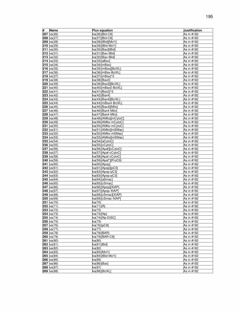
195
# Name Flux equation Justification
207 va(26) ka(26)[Bid-C8] As in #182 208 va(27) ka(27)[Bid-C8] As in #182 209 va(28) ka(28)[tBid][Mcl1] As in #182 210 va(29) ka(29)[tBid-Mcl1] As in #182 211 va(30) ka(30)[Bax][tBid] As in #182 212 va(31) ka(31)[Bax-tBid] As in #182 213 va(32) ka(32)[Bax-tBid] As in #182 214 va(33) ka(33)[aBax] As in #182 215 va(34) ka(34)[mBax] As in #182 216 va(35) ka(35)[mBax][BclXL] As in #182 217 va(36) ka(36)[mBax-BclXL] As in #182 218 va(37) ka(37)[mBax]^2 As in #182 219 va(38) ka(38)[Bax2] As in #182 220 va(39) ka(39)[Bax2][BclXL] As in #182 221 va(40) ka(40)[mBax2-BclXL] As in #182 222 va(41) ka(41)[Bax2]^2 As in #182 223 va(42) ka(42)[Bax4] As in #182 224 va(43) ka(43)[Bax4][BclXL] As in #182 225 va(44) ka(44)[mBax4-BclXL] As in #182 226 va(45) ka(45)[Bax4][Mito] As in #182 227 va(46) ka(46)[Bax4-Mito] As in #182 228 va(47) ka(47)[Bax4-Mito] As in #182 229 va(48) ka(48)[AMito][mCytoC] As in #182 230 va(49) ka(49)[AMito-mCytoC] As in #182 231 va(50) ka(50)[AMito-mCytoC] As in #182 232 va(51) ka(51)[AMito][mSMac] As in #182
233 va(52) ka(52)[AMito-mSMac] As in #182 234 va(53) ka(53)[AMito][mSMac] As in #182 235 va(54) ka(54)[aCytoC] As in #182 236 va(55) ka(55)[cCytoC] As in #182 237 va(56) ka(56)[Apaf][cCytoC] As in #182 238 va(57) ka(57)[Apaf-cCytoC] As in #182 239 va(58) ka(58)[Apaf-cCytoC] As in #182 240 va(59) ka(59)[Apaf*][ProC9] As in #182 241 va(60) ka(60)[Apop] As in #182 242 va(61) ka(61)[Apop][pC3] As in #182 243 va(62) ka(62)[Apop-pC3] As in #182 244 va(63) ka(63)[Apop-pC3] As in #182 245 va(64) ka(64)[aSmac] As in #182 246 va(65) ka(65)[cSmac] As in #182 247 va(66) ka(66)[Apop][XIAP] As in #182 248 va(67) ka(67)[Apop-XIAP] As in #182 249 va(68) ka(68)[cSmac][XIAP] As in #182 250 va(69) ka(69)[cSmac-XIAP] As in #182 251 va(70) ka(70) As in #182 252 va(71) ka(71)[R} As in #182 253 va(72) ka(72) As in #182 254 va(73) ka(73)[flip] As in #182 255 va(74) ka(74)[flip-DISC] As in #182 256 va(75) ka(75) As in #182 257 va(76) ka(76)[pC8] As in #182 258 va(77) ka(77) As in #182 259 va(78) ka(78)[BAR} As in #182 260 va(79) ka(79)[BAR-C8] As in #182 261 va(80) ka(80) As in #182 262 va(81) ka(81)[Bid] As in #182 263 va(82) ka(82) As in #182 264 va(83) ka(83)[Mcl1] As in #182 265 va(84) ka(84)[tBid-Mcl1] As in #182 266 va(85) ka(85) As in #182 267 va(86) ka(86)[Bax] As in #182 268 va(87) ka(87) As in #182 269 va(88) ka(88)[BclXL] As in #182

196
# Name Flux equation Justification
270 va(89) ka(89)[mBax-BclXL] As in #182 271 va(90) ka(90)[Bax2-BclXL] As in #182 272 va(91) ka(91)[Bax4-BclXL] As in #182 273 va(92) ka(92)[AMito] As in #182 274 va(93) ka(93)[Apaf*] As in #182 275 va(94) ka(94) As in #182 276 va(95) ka(95)[XIAP] As in #182 277 va(96) ka(96) As in #182 278 va(97) ka(97)[mSmac] As in #182 279 va(98) ka(98)[cSmac] As in #182 280 va(99) ka(99)[cSmac-XIAP] As in #182 281 va(100) ka(100) As in #182 282 va(101) ka(101)[pC3] As in #182 283 va(102) ka(102)[C3_U] As in #182 284 va(103) ka(103) As in #182 285 va(104) ka(104)[pC6] As in #182 286 va(105) ka(105)[C6] As in #182 287 va(106) ka(106)[Apop-XIAP] As in #182 288 va(107) ka(107) As in #182 289 va(108) ka(108)[Parp] As in #182 290 va(109) ka(109)[cParp] As in #182 291 va(110) ka(110) As in #182 292 va(111) ka(111)[L] As in #182 293 va(112) ka(112) As in #182 294 va(113) ka(113)[mCytoC] As in #182
295 va(114) ka(114)[cCytoC] As in #182 296 vcc(1) kcc(79)[tCycD] See the original
paper for justification [152].
297 vcc(2) kcc(81)[tBcl2] As in #296 298 vcc(3) kcc(9)[CD] As in #296
299 vcc(4) kcc(9)[CycD] As in #296
300 vcc(5) kcc(16)[p27][CycE] As in #296 301 vcc(6) kcc(16)[p27][CycA] As in #296 302 vcc(7) kcc(10)[p27][CycD] As in #296 303 vcc(8) kcc(11)[CD] As in #296 304 vcc(9) kcc(22)[CDc20][CycA] As in #296 305 vcc(10) kcc(22)[CDc20][CA] As in #296 306 vcc(11) kcc(17)[CE] As in #296 307 vcc(12) kcc(17)[CA] As in #296 308 vcc(13) V8[CE] As in #296 309 vcc(14) V8[CycE] As in #296 310 vcc(15) V6[p27] As in #296 311 vcc(16) V6[CE] As in #296 312 vcc(17) V6[CD] As in #296 313 vcc(18) V6[CA] As in #296 314 vcc(19) V2[CycB] As in #296 315 vcc(20) ((kcc(47)+kcc(48)[CDc20](1-[Cdh1]))/(kcc(49)-[Cdh1]+1) if
[Cdh1] <=1 else 0 As in #296
316 vcc(21) V4[Cdh1])/(kcc(50)+[Cdh1]) As in #296 317 vcc(22) kcc(56)[PPX] As in #296 318 vcc(23) (kcc(57)[CycB](1-[IEP]))/(kcc(59)-[IEP]+1) As in #296 319 vcc(24) (kcc(58)[PPX][IEP])/(kcc(60)+[IEP]) As in #296 320 vcc(25) kcc(63)[CDc20T] As in #296 321 vcc(26) (kcc(64)[IEP]([CDc20T]-[CDc20]))/(kcc(66)-[CDc20]+[CDc20T]) As in #296 322 vcc(27) kcc(65)[CDc20]/(kcc(67)+[CDC20]) As in #296 323 vcc(28) kcc(63)[CDc20] As in #296 324 vcc(29) [E2F-
Rb](kcc(40)(([CycD]+[CD])kcc(36)+kcc(39)[CycA]+kcc(38)[CycB]+kcc(37)[CycD]))
As in #296
325 vcc(30) [p-E2F- Rb](kcc(40)(([CycD]+[CD])kcc(36)+ kcc(39)[CycA]+kcc(38)[CycB]+kcc(37)[CycD]))
As in #296
326 vcc(31) kcc(74)(0.01+0.99*GMAct*GMSize) if RbFrac < 0.8, kcc(74)*0.01 otherwise
As in #296

197
# Name Flux equation Justification
327 vcc(32) kcc(75)[GM] As in #296 328 vcc(33) kcc(77)kcc(76)[GM] As in #296 329 vcc(34) kcc(78)CycDAct As in #296 330 vcc(35) kcc(77)(kcc(61)+kcc(62)[CycB]) As in #296 331 vcc(36) kcc(77)kcc(21)[E2F]max(0,GMAct*(vcc(33)-vcc(55))*300)) if
[Mass] > 0.5, 0 otherwise As in #296
332 vcc(37) kcc(77)kcc(55) As in #296 333 vcc(38) kcc(77)(kcc(12)+kcc(13)[E2F]) As in #296 334 vcc(39) kcc(77)kcc(8)[tCycD] As in #296 335 vcc(40) kcc(77)kcc(29) As in #296 336 vcc(41) max(kcc(80)BclAct,0.01kcc(80) As in #296 337 vcc(42) kcc(77)(kcc(24)*(([CycB]/kcc(25))^2/([CycB]/kcc(25))^2+1))+kcc(
23) As in #296
338 vcc(43) [Rb](kcc(40)*([CycD]+[CD]kcc(36)+kcc(39)[CycA]+kcc(38)[CycB]+kcc(37)[CycE]))
As in #296
339 vcc(44) [pp-Rb](kcc(41)(kcc(44)-PP1A)+kcc(42)PP1A) As in #296 340 vcc(45) [E2F-Rb]kcc(73) As in #296 341 vcc(46) [E2F](kcc(70)+kcc(71)([CycA]+[CycB]))) As in #296 342 vcc(47) [p-E2F]kcc(69) As in #296 343 vcc(48) [E2F][Rb]kcc(72) As in #296 344 vcc(49) [p-E2F-Rb]kcc(73) As in #296 345 vcc(50) [Rb][p-E2F]kcc(72) As in #296 346 vcc(51) [p-E2F-Rb]kcc(69) As in #296 347 vcc(52) [E2F-Rb](kcc(70)+kcc(71)([CycA]+[CycB]))) As in #296 348 vcc(53) kcc(82)[tMycTor] As in #296 349 vcc(54) kcc(83)[MycTor] As in #296 350 vcc(55) kcc(84)[Mass] As in #296 351 vcc(56) kcc(85)MycAct As in #296 341 vcc(57) kcc(86)[tMycTor] As in #296
D. Integrated B-cell model reactions # Species Reaction Justification
1 d[tRelA]/dt vm(RelA)-vtm(1,RelA)[tRelA] See [150]
2 d[tp50]/dt vm(p50)-vtm(1,p50)[tp50] As in #1 3 d[tcRel]/dt vm(cRel)-vtm(1,cRel)[tcRel] As in #1
4 d[RelA]/dt vd(3,AA)*2+vd(3,A50)-vd(1,AA)-vd(1,A50)+vtm(2,RelA)[tRelA]-vtm(3,RelA)[RelA]
As in #1
5 d[nRelA]/dt vd(4,AA)*2+vd(4,A50)-vd(2,AA)-vd(2,A50)-vtm(4,RelA)[nRelA] As in #1
6 d[p50]/dt vd(3,5050)*2+vd(3,A50)-+vd(3,C50)-vd(1,A50)-vd(1,C50)-vd(1,5050) )+vtm(2,p50)[tp50]-vtm(3,p50)[p50]
As in #1
7 d[np50]/dt vd(4,5050)*2+vd(4,A50)-+vd(4,C50)-vd(2,A50)-vd(2,C50)-vd(2,5050) -vtm(4,p50)[np50]
As in #1
8 d[cRel]/dt vd(3,C50)-vd(1,C50) )+vtm(2,cRel)[tcRel]-vtm(3,cRel)[cRel] As in #1
9 d[ncRel]/dt vd(4,C50)-vd(2,C50) -vtm(4,cRel)[ncRel] As in #1
10 d[AA]/dt vd(1,AA)-vd(3,AA)-vd(5,AA)+vd(6,AA)-vd(7,AA)-vdi(1,AA,[α,β,ε])+vdi(2,AA,
[α,β,ε])+vdi(7,AA, [α,β,ε])+vdi(8,AA,[α,β,ε]) As in #1
11 d[A50]/dt vd(1,A50)-vd(3,A50)-vd(5,A50)+vd(6,A50)-vd(7,A50)-
vdi(1,A50,[α,β,ε])+vdi(2,A50, [α,β,ε])+vdi(7,A50, [α,β,ε])+vdi(8,A50,[α,β,ε]) As in #1
12 d[5050]/dt vd(1,5050)-vd(3,5050)-vd(5,5050)+vd(6,5050)-vd(7,5050)-
vdi(1,5050,[α,β,ε])+vdi(2,5050, [α,β,ε])+vdi(7,5050, [α,β,ε])+vdi(8,5050,[α,β,ε]) As in #1
13 d[C50]/dt vd(1,C50)-vd(3,C50)-vd(5,C50)+vd(6,C50)-vd(7,C50)-
vdi(1,C50,[α,β,ε])+vdi(2,C50, [α,β,ε])+vdi(7,C50, [α,β,ε])+vdi(8,C50,[α,β,ε]) As in #1
14 d[nAA]/dt vd(2,AA)-vd(4,AA)-vd(6,AA)+vd(5,AA)-vd(8,AA)-vdi(2,AA,[α,β,ε])+vdi(4,AA,
[α,β,ε])+vdi(9,AA, [α,β,ε]) As in #1
15 d[nA50]/dt vd(2,A50)-vd(4,A50)-vd(6,A50)+vd(5,A50)-vd(8,A50)-
vdi(2,A50,[α,β,ε])+vdi(4,A50, [α,β,ε])+vdi(9,A50, [α,β,ε]) As in #1
16 d[n5050]/dt vd(2,5050)-vd(4,5050)-vd(6,5050)+vd(5,5050)-vd(8,5050)-
vdi(2,5050,[α,β,ε])+vdi(4,5050, [α,β,ε])+vdi(9,5050, [α,β,ε]) As in #1
17 d[nC50]/dt
vd(2,C50)-vd(4,C50)-vd(6,C50)+vd(5,C50)-vd(8,C50)-
vdi(2,C50,[α,β,ε])+vdi(4,C50, [α,β,ε])+vdi(9,C50, [α,β,ε])
As in #1

198
# Species Reaction Justification
18 d[AA:IkBα,AA:IkBβ,
AA:IkBε]/dt
vdi(1,AA, [α,β,ε])-vdi(3,AA, [α,β,ε])-vdi(5,AA, [α,β,ε])+vdi(6,AA, [α,β,ε])-
vdi(7,AA, [α,β,ε])-vdi(8,AA, [α,β,ε])-vdi(10,AA, [α,β,ε]) As in #1
19 d[A50:IkBα,A50:IkBβ,
A50:IkBε]/dt
vdi(1,A50, [α,β,ε])-vdi(3,A50, [α,β,ε])-vdi(5,A50, [α,β,ε])+vdi(6,A50, [α,β,ε])-
vdi(7,A50, [α,β,ε])-vdi(8,A50, [α,β,ε])-vdi(10,A50, [α,β,ε]) As in #1
20
d[5050:IkBα,
5050:IkBβ,
5050:IkBε]/dt
vdi(1,5050, [α,β,ε])-vdi(3,5050, [α,β,ε])-vdi(5,5050, [α,β,ε])+vdi(6,5050, [α,β,ε])-
vdi(7,5050, [α,β,ε])-vdi(8,5050, [α,β,ε])-vdi(10,5050, [α,β,ε]) As in #1
21 d[C50:IkBα,C50:IkBβ, C50:IkBε]/dt
vdi(1,C50, [α,β,ε])-vdi(3,C50, [α,β,ε])-vdi(5,C50, [α,β,ε])+vdi(6,C50, [α,β,ε])-
vdi(7,C50, [α,β,ε])-vdi(8,C50, [α,β,ε])-vdi(10,c50, [α,β,ε]) As in #1
22 d[nAA:nIkBα,nAA:nIk
Bβ, nAA:nIkBε]/dt
vdi(2,AA, [α,β,ε])-vdi(4,AA, [α,β,ε])-vdi(6,AA, [α,β,ε])+vdi(5,AA, [α,β,ε])-
vdi(9,AA, [α,β,ε])-vdi(11,AA, [α,β,ε]) As in #1
23
d[nA50:nIkBα,
nA50:nIkBβ,
nA50:nIkBε]/dt
vdi(2,A50, [α,β,ε])-vdi(4,A50, [α,β,ε])-vdi(6,A50, [α,β,ε])+vdi(5,A50, [α,β,ε])-
vdi(9,A50, [α,β,ε])-vdi(11,A50, [α,β,ε]) As in #1
24
d[n5050:nIkBα,
n5050:nIkBβ,
n5050:nIkBε]/dt
vdi(2,5050, [α,β,ε])-vdi(4,5050, [α,β,ε])-vdi(6,5050, [α,β,ε])+vdi(5,5050, [α,β,ε])-
vdi(9,5050, [α,β,ε])-vdi(11,5050, [α,β,ε]) As in #1
25
d[nA50:nIkBα,
nA50:nIkBβ,
nA50:nIkBε]/dt
vdi(2,C50, [α,β,ε])-vdi(4,C50, [α,β,ε])-vdi(6,C50, [α,β,ε])+vdi(5,C50, [α,β,ε])-
vdi(9,C50, [α,β,ε])-vdi(11,C50, [α,β,ε]) As in #1
26 d[tIkbα,tIkBβ,tIkBε]/dt vi([α,β,∈])- vti(1, [α,β,ε])[tIkbα,tIkBβ,tIkBε] As in #1
27 d[Ikbα,IkBβ,IkBε]/dt
Σd=[AA,A50,5050,C50]{vdi(3,d, [Ikbα,IkBβ,IkBε])+vdi(10,d,
[Ikbα,IkBβ,IkBε])- vdi(1,d, [Ikbα,IkBβ,IkBε])}+vti(2, [α,β,ε])[tIkbα,tIkBβ,tIkBε]-
vti(3, [α,β,ε])[Ikbα,IkBβ,IkBε]- vti(4, [α,β,ε])[Ikbα,IkBβ,IkBε]- vti(6,
[α,β,ε])[nIkbα,nIkBβ,nIkBε]+ vti(7, [α,β,ε])[Ikbα,IkBβ,IkBε]
As in #1
28 d[nIkbα,nIkBβ,nIkBε]/dt
Σd=[AA,A50,5050,C50]{vdi(4,d, [Ikbα,IkBβ,IkBε])+vdi(11,d,
[Ikbα,IkBβ,IkBε])- vdi(2,d, [Ikbα,IkBβ,IkBε])}- vti(5,
[α,β,ε])[nIkbα,nIkBβ,nIkBε]+ vti(6, [α,β,ε])[Ikbα,IkBβ,IkBε]- vti(7,
[α,β,ε])[nIkbα,nIkBβ,nIkBε]
As in #1
29 d[L]/dt 0 See [156]
30 d[R]/dt -va(1) + va(2) + va(71) - va(72) As in #29
31 d[L-R]/dt va(1) - va(2) - va(3) As in #29
32 d[DISC]/dt va(3) - va(4) + va(5) - va(6) + va(7) + va(8) As in #29
33 d[flip]/dt -va(4) + va(5) + va(73) - va(74) As in #29
34 d[flip-DISC]/dt va(4) - va(5) - va(75) As in #29
35 d[pC8]/dt -va(6) + va(7) - va(17) + va(18) + va(76) - va(77) As in #29
36 d[DISC-pC8]/dt va(6) - va(7) - va(8) As in #29
37 d[C8]/dt va(8) - va(9) + va(10) - va(11) + va(12) + va(13) + va(19) - va(26) + va(27) + va(28)
As in #29
38 d[Bar]/dt -va(9) + va(10) + va(78) - va(79) As in #29
39 d[Bar-C8]/dt va(9) - va(10) - va(80) As in #29
40 d[pC3]/dt -va(11) + va(12) - va(62) + va(63) + va(101) - va(102) As in #29
41 d[C8-pC3]/dt va(11) - va(12) - va(13) As in #29
42 d[C3]/dt va(13) - va(14) + va(15) + va(16) - va(20) + va(21) - va(23) + va(24) + va(25) + va(64)
As in #29
43 d[pC6]/dt -va(14) + va(15) + va(104) - va(105) As in #29
44 d[C3-pC6]/dt va(14) - va(15) - va(16) As in #29
45 d[C6]/dt va(16) - va(17) + va(18) + va(19) - va(106) As in #29
46 d[C6-pC8]/dt va(17) - va(18) - va(19) As in #29
47 d[XIAP]/dt -va(20) + va(21) + va(22) - va(67) + va(68) - va(69) + va(70) + va(95) - va(96)
As in #29
48 d[XIAP-C3]/dt va(20) - va(21) - va(22) As in #29
49 d[PARP]/dt -va(23) + va(24) + va(108) - va(109) As in #29
50 d[C3-PARP]/dt va(23) - va(24) - va(25) As in #29
51 d[CPARP]/dt va(25) - va(110) As in #29
52 d[Bid]/dt -va(26) + va(27) + va(81) - va(82) As in #29
53 d[C8-Bid]/dt va(26) - va(27) - va(28) As in #29

199
# Species Reaction Justification
54 d[tBid]/dt va(28) - va(29) + va(30) - va(31) + va(32) + va(33) As in #29
55 d[Mcl1]/dt -va(29) + va(30) + va(83) - va(84) As in #29
56 d[Mcl1-tBid]/dt + va(29) - va(30) - va(85) As in #29
57 d[Bax]/dt -va(31) + va(32) + va(86) - va(87) As in #29
58 d[tBid-Bax]/dt va(31) - va(32) - va(33) As in #29
59 d[act_Bax]/dt va(33) - va(34) + va(35) As in #29
60 d[Baxm]/dt va(34) - va(35) -1/mvol*va(36) + va(37) -1/mvol*2*va(38) +2*va(39) As in #29
61 d[Bcl2]/dt -1/mvol*va(36) + va(37) -1/mvol*va(40) + va(41) -1/mvol*va(44) + va(45) + va(88) - va(89)
As in #29
62 d[Baxm-Bcl2]/dt 1/mvol*va(36) - va(37) - va(90) As in #29
63 d[Bax2]/dt 1/mvol*va(38) - va(39) -1/mvol*va(40) + va(41) -2/mvol*va(42) +2*va(43) As in #29
64 d[Bax2-Bcl2]/dt 1/mvol*va(40) - va(41) - va(91) As in #29
65 d[Bax4]/dt 1/mvol*va(42) - va(43)-1/mvol*va(44) + va(45) -1/mvol*va(46) + va(47) As in #29
66 d[Bax4-Bcl2]/dt 1/mvol*va(44) - va(45) - va(92) As in #29
67 d[M]/dt -1/mvol*va(46) + va(47) + va(93) As in #29
68 d[Bax4-M]/dt 1/mvol*va(46) - va(47) - va(48) As in #29
69 d[AMito]/dt va(48) -1/mvol*va(49) + va(50) + va(51) -1/mvol*va(52) + va(53) + va(54) - va(93)
As in #29
70 d[mCytoC]/dt -1/mvol*va(49) + va(50) + va(113) - va(114) As in #29
71 d[AMito-mCytoC]/dt 1/mvol*va(49) - va(50) - va(51) As in #29
72 d[ACytoC]/dt va(51) - va(55) + va(56) As in #29
73 d[mSmac]/dt -1/mvol*va(52) + va(53) + va(97) - va(98) As in #29
74 d[AMito-mSmac]/dt 1/mvol*va(52) - va(53) - va(54) As in #29
75 d[ASmac]/dt va(54) - va(65) + va(66) As in #29
76 d[CytoC]/dt va(55) - va(56) - va(58) + va(59) + va(57) - va(115) As in #29
77 d[Apaf]/dt -va(58) + va(59) + va(94) As in #29
78 d[Apaf-CytoC]/dt va(58) - va(59) - va(57) As in #29
79 d[act_Apaf]/dt va(57) - va(60) + va(61) - va(94) As in #29
80 d[pC9]/dt -va(60) + va(61) As in #29
81 d[Apop]/dt va(60) - va(61) - va(62) + va(63) + va(64) - va(67) + va(68) + va(107) As in #29
82 d[Apop-pC3]/dt va(62) - va(63) - va(64) As in #29
83 d[cSmac]/dt va(65) - va(66) - va(69) + va(70) - va(99) As in #29
84 d[Apop-XIAP]/dt va(67) - va(68) - va(107) As in #29
85 d[cSmac-XIAP]/dt va(69) - va(70) - va(100) As in #29
86 d[C3_Ub]/dt va(22) - va(103) As in #29
87 d[CycA]/dt vcc(36)+vcc(12)+vcc(18)-vcc(9)-vcc(6) See [152]
88 d[CycB]/dt vcc(42)-vcc(19) As in #87
89 d[CycD]/dt vcc(39)+vcc(17)+vcc(8)-vcc(7)-vcc(4) As in #87
90 d[CycE]/dt vcc(38)+vcc(11)+vcc(16)-vcc(14)-vcc(5) As in #87
91 d[mCycD]/dt vcc(34)-vcc(1) As in #87
92 d[mBcl2]/dt vcc(41)-vcc(2) As in #87
93 d[Cdh1]/dt vcc(20)-vcc(21) As in #87
94 d[CA]/dt vcc(6)-vcc(12)-vcc(18)-vcc(10) As in #87
95 d[CD]/dt vcc(7)-vcc(8)-vcc(17)-vcc(3) As in #87
96 d[CDc20]/dt vcc(26)-vcc(27)-vcc(28) As in #87
97 d[CDc20T]/dt vcc(35)-vcc(25) As in #87
98 d[CE]/dt vcc(5)-vcc(11)-vcc(13)-vcc(16) As in #87
99 d[GM]/dt vcc(31)-vcc(32) As in #87
100 d[IEP]/dt vcc(23)-vcc(24) As in #87
101 d[Mass]/dt vcc(33)-vcc(55) As in #87
102 d[p27]/dt vcc(40)+vcc(3)+vcc(8)-vcc(15)-vcc(5)-vcc(6)-vcc(7)+vcc(11)+vcc(12)+vcc(13)+vcc(10)
As in #87
103 d[PPX]/dt vcc(37)-vcc(22) As in #87
104 d[pp-Rb]/dt vcc(29)+vcc(30)+vcc(43)-vcc(44) As in #87
105 d[E2F]/dt vcc(29)+vcc(45)+vcc(47)-vcc(46)-vcc(48) As in #87
106 d[p-E2F]/dt vcc(30)+vcc(49)+vcc(46)-vcc(47)-vcc(50) As in #87
107 d[Rb]/dt vcc(44)+vcc(45)+vcc(49)-vcc(48)-vcc(50)-vcc(43) As in #87
108 d[E2F-Rb]/dt vcc(51)+vcc(48)-vcc(52)-vcc(29)-vcc(45) As in #87
109 d[p-E2F-Rb]/dt vcc(52)+vcc(50)-vcc(51)-vcc(30)-vcc(49) As in #87
110 d[MYC]/dt vcc(53)-vcc(54) As in #87
111 d[mMYC]/dt vcc(56)-vcc(57) As in #87

200
E. Other simulation parameters # Parameter Value Description Justification
1 RCV
0.1
Protein syn/deg CV
For simplicity we assumed synthesis and degradation rates were normally distributed with a CV of 0.1 about the parameter value. Thi s is similar to the approach taken in [156] and results a steady state protein concentration variability with CV ~ 0.25 [24]
2 CCV
0.25 If no protein syn/deg then the total free protein concentration CV
We assumed log-normally distributed initial protein concetrations about the x0 mean with a CV of 0.25 as in [24]
3 PCV 0.07
Partition volume CV The observed variability in relative volumes was normal with mean 1 and standard deviation of 0.07 from microscopy studies in this work
4 VCV 0.05
Starting volume CV The observed starting volume variability of viable cells from microscopy studies.
5 IKKCV 0.25 IKK CV As in #2
6 N 250 Initial number of
cellular agents used in multiscale model.
This number was large enough to ensure that repeated simulations produced very similar results.
7 Simulation Replicates
2 Average of 2 250 agent runs.
Two simulations with 250 agents were used to create each simulation. The averages of two replicate simulations are reported.
8 Tmax 144 h
Total simulation time. Six days of simulations was sufficient for capturing both the expansion and contraction periods of the population response. This is also the typical duration of time-lapse experiments.
9 AbsTol 1e-5 Absolution simulation
tolerance for Matlab function ode15s
This was sufficiently low to produce accurate results. Increasing this number further resulted in noticeable changes in solution accuracy.
10 RelTol
1e-3 Relative tolerationce of simulation s using Matlab function ode15s
As in #9

201
Bibliography
1. Murphy K, Travers P, Walport M (2007) Janeway's Immunobiology (Immunobiology:
The Immune System (Janeway)): Garland Science.
2. Pearce EL, Pearce EJ (2013) Metabolic pathways in immune cell activation and quiescence. Immunity 38: 633-643.
3. LeBien TW, Tedder TF (2008) B lymphocytes: how they develop and function. Blood 112: 1570-1580.
4. Gerondakis S, Siebenlist U (2010) Roles of the NF-kappaB pathway in lymphocyte development and function. Cold Spring Harb Perspect Biol 2: a000182.
5. Wang YH, Zhang Z, Burrows PD, Kubagawa H, Bridges SL, Jr., Findley HW, Cooper MD (2003) V(D)J recombinatorial repertoire diversification during intraclonal pro-B to B-cell differentiation. Blood 101: 1030-1037.
6. Cooper MD (2002) Exploring lymphocyte differentiation pathways. Immunol Rev 185: 175-185.
7. Fulcher DA, Basten A (1994) Reduced life span of anergic self-reactive B cells in a double-transgenic model. J Exp Med 179: 125-134.
8. Treml LS, Quinn WJ, 3rd, Treml JF, Scholz JL, Cancro MP (2008) Manipulating B cell homeostasis: a key component in the advancement of targeted strategies. Arch Immunol Ther Exp (Warsz) 56: 153-164.
9. Nagai Y, Garrett KP, Ohta S, Bahrun U, Kouro T, Akira S, Takatsu K, Kincade PW (2006) Toll-like receptors on hematopoietic progenitor cells stimulate innate immune system replenishment. Immunity 24: 801-812.
10. Cahalan MD, Gutman GA (2006) The sense of place in the immune system. Nat Immunol 7: 329-332.
11. Cerutti A, Puga I, Cols M (2011) Innate control of B cell responses. Trends Immunol 32: 202-211.
12. Tonegawa S (1983) Somatic generation of antibody diversity. Nature 302: 575-581.
13. Malu S, Malshetty V, Francis D, Cortes P (2012) Role of non-homologous end joining in V(D)J recombination. Immunol Res 54: 233-246.
14. Peled JU, Kuang FL, Iglesias-Ussel MD, Roa S, Kalis SL, Goodman MF, Scharff MD (2008) The biochemistry of somatic hypermutation. Annu Rev Immunol 26: 481-511.
15. Cooper MD, Alder MN (2006) The evolution of adaptive immune systems. Cell 124: 815-822.

202
16. Kumar H, Kawai T, Akira S (2011) Pathogen recognition by the innate immune system. Int Rev Immunol 30: 16-34.
17. Browne EP (2012) Regulation of B-cell responses by Toll-like receptors. Immunology 136: 370-379.
18. Agrawal S, Gupta S (2011) TLR1/2, TLR7, and TLR9 signals directly activate human peripheral blood naive and memory B cell subsets to produce cytokines, chemokines, and hematopoietic growth factors. J Clin Immunol 31: 89-98.
19. Krieg AM, Yi AK, Matson S, Waldschmidt TJ, Bishop GA, Teasdale R, Koretzky GA, Klinman DM (1995) CpG motifs in bacterial DNA trigger direct B-cell activation. Nature 374: 546-549.
20. Hawkins ED, Turner ML, Wellard CJ, Zhou JH, Dowling MR, Hodgkin PD (2013) Quantal and graded stimulation of B lymphocytes as alternative strategies for regulating adaptive immune responses. Nat Commun 4: 2406.
21. Hawkins ED, Markham JF, McGuinness LP, Hodgkin PD (2009) A single-cell pedigree analysis of alternative stochastic lymphocyte fates. Proc Natl Acad Sci U S A 106: 13457-13462.
22. Flowers CR, Armitage JO (2010) A decade of progress in lymphoma: advances and continuing challenges. Clin Lymphoma Myeloma Leuk 10: 414-423.
23. Seifert M, Scholtysik R, Kuppers R (2013) Origin and pathogenesis of B cell lymphomas. Methods Mol Biol 971: 1-25.
24. Gaudet S, Spencer SL, Chen WW, Sorger PK (2012) Exploring the contextual sensitivity of factors that determine cell-to-cell variability in receptor-mediated apoptosis. PLoS Comput Biol 8: e1002482.
25. Flusberg DA, Roux J, Spencer SL, Sorger PK (2013) Cells surviving fractional killing by TRAIL exhibit transient but sustainable resistance and inflammatory phenotypes. Mol Biol Cell 24: 2186-2200.
26. Dimberg LY, Anderson CK, Camidge R, Behbakht K, Thorburn A, Ford HL (2013) On the TRAIL to successful cancer therapy? Predicting and counteracting resistance against TRAIL-based therapeutics. Oncogene 32: 1341-1350.
27. Yap TA, Gerlinger M, Futreal PA, Pusztai L, Swanton C (2012) Intratumor heterogeneity: seeing the wood for the trees. Sci Transl Med 4: 127ps110.
28. Schliemann M, Bullinger E, Borchers S, Allgower F, Findeisen R, Scheurich P (2011) Heterogeneity reduces sensitivity of cell death for TNF-stimuli. BMC Syst Biol 5: 204.
29. Fallahi-Sichani M, Honarnejad S, Heiser LM, Gray JW, Sorger PK (2013) Metrics other than potency reveal systematic variation in responses to cancer drugs. Nat Chem Biol 9: 708-714.

203
30. Frank SA, Rosner MR (2012) Nonheritable cellular variability accelerates the evolutionary processes of cancer. PLoS Biol 10: e1001296.
31. Meyer-Bahlburg A, Rawlings DJ (2008) B cell autonomous TLR signaling and autoimmunity. Autoimmun Rev 7: 313-316.
32. Pai S, Thomas R (2008) Immune deficiency or hyperactivity-Nf-kappab illuminates autoimmunity. J Autoimmun 31: 245-251.
33. Rickert RC, Jellusova J, Miletic AV (2011) Signaling by the tumor necrosis factor receptor superfamily in B-cell biology and disease. Immunol Rev 244: 115-133.
34. Goldin LR, Landgren O (2009) Autoimmunity and lymphomagenesis. Int J Cancer 124: 1497-1502.
35. Milner JD, Holland SM (2013) The cup runneth over: lessons from the ever-expanding pool of primary immunodeficiency diseases. Nat Rev Immunol 13: 635-648.
36. Xiao X, Miao Q, Chang C, Gershwin ME, Ma X (2014) Common variable immunodeficiency and autoimmunity - an inconvenient truth. Autoimmun Rev.
37. Kumar H, Kawai T, Akira S (2009) Toll-like receptors and innate immunity. Biochem Biophys Res Commun 388: 621-625.
38. Peng SL (2005) Signaling in B cells via Toll-like receptors. Curr Opin Immunol 17: 230-236.
39. Lopez-Yglesias AH, Zhao X, Quarles EK, Lai MA, VandenBos T, Strong RK, Smith KD (2014) Flagellin induces antibody responses through a TLR5- and inflammasome-independent pathway. J Immunol 192: 1587-1596.
40. Hidmark A, von Saint Paul A, Dalpke AH (2012) Cutting edge: TLR13 is a receptor for bacterial RNA. J Immunol 189: 2717-2721.
41. Raetz M, Kibardin A, Sturge CR, Pifer R, Li H, Burstein E, Ozato K, Larin S, Yarovinsky F (2013) Cooperation of TLR12 and TLR11 in the IRF8-dependent IL-12 response to Toxoplasma gondii profilin. J Immunol 191: 4818-4827.
42. Mulla MJ, Myrtolli K, Tadesse S, Stanwood NL, Gariepy A, Guller S, Norwitz ER, Abrahams VM (2013) Cutting-edge report: TLR10 plays a role in mediating bacterial peptidoglycan-induced trophoblast apoptosis. Am J Reprod Immunol 69: 449-453.
43. Jiang W, Lederman MM, Harding CV, Rodriguez B, Mohner RJ, Sieg SF (2007) TLR9 stimulation drives naive B cells to proliferate and to attain enhanced antigen presenting function. Eur J Immunol 37: 2205-2213.
44. Hawkins ED, Turner ML, Dowling MR, van Gend C, Hodgkin PD (2007) A model of immune regulation as a consequence of randomized lymphocyte division and death times. Proc Natl Acad Sci U S A 104: 5032-5037.
204
45. Hawkins ED, Hommel M, Turner ML, Battye FL, Markham JF, Hodgkin PD (2007) Measuring lymphocyte proliferation, survival and differentiation using CFSE time-series data. Nat Protoc 2: 2057-2067.
46. Duffy KR, Wellard CJ, Markham JF, Zhou JH, Holmberg R, Hawkins ED, Hasbold J, Dowling MR, Hodgkin PD (2012) Activation-induced B cell fates are selected by intracellular stochastic competition. Science 335: 338-341.
47. Shokhirev MN, Hoffmann A (2013) FlowMax: A Computational Tool for Maximum Likelihood Deconvolution of CFSE Time Courses. PLoS One 8: e67620.
48. Spencer SL, Cappell SD, Tsai FC, Overton KW, Wang CL, Meyer T (2013) The proliferation-quiescence decision is controlled by a bifurcation in CDK2 activity at mitotic exit. Cell 155: 369-383.
49. Link JM, Hurlin PJ (2014) The activities of MYC, MNT and the Max-Interactome in lymphocyte proliferation and oncogenesis. Biochim Biophys Acta.
50. Renault TT, Chipuk JE (2013) Getting away with murder: how does the BCL-2 family of proteins kill with immunity? Ann N Y Acad Sci 1285: 59-79.
51. O'Dea E, Hoffmann A (2010) The regulatory logic of the NF-kappaB signaling system. Cold Spring Harb Perspect Biol 2: a000216.
52. Lenert P, Stunz L, Yi AK, Krieg AM, Ashman RF (2001) CpG stimulation of primary mouse B cells is blocked by inhibitory oligodeoxyribonucleotides at a site proximal to NF-kappaB activation. Antisense Nucleic Acid Drug Dev 11: 247-256.
53. Hannink M, Temin HM (1990) Structure and autoregulation of the c-rel promoter. Oncogene 5: 1843-1850.
54. Ten RM, Paya CV, Israel N, Le Bail O, Mattei MG, Virelizier JL, Kourilsky P, Israel A (1992) The characterization of the promoter of the gene encoding the p50 subunit of NF-kappa B indicates that it participates in its own regulation. EMBO J 11: 195-203.
55. Haskill S, Beg AA, Tompkins SM, Morris JS, Yurochko AD, Sampson-Johannes A, Mondal K, Ralph P, Baldwin AS, Jr. (1991) Characterization of an immediate-early gene induced in adherent monocytes that encodes I kappa B-like activity. Cell 65: 1281-1289.
56. Tian B, Nowak DE, Jamaluddin M, Wang S, Brasier AR (2005) Identification of direct genomic targets downstream of the nuclear factor-kappaB transcription factor mediating tumor necrosis factor signaling. J Biol Chem 280: 17435-17448.
57. Shih VF, Tsui R, Caldwell A, Hoffmann A (2011) A single NFkappaB system for both canonical and non-canonical signaling. Cell Res 21: 86-102.
58. Nie Z, Hu G, Wei G, Cui K, Yamane A, Resch W, Wang R, Green DR, Tessarollo L, Casellas R, Zhao K, Levens D (2012) c-Myc is a universal amplifier of expressed genes in lymphocytes and embryonic stem cells. Cell 151: 68-79.

205
59. Duyao MP, Buckler AJ, Sonenshein GE (1990) Interaction of an NF-kappa B-like factor with a site upstream of the c-myc promoter. Proc Natl Acad Sci U S A 87: 4727-4731.
60. Pohl T, Gugasyan R, Grumont RJ, Strasser A, Metcalf D, Tarlinton D, Sha W, Baltimore D, Gerondakis S (2002) The combined absence of NF-kB1 and c-Rel reveals that overlapping roles of these transcription factors in the B cell lineage are restricted to the activation and function of mature cells. PNAS: 4514-4519.
61. Limon JJ, Fruman DA (2012) Akt and mTOR in B Cell Activation and Differentiation. Front Immunol 3: 228.
62. Zeng H, Chi H (2013) mTOR and lymphocyte metabolism. Curr Opin Immunol 25: 347-355.
63. Xu ZZ, Xia ZG, Wang AH, Wang WF, Liu ZY, Chen LY, Li JM (2013) Activation of the PI3K/AKT/mTOR pathway in diffuse large B cell lymphoma: clinical significance and inhibitory effect of rituximab. Ann Hematol 92: 1351-1358.
64. Hanahan D, Weinberg RA (2011) Hallmarks of cancer: the next generation. Cell 144: 646-674.
65. Porta C, Paglino C, Mosca A (2014) Targeting PI3K/Akt/mTOR Signaling in Cancer. Front Oncol 4: 64.
66. Wang R, Dillon CP, Shi LZ, Milasta S, Carter R, Finkelstein D, McCormick LL, Fitzgerald P, Chi H, Munger J, Green DR (2011) The transcription factor Myc controls metabolic reprogramming upon T lymphocyte activation. Immunity 35: 871-882.
67. Dan HC, Cooper MJ, Cogswell PC, Duncan JA, Ting JP, Baldwin AS (2008) Akt-dependent regulation of NF-{kappa}B is controlled by mTOR and Raptor in association with IKK. Genes Dev 22: 1490-1500.
68. Dhingra R, Gang H, Wang Y, Biala AK, Aviv Y, Margulets V, Tee A, Kirshenbaum LA (2013) Bidirectional regulation of nuclear factor-kappaB and mammalian target of rapamycin signaling functionally links Bnip3 gene repression and cell survival of ventricular myocytes. Circ Heart Fail 6: 335-343.
69. Radhakrishnan P, Bryant VC, Blowers EC, Rajule RN, Gautam N, Anwar MM, Mohr AM, Grandgenett PM, Bunt SK, Arnst JL, Lele SM, Alnouti Y, Hollingsworth MA, Natarajan A (2013) Targeting the NF-kappaB and mTOR pathways with a quinoxaline urea analog that inhibits IKKbeta for pancreas cancer therapy. Clin Cancer Res 19: 2025-2035.
70. Wang Z, Sicinski P, Weinberg RA, Zhang Y, Ravid K (1996) Characterization of the mouse cyclin D3 gene: exon/intron organization and promoter activity. Genomics 35: 156-163.
71. Guttridge DC, Albanese C, Reuther JY, Pestell RG, Baldwin AS, Jr. (1999) NF-kappaB controls cell growth and differentiation through transcriptional regulation of cyclin D1. Mol Cell Biol 19: 5785-5799.

206
72. Huang Y, Ohtani K, Iwanaga R, Matsumura Y, Nakamura M (2001) Direct trans-activation of the human cyclin D2 gene by the oncogene product Tax of human T-cell leukemia virus type I. Oncogene 20: 1094-1102.
73. Cheng S, Hsia CY, Leone G, Liou HC (2003) Cyclin E and Bcl-xL cooperatively induce cell cycle progression in c-Rel-/- B cells. Oncogene 22: 8472-8486.
74. Chen F, Demers LM, Vallyathan V, Lu Y, Castranova V, Shi X (1999) Involvement of 5'-flanking kappaB-like sites within bcl-x gene in silica-induced Bcl-x expression. J Biol Chem 274: 35591-35595.
75. Hinz M, Krappmann D, Eichten A, Heder A, Scheidereit C, Strauss M (1999) NF-kappaB function in growth control: regulation of cyclin D1 expression and G0/G1-to-S-phase transition. Mol Cell Biol 19: 2690-2698.
76. Cato MH, Chintalapati SK, Yau IW, Omori SA, Rickert RC (2011) Cyclin D3 is selectively required for proliferative expansion of germinal center B cells. Mol Cell Biol 31: 127-137.
77. Lam EW, Glassford J, Banerji L, Thomas NS, Sicinski P, Klaus GG (2000) Cyclin D3 compensates for loss of cyclin D2 in mouse B-lymphocytes activated via the antigen receptor and CD40. J Biol Chem 275: 3479-3484.
78. Tanguay DA, Colarusso TP, Pavlovic S, Irigoyen M, Howard RG, Bartek J, Chiles TC, Rothstein TL (1999) Early induction of cyclin D2 expression in phorbol ester-responsive B-1 lymphocytes. J Exp Med 189: 1685-1690.
79. Piatelli M, Tanguay D, Rothstein T, Chiles T (2003) Cell cycle control mechanisms in B-1 and B-2 lymphoid subsets. Immunol Res 27: 31-52.
80. Pham LV, Tamayo AT, Yoshimura LC, Lo P, Ford RJ (2003) Inhibition of constitutive NF-kappa B activation in mantle cell lymphoma B cells leads to induction of cell cycle arrest and apoptosis. J Immunol 171: 88-95.
81. Kong LJ, Chang JT, Bild AH, Nevins JR (2007) Compensation and specificity of function within the E2F family. Oncogene 26: 321-327.
82. Hatakeyama M, Weinberg RA (1995) The role of RB in cell cycle control. Prog Cell Cycle Res 1: 9-19.
83. Grumont RJ, Rourke IJ, Gerondakis S (1999) Rel-dependent induction of A1 transcription is required to protect B cells from antigen receptor ligation-induced apoptosis. Genes Dev 13: 400-411.
84. Waterfield M, Jin W, Reiley W, Zhang M, Sun S-C (2004) IκB Kinase Is an Essential Component of the Tpl2 Signaling Pathway. Molecular and Cellular Biology 24: 6040-6048.
85. Babu GR, Jin W, Norman L, Waterfield M, Chang M, Wu X, Zhang M, Sun SC (2006) Phosphorylation of NF-kappaB1/p105 by oncoprotein kinase Tpl2: implications for a novel mechanism of Tpl2 regulation. Biochim Biophys Acta 1763: 174-181.

207
86. Banerjee A, Gugasyan R, McMahon M, Gerondakis S (2006) Diverse Toll-like receptors utilize Tpl2 to activate extracellular signal-regulated kinase (ERK) in hemopoietic cells. Proc Natl Acad Sci U S A 103: 3274-3279.
87. Belich MP, Salmeron A, Johnston LH, Ley SC (1999) TPL-2 kinase regulates the proteolysis of the NF-kappaB-inhibitory protein NF-kappaB1 p105. Nature 397: 363-368.
88. Weston SA, Parish CR (1990) New fluorescent dyes for lymphocyte migration studies. Analysis by flow cytometry and fluorescence microscopy. J Immunol Methods 133: 87-97.
89. M R (2011) Interpretation of Cellular proliferation Data: Avoid the Panglossian. Cytometry: 95-101.
90. Zilman A, Ganusov VV, Perelson AS (2010) Stochastic models of lymphocyte proliferation and death. PLoS One 5.
91. Miao H, Jin X, Perelson A, Wu H (2012) Evaluation of Multitype Mathematical Models for CFSE-Labeling Experiment Data. Bull Math Biol 74: 300-326.
92. Smith JA, Martin L (1973) Do cells cycle? Proc Natl Acad Sci U S A 70: 1263-1267.
93. De Boer RJ, Oprea M, Antia R, Murali-Krishna K, Ahmed R, Perelson AS (2001) Recruitment times, proliferation, and apoptosis rates during the CD8(+) T-cell response to lymphocytic choriomeningitis virus. J Virol 75: 10663-10669.
94. Revy P, Sospedra M, Barbour B, Trautmann A (2001) Functional antigen-independent synapses formed between T cells and dendritic cells. Nat Immunol 2: 925-931.
95. De Boer RJ, Homann D, Perelson AS (2003) Different dynamics of CD4+ and CD8+ T cell responses during and after acute lymphocytic choriomeningitis virus infection. J Immunol 171: 3928-3935.
96. Pilyugin SS, Ganusov VV, Murali-Krishna K, Ahmed R, Antia R (2003) The rescaling method for quantifying the turnover of cell populations. J Theor Biol 225: 275-283.
97. Luzyanina T, Mrusek S, Edwards JT, Roose D, Ehl S, Bocharov G (2007) Computational analysis of CFSE proliferation assay. J Math Biol 54: 57-89.
98. Luzyanina T, Roose D, Schenkel T, Sester M, Ehl S, Meyerhans A, Bocharov G (2007) Numerical modelling of label-structured cell population growth using CFSE distribution data. Theor Biol Med Model 4: 26.
99. Banks HT, Sutton KL, Thompson WC, Bocharov G, Doumic M, Schenkel T, Argilaguet J, Giest S, Peligero C, Meyerhans A (2011) A new model for the estimation of cell proliferation dynamics using CFSE data. J Immunol Methods 373: 143-160.

208
100. Gett AV, Hodgkin PD (2000) A cellular calculus for signal integration by T cells. Nat Immunol 1: 239-244.
101. Leon K, Faro J, Carneiro J (2004) A general mathematical framework to model generation structure in a population of asynchronously dividing cells. J Theor Biol 229: 455-476.
102. De Boer RJ, Perelson AS (2005) Estimating division and death rates from CFSE data. Journal of Computational and Applied Mathematics 184: 140-164.
103. Ganusov VV, Pilyugin SS, de Boer RJ, Murali-Krishna K, Ahmed R, Antia R (2005) Quantifying cell turnover using CFSE data. J Immunol Methods 298: 183-200.
104. De Boer RJ, Ganusov VV, Milutinovic D, Hodgkin PD, Perelson AS (2006) Estimating lymphocyte division and death rates from CFSE data. Bull Math Biol 68: 1011-1031.
105. Lee HY, Perelson AS (2008) Modeling T cell proliferation and death in vitro based on labeling data: generalizations of the Smith-Martin cell cycle model. Bull Math Biol 70: 21-44.
106. Deenick EK, Gett AV, Hodgkin PD (2003) Stochastic model of T cell proliferation: a calculus revealing IL-2 regulation of precursor frequencies, cell cycle time, and survival. J Immunol 170: 4963-4972.
107. Hasenauer J, Schittler D, Allgöwer F (2012) Analysis and Simulation of Division- and Label-Structured Population Models. Bull Math Biol 74: 2692-2732.
108. Metzger P, Hasenauer J, Allgöwer F. Modeling and analysis of division-, age-, and label structured cell populations. In: Larjo AS, S.; Farhan, M.; Bossert, M.; Yli-Harja, O., editor. TICSP; 2012; Ulm, Germany. Tampere International Center for Signal Processing. pp. 60-63.
109. Schittler DH, J.;Allgöwer, F. A model for proliferating cell populations that accounts for cell types. In: Larjo AS, S.; Farhan, M.; Bossert, M.; Yli-Harja, O., editor. TICSP; 2012; Ulm, Germany. Tampere International Center for Signal Processing. pp. 84087.
110. J. Hasenauer DS, F. Allgower (2012) A computational model for proliferation dynamics of division- and label-structured populations. Technical Report arXiv 1202.4923v1.
111. Hyrien O, Chen R, Zand MS (2010) An age-dependent branching process model for the analysis of CFSE-labeling experiments. Biol Direct 5: 41.
112. Hyrien O, Zand MS (2008) A Mixture Model With Dependent Observations for the Analysis of CSFE–Labeling Experiments. Journal of the American Statistical Association 103: 222-239.
113. Shokhirev MN, Hoffmann A (2013) Quantitative deconvolution of CFSE cell population time courses with confidence. PLoS One.

209
114. Lecault V, Vaninsberghe M, Sekulovic S, Knapp DJ, Wohrer S, Bowden W, Viel F, McLaughlin T, Jarandehei A, Miller M, Falconnet D, White AK, Kent DG, Copley MR, Taghipour F, Eaves CJ, Humphries RK, Piret JM, Hansen CL (2011) High-throughput analysis of single hematopoietic stem cell proliferation in microfluidic cell culture arrays. Nat Methods 8: 581-586.
115. Polonsky M, Zaretsky I, Friedman N (2013) Dynamic single-cell measurements of gene expression in primary lymphocytes: challenges, tools and prospects. Brief Funct Genomics 12: 99-108.
116. Chakravorty R, Rawlinson D, Zhang A, Markham J, Dowling MR, Wellard C, Zhou JH, Hodgkin PD (2014) Labour-efficient in vitro lymphocyte population tracking and fate prediction using automation and manual review. PLoS One 9: e83251.
117. Meijering E, Dzyubachyk O, Smal I (2012) Methods for cell and particle tracking. Methods Enzymol 504: 183-200.
118. Li K, Miller ED, Chen M, Kanade T, Weiss LE, Campbell PG (2008) Cell population tracking and lineage construction with spatiotemporal context. Med Image Anal 12: 546-566.
119. Hadjidemetriou S, Gabrielli B, Pike T, Stevens F, Mele K, Vallotton P (2008) Detection and tracking of cell divisions in phase contrast video microscopy. Proc of the Third MICCAI Worshop on Microscopic Image Analysis with Applications in Biology.
120. Hand AJ, Sun T, Barber DC, Hose DR, MacNeil S (2009) Automated tracking of migrating cells in phase-contrast video microscopy sequences using image registration. J Microsc 234: 62-79.
121. Becker T, Rapoport D, Mamlouk A (2011) Adaptive Mitosis Detection in Large in vitro Stem Cell Populations using Timelapse Microscopy. In: Handels H, Ehrhardt J, Deserno TM, Meinzer H-P, Tolxdorff T, editors. Bildverarbeitung für die Medizin 2011: Springer Berlin Heidelberg. pp. 49-53.
122. Kachouie NN, Fieguth PW (2007) Extended-Hungarian-JPDA: exact single-frame stem cell tracking. IEEE Trans Biomed Eng 54: 2011-2019.
123. Musicki D, Evans R. Linear joint integrated probabilistic data association - LJIPDA; 2002 10-13 Dec. 2002. pp. 2415-2420 vol.2413.
124. Rapoport DH, Becker T, Madany Mamlouk A, Schicktanz S, Kruse C (2011) A novel validation algorithm allows for automated cell tracking and the extraction of biologically meaningful parameters. PLoS One 6: e27315.
125. Kiss A, Horvath P, Rothballer A, Kutay U, Csucs G (2014) Nuclear motility in glioma cells reveals a cell-line dependent role of various cytoskeletal components. PLoS One 9: e93431.
126. Sacan A, Ferhatosmanoglu H, Coskun H (2008) CellTrack: an open-source software for cell tracking and motility analysis. Bioinformatics 24: 1647-1649.

210
127. Lamprecht MR, Sabatini DM, Carpenter AE (2007) CellProfiler: free, versatile software for automated biological image analysis. Biotechniques 42: 71-75.
128. Eilken HM, Nishikawa S, Schroeder T (2009) Continuous single-cell imaging of blood generation from haemogenic endothelium. Nature 457: 896-900.
129. Sulston JE, Horvitz HR (1977) Post-embryonic cell lineages of the nematode, Caenorhabditis elegans. Dev Biol 56: 110-156.
130. Boyle TJ, Bao Z, Murray JI, Araya CL, Waterston RH (2006) AceTree: a tool for visual analysis of Caenorhabditis elegans embryogenesis. BMC Bioinformatics 7: 275.
131. Murray JI, Bao Z, Boyle TJ, Waterston RH (2006) The lineaging of fluorescently-labeled Caenorhabditis elegans embryos with StarryNite and AceTree. Nat Protoc 1: 1468-1476.
132. Stadler C, Rexhepaj E, Singan VR, Murphy RF, Pepperkok R, Uhlen M, Simpson JC, Lundberg E (2013) Immunofluorescence and fluorescent-protein tagging show high correlation for protein localization in mammalian cells. Nat Methods 10: 315-323.
133. Lindstrom S (2012) Flow cytometry and microscopy as means of studying single cells: a short introductional overview. Methods Mol Biol 853: 13-15.
134. Wu AR, Neff NF, Kalisky T, Dalerba P, Treutlein B, Rothenberg ME, Mburu FM, Mantalas GL, Sim S, Clarke MF, Quake SR (2014) Quantitative assessment of single-cell RNA-sequencing methods. Nat Methods 11: 41-46.
135. Treutlein B, Brownfield DG, Wu AR, Neff NF, Mantalas GL, Espinoza FH, Desai TJ, Krasnow MA, Quake SR (2014) Reconstructing lineage hierarchies of the distal lung epithelium using single-cell RNA-seq. Nature.
136. Jaitin DA, Kenigsberg E, Keren-Shaul H, Elefant N, Paul F, Zaretsky I, Mildner A, Cohen N, Jung S, Tanay A, Amit I (2014) Massively parallel single-cell RNA-seq for marker-free decomposition of tissues into cell types. Science 343: 776-779.
137. Deng Q, Ramskold D, Reinius B, Sandberg R (2014) Single-cell RNA-seq reveals dynamic, random monoallelic gene expression in mammalian cells. Science 343: 193-196.
138. Islam S, Zeisel A, Joost S, La Manno G, Zajac P, Kasper M, Lonnerberg P, Linnarsson S (2014) Quantitative single-cell RNA-seq with unique molecular identifiers. Nat Methods 11: 163-166.
139. Schmid I, Uittenbogaart CH, Giorgi JV (1991) A gentle fixation and permeabilization method for combined cell surface and intracellular staining with improved precision in DNA quantification. Cytometry 12: 279-285.
140. Ning L, Liu G, Li G, Hou Y, Tong Y, He J (2014) Current Challenges in the Bioinformatics of Single Cell Genomics. Front Oncol 4: 7.

211
141. Dobin A, Davis CA, Schlesinger F, Drenkow J, Zaleski C, Jha S, Batut P, Chaisson M, Gingeras TR (2013) STAR: ultrafast universal RNA-seq aligner. Bioinformatics 29: 15-21.
142. Heinz S, Benner C, Spann N, Bertolino E, Lin YC, Laslo P, Cheng JX, Murre C, Singh H, Glass CK (2010) Simple combinations of lineage-determining transcription factors prime cis-regulatory elements required for macrophage and B cell identities. Mol Cell 38: 576-589.
143. Wang J, Duncan D, Shi Z, Zhang B (2013) WEB-based GEne SeT AnaLysis Toolkit (WebGestalt): update 2013. Nucleic Acids Res 41: W77-83.
144. Oshlack A, Robinson MD, Young MD (2010) From RNA-seq reads to differential expression results. Genome Biol 11: 220.
145. Narang V, Decraene J, Wong SY, Aiswarya BS, Wasem AR, Leong SR, Gouaillard A (2012) Systems immunology: a survey of modeling formalisms, applications and simulation tools. Immunol Res 53: 251-265.
146. An G, Mi Q, Dutta-Moscato J, Vodovotz Y (2009) Agent-based models in translational systems biology. Wiley Interdiscip Rev Syst Biol Med 1: 159-171.
147. Werner SL, Kearns JD, Zadorozhnaya V, Lynch C, O'Dea E, Boldin MP, Ma A, Baltimore D, Hoffmann A (2008) Encoding NF-kappaB temporal control in response to TNF: distinct roles for the negative regulators IkappaBalpha and A20. Genes Dev 22: 2093-2101.
148. Shih VF-S, Kearns JD, Basak S, Savinova OV, Ghosh G, Hoffmann A (2009) Kinetic control of negative feedback regulators of NF-κB/RelA determines their pathogen- and cytokine-receptor signaling specificity. Proceedings of the National Academy of Sciences 106: 9619-9624.
149. Kearns JD, Hoffmann A (2009) Integrating computational and biochemical studies to explore mechanisms in NF-{kappa}B signaling. J Biol Chem 284: 5439-5443.
150. Alves BN, Tsui R, Almaden J, Shokhirev MN, Davis-Turak J, Fujimoto J, Birnbaum H, Ponomarenko J, Hoffmann A (2014) IkappaB{varepsilon} Is a Key Regulator of B Cell Expansion by Providing Negative Feedback on cRel and RelA in a Stimulus-Specific Manner. J Immunol 192: 3121-3132.
151. Powathil GG, Adamson DJ, Chaplain MA (2013) Towards predicting the response of a solid tumour to chemotherapy and radiotherapy treatments: clinical insights from a computational model. PLoS Comput Biol 9: e1003120.
152. Conradie R, Bruggeman FJ, Ciliberto A, Csikasz-Nagy A, Novak B, Westerhoff HV, Snoep JL (2010) Restriction point control of the mammalian cell cycle via the cyclin E/Cdk2:p27 complex. FEBS J 277: 357-367.
153. Singhania R, Sramkoski RM, Jacobberger JW, Tyson JJ (2011) A hybrid model of mammalian cell cycle regulation. PLoS Comput Biol 7: e1001077.

212
154. Gerard C, Goldbeter A (2012) From quiescence to proliferation: Cdk oscillations drive the mammalian cell cycle. Front Physiol 3: 413.
155. Albeck JG, Burke JM, Spencer SL, Lauffenburger DA, Sorger PK (2008) Modeling a snap-action, variable-delay switch controlling extrinsic cell death. PLoS Biol 6: 2831-2852.
156. Loriaux PM, Tesler G, Hoffmann A (2013) Characterizing the relationship between steady state and response using analytical expressions for the steady states of mass action models. PLoS Comput Biol 9: e1002901.
157. Aldridge BB, Burke JM, Lauffenburger DA, Sorger PK (2006) Physicochemical modelling of cell signalling pathways. Nat Cell Biol 8: 1195-1203.
158. Chylek LA, Harris LA, Tung CS, Faeder JR, Lopez CF, Hlavacek WS (2014) Rule-based modeling: a computational approach for studying biomolecular site dynamics in cell signaling systems. Wiley Interdiscip Rev Syst Biol Med 6: 13-36.
159. Gillespie DT, Hellander A, Petzold LR (2013) Perspective: Stochastic algorithms for chemical kinetics. J Chem Phys 138: 170901.
160. Bajikar SS, Janes KA (2012) Multiscale models of cell signaling. Ann Biomed Eng 40: 2319-2327.
161. Powathil GG, Gordon KE, Hill LA, Chaplain MA (2012) Modelling the effects of cell-cycle heterogeneity on the response of a solid tumour to chemotherapy: biological insights from a hybrid multiscale cellular automaton model. J Theor Biol 308: 1-19.
162. Rejniak KA, Anderson AR (2011) Hybrid models of tumor growth. Wiley Interdiscip Rev Syst Biol Med 3: 115-125.
163. Folcik VA, An GC, Orosz CG (2007) The Basic Immune Simulator: an agent-based model to study the interactions between innate and adaptive immunity. Theor Biol Med Model 4: 39.
164. Liu G, Qutub AA, Vempati P, Mac Gabhann F, Popel AS (2011) Module-based multiscale simulation of angiogenesis in skeletal muscle. Theor Biol Med Model 8: 6.
165. Jiao B, Ma H, Shokhirev MN, Drung A, Yang Q, Shin J, Lu S, Byron M, Kalantry S, Mercurio AM, Lawrence JB, Hoffmann A, Bach I (2012) Paternal RLIM/Rnf12 is a survival factor for milk-producing alveolar cells. Cell 149: 630-641.
166. Shokhirev MN, Johnson AA (2014) Effects of extrinsic mortality on the evolution of aging: a stochastic modeling approach. PLoS One 9: e86602.
167. Wolkenhauer O, Auffray C, Jaster R, Steinhoff G, Dammann O (2013) The road from systems biology to systems medicine. Pediatr Res 73: 502-507.

213
168. Wright DW, Wan S, Shublaq N, Zasada SJ, Coveney PV (2012) From base pair to bedside: molecular simulation and the translation of genomics to personalized medicine. Wiley Interdiscip Rev Syst Biol Med 4: 585-598.
169. Subramanian VG, Duffy KR, Turner ML, Hodgkin PD (2008) Determining the expected variability of immune responses using the cyton model. J Math Biol 56: 861-892.
170. Roeder M (2011) Interpretation of Cellular proliferation Data: Avoid the Panglossian. Cytometry: 95-101.
171. Banerjee A, Grumont R, Gugasyan R, White C, Strasser A, Gerondakis. S (2008) NF-kB1 and c-Rel cooperate to promote the survival of TLR4-activated B cells by neutralizing Bim via distinct mechanisms. Blood: 5063-5073.
172. Savinova OV, Hoffmann A, Ghosh G (2009) The Nfkb1 and Nfkb2 Proteins p105 and p100 Function as the Core of High-Molecular-Weight Heterogeneous Complexes. Molecular Cell 34: 591-602.
173. Hulspas R, O'Gorman MR, Wood BL, Gratama JW, Sutherland DR (2009) Considerations for the control of background fluorescence in clinical flow cytometry. Cytometry B Clin Cytom 76: 355-364.
174. Callard R, Hodgkin P (2007) Modeling T- and B-cell growth and differentiation. Immunological Reviews 216: 119-129.
175. Kirkpatrick S, Gelatt CD, Jr., Vecchi MP (1983) Optimization by simulated annealing. Science 220: 671-680.
176. S K, D GC, P VM (1983) Optimization by Simulated Annealing. Science New Series: 671-680.
177. Yusuf I, Fruman DA (2003) Regulation of quiescence in lymphocytes. Trends Immunol 24: 380-386.
178. Grumont RJ, Strasser A, Gerondakis S (2002) B cell growth is controlled by phosphatidylinosotol 3-kinase-dependent induction of Rel/NF-kappaB regulated c-myc transcription. Mol Cell 10: 1283-1294.
179. Church DM, Goodstadt L, Hillier LW, Zody MC, Goldstein S, She X, Bult CJ, Agarwala R, Cherry JL, DiCuccio M, Hlavina W, Kapustin Y, Meric P, Maglott D, Birtle Z, Marques AC, Graves T, Zhou S, Teague B, Potamousis K, Churas C, Place M, Herschleb J, Runnheim R, Forrest D, Amos-Landgraf J, Schwartz DC, Cheng Z, Lindblad-Toh K, Eichler EE, Ponting CP, Mouse Genome Sequencing C (2009) Lineage-specific biology revealed by a finished genome assembly of the mouse. PLoS Biol 7: e1000112.
180. Gilmore TD (2014) NF-kB Target Genes. http://www.bu.edu/nf-kb/gene-resources/target-genes/: Boston University.
181. Schneider HC, Klabunde T (2013) Understanding drugs and diseases by systems biology? Bioorg Med Chem Lett 23: 1168-1176.

214
182. Behar M, Barken D, Werner SL, Hoffmann A (2013) The dynamics of signaling as a pharmacological target. Cell 155: 448-461.
183. Basak S, Kim H, Kearns JD, Tergaonkar V, O'Dea E, Werner SL, Benedict CA, Ware CF, Ghosh G, Verma IM, Hoffmann A (2007) A fourth IkappaB protein within the NF-kappaB signaling module. Cell 128: 369-381.
184. Shih VF, Davis-Turak J, Macal M, Huang JQ, Ponomarenko J, Kearns JD, Yu T, Fagerlund R, Asagiri M, Zuniga EI, Hoffmann A (2012) Control of RelB during dendritic cell activation integrates canonical and noncanonical NF-kappaB pathways. Nat Immunol 13: 1162-1170.
185. Bertolusso R, Tian B, Zhao Y, Vergara L, Sabree A, Iwanaszko M, Lipniacki T, Brasier AR, Kimmel M (2014) Dynamic cross talk model of the epithelial innate immune response to double-stranded RNA stimulation: coordinated dynamics emerging from cell-level noise. PLoS One 9: e93396.
186. Gerard C, Gonze D, Lemaigre F, Novak B (2014) A model for the epigenetic switch linking inflammation to cell transformation: deterministic and stochastic approaches. PLoS Comput Biol 10: e1003455.
187. Mukherjee SP, Behar M, Birnbaum HA, Hoffmann A, Wright PE, Ghosh G (2013) Analysis of the RelA:CBP/p300 interaction reveals its involvement in NF-kappaB-driven transcription. PLoS Biol 11: e1001647.
188. Basak S, Behar M, Hoffmann A (2012) Lessons from mathematically modeling the NF-kappaB pathway. Immunol Rev 246: 221-238.
189. Csikasz-Nagy A (2009) Computational systems biology of the cell cycle. Brief Bioinform 10: 424-434.
190. Walker DC, Hill G, Wood SM, Smallwood RH, Southgate J (2004) Agent-based computational modeling of wounded epithelial cell monolayers. IEEE Trans Nanobioscience 3: 153-163.
191. Pogson M, Smallwood R, Qwarnstrom E, Holcombe M (2006) Formal agent-based modelling of intracellular chemical interactions. Biosystems 85: 37-45.
192. Kanehisa M (2013) Chemical and genomic evolution of enzyme-catalyzed reaction networks. FEBS Lett 587: 2731-2737.
193. Loriaux PM, Hoffmann A (2012) A framework for modeling the relationship between cellular steady-state and stimulus-responsiveness. Methods Cell Biol 110: 81-109.
194. An G (2008) Introduction of an agent-based multi-scale modular architecture for dynamic knowledge representation of acute inflammation. Theor Biol Med Model 5: 11.
195. Spencer SL, Sorger PK (2011) Measuring and modeling apoptosis in single cells. Cell 144: 926-939.

215
196. Hill BT, Sweetenham J (2012) Clinical implications of the molecular subtypes of diffuse large B-cell lymphoma. Leuk Lymphoma 53: 763-769.
197. Lee TK, Denny EM, Sanghvi JC, Gaston JE, Maynard ND, Hughey JJ, Covert MW (2009) A noisy paracrine signal determines the cellular NF-kappaB response to lipopolysaccharide. Sci Signal 2: ra65.
198. Ballard DH (1981) Generalizing the Hough transform to detect arbitrary shapes. Pattern Recognition 13: 111-122.
199. Shen H, Nelson G, Kennedy S, Nelson D, Johnson J, Spiller D, White MRH, Kell DB (2006) Automatic tracking of biological cells and compartments using particle filters and active contours. Chemometrics and Intelligent Laboratory Systems 82: 276-282.
200. Jones TR, Cole MD (1987) Rapid cytoplasmic turnover of c-myc mRNA: requirement of the 3' untranslated sequences. Mol Cell Biol 7: 4513-4521.
Copyright © 2022 FDOKUMEN