UNIVERSITY OF CALIFORNIA, SAN DIEGO

Biological Control of Vertical Carbon Flux in the California Current and Equatorial Pacific

A dissertation submitted in partial satisfaction of the requirements for the degree Doctor of Philosophy

in

Oceanography

by

Michael Raymond Stukel

Committee in Charge:

Professor Michael R. Landry, Chair Professor Mark Ohman, Co-chair Professor Kathy Barbeau Professor Peter J. S. Franks

Professor Andrew Scull

2011

 

Copyright

Michael Raymond Stukel, 2011

All rights reserved.

iii  

The Dissertation of Michael Raymond Stukel is approved, and it is acceptable in quality

and form for publication on microfilm and electronically:

____________________________________________________________________

____________________________________________________________________

____________________________________________________________________

____________________________________________________________________ Co-chair

____________________________________________________________________

Chair

University of California, San Diego

2011

 

This disserta

to Moira, Br

ation is dedi

rendan, and

icated to Foz

Jenny, who

iv

DEDICAT

zzy, who has

are my frien

ION

s guarded the

nds.

e office for mmany years, and

v  

TABLE OF CONTENTS

Signature Page…………………………………………………………………. . iii Dedication……………………………………………………………………… iv Table of Contents………………………………………………………………. v List of Abbreviations………………………………………………………….. ix List of Figures………………………………………………………………… xi List of Tables…………………………………………………………………. xiv Acknowledgements…………………………………………………………. xv Vita and Publications……………………………………………………………… xxi Abstract……………………………………………………………………….. xxiii Introduction………………………………………………………………………… 1 Carbon export, the ecological perspective…………………………………. 1 Measurement of carbon export rates……………………………………….. 3 Carbon flux in the California Current Ecosystem…………………………. 4 Dissertation outline………………………………………………………… 6 References…………………………………………………………………. 9 Chapter 1 Contribution of picophytoplankton to carbon export in the equatorial Pacific: A re-assessment of food-web flux inferences from inverse models……… 14

1.1 Abstract………………………………………………………………........ 14 1.2 Introduction……………………………………………………………….. 16 1.3 Methods…………………………………………………………………… 19

1.3.1 Sampling and data…………………………………………………… 20 1.3.2 Model structure……………………………………………………… 23 1.3.3 Model solution and statistical analyses……………………………… 25 1.3.4 Ecosystem parameters……………………………………………….. 26 1.3.5 Alternative model structure with size-fractionated detritus…………. 27

1.4 Results……………………………………………………………………... 28 1.4.1 Least minimum norm results and comparison to JGOFS EqPac……. 28 1.4.2 Model sensitivity…………………………………………………….. 30 1.4.3 Random-walk exploration of the solution space……………………. 31

1.4.4 Size-fractionated detritus model………………………………… 33

vi  

1.5 Discussion…………………………………………………………….. 34 1.5.1 Inverse model solutions and biases……………………………... 34 1.5.2 Comparisons to EqPac………………………………………….. 35 1.5.3 Processes altering export rates………………………………….. 40 1.6 Tables..……………………………………………………………….. 44 1.7 Figures……………………………………………………………….. 54 1.8 References……………………………………………………………. 61

Chapter 2 Trophic cycling and carbon export relationships in the California Current Ecosystem………………………………………………………………… 67 2.1 Abstract……………………………………………………………………. 67 2.2 Introduction………………………………………………………………... 68 2.3 Methods………………………………………………………………….... 70 2.3.1 Overview of Lagrangian design…………………………………….. 70 2.3.2 Trophic cycling relationships……………………………………….. 71 2.3.3 Biological rate parameters………………………………………….. 73 2.3.4 234Th derived carbon export………………………………………… 74 2.4 Results……………………………………………………………………. 76 2.4.1 Comparison of measured and net rates…………………………….. 76 2.4.2 Offshore, oligotrophic water parcel……………………………….... 77 2.4.3 California Current Proper water parcel…………………………….. 79 2.4.4 Inshore water parcels………………………………………………. 80 2.5 Discussion………………………………………………………………… 83 2.5.1 Trophic cycling and carbon export…………………………………. 83 2.5.2 Export measurements………………………………………………. 84 2.5.3 Timescales………………………………………………………….. 86 2.5.4 Microzooplankton shunt…………………………………………… 88 2.5.5 Decoupling of new and export production…………………………. 89 2.5.6 Changing zooplankton concentrations: implications……………….. 92 2.6 Tables……………………………………………………………………... 95 2.7 Figures……………………………………………………………………. 97 2.8 References………………………………………………………………... 104 Chapter 3 Do inverse ecosystem models accurately reconstruct food web flows? A comparison of two solution methods using field data from the California Current Ecosystem…………………………………………………..…. 109 3.1 Abstract……………………………………………………………………. 109 3.2 Introduction………………………………………………………………... 110 3.3 Methods…………………………………………………………………… 112 3.3.1 Model structure……………………………………………………… 112 3.3.2 Ecological measurements…………………………………………… 114 3.3.3 Model solution………………………………………………………. 115

vii  

3.4 Results…………………………………………………………………….. 117 3.4.1 Comparison of L2MN and MCMC: numerical experiments………... 117 3.4.2 Comparison of L2MN and MCMC: ecosystem parameters………… 120 3.4.3 Effect of steady-state assumption…………………………………... 122 3.4.4 Inverse ecosystem modeling error sources…………………………. 122 3.5 Discussion………………………………………………………………… 123 3.5.1 Spring in the CCE…………………………………………………… 123 3.5.2 Inverse ecosystem modeling………………………………………… 125 3.6 Conclusion………………………………………………………………… 131 3.7 Tables……………………………………………………………………... 134 3.8 Figures……………………………………………………………………. 140 3.9 Appendix 3.1. Model equalities and inequalities………………………… 152 3.10 Appendix 3.2. L2 minimum norm solution method...………………….. 155 3.11 Appendix 3.3. The Markov Chain Monte Carlo solution method………. 157 3.12. References……………………………………………………………… 159 Chapter 4 Mesozooplankton contribution to vertical carbon export in a coastal Upwelling biome…………………………………………………………………... 163 4.1 Abstract…………………………………………………………………… 163

4.2 Introduction……………………………………………………………...... 164 4.3 Methods…………………………………………………………………… 166 4.3.1 Cruises and sampling plans…………………………………………. 166 4.3.2 234Th export measurements…………………………………………. 167 4.3.3 Sediment trap deployment and analyses……………………………. 168 4.3.4 Microscopic enumeration of sediment trap fecal pellets…………… 170 4.3.5 Mesozooplankton community enumeration………………………… 171 4.3.6 Calculation of active carbon transport………………………………. 171 4.3.7 Mesozooplankton gut pigment analyses……………………………. 172 4.4 Results……………………………………………………………………. 174 4.4.1 Cruise conditions……………………………………………………. 174 4.4.2 Carbon export……………………………………………………….. 175 4.4.3 Sediment trap contents……………………………………………… 177 4.4.4 Active transport by DVM mesozooplankton……………………….. 180 4.5 Discussion………………………………………………………………… 182 4.5.1 Export flux measurements………………………………………….. 182 4.5.2 Contribution of fecal carbon to vertical flux……………………….. 184

4.5.3 Role of mesozooplankton in vertical carbon flux…………………... 187 4.6 Tables……………………………………………………………………... 191 4.7 Figures……………………………………………………………………. 196 4.8 References………………………………………………………………… 217 Conclusions……………………………………………………………………….. 222

viii  

Assessing the biological pump……………………………………………….. 222 Biological control of sinking POC in the CCE……………………………….. 223 Going forward………………………………………………………………… 225 References…………………………………………………………………….. 227

ix  

LIST OF ABBREVIATIONS

AU – Activity of uranium-238

ATh – Activity of thorium-234

BP – bacterial production

14C-PP – 14C primary production

CCE – California Current Ecosystem

CCP – California Current Proper

Chl a – chlorophyll a

DOC – dissolved organic carbon

e-ratio – ratio of export to total production

EE – egestion efficiency

EEP – eastern equatorial Pacific

f-ratio – ratio of new to total production

GGE – gross growth efficiency

GPP – gross primary production

HPLC – high pressure liquid chromatography

L2MN – L1 minimum norm

LTER – Long Term Ecological Research

MCMC – Markov chain Monte Carlo

NPP – net primary production

NSS – non-steady state

POC – particulate organic carbon

x  

PP – primary production

RW – random walk

SS – steady state

SVD – singular value decomposition

ThE – ratio of thorium-based export production to total production

xi  

LIST OF FIGURES

Chapter 1 Figure 1.1 Station locations for EB04 (December 2004) and EB05

(September 2005) cruises……………………………………………… 54 Figure 1.2 Schematic representation of ECO model………………………………. 55 Figure 1.3 Random walk exploration of the solution space………………………. 56 Figure 1.4 Grazer diets……………………………………………………………. 57 Figure 1.5 Sources of particulate flux out of the euphotic zone………………….. 58 Figure 1.6 Grazing balance………………………………………………………. 59 Figure 1.7 Carbon fluxes supported by cyanobacterial and diatom production in the RW-solution to the SF-DET model……………………………. 60 Chapter 2 Figure 2.1 Map of the study region……………………………………………… 97 Figure 2.2 Vertical profiles of chlorophyll, primary productivity, phytoplankton growth rate, and microzooplankton grazing rate……………………... 98 Figure 2.3 Vertically integrated cycle averages………………………………….. 99 Figure 2.4 234Th deficiency in Oligotrophic Offshore and California Current Proper water parcels………………………………………………….. 100 Figure 2.5 Vertically averaged temperature and salinity for the upper 50 m of All CTD profiles of the four water parcels…………………………… 101 Figure 2.6 234Th deficiency in inshore water parcels……………………………. 102 Figure 2.7 Comparison of trophic cycling relationships to 234Th deficiency steady-state model…………………………………………………… 103 Chapter 3 Figure 3.1 Model estimation of measured parameters………………………….... 140

xii  

Figure 3.2 Model predictions of gross growth efficiencies of heterotrophic nanoflagellates, microzooplankton, mesozooplankton, and bacteria….. 142 Figure 3.3 Comparisons of the relative strengths of the different food web components by the MCMC and L2MN models……………………….. 143 Figure 3.4 Fraction of vertical carbon export derived from gravitational Sinking of detrital phytoplankton, as determined by the L2MN and the MCMC methods……………………………………………… 145 Figure 3.5 Comparison of steady state and non-steady state models…………….. 146 Figure 3.6 Comparison of the uncertainties due to under-determinacy of the inverse model and to measurement errors……………………………. 147 Figure 3.7 Comparison of food webs…………………………………………….. 149 Figure 3.8 Mesozooplankton trophic levels predicted by the MCMC and the L2MN solution approaches……………………………………………. 150 Figure 3.9 Model predictions of bacterial production with assumed DOC

Accumulation………………………………………………………… 151 Chapter 4 Figure 4.1 Bathymetry map of our study region…………………………………. 196 Figure 4.2 234Thorium export. A comparison of 234Th export rates as estimated by a 238U-234Th deficiency with a one-dimensional steady-state equation that neglects upwelling and the amount of 234Th collected in contemporaneous sediment traps…………………………………… 197 Figure 4.3 234Th deficiency profiles……………………………………………… 198 Figure 4.4 C:234Th ratios………………………………………………………… 199 Figure 4.5 Pigment flux………………………………………………………….. 200 Figure 4.6 Phaeopigment and fecal pellet mass flux…………………………….. 201 Figure 4.7 Flux of recognizable fecal pellets into sediment traps……………….. 202 Figure 4.8 Flux of fecal pellet mass into sediment traps………………………… 204

xiii  

Figure 4.9 Relationship between cylindrical fecal pellets and total crustacean abundance…………………………………………………………… 205 Figure 4.10 Relationship between fecal pellet mass flux and mesozooplankton biomass……………………………………………………………….. 207 Figure 4.11 Vertical distribution of copepod biomass……………………………. 209 Figure 4.12 Vertical distribution of euphausiid biomass………………………….. 210 Figure 4.13 Vertical distribution of chaetognath biomass………………………… 211 Figure 4.14 Vertical distribution of ‘other’ biomass……………………………… 212 Figure 4.15 Active transport of carbon by DVM mesozooplankton………………. 213 Figure 4.16 Contribution of each flux component to total carbon export…………. 215

xiv  

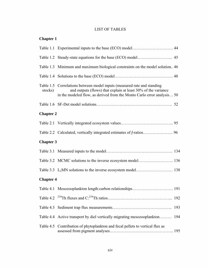
LIST OF TABLES

Chapter 1 Table 1.1 Experimental inputs to the base (ECO) model………………………… 44 Table 1.2 Steady-state equations for the base (ECO) model…………………….. 45 Table 1.3 Minimum and maximum biological constraints on the model solution.. 46 Table 1.4 Solutions to the base (ECO) model……………………………………. 48 Table 1.5 Correlations between model inputs (measured rate and standing stocks) and outputs (flows) that explain at least 30% of the variance in the modeled flow, as derived from the Monto Carlo error analysis… 50 Table 1.6 SF-Det model solutions……………………………………………….. 52 Chapter 2 Table 2.1 Vertically integrated ecosystem values………………………………... 95 Table 2.2 Calculated, vertically integrated estimates of f-ratios…………………. 96 Chapter 3 Table 3.1 Measured inputs to the model…………………………………………. 134 Table 3.2 MCMC solutions to the inverse ecosystem model…………………….. 136 Table 3.3 L2MN solutions to the inverse ecosystem model……………………… 138 Chapter 4 Table 4.1 Mesozooplankton length:carbon relationships………………………… 191 Table 4.2 234Th fluxes and C:234Th ratios………………………………………... 192 Table 4.3 Sediment trap flux measurements…………………………………….. 193 Table 4.4 Active transport by diel vertically migrating mesozooplankton……… 194 Table 4.5 Contribution of phytoplankton and fecal pellets to vertical flux as assessed from pigment analyses……………………………………….. 195

xv  

ACKNOWLEDGMENTS

Finishing a dissertation is almost impossible without a good advisor – and I’ve had

a great one. I’ll always be indebted to Mike for all of his advice, encouragement, and

willingness (not to mention patience) to let me grow as an oceanographer. He

accepted me when I was an idiot undergraduate who knew nothing about the ocean,

and never made me feel stupid when I came to him with less than intelligent questions.

He trusted me and gave me the freedom to explore and choose my own project, and

was amazingly able to advise me across the broad array of topics that my interests

pulled me towards. When I found myself drawn to a topic that he didn’t know as

much about, he set up a meeting for me with one of the experts in the field. He’s spent

countless hours supporting my work at sea and even bled for me on the fantail. He

gave me the space to grow as a scientist while always keeping his door always open,

and for that I’ll always be grateful.

The rest of my committee has been wonderful as well. Mark Ohman’s enthusiasm

for science is infectious (especially when playing ‘Name that plankton’ at 4am) and

he’s been a great help to me many times throughout my career. I can’t count the

amount of times that Mark has saved me when I went to him at the last minute to find

a cruise supply I’d forgotten to order. He’s always given insightful comments for my

work and instilled in me a profound love of metazooplankton. Peter Franks is an

amazingly caring teacher who always puts students first. He’s always been helpful

whenever I’ve needed advice with manuscripts or constructing models and I’ve

learned a ton from classes with him. I’ll always appreciate Kathy Barbeau for being

xvi  

the one member of my committee who was perceptive enough to challenge some of

the BS oversimplifications that tended to spew from my mouth during committee

meetings. Andy Scull brought an outside perspective and was always amazingly

attentive and able to point out aspects of my work that I might otherwise have taken

for granted. It would also be remiss for me to forget to acknowledge Claudia Benitez-

Nelson, who despite being in South Carolina, has been a de facto member of my

committee. Claudia has taught me everything that I know about measuring and

interpreting 234Th distributions and has been more than willing to count all of the

samples that I’ve sent her. My dissertation wouldn’t have been possible without her

advice and counsel and she’s been an incredible joy to work with.

This dissertation relies heavily on the amazingly collaborative efforts of everyone

involved with the CCE LTER Program. While the amount of volunteers, technicians,

students, and professors who’ve contributed to the project are too numerous to list,

some deserve special mention. I feel that Ralf Goericke’s competence at sea forms the

backbone of the CCE Process cruises and many of my favorite moments came while

he, Landry, and I were all leaning against the starboard railing and chatting as we

made our countless approaches on the drifter. From Ralf’s lab, I should also mention

Shonna Dovel and Megan Roadman who do a ton of the crucial, but thankless work,

without making the frequent mistakes that us grad students make, and pitched in and

helped me with my work more times than I can count. Lihini Aluwihare has given me

a lot of advice about organic carbon cycling and also leant me her McLane pump on

many cruises. Dave Checkley has been a good teacher and is fun to work with at sea.

xvii  

Mati Kahru provided invaluable satellite support. E.T. (the wayward little drifter who

phoned home at last) has been a stalwart companion through many cruises. Many of

the CCE grad students have been wonderful friends and collaborators for years. I feel

like we all own small pieces of each others’ dissertations. Moira Decima, Darcy

Taniguchi, Jesse Powell, Ally Pasulka, Alison Cawood, Ryan Rykaczewski, Roman

Dejesus, Travis Meador, Brian Hopkinson, Andrew King, Ty Samo, Byron Pedler…

I’ve loved working and sailing with all of them.

I owe a debt of gratitude to many other people and groups at Scripps, many of

whom I’m probably forgetting to mention. The Scripps graduate office and IOD

administration offices are amazing and actually make dealing with the administration a

pleasure (and we all know how rare that is). Bruce Deck in the Analytical Facility is

great at dealing with students and getting data to us in a timely and efficient manner.

A multitude of wonderful teachers have done credit to SIO as a teaching institution.

Paul Dayton has served as a role model as an ecologist, teacher, and environmentalist.

John and John from the machine shop have taught me to use a wide variety of power

tools necessary to build my equipment. Also Dan Wick, who might be the nicest

person alive. Dave Skydel, Gary Lain, and the rest of the radiation safety group. And

of course, our work wouldn’t be possible without the captains, crews, and restechs

from all of the cruises I’ve been on, particularly Jim Dorrance, Gene Picard, Meghan

Donohue, Gus Aprans, and John (sorry I forgot your last name John).

And then there are others from around the country. Karen Selph has been a big

sister to our lab, and has been an incredible help to me on the two cruises that

xviii  

bookended my graduate career. Stephen Baines has likewise been a ton of fun to work

with and learn from on cruises, as has Sasha Chekalyuk. Tammi Richardson was kind

enough to give a lot of valuable advice for Chapter 1.

My funding has been provided by a National Science Foundation (NSF) Graduate

Research Fellowship and NASA Earth and Space Science (NESSF) Fellowship as well

as two fellowships through SIO (the Wyers Fellowship and the Henry L. and Grace

Doherty Fellowship). The University of California ship funds program graciously

funded our student cruise during April 2009 (CCE-P0904), which was an amazing

learning experience for me. My research has been funded primarily by three NSF

grants; the CCE LTER Program (OCE-04-17616), the Equatorial Biocomplexity grant

(OCE-0322074), and the Arabian Sea / Pirates / Costa Rica Dome grant (OCE-

0826626).

And now for all the friends and family who’ve been my support system through

six and a half years of grad school. My entire family (parents, sister, grandparents,

aunts and uncles (both biological and Maufolk) have encouraged me ever since I was a

five-year old who wanted to save the whales. Even when they thought that marine

biologists did nothing but clean fish tanks or swab the decks on navy ships, they never

tried to squash my dreams. They fostered my love for nature from an early age with

countless trips to the zoo, camping trips almost every weekend of the summer,

museum and aquarium visits, and endless hours of reading “Fish do the Strangest

Things” over and over and over… They’ve allowed me to head further and further

xix  

from home in pursuit of my education, with only the slightest bit of resistance, and

even traveled en masse across country when I moved out to San Diego.

Finally, I’ve had an amazing group of friends while I’ve been out here. They’ve

been family to me in every way possible. Moira is my office mate, lab mate, cruise

mate, soccer teammate, and twin and I can’t imagine what grad school would have

been like without her. Brendan took me on my first backpacking trip, ate lunch with

us almost every day for six years, acts as my proxy whenever I’m at sea, and functions

as my chemist. He and Moira have even followed me up to Sequoia as I sit here

finishing my dissertation. Jenny has taught courses with me repeatedly, taken endless

classes with me, been my roommate, and owns a dog with me. And that dog… He’s

about as dumb as they come, but makes up for it by being so sweet and loyal. I really

don’t know what I’m going to do without those three. And I’d be remiss if I didn’t

mention the youngsters as well. Geoff has been the youngster who’s always given me

advice about grad school stuff. Darcy’s always been a great friend to hang out and

work with, and her pet funerals may qualify as the funniest recurring theme on any of

our cruises (but don’t tell her that). Jesse has been a huge help with all kinds of cruise

related work, and may have spent more time helping other grad students than doing his

own dissertation work. Alison has helped me unravel the ZooScan data many times.

Suki has patiently and consistently tried to teach Fozzy how to have thoughts.

Chapter 1, in full, has been published in Limnology and Oceanography: Stukel, M.

R., Landry, M.R., 2010. “Contribution of picophytoplankton to carbon export in the

equatorial Pacific: A re-assessment of food-web flux inferences from inverse models.”

xx  

Limnol. Oceanogr. 55: 2669-2685. The dissertation author was the primary investigator

and author of this paper.

Chapter 2, in full, has been submitted for publication in Limnology and

Oceanography: Stukel, M. R., Landry, M.R., 2010, Benitez-Nelson, C. R., Goericke,

R. “Trophic Cycling and carbon export relationships in the California Current

Ecosystem.” The dissertation author was the primary investigator and author of this

paper.

Chapter 3, in full, is currently in preparation for submission: Stukel, M. R.,

Landry, M. R., Benitez-Nelson, C. R., Goericke, R. “Do inverse models accurately

reconstruct food web flows? A comparison of two solution methods using field data

from the California Current Ecosystem.” The dissertation author was the primary

investigator and author on this paper.

Chapter 4, in full, is currently in preparation for submission: Stukel, M. R.,

Landry, M. R., Ohman, M. D., Benitez-Nelson, C. R.. “Mesozooplankton and vertical

carbon export in a coastal upwelling biome.” The dissertation author was the primary

investigator and author on this paper.

xxi  

VITA AND PUBLICATIONS

EDUCATION 2011 Doctor of Philosophy, University of Californa, San Diego 2004 Bachelor of Arts, Northwestern University, Evanston, IL CRUISE EXPERIENCE (158 days) CRD-2010 - Measured carbon export, new production, and mesozooplankton gut

phycoerythrin concentrations CCE-P0904 - Chief scientist on a cruise addressing the ecological and

biogeochemical role of fronts in the CCE CCE-P0810 - Continued 234Th & sediment trap measurements and added new

production measurements CCE-P0704 - Continued 234Th measurements and added sediment trap deployments as independent confirmation of measured rates CCE-P0605 - Measured carbon export in the CCE using 234Th disequilibrium EB05 - Investigated mixotrophic nano- and microflagellates in the eastern

Equatoial Pacific

CONFERENCES Ocean Sciences 2010 Talk Carbon cycling in the equatorial Pacific: Export driven

by large phytoplankton LTER ASM 2009 Poster Trophic cycling and vertical flux in the CCE Ocean Sciences 2008 Talk Carbon export and the fate of primary productivity in the California Current LTER ASM 2006 Poster Thorium export in the California Current Ecosystem Ocean Sciences 2006 Poster Mixotrophs are major grazers in the equatorial Pacific

 

TEACHIN 2009 R 2006-2008 A

Bs

2005 A

u PUBLICAT Stukel, M. R

easte Selph, K. E.

R. SspecdistrII. d

Stukel, M. R

expofrom

Landry, M.

studupw

G AND OU

Reality Chan

Academic CBiological ocsummer

Aquatic Advunderprivileg

TIONS

R.; M. R. Laern equatoria

.; M. R. Lantukel; S. Ch

cific phytoplaributions in tdoi:10.1016/

R.; M. R. Laort in the equ

m inverse mo

R.; M. D. Oies of phytop

welling ecosy

UTREACH E

ngers: Tutore

onnections (ceanography

ventures: Heged youth in

andry; K. E. al Pacific.” D

ndry; A. G. Tristenson; Rankton produthe equatoria/j.dsr2.2010.

andry. 2010. uatorial Paciodels.” Limn

Ohman; M. Rplankton gro

ystem off Sou

xxii

EXPERIEN

ed under-pri

(UCSD): Coy course for

lped teach 2n San Diego

Selph. In preDeep-Sea Re

Taylor; E. J. YR. R. Bidigare

uction and gal Pacific bet.08.014

“Contributioific: A re-assnol. Oceanog

R. Stukel; K. owth and grauthern Califo

NCE

ivilege high

o-designed anadvanced hi

2-week marin

ess. “Nanopes. II. doi:10

Yang; C. I. Me. In Press.

grazing dynatween 110 a

on of picophsessment of gr. 55: 2669-

Tsyrklevichazing relationfornia.” Prog

school stude

nd co-taughtigh school st

ne biology c

plankton mix0.1016/j.dsr2

Measures; J“Spatially-r

amics in relaand 140°W.

hytoplanktonfood-web flu-2685

h. 2009. “Lagnships in a c

g. Oceanogr.

ents

t a three-weetudents each

course for

xotrophy in t2.2010.08.0

. J. Yang; Mresolved taxoation to iron

Deep-Sea R

n to carbon ux inference

grangian coastal 83: 208-216

ek h

the 16

M. on-

Res.

es

6

xxiii  

ABSTRACT OF THE DISSERTATION

Biological Control of Vertical Carbon Flux in the California Current and Equatorial

Pacific

by

Michael Raymond Stukel

Doctor of Philosophy in Oceanography

University of California, San Diego, 2011

Professor Michael R. Landry, Chair

Professor Mark D. Ohman, Co-chair

The “biological pump” is a key component in the global biogeochemistry of

carbon dioxide that is sensitive, through a multitude of ecological interactions of

euphotic zone plankton, to climatic fluctuations. In this dissertation I address the

biological control of vertical carbon flux out of the surface ocean in two regions of the

Pacific Ocean. I begin by addressing the hypothesis that most export production in the

xxiv  

equatorial Pacific is derived from the primary production of picophytoplankton.

Using inverse ecosystem modeling techniques to synthesize detailed rate

measurements I show that eukaryotic phytoplankton are the dominant producers of

eventually exported material and that export comes after processing by

mesozooplankton, but that the results of inverse modeling studies are dependent upon

subjective decisions about model structure, input data, and solution schemes. I then

move on to studies in the California Current Ecosystem (CCE), where a combination

of my own in situ measurements of vertical carbon export and collaborators’

measurements of key planktonic rates allow me to address the question of what

constitutes sinking flux in this coastal upwelling biome. I begin with simple trophic

cycling relationships that use phytoplankton growth, micro- and mesozooplankton

grazing, and simple assumptions about organismal efficiency, and show that fecal

pellet production could account for the magnitude and variability in carbon export

measured by 234Th disequilibrium during a cruise in May 2006. I then utilize inverse

modeling techniques to show that on two spring cruises the contribution of grazing

products to export was substantially greater than that of gravitational sinking of

phytoplankton, and also that Markov Chain Monte Carlo methods do an accurate job

of solving inverse ecosystem models. Finally, I use sediment trap samples to directly

assess the contribution of fecal pellets to vertical flux, finding that mesozooplankton

pellets were the dominant component of flux during the spring, but that during a fall

cruise their contribution was variable, with flux becoming increasingly dominated by

non-pigmented small material and marine snow as productivity decreased.

1  

INTRODUCTION

Carbon export, the ecological perspective - While marine phytoplankton are

responsible for roughly half the world’s photosynthesis (see Field et al. 1998 for a

review), most of this fixed carbon is respired in the euphotic zone and hence retained

in the upper ocean-atmosphere system. Marine carbon sequestration is dependent

upon biological and physical processes that transport particulate organic carbon (POC)

to depth, thus removing it from the atmosphere for timescales of up to a millennium.

The “biological pump,” which transports carbon against its concentration gradient, is

mediated primarily by plankton ecological interactions that repackage POC into large

particles and aggregates that sink into the deep ocean. Despite its vast importance in

biogeochemical cycles, climate change, and the supply of energy to the benthos, the

biological pump remains difficult to predict due to the complexity and variability

inherent to marine ecosystems.

The classic ecological paradigm of marine carbon export emphasizes the

crucial role of large phytoplankton, particularly diatoms, in vertical flux (Michaels and

Silver 1988). These large autotrophs are believed to sink faster (Smayda 1970) and

have shorter trophic pathways to large fecal pellet-producing mesozooplankton than

their smaller competitors. These mechanistic explanations are further supported by

the measurement of high new (Eppley and Peterson 1979) and export production

(Buesseler 1998) during bloom conditions dominated by large plankton.

This paradigm has been challenged in a series of studies (Richardson et al.

2004,2006; Richardson and Jackson 2007) that utilized inverse ecosystem modeling

techniques to reconstruct unmeasured fluxes. These inverse results, from the Joint

Global Ocean Flux (JGOFS) Equatorial Pacific (EqPac) and Arabian Sea programs,

suggest that exported carbon in the open ocean is derived primarily from the

2  

production of picophytoplankton, particularly Prochlorococcus. This dominant role

for picophytoplankton in export production follows from the assumption (based on

size-fractionated chlorophyll and HPLC biomass proxies) that picophototrophs are

responsible for the majority of primary production as well as model structures that

allow significant direct flux of picophytoplankton to depth, presumably after particle

aggregation.

The controversial results of these inverse modeling studies also highlight

another dichotomy dealing with the nature of sinking material. While marine chemists

(e. g. Dunne et al. 2005) and ecosystem modelers investigating the effects of inorganic

ballasting (e. g. Armstrong et al. 2002) and aggregation (e. g. Jackson et al. 2005)

emphasize the sinking rates of ungrazed phytoplankton, food web ecologists often

underscore the importance of fecal pellets in rapidly transporting carbon to depth (e.g.

Bruland and Silver 1981; Landry et al. 1994; Dam et al. 1995). These fecal pellets

efficiently pack egested particulate matter within dense membrane-enclosed particles,

which can greatly enhance the sinking rate with vertical velocities that range from

meters to kilometers per day (see Turner 2002 for a review).

While the difference between flux of ungrazed carbon and minerals in organic

aggregates or flux within mesozooplankton fecal pellets may seem semantic, it in fact

implies distinctly different utilization scenarios for primary production. Dominance of

fecal pellet flux suggests a system with a greater number of trophic steps, and hence

higher respiration in the euphotic zone, and also possible control of primary

production by grazing pressure. Furthermore, the relative importance of ungrazed

phytoplankton and fecal pellets in flux would suggest opposite relationships between

mesozooplankton concentration and carbon export rates; if flux is supported by fecal

pellets we can expect a positive correlation between export and mesozooplankton, but

3  

if it is dominated by ungrazed phytoplankton products increased mesozooplankton

grazing pressure would lead to greater recycling and less export.

Measurement of carbon export rates – Sediment traps are a conceptually

simple means of measuring carbon export in the ocean, and are particularly useful

because they allow the collection of sinking material that can be analyzed to ascertain

the nature of sinking particles. However, their efficacy in accurately assessing particle

flux has frequently been questioned (e.g. Buesseler et al. 2007). Comparison studies

that measure 234Th based export during sediment trap deployments have shown biases

that vary significantly between sites, with over one-third of the studies showing a

factor of three difference between the two methods (Buesseler 1991).

Several sources of bias are inherent to moored and tethered sediment traps,

notably dissolution of organic carbon (Knauer et al. 1984), ‘swimmer’ effects (Knauer

et al. 1979), and hydrodynamic biases. These hydrodynamic biases tend to be

magnified at high flow rates and low sinking rates, although many other factors can be

important (Baker et al. 1988). An additional difficulty in interpreting sediment trap

results derives from the long distances over which particles can be transported by

lateral advection as they sink. The source for sediment trap material is thus not a point

directly above the trap, but instead a statistical funnel that varies in size and location

based on the speed, direction, and variability of flow fields above the traps and the

sinking rates of the particles (Siegel et al. 1990; Siegel et al. 2008). The development

of neutrally buoyant sediment traps alleviate many of the hydrodynamic issues,

yielding more accurate flux estimates (Buesseler et al. 2000), but at the same time may

increase the effect of the statistical funnel when vertical shear is high.

4  

An alternative method of approximating carbon export from the euphotic zone

has grown from studies of oceanic thorium distributions (see reviews by Savoye et al.

2006; Van Der Loeff et al. 2006; Waples et al. 2006). 234Th is the first long-lived

(half-life = 24.1 days) intermediary in the decay chain from 238U (half-life = 4.5 * 109

yrs). The rapid decay of 234Th relative to 238U should lead to secular equilibrium

between the two isotopes, with equal decay rates. However, while 238U is conserved

in the upper ocean and covaries with salinity, 234Th scavenges onto particles and hence

is removed from the system as particles sink, creating a disequilibrium between the

parent and daughter isotopes. The assumption of a steady-state model allows

calculation of rates of 234Th removal from the upper ocean over a time scale similar to

the half-life of 234Th:

(1)

where A238U and A234Th are the activities of 238U and 234Th, respectively, and 234Th is

the decay rate of 234Th. This equation calculates the rate of removal of 234Th from the

upper ocean, but it does not directly imply a rate of particle or carbon removal. To

convert to carbon export rate it is necessary to measure the ratio of C:234Th of sinking

material at the depth horizon of interest. This ratio can vary greatly with depth,

location, season, size of particles, and other parameters (Buesseler et al. 2006) thus it

must be determined empirically from each measured water parcel.

Carbon flux in the California Current Ecosystem – The majority of this thesis

is based on studies undertaken as a part of the CCE Long-Term Ecological Research

(LTER) Program. The California Current Ecosystem (CCE) is an eastern boundary

current biome that experiences strong equatorward winds in the spring and summer

months, leading to strong flows out of the north and wind-stress induced coastal

5  

upwelling (Lynn and Simpson 1987; Hickey 1993). This input of nutrients and

concurrent increase in primary production leads to a spring bloom dominated by

diatoms and other large phytoplankton in the coastal region near Point Conception.

Offshore, the floral community exhibits less seasonal variability and is dominated by

smaller taxa (Venrick 1998,2002).

The ocean-atmosphere system of the CCE is clearly highly coupled, and has

been extensively sampled on routine CalCOFI (California Cooperative Oceanographic

Fisheries Investigations) cruises since 1949. El Niño conditions often lead to a

decrease in the spatial extent of eutrophic conditions (e.g. Kahru and Mitchell 2000)

and cause a shift in dominant zooplankton taxa (e.g. Brinton and Townsend 2003;

Lavaniegos and Ohman 2003; Hereu et al. 2006). The Pacific Decadal Oscillation

(PDO) has also been shown to affect the biotic community with a period of 20-30

years (e.g. Mantua et al. 1997; McGowan et al. 2003). Meanwhile, a secular warming

trend has been recorded throughout the region and may be responsible for a significant

decline in zooplankton biovolume (Roemmich and McGowan 1995b; 1995a). This

has been attributed to a decrease in pelagic tunicates (Lavaniegos and Ohman

2003,2007), which are known to have very high rates of grazing and efficient

repackaging into large rapidly settling fecal pellets. Thus the decadal trend of

declining mesozooplankton biovolume and shifting community composition may

significantly alter the efficiency of particle export.

Despite the unparalleled ecological time-series of surface ocean dynamics,

comparatively little work has been conducted on carbon export in the CCE, with the

exception of a few areas in the Southern California Bight, such as the Santa Monica

Basin (Nelson et al. 1987; Landry et al. 1992) and the Santa Barbara Basin (Shipe et

6  

al. 2002). A long term study at Station M to the northwest of Point Conception, has

also measured carbon flux to the deep sea, with time-series sediment traps near the

seafloor (Baldwin et al. 1998; Smith et al. 2006). These studies have shown highly

variable export rates, even within the same regions. Spring carbon fluxes as low 35

mg m-2 day-1 (Nelson et al. 1987) and over 400 mg m-2 day-1 (Landry et al. 1992) were

found in 100 m sediment traps in the Santa Monica Basin. Time series of deeper

sediment traps in the Santa Barbara Basin (Pilskaln et al. 1996), as well as seafloor

traps near Station M (Baldwin et al. 1998), exhibited strong seasonality coupled to

surface productivity.

Dissertation Outline – The primary goal of this dissertation is to elucidate

biological mechanisms controlling the vertical flux of POC, with the eventual goal of

allowing prediction of the feedbacks between marine carbon sequestration and

climate. My approach assumes that experimentally determined carbon export rates

can be understood within the context of contemporary autochthonous ecological

processes. With this in mind, the core of the dissertation (Chapters 2-4) centers

around three Process Cruises of the CCE LTER program during which Lagrangian

drift experiments allowed simultaneous measurements of ecological processes

(including phytoplankton growth and zooplankton grazing) and vertical carbon fluxes.

In many ways, this dissertation involved a continual realization that in situ

measurements are crucial to resolving the difference between alternate hypotheses,

and hence is a progression towards more accurate direct measurement of ecological

and biogeochemical processes.

In Chapter One, entitled “Contribution of picophytoplankton to carbon export

in the equatorial Pacific: A re-assessment of food-web flux inferences from inverse

7  

models,” we addressed the controversial recent hypothesis that picophytoplankton-

derived production dominates carbon export in the equatorial Pacific (Richardson et

al. 2004; Richardson and Jackson 2007). Implicit in this ecosystem view is the

assumption that picophytoplankton contribute to carbon export primarily through the

gravitational sinking of ungrazed picophytoplankton, presumably after aggregation in

marine snow particles. Using a new dataset from two equatorial cruises of the

Equatorial Biocomplexity Program, we showed that picophytoplankton were not the

dominant primary producers in the region and were almost completely grazed in the

euphotic zone by protozoans. While they may have contributed to export in

proportion to their role in primary production, this conclusion relied crucially on the

assumption that all detrital particles (regardless of size) were equally likely to sink. A

more nuanced portrayal of the detrital pool suggested instead that large phytoplankton

contributed disproportionately to export and that sinking carbon existed primarily in

the form of mesozooplankton fecal pellets. The paper based on this chapter has

recently been published in Limnology and Oceanography (Stukel and Landry 2010).

Chapter Two, entitled “Trophic cycling and carbon export relationships in the

California Current Ecosystem,” builds on this idea that vertical carbon flux is largely

dominated by mesozooplankton fecal pellets. To test the hypothesis that grazing

processes largely determine carbon export within the region, we constructed simple

trophic cycling relationships that predicted POC export, phytoplankton accumulation,

and new production from phytoplankton growth and grazing measurements made on

the 2006 CCE Process Cruise. These simple trophic cycling relationships were found

to accurately predict simultaneously measured carbon export rates, suggesting that

fecal production, rather than gravitational sinking of phytoplankton, was the dominant

8  

ecological process controlling carbon export. The paper based on this chapter is

presently in review at Limnology and Oceanography.

Chapter Three, entitled “Do inverse ecosystem models accurately reconstruct

food web flows? A comparison of two solution methods using field data from the

California Current Ecosystem,” was primarily written to contrast two methods of

solving under-constrained inverse ecosystem problems. In addition, it utilized

ecological and biogeochemical data from two cruises of the CCE LTER Program to

constrain an ecosystem model for eight different ecosystem states encountered during

2006 and 2997 spring cruises in the CCE. Sinking POC was estimated to be

composed primarily of fecal material, with a smaller proportion of ungrazed

phytoplankton sinking as well.

Chapter Four, entitled “Mesozooplankton and vertical carbon export in a

coastal upwelling biome,” addressed the same question of what constitutes sinking

POC but more directly, using the results of sediment trap deployments on the 2007

and 2008 Process Cruises of the CCE LTER Program. Identifiable fecal pellets from

sediment trap samples were enumerated and sized. Along with measurements of

pigment sinking rates, the data suggest that fecal material was consistently a much

greater proportion of the sinking material than ungrazed phytoplankton. While fecal

pellets comprised the majority of flux in productive conditions, and particularly during

the spring, sediment traps deployed during the fall contained a large proportion of

unidentifiable marine snow aggregates. Mesozooplankton abundance profiles also

showed that active transport by diel vertically migrating organisms was a significant

portion of total carbon export. 

9  

REFERENCES

ARMSTRONG, R. A., C. LEE, J. I. HEDGES, S. HONJO, and S. G. WAKEHAM. 2002. A new, mechanistic model for organic carbon fluxes in the ocean based on the quantitative association of POC with ballast minerals. Deep-Sea Res. II 49: 219-236.

BAKER, E. T., H. B. MILBURN, and D. A. TENNANT. 1988. Field assessment of

sediment trap efficiency under varying flow conditions. J. Mar. Res. 46: 573-592.

BALDWIN, R. J., R. C. GLATTS, and K. L. SMITH. 1998. Particulate matter fluxes into

the benthic boundary layer at a long time-series station in the abyssal NE Pacific: composition and fluxes. Deep-Sea Res. II 45: 643-665.

BRINTON, E., and A. TOWNSEND. 2003. Decadal variability in abundances of the

dominant euphausiid species in southern sectors of the California Current. Deep-Sea Res. II 50: 2449-2472.

BRULAND, K. W., and M. W. SILVER. 1981. Sinking rates of fecal pellets from

gelatinous zooplankton (salps, pteropods, doliolids). Mar. Biol. 63: 295-300. BUESSELER, K. O. 1991. Do upper-ocean sediment traps provide an accurate record of

particle flux? Nature 353: 420-423. BUESSELER, K. O. 1998. The decoupling of production and particulate export in the

surface ocean. Glob. Biogeochem. Cycle 12: 297-310. BUESSELER, K. O., A. N. ANTIA, M. CHEN, S. W. FOWLER, W. D. GARDNER, O.

GUSTAFSSON, K. HARADA, A. F. MICHAELS, M. R. VAN DER LOEFF'O, M. SARIN, D. K. STEINBERG, and T. TRULL. 2007. An assessment of the use of sediment traps for estimating upper ocean particle fluxes. J. Mar. Res. 65: 345-416.

BUESSELER, K. O., C. R. BENITEZ-NELSON, S. B. MORAN, A. BURD, M. CHARETTE, J.

K. COCHRAN, L. COPPOLA, N. S. FISHER, S. W. FOWLER, W. GARDNER, L. D. GUO, O. GUSTAFSSON, C. LAMBORG, P. MASQUE, J. C. MIQUEL, U. PASSOW, P. H. SANTSCHI, N. SAVOYE, G. STEWART, and T. TRULL. 2006. An assessment of particulate organic carbon to thorium-234 ratios in the ocean and their impact on the application of 234Th as a POC flux proxy. Mar. Chem. 100: 213-233.

BUESSELER, K. O., D. K. STEINBERG, A. F. MICHAELS, R. J. JOHNSON, J. E. ANDREWS,

J. R. VALDES, and J. F. PRICE. 2000. A comparison of the quantity and

10  

composition of material caught in a neutrally buoyant versus surface-tethered sediment trap. Deep-Sea Res. I 47: 277-294.

DAM, H. G., X. S. ZHANG, M. BUTLER, and M. R. ROMAN. 1995. Mesozooplankton

grazing and metabolism at the equator in the central Pacific: Implications for carbon and nitrogen fluxes. Deep-Sea Res. II 42: 735-756.

DUNNE, J. P., R. A. ARMSTRONG, A. GNANADESIKAN, and J. L. SARMIENTO. 2005.

Empirical and mechanistic models for the particle export ratio. Glob. Biogeochem. Cycle 19: doi:10.1029/2004GB002390.

EPPLEY, R. W., and B. J. PETERSON. 1979. Particulate Organic-Matter Flux and

Planktonic New Production in the Deep Ocean. Nature 282: 677-680. FIELD, C. B., M. J. BEHRENFELD, J. T. RANDERSON, and P. FALKOWSKI. 1998. Primary

production of the biosphere: Integrating terrestrial and oceanic components. Science 281: 237-240.

HEREU, C. M., B. E. LAVANIEGOS, G. GAXIOLA-CASTRO, and M. D. OHMAN. 2006.

Composition and potential grazing impact of salp assemblages off Baja California during the 1997-1999 El Niño and La Niña. Mar. Ecol. Prog. Ser. 318: 123-140.

HICKEY, B. M. 1993. Physical Oceanography, p. 19-70. In M. D. Dailey, D. J. Reish

and J. W. Anderson [eds.], Ecology of the Southern California Bight: A Synthesis and Interpretation. University of California Press.

JACKSON, G. A., A. M. WAITE, and P. W. BOYD. 2005. Role of algal aggregation in

vertical carbon export during SOIREE and in other low biomass environments. Geophys. Res. Lett. 32: 4.

KAHRU, M., and B. G. MITCHELL. 2000. Influence of the 1997-98 El Niño on the

surface chlorophyll in the California Current. Geophys. Res. Lett. 27: 2937-2940.

KNAUER, G. A., D. M. KARL, J. H. MARTIN, and C. N. HUNTER. 1984. In situ effects of

selected preservatives on total carbon, nitrogen and metals collected in sediment traps. J. Mar. Res. 42: 445-462.

KNAUER, G. A., J. H. MARTIN, and K. W. BRULAND. 1979. Fluxes of particulate

carbon, nitrogen, and phosphorus in the upper water column of the Northeast Pacific. Deep-Sea Res. 26: 97-108.

11  

LANDRY, M. R., C. J. LORENZEN, and W. K. PETERSON. 1994. Mesozooplankton grazing in the Southern California Bight .2. Grazing impact and particulate flux. Mar. Ecol. Prog. Ser. 115: 73-85.

LANDRY, M. R., W. K. PETERSON, and C. C. ANDREWS. 1992. Particulate flux in the

water column overlying Santa Monica Basin. Prog. Oceanogr. 30: 167-195. LAVANIEGOS, B. E., and M. D. OHMAN. 2003. Long-term changes in pelagic tunicates

of the California Current. Deep-Sea Res. II 50: 2473-2498. LAVANIEGOS, B. E., and M. D. OHMAN. 2007. Coherence of long-term variations of

zooplankton in two sectors of the California Current System. Prog. Oceanogr. 75: 42-69.

LYNN, R. J., and J. J. SIMPSON. 1987. The California Current System: the seasonal

variability of its physical characteristics. J. Geophys. Res. Oceans 92: 12947-12966.

MANTUA, N. J., S. R. HARE, Y. ZHANG, J. M. WALLACE, and R. C. FRANCIS. 1997. A

Pacific interdecadal climate oscillation with impacts on salmon production. Bulletin of the American Meteorological Society 78: 1069-1079.

MCGOWAN, J. A., S. J. BOGRAD, R. J. LYNN, and A. J. MILLER. 2003. The biological

response to the 1977 regime shift in the California Current. Deep-Sea Res. II 50: 2567-2582.

MICHAELS, A. F., and M. W. SILVER. 1988. Primary production, sinking fluxes and the

microbial food web. Deep-Sea Res. 35: 473-490. NELSON, J. R., J. R. BEERS, R. W. EPPLEY, G. A. JACKSON, J. J. MCCARTHY, and A.

SOUTAR. 1987. A particle flux study in the Santa Monica-San Pedro Basin off Los Angeles: particle flux, primary production, and transmissometer survey. Cont. Shelf Res. 7: 307-328.

PILSKALN, C. H., J. B. PADUAN, F. P. CHAVEZ, R. Y. ANDERSON, and W. M.

BERELSON. 1996. Carbon export and regeneration in the coastal upwelling system of Monterey Bay, central California. J. Mar. Res. 54: 1149-1178.

RICHARDSON, T. L., and G. A. JACKSON. 2007. Small phytoplankton and carbon export

from the surface ocean. Science 315: 838-840. RICHARDSON, T. L., G. A. JACKSON, H. W. DUCKLOW, and M. R. ROMAN. 2004.

Carbon fluxes through food webs of the eastern equatorial Pacific: an inverse approach. Deep-Sea Res. I 51: 1245-1274.

12  

RICHARDSON, T. L., G. A. JACKSON, H. W. DUCKLOW, and M. R. ROMAN. 2006.

Spatial and seasonal patterns of carbon cycling through planktonic food webs of the Arabian Sea determined by inverse analysis. Deep-Sea Res. II 53: 555-575.

ROEMMICH, D., and J. MCGOWAN. 1995a. Climatic warming and the decline of

zooplankton in the California Current. Science 267: 1324-1326. ROEMMICH, D., and J. MCGOWAN. 1995b. Climatic warming and the decline of

zooplankton in the California Current (Vol 267, Pg 1324, 1995). Science 268: 352-353.

SAVOYE, N., C. BENITEZ-NELSON, A. B. BURD, J. K. COCHRAN, M. CHARETTE, K. O.

BUESSELER, G. A. JACKSON, M. ROY-BARMAN, S. SCHMIDT, and M. ELSKENS. 2006. 234Th sorption and export models in the water column: A review. Mar. Chem. 100: 234-249.

SHIPE, R. F., U. PASSOW, M. A. BRZEZINSKI, W. M. GRAHAM, D. K. PAK, D. A.

SIEGEL, and A. L. ALLDREDGE. 2002. Effects of the 1997-98 El Niño on seasonal variations in suspended and sinking particles in the Santa Barbara basin. Prog. Oceanogr. 54: 105-127.

SIEGEL, D. A., E. FIELDS, and K. O. BUESSELER. 2008. A bottom-up view of the

biological pump: Modeling source funnels above ocean sediment traps. Deep-Sea Res. I 55: 108-127.

SIEGEL, D. A., T. C. GRANATA, A. F. MICHAELS, and T. D. DICKEY. 1990. Mesoscale

eddy diffusion, particle sinking, and the interpretation of sediment trap data. J. Geophys. Res. Oceans 95: 5305-5311.

SMAYDA, T. J. 1970. The suspension and sinking of phytoplankton in the sea.

Oceanogr. Mar. Biol. Ann. Rev. 8: 353-414. SMITH, K. L., R. J. BALDWIN, H. A. RUHL, M. KAHRU, and B. G. MITCHELL. 2006.

Climate effect on food supply to depths greater than 4,000 meters in the northeast Pacific. Limnol. Oceanogr. 51: 166-176.

STUKEL, M. R., and M. R. LANDRY. 2010. Contribution of picophytoplankton to

carbon export in the equatorial Pacific: A re-assessment of food-web flux inferences from inverse models. Limnol. Oceanogr. 55: 2669-2685.

TURNER, J. T. 2002. Zooplankton fecal pellets, marine snow and sinking

phytoplankton blooms. Aquat. Microb. Ecol. 27: 57-102.

13  

VAN DER LOEFF, M. R., M. M. SARIN, M. BASKARAN, C. BENITEZ-NELSON, K. O.

BUESSELER, M. CHARETTE, M. DAI, O. GUSTAFSSON, P. MASQUE, P. J. MORRIS, K. ORLANDINI, A. R. Y. BAENA, N. SAVOYE, S. SCHMIDT, R. TURNEWITSCH, I. VOGE, and J. T. WAPLES. 2006. A review of present techniques and methodological advances in analyzing Th-234 in aquatic systems. Mar. Chem. 100: 190-212.

VENRICK, E. L. 1998. Spring in the California current: the distribution of

phytoplankton species, April 1993 and April 1995. Mar. Ecol. Prog. Ser. 167: 73-88.

VENRICK, E. L. 2002. Floral patterns in the California Current System off southern

California: 1990-1996. J. Mar. Res. 60: 171-189. WAPLES, J. T., C. BENITEZ-NELSON, N. SAVOYE, M. R. VAN DER LOEFF, M.

BASKARAN, and O. GUSTAFSSON. 2006. An introduction to the application and future use of 234Th in aquatic systems. Mar. Chem. 100: 166-189.

 

14  

CHAPTER 1

Contribution of picophytoplankton to carbon export in the equatorial Pacific: A

re-assessment of food-web flux inferences from inverse models

By Michael R. Stukel and Michael R. Landry

Abstract

The paradigm that carbon export is derived almost exclusively from the primary

production of large phytoplankton has been challenged by inverse ecosystem

modeling studies that suggest that most carbon export in the open ocean is fueled by

picophytoplankton. To re-address this hypothesis, we use an inverse model to

synthesize the planktonic rate measurements from a pair of recent cruises in the

equatorial Pacific. The analysis based on this new experimental data, which crucially

include vertically-integrated taxon-specific production and grazing estimates, largely

resolve the unexpected results of the previous inverse studies, including unbalanced

growth and grazing processes and the dominance of production by

picophytoplankton. While this very small size class does not produce the majority of

phytoplankton carbon that is eventually exported to depth (only 23%, vs. 73% from a

previous analysis of Joint Global Ocean Flux Study Equatorial Pacific data), our base

15  

model supports the conclusion that the role of picophytoplankton in vertical carbon

flux is largely proportional to their contribution to net primary productivity (though

neither is proportional to biomass). We show, however, that export-production

proportionality is sensitive to the model representation of the detrital pool, such that

the relative export role of picophytoplankton declines substantially for an alternate

model with size-structured detritus. A definitive assessment of the role of

picoplankton in vertical carbon flux will thus require detailed experimental

examination of the origin, composition, and fate of euphotic zone detrital material.

16  

Introduction

Small photosynthetic organisms (Prochlorococcus, Synechococcus, and

picoeukaryotes) with cell sizes <2-μm diameter, collectively called the

picophytoplankton, are abundant and important primary producers, especially over the

vast tropical and subtropical regions of the ocean (Li et al. 1983; Takahashi and

Bienfang 1983). Conventional wisdom holds that these picophytoplankton are too

small to sink individually or to be exploited efficiently by most metazooplankton, but

rather are consumed and largely respired in the euphotic zone by protistan consumers.

Indeed, a good deal of experimental evidence from the ocean points to a close balance

between picophytoplankton production and grazing losses to protists (Brown et al.

1999; Landry et al. 2003; Hirose et al. 2008), analogous to the tightly coupled growth-

grazing-recycling processes of the ‘microbial loop’ that are presumed to dissipate most

of the matter and energy produced by heterotrophic bacteria (Azam et al. 1983). If

this is the case, the amount of picophytoplankton production that ultimately leaves the

euphotic zone as exported carbon should be disproportionately small compared to

export that originates as larger phytoplankton, which have more direct pathways to

aggregate sinking and utilization by large pellet-producing zooplankton.

This conventional paradigm has been challenged recently in a series of papers

(Richardson et al. 2004, 2006; Richardson and Jackson 2007) that have applied

inverse modeling techniques to datasets derived from intensive investigations by the

US Joint Global Ocean Flux Study (JGOFS) in the equatorial Pacific and the Arabian

Sea. As synthesized in Richardson and Jackson (2007), these inverse analyses support

two general conclusions regarding the relationship between picophytoplankton and

export in open-ocean systems. The first is that the picophytoplankton contribution to

vertical carbon export by sinking particles from direct and indirect pathways is a high

17  

fraction of the community total, averaging 73% of export (SD = 21%, their table 1)

across a broad range of seasonal and environmental conditions in the two major

ecosystems examined. The second is that the picophytoplankton contribution to

export is proportional to their contribution to net primary production. The

proportionality hypothesis implies that the large percentage contribution of

picophytoplankton to total flux derives mainly from their dominance of primary

production. Whether picophytoplankton dominate production or not emerges as a

separate question, as does the relationship between biomass and production, since

Richardson et al. (2004, 2006) use size-class contributions to total phytoplankton

biomass as a proxy for their relative contributions to net production rate.

Methodological considerations limit our ability to assess directly the actual

contributions of large and small phytoplankton to export flux. However,

picophytoplankton have been found in sediments, transported there by phytodetrital

aggregates (Lochte and Turley 1988) or salp fecal pellets (Pfannkuche and Lochte

1993). Picoplankton-containing aggregates (Waite et al. 2000) and zeaxanthin

(Lamborg et al. 2008) have also been caught in sediment traps, although both may be

derived from unassimilated grazing on picophytoplankton (Gorsky et al. 1999; Waite

et al. 2000). Nonetheless, the few studies that directly compare the flux of large and

small phytoplankton (Silver and Gowing 1991; Rodier and Le Borgne 1997), typically

find intact picophytoplankton to be only a small proportion of total carbon flux.

In a recent synthesis of food web fluxes in the Arabian Sea, Landry (2009) found

that the JGOFS data for that region were consistent with a more conventional analysis

of process rates and relationships than suggested by inverse methods. In particular,

Landry (2009) highlighted potential problems in the model inputs for primary

production, which were partitioned proportionately among size classes according to

18  

filter-fractioned chlorophyll, a method that could inflate the smallest

(picophytoplankton) class due to the extrusion of larger cells (or chloroplasts from

broken cells) through the 2-µm filter pores. Based on size-fractioned chlorophyll,

picophytoplankton comprised 70%, on average, of primary production for the seasons

and stations that were modeled. According to microscopic and flow cytometric

assessments from the same Arabian Sea cruises and stations (Garrison et al. 2000),

however, picophytoplankton only comprised 35% of the total phytoplankton carbon

biomass. Therefore, if production had been assumed to scale with carbon rather than

size-fractioned chlorophyll, the ratio of modeled carbon flows originating from small

and large cells would have decreased by a factor of four, likely affecting the behaviors

of many pathways in the trophic network. In addition, the concept of proportionality

in small cell contribution to export was enhanced in the Richardson et al. (2004, 2006)

inverse models by an uncoupled growth-grazing condition that drove a large ungrazed

fraction of picophytoplankton production directly to detritus. This growth-grazing

imbalance was not, in fact, evident in the experimental data (Verity et al. 1996b), but

arose rather from a decision to scale up computed taxon-specific phytoplankton

growth rates to match 14C-primary production (14C-PP), without adjusting the

corresponding estimates of microzooplankton grazing rates.

Here, we use an inverse ecosystem modeling approach to re-examine the question

of picophytoplankton contribution to export flux in the equatorial Pacific. One

important aspect of our analysis is the use of recent data from a pair of cruises in the

eastern equatorial Pacific in December 2004 and September 2005. Whereas the

JGOFS Equatorial Pacific (EqPac) results available to Richardson et al. (2004) were

an assortment of independent rates lacking vertical resolution and with virtually no

microscopy for estimating carbon biomass values of phytoplankton and protozoans,

19  

the new data provides contemporaneous production, growth, and grazing rates and

microscopical biomass estimates, all integrated for the full euphotic zone at a large

number (31) of stations. This unprecedented assemblage of biomass and rate data

allows us to rigorously constrain the net production (biomass growth) contributions of

major phytoplankton taxa as model input. We further improve the analysis using

variability in the field-measured ratio of gross primary production (GPP) to 14C-PP to

bound the GPP term, by using a random-walk technique to explore all possible

solutions to the model terms and their statistics, and by comparing results to an

alternative model structure that accounts for different fates in a size-structured detrital

pool. We illustrate that picophytoplankton production is an important, but clearly not

dominant source of carbon export in the equatorial Pacific, and that conclusions about

the direct and indirect contributions of picophytoplankton to export vary substantially,

depending on whether the model considers size-structured detritus or not. We also

show that the generally used minimum norm solution significantly underestimates the

flows of carbon to bacteria, and that an unstructured detrital pool significantly

understates the export role of mesozooplankton. Further advances will require

experimental studies that explicitly address the source, composition, and fate of

detritus in the euphotic zone.

Methods

To best compare our results to those of Richardson et al. (2004), we used a similar

construction and physiological constraints (explained in detail below) for our base

ecological model (ECO), while incorporating the data (including group-specific

growth and grazing) from the new cruises. As noted above, we expanded the analysis

of the model results beyond Richardson et al. (2004) by generating confidence

20  

intervals for all model outputs (using a Monte-Carlo technique) and by using a random

walk technique to explore the solution space. In addition, we formatted and ran an

alternative size-fractionated detritus (SF-Det) model construct that incorporates a size-

structured detrital pool.

Sampling and data - Model inputs and constraints on biomass structure, primary

production, nitrate uptake, phytoplankton growth, and micro- and mesozooplankton

grazing came from data collected on Equatorial Biocomplexity cruises EB04

(December 2004) and EB05 (September 2005) in the eastern equatorial Pacific (Table

1). Each cruise included an east-west and a north-south transect of sampling stations

within the region of 110-140°W and 4°N-4°S (Fig. 1). Transit times between stations

were set to allow for collecting a coherent set of plankton biomass and daily rate

measurements at each station on the same schedule each day. Analyses of the

resulting euphotic-zone integrated data demonstrated remarkably low variability, with

coefficients of variation of only 31%, 33%, 43%, and 32% of the mean estimates for

14C-PP, phytoplankton specific growth rate, microzooplankton grazing, and

mesozooplankton grazing, respectively (Balch et al. in press; Décima et al. in press;

Landry et al. in press). We therefore pooled measured rates and standing stocks from

all stations on both cruises to compute composite averages for the region (n = 31

stations, Table 1) over a significantly broader spatiotemporal scale than that of

Richardson et al. (2004).

Phytoplankton growth and microzooplankton grazing rates were determined from

pairs of two-point dilution experiments conducted for 8 sampling depths spanning the

euphotic zone (to 0.1% of surface irradiance) at each station (Selph et al. in press).

These experiments were incubated for 24 hours in seawater-cooled deck incubators at

light levels representing 0.1%, 0.8%, 5%, 8%, 13%, 31%, 52% and 100% of incident

21  

solar irradiance, corresponding to light levels at the depth of sample collection.

Taxon-specific rates were determined by either high pressure liquid chromatography

(HPLC) pigment analysis (divinyl chlorophyll a (Chl a) was considered representative

of Prochlorococcus, fucoxanthin of diatoms, and monovinyl Chl a of total eukaryotic

phytoplankton) or flow cytometry samples (Prochlorococcus and Synechococcus)

(Selph et al. in press). Pigment-derived rates were corrected for systematic changes in

cellular pigment content during incubation using the initial and final experimental

samples to assess the changes in the mean ratios of accessory pigment to

microscopical assessments of phytoplankton biomass (e.g., fucoxanthin:diatom C).

Taxon-specific estimates of production rates were determined from specific growth

rates and carbon biomass according to Landry et al. (2000) and integrated for the full

euphotic zone (Landry et al. in press) Carbon biomass estimates of nano- and

microphytoplankton were determined from the biovolumes of cells measured by

epifluorescence microscopy (Taylor et al. in press) and biovolume:carbon ratios

(Menden-Deuer and Lessard 2000). Carbon biomass estimates of picophototrophs

were determined from flow cytometric analyses of cell abundances and cellular carbon

content estimates (Garrison et al. 2000; Brown et al. 2008; Taylor et al. in press). For

the sake of the present analysis, we divide the phytoplankton community into

cyanobacteria, diatoms, and other eukaryotic phytoplankton, the three groups that

could be differentiated most easily both in epifluorescence microscopy (flow

cytometry for picoplankton) and pigment analysis. For simplicity, we do not

distinguish eukaryotic picophytoplankton from other eukaryotes in this analysis,

although we did microscopically and experimentally in results from the shipboard

studies. True <2-μm pico-eukaryotes comprised a small fraction of the autotrophic

carbon pools (2% of total eukaryotes and 7% of the total <2-µm size class; Taylor et

22  

al. in press) and were therefore deemed to be inconsequential to the major pathways of

carbon flux. Pico-eukaryotes were also determined experimentally to have the same

dynamics as the cyanobacteria (i.e., a close balance between production and grazing

by protistan consumers; Landry et al. in press); therefore, the flux behaviors of

Synechococcus and Prochlorococcus were representative of this group.

Rates of 14C-PP were measured in shipboard incubations of triplicate 250 mL

samples from 6 discrete light levels spanning the euphotic zone (Balch et al. in press).

The f-ratio (ratio of new to total production) was determined by Parker et al. (in press)

from measured uptake rates of 15NO3- and 15NH4

+. Landry et al. (in press) determined

that the depth pattern and magnitudes of primary production rates from 14C-PP

measurements and dilution growth rates were strongly related, with euphotic-

integrated dilution calculations exceeding 14C-PP by 29%, approximately the

percentage difference observed when 12-h daytime incubations were compared to full

24-h incubations by the 14C method (mean = 21%, SD = 6%, Dickson et al. 2001).

Mean daily estimates of mesozooplankton grazing rates on the bulk phytoplankton

community were determined by Décima et al. (in press) from gut pigment analyses of

the animals caught in paired day-night oblique plankton tows (202-μm mesh) at each

station and the gut throughput estimates of Zhang et al. (1995). Mesozooplankton

biomass was determined from size-fractioned dry weights (dry wt) from the same net

tows, converted to carbon equivalents using the C:dry wt conversion factors in Landry

et al. (2001). In synthesizing the production, growth, and grazing results of the EB

cruises, Landry et al. (in press) demonstrated that euphotic zone averaged growth rates

of the phytoplankton community were balanced by the combined grazing effects of

micro- and mesozooplankton, resulting in a -0.01 ± 0.11 d-1 net residual growth rate

for the 31 stations sampled. The community rate dynamics therefore conform to

23  

expectations that the system largely functions as a steady-state chemostat (Frost and

Franzen 1992; Dugdale and Wilkerson 1998). The EB cruise results therefore provide

a well-integrated and strongly constrained data set for the equatorial Pacific system

that includes plankton standing stocks, production, and grazing rates for the full

euphotic zone.

Bacterial production (BP) and GPP were not measured on the EB04 and EB05

cruises. However, both rates showed strong correlations with 14C-PP during the

JGOFS EqPac cruises. BP was a relatively low proportion of primary productivity

(cruise averages of 10-22%, Ducklow et al. 1995; Kirchman et al. 1995). Using the

18O isotope method, Bender et al. (1999) showed that GPP varied from 1.9 to 2.6 times

the concurrently measured rate of 14C-PP. We used these field-derived relationships to

set upper and lower bounds on the ratios of BP: 14C-PP and GPP: 14C-PP. For export,

we chose not to constrain the rate of particulate organic carbon (POC) flux with EqPac

data since a goal of our model was to compare POC cycling estimates to those from

the EqPac study (Richardson et al. 2004); hence, we did not want to force similarities

between the two models in this specific area.

Model structure – To accommodate differences in data collection between EqPac

and EB cruises but staying as close as we could to the Richardson et al. (2004)

structure, we divided the phytoplankton community into three taxonomic groups

(diatoms, other eukaryotic autotrophs, and cyanobacteria – Synechococcus and

Prochlorococcus) and included four size classes of grazers (pico- and nanoflagellates,

microzooplankton, and mesozooplankton), as shown in Fig. 2. Grazers were allowed

to graze on all equal or smaller size classes of organisms (and detritus) with the

exception of the mesozooplankton, which were assumed unable to feed efficiently on

picoplankton (<2 μm) including cyanobacteria, heterotrophic picoflagellates, and

24  

heterotrophic bacteria. All biological compartments contributed to the dissolved

organic carbon (DOC) pool through excretion and to the detrital pool via non-grazer

related death (for phytoplankton and bacteria) and egestion of fecal matter (for grazer

groups).

As in Richardson et al. (2004), standing stocks of the eight biological

compartments in the model, as well as the two non-living compartments (detritus and

DOC), were constrained to steady-state conditions (Table 2). This assumption is

supported by the demonstrated balance between growth and grazing processes in the

region (Landry et al. in press). Phytoplankton group-specific rates of growth and

grazing from dilution experiments and the grazing rates of mesozooplankton were

used as model constraints (Table 1). Since vertical fluxes were not measured on the

cruises, we also required that combined export processes (vertical flux of detrital

carbon, horizontal export of DOC away from the equator, and consumption of

mesozooplankton by higher trophic levels) match the level of new production within

the system, assuming similar N:C ratios for phytoplankton, mesozooplankton, detritus,

and labile DOC. While shallow water nitrification has called into question the use of

nitrate uptake as a proxy for new production in low-nitrate systems (Yool et al. 2007),

it is probably insignificant in the high nitrate, upwelling region of the equatorial

Pacific.

We further constrained the solution by requiring that the flows obey the same suite

of biological inequalities (Table 3) used in the EqPac model (Richardson et al. 2004).

Respiration for phytoplankton groups was allowed to vary from 5-30% of group GPP,

while bacteria and grazers were required to respire a minimum of 20% of ingested

carbon and a maximum set by an allometrically scaled specific respiration rate (see

Table 3 for all biological constraints). DOC excretion was set to 2-55% of net primary

25  

production (NPP) for phytoplankton groups, and between 10% of ingestion and 100%

of respiration for grazers. Assimilation efficiencies for grazers were allowed to vary

between 50-90% and gross growth efficiencies (GGE) between 10-40% (10-50% GGE

for bacteria). As noted above, we used experimentally determined relationships from

EqPac cruises to constrain BP to 10-22% of 14C-PP (Ducklow et al. 1995; Kirchman et

al. 1995) and GPP to 190-260% of 14C-PP (Bender et al. 1999).

Model solution and statistical analyses - Even with the many biological

constraints on the solution space described above, there remain an infinite number of

possible solutions. To choose among these possibilities, we used the minimum norm

technique of Vézina and Platt (1988) and a modified version of the MATLAB code of

Jackson et al. (2001). Briefly, the method uses the singular value decomposition

(SVD) to solve explicitly for the equalities (Ax=b). The SVD decomposes the A

matrix into three matrices (A=U•L•VT). The rank of the problem (less than or equal to

the number of equalities) determines the number of vectors from the V matrix that are

necessary to satisfy the equalities, while the remaining vectors form an orthonormal

basis that can be added or subtracted to the solution while still satisfying the equality.

These remaining vectors are used to find a solution that minimizes the L2-norm while

satisfying the inequality constraints (Gx≥h). While this minimization scheme can be

seen as a mathematically parsimonious approach, there is no a priori reason that it

should approximate the ways in which ecosystems are constructed. Hence other

minimization schemes may be equally valid.

To determine model sensitivity to cruise measurements (rates and standing stocks),

we used the measurement means and their 95% confidence intervals to generate

normal distributions for each variable. We then ran 100,000 simulations during which

we allowed the inputs to vary simultaneously by drawing them randomly from their

26  

respective distributions to generate confidence intervals for all model outputs. When

possible, we utilized the full-rank inverse solution; where not, we followed the method

of Olsen et al. (2006) selecting the highest-rank solution that satisfied the constraints.

The confidence intervals derived from the above method only address errors

associated with the measurements, not with the model construction or the

minimization scheme. To assess errors associated with our choice of minimization

scheme, we used a random walk (RW) algorithm, inspired by Kones et al. (2009), to

sample the solution space of our inverse problem. We drew random samples from a

uniform distribution of the orthonormal set of vectors created by the SVD and added

them to our minimum norm solution. By definition, this produces solutions that

satisfy the equality constraints (Ax=b). After each solution jump, we checked that the

new solution also satisfied the inequality constraints (Gx≥h). If true, the new solution

was used as a starting point for the next iteration, thus allowing a random walk

sampling of the entire solution space (the ensemble of solution vectors that satisfy

both equality and inequality constraints).

Ecosystem parameters - One of the great powers of constructing flux networks

using inverse techniques is the ability to quantify indirect flows through the

ecosystem. If G is the normalized production matrix, depicting the percentage of a

compartment’s carbon flow that originates from each of the other compartments, and I

is the identity matrix, then the matrix (I-G)-1 gives the normalized amount of energy

(direct and indirect) that a compartment derives from any other compartment.

Multiplying the rows of this matrix by the total energy of the compartments gives the

amount of energy a compartment derives indirectly or directly from any other

compartment (Hannon 1973). This technique, as applied in the Network Analysis

approach (Ulanowicz and Kay 1991) used by Richardson et al. (2004), allowed us to

27  

compare the relative importance of different biological groups to export of carbon out

of the ecosystem. We also calculated the equivalent trophic level of each group, using

the convention that detritus, DOC, and phytoplankton have a trophic level of 1 and

that all other groups have a trophic level equal to one plus the sum of the trophic levels

of their prey multiplied by the proportion of their diet comprised by that nutritional

resource (following Christensen and Pauly 1992).

Alternative model structure with size-fractionated detritus - Assessing biases in

calculated flows that result from the choice of model structure is difficult because

ecosystems can be described in many ways. For evaluating the origins of system

export, however, one obvious oversimplification of the base (ECO) model is the

uniform treatment of detrital carbon, implicitly assuming complete and immediate

aggregation and disaggregation of all detritus. While it is reasonable to assume that all

carbon entering a biological compartment will be treated similarly when utilized by a

metabolic pathway, the detrital pool contains no such averaging effect. Rather, one

intuitively expects that the carbon associated with a dead cyanobacterium should

behave very differently than a fecal pellet with regard to its probability of contributing

to export. To address how such differences affect model outputs, we created an

alternative model structure with size-fractionated detritus (hereafter referred to as

model SF-Det), that did not allow detrital aggregation.

In SF-Det, the detrital pool is split into pico-, nano-, and micro-detritus pools. The

cyanobacteria and bacteria that die as individual cells can only contribute to the

picodetritus, while the other phytoplankton can flow to either the nano- or

microdetritus compartments. Grazers contribute fecal pellets to the detrital pool

smaller than themselves (e.g., heterotrophic nanoflagellates produce picodetritus) with

the exception of the heterotrophic picoflagellates, which produce picodetritus.

28  

Grazers were allowed to feed upon detrital size classes their own size or smaller, with

the exception of the mesozooplankton which again could not feed upon pico-sized

particles. We allowed vertical export of both nano- and microdetritus, but not

picodetritus as 0.2-2 μm particles are generally considered to be non-sinking colloids.

Results

Our results are presented in four subsections. In the first, we use the least

minimum norm (MN) solution to directly compare our model results to the EqPac

model of Richardson et al. (2004). We then consider the uncertainties introduced into

the model by errors in the measured ecological data, which raise some issues with the

MN solution. In the third subsection, we use a random-walk assessment of the

solution space to demonstrate the range of values allowed by the model and to show

that the MN norm is not representative of the wider solution space. We then use the

alternative model structure with size-fractionated detritus to show that a slightly more

complex model does not significantly change the structure of the biological

components of the ecosystem, but does give a more realistic assessment of the flux of

sinking detritus to depth.

Least minimum norm (MN) results and comparison to JGOFS EqPac - To

compare with the JGOFS EqPac results of Richardson et al. (2004), we determined the

model solution that minimized the L2-norm. This MN solution minimizes the summed

squares of all the flows but tends to simultaneously set minor flows to zero and

minimize the largest flows in the model.

The use of average rate and biomass measurements from the EB cruises allows us

to model composite averages of the flows in the eastern equatorial Pacific (EEP)

(Table 4). Production is dominated by the non-diatom eukaryotic phytoplankton of

29  

our ‘AUT’ category (Fig. 3). Diatoms and cyanobacteria account for 27% and 28% of

GPP, respectively. Net primary productivity is largely balanced by the direct

utilization of phytoplankton by zooplankton grazers. In the MN solution, only the

‘AUT’ group produces excess ungrazed biomass that passes directly to a detrital pool,

and this flux is only 9% of group NPP. While cyanobacteria net production is grazed

completely by protozoans, mesozooplankton exert a significant proportion of the

grazing pressure on eukaryotic phytoplankton (47% of total grazing on diatoms and

31% on other autotrophs). Protozoan losses to respiration are high, accounting for

more than half (55%, 70%, and 52% for pico-, nano-, and microzooplankton,

respectively) of total carbon ingested. Larger zooplankton rely proportionally more on

carnivory. Mesozooplankton, for example, derive 31% of their carbon requirements

from other heterotrophs and occupy a mean trophic level of 2.29. Bacteria constitute a

relatively small portion of protozoan diets (25%, 9%, and 1% for pico-, nano-, and

microzooplankton), yet play a significant role in carbon flux, respiring 10% of GPP.

Export out of the ecosystem is split between horizontal advection of DOC, vertical

sinking of POC, and energy transport through mesozooplankton to higher trophic

levels. The e-ratio (ratio of vertical carbon flux to net primary productivity) predicted

by the model is a moderate 10%. Some detritus comes directly from phytoplankton

(27%), but most is formed as fecal carbon after digestive processing by the various

zooplankton size classes. System flows indicate that the carbon export derives

primarily from non-diatom eukaryotic phytoplankton (65%), with diatoms and

cyanobacteria contributing 16% and 19%, respectively.

Our results depict an ecosystem that is strikingly different from that of the

similarly structured model of Richardson et al. (2004). While this previous model

predicted a phytoplankton community with production dominated by

30  

picophytoplankton, the present analysis is constrained by field data that establishes

that most production comes from eukaryotes. Cyanobacteria were completely grazed

by protozoan grazers in our experimental data (Landry et al. in press), while the

Richardson et al. (2004) model suggested that over a quarter of picoplankton

productivity was ungrazed and passed directly into the detrital pool (Table 4).

Nonetheless, the two models produce similar estimates of the utilization of

heterotrophic protists in the diets of mesozooplankton, and both suggest that carbon is

exported from the system by DOC advection and by higher trophic levels in relatively

similar amounts. Both models also suggest that detritus must form a significant

portion of mesozooplankton diets, although the contribution is significantly higher for

the EqPac model. Unlike the present results, however, the EqPac model required

significant remineralization of detritus to DOC both to support the bacterioplankton

community and as a sink for the large amount of detritus produced by ungrazed

picophytoplankton. The EqPac model also produced lower vertical fluxes, as a result

of measurement constraints placed on the EqPac model that were absent in the present

analysis.

Model sensitivity - We tested the sensitivity of our ECO model to measurement

inaccuracies using the Monte Carlo approach of simultaneously varying all measured

values based on normal distributions created from their known means and standard

errors (Table 4). To test the role of each measured input (taxon-specific net primary

productivity, taxon-specific protozoan grazing, mesozooplankton grazing, f-ratio, size-

fractionated protozoan biomass, bacterial biomass and 14C-PP) on the model outputs,

we regressed each pair of inputs and outputs (Table 5). Many of the resulting

relationships were trivial dependencies, such as the relationship of diatom GPP to

measured diatom NPP. The strongest correlations, relating pico- and

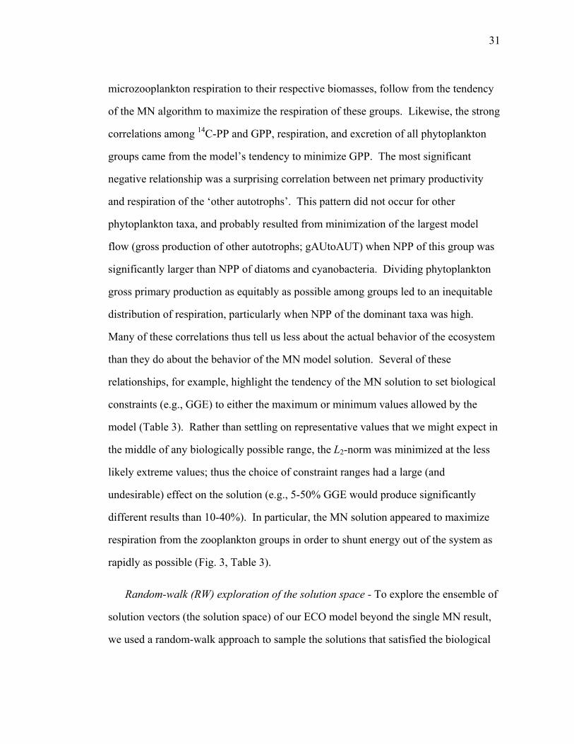
31  

microzooplankton respiration to their respective biomasses, follow from the tendency

of the MN algorithm to maximize the respiration of these groups. Likewise, the strong

correlations among 14C-PP and GPP, respiration, and excretion of all phytoplankton

groups came from the model’s tendency to minimize GPP. The most significant

negative relationship was a surprising correlation between net primary productivity

and respiration of the ‘other autotrophs’. This pattern did not occur for other

phytoplankton taxa, and probably resulted from minimization of the largest model

flow (gross production of other autotrophs; gAUtoAUT) when NPP of this group was

significantly larger than NPP of diatoms and cyanobacteria. Dividing phytoplankton

gross primary production as equitably as possible among groups led to an inequitable

distribution of respiration, particularly when NPP of the dominant taxa was high.

Many of these correlations thus tell us less about the actual behavior of the ecosystem

than they do about the behavior of the MN model solution. Several of these

relationships, for example, highlight the tendency of the MN solution to set biological

constraints (e.g., GGE) to either the maximum or minimum values allowed by the

model (Table 3). Rather than settling on representative values that we might expect in

the middle of any biologically possible range, the L2-norm was minimized at the less

likely extreme values; thus the choice of constraint ranges had a large (and

undesirable) effect on the solution (e.g., 5-50% GGE would produce significantly

different results than 10-40%). In particular, the MN solution appeared to maximize

respiration from the zooplankton groups in order to shunt energy out of the system as

rapidly as possible (Fig. 3, Table 3).

Random-walk (RW) exploration of the solution space - To explore the ensemble of

solution vectors (the solution space) of our ECO model beyond the single MN result,

we used a random-walk approach to sample the solutions that satisfied the biological

32  

constraints. We applied the random-walk algorithm until the average of the random-

walk solutions converged on a value. The entire solution space was then used to

calculate means and 95% confidence intervals for all flows (Table 4, Fig. 3), allowing

us to compare with the MN solution, which was shown to be a biased representative of

the greater solution space. Several of the most unconstrained flows in the model were

pairs of flows allowing bi-directional fluxes of carbon between compartments (e.g.,

DOC to bacteria and bacteria to DOC). These paired flows were strongly related, with

statistical correlations of 0.90, 0.78, and 0.67 for bi-directional flows of bacteria to

DOC, heterotrophic nanoflagellates to detritus, and mesozooplankton to detritus

(flows between detritus and pico- or microzooplankton were better constrained due to

the lower biomass of these grazers). The high correlations imply that the net uptakes

or losses of carbon for each compartment were relatively well constrained and hence

only weakly affected the other modeled flows, with the exception of increased

ingestion leading to a concomitant increase in respiration.

As noted previously with regard to the biological constraints, the MN solution

consistently used extreme values of the parameters (Fig. 3). To minimize the sum of

squares, for example, the MN solution minimized the largest flow in the model

(gAUtoAUT). Since NPP of the AUT group (non-diatom eukaryotic autotrophs) was

a measured input to the model, this model behavior also minimized DOC excretion,

which limited, in turn, the DOC uptake and the respiration of bacteria, leading to a

relatively high bacterial GGE (36%).

The RW solution (Table 4) gave significantly higher GPP for the AUT group and

lower for the DIA and CYA groups in comparison to the MN solution (Fig. 3). It

allowed greater DOC exudation by the phytoplankton community, which was

consumed by a less efficient assemblage of heterotrophic bacteria, which in turn

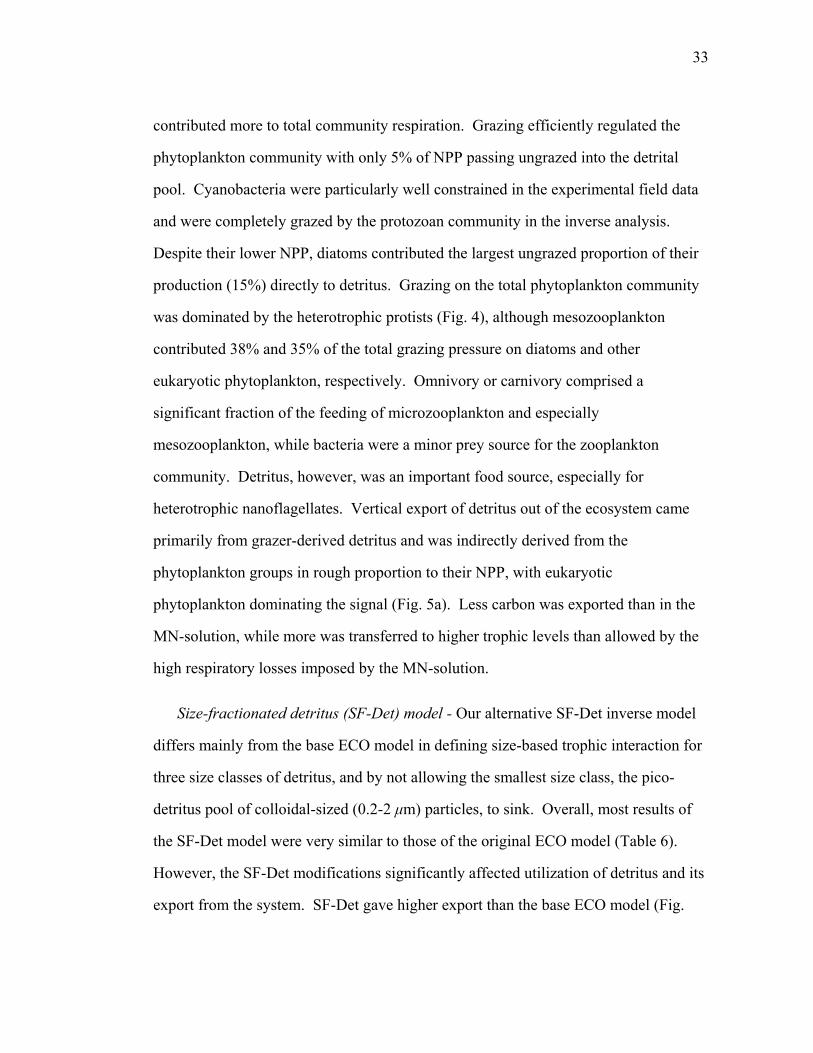
33  

contributed more to total community respiration. Grazing efficiently regulated the

phytoplankton community with only 5% of NPP passing ungrazed into the detrital

pool. Cyanobacteria were particularly well constrained in the experimental field data

and were completely grazed by the protozoan community in the inverse analysis.

Despite their lower NPP, diatoms contributed the largest ungrazed proportion of their

production (15%) directly to detritus. Grazing on the total phytoplankton community

was dominated by the heterotrophic protists (Fig. 4), although mesozooplankton

contributed 38% and 35% of the total grazing pressure on diatoms and other

eukaryotic phytoplankton, respectively. Omnivory or carnivory comprised a

significant fraction of the feeding of microzooplankton and especially

mesozooplankton, while bacteria were a minor prey source for the zooplankton

community. Detritus, however, was an important food source, especially for

heterotrophic nanoflagellates. Vertical export of detritus out of the ecosystem came

primarily from grazer-derived detritus and was indirectly derived from the

phytoplankton groups in rough proportion to their NPP, with eukaryotic

phytoplankton dominating the signal (Fig. 5a). Less carbon was exported than in the

MN-solution, while more was transferred to higher trophic levels than allowed by the

high respiratory losses imposed by the MN-solution.

Size-fractionated detritus (SF-Det) model - Our alternative SF-Det inverse model

differs mainly from the base ECO model in defining size-based trophic interaction for

three size classes of detritus, and by not allowing the smallest size class, the pico-

detritus pool of colloidal-sized (0.2-2 μm) particles, to sink. Overall, most results of

the SF-Det model were very similar to those of the original ECO model (Table 6).

However, the SF-Det modifications significantly affected utilization of detritus and its

export from the system. SF-Det gave higher export than the base ECO model (Fig.

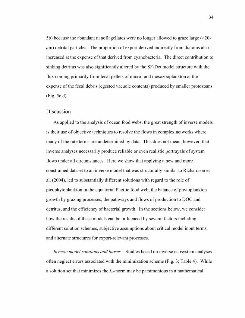
34  

5b) because the abundant nanoflagellates were no longer allowed to graze large (>20-

μm) detrital particles. The proportion of export derived indirectly from diatoms also

increased at the expense of that derived from cyanobacteria. The direct contribution to

sinking detritus was also significantly altered by the SF-Det model structure with the

flux coming primarily from fecal pellets of micro- and mesozooplankton at the

expense of the fecal debris (egested vacuole contents) produced by smaller protozoans

(Fig. 5c,d).

Discussion

As applied to the analysis of ocean food webs, the great strength of inverse models

is their use of objective techniques to resolve the flows in complex networks where

many of the rate terms are undetermined by data. This does not mean, however, that

inverse analyses necessarily produce reliable or even realistic portrayals of system

flows under all circumstances. Here we show that applying a new and more

constrained dataset to an inverse model that was structurally-similar to Richardson et

al. (2004), led to substantially different solutions with regard to the role of

picophytoplankton in the equatorial Pacific food web, the balance of phytoplankton

growth by grazing processes, the pathways and flows of production to DOC and

detritus, and the efficiency of bacterial growth. In the sections below, we consider

how the results of these models can be influenced by several factors including:

different solution schemes, subjective assumptions about critical model input terms,

and alternate structures for export-relevant processes.

Inverse model solutions and biases – Studies based on inverse ecosystem analyses

often neglect errors associated with the minimization scheme (Fig. 3; Table 4). While

a solution set that minimizes the L2-norm may be parsimonious in a mathematical

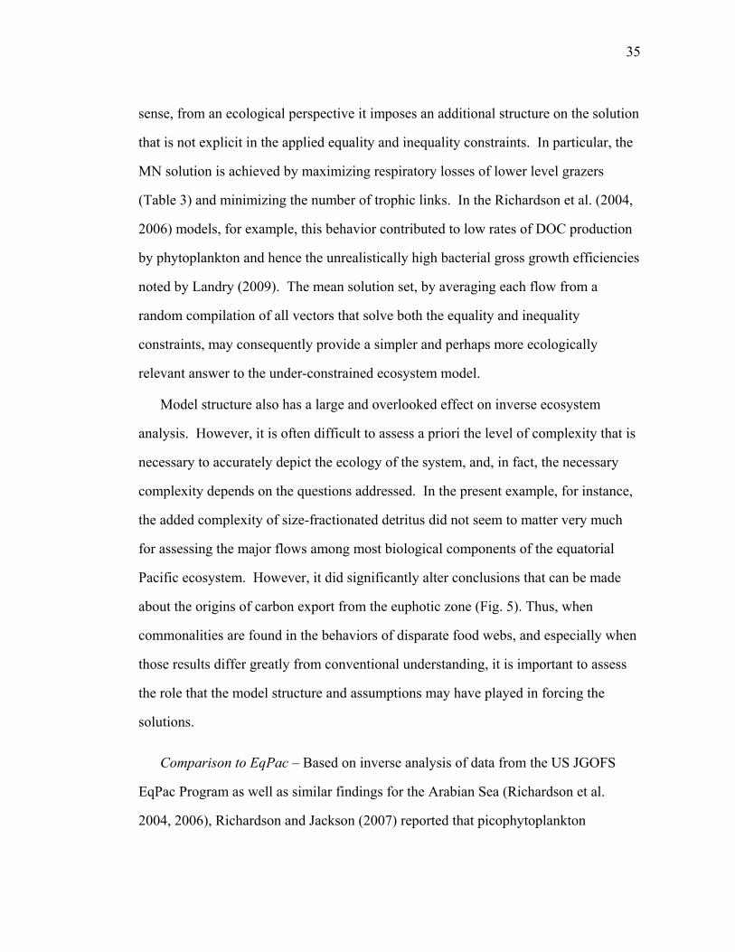
35  

sense, from an ecological perspective it imposes an additional structure on the solution

that is not explicit in the applied equality and inequality constraints. In particular, the

MN solution is achieved by maximizing respiratory losses of lower level grazers

(Table 3) and minimizing the number of trophic links. In the Richardson et al. (2004,

2006) models, for example, this behavior contributed to low rates of DOC production

by phytoplankton and hence the unrealistically high bacterial gross growth efficiencies

noted by Landry (2009). The mean solution set, by averaging each flow from a

random compilation of all vectors that solve both the equality and inequality

constraints, may consequently provide a simpler and perhaps more ecologically

relevant answer to the under-constrained ecosystem model.

Model structure also has a large and overlooked effect on inverse ecosystem

analysis. However, it is often difficult to assess a priori the level of complexity that is

necessary to accurately depict the ecology of the system, and, in fact, the necessary

complexity depends on the questions addressed. In the present example, for instance,

the added complexity of size-fractionated detritus did not seem to matter very much

for assessing the major flows among most biological components of the equatorial

Pacific ecosystem. However, it did significantly alter conclusions that can be made

about the origins of carbon export from the euphotic zone (Fig. 5). Thus, when

commonalities are found in the behaviors of disparate food webs, and especially when

those results differ greatly from conventional understanding, it is important to assess

the role that the model structure and assumptions may have played in forcing the

solutions.

Comparison to EqPac – Based on inverse analysis of data from the US JGOFS

EqPac Program as well as similar findings for the Arabian Sea (Richardson et al.

2004, 2006), Richardson and Jackson (2007) reported that picophytoplankton

36  

production was directly and indirectly responsible for most (73%) of the carbon

export in these two open-ocean ecosystems. In retrospect, this conclusion hangs

critically on the assumption that production can be assigned to different size fractions

based on their contributions to size-fractionated Chl a. For the EqPac program, which

lacked a coherent database on plankton carbon biomass from microscopy, the assumed

chlorophyll-production relationship led to picophytoplankton comprising an average

of 73% (SD = 9%) of the total community primary production (PP) in the four cruise

scenarios that were modeled. In contrast, our new data for the equatorial Pacific,

based on robust microscopical analyses and carbon-based estimates of growth rates

puts total picophytoplankton production at 27% of PP, with 23% originating as the

production of cyanobacteria (Table 1), Prochlorococcus and Synechococcus, the two

components that we have explicitly considered here. Our new model based on this

data consequently shows a large decline in the export flux that can be attributed to

picophytoplankton populations, but the difference principally reflects the former

assumption vs. the new field-estimated rates that determine the input terms for size-

structured production. In other respects, data from the EqPac and EB cruises do not

show substantial differences. For example, a large fraction, 75-80%, of Chl a passed

through 3-µm filters on the EB cruises (Balch et al. in press). The mean estimate of

phytoplankton production consumed directly by protists on the EqPac cruises (88% of

PP, Landry et al. 1997) was even higher than the 70% determined for EB cruises

(Landry et al. in press). As noted above, the uncoupled growth and grazing in the

Richardson et al. (2004) model was artificially imposed, in contradiction to direct field

measurements from the EqPac study (Verity et al. 1996b). It appears therefore that the

strongly different behaviors of the EqPac and our base ECO inverse models with

regard to picophytoplankton flows to detritus and DOC arise not from major changes

37  

in the equatorial Pacific between EqPac and EB studies, but from the carbon cycling

challenges of the former model in meeting system steady-state model constraints when

an unrealistic amount of production is assigned to the smallest size fraction.

Although the magnitude of the export flux contribution of picophytoplankton was

exaggerated in the Richardson et al. (2004) model, according to new data on taxon-

specific contributions to primary production in the equatorial Pacific, our revised

model provides support for a central finding of the previous results. The RW-solution

of our base ECO model indicates, for example, that cyanobacteria production

accounted for 23% of C export (Fig. 5a), the same as their percentage contribution to

production, as predicted by the proportionality tenet of Richardson and Jackson

(2007). Thus, an important part of their challenge to conventional expectations of

phytoplankton size-export relationships is retained in the results of the new model

with well-constrained biomass and rate data. Nonetheless, since picophytoplankton

production in the Richardson et al. (2004; 2006) models was assigned according to a

biomass proxy, size-fractioned chlorophyll, it needs to be noted that the 23%

cyanobacteria contribution to export in the present study falls far short of their

contribution to phytoplankton biomass (36%). Thus, picophytoplankton contribution

to biomass does not substitute for contribution to net production in the proportionality

finding. The inclusion of size-structured detritus in our SF-Det model also led to a

greater export role for larger cells like diatoms at the expense of picophytoplankton

(Fig. 5b). Even under this model construction that did not allow direct sinking of

picodetritus, however, picophytoplankton were responsible for producing 18% of the

exported carbon (3/4 of the percentage predicted by the proportionality argument and

half of their contribution to carbon biomass).

38  

A strong growth-grazing balance for picophytoplankton populations, with protists

applying essentially all of the grazing pressure, follows directly from the experimental

measurements (Landry et al. in press; Selph et al. in press) and is a consistent feature

of both forms of our model and minimization schemes. Thus, unlike the Richardson et

al. (2004, 2006) analyses, the export of picophytoplankton-based production cannot be

said to be unrealistically enhanced by a large fraction escaping consumption in the

microbial food web and passing directly to detritus. As an output, our estimates of the

e-ratio (export of 5.7% of 14C-PP with the base ECO-model and 7.9% with the SF-Det

model), which was left unconstrained by data in the present analyses, agree well with

the region-wide EqPac estimates of <5-10% from Buesseler et al. (1995).

Complete grazing of cyanobacteria by protists may seem at odds with model

results that show picophytoplankton contributing to export in proportion to their

production. In both the EqPac and our base (ECO) models, however, this

proportionality derives from the implicit assumption that there is complete and

immediate homogenization of everything that enters the detrital pool, essentially

allowing protozoan egesta to sink as rapidly as mesozooplankton fecal pellets. The

maintenance of semi-proportionality after inclusion of detrital size-classes

(picophytoplankton contribute 18% of export compared to 23% of NPP) in our SF-Det

model is a more intriguing result, especially since mesozooplankton, which provide

the dominant mechanism for producing sinking particles, are not allowed to graze on

picoplankton. The relevant insight from field measured rates is that protists also

consume most (60%) eukaryotic phytoplankton production (Fig. 6). Thus, the primary

fates of pico- and larger phototrophs are not nearly as distinct as the traditional

dichotomy between the ‘classical food chain’ and the ‘microbial loop’. In fact,

mesozooplankton derive only 44% of their ingestion from phytoplankton in the RW-

39  

solution of our SF-Det model, with an additional 34% derived from grazing on

protozoans and the remainder comprised of detrital material (Fig. 4). Thus, the

contribution of cyanobacteria to export is derived from ecosystem linkages not readily

assessed by traditional techniques (Fig. 7). It is also important to note that

proportionality is only found for the RW-solution to the SF-Det model. The

unrealistically high respiratory demands of the MN solution do not allow efficient

energy transfer up the food chain.

While sediment traps cannot trace the primary source of exported carbon, their

contents provide a glimpse of the nature of sinking particles. Rodier and Le Borgne

(1997) utilized flow cytometry, microscopy and pigment analyses to assess the

contents of drifting sediment traps deployed for a week on the equator at 150°W,

finding that intact picophytoplankton comprised only a tiny fraction of the carbon flux.

The dominant signal was from marine snow and fecal pellets, which were numerically

dominated by particles in the 20-100 μm size class. Pigment analyses suggested that

only 4% of POC flux came from intact phytoplankton while 12% came from recent

herbivory. Similarly, sediment traps deployed at 140°W during EqPac had very low

ratios of chlorophyll to phaeopigment (Newton and Murray 1994), indicative of a low

export percentage of intact cells. These values compare favorably with our model

predictions of direct flux from phytoplankton (7% for the RW solution of the base

ECO-model and 11% for the SF-Det model) and from the fecal pellets of herbivorous

zooplankters (41% for ECO and 36% for SF-Det), with the caveat that the percent

pigmented ratio of detritus should decrease through microbial activity and coprophagy

as particles sink to the depths of the traps.

Dam et al. (1995) determined that mesozooplankton fecal carbon production alone

could have supported all the vertical flux measured during JGOFS EqPac cruises.

40  

Consistent with this, our model suggests that fecal matter comprises the dominant

pathway by which carbon leaves the system (Fig. 5c,d), as a by-product of the growth-

grazing balance of the euphotic zone (Fig. 6), but that most is re-worked or degraded

through coprophagy or dissolution to DOC. The SF-Det model indicated that food

chain length to larger zooplankton was a major determinant of the efficiency of carbon

export from the system, unlike the base ECO model, which, by treating all detrital

particles equally, unrealistically allowed protozoan egesta to sink as rapidly as

mesozooplankton pellets.

Processes altering export rates – Like all models, ours oversimplifies complex

ecology and excludes processes deemed to be of lesser importance or poorly assessed

by field measurements. The absence of phytoplankton density measurements means,

for example, that we could not consider the inorganic ballasting effect of siliceous and

calcareous planktonic taxa (Armstrong et al. 2002), which can significantly increase

flux2es, thereby enhancing the export roles of diatoms and coccolithophores (both

directly and by adding density to zooplankton egesta). We have likewise not

explicitly accounted for particle aggregation (Alldredge and Gotschalk 1989; Walsh

and Gardner 1992; Jackson 2001), which involves both phytoplankton and bacterial

interactions (Passow et al. 1994, 2001) and provides an alternate pathway for flux of

smaller particles to depth. In addition, the model does not expressly consider pelagic

tunicates, like salps that can efficiently pack cyanobacteria into rapidly sinking fecal

pellets (Pfannkuche and Lochte 1993) or appendicularians that concentrate

picophytoplankton in the mucus web feeding nets of their discarded houses (Robison

et al. 2005). By the same token, however, the model does not consider active diel

vertical migrations of mesozooplankton, which transport to depth substantial amounts

of carbon derived primarily from large prey (Dam et al. 1995; Zhang and Dam 1997).

41  

All of these represent poorly constrained mechanisms that can alter the relative

contributions of small and large phytoplankton to total system organic export.

The SF-Det model illustrates, however, the importance of including size-

fractionated detritus when assessing the origin of sinking detritus, although its

equivalent treatment of nano- and microdetritus with respect to sinking is still

simplistic. Micro-sized fecal pellets produced by mesozooplankton are likely to sink

much faster than smaller detrital particles, suggesting that these large fecal pellets may

comprise an even greater proportion of exported material than the 49% suggested by

the SF-Det model. In fact, 20-100 μm particles (equivalent to a portion of our

microdetrital group) were the primary fecal material in the equatorial sediment traps

examined by Rodier and Le Borgne (1997). Our model’s microdetritus was composed

primarily of mesozooplankton fecal pellets and supported by the production of

eukaryotic phytoplankton with only minor contribution from cyanobacteria (Fig. 5).

While this highlights the importance of an accurate treatment of detritus, better

constraints on this non-living fraction will depend on experimental measurement by

techniques such as detrital stains (Verity et al. 1996a) and sediment traps paired with

polyacrylamide gels (Lundsgaard 1995).

In summary, we found that many of the unexpected results of the Richardson et al.

(2004) inverse model of the equatorial Pacific – namely, the picophytoplankton

dominance of export, the imbalance of phytoplankton growth and grazing processes,

the unusual pathways and flows of production to DOC and detritus, and the high

efficiency of bacterial growth – were largely resolved by better data constraints on

biomass and rates for the full euphotic zone and the taxonomic and size-class origins

of primary production, and by solution schemes that avoided the extremes of the

minimal L2-norm. Proportionality of net production and export contributions among

42  

phytoplankton size classes, a central conclusion of Richardson and Jackson (2007),

remained a robust feature of the base model despite the above refinements. We have

shown, however, that this conclusion is sensitive to the treatment of detrital size

classes; thus, this is an area where insights from direct field measurements and model

development would be useful. Future progress in understanding the roles of different

taxa in export processes also clearly requires data sets that more directly and

quantitatively link the growth and trophic dynamics of different functional groups in

the euphotic zone to their incorporation into exported material, so that we might

usefully compare model predictions to measurements and highlight potentially

important missing processes.

43  

Acknowledgments

We thank the captains and crews of the R/V Revelle for their role in making our work

possible. We are grateful to Chief Scientist Dave Nelson and all of our colleagues on the

cruises for their support and collaboration. We give special thanks to Barney Balch, Alex

Parker, Karen Selph, Moira Décima, and Andrew Taylor and their respective labs for

making their data available to us. We are also grateful to Tammi Richardson, Mikhail

Zubkov, and two anonymous reviewers, who provided insightful comments on various

versions of the manuscript. This project was supported by Ocean Sciences Grants

0322074 and 0826626 from the National Science Foundation (NSF), and by NSF and

National Aeronautics and Space Administration Earth and Space Science Graduate

Research Fellowships to M. Stukel.

Chapter 1, in full, has been published in Limnology and Oceanography: Stukel,

M. R., Landry, M.R., 2010. “Contribution of picophytoplankton to carbon export in the

equatorial Pacific: A re-assessment of food-web flux inferences from inverse models.”

Limnol. Oceanogr. 55: 2669-2685. The dissertation author was the primary investigator

and author of this paper.

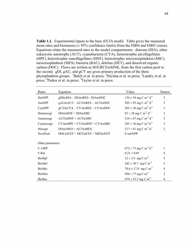
44  

Table 1.1. Experimental inputs to the base (ECO) model. Table gives the measured mean rates and biomasses (± 95% confidence limits) from the EB04 and EB05 cruises. Equations relate the measured rates to the model compartments: diatoms (DIA), other eukaryotic autotrophs (AUT), cyanobacteria (CYA), heterotrophic picoflagellates (HPF), heterotrophic nanoflagellates (HNF), heterotrophic microzooplankton (MIC), mesozooplankton (MES), bacteria (BAC), detritus (DET), and dissolved organic carbon (DOC). Flows are written as SOURCEtoSINK, from the first carbon pool to the second. gDI, gAU, and gCY are gross primary production of the three phytoplankton groups. 1Balch et al. in press; 2Décima et al. in press; 3Landry et al. in press; 4Parker et al. in press; 5Taylor et al. in press.

Rates Equation Value Source

DiaNPP gDItoDIA – DIAtoRES - DIAtoDOC 156 ± 54 mg C m-2 d-1 3

AutNPP gAUtoAUT – AUTtoRES – AUTtoDOC 505 ± 95 mg C m-2 d-1 3

CyaNPP gCYtoCYA – CYAtoRES – CYAtoDOC 203 ± 38 mg C m-2 d-1 3

Diamzoogr DIAtoHNF + DIAtoMIC 83 ± 28 mg C m-2 d-1 3

Autmzoogr AUTtoHNF + AUTtoMIC 316 ± 67 mg C m-2 d-1 3

Cyamzoogr CYAtoHPF + CYAtoHNF + CYAtoMIC 203 ± 36 mg C m-2 d-1 3

Mzoogr DIAtoMES + AUTtoMES 217 ± 41 mg C m-2 d-1 2

NewProd DOCtoEXT + DETtoEXT + MEStoEXT F-rat•NPP

Other parameters

C-14PP 672 ± 73 mg C m-2 d-1 1

F-Rat 0.22 ± 0.05 4

BioHpf 12 ± 3.9 mg C m-2 5

BioHnf 242 ± 39.7 mg C m-2 5

BioMic 78.6 ± 17.8 mg C m-2 4

BioMes 994 ± 77 mg C m-2 2

BioBac 679 ± 53.5 mg C m-2 4

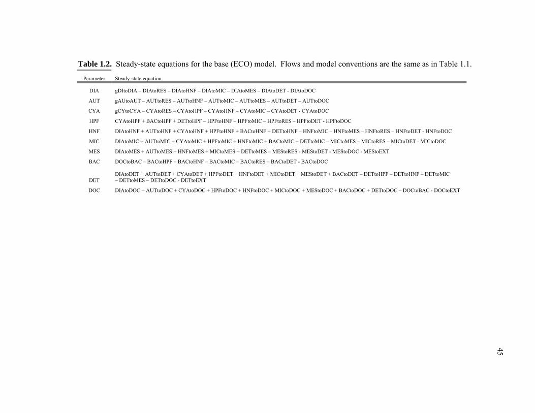
45  

Table 1.2. Steady-state equations for the base (ECO) model. Flows and model conventions are the same as in Table 1.1.

Parameter Steady-state equation

DIA gDItoDIA – DIAtoRES – DIAtoHNF – DIAtoMIC – DIAtoMES – DIAtoDET - DIAtoDOC

AUT gAUtoAUT – AUTtoRES – AUTtoHNF – AUTtoMIC – AUTtoMES – AUTtoDET – AUTtoDOC

CYA gCYtoCYA – CYAtoRES – CYAtoHPF – CYAtoHNF – CYAtoMIC – CYAtoDET - CYAtoDOC

HPF CYAtoHPF + BACtoHPF + DETtoHPF – HPFtoHNF – HPFtoMIC – HPFtoRES – HPFtoDET - HPFtoDOC

HNF DIAtoHNF + AUTtoHNF + CYAtoHNF + HPFtoHNF + BACtoHNF + DETtoHNF – HNFtoMIC – HNFtoMES – HNFtoRES – HNFtoDET - HNFtoDOC

MIC DIAtoMIC + AUTtoMIC + CYAtoMIC + HPFtoMIC + HNFtoMIC + BACtoMIC + DETtoMIC – MICtoMES – MICtoRES – MICtoDET - MICtoDOC

MES DIAtoMES + AUTtoMES + HNFtoMES + MICtoMES + DETtoMES – MEStoRES - MEStoDET - MEStoDOC - MEStoEXT

BAC DOCtoBAC – BACtoHPF – BACtoHNF – BACtoMIC – BACtoRES – BACtoDET - BACtoDOC

DET

DIAtoDET + AUTtoDET + CYAtoDET + HPFtoDET + HNFtoDET + MICtoDET + MEStoDET + BACtoDET – DETtoHPF – DETtoHNF – DETtoMIC – DETtoMES – DETtoDOC - DETtoEXT

DOC DIAtoDOC + AUTtoDOC + CYAtoDOC + HPFtoDOC + HNFtoDOC + MICtoDOC + MEStoDOC + BACtoDOC + DETtoDOC – DOCtoBAC - DOCtoEXT

45

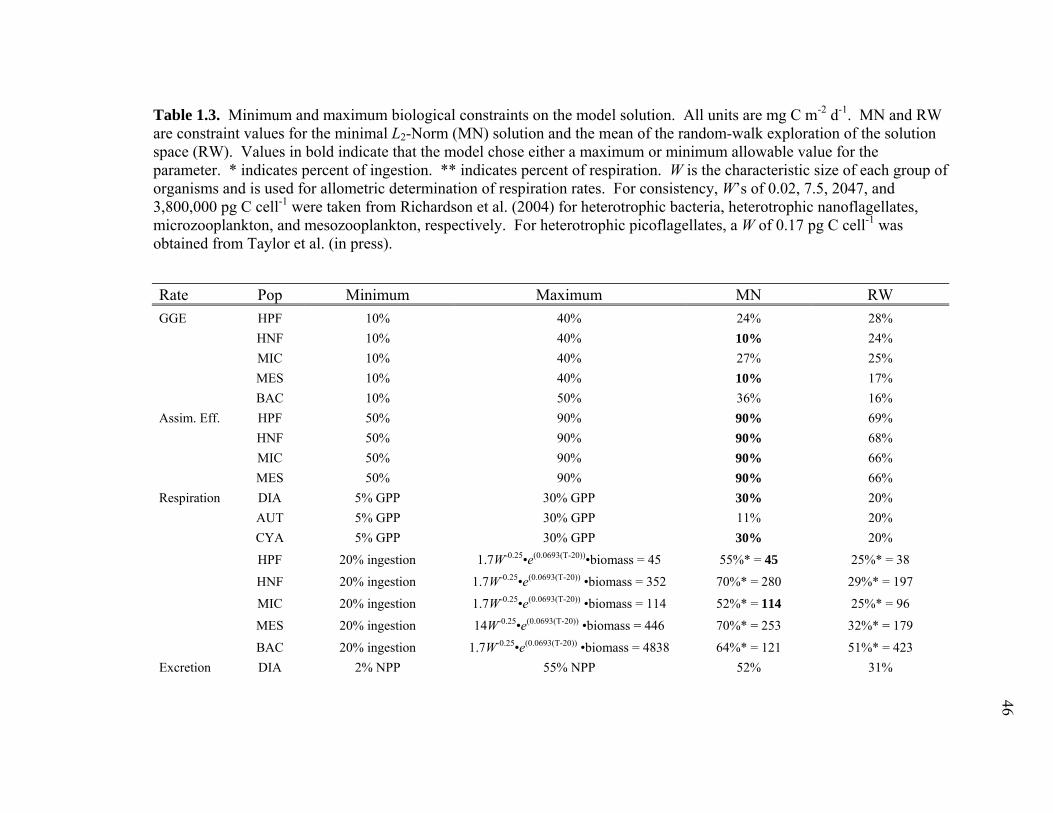
46  

Table 1.3. Minimum and maximum biological constraints on the model solution. All units are mg C m-2 d-1. MN and RW are constraint values for the minimal L2-Norm (MN) solution and the mean of the random-walk exploration of the solution space (RW). Values in bold indicate that the model chose either a maximum or minimum allowable value for the parameter. * indicates percent of ingestion. ** indicates percent of respiration. W is the characteristic size of each group of organisms and is used for allometric determination of respiration rates. For consistency, W’s of 0.02, 7.5, 2047, and 3,800,000 pg C cell-1 were taken from Richardson et al. (2004) for heterotrophic bacteria, heterotrophic nanoflagellates, microzooplankton, and mesozooplankton, respectively. For heterotrophic picoflagellates, a W of 0.17 pg C cell-1 was obtained from Taylor et al. (in press).

Rate Pop Minimum Maximum MN RW

GGE HPF 10% 40% 24% 28%

HNF 10% 40% 10% 24%

MIC 10% 40% 27% 25%

MES 10% 40% 10% 17%

BAC 10% 50% 36% 16%

Assim. Eff. HPF 50% 90% 90% 69%

HNF 50% 90% 90% 68%

MIC 50% 90% 90% 66%

MES 50% 90% 90% 66%

Respiration DIA 5% GPP 30% GPP 30% 20%

AUT 5% GPP 30% GPP 11% 20%

CYA 5% GPP 30% GPP 30% 20%

HPF 20% ingestion 1.7W-0.25•e(0.0693(T-20))•biomass = 45 55%* = 45 25%* = 38

HNF 20% ingestion 1.7W-0.25•e(0.0693(T-20)) •biomass = 352 70%* = 280 29%* = 197

MIC 20% ingestion 1.7W-0.25•e(0.0693(T-20)) •biomass = 114 52%* = 114 25%* = 96

MES 20% ingestion 14W-0.25•e(0.0693(T-20)) •biomass = 446 70%* = 253 32%* = 179

BAC 20% ingestion 1.7W-0.25•e(0.0693(T-20)) •biomass = 4838 64%* = 121 51%* = 423

Excretion DIA 2% NPP 55% NPP 52% 31%

46

46  

Table 1.3. Cont.

Rate Pop Minimum Maximum MN RW AUT 2% NPP 55% NPP 2% 29% C YA 2% NPP 55% NPP 24% 31% HPF 10% ingestion 100% respiration 11%* = 20%** 17%* = 68%** HNF 10% ingestion 100% respiration 10%* = 14%** 16%* = 54%** MIC 10% ingestion 100% respiration 11%* = 9%** 16%* = 36%** MES 10% ingestion 100% respiration 10%* = 14% 17%* = 52%** Ingestion MES - 3.6W-0.25•e(0.0693(T-20)) •biomass = 2006 361 556 BAC - 63W-0.25•e(0.0693(T-20)) •biomass = 10246 189 829

47

48  

Table 1.4. Solutions to the base ECO-model. Flows are, by convention, from the first carbon pool to the second. Carbon pools are GPP of diatoms (gDI), GPP of other eukaryotic phytoplankton (gAU), GPP of cyanobacteria (gCY), diatoms (DIA), other eukaryotic autotrophs (AUT), cyanobacteria (CYA), heterotrophic picoflagellates (HPF), heterotrophic nanoflagellates (HNF), microzooplankton (MIC), mesozooplankton (MES), bacteria (BAC), detritus (DET), dissolved organic carbon (DOC), respiration (RES), and export from the ecosystem (EXT). EqPac is the equivalent solutions of the Richardson et al. (2004) model. ECO MN is the solution that minimizes the L2-norm of our base ECO model. Monte Carlo mean and 95% confidence intervals (conf inter) are derived from randomly drawing possible combinations of the measured inputs to the model. RW mean and 95% conf inter are drawn from a random walk exploration of the possible solution space. 1Solutions are the minimum and maximum of the four time-series assessed by Richardson and Jackson (2004). 2The EqPac model did not allow (na) flow from diatoms to nano-sized protists. 3Combined values for the two non-diatom eukaryotic phytoplankton in the EqPac model. 4The EqPac model’s group of picophytoplankton includes picoeukaryotes but is functionally similar to our cyanobacteria compartment. 5The EqPac model had no heterotrophic picoflagellate (HPF) group. 6Since the EqPac model had no HPF group their protozoan group was equivalent to the sum of our HPF and HNF compartments.

Variable EqPac1 ECO MN ECO Monte Carlo ECO random walk

Mean Conf inter Mean Conf inter

1 gDItoDIA 7.2-192 338 318 (228-381) 255 (188-325)

2 DIAtoRES 0.4-9.6 102 95.3 (67-114) 50.5 (13-92)

3 DIAtoHNF na2 59.1 56.5 (41-72) 46.9 (4-81)

4 DIAtoMIC 2.4-61.2 23.9 21.0 (4-36) 36.1 (2-79)

5 DIAtoMES 0-42 73.0 70.2 (24-115) 50.3 (29-72)

6 DIAtoDET 4.0-75.6 0.0 20.6 (0-95) 22.7 (1-44)

7 DIAtoDOC 0.1-3.6 81.0 61.1 (4-88) 48.4 (6-84)

8 gAUtoAUT 155-4313 579 596 (521-681) 816 (655-1023)

9 AUTtoRES 7.8-21.63 63.8 74.3 (28-168) 164 (46-286)

10 AUTtoHNF 23.2-1403 176 173 (139-207) 228 (64-313)

11 AUTtoMIC 0-77.33 140 137 (103-170) 87.6 (3-252)

12 AUTtoMES 45.6-82.43 144 141 (93-198) 167 (145-188)

13 AUTtoDET 64.2-219.83 45.0 65.3 (0-176) 22.3 (1-44)

14 AUTtoDOC 2.9-5.03 10.1 10.3 (8-12) 147 (23-269)

15 gCYtoCYA 997-11814 359 363 (291-441) 333 (245-424)

16 CYAtoRES 49.9-59.04 108 108 (85-132) 66.8 (17-121)

17 CYAtoHPF na5 65.3 62.0 (50-74) 59.5 (3-143)

18 CYAtoHNF 445-10344,6 86.5 86.4 (73-101) 83.7 (5-176)

49  

Table 1.4. Cont.

Variable EqPac1 ECO MN ECO Monte Carlo ECO random walk

Mean Conf inter Mean Conf inter

19 C YAtoMIC 2.0-1064 51 .2 50.8 (39-62) 59.8 (3-157) 20 C YAtoDET 51.7-4634 0 .0 13.0 (0-60) 0.0 (0-0) 21 CYAto DOC 18.6-22.04 48 .6 47.0 (4-101) 63.2 (8-109) 22 HPFt oHNF na5 20 .0 21.7 (10-36) 22.4 (1-58) 23 HPFt oMIC na5 0. 0 0.0 (0-0) 19.7 (1-54) 24 HPFt oRES na5 45 .0 45.0 (30-60) 37.8 (24-44) 25 HPFt oDET na5 8 .2 8.9 (7-11) 47.1 (14-88) 26 HPFt oDOC na5 9. 0 14.0 (7-31) 25.6 (12-40) 27 HN FtoMIC 0.0 0.0 0.0 (0-0) 68.9 (3-196) 28 H NFtoMES 106-235 40.0 42.3 (36-52) 93.6 (6-238) 29 HNFtoRES 369-543 280 289 ( 250-335) 198 (107-310) 30 H NFtoDET 68.3-112 40.0 41.2 (36-48) 220 (61-476) 31 H NFtoDOC 159-272 40.0 41.2 (36-48) 107 (53-186) 32 MICtoRES 4.3-30.6 114 114 ( 104-123) 95.8 (63-113) 33 M ICtoMES 8.6-61.2 58.1 58.0 (41-78) 95.7 (35-177) 34 M ICtoDET 4.3-30.6 21.7 22.0 (20-25) 134 (40-234) 35 M ICtoDOC 4.3-30.6 23.2 26.7 (20-46) 63.9 (32-101) 36 MEStoRES 124-266 253 259 ( 226-299) 179 (97-294) 37 M EStoDET 41.0-66.6 36.2 37.2 (33-43) 189 (54-381) 38 M EStoDOC 57.1-94.7 36.2 37.2 (33-43) 93.8 (47-166) 39 BA CtoRES 180-265 121 129 (97-172) 423 (256-596) 40 B ACtoHPF na5 15 .4 15.6 (10-20) 33.1 (2-90) 41 B ACtoHNF 88.6-1276 36 .6 40.0 (28-53) 42.7 (2-104) 42 B ACtoMIC 0.0 1.3 4.9 (0-11) 33.7 (2-93) 43 B ACtoDET 3.8-91.6 13.9 7.8 (0-21) 20.8 (1-61) 44 B ACtoDOC 0-5.3 0.0 0.0 (0-0) 276 (11-709) 45 DETt oHPF na5 1 .5 10.7 (0-34) 60.0 (3-150) 46 DETt oHNF 0-1126 2 2.6 34.7 (9-73) 263 (16-650) 47 DETt oMIC 0.0 0.0 5.3 (0-32) 83.7 (3-248) 48 D ETtoMES 236-288 46.5 60.3 (32-108) 148 (6-446) 49 D ETtoDOC 293-318 11.6 22.0 (0-59) 62.2 (2-199) 50 DOCtoBAC 300-450 189 196 ( 158-243) 829 (492-1251) 51 D OCtoEXT 206-304 71.2 64.0 (35-89) 58.2 (4-123) 52 D ETtoEXT 22.8-42.0 82.8 85.0 (50-120) 38.4 (2-109) 53 MESto EXT 164-266 36.2 39.4 (34-50) 93.5 (47-161)

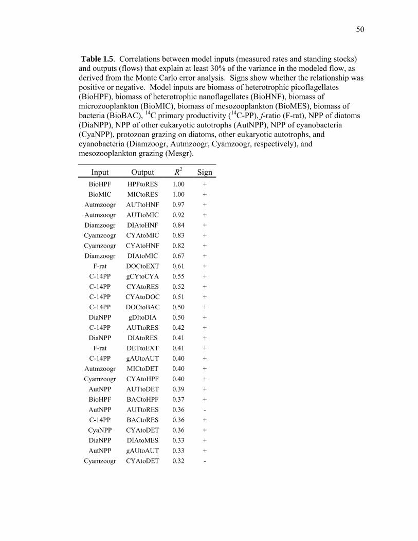
50  

Table 1.5. Correlations between model inputs (measured rates and standing stocks) and outputs (flows) that explain at least 30% of the variance in the modeled flow, as derived from the Monte Carlo error analysis. Signs show whether the relationship was positive or negative. Model inputs are biomass of heterotrophic picoflagellates (BioHPF), biomass of heterotrophic nanoflagellates (BioHNF), biomass of microzooplankton (BioMIC), biomass of mesozooplankton (BioMES), biomass of bacteria (BioBAC), 14C primary productivity (14C-PP), f-ratio (F-rat), NPP of diatoms (DiaNPP), NPP of other eukaryotic autotrophs (AutNPP), NPP of cyanobacteria (CyaNPP), protozoan grazing on diatoms, other eukaryotic autotrophs, and cyanobacteria (Diamzoogr, Autmzoogr, Cyamzoogr, respectively), and mesozooplankton grazing (Mesgr).

Input Output R2 Sign

BioHPF HPFtoRES 1.00 +

BioMIC MICtoRES 1.00 +

Autmzoogr AUTtoHNF 0.97 +

Autmzoogr AUTtoMIC 0.92 +

Diamzoogr DIAtoHNF 0.84 +

Cyamzoogr CYAtoMIC 0.83 +

Cyamzoogr CYAtoHNF 0.82 +

Diamzoogr DIAtoMIC 0.67 +

F-rat DOCtoEXT 0.61 +

C-14PP gCYtoCYA 0.55 +

C-14PP CYAtoRES 0.52 +

C-14PP CYAtoDOC 0.51 +

C-14PP DOCtoBAC 0.50 +

DiaNPP gDItoDIA 0.50 +

C-14PP AUTtoRES 0.42 +

DiaNPP DIAtoRES 0.41 +

F-rat DETtoEXT 0.41 +

C-14PP gAUtoAUT 0.40 +

Autmzoogr MICtoDET 0.40 +

Cyamzoogr CYAtoHPF 0.40 +

AutNPP AUTtoDET 0.39 +

BioHPF BACtoHPF 0.37 +

AutNPP AUTtoRES 0.36 -

C-14PP BACtoRES 0.36 +

CyaNPP CYAtoDET 0.36 +

DiaNPP DIAtoMES 0.33 +

AutNPP gAUtoAUT 0.33 +

Cyamzoogr CYAtoDET 0.32 -

51  

Table 1.5. Cont.

Input Output R2 SignC-14PP DI AtoDOC 0.32 +

Autmzoogr B ACtoMIC 0.31 - C-14PP BACto HNF 0.31 + AutNPP DETto EXT 0.31 +

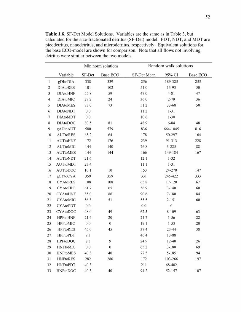
52  

Table 1.6. SF-Det Model Solutions. Variables are the same as in Table 3, but calculated for the size-fractionated detritus (SF-Det) model. PDT, NDT, and MDT are picodetritus, nanodetritus, and microdetritus, respectively. Equivalent solutions for the base ECO-model are shown for comparison. Note that all flows not involving detritus were similar between the two models.

Min norm solutions Random walk solutions

Variable SF-Det Base ECO SF-Det Mean 95% CI Base ECO

1 gDItoDIA 338 339 256 189-325 255

2 DIAtoRES 101 102 51.0 13-93 50

3 DIAtoHNF 55.8 59 47.0 4-81 47

4 DIAtoMIC 27.2 24 36.0 2-79 36

5 DIAtoMES 73.0 73 51.2 33-68 50

6 DIAtoNDT 0.0 11.2 1-31

7 DIAtoMDT 0.0 10.6 1-30

8 DIAtoDOC 80.5 81 48.9 6-84 48

9 gAUtoAUT 580 579 836 664-1045 816

10 AUTtoRES 65.2 64 178 50-297 164

11 AUTtoHNF 172 176 239 91-313 228

12 AUTtoMIC 144 140 76.8 3-225 88

13 AUTtoMES 144 144 166 149-184 167

14 AUTtoNDT 21.6 12.1 1-32

15 AUTtoMDT 23.4 11.1 1-31

16 AUTtoDOC 10.1 10 153 24-270 147

17 gCYtoCYA 359 359 331 245-422 333

18 CYAtoRES 108 108 65.8 17-120 67

19 CYAtoHPF 61.7 65 56.9 3-140 60

20 CYAtoHNF 85.0 86 90.6 7-180 84

21 CYAtoMIC 56.3 51 55.5 2-151 60

22 CYAtoPDT 0.0 0.0 0

23 CYAtoDOC 48.0 49 62.5 8-109 63

24 HPFtoHNF 21.4 20 21.7 1-56 22

25 HPFtoMIC 0.0 0 19.1 1-53 20

26 HPFtoRES 45.0 45 37.4 23-44 38

27 HPFtoPDT 8.3 46.4 13-88

28 HPFtoDOC 8.3 9 24.9 12-40 26

29 HNFtoMIC 0.0 0 65.2 3-180 69

30 HNFtoMES 40.3 40 77.5 5-185 94

31 HNFtoRES 282 280 172 103-266 197

32 HNFtoPDT 40.3 211 68-402

33 HNFtoDOC 40.3 40 94.2 52-157 107

53 

Table 1.6. Cont.

Min norm solutions Random walk solutions

Variable SF-Det Base ECO SF-Det Mean 95% CI Base ECO 34 M ICtoRES 114 114 99.9 73-113 96 35 M ICtoMES 59.8 58 97.5 42-178 96 36 M ICtoNDT 40.5 173 84-251 37 M ICtoDOC 23.8 23 67.1 38-102 64 38 MESto RES 248 253 162 95-256 179 39 M EStoMDT 35.4 194 68-346 40 M EStoDOC 35.4 36 85.9 46-146 94 41 BA CtoRES 124 121 468 300-635 423 42 B ACtoHPF 14.1 15 35.4 2-93 33 43 B ACtoHNF 37.4 37 41.7 2-103 43 44 B ACtoMIC 8.8 1 33.2 2-92 34 45 B ACtoPDT 6.9 21.1 1-60 46 BA CtoDOC 0.0 0 253 10-661 276 47 PDTt oHPF 7.2 57.3 3-145 48 PDTt oHNF 30.6 122 5-347 49 NDTt oHNF 0.0 56.5 2-158 50 PDTt oMIC 1.9 56.1 2-169 51 NDTt oMIC 0.0 40.1 2-127 52 M DTtoMIC 0.0 55.6 2-160 53 NDTt oMES 19.3 44.0 2-134 54 M DTtoMES 17.6 90.8 3-274 55 PDTt oDOC 15.8 42.6 2-134 56 NDTt oDOC 0.0 31.5 1-103 57 M DTtoDOC 0.0 40.8 2-126 58 D OCtoBAC 192 189 852 533-1260 829 59 DOC toEXT 70.6 71 52.4 3-114 58 60 NDTt oEXT 42.9 24.2 1-77 61 M DTtoEXT 41.2 28.9 1-87 62 M EStoEXT 35.4 36 84.6 46-145 93

 

Figure 1.1 –cruisfrom

– Station locases. Inset sh

m 160°W to 7

ations for EBhows the stud70°W and 25

B04 (Decemdy region wi5°S to 25°N

mber 2004) anithin the gre.

nd EB05 (Seater eastern

eptember 20tropical Pac

54

005) cific

 

Figure 1.2 –the cnot eof a grosauto(DIAcarb(MIC(HPFhigh

– Schematic carbon flowsend at any corandom wals primary prtrophs, respe

A), other eukon (DOC), dC), heterotroF). Ext is flu

her predators

representatios between anompartment lk exploratioroduction of ectively. Cokaryotic autodetritus (DETophic nanoflaux of carbon

s, vertical flu

on of our mony two comprepresent re

on of the soluf cyanobacterompartmentsotrophs (AUTT), mesozooagellates (HNn out of the eux of detritus

odel. Arrowpartments. Lespiration. Rution space. ria, diatoms,s are cyanobT), bacteria

oplankton (MNF), heterotecosystem ths, or lateral a

w widths are Light gray arResults are th gCY, gDI, , and other e

bacteria (CYA(BAC), diss

MES), microztrophic picofhrough consuadvection of

proportionarrows that dohe mean valuand gAU are

eukaryotic A), diatoms solved organzooplanktonflagellates umption by f DOC.

55

al to o ues e

nic n

 

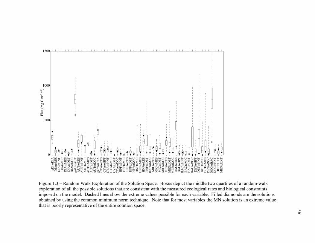
Figure 1.3 explorationimposed onobtained bythat is poor

– Random Waln of all the possn the model. Day using the comrly representativ

k Exploration oible solutions thashed lines show

mmon minimum ve of the entire s

of the Solution Shat are consistenw the extreme vnorm techniquesolution space.

Space. Boxes dent with the measvalues possible fe. Note that for

epict the middlesured ecologicalfor each variablemost variables

e two quartiles ol rates and bioloe. Filled diamothe MN solutio

of a random-walogical constraintnds are the solun is an extreme

56

lk ts utions

value

56

 

 

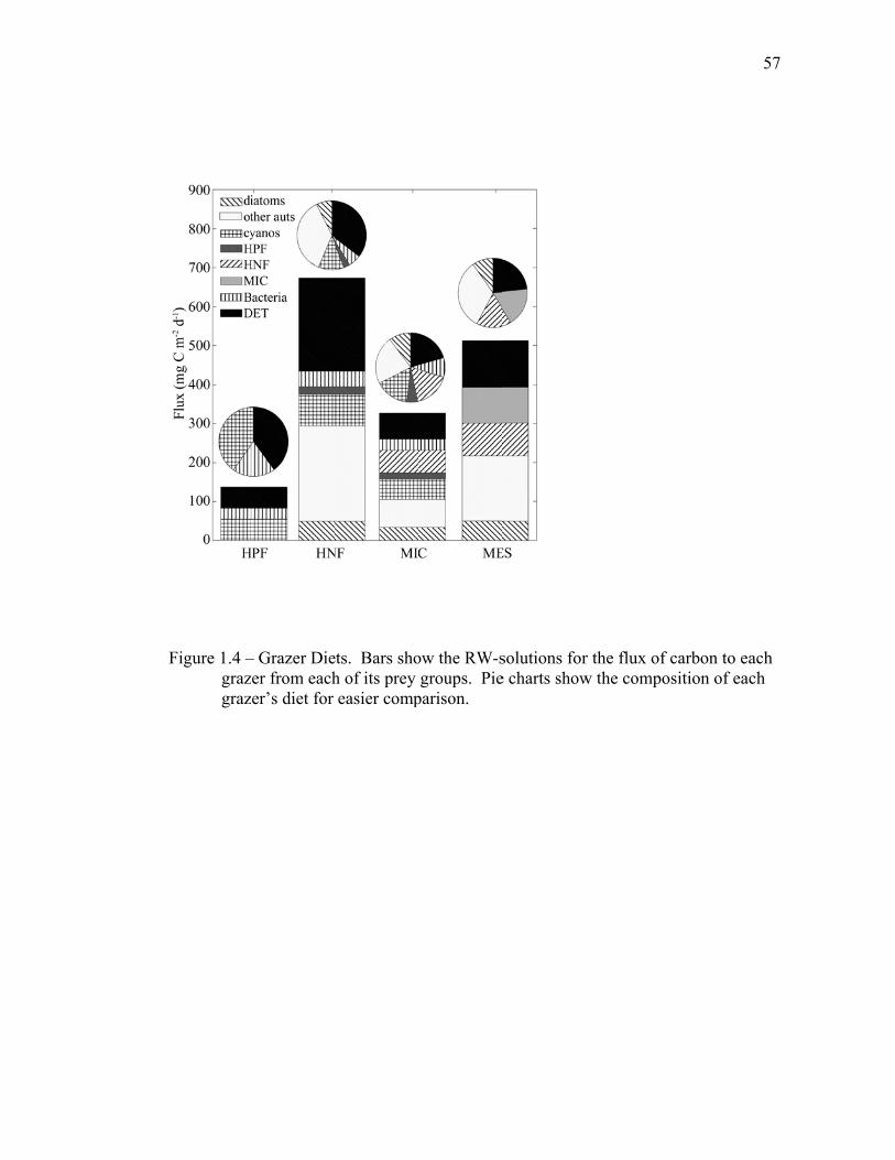
Figure 1.4 –grazgraz

– Grazer Diezer from eachzer’s diet for

ets. Bars shoh of its prey easier comp

57

ow the RW-sgroups. Pie

parison.

solutions fore charts show

r the flux of w the compo

carbon to easition of eac

57

ach ch

 

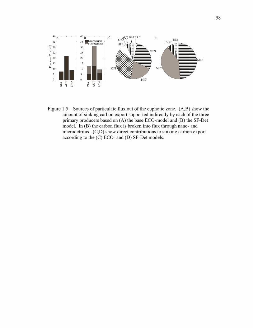
Figure 1.5 –amoprimmodmicracco

– Sources of unt of sinkin

mary producedel. In (B) throdetritus. (Cording to the

particulate fng carbon exers based on he carbon fluC,D) show d(C) ECO- a

flux out of thxport suppor(A) the base

ux is broken direct contriband (D) SF-D

he euphotic zrted indirectle ECO-modeinto flux thr

butions to siDet models.

zone. (A,B)ly by each ofel and (B) through nano- nking carbo

) show the f the three

he SF-Det and n export

58

 

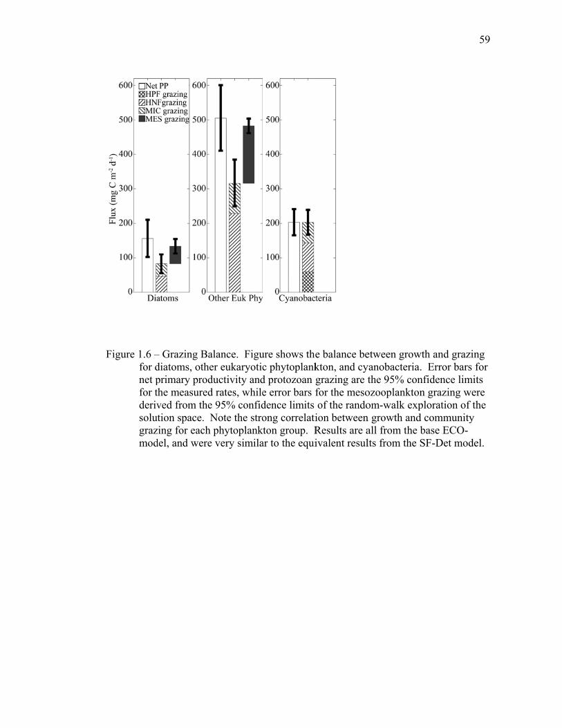
Figure 1.6 –for dnet pfor tderivsolutgrazmod

– Grazing Badiatoms, otheprimary prodhe measuredved from thetion space. N

zing for eachdel, and were

alance. Figuer eukaryoticductivity andd rates, whilee 95% confidNote the stro

h phytoplanke very simila

ure shows thec phytoplankd protozoan ge error bars fdence limits ong correlati

kton group. Rar to the equi

e balance bekton, and cygrazing are tfor the mesoof the randoion betweenResults are aivalent resul

etween growyanobacteria.the 95% con

ozooplanktonom-walk expn growth andall from the blts from the S

wth and grazi. Error bars nfidence limin grazing weploration of td communitybase ECO-SF-Det mod

59

ing for its ere the

y

del.

 

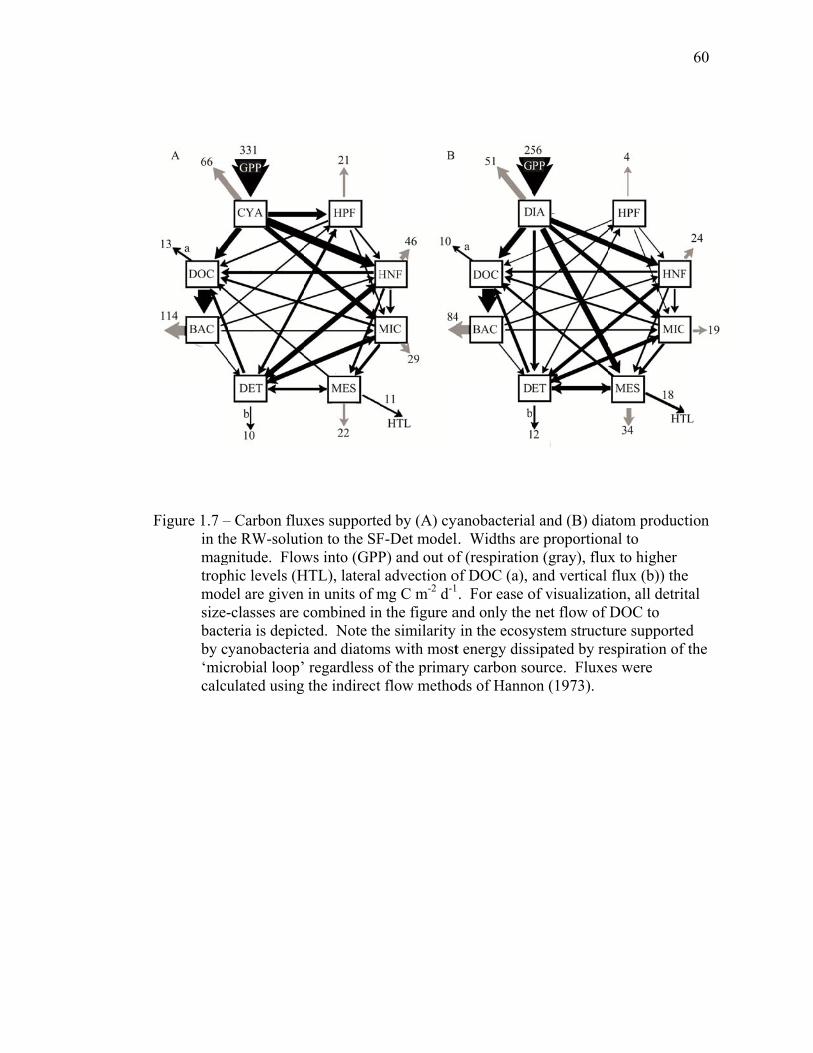
Figure 1.7 –in thmagtrophmodsize-bactby c‘miccalcu

– Carbon fluxhe RW-solutinitude. Flowhic levels (H

del are given -classes are ceria is depicyanobacteria

crobial loop’ulated using

xes supporteion to the SFws into (GPP

HTL), lateralin units of m

combined inted. Note tha and diatom regardless o the indirect

ed by (A) cyF-Det modelP) and out ofl advection omg C m-2 d-1

n the figure ahe similarity ms with mostof the primart flow metho

yanobacteriall. Widths arf (respiration

of DOC (a), 1. For ease oand only the

in the ecosyt energy dissry carbon so

ods of Hanno

l and (B) diae proportionn (gray), fluxand vertical

of visualizatinet flow of

ystem structusipated by reource. Fluxeon (1973).

atom productnal to x to higher flux (b)) the

ion, all detritDOC to ure supporteespiration of es were

60

tion

e tal

ed f the

61  

REFERENCES

ALLDREDGE, A. L., and C. C. GOTSCHALK. 1989. Direct observations of the mass flocculation of diatom blooms: characteristics, settling velocities and formation of diatom aggregates. Deep-Sea Res. 36: 159-171.

ARMSTRONG, R. A., C. LEE, J. I. HEDGES, S. HONJO, and S. G. WAKEHAM. 2002. A

new, mechanistic model for organic carbon fluxes in the ocean based on the quantitative association of POC with ballast minerals. Deep-Sea Res. II 49: 219-236.

AZAM, F., T. FENCHEL, J. G. FIELD, J. S. GRAY, L. A. MEYER-REIL, and F. THINGSTAD.

1983. The ecological role of water-column microbes in the sea. Mar. Ecol. Prog. Ser. 10: 257-263.

BALCH, W. M., A. J. POULTON, D. T. DRAPEAU, B. C. BOWLER, L. A. WINDECKER, and

E. S. BOOTH. in press. Zonal and meridional patterns of phytoplankton biomass and carbon fixation in the equatorial Pacific Ocean, between 110°W and 140°W. Deep-Sea Res. II 57: doi: 10.1016/j.dsr2.2010.08.004

BENDER, M., J. ORCHARDO, M. L. DICKSON, R. BARBER, and S. LINDLEY. 1999. In

vitro O2 fluxes compared with 14C production and other rate terms during the JGOFS Equatorial Pacific experiment. Deep-Sea Res. I 46: 637-654.

BROWN, S. L., M. R. LANDRY, R. T. BARBER, L. CAMPBELL, D. L. GARRISON, and M.

M. GOWING. 1999. Picophytoplankton dynamics and production in the Arabian Sea during the 1995 Southwest Monsoon. Deep-Sea Res. II 46: 1745-1768.

BROWN, S. L., M. R. LANDRY, K. E. SELPH, E. J. YANG, Y. M. RII, and R. R. BIDIGARE.

2008. Diatoms in the desert: Plankton community response to a mesoscale eddy in the subtropical North Pacific. Deep-Sea Res. II 55: 1321-1333.

BUESSELER, K. O., J. A. ANDREWS, M. C. HARTMAN, R. BELASTOCK, and F. CHAI.

1995. Regional estimates of the export flux of particulate organic carbon derived from thorium-234 during the JGOFS EqPac Program. Deep-Sea Res. II 42: 777-804.

CHRISTENSEN, V., and D. PAULY. 1992. ECOPATH II: a software for balancing

steady-state ecosystem models and calculating network characteristics. Ecol. Model. 61: 169-185.

62  

DAM, H. G., X. S. ZHANG, M. BUTLER, and M. R. ROMAN. 1995. Mesozooplankton grazing and metabolism at the equator in the central Pacific: Implications for carbon and nitrogen fluxes. Deep-Sea Res. II 42: 735-756.

DÉCIMA, M., M. R. LANDRY, and R. R. RYKACZEWSKI. in press. Broad-scale patterns

in mesozooplankton biomass and grazing in the eastern equatorial Pacific. Deep-Sea Res. II 57: doi: 10.1016/j.dsr2.2010.08.006

DICKSON, M. L., J. ORCHARDO, R. T. BARBER, J. MARRA, J. J. MCCARTHY, and R. N.

SAMBROTTO. 2001. Production and respiration rates in the Arabian Sea during the 1995 Northeast and Southwest Monsoons. Deep-Sea Res. II 48: 1199-1230.

DUCKLOW, H. W., H. L. QUINBY, and C. A. CARLSON. 1995. Bacterioplankton

dynamics in the equatorial Pacific during the 1992 El-Niño. Deep-Sea Res. II 42: 621-638.

DUGDALE, R. C., and F. P. WILKERSON. 1998. Silicate regulation of new production in

the equatorial Pacific upwelling. Nature 391: 270-273. FROST, B. W., and N. C. FRANZEN. 1992. Grazing and iron limitation in the control of

phytoplankton stock and nutrient concentration: A chemostat analog of the Pacific equatorial upwelling zone. Mar. Ecol. Prog. Ser. 83: 291-303.

GARRISON, D. L., M. M. GOWING, M. P. HUGHES, L. CAMPBELL, D. A. CARON, M. R.

DENNETT, A. SHALAPYONOK, R. J. OLSON, M. R. LANDRY, S. L. BROWN, H. B. LIU, F. AZAM, G. F. STEWARD, H. W. DUCKLOW, and D. C. SMITH. 2000. Microbial food web structure in the Arabian Sea: a US JGOFS study. Deep-Sea Res. II 47: 1387-1422.

GORSKY, G., M. J. CHRETIENNOT-DINET, J. BLANCHOT, and I. PALAZZOLI. 1999.

Picoplankton and nanoplankton aggregation by appendicularians: Fecal pellet contents of Megalocercus huxleyi in the equatorial Pacific. J. Geophys. Res. Oceans 104: 3381-3390.

HANNON, B. 1973. Structure of ecosystems. J. Theor. Biol. 41: 535-546. HIROSE, M., T. KATANO, and S. I. NAKANO. 2008. Growth and grazing mortality rates

of Prochlorococcus, Synechococcus and eukaryotic picophytoplankton in a bay of the Uwa Sea, Japan. J. Plankton Res. 30: 241-250.

JACKSON, G. A. 2001. Effect of coagulation on a model planktonic food web. Deep-

Sea Res. I 48: 95-123.

63  

JACKSON, G. A., N. NIQUIL, A. BURD, and T. L. RICHARDSON. 2001. Ecosystem Modeling Group Software, Inverse model code. Texas A&M Univ. http://oceanz.tamu.edu/~ecomodel/Software/invmodel/invmodel.html.

KIRCHMAN, D. L., J. H. RICH, and R. T. BARBER. 1995. Biomass and biomass

production of heterotrophic bacteria along 140°W in the equatorial Pacific - effect of temperature on the microbial loop. Deep-Sea Res. II 42: 603-619.

KONES, J. K., K. SOETAERT, D. VAN OEVELEN, and J. O. OWINO. 2009. Are network

indices robust indicators of food web functioning? A Monte Carlo approach. Ecol. Model. 220: 370-382.

LAMBORG, C. H., K. O. BUESSELER, J. VALDES, C. H. BERTRAND, R. BIDIGARE, S.

MANGANINI, S. PIKE, D. STEINBERG, T. TRULL, and S. WILSON. 2008. The flux of bio- and lithogenic material associated with sinking particles in the mesopelagic "twilight zone" of the northwest and North Central Pacific Ocean. Deep-Sea Res. II 55: 1540-1563.

LANDRY, M. R. 2009. Grazing processes and secondary production in the Arabian Sea:

A simple food web synthesis with measurement constraints, p. 133-146. In J. D. Wiggert, R. R. Hood, S. W. A. Naqvi, K. H. Brink and S. L. Smith [eds.], Indian Ocean biogeochemical processes and ecological variability. AGU Monograph. American Geophysical Union.

LANDRY, M. R., H. AL-MUTAIRI, K. E. SELPH, S. CHRISTENSEN, and S. NUNNERY.

2001. Seasonal patterns of mesozooplankton abundance and biomass at Station ALOHA. Deep-Sea Res. II 48: 2037-2061.

LANDRY, M. R., R. T. BARBER, R. R. BIDIGARE, F. CHAI, K. H. COALE, H. G. DAM, M.

R. LEWIS, S. T. LINDLEY, J. J. MCCARTHY, M. R. ROMAN, D. K. STOECKER, P. G. VERITY, and J. R. WHITE. 1997. Iron and grazing constraints on primary production in the central equatorial Pacific: An EqPac synthesis. Limnol. Oceanogr. 42: 405-418.

LANDRY, M. R., S. L. BROWN, J. NEVEUX, C. DUPOUY, J. BLANCHOT, S. CHRISTENSEN,

and R. R. BIDIGARE. 2003. Phytoplankton growth and microzooplankton grazing in high-nutrient, low-chlorophyll waters of the equatorial Pacific: Community and taxon-specific rate assessments from pigment and flow cytometric analyses. J. Geophys. Res. Oceans 108: 8142, doi: 8110.1029/2000jc000744

LANDRY, M. R., J. CONSTANTINOU, M. LATASA, S. L. BROWN, R. R. BIDIGARE, and M.

E. ONDRUSEK. 2000. Biological response to iron fertilization in the eastern

64  

equatorial Pacific (IronEx II). III. Dynamics of phytoplankton growth and microzooplankton grazing. Mar. Ecol. Prog. Ser. 201: 57-72.

LANDRY, M. R., K. E. SELPH, A. G. TAYLOR, M. DÉCIMA, W. M. BALCH, and R. R.

BIDIGARE. in press. Phytoplankton growth, grazing and production balances in the HNLC equatorial Pacific. Deep-Sea Res. II 57: doi: 10.1016/j.dsr2.2010.08.011

LI, W. K. W., D. V. S. RAO, W. G. HARRISON, J. C. SMITH, J. J. CULLEN, B. IRWIN, and

T. PLATT. 1983. Autotrophic picoplankton in the tropical ocean. Science 219: 292-295.

LOCHTE, K., and C. M. TURLEY. 1988. Bacteria and cyanobacteria associated with

phytodetritus in the deep sea. Nature 333: 67-69. LUNDSGAARD, C. 1995. Use of a high viscosity medium in studies of aggregates, p.

141-152. In S. Floderus, A.-S. Heisakanen, M. Oleson and P. Wassmann [eds.], Sediment trap studies in the Nordic countries 3. Proceedings of the Symposium on Seasonal Dynamics of Planktonic Ecosystem and Sedimentation in Coastal Nordic Waters.

MENDEN-DEUER, S., and E. J. LESSARD. 2000. Carbon to volume relationships for

dinoflagellates, diatoms, and other protist plankton. Limnol. Oceanogr. 45: 569-579.

NEWTON, J., and J. MURRAY. 1994. Comparison of sinking particulate material in the

central equatorial Pacific measured during the EqPac US-JGOFS field year. EOS, Transactions, American Geophysical Union 75: 82.

OLSEN, Y., S. AGUSTI, T. ANDERSEN, C. M. DUARTE, J. M. GASOL, I. GISMERVIK, A. S.

HEISKANEN, E. HOELL, P. KUUPPO, R. LIGNELL, H. REINERTSEN, U. SOMMER, H. STIBOR, T. TAMMINEN, O. VADSTEIN, O. VAQUE, and M. VIDAL. 2006. A comparative study of responses in planktonic food web structure and function in contrasting European coastal waters exposed to experimental nutrient addition. Limnol. Oceanogr. 51: 488-503.

PARKER, A. E., F. P. WILKERSON, R. C. DUGDALE, A. MARCHI, V. HOGUE, M. R.

LANDRY, AND A. G. TAYLOR. in press. Spatial patterns of nitrogen uptake and phytoplankton in the equatorial upwelling zone (110°W - 140°W) during 2004 and 2005. Deep-Sea Res. II 57: doi: 10.1016/j.dsr2.2010.08.013

PASSOW, U., A. L. ALLDREDGE, and B. E. LOGAN. 1994. The role of particulate

carbohydrate exudates in the flocculation of diatom blooms. Deep-Sea Res. I 41: 335-357.

65  

PASSOW, U., R. F. SHIPE, A. MURRAY, D. K. PAK, M. A. BRZEZINSKI, and A. L.

ALLDREDGE. 2001. The origin of transparent exopolymer particles (TEP) and their role in the sedimentation of particulate matter. Cont. Shelf Res. 21: 327-346.

PFANNKUCHE, O., and K. LOCHTE. 1993. Open ocean pelago-benthic coupling:

cyanobacteria as tracers of sedimenting salp feces. Deep-Sea Res. I 40: 727-737.

RICHARDSON, T. L., and G. A. JACKSON. 2007. Small phytoplankton and carbon export

from the surface ocean. Science 315: 838-840. RICHARDSON, T. L., G. A. JACKSON, H. W. DUCKLOW, and M. R. ROMAN. 2004.

Carbon fluxes through food webs of the eastern equatorial Pacific: an inverse approach. Deep-Sea Res. I 51: 1245-1274.

RICHARDSON, T. L., G. A. JACKSON, H. W. DUCKLOW, and M. R. ROMAN. 2006.

Spatial and seasonal patterns of carbon cycling through planktonic food webs of the Arabian Sea determined by inverse analysis. Deep-Sea Res. II 53: 555-575.

ROBISON, B. H., K. R. REISENBICHLER, and R. E. SHERLOCK. 2005. Giant larvacean

houses: Rapid carbon transport to the deep sea floor. Science 308: 1609-1611. RODIER, M., and R. LE BORGNE. 1997. Export flux of particles at the equator in the

western and central Pacific Ocean. Deep-Sea Res. II 44: 2085-2113. SELPH, K. E., M. R. LANDRY, A. G. TAYLOR, E. J. YANG, C. I. MEASURES, J. J. YANG,

M. R. STUKEL, S. CHRISTENSON, and R. R. BIDIGARE. in press. Spatially-resolved taxon-specific phytoplankton production and grazing dynamics in relation to iron distributions in the equatorial Pacific between 110 and 140°W. Deep-Sea Res. II 57: doi: 10.1016/j.dsr2.2010.08.014

SILVER, M. W., and M. M. GOWING. 1991. The "particle" flux: Origins and biological

components. Prog. Oceanogr. 26: 75-113. TAKAHASHI, M., and P. K. BIENFANG. 1983. Size structure of phytoplankton biomass

and photosynthesis in subtropical Hawaiian Waters. Mar. Biol. 76: 203-211. TAYLOR, A. G., M. R. LANDRY, K. E. SELPH, and E. J. YANG. in press. Biomass, size

structure and depth distributions of the microbial community in the eastern equatorial Pacific. Deep-Sea Res. II 57: doi: 10.1016/j.dsr2.2010.08.017

66  

ULANOWICZ, R. E., and J. J. KAY. 1991. A package for the analysis of ecosystem flow networks. Environmental Software 6: 131-142.

VERITY, P. G., T. M. BEATTY, and S. C. WILLIAMS. 1996a. Visualization and

quantification of plankton and detritus using digital confocal microscopy. Aquat. Microb. Ecol. 10: 55-67.

VERITY, P. G., D. K. STOECKER, M. E. SIERACKI, and J. R. NELSON. 1996b.

Microzooplankton grazing of primary production at 140°W in the equatorial Pacific. Deep-Sea Res. II 43: 1227-1255.

VÉZINA, A. F., and T. PLATT. 1988. Food web dynamics in the ocean .1. Best estimates

of flow networks using inverse methods. Mar. Ecol. Prog. Ser. 42: 269-287. WAITE, A. M., K. A. SAFI, J. A. HALL, and S. D. NODDER. 2000. Mass sedimentation

of picoplankton embedded in organic aggregates. Limnol. Oceanogr. 45: 87-97.

WALSH, I. D., and W. D. GARDNER. 1992. A comparison of aggregate profiles with

sediment trap fluxes. Deep-Sea Res. 39: 1817-1834. YOOL, A., A. P. MARTIN, C. FERNANDEZ, and D. R. CLARK. 2007. The significance of

nitrification for oceanic new production. Nature 447: 999-1002. ZHANG, X., H. G. DAM, J. R. WHITE, and M. R. ROMAN. 1995. Latitudinal variations in

mesozooplankton grazing and metabolism in the central tropical Pacific during the US JGOFS EqPac Study. Deep-Sea Res. II 42: 695-714.

ZHANG, X. S., and H. G. DAM. 1997. Downward export of carbon by diel migrant

mesozooplankton in the central equatorial Pacific. Deep-Sea Res. II 44: 2191-2202.

67

CHAPTER 2

Trophic cycling and carbon export relationships in the

California Current Ecosystem

By Michael R. Stukel, Michael R. Landry, Claudia R. Benitez-Nelson, and

Ralf Goericke

Abstract

The vertical flux of carbon from the surface ocean is a critical component of the

global carbon cycle that remains poorly understood in dynamic coastal regions. To

better understand the relationships between export, plankton rate processes and

plankton community variability in the California Current Ecosystem (CCE), we

constructed a simple model of trophic cycling relationships and tested its predictions

about export of mesozooplankton fecal material against export flux measurements by

the 234Th method. For modeled trophic processes, we used 14C-primary production

and chlorophyll-based rate estimates of phytoplankton growth, microzooplankton

grazing, mesozooplankton grazing, and net phytoplankton growth of the

phytoplankton from Lagrangian experiments conducted in May 2006 over a range of

environmental conditions, from inshore coastal upwelling to offshore oligotrophic

conditions. E-ratios (carbon export/14C-primary production) predicted by the model

ranged from 0.08 - 0.14, in good agreement with both the magnitude and the

variability found in contemporaneous measurements of 234Th export and C: 234Th

ratios of sinking particles. E-ratios were strongly decoupled from new production

estimates, with the lowest measured and predicted e-ratios associated with richer water

68

parcels with net accumulating phytoplankton in the inshore region. For the range of

conditions studied, variability in export efficiency was determined by the local net

balance of growth and grazing and the relative strengths of grazing pathways to

microzooplankton and mesozooplankton. Despite very different plankton assemblages

studied, the good agreement between independently measured production-grazing

processes and biogeochemical rates suggest that zooplankton are the major drivers of

vertical carbon flux in this system during springtime. If that is generally the case,

significant decadal-scale oscillations in large zooplankton, well documented for the

region, may have substantial implications for carbon cycling and export.

Introduction

The vertical export of particulate carbon from the surface to the deep ocean is a

critical component of the ocean’s carbon cycle. While much is known about the

general patterns of export and their relationships to ecosystem properties over large

regions of the open ocean (e.g. Buesseler 1998), our understanding of fluxes and

regulatory mechanisms in coastal regions is sparse by comparison. Because coastal

regions typically have high rates of new and primary production on an areal basis, they

likely play disproportionate roles in carbon cycling and export (Eppley and Peterson

1979). However, they are temporally and spatially complex and difficult to study.

The biologically mediated mechanisms that drive export may also vary among and

within coastal regions, from sinking phytodetritus (Green and Sambrotto 2006) to

fecal pellet flux (e.g. Landry et al. 1994; Umani et al. 2002), with varying additional

effects of the physiological state of phytoplankton, inorganic ballasting (Armstrong et

al. 2002), and aggregation processes (Alldredge and Gotschalk 1989; Walsh and

69

Gardner 1992; Jackson 2001) involving both phytoplankton and bacteria (Passow et al.

1994; 2001). Studies are thus needed that link explicitly measured ecological rates to

vertical carbon flux measurements across the range of conditions that define coastal

ecosystems.

Because coastal regions can be strongly advective systems with uncoupled

production and export processes, Lagrangian sampling schemes that allow

simultaneous measurement of ecosystem processes, net community changes, and

biogeochemical fluxes may be well suited to their study. Landry et al. (2009), for

instance, used a Lagrangian strategy to investigate phytoplankton rate relationships

across a spectrum of ecological conditions and biotic communities in the California

Current Ecosystem (CCE), finding that measured depth-integrated growth and grazing

rates explained >90% of the variability in the observed net growth rates of ambient

phytoplankton over the duration of 3-5 day experiments. This good agreement

between observed and predicted net changes based only on growth rate estimates and

grazing losses to micro- and mesozooplankton suggested that direct sinking of

phytoplankton out of the euphotic zone contributed surprisingly little, on average, to

the temporal dynamics of phytoplankton. Here, we use data from four widely varying

water parcels sampled in May 2006 of that study to ask the question in a different way

-- are experimental measurements of growth and grazing rates sufficient to explain the

magnitude and pattern of export flux in this coastal system, without consideration of

direct cell sinking? To answer this question, we develop a simple trophic relationship

model for computing carbon export estimates from experimental process rates, which

we test against independent measurements of export flux based on the 234Th method.

The underlying hypothesis in this comparison is that variability in vertical carbon flux

in the CCE can be largely explained by the fluxes along trophic pathways that lead to

70

fecal pellet production of metazooplankton. Alternatively, significant underprediction

of export rates from the trophic model would be a strong indication that direct sinking

of unconsumed phytoplankton, or other unmeasured processes, contribute substantially

to the signal. Since direct cell sinking and grazing losses to micro- and

mesozooplankton are each coupled to export with very different efficiencies, our

results highlight the importance of including a mechanistic understanding of

ecological process rates and interactions in biogeochemical flux models. They also

illustrate the strongly advective and unbalanced nature of the CCE upwelling

ecosystem, where contemporaneous export is significantly lower than the expected

rate of new production.

Methods

Overview of Lagrangian design - The study area (Fig. 1) was principally along

historical time-series sampling Line 80 of the CalCOFI Program (California

Cooperative Oceanic Fisheries Investigations), extending from the physically dynamic

coastal upwelling region off of Point Conception, California to nutrient-depleted

offshore waters. For water parcels chosen to exploit the onshore-offshore range of

ecosystem variability, a Lagrangian experimental approach was used to investigate

relationships between measured rates of trophic interactions and vertical carbon flux.

As described by Landry et al. (2009), individual experiments were initiated in

homogenous surface water parcels, identified and surveyed with a combination of

satellite imagery and underway surveys with a Moving Vessel Profiler system (MVP,

M. D. Ohman, unpubl.). Water parcels were tagged with a drift array that included a

3x1 m holey-sock drogue centered at 15-m depth, a surface float equipped with

Globalstar satellite communications, and a line below with attachments for in situ

bottle incubations to assess growth, production and grazing rates of the phytoplankton

71

community. Sampling and experimental studies were conducted daily while tracking

the water parcels for the duration of an experimental cycle (typically 4 days). This

strategy provided estimates of the net observed changes in the ambient phytoplankton

community concurrently with the experimentally determined rates of production and

grazing processes, which we use below for trophic modeling. To estimate vertical

carbon flux, we measured 234Th deficiency and C: 234Th ratios on either 35-75 µm or

20-75 µm particles at specific depth horizons within the same water parcels.

Four experimental cycles were conducted, including two inshore parcels of recent

and aged upwelled water (inshore Cycles 1 and 2, respectively), one in the low-salinity

core of the California Current proper, and one in offshore oligotrophic waters (Fig. 1).

Initial surface chlorophyll a (Chl a) concentrations at these sites varied from 0.10 to

2.87 g Chl a L-1. Regions containing strong gradients were intentionally avoided

when choosing experimental sites to minimize the possibility that the drogued drift

array would cross a frontal feature if it slipped relative to the net mixed-layer currents.

Surface-layer temperature and salinity characteristics of water parcels were assessed

with MVP surveys to ensure coherency of water parcels over the duration of the

experimental cycles.

Trophic cycling relationships - Our experiments provided rate estimates for

phytoplankton growth and production, grazing processes and export flux over the

range of conditions sampled in the marked water parcels. Since growth and grazing

measurements explained >90% of the observed net rate of change in ambient

phytoplankton chlorophyll (Landry et al. 2009), we formulate this net rate of change as

the difference between biomass production and the combined grazing losses to micro-

and mesozooplankton. We describe this relationship below in the format that is most

commonly used in NPZ (nutrient-phytoplankton-zooplankton) models. In Eq. 1,

72

phytoplankton production is the product of biomass (P) and specific growth rate (P,

units of d-1), and grazing losses are determined by the respective biomass-specific

grazing rates (mP and MP, units of d-1 grazer biomass-1) and biomasses (z and Z) of

micro- and mesozooplankton.

(1)

Accordingly, the combined terms mPz and MPZ in Equ. 1 are the instantaneous grazing

rates of the micro- and mesozooplankton assemblages, respectively, feeding on

phytoplankton.

We assume that microzooplankton standing stock grows with a gross growth

efficiency (GGE1) of 30% (Straile 1997) and is grazed upon by mesozooplankton at

the biomass-specific rate of Mz. Thus:

(2)

Mesozooplankton likewise grow with a gross growth rate of GGE2, yielding:

(3)

As discussed further below, but consistent with the results of Landry et al. (2009),

we assume that direct sinking of phytoplankton from the euphotic zone did not account

for significant loss of biomass during our experiments. Potential export as fecal matter

produced by the feeding of mesozooplankton (dF/dt) can therefore be estimated from

the trophic relationships described above, assuming an egestion efficiency (EE) of 30%

(Conover 1966):

Export (4)

73

Assuming steady-state conditions of microzooplankton standing stock over the few

days of each experimental cycle, Equ. 2 simplifies to:

(5)

and equation 4 becomes:

(6)

Dividing the entire equation by the gross growth rate of the phytoplankton community

(PP), allows us to rewrite the equation in terms of the e-ratio:

e‐ratio (7)

According to Eq. 7, the e-ratio therefore becomes a function of the egestion

efficiency of mesozooplankton, the gross growth efficiency of the microzooplankton,

and the ratios of micro- and mesozooplankton community grazing to phytoplankton

specific growth rate. While canonical values of 0.30 are used for both efficiency terms,

the model results are relatively insensitive to ±10% change in either of these

parameters, due to the inherent variability in our repeated biological rate

measurements.

Biological rate parameters – As presented in Landry et al. (2009), daily

instantaneous rates (d-1) of phytoplankton growth (µp in our model) and

microzooplankton community grazing (mcomm, equivalent to mPz in our model) were

determined by two-point dilution experiments conducted in 2.7-L bottle samples

incubated at in situ temperature and light conditions on a line attached below our

surface drifter. Eight sampling depths were chosen to span the euphotic zone with the

deepest bottle pair at a depth corresponding to roughly the 0.4% light level, which

74

varied from 50 m inshore to 100 m offshore. The paired bottles represented whole

(100%) seawater and 33% whole seawater, diluted with 0.1-µm filtered seawater.

Water bottles were incubated for a 24-h period beginning and ending at ~04:00 PST

each day. Rate assessments were based on initial and final 250-mL subsamples for

chlorophyll a (Chl a). For consistency, all biological rates and standing stocks were

vertically integrated to the depth of the deepest 14C primary productivity (14C-PP)

incubation (35 to 40-m inshore and 70-m offshore).

Daily instantaneous rates of mesozooplankton community grazing on

phytoplankton (Mcomm, equivalent to MPZ in our model) were determined from twice

daily (mid-day and mid-night) net tows using 202-µm mesh, 0.71-m diameter bongo

nets with attached flow meter towed to a maximum depth of 210 m (Landry et al. 2009

and M. D. Ohman, unpubl.). Daily community ingestion rates were calculated from

the sum of the day-night means of Chl a and phaeopigment.

14C-PP was measured from 4-L samples incubated in polycarbonate bottles at six

depths (Fig. 2a) on the in situ array. Triplicate 250-mL subsamples were filtered

through GF/F filters, which were then fumed with HCl to remove inorganic 14C. After

addition of scintillation cocktail, beta decays were detected with a Beckman-Coulter

scintillation counter.

234Th derived carbon export - 234Th deficiencies were calculated using the 4-L

method (Benitez-Nelson et al. 2001; Buesseler et al. 2001; Pike et al. 2005). Samples

(4 L) were taken from 8 depths per cast of a Niskin rosette (typically to a depth of

approximately twice the euphotic zone). HNO3 was added to the samples to acidify to

a pH of ~2, and the samples were immediately spiked with a known aliquot of 230Th (1

mL at 10 dpm mL-1) and allowed to sit for >4 h. NH4OH was then added to adjust pH

75

to ~9, after which 100 µL each of 7.5 g L-1 KMnO4 and 33 g L-1 MnCl2 were added.

Samples were shaken and let sit for >8 h to allow Th to co-precipitate with MnO2.

The precipitates were vacuum filtered onto a 25-mm quartz microfiber filter and

allowed to air dry prior to mounting in a RISO cup. They were counted on land with a

low-level RISO beta counter, followed >6 half-lives later by a second count to

establish background beta emission levels. To calculate the yield of the Th-MnO2 co-

precipitation, all samples were dissolved in 8 M HNO3/10% H2O2 solution and spiked

with a gravimetrically measured aliquot of 229Th (typically 1 g at 99.5 dpm g-1). They

were purified on a Poly-Prep chromatography column (Bio-Rad Laboratories)

containing AG 1-X8 100-200 mesh chloride form resin (Bio-Rad Laboratories) and

eluted with HCl. The HCl was subsequently evaporated off so that the residue could

be reconstituted in a solution of 10% HNO3/1% HF for Inductively Coupled Plasma

Mass Spectrometric Analysis of the 229:230Th ratio at the WHOI Analytical Lab.

Recoveries averaged 80 ± 8% (mean ± standard deviation). 234Th deficiency was

calculated as the difference between the measured activity and the expected activity if

234Th was in equilibrium with 238U, the latter being calculated from salinity as: 238U

(dpm L-1) = 0.0686 • salinity • density (Chen et al. 1986). 234Th export estimates for

the three furthest offshore experimental cycles depicted in Fig. 1 were determined

using a one-dimensional steady state model (E = λTh ( AU – ATh) ) and trapezoidal

vertical integration. While this steady-state approximation is an oversimplification of

the complex cycling of particulate and dissolved thorium in the water column, it can

provide a reasonable estimate of flux if 234Th concentrations are near steady-state and

upwelling terms are negligible. It is the only feasible method of estimating carbon

export from water parcels when repeat occupations over long (>2-week) time periods

76

are not possible. The potential errors associated with this steady-state approximation

are addressed in our discussion.

Samples for particulate C: 234Th ratio were collected from beneath the euphotic

zone, typically at 100 m (150 m for the furthest offshore cycle). A McLane WTS-LV

large-volume in situ pump was used to filter 200 to 300-L of water through size-

fractionated filters. We used a 75-µm pre-filter to screen out swimming

mesozooplankton which could significantly alter the measured C: 234Th ratio

(Buesseler et al. 2006; Rodriguez Y Baena et al. 2006). Samples representative of

sinking material were collected on 20- or 35-µm Nitex filters and then washed onto

25-mm quartz microfiber filters, which were dried and mounted on RISO cups for beta

counting. Samples were beta counted as with the 234Th deficiency samples, including

background count following decay of 234Th. The samples were then combusted for

carbon and nitrogen contents using a Costech 4010 Elemental combustion analyzer

(SIO Analytical Facility).

Results

Comparison of measured and net rates – From the Lagrangian experimental

approach, we measured trophic process rates and carbon export in the CCE over

conditions spanning a 30-fold range in sea-surface chlorophyll concentration. Despite

widely differing characteristics of the plankton communities, some generalities

emerged. Microzooplankton grazing was the primary loss term for phytoplankton for

all experiments, accounting for 61 ± 15 to 92 ± 23% (mean ± standard error) of the

measured total grazing impact. Phytoplankton growth rates typically exceeded

microzooplankton grazing pressure near the surface, but decreased more rapidly with

depth relative to grazing rates (Fig. 2). This led to excess grazing over growth at depth,

77

which was likely supported by phytoplankton from the upper layer that either sunk

slowly or were mixed deeper. 14C-PP estimates of production were similar to the

growth-based estimates derived from the growth rates from dilution experiments and

microscopically determined phytoplankton biomass. Both patterns exhibited high

surface productivity nearshore with a distinct subsurface maximum in productivity in

the furthest offshore region.

Despite the relative constancy of microzooplankton grazing as a phytoplankton

loss term, the percentage of phytoplankton growth consumed by microzooplankton

differed appreciably in the experimental water parcels, varying from only 41 ± 9%

inshore to 119 ± 34% of phytoplankton µ offshore. This stark difference drives the

overall pattern in the calculated instantaneous net rates of phytoplankton growth (µP –

mPz – MP Z), which varied from a net decrease of 0.04 ± 0.04 d-1 offshore to a net

increase of 0.20 ± 0.07 d-1 inshore. Calculated net growth rates for the phytoplankton

community were within the error of the net measured rates of change of chlorophyll in

the euphotic zone calculated from daily CTD casts at the drifter locations (Fig. 3). The

ability to predict reasonably well the in situ rate of change of the ambient community

from process rate measurements is a common feature of all four cycles, supporting the

view that direct sinking of phytoplankton was not a major loss term during the study.

Otherwise, we would expect the observed rate of change to be significantly lower than

that predicted solely from growth and grazing terms.

Offshore, oligotrophic water parcel (OOP)- Two of the water parcels studied are

representative of the low productivity waters found offshore in the CCE. The furthest

offshore experiment was initiated 350 km from the coast in water far beyond the low-

salinity core of the California Current, with the marked parcel moving further seaward

for the duration of our 4-d experimental cycle. The phytoplankton community was

78

comprised of relatively small cells (Taylor, A. G., pers. comm.), similar to those of the

relatively stable offshore community commonly found throughout the oligotrophic

subtropical Pacific (Venrick 1998,2002). 234Th profiles taken on the first and final day

of the cycle (Fig. 4a) show little difference (although the final profile was missing

several samples that were lost during filtration). They thus support the assumption of

a general steady state. The profiles exhibit a strong subsurface maximum in

deficiency at the top of the strong deep chlorophyll maximum, which corresponds to

the depth of a subsurface maximum of production measured by the 14C-PP incubations.

The particulate C: 234Th sample (65 ± 9 µg C dpm-1, mean ± measurement error) was

collected on a 20-µm filter at a depth of 150 m to include flux out of the deep euphotic

zone. Inspection of the 234Th deficiency profile shows that remineralization probably

began near 100 m. A comparison of the vertically integrated deficiencies between 100

and 150-m (47,400 and 40,500 dpm m-2, respectively) suggests that as much as 15% of

the 234Th that sank out of the euphotic zone was remineralized before reaching the

150-m depth horizon, with likely a higher percentage of carbon remineralized, due to

preferential carbon remineralization of many microorganisms (Buesseler et al. 2006).

The ThE-ratio (ratio of 234Th derived carbon export to primary productivity),

calculated from carbon export across the 150-m depth horizon and 14C-PP integrated

over the euphotic zone, was 0.15 ± 0.08 (mean ± standard error is reported unless

otherwise specified) for this water parcel.

The biological community for this experimental cycle was comprised of a small

standing stock that exhibited relatively low mean growth rates for the euphotic zone,

of only 0.13 ± 0.02 d-1, and microzooplankton community grazing was an order of

magnitude higher than that for mesozooplankton (Table 1). Grazing exceeded growth

of the phytoplankton, and hence our predicted rate of change for the community was

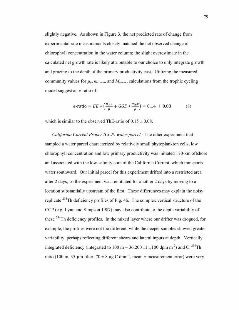
79

slightly negative. As shown in Figure 3, the net predicted rate of change from

experimental rate measurements closely matched the net observed change of

chlorophyll concentration in the water column; the slight overestimate in the

calculated net growth rate is likely attributable to our choice to only integrate growth

and grazing to the depth of the primary productivity cast. Utilizing the measured

community values for µp, mcomm, and Mcomm, calculations from the trophic cycling

model suggest an e-ratio of:

‐ratio ∗ ∗ 0.14 0.03 (8)

which is similar to the observed ThE-ratio of 0.15 ± 0.08.

California Current Proper (CCP) water parcel - The other experiment that

sampled a water parcel characterized by relatively small phytoplankton cells, low

chlorophyll concentration and low primary productivity was initiated 170-km offshore

and associated with the low-salinity core of the California Current, which transports

water southward. Our initial parcel for this experiment drifted into a restricted area

after 2 days; so the experiment was reinitiated for another 2 days by moving to a

location substantially upstream of the first. These differences may explain the noisy

replicate 234Th deficiency profiles of Fig. 4b. The complex vertical structure of the

CCP (e.g. Lynn and Simpson 1987) may also contribute to the depth variability of

these 234Th deficiency profiles. In the mixed layer where our drifter was drogued, for

example, the profiles were not too different, while the deeper samples showed greater

variability, perhaps reflecting different shears and lateral inputs at depth. Vertically

integrated deficiency (integrated to 100 m = 36,200 ±11,100 dpm m-2) and C: 234Th

ratio (100 m, 35-μm filter, 70 ± 8 μg C dpm-1, mean ± measurement error) were very

80

similar to those found in the offshore oligotrophic region, but the higher rates of

primary productivity led to a slightly lower ThE-ratio of 0.12 ± 0.04.

The phytoplankton community of the CCP was largely at steady state during the

time of our sampling, with a net growth rate of -0.04 ± 0.05 d-1. Chlorophyll

concentrations were comparable to that of the oligotrophic offshore water, but specific

growth rates were significantly higher and balanced by losses to grazing, dominated by

microzooplankton but with mesozooplankton accounting for a substantial (>20%)

portion. The net calculated rate of change of phytoplankton in the CCP parcels was

again close to the observed net growth rate of the ambient community (0.01 ± 0.08).

Our trophic cycling model also predicted an e-ratio of 0.13 ± 0.03, which was close to

the measured ThE-ratio.

Inshore water parcels - The two water parcels studied inshore of the CCP were

dominated by larger phytoplankton (Taylor, A. G., pers. comm.) and had higher

chlorophyll concentrations characteristic of the coastal area impacted by seasonally

variable upwelling (Venrick 1998,2002). The cold temperatures and high salinities of

these parcels are indicative of recently upwelled water, and we believe they had

similar origins near Point Conception. Our sampling for inshore Cycle 1 (IC1) began

roughly 30 km from the coast, and the drifter tracked almost directly offshore (west)

for 4 days with an average velocity of 11 km d-1. Inshore Cycle 2 (IC2) began 15 days

later 80 km from the coast and also drifted west at an even higher speed. The drifter

was lost after providing 3 days of data (IC2a), but an additional day of rate

measurements (IC2b) was added by initiating a new experiment at a location close to

where the first drifter was lost. Additional evidence for similar histories of Inshore

Cycles 1 and 2 can be seen in Fig. 5, which plots temperature-salinity values averaged

over the euphotic zone for each water parcel. Both inshore cycles show similar

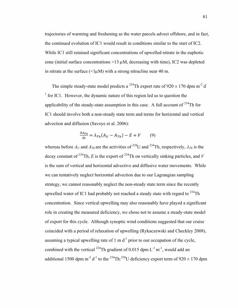
81

trajectories of warming and freshening as the water parcels advect offshore, and in fact,

the continued evolution of IC1 would result in conditions similar to the start of IC2.

While IC1 still retained significant concentrations of upwelled nitrate in the euphotic

zone (initial surface concentrations >13 M, decreasing with time), IC2 was depleted

in nitrate at the surface (<1M) with a strong nitracline near 40 m.

The simple steady-state model predicts a 234Th export rate of 920 ± 170 dpm m-2 d-

1 for IC1. However, the dynamic nature of this region led us to question the

applicability of the steady-state assumption in this case. A full account of 234Th for

IC1 should involve both a non-steady state term and terms for horizontal and vertical

advection and diffusion (Savoye et al. 2006):

λ (9)

whereas before AU and ATh are the activities of 238U and 234Th, respectively, Th is the

decay constant of 234Th, E is the export of 234Th on vertically sinking particles, and V

is the sum of vertical and horizontal advective and diffusive water movements. While

we can tentatively neglect horizontal advection due to our Lagrangian sampling

strategy, we cannot reasonably neglect the non-steady state term since the recently

upwelled water of IC1 had probably not reached a steady state with regard to 234Th

concentration. Since vertical upwelling may also reasonably have played a significant

role in creating the measured deficiency, we chose not to assume a steady-state model

of export for this cycle. Although synoptic wind conditions suggested that our cruise

coincided with a period of relaxation of upwelling (Rykaczewski and Checkley 2008),

assuming a typical upwelling rate of 1 m d-1 prior to our occupation of the cycle,

combined with the vertical 234Th gradient of 0.015 dpm L-1 m-1, would add an

additional 1500 dpm m-2 d-1 to the 234Th:238U deficiency export term of 920 ± 170 dpm

82

m-2 d-1. Thus, the total export of 234Th for this upwelling affected cycle may be over

150% higher than that derived from the steady-state assumption. However, a technical

failure prevented us from measuring the C:234Th ratio of exported particulates for this

cycle; hence, we cannot reliably convert the 234Th export measurement to its C export

equivalent.

IC2 is a better fit to the assumptions required for steady state. Slightly decreasing

density of the surface water, combined with the aforementioned synoptic wind

measurements, suggest that upwelling was not significant. A comparison of the

vertically integrated deficiencies for the final day of IC1 (37,900 dpm m-2) and the first

day of IC2 (37,500 dpm m-2) suggest also that the inclusion of a non-steady state term

would have negligible impact on the export calculation (see Discussion). Repeat

profiles suggest that differences within IC2a were due to a deepening of the

thermocline and nitracline from 38 to 42 m, perhaps driven by some combination of

downwelling and/or internal waves and tides. Further support for a steady-state

interpretation comes from the rapid switch from net deficiency to net remineralization

at the base of the (~50 m) euphotic zone for IC2a. IC2b (a separate one-day

experiment) was in a slightly different water mass that showed a higher deficiency

(65,300 ± 20,000 versus 39,700 ± 2,200 dpm m-2 for IC2b and IC2a, respectively) and

lower C:234Th ratio (50 ± 5 versus 133 ± 16 µmolC dpm-1 and for IC2b and IC2a,

respectively). We therefore use separate C: 234Th ratios for the two segments of IC2 to

calculate carbon export across the 100-m depth horizon.

Although IC1 had a significantly higher biomass than IC2, the biological

community behaved similarly in both inshore cycles. For both cycles (including both

sections of IC2), growth exceeded grazing, and the ambient phytoplankton grew at net

rates similar to those predicted experimentally (Fig. 2, Table 1). Mesozooplankton

83

grazing was slightly higher during IC1 than IC2, contributing 39 ± 29% of grazing

compared to 23 ± 25%. Our trophic relationships suggested an e-ratio of 0.08 ± 0.01

for IC2a compared to a ThE-ratio of 0.09 ± 0.01, and an e-ratio of 0.08 ± 0.03

compared to a ThE of 0.07 ± 0.03 for IC2b. For IC1, the trophic relationships

predicted an e-ratio of 0.12 ± 0.02, but, as mentioned previously, the lack of a C:234Th

ratio did not allow us to calculate a corresponding ThE-ratio.

Discussion

Trophic cycling and carbon export – The suite of measurements from each

experimental cycle in the present study allow us to assess the biological regulation of

two biogeochemically relevant processes, autotrophic biomass accumulation and

vertical carbon flux. By making process rate measurements while monitoring the

temporal evolution of the phytoplankton community, Landry et al. (2009)

demonstrated that phytoplankton growth and grazing losses determine to first order the

observed net growth rates of the phytoplankton in the CCE. Fig. 3b clearly shows the

strong correlation between the calculated and observed net rates of change. For all

cycles, the two measurements fall within the margin of error. Although there is a

slight (0.04 d-1 average) overestimate in the calculated rates of change relative to the

observed rates, this discrepancy reflects, in part, our choice (for consistency) to

integrate all rates to the depth of the deepest primary productivity sample incubations,

as growth typically decreases more rapidly with depth than grazing.

Our simple trophic model builds on these previous findings to explain the

variability of e-ratios (and hence vertical carbon flux) determined on the May 2006

cruise (Fig. 7). In fact, 234Th steady-state estimates of export were in good agreement

with those predicted from measured growth and grazing rates and the trophic model,

84

well within margins of error for all cycles for which carbon export could be assessed

(Cycles 2-4). This agreement, despite major differences in the planktonic

communities investigated, suggests that the underlying processes regulating export are

relatively similar throughout the system. Net phytoplankton growth rate was highly

variable and driven by the balance between growth and grazing processes dominated

by microzooplankton. Export rates, however, were consistent in all cases with the sum

of direct and indirect trophic linkages between phytoplankton and mesozooplankton.

It is important to note that the rates utilized for e-ratio calculations (specific growth

rate, micro- and mesozooplankton grazing rates) were entirely distinct from the

parameters used to calculate ThE-ratios (234Th deficiency, C:234Th ratio, 14C-PP).

Furthermore, the independent parameters in the calculations (egestion efficiency and

gross growth efficiency) were not tuned to the data; canonical mean values of 0.30

were used for each. Thus, the ability to explain the general low magnitude and two-

fold variability in ThE-ratio is a striking result suggesting that we may have

reasonably represented the processes that regulate carbon export in this system. At

worst, it indicates that the Th-derived export estimates are consistent with reasonable

inferences about the plankton trophic interactions leading to fecal pellet production by

mesozooplankton.

Export Measurements – All carbon export methods have limitations and sources of

error. Surface-tethered sediment traps, for instance, collect sinking material for

specific depths and time periods of deployment, but those measurements can be biased

by complex flows around the collector mouth (Buesseler et al. 2007) that may be

exacerbated in a dynamic region like the CCE. Additionally, sediment traps measure

carbon flux not of the water column directly above their deployment, but rather from a

85

statistical funnel determined by the ratio of horizontal diffusivities and current

velocities to vertical sinking rates of particulate material (Siegel et al. 1990).

Radionuclide disequilibrium methods (including 238U-234Th, 210Pb-210Po, and 90Y-

90Sr) overcome this difficulty by explicitly approximating export from specific patches

of water; however, they also have their own associated errors. Each method must

approximate the ratio of C:radionuclide, a value with significant spatiotemporal and

methodological variability (see Buesseler et al. 2006). Additionally, the impracticality

of obtaining fully resolved deficiency profiles requires that assumptions be made about

the relative importance of terms in the full accounting of radionuclide activities (see

Equ. 9). These include vertical and horizontal water movements, advection as well as

diffusion, although the latter parameter is typically neglected assuming that horizontal

gradients and vertical diffusivity are both minimal. For our Lagrangian sampling plan,

we also neglect horizontal processes. Vertical velocities can be a significant term in

coastal regions when strong upwelling transports subsurface sufficiencies of 234Th into

the mixed layer. However, synoptic wind measurements suggest that upwelling was

minimal during our cruise (Rykaczewski and Checkley 2008).

The assumption of temporal steady state is a major issue within our study region,

particularly at inshore sites where high springtime productivity and biomass

accumulation may lead to episodic export events. An ideal study would track a parcel

of water for an extended period to measure the temporal evolution of water-column

deficiency. However, truly effective tracking is methodologically difficult at best and

more likely impossible in regions with vertical shear and horizontal heterogeneity.

Thus, tradeoffs must be made between errors associated with inaccurate assessment of

changing deficiencies and with slip relative to an in situ water parcel. Savoye et al.

(2006) evaluated the uncertainty associated with the non-steady state (NSS)

86

approximation and suggested that water parcels be revisited after a period of >1-2

weeks, as shorter duration studies will have high uncertainties. Tracking a water parcel

unambiguously in a heterogeneous a region like the CCE for weeks would be very

difficult.

Figure 5 is a starting point for addressing the role that a non-steady state term

might play in the inshore region since IC2a seems to have sampled similar water to

IC1 that had aged as it moved offshore. From the mean deficiencies for IC1 and IC2a

(31,800 ± 6000 and 39,700 ± 2200 dpm m-2, respectively) and the time difference

between the 234Th measurements (12.7 days), we can calculate a NSS export of 1790 ±

488 dpm m-2 d-1 (mean ± S.E.) for the period between the two cycles. By this

calculation, the steady-state export estimate of 1140 ± 70 dpm m-2 d-1 for IC2a may be

low by ~36%, although 95% confidence intervals for the two determinations are not

statistically different. The origins of the two water parcels may also not have been

identical, accounting for some of their deficiency difference. Nonetheless, this

comparison helps to put some constraints on the magnitude of the errors associated

with the steady-state assumption.

Timescales - When the ThE-ratio is used to compute the fraction of phytoplankton

production exported to depth, it is important to consider the relevant timescales of the

measurements involved. 234Th disequilibrium averages export over the mean lifetime

of 234Th (35 days). 234Th-derived export values and C:234Th ratio at depth should

therefore not change substantially over a few days. 14C-PP, meanwhile, considers

phytoplankton production only over the duration of the incubation (usually 24 h).

Thus, for a water parcel with high daily variability in primary productivity about a

central mean, the ThE-ratio (234Th derived carbon export / 14C-PP) measured over

87

several days might well show a spurious inverse correlation of primary productivity

with ThE-ratio, driven by variability of the 14C-PP denominator.

With the Lagrangian experimental design, we were able to average several days of

daily euphotic-zone integrated rate measurements for primary productivity,

phytoplankton growth and grazing in each water parcel, thereby minimizing spurious

results that might have arisen from process experiments conducted with more typical

fixed-station sampling and allowing for measurements on the timescale of our

experimental cycles (~4 days). Mesozooplankton grazing, however, is a rate with two

intrinsic time-scales. While grazer-specific grazing rate can vary rapidly due to

changes in both behavior (e.g. diel vertical migration or selective grazing) and prey

field, mesozooplankton biomass itself has a longer time-scale on the order of weeks.

The longer generation times of mesozooplankton may thus serve to dampen changes in

export on short time periods (days to weeks) when fecal carbon flux dominates over

direct sinking of phytoplankton.

For the four water parcels for which we have carbon export measurements (OOP,

CCP, IC2a and IC2b), ThE-ratios are inversely correlated with net rates of change of

the phytoplankton community (Table 1). In the OOP cycle, phytoplankton biomass

declined over the 4-day cycle, and we measured a relatively high ThE-ratio.

Conversely, in the inshore region of accumulating phytoplankton biomass, the ThE-

ratio was lower. Over longer time periods than the experimental cycles, we would

expect phytoplankton to reach a quasi-steady state, with growth balanced by grazing

and other loss processes. Mechanistically, we could hypothesize that zooplankton

grazing had temporarily outpaced phytoplankton growth in the offshore region and

hence was reducing community biomass and primary production. Reduced food

resources for microzooplankton grazers and perhaps mesozooplankton switching

88

predation pressure from phytoplankton to microzooplankton would presumably

resolve this imbalance in time, allowing phytoplankton to increase. Nutrient decline

and increasing grazing capacity would serve similarly as negative feedbacks to bring

the accumulating phytoplankton biomass of the inshore area back into balance. These

patterns are suggestive of a system in which contemporaneous imbalances of growth

and grazing lead to autotrophic biomass accumulation (rather than sinking) or net

heterotrophy on short timescales, while export measurements and the drivers of export

reflect longer (weekly) timescales. Thus, temporal decoupling of the fast

phytoplankton dynamics and the slower timescales of mesozooplankton population

change implies that utilizing a constant e-ratio to estimate export capacity from

primary production alone will have limited efficacy. Instead, rate measurements that

explicitly partition this primary productivity into different utilization pathways may be

necessary.

Microzooplankton shunt - Traditional formulations of the microbial loop (Azam et

al. 1983) assume multiple trophic transfers within the microzooplankton, which

greatly diminish transfer to mesozooplankton. The microbial food web is therefore

considered to function largely as a remineralization pathway. Meanwhile, the

prevalence of mesozooplankton fecal pellets and aggregates of larger cells, like

diatoms, in sediment traps has led to an emphasis on the classical food chain in

vertical carbon flux (Michaels and Silver 1988; Fasham et al. 2001). Contrary to this

simple dichotomy, our rate relationships for the CCE suggest that microzooplankton

can provide an important shunt of production from phytoplankton to mesozooplankton,

with a single trophic step on average. To allow for additional trophic transfers within

the microzooplankton, we need only add an exponent n to the microzooplankton GGE.

‐ratio ∗ ∗ (10)

89

Functionally, n represents the mean number of microzooplankton trophic steps that

separate phytoplankton from mesozooplankton. The need to vary this parameter

would obviously be greater in biological communities dominated by very small

phytoplankton and with high grazing impact of microzooplankton, as is generally the

case in the open ocean (Calbet and Landry 2004). Nonetheless, a meta-analysis of

dilution experiments has shown that the percentage of primary productivity consumed

on average by microzooplankton in coastal regions (60%) is not greatly different from

the 70% consumed in oceanic systems (Landry and Calbet 2004). Although our

coastal-offshore differences in microzooplankton grazing (42-44% vs 77-123%,

respectively) were more extreme than the global averages, there was adequate food

chain transfer for the OOP to support a moderate rate of export via the

mesozooplankton, in fact the highest export ratio that we measured. Thus, the

efficiency of transfer from micro- to mesozooplankton becomes an important

determinant of the amount of primary productivity that can be exported. If we assume

only a single trophic step within the microzooplankton in our experiments, then the

relative proportion of mesozooplankton nutrition derived from microzooplankton

ranges from 32 to 79% for our four cycles, which agrees well with the

C:phaeopigment measurements of Small and Ellis (1992). Our relationships thus

suggest that far from being strictly a remineralization pathway, the microzooplankton

in the CCE shunt a significant amount of carbon into the export pathway.

Decoupling of new and export production - With typical f-ratios ranging from 0.2

to 0.8 in the Southern California Bight (Eppley et al. 1979), new production generally

exceeds export production inshore of the CCP (e.g. Nelson et al. 1987). An estimate

of the f-ratio can be gleaned from our relationships if we assume that the rate of uptake

of recycled nitrogen is equal to its rate of production, which follows from the

90

preferential utilization of NH4+ over NO3

- by phytoplankton. If we assume that

phytoplankton do not exude nutrients, the rate of production of autochthonous material

is simply the difference between the gross phytoplankton growth rate (PP) and the

rate of export and biomass accumulation. Thus:

RecycledProduction (11)

Since new production is the difference between total and recycled production, we can

divide by total production (μPP) to calculate an f-ratio:

f‐ratio e‐ratio (12)

By substituting in Equations (1), (3) and (7) and rearranging, we can see that the f-

ratio is dependent on the rates of phytoplankton growth and micro- and

mesozooplankton community grazing:

f‐ratio (13)

However, this formulation is valid only if autochthonous production (Eq. 11) is less

than total production, which may not be true if the phytoplankton community is

declining (as for our offshore cycle). In addition, this calculated f-ratio neglects

nitrogen excretion by phytoplankton, which would decrease the ratio by a factor of

1/(1+%NPP excreted). Given the uncertainties in our biological rate measurements, a

relatively large excretion rate of 30% would still produce an f-ratio estimate within one

standard error of the results of Eq. 13.

Theabovemodelcalculationscanbecomparedtoregressionestimatesofnew

productionbyHarrisonetal. 1987 that show a linear relationship (slope = 0.77 ±

0.10; intercept = 0.06 ± 0.02) between new production and the nutrient ratio of [NO3-]

to combined [NO3-] + [NH4

+] in the CCE based on measurements from Eppley et al.

91

(1979). f-ratios were calculated at each of our 14C-PP sampling depths and then

vertically integrated to calculate new production and hence the average f-ratio of the

euphotic zone. This approach produces results in close agreement with our trophic

calculations (Table 2), both predicting f-ratios of 0.6 to 0.8 for the nearshore cycles

and ~0.3 for the CCP. For the OOP cycle, the assumption that autochthonous nutrient

uptake matched production was violated, resulting in a negative ratio. Nevertheless,

both calculations clearly predict significantly higher f-ratios in the inshore region, in

contrast to the low measured and modeled e-ratios in this region.

Olivieri and Chavez (2000) and Plattner et al. (2005) have hypothesized that

offshore transport of water upwelled near the California coast leads to a

spatiotemporal decoupling of new and export production. The obvious disparity

between our e- and f-ratios supports this view, and our Lagrangian sampling provides

a unique perspective on the underlying processes. All of our inshore water parcels

drifted rapidly offshore (net speeds of 13, 20 and 18 cm s-1 for IC1, IC2a and IC2b,

respectively) as we measured net positive growth rates for the phytoplankton. In

addition, we observed that particulate organic carbon and chlorophyll accumulated

during offshore transport of each inshore cycle, with average rates of chlorophyll

increase of 0.10, 0.14 and 0.28 d-1 for IC1, IC2a and IC2b, respectively.

The calculated excess of new production to export in the offshore region may be

due to several factors. Carbon export could have been temporally decoupled from new

production, with net production during spring conditions. Active transport of organic

matter from the surface to depth by vertically migrating animals may also have been a

relatively important component of export in these waters (e.g. Steinberg et al. 2000).

Additionally, synoptic wind conditions (Rykaczewski and Checkley 2008) as well as

the net changes in temperature and salinity observed along our drifter tracks were

92

consistent with the possibility of slow subduction of surface water as it moved

offshore. However, we scrupulously avoided areas with strong gradients when we

initiated our experiments and therefore avoided major subduction fronts that can occur

where the offshore advection of cold saline upwelled water reaches the lower salinity

CCP (Kadko et al. 1991; Washburn et al. 1991).

Changing zooplankton concentrations: implications - The discrepancies between

our estimates of e- and f-ratios based on trophic interactions suggest that particulate

flux of sinking phytoplankton and/or subduction may be important export processes in

the CCE at some times and places. Nonetheless, on the daily timescales at which

parcels of water generally move in the system, our relationships suggest that vertical

flux can be reasonably explained by contemporaneous food-web processes leading to

mesozooplankton consumption and fecal pellet production. The central role of

zooplankton as flux mediators in these model calculations suggests a potential

coupling between climate-associated community changes and carbon export in the

CCE. The secular warming trend evident in CalCOFI data (Roemmich 1992) has been

linked, for example, to a 70% decline in the biovolume of large zooplankton

(Roemmich and Mcgowan 1995b,a), notably a decrease in salps (Lavaniegos and

Ohman 2007). Because of their high filtration rates and dense, rapidly sinking fecal

pellets, such organisms contribute disproportionately to the flux of organic matter to

the deep sea (Bruland and Silver 1981; Silver and Bruland 1981; Pfannkuche and

Lochte 1993). This decadal decline in mesozooplankton therefore suggests a

substantial decrease in the efficiency of coupling of primary productivity to export in

the CCE region.

In summary, we found that calculations based on simple trophic relationships and

experimental process rate measurements in the CCE were consistent with measured

93

variations in the e-ratios of water parcels representing a range of conditions from

recently upwelled coastal water to oligotrophic offshore regions. The good agreement

between independently measured ecological and biogeochemical rates in these very

different plankton assemblages suggest that zooplankton dynamics are an important,

though often neglected, primary driver of vertical carbon flux in this system. For the

range of conditions studied, variability in export efficiency was determined by the

local net balance of growth and grazing processes and the relative strengths of grazing

pathways through microzooplankton versus directly to mesozooplankton. This study

was limited however to a few water parcels believed to be representative of the region

during springtime. Therefore, further work is necessary to assess biological controls

of carbon export under different seasonal conditions as well as to quantify and

compare results to purely physical mechanisms of export, such as along subduction

fronts. In this regard, the Lagrangian design that we used to obtain the rate

measurements for this study appears to be a workable approach for constraining

ecological and biogeochemical relationships in complex coastal regions, with the

eventual goal of extending these relationships into mechanistic models with predictive

power.

Acknowledgments

We thank the captain and crew of the R/V Knorr for their professionalism and

contributions to conducting these experiments at sea. We are grateful to all of our

colleagues in the California Current Ecosystem, Long-Term Ecological Research

(CCE LTER) program for their support and collaboration, and particularly to M. D.

Ohman for providing the mesozooplankton grazing results. We give special thanks to

94

M. Décima, S. Dovel, M. Roadman, R. Rykaczewski, J. Powell, D. Taniguchi, and K.

Tsyrklevich for their assistance at sea and in laboratory analyses, and to M.D. Ohman

and P.J.S. Franks for insightful discussions and suggestions on earlier versions of the

paper. This work was supported by National Science Foundation (NSF) funding

(OCE-04-17616) for the CCE LTER site, and by graduate research fellowships (NSF

and NASA Earth and Space Science) to M. Stukel.

Chapter 2, in full, has been submitted for publication in Limnology and

Oceanography: Stukel, M. R., Landry, M.R., 2010, Benitez-Nelson, C. R., Goericke,

R. “Trophic Cycling and carbon export relationships in the California Current

Ecosystem.” The dissertation author was the primary investigator and author of this

paper.

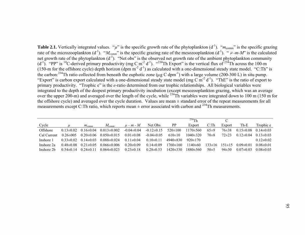
95

Table 2.1. Vertically integrated values. “µ” is the specific growth rate of the phytoplankton (d-1). “mcomm” is the specific grazing rate of the microzooplankton (d-1). “Mcomm” is the specific grazing rate of the mesozooplankton (d-1). “μ-m-M” is the calculated net growth rate of the phytoplankton (d-1). “Net obs” is the observed net growth rate of the ambient phytoplankton community (d-1). “PP” is 14C-derived primary productivity (mg C m-2 d-1). “234Th Export” is the vertical flux of 234Th across the 100-m (150-m for the offshore cycle) depth horizon (dpm m-2 d-1) as calculated with a one-dimensional steady state model. “C:Th” is the carbon:234Th ratio collected from beneath the euphotic zone (g C dpm-1) with a large volume (200-300 L) in situ pump. “Export” is carbon export calculated with a one-dimensional steady state model (mg C m-2 d-1). “ThE” is the ratio of export to primary productivity. “Trophic e” is the e-ratio determined from our trophic relationships. All biological variables were integrated to the depth of the deepest primary productivity incubation (except mesozooplankton grazing, which was an average over the upper 200-m) and averaged over the length of the cycle, while 234Th variables were integrated down to 100 m (150 m for the offshore cycle) and averaged over the cycle duration. Values are mean ± standard error of the repeat measurements for all measurements except C:Th ratio, which reports mean ± error associated with carbon and 234Th measurements.

Cycle μ mcomm Mcomm μ – m - M Net Obs PP

234Th Export C:Th

C Export Th-E Trophic e

Offshore 0.13±0.02 0.16±0.04 0.013±0.002 -0.04±0.04 -0.12±0.15 520±100 1170±560 65±9 76±38 0.15±0.08 0.14±0.03Cal Current 0.26±005 0.20±0.06 0.050±0.015 0.01±0.08 -0.04±0.05 610±10 1040±320 70±8 72±23 0.12±0.04 0.13±0.03Inshore 1 0.33±0.02 0.14±0.03 0.088±0.024 0.11±0.04 0.10±0.11 4940±830 920±170 0.12±0.02Inshore 2a 0.48±0.08 0.21±0.05 0.066±0.006 0.20±0.09 0.14±0.09 1760±160 1140±60 133±16 151±15 0.09±0.01 0.08±0.01Inshore 2b 0.54±0.14 0.24±0.11 0.064±0.023 0.23±0.18 0.28±0.53 1420±330 1880±560 50±5 94±30 0.07±0.03 0.08±0.03

95

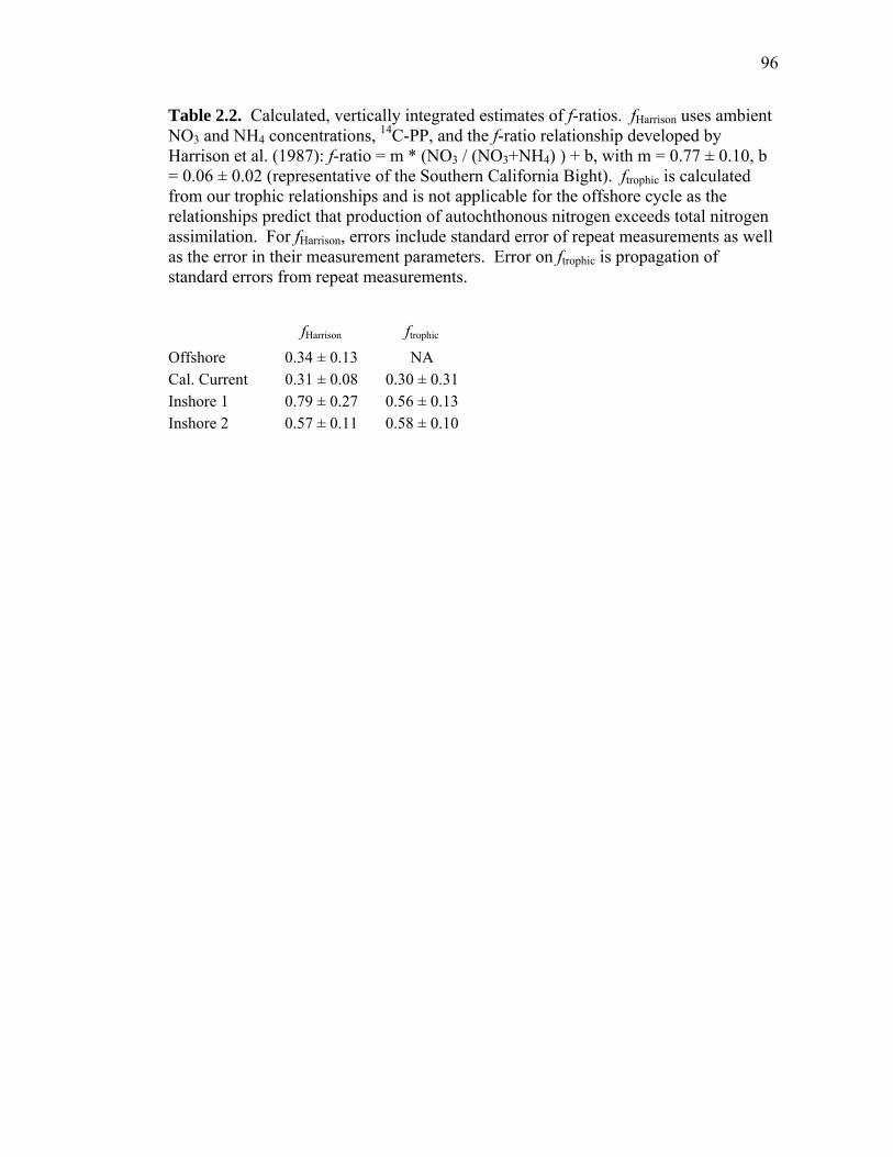
96

Table 2.2. Calculated, vertically integrated estimates of f-ratios. fHarrison uses ambient NO3 and NH4 concentrations, 14C-PP, and the f-ratio relationship developed by Harrison et al. (1987): f-ratio = m * (NO3 / (NO3+NH4) ) + b, with m = 0.77 ± 0.10, b = 0.06 ± 0.02 (representative of the Southern California Bight). ftrophic is calculated from our trophic relationships and is not applicable for the offshore cycle as the relationships predict that production of autochthonous nitrogen exceeds total nitrogen assimilation. For fHarrison, errors include standard error of repeat measurements as well as the error in their measurement parameters. Error on ftrophic is propagation of standard errors from repeat measurements.

fHarrison ftrophic

Offshore 0.34 ± 0.13 NA Cal. Current 0.31 ± 0.08 0.30 ± 0.31 Inshore 1 0.79 ± 0.27 0.56 ± 0.13 Inshore 2 0.57 ± 0.11 0.58 ± 0.10

Figure 2.1 -while thconductContourbottom rsouthwe

- Map of thehe rectanglesed. Light grr lines for searight shows estern coast o

e study regio represent thray dots showafloor depththe study areof North Am

on. The starshe four locatw standard C

hs of 1000, 2ea (black rec

merica.

s show the lotions at whicCalCOFI sam000 and 300ctangle) with

ocations of ach experimenmpling statio00 m are in ghin the conte

all 234Th profntal cycles wons in the aregray. Inset aext of the

97

files, were ea. at

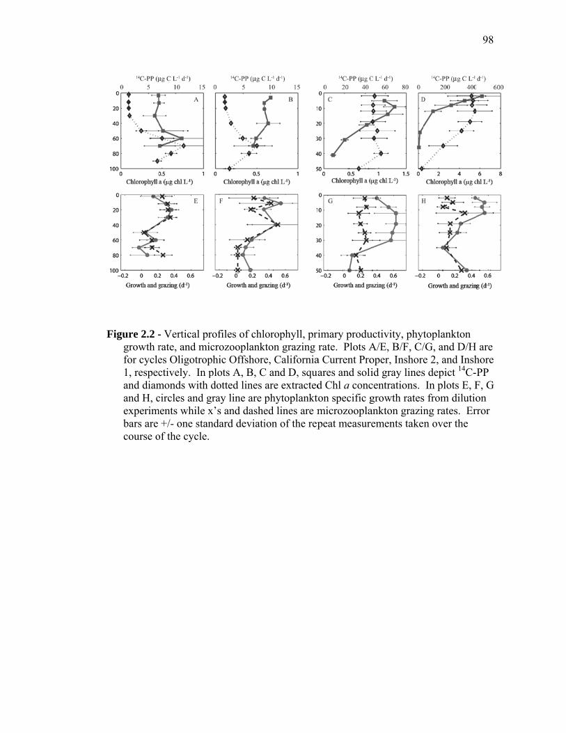
Figure 2.2 -growth rfor cycle1, respecand diamand H, cexperimbars are course o

- Vertical prrate, and mices Oligotropctively. In pmonds with dcircles and g

ments while x+/- one stan

of the cycle.

rofiles of chlcrozooplank

phic Offshoreplots A, B, Cdotted lines ray line are p

x’s and dashendard deviati

orophyll, prikton grazing e, California

C and D, squaare extractedphytoplankted lines are mion of the rep

imary produrate. Plots A

a Current Proares and solid Chl a concton specific gmicrozooplapeat measur

uctivity, phytA/E, B/F, C/oper, Inshoreid gray linescentrations. growth ratesankton grazinrements take

toplankton /G, and D/H e 2, and Inshs depict 14C-In plots E, F

s from dilutiong rates. Ern over the

98

are hore PP F, G on rror

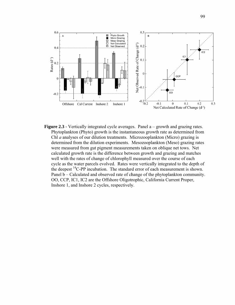
Figure 2.3 -PhytoplaChl a andeterminwere mecalculatewell witcycle as the deepPanel b OO, CCInshore

- Vertically iankton (Phynalyses of ouned from theeasured fromed growth rath the rates othe water pa

pest 14C-PP i– Calculated

CP, IC1, IC2 1, and Insho

integrated cyto) growth i

ur dilution tre dilution exp

m gut pigmenate is the diffof change of arcels evolveincubation. d and observare the Offs

ore 2 cycles,

ycle averages the instanteatments. Mperiments. Mnt measuremference betwchlorophyll ed. Rates wThe standard

ved rate of chshore Oligotr

respectively

es. Panel a –aneous grow

MicrozooplanMesozoopla

ments taken oween growth

measured owere verticall

d error of eahange of therophic, Calify.

– growth andwth rate as denkton (Micro

ankton (Mesoon oblique neh and grazingover the courly integratedach measureme phytoplankfornia Curre

d grazing ratetermined fro) grazing iso) grazing raet tows. Netg and matcherse of each d to the depthment is show

kton communent Proper,

99

tes. rom s ates t es

h of wn. nity.

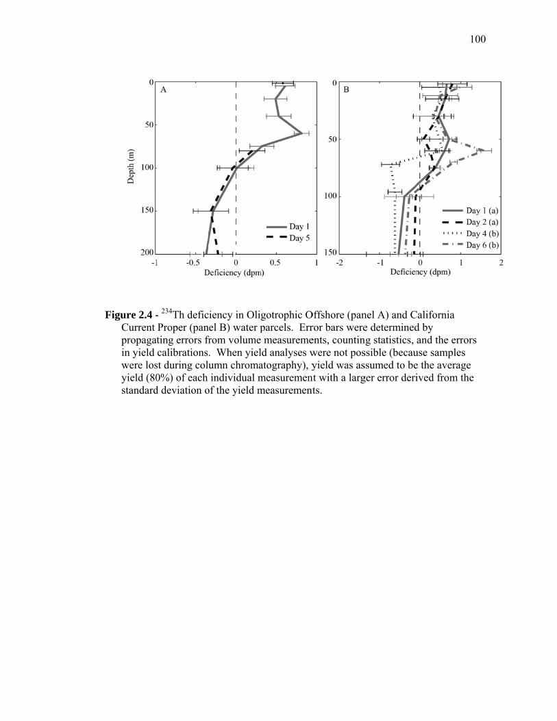
Figure 2.4 -Current propagain yield were losyield (80standard

- 234Th deficProper (pan

ating errors frcalibrations

st during col0%) of each d deviation o

ciency in Olinel B) water pfrom volume. When yielumn chromaindividual m

of the yield m

gotrophic Oparcels. Err

e measuremeld analyses watography), ymeasuremenmeasurement

Offshore (panror bars wereents, countinwere not posyield was as

nt with a largts.

nel A) and Ce determined

ng statistics, ssible (becaussumed to beger error deri

California d by and the error

use samples e the averageived from th

100

rs

e he

Figure 2.5 -CTD proand less

- Vertically aofiles of the saline over

averaged temfour water pthe time per

mperature anparcels. Botriod of our cy

nd salinity foth Inshore Cyycles.

or the upper ycle 1 & 2 b

50 m of all became warm

101

mer

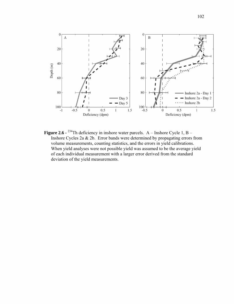
Figure 2.6 -Inshore volume When yiof each ideviatio

- 234Th deficCycles 2a &measuremenield analysesindividual mn of the yiel

ciency in insh& 2b. Error bnts, countings were not p

measurementld measurem

hore water pbands were dg statistics, aossible yieldt with a large

ments.

parcels. A –determined band the errord was assumer error deriv

Inshore Cycby propagatirs in yield ca

med to be the ved from the

cle 1, B – ing errors froalibrations.

average yiee standard

102

om

eld

Figure 2.7 -

state moCurrent

- Comparisoodel. OO, CProper, Insh

on of trophic CP, IC2a, IChore 2a, and

cycling relaC2b are the OInshore 2b c

ationships toOffshore Olicycles, respe

o 234Th deficiigotrophic, Cectively.

iency steadyCalifornia

103

y-

104

References

ALLDREDGE, A. L., and C. C. GOTSCHALK. 1989. Direct observations of the mass

flocculation of diatom blooms: characteristics, settling velocities and formation of diatom aggregates. Deep-Sea Res. 36: 159-171.

ARMSTRONG, R. A., C. LEE, J. I. HEDGES, S. HONJO, and S. G. WAKEHAM. 2002. A

new, mechanistic model for organic carbon fluxes in the ocean based on the quantitative association of POC with ballast minerals. Deep-Sea Res. II 49: 219-236.

AZAM, F., T. FENCHEL, J. G. FIELD, J. S. GRAY, L. A. MEYER-REIL, and F. THINGSTAD.

1983. The ecological role of water-column microbes in the sea. Mar. Ecol. Prog. Ser. 10: 257-263.

BENITEZ-NELSON, C. R., K. O. BUESSELER, M. R. VAN DER LOEFF, J. ANDREWS, L.

BALL, G. CROSSIN, and M. A. CHARETTE. 2001. Testing a new small-volume technique for determining Th-234 in seawater. J. Radioanal. Nucl. Chem. 248: 795-799.

BRULAND, K. W., and M. W. SILVER. 1981. Sinking rates of fecal pellets from

gelatinous zooplankton (salps, pteropods, doliolids). Mar. Biol. 63: 295-300. BUESSELER, K. O. 1998. The decoupling of production and particulate export in the

surface ocean. Glob. Biogeochem. Cycle 12: 297-310. BUESSELER, K. O., A. N. ANTIA, M. CHEN, S. W. FOWLER, W. D. GARDNER, O.

GUSTAFSSON, K. HARADA, A. F. MICHAELS, M. R. VAN DER LOEFF'O, M. SARIN, D. K. STEINBERG, and T. TRULL. 2007. An assessment of the use of sediment traps for estimating upper ocean particle fluxes. J. Mar. Res. 65: 345-416.

BUESSELER, K. O., C. BENITEZ-NELSON, M. R. VAN DER LOEFF, J. ANDREWS, L. BALL,

G. CROSSIN, and M. A. CHARETTE. 2001. An intercomparison of small- and large-volume techniques for thorium-234 in seawater. Mar. Chem. 74: 15-28.

BUESSELER, K. O., C. R. BENITEZ-NELSON, S. B. MORAN, A. BURD, M. CHARETTE, J. K.

COCHRAN, L. COPPOLA, N. S. FISHER, S. W. FOWLER, W. GARDNER, L. D. GUO, O. GUSTAFSSON, C. LAMBORG, P. MASQUE, J. C. MIQUEL, U. PASSOW, P. H. SANTSCHI, N. SAVOYE, G. STEWART, and T. TRULL. 2006. An assessment of particulate organic carbon to thorium-234 ratios in the ocean and their impact on the application of 234Th as a POC flux proxy. Mar. Chem. 100: 213-233.

105

CALBET, A., and M. R. LANDRY. 2004. Phytoplankton growth, microzooplankton grazing, and carbon cycling in marine systems. Limnol. Oceanogr. 49: 51-57.

CHEN, J. H., R. L. EDWARDS, and G. J. WASSERBURG. 1986. 238U, 234U and 232Th in

seawater. Earth Planet. Sci. Lett. 80: 241-251. CONOVER, R. J. 1966. Assimilation of organic matter by zooplankton. Limnol.

Oceanogr. 11: 338-345. EPPLEY, R. W., and B. J. PETERSON. 1979. Particulate Organic-Matter Flux and

Planktonic New Production in the Deep Ocean. Nature 282: 677-680. EPPLEY, R. W., E. H. RENGER, and W. G. HARRISON. 1979. Nitrate and phytoplankton

production in southern California coastal waters. Limnol. Oceanogr. 24: 483-494.

FASHAM, M. J. R., B. M. BALINO, M. C. BOWLES, R. ANDERSON, D. ARCHER, U.

BATHMANN, P. BOYD, K. BUESSELER, P. BURKILL, A. BYCHKOV, C. CARLSON, C. T. A. CHEN, S. DONEY, H. DUCKLOW, S. EMERSON, R. FEELY, G. FELDMAN, V. GARCON, D. HANSELL, R. HANSON, P. HARRISON, S. HONJO, C. JEANDEL, D. KARL, R. LE BORGNE, K. K. LIU, K. LOCHTE, F. LOUANCHI, R. LOWRY, A. MICHAELS, P. MONFRAY, J. MURRAY, A. OSCHLIES, T. PLATT, J. PRIDDLE, R. QUINONES, D. RUIZ-PINO, T. SAINO, E. SAKSHAUG, G. SHIMMIELD, S. SMITH, W. SMITH, T. TAKAHASHI, P. TREGUER, D. WALLACE, R. WANNINKHOF, A. WATSON, J. WILLEBRAND, and C. S. WONG. 2001. A new vision of ocean biogeochemistry after a decade of the Joint Global Ocean Flux Study (JGOFS). Ambio 10: 4-31.

GREEN, S. E., and R. N. SAMBROTTO. 2006. Plankton community structure and export

of C, N, P and Si in the Antarctic Circumpolar Current. Deep-Sea Res. II 53: 620-643.

HARRISON, W. G., T. PLATT, and M. R. LEWIS. 1987. F-ratio and its relationship to

ambient nitrate concentration in coastal waters. J. Plankton Res. 9: 235-248. JACKSON, G. A. 2001. Effect of coagulation on a model planktonic food web. Deep-

Sea Res. I 48: 95-123. KADKO, D. C., L. WASHBURN, and B. JONES. 1991. Evidence of Subduction within

Cold Filaments of the Northern California Coastal Transition Zone. J. Geophys. Res. Oceans 96: 14909-14926.

LANDRY, M. R., and A. CALBET. 2004. Microzooplankton production in the oceans.

ICES J. Mar. Sci. 61: 501-507.

106

LANDRY, M. R., C. J. LORENZEN, and W. K. PETERSON. 1994. Mesozooplankton grazing in the Southern California Bight .2. Grazing impact and particulate flux. Mar. Ecol. Prog. Ser. 115: 73-85.

LANDRY, M. R., M. D. OHMAN, M. R. STUKEL, and K. TSYRKLEVICH. 2009.

Lagrangian studies of phytoplankton growth and grazing relationships in a coastal upwelling ecosystem off Southern California. Prog. Oceanogr. 83: 208-216.

LAVANIEGOS, B. E., and M. D. OHMAN. 2007. Coherence of long-term variations of

zooplankton in two sectors of the California Current System. Prog. Oceanogr. 75: 42-69.

LYNN, R. J., and J. J. SIMPSON. 1987. The California Current System: the seasonal

variability of its physical characteristics. J. Geophys. Res. Oceans 92: 12947-&. MICHAELS, A. F., and M. W. SILVER. 1988. Primary production, sinking fluxes and the

microbial food web. Deep-Sea Res. 35: 473-490. NELSON, J. R., J. R. BEERS, R. W. EPPLEY, G. A. JACKSON, J. J. MCCARTHY, and A.

SOUTAR. 1987. A particle flux study in the Santa Monica-San Pedro Basin off Los Angeles: particleflux, primary production, and transmissometer survey. Cont. Shelf Res. 7: 307-328.

OLIVIERI, R. A., and F. P. CHAVEZ. 2000. A model of plankton dynamics for the

coastal upwelling system of Monterey Bay, California. Deep-Sea Res. II 47: 1077-1106.

PASSOW, U., A. L. ALLDREDGE, and B. E. LOGAN. 1994. The role of particulate

carbohydrate exudates in the flocculation of diatom blooms. Deep-Sea Res. I 41: 335-357.

PASSOW, U., R. F. SHIPE, A. MURRAY, D. K. PAK, M. A. BRZEZINSKI, and A. L.

ALLDREDGE. 2001. The origin of transparent exopolymer particles (TEP) and their role in the sedimentation of particulate matter. Cont. Shelf Res. 21: 327-346.

PFANNKUCHE, O., and K. LOCHTE. 1993. Open ocean pelago-benthic coupling:

cyanobacteria as tracers of sedimenting salp feces. Deep-Sea Res. I 40: 727-737.

PIKE, S. M., K. O. BUESSELER, J. ANDREWS, and N. SAVOYE. 2005. Quantification of

234Th recovery in small volume sea water samples by inductively coupled plasma-mass spectrometry. J. Radioanal. Nucl. Chem. 263: 355-360.

107

PLATTNER, G. K., N. GRUBER, H. FRENZEL, and J. C. MCWILLIAMS. 2005. Decoupling marine export production from new production. Geophys. Res. Lett. 32: 4.

RODRIGUEZ Y BAENA, A. M., M. METIAN, J. L. TEYSSIE, C. DE BROYER, and M.

WARNAU. 2006. Experimental evidence for Th-234 bioaccumulation in three Antarctic crustaceans: Potential implications for particle flux studies. Mar. Chem. 100: 354-365.

ROEMMICH, D. 1992. Ocean warming and sea-level rise along the Southwest U.S.

Coast. Science 257: 373-375. ROEMMICH, D., and J. MCGOWAN. 1995a. Climatic warming and the decline of

zooplankton in the California Current. Science 267: 1324-1326. ROEMMICH, D., and J. MCGOWAN. 1995b. Climatic warming and the decline of

zooplankton in the California Current (Vol 267, Pg 1324, 1995). Science 268: 352-353.

RYKACZEWSKI, R. R., and D. M. CHECKLEY. 2008. Influence of ocean winds on the

pelagic ecosystem in upwelling regions. Proc. Natl. Acad. Sci. U. S. A. 105: 1965-1970.

SAVOYE, N., C. BENITEZ-NELSON, A. B. BURD, J. K. COCHRAN, M. CHARETTE, K. O.

BUESSELER, G. A. JACKSON, M. ROY-BARMAN, S. SCHMIDT, and M. ELSKENS. 2006. 234Th sorption and export models in the water column: A review. Mar. Chem. 100: 234-249.

SIEGEL, D. A., T. C. GRANATA, A. F. MICHAELS, and T. D. DICKEY. 1990. Mesoscale

eddy diffusion, particle sinking, and the interpretation of sediment trap data. J. Geophys. Res. Oceans 95: 5305-5311.

SILVER, M. W., and K. W. BRULAND. 1981. Differential feeding and fecal pellet

composition of salps and pteropods, and the possible origin of the deep-water flora and olive-green cells. Mar. Biol. 62: 263-273.

SMALL, L. F., and S. G. ELLIS. 1992. Fecal carbon production by zooplankton in Santa-

Monica Basin: The effects of body size and carnivorous feeding. Prog. Oceanogr. 30: 197-221.

STEINBERG, D. K., C. A. CARLSON, N. R. BATES, S. A. GOLDTHWAIT, L. P. MADIN, and

A. F. MICHAELS. 2000. Zooplankton vertical migration and the active transport of dissolved organic and inorganic carbon in the Sargasso Sea. Deep-Sea Res. I 47: 137-158.

108

STRAILE, D. 1997. Gross growth efficiencies of protozoan and metazoan zooplankton and their dependence on food concentration, predator-prey weight ratio, and taxonomic group. Limnol. Oceanogr. 42: 1375-1385.

UMANI, S. F., A. ACCORNERO, G. BUDILLON, M. CAPELLO, S. TUCCI, M. CABRINI, P.

DEL NEGRO, M. MONTI, and C. DE VITTOR. 2002. Particulate matter and plankton dynamics in the Ross Sea Polynya of Terra Nova Bay during the Austral Summer 1997/98. J. Mar. Syst. 36: 29-49.

VENRICK, E. L. 1998. Spring in the California current: the distribution of

phytoplankton species, April 1993 and April 1995. Mar. Ecol. Prog. Ser. 167: 73-88.

VENRICK, E. L. 2002. Floral patterns in the California Current System off southern

California: 1990-1996. J. Mar. Res. 60: 171-189. WALSH, I. D., and W. D. GARDNER. 1992. A comparison of aggregate profiles with

sediment trap fluxes. Deep-Sea Res. 39: 1817-1834. WASHBURN, L., D. C. KADKO, B. H. JONES, T. HAYWARD, P. M. KOSRO, T. P.

STANTON, S. RAMP, and T. COWLES. 1991. Water Mass Subduction and the Transport of Phytoplankton in a Coastal Upwelling System. J. Geophys. Res. Oceans 96: 14927-14945.

109  

CHAPTER 3

Do inverse ecosystem models accurately reconstruct food web flows? A comparison of two solution methods using field data from the California Current

Ecosystem

ABSTRACT

Inverse methods have often been used to elucidate ecosystem dynamics when

only a few basic measurements have been made. Despite their increasing use, the only

studies that have directly assessed the efficacy of inverse ecosystem modeling

techniques in recovering system flows have been restricted to simulated datasets.

Meanwhile, new Markov Chain Monte Carlo (MCMC) methods have called into

question the commonly used L2 minimum norm (L2MN) technique and provided an

alternative to cost function minimization schemes. In the present study we test the

MCMC and L2MN methods’ ability to recover measured ecosystem rates that were

sequentially excluded from the input datasets. We utilized data from two cruises of

the CCE LTER program on which Lagrangian tracking of 8 distinct water parcels

(varying from rich upwelling to offshore oligotrophic communities) allowed repeat

measurements of ecosystem rates and simultaneous determination of net

phytoplankton rates of change. Both the MCMC and L2MN methods were able to

accurately determine the well-constrained rates of protozoan and mesozooplankton

grazing rates, although the MCMC method significantly overestimated primary

production. The MCMC method was a much more accurate predictor of the poorly

110  

constrained rate of vertical carbon export than the L2MN method, which consistently

overestimated export. Results involving DOC and bacterial production were

equivocal, because labile DOC concentrations were not determined on the cruise. We

suggest that, when primary production is a measured input, MCMC methods provide a

more accurate depiction of ecosystem processes. We show that most uncertainty in

inverse ecosystem models stems not from measurement uncertainty, but from the

under-determinacy of the solution, which can only be calculated by MCMC methods.

We also suggest that the commonly used steady-state assumption can significantly

bias inverse modeling results, both in bloom and non-bloom situations.

INTRODUCTION

Inverse ecosystem models are a powerful data assimilation tool that allow

synthesis of in situ measurements and a priori assumptions about ecosystem structure.

Pioneering work in inverse ecosystem modeling (Vézina and Platt 1988; Jackson and

Eldridge 1992) was limited by computational power and a dearth of planktonic rate

measurements for setting constraints on the system. While these early studies allowed

comparisons of different ecosystems, the absence of objective methods for assessing

system constraint (analogous to model error) confounded attempts to infer accurate

rates.

The paucity of ecological measurements relative to variables leads invariably

to an under-determined system, and hence an infinite number of inverse solutions that

111  

can fit the sparse data. To choose from among these solutions, investigators have

typically used the L2 minimum norm (L2MN), which selects the least mathematically

complex of all possible solution vectors, but in so doing, biases the results in ways that

are dependent on both the model structure and measured parameters. In particular, the

L2MN consistently inflates the respiration of basal consumers to minimize the sum of

squared flows in the ecosystem by shunting energy out as rapidly as possible (Stukel

and Landry 2010).

An alternative method for solving the under-constrained inverse ecosystem

problem involves the use of Markov Chain Monte Carlo (MCMC) techniques to fully

sample the possible solution space and choose the maximal likelihood solution (Kones

et al. 2006; Soetaert and Van Oevelen 2009; Van Oevelen et al. 2010). Unlike the

L2MN, this method makes no assumption about underlying ecosystem structure, but

instead assumes that a set of ecosystem states fit the available data and chooses the

most likely mean value of any particular ecosystem parameter as its mean from within

the greater solution space. It thus avoids the L2MN’s tendency to choose extreme

parameter values (Stukel and Landry 2010), while simultaneously allowing a

calculation of the underdeterminacy of the solution with regard to each parameter of

interest (Kones et al. 2009).

While the complete sampling of the solution space offered by the MCMC

offers advantages relative to the L2MN, no studies have shown that it provides a better

approximation of the ecosystem. To date, most studies addressing the efficacy of

inverse ecosystem modeling techniques have used simulated ecosystems in which the

112  

ecologically relevant ecosystem components were assumed (Vézina and Pahlow 2003;

Vézina et al. 2004). However, simulated ecosystems, by their very nature, behave in

an easily predictable manner, while the underlying structure of in situ ecosystems is

unknown and hence less apt to be accurately described by the model.

To compare the results of inverse ecosystem models solved using alternately

the L2MN and the MCMC method, we employ data from two cruises of the California

Current Ecosystem (CCE) Long Term Ecological Research (LTER) Program. On

these cruises in May 2006 (P0605) and April 2007 (P0704), a total of eight water

parcels were tracked for an average period of 4 days each. During this period,

ecosystem rates including phytoplankton growth rate, protozoan and mesozooplankton

grazing, net phytoplankton accumulation, vertical carbon flux, and bacterial growth

rates were assessed. By simultaneously running an inverse model using the L2MN and

the MCMC method while sequentially withholding measurements, we were able to

assess each minimization scheme’s ability to predict the measured data. By

comparing a steady-state version of the model to one which allowed the phytoplankton

to accumulate (or decrease) as measured, we also tested the steady-state assumption

commonly used in inverse ecosystem studies.

METHODS

Model structure – The construction of an inverse ecosystem model structure

involves inevitable tradeoffs between constraints (fewer compartments, less

complexity) and broad depiction of ecosystem processes (more compartments, greater

113  

complexity). Determining the correct level of complexity is a matter of judgment, but

has been shown to influence model results (Stukel and Landry 2010). Since the

primary goal of this study is to compare methodologies (with elucidation of flows

within the California Current Ecosystem a secondary goal), we chose to err on the side

of greater constraint and hence fewer compartments. We thus constructed a simple

ecosystem with one phytoplankton group (Phy), three size-structured grazing groups

(Hnf, Mic, Mes), bacteria (Bac), detritus (Det), and dissolved organic carbon (DOC).

Each grazing group was allowed to graze upon phytoplankton and smaller consumers.

Bacterivory was allowed only for nanoflagellates and microzooplankton. Egestion

was incorporated as a flux from grazers to detritus, while phytoplankton contributed to

detritus through cell death. Grazers and phytoplankton were also both allowed to

contribute to DOC production through exudation (phytoplankton) and excretion and

sloppy feeding (grazers). Energy could be dissipated through the respiration of each

group, vertical flux of detritus sinking out of the euphotic zone, or mesozooplankton

consumed by higher trophic levels. The model thus had a total of 29 variables (Tables

1,2). The model was constrained with experimental measurements of net primary

production, herbivorous grazing by the total protistan community, mesozooplankton

grazing, bacterial production, and particulate flux of sinking detritus (although some

measurements were not made for each experimental cycle). The addition of seven

mass-balance constraints (discussed below) led to a maximum of 12 constraints on the

ecosystem.

114  

Ecological Measurements - Model data (Table 3) comes from two spring

cruises of the CCE-LTER Program in May 2006 (P0605) and April 2007 (P0704).

During these cruises, homogeneous water parcels were located using a Moving Vessel

Profiler (MVP, Ohman, unpub.data) and marked with a drift array drogued at 15 m in

the surface mixed layer (Landry et al. 2009). Water parcels were typically followed

for four days while ecological rates were measured simultaneously with net changes in

the euphotic zone phytoplankton community. Landry et al. (2009) showed that (to

first order) changes in the net phytoplankton community could be predicted by the

difference between measured rates of phytoplankton growth and combined grazing

pressure of the protozoan and metazoan communities, thus suggesting that the

experimental measurements accurately assessed the processes controlling ecosystem

changes. For the present study, we assess phytoplankton growth using 14C primary

productivity measurements (14C-PP, Goericke, unpub. data). Protozoan community

grazing pressure on phytoplankton was measured using the dilution technique (Landry

and Hassett 1982; Landry et al. 2009). To ensure that the ratio of protozoan grazing to

phytoplankton production was maintained, protozoan grazing was calculated (in

carbon units) as the product of 14C-PP and the ratio of protozoan grazing to

phytoplankton specific growth rate calculated by the dilution technique.

Mesozooplankton grazing was determined from the gut pigments (chlorophyll a and

phaeopigments) in organisms collected in paired day-night oblique bongo tows with

200-m mesh (Landry et al. 2009 and Ohman, unpub. data). As for protozoa,

mesozooplankton grazing rates were scaled by 14C-PP to convert to carbon units while

115  

maintaining the measured ratios of grazing to production. Vertical carbon flux from

the 2006 cruise was measured from 234Th-238U disequilibrium integrated over the

upper 100-m and C:234Th ratio on particles collected at 100-m depth (Stukel et al.

submitted). For P0605 Cycle 1 (IC1 in Stukel et al. submitted), we followed the

authors’ assumption of 1 m d-1 upwelling, but used variability of upwelling rates

ranging from negligible to 2 m d-1. No export rate was measured for the furthest

inshore cycle (P0605 Cycle 3). For the 2007 cruise, POC flux rates were determined

from 234Th-238U disequilibrium and the average C:234Th on particles collected with

sediment traps and in situ pumps at 100-m depth. Bacterial production was measured

on the P0704 cruise by the leucine incorporation technique (Samo, unpub. data). Net

rates of change in phytoplankton community biomass were assessed by daily changes

in vertically integrated chlorophyll concentrations at the drifter location multiplied by

the ratio of chlorophyll to phytoplankton biomass calculated from epifluorescence

microscopy samples.

Model Solution - The model solutions were further limited by a set of

biological constraints (see Appendix 2). These included bounds on respiration, gross

growth efficiency, and excretion for each group, as well as assimilation, maximum

ingestion, and maximum clearance rates for the grazers. Except for phytoplankton, for

which we measured the net rates of change,, we assumed that net accumulation rates

of other biological components were 0±10% of their average biomass d-1.

Despite these constraints, the model remained under-determined. To choose

between the possible solutions, we utilized two different minimization schemes, the

116  

L2MN and the MCMC. The L2MN procedure (Vézina and Platt 1988; Jackson et al.

2001) begins by using the singular value decomposition to solve the exact system of

equations Ax=b. The solution, x is composed of a minimum exact solution x0 of rank

k, and a series of vectors (xi) that can be added or subtracted to x0 while still solving

Ax=b. If the system of equations is consistent, k = the number of equations (e.g. the

number of measurements plus the number of mass balance equations). At times,

measurement inaccuracies led to an inconsistent system of equations (e.g., if

phytoplankton growth minus grazing was less than the measured net change in

phytoplankton biomass), and we followed the method of Olsen et al. (2006)

decreasing the rank of the solution until we found a solution that fulfilled the

inequalities (Gx≥h). The remaining vectors from the singular value decomposition are

then used to find the linear combination that minimizes the L2 norm while also

satisfying the inequality constraints (for greater detail, see Appendix 2).

The MCMC method (Kones et al. 2009) similarly utilizes the singular value

decomposition to determine x0 and xi. Rather than calculate a single answer, however,

the MCMC method uses the total set of solutions to the equality constraints (Ax=b) to

conduct a random walk through the entire solution space, thus creating a random

subset of the infinite number of solutions that satisfy the inverse problem. The

MCMC method chooses the maximum likelihood solution as the mean value of each

unknown in this subset, but from this subset it can also calculate standard deviations

for all variables, which thus indicate the extent of under-determinacy of the solution

(for full details, see Appendix 3).

117  

In addition to error associated with the under-constrained nature of all inverse

ecosystem models, we also accounted for measurement error with both the L2MN and

MCMC methods. We used a Monte Carlo method of simultaneously varying the input

parameters (measurements and steady-state equations for all biological

compartments), assuming a normal distribution for all measurements. For the L2MN,

we calculated a total of 10,000 solutions based on varied input parameters to calculate

standard deviations for all estimated ecosystem flows. For the MCMC method, we

used a minimum of 100 different sets of input parameters and calculated a subset of

100 solutions for each. These generated at least 10,000 solutions that account for

measurement errors as well as errors associated with under-determinacy.

RESULTS

Comparison of L2MN and MCMC: numerical experiments – To test the ability

of the L2MN and MCMC methods to accurately predict ecosystem flows, we

conducted a series of numerical experiments in which we withheld a particular in situ

rate measurement (14C-PP, microzooplankton grazing, mesozooplankton grazing,

vertical POC flux, or bacterial production) from the dataset and solved the inverse

problem with both the L2MN and MCMC as described above. By varying the input

parameters based on the assumption of a normal distribution, we were able to generate

means and 95% confidence intervals that could then be compared to the experimental

measurements (Figure 1).

118  

We can break these numerical experiments into two sets, one set including the

relatively well-constrained growth and grazing relationships and the other including

POC export and bacterial production. In the full dataset, the measured rate of change

in phytoplankton concentration (P) is equal to the difference between net production

(14C-PP) and the sum of protozoan grazing, mesozooplankton grazing, and

phytoplankton loss to detritus (PHYtoDET). Thus the unconstrained flow,

PHYtoDET, is fixed by the other measurements. This relationship can explain the

relative responses of both the L2MN and the MCMC to the exclusion of the first three

rate measurements. When the 14C-PP measurement is withheld, the difference

between phytoplankton net growth and loss to detritus is fixed by the phytoplankton

rate of change and grazing measurements. Individually, however, there is very little

constraint on the net growth of phytoplankton (since we allowed phytoplankton to

grow at a maximal rate of up to two doublings per day) and there are no constraints on

phytoplankton mortality. To minimize total system flow, the L2MN consistently sets a

low PHYtoDET rate of essentially zero, thus setting 14C-PP roughly equal to the sum

of P and grazing. The MCMC method, by contrast, samples all the possible

combinations, leading to high rates of both primary production and PHYtoDET, which

are highly correlated when the 14C-PP measurement is withheld. Figures 1a,b clearly

show that the L2MN does a better job of predicting primary production than the

MCMC since it minimizes total system flow. However, primary production is the

only rate that has been measured in all pelagic inverse ecosystem models that we have

encountered.

119  

The grazing rates of proto- and metazoans on phytoplankton are likewise

constrained by the balance of P, PHYtoDET, and 14C-PP. With 14C-PP measured,

both solution schemes accurately predict the grazing terms, with the in situ

measurements typically falling within the 95% confidence intervals for both the L2MN

and the MCMC. With both schemes, the inverse models tend to slightly underestimate

grazing terms (Figs. 1c-f), largely because there are maximal constraints placed on

community grazing (see Appendix 1), but PHYtoDET is unconstrained.

Vertical POC flux is much less constrained as a model output since it depends

on detrital production and utilization (which are only loosely constrained) as well as

other fluxes of energy out of the pelagic ecosystem (particularly respiration).

Nonetheless, it is the type of flow that inverse ecosystem models are typically used to

infer. The MCMC method does an accurate job of estimating carbon export, with the

95% confidence interval bracketing the actual measurement value for all seven cycles

(POC flux was not measured on P0605, Cycle 3). In fact, the MCMC values are all

within a single standard deviation of the measured rate (Fig. 1g). The same cannot be

said, however, for the L2MN predictions. For three out of the seven cycles the

measured values fall below the 95% confidence intervals of the L2MN, and for six of

the seven cycles the 67% confidence intervals fail to bracket the measurement (Fig.

1h). The L2MN is thus a poor predictor of vertical carbon flux, consistently

overestimating export due to its tendency to shunt energy out of the system as rapidly

as possible.

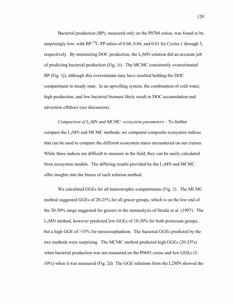
120  

Bacterial production (BP), measured only on the P0704 cruise, was found to be

surprisingly low, with BP:14C-PP ratios of 0.04, 0.04, and 0.01 for Cycles 1 through 3,

respectively. By minimizing DOC production, the L2MN solution did an accurate job

of predicting bacterial production (Fig. 1i). The MCMC consistently overestimated

BP (Fig. 1j), although this overestimate may have resulted holding the DOC

compartment in steady state. In an upwelling system, the combination of cold water,

high production, and low bacterial biomass likely result in DOC accumulation and

advection offshore (see discussion).

Comparison of L2MN and MCMC: ecosystem parameters – To further

compare the L2MN and MCMC methods, we computed composite ecosystem indices

that can be used to compare the different ecosystem states encountered on our cruises.

While these indices are difficult to measure in the field, they can be easily calculated

from ecosystem models. The differing results provided by the L2MN and MCMC

offer insights into the biases of each solution method.

We calculated GGEs for all heterotrophic compartments (Fig. 2). The MCMC

method suggested GGEs of 20-25% for all grazer groups, which is on the low end of

the 20-30% range suggested for grazers in the metanalysis of Straile et al. (1997). The

L2MN method, however predicted low GGEs of 10-20% for both protozoan groups,

but a high GGE of >35% for mesozooplankton. The bacterial GGEs predicted by the

two methods were surprising. The MCMC method predicted high GGEs (20-25%)

when bacterial production was not measured on the P0605 cruise and low GGEs (5-

10%) when it was measured (Fig. 2d) The GGE solutions from the L2MN showed the

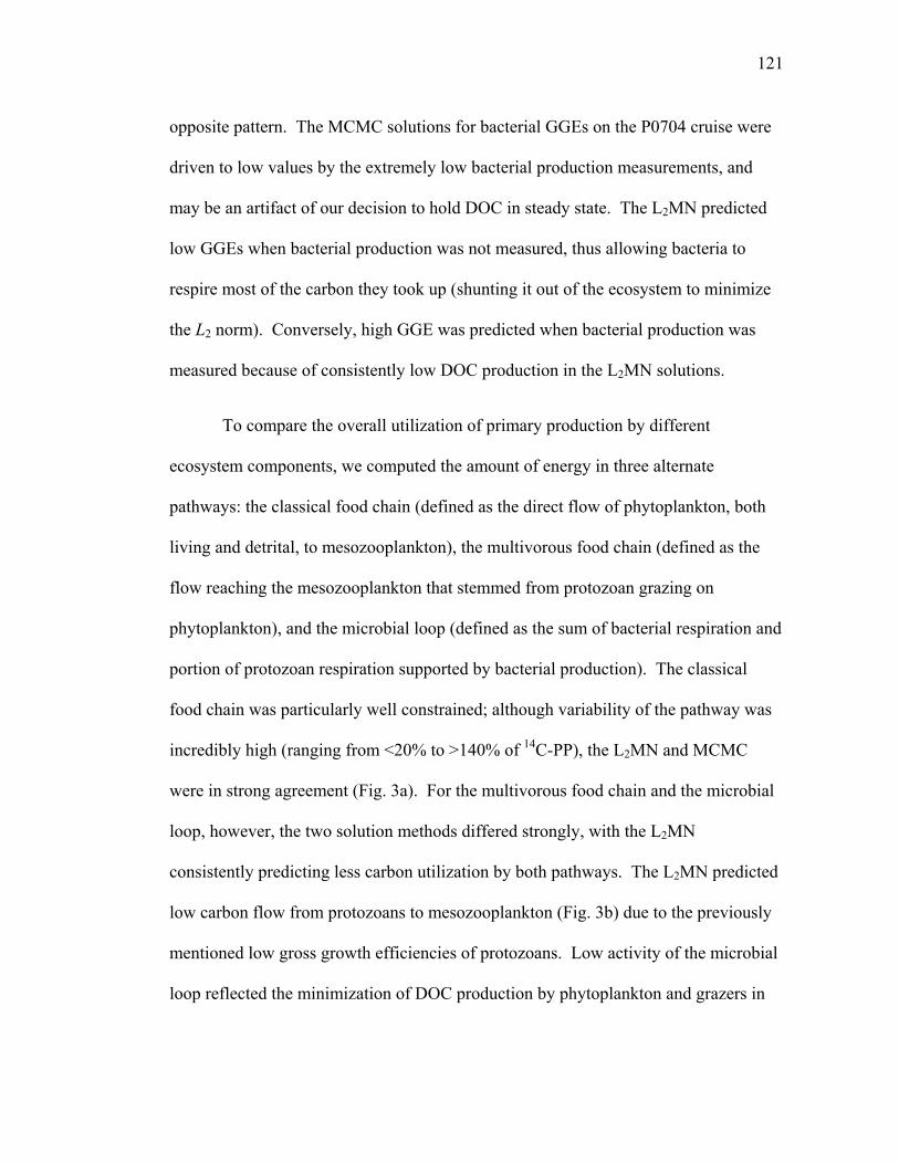
121  

opposite pattern. The MCMC solutions for bacterial GGEs on the P0704 cruise were

driven to low values by the extremely low bacterial production measurements, and

may be an artifact of our decision to hold DOC in steady state. The L2MN predicted

low GGEs when bacterial production was not measured, thus allowing bacteria to

respire most of the carbon they took up (shunting it out of the ecosystem to minimize

the L2 norm). Conversely, high GGE was predicted when bacterial production was

measured because of consistently low DOC production in the L2MN solutions.

To compare the overall utilization of primary production by different

ecosystem components, we computed the amount of energy in three alternate

pathways: the classical food chain (defined as the direct flow of phytoplankton, both

living and detrital, to mesozooplankton), the multivorous food chain (defined as the

flow reaching the mesozooplankton that stemmed from protozoan grazing on

phytoplankton), and the microbial loop (defined as the sum of bacterial respiration and

portion of protozoan respiration supported by bacterial production). The classical

food chain was particularly well constrained; although variability of the pathway was

incredibly high (ranging from <20% to >140% of 14C-PP), the L2MN and MCMC

were in strong agreement (Fig. 3a). For the multivorous food chain and the microbial

loop, however, the two solution methods differed strongly, with the L2MN

consistently predicting less carbon utilization by both pathways. The L2MN predicted

low carbon flow from protozoans to mesozooplankton (Fig. 3b) due to the previously

mentioned low gross growth efficiencies of protozoans. Low activity of the microbial

loop reflected the minimization of DOC production by phytoplankton and grazers in

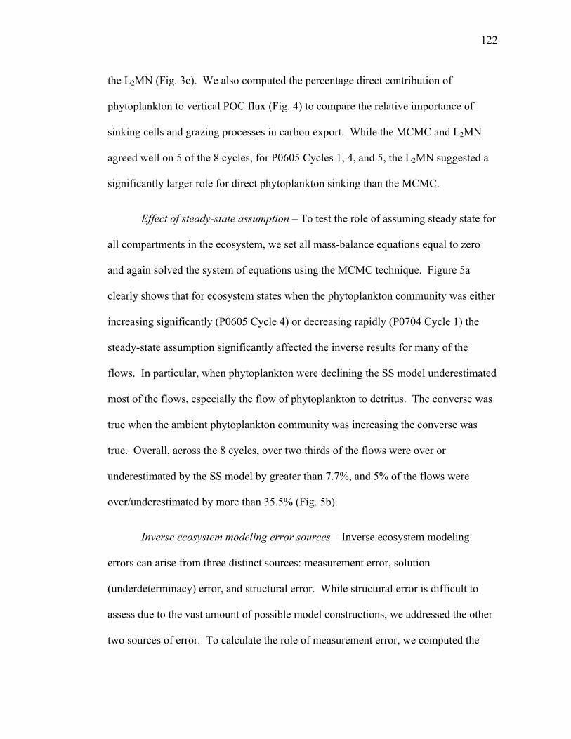
122  

the L2MN (Fig. 3c). We also computed the percentage direct contribution of

phytoplankton to vertical POC flux (Fig. 4) to compare the relative importance of

sinking cells and grazing processes in carbon export. While the MCMC and L2MN

agreed well on 5 of the 8 cycles, for P0605 Cycles 1, 4, and 5, the L2MN suggested a

significantly larger role for direct phytoplankton sinking than the MCMC.

Effect of steady-state assumption – To test the role of assuming steady state for

all compartments in the ecosystem, we set all mass-balance equations equal to zero

and again solved the system of equations using the MCMC technique. Figure 5a

clearly shows that for ecosystem states when the phytoplankton community was either

increasing significantly (P0605 Cycle 4) or decreasing rapidly (P0704 Cycle 1) the

steady-state assumption significantly affected the inverse results for many of the

flows. In particular, when phytoplankton were declining the SS model underestimated

most of the flows, especially the flow of phytoplankton to detritus. The converse was

true when the ambient phytoplankton community was increasing the converse was

true. Overall, across the 8 cycles, over two thirds of the flows were over or

underestimated by the SS model by greater than 7.7%, and 5% of the flows were

over/underestimated by more than 35.5% (Fig. 5b).

Inverse ecosystem modeling error sources – Inverse ecosystem modeling

errors can arise from three distinct sources: measurement error, solution

(underdeterminacy) error, and structural error. While structural error is difficult to

assess due to the vast amount of possible model constructions, we addressed the other

two sources of error. To calculate the role of measurement error, we computed the

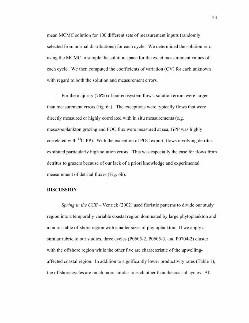
123  

mean MCMC solution for 100 different sets of measurement inputs (randomly

selected from normal distributions) for each cycle. We determined the solution error

using the MCMC to sample the solution space for the exact measurement values of

each cycle. We then computed the coefficients of variation (CV) for each unknown

with regard to both the solution and measurement errors.

For the majority (76%) of our ecosystem flows, solution errors were larger

than measurement errors (fig. 6a). The exceptions were typically flows that were

directly measured or highly correlated with in situ measurements (e.g.

mesozooplankton grazing and POC flux were measured at sea, GPP was highly

correlated with 14C-PP). With the exception of POC export, flows involving detritus

exhibited particularly high solution errors. This was especially the case for flows from

detritus to grazers because of our lack of a priori knowledge and experimental

measurement of detrital fluxes (Fig. 6b).

DISCUSSION

Spring in the CCE – Venrick (2002) used floristic patterns to divide our study

region into a temporally variable coastal region dominated by large phytoplankton and

a more stable offshore region with smaller sizes of phytoplankton. If we apply a

similar rubric to our studies, three cycles (P0605-2, P0605-3, and P0704-2) cluster

with the offshore region while the other five are characteristic of the upwelling-

affected coastal region. In addition to significantly lower productivity rates (Table 1),

the offshore cycles are much more similar to each other than the coastal cycles. All

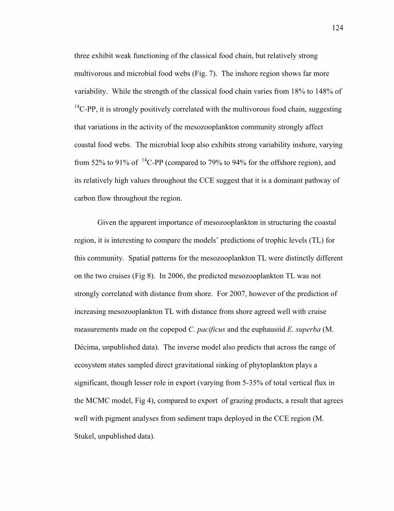
124  

three exhibit weak functioning of the classical food chain, but relatively strong

multivorous and microbial food webs (Fig. 7). The inshore region shows far more

variability. While the strength of the classical food chain varies from 18% to 148% of

14C-PP, it is strongly positively correlated with the multivorous food chain, suggesting

that variations in the activity of the mesozooplankton community strongly affect

coastal food webs. The microbial loop also exhibits strong variability inshore, varying

from 52% to 91% of 14C-PP (compared to 79% to 94% for the offshore region), and

its relatively high values throughout the CCE suggest that it is a dominant pathway of

carbon flow throughout the region.

Given the apparent importance of mesozooplankton in structuring the coastal

region, it is interesting to compare the models’ predictions of trophic levels (TL) for

this community. Spatial patterns for the mesozooplankton TL were distinctly different

on the two cruises (Fig 8). In 2006, the predicted mesozooplankton TL was not

strongly correlated with distance from shore. For 2007, however of the prediction of

increasing mesozooplankton TL with distance from shore agreed well with cruise

measurements made on the copepod C. pacificus and the euphausiid E. superba (M.

Décima, unpublished data). The inverse model also predicts that across the range of

ecosystem states sampled direct gravitational sinking of phytoplankton plays a

significant, though lesser role in export (varying from 5-35% of total vertical flux in

the MCMC model, Fig 4), compared to export of grazing products, a result that agrees

well with pigment analyses from sediment traps deployed in the CCE region (M.

Stukel, unpublished data).

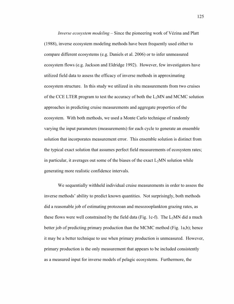
125  

Inverse ecosystem modeling – Since the pioneering work of Vézina and Platt

(1988), inverse ecosystem modeling methods have been frequently used either to

compare different ecosystems (e.g. Daniels et al. 2006) or to infer unmeasured

ecosystem flows (e.g. Jackson and Eldridge 1992). However, few investigators have

utilized field data to assess the efficacy of inverse methods in approximating

ecosystem structure. In this study we utilized in situ measurements from two cruises

of the CCE LTER program to test the accuracy of both the L2MN and MCMC solution

approaches in predicting cruise measurements and aggregate properties of the

ecosystem. With both methods, we used a Monte Carlo technique of randomly

varying the input parameters (measurements) for each cycle to generate an ensemble

solution that incorporates measurement error. This ensemble solution is distinct from

the typical exact solution that assumes perfect field measurements of ecosystem rates;

in particular, it averages out some of the biases of the exact L2MN solution while

generating more realistic confidence intervals.

We sequentially withheld individual cruise measurements in order to assess the

inverse methods’ ability to predict known quantities. Not surprisingly, both methods

did a reasonable job of estimating protozoan and mesozooplankton grazing rates, as

these flows were well constrained by the field data (Fig. 1c-f). The L2MN did a much

better job of predicting primary production than the MCMC method (Fig. 1a,b); hence

it may be a better technique to use when primary production is unmeasured. However,

primary production is the only measurement that appears to be included consistently

as a measured input for inverse models of pelagic ecosystems. Furthermore, the

126  

MCMC’s prediction of primary production would probably have been significantly

improved if we had placed a more stringent upper bound on phytoplankton growth

rates; the maximum of two doublings per day that we allowed is unrealistically high

for the cold water of the CCE.

Model predictions of vertical carbon flux and bacterial production were more

interesting, as they are the type of poorly constrained and highly coupled ecosystem

flows that inverse models are often used to resolve. The MCMC method was much

more accurate at predicting vertical carbon flux than the L2MN (Figs. 1g,h).

Confidence intervals of MCMC solutions consistently bracketed measurement values

and solutions were typically less than a standard deviation away from the measured

values. In contrast, the L2MN solutions consistently overestimated POC export.

Despite the wide uncertainties it predicted for this flow (average CV for the 7 cycles

was 1.98), 95% confidence intervals failed to bracket the true values three out of seven

times. This overestimate of POC export by the L2MN may seem surprising given its

tendency to maximize grazer respiration, but it follows logically from the method’s

minimization of the flows through the system. Rather than allow detritus to be

reworked by grazers, the L2MN exports most detritus directly out of the system.

Bacterial production, as measured on the P0704 cruise by the leucine

incorporation technique, was accurately predicted by the L2MN, but overestimated by

the MCMC. This result may be misleading, however, because we lacked

measurements of labile DOC and chose to hold DOC concentrations constant. The

P0704 cruise took place early in the spring bloom period, when cold nutrient-rich

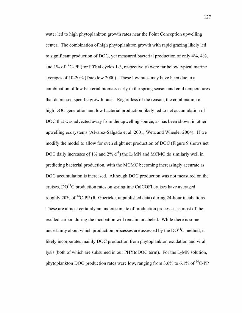
127  

water led to high phytoplankton growth rates near the Point Conception upwelling

center. The combination of high phytoplankton growth with rapid grazing likely led

to significant production of DOC, yet measured bacterial production of only 4%, 4%,

and 1% of 14C-PP (for P0704 cycles 1-3, respectively) were far below typical marine

averages of 10-20% (Ducklow 2000). These low rates may have been due to a

combination of low bacterial biomass early in the spring season and cold temperatures

that depressed specific growth rates. Regardless of the reason, the combination of

high DOC generation and low bacterial production likely led to net accumulation of

DOC that was advected away from the upwelling source, as has been shown in other

upwelling ecosystems (Alvarez-Salgado et al. 2001; Wetz and Wheeler 2004). If we

modify the model to allow for even slight net production of DOC (Figure 9 shows net

DOC daily increases of 1% and 2% d-1) the L2MN and MCMC do similarly well in

predicting bacterial production, with the MCMC becoming increasingly accurate as

DOC accumulation is increased. Although DOC production was not measured on the

cruises, DO14C production rates on springtime CalCOFI cruises have averaged

roughly 20% of 14C-PP (R. Goericke, unpublished data) during 24-hour incubations.

These are almost certainly an underestimate of production processes as most of the

exuded carbon during the incubation will remain unlabeled. While there is some

uncertainty about which production processes are assessed by the DO14C method, it

likely incorporates mainly DOC production from phytoplankton exudation and viral

lysis (both of which are subsumed in our PHYtoDOC term). For the L2MN solution,

phytoplankton DOC production rates were low, ranging from 3.6% to 6.1% of 14C-PP

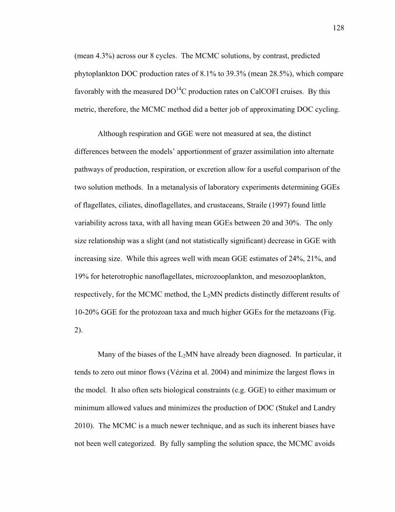
128  

(mean 4.3%) across our 8 cycles. The MCMC solutions, by contrast, predicted

phytoplankton DOC production rates of 8.1% to 39.3% (mean 28.5%), which compare

favorably with the measured DO14C production rates on CalCOFI cruises. By this

metric, therefore, the MCMC method did a better job of approximating DOC cycling.

Although respiration and GGE were not measured at sea, the distinct

differences between the models’ apportionment of grazer assimilation into alternate

pathways of production, respiration, or excretion allow for a useful comparison of the

two solution methods. In a metanalysis of laboratory experiments determining GGEs

of flagellates, ciliates, dinoflagellates, and crustaceans, Straile (1997) found little

variability across taxa, with all having mean GGEs between 20 and 30%. The only

size relationship was a slight (and not statistically significant) decrease in GGE with

increasing size. While this agrees well with mean GGE estimates of 24%, 21%, and

19% for heterotrophic nanoflagellates, microzooplankton, and mesozooplankton,

respectively, for the MCMC method, the L2MN predicts distinctly different results of

10-20% GGE for the protozoan taxa and much higher GGEs for the metazoans (Fig.

2).

Many of the biases of the L2MN have already been diagnosed. In particular, it

tends to zero out minor flows (Vézina et al. 2004) and minimize the largest flows in

the model. It also often sets biological constraints (e.g. GGE) to either maximum or

minimum allowed values and minimizes the production of DOC (Stukel and Landry

2010). The MCMC is a much newer technique, and as such its inherent biases have

not been well categorized. By fully sampling the solution space, the MCMC avoids

129  

many of the problems associated with the L2MN. In particular, rather than choosing

unrealistically low or high values for biological constraints (e.g. GGE), the MCMC

selects a more likely value near the middle of the allowable ranges (Fig. 2). However,

we did identify one bias in the MCMC method that makes the examination of model

structure important. When fully sampling the solution space, the MCMC method

typically apportions unconstrained flows equally between equivalent compartments.

While this may be a reasonable approach, it can lead to biases in the results when

different model constructions are used. For instance pathways of carbon flow from

nanoflagellates will be altered by the structure of the microplankton community. In

our model construction, carbon could flow from nanoflagellates to respiration, DOC,

detritus, microzooplankton, or mesozooplankton. If instead we divided the

microzooplankton community into heterotrophic flagellates and ciliates, which both

graze upon nanoflagellates, the total flow into this combined microzooplankton group

would increase at the expense of other outflows from nanoflagellates, due to the

greater number of states that can be constructed. Thus when comparing different

ecosystems, it is important to maintain similar inverse structures.

Due to the fixed station-based sampling of most oceanographic cruises that do

not allow for Lagrangian-based studies, many inverse studies have assumed steady

state for their compartments. In fact, these unmeasured mass balance constraints are

often assumed to be known exactly, while in situ measurements are assigned error

terms. Vézina and Pahlow (2003) tested this assumption by comparing L2MN inverse

ecosystem reconstructions of steady-state models to reconstructions of transient states

130  

of a time-varying bloom model. They found that the inverse methods that assumed

steady state actually did a better job of evaluating the underlying flows in the bloom

model than in the steady-state simulation, and thereby concluded that steady-state

assumptions are valid even for periods when the ecosystem components are

temporally variable. We chose to readdress this assumption in a different manner,

utilizing the measured rate of change of the largest compartment in the model

(phytoplankton) to construct a non-steady state (NSS) inverse analysis and then

comparing it to an equivalent steady-state (SS) inverse analysis. The differences

between the SS and NSS models were significant, with flows often significantly over

or underestimated by the SS solution when the natural phytoplankton community was

increasing or declining rapidly. Given the biases inherent to the L2MN, it is likely that

the more accurate predictions of the transient states of the bloom model of Vézina and

Pahlow (2003) were in fact due to the increased strength of the classical food chain

during bloom conditions. As our Fig. 3 shows, the L2MN significantly

underestimates flows through the microbial loop and multivorous food webs, which

dominate during steady-state conditions. In fact the results of Vézina and Pahlow

(2003) can be understood as a simple response of the inverse method to the increasing

complexity of the food webs. The L2MN does a good job of estimating the growth

phase of the bloom, but becomes less accurate as the bloom reaches its peak and

decays and in the steady-state simulations with significantly lower phytoplankton

biomass. We suggest that when net biomass changes cannot be measured,

131  

investigators should apply a reasonable error term to their mass balance equations, for

instance assuming 95% confidence intervals of ±10% biomass change per day.

CONCLUSION

Investigators have relied on inverse modeling techniques (particularly the

L2MN) to reasonably resolve complex food webs when only a few basic

measurements are made. We tested the efficacy of inverse methods across a wide

range of ecosystem states within the CCE, and found that they reasonably estimate in

situ measurements when measurement errors are taken into account. While an

ensemble version of the commonly used L2MN technique clearly performs better than

the newer MCMC method when primary production is not specified as a model input,

the MCMC method more accurately depicts pelagic food web flows when primary

production is a measured input. In particular, the MCMC method predicted vertical

carbon flux, which depends on a number of unmeasured rates; hence the MCMC

appears to have more accurately captured the dynamics of the poorly resolved but

highly connected detrital pool. This ability to resolve such an under-constrained

component of the ecosystem suggests that it may perform well with the highly

underdetermined ecosystems often encountered. Nevertheless, results from inverse

modeling techniques are highly uncertain, as shown by coefficients of variation that

are often greater than 50%. Despite the fact that our simple model, with 10-12

equations constraining only 29 variables, was far more constrained than most inverse

models, most of the variability arose from the under-determinacy of the solutions,

rather than from measurement uncertainties. We thus suggest that experimental

132  

programs focusing on food web fluxes require an expanded range of experimental

measurements, in particular, measurements that constrain the behaviors of the DOC

and detrital pools, which play a large role in the model but are very poorly

constrained.

ACKNOWLEDGMENTS

This chapter would not have been possible without the cooperative efforts of

the many different researchers, students, technicians, and volunteers on the P0605 and

P0704 cruises of the California Current Ecosystem (CCE) Long-Term Ecological

Research (LTER) program. I am particularly indebted to my co-workers in the Landry

Lab (M. Landry, A. Taylor, M. Décima, D. Wick) for providing microzooplankton

grazing and microscopy results, the Ohman Lab (M. Ohman, R. Rykaczewski, M.

Décima, J. Powell, K. Tsyrklevich, D. Taniguchi) for mesozooplankton biomass and

grazing results, the Goericke Lab (R. Goericke, S. Dovel, M. Roadman) for 14C-PP,

chlorophyll, and POC data, the Azam Lab (T. Samo) for bacterial production rates,

and the Aluwihare Lab (L. Aluwihare, L. Chong) for TOC concentrations. Thorium

export measurements were only possible because of willing collaborators from the

Benitez-Nelson Lab (C. Benitez-Nelson, K. Maiti, and R. Styles). I am also grateful

to the captains and crews of the R.V. Knorr and the R.V. Thompson.

Chapter 3, in full, is currently in preparation for submission: Stukel, M. R.,

Landry, M. R., Benitez-Nelson, C. R., Goericke, R. “Do inverse models accurately

reconstruct food web flows? A comparison of two solution methods using field data

133  

from the California Current Ecosystem.” The dissertation author was the primary

investigator and author on this paper.

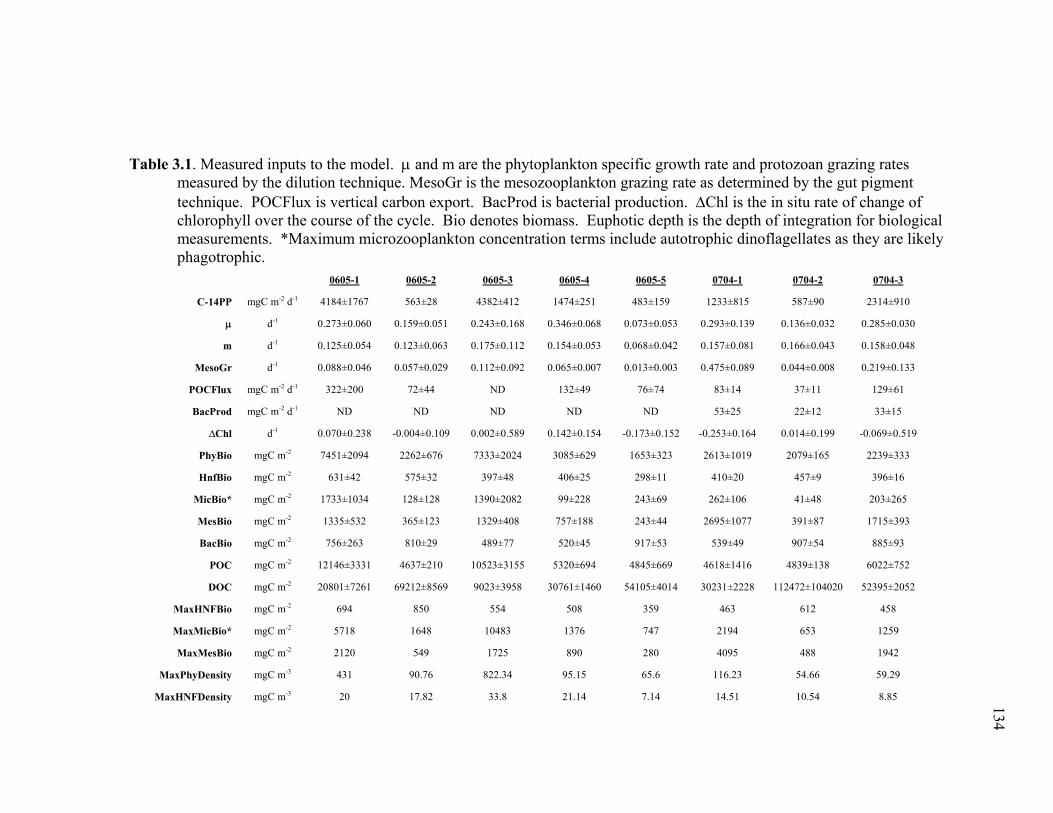
134  

Table 3.1. Measured inputs to the model. and m are the phytoplankton specific growth rate and protozoan grazing rates measured by the dilution technique. MesoGr is the mesozooplankton grazing rate as determined by the gut pigment technique. POCFlux is vertical carbon export. BacProd is bacterial production. Chl is the in situ rate of change of chlorophyll over the course of the cycle. Bio denotes biomass. Euphotic depth is the depth of integration for biological measurements. *Maximum microzooplankton concentration terms include autotrophic dinoflagellates as they are likely phagotrophic.

0605-1 0605-2 0605-3 0605-4 0605-5 0704-1 0704-2 0704-3

C-14PP mgC m-2 d-1 4184±1767 563±28 4382±412 1474±251 483±159 1233±815 587±90 2314±910

d-1 0.273±0.060 0.159±0.051 0.243±0.168 0.346±0.068 0.073±0.053 0.293±0.139 0.136±0.032 0.285±0.030

m d-1 0.125±0.054 0.123±0.063 0.175±0.112 0.154±0.053 0.068±0.042 0.157±0.081 0.166±0.043 0.158±0.048

MesoGr d-1 0.088±0.046 0.057±0.029 0.112±0.092 0.065±0.007 0.013±0.003 0.475±0.089 0.044±0.008 0.219±0.133

POCFlux mgC m-2 d-1 322±200 72±44 ND 132±49 76±74 83±14 37±11 129±61

BacProd mgC m-2 d-1 ND ND ND ND ND 53±25 22±12 33±15

∆Chl d-1 0.070±0.238 -0.004±0.109 0.002±0.589 0.142±0.154 -0.173±0.152 -0.253±0.164 0.014±0.199 -0.069±0.519

PhyBio mgC m-2 7451±2094 2262±676 7333±2024 3085±629 1653±323 2613±1019 2079±165 2239±333

HnfBio mgC m-2 631±42 575±32 397±48 406±25 298±11 410±20 457±9 396±16

MicBio* mgC m-2 1733±1034 128±128 1390±2082 99±228 243±69 262±106 41±48 203±265

MesBio mgC m-2 1335±532 365±123 1329±408 757±188 243±44 2695±1077 391±87 1715±393

BacBio mgC m-2 756±263 810±29 489±77 520±45 917±53 539±49 907±54 885±93

POC mgC m-2 12146±3331 4637±210 10523±3155 5320±694 4845±669 4618±1416 4839±138 6022±752

DOC mgC m-2 20801±7261 69212±8569 9023±3958 30761±1460 54105±4014 30231±2228 112472±104020 52395±2052

MaxHNFBio mgC m-2 694 850 554 508 359 463 612 458

MaxMicBio* mgC m-2 5718 1648 10483 1376 747 2194 653 1259

MaxMesBio mgC m-2 2120 549 1725 890 280 4095 488 1942

MaxPhyDensity mgC m-3 431 90.76 822.34 95.15 65.6 116.23 54.66 59.29

MaxHNFDensity mgC m-3 20 17.82 33.8 21.14 7.14 14.51 10.54 8.85 134

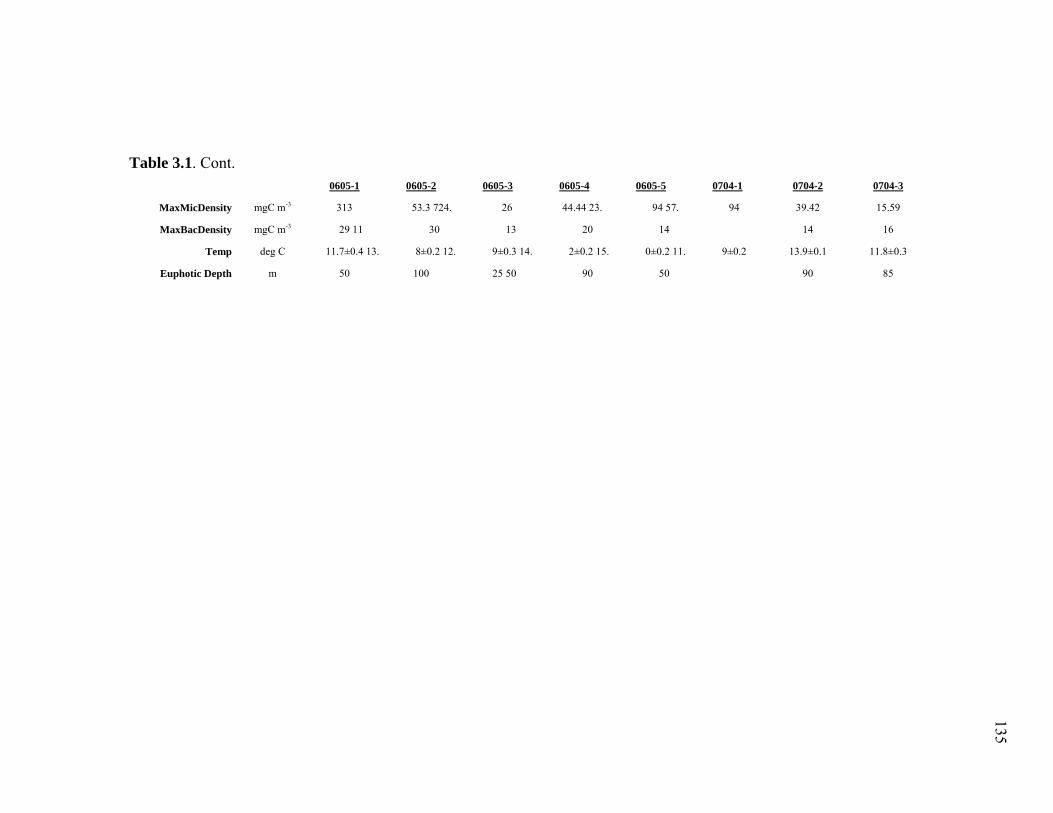
134  

Table 3.1. Cont. 0605-1 0605-2 0605-3 0605-4 0605-5 0704-1 0704-2 0704-3

MaxMicDensity mgC m-3 313 53.3 724. 26 44.44 23. 94 57. 94 39.42 15.59

MaxBacDensity mgC m-3 29 11 30 13 20 14 14 16

Temp deg C 11.7±0.4 13. 8±0.2 12. 9±0.3 14. 2±0.2 15. 0±0.2 11. 9±0.2 13.9±0.1 11.8±0.3

Euphotic Depth m 50 100 25 50 90 50 90 85

135

  

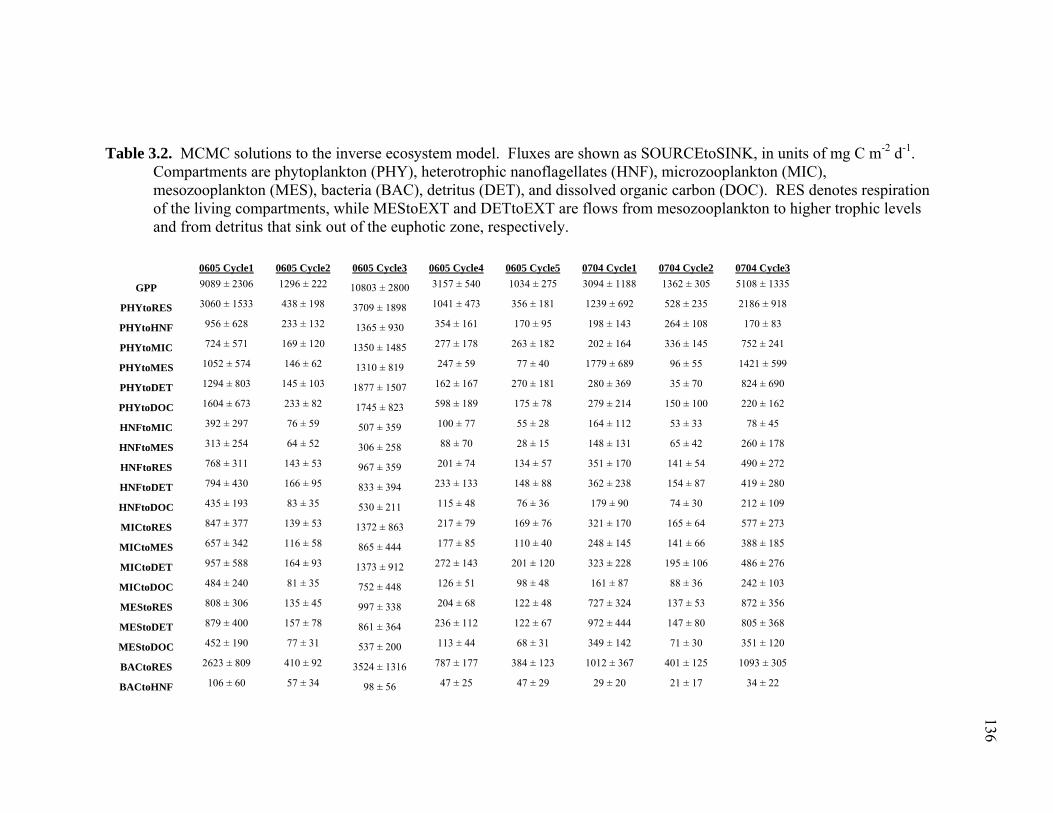
Table 3.2. MCMC solutions to the inverse ecosystem model. Fluxes are shown as SOURCEtoSINK, in units of mg C m-2 d-1. Compartments are phytoplankton (PHY), heterotrophic nanoflagellates (HNF), microzooplankton (MIC), mesozooplankton (MES), bacteria (BAC), detritus (DET), and dissolved organic carbon (DOC). RES denotes respiration of the living compartments, while MEStoEXT and DETtoEXT are flows from mesozooplankton to higher trophic levels and from detritus that sink out of the euphotic zone, respectively.

0605 Cycle1 0605 Cycle2 0605 Cycle3 0605 Cycle4 0605 Cycle5 0704 Cycle1 0704 Cycle2 0704 Cycle3

GPP 9089 ± 2306 1296 ± 222 10803 ± 2800 3157 ± 540 1034 ± 275 3094 ± 1188 1362 ± 305 5108 ± 1335

PHYtoRES 3060 ± 1533 438 ± 198 3709 ± 1898 1041 ± 473 356 ± 181 1239 ± 692 528 ± 235 2186 ± 918

PHYtoHNF 956 ± 628 233 ± 132 1365 ± 930 354 ± 161 170 ± 95 198 ± 143 264 ± 108 170 ± 83

PHYtoMIC 724 ± 571 169 ± 120 1350 ± 1485 277 ± 178 263 ± 182 202 ± 164 336 ± 145 752 ± 241

PHYtoMES 1052 ± 574 146 ± 62 1310 ± 819 247 ± 59 77 ± 40 1779 ± 689 96 ± 55 1421 ± 599

PHYtoDET 1294 ± 803 145 ± 103 1877 ± 1507 162 ± 167 270 ± 181 280 ± 369 35 ± 70 824 ± 690

PHYtoDOC 1604 ± 673 233 ± 82 1745 ± 823 598 ± 189 175 ± 78 279 ± 214 150 ± 100 220 ± 162

HNFtoMIC 392 ± 297 76 ± 59 507 ± 359 100 ± 77 55 ± 28 164 ± 112 53 ± 33 78 ± 45

HNFtoMES 313 ± 254 64 ± 52 306 ± 258 88 ± 70 28 ± 15 148 ± 131 65 ± 42 260 ± 178

HNFtoRES 768 ± 311 143 ± 53 967 ± 359 201 ± 74 134 ± 57 351 ± 170 141 ± 54 490 ± 272

HNFtoDET 794 ± 430 166 ± 95 833 ± 394 233 ± 133 148 ± 88 362 ± 238 154 ± 87 419 ± 280

HNFtoDOC 435 ± 193 83 ± 35 530 ± 211 115 ± 48 76 ± 36 179 ± 90 74 ± 30 212 ± 109

MICtoRES 847 ± 377 139 ± 53 1372 ± 863 217 ± 79 169 ± 76 321 ± 170 165 ± 64 577 ± 273

MICtoMES 657 ± 342 116 ± 58 865 ± 444 177 ± 85 110 ± 40 248 ± 145 141 ± 66 388 ± 185

MICtoDET 957 ± 588 164 ± 93 1373 ± 912 272 ± 143 201 ± 120 323 ± 228 195 ± 106 486 ± 276

MICtoDOC 484 ± 240 81 ± 35 752 ± 448 126 ± 51 98 ± 48 161 ± 87 88 ± 36 242 ± 103

MEStoRES 808 ± 306 135 ± 45 997 ± 338 204 ± 68 122 ± 48 727 ± 324 137 ± 53 872 ± 356

MEStoDET 879 ± 400 157 ± 78 861 ± 364 236 ± 112 122 ± 67 972 ± 444 147 ± 80 805 ± 368

MEStoDOC 452 ± 190 77 ± 31 537 ± 200 113 ± 44 68 ± 31 349 ± 142 71 ± 30 351 ± 120

BACtoRES 2623 ± 809 410 ± 92 3524 ± 1316 787 ± 177 384 ± 123 1012 ± 367 401 ± 125 1093 ± 305

BACtoHNF 106 ± 60 57 ± 34 98 ± 56 47 ± 25 47 ± 29 29 ± 20 21 ± 17 34 ± 22

136

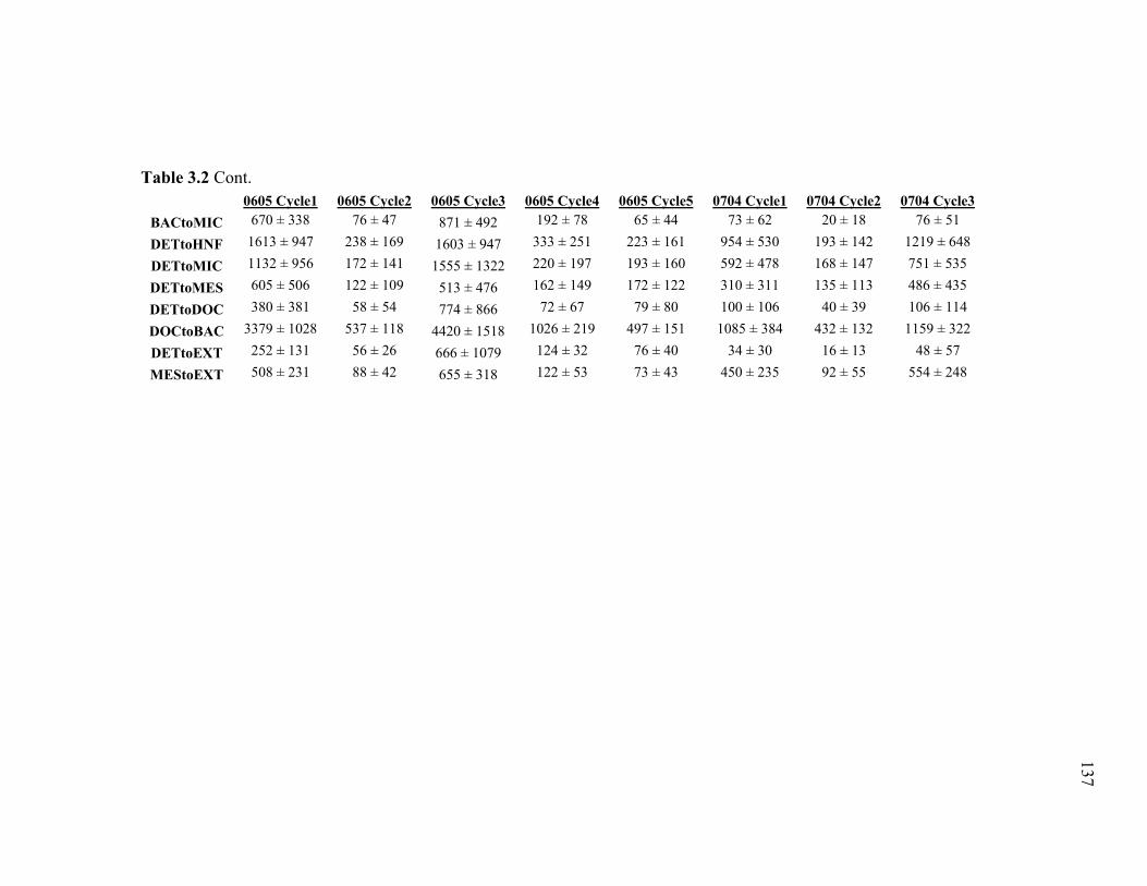
136  

Table 3.2 Cont. 0605 Cycle1 0605 Cycle2 0605 Cycle3 0605 Cycle4 0605 Cycle5 0704 Cycle1 0704 Cycle2 0704 Cycle3

BACtoMIC 670 ± 338 76 ± 47 871 ± 492 192 ± 78 65 ± 44 73 ± 62 20 ± 18 76 ± 51

DETtoHNF 1613 ± 947 238 ± 169 1603 ± 947 333 ± 251 223 ± 161 954 ± 530 193 ± 142 1219 ± 648

DETtoMIC 1132 ± 956 172 ± 141 1555 ± 1322 220 ± 197 193 ± 160 592 ± 478 168 ± 147 751 ± 535

DETtoMES 605 ± 506 122 ± 109 513 ± 476 162 ± 149 172 ± 122 310 ± 311 135 ± 113 486 ± 435

DETtoDOC 380 ± 381 58 ± 54 774 ± 866 72 ± 67 79 ± 80 100 ± 106 40 ± 39 106 ± 114

DOCtoBAC 3379 ± 1028 537 ± 118 4420 ± 1518 1026 ± 219 497 ± 151 1085 ± 384 432 ± 132 1159 ± 322

DETtoEXT 252 ± 131 56 ± 26 666 ± 1079 124 ± 32 76 ± 40 34 ± 30 16 ± 13 48 ± 57

MEStoEXT 508 ± 231 88 ± 42 655 ± 318 122 ± 53 73 ± 43 450 ± 235 92 ± 55 554 ± 248

137

 

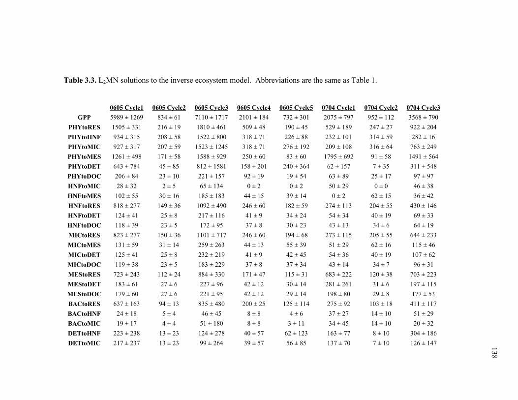
Table 3.3. L2MN solutions to the inverse ecosystem model. Abbreviations are the same as Table 1.

0605 Cycle1 0605 Cycle2 0605 Cycle3 0605 Cycle4 0605 Cycle5 0704 Cycle1 0704 Cycle2 0704 Cycle3

GPP 5989 ± 1269 834 ± 61 7110 ± 1717 2101 ± 184 732 ± 301 2075 ± 797 952 ± 112 3568 ± 790

PHYtoRES 1505 ± 331 216 ± 19 1810 ± 461 509 ± 48 190 ± 45 529 ± 189 247 ± 27 922 ± 204

PHYtoHNF 934 ± 315 208 ± 58 1522 ± 800 318 ± 71 226 ± 88 232 ± 101 314 ± 59 282 ± 16

PHYtoMIC 927 ± 317 207 ± 59 1523 ± 1245 318 ± 71 276 ± 192 209 ± 108 316 ± 64 763 ± 249

PHYtoMES 1261 ± 498 171 ± 58 1588 ± 929 250 ± 60 83 ± 60 1795 ± 692 91 ± 58 1491 ± 564

PHYtoDET 643 ± 784 45 ± 85 812 ± 1581 158 ± 201 240 ± 364 62 ± 157 7 ± 35 311 ± 548

PHYtoDOC 206 ± 84 23 ± 10 221 ± 157 92 ± 19 19 ± 54 63 ± 89 25 ± 17 97 ± 97

HNFtoMIC 28 ± 32 2 ± 5 65 ± 134 0 ± 2 0 ± 2 50 ± 29 0 ± 0 46 ± 38

HNFtoMES 102 ± 55 30 ± 16 185 ± 183 44 ± 15 39 ± 14 0 ± 2 62 ± 15 36 ± 42

HNFtoRES 818 ± 277 149 ± 36 1092 ± 490 246 ± 60 182 ± 59 274 ± 113 204 ± 55 430 ± 146

HNFtoDET 124 ± 41 25 ± 8 217 ± 116 41 ± 9 34 ± 24 54 ± 34 40 ± 19 69 ± 33

HNFtoDOC 118 ± 39 23 ± 5 172 ± 95 37 ± 8 30 ± 23 43 ± 13 34 ± 6 64 ± 19

MICtoRES 823 ± 277 150 ± 36 1101 ± 717 246 ± 60 194 ± 68 273 ± 115 205 ± 55 644 ± 233

MICtoMES 131 ± 59 31 ± 14 259 ± 263 44 ± 13 55 ± 39 51 ± 29 62 ± 16 115 ± 46

MICtoDET 125 ± 41 25 ± 8 232 ± 219 41 ± 9 42 ± 45 54 ± 36 40 ± 19 107 ± 62

MICtoDOC 119 ± 38 23 ± 5 183 ± 229 37 ± 8 37 ± 34 43 ± 14 34 ± 7 96 ± 31

MEStoRES 723 ± 243 112 ± 24 884 ± 330 171 ± 47 115 ± 31 683 ± 222 120 ± 38 703 ± 223

MEStoDET 183 ± 61 27 ± 6 227 ± 96 42 ± 12 30 ± 14 281 ± 261 31 ± 6 197 ± 115

MEStoDOC 179 ± 60 27 ± 6 221 ± 95 42 ± 12 29 ± 14 198 ± 80 29 ± 8 177 ± 53

BACtoRES 637 ± 163 94 ± 13 835 ± 480 200 ± 25 125 ± 114 275 ± 92 103 ± 18 411 ± 117

BACtoHNF 24 ± 18 5 ± 4 46 ± 45 8 ± 8 4 ± 6 37 ± 27 14 ± 10 51 ± 29

BACtoMIC 19 ± 17 4 ± 4 51 ± 180 8 ± 8 3 ± 11 34 ± 45 14 ± 10 20 ± 32

DETtoHNF 223 ± 238 13 ± 23 124 ± 278 40 ± 57 62 ± 123 163 ± 77 8 ± 10 304 ± 186

DETtoMIC 217 ± 237 13 ± 23 99 ± 264 39 ± 57 56 ± 85 137 ± 70 7 ± 10 126 ± 147 138

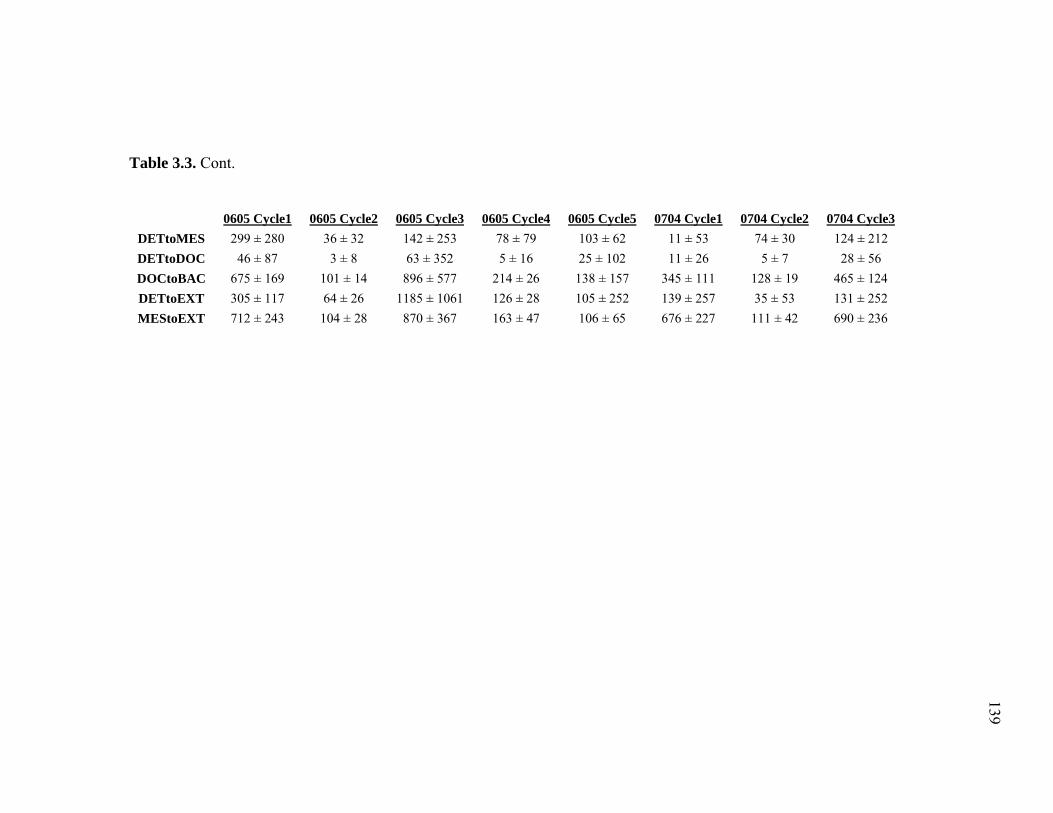
137  

Table 3.3. Cont.

0605 Cycle1 0605 Cycle2 0605 Cycle3 0605 Cycle4 0605 Cycle5 0704 Cycle1 0704 Cycle2 0704 Cycle3

DETtoMES 299 ± 280 36 ± 32 142 ± 253 78 ± 79 103 ± 62 11 ± 53 74 ± 30 124 ± 212 DETtoDOC 46 ± 87 3 ± 8 63 ± 352 5 ± 16 25 ± 102 11 ± 26 5 ± 7 28 ± 56 DOCtoBAC 675 ± 169 101 ± 14 896 ± 577 214 ± 26 138 ± 157 345 ± 111 128 ± 19 465 ± 124 DETtoEXT 305 ± 117 64 ± 26 1185 ± 1061 126 ± 28 105 ± 252 139 ± 257 35 ± 53 131 ± 252 MEStoEXT 712 ± 243 104 ± 28 870 ± 367 163 ± 47 106 ± 65 676 ± 227 111 ± 42 690 ± 236

139

140  

Figure 3.1. Model estimation of measured parameters. Each measurement was withheld from a model iteration in order to assess capabilities of predicting in situ measurements. Panels a, c, e, g, i show the MCMC predictions. Panels b, d, f, h, j show the L2MN predictions. Panels a, b are the predictions of 14C-PP when 14C-PP is not used as a model input. Other measurements are protozoan grazing (c,d), mesozooplankton grazing (e,f), POC export (g,h) and bacterial production (i,j). In situ measurements are on the x-axis and model predictions are on the y-axis. Dotted line is the 1:1 line. Error bars are 95% confidence limits. 

 

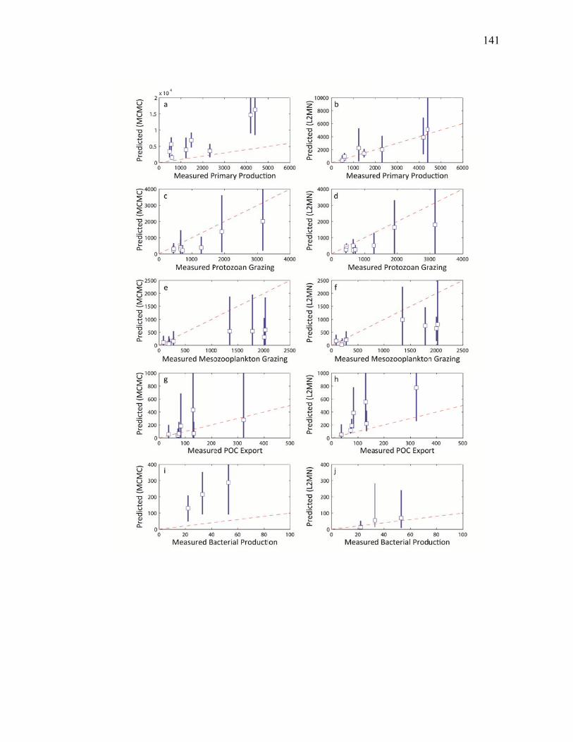
141

 

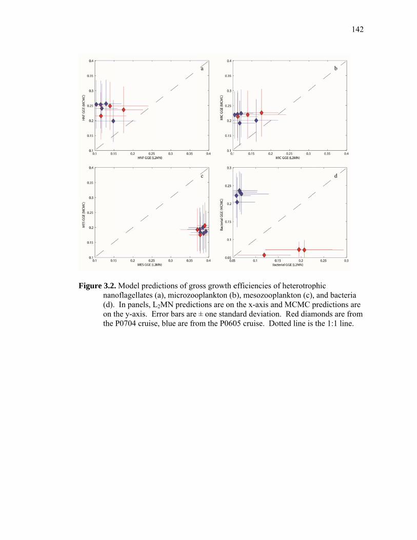
Figure 3.2. nano(d). on ththe P

Model predoflagellates (In panels, L

he y-axis. EP0704 cruise

dictions of gr(a), microzoo

L2MN predicError bars aree, blue are fr

ross growth eoplankton (b

ctions are one ± one standrom the P060

efficiencies b), mesozoop

n the x-axis adard deviatio05 cruise. D

of heterotropplankton (c)and MCMC pon. Red diam

Dotted line is

phic , and bacteripredictions amonds are frs the 1:1 line

142

ia are rom e.

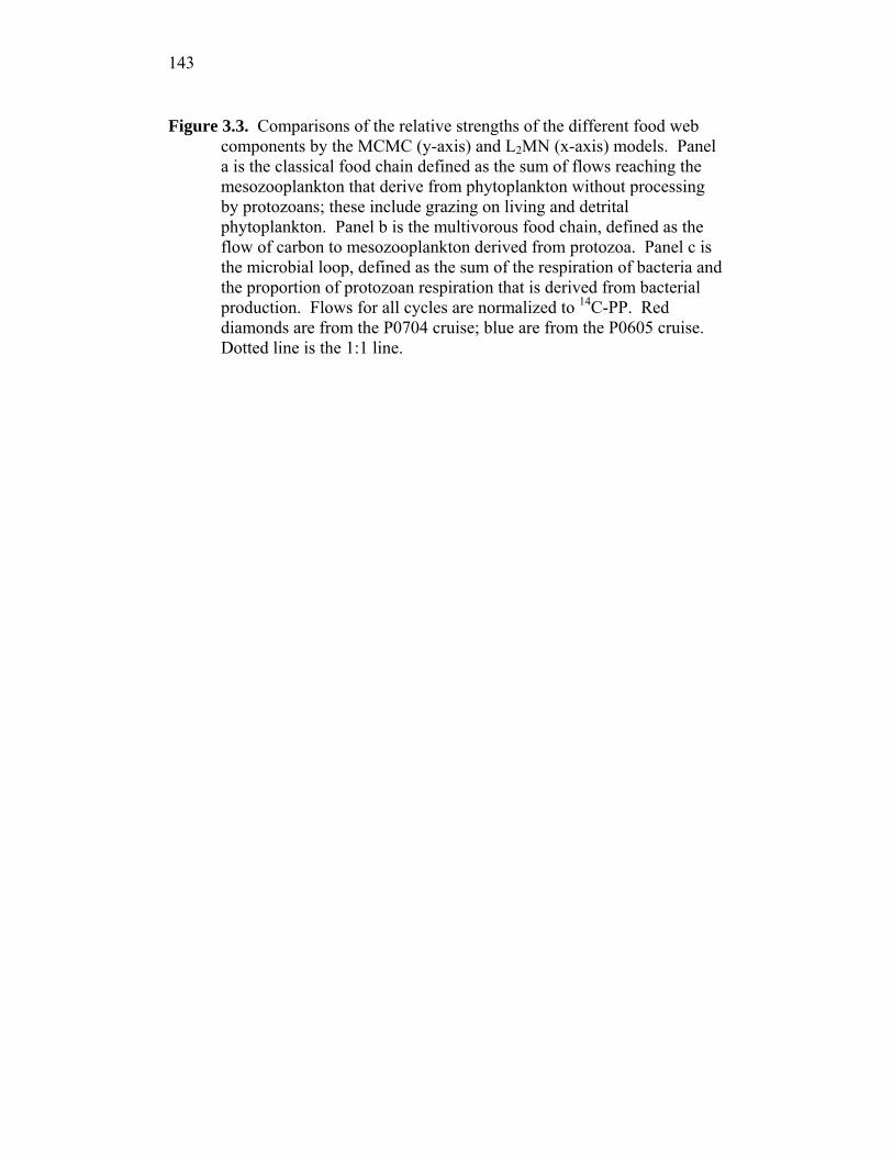
143  

Figure 3.3. Comparisons of the relative strengths of the different food web components by the MCMC (y-axis) and L2MN (x-axis) models. Panel a is the classical food chain defined as the sum of flows reaching the mesozooplankton that derive from phytoplankton without processing by protozoans; these include grazing on living and detrital phytoplankton. Panel b is the multivorous food chain, defined as the flow of carbon to mesozooplankton derived from protozoa. Panel c is the microbial loop, defined as the sum of the respiration of bacteria and the proportion of protozoan respiration that is derived from bacterial production. Flows for all cycles are normalized to 14C-PP. Red diamonds are from the P0704 cruise; blue are from the P0605 cruise. Dotted line is the 1:1 line.

 

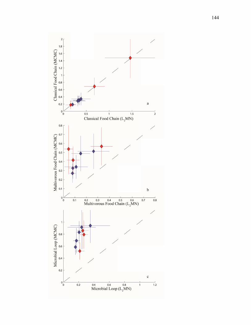
144

 

Figure 3.4. detrimethP060

Fraction ofital phytoplahods (y-axis)05 cruise. D

f vertical carbankton, as de). Red diam

Dotted line is

bon export determined by

monds are fros the 1:1 line

derived fromy the L2MN om the P0704e.

m gravitation(x-axis) and4 cruise; blu

nal sinking od the MCMCue are from t

145

f C the

 

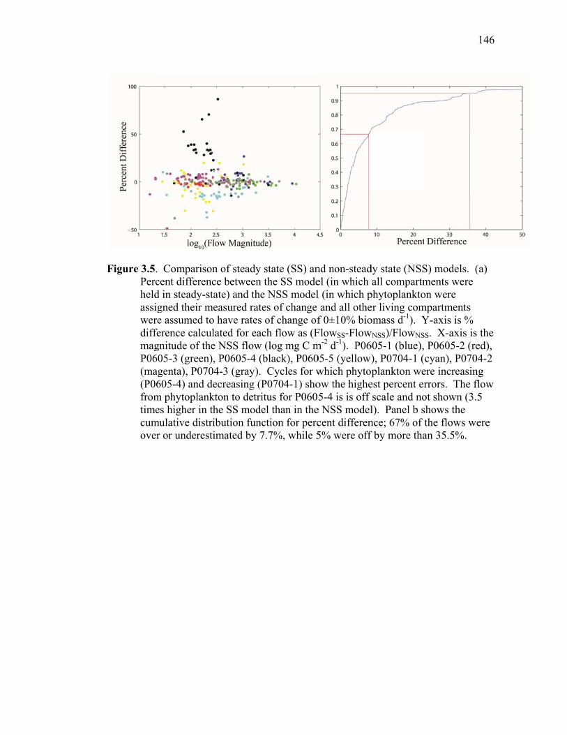
Figure 3.5. PercheldassigwerediffemagP060(mag(P06fromtimecumover

Comparisocent differencd in steady-stgned their me assumed toerence calculnitude of the05-3 (green)genta), P070605-4) and dm phytoplankes higher in t

mulative distrr or underest

n of steady sce between ttate) and the

measured rateo have rates olated for eace NSS flow (), P0605-4 (b04-3 (gray). decreasing (Pkton to detritthe SS moderibution functimated by 7

state (SS) anthe SS modeNSS model

es of change of change of

ch flow as (F(log mg C mblack), P060Cycles for w

P0704-1) shotus for P060el than in thection for perc.7%, while 5

nd non-steadel (in which l (in which pand all othe

f 0±10% bioFlowSS-Flowm-2 d-1). P0605-5 (yellow)which phytoow the highe5-4 is is off

e NSS modelcent differen5% were off

dy state (NSSall compartm

phytoplanktoer living comomass d-1). Y

wNSS)/FlowNS

605-1 (blue),), P0704-1 (plankton we

est percent erscale and nol). Panel b snce; 67% of f by more tha

S) models. (ments were on were mpartments Y-axis is % SS. X-axis is P0605-2 (recyan), P070

ere increasinrrors. The flot shown (3.shows the the flows wean 35.5%.

146

(a)

the ed), 4-2

ng flow 5

ere

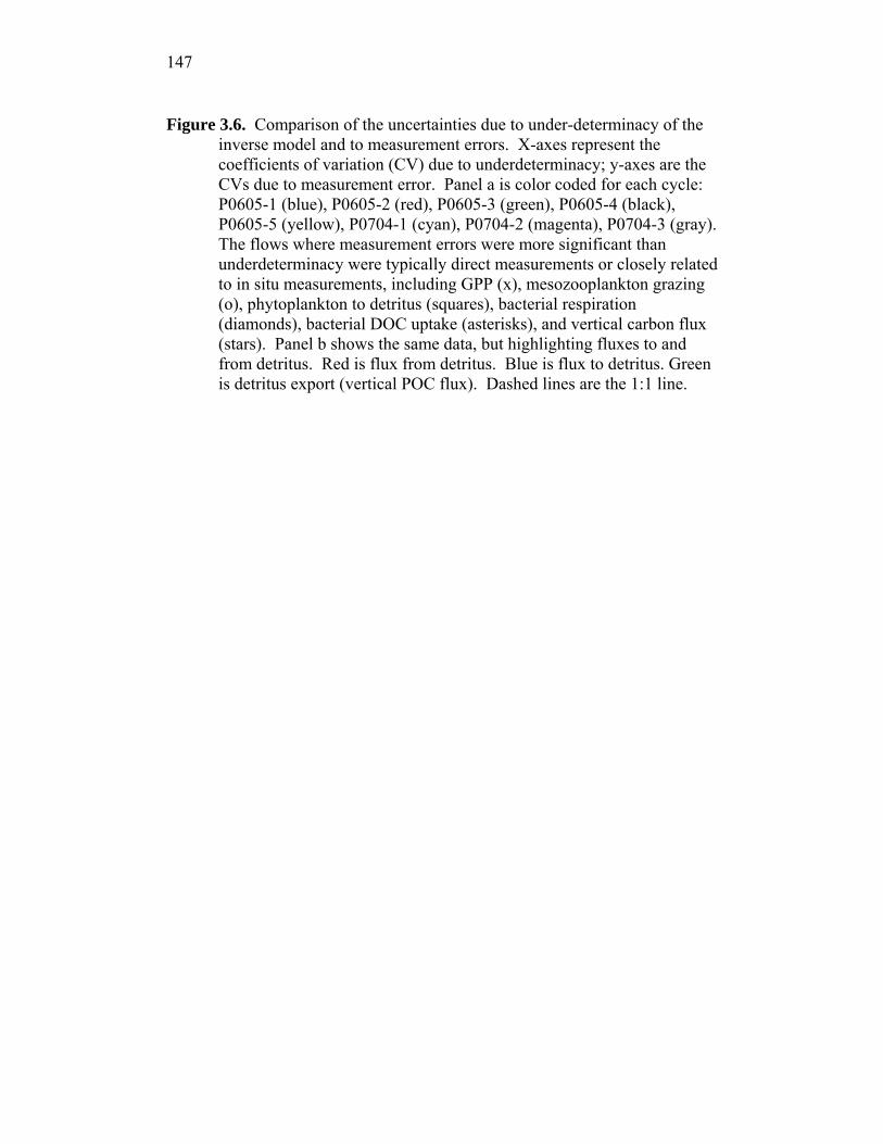
147  

Figure 3.6. Comparison of the uncertainties due to under-determinacy of the inverse model and to measurement errors. X-axes represent the coefficients of variation (CV) due to underdeterminacy; y-axes are the CVs due to measurement error. Panel a is color coded for each cycle: P0605-1 (blue), P0605-2 (red), P0605-3 (green), P0605-4 (black), P0605-5 (yellow), P0704-1 (cyan), P0704-2 (magenta), P0704-3 (gray). The flows where measurement errors were more significant than underdeterminacy were typically direct measurements or closely related to in situ measurements, including GPP (x), mesozooplankton grazing (o), phytoplankton to detritus (squares), bacterial respiration (diamonds), bacterial DOC uptake (asterisks), and vertical carbon flux (stars). Panel b shows the same data, but highlighting fluxes to and from detritus. Red is flux from detritus. Blue is flux to detritus. Green is detritus export (vertical POC flux). Dashed lines are the 1:1 line.

 

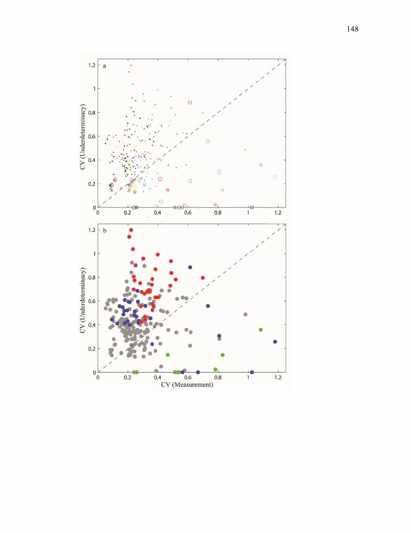
148

 

Figure 3.7. fluxemicrfluxeand are ±

Comparisoes (y-axis) torobial loop (yes are normagreen diamo±1 SD. Dash

n of food weo the classicy-axis) to thalized to 14Conds are the hed line is th

ebs. Panel aal food chain

he classical fo-PP. Magentnearshore (uhe 1:1 line.

a compares thn fluxes (x-a

food chain (xnta diamondsupwelling in

he multivoroaxis). Panel x-axis). All s are the offsnfluenced) cy

ous food chab comparesfood web

shore cycles ycles. Errorb

149

ain s the

bars

 

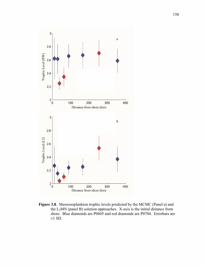
Figure 3.8. the Lshor±1 S

MesozooplL2MN (panere. Blue diamSD.

lankton trophl B) solutionmonds are P

hic levels prn approaches0605 and red

redicted by ths. X-axis is d diamonds

he MCMC (the initial diare P0704.

(Panel a) andistance fromErrorbars ar

150

d m

re

 

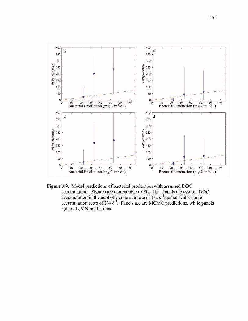
Figure 3.9. accuaccuaccub,d a

Model predumulation. Fumulation in umulation ratare L2MN pr

dictions of bFigures are c

the euphotictes of 2% d-1

redictions.

acterial prodcomparable tc zone at a ra1. Panels a,c

duction withto Fig. 1i,j. Pate of 1% d-

c are MCMC

h assumed DOPanels a,b as-1; panels c,dC predictions

OC ssume DOC

d assume s, while pane

151

C

els

152  

APPENDIX 3.1 – Model equalities (Ax=b) and inequalities (Gx≥h)

Equalities:

 

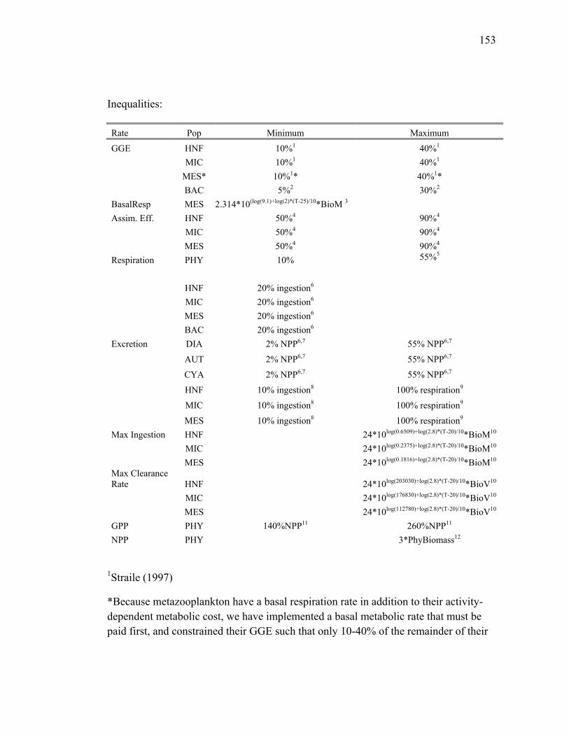
153  

 

Inequalities:

Rate Pop Minimum Maximum

GGE HNF 10%1 40%1

MIC 10%1 40%1

MES* 10%1* 40%1*

BAC 5%2 30%2

BasalResp MES 2.314*10(log(9.1)+log(2)*(T-25)/10*BioM 3

Assim. Eff. HNF 50%4 90%4

MIC 50%4 90%4

MES 50%4 90%4

Respiration PHY 10% 55%5

HNF 20% ingestion6

MIC 20% ingestion6

MES 20% ingestion6

BAC 20% ingestion6

Excretion DIA 2% NPP6,7 55% NPP6,7

AUT 2% NPP6,7 55% NPP6,7

CYA 2% NPP6,7 55% NPP6,7

HNF 10% ingestion8 100% respiration9

MIC 10% ingestion8 100% respiration9

MES 10% ingestion8 100% respiration9

Max Ingestion HNF 24*10log(0.6509)+log(2.8)*(T-20)/10*BioM10

MIC 24*10log(0.2375)+log(2.8)*(T-20)/10*BioM10

MES 24*10log(0.1816)+log(2.8)*(T-20)/10*BioM10 Max Clearance Rate HNF 24*10log(203030)+log(2.8)*(T-20)/10*BioV10

MIC 24*10log(176830)+log(2.8)*(T-20)/10*BioV10

MES 24*10log(112780)+log(2.8)*(T-20)/10*BioV10

GPP PHY 140%NPP11 260%NPP11

NPP PHY 3*PhyBiomass12

1Straile (1997)

*Because metazooplankton have a basal respiration rate in addition to their activity-dependent metabolic cost, we have implemented a basal metabolic rate that must be paid first, and constrained their GGE such that only 10-40% of the remainder of their

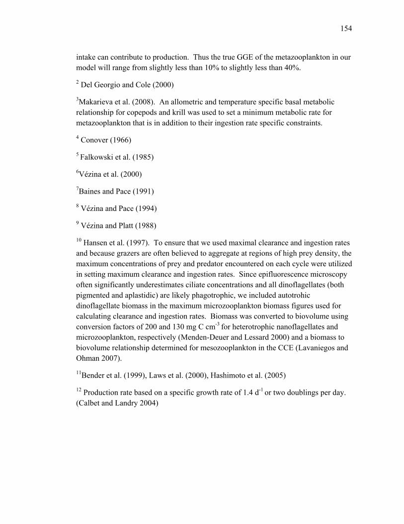
154  

intake can contribute to production. Thus the true GGE of the metazooplankton in our model will range from slightly less than 10% to slightly less than 40%.

2 Del Georgio and Cole (2000)

3Makarieva et al. (2008). An allometric and temperature specific basal metabolic relationship for copepods and krill was used to set a minimum metabolic rate for metazooplankton that is in addition to their ingestion rate specific constraints.

4 Conover (1966)

5 Falkowski et al. (1985)

6Vézina et al. (2000)

7Baines and Pace (1991)

8 Vézina and Pace (1994)

9 Vézina and Platt (1988)

10 Hansen et al. (1997). To ensure that we used maximal clearance and ingestion rates and because grazers are often believed to aggregate at regions of high prey density, the maximum concentrations of prey and predator encountered on each cycle were utilized in setting maximum clearance and ingestion rates. Since epifluorescence microscopy often significantly underestimates ciliate concentrations and all dinoflagellates (both pigmented and aplastidic) are likely phagotrophic, we included autotrohic dinoflagellate biomass in the maximum microzooplankton biomass figures used for calculating clearance and ingestion rates. Biomass was converted to biovolume using conversion factors of 200 and 130 mg C cm-3 for heterotrophic nanoflagellates and microzooplankton, respectively (Menden-Deuer and Lessard 2000) and a biomass to biovolume relationship determined for mesozooplankton in the CCE (Lavaniegos and Ohman 2007).

11Bender et al. (1999), Laws et al. (2000), Hashimoto et al. (2005)

12 Production rate based on a specific growth rate of 1.4 d-1 or two doublings per day. (Calbet and Landry 2004)

155  

APPENDIX 3.2: L2 minimum norm (L2MN) solution method

The typical L2MN method, as originally implemented by Vézina and Platt

(1988), assumes that the measurement and steady-state equations are exact and then

calculates the solution that minimizes the L2 norm. However, as this method tends to

zero out particular values and does not generate any confidence intervals, we instead

adopted an ensemble L2MN approach similar to the L2MN Monte Carlo method used

by Stukel et al. (2010). For each model input (measured rates and biomasses and

steady-state equalities), we generated a normal distribution from the experimentally

determined means (zero for unmeasured steady-state equalities) and variances. Inputs

were then chosen randomly from these distributions to allow for simultaneous

variation of each input. After inputs were chosen, the L2MN solution was computed

as explained below. For each cycle and numerical experiment we solved the L2MN

for 10,000 independent input parameter sets and determined our L2MN solution as the

mean of these 10,000 sets, while also calculating 95% confidence intervals for all

ecosystem flows.

Once the input parameters had been randomly selected, the L2MN solution was

calculated using the algorithm of Vézina and Platt (1988) as implemented in

MATLAB by Jackson et al. (2001). This algorithm is designed to find the solution

vector that simultaneously solves the system of equations Ax=b and Gx≥h while

minimizing the L2 norms of x (and Ax-b if the system of equations cannot be solved

exactly). This method begins by using the singular value decomposition (SVD) to

decompose the A matrix into the matrices U, L, and V, such that A=ULV*. If k is the

156  

rank of the problem, the first k rows of U and the first k columns of V* were used to

find the simplest solution (r1) that satisfies the equality constraints Ax=b. The

remaining columns of V* then form an orthonormal basis of vectors (Vp) that can be

added or subtracted to r1, while still satisfying the equality Ax=b. Vp is then used to

find the solution that minimizes the L2 norm while satisfying the inequality constraints

Gx≥h, which include constraints requiring that each flow be positive. When the

system of equations is solvable (i.e. there are no inconsistencies amongst the equalities

and inequalities) a full rank solution can be used (k = size of b), and the residual error

will be zero, so the algorithm will minimize the complexity of the solution (minimize

the L2 norm of x). Often inconsistencies existed in the data (e.g. when the

randomization process led to grazing rate inputs that were higher than the maximum

clearance rates or when the difference of growth and grazing was less than the rate of

change of the phytoplankton population). In such cases we followed the method of

Olsen et al. (2006) and chose the highest rank solution that could generate an answer

that satisfied the inequality constraints. When the rank was reduced, the algorithm

simultaneously minimized the L2 norms of x and Ax-b.

157  

APPENDIX 3.3 – The Markov Chain Monte Carlo (MCMC) solution method

The L2MN solution method selects a single solution vector from among the

infinite set of solutions to the under-determined inverse ecosystem problem, but there

is no a priori reason to suggest that it selects a solution that accurately depicts the

ways in which an ecosystem is constructed. Lacking evidence that any particular cost

function can be used to approximate ecosystem structure, Kones et al. (2006; 2009)

have suggested fully sampling the allowable solution space and suggest that the most

likely ecosystem state may be the mean of all possible ecosystem states.

To calculate such a maximum likelihood solution, we used the MCMC method

of Kones et al. (2009). We began with the solution vector from the L2MN method,

and utilized a random combination of the orthonormal basis Vp to generate a new

solution that also satisfied the equality constraints. The use of the mirror algorithm

(Van Den Meersche et al. 2009) allowed us to ensure that each new solution also

satisfied the inequality constraints. It works by computing the planes in an n-

dimensional hyperspace that describe the solution space allowed by the inequality

constraints. When the line connecting the original solution to the new solution crossed

a hyperplane, it was instead reflected by the hyperplane, thus ensuring that all

solutions satisfied the inequalities Gx≥h.

When the rank of the problem is full each iteration of the random walk yields a

new solution to the problem. However, when the rank of the solution is not full, due

to inconsistencies in the system of equations, a residual error (Ax-b) exists. In such

cases the probability of accepting any new iteration (xn+1) is calculated as:

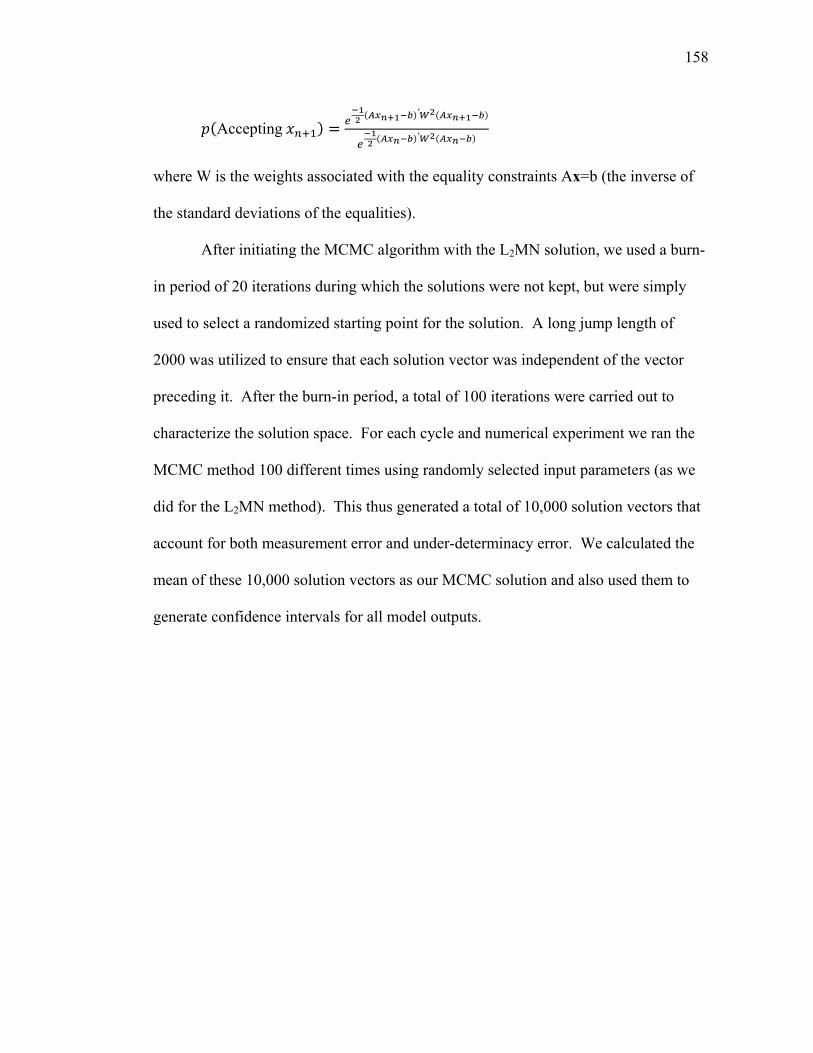
158  

Accepting′

′

where W is the weights associated with the equality constraints Ax=b (the inverse of

the standard deviations of the equalities).

After initiating the MCMC algorithm with the L2MN solution, we used a burn-

in period of 20 iterations during which the solutions were not kept, but were simply

used to select a randomized starting point for the solution. A long jump length of

2000 was utilized to ensure that each solution vector was independent of the vector

preceding it. After the burn-in period, a total of 100 iterations were carried out to

characterize the solution space. For each cycle and numerical experiment we ran the

MCMC method 100 different times using randomly selected input parameters (as we

did for the L2MN method). This thus generated a total of 10,000 solution vectors that

account for both measurement error and under-determinacy error. We calculated the

mean of these 10,000 solution vectors as our MCMC solution and also used them to

generate confidence intervals for all model outputs.

159  

References

ALVAREZ-SALGADO, X. A., M. D. DOVAL, A. V. BORGES, I. JOINT, M. FRANKIGNOULLE, E. M. S. WOODWARD, and F. G. FIGUEIRAS. 2001. Off-shelf fluxes of labile materials by an upwelling filament in the NW Iberian Upwelling System. Prog. Oceanogr. 51: 321-337.

BAINES, S. B., and M. L. PACE. 1991. The production of dissolved organic matter by

phytoplankton and its importance to bacteria: Patterns across marine and freshwater systems. Limnol. Oceanogr. 36: 1078-1090.

BENDER, M., J. ORCHARDO, M. L. DICKSON, R. BARBER, and S. LINDLEY. 1999. In

vitro O2 fluxes compared with 14C production and other rate terms during the JGOFS Equatorial Pacific experiment. Deep-Sea Res. I 46: 637-654.

CALBET, A., and M. R. LANDRY. 2004. Phytoplankton growth, microzooplankton

grazing, and carbon cycling in marine systems. Limnol. Oceanogr. 49: 51-57. CONOVER, R. J. 1966. Assimilation of organic matter by zooplankton. Limnol.

Oceanogr. 11: 338-345. DANIELS, R. M., T. L. RICHARDSON, and H. W. DUCKLOW. 2006. Food web structure

and biogeochemical processes during oceanic phytoplankton blooms: An inverse model analysis. Deep-Sea Res. II 53: 532-554.

DEL GEORGIO, P. A., and J. J. COLE. 2000. Bacterial energetics and growth efficiency,

p. 289-325. In D. L. Kirchman [ed.], Microbial Ecology of the Oceans. Wiley-Liss, Inc.

DUCKLOW, H. 2000. Bacterial Production and Biomass in the Oceans, p. 85-120. In D.

L. Kirchman [ed.], Microbial Ecology of the Oceans. Wiley-Liss. FALKOWSKI, P. G., Z. DUBINSKY, and K. WYMAN. 1985. Growth-irradiance

relationships in phytoplankton. Limnol. Oceanogr. 30: 311-321. HANSEN, P. J., P. K. BJORNSEN, and B. W. HANSEN. 1997. Zooplankton grazing and

growth: Scaling within the 2-2,000-mu m body size range. Limnol. Oceanogr. 42: 687-704.

HASHIMOTO, S., N. HORIMOTO, Y. YAMAGUCHI, T. ISHIMARU, and T. SAINO. 2005.

Relationship between net and gross primary production in the Sagami Bay, Japan. Limnol. Oceanogr. 50: 1830-1835.

160  

JACKSON, G. A., and P. M. ELDRIDGE. 1992. Food web analysis of a planktonic system off Southern California. Prog. Oceanogr. 30: 223-251.

JACKSON, G. A., N. NIQUIL, A. BURD, and T. L. RICHARDSON. 2001. Ecosystem

Modeling Group Software, Inverse model code. Texas A&M Univ. http://oceanz.tamu.edu/~ecomodel/Software/invmodel/invmodel.html.

KONES, J. K., K. SOETAERT, D. VAN OEVELEN, and J. O. OWINO. 2009. Are network

indices robust indicators of food web functioning? A Monte Carlo approach. Ecol. Model. 220: 370-382.

KONES, J. K., K. SOETAERT, D. VAN OEVELEN, J. O. OWINO, and K. MAVUTI. 2006.

Gaining insight into food webs reconstructed by the inverse method. J. Mar. Syst. 60: 153-166.

LANDRY, M. R., and R. P. HASSETT. 1982. Estimating the grazing impact of marine

microzooplankton. Mar. Biol. 67: 283-288. LANDRY, M. R., M. D. OHMAN, M. R. STUKEL, and K. TSYRKLEVICH. 2009.

Lagrangian studies of phytoplankton growth and grazing relationships in a coastal upwelling ecosystem off Southern California. Prog. Oceanogr. 83: 208-216.

LAVANIEGOS, B. E., and M. D. OHMAN. 2007. Coherence of long-term variations of

zooplankton in two sectors of the California Current System. Prog. Oceanogr. 75: 42-69.

LAWS, E. A., M. R. LANDRY, R. T. BARBER, L. CAMPBELL, M. L. DICKSON, and J.

MARRA. 2000. Carbon cycling in primary production bottle incubations: Inferences from grazing experiments and photosynthetic studies using 14C and 18O in the Arabian Sea. Deep-Sea Res. II 47: 1339-1352.

MAKARIEVA, A. M., V. G. GORSHKOV, B. L. LI, S. L. CHOWN, P. B. REICH, and V. M.

GAVRILOV. 2008. Mean mass-specific metabolic rates are strikingly similar across life's major domains: Evidence for life's metabolic optimum. Proc. Natl. Acad. Sci. U. S. A. 105: 16994-16999.

MENDEN-DEUER, S., and E. J. LESSARD. 2000. Carbon to volume relationships for

dinoflagellates, diatoms, and other protist plankton. Limnol. Oceanogr. 45: 569-579.

OLSEN, Y., S. AGUSTI, T. ANDERSEN, C. M. DUARTE, J. M. GASOL, I. GISMERVIK, A. S.

HEISKANEN, E. HOELL, P. KUUPPO, R. LIGNELL, H. REINERTSEN, U. SOMMER, H. STIBOR, T. TAMMINEN, O. VADSTEIN, O. VAQUE, and M. VIDAL. 2006. A

161  

comparative study of responses in planktonic food web structure and function in contrasting European coastal waters exposed to experimental nutrient addition. Limnol. Oceanogr. 51: 488-503.

SOETAERT, K., and D. VAN OEVELEN. 2009. Modeling food web interactions in benthic

deep-sea ecosystems: A practical guide. Oceanography 22: 128-143. STRAILE, D. 1997. Gross growth efficiencies of protozoan and metazoan zooplankton

and their dependence on food concentration, predator-prey weight ratio, and taxonomic group. Limnol. Oceanogr. 42: 1375-1385.

STUKEL, M. R., and M. R. LANDRY. 2010. Contribution of picophytoplankton to

carbon export in the equatorial Pacific: A re-assessment of food-web flux inferences from inverse models. Limnol. Oceanogr. 55: 2669-2685.

STUKEL, M. R., M. R. LANDRY, C. R. BENITEZ-NELSON, and R. GOERICKE. submitted.

Trophic cycling and carbon export relationships in the California Current Ecosystem. Limnol. Oceanogr.

VAN DEN MEERSCHE, K., K. SOETAERT, and D. VAN OEVELEN. 2009. xSample(): An R

function for sampling linear inverse problems. Journal of Statistal Software, Code Snippets 30: 1-15.

VAN OEVELEN, D., K. VAN DEN MEERSCHE, F. J. R. MEYSMAN, K. SOETAERT, J. J.

MIDDELBURG, and A. F. VEZINA. 2010. Quantifying food web flows using linear inverse models. Ecosystems 13: 32-45.

VENRICK, E. L. 2002. Floral patterns in the California Current System off southern

California: 1990-1996. J. Mar. Res. 60: 171-189. VÉZINA, A. F., F. BERREVILLE, and S. LOZA. 2004. Inverse reconstructions of

ecosystem flows in investigating regime shifts: impact of the choice of objective function. Prog. Oceanogr. 60: 321-341.

VÉZINA, A. F., and M. L. PACE. 1994. An inverse model analysis of planktonic food

webs in experimental lakes. Can. J. Fish. Aquat. Sci. 51: 2034-2044. VÉZINA, A. F., and M. PAHLOW. 2003. Reconstruction of ecosystem flows using

inverse methods: how well do they work? J. Mar. Syst. 40: 55-77. VÉZINA, A. F., and T. PLATT. 1988. Food web dynamics in the ocean .1. Best estimates

of flow networks using inverse methods. Mar. Ecol. Prog. Ser. 42: 269-287.

162  

VEZINA, A. F., C. SAVENKOFF, S. ROY, B. KLEIN, R. RIVKIN, J. C. THERRIAULT, and L. LEGENDRE. 2000. Export of biogenic carbon and structure and dynamics of the pelagic food web in the Gulf of St. Lawrence Part 2. Inverse analysis. Deep-Sea Res. II 47: 609-635.

WETZ, M. S., and P. A. WHEELER. 2004. Response of bacteria to simulated upwelling

phytoplankton blooms. Mar. Ecol. Prog. Ser. 272: 49-57.     

163  

CHAPTER 4

Mesozooplankton contribution to vertical carbon export in a coastal

upwelling biome

ABSTRACT

Mesozooplankton can directly impact global biogeochemical cycles by

repackaging particulate organic carbon (POC) into dense, rapidly sinking fecal pellets

and by undertaking vertical migrations that transport carbon and nutrients to depth.

We assessed the contribution of mesozooplankton to vertical flux in the California

Current Ecosystem, a productive but spatiotemporally variable coastal upwelling

biome, during cruises in April 2007 and October 2008. The use of sediment traps and

234Th disequilibrium measurements allowed us to accurately assess the total passive

flux of sinking POC, while pigment analyses and microscopic enumeration of

sediment trap samples provided estimates of total fecal carbon transport.

Identification of mesozooplankton in paired day-night, vertically-stratified plankton

tows allowed calculation of the active transport of carbon by the dominant taxa of

vertically migrating mesozooplankton (particularly copepods and euphausiids).

Across the nine ecosystem states encountered on the cruises, recognizable fecal pellet

mass flux ranged from 3.5 to 135.2 mg C m-2 d-1 (4 to 119% of total passive flux) at

the 100-m depth horizon. Phaeopigment concentrations in sediment traps suggested

164  

that the contribution of herbivorous fecal material may have ranged from 1.3 to 53.6

mg C m-2 d-1 or from 4.3 to 137 mg C m-2 d-1, depending on assumptions about

degradation of pigments in mesozooplankton guts. The active transport of carbon by

migratory mesozooplankton taxa ranged from 2.4 to 42.8 mg C m-2 d-1. Inter-cruise

comparisons suggest that fecal pellets contributed a much greater portion of export

during the productive spring cruise, when fecal material may have been responsible

for 100% source of sinking material, than during the fall cruise. During the fall cruise

a gradient was observed with carbon export in productive water parcels driven by a

large contribution of fecal pellets, but with vertical flux in less productive regions

containing an increasing portion of marine snow and small unidentifiable particles.

INTRODUCTION

The “biological pump,” a critical component of global biogeochemical cycles,

is responsible for transporting the carbon and nitrogen fixed by phytoplankton in the

euphotic zone to the deep ocean. While autotrophs govern the fixation of carbon,

however, the flux of carbon to depth is often driven by interactions of multiple trophic

levels. The relative importance of phytoplankton production, aggregation processes

(Alldredge and Gotschalk 1989; Jackson et al. 2005), mineral ballasting (Armstrong et

al. 2002), and mesozooplankton grazing (Buitenhuis et al. 2006) on vertical carbon

flux are still hotly debated and are likely regionally and spatially variable. While solid

arguments exist supporting the importance of each, the difficulty of directly measuring

their effects in situ has caused investigators to try to compare contributions based on

165  

models, which may support one theory but do not exclude the others. Clearly,

experimental evidence is needed to assess the nature of sinking material.

Within the California Current Ecosystem (CCE), Stukel et al. (submitted) has

suggested that the production of fecal material by mesozooplankton is sufficient to

account for all variability in vertical carbon flux. Mesozooplankton can mediate

biogeochemically-relevant processes in many ways, and thus play crucial roles in the

global carbon and nitrogen cycles. By packaging organic matter into dense, rapidly

sinking fecal pellets, they can efficiently transport carbon out of the surface ocean on

passively sinking particles (Turner 2002). Diel vertically migrating (DVM)

mesozooplankton can also actively transport carbon and nitrogen to depth when they

feed at the surface at night but descend during the day to respire, excrete, and

sometimes die at depth (Longhurst et al. 1990; Steinberg et al. 2000; Al-Mutairi and

Landry 2001). At times, mesozooplankton are also able to decrease carbon export

rates by exerting top-down pressure on phytoplankton (Goericke 2002; Olli et al.

2007; Landry et al. 2009) and consuming sinking particles (Wilson et al. 2010).

In this study we attempt to directly characterize the importance of

mesozooplankton in both active and passive transport of carbon out of the surface

ocean during two cruises of the CCE Long-Term Ecological Research (LTER)

program in April 2007 and October 2008. We show that across the wide range of

environmental conditions sampled identifiable fecal pellets were responsible for 35%

of passive carbon export at 100-m depth, although pigment analyses suggested that the

total sinking flux of fecal material may have been even higher. We also show that on

166  

average mesozooplankton contribute an additional 19 mg C m-2 d-1 that is not assessed

by typical carbon export measurements (e.g. sediment traps and radionuclide

disequilibrium techniques).

METHODS

Cruises and sampling plans – Data for this study come from two cruises of the

California Current Ecosystem (CCE) Long-Term Ecological Research (LTER)

program conducted during April 2007 (CCE-P0704) and October 2008 (CCE-P0810).

During these cruises, water parcels were identified using satellite images of sea

surface temperature and chlorophyll, together with Moving Vessel Profiler site

surveys, and tagged with a surface drifter drogued at 15-m (Fig. 1). A simultaneously

deployed and identically drogued drift array with attached sediment traps (at 1-2

depths) allowed the collection of sinking particulate matter. Paired day-night

deployments of a 1m2, 202-m Multiple Opening and Closing Net with an

Environmental Sensing System (MOCNESS) collected depth-stratified

mesozooplankton samples over the upper 450 m of the water column at the location of

the surface drifter. These samples were later enumerated by Zooscan (as described

below) and grouped into broad taxononomic and size classes. Oblique bongo tows

(0.71-m diameter, 202-m mesh) were also used twice per day to collect organisms

for determination of size-fractionated dry weights and grazing rates of the

mesozooplankton community. Size-fractionated dry weights were converted to carbon

biomass using the dry weight to carbon relationships of Landry et al. (2001).

167  

234Th export measurements – 234Th deficiency was determined from 4-L

samples taken at 8-10 depths per cast of a CTD Niskin rosette, following established

small-volume procedures (Benitez-Nelson et al. 2001b; Buesseler et al. 2001; Pike et

al. 2005). Immediately after collection, samples were acidified to a pH of ~2 with

concentrated HNO3 and spiked with 230Th (1 mL at 10 dpm mL-1). Four hours later,

NH4OH was added to adjust to a pH of ~9, and 100 L each of KMnO4 (7.5 g L-1) and

MnCl2 (33 g L-1) were added. Samples were shaken and allowed to equilibrate for >8

hours as the Th co-precipitated with MnO2. Precipitates were vacuum filtered under

high-pressure onto 25-mm quartz microfiber filters and mounted into RISO cups.

Samples were counted ashore with a low-level RISO beta counter in the Benitez-

Nelson lab at the University of South Carolina. After >6 half-lives had passed, they

were again counted to establish background beta emission levels. Filtration yields

were calculated by Inductively Coupled Plasma Mass Spectrometry (at the WHOI

Analytical Facility) after addition of a gravimetrically measured aliquot of 229Th (99.5

dpm) and column chromatography in AG1-X8 100-200 mesh chloride form resin to

purify the Th isotopes. Recoveries averaged 86%. 238U was assumed to co-vary with

salinity and calculated from the equation: 238U (dpm L-1) = 0.0686•salinity•density

(Chen et al. 1986). Deficiency was calculated as the difference between 238U and

234Th. 234Th export was determined using a one-dimension steady-state model (E =

Th (AU-ATh)) and trapezoidal vertical integration. Although this steady-state model

oversimplifies the complex processes affecting particulate and dissolved Th cycling in

168  

the ocean euphotic zone, it closely matched the 234Th flux results found in sediment

traps for 8 out of the 9 cycles assessed (Fig. 2).

234Th export was converted to vertical carbon flux by multiplying by

experimentally-determined C:234Th ratios. Particulate samples for the determination

of the C:Th ratio were collected using two independent methods, sediment traps and in

situ pumps. C:Th samples were routinely collected at a depth horizon of 100 m and

they were also collected from a depth just below the base of the euphotic zone on the

P0810 cruise. Sediment trap C:Th samples were collected as discussed below. In situ

pump samples were collected using a McLane WTS-LV pump with pre-filters to size-

fractionate collected particles. On the P0704 cruise, >20-m particles were used for

calculating the C:234Th ratio; on the P0810 cruise >50-m particles were used. In each

case, 300-L of seawater were filtered through a Nitex filter, which was then rinsed

onto a 25-mm quartz microfiber filter. Quartz microfiber filters for the C:234Th ratio

were counted on land similarly to the water-column 234Th samples. After background

count, filters were combusted in the Costech 4010 elemental combustion analyzer in

the SIO Analytical Laboratory. Prior to combustion, filters from the P0810 cruise

were acidified to remove inorganic carbon. Filters from the P0704 cruise were not

acidified.

Sediment trap deployment and analyses – VERTEX-style drifting sediment

traps (Knauer et al. 1979) were deployed at the beginning and recovered at the end of

each cycle. Trap arrays consisted of 4-12 particle interceptor traps (PIT) with an inner

169  

diameter of 70-mm and aspect (height:diameter) ratio of 8:1. Each PIT had a baffle on

top that consisted of 14 smaller tubes, also with an 8:1 aspect ratio. The tubes in the

baffle were tapered at the top, and it was assumed that all particles within the inner

diameter of the PIT descended into the trap. The traps were designed to sample

settling material accurately by creating a semi-stable boundary layer immediately

above the trap, while avoiding mixing and resuspension during recovery. On P0704, 8

PITs were deployed at a depth of 100 m on each cycle. On P0810, 8-12 PITs were

deployed at a depth of 100-m and 4-8 PITs were deployed at the base of the euphotic

zone, except on Cycle 2, when the euphotic zone was close to 100 m.

Before deployment, each PIT was filled with 2.2 L of a slurry composed of

filtered seawater with an additional 50 g L-1 NaCl to create a density interface within

the tube that prevented mixing with in situ water. The traps were fixed with a final

concentration of 4% formaldehyde before deployment to minimize decomposition as

well as consumption by mesozooplankton grazers (Knauer et al. 1984). Upon

recovery, the depth of the salinity interface was determined, and the overlying water

was gently removed with a peristaltic pump until only 5 cm of water remained above

the surface. The water was then mixed to disrupt large clumps and screened through a

300-m Nitex filter. Swimmers were removed from the filters under a dissecting

scope, and the remaining material was returned to the sample. The tubes were then

split with a Folsom splitter, and subsamples were taken for C, N, C:234Th, pigment

analyses, and microscopy. Typically, ¼ PIT tube samples were filtered through a pre-

combusted GFF, which was either acidified (to assess organic carbon) or not acidified

170  

(for total carbon) prior to combustion in the Costech 4010 elemental combustion

analyzer in the SIO Analytical Facility. Entire tubes were typically filtered through

quartz microfiber filters for C:234Th analyses as described above. Triplicate

subsamples (typically 50 mL) were analyzed for Chl a and phaeopigment

concentrations using acidification with HCl and a Turner Designs Model 10

fluorometer. Samples for microscopic analysis were stored in dark bottles and

analyzed on land as described below.

Microscopic enumeration of sediment trap fecal pellets – On land, sediment

trap samples were gently filtered through a 60-m filter which was then rinsed onto a

gridded petri dish. The sample was then analyzed under a dissecting microscope at

25X magnification (Wilson et al. 2008). Recognizable fecal pellets were separated

from other sediment trap material. They were then photographed under both bright-

and dark-field illumination. Images were analyzed using ImagePro (Media

Cybernetics, Inc., ver 6.0), with the bright-field images used to draw outlines around

the fecal pellets. Dark-field images were used to determine color of the fecal pellets.

Fecal pellets were manually classified into six different shape categories (ovoid,

cylindrical, spherical, tabular, amorphous, and ellipsoid) with appropriate length and

width relationships used to convert into fecal pellet volumes. For tabular fecal pellets,

we assumed that depth was equal to one half of width. Fecal pellets from several of

the samples were sorted into broad classes (small, cylindrical, and tabular) and sized

and combusted in the CHN analyzer to determine carbon:volume relationships of

0.125 mg C mm-3 for ovoids, spheres, and ellipsoids; 0.055 mg C mm-3 for cylindrical

171  

and amorphous pellets; and 0.029 mg C mm-3 for tabular fecal pellets. Fecal pellets

(particularly tabular and cylindrical pellets) were often found broken, likely due to

sample processing. When they were clearly recognizable as fecal pellets and the

fragment size was apparent, we counted these fragments as individual pellets. While

this may inflate the total number of pellets, it likely gave a more accurate

measurement of the total fecal pellet mass in the sample.

Mesozooplankton community enumeration – MOCNESS samples were

analyzed to determine the concentrations and biomasses of broad taxonomic groups

common in the CCE region (copepods, appendicularians, chaetognaths, salps and

doliolids, eggs, euphausiids, nauplii, ostracods, polychaetes, pteropods,

siphonophores, and others). Mesozooplankton were size-fractionated through a 1-mm

filter, then each size-fraction was subsampled with a Folsom splitter until a reasonable

amount of material (typically 100-1000 organisms) remained. For night-time samples

an additional >5-mm fraction was analyzed to assess more accurately the larger

portion of the community. Subsamples were analyzed using ZooScan hardware with

ZooProcess and Plankton Identifier software (Gorsky et al. 2010). Following

automatic classification of organisms, vignettes were manually checked to ensure

correct taxonomic assessment. Length (feret) and area measurements were used to

estimate carbon weight of each organism using the relationships in Table 1.

Calculation of active carbon transport - The active transport of carbon by

mesozooplankton that feed in the surface at night and respire at depth during the day

was calculated for the dominant diel vertically migrating (DVM) taxa in the CCE

172  

region (copepods, euphausiids, chaetognaths, and others - noted to be primarily

hyperiid amphipods) by first dividing each taxon into 11 size classes. The day-night

biomass difference (integrated to 100-m depth) for each size class was then

determined from paired MOCNESS tows. Specific respiration for each size and

taxonomic class was computed from the equation:

Respiration μLO2ind‐1hr‐1

where CW is carbon weight (mg C) and T is the average temperature (°C) from 100 to

500-m depth. The constants a0, a1, and a2 were assumed to be 0.124, 0.780, and 0.073,

respectively, for copepods (Ikeda et al. 2001) and 0.524, 0.8354, and 0.061,

respectively, for other metazooplankton (Ikeda 1985). This respiration rate is likely

the organisms’ standard metabolism, and hence may be an underestimate of their in

situ metabolism. However, they were unlikely to be feeding at depth, and we believe

their standard metabolism to be representative. We assumed that organisms respired

at depth for 12 h per day. While we allowed individual size-classes to undergo both

normal and reverse DVM, we assumed that bulk taxa (e.g. copepods, euphausiids,

etc.) were not undergoing reverse DVM and hence set a minimum active transport rate

of 0 for each taxa. The active transport of N was similarly calculated, using size-

specific rates of ammonia excretion:

Excretion μgNind‐1hr‐1

173  

where CW and T are again carbon weight and average temperature and a0, a1, and a2

are -2.769, 0.711, and 0.071, respectively, for copepods (Ikeda et al. 2001) and -

2.1763, 0.8293, and 0.0648, respectively, for other metazooplankton (Ikeda 1985).

Since the dominant euphausiid species in our MOCNESS samples (Euphausia

pacifica, Nematoscelis difficilis, and Euphausia gibboides) are known to be both

strong vertical migrators and visual net-avoiders (Brinton 1967), we calculated an

adjusted euphausiid active transport rate by assuming that day time vertically-

integrated euphausiid biomass (0 to 450 m) should be equal to night time biomass and

that net avoidance was constant with depth. When day time tows were deficient in

integrated euphausiid biomass relative to paired night time tows, we scaled the day

time profile proportionally at all depths so that the integrated biomasses were equal

and recalculated respiration at depth. This adjusted active transport rate may be an

underestimate, as it does not take into account euphausiids that may migrate deeper

than 450 m; thus the true transport rate may lie somewhere between the raw and

adjusted rates.  

Mesozooplankton gut pigment analyses - Daily rates of mesozooplankton community

grazing on phytoplankton were determined from mid-day and mid-night bongo tow

samples. The samples were anesthetized with soda water and size-fractionated into size

classes of 0.2-0.5, 0.5-1, 1-2, 2-5 and >5 mm. Each size-fraction was divided on a Folsom

splitter, with 3/8 being frozen in liquid nitrogen and saved for gut fluorescence analyses.

Subsamples of each size class were inspected under a dissecting microscope to remove

phytoplankton and detritus, then sonicated in 90% acetone, centrifuged and read for Chl a

174  

and phaeopigment concentrations using acidification and a Turner Designs Model 10

fluorometer. As suggested by Conover et al. (1986), phaeopigment estimates were not

multiplied by 1.51 (the Chl a:phaeopigment ratio). Pigment degradation to non-fluorescent

products was further assumed (following Durbin and Campbell 2007) to be included in

determination of gut clearance rates, which were estimated using the temperature

dependent function K (min-1) = 0.0124 e0.0765 T (°C) of Dam and Peterson (1988), using mean

temperature in the depth range of highest chlorophyll where zooplankton were expected to

congregate and feed. To determine daily community ingestion rates, the sum of Chl a and

phaeopigments for all size-classes was averaged between day-night paired tows and

multiplied by the gut pigment turnover rate to determine daily community ingestion rates.

RESULTS

Cruise conditions – Nine Lagrangian drift experiments (cycles) were

conducted as a part of this study (3 in Apr. 2007, 6 in Oct. 2009, Fig. 2). The P0704

cruise took place during typical spring upwelling conditions in the CCE. It included

two inshore cycles (Cycles 1 & 3) near the Point Conception upwelling source with

significant surface nitrate concentrations (~5 & 7 mol L-1, for Cycles 1 & 3,

respectively) and surface chlorophyll concentrations (>1 g L-1). Both of these cycles

featured a large and active mesozooplankton community that impacted phytoplankton

with high grazing rates (37.3 and 7.7 mg Chl a m-2 d-1, respectively) and drove an

overall decrease in vertically integrated chlorophyll over the course of the 4-day

cycles (Landry et al. 2009). Cycle 2 took place in an offshore anti-cyclonic eddy with

175  

low surface nitrate (<0.1 M) and chlorophyll (~0.2g L-1) concentrations, a distinct

deep chlorophyll max at ~70 m, and significantly less mesozooplankton grazing (1.3

mg Chl a m-2 d-1).

The P0810 cruise took place during a period when typical hydrographic

conditions would suggest a more quiescent period. However strong winds from the

north beginning on 2 Oct. likely mixed the surface waters near Point Conception

stimulating phytoplankton growth during Cycles 3-6. Surface nitrate was relatively

low through all cycles (~0.15 – 0.3 M) except for Cycle 5, which was near the

productive side of an upwelling front with surface nitrate concentrations of ~2 M.

Cycles 2 and 6 (which was on the unproductive side of the front) were representative

of more oligotrophic conditions, with low surface chlorophyll concentrations of ~0.2

g L-1 and distinct subsurface chlorophyll maxima. While Cycle 1 occurred prior to a

wind event (and had a surface chlorophyll concentration of ~0.5 g L-1), the other

three cycles showed increasing surface chlorophyll concentration from north to south

(~0.7, 1.0, and 1.4 g L-1 for Cycles 3-5, respectively) suggesting that the community

may have been growing as it was advected south. While Cycles 1-3 (like the cycles

from P0704) were typically 4 days long, Cycles 4-6 were shortened mini-cycles of 2-

day duration.

Carbon export – We measured 234Th concentrations on two or three casts per

cycle. With the exception of one anomalous profile on P0810-1, vertical profiles

consistently showed 234Th deficiency at the surface and a switch to remineralization

176  

slightly below the base of the euphotic zone (Fig. 3). Repeated profiles showed no

strong evidence of increasing deficiency over the two- to four-day experimental

cycles. 234Th export rates across the 100-m depth horizon (calculated using a simple

one-dimensional steady-state equation) ranged from 460-1980 dpm m2 d-1, and were

highest during the two nearshore cycles from P0704 and P0810-6, and lowest during

P0810-1 and P0810-3. These steady-state 234Th export rates closely matched 234Th

fluxes determined from sediment traps placed at 100 m (and at the base of the euphotic

zone on P0810) with the exception of cycle P0810-4 (Fig. 2). This cycle was located

close to the Point Conception upwelling center shortly after a strong wind event

moved through the region, and we suspect that upwelling introduced additional 234Th

into the surface waters, leading to an underestimation of export by the one-

dimensional steady-state equation.

To convert 234Th fluxes to carbon export, we measured the C:234Th ratio on

particles collected in two different manners, with sediment traps and with an in situ

pump deployed at the same depth horizon. While the two methods determined the

same broad patterns in C:234Th ratio, including higher C:234Th in surface waters, they

disagreed on the magnitude of the ratio (Fig. 4). The in situ pump typically

underestimated the C:234Th ratio relative to the sediment trap, often by a factor of

almost 2. In the absence of an a priori reason to trust one method over the other, we

used the average C:234Th ratio determined by the two methods to compute our steady-

state estimates of carbon export (Table 2).

177  

For the 9 experimental cycles, steady-state carbon export averaged 60 mg C m-

2 d-1 at the 100-m depth horizon. Export was much more variable on the P0704 cruise,

for which the onshore cycles had export rates of 83 and 129 mg C m-2 d-1 (P0704-1

and P0704-3), while the offshore cycle had significantly lower export of only 37 mg C

m-2 d-1. On P0810, export varied far less and showed no distinct trends with distance

from shore, although this may be due to the greater homogeneity experienced during

the October cruise. A comparison of export at the 100-m depth horizon to export at

the base of the euphotic zone showed significant remineralization, with an average of

46% of carbon remineralized in the 40-50m below the euphotic zone. Our paired

sediment traps, by comparison, suggested that only 21% of carbon was remineralized

in this depth horizon. Regardless, remineralization was substantial, suggesting that the

calculated carbon export for the P0704 cruise (when we only measured export at 100

m) may have underestimated the carbon flux across the base of the euphotic zone.  

Sediment trap contents – Sediment trap carbon and nitrogen samples (Table 3)

suggested that the C:N ratios on sinking material averaged 6.4 (molC:molN) during

the spring cruise, similar to the C:N ratio of particulate organic matter (POM) in the

euphotic zone (6.1). While the C:N ratio of the POM in the surface water in the fall

was not significantly different, the sinking material was depleted in nitrogen, with

average C:N ratios of 10.2 at the base of the euphotic zone and 11.1 at 100 m,

suggesting significant reworking of POM as it sank. The magnitude of total pigment

flux was highly variable, but phaeopigment flux was consistently an order of

magnitude higher than chlorophyll flux (Fig. 5). Pigment fluxes indicate that bulk

178  

phytoplankton sinking rates never exceeded 0.66 m d-1 (with an average across all

cycles of 0.23 m d-1). This is likely an overestimate as the low Chl:Phaeo ratios

suggest that a significant portion of the sediment trap chlorophyll may have sunk

undegraded in fecal pellets. Bulk phaeopigment sinking rates ranged from 0.71 to

18.6 m d-1 (with an average of 5.0 m d-1). Sediment trap phaeopigment concentrations

were strongly correlated with the mass flux of recognizable fecal pellets (Fig. 6),

which were presumably the source of the phaeopigments. Pigment fluxes were

highest during cycles P0704-1 and P0704-3 when an assemblage of large, active

herbivorous mesozooplankton was present.

Two sediment trap samples from each sediment trap deployment and depth

were microscopically sorted at 25X magnification to characterize the >60-m particle

size-fraction, which was assumed to represent most of the carbon flux. A qualitative

assessment suggested that fecal pellets were the dominant component in most

sediment trap samples. For both trap samples of P0704-2, a large number of small

zooplankton likely made it through 303-m mesh screen; we thus believe that organic

carbon flux was overestimated on that cycle. On one of two samples from P0704-3 a

significant portion of the sample was comprised of marine snow that looked like it

contained fragments of degraded fecal pellets and the other sample was primarily fecal

pellets. Recognizable fecal pellets were not common in any of the samples from

P0810-1, with the surface samples dominated by marine snow aggregates and the

deeper samples comprised mainly of small unidentifiable particles. For P0810-2, one

of the samples was fecal pellet dominated while the other contained almost nothing

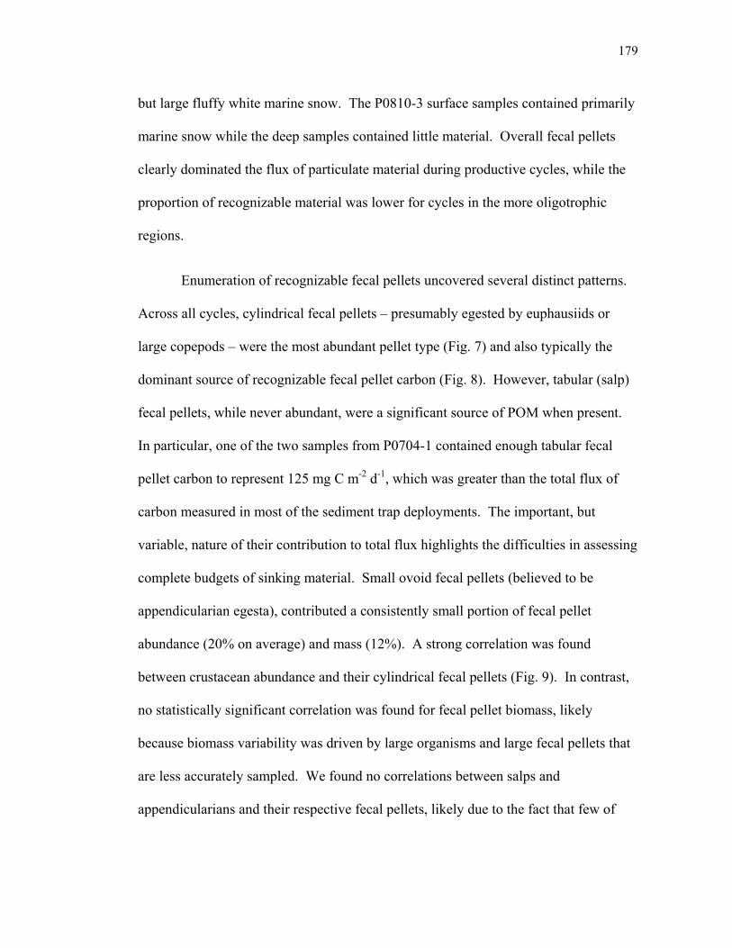
179  

but large fluffy white marine snow. The P0810-3 surface samples contained primarily

marine snow while the deep samples contained little material. Overall fecal pellets

clearly dominated the flux of particulate material during productive cycles, while the

proportion of recognizable material was lower for cycles in the more oligotrophic

regions.

Enumeration of recognizable fecal pellets uncovered several distinct patterns.

Across all cycles, cylindrical fecal pellets – presumably egested by euphausiids or

large copepods – were the most abundant pellet type (Fig. 7) and also typically the

dominant source of recognizable fecal pellet carbon (Fig. 8). However, tabular (salp)

fecal pellets, while never abundant, were a significant source of POM when present.

In particular, one of the two samples from P0704-1 contained enough tabular fecal

pellet carbon to represent 125 mg C m-2 d-1, which was greater than the total flux of

carbon measured in most of the sediment trap deployments. The important, but

variable, nature of their contribution to total flux highlights the difficulties in assessing

complete budgets of sinking material. Small ovoid fecal pellets (believed to be

appendicularian egesta), contributed a consistently small portion of fecal pellet

abundance (20% on average) and mass (12%). A strong correlation was found

between crustacean abundance and their cylindrical fecal pellets (Fig. 9). In contrast,

no statistically significant correlation was found for fecal pellet biomass, likely

because biomass variability was driven by large organisms and large fecal pellets that

are less accurately sampled. We found no correlations between salps and

appendicularians and their respective fecal pellets, likely due to the fact that few of

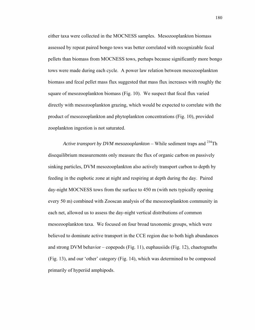
180  

either taxa were collected in the MOCNESS samples. Mesozooplankton biomass

assessed by repeat paired bongo tows was better correlated with recognizable fecal

pellets than biomass from MOCNESS tows, perhaps because significantly more bongo

tows were made during each cycle. A power law relation between mesozooplankton

biomass and fecal pellet mass flux suggested that mass flux increases with roughly the

square of mesozooplankton biomass (Fig. 10). We suspect that fecal flux varied

directly with mesozooplankton grazing, which would be expected to correlate with the

product of mesozooplankton and phytoplankton concentrations (Fig. 10), provided

zooplankton ingestion is not saturated.

Active transport by DVM mesozooplankton – While sediment traps and 234Th

disequilibrium measurements only measure the flux of organic carbon on passively

sinking particles, DVM mesozooplankton also actively transport carbon to depth by

feeding in the euphotic zone at night and respiring at depth during the day. Paired

day-night MOCNESS tows from the surface to 450 m (with nets typically opening

every 50 m) combined with Zooscan analysis of the mesozooplankton community in

each net, allowed us to assess the day-night vertical distributions of common

mesozooplankton taxa. We focused on four broad taxonomic groups, which were

believed to dominate active transport in the CCE region due to both high abundances

and strong DVM behavior – copepods (Fig. 11), euphausiids (Fig. 12), chaetognaths

(Fig. 13), and our ‘other’ category (Fig. 14), which was determined to be composed

primarily of hyperiid amphipods.

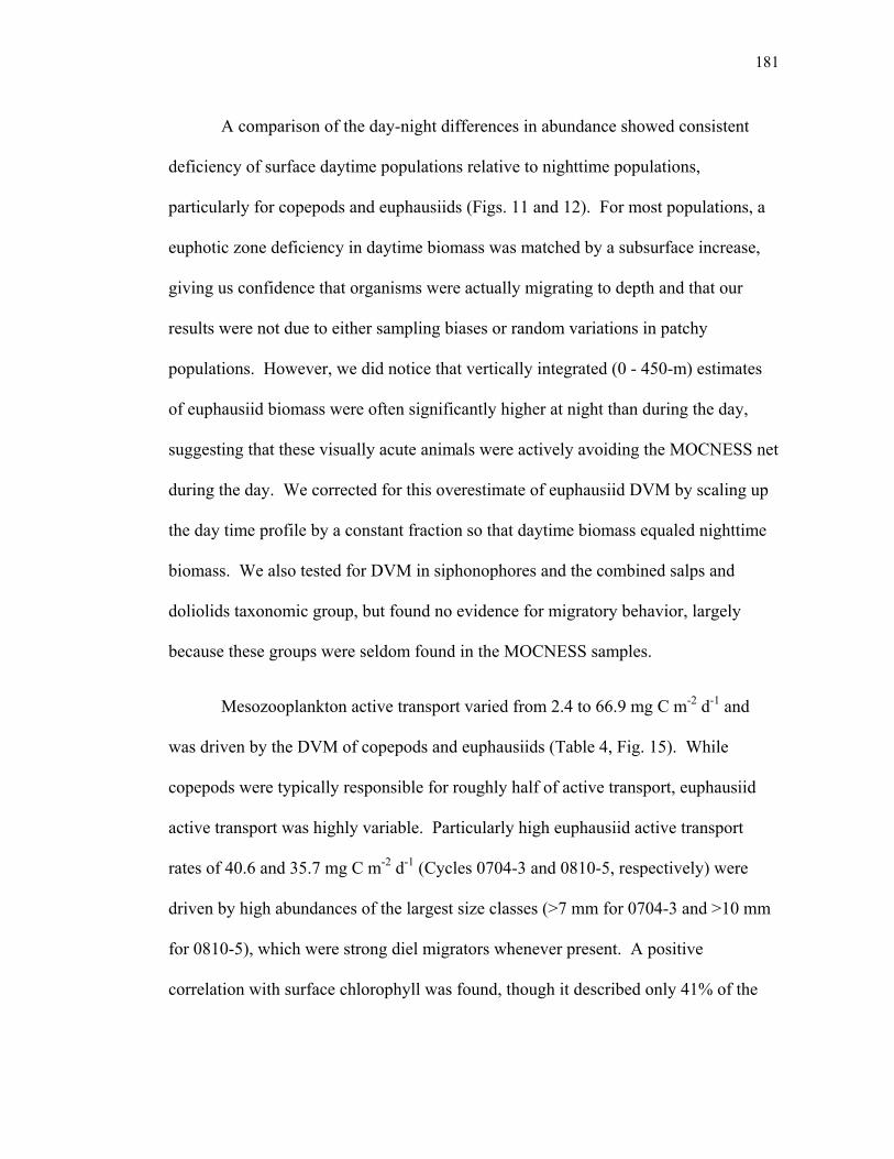
181  

A comparison of the day-night differences in abundance showed consistent

deficiency of surface daytime populations relative to nighttime populations,

particularly for copepods and euphausiids (Figs. 11 and 12). For most populations, a

euphotic zone deficiency in daytime biomass was matched by a subsurface increase,

giving us confidence that organisms were actually migrating to depth and that our

results were not due to either sampling biases or random variations in patchy

populations. However, we did notice that vertically integrated (0 - 450-m) estimates

of euphausiid biomass were often significantly higher at night than during the day,

suggesting that these visually acute animals were actively avoiding the MOCNESS net

during the day. We corrected for this overestimate of euphausiid DVM by scaling up

the day time profile by a constant fraction so that daytime biomass equaled nighttime

biomass. We also tested for DVM in siphonophores and the combined salps and

doliolids taxonomic group, but found no evidence for migratory behavior, largely

because these groups were seldom found in the MOCNESS samples.

Mesozooplankton active transport varied from 2.4 to 66.9 mg C m-2 d-1 and

was driven by the DVM of copepods and euphausiids (Table 4, Fig. 15). While

copepods were typically responsible for roughly half of active transport, euphausiid

active transport was highly variable. Particularly high euphausiid active transport

rates of 40.6 and 35.7 mg C m-2 d-1 (Cycles 0704-3 and 0810-5, respectively) were

driven by high abundances of the largest size classes (>7 mm for 0704-3 and >10 mm

for 0810-5), which were strong diel migrators whenever present. A positive

correlation with surface chlorophyll was found, though it described only 41% of the

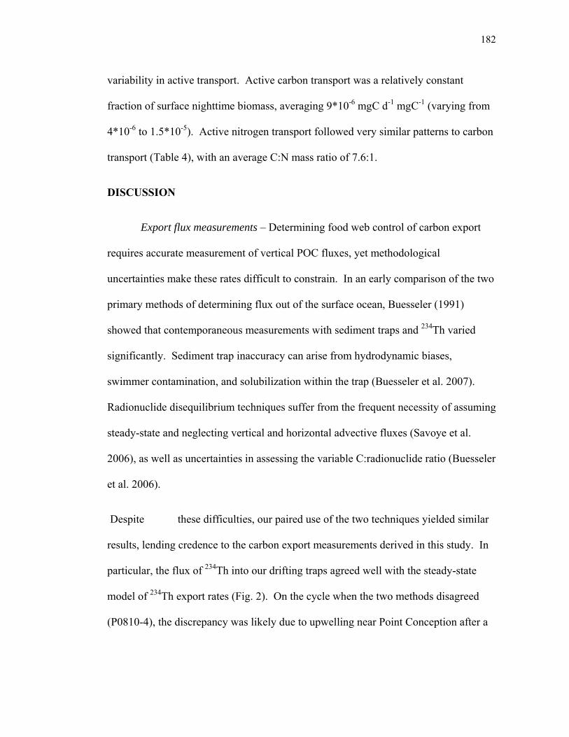
182  

variability in active transport. Active carbon transport was a relatively constant

fraction of surface nighttime biomass, averaging 9*10-6 mgC d-1 mgC-1 (varying from

4*10-6 to 1.5*10-5). Active nitrogen transport followed very similar patterns to carbon

transport (Table 4), with an average C:N mass ratio of 7.6:1.

DISCUSSION

Export flux measurements – Determining food web control of carbon export

requires accurate measurement of vertical POC fluxes, yet methodological

uncertainties make these rates difficult to constrain. In an early comparison of the two

primary methods of determining flux out of the surface ocean, Buesseler (1991)

showed that contemporaneous measurements with sediment traps and 234Th varied

significantly. Sediment trap inaccuracy can arise from hydrodynamic biases,

swimmer contamination, and solubilization within the trap (Buesseler et al. 2007).

Radionuclide disequilibrium techniques suffer from the frequent necessity of assuming

steady-state and neglecting vertical and horizontal advective fluxes (Savoye et al.

2006), as well as uncertainties in assessing the variable C:radionuclide ratio (Buesseler

et al. 2006).

Despite these difficulties, our paired use of the two techniques yielded similar

results, lending credence to the carbon export measurements derived in this study. In

particular, the flux of 234Th into our drifting traps agreed well with the steady-state

model of 234Th export rates (Fig. 2). On the cycle when the two methods disagreed

(P0810-4), the discrepancy was likely due to upwelling near Point Conception after a

183  

strong wind event. The introduction of a modest upwelling term of 0.7 m d-1,

combined with the vertical gradient in 234Th of 0.012 dpm L-1 m-1, could explain the

discrepancy between the steady-state and sediment trap measurements of 234Th flux at

the 100-m depth horizon. Nevertheless, without measurements of upwelling, it is

impossible to state conclusively why the two methods did not agree. We could also

hypothesize the possibility of upwelling affecting cycles P0704-1, P0704-3, and

P0810-1, yet find no need to include an upwelling term for these cycles. When

determining export rates in an upwelling region, we suggest that it is prudent to either

measure upwelling or utilize two different methods of measuring carbon flux.

Unlike the similarity in 234Th flux measurements, a distinct difference was

found between the C:234Th ratio as determined by sediment traps and in situ pumps

(Fig. 4), a result that was also found in the Barents Sea (Coppola et al. 2002). While

234Th export rates in the study varied by a factor of 4, C:234Th ratios varied by a factor

of almost 6 and thus had a greater impact on carbon flux rates computed from 234Th

disequilibrium. The discrepancy between the two methods of collecting particles is

thus a significant issue. In our study, sediment traps predicted significantly higher

C:234Th ratios than in situ pumps. The in situ pump ratio only exceeded the sediment

trap ratio on two out of fourteen measurements (neither significant) while the sediment

trap ratio was often significantly higher than the pump values. This difference may be

a simple result of the oversampling of slowly sinking particles by in situ pumps.

Slowly sinking particles have greater time to equilibrate with deeper water conditions

where POC to total thorium ratios are significantly higher than at the surface, thus

184  

deflating their C:234Th ratio relative to rapidly sinking particles. Despite the

attractiveness of this simple explanation for the methodological differences, this

pattern has not been found in all studies that compare sediment traps to pumps (e.g.

Benitez-Nelson et al. 2001a).

In addition to 234Th methodological issues, sediment traps have their own

biases. While we lack the ability to address hydrological or solubilization effects, our

microscopic sorting of fecal pellet contents allowed us to assess the impact of

swimmer contamination. In general, our method of screening with a 303-m filter and

microscopically sorting the larger size-fraction efficiently removed mesozooplankton

from the samples. However, in oligotrophic cycles (particularly P0704-2, but also to a

lesser extent in P0810-1, P0810-3, and P0810-6) contamination by small swimmers

was a significant issue, suggesting that a smaller mesh size should be used when the

mesozooplankton community is dominated by smaller organisms. In P0704-2,

swimmers may have comprised over 50% of the sample, suggesting that the sediment

traps overestimated carbon flux by a factor of 2 or more. Relative to the steady-state

calculation, the sediment traps were actually underestimating 234Th flux, although this

result may be misleading as mesozooplankton swimmers were found to have very high

C:234Th ratios (data not shown) and hence would not have contributed much thorium

to the trap samples. 

Contribution of fecal carbon to vertical flux – Ecological relationships have

indirectly suggested that fecal pellet flux may drive vertical carbon export in the CCE.

Assuming 30% egestion efficiency and no fecal pellet remineralization, Stukel et al.

185  

(submitted) used a simple trophic model to show that mesozooplankton egestion could

account for all of the variability in measured vertical carbon flux across three disparate

ecosystem states. In Chapter 3, we used inverse ecosystem modeling techniques and

concluded that 65%-95% of the vertical flux could be attributed to combined

zooplankton grazing processes, with the discrepancy likely resulting from the

unrealistic assumption of a completely homogenized detrital pool, which suggested

significant and equal recycling of all euphotic zone detritus, regardless of origin. In

the present study, we used two different approaches to experimentally assess the

contribution of fecal pellets to carbon export: microscopic enumeration of

recognizable fecal pellets and pigment analysis of sediment trap samples.

If all-ingested chlorophyll is converted to phaeopigments and none is lost to

non-fluorescent particles, then the carbon content of fecal pellets derived from recent

herbivory can be calculated as:

, : 1

where, Ph is the phaeopigment concentration, C:Chl is the carbon to chlorophyll ratio

of the mesozooplankton prey, and AE is the assimilation efficiency of the

mesozooplankton (Downs and Lorenzen 1985). Using this equation and the

assimilation efficiencies calculated in Chapter 3, we would conclude that recent

mesozooplankton herbivory was responsible for between 1.4% and 42% of vertical

carbon flux, with an average across all cycles of 12% (Table 4). This estimate is

likely to be very conservative, however, as several studies have shown

186  

mesozooplankton to degrade pigments during digestion (Conover et al. 1986; Lopez et

al. 1988; Landry et al. 1994). If we instead assume that mesozooplankton degrade

pigments in the same proportion that they utilize prey carbon, we can generate an

upper estimate of the amount of carbon-derived from recent herbivory of 4.6% to

106% with an average across all cycles of 36%. While this only represents the fecal

flux of herbivorous mesozooplankton, for the P0704 cruise we can extrapolate to the

total flux of fecal carbon by utilizing the estimated percentage contribution of

phytoplankton to mesozooplankton diets from Chapter 3. With this correction, fecal

pellets are responsible for at least 58%, 44%, and 38% of vertical flux for P0704

cycles 1, 2, and 3, respectively, using lower estimates from the Downs and Lorenzen

equation (Table 5). If we assume that some of the ingested pigments were assimilated

or degraded to non-fluorescing material by the mesozooplankton, fecal flux could

easily account for all vertical carbon flux measured at 100 m during the spring. We

can also calculate the proportion of flux derived from the gravitational sinking of

ungrazed phytoplankton by multiplying the C:Chl ratio by the Chl flux into the

sediment traps, although this is likely to be an overestimate as a small proportion of

ingested chlorophyll can pass through mesozooplankton guts without conversion to

phaeopigments (Downs and Lorenzen 1985). This calculation suggests that

phytoplankton were responsible for only 0.2% to 13% of vertical flux, with an average

across all cycles of 4%. Considering that chlorophyll flux never exceeded 14% of

total pigment flux, it is possible that all pigment flux was derived from fecal pellets.

On P0704, gut pigment measurements allowed us to compare phaeopigment

187  

production by mesozooplankton to flux at the 100-m depth horizon. Mesozooplankton

grazing was almost an order of magnitude higher than phaeopigment vertical flux

(10.6, 9.0, and 2.2x vertical flux, for Cycles 1, 2, and 3, respectively) suggesting

significant degradation of fecal pellets in the upper water column.

Direct assessment of the contribution of fecal pellets to vertical flux is

complicated by processes that mask the amount of fecal material contained in

sediment traps (Turner 2002), including fragmentation of pellets both in the water

column and during sample processing and inclusion in marine snow aggregates that

mask the fecal origin of the particles. Additionally, small <60-m pellets, produced

by metazooplankton nauplii and microzooplankton (Gowing and Silver 1985), would

not have been sampled by our methods, thus indicating that our direct assessment of

fecal pellet flux is conservative. Nevertheless, recognizable fecal pellets were found

to be a dominant source of carbon flux in the study region. While recognizable fecal

pellets represented less than 50% of the mass flux measured in all but two of the

sediment trap samples (and significantly less in most), they could account for ~35% of

total flux across the 100-m depth horizon in the nine cycles due to their dominant role

in vertical flux during higher export periods.

Role of mesozooplankton in vertical carbon flux – Mesozooplankton have been

shown to mediate biogeochemical fluxes in many direct and indirect ways. Their fecal

pellets are often the dominant recognizable contents in sediment traps (Turner 2002),

though the contribution of recognizable fecal pellets to vertical flux is highly variable

(Small and Ellis 1992; Gowing et al. 2001; Wilson et al. 2008). In addition to

188  

disintegration processes that often lead to an underestimate of total fecal material

using such methods, there is significant variation in fecal pellet carbon:volume ratios,

varying from 0.02 to 0.11 mg C m-2 (Silver and Gowing 1991; Carroll et al. 1998).

While such conversion factors are often calculated for live animals, we calculated

conversion factors from the fecal pellets collected in our sediment traps and found that

carbon density was higher for smaller classes of particles, decreasing from 0.125 mg C

mm-3 for small ovoids, spheres, and ellipsoids to 0.055 mg C mm-3 for cylindrical

pellets and 0.029 mg C mm-3 for tabular pellets.

The mesozooplankton role in gravitational particle flux is complicated by the

variety of interactions between mesozooplankton and oceanic POM.

Mesozooplankton can limit the total production of particles in the surface ocean by

exerting grazing pressure on phytoplankton that exceeds growth rate, as observed at

nearshore Cycles 1 and 3 during P0704 (Landry et al. 2009). Mesozooplankton also

transform sinking material by feeding on particles including their own fecal pellets

(Gowing and Wishner 1986) and marine snow aggregates (Wilson et al. 2010). In

addition to their role in passive transport, mesozooplankton DVM behavior is believed

to play an important role in actively transporting carbon and nitrogen to depth,

especially in oligotrophic regions (Longhurst et al. 1990; Steinberg et al. 2000; Al-

Mutairi and Landry 2001).

By simultaneously assessing total particle flux (using sediment traps and

234Th), recognizable fecal pellet flux, pigment flux, and active transport of

mesozooplankton, we were able to constrain the contribution of mesozooplankton to

189  

carbon export in the CCE during April 2007 and October 2008 (Fig. 16). Across all

cycles, the gravitational sinking of ungrazed phytoplankton was only a minor portion

of total flux. The contribution of recognizable fecal pellets was much more variable.

During the spring cruise, fecal pellets likely comprised the majority of all sinking

material. In the fall, however, the contribution of identifiable pellets was significantly

less. While total export rates were not significantly different than those in the spring,

far fewer fecal pellets were found in the sediment traps. In particular, flux during

Cycles 1-3 was dominated by marine snow. The decreased importance of recognizable

fecal pellets and phaeopigments in less productive conditions may have been a result

of greater residence time of fecal material in the surface layer, allowing increased

physical and biological disruption of pellets. Contrary to expectations, the ratio of

active to passive carbon export did not increase with distance from shore. Across all

cycles active transport comprised 19% of total carbon export across the 100-m depth

horizon (varying from 3% to 50%), driven by the DVM of copepods and euphausiids.

While knowledge of mesozooplankton and phytoplankton standing stocks

allowed prediction of fecal pellet flux (Fig. 10b), the decreased role of both

recognizable and pigmented fecal pellets during the P0810 cruise obscures attempts to

predict total sinking flux. The large role of fecal pellets during P0704 compared to

P0810, combined with the increased C:N ratio of sinking material on P0810 suggests

that different processes may be at work during the spring and fall season. During the

spring, a young, actively growing community led to a dominance of export by

contemporaneous autochthonous processes. The fall cruise likely sampled an older

190  

community when the proportion of detritus in total POM may have increased. It is

possible that slowly sinking particles generated earlier in the season and potentially

fragmented and degraded by biological and physical processes may have contributed

more to vertical flux than the biological processes assessed during our short

experimental cycles.

Acknowledgments

This chapter was made possible by the synergistic efforts of many

collaborators working within the CCE LTER Program. I am particularly grateful to

members of the Ohman Lab (M. Ohman, J.-B. Romagnon, T. Langland, J. Powell, A.

Cawood), Landry Lab (M. Landry, M. Décima), Goericke Lab (R. Goericke, S. Dovel,

M. Roadman), and the Benitez-Nelson lab at USC (C. Benitez-Nelson, R. Styles, W.

Plessinger, S. Pal). I would like to thank the captains, restechs, and crews of the R. V.

Thompson and R. V. Melville who were incredibly helpful at sea.

Chapter 4, in full, is currently in preparation for submission: Stukel, M. R.,

Landry, M. R., Ohman, M. D., Benitez-Nelson, C. R.. “Mesozooplankton and vertical

carbon export in a coastal upwelling biome.” The dissertation author was the primary

investigator and author on this paper.

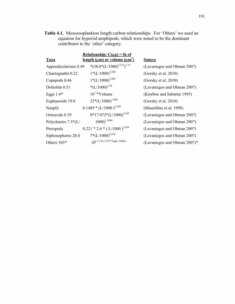
191  

Table 4.1. Mesozooplankton length:carbon relationships. For ‘Others’ we used an equation for hyperiid amphipods, which were noted to be the dominant contributor to the ‘other’ category.

Taxa Relationship: C(g) = fn of length (m) or volume (m3) Source

Appendicularians 0.49 *(38.8*(L/1000)2.574)1.12 (Lavaniegos and Ohman 2007) Chaetognaths 0.22 1*(L/1000)2.580 (Gorsky et al. 2010) Copepods 0.46 1*(L/1000)3.094 (Gorsky et al. 2010) Doliolids 0.51 *(L/1000)2.28 (Lavaniegos and Ohman 2007) Eggs 1.4* 10-7*Volume (Kiorboe and Sabatini 1995) Euphausiids 19.0 32*(L/1000)1.484 (Gorsky et al. 2010) Nauplii 0.1489 * (L/1000 )2.588 (Mauchline et al. 1998) Ostracods 0.39 8*17.072*(L/1000)2.545 (Lavaniegos and Ohman 2007) Polychaetes 7.5*(L/ 1000)1.3848 (Lavaniegos and Ohman 2007) Pteropods 0.221 * 2.6 * ( L/1000 )2.659 (Lavaniegos and Ohman 2007) Siphonophores 20.4 7*(L/1000)0.834 (Lavaniegos and Ohman 2007) Others 365* 10(-2.314+2.957*log(L/1000)) (Lavaniegos and Ohman 2007)*

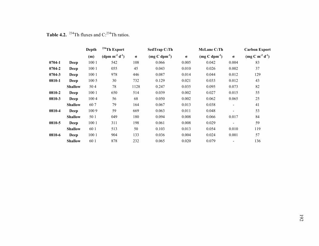
191  

Table 4.2. 234Th fluxes and C:234Th ratios.

Depth 234Th Export SedTrap C:Th McLane C:Th Carbon Export

(m) (dpm m-2 d-1) σ (mg C dpm-1) σ (mg C dpm-1) σ (mg C m-2 d-1)

0704-1 Deep 100 1 542 108 0.066 0.005 0.042 0.004 83 0704-2 Deep 100 1 055 45 0.043 0.010 0.026 0.002 37 0704-3 Deep 100 1 978 446 0.087 0.014 0.044 0.012 129 0810-1 Deep 100 5 30 732 0.129 0.021 0.033 0.012 43

Shallow 50 4 78 1128 0.247 0.035 0.095 0.073 82 0810-2 Deep 100 1 650 514 0.039 0.002 0.027 0.015 55 0810-3 Deep 100 4 56 68 0.050 0.002 0.062 0.065 25

Shallow 60 7 79 164 0.067 0.013 0.038 - 41 0810-4 Deep 100 9 59 669 0.063 0.011 0.048 - 53

Shallow 50 1 049 180 0.094 0.008 0.066 0.017 84 0810-5 Deep 100 1 311 198 0.061 0.008 0.029 - 59

Shallow 60 1 513 50 0.103 0.013 0.054 0.010 119 0810-6 Deep 100 1 904 133 0.036 0.004 0.024 0.001 57

Shallow 60 1 878 232 0.065 0.020 0.079 - 136

192

192  

Table 4.3. Sediment trap flux measurements. Chl and Phaeopigments are in units of g Chl a equivalents m-2 d-1. 

Cycle Depth Ctot Corg N Chl Phaeo FP Mass

(m) (mgC m-2 d-1) σ (mgC m-2 d-1) σ (mgN m-2 d-1) σ (μg m-2 d-1) σ (μg m-2 d-1) σ (mgC m-2 d-1)

P0704-1 100 173.7 60.5 144 12.7 22.2 4.0 443 245 3501 816 135.2

P0704-2 100 41.4 10.0 32 6.3 7.6 1.6 19 2 146 48 3.6

P0704-3 100 194.5 50.1 170 40.8 30.0 8.6 407 153 3449 701 53.6

P0810-1 100 - - 74 10.6 9.0 0.8 47 19 529 133 4.4

P0810-1 50 - - 112 34.4 13.8 5.7 17 7 337 128 6.7

P0810-2 100 - - 69 12.8 7.7 1.3 - - - - 7.6

P0810-3 100 - - 78 6.6 10.2 0.9 12 - 217 - 5.0

P0810-3 60 - - 120 12.5 15.3 2.8 31 20 331 235 22.6

P0810-4 100 - - 149 36.3 14.4 3.9 266 97 2723 232 35.4

P0810-4 50 - - 216 4.4 25.7 0.7 426 116 4214 597 80.4

P0810-5 100 - - 127 21.7 12.4 1.7 123 43 1141 76 14.1

P0810-5 60 - - 128 27.3 13.9 3.8 251 43 1575 145 25.9

P0810-5 100 - - 107 5.0 8.9 1.0 34 9 211 52 3.5

P0810-5 60 - - 112 12.3 10.8 1.7 66 7 438 175 5.1

193

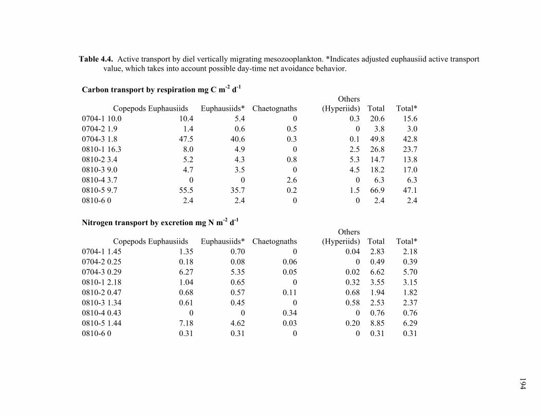
193  

Table 4.4. Active transport by diel vertically migrating mesozooplankton. *Indicates adjusted euphausiid active transport value, which takes into account possible day-time net avoidance behavior.

Carbon transport by respiration mg C m-2 d-1

Copepods Euphausiids Euphausiids* ChaetognathsOthers

(Hyperiids) Total Total*0704-1 10.0 10.4 5.4 0 0.3 20.6 15.60704-2 1.9 1.4 0.6 0.5 0 3.8 3.00704-3 1.8 47.5 40.6 0.3 0.1 49.8 42.80810-1 16.3 8.0 4.9 0 2.5 26.8 23.70810-2 3.4 5.2 4.3 0.8 5.3 14.7 13.80810-3 9.0 4.7 3.5 0 4.5 18.2 17.00810-4 3.7 0 0 2.6 0 6.3 6.30810-5 9.7 55.5 35.7 0.2 1.5 66.9 47.10810-6 0 2.4 2.4 0 0 2.4 2.4

Nitrogen transport by excretion mg N m-2 d-1

Copepods Euphausiids Euphausiids* ChaetognathsOthers

(Hyperiids) Total Total*0704-1 1.45 1.35 0.70 0 0.04 2.83 2.180704-2 0.25 0.18 0.08 0.06 0 0.49 0.390704-3 0.29 6.27 5.35 0.05 0.02 6.62 5.700810-1 2.18 1.04 0.65 0 0.32 3.55 3.150810-2 0.47 0.68 0.57 0.11 0.68 1.94 1.820810-3 1.34 0.61 0.45 0 0.58 2.53 2.370810-4 0.43 0 0 0.34 0 0.76 0.760810-5 1.44 7.18 4.62 0.03 0.20 8.85 6.290810-6 0 0.31 0.31 0 0 0.31 0.31

194

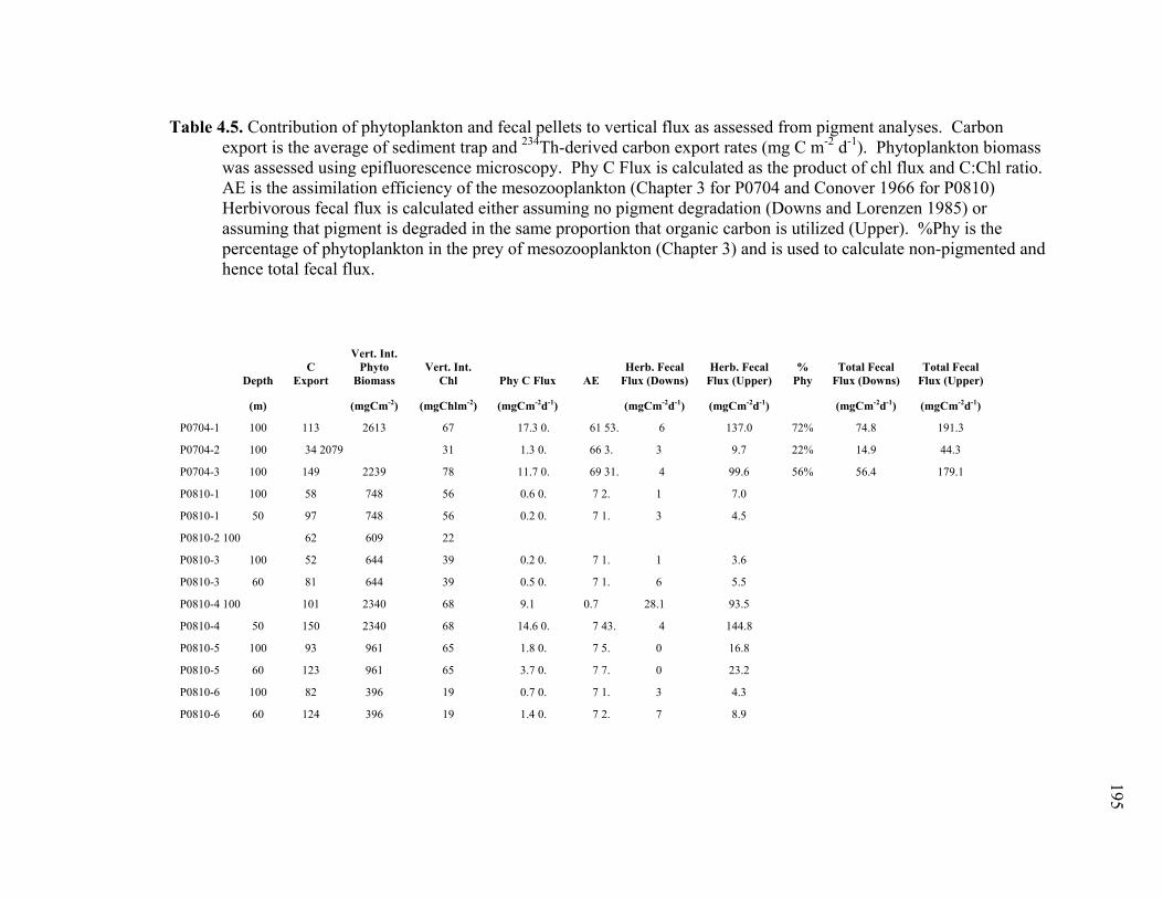
194  

Table 4.5. Contribution of phytoplankton and fecal pellets to vertical flux as assessed from pigment analyses. Carbon export is the average of sediment trap and 234Th-derived carbon export rates (mg C m-2 d-1). Phytoplankton biomass was assessed using epifluorescence microscopy. Phy C Flux is calculated as the product of chl flux and C:Chl ratio. AE is the assimilation efficiency of the mesozooplankton (Chapter 3 for P0704 and Conover 1966 for P0810) Herbivorous fecal flux is calculated either assuming no pigment degradation (Downs and Lorenzen 1985) or assuming that pigment is degraded in the same proportion that organic carbon is utilized (Upper). %Phy is the percentage of phytoplankton in the prey of mesozooplankton (Chapter 3) and is used to calculate non-pigmented and hence total fecal flux.

Depth C

Export

Vert. Int. Phyto

Biomass Vert. Int.

Chl Phy C Flux AE Herb. Fecal

Flux (Downs) Herb. Fecal

Flux (Upper) %

Phy Total Fecal

Flux (Downs) Total Fecal

Flux (Upper)

(m) (mgCm-2) (mgChlm-2) (mgCm-2d-1) (mgCm-2d-1) (mgCm-2d-1) (mgCm-2d-1) (mgCm-2d-1)

P0704-1 100 113 2613 67 17.3 0. 61 53. 6 137.0 72% 74.8 191.3

P0704-2 100 34 2079 31 1.3 0. 66 3. 3 9.7 22% 14.9 44.3

P0704-3 100 149 2239 78 11.7 0. 69 31. 4 99.6 56% 56.4 179.1

P0810-1 100 58 748 56 0.6 0. 7 2. 1 7.0

P0810-1 50 97 748 56 0.2 0. 7 1. 3 4.5

P0810-2 100 62 609 22

P0810-3 100 52 644 39 0.2 0. 7 1. 1 3.6

P0810-3 60 81 644 39 0.5 0. 7 1. 6 5.5

P0810-4 100 101 2340 68 9.1 0.7 28.1 93.5

P0810-4 50 150 2340 68 14.6 0. 7 43. 4 144.8

P0810-5 100 93 961 65 1.8 0. 7 5. 0 16.8

P0810-5 60 123 961 65 3.7 0. 7 7. 0 23.2

P0810-6 100 82 396 19 0.7 0. 7 1. 3 4.3

P0810-6 60 124 396 19 1.4 0. 7 2. 7 8.9

195

 

 

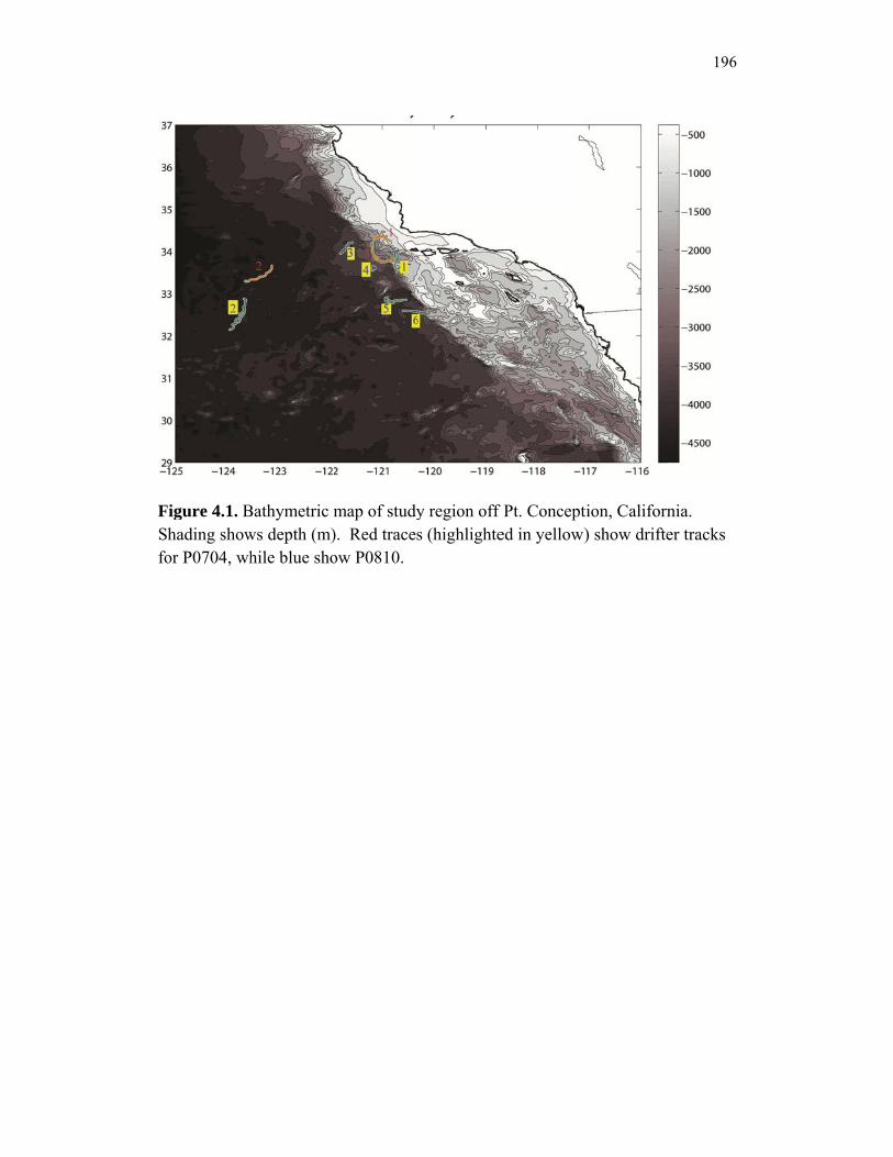
FSfo

Figure 4.1. Bhading showor P0704, wh

Bathymetric mws depth (m)hile blue sho

map of study). Red tracesow P0810.

y region off s (highlighte

Pt. Concepted in yellow)

tion, Californ) show drifte

196 

nia. er tracks

 

 

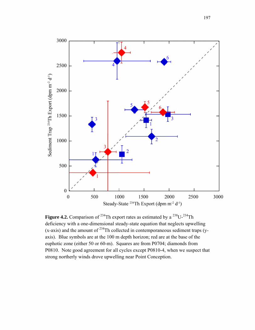
Fd(xaxeuPst

Figure 4.2. Ceficiency wix-axis) and txis). Blue syuphotic zone0810. Note trong northe

Comparison oith a one-dimthe amount oymbols are ae (either 50 ogood agreemrly winds dr

of 234Th expmensional steof 234Th colleat the 100 mor 60-m). Sqment for all rove upwellin

ort rates as eeady-state eqected in cont

m depth horizquares are frcycles excepng near Poin

estimated byquation that temporaneou

zon; red are arom P0704; pt P0810-4, wnt Conceptio

y a 238U-234Tneglects upwus sediment at the base odiamonds frwhen we su

on.

197 

Th welling traps (y-

of the rom spect that

 

 

Fto1alli

Figure 4.3. 2

o 238U. Pane, P0810-2, Plways the firines are the t

234Th deficieels a, b, c, d, P0810-3, P08rst cast of a cthird cast.

ency profilese, f, g, h, i a

810-4, P0810cycle, red lin

s. X-axis is tare cycle P070-5, P0810-6nes are the se

the deficienc704-1, P0706, respectiveecond, and w

cy of 234Th r4-2, P0704-

ely. Blue linwhen presen

198 

relative 3, P0810-

nes are nt green

 

 

Fcapusy(eis

Figure 4.4. Caught in sedumps and siymbols are aeither 50 or 6s the 1:1 line

C:234Th ratioiment traps, ze-fractionatat the 100-m60 m). Squae.

os. X-axis iswhile y-axisted particles

m depth horizares are from

s the C:234Ths is the sames >20 m (P0zon; red are am P0704; dia

h ratio measue ratio measu0704) or >50at the base oamonds from

ured on partiured using in0-m (P0810

of the euphotm P0810. Da

199 

icles n situ

0). Blue tic zone ashed line

 

 

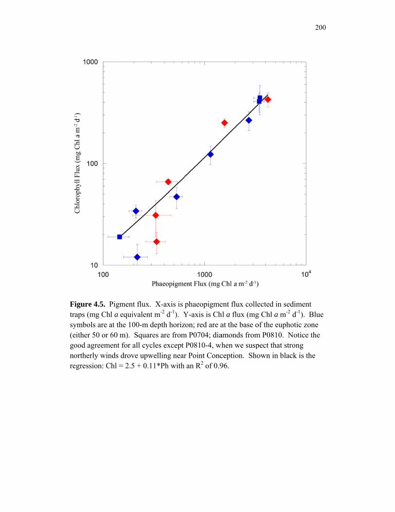
Ftrsy(egnre

Figure 4.5. Praps (mg Chlymbols are aeither 50 or 6ood agreemeortherly winegression: C

Pigment fluxl a equivalenat the 100-m60 m). Squaent for all cy

nds drove uphl = 2.5 + 0.

x. X-axis is nt m-2 d-1). Y

m depth horizares are fromycles except welling near.11*Ph with

phaeopigmeY-axis is Chzon; red are am P0704; dia

P0810-4, whr Point Concan R2 of 0.9

ent flux collehl a flux (mgat the base oamonds fromhen we suspception. Sho96.

ected in sedig Chl a m-2 dof the euphotm P0810. Nopect that stroown in black

200 

iment d-1). Blue tic zone otice the ng

k is the

 

 

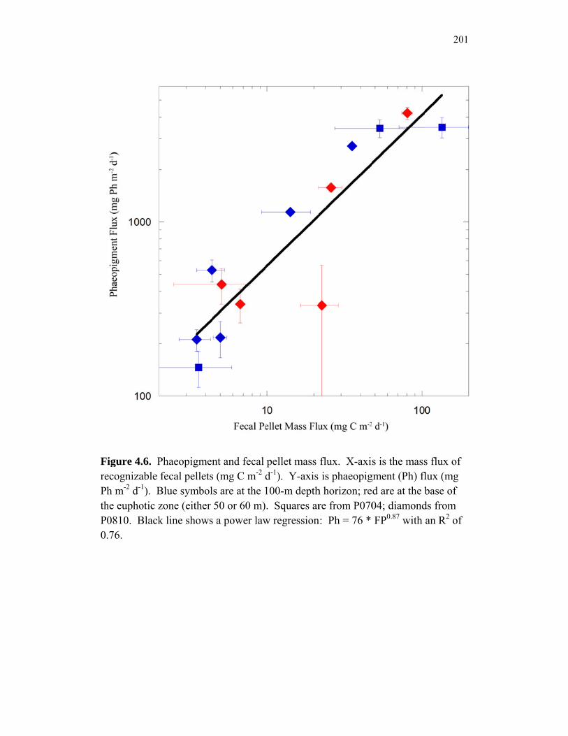
FrePthP0

Figure 4.6. Pecognizable h m-2 d-1). B

he euphotic z0810. Black.76.

Phaeopigmenfecal pellets

Blue symbolzone (either k line shows

nt and fecal s (mg C m-2 dls are at the 150 or 60 m)

s a power law

pellet mass d-1). Y-axis 100-m depth. Squares ar

w regression

flux. X-axi is phaeopig

h horizon; rere from P070

n: Ph = 76 *

s is the massgment (Ph) fled are at the b04; diamondFP0.87 with

201 

s flux of lux (mg base of

ds from an R2 of

202  

Figure 4.7. Flux of recognizable fecal pellets into sediment traps (105 pellets m-2 d-1). Dark blue represents ovoid pellets, blue is ellipsoid, teal is spherical, yellow is cylindrical, orange is amorphous, and maroon is tabular pellets. Samples are grouped by cruise, cycle, and depth horizon (‘d’ denotes 100-m samples, ‘s’ denotes samples from the base of the euphotic zone at either 50 or 60 m). Two samples were enumerated per cycle and depth and are shown next to each other.

 

 

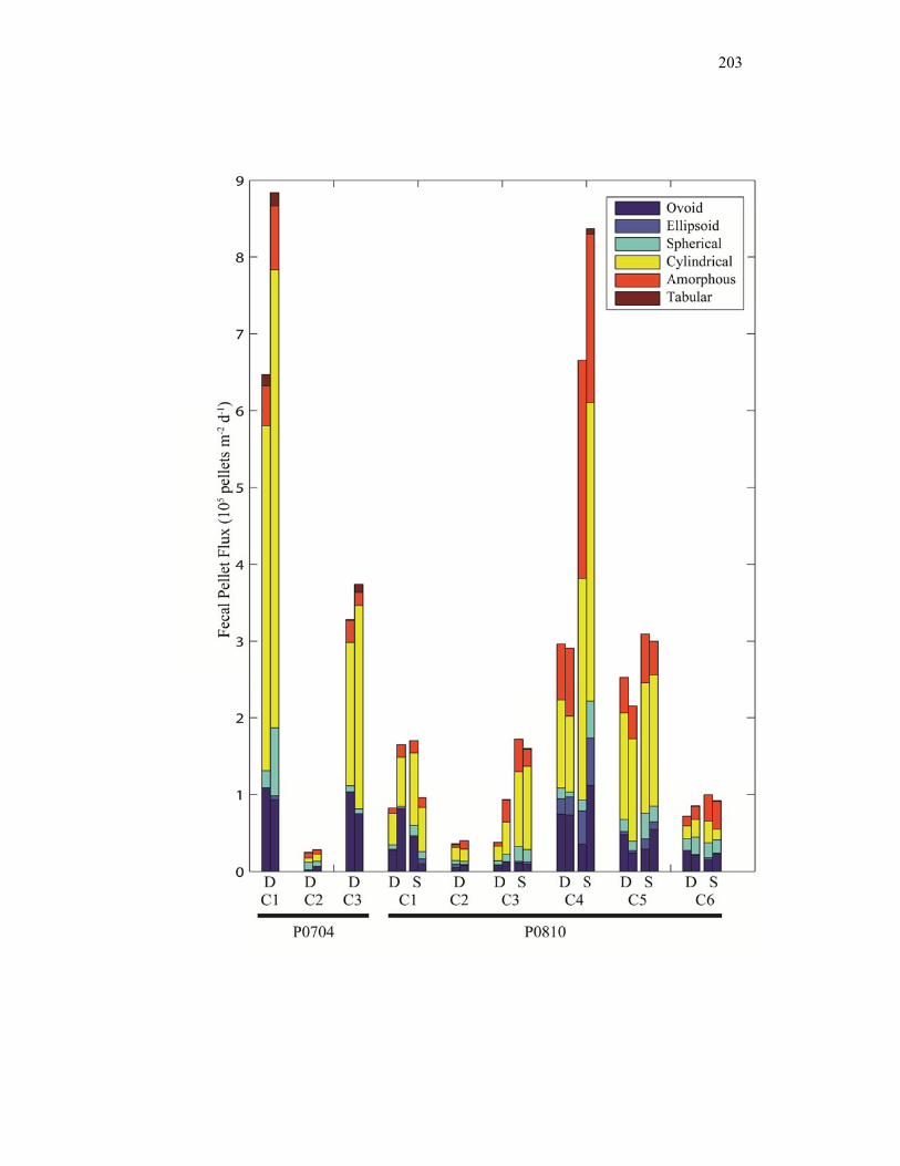
203 

 

Figure 4.8. Symbols an

Flux of fecd samples ar

al pellet masre same as in

ss into sedimn Fig. 7.

ment traps (mmg C m-2 d-1)

204 

).

205  

Figure 4.9. Relationship between cylindrical fecal pellets and total crustacean abundance. Panel a shows the crustacean abundance (day-night average from MOCNESS tows integrated to 100 m) on the x-axis and cylindrical fecal pellet flux (at 100 m). Panel b shows crustacean biomass and fecal pellet mass flux. Squares are P0704, while diamonds are P0810. Regression line shown in panel a is: FP = -140 + 2.6*CA, with R2=0.85.

 

 

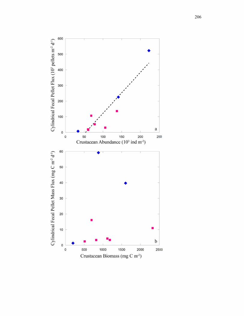
206 

207  

Figure 4.10. Relationship between fecal pellet mass flux and mesozooplankton biomass. In panel a, x-axis is mesozooplankton biomass (mg C m-2) as caught in day-night paired bongo tows. Error bars are one standard error around the mean. Y-axis is fecal pellet mass flux (mg C m-2 d-1) at 100-m depth with error bars that show the difference between paired measurements. Blue squares are P0704, while red diamonds are P0810. Black line is a power law regression: FP = 2.4*10-5 * Biomass1.93, with R2 of 0.95. In panel b, x-axis is the product of mesozooplankton concentration (mg C m-3) and phytoplankton concentration (mg C m-3), with error bars of one standard error. Black line is the regression line: y = -10.2 + 8.1x, with R2 of 0.93.

 

 

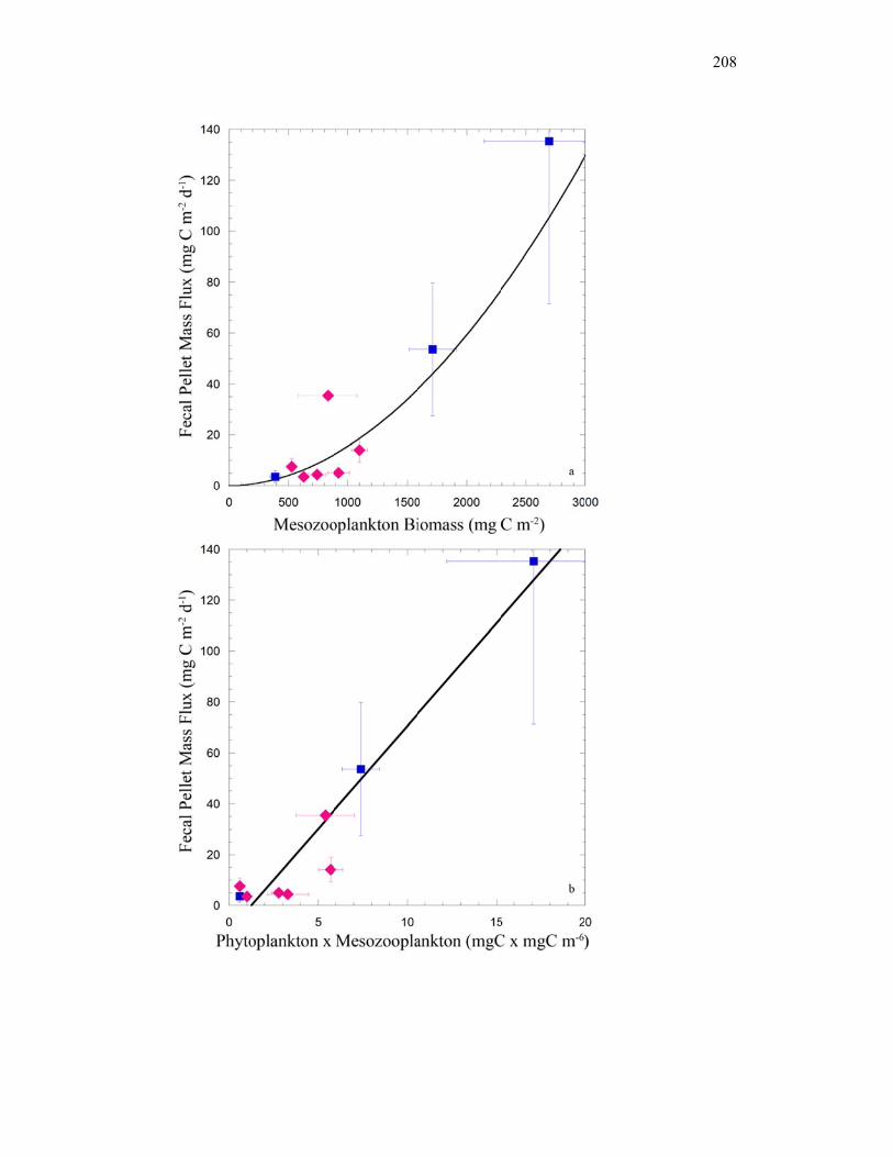
208 

 

 

Figure 4.11biomass, redtaken in a cyindividual toP0810-4, P0

1. Vertical dd night-time ycle, cycle mows. Panels0810-5, and

distribution obiomass. W

means are shs are P0704-P0810-6, for

of copepod bWhen two dahown as the b1, P0704-2, r panels a, b

biomass (mgay-night pairbold line andP0704-3, P0

b, c, d, e, f, g

g C m-3). Blurs of MOCNd the light lin0810-1, P08

g, h, i, respec

ue is daytimeESS tows wnes show the10-2, P0810

ctively.

209 

e were e -3,

 

 

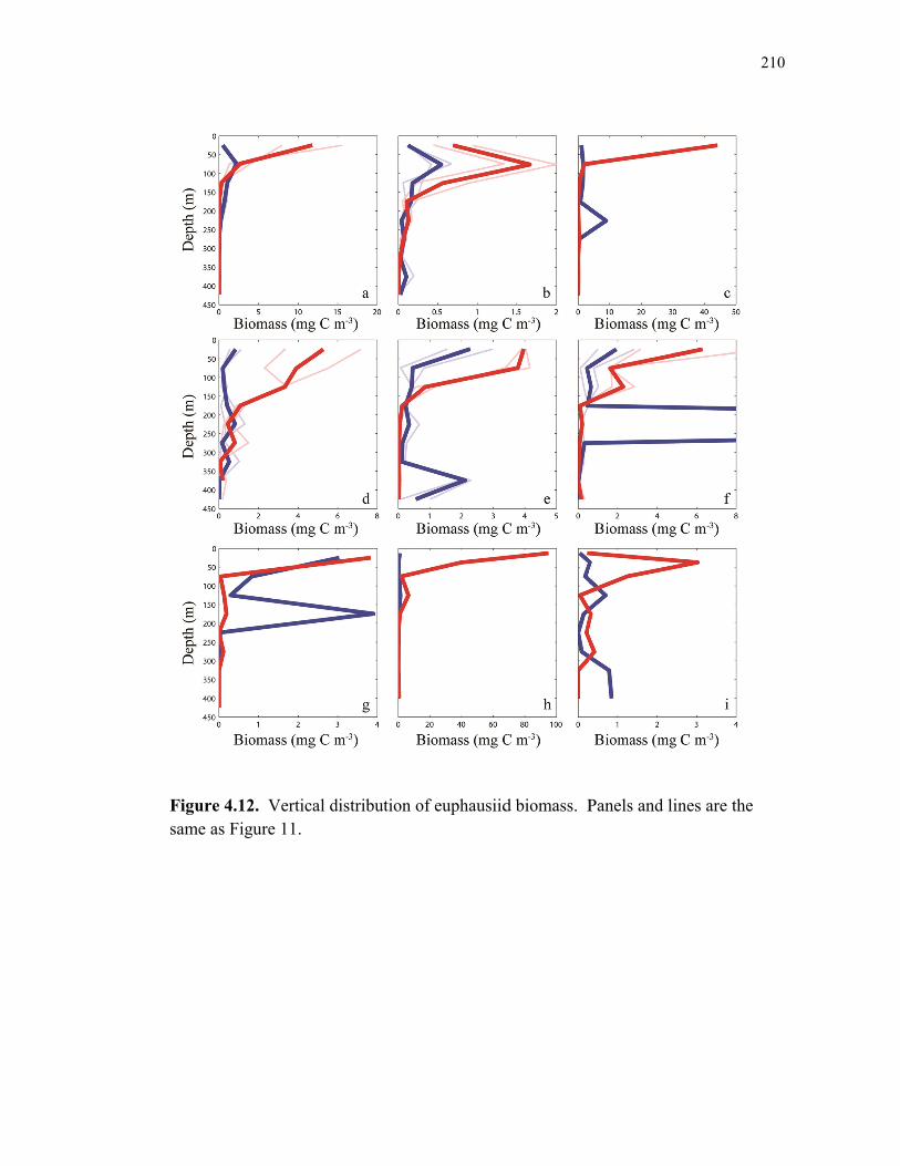
Figure 4.12same as Fig

2. Vertical dure 11.

distribution o

of euphausiidd biomass. PPanels and liines are the

210 

 

 

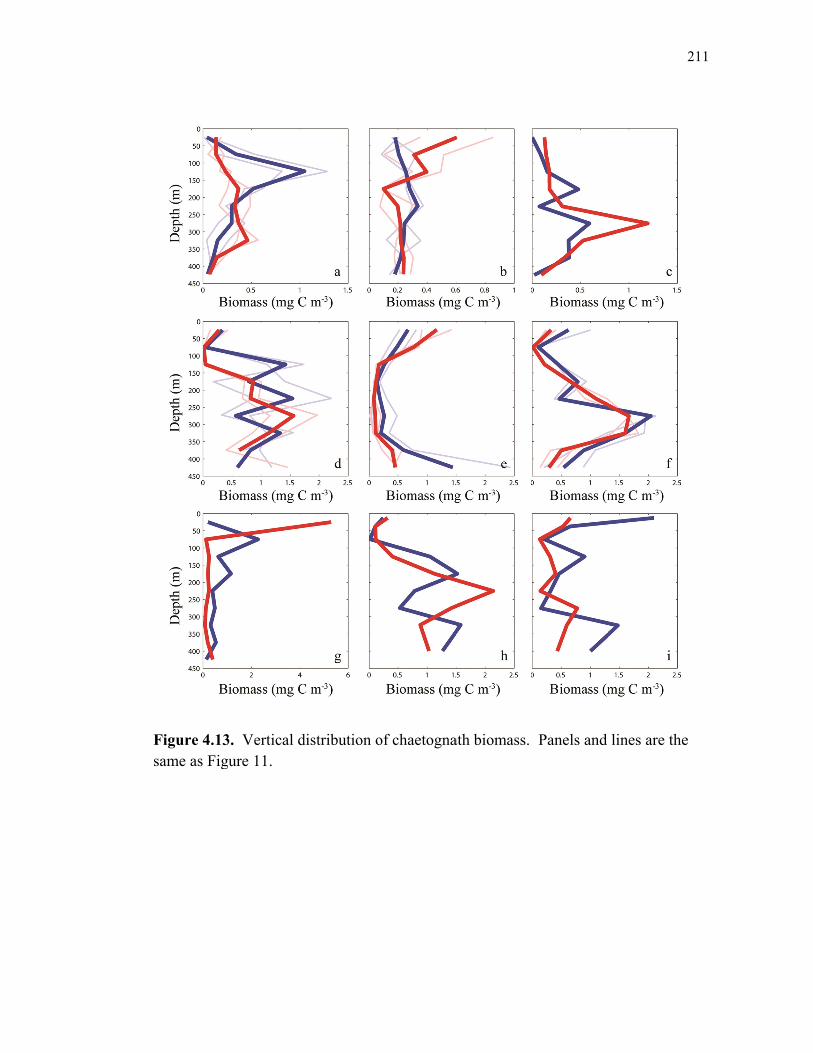
Figure 4.13same as Fig

3. Vertical dure 11.

distribution oof chaetognaath biomass. Panels and lines are the

211 

e

 

 

Figure 4.14includes all doliolids & siphonophorare the same

4. Vertical dorganisms tsalps, eggs, res. It was pe as Figure 1

distribution ohat were noteuphausiids

primarily com11.

of ‘other’ biot classified as, nauplii, osmposed of h

omass. Noteas either coptracods, poly

hyperiid amp

e that our ‘otepods, chaetychaetes, pte

phipods. Pan

ther’ categortognaths, eropods or nels and line

212 

ry

es

213  

Figure 4.15. Active transport of carbon by DVM mesozooplankton. Dark blue is active transport by copepods (mg C m-2 d-1) across the 100-m depth horizon. Light blue, yellow, and maroon are active transport by euphausiids, chaetognaths, and ‘others’, respectively. The ‘others’ group was composed primarily of hyperiid amphipods. Euphausiid active transport was corrected for net avoidance (see Methods).

 

 

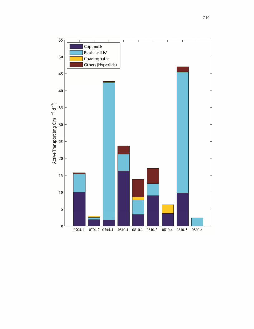
214 

215  

Figure 4.16. Contribution of each flux component to total carbon export. In all panels, green is the flux of sinking phytoplankton, as determined by the product of Chl a flux and measured C:Chl ratio, red is active transport by mesozooplankton, and white is unidentified portions of sinking particulate flux. Panels a and b show fecal flux based on phaeopigment flux measurements; brown is herbivorous fecal flux, while blue is other fecal pellet flux as estimated from the proportion of phytoplankton in the diets of mesozooplankton (Chapter 3). Other fecal pellet flux was only estimated for the cycles from P0704. Panel a is an underestimate of fecal pellet flux determined by assuming that total pigment is conserved as it passes through the guts of mesozooplankton. Panel b is a more realistic estimate that assumes that pigment is destroyed in proportion to assimilation efficiency of organic carbon. Panel c is based on microscopic enumeration of identifiable fecal pellets. In all figures, other particulate flux was estimated as the difference between total sinking flux (the average of 234Th derived carbon export and sediment trap measurements) and phytoplankton and fecal flux rates. When the sum of recognizable components exceeded total measured flux, each component was scaled proportionally to accurately portray carbon export rates. Cycles are arranged in order of decreasing vertically integrated chlorophyll concentrations. ‘d’ denotes deep (100-m) samples, while ‘s’ denotes shallow (50 or 60-m samples).

 

 

216 

217  

REFERENCES

AL-MUTAIRI, H., and M. R. LANDRY. 2001. Active export of carbon and nitrogen at Station ALOHA by diel migrant zooplankton. Deep-Sea Res. II 48: 2083-2103.

ALLDREDGE, A. L., and C. C. GOTSCHALK. 1989. Direct observations of the mass

flocculation of diatom blooms: characteristics, settling velocities and formation of diatom aggregates. Deep-Sea Res. 36: 159-171.

ARMSTRONG, R. A., C. LEE, J. I. HEDGES, S. HONJO, and S. G. WAKEHAM. 2002. A

new, mechanistic model for organic carbon fluxes in the ocean based on the quantitative association of POC with ballast minerals. Deep-Sea Res. II 49: 219-236.

BENITEZ-NELSON, C., K. O. BUESSELER, D. M. KARL, and J. ANDREWS. 2001a. A time-

series study of particulate matter export in the North Pacific Subtropical Gyre based on Th-234 : U-238 disequilibrium. Deep-Sea Res. I 48: 2595-2611.

BENITEZ-NELSON, C. R., K. O. BUESSELER, M. R. VAN DER LOEFF, J. ANDREWS, L.

BALL, G. CROSSIN, and M. A. CHARETTE. 2001b. Testing a new small-volume technique for determining Th-234 in seawater. J. Radioanal. Nucl. Chem. 248: 795-799.

BRINTON, E. 1967. Vertical migration and avoidance capability of euphausiids in

California Current. Limnol. Oceanogr. 12: 451-483. BUESSELER, K. O. 1991. Do upper-ocean sediment traps provide an accurate record of

particle flux? Nature 353: 420-423. BUESSELER, K. O., A. N. ANTIA, M. CHEN, S. W. FOWLER, W. D. GARDNER, O.

GUSTAFSSON, K. HARADA, A. F. MICHAELS, M. R. VAN DER LOEFF'O, M. SARIN, D. K. STEINBERG, and T. TRULL. 2007. An assessment of the use of sediment traps for estimating upper ocean particle fluxes. J. Mar. Res. 65: 345-416.

BUESSELER, K. O., C. BENITEZ-NELSON, M. R. VAN DER LOEFF, J. ANDREWS, L. BALL,

G. CROSSIN, and M. A. CHARETTE. 2001. An intercomparison of small- and large-volume techniques for thorium-234 in seawater. Mar. Chem. 74: 15-28.

BUESSELER, K. O., C. R. BENITEZ-NELSON, S. B. MORAN, A. BURD, M. CHARETTE, J.

K. COCHRAN, L. COPPOLA, N. S. FISHER, S. W. FOWLER, W. GARDNER, L. D. GUO, O. GUSTAFSSON, C. LAMBORG, P. MASQUE, J. C. MIQUEL, U. PASSOW, P.

218  

H. SANTSCHI, N. SAVOYE, G. STEWART, and T. TRULL. 2006. An assessment of particulate organic carbon to thorium-234 ratios in the ocean and their impact on the application of 234Th as a POC flux proxy. Mar. Chem. 100: 213-233.

BUITENHUIS, E., C. LE QUERE, O. AUMONT, G. BEAUGRAND, A. BUNKER, A. HIRST, T.

IKEDA, T. O'BRIEN, S. PIONTKOVSKI, and D. STRAILE. 2006. Biogeochemical fluxes through mesozooplankton. Glob. Biogeochem. Cycle 20: 18.

CARROLL, M. L., J. C. MIQUEL, and S. W. FOWLER. 1998. Seasonal patterns and depth-

specific trends of zooplankton fecal pellet fluxes in the Northwestern Mediterranean Sea. Deep-Sea Res. I 45: 1303-1318.

CHEN, J. H., R. L. EDWARDS, and G. J. WASSERBURG. 1986. 238U, 234U and 232Th in

seawater. Earth Planet. Sci. Lett. 80: 241-251. CONOVER, R. J. 1966. Assimilation of organic matter by zooplankton. Limnol.

Oceanogr. 11: 338-345. CONOVER, R. J., R. DURVASULA, S. ROY, and R. WANG. 1986. Probable loss of

chlorophyll-derived pigments during passage through the gut of zooplankton, and some of the consequences. Limnol. Oceanogr. 31: 878-887.

COPPOLA, L., M. ROY-BARMAN, P. WASSMANN, S. MULSOW, and C. JEANDEL. 2002.

Calibration of sediment traps and particulate organic carbon export using 234Th in the Barents Sea. Mar. Chem. 80: 11-26.

DAM, H. G., and W. T. PETERSON. 1988. The effect of temperature on the gut

clearance rate-constant of planktonic copepods. J. Exp. Mar. Biol. Ecol. 123: 1-14.

DOWNS, J. N., and C. J. LORENZEN. 1985. Carbon : pheopigment ratios of zooplankton

fecal pellets as an index of herbivorous feeding. Limnol. Oceanogr. 30: 1024-1036.

DURBIN, E. G., and R. G. CAMPBELL. 2007. Reassessment of the gut pigment method

for estimating in situ zooplankton ingestion. Mar. Ecol. Prog. Ser. 331: 305-307.

GOERICKE, R. 2002. Top-down control of phytoplankton biomass and community

structure in the monsoonal Arabian Sea. Limnol. Oceanogr. 47: 1307-1323. GORSKY, G., M. D. OHMAN, M. PICHERAL, S. GASPARINI, L. STEMMANN, J. B.

ROMAGNAN, A. CAWOOD, S. PESANT, C. GARCIA-COMAS, and F. PREJGER.

219  

2010. Digital zooplankton image analysis using the ZooScan integrated system. J. Plankton Res. 32: 285-303.

GOWING, M. M., D. L. GARRISON, H. B. KUNZE, and C. J. WINCHELL. 2001. Biological

components of Ross Sea short-term particle fluxes in the austral summer of 1995-1996. Deep-Sea Res. I 48: 2645-2671.

GOWING, M. M., and M. W. SILVER. 1985. Minipellets - a new and abundant size class

of marine fecal pellets. J. Mar. Res. 43: 395-418. GOWING, M. M., and K. F. WISHNER. 1986. Trophic relationships of deep-sea calanoid

copepods from the benthic boundary layer of the Santa Catalina Basin, California. Deep-Sea Res. 33: 939-961.

IKEDA, T. 1985. Metabolic rates of epipelagic marine zooplankton as a function of

body mass and temperature. Mar. Biol. 85: 1-11. IKEDA, T., Y. KANNO, K. OZAKI, and A. SHINADA. 2001. Metabolic rates of epipelagic

marine copepods as a function of body mass and temperature. Mar. Biol. 139: 587-596.

JACKSON, G. A., A. M. WAITE, and P. W. BOYD. 2005. Role of algal aggregation in

vertical carbon export during SOIREE and in other low biomass environments. Geophys. Res. Lett. 32: 4.

KIORBOE, T., and M. SABATINI. 1995. Scaling of fecundity, growth and development

in marine planktonic copepods. Mar. Ecol. Prog. Ser. 120: 285-298. KNAUER, G. A., D. M. KARL, J. H. MARTIN, and C. N. HUNTER. 1984. In situ effects of

selected preservatives on total carbon, nitrogen and metals collected in sediment traps. J. Mar. Res. 42: 445-462.

KNAUER, G. A., J. H. MARTIN, and K. W. BRULAND. 1979. Fluxes of particulate

carbon, nitrogen, and phosphorus in the upper water column of the Northeast Pacific. Deep-Sea Res. 26: 97-108.

LANDRY, M. R., H. AL-MUTAIRI, K. E. SELPH, S. CHRISTENSEN, and S. NUNNERY.

2001. Seasonal patterns of mesozooplankton abundance and biomass at Station ALOHA. Deep-Sea Res. II 48: 2037-2061.

LANDRY, M. R., C. J. LORENZEN, and W. K. PETERSON. 1994. Mesozooplankton

grazing in the Southern California Bight .2. Grazing impact and particulate flux. Mar. Ecol. Prog. Ser. 115: 73-85.

220  

LANDRY, M. R., M. D. OHMAN, M. R. STUKEL, and K. TSYRKLEVICH. 2009. Lagrangian studies of phytoplankton growth and grazing relationships in a coastal upwelling ecosystem off Southern California. Prog. Oceanogr. 83: 208-216.

LAVANIEGOS, B. E., and M. D. OHMAN. 2007. Coherence of long-term variations of

zooplankton in two sectors of the California Current System. Prog. Oceanogr. 75: 42-69.

LONGHURST, A. R., A. W. BEDO, W. G. HARRISON, E. J. H. HEAD, and D. D. SAMEOTO.

1990. Vertical flux of respiratory carbon by oceanic diel migrant biota. Deep-Sea Res. 37: 685-694.

LOPEZ, M. D. G., M. E. HUNTLEY, and P. F. SYKES. 1988. Pigment destruction by

Calanus pacificus: Impact on the estimation of water column fluxes. J. Plankton Res. 10: 715-734.

MAUCHLINE, J., J. H. S. BLAXTER, A. J. SOUTHWARD, and P. A. TYLER. 1998.

Advances in marine biology - The biology of calanoid copepods - Introduction, p. 1-+. Advances in Marine Biology, Vol 33. Advances in Marine Biology.

OLLI, K., P. WASSMANN, M. REIGSTAD, T. N. RATKOVA, E. ARASHKEVICH, A.

PASTERNAK, P. A. MATRAI, J. KNULST, L. TRANVIK, R. KLAIS, and A. JACOBSEN. 2007. The fate of production in the central Arctic Ocean - Top-down regulation by zooplankton expatriates? Prog. Oceanogr. 72: 84-113.

PIKE, S. M., K. O. BUESSELER, J. ANDREWS, and N. SAVOYE. 2005. Quantification of

234Th recovery in small volume sea water samples by inductively coupled plasma-mass spectrometry. J. Radioanal. Nucl. Chem. 263: 355-360.

SAVOYE, N., C. BENITEZ-NELSON, A. B. BURD, J. K. COCHRAN, M. CHARETTE, K. O.

BUESSELER, G. A. JACKSON, M. ROY-BARMAN, S. SCHMIDT, and M. ELSKENS. 2006. 234Th sorption and export models in the water column: A review. Mar. Chem. 100: 234-249.

SILVER, M. W., and M. M. GOWING. 1991. The "particle" flux: Origins and biological

components. Prog. Oceanogr. 26: 75-113. SMALL, L. F., and S. G. ELLIS. 1992. Fecal carbon production by zooplankton in Santa-

Monica Basin: The effects of body size and carnivorous feeding. Prog. Oceanogr. 30: 197-221.

STEINBERG, D. K., C. A. CARLSON, N. R. BATES, S. A. GOLDTHWAIT, L. P. MADIN, and

A. F. MICHAELS. 2000. Zooplankton vertical migration and the active transport

221  

of dissolved organic and inorganic carbon in the Sargasso Sea. Deep-Sea Res. I 47: 137-158.

STUKEL, M. R., M. R. LANDRY, C. R. BENITEZ-NELSON, and R. GOERICKE. submitted.

Trophic cycling and carbon export relationships in the California Current Ecosystem. Limnol. Oceanogr.

TURNER, J. T. 2002. Zooplankton fecal pellets, marine snow and sinking

phytoplankton blooms. Aquat. Microb. Ecol. 27: 57-102. WILSON, S. E., D. K. STEINBERG, and K. O. BUESSELER. 2008. Changes in fecal pellet

characteristics with depth as indicators of zooplankton repackaging of particles in the mesopelagic zone of the subtropical and subarctic North Pacific Ocean. Deep-Sea Res. II 55: 1636-1647.

WILSON, S. E., D. K. STEINBERG, F. L. E. CHU, and J. K. B. BISHOP. 2010. Feeding

ecology of mesopelagic zooplankton of the subtropical and subarctic North Pacific Ocean determined with fatty acid biomarkers. Deep-Sea Res. I 57: 1278-1294.

 

222  

CONCLUSIONS

Assessing the biological pump – The ecological interactions that influence

marine carbon sequestration are diverse and difficult to measure precisely. They

involve both direct and indirect trophic interactions with high degrees of

spatiotemporal variability, and community dynamics that we are only beginning to

understand in the marine realm. All methods have distinct limitations and drawbacks.

Direct measurements are costly and time-intensive and often limited by the difficulties

in visually discerning components of the mixed detrital pool (e.g. microscopy) or

require multiple, and often questionable, assumptions (e.g. pigment analyses).

Forward models invariably involve subjective decisions of which processes should be

included and poorly constrained parameterizations (Franks 2009), and hence seldomly

reject hypotheses. Inverse models, while synthesizing cruise measurements, are

always poorly constrained due to the paucity of relevant in situ measurements (Kones

et al. 2006; Stukel and Landry 2010). Even direct accurate measurements of bulk

vertical carbon flux (without assessment of its constituent particles) are difficult to

make in the dynamic fluid environment of the ocean (Buesseler 1991).

As a result of my lack of faith in any single method, I have taken more of a

pragmatic approach to methodology, utilizing different techniques that seemed to best

fit particular questions. In Chapters 1 and 3, I utilized inverse ecosystem modeling

techniques to assess the relative contributions of large and small phytoplankton to

carbon export and the percentage of vertical flux that was comprised of ungrazed

phytoplankton. Chapters 2-4 relied crucially on field measurements of carbon export

223  

 

(from both sediment traps and 234Th disequilibrium) and the suite of complementary

ecosystem measurements made by collaborators in the CCE LTER Program. In

Chapter 2, I utilized a simple model of trophic cycling relationships to relate vertical

flux to ecological rate measurements and found that the measured variability in carbon

export could be explained by processes that lead to mesozooplankton fecal production.

While the results of both Chapters 2 & 3 suggested that fecal pellets were the

dominant form of sinking material in the CCE region, neither were conclusive

demonstrations of that relationship since alternative model structures could have

predicted different results. The uncertainty of modeling results led me to look directly

at the quantity of fecal pellets in sediment traps in Chapter 4, both by counting

identifiable fecal pellets and by using phaeopigments as a tracer of herbivorous fecal

material. While individually, each of these methods has its flaws, together they

painted a consistent portrait of the biological control of carbon flux in the CCE (at

least during the springtime).

Biological control of sinking POC in the CCE – So what can we conclude

about the role of plankton in vertical flux of POC? Results from a wide-variety of

sources show that during the springtime, at least within the water parcels sampled on

the P0605 and P0704 cruises, export of sinking particles was driven by

mesozooplankton fecal pellets. A disparate suite of evidence supports this general

conclusion. First, phytoplankton net growth rates (growth minus grazing) were

closely matched by the water-column accumulation of autotrophs, suggesting a

negligible role for massive losses of phytoplankton to direct sinking (Landry et al.

224  

 

2009; Stukel et al. submitted). Estimates of sinking rates from SETCOL chambers

(data not shown) and the insignificant concentration of chlorophyll caught in sediment

traps (Chapter 4) both support the view that phytoplankton were not settling out of the

water column at any appreciable rate. Estimates of mesozooplankton ingestion (of

both phytoplankton and protozoans), combined with reasonable estimates of

assimilation efficiency (Stukel et al. submitted and Chapter 3), show that the total flux

of POC could have been maintained by mesozooplankton fecal production. Sediment

trap analyses from the P0704 cruise also indicate that identifiable fecal pellets were

the dominant particle source in sediment traps nearshore, while arguments based on

sediment trap pigment contents are consistent with fecal material (herbivorous and

nonherbivorous) comprising all or most of the sinking detritus measured on the cruise

(Chapter 4).

Results from the P0810 cruise, however, indicate that other processes may

have been at work later in the season. For this cruise, high productivity water parcels

exhibited a predominance of fecal material in sinking flux while sediment traps from

lower productivity regions contained primarily marine snow or particles too small to

be identified (Chapter 4). The significantly higher C:N ratios of sinking material on

the P0810 cruise further suggested that detritus sank much more slowly in October and

that the POC reaching the sediment trap was highly degraded. This combination of

factors raises the possibility that processes occuring prior to our arrival at the

experimental water parcels may have exerted a large influence on the vertical fluxes

measured in our studies.

225  

 

While this dissertation has specifically focused on the role of mesozooplankton

fecal production in carbon export, I do not want to imply that it is the only important

factor. We measured CaCO3 in our sediment traps and are certain that biogenic silica

was also important as a mineral ballast material. Aggregates were often observed in

the sediment traps from October 2008. Mass flocculation and sinking of

phytoplankton may occasionally occur as blooms decay and could be an important

episodic flux of carbon to depth. We also found evidence (Stukel, unpublished data)

for subduction along a front studied on the P0904 cruise (April 2009) that may have

contributed a significant flux of carbon out of the ecosystem. However, during the

productive spring period in the CCE, it is likely that fecal pellets were the primary

source of sinking material in the region. We suggest, therefore, that models

attempting to explain patterns of biogeochemical fluxes in the CCE region need to

account explicitly for mesozooplankton population dynamics and community grazing;

only with the inclusion of mesozooplankton grazing could distinct patterns in

efficiency of the biological pump be determined in our studies.

Going forward - Long-term secular changes on multiple fronts – including

ocean acidification (Doney et al. 2009) and increased stratification (Sarmiento et al.

2004) – will likely alter marine ecosystem structure and function in the future ocean.

In the CCE, long-term trends, possibly related to anthropogenic warming, have

already been noted for both phytoplankton (Aksnes and Ohman 2009) and

mesozooplankton (Lavaniegos and Ohman 2007; Roemmich and Mcgowan 1995).

Anticipating the responses and feedbacks between climate and ocean requires more

226  

 

than a simple realization that ecosystems will change; it requires a mechanistic

understanding of how ecosystem structure drives biogeochemistry (Ducklow et al.

2001). We know that ocean acidification will affect the production of planktonic

calcifiers and hence mineral ballasting of sinking POC. We can surmise that increased

stratification may decrease nutrient input and new production, with cascading effects

on phytoplankton and zooplankton biomass. We can wonder whether a more stratified

surface layer will be more conducive to aggregate formation. Yet we do not know

which of these processes dominate the flux of organic carbon to depth.

The practical difficulties of distinguising among different export mechanisms,

particularly when sinking material is old and degraded (as on our P0810 cruise) has

led to a paucity of direct field evidence; instead, mechanisms are typically inferred

from correlations (e.g. Klaas and Archer 2002) or built into the structure of models

(e.g. Jackson 2001). While these approaches can suggest interesting hypotheses, they

invariably lack crucial data necessary to test their veracity, and often lack any in situ

measurements of carbon flux at all (e.g. Plattner et al. 2005). Going forward, we need

a coordinated effort between modelers and experimentalists to generate testable

hypotheses that can potentially be used to explicitly and simultaneously test these

alternative hypotheses with in situ measurements. In particular, characterization of the

nature of the euphotic zone detrital pool is necessary using a combination of

microscopical (Verity et al. 1996; Verity et al. 2000), optical (Checkley et al. 2008;

Gorsky et al. 2000), and chemical analyses, in conjunction with techniques used to

assess the varied components of sinking material (Dell'anno et al. 1999; Lundsgaard

227  

 

1995; Wilson et al. 2008). Also necessary is explicit inclusion of mesozooplankton

dynamics within ecosystem-based biogeochemical models (see Buitenhuis et al. 2006;

Hood et al. 2006) that are tied to field programs which measure the relevant process

rates necessary for model validation.

References 

Aksnes, D. L., and M. D. Ohman. 2009. Multi-decadal shoaling of the euphotic zone in the southern sector of the California Current System. Limnol. Oceanogr. 54: 1272-1281.

Buesseler, K. O. 1991. Do upper-ocean sediment traps provide an accurate record of

particle flux? Nature 353: 420-423. Buitenhuis, E. and others 2006. Biogeochemical fluxes through mesozooplankton.

Glob. Biogeochem. Cycle 20: 18. Checkley, D. M., R. E. Davis, A. W. Herman, G. A. Jackson, B. Beanlands, and L. A.

Regier. 2008. Assessing plankton and other particles in situ with the SOLOPC. Limnol. Oceanogr. 43: 2123-2136.

Dell'anno, A., M. Fabiano, S. Bompadre, M. Armeni, L. Leone, and R. Danovaro.

1999. Phytopigment and DNA determinations in long-time formalin-preserved trap samples. Mar. Ecol. Prog. Ser. 191: 71-77.

Doney, S. C., W. M. Balch, V. J. Fabry, and R. A. Feely. 2009. Ocean Acidification: a

Critical Emerging Problem for the Ocean Sciences. Oceanography 22: 16-25. Ducklow, H. W., D. K. Steinberg, and K. O. Buesseler. 2001. Upper Ocean Carbon

Export and the Biological Pump. Oceanography 14: 50-58. Franks, P. J. S. 2009. Planktonic ecosystem models: perplexing parameterizations and

a failure to fail. J. Plankton Res. 31: 1299-1306. Gorsky, G., M. Picheral, and L. Stemmann. 2000. Use of the Underwater Video

Profiler for the study of aggregate dynamics in the North Mediterranean. Estuar. Coast. Shelf Sci. 50: 121-128.

228  

 

Hood, R. R. and others 2006. Pelagic functional group modeling: Progress, challenges

and prospects. Deep-Sea Res. Part II-Top. Stud. Oceanogr. 53: 459-512. Jackson, G. A. 2001. Effect of coagulation on a model planktonic food web. Deep-Sea

Res. I 48: 95-123. Klaas, C., and D. E. Archer. 2002. Association of sinking organic matter with various

types of mineral ballast in the deep sea: Implications for the rain ratio. Glob. Biogeochem. Cycle 16: 14.

Kones, J. K., K. Soetaert, D. Van Oevelen, J. O. Owino, and K. Mavuti. 2006. Gaining

insight into food webs reconstructed by the inverse method. J. Mar. Syst. 60: 153-166.

Landry, M. R., M. D. Ohman, M. R. Stukel, and K. Tsyrklevich. 2009. Lagrangian

studies of phytoplankton growth and grazing relationships in a coastal upwelling ecosystem off Southern California. Prog. Oceanogr. 83: 208-216.

Lavaniegos, B. E., and M. D. Ohman. 2007. Coherence of long-term variations of

zooplankton in two sectors of the California Current System. Prog. Oceanogr. 75: 42-69.

Lundsgaard, C. 1995. Use of a high viscosity medium in studies of aggregates, p. 141-

152. In S. Floderus, A.-S. Heisakanen, M. Oleson and P. Wassmann [eds.], Sediment trap studies in the Nordic countries 3. Proceedings of the Symposium on Seasonal Dynamics of Planktonic Ecosystem and Sedimentation in Coastal Nordic Waters.

Plattner, G. K., N. Gruber, H. Frenzel, and J. C. Mcwilliams. 2005. Decoupling marine

export production from new production. Geophys. Res. Lett. 32: L11612. Roemmich, D., and J. Mcgowan. 1995. Climatic warming and the decline of

zooplankton in the California Current. Science 267: 1324-1326. Sarmiento, J. L. and others 2004. Response of ocean ecosystems to climate warming.

Glob. Biogeochem. Cycle 18: 35. Stukel, M. R., and M. R. Landry. 2010. Contribution of picophytoplankton to carbon

export in the equatorial Pacific: A re-assessment of food-web flux inferences from inverse models. Limnol. Oceanogr. 55: 2669-2685.

229  

 

Stukel, M. R., M. R. Landry, C. R. Benitez-Nelson, and R. Goericke. submitted. Trophic cycling and carbon export relationships in the California Current Ecosystem. Limnol. Oceanogr.

Verity, P. G., T. M. Beatty, and S. C. Williams. 1996. Visualization and quantification

of plankton and detritus using digital confocal microscopy. Aquat. Microb. Ecol. 10: 55-67.

Verity, P. G., S. C. Williams, and Y. Hong. 2000. Formation, degradation, and mass :

volume ratios of detritus derived from decaying phytoplankton. Mar. Ecol.-Prog. Ser. 207: 53-68.

Wilson, S. E., D. K. Steinberg, and K. O. Buesseler. 2008. Changes in fecal pellet characteristics with depth as indicators of zooplankton repackaging of particles in the mesopelagic zone of the subtropical and subarctic North Pacific Ocean. Deep-Sea Res. II 55: 1636-1647.