UNIVERSITY OF CALIFORNIA,

IRVINE

Heat Transfer Model for Hot Air Balloons THESIS

submitted in partial satisfaction of the requirements for the degree of

MASTER OF SCIENCE

in Mechanical and Aerospace Engineering

by

Adriana Lladó-Gambín

Thesis Committee: Professor Derek Dunn-Rankin, Chair

Professor Manuel Gamero Castaño Professor Jaeho Lee

2016

© 2016 Adriana Lladó-Gambín

ii

TABLE OF CONTENTS

Page

LIST OF FIGURES .......................................................................................................................................... iii

LIST OF TABLES ............................................................................................................................................. v

ACKNOWLEDGMENTS ............................................................................................................................... vi

ABSTRACT OF THE THESIS ..................................................................................................................... vii

INTRODUCTION ............................................................................................................................................. 1

1. HOT AIR BALLOON CHARACTERISTICS ..................................................................................... 3

1. HEAT TRANSFER MODEL.............................................................................................................. 11

2. PERFORMANCE ................................................................................................................................. 20

3. SOLIDWORKS FLOW SIMULATION ........................................................................................... 25

4. RESULTS ............................................................................................................................................... 28

Heat Transfer Model ................................................................................................................................. 28

Flow Simulation .......................................................................................................................................... 39

5. CONCLUSIONS.................................................................................................................................... 44

REFERENCES ............................................................................................................................................... 46

Appendix I. SIMULATION RESULTS .................................................................................................... 48

Appendix II. MATLAB SCRIPT ............................................................................................................... 52

iii

LIST OF FIGURES

Page

Figure 1. Hot air balloon, model MV-77 4

Figure 2. Hot air balloon basket, model C-1 (standard for 2,200 m3 size balloon) 4

Figure 3. Ultramagic MK-32 single burner 6

Figure 4. Burner in operation during inflation .................................................................................. 6

Figure 5. Data from Enerac 700 combustion analyzer for the pilot flame .............................. 7

Figure 6. Measured flue temperature for the pilot flame .............................................................. 8

Figure 7. Heat transfer modes in a hot air balloon ........................................................................ 11

Figure 8. Air entrainment vs distance from the burner exit ...................................................... 18

Figure 9. Gross weight vs altitude for an ambient temperature of 288 K and a gas

temperature of 373 K ............................................................................................................................... 22

Figure 10. Temperature gradient Tgas-Tambient vs ambient temperature for a gross

weight of 613 kg at sea level .................................................................................................................. 23

Figure 11. Gas temperature vs weight for an ambient temperature of 288 K at SL ........ 24

Figure 12. Picture of the flame with the envelope as a reference ........................................... 25

Figure 13. Basic dimensions (mm) of the balloon model used for the simulation ........... 26

Figure 14. Flow simulation envelope temperature distribution (side and top views) ... 29

Figure 15. Heat transfer modes in a hot air balloon ..................................................................... 31

Figure 16. Hot air balloon heat inputs and heat losses ............................................................... 31

Figure 17. Duty cycle vs ambient temperature .............................................................................. 34

Figure 18. Envelope temperature vs ambient temperature ...................................................... 34

iv

Figure 19. Duty cycle vs albedo coefficient ...................................................................................... 35

Figure 20. Envelope temperature vs albedo coefficient ............................................................. 35

Figure 21. Duty cycle vs solar flux ....................................................................................................... 36

Figure 22. Envelope temperature vs solar flux............................................................................... 36

Figure 23. Duty cycle vs atmosphere IR transmissivity .............................................................. 37

Figure 24. Envelope temperature vs atmosphere IR transmissivity ..................................... 37

Figure 25. Gas temperature at simulation times t=0s (left) and t=30s (right) .................. 39

Figure 26. Average fluid temperature from the flow simulation with SolidWorks .......... 40

Figure 27. Descent rate as a function of time .................................................................................. 41

Figure 28. Gas temperature during burner activity (second 74 to second 77.5) .............. 43

v

LIST OF TABLES

Page

Table 1. Average measured concentrations for the pilot flame .................................................. 8

Table 2. External conditions and fabric properties for the heat transfer analysis ........... 30

Table 3. Emissivity and absorptivity for different surface color ............................................. 33

vi

ACKNOWLEDGMENTS

I would like to express the deepest gratitude to my advisor Professor Dunn-Rankin for all his

support. I feel very lucky to have had the chance to work under his guidance. His continuous

encouragement and our discussions are very valuable to me, and without him none of this

would have been possible.

I also thank Ultramagic for their collaboration as a hot air balloon manufacturer. They

provided very useful information.

vii

ABSTRACT OF THE THESIS

Heat Transfer Model for Hot Air Balloons

By

Adriana Lladó-Gambín

Master of Science in Mechanical and Aerospace Engineering

University of California, Irvine, 2016

Professor Derek Dunn-Rankin

A heat transfer model and analysis for hot air balloons is presented in this work,

backed with a flow simulation using SolidWorks. The objective is to understand the major

heat losses in the balloon and to identify the parameters that affect most its flight

performance. Results show that more than 70% of the heat losses are due to the emitted

radiation from the balloon envelope and that convection losses represent around 20% of the

total. A simulated heating source is also included in the modeling based on typical thermal

input from a balloon propane burner. The burner duty cycle to keep a constant altitude can

vary from 10% to 28% depending on the atmospheric conditions, and the ambient

temperature is the parameter that most affects the total thermal input needed. The

simulation and analysis also predict that the gas temperature inside the balloon decreases

at a rate of −0.25 𝐾/𝑠 when there is no burner activity, and it increases at a rate of +1 𝐾/𝑠

when the balloon pilot operates the burner. The results were compared to actual flight data

and they show very good agreement indicating that the major physical processes responsible

for balloon performance aloft are accurately captured in the simulation.

1

INTRODUCTION

This work presents a heat transfer model for hot air balloons. Developing a thermal

model for a balloon is not new, but this study comprehensively refines past approaches

and includes a flow simulation to compare with the analytical results in order to provide

more insight on the gas temperature distribution inside the balloon envelope. The

distribution is a potentially important aspect to include because non-uniform heating of

the fabric can lead to its early degradation.

There have been a few trajectory and thermal models for gas balloons developed

because of their scientific use at high altitude. Kreith published several studies in the

1970s, including a numerical prediction of the performance [1] and an energy balance

[2]. Later, Carlson and Horn developed another thermal and trajectory model, also for

high-altitude balloons [3].

For hot air balloons the extent of the literature is emore limited. Stefan provided the

first thermal and performance model for hot air balloons in 1979 [4]. He identified the

energy factors affecting the balloon, evaluated all the parameters present in the

equations, and compared his results with real flight data to adjust the convection

coefficients which are otherwise difficult to assess. In 1991 there was an international

symposium for Hot Air Aerostatic Vehicle Technology, which included a suite of different

studies from Hallmann and Herrmann, from Aachen University. These were the first

publications with experimental data. Based on this data, they reported a slightly different

heat transfer model [5], supported by an experimentally determined temperature profile

2

[6] and measurements of velocity distribution and gas composition by Röder et al. [7].

Hallmann and Herrmann also tested the porosity and strength behavior of hot air balloon

fabrics subject to temperature load, and discussed their radiation properties [8]. These

few studies are the only ones that have found their way into the open literature. While their

methodology is globally sound, they have not incorporated some of the modern elements of

hot air balloons and they have not taken advantage of advances in flow simulation. The

refinement and expansion of these earlier models, along with a companion study using

simulation is the goal of this thesis.

The thesis is divided into two main parts. The first part describes the heat transfer model,

which is an update and refinement of older models which includes a new way to estimate

the air entrained by the flame [9] and new convection coefficient correlations from more

recent studies [10][11]. The second part is the flow simulation using a real balloon envelope

geometry and Solidworks finite element modeling software. It is a time dependent study that

simulates the burner operation by activating a heat source in order to verify the analytical

results of burner operation time. Results from the simulation are compared to real flight data

of temperature [6] and velocity. The overall objective of this work is to understand the major

thermal losses in the balloon and the parameters that affect those losses most significantly.

3

1. HOT AIR BALLOON CHARACTERISTICS

There are three main parts in a hot air balloon: envelope, burner and basket.

The envelope (shown in Figure 1) is composed of many gores (the large vertical

sections that are stitched together into the balloon envelope) made of a high resistance

Nylon fabric, reinforced by several polyester load tapes. These load tapes transmit the

loading forces via stainless steel cables to the load frame. In the top of the envelope there

is a large hole, where there is no fabric but the mesh of load tapes continues. The hole is

covered from the inside of the balloon by a loose panel of fabric called parachute. It is

kept closed by the internal pressure of the gas in the balloon and it is opened from the

basket by pulling a cord in a completely reversible process.

The volume of the envelope can range from 1,200 to 12,000 𝑚3. The specific balloon

chosen for this study is an Ultramagic M-77, with a volume of 2,200 𝑚3, but the results

obtained are fairly independent of balloon specifics. Furthermore, the M-77 is

representative of the most common size for ballooning competition and advertisement.

The basket (shown in Figure 2) is made from woven willow and cane in a marine

plywood base. It is connected to the load frame by stainless steel cables that pass down

the sides and through and under the base. The standard basket for a 2,200 𝑚3 balloon

weights 56 𝑘𝑔.

4

Figure 1. Hot air balloon, model MV-77

Figure 2. Hot air balloon basket, model C-1 (standard for 2,200 m3 size balloon)

5

The burner (shown in Figure 3) converts the fuel (liquid propane) stored in the fuel

cylinders into heat energy. This energy is used to heat the air inside the balloon envelope

and thus provide the means of inflation and altitude control during flight. The burner has

two different valves through which the propane can flow. The main or blast valve allows

fuel to pass through a coil to be pre-heated so that it burns in gas phase at the jet’s ring

outlets. This valve of the burner gives the maximum power. The liquid fire or quiet

burner valve feeds fuel directly to the multi hole jet assembly without passing it through

the coil. The liquid fuel mode is less efficient but the flame is quieter for use when flying

near animals. The ignition of the fuel in both cases is provided by a continuous pilot

flame, fitted with a shutoff valve and piezoelectric igniter.

This study considers for specificity the MK-32 burner model from Ultramagic, with a

maximum power of 3.2 𝑀𝑊 at a nominal pressure of 6 𝑏𝑎𝑟. The jet’s ring has 40 holes of

1.35 𝑚𝑚 diameter each.

The air intakes highlighted in Figure 3 allow air to flow into the burner for the correct

combustion of fuel. In addition, they reduce the weight of the can. Figure 4 shows the

burner in operation during inflation.

6

Figure 3. Ultramagic MK-32 single burner

Figure 4. Burner in operation during inflation

7

The fuel flow rate was measured for both the main flame and the pilot flame using a

high precision scale. For the main flame (fuel burning at gas phase under maximum burn

conditions) the obtained flow rate was �̇�𝑏 = 67.8 𝑔𝑟/𝑠, and for the pilot flame �̇�𝑝 =

0.07 𝑔𝑟/𝑠. Even recognizing that the pilot flame is on continuously and the burner is used

in bursts (duty cycle of perhaps 10%-25%) it is clear that the fuel used to keep the pilot

flame alive is negligible (i.e., less than 1%). Assuming 50 kJ/g heat of combustion for

propane, the main burner flow rate is equivalent to 3.04 MW, which is close to the

manufacturer's nominal stated value for the burner.

Figure 5 shows the measured emissions using Enerac 700 combustion analyzer and

Figure 6 the flue temperature for the pilot flame:

Figure 5. Data from Enerac 700 combustion analyzer for the pilot flame

8

Figure 6. Measured flue temperature for the pilot flame

The flue temperature reaches a constant value of approximately 270 ℃ at 𝑡 = 150𝑠.

Table 1 shows the average concentration for every measured parameter from 𝑡 = 150𝑠 to

𝑡 = 600𝑠:

CO 8.53 ppm

CO2 1.49 %

O2 18.35 %

NO 6.82 ppm

NO2 0

HxCy 0

Table 1. Average measured concentrations for the pilot flame

9

Using British Standard BS845 norm [12] we can calculate the combustion efficiency. The heat lost by incomplete combustion of the fuel is:

𝑄𝑙𝑜𝑠𝑠𝑒𝑠 = 𝑘[𝐶𝑂] + [𝐻𝑥𝐶𝑦]

[𝐶𝑂2] + [𝐶𝑂] + [𝐻𝑥𝐶𝑦] (1)

Where 𝑘 = 81.8 for pure propane. The concentration of hydrocarbons has been

measured to be zero. Then the efficiency is:

𝜂 =𝑄𝐶3𝐻8

− 𝑄𝑙𝑜𝑠𝑠𝑒𝑠

𝑄𝐶3𝐻8

(2)

Where 𝑄𝐶3𝐻8= 46.28 𝑀𝐽/𝑘𝑔 is the low heating value for propane. We get an efficiency

for the pilot flame of 99.99%. Fabric properties

For Nylon the maximum continuous acceptable operating temperature is 100℃, and

it should never exceed 125℃.

The fabric weight is approximately 65 𝑔𝑟/𝑚2, its thickness 0.1 𝑚𝑚, and its thermal

conductivity can vary from 0.003 to 0.04 𝑊/𝑚𝐾 depending on the fabric color and the

temperature [8].

As for the radiation properties, the ratio absorptivity/emissivity is critical for the

energy balance and the thermal behavior on the fabric surface. Forty surfaces of hot air

balloon fabric were examined at the FH Aachen [8], and the results show that the

emissivity for most colors is between 0.86 and 0.88, while for silver it is 0.70. The

absorptivity 𝛼 is about 0.5 for light colors to 0.9 for dark colors. For the inner surface the

emissivity ranges from 0.85 to 0.88. The values above show that a fairly dramatic

10

thermal modification effect may be achieved with silver fabric, and some manufacturers

have developed balloons with such fabric for high-efficiency flying.

What we want is a material with a large 𝛼/𝜀 > 1 and a small emissivity to minimize

consumption. All fabrics, except the silver one, have a high emission coefficient, but the

absorption is less with bright colors.

The fabric porosity has been proved to be completely negligible for the first 200 hours,

and after that porosity increases slowly but exponentially [8]. Too much porosity means the

fabric is fatigued, so it can be used to characterize the envelope lifetime.

11

1. HEAT TRANSFER MODEL

The motion of a hot air balloon depends on the heat transfer to and from the gas

inside, since the temperature of the gas determines the lift of the balloon. This section

presents an energy balance and heat transfer model that includes all heat losses.

Figure 7 shows the heat transfer modes involved in the total energy balance.

Figure 7. Heat transfer modes in a hot air balloon

The radiation heat that the envelope absorbs from the environment consists of the

solar radiation, direct and reflected, and the infrared radiation emitted by the Earth’s

surface.

The heat transfer between the contained gas and the envelope is mostly by internal

convection and some radiation.

12

Finally, we need to include in our balance the losses and the burner input. The losses

include the envelope’s emitted radiation, external convection to the ambient air and

what we call the mouth outflow. The latter occurs when the burner is active and exhaust

gases (mostly air) are introduced to the envelope. This leads to an overflow of warm

internal gases that carry away an amount of sensible heat.

Direct solar radiation

𝑄𝑆 = 𝐹𝑆𝛼𝐴

4

(3)

𝐹𝑆 is the solar flux, which varies from 0 to a maximum of about 1260 𝑊/𝑚2, and 𝛼 is the

envelope absorptivity, which is about 0.5 for light colors to 0.9 for dark colors (as described

earlier). The effective receiving area is the projected area 𝐴/4.

Reflected solar radiation

𝑸𝑺 = 𝑭𝑺𝒅𝜶𝑨

𝟒

(4)

𝑑 is the proportion of solar flux reflected by the Earth or clouds (albedo). It is roughly

0.1 over most surfaces, 0.3 over desert, 0.8 over snow or ice and 0.55 over clouds. Since the

reflection is generally diffuse, it acts on an effective area of 𝐴/2.

13

Earth IR radiation

𝑄𝐼𝑅𝑒 = 𝜀𝑒𝜀𝜏𝑎𝜎𝐴

2𝑇𝑒

4 (5)

𝜀𝑒 is the Earth’s surface emissivity, which is usually assumed to be between 0.8 and

1 [13], 𝜏𝑎 is the atmospheric transmissivity, and 𝑇𝑒 is the Earth’s surface temperature

(assumed to be the same as the ambient temperature). 𝜏𝑎 varies from 0 to 1 depending

on altitude and atmospheric conditions. A value of 0.6 to 0.7 is commonly used for clear

sky atmospheric transmission [14].

Emitted radiation

𝑄𝑟𝑎𝑑 = 𝜀𝜎𝐴𝑇s4 (6)

Where 𝑇𝑠 is the envelope (skin) temperature and 𝜀 the envelope emissivity.

External and internal convection heat transfer

𝑄𝑐,𝑒𝑥𝑡 = ℎ𝑒𝑥𝑡𝐴(𝑇𝑠 − 𝑇𝑎) (7)

The convection coefficient varies with temperature, velocity, density, and balloon

size. The similarity parameters for natural convection are the Prandtl number Pr, which

represents the ratio between momentum diffusivity and thermal diffusivity, and the

Grashof number Gr, which represents the ratio of buoyant to viscous forces. The Grashof

number and the Prandtl number are often grouped together as a product GrPr, which is

called the Rayleigh number, Ra.

14

𝑃𝑟 =𝐶𝑝𝜇

𝑘

(8)

𝐺𝑟 =𝑔𝛽(𝑇𝑠 − 𝑇∞)𝐿3

𝜈2

(9)

𝐿 is the length scale, which in this case is the diameter at the equator 𝐷 = 16.67 𝑚.

𝐶𝑝, 𝜇, 𝑘, 𝛽 and 𝜈 are the specific heat capacity, the dynamic viscosity, the thermal

conductivity, the coefficient of thermal expansion, and the kinematic viscosity of air. All

properties are evaluated at the film temperature:

𝑇𝑓 =(𝑇𝑠 + 𝑇∞)

2

(10)

Plugging all the numbers into the equations yields 𝑃𝑟 = 0.708 and 𝐺𝑟 = 7.2 · 1012.

The Rayleigh number is then 𝑅𝑎 = 𝑃𝑟𝐺𝑟 = 5.1 · 1012. Several correlations are available from

the literature, but few for such large Rayleigh number.

For external convection [10] and [15] recommend Campo’s correlation [11]:

𝑁𝑢 = 0.1𝑅𝑎0.340 𝑅𝑎 ≥ 1.5 · 108 (11)

Which gives a Nusselt number of 𝑁𝑢 = 2092 and an external convection coefficient

of ℎ = 𝑘 · 𝑁𝑢/𝐷 = 3.37 𝑊/𝑚2𝐾.

15

Internal convection heat transfer

𝑄𝑐,𝑖𝑛𝑡 = ℎ𝑖𝑛𝑡𝐴(𝑇𝑔 − 𝑇𝑠) (12)

For the internal convection coefficient, the temperature difference in the Grashof

number is the difference between the internal gas temperature 𝑇𝑔 and the envelope

temperature 𝑇𝑠. This gives a Rayleigh number of 𝑅𝑎 = 2.28 · 1013.

Carlson and Horn [3] use

𝑁𝑢 = 0.325 · 𝑅𝑎0.333 𝑅𝑎 ≥ 1.35 · 108 (13)

Which gives a Nusselt number of 𝑁𝑢 = 9122 and an internal convection

coefficient of ℎ = 16 𝑊/𝑚2𝐾. Both correlations are developed for the situation of

convection around a sphere at uniform temperature.

Radiation gas-envelope

𝑄𝑟 = 𝑄𝑔→𝑠 = 𝜎𝐴𝑓(𝑇𝑔4 − 𝑇𝑠

4) (14)

𝑓 =1

1 − 𝜀𝑔

𝜀𝑔+ 1 +

𝐴1

𝐴2

1 − 𝜀𝑖𝑛

𝜀𝑖𝑛

(15)

The equations above are for the net radiation between concentric spheres and the

view factor [2]. It can also be used for a gas and its enclosure with 𝐴1 = 𝐴2 = 𝐴. The

emissivity of the mixture of gases in the atmosphere is 𝜀𝑎 = 0.31. The gas emissivity for

the air inside the balloon will not differ too much. Also, the radiation exchange is almost

negligible (see chapter 0), so a change in this parameter does not significantly affect the

16

overall heat transfer balance. 𝜀𝑖𝑛 is the emissivity of the envelope’s inner surface (see chapter

1).

Mouth outflow loss

𝑄𝑜 = �̇�𝑜𝑢𝑡𝑐𝑝(𝑇𝑔 − 𝑇𝑎) (16)

𝑐𝑝 is the air heat capacity. It is actually a mix of air and combustion products, but it is

generally assumed that there is only hot air since entrainment is very high. This is not a bad

assumption, and the errors produced are something less than 2% [4].

The flow rate �̇�𝑜𝑢𝑡 is the mass introduced by the burner since we are assuming 𝑚𝑖𝑛 =

𝑚𝑜𝑢𝑡 for a whole period. The balloon takes the increase in mass for the short time that the

burner is operation, and then steadies later with the mass leaving slowly. In terms of

calculation, we do not care about actual outflow rate since the balloon acts as a thermal

energy capacitor; we just care about the total outflow in one cycle (from the beginning of a

burst until right after the following one). Therefore we can write �̇�𝑖𝑛 = �̇�𝑜𝑢𝑡 and

approximate 𝐸𝑜𝑢𝑡𝑓𝑙𝑜𝑤 = 𝑘𝑄𝑜𝑢𝑡𝑓𝑙𝑜𝑤, where 𝑘 is the burner duty cycle. The inflow includes the

fuel flow and the air entrained by the flame. It has been calculated following the procedure

described by Becker for vertical free turbulent diffusion flames [9]:

𝜉 < 1 �̇� =0.16�̇�0

𝐷𝑠𝑥

(17)

1 < 𝜉 < 2.5 �̇� =�̇�0

𝐷𝑠(0.0056 · 𝐴𝑥4 + 0.026𝐴

12𝑥

52 + 0.13𝑥)

(18)

𝜉 > 2.5 �̇� =�̇�0

𝐷𝑠(0.082𝐴

12𝑥5/2 − 0.0068𝑥 )

(19)

17

�̇�0 = 67.8 𝑔𝑟/𝑠 is the measured fuel flow (see chapter 1) and 𝐷𝑠 is the effective

source diameter. The expressions above show the flow rate distribution at three

different regimes: forced convection 𝜉 < 1, transition regime 1 < 𝜉 < 2.5 and natural

convection regime 𝜉 > 2.5. The parameter 𝜉 is defined as follows:

𝜉 = (𝜋𝑔𝜌∞

4𝐺0̇

)

1/3

𝑥 (20)

Where 𝐺0̇ is the jet momentum flux at the burner exit 𝐺0̇ = 𝑈𝑠 · �̇�0, so �̇� =

𝑓(𝑥, �̇�0, 𝐷𝑠, 𝑈𝑠, 𝜌∞).

The effective source diameter is the throat diameter of an imagined flow nozzle from

which fluid of density 𝜌∞ issues at mass rate �̇�0, momentum rate �̇�0, and uniform exit

velocity 𝑈𝑠 = �̇�0/�̇�0. For a multiport array where port-exit distributions of density and

velocity are considered uniform:

𝐷𝑠 = (4𝐴𝑠

𝜋)

1/2

(𝜌0

𝜌∞)

1/2

; 𝐴𝑠 = ∑𝜋𝐷𝑖

2

4

(21)

The burner under study (Ultramagic MK-32) has 40 jets with a diameter of 1.35𝑚𝑚

each. With 𝜌∞ = 1.225 𝑘𝑔/𝑚3 and initial fuel density 𝜌0 = 15.808 𝑘𝑔/𝑚3 we get a

source diameter of 𝐷𝑠 = 30.67 𝑚𝑚.

In order to know the flow rate at the mouth envelope, we need to calculate at which

distance the transition from one regime to another one occurs. First of all the jet exit

velocity is needed to get the momentum flux at the burner exit. For a converging tube,

we have choked flow when 𝑃/𝑃0 ≤ 0.528, where 𝑃 is the pressure in the fuel cylinder

and 𝑃0 the ambient pressure. The pressure in the cylinder can go from 3 to 10 bar, so the

18

nozzle is always choked. This means the flow is moving at Mach 1 at the exit. For an ideal gas

we have:

𝑈𝑠 = √𝛾𝑅𝑇

𝑀

(22)

Where 𝛾 = 1.247 is the specific heat ratio for propane, 𝑀 = 44.1 𝑔/𝑚𝑜𝑙 is the molar

mass and 𝑇 is the exit temperature, assumed to be equal to the ambient temperature. By

solving the equation we find that 𝑈𝑠 = 260.5 𝑚/𝑠.

Now using equations 17, 18, and 19 we can plot the mass flow rate as a function of the

flame length 𝑥:

Figure 8. Air entrainment vs distance from the burner exit

19

The mouth of the envelope is at a distance of 2.47 𝑚 from the burner exit, where the

mass flow rate is �̇� = 1.356 𝑘𝑔/𝑠. The heat losses from the outflow generated can now

be determined with equation 16.

20

2. PERFORMANCE

The intention of this section is to show the calculation of performance aspects within

the balloon. First we introduce the forces acting on the body: lift, drag and weight.

Lift L

From the principle of Archimedes, we have:

𝐿 = 𝑉𝑔(𝜌𝑎 − 𝜌𝑔) (23)

Where 𝑉 is the volume of the envelope and 𝜌𝑎 , 𝜌𝑔 are the ambient air density and the gas

density respectively. Assuming the gases to be ideal:

𝐿 = 𝑉𝑔 (𝑃𝑎

𝑅𝑎𝑇𝑎−

𝑃𝑔

𝑅𝑔𝑇𝑔)

(24)

We assumed there is only hot air inside the envelope, so we have that 𝑅𝑔 = 𝑅𝑎. The

equation can be further reduced assuming there is no difference in pressures so 𝑃𝑔 = 𝑃𝑎 .

Rearranging equation 24 we find:

𝐿 = 𝑉𝑔𝜌𝑎(1 − 𝑇𝑎/𝑇𝑔) (25)

So the lift is only a function of the gas volume, the ambient density and temperature, and

the gas temperature.

21

Drag D

The drag force is defined as follows:

𝐷 =1

2𝐶𝑑𝜌𝑎𝑢2𝑆

(26)

Where 𝐶𝑑 is the drag coefficient and 𝑆 = 𝜋𝑅2 the cross-sectional area in the equator

where the radius is maximum 𝑅 = 16.67/2 𝑚. From [4] we know that wind tunnel

measurements for a balloon in vertical motion give a value of about 0.4 for the drag

coefficient.

Gross weight G

The gross weight includes the balloon weight (envelope, burner, basket and

cylinders) and the payload.

Neutral buoyancy

When the balloon is at neutral buoyancy (hovering) there is no vertical speed and we

can say that:

𝐿 − 𝐺 = 0 (27)

Substituting the expression for the lift we find:

𝑇𝑔 =𝑇𝑎

(1 −𝐺

𝑉𝜌𝑎𝑔)

(28)

22

Since the ambient temperature and density are just a function of the altitude, we can

obtain the necessary gas temperature needed to lift a weight 𝐺 at any altitude.

Within the troposphere (ℎ < 11000 𝑚), the ISA temperature and density depend on

the altitude as follows:

𝑇 = 𝑇0 − 0.0065ℎ (29)

𝜌 = 𝜌0 (1 − 0.0065ℎ

𝑇0)

4.2561

(30)

Where 𝑇0 = 288.15 𝐾 and 𝜌0 = 1.225 𝑘𝑔/𝑚3 are the sea level conditions.

With that, we can obtain different plots for a gas volume of 𝑉 = 2200 𝑚3, which

corresponds to the Ultramagic M-77 model. Figure 9 shows the gross weight as a function of

the altitude for a gas temperature of 373 𝐾, which is the maximum continuous temperature

that the Nylon fabric can handle.

Figure 9. Gross weight vs altitude for an ambient temperature of 288 K and a gas temperature of 373 K

23

It is interesting to see that the temperature gradient ∆𝑇 = 𝑇𝑔𝑎𝑠 − 𝑇𝑎𝑚𝑏𝑖𝑒𝑛𝑡 increases with

increasing ambient temperature (Figure 10), for a fixed altitude (SL) and gross weight

(613 𝑘𝑔).

Figure 10. Temperature gradient Tgas-Tambient vs ambient temperature for a gross weight of 613 kg at sea level

And, as shown in Figure 11, for a lower load the internal temperature is going to be lower.

24

Figure 11. Gas temperature vs weight for an ambient temperature of 288 K at SL

Vertical motion

The equation for vertical motion is:

𝐿 − 𝐺 + 𝐷 = 𝑚𝑑𝑣

𝑑𝑡= (𝑉𝜌𝑔 +

𝐺

𝑔)

𝑑𝑣

𝑑𝑡

(31)

Assuming that 𝑇𝑎 and 𝜌𝑎 are constant, and that the drag coefficient is constant too, we

have that the acceleration is:

𝑑𝑢

𝑑𝑡= −

1

(𝑉𝜌𝑎(𝑇𝑎/𝑇𝑔(𝑡)) +𝐺𝑔)

(𝑉𝑔𝜌𝑎(1 − 𝑇𝑎/𝑇𝑔(𝑡)) − 𝐺 +1

2𝐶𝑑𝜌𝑎𝑢2𝑆)

(32)

This equation can be solved for the velocity numerically, using, for example Matlab, once

the gas temperature as a function of time is known.

25

3. SOLIDWORKS FLOW SIMULATION

A time-dependent flow simulation using SolidWorks is presented in this section. The

simulation has been used to check the heat transfer model. At the same time, results are

compared to real flight data to verify the simulation.

Geometry

The balloon geometry was obtained from the Ultramagic manufacturer. The

geometry is a simplification since it is a smooth surface which does not include the shape

of the gores (24 for the M series). The thickness of the envelope is 0.1 𝑚𝑚.

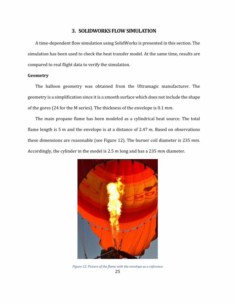
The main propane flame has been modeled as a cylindrical heat source. The total

flame length is 5 𝑚 and the envelope is at a distance of 2.47 𝑚. Based on observations

these dimensions are reasonable (see Figure 12). The burner coil diameter is 235 𝑚𝑚.

Accordingly, the cylinder in the model is 2.5 𝑚 long and has a 235 𝑚𝑚 diameter.

Figure 12. Picture of the flame with the envelope as a reference

26

Figure 13 shows the model dimensions:

Figure 13. Basic dimensions (mm) of the balloon model used for the simulation

General settings

The solar radiation intensity has been set to 600 𝑊/𝑚2.

The fluid inside the envelope is air and the properties for the envelope fabric have been

set to a thermal conductivity of 𝑘 = 0.2 𝑊/𝑚𝐾 and a density of 65 𝑔/𝑚2 [8]. The emissivity

has been set to 𝜀 = 0.87 for both the inner and outer surfaces.

Boundary conditions

There are two boundary conditions that need to be specified. First, there is the outer wall

thermal condition. Since there is external convection, the parameters that needed to be input

were the convection heat transfer coefficient, and the temperature of the external fluid. The

convection coefficient is ℎ𝑒𝑥𝑡 = 3.37 𝑊/𝑚2𝐾 (see chapter 1), and the ambient temperature

for this study is 𝑇 = 288.15 𝐾.

27

Second, we need to set the boundary condition for the envelope opening at the

bottom (or envelope mouth). It is a pressure opening set to ambient pressure 𝑃 =

101325 𝑃𝑎 and temperature 𝑇 = 288.15 𝐾. The temperature at the mouth is probably

higher, around 310 𝐾, but this does not affect the results.

Initial conditions

The initial temperature for the gas is set to 𝑇𝑔 = 373 𝐾, which is the maximum

continuous permitted temperature.

The initial temperature for the envelope is set to 𝑇𝑠 = 335 𝐾, obtained from the heat

transfer balance at the envelope (see chapter 0).

28

4. RESULTS

Heat Transfer Model

This section introduces the results from the heat transfer model. First a general case is

considered, then a sensitivity analysis to atmospheric parameters is presented.

There are two unknown parameters: the envelope temperature 𝑇𝑠 and the burner duty

cycle 𝑘. The duty cycle is defined as the fraction of the total time that the burner has to be

active in order to keep the balloon at a constant altitude, therefore at a constant gas

temperature.

There are two equations that allow us to solve for 𝑇𝑠 and 𝑘. There is the energy balance

at the envelope:

𝑄𝑆(𝐹𝑆, 𝛼, 𝐴) + 𝑄𝑎𝑏(𝐹𝑆, 𝑑, 𝛼, 𝐴) + 𝑄𝐼𝑅𝑒(𝜀𝑒 , 𝜀, 𝜏𝑎, 𝐴, 𝑇𝑒) + 𝑄𝑐,𝑖𝑛𝑡(𝑇𝑠, 𝑇𝑔, ℎ𝑖𝑛𝑡 , 𝐴)

+ 𝑄𝑟(𝑇𝑠, 𝑇𝑔, 𝜀𝑔, 𝜀𝑖𝑛, 𝐴) − 𝑄𝑐,𝑒𝑥𝑡(𝑇𝑠, 𝑇𝑎, ℎ𝑒𝑥𝑡, 𝐴) − 𝑄𝑟𝑎𝑑(𝑇𝑠, 𝜀, 𝐴) = 0 (33)

And the total energy balance:

𝑄𝑆 + 𝑄𝑎𝑏 + 𝑄𝐼𝑅𝑒 + 𝑄𝐼𝑅𝑎 − 𝑄𝑐,𝑒𝑥𝑡 − 𝑄𝑟𝑎𝑑 + 𝑘(𝑄𝑏𝑢𝑟𝑛𝑒𝑟 − 𝑄𝑜) = 0 (34)

By solving the energy balance at the envelope we obtain the envelope temperature,

which we consider to be uniform. The flow simulation shows that this is a good assumption.

There is a 50 𝐾 overall variation in the surface but most of it is at the same temperature (see

Figure 14).

29

Figure 14. Flow simulation envelope temperature distribution (side and top views)

Once the envelope temperature is known, equation 34 can be solved to get the duty

cycle.

General case

The baseline evaluation has incorporated standard sea level conditions, 𝑇𝑎 = 288 𝐾.

The internal temperature has been assumed to be the maximum continuous permitted

temperature 373 𝐾.

The Earth’s surface emissivity 𝜀𝑒 is usually between 0.8 and 1. A value of 0.9 has been

chosen.

It is assumed that it is a sunny day with clear sky, so the atmospheric transmissivity

is set to 𝜏𝑎 = 0.65 and the solar flux to 600 𝑊/𝑚2 (see chapter 1). The albedo can go

from 0.1 to 0.8 but for most surfaces is 𝑑 = 0.1, which is the value selected here.

As for the fabric radiation properties, an average value has been taken for the

absorptivity and the emissivity.

30

Table 2 summarizes the data needed to solve the problem and the conditions chosen for

this study.

Variable Value

Altitude Sea Level

Ambient temperature 𝑇𝑎 = 15℃ = 288.15 𝐾

Gas temperature 𝑇𝑔 = 100℃ = 373.15 𝐾

External convection heat transfer

coefficient

ℎ𝑒𝑥𝑡 = 3.4 𝑊/𝑚2𝐾

Internal convection heat transfer

coefficient

ℎ𝑖𝑛𝑡 = 16 𝑊/𝑚2𝐾

Earth’s surface temperature 𝑇𝑒 = 15℃ = 288.15 𝐾

Atmosphere transmissivity 𝜏𝑎 = 0.65

Earth emissivity 𝜀𝑒 = 0.9

Albedo 𝑑 = 0.1

Solar flux 𝐹𝑠 = 600 𝑊/𝑚2

Gas emissivity 𝜀𝑔 = 0.31

Envelope absorptivity 𝛼 = 0.7

Inner envelope emissivity 𝜀𝑖𝑛 = 0.87

Outer envelope emissivity 𝜀𝑜𝑢𝑡 = 0.87

Table 2. External conditions and fabric properties for the heat transfer analysis

For these conditions, the envelope temperature is calculated to be 𝑻𝒔 = 𝟑𝟑𝟔. 𝟗𝟕 𝑲 and

the duty cycle 𝒌 = 𝟏𝟗. 𝟔𝟑%.

Figure 15 shows the heat transfer modes in a hot air balloon and Figure 16 shows the

heat inputs and losses.

31

Figure 15. Heat transfer modes in a hot air balloon

Figure 16. Hot air balloon heat inputs and heat losses

32

From Figure 15 and Figure 16 we can say that most of the heat losses are due to the

emitted radiation from the envelope. They account for the 77% of the total. The losses from

convection are much smaller but not negligible, accounting for another 20%. The remaining

3% is from the heat carried away by the overflow gases. When the balloon has vertical

motion there is an increase in the convection coefficient and therefore an increase in

convection heat loss, but it is still smaller than the radiative loss.

The percentage of heat that is absorbed by the envelope can change quite a lot, and

therefore the burner operation time is very dependent on the flying conditions.

The radiation exchange from the envelope to the gas is negligible, and so are the errors

associated with determining the gas emissivity.

33

Sensitivity

The overall fuel consumption (which relates to the thermal input balancing the

thermal losses) depends on some parameters that can vary quite a lot. This section

includes various plots that show fuel use dependency on atmospheric variables for

different surface colors: black, white and silver. Black and white were chosen for its

respectively high and low absorptivity, and silver because of its low emissivity. The plots

also include a “general surface” with average values for emissivity and absorptivity.

Table 3. Emissivity and absorptivity for different surface color gives the emissivity and

absorptivity for different surface color:

Surface color Emissivity Absorptivity

Silver 0.7 0.48

White 0.88 0.53

Black 0.88 0.9

General 0.87 0.7

Table 3. Emissivity and absorptivity for different surface color

The atmospheric parameters that have been considered are the ambient

temperature, the solar flux, the atmosphere transmissivity and the albedo coefficient.

34

Ambient temperature

Figure 17. Duty cycle vs ambient temperature

Figure 18. Envelope temperature vs ambient temperature

35

Albedo:

Figure 19. Duty cycle vs albedo coefficient

Figure 20. Envelope temperature vs albedo coefficient

36

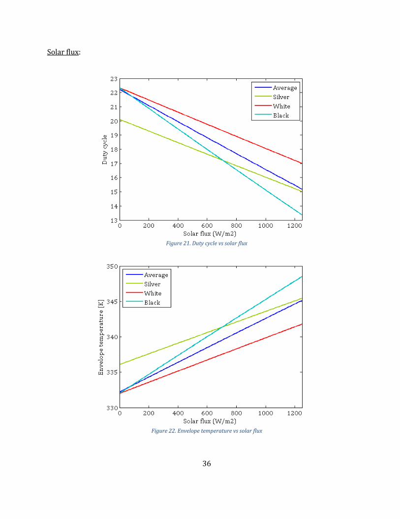
Solar flux:

Figure 21. Duty cycle vs solar flux

Figure 22. Envelope temperature vs solar flux

37

Atmospheric transmissivity:

Figure 23. Duty cycle vs atmosphere IR transmissivity

Figure 24. Envelope temperature vs atmosphere IR transmissivity

38

In all cases, fuel consumption is higher for the white fabric, but the envelope is at lower

temperature which means longer life.

The black and silver fabrics are two extremes when considering fuel consumption. The

black balloon has better performance for high solar flux (direct and reflected) and low

ambient temperature (𝑇𝑎 < 280 𝐾), compared to the silver one. Also, a decrease in the

atmosphere transmissivity has more effect on a black envelope. We can conclude that a black

balloon is better for a sunny clear sky and a silver (reflective) balloon is better for a cloudy

day.

The ambient temperature is the variable that most affects the fuel consumption, but it

affects almost equally all fabric colors.

39

Flow Simulation

The flow simulation is used to verify the heat transfer model. This is done by

activating the heat source, simulating the burner operation, to keep a constant temperature.

Then results are compared to the analytically calculated burner duty cycle.

The initial condition for the fluid is a uniform temperature of 𝑇𝑔 = 373 𝐾. In order to

be closer to the real flow, it is required to let the gas mix. We let it cool down for 30 seconds

until it comes to increasing isothermal layers (see Figure 25) and then we turn on the heat

source until the average fluid temperature goes back to 𝑇𝑔 = 373 𝐾. Next we let it cool down

for 10 seconds and turn on the heat source for 3 seconds, which is the time required for the

average temperature to go back to 373 𝐾 again. We repeat it another two times.

Finally, we let the temperature decrease for about 40 seconds, and from this

temperature decrease with time we can calculate the descent rate and compare it to real

flight data.

Figure 25. Gas temperature at simulation times t=0s (left) and t=30s (right)

40

Figure 26 shows the average gas temperature as a function of time. From point A

(𝑡 = 37 𝑠) to point B (𝑡 = 76𝑠) the heat source is active for ∆𝑡𝑏 = 3 · 3 = 9 𝑠. Then the duty

cycle is 𝑘 = ∆𝑡𝑏/∆𝑡 = 0.23. From the calculation we had obtained 𝑘 = 0.196. It is a similar

value, so it appears that there are no major errors in the analytical model.

Figure 26. Average fluid temperature from the flow simulation with SolidWorks

From point B to the end of the simulation there is a decrease in temperature of

∆𝑇𝑐𝑜𝑙𝑑𝑓𝑎𝑙𝑙 = 362.2 − 373.1 = −10.9 𝐾 for a time period of ∆𝑡𝑐𝑜𝑙𝑑𝑓𝑎𝑙𝑙 = 120 − 77.5 = 42.5 𝑠.

The temperature decrease rate is −0.256 𝐾/𝑠, very similar to the experimental results from

Aachen University [6] which give −14.2 𝐾/𝑚𝑖𝑛 = −0.24 𝐾/𝑠.

A B

41

Then we can say that the temperature as a function of time during descent is

𝑇𝑔(𝑡) = 373 − 0.256𝑡 (35)

The equation for vertical motion is the following (see chapter 2):

𝑑𝑢

𝑑𝑡= −

1

(𝑉𝜌𝑎(𝑇𝑎/𝑇𝑔(𝑡)) +𝐺𝑔

)(𝑉𝑔𝜌𝑎(1 − 𝑇𝑎/𝑇𝑔(𝑡)) − 𝐺 +

1

2𝐶𝑑𝜌𝑎𝑢2𝑆)

(36)

Solving the equation with 𝑇𝑔(𝑡) from the simulation we can obtain the descent

velocity as a function of time (Figure 27), which matches real flight data.

Figure 27. Descent rate as a function of time

42

We can integrate the velocity to get the change in altitude:

Actually the altitude would drop faster. The more velocity the higher the losses for

convection are going to be and the faster the temperature is going to decrease.

43

Figure 28 shows the change in temperature distribution when the burner is active

and few seconds after that. For more detail see Appendix I.

Figure 28. Gas temperature during burner activity (second 74 to second 77.5)

𝒕 = 𝟕𝟒𝒔 𝒕 = 𝟕𝟓𝒔

𝒕 = 𝟕𝟖𝒔 𝒕 = 𝟖𝟏𝒔

𝒕 = 𝟖𝟑𝒔 𝒕 = 𝟖𝟓𝒔

44

5. CONCLUSIONS

A heat transfer model was developed to calculate the fuel consumption in a hot air

balloon. The model was then evaluated by varying typical parameters to determine optimal

designs and important parameters. Since some parameters are difficult to assess, a flow

simulation was used to verify the analytical results and to give more insight on the thermal

distribution.

Results from the flow simulation show that there are no major errors in the analytical

model since burner operation times agree when attempting to maintain a constant altitude.

The gas temperature decreases at a rate of −0.256 𝐾/𝑠 when there is no burner activity, and

it increases at a rate of +1 𝐾/𝑠 when the pilot operates the burner. The simulation results

also show that the assumption of uniform temperature in the envelope is correct, and that

after approximately 10 seconds after burner operation the gas comes to increasing

isothermal layers. The temperature decrease rate matches the experimental one from

Aachen University, and the vertical speed agrees with real flight data, indicating that the

simulation can be trusted.

The analytical results for the general typical case show that most of the heat losses are

due to the emitted radiation from the envelope (more than 70%), the losses from natural

convection account for around 20% of the total, and the mouth outflow losses are relatively

small. From the sensitivity analysis, we get that the burner duty cycle (to keep the balloon at

a constant altitude) at different atmospheric conditions can be from 10% to 28%. We can

conclude that the ambient temperature is the variable that most affects the fuel

consumption, increasing with increasing ambient temperature. Unfortunately, ambient

45

temperature is not a controllable parameter so its effects can only be predicted but not

mitigated. A black fabric is more economical in terms of fuel for a sunny clear sky day, and a

silver balloon is better for a cloudy day. Light colors, which have low absorptivity, have the

worst performance, as expected, but the envelope is at lower temperature which can

mean longer life for the fabric.

Future work

The performance model presented here is very simple. With an improved model the

altitude can be related to the gas temperature more accurately. We already know that

the decrease rate in coldfall is −0.256 𝐾/𝑠 and that 1 second of burner operation is

needed to increase the temperature by 1 𝐾, so it would be possible to approximate the

fuel needed for a planned flight. This is very critical for long distance flights where

maximum payload is a limitation to decide how much fuel to carry in the balloon.

An additional opportunity for future work is to determine if there are methods to

heat the enclosed gas but prevent that heat from reaching the inner envelope surface.

This would provide low density gas with a low temperature envelope to reduce losses.

Such a design might require some careful fluid mechanics study of the entrained gases

during combustion and their eventual flow patterns in the balloon.

Finally, a last aspect of future work is to evaluate more completely the combustion

characteristics of the burner to ensure that it has the combustion efficiency expected.

46

REFERENCES

[1] F. Kreith, “Numerical Prediction of the Performance of High Altitude Balloons,” no. February, 1974.

[2] F. Kreith, “Thermal Design of High-Altitude Balloons and Instrument Packages,” J. Heat Transfer, 1970.

[3] L. A. Carlson and W. J. Hornt, “New Thermal and Trajectory Model for High-Altitude Balloons,” vol. 20, no. 6, pp. 500–507, 1982.

[4] K. Stefan, “Performance Theory for Hot Air Balloons,” J. Aircr., vol. 16, no. 8, pp. 539–542, Aug. 1979.

[5] W. Hallmann and U. Herrmann, “Thermodynamics of Balloon,” in International Symposium on Hot Air Aerostatic Vehicle Technology, 1991.

[6] W. Hallmann and U. Herrmann, “Experimentally determined Temperature Profile in a Hot Air Balloon,” in International Symposium on Hot Air Aerostatic Vehicle Technology.

[7] R. Röder, U. Rönna, and F. Suttrop, “Measurement of velocity distribution and gas composition in the envelope of a flying hot air balloon,” in International Symposium on Hot Air Aerostatic Vehicle Technology, 1991.

[8] W. Hallmann and U. Herrmann, “Energy Losses, Porosity, Strength and Stretch Behavior of Hot Air Balloon Fabrics Subject to Temperature Loads and Ultraviolet Radiation,” in International Symposium on Hot Air Aerostatic Vehicle Technology, 1991.

[9] H. a. Becker and S. Yamazaki, “Entrainment, momentum flux and temperature in vertical free turbulent diffusion flames,” Combust. Flame, vol. 33, pp. 123–149, Jan. 1978.

[10] J. Jones and J. Wu, “Performance model for reversible fluid balloons,” in AIAA, 1995.

[11] A. Campo, “Correlation equation for laminar and turbulent natual-convection from spheres,” Warme Und Stoffubertragung -- Thermo Fluid Dyn., vol. 13, no. 1–2, pp. 93–96, 1980.

[12] “[1] British Standard BS845 : Part 1 : 1987 for assessment of thermal performance,” no. 1. .

47

[13] A. Gillespie, “Land Surface Emissivity,” in Encyclopedia of Remote Sensing, E. G. Njoku, Ed. New York, NY: Springer New York, 2014.

[14] D. F. Al Riza, S. I. U. H. Gilani, and M. S. Aris, “Hourly Solar Radiation Estimation Using Ambient Temperature and Relative Humidity Data,” Int. J. Environ. Sci. Dev., vol. 2, no. 3, pp. 188–193, 2011.

[15] T. Colonius and D. Appelö, “Computational Modeling and Experiments of Natural Convection for a Titan Montgolfiere,” no. x, pp. 1–16, 2016.

48

Appendix I. SIMULATION RESULTS

𝒕 = 𝟎 𝒔 𝒕 = 𝟑𝟎 𝒔

𝒕 = 𝟕𝟒 𝒔

𝒕 = 𝟕𝟓 𝒔

49

𝒕 = 𝟕𝟔 𝒔 𝒕 = 𝟕𝟕 𝒔

𝒕 = 𝟕𝟖 𝒔

𝒕 = 𝟕𝟗 𝒔

50

𝒕 = 𝟖𝟎𝒔 𝒕 = 𝟖𝟏 𝒔

𝒕 = 𝟖𝟐 𝒔

𝒕 = 𝟖𝟑 𝒔

51

𝒕 = 𝟖𝟒 𝒔 𝒕 = 𝟖𝟓 𝒔

𝒕 = 𝟖𝟔 𝒔

𝒕 = 𝟏𝟎𝟎 𝒔

52

Appendix II. MATLAB SCRIPT

Heat transfer balance

%%%%%%%%%DATA%%%%%%%

sigma=5.67e-8; %[W/m2K4] Stephan-Boltzmann constant

R=287; %[J/kgK] Air gas constant

g=9.81; %[m/s2]

%Atmosphere

Ta=15+273.15; %[K] Ambient temperature

P=101325; %[Pa] Ambient pressure

rhoa=P./(R*Ta); % Ambient density

Fs=600; %[W/m2] Solar flux

tau_a=0.65; % Infrarred transmissivity of the atmosphere

%Earth surface

Te=Ta; %[K] Earth surface temperature

eps_e=0.9; % Earth surface emissivity

d=0.1; % Albedo

%Balloon envelope

V=2200; %[m3] Gas volume

A=847; %[m2] Surface area for M77 V=2200m3

eps=0.87; alpha=0.7; %Emissivity and absorptivity of outer

surface

eps_in=0.87; % Emissivity of the inner side of the fabric

%Internal gas

Tg=373; % [K]Emissivity

eps_g=0.45;

%Envelope temperature

[Ts]=EnvelopeT(sigma,R,Ta,P,Fs,tau_a,Te,eps_e,d,A,eps,alpha,eps_

in,Tg,eps_g);

fprintf('Envelope temperature: %.2f K \n',Ts);

%Burner

Qburner=(3255e3)*0.8; %[W] Burner heat input

53

%%%%%%%%%HEAT TRANSFER MODES%%%%%%%

%%EMITTED RADIATION FROM THE ENVELOPE

Qrad=eps*sigma*A*Ts^4;

%%EXTERNAL CONVECTION

h_ext=3.4; %[W/m2K] External convection coefficient

Qc_ext=h_ext*A*(Ts-Ta);

%%SOLAR RADIATION

%Solar direct radiation

Qs=Fs*alpha*A/4;

%Reflected solar radiation (albedo)

Qab=Fs*d*alpha*A/2;

%%INFRARRED RADIATION FROM THE EARTH

%Earth IR radiation

QIRe=eps_e*eps*tau_a*sigma*(A/2)*Te^4;

%%RADIATION GAS-ENVELOPE

f=1/((1-eps_g)/eps_g+1+(1-eps_in)/eps_in);

Qr=sigma*A*f*(eps_g*Tg^4-eps_in*Ts^4);

%%INTERNAL CONVECTION

h_int=16; %[W/m2K] Internal convection coefficient

Qc_int=h_int*A*(Tg-Ts);

%MOUTH OUTFLOW

cpair=1.011; %[J/gK]

m_dot=1356; %[g/s] Mass flow at the mouth

Qo=m_dot*cpair*(Tg-Ta);

%HEAT BALANCE

duty=@(k) Qs+Qab+QIRe+Qburner*k-Qc_ext-Qrad-Qo*k;

k=fzero(duty,0.1);

duty_cycle=k*100;

fprintf('Duty cycle: %.2f \n',duty_cycle);

54

Envelope temperature function

function [Ts] =

EnvelopeT(sigma,R,Ta,P,Fs,tau_a,Te,eps_e,d,A,eps,alpha,eps_in,Tg

,eps_g)

%%%%%%%%%HEAT TRANSFER MODES%%%%%%%

%%EMITTED RADIATION FROM THE ENVELOPE

Qrad=@(Ts) eps*sigma*A*Ts^4;

%%EXTERNAL CONVECTION

h_ext=3.4; %[W/m2K]

Qc_ext=@(Ts) h_ext*A*(Ts-Ta);

%%SOLAR RADIATION

%Solar direct radiation

Qs=Fs*alpha*A/4;

%Reflected solar radiation (albedo)

Qab=Fs*d*alpha*A/2;

%%INFRARRED RADIATION FROM EARTH

%Earth IR radiation

QIRe=eps_e*eps*tau_a*sigma*(A/2)*Te^4;

%%RADIATION GAS-ENVELOPE

Qr=sigma*A*f*(eps_g*Tg^4-eps_in*Ts^4);

Qr=@(Ts) sigma*A*f*(eps_g*Tg^4-eps_in*Ts^4);

%%INTERNAL CONVECTION

h_int=16; %[W/m2K]

Qc_int=@(Ts) h_int*A*(Tg-Ts);

%%%%%%HEAT BALANCE%%%%%%%

envelope=@(Ts) Qs+Qab+QIRe+Qc_int(Ts)+Qr(Ts)-Qc_ext(Ts)-

Qrad(Ts);

Ts=fzero(envelope,Ta);

end

55

Vertical motion

syms v(t)

[t,v] = ode45(@verticalmotion_velocity,[0,60],0)

function dvdt=verticalmotion_velocity(t,v)

g=9.81; %[m/s2]

Ta=288.15; %[K] Ambient temperature

rho=1.225; %[kg/m3] Ambient density

%Balloon parameters

V=2200; %[m3] Gas volume

r=16.67/2; %[m] Radius at the equator

S=pi*r^2; %[m2] Balloon cross-sectional area

Cd=0.43; %Drag coefficient

M=613; %[kg]

G=g*M; %[N] Weight for L=G at sea level and Tg=373 K

Tg=373-0.256*t; %[K] Gas temperature as a function of time

L=V*g*rho*(1-Ta./Tg);

B=Cd*0.5*rho*S;

m=(rho*(Ta./Tg)*V+M);

if L>G

dvdt=(L-G-B*(v^2))./m;

elseif L<G

dvdt=(L-G+B*(v^2))./m;

end

end