Optimal solar PV, battery storage, and smart ... - UC Irvine

UC IrvineUC Irvine Electronic Theses and Dissertations

TitleOptimal solar PV, battery storage, and smart-inverter allocation in zero-net-energy microgrids considering the existing power system infrastructure

Permalinkhttps://escholarship.org/uc/item/1b8795rv

AuthorMartinez de Novoa, Laura Martinez

Publication Date2020 Peer reviewed|Thesis/dissertation

eScholarship.org Powered by the California Digital LibraryUniversity of California

https://escholarship.org/uc/item/1b8795rv

https://escholarship.org

http://www.cdlib.org/

UNIVERSITY OF CALIFORNIA,

IRVINE

OPTIMAL SOLAR PV, BATTERY STORAGE, AND SMART-INVERTER ALLOCATION IN ZERO-NET-ENERGY MICROGRIDS CONSIDERING THE EXISTING POWER SYSTEM

INFRASTRUCTURE

DISSERTATION

submitted in partial satisfaction of the requirements for the degree of

DOCTOR OF PHILOSOPHY

in Mechanical & Aerospace Engineering

by

Laura Martinez de Novoa

Dissertation Committee: Professor Jack Brouwer, Ph.D., Chair

Professor Kia Solmaz, Ph.D. Professor Michael Green, Ph.D.

2020

i

DEDICATION

To

my parents, husband, and friends

my love and gratitude,

for seeing my happiness as their own

some wisdom:

Wherever you go. There you are

~Confucius

and optimism:

It is possible for ordinary people to choose to be extraordinary

~Elon Musk

ii

TABLE OF CONTENTS Page

LIST OF FIGURES iv

LIST OF TABLES vii

ACRONYMS ix

ACKNOWLEDGMENTS xi

VITA xii

ABSTRACT OF THE DISSERTATION xiv

1 Introduction 1

1.1. Research goals 3

1.2. Objectives to meet goals 3

1.3. Approach 3

Task 1: Background 4

Task 2: Determine baseload DER ability to regulate voltage on constrained systems 4

Task 3: Develop a steady state power flow model with high distributed solar PV penetration 5

Task 4: Implement power flow and distribution transformer constraints into a time-series MILP

optimization framework for DER investment planning 5

Task 5: Implement smart inverter functions into the MILP optimization framework 6

1.4. Structure of this dissertation 6

2 Background 8

2.1. DER hosting capacity 8

2.2. Voltage challenges caused by DG 10

2.3. Optimal DER allocation in a microgrid environment 12

2.4. Optimization formulations applied to DER allocation 14

2.5. Smart-inverter functions 24

3 Baseload DER ability to regulate voltage on generation-constrained systems 31

3.1. Approach 32

3.1. Model Development and Assumptions 33

3.2. Scenarios 37

3.3. Results and Discussion 38

3.4. Summary 44

4 Steady-state power flow analysis of the impacts of large solar PV deployments in an urban power system 47

iii

4.1. Test Case 49

4.2. Model development and assumptions 58

4.3. Scenarios 67


4.5. Summary 84

5 Optimal Solar PV and Battery Storage Sizing and Siting Considering Local Transformer Limits85

5.1. Literature Review 85

5.2. Problem Formulation 92

5.3. Test Case 103


5.5. Summary 120

6 Optimal DER Allocation in Meshed Microgrids with Grid Constraints 122

6.1. Literature Review 122

6.2. Contributions 125


6.4. Test Cases 131


6.6. Summary 147

7 Optimal solar inverter sizing considering Volt-Var droop-control and PQ control for voltage regulation 149

7.1. Literature review 149

7.2. Notation 155


7.4. Test Case and Assumptions 165


7.6. Summary 173

8 Conclusions 175

REFERENCES 180

APPENDIX 191

iv

LIST OF FIGURES

Page

Figure 2.1 – Definition of hosting capacity (when a performance index is exceeded) 8

Figure 2.2 – Concept of Minimum and Maximum Hosting Capacity. 10

Figure 2.3 – Two-bus distribution system with DG and a load. 10

Figure 2.4 – DG allocation Optimization Objectives 18

Figure 2.5 – DG Allocation Optimization Constraints 22

Figure 2.6 – IEC and IEEE power factor sign convention. 25

Figure 2.7 – Example Volt-Var function curve. 26

Figure 2.8 – Example of Volt-Var function curve with hysteresis. 27

Figure 2.9 – Example of Volt-Watt function curve. 28

Figure 2.10 – Low Pass Filter Limiter Example. 28

Figure 2.11 – Interaction between Volt-Var and Volt-Watt – Scenario 1. 29

Figure 2.12 – Interaction between Volt-Var and Volt-Watt – Scenario 2. 30

Figure 3.1 – Southern California Main Transmission substations and system boundary for

SONGS System. 34

Figure 3.2 – One-line diagram of SONGS system 35

Figure 3.3 – Voltage improvement index, VII vs. TIGER penetration (%) 38

Figure 3.4 – TIGER Power Factor and resulting power flows 40

Figure 3.5 – (a) 100 MW TIGER. (b) 70 MW/70 MVar TIGER. (c) 100 MVar TIGER 41

Figure 3.6 – P-V curves for TIGER @ San Diego - variable power factors 44

Figure 3.7 – P-V curve at San Diego bus 44

Figure 4.1 – Oak View community, used as the test case, and its different building sectors: 50

Figure 4.2 – View of Ocean View Substation from Google Earth. 51

Figure 4.3 – 66 kV circuits from Ocean View substation. 52

Figure 4.4 – 12 kV circuits from Ocean View Substation. 53

Figure 4.5 – Oak View circuits and Transformers. 54

Figure 4.6 – Oak View pole-top service transformers 55

Figure 4.7 – Power Flow system boundaries geographical location of substations, 66 kV,

and 12 kV lines. 59

Figure 4.8 – High voltage 66/12 kV one line 60

Figure 4.9 – Oak View test case low voltage system network graph. 61

Figure 4.10 – Wiring diagram for sub-transmission and distribution voltages. 62

v

Figure 4.11 – Typical Residential PV installation 62

Figure 4.12 – Example of ETAP model for a typical residential installation 64

Figure 4.13 – Example of ETAP model for a typical C&I installation 65

Figure 4.14 – Oak View annual load profile distribution 66

Figure 4.15 – Normalized PV generation profile for a system in Southern California, at UC Irvine. 67

Figure 4.16 – Peak Load Scenario – Voltage Profile for 66 and 12 kV systems 70

Figure 4.17 – Example of Primary, Secondary (NET) and PV buses at the Oak View test case 70

Figure 4.18 – HOMER Pro© Modeling Environment – Oak View DER assets and connections 71

Figure 4.19 – Oak View hourly dynamics on summer (left) and winter (right). 73

Figure 4.20 – Optimal PV Scenario - Voltage Profile for 66/12 kV system 74

Figure 4.21 – Optimal PV Scenario - Primary Buses Voltage Profile 74

Figure 4.22 – Optimal PV Scenario – Secondary Buses Voltage Profile 75

Figure 4.23 – Realistic PV Scenario - Voltage Profile for 66/12 kV system 76

Figure 4.24 – Realistic PV Scenario - Primary Buses Voltage Profile 76

Figure 4.25 – Realistic PV Scenario – Secondary Buses Voltage Profile 77

Figure 4.26 – EES Charge Power, Discharge Power, and State of Charge for the entire month of

April 2015 79

Figure 4.27 – Optimal PV + EES design. EES = 7,200 kW/30,238 kWh. 79

Figure 4.28 – EES storage deployed behind an overloaded transformer. 82

Figure 4.29 – Optimal PV (with and w/o EES) comparison- Voltage Profile for 66/12 kV system 83

Figure 4.30 – Optimal PV (with and w/o EES) comparison - Voltage Profile for Primary buses 83

Figure 4.31 – Optimal PV (with and w/o EES) comparison - Voltage Profile for Secondary buses 83

Figure 5.1 – Schematic of one Building Energy Hub used in the multi-nodal approach. 101

Figure 5.2 – (a) Operating regions for the transformer must be constrained 103

Figure 5.3 – Transformer-aggregated demand profiles 104

Figure 5.4 – Building total annual demand versus maximum total onsite yearly PV production,

both in (kWh) 105

Figure 5.5 – Advanced Energy Community Low Voltage distribution grid network topology

and load allocation 106

Figure 5.6 – Rate structures for utility electricity. 109

Figure 5.7 – Transformer overloads 113

Figure 5.8 – Transformer 54 (500kVA) kVA power flows: comparison of before (solid red curve)

and after (blue dashed curve) 114

vi

Figure 5.9 – Building DER allocation comparison with and without transformer constraints 116

Figure 6.1 – Polygon relaxation for branch kVA power flows 131

Figure 6.2 – (a) Radial 33-node feeder test case. 132

Figure 6.3 – Test case topology, based on a real-world power system 132

Figure 6.4 – The (a) Voltage Magnitude and (b) Voltage Percent Error at each node of the

radial 33-node case comparing the full AC power flow (ACPF), DLPF,

Bolognani, et al., and LinDistFlow solutions. 136

Figure 6.5 – The (a) Voltage Magnitude and (b) Voltage Percent Error at each node of the

meshed 33-node case comparing the full AC power flow (ACPF), DLPF,

Bolognani et al., and LinDistFlow solutions. 138

Figure 6.6 – The (a) Voltage Magnitude and (b) Voltage Percent Error at each primary (12 kV)

node of the meshed network case comparing the full AC power flow (ACPF),

DLPF, Bolognani et al., and LinDistFlow solutions. 140

Figure 6.7 – Base Case. Voltages range between 0.887 – 1.187 p.u. 142

Figure 6.8 – Comparison of the voltage magnitude solution using DLPF (top) and LinDistFlow

(bottom) against the ACPF (post-processed) true voltage solution. 144

Figure 6.9 – Comparison of the voltage magnitude solution using DLPF (top) and LindistFlow

(bottom) against e ACPF (post-processed) true voltage solution. 146

Figure 6.10 – Comparison of branch kVA power flows for DLPF (a) and LinDistFlow

(B) solutions, compared to the true, post-calculated branch kVA power flow. 147

Figure 7.1 – Schematic of one Building Energy Hub used in the multi-node approach. 158

Figure 7.2 – Depiction of the polygon relaxation constraints and operating regions for the inverter

(shaded in yellow). 160

Figure 7.3 – Volt-Var droop control curve. 161

Figure 7.4 – Piece-wise linearization of a function of tow variables, 163

Figure 7.5 – Meshed benchmark case based on a real-world power system 166

Figure 7.6 – a) Baseline scenario. b) PQ control scenario. c) Volt-Var scenario 169

Figure 7.7 – Inverter dynamics at buildings 11 and 14. Baseline versus PQ control and Volt-Var 171

Figure 7.8 – Optimal AC/DC ratio vs. maximum nodal over voltage curve fit for PQ control and

Volt-Var 173

vii

LIST OF TABLES

Page

Table 3.1– Substation 2017 Peak Load forecast 36

Table 3.2 – Scenario Description 37

Table 3.3 – P-V analysis summary: San Diego bus Maximum shift, Maximum Load Growth,

Initial voltage, and Total System Losses. 43

Table 4.1 – Oak View transformer infrastructure – voltage and power ratings, and

maximum/ minimum loads fed by transformer 56

Table 4.2 – 66/12 kV Substations – Existing generation and projected load [16] . 57

Table 4.3 – 12 kV Feeders – Existing generation and projected load [16]. 58

Table 4.4 – Scenarios simulated in the steady-state power flow model 67

Table 4.5 – Critical and Marginal Limits for Loading and Bus Voltage 68

Table 4.6 – DER technology parameters assumptions 72

Table 4.7 – DER technology cost assumptions 72

Table 4.8 – Oak View test case DER Optimal Design computed by HOMER Pro 72

Table 4.9 – Optimal PV Scenario - Events 75

Table 4.10 – Realistic PV Scenario – Events 77

Table 4.11 – Optimal PV + EES Scenario - EES capacity allocated at AEC transformers 80

Table 4.12 – Optimal PV + EES + VVar Scenario events 84

Table 5.1 – List of decision variables used in DERopt 93

Table 5.2 – List of parameters used in DERopt 94

Table 5.3 – AEC building loads, Maximum demand (kW), Total annual demand (kWh),

Type, Rate Structure, Total Area (ft2), Maximum rooftop PV installed (kW),

Connected Transformer number, Transformer rating (kVA) 107

Table 5.4 – DERopt Cost and Operational Assumptions 108

Table 5.5 – Total Building DER adoption for all scenarios 118

Table 6.1 – Model Parameters 127

Table 6.2 – Model decision variables 128

Table 6.3 – DER adoption DLPF vs. LinDistFlow for the base case and two different voltage

constraints. Percentages show the percentual difference between LinDistFlow solution

and DLPF solution. 143

Table 7.1 – Model decision variables 156

Table 7.2 – List of parameters used in DERopt 156

viii

Table 7.3 – Volt-Var inverter settings 162

Table 1 – Comparison of existing literature on the topic of DER optimal allocation, portfolio

selection, and dispatch 168

Table 2 – Building DER allocation for all scenarios 71

Table 3 – Inverter capacity comparison, at each building, for all scenarios. Highlighted rows

indicate the even inverter locations for Volt-Var droop control 72

ix

ACRONYMS

AC Alternating Current

ACPF Alternating Current Power Flow

AEC Advanced Energy Community

AWG American Wire Gauge

BESS Battery Energy Storage System

C&I Commercial and Industrial

CAISO California Independent system Operator

DC Direct current

DER Distributed Energy Resource

DERopt Distributed Energy Resource Optimization

DG Distributed Generation

DLPF Decoupled Linearized Power Flow

DOE Department of Energy

DSO Distribution System Operator

EES Electric Energy Storage

ETAP Electric Transient Analysis Program

EUI Energy Use intensity

GHG Greenhouse Gas

LP Linear Program

MILP Mixed Integer Linear Program

MV/LV Medium Voltage / Low Voltage

NEC National Electric Code

NEM Net Energy Metering

O&M Operation and Maintenance

OPF Optimal Power Flow

P2G Power to Gas

PCC Point of Common Coupling

PF Power Factor

PV Photovoltaic

REES Renewable Electric Energy Storage

RPF Reverse Power Flow

RTE Round Trip Efficiency

SAIDI System Average Interruption Duration

SAIFI System Average Interruption Frequency

SCE Southern California Edison

SOFC Solid Oxide Fuel Cell

SOS Special Ordered Set

TC Transformer constraints

TIGER Transmission Integrated Grid Energy Resource

TMY Typical Meteorological Year

TOU Time-of-Use

x

VVO Volt-Var Optimization

ZNE Zero Net Energy

xi

ACKNOWLEDGMENTS

I would like to express my sincere and genuine gratitude to my committee chair, Professor Jack Brouwer, for being much more than an academic advisor, but a true mentor, advocator, and friend. Who has always believed in me, and allowed me to do so as well. Whose passion for clean energy inspires positivity and hope. His teachings and guidance shaped my research and made this work possible. My gratitude also goes to Professor Scott Samuelsen, for precious teachings such as Buford — the social-political impacts of technology and innovation and Seabiscuit— a horse for his time. Also, for his leadership in the Advanced Power and Energy Program, whose impacts on the development of clean energy transcend globally and will continue to do so for many years beyond. I would also like to thank my committee members, Professor Kia Solmaz, for all her teachings in optimization techniques, which gave me the first-principles understanding that served as the foundation for my optimization work. Also, for being a great role model for strong women in academia. Professor Michael Green whose expert knowledge in electric power systems have much supported and guided this work. In addition, a thank you to all industry professionals that were also mentors and advisors: Russ Neal, who worked closely with APEP to provide valuable technical guidance on power systems. Roberto Analco, from ETAP, who provided me guidance on power flow state estimation, Jerry Thode, from Southern California Edison, who provided expert insights in the utility industry, and Sarah Walinga, from Tesla, who taught me so much about smart inverters. I am immensely grateful for all my dearest APEP friends, who always created a great community to belong to. I will cherish our memories forever. I am also especially grateful for the infinite support from my husband, Greg Alesso, for the emotional support only one that has married to a Ph.D. will ever understand. Thanks for reminding me to take breaks to pet Momo every so often, and not letting me work too hard.

Lastly, I am (and will eternally be) grateful to Prof. Valerie Sheppard, who taught me how to master life from the eyes of abundance, happiness, and wholeness. Whose teachings were just (or perhaps, more) important than any other technical course I’ve attended during my academic career at UC Irvine. I am profoundly grateful our paths have crossed.

https://www.americasbestracing.net/the-sport/2016-seabiscuit-true-rags-riches-story

xii

VITA


2008 - 2014 B.S. in Energy Engineering

Universidade Federal do ABC, Sao Paulo, Brazil 2014 - 2016 M.S. in Mechanical Engineering

Advanced Power and Energy Program, University of California, Irvine 2016 - 2020 Ph.D. in Mechanical Engineering

Advanced Power and Energy Program, University of California, Irvine Sum. 2016 Internship – Power systems: automation, protection, and communications

applications engineering Schweitzer Engineering Laboratories, Irvine

Sum. 2018 Internship – Power systems: inverter and solar PV modeling

Tesla Inc., Palo Alto Fall 2019 Internship - Powerwall (residential battery storage) applications engineering

Tesla Inc., Palo Alto Spr. 2016 Teaching Assistant

MAE 118/218 Sustainable Energy. Instructor: Dr. Brian. Tarroja

FIELD OF STUDY

Optimal allocation (size and siting) of distributed Energy Resources (DER), focusing on smart-inverter connected solar PV, battery storage within a microgrid for achieving high renewable energy penetration.

PUBLICATIONS Dynamics of an integrated solar photovoltaic and battery storage nanogrid for electric vehicle charging L Novoa, J Brouwer Journal of Power Sources 399, 166-178

Optimal renewable generation and battery storage sizing and siting considering local transformer limits L Novoa, R Flores, J Brouwer Applied Energy 256, 113926 *Also recommended to special edition: Progress in Applied Energy.

https://www.sciencedirect.com/science/article/pii/S0378775318308176

https://www.sciencedirect.com/science/article/pii/S0378775318308176

xiii

Optimal DER Allocation in Meshed Microgrids with Grid Constraints L Novoa, R Flores, J Brouwer Applied Energy (manuscript submitted) Transmission Integrated Grid Energy Resources to Enhance Grid Characteristics L Novoa, R Neal, J Brouwer Applied Energy (manuscript submitted) Optimal solar inverter sizing considering Volt-Var droop-control and PQ control for

voltage regulation

L Novoa, R Flores, J Brouwer Applied Energy (manuscript submitted)

Transformer Infrastructure upgrades for PEV Charging in a solar PV plus storage

microgrid

L Novoa, R Flores, J Brouwer Applied Energy (manuscript to be submitted)

Google Scholar Profile

https://scholar.google.com/citations?hl=en&user=gUMjsowAAAAJ

xiv

ABSTRACT OF THE DISSERTATION

OPTIMAL SOLAR PV, BATTERY STORAGE, AND SMART-INVERTER ALLOCATION IN ZERO-

NET-ENERGY MICROGRIDS CONSIDERING THE EXISTING POWER SYSTEM INFRASTRUCTURE

By


Doctor of Philosophy in Mechanical & Aerospace Engineering

University of California, Irvine, 2020

Professor Jack Brouwer, Chair

In response to climate change and sustainability challenges, various incentive

programs have promoted solar photovoltaic (PV) economic feasibility and interconnection

into the low voltage electrical distribution system. However, the existing power system

infrastructure can only accommodate a limited amount of PV generation before reverse

power flow (PV generation flowing back into the distribution network) becomes an issue.

This limits the ability to achieve Zero Net Energy (ZNE) behind individual meters and in

whole communities since ZNE communities typically require large PV deployments. In

parallel, district-level energy systems, such as Advanced Energy Communities (AEC)

microgrids— electrically contiguous areas that leverage the clustering of load and

generation by integrating multiple utility customer-owned Distributed Energy Resources

(DER) — that include battery storage, offer a great prospect for integrating high levels of

solar PV into the built environment.

Designing the least-cost and technically feasible system to serve a district load has

been a challenge to utilities and city planners. Battery energy storage and smart-inverter

xv

technologies emerge in this context to enable higher penetration of solar PV by locally

regulating voltage and controlling active and reactive power flows. However, there is no

straight forward way nor a practical rule or consensus on how to size such assets optimally.

This work proposes a Mixed Integer Linear Program (MILP) optimization to

determine the least-cost DER portfolio consisting of inverter-connected solar PV and

battery storage. It also allocates it in a multi-node electrical grid and dispatches it

considering the existing electric infrastructure limits (transformer capacities and nodal

voltage magnitudes). Novel linearization techniques such as polygon relaxations are used

to limit otherwise non-linear apparent power flows at transformers. A novel Alternating

Current (AC) decoupled linearized power flow is also integrated into the MILP

optimization. Moreover, for the first time, smart-inverter droop-control functions are

included in the DER optimal allocation problem. Results show that such comprehensive

MILP is achievable and tractable for a 115-node AEC.

1

1 Introduction

Within an Advanced Energy Community microgrid, DER assets allow for most of the energy

demand to be generated and consumed internally. External energy transfers enter the

community if local production is insufficient. Excess electricity is exported to the wide-area

electricity grid.

Optimally designing AEC to serve commercial, and industrial loads, while minimizing cost and

maximizing the penetration of solar PV, has been a challenge to Distribution System Operators

(DSO) and city planners. Moreover, a significant share of AEC project success depends upon

achieving an adequate allocation of DER such as PV and battery storage resources while

considering the existing urban power system infrastructure to support and enhancing the overall

utility grid network characteristics.

We first attempt to demonstrate the local impacts of inverter-connected DER in the local power

systems that it is integrated. We are interested in the challenges associated with the grid

integration of large-scale PV deployments into the existing power system infrastructure. From

the results of worst-case steady-state simulations, presented in Chapter 4 utility distribution

transformer overloads are visibly the worst negative impact of a large deployment of solar PV.

Over voltage excursions showed to be another major limiting factor to large PV deployments.

These results drove the development of novel transformer constraints to limit the reverse power

flow at the transformer level (limiting the total apparent power injection at that node), as

described later in Chapter 5. And also an AC Decoupled Linearized Power Flow (DLPF)

formulation to constrain nodal voltages, as described in Chapter 6

In chapter 5, a Mixed Integer Linear Program optimization is proposed to decide the best DER

portfolio, allocation, and dispatch, for an AEC that achieves ZNE and islanding while respecting

electrical grid operational constraints, with a focus on distribution transformer overloads. The

main strategies to avoid transformer overloads were found to be careful sizing and siting of

2

battery energy storage and also optimally re-distributing PV throughout the community, which

increased the ability of the electric infrastructure to support a PV deployment that is 1.7 times

larger than the existing transformer capacity without the need for infrastructure upgrades.

In Chapter 6, a new approach to model the linearized power flow in distributed energy resources

allocation and dispatch optimization is developed here. The model uses the Decoupled

Linearized Power Flow(J. Yang, Zhang, Kang, & Xia, 2016) approach. DLPF has the advantage

of being suitable for meshed networks, while the majority of current models use LinDistFlow,

which is only suitable for radial networks. First, a validation is provided for the DLPF voltage

magnitude and branch power (in kVA) solutions against LinDistFlow and the true AC power

flow (ACPF) solution for a meshed benchmark network, a 33-node system. Then, the DER

allocation and dispatch problem are formulated as a MILP and DLPF and LinDistFlow are used

to model constraints on the electric power network infrastructure that limits voltages to ANSI

C84 standard limits. The implementation of DLPF developed here improves the accuracy of

nodal voltage calculation for meshed networks. The LinDistFlow solution fails to capture true

under and over voltages; it also underestimates the optimal PV and battery storage capacities

when compared to the DLPF solution.

Advanced inverter controls are a recent requirement for providing voltage support on distribution

feeders with large PV deployments and high reverse power flow. These control functions,

especially those that involve locally injecting or absorbing reactive power, require appropriate

inverter sizing to accommodate for the reactive power support. The industry had historically

adopted an AC/DC ratio smaller than one, which limits the inverter potential for reactive power

support when at full Direct Current (DC) output —and when most needed. Optimal Volt-Var

control (VVO) strategies have been devised, yet, currently, most commercial inverters adopt

droop-control functions (which provide a more equitable share of reactive power regulation

between customers). There is no consensus on how to size inverters optimally, in order to

provide the necessary amount of reactive power compensation when in droop-control. In Chapter

7, a MILP for optimal DER investment planning is developed to optimally size inverters that can

equitably provide voltage support for a ZNE microgrid with high PV penetration. Results show

that the optimal AC/DC ratio is location-specific and ranges from 0.83 to 1.5. We also find a

correlation between inverter AC/DC ratio and maximum nodal over-voltage and provide a curve

fit model for optimal inverter sizing.

3

1.1. Research goals

The goal of the current research is to optimize the allocation (sizing and siting) and dispatch of

inverter-connected solar PV and battery storage to minimize cost and guarantee power quality in

distribution feeders of a grid-connected, or islanded, urban microgrid that requires large

deployments of renewable solar PV, and often, zero-net-energy.

1.2. Objectives to meet goals

1. Continuously review the literature on DER optimal allocation, dispatch, smart inverters,

zero-net energy microgrids, advanced energy communities, and related topics.

2. Determine the ability of baseload inverter-connected DER to regulate voltage on a

constrained system.

3. Develop and verify a steady-state power flow model of a distribution feeder of an urban

microgrid with high penetration of solar PV. Determine the solar PV hosting capacity of

the existing microgrid infrastructure, considering existing service transformers and voltage

limits. Model battery energy storage and smart-inverters with reactive power support into

the model to improve solar PV hosting capacity.

4. Implement power system infrastructure constraints into an existing single-node, time-series

MILP optimization framework for DER allocation in a ZNE microgrid. Constraints focus

on service transformer capacity limits and AC power flow for limiting nodal voltage

excursions. Determine optimal DER allocation in a ZNE microgrid under these constraints.

5. Implement Smart Inverter Volt/Var and optimal PQ control functions into the optimization

framework. Determine optimal inverter sizing and abstract a practical model from the

simulations.

1.3. Approach

This dissertation encompassed six key tasks, one for each objective described previously. This

section describes how each task, and specific activities, maps to the chapters constituting this

dissertation.

4

Task 1: Background (Chapter 2)

An extensive, continuous literature review on the topics below was made throughout

this research. Relevant concepts were extracted and summarized in a background chapter

to familiarize the reader with the following concepts:

DER hosting capacity of power systems

DER and voltage control

Optimization methods applied to renewable, distributed energy systems, and power

flow modeling

Smart-inverter functions

Advanced energy communities

Task 2: Determine baseload DER ability to regulate voltage on constrained

systems (Chapter 3)

Model a generation-constrained transmission system to investigate and demonstrate

the ability of an inverter-connected DER to locally regulate voltage

Carry out steady-state load flow simulations for different DER deployments,

operating at a unity, i.e., pure active power injection) and leading power factor, i.e.,

having a combination of active and reactive power injection.

Determine best DER placement that achieves greater grid benefits

Determine impacts on overall system steady-state voltage stability

5

Task 3: Create an urban microgrid test case with high PV penetration.

Develop a steady-state power flow model to identify and quantify main

impacts in existing power system infrastructure. Implement battery energy

storage and smart-inverters into the steady-state model to mitigate impacts

(Chapter 4)

Create a real-world microgrid test case. Characterize an existing urban district power

system in Southern California through satellite imagery and on-site surveys.

Model the high voltage (230 kV) transmission and medium/low voltage (12kV /

480/240/120 V) distribution feeders, with a high penetration of inverter-connected

solar PV. Model any existing grid-support equipment, such as shunt capacitor banks,

or load tap-changing transformers.

Perform worst-case steady-state load flow simulation to identify and quantify the

negative impacts on the existing power system infrastructure. Determine the

(minimum) PV hosting capacity.

Judiciously size and site battery energy storage and smart-inverters operating at a

fixed power factor to eliminate negative impacts and increase the test case PV hosting

capacity

Task 4: Implement power flow and distribution transformer constraints into a

time-series MILP optimization framework for DER investment planning.

Determine the optimal DER allocation (Chapter 5 and Chapter 6)

Starting from an existing MILP optimization model, namely DERopt (R. J. Flores,

2016). Implement additional decision variables and constraints relevant to microgrid

operations, such as export to the utility grid, and zero-net-energy constraints.

Formulate and implement linearized AC power flow constraints (Decoupled

Linearized Power Flow) into exiting optimization model

Incorporate other relevant grid constraints into the optimization model, such as

transformer capacity constraints and nodal voltage constraints.

6

Use the model to determine optimal DER allocation for the test case.

Task 5: Implement smart inverter functions into the MILP optimization

framework. Determine optimal smart inverter capacity for minimizing

voltage deviation (Chapter 7)

Model within a MILP framework two smart inverter controls Volt-Var and optimal

PQ.

Optimally size the solar PV inverter to minimize voltage deviations caused by solar

PV in high penetrations.

Abstract an approximated model for AC/DC inverter sizing from simulations

1.4. Structure of this dissertation

Chapter one Background intends to provide introductory first-principles knowledge to the reader

that is unfamiliar with some of the concepts that will be explored here. Chapters three through

seven map directly to the tasks outlined. Each chapter has its own applicable introduction,

literature review, gaps found in current literature, contributions, and results. A summary section

at the end of each chapter identifies the major points and insights from the results. Lastly,

Chapter 8 Conclusions consolidates all the most relevant findings and provides the main

conclusions of this work.

It is worth mentioning that the results and analysis of most chapters of this dissertation were

submitted to prestigious peer-reviewed journals, as mapped by the table below. Chapter 5 was

recommended by the editor in Chief of Applied Energy to a special edition Progress in Applied

Energy.

7

Chapter 3:

Transmission Integrated Grid Energy Resources to Enhance Grid Characteristics L Novoa, R Neal, J Brouwer Applied Energy (manuscript submitted, in review process)

Chapter 5:

Optimal renewable generation and battery storage sizing and siting considering local transformer limits L Novoa, R Flores, J Brouwer Applied Energy 256, 113926

Chapter 6:

Optimal DER Allocation in Meshed Microgrids with Grid Constraints L Novoa, R Flores, J Brouwer Applied Energy (manuscript submitted Dec 2019)

Chapter 7:

Optimal solar inverter sizing considering Volt-Var droop-control and

PQ control for voltage regulation

L Novoa, R Flores, J Brouwer Applied Energy (manuscript to be submitted early 2020)

8

2 Background

2.1. DER hosting capacity

Hosting capacity is defined as the maximum level of additional DER penetration that an existing

electric power system can accommodate while maintaining acceptable system performance

(Bollen & Hassan, 2011). Grid performance can be analyzed concerning “performance indices”,

which depend upon applicable technical standards, local network configuration and operation,

which will vary regionally (Schwaegerl, Bollen, Karoui, & Yagmur, 2005). These indices refer

to different aspects of power supply, such as power quality, short circuit contribution, power

system protection, reliability, and safety (Stetz, 2014). Figure 2.1 illustrates the concept of

hosting capacity, where a given performance index limit was exceeded above acceptable

deterioration limit. In a hosting capacity study, however, not only one but a combination of

performance indices is likely to be considered, characterizing it as a multi-dimensional problem;

once one given limit is exceeded the maximum hosting capacity is reached.

Figure 2.1 – Definition of hosting capacity (when a performance index is exceeded) (Bollen & Hassan, 2011).

In general, the three primary criteria used in hosting capacity analysis are (Electric Power

Research Institute (EPRI), 2015; EPRI; APS, 2017; EPRI, Smith, & Rogers, 2015; Southern

California Edison, 2016):

9

Voltage excursions, which is limited by the absolute overvoltage magnitude, or a

percent deviation from the nominal value.

Equipment overloads (or thermal limits) which are limited by current flows, and thus,

power flows allowed through equipment, such as transformers and cables.

Protection, which examines whether the addition of DER interferes with the ability of

existing protection schemes to identify and respond to abnormal conditions. One

example is when DER is located

In a hosting capacity analysis, these indices are usually evaluated under a worst-case scenario for

example, during a severe reverse power flow event; which occurs when a low load condition is

associated with significant PV generation, thus, the power is that is not consumed locally is

exported. In an RPF condition, the receiving bus voltage rises above nominal 1 per unit (P.U.)

The boundedness of these constraints should also be evaluated in practical terms. Thus, the

analysis nature (i.e., steady-state vs. time-domain) plays a vital role in how conservative the

hosting capacity results are. Steady-state worst-case type analysis often results in over-

conservative limits, i.e., it is designed for a condition that only happens during one hour in the

entire year, and most times, over-voltage or overloading issues might be acceptable within a

short period. These nuances are often captured by time-series simulations (Christos, 2016)

Hosting Capacity is heavily influenced by the DER allocation within the system. Thus, one can

also define a Minimum and Maximum hosting capacity (Electric Power Research Institute

(EPRI), 2015), which depicts the more/less optimal DER allocation. In other words, at the same

DER penetration level, different DER allocation (sizes and siting) deployments across the system

can cause different impacts, perhaps because some locations have more voltage rise headroom,

or are close to the head (beginning) of a feeder, where the total impedance is lower. Figure

2.2.illustrates the concept of minimum and maximum hosting capacity.

In this work, optimal allocations of DER will aim to maximize the total hosting capacity of a low

voltage microgrid, which will be further discussed in section 2.3.

10

Figure 2.2 – Concept of Minimum and Maximum Hosting Capacity. Source: (Electric Power Research Institute (EPRI), 2015)

2.2. Voltage challenges caused by DER

To illustrate the prevalent technical challenge caused by high penetrations of DER that are

Distributed Generators (DG), we refer to power flow concepts. The voltage excursion caused by

DG is illustrated in Figure 2.3 (Christos, 2016; Mahmud, Hossain, & Pota, 2011; Stetz, 2014).

Considering a two-bus system with a load and a DG unit, it will likely export power to the

upstream distribution grid (P and Q). In order to do so, it has to operate at a higher voltage than

the voltage at the sending end. For Kirchhoff’s Law of Voltage (KLV), we can express the

voltage phasor at the sending end ( �̂�𝑆 ), or the grid voltage as:

Figure 2.3 – Two-bus distribution system with DG and a load. Adapted from (Mahmud et al., 2011)

11

�̂�𝑆 = �̂�𝑅 − 𝐼 𝑍 (1)

�̂� = 𝑅 + 𝑗𝑋 (2)

Where �̂�𝑆 is the voltage at the receiving end, where the load and DG are connected, 𝐼 is the

current phasor flowing through the line.

The complex power flowing through the network can be expressed as, where 𝑃 and 𝑄 are the

active and reactive power respectively.

�̂� = 𝑃 + 𝑗𝑄 = �̂�𝑆𝐼 ∗ (3)

From which we can write

𝐼 = 𝑃 − 𝑗𝑄

�̂�𝑆

(4)

Thus, we can readily define the voltage difference (raise or drop) ∆𝑉 between the receiving and

sending end as:

∆𝑉 = �̂�𝑅 − �̂�𝑆 = 𝐼 𝑍 = ( 𝑃 − 𝑗𝑄

�̂�𝑆

) (𝑅 + 𝑗𝑋) =𝑅𝑃 + 𝑋𝑄

�̂�𝑆

+ 𝑗𝑋𝑃 + 𝑅𝑄

�̂�𝑆

(5)

Since the voltage drop between the sending and receiving end is small, the voltage drop can be

approximated by the real part of Eq. (5), also, if the sending end voltage is taken as the reference

bus voltage, its angle is zero. Thus, it equals to the sending voltage magnitude.

�̂�𝑆 = 𝑉𝑠 (6)

Moreover, we can finally write

∆𝑉 ≈𝑅𝑃 + 𝑋𝑄

𝑉𝑠 (7)

Moreover, writing the active and reactive power flows 𝑃 = 𝑃𝐷𝐺 − 𝑃𝐿 and 𝑄 = ±𝑄𝐷𝐺 − 𝑄𝐿

∆𝑉 ≈𝑅(𝑃𝐷𝐺 − 𝑃𝐿) + 𝑋(±𝑄𝐷𝐺 − 𝑄𝐿)

𝑉𝑠 (8)

Some important observations can be drawn from Eq. (8):

𝑉𝑠 can be considered a stiff, source, and therefore, constant.

As the DG active power output 𝑃𝐷𝐺 increases, ∆𝑉 increases

As the load active 𝑃𝐿 and reactive 𝑄𝐿 power consumption increases, ∆𝑉 decreases

The DG can absorb (−𝑄𝐷𝐺) or inject (+𝑄𝐷𝐺) reactive power.

12

If DG absorbs reactive power, ∆𝑉 decreases (equivalent to operating at a lagging

PF)

If DG injects reactive power, ∆𝑉 increases (equivalent to operating at a leading PF)

The distribution system’s resistance 𝑅 and reactance 𝑋 can be reduced (typically by costly line

upgrades) in order to reduce the voltage rise.

Voltage rises are likely to occur when DG is exporting power. The legacy power system

networks were designed to handle unidirectional passively (radial) power flows from the

centralized generation resources to the high voltage transmission system, and finally to the

medium and low voltage distribution system, where commercial, industrial, and residential loads

are connected. Extreme RPF events pose a significant technical challenge to the current grid

paradigm and limit the PV hosting capacity of a circuit. In this work, ways to increase PV

hosting capacity by locally controlling active and reactive power flows, using smart-inverter

advanced functions, and more specifically, how to optimally parameterize these functions will be

proposed.

2.3. Optimal DER allocation in a microgrid environment

Microgrids are defined as clusters of load, generation, and storage resources, that can operate

autonomously (independent of the main electric grid, i.e., islanded) or grid-connected. Moreover,

the notion of a microgrid also entails a certain level of advanced control capabilities, which

assure system reliability during islanded operations (Hatziargyriou, 2014). Microgrids provide a

platform to integrate DER into the medium and low voltage distribution network, with focus on

meeting loads with local generation (Kwasinski, Weaver, & Balog, 2017). DER include

distributed generation, including, but not limited to microturbines, solar PV and fuel cells (FC),

and wind turbines and also storage systems such as batteries, power-to-gas (P2G), flywheels,

ultra-capacitors, to mention a few.

To allocate DER in any system, pure analytical techniques, and, more recently, optimization and

artificial intelligence hybrid techniques have been used. The approach of allocating DER in a

Microgrid environment is no different from allocating it in a grid-connected system, only the

goals of the system and constraints might be different to capture the goals of a microgrid

environment, for instance, ZNE, islanding, enhanced reliability, among others.

13

There are in the current literature a large number of different solution methodologies to the DG

allocation problem, which can be broadly categorized in (1) sensitivity/pure analytical, (2)

classical optimization, and (3) artificial intelligence techniques (Arabali, Ghofrani, Bassett,

Pham, & Moeini-Aghtaei, 2017), and also (4) hybrid intelligent (Pesaran H.A, Huy, &

Ramachandaramurthy, 2017)

Sensitivity/pure analytical methods represent the system in a mathematical model and compute

its direct numerical solution. These techniques are fast, simple, accurate, and easy to implement,

but can only be applied to small-scale systems. Techniques used in this approach are Eigenvalue

Based-Analysis (EVA), Index method (IMA), Sensitivity Based Method (SBM) and Point

Estimation Method (PEM). (Arabali et al., 2017).

Classical optimization methods are used to minimize (or maximize) a given goal, or cost

function, subjected to given technical/operational constraints (equality and inequality

constraints). These methods are useful for continuous and differentiable domains and are

characterized by relatively slower convergence rates and computational times. These techniques

involve Optimal Power Flow (OPF), Linear Programming (LP), Mixed Linear Integer

Programming (MILP), Mixed Non-linear Integer Programming (MINLP), Dynamic

Programming (DP), Sequential Quadratic Programming (SQP), and Ordinal Optimization (OO).

(Arabali et al., 2017).

Artificial intelligence (meta-heuristic) techniques are usually applied to solve complex nonlinear

optimization problems through intelligent techniques methodology inspired by natural

phenomena. Some challenges often associated with this technique involve premature

convergence, local optima, and unstable results. Such techniques are the Genetic Algorithm

(GA), Fuzzy Logic (FL), Particle Swarm Optimization (PSO), Artificial Bee Colony (ABC),

Tabu Search (TS), and Ant Colony Search (ACS). (Arabali et al., 2017). For further reading on

these techniques, and many other hybrid intelligent methods, (Rezaee Jordehi, 2016), and

(Pesaran H.A et al., 2017), are recommended, which are a comprehensive review compendium

all these existing approaches.

A number of practices have been used for DER allocation in energy systems. The most simplistic

one involves allocating a single specific type of DER, such as solar PV, or wind, in a single node

according to a particular optimization goal and constraints. This analysis is usually performed in

14

an “aggregate approach”, and it is static, or steady-state. Several “enhancements” to this

approach were developed in subsequent studies, such as (1) optimizing a portfolio (mix) of DER,

and allocating it (2) including heating and cooling demands in the load elements (3)

incorporating the time-coupling of DG and load (and sometimes it’s inherent uncertainty) in a

time-domain, dynamic simulation (4) considering electric power grid constraints, in a multi-node

approach, (5) considering electric energy storage, and lastly, (6) considering smart-grid

technologies to achieve better grid performance. However, most studies in the literature to date

only implement one or two of the improvements mentioned above, but not all of them.

2.4. Optimization formulations applied to DER allocation

Optimization problems for DER allocation are typically non-linear, highly constrained, multi-

objective, mixed-integer, multi node, thus, finding a near-global optimal solution is challenging

(Rezaee Jordehi, 2016). DER type, location, real and reactive power outputs are the standard

decision variables computed. In the following section, typical formulations for steady-state

(static) DG allocation problems found in the recent literature are reviewed. Time-domain

(dynamic) optimizations follow a similar formulation, but compute a decision variable for each

time-step 𝑡, increasing the problem dimension significantly.

2.4.1. Objective function

The optimization problem is built to minimize (or maximize) an objective function that is

formulated using a group of parameters in a logical manner that translates a single objective or a

weighted multi-objective (WMO) (Arabali et al., 2017).

𝑚𝑖𝑛𝑖𝑚𝑖𝑧𝑒 𝑓(𝑥) = 𝛼 𝑥1 + 𝛽 𝑥2 + ⋯ + 𝛾 𝑥𝑛 (9)

Where 𝑥1, 𝑥2 , 𝑎𝑛𝑑 𝑥𝑛 are individual objectives and 𝛼, 𝛽, 𝑎𝑛𝑑 𝛾 are weight factors (the sum of

weight factors should always equal to one).

The most common objective function goals in the existing research works are listed below:

Cost

The costs of DER allocation involve construction/investment (capital cost), financial (principal

and interest), O&M (facility management, regular maintenance fuel, and equipment

15

replacement). Nonetheless, there are also possible financial returns from surplus energy sales,

reduction of emission of pollutants, infrastructure upgrade deferrals, and potential tax credits.

An approach shown in (Arabali et al., 2017) formulates the objective function for cost as:

max 𝑓𝑐𝑜𝑠𝑡 = 𝐶𝐷 + 𝐶𝑒 − 𝐶𝐷𝐺 − 𝐶𝑙 (10)

Where: 𝐶𝐷 = ∑ 𝑇max 𝑖∗ 𝐶𝑤 ∗ 𝐹𝑉 ∗ 𝑃∑ 𝐷𝑔 𝑖

𝑇𝑖=1 is the generated income, where 𝑇 is the number of

years, 𝑇max 𝑖 is the annual average operating hours for the DG. 𝐹𝑉 is the ratio of average output

and the rated power of the DG, and 𝑃∑ 𝐷𝑔 𝑖 is the power produced by the DG unit . 𝐶𝑤 is the grid

electricity price. 𝐶𝑒 = ∑ 𝑇max 𝑖∗ 𝐶𝑐 ∗ 𝐹𝑉 ∗ 𝑃∑ 𝐷𝑔 𝑖

𝑇𝑖=1 are the emission reduction benefits, where

𝐶𝑐 is the conventional fuel generation environmental costs 𝐶𝐷𝐺 = ∑ 𝑇max 𝑖∗ 𝜕 ∗ 𝐶𝐷𝐺𝑗

∗𝑇𝑖=1

𝑃∑ 𝐷𝑔 𝑖 are the investment costs, where 𝐶𝐷𝐺𝑗

is the cost of an individual equipment, 𝜕 =𝑟∗(1+𝑟)𝑡

(1+𝑟)𝑡−1

is the average cost factor of a DG fixed investment, r is the annual profit, t are the planning years

𝐶𝑙 = ∑ 𝛽𝑖 ∗ 𝑐𝑖 ∗ 𝑇max 𝑖∗ 𝑃∑ 𝐷𝑔 𝑖

𝑇𝑖=1 are the O&M costs, where 𝑐𝑖 is the unit capacity factor, 𝛽𝑖 is

the O&M cost per unit of power

System Active Power Losses

When optimally sized and placed, DG can reduce system losses by 10-20% (Arabali et al.,

2017). The power loss formulation usually focuses on reducing branch power, and most times,

active power losses. The exact loss or the “i-squared” loss which is calculated from the branch

current, can be formulated as in (Sultana, Khairuddin, Aman, Mokhtar, & Zareen, 2016). It is

worth pointing out that not only instantaneous, but accumulated losses over time, such as daily

losses or annual losses can also be the focus of the minimization. Equation (11) refers to the

exact active power loss flowing from branch 𝑖 to branch 𝑗 (Arabali et al., 2017) and Equation

(12) refers to the copper losses caused by branch current 𝐼𝑏𝑖 passing through a resistor

𝑅𝑏𝑖 (Prakash & Khatod, 2016). Another approach is to calculate the power loss index (Prakash &

Khatod, 2016) as in Equation (13), which calculates the % reduction in copper losses after DG is

placed, which is a quantity that should be maximized.

𝑚𝑖𝑛 𝑓𝑙𝑜𝑠𝑠𝑒𝑠 = 𝑃𝐿 = ∑ ∑[𝛼𝑖𝑗(𝑃𝑖𝑃𝑗 + 𝑄𝑖𝑄𝑗) + 𝛽𝑖𝑗(𝑄𝑖𝑃𝑗 − 𝑃𝑖𝑄𝑗)]

𝑁

𝑗=1

𝑁

𝑖=1

(11)

16

𝛼𝑖𝑗 =𝑅𝑖𝑗

𝑉𝑖𝑉𝑗cos (𝛿𝑖 − 𝛿𝑗)

𝛽𝑖𝑗 =𝑅𝑖𝑗

𝑉𝑖𝑉𝑗sin (𝛿𝑖 − 𝛿𝑗)

𝑃𝐿 = ∑|𝐼𝑏𝑖|2

𝑁

𝑖=1

𝑅𝑏𝑖 (12)

𝑃𝐿𝑖 = (1 −𝑅𝑒 {𝑃𝐿𝑎𝑓𝑡𝑒𝑟𝐷𝐺

}

𝑅𝑒 {𝑃𝐿𝑏𝑒𝑓𝑜𝑟𝑒𝐷𝐺}) 𝑋 100% (13)

Voltage profile excursions

Voltage profile improvement i.e., maintaining bus voltages 𝑉�̅� as close to their nominal operation

value 𝑉𝑛𝑜𝑚 ̅̅ ̅̅ ̅̅ ̅is also commonly chosen as an optimization goal. One approach is to calculate the

Voltage Profile Index (VPI) (Arabali et al., 2017). When included in the objective function, the

VPI penalizes the size-location pair that gives higher voltage deviations from the nominal value,

as written in Equation (14).

𝑉𝑃𝐼 = max (|𝑉𝑛𝑜𝑚̅̅ ̅̅ ̅̅ | − |𝑉�̅�|

|𝑉𝑛𝑜𝑚̅̅ ̅̅ ̅̅ |

) 𝑖 = 1, … , 𝑛 (14)

Emissions from grid and DER

Emission goals can be translated into economic revenues originated from emission reductions.

One of such approaches was already shown in Equation (9) 𝐶𝑒 . In another approach shown in

(Falke, Krengel, Meinerzhagen, & Schnettler, 2016), the total emissions of CO2 equivalent are

computed. The total emissions include both emissions caused by manufacturing (𝐸𝑖 𝑝𝑟𝑜𝑑𝑢𝑐𝑡𝑖𝑜𝑛

)

and operation (𝐸𝑖 𝑜𝑝𝑒𝑟𝑎𝑡𝑖𝑜𝑛

) of each DG 𝑖, and are minimized, as shown in Equation (15). A Life

Cycle Analysis (LCA) are likely necessary to be applied to the DER technologies to obtain

𝐸𝑖 𝑝𝑟𝑜𝑑𝑢𝑐𝑡𝑖𝑜𝑛

.

min 𝑓𝐶𝑂2𝑒𝑞= ∑[𝐸𝑖

𝑝𝑟𝑜𝑑𝑢𝑐𝑡𝑖𝑜𝑛+ 𝐸𝑖

𝑜𝑝𝑒𝑟𝑎𝑡𝑖𝑜𝑛]

𝑁

𝑖=1

(15)

17

One approach to calculate operation emissions based on power output is shown in (Basu,

Bhattacharya, Chowdhury, & Chowdhury, 2012)

𝐸𝑖 𝑜𝑝𝑒𝑟𝑎𝑡𝑖𝑜𝑛

= ∑ [𝛼𝑖 + 𝛽𝑖 + 𝑃𝐷𝐺𝑖𝑚𝑎𝑥+ 𝛾𝑖𝑃𝐷𝐺𝑖𝑚𝑎𝑥

2]

𝑁

𝑖=1

(16)

Where 𝛼𝑖 , 𝛽𝑖 , 𝑎𝑛𝑑 𝛾𝑖 are CO2 or NOx emission coefficients of the 𝑖𝑡ℎ DER determined by a least-

squares fit on equipment data of emissions vs power output.

Reliability

Multiple analyses had shown that a DG reduced both the magnitude and duration of failures,

directly by being available when the central generation was not or indirectly by reducing stress

on the system components, so the individual system component reliability is increased. Also by

locally reducing load and enabling feeder tie operations that were avoided due to high-load

conditions, (Arabali et al., 2017). The System average interruption frequency index (SAIFI)

indicates how often an average customer is subjected to sustained interruption over a predefined

time interval:

𝑆𝐴𝐼𝐹𝐼 =𝑇𝑜𝑡𝑎𝑙 𝑁𝑢𝑚𝑏𝑒𝑟 𝑜𝑓 𝐶𝑢𝑠𝑡𝑜𝑚𝑒𝑟 𝐼𝑛𝑡𝑒𝑟𝑟𝑢𝑝𝑡𝑖𝑜𝑛𝑠

𝑇𝑜𝑡𝑎𝑙 𝑁𝑢𝑚𝑏𝑒𝑟 𝑜𝑓 𝐶𝑢𝑠𝑡𝑜𝑚𝑒𝑟𝑠 𝑆𝑒𝑟𝑣𝑒𝑑=

∑ 𝜆𝑖𝑁𝑖

∑ 𝑁𝑖 (17)

Where 𝜆𝑖is the failure rate, and 𝑁𝑖 is the number of customers of load point i. (Arabali et al.,

2017)

Another index, the System average interruption duration index (SAIDI) indicates the total

duration of interruption an average customer is subjected to for a predefined time interval:

𝑆𝐴𝐼𝐹𝐼 =𝑆𝑢𝑚 𝑜𝑓 𝐶𝑢𝑠𝑡𝑜𝑚𝑒𝑟 𝑖𝑛𝑡𝑒𝑟𝑟𝑢𝑝𝑠𝑡𝑖𝑜𝑛 𝐷𝑢𝑟𝑎𝑡𝑖𝑜𝑛

𝑇𝑜𝑡𝑎𝑙 𝑁𝑢𝑚𝑏𝑒𝑟 𝑜𝑓 𝐶𝑢𝑠𝑡𝑜𝑚𝑒𝑟𝑠 𝑆𝑒𝑟𝑣𝑒𝑑=

∑ 𝑈𝑖𝑁𝑖

∑ 𝑁𝑖 (18)

Where 𝑈𝑖 is the annual outage time (Arabali et al., 2017). These indices can be included in the

cost function to penalize solutions that are unreliable.

DER hosting capacity, DG penetration

It is worth mentioning that the vast majority of previous literature work is mainly focused on

minimizing cost and copper losses. Another interesting optimization objective, which will be

18

significantly explored in this work, is to maximize the installed capacity of DG installed in the

network, for increasing total renewable energy penetration into the existing power system.

max 𝑓𝐷𝐺𝑐𝑎𝑝𝑎𝑐𝑖𝑡𝑦 = ∑ 𝑃𝐷𝐺𝑖

𝑁

𝑖=1

(19)

A comprehensive list of many other possible objective functions is provided in (Pesaran H.A et

al., 2017), as illustrated in Figure 2.4.

Figure 2.4 – DG allocation Optimization Objectives . (Pesaran H.A et al., 2017)

2.4.2. Constraints

As in a typical optimization formulation, the objective function for the DG allocation problem

should satisfy given equality ℎ𝑖(𝑥) = 0 or inequality 𝑔𝑖(𝑥) ≤ 0 constraints such as:

Voltage constraints

The voltage at the 𝑖𝑡ℎ 𝑉𝑖 bus should always stay within upper and lower limits 𝑉𝑖 and

𝑉𝑖 respectively, as shown in (20) (Arabali et al., 2017). Limits for voltage are usually taken as the

(ANSI, 2005)

19

𝑉𝑖 ≤ |𝑉𝑖| ≤ 𝑉𝑖 (20)

Current (thermal) constraints (line and transformer)

The apparent power flowing from branch 𝑖 to branch 𝑗 (𝑆𝑖𝑗 ) should not exceed the maximum

rated power the circuit or transformer can withstand 𝑆𝑖𝑗 𝑚𝑎𝑥 , as shown in Equation (21) (Arabali

et al., 2017)

𝑆𝑖𝑗 < 𝑆𝑖𝑗 𝑚𝑎𝑥 (21)

Power Balance

At each node, the power generated from the DG at each node 𝑖, (𝑃𝐺𝑖 𝑎𝑛𝑑 𝑄𝐺𝑖

) plus losses

(𝑃𝐿, 𝑎𝑛𝑑 𝑄𝐿) should equal the active and reactive load et each node (𝑃𝐷𝑖 𝑎𝑛𝑑 𝑄𝐷𝑖

), as shown in

Equation (22) (Arabali et al., 2017). If the system is grid-connected and allows for import and

export, these decision variables can be included as shown in Equation (24).

∑ 𝑃𝐺𝑖+ 𝑃𝐿

𝑁

𝑖=1

= ∑ 𝑃𝐷𝑖

𝑁

𝑖=1

∑ 𝑄𝐺𝑖+ 𝑄𝐿

𝑁

𝑖=1

= ∑ 𝑄𝐷𝑖

𝑁

𝑖=1

(22)


𝑁

𝑖=1

+ 𝑃𝑔𝑟𝑖𝑑𝑖𝑚𝑝𝑜𝑟𝑡= ∑ 𝑃𝐷𝑖

𝑁

𝑖=1

+ 𝑃𝑔𝑟𝑖𝑑𝑒𝑥𝑝𝑜𝑟𝑡 (23

Storage constraints

Battery storage can be modeled in the case of a time-domain dynamic simulation, which will

account not only for power but energy balances. An approach to model storage was shown in

(Mashayekh, Stadler, Cardoso, & Heleno, 2016), and can be written as shown in Equations (24),

(25), and (26).

𝑆𝑂𝐶𝑛,𝑠,𝑡 = (1 − 𝜙𝑠) ∗ 𝑆𝑂𝐶𝑛,𝑠,𝑡−1 + 𝑆𝐼𝑛𝑛,𝑠,𝑡 – 𝑆𝑂𝑢𝑡𝑛,𝑠,𝑡

(24)

20

𝑆𝑂𝐶𝑠 ≤ 𝑆𝑂𝑢𝑡𝑛,𝑠,𝑡 ≤ 𝑆𝑂𝐶𝑠 (25)

𝑆𝐼𝑛𝑛,𝑠,𝑡 ≤ 𝐶𝑎𝑝𝑛,𝑠 ∗ 𝑆𝐶𝑅𝑡𝑠

𝑆𝑂𝑢𝑡𝑛,𝑠,𝑡 ≤ 𝐶𝑎𝑝𝑛,𝑠 ∗ 𝑆𝐷𝑅𝑡𝑠 (26)

Where:

𝑆𝐼𝑛𝑛,𝑠,𝑡 = Energy input to storage technology s at node n, kWh

𝑆𝑂𝑢𝑡𝑛,𝑠,𝑡 = Energy output from storage technology s at node n, kWh

𝐶𝑎𝑝𝑛,𝑠 = Installed capacity of continuous technology k at node n, kW or kWh

𝑆𝑂𝐶𝑠/𝑆𝑂𝐶𝑠 = Min/max state of charge for storage technology s, %

𝑆𝐶𝑅𝑡𝑠/ 𝑆𝐷𝑅𝑡𝑠 = Max charge/discharge rate of storage technology s, kW

In the case of storage, the power/energy balance equation will need to also include the power

charge/discharge from the battery, modifying the active power portion of Equation (22) to

include storage would result in:


𝑁

𝑖=1

+ 𝑆𝑂𝑢𝑡𝑛,𝑠,𝑡 = ∑ 𝑃𝐷𝑖

𝑁

𝑖=1

+ 𝑆𝐼𝑛𝑛,𝑠 (27)

Power Flow

The power flow equations are active and reactive power balance equations at each node. An

approach used by (Arabali et al., 2017) uses the AC nonlinear power flow equations as

constraints, where P and Q generated by the DG are 𝑃𝐺𝑖 𝑎𝑛𝑑 𝑄𝐺𝑖

. 𝑉𝑖 and 𝑉𝑗 are the voltages at

nodes 𝑖 and 𝑗 and 𝛿𝑖 𝑎𝑛𝑑 𝛿𝑗 are the respective voltage angles | 𝑌𝑖𝑗| and 𝜃𝑖𝑗 represent the

admittance magnitude and angle from the admittance matrix.

𝑃𝐺𝑖− 𝑃𝐷𝑖

− ∑|𝑉𝑖||𝑉𝑗|

𝑁

𝑗=1

|𝑌𝑖𝑗| cos(𝛿𝑖 − 𝛿𝑗 – 𝜃𝑖𝑗) = 0

𝑄𝐺𝑖− 𝑄𝐷𝑖

− ∑|𝑉𝑖||𝑉𝑗|

𝑁

𝑗=1

|𝑌𝑖𝑗| sin(𝛿𝑖 − 𝛿𝑗 – 𝜃𝑖𝑗) = 0

(28)

21

Power imported from the grid

It is often necessary to limit the power provided by the network 𝑃𝑔𝑟𝑖𝑑. Otherwise, for most cost-

based objective functions, the load is likely going to be supplied fully by power imported from

the grid, which is cheaper, and the optimization problem returns zero DER installed capacity.

0 ≤ 𝑃𝑔𝑟𝑖𝑑 ≤ 𝑃𝑔𝑟𝑖𝑑 (29)

Space and area

Available space for DER installation is a constraint often overlooked in the literature, but

essential for obtaining more realistic results. An approach suggested by (Y. Yang, Zhang, &

Xiao, 2015b) is directly applied to PV systems and rooftop area. 𝑁𝑃𝑉,𝑛 is the installed capacity of

the PV system in building 𝑙. 𝐴𝑟𝑒𝑎𝑃𝑉 , 𝑗 is the area occupied by each kW of the PV panel and

𝑀𝑎𝑥𝑅𝑜𝑜𝑓𝑙 is the roof area space of building 𝑙.

𝑁𝑃𝑉,𝑙 ∗ 𝐴𝑟𝑒𝑎𝑃𝑉 ≤ 𝑀𝑎𝑥𝑅𝑜𝑜𝑓𝑙 (30)

Power factor (PF)

DG units are usually operated in PQ mode with a constant power factor. However, in some

studies, the DER was allowed to operate to export or import reactive power. An approach shown

in (Prakash & Khatod, 2016), an inequality constraint was set to bound the operating PF of the

DG from 0.8 to unity.

0.8 ≤ 𝑃𝐹𝐷𝐺,𝑗 ≤ 1 (31)

The PF can also be controlled by setting a fixed PF value and optimizing the amount of reactive

power output/absorbed by the DG, as shown in (Arabali et al., 2017)

𝑄𝐺𝑖≤ 𝑃𝐺𝑖

√𝑃𝐹−2 − 1 (32)

A comprehensive list of many other possible objective functions is provided in (Pesaran H.A et

al., 2017), as illustrated in Figure 2.5.

22

Figure 2.5 – DG Allocation Optimization Constraints (Pesaran H.A et al., 2017)

2.4.3. Optimal power flow

The first optimal power flow problem was proposed in 1962 by J. Carpentier (Carpentier, 1979).

Since then, many authors have contributed to the development of the central problem

formulation to apply OPF to many different applications. The OPF problem is simply an

optimization formulation, i.e., a minimization or maximization of an objective function having it

constrained within a set of equality and inequality constraints that describe the power flows

across the system nodes and determine the power system operational limits. These equality and

inequality conditions define the feasible region for the OPF problem. Most times, these

formulations are nonlinear and non-convex (Abdi, Beigvand, & Scala, 2017). OPF formulations

are widely used for the economic dispatch of generators, i.e., optimize generation to reduce cost.

Nonetheless, OPF formulations have been gaining attention and applied to other goals such as

minimize losses, regulate voltage and maximize DER penetration.

The decision variables of an OPF control the solution space dimension, thus, for n decision

variables the dimension of the solution space will be n. Examples of such variables may include

active power generation of all nodes (Except slack bus), reactive power injections for voltage

23

regulation equipment, voltages across the system node, tap settings in the transformers, and so

forth.

A sample OPF problem, as taken from (Zhang, 2013) can be expressed as:

minimize 𝑓(𝑃1, 𝑃2, … . , 𝑃𝑛)

subject to ℎ𝑖(𝑥) = 0 𝑖 = 1, … , 𝑚

𝑔𝑗(𝑥) ≤ 0 𝑗 = 1, … , 𝑟

(33)

(34)

(35)

Where (33) is the cost function, usually defined on the real power outputs, Equation (37)

represents the equality constraints, usually expressed by the physical load flow equations, and

equation (38) represents the inequality constraints that typically define system operating limits.

The OPF problem is usually solved using Newton-type methods, which have a non-guaranteed

convergence to a local minimum (Zhang, 2013). Various other methods have also been proposed,

such as Distributed and Parallel OPF (DPOPF), Multiphase OPF (MOPF), linearization

approaches, iterative approaches, unbalanced three-phase OPF (TOPF), Alternating Direction

Method of Multipliers (ADMM). Each of these methodologies is summarized in (Abdi et al.,

2017), and also have their computational performances compared.

Amongst some of the challenges/recommendations identified in the field of OPF applied to

microgrid and smart-grids (Abdi et al., 2017) (Ehsan & Yang, 2017)are:

The increased dimension of the optimization problem, especially when considering

distribution systems at a lower voltage level.

The unbalance nature of loads

The integration of energy storage, which requires a dynamic time-series simulation,

or Optimal Energy Flow (OEF)

The incorporation of uncertainties of renewable generation

Hybrid techniques combining analytic metaheuristic and computations methods

should be explored

24

2.5. Smart-inverter functions

The main smart-inverter functions to be considered in this work and summarized in this section

were initially proposed in the “ERPI, Common Functions for Smart Inverters – Phase 3” report

(Electric Power Research Institute (EPRI), 2014). This report was the result of a collaborative

industry and utility work facilitated by EPRI. It proposes a core set of key smart-inverter

functions that will facilitate higher DG penetration without affecting system power quality or

reliability. These functions are considered mandatory in California under Rule 21, and in other

utilities with the IEEE Standard 1547-2018.

2.5.1. Fixed power factor

This function provides a mechanism to regulate the DER’s power factor to a pre-set fixed value.

Attention is needed for the sign convention used, as illustrated in Figure 2.6, there are two

different sign conventions typically used in industry:

1. IEC: Generated or Supplied active power is positive. Demanded active power be negative.

2. IEEE: leading (capacitive, producing Var) PF is positive and lagging (inductive, absorbing

Var) PF is negative.

Also, a PF of +1.0 and -1.0 are essentially the same (zero Vars).

25

Figure 2.6 – IEC and IEEE power factor sign convention. Adapted from (Electric Power Research Institute (EPRI), 2014)

2.5.2. Volt-Var

A smart inverter with a Volt-Var function controls reactive power, Var, to regulate local voltage.

The function uses a “configurable curve”, i.e., a two-dimensional X-Y array, which defines a

linear function of the desired Volt-Var behavior. Vars are the controlling variable and Volts are

the variable to be controlled. The Y-axis is the percent available Vars, in other words, the power

capacity that the inverter can provide at a given moment without limiting its Watt output, which

usually takes priority. Also, the array X-values are defined as the “Percent Voltage”, as defined

in Equation (36), which is the voltage value but expressed in percentage of the Reference

Voltage (𝑉𝑟𝑒𝑓).

26

𝑉𝑜𝑙𝑡𝑎𝑔𝑒 (%) =𝑉𝑜𝑙𝑡𝑎𝑔𝑒

𝑉𝑟𝑒𝑓 𝑥 100%

(36)

Figure 2.7 illustrates a typical Volt-Var function. The four points, P1 through P4, indicate the

desired percentage available Var level (Q1 through Q4) for a given voltage value in percentage

of 𝑉𝑟𝑒𝑓 (V1 through V4). Noting that P2 and P3 represent a “dead-band”, which a

corresponding Var output of 0%, or 0 Var. In addition, expressing the points in the curve as

percentages allows the use of the curve for many different DERs without having to adjust for

local conditions such as nominal voltage.

Figure 2.7 – Example Volt-Var function curve. Adapted from (Electric Power Research Institute (EPRI), 2014).

Different manufacturers can have different Volt-Var behavior characteristics such as a horizontal

line or two points forming a ramp. In some cases, it might also be desired to have a hysteresis

behavior. The hysteresis adds the benefit of avoiding any unnecessary fluctuations, for instance,

as can be observed in Figure 2.8 the same amount of Vars Q3 = Q5 is outputted when the voltage

decreases from V3 to V5.

27

Figure 2.8 – Example of Volt-Var function curve with hysteresis. Adapted from (Electric Power Research Institute (EPRI),

2014).

Lastly, these curves should be implemented as “modes”, so a single inverter can have many

modes pre-programmed, which can be interchanged by a signal broadcast, or also scheduled over

time.

2.5.3. Volt-Watt

An inverter with a Volt-Watt function is able to reduce its Watt output gradually in order to

achieve a target voltage level at the PCC. The specific need for such a function arises from cases

where a high PV penetration at low loads can cause feeder overvoltage. This function adopts the

same “configurable-curve” approach as the Volt-Var function. An example of such a curve is

shown in Figure 2.9, where a horizontal line extends across the lowest voltage, V1, and to the

highest voltage, V3, until an operational limit is reached. The horizontal axis is expressed in

percent of 𝑉𝑟𝑒𝑓. The vertical axis is the inverter’s Maximum Watt output, also in percentage.

Thus, for a system with nominal 480 V, and the function settings are V2 = 105% and V3 =

110%, the Watt reduction would begin for voltages above 504 V and be reduced to zero at 528

V.

28

Figure 2.9 – Example of Volt-Watt function curve. Adapted from (Electric Power Research Institute (EPRI), 2014).

There is a separately defined function designed for systems containing energy storage: the

Absorbed Volt-Watt function. There are two proposed ways to limit the rate of charging power,

the Low-Pass Filter Limiter, where 𝜔 = 2𝜋𝑓 and 𝜏 is the time-constant of the filter, defined in

Equation (37) and Figure 2.10.

(37)

Figure 2.10 – Low Pass Filter Limiter Example. Adapted from (Electric Power Research Institute (EPRI), 2014).

There is also the Rate of Change Limiter, defined in Equation (38), which establishes a

maximum value for the rising and falling rates of the Watts limits.

𝑑𝑊𝑎𝑡𝑡𝐿𝑖𝑚𝑖𝑡

𝑑𝑡≤ 𝑅𝑖𝑠𝑒 𝐿𝑖𝑚𝑖𝑡

𝑑𝑊𝑎𝑡𝑡 𝐿𝑖𝑚𝑖𝑡

𝑑𝑡≥ 𝐹𝑎𝑙𝑙 𝐿𝑖𝑚𝑖𝑡 (38)

Frequency Domain Time Domain

29

Interactions between Volt-Var and Vol-Watt

The interaction between the Volt-Var and Volt-Watt functions is direct and intentional. In all

functions described so far, Watts must take precedence over Vars regardless of voltage, and it

might be that an inverter that is producing its full Watt capacity does not have any extra Vars to

offer. Nonetheless, in most cases, there is a sufficient margin between the inverter VA rating and

the peak PV array output (W); therefore, there is enough room for significant Vars production.

The combined operation of both functions allows for the reduction of Watts when there is a local

voltage rise, also enabling more Vars production.

To clarify the combined operation described above, consider the following two scenarios. In the

first one (Figure 2.11), the PV active power output, in blue, is 100% of the inverter limit. This

means that the available Var output, in yellow, is zero until the Watts are reduced by the Volt-

Watt function. As the voltage increases so does the ability to produce Vars.

Figure 2.11 – Interaction between Volt-Var and Volt-Watt – Scenario 1. Adapted from (Electric Power Research Institute

(EPRI), 2014).

In the second scenario, shown in Figure 2.12, the PV active power output, in blue, is only 80% of

the maximum inverter output. Thus, there is a maximum available Var output capacity of 60%,

in yellow, (from the constant VA circle) until the Volt-Watt function reduces the Watts.

30

Figure 2.12 – Interaction between Volt-Var and Volt-Watt – Scenario 2. Adapted from (Electric Power Research Institute

(EPRI), 2014).

31

3 Baseload DER ability to

regulate voltage on

generation-constrained

systems

Highlights

Large-scale baseload DER is deployed to support a constrained transmission system

A combined active/reactive power injection is ideal for voltage regulation

Placing DER on the bus with the lowest voltage achieves greater overall grid benefits

DER deployment enhances the overall system steady-state voltage stability

This chapter presents a steady-state power flow analysis that investigates and demonstrates the

ability of an inverter-connected DER to locally regulate voltage in a real-world transmission

(500/230/66 kV) power system that is generation-constrained, that is, it has a generation deficit

and therefore an unbalanced generation/load. A MW-scale DER operating as baseload (that is,

able to output constant power) is able to output a combination of active and reactive power, by

operating at a fixed (leading/lagging) power factor.

Power flow simulations are carried out for different DER deployments. Results show that DER

can reduce line losses and provide local voltage support. The allocation of only three DER

systems operating at a 0.7 leading power factor or as a pure reactive source is able to maintain all

system nodal voltages 0.98 p.u. or above when it otherwise would have dropped to near 0.92 p.u.

when the systems main power source, a 2.0 GW nuclear plant, went off-line. The best DER

placement is proven to be always at the weakest point in the system (at the end of the circuit, at

the lowest voltage bus) as opposed to being distributed across nearby buses. Moreover, the DER

deployment enhances the overall system steady-state voltage stability

32

3.1. Approach

In this chapter, high-temperature fuel cells are proposed as the distributed energy resource and

are referred from this point forward in the text as TIGER (Transmission Integrated Grid Energy

Resources). The practical potential of fuel cell distributed generation was earlier recognized in

numerous studies (Bauen, Hart, & Chase, 2003; Bischoff, 2006; Cragg, 1996; Das, Das, & Patra,

2014; Dufour, 1998; Krumdieck, Page, & Round, 2004; Tarman, 1996; Toonssen, Woudstra, &

Verkooijen, 2009). The attractiveness of this power source stems from the following features:

The high-availability factor: a TIGER station’s power output is constant, non-

intermittent, and only dependent on fuel supply. Thus, most of the challenges

associated with highly dynamic and unpredictable DER no longer apply for TIGER

stations.

The high efficiencies achieved in small-scale systems, which can be further increased

with combined heat and power applications.

The high energy density and availability of sufficient land in many substations or

nearby transmission ROW

The modular design allowing tailored power output and enhanced load following

capabilities

The inverter-based connection, which provides flexibility for reactive power

compensation and minimal short circuit contribution

Low noise and pollutant emissions favoring siting and permitting within urban areas

The resulting short lead times for construction and commissioning.

These features lead to another benefit, namely the ability to site TIGER stations where they can

provide grid benefits such as improving voltage profiles and reducing transmission line losses. In

TIGER stations, all of the produced active and reactive power is transferred to the grid through

an inverter, which allows for a flexible power output that can be adjusted to supply active and

reactive power as needed. In the stationary fuel cell market, there are now a number of

commercially available, next-generation multi-megawatt systems, several of those are the result

from the U.S. distributed generation Fuel Cell Program (Mark C. Williams & Maru, 2006), (M.

33

C. Williams, Strakey, & Singhal, 2004). Moreover, various utilities in the U.S. and Korea are

deploying such systems as large-scale fuel cell power parks (Curtin & Gangi, 2015).

There is a common concern regarding the capabilities of fuel cells to operate dynamically,

providing adequate load following. Appropriate thermal management is a typical challenge,

which can be accomplished well for low temperature fuel cell systems such as proton exchange

membrane or phosphoric acid fuel cells, but is more challenging for high-temperature fuel cells

such as solid oxide or molten carbonate fuel cells. If thermal management is not accomplished

well dynamic temperature excursions could lead to accelerated cell degradation. The benefits of

TIGER stations evaluated in this paper assume a typical steady-state baseload operation, but it is

known that the actual grid is dynamic. Meaningful research progress has been made in achieving

a superior load-following capability for stationary fuel cell systems. In (Barelli, Bidini, &

Ottaviano, 2016) an SOFC was able to respond to a 46% step down in power, this should be

sufficient to meet the part-load operation requirements for a transmission substation.

The key points this chapter will investigate are the ability of TIGER stations to assist in

supporting the local voltage profile of regions with poor load/generation balance, the ability to

reduce resistive line losses, and optimal TIGER placement, when operating at a unity power

factor, 0.7 leading power factor, and at pure reactive power injection. We will also investigate

the effects on the system steady-state voltage stability using P-V curve analysis methods.

3.1. Model Development and Assumptions

The test case used for this analysis is a real-world transmission system located in Southern

California. Figure 3.1 illustrates the geographical location of its primary substations,

transmission lines, and corresponding voltage levels. An “A” substation is one where the

transformer high voltage winding is connected at 230 kV, and an “AA” substation is one

connected at 500 kV. The test case is bounded by the dashed lines and it is referred to here as the

SONGS system.

34

Figure 3.1 – Southern California Main Transmission substations and system boundary for SONGS System. (Southern

California Edison (SCE), 2016a)

A steady-state power flow model of the SONGS system was developed in PowerWorld™, an

industry standard power flow simulation software, to solve for the steady-state power flows and

nodal voltages. Figure 3.2 illustrates a simplified one-line diagram of the model. There are

thirteen 230 kV buses, two synchronous generators, one at the system slack bus and other located

at the SONGS bus, and one synchronous condenser, which corresponds to two generator units

retired in 2013 that currently operate as synchronous condensers to provide voltage support to

the area (“AES Uses Synchronous Condensers for Grid Balancing,” n.d.).

35

Figure 3.2 – One-line diagram of SONGS system

Loads were modeled as constant power (PQ) and having a unity power factor. Demand values on

the 230/66 kV transmission substations were taken from the 2017 peak load forecast contained in

the CAISO 2015-2016 Transmission Plan (California ISO, 2016), and shown in Table 3.1.

Interconnection studies in this area have identified total current distributed generation at those

substations, in MW (Southern California Edison (SCE), 2016a).

The base values for the per-unit calculations used were 𝑆𝑏𝑎𝑠𝑒 = 100 MVA, 𝑉𝑏𝑎𝑠𝑒 = 230 kV, thus

using equations (39) and (40) (Grainger & Stevenson, 1994), we calculated that 𝑍𝑏𝑎𝑠𝑒 = 529 Ω,

and 𝐼𝑏𝑎𝑠𝑒 = 251 A.

𝑍𝑏𝑎𝑠𝑒 =𝑉𝑏𝑎𝑠𝑒

2

𝑆𝑏𝑎𝑠𝑒 (39)

𝐼𝑏𝑎𝑠𝑒 =𝑆𝑏𝑎𝑠𝑒

√3𝑉𝑏𝑎𝑠𝑒

(40)

36

The boundaries of the test case, as shown in Figure 3.1 are the 230 kV buses at Serrano, Del

Amo, and Chino. These points were modeled as Thevenin equivalent reactances assuming a

short circuit duty of 50 kA at Del Amo and Chino substations and 63 kA at Serrano. For these

boundary lines, the short circuit per-unit (p.u.) impedance values used were 𝑍𝑝𝑢 = 0.005, for Del

Amo and Chino buses and 𝑍𝑝𝑢 = 0.004 for Serrano. San Diego was modeled as a 700 MW load

assuming SONGS would typically meet this amount of power flow toward SDG&E service

territory.

Table 3.1– Substation 2017 Peak Load forecast

Substation

Name

Load

Forecast -

2017 (MW)

Total

Distributed

Generation

Barre 723 -

Chino 741.3 -

Del Amo 545.2 -

Ellis 700 450 MVar1

Johanna 461 -

Lewis 657 -

Santiago 879 -

Viejo 378 -

Villa Park 737 -

SONGS - 2,200 MW

San Diego 700 - 1 Source (AES California, n.d.)

Line lengths were obtained from Southern California Edison’s DERiM map (Distributed Energy

Resource Interconnection Map), publicly available at (Southern California Edison (SCE),

2016a). Line impedance was obtained from the following assumptions:

All conductors are assumed to be Aluminum Steel Reinforced (ASCR)

230 kV lines

o Lapwing conductor: 1590 kcmil, R = 0.0622 Ω /mile, and X = 0.364 Ω /mile

o 140 feet height vertical single-circuit transmission tower layout

o 20 feet spacing between phases

o Transposed lines

37

Reliability Must Run (RMR) capacitor banks, usually deployed at the 230kV level to

compensate the inductance of the transmission lines were not modeled since the goal

is to determine the ability of TIGER stations alone to regulate voltage.

3.2. Scenarios

Table 3.2 summarizes all scenarios considered. For each scenario, a steady-state power flow

simulation was performed. Base Case 1 and Base Case 2 (no TIGER stations) represent the test

case before and after the main generation source is retire. The “TIGER with pure active power

injection” scenarios aim to study the ability of TIGER station to provide local voltage support.

Incremental 100 MW TIGER stations were allocated at the nodes with the lowest steady-state-

voltage in the Base Case 2 (San Diego, SONGS, Viejo and Santiago) as described in Table 3.2.

To study the effects of reactive power injection by TIGER stations, i.e., the “TIGER with MVar

injection” scenarios, the same “TIGER with pure active power injection

“ scenarios were simulated with two additional TIGER operating conditions: (1) each TIGER

station operated at a 0.7 constant leading power factor. And (2) the TIGER stations were

operated with pure reactive power injection.

Table 3.2 – Scenario Description

Base Cases Base case 1: Main generation source online

Base case 2: Main generation source offline

TIGER with

pure active

power

injection

(unity power

factor)

1 TIGER

Santiago

SONGS

San Diego

2 TIGER

San Diego + SONGS

SONGS + Viejo

SONGS + Santiago

Santiago + Viejo

2 x San Diego

3 TIGER

SD + SONGS + Viejo

SONGS + Viejo + Santiago

3 x San Diego

TIGER with

MVar

injection

(leading

power factor)

Previous TIGER scenarios, having each a 100 MVA inverter operating at 70

MW /70 MVar (0.7 PF lead) output

Previous TIGER scenarios, having each a 100 MVA inverter operating at 100

MVar (pure MVar injection)

38

3.3. Results and Discussion

3.3.1. Voltage profiles

To capture the effect of TIGER size upon voltage support, i.e., the effect that each given MW

has in voltage profile improvement, an index is here presented, namely, the “Voltage

Improvement Index”, VII. This index was based on similar indices already presented in the

literature (Chiradeja & Ramakumar, 2004; Gil, El Chehaly, Joos, & Cañizares, 2009). For

calculating the VII, the per-unit voltage at a given bus 𝑖 after TIGER placement (𝑉 𝑝𝑢𝑖 ) is

subtracted from the per-unit voltage at a given bus 𝑖 before TIGER placement (𝑉𝑝𝑢𝑖𝑜) and then

divided by the voltage in the base case. The result is then divided by the TIGER penetration

(𝑇𝐼𝐺𝐸𝑅𝑝𝑒𝑛) defined in Equation (41), which is the percentage of the load met by TIGER at a

given bus. For instance, a VII of 0.5 indicates that the bus voltage improved 0.5% per 1%

TIGER penetration increase, and a higher VII implies there are higher voltage improvements per

MW installed. This index was calculated for the deployments of TIGER in the San Diego bus,

and its trend is shown in Figure 3.3

𝑇𝐼𝐺𝐸𝑅𝑝𝑒𝑛 = 100 × ∑ 𝑃𝑇𝐼𝐺𝐸𝑅𝑖

𝐿𝑜𝑎𝑑𝑖

(41)

𝑉𝐼𝐼 =

100 × 𝑉𝑝𝑢𝑖𝑜

− 𝑉 𝑝𝑢𝑖

𝑉𝑝𝑢𝑖𝑜

𝑇𝐼𝐺𝐸𝑅𝑝𝑒𝑛

(42)

Figure 3.3 – Voltage improvement index, VII vs. TIGER penetration (%)

0.045

0.050

0.055

0.060

0.065

0.070

0.075

0.080

0.085

10 25 40 55 70 85 100

VII

TIGER Penetration (%)

VII

linear

39

By analyzing the VII, it is clear that there are diminishing returns associated with the addition of

TIGER station capacity to support system voltage, as VII goes progressively down with TIGER

penetration in a non-linear fashion. This is consistent with prior work suggesting that at low

penetrations of DER, these indices are relative linearly additive, and as the DER penetration

increases, VII becomes non-linear (Gil et al., 2009).

To achieve further voltage improvements, this analysis also considers reactive power injection.

This is possible since TIGER stations are connected to the grid through switching power

electronics inverters. Considering a 100 MVA rated inverter, the total output can be (1) up to 100

MW, (2) or any combination of MW and MVar that respects the apparent power rating. A

combination of 70 MW and 70 MVar output, corresponding to a leading power factor of 0.7, is

evaluated here, or (3) pure 100 MVar of reactive power. Reactive power injection in this system

is intuitive since long transmission lines have a high X/R ratio, i.e., the ratio of its reactance to its

resistance; thus, they are a reactive power sink. The results shown in Figure 3.5 capture that

TIGER stations operating at a 0.7 leading PF (i.e., a combination of active and reactive power

injection) achieved a higher overall rise in voltage profiles of the buses that needed voltage

support compared to pure active power or pure reactive power injection (illustrated in Figure

3.5(b)). These results agree with the results obtained in (Hessenius, Ang, & Hamilton, 2006).

The advantage of using a 0.7 power factor is clear because, as one might expect, voltages rely on

power flows, active and reactive. If the local demand for active power increases, this demand

must be met by an increased amount of power, and current, flowing through transmission lines.

Meeting these demands locally will reduce these flows and regulate local voltages. Also, it is

known from voltage regulation fundamentals that operating at a leading power factor will

increase the receiving end voltage (Grainger & Stevenson, 1994).

To illustrate these facts, consider a two-bus system, shown in Figure 3.4, comprised of a 200

MW load that is fed by a remote System generator (slack) through a transmission line with

impedance Z = 0.01R + j0.1X p.u., with the load also locally supplied by a 100 MVA TIGER.

When the TIGER operates at unity power factor, it will offset 100 MW of active power flow

from the upstream system, but the transmission line still acts as a reactive power sink. In the 0.7

leading PF case, less load is displaced, but now the TIGER bus is a reactive power source, which

will increase the local voltage. In the pure reactive power injection case, the load now needs to

40

be fully met by the upstream remote generator; moreover, 100 MVar is injected back to the

System upstream and the terminal voltage again increases.

Looking again at the voltages in Figure 3.4, one can infer that pure reactive power injection

seems the most attractive solution for regulating voltage, however, reactive power compensation

is only effective over short distances, whereas active power will flow higher upstream. This

effect can be observed by the comparison of the leftmost graphs in Figure 3.5 where the 0.7

leading PF case shows an overall better voltage regulation, i.e., the difference between receiving

end and sending end voltage magnitudes, for the entire system. Thus, a combination of active

and reactive power injection is found to regulate voltage more effectively than only active power

in systems like the SONGS system with long power lines.

Figure 3.4 – TIGER Power Factor and resulting power flows

41

Figure 3.5 – (a) 100 MW TIGER. (b) 70 MW/70 MVar TIGER. (c) 100 MVar TIGER

42

3.3.2. Steady-State voltage stability

Voltage stability typically involves determining the operating point at which a system reaches its

so-called voltage collapse. There have been extensive efforts in the literature devoted to

identifying optimal placement of DER to improve local voltage stability, which is likely in the

weakest bus in the system (Abdel-Akher, Ali, Eid, & El-Kishky, 2011; Angelim & Affonso,

2016; H. Chen, Chen, Shi, & Duan, 2006; P. Chen, Member, Malbasa, & Kezunovic, 2013;

Ranjan & Das, 2003). The primary focus of the current analysis, is not, however, optimal DER

placement. Here, we start from the point that we already know the weakest bus in the system,

namely, the San Diego bus, which is fed by two long lines that transfer power from the system

all the way down to the local loads in San Diego. Thus, we focus rather on how adding a TIGER

station at the weakest bus affects the system’s voltage stability. Though several other papers

have already evaluated this subject, few have compared the effects of different operating power

factors on voltage stability. Besides, in this work, we also consider pure reactive power injection.

The SONGS system was divided into two regions. One region is considered the “Source” (all

buses upstream San Diego) while the other is considered the “Sink” (San Diego) and several

steady-state power flow simulations were carried out increasing the amount of power transfer

between the injection groups until the system in each case reached the point of voltage collapse.

The power transfer increase is determined by an increase in the load at the San Diego bus and a

corresponding increase in generation from the system slack bus (within the Source).

For each simulation, the system bus voltages are plotted against the system total power Shift as

defined by Equation (43) i.e., the amount of power the Source injection group added to its

normal operation, Δ𝑃, to meet San Diego load growth plus the added power losses, Δ𝐿𝑜𝑠𝑠𝑒𝑠.

𝑆ℎ𝑖𝑓𝑡 = Δ𝑃 + Δ𝐿𝑜𝑠𝑠𝑒𝑠 [𝑀𝑊] (43)

These results are usually plotted in what is known as a P-V curve analysis, where the maximum

Shift obtained before the point of voltage collapse is of particular interest. A higher maximum

shift implies that more power can be transferred from Source to Sink before the voltage

collapses, and is associated with a more stable system.

The scenarios simulated in these analyses include (1) Base case (no TIGER), (2) one 100 MW

(unity power factor), (3) one 70 MW /70 MVar (0.7 leading PF), and (4) one 100 MVar (pure

reactive power injection) TIGER stations placed solely at the San Diego bus (Bus 13). Figure 3.6

43

illustrates the P-V curves for all system buses and Figure 3.7 provides a comparison between the

P-V curves for the San Diego bus for each of the scenarios. The obtained values for Maximum

Shift, Maximum Load, and Initial Voltage at the San Diego bus are summarized in Table 3.3.

Table 3.3 – P-V analysis summary: San Diego bus Maximum shift, Maximum Load Growth, Initial voltage, and Total System Losses.

Scenario Maximum

Shift (MW)

Max load at

San Diego

(MW)

Total System

Losses

(MW)

Initial

Voltage

(p.u.)

Base Case 790 1,400 90 0.925

Unity PF 900 1,500 100 0.937

0.7 leading PF 930 1,525 105 0.957

Pure reactive power injection 880 1,450 130 0.958

In the Base Case, without any TIGER station support, a maximum shift of 790 MW is achieved,

which means that the system voltages remain stable (the solution converges) even if the loads at

the San Diego bus increased from 700 MW to 1,400 MW, which is a 700 MW load growth plus

90 MW in line losses. For a 100 MW TIGER station operating at unity power factor, the

maximum shift increases to 900 MW, and, as expected, this means that the system can

accommodate 800 MW of load growth at San Diego up until 1,500 MW, plus 100 MW in line

losses. The maximum shift can be further increased to 930 MW if the TIGER station is operated

at a leading 0.7 power factor and the load that can be accommodated slightly rose to 1,525 MW,

which implies an 825 MW load growth, noting that when a combination of active and reactive

power is involved, the load growth is not just the linear addition of initial load and TIGER

station local active power injection. We attribute this to the positive effect reactive power

injection has in supporting voltage: the initial terminal voltage at the San Diego bus is improved

from 0.937 p.u. (unity PF) to 0.958 p.u. (0.7 leading PF). Thus, an increased Maximum Shift is

allowed before the voltage collapses. The same voltage benefit is observed when the TIGER

station injects purely reactive power. However, as discussed in the previous section, this scenario

comes at the expense of increased line losses, which will offset the voltage benefits and reduce

the Maximum Shift achieved in this scenario to 880 MW, the lowest of all TIGER scenarios.

In summary, the potential for a TIGER station operating with a leading power factor of 0.7 for

enhancing the system voltage stability is higher than that for a TIGER operating with a unity

power factor. Also, pure active power operation demonstrated the smallest improvement in

voltage stability.

44

Figure 3.6 – P-V curves for TIGER @ San Diego - variable power factors

Figure 3.7 – P-V curve at San Diego bus

3.4. Summary

This chapter evaluated how baseload DER, such as TIGER stations, large-scale fuel cells

integrated at transmission substations, affect voltage profiles, line losses, and voltage stability of

a system affected by the loss of a significant part of its power generation. The Southern

California SONGS system was used as a case study; nonetheless, we regard this analysis to be

0.6

0.7

0.8

0.9

1

0 250 500 750

Vo

ltag

e (p

.u.)

Maximum shift (MW)

Base Case

Bus 1

Bus 2

Bus 3

Bus 4

Bus 5

Bus 6

Bus 7

Bus 8

Bus 9

Bus 10

Bus 11

Bus 12

Bus 130.6

0.7

0.8

0.9

1

0 250 500 750

Maximum shift (MW)

TIGER 100 MW

Bus 1

Bus 2

Bus 3

Bus 4

Bus 5

Bus 6

Bus 7

Bus 8

Bus 9

Bus 10

Bus 11

Bus 12

Bus 13

0.6

0.7

0.8

0.9

1

0 250 500 750Maximum shift (MW)

TIGER 70 MW / 70 MVar

Bus 1

Bus 2

Bus 3

Bus 4

Bus 5

Bus 6

Bus 7

Bus 8

Bus 9

Bus 10

Bus 11

Bus 12

Bus 13

0.6

0.7

0.8

0.9

1

0 250 500 750Maximum shift (MW)

TIGER 100 MVar

Bus 1

Bus 2

Bus 3

Bus 4

Bus 5

Bus 6

Bus 7

Bus 8

Bus 9

Bus 10

Bus 11

Bus 12

Bus 13

1

790

1

900

930

0.958

880

0.6

0.65

0.7

0.75

0.8

0.85

0.9

0.95

1

0 200 400 600 800 1000

Vo

ltag

e (p

.u.)

Maximum Shift (MW)

Base Case

100 MW

70 MW / 70 MVAR

100 MVAR

45

representative of similarly constrained systems. One of the major distinguishing features of this

analysis is that several other studies have investigated the impacts of distributed generation in

transmission systems, but few have analyzed inverter-connected DER capable of operating

within a range of power factors.

As seen from the results, the installation of only three TIGER stations operating at 70

MW/70MVar or 100MVar each was able to maintain voltages throughout at 0.98 p.u. or above,

when it otherwise had dropped to near 0.92 p.u. when the 2.0 GW nuclear plant went off-line.

Moreover, the deployment of a single TIGER station operating at 70 MW/70MVar or at 100

MVar was able to maintain voltages throughout at 0.95 p.u. or above.

Regarding baseload DER impact in voltage profiles, we found that:

The location that best contributes to an overall voltage improvement is at the bus with

the lowest voltage. There are also diminishing returns in the system voltage

improvement per MW of TIGER stations deployed.

In systems with long lines, reactive power injection is, in fact, more effective to raise

voltage profiles than active power injection. The combined active/reactive power

injection scenario is found to be most attractive for voltage regulation; thus, the 0.7

leading PF case shows an overall better voltage regulation for the entire system.

Concerning line loss reductions, we found that:

There is a clear trend of diminishing returns in loss reduction per MW of local

generation installed. Thus, line loss reduction and DER size do not scale linearly.

The best locations proved to be the weakest points in the system, i.e., at buses with

the lowest terminal voltages, as opposed to the buses with the highest loads.

As expected, when operating at a leading power factor, i.e., injecting reactive power,

the resistive losses increased.

Finally, in terms of voltage stability:

The potential for a TIGER station operating with a leading power factor of 0.7 for

enhancing the system voltage stability is higher than that for a TIGER station

46

operating with a unity power factor, while pure active power operation demonstrated

the smallest improvement in voltage stability.

47

4 Steady-state power flow

analysis of the impacts of

large solar PV deployments

in an urban power system

Highlights

A novel, real-world urban community microgrid test case is developed from site surveys

of the existing urban infrastructure

Large PV deployments (the economically-optimal) overload most of the transformer

infrastructure, from up to 400% of existing rated capacity.

Limiting PV adoption to not overload the existing transformer infrastructure also avoids

overvoltage deviations above 1.02 per unit.

The primary objective of this chapter is to describe the development of a power system test case

that is representative of a real-world urban community microgrid. We then use this test case to

identify potential challenges associated with large-scale PV deployments into this system

A neighborhood in Huntington Beach, CA known as Oak View and illustrated in Figure 4.1, is

chosen for this purpose. The test case is then modeled in a steady-state load flow software.

Worst-case steady-state load flows are simulated for peak load operation and for the following

PV deployment scenarios: (1) High-Penetration (optimal) PV, which deploys the optimal solar

PV capacity that minimizes cost over the project lifetime (2) Realistic PV (transformer-

constrained), which represents a scenario where PV deployments are constrained by transformer

size and local demand. (3) High-Penetration (optimal) PV +battery energy storage and smart-

inverter, which adds to scenario 1 distributed battery electric energy storage systems and smart

inverters capable of reactive power compensation.

48

From the characterization of the Oak View power system until the test case and steady-state

model development and finally, the result analysis, a significant understanding of challenges on

grid integration of PV in high-penetration was obtained. Below is a summary of the significant

results and findings.

The worst reverse power flow event occurs on a sunny weekend in spring, where temperatures

were mild, and load demand is lower. For this specific test case, the worst-case RPF occurred

during the Easter Sunday of April 2015, at 1:00 PM.

There are locations in the feeder more prone to challenges in hosting DER. As seen from the

results, impacts on the 66 kV level are negligible, i.e., no 66 kV feeders or substation transformer

is overloaded nor registers over voltage problems. Moreover, over voltages and transformer

overloads are, in general, more likely to occur at the lower voltage 480V, 277 V, 208 V or 120/

240 V level, at the secondary buses. Additionally, over voltages are exacerbated as PV is

deployed further away from the substation. Line overloads are more likely to happen at the head

of the feeder (closest to the substation) since at this point all the RPF currents from radial

branches add up.

Judiciously siting the DER can be challenging, especially given the discrete nature of the power

and energy ratings at which DER components (PV panels, battery storage, transformer, and

feeders) scale-up. The analysis approach of this chapter points to the lack of an integrated tool to

optimize the DER size and siting while considering system dynamic (time-series) operation and

the resultant power flows, voltages, and branch currents at the electric grid network and related

infrastructure. The integration of these constraints in the DER allocation problem formulations is

essential for a practical and comprehensive hosting capacity evaluation, especially when

including battery storage and smart inverters. Ideally, the optimization suite would

simultaneously account for all constraints and compute a unique final solution.

The results from this chapter provide key insight into how a high-penetration of solar PV in an

urban power system negatively affects utility equipment, especially transformers. These results

inspired the further development of this work regarding the devising of additional constraints

often overlooked in typical optimal DER allocation analysis. These extra constraints aim to limit

the reverse power flow at the transformer level (limiting the total apparent power injection at that

node). These novel constraints applied to transformer nodes are discussed in Chapter 5

49

Additionally, results from this chapter regarding how voltage excursions are another major

limiting factor to large PV deployments, point to the need of a linearized power flow formulation

(that is also suitable for meshed networks) to accurately describe (and limit) the impact of these

deployments. Chapter 6 describes the development of a linearized decoupled power flow

formulation that can be integrated into a MILP for DER optimal allocation.

The following sections of this chapter provide details concerning the test case and steady-state

power flow model development, the design scenarios studied, and the results obtained.

4.1. Test Case

The Oak View community has over 300 buildings, of which, 280 are multi-family homes.

Remaining buildings are destined for commercial and industrial activities, including a waste

processing facility, small commercial shops, a large manufacturing facility, a primary and an

elementary school, a community center, and a public library.

50

Figure 4.1 – Oak View community, used as the test case, and its different building sectors: Commercial and Industrial, School, and Residential

4.1.1. Power system characterization

An extensive survey to characterize relevant substations and circuits surrounding Oak View was

performed using a tool provided by the local electricity utility, the DERIM (Distributed Energy

Resources Interconnection Map) ArcGIS© database (Southern California Edison (SCE), 2016b).

DERIM provides the precise geographical location of sub-transmission and distribution

substations and circuits throughout the utility’s service territory.

4.1.2. 66/12 kV substation (Ocean View)

Oak View is powered by two 10 MVA transformers at the Ocean View substation, which step-

down voltage from the 66 kV sub-transmission to the 12 kV distribution voltage level (Southern

Commercial &

Industrial School

Residential single and

multi-family

Oak View test case

51

California Edison (SCE), 2016b). Figure 4.2 shows an aerial view of the Ocean View substation

obtained from Google Earth Pro© (Google Inc., 2017).

Figure 4.2 – View of Ocean View Substation from Google Earth.

4.1.3. 66 kV sub-transmission circuits and neighboring substations

Five 66 kV sub-transmission circuits create a network between Ocean View and six other

neighboring 66/12 kV substations: Ellis, Bolsa, Barre, Trask, Brookhurst, and Slater. Figure 4.3

illustrates these feeders and respective lengths, measured using a Google Earth toolbox.

52

Figure 4.3 – 66 kV circuits from Ocean View substation. Source: DERIM circuits exported to Google Earth

4.1.4. 12 kV distribution circuits (from Ocean View)

Seven 12 kV distribution circuits originate from Ocean View and deliver electricity to Oak View

and the surrounding area (Figure 4.4). They are named Smeltzer, Bushard, Beach, Bishop, Heil,

Standard, and Wintersburg. The Oak View residential customers are fed by Smeltzer 12 kV, and

a few north-west commercial customers are fed by Standard 12 kV.

53

Figure 4.4 – 12 kV circuits from Ocean View Substation. Source: DERIM circuits exported to Google Earth.

4.1.5. Service transformers and low voltage distribution circuits

At the time of model development, not all circuit branches that serve Oak View were mapped in

DERIM. Thus, the remaining 12 kV circuit branches that originate from both Smeltzer and

Standard feeders were identified through a site survey. Figure 4.5 shows these branching circuits

in pink. The Smeltzer and the Standard circuits (as mapped in DERIM) are shown in lime green

and light blue, respectively. The pink branch circuits terminate on the primary side of

distribution service transformers, which are either pole-top, pad-mounted, or underground,

depending on the customer type, load, and service voltage.

The local distribution transformer infrastructure used in Oak View was also identified through a

site survey. Examples of pole-top and pad-mounted transformers are illustrated in Figure 4.6. In

total there are 35 single-phase service transformers, which feed the residential loads and 14

three-phase service transformers, which feed the school, commercial, and industrial loads. Figure

4.5 identifies and maps all transformers.

54

Figure 4.5 – Oak View circuits and Transformers. Source: DERIM circuits exported to Google Earth.

(a) (b)

55

(c)

Figure 4.6 – Oak View pole-top service transformers (a) single-phase 25 kVA (left) (b) three-phase 75 kVA pole top (right) (c) three-phase 300 kVA pad mounted.

Transformer voltage and load ratings were determined through communication with SCE

distribution city planners, and through site visits. The transformer rated parameters are shown in

Table 4.1, which also shows the estimated maximum and minimum loads aggregated by each

transformer. These loads were estimated by first calculating total annual building energy

consumption using Energy Use Intensity (EUI) surveys kWh/ft2 multiplied by building areas

surveyed on Google Earth. The national EUI surveys used as reference include the Residential

Energy Consumption Survey (RECS) ( EIA n.d.), the Commercial Buildings Energy

Consumption Survey (CBECS) (EIA n.d.), and the Manufacturing Consumption Survey (MECS)

(EIA n.d.). Full details on building demand modeling are presented in Brouwer et al.(R. Flores et

al., 2018). Since in this analysis we are interested in power flows, not energy totals, once the

estimated energy consumption is calculated, a “flat” (average) load profile is obtained by

dividing the annual energy total by 8,760 hours/year. Then, a peak and valley factor, calculated

based on the DOE synthetic load profiles, are applied to these profiles to determine the minimum

and maximum hourly demand.

56

Table 4.1 – Oak View transformer infrastructure – voltage and power ratings, and maximum/ minimum loads fed by a transformer

# Customer Voltage Max Load

(kVA)

Min Load

(kVA)

Rating

(kVA)

Single-Phase

1 Residential 120/240 19 10 25

2 Residential 120/240 15 9 25

3 Residential 120/240 15 8 25

4 Residential 120/240 14 8 25

5 Residential (Solteros Apt.) 120/240 39 22 100

6 Residential 120/240 37 21 50

7 Residential 120/240 37 20 50

8 Residential 120/240 36 20 50

9 Residential 120/240 25 14 100

10 Residential 120/240 43 24 50

11 FRC + Lib. 120/240 31 17 37.5

12 El School 480, 120/240 14 11 75

13 Residential 120/240 12 7 15

14 Residential 120/240 31 17 50

15 Residential 120/240 29 16 50

16 Residential 120/240 42 23 50

17 Residential 120/240 22 12 25

18 Residential 120/240 23 13 25

19 Residential 120/240 40 22 50

20 Residential 120/240 29 16 50

21 Residential 120/240 19 11 50

22 Residential 120/240 9 5 15

23 Residential 120/240 12 6 15

24 Residential 120/240 25 14 37.5

25 Residential 120/240 48 27 50

26 Residential 120/240 27 15 37.5

27 Residential 120/240 76 42 100

28 Child Day Care 120/240 9 5 15

29 Discount Tire 120/240 20 18 25

30 El School (East) 120/240 17 13 25

31 Residential 120/240 57 32 75

32 Residential 120/240 54 30 75

33 Residential 120/240 38 21 50

57

34 Building Materials 120/240 32 12 75

35 WILLY'S Auto 120/240 50 18 75

3-Phase

1 Ind. Offices 120/208 50 18 75

2 Ind. Offices 120/208 101 36 150

3 Ind. Offices 120/208 101 36 150

4 Ind. Offices 120/208 142 51 150

5 Zodiac 480Y/277 838 302 1500

6 Pre-School 120/208 34 12 75

7 El School 480Y/277 94 52 300

8 El School 480/208Y,120 20 16 75

9 Republic 1 480Y/277 121 43 150

10 Republic 2 480Y/277 23 8 50

11 Republic 3 480Y/277 326 117 350

12 Republic 4 480Y/277 69 25 100

13 Republic 5 480Y/277 117 42 150

14 HBC + Disc Tire 120/208 114 41 150

4.1.6. Current generation and projected load

The DERIM database (Southern California Edison (SCE), 2016b) provides information on the

current existing generation and projected (2018) load at the substations and 12 kV feeders as

well as feeder lengths.

Table 4.2 – 66/12 kV Substations – Existing generation and projected load [16] .

Substation (66/12 kV) Total Existing Generation

(MW)

Projected Load

(MW)

Ocean View 3.13 49.20

Barre 3.35 75.50

Brookhurst 3.30 44.80

Bolsa 2.90 40.00

Ellis 3.95 42.50

Slater 4.42 50.50

Trask 5.58 86.10

58

Table 4.3 – 12 kV Feeders – Existing generation and projected load [16].

Feeder (12 kV) Total Existing

Generation (MW)

Projected Load

(MW)

Length (mi)

Smeltzer 0.39 7.77 6.29

Standard 0.40 9.37 2.98

Bushard 0.63 8.25 6.13

Beach 0.12 3.56 2.76

Bishop 0.08 7.96 2.7

Heil 0.66 6.46 4.25

Wintersburg 0.84 8.93 4.1

4.2. Model development and assumptions

A steady-state power flow model was developed in ETAP© (Operation Technology Inc., 2017),

which is a commercially available power flow software. ETAP utilizes iterative numerical solver

methods to solve the traditional power flow problem, as defined in (Grainger & Stevenson,

1994). The load flow results are nodal voltages, currents, and branch active and reactive power

flows. ETAP has a graphical interface that offers a quick and easy development platform for

modeling spatially-resolved electric circuits. Moreover, it specifies the exact circuit location of

any voltage or rated power capacity limits violation.

The dashed lines of Figure 4.7 define the geographical boundaries that are assumed for this

analysis. The model starts at the high voltage sub-transmission level (66/12 kV) and comprises

the 66/12 kV neighboring substations, 12 kV feeders, and the Oak View community test case.

Figure 4.8 illustrates the one-line diagram of the model in the ETAP environment. Thus, the Oak

View test case is a sub-network (highlighted in pink) connected to the main-area electric grid

network.

To model the current load and generation at each 66/12 kV substation and 12 kV feeder, default

load and generator ETAP “blocks” are connected to each substation. The load and generation

magnitudes are based on the current generation and projected load values from DERIM (Table

4.2 and Table 4.3, respectively

59

Figure 4.7 – Power Flow system boundaries geographical location of substations, 66 kV, and 12 kV lines. Source: (Southern

California Edison (SCE), 2016b)

The base values used for the per-unit calculations are 𝑆𝑏𝑎𝑠𝑒 = 100 MVA, 𝑉𝑏𝑎𝑠𝑒 = 230 kV, thus

using equations (44) and (45) (Grainger & Stevenson, 1994), it follows that 𝑍𝑏𝑎𝑠𝑒 = 529 Ω, and

𝐼𝑏𝑎𝑠𝑒 = 251 A.

𝑍𝑏𝑎𝑠𝑒 =𝑉𝑏𝑎𝑠𝑒

2

𝑆𝑏𝑎𝑠𝑒 (44)

𝐼𝑏𝑎𝑠𝑒 =𝑆𝑏𝑎𝑠𝑒

√3𝑉𝑏𝑎𝑠𝑒

(45)

The boundaries of the system are the 230 kV buses at Bolsa, Trask, Barre, Brookhurst, Ocean

View, Ellis, and Slater, as shown in Figure 4.7. These points are modeled as Thevenin equivalent

Barre

Ocean View

Slater

Bolsa Brookhurst

Trask

Ellis

200 kV

66/12kV substations Substation

System Limits

System nodes

60

reactances, assuming a short circuit duty of 50 kA at all substations. For these boundary lines,

the short circuit impedance values used are 𝑍𝑝𝑢 = 0.0023.

Figure 4.8 – High voltage 66/12 kV one line

For the low voltage Oak View model, we limit our analysis to one single circuit. Therefore,

without loss of generality, we combined Standard and Smeltzer circuits by adding loads from

Standard at the end of Smeltzer (nodes 38, 44, and 28, as shown in Figure 4.9.

61

Figure 4.9 – Oak View test case low voltage system network graph. Triangles represent load clusters connected to

transformer nodes. Load types are residential (R), commercial (C) and industrial (I).

4.2.1. Loads and PV systems

4.2.2. Residential

For modeling residential systems, the three-phase 12 kV overhead distribution feeders are

converted into a single-phase, three-wire (two lines and one neutral, known as split-phase)

connection. Utilities alternate between the phases used in these connections: AB, BC, or CA, to

avoid load unbalances. The same approach is used in this chapter.

In the split-phase configuration, the service transformers’ secondary winding is center-tapped

(each section has the same number of windings, and consequently, the same voltage) and the

center tap is connected to a grounded neutral. In this flexible wiring configuration, there are two

output secondary voltages: 240 V between the two hot phases (L1 and L2) and 120 V between

one phase and the neutral (center tap), in other words, the phase, (or line-to-ground) voltage is

half the line-to-line voltage. This configuration is useful in a residential application since lights

and small plug loads are connected to 120 V, while large appliances such as air conditioners,

62

dish, and clothes washers, and dryers, are connected to 240 V. A wiring diagram for this type of

connection is shown in Figure 4.10.

Figure 4.10 – Wiring diagram for sub-transmission and distribution voltages.

Figure 4.11 shows the circuit schematics of a typical residential PV installation. The PV arrays

are grouped into strings of 10 up to 15 modules and connected in parallel in a junction box. The

junction box then feeds the DC side of the inverter (PV+ and PV-). The AC side of the inverter

outputs the PV power in a single-phase three-wire (L1, L2, N) connection that ties into the

home’s main service panel, which is also the point of connection to the distribution grid.

Figure 4.11 – Typical Residential PV installation (Solar Pro & Berdner, 2008)

63

Due to a limitation on ETAP’s solar PV panel and inverter model blocks, which only support

three-phase connections, the residential PV installations were modeled as AC current sources. It

is expected that this workaround does not affect the accuracy of the steady-state power flow

simulations. Nonetheless, this approach still poses the drawback of not having an inverter

component explicitly modeled to account for efficiency losses. However, converter efficiencies

are usually high (>96%); thus, the expected error is negligible.

Figure 4.12 illustrates a typical residential PV installation modeled in the ETAP environment.

The 12kV 3-phase distribution line originates from the 12kV circuit. A phase-splitter splits

phases A and B, which is used in the single-phase service. A single-phase transformer transforms

the 12kV distribution voltage into the 240/120V residential voltage. In the main service panel,

the multi-family building loads are connected in parallel with the PV array, at 240V. The dashed

lines enclose the aggregate system, i.e., an aggregation of multi-family building loads and PV

arrays, modeled behind each service transformer. All other residential buildings are modeled

following this approach.

64

Figure 4.12 – Example of ETAP model for a typical residential installation

4.2.3. Commercial & industrial

Commercial and Industrial (C&I) customers are serviced with three-phase power. The service

transformer voltage ratings depend upon customer needs. Typical three-phase voltage levels used

by Southern California Edison are 480/277 V for large-scale customers and 120/208 V for

smaller-scale customers. Figure 4.13 illustrates a typical C&I installation modeled in ETAP. The

three-phase transformer steps down the voltage from 12 kV to 480/277 V in a wye configuration.

A three-phase load is connected to the secondary of the transformer, and on the same bus, the

three-phase inverter and PV array system are also connected. A central inverter approach is used

for the PV installation.

65

Figure 4.13 – Example of ETAP model for a typical C&I installation

4.2.4. Conductor sizing

The conductor American Wire Gauge (AWG) sizing methodology followed the

recommendations made in the National Electric Code (NEC) (National Fire Protection

Association (NFPA) n.d.). Section 222.5 regulates that overhead spans serving 1,000 V and

above shall not be smaller 4 AWG, for bare aluminum conductors on air. Moreover, Section

230.23 regulates that for service spans, the conductors shall not be smaller than 6 AWG

aluminum.

Hence, for the three-phase 12kV lines, 4 AWG is used, while for the 240/120V service

connections, 6 AWG is used. The sizes of the conductors are shown in Figure 4.12 and, right

next to the respective conductor (shown as “#6” or “#4). Nonetheless, there are instances where

the wire AWG was increased to accommodate a local load demand that would create a circuit

overload condition for that specific branch. For the PV AC output, three conductors are used, one

for each phase (A, B, and neutral). These conductors provide the thermal limit for the PV power

flows.

4.2.5. Worst-case reverse power flow

A reverse power flow condition is created when the PV generation surpasses the local load,

resulting in power flowing from the local PV node towards the upstream distribution system. The

worst reverse power flow event occurs typically on sunny, cold days in spring, particularly on

66

weekends, when the load is even lower. RPF causes the voltages at the substation and local

nodes to rise above nominal 1 p.u.

The worst-case steady-state simulations in this chapter simulate the system at the worst-case RPF

since it is the operation point that limits the system voltage-based hosting capacity. To identify

the exact time in the year when the worst-case RPF happens, an “RPF Factor” was calculated;

The maximum value of the RPF Factor indicates the time where worst-case RPF happens.

For calculating the RPF we assumed a real-world times-series aggregated demand profile for a

distribution substation in Southern California and a normalized hourly PV generation profile,

obtained from a PV system installed in at UC Irvine. For each hour of the year, the load demand

was subtracted from the PV generation. The worst-case RPF happens during Easter Sunday, on

04/05/2015 at 1:00 PM. Figure 4.14 shows how the load demand on Easter Sunday was much

lower compared to the rest of the year, this can be attributed to the mild temperatures in spring,

which reduces the need for AC cooling, and also the fact that it was a holiday. Moreover, by

observing Figure 4.15, during this same day there was significant PV generation during

compared to the rest of the year, typical of clear sunny spring days. Therefore, 04/05/2015 at

1:00 PM is the snapshot in time chosen for all worst-case steady-state simulations in this

analysis.

Figure 4.14 – Oak View annual load profile distribution - Highlight shows load profile on 04/05/205 (Easter Sunday). Colors

show detail about month

Easter Sunday 04/05/2015

Hour

67

Figure 4.15 – Normalized PV generation profile for a system in Southern California, at UC Irvine. Highlight shows data for

Easter Sunday 04/05/2015. Colors show details about month

4.3. Scenarios

Four scenarios were created to represent the real operational conditions of the Oak View test

system. Table 4.4 provides a detailed description and goals of each scenario. The Peak load

scenario was simulated during the worst-case evening peak, which happened on October 11th,

2015 at 6 PM. The remaining scenarios were simulated during the worst-case reverse power flow

as identified in the previous session, which occurred on Easter Sunday of April 2015 at 1 PM.

Table 4.4 – Scenarios simulated in the steady-state power flow model

Scenario Name Description

Peak Load / No PV

generation

Simulates a period of high congestion: the residential evening

peak demand hour. Oak View loads are modeled as the peak

values and PV generation is zero (no generation in the evening).

High-penetration

(optimal PV)

Simulates a large PV deployment (8.8 MW), or the optimal

amount of solar PV that minimizes the total project lifetime costs

(fixed and operational) while meeting operational constraints.

The amount of PV deployed is calculated using Homer Pro©.

Easter Sunday

04/05/2015

Hour

68

Realistic PV

(transformer-

constrained)

Simulates a reduced PV deployment (6.3 MW) constrained to

avoid transformer overloads and bus overvoltages. the PV array

size connected to a given transformer must add up to 90% of the

transformer rating plus the minimum load connected to that

transformer

Optimal PV + EES +

Smart-Inverter

Simulates the optimal PV capacity and also an (oversized)

electric energy storage (EES) capacity associated with smart-

inverter Var injection function, which can assist the system

during the worst-case RPF. This scenario aims to investigate

the potential of battery energy storage and smart-inverter

technology on improving local power quality; Battery storage

aims to remove the worst-case reverse power flow, i.e., charge to

absorb excess power, and the smart inverter aims to absorb

reactive power (operate at a lagging power factor) to reduce over

voltages.


Table 4.5 provides the capacity and voltage ranges, in % of rated capacity and per-unit, taken as

marginal and critical. Here, only critical values are considered inappropriate, whereas marginal

values are acceptable even though they are not ideal for regular power system operation.

Table 4.5 – Critical and Marginal Limits for Loading and Bus Voltage

Critical Marginal

Loading (%)

Bus 100 95

Cable 100 95

Line 100 95

Transformer 100 95

Generator 100 95

Inverter 100 95

Bus Voltage (p.u.)

Over Voltage 1.05 1.02

Under Voltage 0.95 0.98

69

4.4.1. Peak Load

The Peak Load scenario provides a validation of the Oak View test case. Its results provide a

starting point for any necessary power system infrastructure upgrades, such as transformer TAP

settings, reactive power compensation, and adjustments to conductor AWG sizing to remove any

critical voltage excursions and cable overloads. These upgrades are made under the assumption

that the current real-world system has a good power quality. Thus, 31 MW of distributed

capacitor banks were added to the model to correct the low voltages at the terminal buses of the

12 kV feeders originating from Ocean View, as to approximate 1.0 p.u. Also, the TAP of the

secondary of a 3-phase transformer, which feeds one of the industrial loads, was increased to 2.5.

Moreover, six Smeltzer circuit segments needed to be upgraded from 4 AWG (which is capable

of handling 63.4 A, at 12 kV). The circuit segment closer to the Ocean View substation was

upgraded to 3/0 AWG to handle a 140 A, at 12 kV incoming current to feed all peak loads.

Likewise, five other adjacent segments were upgraded to 2/0 and 1/0 AWG, according to the

current flow they needed to handle (averaging 100 Amps).

Figure 4.16 shows the system voltage profile, staring at the 66 kV System node, and all the way

down to the Oak View secondary nodes. Buses are ordered by distance from the System node.

The 66 kV system operates within the desired voltage margins. The 12 kV system, however,

operates mostly below marginal limits. One can notice how under voltages are aggravated as the

distance from the System node increases. There were no instances of a transformer or cable

overload for this scenario.

70

Figure 4.16 – Peak Load Scenario – Voltage Profile for 66 and 12 kV systems

Figure 4.17 illustrates a PV installation in a utility customer bus and highlights a primary and a

secondary bus. Primary buses connect to the primary side of the transformers, at the high voltage

level (12 kV). Secondary buses are connected to the secondary side of the transformer, at the

lower voltage levels (480, 208 V if 3-phase and 240/120 V if single-phase). Utility customer

loads are connected to the secondary bus.

Figure 4.17 – Example of Primary, Secondary (NET) and PV buses at the Oak View test case

4.4.2. High-penetration (optimal PV)

This scenario, in which we will refer to as Optimal PV, simulates a large PV deployment, which

is the optimal solution to the DER allocation problem, i.e., the system size that reducing overall

project costs. Our initial attempt to solve the optimal DER allocation problem uses a commercial

software for optimal energy systems design, HOMER Pro© (HOMER Energy LLC, 2017). The

software sizes distributed energy assets for grid-connected or islanded loads to minimize cost.

94

95

96

97

98

99

100

101

102

Vo

ltag

e (

% P

.U.)

Distance from System Node

12 kV/ 240, 120 V System

Marginal Limit

Critical Limit

66

kV

Sys

tem

Primary Bus

PV Array

Lumped Load

Secondary Bus

Utility Customer

71

The user indicates the types of generation technologies intended for the project, the hourly load

profile to be met, and the location-specific weather database. A MILP optimization computes the

best design, i.e., the DER and inverter capacities to match the direct current power output of the

DER systems to the alternating current power load requirements. To analyze the grid impacts of

large PV deployments, the DER capacities are judiciously allocated withing the Oak View test

case and a steady-state load flow was performed in ETAP.

4.4.3. Optimal set of DER to serve the Oak View test case

Figure 4.18 shows where the Oak view community modeled in HOMER. The system is grid-tied,

and the DER are solar PV and battery electric energy storage (EES).

Figure 4.18 – HOMER Pro© Modeling Environment – Oak View DER assets and connections

A synthetic load profile is used to represent the aggregate Oak View load (McDonald, 2017)—

which includes residential, commercial, and industrial loads. Table 4.6 lists the parameters of the

DER technology considered. The electric energy storage chemistry assumed here is Lithium-ion,

since the storage needs are short-term and highly-cyclic. Li-ion batteries provide a combination

of technical advantages that make them attractive for grid-scale applications, such as a high

energy density (~200 Wh/kg), a long lifetime (~10,000 cycles), a high cycle efficiency ( 85-

90%), and a suitable depth of discharge (10%)(Zakeri & Syri, 2015). Besides, the recent growing

adoption of Li-ion batteries for ancillary services in improving grid stability and reliability, as

well as recent improvements in its manufacturing, materials, and processing is reducing its final

levelized cost of energy. A four to one energy to power ratio, i.e., a fully charged EES can be

fully discharged at full power for four hours, is assumed. The weather database used is NREL’s

TMY3, using data from the weather station located in Long Beach (NREL, n.d.). The utility rate

structure assumed is the SCE TOU 8-B, and grid exports for revenue are not allowed.

Oak View Load

EES

72

Table 4.6 – DER technology parameters assumptions

Technology Manufacturer Unit Size

PV Panel Canadian Solar C26X 325P (Solar, 2017) 325 W

EES Tesla Power Pack 2 (Tesla, 2017) 50 kW/ 210 kWh

Weather Database TMY3 (NREL, n.d.) --

Table 4.7 – DER technology cost assumptions

Technology Capital

($/kW)

Fixed O&M

($/kW/year)

Variable

O&M

($/MWh)

Fuel Cost

($/MMBtu)

Lifetime

(years)

Solar PV 2,500 15 N/A N/A 25

EES 500 22 – 27.50 N/A N/A 15

Table 4.8 – Oak View test case DER Optimal Design computed by HOMER Pro

Technology Ratings/Units Total Energy

(kWh/year)

PV 8,823 kW 14,667,696

EES

62 units

2,705,520 2,800 kW

11,759 kWh

Inverter 4,129 kW

Grid Import 4,500 kW (peak) 15,226,784

Grid Sales Not allowed 0

Excess Electricity (Curtail) 451,153 kWh

Net Grid Purchases 15,226,784 kWh

Figure 4.19 shows the dynamic operation of the DER optimal design as computed by HOMER

Pro. The following observations can be made:

73

Figure 4.19 – Oak View hourly dynamics in summer (left) and winter (right). BEES = battery energy storage.

The EES charges daily with solar PV generation. It also discharges daily to meet the

evening peak demand. The EES performs a complete cycle (charges and discharges

fully) daily.

There is some excess solar PV generation from 10 AM to 16 PM (red shaded area).

All excess PV is ultimately curtailed since the system cannot store energy (EES is

fully charged) nor export power beyond the grid export limit.

Grid purchases are limited to 4.5 MW. Initially, grid imports were set to equal the

Oak View peak load. This limit then was progressively decreased until an unfeasible

solution was reached. Thus, a 4.5 MW grid import capacity was the lowest feasible

capacity required to meet the peak demand.

4.4.4. Allocation of optimal PV in the Oak View test case

For the Optimal PV scenario, the Realistic PV scenario is used as a starting point. All solar PV

installation are equally scaled up by a factor of 1.4 (8,823 kW/6,277 kW). Using this approach,

however, due to area constraints (i.e., the suitable available area for PV deployment), there is a

1,028 kW PV capacity shortage that can’t be allocated. This remaining capacity is then

judiciously allocated to the larger rooftops, mostly at customers located at the C&I corridor, who

are also connected at a higher service voltage level and usually behind bigger transformers.

The voltage profiles of the Oak View test case under this scenario are shown in Figure 4.20,

Figure 4.21, and Figure 4.22. One can notice that no critical over voltages occur. In fact, for all

primary buses and most of the secondary buses, there are no overvoltage conditions at all. It is at

74

2 of the secondary buses that (marginal) overvoltages occur. Nonetheless, for this scenario, most

of the transformers are overloaded; 43 critical transformer overloads range from 107 to 491% of

rated capacity. Besides, five lines are critically overloaded from 105% to 169% of the rated

capacity. These line overloads occur at the head of the Smeltzer circuit. Table 4.9 summarizes

these results.

Figure 4.20 – Optimal PV Scenario - Voltage Profile for 66/12 kV system

Figure 4.21 – Optimal PV Scenario - Primary Buses Voltage Profile

94

98

102

106

Vo

ltag

e (

% P

.U.)


66

kV

Sys

tem

Low Voltage System

Marginal Limits

Critical Limits

94

98

102

106

Vo

ltag

e (

% P

.U.)

Distance from Ocean ViewOcean View

Critical Limits

Marginal Limits

75

Figure 4.22 – Optimal PV Scenario – Secondary Buses Voltage Profile

Table 4.9 – Optimal PV Scenario - Events

Summary Count Min

(%)

Avg.

(%)

Max

(%)

Transformer Overloads

Critical 43 107 124 491

Marginal 0 -- -- --

Line Overloads

Critical 5 135 150 169

Marginal 0 -- -- --

Over Voltages

Critical 0 -- -- --

Marginal 2 102.6 102.8 103.0

In sum, in this scenario, the power system is severely overloaded. It realistically represents the

current challenge of increasing the PV penetration in urban power systems.

4.4.5. Realistic PV (transformer-constrained)

The Realistic PV scenario aims to reduce the PV deployed at the test case as to never overload

transformers during a reverse power flow event. The approach is to size the PV capacity to equal

the transformer capacity plus 90% of the minimum load demand at that transformer, as shown in

Equation (46). The 90% is used as a “security factor”, since a reverse power flow condition that

equals to 100% of the transformer rated capacity is not desirable.

𝑅𝑒𝑎𝑙𝑖𝑠𝑡𝑖𝑐 𝑃𝑉 (𝑘𝑉𝐴)

= 𝑇𝑟𝑎𝑛𝑠𝑓𝑜𝑟𝑚𝑒𝑟 𝑅𝑎𝑡𝑖𝑛𝑔 (𝑘𝑉𝐴) + 0.9 ∗ 𝑀𝑖𝑛𝑖𝑚𝑢𝑛 𝐿𝑜𝑎𝑑 (𝑘𝑉𝐴) (46)

94

98

102

106V

olt

age

(%

P.U

.)


Critical Limits

Marginal Limits

76

This approach is less conservative than the approach typically adopted in other hosting capacity

analysis. For example, in (Electric Power Research Institute (EPRI), 2015), the PV rated power

in kW is always less or equal than the transformer kVA, therefore, it does not consider the fact

that local loads are contributing to absorbing some PV power, and in turn, reduce RPF. The total

amount of PV deployed in the Realistic PV scenario is 6,277 kW, which is 30% smaller than the

Optimal PV scenario (8,823 kW). It is also only 42% of the maximum area-limited PV potential

(14,661 kW).

The results from the Realistic PV scenario show that this approach eliminates all transformer

overloads, and also critical overvoltages issues. One marginal over voltage above 1.02 p.u. still

occurs at a secondary bus, as seen in Figure 4.25.

Figure 4.23 – Realistic PV Scenario - Voltage Profile for 66/12 kV system

Figure 4.24 – Realistic PV Scenario - Primary Buses Voltage Profile

94

98

102

106

Vo

ltag

e (

% P

.U.)


66

kV

Sys

tem

Low Voltage System

Marginal Limits

Critical Limits

94

98

102

106

Vo

ltag

e (

% P

.U.)


Critical Limits

Marginal Limits

77

Figure 4.25 – Realistic PV Scenario – Secondary Buses Voltage Profile

Table 4.10 summarizes the critical and marginal events for the Realistic scenario. As carefully

intended, there are no transformer overloads, and there is only one occurrence of a marginal

overvoltage, which occurs at one secondary node. Nonetheless, there are still 4 line overloads

(three critical and one marginal), which mostly occur near the head of the Smeltzer 12 kV feeder

and the point where the currents originating from RPF at branches circuits adds up. The critical

overloads range from 103 to 114 % of rated conductor capacity.

Table 4.10 – Realistic PV Scenario – Events

Summary

Count Min

(%)

Avg.

(%)

Max

(%)


Critical 0 N/A N/A N/A

Marginal 0 N/A N/A N/A

Line Overloads

Critical 3 103 107 114

Marginal 1 96 96 96

Over Voltages

Critical 0 - - -

Marginal 1 102 102 102

4.4.6. Optimal PV + EES + Smart inverter (Fixed PF)

This scenario aims to eliminate some of the negative power quality events observed in the High-

penetration (Optimal PV) scenario, such as critical transformer and line overloads, and

undesirable over voltages. The strategy is to use battery electric energy storage, modeled as

constant PQ loads, to absorb the excess solar PV generation and alleviating RPF events.

Moreover, the local control of reactive power is also explored by enabling the solar PV inverter

94

98

102

106V

olt

age

(%

P.U

.)


Critical Limits

Marginal Limits

78

to operate at a fixed power factor, i.e., absorbing or delivering reactive power. For this, it is

necessary to couple two aspects of power system modeling: (1) the dynamic operation of battery

storage, i.e., charging and discharging energy balances, and (2) steady-state power flows. Figure

4.26 shows the daily dynamics of the solar PV, load, and battery energy storage for the high-

penetration (Optimal PV) scenario, where the optimal amount of storage recommended by

HOMER Pro 2,800 kW/11,759 kWh is also deployed. One can see from the battery

charging/discharging dynamics that the EES is already fully charged (100% SOC) on 04/05/2015

at 1:00 PM, which is when our worst-case steady-state power flow simulation is performed.

Hence, the EES does not assist with absorbing excessive PV during the worst-case RPF. In other

words, the EES system does not add value to reduce overloads and overvoltages.

Hence, here we investigate the effects of having a larger (oversized, compared to the optimal

design) EES system that would be able to contribute to absorbing excess PV at the worst-case

RPF. A simple energy balance is performed on April 5th, 2015, accounting for solar PV

production and hourly load demand. The EES is then sized to have enough energy capacity to

charge with all the excess PV generation that occurs at 1:00 PM. The required EES size is

determined to be 7,200 kW and 30,238 kWh. Note that because power and energy rating are

coupled, the power rating of the EES is significantly oversized, since the EES requirements are

based on its energy capacity, and the Tesla Powerpack 2 offers a power-to-energy ratio of one to

four (210 kWh/50kW). These values are then used as inputs in HOMER, which simulates the

battery operation for one year, from which we can get the SOC and charging power at the worst-

case RPF: 85% SOC and a 4,232 kW charging rate. Note that the charging power is only 60% of

total EES rated power capacity, this charging power is used in the steady-state power flow

simulation. Figure 4.27 illustrates the dynamic operation of the resulting design.

79

Figure 4.26 – Battery storage (BESS) Charge Power, Discharge Power, and State of Charge for the entire month of April

2015. Points highlighted show values for the specific day April 5th.

Figure 4.27 – Optimal PV + battery (BESS) design. .Battery rating is 7,200 kW/30,238 kWh. Battery will have around 85%

SOC at 1:00 PM, and will charge at a 4,232 kW rate.

80

Having the total required EES calculated, we judiciously allocate the EES at the C&I corridor.

Residential EES are avoided due to barriers such as high investment cost associated with a lack

of financial incentives/market mechanisms to such systems, besides backup power.

Manually allocating EES throughout the Oak View test case is an iterative process. The approach

taken is to match EES charging power with the local transformer net-load (i.e., PV generation

minus total load behind the given transformer). For this, the net-load at every C&I transformer is

calculated. The required charging power is always 60% of the EES rated capacity, as observed in

Figure 4.27. Thus, the net load is divided by a factor of 0.6 to obtain the EES rated power

needed. Another assumption considered here is that EES rated capacities are discrete values. The

discrete value used in this analysis is based upon the Tesla Powerpack 2 rating of 50 kW. Thus,

each EES system needs to be a multiple of 50 kW. Thus, the final EES values are all rounded up

to the closest multiple of 50.

After the EES is sized for all C&I customers using this methodology, the amount is compared to

the amount required in the energy balance analysis (7,200 kW). The EES capacity allocated is

short by 150 kW. This means that more EES would need to be judiciously deployed at other

locations. For this, we also need to define the maximum allowed EES charging load that can be

supported by each transformer. This amount equals the transformer net-load plus 90% of the

transformer’s rated power. This way, the transformer imports equal to only 90% of its rated

capacity. Therefore, the remaining 150 kW are judiciously allocated at the transformers that

could host new EES charging loads, at 50 kW increments. Table 4.11 shows these values for

every transformer where EES is allocated. The “EES minimum rated power” equals the rated

power that zeros-out the transformer’s net-load. The “EES maximum rated power” equals the

EES rated power that causes an import that equals 90% of the transformer’s rated power. The

“EES rated power” is the final EES system discrete size that is allocated to each transformer.

Table 4.11 – Optimal PV + EES Scenario - EES capacity allocated at AEC transformers

Transformer Customer

EES minimum

rated power

(kW)

EES maximum

rated power

(kW)

EES rated power

(discrete)

(kW)

11 FRC + Library 71.9 134.4 100

7 Elementary School 571.4 1071.4 600

81

27 Child Day Care 28.7 53.7 50

28 Discount Tire 45.4 87.1 50

1 Ind. Offices 143.1 255.6 150

2 Ind. Offices 324.4 549.4 350

3 Ind. Offices 286.1 511.1 300

4 Ind. Offices 1,264.5 1,489.5 1,300

3 Zodiac 1,892.8 4,142.8 2,050*

4 Pre-School 142.8 255.3 150

9 Republic 1 286.4 511.4 300

10 Republic 2 95.2 170.2 100

11 Republic 3 668.9 1,193.9 700

12 Republic 4 190.8 340.8 200

13 Republic 5 260.7 485.7 300

6 Building Materials 48.2 160.7 50

8 WILLY'S 143 255.5 150

9 HBC + Disc. Tire 286.3 511.3 300

TOTAL 7,200 kW

*EES added to match the required capacity of 7,200 kW.

Figure 4.28 illustrates how EES is modeled in ETAP. A 1,300 kVA (1,300 kW) EES is deployed

at transformer 4 and eliminates the overload condition. Note that the EES charges at 790 kW,

which is 60% of its rated power capacity plus wiring losses. Once the EES charging loads are

added, however, it creates a marginal under voltage condition at the secondary bus. To

counteract this problem, the PV inverter at this bus is set to operate at a 98% leading power

factor, i.e., the inverter injects reactive power to increase the local voltage. Thus, for all other

five instances of marginal under voltages created by elevated EES charging loads, the PV

inverter power factor is manually adjusted to correct the local voltage to close to 1 per unit.

82

(a)

(b)

(c)

Figure 4.28 – EES storage deployed behind an overloaded transformer. (a) A 150 kVA transformer is overloaded (red) due to a 755 kVA reverse power flow, (b) A 1,300 kVA EES load is deployed to charge at 791 kVA, causing an under voltage of 97.28 % per unit at the secondary node. (c) Smart-inverter Fixed-PF functionality (98% PF leading) corrects the voltage to 100.3 % per-

unit.

The voltage profiles of this scenario are captured by Figure 4.29, Figure 4.30, and Figure 4.31

which compare the voltage profiles of the previous scenarios: High-penetration (Optimal PV)

and Optimal PV + EES + Volt-Var compensation. One clear observation is that even though EES

is initially deployed to eliminate transformer overloads, it also has a positive impact on reducing

marginal overvoltages, especially on secondary buses, as seen in Figure 4.31. As seen in Table

83

4.12, a significant number (28) of overloads still occur in this scenario, in the residential areas,

where no battery energy storage.

Figure 4.29 – Optimal PV (with and w/o battery (BESS)) comparison- Voltage Profile for 66/12 kV system

Figure 4.30 – Optimal PV (with and w/o battery) comparison - Voltage Profile for Primary buses

Figure 4.31 – Optimal PV (with and w/o EES) comparison - Voltage Profile for Secondary buses

94

98

102

106

Vo

ltag

e (

% P

.U.)

Optimal PVOptimal PV + BESSOptimal PV + BESS (VVAR)


66

kV

Sys

tem

12 kV/ 240, 120 V System

Marginal Limits

Critical Limits

94

98

102

106

Vo

ltag

e (

% P

.U.)


Critical Limits

Marginal Limits

94

98

102

106

Vo

ltag

e (

% P

.U.)


Critical Limits

Marginal Limits

84

Table 4.12 – Optimal PV + EES + VVar Scenario events

Summary Count Min Avg. Max


Critical 28 107 115 120

Marginal 0 -- -- --

Line Overloads

Critical 0 -- -- --

Marginal 0 -- -- --

Over Voltages

Critical 0 -- -- --

Marginal 0 -- -- --

4.5. Summary

A real-world urban neighborhood microgrid test case was developed from site

surveys on the existing urban infrastructure.

Transformer overloads were visibly the worst negative impact of large deployment of

solar PV. For the Optimal PV scenario, an 8,823 kW solar PV deployment overloads

43 transformers up until around 400% rated capacity and causes two over voltages

above 1.02 per-unit besides causing four line overloads.

By limiting PV deployment to not overload the existing transformer capacity, the

total PV deployment is reduced to 6,277 kW (a 30% reduction), and one marginal

overvoltage of 1.02 p.u. occurs.

At all the locations deployed, EES not only avoided transformer overloads but also

eliminated marginal overvoltages.

For the optimal sizing of battery energy storage, a time-series simulation was

necessary to account for charging/discharging dynamics and energy storage capacity

(SOC).

85

5 Optimal Solar PV and

Battery Storage Sizing and

Siting Considering Local

Transformer Limits

Highlights

An optimization for DER allocation incorporates utility transformer constraints

A polygon relaxation models the apparent power flow through power transformers

TOU, NEM, and wholesale rates are modeled for each utility customer type

A novel, renewable energy battery storage is modeled to export under NEM rates

5.1. Literature Review

A significant challenge involving DER integration into the utility grid network is to allocate (i.e.,

to assign an amount or portion of a resource) to a particular recipient node, which entails both

sizing and siting these resources into the existing electric distribution grid. Ideally, DER

allocation and dispatch can be done, so that no additional distribution infrastructure upgrade is

required. Known issues caused by DER, specifically PV systems when installed in high-

penetration, include but are not limited to voltage rise during low load periods, and reverse

power flow, that is, a flow of power from a section of a radial circuit towards the main

distribution substation, which increases electric power losses and creates issues in protection

equipment (Jahangiri & Aliprantis, 2013),(von Appen, Braun, Stetz, Diwold, & Geibel, 2013).

Solving the problems mentioned above is essential to promote an increase in the PV hosting

capacity of urban district systems, which are rising to be one of the most effective ways to

integrate not only PV but a suite of DER into a local distribution grid. Thus, the types of DER,

their allocation within the system, as well as their operation and dispatch have to be carefully

86

chosen to improve the overall system performance while meeting customer demand. Judicious

and systemic DER deployment (allocation and dispatch) is recommended over random

deployment (Prakash & Khatod, 2016) and is essential to enable the very high PV penetrations

required for ZNE.

Simultaneously, there has been much recent interest in developing the concept of Advanced

Energy Communities — electrically contiguous areas that leverage the clustering of load and

generation by integrating multiple utility customer-owned DER (Electric Power Research

Institute (EPRI), 2017). Within an AEC, DER assets allow for most of the energy demand to be

generated and consumed internally. External energy transfers enter the community if local

production is insufficient. Excess electricity is exported to the wide-area electricity grid. AEC

can operate grid-connected or as islanded microgrids (for resiliency purposes) under certain

circumstances of containing a sufficient DER to match the loads and a microgrid controller, AEC

and microgrids may share typical DER and local control resources and electric infrastructure

topology. Moreover, AEC facilitate the integration of clean and innovative DER technologies

into the existing utility grid infrastructure, minimizing the need for upgrades while maximizing

the local renewable generation hosting capacity to provide environmental, societal, and utility

benefits (Electric Power Research Institute (EPRI), 2017).

The present chapter evaluates a piece of the broader AEC vision, assuming total electrification of

community energy demand as ZNE developments are expected to be introduced (Electric Power

Research Institute (EPRI), 2016). Moreover, we only consider PV and battery storage as our

DER. Nonetheless, the analysis and models developed can be easily extended to include a

broader variety of DER.

For most AEC, the ultimate goal is to allow for ZNE operation. To achieve ZNE operation, a big

challenge is how to increase the hosting capacity, i.e., the maximum DER penetration for which

the power system infrastructure operates satisfactorily (Electric Power Research Institute (EPRI),

2015), in urban distribution systems. Historically, DSOs have employed rules-of-thumb for DER

integration. The “15% rule” only allows for DER penetration below 15% of the local maximum

load (Palmintier et al., 2016). Various other DSOs have employed (and some still employ)

similar rules of thumb. For example, in Canada, DG deployment shouldn’t exceed 60% of the

transformer rating at the main substation. In Portugal, the total DG ratings should be lower than

87

25% of the medium voltage/low voltage (MV/LV) transformer rating. In Spain, the total DG

ratings should be lower than 50% of the MV/LV transformer rating and lower than 50% of the

thermal limit of the affected feeders. In Italy, the total DG ratings should be lower than 65% of

the MV/LV transformer rating and lower than 60% of the thermal limit of the affected feeders

(Ismael, Abdel Aleem, Abdelaziz, & Zobaa, 2019). These conservative and somewhat arbitrary

rules are practical but impose a limit on achieving high-penetration of renewable generation and

ZNE.

In California, DSOs have been required to provide a high-level hosting capacity analysis of their

medium-voltage circuits with some utilities developing interactive GIS map tools, such as

DERIM maps (Southern California Edison (SCE), 2016b). However, the DER allocation in the

lower voltage (<12 kV) portion of the circuit, specifically regarding distribution transformer

constraints, has not been addressed.

Given the need of deploying PV in high penetrations to meet AEC ZNE goals, a significant share

of AEC project success depends upon achieving an adequate allocation of DER such as PV and

battery storage resources while supporting and enhancing the overall utility grid network

characteristics. There have been numerous state-of-the-art optimization approaches applied to the

development of computational tools for the investment planning and operation of DER. In

district systems, DER allocation can be performed optimally to maximize benefits to the utilities,

project owners, and customers. These benefits include, but are not limited to: minimizing project

cost, minimizing power system electric losses, maximizing renewable penetration, minimizing

carbon emissions, maximizing the PV hosting capacity, or achieving zero-net-energy operation.

The underlying DER allocation problem is typically non-linear, highly constrained, multi-

objective, mixed-integer, and multi-modal. Thus, finding a global optimal solution is challenging

(Rezaee Jordehi, 2016). Known optimization techniques used in the literature include, but are not

limited to linear programming (LP), mixed integer linear programming, mixed integer non-linear

programming (MINLP), dynamic programming (DP), sequential quadratic programming (SQP),

ordinal optimization (OO), cone programming (CP), and heuristic methods such as genetic

algorithms (GA) and particle swarm optimization (PSO) (Arabali et al., 2017).

Amongst the most common approaches are MILP formulations, in which only some variables are

constrained to be integers, while other variables are allowed to be continuous. Integer programs

88

can model many practical situations, such as scheduling, and resource allocation(Conforti,

Cornuéjols, & Zambelli, 2014) due to their flexibility in modeling constraints involving binary or

integer decisions (yes or no, and on or off behaviors)There is also a wide availability of robust

commercial solvers, that allow control and awareness of the optimality gap between optimal and

integer solution(Mansini, Ogryczak, & Speranza, 2015). MILP algorithms can be solved in

polynomial time, that is, computing time is defined by a polynomial function of the instance size,

therefore, the MILP computational burden increases significantly with the scale of the problem,

typically requiring the program developer to balance model complexity with tractability(Mansini

et al., 2015).

The most straightforward DER allocation problem involves allocating a single specific type of

DER at a single node, according to a particular optimization goal and a set of constraints. This

analysis is usually performed by aggregating all loads and generation together (i.e., “aggregate

approach”) and assuming the lossless transfer of energy between nodes. A number of

enhancements to this approach were developed in subsequent literature, such as (1) optimizing a

portfolio (mix) of DER(Ren & Gao, 2010), (2) considering the time-coupling of generation and

load in a time-domain, dynamic simulation (Falke et al., 2016; R. J. Flores & Brouwer, 2018a;

Huang, Zhang, Yang, Wang, & Kang, 2017; Ren, Zhou, Nakagami, Gao, & Wu, 2010; Stadler,

Groissböck, Cardoso, & Marnay, 2014) (3) siting DER on different nodes of a network (Basu et

al., 2012), (4) incorporating electricity grid constraints (Mashayekh et al., 2017; Morvaj, Evins,

& Carmeliet, 2016; Qiu, Zhao, Yang, Wang, & Dong, 2018; Y. Yang et al., 2015b; Y. Yang,

Zhang, & Xiao, 2015a), (6) energy storage (Grover-Silva, Girard, & Kariniotakis, 2018), (5)

DER uncertainty (Grover-Silva, Heleno, et al., 2018; Z. Wang, Chen, Wang, Kim, & Begovic,

2014), and (7) smart-grid technologies (Chanda & De, 2014; Santos, Fitiwi, Shafie-khah,

Bizuayehu, & Catalão, 2016).

5.1.1. Related Work

Many dynamic optimization approaches for DER allocation already exist where the objective

function is to allocate DER and also dispatch DER such that cost is minimized, or other multi-

objective formulation. A few examples of such analyses are listed below:

89

Falke et al.(Falke et al., 2016) developed a multi-objective optimization for the design of a

district electricity and heat supply system to minimize annual costs (investment, demand, and

operation) of energy supply and CO2 emission equivalents. The decision variables included the

heating network connections, DER types, sizes, and operation. The problem was decomposed

into three sub-problems (heating network, DER, and energy efficiency measures design, and

DER operation) and solved iteratively to reduce computational complexity. The solution

approach involved the heuristic spanning tree method (Kruskal’s method), an evolutionary

algorithm, and a deterministic operation simulation.

Flores et al. (R. Flores & Brouwer, 2017) developed a MILP model to minimize the cost of

energy while limiting greenhouse gas (GHG) emissions. The decision variables used were DER

type, size, and operation. Two primary technology scenarios were explored (DER including

storage with and without electrical export). Li et al. (Li, Roche, Paire, & Miraoui, 2017)

decomposed the DER allocation problem into a leader-follower problem. The leader problem

was a genetic algorithm to search for the best sizing values of each component to minimize cost.

Each candidate solution was then fed into the follower problem, a MILP, which was used to

solve the DER sizing and obtain the optimal energy management strategy.

In many publications that use these optimization strategies, authors did not include grid

constraints (voltage at nodal buses, power flows through distribution lines and transformers), and

assumed that the grid infrastructure has an unlimited capacity. Results from these studies are

optimal for a distributed energy system comprised of a single node but may lead to suboptimality

or infeasibility when applied to a distribution grid network (Mashayekh et al., 2016). Moreover,

single-node, aggregate modeling approaches do not allow for DER siting and can under-estimate

DER capacities and project costs, since they do not account for the electrical distribution grid

infrastructure and its constraints and internal losses (Mashayekh et al., 2016). All previously

mentioned literature sources do not include simultaneous optimization of (1) DER size and

location, (2) DER operation, and (3) impact on the local power system infrastructure. Four recent

studies, however, were found to address these sub-problems simultaneously.

Mashayekh et al. (Mashayekh et al., 2017) used a MILP approach to determine optimal

technology mix, size, placement, and dispatch in a multi-energy (electric, heating, and cooling)

microgrid, using a multi-node, time-series approach. The objective (minimize cost or CO2

90

emissions) was constrained by linearized power flow (LinDistFlow) constraints, nodal voltage

constraints, and linearized apparent power constraints for cable current limits. The DER

simulated here were P-type (can only output active power), but the building loads were assumed

to consume reactive power at a fixed power factor. An 18-node radial test system was used as a

test case, where DER was limited to be installed only at three pre-defined nodes within the

network.

Another study was presented by Morjav et al.(Morvaj et al., 2016) which described a framework

for computing optimal DER size, location, and type, in an energy hub. Different combinations of

a genetic algorithm and a MILP were compared. For the MILP formulation, the objective of

minimizing cost and CO2 emissions was constrained by linearized AC power flow equalities,

voltage limits (±10%), and linearized current limits using a combination of linearization

techniques including a first-order Taylor series approximation, and piece-wise linearization of

the squared real and imaginary current components. The test case consists of 5 residential

buildings connected on a radial network. The authors noted that a system with more buildings

would be computationally intractable.

Additional recent work by Ehsan et al. (Ehsan & Yang, 2019) proposed a Mixed Integer

Quadratically Constrained program for the optimal DER mix, siting, and sizing in multi-energy

microgrids considering load and generation uncertainties. The objective of minimizing cost and

carbon emissions is constrained by the simplified non-linear DistFlow formulation of voltage and

line apparent power flow limits. The DER is PQ (active and reactive power) type, but with no S

(apparent power) limit coupling of P and Q. The test case used was a 19-bus radial microgrid.

Lastly, a recent study by Alturki et al.(Alturki, Khodaei, Paaso, & Bahramirad, 2018) developed

an optimization-based hosting capacity calculation using MILP for sizing and siting DG aiming

to maximize the total DG deployments. Voltage limits were constrained as well as DG output

and line capacities considering active and reactive power flows separately (i.e., without

considering the apparent power coupling). The IEEE-33 bus radial distribution grid was used as

a test case. The near-optimal hosting capacity solution calculated by this method was found

superior compared to traditional iterative hosting capacity calculation methods. While this study

presented a brilliant strategy for maximizing PV penetration, the active and reactive power flow

coupling was not captured.

91

The survey of current literature shows that the focus on modern multi-nodal DER allocation

methods has been on ensuring feasible power flow between nodes while maintaining acceptable

voltage levels. These previous approaches typically do not include:

Limiting the power flow injections through distribution transformers; recent projects

on large scale urban district systems (R. Flores et al., 2018) suggest that transformer

overloads will be a significant hurdle for DER integration into the urban low voltage

network.

The coupling between active (P) and reactive (Q) power in power flow constraints,

due to its non-linear relationship (𝑆 = √𝑃2 + 𝑄2 )

Large-scale test cases. Current formulations typically use a large number of

constraints involving binary and integer variables, which can make the problem

computationally intractable. Hence, most test-cases in the literature consider only

small and non-scalable grid networks.

The variety of utility electricity tariffs that a mix of residential and commercial and

industrial utility customers are subjected to, and the different markets where

renewable DER can participate, namely Net-Energy-Metering (NEM) and wholesale.

Explicit models of battery storage systems that can only charge from renewable

sources, and in turn, meet utility requirements for exporting under NEM rates.

The limited physical area available for a realistic DER deployment into the built

urban environment.

5.1.2. Contributions

This chapter proposes a mixed integer linear program optimization to allocate PV and battery

storage size and location across an AEC with complex existing distribution grid infrastructure.

The objective is to minimize cost throughout the time-resolved dynamic operation of the system

during a representative year using known load and solar insolation profiles. Desired operation

goals such as Zero-Net-Energy and islanding as a microgrid for resiliency during unplanned grid

outages are also modeled. The electrical distribution network is modeled in a multi-nodal

approach, and the flows of both active and reactive power are taken into account. For a realistic

92

formulation of the DER allocation problem, minimum discretized DER sizes are enforced so that

the global optimal solution can be guaranteed within a pre-defined optimality gap.

The present work adds to the previous literature by proposing a novel, yet straight-forward,

approach to avoid distribution transformer overloads by constraining non-linear nodal apparent

power injections with the use of polygon relaxations, which is less computationally intensive

than piecewise-linearization since it does not need the addition of binary variables and special

ordered sets.

In summary, the contributions of the current chapter are:

The optimal DER allocation for a real-world electric distribution system, here defined as an

Advanced Energy Community microgrid, considering its aggregated behavior as a grid-connected

system or islanded, its diverse load profiles (residential, commercial and industrial) and limited

physical space for DER deployment.

Distribution transformer apparent (S) power flows are explicitly limited through a novel constraint,

using a straightforward linearization method that allows for the test system to be scaled to more

than 30 nodes;

Electricity rates used to account for the realistic time of use (TOU) and demand rate structures for

each individual residential, commercial, or industrial customer. Also, DER is allowed to take

advantage of different market mechanisms such as NEM and wholesale rates, to add revenue

streams;

A novel storage concept is modeled, namely the Renewable-tied Energy Storage System (REES)

i.e., storage that charges exclusively from renewable solar PV energy, which is for that reason

allowed to export electricity back to the utility grid under NEM rates; and

District or community-wide operation goals such as Zero Net Energy and islanding are modeled.

5.2. Problem Formulation

The optimization formulation presented here builds upon the work presented in (R. Flores &

Brouwer, 2017; R. J. Flores & Brouwer, 2018), namely the DERopt tool. We review the original

problem formulation in Section 5.2.2 and 0 and expand upon the prior by introducing reactive

power balances to the original formulation and transformer constraints with a polygon relaxation

method, presented in Section 5.2.4.

93

5.2.1. Notation

The applicable model sets, Parameters, and Decision Variables

m ∈ M : Set of all months

s ∈ S : Set of all summer months (S ⊂ M)

t ∈ T : Set of all hourly increments in month m

o ∈ O : Set of all hourly increments during on-peak in summer month s (O ⊂ T)

p ∈ P : Set of all hourly increments during mid-peak in summer month s (P ⊂ T)

b ∈ B : Set of all buildings

x ∈ X: Set of all transformers

j ∈ Jx: Set of buildings that are connected to transformer x (J ⊂ B)

𝜆 ∈ Λ : Set of line segments for polygon relaxation

The applicable decision variables and parameters for the optimization model are shown in Table

5.1 and Table 5.2, respectively.

Table 5.1 – List of decision variables used in DERopt

Decision Variable Description Units

𝑃import𝑡,𝑏 Power imported from the grid

to building b at hour t

kW

𝑃DC𝑚,𝑏 Maximum demand during

month m at building b

kW

𝑃DC𝑠,𝑏

on , 𝑃DC𝑠,𝑏

mid Maximum on-peak and mid-

peak demand during summer

month s and building b

kW

𝑆PV𝑏 Solar PV capacity adopted at

building b

kW

𝑃PV BLDG𝑡,𝑏 Power generated by solar PV

at hour t at building b

kW

𝑃PVNEM,𝑡,𝑏 Power exported under NEM

rates at hour t from building b

kW

𝑃𝑃𝑉𝑊,𝑡,𝑏 Power exported under

wholesale rates at hour t from

building b

kW

𝑆EES𝑏 , 𝑆REES𝑏

EES/REES capacity adopted

at building b

kWh

𝑒EESt,𝑏 , 𝑒REES𝑡,𝑏 EES/REES state of charge t

hour t at building b

kWh

94

𝑃EESch,𝑡,𝑏 𝑃REES𝑐ℎ,𝑡,𝑏

EES/REES charging power

at hour t at building b

kW

𝑃EESdch,𝑡,𝑏 , 𝑃REES𝑑𝑐ℎ,𝑡,𝑏

EES/REES discharging

power at hour t at building b

kW

𝑃REES𝑁𝐸𝑀,𝑡,𝑏 Power exported from REES

at NEM rates at hour t at

building b

kW

𝑛EES , 𝑛REES Binary variable indicating

EES/REES adoption at

building b

n/a

𝑃𝑇𝑥, 𝑄𝑇𝑥

, 𝑆𝑇𝑥 Active, Reactive, and

Apparent Power flows

through transformer x at hour

t

kW/kVAr/kVA

Table 5.2 – List of parameters used in DERopt

Parameter Description Units Value

𝑃BLDG𝑡,𝑏 , 𝑄BLDG𝑡,𝑏

Power (active and reactive)

demand at building b, at

hour t

kW /

kVAr

Based on URBANopt

outputs

𝐴𝑏 Area available for solar PV

installation at building b

m2 Based on methods

described in Section

𝐼𝑡 Normalized Average

available insolation at hour t

kW/kWp Taken from(White,

2016)

𝐶grid𝑡,𝑏 Utility electricity charge at

hour t at building b

$/kWh Southern California

Edison Rate

Structures

𝐶DC𝑚 Non-TOU demand charge

in month m

$/kW 14.88

CDC𝑜

on , CDC𝑠 mid On-peak and Mid-peak

demand charge in summer

month s

$/kW 23.74 (on)

6.55 (mid)

𝐶NEM𝑡,𝑏 Net energy metering price

at which electrical utility

purchases energy from

building b at hour t

$/kWh Energy charge Cgrid,t

minus transmission

and distribution cost

𝐶W𝑡,𝑏 Wholesale price at which

electrical utility purchases

energy from building b at

hour t

$/kWh 0.03

95

𝐶Cap𝑃𝑉 Capital cost for solar PV

system

$/kW 2000

𝐶O&M𝑃𝑉 O&M cost for solar PV

system

$/kWh 0.001

𝜂PV Efficiency of PV at nominal

conditions

% 18

𝐶CapEES , 𝐶Cap

REES Capital cost of EES/REES $/kWh 600

𝐶O&MEES , 𝐶O&M

REES Cost to charge/discharge

EES/REES

$/kWh 0.001(R. J. Flores &

Brouwer, 2018)

𝛼 Retained EES/REES

storage between hourly

periods

% 99.99

𝜂EES𝑐ℎ 𝜂EES𝑑𝑐ℎ

EES/REES charging

efficiency

% 90

𝜂REES𝑐ℎ , 𝜂𝑅𝐸𝐸𝑆𝑑𝑐ℎ

EES/REES charging

efficiency

% 90

𝛿EES , 𝛿REES Maximum EES/REES state

of charge

% of

purchased

capacity

95

𝛿EES , 𝛿REES Minimum EES/ REES state

of charge

% of

purchased

capacity

10

𝜇EES , 𝜇REES Maximum EES/ REES

charging rate

% of

purchased

capacity

25

𝜇EES , 𝜇REES Maximum EES/ REES

discharging rate

%of

purchased

capacity

25

𝑆EES , 𝑆REES Big M constant for

EES/REES size

kWh 99,999

𝑆EES , 𝑆REES Minimum EES/REES size kWh 13.5

𝑆�̅�𝑥 Power Rating of

transformer x

kVA Based on power

system topology

𝑃𝐹 Building power factor n/a 0.90 (Residential)

0.85 (C&I)

𝛼𝑥 Transformer x p.u. loading % 1

σ𝑏 Max PV installation

coefficient at building b

kW/ft2 0.005 (Residential)

96

0.009 ( C&I)

𝜃𝑖 Angle of segment i of

polygon relaxation

degrees Based on the number

of polygon sides 𝐿

𝐿 Number of sides for

polygon relaxation

n/a 22

5.2.2. Objective Function

The objective function 𝐽(𝑥) is the sum of various individual cost components to be minimized.

The cost parameters, defined by the 𝐶 variables, include the cost of utility grid imports (Cgrid),

demand charges (𝐶DC, 𝐶DCon, 𝐶DC

mid), the cost to purchase (Ccap) and operate DER (CO&M), and the

revenue generated by exporting excess electricity to the grid under both NEM (CNEM) and

wholesale rates (CW). The cost parameters are multiplied by the specific decision variables,

which include the building hourly power flows (𝑃 variables for import, PV production, and

battery charge and discharge), the maximum power demand over a month (PDC variables), and

the PV/EES/REES capacity adopted (𝑆PV, 𝑆EES and 𝑆REES). All individual cost components are

added through a specific time interval: 𝑡 (hourly), 𝑚 (monthly), or 𝑠 (during summer months),

and across all buildings 𝑏 as follows in Equation (47). Therefore, the first line of the objective

function captures the costs associated with purchase and sale of energy, the second line captures

the cost associated with demand charges, and the third, fourth and fifth lines capture the cost

associated with purchasing and operating the adopted DER.

𝐽(𝑥) = ∑ (∑ 𝐶grid𝑡,𝑏𝑃import𝑡,𝑏

− 𝐶NEM𝑡,𝑏(𝑃PVNEM,𝑡,𝑏 + 𝑃REESNEM,𝑡,𝑏) − 𝐶𝑊𝑡

𝑃PVW,𝑡,𝑏

𝑇

𝑡=1

𝐵

𝑏=1

+ ∑ 𝐶DC𝑚

𝑀

𝑚=1

𝑃DC𝑚,𝑏+ ∑ (𝐶DC𝑠

𝑜𝑛 𝑃DC𝑠,𝑏

𝑜𝑛 )

𝑆

𝑠=1

+ ∑ (𝐶DC𝑠

𝑚𝑖𝑑𝑃DC𝑠,𝑏

𝑚𝑖𝑑 )

𝑆

𝑠=1

+ 𝐶capPV 𝑆PV𝑏

+ 𝐶O&MPV (𝑃PVBLDG,𝑡,𝑏

+ 𝑃PVNEM,𝑡,𝑏+ 𝑃PV𝑊,𝑡,𝑏

)

+ 𝐶capEES𝑆EES𝑏

+ 𝐶O&MEES (𝑃EESch, 𝑡,𝑏

+ 𝑃EESdch, 𝑡,𝑏)

+ 𝐶capREES𝑆REES𝑏

+ 𝐶O&MREES (𝑃REESch, 𝑡,𝑏

+ 𝑃REESdch, 𝑡,𝑏+ 𝑃REESNEM, 𝑡,𝑏

))

(47)

97

The objective function is thus minimized subject to a set of equality and inequality constraints,

and also integer constraints, lower 𝑙 and upper 𝑢 bounds, which limit strictly positive variables

and Big M limits.

The MILP optimization problem is given by the following functions and constraints: Where 𝐽(𝑥)

is the objective functions and A and B are the respective coefficient matrices for the

𝑥 continuous decision variables and 𝑦 integer decision variables. The problem is subjected to

linear equality and inequality constraints, 𝑙 and 𝑢 upper and lower bounds, and integer

constraints on 𝑦. The objective function is minimized subject to a set of equality and inequality

constraints, and also integer constraints, which are detailed in the following sections.

𝐦𝐢𝐧 𝒔. 𝒕.

𝐽(𝑥)

𝐴𝑥 + 𝐵𝑦 ≤ 𝑏 𝑙 ≤ 𝑥 ≤ 𝑢

𝑦 𝜖 ℤ𝑛

𝑦 ≥ 0

(47)

(49)-(69),(74)

* 𝑙 and 𝑢 are specific to variable

(48)

5.2.3. General Constraints

In this optimization formulation, equality and inequality constraints are formulated to:

Ensure the electrical energy balance within each building, i.e., the electrical demand of the building,

is entirely met at each time step while maintaining feasible operation;

Set maximum and minimum generation output constraints for each DER;

Control the operation of all electrical energy storage systems; and

Limit the states of charge and charging rates for each battery system.

A concept similar to the Energy Hub, introduced in Morvaj et al.(Morvaj et al., 2016), is

explored here, but only applied to electricity balances. Here, each building and its connected

DER (PV, EES, and REES) represent a Building Energy Hub. Hence, the electricity needs of

every building are to be met by an optimally sized combination of PV, EES, REES, and

electricity imports. The model also makes the distinction between active (P), reactive (Q), and

apparent (S) power flows. Considering active power, Equation (49) requires that at all times 𝑡,

for every building 𝑏, the active electrical load (𝑃BLDG𝑡,𝑏) plus any EES charging (𝑃EESch,𝑡,𝑏), is

met through electricity imports (𝑃import𝑡,𝑏), currently available solar production sent to the

building (𝑃𝑃𝑉BLDG,t,𝑏), and the discharging of any EES or REES assets (𝑃EESdch𝑡,𝑏 and

98

𝑃REESdch𝑡,𝑏). Considering reactive power, Equation (50) requires that, the reactive electrical load

of each building (𝑄BLDG𝑡,𝑏), which will depend upon a fixed local power factor (𝑃𝐹) will be

entirely met by utility reactive power imports (𝑄import𝑡,𝑏). Note that no security or reliability

margins are included in our formulation.

𝑃import𝑡,𝑏+ 𝑃PVBLDG, 𝑡,𝑏

+ 𝑃EESdch, 𝑡,𝑏+ 𝑃REESdch, 𝑡,𝑏

= 𝑃BLDG 𝑡,𝑏+ 𝑃EESch, 𝑡,𝑏

(49)

𝑄import𝑡,𝑏= 𝑄BLDG𝑡,𝑏

= PBLDGarctan (𝑃𝐹) (50)

Equations (51), (52) and (53) relate electrical imports to both non-TOU and TOU demand

charges. Where subscripts 𝑜 and 𝑝 are the set of all hourly increments during on-peak and mid-

peak, respectively, in summer month s.

𝑃import,t,𝑏 ≤ 𝑃𝐷𝐶,𝑠,𝑏 (51)

𝑃import,o,𝑏 ≤ 𝑃DC,𝑠,𝑏on (52)

𝑃import,p,𝑏 ≤ 𝑃DC,𝑠,𝑏mid (53)

Solar PV adoption and operation constraints are shown in Equations (54) and (55). Equation (54)

limits PV production by the PV capacity adopted (𝑆𝑃𝑉𝑏) and available insolation (𝐼𝑡 ). Equation

(55) limits the size of the PV adoption at each building according to the maximum available

rooftop area ( A𝑏) and the kW/ft2 ratio (σ).

𝑃PVBLDG, 𝑡,𝑏+ 𝑃PVNEM, 𝑡,𝑏

+ 𝑃PV𝑊, 𝑡,𝑏+ 𝑃REESch, 𝑡,𝑏

≤ 𝐼𝑡𝑆PV𝑏 (54)

𝑆PV,𝑏 ≤ σ A𝑏 (55)

Within electrical energy storage, the model considers two types of storage, (1) electrical energy

storage, or EES, which can store imported utility electricity and excess renewable produced

onsite and also (2) renewable electric energy storage, or REES, which is the storage exclusively

supplied by renewable onsite PV. A distinction between EES and RESS is made because only

energy storage exclusively charged using renewable energy is allowed to be exported to the grid

under California NEM rates. Both the EES and REES share similar types of constraints.

Equations (56) and (60) show the energy balance for the EES and REES respectively. The

difference between EES and REES is the presence of the 𝑃𝑅𝐸𝐸𝑆 𝑁𝐸𝑀 𝑑𝑐ℎ𝑟𝑔,𝑡,𝑏 variable, allowing

electricity export from any adopted REES. Note that wholesale import, i.e., electricity imported

99

to the building, billed at wholesale prices, is not considered for REES charging since initial

simulations indicated that this pathway is not economically attractive due to the REES round trip

efficiency. Equations (57) and (61) limit the maximum state of charge by the installed capacity

for the EES and REES, respectively. Equations (58) and (62) limit the maximum discharge rate

by the size of the adopted battery, and Equations (59) and (63) limit charging to the battery for

the EES and REES system, respectively. Equations (17) and (18) require that if EES and REES

systems are adopted, a minimum system size is installed. The minimum battery size is based

upon the popular Tesla Powerwall size of 13.5 kWh (Tesla, 2019). The variables 𝑛𝐸𝐸𝑆,𝑏 and

𝑛𝑅𝐸𝐸𝑆,𝑏 are binary variables, that is, integer variables that are restricted to values of 0 or 1.

𝑒EES,𝑡,𝑏 = 𝛼EES𝑒EES (𝑡−1),b + 𝜂EES ch𝑃EES ch,𝑡,𝑏 −𝑃EES dch,𝑡,𝑏

𝜂EES dch

(56)

𝛿EES𝐸EES,𝑏 ≤ 𝑒EES ,𝑡,𝑏 ≤ 𝛿E̅ES𝐸EES,𝑏 (57)

𝑃EES dch,𝑡,𝑏 ≤ �̅�EES𝑆EES,𝑏 (58)

𝑃EES ch,𝑡,𝑏 ≤ 𝜇EES𝑆EES,𝑏 (59)

𝑒REES,𝑡,𝑏 = 𝛼REES𝑒REES (𝑡−1),b + 𝜂REES ch𝑃REES ch,𝑡,𝑏 −𝑃REES dch,𝑡,𝑏 + 𝑃REES NEM,𝑡,𝑏

𝜂EES dch

(60)

𝛿REES𝐸REES,𝑏 ≤ 𝑒REES ,𝑡,𝑏 ≤ 𝛿R̅EES𝐸REES,𝑏 (61)

𝑃REES dch,𝑡,𝑏 + 𝑃REES NEM,𝑡,𝑏 ≤ �̅�REES𝑆REES,𝑏 (62)

𝑃REES ch,𝑡,𝑏 ≤ 𝜇REES𝑆REES,𝑏 (63)

(1 − 𝑛EES,𝑏) 𝑆EES ≤ 𝑆EES, 𝑏 ≤ (1 − 𝑛EES,𝑏) 𝑆E̅ES (64)

(1 − 𝑛REES,𝑏) 𝑆REES ≤ 𝑆REES, 𝑏 ≤ (1 − 𝑛REES,𝑏) �̅�REES (65)

100

Equation (66) constrains the value of exported electricity under NEM rates to the cost of

imported electricity. Equation (67) imposes the ZNE operation, i.e., total imports must be less

than or equal to total exports by the end of the year.

∑ ∑ 𝐶NEM𝑡,𝑏 (𝑃PV NEM,𝑡,𝑏 + 𝑃REES NEM 𝑡,𝑏)

𝑇

𝑡=1

𝐵

𝑏=1

≤ ∑ ∑ 𝐶grid,𝑡,𝑏𝑃import.𝑡,𝑏

𝑇

𝑡=1

𝐵

𝑏=1

(66)

∑ ∑ 𝑃PV NEM,𝑡,𝑏

𝑇

𝑡=1

+ 𝑃PV W,𝑡,𝑏 + 𝑃REES NEM ,𝑡,𝑏

𝐵

𝑏=1

≤ ∑ ∑ 𝑃import.𝑡,𝑏

𝑇

𝑡=1

𝐵

𝑏=1

(67)

5.2.4. Transformer Constraints and Polygon Relaxation

Here, we extend the formulation to a multi-node approach, where every Building Energy Hub

(i.e., building load and corresponding DER resources) is connected to spatially resolved nodes

instead of a single physical (aggregated) node. The multi-node method allows for the modeling

of the electric power distribution grid and the constraints involved with the physical power

network and equipment.

The maximum amount of current limits the power capacity of a transformer at the rated voltage,

so it does not exceed its design temperature. Ratings are specified in kilovolt-amperes (kVA),

which corresponds to the total apparent power that can flow through transformer windings,

which includes active (kW) and reactive (kVAr) power flows (Kurtz, Shoemaker, & Mack,

1997), as shown in Figure 5.2. Transformer overloads are typically acceptable for a short amount

of time, and a typical transformer loading curve varies according to different ambient

temperatures (U.S.Department of the Interior Bureau of Reclamation - Facilities Engineering

Branch, 2000). Nonetheless, even short periodic overload conditions will affect the equipment

lifespan and maintenance needs.

We assume a distribution transformer is connected to a given node in the network and serves one

or a cluster of Building Energy Hubs. Figure 5.1 illustrates one such transformer 𝑇𝑥, which

supplies only one Building Energy Hub, and its associated Solar PV and battery electric energy

storage systems.

101

Figure 5.1 – Schematic of one Building Energy Hub used in the multi-nodal approach. Transformer 𝑇𝑥 is one node, to

which a cluster of buildings and DER are connected.

As shown in Figure 5.1, each building has a net energy flow of imports minus exports from solar

PV and REES. The net real and reactive power flows for all building energy hubs that are

connected to the same transformer are aggregated using Equation (68) and (69).

𝑃T𝑥= ∑ 𝑃import𝑗

– 𝑃PVNE𝑀𝑗− 𝑃PV W𝑗

− 𝑃REES dch NEM𝑗

𝑗 ∈ 𝐽𝑘

(68)

𝑄T𝑥= ∑ 𝑄import𝑗

𝑗 ∈ 𝐽𝑘

(69)

In Equations (70) and (71), for each time step, the absolute value of the apparent power flowing

through a given transformer 𝑥, 𝑆𝑇𝑥, defined by the vector sum of active and reactive power,

cannot exceed a given percentage (𝛼) of its kVA rating (𝑆�̅�𝑥), where 𝛼 is a coefficient used to

allow under and overloading. Ultimately, all buildings and DER will have a transformer, or node,

with such constraints associated with it.

𝑆T𝑥= √𝑃T𝑥

2 + 𝑄T𝑥

2 (70)

𝑆T𝑥= 𝛼𝑆T𝑥

(71)

102

Since a MILP method cannot directly capture the nonlinear constraints shown in Equations (70)

and (71), a polygon relaxation of the apparent power circle shown in Figure 5.2 is performed.

The method was inspired by Archimedes’ 𝜋 calculation process using polygons of an increased

number of edges to approximate a circle(Archimedes (ed.Heath), 1897) . This particular

approach was used as an effective method for modeling directional thrust for a ship (Erdal,

2015). First, a polygon with Λ sides is inscribed inside the circle created by Equation (70). A

second circle with radius 𝑠𝑇𝑥< 𝑆�̅�𝑥

can be inscribed within the polygon. In this case, the

maximum 𝑠𝑇𝑥 is defined by 𝑠𝑇𝑥

= 𝑆�̅�𝑥𝑐𝑜𝑠 (

𝜋

Λ), where increasing the number of sides L decreases

the difference between maximum 𝑠𝑇𝑥 and 𝑆�̅�𝑥

. Considering that the error as defined by the

difference between 𝑠𝑇𝑥 and 𝑆�̅�𝑥

is given by Equation (72), absolute error can be reduced below

1% by setting the number of polygon sides Λ to 22. Using this approximation, power through a

transformer can be written as Equation (73), and implemented directly into the MILP

optimization model as Equation (74).

𝜖 = 𝑆T𝑥− 𝑠T𝑥

= 𝑆T𝑥(1 − cos

𝜋

Λ ) → Λ ≥

𝜋

arccos (1 −𝜖

𝑆T𝑥

)

(72)

𝑠T𝑥= 𝑃T𝑥

cos (𝜃𝜆) + 𝑄T𝑥sin (𝜃𝜆) , 𝜃𝜆 =

𝜋

Λ+ 𝜆 (

2𝜋

Λ) ,

𝜆 = 0,1, … , Λ − 1

(73)

𝑠T𝑥≥ [ cos (𝜃𝜆) sin(𝜃𝜆)] [

𝑃T𝑥

𝑄T𝑥

] (74)

103

(a)

(b)

Figure 5.2 – (a) Operating regions for the transformer must be constrained so that 𝛼𝑆𝑇𝑥= √𝑃𝑇𝑥

2 + 𝑄𝑇𝑥

2 and

(b) Depiction of the polygon relaxation constraint

Similar polygon relaxation techniques have been explored and used in recent literature (Ahmadi,

Member, & Mart, 2015; Gholami, Shekari, & Grijalva, 2019; Mashayekh et al., 2017), but to the

best of our knowledge, this concept has not been previously applied to limit transformer apparent

power flows in a linear optimization.

5.3. Test Case

We use as test case the same system introduced in Chapter 4, a neighborhood in Huntington

Beach, CA known as Oak View. The Oak View community includes over 300 buildings,

including commercial and industrial operations, a primary school and library, and over 280

primarily multifamily homes. In this chapter, we take a step further and model the time-varying

load demand as well as the time-varying PV resource, which are necessary inputs for the time-

series MILP. A summary of both modeling and the description of assumed DER properties used

in the current work are presented in this section.

5.3.1. Electrical Demand and Resource Modeling

Representative loads from the entire Oak View community building stock were selected from

each of the three primary building sectors, namely, residential, commercial, and industrial.

Detailed models of these buildings were developed in EnergyPlus (McDonald, 2017). The

104

outputs of these building models were used as inputs to the current DERopt optimization.

Examples of a residential, commercial, and year-round industrial demand, colored by season, are

presented in Figure 5.3.

(a)

(b)

(c)

Figure 5.3 – Transformer-aggregated demand profiles for (a) Residential loads, (b) Commercial loads, and (c) Industrial loads. Color shows representative load variations for different seasons.

The building energy simulations produced hourly-resolved loads over an entire year. In order to

pursue a tractable optimization model, the building annual energy datasets are reduced using the

k-medoids methodology presented in Domíngues et al.(Domínguez-Muñoz, Cejudo-López,

Carrillo-Andrés, & Gallardo-Salazar, 2011). The building energy simulation data was filtered to

yield three representative days for each month. Finally, buildings behind a single transformer

that are not subject to a demand charge were aggregated to reduce problem scale. Since the

applicable Southern California Edison residential rates do not include a demand charge

(Southern California Edison, 2019), most residential buildings were aggregated behind a single

transformer. Thus, for residential loads, the terminology used here as “Building #” in fact refers

to a cluster of residential buildings behind a single transformer.

Solar generation measured from a PV system installed at the University of California, Irvine was

used as input (White, 2016). The annual generation profile dataset captures and seasonal and

weather variations.

The maximum PV capacity for each building (or group of residential buildings) was determined

using aerial images of the neighborhood and the PV software HelioScope (Folsom Labs, 2017).

The maximum amount of PV kWp (kilowatts peak) that each rooftop in the Oak View

community would be able to accommodate was determined considering rooftop geometry, set-

backs and keep-outs determined by rooftop equipment, exhaust ports, and fire safety code

Hour

1 2 3 4 5 6 7 8 9 10 11 12 13 14 15 16 17 18 19 20 21 22 23 24

kW

20

30

40

50

60

70

80Year-Round Horly Demand. Colored by Season - Building: 10

Summer

Spring

Winter

Hour

1 2 3 4 5 6 7 8 9 10 11 12 13 14 15 16 17 18 19 20 21 22 23 24

kW

0

20

40

60

80

100


Summer

Spring

Winter

Hour

1 2 3 4 5 6 7 8 9 10 11 12 13 14 15 16 17 18 19 20 21 22 23 24

kW

0

100

200

300

400

500

600

700

800


Summer

Spring

Winter

105

requirements. From this survey, the kWp installed/ft2 coefficient (𝜎) was determined to be 0.009

kWp installed/ ft2 for commercial and industrial buildings and 0.005 a kWp installed/ft2 for

residential buildings. A detailed list of all building load maximum demand, total energy demand,

allowable PV area, in ft2, the associated transformer number and its power rating, and building

power factor is presented in Table 5.3.

Note that, in the Oak View case, the commercial and industrial rooftop area that is structurally

capable of having a solar PV installation is relatively small in comparison to the loads in those

same buildings. As a result, approximately 25% of some large industrial loads can be met

through onsite solar PV. Prior to optimization, it is clear that community-scale ZNE in this

particular community is only feasible when the remaining 75% is produced elsewhere in the

community. Figure 5.4 illustrates results from this analysis, where C&I buildings 3,5, and 6

cannot meet their total annual energy demand with their own total annual onsite PV generation.

Figure 5.4 – Building total annual demand versus maximum total onsite yearly PV production, both in (kWh)

5.3.2. Electrical Distribution Infrastructure

Our AEC microgrid test system was developed based upon the real-world infrastructure installed

in the Oak View neighborhood. The topology of the electrical power system, was already

presented in Chapter 4, and is shown again in Figure 5.5 for completion. The Oak View AEC

comprises single and multi-family residential buildings, a primary school, a library, a small park,

106

and some industrial and commercial properties. The power distribution system to support the

community is a three-phase 12 kV feeder, which branches into single-phase, 240 V phase-to-

phase (120 V phase-to-ground) circuits, for residential service and three-phase 480/277 V for

commercial and industrial service.

Figure 5.5 – Advanced Energy Community Low Voltage distribution grid network topology and load allocation (loads

identified as residential, R, commercial, C, or industrial, I)

The test system is comprised of 54 nodes, 56 branches, 31 clustered building loads, and 30

transformers. The Slack bus is node 1, and it represents the PCC with the wide-area grid.

A load allocation was performed, using 31 representative buildings (and aggregated residential

buildings), placing them in the nodes as shown in Figure 5.5 and scaling up their loads

(clustering) to obtain a representative share of loads from each sector. For this community,

electricity demand is 60% Industrial, 27% Residential and 13% Commercial. The distribution

transformer kVA ratings, listed in Table 5.3 were sized to accommodate the aggregated loads

served (i.e., all power flows kept below 1.p.u. loading), taking into consideration the discretized

ratings of transformers that are commercially available. We assume only rooftop PV is installed

in the community.

107

Table 5.3 – AEC building loads, Maximum demand (kW), Total annual demand (kWh), Type, Rate Structure, Total Area

(ft2), Maximum rooftop PV installed (kW), Connected Transformer number, Transformer rating (kVA)

Building

#

Max

Load

(kW)

Total

(kWh)

Load

Type

TOTAL

Area (ft2)

Max PV

(kW) PF

Transformer

#

Transformer

Rating

(kVA)

1 872 2,743,640 I 140,086 1296 0.8 37 1250

2 27 78,338 I 23,843 221 0.8 40 37.5

3 100 327,587 I 1,892 18 0.8 28 150

4 18 57,404 I 22,673 210 0.8 44 25

5 170 840,106 I 24,575 227 0.8 39 250

6 1152 6,550,187 I 52,881 489 0.8 41 1500

7 5 8,066 I 6,278 58 0.8 42 25

8 27 99,994 I 21,403 198 0.8 28 37.5

9 21 68,847 I 27,140 251 0.8 43 37.5

10 76 350,279 R 114,103 573 0.9 2 100

11 420 1,585,376 R 308,880 1552 0.9 54 500

12 91 423,972 R 128,665 647 0.9 4 150

13 55 259,589 R 60,870 306 0.9 6 75

14 146 676,063 R 201,141 1011 0.9 30 200

15 6 24,338 R 1,719 9 0.9 18 25

16 138 655,735 R 159,390 801 0.9 22 200

17 90 449,899 R 121,954 613 0.9 8 150

18 10 48,347 R 11,620 58 0.9 31 25

19 81 374,790 R 88,777 446 0.9 16 100

20 24 98,388 C 16,109 149 0.85 29 37.5

21 24 35,067 C 3,987 37 0.85 34 37.5

22 9 12,180 C 1,624 15 0.85 27 25

23 49 56,530 C 4,867 45 0.85 35 75

24 30 36,350 C 5,441 50 0.85 14 37.5

25 74 109,745 C 11,990 111 0.85 38 100

26 35 47,181 C 4,419 41 0.85 10 50

27 79 120,429 C 15,379 142 0.85 33 100

28 108 143,182 C 36,866 341 0.85 12 150

29 779 1,655,836 C 155,232 1436 0.85 36 1000

30 9 12,288 C 1,572 15 0.85 26 25

31 20 38,001 C 6,691 62 0.85 11 25

5.3.3. Cost and Operational Assumptions

All DER cost and operational assumptions used are listed in Table 5.4. Our assumed capital cost

for a battery storage system is based on the 2018 Lazard’s Levelized Cost of Storage Analysis

108

report(Lazard, 2018b), and it is specific to Lithium-ion, behind-the-meter Commercial &

Industrial projects with battery storage co-located with PV. Also, the cost is composed of the

storage module, the balance of system, and related engineering procurement and construction

costs. We also assume that the O&M fixed cost is embedded in the capital cost monthly

payments, and the variable O&M costs are assumed from (R. J. Flores & Brouwer, 2018)

Table 5.4 – DERopt Cost and Operational Assumptions

Assumption PV EES

Capital Cost 2,000 $/kW

(installed)(Lazard, 2018a)

600 $/kWh (installed)(Lazard,

2018b)

O&M Cost 0.001 $/kWh (generated)

(R. J. Flores & Brouwer,

2018)

0.001 $/kWh (charged/discharged)

(R. J. Flores & Brouwer, 2018)

Min SOC - 0.1

Max SOC - 0.95

Ramp rate - 0.25 (% of capacity)

Efficiency 20% 90% (Charge/Discharge)

State of charge holdover - 99.5%

Interest rate 8%

Project lifetime 10 years

Equity 20%

Required Return 12%

DERopt also captures electrical utility rates for all building and sector types and also captures the

intricacies of exporting electricity, under NEM and wholesale rates. Under NEM rates, the utility

customer can export electricity at the rate at which it is purchased, or retail rates, minus a non-

bypassable charge (typically around $0.02 per kWh). However, a utility customer can only

export as much electricity as it is imported. Moreover, the customer can only receive credits on

their monthly bill, and cannot receive direct payment. In DERopt, if more electricity is exported

than imported, the excess is not credited to the utility customer under NEM rates, but the

customer is still able to sell electricity under wholesale rates, with values that are typically

around $0.02 per kWh.

109

The utility electricity tariffs modeled in DERopt are based on Southern California Edison Time-

of-Use (TOU) rates schedules as of 2018. For large C&I customers, Schedule TOU-8-B-2 kV to

50 kV for general service is adopted, and for residential customers, Schedule TOU-D-A for

domestic service is adopted. Figure 5.6 illustrates the TOU rate schedules energy price ($/kWh)

on the primary axis and demand charge ($/kW) on the secondary axis. Note that utility rates vary

by season: Summer (from June to September, spanning 4 months) and Winter (from October to

May, spanning 8 months) and also by day of the week (weekend versus weekday); for a given

season and customer class, weekday rates are almost always more expensive than weekend rates.

Moreover, in the TOU rate schedule assumed here, electricity prices can differ by up to nine-

fold, which is the case for residential summer weekday on-peak rate versus off-peak rate.

Demand charges are applied only to C&I customers and are also time-dependent. The differences

in electricity price, driven by the TOU rate schedules, and demand charges strongly influence

battery storage dispatch.

Figure 5.6 – Rate structures for utility electricity. Schedule TOU-8-B is used for large C&I utility customers, and Schedule D-

A is used for residential utility customers. Color shows detail on different Schedules. Weekend rates are shown by dotted lines, and the secondary axis shows demand rates on dashed lines.

110


The optimization algorithm is implemented in MATLAB R2015a (The MathWorks Inc., n.d.)

using the YALMIP R20181012 toolbox (Lofberg, 2005; Löfberg, 2019) and CPLEX v.12.8

(IBM, 2017) for the MILP solver. The k-medoids methodology reduces our dataset to 36

representative days for simulating the entire year; therefore, 864 hourly intervals are simulated.

The hardware used for the optimization is an Intel Xenon CPU E5-2680 v2 @2.80 GHz server

with 20 cores, 40 threads, and 32 GB of RAM. Simulation times average 280 seconds (with area

and polygon transformer constraints, and around 41 minutes with island constraints. It is worth

noting that piecewise linearization of the transformer constraints was implemented for the same

scenarios and run times ranged from 25 to 30 minutes. Thus, polygon constraints are

approximately 6 times faster.

The results presented in this section aim to identify the relevance and impacts of including

transformer constraints (TC) in the design of AEC systems. To capture common district system

and microgrid goals, two strategies are tested: (1) Zero Net Energy constrained, i.e., to annually

produce as much electricity as demanded, and (2) Islanding constraint, i.e., to be able to meet

critical loads under a non-planned utility grid network outage situation. The solar PV area

constraint was also evaluated. Thus, the first set of scenarios simulated refers to ZNE operation

with and without transformer constraints, the second set explores area constraints added to the

first scenario set, and the third set employs the same constraints of the second set but explores a

microgrid islanded operation instead of ZNE operation. The list of all scenarios simulated is

given below:

1. ZNE / ZNE + Transformer Constraints: ZNE operation, constrained area for rooftop PV

adoption, with or without transformer constraints;

2. ZNE + Area Constraints / ZNE + Area Constraints + Transformer Constraints: ZNE

operation, constrained area for rooftop PV adoption, with or without transformer constraints;

3. Island/ Island + Transformer Constraints: Island operation, constrained area, with or

without transformer constraint. It is assumed that critical loads are industrial and school, all

other loads are shed. During islanding, there is no revenue for NEM and wholesale exports.

111

5.4.1. Using Optimization to Quantify and Eliminate Transformer

Overloads

In all scenarios, excessive amounts of PV power (or REES discharge in some cases) export are

the root cause for transformer overload. The degree to which these overloads exceed transformer

ratings (without transformer constraints considered) is shown in the left panels of Figure 5.7,

where each data point represents a transformer rated power capacity is plotted against its all-time

maximum overload, i.e., its maximum power injection recorded over the optimization timeframe.

The x-axis was split into two data ranges: 25-500 kVA and 500-1500 kVA for better

visualization of results. Overloaded transformers are shown in red and above the dotted line.

Out of a total of 30 transformers, the number of overloaded transformers was 13 for the first

scenario, 17 for the second scenario, and 15 for the islanded scenario. The increase in

transformer overloads when constraining the area points to the leveraging of the available

physical area for PV deployment within the community, and the resulting increased PV adoption

behind transformers feeding buildings with a larger rooftop area, namely transformers T11, T12,

T29, T33, and T36. For almost all of those transformers, the maximum, area-constrained PV

deployment is adopted (see Table 5.3 for maximum area-constrained PV deployment size and

Table 2 in the Appendix, for transformer PV adoption) and these capacities lead to power

production that is well beyond the transformer power ratings.

After transformer constraints are applied, the kVA flows through each transformer are forced to

comply with their kVA power rating, and overloads are eliminated as shown in the right panels

of Figure 5.7. All transformer overloads were eliminated by either reducing PV adoption,

increasing battery energy storage adoption, or curtailing PV at the C&I buildings.

Figure 5.8 plots the net power flow through one given transformer, namely T54, over the

optimization timeframe, before and after transformer constraints were applied; positive flows

indicate exports to the grid. T54 is rated at 500kVA and feeds a large residential load cluster and

hosts a large PV adoption that is in the MW order of magnitude (we refer the reader to Table 2

in the appendix for the detailed adoption values for all scenarios). Overloads, which occurred in

the scenario without transformer constraints, are indicated by the solid red curve and are

compared against the transformer-constrained operation, indicated by the dashed blue curve.

Notice that high exports of excess PV generation cause overloads. These high exports, however,

112

are removed in the constrained scenarios through the adoption of battery energy storage, which

“clips” the high PV exports by charging with the excess PV generation. Transformer constraints

leveraged the adoption of 855 kWh of combined EES and REES for the ZNE case. For the area-

constrained ZNE case, this adoption is even higher, at 2,332 kWh, to meet ZNE with a reduced

PV adoption.

113

ZNE

Without Transformer Constraints

(a)

ZNE

With Transformer Constraints

(b)

ZNE (area-constrained)


(c)



(d)

Island


(e)

Island


(f)

Figure 5.7 – Transformer overloads for (a) ZNE without transformer constraints and (b) ZNE with transformer constraints. (c) ZNE without transformer constraints and (d) ZNE with transformer constraints, (e) Island, without transformer

constraints and (f) Island, with transformer constraints.

Tra

nsf

orm

er M

ax.

Pow

er F

low

(kV

A)

Tra

nsf

orm

er M

ax.

Pow

er F

low

(kV

A)

Tra

nsf

orm

er M

ax.

Pow

er F

low

(kV

A)

Tra

nsf

orm

er M

ax.

Pow

er F

low

(kV

A)

Tra

nsf

orm

er M

ax.

Pow

er F

low

(kV

A)

Tra

nsf

orm

er M

ax.

Pow

er F

low

(k

VA

)

114

ZNE


Figure 5.8 – Transformer 54 (500kVA) kVA power flows: comparison of before (solid red curve) and after (blue dashed

curve) transformer constraints for ZNE (top), ZNE area-constrained (middle) and island (bottom) scenarios.

5.4.2. Impacts of Transformer Constraints on DER Allocation

Figure 5.9 compares the DER allocation in each individual building for each scenario set.

Buildings 1 to 9 are industrial loads, buildings 9 to 19 are residential loads and buildings 20 to 31

are commercial loads. The first scenario set (Figure 5.9a) does not impose any constraints on the

area available for PV installation. With no transformer constraints applied, PV is adopted in

proportion to the magnitude of the building loads. Therefore, most (63%, or 6.7 MW) of the total

community PV capacity is adopted in the residential sector, as our test case has a large number of

residential loads, followed by the industrial sector (24%, or 2.53 MW), and commercial sector

(13%, or 1.37 MW). This allocation, overloads local transformers, as shown in Figure 5.7. When

transformer constraints are added, however, the PV capacity is redistributed leading to a shift of

the PV capacity from the residential to the C&I sector, which has its typically larger transformer

capacity leveraged to compensate for the reduction in PV on the residential sites, with smaller

transformers. For instance, the PV adoption is reduced at Building 11, a cluster of residential

buildings (from 2,222 kW to 1,096 kW) and increased at Building 6, an industrial site (from 894

to 2,766 kW).

115

After imposing area constraints for PV installation (Figure 5.9b), PV adoption becomes more

evenly distributed across the buildings in the community, and little to no EES/REES is adopted.

Intuitively, area constraints recommend PV system placement not at the buildings with larger

loads but upon the buildings with available rooftop space. The constraint leverages the buildings

in the residential and commercial sectors with enough area available for PV adoption to support

the demand in the industrial sector, which cannot meet the energy demand using onsite PV. As

discussed previously, this is often true for industrial building types, and regarding our test-case

system, this fact is illustrated in Figure 5.4. Thus, these loads will likely depend upon energy

imports from neighboring buildings, which reinforces the benefits of aggregating various loads

as a community/microgrid if the goal is community-scale ZNE. As a result, the PV adoption in

the vast majority of commercial and residential buildings equals to the maximum amount of

area-limited maximum PV hosting capacity. For instance, PV adoption on Building 36, a cluster

of commercial loads, is increased from 876 kW to 1,436 kW, the local area-constrained

maximum PV capacity. This DER allocation, however, causes overloads, especially in

residential transformers that are typically smaller in power capacity. When transformer

constraints are added, transformer overloads are avoided through the adoption of EES/REES.

REES storage is shown to be preferred (Figure 5.9) since discharge for grid export is allowed.

For the island case, a significant amount of storage is deployed to accomplish islanding even

without transformer constraints. Nonetheless, excessive exports to meet neighboring loads also

cause transformer overloads. Therefore, there is a shift from EES to REES investment since

batteries are extensively required to export to neighbors.

In sum, all previous cases highlight the value of an optimal DER investment planning with

transformer constraints, especially in area-constrained situations, where the local PV capacity

must be high and can’t be reduced to meet ZNE goals, and storage must be deployed to avoid

transformer overloads. The optimization can find the least cost allocation, where and how much

DER should be installed, even though it might not have been the most obvious solution.

116

(a)

(b)

(c)

Figure 5.9 – Building DER allocation comparison with and without transformer constraintsfor scenarios: (a) ZNE, (b) ZNE (area-constrained), and (c) Island (area-constrained). Transformer kVA ratings are indicated by an x marker.

Island (area-constrained)


ZNE

117

From the aggregate AEC perspective, for all scenarios, transformer constraints promote a slight

increase in overall PV adoption, which is always accompanied by an increase in battery energy

storage adoption. Table 5.5 lists the total DER adoption per DER type (PV, EES, and REES) for

each scenario, where the trend described above is confirmed. At first, the increase in total PV

adoption with transformer constraints may seem counterintuitive. We suspect that this increase is

driven by the round-trip efficiency (RTE) of battery energy storage. A case run with 100% RTE

for both EES and REES shows a marginal 1.4% increase in PV adoption, which confirms our

guess. Moreover, from a design perspective, this trend is indeed reasonable, since the increased

PV and battery storage capacity is (1) better sized to meet loads locally while avoiding large

imports and exports that will result in transformer overloads, and (2) more distributed amongst

buildings, as shown in Figure 5.9.

In total, for the area-unconstrained ZNE case transformer constraints add 101 kW of PV (1%

increase), 2,104 kWh of EES (6 fold increase) and 254 kWh of REES (inexistent beforehand).

For the area-constrained ZNE case, transformer constraints add 631 kW of PV (5.6% increase),

2,259 kWh of EES (12 fold increase), and 10,844 kWh of REES (inexistent beforehand). For the

islanded case, transformer constraints do not significantly change the total PV and EES plus

REES combined installed capacity; interestingly, PV and total storage capacities remain identical

for practical purposes (ignoring differences below 10 kW/ 20 kWh). However, the locations of

the DER resources change noticeably: the optimization reduces PV adoption in certain buildings,

to remove transformer overloads while relocating storage (both EES and REES), and migrating

426 kWh of EES storage capacity to REES.

118

Table 5.5 – Total Building DER adoption for all scenarios

Scenario DER

Type

Total DER allocated

Without

Transformer

Constraints

With

Transformer

Constraints

ZNE

(unconstrained)

PV (kW) 10,585 10,686

EES (kWh) 424 2,528

REES (kWh) 0 254

ZNE

(area-constrained)

PV (kW) 10,580 11,211

EES (kWh) 261 3,220

REES (kWh) 0 10,844

Island

(area-constrained)

PV (kW) 9,902 9,914

EES (kWh) 11,402 10,976

REES (kWh) 19,875 20,280

The different DER allocations of Table 5.5 produce different total project costs. For the ZNE

scenarios, adding transformer constraints substantially increased cost. For our specific test case,

the first year of operation total cost (including equipment capital cost and operational costs) for

the ZNE scenario with no transformer constraints is about $3.5 million. When transformer

constraints are added, this cost goes up to $3.81 million. Similarly, for the area-constrained ZNE

case, the first-year cost is $3.57 million without transformer constraints and $5.07 million with

transformer constraints. The need for battery energy storage adoption drives the cost increase.

However, for the island scenario, since the initial storage adoption was already required for

islanding, there is not a significant difference between costs before and after transformer

constraints are applied; the total cost is $6.66 million without transformer constraints and $6.67

million with transformer constraints

5.4.3. Transformer versus Storage Investment Costs

To address the choice of installing storage instead of upgrading transformer infrastructure, we

provide a brief analysis of costs for each option. In total, using the cost assumptions from Table

5.4, the annual electricity costs for the Oak View AEC ZNE scenario increase by over $1.5

million (this includes the annual amortized capital cost and also operation costs/revenue over one

year). However, a simple cost exercise might show the value of adding this extra DER capacity.

First, the total additional transformer capacity that would otherwise be needed to accommodate

119

the PV reverse power flows to achieve community ZNE is 6,565 kVA. Assuming a transformer

replacement cost of $147/kVA (PG&E, 2016), the total cost of all replacements would be

$965,055. However, with additional DER, the amount of revenue per kWh exported at the PCC

increases from (from $0.17 to $0.26 per kWh). This happens because battery storage reduces

grid imports (and in turn exports because of ZNE operation) at the PCC in 48% (from 8.58 GWh

to 4.49 GWh). Simultaneously, REES performs arbitrage, that is, delayed export until peak cost

periods. All of these effects and capabilities could become extremely valuable to the utility grid

network that attempts to support very high renewable penetrations. The added flexibility inherent

to battery storage will likely introduce possibilities for new and more valuable revenue streams,

not yet considered here, building the case for a possible recovery of the investment throughout

the project lifetime.

Additionally, with the added storage, the PV electricity used to directly power the AEC loads

increases by 12%. Moreover, the reduced grid imports avoid a total of 7,040 MTCO2 over 10

years, estimated considering the hourly grid emission factors for the CAISO grid in 2018

(CAISO, 2018). Moreover, before any DER deployment, 17.39 GWh is imported from the grid

to meet the annual AEC demand. After PV and battery storage deployments, at best, the total

grid electricity imports are reduced by 74% (to 4.49 GWh), and 5.94 GWh electricity is exported

at the PCC back to the bulk system (due to the ZNE constraint) as renewable PV electricity. The

total carbon emissions offset would consider both the time-resolved offset associated with utility

imports and the marginal carbon benefit of exporting excess renewable generation back to the

utility. The detailed analysis required to resolve a useful approximation of these emissions

currently falls outside the scope of this work

From a technical perspective, locally deploying storage to prevent transformer overloads avoids

extremely high reverse power flows, which guarantees that the “duck curve” effect (California

Independent System Operator (CAISO), 2016) does not propagate upstream in the distribution

system which would require infrastructure upgrades elsewhere. Extending this problem to

include additional adjacent communities, connecting electrical infrastructure, and decisions

surrounding infrastructure upgrades and community versus utility energy resources would begin

to capture the various tradeoffs that must be considered as society moves to high renewable

penetration. Moreover, the current analysis does not capture the cost benefits from the added

resilience and reliability inherent to the local generation and storage. Lastly, as is shown for the

120

islanding scenario when storage is inevitably necessary, transformer constraints will provide

valuable information on where to locate these assets, while the sole use of line and voltage

constraints may not.

5.5. Summary

This chapter developed a mixed integer linear program for the optimal DER investment planning

and operation of an advanced energy community microgrid, constrained by available physical

space for rooftop solar PV deployment and also grid constraints with a novel technique to

include transformer power constraints. We used a real-world test case, involving 31 customer

loads modeled in EnergyPlus, to accurately represent the community aggregated load stock of

residential, commercial, and industrial utility customers. We modeled operation goals typically

desired for district systems such as Zero-Net-Energy and islanding as a microgrid during

unplanned grid outages.

Regarding DER allocation in urban district systems, in order to meet ZNE or islanding goals

within an AEC, our results show that:

In urban district systems, ZNE can only be accomplished at a community level; large utility

customers in the C&I sector most likely cannot entirely deploy enough PV to meet local electricity

demand since they typically have high demand and there is a limited amount of space available for

rooftop PV deployment at those sites. Therefore, to accomplish ZNE, the available area for PV

installation in the residential sector needs to be leveraged to support the community energy goals.

Transformer overloads will likely occur as a result of high PV deployments in low voltage

urban networks due to transformer sizes that were not designed to consider significant

reverse power flow of PV electricity. Thus, including transformer constraints in the

optimization problem formulation will provide a more accurate DER allocation; the large

amount of local solar PV required to meet ZNE is most times larger than what currently installed

low-voltage utility distribution transformers can handle. Thus, the negative grid impacts associated

with a high PV penetration will not only manifest as voltage and line ampacity margins being

violated, which is the main focus of previous literature but also likely be accompanied by

transformer overloads due to high reverse power flows (excess PV exported back to the grid).

It is possible to altogether remove transformer overloads while integrating high penetrations

of solar PV into the AEC without any required transformer upgrades; integrating transformer

constraints into a MILP optimization to limit the power flows at the transformer level produces

121

entirely different optimal DER allocation and operation results. The main strategies to avoid

overloads are deploying battery energy storage and also optimally re-distributing PV throughout

the community.

Polygon relaxations are a practical linearization approach for transformer power flow

constraints; using polygon relaxations to capture the non-linear relationship between active and

reactive power flows at the transformer showed adequacy in accuracy (errors below 1%), and

computation tractability (run times of approximately 4 minutes), as well as a superior

computational performance. When compared to comparable linearization methods such as

piecewise linearization or linear interpolation, polygon relaxation run time is about six times faster.

The use of transformer constraints within DER investment planning, associated with the

right battery storage allocation and dispatch, will effectively increase PV penetration as

opposed to the use of practical rules, such as the “15%” rule. Taking the ZNE, area-constrained

scenario as an example, the total PV installed capacity over the entire community is 11,211 kW

which is 1.7 times greater than the total installed transformer capacity of 6,500 kVA which shows

an excellent potential for PV hosting capacity maximization beyond conservative rules of thumb.

122

6 Optimal DER Allocation in

Meshed Microgrids with

Grid Constraints

Highlights

A novel linear decoupled power flow method is applied to a MILP for DER optimal

allocation.

The novel method has an improved accuracy for nodal voltage solution is improved

for meshed networks

As a result, the accuracy of the optimal DER allocation is improved.

6.1. Literature Review

The design of microgrids that enable reliable delivery of clean energy involves numerous

modeling challenges that go beyond simple load and generation balancing. We refer to this

design process as DER optimal allocation problem, which consists of determining the best

(optimal) type, size, location, and dispatch of DER to meet a customer load. The problem is non-

linear, highly constrained, multi-objective, mixed-integer, and multi-modal. Successful solution

methods tend to reduce the complexity of this problem through omission or simplification of

complex components, until a more tractable problem is obtained. The research community has

identified many specific goals and constraints that are crucial to obtaining a cost-effective,

accurate, and realistic design. One approach is centered on modeling the local electric utility

infrastructure in place in order to design the DER system to work within current utility

infrastructure and power quality constraints.

One big challenge is to linearize the highly non-linear power flow equations, which relate active

and reactive power flows through a power system with voltage magnitudes and phase angles

while maintaining sufficient accuracy. There is a vast body of work addressing this individual

123

effort (Akbari & Tavakoli Bina, 2016; Baran & Wu, 1989b; Coffrin & Hentenryck, 2013;

Macedo, Montes, Franco, Rider, & Romero, 2016; Z. Yang, Bose, Xia, Zhong, & Kang, 2016),

and amongst most notable achievements are the formulations proposed by Bolognani et

al.(Bolognani & Zampieri, 2016) and the LinDistFlow(Baran & Wu, 1989a) equations.

Bolognani et al.(Bolognani & Zampieri, 2016) derived a linear approximation of the power flow

equations with a bounded error starting from the relationship between apparent power, voltage,

and current, formulated as nodal injections at PQ nodes (that is, nodes in which the active and

reactive power are imposed, or known, and do not depend on nodal voltage). One of the main

assumptions of this method is that the apparent power flow is sufficiently small, so its

relationship with voltage is explicit. Moreover, in its simplified formulation (considered in this

paper) shunt admittances are assumed negligible.

LinDistFlow(Baran & Wu, 1989a) simplifies a set of recursive branch flow equations for

computing active (P), reactive (Q) powers, and voltages (V) across a radial network using the

forward and backward updates method from known values at the sending/receiving feeder ends.

First, in the backward update (that is, starting from the last branch in the network and moving

towards the reference node) all real and reactive power branch flows are calculated from known

load P and Q injection values. Then, in the forward update (starting from the reference node and

moving towards the end of the circuit), branch voltage drops are calculated, and all nodal

voltages and phase angles are updated. This approximation was explicitly developed for radial

networks. One of its central assumptions is that the branch losses quadratic terms

𝑅(𝑃2 + 𝑄2)/𝑉2 and 𝑋(𝑃2 + 𝑄2)/𝑉2, where R and X are the branch resistance and reactance

respectively, are small (and thus negligible) compared to the branch power flows. Even though

the LinDistFlow equations have been widely used in a variety of models (Fachbereich, 2018;

Klauber, 2016; Mashayekh et al., 2017; H. Wang et al., 2017) to calculate voltage and branch

flows within an optimization model, we identify a clear drawback: it is not suitable for meshed

networks.

Two benefits associated with meshed networks are increased reliability and more uniform

voltage profiles resulting from the redundant power flow paths. Meshed grids architectures have

been used in the medium voltage distribution level. One example is Consolidated Edison’s

underground meshed network in New York City. A common approach to a meshed grid network

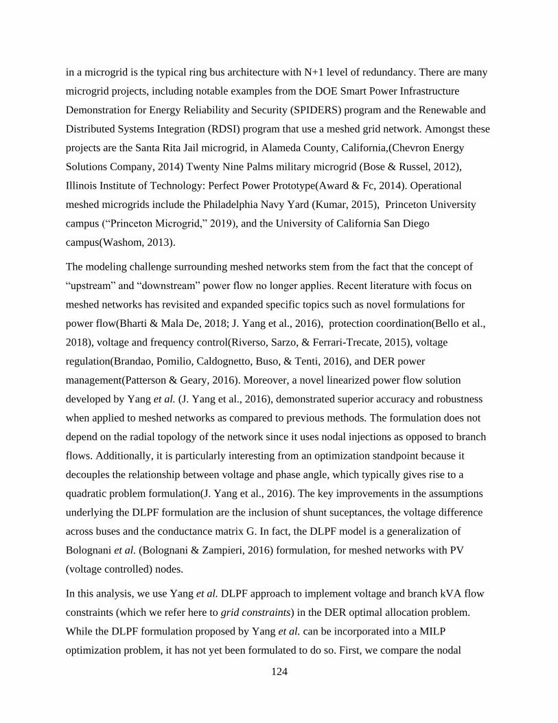
124

in a microgrid is the typical ring bus architecture with N+1 level of redundancy. There are many

microgrid projects, including notable examples from the DOE Smart Power Infrastructure

Demonstration for Energy Reliability and Security (SPIDERS) program and the Renewable and

Distributed Systems Integration (RDSI) program that use a meshed grid network. Amongst these

projects are the Santa Rita Jail microgrid, in Alameda County, California,(Chevron Energy

Solutions Company, 2014) Twenty Nine Palms military microgrid (Bose & Russel, 2012),

Illinois Institute of Technology: Perfect Power Prototype(Award & Fc, 2014). Operational

meshed microgrids include the Philadelphia Navy Yard (Kumar, 2015), Princeton University

campus (“Princeton Microgrid,” 2019), and the University of California San Diego

campus(Washom, 2013).

The modeling challenge surrounding meshed networks stem from the fact that the concept of

“upstream” and “downstream” power flow no longer applies. Recent literature with focus on

meshed networks has revisited and expanded specific topics such as novel formulations for

power flow(Bharti & Mala De, 2018; J. Yang et al., 2016), protection coordination(Bello et al.,

2018), voltage and frequency control(Riverso, Sarzo, & Ferrari-Trecate, 2015), voltage

regulation(Brandao, Pomilio, Caldognetto, Buso, & Tenti, 2016), and DER power

management(Patterson & Geary, 2016). Moreover, a novel linearized power flow solution

developed by Yang et al. (J. Yang et al., 2016), demonstrated superior accuracy and robustness

when applied to meshed networks as compared to previous methods. The formulation does not

depend on the radial topology of the network since it uses nodal injections as opposed to branch

flows. Additionally, it is particularly interesting from an optimization standpoint because it

decouples the relationship between voltage and phase angle, which typically gives rise to a

quadratic problem formulation(J. Yang et al., 2016). The key improvements in the assumptions

underlying the DLPF formulation are the inclusion of shunt suceptances, the voltage difference

across buses and the conductance matrix G. In fact, the DLPF model is a generalization of

Bolognani et al. (Bolognani & Zampieri, 2016) formulation, for meshed networks with PV

(voltage controlled) nodes.

In this analysis, we use Yang et al. DLPF approach to implement voltage and branch kVA flow

constraints (which we refer here to grid constraints) in the DER optimal allocation problem.

While the DLPF formulation proposed by Yang et al. can be incorporated into a MILP

optimization problem, it has not yet been formulated to do so. First, we compare the nodal

125

voltage and branch kVA flow solutions proposed by LinDistFlow and Bolognani et al., against

DLPF solutions for the radial and meshed benchmark 33-node systems. Then, we test the DER

optimal allocation problem in a real-world 115-node meshed microgrid test case, comparing

results when using either DLPF or LinDistFlow formulation for the linearized power flow while

enforcing grid constraints.

6.2. Contributions

This chapter addresses the gap in the literature regarding the study of linearized power flow

formulations applied to meshed networks within a mixed-integer linear optimization. To the best

of our knowledge, all previous DER investment-planning studies that incorporate grid constraints

assume radial circuits, which are indeed the vast majority of low voltage distribution feeders.

Nonetheless, meshed microgrids and networked systems topologies will likely pose a challenge

to the traditional way to implement a linearized power flow within a linear optimization, and so

far, no study has proposed a suitable approach that is accurate for such systems.

The contributions of this chapter are:

To leverage the novel decoupled linearized power flow formulation and implement it

into a MILP optimization for DER investment planning.

To quantify the impact on DER allocation when using a formulation that is not

suitable for meshed networks.

To compare the effects of stricter voltage constraints (ranging between 0.95 – 1.05

p.u) on DER optimal adoption.


This section summarizes the underlying equations that model the grid constraints as implemented

in DERopt, an optimal DER allocation tool initially established in (R. J. Flores & Brouwer,

2018). All-electric network topology parameters, such as per unit branch resistances (𝑟𝑖𝑗),

reactances (𝑥𝑖𝑗), base values for per unit calculations, and branch connections, follows the

format of a MATPOWER (Zimmerman, Murillo-Sánchez, & Thomas, 2011) — an open-source

MATLAB toolbox for solving the AC steady-state power flow problem — test case input file.

126

From this file, we calculate the sparse nodal admittance matrix 𝑌. The constraints developed in

this current work are implemented using the original DERopt formulation described in Chapter

5, section 5.2 such as energy balances and technology constraints, and also referred in (Novoa,

Flores, & Brouwer, 2019).

The optimization algorithm is implemented in MATLAB(The MathWorks Inc., n.d.) R2015a

using the YALMIP(Lofberg, 2005; Löfberg, 2019) R20181012 toolbox and CPLEX(IBM, 2017)

v.12.8 for the MILP solver. The k-medoids methodology reduces our dataset to 36

representative days during the entire year; therefore, we simulate 864 hourly intervals. The

hardware used is an Intel Xenon CPU E5-2680 v2 @2.80 GHz server with 20 cores, 40 threads,

and 32 GB of RAM.

6.3.1. Notation

In this section, we define relevant model sets and subscripts used in the DLPF formulation.

Additionally, Table 6.1and Table 6.2 provide a list and description of all model parameters and

decision variables. Bold variables represent matrices (or vectors) that collect the n (nodal) values

or b (branch) values for t (hourly) increments of the model decision variables.

The variables 𝜽, 𝒗, 𝒑, and 𝒒 are t-dimensional vectors which collect the decision variables for

each time step (𝜃𝑡, 𝑣𝑡 , 𝑝𝑡, and 𝑞𝑡), and are indicated in bold. Also, power flow variables are

indexed by the sets S, the set of PV nodes, L, the set of PQ nodes, and R, the set of reference

nodes.

t ∈ T : Set of hourly increments

n ∈ N : Set of nodes

i ∈ I: Set of “From” nodes

j ∈ J: Set of “To” nodes

b ∈ ℬ: Set of branches

𝜆 ∈ Λ : Set of line segments for polygon relaxation

L: Set of PQ nodes

S: Set of PV nodes

R: Set of reference (slack) nodes

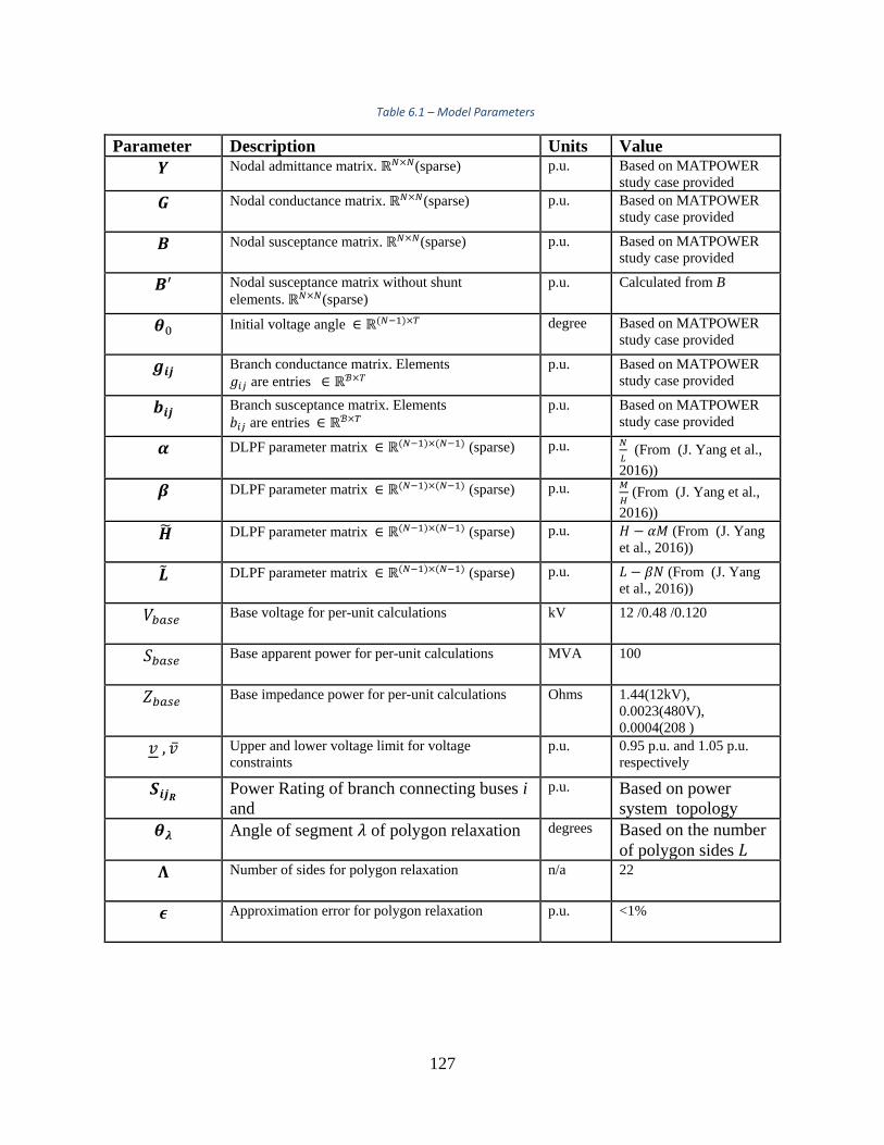
127

Table 6.1 – Model Parameters


𝒀 Nodal admittance matrix. ℝ𝑁×𝑁(sparse) p.u. Based on MATPOWER

study case provided

𝑮 Nodal conductance matrix. ℝ𝑁×𝑁(sparse) p.u. Based on MATPOWER

study case provided

𝑩 Nodal susceptance matrix. ℝ𝑁×𝑁(sparse) p.u. Based on MATPOWER

study case provided

𝑩′ Nodal susceptance matrix without shunt

elements. ℝ𝑁×𝑁(sparse)

p.u. Calculated from B

𝜽0 Initial voltage angle ∈ ℝ(𝑁−1)×𝑇 degree Based on MATPOWER

study case provided

𝒈𝒊𝒋 Branch conductance matrix. Elements 𝑔𝑖𝑗 are entries ∈ ℝℬ×𝑇

p.u. Based on MATPOWER

study case provided

𝒃𝒊𝒋 Branch susceptance matrix. Elements 𝑏𝑖𝑗 are entries ∈ ℝℬ×𝑇

p.u. Based on MATPOWER

study case provided

𝜶 DLPF parameter matrix ∈ ℝ(𝑁−1)×(𝑁−1) (sparse) p.u. 𝑁

𝐿 (From (J. Yang et al.,

2016))

𝜷 DLPF parameter matrix ∈ ℝ(𝑁−1)×(𝑁−1) (sparse) p.u. 𝑀

𝐻 (From (J. Yang et al.,

2016))

�̃� DLPF parameter matrix ∈ ℝ(𝑁−1)×(𝑁−1) (sparse) p.u. 𝐻 − 𝛼𝑀 (From (J. Yang

et al., 2016))

�̃� DLPF parameter matrix ∈ ℝ(𝑁−1)×(𝑁−1) (sparse) p.u. 𝐿 − 𝛽𝑁 (From (J. Yang

et al., 2016))

𝑉𝑏𝑎𝑠𝑒 Base voltage for per-unit calculations kV 12 /0.48 /0.120

𝑆𝑏𝑎𝑠𝑒 Base apparent power for per-unit calculations MVA 100

𝑍𝑏𝑎𝑠𝑒 Base impedance power for per-unit calculations Ohms 1.44(12kV),

0.0023(480V),

0.0004(208 )

𝑣 , �̅� Upper and lower voltage limit for voltage

constraints

p.u. 0.95 p.u. and 1.05 p.u.

respectively

𝑺𝒊𝒋𝑹 Power Rating of branch connecting buses i

and

p.u. Based on power

system topology

𝜽𝝀 Angle of segment 𝜆 of polygon relaxation degrees Based on the number

of polygon sides 𝐿

𝚲 Number of sides for polygon relaxation n/a 22

𝝐 Approximation error for polygon relaxation p.u. <1%

128

Table 6.2 – Model decision variables

Decision

Variable

Description Units

𝜽 Nodal Voltage phase angle matrix. ℝ𝑁−1 degrees

𝒗 Nodal Voltage magnitude matrix. ℝ𝑁−1 p.u.

𝒑 Nodal Active power injection. ℝ𝑁−1 p.u.

𝒒 Nodal Reactive power injection. ℝ𝑁−1 p.u.

𝒑𝒊𝒋 Branch active power flow. ℝ𝑁−1 p.u.

𝒒𝒊𝒋 Branch reactive power flow. ℝ𝑁−1 p.u.

𝐬𝐢𝐣 Branch apparent power flow. ℝ𝑁−1 p.u.

6.3.2. Decoupled Linearized Power Flow

We formulate the governing power flow equations using the original DLPF formulation

presented in (J. Yang et al., 2016). Please refer to (J. Yang et al., 2016) for the original derivation

of the DLPF model. Here, we summarize the resulting linearized power flow equations only. We

adapt the DLPF formulation to a matrix format that can be implemented in a MILP optimization,

i.e., the power flow solution is calculated for every hourly interval t, which corresponds to each

hourly interval at which the decision variables must be calculated, within the optimization

timeframe. Thus, the DLPF constraints are implemented for each time step.

Equation (75) defines the conductance 𝐺 and susceptance 𝐵 matrices as the real and imaginary

parts of the nodal admittance matrix 𝑌𝐵𝑈𝑆 , which collects the individual i-j admittance values.

Equation (76) defines nodal voltage phase angles, 𝜽[𝑆;𝐿], in degrees and Equation (76) (77)

defines the matrix that collects all nodal voltage magnitudes, 𝒗𝐿 , in per-unit.Variables

�̃�−1, �̃�−1, �̃�, �̃�, ∝ 𝒂𝒏𝒅 𝜷 are time-invariant parameters, which only depend upon network

topology ( for the interested reader, the definition of these variables can be found in (J. Yang et

al., 2016)) Variables. 𝒑[𝑆;𝐿] and 𝒒𝐿 collect the per-unit reactive and active power nodal

injections, which equal transformer injections, as defined by Equation (78) .Variables 𝑷𝑇 𝑸𝑇

collect transformer nodal injections (𝑃T𝑥𝑡.and 𝑄T𝑥𝑡

).

129

𝒀𝐵𝑈𝑆 = 𝑮 + 𝑗𝑩 (75)

𝜽[𝑆;𝐿] = �̃�−1[𝒑[𝑆;𝐿] + �̃� − 𝜶(𝒒𝐿 + �̃�)] (76)

𝒗𝐿 = �̃�−1(𝒒𝐿 + �̃�) − 𝜷 (𝒑[𝑆;𝐿] + �̃� ) (77)

𝒑[𝑆;𝐿] = 𝑷𝑇𝑥 , 𝒒𝐿 = 𝑸𝑇𝑥

(78)

𝜶 =𝑵

𝑳=

𝑮[𝑆;𝐿],𝐿

−𝑩𝐿,𝐿, 𝜷 =

𝑴

𝑯−

𝑮[𝐿;𝑆],𝑅

𝑩[𝑆;𝐿],[𝑆;𝐿]′

(79)

�̃� = 𝑯 − 𝜶𝑴 , �̃� = 𝑳 − 𝜷𝑵 (80)

�̃� = [𝑩𝑆,𝑅

′ −𝑮𝑆,𝑅 −𝑮𝑆,𝑆

𝑩𝐿,𝑅′ −𝑮𝐿,𝑅 −𝑮𝐿,𝑆

] [𝜽𝑅 𝒗𝑅

𝒗𝑆

] (81)

�̃� = [𝑮𝐿,𝑅 𝑩𝐿,𝑅 𝑩𝐿,𝑆] [𝜽𝑅 𝒗𝑅

𝒗𝑆

] (82)

𝒑𝒊𝒋 = (𝒗𝑖 − 𝒗𝑗)𝒈𝒊𝒋 − (𝜽𝑖 − 𝜽𝑗)𝒃𝒊𝒋 (83)

𝒒𝒊𝒋 = (𝒗𝑖 − 𝒗𝑗)(−𝒃𝒊𝒋) + (𝜽𝑖 − 𝜽𝑗)𝒈𝒊𝒋 (84)

𝑔𝑖𝑗 =𝑟𝑖𝑗

𝑟𝑖𝑗2 + 𝑥𝑖𝑗

2 , 𝑏𝑖𝑗 =𝑥𝑖𝑗

𝑟𝑖𝑗2 + 𝑥𝑖𝑗

2 (85)

6.3.3. Voltage Constraints

Equation (86) limits all nodal voltages, at time t, to an upper and lower per-unit bound. We use

the voltage bounds suggested by the ANSI C84.1 standard(ANSI, 2005).

𝑣 ≤ 𝑣𝑡 ≤ �̅� (per unit) (86)

130

6.3.4. Branch kVA Constraints

Similar to Chapter 5, where non-linear the transformer capacity limits, we perform a polygon

relaxation of the apparent power circle of branch kVA 𝒔𝒊𝒋2 = 𝒑𝒊𝒋

2 + 𝒒𝒊𝒋2 , A second circle with

radius 𝑠𝑖𝑗 smaller than the branch rated power capacity (𝑆𝑖𝑗𝑅), that is, 𝑠𝑖𝑗 < 𝑆𝑖𝑗𝑅

, can be

inscribed within the polygon. In this case, the maximum 𝑠𝑖𝑗 is defined by 𝑠𝑖𝑗 = 𝑆𝑖𝑗𝑅 𝑐𝑜𝑠 (

𝜋

Λ),

where increasing the number of sides Λ decreases the difference between maximum 𝑠𝑖𝑗 and rated

𝑆𝑖𝑗𝑅. Considering that the error is defined by the difference between 𝑠𝑖𝑗 and 𝑆𝑖𝑗𝑅

is defined by

Equation (88), the absolute error can be reduced below 1% by setting polygon sides Λ to 22.

Using this approximation, power through a branch can be written as Equation(89), and

implemented into the optimization model as Equation (90) For simplifying notation, the

subscript t is omitted here. Nonetheless, the polygon constraints are applied to every time step.

𝒔𝒊𝒋2 = 𝒑𝒊𝒋

2 + 𝒒𝒊𝒋2 (87)

𝝐 = 𝑺𝒊𝒋𝑹− 𝐬𝐢𝐣 = 𝑺𝒊𝒋𝑹

(1 − 𝑐𝑜𝑠 (𝜋

Λ)) Λ ≥ (

𝜋

𝑎𝑟𝑐𝑐𝑜𝑠(1−𝜖

𝑆𝑖𝑗𝑅)

) (88)

𝒔𝒊𝒋 = 𝒑𝒊𝒋𝑐𝑜𝑠 (𝜽𝝀) + 𝒒𝒊𝒋𝑠𝑖𝑛 (𝜽𝝀) , 𝜽𝝀 =𝜋

Λ+ 𝑘 (

2𝜋

Λ) , 𝜆 = 0,1, … , Λ − 1 (89)

𝒔𝒊𝒋 ≥ [ cos (𝜽𝝀) sin(𝜽𝝀)] [𝒑𝒊𝒋

𝒒𝒊𝒋] (90)

131

Figure 6.1 – Polygon relaxation for branch kVA power flows (𝑠𝑖𝑗 ). 𝑝𝑖𝑗 and 𝑞𝑖𝑗 are branch active and reactive flows

respectively. A polygon of 𝛬 sides is inscribed in the complex power circumference (dashed line) that defines the branch kVA flow limit according to its rated power 𝑆𝑖𝑗𝑅

. The k sides of the polygon, and respective angles 𝜃𝜆 are used to calculate the

approximated apparent power limit : 𝑠𝑖𝑗 = 𝑆𝑖𝑗𝑅 𝑐𝑜𝑠 (

𝜋

𝛬), which is the radius of the circumference inscribed within the 𝛬-sided

polygon (solid red line). Equation (72) defines the error of this approximation.

6.4. Test Cases

This section describes the various model inputs required for the comparison of the different

ACPF linearization methods

6.4.1. Radial and Meshed Test Circuits

We use as test circuits the radial IEEE-33 node and an adapted meshed version, as proposed in

Ref (Baran & Wu, 1989a). This circuit is chosen due to the large body of work that has

previously examined it as well as the ease of converting it to a multi-mesh system. The circuit is

a 12.4 kV primary radial distribution feeder with 33 nodes, the total loading of 3.7 MW/2.3

MVar, the official test case loading,(0.85 lagging average power factor), and a maximum R/X

ratio of 3.03. For a meshed test case benchmark, five looping branches are added to the radial

feeder. Figure 6.2 shows the schematics of the feeder radial and meshed topologies. For

complete branch impedance and nodal injection values, the reader can refer to Ref (Baran & Wu,

1989a).

132

(a) (b) Figure 6.2 – (a) Radial 33-node feeder test case. (b) Adapted meshed 33-node network test case, a hypothetical 12.4 kV

system with 33 nodes and 32 branches for the radial case plus five looping branches for the meshed case. Total loading is 3.7 MW/2.3 MVar. The maximum R/X ratio is 3.03.

6.4.2. Real World Meshed Microgrid Circuit

The purpose of this circuit is to represent a real microgrid system. Therefore, we use the real-

world distribution power system introduced in Chapter 4 and load and PV time-series data

detailed in Chapter 5. Node 1 is the slack node and represents the PCC with the wide-area

electricity grid. We assume a balanced, 3-phase power system. The primary service voltage is

12.47 kV, and the secondary voltages are 480 V for C&I customers and 208 V for residential

customers. There are 115 nodes, 31 transformers that serve load clusters, and 117 branches. Of

the 117 branches. Three are looping branches. The maximum R/X ratio is 3.5 for primary circuits

and 5.5 for secondary circuits. Figure 6.3 shows the schematics of the circuit topology.

Figure 6.3 – Test case topology, based on a real-world power system modeled as 115 nodes, 31 of which are transformers that serve clusters of industrial, commercial, and residential loads. The primary voltage is 12.47 kV, and secondary voltages are

480 V, and 208 V. Node 1 is the PCC with the wide-area grid.

133

To capture the worst-case voltage drop possible, we extend our test case to include secondary

circuits. Hence, we model each distribution transformer from which secondary lines (line drops)

extend out to the customer loads. We model transformers as per unit impedances connected in

series between a primary (higher voltage) and a secondary (lower voltage) node. We use typical

values(Eaton & Cooper Industries, n.d.) for distribution transformer equivalent per-unit

impedances. To simplify the analysis, we aggregate customer loads on the same transformer into

a single (constant PQ) load cluster. Each load cluster connects to the secondary of the

transformer through an equivalent line drop circuit. We assume transformer kVA rated power

values are just above the maximum peak load of its load cluster and place all load cluster at the

end of the secondary conductors. We assume an average of five customers per transformer;

therefore, we divide the equivalent line drop circuit impedance by five. Finally, we assume the

length of the secondary conductor is 65 feet. We assume a 0.9 lagging power factor for

residential customers and 0.8 lagging power factor for C&I customers. The primary lines

conductors used are assumed to be in overhead configuration, using ACSR aluminum conductors

with 4 AWG (R=2.17 ohm/mile, X=0.61 ohm/mile) and secondary line drops are assumed to be

6 AWG (R=3.46 ohm/mile, X=0.63 ohm/mile) (CME Wire and Cable, 2016) as per NEC

conductor size minimum requirements for overhead spans and service drops (Articles

225.6(A)(2) and 230.23(B), respectively)(National Fire Protection Association, 2014). The

ampacities assumed for these conductors are 127 A and 101 A, respectively, based on a covered

conductor in free air at ambient 40°C (104°F), according to NEC Table 310.15(B)(21)(National

Fire Protection Association, 2014).

6.4.3. Assumptions on DER Technology and Cost

The ultimate goal of this work is to improve the methods for modeling power flows typically

involved in the DER investment planning and dispatch problem. Although the quantity of

available DER is extensive, without loss of generality, we assume the DER technology available

are renewable solar PV and electrical battery storage.

We assume that the initial cost of solar is $2,000 per kW(Lazard, 2016), that ongoing operations

and maintenance costs are $0.001(R. J. Flores & Brouwer, 2018) per kWh, and that the solar PV

134

panel has a nominal electrical conversion efficiency of 20%(R. J. Flores & Brouwer, 2018). For

the electrical battery energy storage, we assume a generic battery type that has an initial cost of

$600(Lazard, 2018b) per kWh, operations and maintenance cost of $0.001(R. J. Flores &

Brouwer, 2018a) per kWh discharged, has a power to energy ratio of four, and has a charging

and discharging efficiency of 90%(R. J. Flores & Brouwer, 2018). We assume the system is

deployed in the CAISO territory, where the economic value streams available to the battery

change depend upon the charging source. Note that, if a battery is exclusively charged by onsite

renewables, then it can discharge to offset utility imports or export back to the grid at any time

under net energy metering rates. However, if a battery is partially or wholly charged using grid

electricity, it is ineligible to export any electricity back to the grid.


In this section, we perform a validation of the DLPF method against the exact AC power flow

(ACPF) solution and provide a comparison between commonly used linearized power flow

methods proposed in the literature for meshed and radial test-circuits. We follow by testing the

DLPF formulation with our DER optimal allocation model DERopt to constrain voltages, and

branch kVA flows.

The MATLAB toolbox for power flow calculations, MATPOWER(Zimmerman et al., 2011), is

used to provide the benchmark for the exact ACPF solution. The other linearization methods

were implemented in MATLAB using algorithms available at public GitHub repositories

(LinDistFlow(Schweitzer, 2018), Bolognani et al. (Bolognani, 2014) and steady-state DLPF(J.

Yang, 2016)). We use as simulation platform the Intel Xenon CPU E5-2680 v2 @2.80 GHz

server with 20 cores, 40 threads, and 32 GB of RAM. We implement all formulations in

MATLAB R2015a (The MathWorks Inc., n.d.), and for the MILP optimization, we use YALMIP

R20181012 toolbox (Lofberg, 2005; Löfberg, 2019) and CPLEX v.12.8 (IBM, 2017) for the

MILP solver.

135

6.5.1. DLPF validation and comparison with other linearization

techniques for radial and meshed network

The goals of this section are to (1) validate DLPF against the exact ACPF solution and (2) to

demonstrate the improved accuracy of the DLPF method to calculate nodal voltage magnitudes

and branch flows in a meshed network. For this, we compare the steady-state DLPF formulation

against (1) the full AC power flow solution, calculated using MATPOWER (2) the formulation

proposed in Bolognani et al. and (3) LinDistFlow. We use the test feeder proposed in Ref (Baran

& Wu, 1989a) and described in Section 6.4.1 as the benchmark. Starting with the IEEE-33 node

radial feeder, Figure 6.4 presents the results of the comparison between methods. The voltage

profiles (Figure 6.4a.) of the linearized methods match quite closely with the exact solution. Note

that all linearized methods overestimate the true voltage value, which translates into a

conservative constraint if the goal is to limit over-voltages. The errors in Figure 6.4b. are the

percent difference between the approximated solution and the exact AC power flow solution.

Figure 6.4b shows that the voltage magnitude error for all methods falls below 1% for all

linearization methods, indicated a high degree of accuracy for voltage estimation. As expected,

the voltage error increases with distance from the slack node, as the growing impedance will

increase the approximation error of the simplifying assumptions. This echoes the results shown

in (Mashayekh et al., 2017). The LinDistFlow solution is the most accurate and produces a

maximum error of 0.02844 p.u., which is very close to the 0.028 p.u. upper bound approximation

error estimated in (Fachbereich, 2018). This demonstrates the merit of using LinDistFlow for this

particular application.

Figure 6.4.c compares branch power flows (apparent power: 𝑆 = 𝑃 + 𝑗𝑄). Equations (83) and

(84) define the DLPF branch power solution. Since Bolognani et al. does not provide a

formulation for power flow, we use Equations (83) and (84) to calculate the branch power flows

for that method, taking the voltages and phase angle solutions as inputs. All linearized solutions

show similar degrees of accuracy, with some deviations for Bolognani et al.’s method. The

errors lie within 5% of the true value, mostly due to the assumption across all methods of lossless

lines. This assumption leads to the underestimation of power flows necessary to meet the load.

Branch flow errors increase at higher power flows (higher current), which happen most

frequently at the nodes closer to the slack node. While LinDistFlow achieves the most accurate

linearization for this radial test case, all methods perform with a similar error.

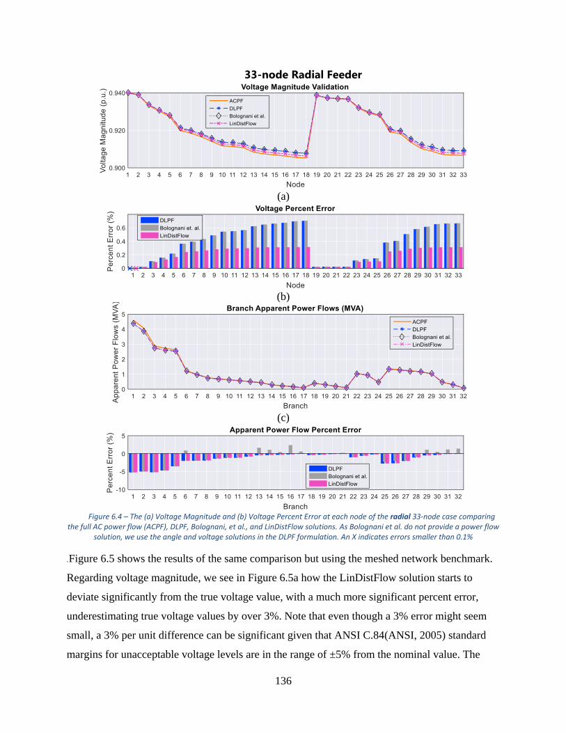
136

33-node Radial Feeder

(a)

(b)

(c)

Figure 6.4 – The (a) Voltage Magnitude and (b) Voltage Percent Error at each node of the radial 33-node case comparing

the full AC power flow (ACPF), DLPF, Bolognani, et al., and LinDistFlow solutions. As Bolognani et al. do not provide a power flow solution, we use the angle and voltage solutions in the DLPF formulation. An X indicates errors smaller than 0.1%

.Figure 6.5 shows the results of the same comparison but using the meshed network benchmark.

Regarding voltage magnitude, we see in Figure 6.5a how the LinDistFlow solution starts to

deviate significantly from the true voltage value, with a much more significant percent error,

underestimating true voltage values by over 3%. Note that even though a 3% error might seem

small, a 3% per unit difference can be significant given that ANSI C.84(ANSI, 2005) standard

margins for unacceptable voltage levels are in the range of ±5% from the nominal value. The

137

DLPF solution, on the other hand, overestimates true voltage slightly for this test case.

Nonetheless, the DLPF and Bolognani et al solutions demonstrate higher accuracy for voltage

magnitudes. Regarding branch power flows, the LinDistFlow solution overestimates the true

value by 3 MVA at the point of common coupling. These results are reasonable considering the

underlying assumptions made during linearization of the AC power flow equations. This

validation shows that the DLPF formulation can achieve higher levels of accuracy for meshed

networks, and comparable accuracy to LinDistFlow for radial networks.

138

33-node Meshed Network

(a)

(b)

(c)

(d)

Figure 6.5 – The (a) Voltage Magnitude and (b) Voltage Percent Error at each node of the meshed 33-node case comparing the full AC power flow (ACPF), DLPF, Bolognani et al., and LinDistFlow solutions. An X indicates errors smaller than 0.1%. As

Bolognani et al. does not provide a power flow solution, we use the angle and voltage solutions in the DLPF formulation

6.5.2. Meshed microgrid test case

The goal of this section is to validate the DLPF performance when applied to our third

benchmark case. Since we are interested in investigating over voltages caused by high PV

penetration and reverse power flows, we simulate a steady-state, worst-case injection that

139

represents an extreme solar PV and load scenario that totals to a 6.2 MW export (negative nodal

injections) back to the grid. The total export is distributed evenly across all transformer nodes.

We also simulate a total reactive power import of 3.1 MVar, which corresponds to a 0.89 lagging

power factor. The magnitude of the MW exports reflects a high PV penetration scenario (above

200% of peak load), while the magnitude of the MVar imported reflect each building assumed

power factor and reactive demand.

Figure 6.6 shows the comparison results. Regarding voltage (Figure 6.6.a), note how the

LinDistFlow solution progressively worsens at the looped branches while DLPF and Bolognani

et al. solutions again, slightly overestimate voltages. Errors (Figure 6.6.b) are kept below 5% for

DLPF and Bolognani et al., while LinDistFlow errors reach -15% at nodes that are found along

and at the end of looped circuits. As expected (Figure 6.6.c), LinDistFlow also has the worse

branch kVA flow accuracy, both overestimating and underestimating kVA flows at different

branches. We omit LinDistFlow solution in the absolute/percent error comparisons of Figure

6.6.c and Figure 6.6.d since it was significantly higher than the other errors. DLPF solution tends

to overestimate kVA flows by less than 5% (0.4 MVA max), while Bolognani et al. solutions

tend to underestimate kVA flows by a maximum of 12% in certain branches.

The test case used here is a real distribution circuit. In this instance, the DLPF is able to produce

a more accurate solution. During simulations, we noticed that Bolognani et al. performance

deteriorated with higher reactive power flows, that is, when operating at a lower 0.70 lagging

power factor, the maximum absolute voltage error went from 0.0364 p.u. to 0.0637 p.u., whereas

the DLPF solution kept a good performance; its absolute voltage error went from 0.0215 p.u.to

0.0287 p.u.

140

Meshed test case (primary nodes)

(a)

(b)

(c)

(d)

Figure 6.6 – The (a) Voltage Magnitude and (b) Voltage Percent Error at each primary (12 kV) node of the meshed network case comparing the full AC power flow (ACPF), DLPF, Bolognani et al., and LinDistFlow solutions. Errors smaller than 0.1% are

indicated by an X.

141

6.5.3. DERopt solution with grid constraints for a meshed microgrid

The goal of this section is to compare results found by our MILP optimization model for DER

allocation for a base case (DERopt without any voltage or power flow grid constraints) versus

using either DLPF or LinDistFlow as the load flow formulation. We selected these two AC

power flow approximations due to their accuracy when analyzing meshed and radial circuits,

respectively.

The primary result of this section is how the optimal DER allocation solution changes depending

upon the load flow formulation. The optimization minimizes investment cost while meeting a

yearly zero-net-energy constraint, i.e., total imports must be less than or equal to total exports by

the end of the year. Also, PV adoption is constrained by the physical area (rooftop) available for

installation. For more details on DERopt formulation, we direct the reader to (R. J. Flores &

Brouwer, 2018)(R. J. Flores & Brouwer, 2018b; Novoa et al., 2019). For the comparison, we use

the 115-node meshed network system presented in Section 6.5.2 as the test case. The grid

constraints considered are nodal voltage and branch kVA flow limits, which were presented in

Section 6.3.3 and 6.3.4, respectively. Therefore, the optimal DER allocation and dispatch

solution will always respect the local electric power system infrastructure limits while achieving

ZNE at the least possible cost.

The base case adopts DER (10,577 kW PV and 120 kWh of EES). Figure 6.7 shows the post-

processed ACPF voltage profiles for this solution. Each curve represents the voltage profile

calculated at a given time-step over the optimization timeframe. The markers indicate the worst

case under-voltage (UV) and over-voltage (OV) – both true and linearized - over the

optimization timeframe. The solid and dotted black lines highlight days in winter and summer,

respectively, at 1 PM and 6 PM. For the base case, voltages range between 0.887 - 1.187 p.u.

These extreme values occur at the same secondary node (node 88), which hosts 1,552 kW of PV

and no EES. The worst UV occurs at an evening peak in October, and the worst OV occurs at

solar max output at 1 PM in August. As shown by other DER interconnection modeling efforts

(Mead, Donde, Garnett, & (PG&E), 2015; NREL & SolarCity, 2016), most of the voltage issues

occur at the lower voltage, secondary circuits. These results show the expected outcome of poor

power quality when neglecting utility infrastructure during DER allocation.

142

Figure 6.7 – Base Case. Voltages range between 0.887 – 1.187 p.u. Markers indicate the worst case under voltage and

over voltage over the optimization timeframe. Solid and dotted black lines highlight days in winter and summer, respectively, at 1 PM and 6 PM.

After testing the base case, we implement the linearized AC power flow constraints. The first

constraint tested prevents only over-voltages. Thus, voltage can only be 5% above its nominal

value, or 𝑉 ≤ 1.05 p.u. The second voltage constraint tested assumes the stricter ANSI Range

A(ANSI, 2005) voltage limits, which also limit under-voltages; thus, voltage is only allowed to

be ± 5% its nominal value, or 0.95 ≤ 𝑉 ≤ 1.05 p.u.

Table 6.3 summarizes results and compares differences in DER (PV, EES, and REES) adoption

when using either DLPF or LinDistFlow load flow formulations for the different voltage

constraints simulated.

To meet only OV constraints, i.e., 𝑉 ≤ 1.05 𝑝. 𝑢., DLPF recommends a 10,857 kW solar PV

system, while LinDistFlow recommended a 10,771 kW system, which is 0.8% smaller.

Regarding energy storage, DLPF recommends a combined capacity (EES and REES) of 6,004

kWh, while LinDistFlow recommends a 4,308 kWh system, which is 28.3% smaller.

143

To meet the stricter voltage limits 0.95 ≤ 𝑉 ≤ 1.05 𝑝. 𝑢. , i.e., limiting both over and under-

voltages, the DLPF solution recommends 11,052 kW of solar PV, while the LinDistFlow

solution recommends 10,953 kW, which is 8.96% smaller. Regarding battery energy storage, the

DLPF solution recommends a combined capacity of 11,006 kWh while the LinDistFlow solution

recommends 8,887 kWh, which is 19.3% smaller.

Therefore, the LinDistFlow solution underestimates both PV and the total battery storage

capacity needed to meet voltage constraints; it also suggests a higher share of the battery be

strictly REES.

Table 6.3 –DER adoption DLPF vs. LinDistFlow for the base case and two different voltage constraints. Percentages show the percentual difference between LinDistFlow solution and DLPF solution.

DER

total adoption

Base Case 𝑉 ≤ 1.05 0.95 ≤ 𝑉 ≤ 1.05 No V

constraints DLPF LinDistFlow DLPF LinDistFlow

PV (kW) 10,577 10,857 10,771(-0.8%) 11,052 10,953(-8.95%)

EES (kWh) 120 3,536 3,216 (-9.95%) 8,767 7,760 (-11.5%)

REES (kWh) 0 2,468 1,092(-55.8%) 2,239 1,127(-49.7%)

Total Storage

(kWh)

120 6,004 4,308(-28.3%) 11,006 8,887(-19.3%)

To understand the underlying reasons for the results above, we look at the ability of each method

to accurately approximate nodal voltage and branch power flows. We simulate the first constraint

that prevents OV greater than 1.05 p.u. Figure 6.7 compares the linearized voltage profiles

calculated using DLPF and LinDistFlow against the exact (post-processed) true voltage solution,

or ACPF, calculated using MATPOWER. The DLPF voltage profiles for the entire optimization

timeframe and for only a single time step (solid and dotted black lines), shown in Figure 6.7show

an accurate linear approximation for voltage magnitude. The linearized voltage solutions range

between 0.873 - 1.050 p.u. while the true (ACPF) voltage values range between 0.851 - 1.048

p.u. Recall that the base case (no voltage constraints) maximum OV reaches 1.179 p.u.; thus

DLPF was effective in limiting OV. We note that the DLPF solution always suggests that the

voltage at a given node is higher than the true voltage, or over-voltages are overestimated and

under-voltages are underestimated. Thus, DLPF always captures and limit OV events but may be

unable to capture and limit UV events.

144

Figure 6.8 – Comparison of the voltage magnitude solution using DLPF (top) and LinDistFlow (bottom) against the ACPF

(post-processed) true voltage solution. Each curve represents the voltage profile at a given time-step over the optimization timeframe. Markers indicate the worst case UV and OV (true and linearized) over the optimization timeframe. Solid and dotted black lines highlight the true and linearized voltages, respectively, at a given time step.

145

The LinDistFlow voltage profiles, however, differ significantly from the true voltage solution

across the meshed nodes, as shown in Figure 6.8. One can observe this difference over a single

time step — the true voltage is plot as a solid line, and the LinDistFlow solution is plot as a

dotted line. The linearized voltage solutions range between 0.856 – 1.050 p.u. while the true

voltage solution values range between 0.805 – 1.077 p.u. Therefore, LinDistFlow underestimates

over-voltages and overestimates under-voltages across meshed nodes.

We then simulate the full ANSI Range A voltage limits of 0.95 – 1.05 p.u. to test the stricter

voltage constraints. Figure 6.9 shows that for both DLPF and LinDistFlow, the linearized voltage

solution ranges between 0.95 and 1.05 p.u.; however, the true voltage solution ranges, for DLPF,

from 0.947 to 1.048 p.u., while for LinDistFlow, from 0.932 to 1.077 p.u. Therefore, neither

DLPF nor LinDistFlow are able to capture and prevent UV below the 0.95 p.u. constraint.

However, DLPF is still effective in preventing the OV in this particular case, while LinDistFlow

exceeds the OV constraint by 0.022 p.u., or 2.2%.

146

Figure 6.9 – Comparison of the voltage magnitude solution using DLPF (top) and LindistFlow (bottom) against e ACPF (post-

processed) true voltage solution. Each curve represents the voltage profile at a given time step over the optimization timeframe. Markers indicate the worst case UV and OV (true and linearized) over the optimization timeframe. Solid and dotted black lines highlight the true and linearized voltages, respectively, at a given time step.

From the results of Table 6.3 we can also investigate the effects of voltage constraints in the

optimal DER allocation. Strictly looking at the DLPF solution, compared to the base case,

constraining OV causes a 2% increase in solar capacity and the combined battery storage

capacity increases by 50-fold. If under voltages are also to be limited, the PV capacity increases

by 2.7% from the base case, and total storage capacity increases by nearly two-fold from the OV

limit case. Therefore, voltage constraints suggest a need for slightly more solar PV and

significantly larger storage capacity when compared to the base case.

Regarding branch kVA power flows, Figure 6.10 compares solutions for the DLPF and

LinDistFlow, and the true, post-calculated ACPF solution. Each curve shows the kVA power

flows at all branches for a given time step. Solid and dotted black lines highlight true and

linearized, respectively, branch kVA flows at a single given time step. Markers show the worst

case (maximum) true and linearized kVA branch flows. For both DLPF and LinDistFlow, the

true worst-case kVA flow happens at the node closest to the PCC, the branches with the highest

power flow magnitude. Both approximation methods underestimate kVA flows (which is

147

expected form the underlying assumption of lossless lines), but DLPF is closer to predicting the

correct solution than LinDistFlow. Nonetheless, both DLPF and LinDistFlow underestimate true

kVA branch flows, which indicates that the solution does not respect branch kVA limits

imposed, and the model likely needs to include a safety margin.

(a)

(b)

Figure 6.10 – Comparison of branch kVA power flows for DLPF (a) and LinDistFlow(B) solutions, compared to the true, post-calculated branch kVA power flow. Each curve shows the kVA power flows at all branches for a given time step. Markers

indicate the worst case kVA power flows (true and linearized) over the optimization timeframe. Solid and dotted black lines highlight true and linearized, respectively, branch kVA flows at a single given time step.

The run times for both implementations varied between 70 minutes to 3 hours, depending on the

number of constraints. The base case (no voltage or branch constraints) ran in 150 seconds. The

LinDistFlow solution with only overvoltage constraints ran in 70 minutes while the DLPF

solution took 85 minutes. For the full voltage constraints, the LinDistFlow solution took 83

minutes while the DLPF solution took 185 minutes. The optimality gap between the optimal and

integer solution was limited to 0.4% in all runs.

6.6. Summary

This chapter developed a new approach to model the linearized power flow in a MILP for DER

optimal allocation and dispatch to minimize cost. We provided a validation of the DLPF voltage

magnitude and branch kVA power solutions against LinDistFlow and ACPF for a meshed

benchmark network. We then formulated the DER allocation and dispatch problem as a MILP

and used DLPF and LinDistFlow to model voltage and branch kVA flow constraints.

Our results show that:

148

For radial circuits, LinDistFlow is the most accurate linearization method.

Considering voltage magnitude, all linearized methods achieve a high degree of

accuracy for voltage estimation: for our steady-state validation, linearization errors lie

within 1% of the true value. For branch kVA flows, the errors lie within 5% of the

true value.

For meshed networks, DLPF is the most accurate linearization method. At the

loops, LinDistFlow underestimates true voltage values, which occurred in both our

steady-state validation and within our dynamic MILP optimization. Bolognani et al.

approximation errors have the same order of magnitude, but slightly higher.

The use of LinDistFlow within a DER optimization for a meshed network with

voltage constraints may lead to undersized optimal PV and battery systems. The

LinDistFlow solution will underestimate both OV and UV. Thus, it is not able to fully

capture the magnitude of over and under voltages, and as a result, recommending

undersized PV and battery systems.

The DLPF solution is effective for limiting overvoltages, but might not capture under

voltages. The DLPF solution slightly overestimates overvoltages (conservative) and

underestimates under voltages (not strict enough).

149

7 Optimal solar inverter

sizing considering Volt-Var

droop-control and PQ

control for voltage

regulation

Highlights

A MILP optimization for inverter sizing minimizes voltage deviations in a ZNE

microgrid

Smart inverter Volt-Var and optimal PQ functions are modeled within a linear

optimization

A novel linear approach to minimize the absolute voltage deviations is introduced

An approximated model for AC/DC inverter sizing model was abstracted from

simulations

7.1. Literature review

The low voltage electric distribution grid is being required to interconnect an increasing number

of distributed energy resources such as solar photovoltaics. As a result, in moments of low load

and high PV generation, reverse power flow — and subsequent overvoltages — threaten the

local power quality. Reactive power support (by injecting or absorbing Vars) is a useful

technique for controlling voltage excursions, and system operators have historically used

Capacitor banks and Static Var Controllers (SVCs) for this end. However, they usually allow for

only fixed-step Var increments and often operate at slower time scales, which can lead to over or

under-voltage compensation (Thompson, Martini, & Seeley, n.d.).

150

A more effective way to provide reactive power support and local voltage control is by

leveraging the potential of existing DER-interfacing power inverters to control Var absorption

and injection. This method has only started to be considered in the U.S. somewhat recently since

early grid interconnection standards, such as the IEEE 1547-2003 (IEEE, 2003), strictly

prohibited the DER from regulating local voltage actively. There have been several initiatives

started mostly by professionals in the utility sector to update such regulations. In California, the

Smart-Inverter Working Group (SIWG) worked with the California Public Utilities Commission

(CPUC) to update California interconnection standard, Rule 21, to accommodate and make

advanced smart-inverter functions mandatory for new projects. A revision to Rule 21 (California

Energy Commission, 2014) states that all new inverters interconnecting DER must have smart-

inverter capabilities, i.e., be equipped with a set of control functions that enable the local control

active and reactive power. California’s updated Rule 21 also drove the review process to the

widely-used IEEE 1547-2003 interconnection standard, now in a most updated version, IEEE

1547-2018 (IEEE, 2018). Per the new standard, a category framework is established for voltage

regulation (Category A and B) and disturbance ride-through requirements and (Category I, II,

and III). Depends on the category, the DER inverter is required to absorb/inject, a certain

percentage of its nameplate kVA.

Smart-inverters and their advanced control functions can play a crucial role in facilitating the

penetration of renewable solar PV into the electric grid and the hosting capacity, i.e., how much

solar PV any given feeder can accommodate before causing an overvoltage (EPRI et al., 2015),

of distribution feeders (NREL & Schauder, 2014). The relationship between voltage, DER active

and reactive power consumption and generation, and network impedance is well known: the

consumption of active power and/or consumption of reactive power (inductive Vars) locally

reduces voltage. Conversely, the generation of active power and/or injection of reactive power

(capacitive Vars) will locally raise voltage proportionally to system resistive and reactive

impedances (Marra, Fawzy, Bulo, & Blažič, 2012; Smith, Sunderman, Dugan, & Seal, 2011).

Therefore, smart-inverters can regulate voltage by (1) controlling the local reactive power, (2)

controlling the local active power output, which poses the clear drawback of hindering the full

utilization of PV assets, (3) leveraging co-located battery energy storage to store surplus

generation, or (4) a combination of the above. Nonetheless, as already observed in previous

studies (Alyami, Wang, Wang, Zhao, & Zhao, 2014), low voltage distribution systems are more

151

resistive than reactive, usually referred to as having a high R/X ratio, due to the short length of

its circuits. Therefore, regulating the real power output in these types of networks is a very

effective way of managing voltage.

Another current challenge involving DER integration to the grid is to allocate, i.e., to assign an

amount of a resource to a particular recipient node, commonly known as the process of “sizing

and siting” these resources into the existing electric distribution grid. Thus, the types of DER

(solar, storage, demand response) as well as their allocation within the grid network, and their

operation has to be carefully chosen to meet customer demand without creating power quality

issues and hindering system reliability.

In this context, this chapter proposes the optimal sizing of smart-inverters that are equipped with

typical advanced functions such as Volt-Var-Optimization (VVO), to increase the PV hosting

capacity of a community microgrid required to have a high penetration of solar PV to meet Zero-

Net-Energy.

The goals of this chapter are (1) determine the optimal solar PV portfolio, size, and location

within a real-world, ZNE urban electric distribution system (2) implement smart-inverter Volt-

Var and PQ control function into the existing optimization framework to (3) optimally size the

interfacing inverter while (4) minimizing cost and voltage deviations while (4) considering

physical, electrical power system constraints. We then quantify power quality improvements in

voltage.

The smart-inverter droop-control functions considered in the last analysis were initially proposed

in the “ERPI, Common Functions for Smart Inverters – Phase 3” report (Electric Power Research

Institute (EPRI), 2014).

7.1.1. Related Work

Many authors have explored novel methods for voltage regulation and control for high

penetration of DER, their effectiveness, their impact on the network, and their interoperability

with existing network devices.

One method is by the use of droop control curves programmed in DER inverters, known as

“smart-inverter functions”. The Volt-Watt and Volt-Watt, for example, define active and reactive

power injections as piecewise linear functions of voltage and are a standard set of autonomous

functions applied to voltage control.

152

A widely used approach to voltage control with a solar PV DER is the Volt-Watt function –

active power curtailment based on local voltage – which uses the inverter rated apparent power

as the static reference for the droop-based active power curtailment. (Luthander, Lingfors, &

Widén, 2017) implemented a fixed-slope Volt-Watt control that was effective in removing all

overvoltages in a three-phase 10 kV/400V distribution test system with a 100% PV penetration at

the expense of a 31% reduction of the total PV generation. Dynamic approaches, on the other

hand, use the inverter operation points at the time the overvoltage occurs as the reference for

curtailment. (Y. Wang, Zhang, Li, Xiao, & Abdollahi, 2012) described a dynamic Volt-Watt

control that curtails active power by predicting the resulting voltage variation using a Thevenin

equivalent circuit at the point of injection. The method continually updated the droop-control

curve slopes, and completely prevented overvoltages in the IEEE 34-bus test case. (Alyami et al.,

2014) proposed a dynamic Volt-Watt control that does not require global system information,

which eliminated overvoltages in the IEEE-13 bus system.

The Volt-Var function – Var output based on local voltage – is another common smart-inverter

droop control strategy that regulates local reactive power absorption or injection. (Smith et al.

2011) demonstrated a static Volt-Var function, which provided adequate voltage support for a 12

kV circuit with 450 inverters operating in parallel. (Jahangiri and Aliprantis 2013) proposed a

distributed control strategy for a dynamic Volt-Var function that avoids instabilities caused by

the interactions of a large number of inverters operating in parallel. In that previous work, the

proposed distributed control scheme mitigated overvoltages successfully in simulations of

realistic distribution feeders with high (50%) smart-inverter penetration. (Seuss et al. 2015),

showed a Volt-Var control that improved hosting capacity in a 12.47 kV distribution feeder by

72% (from 600 to 900 kVA). The author also points out that, at voltage-constrained buses, the

Volt-Var control only improves the hosting capacity until a line thermal constraint is hit due to

the injection of extra reactive currents, which may be even more challenging in distribution

systems with a low X/R ratio. (Turitsyn et al. 2011) also points out the increased losses due to

Volt-Var control.

One other method is the optimization of reactive power dispatch in a Volt-Var Optimization

(VVO). (Farivar, Neal, Clarke, & Low, 2012) proposed an optimal inverter reactive power

dispatch that was able to mitigate rapid and significant voltage fluctuations caused by a 5 MW

PV deployment in a 12 kV, 56-node radial rural distribution feeder in Southern California.

153

Another VVO method to dispatch inverter Var resources was proposed by (Arnold et al., 2016),

where a linearized optimal power flow formulation (LinDistFlow) was effective in limiting the

voltage to +-5% bounds while minimizing voltage imbalance between phases in the radial IEEE

13 node test feeder.

Some authors extended the optimal Var control to both optimal Var and Watt control (or active

power curtailment), which we refer here as optimal inverter PQ control. (Su, Masoum, & Wolfs,

2014) proposed an optimal PQ control strategy to minimize generation cost, losses, and voltage

imbalance. The authors extended the analysis to single-phase inverters, which, when optimally

dispatched, removed overvoltage and phase voltage imbalances in a 101 node three-phase, four-

wire 22 kV/415V/240 V low voltage distribution feeder in Perth, Australia, with 39% solar PV

penetration. (Sepehry, Heidari Kapourchali, Aravinthan, & Jewell, 2019) showed a similar

optimal inverter PQ dispatch strategy, using a linearized unbalanced power flow, which

minimized cost and wind curtailment while meeting power quality operational grid constraints in

the radial IEEE-37 and IEEE-60 bus test cases. (Dall’Anese, Dhople, Johnson, & Giannakis,

2014) optimized inverter PQ dispatch in a 12-node residential low voltage (LV) test feeder with

pre-selected inverter deployments to minimize losses, curtailment cost, and flat out the voltage

profile. In that early work, the authors noted that inverters at the end of the feeder curtailed more

active power and absorbed more reactive power to regulate voltage as compared to the other

inverters.

Therefore, having PQ control does not provide a fair share between inverters of the burden of

regulating system voltage by providing reactive power compensation and/or active power

curtailment. As noted, inverters located at nodes with high impedance will be taxed with more

regulation (Collins & Ward, 2015; Dall’Anese et al., 2014; Marra et al., 2012; Turitsyn, Šulc,

Backhaus, & Chertkov, 2011). Droop-control strategies are usually employed to guarantee a

more equal share of voltage regulation, and we will explore to what extent this regulation is

distributed equally amongst inverters in our simulations.

The literature has shown successful use of different smart-inverter functions to mitigate

overvoltages and, in turn, increase a feeder’s voltage-based hosting capacity. However, the

optimal choice of inverter size (kVA) is still a standing research question. Most inverters are set

to operate in droop control with watt-priority, i.e., reducing reactive power output to meet the

maximum rated active power output. Thus, in watt-priority mode, the inverter kVA capability

154

limits its ability to provide reactive power regulation, especially in instances where the inverter

size margin (i.e., the inverter capacity beyond DER nameplate) is tight, and the DER is at full

active power output. In a study led by the utility PG&E (Mead et al., 2015), it was shown that

droop-controlled smart-inverters on the secondary (low voltage side) of a typical distribution

feeder with high PV penetration had limited effect on reducing high voltage conditions due to an

inverter capacity limitation for reactive power injection. In this previous study, the inverters were

slightly undersized – a common practice in large-scale deployments, namely inverter clipping.

(Seuss, Reno, Broderick, & Grijalva, 2015) also demonstrated a case where the inverter did not

have enough capacity for reactive power injection to remove all overvoltages violations in a 12.4

kV feeder with a 1.3 X/R ratio. The previous study also performed a sensitivity analysis to

explore the role of inverter sizing and Volt-Var control potential and showed that the best

inverter size, i.e., the size that will maximize the PV hosting capacity before reaching the point

of diminishing returns, varied for one feeder to another, and ranged from 121% to 135%.

In the literature, there is not a clear consensus on how much inverter capacity beyond or below

DG nameplate is needed, and many authors have judiciously assumed different values. For

example, (Abate, McDermott, Rylander, & Smith, 2015; Dall’Anese et al., 2014; Farivar et al.,

2012; Rylander, Li, Smith, & Sunderman, 2016; Rylander et al., 2017; Schultis, 2019; Smith et

al., 2011; Turitsyn et al., 2011) assumed a 10% oversizing margin, which is the equivalent of

allowing a reactive power injection with a power factor of 0.90 lagging, even during peak active

power production. (Jafari, Olowu, & Sarwat, 2019) oversized inverters by 15%, (EPRI et al.,

2015; Seuss et al., 2015) oversized inverters by 20%, and (Su et al., 2014) oversized the inverters

by 60%. Authors in (Jahangiri & Aliprantis, 2013; Sepehry et al., 2019), assumed the inverter

rating matches the DG rated capacity, while in (Ding et al., 2016; Stetz, 2014) the inverters were

undersized by up to 10% below DG rated capacity.

Ideally, for each control function, there would be one global inverter size margin that is effective

in all situations. However, the amount of reactive power necessary for a given compensation

strategy to be useful is shown to be strongly related to the electric power system characteristics

such as feeder R/X (resistance versus reactance) ratio, source impedance, and PV penetration

levels (EPRI et al., 2015; Rylander et al., 2017; Seuss et al., 2015; Smith et al., 2011; Su et al.,

2014). Therefore, the optimal inverter size margin is likely location/feeder-specific. One recent

study by (Ali, Raisz, & Mahmoud, 2019) proposed an optimization-based method to oversize

155

inverter capacity. However, it did not consider a droop-control strategy, nor a fair sharing of

regulation amongst inverters.

The previous discussion points to a gap identified in literature regarding the lack of studies that

optimally size inverters that use voltage-reactive power droop-control within an optimal DER

allocation (size and site) problem.

7.1.2. Contributions

Include smart inverter Volt/Var droop-control and optimal PQ control functions in a

MILP optimization formulation for the DER allocation problem. By introducing a

novel linearization approach.

Optimally size inverters for minimizing voltage deviations in a low voltage

distribution feeder with a high PV penetration. A novel approach to minimize the

absolute voltage deviations is introduced in the objective function

Model and compare optimal AC/DC inverter sizing for inverter PQ and droop-control

strategies.

7.2. Notation

We define below relevant model sets and the subscripts defined in this chapter regarding smart

inverter integration into the model. We assume the reader is familiar with the previous DERopt

model sets and decision variables. For reference see the notation sessions on Chapters 4 and 5.

Table 7.1 and Table 7.2 provide a list and description of new model parameters and decision

variables.

t ∈ T: Set of hourly increments

n ∈ N: Set of nodes

i ∈ I: Set of “From” nodes

j ∈ J: Set of “To” nodes

b ∈ ℬ: Set of buildings

𝜆 ∈ Λ: Set of line segments for polygon relaxation

x ∈ X: Set of transformers

h ∈ H: Set of inverters

L: Set of PQ nodes

156

S: Set of PV nodes

R: Set of reference (slack) nodes

Table 7.1 – Model decision variables

Decision Variable Description Units

𝑆i̅nv𝑏 Inverter adoption at building b kV

𝑃Invℎ𝑡, 𝑄Invℎ𝑡

, 𝑆Invℎ𝑡 Active, Reactive, and Apparent Power flows through

inverter h at hour t

kW/

kVar/

kVA

𝑄invBLDG Building reactive power demand kVA

𝑄𝑖𝑛𝑑ℎ,𝑡 Inductive Reactive Power absorbed by inverter h at hour t kVar

𝑄𝑐𝑎𝑝ℎ,𝑡 Capacitive Reactive Power injected by inverter h at hour t kVar

𝜽 Nodal Voltage phase angle matrix. ℝ𝑁−1 degrees

𝒗 Nodal Voltage magnitude matrix. ℝ𝑁−1 p.u.

𝒑 Nodal Active power injection. ℝ𝑁−1 p.u.

𝒒 Nodal Reactive power injection. ℝ𝑁−1 p.u.

𝑞𝑎𝑛𝑐 Linearized reactive power regulation for Volt-Vat curve p.u.

Table 7.2 – List of parameters used in DERopt


𝜔 Weight for penaltty function N/A 1 for PQ control

1,000 for Volt-Var control

𝑣1, 𝑣2, 𝑣3 , 𝑣4 Volt-Var inverter voltage curve

settings

p.u. 0.90, 0.97, 1.03, 1.1

𝑞1, 𝑞2, 𝑞3 , 𝑞4 Volt-Var inverter Var curve

settings

p.u. (Var) 0.60, 0, 0, -0.60

𝑚𝑐𝑎𝑝, 𝑚𝑖𝑛𝑑 Volt-Var curve slopes N/A Dedepnds upon Volt-Var

curve


We extend the Building Energy Hub concept presented in Chapter 5 and in (Novoa et al., 2019)

to include an interfacing DER inverter. The schematics in Figure 7.1 illustrates a building energy

157

hub, which includes the building load (𝐵𝐿𝐷𝐺𝑏) the local DER adopted (𝑃𝑉𝑏 , 𝐸𝐸𝑆𝑏, 𝑅𝐸𝐸𝑆𝑏), and

the interfacing inverter (𝐼𝑛𝑣𝑏), which connects the direct current DER to the building AC loads

and a distribution transformer (𝑇𝑥). Each distribution transformer connects one or a cluster of

building energy hubs to the AC low voltage electric grid network. DERopt optimally sizes the

interfacing inverter (𝑆i̅nv𝑏) accommodate the active net power flows from PV generation, battery

storage charging and discharging, and also the necessary reactive power flows to provide voltage

local support. Equations (91) and (92) provide the active and reactive power balances within the

building energy hub. Each building load 𝑃BLDG can be fed by a mix of power imported to the hub

(𝑃import), PV generation ( 𝑃PVBLDG), and any battery power (𝑃EESdch

, 𝑃REESdch). The building

reactive power demand (is calculated at a fixed power factor from the active power demand,

thus, 𝑄BLDG = PBLDGarctan (𝑃𝐹).The building reactive demand can be met by grid imports

(𝑄import) or by reactive power produced by the inverter (𝑄invBLDG). Equation (93) constrains all

PV power generation, that is, the PV generation to meet building loads (𝑃PVBLDG) and the PV

generation exported for revenue under the NEM and wholesale markets (𝑃𝑃𝑉𝑁𝐸𝑀, 𝑃𝑃𝑉𝑊

) to the

PV system rated power (𝑆P̅V𝑏) times the normalized local insolation (𝐼). Note that equation (93)

calculates the value of the decision variable (𝑆P̅V𝑏) and since it is an inequality, it allows for

power curtailment. We adopt the load convention for all power flow throughout the entire hub;

therefore, positive values mean import, and negative values mean export. All variables described

above have positive values. Equations (94) and (95) calculate the net real and reactive power

flows through the inverter (𝑃inv𝑡,𝑏, 𝑄inv𝑡,𝑏

), therefore these variables can assume either a positive

(import) or negative (export) value, and using this modeling approach, the inverter cannot import

and export power at the same time. The only active power import through the inverter happens

when EES charges using grid power (𝑃EESch) and all other power flows regarding PV generation

(𝑃𝑉BLDG, 𝑃𝑉NEM, 𝑃𝑉𝑊) and battery discharge (𝑃EESdch, 𝑃REESdch

, 𝑃REESNEM) are exports.

Regarding reactive power flows, the inverter can meet part (or all) of the reactive building load

(𝑄invBLDG) or also provide ancillary services (𝑄anc) such as when a smart-inverter has a Volt-Var

droop-control curve implemented. 𝑄anc can assume either a positive or negative value. A

positive value indicates that inductive reactive power is absorbed by the inverter and a negative

value, capacitive reactive power being injected. By this modeling approach, the inverter cannot

provide both capacitive and reactive compensation at the same time, which makes physical

158

sense. The variable 𝑄anc can be broken down into two positive quantities: 𝑄cap and 𝑄ind. Such as

𝑄anc = 𝑄ind − 𝑄cap Equations (96) and (97) calculate the net real and reactive power flows

through the transformer 𝑇𝑥, 𝑃T𝑥 and 𝑄T𝑥

respectively . These net flows take into account grid

imports (𝑃𝑖𝑚𝑝𝑜𝑟𝑡, 𝑄𝑖𝑚𝑝𝑜𝑟𝑡), renewable power exports (𝑃𝑃𝑉𝑁𝐸𝑀, 𝑃𝑃𝑉𝑊

, 𝑃REESNEM ), and inverter

ancillary services (𝑄𝑎𝑛𝑐 , 𝑄cap, 𝑄ind), as illustrated in Figure 7.1.

We note that even though battery storage is defined here, this analysis does not consider the

adoption of battery energy storage since we want to focus on the sole ability of smart inverters to

locally regulate voltages.

Figure 7.1 – Schematic of one Building Energy Hub used in the multi-node approach. Transformer 𝑇𝑥 is one node, to which

a cluster of buildings and adopted DER (𝑃𝑉𝑏 , 𝐸𝐸𝑆𝑏 , 𝑅𝐸𝐸𝑆𝑏) are connected. Inverter 𝐼𝑛𝑣𝑏 connects the DER adopted at building b to the AC side of the distribution system.

𝑃import𝑡,𝑏+ 𝑃PVBLDG,𝑡,𝑏

+ 𝑃EESdch,𝑡,𝑏+ 𝑃REESdch,𝑡,𝑏

= 𝑃BLDG 𝑡,𝑏+ 𝑃EESch,𝑡,𝑏

(91)

𝑄import𝑡,𝑏= PBLDGarctan (𝑃𝐹) − 𝑄invBLDG𝑡,𝑏

(92)

𝑃PVBLDG,𝑡,𝑏+ 𝑃PVNEM,𝑡,𝑏

+ 𝑃PV𝑊,𝑡,𝑏+ 𝑃EESchPV,𝑡,𝑏

+ 𝑃REESch,𝑡,𝑏≤ 𝐼𝑡𝑆PV𝑏

(93)

159

𝑃inv𝑡,𝑏= 𝑃EESch,𝑡,𝑏

− 𝑃EESdch,𝑡,𝑏− 𝑃REESdch,𝑡,𝑏

− 𝑃REES,NEM𝑑𝑐ℎ,𝑡,𝑏− 𝑃PVBLDG,𝑡,𝑏

− 𝑃PVNEM,𝑡,𝑏 − 𝑃PVW,𝑡,𝑏

(94)

𝑄inv𝑡,𝑏= − 𝑄invBLDG𝑡,𝑏

+ 𝑄anc𝑡,b (95)

𝑃T𝑥𝑡= ∑ 𝑃import𝑗

– 𝑃PVNE𝑀𝑗− 𝑃PV W𝑗

− 𝑃REES dch NEM𝑗

𝑗 ∈ 𝐽𝑘

(96)

𝑄𝑇𝑥𝑡= ∑ 𝑄import𝑐

+ 𝑄anc𝑐

𝑐 𝜖 𝒞𝑥

(97)

7.3.1. Zero-Net-Energy Operation

The Zero Net Energy operation is formulated using the same Equations defined in Chapter 5,

section 5.2.3 and omitted here for brevity.

7.3.2. Decoupled Linearized Power Flow

We formulate the governing power flow equations using the decoupled linearized power flow

formulation introduced in Chapter 6, session 6.3.2 and we omit it for brevity.

7.3.3. Inverter Constraints

7.3.4. Polygon Relaxation

The inverter rated power capacity 𝑆i̅nv limits the amount of current (equivalently, the amount of

power) it can inject into the grid. The industry expresses power ratings in kilovolt-amperes

(kVA), i.e., the vectorial sum of the active 𝑃inv (kW) and reactive 𝑄inv (kVAr) power injections;

Equation (98) shows this relationship. Therefore, the inverter apparent power injection at any

given time 𝑆inv can’t exceed its power rating 𝑆�̅�𝑛𝑣

𝑆𝑖𝑛𝑣 = √𝑃𝑖𝑛𝑣2 + 𝑄𝑖𝑛𝑣

2 ≤ 𝑆�̅�𝑛𝑣 (98)

160

Equation (98) dictates inverter power flows; however, a MILP formulation cannot directly

capture non-linearities. Thus, we perform a polygon relaxation of the apparent power circle, as

shown in Figure 7.2 and formulated by the constraints in equations (99) through (102). Equation

(102) defines the approximation error, which is the difference between 𝑠 and 𝑆̅. For our particular

problem, we can reduce the absolute error below 1% by setting the number of polygon sides Λ to

22. Using this approximation, power through an inverter can be written as equation (100), and

implemented into the MILP optimization as equation (101). Equation (99) obtains the optimal

value for the inverter size (𝑆�̅�𝑛𝑣) decision variable.

Figure 7.2 – Depiction of the polygon relaxation constraints and operating regions for the inverter (shaded in yellow).

𝑠 = 𝑆�̅�𝑛𝑣𝑐𝑜𝑠 (𝜋

Λ) (99)

𝑠 = 𝑃𝑖𝑛𝑣 cos(𝜃𝜆)+ 𝑄𝑖𝑛𝑣 sin(𝜃𝜆),

𝜃𝜆 =𝜋

Λ+ 𝜆 (

2𝜋

Λ) 𝜆 = 0,1, … , Λ − 1

(100)

𝑠 ≥ [cos (𝜃𝜆) sin(𝜃𝜆) ] [𝑃𝑖𝑛𝑣

𝑄𝑖𝑛𝑣]

(101)

𝜖 = 𝑆�̅�𝑛𝑣 − 𝑠 = 𝑆�̅�𝑛𝑣 (1 − cos𝜋

Λ )

Λ ≥𝜋

arccos (1 −𝜖

𝑆�̅�𝑛𝑣)

(102)

161

7.3.5. Inverter Droop Control (Volt-Var)

The inverter static Volt-Var droop-control curve is illustrated in Figure 7.3. The per-unit reactive

power injection/absorption (𝑞) varies as a linear function of the per-unit voltage at the inverter

terminals (𝑣). This curve is defined by four points, or v-q pairs, namely the inverter settings. A

dead band between points 𝑣2 and 𝑣3 is the region where no reactive power compensation occurs.

The inverter settings used here are based upon the settings recommended by the IEEE-1547 2018

standard for Category A, except for the reactive power absorption limit was increased from 44%

to 60% to improve voltage compensation capacity. The settings used are shown in Table 7.3

We assumed the inverters operate in Q- priority, that is, active power is curtailed in favor of

accommodating the necessary reactive power compensation, that is: 𝑃𝑖𝑛𝑣 = √𝑆𝑖𝑛𝑣2 − 𝑄𝑖𝑛𝑣

2 . This

behavior is modeled by the inequality constraint on equation (93) and the equality constraint of

equations (95) and (105). Nonetheless, as recommended by IEEE-1547, the maximum

compensation an inverter will produce can only go up to 44% of its capacity (0.44 per-unit).

Equation (104) calculates the curve fixed (pre-defined) slope.

Figure 7.3 – Volt-Var droop control curve. The curve is defined by four points, or v-q pairs, that define the reactive power

output𝑞𝑎𝑛𝑐 as a function of the voltage 𝑣 at the inverter terminals

162

Table 7.3 – Volt-Var inverter settings

Volt-Var

droop-control

parameter

Value (p.u.)

𝑣1 0.90

𝑣2 0.97

𝑣3 1.03

𝑣4 1.1

𝑞1 0.60

𝑞2 0

𝑞3 0

𝑞4 -0.60

𝑞𝑎𝑛𝑐 =

𝑞1 , 𝑖𝑓 𝑣 < 𝑣1

(103)

𝑚𝑐𝑎𝑝(𝑣 − 𝑣2) , 𝑖𝑓 𝑣1 < 𝑣 < 𝑣2

0 𝑖𝑓 𝑣2 < 𝑣 < 𝑣3

𝑚𝑖𝑛𝑑(𝑣 − 𝑣3) 𝑖𝑓 𝑣3 < 𝑣 < 𝑣4

𝑞4 𝑖𝑓 𝑣 > 𝑣4

𝑚𝑐𝑎𝑝 =𝑞2 − 𝑞1

𝑣2 − 𝑣1, 𝑚𝑖𝑛𝑑 =

𝑞4 − 𝑞3

𝑣4 − 𝑣3

(104)

𝑄𝑎𝑛𝑐 = −𝑞𝑎𝑛𝑐𝑆�̅�𝑛𝑣 (105)

𝑓𝑎(𝑞𝑎𝑛𝑐 , 𝑆�̅�𝑛𝑣,) (106)

Equation (105) is, however, non-linear when both 𝑞𝑎𝑛𝑐 and 𝑆�̅�𝑛𝑣 are decision variables, i.e., when

we are interested in sizing the inverter. The challenge of modeling Volt-Var behavior in a MILP

model requires a novel approach to linearize this relationship. We then devise a method that

takes advantage of the linearity of the feasible region. Thus, we model equation (105) as a

piecewise-linear approximation of a surface, which is a function of two variables, i.e.,

𝑓𝑎(𝑞𝑎𝑛𝑐 , 𝑆�̅�𝑛𝑣), Figure 7.4 illustrates the piece-wise linear surface. We then calculate the inverter

reactive power 𝑄𝑎𝑛𝑐 by interpolating between points in the feasible surface. We use the solver’s

built-in linear interpolation function, which creates SOS2 sets. This linearization could have been

163

modeled directly, using binary variables and appropriate auxiliary SOS constraints. We chose to

use the built-in function since it produces a model with pure SOS2 sets, which the branch-and-

cut algorithm can process and solve more efficiently and faster as opposed to processing binary

sets. Also, the surface in Figure 7.4 has a high number of breakpoints (fine mesh grid) for

illustrational purposes, in reality, to minimize problem scale, the surface is implemented using a

much sparse mesh grid that only uses the inverter settings voltage points, i.e., 𝑣𝑖 =

[𝑣1, 𝑣2, 𝑣3, 𝑣4] and two inverter size limits 𝑠𝑖 = [0, 𝑆�̅�𝑛𝑣𝑚𝑎𝑥 ] where 𝑆�̅�𝑛𝑣𝑚𝑎𝑥

is assumed based

upon the order of magnitude of the maximum PV adoption in the Baseline scenario. Nonetheless,

the solver function also performs linear extrapolation when necessary.

Figure 7.4 – Piece-wise linearization of a function of tow variables, 𝑄𝑎𝑛𝑐 = −𝑞𝑎𝑛𝑐𝑆�̅�𝑛𝑣 . As the inverter size increases, so

does the ability of the inverter to provide more reactive compensation (𝑄𝑎𝑛𝑐 ).

7.3.6. Inverter PQ control

In this inverter control mode, the per-unit active and reactive power injection/absorption

(𝑃𝑖𝑛𝑣, 𝑄𝑖𝑛𝑣) vary freely (unconstrained). The inverter capacity 𝑆𝑖𝑛𝑣 is determined according to

Equations (99) and (100)

164

7.3.7. MILP Formulation

7.3.8. Objective Function

The objective function used here 𝐺(𝑥)adds to the already defined cost function 𝐽(𝑥), defined in

Chapter 5, Equation (47), which captures the costs associated with purchase and sale of energy,

the cost associated with demand charges, and the cost associated with purchasing and operating

the adopted DER. We add to the existing objective function e cost of purchasing the interfacing

DER inverter. Therefore, the model will drive inverter adoption the minimum necessary to meet

system constraints. The voltage deviation penalty parameter Δ𝑣aims to drive system voltages

closer to 1 p.u. and it is described below

𝐺(𝑥)= 𝐽(𝑥) + 𝐶capinv𝑆𝑖𝑛𝑣𝑏

+ Δ𝑣 (107)

The voltage deviation penalty term Δ𝑣 aims to capture the sum (of the absolute values) of all

hourly voltage deviations (from 1 p.u.) across all system nodes, i.e., |1 − 𝒗|, where the boldface

vector 𝒗 𝝐 ℝ𝑺𝒙𝑇 collects all nodal voltages for the optimization timeframe. However, since the

absolute value is a non-linear function: |1 − 𝑣| = √(1 − 𝑣)2, We cannot directly implement it

into the MILP. Hence, a mathematical artifice, namely the decision variable 𝜹 𝝐 ℝ𝑺𝒙𝑇 is used to

linearize the absolute voltage deviation as follows: two constraints described by equations (108)

and (109) are added to the model formulation and Equation (110), which describes the sum of all

individual 𝜹 terms (Δ𝑣) is added to the objective function preceded with a weight 𝜔. Therefore,

the minimzation of Δ𝑣 (and consequently) will drive the individual nodal voltages 𝑣 towards 1

p.u. The weight 𝜔 assumed for PQ control is 1 and for Volt-Var control, 1,000 in order to drive

adequate voltage regulation.

𝜹 ≥ 1 − 𝒗 (108)

𝜹 ≥ −(1 − 𝒗) (109)

Δ𝑣 = 𝜔 ∑ ∑ 𝜹

𝑇

𝑡=1

S

𝑖=1

(110)

165

The objective function is thus minimized subject to a set of equality and inequality constraints,

and also integer constraints, lower 𝑙 and upper 𝑢 bounds, which limit strictly positive variables

and Big M limits.

The MILP optimization problem is given by the following functions and constraints: Where

𝐺(𝑥) is the objective function and A and B are the respective coefficient variables for

𝑥 continuous decision variables and 𝑦 integer decision variables. The problem is subjected to

linear equality and inequality constraints, 𝑙 and 𝑢 upper and lower bounds, and integer

constraints on 𝑦.

𝐦𝐢𝐧 𝒔. 𝒕.

𝐺(𝑥)

𝐴𝑥 + 𝐵𝑦 ≤ 𝑏 𝑙 ≤ 𝑥 ≤ 𝑢

𝑦 𝜖 ℤ𝑛

𝑦 ≥ 0

(107)

(76),(77),(86),(91)-(97), (99)- (103),(105),(106)

*specific to each variable

(111)

7.4. Test Case and Assumptions

We use the test case introduced in Chapters 5 and 6, the Oak View microgrid. All assumptions

for circuit topology, technology cost, electrical demand, and PV resources are the same. Inverter

cost is assumed to be $150/kW based on current market research for inverters up to 6 kVA.

To pursue a tractable optimization, we perform a worst-case type analysis, where we only

simulate the day (24-hours) in the year flagged with the worst (maximum) RPF. Therefore, our

design results indicate the inverter size that can provide support to the worst RPF event in the

year. The worst-case RPF day was identified by scaling up the normalized PV annual generation

profile to just above the local peak load (3111.6 kW), calculating the net-load (load minus

generation), and identifying the hour with the most negative net-load. For our test system, the

worst-case RPF happens on a Sunday in March, a sunny, clear day in spring with mild

temperatures and low load.

A detailed list of all building load maximum demand, total energy demand, the associated

transformer, and its power rating, and building power factor is presented in Chapter 6. We also

assume smart-inverters are adopted in 7 out of the 31 building nodes. The other inverters are

assumed to be standard inverters, with no reactive power output. Figure 5.5 shows a schematics

166

of the circuit topology. We represent loads as triangles, building numbers in red, primary node

numbers in black and secondary node numbers in blue.

Figure 7.5 – Meshed benchmark case based on a real-world power system (left) and modeled as 115 nodes, 31 of which

are transformers that serve clusters of industrial, commercial, and residential loads. We represent loads as triangles, building

numbers in red, primary node numbers in black and secondary node numbers in blue. Node 1 is the PCC with the wide-area

grid. (right) The primary voltage is 12.47 kV, and secondary voltages are 480 V or 208 V, depending upon customer type. Each

transformer is modeled as a series impedance (𝑍𝑋𝐹𝑀𝑅) with the secondary line drop equivalent impedance (𝑍𝑠𝑒𝑐𝑒𝑞 ), which

represents five customers aggregated in parallel in a load cluster.

7.4.1. Scenarios

The goal of this chapter is to use our MILP optimization to determine the optimal inverter size

(kVA) for pre-defined smart-inverter locations within the test-case under two different smart

inverter control strategies. We are interested in analyzing the challenging cases of large PV

deployments. Therefore, for all simulations, the test case is constrained to be Zero-Net-Energy,

defined as able to produce as much electricity as demand over one day, or 24 hours.

In the Baseline scenario, the DER allocation problem is simulated to meet ZNE constraints with

conventional inverters, i.e., inverters without smart-inverter features. There are no other

constraints limiting voltage magnitudes or power flows through transformers, nodes, or feeders;

in other words, the system power quality is not actively controlled.

In the Optimal PQ scenario, solar PV smart-inverters will be optimally sized to provide over-

voltage support to the Baseline scenario. All inverters can produce and absorb P and Q freely.

In the Volt-Var scenario, we simulate the Baseline solar PV allocation, and we apply a droop-

control Volt-Var function to seven pre-defined inverter locations. The locations chosen are the

167

seven buildings with higher overvoltages recorded over the optimization timeframe. The other

inverters are assumed to be standard inverters.

A summary of all scenarios is given below:

Baseline: Solar PV allocation problem for a ZNE test case with standard inverters (no

local reactive power control)

Optimal PQ: Baseline solar PV allocation. All inverters inject/absorb an

unconstrained amount of active (P) and reactive (Q) power.

Droop control (Volt-Var): Baseline solar PV allocation. Reactive power output is a

function of voltage, following a droop-control function at seven pre-defined locations

at buildings 1, 10, 11, 12, 14, 16, and 17. Remaining inverters are standard inverters.

The optimization algorithm is implemented in MATLAB R2015a (The MathWorks Inc., n.d.)

using the YALMIP R20181012 toolbox (Lofberg, 2005; Löfberg, 2019) and CPLEX v.12.8

(IBM, 2017) for the MILP solver. The worst-case analysis reduces our dataset to 24 hourly

intervals. The hardware used for the optimization is an Intel Xenon CPU E5-2680 v2 @2.80

GHz server with 20 cores, 40 threads, and 32 GB of RAM. Simulation times are no longer than

30 seconds.


7.5.1. Baseline

The Baseline scenario adopts 5,090 kW of solar PV and a total inverter capacity of 4,227 kVA

(i.e., AC/DC ratio <1). Figure 7.6a. shows the resulting post-processed true AC voltage profiles.

Each curve represents the voltage profile at a given hour over the optimization timeframe (24

hours). The markers indicate the worst-case under voltage and over voltage recorded. The dotted

black lines highlight the voltage profile at 1 PM and 8 PM. The Baseline voltages range between

0.94 - 1.07 p.u. These extreme values occur at building 11 (located at the secondary node 88),

which hosts a large 404 kW PV system. The lowest voltage occurs at 8 PM, and the highest

voltage occurs at 2 PM. Similarly to the results of other DER interconnection modeling efforts

(Mead et al., 2015; NREL & SolarCity, 2016), the worst voltages here occur at the secondary

nodes. Our results show the expected outcome of poor power quality when large PV systems are

168

deployed into the existing grid infrastructure. We aim to overcome with both optimal PQ and

Volt-Var droop control.

7.5.2. Optimal PQ control and Volt-Var droop-control

In the Optimal PQ scenario, all inverters are allowed to perform PQ control locally. In these

inverter nodes, unconstrained active and reactive power injections will regulate voltage. In the

Volt-Var scenario, smart inverters are installed in seven pre-defined building nodes (11, 14, 1,

17, 12, 10, 16). To drive voltage regulation, a penalty for voltage deviation from 1 p.u., as

described in section 5.2.2, is introduced in the objective function. Figure 7.6.b shows the

resulting post-processed true AC voltage profiles for the Optimal PQ and Volt-Var control

scenarios. The min/max voltage values occur at buildings 11 and 14 (at secondary nodes 88 and

87, respectively). Building 14 hosts 336 kW of solar PV. For both controls, the min/max per unit

voltages are the same, 0.94 /1.05 per unit. However, the average standard deviation for PQ

control is the lowest (�̅� = 0.0039) followerd by Volt-Var (�̅� = 0.0048). Therefore, on the

voltage controlled methods, there is less voltage dispersion compared to Baseline (�̅� = 0.0052),

in other words, the voltages are overall closer to 1 per-unit.

Compared to the Baseline, the maximum overvoltage is now compliant with the ANSI C.84 1.05

p.u. limit. The minimum voltage 0.94 is still below the recommended ANSI C84 limit of 0.95

p.u. — inverter controls did not assist with under voltages. That happens because the worst under

voltages occur at 8 PM, which is outside the PV generation window. At this time, the inverter is

idle because there is no PV generation (DC voltage). An alternative to regulating evening under-

voltages would be to co-locate DC-coupled battery energy storage. Nonetheless, as under

voltages are not usually the limiting factor for PV deployments, the reactive power control

efforts here will target overvoltages during the PV generation window.

169

�̅� = 0.0052 �̅� = 0.0039

(a) (b)

�̅� = 0.0048

(c) Figure 7.6 – a) Baseline scenario. b) PQ control scenario. c) Volt-Var scenario Markers indicate the worst case under and

overvoltages. Solid and dotted black lines highlight the voltage profile at 1 PM and 8 PM.

Figure 7.7 compares the inverter dynamics at buildings 11 and 14 for the Baseline, PQ, and Volt-

Var droop control. The dynamics include the inductive reactive power absorption, 𝑄ind, and

capacitive reactive power injection, 𝑄cap, both shown as positive bars. The inverter net active

170

and reactive power flows are also shown by 𝑃inv and 𝑄inv, respectively, those can assume

positive or negative values, with the positive sign convention indicating power absorbed by the

inverter and negative indicating power injected by the inverter. 𝑆inv is the absolute value of the

inverter apparent power throughput, and its maximum value dictates the inverter capacity, in

kVA. 𝑄invbldg is the building inductive reactive power demand that is supplied by the inverter.

𝑄import is the building inductive reactive power demand that is supplied by the grid. The solar

PV (DC) production indicates solar PV power generated (DC voltage present) at the inverter.

The per-unit voltage hourly variation is shown in the secondary axis.

At both buildings, for the Baseline case, voltages rise during the PV generation window, and sag

otherwise during the evening and morning due to the building load demand, in an “inverse duck

curve” trend. In both PQ and Volt-Var control, there is a clear correlation between solar PV

production, voltage rise, and inverter 𝑄ind regulation. Similarly, there is a correlation between

lower morning/evening voltage sags (due to the building load power demand) and inverter 𝑄cap

regulation. Also, none of the inverter controls use active power curtailment as a voltage

regulation strategy. This happens because of the ZNE constraints, which make active power

generation to be prioritized in order to meet ZNE.

At Building 14, the AC/DC ratio is < 1. Therefore, there is not much room to absorb inductive

reactive power during peak PV generation hours. Thus, there is a clear drop-in 𝑄ind proportional

to solar PV active power generation, (notice the “V shape” of the 𝑄ind bars) to give priority to

PV active power output by the inverter. At building 11, since the AC/DC ratio is >1, this is not a

problem. We will discuss the optimal AC/DC ration and inverter sizing in the following section.

171

Baseline PQ Control Volt-Var droop-control

Figure 7.7 – Inverter dynamics at buildings 11 and 14. Baseline versus PQ control and Volt-Var Sinv, Pinv, and Qinv are the

net apparent, active, and reactive power flow through the inverter. Qelec is the reactive power used by the building; Qind and Qcap are inverter induction (absorption) and capacitive (injection) controls. Qimport is the reactive power imported from the

grid. PV is the DC solar generation. Inverter kVA is the inverter capacity. Voltage in per-unit is plot on the secondary axis to the left.

7.5.3. Inverter sizing and optimal AC/DC ratio

Here we compare the optimal inverter sizing, or AC/DC ratio, for each scenario and attempt to

find a correlation between the maximum Baseline over-voltage value at a given inverter location

and the optimal inverter AC/DC ratio. The inverter AC/DC ratio is simply the inverter capacity,

in kVA, divided by the solar PV system DC rating, in kW. Inverter AC/DC ratios were

calculated for all inverters for the different scenarios; we provide these data in

172

Table 3, in the Appendix.

For the Baseline, the same optimal AC/DC ratio of 0.83 is used for all inverters, and this occurs

because of the assumed solar PV generation profiles used for all buildings. In this profile, the PV

system does not generate 100% of the DC nameplate power due to expected generation losses.

Therefore, the Baseline inverter is sized to be just large enough to accommodate the solar PV

generation output. For the PQ control scenario, we observe that only two buildings (11 and 14)

require an inverter AC/DC ratio beyond the Baseline. The inverter at building 11 adopts an

optimal AC/DC ratio of 1.53, and the inverter at building 14, 0.87. All other inverters did not

require a kVA capacity beyond Baseline because the voltages at those locations did not extend

far from 1 per unit in order to drive regulation. For Volt-Var control, on the other hand, 5 out of 7

inverter locations (building 1, 11, 12, 14, and 17) adopted an inverter AC/DC ratio beyond

Baseline. This happens because, in droop-control, any voltage deviation will drive voltage

regulation. However, we note that the AC/DC oversize is less on a droop-control model, and will

be dictated by the Volt-Var curve limit points and slope.

We want to find a correlation between the inverter AC/DC ratio and a local variable, such as

voltage. We use MATLAB’s corrcoef()function to calculate the R values between variable

pairs, and we find a reasonable linear correlation between AC/DC ratio and maximum nodal

overvoltages (R = 0.649 for PQ control and R = 0.7351 for Volt-Var control). For Volt-Var, we

only use 7 data points, corresponding to the nodes of the seven pre-defined inverter locations.

We then attempt to find a curve fit, using MATLAB’s fit() function and choosing the power2

as the fit model, which assumes the equation of the form 𝑌 = 𝑎𝑥𝑏 + 𝑐. Where 𝑎, 𝑏, and 𝑐 are the

fitness coefficients. The resulting fitted curve, goodness of fit, and model are shown in Figure

7.8, where 𝑌 is the inverter AC/DC ratio (for their PQ control or Volt-Var control), and 𝑥 is the

node’s maximum over voltage at Baseline. 𝑅2 is the determination coefficient, 𝑅𝑀𝑆𝑒𝑟𝑟𝑜𝑟 is the

root mean squared error (standard error), and. coefficients are calculated with (with 95%

confidence bounds)

173

Curve fit model: 𝑌 = 𝑎𝑥𝑏 + 𝑐

𝑎 = 2.641e − 06

𝑏 = 175.3

𝑐 = 0.8303 𝑅2 = 0.99939

𝑅𝑀𝑆𝑒𝑟𝑟𝑜𝑟= 0.003188

𝑎 = 2.02e − 05 𝑏 = 136.5 𝑐 = 0.844

𝑅2 = 0.98872

𝑅𝑀𝑆𝑒𝑟𝑟𝑜𝑟 = 0.01629

Figure 7.8 – Optimal AC/DC ratio vs. maximum nodal over voltage curve fit for PQ control and Volt-Var using the power2 MATLAB curve fit model.

7.6. Summary

In this chapter, a new approach to model inverter Volt-Var droop-control and PQ control within

a MILP for optimal DER allocation and dispatch to minimize cost and minimize voltage

deviation was developed. We provide a comparison of the optimal inverter sizes for inverters

with Volt-Var droop control and optimal PQ control.

Our results show that:

Volt-Var droop-control and optimal PQ control are effective strategies to

regulate the voltage to be within the compliant upper level of 1.05 p.u of a ZNE

microgrid. Especially when active power curtailment is not feasible since the system

needs to meet ZNE (and therefore export a lot of solar PV generation). Because

voltage control only occurs during the PV generation window (when DC voltage is

present), the control methods were not able to eliminate under-voltages that occur in

the evening.

174

If there are no voltage regulation needs, the optimal AC/DC ratio will be <1.

Optimal PQ recommends a larger inverter size than Volt-Var droop control for

the same node. The maximum oversize needed to be 1.53 for optimal PQ and 1.18

for Volt-Var droop control. Optimal PQ control will recommend a larger inverter size

than droop control for the same node because reactive power output is only limited by

inverter capacity and to minimize voltage deviations, it will maximize reactive power

control.

The optimal inverter AC/DC ratio is location-dependent and is correlated to the

maximum Baseline overvoltage (without regulation) at that inverter location.

From our optimization model solution, we derived an approximated practical model

for inverter sizing when operating either with at Volt-Var droop control or optimal

PQ. choosing the power2 as the fit model, which assumes the equation of the form

𝑌 = 𝑎𝑥𝑏 + 𝑐, where Y is the inverter oversizing and x, is the maximum baseline

overvoltage.

175

8 Conclusions

The main takeaways from this work, separated by chapter are as follows:

Chapter 3, demonstrated the ability of an inverter-connected baseload DER to locally reduce

line losses and provide local voltage support in a real-world transmission (500/230/66 kV) power

system that is generation-constrained. It showed that:

The best DER placement is at the weakest point in the system, at the end of the

circuit, at the lowest voltage bus.

In systems with long lines, reactive power injection is, in fact, more effective to

raise voltage profiles than active power injection. The combined active/reactive

power injection scenario is found to be most attractive for voltage regulation; thus,

the 0.7 leading PF case shows an overall better voltage regulation for the entire

system. Operating at a 0.7 leading power factor also improved system voltage

stability

Chapter 4 developed an urban microgrid test case that is representative of a real-world

power system. It also identified potential challenges associated with grid integration of large-

scale PV deployments into that existing system:

There are locations in the feeder more prone to challenges in hosting DER:

impacts on the 66 kV level are negligible while on the lower voltage 480, 277 V, 208

V or 120, 240 V level, at secondary buses, transformer and cable overloads occurred

as well as over voltages. These impacts are extremely locational: over voltages are

exacerbated as PV is deployed further away from the substation. Line overloads are

more likely to happen at the head of the feeder

The challenging approach of judiciously siting and sizing of battery storage

points to the lack of an integrated tool to optimize all DER allocation

simultaneously while considering system dynamic (time-series) operation and the

176

resultant power flows, voltages, and branch currents at the electric grid network.

Ideally, the optimization suite would simultaneously account for all constraints and

compute a unique final solution. These results drove the development of such an

optimization model, a MILP for DER optimal allocation, namely DERopt.

Utility distribution transformer overloads are a significant negative impact of

large deployments of solar PV. These results drove the development of novel

transformer constraints to limit the reverse power flow at the transformer level

(limiting the total apparent power injection at that node). These novel constraints

were discussed in Chapter 5

Over voltage excursions during midday are another major limiting factor to

large PV deployments, point to the need for a linearized power flow formulation that

is also suitable for meshed networks to accurately describe (and limit) the impact of

these deployments. This results drove the development of a linearized decoupled

power flow formulation that can be integrated into a MILP, as described in Chapter 6

Chapter 5 proposed a Mixed Integer Linear Program optimization to decide the best

DER portfolio, allocation, and dispatch, for an AEC microgrid that achieves ZNE and islanding

while respecting electrical grid operational constraints, with a focus on distribution transformer

overloads. It used the same real-world test case of Chapter 4, with time-series loads modeled in

EnergyPlus, to accurately represent the community aggregated load stock of residential,

commercial, and industrial utility customers. It modeled operation goals typically desired for

district systems such as Zero-Net-Energy and islanding as a microgrid during unplanned grid

outages. A novel polygon relaxation was used as a practical linearization approach for transformer

power flow constraints; using polygon relaxations to capture the non-linear relationship between active

and reactive power flows at the transformer showed adequate accuracy (errors below 1%), and

computation tractability, as well as superior computational performance. When compared to comparable

linearization methods such as piecewise linearization or linear interpolation, polygon relaxation run time

is about six times faster Polygon relaxations are a versatile tool can also be used to limit branch

kVA flows to their allowed thermal limit.

177

Effective strategies to avoid transformer overloads are careful sizing and siting

of battery energy storage behind those transformers and also optimally re-

distributing PV throughout the community, which increased the ability of the electric

infrastructure to support a PV deployment that is 1.7 times larger than the existing

transformer capacity without the need for infrastructure upgrades.

The use of transformer constraints within DER investment planning, associated

with the right battery storage allocation and dispatch, increases PV penetration

as opposed to the use of practical rules, such as the “15%” rule. Taking the ZNE,

area-constrained scenario as an example, the total PV installed capacity over the

entire community is 11,211 kW which is 1.7 times greater than the total installed

transformer capacity of 6,500 kVA, which shows an excellent potential for PV

hosting capacity maximization beyond conservative rules of thumb.

ZNE can be accomplished at a community level in urban district systems, large

utility customers in the C&I sector most likely cannot entirely deploy enough PV to

meet local electricity demand since they typically have high demand and there is a

limited amount of space available for rooftop PV deployment at those sites.

Therefore, to accomplish ZNE, the available area for PV installation in the residential

sector needs to be leveraged to support the community energy goals.

Chapter 6 described and validated a new approach to model the linearized AC power

flow in a MILP. The approach used the Decoupled Linearized Power Flow (J. Yang et al., 2016).

DLPF demonstrated the advantage of being suitable for meshed networks, while the majority of

current models use LinDistFlow, which is only suitable for radial networks. The DLPF voltage

magnitude and branch power (in kVA) solutions were validated against LinDistFlow and the true

AC power flow (ACPF) solution for a meshed benchmark network, a 33-node system. Then, we

integrated the DLPF formulation into our MILP. Both DLPF and LinDistFlow were used to

model constraints on the electric power network infrastructure that limits voltages to ANSI C84

standard limits.

The main takeaways were:

For radial circuits, LinDistFlow is the most accurate linearization method, while

for meshed networks, DLPF is the most accurate linearization method Overall,

178

all linearization methods evaluated performed a good linearization at radial circuits

(voltage errors lied within 1% of the true value and branch kVA flows errors lied

within 5% of the true value). However, at the loops, LinDistFlow underestimates true

voltage values. Bolognani et al. approximation errors had the same order of

magnitude, but slightly higher.

The use of LinDistFlow within a DER optimization for a meshed network with

voltage constraints may lead to undersized optimal PV and battery systems. The

LinDistFlow solution underestimated both overvoltage and undervoltage. Thus, it is

not able to fully capture the magnitude of over and under voltages, and as a result,

recommending undersized PV and battery systems.

The DLPF solution was effective for limiting overvoltages, but would not capture

under voltages. The DLPF solution slightly overestimated overvoltages

(conservative) and underestimated under voltages (not strict enough).

Both DLPF and LinDistFlow underestimate branch kVA power flows by up to 2

MW. Both solutions were found not to be able to capture the true branch kVA flow

due to the underlying assumption of lossless lines, which may lead to line overloading

for practical systems. It is suggested that a safety margin should be included, reducing

the quantity of power that can flow through individual power lines.

Chapter 7 developed a new approach to model inverter Volt-Var droop-control and

optimal PQ control within a MILP, then applied these models into an optimal DER investment

planning to optimally size inverters that can provide voltage support for a microgrid with high

PV penetration. Inverters were solely capable of removing all over voltage issues by controlling

local reactive power. Controlling reactive power is preferred since active power curtailment

would compromise the meeting of ZNE operation, where solar PV exports a highly necessary.

Inverter oversizing proved to be location-dependent and control-mode dependent. A correlation

between inverter AC/DC ratio and maximum nodal over-voltage was fond. A curve fit model for

optimal inverter sizing was then provided for each control strategy Volt-Var droop control and

optimal PQ control. We used the power2 as the fit model unction in MATLAB, which assumes

the equation of the form 𝑌 = 𝑎𝑥𝑏 + 𝑐 where Y is the inverter oversizing and x is the maximum.

baseline overvoltage.

179

Overall, the current aggressive (and much needed) global decarbonization agenda and the

current incentive-driven favorable techno-economic feasibility of renewable solar PV coupled

with battery storage will drive an ever-increasing adoption of such systems. These ambitious

deployment levels will require DER to be integrated within the current urban space, likely at the

distribution level feeders. The challenges of this integration are many and will require careful

consideration of the existing power system infrastructure equipment and local power quality. In

parallel, the cost-effectiveness of such deployments is still the main focus of project owners and

stakeholders. Optimal DER investment planning optimization tools, especially MILPs to

minimize overall project cost, are becoming gradually popular for achieving feasible microgrid

design at the least-cost. This research work was entirely motivated by the identification of

existing gaps in the current sate-of-the art optimization tools: no previous tool was able to

simultaneously optimize DER allocation while considering distribution power transformer

infrastructure, for instance. No tools also employed a suitable AC power flow solver for meshed

microgrid networks. Moreover, smart-inverter inverter technology was often not leveraged to

provide local voltage control and increase PV hosting capacity. This work addresses these gaps

by proposing novel approaches such as polygon relaxations, the integration of the novel linear

DLPF AC power flow, and the linearization of smart-inverter functions. The resulting tool

optimizes DER allocation for a 115-node microgrid that achieves ZNE over one year period.

Future work points to the need for even more detailed power system modeling, such as

individual phasing, transformer automatic TAP changers, and existing power system protection

equipment, for instance, while keeping the model tractable and feasible for an increased number

of nodes and meshes. By taking some of these aspects into account, there is still a great potential

in increasing the optimality of such designs.

180

REFERENCES

Abate, S. R., McDermott, T. E., Rylander, M., & Smith, J. (2015). Smart inverter settings for improving

distribution feeder performance. IEEE Power and Energy Society General Meeting, 2015-Septe, 1–

5. https://doi.org/10.1109/PESGM.2015.7286560

Abdel-Akher, M., Ali, a. a., Eid, a. M., & El-Kishky, H. (2011). Optimal size and location of distributed

generation unit for voltage stability enhancement. 2011 IEEE Energy Conversion Congress and

Exposition, 104–108. https://doi.org/10.1109/ECCE.2011.6063755

Abdi, H., Beigvand, S. D., & Scala, M. La. (2017). A review of optimal power flow studies applied to

smart grids and microgrids. Renewable and Sustainable Energy Reviews, 71(May 2015), 742–766.

https://doi.org/10.1016/j.rser.2016.12.102

AES California. (n.d.). Facilities: Huntington Beach | AES California. Retrieved December 12, 2016,

from http://www.aescalifornia.com/facilities/huntington-beach

AES Uses Synchronous Condensers for Grid Balancing. (n.d.). Retrieved December 12, 2016, from

http://www.powermag.com/aes-uses-synchronous-condensers-for-grid-balancing/?pagenum=1

Ahmadi, H., Member, S., & Mart, J. R. (2015). Linear Current Flow Equations with Application to

Distribution Systems Reconfiguration. 30(4), 2073–2080.

Akbari, T., & Tavakoli Bina, M. (2016). Linear approximated formulation of AC optimal power flow

using binary discretisation. IET Generation, Transmission & Distribution, 10(5), 1117–1123.

https://doi.org/10.1049/iet-gtd.2015.0388

Ali, A., Raisz, D., & Mahmoud, K. (2019). Optimal oversizing of utility-owned renewable DG inverter

for voltage rise prevention in MV distribution systems. International Journal of Electrical Power

and Energy Systems, 105(June 2018), 500–513. https://doi.org/10.1016/j.ijepes.2018.08.040

Alrashidi, M. R., & Alhajri, M. F. (2011). Optimal planning of multiple distributed generation sources in

distribution networks: A new approach. Energy Conversion and Management, 52(11), 3301–3308.

https://doi.org/10.1016/j.enconman.2011.06.001

Alturki, M., Khodaei, A., Paaso, A., & Bahramirad, S. (2018). Optimization-based distribution grid

hosting capacity calculations. Applied Energy, 219(September 2017), 350–360.

https://doi.org/10.1016/j.apenergy.2017.10.127

Alyami, S., Wang, Y., Wang, C., Zhao, J., & Zhao, B. (2014). Adaptive real power capping method for

fair overvoltage regulation of distribution networks with high penetration of PV systems. IEEE

Transactions on Smart Grid, 5(6), 2729–2738. https://doi.org/10.1109/TSG.2014.2330345

Angelim, J. H., & Affonso, C. M. (2016). Impact of distributed generation technology and location on

power system voltage stability. IEEE Latin America Transactions, 14(4), 1758–1764.

https://doi.org/10.1109/TLA.2016.7483512

ANSI. (2005). ANSI Std C84.1-1995 (R2005) , Electric Power Systems and Equipment - Voltage Ratings

(60 Hertz).

Arabali, A., Ghofrani, M., Bassett, J. B., Pham, M., & Moeini-Aghtaei, M. (2017). Chapter 7 - Optimum

Sizing and Siting of Renewable-Energy-based DG Units in Distribution Systems. In Optimization in

Renewable Energy Systems. https://doi.org/10.1016/B978-0-08-101041-9.00007-7

Archimedes (ed.Heath). (1897). Works of Archimedes. Cambridge University Press.

Arnold, D. B., Sankur, M., Dobbe, R., Brady, K., Callaway, D. S., & Meier, A. Von. (2016). Optimal

Dispatch of Reactive Power for Voltage Regulation and Balancing in Unbalanced Distribution

181

Systems. IEEE Transactions on Power Systems, 31(4), 2903–2913.

https://doi.org/10.1109/TPWRS.2015.2451519

Award, D. O. E., & Fc, N. D. E. (2014). Perfect Power Prototype for Illinois Institute of Technology

Final Technical Report.

Babacan, O., Torre, W., & Kleissl, J. (2017). Siting and sizing of distributed energy storage to mitigate

voltage impact by solar PV in distribution systems. Solar Energy, 146, 199–208.

https://doi.org/10.1016/j.solener.2017.02.047

Baran, M. E., & Wu, F. F. (1989a). Network reconfiguration in distribution systems for loss reduction and

load balancing. IEEE Transactions on Power Delivery, 4(2), 1401–1407.

Baran, M. E., & Wu, F. F. (1989b). Optimal Sizing of Capacitors Placed on a Radial Distribution System.

IEEE Transactions on Power Delivery, 4(1), 735–743.

Barelli, L., Bidini, G., & Ottaviano, A. (2016). Solid oxide fuel cell modelling: Electrochemical

performance and thermal management during load-following operation. Energy, 115, 107–119.

https://doi.org/10.1016/j.energy.2016.08.107

Basu, A. K., Bhattacharya, A., Chowdhury, S., & Chowdhury, S. P. (2012). Planned scheduling for

economic power sharing in a CHP-based micro-grid. IEEE Transactions on Power Systems, 27(1),

30–38. https://doi.org/10.1109/TPWRS.2011.2162754

Bauen, A., Hart, D., & Chase, A. (2003). Fuel cells for distributed generation in developing countries -

An analysis. International Journal of Hydrogen Energy, 28(7), 695–701.

https://doi.org/10.1016/S0360-3199(02)00248-3

Bello, M., Maitra, A., Dugan, R., McGrail, M., Reid, A., & Rodrigo, R. (2018). Protection coordination

considerations for a highly meshed urban microgrid. 2018 IEEE Power and Energy Society

Innovative Smart Grid Technologies Conference, ISGT 2018, 1–5.

https://doi.org/10.1109/ISGT.2018.8403351

Bharti, D., & Mala De. (2018). A New Graph Theoretic Power Flow Framework for Microgrid.

WIECON-ECE 2017 - IEEE International WIE Conference on Electrical and Computer Engineering

2017, (December), 137–140. https://doi.org/10.1109/WIECON-ECE.2017.8468900

Bischoff, M. (2006). Large stationary fuel cell systems: Status and dynamic requirements. Journal of

Power Sources, 154(2), 461–466. https://doi.org/10.1016/j.jpowsour.2005.10.027

Bollen, M., & Hassan, F. (2011). Integration of Distributed Generation in the Power System. Hoboken,

New Jersey: John Wiley & Sons, Inc.

Bolognani, S. (2014). approx-pf - approximate linear solution of power flow equations in power

distribution networks. Retrieved from GitHub website: http://github.com/saveriob/approx-pf

Bolognani, S., & Zampieri, S. (2016). On the existence and linear approximation of the power flow

solution in power distribution networks. IEEE Transactions on Power Systems, 31(1), 163–172.


Borges, C. L. T., & Falcão, D. M. (2006). Optimal distributed generation allocation for reliability, losses,

and voltage improvement. International Journal of Electrical Power and Energy Systems, 28(6),

413–420. https://doi.org/10.1016/j.ijepes.2006.02.003

Bose, S., & Russel, M. (2012). The Microgrid solutin at Twenty-Nine Palms. Retrieved from

https://slideplayer.com/slide/1638874/

Brandao, D. I., Pomilio, J. A., Caldognetto, T., Buso, S., & Tenti, P. (2016). Coordinated control of

distributed generators in meshed low-voltage microgrids: Power flow control and voltage regulation.

Proceedings of International Conference on Harmonics and Quality of Power, ICHQP, 2016-

182

Decem(Mc), 249–254. https://doi.org/10.1109/ICHQP.2016.7783458

CAISO. (2018). Greenhouse Gas Emission Tracking Report - Total hourly GHG emissions to serve ISO

load. Retrieved from

http://www.caiso.com/market/Pages/ReportsBulletins/RenewablesReporting.aspx#ghgreport%0A

California Energy Commission. (2014). CA Rule 21 Smart Inverter Update.

California Independent System Operator (CAISO). (2016). What the duck curve tells us about managing a

green grid. Retrieved from

https://www.caiso.com/documents/flexibleresourceshelprenewables_fastfacts.pdf

California ISO. (2016). 2015-2016 Transmission Plan.

Carpentier, J. (1979). Optimal power flows. International Journal of Electrical Power & Energy Systems,

1(1), 3–15. https://doi.org/10.1016/0142-0615(79)90026-7

Chanda, S., & De, A. (2014). A multi-objective solution algorithm for optimum utilization of Smart Grid

infrastructure towards social welfare. International Journal of Electrical Power and Energy

Systems, 58, 307–318. https://doi.org/10.1016/j.ijepes.2014.01.029

Chen, H., Chen, J., Shi, D., & Duan, X. (2006). Power flow study and voltage stability analysis for

distribution systems with distributed generation. 2006 IEEE Power Engineering Society General

Meeting, 8 pp. https://doi.org/10.1109/PES.2006.1709198

Chen, P., Member, S., Malbasa, V., & Kezunovic, M. (2013). Analysis of Voltage Stability Issues with

Distributed Generation Penetration in Distribution Networks. North American Power Symposium

(NAPS), 1–6.

Chevron Energy Solutions Company. (2014). CERTS Microgrid demonstration with large-scale energy

storage and renewables at Santa Rita Jail. 214.

Chiradeja, P., & Ramakumar, R. (2004). An approach to quantify the technical benefits of distributed

generation. IEEE Transactions on Energy Conversion, 19(4), 764–773.

https://doi.org/10.1109/TEC.2004.827704

Christos, A. (2016). Investigation of the distribution grid hosting capacity for distributed generation and

possible improvements by SmartGrid technologies. Retrieved from

https://www.ethz.ch/content/dam/ethz/special-interest/itet/institute-eeh/power-systems-

dam/documents/SAMA/2016/Antonakopoulos-MA-2016.pdf

CME Wire and Cable. (2016). ACSR Aluminum Conductor Steel Reinforced Bare Overhead Concentric

Lay Stranded Conductors ASTM B232. Retrieved from http://www.cmewire.com/catalog/sec03-

bac/bac-07-acsr.pdf

Coffrin, C., & Hentenryck, P. Van. (2013). A Linear-Programming Approximation of AC Power Flows.

1–13.

Collins, L., & Ward, J. K. (2015). Real and reactive power control of distributed PV inverters for

overvoltage prevention and increased renewable generation hosting capacity. Renewable Energy, 81,

464–471. https://doi.org/10.1016/j.renene.2015.03.012

Conforti, M., Cornuéjols, G., & Zambelli, G. (2014). Integer Programming. https://doi.org/10.1007/978-

3-319-11008-0

Cragg, C. T. (1996). Changing nature of the power generation market - does it create opportunities for

fuel cells? Journal of Power Sources, 61(1–2), 1–6. https://doi.org/10.1016/S0378-7753(96)02331-2

Curtin, S., & Gangi, J. (2015). Fuel Cell Technologies Market Report 2015.

Dall’Anese, E., Dhople, S. V., Johnson, B. B., & Giannakis, G. B. (2014). Optimal Dispatch of

Photovoltaic Inverters in Residential Distribution Systems. IEEE Transactions on Sustainable

183

Energy, 5(2), 487–497. https://doi.org/10.1109/TSTE.2013.2292828

Das, S., Das, D., & Patra, A. (2014). Operation of Solid Oxide Fuel Cell based Distributed Generation.

Energy Procedia, 54, 439–447. https://doi.org/10.1016/j.egypro.2014.07.286

Ding, F., Pratt, A., Bialek, T., Bell, F., McCarty, M., Atef, K., … Gotseff, P. (2016). Voltage support

study of smart PV inverters on a high-photovoltaic penetration utility distribution feeder. 2016 IEEE

43rd Photovoltaic Specialists Conference (PVSC), 1375–1380.

https://doi.org/10.1109/PVSC.2016.7749840

Domínguez-Muñoz, F., Cejudo-López, J. M., Carrillo-Andrés, A., & Gallardo-Salazar, M. (2011).

Selection of typical demand days for CHP optimization. Energy and Buildings, 43(11), 3036–3043.

https://doi.org/10.1016/j.enbuild.2011.07.024

Dufour, A. U. (1998). Fuel cells – a new contributor to stationary power. Journal of Power Sources,

71(1–2), 19–25. https://doi.org/10.1016/S0378-7753(97)02732-8

Eaton, & Cooper Industries. (n.d.). Short-Circuit Current Calculations Basic Point-to-Point Calculation

Procedure. Retrieved from

http://www.cooperindustries.com/content/dam/public/bussmann/Electrical/Resources/solution-

center/technical_library/BUS_Ele_Tech_Lib_Electrical_Formulas.pdf

Ehsan, A., & Yang, Q. (2017). Optimal integration and planning of renewable distributed generation in

the power distribution networks: A review of analytical techniques. Applied Energy, 210(July 2017),

44–59. https://doi.org/10.1016/j.apenergy.2017.10.106

Ehsan, A., & Yang, Q. (2019). Scenario-based investment planning of isolated multi-energy microgrids

considering electricity, heating and cooling demand. Applied Energy, 235(July 2018), 1277–1288.


Electric Power Research Institute (EPRI). (2014). Common Functions for Smart Inverters, Version 3.

https://doi.org/Report 3002002233,

Electric Power Research Institute (EPRI). (2015). Alternatives to the 15% Rule: Modeling and Hosting

Capacity Analysis of 16 Feeders. Palo Alto, CA.

Electric Power Research Institute (EPRI). (2016). Grid Integration of Zero Net Energy Communities -

Final Report (Vol. 2021). Palo Alto, CA.

Electric Power Research Institute (EPRI). (2017). An Overview of Advanced Energy Communities.

EPRI; APS. (2017). Arizona Public Service Solar Partner Program - Research Results.

EPRI, Smith, J., & Rogers, L. (2015). Smart Grid Inverters To Support Photovoltaics in New York

Distribution Systems.

Erdal, M. (2015). Optimal Thrust Allocation for Dynamic Positioning Systems using Linear Programming

and Quadratic Programming. (June).

Fachbereich, V. (2018). A Concept of Distributed Energy Management Systems with Fully Decentralized

Primary Control Strategies for Microgrids. (April).

Falke, T., Krengel, S., Meinerzhagen, A.-K., & Schnettler, A. (2016). Multi-objective optimization and

simulation model for the design of distributed energy systems. Applied Energy, 184, 1508–1516.


Farivar, M., Neal, R., Clarke, C., & Low, S. (2012). Optimal inverter VAR control in distribution systems

with high PV penetration. IEEE Power and Energy Society General Meeting, 1–7.

https://doi.org/10.1109/PESGM.2012.6345736

Flores, R., & Brouwer, J. (2017). Optimal Design of a Distributed Energy Resources System That

Minimizes Cost While Reducing Carbon Emissions. ASME 2017 11th International Conference on

184

Energy Sustainability.

Flores, R. J. (2016). Costs and Operating Dynamics of Integrating Distributed Energy Resources in

Commercial and Industrial Buildings with Electric Vehicle Charging [DISSERTATION].

Flores, R. J., & Brouwer, J. (2018a). Optimal design of a distributed energy resource system that

economically reduces carbon emissions. Applied Energy, 232(September), 119–138.


Flores, R. J., & Brouwer, J. (2018b). Optimal design of a distributed energy resource system that

economically reduces carbon emissions. Applied Energy, 232, 119–138.


Flores, R., Novoa, L., Brouwer, J., Jordan Raffo, Maclay, J., Graham, A., … Silverman, R. (2018).

Huntington Beach Advanced Energy Community Blueprint. Retrieved from

https://www.energy.ca.gov/2019publications/CEC-500-2019-047/CEC-500-2019-047.pdf

Folsom Labs. (2017). Helioscope [Software]. San Francisco, CA.

Gholami, A., Shekari, T., & Grijalva, S. (2019). Proactive Management of Microgrids for Resiliency

Enhancement: An Adaptive Robust Approach. IEEE Transactions on Sustainable Energy, 10(1),

470–480. https://doi.org/10.1109/TSTE.2017.2740433

Gil, H. A., El Chehaly, M., Joos, G., & Cañizares, C. (2009). Bus-based indices for assessing the

contribution of DG to the voltage security margin of the transmission grid. 2009 IEEE Power and

Energy Society General Meeting, PES ’09, 1–7. https://doi.org/10.1109/PES.2009.5275276

Google Inc. (2017). Google Earth v.7.1.7.2606 [Software]. Retrieved from

https://www.google.com/earth/download/gep/agree.html

Grainger, J. J., & Stevenson, W. D. (1994). Power System Analysis.

Grover-Silva, E., Girard, R., & Kariniotakis, G. (2018). Optimal sizing and placement of distribution grid

connected battery systems through an SOCP optimal power flow algorithm. Applied Energy,

219(April 2017), 385–393. https://doi.org/10.1016/j.apenergy.2017.09.008

Grover-Silva, E., Heleno, M., Mashayekh, S., Cardoso, G., Girard, R., & Kariniotakis, G. (2018). A

stochastic optimal power flow for scheduling flexible resources in microgrids operation. Applied

Energy, 229(609687), 201–208. https://doi.org/10.1016/j.apenergy.2018.07.114

Harrison, G.P., & Wallace, A. R. (2005). Optimal power flow evaluation of distribution network capacity

for the connection of distributed generation. IEE Proceedings-Generation, Transmission and …,

151(3), 201–212. https://doi.org/10.1049/ip-gtd

Harrison, Gareth P, Piccolo, A., Siano, P., & Wallace, A. R. (2007). Distributed Generation Capacity

Evaluation Using Combined Genetic Algorithm and OPF. International Journal of Emerging

Electric Power Systems, 8(2), 750–757. https://doi.org/10.2202/1553-779X.1517

Hatziargyriou, N. (2014). Microgrid: Architectures and Control - Chapter 1 - The Microgrid Concept. In

I. Press (Ed.), Microgrids: Architecture and Control. Wiley.

Hessenius, C. A., Ang, A., & Hamilton, S. (2006). Fuel cells: A utilities perspective. Journal of Power

Sources, 158(1), 436–445. https://doi.org/10.1016/j.jpowsour.2005.09.049

HOMER Energy LLC. (2017). HOMER Pro v.3.9.2 [Software]. Retrieved from

https://www.homerenergy.com/homer-pro.html

Huang, W., Zhang, N., Yang, J., Wang, Y., & Kang, C. (2017). Optimal Configuration Planning of Multi-

Energy Systems Considering Distributed Renewable Energy. IEEE Transactions on Smart Grid,

3053(c), 1–12. https://doi.org/10.1109/TSG.2017.2767860

IBM. (2017). CPLEX. Retrieved from https://www.ibm.com/analytics/cplex-optimizer

185

IEEE. (2003). IEEE 1547-2003, Standard for Interconnecting Distributed Resources with Electric Power

Systems. In Test (Vol. 2003). https://doi.org/10.1109/IEEESTD.2002.94130

IEEE. (2018). IEEE Std. 1547-2018 (Revision of IEEE Std 1547-2003) Standard for Interconnection and

Interoperability of Distributed Energy Resources with Associated Electric Power Systems

Interfaces. IEEE Std 1547-2018 (Revision of IEEE Std 1547-2003), pp. 1–138.

https://doi.org/10.1109/IEEESTD.2018.8332112

Ismael, S. M., Abdel Aleem, S. H. E., Abdelaziz, A. Y., & Zobaa, A. F. (2019). State-of-the-art of hosting

capacity in modern power systems with distributed generation. Renewable Energy, 130, 1002–1020.

https://doi.org/10.1016/j.renene.2018.07.008

Jafari, M., Olowu, T. O., & Sarwat, A. I. (2019). Optimal Smart Inverters Volt-VAR Curve Selection

with a Multi-Objective Volt-VAR Optimization using Evolutionary Algorithm Approach. 2018

North American Power Symposium, NAPS 2018, 1–6. https://doi.org/10.1109/NAPS.2018.8600542

Jahangiri, P., & Aliprantis, D. C. (2013). Distributed Volt/VAr control by PV inverters. IEEE

Transactions on Power Systems, 28(3), 3429–3439. https://doi.org/10.1109/TPWRS.2013.2256375

Klauber, C. (2016). Advanced Modeling and Computational Methods for Distribution System State

Estimation. Retrieved from

https://www.ideals.illinois.edu/bitstream/handle/2142/95400/KLAUBER-THESIS-

2016.pdf?sequence=1&isAllowed=y

Kroposki, B., Sen, P. K., & Malmedal, K. (2013). Optimum sizing and placement of distributed and

renewable energy sources in electric power distribution systems. IEEE Transactions on Industry

Applications, 49(6), 2741–2752. https://doi.org/10.1109/TIA.2013.2262661

Krumdieck, S., Page, S., & Round, S. (2004). Solid oxide fuel cell architecture and system design for

secure power on an unstable grid. Journal of Power Sources, 125(2), 189–198.

https://doi.org/10.1016/j.jpowsour.2003.07.011

Kumar, J. (2015). Alstom Microgrid system for Philadelphia Navy Yard. Retrieved from

https://www.nrel.gov/esif/assets/pdfs/agct_day3_kumar.pdf

Kurtz, E. B., Shoemaker, T. M., & Mack, J. E. (Engineer). (1997). The lineman’s and cableman’s

handbook. 18-8 through 18-15.

Kwasinski, A., Weaver, W., & Balog, R. S. (2017). Microgrids and Other Local Area Power and Energy

Systems. Cambridge: Cambridge University Press.

Lazard. (2016). Lazard’s Levelised Cost of Energy Analysis - version 10.0. Retrieved from

https://www.lazard.com/media/438038/levelized-cost-of-energy-v100.pdf

Lazard. (2018a). Lazard’s Levelized Cost of Energy Analysis - version 12.0. (November), 0–19. Retrieved

from https://www.lazard.com/media/450784/lazards-levelized-cost-of-energy-version-120-

vfinal.pdf

Lazard. (2018b). Levelized Cost of Storage Analysis - version 4.0. (November).

https://doi.org/10.1097/01.psy.0000529859.93952.b1

Li, B., Roche, R., Paire, D., & Miraoui, A. (2017). Sizing of a stand-alone microgrid considering electric

power, cooling/heating, hydrogen loads and hydrogen storage degradation. Applied Energy,

205(August), 1244–1259. https://doi.org/10.1016/j.apenergy.2017.08.142

Lofberg, J. (2005). YALMIP : a toolbox for modeling and optimization in MATLAB. 284–289.

https://doi.org/10.1109/cacsd.2004.1393890

Löfberg, J. (2019). YALMILP. Retrieved from https://yalmip.github.io/

Luthander, R., Lingfors, D., & Widén, J. (2017). Large-scale integration of photovoltaic power in a

186

distribution grid using power curtailment and energy storage. Solar Energy, 155, 1319–1325.

https://doi.org/10.1016/j.solener.2017.07.083

Macedo, L. H., Montes, C. V., Franco, J. F., Rider, M. J., & Romero, R. (2016). MILP branch flow model

for concurrent AC multistage transmission expansion and reactive power planning with security

constraints. IET Generation, Transmission and Distribution, 10(12), 3023–3032.

https://doi.org/10.1049/iet-gtd.2016.0081

Mahmud, M. A., Hossain, M. J., & Pota, H. R. (2011). Analysis of Voltage Rise Effect on Distribution

Network with Distributed Generation. IFAC Proceedings Volumes, 44(1), 14796–14801.

https://doi.org/10.3182/20110828-6-IT-1002.01305

Mansini, R., Ogryczak, W., & Speranza, M. G. (2015). Linear and mixed integer programming for

portfolio optimization. In Springer (Ed.), Linear and Mixed Integer Programming for Portfolio

Optimization. https://doi.org/10.1007/978-3-319-18482-1

Marra, F., Fawzy, Y. T., Bulo, T., & Blažič, B. (2012). Energy storage options for voltage support in low-

voltage grids with high penetration of photovoltaic. IEEE PES Innovative Smart Grid Technologies

Conference Europe, 1–7. https://doi.org/10.1109/ISGTEurope.2012.6465690

Mashayekh, S., Stadler, M., Cardoso, G., & Heleno, M. (2016). A mixed integer linear programming

approach for optimal DER portfolio, sizing, and placement in multi-energy microgrids. Applied

Energy, 187, 154–168. https://doi.org/10.1016/j.apenergy.2016.11.020

Mashayekh, S., Stadler, M., Cardoso, G., Heleno, M., Chalil Madathil, S., Nagarajan, H., … Wang, J.

(2017). Security-Constrained Design of Isolated Multi-Energy Microgrids. IEEE Transactions on

Power Systems, (September). https://doi.org/10.1109/TPWRS.2017.2748060

McDonald, A. N. (2017). Method for Calibrating Community Scale Energy Demand using Whole

Building Simulation Tools for Advanced Energy Community Planning.

Mead, J., Donde, V., Garnett, J., & (PG&E). (2015). Advanced Control Technologies for Distribution

Grid Voltage and Stability With Electric Vehicles and Distribute Generation.

Morvaj, B., Evins, R., & Carmeliet, J. (2016). Optimization framework for distributed energy systems

with integrated electrical grid constraints. Applied Energy, 171, 296–313.


National Fire Protection Association. (2014). NFPA 70: National Electrical Code (NEC) 2014 (2014th

ed., Vol. 70). Quincy, Massachusetts: NFPA.

Novoa, L., Flores, R., & Brouwer, J. (2019). Optimal renewable generation and battery storage sizing and

siting considering local transformer limits. Applied Energy, 256.

https://doi.org/10.1016/j.apenergy.2019.113926

NREL. (n.d.). NSRDB: 1991- 2005 Update: TMY3. Retrieved October 22, 2017, from

http://rredc.nrel.gov/solar/old_data/nsrdb/1991-2005/tmy3/

NREL, & Schauder, C. (2014). Advanced Inverter Technology for High Penetration Levels of PV

Generation in Distribution Systems. In Nrel. https://doi.org/NREL/SR-5D00-60737

NREL, & SolarCity. (2016). Photovoltaic Impact Assessment of Smart Inverter Volt-VAR Control on

Distribution System Conservation Voltage Reduction and Power Quality. In National Renewable

Energy Laboratory. Retrieved from https://www.nrel.gov/docs/fy17osti/67296.pdf

Operation Technology Inc. (2017). Electric Transient Analysis Program (ETAP) v.16.00 [Software].

Palmintier, B., Broderick, R., Mather, B., Coddington, M., Baker, K., Ding, F., … Bharatkumar, A.

(2016). On the Path to SunShot: Emerging Issues and Challenges in Integrating Solar with the

Distribution System. https://doi.org/NREL/TP-5D00-6533, SAND2016-2524

187

Patterson, B. T., & Geary, D. E. (2016). Real-Time transactional power management in a microgrid mesh

network: The enernet. INTELEC, International Telecommunications Energy Conference

(Proceedings), 2016-Novem, 1–7. https://doi.org/10.1109/INTLEC.2016.7749106

Pesaran H.A, M., Huy, P. D., & Ramachandaramurthy, V. K. (2017). A review of the optimal allocation

of distributed generation: Objectives, constraints, methods, and algorithms. Renewable and

Sustainable Energy Reviews, 75(October 2016), 293–312. https://doi.org/10.1016/j.rser.2016.10.071

PG&E. (2016). Transformer Unit Cost data sheet received from Utility Distribution Planner.

Prakash, P., & Khatod, D. K. (2016). Optimal sizing and siting techniques for distributed generation in

distribution systems: A review. Renewable and Sustainable Energy Reviews, 57, 111–130.


Princeton Microgrid. (2019). Retrieved from https://facilities.princeton.edu/node/1486

Qiu, J., Zhao, J., Yang, H., Wang, D., & Dong, Z. Y. (2018). Planning of solar photovoltaics, battery

energy storage system and gas micro turbine for coupled micro energy grids. Applied Energy,

219(June 2017), 361–369. https://doi.org/10.1016/j.apenergy.2017.09.066

Ranjan, R., & Das, D. (2003). Voltage Stability Analysis of Radial Distribution Networks. Electric Power

Components and Systems, 31(1), 501–511. https://doi.org/10.1080/15325000390127011

Ren, H., & Gao, W. (2010). A MILP model for integrated plan and evaluation of distributed energy

systems. Applied Energy, 87(3), 1001–1014. https://doi.org/10.1016/j.apenergy.2009.09.023

Ren, H., Zhou, W., Nakagami, K., Gao, W., & Wu, Q. (2010). Multi-objective optimization for the

operation of distributed energy systems considering economic and environmental aspects. Applied

Energy, 87(12), 3642–3651. https://doi.org/10.1016/j.apenergy.2010.06.013

Rezaee Jordehi, A. (2016). Allocation of distributed generation units in electric power systems: A review.

Renewable and Sustainable Energy Reviews, 56, 893–905.


Riverso, S., Sarzo, F., & Ferrari-Trecate, G. (2015). Plug-and-Play Voltage and Frequency Control of

Islanded Microgrids with Meshed Topology. IEEE Transactions on Smart Grid, 6(3), 1176–1184.

https://doi.org/10.1109/TSG.2014.2381093

Rylander, M., Li, H., Smith, J., & Sunderman, W. (2016). Default volt-var inverter settings to improve

distribution system performance. IEEE Power and Energy Society General Meeting, 2016-Novem,

1–5. https://doi.org/10.1109/PESGM.2016.7741947

Rylander, M., Reno, M. J., Quiroz, J. E., Ding, F., Li, H., Broderick, R. J., … Smith, J. (2017). Methods

to determine recommended feeder-wide advanced inverter settings for improving distribution

system performance. 2017 IEEE 44th Photovoltaic Specialist Conference, PVSC 2017, 1–6.

https://doi.org/10.1109/PVSC.2017.8366289

Santos, S. F., Fitiwi, D. Z., Shafie-khah, M., Bizuayehu, A. W., & Catalão, J. P. S. (2016). Optimal sizing

and placement of smart-grid-enabling technologies for maximizing renewable integration. In Smart

Energy Grid Engineering. https://doi.org/10.1016/B978-0-12-805343-0.00003-6

Schultis, D.-L. (2019). Comparison of Local Volt/var Control Strategies for PV Hosting Capacity

Enhancement of Low Voltage Feeders. Energies, 12(8), 1560. https://doi.org/10.3390/en12081560

Schwaegerl, C., Bollen, M. H. J., Karoui, K., & Yagmur, A. (2005). Voltage control in distribution

systems as a limitation of the hosting capacity for distributed energy resources. CIRED 2005: 18th

International Conference And Exhibition on Electricity Distribution, (June), 6–9. Retrieved from

https://vpn.upc.edu:11001/articleDetails.jsp?arnumber=5427947

Schweitzer, E. (2018). Lossless DistFlow implementation. Retrieved from GitHub website:

188

https://github.com/eranschweitzer/distflow

Sepehry, M., Heidari Kapourchali, M., Aravinthan, V., & Jewell, W. (2019). Robust Day-Ahead

Operation Planning of Unbalanced Microgrids. IEEE Transactions on Industrial Informatics, PP(c),

1–1. https://doi.org/10.1109/tii.2019.2895080

Seuss, J., Reno, M. J., Broderick, R. J., & Grijalva, S. (2015). Improving distribution network PV hosting

capacity via smart inverter reactive power support. IEEE Power and Energy Society General

Meeting, 2015-Septe(1), 0–4. https://doi.org/10.1109/PESGM.2015.7286523

Singh, D., Singh, D., & Verma, K. S. (2009). Multiobjective optimization for DG planning with load

models. IEEE Transactions on Power Systems, 24(1), 427–436.


Smith, J. W., Sunderman, W., Dugan, R., & Seal, B. (2011). Smart inverter volt/var control functions for

high penetration of PV on distribution systems. 2011 IEEE/PES Power Systems Conference and

Exposition, PSCE 2011, 1–6. https://doi.org/10.1109/PSCE.2011.5772598

Solar, C. (2017). Canadian Solar CS6X-325 P Data Sheet. Retrieved from

https://www.canadiansolar.com/fileadmin/user_upload/downloads/datasheets/v5.5/Canadian_Solar-

Datasheet-MaxPower-CS6X-P-v5.51en.pdf

Solar Pro, & Berdner, J. (2008). From kW to MW: System Design Considerations. Retrieved January 1,

2017, from https://solarprofessional.com/articles/design-installation/from-kw-to-mw-system-design-

considerations#.WfrabBNSwWo

Southern California Edison. (2016). Distribution Resources Plan (DRP) - Demo A and Demo B Final

Reports. (626).

Southern California Edison. (2019). Schedule TOU-D TIME-OF-USE DOMESTIC.

Southern California Edison (SCE). (2016a). Distributed Energy Resource Interconnection Map (DERiM).

Retrieved from http://www.energy.ca.gov/distgen/equipment/equipment.html

Southern California Edison (SCE). (2016b). Distributed Energy Resource Interconnection Map (DERiM).

Retrieved from http://www.energy.ca.gov/distgen/equipment/equipment.html

Stadler, M., Groissböck, M., Cardoso, G., & Marnay, C. (2014). Optimizing Distributed Energy

Resources and building retrofits with the strategic DER-CAModel. Applied Energy, 132, 557–567.


Stetz, T. (2014). Autonomous Voltage Control Strategies in Distribution Grids with Photovoltaic Systems:

Technical and Economic Assessment. Retrieved from

https://www.researchgate.net/publication/275341268_Autonomous_Voltage_Control_Strategies_in_

Distribution_Grids_with_Photovoltaic_Systems_-_Technical_and_Economic_Assessment

Su, X., Masoum, M. A. S., & Wolfs, P. J. (2014). Optimal PV inverter reactive power control and real

power curtailment to improve performance of unbalanced four-wire LV distribution networks. IEEE

Transactions on Sustainable Energy, 5(3), 967–977. https://doi.org/10.1109/TSTE.2014.2313862

Sultana, U., Khairuddin, A. B., Aman, M. M., Mokhtar, A. S., & Zareen, N. (2016). A review of optimum

DG placement based on minimization of power losses and voltage stability enhancement of

distribution system. Renewable and Sustainable Energy Reviews, 63, 363–378.


Tarman, P. B. (1996). Fuel cells for distributed power generation. Journal of Power Sources, 61, 87–89.

Tesla. (2017). Tesla Power Pack 2 Data Sheet. Retrieved from https://www.tesla.com/powerpack

Tesla. (2019). Powerwall Technical Specs. Retrieved from https://www.tesla.com/powerwall

The MathWorks Inc. (n.d.). MATLAB v.2011a. Retrieved from

189

https://www.mathworks.com/products/matlab.html

Thompson, M., Martini, T., & Seeley, N. (n.d.). Wind Farm Volt/VAR Control Using a Real-Time

Automation Controller. SEL POWERMAX Papers.

Toonssen, R., Woudstra, N., & Verkooijen, A. H. M. (2009). Decentralized generation of electricity from

biomass with proton exchange membrane fuel cell. Journal of Power Sources, 194(1), 456–466.

https://doi.org/10.1016/j.jpowsour.2009.05.044

Turitsyn, K., Šulc, P., Backhaus, S., & Chertkov, M. (2011). Options for control of reactive power by

distributed photovoltaic generators. Proceedings of the IEEE, 99(6), 1063–1073.

https://doi.org/10.1109/JPROC.2011.2116750

U.S.Department of the Interior Bureau of Reclamation - Facilities Enineering Branch. (2000). Permissible

Loading of Oil-Immersed Transformers and Regulators (Vol. 1–5, pp. 1–25). Vol. 1–5, pp. 1–25.

Retrieved from https://www.usbr.gov/power/data/fist/fist1_5/vol1-5.pdf

Varikuti, R., & Reddy, M. D. (2009). Optimal Placement of DD Units Using Fuzzy and Real Coded

Genetic Algorithm. Journal of Theoretical and Applied Information Technology, 145–151.

von Appen, J., Braun, M., Stetz, T., Diwold, K., & Geibel, D. (2013). Time in the Sun: The Challenge of

High PV Penetration in the German Electric Grid. IEEE Power & Energy Magazine, (February),

55–64. https://doi.org/10.1109/MPE.2012.2234407

Wang, H., Huang, Y., He, H., Lv, C., Liu, W., & Khajepour, A. (2017). Energy Management of Hybrid

Electric Vehicles. In Modeling, Dynamics, and Control of Electrified Vehicles.

https://doi.org/10.1016/B978-0-12-812786-5.00005-7

Wang, Y., Zhang, P., Li, W., Xiao, W., & Abdollahi, A. (2012). Online overvoltage prevention control of

photovoltaic generators in microgrids. IEEE Transactions on Smart Grid, 3(4), 2071–2078.

https://doi.org/10.1109/TSG.2012.2222679

Wang, Z., Chen, B., Wang, J., Kim, J., & Begovic, M. M. (2014). Robust optimization based optimal DG

placement in microgrids. IEEE Transactions on Smart Grid, 5(5), 2173–2182.

https://doi.org/10.1109/TSG.2014.2321748

Washom, B. (2013). Enabling Renewable Energy , Energy Storage , Demand Response , and Energy

Efficiency With a Community ‐ Based Master Controller ‐ Optimizer.

White, D. (2016). Important Factors for Early Market Microgrids: Demand Response and Plug-in

Electric Vehicle Charging. Univeristy of California, Irvine.

Williams, M. C., Strakey, J. P., & Singhal, S. C. (2004). U.S. distributed generation fuel cell program.

Journal of Power Sources, 131(1–2), 79–85. https://doi.org/10.1016/j.jpowsour.2004.01.021

Williams, Mark C., & Maru, H. C. (2006). Distributed generation-Molten carbonate fuel cells. Journal of

Power Sources, 160(2 SPEC. ISS.), 863–867. https://doi.org/10.1016/j.jpowsour.2006.05.019

Yang, J. (2016). A linear power flow model. Retrieved from GitHub website: https://github.com/Jingwei-

THU/linear-power-flow

Yang, J., Zhang, N., Kang, C., & Xia, Q. (2016). A State-Independent Linear Power Flow Model with

Accurate Estimation of Voltage Magnitude. IEEE Transactions on Power Systems, 8950(c), 1–1.


Yang, Y., Zhang, S., & Xiao, Y. (2015a). An MILP (mixed integer linear programming) model for

optimal design of district-scale distributed energy resource systems. Energy, 90, 1901–1915.


Yang, Y., Zhang, S., & Xiao, Y. (2015b). Optimal design of distributed energy resource systems coupled

with energy distribution networks. Energy, 85, 433–448.

190


Yang, Z., Bose, A., Xia, Q., Zhong, H., & Kang, C. (2016). Optimal power flow based on successive

linear approximation of power flow equations. IET Generation, Transmission & Distribution,

10(October), 3654–3662. https://doi.org/10.1049/iet-gtd.2016.0547

Zakeri, B., & Syri, S. (2015). Electrical energy storage systems: A comparative life cycle cost analysis.

Renewable and Sustainable Energy Reviews, 42, 569–596.


Zhang, B. (2013). Control and Optimization of Power Systems with Renewables : Voltage Regulation and

Generator Dispatch. University of California, Berkeley.

Zimmerman, R. D., Murillo-Sánchez, C. E., & Thomas, R. J. (2011). MATPOWER: Steady-state

operations, planning, and analysis tools for power systems research and education. IEEE

Transactions on Power Systems, 26(1), 12–19. https://doi.org/10.1109/TPWRS.2010.2051168

191

APPENDIX

Table 1 – Comparison of existing literature on the topic of DER optimal allocation, with a MILP considering power system

constraints

Author Type Technology Grid Constraints Objecti

ve

(minimi

ze)

Power

Flow

Method

Test

System

Stora

ge

Smart

Inverte

r

Line

Capacity

DG

Capacity

Voltage

Yang, Y. et. al.

(2015)

MILP

X X

Cost Not

formal

power

flow

4 nodes

(Meshed)

Mashayekh, S. et. al.

(2016)

MILP X

X X X Cost Bolognani

et. al.

5 nodes

(Meshed)

Morvaj, B. et. al.

(2016)

MILP X

X X X Cost +

Emissio

ns

Linear

approxima

tion of

ACPF

7 nodes

(Radial)

Santos, S. et. al.

(2016)

MILP X

X P and Q

limits

separatel

y

X (max)

Hosting

capacity

+ Cost

Piecewise

- linear

ACPF

IEEE 41-

node

(Radial)

Arnold, D. et. al.

(2016)

MILP

PQ

control

X X X Voltage

deviatio

n

LinDistFl

ow

IEEE 13-

node

(Radial)

Mashayekh , S. et.

al. (2017)

MILP X

X X X Cost +

Emissio

ns

LinDistFl

ow

19 nodes

(Radial)

Zou, G. et.al.

(2018)

MILP X

X X X Cost LinDistFl

ow

IEEE 33-

node

(Radial)

Gholami, A. et. al.

(2019)

MILP X

X X X Cost Piecewise

- linear

ACPF

IEEE 33-

node

(Radial )

Sepehry, M. et. al.

(2019)

MILP X PQ

control

X X X Cost

and

wind

curtailm

ent

Piecewise

- linear

ACPF

IEEE 60-

node

(Radial)

This study MILP X PQ

control

/

droop

control

X X X Cost +

Voltage

Deviati

ons

DLPF 115-node

(Meshed)

real-world

microgrid

192

Table 2 – Building DER allocation for all scenarios

# ZNE ZNE+TC ZNE+area ZNE+area+TC Island+area Island+area+TC

BDG PV EES REES PV EES REES PV EES REES PV EES REES PV EES REES PV EES REES

1 1152 0 0 1523 0 0 1296 0 0 1296 0 0 1296 2328 2445 1296 2250 2758

2 58 0 0 61 0 0 101 0 0 175 0 354 221 79 428 221 92 211

3 253 0 0 245 0 0 18 0 0 18 0 0 18 528 55 18 528 55

4 45 0 0 43 0 0 73 0 0 120 0 241 210 54 298 210 72 302

5 11 0 0 442 0 0 227 0 0 227 0 0 227 784 883 227 780 857

6 894 0 0 2766 0 0 489 0 0 489 0 0 489 6191 1077 489 5774 1258

7 5 0 0 7 0 0 13 0 0 58 0 46 58 13 62 58 15 73

8 60 0 0 54 13 0 142 0 0 198 0 0 198 109 528 198 86 591

9 54 0 0 55 0 0 88 0 0 168 13 319 251 66 360 251 87 299

10 478 0 0 230 169 0 482 0 0 573 321 1268 0 0 0 301 67 835

11 2222 0 0 1096 656 198 1552 0 0 1552 424 1907 1422 302 3736 1503 324 3892

12 582 0 0 299 148 0 588 0 0 647 390 1064 647 159 1837 451 104 1343

13 350 0 0 172 114 13 306 0 0 306 192 422 306 76 885 225 53 706

14 917 0 0 453 312 15 925 0 0 1011 646 1914 942 188 2562 601 132 1556

15 36 0 0 36 0 0 9 0 0 9 0 0 0 0 0 9 0 0

16 901 0 0 446 292 15 801 0 0 801 499 1078 83 15 199 601 118 1327

17 625 0 0 316 178 0 613 0 0 613 387 864 613 128 1612 451 105 1359

18 66 0 0 39 0 0 58 0 0 58 29 28 58 16 192 58 13 139

19 502 0 0 236 169 13 446 0 0 446 297 688 420 88 1109 301 72 840

20 17 0 0 56 0 0 149 0 0 149 0 270 149 0 0 149 13 197

21 29 0 0 33 0 0 37 0 0 37 0 0 37 13 109 37 13 117

22 10 0 0 12 0 0 15 0 0 15 0 0 15 13 27 15 13 33

23 49 0 0 52 0 0 45 0 0 45 0 0 45 40 177 45 38 185

24 31 0 0 37 0 0 50 0 0 50 0 0 50 0 0 50 0 0

25 89 0 0 104 0 0 111 0 0 111 0 0 111 37 359 111 35 382

26 29 0 0 36 0 0 41 0 0 41 0 0 41 0 0 41 0 0

27 90 0 0 118 0 0 142 0 0 142 0 0 142 51 388 142 49 396

28 124 0 0 159 0 0 251 0 0 341 0 329 341 89 372 341 101 446

29 876 424 0 1515 476 0 1436 261 0 1436 20 0 1436 0 0 1436 0 0

30 10 0 0 12 0 0 15 0 0 15 0 0 15 0 0 15 0 0

31 17 0 0 34 0 0 59 0 0 62 0 51 62 34 176 62 41 125 Total 10585 424 0 10686 2528 254 10580 261 0 11211 3220 10844 9902 11402 19875 9914 10976 20280

193

Table 3 – Inverter capacity comparison, at each building, for all scenarios. Highlighted rows indicate the even inverter locations for Volt-Var droop control

BLDG

#

Solar

PV

Installed

(kW)

Inverter

capacity

Baseline

(kVA)

Inverter

capacity

PQ

control

(kVA)

Inverter

capacity

Droop-

control

(kVA)

1 1,846 0.83 0.83 0.86

2 22 0.83 0.83

3 97 0.83 0.83

4 18 0.83 0.83

5 155 0.83 0.83

6 385 0.83 0.83

7 4 0.83 0.83

8 86 0.83 0.83

9 21 0.83 0.83

10 176 0.83 0.83 0.83

11 405 0.83 1.53 1.18

12 212 0.83 0.83 0.86

13 128 0.83 0.83

14 336 0.83 0.87 0.87

15 7 0.83 0.83

16 329 0.83 0.83 0.83

17 228 0.83 0.83 0.87

18 24 0.83 0.83

19 183 0.83 0.83

20 16 0.83 0.83

21 11 0.83 0.83

22 3 0.83 0.83

23 2 0.83 0.83

24 6 0.83 0.83

25 26 0.83 0.83

26 19 0.83 0.83

27 44 0.83 0.83

28 20 0.83 0.83

29 257 0.83 0.83

30 3 0.83 0.83

31 20 0.83 0.83

Optimal solar PV, battery storage, and smart ... - UC Irvine

Documents

Transcript of Optimal solar PV, battery storage, and smart ... - UC Irvine