INFORMATION TO USERS

This reproduction was made from a copy o f a docum ent sent to us fo r m icro film ing . While the most advanced technology has been used to photograph and reproduce this docum ent, the qua lity o f the reproduction is heavily dependent upon the qua lity o f the material subm itted.

The fo llow ing explanation o f techniques is provided to help c la rify markings or notations which may appear on this reproduction.

1.The sign or “ target” fo r pages apparently lacking from the docum ent photographed is “ Missing Page(s)” . I f it was possible to obtain the missing page(s) or section, they are spliced in to the film along w ith adjacent pages. This may have necessitated cu ttin g through an image and dup licating adjacent pages to assure complete co n tin u ity .

2. When an image on the film is obliterated w ith a round black mark, it is an ind ica tion o f e ither b lurred copy because o f movement during exposure, duplicate copy, o r copyrighted materials tha t should no t have been film ed. For blurred pages, a good image o f the page can be found in the adjacent frame. I f copyrighted materials were deleted, a target note w ill appear lis ting the pages in the adjacent frame.

3. When a map, drawing o r chart, etc., is part o f the material being photographed, a defin ite method o f “ sectioning” the material has been fo llow ed. I t is customary to begin film ing at the upper le ft hand corner o f a large sheet and to continue from le ft to righ t in equal sections w ith small overlaps. I f necessary, sectioning is continued again-beg inn ing below the firs t row and continu ing on un til complete.

4. For illustra tions tha t cannot be satisfactorily reproduced by xerographic means, photographic p rin ts can be purchased at additional cost and inserted in to you r xerographic copy. These prin ts are available upon request from the Dissertations Customer Services Department.

5. Some pages in any docum ent may have ind is tinc t p rin t. In all cases the best available copy has been film ed.

UniversityMicrofilms

International300 N. Zeeb Road Ann Arbor, Ml 48106

8510610

N abaee-Tabriz , Saeed

AN ECONOMIC ANALYSIS OF SOIL CONSERVATION LIMITATIONS ON THE INTENSITY OF CROPLAND USE IN OHIO

The Ohio State University Ph.D. 1985

UniversityMicrofilms

International 300 N. Zeeb Road, Ann Arbor, Ml 48106

PLEASE NOTE:

In all cases this material has been filmed in the best possible way from the available copy. Problems encountered with this document have been identified here with a check mark V .

1. Glossy photographs or pages_______

2. Colored illustrations, paper or print______

3. Photographs with dark background______

4. Illustrations are poor copy_______

5. Pages with black marks, not original copy___

6. Print shows through as there is text on both sides of page______

7. Indistinct, broken or small print on several pages ) /

8. Print exceeds margin requirements______

9. Tightly bound copy with print lost in spine_______

10. Computer printout pages with indistinct print______

11. Page(s)_____________lacking when material received, and not available from school orauthor.

12. Page(s)_____________seem to be missing in numbering only as text follows.

13. Two pages num bered______________ . Text follows.

14. Curling and wrinkled pages_______

15. O t h e r __________________________________________________ __

UniversityMicrofilms

International

AN ECONOMIC ANALYSIS OF SOIL CONSERVATION LIMITATIONS ON THE INTENSITY OF CROPLAND USE IN OHIO

•*

DISSERTATION

Presented in Partial Fulfillment of the Requirements for

the Degree Doctor of Philosophy in the Graduate

School of the Ohio State University

By

Saeed Nabaee-Tabriz, B.A., M.A.

it it * * A

The Ohio State University

1985

Reading Committee:

Norman Rask Approved by

D. Lynn Forster

Douglas Southgate

Fred HitzhusenAdvisor

Department of Agricultural Economics and Rural Sociology

Dedicated to my

dearest brother:

Hamid

ii

ACKNOWLEDGMENTS

I wish to extend my special thanks to the many people who

assisted me in my doctoral program at the Ohio State University.

To Dr. Norman Rask for his excellent guidance, patience, and

encouragement in the development of this dissertation.

To the rest of my committee members, Drs. D. Lvnn Forster,

Fred Hitzhusen, and Douglas Southgate for their constructive

comments and assistance in writing this dissertaion.

To Dr. Don Eckert whose expertise provided the writer with a

great help on the agronomy aspects of the study.

To Mr. Mike McCullough for his technical assistance in

computer programming, and for his friendship and moral support.

To Mrs. Beth Burger and Mrs. Judy Petticord for their sincere

moral support and their professional advice in typing this disser­

tation .

To my special friends and fellow graduate students, Adelaida

Alicbusan, Guaracy Vieira, Gill Miranda, Ming Ming Wu , and

Dowlat Budhram for giving me the moral support when I needed.

Finally, special thanks to my brother, Hamid who provided

me with the opportunity of graduate studies, and gave me his love and

invaluable support throughout my entire college education.

LIST OF CONTENTS

PageDEDICATION ........ ii

ACKNOWLEDGEMENTS ........... „........ m

LIST OF TABLES ............................................ vi

LIST OF FIGURES .......................... viii

Chapter

I. INTRODUCTION .......................................... 1

1.1 The Problem ............................. 11.2 Sources of Soil Erosion in Ohio 61.3 Needed Research in Ohio ......... 81.4 The Study Objectives ................ 10

II. THE PROBLEM OF EXTERNALITIES AND ALTERNATIVEMETHODS OF ABATING SOIL EROSION ...... 12

2.1 Introduction ....... ............. 122.2 The Problem of Externalities ............ 132.3 The Benefits and Costs of Soil Conervation 152.4 Alternative Methods of Abating Soil Erosion 16

III. REGIONAL DIFFERENCES IN SOIL CHARACTERISTICSINFLUENCING A0R1CULTUTAL LAND-USE IN OHIO .......... 30

3.1 Introduction ............................. 303.2 Ohio’s Soil Regions ..................... 303.3 Classification of Ohio Soils ............ 343.4 Regionalization of the S t a t e .......... 36

IV. METHODOLOGY .......................................... 43

4.1 Objective Function ....................... 444.2 Activity Matrix ........ 464.3 Restrictions 474.4 Soil Groups in the Model ................. 504.5 Universal Soil Loss Equation ............ 604.6 Alternative Tillage Systems in the Model. 61

iv

Page

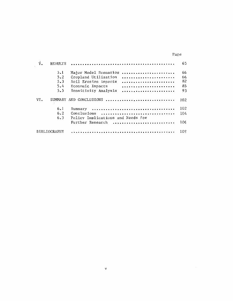
V. RESULTS ............................................... 65

5.1 Major Model Scenarios ........................ 6 65.2 Cropland Utilization ........................ 6 65.3 Soil Erosion Impacts ........................ 825.4 Economic Impacts 855.5 Sensitivity Analysis ....... 93

VI. SUMMARY AND CONCLUSIONS .............................. 102

6.1 Summary ...................................... 1026.2 Conclusions .................................. 1046.3 Policy Implications and Needs for

Further Research ............................ 106

BIBLIOGRAPHY .............. 10?

v

LIST OF TABLES

Table Page

2.1.1. Funding for Soil and Water Conservationin the U.S. 195Q-1980 27

. Parameters of Price Determinant Equations...................114

4.4.1. Classification of Ohio Soils by Slope, Erodibility,T—value, Response to Reduced Tillage, and Productivity .. 51

4.4.2. Ohio Agricultural Cropland by Region and Slope ........... 54

4.4.3. Ohio Agricultural Cropland by Region and Erosion Class .. 56

4.4.4. Ohio Agricultural Cropland by Region, Productivity Category, and Crop Yield Levels ....................... 58

4.6.1. Description of Alternative Tillage Systems .......... 62

5.1.1. Major Model Scenarios .................................... 6 6

5.2.1. Changes in Ohio Crop Yield Levels by SoilManagement Group and Tillage System ..................... 67

5.2.2. Changes in Per Acre Production Costs of Ohio's Major Crops Under Conservation Tillage Systems ....................... 69

5.2.3. Ohio's Simulated Cropland Use Patterns by Region and Tillage Method, with and Without T-Restrictions onSoil Loss ........... 70

5.3.1. Simulated Annual Erosion Rates by Tillage System andSoil Loss Limits ................................... 83

5U4.1. Simulated Percent Changes in Ohio Agricultural Production Resulting from Tillage System Substitution and Soil Loss Restriction .................................... 8 6

5.4.2. Simulated Percent Changes in Ohio Agricultural Prices Resulting from Tillage System Substitution andSoil Loss Restriction by Region ......................... 87

5.4.3. Simulated Changes in Ohio's Average Crop YieldsUnder Alternative Tillage Systems ................ 8 8

vi

Table Page

5.4.4. Simulated Changes in Ohio Farmers? Net Returnsresulting from Changes in Tillage Systems and Soil Loss Restriction by Region ..................... 90

5.5.1. Simulated Percent Changes in Ohio Agricultural Land-Use?Production, and Prices at Three Levels of ExportDemand for Corn, Soybeans, and Wheat ................ 95

5.5.2. Simulated Percent Changes in Ohio Agricultural Land-Use Production and Prices at Three Levels of Expansionin Export Demand for Corn, Soybeans, and Wheat,Soil Loss Restricted to T—values....................... 96

5.5.3. Simulated Changes in Annual Erosion Rates at ThreeLevels of Expansion in Export Demand ................. 9 7

5.5.4. Simulated Changes in Annual Erosion Rates at TwoLevels of Expansion in Industrial Demand for CornUnder Conventional Tillage Methods ..... 100

vii

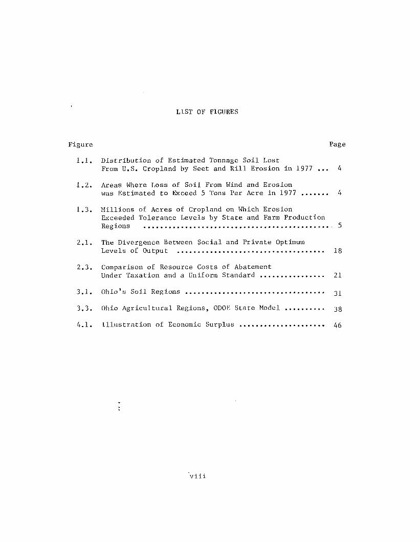
LIST OF FIGURES

Figure Page

1.1. Distribution of Estimated Tonnage Soil LostFrom U.S. Cropland by Seet and Rill Erosion in 1977 ... 4

1.2. Areas Where Loss of Soil From Wind and Erosionwas Estimated to Exceed 5 Tons Per Acre in 1977 ...... 4

1.3. Millions of Acres of Cropland on Which ErosionExceeded Tolerance Levels by State and Farm Production Regions ................. 5

2.1. The Divergence Between Social and Private OptimumLevels of Output ................................... 18

2.3. Comparison of Resource Costs of AbatementUnder Taxation and a Uniform Standard ................ 21

3.1. Ohio's Soil Regions ...................... 3 3

3.3. Ohio Agricultural Regions, ODOE State Model .......... 3 3

4.1. Illustration of Economic Surplus ...................... 46

CHAPTER I

INTRODUCTION

1.1 The Problem

Soil erosion is a natural process that occurs even without

human intervention. Excessive soil erosion, however, is usually a

by-product of interaction of human activities with land. A major

cause of excessive erosion is intensive agricultural use of land,

particularly for production of row crops which exposes unprotected

soil to wind and water.

In the United States, especially during the recent decades,

several factors have contributed to more intensive use of cropland.

A continuing growth in domestic population and per capita income have

favored grain-fed cattle, poultry, and other commodities based on row

crop farming. Furthermore, since 1972, the acreage of corn, sorghum,

soybeans, and wheat has increased substantially to meet increased

worldwide demand for these crops. Despite the present decline in

rapid growth rate of crop exports, further intensification of U.S.

agriculture may continue as world demands for food increase and new

(unconventional) demands upon agriculture are developed. Expanding

production of alcohol and sugar substitutes from grain are the major

examples of new demands made upon agriculture.

These developments, on the one hand, have contributed positively

to the U.S. balance of payments. On the other hand, they set off an

2

inflationary price explosion of farm commodites, farm inputs, and

agricultural land. Paying high prices for land in the 1970s, a large

number of farmers had been placed in a situation where they had to

"farm the hell out of the land" to maintain an immediate cash flow

and to be able to service debts (Heady, 1980). Specifically, land

purchased on credit at $4,000 per acre, tractors at $50,000-$75,000,

and cash rent at $150 per acre in the Corn-Belt, with parallel con­

ditions elsewhere have given rise to high fixed costs in interest

rates and rents which have emphasized heavy immediate cropping at

the expense of future productivity (Heady, 1980).

The commodity-resource pricing complex which has encouraged

intensive cropland-use patterns, has also intervened with the

developing structure of U.S. agriculture. That is, under a rise in

the real price oJ farm labor against machine capital, the machinary

industry has generated Large tractors and complementary field

equipment that can pull 60-80 feet wide planters and tilling equip­

ment. This has enabled many larger farms to specialized in row-crop

monoculture, resulting in an increased tempo of soil erosion (Heady,

1980).

The above-mentioned economic developments have given rise to

a continuously increasing concern over excessive loss of topsoil

from U.S. cropland. I'he ability of soil to tolerate erosion is called

the soil-loss-tolerance level, or T-value. The relation of T-values

to actual, rates of erosion and soil formation is highly important in

establishing what constitutes excessive erosion from the long-term,

societal point of view. T-value has been defined as the maximum rate

of soil erosion which will permit a high level of crop productivity

to .be sustained economically for the indifinite future (USDA, 1978a).

Accordingly, annual erosion rates exceeding T-values are considered

excessive. Typical T—values for many major agricultural soils in the

U.S. are between 3 to 5 tons per acre per year.

Avereage soil erosion rates are not strongly alarming for the

U.S. as whole, however, serious problems exist in many regions and

localized areas where rates of erosion exceed the rates of soil form­

ation. According to the 1977 National Resource Inventories (NRI),

erosion is the most important conservation problem on 51% of the

nation's cropland (USDA, 1978b). In other words, about 97 million

acres, or about 23% of the 413 million acres of cropland in the U.S.,

suffer erosion which exceeds T-value. Such soils are deteriorating

and their long-term productivity is in danger. In the aggregate,

nearly 2 billion tons of topsoil are removed from U.S. cropland each

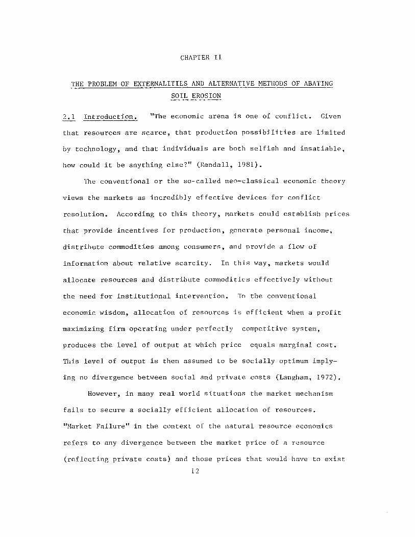
year. Figures 1.1 and 1.2 show the broad geographic distribution of

cropland erosion and the distribution of areas where wind and water

erosion exceeded 5 tons per acre per year in 1977.

Soil erosion is especially serious in the 12 north central

states. The long-term seriousness of this situation is emphasized

by the fact that these states produce 46% of the nation's food grains,

77% of the feed grains, 64% of the oilseeds, 42% of all crops, and

45% of all livestock sales (USDA, 1981a). The heart of this region

is the Corn-Belt, including Ohio, which is one of the richest agri-

4

Figure 1.1

Distribution of estimated tonnage o f soii lost from U.S. cropland by sheet and rill erosion in 1977. One dot equals 250,000 torts of soil. The tota l soil loss in 1977 was estimated at 2 billion tons. The m ost serious sheet and nil erosion occurred in the Corn Baft and Mississippi Defte states and in western Tennessee <U.S. Department o f Agriculture, 1980).

30.000 acni

Areas where loss o f soil from w ind and water erosion was estimated to exceed 5 tons per acre in 1977 One dot equals 30.000 acres. The loss exceeded 5 tons o f sort per acre on 241 million acres <U. S. Departm ent of A gricu ltu re , 19801.

5

cultural regions in the world. NRI data show that erosion losses of

5 tons or more per acre per year are common in this region, and

losses of 1 0 tons or more per acre per year occur on approximately

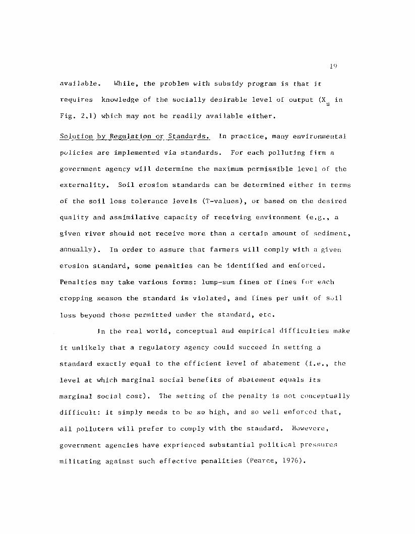
20 percent of row-cropped land (USDA, 1978b). Figure 1.3 shows the

situation of excessive soil erosion for the nation's different regions

in 1977.

From the standpoint of natural resource economics, there are

two major problems associated with excessive soil erosion.

1) If soil is allowed to erode too far, crop yields could be

Figure 1.3

303.11o

2.0 jrtpTN ortheast

0.5P a c i f i c

5 2 Northern \ 12 3 881 Plains \ ------- no 11“ t“ „ i Corn Belt 2.9

R 1 U 6-kuafMountain/ 0.1 I -^ A p p a la c h ia n

T q 2.7

S ou theast

2.8 \ 3.2 sDelta

StatesSouthernPlains

A la ska ■ Oata not a va ilab le H a w a ii 0 1C aribbean 0.2

M illio n s o f acres o f c ro p lan d on w h ic h the ra te o f shee t end n il e ro s ion e xceeded th e so il loss to le ran ce level by s ta te and farm p ro d u c tio n re g ion s in 1977 IU S D e p a rtm e n t o f A g r ic u ltu re , 1980).

depressed to the extent that commodity production costs and supply

prices rise sharply over the long-run, as natural formation capabi­

lity of soil is depleted. In other words, intensive use of soil in

the present could inversely affect economic welfare of the future

generations through lower supply and higher prices of food and fiber.

2) The sediment resulting from erosion of agricultural land

which is the largest nonpoint pollutant by volume, imposes substan­

tial external costs on society . The sediment may lower water

qaulity, or require removal in order to restore adequate drainage,

flood control or navigation. In the U.S., from the aforementioned

2 billion tons of soil which are pemoved annualy from cropland, only

about one-half billion tons reach the ocean, the rest are deposited

in uplands, flood plains, channel systems, and reservoirs (USDA,

1974).

1.2 Sources of Soil Erosion in Ohio

A. Water Erosion. Soil erosion by water is the dominant

hazard on almost 50 percent of Ohio cropland. Sixty-four percent of

the soil loss from the State's agricultural land is from cropland,

21 percent from forest, and 15 percent from pasture land (Ohio State

University, 1979). Estimated annual soil loss on Ohio's cropland

1/ Nonpoint pollutants are those environmental pollutants which do not originate from discrete locations. These include sediment, pesticides, minerals, natural organic waste materials, radio activity, and microbes (Abraham, 1982).

ranges from less than 1 ton per acre on nearly level cropland in

the northwest and up to 13 tons per acre on 12-18 percent slope

cropland in the southeast. T-values for Ohio soils range from 1 to

5 tons per acre per year. Excessive soil loss beyond T—values

results in soil structure damage and increased crusting problems,

reduced crop yields due to plant nutrient loss, and loss of available

water to plants by reduction of the water holding capacity of soil

(USDA, 1978b).

Types of water erosion include soil detachment, sheet erosion,

and rill erosion. Soil detachment is the breakdown of soil aggregate

and the scattering of small soil particles by falling raindrops. It

is the first step in water erosion and the formation of soil crusts.

The formation of a crust results in reduced ability of the soil to

absorb water, and consequently, more run off and erosion. Sheet

erosion is the removal of a uniform layer of soil material from the

surface by flowing water. Sheet erosion is not easily recognized,

but often removes 3-5 tons of soil per acre per year. Rill erosion

is the removal of soil particles by water flowing in small channels

or between rows. This erosion may result in movement of 7-10 tons

of soil per acre per year (Ohio State University, 1979).

B. Wind Erosion. Wind erosion can be another source of

sediment pollution, resulting in fine particles of soil material

being removed from the soil surface and carried by the wind. This

results in severe crop damage, soil loss, air pollution, and off-site

soil deposits. Wind erosion damage has been increasing on the

wind-erodible soils in northwestern Ohio. These are primarily

sandy soils of the flat lakebed region, but also include areas of

organic soils and fine-textured clay soils with finely aggregated

surfaces throughout the State. Studies on sandy-textured soils in

northwestern Ohio have shown soil losses caused by wind erosion as

high as 130 tons per acre per year during a severe windstorm (Ohio

State University, 1979).

Research has considerably increased the understanding of soil

erosion and the factors affecting it. Farmers now have a wide

variety of research-based soil and water conservation practices

from which to choose. Crop management and erosion control practices

are the main examples of these options. Specifically, soil conserving

crop management practices include crop rotations, conservation

tillage methods which increase vegetative cover for reducing run-off

and erosion, and incorporating of crop residues in the fall for

soil protection, plant nutrient utilization and greater fertilizer

efficiency ( USDA, 1978b). Erosion control practices include

contour tillage, stripcropping, terraces, and diversions with

stabilized waterways ( Ohio State University, 1979).

1.3 Needed Research in Ohio

For long-term societal continuity, there must be a balance

between human activity and a natural resource such as soil which

will permit permanent use of the resource '. From the echological

perspective, soil will be needed for food and fiber production into

9

the indefinite future. Hence, private and public actions are needed

to bring rates of soil loss by erosion into equilibrium with rates

of soil formation.

However, a policy or set of goals to eliminate excessive soil

erosion from U.S. cropland may pose important economic impacts upon

farmers and consumers. These impacts would be even more significant

from regional perspective when vast differences in soil characteris­

tics and cropland-use patterns across the nation are taken into

account.

In Ohio, predominant substitution of soil conserving tillage

systems for conventional tillage practices, and imposition of T-value

limits on soil loss would each have a significant impact on the

State's agricultural economy. These impacts would emerge primarily

from the State's regional diversity of soil and topographic con­

ditions which historically have resulted in a variety of cropland

use patterns and other agricultural activities. Specifically,

nearly 60 percent of the agricultural land in Ohio has slopes of

greater than two percent which can seriously erode if not properly

managed. The most erosive of this is in the southeast, where, the

average slope is about 12 percent. The remaining of the State's

agricultural land has little or no slope (less than 2 percent). A

large percentage of this is in northwestern Ohio. Since these

soils have little slope, minor concern has been given to soil loss.

However, erosion can occut on these soils because of their high

content of fine, collodial material that is easily dispersed and

10

carried by surface water runoff, the high percentage of intensive

cropping, and bare surfaces over winter and spring (Ohio State Univ­

ersity, 1980).

Two major studies, Becker 1977, and Abraham 1982, have modelled

the economic impacts of conservation tillage methods and T—based

restrictions on soil loss in Ohio. Both of these studies are

region-specific. Becker's work focuses on the Honey Creek watershed

in north central Ohio, and Abraham's study covers northwestern Ohio.

These studies used a price-exogeneous (linear programming) model as

their quantitative tool of analysis. Linear programmign models as

will be described in Chapter IV, are built based on the simplistic

assumption of fixed output prices that does not allow the model to

determine the price flexibilities which take place in response to

some changes in policy.

The present study builds on this earlier work in several ways.

The diverse regional soil and type of farming characteristics of

Ohio agriculture, including regional economic inter-relationships

are incorporated into a price-endogenous programming model of the

State's agricultural economy. This is used to analyze the potential

land-use and economic impacts of alternative soil conservation

strategies for Ohio. The specific objectives are the following.

1.4 The Study Objectives

The general objective of this study is to determine the poten­

tial economic trade-offs between alternative soil conservation

11

strategies and Ohio agricultural production, farmers' net returns,

and consumers' surplus. Three different tillage systems, and T-values

will be evaluated through a multi-region, soil-specific, and price-

endogeneous programming model of Ohio's agricultural economy.

The operational objectives are to determine the following:

1 ) the soil-specific cropland use patterns under the alternative

tillage methods, with and without limiting annual erosion to T-values;

2) the changes in the State's average and regional erosion rates

resulting from soil conserving tillage practices and T-value rest­

riction of soil loss;

3) the impacts on agricultural production, farm prices, crop

exports, farmers' net returns, and consumers' surplus from tillage

system substitutions and T-value. restriction of soil loss;

4) sensitivity of the model to some potential expansions in

export demands for grain and soybeans, and domestic industrial

demand for corn, under alternative tillge systems, with and without

T—value limitations on soil loss.

The three different tillage systems which will be incorporated

into the model are conventional tillage (moldboard plow), conser­

vation tillage (chisel plow), and no-tillage, These tillage systems

are described in detail in Chapter IV.

CHAPTER II

THE PROBLEM OF EXTERNALITIES AND ALTERNATIVE METHODS OF ABATINGSOIL EROSION

2.1 Introduction. "The economic arena is one of conflict. Given

that resources are scarce, that production possibilities are limited

by technology, and that individuals are both selfish and insatiable,

how could it be anything else?" (Randall, 1981).

The conventional or the so-called neo-classical economic theory

views the markets as incredibly effective devices for conflict

resolution. According to this theory, markets could establish prices

that provide incentives for production, generate personal income,

distribute commodities among consumers, and provide a flow of

information about relative scarcity. In this way, markets would

allocate resources and distribute commodities effectively without

the need for institutional intervention. To the conventional

economic wisdom, allocation of resources is efficient when a profit

maximizing firm operating under perfectly competitive system,

produces the level of output at which price equals marginal cost.

This level of output is then assumed to be socially optimum imply­

ing no divergence between social and private costs (Langham, 1972).

However, in many real world situations the market mechanism

fails to secure a socially efficient allocation of resources.

"Market Failure" in the context of the natural resource economics

refers to any divergence between the market price of a resource

(reflecting private costs) and those prices that would have to exist12

11

(reflecting social costs) if a socially optimal state ol resource

utilization is to be secured. For example, some functions of

environmental resources such as their waste receiving facilities are

generally not marketed at all. But their ’shadow’ price (the price

that would exist if these functions were marketed in an optimal way)

is clearly positive because using the environment in this way would

preclude its use from other purposes. Specifically, if we permit

watercourses to be used as dumps for municipal and industrial wastes,

or to be saturated with cropland sediments, we preclude that resource

from alternative uses such as fishing, navigation, recreation, etc.

However, if prices were charged for using waste receiving facilities

of the environment we would expect a different pattern of uses compared

to a situation in which prices are not charged. The failure of the

market mechanism to recognize the 'shadow' prices associated with the

use of the similar functions of many natural resources results in the

divergence between social and private costs.

This chapter attempts to explore a major source of the

market failure , the so-called externalities, which are pertinent to

utilization of many natural resources including cropland. It will

further discuss the benefits and costs of soil conservation, and

finally will identify alternative economic methods of dealing with

soil erosion problem.

2.2. The Problem of Externalities. Effects upon economic agents

not associated with their own economic activities are called

14externalities (Davis and Kamien, 1977). Alternative terms for

externalities are "spillovers", "external effects", and "social

"effects" (Mishan, 1976; Dasgupta and Pearce, 1974; and Pearce

1976).

While the contemporary economic literature distinguishes

many kinds of externalities, for the purpose of this study, it is

necessary to focus on so-called "technological, or non-pecuniary

external diseconomies". This type of externality refers to those

costs that one economic agent might impose on another, or perhaps

on all members of society — . Technological external diseconomies

arise when there is a lack of institutions which i\/ould insure that

individuals pay for all costs of their actions. External costs

prevent the market mechanism from functioning efficiently and result

in the divergence between social and private costs (Davis and Kamien,

1977).

An important case of external diseconomies, which is related to

the subject matter of the present research, is the sediment problem

caused by soil run—off from agricultural land. Looking from the

standpoint of natural resource economics, soil erosion imposes two

types of external costs on society:

i) depleting the long-run productive capacity of the cropland;

ii) contributing significantly to the non-point source pollution

_1/ Pecuniary externalities refer only to changes in prices as a result of individual decisions. Since they pose no problem for market economy, their discussion in this study is unnecessary.

15

of the waterways.

The first of the above external costs can be interpreted as

inter-generational or user costs reflecting the present value of

future sacrifices associated with the loss of a particular unit of

topsoil. The second of the above, represents the so-called

off-site damage costs, major examples of which include lost reservoir

capacity, increased flood damages, increased navigational channel

dredging, and water treatment costs. These external costs are

imposed upon present as well as future generations. In fact, crop­

land sediments comprise almost half of the total amount of sediments

entering the U.S. waterways (Bogges, ejt £l. , 1980). Monetarily,

these damages have been estimated to be nearly a billion dollars

per year (Cooley, 1976).

Existence of the aforementioned external effects calls for some

collective measures to eliminate or internalize these social costs.

Accordingly, the succeeding sections of this chapter discuss the

benefits and costs of soil conservation, and alternative ways of

abating soil erosion.

2.3 The Benefits and Costs of Soil Conservation.

A. Benefits The benefits of a soil conservation policy may

be divided into two categories. 1) a reduction in off—site damages

due to sedimentation of streams, rivers, and lakes; also, there may

be reductions in levels of some plant nutrients in these surface

waters, particularly, phosphorus which tends to be chemically bound

16

to soil particles. 2) Preserving the productive capacity of soils

for a longer time than if no conservation measures were practiced.

From the productivity standpoint, if conservation is successful,

then a benefit will accrue to society through larger supplies of

agricultural products at sometime in the future.

B. Costs. The costs of a soil conservation program may also

be placed into two categories. 1) The costs that are incured by

society in forms of program payments and/or administrative costs

in encouraging or forcing land-owners and farm operators to

practice soil conservation methods that they would not ordinarily

use if acting on their own individual self-interest. 2) The costs

to society that would emerge from adoption of conservation tillage

methods and/or land-use restrictions. These conservation measures

may reduce current farm output and increase food prices for the

present generations. They may also result in some off-site damage

costs as a result of more intensive application of fertilizers in

substitution for the land to be set aside, and additional herbicide

and pesticide loads used under conservation tillage systems.

2.4 Alternative Methods of Abating Soil Erosion.

A. Theoretical Approach The economic literature of external­

ities identifies three major approaches for correcting environmental

externalities including soil erosion. These approches are the

following:

(1) tax-subsidy solution,

17

(.2) soultion hy regulation or standards, and

(3) market or bargaining solution.

Tax-Subsidy Solution. as discussed earlier in this chapter, the

economic approach to environmental problems requires us to think of

soil erosion as an external cost, and to identify the socially optimal

level of these costs. Invariably, this level will not be zero, since

some positive amount of soil loss is justified. Figure 2.1 shows the

situation of a perfectly competitive farm firm for which the demand

curve ( PP ) is perfectly elastic. MPS represents marginal private

costs which differ from marginal social costs (MSC) by an amount equal

to marginal external costs (MEC), i.e., the marginal cost of soil

erosion. The private optimal level of output for this firm is at X ,P

but at this level of output external costs of Ocd (the two shaded

areas) are imposed. The social optimum output is at Xg , where, the

product price ,p , equals MSC. Moving from the private to social

optimum saves external costs ol abed but leaves Oab external costs.

One method of achieving the socially optimal level of output,

Xg, at the optimal level of soil loss, Oab, is to tax the farmer

according to the undesirable external costs he imposes on society.

Mathematically, it can be proven that the optimal tax is equal to MEC.

That is, social profit is maximized by setting a tax equal to marginal

erosion cost at the optimal output. The firm will now bear the

external costs in form of a tax which it will obviously treat as a

private cost. In this way, the external cost is said to be 'inter-

18

MSC MPC+MEC

c o s t , revenue

price MPC

MR

Output

= AR

Figure 2.1

The Divergence Between Social and Private Optimum Levels of Output

nalized' .

Alternatively, the correction of externality may be approached

by subsidizing the firm at the rate of S = MEC for every unit of output

produced below X^ upto Xg . The decision by the firm to produce a unit

of output beyond Xg implies that the foregoing of the subsidy on that

output. Accordingly, the firm will choose to produce at X^ in order to

benefit from the total amont of subsidy, abc.

Both the taxation and subsidy schemes result in exactly the

same net social gains. However, in terms of income distribution, the

firm is better off under a subsidy scheme and the rest of society is

worse off. While, under a taxation program the opposite is true. A

major difficulty with the tax solution is that it requires knowledge of

the magnitude of the marginal damage costs which may not be readily

19

available. While, the problem with subsidy program is that it

requires knowledge of the socially desirable level of output (X in

Fig. 2.1) which may not be readily available either.

Solution by Regulation or Standards. In practice, many environmental

policies are implemented via standards. For each polluting firm a

government agency will determine the maximum permissible level of the

externality. Soil erosion standards can be determined either in terms

of the soil loss tolerance levels (T-values), or based on the desired

quality and assimilative capacity of receiving environment (e.g., a

given river should not receive more than a certain amount of sediment,

annually). In order to assure that farmers will comply with a given

erosion standard, some penalties can be identified and enforced.

Penalties may take various forms: lump-sum fines or fines for each

cropping season the standard is violated, and fines per unit of soil

loss beyond those permitted under the standard, etc.

In the real world, conceptual and empirical difficulties make

it unlikely that a regulatory agency could succeed in setting a

standard exactly equal to the efficient level of abatement (i.e., the

level at which marginal social benefits of abatement equals its

marginal social cost). The setting of the penalty is not conceptually

difficult: it simply needs to be so high, and so well enforced that,

all polluters will prefer to comply with the standard. Howevere,

government agencies have exprienced substantial political pressures

militating against such effective penalities (Pearce, 1976).

20

Taxes versus Regulations Most of the economic literature on environ­

ment, such as Randall,1981; Davis and Kamien, 1977; Pearce, 1976;

and Layard and Walters, 1978 tend to argue that taxes are the least-

cost method of securing a given level of pollution abatement. A

brief elaboration of this argument using an example from Randall is

presented below.

Let's consider a three firm industry which emits a particular

kind of pollution. The respective marginal abatement cost curves of

these firms (MAC)^, (MAC)2, and (MAC)^ are shown in Figure 2,2.

Now, if a fixed rate emmission tax is imposed on this industry, each

firm will act to abate its pollution discharge upto the point where

its marginal abatemeent cost (MAC) equals the tax rate. Accordingly,

the respective abatement levels of these firms are shown by Q^,Q2 ,and

Q^, in Figure 2.2. Under this scheme, the total resource copt

of abatement is equal to (OAQ^+OBC^+OCQ^). Now, if instead of tax,

a uniform standard is enforced such that each firm is required to

provide pollution abatement of Q2> the total resource cost of abate­

ment will be equal to (ODQ2+OBQ2+OEQ2). In order to let the total

amount of abatement under two schemes be the same, Figure 2.2 is

drawn such that (Q^-K^+Q^) = 3Q2 and ~ Abstraction

of the total resource cost of abatement under taxtation from the one

under standard yields: (DQ2Q^A - CQ^Q2E). DQ2Q^A is greater than

CQ^Q^E, since (Q2~Q0) = ((>2-Q^) . Thus, the total resource cost of

abatement under taxation is less than the one inder regulation for

21

Lhe same level of abatement.

(MAC)s t a n d a r d .

/

(MAC)

(MAC)

Z e r o p o l l u t i o n

Figure 2.2

Comparison of Resource Costs of Abatement Under Taxation and a Uniform Standard

It is important to note that the strength of the above

conclusion, heavily relies upon the assumption of setting a uniform

standard . However, the inefficiency of a regulatory scheme mav be

avoided through application of differential standards. That is,

varying levels of abatement requirements can be established with

regard to the differences in polluting firm’s economic and technolog­

ical constraints in providing the abatement. In the above example,

the emissions tax is more efficient than the standard because it

encourages the most efficient supplier of abatement, the firm with

(MAC)^, to provide the most share of abating, and the least efficient

22abator, the firm with (MAC)^, to do the least abating. While, under

the uniform standard, regardless of its highest MAC, firm 1 is

required to provide the same amount of abatement as the other two.

This is the major reason for inefficiency.

In general, emissions taxes may have the advantage of

providing continuing incentives for innovations and investments in

pollution abatements which would reduce both the remaining emissions

and the pollution-associated costs with the polluter.

As far as the soil erosion abatement is concerned, the

availability of soil loss tolerance levels (T-values) makes the use

of both taxation and differential standards two alternative policy

options. The present study will incorporate T-based differential

standards to analyze the economic impacts of soil erosion abatement

in Ohio . The specific procedure for using this policy option will

be discussed in Chapter IV.

Market or Bargaining Solution. Coase, I960, has theoretically

proven that "given non-attenuated property rights, trade among the

involved parties will eliminate (Pareto-relevant) externalities,2/resulting in an efficient solution" — . The economic logic behind

the Coase Theorem is that it will be in the interests of the acting

and affected parties to enter a bargaining process to correct the

externality since there are potential benefits to be gained from such

2 / Pareto-relevant externalities refer to those technological external dis-economies that can be modified to make the affected party better-off without making the acting party worse-off.

23

bargaining. But in reality, the bargaining solution faces many

problems. First, it depends on sufficiently well-defined property

right. Second, it presumes that external costs in question involve

readily identifiable parties. Consequently, a bargaining solution

does not seem to be applicable to more complex or non-point cases

of externalities such as soil erosion. Erosion entails a large and

probably unidentifiable number of sufferers, and it is uncertain in

magnitude, liable to occur at considerable geographical distance

from the source of emraision, and is liable to occur at a point in

time quite far from the time of eramision. For these reasons, it

is less likely that farmers and sufferers ever could come together

to bargain.

B. Soil Conservation Strategies in Practice

The aforementioned corrective approaches to externalities are

principally general within a theoretical framework. Looking from

the real world perspective, this section focuses on the major U.S.

soil conservation efforts in the past and present, and some future

policy alternatives of achieving control of excessive soil erosion.

The Past and Present Soil Conservation Efforst. In the U.S.,

the first public program to aid in soil conservation were enacted in

1930s. These programs provided financial and technical assistance

to encourage land owners and farm operators to control excessive

runoff and erosion.

Initially, soil conservation practices were presented to farmers

as ways to maintain soil productivity and promote viable farm

operations. However, unlike many other farm policy issues that call

for rapid and dramatic governmental action during crisis, conserv­

ation efforts remained in the background for many years. Low farm

income and commodity supply problems .especially in 1960s, diverted

the policy makers' attention from conservation goals (Clawson, 1976)..

Recent legislative efforts, namely, the Soil and Water

Resources Conservation Acts of 1972, and 1977, demonstrated that many

politicians and farm leaders feel that the goal of soil conservation

deserves a renewed federal commitment. These Acts have directed the

U.S. Department of Agriculture to undertake a thorough examination

of existing soil resources (USDA, 1980).

Currently, public programs are carried out at local, state,

and federal levels. Thirty-four programs administered by the USDA

have a conservation mission or componenet (CAST,1982).The programs are

carried out to inform the public about soil and water conservation,

identify and locate conservation problems, develop proposed solutions,

and establish institutional agreements for action. The programs

provide cost-sharing, loans, on-site technical assistance in

planning, research, and education. A brief description of these

programs follows.

Cost-Sharing (Subsidy). The cost-sharing strategy which

has been studied more than any other over the past four decades has

been Agricultural Conservation Program (ACP). Since 1936, ACP has

expanded over $8 billion to assist farmers and landowners In adopting

soil conserving practices. This program, during the period of excess

agricultural capacity (1950s and 1960s) was criticized for assisting

25

short-term output enhancing practices such as drainage, irrigation,

and liming rather than soil conservation (Conter, 1964).

Low Interest Loans. The low interest loans for conservation

practices would seem to be well suited to deal with two types of

problems,, First would be private discount rates that are higher

than those society would select for long-term investment decisions.

Second would be farm operators or landowners who have time prefere­

nce that are shorter than those of society. The problem is to

identify those cases and to estimate the reduction in interest

rate necessary to bring the private soil conservation investment

up to the level desired by society. Currently, federal loans for

conservation practices account for only 3 percent of the investment

in selected conservation practices (USDA, 1981).

Technical Assistance, Research, and Education. Technical

assistance and educational programs help reduce information or

knowledge gaps and complement other strategies. Examples might be

information concerning a new or no-till farming system from a land

grant university, or SCS's help in designing terraces. Educational

and technical assistance can be an important part of any soil

conservation strategy involving new practices or special design and

layout problems (CAST, 1982). Yet, just the lack of information

about programs may be a restraint to soil conservation. For

example, a survey by Leitch and Danielson,1979, found that the

primary reason for farmers not participating in waterland programs

was the lack of information concerning the available program.

26

The total federal funding of the aforementioned programs was

nearly 1.5 billion dollars in 1980. Table 2.1 shows the distribut­

ion of the federal expenditure on these programs for the period of

1950-1980.

The combined effects of public programs and private soil

conservation efforts over the past 45 years has been substantial.

Although, U.S. waterways currently receive an estimated 3.5 billion

tons of soil per year, soil conservation programs have been credited

with preventing the loss of an additional one billion tons (Abraham,

1982).

Some Policy Options for the Future. The Council for Agricultural

Science and Technology (CAST), in its 1982 report has suggested

two general objectives of achieving control of excessive

as a base for considering policy alternatives for the future.

i) Protect U.S. soils from excessive runoff so as to retain

indefinitely the capability to produce crops for food, feed, fiber,

and energy to meet national needs, with consideration of apDropriate

exports.

ii) Protect water resources from unwarranted damages by

sediment and other pollutants from excessive soil erosion.

To attain these goals the Council has outlined a number of policy

alternatives for the future. The foregoing section focuses on these

policy alternatives.

Regulations. Each landowner or farm operator could be

T a b le 2 .1 .1

F u n d in g f o r S o i l and W ater C o n s e r v a t io n i n t h e U .S .

1950-1980

y e a r jC o s t :

S h a r in g :T e c h n ic a l : A s s i s t a n c e :

R eso u rc em anagem ent : L oans

R e se a r c h: •

••

E d u c a t io n T o t a l >"1572

d o l l a r s

1 9 5 0 -5 4 1 ,2 4 6 291 98

m i l l i o n

16

d o l l a r s

5 NA 1 ,6 5 5 3 ,0 3 1

1 9 5 5 -5 9 1 ,3 6 3 352 144 67 21 NA 1 ,9 4 7 3 ,1 8 7

1 9 6 0 -6 4 1 ,5 8 4 454 322 80 47 NA 2 ,4 8 7 3 ,8 7 4

1 9 6 5 -6 9 1 ,6 8 1 643 381 141 112 NA 2 ,9 5 8 4 ,0 3 5

1 9 7 0 -7 4 1 ,7 2 5 953 747 192 171 54 3 ,8 4 2 3 ,8 0 8

1 9 7 5 -7 9 2 ,3 7 7 1 ,4 3 3 1 ,7 2 2 313 309 44 6 ,1 9 8 3 ,8 9 3

1980 487 327 458 62 91 11 1 ,4 3 6 717

S o u r ce : I n i t i a l r e p o r t on t h e Land and w a te r C o n s e r v a t io n P ro g ra m s, USDA, D ec . 1 9 7 7 . U p d ated by

D a l la s L e a , N a tu r a l R e so u rc e E con om ics D i v . , E SS, USDA, F eb . 1 9 8 1 .

28

required to develop and implement a soil conservation plan. A number

of years would be required to develop and implement such plans and to

install the needed conservation practices. In many cases, substantial

progress could be made toward compliance by simple changes in tillage

practices which could significantly reduce erosion with little or no

added costs.

However, implementation of such a policy would challenge

some existing beliefs about social equity. Some research findings

suggest that a regulatory policy would have the greatest negative

impacts upon small farm operations located on poor quality land with

operators lacking managerial capacity or capital to adopt many of the

recommended practices. To counter this potential inequality,

a desirable feature of any regulation would be flexibility to include

consideration of managerial and other characteristics of a specific

farm operation including the soil characteristics such as T-values.

Investment Tax Credits. For some farmers, tax implications

exert a powerful influence upon their decisions. If investment in

conservation practices and equipment were given liberal tax breaks,

these activities might increase significantly.

Conservation Incentive Payments. A farmer would be offered

a payment based upon estimated soil loss reductions due to changing

of farming practices. It would encourage control of erosion whenever

the payment offered exceeded the sum of the control costs and the

crop income reductions. Problems of this alternative would be likely

29

in determining the appropriate payment rates and in documenting whether

or not the standards of soil conservation applicable to a particular

field or farm had been met.

Taxation of Soil Loss. Under this scheme, farmers would pay

taxes on the estimates of soil losses exceeding soil loss tolerance

limits and thus would be expected to adop conservation practices to

avoid the tax. Previous studies (Seitz, et_ al., 1978; and Taylor

et al., 1978) suggest that such a tax system would achieve erosion

control efficiently. However, it would likely meet with considerable

resistance from agricultural community,, This system would tend to

penalize farm operations on highly erodible lend. Farms on such land

are usually smaller, and owners or operators often have lower manag­

erial capabilities and less economic flexibility than those on high

quality land with less erodibility.

Cross-Compliance. This would be a policy requiring control

of erosion to a certain degree or in some specified way, for a farm

operator to be eligible for other governmnet agricultural programs.

For example, a farmer might be required to demonstrate effective soil

conservation practices to be eligible for crop price support payments

or loans. Another from of cross-compliance would provide crop price

support payment bonuses to farmers with adequate soil conservation

programs.

CHAPTER III

Regional Differences in Soil Characteristics Influencing Agricultural Land-Use in Ohio

3.1. INTRODUCTION. As specified in Chapter I, a major objective

of the present study is to determine the potential impacts of soil

conservation strategies on the pattern of agricultural land-use in

Ohio. Since the State has a wide variety of soils (i.e., more than

500 soil types), achievement of this objective requires knowledge of

the basic characteristics of these soils and their regional locations

Accordingly, this chapter explores the following:

i) regional classification of Ohio soils on the basis of

their origin and parent materials,

ii) classification of Ohio soils based on the so-called

'capability class'; and

iii) regionalization of the State for model formulation.

3.2. Ohio's Soil Regions. The soils of Ohio have been classifie

by soil specialists into eight major soil regions (Figure 3.1) This

classification has been performed on the basis of soil properties as

they relate to the parent material and the length of time they have

been exposed at the surface of the earth. Most soils in the western

half of the State have been derived from limestone and have a fairly

high soil pH throughout the profile — ^, while those in the eastern

j_/ Soil reaction, pH, is a measure of the intensity of acidity oralkalinity. Most of Ohio soils have pH values ranging from 4.0 to 8.5. The higher the pH, the lower intensity of acidity.

31

Figure 3.1

Oh io1s Soil Reg ions Source: Ohio State University, 1981

half of Ohio have been derived, for the most part, from sandstone and

shales and tend to have a lower pH (Sitterley, 1935).

Approximately, 3/4 of the State has been involved in several

glacial inva'ions which have affected both its soils and topography.

Topographically, the glaciers tended to have a leveling effect.

They have left most of the land surface in western Ohio level to near

level. In the eastern half of the State, only northern and a part of

the east central areas were glaciated. The remainder of eastern Ohio

along with all or parts of five counties in southwest were unaffected

by glacial action. The topography in unglaciated Ohio can be

characterized as generally rolling or hilly, with parts rough and

broken (Sitterley, 1976). The following briefly describes the

general classification of Ohio soils as shown in Figure 3.. 1.

Soil Region I . This region consists of soils in high lime

glacial lake sediments which include the great lake plain area of

northwestern Ohio. The larger part of this region is occupied by flat

areas of dark-colored, natutally poorly-drained clay soils such as

Brookston, Paulding clay, and Toledo silty clay. With adequate drain

age these heavy soils are very suitable for corn, sugar beets,

and similar crops. In this region the associated heavy light-colored

soils such as Nappanee and Fulton silty clay loam are of only fair

agricultural value.

Soil Region II. Soils of this region are fine-textured and

have been developed from "calcareous glacial drift" . They include

some of the most fertile lands in Ohio. The light colored soils have

been leached of lime to a depth of 24 to 36 inches and are commonly

slightly acid in reaction in the surface soil. These soils with

adequate artificial drainage include some of the best corn land in th

State.

Soil Region III. Soils in Medium-Textured High Lime

Glacial Drifts: these soils have the same general features

of those in Soil Region II, except that the size of soil particles in

this region are larger.

Soil Region IV. Old Glacial Limestone Soils: this soil

region includes glacial limestone soils derived from "very old cal­

3 J

careous glacial drift" which has been leached of lime to a depth of 8

to 10 feet. Because of this extreme leaching these soils are all very

acid in reaction and relatively low in natural productivity. Those

with fair to good natural drainage are of fair agricultural value,

whereas the very pooly-drained gray soils would be ranked as low in

value.

Soil Region V . Lacustrine Sandstone and Shale Soils: the

narrow belt of lake plain soils in northeastern Ohio includes much the

same range in texture as in northwestern Ohio. Being derived primarily

from sandstone and shale material these soils are naturally acid in

reaction. The area of dark colored heavy soils is somewhat limited.

In this region, the sandy soils are well adapted to truck crops and

fruits.

Soil Region VI. These soils have been derived from galcial

drift made up largely of non-calcareous sandstone and shale. Where

sandstone predominates the subsoils are open and porous, making it

possible to drain the wet area by tilling fairly easily. The soils

with fair to good natural drainage are some of the best grain soils

in the State.

Soil Region VII. Residual sandstone and shale soils: this is

the largest residual soil region in Ohio. Glaciation has had little

influence on the soils in this area. As a result, topography ranges

from nearly level to extremely steep. The residual soils derived

from sandstone and shale are acid in reaction and of fair fertility.

34

Soil Region VIII. This area in Adams and adjointing counties

includes residual soils from limstone or from limestone and shale.

A considerable proportion of the area has a very steep topogarphy.

These sloping lands vthich are well supplied with lime are excellent

for pasture and legumes like alfalfa.

3.3. Classification of Ohio Soils Based on Capability Class.The nature of the above classification is very general in the

sense that it groups the Ohio soils principally on the basis of origin

and parent materials. There is a second method which has been use

to classify soils of the State for their agricultural potential by

capability class . These range from Class I soils which have few

limitations for producing crops through Class VIII soils which are

not capable of producing crops or timber and are suitable only for

wildlife, water supply, recreation, etc.

The following is a brief discription of the eight land

capability classes adapted from the USDA Conservation Needs Inventory

Committee (CNIC) report for 1971.

Class I. Soils with few limitations that restrict their use.

These soils are on slopes of 0 to 2 percent. They are medium textured,

deep, well drained with good water holding capacity. They are suited

for continuous use for row crops, small grains, hay crops, and pasture

as well as vegtables and other specialty crops.

Class II. These soils have moderate limitations tli.iL affect

the choice of plant grown or that require the use of moderate

3 5

conservation practices. These soils based on their dominant hazard

have been divided into three subclasses: He, IIw, and IIs. The

respective dominant hazard or problem in their use are erosion,excess

water, and root limitations.

Class III. Soils with severe limitations which influence

the choices for plants and require special conservation practices.

Similar to Class II, the subclasses of this category are IHe, IIIw,&

Ills, which represent respective limitations of erosion, prolonged

wetness, and shallow depth to bedrock.

Class IV. Soils with very severe limitations that restrict

the choice of plants, require very careful management or both.

The subclasses of these soils are IVe, IVw, and IVs. The respective

limitations of these are severe erosion, drainage, and shallow depth

to bedrock.

Class V. These soils are neary level so they have no erosion

problems but have limitations that are impractical to remove. They

frequently overflow or are stoney or shallow.

Class VI. Soils in this class are generally unsuited for

cultivation. They usually need liming, fertilizing, water diversions,

drainage ditches, etc.

Class VII. Soils with very severe limitations but with good

management 5 they can be safely used for grazing and woodland, the

physical conditions of these soils are such that it is impractical

to apply improvements such as lime, fertilizer, water control, etc.

36

Class VIII. Soils and land forms in this class have

limitations that preclude their use for commercial plant production

and restrict their use to recreation, wildlife, water supply, or

similar purposes.

3.4. Regionalization of the State for Model FormulationFrom the economic standpoint, the aforementioned differences

in soil characteristics within the State have varying degrees of

comparative advantage in terms of crop yield levels and production

costs of each region to specialize in different agricultural

production activities. In turn, the differences in comparative

advantage among regions have resulted in a tremendous diversity in

agricultural land-use in Ohio. The general structure of this diversity

can be described by the greatest concentration of land under corn

and soybeans in the west/northwest, of dairy activities in the north­

east, and of woodland and pastureland in southeastern Ohio.

A major problem in attempting to model the economic trade-offs

between soil conservation policies and agricultural production levels

in Ohio emerges from the above mentioned diversity in cropland use

within the State. In other words, analyzing the State as one homo­

geneous unit would not permit a realistic representation of its

differences in soil series and agricultural production activities.

Thus, in order to build a reliable model for achieving the objectives

of this study it is necessary to divide the State into subareas

which are relatively homogeneous with respect to physical character­

istics and current agricultural production patterns.

37

Based on the regional differences in soil characteristics and

land capability classes described above, Sitterley's subareas, and

major transportation nodes Ohio was divided into seven agricultural

regions (Fig. 3.3). The following describes main features of these

regions which have been incorporated into the model used in the

present study.

Region 1 This region comprises 14 counties in northwestern

Ohio. Most of this region was covered by water (Lake Maumee) some

thousand years ago during the glacial period. Topographically, with

minor exceptions the are is quite level and when artificially

drained is highly productive. In terms of percent of land suitable

for cropping this region ranks the second among the seven regions.

In 1982, 28 percent of the harvested crops was corn, 47 percent was

soybeans, and the remaining 25 percent was comprised of small grains

and vegtables (Ohio Agricultural Statistics, 1983).

Region 2. This region is formed of 18 counties in western

Ohio. Approximately 97 percent of the total land in this region was

classified by CNIC as capable of being used for crop production with

proper erosion control practices. The most visible features which

distinguish this region from region 1 are the larger concentration of

corn and livestock production and the higher percentage of total land

being in farms. In 1982, 41 percent of the harvested crops acreage

was corn, 39 percent was soybeans, and the remaining 20 percent was

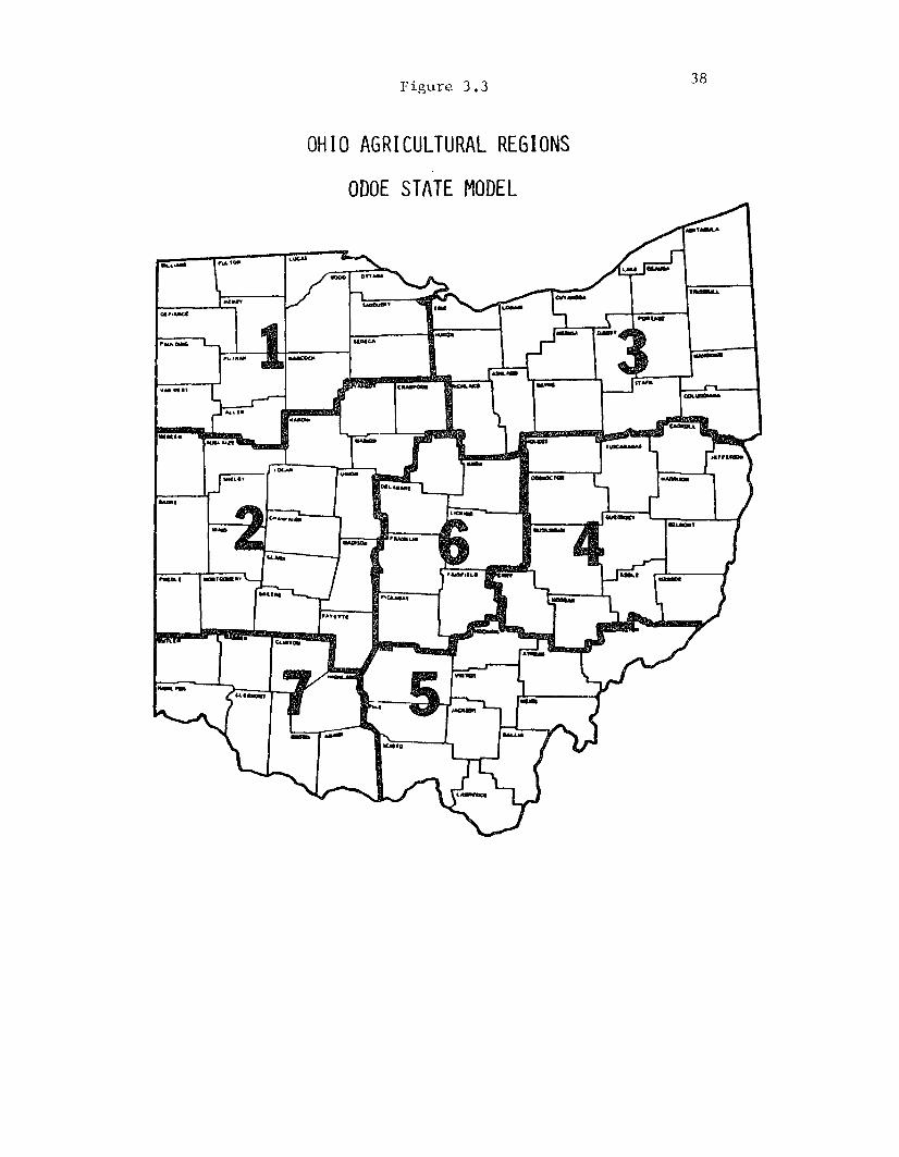
Figure 3.3

OHIO AGRICULTURAL REGIONS

ODOE STATE MODEL

39

comprised of small grains, hay crops, and fruits. In terms of the

total land in farms as well as in terms of percent of land considered

suitable for cropping, this region ranks first among the 7 regions.

Region 3 contains 17 counties in northeastern Ohio. For

the most part, this region was settled by the Pennsylvania Dutch who

brought with them a livestock and wheat farming* It mostly was

covered by glaciers of the Wisconsin Ice Age, resulting in formation

of glacial soils derived from sandstone and shale. In 1982, one acre

out of every four was occupied by urban uses and slightly

more than 44 percent of the total land was in farms.In the same year,

cash receipts from livestock was approximately 75 percent of total

cash receipts from farming.

Region 4 consists of 13 counties in the central section of

eastern Ohio. These counties are part of Appalachian Highlands

and are either predominantly or totally unglaciated. The soils are

largely derived from sandstone and shale are deficient in lime.

Except for a limited amount of river land, the topography ranges from

hilly to rough. This makes the land highly erosive if used for crop

production. The CNI has classified only 63.5 percent of the land

in this region as suitable for crop production, compared to the 84.0

average for the State. The small and irrigular shaped areas suitable

for cropping are generally inconvenient and costly to use lor ctop

production. In 1982, crops where harvested on 12 percent of total

land area or 23 percent of the land in farms. Hay was the region's

most imporatnt single crop in terms of acreage, followed by corn.

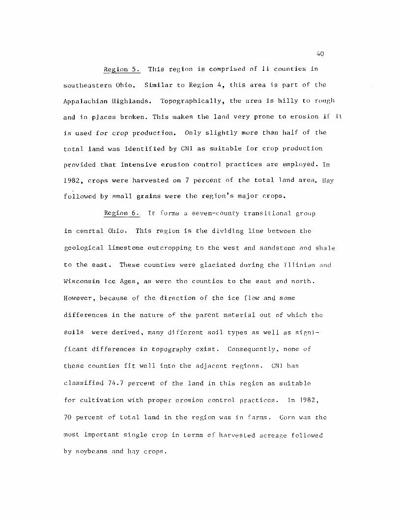
4 0Region 5. This region is comprised of 11 counties in

southeastern Ohio. Similar to Region 4, this area is part of the

Appalachian Highlands. Topographically, the area is hilly to rough

and in places broken. This makes the land very prone to erosion if it

is used for crop production. Only slightly more than half of the

total land was identified by CNI as suitable for crop production

provided that intensive erosion control practices are employed. In

1982, crops were harvested on 7 percent of the total land area. Hay

followed by small grains were the region's major crops.

Region 6. It forms a seven-county transitional group

in cenrtal Ohio. This region is the dividing line between the

geological limestone outcropping to the west and sandstone and shale

to the east. These counties were glaciated during the Illinian and

Wisconsin Ice Ages, as were the counties to the east and north.

However, because of the direction of the ice flow and some

differences in the nature of the parent material out of which the

soils were derived, many different soil types as well as signi­

ficant differences in topography exist. Consequently, none of

these counties fit well into the adjacent regions. CNI has

classified 74.7 percent of the land in this region as suitable

for cultivation with proper erosion control practices. In 1982,

70 percent of total land in the region was in farms. Corn was the

most important single crop in terms of harvested acreage followed

by soybeans and hay crops.

41

Region 7. This region includes eight counties in southwestern

Ohio. Most of this area was covered by Illinoian Glacier. However,

the southeastern parts of Brown and Adams counties were not affected

by glaciation. In this region, the topography ranges from level to

steep and broken with both drainage and erosion being major hazards.

Approximately, 26 percent of the land in this region was classified

by CNI as not suitable for crop production. In 1982, about 55 percent

of the total land was in farms, and almost 30 percent of the total

land was in forests. Nearly 20 percent of the total farmland was

used for pasture,and crops were harvested in 33 percent of the total

land in farms.

Analyzing Ohio's agricultural economy based on the above

regions allows us to determine the potential land—use and economic

impacts resulting from implementing alternative soil conservation

strategies, and expansions in export/and or industrial demand for the

State's major crops more accurately. For example, as it will be shown

in Chapter V, . 1—value restriction of soil loss would pose

different land-use and economic impacts on each of the seven regions

described above. Alternatively, the main impact of a major rise in

idustrial demand for corn on regions 1 and 2, where most of the land

'.nut is suitable lor row crops has already been utilized for that

purpose, would consist of corn production expanding at the expense of

oLiier crops. Whereas, such a change in demand for corn, would reverse

a long, declining trend in row crop production in the State's most

42

erosive regions, i.e., eastern and southeastern Ohio, by possible

conversion of woodland and pastureland into cropland. Therefore,

from the policy making standpoint, regionalization of the State as

described above, seems to be an essential part of a programming model

which is designed to represent an accurate picture of Ohio's

agricultural economy.

CHAPTER IV

METHODOLOGY

4.1 Introduction. To achieve the proposed objectives, this study

uses a mathematical programming model as its quantitative tool of

analysis. Mathematical programming (MP) models are optimization

techniques with wide application in economics and business. The MP

technique used most often in agricultural policy and planning are

linear programming (LP) and quadratic programming (QP). For example,

several previous studies on the economic impacts of restricting soil

loss at the watershed level (Alt, 1976; Kasai, 1976; Forster, 1978;

Forster and Becker, 1979; Abraham, 1982; and Narayanan, 1974), at

the state level (Nagadevara, 1975), at the regional level (Osteen,

1978) and at the national level (Wade, 1977) have used linear

programming as their quantitative method of analysis. Examples of

the economic studies which have applied quadratic programming are

Ott, 1981, and Meister, 1978.

The Lp and QP techniques can be considered as two alternative

ways of delieating a problem where limited resources are to be

allocated among the competing activities in an optimal manner.

However, as far as the economic theory is concerned there is a major

conceptual difference between the two models. In an LP model, demand

for all outputs is assumed to be perfectly elastic. However, the

QP technique relaxes this simplistic assumption by allowing any

output demand function of a linear form to be incorporated

43

4 4

into the model. Therefore, when commodity demand functions or the

price elasticities of demand are available, formulation of a QP

model would be more appropriate than an LP model in the sense that

the former allows output prices to be endogeneously determined by

the model.

To utilize the conceptual strength of a price-endogeneous model,

the specific quantitative method employed in the present study is a

QP model. It adapts the main structure and assumptions of a seven-

region, price-endogenous model of Ohio's agricultural economy

developed by Raslt et_ al., 1983. However, the present model

substantially expands the activity matrix and restrictions set of the

ODOE model by adding over 200 soil groups and incorporating nearly

250 soil loss constraints. The following describes main

features of the model, and discusses the procedures used for

classification of Ohio soils and developing soil loss restrictions.

The Model

4.1. Objective Function. The objective function comprises maximiz­

ation of economic surplus or net social welfare pertaining to Ohio's

nine principle agricultural commodities,beef, pork, poultry meat,

eggs, milk, and exports of corn, soybeans, wheat, and soybean meal.

Conceptually, economic surplus gained by society from production and

consumption of a commodity, x, at an equilibrium level of output and

the corresponding market price, is the area under (ordinary) demand

4 5

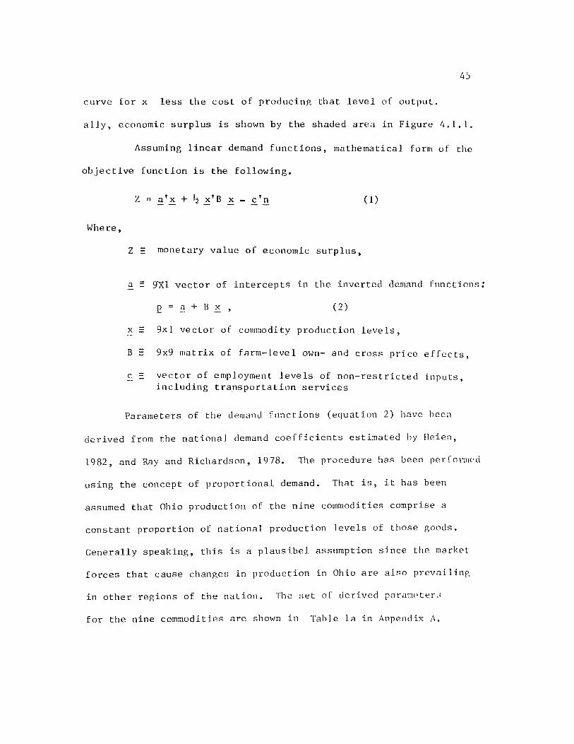
curve for x less the cost of producing that level of output,

ally, economic surplus is shown by the shaded area in Figure 4.1.1.

Assuming linear demand functions, mathematical form of the

objective function is the following.

Z = a'x + h x ' B x ~ £ ’n (1)

Where,

Z = monetary value of economic surplus,

a = 9~X1 vector of intercepts in the inverted demand functions:

p = a + B x , (2)

x = 9x1 vector of commodity production levels,

B E 9x9 matrix of farm-level own- and cross price effects,

c 5 vector of employment levels of non-restricted inputs,including transportation services

Parameters of the demand functions (equation 2) have been

derived from the national demand coefficients estimated by Heien,

1982, and Ray and Richardson, 1978. The procedure has been performed

using the concept of proportional demand. That is, it has been

assumed that Ohio production of the nine commodities comprise a

constant proportion of national production levels of those goods.

Generally speaking, this is a plausibel assumption since the market

forces that cause changes in production in Ohio are also prevailing

in other regions of the nation. The set of derived parameters

for the nine commodities are shown in Table la in Anpendix A.

4 6Figure 4.1.1

Illustration of Economic Surplus

Price

Supply

Demand

Q*0 Quantity

(AP*E = Consumers' Surplus [BP*E = Producers' Surplus

ABE = Economic Surplus OBEQ* = Cost of Production

4.2 Activity Matrix. The model's activity matrix defines the

relationship between inputs (i.e., capital,labor,energy,and land) and

agricultural outputs. In building this matrix it was assumed that

(Ohio) agriculture is a constant cost industry upto the point where a

given type of land-resource is available. This assumption means that

for a given type of land, input-output ratio and marginal cost at any

level of output remains the same. Since the model's land-resonrce

constraints reflect the differences in productivity levels, the

assumption of constant returns to scale has not caused a significant

distortion in the study results.

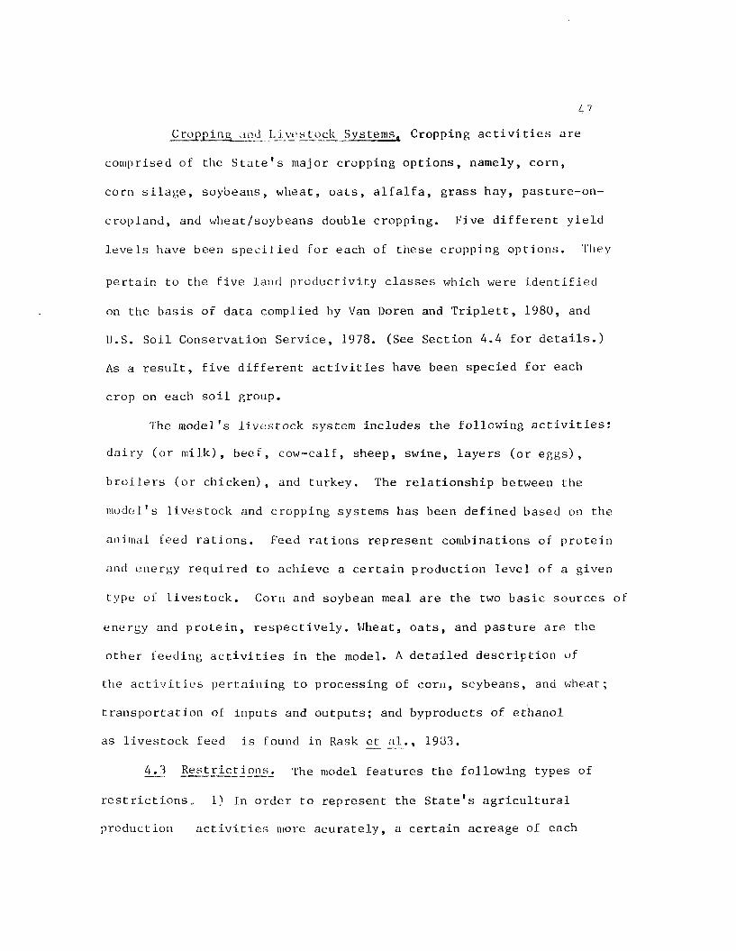
4-7Cropping a nd Livestock Systems. Cropping activities are

comprised of the State's major cropping options, namely, corn,

corn silage, soybeans, wheat, oats, alfalfa, grass hay, pasture-on-

cropland, and wheat/soybeans double cropping. Five different yield

levels have been specified for each of these cropping options. They

pertain to the five land productivity classes which were identified

on the basis of data complied by Van Doren and Triplett, 1980, and

U.S. Soil Conservation Service, 1978. (See Section 4.4 for details.)

As a result, five different activities have been specied for eacb

crop on each soil group.

The model's livestock system includes the following activities:

dairy (or milk), beef, cow-calf, sheep, swine, layers (or eggs),

broilers (or chicken), and turkey. The relationship between the

model's livestock and cropping systems has been defined based on the

animal feed rations. Feed rations represent combinations of protein

and energy required to achieve a certain production level of a given

type of livestock. Corn and soybean meal are the two basic sources of

energy and protein, respectively. Wheat, oats, and pasture are the

other feeding activities in the model. A detailed description of

the activities pertaining to processing of corn, soybeans, and wheat;

transportation of inputs and outputs; and byproducts of ethanol

as livestock feed is found in Rask et_ al., 1983.

4.3 Restrictions. The model features the following types of

restrictions., 1) In order to represent the State's agricultural

production activities more acurately, a certain acreage of each

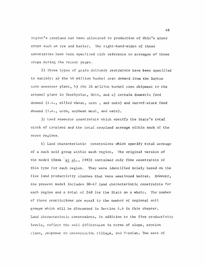
48

region's cropland has been allocated to production of Ohio's minor

crops such as rye and barley. The right-hand-sides of these

constraints have been specified with reference to acreages of those

crops during the recent years-

2) Three types of grain delivery restraints have been specified

to satisfy: a) the 40 million bushel c o m demand from the Dayton

c o m sweetner plant, b) the 24 million bushel corn shipment to the

ethanol plant in Southpoint, Ohio, and c) certain domestic food

demand (i,e., milled wheat, corn , and oats) and out-of-state feed

demand (i.e., corn, soybean meal, and oats).

3) Land resource constraints which specify the State's total

stock of cropland and the total cropland acreage within each of the

seven regions,,

4) Land characteristic constraints which specify total acreage

of a each soil group within each region. The original version of

the model (Rask et al., 1983) contained only five constraints of

this type for each region. They were identified solely based on the

five land productivity classes that were mentioned before. However,

the present model includes 30-47 land characteristic constraints for

each region and a total of 248 for the State as a whole. The number

of these restrictions are equal to the number of regional soil

groups which will be discussed in Section 4.4 in this chapter.

Land characteristic constraints, in addition to the five productivity

levels, reflect the soil differences in terms of slope, erosion

class, response to conservation tillage, and T-value. Two sets of

49

data were employed to identify the right-hand-sides of the land

resource and land characteristic constraints: i) estimates from

the Bureaue of Census,1980; and ii) the SCS Conservation Needs

Inventory, 1967. The latter is a county-reliable, soil-specific

data.

5) Based on maximum sustainable soil loss limits (T-values)

an upperlimt has been placed on total amount of annual erosion corres­

ponding to each soil group in each region. T-values, as defined by

agronomists, represent maximum permissible topsoil loss per acre per

year that will allow a high level of crop productivity to be sustained

economically and indefinitely(USDA, 1978).

Mathematically, the soil loss constraint for a given soil group in a

region in the model has been formulated as follows:

_l'x - T * ACR -AO

Where, 1_ represents vector of the soil loss coefficients which

are the topsoil losses per acre per year pertaining to each of the

model's cropping activities. Soil loss coefficients have been

estimated using the Universal Soil loss Equation (USLE) which will

be described in Section 4.5 in this chapter.

x represents vector of acreages of the cropping activities

optimal amounts of which are determined by the model.

T represents the soil group's maximum permissible erosion

per acre per year.

ACR represents the soil group's total cropland acreage in

50

the region.

4.4 Soil Groups in the Model As discussed in the preceeding

chapter, there are more than 500 soil types in Ohio. These soils

have been distinguished from each other according to differences

in parent material, natural drainage, surface texture, and natural

productivity. For the modelling purpose, in the present research,

many of the different soil types withir each region were grouped

together based on their similarities in slope, erosion class,

productivity level, response to conservation tillage, and T-value.

The soil grouping procedure has resulted in 77 different soil

categories in the State. However, since many of these soil groups

are prevalently found across the seven regions. the total number of

soil categories represented by the model is 248. The respective

number of the soil groups corresponding to each of the seven regions

is 30, 36, 47, 33 ,35 ,33., and 34. Table 4.4.1. illustrates

the identified soil groups including the names of the major soil

types within each soil group.

Specifically, the soil grouping process has included four

slopes, three erosion classes,five productivity levels, four indices

of suitability of conservation tillage, and four different T-values,

these factors are described blow.

The four different slopes which represent almost 100% of the

State's cropland area are 0 < 2% , 2^B<^6%, 6 12%, and

12V< D < 18% . Table 4.4.2 shows the distribution of of each region's

Table 4.4.1 5 1

Classification of Ohio Soils by Slope, Erodibility, T-value, Response to Reduced Tillage, and Productivity

Soil Soil Principle _____________ Area by RegionNo. Code Soils 1 2 3 4 5 6 7 St at<

1 11151 Da rroch 0 5(000

1Ac res)

0 0 0 5 112 11451 Hoytville 862 59 10 0 0 0 0 9313 11351 Brookston 0 594 0 0 55 71 109 8294 11141 Ross 0 0 0 0 5 0 0 55 1 1341 Pewamo 269 389 17 39 0 90 0 8046 12451 Wetzel 6 0 0 0 0 0 0 67 11152 Chagrin, Crane 0 31 13 0 0 16 39 998 11452 Latty, Toledo 315 59 10 0 0 0 29 4139 11352 Bono, Marengo 0 90 38 39 26 91 0 28410 11142 Haney, Sketh 14 0 0 21 16 0 0 5111 11132 Unidentified 0 4 0 0 0 0 0 412 12452 Montgomery 0 25 0 0 0 0 25 5013 12352 Algiers, Sloan 14 74 15 20 36 37 39 23514 12142 Lorain, Lippincott 0 56 15 0 0 19 31 12115 12232 Crosby 0 251 25 0 11 53 36 37616 13342 Avonburg 0 0 0 0 0 0 92 9217 132 32 Blount, Del.Ray 191 242 15 8 12 0 0 46818 21142 Wooster, Alleghney 17 0 75 19 0 0 0 1 1 119 22152 Celina, Miamian 0 4 70 42 0 0 136 100 74820 22142 Canefield, Tuscola 0 0 186 43 30 53 87 39921 22232 Crosby 0 125 33 0 0 0 104 26222 23232 Blount 159 434 23 11 3 23 24 67723 32142 Cardington 0 2 7 0 0 0 0 924 11153 Ottokoe, Sloan 0 0 19 0 10 0 0 2925 11453 Miner 78 0 21 0 0 0 4 10 326 11353 Me tea, Bogart 165 0 12 0 0 0 0 17727 11143 Ottokee, Haskins 24 0 33 12 0 0 o 0928 11133 Rimer, Willette 25 0 0 0 0 0 o

\J j

2529 12353 Milton, Fitchville 0 0 41 15 14 38 o 10830 12143 Sloan, Haskins 37 0 0 0 4 33 12 8631 13233 Nappanee, Fulton 125 32 174 6 6 107 0 45 132 13333 Fulton, Nappanee 87 0 0 0 0 0 0 8733 21143 Alexandria, Haney 31 0 13 18 0 0 18 8034 21133 Clymer, Galen 0 0 31 0 6 0 0 3735 22143 Zanesville 0 0 0 0 19 69 4 9 736 22 133 Fitchville 0 0 0 32 0 0 57 4

3 7 2 7537 23233 Nappanne, Blount 14 0 108 45 40 57 1138 31 133 Wooster, I.oudonville 0 0 102 32 6 22 15 1 7739 32143 Alexandria, Celina 0 91 14 22 14 50 22 2 1 3 6 340 32133. Keene, Ockley 0 0 0 44 0 0 19

(continued)

Table 4.1.1 (continued from page 51)

5 2

No Soil Principle _____________Area by ReRlon11U 1 Code Soils 1 2 3 4 5 6 7 State

(000 Acres)

42 4 1 133 Wooster 0 0 13 12 0 14 10 494 3 1 1 154 Oakville, Plainfield 0 0 3 0 0 2 0 544 1 1 154 U n i de n t. 0 0 7 0 0 0 0 745 1 1 244 fed row 14 0 0 0 0 0 0 1446 l 1 134 Spinks 0 0 4 0 0 8 0 1247 12 354 Orrville 0 3 87 6 20 0 0 1 1648 12144 Fox, Condit 0 34 0 0 14 0 0 4849 1 33 34 Remsen, Candice 0 0 29 7 0 0 0 3650 21154 Unident. 38 0 0 0 0 0 0 3851 21 144 Seward, Tedrow 16 0 12 0 0 0 0 2852 22134 Fox, Milton 0 39 0 0 4 7 12 6253 2 32 34 Unident. 147 209 73 0 0 0 0 42954 31134 Unident. 2 0 20 68 8 1 0 9955 32144 Unident. 0 22 0 0 0 0 0 2256 32134 Kendallville 0 26 25 79 0 0 7 1 3 757 33124 florley 0 30 0 11 8 10 14 7 358 33324 Un ident. 0 4 0 32 0 0 0 3659 41134 Muskingum 0 0 28 1 11 39 10 0 18860 42144 Unident. 0 0 6 0 0 0 0 661 42134 Unident. 0 10 0 4 0 0 3 1 762 43134 Morley 0 0 7 0 12 0 0 1963 11 355 Unident. 8 0 0 0 0 0 0 864 12255 Unident. 0 34 0 0 0 7 2 4 365 12145 Mentor 0 0 8 0 0 0 0 866 1 3335 Rose 1ms 12 3 0 0 3 0 0 1867 21155 Oakville 11 0 6 0 0 0 0 1 768 22135 Ritchy, Fox 2 14 0 0 0 0 7 2 369 23135 Unident. 0 0 0 0 4 32 0 3670 31135 Oakville 3 0 4 7 26 10 0 5071 32135 Cardington 0 10 0 0 26 27 17 8072 33125 Horne 0 0 8 4 14 6 0 3273 33325 St. Clair 10 9 0 0 0 0 0 1974 41 135 Uniden t. 0 0 4 31 32 5 2 7475 42145 Unident. 0 16 0 0 4 16 1 7 5 376 42 135 Uni dent. 0 0 0 35 7 0 1 1 5 377 4 3 1 35 Morley 7 10 6 22 7 4 1 4 70

(continued)

53

Classification of Ohio Soils by Slope, Erodibi11ty, T-value, Response to Reduced Tillage, and Productivity

Guide for 1 nter;>retlng Soil Codes

Co 1 umn D e s l g n a t ion Explanat ion

1 (Slope) 1 ..... Slope of 0- 2%2 ...... 3- 6%3 ..... 7-11%4 ..... ' 12-18%

2 (Erosion 1....... Slight erosionClass) 2....... Mode r a t e e r osion

3 ..... Severe erosion

3 (Soil Magmnt. 1........ Very well drained, resulting hig h e r yieldsGroup) wit h conservation tillage.

2 ..... Well to m o derately well drained, no changein yield with conservation tillage.

3.. ..... Frequently flooded, unsuitable forc o nservation tillage.

4 ..... Poorly drained, resulting lower yieldswith conservation tillage.

4( 1-value) 5 Tolerable topsoil loss of i tons per acre per year4 4 t ons3 3 tons2 2 tons1 1 ton

5 (Productivity) 1 Havi n g corn-equivalent yield ol 130 bu per arce2 ..... 115 bu3 100 bu4 ! 85 bu5 70 bu

Table 4.4.2

Ohio A g r icultural Crop l a n d by Region and H o p e

Ohio Agricultural Model 1981

(000)Acres

1 (C C C : Acres

(000'Acres

(0 0 0 )Acresi Acres 1 Acres i: Acres

216673 36 ' 38 6 , 4 2 8

1, 338 671 181 130 398 413 39 3 , 5 8 9

189 335 139242 23! 102 195 18 1 , 2 3 7 •

36 255 118 19 Of 600

1,661 100'15100 3,642 IOC 30 5 I 1,011100 623 100 10CTOTAL: 987 100

a: P e rcent of crop l a n d in the region b: P e r c e n t of the state's total cropland

Canplied based on the 1967 en-SCS Data.Cropland acres have been adjusted to approximate the present situation.

tn

as well as the State's cropland among the four slopes.

The three erosion classes iu ve been identified based on the

erodibility factor (K-value) in the USLE. From direct soil loss

measurements on selected soils, soil scientists have determined the

relative erodibility for most soil types in tons per acre per year,

per unit of erosion potential (5). The soil erodibility or K-values

for Ohio soils range from 0.15 for sandy soils (e.g., Spinks) to 0.49

for some highly erosive medium-textured soils such as Nappanee. After

consultation with agronomists, the present study divided the different

K-values of Ohio soils into three categories (Eckert and Zobeck,1983).

These categories are K-values of .15-.32, .37, and .40-.49, respect­

ively. According to this classification, the category containing

K-values of .15-.32 represents a situation of slight erosion, while

the two latter categories indicate situations of moderate and severe

erosion, respectively. Table 4.4.3 illustrates cropland acreages of

the three erosion classes for each of the seven regions.

The productivity categories used in the soil grouping

process represent five different yield levels for each crop in the

model. They have been adapted from the original version of the ODOE

model (57) , in which the following procedure was used to arrive at

these crop yield levels. First, utilizing two comprehensive data

sets (USDA, 1967; and Ohio State University, 1981) a total of 22

different productivity levels for each region were identified.

Then, those productivity categories which had similar corn yields or

very small cropland acreage were combined together. (Corn yield was

Table A.4.3

Ohio Agricultural Cropland by Region and Erosion Class

Ohio Agricultural Model-1984\ - - \r£gio R E G I 0 N S S T A T E

1 2 I— 3 ...... '4 -----5 ■■ - 6 7\__\ (000) | (000) | 1 (000) 1 (000) (000) (000) (000) (COO)\ Acres a 1 b Acres a b ! Acres a • b Acres a b Acres a b Acres a b Acres a b Acres b

1 1,996 70 17 1,278 35 11

1

545'

33 : 4 447 45 4 253 41 2 258 25 2 242 23 2 5,019 42

:: 62 2 0.5 1,370 38 i: 576 35 ' 5 391 40 3 221 35 2 544 54 4 612 58 5 3,776 ■5 -»

::i 814 28 7

j

994 27 8 540 32 ; 4 149 15 1 149 24 1 209 2] 2 204 19 2 3,059 26

Octal: 2,872i

100 24! i I 1

3,642 ,100 30: |

1,6611

100j 13 987 100 8 623 100 5 1,011 10C 8 1,058 100 9 11,854 10

a: Percent of cropland in the region b: Percent of cropland in the state

Canplied based on the 1967 QJI-SCS Data.

Cropland acres have been adjusted to approxinete the present sitiation.

LnO'

57

used as the primary basis of combining productivity categories

because it is highly important in Ohio's agriculture.) As a result,

five different yields for each crop were specified. These yield

levels and their pertinent regional cropland acreages are shown in

Table 4.4.4,.

The four indices of suitability of conservation tillage incorp­

orated in the model, have been determined based on the "No-tillage

Soil Classification Identification" prepared by Van Doren and

Triplett (1980). Van Doren and Triplett(V&T) divided Ohio soils into

five categories with respect to their response to no-tillage. Their

categories 1,2, and 4 include those soils which are suitable for

no-tillage, but may need adequate drainage or sufficient residue

cover. The expected yields pertaining to these categories are

greater than normal (i.e., with conventional tillage), normal, and

less than norma, respectively. On the other hand, soil categories

3 and 5 are unsuitable for no-tillage in the sense that adoption of

no-till on these soils results in reduced stands and/or depressed

yields. Accordingly, the four indices of conservation tillage

suitability used in the present model represents the following

situations„

1) V&T *s soil category one: based on consultation with agro­

nomist (Eckert, 1983) it is assumed that adoption of chisel plowing

and no-tillage on these soils results in 5 and 10 percent higher

yields than those under conventional tillage, respectively;

2) V&T's soil category two: for these soils no changes in yield

Table 4.4.4

O h i o A g r i c u l t u r a l Cropland by Region, Produc t i v i t y Category, andCrop Yield Levels

Ohio Agricultural Model - 1981

Produc­tivityCatego­ry

Crop Yield Levels/Acre bushels tons

Region Region 1 2

Region Region 3 4

Region Pecion Region 5 6 7 S"ATE

S0YBNS.

( 000) ? ( 000 ) ; %

Of 'Oft o e s rcl*i Acres rcl

(000)

tores

-t“

of*-rcl

(000)

Acres

(000)

Acres

i -lofrcl

(000) % I (000)of • of

Acres , trj Acrestrcl1 rci.

(000)

ACHES

, ; 1 1-i

!

140 ,14! 122 12i1

394 . 39 : 680 64

of

130 41 50 75 5.0

115 36 45 70 4.5

100 31 40 65 4.0

85 26 35 60 3.5

70 21 30 55 3.0

1,205 42 1,085 ( 30

753 26 1,932 ' 53

637 j 22 : 128 , 3

229

48

390 j 11

107 3

31

547

691

348

44

2 ' 41

33

42

173 18

299 30

362 37

112 jll

63

145

166

116

133

27 I 342 : 34 ' 143 13

40

95

28 | 3

85

2,687

4,624

2,406

1,513

624

1 23 II 39 ii 20 I; 13

5

TOTAL j2,872 100 3,642) 100 1,661 100 987 100 623 100)1,011 j100 1,058 100 11,854 100

* Percent of Cropland in Region.** Percent of Total Cropland in the State.

Canplied 3ased on the Information frcm "A Model of Ohio's Aaricultural E c r w r w " ,CD30 Model ( 57 ).

5 9

levels is assumed;

3) V&T's categories three and five: these soils are assumed ro

be cultivated by conventional tillage methods only; and

4) V&T's category four: it is assumed that with chisel plowing

or no-tillage these soils result in 5 percent lower yields than those

under conventional tillage„

The four T-values used in the model represent annual

soil losses of 5,4,3, and 2 tons per acre. They have been developed

by soil scientists based on research data, experience, and knowledge

of soil properties such as soil depth, root depth, permeability, and

prior erosion. In Ohio (and most part of the U.S.) T-values range

from 1 to 5 tons per acre per year. However, the Ohio soils with

T-value of 1 ton comprise even less than one percent of the State's

total cropland. To avoid an unnecessary expansion in the model

size, those soil types having T-value of 1 were combined with soils

which have T-value of 2 or 3 but have similar slope, erosion class,

productivity level, and conservation tillage suitability index.

In summary, the specified soil groups within a region differ

from one another at least with respect to one factor. For example,

soil groups 6 and 7 have the same slope, erosion class, index of

conservation tillage suitability, and T-value, but they have

different productivity levels. Example of an extreme case is com­

parison of soil groups 6 and 41 which differ from one another with

respect to all the described factors included in the soil grouping

process (Table 4.4.1).

60

4.5._____ The Universal Soil Loss Equation (USLE) The USLE is an

erosion model designed to predict the longtime average soil losses in

runoff from specific field areas in specific cropping and management

systems. With appropriate selection of it s factor values, the USLE

can compute the average annual soil loss per acre for a multicrop

system, or for a particular crop year in a rotation (USDA, 1978).

Mathematically, the IJST.F, is written as follows:

A = R * K * LS * C * P.

Where, A is the computed soil loss in tons per acre per year;

R, the rainfall and runoff factor, is the number of rainfall erosion index units, plus a factor for runoff from snowmelt or applied water, where such runoff is significant; the R factors for Ohio range from 175 at Cincinnati to about 110 in Toledo;

K, the soil erodibility factor, is the soil loss rate per erosion index unit for a specified soil as measured on a unit plot, which is defined as a 72.6-ft length of a uniform 9-percent slope continuosly in a clean-tilled fallow.

LS, the topographic factor, is the expected ratio of soil loss per unit area from a field slope to that from a 72.6-ft length of uniform 9-percent slope under otherwise identical conditions; Mathematically: „LS (X/72.6)IP a (65.41 Sin d +4.56 Sind- + .065); where, ^ *= slope length in feet, -Q - angle of slope,and m =.5 if slope ^>5 percent,=.4 on slopes of 3.5 to4.5 percent, etc;

C, the cover and management factor, is the ratio of soil loss from an area with specified cover and management to thatfrom an identical area in tilled continuous fallow.

61P, the support practice factor, is the ratio of soil loss

with a support practice like contouring, strip cropping, or terracing to that with straight-row farming up and down slope.

4.6 Tillage Systems in the Model

To analyze the statewide economic and land-use impacts of

soil conserving tillage systems, in addition to conventional tillage

(i.e., moldboard plowing) the model features two other tillage

methods. These are chisel plowing or reduced tillage, and no-tillage.

Table 4.6.1 indicates the typical operations and equipment which are

applied under each tillage system.

In general, there are three major differences between conven­

tional and soil conserving tillage systems.

1) Conservation tillage systems reduce excessive cropland

erosion by 30 to 75 percent. This is related, primarily, to the

fact that reduced tillage and no-tillage provide a good amount of

residue cover on bare cropland during fall and spring, hence,

decreasing soil's erosion susceptibility. These factors have been

incorporated into the model in calculation of C-factor for the USLE.

2) Conservation tillage systems require less machinary, and

therefore, less repairs and fuel. However, they require more

chemicals for weed control such as herbicides. Changes in per acre

production costs of Ohio's major crops under chisel plowing and

no-till which have been estimated by the present study, are shown

in Table 5.2.2 in Chpater V.

3) Conservation tillage systems may result in an increase or

Table 4.6.1

Description of the Alternative Tillage Systems

Ohio Agricultural Model - 1984

kTillage System Operations and Equipment Used

Moldboard chisel Disking Field Planter Fertilizer Herbecide Plow Plow Cultivator Spreader Sprayer

Conventional yes no yes no yes yes yes

Reduced no yes no yes yes yes yes

No-Till no no no no yes yes yes

* Source: Eckert (1983), Duvick (1983), and Lines (1983).

ho

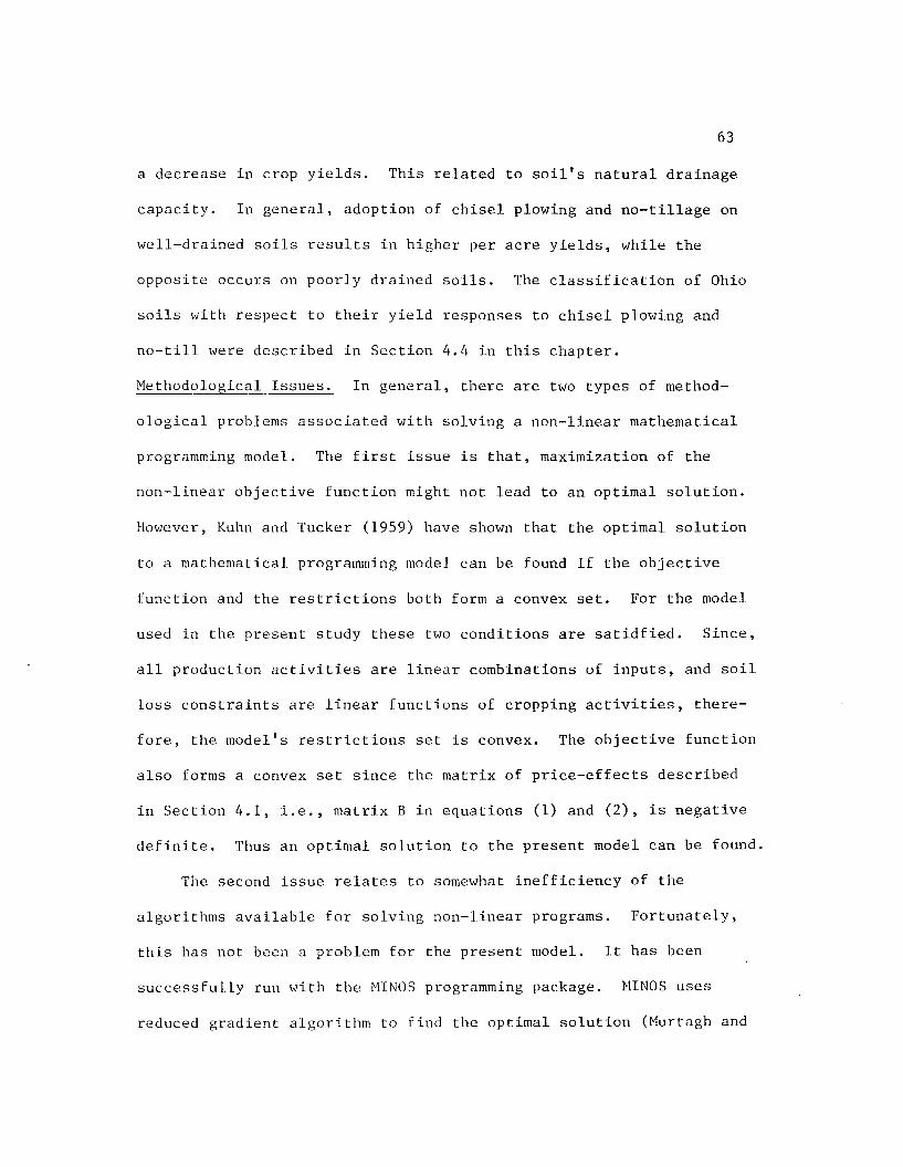
63

a decrease in crop yields. This related to soil's natural drainage

capacity. In general, adoption of chisel plowing and no-tillage on

well-drained soils results in higher per acre yields, while the

opposite occurs on poorly drained soils. The classification of Ohio

soils with respect to their yield responses to chisel plowing and

no-till were described in Section 4.4 in this chapter.

Methodological Issues. In general, there are two types of method­

ological problems associated with solving a non-linear mathematical

programming model. The first issue is that, maximization of the

non-linear objective function might not lead to an optimal solution.

However, Kuhn and Tucker (1959) have shown that the optimal solution

to a mathematical programming model can be found if the objective

function and the restrictions both form a convex set. For the model

used in the present study these two conditions are satidfied. Since,

all production activities are linear combinations of inputs, and soil

loss constraints are linear functions of cropping activities, there­

fore, the model's restrictions set is convex. The objective function

also forms a convex set since the matrix of price-effects described

in Section 4.1, i.e., matrix B in equations (1) and (2), is negative

definite. Thus an optimal solution to the present model can be found.

The second issue relates to somewhat inefficiency of the

algorithms available for solving non-linear programs. Fortunately,

this has not been a problem for the present model. It has been

successfully run with the MINOS programming package. MINOS uses

reduced gradient algorithm to find the optimal solution (Murtagh and

64

Saunders (1977).

CHAPTER V

RESULTS

This chapter is comprised of five sections. The first section

describes the major model scenarios of the analysis. The second

section discusses the cropland use patterns under the alternative

tillage methods and the land use impacts from limiting annual

erosion to soil loss tolerance levels, or T-values. The changes in

erosion rates resulting from soil conserving tillage practices and

soil loss restrictions are presented in the third section. The

fourth part discusses the impacts on agricultural production, farm

prices, crop exports, farmers* net returns,and consumers' surplus

from tillage system substitutions and T-value restrictions on soil

loss. The results of sensitivity analysis pertaining to some

potential expansions in grain exports and industrial demand for

corn are presented in the fifth section.

5.1. Major Model Scenarios. To achieve the study objectives, model

simulations reflecting three different tillage systems, with and

without restrictions on soil loss were analyzed. The six principal

model scenarios are listed in Table 5.1.1.

The Base Run (Scenario I) simulates Ohio's agricultural

economy under current demand levels, assuming that conventional

tillage (fall molboard plow) is practiced on all soil groups. Scen­

arios II and III replace this assumption by using reduced tillage

6 5

Table 5.1.1

Major Model Scenarios

66

Model Scenario Tillage System Soil Loss Restriction

I (Base Run) Conventional None

II Chisel Plow None

III No-Tillage None

IV Conventional at T-value

V Chisel Plow at T-value

VI No-Tillage at T-value

(fall chisel plow) and no-tillage on all economically suitable soils,

respectively. Scenarios IV,V, and VI add the soil loss restrictions

to the model under each of the three tillage systems. On soils where

farm net income is significantly reduced with chisel plowing or

no-tillage, conventional tillage is used.

5.2 Cropland Utilization Under Alternative Tillage Methods, withand without Restrictions on soil loss

Aside from their long-run soil conservation and environmental

benefits, the economic impacts of soil conserving tillage systems on

farmers' cropland use decisions consist of two major factors:

1) variation in crop yields;

2) changes in per acre costs of certain inputs.

Crop yield differences by tillage systems are related to soil drainage

67

capacity. As described in the previous chapter, adoption of chisel

plowing and no-tillage on well-drained soils will result in higher

yields per acre, while the opposite occurs on poorly drained soils.

The use of the above soil conserving tillage methods on farmland

with severe drainage problems is considered to be economically

unsuitable because of resulting in depressed yields. In terms of

their suitability and yield response to soil conserving tillage

practices, Ohio soils can be placed into four major soil management

groups. These soil management groups which have been incorporated

in the present study were described in Chapter IV. Table 5.2.1

shows the changes in crop yield levels pertaining to the four

soil management groups under alternative tillage systems.

Tab 1e 5.2.1

Changes in Ohio Crop Yield Levels by Soil Management Group and TillageTillage System

Management Group Conventional Conservation No-Tillage

1 100 105 110

2 100 100 100

3 100 NA NA

4 100 95 95

Source: Eckert (1983).

68

Substitution of tillage system also affects production costs,

depending on cropping patterns and the type and quantity of inputs

required. However, the changes in cost levels for specific components

of the tillage systems such as machinary or chemicals is often greater

than the difference in overall costs. For example, compared to con­

ventional tillage, production of corn under a no-tillage system

demonstrates substantial savings in costs of machinary, repairs, fuel,

and labor, while, it increases substantially the application levels and

costs of chemicals. Specific changes in per acre production costs of

Ohio's major crops, resulting from substitution of conservation tillage

systems are presented in Table 5.2.2.

In Ohio, because of regional differences in soil types and

agricultural activities, statewide adoption of soil conserving tillage

methods, especially, on the basis of changes in crop yields, would

have a major impact on the State's cropland use patterns. Simulated

cropland use patterns in Ohio under the three tillage systems, with

and without T-value restriction of soil loss (Scenarios I-VI) are

presented in Table 5.2.3.

In the absence of soil loss restraints, under each tillage

method (Scenarios I-III), the State's currently available cropland

(appriximately, 11,250,000 acres) is completely utilized. However,

substitution of soil conserving tillage systems for conventional

tillage on all adaptable farmland would result in a transfer of up to

200,000 acres from corn, small grains, and forages to soybeans. This.

Table 5.2.2

Changes in Per Acre Production

1'nder Conservation 1

i Costs

ii iiayo

o : Oh i o '

Systems

s Maji r Crops

corncorn

andsilage soybeans wheat oats a 11 n 1 f a grass

hay

Ti l l a g e : A B A B A B A B A B A B

Inputs ( S per acre)

Chemicals +3.6 + 12.0 +2.0 +12.7 - +6.0 - +6.0 NA + 8 . 5 NA + 8 . 5

Repairs -2.4 - 5.3 -2.2 - 5.8 -2.6 -5.0 -2.9 -5.3 NA - 3.6 NA - 3.3

Fuel -0.7 - 2.7 -0.8 - 2.8 -0.8 -1.6 -0.8 -1.6 NA - 1 . 3 NA - 1 . 6

Labor -1.4 - 4.3 -0.5 - 4.5 -1.4 -3.6 -1.4 -4.0 NA -14.0 NA -10.8

Net Difference -0.9 - 0.3 -1.5 - 0.4 -4.8 -4.2 -5.1 -4.9 NA -10.4 NA - 7.2

A :chisel plow vs. conventional tillage Source: Complied based on '‘Ohio Farm Machinary EconomicB :no-tillage vs. conventional tillage Cost Estimates for 1983" ( 63 ), and "Ohio cropX a : data not available Enterprise Budgets for 1984" ( 64 ).

CTnvo

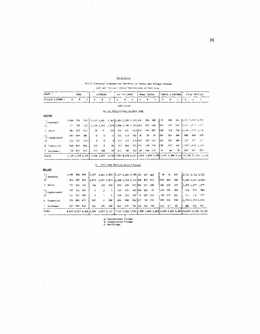
70

Table 5.2,3

Ohio's Simulated Cropland Use Patterns, by Region and Tillage Methods

-tch and ’-'lthout T-Value cestrlctions on Soil Loss

ALL ROW CROPS SMALL CRAINS rORAOE & PASTURE TOTAL rRrP’ANU

TILLAGE SYSTEMS

(UOO Acres)

a. Nj Restrictions on Soil Loss

196 16-1,066 716

267,886 2,786 2 , 790 |L6)730

120350585502 502

Lnglaclaced166>632-9

157133 119 158212

957 9 b ' 9577656777 Southwest 98

1,7597,995 8,078 8,05'State

b. Soil Loss Restricted to T-Values

11 1,186 840 694 1,137 1,441 1,452 2,323 2,281 2,145 |310 357 409 78 73 157 2,711 2,711 2,711

JCornbelt871 827 962 1,473 1,927 1,813 2,344 2,754 2,776 434 457 512 575 302 226 3,353 3,513 3,513

3 Dairy 713 590 538 120 109 114 833 695 632 295 53“ 508 341 239 315 1,469 1,475 1,475

245 370 461 0 0 0 245 370 461 140 106 35 234 395 384 619 871 880'

57Unglaciated

251 253 249 4 c C 234 253 249 94 129 142 8, 174 166 A Z 2 356 357

6 Transition 530 B92 673 121 6 189 651 698 862 307 92 133 195 163 158 1,153 1,153 1,153

7 Suuthwest 217 545 632 245 130 159 462 675 791 310 214 84 113 67 81 885 956 95t

State 4,012 4,317 4,209 3,100 3,607 3,727 7,112 7,924 7,936 1.89C 1,892 1,823 1,620 1,413 1,407 10,622 11,235 11,245

A: Conventional Tillage B: Conservation Tillage C: No-Tillage

71

reallocation would occur as a result of higher net returns per acre

associate with growing soybeans under conservation tillage practices,

on specific soil groups . (See the succeeding section on regional

impacts.)

Under conventional tillage practices, implementation of the

soil conservation policy (Scenario IV vs. I) would force Ohio farmers

to remove nearly six percent ( approximately, 650,000 acres) of the

State's currently utilized cropland from production. This adjustment

would consist of a 900,000 acre (11 percent) reduction in row crops,

a nearly 200,000 acre (14 percent) increase in forages and pasture,

and a 50,000 acre (3 percent) expansion in small grains.

Adoption of chisel plowing or no-tillage on all suitable soils,

however, would largely eliminate the need for these changes, since the

two soil conserving tillage methods would potentially drop the average

annual erosion rate on Ohio farmland to a level very close or even

below the State's average T-value.(See Section 5.3 for details.) With

chisel plow and no-till, respective impacts of soil loss constraints

on the State's total row crop acreage would only be a 2 and 1 percent

reduction (vs. the 11 percent with conventional tillage). As a result,

the expansion in forages and pasture acreage would only be 4 percent

(compared to the 14 percent under conventional tillage).

Regional cropland use changes resulting from substitution of

soil conserving tillage system for conventional tillage and T-value

restriction of soil loss would be more substantial than the overall

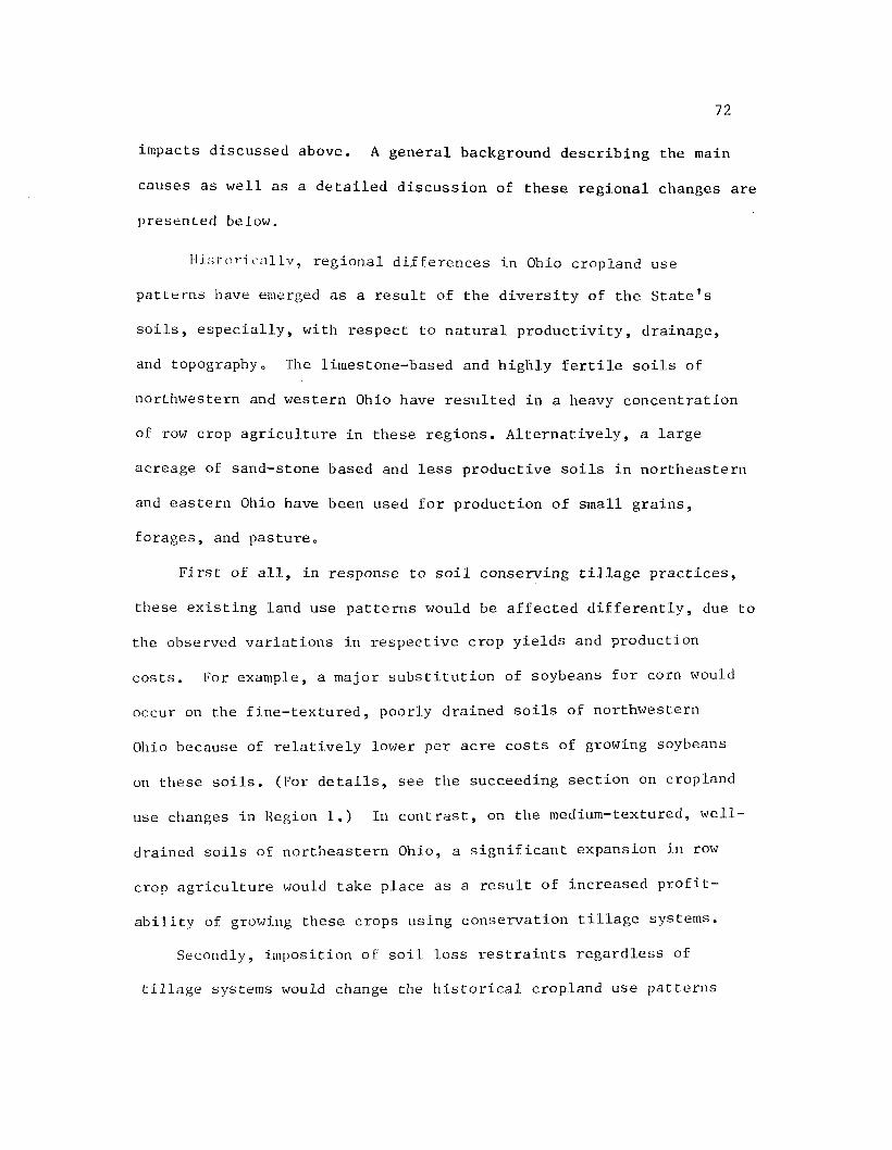
72

impacts discussed above. A general background describing the main

causes as well as a detailed discussion of these regional changes are

presented below.

Historically, regional differences in Ohio cropland use

patLerns have emerged as a result of the diversity of the State's

soils, especially, with respect to natural productivity, drainage,

and topographyo The limestone-based and highly fertile soils of

northwestern and western Ohio have resulted in a heavy concentration

of row crop agriculture in these regions. Alternatively, a large

acreage of sand-stone based and less productive soils in northeastern

and eastern Ohio have been used for production of small grains,

forages, and pasture,,

First of all, in response to soil conserving tillage practices,

these existing land use patterns would be affected differently, due to

the observed variations in respective crop yields and production

costs. For example, a major substitution of soybeans for corn would

occur on the fine-textured, poorly drained soils of northwestern

Ohio because of relatively lower per acre costs of growing soybeans

on these soils. (For details, see the succeeding section on cropland

use changes in Region 1.) In contrast, on the medium-textured, well-

drained soils of northeastern Ohio, a significant expansion in row

crop agriculture would take place as a result of increased profit­

ability of growing these crops using conservation tillage systems.

Secondly, imposition of soil loss restraints regardless of

tillage systems would change the historical cropland use patterns

73

in Ohio on the basis of regional differences in topography, erosion

susceptibility, and soil loss tolerance levels (T-values). In

general, the direction of regional cropland use changes resulting

from soil loss restraints would be a fairly significant expansion

of row crop agriculture on less erosive soils of northwestern and

northeastern Ohio in conjunction with restriction of corn and

soybeans production on more erosive soils, especially, in western,

southwestern, and eastern regions.

A. Land Use Changes in Northwestern Ohio (Region 1)

As described in Chapter III, most of northwest Ohio's cropland

is level and is comprised of highly fertile and poorly-drained clay

soils such as Hoytville, Pewamo, Paulding, and Toledo. As a result,

excessive surface water rather than erosion has been the dominant

agricultural hazard in this region. Historically, row crop agri­

culture has occupied more tahn 80 percent of the region's cropland

under conventional tillage systems.

In this region, the main impacts of replacing moldboard plow­

ing with conservation tillage systems would be the following.

1) A major susbstitution of soybeans for corn would take

place on almost 10 percent (250,000 acres) of the region's cropland.

The substitution would primarily occur on soil group 8 which is

comprised of the poorly drained soils, i.e„, Latty and Toledo. On

these soils, adoption of conservation tillage practices results in

five percent yields, and hence five percent less gross returns.

(See Table 5.2.1.) Production of soybeans on these soils, however,

74

would result in a smaller reduction in net returns than corn by2/almost $4.00 per acre — .

2) Nearly 8 percent (80,000 acres) would be transferred from

corn to wheat on the well-drained, moderately productive soils

such as Haskins and Rimer.

The major conclusions from imposing T-value soil loss

restrictions on northwestern Ohio cropland are the following.

1) There would be no impact on the region's total acreage of

utilized cropland resources. This is the State's only region in

which the average annual erosion per acre, under conventional tillage

practices, is less than the average T-value. (See section 5.3 for

details.) As a result, limiting soil loss to T-values would not

restrain utilization of northwest Ohio's cropland resources.

2) The region's row crop acreage would be expanded by nearly

6 percent in response to reduction of row crop acreage in the

State's more erosive regions (i,e., 2, 4, 6, and 7). With moldboard

or chisel plowing about 120,000 acres of well-drained soils of

average productivity (e.g., Bennington and Fulton) would be shifted

from wheat to com. In return, almost an equal amount of land of

less fertile soils such as (Seward and Tedrow) would be transferred

from oats and pasture to wheat production. The primary reason for

a major reduction in oats and pasture acreages in northwest Ohio

would be a substantial expansion in producing these crops in regions

2,6,and 7 because of imposing soil loss restraints.

7 5

B . Land-Use Changes in Western and Southwestern Ohio(Regions 2 and 7)

More than 90 percent of western Ohio cropland has slopes of

less than six percent and nearly two-third of the soils in this region

are well- to fairly well-drained. Region 2 has the State's largest

portion of cropland (31 percent), the largest of row crop acreage

(36 percent), and the most fertile soils such as Brookston, Pewamo,

Crosby, Celina, and Blount. In contrast southwestern Ohio

comprises one of the State's smallest cropland regions. (It ranks the

fifth among the seven regions in terms of cropland acreage) , In

addition to the major soils of western Ohio, this region includes

more erosive and less fertile soils such as Hagerstown, Russel,

and Rossmoyne.

In these regions, the most noticeable cropland use changes

stemming from conservation tillage practices would be: a moderate

substitution of small grains and pasture for row crops on the poorly-

drained soils such as Raub, Wetzel, and Montgomery.

In region 2, nearly three percent (100,000 acres) of total row crop

acreage would be transferred to wheat and pasture. Similarly, in region

7, about 8 percent (60,000 acres) of corn would be shifted to wheat

production. Substitution of wheat and pasture for row crops in

regions 2 and 7 would take place, primarily, because of two

reasons: (i) a major substitution of row crops for wheat on

the well-drained soils of regions 3,4, and 6; and (ii) a relatively

7 6larger reductions in per acre costs of wheat and pasture using

conservation tillage (Table 5.2.2).

Under conventional tillage systems, T-value limitations of

soil loss would cause the following changes in these regions'cropland

utilization.

(1) A relatively small portion of total cropland would be

removed from production.

In western Ohio, the area to be set aside from production would amount

to approximately five percent (160,000 acres) of total cropland. In

southwestern Ohio, this adjustment would be close to seven percent

(70,000 acres) of total cropland.

(2) A major reduction in row crop acreage and a 1arge

expansion in forages, pasture, and small grain acreages would occur

on more sloped soil groups, i.e., 19 and 21.

In region 2, soybeas acreage would be reduced by nearly 31 percent

(670,000 acres). Almost 20 percent (125,000 acres) of this area may

be shifted to corn, nearly 60 percent (400,000 acres) would be trans­

ferred to forages and pasture, and the remaining 20 percent would be

left unutilized. In summary, imposition of soil loss restraints

would cause a 20 percent (550,000 acre) reduction in western Ohio's

total row crop acreage and more than a 250 percent increase in the

region's acreages of hay and pasture-on-cropland.

In Southwestern Ohio, the decline in row crop acreage would be

considerably sharper than in region 2, because of a proportionally

heavier concentration of these crops on more erosive soils such as

7 7

Xenia, Miamian, and Cincinnati. Specifically, region seven's

total row crop acreage would decrease by 45 percent or nearly

400,000 acres. While small grain agriculture is this region would

expand by almost 700 percent.

Under conservation tillage systems, T-value erosion control

limitations would place no restraint on utilization of total cropland

resources in western and southwestern Ohio. Nevertheless, some minor

changes in land-use composition of these regions similar to those under

conventional tillage systems would still prevail (Table 5.2.3).

C. Changes in Land-Use Patterns in Northeastern Ohio(Region 3)

Similar to northwestern Ohio, more than 80 percent of the

cropland in northeastern Ohio is level to moderately-sloped. However,

most of the region's soils are sandstone, well-drained, and less

productive . In terms of the total cropland acreage, after regions 2

and 1, region 3 ranks the third among the seven regions. Dairy

and livestock production comprise northeast -Ohio's main agricultural

activities. Historically, row crop agriculture has occupied only one-

third of this region's cropland. Forages, pasture, and small grains

have been grown on nearly two-third of the cropland.

A significant substitution of row crops (mainly soybeans)

for pasture and wheat would be the main land-use impact of con­

servation tillage systems in northeastern Ohio. Specifical.lv, row-

crop acreage would be expanded by approximately 20 percent (100,000

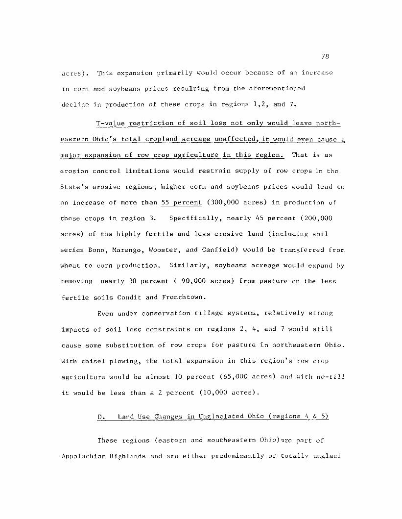
7 8

acres). This expansion primarily would occur because of an increase

in corn and soybeans prices resulting from the aforementioned

decline in production of these crops in regions 1,2, and 7.

T-value restriction of soil loss not only would leave north­

eastern Ohio's total cropland acreage unaffected, it would even cause a

major expansion of row crop agriculture in this region. That is as

erosion control limitations would restrain supply of row crops in the

State's erosive regions, higher corn and soybeans prices would lead to

an increase of more than 55 percent (300,000 acres) in production of

these crops in region 3. Specifically, nearly 45 percent (200,000

acres) of the highly fertile and less erosive land (including soil

series Bono, Marengo, Wooster, and Canfield) would be transferred from

wheat to corn production. Similarly, soybeans acreage would expand by

removing nearly 30 percent ( 90,000 acres) from pasture on the less

fertile soils Condit and Frenchtown.

Even under conservation tillage systems, relatively strong

impacts of soil loss constraints on regions 2, 4, and 7 would still

cause some substitution of row crops for pasture in northeastern Ohio.

With chisel plowing, the total expansion in this region's row crop

agriculture would be almost 10 percent (65,000 acres) and with no-till

it would be less than a 2 percent (10,000 acres).

D. Land Use Changes in Unglaciated Ohio (regions 4 & 5)

These regions (eastern and southeastern Ohio)are part of

Appalachian Highlands and are either predominantly or totally unglaci

7 9

ated. As a result, the topography in 40-60% of cropland ranges from

hilly to rough. They include the State's most erosive and less fertile

sandstone soils such as Musk ingum,Clymer,Zanesville, and Coolville.

Among the seven regions, eastern and southeastern Ohio comprise the

State's smallest portions of cropland as well as the smallest shares

of row-crop agriculture.

Similar to the northeast, adoption of conservation tillage

methods would encourage a major substitution of corn for forages and

pasture in eastern Ohio. The corn-to-pasture substitution would be

up to a 30 percent (150,000 acre) expansion in region 4's row crop

acreage.

Since eastern and southeastern Ohio have the largest proportions

fo rolling and hilly cropland, impacts of T-value limits on these

regions' cropland utilization would be the strongest among the

seven regions. Under conventional tillage, imposition of soil loss

constraints would cause the following land-use changes to take place.

(1) In eastern Ohio, approximately 30 percent (270000 acres)

of total cropland would be removed from production. As a result, the

region's row crop (corn) acreage would decline by nearly 50 percent.

Almost half of this area (formed of soil groups 20 and 37-40) would be

transferred to oats and the other half would be set aside. The rest of

cropland to removed from production would mostly consist of soil group

59 which includes the poorly fertile soils such as Muskingum with

slopes of 12-18 percent.

8 0

(2) In Southeast Ohio, about 22 percent (125,000 acres) of

total cropland would be removed from productions of small grains,

forages, and pasture. This adjustment would take place on the

region's marginal and highly erosive soil groups 35-41,59,62, and

70-77. Row crop acreage would not be restrained in this region.

Corn acreage would be expanded by nearly 5 percent (10,000 acres) on

the highly fertile and level soil Lindside (soil group 3). The minor

increase in this region's row crop acreage would occur as a result of

the sharp decline in row-crop agriculture on more erosive soils of

regions 2, 4, and 7.

Under conservation tillage systems, the impacts of soil loss

constraints on these regions' total cropland acreage would be

negligible. However, in region 4, a substantial decline in row-crop

agriculture and a large expansion in small grains production would

still take place (Table 5.2.3).

E. Cropland Use Changes in Central Ohio (Region 6)

This region is the so-called transitional area between the

highly fertile, limestone soils of western- and the predominantly

less productive, sandstone and shale soils of eastern Ohio. The

topography on more than 85 percent of central Ohio cropland is level

to moderately sloped and nearly 2/3 of the region's soils are well-

to fairly well drained. Historically, row crops have been grown on

almost 70%, small grains on about 20%, and forages and pasture on

81

nearly 10% of this region's cropland.

Statewide substitution of conservation tillage methods for

conventional tillage would result in a considerable substitution of

corn for soybeans and small grains in central Ohio.

With chisel plowing, the land displacement would consist of a 30 per­

cent (200,000 acre) expansion in corn acreage, a complete ( 115,000

acre) removal of land from soybeans, and nearly 40 percent (80,000 acre)

reduction in small grains. With no-tillage, however, the land-use

changes would be somewhat moderate. That is^a 20 percent increase in

corn, 50 percent decrease in soybeans and a 44 percent reduction in

small grains. In both cases, the corn-for-soybeans substitution would

take place, primarily, because of the mjor soybeans-for-corn substitu­

tion on the poorly-drained soils of region 1. Similarly, substitution

of corn for small grains in central Ohio would occur in conjunction

with the described wheat-for-corn substitution in region 7.

Statewide restriction of soil loss to T-values would not

restrain utilization of available cropland resources in central Ohio.

However, under conventional tillage, the region's total row crop

acreage would be reduced by nearly 17 percent (130,000 acres),

corn production would become more intensified on the region’s level

soil groups (5-15), while, it would be diminished or discontinued on

more erosive soil groups 19,20, and 31-37. Approximately, 3/4 of the

land to be removed from corn would be shifted to wheat and the balance

would be used for forages and pasture on the region's most erosive and

less productive soils groups 70-77. With chisel plowing, cropland use

8 2impacts of soil loss restrictions in central Ohio would be very

moderate. It would be a minor substitution of small grains for corn.

On the other hand, under no-tillage sytem, enforcement of T-value

limits on soil loss would cause a major soybeans-for-corn substitution

in region 6. That is, as soil loss constraints raise soybeans prices

by depressing its production in western Ohio, they would stimulate a

transfer of nearly 15 percent (135,000 acres) from corn to soybeans

on the moderatley erosive soils in central Ohio (Table 5.2.3).

5.3 Soil Erosion Impacts of Alternative Tillage Systems on Ohio Cropland with and without Limiting Annual Soil Loss to T-values

Based on the cropland use patterns described in the preceding

section, average annual erosion rates (soil losses per acre per year)

for the State as a whole, as well as the seven regions were computed.

Soil loss computations for each soil group, under each model

scenario , were performed through the Universal Soil Loss Equation

(USLE). A detailed discussion of the USLE and the procedure of

estimating its factors for Ohio soils was presented in Chapter IV.

Ohio's simulated annual erosion rates under each of the six model

scenarios are presented in Table 5.3.1. These results are described

below.

1) Under conventional tillage systems the erosion impacts

associated with the aforementioned cropland use patterns would be

the following.

With no restrictions imposed on soil loss, the average

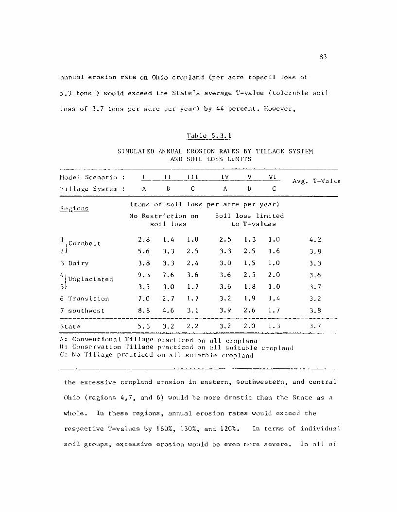
83

annual erosion rate on Ohio cropland (per acre topsoil loss of

5.3 tons ) would exceed the State's average T-value (tolerable soil

loss of 3.7 tons per acre per year) by 44 percent. However,

Tab le 5.3.1

SIMULATED ANNUAL EROSION RATES BY TILLAGE SYSTEM AND SOIL LOSS LIMITS

Model Scenario : I 11 III IV V vi T-ValueAvg.i illage Sys tern : A B C A B C

Regions (tons of soil loss per acre per year)No Restriction1 on Soil loss limited

soil loss to T-values

^.CornbeIt 2.8 1.4 1.0 2.5 1.3 1.0 4.22) 5.6 3. 3 2.5 3.3 2.5 1.6 3.83 Dairy 3.8 3. 3 2.4 3.0 1.5 1.0 3.34)(Unglaciated 9.3 7.6 3.6 3.6 2.5 2.0 3.65) 3.5 3.0 1.7 3.6 1.8 1.0 3. 76 Transition 7.0 2.7 1.7 3.2 1.9 1.4 3.27 southwest 8.8 4.6 3. 1 3.9 2.6 1.7 3.8

State 5.3 3.2 2.2 3.2 2.0 1.3 3. 7

A: Conventional Tillage practiced on all croplandB : Conse rva t i 011 Tillage practiced on all suitable t■ roplandC: No 'Ullage practiced on all suiatble cropland

the excessive <cropland erosion in eastern, southwestern, and central

Ohio (regions 4,7, and 6) would be more drastic than the State as a

whole. In these regions, annual erosion rates would exceed the

respective T-values by 160%, 130%, and 120%. In terms of individual

soil groups, excessive erosion would be even more severe. In all of

8 4

the seven regions, a number of major soils would erode at annual rates

considerably higher than the regional average rates.

For example, in northwestern Ohio, under the described

cropping patterns, the average per acre soil loss would be 33 percent

less than the region's average T-value, while a major soil,

i.e„, Blount, would erode at a rate 225% higher than its corresponding

T-value. Similarly, in western Ohio, annual erosion on three

principle soils, i.e., Miamian, Celina, and Blount (comprising nearly

26% of the region's cropland), would be 250-350 percent greater than

the pertinent T-values. An example of a more rigorous case would be

in region 4, where, annual soil loss rate on soil group 56 (forming

almost 10% of the regions cropland) would exceed its corresponding

T-value by more than 600 percent.

2) Switching to conservation tillage (chisel plowing) on all

adaptable soils, would drop the average annual erosion rate on Ohio

cropland to a level 14 percent below the State's average T-value.

Nevertheless, the excessive erosion in eastern and southwestern Ohio

still would remain approximately 120 percent above the pertinent

T-values (Table 5.3.1). Also, in all regions,except in the northwest,

excessive soil loss on highly erosive soil groups such as groups 22

and 75 in regions 2 and 7, and group 38 in regions 3,4,6, and 7

still would prevail.

3) Adoption of no-tillage on all suitable soils would

reduce the annual erosion on Ohio cropland to a level nearly

8 5

40 percent below the State's average T-value. In this case,

on average, none of the seven regions would suffer from excessive

erosion (Table 5.3.1). However, excessive soil loss on a total of

ten soil groups having slopes of higher than 6 percent still would

persist.

5.4. Economic Impacts Associated with Tillage Systems Substitutionand T-value Restriction of Soil Loss.

As described in Section 5.2, statewide substitution of

conservation tillage practices for conventional tillage, and T-value

restriction of soil loss would each result in a number of major

changes in regional cropland use patterns in Ohio. This section

discusses the potential economic impacts associated with these land-

use changes in terms of the State's agricultural production, farm

prices, crop exports, net returns to farmers, and consumers' surplus.

A. Economic Impacts Associated with Change to Conservation Tillage Systems

At the State level, soil conserving tillage practices would

have a moderate impact on Ohio's agricultural economy. However,

regional economic changes stemming from these tillage systems would

be more noticeable (Tables 5.4.1 and 5.4.2).

Under chisel plowing, total production levels of corn, soy­

beans, wheat and oats would increase at respective rates of 0.6, 1.4,

0.6, and 1.0 percent. With no-tillage, however, corn and soybeans

production would increase at a higher rate, i.e., 1.6 and 2.5 percent

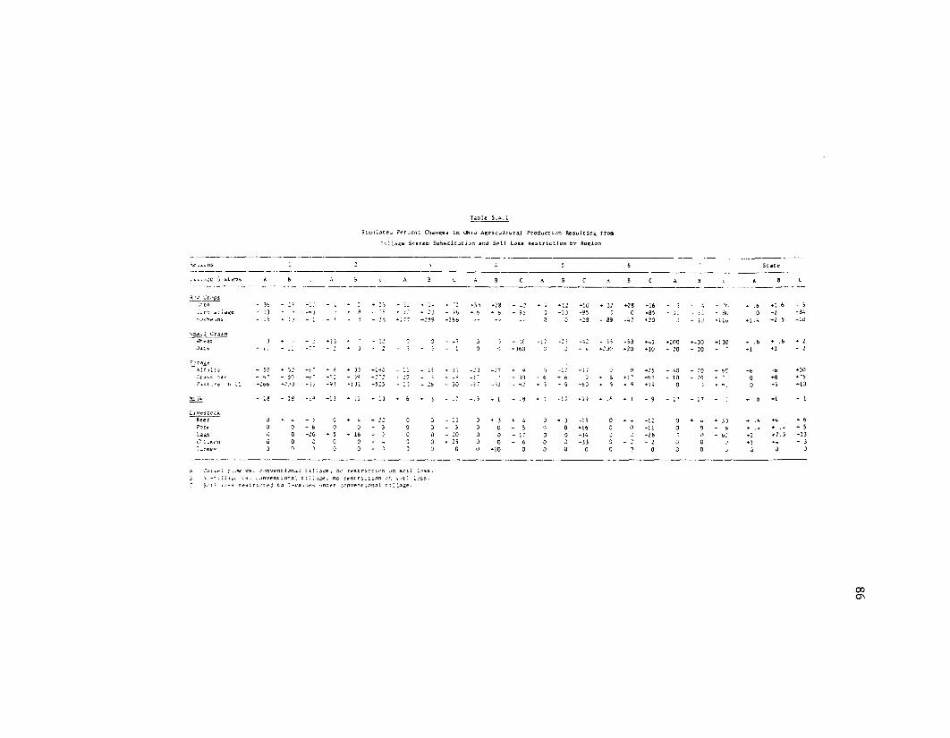
Ta bl e 5 .4 . 1

Siauiacea Percent Changes in d u o Agricultural Production Resulting froo Tillage Svsteo Substitution and Soil Loss Restriction bv Region

A«* _ic ns 6 State

c. IL.jiC 5 • stec.s A 8 3 c A 8 *- A c A c A C A 3 A B

Row Cr. Ps-icrn - 56 - 2' •1 0 - * - • I S ♦ i: * 1- - ■: •33 •28 - .2 • - *12 *lu * 32 *28 -16 - 5 - - V, * . ♦ 1.6 - 3.cm Si! a<e - 13 - -i -* i - - ■; * • 20 - ib * b * 0 - 93 0 -i 0 -85 0 -85 - ;; - - 60 0 -2 -64*> ovbe m s * 15 - 1 -• * 1 - 1 - - 2 5 * •:?9 •266 ~ " o 0 -23 - 89 --7 *20 0 - 10 *1 iv *1.9 *2.5 -10

Ssa.l Crain■heat •J * 0 * J *13 * - i2 0 - j 0 - :c -2 i -a: - 3 3 -58 *200 *-00 +1 30 - .6 + .6 * 2Cat s “ L- " * * * - * - 2 ■ > 0 0 *360 3 0 ■ 4 *200 *20 *10 - 20 - 10 ’ *1 *1

' 2Alfa! : j * 50 * 52 „C - * A , 33 •1 •yC - 13 ♦ i n -2 3 -27 * 9 r -17 0 0 *25 - A0 20 . A-- -6 -o ♦30Crass nav - - 3r- — :' • 'j - N •2*2 - 1? - 3 - .A -1* ■> - 30 * 6 • 6 0 * 8 *1" *67 - 10 - 20 - . 0 ♦8 * '5Past re n LL -2ee> *:jc -9 3 31 •515 - 15 - 2b - 30 -32 - n: * 3 * 9 -60 • 5 * q *19 0 * n; 0 *> *10

Hi ik - 18 - 18 - * ♦13 * 13 - 13 * .6 - 3 - -- -. 5 * i - .8 • 1 -1? -19 - .6 * 1 - 9 - 17 - 17 - : ♦ .6 +1 - 1

LivestocASee t 0 * 4 - ; 0 * ♦ 22 0 0 - 13 0 * 3 * u 0 * 3 -15 0 • 4 -i: 0 + i. * 33 * .4 *4 * 6?or« 0 0 - fc 0 LI - 3 0 0 - 5 0 0 - 5 0 0 *16 0 0 -11 0 0 - 6 ♦ .4 ♦ .- * 5Ugs 0 0 -:o ♦ 5 - 16 - 5 0 0 - 20 0 0 - i: 0 0 -14 0 -28 0 - ei *7.3 -13CH;ck •n 0 0 o 0 0 - - o • 25 0 0 - 6 0 0 -33 0 - 2 - 2 0 0 _• *1 ♦4 - 3T -ruev 3 0 n 3 0 i 0 0 0 *10 0 0 0 0 0 0 0 0 0 - cl 0 3

A C.u,t*; r.ov vs. conventional tillage, no restriction on soil loss, j. -rill ui vs. conventional til..ice. no restriction or. -.c-il loss.

S.ii i.o* restricted co T-va»cej> unaer conventional ttllaae.

00ON

Table 5.4.2

Simulated Percent Changes in Ohio Agricultural Prices Resulting from Tillage System Substitution and Soil Loss Restriction by Region

Regions 1 + - * 5 6 7 State

Scenarios A B C A B C A B C A B C A B C A B C A B C A B C

Row CropsCorn _2 -6 + 19 _2 - 6 + 18 - 2 - 6 *19 _ i - 6 + 19 -2 - 6 +16 _ -i -6 + 19 -6 + 19 -2 - 6 -19Corn silage -I -b *-L j - 2 - 6 + 19 _ ^ - 6 + 19 -2 - 6 -19 _ T - 6 + 16 -2 - b + 19 _ T -6 -19 -2 - 6 + 19Soybeans -3 -8 *25 -3 - 8 +26 - 3 - 8 +22 -3 - 8 +26 -3 - S +26 -3 -8 +26 - 3 -3 + 2 5 -3 - B +2 5

Small CrainWheat -3 -5 + 16 -4 - 8 - 8 - 6 -10 + 2 -5 - 9 - 4 —4 - 8 - 8 -3 -8 - 3 -4 -8 - 8 -4 - 9 _ -)Oats -1 -6 +16 -3 -10 -10 -27 -31 -14 -5 -11 -10 -6 -11 - 8 -5 -9 - - -3 -8 -12 -8 -12 - 7

Milk -1 -3 + 12 -2 - - - 2 _ 2 - 4 + 3 -2 — 4 + 1 - 3 + 2 -1 -3 + 3 -1 -3 0 - 3 + 3

LivestockBeef -1 -6 0 -1 - 6 -10 - 2 - 7 + 6 +3 - 2 + 3 -1 - 7 _ 2 _2 -7 - 1 -.2 -6 - 9 -1 - 6 - 3Pork -1 +12 -1 - <4 +11 - 2 - 5 +11 -1 - 4 + 12 -1 - 4 +11 -2 -4 +12 1 -4 + 11 -1 - 3 + 11

_ 2 -5 + 12 _2 - 5 + 9 - 2 - 5 + 8 -2 - 5 + 9 —4. - 5 + 9 -2 -5 + 9 -2 -5 + 9 -2 - 5 + 9Broilers and -2 -4 +-13 -2 - 4 +13 - 2 - 4 + 13 -2 - 4 +13 -2 - 4 +13 -2 —4 +13 _2 -4 +13 -2 - 4 + 13turkeys

A: Conservation tillage vs. conventional tillage no soil loss restriction. B: No-cillage vs. conventional tillage no soil loss restriction.C: Soil loss restricted to T-values with conventional tillage.

00

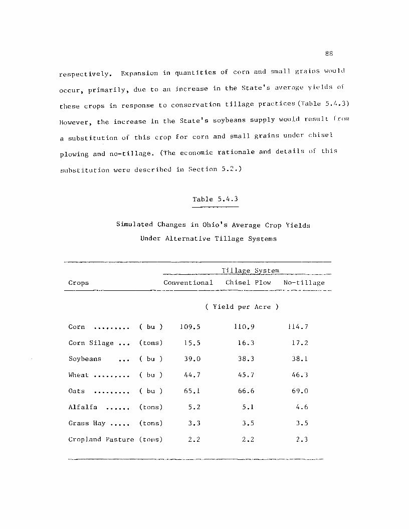
8 8

respectively. Expansion in quantities of corn and small grains would

occur, primarily, due to an increase in the State's average yields ol

these crops in response to conservation tillage practices(Table 5.4.3)

However, the increase in the State's soybeans supply would result from

a substitution of this crop for corn and small grains under chisel

plowing and no-tillage. (The economic rationale and details of this

substitution were described in Section 5.2.)

Table 5.4.3

Simulated Changes in Ohio's Average Crop YieldsUnder Alternative Tillage Systems

CropsTillage System

Conventional Chisel Plow No-tillage

( Yield per Acre )

Corn ......... ( bu ) 109.5 110.9 114.7

Corn Silage ... (tons) 15.5 16.3 17.2

Soybeans ( bu ) 39.0 38.3 38.1

Wheat ......... ( bu ) 44.7 45.7 46.3

Oats ......... ( bu ) 65.1 66.6 69.0

Alfalfa ..... (tons) 5.2 5.1 4.6

Grass Hay .... (tons) 3.3 3.5 3.5

Cropland Pasture (tons) 2.2 2.2 2.3

89In response to expansion in crop production levels under

chisel plowing, the State's average prices of corn, soybeans, and

wheat would fall by nearly 2, 3, and 4 percent, respectively.

Average prices of these commodities would fall even more noticeably

with no-tillage, i.e., by 6, 8, and 9 percent respectively. As a

result, quantities of corn, soyebeans, and wheat exported would

increase, (3,4, and 4 percent, respectively). Also, the rise in

supply and the fall in prices of major feed crops (i.e., corn,

soybeans, and oats) would induce a small increase in production and

a minor decrease in the State's average prices of milk, beef,

pork, poultry meat, and eggs (Table 5.4.2).

Substitution of chisel plowing and no-tillage for con­

ventional tillage would also increase the State's economic surplus

from the farm sector (i.e., farmers' net returns + consumer's

surplus) by 1.5 and 5.5 percent, respectively. Specifically,

because of the higher production levels and lower prices, under

the two tillage systems consumers' surplus would rise by nearly

4 and 13 percent. However, for the same reasons, farmers' net

returns would decline , approximately, by 6 and 14 percent, res­

pectively (Table 5.4.4).

In terms of the changes in crop production and farmers'

net returns, regional impacts of conservation tillage systems would

be much stronger than the State as a whole (Tables 5.4.1, 5.4.2,

and 5.4.4). As described in Section 5.2, production of row crops

would be substantially expanded in northeastern and eastern Ohio,

where, cropland is predominantly well-drained. In contrast, in

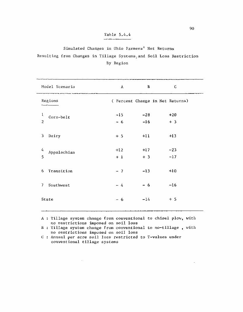
90Table 5.4.4

Simulated Changes in Ohio Farmers' Net Returns Resulting from Changes in Tillage Systems.and Soil Loss Restriction

By Region

Model Scenario A B C

Regions ( Percent Change in Net Returns)

Corn-belt -15 -28 +202 - 6 -16 + 3

3 Dairy + 5 +11 +13

Appalachian +12 +17 -235 + 1 + 3 -17

6 Transition - 7 -13 +10

7 Southwest - 4 - 6 -16

State - 6 -14 + 5

A : Tillage system change from conventional to chisel plow, with no restrictions imposed on soil loss

B : Tillage system change from conventional to no-tillage , with no restrictions imposed on soil loss

C : Annual per acre soil loss restricted to T-values under conventional tillage systems

91

western and southwestern Ohio, a large increase in production of

small grains and/or forages in substitution for row crops would

take place. As a result, total net returns to farmers would

noticeably rise in regions 3 and 4, while, they would significantly

decline in rest of the State (Table 5.4.4). The strongest negative

impact on farmers' net returns would occur in northwest Ohio.

In that region, (primarily, because of the yield-depressing-effects

of conservation tillage on poorly-drained soils), farmers' total3/net returns would decline 15-28 percent — .

B. Economic Impacts from T-value Restriction ofSoil Loss

Under conventional tillage systems, T-value limitation of

annual erosion from Ohio cropland would cause a considerable

cut-back in the State's row crop acreage and a major expansion in

acreages of forages and pasture-on-cropland. Major economic impactsVstemming from these land-use adjustments would be the following — .

(1) The State's corn and soybeans production would decline

by 5 and 10 percent, respectively. As a result, prices of these

crops would rise at respective rates of 20 and 25 percent.

3_/ As discussed in Section 5.2, this study has assumed that adoption of conservation tillage methods on poorly-drained soils decreases average crop yields by 5 percent.

4/ Remember from Chapter IV that,based on the proportionaldemand, model assumes similar changes in other major production areas in the nation.

92

(2) Production of forages and pasture would expand upto

75 percent. As a result, shadow prices of hay and pasture-on-

cropland (i.e., oppotunity cost of allocating cropland to these

crops) would decrease by 18 percent.

(3) The changes in production and prices of feed grains,

forages, and pasture-on-cropland would induce:

a) a 6 percent increase in production, and a 3 percent

reduction in price of beef; and

b) respective reductions of 5, 13, and 3 percent in

production of pork, eggs, and poultry meat; and the respective

increases of 11, 9, and 13 percent in prices of these commodities.

(4) As a result of higher corn and soybeans prices, Ohio's

exports of these crops would decline by 10 and 16 percent, respectively.

(5) The cut-back in production and the rise in prices of

major crops and livestock commodities would decrease the farm-sector's

consumers’ surplus by almost 5 percent. However, because of a

relatively large increase in farm prices, total net returns to

farmers would rise nearly 5 percent. Nevertheless, total economic

surplus from the State's farm sector would decline by approximately

2.5 percent. That is, the total loss occuring to consumers from

T-value restriction of soil loss would be greater than the total

gains accruing to Ohio farmers.

(6) Regionally, T—value limitation of soil loss would lead

to a 20 percent rise in farmers' total net returns in regions 1, 3,

and 6, where, cropland is relatively less prone to erosion. In

93

contrast, implementation of this policy would substantially squeeze

farmers' net income in regions 4, 5, and 7 , where, cropland is

highly erosive ( Table 5.4.4). Northwestern Ohio, the State's

least erosive region, would benefit the most among three regions

which would gain from a T-value based erosion control policy. On

the other hand, eastern Ohio farmers would lose the most from

such a policy, as their net returns would decline as much as 25

percent . In western Ohio (region 2), despite a considerable

reduction in soybeans acreage, soil loss restriction would have

the least impact on farmers' net returns. In this region, a major

corn-for-soybeans substitution and the higher row crop prices

resulting from soil loss restraints would increase farmers' total

net returns by nearly 3 percent.

5.5._____ Sensitivity Analysis

In order to investigate sensitivity of the model to some

potential expansions in export and industrial demand for grain and

soybeans, a total of 17 runs were made. They reflect a 5, 10, 15,

and 20 percent increase in export demand for corn, soybeans, and

wheat, and a 60 and 100 percent increase in (domestic) industrial 5/

demand for corn . These scenarios were analyzed under both

conventional and conservation tillage systems, with and without

The 60 and 100 percent increase in industrial demand for corn — refer to 60 and 100 million gallons of alcohol production,

respectively. These levels of alcohol production add a 24 million and a 40 million bushel increase in industrial corn demand to the 40 million bushels of corn which are currently used by the corn sweetner plant at Dayton.

imposing T-value limits on soil loss. In general, the results

indicate that, under conventional tillage practices, soil erosion

and economic impacts from the potential expansions in demand for

grain and soybeans would be fairly strong. Especially, with

T-value restriction of soil loss, the aforementioned levels of

expansion in export demand would cause a sharp increase in crop and

livestock prices. Under conservation tillage systems, soil erosion

impacts from the above changes in demand would be insignificant,

however,the economic impacts would be similar to those under

conventional tillage systems. The following focuses on the results

of conventional tillage scenarios.

A. Impacts from the Potential Expansions in Export Demand

Simulated changes in Ohio's agricultural land-use, production,

prices, and annual erosion rates at different levels of export

demand are presented in Tables 5.5.1, 5.5.2, and 5.5.3.

Changes in Land-Use and Erosion Rates. With no limits

imposed on soil loss, a 5-20 percent increase in export demand

would cause a minor to moderate expansion in corn, soybeans, and

wheat acreages in substitution for forages and pasture. The

increase in row crops acreage would occur mainly in northeastern,

eastern, and central Ohio, while, wheat acreage would expand in

western and southwestern Ohio. As a result, the State's average

erosion rate would rise by 10 percent. Regionally, the most drastic

increase in soil loss would take place in eastern Ohio, where,

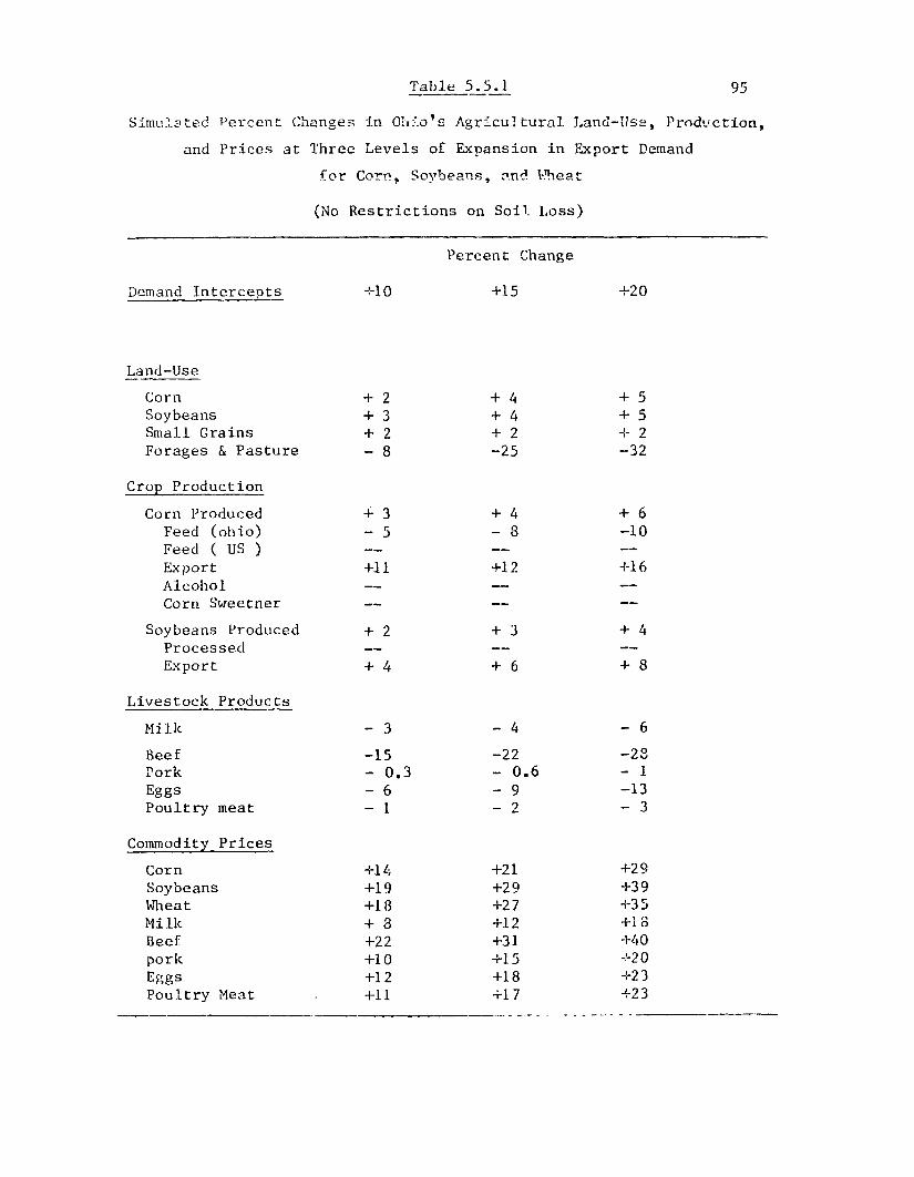
Table 5.5.1 95

Simulated Percent Changes in Ohio's Agricultural Land-Usa, Production, and Prices at Three Levels of Expansion in Export Demand

for Corn, Soybeans, and Wheat

(No Restrictions on Soil Loss)

Percent Change

Demand Intercepts +10 +15 +20

Land-UseCorn + 2 + 4 + 5Soybeans + 3 + 4 + 5Small Grains + 2 + 2 + 2Forages & Pasture - 8 -25 -32

Crop ProductionCorn Produced + 3 + 4 + 6

Feed (ohio) - 5 - 8 -10Feed ( US ) — — —Export +11 +12 +16Alcohol — — —Corn Sweetner — — —

Soybeans Produced + 2 + 3 + 4Processed — — —

Export + 4 + 6 + 8

Livestock ProductsMilk - 3 - 4 - 6Beef -15 -22 -28Pork - 0.3 - 0 .6 - 1Eggs - 6 - 9 -13Poultry meat - 1 - 2 - 3

Commodity PricesCorn +14 +21 +29Soybeans +19 +29 +39Wheat +18 +27 +35Milk + 3 +12 +18Beef +22 +31 +40pork +10 +15 +20Eggs +12 +18 +23Poultry Meat +11 +17 +23

Table 5.5.2 96

Simulated Percent Changes in Ohio's Agricultural Land-Use, Production, and Prices at Three Levels of Expansion In Export Demand

for Corn, Soybeans, and Wheat

(Soil Loss Restricted to T-Values )

Demand Intercepts +10

Percent Change

+15 +20

Land-UseCorn Soybeans Small Grains Forages & Pasture

Crop ProductionCorn Produced

Feed (Ohio) Feed ( US ) Export Alcohol Corn Sweetner

Soybeans Produced Processed Export

Livestock ProductsMilkBeefPorkEggsPoultry Meat

Commodity PricesCornSoybeansWheatMilkBeefPorkEggsPoultry Meat

- 9 -13 + 6 +18

- 3- 9

- 3

- 9

-15

- 2.5+ 2.5- 9 -24- 4

+37 +51 + 1 + 7 + 5 +24 +22 +28

- 8.5 -14 + 7 +23

- 3 -12

- 2

- 9.5

-16

- 3+ 0.6 -11 -29- 5

+47 +64 + 7 +10 + 9 +31 +28 +35

- 8 -15 + 8 +22

- 3 -15

+ 2

-10

-16

- 4.5- 2 -35 -35 - 6

+57+90+13+17+15+38+34+42

97

Table 5.5.3

Simulated Changes in Annual Erosion Rates At Three Levels of Expansion in Export Demand for

Corn, Soybeans, and Wheat Under Conventional Tillage Methods - Ohio

Percent Change in)emand Intercepts +10 +15 +20

legions percent Change in Top-■Soil Loss

1 — —

Corn-Belt2 + 0.5 + 0.7 + 0.9

3 Dairy + 3.0 + 7.0 +21.0

A +30.0 +43.0 +49.0Appalachian

5 + 3.0 + 6.0 + 9.0

6 Central + 1.0 + 1.3 + 2.0

7 Southwest + 5.0 + 8.0 +11.0

State + 6.0 + 8.0 +10.0

98

annual erosion rates would rise 30 to 50 percent (Table 5.5.3).

Changes in Crop and Livestock Prices. The general price

impacts from the above changes in crop exports would be fairly

strong. Especially, within the range of a 10-20 percent increase

in demand, prices of corn, soybeans, and wheat rise 30, 35, and 40

percent, respectively. This would induce a significant upsurge

in prices of beef, pork, poultry meat, and eggs. However, the

sharpest impact would be on beef price which would rise 40 percent

(Table 5.5.1). The stronger impact on price of beef, (in addition to

higher corn and soybeans prices), would be caused by a major

cut-back in production of foragesand pasture-on-cropland.

These price impacts would become even more substantial when the

State's erosion rates are restricted to T-values. In that case,

the expansions in export demand combined with more than a 10 percent

reduction in the State's row crop acreage would push respective

prices of corn and soybeans up to 60 and 90 percent above their

current levels. However, since soil loss restraints would cause

nearly a 20 percent expansion in acreages of forages and pasture,

the rise in beef price would be relatively moderate (Table 5.5.2).

B. Impacts from Expansions in Industrial Demandfor Corn

99Impacts on Land-Use and Soil Erosion. With no restrictions

on soil loss, production of 60 and 100 million gallons of ethanol,

(demanding an additional 24-40 million bushel of corn) would induce

a 5-8 percent expansion the State's corn acreage — ^. Close to a 90

percent of the new corn acreage would be shifted from soybeans and

the rest would be removed from other crops. Regionally, the major

increase in corn production would occur in northeastern, central,

and southeastern Ohio.

The new demand for corn would not lead to an increase in the State's

average erosion rate. In fact, due to the substitution of corn for

soybeans, Ohio's overall annual soil loss per acre would fall

nearly 2 percent. Especially, in central Ohio, a larger corn-for-

soybeans substitution would result in upto 16 percent reduction in

average annual soil loss. However, in eastern and southeastern

Ohio (location of alcohol plants) because of a net expansion in row-

crop agriculture, average annual erosion would rise about 20 percent

(Table 5.5.4).

Impacts on Commodity Prices. The 24-40 million bushels of

additional demand for corn would not pose an important impact on the

State's average prices of major crops or livestock commodities.

Specifically, corn price would rise upto two percent or $0.06

6/ Remember that, 60 million gallons is the State's current alcohol — production level. The 24 million bushel demand for corn pertaining

to this level of alcohol production was included in all other runs of the model which were discussed earlier. However, in this section, to show the specific impacts from the alcohol industry's demand for corn, the results are compared with a situation of zero- alcohol production, for which additional runs have been made.

100

Tahlp 5.5.4

Simulated Changes in Annual Erosion Rates at Two Levels of Expansion in Industrial Demand for Corn

Under Conventional Tillage Methods - Ohio

Industrail Demand of

P.egions 24 mil. bu. 40 mil. bu.

( percent change in annual soil loss )

12

Corn-belt : —

3 Dairy — —

45

Appalachian + 4 +12

+ 7 +20

6 Transition -10 -16

7 Southwest — —

State

per bushel at the State levels and in regions distant from

the alcohol plant site. However, in the vicinity of the plant

location (southeastern Ohio), corn price would increase 5 percent

or $0.15 per bushel.

CHAPTER VI

Summary and Conclusions

6.1. Summary.

The ability of soil to tolerate impact of erosion is called

the soil loss tolerance level, or T-value. T-value has been defined

as the maximum rate of soil erosion that will permit a high level of

crop productivity to be maintained economically and indefinitely.

Annual erosion rates exceeding T-values are considered excessive.

A major cause of excessive soil erosion is intensive use

of agricultural land. Production of row crops such as corn and

soybeans accelerates excessive soil loss from cropland, as it exposes

unprotected soil to wind and water.

From the economic and societal standpoints, excessive

erosion causes two major problems. 1) It depletes the future

productivity of cropland. 2) sedimentation caused by cropland

erosion imposes substantial costs upon society.

In order to maintain the long-term productivity of soils

and to prevent the substantial external costs of cropland erosion,

private and public actions are needed to reduce excessive

soil loss.However, implementation of a soi] conservation policy may have important economic impacts on farmers and consumers.

In Ohio, given the State's regional diversity of soil and

topographic conditions, statewide use of soil conserving tillage

systems, and T—value restriction of soil loss would each have

significant regional economic impacts.1 0 2

103

To analyze these potential impacts, the objectives of the

present study have been to determine the following:

a) the State's cropland use patterns, agricultural production,

farm prices, and annual erosion rates under conventional and

conservation tillage systems;

b) the potential land-use and economic impacts from T-value

restriction of annual soil loss; and

c) Sensitivity of the State's agricultural economy and soil

erosion rates to some potential levels of expansion in export and

industrial demand for grain and soybeans.

These objectives were achieved by using a seven-region,

price-endogenous mathematical programming model of Ohio' agricultural

economy. Under assumption of proportional demand, competitive

equilibrium production and prices for Ohio's major agricultural

commodities (i.e., corn, soybeans, wheat, milk, beef, pork, poultry

meat, and eggs) were determined by maximizing total economic surplus

of the farm sector and consumers. The objective function was

maximized subject to four major types of restrictions: 1) land

resource constraints, 2) minimum output of Ohio's minor farm prodcuts

3) grain delivery constraints, and 4) soil loss restrictions.

To capture the diversity in soil characteristics, and to

estimate the State's soil erosion rates, the more than 500 soil series

of Ohio were divided into 77 soil groups. Similarities in slope,

erodibility, response to conservation tillage, T-value, and natural

productivity were used as criteria for the soil grouping process.

104

Average annual erosion rates for each soil group under different

cropping activities and tillage systems were estimated through

the Universal Soil Loss Equation.

The analysis included six major scenarios and a set of

sensitivity runs. They reflect three different tillage systems,

namely, conventional (moldboard plowing), reduced (chisel plowing)

and no-tillage. In general adoption of each tillage system (depending

on soil type) would result in different crop yields and/or different

production costs. These scenarios were analyzed with and without

imposing T-value restrictions on soil loss.

6.2. Conclusions. The principal conclusions are the following.

1) Substitution of conservation tillage systems for

conventional tillage would not cause any major change in Ohio's

total cropland allocation. However, regionally, conservation

tillage practices, especially, no-tillage, would have a major impact

on cropland-use patterns. For example, a major soybeans-for-corn

substitution on poorly-drained soils in the northwest, a major

expansion in row-crop production on well-drained soils in the north­

east, and a moderate substitution of small grains for row crops in

western Ohio would take place.

2) Under conventional tillage systems, the State's overall

erosion rate would exceed its average T-value by nearly 44 percent.

However, in central, southwestern, and eastern Ohio excessive soil

loss would range from 120-160 percent. Predominant adoption of

1 0 5

conservation tillage systems on all suitable soils would decrease

overall annual erosion rates to a level nearly 15 percent below the

State's average T—value. Nevertheless, in eastern and southwestern

Ohio excessive soil loss still would persist,

3) Substitution of soil conserving tillage methods for

conventional tillage would result in a slight increase in Ohio's

average crop yields. This would lead to a small rise in production

and a moderate fall in the State's average prices of major crops

and livestock commodities. As a result, consumers' surplus would

increase by nearly 10 percent, while, farmers' net returns would

fall by almost the same amount. However, there would be a net

improvement in the farm sector's total economic surplus. That is,

the potential gain in consumers' surplus would be greater than the

potential decline in net returns to farmers.

4) Under conventional tillage systems, imposition of

T-value limits on soil loss would force Ohio farmers to remove

nearly 6 percent of the State's currently utilized cropland from

production. This would result in more than a 10 percent reduction in

row crop acreage and about 15 percent expansion in acreages of forage

and cropland pasture. As a result, average prices of corn and

soybeans would rise by nearly 20 percent, and a moderate increase in

prices of livestock commodities (except beef) would follow. The

cut-back in production and the rise in prices of major crops and

livestock products would decrease consumers' surplus by close to a

5 percent. At the same time, total net returns to farmers would

106

increase by 5 percent. Nevertheless, total economic surplus attribuat—

able to the State’s farm sector would decline by 2.5 percent.

Regionally, farmers and/or cropland owners in less erosive regions

(i.e., northwestern, northeastern, and central Ohio) would benefit

fror.i a T-value based erosion control policy, while, the opposite

would take place in Ohio's more erosive regions (i.e.,eastern,

southeastern, and southwestern Ohio).

5) T-value restriction of soil loss under conservation

tillage systems would not pose any restraints on utilization of

the State's available cropland acreage. However, some moderate

reduction in acreages of row crops in the State's most erosive

regions (i.e., eastern and southwestern Ohio) would prevail.

6) a 5-20 percent expansion in export demand for grains

and soybeans would cause a small expansion in acreage of corn,

soybeans, and wheat. As a result, Ohio's average erosion rate would

increase by 10 percent. The price impacts resulting from expansions

in export demand would be fairly strong. In this case, when annual

soil loss is restricted to T-values, corn and soybeans prices would

rise 60 and 90 percent above their current levels. In contrast,

channelling 24-40 million bushels of corn to Ohio's alcohol industry

would pose little overall impact on the State's agricultural economy.

6.3. Policy Implications and Needs for Further Research.

Viewed from the perspective of long-term soil conservation

policy, the major findings of this study suggest the following.

1 0 7

1) Abatement of excessive soil loss on Ohio cropland

can be well achieved by statewide substitution of conservation tillage

methods for conventional tillage practices. Furthermore, dealing with

the soil erosion problem through this approach would improve the

State's net economic welfare, although, specific groups of farmers

would incure moderate reduction in net returns.

2) If the predominant use of conventional tillage systems

is continued, then, imposition of soil-specific T-value limits to

eliminate excessive soil loss, would make consumers economically

worse-off, penalize farmers operating in the State's highly erosive

regions, and reward those farmers who operate on less erosive cropland.

3) In analyzing the economic and soil erosion impacts of

alternative cropland—use patterns in Ohio, the present study has deter­

mined only those direct costs and benefits which would occur to the

present generation of farmers and consumers. However, the off-site

as well as the inter-generational economic impacts associated with

these land-use patterns remain undetermined. These general issues

require further research at the state level. They are:

a) the off-site damage costs of excessive cropland erosion

in Ohio;

b) the off-site benefits and costs associated with use of

alternative soil conservation strategies in Ohio; and

c) the potential inter-generational impacts resulting from

the present excessive loss of topsoil and implementation of alternative

erosion control strategies.

108

Results of the present study provide some structural

information towards formulation of the suggested research. The

soil-specific quantities of annual erosion and the shadow prices

associated with these soil losses which have been determined by the

present model can be used as a base for estimation of the off-site

economic impacts and the loss of future productivity.

Bibliography

109

Abraham, G., "Estimating Sediment Off-Site Damage Costs in Northwestern Ohio," Unpublished Ph.D. Dissertation,The Ohio State University, Columbus, Ohio 1982.

Alt, K.F., "An Economic Analysis of Field Crop Production:Insecticide Use and Soil Erosion in a Sub—Basin of the Iowa River," Unpublished Ph.D. Dissertation, Iowa State University, Ames, Iowa, 1976.

Becker, G. S., "The Economic Cost of Reducing Soil and Phosphorous Losses in the Honey Creek Watershed of North Central Ohio," Unpublished M.S. Thesis, The Ohio State University,Columbus, Ohio 1977.

Bassoco, L.M. and R.D. Norton, "A Quadratic Approach to Agricultural Policy and Planning," Ann. Economic & Social Measures,4 (1975).

Bogges, W. et al., "Sediment Damage and Farm Production Costs:A Multiple Objective Analysis," North Central Journal of Agricultural Economics, July 1980.

Campbell, J.C., and E.O. Heady, "Potential Economic and Environ­mental Impacts of Alternative Sediment Control Practices,"CARD Report No. 87, Center for Agricultural Rural Development, Iowa State University, Ames, Iowa, 1979.

Council for Agricultural Science and Technology, CAST Report No.92 , Ames, Iowa,1982.

Clawson, M. et al., "Soil and Water Conservation Oversight,"Council for Agricultural Science and Technology, Report No.60, Ames, Iowa, 1976.

Coase, R.H., "The Problem of Social Cost," The Journal of Law and Economics, October, 1960

Conter, M.L., "The Impact of Sgricultural Conservation Program andSelected Farm Policy Areas," Department of Agr. Economics,Mimo #943» March 1964.

Cooley, J.L., "Nonpoint Pollution and Water Quality," Journal ofSoil and Water Conservation, March-April, 1976.

Davis, O.A. and M.I. Kamien, "Externalities, Information andAlternative Collective Actions," Economics of Environment,

110

Dorfraan and Dorfman (eds), Norton Publishing Co., New York,1977.

Dasgupta, A.K. and D.W. Pearce, Cost Benefit Analysis: Theory and Practice, The Macmillan Press Ltd., London, U.K., 1974.

Duvick, R.D., Associatae Professor, Department of Agr. Economics & Rur. Soc., The Ohio State University, Personal Cosultation.

Eckert D., Associate Professor, Department of Agronomy, the Ohio State University, Personal Consultation.

Forster, D.L., Economic Impacts of Changing Tillage Practices in the Lake Erie Basin, U.S. Army Corp of Engineers, Buffalo,New York, Augus 1978.

Forster, D.L. and G.S. Becker, "Costs and Income Effects of Alternative Erosion Control Strategies," North Central Journal of Agricultural Economics, 1 (1979).

Heady, E.0.,"Trade-Offs Between Soil Conservation, Energy Use,Exports, and Environmental Quality," Iowa State University, Ames, Iowa, 1980.

Heien, D.M., "The Structure of Food Demand: Interrelatedness and Duality," American Journal of Agricultural Economics,64 (1982).

Hughes, A.J. and D.E. Grawing, Linear Programming: An Emphasis on Decision Making, Addison-Wedley Publishing Co.,London, U.K., 1973.

Jacobs, J.J., "Economics of Water Quality Management: Exemplified by Specified Pollutants in Agricultural Runoff,"Unpublished Ph.D. Dissertation, Iowa State University,Ames, Iowa, 1972.

Korsching, P.F. and P. Nowak, "environmental Criteria and Farm Structure: Flexibility in Conservation Policy," InD.E. Brewster, et al., editors, Farms in Transition: Interdiciplinary Perspectives on Farm Structure, Iowa State University Press, Ames, Iowa, 1982.

Kasai, J. "Trade-Offs Between Farm Income and Selected Environ­mental Indicators: A Case Study of Soil Loss, Fertilizer,and Land-Use Constraints," Technical Bulletin No. 1550, Economic Research Service, U.S.D.A., 1976.

Kuhn, H.W. and A.W. Tucker, "Non-Linear Programming," Proceedings of Second Berkeley Simposium on Mathematical Statistics and

Ill

Probability, Berkeley Calif: University of California,1959.

Layard,P.R.G. and A.A. Walters, Microeconomic Theory, McGraw-Hill Book Company, New York, 1978.

Leitch, J.A. and L.E. Danielson, Social, Economic, and InstitutionalIncentives to Drain or Preserve Praire Waterlands, Econ. Report, ER 79-b, Dept, of Agr. Econ., University of Minnesota, 1979.

Lines, A.E., Associate Professor, Dept, of Agr. Economics & Rur. Soc., The Ohio State University, Personal Consultation.

Meister, A.D. et al., Quadratic Programming Models Applied toAgricultural Policies, Iowa State University Press, Ames,Iowa 19 78.

Miller, M.F. and H.H. Krusekoph, The Influence of Cropping and Methods of Culture on Surface Runoff and. Soil Erosion,Research Bulletin 17 7, Missouri Agricultural Experiment Station, 1932.

Miller, C., "The Simplex Method for Local Separable Programming,"Recent Advances in Mathematical Programming, eds. R.L. Graves and P. Wolf, New York, John Willey and Sons, 1963.

Mishan, E.J., Cost-Benefit Analysis, Praeger Publishers, New York,1976.

Murtagh, B.A. and M.A. Saunders, MINOS User's Guide, Stanford: Technical Report 77-9, Department of Operations Research, Stanford University, 1977.

Narayanan, A. S. ej; ad. "Economic Analysis of Erosion and Sediment­ation, Mendota West Fork Watershed," Agricultural Economics Research, Report 126, University of Illinois, Urbana,April 1974.

Nagadevara, V.S. et al., "Implication of Application of SoilConservancy and Environmental Regulations in Iowa within a National Framework," Report No. 57, Center for Agricultural and Rural Development, Iowa State University, Ames, Iowa,1975.

Ohio Agricultural Research and Development Center, 1980 Ohio Farm Income, Wooster, Ohio , 1981.

Ohio Agricultural Statistics, 1980, Ohio Crop Reporting Service,May 1981.

Osteen,C. and W.D. Seitz "regional Economic Impacts of Policies

112

to Control Erosion and Sedimentation in Illinois and otherC o m Belt States," American J. of Agr. Economics, August 1978.

Ott, S.O. "The Economics of Producing Fuel-Grade Alcohol from Corn in Western Ohio," Unpublished Ph.D. Dissertation,The Ohio State University, 1981.

Pearce, D.W., Environmental Economics, Longman Inc., New York,1976.

Randall, A. Resource Economics: An Economic Approach to Natural Resource and Environmental Policy, Grid Publishing Inc., Columbus, Ohio 1981.

Rask, N. ejt al. , An Integrated Regional Analysis of Potential Biomass Energy Production in Ohio, Final Report,Department of Agricultural Econ. & Rur. Soc. , 'The Ohio State University, Columbus, Ohio Feb. 1983.

Ray, D.E. and J.W. Richardson, Detailed Description of Polysim Stillwater: Technical Report T-151,Agricultural Experiment Station, Oklahoma State University,1978.

Seitz, W.D. £t jil., Alternative Policies for Controlling Non-point Agricultural Sources of Water Pollution, EPA-600, U.S. Environmental Protection Agency, Athens, Georgia, 1978.

Sitterley, J.H. Land Use in Ohio, 1900-1970: How and Why it Has Changed, Bull. No. 1084, Ohio Agricultural Research and Development Center, Wooster, Ohio 1976.

Sitterley, J.H., R.H. Baker, and J.I. Falconer, Major Land UseProblem Areas and Land Utilization in Ohio, Ohio Agricultural Experiment Station, Mimo. No. 79, Columbus, Ohio 1935.

Taylor, C.R. et_ al., "Potential Erosion and Fertilizer Control in the Corn-Belt: An Economic Analysis," J. of Soil andWater Conservation, April 1978.

The Ohio State University, Cooperative Extension Service:Ohio Erosion Control and Sediment Pollution Abatement Guide, Bulletin No. 594, May 1979.

The Ohio State University, Cooperative Extension Service: 1981-1982 Agronomy Guide, Bulletin No. 472, Feb. 1980.

U.S. Department of Agriculture, Predicting Rainfall Erosion Losses: A Guide to Conservation Planning, Agricultural Hand Book No. 537, Washington D.c., 1978.

113

U.S. Department of Agriculture, National Resource Inventories,USDA Soil Conservation Service, 1978.

U.S. Department of Agriculture, National Summary and Evaluation of the Agricultural Conservation Program, Agricultural Stabilization and Conservation Service, Nov. 1980.

U.S. Department of Agriculture, Report on the Land and Water Conservation Programs, Agricultural Stabilization and Conservation Service, 1981.

U.S. Department of Agriculture, Economics and Statistics Service, 1981.

Van Doren, D.M. and G.B.. Triplett Properties and Uses of Ohio Soils: Data Base SQILSV-1980, OAKDC, Wooster, Ohio 1980.

Wade, J.C. and E.O. Heady, "Controlling Nonpoint Sediment Sources with Cropland Management: A National Economic Assessment,11 American J. Agr. Econ., Feb. 1977.

Zobeck, T., Assistant Professor of Agronomy, The Ohio State University, Personal Consultation.

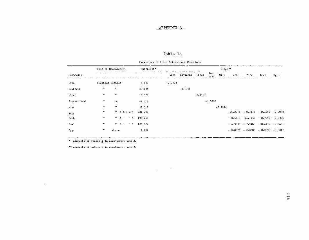
APPENDIX A

Table la

Commodity

Parameters of Price-Determinant Equations

Unit of Measurement Intercept* Slope*

Corn Soybeans Wheat w ' , Milk Meal Pork Fowl Eggs

Corn

Soybeans

Wheat

Soybean Meal

Milk

BeefPork

Fowl

Eggs

thousand bushels 9,600

20,135

13,170

41,316

52,517(live wt) 201,225

C " JC " )

195,489

185,677

1 ,782

-0.0278

-0.1781

-0.3313

-2.5800

-0.9994-16.2071 - 0.3134 - 0.5362 -0.0048

- 8.5819 -14.1735 - 8,7253 -0.0835

- 4.9832 - 2.948h -50.4437 -0.0481

- 0.0976 - 0.0580 - 0.0993 -0.0017

* elements of vector in equations 1 and 2.

** elements of matrix B in equations 1 and 2.