What the no free lunch theorems really mean;how to improve search algorithms

David H. Wolpert

Santa Fe Institute1399 Hyde Park Road, Santa Fe, NM, 87501

andInformation Sciences Division

MS B256, Los Alamos National Laboratory, Los Alamos, NM, 87545david.h.wolpert@gmail.com

November 18, 2013

1 IntroductonThe first No Free Lunch (NFL) theorems were introduced in [9], in the contextof supervised machine learning. These theorems were then popularized in [8],based on a preprint version of [9]. Loosely speaking, these original theorems canbe viewed as a formalization and elaboration of concerns about the legitimacyof inductive inference, concerns that date back to David Hume (if not earlier).Shortly after these original theorems were published, additional NFL theoremsthat apply to search were introduced in [12].

The NFL theorems have stimulated lots of subsequent work, with over 2500citations of [12] alone by spring 2012 according to Google Scholar. However ar-guably much of that research has missed the most important implications of thetheorems. As stated in [12], the primary importance of the NFL theorems forsearch is what they tell us about “the underlying mathematical ‘skeleton’ of op-timization theory before the ‘flesh’ of the probability distributions of a particularcontext and set of optimization problems are imposed”. So in particular, while theNFL theorems have strong implications if one believes in a uniform distributionover optimization problems, in no sense should they be interpreted as advocatingsuch a distribution.

1

In this short note I elaborate this perspective on what it is that is really im-portant about the NFL theorems for search. I then discuss how the fact that thereare NFL theorems for both search and for supervised learning is symptomatic ofthe deep formal relationship between those two fields. Once that relationship isdisentangled, it suggests many ways that we can exploit practical techniques thatwere first developed in supervised learning to help us do search. I summarizesome experiments that confirm the power of search algorithms developed in thisway. I end by briefly discussing the various free lunch theorems that have beenderived, and possible directions for future research.

2 The inner product at the heart of all searchLet X be a countable search space, and specify an objective function f : X → Ywhere Y ⊂ R is a countable set. Everything presented in this paper can be extendedin a straightforward way to the case of a stochastic search algorithm, stochasticobjective function, time-varying objective function, etc. Sometimes an objectivefunction is instead called a “search problem”, “fitness function”, “cost function”,etc.

In practice often one does not know f explicitly. This is the case whenever fis a “blackbox”, or an “oracle”, that one can sample at a particular x, but does notknow in closed form. Moreover, often even if a practitioner does explicitly knowf , they act as though they do not, for example when they choose what searchalgorithm to use on f . For example, often someone trying to solve a TravelingSalesman Problem (TSP) will use the same search algorithm for any TSP. In sucha case, they are behaving exactly as they would if they only knew that the objectivefunction is an TSP, without knowing specifically which one it is.

These kinds of uncertainty about the precise f being searched can be expressedas a distribution P( f ). Say we are given such a P( f ), along with a search algo-rithm, and a real-valued measure of the performance of that algorithm when it isrun on any objective function f . Then we can solve for the probability that thealgorithm results in a performance value φ. The result is an inner product of tworeal-valued vectors each indexed by f . (See Appendix.) The first of those vectorsgives all the details of how the search algorithm operates, but nothing concern-ing the world in which one deploys that search algorithm. The second vector isP( f ). All the details of the world in which one deploys that search algorithm arespecified in this vector, but nothing concerning the search algorithm itself.

This result tells us that at root, how well any search algorithm performs isdetermined by how well it is “aligned” with the distribution P( f ) that governs theproblems on which that algorithm is run. For example, Eq. (2) means that theyears of research into the traveling salesman problem (TSP) have (presumably)

2

resulted in algorithms aligned with the implicit P( f ) describing traveling salesmanproblems of interest to TSP researchers.

3 The no free lunch theorems for searchThe inner product result governs how well any particular search algorithm doesin practice. Therefore, either explicitly or implicitly, it serves as the basis forany practitioner who chooses a search algorithm to use in a given scenario. Moreprecisely, the designer of any search algorithm first specifies a P( f ) (usually im-plicitly, e.g., by restricting attention to a class of optimization problems). Thenthey specify a performance measure Φ (sometimes explicitly). Properly speaking,they should then solve for the search algorithm that the inner product result tellsus will have the best distribution of values of that performance measure, for thatP( f ). In practice though, instead informal arguments are often used to motivatethe search algorithm.

In addition to governing both how a practitioner should design their searchalgorithm, and how well the actual algorithm they use performs, the inner productresult can be used to make more general statements about search, results that holdfor all P( f )’s. It does this by allowing us to compare the performance of a givensearch algorithm on different subsets of the set of all objective functions. Theresult is the no free lunch theorem for search (NFL). It tells us that if any searchalgorithm performs particularly well on one set of objective functions, it must per-form correspondingly poorly on all other objective functions. This implication isthe primary significance of the NFL theorem for search. To illustrate it, choosethe first set to be the set of objective functions on which your favorite search algo-rithm performs better than the purely random search algorithm that chooses thenext sample point randomly. Then the NFL for search theorem says that comparedto random search, your favorite search algorithm “loses on as many” objectivefunctions as it wins (if one weights wins / losses by the amount of the win / loss).This is true no matter what performance measure you use.

As another example, say that your performance measure prefers low values ofthe objective function to high values, i.e., that your goal is to find low values ofthe objective rather than high ones. Then we can use the no free lunch for searchtheorem to compare a hill-descending algorithm to a hill-ascending algorithm, i.e.,to an algorithm that “tries” to do as poorly as possible according to the objectivefunction. The conclusion is that the hill-descending algorithm “loses to the hill-ascending algorithm on as many” objective functions as it wins. The lesson is thatwithout arguing for a particular P( f ) that is biased towards a set B of objectivefunctions on which one’s favorite search algorithm performs well, one has noformal justification that that algorithm has good performance.

3

A secondary implication of the NFL theorem for search is that if it so happensthat you assume / believe that P( f ) is uniform, then the average over f ’s used inthe NFL for search theorem is the same as P( f ). In this case, you must concludethat all search algorithms perform equally well for your assumed P( f ). This con-clusion is only as legitimate as is the assumption for P( f ) it is based on. Onceother P( f )’s are allowed, the conclusion need not hold.

An important point in this regard is that simply allowing P( f ) to be non-uniform, by itself, does not nullify the NFL theorem for search. Arguments thatP( f ) is non-uniform in the real world do not, by themselves, establish anythingwhatsoever about what search algorithm to use in the real world.

In fact, allowing P( f )’s to vary provides us with a new NFL theorem. In thisnew theorem, rather than compare the performance of two search algorithms overall f ’s, we compare them overall P( f )’s. The result is what one might expect: Ifany given search algorithm performs better than another over a given set of P( f )’s,then it must perform corresponding worse on all other P( f )’s. (See appendix forproof.)

4 The supervised learning no free lunch theoremsThe discussion above tells us that if we only knew and properly exploited P( f ), wewould be able to design an associated search algorithm that performs better thanrandom. This suggests that we try to use a search process itself to learn some-thing about the real world’s P( f ), or at least about how well one or more searchalgorithms perform on that P( f ). For example, we could do this by recording theresults of running a particular search algorithm on a set of (randomly chosen) real-world search problems, and using those results as a “training set” for a supervisedmachine elearning algorithm that models how those algorithms compare to oneanother on such search problems. The hope would be that by doing this, we cangive ourselves formal assurances that one search algorithm should be used ratherthan another, for the P( f ) that governs the real world.

The precise details of how well such an approach would perform depend onthe precise way that it is formalized. However two broadly applicable restrictionson its performance are given by an inner product formula for supervised learningand an associated NFL theorem for supervised learning.

Just like search, supervised learning involves an input space X, an output spaceY , a function f relating the two, and a data set of (x, y) pairs. The goal in super-vised learning though is not to iteratively augment the data to find what x mini-mizes f (x). Rather it is to take a fixed data set and estimate the entire function f .Such a function mapping a data set to an estimate of f (or more generally an es-timate of a distribution over f ’s) is called a learning algorithm. We then refer to

4

the accuracy of the estimate for x’s that do not occur in the data set as off-trainingset error.

The supervised learning inner product formula tells us that the performance ofany supervised learning algorithm is governed by an inner product between twovectors both indexed by the set of all target functions. More precisely, it tellsus that as long as the loss function is symmetric, how “aligned” the supervisedlearning algorithm is with the real world (i.e., with the posterior distribution oftarget functions conditioned on a training set) determines how well that algorithmwill generalize from any training set to a separate test set. (See appendix.)

This supervised learning inner product formula results in a set of NFL theo-rems for supervised learning, applicable when some additional common condi-tions concerning the loss function hold. The implications of these theorems forthe entire scientific enterprise (and for trying to design good search algorithmsin particular) are wide-ranging. In particular, we can let X be the specificationof how to configure an experimental apparatus, and Y the outcome of the asso-ciated experiment. So f is the relevant physical laws determining the results ofany such experiment, i.e., they are a specification of a universe. In addition, d isa set of such experiments, and h is a theory that tries to explain that experimentaldata (P(h | d) being the distribution that embodies the scientist who generates thattheory). Under this interpretation, off-training set error quantifies how well anytheory produced by a particular scientist predicts the results of experiments notyet conducted. So roughly speaking, according to the NFL theorems for search, ifscientist A does a better job than scientist B of producing accurate theories fromdata for one set of universes, scientist B will do a better job on the remaining setof universes. This is true even if both universes produced the exact same set ofscientific data that the scientists use to construct their theories — in which caseit is theoretically impossible for the scientists to use any of the experimental datathey have ever seen in any way whatsoever to determine which set of universesthey are in.

As another implication of NFL for supervised learning, take x ∈ X to be thespecification of an objective function, and say we have two professors, Smith andJones, each of whom when given any such x will produce a search algorithm torun on x. Let y ∈ Y be the bit that equals 1 iff the performance of the searchalgorithm produced by Prof. Smith is better than the performance of the searchalgorithm produced by Prof. Jones.1 So any training set d is a set of objectivefunctions, together with the bit of which of (the search algorithms produced by)the two professors on those objective functions performed better.

1Note that as a special case, we could have each of the two professors always produce theexact same search algorithm for any objective function they are presented. In this case comparingthe performance of the two professors just amounts to comparing the performance of the twoassociated search algorithms.

5

Next, let the learning algorithm C be the simple rule that we predict y for allx < dm

X to be 1 iff the majority of the values in dmY is 1, and the learning algorithm

D to be the rule that we predict y to be -1 iff the majority of the values in dmY is 1.

So C is saying that if Professor Smith’s choice of search algorithm outperformedthe choice by Professor Jones the majority of times in the past, predict that theywill continue to do so in the future. In contrast, D is saying that there will bea magical flipping of relative performance, in which suddenly Professor Jones isdoing better in the future, if and only if they did worse in the past.

The NFL for supervised learning theorem tells us that there are as many uni-verses in which algorithm C will perform worse than algorithm D — so that Pro-fessor Jones magically starts performing worse than Professor Smith — as thereare universes the other way around. This is true even if Professor Jones producesthe random search algorithm no matter what the value of x (i.e., no matter what ob-jective function they are searching). In other words, just because Professor Smithproduces search algorithms that outperform random search in the past, withoutmaking some assumption about the probability distribution over universes, wecannot conclude that they are likely to continue to do so in the future.

5 Exploiting the relation between supervised learn-ing and search to improve search

Given the preceding discussion, it seems that supervised learning is closely analo-gous to search, if one replaces the “search algorithm” with a “learning algorithm”and the “objective function” with a “target function”. So it should not be too sur-prising that the inner product formula and NFL theorem for search have analogs insupervised learning. This close formal relationship between search and supervisedlearning means that techniques developed in one field can often be “translated” toapply directly to the other field.

A particularly pronounced example of this occurs in the simplest (greedy)form of the Monte Carlo Optimization (MCO) approach to search [3]. In thatform of MCO, one uses a data set d to form a distribution q(x ∈ X) rather than (asin most conventional search algorithms) directly form a new x. That q is chosenso that that one expects the expected value of the objective function,

∑x q(x) f (x)

to have a low value, i.e., so that one expects a sample of q(.) to produce an x witha good value of the objective function. One then forms a sample x of that q(.), andevaluates f (x). This provides a new pair (x, f (x)) that gets added to the data set d,and the process repeats.

MCO algorithms can be viewed as variants of random search algorithms likegenetic algorithms and simulated annealing, in which the random distribution gov-

6

erning which point to sample next is explicitly expressed and controlled, ratherthan be implicit and only manipulated indirectly. Several other algorithms canbe cast as forms of MCO (e.g., the cross-entropy method [7], the MIMIC algo-rithm [1]). MCO algorithms differ from one another in how they form the distri-bution q for what point next to sample, with some not trying directly to optimize∑

x q(x) f (x) but instead using some other optimization goal.It turns out that the problem of how best to choose a next q in MCO is for-

mally identical to the supervised learning problem of how best to choose a hy-pothesis h based on a training set d [13, 5, 6]. If one simply re-interprets all MCOvariables as appropriate supervised learning variables, one transforms any MCOproblem into a supervised learning problem (and vice-versa). The rule for this re-interpretation is effectively a dictionary that allows us to transform any techniquethat has been developed for supervised learning into a technique for (MCO-based)search. Regularization, bagging, boosting, cross-validation, stacking, etc., can allbe transformed this way into techniques to improve search.

As an illustration, cross-validation in supervised learning is a technique forusing an existing training set d to choose a value for a hyperparameter arising ina given supervised learning algorithm. We can use the dictionary to translate thisuse of cross-validation from the domain of supervised learning into the domain ofsearch. Training sets become data sets, and the hyperparameters of a supervisedlearning algorithm become the parameters of an MCO-based search algorithm.For example, a regularization constant in supervised learning gets transformedinto the temperature parameter of a form of MCO that is very similar to simulatedannealing. In this way using the dictionary to translate cross-validation into thesearch domain shows us how to use it on one’s data set in search to dynamicallyupdate the temperature in the temperature-based MCO search algorithm. Thatupdating proceeds by running the MCO algorithm repeatedly on subsets of one’salready existing data set d. (No new samples of the objective function f beyondthose already in d are involved in this use of cross-validation for search, just likeno new samples are involved in the use of cross-validation in supervised learning.)

Experimental tests of MCO search algorithms designed by using the dictio-nary have established that they work quite well in practice [13, 5, 6]. Applyingbagging and and stacking, in addition to cross-validation, have all been found totransform an initially powerful search algorithm into a new one with improvedsearch performance.

Of course, these experimental results do not mean there is any formal jus-tification for these kinds of MCO search algorithms; NFL for search cannot becircumvented. To understand in more detail why one cannot provide a formaljustification for a technique like cross-validation in search, it is worth elaboratingwhy there is not even a formal justification for using cross-validation in supervisedlearning. Let Θ be a set of learning algorithms. Then given a training set d, let

7

scientist A estimate what f produced their training set the following way. Firstthey run cross-validation on d to compare the algorithms in Θ. They then choosethe algorithm θ ∈ Θ with lowest such cross-validation error. As a final step, theyrun that algorithm on all of d. In this way A generates their final hypothesis h togeneralize from d. Next let scientist B do the exact same thing, except that theyuse anti-cross-validation, i.e., the algorithm they choose to train on all of d is theelement of Θ with greatest cross-validation error on d, not smallest error. By theNFL theorems for supervised learning, we have no a priori basis for preferringscientist A ’s hypothesis to scientist B’s. Although it is difficult to produce f ’sin which B beats A , by the NFL for supervised learning theorem we know thatthere must be “as many” of them (weighted by performance) as there are f ’s forwhich A beats B.

Despite this lack of formal guarantees behind cross-validation in supervisedlearning, it is hard to imagine any scientist who would not prefer to use it to usinganti-cross-validation. Indeed, one can view cross-validation (or more generally“out of sample” techniques) as a formalization of the scientific method: chooseamong theories according to which better fits experimental data that was generatedafter the theory was formulated, and then use that theory to make predictionsfor new experiments. By the inner product formula for supervised learning, thisbias of the scientific community in favor of using out-of-sample techniques ingeneral, and cross-validation in particular, must correspond somehow to a bias infavor of a particular P( f ). This implicit prior P( f ) is quite difficult to expressmathematically. Yet almost every conventional supervised learning prior (e.g., infavor of smooth targets) or non-Bayesian bias favoring some learning algorithmsover others (e.g., a bias in favor of having few degrees of freedom in a hypothesisclass, in favor of generating a hypothesis with low algorithmic complexity, etc.)is often debated by members of the scientific community. In contrast, nobodydebates the “prior” implicit in out-of-sample techniques. Indeed, it is exactly thisprior which justifies the ubiquitous use of contests involving hidden test data setsto judge which of a set of learning algorithms are best.

6 Free lunches and future researchThere are many avenues of research related to the NFL theorems which have notyet been properly explored. Some of these involve free lunch theorems whichconcern fields closely related to search, e.g., co-evolution [11]. Other free lunchesarise in supervised learning, e.g., when the loss function does not obey the condi-tions that were alluded to above [10].

However it is important to realize that none of these (no) free lunch theoremsconcern the covariational behavior of search and / or learning algorithms. For

8

example, despite the NFL for search theorems, there are scenarios where, for somef ’s, E(Φ | f ,m,A ) − E(Φ | f ,m,B) = k (using the notation of the appendix),but there are no f ’s for which the reverse it true, i.e., for which the differenceE(Φ | f ,m,B)−E(Φ | f ,m,A ) = k. It is interesting to speculate that such “head-to-head” distinctions might ultimately provide a rationale for using many almostuniversally applied heuristics, in particular for using cross-validation rather thananti-cross-validation in both supervised learning and search.

There are other results where, in contrast to the NFL for search theorem, onedoes not consider fixed search algorithms and averages over f ’s, but rather fixes fand averages over algorithms. These results allow us to compare how intrinsicallyhard it is to search over a particular f . They do this by allowing us to comparetwo f ’s based on the sizes of the sets of algorithms that do better than the randomalgorithm does on those f ’s [4]. While there are presumably analogous results forsupervised learning, which would allow us to measure how intrinsically hard it isto learn a given f , nobody currently knows. All of these issues are the subject offuture research.

A Appendix of mathematical derivations

A.1 NFL and inner product formulas for searchTo formalize the discussion in the text, it will be useful to use the following nota-tion. Let a data set dm = dm

X , dmY be any set of m separate pairs (x ∈ X, f (x)). A

search algorithm is a function A that maps any dm for any m ∈ 0, 1, . . . to anx < dm

X . (Note that to “normalize” different search algorithms, we only considertheir behavior in terms of generating new points to search that have not yet beensampled.) By iterating a search algorithm we can build successively larger datasets: dm+1 = dm ∪ (A(dm

X ), f [A(dmX )]) for all m ≥ 0. So if we are given a perfor-

mance measure Φ : dmY → R, then we can evaluate how the performance of a

given search algorithm on a given objective function changes as it is run on thatfunction.

This allows us to establish the inner product for search result, mentioned inthe text. To begin expand

P(φ | A ,m) =∑dm

Y

P(dmY | A ,m)P(φ | dm

Y ,A ,m)

=∑dm

Y

P(dmY | A ,m)δ(φ,Φ(dY

m)) (1)

where the delta function equals 1 if its two arguments are equal, zero otherwise.

9

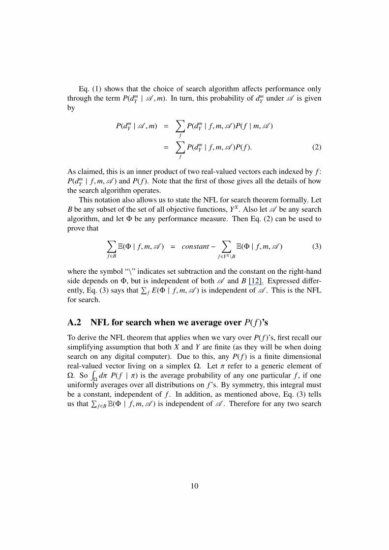
Eq. (1) shows that the choice of search algorithm affects performance onlythrough the term P(dm

Y | A ,m). In turn, this probability of dmY under A is given

by

P(dmY | A ,m) =

∑f

P(dmY | f ,m,A )P( f | m,A )

=∑

f

P(dmY | f ,m,A )P( f ). (2)

As claimed, this is an inner product of two real-valued vectors each indexed by f :P(dm

Y | f ,m,A ) and P( f ). Note that the first of those gives all the details of howthe search algorithm operates.

This notation also allows us to state the NFL for search theorem formally. LetB be any subset of the set of all objective functions, YX. Also let A be any searchalgorithm, and let Φ be any performance measure. Then Eq. (2) can be used toprove that ∑

f∈B

E(Φ | f ,m,A ) = constant −∑

f∈YX\B

E(Φ | f ,m,A ) (3)

where the symbol “\” indicates set subtraction and the constant on the right-handside depends on Φ, but is independent of both A and B [12]. Expressed differ-ently, Eq. (3) says that

∑f E(Φ | f ,m,A ) is independent of A . This is the NFL

for search.

A.2 NFL for search when we average over P( f )’sTo derive the NFL theorem that applies when we vary over P( f )’s, first recall oursimplifying assumption that both X and Y are finite (as they will be when doingsearch on any digital computer). Due to this, any P( f ) is a finite dimensionalreal-valued vector living on a simplex Ω. Let π refer to a generic element ofΩ. So

∫Ω

dπ P( f | π) is the average probability of any one particular f , if oneuniformly averages over all distributions on f ’s. By symmetry, this integral mustbe a constant, independent of f . In addition, as mentioned above, Eq. (3) tellsus that

∑f∈B E(Φ | f ,m,A ) is independent of A . Therefore for any two search

10

algorithms A and B,∑f

E(Φ | f ,m,A ) =∑

f

E(Φ | f ,m,B),

∑f

E(Φ | f ,m,A )[ ∫

Ω

dπ P( f | π)]

=∑

f

E(Φ | f ,m,B)[ ∫

Ω

dπ P( f | π)],

∑f

E(Φ | f ,m,A )[ ∫

Ω

dπ π( f )]

=∑

f

E(Φ | f ,m,B)[ ∫

Ω

dπ π( f )],∫

Ω

dπ∑

f

E(Φ | f ,m,A )π( f ) =

∫Ω

dπ∑

f

E(Φ | f ,m,B)π( f ), (4)

i.e., ∫Ω

dπ Eπ(Φ | m,A ) =

∫Ω

dπ Eπ(Φ | m,B). (5)

We can re-express this result as the statement that∫

Ωdπ Eπ(Φ | m,A ) is indepen-

dent of A .Next, let Π be any subset of Ω. Then our result that

∫Ω

dπ Eπ(Φ | m,A ) isindependent of A implies∫

π∈Π

dπ Eπ(Φ | m,A ) = constant −∫π∈Ω\Π

dπ Eπ(Φ | m,A ) (6)

where the constant depends on Φ, but is independent of both A and Π. So ifany search algorithm performs particularly well for one set of P( f )’s, Π, it mustperform correspondingly poorly on all other P( f )’s. This is the NFL theorem forsearch when P( f )’s vary.

A.3 NFL and inner product formulas for supervised learningTo state the supervised learning inner product and NFL theorems requires intro-ducing some more notation. Conventionally, these theorems are presented in theversion where both the the learning algorithm and target function are stochastic.(In contrast, the restrictions for search — presented above — conventionally in-volve a deterministic search algorithm and deterministic objective function.) Thismakes the statement of the restrictions for supervised learning intrinsically morecomplicated.

Let X be a finite input space, Y a finite output space, and say we have atarget distribution f (y f ∈ Y | x ∈ X), along with a training set d = (dm

X , dmY )

of m pairs (dmX (i) ∈ X, dm

Y (i) ∈ Y), that is stochastically generated according to

11

a distribution P(d | f ) (conventionally called a likelihood, or “data-generationprocess”). Assume that based on d we have a hypothesis distribution h(yh ∈ Y |x ∈ X). (The creation of h from d — specified in toto by the distribution P(h | d)— is conventionally called the learning algorithm.) In addition, let L(yh, y f ) be aloss function taking Y × Y → R. Finally, let C( f , h, d) be an off-training set costfunction2,

C( f , h, d) ∝∑

y f ∈Y,yh∈Y

∑q∈X\dm

X

P(q)L(y f , yh) f (y f | q)h(yh | q) (7)

where P(q) is some probability distribution over X assigning non-zero measure toX \ dm

X .All aspects of any supervised learning scenario — including the prior, the

learning algorithm, the data likelihood function, etc. — are given by the jointdistribution P( f , h, d, c) (where c is values of the cost function) and its marginals.In particular, in [2] it is proven that the probability of a particular cost value c isgiven by

P(c | d) =

∫d f dh P(h | d)P( f | d)Mc,d( f , h) (8)

for a matrix Mc,d that is symmetric in its arguments so long as the loss functionis. P( f | d) ∝ P(d | f )P( f ) is the posterior probability that the real world has pro-duced a target f for you to try to learn, given that you only know d. It has nothingto do with your learning algorithm. In contrast, P(h | d) is the specification ofyour learning algorithm. It has nothing to do with the distribution of targets f inthe real world. So Eq. (8)

References[1] J.S. De Bonet, C.L. Isbell Jr., and P. Viola, Mimic: Finding optima by es-

timating probability densities, Advances in Neural Information ProcessingSystems - 9, MIT Press, 1997.

[2] Wolpert. D.H., On the connection between in-sample testing and generaliza-tion error, Complex Systems 6 (1992), 47–94.

2The choice to use an off-training set cost function for the analysis of supervised learning isthe analog of the choice in the analysis of search to use a search algorithm that only searches overpoints not yet sampled. In both the cases, the goal is to “mod out” aspects of the problem that aretypically not of interest and might result in misleading results: ability of the learning algorithmto reproduce a training set in the case of supervised learning, and ability to revisit points alreadysampled with a good objective value in the case of search.

12

[3] Y. M. Ermoliev and V. I. Norkin, Monte carlo optimization and path depen-dent nonstationary laws of large numbers, Tech. Report IR-98-009, Interna-tional Institute for Applied Systems Analysis, March 1998.

[4] W. G. Macready and D. H. Wolpert, What makes an optimization problemhard?, Complexity 1 (1995), 40–46.

[5] D. Rajnarayan and David H. Wolpert, Exploiting parametric learning toimprove black-box optimization, Proceedings of ECCS 2007 (J. Jost, ed.),2007.

[6] , Bias-variance techniques for monte carlo optimization: Cross-validation for the ce method, arXiv:0810.0877v1, 2008.

[7] R. Rubinstein and D. Kroese, The cross-entropy method, Springer, 2004.

[8] C. Schaffer, A conservation law for generalization performance, Interna-tional Conference on Machine Learning, Morgan Kaufmann, 1994, pp. 295–265.

[9] D. H. Wolpert, The lack of a prior distinctions between learning algorithmsand the existence of a priori distinctions between learning algorithms, Neu-ral Computation 8 (1996), 1341–1390,1391–1421.

[10] , On bias plus variance, Neural Computation 9 (1997), 1211–1244.

[11] D. H. Wolpert and W. Macready, Coevolutionary free lunches, Transactionson Evolutionary Computation 9 (2005), 721–735.

[12] D. H. Wolpert and W. G. Macready, No free lunch theorems for optimization,IEEE Transactions on Evolutionary Computation 1 (1997), no. 1, 67–82.

[13] D. H. Wolpert, D. Rajnarayan, and Bieniawski S., Probability collectives inoptimization, Encyclopedia of Stastistics, 2012.

13