Two Regimes of Laboratory Whitecap Foam Decay: Bubble-Plume Controlledand Surfactant Stabilized

ADRIAN H. CALLAGHAN

Scripps Institution of Oceanography, University of California, San Diego, La Jolla, California, and School of Physics

and Ryan Institute, National University of Ireland, Galway, Ireland

GRANT B. DEANE AND M. DALE STOKES

Scripps Institution of Oceanography, University of California, San Dieg, La Jolla, California

(Manuscript received 9 August 2012, in final form 20 January 2013)

ABSTRACT

A laboratory experiment to quantify whitecap foam decay time in the presence or absence of surface active

material is presented. The investigation was carried out in the glass seawater channel at the Hydraulics Fa-

cility of Scripps Institution of Oceanography.Whitecaps were generated with focused, breaking wave packets

in filtered seawater pumped fromLa Jolla Shores Beachwith andwithout the addition of the surfactant Triton

X-100. Concentrations of Triton X-100 (204 mg L21) were chosen to correspond to ocean conditions of

mediumproductivity.Whitecap foamand subsurface bubble-plume decay times were determined fromdigital

images for a range of wave scales and wave slopes. The experiment showed that foam lifetime is variable and

controlled by subsurface bubble-plume-degassing times, which are a function of wave scale and breakingwave

slope. This is true whether or not surfactants are present. However, in the presence of surfactants, whitecap

foam is stabilized and persists for roughly a factor of 3 times its clean seawater value. The range of foam decay

times observed in the laboratory study lie within the range of values observed in an oceanic dataset obtained

off Martha’s Vineyard in 2008.

1. Introduction

Whitecaps are the surface expression of breaking

waves, which play a key role in coupling the ocean and

atmosphere, and influence weather and climate on time

scales of days to decades. Breaking waves are one of the

important processes mediating the transfer of mass, mo-

mentum, heat, and gas across the ocean–atmosphere in-

terface (Melville 1996). Here we are primarily concerned

with whitecap foam and the critical role it plays in

aerosol formation and the sea-to-atmosphere transport

of biologically active and climatically relevant material.

The areal coverage of whitecaps, which in one way or

another is implicit in remote sensing of wave breaking

and resulting air–sea exchange processes, critically de-

pends on whitecap foam lifetime, which is the subject of

this work.

The term ‘‘whitecap’’ generally refers to the surface

expression of wave breaking that persists for a length of

time over which it can be visually distinguished from the

background water. Thus the term whitecap includes all

those physical processes that result in the scattering of

light, such as subsurface bubbles, foam, and sea spray.

This signal is often captured with photographs of the sea

surface and processed into estimates of whitecap cov-

erage, which is the instantaneous fraction of sea surface

covered in whitecaps (e.g., Monahan 1971; Callaghan

et al. 2008). We make a distinction between the general

term ‘‘whitecap’’ as just defined and ‘‘whitecap foam’’ as

defined below.

When a wave breaks, air is initially entrained within

the actively breaking wave crest. The formation and

fragmentation of bubbles in a breaking wave results in

the generation of underwater noise and hence this initial

phase has been referred to as the ‘‘acoustically active’’

period of breaking (Deane and Stokes 2002). The over-

turning wave face and the burst of fluid turbulence active

during this phase result in the entrainment of a plume

of bubbles immediately beneath the ocean surface, with

Corresponding author address: Adrian H. Callaghan, UCSD,

Scripps Institution of Oceanography, Code 0238, 9500 Gilman

Drive, La Jolla, CA 92093-0238.

E-mail: callaghan.adrian@gmail.com

1114 JOURNAL OF PHYS ICAL OCEANOGRAPHY VOLUME 43

DOI: 10.1175/JPO-D-12-0148.1

� 2013 American Meteorological Society

void fractions of air greater than 0.5 possible (Lamarre

and Melville 1991) and bubbles ranging in radius from

tens of micrometers to centimeters (Deane and Stokes

2002). The end of the acoustically active period signifies

the end of active air entrainment and the decay of the

fluid turbulence holding the entrained bubbles in sus-

pension. The combination of decaying turbulence and

buoyancy forces leads to a degassing of bubbles, which

rise to the surface and form what we will call ‘‘whitecap

foam’’ or just ‘‘foam.’’

The quantification of whitecaps is often represented

in terms of whitecap coverage W, which is commonly

parameterized in terms of wind speed (for relevant

literature reviews, see Anguelova and Webster 2006;

Goddijn-Murphy et al. 2011). The whitecap coverage

measurements are typically composed of the signal from

active air-entraining breaking waves and that from de-

caying foam patches. Relationships between wind speed

andW have spanned several orders of magnitude across

a large range of wind speeds, strongly indicating the

need to better constrain variability in W (Anguelova

and Webster 2006). Some of this scatter is probably

due to variability in the decay time of whitecap foam,

and it has been noted that the contribution from de-

caying whitecap foam to W is between 1.5 and 40 times

that from active air-entraining breaking waves (Bondur

and Sharkov 1982; Kleiss and Melville 2011). Labora-

tory and field measurements show a large degree of

variability in the decay time of whitecap foam, which

has been found to vary by a factor of 50 between

about 0.2 and 10.4 s (Monahan et al. 1982; Nolan 1988;

Sharkov 2007; Callaghan et al. 2012). Studying the

physical processes that influence the decay of whitecap

foam offers the potential to further understand vari-

ability in W beyond the direct influence of wind speed

alone.

This work is a laboratory investigation of whitecap

foam in response to an analysis of recent field observa-

tions (Callaghan et al. 2012). We explore the roles that

bubble buoyancy and soluble surfactant play in de-

termining the decay time of whitecap foam generated

from focused wave packets in the glass channel wave

flume at the Scripps Institution of Oceanography. In

section 2 we present our methodology, including a de-

scription of the breaking wave generation mechanism,

image-processing techniques, and surfactant addition.

Section 3 provides an overview of the whitecaps gen-

erated by 30 breaking wave events and the estimation

of foam decay times. In section 4 we provide a de-

tailed analysis of the factors controlling the white-

cap foam decay and a comparison with recent field

data. Finally, we give our summary and conclusions

in section 5.

2. Methodology

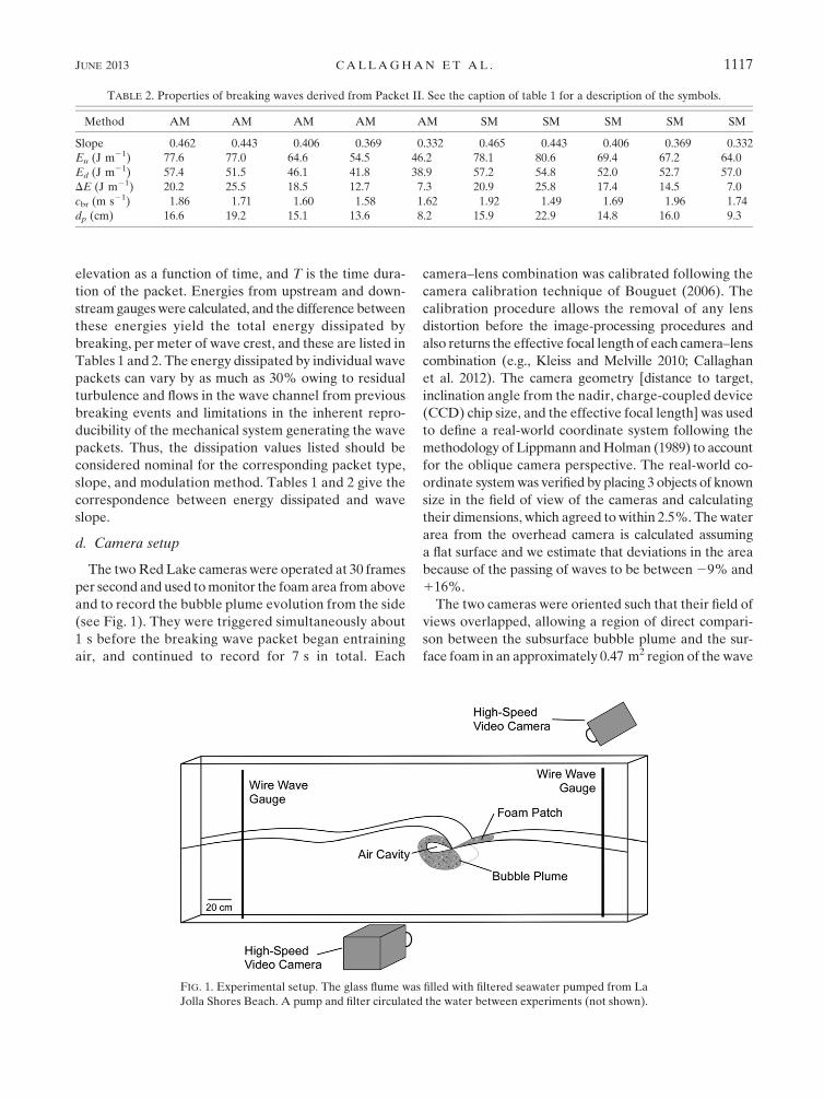
a. Overview of experimental setup

The experiments were carried out in the 33 m long

seawater glass wave channel operated by the Hydraulics

Facility at Scripps Institution of Oceanography. Waves

of adjustable amplitude and slope were designed using

the focused packet technique introduced by Longuet-

Higgins (1974) and created with a hydraulic wave paddle

at one end of the channel.Wave packets focus and break

roughly 6 m downstream of the paddle in an area in-

strumented with sideview and overhead 1 Megapixel,

high-speed Red Lake Motion Pro X cameras and 2

custom-built wire wave gauges calibrated to an accuracy

of 61 mm (one upstream and one downstream of the

wave break region).

The experiment was divided into clean (surfactant

free) and medium-productivity (surfactant added) pha-

ses, as described further below. A sequence of breaking

events using a wave packet of specified amplitude, slope,

and wave scale was executed during each phase. The

salinity and temperature of the filtered seawater used in

the experiment (drawn from La Jolla Shores beach),

were monitored with a FSI microCTD. During the ex-

periment the mean water temperature was 15.58C with

a range of 618C and the mean salinity was 33.52 PSU

with a range of 60.07 PSU. For reference, the temper-

ature and salinity ranges reported in Callaghan et al.

(2012) were 13.88 to 15.98C and 31.52 to 31.77 PSU re-

spectively. In addition, water samples were taken before

and after a series of breaking waves and analyzed for

surface tension values using a tensiometer (Kruss

model K11).

b. The addition of surfactant

Surface tension was varied by the addition of Triton

X-100 soluble surfactant (204 mg L21). This resulted in

a surface tension of 70 mN m21 (60.5 mN m21), which

gave a film pressure of about 4 mN m21. Film pressure

can be defined as the difference in surface tension be-

tween uncontaminated seawater (nominally 74 mN m21)

and contaminated seawater (Barger et al. 1974). Triton

X-100 has been used in prior studies to simulate the ef-

fects of soluble surface active materials in the ocean, and

corresponds tomoderately productive oceanic conditions

in concentrations between 170 and 250 mg L21 within the

water column (Wurl et al. 2011). In the text that follows,

we will use the terms ‘‘medium productivity’’ and ‘‘sur-

factant added’’ interchangeably to denote experiments

with the addition of Triton X-100. Similarly, we will use

the terms ‘‘clean’’ or ‘‘surfactant free’’ regimes to denote

experiments with filtered seawater without the addition

of Triton X-100. We note that, despite the implication of

JUNE 2013 CALLAGHAN ET AL . 1115

water that is free of any surface-active material, the fil-

tered seawater likely did contain low levels of surfactant.

The measured film pressure for the clean water regime

was 1 mN m21 (60.5 mN m21), indicating clean water

conditions acceptable for our purposes. Indeed, Lewis

and Schwartz (2004) note that it is ‘‘extremely difficult’’

to eliminate surfactants even when making clean water

for laboratory experiments.

c. Wave packet description

The wave packets used here were generated by the

linear superposition of a discrete set of N spectral com-

ponents of specified frequencyvj, amplitude aj, and phase

uj. The propagation velocity and wavenumber kj of each

component is determined by the dispersion equation for

the finite water depth channel. The phase of each com-

ponent at the source paddle is determined by requiring

that the phases of all components be zero at the chosen

downstream focal point (approximately 6 m for this

experiment).

Because the energy dissipated by a focusedwave packet

is controlled by its slope (Rapp and Melville 1990), we

have characterized our packets using the linear maxi-

mum slopemetric (hereafter referred to as wave slope or

simply slope) as employed in other studies (e.g., Romero

et al. 2012). The wave slope used here, s, is based on a

summation of wave spectral components, which are as-

sumed to be in phase at the wave break point:

s5 �N

j51

ajkj , (1)

where N is the number of discrete spectral components

in the wave packet.

The selection of frequencies and amplitudes for a

breaking packet involves a process of trial and error. A

characteristic frequency is selected that determines the

scale of the wave, and the bandwidth of the packet is

determined by the range of frequencies that can be

practically generated by the paddle. Then a ‘‘maximum

breaking intensity’’ packet is designed by systematically

increasing the amplitude of the highest frequency spec-

tral component until prebreaking of the packet occurred.

Prebreaking of a packet occurs when the evolution of the

packet causes breaking before the focal point is reached,

resulting in disruption of the packet. The maximum in-

tensity breaking packet is the largest packet that can be

generated without prebreaking.

Two maximum intensity breaking packets based on

slightly different spectral compositions were designed;

packet types I and II, with packet I having the greatest

overall amplitude and scale. The slope of each packet

type was then varied using twomethods. The first method

[amplitude modulation (AM)] scaled the overall ampli-

tude of the packet downward to decrease the wave slope.

The secondmethod [spectral modulation (SM)] decreased

the amplitude of the highest spectral component in the

packet until the desired slope was reached. If the slope

was still too large after the complete removal of the highest

spectral component, then the next highest spectral com-

ponent was also attenuated. In total, five different slopes

were chosen to achieve a range of breaking waves from

plunging (largest slope) to gently spilling (smallest slope)

and these slopes are within the range reported inRomero

et al. (2012). There were a total of 20 distinct breaking

wave types used in this experiment, equally divided

between packets I and II, and for each packet type five

breaking waves of varying slope were generated using

both the AM and SM methods. The properties of these

packets are listed in Tables 1 and 2. The energy in each

packet in units of Joules per along-crest meter of wave

was calculated from the wire wave gauge time series

using the formula:

E5rg

2c

ðT0h2(t) dt , (2)

where r is the density of seawater, g is the acceleration

becauseof gravity, c5 1.64 m s21 is a spectral composition-

weighted, mean packet wave speed, h(t) is the surface

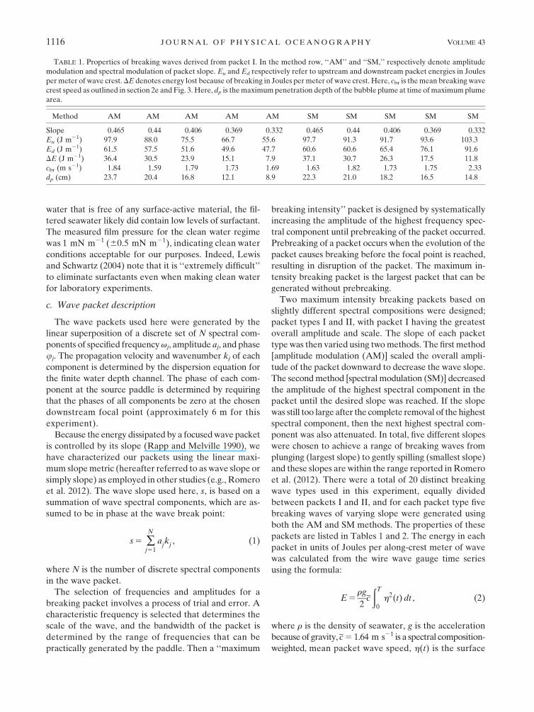
TABLE 1. Properties of breaking waves derived from packet I. In the method row, ‘‘AM’’ and ‘‘SM,’’ respectively denote amplitude

modulation and spectral modulation of packet slope. Eu and Ed respectively refer to upstream and downstream packet energies in Joules

per meter of wave crest.DE denotes energy lost because of breaking in Joules per meter of wave crest. Here, cbr is themean breaking wave

crest speed as outlined in section 2e and Fig. 3. Here, dp is themaximumpenetration depth of the bubble plume at time ofmaximumplume

area.

Method AM AM AM AM AM SM SM SM SM SM

Slope 0.465 0.44 0.406 0.369 0.332 0.465 0.44 0.406 0.369 0.332

Eu (J m21) 97.9 88.0 75.5 66.7 55.6 97.7 91.3 91.7 93.6 103.3

Ed (J m21) 61.5 57.5 51.6 49.6 47.7 60.6 60.6 65.4 76.1 91.6

DE (J m21) 36.4 30.5 23.9 15.1 7.9 37.1 30.7 26.3 17.5 11.8

cbr (m s21) 1.84 1.59 1.79 1.73 1.69 1.63 1.82 1.73 1.75 2.33

dp (cm) 23.7 20.4 16.8 12.1 8.9 22.3 21.0 18.2 16.5 14.8

1116 JOURNAL OF PHYS ICAL OCEANOGRAPHY VOLUME 43

elevation as a function of time, and T is the time dura-

tion of the packet. Energies from upstream and down-

stream gaugeswere calculated, and the difference between

these energies yield the total energy dissipated by

breaking, per meter of wave crest, and these are listed in

Tables 1 and 2. The energy dissipated by individual wave

packets can vary by as much as 30% owing to residual

turbulence and flows in the wave channel from previous

breaking events and limitations in the inherent repro-

ducibility of the mechanical system generating the wave

packets. Thus, the dissipation values listed should be

considered nominal for the corresponding packet type,

slope, and modulation method. Tables 1 and 2 give the

correspondence between energy dissipated and wave

slope.

d. Camera setup

The twoRed Lake cameras were operated at 30 frames

per second and used tomonitor the foamarea from above

and to record the bubble plume evolution from the side

(see Fig. 1). They were triggered simultaneously about

1 s before the breaking wave packet began entraining

air, and continued to record for 7 s in total. Each

camera–lens combination was calibrated following the

camera calibration technique of Bouguet (2006). The

calibration procedure allows the removal of any lens

distortion before the image-processing procedures and

also returns the effective focal length of each camera–lens

combination (e.g., Kleiss and Melville 2010; Callaghan

et al. 2012). The camera geometry [distance to target,

inclination angle from the nadir, charge-coupled device

(CCD) chip size, and the effective focal length] was used

to define a real-world coordinate system following the

methodology of Lippmann andHolman (1989) to account

for the oblique camera perspective. The real-world co-

ordinate systemwas verified by placing 3 objects of known

size in the field of view of the cameras and calculating

their dimensions, which agreed towithin 2.5%. Thewater

area from the overhead camera is calculated assuming

a flat surface and we estimate that deviations in the area

because of the passing of waves to be between29% and

116%.

The two cameras were oriented such that their field of

views overlapped, allowing a region of direct compari-

son between the subsurface bubble plume and the sur-

face foam in an approximately 0.47 m2 region of the wave

TABLE 2. Properties of breaking waves derived from Packet II. See the caption of table 1 for a description of the symbols.

Method AM AM AM AM AM SM SM SM SM SM

Slope 0.462 0.443 0.406 0.369 0.332 0.465 0.443 0.406 0.369 0.332

Eu (J m21) 77.6 77.0 64.6 54.5 46.2 78.1 80.6 69.4 67.2 64.0

Ed (J m21) 57.4 51.5 46.1 41.8 38.9 57.2 54.8 52.0 52.7 57.0

DE (J m21) 20.2 25.5 18.5 12.7 7.3 20.9 25.8 17.4 14.5 7.0

cbr (m s21) 1.86 1.71 1.60 1.58 1.62 1.92 1.49 1.69 1.96 1.74

dp (cm) 16.6 19.2 15.1 13.6 8.2 15.9 22.9 14.8 16.0 9.3

FIG. 1. Experimental setup. The glass flume was filled with filtered seawater pumped from La

Jolla Shores Beach. A pump and filter circulated the water between experiments (not shown).

JUNE 2013 CALLAGHAN ET AL . 1117

tank. The surface area viewed by the top camera ex-

tended beyond the sides of the wave flume and this

portion was masked in all further image analysis. The

area viewed by the side looking camera did not need to

be masked.

e. Image analysis

After translation from pixel coordinates into real-

world coordinates, the image analysis consisted of three

processing steps: subtraction of a background image, ap-

plication of a threshold, and glint removal. Each of these

steps is described in greater detail below. Background

images were acquired at the beginning of each breaking

event by the two cameras. These images were then sub-

tracted from all other images to eliminate any unwanted

stationary signals such as the presence of submerged

instruments.

To separate the whitecap and bubble-plume signals

from the background water, a threshold was applied to

each image for both the top- and side-viewing cameras

and remained unchanged throughout the experiment.

The threshold was determined by trial and error to cap-

ture even the dimmest of foampatches and bubble plumes

while eliminating any unwanted signal, for example, from

surface reflections. Illumination conditions were constant

throughout the experiment, justifying the use of a single

threshold for each camera.

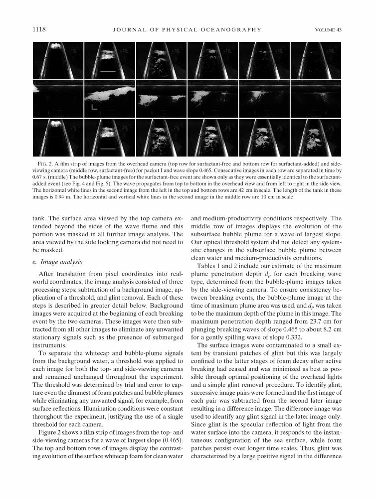
Figure 2 shows a film strip of images from the top- and

side-viewing cameras for a wave of largest slope (0.465).

The top and bottom rows of images display the contrast-

ing evolution of the surface whitecap foam for clean water

and medium-productivity conditions respectively. The

middle row of images displays the evolution of the

subsurface bubble plume for a wave of largest slope.

Our optical threshold system did not detect any system-

atic changes in the subsurface bubble plume between

clean water and medium-productivity conditions.

Tables 1 and 2 include our estimate of the maximum

plume penetration depth dp for each breaking wave

type, determined from the bubble-plume images taken

by the side-viewing camera. To ensure consistency be-

tween breaking events, the bubble-plume image at the

time of maximum plume area was used, and dpwas taken

to be the maximum depth of the plume in this image. The

maximum penetration depth ranged from 23.7 cm for

plunging breaking waves of slope 0.465 to about 8.2 cm

for a gently spilling wave of slope 0.332.

The surface images were contaminated to a small ex-

tent by transient patches of glint but this was largely

confined to the latter stages of foam decay after active

breaking had ceased and was minimized as best as pos-

sible through optimal positioning of the overhead lights

and a simple glint removal procedure. To identify glint,

successive image pairs were formed and the first image of

each pair was subtracted from the second later image

resulting in a difference image. The difference image was

used to identify any glint signal in the later image only.

Since glint is the specular reflection of light from the

water surface into the camera, it responds to the instan-

taneous configuration of the sea surface, while foam

patches persist over longer time scales. Thus, glint was

characterized by a large positive signal in the difference

FIG. 2. A film strip of images from the overhead camera (top row for surfactant-free and bottom row for surfactant-added) and side-

viewing camera (middle row, surfactant-free) for packet I and wave slope 0.465. Consecutive images in each row are separated in time by

0.67 s. (middle) The bubble-plume images for the surfactant-free event are shown only as they were essentially identical to the surfactant-

added event (see Fig. 4 and Fig. 5). The wave propagates from top to bottom in the overhead view and from left to right in the side view.

The horizontal white lines in the second image from the left in the top and bottom rows are 42 cm in scale. The length of the tank in these

images is 0.94 m. The horizontal and vertical white lines in the second image in the middle row are 10 cm in scale.

1118 JOURNAL OF PHYS ICAL OCEANOGRAPHY VOLUME 43

images, while foampatcheswere characterized by smaller,

often negative signals. Any glint identified in the dif-

ference images after active breaking had ceased was

removed from further processing allowing each later

image within an image pair to be compared to the pre-

vious glint ‘‘free’’ image within each image pair. This

procedure helped to minimize the glint contamination

but did not totally remove it.Wehave estimated the noise

floor for the area measurements, which include contam-

ination from residual glint, at about 0.01 m2.

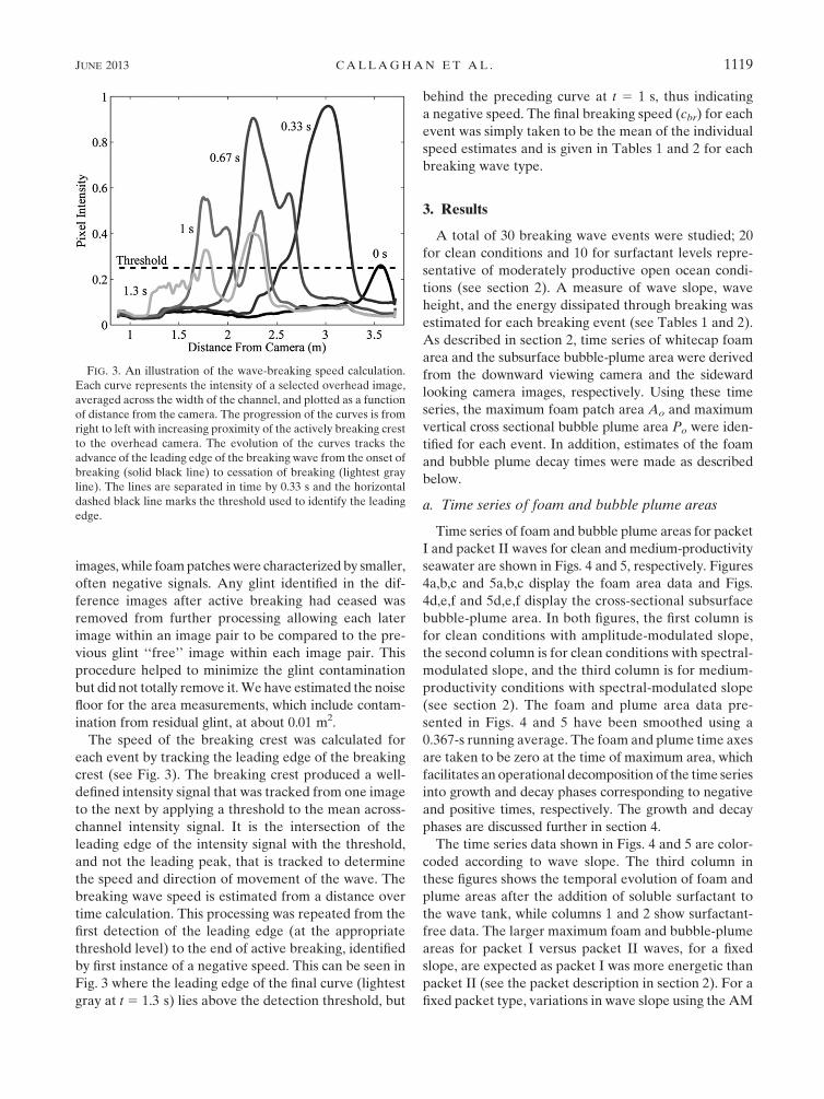
The speed of the breaking crest was calculated for

each event by tracking the leading edge of the breaking

crest (see Fig. 3). The breaking crest produced a well-

defined intensity signal that was tracked from one image

to the next by applying a threshold to the mean across-

channel intensity signal. It is the intersection of the

leading edge of the intensity signal with the threshold,

and not the leading peak, that is tracked to determine

the speed and direction of movement of the wave. The

breaking wave speed is estimated from a distance over

time calculation. This processing was repeated from the

first detection of the leading edge (at the appropriate

threshold level) to the end of active breaking, identified

by first instance of a negative speed. This can be seen in

Fig. 3 where the leading edge of the final curve (lightest

gray at t 5 1.3 s) lies above the detection threshold, but

behind the preceding curve at t 5 1 s, thus indicating

a negative speed. The final breaking speed (cbr) for each

event was simply taken to be the mean of the individual

speed estimates and is given in Tables 1 and 2 for each

breaking wave type.

3. Results

A total of 30 breaking wave events were studied; 20

for clean conditions and 10 for surfactant levels repre-

sentative of moderately productive open ocean condi-

tions (see section 2). A measure of wave slope, wave

height, and the energy dissipated through breaking was

estimated for each breaking event (see Tables 1 and 2).

As described in section 2, time series of whitecap foam

area and the subsurface bubble-plume area were derived

from the downward viewing camera and the sideward

looking camera images, respectively. Using these time

series, the maximum foam patch area Ao and maximum

vertical cross sectional bubble plume area Po were iden-

tified for each event. In addition, estimates of the foam

and bubble plume decay times were made as described

below.

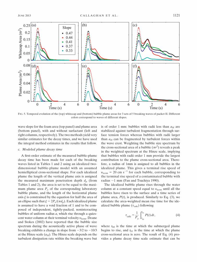
a. Time series of foam and bubble plume areas

Time series of foam and bubble plume areas for packet

I and packet II waves for clean and medium-productivity

seawater are shown in Figs. 4 and 5, respectively. Figures

4a,b,c and 5a,b,c display the foam area data and Figs.

4d,e,f and 5d,e,f display the cross-sectional subsurface

bubble-plume area. In both figures, the first column is

for clean conditions with amplitude-modulated slope,

the second column is for clean conditions with spectral-

modulated slope, and the third column is for medium-

productivity conditions with spectral-modulated slope

(see section 2). The foam and plume area data pre-

sented in Figs. 4 and 5 have been smoothed using a

0.367-s running average. The foam and plume time axes

are taken to be zero at the time of maximum area, which

facilitates an operational decomposition of the time series

into growth and decay phases corresponding to negative

and positive times, respectively. The growth and decay

phases are discussed further in section 4.

The time series data shown in Figs. 4 and 5 are color-

coded according to wave slope. The third column in

these figures shows the temporal evolution of foam and

plume areas after the addition of soluble surfactant to

the wave tank, while columns 1 and 2 show surfactant-

free data. The larger maximum foam and bubble-plume

areas for packet I versus packet II waves, for a fixed

slope, are expected as packet I was more energetic than

packet II (see the packet description in section 2). For a

fixed packet type, variations in wave slope using the AM

FIG. 3. An illustration of the wave-breaking speed calculation.

Each curve represents the intensity of a selected overhead image,

averaged across the width of the channel, and plotted as a function

of distance from the camera. The progression of the curves is from

right to left with increasing proximity of the actively breaking crest

to the overhead camera. The evolution of the curves tracks the

advance of the leading edge of the breaking wave from the onset of

breaking (solid black line) to cessation of breaking (lightest gray

line). The lines are separated in time by 0.33 s and the horizontal

dashed black line marks the threshold used to identify the leading

edge.

JUNE 2013 CALLAGHAN ET AL . 1119

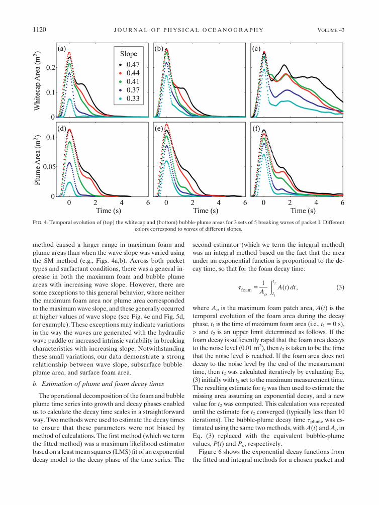
method caused a larger range in maximum foam and

plume areas than when the wave slope was varied using

the SM method (e.g., Figs. 4a,b). Across both packet

types and surfactant conditions, there was a general in-

crease in both the maximum foam and bubble plume

areas with increasing wave slope. However, there are

some exceptions to this general behavior, where neither

the maximum foam area nor plume area corresponded

to themaximumwave slope, and these generally occurred

at higher values of wave slope (see Fig. 4e and Fig. 5d,

for example). These exceptions may indicate variations

in the way the waves are generated with the hydraulic

wave paddle or increased intrinsic variability in breaking

characteristics with increasing slope. Notwithstanding

these small variations, our data demonstrate a strong

relationship between wave slope, subsurface bubble-

plume area, and surface foam area.

b. Estimation of plume and foam decay times

The operational decomposition of the foam and bubble

plume time series into growth and decay phases enabled

us to calculate the decay time scales in a straightforward

way. Twomethods were used to estimate the decay times

to ensure that these parameters were not biased by

method of calculations. The first method (which we term

the fitted method) was a maximum likelihood estimator

based on a leastmean squares (LMS) fit of an exponential

decay model to the decay phase of the time series. The

second estimator (which we term the integral method)

was an integral method based on the fact that the area

under an exponential function is proportional to the de-

cay time, so that for the foam decay time:

tfoam 51

Ao

ðt2

t1

A(t) dt , (3)

where Ao is the maximum foam patch area, A(t) is the

temporal evolution of the foam area during the decay

phase, t1 is the time of maximum foam area (i.e., t15 0 s),

> and t2 is an upper limit determined as follows. If the

foam decay is sufficiently rapid that the foam area decays

to the noise level (0.01 m2), then t2 is taken to be the time

that the noise level is reached. If the foam area does not

decay to the noise level by the end of the measurement

time, then t2 was calculated iteratively by evaluating Eq.

(3) initially with t2 set to themaximummeasurement time.

The resulting estimate for t2 was then used to estimate the

missing area assuming an exponential decay, and a new

value for t2 was computed. This calculation was repeated

until the estimate for t2 converged (typically less than 10

iterations). The bubble-plume decay time tplume was es-

timated using the same twomethods, withA(t) andAo in

Eq. (3) replaced with the equivalent bubble-plume

values, P(t) and Po, respectively.

Figure 6 shows the exponential decay functions from

the fitted and integral methods for a chosen packet and

FIG. 4. Temporal evolution of (top) the whitecap and (bottom) bubble-plume areas for 3 sets of 5 breaking waves of packet I. Different

colors correspond to waves of different slopes.

1120 JOURNAL OF PHYS ICAL OCEANOGRAPHY VOLUME 43

wave slope for the foam area (top panel) and plume area

(bottom panel), with and without surfactant (left and

right columns, respectively). The twomethods yield very

similar estimates for the decay times, and we have used

the integral method estimates in the results that follow.

c. Modeled plume decay time

A first-order estimate of the measured bubble-plume

decay time has been made for each of the breaking

waves listed in Tables 1 and 2 using an idealized two-

dimensional bubble-plume model with an assumed

hemielliptical cross-sectional shape. For each idealized

plume the length of the vertical plume axis is assigned

the measured maximum penetration depth dp (from

Tables 1 and 2), the area is set to be equal to the maxi-

mum plume area Po of the corresponding laboratory

bubble plume, and the length of the horizontal plume

axis j is constrained by the equation for half the area of

an ellipse such that j5 2Po/(pdp). Each idealized plume

is assumed to have a void fraction of 1 and to be com-

posed of independent, tightly-packed, noninteracting

bubbles of uniform radius a, which rise through a quies-

cent water column at their terminal velocity yterm. Deane

and Stokes (2002) have reported that the bubble size

spectrum during the acoustically active phase of wave

breaking exhibits a change in slope from 23/2 to 210/3

at the Hinze scale (aH). The Hinze scale depends on the

turbulent dissipation rate within the breaking wave but

is of order 1 mm: bubbles with radii less than aH are

stabilized against turbulent fragmentation through sur-

face tension forces whereas bubbles with radii larger

than aH can be fragmented by turbulent forces within

the wave crest. Weighting the bubble size spectrum by

the cross-sectional area of a bubble (pr2) reveals a peak

in the weighted spectrum at the Hinze scale, implying

that bubbles with radii order 1 mm provide the largest

contribution to the plume cross-sectional area. There-

fore, a radius of 1mm is assigned to all bubbles in the

idealized plume. This gives a terminal rise speed of

yterm 5 20 cm s21 for each bubble, corresponding to

the terminal rise speed of a contaminated bubble with

radius ;1 mm (Fan and Tsuchiya 1990).

The idealized bubble plume rises through the water

column at a constant speed equal to yterm until all the

bubbles have risen to the surface and a time series of

plume area, P(t), is produced. Similarly to Eq. (3), we

calculate the area-weighted mean rise time for the ide-

alized bubble plume (tcalc) following

tcalc51

Po

ðtb1

tb0

P(t) dt , (4)

where tb0 is the time at which the submerged plume

begins to rise, and tb1 is the time at which the plume

cross-sectional area is zero. The result of Eq. (4) pro-

vides a plume decay time scale estimate that can be

FIG. 5. Temporal evolution of the (top) whitecap and (bottom) bubble plume areas for 3 sets of 5 breaking waves of packet II. Different

colors correspond to waves of different slopes.

JUNE 2013 CALLAGHAN ET AL . 1121

directly compared to the integral method calculation

(see above) of the laboratory bubble plume decay time

scale. The idealized model does not take into account

the decaying turbulent velocity fluctuations within the

bubble plume that act to retard bubble degassing, it uses

a single bubble size and our model assumes all entrained

air forms a single bubble plume. Additionally, it does

not include details about the larger scale orbital motions

of the surface wave field, which could act to force the

bubble upward or downward depending on the phase of

the wave.

Figure 7 shows the relationship between tplume and

tcalc for the plume depths reported in Tables 1 and 2.

Larger values of tplume are associated with larger values

of energy loss through breaking as the breaking de-

velops from gently spilling to plunging. The measured

values of tplume are all greater than tcalc, and they di-

verge with increasing breaking severity. This result is to

be expected since bubble-degassing rates are reduced

in the presence of energetic turbulent motions, and this

is not included in our simple model. The terminal rise

speed of bubbles is a function of their radius, and bubbles

will only degas when the turbulent velocity fluctua-

tions fall below levels that are comparable to the size-

dependent bubble rise speed. Therefore, more energetic

breaking waves have the potential to keep more bubbles

submerged for a longer period of time than weaker

breaking waves. As the turbulence from a breaking wave

decays, more bubbles are able to degas to the surface.

Although the estimates of tcalc involve gross simplifica-

tions, Fig. 7 demonstrates that themeasured values of the

plume decay times from the laboratory study are physi-

cally reasonable, and certainly not an underestimate.

4. Discussion

a. Foam decay regimes

The laboratory observations suggest that the behavior

of the whitecap foam decay is controlled by two regimes:

a surfactant-stabilized regime associated with medium-

productivity conditions and a plume-driven regime

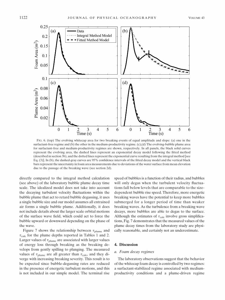
FIG. 6. (top) The evolving whitecap area for two breaking events of equal amplitude and slope: (a) one in the

surfactant-free regime and (b) the other in the medium-productivity regime. (c),(d) The evolving-bubble plume area

for surfactant-free and medium-productivity regimes are shown, respectively. In all panels, the black solid curves

represent the evolving area, the dashed lines represent an exponential decay model following the fitted method

(described in section 3b), and the dotted lines represent the exponential curve resulting from the integral method [see

Eq. (3)]. In (b), the dashed-gray curves are 95% confidence intervals of the fitted decay model and the vertical black

bars represent the uncertainty in foam areameasurements due to deviations of thewater surface frommean elevation

due to the passage of the breaking wave (see section 2d).

1122 JOURNAL OF PHYS ICAL OCEANOGRAPHY VOLUME 43

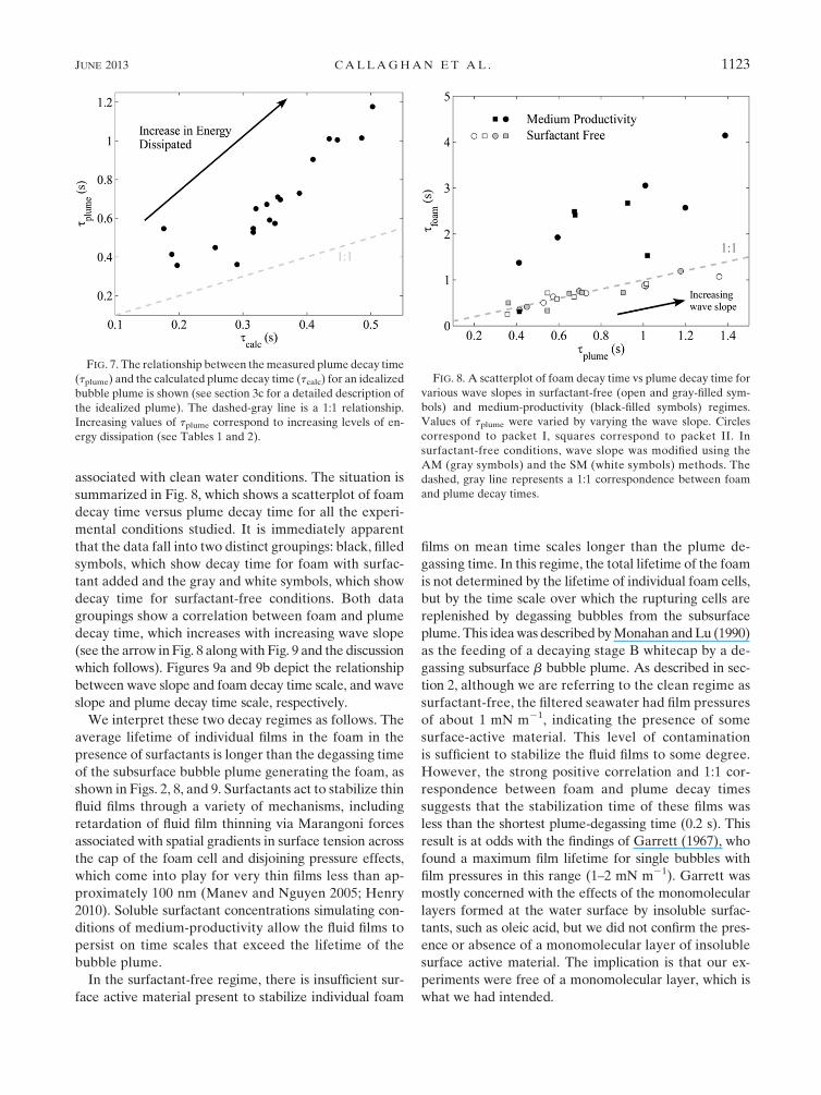
associated with clean water conditions. The situation is

summarized in Fig. 8, which shows a scatterplot of foam

decay time versus plume decay time for all the experi-

mental conditions studied. It is immediately apparent

that the data fall into two distinct groupings: black, filled

symbols, which show decay time for foam with surfac-

tant added and the gray and white symbols, which show

decay time for surfactant-free conditions. Both data

groupings show a correlation between foam and plume

decay time, which increases with increasing wave slope

(see the arrow inFig. 8 alongwith Fig. 9 and the discussion

which follows). Figures 9a and 9b depict the relationship

between wave slope and foam decay time scale, and wave

slope and plume decay time scale, respectively.

We interpret these two decay regimes as follows. The

average lifetime of individual films in the foam in the

presence of surfactants is longer than the degassing time

of the subsurface bubble plume generating the foam, as

shown in Figs. 2, 8, and 9. Surfactants act to stabilize thin

fluid films through a variety of mechanisms, including

retardation of fluid film thinning via Marangoni forces

associated with spatial gradients in surface tension across

the cap of the foam cell and disjoining pressure effects,

which come into play for very thin films less than ap-

proximately 100 nm (Manev and Nguyen 2005; Henry

2010). Soluble surfactant concentrations simulating con-

ditions of medium-productivity allow the fluid films to

persist on time scales that exceed the lifetime of the

bubble plume.

In the surfactant-free regime, there is insufficient sur-

face active material present to stabilize individual foam

films on mean time scales longer than the plume de-

gassing time. In this regime, the total lifetime of the foam

is not determined by the lifetime of individual foam cells,

but by the time scale over which the rupturing cells are

replenished by degassing bubbles from the subsurface

plume. This ideawas described byMonahan andLu (1990)

as the feeding of a decaying stage B whitecap by a de-

gassing subsurface b bubble plume. As described in sec-

tion 2, although we are referring to the clean regime as

surfactant-free, the filtered seawater had film pressures

of about 1 mN m21, indicating the presence of some

surface-active material. This level of contamination

is sufficient to stabilize the fluid films to some degree.

However, the strong positive correlation and 1:1 cor-

respondence between foam and plume decay times

suggests that the stabilization time of these films was

less than the shortest plume-degassing time (0.2 s). This

result is at odds with the findings of Garrett (1967), who

found a maximum film lifetime for single bubbles with

film pressures in this range (1–2 mN m21). Garrett was

mostly concerned with the effects of the monomolecular

layers formed at the water surface by insoluble surfac-

tants, such as oleic acid, but we did not confirm the pres-

ence or absence of a monomolecular layer of insoluble

surface active material. The implication is that our ex-

periments were free of a monomolecular layer, which is

what we had intended.

FIG. 7. The relationship between themeasured plume decay time

(tplume) and the calculated plume decay time (tcalc) for an idealized

bubble plume is shown (see section 3c for a detailed description of

the idealized plume). The dashed-gray line is a 1:1 relationship.

Increasing values of tplume correspond to increasing levels of en-

ergy dissipation (see Tables 1 and 2).

FIG. 8. A scatterplot of foam decay time vs plume decay time for

various wave slopes in surfactant-free (open and gray-filled sym-

bols) and medium-productivity (black-filled symbols) regimes.

Values of tplume were varied by varying the wave slope. Circles

correspond to packet I, squares correspond to packet II. In

surfactant-free conditions, wave slope was modified using the

AM (gray symbols) and the SM (white symbols) methods. The

dashed, gray line represents a 1:1 correspondence between foam

and plume decay times.

JUNE 2013 CALLAGHAN ET AL . 1123

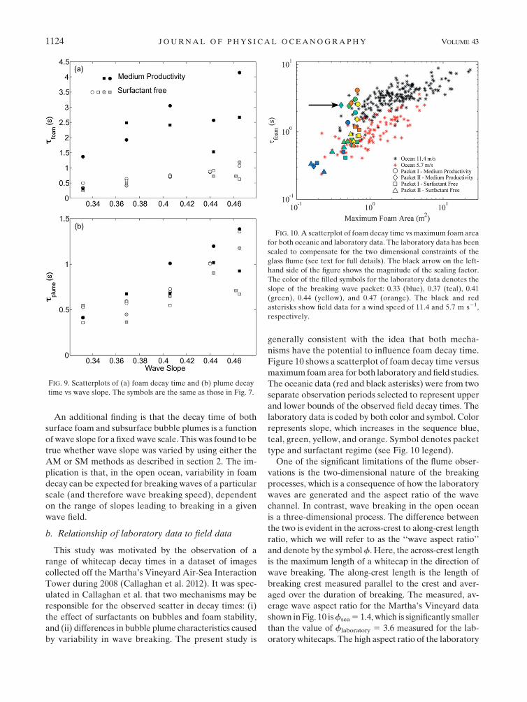
An additional finding is that the decay time of both

surface foam and subsurface bubble plumes is a function

of wave slope for a fixedwave scale. This was found to be

true whether wave slope was varied by using either the

AM or SM methods as described in section 2. The im-

plication is that, in the open ocean, variability in foam

decay can be expected for breaking waves of a particular

scale (and therefore wave breaking speed), dependent

on the range of slopes leading to breaking in a given

wave field.

b. Relationship of laboratory data to field data

This study was motivated by the observation of a

range of whitecap decay times in a dataset of images

collected off the Martha’s Vineyard Air-Sea Interaction

Tower during 2008 (Callaghan et al. 2012). It was spec-

ulated in Callaghan et al. that two mechanisms may be

responsible for the observed scatter in decay times: (i)

the effect of surfactants on bubbles and foam stability,

and (ii) differences in bubble plume characteristics caused

by variability in wave breaking. The present study is

generally consistent with the idea that both mecha-

nisms have the potential to influence foam decay time.

Figure 10 shows a scatterplot of foam decay time versus

maximum foamarea for both laboratory and field studies.

The oceanic data (red and black asterisks) were from two

separate observation periods selected to represent upper

and lower bounds of the observed field decay times. The

laboratory data is coded by both color and symbol. Color

represents slope, which increases in the sequence blue,

teal, green, yellow, and orange. Symbol denotes packet

type and surfactant regime (see Fig. 10 legend).

One of the significant limitations of the flume obser-

vations is the two-dimensional nature of the breaking

processes, which is a consequence of how the laboratory

waves are generated and the aspect ratio of the wave

channel. In contrast, wave breaking in the open ocean

is a three-dimensional process. The difference between

the two is evident in the across-crest to along-crest length

ratio, which we will refer to as the ‘‘wave aspect ratio’’

and denote by the symbolf. Here, the across-crest length

is the maximum length of a whitecap in the direction of

wave breaking. The along-crest length is the length of

breaking crest measured parallel to the crest and aver-

aged over the duration of breaking. The measured, av-

erage wave aspect ratio for the Martha’s Vineyard data

shown inFig. 10 isfsea5 1.4, which is significantly smaller

than the value of flaboratory 5 3.6 measured for the lab-

oratory whitecaps. The high aspect ratio of the laboratory

FIG. 9. Scatterplots of (a) foam decay time and (b) plume decay

time vs wave slope. The symbols are the same as those in Fig. 7.

FIG. 10. A scatterplot of foam decay time vsmaximum foam area

for both oceanic and laboratory data. The laboratory data has been

scaled to compensate for the two dimensional constraints of the

glass flume (see text for full details). The black arrow on the left-

hand side of the figure shows the magnitude of the scaling factor.

The color of the filled symbols for the laboratory data denotes the

slope of the breaking wave packet: 0.33 (blue), 0.37 (teal), 0.41

(green), 0.44 (yellow), and 0.47 (orange). The black and red

asterisks show field data for a wind speed of 11.4 and 5.7 m s21,

respectively.

1124 JOURNAL OF PHYS ICAL OCEANOGRAPHY VOLUME 43

whitecaps relative to the ocean whitecaps is expected

given the two dimensional nature of themechanical wave

maker and the limited width of the laboratory channel,

which confines the lateral spreading of the breaking crest

and hence the resulting surface foam area. We can at-

tempt to scale the laboratory whitecaps to an oceanic

context by scaling their along-crest lengths such that their

mean aspect ratio is the same as the oceanic whitecaps.

The net result is an increase in laboratory whitecap area

by a factor flaboratory/fsea 5 2.6. On the horizontal log

scale of Fig. 10, thismultiplicative factor is represented by

a constant shift to the right of all the laboratory data

points. The extent of this shift is indicated by the hori-

zontal arrow on the left-hand side of the figure.

The span of decay times observed in the field is gen-

erally consistent with those observed in the surfactant-

free and medium-productivity experiments. The spread

of decay times at a given wave scale in the surfactant-

free and medium-productivity regimes is determined

by wave slope, and the spread of times in the laboratory

and field data are in good agreement at the overlapping

scales. However, because the field data correspond to

different meteorological conditions (mean wind speed

of 5.7 and 11.4 m s21), and without appropriate in situ

measurements of surface active material, the observed

increase in foam decay time for the higher wind speed

period cannot be attributedwith certainty to either plume

dynamics or the presence of surfactants.

5. Summary and conclusions

A laboratory study of foam generated by seawater

breaking wave packets has demonstrated that foam

lifetime is variable and controlled by subsurface bubble

plume degassing times, which are a function of wave

scale and breaking wave slope. This is true whether or

not surfactants are present. However, in the presence of

surfactants, whitecap foam is stabilized and persists for

roughly a factor of 3 times its clean seawater value for

the surfactant concentration studied (204 mg L21 corre-

sponding to conditions of medium ocean productivity,

see Wurl et al. 2011).

The range of foam decay times observed in the labo-

ratory study lie within the range of values observed in

a dataset obtained off Martha’s Vineyard in 2008. The

scale of the laboratory breakers, when adjusted to ac-

count for three-dimensional breaking effects in the

ocean through the breaking wave aspect ratio, lie at the

lower end of the scale observed at sea, but with good

overlap between the laboratory and oceanic studies.

This study has enabled us to explore the speculations

put forward in the Martha’s Vineyard study (Callaghan

et al. 2012) to explain the variability of foam decay times

observed at sea. Each of the postulated mechanisms,

plume-driven bubble lifetime and surfactant-stabilized

foam, appear to play a role in the lifetime of oceanic

whitecaps. Given the overlap in decay times between the

field measurements and the medium-productivity and

clean laboratory data, it is tempting to suggest that the

increase in oceanic decay times observed during the

11.4 m s21 wind conditions is due to surfactants present

in the upper ocean boundary layer that were absent in

the 5.7 m s21 oceanic observational period. It may also

reflect a change in the composition and concentration

of surfactants in the upper mm of the ocean as rising

bubbles scavenge surfactants in the bulk water and trans-

port them to the surface (see Callaghan et al. 2012).

However, the very strong possibility that the differ-

ences are due to changes in plume dynamics associated

with the increase in wind speed cannot be ruled out.

Finally, we note that the observation of bubble-

controlled and surfactant-controlled regimes of foam

decay has implications for understanding the observed

scatter in historical measurements of whitecap coverage

(see Anguelova and Webster 2006) and the boundary

layer exchange processes they are used to parameter-

ize such as air–sea gas exchange (Woolf 1997), marine

aerosol production flux (Monahan et al. 1986; Lewis and

Schwartz 2004), ocean albedo due to whitecaps (Frouin

et al. 1996), and wave energy dissipation (Hwang and

Sletten 2008). Although there is no way to augment ex-

isting datasets with measurements of concentrations of

surface-active materials, this study suggests it would be

beneficial to do so in future studies.

Until simultaneous, in situmeasurements of wave slope

and surfactant concentration are made, uncertainty will

remain about which factor has the greater influence on

whitecap decay times at sea. Notwithstanding the current

uncertainties, there may be important implications for

using above-water remote sensing techniques (optical

and microwave emissivity) to study subsurface plume

dynamics. For instance, in clean water conditions where

the role of surfactants is expected to be minimized, the

laboratory study shows that monitoring the decay time of

whitecap foam yields a first-order estimate of plume-

degassing time. The coupling of the whitecap foam de-

cay time information with knowledge of bubble size

distributions, bubble terminal rise velocity and turbu-

lence generated by breaking waves, could facilitate the

formation ofmodels for subsurface bubble plume spatial

structure and its evolution over time. When surfactants

are present in the upper ocean boundary layer in suffi-

cient concentration to stabilize foam beyond bubble-

plume-degassing time scales, the decay time of whitecap

foam may provide a method for remotely sensing the

presence of these surface-active materials. Determining

JUNE 2013 CALLAGHAN ET AL . 1125

when the foam lifetime is controlled by plume persis-

tence or water chemistry may prove quite difficult. How-

ever, there are sensing techniques that could be explored,

such as differences in microwave emissivity at different

frequencies; lower frequencies being more sensitive to

bubble plume structure a few tens of cm below the sur-

face, and higher frequencies being sensitive to thinner

layers of foam floating on the surface (Anguelova and

Gaiser 2011, 2012).

Acknowledgments. We gratefully acknowledge finan-

cial support from the National Science Foundation, Phys-

ical Oceanography Division (Grant OCE-1155123).

Primary financial support for AHCwas provided by the

IrishResearchCouncil, cofunded byMarieCurieActions

under FP7. We gratefully acknowledge the support of

James Uyloan in experimental preparation and setup.

REFERENCES

Anguelova, M. D., and F. Webster, 2006: Whitecap coverage from

satellite measurements: A first step towards modeling the

variability of oceanicwhitecaps. J. Geophys. Res., 111,C03017,

doi:10.1029/2005JC003158.

——, and P. W. Gaiser, 2011: Skin depth at microwave frequencies

of sea foam layers with vertical profile of void fraction. J. Geo-

phys. Res., 116, C11002, doi:10.1029/2011JC007372.

——, and ——, 2012: Dielectric and radiative properties of sea

foam at microwave frequencies: Conceptual understanding

of foam emissivity. Remote Sens., 4, 1162–1189, doi:10.3390/

rs4051162.

Barger, W. R., W. H. Daniel, and W. D. Garrett, 1974: Surface

chemical properties of banded sea slicks. Deep-Sea Res., 22,

83–89.

Bondur, V. G., and E. A. Sharkov, 1982: Statistical properties of

whitecaps on a rough sea.Oceanology (Moscow), 22, 274–279.Bouguet, J. Y., cited 2006: Camera calibration toolbox for Matlab.

[Available online at http://www.vision.caltech.edu/bouguetj/

calib_doc/.]

Callaghan, A. H., G. Deane, and M. D. Stokes, 2008: Observed

physical and environmental causes of scatter in whitecap

coverage values in a fetch limited coastal zone. J. Geophys.

Res., 113, C05022, doi:10.1029/2007JC004453.

——, G. B. Deane, M. D. Stokes, and B. Ward, 2012: Observed

variation in the decay time of oceanic whitecap foam. J. Geo-

phys. Res., 117, C09015, doi:10.1029/2012JC008147.

Deane, G. B., and M. D. Stokes, 2002: Scale dependence of bubble

creation mechanisms in breaking waves.Nature, 418, 839–844.

Fan, L. S., and K. Tsuchiya, 1990: Bubble Wake Dynamics in

Liquids and Liquid-Solid Suspensions.Butterworth-Heinemann

Series in Chemical Engineering, Butterworth-Heinemann,

363 pp.

Frouin, R., M. Schwindling, and P.-Y. Deschamps, 1996: Spectral

reflectance of sea foam in the visible and near-infrared: In situ

measurements and remote sensing implications. J. Geophys.

Res., 101 (C6), 14 361–14 371.

Garrett, W. D., 1967: Stabilization of air bubble at the air-sea in-

terface by surface active material.Deep-Sea Res., 14, 661–672.

Goddijn-Murphy, L., D. K. Woolf, and A. H. Callaghan, 2011:

Parameterizations and algorithms for oceanic whitecap cov-

erage. J. Phys. Oceanogr., 41, 742–756.

Henry, C. L., 2010: Bubbles, thin films and ion specificity. Ph.D.

thesis, The Australian National University, 220 pp.

Hwang, P. A., andM. A. Sletten, 2008: Energy dissipation of wind-

generatedwaves andwhitecap coverage. J. Geophys. Res., 113,

C02012, doi:10.1029/2007JC004277.

Kleiss, J. M., and W. K. Melville, 2010: Observations of wave-

breaking kinematics in fetch-limited seas. J. Phys. Oceanogr.,

40, 2575–2604.

——, and ——, 2011: The analysis of sea surface imagery for

whitecap kinematics. J. Atmos. Oceanic Technol., 28, 219–

243.

Lamarre, E., and W. K. Melville, 1991: Air entrainment and dis-

sipation in breaking waves. Nature, 351, 469–472.Lewis, E. R., and S. E. Schwartz, 2004: Sea Salt Aerosol Production:

Mechanisms, Methods, Measurements and Models—ACritical

Review, Geophys. Monogr.,Vol. 152, Amer. Geophys. Union,

412 pp.

Lippmann, T. C., and R. A. Holman, 1989: Quantification of sand

bar morphology: A video technique based on wave dissipa-

tion. J. Geophys. Res., 94 (C1), 995–1011.

Longuet-Higgins, M. S., 1974: Breaking waves—In deep or shallow

water. Proc. 10th Conf. on Naval Hydrodynamics,Cambridge,

MA, MIT, 597–605.

Manev, E. D., and A. V. Nguyen, 2005: Critical thickness of mi-

croscopic thin liquid films.Adv. Coll. Inter. Sci., 114–115, 133–

146.

Melville, W. K., 1996: The role of surface wave breaking in air-sea

interaction. Annu. Rev. Fluid Mech., 28, 279–321.

Monahan, E. C., 1971: Oceanic whitecaps. J. Phys. Oceanogr., 1,

139–144.

——, and M. Lu, 1990: Acoustically relevant bubble assemblages

and their dependence on meteorological parameters. IEEE

J. Oceanic Eng., 15, 340–349.

——, K. L. Davidson, and D. E. Spiel, 1982: Whitecap aerosol

productivity deduced from simulation tank measurements.

J. Geophys. Res., 87 (C11), 8898–8904.

——, D. E. Spiel, and K. L. Davidson, 1986: A model of marine

aerosol generation via whitecaps and wave disruption. Oce-

anic Whitecaps and Their Role in Air-Sea Exchange Pro-

cesses, E. C. Monahan and G. MacNiochaill, Eds., Springer,

167–174.

Nolan, P. F., 1988: Decay characteristics of individual whitecaps.

Oceanic Whitecaps and the Fluxes of Droplets from, Bubbles

to, and Gases through, The Sea Surface, E. C. Monahan et al.,

Eds., University of Connecticut, 41–56.

Rapp, R. J., andW. K.Melville, 1990: Laboratory measurements of

deep-water breaking waves. Philos. Trans. Roy. Soc. London,

A331, 735–800.Romero, L., W. Melville, and J. Kleiss, 2012: Spectral energy dissi-

pation due to surface-wave breaking. J. Phys. Oceanogr., 42,

1421–1444.

Sharkov, E. A., 2007: Breaking Ocean Waves: Geometry, Structure

and Remote Sensing. Springer, 278 pp.

Woolf, D. K., 1997: Bubbles and their role in gas exchange. The Sea

Surface and Global Change, P. S. Liss and R. A. Duce, Eds.,

Cambridge University Press, 173–206.

Wurl, O., E. Wurl, L. Miller, K. Johnson, and S. Vagle, 2011:

Formation and distribution of sea-surface microlayers. Bio-

geosciences, 8, 121–135.

1126 JOURNAL OF PHYS ICAL OCEANOGRAPHY VOLUME 43