The Economics of Ireland's Property Market Bubble
218
The Economics of Ireland’s Property Market Bubble Ronan C. Lyons Balliol College University of Oxford A thesis submitted for the degree of Doctor of Philosophy in Economics Trinity Term, 2013
-
Upload
khangminh22 -
Category
Documents
-
view
0 -
download
0
Transcript of The Economics of Ireland's Property Market Bubble

The Economics of Ireland’sProperty Market Bubble
Ronan C. Lyons
Balliol College
University of Oxford
A thesis submitted for the degree of
Doctor of Philosophy in Economics
Trinity Term, 2013


Acknowledgements
This research has relied on the cooperation and goodwill of a large numberof people. I would particularly like to thank my supervisor, Professor JohnMuellbauer, for his interest, supervision and support since our very first meet-ing. The research utilising Central Bank of Ireland data would not be possi-ble without the extensive work carried out by, and cooperation of, membersof the Financial Stability Unit at the Central Bank of Ireland, in particularTara McIndoe-Calder, in constructing the dataset, and Kieran McQuinn, forfacilitating my spells as Research Associate there. Similarly, I owe a debt ofgratitude to the on-going cooperation and patience of Brian Fallon, Paul Con-roy and many others at Distilled Media. Any errors are, of course, mine andmine alone.
Thanks are due to Justin Gleeson and Rob Kitchin of the National Institutefor Regional & Spatial Analysis, NUI Maynooth, for their on-going collabora-tion and to them and Richard Dolan, Grainne Faller, Sean Lyons and BruceMcCormack for assistance with data. I am grateful to the following for helpfulcomments and discussions: Paul Cheshire, Thomas Conefrey, Vahagn Galstyan,Reamonn Lydon, Karen Mayor, David McWilliams, Peter Neary, Bent Nielsen,John O’Hagan, Kevin O’Rourke, Henry Overman, James Poterba, Steve Red-ding, Frances Ruane, Christopher Timmins, Richard Tol and Tony Venables.Additionally, I would like to thank both my examiners, Geoff Meen and Chris-tine Whitehead, as well as all anonymous referees that have commented on ver-sions of this research that were submitted to academic journals and participantsat the following conferences and seminars for their input: ESRI (Dublin 2010),Oxford Trade Group & Gorman Economics Workshop (Oxford 2011), SERC(London 2011), Statistical & Social Inquiry Society of Ireland and UCD (Dublin2012), IEA (Dublin 2012 and Maynooth 2013), ERES (Edinburgh 2012 andVienna 2013), ERSA-UAE (Bratislava 2012), SUERF-NyKredit (Copenhagen2012), AREUEA (Washington 2013), TCD (Dublin 2013) and EEA (Gothen-burg 2013).
I would also like to take this opportunity to thank my mother, Aileen, andlate father, Gay, for their efforts from the start to encourage my curiosity andsupport my education. Last, but by no means least, I would like to thankmy wife, Naoise. It is a simple truth that, without her, this thesis would notexist.

Abstract
This doctorate explores key aspects of the economics of housing by exam-ining Ireland’s housing market bubble of the early 2000s. For earlier chapters,the main source material is a previously unused dataset of almost two millionproperty listings, covering the entire country from 2006 until 2012, maintainedby property website daft.ie. An initial chapter outlines stylised facts of Ire-land’s housing market 2007-2012, including a greater spread of prices overproperty size in the crash but a narrower spread of rents. In contrast, thegeographical spread of prices and rents was largely unchanged. The spread ofrents was constrained relative to the spread of prices, suggesting either rentersearch thresholds or buyer “lock-in” effects. To examine which was at work, thedaft.ie dataset is combined with information on a range of amenities, includ-ing landscape, transport, education, social capital and market depth. Overall,there is clear evidence that the rent effects of a range of amenities are smallerthan the price effects. There is limited evidence of procyclical amenity pric-ing, which would indicate “lock-in” effects, with the analysis suggesting insteadcountercyclical pricing, or “property ladder” effects during the bubble. Resultsfrom these analyses are based on listed price and rents, rather than transactionprices. The relationship between the two is examined in a separate chapter,using an additional Central Bank of Ireland dataset on mortgages. The spreadbetween list and sale prices gap that exists between the two is decomposedinto four parts, a selection spread, a matching spread, a counteroffer spreadand a drawdown spread. A selection spread of up to 10% emerged in the Irishhousing market after 2009, while the counteroffer spread was positive before2009 but negative for much of the period 2009-2011. The final chapter usesboth inverted-demand and price-rent ratio methods to examine the long-rundeterminants of house prices in Ireland from 1980 on. In addition to carefultreatment of standard fundamentals, it includes a measure of credit conditionsas well as the ratio of persons to households, both contributions to the lit-erature. The resulting inverted demand error-correction model shows a clearand stable long-run relationship, which is largely preserved when cointegra-tion between series is explored. Similarly, a model of the price-rent ratio from2000 shows clear error-correction properties. Together, they suggest that whilea range of factors drove Irish prices 1995-2001, credit conditions were largelyresponsible for the subsequent increase.


Contents
List of Figures iii
List of Tables vii
1 Introduction 1
2 Stylised Facts 9
2.1 Theory & Literature . . . . . . . . . . . . . . . . . . . . . . . . 11
2.2 Data & Models . . . . . . . . . . . . . . . . . . . . . . . . . . . 17
2.3 Distribution of Prices . . . . . . . . . . . . . . . . . . . . . . . . 23
2.4 Distribution of Rents . . . . . . . . . . . . . . . . . . . . . . . . 30
2.5 Conclusion . . . . . . . . . . . . . . . . . . . . . . . . . . . . . . 35
3 Cyclicality of Amenity Prices 39
3.1 Theory . . . . . . . . . . . . . . . . . . . . . . . . . . . . . . . . 41
3.2 Literature . . . . . . . . . . . . . . . . . . . . . . . . . . . . . . 46
3.3 Data . . . . . . . . . . . . . . . . . . . . . . . . . . . . . . . . . 50
3.4 Model . . . . . . . . . . . . . . . . . . . . . . . . . . . . . . . . 60
3.5 Results . . . . . . . . . . . . . . . . . . . . . . . . . . . . . . . . 62
3.6 Conclusion . . . . . . . . . . . . . . . . . . . . . . . . . . . . . . 69
4 Relationship between list and sale prices 73
4.1 Theory . . . . . . . . . . . . . . . . . . . . . . . . . . . . . . . . 75
4.2 Literature . . . . . . . . . . . . . . . . . . . . . . . . . . . . . . 77
4.3 Data . . . . . . . . . . . . . . . . . . . . . . . . . . . . . . . . . 79
i

ii CONTENTS
4.4 Model . . . . . . . . . . . . . . . . . . . . . . . . . . . . . . . . 84
4.5 Results . . . . . . . . . . . . . . . . . . . . . . . . . . . . . . . . 88
4.6 Conclusion . . . . . . . . . . . . . . . . . . . . . . . . . . . . . . 94
5 Modelling the Irish housing market 99
5.1 Theory . . . . . . . . . . . . . . . . . . . . . . . . . . . . . . . . 101
5.2 Literature . . . . . . . . . . . . . . . . . . . . . . . . . . . . . . 105
5.3 Data . . . . . . . . . . . . . . . . . . . . . . . . . . . . . . . . . 112
5.4 Inverted Demand Model . . . . . . . . . . . . . . . . . . . . . . 128
5.5 Exogeneity and cointegration . . . . . . . . . . . . . . . . . . . 138
5.6 House Price-to-Rent Model . . . . . . . . . . . . . . . . . . . . . 146
5.7 Decomposition & Analysis . . . . . . . . . . . . . . . . . . . . . 150
5.8 Conclusion . . . . . . . . . . . . . . . . . . . . . . . . . . . . . . 157
6 Conclusions 161
6.1 Contributions to the literature . . . . . . . . . . . . . . . . . . . 161
6.2 Insights for policymakers . . . . . . . . . . . . . . . . . . . . . . 163
Bibliography 167
Appendices
.1 Appendix material for Chapter 2 . . . . . . . . . . . . . . . . . 179
.2 Appendix material for Chapter 3 . . . . . . . . . . . . . . . . . 188
.3 Appendix material for Chapter 4 . . . . . . . . . . . . . . . . . 192
.4 Appendix material for Chapter 5 . . . . . . . . . . . . . . . . . 195

List of Figures
2.1 Percentage point change in price premium between bubble and
crash, by type and size (Model 3) . . . . . . . . . . . . . . . . . 24
2.2 Percentage point change in price premium between bubble and
crash, by bathroom number (Model 3) . . . . . . . . . . . . . . 25
2.3 Percentage point change in price premium between bubble and
crash, by type and size (Model 4) . . . . . . . . . . . . . . . . . 26
2.4 Scatter-plot of existing sales premium and change in premium
(Model 4) . . . . . . . . . . . . . . . . . . . . . . . . . . . . . . 27
2.5 Lorzenz curve of average property prices across 1,117 zones (Model
4) . . . . . . . . . . . . . . . . . . . . . . . . . . . . . . . . . . . 30
2.6 Percentage point change in rental premium between bubble and
crash, by size (Model 4) . . . . . . . . . . . . . . . . . . . . . . 31
2.7 Scatter-plot of existing lettings premium and change in premium
(Model 4) . . . . . . . . . . . . . . . . . . . . . . . . . . . . . . 33
2.8 Lorzenz curve of average rents across 312 zones (Model 4) . . . 34
4.1 Average number of bedrooms, by property type, daft.ie dataset . 83
4.2 Year-on-year change in sale and list prices, 2007-2012 . . . . . . 87
4.3 The “selection spread”, daft.ie dataset, 2006-2012 . . . . . . . . 89
4.4 Median time-to-sell and time-to-drawdown (in weeks), daft.ie
and CBI datasets, 2006-2012 . . . . . . . . . . . . . . . . . . . . 90
4.5 The “matching spread”, daft.ie dataset, 2006-2012 . . . . . . . . 91
4.6 The “counteroffer spread”, daft.ie and CBI datasets, 2006-2012 . 91
iii

iv LIST OF FIGURES
4.7 The “drawdown spread”, CBI dataset, 2006-2011 . . . . . . . . 93
4.8 Four spreads for sample period (2010Q2) . . . . . . . . . . . . . 94
4.9 Overview of four spreads, 2006-2011 . . . . . . . . . . . . . . . . 96
5.1 Standard deviation in quarterly real house price changes, 1975-
2012 . . . . . . . . . . . . . . . . . . . . . . . . . . . . . . . . . 114
5.2 Plot of dependent variables, 1975-2012 . . . . . . . . . . . . . . 115
5.3 Plot of regressors: income and housing stock, 1975-2012 . . . . . 116
5.4 Plot of regressors: change in unemployment, 1975-2012 . . . . . 118
5.5 Plot of regressors: demographics, 1975-2012 . . . . . . . . . . . 119
5.6 Plot of regressors: user-cost, 1975-2012 . . . . . . . . . . . . . . 122
5.7 Plot of regressors: credit conditions, 1975-2012 . . . . . . . . . . 125
5.8 Actual and fitted real house prices, national average, 1975-2012 151
5.9 Annual house price growth attributed to fundamentals, by mar-
ket phase, 1975-2012 . . . . . . . . . . . . . . . . . . . . . . . . 152
5.10 Actual and scenario house prices, national average, 1980-2012 . 156
1 Average asking prices for property in Ireland by district, 2012:II 186
2 Fall in average asking prices by district, 2007:II-2012:II . . . . . 186
3 Average advertised rent in Ireland by district, 2012:II . . . . . . 187
4 Fall in average advertised rent by district, 2007:II-2012:II . . . . 187
5 Effect of moving from 1km to 100m away, by segment, natural
amenities . . . . . . . . . . . . . . . . . . . . . . . . . . . . . . 190
6 Effect of moving from 1km to 100m away, by segment, transport
amenities . . . . . . . . . . . . . . . . . . . . . . . . . . . . . . 190
7 Effect of moving from 1km to 100m away (†: 5km to 1km), by
segment, education & agglomeration amenities . . . . . . . . . . 191
8 Effect of one standard deviation change, by segment, neighbour-
hood & employment amenities . . . . . . . . . . . . . . . . . . . 191
9 Rate of mortgage interest relief, marginal and average wage,
1975-2012 . . . . . . . . . . . . . . . . . . . . . . . . . . . . . . 195
LIST OF FIGURES v
10 Actual and fitted values of dlrhp, 1980-2012 . . . . . . . . . . . 200
11 Actual and fitted values of dlrhp, 1975-2012 . . . . . . . . . . . 201
12 Actual and fitted values of dlhpr, 2000-2012 . . . . . . . . . . . 201
13 Recursive estimates of coefficients, inverted demand model, 1990-
2012 . . . . . . . . . . . . . . . . . . . . . . . . . . . . . . . . . 202
14 Plots of changes in house prices, income and housing stock . . . 202
15 Plots of changes in other regressors . . . . . . . . . . . . . . . . 203
16 Plots of changes in per household and per capita income . . . . 204
17 Plots of changes in per household and per capita housing stock . 204

vi LIST OF FIGURES

List of Tables
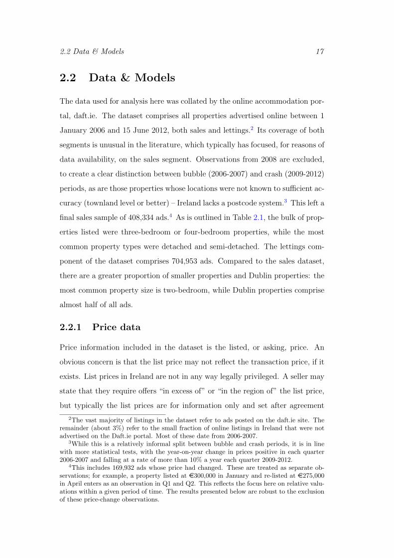
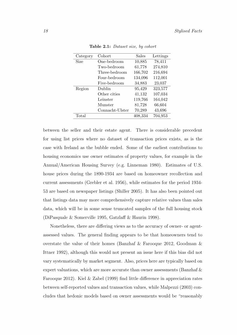
2.1 Dataset size, by cohort . . . . . . . . . . . . . . . . . . . . . . . 18
2.2 Summary of variables used . . . . . . . . . . . . . . . . . . . . . 20
2.3 Outline of models employed and their categorical variables . . . 23
2.4 Summary measures of spread in house prices, various models . . 28
2.5 Summary measures of spread in rents, various models . . . . . . 33
3.1 Dataset size, by cohort . . . . . . . . . . . . . . . . . . . . . . . 51
3.2 Summary of location-specific variables used – for legend, see text 63
3.3 Selected regression output: coefficients on amenities (and asso-
ciated p-values in brackets below) . . . . . . . . . . . . . . . . . 64
3.4 Effect of moving a property from 1km to 100m away from an
amenity; for exceptions (†, �), see text . . . . . . . . . . . . . . 68
4.1 Summary statistics of the daft.ie and CBI datasets . . . . . . . 82
5.1 Overview of literature on Irish housing market; for notes, see text108
5.2 Overview of dataset . . . . . . . . . . . . . . . . . . . . . . . . . 126
5.3 ADF unit root tests . . . . . . . . . . . . . . . . . . . . . . . . . 128
5.4 Model of dlrhp with parsimonious dynamics, 1980-2012 . . . . . 131
5.5 Model of dlrhp, 1980-2012, allowing nominal inertia after 1985 . 137
5.6 Model of dlrhp extended back to 1975 . . . . . . . . . . . . . . 138
5.7 Unrestricted 4-CIV model, 1980-2012: beta values and alpha
values, SEs . . . . . . . . . . . . . . . . . . . . . . . . . . . . . 141
5.8 4-CIV model, 1980-2012, with diagonal alpha matrix . . . . . . 142
vii

viii LIST OF TABLES
5.9 4-CIV model, 1980-2012, diagonal alpha matrix & some beta
restrictions . . . . . . . . . . . . . . . . . . . . . . . . . . . . . . 143
5.10 Modelling changes in the price-rent ratio (dlhpr), 2000-2012 . . 149
1 Abbreviated regression output for house price models . . . . . . 180
2 Abbreviated regression output for rental models . . . . . . . . . 182
3 Type and region controls for primary amenities . . . . . . . . . 189
4 Standard deviations for score-type amenities . . . . . . . . . . . 189
5 Regression output: four spreads . . . . . . . . . . . . . . . . . . 193
6 Model 1: dlrhp with full potential dynamics, 1980-2012 . . . . . 196
7 Robustness analysis of inverted demand model: alternative fun-
damentals . . . . . . . . . . . . . . . . . . . . . . . . . . . . . . 198
8 Robustness analysis of inverted demand model: logs vs. levels
for ratios . . . . . . . . . . . . . . . . . . . . . . . . . . . . . . . 199
9 ADF unit root tests: supplementary series . . . . . . . . . . . . 203

Chapter 1
Introduction
The housing boom that affected much of the OECD during the 1990s and early
2000s has led to renewed focus on the links between housing and the rest of
the economy. The pivotal role played by housing markets and housing wealth
in the so-called “Great Recession” and in previous cycles has convinced many
economists that understanding housing is central to understanding business
cycles, one of the primary focuses of macroeconomics (see, for example, Leamer
2007). Indeed, there is evidence of a strong link between housing and business
cycles not just throughout the postwar era (e.g. Holly & Jones 1997), but even
predating the Industrial Revolution (Eichholtz et al. 2012, O’Rourke & Polak
1991). The strong link between housing and broader economic outcomes should
hardly be a surprise, given that even in modern developed economies housing
remains both the single most important consumption good and the principal
asset in household wealth. In the U.S., for example, shelter comprises roughly
one third of the basket underlying the urban CPI, while a 2001 study estimated
that over half of household wealth was in housing (Luckett 2001).
Where to live is both a consumption decision and an investment decision.
It is a consumption decision as choosing a residence is more than choosing a
location for shelter as a service. The choice of accommodation is the choice
of a bundle of services, from the amount of space per person to a range of
amenities specific to the location or the population that lives there, both clear,
such as access to transport services, and nebulous, such as heritage or social
1
2 Introduction
capital. The choice of accommodation is also an investment decision. Those
who buy are, even if only implicitly, making a statement about the expected
capital gain relative to the cost of borrowing, as are those who rent. As an
investment decision, the purchase of a dwelling typically involves significant
leverage. This means that conditions not only in the housing market but also
in the mortgage market – which turns latent demand into effective demand –
are also hugely important.
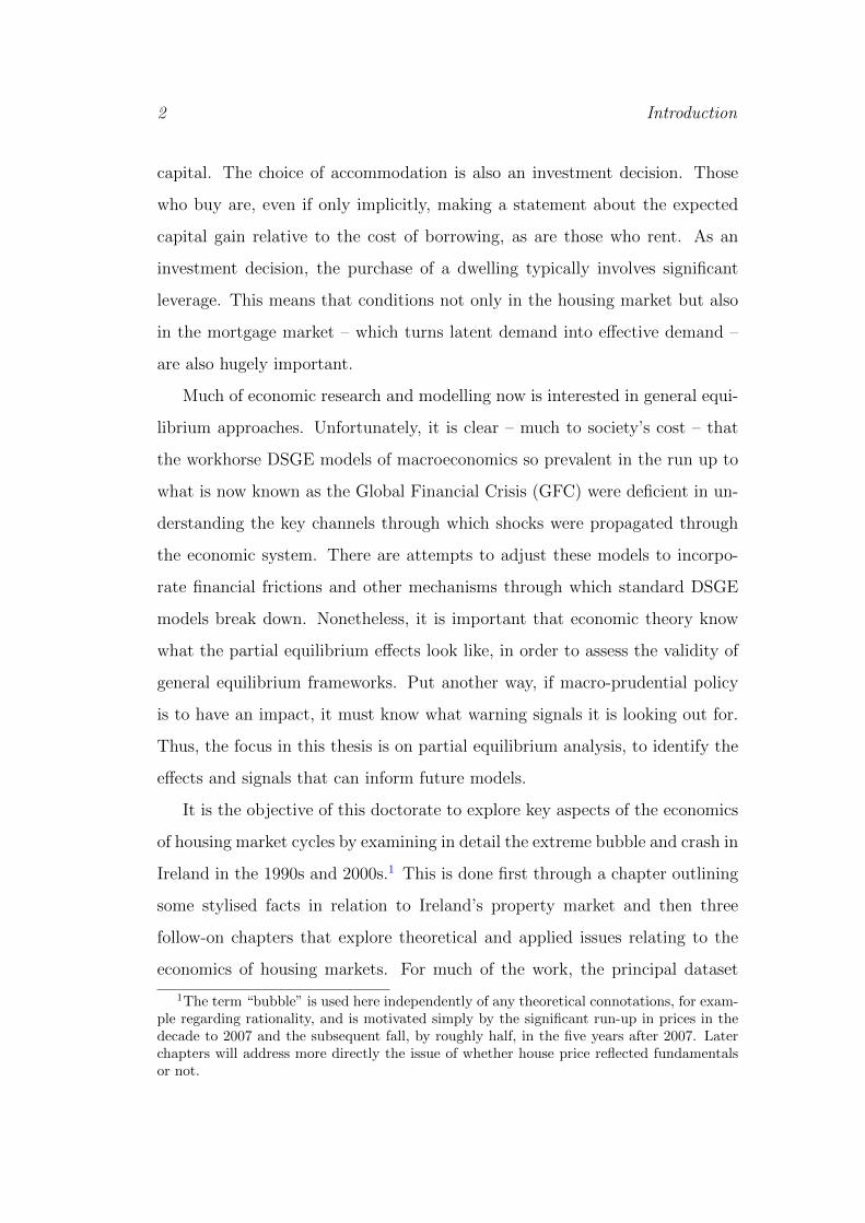
Much of economic research and modelling now is interested in general equi-
librium approaches. Unfortunately, it is clear – much to society’s cost – that
the workhorse DSGE models of macroeconomics so prevalent in the run up to
what is now known as the Global Financial Crisis (GFC) were deficient in un-
derstanding the key channels through which shocks were propagated through
the economic system. There are attempts to adjust these models to incorpo-
rate financial frictions and other mechanisms through which standard DSGE
models break down. Nonetheless, it is important that economic theory know
what the partial equilibrium effects look like, in order to assess the validity of
general equilibrium frameworks. Put another way, if macro-prudential policy
is to have an impact, it must know what warning signals it is looking out for.
Thus, the focus in this thesis is on partial equilibrium analysis, to identify the
effects and signals that can inform future models.
It is the objective of this doctorate to explore key aspects of the economics
of housing market cycles by examining in detail the extreme bubble and crash in
Ireland in the 1990s and 2000s.1 This is done first through a chapter outlining
some stylised facts in relation to Ireland’s property market and then three
follow-on chapters that explore theoretical and applied issues relating to the
economics of housing markets. For much of the work, the principal dataset
1The term “bubble” is used here independently of any theoretical connotations, for exam-ple regarding rationality, and is motivated simply by the significant run-up in prices in thedecade to 2007 and the subsequent fall, by roughly half, in the five years after 2007. Laterchapters will address more directly the issue of whether house price reflected fundamentalsor not.
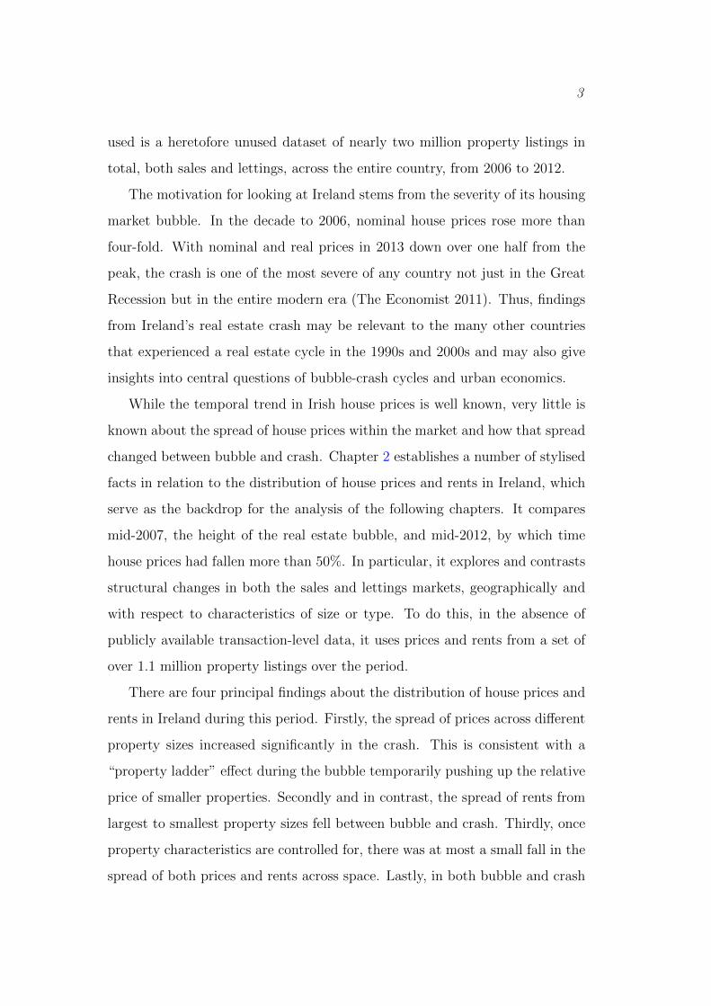
3
used is a heretofore unused dataset of nearly two million property listings in
total, both sales and lettings, across the entire country, from 2006 to 2012.
The motivation for looking at Ireland stems from the severity of its housing
market bubble. In the decade to 2006, nominal house prices rose more than
four-fold. With nominal and real prices in 2013 down over one half from the
peak, the crash is one of the most severe of any country not just in the Great
Recession but in the entire modern era (The Economist 2011). Thus, findings
from Ireland’s real estate crash may be relevant to the many other countries
that experienced a real estate cycle in the 1990s and 2000s and may also give
insights into central questions of bubble-crash cycles and urban economics.
While the temporal trend in Irish house prices is well known, very little is
known about the spread of house prices within the market and how that spread
changed between bubble and crash. Chapter 2 establishes a number of stylised
facts in relation to the distribution of house prices and rents in Ireland, which
serve as the backdrop for the analysis of the following chapters. It compares
mid-2007, the height of the real estate bubble, and mid-2012, by which time
house prices had fallen more than 50%. In particular, it explores and contrasts
structural changes in both the sales and lettings markets, geographically and
with respect to characteristics of size or type. To do this, in the absence of
publicly available transaction-level data, it uses prices and rents from a set of
over 1.1 million property listings over the period.
There are four principal findings about the distribution of house prices and
rents in Ireland during this period. Firstly, the spread of prices across different
property sizes increased significantly in the crash. This is consistent with a
“property ladder” effect during the bubble temporarily pushing up the relative
price of smaller properties. Secondly and in contrast, the spread of rents from
largest to smallest property sizes fell between bubble and crash. Thirdly, once
property characteristics are controlled for, there was at most a small fall in the
spread of both prices and rents across space. Lastly, in both bubble and crash

4 Introduction
periods, the spread of rents was constrained relative to the spread of prices,
particularly in the upper tail, a finding suggestive of renter search thresholds.
Housing is a composite good, with each dwelling a bundle of property-
specific attributes and location-specific amenities, each with its own price.
Changing price differentials can reveal demand shifts between these attributes
and thereby offer insights in to what happens in a housing bubble. There
are competing theoretical suggestions as to what will happen to price changes
across different segments during a housing cycle. According to Stein (1995),
down-payment constraints make high-value properties more volatile than low-
value ones. Costello (2000), however, suggests that if more affordable homes
are more liquid and thus more competitive, then these segments may be more
volatile over the boom/bust cycle. Empirically, is high-end housing the epi-
centre of a bubble, as people “lock in” exposure to the asset, and thus more
badly affected in the crash? Or are peripheral properties worse hit, a “property
ladder” effect where in the frenzy of the bubble, people buy whatever property
they can afford in the hope of capital gains?
As housing is an inherently spatial market, an understanding of the eco-
nomics of location-specific amenities is needed, a topic examined in detail in
Chapter 3. It examines the cyclicality of the prices of a range of location-
specific amenities, using over 1.2 million sales and rental listings in Ireland,
covering both bubble and crash periods, and 25 primary location-specific char-
acteristics, as well as various controls. The first hypothesis tested is whether
the valuation of amenities is greater in the sales segment than in the lettings
segment, reflecting either tenants’ search costs or buyers’ desire to lock in sup-
ply of the amenity. This was typically found to be the case – there is evidence
of an attenuated rental effect for 18 of the 25 amenities. For example, the
rental premium for a coastline property was 2.1%, less than half the 4.7% price
effect.
To distinguish between tenant search costs and buyer lock-in concerns, the
severity of Ireland’s housing bubble and crash was exploited. “Lock-in” effects

5
would be expected to be most severe during a bubble, as people pay over the
odds to secure access to amenities which are by their very nature fixed in
supply. This would suggest relative amenity prices are procyclical, rising in the
bubble and falling in the crash. If instead the price of amenities increased in
the crash, this would suggest that “property ladder” concerns dominated: in
the bubble, the principal concern is not having any property, pushing up the
relative price of low-amenity properties. Chapter 3 finds evidence of a lock-in
effect, with counter-cyclical amenity pricing for a greater number of amenities,
including prominent housing market amenities such as commute time, distance
to CBD and proximity to train stations and the coastline. For example, the
premium enjoyed by a property 100m from the coast compared to one 1km away
increased from 3.4% to 4.4% between bubble and crash. Similarly, moving a
property from 5km from the CBD to 1km away was associated with an increase
in price of 7.4% in the bubble and 8.2% in the crash.
These findings are based on list prices and rents, rather than sale prices,
which are not available in Ireland for this period. While there is a long history
of using advertised or assessed values where transactions data are not available,
the relationship between the two is not constant. Indeed, in the very first issue
of the Journal of Real Estate Research, Miller & Sklarz (1986) highlight the
relationship between the two as one of five leading indicators in the housing
market. However, their call for future research has largely gone unheeded.
Chapter 4 addresses this issue, by combining the daft.ie dataset used in
Chapters 2 and 3 with a dataset maintained by the Central Bank of Ireland
(CBI), as part of that country’s Prudential Capital Assessment Review (PCAR)
“stress tests” of the financial system. It takes as its starting point two pieces of
conventional wisdom about the housing market, which would appear to conflict
in a market downturn. Firstly, it is expected that in a downturn sale prices
will be below list prices, while secondly, it is often asserted that list prices are a
lead indicator of sale prices. The analysis shows that both were true for Ireland
during the period 2006-2012. The apparent contradiction is thus: if list prices

6 Introduction
lead sale prices in switching from boom to bust market, how are they above
sale prices in the bust? This is resolved by disentangling the ratio of list prices
to sale prices into four main components.
The first of the four is the selection spread, a comparison of all list prices to
only those that go on to find a buyer. A selection spread exists throughout the
period but is particularly pronounced during the market downturn: properties
that list for less, ceteris paribus, are more likely to find a buyer – a finding that
accords with basic economic theory.
The matching spread, secondly, reflects how much house prices change be-
tween when a property is listed and it is sale agreed. Given the speed with
which prices fell in Ireland during much of the period covered, and the length
of the typical time-to-sell, this is quantitatively important in explaining the
gap between the two. For most of the period 2008-2011, the list price of prop-
erties on which a sale was agreed was 10% or more higher than newly listed
properties. While the exact role of nominal price rigidities is a topic for further
research, this finding highlights the limitations of comparisons made in the ex-
isting literature on valuation accuracy, which use valuations and transactions
from different time periods. The drawdown spread, reflecting the time gap
between valuations for mortgages and their ultimate draw-down, was similar
in nature but much smaller in significance.
The counteroffer spread, finally, is the closest counterpart in the housing
market, which lacks liquidity and fungibility, to the bid-ask spread in other
financial markets. It reflects how list prices and sale prices compare, when
adjusted for time-to-sell and time-to-drawdown, as well as for the fact that some
listings will not result in a transaction. Early in the period, the counteroffer
spread was large and positive, suggesting that buyers had tough competition
in securing a property and thus they offered more than the list price. As boom
turned to bust in the Irish housing market, the counteroffer spread turned
negative. This idea of the sale price in boom-times “breaking the price ceiling”

7
offered by the list price has also emerged from recent research (Haurin et al.
2013).
The final substantive chapter of this thesis, Chapter 5, examines the deter-
minants of real house prices and the price-rent ratio in the Irish housing market.
Credit conditions have been considered in many studies of other housing mar-
kets, particularly since the GFC, but the existing literature on Irish housing
largely ignores the issue of credit conditions, empirically if not theoretically. In
addition, there have been no models of the price-rent ratio in the Irish market.
A quarterly dataset from 1980 to 2012 is used to estimate an error-correction
model that reveals the long-run relationship between house prices and their
long-run determinants. Those determinants include the ratio of income to the
stock of housing, the ratio of persons to households, user and transaction costs,
and credit conditions, as measured by the ratio of mortgage credit to deposits.
This long-run relationship is largely robust to allowing variables such as the
income/stock ratio, user cost and the credit/deposit ratio to be endogenous to
the system.
The results indicate that while the earlier phase of Ireland’s house price
boom was a product of many factors, growth between 2001 and 2007 was due
almost entirely to an easing of credit conditions. The actual average real house
price tracked very closely the price predicted by the long-run relationship. In
this sense, it could be argued that there was no bubble in the conventional sense,
of prices detaching from fundamentals. This is true to the extent that those
fundamentals include supply conditions in the credit market and expectations
(reflected in user-cost), both of which changed rapidly during the period 2001-
2012.
Using new data on LTVs for first-time buyers, an error correction model of
the price-rent ratio in Ireland is presented for the first time, covering the period
2000-2012. In line with the inverted demand model, this indicates that credit
conditions were, along with the real rate of interest, key to determining equilib-
rium in the housing market. This research is rich in policy implications, in par-

8 Introduction
ticular about the importance of expectations and credit conditions. Assuming
that credit conditions fulled readjusted by 2012, normalization of expectations
in relation to housing can be expected to generate some upward pressure on
prices in coming years.
Chapter 6 draws together the contributions of this thesis and suggests some
insights from the Irish housing market bubble for policymakers aiming to both
diagnose and prevent future housing bubbles.

Chapter 2
Stylised Facts
As mentioned in Chapter 1, in modern developed economies, housing is both the
single most important consumption good and the principal asset in household
wealth. Its cycles are closely related to broader macroeconomic fluctuations,
with some economists going so far as to argue that housing is the business cycle
(Leamer 2007). There remains much to learn, however, about the internal me-
chanics of the housing market, if a proper understanding of what drives housing
cycles is to help economists and policymakers understand and ameliorate them
in the future. In particular, a growing field is interested in the efficiency of
housing markets, as a counterpart to the study of the efficiency of other finan-
cial markets. While there is significant research using aggregate data, much
less work has been done using more refined housing market segments.
Ultimately, housing is a composite good, with each dwelling made of up
property-specific attributes and location-specific amenities, each with its own
price. If differentials for particular attributes or locations change, this can re-
veal demand shifts that offer insights into what happens over the housing mar-
ket cycle. The Global Financial Crisis (GFC) and the related fall in house prices
in a number of countries has generated renewed interest among economists in
the structure of house prices. For example, Glaeser et al. (2012) examine the
decade-long boom in U.S. house prices, finding evidence that “buyers during
the boom overestimated the long-run value of positive local attributes”.
There are competing theoretical suggestions as to what will happen price
9
10 Stylised Facts
changes across different segments during a housing cycle. According to Stein
(1995), down-payment constraints make high-value properties more volatile
than low-value ones. Costello (2000), however, suggests that if more affordable
homes are more liquid and thus more competitive, then these segments may be
more volatile over the boom/bust cycle. This chapter is the first to contrast
these two hypotheses with granular housing market data. It examines the
property market in Ireland, which has experienced one of the most severe real
estate cycles on record, comparing the distribution of both house prices and
rents in Ireland in 2007, the height of a real estate boom which saw prices
increase four-fold in a decade, and 2012, by which time house prices had fallen
by half. In particular, it explores and contrasts structural changes in both the
sales and lettings markets, geographically and with respect to characteristics
of size or type. To do this, in the absence of publicly available transaction-
level data, it uses advertised prices and rents from a dataset of over 1.1 million
property listings over the period.
The principal method used is the hedonic regression, drawing on the long
literature established by Rosen (1974), with housing understood as a composite
good comprising property-specific attributes and location-specific amenities. In
addition to a range of type, time and size controls, to understand changes in
the geographic spread of prices, an algorithm is used to aggregate 4,500 Census
areas into just over 1,100 sales zones of sufficient sample size (312 zones for
lettings). These zones are then used in a series of hedonic prices models, which
give the estimated average price for a range of standardised properties per zone
and per quarter. Figures for the peak and for mid-2012 are then compared.
The chapter is structured as follows. The next section presents a brief
overview of related literature on structural changes in the spread of property
prices, on Ireland’s property market and the hedonic method. Section 3 outlines
the data used in this study, the algorithm for compilation of the price zones
and the specific hedonic specifications employed. Sections 4 and 5 present the
2.1 Theory & Literature 11
results for the various house price models and for analogous models for the
lettings segment. Section 6 presents concluding thoughts.
2.1 Theory & Literature
The theoretical starting point for thinking about the housing market is as an
efficient financial market (e.g. Case & Shiller 1989). Such a perspective sug-
gests that house prices can be thought of as forward-looking, depending on
fundamentals such as rents or user-costs (Poterba 1992), and that expected
capital gains should reflect factors such as demographics (Case & Shiller 1990).
However, there is ample evidence that the market is not efficient, as housing
prices exhibit boom-bust behaviour and can be predicted to a certain extent
by past price changes and the rent-price ratio (see, for example, Gallin 2008).
There is particular interest in the extent to which housing markets are infor-
mationally efficient, i.e. that prices reflect accurately the forces of supply and
demand, although much of the research is at aggregate market level, ignoring
differences across segments (Gatzlaff & Tirtiroglu 1995).
In relation to the structure of house prices, Stein (1995) suggests that one
might expect higher price housing to be more volatile over the market cycle.
This is due to the presence of down payments and the fact that the typical
household holds most of their private net wealth in housing. Consider a neg-
ative shock to house prices: this hinders movers from making their next down
payment, depressing demand. If high-priced homes are purchased primarily
by trade-up buyers, then their prices should have a greater variance over the
real estate cycle. The prior expectation, according to this liquidity constraint
model, is that houses with higher prices would both rise and fall more dramat-
ically over the cycle than those with lower prices.
There is limited evidence for the thesis, however. Smith & Tesarek (1991)
find evidence that this may hold in the property market cycle in the U.S. city of
Houston, Texas, over the 1970s and 1980s, where they estimated that during the

12 Stylised Facts
boom years, the marginal price of quality rose, and when prices started to fall,
the structure of prices flattened. However, Case & Shiller (1994) explore two
other 1980s boom-bust cycles in U.S. cities, those of Boston and Los Angeles,
and largely find the opposite. In Boston, they find evidence of a shift in house
price inflation to the lower tier after other tiers had stabilised (1987-9), giving
that part of the market the greatest boom in prices. In L.A., there was very
similar appreciation across high, medium and low tiers of housing, although
higher tier housing did see significantly larger falls. Case & Mayer (1996) focus
more closely on the impact of amenities on the distribution of relative house
prices, and, contrary to Stein’s (1995) hypothesis, controlling for amenities,
low-priced towns saw faster house price growth to 1988 and then greater falls
after that.
Lower-priced segments experiencing more volatile swings in prices may in-
stead represent another consequence of down-payments for real estate. In equi-
ties markets, differing liquidity is believed to explain the so-called “size effect”,
where returns on the shares of small companies exceed those of larger ones.
In housing markets, Costello (2000) suggests, more affordable properties are
more liquid and thus these segments will be more competitive, rising more in
boom markets and falling more in down markets. Using data for the city of
Perth, Western Australia, during the period 1988-1996, Costello finds that re-
peat sales were biased towards lower price quartiles, suggesting greater liquidity
in cheaper segments. He also finds that the top quartile in particular exhibited
significantly less real house price inflation than other segments.
Since the start of the Global Financial Crisis (GFC) in 2007, there has been
a significant increase in research focus on the housing market. Much of this
research examines the relationship between one aggregate measure of house
prices and fundamentals such as income, demographics, user cost and housing
stock (see, for example, Duca et al. 2011a, Fraser et al. 2012, Muellbauer &
Williams 2011). The connection between the housing and credit markets and
2.1 Theory & Literature 13
financial stability is also an active area of research (see Muellbauer 2012, and
other papers at the same conference).
A smaller literature has examined the internal mechanisms of the housing
market during the build-up to the GFC. McMillen (2008) is one of the first
works to examine in detail the distribution of house prices across a market.
Studying the Chicago market of 1995 and 2005, he finds that the increase
in prices in this period was greater for higher value homes. The change in
distribution is attributed to changes in the coefficients, rather than changes in
the characteristics of the dwellings. Deng et al. (2012) reach a similar conclusion
for the housing market in Singapore over the period 1995-2010.
Lastly, Glaeser et al. (2012) analyse the housing price boom in the U.S.
in the decade to 2006. They find that price growth was significantly greater
in cities that were warmer, less educated, with less initial density and higher
initial housing values. They also study within-city changes and conclude that
price growth was faster in neighborhoods closer to the city center. The authors
conclude that this is largely consistent with a model of buyers during the boom
overestimating the long-run value of positive local amenities and the urban
amenity in general. Nonetheless, this conclusion is based on a comparison of
2006 with 1996 and any number of factors, including shifts in the distribution
of income or in credit conditions, or the impact of technology on work practices
and locations, may mean that 1996 is not the appropriate reference point for
prices in 2006.
2.1.1 House Prices in Ireland
A number of papers trace the development of Irish house prices from the 1970s;
see, for example, Kennedy & McQuinn (2012), Kenny (1999), Murphy (2005),
Roche (2001), Stevenson (2003). These papers typically try to model house
price using some combination of economic theory (typically a variant of the
textbook inverted demand approach, sometimes with a simultaneous supply
equation) and statistical methods (for example, regime switching). As noted
14 Stylised Facts
by Murphy (2005), however, many are ad-hoc specifications and typically suffer
from omitted variable bias, as they eschew any treatment of credit conditions
(a more recent exception is Addison-Smyth et al. 2009).
A further issue is the quality of data available to the researcher. Until the
mid-1990s, hedonic price indices were not available for Ireland and the only
published series was a simple mean price, which over time would be subject
to a number of limitations, including a quality bias, particularly for regional
data. Trends in the mean price differ significantly in the post-2007 period from
hedonic trends based on either list or transaction price. This places a limit
on the reliability of existing research into house prices in Ireland, in particu-
lar research that examines regional trends in house prices, such as Stevenson
(2004).
Nonetheless, the broad history of the Irish property market is reasonably
well established. Prices were relatively stagnant in real terms from the mid-
1970s until the mid-1990s, after which export-led economic growth fuelled eco-
nomic and demographic expansion, which lifted house prices (Murphy 2005).
The policy response stimulated new housing supply. However the expansion in
credit meant that prices in the early 2000s increased rapidly, rather than fell
due to the increase in supply. By the mid-2000s, with the average house price
up almost 300% in just ten years, a growing number of commentators were
concerned about likelihood of a domestic real estate bubble. Between 2007 and
2012, prices fell by at least half.1
A related strand of reseach examined the relationship between fiscal policy
and the housing market (e.g. Berry et al. 2003). Barham (2004), for example,
finds that the combination of beneficial fiscal incentives and declining costs,
in terms of falling interest rates, drove down the costs associated with owner-
occupancy. In particular, the untaxed capital gain afforded to homeowners
meant that for the majority of the period he analyses, the user cost of housing
1By the end of 2012, the official CSO index of house prices, based on mortgage transac-tions, was down 49.9% from the peak, while the daft.ie index of list prices was down 55.3%.

2.1 Theory & Literature 15
in Ireland was negative. In this context, rising house prices were to be expected.
An OECD review in 2006 found that the huge increases in house prices in
Ireland stemmed from a combination of fundamentals, such as strong economic
growth, demographics and low interest rates, but also policy, in particular very
generous tax advantages for owner-occupancy and loose banking credit (Rae &
van den Noord 2006).
2.1.2 The Hedonic Methodology
The research presented here uses the hedonic price method to estimate the
value associated with certain attributes, in particular location, type and size.
The hedonic method is well established in the literature and its theoretical
foundations are described in Rosen (1974). Its limitations and implicit as-
sumptions are described in Maclennan (1977). Of relevance here is the risk of
pooling over submarkets where underlying parameters differ, i.e. aggregation
imposing one price structure when in fact price structures may differ across
sub-markets. As outlined in Section 2.2.4, the purpose of this analysis is to un-
derstand submarkets in the Irish property market and the empirical strategy is
designed with this in mind, including specifications that allow type differentials
to vary by region. Maclennan (1977) also notes that concerns in relation to
implicit assumptions about preferences are less relevant where the aim merely
to statistically explain the apparent determinants of relative house values, as
is the case here.
More recently, Malpezzi (2003) reviews the hedonic methodology one gen-
eration on. Three recurring issues relate to its theoretical footing, the problem
of mis-specification (including omitted variables and market definition) and the
relationship between design and purpose. He notes that “if samples are large
and well-drawn . . . more flexible forms and more careful attention to the delin-
eation of submarkets will generally pay off” (Malpezzi 2003, p.24). This is still
an active area for discussion. Ellen (2012) notes that while stratification, by
type, neighbourhood and even ethnicity, is possible, there exists nonetheless a

16 Stylised Facts
relationship between the different submarkets, concluding “the debate about
segmentation is really about degree – about how large the cross-price elasticity
is between different types of housing”.
Another segment of the literature examines the accuracy of estimation
methods employed in constructing house price indices, including the hedonic
method and the repeat-sales method. As is discussed in more detail in Chapter
4, the use of simple averages or indeed repeat sales may lead to biased esti-
mates of house prices changes, as the characteristics of the sample of properties
transacted over the cycle changes (Dorsey et al. 2010, Pollakowski 1995). The
finding from this literature is that the hedonic methods used here are most
appropriate when examining prices across space and time, as well as general
price levels and changes.
A paper by Conniffe & Duffy (1999) was one of the first to apply economic
and econometric techniques to Irish house prices, using a 1996-1998 dataset
from an Irish mortgage provider. They adapted the hedonic method developed
for the Halifax House Price Index (Fleming & Nellis 1985), the exponential
form of hedonic equation, with log of price regressed on a linear combination
of attributes. The authors distinguish between locations in the same region
(e.g. within Dublin) and locations in different regions, highlighting that while
the price difference between suburbs may capture neighbourhood quality, dif-
ferences between regions may reflect more fundamental economic differences.
They discuss the stability of housing attributes and note the lack of models
using interactive terms: most models assume that only one element is time-
varying (a dummy capturing that period), while the relative prices of other
attributes such as location, house type or size does not change. This lack of
interactive terms will be addressed in this study.
2.2 Data & Models 17
2.2 Data & Models
The data used for analysis here was collated by the online accommodation por-
tal, daft.ie. The dataset comprises all properties advertised online between 1
January 2006 and 15 June 2012, both sales and lettings.2 Its coverage of both
segments is unusual in the literature, which typically has focused, for reasons of
data availability, on the sales segment. Observations from 2008 are excluded,
to create a clear distinction between bubble (2006-2007) and crash (2009-2012)
periods, as are those properties whose locations were not known to sufficient ac-
curacy (townland level or better) – Ireland lacks a postcode system.3 This left a
final sales sample of 408,334 ads.4 As is outlined in Table 2.1, the bulk of prop-
erties listed were three-bedroom or four-bedroom properties, while the most
common property types were detached and semi-detached. The lettings com-
ponent of the dataset comprises 704,953 ads. Compared to the sales dataset,
there are a greater proportion of smaller properties and Dublin properties: the
most common property size is two-bedroom, while Dublin properties comprise
almost half of all ads.
2.2.1 Price data
Price information included in the dataset is the listed, or asking, price. An
obvious concern is that the list price may not reflect the transaction price, if it
exists. List prices in Ireland are not in any way legally privileged. A seller may
state that they require offers “in excess of” or “in the region of” the list price,
but typically the list prices are for information only and set after agreement
2The vast majority of listings in the dataset refer to ads posted on the daft.ie site. Theremainder (about 3%) refer to the small fraction of online listings in Ireland that were notadvertised on the Daft.ie portal. Most of these date from 2006-2007.
3While this is a relatively informal split between bubble and crash periods, it is in linewith more statistical tests, with the year-on-year change in prices positive in each quarter2006-2007 and falling at a rate of more than 10% a year each quarter 2009-2012.
4This includes 169,932 ads whose price had changed. These are treated as separate ob-servations; for example, a property listed at e300,000 in January and re-listed at e275,000in April enters as an observation in Q1 and Q2. This reflects the focus here on relative valu-ations within a given period of time. The results presented below are robust to the exclusionof these price-change observations.
18 Stylised Facts
Table 2.1: Dataset size, by cohort
Category Cohort Sales Lettings
Size One-bedroom 10,885 78,411Two-bedroom 61,778 274,810Three-bedroom 166,702 216,694Four-bedroom 134,096 112,001Five-bedroom 34,883 23,037
Region Dublin 95,429 323,577Other cities 41,132 107,034Leinster 119,766 164,042Munster 81,728 66,604Connacht-Ulster 70,289 43,696
Total 408,334 704,953
between the seller and their estate agent. There is considerable precedent
for using list prices where no dataset of transaction prices exists, as is the
case with Ireland as the bubble ended. Some of the earliest contributions to
housing economics use owner estimates of property values, for example in the
Annual/American Housing Survey (e.g. Linneman 1980). Estimates of U.S.
house prices during the 1890-1934 are based on homeowner recollection and
current assessments (Grebler et al. 1956), while estimates for the period 1934-
53 are based on newspaper listings (Shiller 2005). It has also been pointed out
that listings data may more comprehensively capture relative values than sales
data, which will be in some sense truncated samples of the full housing stock
(DiPasquale & Somerville 1995, Gatzlaff & Haurin 1998).
Nonetheless, there are differing views as to the accuracy of owner- or agent-
assessed values. The general finding appears to be that homeowners tend to
overstate the value of their homes (Banzhaf & Farooque 2012, Goodman &
Ittner 1992), although this would not present an issue here if this bias did not
vary systematically by market segment. Also, prices here are typically based on
expert valuations, which are more accurate than owner assessments (Banzhaf &
Farooque 2012). Kiel & Zabel (1999) find little difference in appreciation rates
between self-reported values and transaction values, while Malpezzi (2003) con-
cludes that hedonic models based on owner assessments would be “reasonably

2.2 Data & Models 19
reliable”. This issue is addressed in relation to the Irish housing market during
this period in detail in Chapter 4.5
2.2.2 Location
Based on the earlier discussion of the hedonic method, including points made
by Maclennan (1977) and Ellen (2012), the empirical approach allows dif-
ferentials between property types to vary by region. The model defines five
broad regions in the Irish property market, the first of which is Dublin city.
The second regional market contains the four other cities in Ireland combined
(Cork, Galway, Limerick and Waterford), whose populations vary from 50,000
to 275,000. These are not contiguous but may share marginal price effects due
to their status as regional cities. The other three regional markets are based
on Ireland’s provinces, but excluding the city areas: Leinster, Munster and
Connacht-Ulster.
Each of these regions is broken down into zones. There are in total 1,117
sales zones and 312 lettings zones around the country. These zones were devel-
oped algorithmically by the National Institute of Regional & Spatial Analysis
at NUI Maynooth. The algorithm took as its starting point Ireland’s 4,500
Census districts (electoral divisions outside the cities and enumerator areas
within the cities). If an individual district k did not have sufficient sample size
in both bubble and crash periods (roughly, ntk ≥ 100 for t = bubble, crash), it
was paired with adjoining zones until the threshold was reached.
The principal reason that there are significantly fewer lettings zones is likely
to be related to the bubble itself. Those investing in property during the final
stages of the bubble appear to have done so principally for capital gains, rather
than rental income, and the volume of rental listings in non-urban markets
prior to 2008 was small. This motive disappeared as prices fell, leading to a
5For example, a possible concern could be that those in larger/higher-value propertiesmay be more averse to realising losses and thus have stickier list prices that are not reflectedin outcomes. Evidence from Chapter 4 and from the CBI dataset used in that chapter,however, suggests that this is not the case.

20 Stylised Facts
Table 2.2: Summary of variables used
Variable Description (variable names in Regression output tables includedwhere appropriate; controls, where relevant, in italics)
Price Advertised sale price or monthly rentTime Categorical time variables for each quarter from 2006:I to 2012:II;
variables with the suffix cr are the original variable interactedwith a categorical variable taking a value of one for the crashperiod (2009-2012)
Location Price zone, as described above; 1,117 sales zones, 312 lettings zonesRegion Variables with the suffix regx have been interacted with a par-
ticular region (1-5, which are respectively Dublin, other cities,Leinster, Munster, Connacht-Ulster)
Type Property type; five possible values in sales: terraced (ht1), semi-detached (ht2), detached (ht3), apartment (ht4), bungalow(ht6);three in lettings: apartment (pt1), house (pt2), flat (pt4)
Bedrooms For both sales and lettings segments, number of bedrooms (one,two, three, four, five)
Bathrooms For both sales and lettings segments, number of bathrooms relativeto number of bedrooms as follows: one-bed (1 or more), two-bed(1, 2 or more), three-bed (1, 2, 3 or more), four-bed (1, 2, 3, 4or more), five-bed (1, 2, 3, 4 or more); variable names take theformat bbxy where x refers to bedroom number and y to bathroomnumber, where y = m refers to any greater number of bathrooms
Bedroom size For lettings only, stated occupancy of bedrooms (measured bynumber of single rooms): one-bed (zero or one), two-bed (zero, oneor two), three-bed (zero, one or more), four-bed (zero, one, twoor more), five-bed (zero, one, two or more); variable names takethe format bx zs where x refers to the total number of bedroomsand z to number of single rooms (the highest number covers thatnumber and any greater
Facilities For lettings only, information is available for a range of utilities(including central heating, an alarm system, cable TV and theinternet), white goods (washing machine, dryer, dishwasher andmicrowave) and other features (wheelchair accessible, parking andgarden, the one feature also available for sales)
Terms A range of contract terms are also included in lettings ads (whetherpets are allowed, whether rental allowance is considered, a shortor long lease, relative to a 12-month control, and whether an agentis used, which is also available for sales)

2.2 Data & Models 21
significant increase in the number of rental listings – for example, the total
number of rental properties listed outside the main cities increased from less
than 30,000 in 2007 to over 100,000 in 2009. Dublin witnessed a similar increase
in listings. While the purpose of the analysis in this chapter is to describe,
rather than model, trends in property values, this very significant outward
shift in the supply curve is likely to have contributed to the fall in average
rents.
2.2.3 Other property attributes
There are five categories of attribute used to explain observed prices and rents,
including location (as explained above), the time the ad was listed (grouped
by quarter), type, size (measured in bedrooms and bathrooms, and in the
case of lettings properties the occupancy of the bedrooms), and other features
including facilities and terms of the ad. All variables are categorical variables,
as explained in Table 2.2.
2.2.4 Models
Table 2.3 outlines the five models that are applied to both sales and lettings
datasets. Model (1), the baseline model, regresses the log of the price (or rent)
on five sets of property attributes: time (quarterly dummies); property type;
size (bedroom number and bathroom number, relative to bedroom number);
and the 1,117 sales zones (312 lettings zones). In effect, it assumes that any
changes over time are captured by the time dummies and that no change takes
place in the distribution of prices across location or type.6 As outlined earlier,
however, an important finding of the literature is that time, location and other
attributes interact. This is explored in the other models.
In equation form, the five empirical models are given below in Equations
2.1-2.5. Each vector of Q, X and Y omits one category as control, and where
6This is similar to standard hedonic models used for house price indices, although thesetypically use no more than four quarters of data.
22 Stylised Facts
s refers to the quarter within the year, t to the year (with no s = 3 or s = 4
for 2012), n to attribute n of N = 29 for sales (comprising 5 types, 5 bedroom
sizes, and 19 bedroom-bathroom combinations; see Table 2.2) and N = 50 for
lettings (3 types, 5 bedrooms, 19 bathroom combinations, 16 bedroom sizes
and 14 binary features; see Table 2.2), r to regions 1-5 and z to the zones
outlined above. C refers to a categorical variable that takes the value of 1 for
the crash period only (2009-2012). For the Y -vector of zones, the upper limit,
Z, for the sales segment is 1,117; for the rental segment, it is 312.7
ln(hp)i = α0 +2012∑
t=2006
4∑s=1
αtsQtsi +
N∑n=1
βnrXnri +
Z∑z=1
γzYzi + εi (2.1)
ln(hp)i = α0 +2012∑
t=2006
4∑s=1
αtsQtsi +
N∑n=1
βnrXnri +
1∑C=0
Z∑z=1
γCzYCzi + εi (2.2)
ln(hp)i = α0 +2012∑
t=2006
4∑s=1
αtsQtsi +
1∑C=0
N∑n=1
βCnXCni +
1∑C=0
Z∑z=1
γCzYCzi + εi (2.3)
ln(hp)i = α0 +2012∑
t=2006
4∑s=1
αtsQtsi +
1∑C=0
N∑n=1
5∑r=1
βCnrXCnri +
1∑C=0
Z∑z=1
γCzYCzi + εi
(2.4)
ln(hp)i = α0 +5∑
r=1
2012∑t=2006
4∑s=1
αrtsQrtsi +
1∑C=0
N∑n=1
βCnXCni +
1∑C=0
Z∑z=1
γCzYCzi + εi
(2.5)
Conceptually, Model (2) includes an additional variable, an interaction with
a categorical crash variable, for each sales/lettings zone for the crash period
(2009 on). This allows the distribution of house prices (rents) across the coun-
try, controlling for type and size, to change between bubble (2006-2007) and
crash (2009-2012) periods. Model (3) includes similar “crash” interacted vari-
ables for each of the type and size variables, as well as zone. This means
that the model allows the relative price between, for example, two and three-
bedroom properties or between semi-detached properties and apartments to
vary between bubble and crash periods.
7For ease of identification, regression output in Appendix .1 uses the naming conventionsoutlined in Table 2.2, rather than the parsimonious forms given in the equations.

2.3 Distribution of Prices 23
Table 2.3: Outline of models employed and their categorical variables
Model Time Type & size Sales/lettings zonesModel 1 National National YesModel 2 National National Yes, with crashModel 3 National National, with crash Yes, with crashModel 4 National Regional, with crash Yes, with crashModel 5 Regional National, with crash Yes, with crash
Extending the possibility for interaction between attributes, in Model (4),
allowance is made for the price effects of particular property types (and sizes)
varying by region, by inclusion of categorical variables where type and size are
interacted with the five regions outlined above. Dublin is used as the con-
trol region, so statistical significance of region-type-time variable combinations
signifies that the price differential (or change in price differential, for crash
variables) in a particular region is different to that in Dublin. Lastly, Model
(5) captures regional variations in a different way, by interacting quarterly time
trends with the regions. In general terms, this should be roughly equivalent to
Model (3).
2.3 Distribution of Prices
2.3.1 Price differentials by property size
To what extent did the price differentials associated with particular property
types change? Did the gap between, say, a four-bedroom property and a two-
bedroom property grow or shrink between bubble and crash periods? As de-
scribed above, Models (3)-(5) allow the relative prices of particular property
attributes (measured by building type or number of bedrooms and bathrooms)
to vary between bubble and crash periods. Figure 2.1 shows the effect of the
crash on the premium associated with various property types and sizes, as
measured by Model (3), i.e. national-level price effects.
The figures shown are the percentage point changes in differential associated
with the various major property types, from apartments to detached properties,

24 Stylised Facts
Figure 2.1: Percentage point change in price premium between bubble and crash,by type and size (Model 3)
and sizes, as captured by bedroom numbers, relative to the controls (which are
semi-detached and three bedroom properties).8 All results are statistically
significant well above the p = 0.01 level (as outlined in Table 1 in Appendix
.1).
This change in the pattern of differentials in favour of larger properties
indicates that the price of larger properties fell by less in the crash. This
suggests an increase in the price of space at the margin, in relative terms (i.e.
once the overall fall in the price level of real estate is accounted for). It can
be explored with a secondary metric of size, number of bathrooms relative
to number of bedrooms. This is shown in Figure 2.2; the controls for this
dimension are one bathroom for properties with three or fewer bedrooms and
two bathrooms otherwise. Again all results are strongly statistically significant,
8Differentials are calculated in line with Halvorsen & Palmquist’s (1980) recognition ofthe limitation of the log approximation to percentages and follow the approach of Bourassaet al. (2004); in percentage point terms, they are given by 100[exp(βj)−1], where βj refers toa variable capturing both type and crash indicators (e.g. beds1 cr). For models with regionalinteractons, βj represents the sum of all relevant coefficients, including the base effect, thebase crash effect, the regional effect and the regional crash effect.

2.3 Distribution of Prices 25
Figure 2.2: Percentage point change in price premium between bubble and crash,by bathroom number (Model 3)
with only three exceptions, where the size of the effect is smaller than 1%: four-
bed four-bath, five-bed three-bath and five-bed more than four bathrooms.
As noted earlier, Model (3) assumes that the differentials between property
types are national, whereas in fact regional differences may exist. Of the 176
additional type-region coefficients generated by Model (4), 77 are statistically
significant at the 1% level, while a further 22 are significant at 5% level. This
indicates that not only is there strong evidence from Model (3) that price
differentials changed but also that there is evidence that these changes in price
differentials varied by region. Figure 2.3 outlines the change in coefficient in
the crash period, compared to the bubble, by region and property type. Of
the 40 differential changes, just one has a sign counter to expectations, that for
Dublin bungalows (which are rare).
What is striking about all three graphs (Figures 2.1-2.3) is the clarity of the
result: once the overall fall in property price levels is accounted for, any prop-
erty associated with more space (across type, bedroom number or bathroom
number) saw its relative price increase. For example, using the national average,
26 Stylised Facts
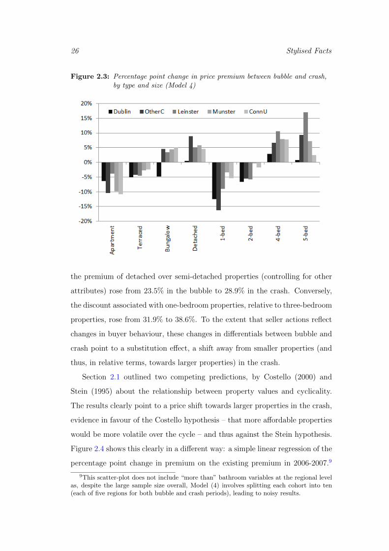
Figure 2.3: Percentage point change in price premium between bubble and crash,by type and size (Model 4)
the premium of detached over semi-detached properties (controlling for other
attributes) rose from 23.5% in the bubble to 28.9% in the crash. Conversely,
the discount associated with one-bedroom properties, relative to three-bedroom
properties, rose from 31.9% to 38.6%. To the extent that seller actions reflect
changes in buyer behaviour, these changes in differentials between bubble and
crash point to a substitution effect, a shift away from smaller properties (and
thus, in relative terms, towards larger properties) in the crash.
Section 2.1 outlined two competing predictions, by Costello (2000) and
Stein (1995) about the relationship between property values and cyclicality.
The results clearly point to a price shift towards larger properties in the crash,
evidence in favour of the Costello hypothesis – that more affordable properties
would be more volatile over the cycle – and thus against the Stein hypothesis.
Figure 2.4 shows this clearly in a different way: a simple linear regression of the
percentage point change in premium on the existing premium in 2006-2007.9
9This scatter-plot does not include “more than” bathroom variables at the regional levelas, despite the large sample size overall, Model (4) involves splitting each cohort into ten(each of five regions for both bubble and crash periods), leading to noisy results.

2.3 Distribution of Prices 27
Figure 2.4: Scatter-plot of existing sales premium and change in premium (Model4)
The pattern is clear and positive, with an R-squared of 26%. Controlling for
the change in the overall price of housing, the price of quality increased between
2007 and 2011.
2.3.2 Geographic spread of prices
The results presented above indicate that a model which does not allow for
changing property-type differentials may draw false conclusions about changes
in the geographical spread of house prices. This section compares the conclu-
sions about the spread of house prices from the various models. Eight measures
of dispersion are used, based on the average house price (over a basket of five
standardised properties) across the 1,117 zones – the coefficient of variation,
the Gini coefficient, the 99:1 ratio (and its component 99:50 and 50:1 ratios),
the 90:10 ratio, the 80:20 ratio and the 60:40 ratio.10
10The coefficient of variation expresses variation in percentage terms (the standard devia-tion divided by the mean). The Gini coefficient is a measure of inequality where a value of
28 Stylised Facts
Table 2.4: Summary measures of spread in house prices, various models
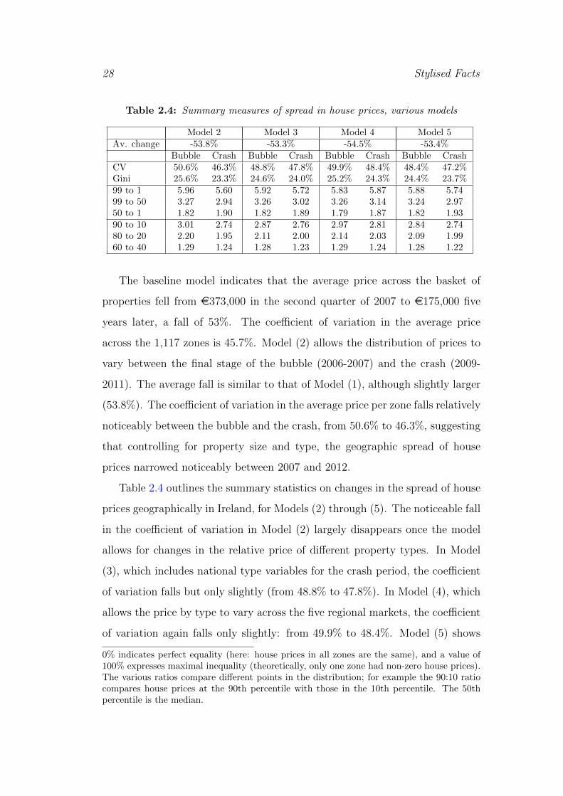
Model 2 Model 3 Model 4 Model 5Av. change -53.8% -53.3% -54.5% -53.4%
Bubble Crash Bubble Crash Bubble Crash Bubble CrashCV 50.6% 46.3% 48.8% 47.8% 49.9% 48.4% 48.4% 47.2%Gini 25.6% 23.3% 24.6% 24.0% 25.2% 24.3% 24.4% 23.7%99 to 1 5.96 5.60 5.92 5.72 5.83 5.87 5.88 5.7499 to 50 3.27 2.94 3.26 3.02 3.26 3.14 3.24 2.9750 to 1 1.82 1.90 1.82 1.89 1.79 1.87 1.82 1.9390 to 10 3.01 2.74 2.87 2.76 2.97 2.81 2.84 2.7480 to 20 2.20 1.95 2.11 2.00 2.14 2.03 2.09 1.9960 to 40 1.29 1.24 1.28 1.23 1.29 1.24 1.28 1.22
The baseline model indicates that the average price across the basket of
properties fell from e373,000 in the second quarter of 2007 to e175,000 five
years later, a fall of 53%. The coefficient of variation in the average price
across the 1,117 zones is 45.7%. Model (2) allows the distribution of prices to
vary between the final stage of the bubble (2006-2007) and the crash (2009-
2011). The average fall is similar to that of Model (1), although slightly larger
(53.8%). The coefficient of variation in the average price per zone falls relatively
noticeably between the bubble and the crash, from 50.6% to 46.3%, suggesting
that controlling for property size and type, the geographic spread of house
prices narrowed noticeably between 2007 and 2012.
Table 2.4 outlines the summary statistics on changes in the spread of house
prices geographically in Ireland, for Models (2) through (5). The noticeable fall
in the coefficient of variation in Model (2) largely disappears once the model
allows for changes in the relative price of different property types. In Model
(3), which includes national type variables for the crash period, the coefficient
of variation falls but only slightly (from 48.8% to 47.8%). In Model (4), which
allows the price by type to vary across the five regional markets, the coefficient
of variation again falls only slightly: from 49.9% to 48.4%. Model (5) shows
0% indicates perfect equality (here: house prices in all zones are the same), and a value of100% expresses maximal inequality (theoretically, only one zone had non-zero house prices).The various ratios compare different points in the distribution; for example the 90:10 ratiocompares house prices at the 90th percentile with those in the 10th percentile. The 50thpercentile is the median.

2.3 Distribution of Prices 29
similar results.
These summary statistics suggest then that there is little evidence of a Stein
effect, where high value properties are more volatile, proportionately rising
more in the bubble and falling more in the crash. Once changes in relative
prices of property types are adequately accounted for, the geographic spread
of prices did not narrow significantly between the bubble and crash periods.
The percentile ratios shown paint a slightly more nuanced picture. Taking
Model (4), for example, zones in the 99th percentile were 3.26 times more
expensive than the median in the bubble but just 3.14 times in the crash –
this suggests that the top half of the geographic spread of price narrowed in
the crash. However, the bottom half of the distribution widened in the same
period: the median zone was 1.87 times more expensive than the 1st percentile
in the crash, compared to just 1.79 in the bubble. While these are not large
changes, they indicate that different effects may have been at work at different
parts of the distribution of house prices in Ireland in the bubble.
The slightly more nuanced picture suggests that a number of effects may be
at work at different parts of the distribution, in a way that the simple dichotomy
between the Stein and Costello hypotheses cannot capture. Changes in income
and unemployment are likely to have affected different regions and segments
differently, with unemployment in particular affecting certain categories of first-
time buyer while a switch to more cash-only purchases may have taken place
at the top end of the market.
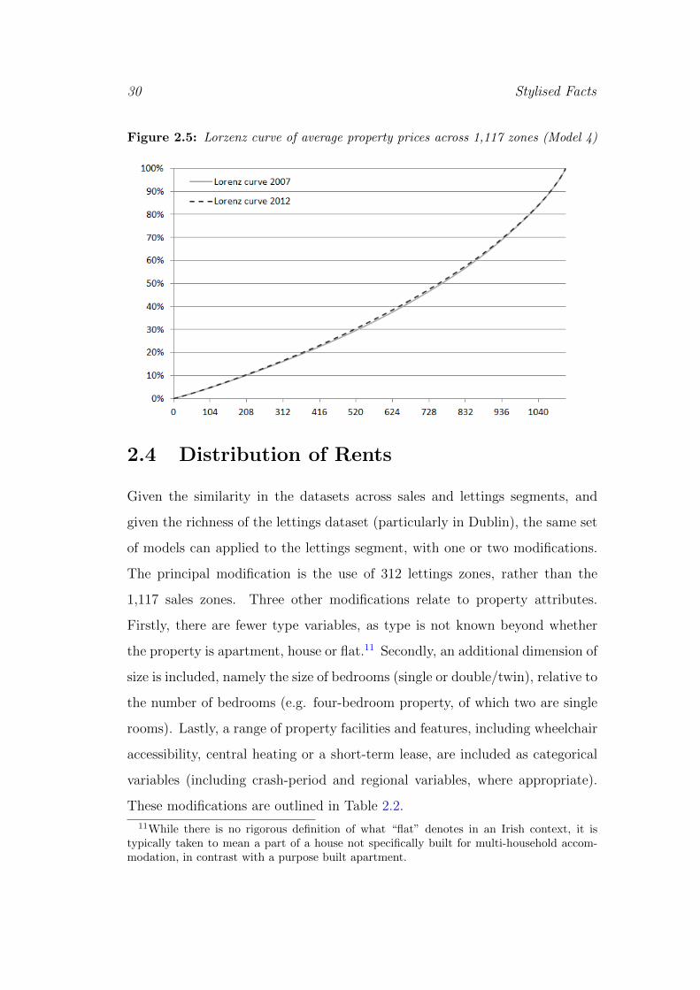
The distribution of prices can be shown in a more comprehensive way using
Lorenz curves. The Lorenz curve is a graphical representation of the equality of
a distribution, showing in this instance for the bottom x zones, what percentage
y% of housing wealth they have (controlling for differences in property types
between areas); perfect equality would be represented by the 45◦ line. As would
be expected from the Gini coefficients, the Lorenz curves shown in Figure 2.5,
for Model (4), suggests very little change overall.
30 Stylised Facts
Figure 2.5: Lorzenz curve of average property prices across 1,117 zones (Model 4)
2.4 Distribution of Rents
Given the similarity in the datasets across sales and lettings segments, and
given the richness of the lettings dataset (particularly in Dublin), the same set
of models can applied to the lettings segment, with one or two modifications.
The principal modification is the use of 312 lettings zones, rather than the
1,117 sales zones. Three other modifications relate to property attributes.
Firstly, there are fewer type variables, as type is not known beyond whether
the property is apartment, house or flat.11 Secondly, an additional dimension of
size is included, namely the size of bedrooms (single or double/twin), relative to
the number of bedrooms (e.g. four-bedroom property, of which two are single
rooms). Lastly, a range of property facilities and features, including wheelchair
accessibility, central heating or a short-term lease, are included as categorical
variables (including crash-period and regional variables, where appropriate).
These modifications are outlined in Table 2.2.
11While there is no rigorous definition of what “flat” denotes in an Irish context, it istypically taken to mean a part of a house not specifically built for multi-household accom-modation, in contrast with a purpose built apartment.

2.4 Distribution of Rents 31
Figure 2.6: Percentage point change in rental premium between bubble and crash,by size (Model 4)
2.4.1 Rental differentials by property size
Figure 2.6 is the lettings equivalent of Figure 2.3 for the sales segment presented
earlier, showing the change in differential by bedroom number, for each of the
five regions. Overall, the findings are the opposite of the sales segment, where
premiums for larger properties and discount for smaller properties grew. The
spread of rents between property types narrowed between bubble and crash
periods. For example, in the Dublin lettings market, the discount for a 1-
bed (relative to 3-bed) fell from 32% to 29% in the crash, while the premium
associated with 5-bed (relative to 3-bed) fell from 47% to 39%. Of 20 size-
related differentials, fourteen are associated with a narrowing of the spread of
rents across types between bubble and crash.
The extent to which state intervention in the lettings segment through Rent
Supplement has an impact on these results, compared to the role of potential
first-time buyers excluded from the owner-occupier market, is a topic worthy
of future research. In particular, a binding price floor would alter rental dif-

32 Stylised Facts
ferentials by compressing the spread of rents. Rent Supplement is paid by
the State to people living in private rented accommodation who cannot afford
their accommodation. It is based on a system of maximum thresholds that
vary by the applicant household (a couple with three dependent children will
be entitled to more than a single person with no children) and by location (the
same household may be entitled to twice as much in Dublin as in some local
authorities). With the sharp fall in rents in 2008/2009, it is possible that these
thresholds have formed a price floor in some segments of the market.
The above evidence is suggestive of extra space in the lettings market being
viewed as a luxury: a couple that enjoyed a two-bedroom apartment downsizing
to a one-bedroom apartment in the crash, or a family where each child had a
double room switching to single rooms. Figure 2.7 plots the change in the
premium against the existing 2006-2007 premium, using regional type and size
effects (Model 4, 155 differentials in total). While there are exceptions, the
overall contrast with the sales segment (cf. the upward-sloping line in Figure
2.4) is clear. Unlike the finding for the sales segment, the larger the rental
market premium in the final stages of the bubble, the greater the fall between
bubble and crash.
2.4.2 Geographic spread of rents
Table 2.5 outlines measures of the spread of rents, including selected percentile
ratios, for the various models presented. As discussed in the previous section,
though, there is evidence to suggest that the distribution of rents across size
changed, thus the focus should be on models that allow type differentials to
vary between bubble and crash [Models (3)-(5)]. These models indicate a more
pronounced average fall in rents (nearly 30%) than Model (2), and a slight
decline in the spread of rents, the coefficient of variation falling from 33.2% to
31.4% under Model (4). No model suggests a dramatic change in the geographic
spread of rents – it is worth noting that Model (5), which allows for different
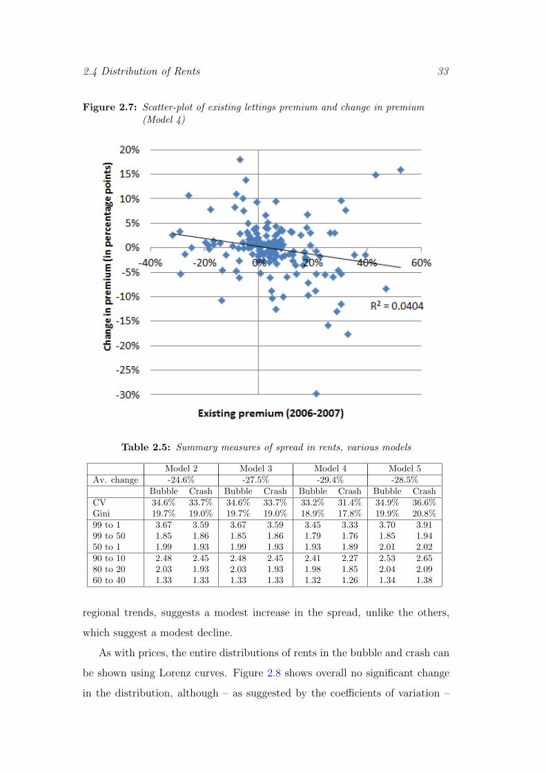
2.4 Distribution of Rents 33
Figure 2.7: Scatter-plot of existing lettings premium and change in premium(Model 4)
Table 2.5: Summary measures of spread in rents, various models
Model 2 Model 3 Model 4 Model 5Av. change -24.6% -27.5% -29.4% -28.5%
Bubble Crash Bubble Crash Bubble Crash Bubble CrashCV 34.6% 33.7% 34.6% 33.7% 33.2% 31.4% 34.9% 36.6%Gini 19.7% 19.0% 19.7% 19.0% 18.9% 17.8% 19.9% 20.8%99 to 1 3.67 3.59 3.67 3.59 3.45 3.33 3.70 3.9199 to 50 1.85 1.86 1.85 1.86 1.79 1.76 1.85 1.9450 to 1 1.99 1.93 1.99 1.93 1.93 1.89 2.01 2.0290 to 10 2.48 2.45 2.48 2.45 2.41 2.27 2.53 2.6580 to 20 2.03 1.93 2.03 1.93 1.98 1.85 2.04 2.0960 to 40 1.33 1.33 1.33 1.33 1.32 1.26 1.34 1.38
regional trends, suggests a modest increase in the spread, unlike the others,
which suggest a modest decline.
As with prices, the entire distributions of rents in the bubble and crash can
be shown using Lorenz curves. Figure 2.8 shows overall no significant change
in the distribution, although – as suggested by the coefficients of variation –

34 Stylised Facts
Figure 2.8: Lorzenz curve of average rents across 312 zones (Model 4)
some compression in the middle of the distribution. In contrast to the sales
market, the fall in 99:1 differential, from 3.45 to 3.33 in Model (4), is due to
both a narrowing of the 99:50 and 50:1 differentials.
Appendix .1.2 includes two heatmaps for Ireland’s lettings market. Figure
3 outlines a heatmap of the average rent for each of 312 zones for 2012:II rents,
across a weighted basket of five stylised properties. Ten bands are shown, the
highest being an average rent of more than e1,300 and the lowest band being
below e500. Controlling for district-specific differences in housing supply, the
most expensive areas to rent in like-for-like terms are largely the same for
sales, in the south-eastern part of Dublin. Figure 4 outlines geographically
the percentage fall in the average rent by zone. The scale runs from a fall of
15%-20% (lightest purple) to a fall of 35%-45% (darkest purple). Among those
areas seeing the largest falls in rents are large parts of Dublin and some of its
commuter belt to the south and south-west.

2.5 Conclusion 35
2.5 Conclusion
Housing market cycles are an integral part of modern economies and a key
part of broader economic fluctuations. The intention is that this thesis will
contribute to a better understanding – and management – of housing market
cycles. To do that, an understanding of the internal mechanics of housing
markets is necessary and this chapter is one of the first to explore this issue
using a granular perspective of housing sub-markets. Contrasting theoretical
predictions exist in relation to how values change in different market segments,
with high- or low-value segments potentially more volatile over the market
cycle. Using a comprehensive listings dataset to provide a unique window
into the extreme Irish property market bubble and crash, the aim here was to
analyse changes in the structure of prices in Ireland’s sales and lettings markets
over the five years following the end of the housing bubble in 2007. There are
four key findings:
1. In the sales segment, the spread of prices across property types rose sub-
stantially in the crash. For example, the fall in price of a five-bedroom
property was significantly smaller than that of a one-bedroom property in
the same location; the differential between these two properties increased
from 118% to 164% nationally.
2. In the lettings segment, the opposite was the case: the spread of rents
across different property sizes fell in the crash. The differential between a
five-bedroom property and a one-bedroom property in the same location
narrowed from 97% to 82%.
3. The geographic spread of both prices and rents was largely preserved
across bubble and crash periods, falling only slightly in most models.
The Gini coefficient of prices fell slightly (in Model (4), from 25% to
24%), similar to what happened in rents (20% to 19%).

36 Stylised Facts
4. As suggested by these Gini coefficients, it is clear that the spread of rents
was significantly less than the spread in house prices in both bubble and
crash periods. Most of this difference appears to be concentrated in high-
amenity areas: while the 50:1 percentile ratios of prices and rents were
similar (1.89 compared to 1.93), the 99:50 ratio was substantially greater
in prices (3.02 compared to 1.86).
Policy implications from this analysis exist, both for Ireland and further
afield. Firstly, if owner-occupier demand in post-GFC Ireland has shifted to-
wards larger property types, this has implications for policy in relation to deal-
ing with legacy vacant properties and “ghost estates”. Much of the supply
overhang is apartments or smaller homes in developments, which according to
the analysis presented here have suffered significantly larger falls in value and
face weaker demand. Secondly, there are also implications for policy in relation
to future development and planning. The shift in demand away from smaller
properties towards larger properties will require a supply-side response, to en-
sure affordability of family homes. The change in price structure in Ireland
since 2007 has implications, thirdly, for financial stability policy in Ireland, in
particular in relation to bank recapitalization. If uniform falls from the peak
are assumed across different market segments in stress-test calculations, this
may lead to an inaccurate assessment of risk for Ireland’s financial institutions
and the taxpayer.
A related implication, finally, is about warning signals for future bubbles.
The Stein and Costello hypotheses have very different implications for poli-
cymakers keen to spot potential housing bubbles early on. The experience of
Ireland indicates that narrowing differentials between large and small property
types when prices are rising might not represent a sustainable shift in consumer
demand towards smaller properties, rather an unsustainable trend. This tallies
with anecdotal evidence in Ireland that during the bubble, “property ladder”
concerns pushed people to buy lower-attribute properties they would other-
2.5 Conclusion 37
wise not consider, for capital gains and subsequent trading up. Alternatively,
high-LTV lending to borrowers with risky income profiles could explain greater
demand for smaller properties.
There are a number of limitations to be noted to this study. Firstly, the
dataset does not cover the period prior to 2006, so it is not possible to compare
run-up over the decade to 2007 with subsequent falls, as other studies have
done, and stops in mid-2012, at which point Dublin prices had largely levelled
off but prices elsewhere may not have.12 Secondly, there are omitted variables,
such as age, square meterage and energy efficiency, which may have a role in
explaining observed variations. Lastly, the prices presented above are based on
advertised prices and rents. Chapter 4 investigates how list and transaction
prices are related over the course of the market cycle.
In relation to other avenues for research, the contrast between the findings
for sales and lettings segments suggests a model where income and substitution
effects apply in different markets. Income effects appear to dominate where
there is no outside option (demand for accommodation is income-inelastic if
you are a renter): space in the crash is a luxury for tenants. Where there is
an outside option – many would-be first-time buyers stayed as renters during
this period – substitution effects kicked in: if you are going to buy, you might
as well buy big. An implication for future research on tenure choice is that the
real estate cycle may not just affect the choice of whether to buy or rent but
also what type of property to buy.
While the conclusions about property size are unambiguous, those about
location are much less clear. Ultimately, location is a short-hand for bundles
of amenities, ranging from labour and consumer markets to social and natural
capital amenities. The final finding – that the geographic spread of rents is in
some sense constrained at the upper end of the distribution of locations – is
consistent with either renters under-valuing certain amenities, for example due
12By mid-2013, prices in Dublin had risen 8% year-on-year, while prices elsewhere in thecountry fell by 1%, according to the official CSO house price index.

38 Stylised Facts
to search thresholds, or alternatively buyers over-valuing those amenities, for
example due to fear about future access to an amenity that is in fixed supply
(e.g. access to schools). Buyer over-valuation due to a desire to lock in access
to amenities would reasonably be at its most acute in a bubble and be seen in
pro-cyclical pricing of attributes and amenities. The evidence here, however,
certainly in relation to attributes, is that pricing was counter-cyclical. Thus,
if the “true” valuation is the same in both markets, i.e. assuming buyers and
renters are drawn from the same population, this suggests that it is renter
under-valuation at work. This issue is explored in more detail looking at a
range of location-specific amenities in Chapter 3.
Lastly, the very different trends in prices and rents suggest that the capi-
talization rate of property narrowed significantly but also that its change was
different across market segments. While the first part is consistent with an
error-correction set-up for the property market, which reverts back to its equi-
librium cap rate, the fact that the equilibrium cap rate could vary significantly
by segments is intriguing. A natural avenue for future research is to describe
and explain the significant variation over time and space in this fundamental
barometer of the property market. Trends and corrections in house prices and
the price-rent ratio are explored in more detail in Chapter 5.
Chapter 3
Cyclicality of Amenity Prices
Understanding the link between housing market cycles and the macroecon-
omy is particularly important given the aftermath of the global economic and
financial crisis starting in 2007. A number of OECD economies enjoyed an un-
precedented boom in housing prices over the late 1990s and early 2000s. This
was followed by a rise in defaults in the U.S. mortgage market, in particular its
sub-prime segment, which – due to a range of financial innovations such as se-
curitization – had an impact on the global financial system (Duca et al. 2010).
The following years have seen the effects spread to global trade (2008-2009)
and sovereign debt (from 2010).
Ireland’s economic fortunes have in many respects been a microcosm of
those globally. The period from the mid-1990s to 2007 was one of very strong
economic growth in Ireland, initially export-led but in later years fuelled by
the availability of cheap credit and an unprecedented building boom. From
2007, the economic downturn was severe. National income fell from e163bn
in 2007 to e128bn in 2011 (GNP in current prices), while government finances
deteriorated sharply, with fiscal deficits of 10% of GDP per year by 2010.
Unemployment rose from below 5% in 2007 to almost 15% by 2011, while large
inward migration flows changed to emigration. Despite the global nature of
the crisis, central to the dramatic change in Ireland’s economic fortunes were
domestic factors, in particular the end of a domestic real estate bubble.
The case of Ireland highlights the links that exist between housing and
39

40 Cyclicality of Amenity Prices
other aspects of the economy, including financial stability, the labour market,
the government finances, and public service provision. To understand how
a housing cycle can affect economic fluctuations, it is important not only to
understand the channels through which housing and the wider economy are
related (see, for example, Muellbauer (2012), as well as Chapter 5), but also
how the housing market itself works. Yet the mechanics of the housing market
and its cycles remain poorly understood. The housing market is an inherently
spatial one and, property-specific attributes aside, differences in price across
the market reflect location-specific amenities. With nominal house prices falls
of over 50% between 2006 and 2012, Ireland is a natural case study for studying
the ups and downs of housing markets.
This chapter uses a detailed dataset of property listings in Ireland, both
sales and lettings, over the period 2006-2012 – and a large dataset of location-
specific amenities – to investigate the relationship between amenities and the
housing market cycle. Taking the hedonic regression literature started by Rosen
(1974), that amenities will be reflected in property prices, it explores two related
hypotheses. The first is that price and rent effects of amenities may differ. This
may be due to fundamental differences between households that buy and rent
specifically about the utility derived from location-specific amenities. If this is
not the case, economic theory suggests that a desire on the part of buyers to lock
in access to amenities – facilitated by changing credit conditions over time –
may push up the price of amenities, relative to their rent effect. Alternatively,
renter search thresholds (as outlined in more detail below) may lead to an
attenuated rent price of amenities, compared to the sales segment. Secondly,
the effect of amenities on the cost of accommodation may vary with the cycle.
This may be pro-cyclical, reflecting buyer lock-in concerns, or counter-cyclical,
reflecting “property ladder” effects.
The chapter is structured as follows. Sections 3.1 and 3.2 outline briefly the
economic theory and existing literature in relation to amenity valuation and
the structure of prices in the housing market, while section 3.3 provides details
3.1 Theory 41
on the data used in this analysis. Section 3.4 outlines the model and empirical
strategy and Section 3.5 presents the results. Section 3.6 concludes.
3.1 Theory
3.1.1 Urban economics & bid-rent gradients
Von Thunen’s (1863) theory of farmers sorting by opportunity cost of distance
to a market extends in a straightforward fashion to models of household loca-
tion selection. Models along these lines date from Alonso (1964), where, in a
monocentric city, one would expect those households with the highest oppor-
tunity cost of distance from a given central business district (CBD) to locate
closest to it. As outlined by Straszheim (1987), in a standard monocentric
model, a household derives utility from its quantity of land consumed (q), its
location or distance from the centre (u), and the numeraire composite con-
sumption good (z). Its expenditure includes rent per unit of house size (r) and
transport costs (T ).
The optimization problem yields an equation of the marginal rate of substi-
tution across housing and non-housing with their price ratio: Vz/Vq = 1/r(u).
Choice of location must satisfy a condition equating the change in rent to the
trade-off between monetized value of the disutility of a longer commute and
the change in transport expenditure: ∂r/∂u · q = Vu/Vz−∂T/∂u. The bid-rent
gradient from the CBD outwards can be assumed, via partial equilibrium anal-
ysis, or derived, via general equilibrium analysis, where assumptions are made
about utility levels at different locations. Either way, households will move
away from the centre, along the rent gradient, until the marginal disutility of
a longer trip just offsets the savings achieved for land consumed.
3.1.2 Hedonic Markets and Implicit Prices
There is an important caveat to the von Thunen set of theories, namely that
all models assume that cities are monocentric and indeed that these centres

42 Cyclicality of Amenity Prices
are exogenous. Work such as that by Dubin & Sung (1987) suggests that there
are limitations to models that focus on one particular amenity, i.e. proximity
to employment, and that impose a particular distribution of that amenity, i.e.
entirely within a set central business district. There are a large number of po-
tential considerations beyond employment that may affect a household’s choice
of residence, from market depth to environmental. Allowing an n-dimensional
amenity vector and relaxing the restrictions on the location of amenities across
the city space suggests that a more complicated bid function for given levels of
utility and income is required.
Rosen’s (1974) model contains a market for good z comprising i = 1, . . . , n
attributes (or amenities), where p(z1, . . . , zn) is increasing in all its arguments
and has second derivatives. Due to indivisibilities in the good directly traded,
its package of amenities cannot be “untied” and therefore there cannot be the
arbitrage required to make p(z) linear. The value function θ(z1, . . . , zn;u, y)
represents the expenditure a consumer is willing to pay for different alterna-
tive values of z, for a given utility index and income level and is the multi-
dimensional counterpart to Alonso’s bid-rent function.
The value function θ gives the amount the consumer is willing to pay, while
market prices are given by p(z). The optimum will be where these two surfaces
are tangent to each other. While utility increases with income, the exact rela-
tionship between zi and income – i.e. whether a particular amenity is a normal
good or not – depends on the shape of the price function. Only if p(z) were
convex and sufficiently regular everywhere would each zi be a normal good at
all income levels (Rosen 1974).
In practical terms, this means that the value of an amenity should be re-
flected in the price. A suitable empirical strategy will be able to highlight the
marginal willingness to pay for access to that amenity by holding other factors
constant and varying access to the amenity. This is the approach used here.

3.1 Theory 43
3.1.3 Amenity valuation by tenure
It is possible that, once household characteristics are controlling for, renters and
buyers place different relative valuations on the set of amenities. In particular,
two mechanisms suggest that buyers will factor in a wider range of amenities
than renters; relative to some hypothetical “true value” of an amenity, it is
possible that renters underpay or alternatively that buyers overpay.
The first is that there are factors, such as indivisibilities related to search
costs, that restrict renters’ willingness to pay for amenities. The market for
accommodation is one where matching is important, as both occupants and
properties have idiosyncratic attributes. Suppose that search costs (s) in the
property market, whether renting or buying, involve indivisibilities: finding
somewhere to live cannot be done without a given minimum amount of time
spent online and visiting properties (κ), in addition to any tenure-specific search
costs and/or searcher intensities. Suppose also that prospective buyers and
tenants have maximum thresholds (t) to their search costs that are roughly
proportional to the value of the transaction (λV , where V denotes the value
of the transaction): in practical terms, those buying their home for the next
twenty years might be prepared to spend six months searching for the right
property, but those renting for the next two years might not.
In such a market, there would be a disproportionality in the s(κ) : t(λ)
ratios for the same household buying or renting: renters are likely to hit their
thresholds of search costs sooner. For example, while both buyers and renters
may prefer properties closer to the coast or with a southerly orientation, per-
haps only buyers may hold out and reward these amenities. Thus, one may ex-
pect certain amenities, particularly those that could be regarded as secondary,
will not be rewarded to the same extent in the lettings market as in the sales
market.
An alternative theory is that there are factors that encourage buyers to
“over-capitalize” amenities. One obvious candidate is the frenzy of the bubble,
44 Cyclicality of Amenity Prices
where, due to the fixed supply of amenities, buyers are concerned about securing
access to amenities (for example having schools nearby). In particular, buyers
may worry about the cost of accessing amenities in the future, leading to a
greater valuation by buyers than renters. Alternatively, transaction costs, such
as legal fees and transaction-based taxes, may be significant for buyers (but
unimportant for renters), restricting buyer mobility and thus encouraging them
to lock in supply of particular amenities.1
Hypothesis 1 The first hypothesis to be tested empirically is, therefore, that
the price effect of amenities is, in relative terms, greater than the rent effect.
3.1.4 Valuation of amenities over the market cycle
One theory suggests that higher price housing should be more volatile over
the market cycle, due to the presence of down-payments and the fact that
the typical household holds most of their private net wealth in housing (Stein
1995).2 Consider a negative shock to house prices: this hinders movers from
making their next down-payment, depressing demand. If high-priced homes
are purchased primarily by buyers trading up (rather than first-time buyers),
then their prices should have a greater variance over the real estate cycle. The
prior expectation, according to this liquidity constraint model, is that houses
with higher prices would both rise and fall more dramatically than those with
lower prices. As houses with higher prices are those in locations with greater
amenities, this liquidity constraint model suggests procyclical amenity prices:
that the price of amenities would rise in the bubble and then fall in the crash.
Alternatively, lower segments of the housing market may experience more
volatile swings in prices. Costello (2000) suggests that more affordable prop-
1Note also that even if the buyer does not value a particular amenity, if they believethat the amenity will contribute to future capital gains, they will be prepared to pay for itnow, unlike a tenant, who has no financial gain for an amenity they do not derive utilityfrom directly. Using U.S. data on expenditure on education, Hilber & Mayer (2009) extendthis argument to willingness-to-pay for new amenities by households that will only benefitthrough the capitalization of the amenity in house prices.
2See also Section 2.1.

3.1 Theory 45
erties are more liquid and thus these segments will be more competitive, rising
more in boom markets and falling more in down markets. This effect may be
related to credit conditions. As credit rationing eases, and marginal borrowers
become active in the market, there should be greater demand at entry level,
a process that goes into reverse when credit rationing tightens again. In lay
terms, this can be thought of as a “property ladder” effect. In such a situa-
tion, greater importance is attached by buyers to having any property, even
one with poor amenities, than at other points in the cycle, as (expected) cap-
ital gains will facilitate trading up in the future. Consequently, demand for
low-quality (low-amenity) properties shifts up. With relatively less importance
attached to amenities in the bubble than at other points in the market cycle,
countercyclical amenity prices would be evidence of “property ladder” effects.
Hypothesis 2 The second hypothesis to be tested empirically is, therefore,
whether the price effect of amenities is pro-cyclical or counter-cyclical.
3.1.5 Categories of amenities
It is possible to think of a multitude of location-specific characteristics that
may impact on a property’s desirability. A natural ordering of these amenities
is by permanence or mobility. At one end of the spectrum are first-nature
endowments of geography and environment. At the other end are population-
specific, rather than location-specific amenities, such as market depth or social
capital. Such amenities are hypothetically mobile, although taken as given by
any individual agent at a point in time.3
For the purposes of this analysis, six categories of amenities are considered.
Roughly in order from more fixed (first nature) to less (second nature), they
are: environmental amenities; transport facilities; educational amenities; the
labour market; neighbourhood quality; and agglomeration or market depth:
3The categorizaton presented is merely for ease of exposition and does not affect theconclusions reached.

46 Cyclicality of Amenity Prices
1. Environmental factors, such as proximity to coastline, lakes, rivers, forests
or urban green space
2. Transport facilities, such as primary and secondary roads, train stations
or light rail services
3. Education facilities, including primary and post-primary schools and higher
education institutes; the latter may be particularly important for renters
(due to demographic reasons)
4. Labour market amenities, including the unemployment rate, the length of
commuting to work and the diversity of general employment opportunities
5. Neighbourhood quality, measured through either incidents (e.g. crime
rates) or inhabitants (for example the proportion with a third-level de-
gree)
6. Agglomeration amenities, such as those of von Thunen and Alonso recast,
proximity to centres of economic activity, and distance from borders
While the focus here is on the amenities listed above as reflecting the primary
location-specific factors, a large number of other amenities may affect house
prices, including polluting facilities, national monuments, and facilities such as
prisons and stadiums. In addition, location-specific housing supply variables
may affect property values, for example proximity to “ghost estates” or zoned
land.
3.2 Literature
3.2.1 Hedonic pricing of amenities
Since Rosen’s (1974) seminal paper, a large empirical literature has developed,
estimating the implicit price of a wide range of amenities.4 Much of the early
4There are over 5,600 papers citing Rosen (1974), according to Google Scholar (Harzing2007).

3.2 Literature 47
literature was focused on environmental public goods, such as air and water
quality – reviews are given by Smith & Huang (1995) on air quality, Boyle
& Kiel (2001) on water quality and Kuminoff et al. (2010) on environmental
amenities. There is also a large literature on the effect of transport facilities
on property values, although the hedonic method is just one of a number of
methods used here (Debrezion et al. 2007, RICS Policy Unit 2002, Wrigley
et al. 2001).
An overview of the importance of amenities and land values in general, when
attempting to understanding housing values, is given by Cheshire & Sheppard
(1995). The provision of other public services, in particular education, has
been the subject of a significant amount of analysis using hedonic pricing meth-
ods. Black (1999) exploits differences across boundaries of school districts to
estimate household willingness to pay for better school performance in Mas-
sachusetts, while similar work exists for England (Gibbons & Machin 2003).
The same authors have estimated the impact of the opening of new rail lines
in London in 1999 (Gibbons & Machin 2005). In general, well-specified studies
find not only statistically significant positive effects of amenities on housing
values but also reasonably precise estimates of the average impact of a greater
amenity, such as distance to transport facility or better educational outcomes.
A good overview of the hedonic valuation of amenities method and of the
findings from recent research on the value of education, transport and safety
amenities, is given by Gibbons & Machin (2008). They stress the use of quasi-
experimental approaches that exploit variations in the supply of amenities,
although recent theoretical research has highlighted the limits to reliance on
supply shocks (Coate 2013). Literature on other amenities – in particular
social capital but also market-depth – is much less developed at this stage,
most likely as the bulk of empirical work is at city- or county-level and thus
there is significantly less variation in population-specific characteristics than at
country-level.
48 Cyclicality of Amenity Prices
The literature on the hedonic pricing of amenities in the Irish property
market is somewhat more limited. Mayor et al. (2009) and Mayor et al. (2008)
examine amenities in the Dublin housing market during the final stages of
the bubble (2001-2006). They find evidence that both urban green space and
transport access are valued in house prices: increasing by 10% the proportion
of urban green space within two kilometres of a house was associated with an
increase of at least 7% in the house price. The effect of being less than 2km
from a light rail station (Green Luas line) was of a similar magnitude. Another
amenity they report is proximity to the coast, associated with a premium of
12%-22% premium for being within a kilometer of the coast (the closer to the
coast, the larger the premium). The effect of various amenities is not broken
down by phase in the market cycle, however, most likely due to sample size
constraints.
Two comments on the general literature are worthwhile. The first is that,
by and large, well-specified studies – especially those that both control for
omitted variables and exploit supply-side variation – do find that a wide range
of amenities is factored into the cost of accommodation with the expected sign,
although there is often little agreement across researchers on the magnitude.
This is understandable given that the studies vary hugely in terms of regions
(and time periods) analyzed, as well as sample sizes and exact specification.
The second is that the established literature has a number of limitations.
As is pointed out by Kuminoff et al. (2010), there is no reason to assume that
amenities have time-constant prices, yet this is overwhelmingly the strategy
adopted in the literature to date, more than likely due to sample size limita-
tions. Likewise, there is very little information on the valuation of amenities in
the lettings segment of the residential property market, again more than likely
due to limitations of data.
One glimpse into the relationship between amenities and the housing mar-
ket cycle is given by Case & Mayer (1996). Their study is of 135,000 repeat
sales in 168 towns in Eastern Massachusetts over the period 1981-1994, when
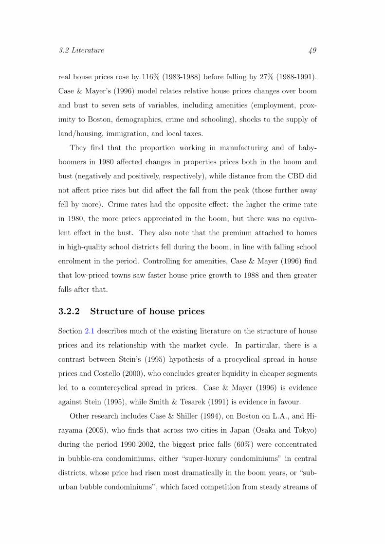
3.2 Literature 49
real house prices rose by 116% (1983-1988) before falling by 27% (1988-1991).
Case & Mayer’s (1996) model relates relative house prices changes over boom
and bust to seven sets of variables, including amenities (employment, prox-
imity to Boston, demographics, crime and schooling), shocks to the supply of
land/housing, immigration, and local taxes.
They find that the proportion working in manufacturing and of baby-
boomers in 1980 affected changes in properties prices both in the boom and
bust (negatively and positively, respectively), while distance from the CBD did
not affect price rises but did affect the fall from the peak (those further away
fell by more). Crime rates had the opposite effect: the higher the crime rate
in 1980, the more prices appreciated in the boom, but there was no equiva-
lent effect in the bust. They also note that the premium attached to homes
in high-quality school districts fell during the boom, in line with falling school
enrolment in the period. Controlling for amenities, Case & Mayer (1996) find
that low-priced towns saw faster house price growth to 1988 and then greater
falls after that.
3.2.2 Structure of house prices
Section 2.1 describes much of the existing literature on the structure of house
prices and its relationship with the market cycle. In particular, there is a
contrast between Stein’s (1995) hypothesis of a procyclical spread in house
prices and Costello (2000), who concludes greater liquidity in cheaper segments
led to a countercyclical spread in prices. Case & Mayer (1996) is evidence
against Stein (1995), while Smith & Tesarek (1991) is evidence in favour.
Other research includes Case & Shiller (1994), on Boston on L.A., and Hi-
rayama (2005), who finds that across two cities in Japan (Osaka and Tokyo)
during the period 1990-2002, the biggest price falls (60%) were concentrated
in bubble-era condominiums, either “super-luxury condominiums” in central
districts, whose price had risen most dramatically in the boom years, or “sub-
urban bubble condominiums”, which faced competition from steady streams of

50 Cyclicality of Amenity Prices
fresh supply. Chapter 2 found that for property-specific attributes, there are
countercyclical relative prices, which suggests that “property ladder” effects
may dominate. Is the same true for location-specific amenities?
3.3 Data
The principal dataset used is provided by the online accommodation portal,
daft.ie, which provides price (rent) information as well as property attributes,
including location. In addition to information on listed purchase or rental
price (outlined below), there are seven further dimensions along which the
data are segmented: segment; size; type; time; location; property attributes;
and location amenities. For time (in particular phase of the market, whether
bubble or crash), but also for segment (sales or lettings) and for certain variables
type and location, interactions between dimensions are included.
The sales component of the full dataset includes 416,899 properties listed
for sale between 2006 and 2012.5 As is outlined in Table 3.1, almost three-
quarters of properties listed were three-bedroom or four-bedroom in size. In
terms of regional distribution, two-fifths of the listings were in Ireland’s five
cities (almost 30% alone in Dublin). Roughly one third of properties were from
the Leinster province, large parts of which act as commuter areas for Dublin.
The lettings component of the dataset comprises just over 825,000 ads. Com-
pared to the sales dataset, there are a greater proportion of smaller properties
and Dublin properties: the most common property size is two-bedroom, while
Dublin properties comprise almost half of all ads. Summary stats for both
components of the dataset are given in Table 3.1.
There are three distinguishing features about this dataset. The first is its
size (well over a million observations), not only relative to the size of Ireland’s
5The vast majority of listings in the dataset refer to ads posted on the daft.ie site. Roughly34,000 refer to the small fraction of online listings in Ireland that were not advertised on thedaft.ie portal, most of which date from 2006-2007. Where the list price was changed, therevised ad was treated as a new observation, reflecting the fact that the focus here is on pricerelativities within a given period of time and general market trends are controlled for.
3.3 Data 51
Category Cohort Sales LettingsCount Percent Count Percent
Size One-bedroom 11,459 2.7% 83,954 10.2%Two-bedroom 67,124 16.1% 314,140 38.1%Three-bedroom 190,076 45.6% 267,530 32.4%Four-bedroom 121,050 29.0% 133,886 16.2%Five-bedroom 27,190 6.5% 25,589 3.1%
Region Dublin 119,898 28.8% 394,376 47.8%Other cities 53,069 12.7% 128,806 15.6%Leinster 125,467 30.1% 189,041 22.9%Munster 69,396 16.6% 69,837 8.5%Connacht-Ulster 49,069 11.8% 43,039 5.2%
Total 416,899 100.0% 825,099 100.0%
Table 3.1: Dataset size, by cohort
housing market – the country had in Census 2011 just over two million house-
holds – but also in absolute terms, compared to studies from other countries.
In their review of 69 hedonic studies of willingness to pay for environmental
amenities in the two decades to 2006, Kuminoff et al. (2010) find that only
about one in five (22%) contains more than 10,000 observations. The second
is the fact that the dataset covers an entire country. Only about one in ten
hedonic studies (9%) has been at the national level (Kuminoff et al. 2010). The
third distinguishing feature is the fact that both sales and lettings markets are
included: this is the first study of this type known to the author that has
comparable data for both.
3.3.1 Price data
Price information included in the dataset is listed, or asking, price. An obvious
concern is that the list price may not reflect any subsequent transaction price.
For a discussion of this issue and the findings from the literature, please see
Section 2.2.1 and also the analysis in Chapter 4.
3.3.2 Segment
In standard specifications, regressions are pooled across sales and lettings seg-
ments, in order to assess whether differences between price and rent effects are

52 Cyclicality of Amenity Prices
statistically signficant. For this, a categorical variable let is included, which
takes a value of 1 for lettings ads. Interactions are also included between this
variable and all other dimensions of the data, i.e. size, type, time, location,
attributes and amenities. For example, in relation to size, examples of inter-
acted variables include beds2 let and beds2 let cr, which capture respectively
(1) how the differential between 2-bed properties and 3-bed properties (the
control) varied across sales and lettings segments, and (2) how the lettings
differential changed in the crash period (defined below). Similar variables are
included for type, while interactions between let and property attributes, quar-
terly dummies and location dummies (explained below) are also included.
3.3.3 Size
Size in square metres is not a widely used metric by consumers in Ireland and
consequently, the majority of sales listings (and all lettings listings) do not
include this information. To capture a property’s size, indicator variables are
included for number of bedrooms (one to five) and then number of bathrooms
relative to number of bedrooms.6 For lettings properties, the occupancy of each
bedroom is also known and this is measured by number of single bedrooms out
of the total number of bedrooms. Interactions between segment and size are
included, as described above.
3.3.4 Type
The most fundamental distinction by type is between apartments and houses.
Within apartments, there are additional variables for duplexes (in sales) and
“flats” (in lettings; referring to parts of houses that have been subdivided for
lettings accommodation). For houses, there is additional information in the
sales segment: terraced, semi-detached, detached and bungalow. These are all
captured with categorical variables.
6For example, bb41 refers to properties with four bedrooms and one bathroom.

3.3 Data 53
3.3.5 Time
Categorical variables by quarter are included to reflect the trend in property
prices over time. Additional variables (e.g. 2010q1 let) allow the trend in rents
(which fell 25% between 2007 and 2012) to differ from the trend in list prices
(which fell more than 50%). As noted by Conniffe & Duffy (1999), a frequently
absent feature of hedonic models was investigating the extent to which time
and other attributes interact. Thus, the model includes interactions between
different phases of the market and other dimensions of the data. Phases are
defined as follows: the bubble (2006-2007, prices rising) and the crash (2010-
2012, prices down by at least one third), with the intermediate period 2008-2009
is used as a control where relevant.
3.3.6 Location
Three dimensions of a property’s location are used in this research: its regional
market, to enable accurate pricing of different property types; its local market,
to capture factors not included in the analysis; and its exact physical location,
used to calculate distance to amenities.
Regional markets
Five broad regions in the Irish property market are defined. The first is Dublin
city, while the second regional market contains the four other cities in Ireland
combined (Cork, Galway, Limerick and Waterford), whose populations vary
from 50,000 to 275,000. These are not contiguous but may share marginal
price effects due to their status as regional cities. The other three regional
markets are based on Ireland’s provinces, but excluding the city areas: Leinster,
Munster and Connacht-Ulster.
Local markets
At a more granular level, areas are grouped into one of about 400 local markets.
The model incorporates fixed effects, designed to capture the impact on price

54 Cyclicality of Amenity Prices
of locality-specific factors that are not included in a given specification, includ-
ing location-specific and population-specific attributes or indeed any pure label
effects. Ireland lacks a postcode system, so these markets were manually con-
figured for each part of the country, according to a combination of the volume
of listings, geographic coherence and market logic. Each is interacted with the
let categorical variable, allowing the fixed effect for each local market to vary
between sales and lettings segments.
Exact location
The final locational attribute used is the property’s physical coordinates. The
address of each property advertised is converted at the time of listing into xy
coordinates. Also given is a level of accuracy with which these coordinates are
known. Both are products of addresses being run through the Geodirectory
service, administered jointly by Ireland’s official mapping and postal services
(OSI and An Post). This accuracy can vary from area-level through townland,
village and street-level to building-level. Only observations known to building
or street level were included, given the focus of the study on amenity valuation
using distance based on xy coordinates.7
3.3.7 Property attributes
A range of property-specific attributes can be measured from the data. A num-
ber, particularly for lettings listings, are included as separate fields in listings;
these include white goods (the presence of a washing machine, dryer, dishwasher
or microwave), utilities (cable TV, internet, an alarm or central heating), and
whether the property has parking, is suitable for pets, wheelchair-accessible,
furnished, or available to those on rent allowance. Information is also available
on the lease length. For sales properties, there is information on whether the
7This restriction involved the exclusion of an additional 264,975 sales listings and 322,809rental listings over the period 2006-2012.

3.3 Data 55
property is part of a new development, whether it is a re-listing at a differ-
ent price, and whether the property is being sold by the owner or through an
agent. For both sales and lettings listings, there is information on whether the
property has a garden.
In addition, it is possible to reflect other potentially important property-
specific features, using the text of the ad. This process generates an indicator
variable capturing a particular attribute, when one of a number of key phrases
that reflect the presence of that attribute occurs in the text of an ad. These
variables include a property’s aspect (south, west or south-west facing), its
age (period, Edwardian, Victorian or Georgian), condition (whether the prop-
erty has been recently refurbished or renovated), views, whether the property
is in a cul-de-sac (no through road), various types of rooms (utility room,
conservatory, granny-flat, walk-in wardrobe, wetroom), features related to en-
ergy efficiency (underfloor heating, fireplace solar panels, double-glazing) and
other features (balcony, bay windows, jacuzzi, fitted wardrobes, ensuite, garage,
French doors, high or corniced ceilings, and branded kitchen appliances).
All property attributes are set up as categorical variables, with interactions
for segment and for bubble and crash periods. An overview of the property-
specific attributes included is given in Table 3.2 in Section 3.4.2.
3.3.8 Location amenities
The focus of this research is on location-specific amenities. A total of 25
location-specific characteritics were included. As explained in more detail in
Section 3.4.2, the relationship between many of these characteristics and hous-
ing market outcomes is defined by distance, while for others (such as nearby
crime or the local unemployment rate) the relationship will be a value, rather
than a distance. The data are described below, by broad category of amenity.
While the focus here is the estimation of price and rent effects for a range of
amenities individually, alternative approaches are also possible. These include
a principal components analysis (PCA) of amenities, where the various different
56 Cyclicality of Amenity Prices
amenities are grouped into a small number of series, or an index of amenity
value, as is done in Glaeser et al. (2001). For the purposes of this research,
it was felt that analysing a large number of amenities together would offer a
better insight into the likely stylised facts of amenity valuation across segments
and over the cycle than a smaller number of aggregated amenities (or indeed
a single index). It is left to future research to explore which amenities are
most important and to see whether PCA would generate substantially different
results.
Environmental amenities
Five environmental amenities were included: coastline, rivers, lakes, urban
green space and forests. For data on the location of Ireland’s coastline, lakes
and rivers, the source is Ireland’s Environmental Protection Agency (EPA).
For both lakes and rivers, controls are included for scale. Data on urban green
spaces come from the European Urban Atlas and on Ireland’s forests come
from the 2006 CORINE Land Cover project (Environmental Protection Agency
2013a, European Environment Agency 2013); for both, controls for size are
included, as described in Appendix .2.1.
Transport facilities
Six amenities reflecting transport services were included. Four relate to the rail
network: stations for commuter/intercity traffic, for DART (suburban) trains,
and for Dublin’s Luas Red and Luas Green light rail networks. Information
on the location of stations is from Railway Procurement Agency (2012). In-
formation is also included on the primary and secondary road network, from
a complete dataset of the road network on the island of Ireland, produced by
NavTeq (2012) and courtesy of National Institute of Regional & Spatial Anal-
ysis (NIRSA) at NUI Maynooth. Controls are included for the speed limit that
applies on the nearest stretch of road; see Appendix .2.1.

3.3 Data 57
Educational amenities
Proximity to primary and post-primary schools and higher education institutes
is included in this research. The coordinates of all primary and secondary
schools were provided directly by the Department of Education and Skills in
Ireland, which maintains an annual census of all schools in Ireland (Depart-
ment of Education 2013). Information on the number and size of classes in
each primary school is available from the same source, while information on
the proportion of students progressing to higher education from post-primary
schools was provided to the author by Grainne Faller, author of the Irish Times
ranking of secondary schools. As outlined in Appendix .2.1, controls were in-
cluded for large and small schools both primary and post-primary, large and
small average class sizes (primary) and the rate of progression to university
(post-primary).
Labour market
Three labour market amenities are included. Information is available from
the April 2011 Census on the neighbourhood (“Small Area”) unemployment
rate, on the average commute in minutes, and the contemporaneous sectoral
allocation of the labour force (Central Statistics Office 2013).8 The proportion
of people employed in agriculture is used as a simple reduced form index of
employment opportunity for an area. These three indicators give different
measures of the local labour market amenity: unemployment, commuting, and
opportunity. These can be best thought of as area-level cardinal rankings, as
they are not time-varying and labour market conditions changed substantially
over the period under consideration. Information from the 2011 Census, rather
than the 2006 Census, is included due to the introduction of “Small Areas” in
8The 2011 Census in Ireland was the first to launch administrative units below the levelof Electoral Divisions (of which there are 3,409). Almost 18,500 “Small Areas” were used asthe basis for enumeration in Census 2011. Each “Small Area” has a population of between 50and 200 dwellings. They were created by NIRSA to be the lowest level of geography for thecompilation of statistics in line with data protection and generally comprise either completeor partial townlands or neighbourhoods.
58 Cyclicality of Amenity Prices
the later census, allowing a much more granular treatment of neighbourhood-
specific labour market conditions.
Neighbourhood
Factors such as class, educational attainment, diversity or sense of community
in an area may have an impact on property prices. However, without a more
rigorous treatment, many of these factors belong in a second-stage analysis
that attempts to describe the underlying demand curve. Much of the literature
includes local unemployment rates, to capture some index of neighbourhood
quality. Here, unemployment is treated as part of the labour market amenity.
Instead, for neighbourhood quality, the focus is on attributes related to social
capital that are, in a relative sense, more exogenous or difficult to change.
Five neighbourhood amenities were included that will be relatively fixed, at
least in the short run. These include the percentage of residents with a degree
and the neighbourhood’s population density. As with the labour market ameni-
ties, these are the equivalent of cardinal fixed effects, based on a property’s
“Small Area” district in Central Statistics Office (2013). Three crime-related
variables were included, based on station-level statistics for three types of crime
over the period 2004-2010: burglary, murders, and drug-related offences. Each
property was assigned a unique value for each category of crime, based on an
interpolated map of crime incidents. The resulting figure gives an indication
of the number of incidents in the nearby area. As with Census-based values,
these represent an ordering of areas, rather than reflecting innovations in crime
rates over the period under investigation, which is left for future research.
Agglomeration
Lastly, three more general market depth or agglomeration amenities are in-
cluded. The first two comprise distance from the “national CBD” (central
Dublin) and, where relevant, distance from the nearest CBD, which may be

3.3 Data 59
across the border in Northern Ireland. The third is distance from the border
with Northern Ireland.
Additional controls
To aid exposition, the treatment focuses primarily on these 25 location-specific
characteristics. However, other factors may matter in determining the cost of
accommodation. In addition to amenity-specific controls (as outlined above)
and micro-market fixed effects, a further 45 location features are included as
controls. In brief, they include distance from bathing facilities (mostly coast-
side beaches), existing and proposed National Heritage Areas, elevation, sports
& leisure facilities, rail track, and sea- and airports. They also include 17
different categories of facilities, eleven polluting facilities, so-termed under the
system of Integrated Pollution Prevention Control (IPPC) Licensing, and a
further six categories of waste facilities, which require a permit to operate and
are available from the same source. Also included are the location of mobile
phone masts, prisons, stadiums, hospitals, supermarkets, convenience stores
and disused mines.
In relation to neighbourhood quality, the following controls were included:
an area’s maturity and spaciousness, as captured by the proportion of pre-
1914 buildings and the average building size (in rooms), the proportion in
State-provided housing and whether the property is in (or close to) an Irish-
speaking Gaeltacht area. Six prominent categories of national monument were
also included: castles, church monuments, historic houses, ring-forts, holy wells,
and stone monuments (such as standing crosses or Ogham stones). Controls
are also included for whether the property lies within the boundaries of a town
and, if so, what size of town (by population; seven categories).
Two further controls are included, reflecting housing supply conditions. The
first is proximity to officially designated “ghost estates”, of which almost 2,900
were recorded by the Department of the Environment in 2011 (Department of
the Environment, Community & Local Government 2013b). The location of

60 Cyclicality of Amenity Prices
each is known (as a point rather than a polygon), as are a number of other
details, including the size of the proposed development and its state of comple-
tion. Lastly, information is available on standardized zoning of land around the
country, and in particular whether or not the property is on or near land zoned
for residential development (Department of the Environment, Community &
Local Government 2013a).
3.4 Model
3.4.1 General specification
The price of each property in the database can be represented as the sum of
the estimated value of its constituent components as well as an error term, ε,
reflecting the gap between the predicted value and the actual value; in simplified
equation form:
log(pricei) = α + β0leti +X ′1iβ1 +X ′2iβ2 +X ′3iβ3 +X ′4iβ4 + εi (3.1)
where: leti refers to whether the property is for sale or to let, X ′1i refers to
property-specific characteristics, including size and type and interactions out-
lined earlier, X ′2i refers to the time period (quarterly fixed effects); and X ′3i
refers to local market fixed effects, and X ′4i refers to a vector of location-specific
amenities.9
3.4.2 Amenity variables
For each amenity, five core sets of variables are included: the base effect (e.g.
distance from the coast), the lettings effect (distance from coast interacted
with let), effects by phase (interactions with indicators variables bubble and
9The specific functional form applied here – the natural log – is used for reasons of consis-tency with the vast majority of the literature on amenity pricing (as well as for consistencywith other analysis in this thesis). However, it should be noted that a more flexible approach,in particular the Box-Cox functional form, could also be applied. In such an approach, dataare transformed using a power parameter of λ, which is estimated; the natural log functionalform adopted here is where λ = 0.

3.4 Model 61
crash, reflecting the 2006-2007 and 2009-2012 periods) and lettings effects by
phase (distance interacted with both let and one of bubble or crash). For each
amenity, there may also be controls, reflecting amenity type, size and region,
as described above. Regional controls may reflect a difference in the nature
or supply of the amenity or alternatively income elasticities. Size and type
controls are included where possible to ensure that like-for-like comparisons
are being made for different instances of what are classed as the same amenity.
How the base effect is captured affects the treatment of the other effects
and controls. For most amenities, the treatment of distance is through the use
of log-distance with a second-order polynomial, to capture orders of magnitude
and diminishing marginal effects. For certain amenities, this will impose an
overly restrictive relationship between space and price, particularly where larger
distances may matter. Thus, for distance from central Dublin, other CBDs
and the border, a combination of log-distance and buffer variables was used,
allowing the relationship between distance and price to vary over the following
ranges 0-250m, 250m-1600m, 1600m-5000m and beyond.10
For the typical distance-based amenity, regression output will be in the
form of a number of distance variables: log distance and its square, and similar
variables that apply to all lettings, all listings during the bubble, all listings
during the crash, lettings listings during the bubble, and lettings listings during
the crash. For other amenity-related variables, in particular controls for type,
size or region, one additional interacted variable was included.
The final treatment of amenity relates to “score” variables, rather than dis-
tance variables (such as the local unemployment rate or the incidence of bur-
glaries nearby). As with distance, it is possible to interact these with indicator
variables for let, bubble, crash, let bubble and let crash, as well as regions.
10All properties and many amenities are indicated on the map as points, whereas in realitythey are polygons. Thus, one other modification, to prevent small distances (and any mea-surement error at small distances) skewing the results was to set the minimum log-distancefrom an amenity to 3 (20 metres), or 4 (55 metres) where the property’s location is knownonly to street level.

62 Cyclicality of Amenity Prices
An overview of the treatment of amenities and location specific controls is
given in Table 3.2. Numbers after each refer to the treatment of distance, where
1 refers to log distance with a second-order polynomial, 2 refers to buffer vari-
ables (controls only), while 3 refers to a combination log-buffer treatment, as
described above, and 4 refers to a “score” variable. Letters refer to the source
of the data, where a refers to Environmental Protection Agency (2013a), b Nat-
ural Earth Project (2013), c European Environment Agency (2013), d National
Parks & Wildlife Service (2013), e Environmental Protection Agency (2013b),
f Commission for Communications Regulation (2013), g Railway Procurement
Agency (2012), h Geofabrik.de (2013), i NavTeq (2012), j Department of Ed-
ucation (2013), k Faller (2011), m Central Statistics Office (2013), n Office
of the Garda Commissioner (2011), o National Monuments Service (2013), p
the Competition Authority, q Department of the Environment, Community &
Local Government (2013b), r Department of the Environment, Community &
Local Government (2013a) and z refers to manual calculations by the author.
3.5 Results
Table 3.3 presents regression output, both coefficient size and the associated
p-values, for each of the 25 location-specific amenities being considered. Values
shown for the DART, Luas Green and Luas Red amenities are the net effects,
i.e. capturing the difference relative to standard train stations. Amenities
marked with a diamond (�) represent those measured with combined log-buffer
variables, rather than a second-order polynomial in log distance; the second
coefficient shown in each case represents the outermost effect (all those prop-
erties less than 5km). Those marked with a dagger (†) are score-based, rather
than distance-based amenities.

3.5 Results 63
Category Amenity (treatment of distance, source)
Environmental Coastline (1,a); Lakes (1,a); Rivers (1,a); Urban green space(1,c); Forest (1,c)
Transport Train stations [including Luas and DART] (1,g); Primaryroads (1,i); Secondary roads (1,i)
Education Primary schools (1,j); Post-primary schools (1,jk); Highereducation institutes (1,z)
Labour market Unemployment (4,m); Commute length (4,m); % in agricul-ture (4,m)
Neighbourhood Education levels (4,m); Population density (4,m); Burglary(4,n); Murders (4,n); Drugs-related crime (4,n)
Market Depth Dublin CBD (3,z); nearest CBD (3,z); border (3,b)Other Controls IPPC & waste facilities (2/3, e); Prisons (1,z); Mobile phone
masts (1,f); Historical Mines (1,a); Stadiums (1,z); Bathingfacilities (1,a); Elevation (4,b); Hospitals (1,z); Sports facil-ities (1,c); National Heritage Areas (2,d); National mon-uments (2,o); Train track (1,h); Sea port (2,c); Airport(1,c); Area maturity (4,m); Area spaciousness (4,m); Irish-speaking Gaeltacht area (2,m); Local authority housing(4,m); Garda station (1,n); Town size (2,m); Supermarketlocation (1,p); Convenience store location (1,p); % single(4,m); Ghost estates (1,q); Zoned land (2,r)
Table 3.2: Summary of location-specific variables used – for legend, see text
3.5.1 Regression output
On the following pages is an overview of the regression output underlying the
results presented above. For each amenity, coefficients and p-values are shown
for a range of variables. Four categories of coefficient are reported: the core
price effect, the lettings effect, and the price and rent effects in both bubble
and crash periods. The figures given are the net effects, so p-values indicate
whether that effect is statistically significantly different from the core price
effect and any other segment-relevant effects. For further details, see the text
discussing the results.

64 Cyclicality of Amenity Prices
Table
3.3:
Sel
ecte
dre
gres
sion
ou
tpu
t:co
effici
ents
on
am
enit
ies
(an
dass
ocia
ted
p-v
alu
esin
brack
ets
belo
w)
Amenity
Cor
eS
qu
are
Let
Let
sqB
ub
ble
Bu
sqC
rash
Cr
sqL
etb
uL
etb
usq
Let
crL
etcr
sqC
oast
lin
e−
0.10
930.
0069
0.10
03−
0.00
69
0.0189−
0.0008
0.0182−
0.0013−
0.0201
0.0009−
0.0198
0.0017
(0.0
000)
(0.0
000)
(0.0
000)
(0.0
000)
(0.0
008)
(0.0
243)
(0.0
002)
(0.0
000)
(0.0
042)
(0.0
627)
(0.0
003)
(0.0
000)
Lak
es0.
0238
−0.
0028
−0.
0477
0.00
35−
0.0078
0.0007−
0.0398
0.003
−0.
0057
0.0003
0.034
−0.
0026
(0.0
067)
(0.0
000)
(0.0
000)
(0.0
000)
(0.5
082)
(0.3
85)
(0.0
001)
(0.0
000)
(0.7
37)
(0.7
881)
(0.0
07)
(0.0
038)
Riv
ers
−0.
0133
0.00
190.
0107
−0.
0014−
0.0223
0.0022−
0.0231
0.002
0.0359
−0.
0032
0.0251
−0.
0023
(0.0
139)
(0.0
001)
(0.1
256)
(0.0
262)
(0.0
021)
(0.0
01)
(0.0
005)
(0.0
008)
(0.0
011)
(0.0
012)
(0.0
022)
(0.0
02)
Gre
ensp
ace
0.00
92−
0.00
03−
0.00
860.
0003
0.0132−
0.001
−0.
0109
0.0009−
0.0053
0.0003
0.0024
−0.
0001
(0.0
015)
(0.2
827)
(0.0
16)
(0.3
279)
(0.0
000)
(0.0
000)
(0.0
001)
(0.0
000)
(0.2
231)
(0.3
963)
(0.4
697)
(0.5
873)
For
est
−0.
0498
0.00
310.
0326
−0.
0019
0.019
−0.
0016−
0.0029
0.0007−
0.0411
0.0035
0.0071
−0.
0011
(0.0
000)
(0.0
000)
(0.0
004)
(0.0
039)
(0.0
296)
(0.0
087)
(0.7
06)
(0.1
933)
(0.0
024)
(0.0
002)
(0.4
664)
(0.0
955)
Sta
tion
−0.
0472
0.00
270.
0575
−0.
0034
0.0333−
0.0018
0.0075−
0.0007−
0.0601
0.0038−
0.018
0.0012
(0.0
000)
(0.0
000)
(0.0
000)
(0.0
000)
(0.0
001)
(0.0
005)
(0.3
428)
(0.1
242)
(0.0
000)
(0.0
000)
(0.0
419)
(0.0
263)
DA
RT
0.01
98−
0.00
25−
0.01
160.
0014−
0.0026
0.0001
0.0199−
0.0027−
0.0036
0.0009−
0.0176
0.0024
(0.0
003)
(0.0
009)
(0.0
63)
(0.1
158)
(0.7
197)
(0.9
267)
(0.0
015)
(0.0
02)
(0.6
926)
(0.4
877)
(0.0
136)
(0.0
153)
Lu
asG
0.03
79−
0.00
39−
0.02
010.
0016
0.0127−
0.0019
0.0011−
0.0002−
0.0298
0.0042−
0.0263
0.0036
(0.0
000)
(0.0
000)
(0.0
017)
(0.0
643)
(0.0
606)
(0.0
423)
(0.8
408)
(0.8
017)
(0.0
001)
(0.0
001)
(0.0
000)
(0.0
000)
Lu
asR
−0.
0245
0.00
320.
0295
−0.
0043−
0.0052
0.0007
0.0034−
0.0006
0.0065
−0.
0007−
0.0088
0.0013
(0.0
000)
(0.0
000)
(0.0
000)
(0.0
000)
(0.2
796)
(0.3
165)
(0.4
446)
(0.3
618)
(0.2
573)
(0.3
783)
(0.0
738)
(0.0
612)
Pri
mar
yR
d−
0.00
450.
0003
0.01
43−
0.00
07−
0.0057
0.0003−
0.0127
0.0008
0.0044
−0.
0003
0.0076
−0.
0006
(0.2
891)
(0.2
892)
(0.0
061)
(0.0
52)
(0.2
384)
(0.4
412)
(0.0
038)
(0.0
049)
(0.5
093)
(0.5
366)
(0.1
397)
(0.0
761)
Sec
ond
Rd
−0.
0088
0.00
050.
0259
−0.
0019−
0.0097
0.0007−
0.0025
0.0004−
0.0042
0.0005−
0.0092
0.0003
(0.0
235)
(0.1
04)
(0.0
000)
(0.0
000)
(0.0
33)
(0.0
297)
(0.5
49)
(0.1
862)
(0.5
02)
(0.2
472)
(0.0
538)
(0.2
822)
Pri
mS
chool
−0.
0861
0.00
850.
0412
−0.
0045
0.0323−
0.0027
0.0443−
0.0039−
0.0364
0.003
0.0038
−0.
0001
(0.0
000)
(0.0
000)
(0.0
001)
(0.0
000)
(0.0
071)
(0.0
059)
(0.0
000)
(0.0
000)
(0.0
39)
(0.0
427)
(0.7
678)
(0.9
246)
Sec
Sch
ool
−0.
0377
0.00
30.
0476
−0.
0034−
0.0277
0.002
0.0317−
0.0022
0.0041
−0.
0002−
0.0284
0.002
(0.0
000)
(0.0
000)
(0.0
000)
(0.0
000)
(0.0
032)
(0.0
036)
(0.0
003)
(0.0
005)
(0.7
657)
(0.8
583)
(0.0
069)
(0.0
078)
3rd
Lev
el0.
0846
−0.
0042
−0.
0407
0.00
15
0.0132−
0.0002
0.0825−
0.0054−
0.0124
0.0003−
0.1316
0.0081
(0.0
000)
(0.0
000)
(0.0
034)
(0.0
973)
(0.2
755)
(0.7
794)
(0.0
000)
(0.0
000)
(0.4
396)
(0.7
378)
(0.0
000)
(0.0
000)
Con
tin
ued
on
nex
tpa
ge..
.
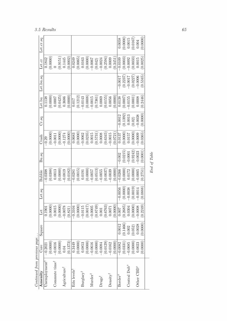
3.5 Results 65
Con
tin
ued
from
pre
viou
spa
ge..
.Amenity
Cor
eS
qu
are
Let
Let
sqB
ub
ble
Bu
sqC
rash
Cr
sqL
etb
uL
etb
usq
Let
crL
etcr
sqU
nem
plo
ym
ent†
−0.
2021
0.19
01−
0.0398
−0.
29
0.1138
0.1842
(0.0
000)
(0.0
000)
(0.0
388)
(0.0
000)
(0.0
000)
(0.0
000)
Com
mu
teti
me†
−0.
0016
0.00
150.
0013
−0.
0011
0.0007
0(0.0
000)
(0.0
000)
(0.0
000)
(0.0
000)
(0.0
425)
(0.9
151)
Agr
icu
ltu
re†
0.04
−0.
0078
−0.
0819
−0.
1274
0.3686
0.1445
(0.1
373)
(0.8
21)
(0.0
182)
(0.0
000)
(0.0
000)
(0.0
002)
Ed
ule
vels†
0.34
49−
0.31
04−
0.0281
0.0683
0.017
0.0249
(0.0
000)
(0.0
000)
(0.0
015)
(0.0
000)
(0.1
212)
(0.0
065)
Bu
rgla
ry†
0.08
53−
0.01
150.
0191
−0.
0062
−0.
0143
0.0163
(0.0
000)
(0.0
017)
(0.0
000)
(0.0
235)
(0.0
008)
(0.0
000)
Mu
rder†
−0.
0616
−0.
0005
−0.
0057
0.0015
−0.
0015
−0.
0067
(0.0
000)
(0.8
749)
(0.0
513)
(0.5
731)
(0.7
361)
(0.0
42)
Dru
gs†
−0.
0084
0.00
1−
0.0055
0.0008
0.0069
−0.
0024
(0.0
129)
(0.6
763)
(0.0
037)
(0.6
345)
(0.0
155)
(0.2
594)
Den
sity†
−0.
0162
0.00
71−
0.0039
−0.
0015
0.0056
0.0009
(0.0
000)
(0.0
000)
(0.0
000)
(0.0
721)
(0.0
000)
(0.3
451)
Bor
der�
−0.
0082
0.00
120.
007
−0.
0056−
0.0266−
0.002
0.0137−
0.0012
0.0138
−0.
0017−
0.0109
0.0058
(0.0
331)
(0.1
466)
(0.2
685)
(0.0
000)
(0.0
000)
(0.0
215)
(0.0
000)
(0.1
392)
(0.0
007)
(0.2
237)
(0.0
003)
(0.0
000)
Cen
tral
Du
b�
−0.
0685
0.00
20.
0304
−0.
0038
0.0172−
0.0001
0.0157
0.0013−
0.0155
−0.
0017−
0.0092
0.0015
(0.0
000)
(0.0
52)
(0.0
000)
(0.0
019)
(0.0
000)
(0.9
242)
(0.0
000)
(0.0
2)
(0.0
001)
(0.0
227)
(0.0
033)
(0.0
167)
Oth
erC
BD�
0.00
230.
0028
−0.
0008
−0.
0014−
0.0005−
0.0023−
0.0009−
0.0038
0.0008
−0.
0006
0.0015
0.004
(0.0
000)
(0.0
000)
(0.2
249)
(0.0
888)
(0.2
751)
(0.0
001)
(0.0
365)
(0.0
000)
(0.2
446)
(0.5
345)
(0.0
025)
(0.0
000)
En
dof
Tabl
e
66 Cyclicality of Amenity Prices
The pattern of p-values indicates that for amenities there is a statistically
significant relationship with the cost of accommodation. Of 25 amenities, the
core effect was statistically significant at the 5% for 23, the exceptions being
proximity to a primary road and the percentage involved in agriculture in an
area. The majority of base effects for the lettings segment are also statistically
significant (18 of 25 at the 5% level), indicating that different price gradients
with respect to distance applied during the period across sales and lettings
segments. Similarly, for the bulk of amenities, the bubble and crash base
effects are statistically significant (17 of 25 at the 5% level for both).
Model Fit The presence of two distinct segments in pooled regressions pre-
vents the reporting of any meaningful statistics for the full sample. However,
running regressions separately on sales and lettings samples can give an indi-
cation of model fit. For the sales segment, the R2 is 80%, compared to 77% for
a model without amenity variables. This implies that much of the explanatory
power of amenities is at the expense of area-specific fixed effects, although area
coefficients in models with and without amenities are highly correlated. Also
of note is the signficant improvement in root mean square error when amenities
are included; RMSE falls from 0.2583 to 0.2413. The fit of lettings models is
similar (R2 of 79.5% with and 78.7% without amenities; RMSE of 0.1803 and
0.1834 respectively).
Due to the necessarily detailed treatment of distance, the actual effect in a
given phase or segment may be different to the simple sign on the coefficient.
For that reason, results are presented in Table 3.4 for the following thought ex-
periment: the estimated effect on the price (or rent) of moving a property from
1km to 100m from a particular amenity or facility. The results are displayed
graphically in Appendix .2.2, in Figures 5-8.
For those amenities and facilities marked with a diamond (�), the results
shows moving a property from 5km to 1km away. Those marked with a dagger
(†) are not distance-based amenities and the percentage figures shown represent

3.5 Results 67
a one-standard-devation change in the variable; for more details see Table 4
in Appendix .2. Where the effect is not statistically significant at the 5%
level, the percentage is shown in italics, signifying for price effects that it is
not statistically significantly different from zero and for other effects that one
cannot reject the null hypothesis that the particular effect is no different from
the base price effect.
The second and third columns show the expected sign and the outcome.
The vast majority are in agreement. The positive association between property
prices and burglaries appears to be in line with research suggesting that the
causality runs in the opposite direction, i.e. burglaries are more likely to occur
in valuable areas (Gibbons & Machin 2008). Similarly, the negative relationship
between proximity to rivers and property prices may reflect the dominance of
flood risk concerns over natural amenity value (Harrison et al. 2001). Costs of
congestion may explain the result in relation to primary schools, particularly
given that the vast majority of properties in the sample are within 1.6km of a
primary school.
More difficult to explain are negative effects associated with green space
(particularly given the results in Mayor et al. 2009), higher education institutes
and distance from the border. These results are largely robust to specification
and are worthy of more detailed future research.
3.5.2 Comparing Price & Rent Effects
The fourth and fifth columns compare the price and rent effects. Evidence in
favour of the first core hypothesis, i.e. where the price effect (P ) is greater
than the rent effect (R) is summarized in the second last column. For all 25
amenities, there is evidence from 18 of an attenuated rent effect, compared
to the price effect. In other words, there is overwhelming evidence that a
mechanism is at work in the Irish housing market similar in effect to either the
search thresholds or buyer lock-in effects described above. It is notable that
the principal exceptions relate to distance from the centre (either Dublin or
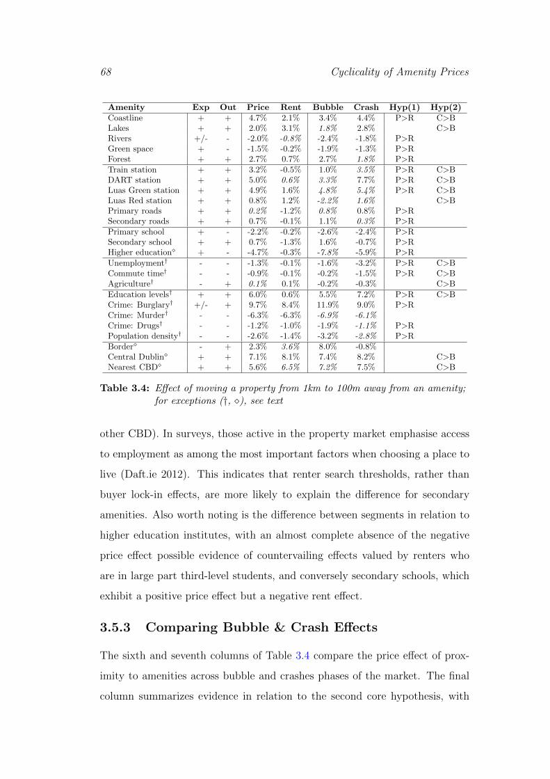
68 Cyclicality of Amenity Prices
Amenity Exp Out Price Rent Bubble Crash Hyp(1) Hyp(2)Coastline + + 4.7% 2.1% 3.4% 4.4% P>R C>BLakes + + 2.0% 3.1% 1.8% 2.8% C>BRivers +/- - -2.0% -0.8% -2.4% -1.8% P>RGreen space + - -1.5% -0.2% -1.9% -1.3% P>RForest + + 2.7% 0.7% 2.7% 1.8% P>RTrain station + + 3.2% -0.5% 1.0% 3.5% P>R C>BDART station + + 5.0% 0.6% 3.3% 7.7% P>R C>BLuas Green station + + 4.9% 1.6% 4.8% 5.4% P>R C>BLuas Red station + + 0.8% 1.2% -2.2% 1.6% C>BPrimary roads + + 0.2% -1.2% 0.8% 0.8% P>RSecondary roads + + 0.7% -0.1% 1.1% 0.3% P>RPrimary school + - -2.2% -0.2% -2.6% -2.4% P>RSecondary school + + 0.7% -1.3% 1.6% -0.7% P>RHigher education� + - -4.7% -0.3% -7.8% -5.9% P>RUnemployment† - - -1.3% -0.1% -1.6% -3.2% P>R C>BCommute time† - - -0.9% -0.1% -0.2% -1.5% P>R C>BAgriculture† - + 0.1% 0.1% -0.2% -0.3% C>BEducation levels† + + 6.0% 0.6% 5.5% 7.2% P>R C>BCrime: Burglary† +/- + 9.7% 8.4% 11.9% 9.0% P>RCrime: Murder† - - -6.3% -6.3% -6.9% -6.1%Crime: Drugs† - - -1.2% -1.0% -1.9% -1.1% P>RPopulation density† - - -2.6% -1.4% -3.2% -2.8% P>RBorder� - + 2.3% 3.6% 8.0% -0.8%Central Dublin� + + 7.1% 8.1% 7.4% 8.2% C>BNearest CBD� + + 5.6% 6.5% 7.2% 7.5% C>B
Table 3.4: Effect of moving a property from 1km to 100m away from an amenity;for exceptions (†, �), see text
other CBD). In surveys, those active in the property market emphasise access
to employment as among the most important factors when choosing a place to
live (Daft.ie 2012). This indicates that renter search thresholds, rather than
buyer lock-in effects, are more likely to explain the difference for secondary
amenities. Also worth noting is the difference between segments in relation to
higher education institutes, with an almost complete absence of the negative
price effect possible evidence of countervailing effects valued by renters who
are in large part third-level students, and conversely secondary schools, which
exhibit a positive price effect but a negative rent effect.
3.5.3 Comparing Bubble & Crash Effects
The sixth and seventh columns of Table 3.4 compare the price effect of prox-
imity to amenities across bubble and crashes phases of the market. The final
column summarizes evidence in relation to the second core hypothesis, with

3.6 Conclusion 69
C>B noted for instances where the price effect in the crash period is greater
than in the bubble period. For 12 amenities, this is the case, in particular
relating to transport amenities (all four categories of train station) and dis-
tance from the CBD. The premium associated with moving from 1km to 100m
away from the coastline increased from 3.4% to 4.4% in the crash, while the
equivalent effect for a suburban DART train station increased from 3.3% to
7.7%.
Particularly noteworthy is the finding that a 30-minute longer commute,
ceteris paribus, was associated with a 1% lower house price during the bubble
but an 8.4% lower price during the crash. This suggests that during the bubble,
households were prepared to pay the opportunity and resource costs of longer
commutes, possibly as these were offset by capital gains. However, in the crash,
the lack of any such capital gains appears to have strengthened the forces of
agglomeration in Ireland.
There are a number of amenities where the percentage price effect during
the bubble is greater than in the crash, something that would suggest a pro-
cyclical “buyer lock-in” effect (similar to the Stein hypothesis), rather than a
counter-cyclical “property ladder” effect (similar to the Costello hypothesis).
This is clearest for the crime-related amenities, where although not dramatic
there was a fall in the discount associated with higher murder and drugs-related
crime in the crash.
3.6 Conclusion
Due to the importance of housing as a good and an asset, understanding hous-
ing markets cycles and tenure choice will aid policymaker efforts not in relation
to housing policy but also in understanding economic fluctuations. This chapter
has explored the relationship between the economics of location-specific ameni-
ties and both tenure and housing market cycles. Following in the footsteps of a
long literature, it traced the impact of amenities on property prices but also on

70 Cyclicality of Amenity Prices
rents, a less common feature of the literature. Of twenty-five location-specific
characteristics, almost all were reflected in the housing market with a sign in
line with expectations or the existing literature. For example, moving a prop-
erty from 1km from the coast to 100m away was associated with a 4.7% increase
in price.
This chapter exploited the dataset’s large size, its coverage of both sales
and lettings segments and huge variations in market conditions over the period
covered to test whether the valuation of amenities is greater in the sales segment
than in the lettings segment, reflecting either tenants’ search costs or buyers’
desire to lock in supply of an amenity. This was typically found to be the case
– there is evidence of an attenuated rental effect for 18 of the 25 amenities. For
example, the rental premium for a coastline property was 2.1%, less than half
the 4.7% price premium.
To distinguish between tenant search costs and buyer lock-in concerns, Ire-
land’s violent property market cycle was exploited. A sign of “lock-in” effects
would be if relative amenity prices were procyclical, rising in the bubble and
falling in the crash: during the frenzy of a bubble, people pay over the odds
to secure access to amenities which are by their very nature fixed in supply.
However, if the relative price of amenities increased in the crash, this would
suggest that “property ladder” concerns dominated: normally people prefer
to reward access to amenities, but in the bubble, the principal concern is not
having any property at all, pushing up the relative price of low-amenity prop-
erties. Alternatively, the relaxation of credit constraints boosted demand for
lower-amenity housing, an effect that evaporated in the crash.
There was evidence of counter-cyclical amenity pricing, i.e. the relative
price rising in the crash, for the majority of amenities for which sensible and
statistically significant results emerged, including prominent housing market
amenities such as commute time, distance to CBD and proximity to train
stations and the coastline. For example, the premium enjoyed by a property
100m from the coast compared to one 1km away increased from 3.4% to 4.4%
3.6 Conclusion 71
between bubble and crash. Similarly, moving a property from 5km from the
CBD to 1km away was associated with an increase in price of 7.4% in the
bubble and 8.2% in the crash.
It is left to future work to examine income elasticities, using county-level
information on incomes, and to exploit supply-side innovations, such as the
opening of new motorways, by-passes and train stations, and the opening and
closure of schools and hospitals. The publication in late 2012 of the Prop-
erty Price Register opens the possibility of developng a micro-level datasets
of transaction prices, which would enable a comparison of list price and sale
price effects that could reveal important differences between the expectations
of market participants and final outcomes. The relationship between list prices
and sale prices is analysed in Chapter 4.

72 Cyclicality of Amenity Prices

Chapter 4
Relationship between list andsale prices
Trends in residential house prices matter. They are of interest not only to
economists, but also to policymakers and consumers, given the dominant role
of housing both as a consumption good and as a vehicle for household invest-
ment. The Global Financial Crisis (GFC) starting in 2007 underscores the im-
portance of understanding housing markets, in particular if macro-prudential
policy hopes to identify when conditions in the housing market change and
bubbles emerge.
Unlike other financial markets, the matching process in housing is one that
can take months or indeed fail entirely, particularly during market downturns.
The lack of fungibility and liquidity in housing means that statistics relating
to the market are patchy and rarely comparable across countries (Malpezzi
2003, Warnock & Warnock 2012).1 This makes it all the more difficult for
economists, policymakers and consumers to identify when the housing market
may be overheating.
Despite its potential significance, the relationship between list and sale
prices for housing has been the focus of only a handful of studies to date.
In the very first issue of the Journal of Real Estate Research, Miller & Sklarz
1In the EU, even the introduction of residential house prices – typically the largest singlecomponent in a national basket of consumer goods – into the harmonised index of consumerprices (HICP) is a twenty-year project due to come to fruition in 2018 (O’Hanlon 2011).
73

74 Relationship between list and sale prices
(1986) highlight the gap between the two as one of five leading indicators in
the housing market. However, their analysis – and their call for future research
– has largely gone unheeded. A related literature has emerged in commercial
real estate, assessing the accuracy of valuations, but the findings are typically
not based on like-for-like comparisons, with valuations made at a different time
to transactions.
This research uses two population-level datasets of the Irish housing market,
over the period 2006-2012, to investigate in detail the relationship between
aggregate list and sale prices and establish like-for-like comparisons of buyer
and seller valuations. It takes as its starting point two pieces of conventional
wisdom about the housing market. Firstly, it is expected that in a downturn
sale prices will be below list prices, while secondly, it is often asserted that list
prices are a lead indicator of sale prices. At first glance, these would appear to
conflict in a market downturn: if list prices lead sale prices in switching from
boom to bust market, how are they above sale prices in the bust?
The analysis here shows that both were true for Ireland during the period
2006-2012. This somewhat contradictory finding is explained by disentangling
the relationship between the two series into four main components. The first
of the four is the selection spread, where properties that ultimately go on to
find a seller are listed at lower prices. The matching spread, secondly, reflects
how much house prices change between when a property is listed and it is sale
agreed. The third component is the counteroffer spread, reflecting whether the
sale price achieved is higher or lower than the list price, focusing only on those
listings that result in a sale and adjusting for time-to-sell. This is the closest
to a bid-ask spread in housing. The final component is the drawdown spread,
reflecting how prices change between when a property is sale agreed and when
the mortgage is actually drawn down; this largely reflects administrative time
costs.
The chapter is structured as follows. The next section presents a more
formal discussion of these spreads, while Section 4.2 discusses some of the
4.1 Theory 75
related literature on this topic. Section 4.3 describes the two datasets used
here, Central Bank of Ireland (CBI) and daft.ie, and Section 4.4 describes
the empirical specifications employed. Section 4.5 presents the results of the
analysis, showing estimates for each of the four spreads for the Irish housing
market 2006-2012, while the final section concludes.
4.1 Theory
Housing is in effect a very high-dimension composite good, comprising a bundle
of property-specific attributes and location-specific amenities. Not only can
each property vary in each composite good, but so too can consumer tastes.
The fact that only bundles of these composite goods are available leads to
frictions, which mean that it may take a property a significant period of time
to sell. This is contrast to most other financial markets and indeed consumer
markets.
Suppose there are two datasets: the first contains all properties listed for
sale and their list price (pL), while the second contains all properties sold and
their (mortgage-backed) transaction price (pM). A stylised transaction from
the housing market might be as follows. In month 1, a property is listed by its
seller. At this point, a list price is revealed. A list price index would use such
information, and in that index, this property enters into the list price index in
month 1. In month 4, the property has found a buyer whose offer is accepted.
The status of the property is changed to “sale agreed”. At this time, the bank
makes its valuation, upon which the mortgage amount is based. In month 6,
the transaction is completed, when the mortgage is drawn down. This property
thus enters into any sales price index in month 6.
The issue in assessing valuation accuracy is immediately apparent, as this
typically involves comparing the valuation from month 1 with the transaction in
month 6. What is needed instead is a comparison of what the seller’s valuation
would have been in month 4 with the buyer’s valuation at the same time. Where

76 Relationship between list and sale prices
the goal is to make like-for-like comparisons of seller and buyer valuations,
neither a published list price index, in which the property described above will
enter in month 1, nor a sales price index, in which it enters in month 6, is using
the correct information at the correct time.
More formally, the ratio of list prices (pL) to (mortgage-backed) sale prices
(pM) can be decomposed into four distinct market processes:
pL(0)/pM(τ) = pL(0)/pL(0) · pL(0)/pL(υ) · pL(υ)/pM(υ) · pM(υ)/pM(τ) (4.1)
where there are three time periods, time of listing (t = 0), the time when a sale
and price are agreed (t = υ), and the time when the mortgage is drawn down
(t = τ), and where L refers to only those listings that result in a transaction
(and hence a mortgage being drawn down).2 Conceptually, the price spread
can be described as follows:
1. the “selection spread”, pL(0)/pL(0): what is the point-in-time list-price
difference between all properties that are listed and those that subse-
quently are sale-agreed?
2. the “matching spread”, pL(0)/pL(υ): what is the point-in-time list-price
difference between newly listed properties that go on to be sale-agreed
and those being sale-agreed now?
3. the “counteroffer spread”, pL(υ)/pM(υ): what is the point-in-time differ-
ence between the list price of properties that are sale-agreed and the sale
price of properties at the time of their valuation?
4. the “drawdown spread”, pM(υ)/pM(τ): what is the point-in-time sale-
price difference between properties that are being valued and those whose
mortgage is being drawn down?
2Note that this assumes that all housing transactions are mortgage-backed, which is asimplification.

4.2 Literature 77
The counteroffer spread is the closest equivalent to a bid-ask spread in the
housing market, due to the frictions involved. It is also the only comparison of
the four that uses both datasets.
4.2 Literature
A number of papers examine the accuracy of valuations in the commercial
real estate sector; see Crosby (2000) and Dunse et al. (2010) and references
therein. However, the literature comparing list and sale prices in residential
housing is small. To our knowledge, there is no paper for either sector that
decomposes the gap between list and sale prices into various components, as
is done here. Nonetheless, a number of papers touch on issues related to the
spreads outlined in the introduction (and explained in more detail in Section
4.1); these are described below.
Adjusting valuations to take account of time-to-sell is an issue that has
been highlighted by a number of authors on commercial real estate. Matysiak &
Wang (1995) suggests some tentative findings in relation to how valuations and
sale prices are related across the market cycle, namely that valuers undervalue
in rising markets and overvalue in falling markets. Complicating this analysis,
however, is the fact that valuations took place between three and six months
prior to the sale. As Crosby (2000) notes, this affects the comparability of
valuations and sale prices.
The selection spread presented here is related to a point raised by Jud &
Seaks (1994) among others, namely that a house price index based on sales
will not be representative of housing values more generally, where a sample
selection bias exists in properties that are sold. Using a Heckman-style two-
stage model, they document such a selection bias, using a decade of sales and
property tax returns for Greensboro, North Carolina. The comparison in Jud
& Seaks (1994) is between all properties and those that successfully sell, while

78 Relationship between list and sale prices
in this research, the selection spread refers instead to all listings versus those
that successfully sell.
The earliest paper that structurally compares both list and sale prices of res-
idential property is Genesove & Mayer (2001), which examines the gap between
the two for a sample of just under 6,000 downtown Boston condominiums, dur-
ing the period 1990-1997. Their focus is not directly on the gap between the
two; rather they examine whether loss aversion affects seller behavior (includ-
ing list price) in the housing market. Their findings suggest that sellers are
indeed averse to realizing nominal losses: a 10% increase in a prospective loss
leads a seller to set a list price roughly 3% higher, everything else being equal.
Related to this, they find evidence that “list prices do not immediately adjust
to changes in market prices”.
In comparing the Swiss National Bank’s median-based house price index
using listings (both newspaper and online) with a hedonic index based on sale
prices over the period 1985-2006, Bourassa et al. (2008) outline some concerns
relating to the use of datasets of list prices. One of these is that the spread
between list and sale prices is likely to vary depending on the state of the
housing market. This is the issue addressed in this research.
Shimizu et al. (2012) compare the distribution of properties across differ-
ent datasets for Japan and conclude that – once like-for-like comparisons are
being made across the datasets – there are no substantial differences in the
distribution of list prices and those on price registers. Like-for-like compar-
isons are central to this result, suggesting it is related to a stylised fact of the
literature on constructing house price indices: hedonic techniques are needed
(Knight et al. 1995, Wallace & Meese 1997).3 The finding from Japan also
tallies with published house price indices for Ireland. Two hedonic indices, the
mortgage-based CSO index and the listings-based daft.ie index, showed house
prices falling at 12-14% year-on-year in early 2011; in contrast, a simple un-
3For a fuller treatment of hedonic pricing methods, see Malpezzi (2003).

4.3 Data 79
weighted average (produced by the Dept of the Environment) showed prices
9% higher.
More recently, a paper by Haurin et al. (2013) examines the relationship
between list and sale prices over the market cycle in Belfast (Northern Ireland),
2002-2009. They find, contrary to standard assumptions made regarding the
selling process, that when the housing market is strong, properties sell for more
than their list price. (In down or normal markets the list price generally exceeds
the sales price.) This is also a feature of the data presented here. The authors
conclude that the selling mechanism must switch during boom markets, with
the list price acting as a floor, rather than a ceiling. Of relevance for this study
is their finding that the list to sale price ratio is “unusually high” during the
downturn in Northern Ireland, a finding they attribute to seller loss aversion.
4.3 Data
Two datasets are used in this chapter, one containing list prices and the other
mortgage-backed sale prices. For details on the nature of property market
transactions in Ireland, see earlier chapters. Worth noting here is that a seller
may state that they require offers “in excess of” or “in the region of” the list
price, but typically the list price is for information only and set after agreement
between the seller and their estate agent. The presence of “in excess of” list
prices runs somewhat counter to the assumption made in much of the (typically
North American) literature, that the list price represents a ceiling on offers.
Since late 2012, prices for individual transactions have been freely available to
the public through a Property Price Register.
4.3.1 daft.ie dataset
List price information used for analysis here was collated by online accommo-
dation portal, Daft.ie. The dataset comprises all properties advertised online

80 Relationship between list and sale prices
between 1 January 2006 and 31 December 2012. The dataset contains the
following information:
• Price: For each property, the list price is known.4
• Location: Location is known, both generally (all listings are assigned
to one of 4,000 areas in the country) and specifically (all listings are
assigned latitude and longitude coordinates, and a degree of precision for
those coordinates). For comparability with the CBI dataset, the principal
information on location used refers to broad region (of which there are
four: Dublin, Leinster, Munster and Connacht-Ulster) and county (or
postcode within Dublin).
• Type & Size: There is information on the property’s type (apartment,
terraced, semi-detached or detached dwelling). Information is also known
about the property’s size, measured in terms of bedrooms, and bathrooms
relative to bedrooms, while for a subset of properties size in square metres
is available.
• Date: Information is available for properties within the daft.ie dataset
on when they were originally listed, when marked as “sale agreed” (if
relevant) and when withdrawn from the market. The time between listing
and sale-agreed status is central to estimation of the counteroffer spread
in housing outlined in Section 4.1.
Summary statistics on the key variables, for both the full set of listings [daft.ie
1] and the set of listings that subsequently went to be sale-agreed [daft.ie 2]
are given in Table 4.1.5
4Other chapters in this doctorate use a dataset that includes listings where price is changedas separate observations, due to the focus on relative values, with time/market conditionsbeing controlled for. Here the focus is on the set of properties, not the set of seller expecta-tions, and the sale process in its entirety, from first listing to ultimate sale. Therefore, theseobservations are omitted from the analysis. Future research will examine the role of nominalrigidities within a listing.
5It is worth clarifying why the full sample of properties for sale provided by daft.ie isdifferent in Chapters 2, 3 and 4. The sales dataset in Chapter 2 comprised 408,334 listings
4.3 Data 81
4.3.2 CBI dataset
Sale price information comes from the Central Bank of Ireland (CBI) dataset,
itself a product of the Prudential Capital Assessment Review (PCAR) process,
also known as the “stress tests” of the Irish banking system that followed
its collapse in 2009-10. Under PCAR, Irish banks covered by a government
guarantee were recapitalized by CBI in return for equity. Such action required
loan-level analysis, including of the mortgage portfolio, which involved detailed
information for over 600,000 loans on 475,000 properties being made available
to CBI.
The analysis here is of loans associated with a housing market transaction
(i.e. first-time buyer, mover-purchaser or “buy-to-let” investment) and where
certain information criteria are met. The dataset includes all observations from
2006Q1 (when the daft.ie dataset starts) until 2011Q4 (the date of the PCAR
process) and contains the following information:
• Price: Price information is available in the form of the bank’s valuation
as part of the mortgage drawdown process, which becomes the official
transaction price.
• Location: Information on location is known only to county level, of
which there are 26 in the Republic of Ireland. However, for two of the
four financial institutions covered by PCAR, information is available for
Dublin postal districts, of which there are 22 in the most built-up parts
of the capital (this dataset is referred to as CBI-2).
• Type & Size: Property type relates to whether the property is a semi-
detached, detached or terraced house, a bungalow or an apartment. No
further information on a property’s size is available for all properties.
from 2006 to mid-2012, and excluded all those whose location was not known to sufficientaccuracy (street or building level). The analysis in Chapter 3 included additional listingsfrom late 2012, leaving a total sales sample of 416,829. Lastly, the sample here – 420,691 –includes all properties known only to estate or area level (as location in the CBI dataset isimprecisely measured) but excludes all relistings at a different price.

82 Relationship between list and sale prices
Dataset daft.ie 1 daft.ie 2 CBITotal 420,691 76,647 216,685Av price e281,478 e269,628 e323,796Dublin 84,018 23,886 57,074Leinster 121,052 21,212 59,498Munster 126,186 19,980 61,542Conn-Ulster 89,435 11,389 37,571Terraced 63,916 15,603 36,417Semi-detached 111,405 24,427 68,424Detached 199,671 29,038 85,656Apartments 45,699 7,399 25,1882006 76,435 3,381 63,0162007 113,763 17,675 58,7632008 73,320 12,648 42,4602009 46,105 8,940 24,7042010 40,571 10,150 17,6032011 37,433 9,830 9,1392012 33,064 13,843 0
Table 4.1: Summary statistics of the daft.ie and CBI datasets
• Date: For all observations, the dataset contains information on when the
mortgage was drawn down. For most observations, there is also informa-
tion on when the property was valued, information that can be used to
estimate the counteroffer spread.6
Some summary statistics of the CBI PCAR dataset across all three main di-
mensions (location, type and date) are given in Table 4.1. For more on the CBI
PCAR dataset, the interested reader is directed to Kennedy & McIndoe-Calder
(2011).
Omitted variables An obvious omitted variable from the CBI dataset is a
detailed measure of size. Standard in the housing economics literature is size
in square metres, with number of rooms (or number of bedrooms, available in
the case of the daft.ie dataset) also widely used. The lack of information on
property size in the CBI dataset raises the question of omitted variables. Using
6Only mortgage loans with complete information were included. Roughly 36,000 loansreferred to properties where the valuation date was not known and these were thus excluded.
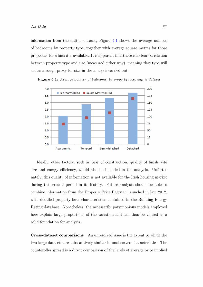
4.3 Data 83
information from the daft.ie dataset, Figure 4.1 shows the average number
of bedrooms by property type, together with average square metres for those
properties for which it is available. It is apparent that there is a clear correlation
between property type and size (measured either way), meaning that type will
act as a rough proxy for size in the analysis carried out.
Figure 4.1: Average number of bedrooms, by property type, daft.ie dataset
Ideally, other factors, such as year of construction, quality of finish, site
size and energy efficiency, would also be included in the analysis. Unfortu-
nately, this quality of information is not available for the Irish housing market
during this crucial period in its history. Future analysis should be able to
combine information from the Property Price Register, launched in late 2012,
with detailed property-level characteristics contained in the Building Energy
Rating database. Nonetheless, the necessarily parsimonious models employed
here explain large proportions of the variation and can thus be viewed as a
solid foundation for analysis.
Cross-dataset comparisons An unresolved issue is the extent to which the
two large datasets are substantively similar in unobserved characteristics. The
counteroffer spread is a direct comparison of the levels of average price implied
84 Relationship between list and sale prices
by the two datasets and, in level if not in trend, is subject to any structural dif-
ferences across the two datasets. To some extent, with both datasets covering
the vast majority of housing market transactions for the period under analysis,
this is less likely to be an issue. Nonetheless, it is not possible rule out all
potential effects. For example, if within one county, an estate agent did not
advertise online but was facilitating mortgage-backed transactions, the proper-
ties sold by that agent would appear in the CBI dataset but not in the daft.ie
dataset. Alternatively, if the proportion of transactions that were backed by
a mortgage varied with the market cycle, this could introduce some selection
effect in the CBI dataset. Ultimately, as these are population-level datasets (all
online listings and all mortgage-backed transactions), it is left to the reader to
judge the potential relevance of any structural differences across datasets. As
noted earlier, this affects only the size of the counteroffer spread, not its trend,
nor any of the other spreads calculated.
4.4 Model
The empirical strategy adopted is, per the recommendation of the literature,
the hedonic regression, i.e. controlling for the characteristics of the proper-
ties traded, to ensure a like-for-like comparison over time. As with O’Hanlon
(2011), outliers are excluded from final figures by adopting a two-stage process,
and filtering out excessively influential observations by using Cook’s Distance
(Cook 2000). Similar to the vast bulk of the housing literature, a log-linear
model is applied, allowing coefficients to be interpreted, to an approximation,
as percentage differentials.
Time The principal options in relation to the treatment of time are monthly
or quarterly dummy variables. Due to the long period under investigation,
it is not obvious what benefit monthly variables would bring, thus quarterly
variables are chosen instead. (An alternative – quite separate from the house

4.4 Model 85
price index literature – would be to impose a polynomial on the time-span,
although it is not obvious a priori what order polynomial would apply. Thus
this would become a fitting exercise and effectively tend in the limit to a model
with monthly or quarterly dummies.)
Location While specific location is known for the daft.ie dataset, there is
limited information on location in the CBI dataset. Thus, county-specific fixed
effects are used in all specifications. The treatment of location here is very
similar to the official CSO Residential Property Price Index (O’Hanlon 2011).7
Type and size As discussed above, very limited information is available on
the property’s size in the CBI dataset. That information is limited to property
type, which is correlated with size. Type-specific fixed effects are included,
relative to semi-detached properties as a control. As discussed in Chapter
2, premiums or discounts associated with particular property types may vary
by region. Therefore, type interactions with four broad regions are included.
Those four regions are: Dublin, the rest of the Leinster province, the Munster
province, and Connacht-Ulster.
In equation form, the empirical model is given below, where each vector of
Q, X and Y omits one category as control (first quarter of 2007, County Louth
and semi-detached properties, respectively), and where s refers to the quarter
within the year, t to the year8, c to county c of C = 25, r to regions 1-5 and n
to the property type (N = 4).
ln(hp)i = α0 +2012∑
t=2006
4∑s=1
αtsQtsi +
C∑c=1
βcXci +
N∑n=1
R∑r=1
βnrYnri + εi (4.2)
7For a subset of the CBI dataset (two of the four lenders), as well as for the entire daft.iedataset, information is available on postal district for Dublin city properties. Robustnesschecks were carried out using this subsample, i.e. excluding lenders with no informationon postal district. The results were substantively similar, with the bulk of the differencestemming from variations between the lenders included and excluded, rather than the impactof additional location controls.
8As discussed above, there are no data for 2012 in the CBI dataset, thus the summationfor that dataset runs to 2011.

86 Relationship between list and sale prices
This model is applied to five datasets, in order to calculate the four spreads
outlined above:
1. The first dataset is the population of listings, where the date refers to the
initial date of listing. This uses the daft.ie dataset in full.
2. The second dataset is the set of listings that subsequently go on to be
“sale agreed”, where the date used refers to the date of listing. This uses
a proportion of the daft.ie dataset.
3. The third dataset is also the set of listings that are “sale agreed” before
being withdrawn, but where the date used refers to the date the property
was marked sale agreed. This uses the same subset of the daft.ie dataset.
4. The fourth dataset is the population of mortgage-backed transactions,
where the date refers to the date at which the property is valued. This
uses the CBI dataset in full.
5. The final dataset is the population of mortgage-backed transactions, where
this time the date refers to the date of the transaction. This also uses
the CBI dataset in full.
4.4.1 Calculation of averages
As individual properties cannot be matched across datasets, due to the lack of
specific information on location in the CBI dataset of transactions, the analysis
here uses comparable weighted average hedonic prices. The empirical model
given above is used to generate regression output in the form of coefficients,
while the CBI dataset of transactions is used to give weights for each of the
four property types for each of the counties, as well as for each county within
the country.
With four property types and one control, there are three type coefficients
for each county. Each county-level type coefficient, which takes into account any
region-specific type effects, is then multiplied by the weights within that county

4.4 Model 87
for each property type. These three numbers are then added to the generic
county coefficient to give a county-specific type-weighted coefficient. Whereas
coefficients from regression output give like-for-like differences in prices between
areas, these adjusted coefficients reflect the mix of property types and sizes in
an area. Thus, counties where apartments and terraced properties are more
common will have this reflected in the adjusted coefficients.
These county-specific adjusted coefficients can be used, along with the
constant, to calculate a county-specific average price for the control period
(2007Q1). The weighted sum of all these county-specific average prices gives a
national average price for 2007Q1. Quarter-specific coefficients are then used to
generate a series for the period 2006Q1-2012Q4 (2011Q4 for the CBI dataset).
The output for each dataset is thus a national average price that reflects the
mix of properties within and across counties.
Figure 4.2: Year-on-year change in sale and list prices, 2007-2012
Initial overview The introduction made reference to two pieces of conven-
tional wisdom about the housing market. The first is that it is expected that
in a downturn, sale prices will be below list prices. Indeed, until recently, it

88 Relationship between list and sale prices
was typically assumed that the list price was an upper bound, but recent re-
search shows that this is not the case (Haurin et al. 2013). Secondly, it is often
asserted that list prices are a lead indicator of sale prices. These two appear
to be in conflict when the market turns from a rising market to a falling one.
Datasets (1) and (5) above are what would be used to generate indices of
list prices and sale prices. Applying the method described above, it is possible
to compare trends in both. Figure 4.2 shows the year-on-year change in list and
sale prices. What is particularly noteworthy is that list prices appear to lead
sale prices throughout: the year-on-year change turns negative earlier, falls in
prices abate earlier in 2009 and accelerate earlier in 2010/11.
Thus, in the recent Irish housing market downturn, list prices were above
sale prices – but they also led sale prices from boom to bust and throughout
the bust. The next section reconciles these two findings, by decomposing the
gap between the two series into its constituent components.
4.5 Results
4.5.1 Selection spread
Figure 4.3 shows the estimated quarterly “selection spread” among listed prop-
erties. The gap shown is the percentage gap in list price between those properies
that go on to find a buyer (i.e. are marked as sale agreed) and the full comple-
ment of properties listed in a given month. As a buyer is not known at time of
listing, this is only able to be calculated ex-post by the researcher (not in real
time, by the analyst).
A positive number could indicate the importance of unobserved factors
(which in this analysis include any factors other than quarter, property type
or county). However, the selection spread is negative throughout, indicating
that those properties that subsequently find buyers are listed at systematically
cheaper prices than those that do not. The fact that the selection spread is

4.5 Results 89
Figure 4.3: The “selection spread”, daft.ie dataset, 2006-2012
cyclical (a larger negative number when prices are falling faster) indicates that,
in a downturn, properties priced more realistically are more likely to sell.
An alternative explanation is that, as quality differences are not included
as regressors, lower-quality properties (within property-county cohorts) were
more likely to sell as property conditions worsened. However, the evidence
from Chapter 2 suggests demand has shifted in the crash period to higher
attribute properties, not lower attribute ones, thus this is unlikely to be the
case and thus what is captured is indeed the extent to which properties that
sell are listed systematically cheaper, ceteris paribus, than those that do not.
4.5.2 Matching spread
The second component of the gap between list and sale prices is the match-
ing spread, reflecting time-to-sell: how have prices changed between when the
property was initially listed and when a buyer is found? This will reflect infor-
mation available to the buyer at the time the property is sale agreed but not
to the seller when the property was listed. Figure 4.4 shows median time to
sell (TTS) nationwide, from initial listing until the property is sale agreed, and
indicates a dramatic increase in TTS between late 2006, when it took typically

90 Relationship between list and sale prices
two months to find a buyer, and early 2009, when it took over six months on
average. After that, the duration largely remained between five and six months
for most of the period 2009-2012.
Figure 4.4: Median time-to-sell and time-to-drawdown (in weeks), daft.ie andCBI datasets, 2006-2012
As property prices were falling at more than 10% a year from 2008 until
2011, the fact that it took half a year on average – and significantly longer in
many cases – for properties to find a buyer means the time-to-sell spread will
be quantitatively significant in explaining the gap between list and sale prices.
This gap is shown in Figure 4.5. A positive number – as occurs throughout the
period from mid-2008 on – indicates that properties that turned sale-agreed in
a given quarter had a higher listed price than properties listed for the first time
in that quarter that would ultimately go on to find a buyer.
4.5.3 Counteroffer spread
The third stage in the decomposition of the gap between list and sale price is
the counteroffer spread, i.e. comparing suitably adjusted list and sale prices,
at the time the property was sale-agreed and valued by the mortgage issuer.
This is shown in Figure 4.6. It suggests that during 2007, allowing for prices

4.5 Results 91
Figure 4.5: The “matching spread”, daft.ie dataset, 2006-2012
to have changed between the time of listing and the time the sale was agreed,
the offer was typically 8% above the list price. This is supportive of the finding
from Haurin et al. (2013) that list prices do not act as a ceiling on offers in
booming markets.
Figure 4.6: The “counteroffer spread”, daft.ie and CBI datasets, 2006-2012
During the market downturn, in particular in 2009 and 2010, buyer offers
were typically 2-4% below the list prices of properties that would ultimately

92 Relationship between list and sale prices
find a buyer, even when those list prices were adjusted by how much prices had
fallen since their initial listing. However, by 2011, the counteroffer spread was
positive again: adjusted list prices were surpassed on average by sale prices.
At first, this may seem counterintuitive, particularly given that Ireland became
reliant on IMF-EU financing in late 2010. The answer appears to lie in the
collective decision of sellers to aggressively cut list prices in 2011: list prices
fell 18% that year, compared to 9% in 2010 (see Figure 4.2).
It is worth noting that unlike the other stages, which involve within-dataset
comparison, this stage involves comparing price levels across the two datasets.
As such, this may be sensitive to the samples underpinning both datasets and
any differences in categorization.
4.5.4 Drawdown spread
The final stage in the housing transaction is the drawdown spread, i.e. reflecting
changes in prices in the period between when a property is valued (typically
when the sale is agreed) and when the mortgage is actually processed (typically
when the new owner moves in). Figure 4.4 shows the median time between
valuation and mortgage drawdown. While there are fluctuations, the time-
to-drawdown is remarkably stable throughout what are very turbulent market
conditions. While time-to-sell reflects market conditions and the matching
process, time-to-drawdown appears to reflect administrative time-costs.
As a consequence of the relatively stable and short time-to-drawdown, its
effect on prices is typically small. When prices are rising early in the period,
properties having their mortgage drawn down were worth less than those just
being valued (typically by no more than 1%). As prices started to fall in 2008-
2009, the opposite was the case – properties having their mortgage drawn down
in mid-2009 were valued at roughly 1.5% more than those just being valued.
By late 2010, the drawdown spread had turned negative again, although this
was close to zero by the end of 2011. Overall, quantitatively, the effect of the
drawdown spread on prices is the smallest of all the spreads.
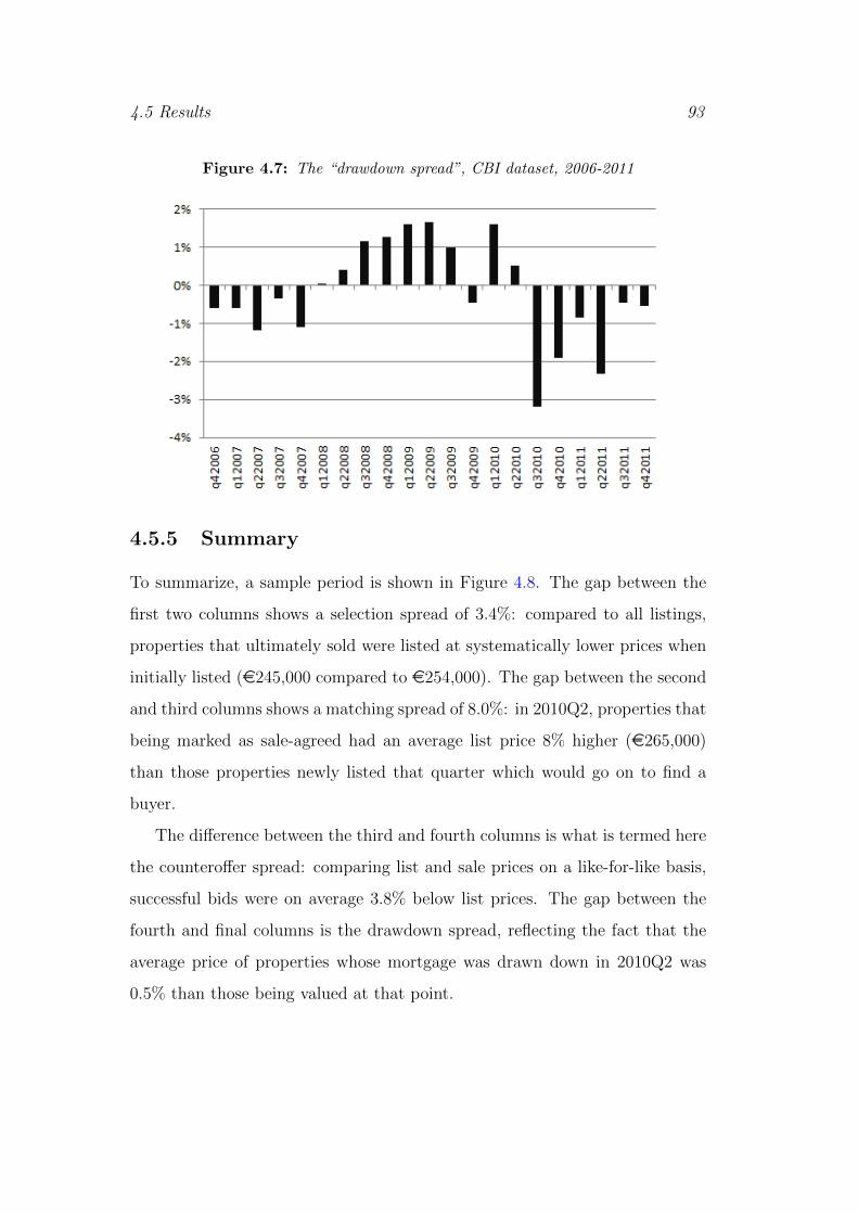
4.5 Results 93
Figure 4.7: The “drawdown spread”, CBI dataset, 2006-2011
4.5.5 Summary
To summarize, a sample period is shown in Figure 4.8. The gap between the
first two columns shows a selection spread of 3.4%: compared to all listings,
properties that ultimately sold were listed at systematically lower prices when
initially listed (e245,000 compared to e254,000). The gap between the second
and third columns shows a matching spread of 8.0%: in 2010Q2, properties that
being marked as sale-agreed had an average list price 8% higher (e265,000)
than those properties newly listed that quarter which would go on to find a
buyer.
The difference between the third and fourth columns is what is termed here
the counteroffer spread: comparing list and sale prices on a like-for-like basis,
successful bids were on average 3.8% below list prices. The gap between the
fourth and final columns is the drawdown spread, reflecting the fact that the
average price of properties whose mortgage was drawn down in 2010Q2 was
0.5% than those being valued at that point.
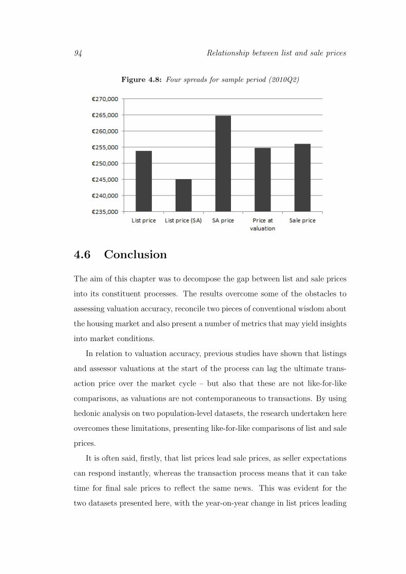
94 Relationship between list and sale prices
Figure 4.8: Four spreads for sample period (2010Q2)
4.6 Conclusion
The aim of this chapter was to decompose the gap between list and sale prices
into its constituent processes. The results overcome some of the obstacles to
assessing valuation accuracy, reconcile two pieces of conventional wisdom about
the housing market and also present a number of metrics that may yield insights
into market conditions.
In relation to valuation accuracy, previous studies have shown that listings
and assessor valuations at the start of the process can lag the ultimate trans-
action price over the market cycle – but also that these are not like-for-like
comparisons, as valuations are not contemporaneous to transactions. By using
hedonic analysis on two population-level datasets, the research undertaken here
overcomes these limitations, presenting like-for-like comparisons of list and sale
prices.
It is often said, firstly, that list prices lead sale prices, as seller expectations
can respond instantly, whereas the transaction process means that it can take
time for final sale prices to reflect the same news. This was evident for the
two datasets presented here, with the year-on-year change in list prices leading
4.6 Conclusion 95
that in sale prices throughout the period studied. This suggests that, with
appropriate controls for market conditions, list prices can function adequately
as a substitute in the absence of sale prices, even in an illiquid market.
It is also said that, in a falling market in particular, the average sale price
will be below the average list price, as weak demand means sellers have to accept
lower-than-expected outcomes. The research here reconciles those two state-
ments by decomposing the gap between list and sale prices into four spreads:
the selection spread, the matching spread, the counteroffer spread, and the
drawdown spread. An overview of trends in these over time, and their relative
importance, is given in Figure 4.9. The selection spread, capturing the extent
to which properties that sell systematically list for less, exists throughout the
period but is particularly pronounced during the market downturn: properties
that list for less, ceteris paribus, are more likely to find a buyer
While this finding accords with basic economic theory, it does not support
findings from some behavioural research that a higher list price can having
a priming effect, thereby bringing about better outcomes for the seller (Kah-
neman 2011). The finding here is based on aggregate data; a study using
individual listings and outcomes may shed light on whether this behavioural
effect exists and the extent to which it affects quantity outcomes (the prob-
ability of a transaction) and price outcomes (the sale price, conditional on a
transaction occurring).
The matching spread is a product of both the length of time it takes to
find a buyer and the change in prices during that period. Given the speed with
which prices fell in Ireland during much of the period covered, and the length of
the typical time-to-sell, this is quantitatively important in explaining the gap
between the two. For most of the period 2008-2011, the list price of properties
being sale agreed was 10% or more higher than newly listed properties. While
the exact role of nominal price rigidities is a topic for further research, this
highlights the limitations of comparisons using valuations and transactions from
different time periods. The drawdown spread, reflecting the time gap between

96 Relationship between list and sale prices
Figure 4.9: Overview of four spreads, 2006-2011
valuations for mortgages and their ultimate draw-down, was similar in nature
but much smaller in significance.
The counteroffer spread, finally, is the closest counterpart in the housing
market, which lacks liquidity and fungibility, to the bid-ask spread in other
financial markets. It reflects how list prices and sale prices compare, when
adjusted to time-to-sell and time-to-drawdown, as well as for the fact that some
listings will not result in a transaction. Early in the period, the counteroffer
spread was large and positive, suggesting that buyers had tough competition
in securing a property and thus they offered more than the list price. This idea
of the sale price in boom-times “breaking the price ceiling” offered by the list
price supports the findings of Haurin et al. (2013).
During the down market, the counteroffer spread was negative for much of
2009 and 2010. However, the entry of Ireland into the IMF-EU program in
late 2010 appears to have had an impact on seller expectations, as the fall in
list prices in 2011 was twice that of 2010. This greater realism on the part of
sellers might explain the return of a positive counteroffer spread in early 2011,
although as sale price falls increased in late 2011, the spread turned negative
again.

4.6 Conclusion 97
Regarding insights into market conditions, the selection effect is likely to
persist, even in a market in equilibrium, as sellers’ expectations will not be
uniform and those with excessive expectations need to experience market con-
ditions to change. The matching spread is a product of two other process: the
matching function itself (time-to-sell) and trends in house prices. Thus, it is
likely to be strongly countercyclical as measured here (a large positive number
in a falling market).
The counteroffer spread presented here appears broadly procyclical and may
offer useful insights into market conditions. While the research presented here
relies on aggregate prices from two population-level datasets, future research
for Ireland may be able to utilize the Property Price Register, which dates
from 2010, to construct a micro-level dataset in real-time of the matching and
counteroffer spreads. Similarly, detailed datasets in other countries may allow
the calculation of equivalent series to inform policymakers.
Such segment-by-segment analysis should aid policymakers greatly in under-
standing not only conditions in the housing market generally, which are crucial
in determining broader economic conditions, but also conditions in different
sub-markets. Future research could explore in more detail what determines
time-to-sell and also price rigidities, i.e. looking within the first and second
spreads above. Insights from this will be of use not just for macro-prudential
policy but also in understanding housing demand and thus shaping policy in
relation to development and planning/building permits. Chapter 5 explores the
relationship between house prices and other economic factors in more detail.

98 Relationship between list and sale prices

Chapter 5
Modelling the Irish housingmarket
As noted in Chapter 3, the case of Ireland exemplifies the links between hous-
ing and other aspects of the economy, including financial stability, the labour
market, government finances, and public service provision. Research examin-
ing its housing crash, however, remains scarce. This chapter uses a quarterly
dataset to examine the long-run relationship and short-run dynamics that gov-
erned house prices in Ireland from the mid-1970s until 2012. A key focus is on
the role of credit conditions, which featured in many earlier models of house
prices (see, for example, Jaffee et al. 1979, Meen 1990, Thom 1983) but have
been acknowledged as an omitted variable in many housing market analyses in
the period preceding the Global Financial Crisis (Duca et al. 2011a). Given
the huge changes in the financial sector in Ireland between 1980 and 2012, in
addition to metrics of income, housing stock, demographics and user cost, the
analysis here includes a readily available measure of credit conditions, the ratio
of mortgage credit to household deposits.
An error correction model is developed that explains the extraordinary run-
up in house prices in Ireland in the decade to 2007, which reveals a clear and
stable long-run relationship, to which real house prices respond rapidly. Given
how closely actual prices track their fitted values, the Irish housing market
“bubble” in some sense disappears – the average Irish house price was well
99

100 Modelling the Irish housing market
explained in 2007 by its determinants, just as it was in 1987. Those long-run
determinants, however, include not only relatively slow-moving fundamentals
such as income, demographics and housing stock, but also more rapidly chang-
ing factors in relation to extrapolative expectations about future prices and
credit conditions. In relation to credit conditions, these fragile fundamentals
include a dangerous maturity mismatch embedded in much of the financing of
Irish mortgages. The “bubble” remains but at a level further up in the analysis.
It is likely that other factors, in particular the income/stock ratio, user cost
and the ratio of credit to deposits, respond in turn to house prices. For this
reason, a four-vector system of cointegration is developed, in which the house
price relation that emerged from error-correction analysis is largely unchanged.
Cointegration results suggest that there exists a latent variable capturing up-
stream exogenous factors driving both domestic credit conditions and house
prices, a topic worthy of future research. Lastly, using new data on the typical
loan-to-value for Irish first-time buyers, it also develops the first model of the
price-rent ratio in Ireland, covering the period 2000-2012.
The chapter is structured as follows. Sections 5.1 and 5.2 outline briefly
the economic theory behind models of house prices and the existing litera-
ture on the relationship between credit conditions and housing prices and on
the Irish housing market. Section 5.3 provides details on the data used in
this analysis. Section 5.4 outlines the empirical results of an error-correction
framework applied to an inverted demand model of the Irish housing market,
while Section 5.5 explores the cointegration properties between house prices,
the income/stock ratio, user-cost and the ratio of credit to deposits. Section
5.6 presents a model of the price-rent ratio in Ireland from 2000 to 2012, while
Section 5.7 decomposes Irish house price growth since the 1970s and assesses
the policy implications of the analysis presented here. Section 5.8 concludes.

5.1 Theory 101
5.1 Theory
There are two main methods with which house prices are modeled over time.
The first is the inverted demand approach, which draws on basic consumer
theory and the fixed nature of housing supply in the short run. The second,
drawing more on financial theory, is the price-rent ratio approach. As both
forms of model are employed in this analysis, both are described below.
5.1.1 Inverted Demand
Theoretically, demand for a good depends on its prices, the income of consumers
and other demand shifters. Applied to housing, suppose that in any given
period t, the quantity of housing demanded, ht, can be approximated log-
linearly by:
ln(ht) = −αln(rhpt) + βln(yt) + zt (5.1)
where rhpt refers to the real housing price, yt to (real) household income and
zt to demand shifters, as discussed below. As the supply of housing is fixed in
the short run, the demand function can be inverted, giving:
ln(rhpt) = (βln(yt)− ln(ht) + zt)/α (5.2)
Where the income elasticity of demand, β, is one, this simplifies further, with
house prices being determined by the log income per house ( yh) and other
demand shifters, z.
Demand shifters can be split into those reflecting fundamentals (and thus
would affect the explicit or implicit rent associated with housing), zF , such
as demographics, and those reflecting asset considerations, zA, in particular
user costs and credit conditions. Demographics, for example the proportion of
the population of household-forming age (typically 25-34 year-olds), may have
an impact on house prices, ceteris paribus. Other demographic variables that
may capture similar effects include net migration or the ratio of persons to
households.

102 Modelling the Irish housing market
As discussed in more detail below, the user cost, uct, reflects the durable
asset nature of housing. Measures of the user cost typically include the inter-
est rate, reflecting capital and opportunity costs, any depreciation and main-
tenance and any transaction or taxation costs. From this is subtracted any
expected capital gain: the faster house prices are expected to rise, the less the
anticipated cost of owning a house. Theory also suggests that a risk premium
term should be included in user cost: everything else being equal, if market
participants believe there to be risk associated with current market conditions,
this will depress demand and thus prices.
Income, housing stock, user costs and demographics are typically included in
inverted demand models. Credit conditions, however, have until recently been
omitted, often because such conditions are hard to measure. Theoretically,
however, everything else being equal, at a given interest rate, house prices will
be higher if banks are more prepared to lend, i.e. if credit conditions are more
favourable. This can be thought of as a relaxation of credit rationing, or a fall
in shadow price of credit (see Meen 1990). In practical terms, one may think
of this as either secular financial liberalization (as occurred in many OECD
economies in the generation to 2007) and/or cyclical appetite among financial
institutions for mortgage assets. Credit conditions can be captured by proxies,
such as the average or maximum loan-to-value offered to first-time buyers (see,
for example, Duca et al. 2011a) or alternatively can be estimated using latent
variables (e.g. Muellbauer & Williams 2011).
5.1.2 Price-to-rent Ratio
An alternative but related approach for establishing the equilibrium level of
housing prices is related to the concept of financial arbitrage, where housing
prices reflect the discounted future stream of rents: hpt = rentt/ρt, where ρt
represents a discount rate (Poterba 1984). From a consumer theory perspective,
the special treatment of housing reflects its unique position in the household
utility function. Unlike general consumption goods, housing is also an asset,
5.1 Theory 103
while unlike general assets, housing is also a good. This can be thought of as
completely equivalent to an inverted demand model, where all the fundamentals
(income, supply and zF ) have the same effect on rents as house prices and
thus, “dividing through” by rents, the right-hand side consists only of asset
considerations (zA, factors that affect house prices but not rents):
hp/p = f(y, h, zF , zA) (5.3)
r/p = f(y, h, zF ) (5.4)
hp/r = f(zA) (5.5)
This, of course, only applies where markets are fully efficient and thus any
factor affecting rents is reflected fully in house prices.
Drawing on earlier work, Meen (1990) develops a model where consumers
with non-housing assets maximise utility over housing and consumption goods
over multiple periods. First-order conditions give a marginal rate of substitu-
tion between housing and consumption that can be interpreted as the user cost
(a monetary amount). It reflects borrowing costs (rt, net of any tax relief) and
depreciation (δt), less expected capital gains in housing (κt). To this one may
add costs of transaction and taxation (τt).
The monetary user cost can be expressed as a percentage yield (or rental
rate) by dividing across by house prices. This means that the ratio of housing
prices to rents depends on the yield. Inverting, this gives:
hpr = 1/(r + δ + τ − κ) (5.6)
In semi-log formulation, and allowing for flexibility in relation to the relative
importance with which the various factors affect the ratio, for period t:
ln(hprt) = β0 + β1rt + β2δt + β3τt + β4κt + ut (5.7)
where ut is a residual and where the expectation is that β1, β2 and β3 are neg-
ative and β4 is positive (greater expected capital gains push up house prices).
As mentioned above, a risk premium term, πt, should be included in user cost,
while tax relief on mortgage interest will also affect the net cost of capital.

104 Modelling the Irish housing market
User cost and credit conditions In this canonical model, the differential
of the yield with respect to expected inflation is thus dependent on the marginal
tax rate and the effect of inflation on nominal interest rates. An increase in
inflation should lead to a reduction in the yield. However, Meen (1990) points
out two caveats to this result. Firstly, if real interest rates are constant, an
increase in expected inflation implies an increase in the nominal interest rate
and thus a higher mortgage repayment, leading to potential cashflow problems.
This is known as the “tilting” of real mortgage payments. Secondly, capital
market constraints may exist such that interest rates for borrowing and lending
are different. The budget constraint, therefore, comprises gross assets and
gross loans separately, rather than as net financial assets. Where a rationing
constraint exists, this increases the user cost of capital by the ratio of lambda
(the shadow price of the rationing constraint) and marginal utility of general
consumption.
Lastly, as outlined in Kim (2008), if a house provides a different level of
rental service to an owner-occupier than to a tenant, and houses are rented
out reflecting this “rental efficiency”, then the ratio of prices to rents will be
positively related to rates of home ownership, θt. Put another way, the dividend
on housing (the rent-price ratio) will be lower when home ownership is greater,
due to the different level of service derived from housing by owner occupiers.
Empirically, the log form allows the estimation of the long-run relationship
between the various factors:
ln(hpr)t = β0 + β1rt + β2δt + β3τt + β4κt + β5CCIt + β6θt + β7πt + ut (5.8)
where CCI is specified such that an increase reflects an easing of credit condi-
tions and a reduction in the shadow price of the rationing constraint. Thus the
expectation is that β4, β5 and β6 are positive, with all other coefficients (apart
from the intercept) negative.

5.2 Literature 105
5.2 Literature
5.2.1 Credit Conditions & House Prices
Some of the earliest econometric research on housing market outcomes includes
some measure of the non-price conditions in the credit market. For the U.S.,
Jaffee et al. (1979) stressed the importance of the availability of credit, as
well as its cost, and document some research on its importance in determining
post-war cycles in housing and construction. They also include in their model
fundamentals such as the population aged 25-34 and the “headship rate”, or
ratio of persons to households. For the availability of credit, their model uses
the flow of deposits into thrift institutions and the flow of mortgage credit from
federal agencies (both relative to house prices).
The availability of credit – also described in the literature as mortgage
rationing – affects prices by acting as a shadow price on the credit constraint.
This affects both real house prices and the ratio of prices to rent; for more
on the early literature on this, see Meen (1990). Whereas Meen estimated
mortgage rationing through the percentage increase in mortgages advanced,
Dicks (1990) used loan-to-value (LTV) information for the housing market.
More recently, Fernandez-Corugedo & Muellbauer (2006) developed a credit
conditions index for the UK over the period 1976-2001. This is done by using
quarterly microdata from the Survey of Mortgage Lenders on LTV and loan-
to-income (LTI) ratios for first-time buyers, in particular combining data on
the proportion of high LTV and LTI loans with aggregate information on debt
to give ten quarterly series. A single index is then calculated from the common
variation in these ten series that cannot be explained by an extensive set of
economic and demographic influences.
Where such rich micro-data is not available, reduced-form proxies have
been used as alternatives. Duca et al. (2011a,b) use American Housing Survey
information on the average LTV for first-time buyers in the U.S., for the period
1979-2007, to capture credit conditions. Doing so, they find that the inclusion of

106 Modelling the Irish housing market
credit conditions notably improves models of house price, giving better model
fits, reasonable speeds of adjustment, and stable long-run relationships with
sensible and more precisely estimated income and user cost coefficients, both
for the pre-2002 sample and for the whole period. An alternative approach
is taken in Muellbauer & Williams (2011), which models large, unobserved
structural changes in the macroeconomy using a latent interactive variable
equation system. This involves using smoothed step dummies, informed by
knowledge of the specific institutional environment – in this case Australia –
to form a spline function.1
5.2.2 Ireland’s Property Market
Broadly speaking, there have been four phases of applied research on the Irish
housing market, with the principal works summarised in Table 5.1. For the
table, it is worth noting that the specific data series vary significantly between
studies. SOA refers to error-correction speed of adjustment, while regressors
are denoted as follows: Y is income (dY change in income), typically in log
form so that coefficients reported are the elasticity of price with respect to
income; S is housing stock (a count of dwellings); r r and r n real and nominal
rates of mortgage interest; pop is population, pop2534 the population aged
25-34 (demog refers to an alternative measure of demographics); CCI is a
credit conditions index; q mort is quantity of mortgages; rhp 1 is the lagged
dependent variable; uc is user cost (as distinct from interest rate); c build and
c land refer to cost indices for building and land.
The first cohort of studies dates from the late 1970s and early 1980s, in
response to the publication of official housing price statistics in the 1970s.
Very little research on the market was then undertaken until the late 1990s,
when a number of papers attempted to understand the long-run fundamentals
determining house prices, in order to assess the probability of a bubble in the
1This is similar in spirit to work such as Barrell & Davis (2007), whose research uses indi-cator variables informed by OECD research to measure the effects of financial liberalizationon consumption.

5.2 Literature 107
housing market at that time. A similar phenomenon occurred around 2004-
2005, as there was growing concern again that house prices were over-valued.
Since the crash, a number of papers – led by economists at the Central Bank
of Ireland – have undertaken analyses of the housing market, to shed light on
where house prices should be and whether they have over-corrected.
Early 1980s Official quarterly bulletins relating to the Irish housing market
started around 1970 and by the late 1970s, the first econometric research on
the market was emerging (see, for example, Kenneally & McCarthy 1982).
While it is not proposed to examine this early literature in detail, the details
of one paper are useful motivation for this research. Using a partially mix-
adjusted quarterly dataset of new house prices from 1971 to 1980, Thom (1983)
outlined a model where the change in house prices is positively related to excess
demand. Six demand shifters were included in the analysis: income (proxied
by higher-frequency industrial production data); demographic factors (the ratio
of marriages to private sector completions); user-cost (net real rate of interest
less anticipated change in house prices); credit conditions (described presently);
and two other credit market factors, the mortgage repayment in real terms and
the elasticity of the present value of the stream of mortgage repayments with
respect to the discount rate.

108 Modelling the Irish housing market
Au
thor
Per
iod
Met
hod
Fu
nd
am
enta
lsF
ind
ing/C
om
men
tK
enn
eally
&M
cCart
hy
(1982)
1969IV
-1976II
IQ
uasi
-inver
ted
D;
6-
eq’n
syst
emY
,S
,r
r,d
emog,
qm
ort
,rh
p1
Lev
els
not
logs,
lack
of
stati
stic
al
sign
ifica
nce
;u
nsu
cces
sfu
lin
clu-
sion
of
cred
itra
tion
ing
Th
om
(1983)
1971I-
1980IV
Inver
ted
D;qu
asi
-EC
MY
,S
,r
r,d
emog,
CC
I,re
paym
ent,
TT
as
des
crib
edin
text;
coeff
on
Y1.6
8,
coeff
on
CC
I0.6
9
Mu
rphy
(1998)
1974-1
997
Inver
ted
DY
,S
,r
r,p
op
2534,
dY
Coeff
son
Y,
r1.4
an
d-0
.35
resp
ecti
vel
y:
both
low
com
pare
dto
oth
erco
untr
ies
Ken
ny
(1999)
1975I-
1997I
Inver
ted
D;
VE
CM
Y,
S,
rn
Un
itel
ast
icit
ies
imp
ose
d;
Ym
easu
red
by
agg
GN
P(n
od
emo-
gra
ph
ics)
Harm
on
&H
ogan
(2000)
1972-1
999
Inver
ted
DY
,S
,r
n,
pop
2534
On
lyY
sign
ifica
nt;
pri
ces
in2000
ab
ove
LR
pre
dic
tion
Mu
rphy
&B
rere
ton
(2001)
1974-1
999
Inver
ted
DY
,S
,r
r,p
op
2534,
dY
LR
equ
ati
on
un
stab
lein
per
iod
1997-9
;d
eman
dh
igh
erth
an
pre
-d
icte
dIM
F(2
003)
1976-2
002
Inver
ted
D;
EC
MY
,r
r,p
op
2534
1976-9
7m
od
elsu
gges
ts50%
over
valu
edin
2002;n
ost
ock
mea
sure
;S
OA
=0.3
1S
teven
son
(2003)
1978-2
001
Ad
hoc,
base
don
in-
ver
ted
DY
,S
,r
r,p
op
,co
nf,
emp
l,rh
p1
Inte
rpre
tati
on
un
clea
r;m
od
elw
ith
ou
tla
gged
DV
per
form
sp
oorl
y
Roch
e(2
004)
1979I-
2003I
Reg
ime-
swit
chin
g;
ad
hoc
Y,
rr,
av
mort
,m
igr,
cb
uild
,c
lan
dG
ood
fit,
bu
tlikel
yd
ue
toen
dogen
eity
issu
es(i
ncl
of
lan
dvalu
es)
McQ
uin
n(2
004)
1980I-
2002IV
Inver
ted
D;
EC
Min
3-
eqsy
stem
Y,
S,
rr,
av
mort
,m
igr,
uc
Use
rco
stte
rmd
rop
ped
;L
Rco
effici
ent
on
inco
me
ver
ylo
w(<
0.2
),S
OA<
0.1
4M
urp
hy
(2005)
1974-2
004
Inver
ted
D;
two-s
tage
EC
MY
,S
,u
c,r
r,p
op
2534
Low
erco
effon
Yth
an
S;
du
mm
ies
for
fin
an
cial
lib
eraliza
tion
;S
OA
=0.4
4R
ae
&van
den
Noord
(2006)
1977I-
2004I
Inver
ted
D;
two-s
tage
EC
MY
,S
,r,
pop
2544
2n
d-h
an
d:
coeff
on
Yan
dS
sim
ilar
(1.6
9,
-1.6
8),
SO
A=
0.3
4;
new
:on
lyY
,S
incl
ud
edS
teven
son
(2008)
1978I-
2003I
Inver
ted
D;
two-s
tage
EC
MY
,S
,r
r,p
op
2534
Larg
eL
Rco
effs
on
Y(3
.3),
S(1
1);
SO
A=
0.0
8(t
-sta
tof
2);
18%
over
valu
ati
on
by
2003
McQ
uin
n&
O’R
eill
y(2
008)
1980I-
2005IV
Inver
ted
D;
two-s
tage
EC
MY
+r
n(s
pec
ific
fun
c-ti
on
al
form
),S
LR
coeff
on
Y,r
term
0.8
;S
OA
=0.0
5;
rep
ort
that
LT
Vw
hen
in-
clu
ded
not
sign
ifica
nt
Ad
dis
on
etal
(2009)
1982IV
-2009I
Inver
ted
D;
2-e
qsy
s-te
mE
CM
Y+
rn
(sp
ecifi
cfu
nc-
tion
al
form
),S
SO
A=
0.1
7;
coeff
on
join
tY
,rte
rmcl
ose
to1
Ken
ned
y&
McQ
uin
n(2
011)
1982I-
2010IV
Inver
ted
D;
2-e
qsy
s-te
mE
CM
Y+
rn
(sp
ecifi
cfu
nc-
tion
al
form
),S
Det
ailed
resu
lts
not
rep
ort
ed;
DO
Ep
rice
data
rep
lace
dw
ith
he-
don
icp
rice
data
post
-1996
Ken
ned
y&
McQ
uin
n(2
012)
1980I-
2011II
IIn
ver
ted
D;
4vari
ants
Y,
S,
rr,
pop
/Y
+r
n,
S(a
sab
ove)
Det
ailed
resu
lts
not
rep
ort
ed;
pri
ces
esti
mate
dat
12-2
6%
bel
ow
fun
dam
enta
lle
vel
sB
row
ne
etal
(2013)
1980I-
2012IV
Use
rco
stN
/A
Rea
lu
ser
cost
of
cap
ital
neg
ati
ve
1980-4
an
d1998-2
008
Table
5.1:
Ove
rvie
wof
lite
ratu
reon
Iris
hhou
sin
gm
ark
et;
for
note
s,se
ete
xt
5.2 Literature 109
Credit conditions are measured using the growth rate in building society
share and deposit liabilities; this measure performed statistically better than
alternatives such as average loan-to-value or total mortgage approvals. While
not an error correction model, as no lagged level is included, all variables are
statistically signifcant at 5% with the expected sign. The implied long-run
equation suggested an elasticity of prices with respect to income of 1.68 and to
mortgage availability of 0.69.
Late 1990s A number of studies of the Irish housing market appeared be-
tween 1998 and 2001, concurrent with a major review of policy in relation to
the housing market, known as the Bacon Report. These were typically inverted
demand models, using annual data from the 1970s. A summary of four of these,
Harmon & Hogan (2000), Kenny (1999), Murphy (1998), Murphy & Brereton
(2001), is given in Table 5.1. The most comprehensive, by Murphy & Brereton
(2001), concludes that the long-run equation for real house prices was unstable
towards the end of the sample (1997-9), suggesting that demand was higher
than predicted, a possible indicator of bubble conditions.
Mid-2000s Between 2003 and 2006, a number of studies of Irish housing
prices were undertaken, as there were renewed concerns, particularly among
international organisations, that the Irish housing market exhibited bubble
conditions. In particular, two key metrics – the price-income and price-rent
ratios – had risen steadily from 1996 onwards. Table 5.1 lists seven studies:
IMF (2003), McQuinn (2004), Murphy (2005), Rae & van den Noord (2006),
Roche (2004), Stevenson (2003). This includes papers by the IMF, the OECD
and papers commissioned by the Central Bank of Ireland and Ireland’s National
Competitiveness Council. Two further papers, Stevenson (2008) and McQuinn
& O’Reilly (2008), also date from this period, with the later date of publication
reflecting the peer-review process.
110 Modelling the Irish housing market
None of these includes a continuous measure of credit conditions or financial
liberalization and some suffer from other issues. For example, analysis by IMF
(2003) includes no measure of housing stock, while the preferred specifications
in Stevenson (2003) and Roche (2004) are ad-hoc in nature. While McQuinn
(2004) uses solid theoretical foundations, the inclusion of the average mortgage
term is problematic, and the model has a very low long-run elasticity of price
with respect to income (less than 0.2) and slow speed of adjustment (0.14).
Both Murphy (2005) and Rae & van den Noord (2006) use inverted demand
error-correction models (ECM), although both impose an error correction term
using first-stage OLS results. Murphy (2005) includes dummy variables for
financial liberalization and the results indicate rapid adjustment to equilibrium
prices, although the coefficient on income is less than on the stock of dwellings,
perhaps due to the use of a count of dwellings, rather than their value, which
may fail to capture quality increases over time. Rae & van den Noord (2006)
use quarterly data in an ECM framework, and the results (for prices of second-
hand houses at least) indicate rapid adjustment (speed of adjustment, SOA,
of 0.34) and a similar magnitude of coefficients on income and housing stock
(roughly 1.7). These strong results come despite the inclusion of no measure of
credit conditions; however, the authors do not explain how their results differ
so substantially to the existing literature at that time.
Post-crash Since the crash, there has been a growing body of work examin-
ing the determinants of Irish house prices. Of interest for this analysis is work
by Addison-Smyth et al. (2009), who present a two-equation system of average
mortgage levels and house prices that builds on McQuinn & O’Reilly (2008).
Analysis by McQuinn & O’Reilly (2008), on the price of new dwellings, uses
a specific form of borrowing capacity, that is effectively a restriction on how
income and interest rates affect prices. Addison-Smyth et al. (2009) extend
this, before undertaking a supplementary specification including the “funding
rate”, the ratio of the outstanding level of mortgage lending to total domestic

5.2 Literature 111
deposits. This is found to have considerable power in explaining average mort-
gage levels in the first stage and thus in explaining average house prices. A plot
of fundamental house prices including this factor matches price developments
more closely than the more restricted model of mortgage levels.2
Two technical papers by economists at the Central Bank of Ireland have re-
cently attempted to understand fundamental house price levels and their likely
future path in the post-crash era. Kennedy & McQuinn (2011) uses the model
in Addison-Smyth et al. (2009), extending the sample to 2010Q4 and using
improved house price information from 1996. They do not report their econo-
metric results in detail, however. Similarly, an overview of house prices in 2011
using four different specifications, all based on the inverted demand approach
and including the Addison-Smyth et al. (2009) funding-rate specification, sug-
gests that house prices in mid-2011 were below their fundamentals, by between
12% and 26% (Kennedy & McQuinn 2012).
User cost It is worth noting that there are no known price-rent models of
the Irish housing market exist and there has been only a limited interest in the
user-cost of Irish housing. Research by Barham (2004) found that user cost
associated with owning housing in the Irish market was negative for large parts
of the period from 1976 on, principally due to the favourable tax treatment
afforded owner-occupancy (including the lack of an annual property tax, any
capital gains tax on principal private residences, and generous mortgage interest
relief, grants and subsidies). More recently, Browne et al. (2013) have updated
this analysis, finding that the user cost is dominated by expected capital gain,
where this is measured with the annual gain over the last four years.
Clearly, a negative user cost implies a negative real price of capital, which
would be associated with infinite demand. This can be reconciled with basic
2McQuinn & O’Reilly (2008) include the average loan-to-value reported by the DOE inrobustness checks but this does not improve the fit of their model, which has a very slowspeed of adjustment (close to 0.05). For why this might be, see Section 5.3.10.
112 Modelling the Irish housing market
economic theory in one of two ways. The first is that demand was indeed infi-
nite when the measured user cost was strongly negative, but credit constraints
remained – even if in diminishing form during periods of credit liberalization
– which limited the quantity of credit and thus the quantity of housing de-
manded. Alternatively, with credit market liberalization, there were no re-
maining constraints on demand but instead the measured user cost was not
accurate, excluding among other things the risk premium (which is likely to
be time-varying), other costs of transactions (such as agent and movers’ fees),
and psychological costs of moving, which may be significant. In particular,
the omitted risk premium is plausibly a function of variables included in the
long run solution: for example, it might depend on a measure of overvaluation
represented by the deviation of prices from the included long run determinants.
5.3 Data
This section outlines the data used in the analysis of Ireland’s housing mar-
ket. In addition to discussions of the price and rent data, there are sections
reflecting each of the fundamentals outlined in Section 5.1: income, housing
stock, demographics, interest rates, expected capital gain, transaction costs
and credit conditions.
5.3.1 House Prices
The quality of information on trends in Irish housing prices over the period
analysed is mixed. Nonetheless, it possible to connect up two sources, the
Residential Property Price Index by Ireland’s Central Statistics Office (CSO,
2005-2012) and the ESRI index (1996-2010, based on mortgages issued by the
PTSB bank) to generate a hedonic index of Irish housing prices from 1996 until
the end of the sample.3
3Where a level of house prices is needed, for example comparing actual and fitted values,the Census-weighted average price from the 2012Q4 Daft.ie Report was used.
5.3 Data 113
For the period prior to 1996, however, the only information is a raw average
of transaction prices (as reflected by mortgage transactions), provided by the
Department of the Environment from the 1970s. Quarterly information for all
dwellings (both new and second-hand) is available from 1978Q1, while informa-
tion on new dwellings is provided quarterly from 1975Q1. There is information
on housing prices in Ireland published by the Department of the Environment
from 1950 to 1975, but it is affected by changing periodicity (annual from 1965
and 5-yearly prior to this), geographic coverage (Dublin-only, prior to 1968)
and scope (alternating between all properties, new dwellings, and new and
second-hand separately).
Inflation Conversion from nominal to real house prices is done using the
Consumer Price Index (CPI), excluding mortgage interest. This is available
from 1975Q4 on. (For any analysis prior to this, the CPI ex-mortgage interest
is extended backwards using quarterly changes in the full CPI.) Using the in-
formation on house prices and general price levels, this yields two key variables:
lrhp and dlrhp, the log and change in log of real house prices.
Extending back to 1975 In Section 5.4, the principal analysis is undertaken
on the period 1980-2012. As explained above, quarterly data on prices of new
dwellings do exist for the period 1975-1978; however, as is shown in Figure
5.1, there is significantly greater volatility in the quarterly change in real house
prices in this earlier period. The standard deviation in the quarterly change in
real house prices for 1975-9 was over 5%, more than twice the average standard
deviation for other intervals shown. This may result from economic factors –
the late 1970s saw high inflation which ultimately saw Ireland break its peg
with sterling – or due to data issues, as mean prices refer before 1978 solely to
new dwellings. Regardless, the greater volatility during the late 1970s affects
the precision with which the long-run equation can be estimated, thus a model

114 Modelling the Irish housing market
spanning the entire 1975-2012 period is presented as a supplement to the main
analysis.
Figure 5.1: Standard deviation in quarterly real house price changes, 1975-2012
5.3.2 Rents
Information on rents, needed to calculate the price-rent ratio, is from the CSO.
While an alternative, mix-adjusted series is available for the period 2002-2012,
to investigate the ratio prior to this date, CSO information – typically gathered
via a small survey of landlords and lettings agents – is needed. This is available
on a quarterly basis, as part of the Consumer Price Index, from 1947 on. As
with prices, these indices are converted to levels using the Census-weighted
average rent according to daft.ie in 2012Q4 and, where necessary, nominal rents
are converted to real rents using the CPI excluding mortgage interest. Using
series for house prices and rents gives: lhpr and dlhpr, the log and change in
log of the house price to rent ratio, hpr. The various dependent variables are
shown in Figure 5.2.
Private renting in Ireland Between 1961 and 1991, the proportion of peo-
ple renting in Ireland halved to 18%, led initially by falling numbers in private
rented dwellings and then by those renting from local government. The frac-
tion of renters rose to 26% between 2002 and 2011, as the proportion privately

5.3 Data 115
Figure 5.2: Plot of dependent variables, 1975-2012
renting almost doubled from 11% to 19% in that period. The rapid decline in
renting, particularly in the 1970s and 1980s, was associated with a halving in
real rents between 1973 and 1983.4 Coupled with this, there were significant
reforms of the private rented sector in Ireland in the late 1990s and early 2000s.
This is discussed in more detail in Section 5.6 on the price-rent ratio.
5.3.3 Income
Information is available annually from the AMECO database for the period
1960-2012 on per capita real and nominal gross national disposable income
(GNDI)DG ECFIN (2013). As this includes non-labour sources of income, and
is after-tax, this is preferred to alternatives such as nominal compensation per
employee, which is available on an annual basis, or quarterly earnings data,
which are only available (through the CSO) from the 1980s on. Annual infor-
4The impact of any rent controls on the level of rents and proportion renting is a topicfor future research.
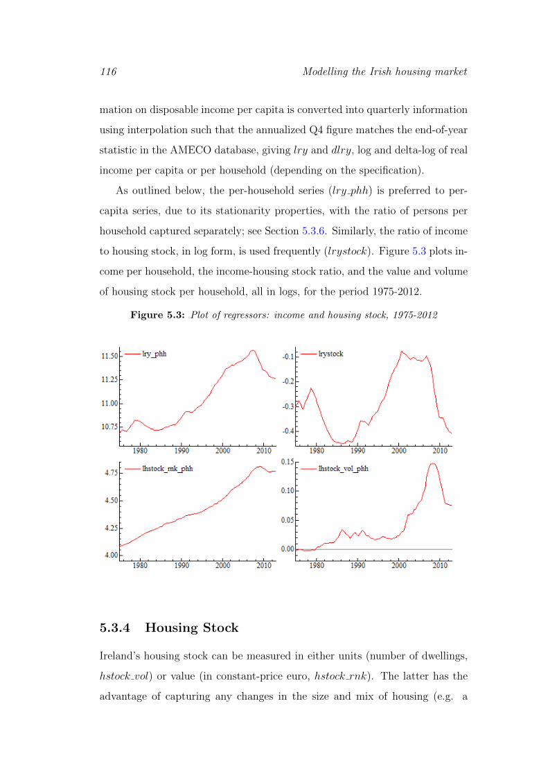
116 Modelling the Irish housing market
mation on disposable income per capita is converted into quarterly information
using interpolation such that the annualized Q4 figure matches the end-of-year
statistic in the AMECO database, giving lry and dlry, log and delta-log of real
income per capita or per household (depending on the specification).
As outlined below, the per-household series (lry phh) is preferred to per-
capita series, due to its stationarity properties, with the ratio of persons per
household captured separately; see Section 5.3.6. Similarly, the ratio of income
to housing stock, in log form, is used frequently (lrystock). Figure 5.3 plots in-
come per household, the income-housing stock ratio, and the value and volume
of housing stock per household, all in logs, for the period 1975-2012.
Figure 5.3: Plot of regressors: income and housing stock, 1975-2012
5.3.4 Housing Stock
Ireland’s housing stock can be measured in either units (number of dwellings,
hstock vol) or value (in constant-price euro, hstock rnk). The latter has the
advantage of capturing any changes in the size and mix of housing (e.g. a

5.3 Data 117
greater proportion of apartments over time, or counter-cyclical improvements
to housing due to negative equity and thus a lack of mobility). For this reason,
the real net capital stock in dwellings was used. This is available on an annual
basis as part of the CSO National Accounts from 1985 on. For the period
preceding this, real gross fixed capital formation in dwellings was used, together
with the depreciation rate implied by the National Accounts, to give net fixed
capital formation. This rate was estimated from difference between gross and
net formation for the period after 1985. For the decade 1986-1995, the rate
was a constant 1.66%, so this rate was applied to figures prior to 1985.
Combining the log of housing stock per household in constant prices (lhstock rnk phh)
with the series on real income gives lrystock, the log of the ratio of real income
to the stock of housing, measured in 2012e. To give an idea of the scale of this
variable, in late 2012, per-household income was measured at e78,000, while
per-household housing stock was valued at e117,000, giving a ratio of income
to stock of 0.67.
5.3.5 Unemployment
While the bulk of labour market effects will be captured by disposable in-
come, included in certain specifications of the dynamic modelling of changes in
real house prices and the price-rent ratio are measures of unemployment. For
the period 1998Q1 to 2012Q4, the (seasonally adjusted) unemployment rate is
taken from Ireland’s Quarterly National Household Survey (QNHS), adminis-
tered by the CSO, which is Ireland’s official unemployment rate. The series
is extended to the 1970s using the percentage change in the Live Register, a
monthly indicator of those in receipt of unemployment benefits. An alternative
is to use a four-quarter moving average of the annual unemployment rate pro-
vided by AMECO (ultimately also from the CSO). In all cases, it is the change
in percentage points (delta ue) that is included in dynamic specifications.
As illustrated in Figure 5.4, using the AMECO annual data on unemploy-
ment (delta ue ann) results in the same change in unemployment rate in each
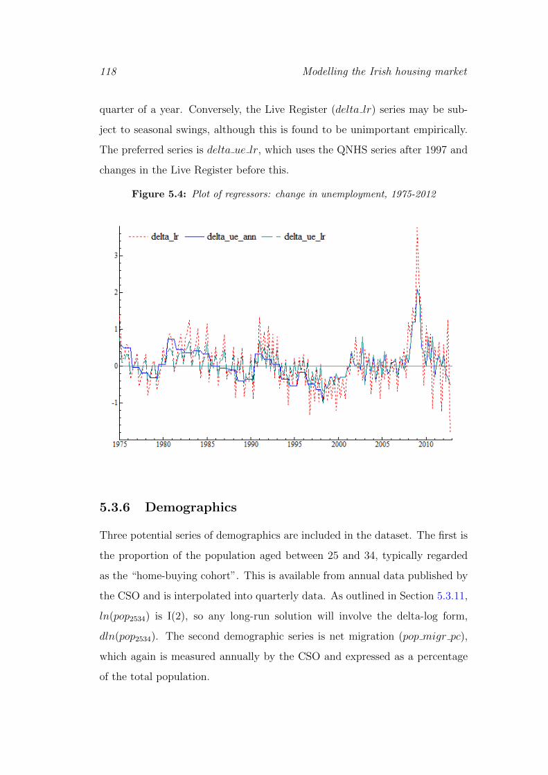
118 Modelling the Irish housing market
quarter of a year. Conversely, the Live Register (delta lr) series may be sub-
ject to seasonal swings, although this is found to be unimportant empirically.
The preferred series is delta ue lr, which uses the QNHS series after 1997 and
changes in the Live Register before this.
Figure 5.4: Plot of regressors: change in unemployment, 1975-2012
5.3.6 Demographics
Three potential series of demographics are included in the dataset. The first is
the proportion of the population aged between 25 and 34, typically regarded
as the “home-buying cohort”. This is available from annual data published by
the CSO and is interpolated into quarterly data. As outlined in Section 5.3.11,
ln(pop2534) is I(2), so any long-run solution will involve the delta-log form,
dln(pop2534). The second demographic series is net migration (pop migr pc),
which again is measured annually by the CSO and expressed as a percentage
of the total population.
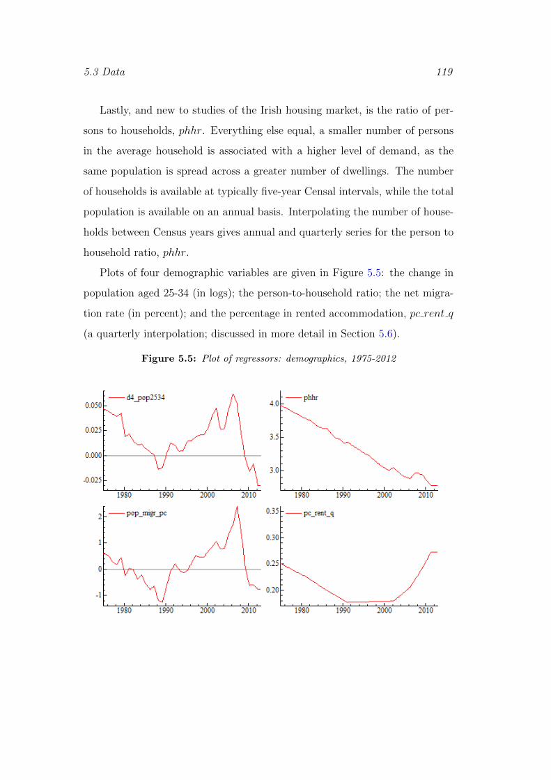
5.3 Data 119
Lastly, and new to studies of the Irish housing market, is the ratio of per-
sons to households, phhr. Everything else equal, a smaller number of persons
in the average household is associated with a higher level of demand, as the
same population is spread across a greater number of dwellings. The number
of households is available at typically five-year Censal intervals, while the total
population is available on an annual basis. Interpolating the number of house-
holds between Census years gives annual and quarterly series for the person to
household ratio, phhr.
Plots of four demographic variables are given in Figure 5.5: the change in
population aged 25-34 (in logs); the person-to-household ratio; the net migra-
tion rate (in percent); and the percentage in rented accommodation, pc rent q
(a quarterly interpolation; discussed in more detail in Section 5.6).
Figure 5.5: Plot of regressors: demographics, 1975-2012
120 Modelling the Irish housing market
5.3.7 Interest Rates
Mortgage market interest rates are taken from official sources. For the pe-
riod from 2003, the quarterly average of the annual percentage rate of charge
(APRC) reported by the ECB is used. For the period 1975-2002, the data
are from the CSO “representative Building Society mortgage rate”. These are
variable rates, as these represent the vast majority of mortgages in Ireland; ac-
cording to Kennedy & McIndoe-Calder (2011), just 15% of the loan-book of the
four major Irish lending institutions at the end of 2010 was based on fixed-rate
mortgages, most of which revert to variable rates after a certain period.
The series form the gross nominal mortgage rate rmGN , where rm stands
for mortgage rate (as opposed to deposit rate or some combination), G for gross
and N for nominal. The net nominal mortgage rate, rmNN , is calculated by
deducting the marginal rate of mortgage interest relief. For the period 1975-
1992, the marginal tax rate for first-time-buyers is lower than the top marginal
rate. This is typically lower by one band and is based on average salaries at
the time; see Figure 9 in the appendix for more details.
Opportunity cost Technically, if a downpayment of θP is required, where
P is the house price, the opportunity cost for a first-time buyer is not given
solely by rm. Rather it is given by a weighted average of θrd + (1 − θ)rm,
where rd represents the (after-tax) rate of return on alternative investments.
Using typical deposit rates for rd, a series giving this overall rate of interest is
available, using crude information on loan-to-value as discussed below, for θ.
In this case, information on rdNN , the net nominal interest rate on deposits,
comes from the Central Bank of Ireland (the gross rate) and the Revenue
Commissioners (on the rate of tax applied to interest, DIRT).
5.3.8 Expected Capital Gain
Gross interest rates are only part of the cost of home ownership. An offsetting
component of user cost is the expected capital gain: if interest costs are 5%

5.3 Data 121
per year but nominal house prices are expected to grow by 10% per year,
assuming no other costs to ownership, the real user cost would be perceived
as negative. Unfortunately, there are no consistent data on expected capital
gains in residential housing for the whole period under analysis. Two separate
surveys exist, one by ESRI-IIB for the period 2003-2007 and another by daft.ie
from 2012 on.
Based on the top-level findings of both these surveys, one cannot reject a
null hypothesis of adaptive expectations, i.e. that housing market participants
look at the recent history of the market as their best guide regarding the future
direction of prices. For example, in early 2007, a year when nominal house
prices were at best stable, participants expected strong price growth, as had
been the case in recent years. Similarly, in early 2012, consumers expected
prices to fall 10%, the average rate over the previous four years; prices actually
fell by 4% in 2012.
The existing literature suggests that for other countries, the four-year aver-
age and one-year rates of change in nominal house prices often perform well as
measures of expected capital gains based on adaptive or extrapolative expec-
tations (Muellbauer 2012). Depending on the specification, either or both are
used here in explaining real house prices and the price-rent ratio, as explained
below. This is denoted in the suffix to the net interest rate, where rmNR4
indicates an interest rate net of expected capital gains, based on four-year
appreciation.
Figure 5.6 plots on one chart annualized changes in nominal house prices
over 1- and 4-years (d4lhp and d16lhp ann; blue lines), the gross and net nom-
inal interest rates (rm gr nom and rm net nom; red lines), and the principal
measure of net user cost, based on deducting four-year house price inflation
from the net nominal rate (rm net r 4y; black line). Also included in this plot
is the stamp duty rate that applied to first-time buyers at prevailing house
prices (tau sd ftb).
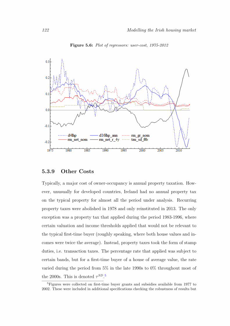
122 Modelling the Irish housing market
Figure 5.6: Plot of regressors: user-cost, 1975-2012
5.3.9 Other Costs
Typically, a major cost of owner-occupancy is annual property taxation. How-
ever, unusually for developed countries, Ireland had no annual property tax
on the typical property for almost all the period under analysis. Recurring
property taxes were abolished in 1978 and only reinstituted in 2013. The only
exception was a property tax that applied during the period 1983-1996, where
certain valuation and income thresholds applied that would not be relevant to
the typical first-time buyer (roughly speaking, where both house values and in-
comes were twice the average). Instead, property taxes took the form of stamp
duties, i.e. transaction taxes. The percentage rate that applied was subject to
certain bands, but for a first-time buyer of a house of average value, the rate
varied during the period from 5% in the late 1990s to 0% throughout most of
the 2000s. This is denoted τSD.5
5Figures were collected on first-time buyer grants and subsidies available from 1977 to2002. These were included in additional specifications checking the robustness of results but

5.3 Data 123
Maintenance & transaction costs It is possible to use the CSO House-
hold Budget Survey 2010 to estimate the amount spent on maintenance; based
on spending and housing prices in 2010, households spend on average about
0.5% of the value of their dwelling on maintenance. However, setting a fixed
proportional cost of maintenance means that this does not vary over the pe-
riod and thus is irrelevant for a dynamic model of changes in house prices over
time. Likewise, based on costs prevailing in early 2013, the (one-off, rather
than annualized) financial costs of moving were set at 5%, and as research on
the housing market suggests that psychological costs of moving are at least as
large as financial costs, these were also set at 5% (Bayer et al. 2011). However,
as these do not vary, by construction, they too can play no role in explaining
house price changes if the model is linear in user cost. A more detailed under-
standing of these costs and how they vary over time is a topic worthy of further
research.
Risk premium It is very likely that prospective first-time buyers have some
assessment of how risky a purchase would be. Nonetheless, research under-
standing the risk premium associated with owner-occupancy is in its infancy –
although Sinai & Souleles (2005) use a model where owner-occupancy is itself a
hedge against rent risk. Crucially, the risk premium is likely to be time-varying.
Two ad-hoc formulations of the risk premium were included in candidate mod-
els: the first uses a discounted average of the absolute value of changes in
prices over the last four years; the second uses the standard deviation of the
last four annual changes in house prices. Neither features as an economically
or statistically significant variable.
5.3.10 Credit Conditions
The final fundamental in the housing market – often an omitted variable –
is credit conditions. Like the risk premium discussed above, this is often ex-
were found to have no significant effect on real house prices.
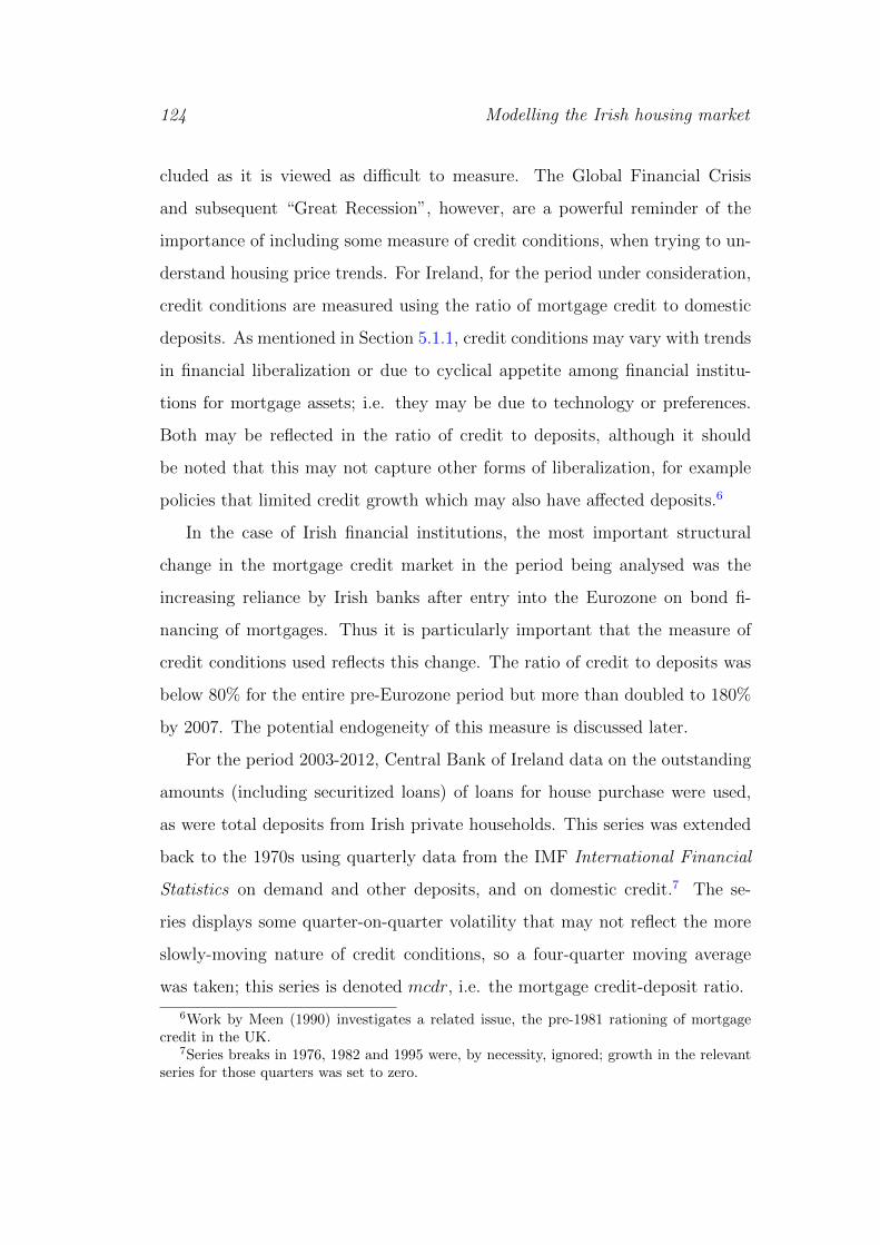
124 Modelling the Irish housing market
cluded as it is viewed as difficult to measure. The Global Financial Crisis
and subsequent “Great Recession”, however, are a powerful reminder of the
importance of including some measure of credit conditions, when trying to un-
derstand housing price trends. For Ireland, for the period under consideration,
credit conditions are measured using the ratio of mortgage credit to domestic
deposits. As mentioned in Section 5.1.1, credit conditions may vary with trends
in financial liberalization or due to cyclical appetite among financial institu-
tions for mortgage assets; i.e. they may be due to technology or preferences.
Both may be reflected in the ratio of credit to deposits, although it should
be noted that this may not capture other forms of liberalization, for example
policies that limited credit growth which may also have affected deposits.6
In the case of Irish financial institutions, the most important structural
change in the mortgage credit market in the period being analysed was the
increasing reliance by Irish banks after entry into the Eurozone on bond fi-
nancing of mortgages. Thus it is particularly important that the measure of
credit conditions used reflects this change. The ratio of credit to deposits was
below 80% for the entire pre-Eurozone period but more than doubled to 180%
by 2007. The potential endogeneity of this measure is discussed later.
For the period 2003-2012, Central Bank of Ireland data on the outstanding
amounts (including securitized loans) of loans for house purchase were used,
as were total deposits from Irish private households. This series was extended
back to the 1970s using quarterly data from the IMF International Financial
Statistics on demand and other deposits, and on domestic credit.7 The se-
ries displays some quarter-on-quarter volatility that may not reflect the more
slowly-moving nature of credit conditions, so a four-quarter moving average
was taken; this series is denoted mcdr, i.e. the mortgage credit-deposit ratio.
6Work by Meen (1990) investigates a related issue, the pre-1981 rationing of mortgagecredit in the UK.
7Series breaks in 1976, 1982 and 1995 were, by necessity, ignored; growth in the relevantseries for those quarters was set to zero.
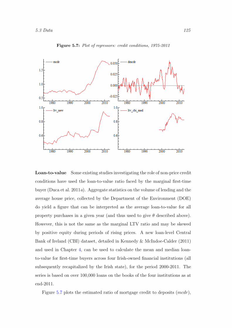
5.3 Data 125
Figure 5.7: Plot of regressors: credit conditions, 1975-2012
Loan-to-value Some existing studies investigating the role of non-price credit
conditions have used the loan-to-value ratio faced by the marginal first-time
buyer (Duca et al. 2011a). Aggregate statistics on the volume of lending and the
average house price, collected by the Department of the Environment (DOE)
do yield a figure that can be interpreted as the average loan-to-value for all
property purchases in a given year (and thus used to give θ described above).
However, this is not the same as the marginal LTV ratio and may be skewed
by positive equity during periods of rising prices. A new loan-level Central
Bank of Ireland (CBI) dataset, detailed in Kennedy & McIndoe-Calder (2011)
and used in Chapter 4, can be used to calculate the mean and median loan-
to-value for first-time buyers across four Irish-owned financial institutions (all
subsequently recapitalized by the Irish state), for the period 2000-2011. The
series is based on over 100,000 loans on the books of the four institutions as at
end-2011.
Figure 5.7 plots the estimated ratio of mortgage credit to deposits (mcdr),

126 Modelling the Irish housing market
Indicator Source Period Orig. FrequencyHouse prices DoE 1975-1996 Quarterly
ESRI-PTSB 1996-2005 MonthlyCSO 2005-2012 Monthly
Rents CSO 1975-2012 MonthlyConsumer prices CSO 1975-2012 MonthlyIncome AMECO 1975-2012 AnnualUnemployment rate QNHS 1998-2012 Quarterly
AMECO 1975-1998 AnnualLive Register CSO 1975-2012 MonthlyStock capital in dwellings CSO 1975-2012 AnnualHousing stock (volume) DOE 1975-2012 AnnualMortgage rates ECB 2003-2012 Monthly
CSO 1975-2002 MonthlyDeposit rates CBI 1975-2012 MonthlyDIRT rates RevComm 1986-2012 MonthlyStamp duty rates RevComm 1975-2012 MonthlyMIR rate RevComm, Barham 1975-2012 MonthlyGrants & subsidies Barham 1975-2012 AnnualMortgage credit CBI 2003-2012 MonthlyHousehold deposits CBI 2003-2012 MonthlyPrivate sector credit IFS 1975-2003 QuarterlyPrivate deposits IFS 1975-2003 QuarterlyAverage LTV DoE 1975-2012 AnnualMedian LTV CBI 2000-2012 MonthlyMaintenance CSO HBS 2011 ParameterMoving costs Author calculations 2013 Parameter
Table 5.2: Overview of dataset
the change in that ratio (dmcdr, used in dynamics), the estimated DOE series
for loan-to-value on new dwellings8, ltv new, and the CBI series on median
loan-to-value for first-time buyers, from 2000 on (ltv cbi med). What is striking
is how the DOE loan-to-value series peaks after the bubble. The average loan-
to-value on new dwellings in mid-2006 was 65%, when both prices and the CBI
series on LTV peaked, but nearly 95% at the turn of 2010. Overall, it is clear
from the series that the DOE data do not capture accurately the timing of
peak in loan-to-value and its subsequent fall. Thus, where the focus of analysis
is a period longer than 2000-2012, the ratio of credit to deposits will be used,
instead of DOE data on loan-to-value. An overview of all data is presented in
Table 5.2.
8Note that this includes purchases of new dwellings by investors and other purchasers, aswell as by first-time buyers.
5.3 Data 127
5.3.11 Stationarity properties
Table 5.3 outlines the results of augmented Dickey-Fuller tests for a unit root,
across all the major variables. Results are shown for the deltas of each variable,
thus highlighting whether any series are I(2), thus potentially biasing analysis
including such variables in a long-run solution with I(1) series. For all variables
in Table 5.3, the sample is 1980I-2012IV, with the 1%, 5% and 10% critical
values of -3.48, -2.88 and -2.57 denoted by three, two and one stars respectively.
Using a 10% significance level, it is possible to conclude that in delta form,
almost all the variables are stationary, including dlrhp, dlhs ph, dlyhs, dmcdr,
drm net, dphhr and due. Failure to reject the null of a unit root occurs for
income per household (dlry ph), although this appears to be marginal, and
the proportion of the population aged 25-34, (d4p2534). These are explored in
more detail in Table 9 in the Appendix. This table presents strong evidence
in favour of using the per-household formulation of income and housing stock
(suffix ph), instead of the per-capita series ( ph), with no rejection of the null
hypothesis of a unit root at any conventional significance level for either income
per capita or housing stock per capita.
Thus, it is clear that per-capita series for income and housing stock are I(2).
Are the per-household series I(2) or I(1)? Results for the 1975-2012 sample for
both, denoted by the suffix † in Table 9, suggest that the lack of statistical
significance at the 5% or 1% levels for income and stock per household in
the 1980-2012 sample may relate more to the power of the test than to the
underlying data series. One means of overcoming any uncertainty about the
stationarity of changes in income and stock is to use instead changes the ratio
of income to stock: at the 10% level for the 1980-2012 series, and at the 1% for
the 1975-2012 series, the null of a unit root in dlrystock can be rejected.9
9These results come from use of quarterly data interpolated from annual data. Nonethe-less, test results do not change if only annual data are used instead.
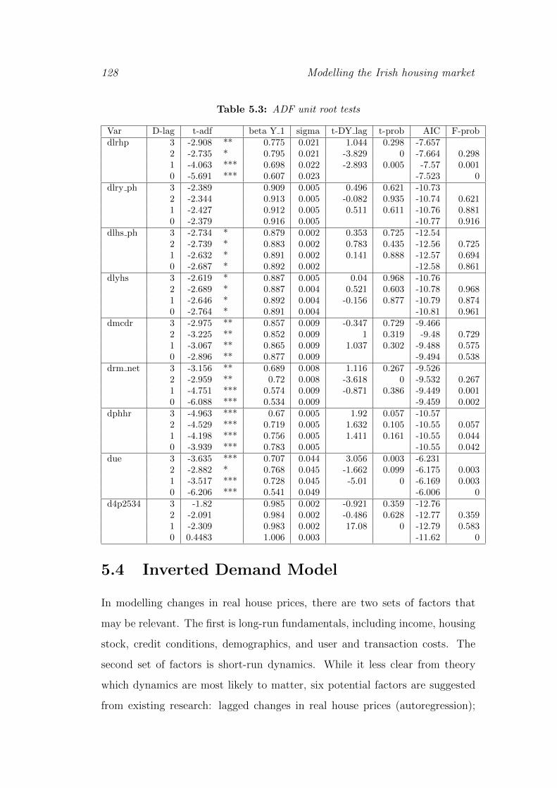
128 Modelling the Irish housing market
Table 5.3: ADF unit root tests
Var D-lag t-adf beta Y 1 sigma t-DY lag t-prob AIC F-probdlrhp 3 -2.908 ** 0.775 0.021 1.044 0.298 -7.657
2 -2.735 * 0.795 0.021 -3.829 0 -7.664 0.2981 -4.063 *** 0.698 0.022 -2.893 0.005 -7.57 0.0010 -5.691 *** 0.607 0.023 -7.523 0
dlry ph 3 -2.389 0.909 0.005 0.496 0.621 -10.732 -2.344 0.913 0.005 -0.082 0.935 -10.74 0.6211 -2.427 0.912 0.005 0.511 0.611 -10.76 0.8810 -2.379 0.916 0.005 -10.77 0.916
dlhs ph 3 -2.734 * 0.879 0.002 0.353 0.725 -12.542 -2.739 * 0.883 0.002 0.783 0.435 -12.56 0.7251 -2.632 * 0.891 0.002 0.141 0.888 -12.57 0.6940 -2.687 * 0.892 0.002 -12.58 0.861
dlyhs 3 -2.619 * 0.887 0.005 0.04 0.968 -10.762 -2.689 * 0.887 0.004 0.521 0.603 -10.78 0.9681 -2.646 * 0.892 0.004 -0.156 0.877 -10.79 0.8740 -2.764 * 0.891 0.004 -10.81 0.961
dmcdr 3 -2.975 ** 0.857 0.009 -0.347 0.729 -9.4662 -3.225 ** 0.852 0.009 1 0.319 -9.48 0.7291 -3.067 ** 0.865 0.009 1.037 0.302 -9.488 0.5750 -2.896 ** 0.877 0.009 -9.494 0.538
drm net 3 -3.156 ** 0.689 0.008 1.116 0.267 -9.5262 -2.959 ** 0.72 0.008 -3.618 0 -9.532 0.2671 -4.751 *** 0.574 0.009 -0.871 0.386 -9.449 0.0010 -6.088 *** 0.534 0.009 -9.459 0.002
dphhr 3 -4.963 *** 0.67 0.005 1.92 0.057 -10.572 -4.529 *** 0.719 0.005 1.632 0.105 -10.55 0.0571 -4.198 *** 0.756 0.005 1.411 0.161 -10.55 0.0440 -3.939 *** 0.783 0.005 -10.55 0.042
due 3 -3.635 *** 0.707 0.044 3.056 0.003 -6.2312 -2.882 * 0.768 0.045 -1.662 0.099 -6.175 0.0031 -3.517 *** 0.728 0.045 -5.01 0 -6.169 0.0030 -6.206 *** 0.541 0.049 -6.006 0
d4p2534 3 -1.82 0.985 0.002 -0.921 0.359 -12.762 -2.091 0.984 0.002 -0.486 0.628 -12.77 0.3591 -2.309 0.983 0.002 17.08 0 -12.79 0.5830 0.4483 1.006 0.003 -11.62 0
5.4 Inverted Demand Model
In modelling changes in real house prices, there are two sets of factors that
may be relevant. The first is long-run fundamentals, including income, housing
stock, credit conditions, demographics, and user and transaction costs. The
second set of factors is short-run dynamics. While it less clear from theory
which dynamics are most likely to matter, six potential factors are suggested
from existing research: lagged changes in real house prices (autoregression);
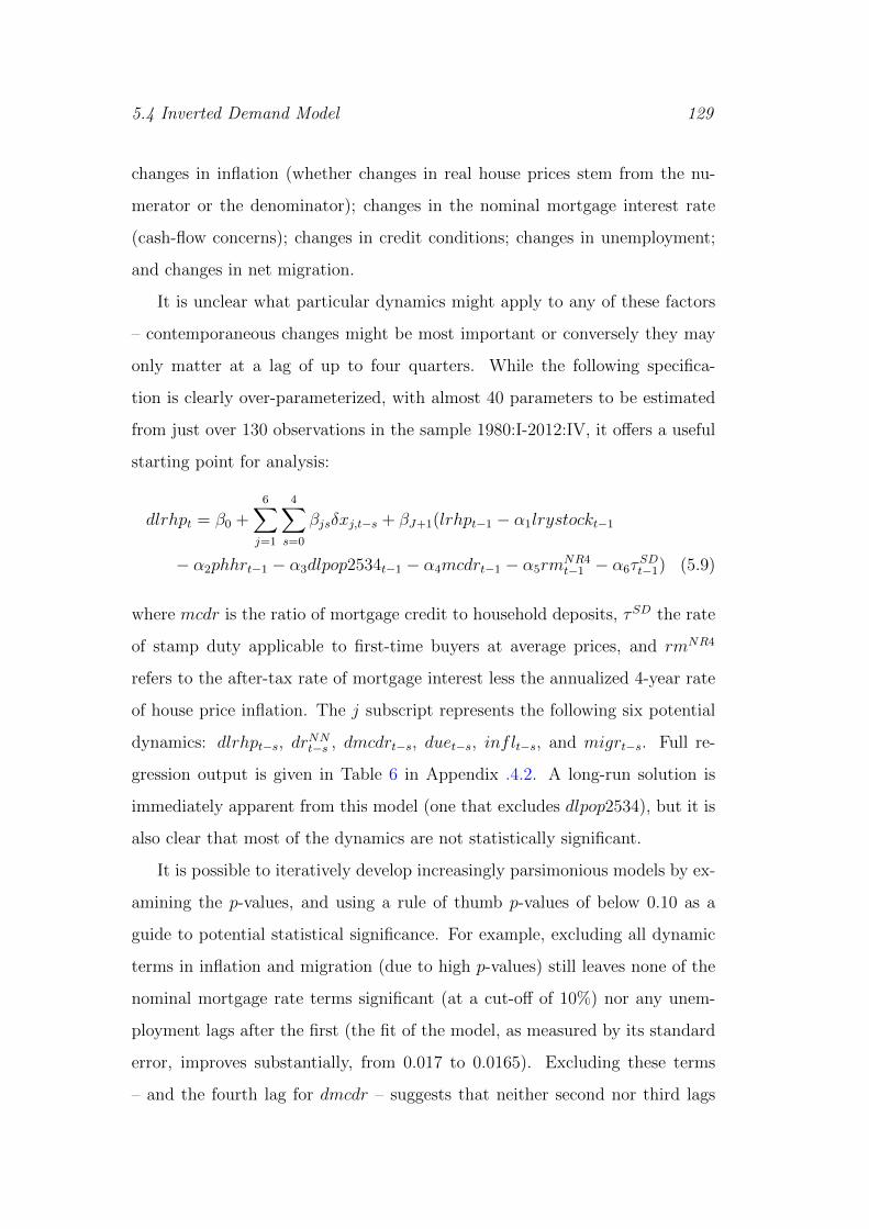
5.4 Inverted Demand Model 129
changes in inflation (whether changes in real house prices stem from the nu-
merator or the denominator); changes in the nominal mortgage interest rate
(cash-flow concerns); changes in credit conditions; changes in unemployment;
and changes in net migration.
It is unclear what particular dynamics might apply to any of these factors
– contemporaneous changes might be most important or conversely they may
only matter at a lag of up to four quarters. While the following specifica-
tion is clearly over-parameterized, with almost 40 parameters to be estimated
from just over 130 observations in the sample 1980:I-2012:IV, it offers a useful
starting point for analysis:
dlrhpt = β0 +6∑
j=1
4∑s=0
βjsδxj,t−s + βJ+1(lrhpt−1 − α1lrystockt−1
− α2phhrt−1 − α3dlpop2534t−1 − α4mcdrt−1 − α5rmNR4t−1 − α6τ
SDt−1) (5.9)
where mcdr is the ratio of mortgage credit to household deposits, τSD the rate
of stamp duty applicable to first-time buyers at average prices, and rmNR4
refers to the after-tax rate of mortgage interest less the annualized 4-year rate
of house price inflation. The j subscript represents the following six potential
dynamics: dlrhpt−s, drNNt−s , dmcdrt−s, duet−s, inflt−s, and migrt−s. Full re-
gression output is given in Table 6 in Appendix .4.2. A long-run solution is
immediately apparent from this model (one that excludes dlpop2534), but it is
also clear that most of the dynamics are not statistically significant.
It is possible to iteratively develop increasingly parsimonious models by ex-
amining the p-values, and using a rule of thumb p-values of below 0.10 as a
guide to potential statistical significance. For example, excluding all dynamic
terms in inflation and migration (due to high p-values) still leaves none of the
nominal mortgage rate terms significant (at a cut-off of 10%) nor any unem-
ployment lags after the first (the fit of the model, as measured by its standard
error, improves substantially, from 0.017 to 0.0165). Excluding these terms
– and the fourth lag for dmcdr – suggests that neither second nor third lags

130 Modelling the Irish housing market
of dlrhp, nor the contemporaneous value of dmcdr, is statistically significant.
Parsimony suggests omitting the second and third lags of dmcdr. Dropping the
population aged 25-34, which is significant in none of the specifications, leaves
a model with the following specification10:
dlrhpt = β0 + β1dlrhpt−1 + β2dlrhpt−4 + β3dmcdrt−1 + β4duet + β5duet−1
+ β6(lrhpt−1 − α1lrystockt−1 − α2phhrt−1
− α4mcdrt−1 − α5rmNR4t−1 − α6τ
SDt−1) (5.10)
A model with the fourth lag of dlrhp is strongly preferred to one without
(sigma rises from 0.01673 to 0.01762 without this term), while similarly a model
with the one-quarter lag in unemployment included is preferred to one with
just contemporaneous changes in unemployment (sigma rises from 0.01673 to
0.01702).
Regression output for this model is shown in Table 5.4, while actual and fit-
ted values are plotted in Figure 10 in Appendix .4.4. As noted above, the sigma
for the regression is 0.01673, with the none of the six core tests of model speci-
fication indicating a rejection of the null hypothesis. For the period from 1980
to 2012, this model explains over two thirds of the changes in real house prices
(R2 = 0.696), with all variables strongly statistically significant (particularly
fundamentals) and all with the sign suggested by theory.
5.4.1 Short-run dynamics
The model suggests that for the 33-year period under analysis, there were four
elements that mattered for short-run house price dynamics, independent of
forces pushing prices back towards their equilibrium level. The first is changes
in real house prices in the previous quarter, an element of momentum in house
prices. Every one percentage point (pp) increase in prices in the previous
10The same equation results from the use of Autometrics software that algorithmicallydevelops a parsimonious model by omitting regressors based on statistical significance, oncethe long-run variables are forced to be included.

5.4 Inverted Demand Model 131
Table 5.4: Model of dlrhp with parsimonious dynamics, 1980-2012
Coeff S.E. t-stat p-valuedlrhpt−1 0.1661 ** 0.0791 2.10 0.0378dlrhpt−4 -0.256 *** 0.0681 -3.76 0.0003delta ue -0.0162 *** 0.0044 -3.67 0.0004delta uet−1 -0.0104 ** 0.0046 -2.29 0.024dmcdrt−1 0.3097 ** 0.1209 2.56 0.0117Constant 4.0786 *** 0.6618 6.16 0.000log rhp (lrhpt−1) -0.3137 *** 0.0522 -6.01 0.000log y/stock (lrystockt−1) 0.3952 *** 0.0777 5.08 0.000person:HH (phhrt−1) -0.1222 *** 0.0222 -5.49 0.000credit:deposit (mcdrt−1) 0.1743 *** 0.0345 5.05 0.000user cost (rmNR4
t−1 ) -0.4812 *** 0.0915 -5.26 0.000stamp duty (τSDt−1) -0.4757 ** 0.2118 -2.25 0.0265AR 1-5 F(5,115) 1.96 0.090ARCH 1-4 F(4,124) 1.05 0.386Normality Chi2(2) 1.31 0.520Hetero F(22,109) 0.57 0.937Hetero-X F(77,54) 0.90 0.665RESET23 F(2,118) 1.12 0.331
quarter was associated with a 0.16pp increase in the current period. The second
is the change in real house prices a year ago. Here, the relationship is negative: a
percentage point increase in prices in the same quarter a year ago was associated
with a 0.26pp decrease in the current period. Everything else being equal, large
house price gains in particular quarter in one year were associated with price
falls a year later, perhaps a form of supplemental error correction.
The other two factors reflect conditions in the mortgage and labour mar-
kets. A percentage point increase in the ratio of mortgage credit to deposits
in the previous quarter was associated with a increase in real house prices of
0.31pp in the current period. Lastly, there was a negative relationship between
unemployment and changes in house prices in the short-run, an effect that
lasted two quarters: a one-percentage point increase in the unemployment rate
in a given quarter was associated with a fall in house prices of roughly 1.6% in
the same period and 1% in the following period.
132 Modelling the Irish housing market
5.4.2 Long-run equation
The model presents a clear long-run relationship that determines house prices
over this period and indicates that there was fast adjustment to this equilibrium
in the Irish housing market. The coefficient on lrhpt−1 of -0.314 implies that
almost one third of the gap between actual and equilibrium house prices was
corrected every quarter. Compared to similar studies for other economies, this
represents rapid adjustment, possibly reflecting Ireland’s nature as a small,
relatively homogeneous economy.
This coefficient can also be used to reveal the underlying long-run relation-
ship between real house prices and their determinants. For the period under
analysis, there are five fundamental factors that affected the equilibrium level of
house prices. The long-run relationship suggested by the analysis is as follows:
lrhpt = 13.002 + 1.26lrystockt−0.39phhrt + 0.56mcdrt−1.53rmNR4t −1.52τSDt
(5.11)
Income-stock ratio The model suggests a strong positive long-run relation-
ship between real house prices and the ratio of household income to the stock of
residential housing. The coefficient of just over 1.26 implies that price responds
more than proportionately to changes in income and to housing supply. An
increase in real income of 10% (relative to the stock of housing) is associated
with a 12.6% increase in the real price of housing. The same coefficient can
be interpreted as the absolute value of the inverse of the price elasticity with
respect to supply; i.e. an increase in the real value of the housing stock of 10%
is associated with a fall in real house prices of 8% (-1/1.26).
This coefficient is somewhat smaller than much of the existing literature,
both for Ireland and for other countries. One set of existing estimates for Ire-
land have found the responsiveness of prices with respect to income is between
1.6 and 1.7 (Rae & van den Noord 2006, Thom 1983), while Murphy (1998)

5.4 Inverted Demand Model 133
presents a lower estimate of 1.4. Similarly, studies of the UK market also sug-
gest higher price elasticities with respect to income. The estimated elasticity
presented here is stable, however, with the coefficient on the income/stock ra-
tio stable from 1995 on (see Figure 13 in the Appendix). The data on which
this estimate is based are in some sense novel, at least for the Irish case, as
they reflect various periods in which incomes were rising rapidly, falling rapidly
and also largely stable – most studies do not cover periods when incomes fell
rapidly. This may explain the difference not only with respect to the UK case,
but also the Irish case. Another window into price elasticities with respect to
income could be given by a panel analysis exploiting variation in incomes and
housing market outcomes across Irish counties.
Person-household ratio The results indicate a clear relationship between
real housing prices in Ireland and the average number of persons per household.
The negative coefficient in the long-run relationship of -0.389 can be interpreted
as follows: between 1980 and 2012, the average number of people per household
fell by one (from 3.79 to 2.78). This increase in effective demand per head of
population was associated with a 39% increase in real house prices, controlling
for other factors. Breaking the income per house restriction and including
per-person or per-household income and stock separately and omitting average
household size leads to omitted variable bias, in particular an upward bias on
the income coefficient on this interpretation.11
11It is likely that average household size has some endogenous elements; in the long run,affordability and credit conditions may have an effect on household size. However, therewill also be a large demographic component, including longer life spans, more widows, latermarriages and more divorces, that will be mostly exogenous and, if excluded, caught up bythe income coefficient. Here, omitting phhr from the model reduces the speed of adjustmentto 10% and doubles the implied long-run coefficient on the ratio of income to housing stockfrom 1.26 to 2.57. The fit of such a model is substantially worse: the sigma of the regressionincreases from 0.01673 to 0.01864 and the R2 reduces from almost 70% to 61.9%. This can bepartially remedied by including per-capita income and housing stock separately; see Section5.4.3 for more details.

134 Modelling the Irish housing market
Credit-deposit ratio Credit conditions, as measured by the ratio of the
stock of mortgages to the stock of deposits, have a long-run impact on house
prices, as well as a short-run impact. The coefficient of roughly 0.56 on the
credit conditions term in the long-run equation indicates that an increase of ten
percentage points in the ratio of mortgage credit to deposits was associated with
an increase in real house prices of 5.6%. Ireland’s credit-deposit ratio increased
by 100 percentage points in the decade to 2007. The model suggests that this
was associated with an increase in the equilibrium level of real house prices of
56%.12
Real interest rates The user cost for housing – as measured by the difference
between nominal rates after tax reliefs and the expected capital gain based on
the last four years – represent a drag on housing prices. The coefficient of -1.53
indicates that an increase in user cost of 1 percentage point is associated with
a decrease in equilibrium real house prices of 1.53%. The user cost measured
in this way increased by 30 percentage points (roughly speaking, from -10% to
+20%) between 2006 and 2012. This was associated with a fall in equilibrium
prices of 45%.
Stamp duty The final factor suggested by the error correction model as im-
portant for the long-run level of house prices is the rate of stamp duty applying
to first-time buyer purchases. The coefficient of close to -1.5 on indicates that
a decrease in the rate of stamp duty applying to first-time buyers of one per-
centage point was associated with a 1.5% increase in real housing prices. This
more-than-proportionate response indicates that down-payment constraints for
first-time buyers were important in the housing market, in the period under
analysis. Nonetheless, the small number of changes to the stamp duty rate ap-
12Strictly speaking, these are increases in the log of real house prices, rather than inpercentage terms. For a more formal discussion of the sources of house price changes overthe period, see Section 5.7.

5.4 Inverted Demand Model 135
plicable to first-time buyers means that caution should be exercised in relying
on this result.
5.4.3 Robustness & Sensitivity
A number of choices were made in the construction of the dataset, each of
which may impact the results presented. Two tables in Appendix .4.3 outline a
number of robustness and sensitivity checks. Coefficients and p-values are pre-
sented for variables, along with two measures of model fit (sigma and R2) and
also whether any of six standard tests failed: AR 1-5, ARCH 1-4, Normality,
Hetero, Hetero-X, and RESET23. Also presented, in Figure 13, are recursive
estimates of the parameters associated with the long-run variables. It is clear
that there are no statistically significant changes in any of the coefficients, al-
though there is small shift in a number of the coefficients between 2002 and
2004.
Table 7 in Appendix .4.3 takes the various fundamentals and explores al-
ternatives for each. An extra fundamental is added, delta log of the proportion
aged 25-34, which has almost no impact on the results, as the coefficient on the
variable is close to zero. For credit conditions, instead of the ratio of credit to
deposits, the estimated average loan-to-value for new dwellings is used. Pre-
sumably reflecting the weakness of this data series, the inclusion of this variable
effectively destroys the long-run relationship.13
Five other specifications are included in Table 7, including splitting out
income and stock (which reveals coefficients of similar magnitudes), using per-
capita instead of per-household measures of income and stock (replacing the
stock of housing measured in constant price values with a series on the number
of dwellings, using a weighted rate of interest (across both mortgages and de-
posits), including a measure of grants for first-time buyers (relative to value),
and an alternative measure of quarterly unemployment, based on interpolated
13In house price booms, repeat buyers have higher net equity stakes from past appreciationand so can reduce their LTV; hence, average LTV series that include purchasers other thanfirst-time buyers will be a very misleading indicator of credit availability.
136 Modelling the Irish housing market
official annual unemployment rates instead of changes in unemployment im-
plied by Live Register data. None of these changes has a meaningful effect on
the long-run equation, but have worse fit than the specification outlined above.
The second table explores functional form, particularly for the three ratios
included in the fundamental long-run equaton. The log of the ratio of income
to housing stock was used in the principal specification, while the level of the
two other ratios – mortgage credit to deposits, and persons to households –
was used. In principle, one might think that as income and housing stock are
both euro amounts, relativities matter more than levels, while for the credit-
deposit ratio, ten percentage points of deposits lent out at the margin is roughly
equivalent at different starting points. Table 8 investigates the importance of
this, using different combinations of logs and levels for the three ratios.
While the overall fit of the model does not change greatly across all five
specifications, it appears from the fit and test results that the level of the
credit to deposit ratio is a better measure of credit conditions than the log,
particularly in relation to dynamic effects. A specification where all three
ratios (income/stock, credit/deposits, and persons/households) are included in
logs suggests the following long-run house price elasticities: 1.15 for the income
(relative to stock), 0.64 for the mortgage-deposit ratio, and -1.57 for the ratio
of persons to households.
5.4.4 Nominal rigidities
The long-run relationship outlined in the previous section describes the deter-
minants of real house prices in Ireland from 1980 on. However, this period
comprises both high and low inflation regimes. The average quarterly change
in consumer prices for the period 1975-1984 was 3.4% while for 1985-1994 it was
0.8% (very similar to the average for 1995-2013: 0.6%). Noticeably lower infla-
tion increases the likelihood of some degree of money illusion, where households
treat real and nominal prices as equivalent.
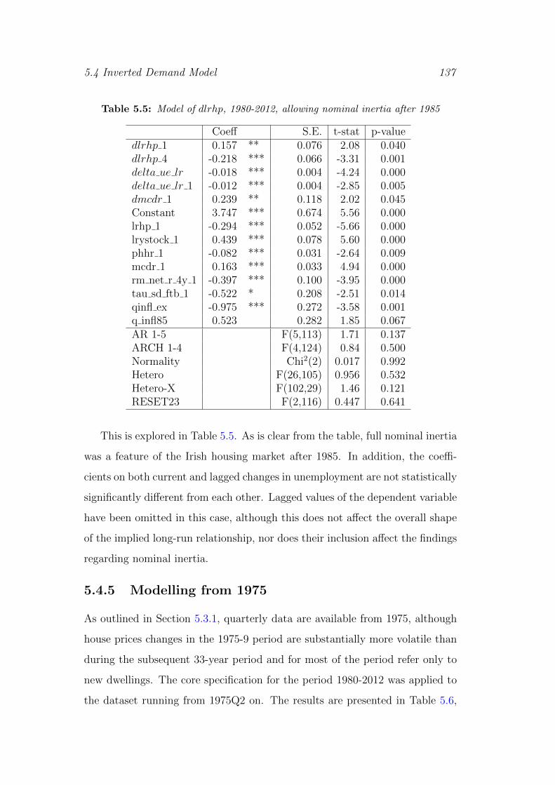
5.4 Inverted Demand Model 137
Table 5.5: Model of dlrhp, 1980-2012, allowing nominal inertia after 1985
Coeff S.E. t-stat p-valuedlrhp 1 0.157 ** 0.076 2.08 0.040dlrhp 4 -0.218 *** 0.066 -3.31 0.001delta ue lr -0.018 *** 0.004 -4.24 0.000delta ue lr 1 -0.012 *** 0.004 -2.85 0.005dmcdr 1 0.239 ** 0.118 2.02 0.045Constant 3.747 *** 0.674 5.56 0.000lrhp 1 -0.294 *** 0.052 -5.66 0.000lrystock 1 0.439 *** 0.078 5.60 0.000phhr 1 -0.082 *** 0.031 -2.64 0.009mcdr 1 0.163 *** 0.033 4.94 0.000rm net r 4y 1 -0.397 *** 0.100 -3.95 0.000tau sd ftb 1 -0.522 * 0.208 -2.51 0.014qinfl ex -0.975 *** 0.272 -3.58 0.001q infl85 0.523 0.282 1.85 0.067AR 1-5 F(5,113) 1.71 0.137ARCH 1-4 F(4,124) 0.84 0.500Normality Chi2(2) 0.017 0.992Hetero F(26,105) 0.956 0.532Hetero-X F(102,29) 1.46 0.121RESET23 F(2,116) 0.447 0.641
This is explored in Table 5.5. As is clear from the table, full nominal inertia
was a feature of the Irish housing market after 1985. In addition, the coeffi-
cients on both current and lagged changes in unemployment are not statistically
significantly different from each other. Lagged values of the dependent variable
have been omitted in this case, although this does not affect the overall shape
of the implied long-run relationship, nor does their inclusion affect the findings
regarding nominal inertia.
5.4.5 Modelling from 1975
As outlined in Section 5.3.1, quarterly data are available from 1975, although
house prices changes in the 1975-9 period are substantially more volatile than
during the subsequent 33-year period and for most of the period refer only to
new dwellings. The core specification for the period 1980-2012 was applied to
the dataset running from 1975Q2 on. The results are presented in Table 5.6,

138 Modelling the Irish housing market
Table 5.6: Model of dlrhp extended back to 1975
Coeff S.E. t-stat p-valueConstant 2.2556 *** 0.4695 4.8 0.000log rhp (lrhpt−1) -0.1646 *** 0.0349 -4.72 0.000log y/stock (lrystockt−1) 0.1637 *** 0.0515 3.18 0.0018person:HH (phhrt−1) -0.099 *** 0.0249 -3.97 0.0001credit:deposit (mcdrt−1) 0.0751 *** 0.0261 2.88 0.0046user cost (rmNR4
t−1 ) -0.3205 *** 0.106 -3.02 0.003stamp duty (τSDt−1) -0.1766 0.2495 -0.71 0.4802dlrhpt−1 0.0739 0.0789 0.94 0.3509dlrhpt−4 -0.0378 0.0758 -0.5 0.6185delta ue -0.0175 *** 0.0059 -2.97 0.0036delta uet−1 -0.0093 0.006 -1.55 0.1241dmcdrt−1 0.2982 * 0.1662 1.79 0.0749
while the actual and fitted values of dlrhp are shown in Figure 11 in Appendix
.4.4.
The zig-zag nature of changes in real house prices in the late 1970s affects
the autoregressive properties and thus the overall fit of the model (the R2 is
51% compared to 70% for the model from 1980 on). The estimated income and
credit conditions effects are smaller for the model from 1975 than from 1980
(such that the 1980 coefficients are well outside the 95% confidence interval).
The effect of real interest rates and the person-household ratio, however, are
larger in absolute size, while the stamp duty effect is not significant.
The substantially different results and fit for the 1970s suggests that a
structural break in the Irish housing market around 1980. One candidate is
the end of the parity peg between the Irish pound and sterling in early 1979,
although it is left to future research – with data extending further back and
of a higher quality – to examine the nature of the break and the model that
preceded it.
5.5 Exogeneity and cointegration
The analysis undertaken in Section 5.4 shows a clear long-run relationship
between real house prices and a range of fundamentals, including user cost, the
5.5 Exogeneity and cointegration 139
ratio of income to housing stock, the ratio of persons to households and the ratio
of mortgage credit to household deposits. However, housing supply, household
income and mortgage credit may not be exogenous to the system. When house
prices rise, this should increase profitability in the construction sector and
may stimulate a supply-side response. Similarly, a rise in house prices may
bring about an increase in household income, particularly in sectors related to
housing such as construction, banking, real estate, various retail services and
even public administration. Lastly, house price increases may make banks more
confident and thus cause them to increase loan-to-value ratios (see, for example,
Gerlach & Peng 2005), while higher incomes may have a similar effect.
This suggests a rich economic system within which house prices operate.
Cointegration between these variables is analysed in this section, with four
variables – real house prices, the ratio of real income to the real net housing
stock, the user-cost as measured by the real interest rate and the ratio of
mortgage credit to deposits – treated as endogenous. There are two issues that
arise here.
Firstly, the number of vectors can be tested but a certain degree of cau-
tion is needed relying on conventional statistical tests regarding the number
of cointegrating vectors. Suppose the model has k endogenous variables and
s weakly exogenous variables, i.e. where the reduced rank matrix is of dimen-
sion kx(k+ s). Because there are more parameters, test statistic tables will be
shifted to the right, compared to testing the rank of a standard kxk matrix.
Thus, the risk is present, using standard statistical tests, of finding too many
cointegrating vectors (Harbo et al. 1998).
I(1) cointegration analysis for the sample from 1980 to 2012 does indicate
the presence of 4 cointegrating vectors (CIVs). The trace test associated with
a null of 3 vectors is 20.15 and the associated p-value is less than 0.001. Harbo
et al. (1998) report that for a system with four exogenous variables (here:
phhr, delta ue, q infl, and tau sd), and a null hypothesis of one endogenous
variable more than the number of cointegrating vectors (4 and 3 in this case),

140 Modelling the Irish housing market
the revised test statistic with a 5% cut-off is 16.7; thus, it seems likely that even
correcting for the dimensionality of the full matrix, there are as many vectors
as endogenous variables.
Secondly, a finding of four cointegrating vectors where there are only four
endogenous variables would be a concern where the system is closed, as it im-
plies the variables would have to be stationary. However, the system here is
open, with exogenous, non-stationary variables as outlined above. In a system
with four endogenous and two exogenous, non-stationary variables, a system
with four cointegrating vectors could be perfectly coherent. Where an unre-
stricted regression is run on the system from 1985 to 2012 and including all
variables as endogenous (with two lags), rank tests reject a null of three vectors,
as per above (p-value of 0.006), but not a null of four CIVs (p-value of 0.085).
Allowing for both findings above, identification of the model requires as-
sumptions about the weighting matrix across the four vectors, in particular
that the matrix is diagonal. This is tested using two models reported below.
The first, described in detail in Table 5.7, is an unrestricted model, i.e. no
restrictions on the alpha or beta matrices, meaning that the beta matrix is not
identified. Three stars indicates a ratio of the coefficient to its standard error
of more than two.
The first vector is clearly recognisable as a house price relationship with
rapid error-correction by house prices to that vector. In this unrestricted case,
both the user-cost and the credit-deposit ratio respond to this vector, although
at significantly slower speeds of adjustment and the smaller ratios of alphas to
their standard errors. Given the full rank of the system, reduced rank regression
models are not appropriate and a diagonal structure of alphas is legitimate to
identify the beta matrix. The output from this model is shown in Table 5.8.
The identification of the beta matrix allows the elimination of variables
whose coefficients are very small relative to their standard errors, such as mcdr
in the second and third vectors and the stamp duty and inflation variables in
all vectors apart from the first. This system is shown in Table 5.9. It is possible

5.5 Exogeneity and cointegration 141
Table 5.7: Unrestricted 4-CIV model, 1980-2012: beta values and alpha values,SEs
Type CIV1 CIV2 CIV3 CIV4
beta
lrhp 1 0.914 1.558 -0.542lrystock -1.463 1 -2.144 -6.362rm net r4y 1.231 3.012 1 -13.394mcdr -0.595 -0.341 -1.134 1phhr 1 0.236 1.226 0.276 -2.393delta ue2q 0.029 0.015 -0.117 0.019tau sd ftb 1 2.007 -0.169 1.324 -2.292qinfl ex 3.5 -1.457 -1.787 -7.868q infl85 -2.248 -1.93 -2.024 14.355
alpha
lrhp -0.311 *** 0 0.032 -0.003lrystock -0.004 -0.027 *** 0.01 *** -0.001rm net r4y 0.048 *** -0.005 -0.003 0.009 ***mcdr 0.039 *** 0.016 0.043 *** 0
SE
lrhp 0.038 0.02 0.017 0.005lrystock 0.009 0.005 0.004 0.001rm net r4y 0.018 0.009 0.008 0.002mcdr 0.017 0.009 0.008 0.002
to relax the assumption of a diagonal alpha matrix, to test whether any of the
other endogenous variables responds to the house price vector. Doing this does
not indicate any strong response by other variables to the house price vector,
suggesting weak exogeneity of these variables to the house price relationship.
The exogeneity of the credit-deposit ratio is interesting, in light of the find-
ings by (Gerlach & Peng 2005) among others. Relaxing the assumption of a
zero coefficient on αmcdr in the first cointegrating vector, the house price rela-
tion, there is some evidence of a positive response – error amplification, rather
than error correction – of the credit deposit ratio to house prices being above
equilibrium: the coefficient on alpha is 0.05 with a standard error of 0.02. This
suggests some role for credit demand to show up in the ratio of credit to de-
posits, although it appears credit supply technology, in particular the ability
of Irish banks to borrow from abroad once in the eurozone, is the dominant
factor.

142 Modelling the Irish housing market
Table
5.8:
4-C
IVm
odel
,1980-2
012,
wit
hdia
gon
al
alp
ha
matr
ix
Typ
eC
IV1
CIV
2C
IV3
CIV
4
bet
aco
effs.
e.t
coeff
s.e.
tco
effs.
e.t
coeff
s.e.
t
lrh
p1
00.
389
0.27
1.44
1-0
.428
0.22
8-1
.877
-1.5
60.1
11
-14.0
54
lryst
ock
-1.5
570.2
06
-7.5
581
01.
583
0.47
23.3
54
1.717
0.3
39
5.0
65
rmn
etr4
y1.2
06
0.271
4.4
51.
829
0.74
2.47
21
0-1
.804
0.4
45
-4.0
54
mcd
r-0
.562
0.0
45
-12.4
89
0.00
30.
173
0.01
70.
182
0.14
61.2
47
10
ph
hr
10.2
23
0.091
2.4
51
0.83
50.
235
3.55
30.
213
0.10
12.1
09
-0.5
30.1
66
-3.1
93
tau
sdft
b1
2.2
15
0.715
3.0
98
-0.3
091.
44-0
.215
-0.9
051.
25-0
.724
-1.7
071.2
08
-1.4
13
qin
flex
4.3
25
1.091
3.9
64
-0.4
212.
021
-0.2
08-1
.352
1.70
8-0
.792
-0.4
581.6
69
-0.2
74
del
tau
e2q
0.0
49
0.013
3.7
69
0.04
80.
024
2-0
.023
0.02
-1.1
50.
047
0.0
22.3
5q
infl
85-2
.288
1.1
4-2
.007
-0.8
072.
128
-0.3
79-0
.472
1.76
6-0
.267
2.655
1.7
57
1.5
11
alp
ha
coeff
s.e.
tco
effs.
e.t
coeff
s.e.
tco
effs.
e.t
lrh
p-0
.26
0.0
28
-9.2
860
00
00
0lr
yst
ock
00
-0.0
340.
006
-5.6
670
00
0rm
net
r4y
00
00
-0.0
80.
015
-5.3
33
00
mcd
r0
00
00
0-0
.077
0.0
13
-5.9
23
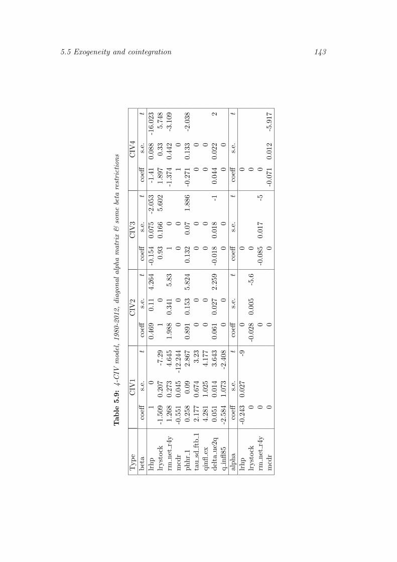
5.5 Exogeneity and cointegration 143
Table
5.9:
4-C
IVm
odel
,1980-2
012,
dia
gon
al
alp
ha
matr
ix&
som
ebe
tare
stri
ctio
ns
Typ
eC
IV1
CIV
2C
IV3
CIV
4
bet
aco
effs.
e.t
coeff
s.e.
tco
effs.
e.t
coeff
s.e.
t
lrh
p1
00.
469
0.11
4.26
4-0
.154
0.07
5-2
.053
-1.4
10.
088
-16.0
23
lryst
ock
-1.5
090.2
07
-7.2
91
00.
930.
166
5.6
02
1.897
0.3
35.7
48
rmn
etr4
y1.2
68
0.273
4.6
45
1.98
80.
341
5.83
10
-1.3
74
0.442
-3.1
09
mcd
r-0
.551
0.0
45
-12.2
44
00
00
10
ph
hr
10.2
58
0.09
2.867
0.89
10.
153
5.82
40.
132
0.07
1.886
-0.2
71
0.133
-2.0
38
tau
sdft
b1
2.1
77
0.674
3.2
30
00
00
0qin
flex
4.2
81
1.025
4.1
77
00
00
00
del
tau
e2q
0.0
51
0.014
3.6
43
0.06
10.
027
2.25
9-0
.018
0.01
8-1
0.044
0.0
22
2q
infl
85-2
.584
1.0
73
-2.4
080
00
00
0
alp
ha
coeff
s.e.
tco
effs.
e.t
coeff
s.e.
tco
effs.
e.t
lrh
p-0
.243
0.0
27
-90
00
lryst
ock
0-0
.028
0.00
5-5
.60
0rm
net
r4y
00
-0.0
850.
017
-50
mcd
r0
00
-0.0
71
0.012
-5.9
17
144 Modelling the Irish housing market
What do these results suggest about the broader economic system within
which house prices existed? Firstly, it is worth stating that the house price re-
lationship revealed through error correction methods above is largely preserved
when analysis is extended to allow for potential endogeneity of other variables.
In addition, three long-run relationships are implied by the analysis carried
about above.
Income/stock relation The ratio of income to housing stock is negatively
associated with user cost, the person-household ratio, real house prices and
changes in unemployment. This suggests that high user cost and growing un-
employment had a stronger effect on income (the numerator) than on supply
(the denominator). The negative relationship between the person-household
ratio and incomes may reflect growing female participation in the labour force
during the period analysed, which would be expected to increase household in-
come, or may reflect an upward trend over time. The negative long-run effect
of prices on the income-stock ratio may indicate a greater supply response –
where prices represent profitability – than income response. As Figure 5.3 sug-
gests, the rise in income/stock from the late 1980s to 2007 and the subsequent
fall is strongly correlated with real house prices. In terms of a housing supply
relationship, future research will be required to include currently omitted vari-
ables such as costs of inputs (land, labour and materials) and planning/permit
conditions.
User-cost relation The user cost (as measured by the real rate of interest) is
positively associated with real house prices (and perhaps changes in unemploy-
ment) and negatively with income/stock and the person-household ratio. The
relationship with house prices may reflect extremely high user cost at a time of
high prices late in the sample. Put another way, since user cost is negatively
related to 4-year house price appreciation, this seems to suggest greater scope
for appreciation when lrhp is low.

5.5 Exogeneity and cointegration 145
Credit/deposit relation The fourth vector says that mcdr rises with lhpr,
user cost and phhr and falls with changes in unemployment but also the
income/stock ratio. The finding in relation to income/stock seems counter-
intuitive but does make sense in terms of a latent variable story. The ratio of
credit to deposits was included in error-correction analysis as a proximate in-
dicator of credit conditions. Suppose instead that both it and real house prices
depend on something further “upstream”, such as international capital market
conditions or sentiment, or the degree of European capital market integration.
Suppose that the underlying relationship in vector 1 is as follows:
lrhp = β0 + β1lrystock + β2rm net r4y + β3phhr + Λ (5.12)
where Λ is a latent variable capturing exogenous credit conditions (normalized
so that its coefficient is 1). Similarly, mcdr = γ0 + γ1Λ + f(X), where X could
include variables such as lrystock, rm net r4y and phhr. Estimating lrhp
using the observable mcdr, rather than the unobserved Λ, thus has a different
interpretation than before. To the extent that lrystock, rm net r4y and phhr
are not major determinants of mcdr, β coefficients may not be that different
using mcdr, rather than Λ, although this would depend on the exact nature of
f(X). The coefficient on lrhp suggests that γ1 may be close to 1.4. Measuring
upstream credit conditions, and how they affect both real house prices and the
credit-deposit ratio, is left to future research.
Additional variables Other factors that could be included in the cointe-
gration analysis include further measures of demographics (for example, the
annual change in the percentage of the population aged 25-34) and the typical
nominal (net) mortgage rate of interest. The inclusion of change in the per-
centage of the population into a model with a diagonal alpha matrix suggests
that this is not a statistically significant determinant of any of the four endoge-
nous variables. Similarly, the inclusion of the log nominal interest rate is not
significant in any of the first three vectors, although it is strongly significant

146 Modelling the Irish housing market
in the fourth (mdcr) vector. The implied sign in the long-run equation is, as
expected, negative. The parameter estimates for the long-run solution for real
house prices with this augmented system are much the same as those reported
in Table 5.8.
In summary, there is clear evidence of a robust house price relationship
and also that house prices respond rapidly to this equation – and not to any
other equations when other variables, such as income/stock, user-cost and the
ratio of credit to deposits are made endogenous. In addition, there is no strong
evidence that any of these other variables responds to the house price relation-
ship, meaning that it is reasonable to assume that these variables are indeed
(weakly) exogenous for purposes of modelling.
5.6 House Price-to-Rent Model
While there are a variety of factors affect house prices, many will also affect
rents, such as incomes, or the ratio of persons to households. The principal
difference is the asset nature of housing. “Dividing through” the house price
equation, in effect, by rents allows the opportunity to look in more detail as
user cost and credit conditions, those aspects unique to the asset nature of
house prices.
As outlined in Section 5.3.2, the scale and nature of the private rented sec-
tor in Ireland has changed substantially over the period 1975-2012. The first
decade or so represents a one-off downward shift in the real cost of renting
in Ireland, while the second decade witnessed continued falls in the total pro-
portion renting. This, combined with reforms of the private rented sector in
the late 1990s, mean that there is little evidence of any error correction in the
price-rent ratio for the period as a whole.14
Taking the period 2000-2012, however, during which there was a relatively
well-developed private rented sector nationwide, there is strong evidence of an
14The extent of any rent controls in the private and State-supported rental sectors is notaddressed here – future research may assess the role of such market interventions.
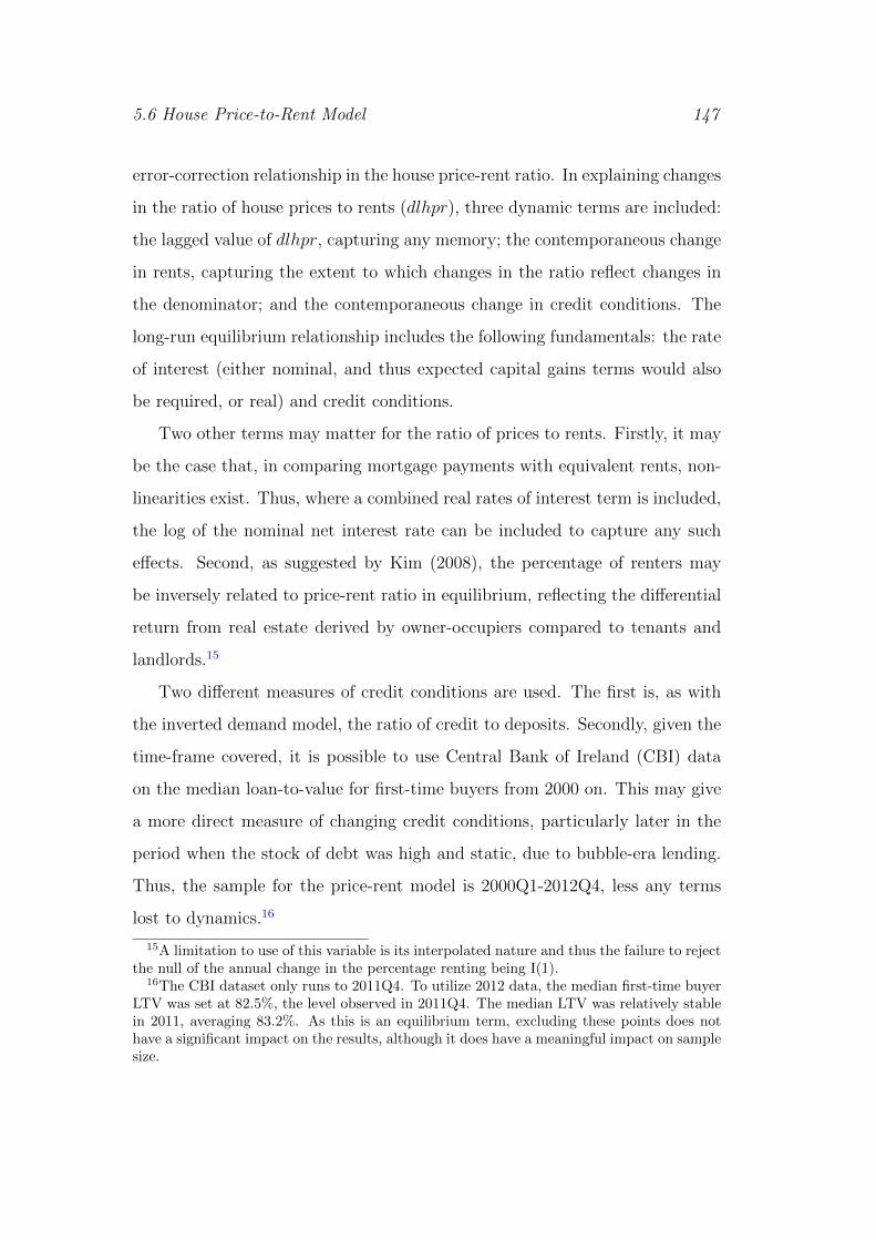
5.6 House Price-to-Rent Model 147
error-correction relationship in the house price-rent ratio. In explaining changes
in the ratio of house prices to rents (dlhpr), three dynamic terms are included:
the lagged value of dlhpr, capturing any memory; the contemporaneous change
in rents, capturing the extent to which changes in the ratio reflect changes in
the denominator; and the contemporaneous change in credit conditions. The
long-run equilibrium relationship includes the following fundamentals: the rate
of interest (either nominal, and thus expected capital gains terms would also
be required, or real) and credit conditions.
Two other terms may matter for the ratio of prices to rents. Firstly, it may
be the case that, in comparing mortgage payments with equivalent rents, non-
linearities exist. Thus, where a combined real rates of interest term is included,
the log of the nominal net interest rate can be included to capture any such
effects. Second, as suggested by Kim (2008), the percentage of renters may
be inversely related to price-rent ratio in equilibrium, reflecting the differential
return from real estate derived by owner-occupiers compared to tenants and
landlords.15
Two different measures of credit conditions are used. The first is, as with
the inverted demand model, the ratio of credit to deposits. Secondly, given the
time-frame covered, it is possible to use Central Bank of Ireland (CBI) data
on the median loan-to-value for first-time buyers from 2000 on. This may give
a more direct measure of changing credit conditions, particularly later in the
period when the stock of debt was high and static, due to bubble-era lending.
Thus, the sample for the price-rent model is 2000Q1-2012Q4, less any terms
lost to dynamics.16
15A limitation to use of this variable is its interpolated nature and thus the failure to rejectthe null of the annual change in the percentage renting being I(1).
16The CBI dataset only runs to 2011Q4. To utilize 2012 data, the median first-time buyerLTV was set at 82.5%, the level observed in 2011Q4. The median LTV was relatively stablein 2011, averaging 83.2%. As this is an equilibrium term, excluding these points does nothave a significant impact on the results, although it does have a meaningful impact on samplesize.
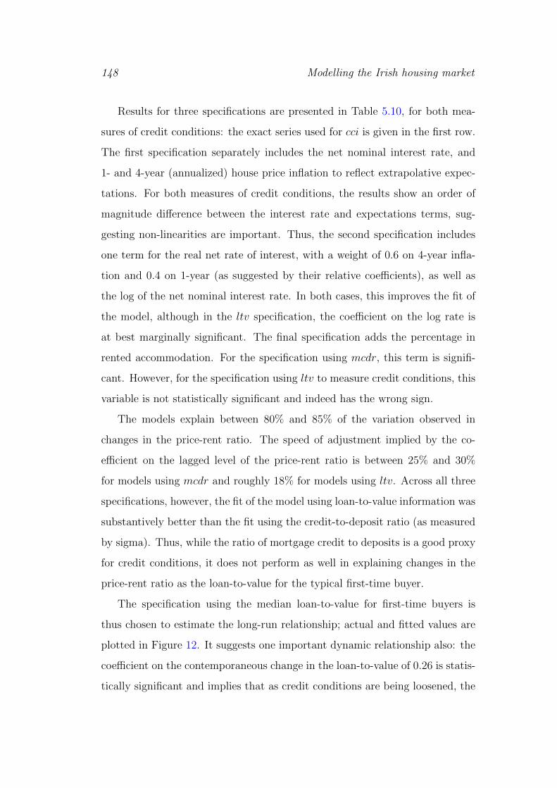
148 Modelling the Irish housing market
Results for three specifications are presented in Table 5.10, for both mea-
sures of credit conditions: the exact series used for cci is given in the first row.
The first specification separately includes the net nominal interest rate, and
1- and 4-year (annualized) house price inflation to reflect extrapolative expec-
tations. For both measures of credit conditions, the results show an order of
magnitude difference between the interest rate and expectations terms, sug-
gesting non-linearities are important. Thus, the second specification includes
one term for the real net rate of interest, with a weight of 0.6 on 4-year infla-
tion and 0.4 on 1-year (as suggested by their relative coefficients), as well as
the log of the net nominal interest rate. In both cases, this improves the fit of
the model, although in the ltv specification, the coefficient on the log rate is
at best marginally significant. The final specification adds the percentage in
rented accommodation. For the specification using mcdr, this term is signifi-
cant. However, for the specification using ltv to measure credit conditions, this
variable is not statistically significant and indeed has the wrong sign.
The models explain between 80% and 85% of the variation observed in
changes in the price-rent ratio. The speed of adjustment implied by the co-
efficient on the lagged level of the price-rent ratio is between 25% and 30%
for models using mcdr and roughly 18% for models using ltv. Across all three
specifications, however, the fit of the model using loan-to-value information was
substantively better than the fit using the credit-to-deposit ratio (as measured
by sigma). Thus, while the ratio of mortgage credit to deposits is a good proxy
for credit conditions, it does not perform as well in explaining changes in the
price-rent ratio as the loan-to-value for the typical first-time buyer.
The specification using the median loan-to-value for first-time buyers is
thus chosen to estimate the long-run relationship; actual and fitted values are
plotted in Figure 12. It suggests one important dynamic relationship also: the
coefficient on the contemporaneous change in the loan-to-value of 0.26 is statis-
tically significant and implies that as credit conditions are being loosened, the
5.6 House Price-to-Rent Model 149
Table 5.10: Modelling changes in the price-rent ratio (dlhpr), 2000-2012
MCDR MCDR (non-lin) MCDR (%rent) LTV LTV (non-lin) LTV (%rent)Coeff p-value Coeff p-value Coeff p-value Coeff p-value Coeff p-value Coeff p-value
Constant 1.296 0.000 1.333 0.000 1.766 0.000 0.732 0.000 0.731 0.000 0.751 0.000lhprt−1 -0.249 0.001 -0.255 0.000 -0.305 0.000 -0.177 0.000 -0.175 0.000 -0.185 0.000ccit−1 0.131 0.007 0.134 0.005 0.219 0.000 0.361 0.000 0.36 0.000 0.362 0.000rmNN
t−1 -3.001 0.000 -1.036 0.04d16lhp annt−1 0.343 0.002 0.211 0.000d4lhpt−1 0.24 0.001 0.126 0.004rrmNR41
t−1 -0.581 0.000 -0.409 0.013 -0.34 0.000 -0.402 0.012l(rmNN
t−1 ) -0.078 0.000 -0.081 0.000 -0.024 0.122 -0.026 0.116pc rentt−1 -1.244 0.025 0.175 0.667dlhprt−1 0.21 0.099 0.228 0.058 0.29 0.015 0.192 0.109 0.186 0.105 0.174 0.141dlrent -0.707 0.000 -0.685 0.000 -0.519 0.001 -0.72 0.000 -0.741 0.000 -0.782 0.000dcci 0.389 0.057 0.466 0.014 0.458 0.012 0.257 0.016 0.261 0.012 0.271 0.012sigma 0.01377 0.01372 0.01307 0.01287 0.0127 0.01283R2 0.819 0.816 0.837 0.842 0.842 0.843p-values for diagnostic testsAR 1-4 0.889 0.917 0.763 0.619 0.632 0.620ARCH 1-4 0.832 0.906 0.979 0.995 0.993 0.988Normality 0.951 0.926 0.947 0.219 0.192 0.197Hetero 0.044** 0.320 0.263 0.061 0.610 0.657Hetero-X NA 0.300 NA NA 0.380 NARESET23 0.175 0.282 0.412 0.152 0.165 0.205
price-rent ratio rises beyond just what is suggested by the long-run coefficient.
The implied long-run relationship from this model is as follows:
ln(hprt) = 4.18 + 2.05ltvt − 1.94rmRN∗t − 0.13ln(rmNN
t ) (5.13)
Credit conditions Credit conditions have a long-run impact on the price-
rent ratio, with the coefficient of 2.05 indicating that an increase of ten percent-
age points in the loan-to-value of the typical first-time buyer was associated
with an increase in ratio of prices to rents of 20.5%. Assuming static rents,
this translates into a 20.5% increase in house prices. Put another way, suppose
average house prices are e170,000 and the average monthly rent is e800; thus
the average gross yield (annual rent relative to prices) is 5.6%. An increase in
the LTV by 10pp is associated with a fall in the yield from 5.6% to 5.2% in
equilibrium. (There would also be a dynamic effect on the price-rent ratio, as
outlined above, in this example of 2.6%, pushing the yield down to 5.0%.)17
17Duca et al. (2011a) use the log form of the loan-to-value for first-time buyers and reporta long-run elasticity of prices with respect to LTV of 1.4. Here, a model with level ofLTV/downpayment (σ = 0.01270) has better fit than one with log LTV (σ = 0.01282),and also performs better than one with log down-payment, which will have different non-linearities (σ = 0.01278). For reference, the implied long-run elasticity of prices with respectto LTV for Ireland 2000-2012 was roughly 1.6, compared to 1.4 in the case of the USA,1980-2007.)

150 Modelling the Irish housing market
Real interest rates Real interest rates for housing – as measured by the
difference between nominal rates after tax reliefs and the expected capital gain
(based on 4-year and 1-year inflation) – are associated with a lower price-rent
ratio, as expected. The coefficient of 1.94 indicates that an increase in real
interest rates of 1 percentage point is associated with an increase in equilibrium
price-rent ratio of 1.94%. This is somewhat larger than the coefficient in the
inverted demand model (1.53).
Nominal interest rates In addition to real interest rates for housing, the
nominal rate may also matter, although its statistical significance is marginal
(potentially a product of the small sample size). A 10% reduction in the nom-
inal after-tax mortgage rate is associated with a 1.3% rise in the price-rent
ratio. This may reflect the cash-flow constraints and the direct choice faced
by would-be first-time buyers of a particular rent or nominal net mortgage
payment.
Robustness & Sensitivity Overall, these results are sensitive to series cho-
sen, due to the small period for which the model is computed. Nonetheless,
largely similar results are obtained if an alternate series for rents (from prop-
erty website daft.ie) is used for the period 2002-2012. Adding other dynamics
does not improve model fit, while using loan-to-income information contained
in the same CBI data is not preferred. Using the DOE series on LTVs for new
dwellings results in a significantly poorer model fit, with neither house price
appreciation term statistically significant and the nominal rate only marginally
significant.
5.7 Decomposition & Analysis
This section decomposes real house price growth in each of six phases from
1975 to 2012 into changes due to the various fundamentals. It also uses the
5.7 Decomposition & Analysis 151
information contained in the inverted demand model to comment on likely
future pressures on Irish house prices.
5.7.1 Decomposing Irish house price growth
Figure 5.8 compares actual with fitted values, using the error-correction model
outlined above to estimate fitted values of house prices. It shows that there were
roughly six phases in the Irish housing market between 1975 and 2012. The
first was from 1975 (the start of quarterly information) until 1979:Q2, during
which real house prices rose 60%, or almost 12% on an annualized basis. The
second finished in 1987:Q2, and between 1979 and 1987, real house prices fell
by 32% (or almost 5% on an annualized basis). Between 1987:Q2 and 1995:Q3,
real house prices rose by 31%, or 3.3% per year on average.
Figure 5.8: Actual and fitted real house prices, national average, 1975-2012
The fourth phase, the period between 1995:Q3 and 2001:Q3, saw the strongest
growth, as real house prices rose by 117%, or 13.7% per year on average. Be-
tween 2001:Q3 and 2007:Q1, when real house prices peaked, there was further
growth of 52%, or just under 8% on an annualized basis. The final phase is
from 2007:Q1 to 2012:Q4 (the end of the time series), during which house prices

152 Modelling the Irish housing market
fell by 52%, or an annual average rate of 12%. The overall picture that emerges
from Figure 5.8 is one where actual house prices rarely deviated substantially
from the level suggested by their long-run determinants, although it should be
noted that these “fundamentals” include unrealistic extrapolative expectations
and potentially unsustainable levels of mortgage credit relative to household
deposits.
Figure 5.9: Annual house price growth attributed to fundamentals, by marketphase, 1975-2012
Figure 5.9 uses the long-run equilibrium relationship for the period 1980-
2012 to decompose Irish house price growth in each of these six phases into
growth driven by each of the five fundamental factors, as well as a proportion
not explained by the long-run component of the model, which can be broken
into dynamic and residual factors. The percentage rates of change in real house
prices are annualized and thus comparable across periods.
Aside from the sheer volatility of house price growth in Ireland during the
period as a whole, two things are striking about the figure. The first is the
large proportion of house price growth in the 1970s not explained by the long-
run component of the model. The second is the nature of house price growth
5.7 Decomposition & Analysis 153
between 2001 and 2007. Unlike the preceding period, where house price growth
appears to have been driven by a mix of factors, including income growth
(relative to the stock of housing) and demographics, growth in real house prices
from 2001 to 2007 was almost entirely driven by credit conditions. Most of the
remainder of the growth in house prices during this period is either due to
short-run dynamics or else is a residual that may be considered a pure bubble
effect. Dynamics and the residual offset a falling ratio of income to housing
stock, due to Ireland’s extraordinary building boom, and a higher real interest
rate (reflecting slower house price growth overall).
5.7.2 Future pressures on Irish house prices
The end of 2012 saw the end of mortgage-interest relief available to first-time
buyers. Based on prevailing interest rates at end-2012, this is the equivalent of
a 0.07 percentage point increase in the interest rate. According to the long-run
coefficient on interest rates, this could be expected to push equilibrium real
house prices down by 1.1%, if the model pertaining to the generation to 2012
were to hold in coming years.
Similarly, the local property tax – levied at 0.18% of the value of a property
– may be thought of in present value terms as the equivalent of an increase
in stamp duty, although this assumes away any deposit constraints associated
with stamp duty. Assuming a discount rate of 5% per annum and a seven-
year horizon for households, this could be expected to lower equilibrium house
prices by 1.7%. It should be noted, however, that it is likely the effect of stamp
duty was through down-payment constraints, while it is also worth stating that
the long-run effect of stamp duty is not precisely estimated, due to the small
number of changes to it during the period analysed.
A final tax issue is one brought up by Browne et al. (2013), namely the
preferential tax treatment of capital gains associated with owner-occupancy.
Given the significance of expected capital gains in the long-run equation of

154 Modelling the Irish housing market
fundamentals determining Irish house prices, it is clear that were a tax liabil-
ity to apply for realised capital gains, this would have the ability to dampen
somewhat the extrapolative nature of the Irish housing market. If the rate of
33% were to apply to principal private residences, this would clearly have an
impact on the user cost calculation of Irish housing market participants.
Related to this, the likely presence of extrapolative expectations suggests
that the user cost associated with housing in Ireland in late 2012 was very high:
the real rate of interest in housing is estimated at over 20% for late 2012. At
some point, this will fall, as the average rate of change in real house prices goes
to zero. If house prices were stable between 2012 and 2016, this alone would
represent an improvement in the user cost of 18 percentage points. Such an
improvement in expectations would – according to the model presented – be
associated with an increase in real house prices of more than 25% – which of
course would feed in itself into house price expectations.
Lastly, there is the issue of credit conditions. As measured, credit conditions
are a linear combination of the level and change in the credit-deposit ratio.
While the coefficient on the change term is nearly twice as large as that on
the level, the scale of the level of roughly two orders of magnitude larger (for
example, between 2000 and 2007, the average value of mcdr was 1.4, while for
dmcdr it was 0.026). Thus, as measured, credit conditions remained in late 2012
quite loose by historical standards: the linear combination of mcdr+ 1.78dmcr
stood at 1.69 in late 2012, down from 1.87 in 2007 but well above the pre-2000
average of 0.74. If a measure that gives greater weight to stocks than flows
proves too sticky to capture marginal credit conditions, the typical loan-to-
value (as highlighted by the model of the price-rent ratio) may be a better
indicator in the future. Nonetheless, the question of how Irish banks will fund
their loan books in the future – in particular the balance between internal
deposits and external financing – is relevant for the future path of Irish house
prices.
5.7 Decomposition & Analysis 155
5.7.3 Could the bubble have been prevented?
Understanding the determinants of house prices is a key concern for policy-
makers, particularly with greater focus now on macro-prudential policy and
tracking financial conditions other than the Central Bank interest rate. The
analysis undertaken above can be used – however tentatively – to give in-
sights into the potential scale of impact of particular kinds of policy measures.
Three alternative scenarios, based on the long-run relation implied by the error-
correction model, are presented in Figure 5.10, alongside nominal house prices
during the period 1980-2012. These are meant as thought experiments, rather
than predicted counterfactuals, as the dynamics between house price and other
variables, such as housing stock, are for simplicity not included.
The first, Scenario 1, simulates house prices where the real user cost is ad-
justed to include a Capital Gains Tax of 33% on principal primary residences.18
This line closely matches actual house prices, although it is worth noting that
both the bubble and the crash are slightly attenuated. At the margins, there-
fore, this is evidence from static simulations to suggest that a tax on profit
from home-ownership may have smoothed the housing market cycle.
However, even with a tax on gains, the bulk of the housing bubble and crash
would likely still have occurred. Scenario 2 presents simulated house prices in a
situation where macro-prudential policy restricted the ratio of mortgage credit
to deposits of 80%. This policy measure would have prevented Irish banks
from engaging in any substantial bond-financing of mortgages upon entry into
the eurozone. There is a noticeable impact on the run-up of house prices
between 1995 and 2007. The increase in prices in Scenario 2 is 180%, just
over half the increase actually seen (350%). Clearly, a fuller understanding of
the determinants of the credit-deposit ratio within a multi-equation system –
including house prices themselves – may change the magnitude of this result,
but this offers a useful starting point for the impact of credit on house prices.
18For the purposes of simulation, the tax is assumed to have been introduced in 1980:Q1.No further feedback, for example through diminished down-payments, is included.

156 Modelling the Irish housing market
A more likely policy would be a cap on loans-to-value, as was implemented in
Hong Kong. Given the lack of a long-running series on loan-to-value, however,
this is not possible here. Nonetheless, the ratio of credit to deposits can be
thought of as similar to a system-wide loan-to-value.
Figure 5.10: Actual and scenario house prices, national average, 1980-2012
The fall in house prices from the peak in Scenario 2 is still substantial.
This indicates that while credit conditions were key to driving up prices, they
have not played a significant role in the crash. This, of course, assumes the
exogeneity of factors such as housing supply. If the significant easing of credit
conditions stimulated a supply response, its absence would alter the ratio of
income to stock, thereby affecting the level of real house prices.
The final scenario, Scenario 3, replaces one simplistic calculation of expec-
tations – whatever happened in recent years is the best guide to the near future
– with another: the empirical evidence is that in the long run, house price in-
creases match but rarely exceed inflation. That is, user cost is calculated as net
interest rates minus average consumer price inflation over the last four years,
instead of net interest rates minus average house price inflation. As can be

5.8 Conclusion 157
seen in Figure 5.10, this has a far greater impact on prices falls than preceding
price rises. Whereas prices are estimated to still have increased by a factor of
four, the fall from the peak is 26%, rather than 50%.
Thus, the preliminary evidence from the bubble and crash in Ireland is that
both macro-prudential regulation of mortgage products and ensuring consumer
expectations are well-educated are important tools in the policymakers fight
against destructive housing market cycles.
5.8 Conclusion
This chapter has examined the housing market in Ireland from the mid-1970s
until 2012, with a particular focus on the bubble that peaked in 2007 and
the crash that followed. Following a growing literature that focuses on the
role of credit conditions, a readily available measure of credit conditions was
included, the ratio of mortgage credit to deposits, one with both early and
more recent antecedents in the Irish housing market literature, which proved
highly significant in both inverted demand and price-rent models of the Irish
housing market.
The error-correction model developed for the Irish housing market for the
period 1980-2012 found that there were four principal fundamentals that deter-
mined the long-run equilibrium level of real house prices: the ratio of income
to the housing stock, the ratio of persons to households, the ratio of mortgage
credit to deposits, and the user cost, as measured by difference between net
nominal mortgage interest rates and the annualized 4-year rate of house price
inflation. In addition, it seems likely that the rate of stamp duty was important
for the level of house prices, while other factors mattered for short-run changes
in house prices, in particular conditions in the labour and mortgage markets.
An error-correction approach assumes that variables such as the four fun-
damentals described above are exogenous when looking at the housing market.
This was tested thoroughly, allowing the income/stock ratio, user-cost and also
158 Modelling the Irish housing market
the credit-deposit ratio to be endogenous, and allowing up to four cointegrat-
ing vectors across the system. Analysis showed the house price relationship
that emerged from single-equation ECM analysis was largely robust as was the
speed of adjustment by house prices to this equation. The analysis also found
that prices did not respond to any other cointegrating vectors. In addition,
there is no strong evidence that any of these other variables responds to the
house price relationship, although as house prices enters other cointegrating
vectors, there would be important feedbacks.
For much of the early period analysed, the rental market in Ireland was
in secular decline. From the mid-1990s, though, the proportion in rented ac-
commodation started to grow, and there is significant evidence of an error-
correction relationship in the price-rent ratio for the period 2000-2012. The
long-run relationship between prices and rents is more parsimonious than for
prices alone, with the user cost and credit conditions the most important fac-
tors. Here, user cost is the net interest rate less a combination of 1-year and
4-year inflation, with potential non-linearities applying in relation to the nom-
inal rate of interest. Credit conditions were measured in two ways: firstly, the
ratio of credit to deposits, as above, and secondly, using a new dataset of typi-
cal loan-to-value rates for first-time buyers from 2000 on. While both measures
capture significant variation in the sample, the LTV measure performs better,
reflecting the importance of including the change in the credit-deposit ratio, as
well as the level.
In both models, credit conditions matter, both for the long-run solution and
for short-run dynamics. An increase in the credit-deposit ratio of 10 percentage
points was associated with a 5.6% increase in equilibrium house prices but also
a 1.7% short-run effect in the following quarter. Similarly, an increase of ten
percentage points in the typical first-time buyer LTV was associated with an
increase in the long-run price-rent ratio of 20.5%, as well as a short-run effect
of 2.6%. This suggests that previous studies of the Irish housing market have

5.8 Conclusion 159
suffered from omitted variable bias, attempting to model prices but without
accounting for credit conditions.
Indeed, a decomposition of Irish house price growth from 1975 to 2012 into
its various phases highlights the importance of credit conditions in the last
phase of Ireland’s bubble. Whereas house price growth between 1995 and 2001
was due to a combination of factors, including rising income relative to housing
stock, lower real interest rates, demographics and credit conditions, during the
2001-2007 period, looser credit conditions were responsible for 7.5 percentage
points of growth per annum on average, at a time when annual growth was
7.9%. While incomes were rising during this period, the housing stock rose
faster, to the extent that the ratio of income to stock was actually a drag on
prices during this time and became a major factor in the post-2007 period.
The demographic variable included in the inverted demand model – the ratio
of persons to households – is one rarely commented on in the recent literature,
but it is a largely common-sense variable: a population of 4 million with four
to a house will demand fewer houses and occupy less land than a population
with three to a house. Previous studies, not just for Ireland, that focus solely
on income (relative to supply) may be overstating the effect, if part of the effect
is actually a greater spread of the population. With an ageing population and
smaller family units, it is likely that this variable will continue to put upward
pressure on prices over the coming decade, even if income pressures are weak.
Of note in both models, but in particular in the inverted demand approach,
is the speed with which real house prices in Ireland during this period adjusted
to a new equilibrium. The principal specification suggests that almost one third
of the gap between actual and equilibrium prices was closed every quarter. In
this sense, Ireland’s bubble was not an irrational bubble in the housing mar-
ket, marked by prices deviating significantly from fundamentals. Rather, the
analysis here suggests that Ireland’s bubble was one step further up: it was the
“fundamentals” themselves – in particular credit conditions and expectations
– that had deviated from sustainable levels. However, given the extrapolative

160 Modelling the Irish housing market
nature of expectations of capital gains, one should not regard expectations as
a true fundamental: they are ultimately driven by all the shocks that drive
house prices. The extrapolative nature of these expectations generates a natu-
ral mechanism for house price to overshoot on both upside and downside. How
policy can prevent this recurring, for example tracking expectations with regu-
lar surveys to warn about future problems, should be an active topic of future
research and policy analysis.

Chapter 6
Conclusions
6.1 Contributions to the literature
With the overall objective of a better understanding of the economics of hous-
ing market cycles, this thesis has focused in detail on Ireland, the location
of the most extreme housing bubble and crash of the Great Moderation and
subsequent Global Financial Crisis. Through developing a range of research
questions and stylised facts and then exploring those in subsequent chapters, a
number of insights have emerged, which make contributions to the literature.
While the economic theory underpinning what happens to the spread of
property values in a housing market cycle remains under-developed, two com-
peting predictions emerge from the literature. According to Stein (1995), down-
payment constraints make high-value properties more volatile than low-value
ones. Costello (2000), however, suggests that if more affordable homes are more
liquid and thus more competitive, then these segments may be more volatile
over the boom/bust cycle. The research presented here – in particular in Chap-
ters 2 and 3 – is the first to examine which is most likely to have been at work
in the Irish market. Chapter 2 did this through a uniquely granular perspective
that divided the Irish market into over 1,100 sub-markets. Chapter 3 did this
by exploiting a wealth of data on location-specific amenities.
In both chapters, there is little evidence of a Stein effect, where high value
properties are more volatile, proportionately rising more in the bubble and
161
162 Conclusions
falling more in the crash. Looking at particular property types, it is certainly
the case that the opposite happened, while there was also evidence of counter-
cyclical pricing of core housing market amenities, such as commute time, dis-
tance to CBD and proximity to train stations and the coastline. Another con-
tribution of chapter 3 is the presentation of results for the lettings segment of
the market, which has mostly been ignored in the literature on amenities. For
almost all amenities analysed, compared to the price premium, there was an
attenuated rent effect (i.e. a smaller premium or discount in absolute terms).
As suggested by the renter search threshold mechanism, the notable exception
is distance from the CBD, which actually is valued in percentage terms more
by renters than owners.
Another heretofore unaddressed issue in the literature on the accuracy of
valuations is that seller and buyer valuations date from different periods. Chap-
ter 4 addressed this by decomposing the gap between list and sale prices into
its constituent processes. The results not only overcome some of the obstacles
to assessing valuation accuracy but also reconcile two pieces of conventional
wisdom about the housing market and also present a number of metrics that
may yield insights into market conditions.
The Irish housing market has been the subject of a number of economic
studies over the last generation but the vast majority have omitted a treat-
ment of credit conditions while the econometric techniques vary, with the more
advanced econmetrically until now imposing a long-run relationship using a
two-step Engle-Granger method. Chapter 5 overcame both these issues, in-
cluding a readily available measure of credit conditions while also allowing the
long-run relationship to emerge from house price dynamics. The resulting equa-
tion explained the path of Irish house prices from 1980 to 2012, highlighting
also a much neglected factor that may be relevant to other economies, namely
the ratio of persons to households. Using a new series of loan-to-value for
the median first-time-buyer from 2000 on, this chapter also outlined the first
error-correction model of the price-rent ratio in the Irish economy.

6.2 Insights for policymakers 163
6.2 Insights for policymakers
There are obvious uses for much of the analysis undertaken in this thesis. The
difference in house price falls by size and type will be of use not only for real
estate professionals and valuers but also for Irish financial institutions; much
of the work on recapitalising the Irish financial system assumed – implicitly –
that price falls would be equal across property types and sizes but this is far
from the case. The estimation of price and rent effects of a range of location-
specific amenities is relevant for local authorities in estimating property tax
revenues and burdens, as well as for valuers, homeowners and landlords. The
resilience of – and indeed growth in – the value of many non-market amenities
will equally be of interest.
However, there are also insights of a broader relevance. As conditions in a
housing market heat up, the Irish experience indicates that this may be seen
in narrowing differentials between high-quality and low-quality housing, as a
“property ladder” concern affects expectations and actions in the housing mar-
ket (see Chapters 2 and 3). While such effects may not dominate over “lock-in
concerns” in all housing markets, the Irish experience does offer another sug-
gestion for the macro-prudential dashboard, as policymakers seek to establish
a tool-kit for managing not only the price level of goods but also of assets, in
particular housing.
Related to this, Chapter 4 indicates that readily and freely available datasets,
such as those made available through the Internet, are appropriate for policy
analysis. In general, price trends derived from large datasets of list prices are
extremely highly correlated with those from transactions. Where analysis of
both is possible, policymakers may derive insights from the cyclical properties
of the ratio of average list prices and average sale prices, as shown with the
counteroffer spread developed earlier.
One of the main results from chapter 5 was that actual prices tracked their
fitted values very closely, even at the height of what would be termed the Irish

164 Conclusions
housing bubble in 2006-07. This is not to suggest that there was no bubble
in Irish house prices, but rather that while Ireland’s housing market appears
to have been very efficient throughout the period 1980-2012, its determinants
include not only slow-to-change fundamentals such as hosuehold incomes, de-
mographics and the stock of housing but also factors much more prone to
dramatic adjustment, including credit conditions and expectations about the
future, a key ingredient of user cost.
Two broad themes have emerged from the thesis. The first is the importance
of consumer expectations in the housing market. The increase in user cost
alone between 2007 and 2012 is estimated to have lowered real house prices
by roughly 40% and this is due not to changing interest rates but to changing
expectations about future house prices, although clearly these were driven by
negative shocks to other fundamentals such as income. Secondly, as other
research has highlighted, non-price conditions in the credit market are pivotal
in understanding developments in the housing market. The relevance of these
insights is, to borrow medical terminology, in both diagnosis and prevention of
housing bubbles.
As macro-prudential policy matures and develops, the findings here suggest
that two of the most important things to measure in assessing the risk of a
housing price bubble, are consumer expectations, which if unrealistic may drive
house prices to unsustainable levels, and the typical loan-to-value for first-time
buyers, which is directly related to leverage and risk in housing. These are not
yet a priority for policymakers, however, with neither featuring in EU, OECD
or national statistics. Ironically, given the resource cost of preparing so many
economic indicators, these are remarkably easy to measure – metrics of both
have been presented in this research.
In terms of preventing bubbles, there is of course no solution to what is
the by-product of intrinsically human behaviour. However, there is significant
potential to minimise housing bubbles and their subsequent economic cost. In
relation to expectations, the obvious treatment is consumer education. It was a
6.2 Insights for policymakers 165
cliche in Ireland before-2007 that house prices only went one way, even though
long-run counter-evidence existed – for Ireland as well as for other economies.
It is possible that assessments of financial literacy will become part of mortgage
approval in the future; assessing the realism of expectations should be central
to that.
Behavioural economics may be able to contribute on whether methods ex-
ist to reveal what those applying for a mortgage expect to happen housing in
the future: financial literacy tests may be too easy to game or alternatively
attentional bias may mean that making such expectations explicit does in fact
alter behaviour. Successfully done, this would not only identify the level of
expectations but also their rationale, which could be assessed by those respon-
sible for macro-prudential policy. A range of initiatives by policymakers in
developed countries already aim to shape household behaviour in relation to
their decisions, for example in relation to exercise, diet, consumption of alcohol
and tobacco, and pensions. Efforts to educate consumers about their dominant
consumption good and asset would thus not be out of place.
In relation to credit conditions, policy implications are probably more straight-
forward. A maximum loan-to-value – as was introduced in Hong Kong after a
bubble there – would help prevent a repeat of the worst excesses of Irish hous-
ing bubble. Just as with measuring loan-to-value, an acyclical downpayment
constraint is easy to introduce. As the severe Irish bubble and crash show,
preventing the next bubble would be far preferable to cleaning it up.

166 Conclusions

Bibliography
Addison-Smyth, D., McQuinn, K. & O’Reilly, G. (2009), ‘Modelling credit inthe Irish mortgage market’, Economic and Social Review 40(4), 371–392.
Alonso, W. (1964), Location and land use: toward a general theory of landrent, Vol. 204, Harvard University Press Cambridge, MA.
Banzhaf, H. S. & Farooque, O. (2012), Interjurisdictional housing prices andspatial amenities: Which measures of housing prices reflect local publicgoods?, Working Paper 17809, National Bureau of Economic Research.URL: http://www.nber.org/papers/w17809
Barham, G. (2004), The effects of taxation policy on the cost of capital inhousing–a historical profile (1976 to 2003), in ‘Financial Stability Report’,Central Bank of Ireland, pp. 89–101.
Barrell, R. & Davis, E. (2007), ‘Financial liberalisation, consumption andwealth effects in seven OECD countries’, Scottish Journal of PoliticalEconomy 54(2), 254–267.
Bayer, P., McMillan, R., Murphy, A. & Timmins, C. (2011), A dynamicmodel of demand for houses and neighborhoods, Working Paper 17250,National Bureau of Economic Research.
Berry, J., McGreal, S., Stevenson, S., Young, J. & Webb, J. (2003),‘Estimation of apartment submarkets in Dublin, Ireland’, Journal of RealEstate Research 25(2), 159–170.
Black, S. (1999), ‘Do Better Schools Matter? Parental Valuation ofElementary Education’, Quarterly Journal of Economics 114(2), 577–599.
Bourassa, S. C., Hoesli, M., Scognamiglio, D. F. & Sormani, P. (2008),Constant-quality house price indexes for Switzerland, Research PaperSeries 08-10, Swiss Finance Institute.
Bourassa, S., Hoesli, M. & Sun, J. (2004), ‘What’s in a view?’, Environmentand Planning 36, 1427–1450.
167

168 BIBLIOGRAPHY
Boyle, M. & Kiel, K. (2001), ‘A survey of house price hedonic studies of theimpact of environmental externalities’, Journal of Real Estate Literature9(2), 117–144.
Browne, F., Conefrey, T. & Kennedy, G. (2013), Understanding Irish houseprice movements – a user cost of capital approach, Research TechnicalPaper 04RT13, Central Bank of Ireland.
Case, K. E. & Shiller, R. J. (1990), ‘Forecasting prices and excess returns inthe housing market’, Real Estate Economics 18(3), 253–273.
Case, K. & Mayer, C. (1996), ‘Housing price dynamics within a metropolitanarea’, Regional Science and Urban Economics 26(3-4), 387–407.
Case, K. & Shiller, R. (1989), ‘The Efficiency of the Market for Single-FamilyHomes’, American Economic Review 79(1), 125–37.
Case, K. & Shiller, R. (1994), ‘A decade of boom and bust in the prices ofsingle-family homes: Boston and Los Angeles, 1983 to 1993’, New EnglandEconomic Review 5(2), 40–51.
Central Statistics Office (2013), ‘Census 2011 reports’.http://www.cso.ie/en/census/census2011boundaryfiles/ (accessedFebruary 19, 2013).
Cheshire, P. & Sheppard, S. (1995), ‘On the price of land and the value ofamenities’, Economica pp. 247–267.
Coate, S. (2013), Evaluating durable public good provision using housingprices, NBER Working Paper Series WP18767, National Bureau ofEconomic Research.
Commission for Communications Regulation (2013), ‘Comreg siteviewer’.http://www.askcomreg.ie/mobile/siteviewer.273.LE.asp (accessedFebruary 15, 2013).
Conniffe, D. & Duffy, D. (1999), ‘Irish house price indices: Methodologicalissues’, Economic and Social Review 30(4), 403–424.
Cook, R. (2000), ‘Detection of influential observation in linear regression’,Technometrics 42(1), 65–68.
Costello, G. J. (2000), ‘Pricing size effects in housing markets’, Journal ofProperty Research 17(3), 203–219.
Crosby, N. (2000), ‘Valuation accuracy, variation and bias in the context ofstandards and expectations’, Journal of Property Investment & Finance18(2), 130–161.

BIBLIOGRAPHY 169
Daft.ie (2012), 2012 Consumer Attitudes Survey, Technical report, Daft.ie.URL: http://blog.daft.ie/2012/02/daft-ie-release-inaugural-consumer-attitudes-survey/
Debrezion, G., Pels, E. & Rietveld, P. (2007), ‘The impact of railway stationson residential and commercial property value: A meta-analysis’, TheJournal of Real Estate Finance and Economics 35, 161–180.URL: http://dx.doi.org/10.1007/s11146-007-9032-z
Deng, Y., McMillen, D. P. & Sing, T. F. (2012), ‘Private residential priceindices in Singapore: a matching approach’, Regional Science and UrbanEconomics 42(3), 485–494.
Department of Education (2013), ‘Search for a school’.http://www.education.ie/home/home.jsp?pcategory=
10917&ecategory=12016&language=EN (accessed February 15, 2013).
Department of the Environment, Community & Local Government (2013a),‘myplan.ie’. http://www.myplan.ie/en/index.html (accessed February15, 2013).
Department of the Environment, Community & Local Government (2013b),‘National housing development survey, 2011’. http://www.environ.ie/en/DevelopmentHousing/Housing/UnfinishedHousingDevelopments/
(accessed February 15, 2013).
DG ECFIN (2013), AMECO database, Technical report, EuropeanCommission Directorate General for Economic and Financial Affairs.
Dicks, M. J. (1990), A simple model of the housing market, EconomicsDivision Discussion Paper 49, Bank of England.
DiPasquale, D. & Somerville, C. (1995), ‘Do house price indices based ontransacting units represent the entire stock? evidence from the americanhousing survey’, Journal of Housing Economics 4(3), 195–229.
Dorsey, R. E., Hu, H., Mayer, W. J. & Wang, H.-c. (2010), ‘Hedonic versusrepeat-sales housing price indexes for measuring the recent boom-bustcycle’, Journal of Housing Economics 19(2), 75–93.
Dubin, R. & Sung, C. (1987), ‘Spatial variation in the price of housing: rentgradients in non-monocentric cities’, Urban Studies 24(3), 193–204.
Duca, J., Muellbauer, J., Murata, K. & Murphy, A. (2010), Credit, HousingCollateral and Consumption: Evidence from the UK, Japan and the US,Technical Report 1002, Federal Reserve Bank of Dallas.

170 BIBLIOGRAPHY
Duca, J. V., Muellbauer, J. & Murphy, A. (2011a), ‘House Prices and CreditConstraints: Making Sense of the US Experience’, Economic Journal121(552), 533–551.
Duca, J. V., Muellbauer, J. & Murphy, A. (2011b), Shifting credit standardsand the boom and bust in u.s. house prices, Working Papers 1104, FederalReserve Bank of Dallas.
Dunse, N., Jones, C. & White, M. (2010), ‘Valuation accuracy and spatialvariations in the efficiency of the property market’, Journal of EuropeanReal Estate Research 3(1), 24–45.
Eichholtz, P., Straetmans, S. & Theebe, M. (2012), ‘The Amsterdam RentIndex: The Housing Market and the Economy, 1550-1850’, Journal ofHousing Economics 21(4), 269–282.
Ellen, I. (2012), Economics of Housing Market Segmentation, in S. J. Smith,ed., ‘International Encyclopedia of Housing and Home’, Elsevier, pp. 51–54.
Environmental Protection Agency (2013a), ‘Corine land cover data’.http://www.epa.ie/downloads/data/corinedata/ (accessed February15, 2013).
Environmental Protection Agency (2013b), ‘Licensing & permitting’.http://www.epa.ie/whatwedo/licensing/files/ (accessed February 15,2013).
European Environment Agency (2013), ‘Gmes urban atlas’.http://www.eea.europa.eu/data-and-maps/data/urban-atlas
(accessed February 15, 2013).
Faller, G. (2011), ‘Feeder schools in the republic of ireland’. Provided viaemail correspondence.
Fernandez-Corugedo, E. & Muellbauer, J. (2006), Consumer credit conditionsin the United Kingdom, Working Paper 314, Bank of England.
Fleming, M. & Nellis, J. (1985), ‘The application of hedonic indexingmethods: a study of house prices in the united kingdom’, StatisticalJournal of the United Nations 3, 249–270.
Fraser, P., Hoesli, M. & McAlevey, L. (2012), ‘House prices, disposableincome and permanent and temporary shocks: The nz, uk and usexperience’, Journal of European Real Estate Research 5, 5–28.
Gallin, J. (2008), ‘The long-run relationship between house prices and rents’,Real Estate Economics 36(4), 635–658.

BIBLIOGRAPHY 171
Gatzlaff, D. H. & Tirtiroglu, D. (1995), ‘Real estate market efficiency: issuesand evidence’, Journal of Real Estate Literature 3(2), 157–189.
Gatzlaff, D. & Haurin, D. (1998), ‘Sample selection and biases in local housevalue indices’, Journal of Urban Economics 43(2), 199–222.
Genesove, D. & Mayer, C. (2001), ‘Loss aversion and seller behavior:Evidence from the housing market’, Quarterly Journal of Economics116(4), 1233–1260.
Geofabrik.de (2013), ‘Openstreetmap’. http://www.openstreetmap.org/(accessed February 15, 2013).
Gerlach, S. & Peng, W. (2005), ‘Bank lending and property prices in hongkong’, Journal of Banking & Finance 29(2), 461–481.
Gibbons, S. & Machin, S. (2003), ‘Valuing English primary schools’, Journalof Urban Economics 53(2), 197–219.
Gibbons, S. & Machin, S. (2005), ‘Valuing rail access using transportinnovations’, Journal of Urban Economics 57(1), 148–169.
Gibbons, S. & Machin, S. (2008), ‘Valuing school quality, better transport,and lower crime: evidence from house prices’, Oxford Review of EconomicPolicy 24(1), 99.
Glaeser, E., Kolko, J. & Saiz, A. (2001), ‘Consumer city’, Journal of economicgeography 1(1), 27.
Glaeser, E. L., Gottlieb, J. D. & Tobio, K. (2012), ‘Housing booms and citycenters’, American Economic Review 102(3), 127–33.URL: http://ideas.repec.org/a/aea/aecrev/v102y2012i3p127-33.html
Goodman, J. L. & Ittner, J. B. (1992), ‘The accuracy of home owners’estimates of house value’, Journal of Housing Economics 2(4), 339–357.
Grebler, L., Blank, D. M. & Winnick, L. (1956), Capital Formation inResidential Real Estate: Trends and Prospects, Princeton University Press.
Halvorsen, R. & Palmquist, R. (1980), ‘The interpretation of dummy variablesin semilogarithmic equations’, American Economic Review 70(3), 474–75.
Harbo, I., Johansen, S., Nielsen, B. & Rahbek, A. (1998), ‘Asymptoticinference on cointegrating rank in partial systems’, Journal of Business &Economic Statistics 16(4), 388–399.
Harmon, C. & Hogan, V. (2000), Econometric Analysis of the HousingMarket and Projections of Future Developments, in P. Bacon &F. MacCabe, eds, ‘The Housing Market in Ireland: An EconomicEvaluation of Trends & Prospects’, Government of Ireland Publications.

172 BIBLIOGRAPHY
Harrison, D., T. Smersh, G. & Schwartz, A. (2001), ‘Environmentaldeterminants of housing prices: the impact of flood zone status’, Journal ofReal Estate Research 21(1), 3–20.
Harzing, A. (2007), ‘Publish or perish’. http://www.harzing.com/pop.htm(accessed February 15, 2012).
Haurin, D., McGreal, S., Adair, A., Brown, L. & Webb, J. R. (2013), ‘Listprice and sales prices of residential properties during booms and busts’,Journal of Housing Economics 22, 1–10.
Hilber, C. & Mayer, C. (2009), ‘Why do households without children supportlocal public schools? Linking house price capitalization to school spending’,Journal of Urban Economics 65(1), 74–90.
Hirayama, Y. (2005), ‘Running hot and cold in the urban home-ownershipmarket: the experience of japans major cities’, Journal of Housing and theBuilt Environment 20(1), 1–20.
Holly, S. & Jones, N. (1997), ‘House prices since the 1940s: Cointegration,demography and asymmetries’, Economic Modelling 14(4), 549 – 565.
IMF (2003), Ireland: 2003 Article IV Consultation–Staff Report; StaffSupplement; and Public Information Notice on the Executive BoardDiscussion for Ireland, Country Report 03/242, International MonetaryFund.
Jaffee, D. M., Rosen, K. T., Friedman, B. M. & Klein, L. R. (1979),‘Mortgage credit availability and residential construction’, BrookingsPapers on Economic Activity 1979(2), 333–386.
Jud, D. G. & Seaks, T. G. (1994), ‘Sample selection bias in estimatinghousing sales prices’, Journal of Real Estate Research 9(3), 289–298.
Kahneman, D. (2011), Thinking, fast and slow, Farrar, Straus and Giroux.
Kenneally, M. F. & McCarthy, J. V. (1982), ‘A Preliminary EconometricInvestigation of the Irish Housing Market’, Economic and Social Review14(1), 41–69.
Kennedy, G. & McIndoe-Calder, T. (2011), The Irish Mortgage Market:Stylised Facts, Negative Equity and Arrears, Research Technical Paper12RT11, Central Bank of Ireland.
Kennedy, G. & McQuinn, K. (2011), Scenarios for Irish House Prices,Economic Letters 2011:2, Central Bank of Ireland.
Kennedy, G. & McQuinn, K. (2012), Why are Irish house prices still falling?,Economic Letters 2012:5, Central Bank of Ireland.

BIBLIOGRAPHY 173
Kenny, G. (1999), ‘Modelling the demand and supply sides of the housingmarket: evidence from Ireland’, Economic Modelling 16(3), 389–409.
Kiel, K. A. & Zabel, J. E. (1999), ‘The accuracy of owner-provided housevalues: The 1978–1991 american housing survey’, Real Estate Economics27(2), 263–298.
Kim, Y. (2008), Rent-price ratios and the earnings yield on housing, mimeo,University of South Carolina.URL: http://www-rcf.usc.edu/ yongkim/housingApril08.pdf
Knight, J., Dombrow, J. & Sirmans, C. (1995), ‘A varying parametersapproach to constructing house price indexes’, Real Estate Economics23(2), 187–205.
Kuminoff, N., Parmeter, C. & Pope, J. (2010), ‘Which hedonic models can wetrust to recover the marginal willingness to pay for environmentalamenities?’, Journal of Environmental Economics and Management60, 145–160.
Leamer, E. E. (2007), Housing IS the Business Cycle, NBER Working Papers13428, National Bureau of Economic Research, Inc.
Linneman, P. (1980), ‘Some empirical results on the nature of the hedonicprice function for the urban housing market’, Journal of Urban Economics8(1), 47–68.
Luckett, S. (2001), Did You Know? Homes Account for 44 Percent of AllWealth - Findings from the SIPP, Report, U.S. Department of Commerce.
Maclennan, D. (1977), ‘Some thoughts on the nature and purpose of houseprice studies’, Urban Studies 14(1), 59–71.
Malpezzi, S. (2003), Hedonic pricing models: A selective and applied review,in T. OSullivan & K. Gibb, eds, ‘Housing Economics and Public Policy:Essays in honour of Duncan Maclennan’, Blackwell Science, pp. 67–89.
Matysiak, G. & Wang, P. (1995), ‘Commercial property market prices andvaluations: analysing the correspondence’, Journal of Property Research12(3), 181–202.
Mayor, K., Lyons, S., Duffy, D. & Tol, R. (2008), A Hedonic Analysis of theValue of Rail Transport in the Greater Dublin Area, Technical Report 264,Economic & Social Research Institute.
Mayor, K., Lyons, S., Duffy, D. & Tol, R. (2009), A Hedonic Analysis of theValue of Parks and Green Spaces in the Dublin Area, Technical Report 331,Economic & Social Research Institute.

174 BIBLIOGRAPHY
McMillen, D. P. (2008), ‘Changes in the distribution of house prices overtime: Structural characteristics, neighborhood, or coefficients?’, Journal ofUrban Economics 64(3), 573–589.
McQuinn, K. (2004), A Model of the Irish Housing Sector, Research TechnicalPapers 1/RT/04, Central Bank of Ireland.
McQuinn, K. & O’Reilly, G. (2008), ‘Assessing the role of income and interestrates in determining house prices’, Economic modelling 25(3), 377–390.
Meen, G. P. (1990), ‘The removal of mortgage market constraints and theimplications for econometric modelling of UK house prices’, Oxford Bulletinof Economics and Statistics 52(1), 1–23.
Miller, N. & Sklarz, M. (1986), ‘A note on leading indicators of housingmarket price trends’, Journal of Real Estate Research 1(1), 99–109.
Muellbauer, J. (2012), When is a housing market overheated enough tothreaten stability?, in A. Heath, F. Packer & C. Windsor, eds, ‘PropertyMarkets and Financial Stability’, Reserve Bank of Australia and the Bankfor International Settlements, pp. 73–105.
Muellbauer, J. & Williams, D. (2011), Credit conditions and the realeconomy: the elephant in the room, Discussion Paper DP8386, CEPR.
Murphy, A. (1998), Econometric Modelling of the Irish Housing Market, inP. Bacon, F. MacCabe & A. Murphy, eds, ‘An Economic Assessment ofRecent House Price Developments’, Government of Ireland Publications.
Murphy, A. (2005), Modelling Irish House Prices: A Review and Some NewResults, Working Papers Dec, Nuffield College.
Murphy, A. & Brereton, F. (2001), Modeling Irish House Prices: A Review, in‘Irish Economic Association Annual Conference’.
National Monuments Service (2013), ‘Archaeological survey database’.http://www.archaeology.ie/ArchaeologicalSurveyDatabase/
(accessed February 15, 2013).
National Parks & Wildlife Service (2013), ‘Npws maps and data’.http://www.npws.ie/mapsanddata/ (accessed February 15, 2013).
Natural Earth Project (2013), ‘Natural earth data’.http://www.naturalearthdata.com/downloads/10m-raster-data/
10m-cross-blend-hypso/ (accessed February 15, 2013).
NavTeq (2012), ‘Irish road network data’. Accessed in capacity as VisitingResearcher at the National Institute for Regional & Spatial Analysis, NUIMaynooth. http://www.navteq.com/ (accessed February 15, 2013).

BIBLIOGRAPHY 175
Office of the Garda Commissioner (2011), ‘Location of police stations inireland’. Provided via email correspondence.
O’Hanlon, N. (2011), ‘Constructing a national house price index for Ireland’,Journal of the Statistical and Social Inquiry Society of Ireland 40, 167–196.
O’Rourke, K. H. & Polak, B. (1991), Property transactions in Ireland,1708-1988: an introduction, UCD Centre for Economic Research WorkingPaper Series WP92/12, University College Dublin School of Economics.
Pollakowski, H. (1995), ‘Data sources for measuring house price changes’,Journal of Housing Research 6, 377–388.
Poterba, J. (1984), ‘Tax subsidies to owner-occupied housing: an asset-marketapproach’, The Quarterly Journal of Economics 99(4), 729–752.
Poterba, J. (1992), ‘Taxation and housing: Old questions, new answers’, TheAmerican Economic Review 82(2), 237–242.
Rae, D. & van den Noord, P. (2006), ‘Ireland’s Housing Boom: What hasDriven it and Have Prices Overshot?’, OECD Economics DepartmentWorking Papers .
Railway Procurement Agency (2012), ‘Irish rail network data’.http://www.rpa.ie/en/Pages/default.aspx (accessed February 15,2013).
RICS Policy Unit (2002), Land Value and Public Transport: Stage 1 –Summary of Findings, in ‘Paper presented at RICS Cutting EdgeConference’, Vol. 5, p. 7.
Roche, M. (2004), ‘Will there be a Crash in Irish House Prices?’, QuarterlyEconomic Commentary 2003(4), 1–16.
Roche, M. J. (2001), ‘The rise in house prices in Dublin: bubble, fad or justfundamentals’, Economic Modelling 18(2), 281–295.
Rosen, S. (1974), ‘Hedonic prices and implicit markets: product differentiationin pure competition’, The Journal of Political Economy 82(1), 34–55.
Shiller, R. (2005), Irrational Exuberance, Princeton University Press.
Shimizu, C., Nishimura, K. G. & Watanabe, T. (2012), House prices frommagazines, realtors,and the land registry, in Bank for InternationalSettlements, ed., ‘Property markets and financial stability’, Vol. 64, Bankfor International Settlements, pp. 29–38.URL: http://EconPapers.repec.org/RePEc:bis:bisbpc:64-06
Sinai, T. & Souleles, N. (2005), ‘Owner-Occupied Housing as a Hedge AgainstRent Risk’, Quarterly Journal of Economics 120(2), 763–789.

176 BIBLIOGRAPHY
Smith, B. & Tesarek, W. (1991), ‘House prices and regional real estate cycles:Market adjustments in Houston’, Real Estate Economics 19(3), 396–416.
Smith, V. & Huang, J. (1995), ‘Can markets value air quality? Ameta-analysis of hedonic property value models’, Journal of politicalEconomy 103(1), 209–227.
Stein, J. (1995), ‘Prices and trading volume in the housing market: A modelwith down-payment effects’, Quarterly Journal of Economics110(2), 379–406.
Stevenson, S. (2003), Economic, demographic & fiscal influences on housingmarket dynamics, UCD Centre for Real Estate Research Working PaperSeries, University College Dublin School of Economics.
Stevenson, S. (2004), ‘House price diffusion and inter-regional andcross-border house price dynamics’, Journal of Property Research21(4), 301–320.
Stevenson, S. (2008), ‘Modeling housing market fundamentals: Empiricalevidence of extreme market conditions’, Real Estate Economics 36(1), 1–29.
Straszheim, M. (1987), ‘The theory of urban residential location’, Handbookof regional and urban economics 2, 717–757.
The Economist (2011), ‘Clicks and mortar: Our interactive overview of globalhouse prices and rents’. http://www.economist.com/blogs/freeexchange/2011/03/global_house_prices (accessed June 28, 2012).
Thom, D. R. (1983), ‘House prices, inflation and the mortgage market’,Economic and Social Review 15(1), 57–68.
Von Thunen, J. (1863), Isolated state, Pergamon Press.
Wallace, N. & Meese, R. (1997), ‘The construction of residential housing priceindices: a comparison of repeat-sales, hedonic-regression, and hybridapproaches’, Journal of Real Estate Finance and Economics 14(1), 51–73.
Warnock, F. E. & Warnock, V. C. (2012), Developing housing financesystems, in A. Heath, F. Packer & C. Windsor, eds, ‘Property Markets andFinancial Stability’, Reserve Bank of Australia and the Bank forInternational Settlements, pp. 49–67.
Wrigley, M., Wyatt, P. & Lane, C. (2001), Transport policy and propertyvalues, in ‘Paper presented at RICS Cutting Edge Conference’, Vol. 5, p. 7.

Appendices
177


.1 Appendix material for Chapter 2 179
.1 Appendix material for Chapter 2
.1.1 Regression output for Chapter 2
On the following pages is an overview of the regression output for the five mod-els outlined in Section 2.2, for both sales and lettings segments. For each model,coefficients and p-values are shown for variables. The naming of variables isexplained in Table 2.2.
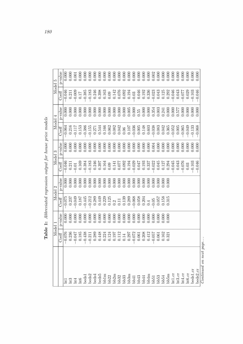
180
Table
1:
Abb
revi
ate
dre
gres
sion
ou
tpu
tfo
rhou
sepri
cem
odel
s
Mod
el1
Mod
el2
Mod
el3
Mod
el4
Mod
el5
Coeff
p-v
alu
eC
oeff
p-v
alu
eC
oeff
p-v
alu
eC
oeff
p-v
alu
eC
oeff
p-v
alu
eht1
−0.0
760.
000−
0.0
75
0.000−
0.0
46
0.000−
0.0
64
0.000−
0.0
46
0.000
ht3
0.2
360.
000
0.2
37
0.000
0.2
11
0.000
0.2
16
0.000
0.2
11
0.000
ht4
−0.0
470.
000−
0.0
49
0.000−
0.0
10.
000−
0.1
17
0.000−
0.0
09
0.001
ht6
0.1
850.
000
0.1
87
0.000
0.1
69
0.000
0.1
53
0.000
0.1
70.
000
bed
s1−
0.4
380.
000−
0.4
45
0.000−
0.3
84
0.000−
0.3
86
0.000−
0.3
85
0.000
bed
s2−
0.2
110.
000−
0.2
12
0.000−
0.1
83
0.000−
0.1
55
0.000−
0.1
83
0.000
bed
s40.2
890.
000
0.2
89
0.000
0.2
46
0.000
0.2
71
0.000
0.2
46
0.000
bed
s50.4
480.
000
0.4
49
0.000
0.3
97
0.000
0.5
44
0.000
0.3
98
0.000
bb
1m0.2
240.
000
0.2
29
0.000
0.1
64
0.000
0.1
66
0.000
0.1
63
0.000
bb
220.1
240.
000
0.1
25
0.000
0.0
90.
000
0.0
62
0.000
0.0
90.
000
bb
2m0.1
970.
000
0.2
0.000
0.1
41
0.000
0.0
82
0.000
0.1
42
0.000
bb
320.1
120.
000
0.1
10.
000
0.0
77
0.000
0.0
42
0.000
0.0
76
0.000
bb
330.1
40.
000
0.1
39
0.000
0.0
92
0.000
0.0
60.
000
0.0
92
0.000
bb
3m0.2
970.
000
0.2
89
0.000
0.1
94
0.000
0.1
07
0.005
0.1
94
0.000
bb
41−
0.0
720.
000−
0.0
68
0.000−
0.0
29
0.000−
0.0
36
0.000−
0.0
30.
000
bb
430.0
610.
000
0.0
58
0.000
0.0
47
0.000
0.0
05
0.55
0.0
46
0.000
bb
440.2
080.
000
0.2
04
0.000
0.1
93
0.000
0.1
48
0.000
0.1
92
0.000
bb
4m0.4
120.
000
0.4
0.000
0.3
37
0.000
0.6
03
0.000
0.3
36
0.000
bb
51−
0.0
570.
000−
0.0
50.
000−
0.0
22
0.004−
0.0
38
0.354−
0.0
23
0.002
bb
530.0
610.
000
0.0
57
0.000
0.0
45
0.000
0.0
83
0.003
0.0
43
0.000
bb
540.1
620.
000
0.1
58
0.000
0.1
27
0.000
0.0
42
0.241
0.1
25
0.000
bb
5m0.3
210.
000
0.3
15
0.000
0.2
94
0.000
0.3
65
0.000
0.2
92
0.000
ht1
cr−
0.0
45
0.000−
0.0
52
0.000−
0.0
46
0.000
ht3
cr0.0
43
0.000
0.0
05
0.577
0.0
43
0.000
ht4
cr−
0.0
76
0.000−
0.0
65
0.000−
0.0
77
0.000
ht6
cr0.0
30.
000−
0.0
49
0.000
0.0
29
0.000
bed
s1cr
−0.1
03
0.000−
0.1
33
0.000−
0.1
03
0.000
bed
s2cr
−0.0
46
0.000−
0.0
68
0.000−
0.0
46
0.000
Con
tin
ued
on
nex
tpa
ge..
.
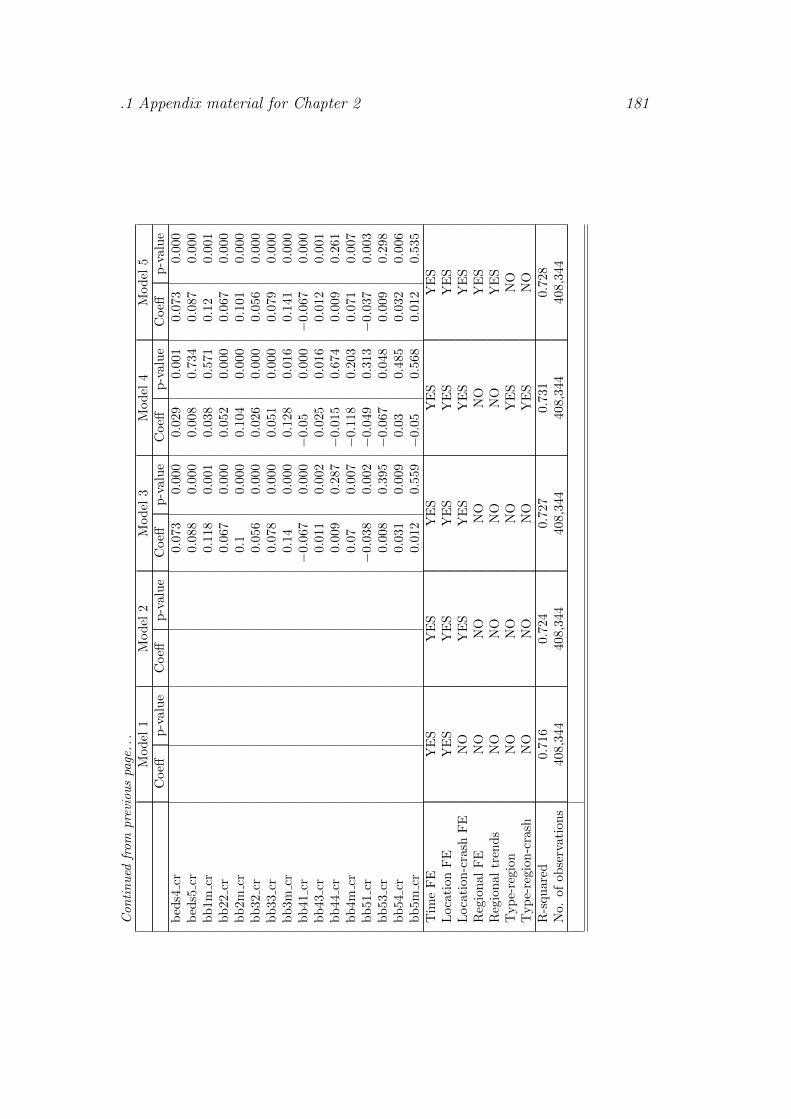
.1 Appendix material for Chapter 2 181
Con
tin
ued
from
pre
viou
spa
ge..
.M
od
el1
Mod
el2
Mod
el3
Mod
el4
Mod
el5
Coeff
p-v
alu
eC
oeff
p-v
alu
eC
oeff
p-v
alu
eC
oeff
p-v
alu
eC
oeff
p-v
alu
eb
eds4
cr0.0
73
0.000
0.0
29
0.001
0.0
73
0.000
bed
s5cr
0.0
88
0.000
0.0
08
0.734
0.0
87
0.000
bb
1mcr
0.1
18
0.001
0.0
38
0.571
0.1
20.
001
bb
22cr
0.0
67
0.000
0.0
52
0.000
0.0
67
0.000
bb
2mcr
0.1
0.000
0.1
04
0.000
0.1
01
0.000
bb
32cr
0.0
56
0.000
0.0
26
0.000
0.0
56
0.000
bb
33cr
0.0
78
0.000
0.0
51
0.000
0.0
79
0.000
bb
3mcr
0.1
40.
000
0.1
28
0.016
0.1
41
0.000
bb
41cr
−0.0
67
0.000−
0.0
50.
000−
0.0
67
0.000
bb
43cr
0.0
11
0.002
0.0
25
0.016
0.0
12
0.001
bb
44cr
0.0
09
0.287−
0.0
15
0.674
0.0
09
0.261
bb
4mcr
0.0
70.
007−
0.1
18
0.203
0.0
71
0.007
bb
51cr
−0.0
38
0.002−
0.0
49
0.313−
0.0
37
0.003
bb
53cr
0.0
08
0.395−
0.0
67
0.048
0.0
09
0.298
bb
54cr
0.0
31
0.009
0.0
30.
485
0.0
32
0.006
bb
5mcr
0.0
12
0.559−
0.0
50.
568
0.0
12
0.535
Tim
eF
EY
ES
YE
SY
ES
YE
SY
ES
Loca
tion
FE
YE
SY
ES
YE
SY
ES
YE
SL
oca
tion
-cra
shF
EN
OY
ES
YE
SY
ES
YE
SR
egio
nal
FE
NO
NO
NO
NO
YE
SR
egio
nal
tren
ds
NO
NO
NO
NO
YE
ST
yp
e-re
gion
NO
NO
NO
YE
SN
OT
yp
e-re
gion
-cra
shN
ON
ON
OY
ES
NO
R-s
qu
ared
0.71
60.7
24
0.7
27
0.7
31
0.7
28
No.
ofob
serv
atio
ns
408,
344
408,3
44
408,3
44
408,3
44
408,3
44

182
Table
2:
Abb
revi
ate
dre
gres
sion
ou
tpu
tfo
rre
nta
lm
odel
s
Mod
el1
Mod
el2
Mod
el3
Mod
el4
Mod
el5
Coeff
p-v
alu
eC
oeff
p-v
alu
eC
oeff
p-v
alu
eC
oeff
p-v
alu
eC
oeff
p-v
alu
ep
t20.
004
0.00
00.
005
0.000−
0.009
0.000−
0.001
0.578−
0.009
0.000
pt4
−0.
216
0.00
0−
0.215
0.000−
0.217
0.000−
0.201
0.000−
0.217
0.000
bed
s1−
0.34
10.
000−
0.342
0.000−
0.367
0.000−
0.382
0.000−
0.366
0.000
bed
s2−
0.18
20.
000−
0.182
0.000−
0.18
0.000−
0.203
0.000−
0.18
0.000
bed
s40.
154
0.00
00.
154
0.000
0.17
0.000
0.204
0.000
0.17
0.000
bed
s50.
281
0.00
00.
28
0.000
0.311
0.000
0.386
0.000
0.311
0.000
bb
1m0.
085
0.00
00.
084
0.000
0.027
0.091
0.025
0.149
0.025
0.104
bb
220.
074
0.00
00.
074
0.000
0.066
0.000
0.075
0.000
0.066
0.000
bb
2m0.
119
0.00
00.
119
0.000
0.107
0.000
0.116
0.000
0.106
0.000
bb
320.
059
0.00
00.
058
0.000
0.055
0.000
0.059
0.000
0.055
0.000
bb
330.
082
0.00
00.
082
0.000
0.074
0.000
0.085
0.000
0.074
0.000
bb
3m0.
193
0.00
00.
192
0.000
0.213
0.000
0.303
0.000
0.213
0.000
bb
41−
0.05
30.
000−
0.052
0.000−
0.054
0.000−
0.078
0.000−
0.054
0.000
bb
430.
036
0.00
00.
036
0.000
0.03
0.000
0.035
0.000
0.031
0.000
bb
440.
144
0.00
00.
143
0.000
0.148
0.000
0.167
0.000
0.149
0.000
bb
4m0.
302
0.00
00.
302
0.000
0.295
0.000
0.422
0.000
0.295
0.000
bb
510.
009
0.36
0.009
0.365
0.089
0.000
0.193
0.000
0.089
0.000
bb
530.
065
0.00
00.
065
0.000
0.082
0.000
0.119
0.000
0.083
0.000
bb
540.
177
0.00
00.
175
0.000
0.187
0.000
0.234
0.000
0.189
0.000
bb
5m0.
312
0.00
00.
311
0.000
0.286
0.000
0.36
0.000
0.286
0.000
b1
s−
0.17
70.
000−
0.178
0.000−
0.201
0.000−
0.217
0.000−
0.201
0.000
b2
0s0.
055
0.00
00.
054
0.000
0.053
0.000
0.063
0.000
0.053
0.000
b2
2s−
0.09
60.
000−
0.096
0.000−
0.066
0.000−
0.085
0.000−
0.066
0.000
b3
0s0.
072
0.00
00.
072
0.000
0.079
0.000
0.107
0.000
0.079
0.000
b3
2s−
0.01
80.
000−
0.017
0.000−
0.014
0.000−
0.022
0.000−
0.015
0.000
b4
0s0.
112
0.00
00.
111
0.000
0.153
0.000
0.266
0.000
0.153
0.000
b4
1s0.
019
0.00
00.
018
0.000
0.03
0.000
0.064
0.000
0.03
0.000
b4
3s0.
007
0.10
70.
007
0.12
0.017
0.02
0.002
0.836
0.015
0.036
Con
tin
ued
on
nex
tpa
ge..
.
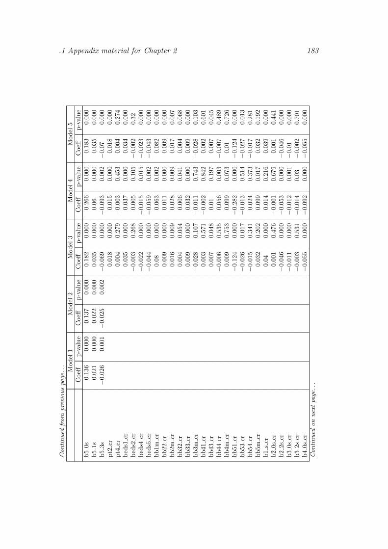
.1 Appendix material for Chapter 2 183
Con
tin
ued
from
pre
viou
spa
ge..
.M
od
el1
Mod
el2
Mod
el3
Mod
el4
Mod
el5
Coeff
p-v
alu
eC
oeff
p-v
alu
eC
oeff
p-v
alu
eC
oeff
p-v
alu
eC
oeff
p-v
alu
eb
50s
0.13
60.
000
0.137
0.000
0.182
0.000
0.266
0.000
0.183
0.000
b5
1s0.
021
0.00
00.
022
0.000
0.035
0.000
0.06
0.000
0.035
0.000
b5
3s−
0.02
60.
001−
0.025
0.002−
0.069
0.000−
0.093
0.002−
0.07
0.000
pt2
cr0.
018
0.000
0.015
0.000
0.018
0.000
pt4
cr0.
004
0.279−
0.003
0.453
0.004
0.274
bed
s1cr
0.035
0.000
0.037
0.000
0.034
0.000
bed
s2cr
−0.
003
0.268
0.005
0.105−
0.002
0.32
bed
s4cr
−0.
022
0.000−
0.015
0.015−
0.023
0.000
bed
s5cr
−0.
044
0.000−
0.059
0.002−
0.043
0.000
bb
1mcr
0.08
0.000
0.063
0.002
0.082
0.000
bb
22cr
0.009
0.000
0.011
0.000
0.009
0.000
bb
2mcr
0.016
0.009
0.028
0.009
0.017
0.007
bb
32cr
0.004
0.054
0.006
0.041
0.004
0.068
bb
33cr
0.009
0.000
0.032
0.000
0.009
0.000
bb
3mcr
−0.
028
0.107−
0.011
0.743−
0.028
0.103
bb
41cr
0.003
0.571−
0.002
0.842
0.002
0.601
bb
43cr
0.007
0.048
0.01
0.197
0.007
0.045
bb
44cr
−0.
006
0.535
0.056
0.003−
0.007
0.489
bb
4mcr
0.009
0.753
0.099
0.073
0.01
0.726
bb
51cr
−0.
124
0.000−
0.282
0.000−
0.124
0.000
bb
53cr
−0.
026
0.017−
0.013
0.514−
0.027
0.013
bb
54cr
−0.
015
0.341
0.024
0.373−
0.017
0.281
bb
5mcr
0.032
0.202
0.099
0.017
0.032
0.192
b1
scr
0.04
0.000
0.014
0.216
0.039
0.000
b2
0scr
0.001
0.476−
0.001
0.679
0.001
0.441
b2
2scr
−0.
046
0.000−
0.053
0.000−
0.046
0.000
b3
0scr
−0.
011
0.000−
0.012
0.001−
0.01
0.000
b3
2scr
−0.
003
0.531−
0.014
0.03
−0.
002
0.701
b4
0scr
−0.
055
0.000−
0.092
0.000−
0.055
0.000
Con
tin
ued
on
nex
tpa
ge..
.

184
Con
tin
ued
from
pre
viou
spa
ge..
.M
od
el1
Mod
el2
Mod
el3
Mod
el4
Mod
el5
Coeff
p-v
alu
eC
oeff
p-v
alu
eC
oeff
p-v
alu
eC
oeff
p-v
alu
eC
oeff
p-v
alu
eb
41s
cr−
0.015
0.000−
0.031
0.000−
0.016
0.000
b4
3scr
−0.
015
0.101−
0.005
0.776−
0.014
0.141
b5
0scr
−0.
059
0.000−
0.042
0.076−
0.059
0.000
b5
1scr
−0.
016
0.157
0.001
0.952−
0.016
0.149
b5
3scr
0.063
0.000
0.087
0.011
0.064
0.000
Tim
eF
EY
ES
YE
SY
ES
YE
SY
ES
Fac
ilit
ies
YE
SY
ES
YE
SY
ES
YE
SF
acil
itie
s-cr
ash
NO
NO
YE
SY
ES
YE
SF
acil
itie
s-re
gion
sN
ON
ON
OY
ES
NO
Fac
ilit
ies-
regi
ons-
cras
hN
ON
ON
OY
ES
NO
Loca
tion
FE
YE
SY
ES
YE
SY
ES
YE
SL
oca
tion
-cra
shF
EN
OY
ES
YE
SY
ES
YE
SR
egio
nal
FE
NO
NO
NO
NO
YE
SR
egio
nal
tren
ds
NO
NO
NO
NO
YE
ST
yp
e-re
gion
NO
NO
NO
YE
SN
OT
yp
e-re
gion
-cra
shN
ON
ON
OY
ES
NO
R-s
qu
ared
0.77
70.7
80
0.7
82
0.7
91
0.7
82
No.
ofob
serv
atio
ns
7049
53704953
704953
704953
704953

.1 Appendix material for Chapter 2 185
.1.2 Heatmaps of list prices and rents in Ireland 2012
The following pages outline “heatmaps” of the variation in like-for-like listprices and rents, across Ireland, for 2012:II, and of the change in prices andrents between 2007:II and 2012:II. An interactive mapping tool, based on thisresearch, is available at Daft.ie/AIRO Property Value Heatmaps.
The maps are based on weighted average prices, where the basket consistsof five properties: a one-bedroom apartment, a two-bedroom terraced house,a three-bedroom semi-detached house, a four-bedroom bungalow, and a five-bedroom detached house. (In the lettings segment, the type distinction isbetween apartments and houses only.) The weights for each of the five propertytypes are an unweighted average of the prevalence of each bedroom size in thesales and lettings segments. Based on this, the weight associated with one-and five-bedroom properties is 6%, while the weights for two-, three- and four-bedroom properties are 27%, 36% and 24% respectively.

186
Figure
1:
Ave
rage
ask
ing
pri
ces
for
pro
pert
yin
Irel
an
dby
dis
-tr
ict,
2012:I
IFigure
2:
Fall
inave
rage
ask
ing
pri
ces
bydis
tric
t,2007:I
I-2012:I
I

.1 Appendix material for Chapter 2 187
Figure
3:
Ave
rage
adve
rtis
edre
nt
inIr
elan
dby
dis
tric
t,2012:I
IFigure
4:
Fall
inave
rage
adve
rtis
edre
nt
bydis
tric
t,2007:I
I-2012:I
I
188
.2 Appendix material for Chapter 3
.2.1 Amenity controls
Where possible, controls are included for the class of a particular amenity. Forexample, the effect on prices of proximity to a lake may be different for smalllakes and large lakes, while the effect of proximity to post-primary schools mayvary with the proportion of students at those schools that progresses to highereducation. Table 3 describes the type controls that apply to various amenitiesanalysed and also describes any region controls. Numbers refer to cut-offs withthe control being the middle category; for example, with forests, the control isforests of 50-100 hectares, with variables (indicator variables interacted withany relevant measures of distance) for less than 30, 30-50, 100-200 and morethan 200.
The table also outlines regional controls. For most variables to which thisapply, they are based on the five broad regions described in Section 3.3.6.For urban green space, they refer to a more refined set of regional markets:six regions within Dublin (central, north city, south city, north county, southcounty and west); each of the other four cities (Cork, Galway, Limerick andWaterford); Dublin’s commuter counties; and all other parts of Ireland.
Table 4 outlines the standard deviation of each of the score-based amenities.These are used to construct price and other effects, as described in the text.
.2.2 Effect of amenities on accommodation costs
Figures 5-8 indicate the estimated effect, in percent, on prices and rents ofmoving a property from 1km away to 100m away from an amenity (or similar;see text).
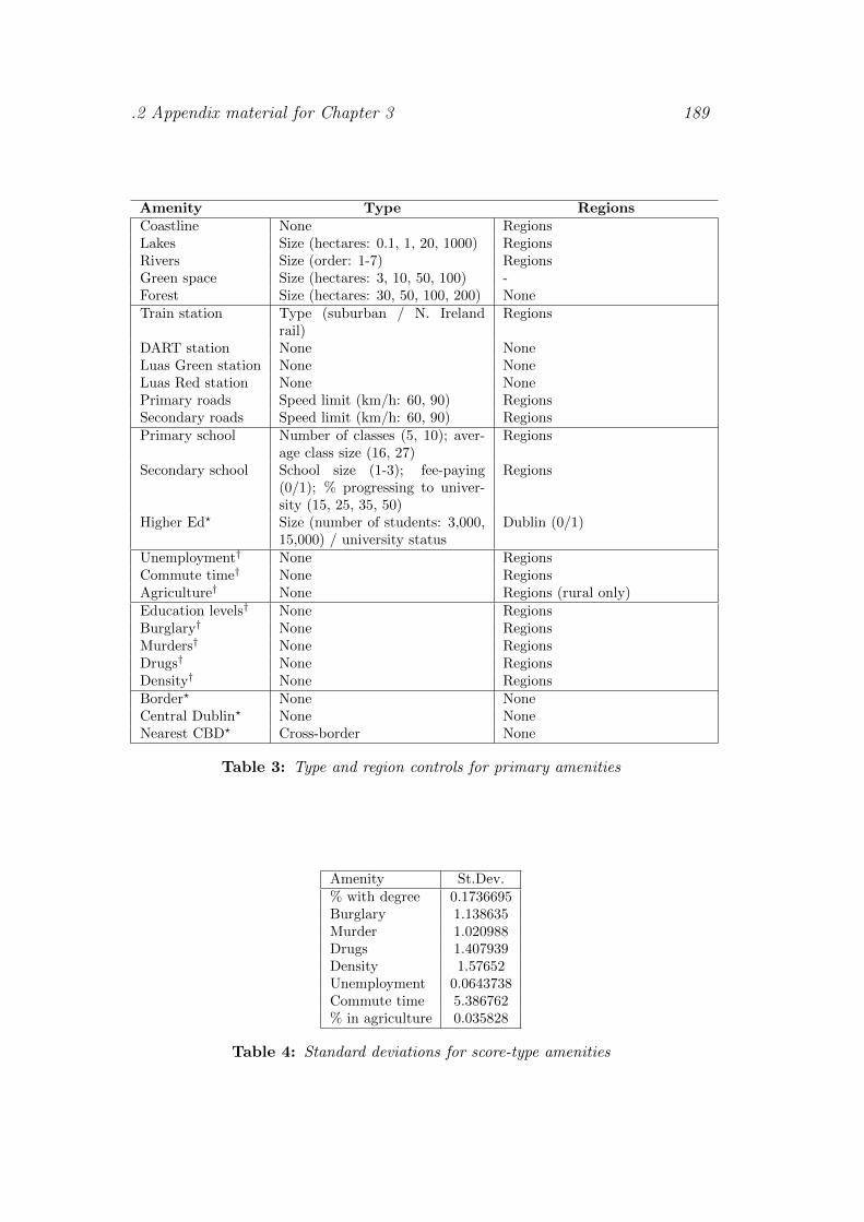
.2 Appendix material for Chapter 3 189
Amenity Type RegionsCoastline None RegionsLakes Size (hectares: 0.1, 1, 20, 1000) RegionsRivers Size (order: 1-7) RegionsGreen space Size (hectares: 3, 10, 50, 100) -Forest Size (hectares: 30, 50, 100, 200) NoneTrain station Type (suburban / N. Ireland
rail)Regions
DART station None NoneLuas Green station None NoneLuas Red station None NonePrimary roads Speed limit (km/h: 60, 90) RegionsSecondary roads Speed limit (km/h: 60, 90) RegionsPrimary school Number of classes (5, 10); aver-
age class size (16, 27)Regions
Secondary school School size (1-3); fee-paying(0/1); % progressing to univer-sity (15, 25, 35, 50)
Regions
Higher Ed? Size (number of students: 3,000,15,000) / university status
Dublin (0/1)
Unemployment† None RegionsCommute time† None RegionsAgriculture† None Regions (rural only)Education levels† None RegionsBurglary† None RegionsMurders† None RegionsDrugs† None RegionsDensity† None RegionsBorder? None NoneCentral Dublin? None NoneNearest CBD? Cross-border None
Table 3: Type and region controls for primary amenities
Amenity St.Dev.% with degree 0.1736695Burglary 1.138635Murder 1.020988Drugs 1.407939Density 1.57652Unemployment 0.0643738Commute time 5.386762% in agriculture 0.035828
Table 4: Standard deviations for score-type amenities

190
Figure 5: Effect of moving from 1km to 100m away, by segment, natural ameni-ties
Figure 6: Effect of moving from 1km to 100m away, by segment, transport ameni-ties

.2 Appendix material for Chapter 3 191
Figure 7: Effect of moving from 1km to 100m away (†: 5km to 1km), by segment,education & agglomeration amenities
Figure 8: Effect of one standard deviation change, by segment, neighbourhood &employment amenities

192
.3 Appendix material for Chapter 4
Table 5 presents the regression output associated with the models and empir-ical specification presented in Section 4.4 above. The variables terr, det andapart/apt refer to the following house types respectively, where semi-detachedis the control: terraced, detached and apartment. Regions 2, 3 and 4 refer toLeinster (ex-Dublin), Munster and Connacht-Ulster repectively.

.3 Appendix material for Chapter 4 193Table
5:
Reg
ress
ion
ou
tpu
t:fo
ur
spre
ads
Lis
tin
gs
Lis
tin
gs
(SA
)S
ale
-agee
dV
alu
ati
on
sD
raw
dow
ns
Coeff
p-v
alu
eC
oeff
p-v
alu
eC
oeff
p-v
alu
eC
oeff
p-v
alu
eC
oeff
p-v
alu
eD
ub
lin
0.4
65
00.4
62
00.4
41
00.4
63
00.4
62
0M
eath
0.0
85
00.1
05
00.1
00.0
66
00.0
65
0K
ild
are
0.1
21
00.1
57
00.1
45
00.1
21
00.1
21
0W
icklo
w0.2
89
00.2
93
00.2
93
00.2
59
00.2
59
0L
on
gfo
rd−
0.3
71
0−
0.4
12
0−
0.4
01
0−
0.4
01
0−
0.3
99
0O
ffaly
−0.1
61
0−
0.1
98
0−
0.1
83
0−
0.2
09
0−
0.2
08
0W
estm
eath
−0.1
63
0−
0.1
87
0−
0.1
90
−0.1
80
−0.1
75
0L
aois
−0.2
45
0−
0.2
60
−0.2
65
0−
0.2
35
0−
0.2
36
0C
arl
ow
−0.1
87
0−
0.1
89
0−
0.1
87
0−
0.2
19
0−
0.2
19
0K
ilken
ny
−0.1
18
0−
0.1
20
−0.1
27
0−
0.1
50
−0.1
51
0W
ate
rford
−0.0
71
0−
0.1
02
0−
0.1
14
0−
0.1
21
0−
0.1
20
Wex
ford
−0.1
40
−0.1
91
0−
0.1
85
0−
0.1
92
0−
0.1
94
0K
erry
−0.1
40
−0.1
47
0−
0.1
35
0−
0.1
66
0−
0.1
66
0C
ork
0.0
56
00.1
30
0.1
15
00.0
85
00.0
84
0C
lare
−0.1
27
0−
0.1
23
0−
0.1
29
0−
0.1
52
0−
0.1
54
0L
imer
ick
−0.1
36
0−
0.0
91
0−
0.0
96
0−
0.1
84
0−
0.1
84
0T
ipp
erary
−0.2
41
0−
0.2
54
0−
0.2
48
0−
0.2
58
0−
0.2
58
0G
alw
ay
−0.0
62
00.0
40
0.0
40
−0.0
48
0−
0.0
50
Mayo
−0.3
21
0−
0.3
19
0−
0.3
11
0−
0.3
09
0−
0.3
08
0R
osc
om
mon
−0.4
12
0−
0.4
33
0−
0.4
34
0−
0.3
49
0−
0.3
48
0S
ligo
−0.2
50
−0.2
19
0−
0.2
13
0−
0.2
35
0−
0.2
36
0L
eitr
im−
0.3
96
0−
0.4
25
0−
0.4
10
−0.3
63
0−
0.3
65
0D
on
egal
−0.3
24
0−
0.3
89
0−
0.3
87
0−
0.3
79
0−
0.3
78
0C
avan
−0.2
77
0−
0.2
84
0−
0.2
73
0−
0.2
95
0−
0.2
93
0M
on
agh
an
−0.1
83
0−
0.1
63
0−
0.1
40
−0.1
87
0−
0.1
88
0q12006
−0.0
94
0−
0.1
20
−0.1
26
0q22006
−0.0
65
0−
0.0
67
0−
0.0
74
0q32006
−0.0
27
0−
0.0
38
0−
0.0
35
0q42006
−0.0
14
0−
0.0
07
0.1
92−
0.0
06
0.3
78−
0.0
16
0−
0.0
15
0q22007
0.0
19
00.0
06
0.2
59
0.0
12
0.0
69
0.0
14
00.0
09
0.0
08
q32007
0.0
21
00.0
12
0.0
33
0.0
09
0.1
86
0.0
16
00.0
20
q42007
0.0
14
00.0
15
0.0
17
0.0
24
0.0
01
0.0
23
00.0
20
q12008
0.0
14
00.0
07
0.2
75
0.0
13
0.0
66
0.0
14
00.0
19
0q22008
−0.0
12
0−
0.0
07
0.2
28
0.0
29
00.0
03
0.3
09
0.0
15
0q32008
−0.0
41
0−
0.0
50
−0.0
02
0.7
83−
0.0
28
0−
0.0
07
0.0
54
q42008
−0.0
96
0−
0.1
11
0−
0.0
02
0.7
99−
0.0
62
0−
0.0
39
0q12009
−0.1
36
0−
0.1
62
0−
0.0
59
0−
0.1
44
0−
0.1
12
0Continued
onnextpa
ge..
.
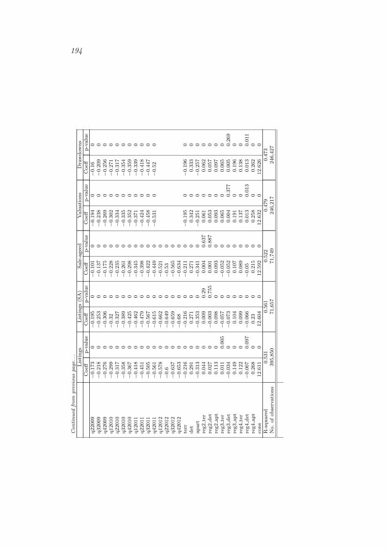
194
Continued
from
previouspa
ge..
.L
isti
ngs
Lis
tin
gs
(SA
)S
ale
-agee
dV
alu
ati
on
sD
raw
dow
ns
Coeff
p-v
alu
eC
oeff
p-v
alu
eC
oeff
p-v
alu
eC
oeff
p-v
alu
eC
oeff
p-v
alu
eq22009
−0.1
73
0−
0.1
95
0−
0.1
01
0−
0.1
94
0−
0.1
60
q32009
−0.2
18
0−
0.2
53
0−
0.1
37
0−
0.2
38
0−
0.2
09
0q42009
−0.2
76
0−
0.3
06
0−
0.1
75
0−
0.2
69
0−
0.2
56
0q12010
−0.2
99
0−
0.3
20
−0.2
28
0−
0.3
02
0−
0.2
71
0q22010
−0.3
17
0−
0.3
27
0−
0.2
35
0−
0.3
34
0−
0.3
17
0q32010
−0.3
58
0−
0.3
89
0−
0.2
61
0−
0.3
35
0−
0.3
54
0q42010
−0.3
67
0−
0.4
25
0−
0.2
98
0−
0.3
52
0−
0.3
59
0q12011
−0.4
18
0−
0.4
62
0−
0.3
45
0−
0.3
71
0−
0.3
39
0q22011
−0.4
51
0−
0.4
79
0−
0.3
98
0−
0.4
24
0−
0.4
18
0q32011
−0.5
05
0−
0.5
67
0−
0.4
22
0−
0.4
58
0−
0.4
47
0q42011
−0.5
61
0−
0.6
15
0−
0.4
49
0−
0.5
31
0−
0.5
20
q12012
−0.5
78
0−
0.6
62
0−
0.5
21
0q22012
−0.6
0−
0.6
49
0−
0.5
30
q32012
−0.6
37
0−
0.6
59
0−
0.5
65
0q42012
−0.6
53
0−
0.6
80
−0.6
34
0te
rr−
0.2
16
0−
0.2
16
0−
0.2
11
0−
0.1
95
0−
0.1
96
0d
et0.2
91
00.2
71
00.2
71
00.3
42
00.3
33
0ap
art
−0.3
13
0−
0.3
53
0−
0.3
41
0−
0.2
51
0−
0.2
57
0re
g2
ter
0.0
44
00.0
09
0.2
90.0
04
0.6
37
0.0
61
00.0
62
0re
g2
det
0.0
27
0−
0.0
03
0.7
55
0.0
01
0.8
87
0.0
53
00.0
57
0re
g2
ap
t0.1
13
00.0
98
00.0
93
00.0
93
00.0
97
0re
g3
ter
0.0
11
0.0
05−
0.0
57
0−
0.0
52
00.0
65
00.0
65
0re
g3
det
−0.0
34
0−
0.0
73
0−
0.0
52
00.0
04
0.3
77
0.0
05
0.2
69
reg3
ap
t0.1
49
00.1
04
00.1
07
00.1
91
00.1
96
0re
g4
ter
0.1
22
00.0
99
00.0
89
00.1
37
00.1
38
0re
g4
det
−0.0
07
0.0
97−
0.0
66
0−
0.0
50
0.0
13
0.0
13
0.0
13
0.0
11
reg4
ap
t0.2
68
00.2
30
0.2
15
00.2
58
00.2
62
0co
ns
12.6
11
012.6
04
012.5
92
012.6
32
012.6
26
0R
-squ
are
d0.5
31
0.5
61
0.5
22
0.4
79
0.4
73
No.
of
ob
serv
ati
on
s395,8
50
71,6
57
71,7
49
246,2
17
246,4
27

.4 Appendix material for Chapter 5 195
.4 Appendix material for Chapter 5
.4.1 Mortgage Interest Relief
In Section 5.3.7, reference was made to mortgage interest relief, through whichowner-occupiers received an income tax rebate. This relief was at the marginalrate for earners, and subject to ceilings to time limits at different points. For thepurposes of this study, as the relief applied for more than five years throughoutthe sample, and the ceilings were not binding for those buying at average prices,the key variable in determining the net mortgage rate was the marginal rateof income tax paid. Figure 9 shows the full marginal rate and the marginalrate that would have applied at the average industrial wage, using data fromAMECO on nominal average compensation per employee. Mortgage interestrelief did not apply in the Irish market from January 2013.
Figure 9: Rate of mortgage interest relief, marginal and average wage, 1975-2012
.4.2 Regression Output
Table 6 details the regression output, including coefficients and associated stan-dard errors, t-statistics and p-values, for the model with full dynamics outlinedin Section 5.4. As is outlined in the text, the long-run solution is clear, whilefew of the dynamic terms are statistically significant.
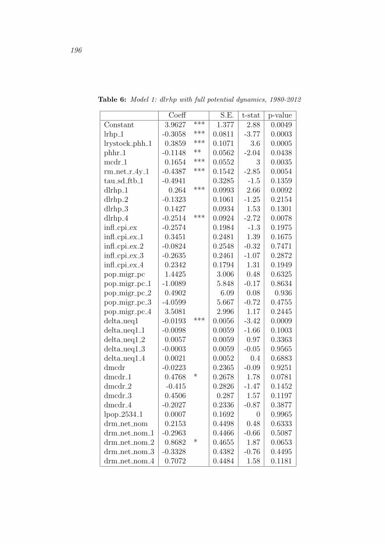
196
Table 6: Model 1: dlrhp with full potential dynamics, 1980-2012
Coeff S.E. t-stat p-valueConstant 3.9627 *** 1.377 2.88 0.0049lrhp 1 -0.3058 *** 0.0811 -3.77 0.0003lrystock phh 1 0.3859 *** 0.1071 3.6 0.0005phhr 1 -0.1148 ** 0.0562 -2.04 0.0438mcdr 1 0.1654 *** 0.0552 3 0.0035rm net r 4y 1 -0.4387 *** 0.1542 -2.85 0.0054tau sd ftb 1 -0.4941 0.3285 -1.5 0.1359dlrhp 1 0.264 *** 0.0993 2.66 0.0092dlrhp 2 -0.1323 0.1061 -1.25 0.2154dlrhp 3 0.1427 0.0934 1.53 0.1301dlrhp 4 -0.2514 *** 0.0924 -2.72 0.0078infl cpi ex -0.2574 0.1984 -1.3 0.1975infl cpi ex 1 0.3451 0.2481 1.39 0.1675infl cpi ex 2 -0.0824 0.2548 -0.32 0.7471infl cpi ex 3 -0.2635 0.2461 -1.07 0.2872infl cpi ex 4 0.2342 0.1794 1.31 0.1949pop migr pc 1.4425 3.006 0.48 0.6325pop migr pc 1 -1.0089 5.848 -0.17 0.8634pop migr pc 2 0.4902 6.09 0.08 0.936pop migr pc 3 -4.0599 5.667 -0.72 0.4755pop migr pc 4 3.5081 2.996 1.17 0.2445delta ueq1 -0.0193 *** 0.0056 -3.42 0.0009delta ueq1 1 -0.0098 0.0059 -1.66 0.1003delta ueq1 2 0.0057 0.0059 0.97 0.3363delta ueq1 3 -0.0003 0.0059 -0.05 0.9565delta ueq1 4 0.0021 0.0052 0.4 0.6883dmcdr -0.0223 0.2365 -0.09 0.9251dmcdr 1 0.4768 * 0.2678 1.78 0.0781dmcdr 2 -0.415 0.2826 -1.47 0.1452dmcdr 3 0.4506 0.287 1.57 0.1197dmcdr 4 -0.2027 0.2336 -0.87 0.3877lpop 2534 1 0.0007 0.1692 0 0.9965drm net nom 0.2153 0.4498 0.48 0.6333drm net nom 1 -0.2963 0.4466 -0.66 0.5087drm net nom 2 0.8682 * 0.4655 1.87 0.0653drm net nom 3 -0.3328 0.4382 -0.76 0.4495drm net nom 4 0.7072 0.4484 1.58 0.1181

.4 Appendix material for Chapter 5 197
.4.3 Robustness & sensitivity analysis
Tables 7 and 8 show the coefficients and associated p-values for a number ofspecifications designed to check the robustness of the results outlined in Section5.4.3. The first table examines alternative data series for a range of fundamen-tals, while the second table shows results for different functional specificationsof the three core fundamental ratios: income to supply, mortgages to deposits,and persons to households. The final rows of each table show measures ofmodel fit and also whether the model failed any of six core tests. Commentaryon these results is given in Section 5.4.3.
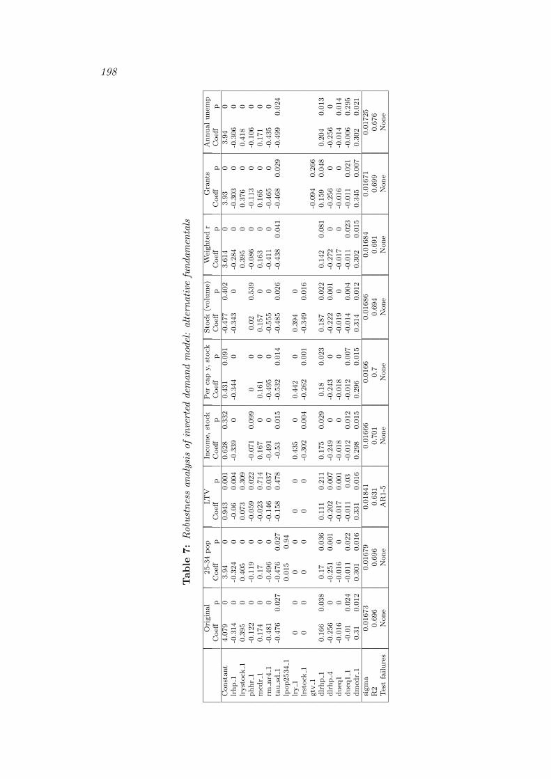
198
Table
7:
Robu
stn
ess
an
aly
sis
of
inve
rted
dem
an
dm
odel
:alt
ern
ati
vefu
ndam
enta
ls
Ori
gin
al
25-3
4p
op
LT
VIn
com
e,st
ock
Per
cap
y,st
ock
Sto
ck(v
olu
me)
Wei
ghte
dr
Gra
nts
An
nu
al
un
emp
Coeff
pC
oeff
pC
oeff
pC
oeff
pC
oeff
pC
oeff
pC
oeff
pC
oeff
pC
oeff
pC
on
stant
4.0
79
03.9
40
0.9
43
0.0
01
0.6
28
0.3
32
0.4
31
0.0
91
-0.4
77
0.4
02
3.6
14
03.9
30
3.9
40
lrh
p1
-0.3
14
0-0
.324
0-0
.06
0.0
04
-0.3
39
0-0
.344
0-0
.343
0-0
.284
0-0
.303
0-0
.306
0lr
yst
ock
10.3
95
00.4
05
00.0
73
0.3
09
0.3
95
00.3
76
00.4
18
0p
hh
r1
-0.1
22
0-0
.119
0-0
.059
0.0
22
-0.0
71
0.0
99
00
0.0
20.5
39
-0.0
86
0-0
.113
0-0
.106
0m
cdr
10.1
74
00.1
70
-0.0
23
0.7
14
0.1
67
00.1
61
00.1
57
00.1
63
00.1
65
00.1
71
0rm
nr4
1-0
.481
0-0
.496
0-0
.146
0.0
37
-0.4
91
0-0
.495
0-0
.555
0-0
.411
0-0
.465
0-0
.435
0ta
usd
1-0
.476
0.0
27
-0.4
76
0.0
27
-0.1
58
0.4
78
-0.5
30.0
15
-0.5
32
0.0
14
-0.4
85
0.0
26
-0.4
38
0.0
41
-0.4
68
0.0
29
-0.4
99
0.0
24
lpop
2534
10.0
15
0.9
4lr
y1
00
00
00
0.4
35
00.4
42
00.3
94
0lr
stock
10
00
00
0-0
.302
0.0
04
-0.2
62
0.0
01
-0.3
49
0.0
16
gtv
1-0
.094
0.2
66
dlr
hp
10.1
66
0.0
38
0.1
70.0
36
0.1
11
0.2
11
0.1
75
0.0
29
0.1
80.0
23
0.1
87
0.0
22
0.1
42
0.0
81
0.1
59
0.0
48
0.2
04
0.0
13
dlr
hp
4-0
.256
0-0
.251
0.0
01
-0.2
02
0.0
07
-0.2
49
0-0
.243
0-0
.222
0.0
01
-0.2
72
0-0
.256
0-0
.256
0d
ueq
1-0
.016
0-0
.016
0-0
.017
0.0
01
-0.0
18
0-0
.018
0-0
.019
0-0
.017
0-0
.016
0-0
.014
0.0
14
du
eq1
1-0
.01
0.0
24
-0.0
11
0.0
22
-0.0
11
0.0
3-0
.012
0.0
12
-0.0
12
0.0
07
-0.0
14
0.0
04
-0.0
11
0.0
23
-0.0
11
0.0
21
-0.0
06
0.2
95
dm
cdr
10.3
10.0
12
0.3
01
0.0
16
0.3
31
0.0
16
0.2
98
0.0
15
0.2
96
0.0
15
0.3
14
0.0
12
0.3
02
0.0
15
0.3
45
0.0
07
0.3
02
0.0
21
sigm
a0.0
1673
0.0
1679
0.0
1841
0.0
1666
0.0
166
0.0
1686
0.0
1684
0.0
1671
0.0
1725
R2
0.6
96
0.6
96
0.6
31
0.7
01
0.7
0.6
94
0.6
91
0.6
99
0.6
76
Tes
tfa
ilu
res
Non
eN
on
eA
R1-5
Non
eN
on
eN
on
eN
on
eN
on
eN
on
e
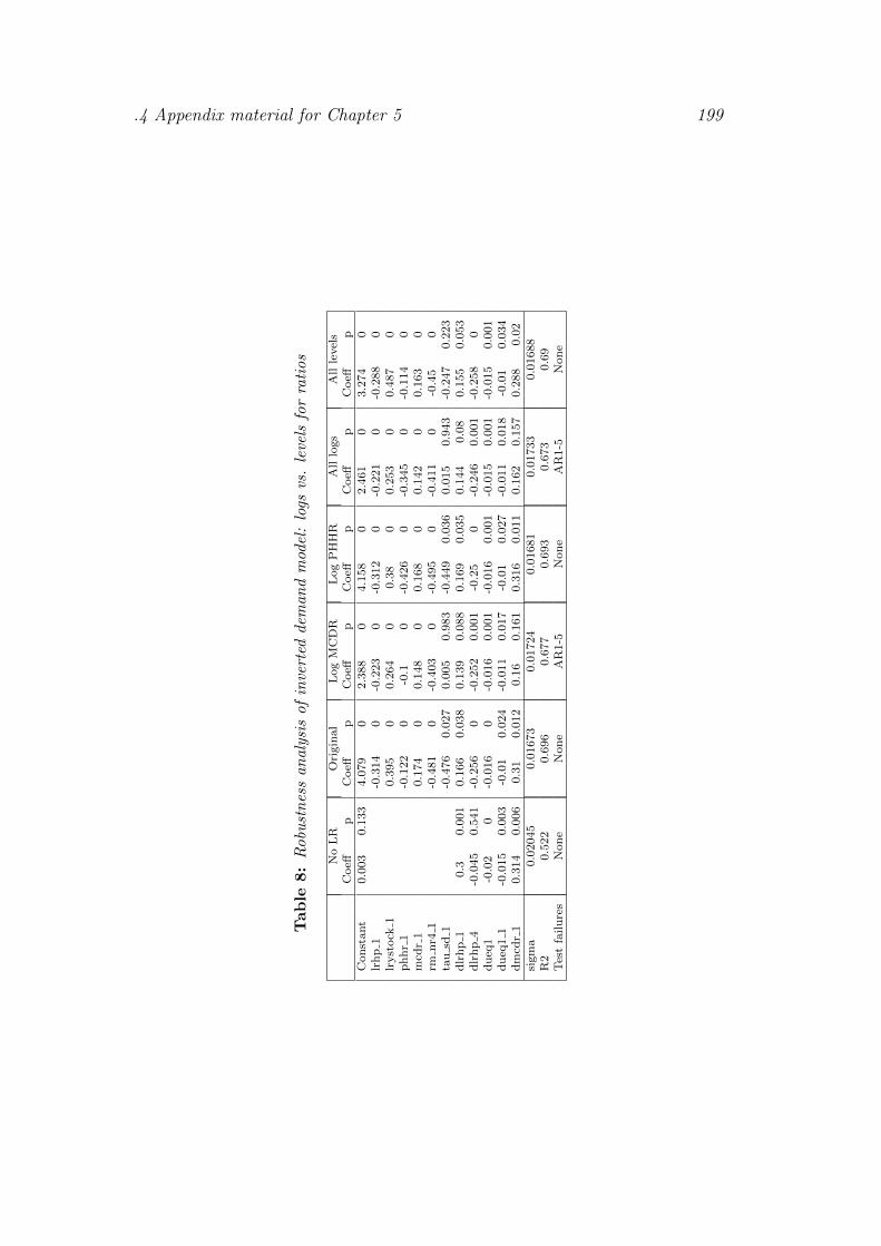
.4 Appendix material for Chapter 5 199
Table
8:
Robu
stn
ess
an
aly
sis
of
inve
rted
dem
an
dm
odel
:lo
gsvs
.le
vels
for
rati
os
No
LR
Ori
gin
al
Log
MC
DR
Log
PH
HR
All
logs
All
level
sC
oeff
pC
oeff
pC
oeff
pC
oeff
pC
oeff
pC
oeff
pC
on
stant
0.0
03
0.1
33
4.0
79
02.3
88
04.1
58
02.4
61
03.2
74
0lr
hp
1-0
.314
0-0
.223
0-0
.312
0-0
.221
0-0
.288
0lr
yst
ock
10.3
95
00.2
64
00.3
80
0.2
53
00.4
87
0p
hh
r1
-0.1
22
0-0
.10
-0.4
26
0-0
.345
0-0
.114
0m
cdr
10.1
74
00.1
48
00.1
68
00.1
42
00.1
63
0rm
nr4
1-0
.481
0-0
.403
0-0
.495
0-0
.411
0-0
.45
0ta
usd
1-0
.476
0.0
27
0.0
05
0.9
83
-0.4
49
0.0
36
0.0
15
0.9
43
-0.2
47
0.2
23
dlr
hp
10.3
0.0
01
0.1
66
0.0
38
0.1
39
0.0
88
0.1
69
0.0
35
0.1
44
0.0
80.1
55
0.0
53
dlr
hp
4-0
.045
0.5
41
-0.2
56
0-0
.252
0.0
01
-0.2
50
-0.2
46
0.0
01
-0.2
58
0d
ueq
1-0
.02
0-0
.016
0-0
.016
0.0
01
-0.0
16
0.0
01
-0.0
15
0.0
01
-0.0
15
0.0
01
du
eq1
1-0
.015
0.0
03
-0.0
10.0
24
-0.0
11
0.0
17
-0.0
10.0
27
-0.0
11
0.0
18
-0.0
10.0
34
dm
cdr
10.3
14
0.0
06
0.3
10.0
12
0.1
60.1
61
0.3
16
0.0
11
0.1
62
0.1
57
0.2
88
0.0
2si
gm
a0.0
2045
0.0
1673
0.0
1724
0.0
1681
0.0
1733
0.0
1688
R2
0.5
22
0.6
96
0.6
77
0.6
93
0.6
73
0.6
9T
est
failu
res
Non
eN
on
eA
R1-5
Non
eA
R1-5
Non
e

200
.4.4 Fitted values & Parameter stability
Figures 10 and 11 show the actual and fitted values of the change in real houseprices (dlrhp) for the model applied to the 1980-2012 period and the samemodel applied to the 1975-2012 period. Figure 12 shows the actual and fittedvalues of the change in the house price-to-rent ratio, 2000-2012. Figure 13shows the recursive estimates of parameters on the long-run variables in theinverted demand specification, starting with a ten-year window (1980-1990).Commentary on all these results is given in the text.
Figure 10: Actual and fitted values of dlrhp, 1980-2012
.4.5 Stationarity & Cointegration
Table 9 presents supplementary augmented Dickey-Fuller tests, as describedin the text. Figures 14-15 show plots of the following variables in delta form:log real house prices, log real income per household, log real housing stock perhousehold, log of the income-stock ratio, the credit-deposit ratio, user-cost, theperson-household ratio and the change in population aged 25-34. Figures 16and 17 contrast changes in per household income and housing stock (likely tobe stationary) with changes in per capita income and stock, which fail unitroot tests at all conventional levels of statisticaly significance.

.4 Appendix material for Chapter 5 201
Figure 11: Actual and fitted values of dlrhp, 1975-2012
Figure 12: Actual and fitted values of dlhpr, 2000-2012
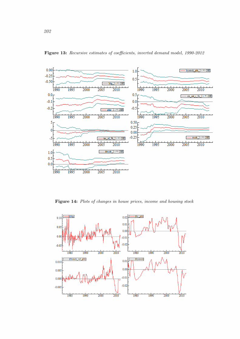
202
Figure 13: Recursive estimates of coefficients, inverted demand model, 1990-2012
Figure 14: Plots of changes in house prices, income and housing stock

.4 Appendix material for Chapter 5 203
Table 9: ADF unit root tests: supplementary series
Var D-lag t-adf beta Y 1 sigma t-DY lag t-prob AIC F-prob
dlry pc 3 -2.286 0.919 0.004 0.471 0.639 -10.872 -2.243 0.922 0.004 0.453 0.652 -10.89 0.6391 -2.204 0.925 0.004 0.436 0.664 -10.9 0.8090 -2.167 0.928 0.004 -10.91 0.893
dlhs pc 3 -0.1197 0.996 0.001 -1.658 0.1 -13.622 -0.437 0.985 0.001 -3.116 0.002 -13.61 0.11 -1.121 0.96 0.001 -3.272 0.001 -13.55 0.0030 -1.912 0.932 0.001 -13.49 0
dlry phdagger 3 -3.441** 0.854 0.005 0.814 0.417 -10.452 -3.347** 0.862 0.005 0.379 0.705 -10.46 0.4171 -3.363** 0.866 0.005 0.785 0.434 -10.47 0.6690 -3.274** 0.873 0.005 -10.48 0.702
dlhs phdagger 3 -2.949** 0.878 0.002 0.392 0.696 -12.672 -2.950** 0.882 0.002 0.854 0.395 -12.68 0.6961 -2.831* 0.89 0.002 0.168 0.867 -12.69 0.6460 -2.886** 0.892 0.002 -12.7 0.824
dd4pop2534 3 -4.471*** 0.746 0.002 1.551 0.124 -12.762 -4.170*** 0.777 0.002 1.366 0.174 -12.75 0.1241 -3.927*** 0.8 0.002 1.065 0.289 -12.75 0.1210 -3.778*** 0.815 0.002 -12.76 0.148
dlyhsdagger 3 -3.937*** 0.812 0.005 0.664 0.508 -10.462 -3.905*** 0.82 0.005 0.972 0.333 -10.47 0.5081 -3.783*** 0.832 0.005 0.464 0.644 -10.47 0.5030 -3.800*** 0.837 0.005 -10.49 0.661
Figure 15: Plots of changes in other regressors
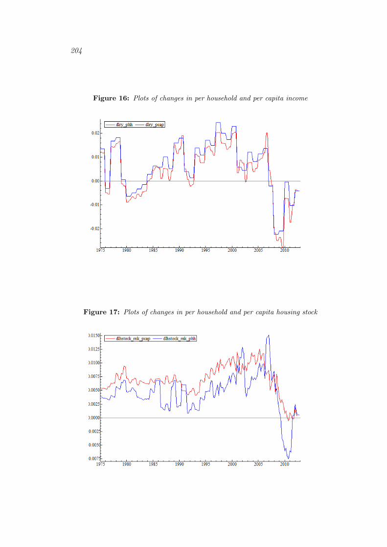
204
Figure 16: Plots of changes in per household and per capita income
Figure 17: Plots of changes in per household and per capita housing stock