HAL Id: tel-00444898https://tel.archives-ouvertes.fr/tel-00444898

Submitted on 7 Jan 2010

HAL is a multi-disciplinary open accessarchive for the deposit and dissemination of sci-entific research documents, whether they are pub-lished or not. The documents may come fromteaching and research institutions in France orabroad, or from public or private research centers.

L’archive ouverte pluridisciplinaire HAL, estdestinée au dépôt et à la diffusion de documentsscientifiques de niveau recherche, publiés ou non,émanant des établissements d’enseignement et derecherche français ou étrangers, des laboratoirespublics ou privés.

Experimental and numerical investigation of the thermaldecomposition of materials at three scales: application

to polyether polyurethane foam used in upholsteredfurniture

Lucas Bustamante Valencia

To cite this version:Lucas Bustamante Valencia. Experimental and numerical investigation of the thermal decompositionof materials at three scales: application to polyether polyurethane foam used in upholstered furni-ture. Engineering Sciences [physics]. ISAE-ENSMA Ecole Nationale Supérieure de Mécanique etd’Aérotechique - Poitiers, 2009. English. �tel-00444898�

THÈSE pour l’obtention du grade de

DOCTEUR DE L’ÉCOLE NATIONALE SUPÉRIEURE DE MÉCANIQUE ET D’AÉROTECHNIQUE

(Diplôme National – Arrêté du 7 août 2006)

École Doctorale : Sciences pour l’Ingénieur et Aéronautique

Secteur de recherche : Energétique, Thermique, Combustion

Option : Energétique

Présentée par :

Lucas Bustamante Valencia

********************

Étude expérimentale et numérique de la décomposition thermique des matériaux à trois échelles : Application à une mousse polyéther

polyuréthane utilisée dans les meubles rembourrés

Experimental and numerical investigation of the thermal decomposition of materials at three scales: application to polyether

polyurethane foam used in upholstered furniture

********************

Directeur de thèse : Patrick ROUSSEAUX

Co-Directeur : Thomas ROGAUME

********************

Soutenue le 20 novembre 2009 devant la Commission d’Examen

********************

- Jury -

M. P. BOULET Professeur, LEMTA Université de Nancy Président M. B. PORTERIE Professeur, IUSTI Université de Marseille Rapporteur M. J.L. TORERO Professeur, Université d’Édimbourg, Ecosse Rapporteur M. P. ROUSSEAUX Professeur, LCD Université de Poitiers Examinateur Mme. C. CHIVAS-JOLY Ingénieur de recherche, LNE de Trappes Examinateur M. E. GUILLAUME Ingénieur de recherche, LNE de Trappes Examinateur M. G. REIN Maître de Conf. Université d’Edimbourg, Ecosse Examinateur M. T. ROGAUME Maître de Conférences, LCD Université de Poitiers Examinateur

2

3

To Carine Cordier

Yes, this work is also yours…

To Luz Elena Valencia

4

5

Abstract

The fire behaviour of polyether polyurethane foam has been studied at three scales:

matter scale, small scale and product scale. A method to determine the thermal

decomposition mechanism of materials was defined at the matter scale. This method is

based on the analysis of the mass-loss rate (solid phase) and gas release (gas phase)

obtained in thermogravimetric analysis coupled to FTIR gas analysis. Using a model

and genetic algorithms, the kinetic parameters of the decomposition process were

calculated, which allowed an accurate prediction of the mass-loss rate.

Measurements of heat release rate and gas release were carried out in cone

calorimeter coupled to gas analysers (small scale). This data as well as the results

from the model were used as input data for the numerical simulation of fire behaviour.

This study highlighted that some improvements need to be carried out to the simulation

codes.

Measurements of heat release rate and mass-loss rate were also performed during the

fire of a simplified piece of upholstered furniture (product scale). It was pointed out that

the decomposition mechanism of the foam remains unchanged independently of the

scale analysed.

7

Résumé

L’amélioration de la sécurité incendie au sein de l’habitat est un des principaux

objectifs de la recherche actuelle. En effet, chaque année, un grand nombre de feux

sont déclarés, générant la perte de nombreuses vies humaines, de fortes pertes

financières, l’endommagement des structures et la pollution de l’environnement.

Face à cette problématique, on remarque qu’un grand nombre de pays d’Europe

possèdent une législation très pauvre vis-à-vis de la protection incendie dans l’habitat.

Historiquement, les bâtiments ont été dessinés suivant des obligations prescriptives.

La tendance de l’ingénierie de la sécurité incendie (Fire Safety Engineering, FSE selon

le sigle Anglais) a changé amplement pendant la dernière décennie : des groupes de

recherche dans le domaine de l’incendie ont mis au point les principes du design fondé

sur la performance (Performance Building Design, PBD en Anglais). Le PBD a permis

une approche de la sécurité incendie fondée sur la prédiction du comportement d’un

incendie dans des scénarios donnés, en utilisant des outils numériques d’ingénierie.

L’approche PBD de FSE est une méthodologie qui a été initialement développée pour

les établissements recevant du public, toutefois peu à peu cette approche commence à

être utilisée dans tout type d’habitat.

La prédiction du comportement d’un incendie nécessite le calcul du débit calorifique

(Heat Release Rate, HRR en Anglais) qui est la grandeur physique utilisée pour la

mesure de la puissance d’un feu. En ingénierie, le HRR est indispensable à

l’estimation de la sévérité du sinistre et des possibles endommagements causés dans

un scénario donné. Sa détermination dépend des combustibles présents lors de

l’incendie ainsi que de l’environnement du sinistre. La prédiction du HRR est réalisée à

l’aide des codes de simulation numérique de l’incendie. Ceux-ci sont un assemblage

de plusieurs sous modèles dont chacun calcule un ensemble des phénomènes

présents dans la combustion p. ex. la pyrolyse, le rayonnement, la turbulence, etc.

8

La capacité à prédire correctement le HRR est limitée par les calculs très simplifiés du

processus de décomposition thermique des solides. La décomposition est notamment

dépendante des processus diffusifs et chimiques mis en jeu dans la zone comprise

entre le solide et la flamme, lesquels ne sont pas modélisés de façon rigoureuse. Par

le passé, plusieurs études expérimentales ont permis de mesurer le HRR d’un certain

nombre de produits, cependant, ils ne contribuent pas à la compréhension de la

physique du processus de décomposition de la matrice solide, donnée pourtant

essentielle car source des espèces volatiles et du débit massique du combustible. En

effet, un grand nombre de simulations trouvées dans la littérature font une approche

empirique de la production de fuel ou considèrent une seule étape de décomposition.

C’est dans ce contexte que prend place la présente étude qui vise à caractériser la

cinétique de décomposition de combustibles solides et de formation des espèces

volatiles : les changements survenus dans la phase solide sont pris en compte

ensemble avec ceux de la phase gazeuse (dégagement d’espèces). La détermination

du mécanisme de décomposition est une tâche fondamentale de l’analyse thermique.

Le mécanisme doit considérer la succession des transformations de la matière pendant

la gazéification des solides. Cette succession inclus les échantillons vierges ainsi que

ceux qui ont déjà souffert des attaques thermiques (sous produits des étapes de

décomposition). Le mécanisme de décomposition constitue une des principales

données d’entrée de la grande majorité de modèles de décomposition thermique.

Cette recherche tient compte de la décomposition thermique d’une mousse polyéther

polyuréthane (PPUF) à trois échelles différentes. Chaque échelle caractérise le

comportement au feu d’une masse différente de mousse et est concentrée sur l’étude

de phénomènes particuliers :

• L’échelle matière permet l’analyse du comportement d’échantillons avec des

masses proches d’un milligramme. À l’échelle matière, les effets de transfert de

chaleur et des espèces sont minimisés et l’effet de l’augmentation de la

température du solide peut être étudié précisément. L’échantillon est considéré

comme une particule de masse et de dimension négligeables, de sorte que sa

température soit homogène.

• La petite échelle permet l’analyse des échantillons avec des masses proches de

dix grammes. À l’échelle matière des gradients de transfert de chaleur et d’espèces

existent. L’échantillon est irradié seulement par une des surfaces, produisant ainsi

9

le déplacement du front de décomposition. La combustion de matériaux

polymériques est complexe et concerne souvent des processus simultanés tels que

la pyrolyse, la décomposition oxydative et le processus de combustion avec

présence de flamme.

• L’échelle produit concerne des échantillons avec des masses proches d’un

kilogramme. À cette échelle, la géométrie et le positionnement d’un produit ont un

rôle fondamental dans la croissance du feu. La ventilation (la disponibilité

d’oxygène et la turbulence) affecte également le processus de combustion.

L’échelle produit montre le comportement au feu d’une mousse dans des

conditions d’utilisation proches de celles de la réalité.

Les résultats obtenus dans cette recherche vérifient que le mécanisme de

décomposition reste inchangé indépendamment de l’échelle. Dans la littérature, ces

trois échelles n’ont jamais été considérées ensemble. Généralement, chaque échelle

est considérée indépendamment et les chercheurs restent concentrés sur les

phénomènes observés à l’échelle étudiée. De plus, les résultats de l’échelle matière

sont souvent extrapolés à l’échelle produit. Toutefois, les phénomènes

supplémentaires qui apparaissent entre une échelle et l’autre ne sont pas pris en

compte, engendrant une grande incertitude dans la prédiction des résultats.

Cette recherche propose une contribution vis-à-vis de l’intégration verticale des

résultats obtenus dans les trois échelles. L’intégration verticale signifie explorer la

possibilité d’identifier quelles propriétés de la matière doivent être mesurées et fournies

en tant que données d’entrée des codes de simulation incendie afin de pouvoir prédire

la décomposition thermique des solides. Ces travaux constituent un pas dans une

vision globale de la science des matériaux qui permettrait une prédiction très juste du

comportement au feu des solides à diverses échelles tout en utilisant principalement

des mesures menées à l’échelle matière et la petite échelle.

La cinétique de la décomposition a été étudié à la petite échelle grâce à des analyses

thermogravimétriques (TGA). Cette technique a permis de mettre en évidence le

nombre d’étapes, les espèces qui entrent en réaction et de détailler le mécanisme de

réaction. En outre, des algorithmes génétiques ont été utilisés pour calculer les

paramètres cinétiques optimum qui permettent de prédire le changement de la masse

d’un échantillon en fonction de la température. Selon la démarche à échelle croissante

décrite ci-dessus, les propriétés thermiques ainsi que les paramètres cinétiques de la

10

décomposition du PPUF ont été utilisés comme données d’entrée dans un code de

simulation incendie. Les simulations ont été réalisées avec le code de calcul le plus

amplement utilisé dans le monde, Fire Dynamics Simulator (FDS V 5.3).

Les simulations tentent de prédire le comportement du PPUF en cône calorimètre

(petite échelle). Un faible calage entre les courbes de changement de la masse

expérimentales et numériques a été observé. Une grande incertitude vis-à-vis de la

façon d’introduire les données d’entrée a été identifiée ainsi que de leur interprétation.

Des possibles voies d’amélioration des modèles de pyrolyse ont été proposées.

Acknowledgement

There are so many people to acknowledge for their direct or indirect contribution that

the acknowledgements could be as long as the document itself.

To the director of the Laboratoire de Combustion et de Détonique (UPR 9028 CNRS)

Prof. Henri-Noël Presles and to Prof. Patrick Rousseaux, who accepted my presence in

their laboratory, for their financial support to present this work in many countries and for

their help allowing this manuscript to be written in English.

To Prof. Bernard Porterie and to Prof. José Luis Torero who have accepted to be the

advisors of this work. Thanks also to Prof. Pascal Boulet and Dr. Carine Chivas-Joly for

their time and participation to the committee and their remarks concerning the work that

has been done. To Dr. Richard Gann for his careful reading of the manuscript and his

pertinent comments.

Thanks to Eng. Eric Guillaume and Dr. Thomas Rogaume for their constant follow-up

of the progress of this research. They have been available to enrich the scientific and

personal discussions. It is a great pleasure to work with both of you!

To Prof. José Luis Torero and Dr. Guillermo Rein for their scientific contribution to this

research, their invitation to work with them in Edinburgh, their financial support and of

course their comments on how to make things in a better way.

To the Ministère de l’Economie de l’Industrie et de l’Emploi (Ministry of Economy,

Industry and Employment), the Association Nationale de la Recherche et de la

Technologie, Eng. Jean-Luc Laurent, Dr. Alain Sainrat and Eng. Bernard Picque who

believed in this project and provided funds.

To the people of the Fire Engineering Division from LNE who actively participated in

this research: Eng. Damien Marquis, Mr Franck Didieux, Mr Laurent Saragoza,

Mr Damien Lesenechal, Mr Aymeric Ragideau and Eng. Bruno Rochat.

12

To the people from the various LNE divisions who performed tests and provided

experimental results: Eng. Bruno Hay and his workgroup, Mrs Fabienne Carpentier and

her workgroup, Eng. Valérie Rumbau and her workgroup.

To Dr. Nicolas Fischer, Dr. Géraldine Ebrard, Eng. Aurélie Quoix, Eng. Allexandre

Allard from the statistics division of LNE for their contribution with data analysis and

simulations.

To Mrs Jocelyne Bardeau, Mrs Ariel Collet, Mrs Isabelle Gommard, Mrs Anne Duclos

who have made my life easier by helping me with the administrative tasks.

To my friends Dr. Andres Mahecha Botero and Prof. Jean-Claude Arnould, you

probably do not know, but you tought to me what is important in a thesis.

To the people I met at the University of Edinburgh, we shared great moments together:

Dr. Pedro Reszka, Eng. Hubert Biteau, Dr. Andres Fuentes, Dr. Albert Simeoni,

Dr. Mercedez Gomez.

To Prof. Dougal Drysdale, Prof. Elizabeth Weckman, Prof. Michel Pavageau,

Dr. William Pitts, Dr. Kuldeep Prassad, Dr. Kathryn Butler, Dr. Diane Daems for their

interesting discussions about the fire behaviour of polyurethane foam.

To the reader for being patient and understand that my English is not the best.

À mes amis Gilles et Annie Quiecout et les commerçants du marché Saint-Quentin qui

ont demandé de mes nouvelles chaque dimanche lorsque j’étais absent au moment de

faire des courses.

13

Contents

Abstract........................................................................................................................ 5 Résumé........................................................................................................................ 7 Acknowledgement.......................................................................................................11 Contents......................................................................................................................13 List of Figures..............................................................................................................15 List of Tables...............................................................................................................21 Nomenclature..............................................................................................................23 1 General introduction .................................................................................................29 2 Matter scale experiments .........................................................................................37

2.1 Introduction........................................................................................................37 2.2 State of the art in matter scale measurements...................................................39

2.2.1 Characteristics of polyurethane molecule ....................................................40 2.2.2 Generalities about the thermal decomposition of polyurethane....................41 2.2.3 Determination of the polyurethane decomposition mechanism based

on the analysis of the gas effluents. ..........................................................43 2.2.4 Use of tubular furnace in the determination of the decomposition

mechanism of materials. ...........................................................................48 2.2.5 A few comments on the thermogravimetric technique..................................52 2.2.6 Summary of the state of the art in matter scale measurements ...................53

2.3 Characteristics of the Polyether Polyurethane Foam used in this research...........................................................................................................55

2.4 Measurement of thermal properties ...................................................................57 2.4.1 Enthalpy of reaction.....................................................................................57 2.4.2 Mass thermal capacity.................................................................................61 2.4.3 Thermal conductivity ...................................................................................62 2.4.4 Superior calorific power ...............................................................................64

2.5 Experimental measurement of the solid and gas phases ...................................65 2.5.1 Fourier Transform Infrared Spectroscopy gas analysis (FTIR).....................65 2.5.2 Thermogravimetric analysis (TGA) ..............................................................72 2.5.3 Tubular furnace ...........................................................................................79 2.5.4 Results of TGA + FTIRqlt and TF + FTIRqnt...................................................81

2.6 Analysis of the solid phase - Verification of the decomposition mechanism of PPUF ........................................................................................85

2.6.1 Visual characterisation of the solid phase....................................................87 2.6.2 Characterisation of the molecular structure of the solid ...............................92

2.7 Conclusion.........................................................................................................93 3 Matter scale model ...................................................................................................95

3.1 Introduction........................................................................................................95 3.2 State of the art in matter scale modelling ...........................................................97

3.2.1 Background.................................................................................................97 3.2.2 The model-fitting (modelistic) method..........................................................99 3.2.3 The free model method (Isoconversional)..................................................108

14

3.2.4 Combined model-fitting and model-free methods ......................................115 3.2.5 Models of the decomposition of solids based on TGA isothermal

tests ........................................................................................................116 3.2.6 Deduction of a multi-reaction, multi-step model of thermal

decomposition.........................................................................................118 3.2.7 The problem of thermal decomposition under vitiated atmospheres ..........121 3.2.8 Some comments about the reaction rate equations...................................124

3.3 Improvement of the model of PPUF thermal decomposition.............................127 3.3.1 Verification of the influence of the kinetic mechanism in MLR

calculations .............................................................................................128 3.3.2 Analysis of the kinetic mechanisms based on effluents

measurements ........................................................................................138 3.3.3 Coupling of the model of solid phase to the model of gas effluents

release rate.............................................................................................146 3.4 Analysis of code stability ..................................................................................155

3.4.1 Study of the input ranges of the ODE unsolvable cases. ...........................157 3.4.2 Descriptive study.......................................................................................160

3.5 Analysis of sensitivity .......................................................................................164 3.6 Conclusion.......................................................................................................167

4 Small scale experiments and simulations ...............................................................171 4.1 Introduction......................................................................................................171 4.2 Reaction-to-fire experimental setup .................................................................173 4.3 Cone calorimeter experimental results .............................................................176 4.4 Numerical simulation of cone calorimeter results .............................................197 4.5 Fire behaviour of a simplified seat (product-scale) ..........................................207 4.6 Conclusions .....................................................................................................211

5 Discussions ............................................................................................................213 5.1 Discussions about the matter scale (TGA and TF) experiments.......................213 5.2 Discussion about the matter scale (TGA and TF) modelling.............................214 5.3 Discussion about the small scale (cone calorimeter) experiments....................216 5.4 Discussions about the small scale (cone calorimeter) simulations ...................219 5.5 Discussions about the oxygen mass fraction ...................................................225

6 General conclusions and future works....................................................................227 6.1 Conclusions .....................................................................................................227 6.2 Future works....................................................................................................229

7 References.............................................................................................................231 Appendix A................................................................................................................245 Appendix B................................................................................................................247 Appendix C ...............................................................................................................251 Appendix D ...............................................................................................................253

15

List of Figures

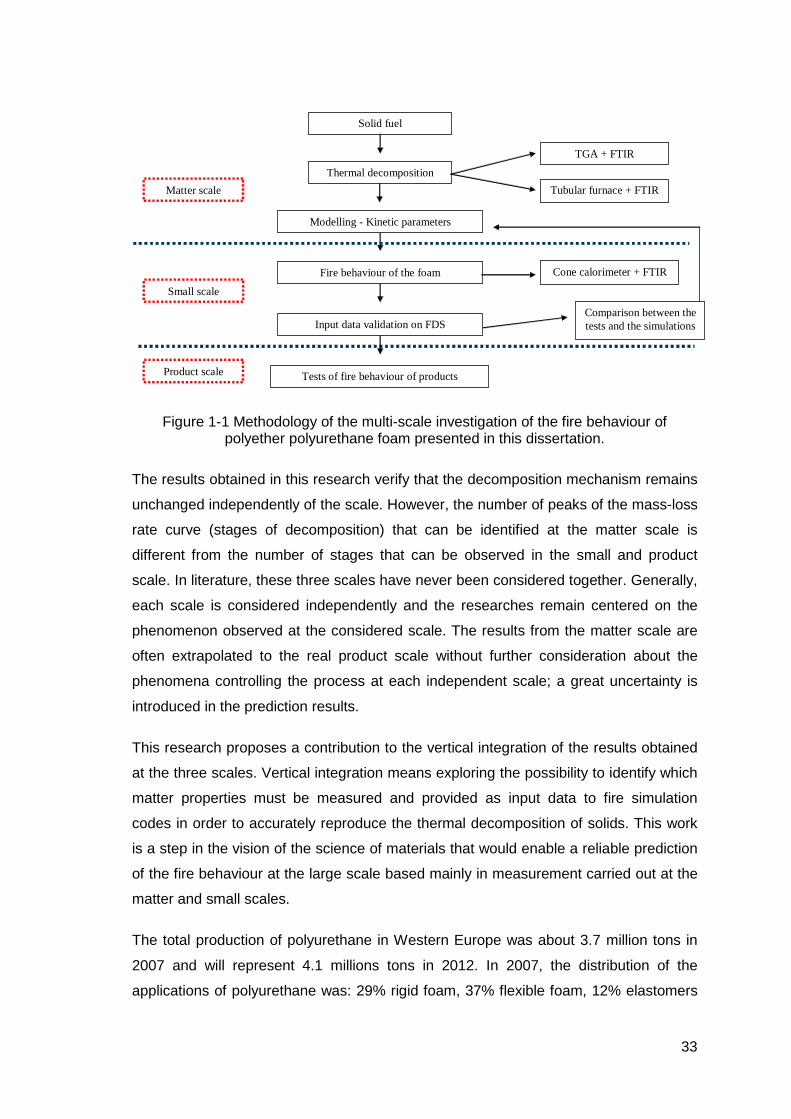
Figure 1-1 Methodology of the multi-scale investigation of the fire behaviour of polyether polyurethane foam presented in this dissertation.....................................33

Figure 2-1. DSC and TGA results under air and nitrogen atmospheres. Upper curves are under air atmosphere. Bottom curves are under nitrogen atmosphere. TGA curves are presented in blue circles, referenced at the left hand side y-axis. DSC curves are presented in green pluses reported at the right hand side y-axis. Heating rate was 8 °C·min -1. Positive enthalpy means endothermic reaction. Enthalpy is negative in exothermic reactions........................59

Figure 2-2. Thermal capacity data of virgin PPUF and char. Char data have been obtained without settled holder.......................................................................62

Figure 2-3 Cross-section view of the LNE’s high temperature guarded hot plate. This facility enabled the conductivity measurement of PPUF from room temperature up to 250 °C (Source [56]) ........ .................................................63

Figure 2-4 Conductivity of virgin PPUF from room temperature up to 190 °C. Measurement carried out with high temperature guarded hot plate.........................64

Figure 2-5. Exemple of the absorbance spectra measured in FTIR for various common combustion gases of PPUF (Source [43]).................................................67

Figure 2-6 Scheme of the diluter used during the FTIR calibration. RDM B, RDM C RDM D are mass flowmeters. “V” are gas valves (Source [69])..................69

Figure 2-7. FTIR facility layout.....................................................................................70

Figure 2-8. Scheme of the horizontal TGA facility used in this research. .....................74

Figure 2-9. Results of TGA tests carried out under air and nitrogen at four heating rates: 5, 8, 10 and 15 °C·min -1. a) Mass change vs temperature; b) MLR vs temperature. ..............................................................................................75

Figure 2-10. Plot of actual heating rate calculated at each second together with MLR under air and nitrogen atmospheres at set heating rate of 10°C·min -1. ...........77

Figure 2-11. Scheme of tubular furnace facility coupled to FTIR gas Analyser for analysis of exhaust gas release produced during combustion of PPUF .............80

Figure 2-12 Tubular furnace sample. The mass is around 110 mg..............................81

16

Figure 2-13. Releasing of isocyanate, polyol and aldehyde compounds in TGA + FTIRqnt and FT + FTIRqlt at β of 10 °C·min -1 under nitrogen atmosphere. Aldehyde compounds has been scaled by a factor of 0.6...................82

Figure 2-14. Releasing of a) isocyanate; b) CO2; c) CO and d) polyol vs temperature in TGA + FTIRqlt and FT + FTIRqnt at β of 10 °C·min -1 under air atmosphere. The experimental curve of MLR is used as reference in all the plots........................................................................................................................84

Figure 2-15. Binocular and SEM pictures of virgin PPUF.............................................88

Figure 2-16. Binocular and SEM pictures of DSC residues. PPUF samples were heated up to 500 °C under nitrogen (top) and a ir (bottom) atmospheres...........................................................................................................89

Figure 2-17. Pictures and SEM images of cone calorimeter residues. PPUF samples were exposed to irradiance level of 30 kW·m-2 under nitrogen (top) and air (bottom) atmospheres. ................................................................................91

Figure 3-1 Definition of the asymmetry of MLR curves in the Kissinger’s method. Source (Kissinger [83])............................................................................109

Figure 3-2 Kinetic mechanism used in the works of Rein et al. [109]. Written with the condensed species identified in this research. .........................................130

Figure 3-3 Kinetic mechanism 1 proposed in this research........................................130

Figure 3-4 Kinetic mechanism 2 proposed in this research........................................130

Figure 3-5 Schematic representation of the problem of mass transformation during the thermal decomposition of PPUF for the decomposition mechanism 1 see (Figure 3-3). The mass balance for each solid species is also presented. .....................................................................................................132

Figure 3-6 Comparison of MLR calculated with the three kinetic mechanisms from Figure 3-2 to Figure 3-4. β = 10 °C·min -1. Kinetic mechanism 1 and kinetic mechanism 2 presented exactly the same shape.......................................137

Figure 3-7 Effluents release in function of temperature under nitrogen atmosphere. Measurements carried out in TF + FTIRqnt and TF + FTIRqlt for β = 10 °C·min -1. The MLR shape is included for comparison of the behaviour of solid and gas phases........................................................................139

Figure 3-8 Release of gases in function of temperature under air. a) plots of H2O, CO and CO2; b) plots of polyol, isocyanate, H2CO and CH4. Measurements carried out in TF + FTIRqnt and TF + FTIRqlt for β = 10 °C·min -1. The same MLR shape is included in both plots for comparison of the behaviour of solid and gas phases...........................................140

Figure 3-9 Comparison of MLR experimental and calculated at four heating rates: 5, 8, 10 and 15 °C·min -1. Up: nitrogen. Bottom: air. .....................................145

17

Figure 3-10 Coupling of plots of reaction rates and gases evolution: Up CO2. Bottom polyol. Reaction 2 is scaled by a factor of 500 for easy of view.................148

Figure 3-11 Comparison of experimental and calculated kinetics of release of gases. Up: CO2. Bottom H2CO. Experimental curves of gas release have been obtained in TF+FTIRqnt (see subsection 2.5.4). The MLR curbe obtained in TGA has been included as reference. β = 10 °C·min -1. ......................152

Figure 3-12 Frequency of unsolved ODE in function of the range of pre-factor of decomposition reaction No 1.............................................................................158

Figure 3-13 Frequency of unsolved ODE in function of variables range. Up, histogram of the activation energy of decomposition reaction No 2. Down, histogram of the reaction order of decomposition reaction No 2............................159

Figure 3-14 Plot of reaction orders in function of activation energies. Up, kinetic reaction No 2. Down, kinetic reaction No 1. The solved cases are labelled “Ok” represented as red x and the unsolved cases are labelled “Crash” represented in blue squares. ................................................................................163

Figure 3-15 Histograms of fitness factors found in the fine parameters analysis of sensitivity. The range of kinetic parameters is limited by ± 5% of the optimum values. Up, Nitrogen atmosphere. Bottom, air atmosphere.....................165

Figure 3-16 Histogram of influence of the activation energy of reaction No. 4 in the fitness factor. The 500 groups of parameters that best fit the calculations with experimental results are analysed. Atmosphere: Air. .....................................166

Figure 4-1 Pictures of the cone calorimeter used in this research. a) Cone calorimeter; b) Detail of the sample exposed to the radiative heat flux produced by the electric heater, the ignition spark is also shown. .........................174

Figure 4-2 Schematic layout of the coupling of cone calorimeter and gas analysers: FTIR and FID. The temperature register is not shown in the scheme.................................................................................................................176

Figure 4-3 Results in cone calorimeter at five irradiance levels. a) Mass-Loss Rate; b) Heat Release Rate..................................................................................179

Figure 4-4 Change over time of HRR, MLR and gas species concentration during combustion of PPUF at an irradiance level of 50 kW·m-2 in CC. CO2 and H2O are quantified at the left-hand side y-axis. CO, NO, THC, HRR and MLR are quantified at the right-hand side y-axis. The MLR curve is scaled by a factor of 2000 (Source [138]).........................................................................182

Figure 4-5 Change over time of HRR, MLR and gas species concentration during combustion of PPUF at an irradiance level of 10 kW·m-2 in CC. CO2 and H2O are quantified at the left-hand side y-axis. CO, NO, THC, HRR and MLR are quantified at the right-hand side y-axis. The MLR curve is scaled by a factor of 2000 (Source [138]).........................................................................186

Figure 4-6 Change over time of HRR, MLR and gas species concentration during combustion of PPUF at an irradiance level of 20 kW·m-2 in CC. CO2

18

and H2O are quantified at the left-hand side y-axis. CO, NO, THC, HRR and MLR are quantified at the right-hand side y-axis. The MLR curve is scaled by a factor of 2000................................................................................................186

Figure 4-7 Change over time of HRR, MLR and gas species concentration during combustion of PPUF at an irradiance level of 30 kW·m-2 in CC. CO2 and H2O are quantified at the left-hand side y-axis. CO, NO, THC, HRR and MLR are quantified at the right-hand side y-axis. The MLR curve is scaled by a factor of 2000................................................................................................187

Figure 4-8 Change over time of HRR, MLR and gas species concentration during combustion of PPUF at an irradiance level of 40 kW·m-2 in CC. CO2 is quantified at the left-hand side y-axis. CO, THC, HRR and MLR are quantified at the right-hand side y-axis. The MLR curve is scaled by a factor of 2000. At this irradiance level the plots of H2O and NO are not available. ..........187

Figure 4-9 Schematic view of the PPUF decomposition mechanism observed in cone calorimeter at five irradiance levels 10, 20, 30, 40 and 50 kW·m-2 (Source [148]). ......................................................................................................188

Figure 4-10 Evolution of mass flow of four gas species: a) CO2, b) CO, c) NO and d) THC at three irradiance levels 10, 30 and 50 kW·m-2. ................................190

Figure 4-11 Ratio of HRR to CO2 mass flow at three CC irradiance levels 10, 30 and 50 kW·m-2..................................................................................................195

Figure 4-12 Ratio of HRR to SMLR (i.e. the EHC) for three irradiance levels 10, 30 and 50 kW·m-2..................................................................................................196

Figure 4-13 Virtual cone calorimeter, 1 800 mesh. The temperature imposed on the heater is 880 °C producing an irradiance lev el on the surface of the material equal to 50 kW·m-2 ..................................................................................199

Figure 4-14 Case 1. Comparison of experimental and calculated results of HRR and MLR. Experiments: cone calorimeter at an irradiance level of 50 kW·m-2. Calculations: FDS V.5.3, five-stages decomposition mechanism set to the pyrolysis model. ....................................................................................201

Figure 4-15 Case 2.Comparison of cone calorimeter experimental and calculated results. Five reactions decomposition mechanism. Thermal and kinetic parameters set in order to improve the fitness between the experimental and calculated curves. .....................................................................203

Figure 4-16 Case 3. Comparison of cone calorimeter experimental results. Five-reactions decomposition mechanism, three solid species entering into reaction. The yield of residue of pyrolysis (reaction 2) and the oxidation of char (reaction 5) have been set to 0 kg·kg-1 ..........................................................204

Figure 4-17 Comparison of MLR experimental and calculated with the decomposition mechanism stated in Figure 3-3 and with the modifications presented in case 3. Comparison at β = 10 °C·min -1. ...........................................205

19

Figure 4-18 Case 4. Comparison of cone calorimeter experimental and calculated results. Five-reactions decomposition mechanism, three solid species entering into reaction. The thermal properties are expressed as a function of temperature. ........................................................................................206

Figure 4-19 Layout of the simplified seat used to analyse the fire behaviour of PPUF in a real configuration (source [161]). .........................................................208

Figure 4-20 MLR and HRR measurements of a simplified seat (source [161])...........209

Figure 4-21 Yield of toxic gases during the combustion of a simplified seat (Souce [161]). .......................................................................................................210

Figure 5-1 Experimental result of cone calorimeter experiments obtained with a foam of density 22 kg·m-3. The irradiance level was 50 kW·m-2 imposed in horizontal configuration (Source [164]). ................................................................218

20

21

List of Tables

Table 2-1. Mass balance for three TGA experiments of PU waste pyrolysis products. Tests carried out from room temperature up to 700 °C. Three residence times were analysed (Source [42]). ........................................................49

Table 2-2 Yield of gaseous compounds produced by combustion of PU in tubular furnace at 700 °C (Source [9][44])......... ......................................................51

Table 2-3 Summary of the main researches found in literature related to the determinatikon of PU decomposition mechanism....................................................54

Table 2-4 Elementary analysis of the foam used in this research and reported by other authors. ‘Coeff’ is the stoichiometric coefficient of the molecule formula (Source [5][30][26][31][42][44])...................................................................56

Table 2-5. List of calibrated products in the FTIR of LNE. Lower and higher quantification limits are also presented. ..................................................................68

Table 2-6. Temperatures corresponding to peaks of MLR observed in TGA experiments. Air and nitrogen atmospheres at four heating rates 5, 8, 10 and 15 °C·min -1.......................................................................................................76

Table 3-1. Set of reaction rate models applied to describe the reaction kinetics in heterogeneous solid state systems (e.g. polymers). (Source [23][41][82][98][99])...............................................................................................102

Table 3-2. Approximations of the integral temperature in the isoconversional method (Source [99][101]). ...................................................................................112

Table 3-3. Kinetic mechanism for thermal and thermo-oxidative decomposition of PU foam. Proposed by Ohlemiller in 1985 (Source [23][106]). ..........................119

Table 3-4. Kinetic mechanism for pyrolysis and oxidization of PU foam during smouldering combustion. Proposed by Rein in 2005 (Source [107]). ....................120

Table 3-5 Kinetic mechanisms analysed ...................................................................141

Table 3-6 Kinetic mechanism of PPUF decomposition taking into account the behaviour of the solid and the gas phases............................................................149

Table 3-7 Comparison of experimental and calculated yields ....................................151

22

Table 3-8 Output of the coupled model of solid and the gas phases. Each reaction of the kinetic mechanism has five kinetic parameters. .............................154

Table 3-9 Analysis of reproducibility. Number of unsolved cases per model run. The ranges of input parameters have remained constant. ....................................161

Table 3-10 Descriptive study of 2E and 2n . ..............................................................161

Table 4-1 Experimental results of PPUF in CC measured at five irradiance levels (mean): time to ignition, time to extinction, total combustion time and ratio between burnt and initial sample mass .........................................................180

Table 4-2 Experimental results of PPUF in CC measured at five irradiance levels: total heat, CO2 and CO released during a test. The results are normalized by unit of area.....................................................................................191

Table 4-3 Yield of the main gas species released during PPUF combustion in well-ventilated condition. The column “mean” is the release of species in the semi-steady state period. “St Dev.” is the standard deviation of the species releasing in the semi-steady state zone. ...............................................................192

Table 4-4 Data in the literature [151][152][153] on yields of gas species released from polyurethane formulations in CC at various irradiances levels........193

Table 4-5 Carbon balance between the burnt fraction of virgin PPUF (determined by elementary analysis) and the gas emissions (measured by gas analysis) for five irradiance levels. The mass of soot is calculated as the difference between the mass of carbon in the burnt PPUF and the mass of carbon contained in the gas products. ..................................................................194

Table 4-6 Mean and standard deviation of the effective heat of combustion (EHC) measured at five irradiance levels. .............................................................196

Table 4-7 Thermal and kinetic properties set to the fire simulation labelled case 1. The code of the simulation is presented in Appendix D. ...........................200

Table 4-8 Thermal and kinetic properties that were modified with respect to case 1 to obtain the simulations of case 2, 3 and 4. The code used during the simulations is presented in Appendix D in which the listed thermal properties were changed. .....................................................................................202

23

Nomenclature

Variables

A Pre-exponential factor [s-1] )(λAb Absorbance in function of wavenumber [-]

rA Area of the solid sample in CC [m2]

ia Slope of the straight line at irradiance level i [-]

( )λa Molar absorptivity in function of wavenumber [l·mol-1·m-1]

mA Amplitude of the modulation of a sinusoidal wave [°C]

ib Y-intercept of the straight line at irradiance level i [-]

c Concentration of absorbing species [mol·l-1] C Orifice plate calibration constant [kg1/2·m1/2·K1/2]

pc Mass thermal capacity at constant pressure [kJ·kg-1·K-1]

sc Solid material specific heat [kJ·kg-1·K-1]

d Thickness [m] E Apparent activation energy [kJ·mol-1]

2OE Heat of combustion per unit mass of oxygen consumed (13.1 in this work)

[MJ·kgO2-1]

EHC Effective heat of combustion [kJ·kg-1]

ch Convective heat transfer coefficient [W·m-2·K-1]

HRR Heat release rate per unit area [kW·m-2] IL Irradiance level [kW·m-2]

sk Thermal conductivity [W·m-1·K-1]

iK Solid mass fraction of the reaction i [g·g-1]

l Path length of cell gas [m] m Mass [kg]

bm& Mass-flow rate of species b [g·s-1]

bm′′& Mass flux of species b [g·s-1·m-2]

em& Mass flow rate at cone calorimeter exhaust duct [kg·s-1]

MLR Mass Loss Rate [g·s-1]

bMW Molar mass of species b [g·mol-1]

n Reaction order [-] P Pressure [atm]

24

2OP Partial pressure of the oxygen [Pa]

eQ ′′ Incident irradiance level or heat flux by unit area [kW·m-2]

)( crfQ + Incident heat from the flame (radiation and convection)

[kW·m-2]

rrQ Reradiation heat losses [kW·m-2]

R Universal constant of gases equal to 0.082 [l·atm·mol-1·K-1] 2iR Least-square fitness factor [-]

S Shape index (Kissinger method) [-] SCP Superior Calorific Power [kJ·kg-1] SMLR Specific mass-loss rate (per unit area) [g·s-1·m-2] T Temperature [°C] or [K]

eT Gas temperature at flow meter [K]

V& Volumetric flow in measurement apparatus [l·s-1]

bVmol Volume of one mole of species b [l·mol-1]

W Maximum weight in isothermal TGA tests (Norm.) [-] x Distance [m]

0bx Initial concentration of species b [ppm]

bx Volumetric concentration of species b [ppm]

bY Yield of the gaseous species b [g·g-1]

by Mass fraction of species b [g·g-1]

p∆ Pressure difference across the orifice plate [Pa]

Q∆ Sensible heat [kJ·kg-1·K-1]

H∆ Enthalphy of the reaction [kJ·kg-1]

Greek symbols

α Degree of conversion [-] β Heating rate [°C·min -1]

Φ Oxygen depletion factor [-] δ Reaction order for oxygen mass fraction [-] λ Wavelength [m-1] φ Fitness factor between curves [-] ρ Density [kg·m-3]

iυ Stoichiometric coefficient of a solid or liquid product of reaction i

[-]

iω Arrhenius reaction rate of reaction i [s-1] ψ Scale factor [-]

25

Subscripts

b Generic gaseous chemical compound (Yield) blank Blank (DSC) cal Calibration (Sample) f Final (mass) g Gas i Reaction index or irradiance level m Reference temperature of DTA deflection (Kissinger method) mod Modulation of temperature (Mamleev method) qlt Qualitative (FTIR) qnt Quantitative (FTIR) s Limit of conversion (isothermal TGA tests) or surface sp Sample t At a time t us Unburnt solid v Apparent solution in the IKP method 0 Initial (mass)

Abbreviations

CC Cone Calorimeter CFD Computational Fluid Dynamics DSC Power Compensation Differential Scanning Calorimetry DAT Diamino Toluene DTG Differential Thermogravimetry EVA Ethylene-vinil acetate FID Flame Ionisation Detector FTIR Fourier Transform Infrared Spectroscopy Analysis FTIR-ATR FTIR - Attenuated Total Reflectance FSE Fire Safety Engineering GC/MS Gas Chromatography/Mass Spectrometry GPC Gel Permeation Chromatography HPLC High Performance Liquid Chromatography IKP Invariant Kinetic Parameters method LC/MS Liquid Chromatography/Mass Spectrometry LNE Laboratoire national métrologie et d’éssais, France LP-FTIR Laser Pyrolysis-FTIR MDI Diphenylmethane p,p’-diisocyanate MALDI-MS Matrix Assisted Laser Desorption/Ionisation Mass Spectrometry NIST National Institute of Standards and Technology – USA NMR Nuclear Magnetic Resonance ND-IR Non Dispersive Infrared Analysis

26

ODE Ordinary Differential Equations PAH Polycyclic Aromatic Hydrocarbon PBD Performance-Based Design of Buildings PE Polyethylene PMMA Polymethylmethacrylate PPUF Polyether Polyurethane Foam PU Polyurethane Py-GC/MS Pyrolysis Gas Chromatography/Mass Spectrometry SCA Service central d’analyse – CNRS, France SEM Scanning Electron Microscopy SFPE Society of Fire Protection Engineers – USA SwRI Southwest Research Institute (SwRI) – USA TDI Toluene diisocyanate TF Tubular furnace TGA Thermogravimetric Analysis THC Total Hydrocarbons WPI Worcester Polytechnic Institute – USA

27

28

Example of the surface defaults caused in the main branches of polyether polyurethane foam by the increase of temperature up to 500°C und er air atmosphere.

29

1 General introduction

The improvement of fire safety in dwellings is a main concern for research teams

around the world. According to data reported to DG Sanco by 14 Member States of the

European Union and Norway from 2005 to 2007, accidental ignition caused by

cigarettes in dwelling houses is at the origin of 11 000 fires every year, with 520

deaths, 1 600 injuries and 14 million € in material damage, for a population of about

160 million people [1][2]. A great number of fires are also produced every year by other

multiple causes than cigarette. They are responsible for the loss of human lives,

damages to structures and pollution to the environment. According to the Fire Statistics

Report 2006 [3], in the UK in 2006, the fire services attended 862 100 fires or false

alarms. There were 491 deaths caused by fire. The distribution of the deceases causes

are: 40% intoxication by smoke inhalation, 21% by smoke inhalation and burning and

23% by burnings.

Many countries in Europe have a very poor legislation on fire protection in dwellings.

Historically, buildings have been designed following prescriptive guidelines of

handbooks. The trend in Fire Safety Engineering (FSE) has been changing during the

last decade: fire research groups have developed the principles of the building

Performance-Based Design (PBD) allowing new options to the prescriptive approach.

The PBD of FSE is a methodology that has been initially developed for buildings

destinated to the affluence of public. However, this approach has begin to be used for

appartament buildings.

The PBD is based on the very near prediction of fire growth in various scenarios, which

means the understanding of a great number of phenomena such as: the flame height,

the heat transfer from the fire source to the structure, the fire propagation to the

furniture, the fire behaviour of materials, the flashover and explosion risk, the

displacement of the smoke stream, the rate of production of toxic gases, the

evacuation of inhabitants, the improvement of the effectiveness of fire alarms, the fire

fighters intervention, etc. In this complicated analysis process, the fire simulation has

30

become an essential tool, it allows improving the understanding of the key phenomena

that contribute to the reduction of the hazards.

The heat release rate (HRR) is the magnitude used to measure the intensity of fire. In

the engineering field, the HRR is required in order to estimate the possible damages

caused by fire in a given scenario. The release of heat is only possible if the four

components of the “fire tetrahedron” are present at the same time in a given place: gas

combustible, reaction kinetics, oxygen, and a heat source. The analysis of gas fuel

production and transport phenomena towards the flame has a primary role in the

combustion process. It represents the source term in the global energy balance of the

oxidization reaction. The source term is the potential chemical energy that can be

converted into heat.

Many experimental studies are centered on the measurement of HRR, but they do not

help improving the knowledge of the physics of the decomposition process. An

accurate predition of HRR requires a huge understanding of the species production,

the release of toxic gases and the chemistry of the process. This study deals with the

chemistry of the decomposition process: the changes of the solid phase are analysed

together with the ones of the solid phase (release of gas species).

In a very simplified manner, the combustion and the rate of solid decomposition of non-

charring materials constitute an auto-catalytic process: the heat produced by the flame

increases the irradiation level towards the solid, and the increase of irradiance level

increases the rate of thermal decomposition of the solid. This loop simultaneously

increases the reaction rate and the intensity of the flame allowing the fire growth. It is

repeated until the complete depletion of the solid fuel. The fire growth is also affected

by the external heat losses and the heat losses inside the solid matrix. This research

covers all the aspects that affect the decomposition rate.

The production of gas fuel molecules is caused by the thermal decomposition of the

solid. Thermal decomposition is “a process of extensive chemical species change

caused by heat” [4]. Once it has occurred, the raw material cannot be obtained any

more, the structure of matter has been definitively damaged. The major concern about

thermal decomposition and fire safety engineering is the release of gas species and

their successive combustion. However, effects such as dripping, leak and flow have

also been studied because they represent a hazard of displacement of the flaming front

through zones that are not involved in the initial fire.

31

Thermal decomposition was studied at the end of the 19th century by chemists during

works on heterogeneous reactions in applications other than fire. The interest of

scientists and fire researchers in the problem of how a solid becomes a potentially

combustible gas has greatly increased in the last 20 years. This interest has been

particularly motivated by the need of quantification of the source term of numerical

simulations and by the increase of calculation capacities. The accurate prediction of the

source term can only be attained by the very precise knowledge of the physics and the

chemistry of the decomposition process. It other words, the pyrolysis products are

combustible compounds with high chemical energy that are converted into heat in the

flame region. Thus, the prediction of the fire growth requires the quantification of the

dynamics of the solid fuel.

Since the first works on thermal decomposition, the main parameter used in order to

characterise the process is the change of sample mass with temperature or time.

These researches allowed the development of models and the calculation of reaction

parameters. Unfortunately, the single data on mass change does not allow

unambiguous determination of the decomposition mechanism.

Other researchers have analysed the decomposition mechanism according to the

species identified in the gas stream released by the sample pyrolysis or combustion. A

wide range of sophisticated analytical methods has been used to analyse the effluents.

However, most of these laboratory results are useless in the field of fire safety, since

the vast majority of the species identified are impossible to detect by analytical

techniques at larger scales. Very few works have considered together the change of

mass and gas release kinetics in function of time and temperature. The simultaneous

analysis of data from solid and gas phases provide valuable information on the

decomposition mechanism of solids.

The accurate determination of the decomposition mechanism is a primary task in

thermal analysis. This mechanism accounts for the successive transformations of the

matter that takes place during the gasification of solids. This succession includes virgin

and thermally attacked samples. The decomposition mechanism is one of the main

input data in a vast majority of thermal decomposition models.

This research analyses the decomposition mechanism of Polyether Polyurethane

Foam (PPUF) at three different scales. Each scale characterises the fire behaviour of a

given mass of foam and is centred in particular phenomena:

32

• The matter scale analyses the behavior of samples with masses near to one

milligram. At the matter scale, the effects of heat and species transfer are

minimized and the effect of the increase of temperature of the solid can be studied

accurately. The sample is considered as a particle with negligible mass and

dimensions. It is also accepted that the particle has an homogeneous temperature.

• The small scale analyses samples with masses around ten grams. At the matter

scale, important gradients of heat and species exist. The sample is irradiated only

by one of the surfaces producing the displacement of the decomposition front. The

combustion of polymeric materials is complex and often involves simultaneous

pyrolysis, oxidative degradation and flaming combustion processes [5].

• The product scale considers samples with masses around one kilogram. At this

scale, the geometry and the positioning of the product have a prime role in the fire

growth. The ventilation (oxygen availability and turbulence phenomena) affects the

combustion process as well. The real product analysis shows the fire behaviour of

the foam in real conditions of use.

Figure 1-1 presents the methodology of the multi-scale study performed in this thesis.

The knowledge acquired at the small scale is used to understand the behaviour at the

largest scale.

33

Tubular furnace + FTIR

Cone calorimeter + FTIR

Thermal decomposition

Solid fuel

TGA + FTIR

Modelling - Kinetic parameters

Fire behaviour of the foam

Tests of fire behaviour of products

Comparison between the tests and the simulations

Matter scale

Product scale

Input data validation on FDS

Small scale

Figure 1-1 Methodology of the multi-scale investigation of the fire behaviour of polyether polyurethane foam presented in this dissertation.

The results obtained in this research verify that the decomposition mechanism remains

unchanged independently of the scale. However, the number of peaks of the mass-loss

rate curve (stages of decomposition) that can be identified at the matter scale is

different from the number of stages that can be observed in the small and product

scale. In literature, these three scales have never been considered together. Generally,

each scale is considered independently and the researches remain centered on the

phenomenon observed at the considered scale. The results from the matter scale are

often extrapolated to the real product scale without further consideration about the

phenomena controlling the process at each independent scale; a great uncertainty is

introduced in the prediction results.

This research proposes a contribution to the vertical integration of the results obtained

at the three scales. Vertical integration means exploring the possibility to identify which

matter properties must be measured and provided as input data to fire simulation

codes in order to accurately reproduce the thermal decomposition of solids. This work

is a step in the vision of the science of materials that would enable a reliable prediction

of the fire behaviour at the large scale based mainly in measurement carried out at the

matter and small scales.

The total production of polyurethane in Western Europe was about 3.7 million tons in

2007 and will represent 4.1 millions tons in 2012. In 2007, the distribution of the

applications of polyurethane was: 29% rigid foam, 37% flexible foam, 12% elastomers

34

and 12% coatings. From the proportion of flexible foams, 1.5 million tons represented

slab stock and 0.5 million tons corresponded to molded foams [6][7]. PU refuses

represent around 6% of the total plastic waste produced in Western Europe [8].

Flexible PU foams are mainly found in upholstered furniture [9], bedding and carpet

underlay for home or office; semi flexible PU foams are used in motor vehicles; rigid

PU foams mainly in buildings and insulated appliances such as refrigerator cabinets,

deep freeze panels, tank and pipe insulation, sandwich panels, acoustical insulation,

etc [10][11].

The main application of flexible non-flame-retarded PPUF, such as the one used in this

research, is in upholstered furniture for dwelling houses, offices and seats for

vehicles [4]. This type of foam is commonly used in France, Italy, Spain, Portugal and

several countries in Latin America among others [12] in which legislation does not

require yet flame-retarded furniture materials.

Polyurethanes are largely produced worldwide, are involved in numerous fires [5], have

a high flammability and their effluents have very high toxicity (such as NH3, NO, H2CO,

CO, CO2, etc), so, polyurethane is a major concern in fire safety.

This thesis is divided into six chapters. Chapter 2 deals with matter scale tests. The

first section of the chapter presents the state of the art of the techniques used to

analyse the decomposition of a solid, including analytical techniques for solids and

gases. The second section presents the results obtained in this research that allowed

measuring the thermal properties and highlighting the decomposition mechanism of the

foam.

Chapter 3 deals with matter scale modelling. The first section of this chapter presents a

literature review of the methods used to model the thermal decomposition of solids and

to calculate the kinetic constants. It includes the development of the model used in this

research. The improvement carried out to the model allows calculating the kinetic

parameters that enables the prediction of the mass-loss rate as well as the gas release

in function of the temperature. The last section of the chapter is centered on the

analysis of the code stability and sensitivity.

Chapter 4 has four main parts. The first part presents the experimental facility used to

determine the fire behaviour of PPUF: cone calorimeter coupled with gas analysers.

35

The second part presents the experimental results of mass-loss rate and gas release.

The change in mass and gas release is used to analyse the decomposition mechanism

and to calculate the yield of the main species released. This analysis allows verifying

that the decomposition mechanism remains unchanged in comparison to the results

obtained at the small scale. The third part presents the numerical simulation of the

cone calorimeter experiments. The input data for the fire simulation are those obtained

at the matter scale (Chapters 2 and 3). The fourth part presents the experimental

results obtained at the real product scale: heat release rate, mass-loss rate and yield of

gas release of a simplified seat.

In Chapter 5 are discussed particular aspects of the experiments and calculations

carried out. This discussion is the key to understand the fitting between the

experiments and the simulations.

Chapter 6 are the general conclusion and future works.

36

37

2 Matter scale experiments

2.1 Introduction

The analyses carried out at the matter scale comprise masses between 1 mg and

110 mg of PPUF. These correspond respectively to the masses used in

thermogravimetric analysis (TGA) and in tubular furnace (TF). These are the smallest

masses considered in this research. The samples used in the analysis at the matter

scale are called particles along the chapter. A particle denotes a small amount of mass

and consequently a very small geometric dimension. In comparison to the volume and

masses of foam used in real applications such upholstered furniture, the samples are

negligible. The alveolar nature of the foam also contributes to this assumption while the

effective area of heat and gas exchange is big compared to the size of the sample,

thus the effect of gradients of temperature and especies concentration can be

neglected. Moreover, this approach can be chosen because PPUF has an isotropic

structure: The main branches are distributed randomly in the three dimensions but are

short compared to the sample size. The interest of analysing such small masses is to

reduce as much as possible uncertainties due to [13]:

• Thermal gradient between surface and centre of the particle

• Solid phase diffusion effects

• Aerodynamics of gaseous phase around the particle

• Heat transfer with environment

• Oxygen diffusion from the surface toward the centre of the particle

38

• Etc.

These simplifications allow to hypothesising that the behaviour observed in

measurement instruments is caused mainly by the mechanism of decomposition and is

very little influenced by external noise. Thus, the temperature and especies

concentration particularly O2 can be considered homogeneous all around the particle.

The aim of this chapter is to present the experimental devices and the results obtained

at the matter scale. This experimental data is fundamental to understand the chemical

and physical processes that take place during the thermal attack of the foam. The

succession of stages of chemical and physical changes constitutes the decomposition

mechanism of matter. According to the experiment carried out, the velocity at which the

reactions take place can change. The velocity of reaction is called in this document

“kinetics of reaction”.

As shown along this chapter, the contribution of this work consists in considering

experimentally the effect of the increase of temperature in the transformations induced

in solid and gas phases. These transformations are studied at various heating rates

and atmospheres. Considering various experimental conditions allows verifying if the

decomposition mechanism is affected by the environmental conditions.

The data reported in this chapter represent input data to the model developed in

chapter 3. The understanding of the decomposition mechanism obtained at the

smallest scale showed to be of great interest to understand the experimental results

obtained in cone calorimeter (see section 4.3). This data also represent the input data

to the computational fluid dynamics simulations (CFD) presented in section 4.4.

Information from the matter scale is also useful while analysing the behaviour of the

foam in larger scale fire. This was verified by the test of a simplified seat presented in

section 4.5.

The need of studying the decomposition of PPUF is to improve our hability to predict

the transformation of the virgin solid into flammable and toxic gases. The detail of the

chemistry and the physics of the process need to be taken into account.

39

2.2 State of the art in matter scale

measurements

The present research deals with the thermal decomposition of solids. The phenomena

occurring during thermal decomposition are of primary interest in fire safety

engineering since the rate of thermal decomposition controls fire growth, spread

velocity, release of toxic gases, dripping, production of liquid by-products, fire

propagation, etc. As presented in the introduction, thermal decomposition concerns the

changes in the chemical structure caused by heat. This research also deals with the

thermal degradation of foam. Thermal degradation and thermal decomposition are

different concepts, although these two terms are often considered as synonyms in

literature (e.g. Ref. [14][15][16][17][18][19]). Thermal degradation is “a process

whereby the action of heat or elevated temperature on a material, product, or assembly

causes a loss of physical, mechanical, or electrical properties” [4]. The thermal

degradation is mostly related to materials’ applications. The thermal degradation is

taken into account in this research because thermal properties are measured in

function of temperature. Changes in thermal properties with temperature highly

influences the heat transfer into the particle and the heat and mass transfer towards

environment.

The thermal decomposition mechanism of solids has been typically studied using only

the curve of mass-loss rate. The curves of mass-loss rate are obtained by registering

the mass of a small sample in function of temperature. Nevertheless, the information

that can be obtained is very limited. Multiple hypothetical kinetic mechanisms can fit

very well the shape of the mass-loss rate vs temperature. It does not allow the

assessment of a single kinetic mechanism. The analysis of gas effluents provides

valuable information because:

a) It provides further information about the bulk chemical reactions taking place in the

solid.

b) It allows the correlation of the mass change stages to the corresponding chemical

reactions.

40

c) It allows the assessment of one kinetic mechanism. This mechanism can be

considered as chemically correct because it takes into account the chemistry of the

process.

d) It allows understanding the change of toxic compounds released with time or

temperature as well as the calculation of yields [18]. Yields constitute the basis of

comparison when interpolating results of gas species from bench-scale to full-scale

tests [20].

The state of the art in matter scale measurements is focused on listing the mechanisms

of polyurethane (PU) decomposition found in literature and the experimental methods

that the authors used at this typical scale. Because of the widespread range of

polyurethane formulations and applications, data from authors concern various

products such as flexible foam, rigid foam and solid polyurethane. Nevertheless, in

most cases, the decomposition mechanism remains unchanged.

2.2.1 Characteristics of polyurethane molecule

The urethane molecules have been discovered at the end of the 19th century. But it

was Otto Bayer in 1937 [9] who discovered the polyaddition procedure that allowed the

production of polyurethanes. His findings gave the structure and properties that made

PU the very useful plastic used nowadays. The main reaction is the conversion of

polyisocyanates with polyhydroxyl combinations to produce a covalent bond of

polyurethane [21]. Polyaddition reaction is presented in Eq. (2-1) [22]:

n

nePolyurethaPolyolnatePolyisocya

NHCOO-R-NHCOO-R HO-R-HO nNCO-R-OCN n44444 344444 21443442144 344 21 )( ′→′+ (2-1)

Where, R′ is typically a polyester or a polyether chain. Additionally water or amines

may be added as chain extenders [23].

Polyethers and polyesters are used as the preferable polyhydroxyl compound (alcohols

that usually are not toxics). They constitute the “base resin” [8]. Depending on the

functionality of polyol (molar weight, reactivity, viscosity, etc) different PU can be

obtained. The change of the formulation allows controlling the characteristics of the

41

product according to the design requirements [10][18][24]. However, it influences as

well the kinetic of thermal decomposition [25] and indirectly the fire behaviour.

Polyisocianates present highly polarised double bonds OCN-R == that react with

hydrogenated compounds (alcohols); it constitutes the “catalyst” to reaction. The

tolylene-diisocyanate (TDI) and diphenylmethane p,p’-diisocyanate (MDI) are the most

commonly used compounds within the group of isocyanates. TDI is mainly used in

flexible foam production and MDI in rigid polyurethane production [8][9][26][27].

Contrary to polyols, isocyanates require highly secured manipulations techniques

because they are highly toxic [18], volatile and extremely reactive with water.

Formulations of common PU referenced in literature contains a wide range of

isocyanate mass fraction from 8% up to 35% for TDI based PU and from 12% to 22%

when based on MDI [22]. Selection of reactants allow controlling properties such as

density, resistance to compression strain comfort, resistance to fatigue, resistance to

linear traction, thermal resistance, thermal conductivity, reaction to fire, chemical

inertia, etc [8]. Molecular weight of polymers is one of the principal characteristics that

dictates the final properties. Additives, impurities and other compounds added to the

matrix may largely modify the polymer chain structures and with it, the properties [28].

2.2.2 Generalities about the thermal decomposition of

polyurethane

Polymers can be classified in a huge variety of forms depending on particular

properties. All these possible classifications are the matter of interest here, and are

therefore not detailed. For fire engineering applications, PU is considered as a

thermoset plastic. When heated abroad a certain temperature, long chains of polymer

are broken down into small molecules that are volatilized [4]; this process occurs

without any change of state (melting or vaporisation). The breakdown mechanisms are

typically divided into two groups: pyrolysis and oxidative decomposition. Pyrolysis is the

irreversible chemical scission without oxygen availability. Oxidative decomposition is

the scission occurring in the presence of oxygen from air [27][29].

Notling was the first to report the thermolysis of urethanes bounds in 1888 [30]. His

works had to do with the destruction of the urethane molecule, since the polyurethane

42

had not already been discovered. Later, between 1929 and 1961, a number of papers

were published which generally agreed that the initial thermal urethane breakdown

occurs by combination of three independent mechanisms [18][21][30][31][32]:

1) dissociation to isocyanate and polyol

OR N

H

C O R’ R N C +

O

R’OHOR N

H

C O R’ R N C +

O

R’OH

2) dissociation to primary amine, olefin and carbon dioxide

+ CHO CH2R N

H

C R’ R NH2 CO2

O

R’CH2 +CH2 + CHO CH2R N

H

C R’ R NH2 CO2

O

R’CH2 +CH2

3) elimination of carbon dioxide, leading to formation of a secondary amine

R N

H

C O R’

O

R N R’

H

CO2+R N

H

C O R’

O

R N R’

H

CO2+

However, the description of large-scale material decomposition according to these

reactions is not practical. During a fire, all of these reactions take place at the same

time. Moreover, lack of knowledge makes this theoretical approach useless [33]. Thus,

the analysis of the global kinetics of reactions is carried out using semi-mechanistic

methods [9]. The semi-mechanistic methods are centred on the prediction of the bulk

transformations suffered by the particle, but they do not allow gaining information about

the phenomenon taking place at the main branches. Arrhenius equations are usually

used to express the reaction rates in such methods.

The characterisation of gas products have been largely performed by conventional

chemistry analytical techniques such as bubbling combined to High Performance Liquid

Chromatography (HPLC) or Gas Chromatography/Mass Spectrometry (GC/MS). More

43

sophisticated systems such as Pyrolysis Gas Chromatography/Mass Spectrometry

(Py-GC/MS) have also been used, in which pyrolysis is performed directly into the gas

measurement apparatus. Various authors have combined these techniques in order to

carry out analyses concerning particular groups of compounds. Some findings that

clarify thermal processes are presented here after.

In 1976, Fabris [34] stated that urethanes containing primary and secondary alcohols

start to decompose very slowly at temperatures between 150 °C and 200 °C. The

decomposition proceeds at a measurable rate between 200 °C and 250 °C. In the

temperature range of 200 °C and 300 °C, there is a rapid and complete loss of TDI [35]

or MDI units [21], remaining a polyol residue. The characteristic yellow smoke formed

during the process was not analysed. Rogers et al. [23] detailed more the chemistry of

the process in 1981. They showed that the urethane is the most thermo-labile bond of

PU (i.e. lower bounding energy [36]). The break up of the urethane urea blocks lead to

the collapse of the cellular structure. At higher temperatures, the more stable polyol

segments are fragmented. The yellow smoke released at temperatures between

200 °C to 300 °C is a TDI propylene oxide polymer. However, some TDI is retained

during carbodiimide formation at the semi-liquid phase [23].

According to Saunders et al. [37] (1961), PU decomposition to amines and olefins is

favoured when the corresponding alcohol is easily dehydrated (e.g. tertiary alcohols).

Bilbao et al. [11] verified that PU decomposition gives rise to its original compounds

(diisocyanates and polyols). Because of the breakage of the polymeric chain, amines,

olefins and carbon dioxide are created. When the temperature reaches 300 °C, the PU

decomposition is completed; polyol is decomposed at around 290 °C. The diisocyanate

created during the first stage of decomposition may form carbodiimide that

decomposes and vaporises at around 320 °C.

2.2.3 Determination of the polyurethane decompositi on

mechanism based on the analysis of the gas effluent s.

Ohtani et al. [22] studied nine PU based on TDI, MDI and hexamethylene diisocyanate.

Analytical technique was Py-GC/MS using a thermally stable fused-silica capillary

column. Pyrolysis temperature was set to 600°C. The gas carrier was nitrogen. Up to

41 organic pyrolysis products were identified, corresponding to the volatilisation of PU

44

raw products and repolymerisation compounds. Because of the absence of oxygen in

the gas stream, combustion gases such CO and CO2 were not observed.

Under current experimental conditions, urethane linkage in the polymer chain

predominantly cleaves through a reaction that produces isocyanate terminal groups

and hydroxyl terminal groups. Increasing carrier gas flow from 50 ml·min-1 to

200 ml·min-1, the authors evidenced that the liberated isocyanate (MDI) undergoes

secondary reaction in gas phase (in the hot zone). This is characterized by an

incomplete diisocyanate recovery comparing pyrogram to chromatogram mass

measurements. Authors also stated that fragments from the polyol moiety decompose

to produce less volatile products. Polyol segments degrade as presented in

Eq. (2-2) [22].

HO THF, ~ →′RHOROCO or ~RHOCOVC ′+

22226242 )()(or )( ,)(' CHOCHCHCHR =

(2-2)

Where, THF is tetrahydrofuran and VC is vinil-cellosolve. Hydrolysis, followed by

various chromatographic separations and/or spectroscopic determinations, has been

used for elucidation of the chemical components of PU. However, these methods not

only involve time-consuming procedures but also provide limited structural information

on the polymers [22].

Hileman et al. [5] in 1975 carried out an interesting study of the decomposition of

flexible PU using a pyrolyser and setting the temperature between 300 °C and 1000 °C

in helium or argon atmosphere. The pyrolysates were analysed using a gas

chromatograph set out with two detectors: thermal conductivity detector and flame

ionisation detector. About 30 different gases were identified. They observed, by

analysing independently PU and the raw chemicals, that the pyrolysis products of

urethane can be obtained by combining the pyrolysis products of the individual

constituents. Thus, lightweight hydrocarbons (CH4, C2H6, etc.) result from the

decomposition of TDI, polyol and urethane. In contrast, CO2 appears to come mainly

from the decomposition of TDI and urethane, since little or no CO2 is detected from the

pyrolysis of the polyol. Oxygen containing compounds such as aldehydes and ketones

results from the decomposition of polyol and urethane. Nitrogen containing compounds

45

result from the decomposition of urethane and TDI. This analysis was carried out in a

qualitative manner, no transformation yields of the different products were reported.

The authors also analysed a crystallised portion of the residue during pyrolysis

process. A higher nitrogen content was found compared to virgin PU. The high nitrogen

content of residue points out that the nitrogen is being concentrated in the residue

during the pyrolysis process. The yellow crystals were also pyrolysed, residues were

comparable to the original urethane. This suggests that the yellow crystals were small

molecular weight pieces of the original foam. In their paper [5], the authors do not

discuss how it is possible that the solid phase of yellow crystals contains more

nitrogen, but that their gaseous residues are comparable to the original urethane ones.

Voorhees et al. [30] in 1978 developed a methodology for in-depth product analysis by

GC/MS to study the thermal decomposition of the polyol portion after breakdown of the

PU bounds. Chemical analyses allowed identification of up to 50 chemical compounds

released during pyrolysis. They observed that as the pyrolysis temperature increased,

the percentage of char residue was reduced while the percentage of volatiles increased

significantly. The authors proposed a complete decomposition mechanism for PU.

They highlighted that a major fraction of the polyol decomposes by a systematic

sequence of reaction rather than by random fracture.

Ravey et al. [38] and Ketata et al. [18] studied the pyrolysis of a commercial PU foam

based on polyether. In the first decomposition stage, the foam collapses to a liquid

losing one third of its weight as volatile decomposition products. The composition of the

products depends on the condition of the pyrolysis and the nature of the substituents

on the nitrogen and oxygen atoms. If the volatiles were rapidly removed from the

system, they would contain TDI. However, under defined conditions, the TDI would be

replaced by diamino toluene (DAT). They showed that during pyrolysis, the urea

groups in the foam dissociate into TDI and DAT. These products would recombine in

the vapour phase to form an aerosol of polyurea. This aerosol is the yellow smoke

reported in the literature, and therefore it is not a condensate or polymer of TDI as was

proposed by other authors (e.g. Rogers et al. [23]).

Many references claim that TDI is a major decomposition product of PU, nevertheless

quantification of this chemical component showed that only a low fraction was

recovered. Pyrolysis residues are very similar to source TDI and polyol, however not

46

identical. In addition, the released TDI undergoes a secondary reaction in the pyrolysis

zone.

Ravey’s research was carried out using a large panoply of instruments such as TGA,

capillary tube pyrolysis, in-line pyrolysis-GC, glass tube pyrolysis, GC/MS, etc. The key

of their experiments consists in maintaining a constant temperature of 340 °C while

varying the total time of pyrolysis. There has been a vast debate on the kinetics of the

transformation of nitrogen. Above a weight loss of 35% of the virgin PU sample, a

maximum nitrogen loss is reached of about 96% during TDI gasification. However, the

few reported attempts to recover the released TDI, results under nitrogen recoveries of

2% and less. The authors analysed the residues of PU pyrolysis which are composed

of solid and semi-liquid portions: TGA tests combined with elementary analysis showed

that the solid black portion contains a higher proportion of nitrogen than the virgin PU

molecule. On the other hand, the semi-liquid is soluble in alcohol while the solid is not.

This research highlighted the difficulty to recover the nitrogen contained in the solid

matrix as well as to prove the process of nitrogen transformation during the solid

decomposition.

Rotival et al. [39] studied thermal decomposition of a polyurethane adhesive by TGA at

a Heating Rate ( β ) of 5 °C·min -1 under air. Gases released in the two decomposition

steps were collected by bubbling and solutions were analysed by HPLC. Authors find

that the yield of formed carbon dioxide is higher in the second decomposition step than

in the first one. Therefore, in the second zone, less carbon monoxide is released. This

is in opposition to the observations of Hileman et al. [5]. The measured nitrogen

compounds were HCN and isocyanate; nitrogen balance shows that only 1% of total

nitrogen contained in sample was found in gaseous products.

Yang et al. [21] used DSC and Gel Permeation Chromatography (GPC) to study the

thermal decomposition of monodisperse urethane based on MDI/butanediol. They

found that polymerization as well as depolymerization occurs through the

recombination of the dissociated segments, so that an original monodisperse sample is

converted to one with a broad molecular weight distribution. They used an interesting

technique to study the decomposition of PU in solid phase with FTIR: A thin polymer

film was cast in a NaCl plate. The plate was placed in a temperature-controlled cell

from room temperature up to 260 °C. FTIR beam shots were carried out at 10 °C

intervals; traces of free isocyanate become detectable as temperature increases.

47

Zhang et al. [31] studied two PU, the first one based on isophorone diisocyanate of

stoichiometric formula 08.034.067.11 NOHC and the second one base on Toluene

diisocyanate (TDI). Around 20 different gases were identified with Pyrolysis Gas

Chromatography/Mass Spectrometry (Py-GC/MS) at ten different pyrolysis

temperatures ranging from 250 °C to 700 °C in heliu m atmosphere. In this analytical

technique, thermal decomposition was carried out inside the mass spectrometer during

6 s. For both PU, the authors classified chemical compounds in three groups, each one

released by a particular reaction: 1) solvents and additives; 2) primary scission of the

urethane linkages and the ester bonds; 3) thermal degradation of polyether-polyol,

followed by dehydration, hydrogen transfer and ester exchange reactions. This

classification means that the catalyst used during PU production may change the yield

of gases. Authors found that pyrolysates distribution of PU depends strongly on the

pyrolysis temperature. However, the mechanism of CO2 production could not be

clarified according to experimental results.

Gaboriaud et al. [40] studied the thermal decomposition of polyurethane based on MDI

and propoxylated trimethylol propane. A sample was pyrolysed at 600 °C in a helium

stream. Pyrolysis gases were analysed using a GC/MS with two detectors, flame

ionisation and thermal conductivity. Their results pointed out that the first step of the

decomposition process is the break-down into polyol and isocyanate. Polyol

decomposed at relative low temperature producing various volatile species. The MDI

vaporised and condensed at 200 °C, undergoing more or less extended polymerization.

This kinetic mechanism is opposed to the one observed by other

authors [5][21][30][41], in which polyol is more thermally stable and remains in the

holder as semi-liquid residue.

Lattimer et al. [32] studied the gases and the solid residue from pyrolysis of a PU

consisting of MDI, poly(butylenes adipate) and 1,4-butanediol. Pyrolysis was carried

out under argon flow at temperatures ranging from 250 °C to 325 °C. Gases were

analysed by GC. The solid residue in the pyrolysis tube was analysed by

Matrix-Assisted Laser Desorption/Ionisation Mass Spectrometry (MALDI-MS). At lower

temperatures (up to 250 °C), the products of pyroly sis were explained by two principal

mechanisms: The first the is dissociation of the urethane linkage (by depolimerization)

releasing isocyanate and hydroxyl end groups; the second is the ester exchange

producing cyclic pyrolyzate oligomers. However, their results suggest that nitrogen-

containing series have essentially disappeared at 300 °C. At temperatures above

48

300 °C, dehydration occurs to yield products with u nsaturated end groups, although

this mechanism has not been widely studied. The results of their work are in agreement

with results from Rotival et al. [39].

These analytical pyrolytic techniques are readily applicable even to intractable

polymers. However, it is often difficult for the former technique to discriminate whether

the fragments of interest are formed through thermal decomposition or mass spectral

fragmentation during the ionisation processes, except for the very soft ionisation

methods [22].

This subsection presented multiple analytical techniques reported in literature to

determine the composition of effluents produced during the decomposition of PU.

Authors used the information of gas release to determine the reactions taking place in

the solid phase and sense the decomposition mechanism of PU. However, the analysis

of gases remains a tricky task and provides limited information on how heat affects the

PU molecules and on the induced reactions.

As presented, the complete recovery of sample mass according to the mass

measurement of gas effluents cannot be performed successfully. Because of the

limitation of the gas analytical techniques, the study conducted in the present research

was focused on the identification of the main gases. The main gases are the result of a

combination of heterogeneous and homogeneous reactions. Thus, the composition of

main gases can change with residence time and with reactions occurring with oxygen.

Table 2-3 presents a summary of the main researches carried out to determine the

decomposition mechanism of PU. These findings of many authors have been allowed

by the analysis of the solid and gaseous residues by using multiple analytical facilities.

The next subsection describes the use of tubular furnace in FSE; further subsections

describe the test protocol used to improve the accuracy of the gas measurements.

2.2.4 Use of tubular furnace in the determination o f the

decomposition mechanism of materials.

The Tubular Furnace (TF) is a primordial instrument used in this research. It is used to

analyse the gas release and to calculate the yield of the main exhaust gases. This

49

subsection reports on the few researches found in which the tubular furnace was used

to analyse the decomposition mechanism of materials. Unfortunately, the researches

cited here-after did not take into account polyurethane only but various materials; they

are not specific to the French tubular furnace but also the to Purser tubular furnace.

Esperanza et al. [42] analysed the pyrolysis of varnish waste based on polyurethane.

They studied the influence of gas residence time into the reactor in their composition.

The reactor used was a tube furnace in which the speed of the insertion of the sample

may be set from 20 to 0.05 mm·s-1. In total, 31 organic compounds were analysed by

GC/MS under air atmosphere. The main evolved gases were CO, CO2, ethylene,

naphthalene and acetylene. They found that the amount of lighter hydrocarbons, CO,

CO2, benzene and Polycyclic Aromatic Hydrocarbon (PAH) increases proportionally to

the degree of conversion of decomposition. The presence of PAHs in pyrolysis

products means a severe fuel-rich pyrolytic condition. The concentration of other

organic gases decreases as the residence time increases. Differential

thermogravimetry (DTG) experiments present two decomposition stages for all the

heating rates. The first series of peaks appears at temperatures between 340 °C and

380 °C and the second between 420 °C and 450 °C. Ta ble 2-1 presents the mass

balance established by the authors according to the species measured.

Table 2-1. Mass balance for three TGA experiments of PU waste pyrolysis products. Tests carried out from room temperature up to 700 °C. Three residence times were

analysed (Source [42]).

0.1 4 4.5Gas fraction 37% 47% 60%

Tars and soot 31% 20% 15%PAHs 6% 6% 6%Water - - -Total 74% 71% 79%

Residence time [s]Species

As presented in Table 2-1, with increasing the residence time, the mass of tar and soot

decreases while the portion of gaseous products increases. Thus, the residence time of

the gases in the reactor is a capital parameter to control the pollutants emission. This

siggest that the composition of the gases in a closed room in fire can drastically change

with time.

Morimoto et al. (1976) in reference [9] measured the yield of chemical compounds

listed in Table 2-2 during the combustion of polyurethane in tubular furnace at 700 °C.

50

Stec et al. [43] presented the yields of gaseous products generated during isothermal

tests in Purser Furnace apparatus (BS7990 and ISO TS 19700) together with FTIR.

They studied the relationship between furnace temperatures (from 650 °C to 850 °C)

and ventilation conditions (the type of fire) to the yield of toxic products. Four bulk

polymers were studied: low-density polyethylene (PE), polystyrene, polyamide 6.6 and

polyvinyl chloride. Yields of CO, HCN, THC and HCl have shown that they are highly

dependent upon the fuel/oxygen ratio as well as the nature of the material. Yields have

show not to be highly affected by furnace temperature. The authors did not compare

data to the mechanisms of decomposition of each plastic and to the kinetics of gas

release with time.

Blomqvist et al. [44] used the same furnace to determine the yields of fire-generated

products from seven materials including expanded polymers, flame retarded materials,

pelletized polymer materials and electrical cables. Experiments were performed under

well-ventilated and vitiated combustion conditions, showing a good repeatability and

stability. The yields measured for a mattress PU of composition 09.030.053.11 NOHC are

presented in Table 2-2. The yields of effluents showed to be highly dependent on the

ventilation conditions. Focusing on nitrous compounds, they highlighted that NO was

found only in well-ventilated condition and NH3 only in vitiated condition, whereas HCN

was found in both cases. Particles sizes were also measured with a low-pressure

impactor. The maximum diameter of particles is larger under vitiated conditions; the

larger particles are found in pyrolysis. The authors have not discussed the

recombination of particles to form large-size particles in function of residence time.

51

Table 2-2 Yield of gaseous compounds produced by combustion of PU in tubular furnace at 700 °C (Source [9][44]).

Material Temp. Atm. Mass Yield Remarks

[°C] [mg·min -1] [mgb·gsample-1]

Sampling Analysis

Marimoto 700 Air N/D CO2 666.00 N/D

1976 CO 173.00 N/D[9] HCN 3.00 N/D

CH4 21.00 N/D

C2H4 43.00 N/D

C2H2 14.00 N/D

700 Air N/D CO2 625.00 N/D

CO 160.00 N/DHCN 1.00 N/DCH4 17.00 N/D

C2H4 37.00 N/D

C2H2 6.00 N/D

Blomqvist 650 Air 25 CO2 1800 FTIR

2007 CO 50 FTIR[44] HCN 3 FTIR

NO 3 to 1a FTIRNH3 N/P FTIR

Isocyanates 1.5 Impigers LC/MS825 Air 25 CO2 900 FTIR

CO 190 FTIRHCN 8 FTIRNO N/P FTIRNH3 0.8 to 2.5a FTIR

Isocyanates 1.5 Impigers LC/MS

N/D No data is available

Gases measurement

Polyester PU - TDI

a No steady state is observated during the measurement time

Purser tubular furnace.

Well ventilated (Φ = 2).

Air flow rate

5 l·min-1

Purser tubular furnace.

Vitiated cond.(Φ < 0.75).Air flow rate

1.9 l·min-1

Tubular furnace Air flow rate

1.6 l·min-1

Tubular furnace Air flow rate0.83 l·min-1

AuthorYear Ref.

Mattress PU

Gases released

As presented in Table 2-2, the proportions of measured CO and CO2 depend on the

temperature of combustion and on the amount of available oxygen [9]. Thus, the

stoichiometric amounts of gases released are not allowed to predict the concentration

of toxic compounds found in real combustion.

Purser tube furnace is a promising technique because it enables the simulation of

various fire scenarios (equivalence ratio), but presents some disadvantages: a) The

stoichiometric air-to-fuel ratio and the combustible part of the sample must be

determined very precisely. This requires complementary testing, standards, includes

uncertainty, etc; b) If a material burns faster than the sample feed rate (propagation at

counter flow) combustion does not occur in steady-state; c) Steady-state combustion is

one of the main hypotheses of purser furnace; d) Primary and secondary flow rates

need to be adjusted for each material; e) The last part of the sample is introduced into

the entrance of the tube furnace, where the temperature is low, resulting in around 16%

of the total mass that may be unharmed by heat damages; f) The test run-time test is

52

very long (t~25 min); g) Further comparison with yields from full-scale fire tests are

needed.

The French Tubular Furnace and Purser Tubular Furnace have been used to analyse

the toxicity of the effluents generated during the decomposition of materials. The

analysis of the toxicity of combustion gases, though not part of the aim of this work, is

actually one of the numerous effects of fire on people [45]. The effects of fire on people

are a very active research topics but also remain very controversial. Aspects such as

irritation, evacuation, incapacitation, lethality, etc, are also part of the effects and must

be considered when elaborating a safety strategy. In this field, a very precise

knowledge of the effluents released during materials combustion is required. In this

regard, nitrogenated compounds have a main role. However, further analyses are

required, while the amount of nitrogenated compounds measured in materials

containing nitrogen is lower than expected according to theoretical considerations [9].

Improving the balance of the nitrogen contained in the solid matrix and in the gas

effluents is not part of the aim of the present research, but is of great importance

because of the potential to save lives.

2.2.5 A few comments on the thermogravimetric

technique

As has been shown, many authors have used Thermogravimetric Analysis (TGA) for

analysing the mechanism of PU molecules breakdown. However, the elucidation of

decomposition mechanisms generally involves identifying and quantifying the primary

decomposition products [38]. The semi-liquid product has also been intensively studied

with analytical chemistry techniques [18].

TGA experiments are carried out both under isothermal and dynamic temperature

conditions. Isothermal experiments start at room temperature; a relatively low heating

rate is imposed (e.g. 10 °C·min -1) until the desired temperature is reached. The

temperature is kept constant throughout the pyrolysis process and the experiment is

considered finished when no further weight loss is observed.

Dynamic temperature experiments begin at the room temperature. The desired heating

rate is imposed until the final temperature is reached. In general, the heating rate is

53

constant in over the whole temperature range. Bockhorn et al. [46] suggest that both

isothermal and non-isothermal experiments should be combined in kinetic studies.

Thermal decomposition of molecules is one of the first steps in the combustion process

of solid and liquids [42]. It provides fuel to fire in gaseous phase. The analysis of

chemical compounds released by pyrolytic decomposition have multiple applications:

Determination of the decomposition mechanisms of materials, calculation of fire loads,

thermal recovery of wastes [26][47], reactors design [13], research of fossil energy

resources [48], forensic sciences and toxicology [49], etc.

The thermal decomposition of polymers, particularly PU, is highly dependent on the

following factors: type of polymer, heating rate, atmosphere, oxygen concentration,

catalyst used in the production, fire retardants, and other parameters [42][44]. Oxygen

has a critical influence in decomposition kinetics; an excess of oxidizer may accelerate

the reaction, i.e. the minimum temperature of decomposition may become lower [4].

Some authors claim that in the solid phase of plastics, the thermo-oxidative reactions

are negligible because of the low capacity of oxygen to diffuse itself into the polymer.

The thermal decomposition controls the consumption of the material and combustion

occurs at the surface. This is not the case in PPUF, due to their alveolar structure.

In the case of smoldering combustion, the PU semi-liquid decomposition by-product,

“tar”, can restrict the flow of air and consequently, inhibit the propagation of such a

smolder wave. The power consumed by pyrolysing processes is much smaller than the

power released in the reaction zone, for steady smolder. Thus, the decomposition

reaction has only a small effect on the temperature profile [50].

2.2.6 Summary of the state of the art in matter sca le

measurements

This subsection presents a summary of the state of the art in matter scale

measurements described in this section.

54

Table 2-3 Summary of the main researches found in literature related to the determinatikon of PU decomposition mechanism.

Author/Ref. Year Comment Notling [30] 1888 Discovery of urethane bounds thermolysis. Bayer [9] 1937 Discovery of polyaddition procedure used for PU production.

Woolley [35] 1972 All the isocyanate contained in the PU molecule is lost in the temperature range of 200 °C and 300 °C.

Hileman [5] 1975 The pyrolysis products of PU can be obtained by combining the pyrolysis products of individual constituents. The crystallized pyrolysis product present higher nitrogen content than the virgin PU.

Voorhees [30] 1978 Summary of the urethane decomposition mechanism as independent molecular reactions. Polyol decomposes by a systematic sequence of reactions rather than by random fracture.

Rogers [23] 1981 The urethane bound has the lower bounding energy in PU. The yellow smoke released at temperatures between 200 °C to 300 °C is a TDI propylene oxide polymer.

Gaboriaud [40]

1981 Presented experimental results showing a decomposition mechanism in which the polyol is released in the first stage of decomposition. It is opposed to observed by other authors.

Yang [21] 1986 The depolymerization of PU occurs through the dissociation of molecules forming monodisperse samples with low molecular weight.

Ohtani [22] 1987 The pyrolysis products of PU can repolymerise in the gas stream. However, isocyanate undergoes secondary decomposition reaction in the gas stream. Incomplete recovery of diisocyanate is evidenced.

Allen [28] 1992 The molecular weight of reactants dictates the final properties.

Rotival [39] 1994 The decomposition of PU under air present two stages. Bilbao [11] 1996 The yield of formed carbon dioxide is higher in the second

decomposition step than in the first one. Therefore, in the second zone, less carbon monoxide is released.

Ravey [38] 1997 Affirm that PU decomposition gives rise to its original compounds. Polyol decomposed at around 290 °C.

Esperanza [42]

1997 The yellow smoke released during PU pyrolysis is an aerosol of polyurea. It is not a condensate or polymer of TDI.

Lattimer [32] 1998 Showed that in tubular furnace the residence time has a prime role in the composition of the gases released.

Marotel [8] 2000 Presented a new mechanism for the nitrogen transformation. The nitrogen containing series have disappeared at 300 °C.

Prager [27] 2006 Polyol is the base resin of PU. It gives the characteristics to the final product.

Blomqvist [44] 2007 Isocyanate is the catalyst of PU. The TDI and MDI isocyanates are used in the manufacture flexible and rigid foams respectively.

Stec [43] 2008 Verified that the release of higly toxic nitrogenated compounds is function of the ventilation

55

Author/Ref. Year Comment Ezekoye [33] 2008 The theoretical approach of molecular reactions is not useful

in fire applications because of the lack of understanding of the processes.

Zhang [31] 2009 The catalyst and additives used for the manufacture of PU may strongly change the yield of gases.

This section presented the state of the art in measurements carried out in order to

determine the decomposition mechanism of polyurethane. As presented along the

section, these analyses have been carried out for the gas and solid phases. Many

chemistry analytical facilities such MALDI-MS, GC/MS, Py-GC/MS, GPC, TGA, TF and

FTIR have been used to detect the chemical species released during PPUF

decomposition under air and nitrogen atmospheres. The vast majority of authors agree

that PPUF decomposition takes place in two phases: the first is the breakdown of

urethane molecules releasing mainly isocyanate as yellow smoke; the second is the

thermal decomposition of polyol and combustion in the gas phase. A part of the aim of

this research is to verify these observations.

2.3 Characteristics of the Polyether

Polyurethane Foam used in this research

The polyether polyurethane foam used in this research is a commercial foam of

nominal density 22 kg·m-3. Measurements of dimensions and mass showed that real

density is 20.9 kg·m-3. Density is an essential parameter in the fire behaviour of foams.

However, because of the blowing-up process, it is very difficult to ensure homogeneous

density all around the foam slab.

The foam is the “simplest” commercial foam available on the market, without fillers or

fire retardants. This material has been used for years at the LNE as reference material

for analysing the protection effect against fire of fabrics commonly used in the

production of upholstered furniture. The tests are performed following the procedures

of the standards NF D 60-013 [51] and BS 3379:1991 [52].

According to reactive purchaser, the PPUF is manufactured with polyoxyalkylene triol

CAS No. 25791-96-2. and TDI, toluene Diisocyanate – Type 1 composed 80% from

56

2,4 Isomer – TDI and 20% 2,6 Isomer – TDI. The proportion by mass of reactants used

was approximately 32% toluene diisocyanate and 68% polyol.

In order to carefully identify the foam, elementary analyses were carried out by the

SCA laboratory using a combination of catharometry and Non Dispersive Infrared

Analysis (ND-IR). This has a precision of ± 0.3 Wt% absolute and accounts for up to

98.8% of the total mass of the sample (the difference is ash). Analyses have been

repeated three times. Table 2-4 presents the mean composition of the virgin foam used

in this research as well as elementary analyses reported by various authors.

Table 2-4 Elementary analysis of the foam used in this research and reported by other authors. ‘Coeff’ is the stoichiometric coefficient of the molecule formula

(Source [5][30][26][31][42][44])

C H O N Others Total RemarksWt [%] 61.90 8.50 22.50 5.90 <0.2 98.80 Virgin foamCoeff 1.00 1.53 0.27 0.08Wt [%] 57.80 5.86 25.64 10.70 100.00Coeff 1.00 1.13 0.33 0.16Wt [%] 61.66 8.74 23.12 5.63 0.85 100.00 FoamCoeff 1.00 1.58 0.28 0.08

Wt [%] 47.95 5.47 38.06a 8.52 100.00 Crystals residueCoeff 1.00 1.27 0.60 0.15

Wt [%] 63.90 8.30 1.60 73.80Coeff 1.00 1.44 0.02

Wt [%] 64.00 6.50 22.40a 7.1 100.00Coeff 1.00 1.13 0.26 0.10

Wt [%] 55.00 5.73 33.28a 5.99 100.00Coeff 1.00 1.16 0.45 0.09

Wt [%] 78.21 2.87 8.69a 10.23 100.00Coeff 1.00 0.41 0.08 0.11

Wt [%] 59.10 8.90 26.70a 5.3 100.00Coeff 1.00 1.67 0.34 0.08

Wt [%] 64.03 7.19 3.31 8.00 82.53Coeff 1.00 1.25 0.04

Wt [%] 60.90 8.40 24.30a 6.4 100.00Coeff 1.00 1.53 0.30 0.09

Mean Mean 61.31 6.95 20.87 7.31St. Dev. 7.37 1.87 11.65 2.03

a Data not reported by the authors, calculated as the difference in mass balance

Source Magnitude

Foam

Voorhees et al. [30]

Particulate

Hileman et al. [5]

Voorhees et al. [30]

Voorhees et al. [30]

Char

Element

This research

LNE Data base

Esperanza et al . [42]

Font et al. [26]

Zhang et al. [31]

Blomqvist et al. [44]

Hileman et al. [5]

As can be seen in Table 2-4, PU formulations are widespread. However, in most cases

carbon and oxygen represent between 80% and 90% of the total sample mass. As

presented in subsection 2.2.1, the composition affects the fire behaviour of materials

and toxic gases releasing. Pal et al. [9] consider that the combustibility of materials

may not be characterised only on the basis of the elementary composition. It is highly

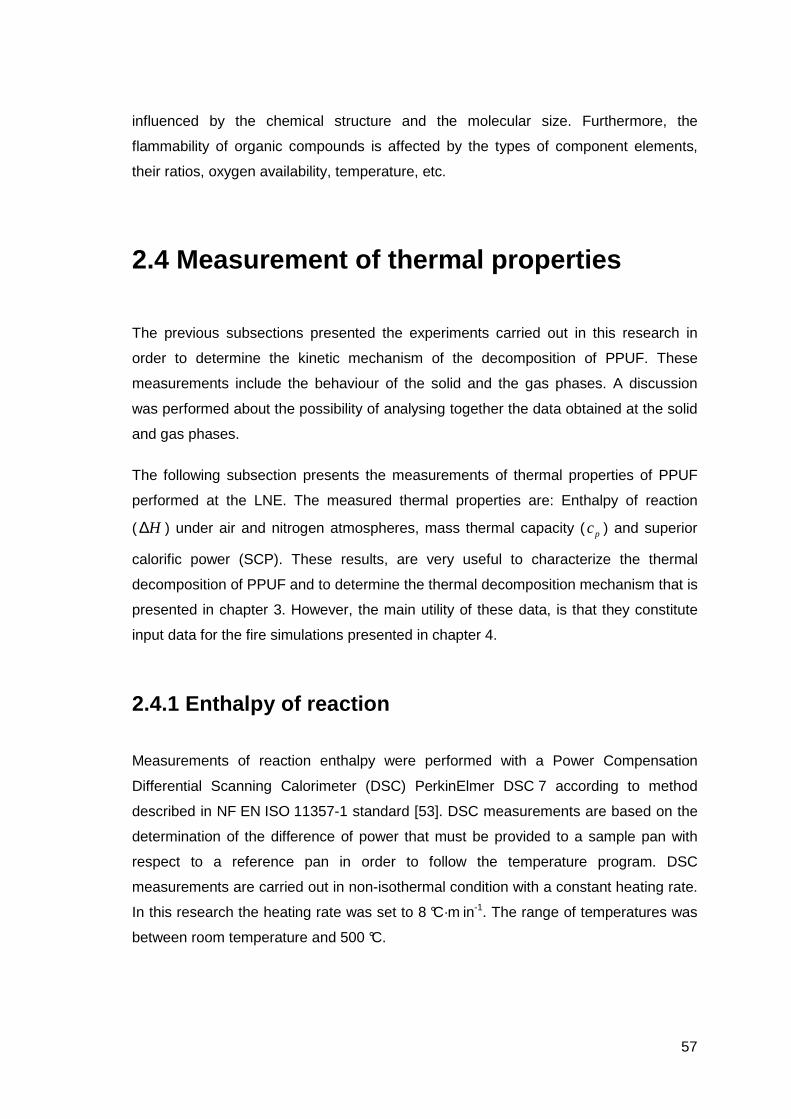
57

influenced by the chemical structure and the molecular size. Furthermore, the

flammability of organic compounds is affected by the types of component elements,

their ratios, oxygen availability, temperature, etc.

2.4 Measurement of thermal properties

The previous subsections presented the experiments carried out in this research in

order to determine the kinetic mechanism of the decomposition of PPUF. These

measurements include the behaviour of the solid and the gas phases. A discussion

was performed about the possibility of analysing together the data obtained at the solid

and gas phases.

The following subsection presents the measurements of thermal properties of PPUF

performed at the LNE. The measured thermal properties are: Enthalpy of reaction

( H∆ ) under air and nitrogen atmospheres, mass thermal capacity ( pc ) and superior

calorific power (SCP). These results, are very useful to characterize the thermal

decomposition of PPUF and to determine the thermal decomposition mechanism that is

presented in chapter 3. However, the main utility of these data, is that they constitute

input data for the fire simulations presented in chapter 4.

2.4.1 Enthalpy of reaction

Measurements of reaction enthalpy were performed with a Power Compensation

Differential Scanning Calorimeter (DSC) PerkinElmer DSC 7 according to method

described in NF EN ISO 11357-1 standard [53]. DSC measurements are based on the

determination of the difference of power that must be provided to a sample pan with

respect to a reference pan in order to follow the temperature program. DSC

measurements are carried out in non-isothermal condition with a constant heating rate.

In this research the heating rate was set to 8 °C·m in-1. The range of temperatures was

between room temperature and 500 °C.

58

PPUF masses used for DSC measurements were around 7 mg. Air or nitrogen volume

flow rates were 50 ml·min-1. Sample and reference pans were manufactured in

aluminium and had a volume of 10 µl. The pans were covered with a reforming tool in

order to improve homogeneity of the heat flux toward the sample.

When carried out under nitrogen atmosphere, the DSC test provides information on the

endothermic energy required to break down the molecules while the material is heated

up. When performed under air atmosphere, they provide information on the heat

release rate by heterogeneous reactions. DSC results are expressed as heat flux endo

up [mW]. When the measurement curve is downwards from baseline, the sample is

releasing energy (exothermic reactions). In PPUF, exothermic reactions only occur

under air atmosphere. When DSC curve is upwards from baseline, the reaction is

endothermic and the molecules are dissipating energy in the breakdown process.

TGA data provide invaluable information for DSC curves interpretation. They allow

distinguishing between irreversible or slow-reversible phase transitions (e.g. vitreous

transition, crystalline structure transformations) and decompositions [41]. Figure 2-1,

presents the experimental results from DSC together with TGA obtained under air and

nitrogen atmospheres at a heating rate of 8 °C·min -1.

One major limitation in the comparison of DSC data with TF or TGA results is that the

experimental conditions are highly different in each test: The main heat transfer

mechanism between DSC pan and sample is conduction. The heat transfer occurs

mainly by the bottom of the pan. In TGA and TF, the heat transfer occurs mainly by

radiation, particularly at higher set temperatures. The sample is located in the center of

the isothermal zone. Thus, it can be considered that the particle is homogeneously

irradiated on all surfaces and the side effects can be neglected.

It was observed that in TGA and DSC tests where PPUF was heated up to 500 °C, the

remaining residues had dissimilar visual characteristics. Analytical tests were

performed in order to figure out differences in their structures. None could be found,

however.

59

Figure 2-1. DSC and TGA results under air and nitrogen atmospheres. Upper curves are under air atmosphere. Bottom curves are under nitrogen atmosphere. TGA curves are presented in blue circles, referenced at the left hand side y-axis. DSC curves are

presented in green pluses reported at the right hand side y-axis. Heating rate was 8 °C·min -1. Positive enthalpy means endothermic reaction. Enthalpy is negative in

exothermic reactions.

DSC is essentially a test designed to measure enthalpy in non-decomposing materials

such as metals or ceramics. Using DSC with plastics during thermal decomposition

could perhaps be interpreted as “out of the limits of the instrument”. The feature of

interest in DSC curves is the deviation of the signal from the baseline. Nevertheless,

the baseline is not always easy to establish. In this research, a sloping baseline was

found, which required particular treatments to make data interpretation possible [54]. A

sloped baseline means that after thermal events, the response of the instrument does

not return to the original baseline level. The baseline tends to have a higher slope after

a decomposition event. This is due to:

• The fact that the thermal properties of the residue (by-product) left by one reaction

are different from those of the reactive (e.g. virgin material) . This behaviour

remains the same in successive reactions. For example, the baseline slope after

60

the second reaction under nitrogen (see bottom plot of Figure 2-1) was higher than

the slope after the first reaction.

• The mass of the sample changes during each reaction. However, in the current

test, the calculation of the power supplied to the sample is referenced to the initial

mass and not to the actual mass. Unfortunately, DSC facility does not allow

measuring the mass in real time. Thus, the actual amount of energy required per

unit of mass to decompose the solid is difficult to establish.

Because of the problem of baseline, under nitrogen tests, a sigmoid baseline was

used. This curved baseline allowed calculating the first peak of heat flow endo up. It

was observed that a straight baseline did not allow to calculating the heat exchange

caused by the first reaction. The standard NF EN ISO 11357-1 [53] describes an onset

temperature method to define a DSC baseline. This method turned out not to be

adequate to be applied to the data of this research.

DSC results under air showed to be dependent on ventilation in the sample holder. The

first series of tests were performed using a cover. The tests were repeated later, using

hand-perforated covers. The results were highly different. Nevertheless, in the case of

materials that may burn, this technique is not designed to separate the effect of the

heterogeneous reactions in the solid phase and the possible effects of the

homogeneous reactions in the gas phase.

As shown in Figure 2-1, TGA and DSC peaks under air and nitrogen do not fit very

well. This is a topic requiring further research. In particular, the deviation of enthalpy

measurement caused by the heat release rate of PPUF heterogeneous reactions under

oxidizing atmosphere (if any) must be quantified. This could also give an idea of the

proportions of heat produced at the solid phase and at the gaseous phase.

Nevertheless, there are no further methods available to measure the enthalpy of

reaction, so espite of this cause of uncertainty, one enthalpy datum is calculated under

air and two data under nitrogen [54]. The enthalpy of reaction data is used in fire

simulation (Chapter 4).

61

2.4.2 Mass thermal capacity

Mass thermal capacity at constant pressure is also measured by the principle of

differential calorimetry. The instrument used is a Setaram DSC III. Measurements are

conducted according to the standard ISO 11357-4:2005 [55]. Mass thermal capacity of

sample, sppc , , is calculated in function of thermal capacity of calibration sample, calpc , ,

initial sample mass, spm , mass of calibration sample, calm , their respective heats spQ∆

and calQ∆ and heat at blank blankQ∆ . It is mathematically expressed in Eq. (2-3).

blankcal

blanksp

sp

calcalpspp QQ

QQ

m

mcc

∆−∆∆−∆

⋅⋅= ,, (2-3)

Because of PPUF thermal decomposition processes, thermal capacity of the foam is

only defined at low temperature, up to T~200 °C. As shown in TGA curves, above this

temperature, the solid structure begins to decompose and gas is released. At higher

temperatures, it is uncertain what is in reality being measured. pc measurement is

performed withunder airtight settled holders in which pressure can increase due to

PPUF gasification. Increase of pressure is a cause of uncertainty as well. Figure 2-2,

shows the thermal capacity results of virgin PPUF and char. The char considered here

is the residue obtained in cone calorimeter during tests carried out in non-flaming

condition at an irradiance level of 30 kW·m-2 (see chapter 4).

62

Figure 2-2. Thermal capacity data of virgin PPUF and char. Char data have been obtained without settled holder.

pc measurement of virgin PPUF has been performed once, while pc measurement of

char has been performed four times: twice with settled holders and twice with open

holders. As shown in Figure 2-2, pc of virgin foam at environment temperature is

2 kJ·kg-1·K-1 and increases linearly up to 2.4 kJ·kg-1·K-1 at T~200 °C. pc of char at

environment temperature is around 1.4 kJ·kg-1·K-1 and increases to 1.8 kJ·kg-1·K-1 at

500 °C. When pc measurements are performed with settled holder, an important noise

is registered from T~50 °C to T~150 °C. The noise i s manifested as a peak with a

maximum thermal capacity of 7.2 kJ·kg-1·K-1 (This curve is not presented). Char

samples were dried prior to the test in an oven at 250 °C for 15 min, so as to discard

any potential influence of moisture. This peak is not observed in the tests with opened

holders.

2.4.3 Thermal conductivity

The thermal conductivity of virgin PPUF as a function of temperature is measured. The

measurement was conducted from the room temperature up to 190 °C. It was found

that after 190 °C, the structure of the solid is hi ghly degraded and the dimensions of the

63

foam change, leading to the lose of the contact between the sample and the

measurement plates.

The facility that enables the measurement of conductivity in function of temperature is

not yet a standard method. It has been designed and built in at the LNE. The method is

called guarded hot plate for thermal conductivity measurement at high

temperature [56], which can perform conductivity measurements up to 250 °C. The

cross-section view of the LNE’s high temperature guarded hot plate is presented in

Figure 2-3.

Guarded area Meter area Guarded area

Main heater

Specimens

Electricalresistances

Heat sink

Top cold plate (T1)

Hot plate (T2)

Bottom cold plate (T1)

Heat sink

Insulation

Air gap

Guarded area Meter area Guarded area

Main heater

Specimens

Electricalresistances

Heat sink

Top cold plate (T1)

Hot plate (T2)

Bottom cold plate (T1)

Heat sink

Insulation

Air gap

Figure 2-3 Cross-section view of the LNE’s high temperature guarded hot plate. This facility enabled the conductivity measurement of PPUF from room temperature up to

250 °C (Source [56])

Basically, the measurement of conductivity ( sk ) with the high temperature guarded hot

plate facility consists in determining the power required at the hot plate (centre at

temperature 2T ) to attain reach a difference of in temperature equal to 10 °C with the

cold plates (boundaries at temperature 1T ) for samples of thickness d . The calculation

of conductivity is carried out using Eq. (2-4). In order to avoid diffusion and boundary

condition problems, two samples are used at the same time.

( )d

TTkQ s

e12 −⋅=′′

(2-4)

Figure 2-4 presents the results of conductivity carried out in virgin PPUF.

64

Figure 2-4 Conductivity of virgin PPUF from room temperature up to 190 °C. Measurement carried out with high temperature guarded hot plate.

As shown in Figure 2-4, the conductivity of the foam increases from 0.045 W·m-1·K-1 at

room temperature up to 0.085W·m-1·K-1 at 190 °C.

2.4.4 Superior calorific power

Superior Calorific Power (SCP) is measured with a bomb calorimeter Parr 1266. The

measurement procedure used is described in the standards NF EN ISO 1716:2002 [57]

and NF ISO 1928:2004 [58]. Test masses are 215 ± 5 mg. No benzoic acid is used

because PPUF is combustible. Tests are repeated three times, the mean SCP is

29 832 ± 221 kJ·kg-1. As shown in the next section this measurement allows calculation

of combustion efficiency. The Inferior Calorific Power and Thornton factor can also be

calculated with this data.

65

2.5 Experimental measurement of the solid

and gas phases

This section describes the experimental measurements carried out in order to

determine experimentally the decomposition mechanism of PPUF. The measurement

techniques that are described here are thermogravimetric analysis, tubular furnace and

Fourier transform infrared spectroscopy analysis.

A discussion is performed in order to validate the comparison of the results obtained

with TGA coupled to FTIR, and those of TF coupled to FTIR. The TGA coupled to FTIR

is mainly used to characterise the behaviour of the solid phase across mass loss

measurement, while TF coupled to FTIR data is used mainly to characterise the

behaviour of the gas phase. Quantitative data from gas phase was collected at the

LNE. It allowed the calculation of the yield of release of the main gas species.

A particular attention is given to TGA results since it is the most conventional

measurement technique to study the decomposition of materials. It provides

information that allows to inferring the decomposition mechanisms. However, it turned

out to be insufficient to select an unambiguous decomposition mechanism. In this

research, TGA data is combined with information from gas analysis instruments. The

coupling of data from both phases allows determining a decomposition mechanism in

agreement with the chemistry of the processes [59]. The changes in solid phase

simultaneously with gaseous phase as a function of time (or temperature), has been

poorly analysed in the past [52][60]. Data from both phases together with a

mathematical model are used to calculate the kinetic parameters of the decomposition

reaction.

2.5.1 Fourier Transform Infrared Spectroscopy gas

analysis (FTIR)

The Fourier Transform Infrared Spectroscopy gas analysis is the only measurement

technique used at all the scales considered in this research. FTIR is a powerful

technique that is currently used for a wide range of industrial and research applications

66

such as: classification and authenticity verification of lactic products [61], polymer

additive decomposition [62], nitrogen transformation in catalytic reactions [63], alloy

oxidization processes [64], analysis of pharmaceutical products ageing and

stability [65], etc.

The chemical bounds of a sample can absorb the energy from an IR source in the near

and mid-infrared wavelengths (5 000 cm-1 to 200 cm-1). The absorption of radiative

energy is caused by the interaction of light beams and chemical bonds, the atoms

vibrate one with another at a given frequency. If atoms are of different nature, an

induced electrical dipole vibrates at the same frequency of mechanical vibrations.

When a non-symmetric bond is irradiated by a monochromatic light source with the

same frequency of bond vibration, an interaction with the electric dipole is produced.

The energy absorbed correspond to vibration frequency

FTIR is a simple light IR beam apparatus in which an interferometer (Michelson type) is

located between an IR radiation source and sample [66]. An Interferometer allows the

modulation of infrared frequencies. The displacement of a mobile mirror scans the

entire range of IR frequencies enabling the measurement of sample transmittance. The

position of the mirror needs to be measured as well because it allows determining the

frequency of the spectral response; it is measured using a helium neon laser beam. In

other words, two measurements are performed at the same time using two sensors:

the position of the mirror (the frequency) and the intensity of the IR beam (the

transmittance). The signal obtained is an interferogram that is converted in IR spectrum

by using a mathematical function called Fourier Transform. FTIR provides absorbance

in function of wavenumber, )(λAb , calculated as a logarithm of ratio between source

intensity, )(0 λI and intensity measurement of the beam passing through the sample,

)(λI . It is mathematically expressed in Eq. (2-5) [67].

( ) ( )( )

=λλλ

I

IAb 0log

(2-5)

The group of frequencies absorbed by a molecule constitutes its “digital identification”;

which is related to geometry, chemical bonding and functional groups. It is possible to

carry out a qualitative identification of a gas mixture by analysing the absorbance

response in a wide range of wavenumbers. In this research, qualitative

67

characterisations of species are noted FTIRqlt. Figure 2-5 shows the spectral response

(absorbance) of various gases commonly found during the combustion of PPUF.

Figure 2-5. Exemple of the absorbance spectra measured in FTIR for various common combustion gases of PPUF (Source [43])

The characteristic of spectral response in precise regions is used to calibrate FTIR

(quantitative measurement). For calibration, the absorbance is expressed in function of

molar absorptivity, ( )λa , path length of cell gas, l and concentration, c . This is

mathematically presented in Eq. (2-6). Reference gas mixtures are used to perform

quantification of the chemical species present in a sample. Nevertheless, the complex

spectral features of many multi-component data sets often make it difficult or even

impossible to develop reliable IR quantitative methods.

( ) ( ) claAb ⋅⋅= λλ (2-6)

The analysis of multi-component spectra is done in two steps. First, a method is

constructed, based on the spectra obtained with known concentrations of the gases of

interest. It is usually called the calibration or training step. Second, the method is

validated and used to predict the unknown concentrations of the gases in the spectra

contained in an independent data set.

One calibration point is the peak height at one or more wavenumbers according to a

known concentration of a gas (see Eq. (2-6) and Figure 2-5). The calibration of a gas

consists in establishing the relation between the intensities in the wavenumber region

and the gas concentrations (curve of calibration). Gases dilution or mixing of certified

68

standard gases enable to obtain a batch of spectra of several concentrations. It

represent a major task of the operator during facility calibration.

The curve of calibration needs to be modelled using conventional methods such as

least squares or partial least squares. Prediction of unknown concentrations is

performed using the model established for each species. A variety of methods,

univariate and multivariate, linear and non-linear, exist to perform the quantification of

gas components in real smoke gas spectra (for more details about FTIR calibration see

reference [68]). The column “Calibration points” of Table 2-5 show the total number of

concentrations acquired over the whole range of quantification of the listed gases; they

link up the concentrations of the calibration gases with the spectral absorbances.

Table 2-5. List of calibrated products in the FTIR of LNE. Lower and higher quantification limits are also presented.

Symbol Low Conc [ppm] (2σ) [%]CO 2.5 50a 10006bc 0.3CO2 260.4 56a 50140bc

0.7

H2O 21.1 13 - -

NO 4.9 22 494bd 0.8NO2 1.0 5 499bc

0.6

N2O 8.5 31 1005c2

HCN 5.0 55 4840c 3HCl 2.1 24 5000c 5HBr 2.0 1 998c 2CH4 0.3 37 4990c

2

C2H2 2.1 35 994c2

C2H4 2.7 34 995c2

H2CO 21.7 10 198c2

SO2 1.0 26 1001bc0.2

NH3 1.0 17 1085c3

Reference gas cylinder

995

131

852

1085

5000998

4990

994

Ammonia

High880250140

22560

494499

1005

1020

Acetylene

Sulfur dioxide

Hidrogen cyanideHidrogen chlorideHidrogen bromide

Methane

Nitrogen dioxide

Nitrous oxide

Ethylene

Formaldehyde

Calibrated gasComponent

Watere

Nitrogen monoxide

c Certification of concentration by weightd Analysis by chimiluminescence spectrometrye The calibration of water is performed by the combustion of methane

Calibration points

a Two ranges of measurementb Cofrac calibration certification

Carbon monoxideCarbon dioxide

Quantification limits [ppm]

The last three columns at the right hand side of Table 2-4 show very important data for

the calibration process: the number of calibration points, the concentration of the

reference cylinder and the relative uncertainty of the concentration expressed in

percentage. CO, CO2, NO, NO2 and SO2, are reference gas cylinders with the quality

label “Cofrac” which guarantees a high standard production process process allowing a

very low concentration uncertainty.

69

The calibration concentrations are experimentally generated using the certified

cylinders and a diluter that mixes very precise amounts of the calibration gas with high

purity nitrogen ( 0.3% 2 =σ ). The dilutors are also calibrated guaranteeing a mass flow

deviation lower than %7.0± . A schematic layout of the dilution facility is shown in

Figure 2-6: Pressure regulators reduce the pressure of the gases contained in the

cylinders; the mass flows are then regulated to obtain the desired concentration and

the mix of gases is finally transported to the FTIR.

Figure 2-6 Scheme of the diluter used during the FTIR calibration. RDM B, RDM C RDM D are mass flowmeters. “V” are gas valves (Source [69])

In Figure 2-6 the volume flow rate of the three flowmeters are specified. At room

temperature and pressure, they behave as ideal gases, thus, the mass flow rate is

determined accurately. The dilution facility allows a large range of gas mix with very

high precision: The flow meters RDM B and RDM C are used for high concentrations

and the flow meters RDM B and RDM D are used for low concentrations. A very

detailed description of the dilution procedure and of the calculation of the uncertainty of

the calibration curve is presented in Ref. [69]

After calibration, performing continuous absorbance analysis vs time allows FTIR to

make a large number of spectrum with relatively higy frequency. Thus, the change of

concentration with time of a sample stream can be determined. In fire applications,

FTIR would be able to measure, in real time, the composition of products streams

generated by flames of different natures [68]. In this research, when quantification is

possible, notation is FTIRqnt.

70

In comparison to conventional analytical methods, FTIR offers a main advantage in

terms of flexibility of information analysis: Data acquisition and interpretation are

separated processes. Spectra obtained from a particular sample can be compared later

with data from an additional library of spectral response in order to identify and quantify

new gases that were not observed with current libraries. This reduces the need to

repeat tests in order to identify particular gases.

Figure 2-7, presents a schematic layout of the FTIR facility used in this research. The

entire transport line (from the sampling point until the gas cell) is heated up to 180 °C. It

allows the transport of combustion products while avoiding water vapour condensation

and water-soluble compounds trapping. Sampling line is 5 m length giving FTIR facility

more flexibility to be used together with test apparatuses. The FTIR facility is in

accordance with the guidelines of the standard ISO 19702:2006 [70].

Sampling line at 180 °C

FTIR with a cell gas of 10 m

FTIR with a cell gas of 10 m

Line of Gas Data transmission

Gas Evacuation Line of Gas Data transmission

Gas Evacuation

Filtration box at 180 °C for particles of diameter

10µm and 2µm

Transport line at 180 °C

Gas measurement cell at 180 °C

Pump and flowmeter

Data acquisition

Figure 2-7. FTIR facility layout

The sampling line is connected to a filtration box where two stainless steel filters are

used to retain soot particles and heavy products. The first filter retains particles of

diameter greater than 10 µm and the second one particles of diameter greater than

2 µm. The two filters are regularly pyrolysed at 600 °C to eliminate all the particles laid

71

down in the filtration grid. After filtration, gases are transported to the gas measurement

cell. It has an optical length of 10 m and a volume of 2 l.

The spectrometer for gas analysis is a FTIR Thermo-Nicolet Magna IR 550 Series II

equipped with MCT-A detector. The data acquisition resolution can be set between 0.5

and 4 cm-1. In this research, the resolution was set to 0.5 cm-1 in order to improve the

sensitivity and the capacity to identify qualitatively minor species. The pressure of the

gas cell is regulated in real time. Previous studies carried out at the LNE (not published

yet), have shown that pressure is one of the main experimental parameters to control in

order to ensure the accuracy of FTIR measurement. Pressure is regulated at

86.7 ± 0.7 kPa (650 ± 5 torr) and gas flow rate is set at 6.5 l·min-1. Finally, the gases

are cooled, dried and filtered before being extracted and eliminated with a membrane

pump.

The sampling gas flow is not dried before passing through FTIR cell measurement.

This enables quantification of H2O (vapour). H2O is not a toxic gas, but is very useful to

establish the mass balance of combustion effluents and to analyse the kinetics of

decomposition of PPUF. The FTIR Analyser is calibrated to quantify around 15

gaseous combustion products at the same time; this analysis technique (including

sampling and filtering device) has been validated during the SAFIR project [71] in the

year 2000. This project constituted the basis for toxicity analysis carried out following

the guidelines of the standard ISO 19702:2006 [70].

Table 2-5 presents the current calibrated gases in the FTIR used in this research. The

lower and higher quantification limits are presented as well. The lower and higher FTIR

limits presented in Table 2-5, allow the analysis of the gas effluents from the vast

majority of the materials tested.

Quantification of particular gases is the basis for calculation of the yield of gaseous

products. Yield of production of a particular gaseous species b in function of time, bY ,

is calculated as the ratio between mass-flow rate of gas b and Mass-Loss Rate (MLR)

of sample (see Eq. (2-7)). The mass-flow rate of a species, expressed in Eq. (2-8), is

given by the following: The product of the species concentration, the volume flow rate

in the exhaust line times, the molar mass divided by the volume of one mole of the

species. Eq. (2-9) is used to calculate the volume of one mole of species b. The main

hypothesis of Eq. (2-9) is that exhaust gases behave as perfect gases.

72

MLR

mY b

b

&=

(2-7)

b

bbb Vmol

MWVxm ⋅⋅= &&

(2-8)

P

TRVmolb

⋅= (2-9)

Calculation of yield in function of time is desirable because it provides important

information on the interaction of the transformations carried out in solid and gaseous

phases (decomposition mechanism) and about the change of toxicity of gases

according to the advancing of decomposition. Unfortunately, some tests, such as TF,

do not allow real-time mass measurement. In this case, the yield cannot be expressed

in function of time. Thus, a single global data is calculated. This single data is the

global yield of species b. It is calculated as the ratio between total mass released of

gas b and total burnt mass.

2.5.2 Thermogravimetric analysis (TGA)

Thermogravimetric analysis is the measurement of sample mass with the increase in

temperature [41]. It is essentially used to determine the properties of materials in fields

such as pharmaceutics, mineralogy, chemical industries, fire retardancy, etc. The key

of the TGA technique is the very high resolution of the mass measurement even with

sample temperatures up to 1600 °C. Recent developme nts of TGA instruments allow

simultaneous DSC measurements by an assembly of thermocouples located into the

sample ceramic support. The DSC measurement is performed comparing heat fluxes in

sample and reference pans [72].

A schematic representation of TGA apparatus is presented in Figure 2-8. Essentially,

TGA is a cylindrical electric heated furnace disposed horizontally. The furnace can be

displaced so as to allow positioning the samples into the high-precision weighing

device (position open). The high precision weighing device is stationary and thermally

conditioned. TGA facility supports the sample and reference holders at the end of a

horizontal beam built with a low conductivity material. In thermogravimetric analysis an

73

infinite quantity of heating protocols can be defined, but they can be classified into two

configurations detailed here-after:

• Isothermal condition: The temperature remains stable during the tests. The main

parameter of this condition is the reaction time. Isothermal tests are used to

analyse in detail the processes of phase change (fusion or evaporation), virtuous

transitions of plastics, inner structure change of metals, etc.

• Non-isothermal or dynamic temperature condition: The temperature changes with

time, following in general a linear heating rate. Heating rate and atmospheres are

the main parameters to be controlled in this configuration. The kinetics of

decomposition have shown to be affected by these two parameters. These tests

provide information on the temperatures at which the phases of the materials

change, and help to define the number of stages of polymers decomposition.

It is known that high amounts of sample in TGA tests would involve a significant gap

between actual sample temperature and temperature registered by the

thermogravimetric system. A main parameter in thermogravimetry experiments is a

very reliable knowledge of the actual temperature of furnace and sample [73].

74

Sample pan

High precisionweighing device

Position closed

Position open

Sample support

Transport gas inlet

Surface of furnace displacement

Exhaust gas outlet towards FTIR

Furnace

Figure 2-8. Scheme of the horizontal TGA facility used in this research.

The TGA tests used in this research were gently performed by Mettler Toledo using a

Mettler Toledo TGA/DSC 1 Star System with a precision in temperature of ± 0.5 K and

in mass of ± 1 µg. The decomposition atmosphere is provided by a gas flow of

20 ml·min-1 of air or nitrogen. Figure 2-9, presents the curves of mass and MLR

obtained by Mettler Toledo with PPUF. In Figure 2-9, curves are not grouped by

atmosphere as generally presented in literature, but are instead grouped by type of

curve (mass or MLR curves). This is interesting to easily evidence the influence of

oxygen on the decomposition mechanism.

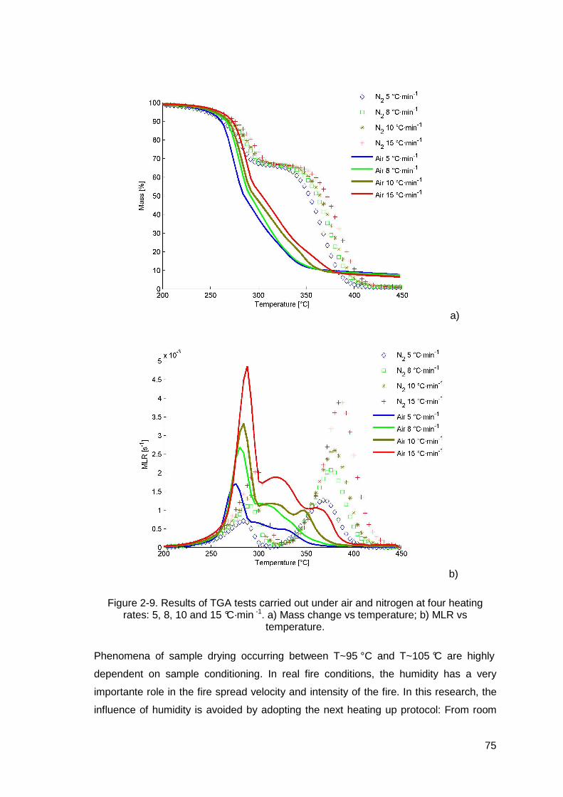
75

a)

b)

Figure 2-9. Results of TGA tests carried out under air and nitrogen at four heating rates: 5, 8, 10 and 15 °C·min -1. a) Mass change vs temperature; b) MLR vs

temperature.

Phenomena of sample drying occurring between T~95 °C and T~105 °C are highly

dependent on sample conditioning. In real fire conditions, the humidity has a very

importante role in the fire spread velocity and intensity of the fire. In this research, the

influence of humidity is avoided by adopting the next heating up protocol: From room

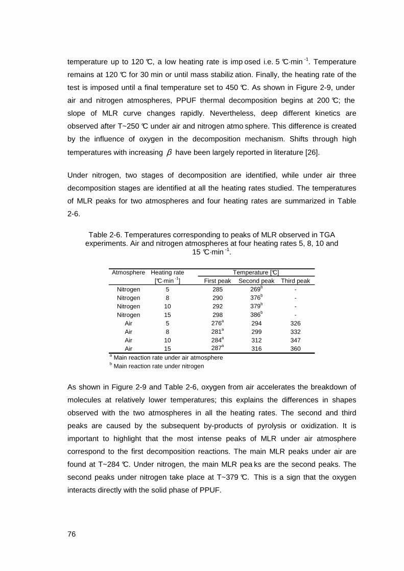
76

temperature up to 120 °C, a low heating rate is imp osed i.e. 5 °C·min -1. Temperature

remains at 120 °C for 30 min or until mass stabiliz ation. Finally, the heating rate of the

test is imposed until a final temperature set to 450 °C. As shown in Figure 2-9, under

air and nitrogen atmospheres, PPUF thermal decomposition begins at 200 °C; the

slope of MLR curve changes rapidly. Nevertheless, deep different kinetics are

observed after T~250 °C under air and nitrogen atmo sphere. This difference is created

by the influence of oxygen in the decomposition mechanism. Shifts through high

temperatures with increasing β have been largely reported in literature [26].

Under nitrogen, two stages of decomposition are identified, while under air three

decomposition stages are identified at all the heating rates studied. The temperatures

of MLR peaks for two atmospheres and four heating rates are summarized in Table

2-6.

Table 2-6. Temperatures corresponding to peaks of MLR observed in TGA experiments. Air and nitrogen atmospheres at four heating rates 5, 8, 10 and

15 °C·min -1.

Atmosphere Heating rate[°C·min -1] First peak Second peak Third peak

Nitrogen 5 285 269b -Nitrogen 8 290 376b -Nitrogen 10 292 379b -Nitrogen 15 298 386b -

Air 5 276a 294 326Air 8 281a 299 332Air 10 284a 312 347Air 15 287a

316 360a Main reaction rate under air atmosphereb Main reaction rate under nitrogen

Temperature [°C]

As shown in Figure 2-9 and Table 2-6, oxygen from air accelerates the breakdown of

molecules at relatively lower temperatures; this explains the differences in shapes

observed with the two atmospheres in all the heating rates. The second and third

peaks are caused by the subsequent by-products of pyrolysis or oxidization. It is

important to highlight that the most intense peaks of MLR under air atmosphere

correspond to the first decomposition reactions. The main MLR peaks under air are

found at T~284 °C. Under nitrogen, the main MLR pea ks are the second peaks. The

second peaks under nitrogen take place at T~379 °C. This is a sign that the oxygen

interacts directly with the solid phase of PPUF.

77

A higher amount of solid residue remains in sample holder at the end of the test under

air atmosphere than under nitrogen atmosphere for a given β . It evidences

heterogeneous chemical reactions where oxygen from air is trapped by PPUF by-

products to form a solid residue. This residue can pyrolyse and oxidize at temperatures

around 500 °C. The oxidization of the residue is no t considered in this research

because of the low amount that remained after combustion of the PPUF.

In large-scale tests, the radiative heat flux from flame towards the sample modifies the

thermal balance of the solid. The thermal balance of the solid also changes the

decomposition kinetics of the element; the decomposition kinetics along with ventilation

control the pollutant emissions. The radiation of flame is of main interest in fire

research. The problem of flame radiation towards the solid was analysed by

Rhodes et al. in 1996 [74]. Their study was performed in cone calorimeter using PMMA

as analysis material. In order to analyse if this is also the case with TGA, the MLR is

compared to the actual heating rate. Figure 2-10, presents the comparison of MLR and

actual heating rate at a set β of 10 °C·min -1.

Figure 2-10. Plot of actual heating rate calculated at each second together with MLR under air and nitrogen atmospheres at set heating rate of 10°C·min -1.

78

In Figure 2-10, the calculation of actual heating rate was performed every second for

the two atmospheres. If heat release rate produced by the particle would have an

influence in heating rate of the furnace, vibration in the temperature program would be

observed. This vibration would be evidenced by local noise in the actual heating rate

curve. Moreover, the noise in the heating rate curve would appear in regions were the

shape of MLR changes strongly (producing endothermic or exothermic reactions). A

change in the slope of MLR leads to a high production of combustible gases.

Nevertheless, as can be seen in Figure 2-10, the temperature controller fits very well

with set temperatures. Some deviations can be observed in the region from 250 °C to

300 °C and from 390 °C to 420 °C. These deviations, however, are of low duration and

they are not observed systematically in the regions where the mass changes strongly.

In conclusion, the mass-loss rate measured in TGA is not influenced by the kinetics of

degradation nor by the heat release rate of the particle. This also means that the heat

released in the gas phase does not control the dynamics of the decomposition process

such observed in larger scale tests (e.g. cone calorimeter, etc). In large-scale tests, the

kinetics of decomposition are controlled by factors such as the temperature and

ventilation at the decomposition front.

TGA provide valuable information about changes of total mass remaining in the sample

holder. However, the identification of the phenomenon causing these mass changes

remains a tricky task. It must be identified with complementary experimental analysis,

data from literature or theoretical approaches. In this research, the nature of solid

phase transformations is identified by the analysis of the released gas products. The

main hypothesis in this methodology is that in TGA, each reaction of the solid releases

particular gaseous compounds in a precise temperature range. In order to validate this

assumption, two series of tests have been performed:

• TGA + FTIR test: As TGA apparatus is available in any of the groups co-operating

in this research, these tests were performed by the SCA laboratory. Unfortunately,

gas identification are only qualitative (FTIRqlt). No calibrations have been performed

to allow quantification.

• Tubular Furnace + FTIR test: These test have been performed in LNE. FTIR

analyser calibration allows gases quantification (FTIRqnt). Nevertheless, TF does

not allow real-time mass measurement. While using TF, calculation of the change

79

of gas yield with increasing temperature is not allowed. Thus, a single global yield

is found.

TGA + FTIRqnt were not performed because of the technical difficulties and the very

high fares to have these tests performed by a third-party organization.

The next subsection describes the tests performed in tubular furnace together with

FTIR in order to identify the kinetics of gas release.

2.5.3 Tubular furnace

Tubular furnace was developed at the end of the 1970’s by different research groups,

including the LNE. It was first used to analyse the chemical compounds released by

cables on fire. In the early 1980’s this facility was adopted by train design and

operation companies to analyse toxicity of materials used for the manufacture of

trains [75]. TF facility was largely used in research projects such as Firestarr (finished

in 2001) [76], in which were largely studied the fire risks in European trains.

The TF is constituted of a quartz tube located in the centre of a cylindrical furnace

disposed horizontally (see Figure 2-11). The inner TF temperature changes with

transversal distance from side wall. Sample must be carefully placed at the isothermal

zone located in the centre of the furnace. Contrary to Purser Furnace apparatus

(BS7990 and ISO TS 19700) [43], in TF, sample boat is introduced manually using a

stainless still rod. A gas flow passes through the quartz tube (vector gas) transporting

the products released by the sample directly to the FTIR. A bypass allows atmospheric

air to enter to the gas line in order to dilute the highly concentrated gas products

released in TF and ensures atmospheric pressure in the transport line.

The tubular furnace used in this research is 600 ± 10 mm long. The combustion tube

has an inner diameter of 40 ± 10 mm and a nominal length of 1000 ± 10 mm as

specified in reference [77]. The temperature programmer is a XS30 Perkly Herrmann

Moritz. The TF is installed under a hood in order to ensure the safety of the operators

in case of leak a of combustion gases.

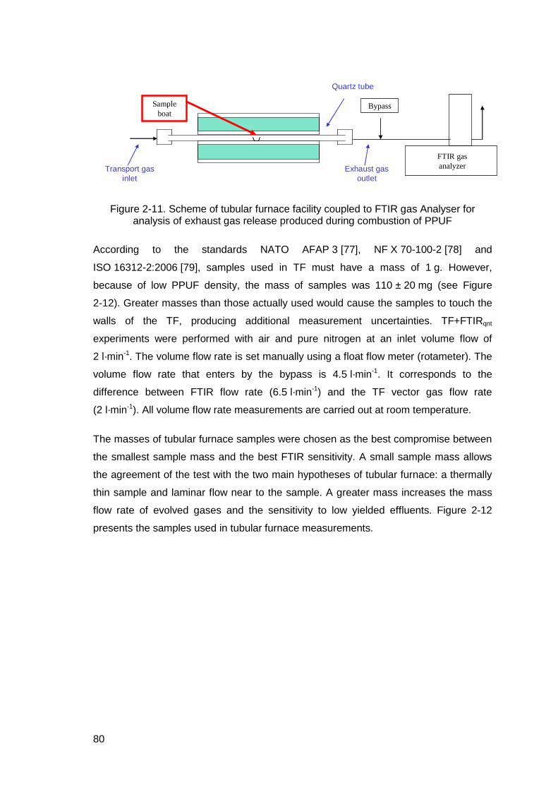
80

FTIR gas analyzer

Sample boat

Bypass

Transport gas inlet

Exhaust gas outlet

Quartz tube

Figure 2-11. Scheme of tubular furnace facility coupled to FTIR gas Analyser for analysis of exhaust gas release produced during combustion of PPUF

According to the standards NATO AFAP 3 [77], NF X 70-100-2 [78] and

ISO 16312-2:2006 [79], samples used in TF must have a mass of 1 g. However,

because of low PPUF density, the mass of samples was 110 ± 20 mg (see Figure

2-12). Greater masses than those actually used would cause the samples to touch the

walls of the TF, producing additional measurement uncertainties. TF+FTIRqnt

experiments were performed with air and pure nitrogen at an inlet volume flow of

2 l·min-1. The volume flow rate is set manually using a float flow meter (rotameter). The

volume flow rate that enters by the bypass is 4.5 l·min-1. It corresponds to the

difference between FTIR flow rate (6.5 l·min-1) and the TF vector gas flow rate

(2 l·min-1). All volume flow rate measurements are carried out at room temperature.

The masses of tubular furnace samples were chosen as the best compromise between

the smallest sample mass and the best FTIR sensitivity. A small sample mass allows

the agreement of the test with the two main hypotheses of tubular furnace: a thermally

thin sample and laminar flow near to the sample. A greater mass increases the mass

flow rate of evolved gases and the sensitivity to low yielded effluents. Figure 2-12

presents the samples used in tubular furnace measurements.

81

Figure 2-12 Tubular furnace sample. The mass is around 110 mg

In this research a dynamic temperature condition was imposed to TF. Unfortunately,

because of the thermal inertia of the instrument, the maximum β is 10 °C·min -1. The

non-isothermal condition allows studying the influence of temperature in the dynamics

of release of gaseous products.

In this research, the influence of the vector gas flow rate in the exhaust gas

composition was not studied, during the dynamic temperature experiments it was set to

2 l·min-1. Some experiments were performed in TF in isothermal condition. The

temperature was set to 650 °C and the volume flow r ates of the vector gas were set to

2 l·min-1 and 4 l·min-1. A clear influence of the ventilation was observed in the yield of

CO2, CH4 and C2H2 but not for the other gases (see Table 2-5). The main difference

between the isothermal and non-isothermal tests is that the reaction time in isothermal

tests is of the order of 100 s, while in non-isothermal tests the reaction time is near to

30 min. Thus, the effect of vector gas flow rate (i.e. ventilation) cannot be compared.

2.5.4 Results of TGA + FTIR qlt and TF + FTIR qnt

As already explained, TGA tests are necessary because they provide information

centered on the decomposition mechanism of PPUF. FTIRqlt measurements were

performed in this research because they served to write a “chemically correct” model of

PPUF decomposition which is presented in Chapter 3. A “chemically correct” model

82

means that the stages of the decomposition mechanism are in agreement with the

evidence of the release of gas effluents. This allows a model that includes the reactions

taking place in the solid phase.

This subsection presents the results obtained during tests carried out in TGA + FTIRqlt

and TF + FTIRqnt. Before following the analysis, it is necessary to verify that the release

of gas compounds during PPUF decomposition is the same in both experimental

techniques. In other words, to check if the combustion models are equivalent. As

explained, this approach is used because no TGA experiments coupled to quantitative

FTIR have been performed during this research.

Figure 2-13, presents the curves of release of isocyanate, polyol and aldehyde

compounds obtained in both experiments. As stated, these results were obtained in

different laboratories (LNE and SCA) and with different instruments (TF and TGA). The

convention for gases labelling is: TGA + FTIRqlt corresponds to experiments performed

in SCA laboratory, where the FTIR measurement are purely qualitative, and

TF + FTIRqnt correspond to tests performed at the LNE, where the FTIR measurements

are quantitative. The experimental conditions for this comparison are: a heating rate of

10 °C·min -1 and nitrogen atmosphere.

Figure 2-13. Releasing of isocyanate, polyol and aldehyde compounds in TGA + FTIRqnt and FT + FTIRqlt at β of 10 °C·min -1 under nitrogen atmosphere.

Aldehyde compounds has been scaled by a factor of 0.6.

The aim of the comparison presented in Figure 2-13, is to see if the shapes of gas

release are similar in both experiments. This comparison is merely qualitative, the

83

y-axis has no dimension. Intensities in the y-axis were normalized, and for ease of view

the intensities of aldehyde compound were multiplied by a factor of 0.6. The intensities

reported for FTIRqlt (SCA laboratory) were calculated quantifying the change of area of

the spectral response of each gas. The quantification of the area of the spectral

response is the principle of FTIR quantification (see subsection 2.5.1).

Figure 2-13, shows clearly that under nitrogen atmosphere at a β of 10 °C·min -1, the

shapes of gases release in function of temperature are very close for polyol, isocyanate

and aldehyde compounds. The small difference in shapes can be due to a difference in

the spectral bands considered for gases identification in both laboratories.

A similar analysis to the one performed in Figure 2-13 is performed under air

atmosphere in Figure 2-14. The interpretation turned out to be complicated because

some shifts between curves were found. The comparison is performed by families of

gases. Contrary to the case of nitrogen, under air atmosphere the curve of MLR (blue

line with triangles) is taken as reference in all the plots.

It is highlighted that in Figure 2-13 and Figure 2-14, the compound labelled as ‘polyol’,

corresponds to OH− functions found in the gas effluents. These functions are created

during the thermal decomposition of polyol that cannot be found in vaporised form. The

molecules found in gas effluents have a structure that is near to the one of virgin polyol.

To clarify, in this dissertation polyol represent a semi-liquid product of the

decomposition of PPUF (particularly in Chapter 3) and a gas produced by the

decomposition of the semi-liquid. The particular discussions concerning the solid or the

gas phases would say to the reader which one is being considered.

Similarly to poluol, the gas labelled ‘Isocyanate’ corresponds to OCN− functions

which are residues from the decomposition of the isocyanate contained in the

polyurethane molecules. Along this manuscript, ‘isocianate’ in the gas phase represent

the family of effluents described.

84

a) b)

c) d)

Figure 2-14. Releasing of a) isocyanate; b) CO2; c) CO and d) polyol vs temperature in TGA + FTIRqlt and FT + FTIRqnt at β of 10 °C·min -1 under air atmosphere. The

experimental curve of MLR is used as reference in all the plots.

Figure 2-14 a), presents the release of isocyanate. The curve obtained in TF is shifted

around 25 °C toward the lower temperatures compared to MLR and TGA curves. This

shift does not seem to be very physical because it does not correspond to an important

change of mass. This can be caused by interference of water bands produced during

combustion or to the earlier break-down of PPUF molecules in TF due to the sample

surface.

n

nePolyurethaPolyolnatePolyisocya

NHCOO-R-NHCOO-R HO-R-HO nNCO-R-OCN n44444 344444 21443442144 344 21 )( ′→′+ Recall of

Eq. (2-1)

The structure of the polyurethane molecule is recalled in order to facilitate the

comprehension of the following analysis. Figure 2-14 b), presents the release of CO2.

In both experimental techniques the peak of CO2 release takes place at a temperature

corresponding to the second peak of MLR, i.e. T~312 °C. At the temperature of the first

peak of MLR, at T~284 °C, the curves of TF and TGA present important inflection

points. The shape of LNE’s curve (TF) is smoother than SCA’s (TGA). This is a typical

85

behaviour caused by the difference in volume of gas cell measurements: LNE cell

measurement is 2 l while SCA cell measurement is 0.17 l volume for similar flow rates.

The peak of CO2 release observed in the TF measurement at T~390 °C does not

appear in TGA’s curve. This peak can be produced by the post-combustion of soot or

solid particles laid in the quartz tube.

Figure 2-14 c), presents the release of CO. The peak of CO release is found at

T~310 °C; this is also the temperature of the secon d peak of MLR. The second and

third peaks of CO production are detected in TF tests at T~360 °C and T~390 °C

respectively. These temperatures correspond to changes in slope of CO curve found

by TGA.

Figure 2-14 d), presents the comparison of release of polyol. TF curve presents three

peaks while TGA presents two. The first peaks are found at T~284 °C and the second

at T~312 °C. However, the third peak found in TF is not found on the TGA curve.

In conclusion, a quite satisfying correspondence is found between gases detected by

SCA and LNE in comparison to the MLR curve. This has two meanings: first that gases

release in TGA and TF during PPUF decomposition are the same, and second, that the

shapes of gas release in function of temperature are quite similar in both cases. This

allows the comparison of the results. The aim of this comparison is to be able to

analyse together the results obtained in TF for the gas phase and the results of TGA

for the solid phase. Thus, the coupling of measurements of solid and gaseous phases

of PPUF decomposition can be carried out.

2.6 Analysis of the solid phase - Verification

of the decomposition mechanism of PPUF

In the previous subsections, the experimental results that allowed coupling the

behaviour of the solid and gas phases have been presented. This information as well

as the measurements of thermal properties represents input data for the numerical

studies presented in the following chapters. Nevertheless, direct analysis in the solid

phase are required in order to study the heterogeneous chemical reactions that occur,

86

particularly those with oxygen. This section presents the works carried out in order to

extract information directly from the solid phase. This information is of prime

importance to understand the physics of the reaction.

During this research, important means were employed to try to identify which changes

are induced by heat in the main structure of foam (condensed phase). The

transformations induced by heat in the solid structure, force all “chemical components”

of virgin matter to react. However, each component reacts at a different time during the

thermo-oxidative process. This produces the different PPUF combustion stages that

were presented in section 2.4.

The aims of analysing the chemical transformations of the solid phase are:

• To identify how they influence the combustion process,

• To identify the reactants and products of each reaction stage (in the solid phase),

• To identify how each reaction in the solid phase can influence the production of

pollutant gases,

• To establish the mass balance in the solid and gas phases.

Data from the solid and gas phases are primordial to determine the decomposition

mechanism of PPUF. Coupled information from both phases allows giving a chemical

meaning to the reaction mechanism proposed in chapter 3.

Extracting useful information in the solid phase turned out to be a tricky task. More

specifically, it was very difficult to get quantitative information because the analytical

methods do not seem fit for the problem addressed in this research (microanalysis X,

FTIR in condensed phase, ATR, elementary analysis, etc). Thermal attack and fire

cause modifications in the structure that are not well known. In addition, the classical

techniques of analysis used for verification in industrial processes cannot be accurately

used here because of strong difference between the samples required for the

instruments and the actual samples found in fire applications.

Conventional spectroscopic methods such as IR and Nuclear Magnetic Resonance

(NMR) have been widely used for the characterisation of PU, but their applications are

often limited and complete analysis is hard to perform [22]. Indeed these methods are

87

based on the study of the spectral response of molecules when irradiated in a given

range of frequency. Still, the interpretation of the spectral response is difficult because:

a) A huge number of libraries of spectral response are required in order to compare the

current response with data from the library; b) Multiple molecules can have very close

spectral responses, which makes it difficult to distinguish the actual molecules of the

solid.

In this research, two types of analysis of the solid phase have been carried out: a visual

characterisation and measurements using various analytical techniques. The

techniques and findings are detailed here after.

2.6.1 Visual characterisation of the solid phase

The visual characterisation was performed at various scales by binocular images and

Scanning Electron Microscopy (SEM). Binocular images were taken from structure of

virgin foam and the residues remaining after heating up to 500 °C. The binocular

instrument used was a Leica M3Z with maximum zoom of 260X. Scales of the

binocular images were between 500 µm to 1 mm. The images were of great usefulness

because they suggested that imagery at smaller scale would give more information on

the PPUF decomposition phenomena.

Scanning Electron Microscopy (SEM) pictures were taken of four types of PPUF

residues: samples after DSC measurement under air and nitrogen atmospheres and

samples obtained directly from cone calorimeter under air and nitrogen. The SEM

instrument used was a LEO 440, S440 3802 series. SEM images can be taken only in

power conductive materials. A gold electroless deposition of about 1.5 nm to 3 nm was

laid on the surface of virgin and PPUF residues in order to enable image acquisition.

PPUF is not a electrical conductor material, thus it can be hypothesised that this

surface treatment does not change the sample properties.

Figure 2-15, presents binocular and SEM pictures of virgin foam. Pictures are

presented in a two columns table. The larger scale image is on the left presenting the

global morphology of the sample (observed used optical instruments), and the smallest

scale is shown on the right presenting the inner structure (SEM photographies). This

distribution of pictures lets to the reader know what the SEM picture is showing.

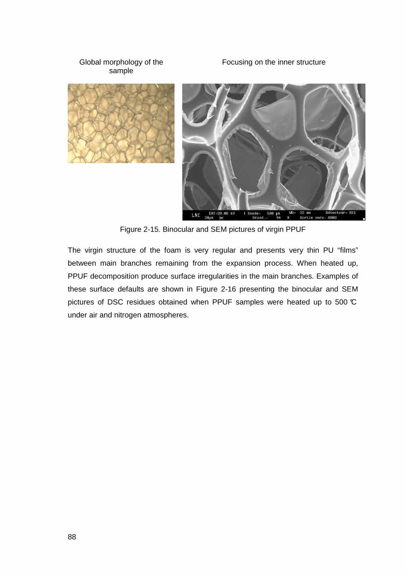
88

Global morphology of the sample

Focusing on the inner structure

Figure 2-15. Binocular and SEM pictures of virgin PPUF

The virgin structure of the foam is very regular and presents very thin PU “films”

between main branches remaining from the expansion process. When heated up,

PPUF decomposition produce surface irregularities in the main branches. Examples of

these surface defaults are shown in Figure 2-16 presenting the binocular and SEM

pictures of DSC residues obtained when PPUF samples were heated up to 500 °C

under air and nitrogen atmospheres.

89

Global morphology of the sample

Focusing on the inner structure N

itrog

en a

tmos

pher

e

Air

atm

osph

ere

Figure 2-16. Binocular and SEM pictures of DSC residues. PPUF samples were heated up to 500 °C under nitrogen (top) and air (bottom) atmospheres.

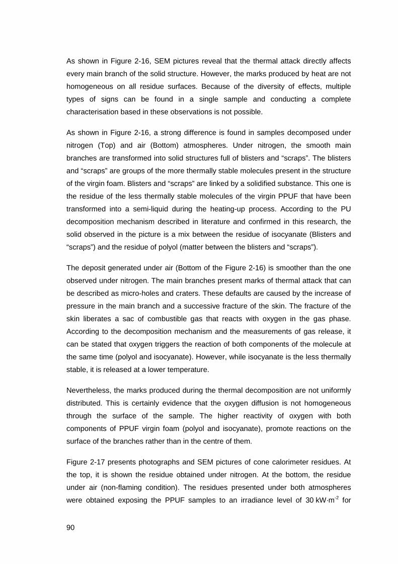
90

As shown in Figure 2-16, SEM pictures reveal that the thermal attack directly affects

every main branch of the solid structure. However, the marks produced by heat are not

homogeneous on all residue surfaces. Because of the diversity of effects, multiple

types of signs can be found in a single sample and conducting a complete

characterisation based in these observations is not possible.

As shown in Figure 2-16, a strong difference is found in samples decomposed under

nitrogen (Top) and air (Bottom) atmospheres. Under nitrogen, the smooth main

branches are transformed into solid structures full of blisters and “scraps”. The blisters

and “scraps” are groups of the more thermally stable molecules present in the structure

of the virgin foam. Blisters and “scraps” are linked by a solidified substance. This one is

the residue of the less thermally stable molecules of the virgin PPUF that have been

transformed into a semi-liquid during the heating-up process. According to the PU

decomposition mechanism described in literature and confirmed in this research, the

solid observed in the picture is a mix between the residue of isocyanate (Blisters and

“scraps”) and the residue of polyol (matter between the blisters and “scraps”).

The deposit generated under air (Bottom of the Figure 2-16) is smoother than the one

observed under nitrogen. The main branches present marks of thermal attack that can

be described as micro-holes and craters. These defaults are caused by the increase of

pressure in the main branch and a successive fracture of the skin. The fracture of the

skin liberates a sac of combustible gas that reacts with oxygen in the gas phase.

According to the decomposition mechanism and the measurements of gas release, it

can be stated that oxygen triggers the reaction of both components of the molecule at

the same time (polyol and isocyanate). However, while isocyanate is the less thermally

stable, it is released at a lower temperature.

Nevertheless, the marks produced during the thermal decomposition are not uniformly

distributed. This is certainly evidence that the oxygen diffusion is not homogeneous

through the surface of the sample. The higher reactivity of oxygen with both

components of PPUF virgin foam (polyol and isocyanate), promote reactions on the

surface of the branches rather than in the centre of them.

Figure 2-17 presents photographs and SEM pictures of cone calorimeter residues. At

the top, it is shown the residue obtained under nitrogen. At the bottom, the residue

under air (non-flaming condition). The residues presented under both atmospheres

were obtained exposing the PPUF samples to an irradiance level of 30 kW·m-2 for

91

about 10 min. These figures can be compared with the SEM pictures obtained by

Branca et al. [10] presented on Appendix A

Global morphology of the sample

Focusing on the inner structure

Nitr

ogen

atm

osph

ere

Air

atm

osph

ere

Figure 2-17. Pictures and SEM images of cone calorimeter residues. PPUF samples were exposed to irradiance level of 30 kW·m-2 under nitrogen (top) and air (bottom)

atmospheres.

As shown in Figure 2-17, the characteristics of the surfaces are highly different in

function of the atmosphere. Under nitrogen, solidification of a semi-liquid product is

evidenced by folds indicating that the surface has been submitted to strain, as can be

observed when a fabric is stretched. Under air, a very thin layer at the top of the

sample can be observed. The thin layer is the decomposition front that shifts from the

top towards the bottom of the sample during decomposition. Under this layer, thermally

92

attacked branches are found. The decomposition front constitutes a thermal barrier that

reduces the damage rate caused by heat in the structure of the branches. These

observations are in agreement with those made on DSC residues, which suggests that

the decomposition mechanism remains constant independently of the test.

Under both atmospheres, the displacement shift of the decomposition front is always

parallel to the top of the sample, denoting a homogeneous irradiance level from CC in

the radial direction of the cone.

Comparison of SEM photographs of Figure 2-16 and Figure 2-17 shows that the

remaining branches in cone calorimeter (under both atmospheres) present smoother

surfaces than the remaining residues of DSC tests. It allows concluding that the mode

of heat transfer affects the kinetic of solid decomposition. Nevertheless, the

decomposition mechanism remains constant: The first decomposition stage is the

breakdown of PPUF molecules that allows release of isocyanate and the second is the

decomposition and further reaction of polyol.

In cone calorimeter, the semi-liquid polyol is formed in the decomposition front. It is

present almost homogeneously in the surface exposed to the irradiance level from the

heater. This semi-liquid produces the smooth surface observed in both atmospheres in

Figure 2-17. At the matter scale (DSC), the liquid polyol is formed and decomposed

directly in the surface of the main branches, and it does not spread from one branch to

the next one. So, as the polyol cannot spread between the branches, a smooth surface

is not generated. The surface defaults are produced by the physical and chemical

transformation occurred into the branch.

2.6.2 Characterisation of the molecular structure o f the

solid

Various analytical techniques were used in order to identify the transformations of the

solid phase. These analyses provided information about the nature of the molecular

structure of the virgin foam. Unfortunately, they provided few information about the

transformation induced by heat in the solid matrix. We consider it is of main interest to

reference these tests even if the result were not very useful the determination of the

effects of thermal attack in the solid phase. The techniques used were:

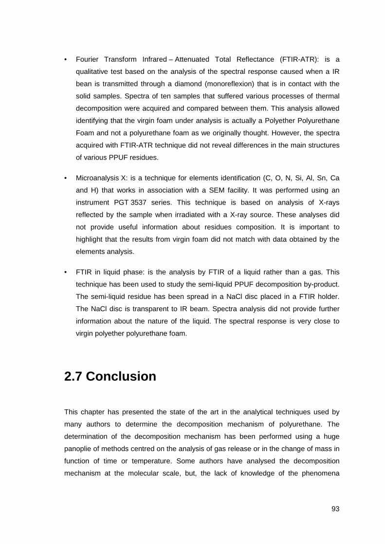
93

• Fourier Transform Infrared – Attenuated Total Reflectance (FTIR-ATR): is a

qualitative test based on the analysis of the spectral response caused when a IR

bean is transmitted through a diamond (monoreflexion) that is in contact with the

solid samples. Spectra of ten samples that suffered various processes of thermal

decomposition were acquired and compared between them. This analysis allowed

identifying that the virgin foam under analysis is actually a Polyether Polyurethane

Foam and not a polyurethane foam as we originally thought. However, the spectra

acquired with FTIR-ATR technique did not reveal differences in the main structures

of various PPUF residues.

• Microanalysis X: is a technique for elements identification (C, O, N, Si, Al, Sn, Ca

and H) that works in association with a SEM facility. It was performed using an

instrument PGT 3537 series. This technique is based on analysis of X-rays

reflected by the sample when irradiated with a X-ray source. These analyses did

not provide useful information about residues composition. It is important to

highlight that the results from virgin foam did not match with data obtained by the

elements analysis.

• FTIR in liquid phase: is the analysis by FTIR of a liquid rather than a gas. This

technique has been used to study the semi-liquid PPUF decomposition by-product.

The semi-liquid residue has been spread in a NaCl disc placed in a FTIR holder.

The NaCl disc is transparent to IR beam. Spectra analysis did not provide further

information about the nature of the liquid. The spectral response is very close to

virgin polyether polyurethane foam.

2.7 Conclusion

This chapter has presented the state of the art in the analytical techniques used by

many authors to determine the decomposition mechanism of polyurethane. The

determination of the decomposition mechanism has been performed using a huge

panoplie of methods centred on the analysis of gas release or in the change of mass in

function of time or temperature. Some authors have analysed the decomposition

mechanism at the molecular scale, but, the lack of knowledge of the phenomena

94

occurring at this scale makes this approach useless for fire safety engineering

applications.

The experimental results obtained at the matter scale have been presented. The matter

scale takes into account samples from 1 mg up to 110 mg, which are the smallest

samples considered in this research. The equipment for measurements at the matter

scale have been designed in order to reduce the influence of environmental conditions,

and to focus on the analysis of some particular phenomena. The main assumption is

that they do not deal with the diffusive effect and the mass and heat transfer

phenomena from the centre of the particle towards the boundaries. This is a powerful

hypothesis that allows considering that the experimental results are not affected by

external noise. Nevertheless the very low density and the alveolar structure of the foam

can probably be a cause of noise in the results while the effective area of heat and

species exchange is unknown. However, up to date there is no mean to verify and

quantify these effects. Despite of this, It was accurately determined the decomposition

mechanism of PPUF under air and nitrogen atmospheres.

The experimental facilities used were TGA+FTIRqlt and TF+FTIRqnt, which provided

information on the change of the solid mass and gas release. Each event of mass

change of the condensed phase has been correlated to particular gases release. It

allowed verifying the decomposition mechanism, based on information from the solid

and the gas phases with increasing temperature. This information, as well as the

measurements of thermal properties represent the main input data for the numerical

studies presented in the following chapters.

The transformations of the solid phase have also been analysed by imagery and

chemical analyses. Binocular and SEM pictures were performed in order to examine

the transformations suffered by the solid phase and the influence of oxygen during the

decomposition process. The visual observation confirmed the mechanism found while

analysing the change of mass and gas release. It was also found that the oxygen and

the mode of heat transfer influence the kinetics of decomposition but that the

mechanism of decomposition remains unchanged: Two decomposition stages are

observed, the first decomposition stage is the breakdown of PPUF molecules that

allows release of isocyanate and the second is the pyrolysis and further oxydation of

polyol.

95

3 Matter scale model

3.1 Introduction

The experimental results obtained at the matter scale were presented in chapter 2.

They provided valuable information on the behaviour of PPUF with the change of

temperature. These results allowed determining the decomposition mechanism of

PPUF based on the observations of solid as well as the gas phases.

The prediction of thermal decomposition is a main concern in FSE because it allows

calculating the source term of fire. The source term is the quantification of the chemical

energy that can be converted into heat by the flame. The prediction of thermal

decomposition also allows calculation of pollutants release and fire spread, which are

primary hazards of fire. The main limitations for the improvement of the predictions of

fire behaviour of materials is the diversity of physical chemical phenomena that must

be taken into account. Moreover, during the fire spread the heat and species transport

occurs in transient state. The accurate prediction of the decomposition kinetics of solids

must take into account parameters such as: temperature, heating rate, thermal

history [80], oxygen concentrarion, porosity, nature of the solid fuel, etc.

The decomposition mechanism is the succession of stages that take place during the

thermo-chemical decomposition of matter. This allows writing the mass balance and

the comparison of experimental and calculated results, which is the basis of the

method used to “calibrate” the model and to find the kinetic parameters of the reaction.

So, the decomposition mechanism is the main input data for the model of PPUF

thermal decomposition.

96

All the models referenced to matter scale found in literature are based on the

hypothesis that samples behave as particles and no gradients between the centre and

the boundary are found. Many authors have proposed methods to calculate the kinetic

parameters of matter decomposition. Each model of thermal decomposition allows the

calculation of a group of kinetic parameters, usually those of Arrhenius equations:

Activation energy, pre-factor and reaction order. Nevertheless, up to now, all the

methods used to determine the decomposition mechanism and to calculate the kinetic

parameters are based on the single information of the condensed phase (TGA

experiments).

The models from literature do not take into account information from the gas phase. As

presented in chapter 2, the kinetic of gas release provide information on the reactions

taking place in the solid phase. Analysing together information of the solid phase and

gas phases allowed verifying that the decomposition mechanism is in agreement with

the chemistry of the process. A decomposition mechanism that takes into account both

information from the solid and gas phases, can be considered as “chemically correct”

which is necessary for further improvements of the model.

The aim of this chapter is to improve a model of thermal decomposition of PPUF in

order to be able to predict both the change of total mass and the kinetics of gases

release in function of time or temperature. This allows calculating the kinetic

parameters of a chemically correct process. Moreover, the groups of parameters found

allow an accurate prediction of the decomposition process of PPUF under various

experimental conditions, notably concerning the heating rates and atmospheres.

The kinetic parameters calculated by the current model are used into the pyrolysis

models of Computational Fluid Dynamics (CFD) in order to simulate large-scale fire

tests. Calculation of the decomposition rates constitutes a crucial challenge for the

development of fire codes in order to make reliable predictions of HRR and pollutants

formation.

This chapter is divided into six sections. Section one is the introduction. Section two is

the state of the art in matter scale models with notably:

• A literature review of the methods defined by other authors to analyse

mathematically the decomposition of PU and to calculate the kinetic parameters.

97

• The methods of thermal analysis applicable to PU, but used for various types of

organic materials commonly found in buildings: wood, plastics, waste, biomass, etc.

Section three presents the improvements carried out to the model in order to take into

account the gas phase. Section four deals with the analysis of stability of the model’s

code. Section five is the analysis of sensitivity. Section six presents the conclusions of

the chapter.

3.2 State of the art in matter scale modelling

A better description of the source term is a current need for the evolution of FSE. The

study and modelling of thermal decomposition of the materials involved in real fire is a

crucial issue to accurately predict the source term. However, It is usually not well

predicted or neglected in the fire simulation codes that are found on the market. A very

precise prediction of fire behaviour is needed in the performance-based design of

structures, which is the current trend in fire protection building design [80][81].

3.2.1 Background

The basic kinetic concepts used in thermal decomposition have been stated at the end

of the nineteenth century by van’t Hoff (1884), Arrhenius (1889), Wilhelmy (1891),

Guldberg (1899) and Lewis (1905) during studies of single-step heterogeneous

reactions. The rates of multi-step reactions were experimentally studied in the

beginning of the twentieth century [82]. The modelling methods for multi-step thermal

decomposition as known (used) nowadays have been developed in the end of the

1950’s [83]. Since then, different methods have been proposed; the most widely used

methods are described in the next subsections.

The models of thermal decomposition of solids is a compromise between

simplifications of physical phenomena and the ability to take into accound as many

details as possible. This compromise allows reproducing the reality in an acceptable

manner dealing with mathematical and physical problems that can be resolved in a

reasonable calculation time. Models are limited by: the knowledge of the physics [84],

98

calculation time [85], availability of measurements of material properties (data from

literature), accuracy of these measurements [86], experimental perturbations, chemical

knowledge of the process [87], criteria about what is acceptable and what is not, etc.

The problem of the validity of decomposition models at different scales appears very

often: Very few models consider the transformations at the molecular level [33]. The

analysis at the molecular level is crucial to understand the physics of the

decomposition. Yet, the reactions at the scale of molecular chains such as initiation,

branched chain, propagation and termination do not follow Arrhenius’ law behaviour [9].

The models are stated at scales at which the mass is of a few milligrams, for which the

reaction rates of the overall processes can be described using Arrhenius’ equations.

Nevertheless, the most useful applications of decomposition models are in FSE, where

the masses burning are of a few kilograms. The description of thermal decomposition

required in FSE (behaviour in the solid phase) must reproduce the pattern observed at

sizes near to the one of the product that is burning; this is not the case of the

information found in literature. All the kinetic schemes of thermal decomposition

considered in this work allow the prediction of solid transformations of masses of a few

milligrams. Although, at the real scale, gradients of temperature and oxygen mass

fraction as well as the interaction between the flame and the solid modify the

decomposition kinetics. These effects are not considered at the matter scale because

the dimensions of the sample are negligible: the sample is considered as a particle.

As stated, for years the main application of the modelling of thermal decomposition has

been the FSE. But, the knowledge of decomposition mechanisms also has other

applications such as: lost foam casting [88], smoldering combustion [89], remediation

of polluted soils [15], pyrolysis and combustion of toxic and dangerous wastes [42][90],

processes optimization [91][92], energetic recovery of biomass [93][94], etc.

Experimentally, TGA is the most widely used technique for estimating the kinetic

mechanism and the corresponding kinetic parameters of thermal decomposition.

Nevertheless, thermal analysis carried out based on TGA experiments may present

some difficulties such as: scatter on kinetic parameters calculated with various

methods, scatter on TGA curves with various heating rates or atmospheres, various

kinetic behaviors of a single material, different kinetic parameters found from different

manufacturers, possible influence of the transport phenomena into the material

(generally neglected), etc [13][15].

99

Prior to the calculation of the kinetic parameters, the kinetic mechanism of

decomposition must be found. It is one of the main tasks in FSE research. It requires

the analysis of data from TGA and other experimental techniques.

In order to settle these difficulties, TGA data must be analysed together with qualitative

and quantitative results from other experimental facilities. It allows the division of the

bulk decomposition process into successive sub-processes activated when the matter

temperature is increased. The division into sub-processes allows a particular

characterisation and independent analysis of the species created and decomposed in

each phase. Particularly, it allows an interpretation of the peaks observed in TGA

mass-loss rate curve.

The next subsections present a detailed literature review of the methods existing for

calculating the kinetic parameters of the thermal decomposition of solids. However, it

has been found that the methods for determining the decomposition mechanism have

not been as widely discussed, the one used in this research is discussed in

subsections 2.5.4 and 3.3.1.

3.2.2 The model-fitting (modelistic) method

3.2.2.1 Principle of the model-fitting method

The model-fitting (modelistic) method consists in selecting from a list of models the one

that best fits TGA non-isothermal experimental curves. In this method, the Arrhenius

equations are referenced to remaining mass in sample holder. Thus, the model-fitting

method is expressed in terms of the degree of conversion, α , which is equal to 0 at

the beginning of the test and to 1 when all the mass has been decomposed. The

degree of conversion is an overall property of the transformation kinetics, defined in

Eq. (3-1).

f

t

mm

mm

−−=

0

0α (3-1)

100

Where, 0m is the mass of the sample at the beginning of the process, tm is the mass

of the sample at an arbitrary time t . fm is the mass of the sample at the end of the

process. The solid-state rate of reaction is assumed to be described by the product of

two separate functions: )(Tk , the rate constant and )(αf , differential conversion

function. The rate constant is the Arrhenius equation, while the conversion function is

the reaction model. The reaction rate is defined mathematically in Eq. (3-2). The main

hypothesis for allowing the use of Eq. (3-2) is that reactions are autocatalytic, in other

words, they do not require a complementary chemical product to initiate the reaction.

Thus, )(αf is only function of the degree of conversion and )(Tk is only function of

temperature [95].

)(exp)()( αααf

RT

EAfTk

dt

d

−== (3-2)

The Arrhenius equation is expressed in function of: A , pre-exponential factor. E ,

apparent activation energy. R , universal gas constant. T , absolute temperature. For

non-isothermal conditions, authors prefer to write Eq. (3-2) as a function of heating

rate, β . In this case, the derivative of the degree of conversion is expressed with

respect to temperature, see Eq (3-3).

dt

dT

fRT

EA

dT

d

=∴

−=

β

ααβ )(exp

(3-3)

In Eq. (3-2) and (3-3), the reaction model, )(αf , represents a certain solid-state

mechanism that gives rise to the characteristic change of the degree of conversion with

time (α vs t ). Experimental data can be compared against a set of model plots in

order to choose the one that accurately reproduces experiments. This enables the data

to be interpreted in terms of the mechanism represented by the chosen reaction

model [82][96].

The Arrhenius law of Eq. (3-3) relates the rate constant of a single-step reaction to

temperature. It is generally assumed that E and A remain constant. However, it has

been shown that in solid-state reaction kinetics, the parameters may vary with the

101

degree of conversion. In solid state, a variation in apparent activation energy could be

observed due to a complex decomposition mechanism [82].

The reaction models, )(αf , are in general listed in the integral form, )(αg , of

Eq. (3-3), which is presented in Eq. (3-4) [97].

[ ] αααα

dfg ∫−=

0

1)()( (3-4)

The models the most commonly used are listed in Table 3-1.

102

Table 3-1. Set of reaction rate models applied to describe the reaction kinetics in heterogeneous solid state systems (e.g. polymers). (Source [23][41][82][98][99]).

No. Symbol Reaction model source

( )αf ( )αg

1 P1 Power law [23][41][82][99]

43

4α 41

α

2 P2 Power law [23][41][82][99]

32

3α 31

α

3 P3 Power law [23][41][82][99]

21

2α 21

α

4 P4 Power law [23][41][82][99]

21

32 −α 3

2α

5 R2 Phase boundary controlled reaction

(contracting cylinder, i.e. bidimensional

shape) [23][41][82][98][99]

21

)1(2 α− 21

)1(1 α−−

6 R3 Phase boundary controlled reaction

(contracting sphere, i.e. tridimensional

shape) [23][41][82][98][99]

32

)1(3 α− 31

)1(1 α−−

7 F1 First-order (Marpel)/ Random nucleation [23][41][82][98][99]

α−1 )1( α−− Ln

8 F2 Second-order reaction

[41] )1(

1α−

2)1( α−

9 F3 Third-order reaction [41]

2

)1(1

−α 3)1( α−

10 E1 Exponential law [41][98]

α )(αLn

11 A2 Avrami-Erofe’ev(m=2) [23][41][82][98][99] [ ] 2

1

)1()1(2 αα −−− Ln [ ] 21

)1( α−− Ln

12 A3 Avrami-Erofe’ev(m=3) [23][41][82][98][99] [ ] 3

2

)1()1(3 αα −−− Ln [ ] 31

)1( α−− Ln

13 A4 Avrami-Erofe’ev(m=4) [23][41][82][99] [ ] 4

3

)1()1(4 αα −−− Ln ( )[ ] 41

1 α−− Ln

14 A5 Avrami-Erofe’ev(m=3/2)

[23]

[ ] 32

)1()1(23 αα −−− Ln ( )[ ] 3

21 α−− Ln

15 B1 Proust-Tompkins [41]

)1( αα − ))1(( αα −Ln

16 D1 One-dimensional diffusion

[23][41][82][98][99]

1

21 −α

2α

103

No. Symbol Reaction model source

( )αf ( )αg

17 D2 Two-dimensional diffusion

(bidimensional particle shape)

Valensi Equation [23][41][98]

[ ] 1)1( −−− αLn ααα +−− )1()1( Ln

18 D3 Three-dimensional diffusion

(bidimensional particle shape)

Jander Equation [23][41][82][98][99]

13

13

2)1(1)1(2

3−

−−− αα

23

1)1(1

−− α

19 D4 Three-dimensional diffusion

(bidimensional particle shape)

Ginstling-Brounshtein Equation

[23][41][98]

13

11)1(2

3−

−−α ( ) ( )[ ]3

213

21 αα −−−

The model-fitting method involves the comparison of various calculated α vs T curves

with non-isothermal experimental ones. Simultaneously, the calculation of E and A is

carried out by resolving the model. The main disadvantage of this method is that

usually, different reaction models may lead to indistinguishable fits of experimental

data, whereas the numerical values of the corresponding Arrhenius parameters

crucially differ. The various acceptable Arrhenius parameters have been shown to be

correlated through the relation of compensation effects. The opposite situation may

also be found: the experimental data do not closely follow any of the model plots. In

both cases, the model cannot practically lead to unambiguous mechanistic

interpretation.

Eq. (3-4) is also usually presented in the form of Eq. (3-5).

( ))(

expexp)(

2

0

xpR

AEdx

x

x

R

AEdT

RT

EAg

x

T

T βββα ∫∫

∞

=−=

−=

Where, RT

Ex =

(3-5)

The term )(xp is the temperature integral that does not have analytical solution. Many

of the problems connected with the application of the reaction rate containing the )(xp

104

term result from the inability to accurately approximate the temperature integral by a

simple closed-form. )(xp is suitable for use in graphical form to determine the

Arrhenius parameters [95]. According to Flynn [95], at least several hundred papers

can be found in literature about the temperature integral. Most of them have been

devoted to its evaluation by series, to numerical solutions and various approximations.

Many authors presented tables of )(xp for wide ranges of values of x . The aim of the

present research is not to discuss the approximations and accuracy of the temperature

integral term.

3.2.2.2 Application of the model-fitting method to

polyurethane

Rogers et al. [23] in 1981, studied the kinetics of the decomposition of a flexible

polyurethane foam composed of tolylene diisocyanate (TDI, 80% of 2,4 isomers and

20% of 2,6 isomers). They used TGA experiments under nitrogen atmosphere. Two

steps of decomposition were observed. These steps corresponded to the mechanism

stated in the chapter on matter scale experiments: The first stage, is the collapse of the

cellular structure of the foam to form a tarry viscous liquid. The second stage, is the

decomposition of the intermediate product.

They apply the model-fitting method using reaction rate models of Table 3-1. Selection

of the best reaction laws was not a simple task. They use the Gorbachev equation

presented in Eq. (3-6) to find a solution of the reaction rate law.

−+

≈

−= ∫ RT

E

RTE

ARTdT

RT

EAg exp

)2(exp)(

2

ββα

(3-6)

The authors validated this approach with an integral Runge-Kutta algorithm of the

random nucleation model (model No. 7 in Table 3-1). They found good accuracy

between the algorithm and the theoretical approach. This allowed the authors to

calculate the kinetic parameters at a heating rate of 5 °C·min -1. The non-uniqueness of

the kinetic parameters did not permit the authors to accurately define a decomposition

mechanism. In order to clarify the mechanism, authors compared results from model

105

No. 7 with results obtained supposing simple competitive, independent and

consecutive reactions models No. 13 and 16 from Table 3-1.

Branca el al. [10] analysed the thermogravimetric curves obtained in isothermal and

non-isothermal tests. The material analysed was a rigid polyurethane foam of density

38 kg·m-3. Authors stated that the polyurethane foam conversion in isothermal tests is

higher under air than under nitrogen at a given time. This is produced by the highest

reactivity in presence of environment oxygen causing breakage of the polymeric

chains. In our works no isothermal tests were performed, nevertheless, this behaviour

can be derived from dynamic tests, setting a low pyrolysis temperature.

MLR curves obtained in TGA non-isothermal tests (5, 10, 15 and 20 °C·min -1.)

presented three peaks under both atmospheres, air and nitrogen. Authors found that at

low heating rate (3 °C·min -1), the first pick remained at the same temperature

independently of the atmosphere. The second and third peaks of MLR under air were

delayed respectively of 30 °C and 55 °C through the lower temperatures with respect to

nitrogen tests. Based on those results, the authors concluded that the “oxygen exerts a

small influence on the decomposition rate of polyurethane to diisocyanate and polyols

[…]”. As shown in last section, in our research MLR curves under nitrogen present only

two peaks and oxygen has a very strong influence on PPUF decomposition kinetics.

The three reactions mechanism proposed by Branca el al. [10] is (3-7):

1111 )1( VolatileCharFoam ⋅−+⋅→ υυ

222211 )( VolatileCharChar ⋅−+⋅→⋅ υαυυ

3222 VolatileChar ⋅→⋅ υυ

(3-7)

Where, 1υ and 2υ .are stoichiometric coefficients. The reaction rates were calculated

with Eq. (3-8) and MLR were considered to be linear functions of the solid mass

fractions, iK (see Eq. (3-9)).

−=RT

EA i

ii expω (3-8)

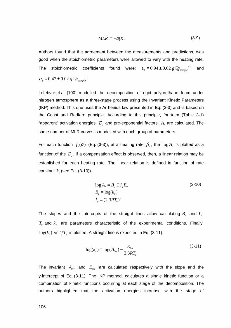
106

iii KMLR ω−= (3-9)

Authors found that the agreement between the measurements and predictions, was

good when the stoichiometric parameters were allowed to vary with the heating rate.

The stoichiometric coefficients found were: 11 02.094.0 −⋅±= sampleggυ and

12 02.047.0 −⋅±= sampleggυ .

Lefebvre et al. [100] modelled the decomposition of rigid polyurethane foam under

nitrogen atmosphere as a three-stage process using the Invariant Kinetic Parameters

(IKP) method. This one uses the Arrhenius law presented in Eq. (3-3) and is based on

the Coast and Redfern principle. According to this principle, fourteen (Table 3-1)

“apparent” activation energies, vE and pre-exponential factors, vA are calculated. The

same number of MLR curves is modelled with each group of parameters.

For each function )(αvf (Eq. (3-3)), at a heating rate vβ , the vAlog is plotted as a

function of the vE . If a compensation effect is observed, then, a linear relation may be

established for each heating rate. The linear relation is defined in function of rate

constant vk (see Eq. (3-10)).

1)3.2(

)log(

log

−=

=+=

vv

vv

vvvv

RTI

kB

EIBA

(3-10)

The slopes and the intercepts of the straight lines allow calculating vB and vI .

vT and vk are parameters characteristic of the experimental conditions. Finally,

)log( vk vs vT1 is plotted. A straight line is expected in Eq. (3-11).

v

invinvv RT

EAk

3.2)log()log( −=

(3-11)

The invariant invA and invE are calculated respectively with the slope and the

y-intercept of Eq. (3-11). The IKP method, calculates a single kinetic function or a

combination of kinetic functions occurring at each stage of the decomposition. The

authors highlighted that the activation energies increase with the stage of

107

decomposition. Moreover, the calculation of the kinetic parameters is only carried out

taking into account the degree of conversion between 0.1 and 0.5 at each stage. The

main disadvantage of this method is that if no compensation effect is identified, it is

impossible to calculate the invariant kinetic parameters. The compensation effect has

not been precisely characterized yet (some more comments on the compensation

effect are given in subsection 3.2.5).

Esperanza et al. [42] modelled the thermal decomposition of polyurethane refuses.

Because of the heterogeneity of raw materials, they considered a sample as

constituted of three different fractions of refuse, iM . The fractions follow competitive

parallel decomposition. Each fraction follows a reaction with different kinetic

parameters. iR and iV are respectively the solid residues and the volatiles generated

during the reactions, see Eq. (3-12).

iiiii VbRaM +→ , 3 ,2 ,1=i (3-12)

Where, ia and ib are respectively the yields of solid and volatiles released per unit of

burnt mass. Eq. (3-13) expresses the MLR as a function of: iW , the remaining mass at

a time t . iW∞ , the final fraction of solid residue; ik is the Arrhenius rate constant of the

process, and in is the reaction order.

( ) iniii

i WWkdt

dW∞−−= , 3 ,2 ,1=i

(3-13)

Authors numerically integrated Eq. (3-13) and optimized a total of seventeen

parameters. Optimization was performed using the Objective Function (OF) presented

in Eq. (3-14), which compares experimental and calculated data. The optimization

method is not detailed in their paper.

2

exp

∆∆−

∆∆=

calct

W

t

WOF

(3-14)

Font et al. [26] used in 2001 the model proposed by Esperanza et al. [42] in 1997 to

calculate the kinetic parameters of decompositions of PU-based additives. Authors,

numerically integrated the differential equations (Eq. (3-13)) and used a “flexible

108

simplex method” to optimize the kinetic parameters. The objective function is the one

presented in Eq. (3-14). Font et al. [26] stated as a conclusion of their work, that the

reactions leading to the formation of volatiles have similar apparent activation energies

to those leading to the formation of carbon residue. However, this represents a general

hypothesis of the models of thermal decomposition, because a single reaction

transforms a reactive into a solid residue and gases.

As shown, multiple methods relative to the model-fitting technique have been proposed

by various authors. Nevertheless, the uncertainty mentioned above in the Arrhenius

parameters obtained by model-fitting makes them virtually useless for practical

purpose, e.g. predicting the reaction kinetics at an arbitrary temperature [82].

3.2.3 The free model method (Isoconversional)

3.2.3.1 Principle of the isoconversional method

Kissinger, in 1957 [83], described a method to determine the pre-exponential factor, the

activation energy and the reaction order of thermal decomposition of magnesite,

calcite, brucite, kaolite and halloysite. The type of reactions observed with these

minerals are single-stage. In these reactions, the solid is transformed into residue and

gas. The experimental approach was Differential Thermal Analysis (DTA). The reaction

rate is presented in Eq. (3-15).

n

RT

EA

dt

d)1(exp αα −

−= (3-15)

Kissinger’s method is based on the analysis of the conditions needed to attain the

maximum reaction rate. The postulate is: if a reaction proceeds at a rate varying with

temperature (i.e. possesses an activation energy), the position of the peak varies with

heating rate if the others experimental conditions are kept unchanged.

The activation energy E may be calculated by resolving Eq. (3-16), where, β is the

heating rate and mT is the sample temperature at which the peak DTA deflection

occurs.

109

R

E

Td

TLnd

m −=

1

2

β

(3-16)

The calculation of the reaction order, n , is performed using a variable called the

“shape index”, S . The shape index is the absolute value of the ratio of the slopes of

tangents at the inflection points of the curve of MLR vs temperature. It accounts for the

asymmetry of the MLR (single peak curve). n is calculated according to Eq. (3-17).

2

1

26.1 Sn ⋅=

b

aS =

(3-17)

Where, a and b are the horizontal distances from the centre of the MLR peak to the

tangents of the inflections points (asymmetry) as presented in Figure 3-1.

Figure 3-1 Definition of the asymmetry of MLR curves in the Kissinger’s method. Source (Kissinger [83]).

Kissinger [83], assumed that n remains constant during a TGA run. This is the main

hypothesis for deduction of Eq (3-16). Thus, this method is valid only for single-stage

reactions. The pre-exponential factor, can be calculated as shown in Eq. (3-18).

−⋅−

=−

m

nmm RT

EnRT

EA

exp)1( 12 α

β

(3-18)

110

Friedman, in 1963 [19], studied the kinetics of thermal decomposition of a phenolic

resin reinforced with laminated fiberglass composite. In this research, the kinetic

parameters were calculated using a method based on the intercomparison of TGA

experiments carried out at several different rates of temperature rise. The linear

heating rates were between 0.8 °C·min -1 to 6 °C·min -1. Tests were performed under

nitrogen atmosphere up to a temperature of 900 °C. Finally, the residues were burnt

under air at 1000 °C. This constitutes the basis fo r the development of the

isoconversional method for non-isothermal conditions.

Friedman defined the mass change in terms of kinetic parameters in Eq. (3-19).

( )RT

E

m

mfLnALn

dt

dm

mLn −

+=

−

00

1

(3-19)

Where, m , is the mass of organic material. 0m , is the original weight of the reinforced

plastic. ( )0mmf , is a function of the weight of organic material. ( )0mmf is assumed

to be constant for constant values of 0mm . This is comparable to assuming that the

process is independent from the temperature and is only dependent on the

instantaneous weight of the organic material. Friedman selected twelve values of

0mm between 0.675 and 0.950 and plotted

−

dt

dm

mLn

0

1 vs

T

1, finding straight

lines.

−R

E are the slopes of straight lines and

0m

mAfLn the intercepts to y-axis. From

this analysis Friedman [19] pointed out a compensation effect between kinetic

parameters: “[…] a positive error in A , which would make the reaction appear to go

faster, is compensated for by a positive error in E [ E∆ in the paper], which would tend

to make the reaction appear to go slower.” The author also defined the function of

mass change in terms of the initial mass of sample, 0m , the final mass of char, fm and

kinetic order of the reaction, n ; see Eq. (3-20).

111

n

f

m

mm

m

mf

−=

00

(3-20)

The plot of

0m

mAfLn vs

−

0m

mmLn f is a straight line, in which n is the slope

and ( )Aln is the y-intercept. This method present a particularity: The fitting between

the experimental and the theoretical curves is highly dependent on the value of 0m .

The isoconversional method is often called in literature the Friedman method. It allows

the estimation of the Arrhenius parameters in a model-independent manner. This

analysis is recommended in order to obtain a reliable kinetic description of the process

studied. It provides a good compromise between the oversimplified but widely used

single-step Arrhenius kinetic treatment and the prevalent occurrence of processes with

multi-step and/or non-Arrhenius kinetics. The isoconversional methods usually

produce E values that vary with α and T . This can be used to detect multiple-step

kinetics [82].

The isoconversional integral method is based on an approximate form of the

temperature integral that results from the rearrangement and integration of Eq. (3-5).

However, as explained, the temperature integral, )(xp , has no analytical solution.

Various authors proposed approximations of the integral temperature term in the

isoconversional method. Some of these simplifications are presented in Table 3-2. This

table presents the method, approximations, forms of integral temperatures and

required plots.

112

Table 3-2. Approximations of the integral temperature in the isoconversional method (Source [99][101]).

No Plot

Method, source

Approx. Form of the integral temperature X-axis Y-axis

1 Kissinger-Akahira-Sunose

[99]

Coats-Redfern

α

α

α

α

α αβ

RT

E

gE

RALn

TLn −

=

)(2

2

α

βT

Ln αT

1

2 Flynn-Wall-

Ozawa [99]

Doyle ( )

α

ααα

αβ

RT

E

Rg

EALnLn i 052.1331.5

)(−−

=

Where ( ) xxpLn 052.1331.5)( −−=

( )iLn β

αT

1

3 Vyazovkin [101]

Senum-Yang

( )( )∑∑

= ≠

=m

i

m

ij ij

ji

TEI

TEI

1 ,

,

,

,

ββ

φαα

αα

Where

)1810()243612)(exp(

)(2

23

+++++−=

xxx

xxxxxp

For .const=α , the plots of Table 3-2, are obtained from thermal curves recorded at

several heating rates. In the straight lines, the slopes allow evaluation of the apparent

activation energies and y-intercepts allow calculation of the pre-exponential factors.

These approximations imply that A and E are calculated for a known analytical form

of the integral function of conversion ( )αg (see Table 3-1) [101]. The approximations

in Table 3-2 are allowed by very important simplifications of the temperature integral

that can induce error in the parameters calculated [99].

In the Doyle approximation, if 20<x errors are higher than 10%. Flynn in Ref. [82]

suggested corrections in order to obtain accurate activation energy values. These

corrections are not presented here.

The Vyazovkin method is called nonlinear isoconversional method, where m is the

number of heating rates. ( )iTEI ,, αα is the exponential integral ( )(xp ) that results from

the heating rate iβ . ( )jTEI ,, αα is the exponential integral from heating rate jβ . The

apparent activation energy is the value that minimizes φ for given values of αT

and β [99].

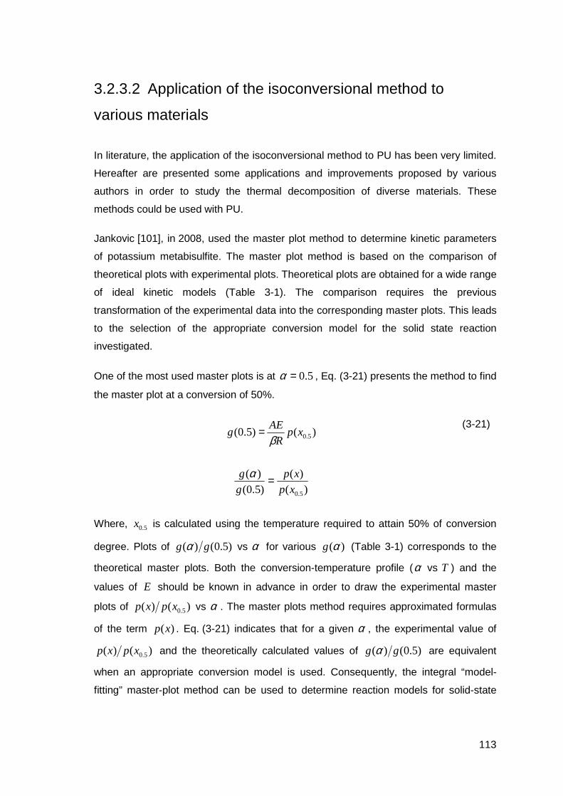
113

3.2.3.2 Application of the isoconversional method to

various materials

In literature, the application of the isoconversional method to PU has been very limited.

Hereafter are presented some applications and improvements proposed by various

authors in order to study the thermal decomposition of diverse materials. These

methods could be used with PU.

Jankovic [101], in 2008, used the master plot method to determine kinetic parameters

of potassium metabisulfite. The master plot method is based on the comparison of

theoretical plots with experimental plots. Theoretical plots are obtained for a wide range

of ideal kinetic models (Table 3-1). The comparison requires the previous

transformation of the experimental data into the corresponding master plots. This leads

to the selection of the appropriate conversion model for the solid state reaction

investigated.

One of the most used master plots is at 5.0=α , Eq. (3-21) presents the method to find

the master plot at a conversion of 50%.

)()5.0( 5.0xpR

AEg

β=

)()(

)5.0()(

5.0xp

xp

g

g =α

(3-21)

Where, 5.0x is calculated using the temperature required to attain 50% of conversion

degree. Plots of )5.0()( gg α vs α for various )(αg (Table 3-1) corresponds to the

theoretical master plots. Both the conversion-temperature profile (α vs T ) and the

values of E should be known in advance in order to draw the experimental master

plots of )()( 5.0xpxp vs α . The master plots method requires approximated formulas

of the term )(xp . Eq. (3-21) indicates that for a given α , the experimental value of

)()( 5.0xpxp and the theoretically calculated values of )5.0()( gg α are equivalent

when an appropriate conversion model is used. Consequently, the integral “model-

fitting” master-plot method can be used to determine reaction models for solid-state

114

reactions. The author also concluded that even combining the analytical methods, the

kinetic data cannot be calculated unambiguously.

Mamleev et al. [102] proposed a model-free method called Modulated

Thermogravimetric Analysis (MTGA). It is based on a TGA test in which the linear

heating rate is perturbed by a sinusoidal wave with controlled amplitude and frequency.

The modulated temperature )(mod tT at a time t , is calculated with Eq. (3-22).

)2sin()( 0mod tAtTtT mm ωβ Π++= (3-22)

Where, mA is the amplitude of the modulation ( CAm °= 5 ) and mω is the number of

oscillations per second [s-1]. The aim of temperature modulation is to predict a

hypothetical derivative of mass-loss that corresponds to the absence of the modulation

(perturbation). The advantage of their method is that kinetic parameters can be

calculated with a single experimental curve.

Authors illustrated the method with a hypothetical example of a two-stage

decomposition similar to observed in PPUF under nitrogen atmosphere. The equations

that governed the reactions are of the type:

( )

−−=RT

Ek

dt

d 1211

1 exp1 αα

(3-23)

( )

−−=RT

Ek

dt

d 222

2 exp1 αα

(3-24)

Note that the first reaction (Eq. (3-23)) is a second-order equation and the second

reaction (Eq. (3-24)) is of the first order. In the MTGA method, the oscillation of the

derivative is the main source of kinetic information. The perturbation function allowed

the authors to conclude that the unmodulated MLR curve corresponds to the

modulated one at the inflection points (maxima and minima) for the periodic component

of temperature.

The method proposed by Mamleev et al. [102], becomes less accurate when

increasing the heating rate. The accuracy is acceptable only if the heating rate is

selected providing 10 to 15 periods of modulation for each stage of decomposition (i.e.

the heating rate is less than 5 °C·min -1). The calculation of the kinetic parameters A

115

and E for a given n is accurate only for a one-stage process and small periods of

modulation. The calculation of kinetic parameters is based on the minimization of a

deviation function between experimental and calculated curves [103].

Mamleev et al. [103], affirmed that the activation energy is an effective (apparent) value

for a model. E may not be associated with a temperature range or degree of

conversion. Otherwise, no physical sense may be attributed to it. In consequence, it

cannot be used for predictions. This does not seem to be a very precise conclusion,

because a reaction rate calculated with given kinetic parameters is measurable only in

a particular range of temperature.

Mamleev et al. [16], presented a generalisation of the MTGA method. It allowed the

analysis of TGA results for materials with more than one decomposition stage. A point

of their procedure that needs to be highlighted is the requirement that each stage must

be independent and well resolved. The presence of several stages not well resolved

represents complications to the analysis [103]. The methodology was used for the

analysis of rigid PU foam. Under air, the TGA curves presented three decomposition

stages.

3.2.4 Combined model-fitting and model-free methods

This procedure is issued from a combination of the model-fitting and the model-free

methods explained above. It was used by Cancellieri et al. in 2005 [104] to determine

the kinetic parameters of the thermo-oxidative decomposition of organic materials

(biomass). DSC and TGA data were obtained under air sweeping. The experiments

allowed identifying two oxidative reactions at heating rates between 10 °C·min -1 and

40 °C·min -1. This method requires the numerical and experimental individualization of

each reaction peak. This allowed the measurement of the enthalpy variation of each

exothermic reaction.

The numerical separation of the reaction peaks was carried out fitting the global curve

with empirical equations. These equations have adjustable parameters for each peak

of fuel release. The parameters of the empirical equations showed to be constant for all

the species and heating rates.

116

A model-free method was used to determine the apparent activation energies of each

insulated curve. Cancellieri et al. [104] used the Kissinger-Akahira-Sunose

approximation described in Table 3-2 for degrees of conversion between 0.1 and 0.9.

The enthalpy variations and the apparent activation energies calculated experimentally

were injected in a model-fitting method. It allowed calculating the reaction order and

pre-exponential factor of each oxidative reaction. Their model-fitting method is based

on Eq. (3-2) and the )(αf was chosen from the options of the Table 3-1.

However, the interpretation of DSC curves showed not to be a simple task. Particularly,

because of the position change of the DSC baseline. The abrupt changes in slope or

position of the DSC baseline usually indicate second-order transitions (i.e. glass

transition in polymers) [41] and strong change in the nature of the solid sample.

3.2.5 Models of the decomposition of solids based o n

TGA isothermal tests

The main disadvantage of the results obtained from TGA isothermal experiments is

that they are strictly valid for the temperatures for which they have been obtained [96].

Ceamanos et al. [13], used a variation of Eq. (3-3) (reminded here after) to model the

isothermal test of polyethylene, allowing the deduction of an expression for the change

of the degree of conversion (see Eq. (3-25)).

)(exp ααβ fRT

EA

dT

d

−= Reminder of

Eq (3-3)

( )αα −+=

si Wnk

dt

dlogloglog

(3-25)

Where, sW , is the weight of the non-pyrolysable fraction at the set temperature. The

reaction order, n , is the slope of the plot ( )dtdαlog vs ( )ss XA −log . n , is defined

117

between a range of conversion factor from 0.1 to 0.95. The kinetic constant, ik , may

be calculated from the slope of the plot ( )ss XALn − vs t .

In the same study, the authors plotted pre-exponential factors in function of the

activation energies issued from the literature (for PE). They found a linear relation

between the all data groups. Ceamanos et al. [13] explained the linearity by the

compensation effect resulting from the combination of mathematical, physicochemical

and experimental causes. The points (couples of A and E ) have been obtained under

different experimental conditions and with reaction orders.

Bilbao et al. [11], determined kinetic equations and the corresponding constants for the

weight loss of TGA tests. The materials used were PPUF of densities between

20 kg·m-3 and 30 kg·m-3. They performed isothermal and dynamic runs under air and

nitrogen atmospheres. Under nitrogen, the experiments were carried out

between 200 °C and 385 °C. Under air the range was between 200 °C and 300 °C.

They observed the same dynamics of mass change independently of the density.

However, Kanakia in [23] stated that the increase in the molecular weight of polyol

generates a decrease of the activation energy and the reaction order, and thus a

variation in the dynamics of mass.

Bilbao et al. [11] referenced the works of Benbow and Cullis (1975) [105]. They wrote

that “the presence of oxygen does not influence the decomposition rate of polyurethane

to diisocyanate and polyols, although it affects the breakage of the polymeric chains”.

First, this is not a conclusion of the works of Benbow. Second, this is in contrast to

experimental results found in this research (see Figure 2-9 b).

Criado et al. [98], studied in 1984 methods to calculate the activation energies based

on a series of laws for the mass change. They conducted their study using hypothetical

isothermal experiments. They assumed that discrete isothermal data allowed the

discernment of the best kinetic model. The authors proposed the Arrhenius law

dependent on time instead of temperature. The integral function of the degree of

conversion is presented in Eq. (3-26).

( )0exp)( ttRT

EAg i −

−=α (3-26)

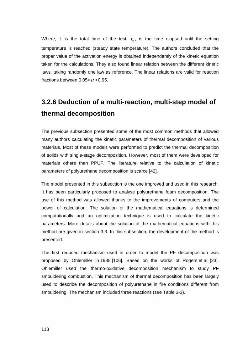
118

Where, t is the total time of the test. 0t , is the time elapsed until the setting

temperature is reached (steady state temperature). The authors concluded that the

proper value of the activation energy is obtained independently of the kinetic equation

taken for the calculations. They also found linear relation between the different kinetic

laws, taking randomly one law as reference. The linear relations are valid for reaction

fractions between 0.05<α <0.95.

3.2.6 Deduction of a multi-reaction, multi-step mod el of

thermal decomposition

The previous subsection presented some of the most common methods that allowed

many authors calculating the kinetic parameters of thermal decomposition of various

materials. Most of these models were performed to predict the thermal decomposition

of solids with single-stage decomposition. However, most of them were developed for

materials others than PPUF. The literature relative to the calculation of kinetic

parameters of polyurethane decomposition is scarce [42].

The model presented in this subsection is the one improved and used in this research.

It has been particularly proposed to analyse polyurethane foam decomposition. The

use of this method was allowed thanks to the improvements of computers and the

power of calculation: The solution of the mathematical equations is determined

computationally and an optimization technique is used to calculate the kinetic

parameters. More details about the solution of the mathematical equations with this

method are given in section 3.3. In this subsection, the development of the method is

presented.

The first reduced mechanism used in order to model the PF decomposition was

proposed by Ohlemiller in 1985 [106]. Based on the works of Rogers et al. [23],

Ohlemiller used the thermo-oxidative decomposition mechanism to study PF

smouldering combustion. This mechanism of thermal decomposition has been largely

used to describe the decomposition of polyurethane in fire conditions different from

smouldering. The mechanism included three reactions (see Table 3-3).

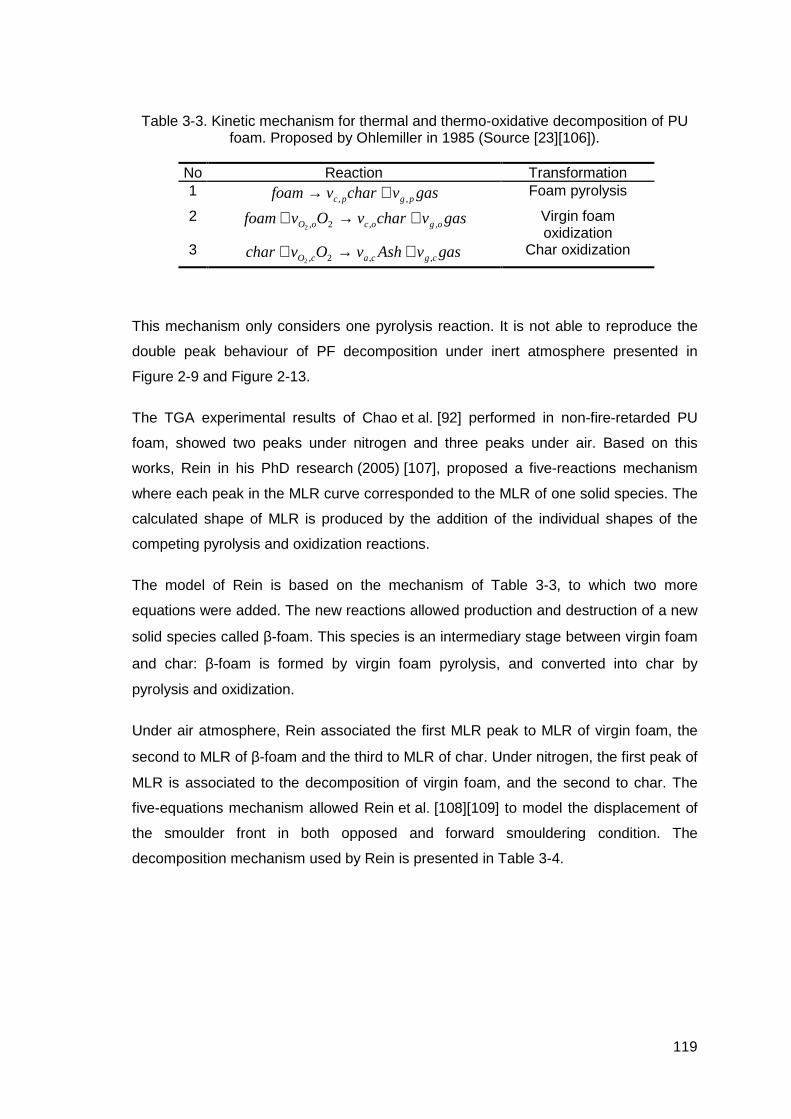
119

Table 3-3. Kinetic mechanism for thermal and thermo-oxidative decomposition of PU foam. Proposed by Ohlemiller in 1985 (Source [23][106]).

No Reaction Transformation 1 gasvcharvfoam pgpc ,, +→ Foam pyrolysis

2 gasvcharvOvfoam ogocoO ,,2,2+→+ Virgin foam

oxidization 3 gasvAshvOvchar cgcacO ,,2,2

+→+ Char oxidization

This mechanism only considers one pyrolysis reaction. It is not able to reproduce the

double peak behaviour of PF decomposition under inert atmosphere presented in

Figure 2-9 and Figure 2-13.

The TGA experimental results of Chao et al. [92] performed in non-fire-retarded PU

foam, showed two peaks under nitrogen and three peaks under air. Based on this

works, Rein in his PhD research (2005) [107], proposed a five-reactions mechanism

where each peak in the MLR curve corresponded to the MLR of one solid species. The

calculated shape of MLR is produced by the addition of the individual shapes of the

competing pyrolysis and oxidization reactions.

The model of Rein is based on the mechanism of Table 3-3, to which two more

equations were added. The new reactions allowed production and destruction of a new

solid species called β-foam. This species is an intermediary stage between virgin foam

and char: β-foam is formed by virgin foam pyrolysis, and converted into char by

pyrolysis and oxidization.

Under air atmosphere, Rein associated the first MLR peak to MLR of virgin foam, the

second to MLR of β-foam and the third to MLR of char. Under nitrogen, the first peak of

MLR is associated to the decomposition of virgin foam, and the second to char. The

five-equations mechanism allowed Rein et al. [108][109] to model the displacement of

the smoulder front in both opposed and forward smouldering condition. The

decomposition mechanism used by Rein is presented in Table 3-4.

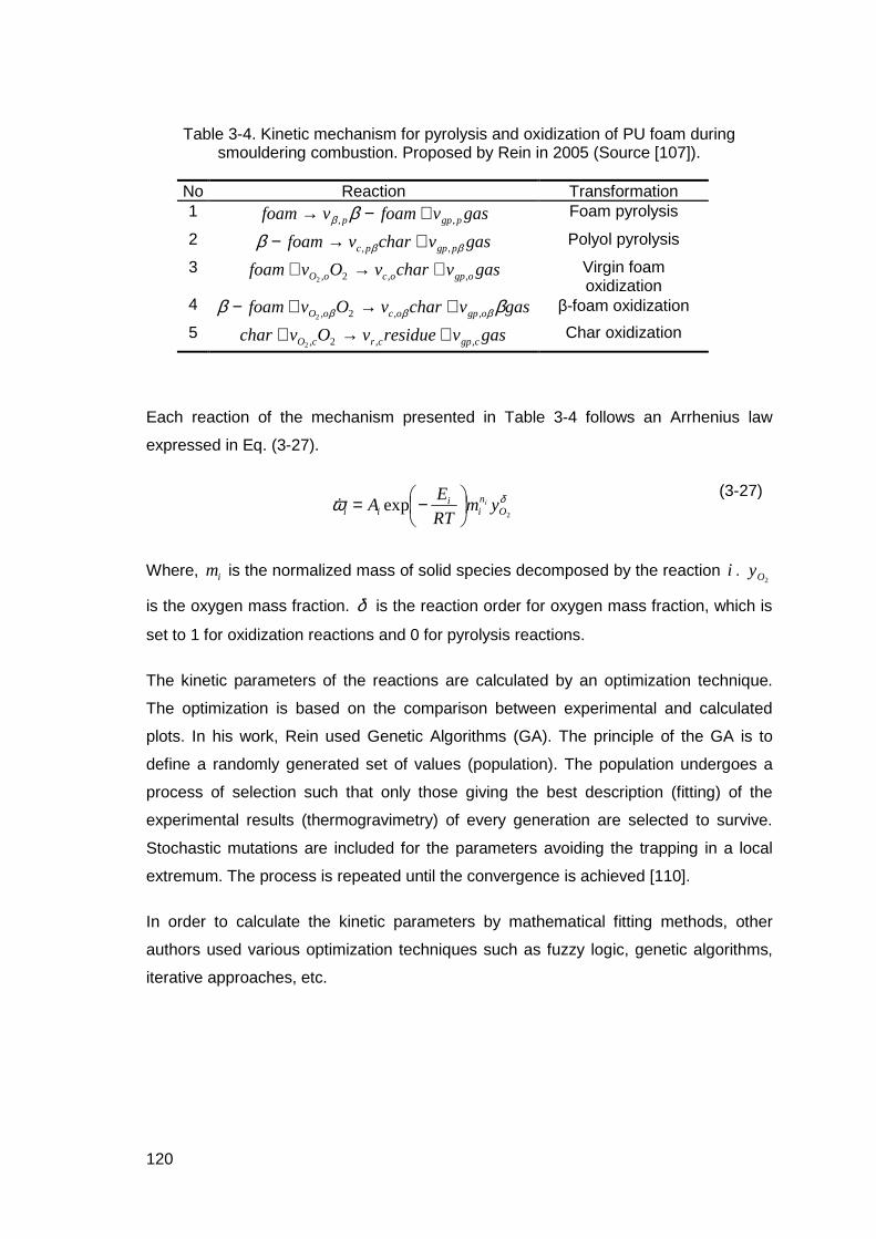
120

Table 3-4. Kinetic mechanism for pyrolysis and oxidization of PU foam during smouldering combustion. Proposed by Rein in 2005 (Source [107]).

No Reaction Transformation 1 gasvfoamvfoam pgpp ,, +−→ ββ Foam pyrolysis

2 gasvcharvfoam pgppc βββ ,, +→− Polyol pyrolysis

3 gasvcharvOvfoam ogpocoO ,,2,2+→+ Virgin foam

oxidization 4 gasvcharvOvfoam ogpocoO ββ βββ ,,2,2

+→+− β-foam oxidization

5 gasvresiduevOvchar cgpcrcO ,,2,2+→+ Char oxidization

Each reaction of the mechanism presented in Table 3-4 follows an Arrhenius law

expressed in Eq. (3-27).

δω2

exp Oni

iii ym

RT

EA i

−=& (3-27)

Where, im is the normalized mass of solid species decomposed by the reaction i . 2Oy

is the oxygen mass fraction. δ is the reaction order for oxygen mass fraction, which is

set to 1 for oxidization reactions and 0 for pyrolysis reactions.

The kinetic parameters of the reactions are calculated by an optimization technique.

The optimization is based on the comparison between experimental and calculated

plots. In his work, Rein used Genetic Algorithms (GA). The principle of the GA is to

define a randomly generated set of values (population). The population undergoes a

process of selection such that only those giving the best description (fitting) of the

experimental results (thermogravimetry) of every generation are selected to survive.

Stochastic mutations are included for the parameters avoiding the trapping in a local

extremum. The process is repeated until the convergence is achieved [110].

In order to calculate the kinetic parameters by mathematical fitting methods, other

authors used various optimization techniques such as fuzzy logic, genetic algorithms,

iterative approaches, etc.

121

3.2.7 The problem of thermal decomposition under

vitiated atmospheres

In the last subsections were presented the methods most commonly used in literature

to determine the decomposition mechanism of materials and calculate the respective

kinetic parameters. In all cases, the models were stated to air and nitrogen

atmospheres.

The problem of thermal decomposition under vitiated atmospheres has been poorly

discussed in the past but is of great interest in FSE. Fires under vitiated atmospheres

describe fire situations in which the oxygen mass fraction of the environment gas is

found between zero and the one of air ( 23.002

<< Oy ). This type of fire often occurs in

closed rooms [111][112]. The oxygen initially present in the atmosphere is consumed

by the flame during the phases of fire ignition and propagation (heterogeneous

reactions are often neglected). Fire in closed rooms has two main consequences that

highly affect the kinetics of thermal decomposition: the increase in the mean

temperature and the depletion of oxygen into the room [113][114].

Figure 2-9 represents an example of the strong influence of temperature and oxygen

mass fraction in the kinetic of decomposition of solids. The increase in temperature

tends to increase the rate of solid decomposition and gas release. The effect of the

oxygen depletion is the reverse of the one of temperature: A reduction of the quantity of

oxygen in the surrounding atmosphere tends to reduce the decomposition rate.

Nevertheless, a change in the kinetics of decomposition produces a change in the

amount and the composition of the gas products. As discussed, the composition of the

gas products controls the potential of chemical energy available to be converted into

heat during a subsequent combustion.

Thus, a general model of thermal decomposition should accurately predict the rate of

mass-loss as a function of temperature and oxygen mass fraction. Nevertheless, the

determination of these two variables in real fire situations remains a tricky task because

they are affected by a huge number of phenomena such as: turbulence, thermal

balance, heat losses, diffusion velocity, ventilation, etc.

122

In this subsection are presented the few models and experimental finding referenced in

literature which include a term of oxygen mass fraction. The quotes are not specific to

PU but to wood, biomass and plastics. They could however be applied to PPUF.

Fang et al. [115] studied the relation between the kinetic parameters calculated during

pyrolysis and combustion of wood under various oxygen concentrations. The samples

were: merbau, cotton straw, birch, red sandal and their semi coke. They observe that

the MLR curves have the same behaviour until 250 °C independently of the oxygen

concentration. Above that temperature, the increase in oxygen concentration increases

the MLR intensity.

The increase in the oxygen concentration, attempt the combustion process to vary from

a single stage to double stage. If oxygen concentration continues increasing, a single-

stage combustion is produced again. However, further researches are needed to

characterise the critical concentrations of oxygen that allows many decomposition

stages.

Caballero et al. [116] studied the decomposition of kraft lignin material using non-

isothermal TGA. They characterise the biomass as being composed of various

polymers which decompose at different temperatures. Their model assumes that a

given fraction begins to decompose only if the temperature of the biomass is greater or

equal to a characteristic temperature RT . Thus, each component of the biomass has

characteristic temperatures corresponding to the ones of the beginning and the end of

the decomposition reaction. A function C is used to estimate the distribution of mass

fractions that can react in each temperature range. So, RCdT designate the mass

fraction of the sample that can decompose at a given temperature range

RRR dTTTT +≤≤ . The mass conservation is mathematically expressed in Eq. (3-28).

∫∞

=0

1RCdT (3-28)

The curve C cannot be measured directly, but can be deduced from the variation of

the residue yield obtained at time infinity vs operating temperature RT .

Senneca et al. [117] studied the kinetics of decomposition of four materials: bituminous

coal, PET, PE and lignocellulosic material. The model called a power law kinetic model

123

is of the type presented in Eq. (3-29). This is one of the few models presented in

literature that takes into account the presence of oxygen.

nO

D PRT

EA

dt

d2

exp αα

−−= (3-29)

Where, D is the strength of the dependency of the pyrolysis rate on the mass of

unpyrolized carbon. 2OP is the partial pressure of the oxygen. n is the reaction order

with respect to oxygen partial pressure.

The parameters A , E and n were calculated by a non linear regression analysis of

the peak temperatures at different heating rates and oxygen concentrations. Authors

used the Kissinger and Friedman methods.

The general behaviour that Senneca et al. [117] found for all the materials tested

(bituminous coal, PET, PE and lignocellulosic material) was:

• For all the materials, increasing the oxygen concentration shifts the weight loss

towards lower temperatures especially at high heating rates, which is in accordance

to observations of Caballero et al. [116]: A maximum pyrolysable fraction is

observed for each final temperature (as observed in isothermal tests). The amount

of residue was found not to be dependent on the heating rate, but on the final

temperature and the nature of the biomass. This is also in accordance with the

theory that different fractions decompose at different ranges of temperatures. Thus,

the activation energy changes during the heating process.

• Materials can be classified into low, medium and high volatile content. In solid fuels

with low volatile content, the diphasic combustion prevails over the release of

volatiles. For materials with medium to high volatiles content, the release of

volatiles and heterogeneous char combustion are both relevant and may occur in

sequence. For materials with very high volatile content, the presence of oxygen

results into conversion patterns that are not easy to predict.

The kinetics of thermal decomposition of materials that can suffer smoldering

combustion need to be studied because it occurs in environments with reduced

oxygen. They present a potential hazard because of the flameless combustion and

high release of toxic gaseous products, particularly CO. The materials that can sustain

124

smoldering are powders, grains, particulates, aggregates, fibers, porous or alveolar

matrix, such as: Coal, cotton, tobacco, paper, duff, wood, foams, etc. They facilitate the

surface reaction with oxygen by providing a large (internal) surface for the heat and

mass exchange [15].

Dosanjh et al. [50], in 1997, modelled the polyurethane foam smoldering as a single

reaction process (Eq.(3-30)).

)()_()()_(1 2 QproductsGasAshOsolidUnburnedg ogpao υυυυ ++→+ (3-30)

Where, υ are the stoichiometric coefficients in [g·gSample-1]. Q is the energy released

per unit of mass of O2 consumed.

The calculation of the reaction rate is expressed in function of the oxygen mass fraction

(2Oy ), the gas density ( gρ ), the fraction of unburnt solid polyurethane foam ( usy ) and

the density of the solid polyurethane foam ( usρ ). This is mathematically presented in

Eq. (3-31).

))((exp2 ususgO yy

RT

EA

dt

d ρρω

−= (3-31)

Because all of the incoming oxygen is consumed in the reaction zone, the total heat

released is proportional to the initial oxygen mass flow. Both the smoldering velocity

and the final temperature are highly dependent on the oxygen mass flow.

3.2.8 Some comments about the reaction rate equatio ns

The last subsections presented many methods usually found in literature to determine

the decomposition mechanism and the kinetic parameters of PPUF and various

materials. The problem of the influence of oxygen in the kinetic of decomposition was

also discussed. The methods presented were classified into groups: the model-fitting

method, the isoconversional method (model-free), a combination of both and a multi-

reaction multi-step model in which kinetic parameters are calculated using optimization

techniques. Some less famous methods were also presented, such as the IKP method,

etc.

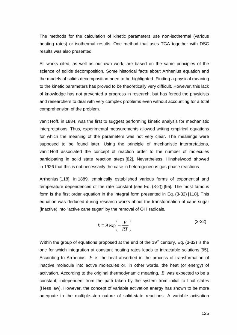
125

The methods for the calculation of kinetic parameters use non-isothermal (various

heating rates) or isothermal results. One method that uses TGA together with DSC

results was also presented.

All works cited, as well as our own work, are based on the same principles of the

science of solids decomposition. Some historical facts about Arrhenius equation and

the models of solids decomposition need to be highlighted. Finding a physical meaning

to the kinetic parameters has proved to be theoretically very difficult. However, this lack

of knowledge has not prevented a progress in research, but has forced the physicists

and researchers to deal with very complex problems even without accounting for a total

comprehension of the problem.

van’t Hoff, in 1884, was the first to suggest performing kinetic analysis for mechanistic

interpretations. Thus, experimental measurements allowed writing empirical equations

for which the meaning of the parameters was not very clear. The meanings were

supposed to be found later. Using the principle of mechanistic interpretations,

van’t Hoff associated the concept of reaction order to the number of molecules

participating in solid state reaction steps [82]. Nevertheless, Hinshelwood showed

in 1926 that this is not necessarily the case in heterogeneous gas-phase reactions.

Arrhenius [118], in 1889, empirically established various forms of exponential and

temperature dependences of the rate constant (see Eq. (3-2)) [95]. The most famous

form is the first order equation in the integral form presented in Eq. (3-32) [118]. This

equation was deduced during research works about the transformation of cane sugar

(inactive) into “active cane sugar” by the removal of OH- radicals.

−=RT

EAk exp

(3-32)

Within the group of equations proposed at the end of the 19th century, Eq. (3-32) is the

one for which integration at constant heating rates leads to intractable solutions [95].

According to Arrhenius, E is the heat absorbed in the process of transformation of

inactive molecule into active molecules or, in other words, the heat (or energy) of

activation. According to the original thermodynamic meaning, E was expected to be a

constant, independent from the path taken by the system from initial to final states

(Hess law). However, the concept of variable activation energy has shown to be more

adequate to the multiple-step nature of solid-state reactions. A variable activation

126

energy should be used to describe the temperature dependence of the overall reaction

rates.

The demonstration that E actually represents an energy of molecular reaction

activation has shown not to be a simple task. Various rationales and theories for an

exponential relation between the reaction rate and temperature have been developed.

They are based on collision probabilities, energetic, thermodynamics, and/or statistical

mechanics [95]. In 1935, Eyring, Evans and Polanyi developed the Transition-state

theory (TST). TST is a statistical-mechanical treatments theory [119] based on the

mechanistic interpretation method of van’t Hoff. TST theory made possible to obtain

quick estimates for reaction rates for a wide variety of processes even during the days

when sophisticated computers were not available. “In 1978, Chandler [J. Chem. Phys.

68, 2959 (1978)] finally showed that especially when considering condensed phases,

the activation energy is a free energy, it is the barrier height in the potential of mean

force felt by the reacting system” [120].

To this day, a definite quantum TST has not been formulated, although some very

useful approximate quantum rate theories have been invented. An open problem which

is being intensively investigated is rate theory away from equilibrium. TST is no longer

valid and cannot even serve as a conceptual guide for understanding the critical factors

which determine rates away from equilibrium. The non-equilibrium quantum theory is

even less well developed than the classical theory, and suffers from the fact that even

today, we do not know how to solve the real-time quantum dynamics for systems with

many degrees of freedom [120].

Cukrowski in 2006 [121], calculated the Arrhenius activation energy as a function of

appropriate threshold energies for a simple reaction BBAA +↔+ in a dilute gas.

E is calculated from a temperature dependence of the rate constant. It is obtained

from the perturbation solution of the Boltzmann equation. The complexity of the

equations threaded is greater while they take into account together the solid and

gaseous phases transformations.

The temperature-independent pre-exponential factor has no theoretical justification yet.

In some theoretical approaches, authors used temperature-dependent pre-exponential

factors. However, in all cases, redefining the Arrhenius equation with temperature-

dependent pre-exponential factor makes the new calculated parameters, E and A ,

strictly not comparable with parameters already published [95].

127

As shown, the validity of applying the Arrhenius equation to heterogeneous reactions

has been largely questioned. The kinetic parameters (activation energy, pre-

exponential factor and reaction order) do have practical value [41]. However, their

theoretical interpretation is not very clear even in the higher spheres of research in

physics.

As shown, the interpretation of parameters has not been clarified. Thus, it cannot be

known reliably if kinetic parameters are constant or variable throughout the

decomposition reaction [116]. It is neither clear if the approach used in this research is

acceptable or not. In our method, a single group of kinetic parameters is valid for

various experimental conditions (oxygen concentrations and heating rates). We

assume (as many authors do) that the kinetic parameters are constant for each

independent reaction and that this approach would be accepted.

3.3 Improvement of the model of PPUF

thermal decomposition

In the last subsection, were presented the methods found in literature to study the

thermal decomposition of materials. This section presents the improvements carried

out to the model. The model allows calculation of the kinetic parameters of the

decomposition reaction, which constitutes primordial input data for the pyrolysis-

calculated CFD fire simulations presented in the next chapter.

A realistic model of thermal decomposition must be able to predict the bulk mass

change as a function of the variation of temperature and oxygen mass fraction. It must

also reproduce the release of gas species, which are responsible for the toxicity in real

fire situations. As explained, the gas effluents also transport combustible species from

the decomposed solid to the flame. It constitutes the term source of the energy

balance.

Thus, a realistic model must simultaneously allow the calculation of kinetic and

stoichiometric parameters from the reactions of solid and gas phases. The

improvements of the model of thermal decomposition carried out in this research aims

128

at the coupling of the transformations suffered in the solid and gas phases. This allows

stating a kinetic mechanism in accordance to the chemistry of the process: The

mechanism can be considered as “chemically correct”. However, because of the

complexity of the problem of interaction between solid and gas phases, a pseudo

mechanistic (simplified) approach [8][82] with as few reactions as possible is used to

predict PPUF transformations.

The method used in this research to lay down the mathematical model is based on the

works of Rein et al. [109]. The model has two main input data: The kinetic mechanism

and the possible range of existence of each kinetic parameter from the Arrhenius

equation. Up to date, the decomposition mechanisms have been defined based on the

solid behavior observed in TGA. In this work, measurements of gas compounds

release provide essential information to describe the decomposition mechanism. The

experiments that allowed the chemical results used in the following analyses are

presented in the section 2.4.

The method and results presented in the next subsections have to do with PPUF only.

However, this method has also been used with other materials such as polyester resin,

laminated glass reinforced polymer [122] and PMMA [123] with very satisfactory

results.

3.3.1 Verification of the influence of the kinetic

mechanism in MLR calculations

The decomposition mechanism is a primordial input data for the model because it

allows stating the mass balance of solid and gaseous products release. The analysis of

the experimental results of mass change as a function of temperature at various

heating rates showed that various kinetic mechanisms permit to reproduce in a

satisfying manner the curves of MLR obtained in TGA.

The three kinetic mechanisms that best allows the MLR prediction are compared here

after: One is issued from literature (Figure 3-2) and two are proposed in this research

(Figure 3-3 and Figure 3-4). However, only one of the three decomposition mechanism

has a meaning according to the reactions actually taking place in the solid phase. One

part of the improvements of the method proposed is a procedure to choose the

129

“correct” decomposition mechanism. This subsection studies the influence of the kinetic

mechanism in the MLR calculations and constitutes one part of the method of

identification of the actual decomposition patterns.

The kinetic mechanism issued from literature, is the one used by Rein et al. [109]

schematized in Figure 3-2. Their mechanism was originally written using generic solid

species: The virgin matter was called “foam” and the first decomposition product was

called “β-foam” the nature of the solids was not determined. The analytical

characterisation presented in Chapter 2 allows rewriting this mechanism using the

specific condensed species identified.

130

Pyrolysis reaction

Oxidation reaction

Pyrolysis reaction

Oxidation reaction

PPUF Polyol Char ResiduePPUF Polyol Char Residue1

2

3

4 5

Figure 3-2 Kinetic mechanism used in the works of Rein et al. [109]. Written with the condensed species identified in this research.

1

2

3

4 5

Pyrolysis reaction

Oxidation reaction

Pyrolysis reaction

Oxidation reaction

PPUF Polyol Char Residue

Figure 3-3 Kinetic mechanism 1 proposed in this research.

1 2

3 4

5

Pyrolysis reaction

Oxidation reaction

Pyrolysis reaction

Oxidation reaction

PPUF Polyol Char Residue

Figure 3-4 Kinetic mechanism 2 proposed in this research.

The two mechanisms proposed in this research are the ones presented in Figure 3-3

and Figure 3-4. Both mechanisms are allowed to explain the TGA results presented in

Figure 2-9. They are as well in accordance with the visual observations of SEM and

binocular images presented by Bustamante Valencia et al. [124] (see Figure 2-15 and

Figure 2-16). Nevertheless, they are hypothetical. The deal of the following work is

finding evidence that one of these mechanism is correct.

The three mechanisms considered have been written based on the hypothesis that

each peak of the MLR curves of TGA is generated by a reaction at the solid phase, it is

remainded that similar assumptions has been done by the authors that deduced the

multi-reaction, multi-step model presented in section 3.2.6.

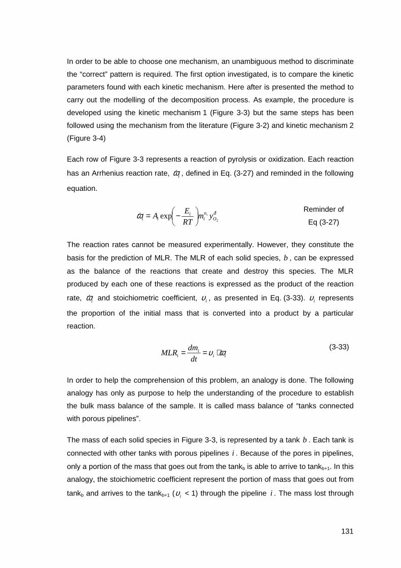
131

In order to be able to choose one mechanism, an unambiguous method to discriminate

the “correct” pattern is required. The first option investigated, is to compare the kinetic

parameters found with each kinetic mechanism. Here after is presented the method to

carry out the modelling of the decomposition process. As example, the procedure is

developed using the kinetic mechanism 1 (Figure 3-3) but the same steps has been

followed using the mechanism from the literature (Figure 3-2) and kinetic mechanism 2

(Figure 3-4)

Each row of Figure 3-3 represents a reaction of pyrolysis or oxidization. Each reaction

has an Arrhenius reaction rate, iω& , defined in Eq. (3-27) and reminded in the following

equation.

δω2

exp Oni

iii ym

RT

EA i

−=& Reminder of

Eq (3-27)

The reaction rates cannot be measured experimentally. However, they constitute the

basis for the prediction of MLR. The MLR of each solid species, b , can be expressed

as the balance of the reactions that create and destroy this species. The MLR

produced by each one of these reactions is expressed as the product of the reaction

rate, iω& and stoichiometric coefficient, iυ , as presented in Eq. (3-33). iυ represents

the proportion of the initial mass that is converted into a product by a particular

reaction.

iii

i dt

dmMLR ωυ ⋅==

(3-33)

In order to help the comprehension of this problem, an analogy is done. The following

analogy has only as purpose to help the understanding of the procedure to establish

the bulk mass balance of the sample. It is called mass balance of “tanks connected

with porous pipelines”.

The mass of each solid species in Figure 3-3, is represented by a tank b . Each tank is

connected with other tanks with porous pipelines i . Because of the pores in pipelines,

only a portion of the mass that goes out from the tankb is able to arrive to tankb+1. In this

analogy, the stoichiometric coefficient represent the portion of mass that goes out from

tankb and arrives to the tankb+1 ( iυ < 1) through the pipeline i . The mass lost through

132

the pipelines produce the gaseous products ( iυ−1 ). This is schematically presented for

kinetic mechanism 1 in Figure 3-5, as well as the mass balance for each solid species

as a function of time (differential equations).

31 ωω && −−

=dt

dmPPUF

42

33

11

ωωωυ

ωυ

&&

&

&

−−⋅

⋅+

=dt

dmPolyol

5

44

ωωυ&

&

−⋅

=dt

dmChar

55

22

ωυωυ

&

&

⋅+⋅

=dt

dmResidue

PPUF Polyol ResidueChar

1ω&− 11 ωυ &⋅1

2

3 4 53ω&− 33 ωυ &⋅

2ω&−22 ωυ &⋅

4ω&− 5ω&−44 ωυ &⋅ 55 ωυ &⋅PPUF Polyol ResidueChar

1ω&− 11 ωυ &⋅1

2

3 4 53ω&− 33 ωυ &⋅

2ω&−22 ωυ &⋅

4ω&− 5ω&−44 ωυ &⋅ 55 ωυ &⋅

Figure 3-5 Schematic representation of the problem of mass transformation during the thermal decomposition of PPUF for the decomposition mechanism 1 see (Figure 3-3).

The mass balance for each solid species is also presented.

Total mass remaining in TGA sample holder at a time t , can be obtained by addition of

the mass of the individual solid or liquid products b . In the analogy, the total mass at

time t , is determined by measuring the mass in all the tanks. It is written

mathematically in Eq. (3-34).

dt

dm

dt

dm

dt

dm

dt

dmMLR

dt

dm CharPolyolPPUF

bb

Residue4

1

+++==∑=

(3-34)

The bulk mass balance of the system may be written in terms of reaction rates and

stoichiometric coefficients by replacing Eq (3-33) in Eq. (3-34), resulting in Eq. (3-35).

In this research, it was verified that the form of Eq. (3-35) remains unchanged for the

three kinetic mechanisms (Figure 3-2 to Figure 3-4), although in each mechanism, the

interpretation of kinetic coefficients is different due to the reactants and products

involved in each reaction.

5544332211 )1()1()1()1()1( ωυωυωυωυωυ &&&&& −+−+−+−+−=dt

dm

(3-35)

133

In the mass balance presented in Eq. (3-35), the total number of unknowns (kinetic

parameters) of the problem is 20. Each equation (row) from Figure 3-5 comprises four

parameters that need to be adjusted: Pre-exponential factor, activation energy, reaction

order and stoichiometric coefficient.

The kinetic parameters and stoichiometric coefficients of the decomposition process

are those that best fit calculated and experimental curves (mass and MLR of TGA). In

this research, the calculation of kinetic parameters is carried out by iteration using a

Genetic Algorithms (GA) toolbox. The GA toolbox was developed by Houck et al. [110]

and was used for the first time in thermal decomposition for fire applications by

Lautenberger et al. [15] and Rein et al. [109].

The GA method has lots of advantages such as the ability to treat highly non-linear

problems and search spaces having high dimensionality [110]. GA uses an evaluation

function that compares experimental and calculated curves. The accuracy between

curves is called fitness, φ . The improvement of fitness, means a best fitting between

experiments and calculations. Optimum parameters are found with the maximisation

of φ . Thus, based on the comparison of experimental and calculated curves, the

evaluation function has a main role in the modelling while it indicates to the code if the

result is adequate or not.

The evaluation function presented in Eq. (3-36) is the one used by Rein et al. [109].

Due to several lack of this function, two new evaluation functions have been developed

and tested in this research see Eq. (3-37) and (3-38).

( )β

βψφ ∑ ∫∫

=

−−

−+

−=

cExpCalc

ExpCalc

dTmmdTdt

dm

dt

dm

1

11

(3-36)

Where, c , is the number of heating rates that are compared (four in this research). The

function presented in Eq. (3-36), is formed by the addition of two terms: The first term

of the right hand side accounts for the absolute value of the difference between the

experimental and calculated curves of MLR. The second term of the right hand side is

the absolute value of the difference of the experimental and calculated curves of mass

change in function of temperature. It is highlighted that:

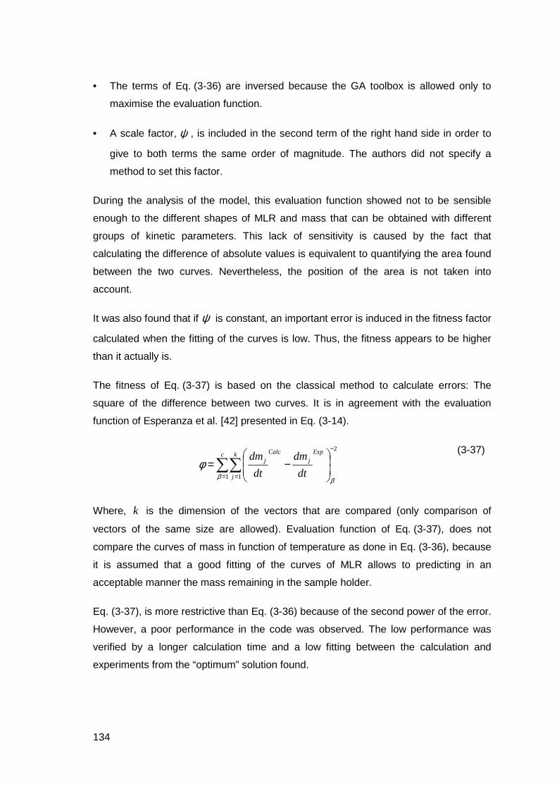
134

• The terms of Eq. (3-36) are inversed because the GA toolbox is allowed only to

maximise the evaluation function.

• A scale factor, ψ , is included in the second term of the right hand side in order to

give to both terms the same order of magnitude. The authors did not specify a

method to set this factor.

During the analysis of the model, this evaluation function showed not to be sensible

enough to the different shapes of MLR and mass that can be obtained with different

groups of kinetic parameters. This lack of sensitivity is caused by the fact that

calculating the difference of absolute values is equivalent to quantifying the area found

between the two curves. Nevertheless, the position of the area is not taken into

account.

It was also found that if ψ is constant, an important error is induced in the fitness factor

calculated when the fitting of the curves is low. Thus, the fitness appears to be higher

than it actually is.

The fitness of Eq. (3-37) is based on the classical method to calculate errors: The

square of the difference between two curves. It is in agreement with the evaluation

function of Esperanza et al. [42] presented in Eq. (3-14).

∑∑= =

−

−=

c k

j

Expj

Calcj

dt

dm

dt

dm

1 1

2

β β

φ (3-37)

Where, k is the dimension of the vectors that are compared (only comparison of

vectors of the same size are allowed). Evaluation function of Eq. (3-37), does not

compare the curves of mass in function of temperature as done in Eq. (3-36), because

it is assumed that a good fitting of the curves of MLR allows to predicting in an

acceptable manner the mass remaining in the sample holder.

Eq. (3-37), is more restrictive than Eq. (3-36) because of the second power of the error.

However, a poor performance in the code was observed. The low performance was

verified by a longer calculation time and a low fitting between the calculation and

experiments from the “optimum” solution found.

135

The best results in terms of calculation time and ability to fit the experiments and the

calculation curves were obtained with the evaluation function of Eq. (3-38), being the

function used in the present work.

( )[ ]β

βφ ∑

=

−

−⋅∠=

c

x

yxyx

1

1

,cos r

rrrr

Exp

dT

dmx =r ;

Calc

dT

dmy =r

(3-38)

In Eq. (3-38), xr

and yr

are respectively, arrays of experimental and calculated mass-

loss rates in function of temperature. These vectors are of the same dimension, i.e. the

data points are taken at the same temperature. The evaluation function, presented in

Eq. (3-38) has been obtained by the combination of the two indexes calculated in the

standard ISO 16730:2007 [125] for the comparison of curves. These indexes have

been defined based on the groups’ theory of Hilbert et al. in 1928 [126].

The first index calculated in the standard corresponds to the first term of the right hand

side of Eq. (3-38) which refers to the phase difference between the curves. The range

of variation of this index is between -1 and 1.

The second index calculated by the standard, is found in the second term of the right

hand side of Eq. (3-38). This term refers to the distance between the curves in the

vertical direction (ordinate axis). The range of variation of this index is between 0

and 1. It is highlighted that in the case where the experimental and calculated curves

are equal (same shape and location) the distance between them is null and the

evaluation would not be defined, i.e. division by zero. However, this case has not been

referenced yet in literature.

The definition of φ takes into account the scalar product yxrr

, and the Euclidean norm

of vectors xr

. These functions are reminded in Eq. (3-39). The analysis carried out

here was limited to Euclidean spaces, however, other non-Euclidean spaces can be

used, e.g. Hellinger, secant, and a hybrid of Euclidean and secant.

136

∑=

=m

iixx

1

2r with m being the length of x

r

( )[ ]yx

yxyx rr

rrrr ,

,cos =∠

=yxrr

, ∑=

m

iii yx

1

(3-39)

As explained, the aim is to verify the influence of the decomposition mechanism in the

prediction of MLR. Three decomposition mechanisms are evaluated, but the optimum

parameters can change while using a different evaluation function to compare

experimental and calculated results. The vectorial evaluation function of Eq. (3-38) was

selected because of his best capacity to predict TGA experimental results in a

reasonably calculation time.

The initial conditions used for the MLR calculations are:

( ) ( ) ( ) ( )

==

=

====

Constant

393)0(

00 ;00 ;00 ;10

βdt

dT

KT

mmmm residuecharpolyolPPUF

The analysis of the influence of the kinetic mechanism on the optimum parameters was

carried out using an inverse method. The inverse method means that we studied the

change of the calculated MLR (output) with the three mechanisms presented in Figure

3-2 to Figure 3-4 using a single group of kinetic parameters. The comparison of the

experimental and calculated MLR curves for β = 10 °C·min -1 is presented in Figure 3-6.

The curve of kinetic mechanism 2 (Figure 3-4) is omitted because the shape is exactly

the same as that of kinetic mechanism 1.

137

Figure 3-6 Comparison of MLR calculated with the three kinetic mechanisms from Figure 3-2 to Figure 3-4. β = 10 °C·min -1. Kinetic mechanism 1 and kinetic

mechanism 2 presented exactly the same shape.

The aim of the comparison of experimental and calculated MLR shapes, is to

determine the best model, and to be allowed to select one kinetic mechanism of PPUF

decomposition. The plots of Figure 3-6, are obtained using the group of kinetic

parameters that best fit the model proposed by Rein et al. [109] and the experimental

MLR. As showed, the first peak of MLR is well predicted by the three models

(T = 370 °C). The second peak of MLR is found at a temperature near 310 °C. Kinetic

mechanism 1 overestimates the second peak of MLR by 20% compared to the

experimental curve. The third peak of MLR is found at 350 °C. The overestimation of

kinetic mechanism 1 in the second peak is compensated by an underestimation of the

third peak of MLR by 20%.

As shown in Figure 3-6, there is little difference in the results found with the three

models. The comparison of MLR curves is performed to analyse the sensitivity to the

decomposition mechanism. The inverse method that is used to analyse the sensitivity

is based on the following principle: If each model requires a specific group of Arrhenius

parameters to reproduce experimental MLR curves in a satisfying manner, then the

138

comparison of the groups of parameters would provide a mean to determine which

model is the best. Nevertheless, it was found that a single group of kinetic parameters

allows all the models to reproduce the MLR experiments in a satisfying manner. Thus,

the actual kinetic mechanism of PPUF cannot be determined by the comparison of the

respective kinetic parameters calculated with each model.

The comparison of the experimental and calculated curves of mass as a function of

temperature has been also performed. However, the curves are not presented here

because they do not provide additional useful information. As a conclusion, the

comparison of the kinetic parameters calculated using various models does not

constitute an unambiguous form that could be used to determine the actual

decomposition mechanism of PPUF. As shown, various models are allowed to predict

the behaviour of mass and MLR. The gas release with the change of temperature

represents a means to gain information on the chemistry of the process allowing

definition of the current decomposition mechanism and the model to be used.

3.3.2 Analysis of the kinetic mechanisms based on

effluents measurements

The data presented in the last subsections corresponds to the identification of the

kinetic mechanism based on the results from the solid phase. As shown, the analysis of

the single data from the solid phase does not provide enough information to state

accurately a realistic kinetic mechanism of PPUF decomposition. In this subsection, the

observations of the solid phase are analysed together with data from the evolved

effluents. The possibility of occurrence of a given kinetic mechanism is analysed from

the point of view of gas release evidence.

The kinetics of the release of gases provide complementary information about the

decomposition mechanism of PPUF. The effluents released during PPUF pyrolysis in

dynamic temperature in TF under nitrogen atmosphere are presented in Figure 3-7.

The effluents released under air atmosphere are plotted in Figure 3-8. The respective

MLR shapes have been included for comparison of the behaviour of solid and gas

phases.

139

Figure 3-7 Effluents release in function of temperature under nitrogen atmosphere. Measurements carried out in TF + FTIRqnt and TF + FTIRqlt for β = 10 °C·min -1. The

MLR shape is included for comparison of the behaviour of solid and gas phases.

It is remebered that in Figure 3-7 and Figure 3-8, the compound labelled as ‘polyol’ is a

gas product of the decomposition of semi-liquid polyol. The gas labelled ‘Isocyanate’ is

the effluent released during the breakdown of the isocyanate contained in the

polyurethane molecules.

The functions created by the thermal decomposition of polyol and isocyanate, are

commonly destroyed in the flame region. Thus, such compounds are much more

difficult to identify in large-scale tests (or real fires) because of factors such as the

ventilation conditions and a high dilution rate of effluents. The functions from

isocyanate are transformed into CO2, CO, H2O, NOx and HCN, while the functions from

polyol are transformed into CO2, CO, H2O [5][23][30][32][38][39].

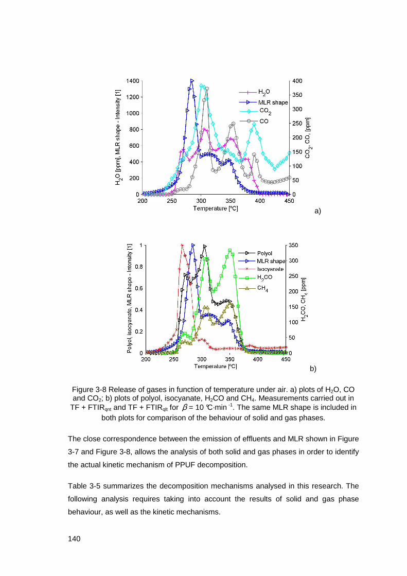
140

a)

b)

Figure 3-8 Release of gases in function of temperature under air. a) plots of H2O, CO and CO2; b) plots of polyol, isocyanate, H2CO and CH4. Measurements carried out in

TF + FTIRqnt and TF + FTIRqlt for β = 10 °C·min -1. The same MLR shape is included in both plots for comparison of the behaviour of solid and gas phases.

The close correspondence between the emission of effluents and MLR shown in Figure

3-7 and Figure 3-8, allows the analysis of both solid and gas phases in order to identify

the actual kinetic mechanism of PPUF decomposition.

Table 3-5 summarizes the decomposition mechanisms analysed in this research. The

following analysis requires taking into account the results of solid and gas phase

behaviour, as well as the kinetic mechanisms.

141

Table 3-5 Kinetic mechanisms analysed

Decomposition mechanism Source/figure

Pyrolysis reaction

Oxidation reaction

Pyrolysis reaction

Oxidation reaction

PPUF Polyol Char ResiduePPUF Polyol Char Residue1

2

3

4 5

Rein et al. [109].

See Figure 3-2.

1

2

3

4 5

Pyrolysis reaction

Oxidation reaction

Pyrolysis reaction

Oxidation reaction

PPUF Polyol Char Residue

This research.

Kinetic mechanism 1.

See Figure 3-3.

1 2

3 4

5

Pyrolysis reaction

Oxidation reaction

Pyrolysis reaction

Oxidation reaction

PPUF Polyol Char Residue

This research.

Kinetic mechanism 2.

See Figure 3-4.

The following analysis study one by one the reactions (arrows) in order to verify their

existence according to the evidence of the solid and gas phase measurements.

The results of the solid and gas phases of PPUF decomposition under nitrogen

atmosphere present two well-identified stages. The first stage releases isocyanate. As

explained (see section 2.5.4), isocyanate is released during the collapse of the solid

structure of PPUF. The condensed-phase product of this reaction is polyol, which

remains in the sample holder as a semi-liquid. This reaction is presented by arrow No 1

in the three mechanisms. In Figure 3-7 is observed that the first reaction of pyrolysis

release only isocyanate while in the second the polyol is pyrolysed as well as other

gases.

The second stage of the pyrolysis evolves polyol, H2CO, H2O and CH4. No CO and

CO2 are observed because no oxygen is present in the inlet gas stream, and the

proportion of oxygen in the solid matrix of PPUF is weak. Discrepancies appear in the

three mechanisms according to the transformations caused in the solid phase by the

142

second reaction, see arrow No 2. Experimental evidence shows that during pyrolysis

no char is formed but do a residue. In other words:

• Char is a product of the reaction of solids with the oxygen (heterogeneous

oxidization). Char can suffer further decomposition reaction in which oxidized

molecules are broken down, releasing CO2 and CO [127]. Oxidization of char is a

process observed in polymeric fuels [128] as well as in biomass [129].

• The mass of the residue that remains in the holder at the end of the tests is higher

under air (8%) than under nitrogen (3%). Thus, at the temperature of the end of the

test (450 °C), no further reaction occurs. The samp le mass has been completely

consumed.

• Comparison of MLR and gas release curves under air and nitrogen shows that char

is decomposed to form a residue. During PPUF decomposition, char exists at a

lower temperature than the one of residue formation. At a temperature of 450 °C,

the solid species remaining in the sample holder is a residue, not char. In tests not

presented here, it was shown that the residue of PPUF found under nitrogen

atmosphere (3%Wt) decomposes at nearly 600 °C.

These observations show that the reaction represented by arrow No 2 actually

transforms polyol into a residue. This kinetic step during PPUF pyrolysis is well

predicted by the kinetic mechanism 1 presented in Figure 3-3. Thus, the mechanism of

Figure 3-3 is the one that best explains the thermal behaviour of PPUF under nitrogen

decomposition condition.

The same analysis is carried out to verify if the mechanism of decomposition under

nitrogen is the best for the oxidization reactions.

The beginning of PPUF decomposition under air is shifted through the lower

temperatures compared to tests under nitrogen as observed in the plots of MLR and

gases evolution. This is in agreement with the observations made by

Caballero et al. [116] and Senneca et al. [117]. The earlier reaction of PPUF under

oxidizing atmosphere shows a strong influence of oxygen on the virgin foam

decomposition reaction. This suggests that the oxidization reaction that transforms

PPUF into polyol (arrow No. 3 in Figure 3-3) does exist and plays a very important role

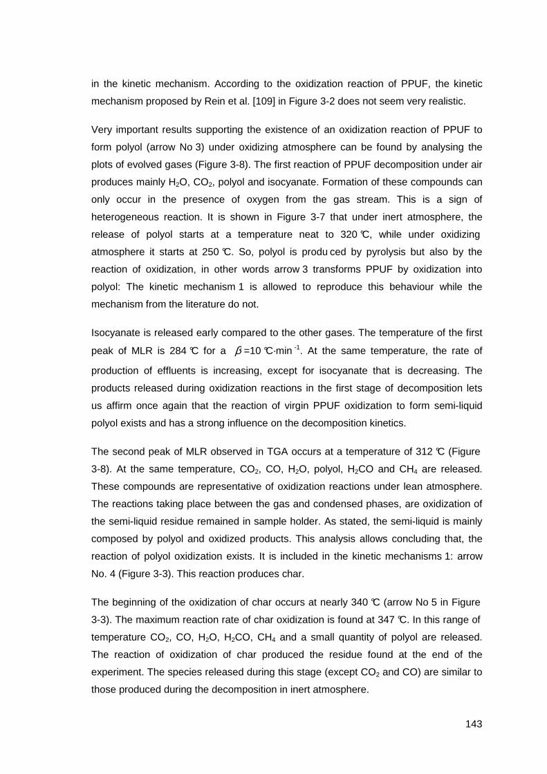
143

in the kinetic mechanism. According to the oxidization reaction of PPUF, the kinetic

mechanism proposed by Rein et al. [109] in Figure 3-2 does not seem very realistic.

Very important results supporting the existence of an oxidization reaction of PPUF to

form polyol (arrow No 3) under oxidizing atmosphere can be found by analysing the

plots of evolved gases (Figure 3-8). The first reaction of PPUF decomposition under air

produces mainly H2O, CO2, polyol and isocyanate. Formation of these compounds can

only occur in the presence of oxygen from the gas stream. This is a sign of

heterogeneous reaction. It is shown in Figure 3-7 that under inert atmosphere, the

release of polyol starts at a temperature neat to 320 °C, while under oxidizing

atmosphere it starts at 250 °C. So, polyol is produ ced by pyrolysis but also by the

reaction of oxidization, in other words arrow 3 transforms PPUF by oxidization into

polyol: The kinetic mechanism 1 is allowed to reproduce this behaviour while the

mechanism from the literature do not.

Isocyanate is released early compared to the other gases. The temperature of the first

peak of MLR is 284 °C for a β =10 °C·min -1. At the same temperature, the rate of

production of effluents is increasing, except for isocyanate that is decreasing. The

products released during oxidization reactions in the first stage of decomposition lets

us affirm once again that the reaction of virgin PPUF oxidization to form semi-liquid

polyol exists and has a strong influence on the decomposition kinetics.

The second peak of MLR observed in TGA occurs at a temperature of 312 °C (Figure

3-8). At the same temperature, CO2, CO, H2O, polyol, H2CO and CH4 are released.

These compounds are representative of oxidization reactions under lean atmosphere.

The reactions taking place between the gas and condensed phases, are oxidization of

the semi-liquid residue remained in sample holder. As stated, the semi-liquid is mainly

composed by polyol and oxidized products. This analysis allows concluding that, the

reaction of polyol oxidization exists. It is included in the kinetic mechanisms 1: arrow

No. 4 (Figure 3-3). This reaction produces char.

The beginning of the oxidization of char occurs at nearly 340 °C (arrow No 5 in Figure

3-3). The maximum reaction rate of char oxidization is found at 347 °C. In this range of

temperature CO2, CO, H2O, H2CO, CH4 and a small quantity of polyol are released.

The reaction of oxidization of char produced the residue found at the end of the

experiment. The species released during this stage (except CO2 and CO) are similar to

those produced during the decomposition in inert atmosphere.

144

In conclusion, the kinetic mechanism presented in Figure 3-3 is the one which seems

to best corresponds to the observations of the chemical process. The analyses

considered decomposition under air and nitrogen atmospheres. The following study is

performed with the results obtained with this model.

The knowledge of the kinetic mechanism allows calculating the mass-loss rate and

mass change in function of temperature in an accurate manner. Figure 3-9 presents

the comparison of experimental and calculated results under two atmospheres (air and

nitrogen) and four heating rates (5, 8, 10 and 15 °C·min-1). The plots of mass change

with temperature are not presented here, because they provide less useful information

than MLR shapes.

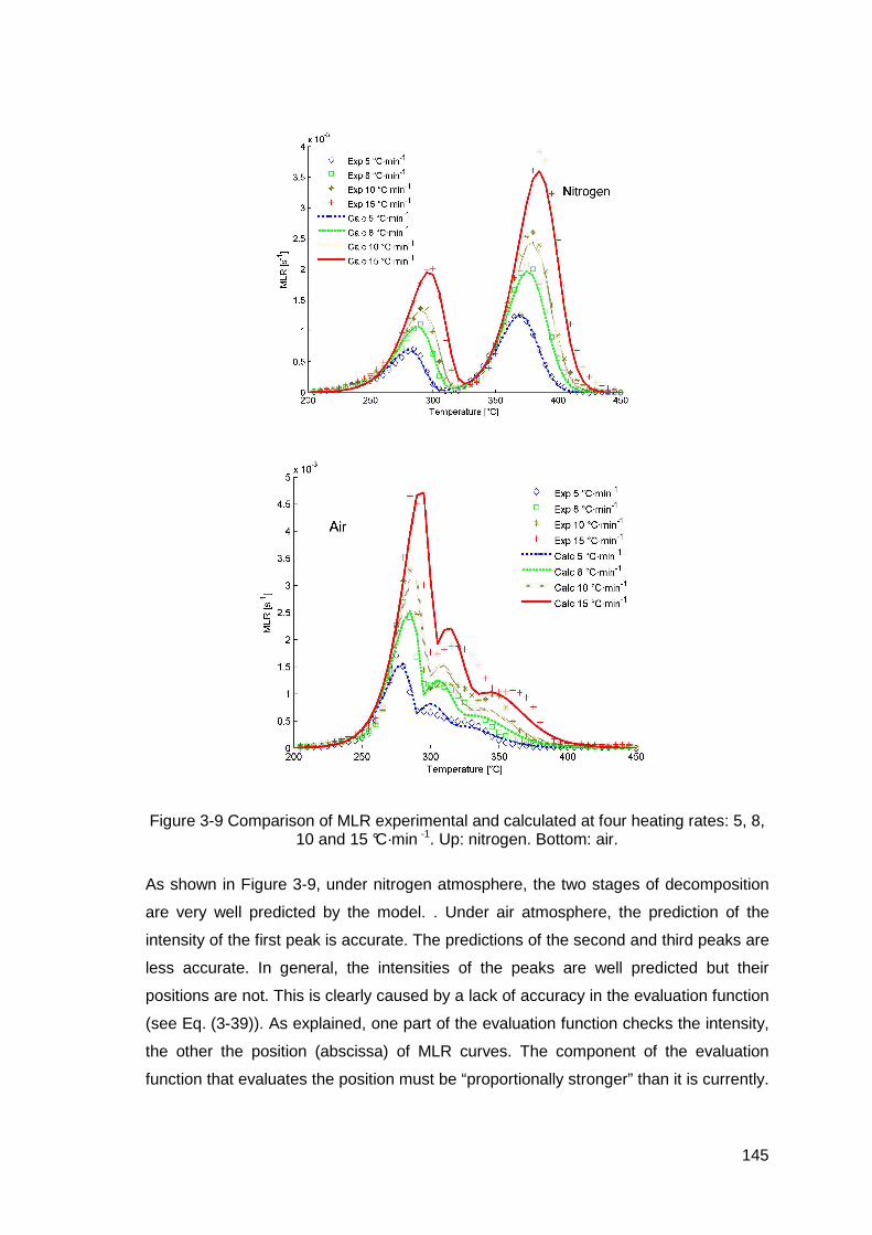
145

Figure 3-9 Comparison of MLR experimental and calculated at four heating rates: 5, 8, 10 and 15 °C·min -1. Up: nitrogen. Bottom: air.

As shown in Figure 3-9, under nitrogen atmosphere, the two stages of decomposition

are very well predicted by the model. . Under air atmosphere, the prediction of the

intensity of the first peak is accurate. The predictions of the second and third peaks are

less accurate. In general, the intensities of the peaks are well predicted but their

positions are not. This is clearly caused by a lack of accuracy in the evaluation function

(see Eq. (3-39)). As explained, one part of the evaluation function checks the intensity,

the other the position (abscissa) of MLR curves. The component of the evaluation

function that evaluates the position must be “proportionally stronger” than it is currently.

146

This, would help the GA tool to assign better fitness to candidates with accurate

position.

3.3.3 Coupling of the model of solid phase to the m odel

of gas effluents release rate

The last subsection analysed the kinetic mechanisms from the point of view of

chemistry. The three possible kinetic mechanisms that can reproduce the mass change

with temperature were analysed. It was concluded that the mechanism that is in best

agreement with the chemistry of the process was kinetic mechanism 1, presented in

Figure 3-3.

In this subsection the coupling of the model of solid phase to the model of effluents

release rate is performed. A deductive method is used to couple the models of both

phases. The first step consists in determining which gases are specifically produced by

each reaction. The second step is the calculation of yields. The modelling of gas

release provide further evidence to the discussion of the decomposition mechanism.

3.3.3.1 Determination of the gases released by each

reaction

The determination of the gases that are released by each reaction is a main task of the

coupling of the models of solid and gas phases. It is based on the following hypothesis:

the curve of release of one particular gas can be obtained by the addition of the

kinetics of release of this gas by various successive reactions. Thus, if the gases

released by each reaction are carefully identified, the global gas release can be

predicted.

The method to determine which gases are produced by each reaction consists in

plotting the reaction rates calculated with Eq. (3-27) together with the curves of gases

evolution. It is considered that one reaction releases one gas when common peaks are

found between them. As example, the plots of CO2 and polyol together with reaction

rates are presented in Figure 3-10. The number of the reactions are the same as the

147

arrows of kinetic mechanism 1, which is reminded hereafter. Similar plots for the other

gases are presented in Appendix B. The following analysis is developed only using the

results obtained with kinetic mechanism 1.

1

2

3

4 5

Pyrolysis reaction

Oxidation reaction

Pyrolysis reaction

Oxidation reaction

PPUF Polyol Char Residue

Reminder of Figure 3-3 Kinetic mechanism 1 proposed in this research.

148

Figure 3-10 Coupling of plots of reaction rates and gases evolution: Up CO2. Bottom polyol. Reaction 2 is scaled by a factor of 500 for easy of view.

All the information on the kinetic mechanism 1, including the transformations suffered

by the solid and gas phases are summarized in Table 3-6.

149

Table 3-6 Kinetic mechanism of PPUF decomposition taking into account the behaviour of the solid and the gas phases

No Type of reaction

Temp. [ºC]

Reactives Products

solid or liquid Products

gas 1 Pyrolysis 200 – 340 PPUF →

1υ ·Polyol + 1τ ·[Isocyanate]

2 Pyrolysis 340 – 450 Polyol → 2υ ·Residue +

2τ ·[Polyol + H2CO + H2O + CH4] 3 Oxidation 200 – 275 PPUF + O2 →

3υ ·Polyol + 3τ ·[Polyol + CO2 + H2O]

4 Oxidation 220 – 300 Polyol + O2 → 4υ ·Char +

4τ ·[Polyol + H2CO + CH4+ CO + CO2 + H2O] 5 Oxidation 300 – 450 Char + O2 →

5υ ·Residue + 5τ ·[Polyol + H2CO + CH4+ CO + CO2 + H2O]

In Table 3-6, the first column is the number of the reaction that corresponds to the

number shown in Figure 3-3. The column “Reactives” is the substance that is

transformed during the reaction i . The column “Products solid or liquid” corresponds to

the condensed phase that remains in the sample holder at the end of the reaction. The

gas effluents are listed in the column “Product gas”.

In this subsection, the released gases were associated to each reaction. The next step

is the prediction of the leak of each gas as a function of temperature.

3.3.3.2 Prediction of the kinetics of gas release

The cornerstone of the improvements carried out to the model of thermal

decomposition of PPUF is to couple a model to predict the release of gas species.

Thus, the prediction of the change of the mass as a function of temperature as well as

the kinetics of the release of gases is allowed.

The coupling of models permits the calculation of iυ and iτ , which are the respective

stoichiometric coefficients of the solid and gas phases (see Table 3-6). They are the

quantification of the proportion of reactives that are transformed into solid or gas

products, and are required for establishing the mass balances. The calculation of iυ is

presented in subsection 3.2.6.

The coupling of the models of solid and gas phases is conducted by means of the

calculation of iτ as a function of the stoichiometric coefficient of the solid phase iυ .

The optimization of iυ allows predicting accurately the MLR with time (temperature)

150

and carry out the optmisation of iτ , which allows the prediction of effluents release.

The function between the stoichiometric coefficients iυ and iτ is presented in

Eq. (3-40).

( )iii υγτ −⋅= 1 (3-40)

The second term of the right hand side of Eq. (3-40) is the fraction of the solid

transformed into gas during a reaction (see Table 3-6). iγ , is a coefficient calculated in

Eq. (3-41).

∑=

⋅= h

b

Expb

Expi

ii

Y

Y

1

κγ (3-41)

Where, ExpiY is the experimental yield of gas released by the reaction i . h is the

number of species released by the reaction i . ∑=

h

b

ExpbY

1

is the total mass of gases

released during the decomposition process.

In Eq. (3-41), the term iκ is a dimension-less coefficient calculated using genetic

algorithms. The optimum value of iκ is the one that allows the best fitting between the

experimental and calculated mass flow rate of gases. A single value of iκ is calculated

for each reaction of Table 3-6. The physical meaning of iκ has not been determined

yet, but it has been observed to be function of the particular gases that are produced

during a reaction and their mass flow rate. The second term of Eq. (3-41) is the

experimental yields that can be read directly from Table 3-7 (column Experimental

yields – Air).

Eq. (3-33) presented the calculation of the mass-loss rate of a given solid species. A

similar calculation is presented in Eq. (3-42) but referenced to the mass of gas

produced by a reaction: The yield of gases produced by a given reaction i is

calculated as the product of the stoichiometric coefficient, iτ and the reaction rate iω& .

iiiY ωτ && ⋅= (3-42)

151

The yield of a particular gas species b , is also calculated. This yield takes into account

the fraction of the species b produced by each reaction. It is calculated in Eq. (3-43).

∑=

=5

1,

i

Calcib

Calcb YY

(3-43)

Where, CalcibY , is the yield of a gas b produced by the reaction i . The results of

calculated yields CalcbY are presented in Table 3-7.

Table 3-7 Comparison of experimental and calculated yields

Gas [mg·g-1] % [mg·g-1] % [mg·g-1] % [mg·g-1] %CO2 42.3 35.6% - - - - 20.1 30.1%CO 13.6 11.5% 6.8 23.1% 0.6 13.7% 13.1 19.6%H2O 47.7 40.1% 13.4 45.1% 0.7 15.8% 18.9 28.3%

H2CO 10.1 8.5% 6.8 22.8% 2.3 53.8% 12.8 19.2%

CH4 2.6 2.2% 1.8 6.1% 0.7 16.7% 1.8 2.7%HCN 2.5 2.1% 0.8 2.8% - - - -Total 118.9 100.0% 29.6 100.0% 4.2 100.0% 66.7 100.0%

Air 10.5% O2 NitrogenCalculated yields

AirExperimental yields

Figure 3-11, presents the experimental and calculated kinetics of release of CO2 and

H2CO under air atmosphere. The plots show the concentration of the gases and not

their respective yield because the gas measurement has been obtained with tubular

furnace, where the change of mass with the increase in temperature is not measured.

The curve of MLR obtained in TGA is included as reference. The plots for the CO, H2O

and CH4 are presented in Appendix C. The curves of polyol and isocyanate are not

presented because no quantitative data are available.

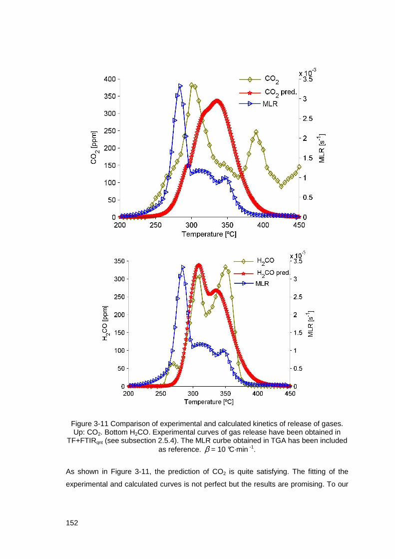
152

Figure 3-11 Comparison of experimental and calculated kinetics of release of gases. Up: CO2. Bottom H2CO. Experimental curves of gas release have been obtained in

TF+FTIRqnt (see subsection 2.5.4). The MLR curbe obtained in TGA has been included as reference. β = 10 °C·min -1.

As shown in Figure 3-11, the prediction of CO2 is quite satisfying. The fitting of the

experimental and calculated curves is not perfect but the results are promising. To our

153

knowledge, this work is the first to offer an approach of the prediction of the kinetics of

the main toxic gases release as a function of temperature.

The model as well as the experiments presents three peaks of gas release. The peaks

are not located at the correct temperatures, but they reproduce the respective

concentration of CO2 production.

The position of the peak of CO2 production found at a temperature of 400 °C is not well

predicted. However, this peak also represents a discrepancy between the experimental

results found in TF+FTIRqnt and TGA+FTIRqlt (see Figure 2-14-b in subsection 2.5.4).

This discrepancy is also responsible for the difference found in the total yields

(experimental and calculated) observed in Table 3-7. As stated, this difference can be

due to the post-combustion of residues laid inside the TF quartz tube.

The prediction of H2CO is more accurate than the one of CO2. The entire shape of the

curve is quite well reproduced, except that the third peak of the experimental one is

higher, while in the model, the first one is the most intense. The model does not allow

the prediction of the peak found at a temperature of 270 °C.

In conclusion, the model that allows the calculation of the kinetics of gas release

requires, as input data for the calibration, the experimental yield of the gases leaked by

every reaction of the decomposition mechanism. The method for determining which

gases are released by each reaction is the one presented in Figure 3-10, which is

based on the hypothesis that a curve of gas release can be calculated as the sum of

the gases released by each individual reaction. This allows setting one single

parameter per reaction. The output of the model of gas phase is the prediction of the

kinetics of gas release and their respective total yield.

Table 3-8, presents the kinetic parameters of the coupled model that allows predicting

the behaviour of solid and gas phases. Each reaction has five parameters: three are

specific to the solid phase (Arrhenius parameters) and two stoichiometric parameters,

one for the solid phase and one for the gas phase. The five parameters of each

reaction are optimized simultaneously using Genetic Algorithms.

154

Table 3-8 Output of the coupled model of solid and the gas phases. Each reaction of the kinetic mechanism has five kinetic parameters.

Range Reaction Parameter Value High Low

Units

PPUF pyrolysis 1E

169.9 190 150 kJ·mol-1

1A 6.09 x 1013 1 x 1022 1 x 107 s-1

1n 0.91 1 0.1 _

1υ 0.69 0.9 0.1 kg·kg-1

1τ _ 9 x 109 1.5 x 109 _

Polyol pyrolysis 2E 243.9 260 100 kJ·mol-1

2A 4.42 x 1017 1 x 1019 1 x 107 s-1

2n 1.26 1.5 0.1 _

2υ 0.10 0.81 0.1 kg·kg-1

2τ 4.9 x 109 9 x 109 1.5 x 109 _

PPUF oxidization 3E 214.1 240 161 kJ·mol-1

3A 3.07 x 1018 1 x 1020 1 x 107 s-1

3n 0.48 3 0.2 _

3υ 0.44 0.7 0.1 kg·kg-1

3τ 8.9 x 104 1.5 x 105 3 x 104 _

Polyol oxidization 4E 213.6 240 161 kJ·mol-1

4A 1.26 x 1018 1 x 1022 1 x 107 s-1

4n 0.95 3 0.3 _

4υ 0.56 0.7 0.1 kg·kg-1

4τ 8 x 105 2.2 x 106 2 x 104 _

Char oxidization 5E 160.8 240 160 kJ·mol-1

5A 4.30 x 1012 3 x 1015 1 x 1011 s-1

5n 1.64 3 0.5 _

5υ 0.25 0.8 0.1 kg·kg-1

5τ 3.4 x 106 9 x 106 1.7 x 105 _

In this section, the improvements carried out to the model of PPUF thermal

decomposition are presented. A discussion is performed on the sensitivity to the

decomposition mechanism and to the evaluation function. The need of analysing the

chemistry in order to figure out the actual decomposition patterns is clearly identified.

The method for the coupling of the models of solid and gas phases is also presented.

Finally, the comparison of the experimental and calculated yields of gases is presented

as well as the prediction of the kinetics of gas release. It is found that the coupled

155

models predict in a satisfying manner the behaviour of the solid phase and in a quite

satisfying manner the behaviour of the gas phase.

The following sections discuss particular technical aspects of the code, such as the

stability and the sensitivity to input parameters.

3.4 Analysis of code stability

In the last section the model used to predict the MLR of a sample being heated up was

presented, to which a model that allows the prediction of the kinetic of toxic gases

release is coupled. It is shown that the results are satisfying in both the solid and gas

phases. This section deals with particular technical aspects of the code used to resolve

the mathematical equations: Problems with the code stability have been found that

made the computational process difficult. This section is devoted to the analysis of the

code stability.

The stability of the code used for the model is a main requirement in order to allow a

sensitivity analysis, i.e. the space of solutions must be continuous in order to enable

the understanding of the influence of the input parameters on the output of the model

(presented in the next section). The analysis of stability is aimed at verifying the ability

of the solver of Ordinary Differential Equations (ODE) to converge to a solution. It is

considered that the solver has successfully found a candidate solution (output) when it

is able to calculate a MLR curve and a fitness factor between calculations and

experiments. Successfully finding a candidate solution does not necessarily mean that

the fitting between the experiments and calculations is good. It only means that the

comparison is possible. During the process of ODE solutions, it was found that in some

cases, the solver was unable to converge to a solution: the calculation time becomes

unacceptably long or the code becomes trapped in infinite loops. The solver used in

this research was ‘ode15s’ from MatLab®.

It is remembered that the input data for the model are the kinetic mechanism

(discussed in chapter 3) and a range of values for each kinetic parameter (see Table

3-8). The output of the model is a group of 25 kinetic parameters that fits in a satisfying

manner with the experimental results of mass and gas release. These parameters are

156

calculated by optimization using genetic algorithms. The analysis of code stability was

performed giving to each kinetic parameter an input range as large as possible in order

to explore the largest field of candidate solutions. The higher and lower limits of the

ranges were established according to data found in literature or to the physical

meaning of each kinetic parameter (see subsection 3.2.8).

As stated, one candidate group of kinetic parameters is formed by the combination

of 25 random kinetic parameters. In total, 2 000 groups were produced and tested

within the model. A specific application was developed in order to detect the lack of

convergence of the ODE solver with some of the groups. Two limits were imposed to

the solver: a critical calculation time and a critical number of iterations. Once the

current calculation time or the number of iterations exceeds the critical limits, the ODE

solver is forced to stop and classifies the group of kinetic parameters as “unsolvable”.

Critical time was set to 5 s and critical number of iterations to 8 000. These limits were

set beyond the calculation time and number of iterations required for a typical solved

case. A typical solved case was achieved in a calculation time near to 0.25 s and

required around 400 iterations. When these two limits were imposed to the solver, it

was found that around 13.7% of the candidate groups were classified as unsolvable.

In order to find possible explanations to the problem, various studies were carried out

with the groups of kinetic parameters that offered solved and unsolved cases. To

discard one possible cause of problems, a verification of the random values generator

was conducted. It was found that the values produced for each kinetic parameter

followed a uniform distribution and behaved as independent variables, which is a

characteristic of good performance for the random values generator. Thus, the ODE

output is considered free of possible noise effects caused by dependency relations

between the input variables1.

Two different statistical studies were performed in order to characterise the instability of

the code produced by some of the groups of kinetic parameters. The first is a

classification of the unsolvable groups with respect to the input ranges given to each

1 To avoid confusions, the possible dependency relations between input parameters is a

different problem to compensation effects found by various authors. The compensation effect

refers to groups of kinetic parameters that constitute accurate solutions of the model.

157

kinetic parameter. The second is a descriptive study that statistically compares the

groups of parameters that produced unsolvable cases with the totality of the analysed

groups. These studies are detailed here-after.

3.4.1 Study of the input ranges of the ODE unsolvab le

cases.

This study was limited to the groups of kinetic parameters classified as unsolvable. The

groups were statistically analysed using the following method: The range of possible

values of each variable (input range) was divided into ten subgroups. The number of

unsolved ODE in each subgroup was counted. Histograms of the frequency of

occurrence of unsolved ODE per subgroup were plotted. As an example of the results

obtained, Figure 3-12 presents the frequency of unsolved ODE over the whole input

range of pre-factor of decomposition reaction No 1, 1A (see Table 3-6). Figure 3-13

shows the histograms of activation energy and reaction order of the decomposition

reaction No 2, 2E and 2n respectively. These statistical analyses aim at highlighting

possible common characteristics between the input parameters that produced

unsolvable ODE.

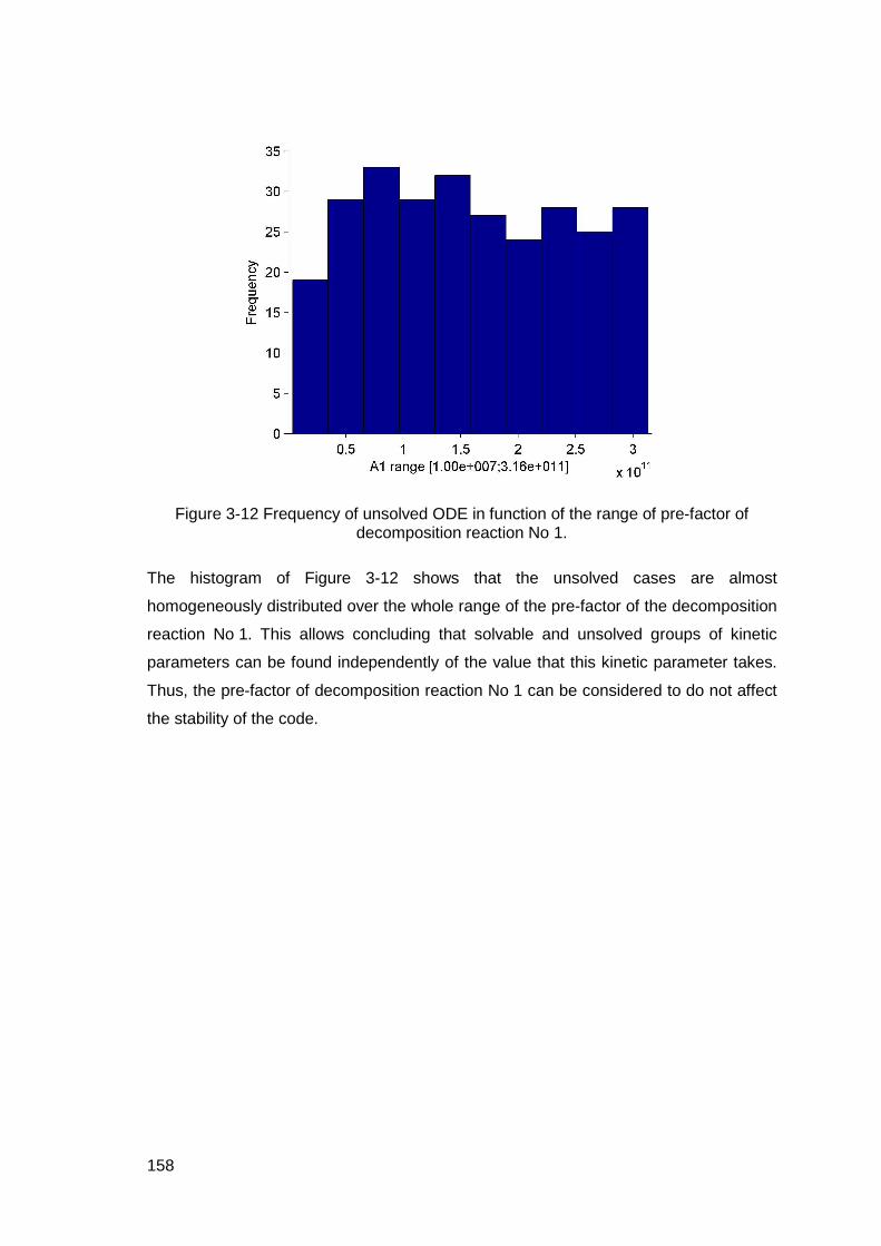
158

Figure 3-12 Frequency of unsolved ODE in function of the range of pre-factor of decomposition reaction No 1.

The histogram of Figure 3-12 shows that the unsolved cases are almost

homogeneously distributed over the whole range of the pre-factor of the decomposition

reaction No 1. This allows concluding that solvable and unsolved groups of kinetic

parameters can be found independently of the value that this kinetic parameter takes.

Thus, the pre-factor of decomposition reaction No 1 can be considered to do not affect

the stability of the code.

159

Figure 3-13 Frequency of unsolved ODE in function of variables range. Up, histogram of the activation energy of decomposition reaction No 2. Down, histogram of the

reaction order of decomposition reaction No 2.

Contrary to what was observed for 1A in Figure 3-12, the histograms of 2E and 2n

present clear trends in the ODE insolvability. The upper histogram of Figure 3-13,

160

shows that at the center of the input range, the activation energy of decomposition

reaction No 2 presents a higher probability of producing an unsolved ODE. However,

the probability of finding an unsolved ODE is lower near to the extremes of the range.

A different behaviour is observed in the histogram of the reaction order of

decomposition reaction No 2. Values of 2n near to the lower limit of the input range

tend to produce a great number of unsolved cases, while values near the upper limit

tend to produce less unsolved ODE.

Under both atmospheres (air and nitrogen), it was found that the kinetic parameters of

decomposition of reaction No 2 have a high influence on the stability of the code. The

kinetic parameters of the other reactions showed not to be so critical in the production

of unsolvable cases. A more detailed study is performed in order to understand why the

stability of the code is controlled by the kinetic parameters of the reaction No 2.

3.4.2 Descriptive study

The descriptive study of the groups of kinetic parameters has two aims: The verification

of the reproducibility of the appearance of unsolvable cases in the given input ranges of

values, and the identification of the ranges of kinetic parameters that produce

discontinuities in the field of outputs.

In total, the model was run four times. Twice under nitrogen atmosphere and twice

under air atmosphere. Each run evaluated 2 000 groups of kinetic parameters and

classified each candidate group as solvable or unsolvable. In all cases, the input

ranges remained unchanged.

Table 3-9, presents the summary of the tests run and their respective number of

unsolved cases.

161

Table 3-9 Analysis of reproducibility. Number of unsolved cases per model run. The ranges of input parameters have remained constant.

No Atmosphere Total cases

Unsolved cases

Ratio of unsolved

1 Nitrogen 2000 300 15.0%2 Nitrogen 2000 283 14.2%3 Air 2000 238 11.9%4 Air 2000 237 11.9%

Mean 264.5 13.2%St. Deviation 31.9 1.6%

As shown in Table 3-9, the problem of insolvability of some cases is reproducible. The

results of Table 3-9, also confirm that the problem of stability is caused directly by the

input data furnished to the model and not by the output produced by the ODE solver. It

is remembered that the change of atmosphere modifies the mass balance because the

solid species entering into account in the process are not the same, and the calculated

reaction rates are different as well.

In Table 3-10 the descriptive study of 2E and 2n is presented, which is allowed by the

reproducibility condition presented in Table 3-9. The study is focused on these two

variables, because of their stronger influence in the stability of the code rather than any

other kinetic parameters.

Table 3-10 Descriptive study of 2E and 2n .

Kinetic parameter

Atm.-test No.

Solution status

Population Mean Standard deviation

Variation coefficient

Minimum Maximum Range extent

Nitrogen 1 Total 2000 181.25 46.24 25.51% 100.05 259.99 159.94Nitrogen 1 Unsolved 300 121.57 18.38 15.12% 100.05 258.04 158.00Nitrogen 1 Solved 1700 191.78 41.42 21.60% 100.10 259.99 159.89Nitrogen 2 Total 2000 180.66 45.99 25.45% 100.05 259.90 159.85Nitrogen 2 Unsolved 283 121.62 15.08 12.40% 100.05 222.02 121.97Nitrogen 2 Solved 1717 190.39 41.91 22.01% 100.10 259.90 159.80

Air 1 Unsolved 238 119.55 15.34 12.83% 100.02 192.33 92.31Air 1 Solved 1762 187.62 42.70 22.76% 100.19 260.00 159.81Air 2 Unsolved 237 117.51 11.62 9.89% 100.17 167.89 67.72Air 2 Solved 1763 186.78 42.40 22.70% 100.50 259.95 159.44

Nitrogen 1 Total 2000 0.78 0.40 51.95% 0.10 1.50 1.40Nitrogen 1 Unsolved 300 0.54 0.34 63.69% 0.10 1.48 1.38Nitrogen 1 Solved 1700 0.82 0.40 48.72% 0.10 1.50 1.40Nitrogen 2 Total 2000 0.81 0.40 50.16% 0.10 1.50 1.40Nitrogen 2 Unsolved 283 0.58 0.38 64.86% 0.10 1.48 1.38Nitrogen 2 Solved 1717 0.84 0.40 47.07% 0.10 1.50 1.40

Air 1 Unsolved 238 0.55 0.38 68.58% 0.10 1.47 1.36Air 1 Solved 1762 0.82 0.40 49.06% 0.10 1.50 1.40Air 2 Unsolved 237 0.58 0.38 66.19% 0.11 1.50 1.39Air 2 Solved 1763 0.84 0.40 48.29% 0.10 1.50 1.40

E2

n2

In Table 3-10, the column “Solution status” is linked to the “population”: they represent

the size of the sample. The “Variation coefficient” is calculated as the ratio between the

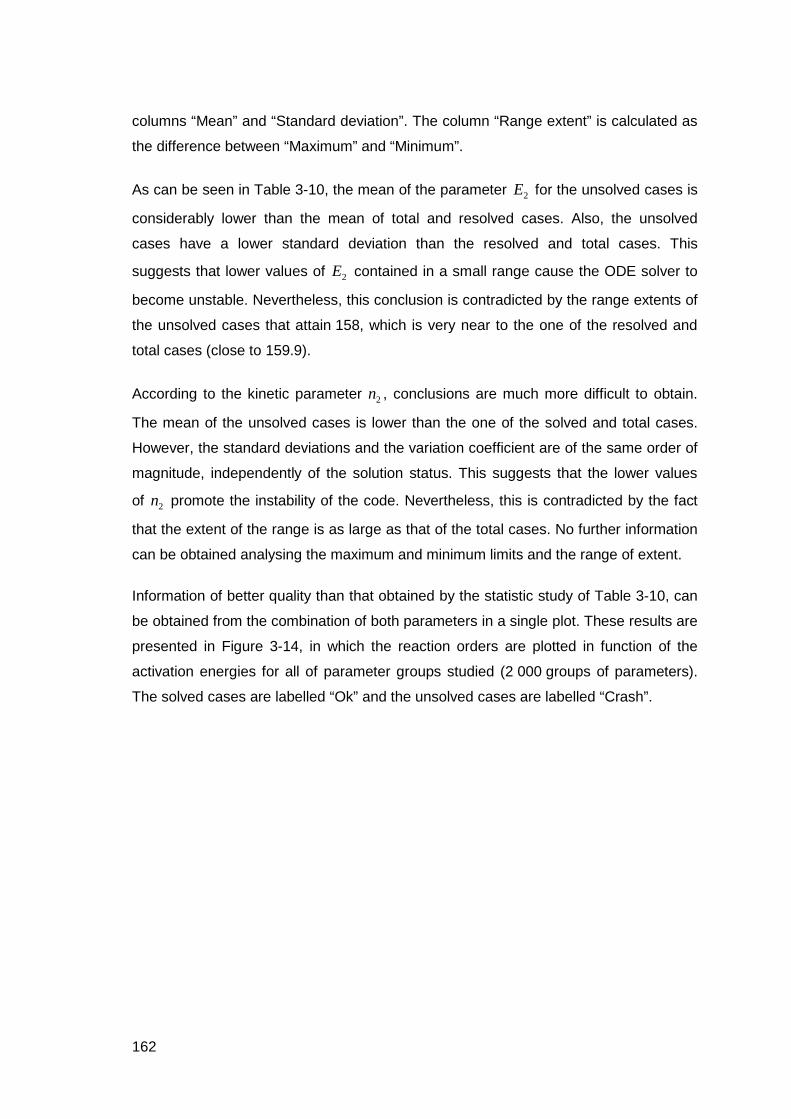
162

columns “Mean” and “Standard deviation”. The column “Range extent” is calculated as

the difference between “Maximum” and “Minimum”.

As can be seen in Table 3-10, the mean of the parameter 2E for the unsolved cases is

considerably lower than the mean of total and resolved cases. Also, the unsolved

cases have a lower standard deviation than the resolved and total cases. This

suggests that lower values of 2E contained in a small range cause the ODE solver to

become unstable. Nevertheless, this conclusion is contradicted by the range extents of

the unsolved cases that attain 158, which is very near to the one of the resolved and

total cases (close to 159.9).

According to the kinetic parameter 2n , conclusions are much more difficult to obtain.

The mean of the unsolved cases is lower than the one of the solved and total cases.

However, the standard deviations and the variation coefficient are of the same order of

magnitude, independently of the solution status. This suggests that the lower values

of 2n promote the instability of the code. Nevertheless, this is contradicted by the fact

that the extent of the range is as large as that of the total cases. No further information

can be obtained analysing the maximum and minimum limits and the range of extent.

Information of better quality than that obtained by the statistic study of Table 3-10, can

be obtained from the combination of both parameters in a single plot. These results are

presented in Figure 3-14, in which the reaction orders are plotted in function of the

activation energies for all of parameter groups studied (2 000 groups of parameters).

The solved cases are labelled “Ok” and the unsolved cases are labelled “Crash”.

163

Figure 3-14 Plot of reaction orders in function of activation energies. Up, kinetic reaction No 2. Down, kinetic reaction No 1. The solved cases are labelled “Ok”

represented as red x and the unsolved cases are labelled “Crash” represented in blue squares.

At the bottom of Figure 3-14 the typical distribution of variables that do not influence

the stability of the code is presented. The squares and crosses are homogeneously

distributed all over the area, which means that independently of the values given to

these variables, the code can or cannot find a solution.

At the top of Figure 3-14, the results for the kinetic parameters of the decomposition

reaction No 2 are presented. The unsolved cases are concentrated in the low values

of 2E and along all the values of the input range of 2n . Nevertheless, a few number of

blue squares can be observed in a zone where the range of 2n is [0.15;0.3] and the

one of 2E is [190;260]. These few unsolved cases are found in regions were the solver

164

was normally able to find ODE solutions. These visual results confirm the interpretation

done according to the data of Table 3-10.

A reliable stability of the code is a primary requirement for further developments of the

model. The improvement of the code stability can only be conducted understanding

how the ODE solver works and why a given range of parameters produces instabilities.

The high nonlinearity of the problem treated, makes it difficult to identify the wrong

steps of the solver. However, finding the causes of the insolvability as well as

implementing solutions are out of the scope of this research. In all the analyses

performed in this research, the unsolved cases have not been taken into account.

3.5 Analysis of sensitivity

In section 3.4, the problem of the insolvability of a non-negligible portion of candidate

groups of parameters was presented. The continuity of the space of solutions is a

primary requirement of the analysis of sensitivity, thus it cannot be performed for the

full range initially assigned to each variable (see Table 3-8).

The space of solutions of the model calculated using kinetic parameters set within a

restricted interval is found to be continuous (Outputs: fitness factor and MLR curves).

Because of the small size of the interval used, the analysis of sensitivity is called: “Fine

parameters analysis of sensitivity”.

The fine parameters analysis of sensitivity, is performed with parameters values

comprised in an interval limited by ± 5% of the optimum values presented in Table 3-8.

This range has been selected as a compromise between the largest ranges of kinetic

parameters in which the space of solutions remains continuous. The fine parameters

analysis allows studying the change of MLR curve and fitness factor with the deviation

of input parameters.

A total of 10 000 groups of parameters were tested in the range of ± 5% of the

optimum. The fitness factors under nitrogen atmosphere are between 0 and 52 and

those under air are between 0 and 22. These intervals were divided into 10 subgroups.

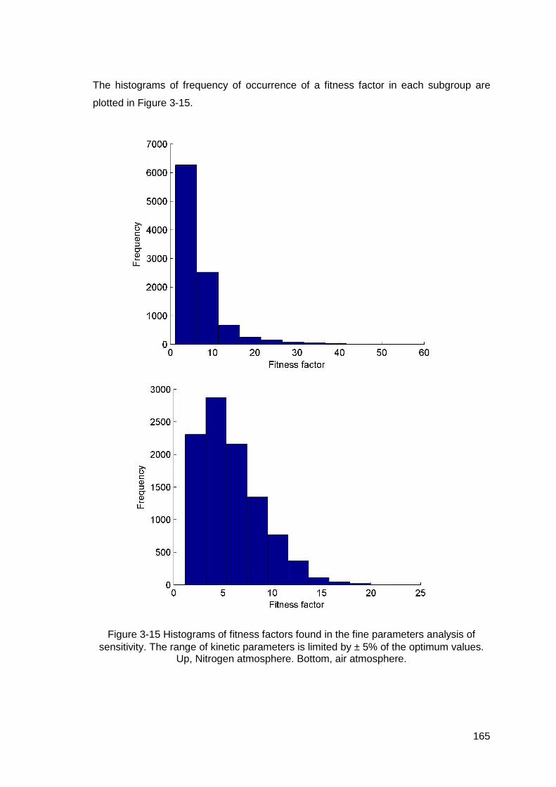
165

The histograms of frequency of occurrence of a fitness factor in each subgroup are

plotted in Figure 3-15.

Figure 3-15 Histograms of fitness factors found in the fine parameters analysis of sensitivity. The range of kinetic parameters is limited by ± 5% of the optimum values.

Up, Nitrogen atmosphere. Bottom, air atmosphere.

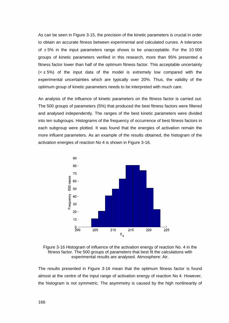
166

As can be seen in Figure 3-15, the precision of the kinetic parameters is crucial in order

to obtain an accurate fitness between experimental and calculated curves. A tolerance

of ± 5% in the input parameters range shows to be unacceptable. For the 10 000

groups of kinetic parameters verified in this research, more than 95% presented a

fitness factor lower than half of the optimum fitness factor. This acceptable uncertainty

(< ± 5%) of the input data of the model is extremely low compared with the

experimental uncertainties which are typically over 20%. Thus, the validity of the

optimum group of kinetic parameters needs to be interpreted with much care.

An analysis of the influence of kinetic parameters on the fitness factor is carried out.

The 500 groups of parameters (5%) that produced the best fitness factors were filtered

and analysed independently. The ranges of the best kinetic parameters were divided

into ten subgroups. Histograms of the frequency of occurrence of best fitness factors in

each subgroup were plotted. It was found that the energies of activation remain the

more influent parameters. As an example of the results obtained, the histogram of the

activation energies of reaction No 4 is shown in Figure 3-16.

Figure 3-16 Histogram of influence of the activation energy of reaction No. 4 in the fitness factor. The 500 groups of parameters that best fit the calculations with

experimental results are analysed. Atmosphere: Air.

The results presented in Figure 3-16 mean that the optimum fitness factor is found

almost at the centre of the input range of activation energy of reaction No 4. However,

the histogram is not symmetric. The asymmetry is caused by the high nonlinearity of

167

the mathematical equations used in the model. Asymmetry also means a high

sensitivity to input parameters.

The high sensitivity to input parameters and the high nonlinearity of the model present

a major drawback to this technique: The optimum group of kinetic parameters

presented in Table 3-8 is from a statistical point of view a probable maximum, but not

the absolute one. Further researches must analyse the possible existence of other

combinations of kinetic parameters within different ranges to the ones used in this

research that allow as well predicting the thermal behaviour of PPUF under air and

nitrogen. If this is the case, the problem would be multi-solution.

3.6 Conclusion

The improvement of accuracy in prediction of PPUF decomposition is a prime task for

thermal analysis and FSE, since it allows calculating the source term of fire, thus

enabling the determination of the power of fire and the potential damages that can be

cause to structures.

Many methods have been proposed in literature in order to model the thermal

decomposition of PU. The great majority are based on TGA experimental results, which

allow determining the decomposition mechanism and calculate the kinetic parameters

of the Arrhenius reactions. Nevertheless, the group of parameters calculated depends

on the method and the model defined. The kinetic parameters do not represent

intensive properties of the matter. Moreover, it was found that TGA experimental

results must be accurately reproduced by many decomposition mechanisms.

A reliable knowledge of the decomposition mechanism is required because it allows

determining the mass balance and controls the number of parameters required for the

calculation. The method used to find the decomposition mechanism was improved

taking into account the effluents released, which enabled us to select the one that is in

accordance to the chemistry of the process.

The model of thermal decomposition was improved as well. The new model can not

only predict the MLR as a function of temperature, but also the kinetic of release of

168

exhaust gases. A single parameter calculated using genetic algorithms is necessary to

enable the calculation of the yield of toxic gases. This is a promising result for the

purpose of estimating toxic hazard in fire scenarios.

The main hypotheses and input data of the method used are:

• The mechanism of thermal decomposition must be determined prior to modelling.

Experimental observations must enable the understanding of the decomposition

patterns.

• Each reaction of decomposition follows an Arrhenius law. The Arrhenius equations

are function of the remaining mass and the oxygen mass fraction.

• The kinetic parameters are calculated using genetic algorithms (optimization tool)

by comparison of experimental and calculated curves of MLR and gases release in

function of temperature. GA showed to be adequate for highly nonlinear

mathematical problems such as those found in this model.

• Each variable (kinetic parameter) is optimized within a range defined by the user.

The best solution is not a unique solution, but the one that statistically best fits the

experimental and calculated results. In order to perform a general analysis, the

ranges given were as wide as possible.

Three decomposition mechanisms, one from the literature (Rein et al. [107]) and two

proposed in this research (kinetic mechanism 1 and 2) were analysed. The kinetic

mechanism 1 was found to be the one that best explains the behaviour of the solid and

the gas phases. The best kinetic mechanism was used to calculate the kinetic

constants of the process. It was found as well, that the results of the modelling are

dependent on the evaluation function used to compare the experimental and calculated

curves. Three evaluation functions were analysed, the one that presented the best

performance in terms of calculation time and ability to fitting nearly both curves is the

one based on the Hilbert vectorial analysis.

A study of code stability was conducted in order to determine the possible causes of

the insolvability of the ODE solver, which has been observed for some of the groups of

kinetic parameters used. It was shown that the activation energy and reaction order are

the most sensible parameters, particularly those of the second reaction of pyrolysis.

169

An analysis of sensitivity of the model to the input parameters was conducted. It was

found that a deviation in input data of 5% is unacceptable. Nevertheless, in FSE

applications, a tolerance lower than 5% in the input data of the model is not in the

same order of magnitude as the experimental uncertainties, which are typically close to

20%. Thus, the validity of the optimum group of kinetic parameters needs to be

interpreted with much care.

The output data of the model represent primary input data to the pyrolysis model of

CFD simulations presented in the following chapter.

170

171

4 Small scale experiments and

simulations

4.1 Introduction

In chapter 2 were presented the experimental results obtained at the matter scale,

which allowed stating the decomposition mechanism of PPUF. Chapter 3 presented the

model of decomposition kinetics of the foam. The model was improved in order to be

able to consider the changes of the solid and gas phases with the increase in

temperature. In both chapters, the masses concerned were under 250 mg. The

samples are then considered as particles and no gradient effects are taken into

account.

The decomposition mechanisms found at the matter scale is verified at a larger scales

in order to analyse the influence of phenomena that play a main role in large scale

such as thermal gradients, the effect of turbulence, the formation of a decomposition

front, gradients of concentration of species, etc. So, the kinetic parameters obtained

with the modelling performed at the matter scale are used in numerical simulations and

a validation with experimental results is carried out. This chapter presents the

experimental results and fire simulation at small scale, which is often called bench-

scale in literature. It is greater than the one dealt with in the previous chapters, but is

intermediary between the matter scale and the real scales concerned by FSE. The

tests are performed using the Cone Calorimeter (CC) apparatus, so the masses

considered are 11 ± 1 g.

The main difference between the samples used at the small scale compared to matter

scale is that the samples cannot be considered as particles; the temperature of the

172

sample is therefore not homogeneous. Gradients of temperature are allowed between

the boundaries and the centre of the sample. So, the sample is considered thermally

thick (some comments about the Biot number are presented in section 5.1). Differential

concentrations of gases, particularly oxygen, have also been found in-depth of porous

samples, e.g. in smouldering combustion [130]. The gradient of gaseous species are

formed by the diffusion of oxygen from the boundaries towards the centre of the

sample and the subsequent transport of gas products from the decomposition zone

towards the environment. Both gradients (temperature and species) strongly influence

the PPUF decomposition kinetics.

At the matter scale, it is considered that the particles are homogeneously irradiated at

all the exposed surface (sides) and the sample mass is at uniform temperature equal to

the one of the furnace. The concentration of oxygen and gas species is homogeneous

as well because there is not resistance to species transport. In the tests presented in

this chapter, samples are heated by an external irradiation source concentred towards

a single surface. It causes an increase in surface temperature that consequently

initiates the decomposition process. Combustible gases are released during the

breakdown of solid molecules, and are ignited by contact with a spark igniter.

In CC tests (small scale), gas effluents are analysed in order to acquire information on

the chemistry of the processes taking place in the solid phase. The sampling of gases

is conducted downstream of the CC fan, where no further reactions in the gas phase

are supposed to occur.

The experimental results obtained in CC are compared to numerical simulations carried

out using the widest spread CFD code used for fire simulation: FDS V 5.3.0. The

process of thermal decomposition of the solid fuel is predicted, so the calculations are

called “pyrolysis calculated fire simulation”. The required input data can be classified

into two groups: a) the thermal properties of the solids, and b) the decomposition

mechanisms and their kinetic parameters. These input data are presented in

sections 2.4 and 3.3 respectively. The main differencies between the pyrolysis

calculated fire simulations and the set heat release rate simulations is explained later in

the chapter.

The main objectives of the study at the small scale are:

173

• To determine the fire behaviour of PPUF by measurement of Heat Release Rate

(HRR), MLR and Effective Heat of Combustion (EHC).

• To analyse the decomposition mechanism of the foam at the small scale in order to

allow a comparison with the one observed at the matter scale.

• To analyse 16 gases in real time in order to understand the chemical process

taking place.

• To measure the yield of release of the main toxic gases: CO2, CO, H2O, NO and

total hydrocarbons.

• To establish a ratio between HRR and the release of gases.

• To conduct a numerical simulation of the fire behaviour of PPUF in order to predict

the HRR and MLR, and to compare them with experimental results.

This chapter is divided into six sections. Section one is the introduction. Section two is

the experimental setup used to analyse the PPUF reaction-to-fire. Section three

presents the experimental results and the analysis. Section four presents the numerical

simulation. Section five presents the comparison between experimental and calculated

results. Section six presents the validation of the decomposition mechanism of PPUF in

a simplified seat (product scale). Section seven is the conclusions of the chapter.

4.2 Reaction-to-fire experimental setup

This section presents the experimental setup used to determine the reaction-to-fire of

the non-flame-retarded PPUF studied in this research. The experiments provide

important understanding of its thermo-oxidative decomposition and evolved gases. The

PPUF data required in this research include phenomena taking place in the gaseous

and solid phases. The gaseous phase is characterized by measuring the mass flow of

evolved gases as a function of time and CC irradiance level, while the MLR was used

to study the solid phase. Analysing information from both phases provided very useful

information about the chemistry of reactions taking place in the solid foam slab. The

experimental devices used are cone calorimeter, Fourier Transform Infrared

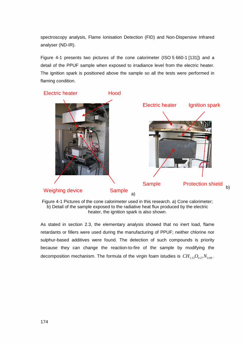
174

spectroscopy analysis, Flame Ionisation Detection (FID) and Non-Dispersive Infrared

analyser (ND-IR).

Figure 4-1 presents two pictures of the cone calorimeter (ISO 5 660-1 [131]) and a

detail of the PPUF sample when exposed to irradiance level from the electric heater.

The ignition spark is positioned above the sample so all the tests were performed in

flaming condition.

Weighing device

Electric heater Hood

Samplea)

Electric heater Ignition spark

Sample Protection shieldb)

Figure 4-1 Pictures of the cone calorimeter used in this research. a) Cone calorimeter; b) Detail of the sample exposed to the radiative heat flux produced by the electric

heater, the ignition spark is also shown.

As stated in section 2.3, the elementary analysis showed that no inert load, flame

retardants or fillers were used during the manufacturing of PPUF; neither chlorine nor

sulphur-based additives were found. The detection of such compounds is priority

because they can change the reaction-to-fire of the sample by modifying the

decomposition mechanism. The formula of the virgin foam istudies is 08.027.053.1 NOCH .

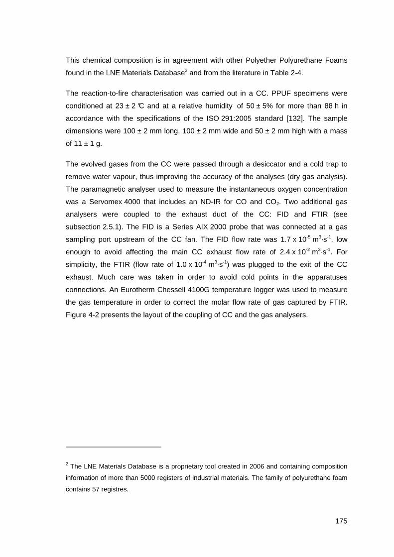
175

This chemical composition is in agreement with other Polyether Polyurethane Foams

found in the LNE Materials Database2 and from the literature in Table 2-4.

The reaction-to-fire characterisation was carried out in a CC. PPUF specimens were

conditioned at 23 ± 2 °C and at a relative humidity of 50 ± 5% for more than 88 h in

accordance with the specifications of the ISO 291:2005 standard [132]. The sample

dimensions were 100 ± 2 mm long, 100 ± 2 mm wide and 50 ± 2 mm high with a mass

of 11 ± 1 g.

The evolved gases from the CC were passed through a desiccator and a cold trap to

remove water vapour, thus improving the accuracy of the analyses (dry gas analysis).

The paramagnetic analyser used to measure the instantaneous oxygen concentration

was a Servomex 4000 that includes an ND-IR for CO and CO2. Two additional gas

analysers were coupled to the exhaust duct of the CC: FID and FTIR (see

subsection 2.5.1). The FID is a Series AIX 2000 probe that was connected at a gas

sampling port upstream of the CC fan. The FID flow rate was 1.7 x 10-5 m3·s-1, low

enough to avoid affecting the main CC exhaust flow rate of 2.4 x 10-2 m3·s-1. For

simplicity, the FTIR (flow rate of 1.0 x 10-4 m3·s-1) was plugged to the exit of the CC

exhaust. Much care was taken in order to avoid cold points in the apparatuses

connections. An Eurotherm Chessell 4100G temperature logger was used to measure

the gas temperature in order to correct the molar flow rate of gas captured by FTIR.

Figure 4-2 presents the layout of the coupling of CC and the gas analysers.

2 The LNE Materials Database is a proprietary tool created in 2006 and containing composition

information of more than 5000 registers of industrial materials. The family of polyurethane foam

contains 57 registres.

176

FTIR with a cell gas of 10 m

FID

Oxygen, CO and CO2analyser

Sampling line at 180 °C

Filtration box at 180 °C for particles of

diameter 10µm and 2µm

Cone calorimeter hood

Sample

Balance

Cone calorimeter fan

Figure 4-2 Schematic layout of the coupling of cone calorimeter and gas analysers: FTIR and FID. The temperature register is not shown in the scheme.

Five irradiance levels were used: 10, 20, 30, 40 and 50 kW·m-2. Tests at 10, 20 and

30 kW·m-2 were repeated four times, while those at 40 and 50 kW·m-2 were repeated

twice. All the experiments were carried out under air atmosphere. The measurements

were performed without an insulator on the bottom side of the sample. In order to

analyse the influence of the insulator layer, tests were repeated using a 13-mm-thick

silica wool insulation layer with a density of 64 kg·m-3as described in the ISO 5 660-1

standard [131].

4.3 Cone calorimeter experimental results

HRR is an important variable for evaluating material fire hazards [133][134]. It was

measured using the oxygen consumption calorimetry technique [20]. This technique is

the basis of the ISO 5 660-1 standard [131] and uses Eq. (4-1) to calculate the HRR

177

in [kW·m-2]. It is a function of 2OE , the heat of combustion per unit mass of oxygen

consumed (also known as the Thornton factor and assumed to be

13.1 MJ·kgO2-1 ± 5% [131]), Φ , the oxygen consumption factor defined in Eq. (4-2),

and em& , the mass-flow rate in the CC exhaust duct defined in Eq. (4-3) and determined

from the pressure drop across and temperature at an orifice plate:

eoOO mxEHRR &⋅

Φ⋅+Φ−Φ⋅⋅⋅=

105.1)1(10.1

22

(4-1)

( ) ( )( )

222

2222

1

110

00

OCOO

COOCOO

xxx

xxxx

−−−−−

=Φ (4-2)

ee T

pCm

∆=& (4-3)

In order to use these equations, some simplifications and experimental facts are

required. The environmental H2O concentration was neglected because the exhaust

gas passes through a calcium chloride filter and a cold trap in order to eliminate all

moisture. CO concentration was also neglected because of its typically low

concentration during well ventilated flaming combustion (Notably in proportion to the

CO2 concentrations). Calculations were carried out to verify the influence of neglecting

the release of CO, and the error in HRR was found to be less than 1%. Nevertheless,

this error is low compared with the relative uncertainty of the cone calorimeter, which is

10% for HRR greather than 1 kW following to calculations carried out in LNE.

The baseline calibration of the CO2 and O2 analysers was conducted with pure nitrogen

allowing an accurate determination of the environmental concentrations prior to test.

The measurement of the oxygen concentration is the basis of the HRR calculation. It is

assumed here that the mass of oxygen contained in the PPUF molecule (22.5Wt%) is

low compared to the mass of air that is transported into the exhaust line (well-ventilated

fire), thus the calculation of HRR is not affected by the oxygen present in the virgin

PPUF.

At the beginning of each test, the CC calorimeter thermal shield was opened and the

sample was suddenly exposed to the set irradiance level. A decomposition front was

formed and advanced rapidly from the top to the bottom of the sample. The results

178

shown here correspond to flaming conditions initiated with a spark ignition source. In

experiments not discussed in this dissertation, it was found that the critical irradiance

level (CHF) for ignition of the foam is 9 kW·m-2 and the irradiance level for auto-ignition

is 35 kW·m-2.

Figure 4-1 shows the transient evolution of MLR and HRR at the five different

irradiance levels. Since a good repetability of the experimental results has been

observed, one experimental result has been chosen for the plots.

179

a)

b)

Figure 4-3 Results in cone calorimeter at five irradiance levels. a) Mass-Loss Rate; b) Heat Release Rate.

In Figure 4-3 time 0=t marks the beginning of the exposure to the desired irradiance

level rather than the moment of ignition. As shown, the shapes of HRR and MLR

curves changed with the irradiance level. In the HRR plots are evidenced two stages of

decomposition (combustion regimes) at all the irradiance levels. At 10 kW·m-2, the two

stages are very close making difficult the idenfication. The intensity of the secondary

180

HRR peak increases with the irradiance level and at an irradiance level of 50 kW·m-2,

the second peak has a similar intensity as the first peak.

In the MLR curves, two decomposition stages are identified as well, nevertheless the

secondary peaks never reach the intensity of the first peak meaning that the ratio

between the MLR and HRR is not constant. This observations are discussed later in

the chapter.

Table 4-1 Experimental results of PPUF in CC measured at five irradiance levels (mean): time to ignition, time to extinction, total combustion time and ratio between

burnt and initial sample mass

Irradiance level of CC

Time to ignition

Time to extinction

Combustion time

Ratio of burnt to initial mass

[kW·m-2] [s] [s] [s] [%]10 87 176 89 4120 10 220 210 6830 5 273 268 9740 3 240 237 10050 2 173 171 98

Table 4-1 presents the time to ignition, the time to extinction, the total combustion time

of PPUF and the ratio between the burnt and initial masses. As expected, time to

ignition decreased when the irradiance level increased. Total combustion time is the

difference between time to extinction and time to ignition. Total combustion times were

shorter at low and high irradiance levels, with a maximum at 30 kW·m-2. This can be

explained because for the low irradiance levels of 10 and 20 kW·m-2, the initial mass of

the sample was not totally consumed during combustion and the combustion rate is

low. A significant amount of char remained in the sample holder after fire extinction.

Thus, low irradiance levels provided shorter combustion times compared to the test at

30 kW·m-2, in which the sample is completely burnt. At 50 kW·m-2, the decomposition

reaction rate was faster than at 30 kW·m-2 due to the strong irradiance received by the

sample from the radiant cone. It provided a shorter combustion time.

Comparison tests were performed using a silica wool insulating layer instead of non-

insulating backing at the PPUF sample to investigate the effect of this boundary

condition. The results show that the decomposition kinetics, gas release and HRR do

not change significantly with the insulating layer. This suggests that under the current

181

test conditions, the decomposition rate is not controlled by sample heat losses. The

thermal balance of the experiments in CC is written in Eq. (4-4) [135].

0)( =∆⋅−−+′′ + HSMLRQQQ rrcrfe (4-4)

Where, eQ ′′ is the incident irradiance level from the electric heater. )( crfQ + is the

incident heat flux from the flame towards the sample which has radiative and

convective fractions. rrQ is the reradiation heat lose caused by the radiation of the hot

sample surface towards the environment. HSMLR ∆⋅ is the heat of reaction, which

accounts for the power consumed during the breakdown of the molecules from the

condensed phase. The thermal balance allows to explain the change of HRR peak with

the increase of the irradiance level. If it is considered that the heat of reaction and the

reradiation heat losses are constant (acceptable hypotheses), the combustion process

is controlled by the incident irradiance from the flame and the electric heater [135].

In addition to the heat release rate, the toxicity of the burning products must be taken

into account when analysing the fire hazard of a material [113]. PPUF is manufactured

from the condensation of polyisocyanates and polyether polyols in the presence of

catalysts and/or additives [8][136]. Rogers et al. [23], Saunders et al. [37] and

Woolley [35] studied the thermal decomposition of urethane-based plastics. They

stated that, when PPUF is heated, urethane bonds break into polyol and isocyanate. In

the first stage, isocyanate pyrolyses and oxidizes. It is released as yellow smoke.

Liquid polyol remains in the sample holder as a semi-product of the decomposition

process. Pyrolysis and oxidization of liquid polyol occur in a second decomposition

stage. The gases released during a PPUF fire (burnt and unburnt) are considered

highly hazardous to life, safety and the environment [9][45][137].

182

Figure 4-4 Change over time of HRR, MLR and gas species concentration during combustion of PPUF at an irradiance level of 50 kW·m-2 in CC. CO2 and H2O are

quantified at the left-hand side y-axis. CO, NO, THC, HRR and MLR are quantified at the right-hand side y-axis. The MLR curve is scaled by a factor of 2000 (Source [138]).

Figure 4-4 presents the transient evolution of different gas species concentration, HRR

and MLR at an irradiance level of 50 kW·m-2. The x-axis is common for all curves. The

concentrations of CO2 and H2O were quantified at the left-hand side y-axis. The

concentrations of CO, NO and total hydrocarbons (THC) as well as the plots of HRR

and MLR were quantified at the right-hand side y-axis. The plot of MLR has been

scaled by a factor of 200 for ease of viewing. Gas concentrations are expressed

in [ppm], with THC units as the ppm equivalent of methane because of the FID

calibration method. The results have been corrected for the transport delay and the

response time of the instruments.

Figure 4-4 shows that the general change with time of the HRR, MLR and the curves of

gases release are similar, thus suggesting the underlying kinetics throughout the

burning process. This provided important information about solid decomposition

reactions and production of gas species. The release curves for the different gas

species did not have the same shapes, but did share common maxima and minima at

various points in time. These common points represent the basis for the analysis of the

PPUF decomposition kinetics and allowed identifying the PPUF decomposition stages.

183

As shown in Figure 4-4, at an irradiance level of 50 kW·m-2, the maximum in the HRR

curve occurred approximately 17 s after the beginning of the exposure. Using the HRR

peak as a reference, we can see that the first peaks of MLR, CO2, THC, CO and NO

occurred at exactly the same time. H2O was not considered as a hazardous gas, but it

served as a marker for the occurrence of one particular reaction. This reaction involved

the combustion of polyol and occurred during the second stage of decomposition

(hydroxyl groups [22]). The curve corresponding to H2O concentration showed an

important inflection point when the HRR reached a maximum. However, with increasing

time, the amount of H2O released continued to grow. Hydrogen was consumed by the

production of H2O. The late release of H2O in comparison to CO2 suggested that the

reaction of most hydrogenated compounds of foam was delayed.

The maximum release of H2O appeared 55 s after exposure to the CC irradiance. At

about the same time, the second peak in the HRR and CO2 appeared, along with a

local minimum of MLR, a local maximum of CO and an important decrease in the

amount of THC production. At 50 kW·m-2, a third peak in the HRR curve appeared

approximately 70 s after exposure to CC irradiance. This time corresponded to a

maximum of CO2 release, a local maximum of MLR, the beginning of the decrease of

H2O production and an important change in the slope of THC.

At 50 kW·m-2, before the second peak of HRR at approximately 50 s, the solid has

been completely consumed, leaving a semi-liquid residue in the holder. This dark

brown viscous product consisted primarily of polyol with traces of isocyanate and

oxidized residues. This semi-liquid product continued to oxidize as a pool fire until the

extinction of flames, approximately 173 s after exposure to CC irradiance.

The evolution of gas species can be used to determine the decomposition stages in the

solid phase. In the 50 kW·m-2 test (Figure 4-4), from the beginning of exposure at 0=t

to approximately 50 s (about 48 s after flaming ignition), high concentrations of CO,

CO2 and THC were measured coming from the sample, suggesting the presence of a

rich combustible mixture. After 65 s, productions of CO and THC were low, but the

release of CO2 remained high (less rich combustible mixture).

The hydrocarbons, CO and CO2 are released by the pyrolysis of PPUF process (see

the molecular decomposition mechanism presented in subsection 2.2.2 and Eq (2-2)).

As shown in Figure 4-4, the concentration of THC strongly decreases after 50 s

attaining very low concentrations. Nevertheless, high amounts of CO and CO2 are

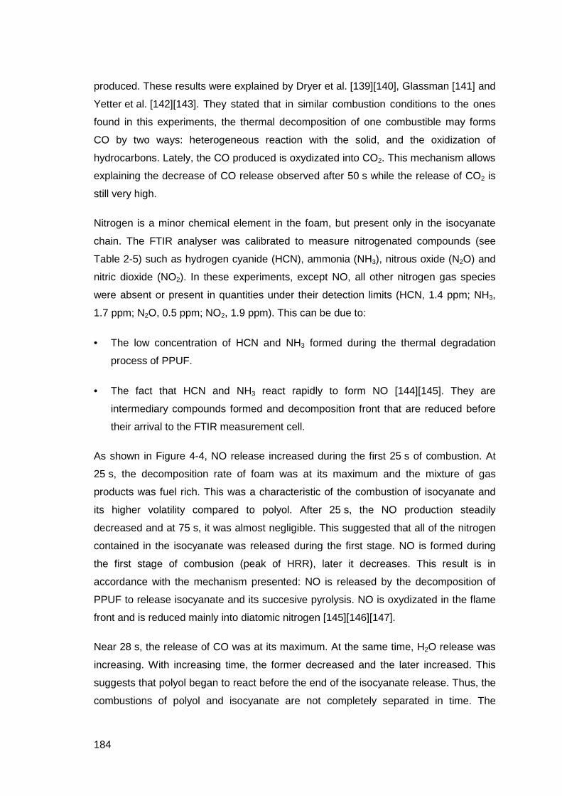
184

produced. These results were explained by Dryer et al. [139][140], Glassman [141] and

Yetter et al. [142][143]. They stated that in similar combustion conditions to the ones

found in this experiments, the thermal decomposition of one combustible may forms

CO by two ways: heterogeneous reaction with the solid, and the oxidization of

hydrocarbons. Lately, the CO produced is oxydizated into CO2. This mechanism allows

explaining the decrease of CO release observed after 50 s while the release of CO2 is

still very high.

Nitrogen is a minor chemical element in the foam, but present only in the isocyanate

chain. The FTIR analyser was calibrated to measure nitrogenated compounds (see

Table 2-5) such as hydrogen cyanide (HCN), ammonia (NH3), nitrous oxide (N2O) and

nitric dioxide (NO2). In these experiments, except NO, all other nitrogen gas species

were absent or present in quantities under their detection limits (HCN, 1.4 ppm; NH3,

1.7 ppm; N2O, 0.5 ppm; NO2, 1.9 ppm). This can be due to:

• The low concentration of HCN and NH3 formed during the thermal degradation

process of PPUF.

• The fact that HCN and NH3 react rapidly to form NO [144][145]. They are

intermediary compounds formed and decomposition front that are reduced before

their arrival to the FTIR measurement cell.

As shown in Figure 4-4, NO release increased during the first 25 s of combustion. At

25 s, the decomposition rate of foam was at its maximum and the mixture of gas

products was fuel rich. This was a characteristic of the combustion of isocyanate and

its higher volatility compared to polyol. After 25 s, the NO production steadily

decreased and at 75 s, it was almost negligible. This suggested that all of the nitrogen

contained in the isocyanate was released during the first stage. NO is formed during

the first stage of combusion (peak of HRR), later it decreases. This result is in

accordance with the mechanism presented: NO is released by the decomposition of

PPUF to release isocyanate and its succesive pyrolysis. NO is oxydizated in the flame

front and is reduced mainly into diatomic nitrogen [145][146][147].

Near 28 s, the release of CO was at its maximum. At the same time, H2O release was

increasing. With increasing time, the former decreased and the later increased. This

suggests that polyol began to react before the end of the isocyanate release. Thus, the

combustions of polyol and isocyanate are not completely separated in time. The

185

chemical analyses showed that the PPUF mass fractions of isocyanate and polyol were

approximately 32% and 68%, respectively. Therefore, in the first 28 s, the majority of

the mass loss would correspond to the decomposition of the isocyanate (32%), with

most of the remaining mass corresponding to the polyol (68%) that decomposes later.

From Figure 4-5 until Figure 4-8 are presented the coupling of the thermal behaviour

(HRR and MLR) of PPUF in CC with the kinetic of release of toxic gases at 10, 20, 30

and 40 kW·m-2.

186

Figure 4-5 Change over time of HRR, MLR and gas species concentration during combustion of PPUF at an irradiance level of 10 kW·m-2 in CC. CO2 and H2O are

quantified at the left-hand side y-axis. CO, NO, THC, HRR and MLR are quantified at the right-hand side y-axis. The MLR curve is scaled by a factor of 2000 (Source [138]).

Figure 4-6 Change over time of HRR, MLR and gas species concentration during combustion of PPUF at an irradiance level of 20 kW·m-2 in CC. CO2 and H2O are

quantified at the left-hand side y-axis. CO, NO, THC, HRR and MLR are quantified at the right-hand side y-axis. The MLR curve is scaled by a factor of 2000

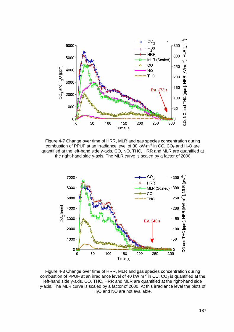
187

Figure 4-7 Change over time of HRR, MLR and gas species concentration during combustion of PPUF at an irradiance level of 30 kW·m-2 in CC. CO2 and H2O are

quantified at the left-hand side y-axis. CO, NO, THC, HRR and MLR are quantified at the right-hand side y-axis. The MLR curve is scaled by a factor of 2000

Figure 4-8 Change over time of HRR, MLR and gas species concentration during combustion of PPUF at an irradiance level of 40 kW·m-2 in CC. CO2 is quantified at the

left-hand side y-axis. CO, THC, HRR and MLR are quantified at the right-hand side y-axis. The MLR curve is scaled by a factor of 2000. At this irradiance level the plots of

H2O and NO are not available.

188

Figure 4-5 presents HRR, MLR and the concentration of the main gases released on

CC at an irradiance level of 10 kW·m-2. As in Figure 4-3, the initial time corresponds to

initial exposure at the desired irradiance level. The difference in curve shapes between

10 and 50 kW·m-2 allowed us to extract a divergence in gas release: the maximum

concentration of H2O release for an irradiance of 10 kW·m-2 occurred at 140 s. This

corresponded to an inflection point of HRR (in addition to the single peak in the HRR

curve), the second peak of MLR, a local minimum of CO and the beginning of the

decrease in NO release. Any further decomposition stages could be clearly identified at

this irradiance level.

The thermal mechanism for PPUF decomposition analysed in this work was validated

for the five irradiance levels studied (see Figure 4-4 until Figure 4-8). The validation

was allowed by the coupling of the information from the gas phase to the one of the

solid phase. The decomposition mechanism in CC under well-ventilated condition can

be schematized as follows (see Figure 4-9).

PPUF

Isocyanate

+

Polyol

First stage pyrolysis and oxidization of PPUF molecules.

Yellow smoke

Second stage pyrolysis and

oxidization of semi-liquid polyol

32 Wt%

68 Wt%

+Combustion of

yellow smoke in gas phase

Combustion the polyol pyrolysis

products+

Figure 4-9 Schematic view of the PPUF decomposition mechanism observed in cone calorimeter at five irradiance levels 10, 20, 30, 40 and 50 kW·m-2 (Source [148]).

As a matter of fact, during the first decomposition stage, so the first peak of MLR the

analysis of gaseous compounds released show the formation of hydrocarbon

compounds, CO, CO2 and NO that are produced during the molecules break-down

process and the pyrolysis of isocyante.

Lately, during the second peak of MLR only the compounds containing carbon

(particularly CO and CO2) and water are formed, which is characteristic of the

decomposition and combustion of polyol.

189

For comparison purposes, the kinetic mechanism determined at the matter scale is

rememberes here bellow.

1

2

3

4 5

Pyrolysis reaction

Oxidation reaction

Pyrolysis reaction

Oxidation reaction

PPUF Polyol Char Residue

Reminder of Figure 3-3 Kinetic mechanism 1 proposed in this research.

The results of CC coupled to gas analysis (Figure 4-9) are in agreement with the

decomposition patterns identified at the matter scale using TF + FTIRqnt and

TGA + FTIRqlt: when the material is heated up, the urethane bounds breakdown by

pyrolysis and oxidization reactions, arrows 1 and 3 respectively. It releases as gas

product the isocyanate and remains as condensed residue the polyol. It is remainded

that the molecules breakdown occurs into the decomposition front which is thin and

displaces from the top towards the bottom of the sample holder. The polyol is more

thermally stable than isocyanate and than polyurethane molecules, so the irradiance

level produced by the electric heater and the flame preferentially decomposes the

urethane bounds and with the polyol remaining as a semi-liquid product. This explains

for example, why the nitrogenated compounds are released in the first decomposition

stage (see Figure 4-4).

The reactions represented by the arrows 2, 4 and 5 occurs mainly when the polyol is

condensed at the bottom of the sample holder. Nevertheless as explained, due to the

high incident irradiance level to which the sample is submitted in the CC, these

reactions cannot be completely separated in time. So, the reactions represented by the

five arrows take place at the same time.

At all studied CC irradiance levels, the curves for HRR and CO2 release have similar

shapes. However, the correlation between these two values may be more complicated

than the shapes suggest, since HRR was measured as a function of oxygen depletion

under air. This proportion is highly influenced by characteristics of the material being

burnt, such as high oxygen content in the molecular structure [149].

The volume of each mole of species, the mass-flow rate and the yield of species were

calculated using Eq. (2-7) to Eq. (2-9). Figure 4-10 shows the results of mass flow of

190

the main gases released during PPUF combustion (CO2, CO, NO and THC), for easy

of view only the results of three irradiance levels are presented.

Figure 4-10 Evolution of mass flow of four gas species: a) CO2, b) CO, c) NO and d) THC at three irradiance levels 10, 30 and 50 kW·m-2.

The mass flux of a gas species is calculated as the mass-flow rate divided by the area

of the solid sample ( rbb Amm && =′′ ). The area of the sample exposed to the irradiance

level in CC is equal to 0.0088 m2. Figure 4-10 shows the mass flux for four principal

gas species CO2, CO, NO and THC, at three irradiance levels 10, 30 and 50 kW·m-2.

The mass flux at 20 and 40 kW·m-2 are not shown for easy of view of the plots. These

curves confirmed that the toxicity of the gases released during PPUF combustion

changed with time. The maximum toxicity of the gas release stream occurred in the first

150 s of the fire. However, the single composition of the gas stream does not constitute

enough information to stablish the toxicity hazard of the effluents because it depends of

the properties of the material in fire, ventilation, dilution, exposition time, environment,

etc [150].

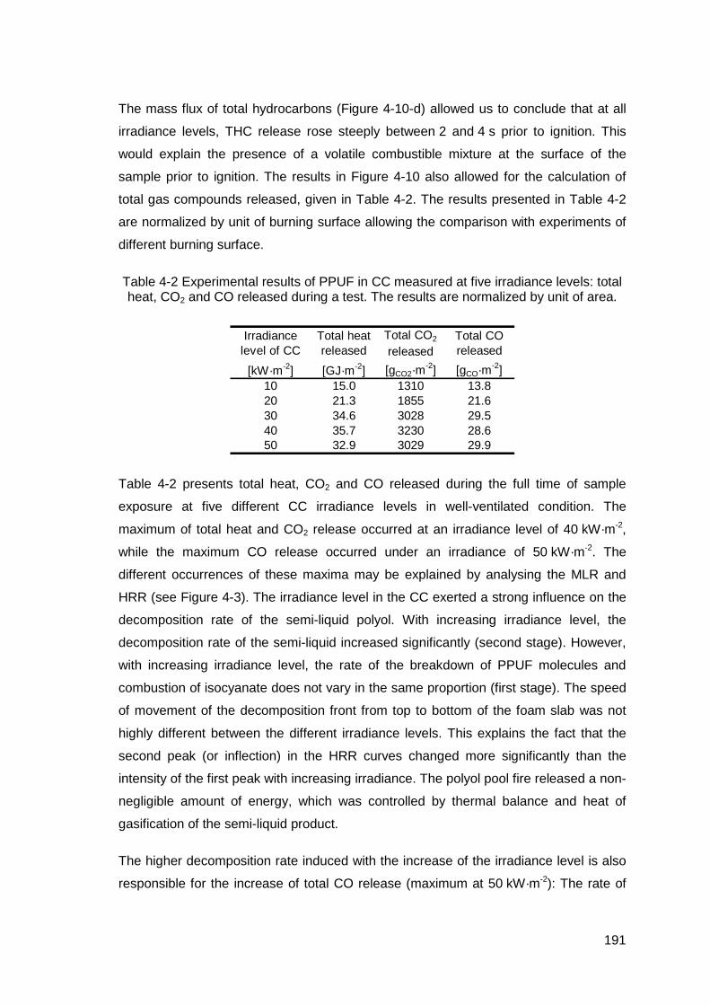
191

The mass flux of total hydrocarbons (Figure 4-10-d) allowed us to conclude that at all

irradiance levels, THC release rose steeply between 2 and 4 s prior to ignition. This

would explain the presence of a volatile combustible mixture at the surface of the

sample prior to ignition. The results in Figure 4-10 also allowed for the calculation of

total gas compounds released, given in Table 4-2. The results presented in Table 4-2

are normalized by unit of burning surface allowing the comparison with experiments of

different burning surface.

Table 4-2 Experimental results of PPUF in CC measured at five irradiance levels: total heat, CO2 and CO released during a test. The results are normalized by unit of area.

Irradiance level of CC

Total heat released

Total CO2

releasedTotal CO released

[kW·m-2] [GJ·m-2] [gCO2·m-2] [gCO·m-2]

10 15.0 1310 13.820 21.3 1855 21.630 34.6 3028 29.540 35.7 3230 28.650 32.9 3029 29.9

Table 4-2 presents total heat, CO2 and CO released during the full time of sample

exposure at five different CC irradiance levels in well-ventilated condition. The

maximum of total heat and CO2 release occurred at an irradiance level of 40 kW·m-2,

while the maximum CO release occurred under an irradiance of 50 kW·m-2. The

different occurrences of these maxima may be explained by analysing the MLR and

HRR (see Figure 4-3). The irradiance level in the CC exerted a strong influence on the

decomposition rate of the semi-liquid polyol. With increasing irradiance level, the

decomposition rate of the semi-liquid increased significantly (second stage). However,

with increasing irradiance level, the rate of the breakdown of PPUF molecules and

combustion of isocyanate does not vary in the same proportion (first stage). The speed

of movement of the decomposition front from top to bottom of the foam slab was not

highly different between the different irradiance levels. This explains the fact that the

second peak (or inflection) in the HRR curves changed more significantly than the

intensity of the first peak with increasing irradiance. The polyol pool fire released a non-

negligible amount of energy, which was controlled by thermal balance and heat of

gasification of the semi-liquid product.

The higher decomposition rate induced with the increase of the irradiance level is also

responsible for the increase of total CO release (maximum at 50 kW·m-2): The rate of

192

production of pyrolysed products is higher than that rate of transport of oxygen towards

the flame. Thus, a fuel rich combustion regime is stablished promoting the formation of

CO rather than CO2. It is pointed out that the ventilation condition is remained constant

for all the experiments, the difference in the combustion regimes is created by the

pyrolysis rate established in function of the total irradiance level generated by the

external source and the flame (see Eq. (4-4)).

Table 4-3 Yield of the main gas species released during PPUF combustion in well-ventilated condition. The column “mean” is the release of species in the semi-steady state period. “St Dev.” is the standard deviation of the species releasing in the semi-

steady state zone.

CO/CO2

[kW·m-2] Mean St. Dev. Mean St. Dev. Mean St. Dev. Mean St. Dev. Mean St. Dev. [%]10 2.69 1.06 0.92 0.95 0.036 0.023 0.003 0.002 0.104 0.117 1.34%20 2.17 0.24 1.54 0.74 0.029 0.012 0.004 0.003 0.062 0.028 1.32%30 2.15 0.21 0.61 0.11 0.018 0.005 0.002 0.002 0.018 0.011 0.85%40 2.32 0.39 - - 0.016 0.007 - - 0.028 0.018 0.68%50 2.31 0.69 0.78 0.46 0.019 0.009 0.003 0.002 0.032 0.019 0.82%

Mean 2.33 0.52 0.96 0.57 0.024 0.011 0.003 0.002 0.049 0.039 1.01%

Irradiance level of

CC THC

Yield of chemical compounds [gespecies·gsample-1]

COH2OCO2 NO

Table 4-3 gives yields of the main gas species released during PPUF combustion.

Yields measured in experiments can be the basis for extrapolating results of gas

species production from bench-scale to full-scale scenarios [20]. Yields have been

calculated for the steady-state regime. The transient periods at the beginning and end

of tests were not considered for calculations. Yields of CO2, H2O and THC were at their

lowest at an irradiance level of 30 kW·m-2, with the lowest yield of CO at 40 kW·m-2.

There was no clear dependence of NO yield on irradiance level. However, accounting

for the calculated standard deviations, only CO2 yield measurements are of high

consistency. The very limited amount of data found in the literature on the gas product

yields of polyurethane foam is listed in Table 4-4. Note that the polyurethane

formulations significantly differ from one type of foam to another.

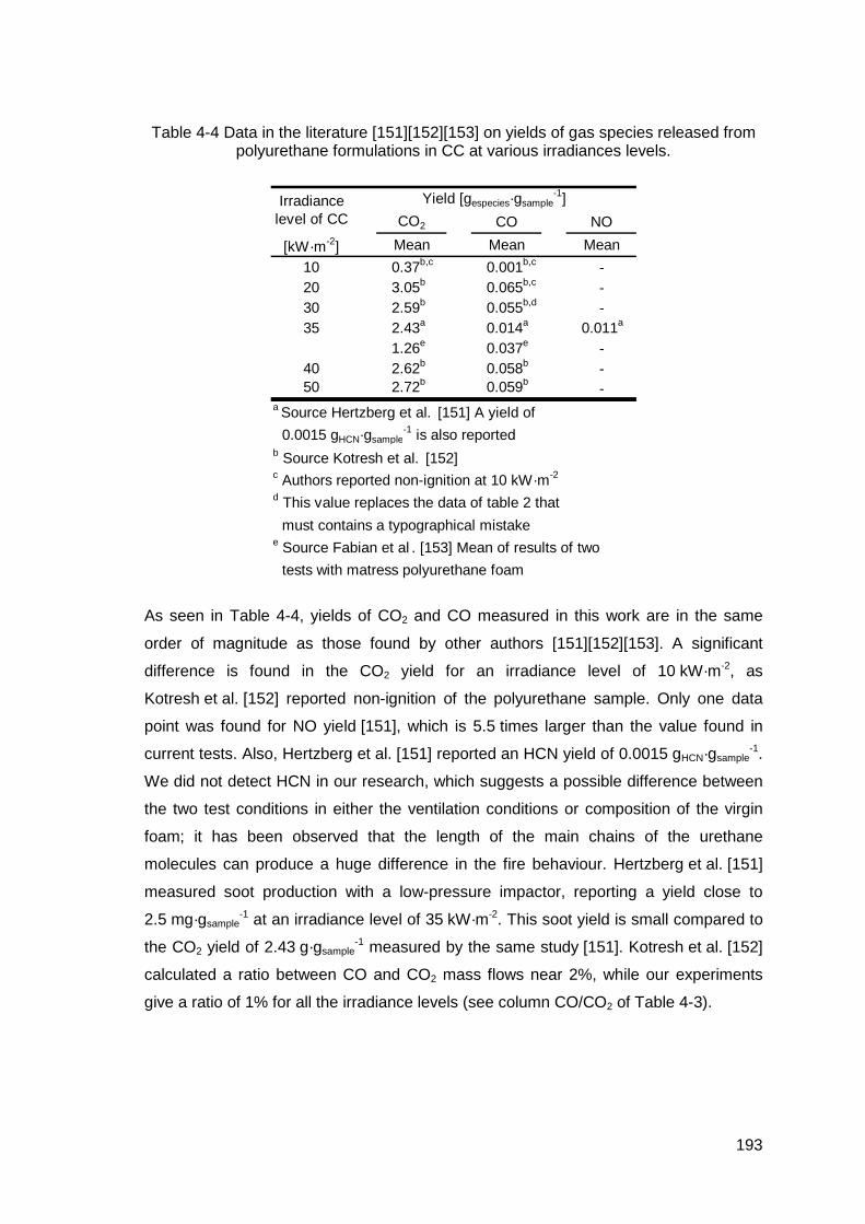
193

Table 4-4 Data in the literature [151][152][153] on yields of gas species released from polyurethane formulations in CC at various irradiances levels.

CO2 CO NO

[kW·m-2] Mean Mean Mean

10 0.37b,c 0.001b,c -20 3.05b 0.065b,c -30 2.59b 0.055b,d -35 2.43a 0.014a 0.011a

1.26e 0.037e -40 2.62b 0.058b -50 2.72b 0.059b

-a Source Hertzberg et al. [151] A yield of

0.0015 gHCN·gsample-1 is also reported

b Source Kotresh et al. [152]c Authors reported non-ignition at 10 kW·m-2

d This value replaces the data of table 2 that

must contains a typographical mistakee Source Fabian et al . [153] Mean of results of two

tests with matress polyurethane foam

Yield [gespecies·gsample-1]Irradiance

level of CC

As seen in Table 4-4, yields of CO2 and CO measured in this work are in the same

order of magnitude as those found by other authors [151][152][153]. A significant

difference is found in the CO2 yield for an irradiance level of 10 kW·m-2, as

Kotresh et al. [152] reported non-ignition of the polyurethane sample. Only one data

point was found for NO yield [151], which is 5.5 times larger than the value found in

current tests. Also, Hertzberg et al. [151] reported an HCN yield of 0.0015 gHCN·gsample-1.

We did not detect HCN in our research, which suggests a possible difference between

the two test conditions in either the ventilation conditions or composition of the virgin

foam; it has been observed that the length of the main chains of the urethane

molecules can produce a huge difference in the fire behaviour. Hertzberg et al. [151]

measured soot production with a low-pressure impactor, reporting a yield close to

2.5 mg·gsample-1 at an irradiance level of 35 kW·m-2. This soot yield is small compared to

the CO2 yield of 2.43 g·gsample-1 measured by the same study [151]. Kotresh et al. [152]

calculated a ratio between CO and CO2 mass flows near 2%, while our experiments

give a ratio of 1% for all the irradiance levels (see column CO/CO2 of Table 4-3).

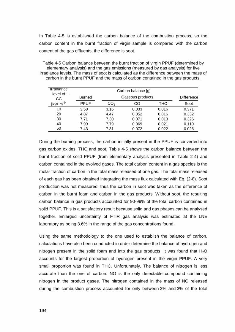
194

In Table 4-5 is established the carbon balance of the combustion process, so the

carbon content in the burnt fraction of virgin sample is compared with the carbon

content of the gas effluents, the difference is soot.

Table 4-5 Carbon balance between the burnt fraction of virgin PPUF (determined by elementary analysis) and the gas emissions (measured by gas analysis) for five

irradiance levels. The mass of soot is calculated as the difference between the mass of carbon in the burnt PPUF and the mass of carbon contained in the gas products.

Burned Difference

[kW·m-2] PPUF CO2 CO THC Soot10 3.58 3.16 0.033 0.016 0.37120 4.87 4.47 0.052 0.016 0.33230 7.71 7.30 0.071 0.013 0.32640 7.99 7.79 0.069 0.021 0.11050 7.43 7.31 0.072 0.022 0.026

Irradiance level of

CC

Carbon balance [g]

Gaseous products

During the burning process, the carbon initially present in the PPUF is converted into

gas carbon oxides, THC and soot. Table 4-5 shows the carbon balance between the

burnt fraction of solid PPUF (from elementary analysis presented in Table 2-4) and

carbon contained in the evolved gases. The total carbon content in a gas species is the

molar fraction of carbon in the total mass released of one gas. The total mass released

of each gas has been obtained integrating the mass flux calculated with Eq. (2-8). Soot

production was not measured; thus the carbon in soot was taken as the difference of

carbon in the burnt foam and carbon in the gas products. Without soot, the resulting

carbon balance in gas products accounted for 90-99% of the total carbon contained in

solid PPUF. This is a satisfactory result because solid and gas phases can be analysed

together. Enlarged uncertainty of FTIR gas analysis was estimated at the LNE

laboratory as being 3.6% in the range of the gas concentrations found.

Using the same methodology to the one used to establish the balance of carbon,

calculations have also been conducted in order determine the balance of hydrogen and

nitrogen present in the solid foam and into the gas products. It was found that H2O

accounts for the largest proportion of hydrogen present in the virgin PPUF. A very

small proportion was found in THC. Unfortunately, The balance of nitrogen is less

accurate than the one of carbon. NO is the only detectable compound containing

nitrogen in the product gases. The nitrogen contained in the mass of NO released

during the combustion process accounted for only between 2% and 3% of the total

195

nitrogen contained in the virgin sample. Two different hypotheses can explain this

difference: a) nitrogen may be reduced into N2, which is impossible to detect by the

FTIR because it is a symmetric molecule (This is the most accepted hypothesis in PU

combustion) and b) nitrogen did not only form NO, but reacted to form other

nitrogenated compounds in very low concentrations that could not be measured in the

conditions of dilution generated by cone calorimeter ventilation.

Figure 4-11 Ratio of HRR to CO2 mass flow at three CC irradiance levels 10, 30 and 50 kW·m-2.

Figure 4-11 shows curves representing the ratio between HRR and CO2 mass flow at

three cone calorimeter irradiance levels of 10, 30 and 50 kW·m-2. This ratio expresses

the equivalent quantity of released heat when 1 g of CO2 was produced. For materials

with single-stage decomposition kinetics (e.g. PMMA), the gas fuel molecules produced

over the entire decomposition process are of the same nature and this ratio is therefore

constant. During PPUF combustion, at least two different products were burning and

each one released a different amount of heat and CO2. The slopes, ia , y-intercepts,

ib , and the least-squares fit factors, 2iR , of straight lines that best fit the three curves in

Figure 4-11 are, respectively, 038.010 =a , 6.610 =b , 87.0210 =R ; 0068.030 =a ,

7.1030 =b , 68.0230 =R ; 011.050 =a , 4.1050 =b , 88.02

50 =R .

196

Figure 4-12 Ratio of HRR to SMLR (i.e. the EHC) for three irradiance levels 10, 30 and 50 kW·m-2.

Figure 4-12 shows for three irradiance levels the ratio between HRR and Specific

Mass-Loss Rate (SMLR), which is defined as the mass-loss rate by sample unit area.

This ratio is equivalent to the Effective Heat of Combustion (EHC). In general, the EHC

is seen to vary in time and also depends on the irradiance level with values ranging

from 20 000 to 40 000 kJ·kg-1 with the average at 26 134 kJ·kg-1. The mean and

standard deviations for each irradiance level are calculated and presented in Table 4-6.

Table 4-6 Mean and standard deviation of the effective heat of combustion (EHC) measured at five irradiance levels.

Mean St. Dev.[kW·m-2]

10 26379 544320 25665 274330 24502 257740 25658 169850 28467 6061

Mean 26134 3704

Irradiance level of CC

EHC = HRR / SMLR

[kJ·kg-1]

As shown in Table 4-6, the highest EHC values are found at the extreme irradiance

levels 10 and 50 kW·m-2, but have standard deviations of up to 20.6% and 21.3% with

respect to the mean value. For irradiance levels between 20 and 40 kW·m-2, the

standard deviations are between 6% and 10%.

197

Babrauskas and Grayson [20] reported an EHC value of 23 900 kJ·kg-1 for a

polyurethane with the chemical formula 08.027.053.1 NOCH and with a molecular weight

20.63 g·mol-1 (for reference, the molecular weight of the foam used in our study is

19.10 g·mol-1). Babrauskas and Grayson [20] also report a general range of EHC

values between 26 100 and 31 600 kJ·kg-1 for a wide variety of flexible polyurethane

foam formulations in the market. The EHC value for the material in this work is closer to

the lower limit of the range reported by Babrauskas. Hirschler in Ref. [20], which

presented HRR curves of non-fire retarded polyurethane foam at three cone

calorimeter irradiance levels of 20, 40 and 70 kW·m-2. Their respective maxima of heat

release rates were near 290, 710 and 1 220 kW·m-2, while in our research, irradiance

levels of 20 and 40 kW·m-2 resulted in HRR maxima at 300 and 330 kW·m-2. The

shapes of the HRR curves found by Babrauskas and Grayson [20] were not the same

as those found in this research. The author reported two peaks, with the intensity of the

first lower than the second, while in our research, the first peak is always higher than

the second. This means that even if the two foams had a similar density, the kinetics of

solid decomposition differed probably because of the PU composition.

In conclusion, the analysis of gas release in cone calorimeter represents a main tool to

identify the decomposition mechanism of polyurethane foam in any irradiance level. It

also represents a new approach to the identification of the transient toxicity of the

gaseous effluents with the advance of the combustion process. In the case of PPUF

used, the first 50 s after ignition are critical because of the release of the most toxic

compounds. It was also verified that fire behaviour of PPUF is extremely sensitive to

the raw materials used during manufacture.

4.4 Numerical simulation of cone

calorimeter results

The work performed at the matter and small scales aimed at acquiring experimental

information on the decomposition mechanism of PPUF. This information represents the

main input data to the codes that allow predicting the fire behaviour by calculated

198

pyrolysis. As we have already mentioned, an accurate prediction of the fire behaviour is

crucial in FSE in order to enable performance-based design of buildings and structures.

The numerical simulations of fire are pyrolysis calculated and imposed HRR. The main

difference between them is that in the former the HRR is predicted and in the later it is

set as input data. The pyrolysis calculated simulations require as input data the kinetic

parameters of the solid decomposition process. A discussion on the advantages and

disadvantages of the pyrolysis calculated simulations in comparison to imposed HRR

fire simulations is performed in section 5.4.

In this research, the CFD code used to simulate the fire behaviour is Fire Dynamics

Simulator (FDS) V 5.3. FDS is an open-source software for computational fluid

dynamics simulation of fire-driven fluid flows. FDS numerically solves a form of the

Navier-Stokes equations appropriate for low-speed, thermally-driven flows with an

emphasis on smoke and heat transport from fires [154]. The formulation of the

equations and the numerical algorithm are contained in the FDS Technical Reference

Guide [155].

The aim of this research is not to perform a huge description of how FDS V 5.3

operates. The reader can find this information in a number of thesis and papers such

as [85][156][157][158][159][160]. In this chapter only the equations required to

understand the problems treated are presented.

The cone calorimeter fire simulations have been performed using a virtual

reconstitution of the real cone. All the geometrical characteristics have been

reproduced as close as possible to those of the real cone. Three mesh sizes were

defined: 1 800, 14 400 and 96 000 cells with respective calculation times near to 5 min,

3 days and one week. The three mesh sizes have been designed to study the

sensitivity to the cell dimension; nevertheless, as shown above, the sensitivity to input

parameters needs to be studied prior to taking into account the problem of grid size.

Figure 4-13 presents a picture of the simulated cone with 1 800 mesh.

199

Figure 4-13 Virtual cone calorimeter, 1 800 mesh. The temperature imposed on the heater is 880 °C producing an irradiance level on t he surface of the material equal to

50 kW·m-2

The centre of the following numerical study is to perform only calculated pyrolysis

simulations (any set HRR simulation is carried out). The discussion concerns two

objectives: a) to verify the ability to predict the CC results when the pyrolysis model is

used (the kinetic parameters are specified), and b) to analyse the results when the

thermal properties set are the ones find experimentally. These aspects need to be

studied because very few fire simulations can be found in the literature in which

pyrolysis models are used and some others use thermal properties that are extremely

different to the experimental ones; a wide discussion about this is performed in

section 5.4.

Providing correct input data to the fire simulation codes represent a main strategy to

guarantee the reliability of the calculations. Very often, data from the publications

cannot be used reliably because the solid fuels are not well characterised, so the

material simulated and the one found in literature are not exactly the same. In this

research, we wanted to find experimentally the thermal and kinetic properties, the input

data provided to numerical simulations has a very good traceability.

The input data for the following simulations have been obtained with the experiments

and calculations conducted in chapters 2 and 3, however in particular cases, different

200

input data are used in order to analyse the fitness of the calculations. The results of

HRR obtained in CC presented in section 4.3, are used here to verify the fitting

between the experiments and the calculations.

Four numerical simulations are discussed; the aim is to compare the results obtained

when particular changes in the input data are carried out. The interest of each one of

the following simulations can be summarized as follows:

• Case 1 compares the experimental and numerical results of HRR and MLR when

the decomposition mechanism and the thermal parameters are those found in this

research.

• Case 2 compares the experimental and numerical results of MLR when the

parameters are changed by trial-and-error in order to better fit the CC

measurements.

• Case 3 compares the experimental and numerical MLR when the reaction of char is

erased from the kinetic mechanism. The residue represents around 1% of the initial

mass.

• Case 4 compares the experimental and numerical MLR when the conductivity and

the specific heat are not set as scalars but as vectors in function of temperature.

The philosophy of each case is largely detailed later in the chapter. The FDS code

presented in Appendix D is the one that produced the result of the case 1 (see Figure

4-14). The thermal and kinetic properties used are listed In Table 4-7.

Table 4-7 Thermal and kinetic properties set to the fire simulation labelled case 1. The code of the simulation is presented in Appendix D.

Conductivity Specific heat Density Comments

W·m-1·K-1 kJ·kg-1·K-1 kg·m-3

Case 1 PPUF 0.04 1.3 22 -318 1400 0.69 0.44Fig. 4-14 Polyol 0.8 2 800 -236 2000 0.1 0.45

Char 0.12 2.50 300 400 - 0.25 -Residue 0.08 1.34 300 - - -

Kinetic prop.

Residue is formed by the pyrolysis of polyol and the oxydation of char

Simulation Material Heat of reactions Residue yieldThermal properties

kg·kg-1kJ·kg-1

The input data used for the FDS simulation of case 1 are the ones found in this

research: The five-reactions decomposition mechanism was discussed in section 3.3

(see Figure 3-3). The kinetic parameters are the ones listed in Table 3-8. The thermal

properties were the ones found at room temperature, in other words they are

201

considered as scalars and do not change with temperature. The heat of reaction was

deduced using Figure 2-1 and the thermal capacity was set using the data from Figure

2-2 (see section 2.4). The results of the case 1 calculated pyrolysis FDS simulation is

presented in Figure 4-14.

Figure 4-14 Case 1. Comparison of experimental and calculated results of HRR and MLR. Experiments: cone calorimeter at an irradiance level of 50 kW·m-2. Calculations:

FDS V.5.3, five-stages decomposition mechanism set to the pyrolysis model.

As shown in Figure 4-14, the intensity of the first peak of MLR is underestimated by

30% in comparison to the experiments. Moreover, the shape of the curve is not the

same. The model is unable to predict the multiple peaks observed in the MLR and HRR

curves: The decomposition stages do not seem to be succesive one after the other.

The experimental peak of MLR found at s 20~t is produced by the process of virgin

PPUF molecules break-down which is responsible as well of the displacement of the

decomposition front. The pyrolysis model of FDS cannot simulate the displacement of

the decomposition front, so the zone of MLR growing until s 20~t cannot be predicted

accurately.

For the following comparison of results, only the experimental and calculated curves of

MLR are presented. The HRR curves have the same shapes as the MLR ones

because HRR is calculated as the product of the mass of combustible fuel released

and the set heat of combustion. The heat of combustion is the energy released per unit

202

mass of fuel gas that mixes with oxygen and combusts; it was similar for all the solid

species.

In order to obtain the results of case 2 presented in Figure 4-15, a few input data were

changed with respect to case 1. For example, the thermal conductivity of PPUF in

case 2 was set to 0.005 W·m-1·K-1 while in case 1 was 0.04 W·m-1·K-1. The specific heat

in case 2 was 1.885 kJ·kg-1·K-1 while in case 1 was 1.3 kJ·kg-1·K-1. The same procedure

was followed for the rest of the thermal and kinetic properties labelled “case 2” in Table

4-8. Appart to the properties listed in Table 4-8 the code was remained unchanged.

Table 4-8 Thermal and kinetic properties that were modified with respect to case 1 to obtain the simulations of case 2, 3 and 4. The code used during the simulations is

presented in Appendix D in which the listed thermal properties were changed.

Conductivity Specific heat Density Comments

W·m-1·K-1 kJ·kg-1·K-1 kg·m-3

Case 2 PPUF 0.005 1.885 22 550 -850 0.69 0.44Fig. 4-15 Polyol 0.8 1.885 820 236 -1297 0.1 0.45

Char 0.8 1.34 820 -1297 - 0.25 -Residue 0.08 1.34 820 - - - -

Case 3 PPUF 0.04 1.3 22 -318 1400 0.69 0.44Fig. 4-16 Polyol 0.8 2 800 -236 2000 0 0.45

Char 0.12 2.50 300 400 - 0 -Residue 0.08 1.34 300 - - -

Case 4 PPUF 0.045…0.084 1.885…2.469 22 -318 1400 0.69 0.44Fig. 4-17 Polyol 0.045…0.084 2 800 -236 2000 0 0.45

Char 0.12 1.337…1.784 300 400 - 0 -Residue 0.08 1.34 300 - - -

Residue is formed by the pyrolysis of polyol and the oxydation of char

Simulation Material

The pyrolysis of polyol (Reac. 2) and the oxydation of char (Reac. 3) does not produce solid residue

The pyrolysis of polyol and oxydation of char do not produce solid residue. Thermal prop. In

function of Temp.

Thermal properties Kinetic prop.Heat of reactions Residue yield

kJ·kg-1 kg·kg-1

The thermal properties used for the simulation (case 2) presented in Figure 4-15 are

not the ones found in this research. They were set by trial-and-error in order to improve

the fitness of the calculations with respect to the experiments. Around 300 simulations

were developed in which the input parameters were changed as “potentiometers”. So,

the input data allowed a better fitness of the curves but they do not have physical

meaning according to the material studied.

203

Figure 4-15 Case 2.Comparison of cone calorimeter experimental and calculated results. Five reactions decomposition mechanism. Thermal and kinetic parameters set

in order to improve the fitness between the experimental and calculated curves.

It is highlighted that Figure 4-15, is obtained by increasing the yields of polyol residue

by 10 times: it is 0.01 kg·kg-1 in case 1 and it is 0.1 kg·kg-1 in case 2. The char residue

has been changed as well, from 0 kg·kg-1. in case 1 to 0.25 kg·kg-1 in case 2. The

negative heat of reactions means that the reactions are endothermic, which is the case

for pyrolysis reactions3.

As can be seen in Figure 4-15 (case 2), the change of thermal and kinetic properties of

the solid species with respect to case 1 produced a MLR peak three times greater than

the experimental one. Moreover, the numerical peak is located 20 s earlier. This

simulation allowed reproducing the phase of MLR decay observed at time st 20> .

However, the shape of the calculation is very noisy, making it difficult to get the bulk

behaviour of the curve. In general terms, the calculations do not follow the

experimental shape.

At an irradiance level as high as 50 kW·m-2, the mass of the residue remaining in the

sample holder was lower than 2%. In FDS simulations, it was observed that properties

3 In FDS simulations an endothermic reaction has a negative heat of reaction, while in the

enthalpy measurements presented in subsection 2.4.1 (page 57) an endothermic reaction has a

positive sign. This is due to the units of the enthalpy measurement.

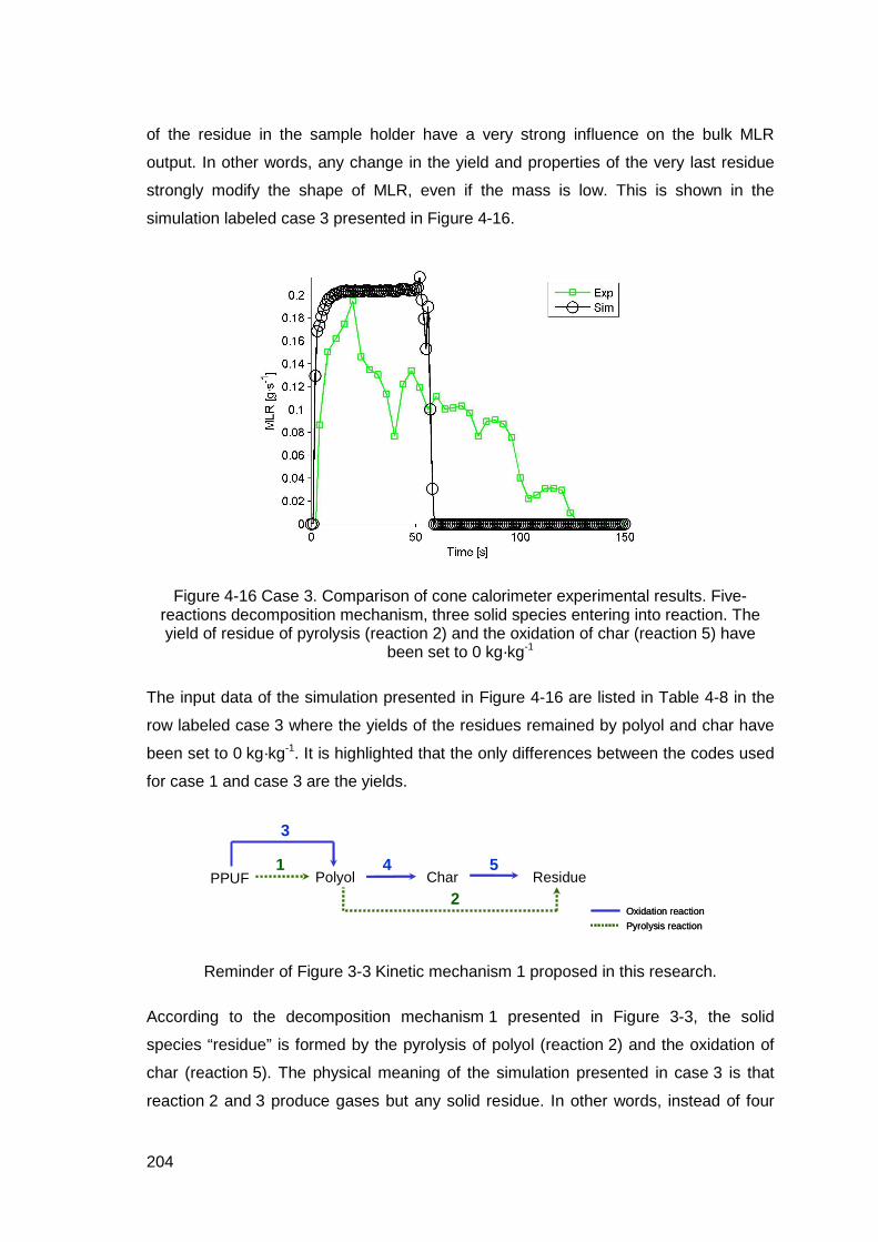
204

of the residue in the sample holder have a very strong influence on the bulk MLR

output. In other words, any change in the yield and properties of the very last residue

strongly modify the shape of MLR, even if the mass is low. This is shown in the

simulation labeled case 3 presented in Figure 4-16.

Figure 4-16 Case 3. Comparison of cone calorimeter experimental results. Five-reactions decomposition mechanism, three solid species entering into reaction. The yield of residue of pyrolysis (reaction 2) and the oxidation of char (reaction 5) have

been set to 0 kg·kg-1

The input data of the simulation presented in Figure 4-16 are listed in Table 4-8 in the

row labeled case 3 where the yields of the residues remained by polyol and char have

been set to 0 kg·kg-1. It is highlighted that the only differences between the codes used

for case 1 and case 3 are the yields.

1

2

3

4 5

Pyrolysis reaction

Oxidation reaction

Pyrolysis reaction

Oxidation reaction

PPUF Polyol Char Residue

Reminder of Figure 3-3 Kinetic mechanism 1 proposed in this research.

According to the decomposition mechanism 1 presented in Figure 3-3, the solid

species “residue” is formed by the pyrolysis of polyol (reaction 2) and the oxidation of

char (reaction 5). The physical meaning of the simulation presented in case 3 is that

reaction 2 and 3 produce gases but any solid residue. In other words, instead of four

205

species, only three enter into reaction. Eq. (3-35), which allows the calculation of total

MLR at the matter scale modelling is transformed into Eq. (4-5).

54433211 )1()1()1( ωωυωυωωυ &&&&& −−+−+−−=dt

dm

(4-5)

The verification that this modifications do not change strongly the decomposition

mechanism and the ability to predict the MLR at the matter scale is carried out: the

modelling was run setting to zero the stoichiometric coefficients of the reactions 2

and 5, 2υ and 5υ respectively. The comparison of MLR experimental and calculated

using the decomposition mechanism presented in Figure 3-3 with four and three solid

species are presented in Figure 4-17.

Figure 4-17 Comparison of MLR experimental and calculated with the decomposition mechanism stated in Figure 3-3 and with the modifications presented in case 3.

Comparison at β = 10 °C·min -1.

As presented in Figure 4-17, setting the stoichiometric coefficients 2υ and 5υ to zero,

do not change strongly the prediction of MLR at the matter scale. Nevertheless, the

shape of the FDS (small scale) simulations changes strongly. This is the sign of a great

uncertainty about how the fire code interprets the input data of the pyrolysis model.

206

The comparison between Figure 4-15 and Figure 4-16 evidences a huge difference in

the MLR shapes. The MLR shape of Figure 4-16 attains a level that is at the same

observed experimentally and remains as a plateau for about 55s. After the “steady

state” zone where the combustible matter is completely consumed at a constant rate,

the MLR drops to zero and remains at this level until the end of the calculation time.

The change of the decomposition mechanism seems to induce uncontrolled changes in

the output of MLR while the mass of residue was negligible (i.e. in case 1 yield of

polyol residue = 0.1 kg·kg-1).

In this research, the thermal properties were measured in function of the temperature.

The influence of setting variable thermal properties in function of temperature was also

verified: To the case 3 presented in Figure 4-16 were included the variable thermal

properties (see Table 4-8) releasing case 4. The MLR release is presented in Figure

4-18.

Figure 4-18 Case 4. Comparison of cone calorimeter experimental and calculated results. Five-reactions decomposition mechanism, three solid species entering into

reaction. The thermal properties are expressed as a function of temperature.

Figure 4-16 and Figure 4-18 present exactly the same shape, the MLR level at which

both plateaux are found is 0.2 g·s-1. The influence of the thermal properties in this case

is difficult to understand and does not seems to follow the trend observed in the

comparison between cases 1 and 2.

Because of the lack of accuracy of the simulations in comparison to the experimental

results, it is concluded that further researches are required in order to understand how

207

to use the pyrolysis model of FDS in the case of PPUF where the decomposition is

multi-reaction. A huge discussion about the possible causes of the lack of accuracy is

presented in section 5.4.

4.5 Fire behaviour of a simplified seat

(product-scale)

Fire experiments were performed on a simplified seat. The aim of these experiments is

to compare the decomposition mechanism at large scale with the one found at matter-

scale. In this section, no simulations are presented because of the lack of accuracy

found between the experiments and the calculations at the small-scale. Numerical

prediction of the small-scale results constitutes the preliminary stage before the

prediction of the product-scale tests. A huge understanding of the pyrolysis model is a

prime requirement before considering simulations at a larger scale in which further

phenomena need to be taken into account.

The layout of the seat is presented in Figure 4-19. The structure that supports the

sample is the one used for assessing the ignitability of upholstered furniture as

described in the standard NF D 60-013 [51]. In the seat and the back of the structure

were placed a thermal insulating layer of calcium silicate 20 mm thick, an aluminum foil

to avoid dripping and the polyurethane foam slabs. The two PPUF slabs were of the

same dimensions 300x450x150 mm3 and were of the same foam used throughout this

research. The structure and the sample were located in a weighing device in order to

determine the MLR.

208

Structure

Insulating layer

Aluminum foil

Polyurethane Foam

Weighing device

Figure 4-19 Layout of the simplified seat used to analyse the fire behaviour of PPUF in a real configuration (source [161]).

The ignition source to PPUF was a propane burner of 7 kW equivalent to a 100 g paper

cushion burning. The burner is also described in the standards NF D 60-013 [51] and

prCEN/TS 45545-1 [162], it was applied to the surface of the sample for 120 s and

removed when that time was reached. The burner was located at the centre of the

seat; gaps of 10 mm were left with the back (vertical surface) and the seat (horizontal

surface) in order not to affect the mass measurement, see Figure 4-20. The curves of

MLR and HRR as well as the visual characteristics of the burning solid are presented in

Figure 4-20.

209

t = 0 s

t = 70 st = 120 s

t = 180 s

Figure 4-20 MLR and HRR measurements of a simplified seat (source [161]).

As can be seen in Figure 4-20, the visual characterisation of the fire and the solid

behaviour (MLR) allows identifying two different combustion stages. The first one is

comprised between ignition at s 0=t , until around s 120=t with the maximum present

at s 70=t . During this period, the fire propagates from the seat (where the ignition is

induced) to the back. The HRR and MLR are increasing.

At s 70=t , the HRR and MLR are maximum; the entire sample is on fire. The PPUF is

burning as a solid; nevertheless, a semi-liquid residue is formed. This semi-liquid drops

by gravity onto the seat. The second stage of combustion is observed at s 120=t and

is produced by the burning of a different product than the one burning in the first stage.

It is caused by the pyrolysis and oxidation of polyol that burns near a pool fire.

The evidence of the two stages of decomposition that were found while analysing the

MLR and HRR is also supported by the yield of gases released during the combustion

of the simplified seat presented in Figure 4-21. The gas measurements were carried

out using the FTIR presented in section 2.5. The sampling was performed at the

effluents evacuation duct before the fan see Ref. [51].

210

Figure 4-21 Yield of toxic gases during the combustion of a simplified seat (Souce [161]).

As presented in Figure 4-21, the rate of gas release changes at s 120=t , meaning a

change in the combustion regime: The first stage is characterized by a higher

production of NO and CO as well as the peak of HRR. The second stage is

characterized by the higher yield of H2O and a lower HRR. This behaviour of both, the

solid and gas phases is similar to the one presented at the matter scale (see Figure

3-8) and at the small scale (see Figure 4-4).

The higher release of very toxic gases in the first 120 s of the combustion process,

causes the first stage to be of higher hazard than the second one. Nevertheless, the

second stage of decomposition also needs to be analysed because of the risk of fire

spread by the dripping of combustible liquid in fire.

The results presented, allows accomplishing the first aim of the analysis at larger scale

(simplified seat). Unfortunately, no fire simulations can be carried out in order to predict

the fire behaviour of the product on fire. Our inability to reproduce the results found at

the cone calorimeter scale in a satisfying manner prevents us from simulating fire

experiments at a larger scale.

211

4.6 Conclusions

This chapter presented the study of the release of the main gas species produced

during the combustion of a non-flame-retarded Polyether Polyurethane Foam (PPUF)

of density of 20.9 kg·m-3 in the cone calorimeter apparatus. Five irradiance levels are

studied: 10, 20, 30, 40 and 50 kW·m-2. HRR, MLR, bulk gas mass flow and yields of

gas species are measured. The numerical simulation of the CC experiments is also

presented for an irradiance level of 50 kW·m-2.

The analysis of the gas products was performed using FTIR, FID and ND-IR. It allowed

studying the different stages in the kinetics and quantification of the gas composition.

Of the seventeen different gas species that are monitored simultaneously, the main

species found are CO2, CO, H2O, NO and THC. According to the species released, two

decomposition stages are clearly identified. In the first stage, the solid structure breaks

down triggering the decomposition of isocyanate, which is characterized by the

detection of CO, NO and THC gases. The second stage involves the decomposition

and combustion of polyol, which is characterized by the formation of H2O.

The thermal mechanism for PPUF decomposition proposed in this work is valid for the

five irradiance levels studied. The two stages observed are in agreement with the

decomposition mechanism proposed in the literature [23][35][37] but the data

presented here constitute, to the best knowledge of the authors, the first experimental

study of the behaviour of burning PPUF taking also into account the release of gas

species.

The yields of the major gases released during steady-state combustion are calculated.

Results are compared with data available in the literature, showing very good

correlation.

Foam characterisation is carried out by an elementary analysis of the matrix, with the

raw chemical formula being 08.027.053.1 NOCH . The chemical formula allows carbon,

hydrogen and nitrogen to be balanced between burnt mass and gas products. Carbon

and hydrogen balances are accurate, but the nitrogen balance is not, with only 3% of

total nitrogen content in the solid foam accounted for in the gases.

212

The ratio between HRR and CO2 releases was calculated. The EHC was not constant

and depended on the irradiance level with an average value of 26 134 kJ·kg-1. The

EHC results correspond to the polyurethane the EHC values found in the literature. The

ratio between HRR and CO2 mass flow are calculated for each irradiance level in order

to verify the mass of gas release per unit of power released.

Fire simulations were performed to predict the behaviour of the foam in cone

calorimeter. The input data for the fire simulations were obtained by the experiments at

the matter scale and the modelling of the thermal decomposition. The use of the

decomposition mechanism found at the small scale (TGA experiments and modelling)

as well as the thermal properties measured do not guarantee the adequate fitting

between the experimental and the numerical results; the simulation results are not

satisfactory. A great uncertainty exists on what input parameters must be provided to

the FDS pyrolysis model and their corresponding physical meaning. Further works are

required to improve the predictions.

Fire experiments were also performed at a larger scale. A simplified seat was burnt and

the MLR, HRR and gas release was measured. It was verified that the decomposition

mechanism remains unchanged with respect to the one observed in cone calorimeter.

The verification of the decomposition mechanism was performed analysing the MLR

and the kinetics of release of toxic gases. Nevertheless, our inability to numerically

reproduce the experiments restrains our ability to predict the fire behaviour of a

simplified product (seat).

213

5 Discussions

5.1 Discussions about the matter scale (TGA

and TF) experiments

In chapter 2 the experimental results obtained at the matter scale are presented. They

are based on the hypothesis that diffusion effects are avoided when analysing a small

sample, and that the measurements reflect solely the thermal behaviour of the solid in

thermal decomposition.

The information found in literature is generally related to the solid phase or to the gas

phase. Very few information has been found combining both of them. One of the

contributions of this work is a method to couple the information from the solid and the

gas phases. To our knowledge, this is the first time that such analysis is carried out.

Data found in literature showed that the decomposition mechanism is usually

determined by the model itself by means of the plot of energy of activation in function of

the degree of conversion ( E vs α ). In this research, it was shown that the model did

not allow determining unambiguously the decomposition mechanism, which must

rather be determined analytically by studying the chemistry of the thermal processes.

However, the method to determine the decomposition mechanism based on the

chemistry is not standard, huge analysis of the chemical reactions taking place need to

be carried out. Also, the coupling of instruments using TGA + FTIR is relatively recent

and has not been widely used in fire applications to find input data for the models. The

coupling of these instruments represents a great opportunity to gain knowledge about

the influence of temperature and oxygen mass fraction from atmosphere in the kinetics

214

of decomposition. Very few authors have discussed the influence of oxygen in the

decomposition process and the ones who did were limited to two atmospheres: air (so

oxygen mass fraction of 0.23) and nitrogen, but not vitiated condition (oxygen mass

fraction between 0 and 0.23).

The quantitative analysis of gases was made possible by the comparison of the results

obtained in TF + FTIRqnt and TGA + FTIRqlt. The basis for the coupling of these

experiments was the similar shapes of gas release obtained in both cases. It was

shown that save for a few exceptions, the release was similar. The matter scale

analyses have many advantages such as the homogeneity of the temperature, gas

species and a precise determination of the decomposition mechanism. So, no

boundary conditions and transfer problems need to be considered. Nevertheless, it

provides limited information about the real behaviour of materials on fire.

The Biot number is the ratio between resistance to heat transfer due to conduction

inside the solid and the resistance to heat transfer due to convection in the fluid, which

allows defining whether a material behaves as thermally thick or thin [163]. It is

mathematically expressed as sc kdhBi = . Where, d is the thickness, ch is the

convective heat transfer coefficient (15 W·m-2·K-1), sk is the thermal conductivity

(0.04 W·m-1·K-1). For the TGA samples4, m 001.0=d , and for TF samples

m 012.0=d , thus the respective Biot numbers are 5.4=Bi and 38.0=Bi

respectively. The Biot number cannot be accurately applied to polyurethane foam. This

index is defined for solid materials and the results for alveolar ones are not adequate.

As a conclusion, the Biot number is not a criterion that can be used to compare the

experimental facilities used in this research [163].

5.2 Discussion about the matter scale (TGA

and TF) modelling

4 This data is given only to bear on mind an order of magnitude. The TGA samples are

considered as particles, so, the thickness is negligible.

215

The modelling of the behaviour of PPUF with the increase of temperature at various

experimental conditions was investigated. The modelling is used together with genetic

algorithms in order to calculate the kinetic parameters that control the reactions of the

solid and gas phases.

In subsection 3.2.8 the problem of the physical meaning of the Arrhenius parameters

has been discussed. Nevertheless, these kinetic parameters are used to describe the

kinetics of macroscopic reactions, not the molecular processes that probably follow

non-Arrhenius reaction rates (semi-mechanistic approach).

The Arrhenius kinetic parameters have been used for engineering purposes with good

success. Nevertheless, the ability to use these variables for prediction purposes is

limited. The kinetic parameters calculated are dependent of the model. So, the results

from two different models are rarely comparable between them (e.g. from the

literature). Moreover, until now, no relation has been found between the activation

energy and the temperature of ignition [9]. The temperature of ignition of a material is

not a physical-chemical constant of the system. It depends on the chemical

construction, thermal conductivity, pressure, geometric characteristics, testing

equipment, the environmental conditions, etc.

The kinetic parameters calculated using genetic algorithms made the prediction of the

MLR in air and nitrogen possible, and the numerical process helped to improve the

mechanistic comprehension of the decomposition patterns. In other words, a

chemically correct decomposition mechanism was possible. The main experimental

data to determine the mechanism in accordance with the chemistry of the process is

TF + FTIRqnt and TGA + FTIRqlt.

However, it was observed that a more intelligent strategy to set the evaluation function

must be implemented. This strategy can be established based on the improvement of

acceptability criteria. In other words, a calculated curve of MLR must be classified as

acceptable or unacceptable according to engineering concepts. The acceptability of a

numerical MLR curve must be defined based on its ability to reproduce the more critical

characteristics of the experimental MLR, such as: the peak intensities, the number of

peaks, the general shape of the curve, the position of the peaks, the slope of the

growing phase, the time of decay, etc. Following the criteria that are defined as the

prime ones, the evaluation function can be improved i.e. to use the function that best

216

reproduces the desired characteristic. It is important to bear in mind that the calculated

Arrhenius parameters are also function of the evaluation function.

The heterogeneous chemical reactions taking place during the gasification of solids in

the experimental facilities are not well known. Moreover, the reaction occurs in

transient state because of the increase of the sample temperature that changes

continuously the potential of chemical reactions. The engineering method used in this

research to predict the toxic gases release seems to be a promising method.

Verification of the results with various atmospheres is required to establish a

cartography of the yield of toxic gases with multiple experimental conditions (oxygen

mass fractions).

5.3 Discussion about the small scale (cone

calorimeter) experiments

The comparison of experimental results at different scales represents a major issue

because the phenomena observed are not the same. Also, the limitations and/or the

possible influence of each experimental technique in the result must be understood. As

an example, the main TGA and TF parameter is the temperature, while in CC it is the

irradiance level, and these two cannot be compared.

The cone calorimeter tests comprise gradient effects of temperature and oxygen mass

fraction at the surface and into the solid matrix that are not considered at the matter

scale. These are conditions found in real fires that need to be simulated adequately,

because they influence the kinetics of decomposition. Extrapolating the results of

models and tests at bench scale to tests carried out at real scale, presumes that the

mechanisms are invariable for the range of temperatures, heating rates and ventilation

found in both cases [82].

In chapter 3 the experimental results performed in cone calorimeter were presented. It

was observed that the decomposition front moves from the top towards the bottom of

the sample slab. The hypothesis is that the decomposition zone is of constant

thickness and fresh polymer replaces the decomposed polymer by surface

217

regression [28]. However, the movement of the decomposition front is influenced by the

external irradiance level, the temperature gradients and the diffusion effects of oxygen

(rate of heterogeneous reactions). It was shown that the effects of the combination of

oxygen mass fraction and temperature are not well known. Currently, no adapted

models exist to predict their influence on the fire behaviour of solids.

The models require as input data the properties of all the solids that are present at the

different stages of decomposition. Some thermal properties such as conductivity,

specific heat or others can be specified as function of temperature. Nevertheless, some

experimental obstacles need to be overcome:

• The thermal properties of polymers can only be defined for a very precise range of

temperatures. When the solid is heated, the decomposition processes produce the

change of the solid matrix, making the measurements highly uncertain or even

impossible. On the other hand, the fire simulation codes require input data over a

very wide range of temperature, which cannot be obtained experimentally.

• Within numerical simulation, the influence of the thermal parameters on the output

of the simulation is difficult to determine. The influence of the parameters needs to

be also studied in terms of the shape of the property as a function of temperature,

not only in terms of initial or final values.

The physical and chemical transformations of the solid need to be more closely studied

in order to understand how the properties of the solid remaining in the sample holder

change with the progress of the reaction. The knowledge of the role of the

transformation in the kinetics of mass-loss rate and the kinetics of gas release also

need to be improved. The alveolar nature of PPUF needs also to be taken into account

while the diffusion of species inside the matrix and the heat transfer are modified with

the collapse of the solid structure. The lack of knowledge of the boundary conditions

(oxygen diffusion and temperature) largely limits the capacity to simulate the behaviour

of the foam in cone calorimeter and in larges scales.

Pitts [164] carried out experiments at the NIST using a polyurethane foam similar to the

one used in this research. The cone calorimeter was ISO 5660 and was used in non-

piloted ignition condition. The exposed surface of the fuel bed was facing upwards. The

samples were of the same density to the ones used in this research 22 kg·m-3 so the

mass of the samples were 11 g. No fire retardants were used for the manufacture of

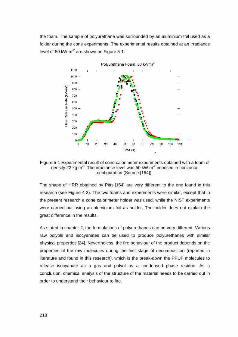
218

the foam. The sample of polyurethane was surrounded by an aluminium foil used as a

folder during the cone experiments. The experimental results obtained at an irradiance

level of 50 kW·m-2 are shown on Figure 5-1.

Figure 5-1 Experimental result of cone calorimeter experiments obtained with a foam of density 22 kg·m-3. The irradiance level was 50 kW·m-2 imposed in horizontal

configuration (Source [164]).

The shape of HRR obtained by Pitts [164] are very different to the one found in this

research (see Figure 4-3). The two foams and experiments were similar, except that in

the present research a cone calorimeter holder was used, while the NIST experiments

were carried out using an aluminium foil as holder. The holder does not explain the

great difference in the results.

As stated in chapter 2, the formulations of polyurethanes can be very different. Various

raw polyols and isocyanates can be used to produce polyurethanes with similar

physical properties [24]. Nevertheless, the fire behaviour of the product depends on the

properties of the raw molecules during the first stage of decomposition (reported in

literature and found in this research), which is the break-down the PPUF molecules to

release isocyanate as a gas and polyol as a condensed phase residue. As a

conclusion, chemical analysis of the structure of the material needs to be carried out in

order to understand their behaviour to fire.

219

5.4 Discussions about the small scale (cone

calorimeter) simulations

The experimental results obtained in CC are compared to numerical simulations in

order to identify the ability to predict the fire behaviour of solids. The numerical study is

carried out with the most widespread CFD code used for fire simulation: FDS V 5.3.0.

This code can be used in two modes: The largest one is used by setting the HRR as a

function of time. Thus, the power released constitutes an input data that must be

determined experimentally. The great disadvantage of this method is that a new

measurement of HRR must be carried out with every burning element and every

possible configuration of the room or fire scenario. This approach requires the

classification and rating of the fire scenarios according to the risks that they can

produce. The rating can only be done by fire experts based on their knowledge in fluid

mechanics, chemistry, propagation, heat transfer, etc.

The second mode of the CFD code is the “pyrolysis calculated fire simulations”,

meaning that the process of thermal decomposition of the solid fuel (MLR and HRR) is

predicted using set kinetic parameters. This method has been included to FDS recently

and has not been used by many authors, particularly in multi-reaction cases. The main

advantage of the pyrolysis calculated simulations is a better knowledge of the

requirements of the process of thermal decomposition and the possibility to predict the

fire behaviour in multiple configurations. As a consequence, less large-scale tests are

needed, which considerably reduces experimental costs.

The main input of the pyrolysis calculated fire simulations can be classified into two

groups: a) thermal properties, and b) decomposition mechanism and the respective

kinetic parameters. In this research, these input parameters were presented in

section 2.4 and section 3.3 respectively.

As presented in section 4.4, the simulations results did not make it possible to

reproduce the experiments in a satisfying manner. Instabilities and results not in

agreement with the physics are often observed. The lack of accuracy can be due to

many causes. Some of the possible causes are discussed here; nevertheless, the aim

of this research is not to evaluate their relevance. Understanding the influence of the

220

inaccuracy of the results of calculations is the key to improve the models of fire

behaviour.

Written in a simplified manner and using the notation of this dissertation, the FDS

reaction rates are calculated with Eq. (5-1). The Eq (3-27) used for the modelling work

carried out in this research is also reminded.

[ ]ithrsi

i

n

ii TT

RT

EA

i

,0

,0maxexp −

−

=

ρρω&

(5-1)

δω2

exp Oni

iii ym

RT

EA i

−=& Reminder of

Eq. (3-27)

Where, ithrT , , is an optional “threshold” temperature that allows the definition of non-

Arrhenius pyrolysis function and ignition criteria (by default CT ithr °= 15.273, ). In

contrast to the equation used to express the reaction rates in this research, Eq. (3-27),

the pyrolysis model from FDS V.5.3, Eq. (5-1), does not contain a term of oxygen mass

fraction. The mixture fraction combustion model used for the calculation of the flame

surface does not allow calculating the concentration of oxygen in the fuel side of the

reaction zone. It means that in FDS, the heterogeneous oxidation reactions cannot be

considered and all the decomposition reactions are of pyrolysis. Thus, corrections must

be introduced to the kinetic parameters calculated at the matter scale or to the

decomposition mechanism. These corrections must force FDS to calculate the correct

MLR at a given temperature in order to produce the adequate quantity of gas fuel.

However, some authors argued that, experimentally speaking, it could be considered

that the decomposition of the sample in CC occurs purely in absence of oxygen

(pyrolysis), yet no demonstration of this phenomenon has been performed on solid

combustibles with multi-reaction decomposition.

There is a serious lack of knowledge regarding the sensitivity of the Arrhenius

parameters (input data of pyrolysis model) in the MLR output. Moreover, the

combination of the lack of knowledge of the sensitivity of thermal and Arrhenius

parameters makes the task of accurately fitting the experimental MLR curve very

complicated. In the preliminary tests performed (not detailed here), it was found that

the influence of the Arrhenius parameters and the decomposition mechanism are very

221

strong. Thus, the experimental effort (and cost) needed to determine the thermal

properties in function of temperature for simulation purposes is perhaps not justified

until an improvement of the models is carried out.

The shape of MLR released by FDS depends on the temperature provided to the

Arrhenius equation. The temperature is calculated by the solution of the energy

balance of the solid. The energy balance must take into account:

• The heat contribution of the flame (convection and radiation) and of an external

heat source

• The heat losses by radiation and convection

• The heat conduction into the material

• The heat of reaction, that is to say the power consumed for the gasification of the

solid fuel.

The energy balance of the solid is affected by many phenomena produced at the same

time by the interaction between the solid and gas phases (e.g. combustion) and the

intrinsic characteristics of the solid. If the energy balance is not established in an

adequate manner, the bulk decomposition reaction can appear to go faster, slower or

follow a shape that is different from the actual one. Some of the terms of the heat

exchange are very difficult to determine experimentally. They are estimated using

correlations or constant values set by experience.

The conduction model of FDS is presented in Eq. (5-2), which plays a main role in the

energy balance.

ss

ss

ss qx

TTk

xt

Tc ′′′+

∂∂

∂∂=

∂∂

&ρ (5-2)

Where, sq ′′′& , is the source term consisting of chemical reactions and radiative

absorption. Eq. (5-2) is a one-dimensional heat conduction equation for the solid phase

temperature ),( txTs is applied in the direction x pointing into the solid (the point 0=x

represents the surface) [155]. This equation does not allow calculating the heat losses

in the transversal direction to the incident heat flux. It neither takes into account the

222

effects caused by the alveolar nature of the foam, nor the change of the solid

characteristics (i.e. solid to semi-liquid).

The in-depth distribution of the temperature of the PPUF foam slab was not reliably

measured in this research. Some preliminary tests carried out using thermocouples into

the solid showed a great uncertainty because of the formation of a char layer in the

welding during the displacement of the decomposition front. A comparison of the

experimental and calculated temperature profiles would allow the validation of the

conduction model of FDS. The knowledge of the temperature profile can also help the

comprehension of the formation, thickness and displacement velocity of the

decomposition front.

The CC irradiance level imposed to the solid may be increased by around 40% by the

contribution of the flame radiation towards the solid surface [74]. This increase of total

heat income modifies the kinetics of decomposition (gas fuel production). The curve of

HRR in FDS is calculated as the linear combination of the reaction rate and the heat of

combustion of each solid in decomposition. But, up to date, the heat of combustion for

every product reacting cannot be determined experimentally. As shown in Figure 4-12,

the experimental EHC is not constant and changes greatly with the irradiance level and

the combustion advancement. In other words, the model cannot be used to predict the

actual heat release rate by solids with multiple decomposition stages in which the

potential chemical energy varies with the reaction progress.

The CC numerical simulations have shown to be extremely sensible to the heat of

reaction. It is highlighted that in the simulations presented from Figure 4-14 to Figure

4-15, the heat of reactions used are in the order of magnitude of the experimental

enthalpic results. Nevertheless, these parameters represent a non negligible drawback,

both numerically and experimentally. Numerically, because: a) a very reliable input

value is required in order to reproduce the cone calorimeter results; b) the values that

would allow an acceptable fit between calculations and experiments do not necessarily

correspond to the ones measured experimentally. Experimentally, it is not possible to

measure the enthalpy of every species present in the decomposition mechanism. As

showed in Figure 2-1, under nitrogen, two distinct stages of decomposition were

observed, for which it is possible to measure the enthalpy. However, under air a single

datum of enthalpy was measured. We can therefore only hypothesize which one

reflects the power released or consumed by every single reaction of the mechanism.

223

To avoid confusions, it is important to clarify that PPUF is a non-charring thermoset

polymer in flaming condition5. In the decomposition mechanism found during the matter

scale analysis, one of the solid species has been called “char”. Nevertheless, this

species represents a small mass fraction and does not have characteristics similar to

those of the char yielded by wood or other charring materials.

Experimentally, the rate of decomposition of charring materials is highly influenced by

the mass of char while this layer produces a thermal barrier that prevents heat from

penetrating into the material. An accurate description of the char layer is required in

order to model the heat transfer inside the solid, which is responsible for the in-depth

decomposition of the solid sample. The case of PPUF decomposition during flaming

combustion is very different: no char is produced, thus no thermal barrier exists. The

residue remaining at the bottom of the holder does not influence the decomposition

kinetics during the combustion process; is the residue remaining at the very end of the

process. In the FDS pyrolysis model, there is no particular setting indication for

charring or non-charring material. Perhaps the “interpretation of the role” of the residue

in the model is responsible for the strong differences observed in Figure 4-15 and

Figure 4-16.

Lautenberger et al. [15] developed a methodology that uses GA to estimate the

material properties (model parameters) needed for CFD-based fire growth modelling of

bench-scale fire test data. The inputs of the method are the MLR and surface

temperature histories. This method was used for charring materials (redwood and red

oak) and a thermoplastic material (polypropylene), considering an infinitely thin

pyrolysis front and volatiles that were instantaneously transported towards the surface.

The approach of the decomposition process was single-stage, where the virgin foam is

transformed only into char. This tool was integrated to FDS V 4.0. The reaction

properties calculated were the Arrhenius parameters and the heat of reaction. The

material properties calculated were the thermal conductivity, specific heat and density

of char and virgin material.

5 Experiments in cone calorimeter showed that in non flaming condition a char layer is formed

mainly at the bottom of the sample holder which contains a non negligible residual mass.

224

The same methodology was generalised to multi-step reactions. The TGA behaviour of

a fire-retarded (brominated) polyester is predicted. This information was used

subsequently to reproduce the MLR of a fiber reinforced polymer slab in Fire

Propagation Apparatus [165]. This methodology has been generalised to the multi-

stage, multi-reaction combustion of solids from various natures [166] and released as

an independent code called “Gpyro” that can be coupled to FDS V.5.3 [167][168].

Some preliminary tests of this code have shown that it is very expensive in calculation

time and generates results that are difficult to interpret.

Researchers from other teams estimated the thermal properties of pyrolysis solids

using GA. The input data were TGA and CC experimental results. The optimum kinetic

parameters and thermal properties were those that best fitted the results from both

experimental techniques. In their work, virtual TGA and cone calorimeter were “built”

using FDS [169]. This method was used for up to two decomposition stages of

materials such wood and non-fire retarded polymers [170]. The authors defined thumb

rules about which property to change in order to attain a desired movement from the

MLR curve. Some of the kinetic parameters calculated do not seem in accordance with

the ones normally found in literature, for example reaction orders as high as

seven [169]. The same method was also used to estimate the parameters of electrical

cables for nuclear power plants [171][172].

In order to clarify the sensitivity to kinetic, stoichiometric and thermal input parameters

of the numerical simulations, a parametric study was launched. In total 7 000 FDS

simulations were carried out with random input parameters in each simulation. The

simulations tried to reproduce the CC experiments presented in section 4.4.

Unfortunately, the results have not been treated and the results are not available yet.

An interesting discussion should take place among the scientific community of fire in

order to answer to the following questions: Is it useful to keep on devoting time and

effort to fit numerically fit curves by using parameters that do not have a physical

meaning and that have a very uncertain application domain? How could the models be

improved in order be able to use the experimental results?

If the scientific community answers the former question and finds that it is necessary to

mathematically fit the curves, the best progress would be obtained by determining

numerically which parameters actually have a strong influence on the simulation

output. The experimental efforts must focus on the measurement of the very high

225

sensible parameters rather than the low sensible ones. The analysis of sensitivity must

also clarify what parameters need to be determined in function of temperature and

which ones can be set as scalars. Ho in 2007 [156] performed an interesting analysis

of sensitivity, centred on the ignition criteria and fire propagation in wood. His study

was performed using FDS V.4.0, which did not allow multi-reaction pyrolysis

processes.

Concerning the latter question, a huge work must be carried out in order to improve the

reliability of the experimental measurements in order to be able to provide accurate

description of the interaction between the solid and the gas phases and providing as

well data in all the stages of the decomposition as a function of temperature. Using this

experimental data, improvements to the models can be performed.

As a conclusion, the greatest disadvantage of the pyrolysis calculated fire simulation is

that the method is still very recent and very intensive research is being carried out to

improve the models. There is no input data for the model, and in some cases it is not

very clear how to perform the experimental measurements. As a matter of fact, NIST,

WPI, SwRI and SFPE are currently working on a project, the main goal of which is to

develop a standard guide with procedures for obtaining material parameters for fire

models input such as algebraic, zone and field/CFD. These parameters include, but are

not limited to, thermal parameters, ignition parameters, pyrolysis parameters and

kinetic parameters [173].

5.5 Discussions about the oxygen mass

fraction

The oxygen mass fraction plays a major role in the decomposition mechanism and

kinetics. In this research, the decomposition pattern was determined in apparatuses

where the sample masses were small. It is hypothesised that no transport effects exists

from the centre of the particle toward the boundaries. The oxygen mass fraction

contained in the air stream is supposed to be enough to create a condition of well-

ventilated oxidation reaction. Unfortunately, no tests were performed to verify the

226

shape of MLR under vitiated or oxygen-rich atmosphere conditions, i.e. oxygen mass

fractions of 0.11 and 0.3 kg·kg-1.

Nevertheless, tests with various vector gas mass flows must be conducted in order to

verify if it influences the decomposition kinetics. Thus, the data to be considered as the

current patterns are the ones of the lower mass flow that do not cause a change in the

shape of MLR. This validation would be performed considering the change of the solid

phase as well as the gas phase. It can constitute a basis for the study of the

differentiation of the heterogeneous reactions and the homogeneous reactions. It is

perhaps a more precise method than the one used in this research to determine which

gases are released by each decomposition stage.

In general terms, the increase of the oxygen in the atmosphere shift the reaction rate

towards the lower temperatures in TGA and TF facilities and causes the ignition and

maximum of HRR to occur faster in cone calorimeter [115]. The influence of oxygen in

CC decomposition kinetic needs to be studied from three points of view:

• The oxygen mass fraction can change over the surface of the CC sample because

of the oxygen consumption in the flame. In other words, a gradient of concentration

may exist from the boundary to the centre of the CC sample, which can have a

non-negligible influence on the decomposition kinetics.

• The oxygen mass fraction can change in-depth in a porous material. This produces

a gradient of oxygen present from the surface to the core of the matrix, which

causes the kinetics of decomposition in the decomposition front to change with the

thickness.

• The oxygen mass fraction of the atmosphere changes in a closed room on fire. The

oxygen available for the combustion in gas phase and heterogeneous reactions

between gas and solid changes with time. The depletion of oxygen has a main

influence in the kinetics of decomposition and the nature of the toxic gases

released.

In conclusion, the influence of oxygen needs to be analysed in all the scales

considered in this research. The availability of oxygen in the atmosphere influences the

amount of power release by the fire as well as the toxicity potential in the environment.

227

6 General conclusions and future

works

6.1 Conclusions

The improvement of fire safety in dwellings can be attained by the combination of a

huge number of strategies focused on reducing the hazards caused by fire. The

improvement of our knowledge of the physics and chemistry of fire and our ability to

predict fire behaviour is the major issue in order to reduce these hazards. The reliable

prediction of fire behaviour allows performance-based fire safety design of buildings,

which has become the trend nowadays.

In this research the decomposition mechanism of PPUF was studied using techniques

of thermal analysis and gas release measurements. Analysing together the solid and

gas phases required the coupling of multiple measurement facilities. It allowed for the

first time to state a “chemically correct” decomposition mechanism that takes into

account the chemistry of the process. A part of the complexity of the problem is that, at

any scale, the decomposition process occurs in a transient state: since the

decomposition of PPUF presents many stages, the steady state is never reached. The

scales considered in the present study are: matter scale analysed using TF and TGA

apparatus; small scale studied using CC; and product scale tested with SBI

calorimeter. The FTIR for examining the gas composition was used in all the scales.

The most common methods of thermal analysis found in literature allow hypothesising

a decomposition mechanism and calculating the decomposition parameters.

Nevertheless, it was found that these methods are not necessarily in accordance with

the chemical reactions taking place in the solid phase.

228

Improvements to a multi-stage, multi-decomposition mechanism were carried out in

order to use the new decomposition mechanism but also to predict the toxic gas

release. A single supplementary kinetic parameter is required to enable the prediction

of toxic gases. To the best of our knowledge, this is the first time that a method is

proposed to predict the toxic gases released by the decomposition of polyurethane.

The hypothesis used for this improvement was to consider that the curve of release of

one gas could be calculated as the sum of the mass of this gas released by the

successive reactions. From the results at the matter scale under air and nitrogen, two

new decomposition mechanisms have been proposed. One mechanism from the

literature has also been considered. A discussion was developed in order to determine

which mechanism is correct and constitutes main input data for the modelling of

thermal decomposition. The kinetic parameters of each reaction were calculated using

genetic algorithms. The comparison of the numerical results with the experimental

ones, particularly concerning the MLR and pollutants emission have permitted to

validate the mechanism of PPUF decomposition.

The results of gas release prediction are very promising. Some differences between

the experimental and calculated shapes were found. Nevertheless, the lack of fitness

between the experimental and calculated curves can be explained by the differences

found between the experimental facilities that were coupled in this research.

A single group of kinetic and stoichiometric parameters allowing the prediction of the

mass and gas phase behaviour at various heating rates under two atmospheres (air

and nitrogen) was found.

Experimental measurements were also performed in cone calorimeter. The MLR and

HRR in function of time were determined by the oxygen consumption calorimetry. The

results are in agreement with the results found in literature. The cone calorimeter was

coupled to gas analysers (FTIR and FID). The coupled experiments allowed the

verification of the decomposition mechanism at this scale. A two-stages decomposition

was found, which remains unchanged independently of the irradiance level set to the

electric heater: The first stage is the breakdown of PPUF molecules that carry the

pyrolysis and oxidation of isocyanate remaining polyol as a semi-liquid residue. The

second stage is the pyrolysis and oxidation of polyol that burns near a pool fire. The

two stages of decomposition cannot be isolated in time. This decomposition

229

mechanism is valid at bench-scale (CC measurements) as well as at larger scales

(simplified product burning).

The kinetic and thermal parameters found at the matter scale were used as input data

in the pyrolysis-based fire simulation of CC experiments. Inaccurate results were found,

caused by the combination of effects such as: the pyrolysis mechanism set in FDS

cannot take into account heterogeneous oxidation reactions, the experimental thermal

parameters are not allowed to fit adequately the experiments and calculations, strong

uncertainties exist in the experimental measurement in function of temperature, the

model of heat conduction is not allowed to take into account the heat losses by the

lateral boundaries as well as the change of properties with the change of physical and

chemical structure, etc.

At all the scales considered in this research, the decomposition mechanism was the

same. A strong influence of the oxygen was verified but unfortunately, the models

currently found in literature do not make it possible to predict the effects of the oxygen

diffusion and the temperature distribution in-dept of the foam slab.

6.2 Future works

The analysis of the gases released during pyrolysis and combustion showed to be

crucial information in order to understand the transformation taking place in the solid

phase. The techniques such as FTIR that allows measuring multiple gases in real time

have a very high potential in fire analysis. Nevertheless, these techniques in fire

applications are still recent and their implementation is not easy. The TGA + FTIR or

TGA + GC/MS for example are very promising techniques that need to be extensively

used by the teams working on thermal decomposition.

In this research, the yield of soot was not measured at any scale. Considering soot is a

primary need in further researches in order to determine the carbon balance. The

carbon balance constitutes a good means of verifying the reliability of the gas phase

measurements. It also allows writing a semi-steady state combustion equation that can

be used as an engineering approach for the toxic gases production estimation.

230

Further works must also be conducted to understand the transport of the tar produced

during the pyrolysis of PPUF. Some authors also reported tar transport in gas effluents

of experiments carried out under oxidizing atmosphere. The PU tar has shown to

solidify even with a lean decrease of temperature causing problems in the connexion

lines of experimental facilities.

Efforts must focus on the improvement of the understanding of the transformations

suffered by the nitrogen contained in the solid phase. A low portion of the nitrogen

contained in the solid phase was found in the gas phase. It was hypothesised that the

vast majority was reduced into N2. However, experimental evidence should support this

claim. The need for an analysis of the transformation of nitrogen is prompted by the

potential to form very toxic compound (i.e. NOx, HCN, etc).

Interesting experimental techniques such as Laser Pyrolysis-FTIR [174] need to be

considered in order to analyse the decomposition mechanism of polymers. This

technique offers the advantage of very rapid testing on small samples. Moreover, the

control of the power of the laser allows setting well-controlled irradiance levels at the

surface of the sample. This may constitute a complement to cone calorimeter results,

because the experiments can be performed on small samples where the conduction

problems can be simplified.

The models also need to be improved based on the knowledge of the decomposition

kinetics. The influence of oxygen in the atmosphere needs to be taken into account as

well as the problem of the oxygen diffusivity inside the solid structure. Better methods

to set the parameters of the simulation need to be stated, making the results of various

calculations comparable between them.

The methods to determine and set the input data in the fire codes need to be improved

for other materials than thermoplastics. A great deal is the charring materials: Their

decomposition mechanism can be determined using TGA and TF as presented in this

research. Nevertheless the fire behaviour in CC is difficult to predict because of the

great number of reactions taking place in depth of the solid structure. So, for charring

materials the hypothesis of infinitely thin decomposition front is not valid. The study of

the mechanisms of decomposition must be kept out with other materials used in

dwellings.

231

7 References

[1] CHIVAS C, GUILLAUME E, SAINRAT A, BARBOSA V. Assessment of risk and benefits in the use of flame retardants in upholstered furniture in continental Europe. Fire Safety Journal 44 (2009): 801-807.

[2] Unknown author. Standardisation mandate to CEN relative to the safety requirement for cigarettes. Commission of the European Communities, Directorate General Health and Consummers, 2008. M/425 EN.

[3] Unknown author. Fire statistics – United Kingdom, Department of communities and Local Government, 2008. ISBN: 978 1 4098 0046 0 <www.communities.gov.uk>.

[4] BEYLER C, HIRSCHLER M. Thermal decomposition of polymers. In: SFPE Handbook of Fire Protection Engineering (second edition), 1995, Section 1, Chapter 7: 99-199. ISBN 0-87765-354-2.

[5] HILEMAN F, VOORHEES K, WOJCIK L, BIRKY M, RYAN P, EINHORN I. Pyrolysis of a flexible urethane foam. Journal of Polymer Science 13 (1975): 571-584.

[6] TROITZSCH J. Plastics Flammability Handbook. Principles, regulations, testing and approval (Third edition). Carl Hansel Verlag, Munich, 2004. ISBN 3-446-21308-2.

[7] Unknown author. IAL CONSULTANTS. PU chemicals and products in Europe, Middle East & Africa (EMEA), 2007. <http://www.ialconsultants.com/>.

[8] MAROTEL Y. Polyuréthannes. Techniques de l’ingénieur, traité de plastiques et composites. AM3 425 (2000): 1-18.

[9] PAL G, MACSKASY H. Plastics: Their Behaviour in Fires. Elsevier Sciences Publishers, Amsterdam, Netherlands, 1991, 431 pp. ISBN 0-44-98766-5.

[10] BRANCA C, DI BLASI C, CASU A, MORONE V, COSTA C. Reaction kinetics and morphological changes of a rigid polyurethane foam during combustion. Thermochimica Acta 399 (2003): 127-137.

[11] BILBAO R, MASTRAL J, CEAMANOS J, ALDEA M. Kinetics of the thermal decomposition of polyurethane foams under nitrogen and air atmospheres. Journal of Analytical and Applied Pyrolysis 37 (1996): 69-82.

232

[12] SAINRAT A. Regulatory trends and standardization towards the reaction to fire of the upholstery furniture in France and in Europe. In: Flame Retardants 2006 Proceedings.

[13] CEAMANOS J, MASTRAL J, MILLERA A, ALDEA M. Kinetics of pyrolysis of high density polyethylene. Comparison of isothermal and dynamic experiments. Journal of Analytical and Applied Pyrolysis 65 (2002): 93-110.

[14] DUQUESNE S, LE BRAS M, BOURBIGOT S, DELOBEL R, POUTCH F, CAMINO G, ELING B, LINDSAY C, ROELS T. Analysis of fire gases released from polyurethane and fire-retarded polyurethane coatings. Journal of Fire Sciences 18 (2000): 456-482.

[15] LAUTENBERGER C, REIN G, FERNANDEZ-PELLO C. The application of a genetic algorithm to estimate material properties for fire modeling from bench-scale fire test data. Fire Safety Journal 41 (2006): 204-214.

[16] MAMLEEV V, BOURBIGOT S, LE BRAS M, DUQUESNE S, SESTAK J. Modelling of nonisothermal kinetics in thermogravimetry. Physical Chemistry Chemical Physics 2 (2000): 4708-4716.

[17] CHANG T, SHEN W, CHIU Y, HO S. Thermo oxidative degradation of phosphorus-containing polyurethane. Polymer Degradation and Stability 49 (1995): 353-360.

[18] KETATA N, SANGLAR C, WATON H, ALAMERCERY S, DELOLME F, RAFFIN G, GRENIER-LOUSTALOT ME. Thermal degradation of polyurethane bicomponent systems in controlled atmospheres. Polymer and Polymer Composites 13, 1 (2005): 1-26.

[19] FRIEDMAN H. Kinetics of thermal degradation of char forming plastics from thermogravimetry. application to a phenolic plastic. Journal of Polymer Science, Part C, 6 (1963): 183-195.

[20] BABRAUSKAS V, GRAYSON S. Heat release in fires. Elsevier Science Publishers Ltd, Essex, England, 1992. ISBN 1-85166-794-6.

[21] YANG W, MACOSKO C, WELLINGHOFF S. Thermal degradation of urethanes based on6 4,4’-diphenylmethane diisocyanate and 1,4-butanediol (MDI/BDO). Polymer 27 (1986): 1235-1240.

[22] OHTANI H, KIMURA T, OKAMOTO K, TSUGE S. Characterization of polyurethanes by high-resolution pyrolysis-capillary gas chromatography. Journal of Analytical and Applied Pyrolysis 12 (1987): 115-133.

[23] ROGERS F, OHLEMILLER T. Pyrolysis kinetics of a polyurethane foam by thermogravimetry; a general kinetic method. Journal of Macromolecular Science A 15, 1 (1981): 169-185.

[24] SHARMA V, KUNDU P. Condensation polymers from natural oils. Progress in Polymer Science 33 (2008): 1199-1215.

233

[25] WANG T, HSIEH T. Effect of polyol structure and molecular weight on the thermal stability of segmented poly(urethaneureas). Polymer degradation and stability 55 (1997): 95-102.

[26] FONT R, FULLANA A, CABALLERO J, CANDELA J,GARCÍA A. Pyrolysis study of polyurethane. Journal of Analytical and Applied Pyrolysis 58-59 (2001): 63-77.

[27] PRAGER F, ROSTECK H. Polyurethane and fire: fire performance testing under real conditions. Wiley-Vch Verlag Gmbh & Co, KGaA, Weinheim, 2006. ISBN 3-527-30805-9.

[28] ALLEN N, EDGE M, Fundamentals of polymer degradation and stabilisation. Elsevier Science Publishers Ltd, England,1992. ISBN 1-85166-773-3.

[29] ELOMA M, SARVARANTA L, MIKKOLA E, KALLONEN R, ZITTING A, ZEVENHOVEN C, HUPA M. Combustion of polymeric materials. Critical Reviews in Biochemistry and Molecular Biology 27, 3 (1997):137-197.

[30] VOORHEES K, HILEMAN F, EINHORN I, FUTRELL J. An investigation of the thermolysis mechanism of model urethanes. Journal of Polymer Science 16 (1978): 213-228.

[31] ZHANG Y, XIA Z, HUANG H, CHEN H. Thermal degradation of polyurethane based on IPDI. Journal of Analytical and Applied Pyrolysis 84 (2009): 89-94.

[32] LATTIMER R, POLCE M, WESDEMIOTIS C. MALDI-MS analysis of pyrolysis products from segmented polyurethane. Journal of Analytical and Applied Pyrolysis 48 (1998): 1-15.

[33] EZEKOYE O, BRUNS M. Radical based thermal decomposition of polyethylene. NIST Annual Fire Conference, USA, 2008.

[34] FABRIS H. Thermal and oxidative stability of urethanes. Advances in Urethane Science and Technology 4 (1976): 89-111.

[35] WOOLLEY W. Nitrogen-containing products from the thermal decomposition of flexible polyurethane foams. British Polymer Journal 4 (1972): 27-43.

[36] MOLERO C, DE LUCAS A, RODRIGUEZ J. Recovery of polyols from flexible polyurethane foam by “split-phase” glycolysis: Study on the influence of reaction parameters. Polymer Degradation and Stability 93 (2008): 353-361.

[37] SAUNDERS J, BACKUS J. Thermal degradation and flammability of urethane polymers. Rubber Chemistry and Technology 39 (1961): 461-480.

[38] RAVEY M, PEARCE E. Flexible polyurethane foam. I. Thermal decomposition of a polyether-based, water-blown commercial type of flexible polyurethane foam. Journal of Applied Polymer Science 63 (1997): 47-74.

[39] ROTIVAL C, RENACCO C, ARFI C, PAULI A, PASTOR J. Gases emitted during thermal decomposition of a polypropylene film and a polyurethane adhesive. Journal of Thermal Analysis 41 (1994): 1519-1527.

234

[40] GABORIAUD F, VANTELON J. Thermal degradation of polyurethane based on MDI and propoxylated trimethylol propane. Journal of Polymer Science 19 (1981): 139-150.

[41] BROWN M. Introduction to thermal analysis: Techniques and applications. Chapman and Hall Ltd. Cambridge, 1988. ISBN 0 412 30230 6.

[42] ESPERANZA M, GARCIA A, FONT R, CONESA J. Pyrolysis of varnish based on a polyurethane. Journal of Analytical and Applied Pyrolysis 52 (1997): 151-166.

[43] STEC A, HULL T, LEBEK K, PURSER J, PURSER D. The effect of temperature and ventilation condition on the toxic product yields from burning polymers. Fire and Materials 32 (2008): 49-60.

[44] BLOMQVIST P, HERTZBERG T, TUOVINEN H, ARRHENIUS K, ROSELL L. Detailed determination of smoke gas contents using a small-scale controlled equivalence ratio tube furnace method. Fire and materials 31 (2007): 495-521.

[45] GUILLAUME E. Effets du feu sur les personnes. Synthèse bibliographique. Laboratoire national de métrologie et d’essais (LNE), 2006.

[46] BOCKHORN H, HORNUNG A, HORNUNG U, JAKOBSTRÖER P. Modelling of isothermal and dynamic pyrolysis of plastics considering non-homogeneous temperature distribution and detailed degradation mechanism. Journal of Analytical and Applied Pyrolysis 49 (1999): 53-74.

[47] SAHA B, GHOSHAL A. Thermal degradation kinetics of poly(ethylene terephthalate) from waste soft drink bottles. Chemical Engineering Journal 111 (2005): 39-43.

[48] FENG J, LI W.Y, XIE K. Relation between coal pyrolysis and corresponding coal char gasification in CO2. Energy Sources 26 (2004): 841-848.

[49] GAYTON-ELY M, SHAKLEYA D, BELL S. Application of a pyroprobe to simulate smoking and metabolic degradation of abused drugs through analytical pyrolysis. Journal of Forensic Sciences 52 (2007): 473-478.

[50] DOSANJH S, PAGNI P, FERNANDEZ-PELLO C. Forced Cocurrent Smoldering Combustion. Combustion and Flame 68 (1987): 131-142.

[51] NF D 60-013. Protocol for assessment of the ignitability of upholstered furniture – Ignition source equivalent to a burning 20 g paper cushion – Coverings and upholstered materials. ICS 13.220.40, 97.140.

[52] BS 3379:1991. Flexible polyurethane cellular materials for loadbearing applications. UDC 678.664 405.8:006.3/8. ISBN 0 580 18176 6.

[53] NF EN ISO 11357-1 (1997). Plastics - Differential scanning calorimetry (DSC) – Part 1: General principles. ICS: 83.080.01.

[54] BUSTAMANTE VALENCIA L, ROGAUME T, GUILLAUME E, REIN G, TORERO J. Improving the Modelling of Thermal Decomposition of Polyether

235

Polyurethane Foam. Poster presented in the 9th Symposium on Fire Safety Science 2008, Germany.

[55] ISO 11357-4:2005. Plastics - Differential scanning calorimetry (DSC) – Part 4: Determination of specific heat capacity.

[56] SCOARNEC V., HAMEURY J., HAY B., FILTZ J. A new reference guarded hot plate designed for thermal conductivity measurements at high temperature. Poster presented in the 14th International Congress of Metrology 2009, France.

[57] NF EN ISO 1716:2002 Reaction to fire tests for building products – Determination of the heat of combustion. ICS: 13.220.50.

[58] NF ISO 1928:2004. Solid mineral fuels - Determination of gross calorific value by the bomb calorimetric method, and calculation of net calorific value. ICS: 75.160.10.

[59] SARAJI-BOZORGZAD M, GEISSLER R, STREIBEL T, MUHLBERGER F, SKLORZ M, KAISERSBERGER E, DENNER T, ZIMMERMANN R. Thermogravimetry coupled to single photon ionization quadrupole mass spectrometry: A tool to investigate the chemical signature of thermal decomposition of polymeric materials. Analytical Chemistry 80 (2008): 3393-3403.

[60] SOUDAIS Y, MOGA L, BLAZEK J, LEMORT F. Coupled DTA-TGA-FT-IR investigation of pyrolytic decomposition of EVA, PVC and cellulose. Journal of Analytical and Applied Pyrolysis 78 (2007): 46-57.

[61] DEL CAMPO S. Identification des paramètres d’autenthicité du lait et produits laitiers (thèse de doctorat). Institut national agronomique Paris-Grignon, France, 2006.

[62] PIELICHOWSKI K, LESZCZYNSKA A. TG-FTIR Study of the thermal degradation of polyoxymethylene (POM)/Thermoplastic Polyurethane (TPU) Blends. Journal of Thermal Analysis and Calorimetry 78 (2004): 631-637.

[63] RAHKAMAA-TOLONEN K. Investigation of catalytic NOx reduction with transient techniques, isotopic exchange and FTIR spectroscopy (PhD. Thesis). Åbo Akademi University, Turku, Finland, 2001.

[64] PEPIN MARIEY L. Etude par spectroscopie IR-TF de l’adsorption et de la réactivité de l’ozone sur oxydes métalliques (thèse de doctorat). Université de Caen, France, 1997.

[65] MASMOUDI H. Vieillissement d’émulsions cosmétiques : apports comparés de la spectroscopie IRTF et de la rhéologie (thèse de doctorat). Université Paul Cézanne, Aix-Marseille, France, 2005.

[66] MALINGREY B. Spectrométrie d’absorption dans l’infrarouge : Appareils. Techniques de l'Ingénieur, P2855 parution 01/1981.

[67] MARSCHALLEK-WATROBA K. Analyse de flammes prémélangées méthane, monoxyde d’azote, air: expérience, modélisation, application à la réduction des

236

oxydes d’azote (thèse de doctorat). Université des sciences et technologies de Lille, France, 2006.

[68] POTTEL H. Quantitative models for prediction of toxic component concentrations in smoke gases from FTIR spectra. Fire and Materials 20 (1996): 273-291.

[69] SARAGOZA L, YARDIN C, GUILLAUME E. Dosage des gaz dans les effluents de combustion par spectroscopie infrarouge à transformée de Fourier (selon la norme ISO 19702) : incertitude des spectres étalons. Proceedings of the 14th International Congress of Metrology, France, 2009.

[70] ISO 19702:2006. Toxicity testing of fire effluents – Guidance for analysis of gases and vapours in fire effluents using FTIR gas analysis. ISC 13.220.01.

[71] HAKKARAINEN T. et al. Smoke gas analysis by Fourier Transform Infrared Spectroscopy – Summary of the SAFIR project results. Fire and Materials 24 (2000): 101-112.

[72] Unknown author. Thermogravimétrie – Thermal analysis excellence. Mettler Toledo, Schwerzenbach, Suize 2007.

[73] CONESA J, MARCILLA A, CABALLERO J, FONT R. Comments on the validity and utility of the different methods for kinetic analysis of thermogravimetric data. Journal of Analytical and Applied Pyrolysis 58-59 (2001): 617-633.

[74] RHODES B, QUINTIERE J. Burning rate and flame heat flux for PMMA in cone calorimeter. Fire Safety Journal 26 (1996): 221-240.

[75] SAINRAT A. Personal communication. Laboratoire national de métrologie et d’éssais. 2009.

[76] Unknown author. Final Report. Fire standardisation research in railways - Firestarr Project. Contract SMT4 – CT 97 – 2164 Commission of the European Communities, 2001.

[77] NATO AC/301 SG/B. NATO Reaction-to-fire tests for materials – Toxicity of fire effluents. Edition 2: Draft I, Dec 2005.

[78] NF X 70-100-2 Fire tests - Analysis of gaseous effluents - Part 2: Tubular furnace thermal degradation method. ICS : 13.220.40 AFNOR 2006.

[79] ISO 16312-2:2006 Guidance for assessing the validity of physical fire models for obtaining fire effluents toxicity data for fire hazard and risk assessment – Part 2: Evaluation of individual physical fire models. Afnor 2006. ICS 13.220.99.

[80] REIN G. From pyrolysis kinetics to models of condensed-phase burning. In: Recent Advances in Flame Retardancy of Polymeric Material 19 (2008): 1-10 <www.era.lib.ac.uk/handle/1842/1152>.

[81] Unknown author. Benefits of fire safety engineering in the EU – BENEFEU project. The potential benefits of fire safety engineering in the European Union. Final report to DG Enterprise, 2002. (EC contract EDT/01/503480).

237

[82] VYAZOVKIN S. Kinetic concepts of thermally stimulated reactions in solids: a view from a historical perspective. International Reviews in Physical Chemistry 19 (2000); 45-60.

[83] KISSINGER H. Reaction Kinetics in Differential Thermal Analysis. Analytical Chemistry 29, 11 (1957): 1702-1706.

[84] BABRAUSKAS V. Fire Modeling Tools for Fse: Are They Good Enough? Journal of Fire Protection Engineering 8, 2 (1996): 87-93.

[85] JIANG Y. Decomposition, ignition and flame spread on furnishing material (PhD. Thesis). Victoria University, Australia, 2006.

[86] MOGHTADERI B. Pyrolysis of char forming solid fuels: a critical review of the mathematical modelling techniques. 5th AOSFST, Newcastle, Australia, 2001. <www.newcastle.edu.au>

[87] ANDZI BARHE T, ROGAUME T, RICHARD F, TORERO J. Numerical characterization of the mechanism of NOx formation during MSW incineration. Proceedings of the 6th Mediterranean Combustion Symposium 2009. France.

[88] KANNAN P, BIERNACKI J, VISCO D. A review of physical and kinetic models of thermal degradation of expanded polystyrene foam and their application to the lost foam casting process. Journal of Analytical and Applied Pyrolysis 78 (2007): 162-171.

[89] ANDERSON M, SLEIGHT R, TORERO J. Downward smolder of polyurethane foam: ignition signatures. Fire Safety Journal 35 (2000): 131-147.

[90] FONT R, MANCILLA A, GARCIA A, CABALLERO J, CONESA J. Comparison between the pyrolysis products obtained from different organic waste at high temperatures. Journal of Analytical and Applied Pyrolysis 32 (1995): 41-49.

[91] MANCILLA A, CONESA J. Reciclado terciario de plásticos vía pirólisis. Revista de plásticos modernos 79, 527 (2000): 559-566.

[92] CHAO C, WANG J. Comparison of the thermal decomposition behaviour of a non-fire retarded and a fire retarded flexible polyurethane foam with phosphorus and brominated additives. Journal of Fire Sciences 19, 2 (2001): 137-156.

[93] CONESA J, CABALLERO J, MANCILLA A, FONT R. Analysis of different kinetic models in the dynamic pyrolysis of cellulose. Thermochemica Acta 254 (1995): 175-192.

[94] MÜLLER-HAGEDORN M, BOCKHORN H, KREBS L, MÜLLER U. A comparative kinetic study on the pyrolysis of three different wood species. Journal of Analytical and Applied Pyrolysis 68-69 (2003): 231-249.

[95] FLYNN J. The ‘Temperature Integral’ – Its use and abuse. Thermochimica Acta 300 (1997): 83-92.

[96] VYAZOVKIN S. Thermal analysis. Analytical Chemistry 80,12 (2008): 4301-4316.

238

[97] VYAZOVKIN S. A unified approach to kinetic processing of nonisothermal data. International Journal of Chemical Kinetics 28 (1996): 95-101.

[98] CRIADO J, GONZALEZ M, ORTEGA A, REAL C. Some considerations regarding the determination of the activation energy of solid-state reactions from a series of isothermal data. Journal of Thermal Analysis 29 (1984): 243-250.

[99] VYAZOVKIN S, DOLLIMORE S. Linear and nonlinear procedures in isoconversional computations of the activation energy of nonisothermal reactions in solids. Journal of Chemical Information and Computer Science 36 (1996): 42-45.

[100] LEFEBVRE J, DUQUESNE S, MAMLEEV V, LE BRAS M, DELOBEL R. Study of the kinetics of pyrolysis of a rigid polyurethane foam: use of the invariant kinetics parameters method. Polymers for Advanced Technologies 14 (2003): 796-801.

[101] JANKOVIC B. Kinetic analysis of the nonisothermal decomposition of potassium metabisulfite using the model fitting and isoconversional (model free) methods. Chemical Engineering Journal 139 (2008): 128-135.

[102] MAMLEEV V, BOURBIGOT S. Calculation of activation energies using the sinusoidally modulated temperatures. Journal of Thermal Analysis and Calorimetry 70 (2002): 565-579.

[103] MAMLEEV V, BOURBIGOT S, LE BRAS M, DUQUESNE S, SESTAK J. Modelling of nonisothermal kinetics in thermogravimetry. Physical Chemistry Chemical Physics 2 (2000): 4708-4716.

[104] CANCELLIERI D, LEONI E, ROSSI J. Kinetics of the thermal degradation of Erica arborea by DSC: Hybrid kinetic method. Thermochemica Acta 438 (2005): 41-50.

[105] BENBOW A, CULLIS F. The combustion of flexible polyurethane foams: mechanisms and evaluation of flame retardance. Combustion and Flame 24 (1975): 217-230.

[106] OHLEMILLER T. Modeling of smoldering combustion propagation. Progress in Energy and Combustion Science 11 (1985): 277-310.

[107] REIN G. Computational Model of Forward and Opposed Smoldering Combustion with Improved Chemical Kinetics (PhD. Thesis). University of California, Berkeley, San Francisco, US, 2005.

[108] REIN G, FERNANDEZ-PELLO C, URBAN D. Computational model of forward and opposed smoldering combustion in microgravity. Proceedings of THE Combustion Institute 31, 2 (2007): 2677-2684. <http://www.era.lib.ed.ac.uk/bitstream/1842/897/1/Rein_Heidelberg.pdf>.

[109] REIN G, LAUTENBERGER C, FERNANDEZ-PELLO C, TORERO J, URBAN D. Application of genetic algorithms and thermogravimetry to determine the kinetics of polyurethane foam in smoldering combustion. Combustion and Flame 146 (2006): 95-108.

239

[110] HOUCK C, JOINES J. A genetic algorithm for function optimization: a matlab implementation. Report NCSU IE TR 95-09. <http:// www.ise.ncsu.edu>.

[111] MOWRER F. Enclosure smoke filling revisited. Fire Safety Journal 33 (1999): 93-114.

[112] ABECASSIS-EMPIS C, RESZKA P, STEINHAUS T, COWLARD A, BITEAU H, WELCH S, REIN G, TORERO J. Characterisation of Dalmarnock fire test one. Experimental Thermal and Fluid Science 32 (2008): 1334-1343.

[113] WICHMAN I. Material flammability, combustion, toxicity and fire hazard in transportation. Progress in Energy and Combustion Science 29 (2003): 247-299.

[114] DELICHATSIOS M. Piloted ignition times, critical heat fluxes and mass loss rates at reduced oxygen atmospheres. Fire Safety Journal 40 (2005): 197-212.

[115] FANG M, SHEN D, LI Y, YU C, LUO Z, CEN K. Kinetic study on pyrolysis and combustion of wood under different oxygen concentrations by using TG-FTIR analysis. Journal of Analytical and Applied Pyrolysis 77 (2006): 22-27.

[116] CABALLERO J, FONT R, MANCILLA A, CONESA J. New kinetic model for thermal decomposition of heterogeneous materials. Industrial and Engineering Chemistry Research 34 (1995): 806-812.

[117] SENNECA O, CHIRONE R, SALATINO P. Oxidative pyrolysis of solid fuels. Analytical and Applied Pyrolysis 71 (2004): 959-970.

[118] ARRHENIUS S. On the reaction velocity of the inversion of cane sugar by acids. Zeitschrift für Physikalische Chemie 4, 226 (1889).

[119] LAIDLER K, KING M. The Development of Transition-State Theory. Journal of Physical Chemistry 87 (1983): 2657-2664.

[120] POLLAK E., TALKNER P. Reaction rate theory: What it was, where is it today, and where is it going? Chaos 15 (2005): 026116-026116-11; DOI:10.1063/1.1858782.

[121] CUKROWSKI A. Relations between the arrhenius activation energy and threshold energy for simple models of the reactive cross sections in a dilute gas. Acta Physica Polonica B. 37 (2006): 1715-1726.

[122] MARQUIS D, BUSTAMANTE VALENCIA L, GUILLAUME E, PAVAGEAU M, CHIVAS C. Modélisation du comportement au feu d’un composite par calcul de pyrolyse : approche combinée expérience-simulation à petite échelle. Mécanique & Industries 10 (2009) : 245-253.

[123] COMUCE M. Comportement au feu des matières plastiques – Application à la sécurité incendie. Meeting GDR Incendies in CORIA UMR 6614, 2009, France.

[124] BUSTAMANTE VALENCIA L, ROGAUME T, GUILLAUME E, REIN G, TORERO J. Characterization of the kinetic of decomposition of polyether polyurethane foam (ppuf) – A way for finding input data for fire simulations. BFRL Annual Fire Conference 2008. USA.

240

[125] ISO 16730:2007 (E). Fire safety engineering-Assessment. Verification and validation of calculation methods.

[126] HILBERT D, NEUMANN J, NORDHEIM L. Über die Grundlagen der Quantenmechanik. Mathematische Annales 98, 1 (1928): 1-30.

[127] DI BLASI C, Modeling chemical and physical processes of wood and biomass pyrolysis. Progress in Energy and Combustion Science 34 (2008): 47-90.

[128] DI BLASI C. The state of the art of transport models for charring solid degradation, Polymer International 49 (2000): 1-14.

[129] DI BLASI C. Modeling and simulation of combustion processes of charring and non-charring solid fuels. Progress in Energy and Combustion Science 19 (1993): 71-104.

[130] TORERO J, FERNANDEZ-PELLO A. Forward smolder of polyurethane foam in a forced air flow. Combustion and Flame 106 (1996): 89-109.

[131] ISO 5 660-1:2002 Reaction to fire tests – Heat release, smoke production and mass loss rate – Part 1 Heat release rate (cone calorimeter method). Second edition 2002.

[132] ISO 291:2005. Plastics – Standard atmospheres for conditioning and testing. ISC: 83.080.01.

[133] BABRAUSKAS V, PEACOCK R. Heat release rate: the single most important variable in fire hazard. Fire Safety Journal 18 (1992): 255-272.

[134] BABRAUSKAS V. Ignition Handbook. Fire Sciences Publishers, 2003. ISBN 0-9728111-3-3.

[135] TEWARSON A. Generation of heat and gaseous, liquid, and solid products in fire. The SFPE Handbook of Fire of Fire Protection Engineering, fourth edition, section 3, chapter 4, P 109-194. National Fire Protection Association, USA, 2008. ISBN-10: 0-87765-821-8.

[136] NORMANT H, NORMANT J. Chimie organique – Cours de chimie (deuxième édition), Masson et Cie Editeurs, 1968.

[137] RASBASH D, DRYSDALE D. Fundamentals of smoke production. Fire Safety Journal 5, 1 (1982): 77-86.

[138] BUSTAMANTE VALENCIA L, ROGAUME T, GUILLAUME E, REIN G, TORERO J. Analysis of principal gas products during combustion of polyether polyurethane foam at different irradiance levels. Fire Safety Journal 44 (2009): 933–940.

[139] DRYER F, NAEGELI D, GLASSMAN I. Temperature dependence of the reaction CO+OH --> CO2+H. Combustion and Flame 17 (1971): 270-272.

[140] DRYER F, GLASSMAN I. High temperature oxidation of CO and CH4. Proceeding of the 14th International Symposium on Combustion, The Combustion Institute (1972): 987-1003.

241

[141] GLASSMAN I. Combustion, Third edition, Academic Press, 1996.

[142] YETTER R, DRYER F, RABITZ H. A comprehensive reaction mechanism for carbon monoxide/hydrogen/oxygen kinetics. Combustion Science and Technology 79 (1991): 97-128.

[143] YETTER R, DRYER F, RABITZ H. Flow reactor studies of carbon monoxide/hydrogen/oxygen kinetics. Combustion Science and Technology 79 (1991): 129-140.

[144] GLARBORG P, ALZUETA M, DAM-JOHANSEN K, MILLER J. Kinetic modeling of hydrocarbons/nitric oxide interactions in a flow reactor. Combustion and Flame 115 (1998) 1-27.

[145] ROGAUME T, JABOUILLE F, TORERO J. Computational model to investigate the mechanisms of formation of NOx during waste incineration. Combustion Science and Technology 176 (2004): 925-943.

[146] GLARBORG P, MILLER J, KEE R. Kinetic modeling and sensitivity analysis of nitrogen oxide formation in well stirred reactors. Combustion and Flame 65 (1986): 177-202.

[147] DE SOETE G. Mécanismes de formation et de destruction des oxydes d'azote dans la combustion. Revue Générale de Thermique 330-331 (1989): 353-373.

[148] BUSTAMANTE VALENCIA L, ROGAUME T, GUILLAUME E, REIN G, TORERO J. Yield of toxic species in cone calorimeter tests during polyether polyurethane foam fire. Proceeding of the 6th Mediterranean Combustion Symposium, France, 2009.

[149] BITEAU H, STEINHAUS T, SCHEMEL C, SIMEONI A, MARLAIR G, BAL N, TORERO J. Calculation methods for the heat release rate of materials of unknown composition. Proceedings of the 9th International Symposium of Fire Safety Science IAFSS, 2008.

[150] GUILLAUME E., CHIVAS C. Fire models used in toxicity testing. In: Hazard of combustion products. Proceedings of the hazard of combustion products: toxicity, opacity, corrosivity and heat release conference, Interscience Communications Limited, UK, 2008. ISBN 978-0-9556548-2-4.

[151] HERTZBERG T, BLOMQVIST P, DALENE M, SKARPING G. Particles and isocyanates from fires, SP Swedish National Testing and Research Institute, 2003:05, Boras, 2003.

[152] KOTRESH T et al. Effect of heat flux on the burning behaviour of foam and foam/Nomex III fabric combination in the cone calorimeter. Polymer Testing 25 (2006): 744-757.

[153] FABIAN T, GANDHI P. Smoke characterization project. Technical report. NFPA – Underwriters Laboratories Inc., 2007. <http://www.nfpa.org/>.

242

[154] MCGRATTAN K, KLEIN B, HOSTIKKA S, FLOYD J. Fire Dynamics Simulator (Version 5.3), User’s Guide. NIST Special Publication 1019-5, National Institute of Standards and Technology, Gaithersburg, Maryland, February 2009.

[155] MCGRATTAN K, BAUM H, REHM R, HOSTIKKA S, FLOYD J. Fire Dynamics Simulator (Version 5.3), Technical Reference Guide. NIST Special Publication 1018-5, National Institute of Standards and Technology, Gaithersburg, Maryland, February 2009.

[156] HO K. Flame spread modelling using FDS 4 CFD model (PhD Thesis). University of Canterbury, Christchurch, New Zealand, 2007.

[157] DESANGHERE S. Détermination des conditions d’échauffement de structure extérieure à un bâtiment en situation d’incendie (PhD thesis), INSA de Rouen, France, 2006.

[158] FUENTES A. Interaction entre la zone réactionnelle et le champ de concentration des suies : cas de la flamme de diffusion laminaire au sein d’une couche-limite (PhD thesis). Université de Poitiers, France, 2006.

[159] KWON J. Evaluation of FDS V4: Upward flame spread (MSc thesis). Worcester Polytechnic Institute, Massachusetts, US, 2006.

[160] LIANG K, MA T, QUINTIERE J, ROUSON D. Application of CFD modeling to room fire growth on walls. NIST GCR 03-849, 2003.

[161] BUSTAMANTE VALENCIA L, ROGAUME T, GUILLAUME E. New method for simulating the kinetic of toxic gases production of upholstered furniture fire. Proceedings of the 12th Fire and Material Conference 2009, USA.

[162] prCEN/TS 45545-1 to prCEN/TS 45545-7. Railway applications – Fire protection of railway vehicles, final draft. CEN, CENELEC, 2008. ICS 45.060.01.

[163] QUINTIERE J. Fundamentals of fire phenomena. John Wiley & Sons Ltd, England, 2006. ISBN 13 978-0-470-09113-5.

[164] PITTS W. Ignition of cellulosic fuels by heated and radiative surfaces. NIST Technical note 1481, 2007. <www.fire.nist.gov/bfrlpubs/fire07/art014.html>.

[165] LAUTENBERGER C, KIM E, DEMBSEY N, FERNANDEZ-PELLO C. The role of decomposition kinetics in pyrolysis modeling – Application to a fire retardant polyester composite. Proceedings of the 9th Symposium on Fire Safety Science IAFSS, 2008.

[166] LAUTENBERGER C, FERNANDEZ-PELLO C. Generalized pyrolysis model for combustible solids. Fire Safety Journal 44 (2009): 819-839.

[167] LAUTENBERGER C. Gpyro– A generalized pyrolysis model for combustible solids. Users’ Guide, 2009. <http://code.google.com/p/gpyro/>.

[168] LAUTENBERGER C. Gpyro– A generalized pyrolysis model for combustible solids. Technical reference, 2009. <http://code.google.com/p/gpyro/>.

243

[169] MATALA A. Estimation of solid phase reaction parameters for fire simulation (Master’s thesis). Helsinki University of Technology, Finland, 2008.

[170] MATALA A, HOSTIKKA S, MANGS J. Estimation of pyrolysis model parameters for solid materials using thermogravimetric data. Proceedings of the 9th International Symposium of Fire Safety Science IAFSS, 2008.

[171] MATALA A. Application of genetic Algorithm in pyrolysis model parameter estimation. <http://www.sal.tkk.fi/Opinnot/Mat-2.108/pdf-files/emat07.pdf>.

[172] HOSTIKKA S, MATALA A. Modelling the fire behaviour of electrical cables. 20th International Conference on Structural Mechanics in Reactor Technology (SMiRT 20) – 11th International Post Conference Seminar on Fire Safety in Nuclear Power Plants and Installations, 2009.

[173] DEMBSEY N, JANSSENS M, HURLEY M. Fire Pyrolysis Parameters Guidance. <http://sites.google.com/a/fire-pyrolysis-parameter-guidance.org/>, 2009.

[174] BODZAY B, MAROSFOI B, IGRICZ T, BOCZ K, MAROSI G. Polymer degradation studies using laser pyrolysis-FTIR microanalysis. Journal of Analytical and Applied Pyrolysis 85 (2009): 313-320.

244

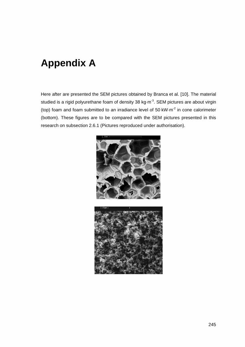
245

Appendix A

Here after are presented the SEM pictures obtained by Branca et al. [10]. The material

studied is a rigid polyurethane foam of density 38 kg·m-3. SEM pictures are about virgin

(top) foam and foam submitted to an irradiance level of 50 kW·m-2 in cone calorimeter

(bottom). These figures are to be compared with the SEM pictures presented in this

research on subsection 2.6.1 (Pictures reproduced under authorisation).

246

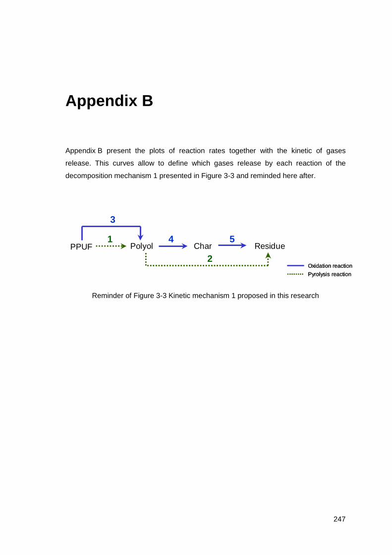
247

Appendix B

Appendix B present the plots of reaction rates together with the kinetic of gases

release. This curves allow to define which gases release by each reaction of the

decomposition mechanism 1 presented in Figure 3-3 and reminded here after.

1

2

3

4 5

Pyrolysis reaction

Oxidation reaction

Pyrolysis reaction

Oxidation reaction

PPUF Polyol Char Residue

Reminder of Figure 3-3 Kinetic mechanism 1 proposed in this research

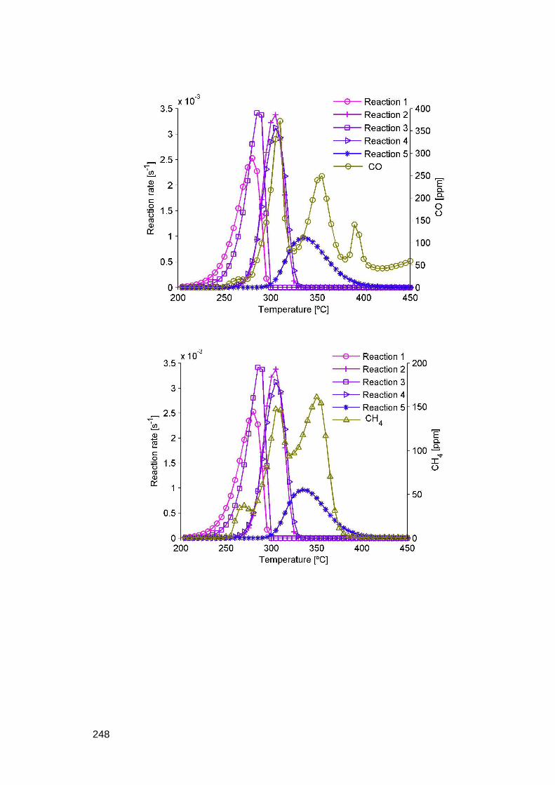
248

249

250

251

Appendix C

Appendix C presents the experimental and calculated kinetic of gas release of CO, H2O

and CH4 (see subsection 3.3.3.2).

252

253

Appendix D

&HEAD CHID='PPUF_air_cone_grossier' ,TITLE='Virtual cone calorimetre - 50 kW_m-2,low resolution'/ &TIME TWFIN = 100.0, WALL_INCREMENT = 1./ &MESH IJK = 10,10,18, XB = -0.125,0.125,-0.125,0.125,-0.075,0.375/ &DUMP DT_HRR=1., DT_DEVC=1., DT_PROF=30./ Recall of input data units: --------------------------- / THICKNESS = [ m ] / CONDUCTIVITY = [ W m-1 K-1 ] / SPECIFIC_HEAT = [ kJ kg-1 K-1 ] / DENSITY = [ kg m-3] / REFERENCE_TEMPERATURE = [ °C ] / HEAT_OF_REACTION = [ kJ kg-1 ] / HEAT_OF_COMBUSTION = [ kJ kg-1 ] / HRRPUA = [ kW m-2 ] / A = [ s-1 ] / E = [ kJ Kmol-1] / N_S = [ 1 ] Recall of the decomposition mechanism: -------------------------------------- / PPUF -o-3-o-> Polyol -o-4-o-> Char -o-5-o-> Residue / ---1---> -----------2---------> Convention: -----> pyrolysis reaction --o--> oxydation reaction Sample definition: ------------------ &SURF ID = 'PPUF SLAB' STRETCH_FACTOR = 0.5 CELL_SIZE_FACTOR = 0.25 COLOR = 'GOLD' MATL_ID = 'PPUF' THICKNESS(1:2) = 0.05/ Matter properties: ////////////////////////////////////////////////////////////////////// &MATL ID = 'PPUF' CONDUCTIVITY = 0.04 SPECIFIC_HEAT = 1.3 DENSITY = 22 N_REACTIONS = 2 E(1:2) = 169938.9, 214144.2 A(1:2) = 6.09E+13, 3.07E+18 N_S(1:2) = 0.91, 0.48 NU_RESIDUE(1:2) = 0.69, 0.44 NU_FUEL(1:2) = 0.31, 0.56 HEAT_OF_REACTION(1:2) = -318, 1400 RESIDUE(1:2) = 'POLYOL', 'POLYOL' HEAT_OF_COMBUSTION = 26000/ &MATL ID = 'POLYOL' CONDUCTIVITY = 0.8 SPECIFIC_HEAT = 2 DENSITY = 800 N_REACTIONS = 2 E(1:2) = 243927.3, 213625.3 A(1:2) = 4.42E+17, 1.26E+18 N_S(1:2) = 1.26, 0.95 NU_RESIDUE(1:2) = 0.1, 0.45 NU_FUEL(1:2) = 0.9, 0.55 HEAT_OF_REACTION(1:2) = -236, 2000 RESIDUE(1:2) = 'RESIDUE', 'CHAR' HEAT_OF_COMBUSTION = 26000/

254

&MATL ID = 'CHAR' CONDUCTIVITY = 0.12 SPECIFIC_HEAT = 2.5 DENSITY = 300 N_REACTIONS = 1 E(1) = 160866.2 A(1) = 4.30104E+12 N_S(1) = 1.64 NU_RESIDUE(1) = 0.25 NU_FUEL(1) = 0.75 HEAT_OF_REACTION(1) = 400 RESIDUE(1) = 'RESIDUE' HEAT_OF_COMBUSTION = 26000/ &MATL ID = 'RESIDUE' EMISSIVITY = 0.9 CONDUCTIVITY = 0.08 SPECIFIC_HEAT = 1.337 DENSITY = 300./ ////////////////////////////////////////////////////////////////////// Definition of properties as a function of temperature ////////////////////////////////////////////////////////////////////// Conductivity of virgin PPUF --------------------------- [°C] [ W�m-1�K-1 ] &RAMP ID='k_ramp', T= 24., F=0.045 / &RAMP ID='k_ramp', T= 99., F=0.062 / &RAMP ID='k_ramp', T= 148., F=0.076 / &RAMP ID='k_ramp', T= 178., F=0.084 / Specific heat of virgin PPUF ---------------------------- [°C] [ kJ�kg-1�K-1 ] &RAMP ID='c_ramp', T= 23., F=1.885 / &RAMP ID='c_ramp', T= 50., F=1.988 / &RAMP ID='c_ramp', T= 100., F=2.135 / &RAMP ID='c_ramp', T= 150., F=2.246 / &RAMP ID='c_ramp', T= 200., F=2.349 / &RAMP ID='c_ramp', T= 250., F=2.469 / Specific heat of Residue ------------------------- [°C] [ kJ�kg-1�K-1 ] &RAMP ID='c_ramp_residue', T= 23., F=1.337 / &RAMP ID='c_ramp_residue', T= 50., F=1.340 / &RAMP ID='c_ramp_residue', T= 100., F=1.370 / &RAMP ID='c_ramp_residue', T= 150., F=1.425 / &RAMP ID='c_ramp_residue', T= 200., F=1.495 / &RAMP ID='c_ramp_residue', T= 250., F=1.573 / &RAMP ID='c_ramp_residue', T= 300., F=1.650 / &RAMP ID='c_ramp_residue', T= 350., F=1.718 / &RAMP ID='c_ramp_residue', T= 400., F=1.769 / &RAMP ID='c_ramp_residue', T= 450., F=1.793 / &RAMP ID='c_ramp_residue', T= 500., F=1.784 / ////////////////////////////////////////////////////////////////////// Definition of the sample and sample holder ////////////////////////////////////////////////////////////////////// Definition of the sample: ------------------------- &OBST XB = -0.05, 0.05, -0.05, 0.05, -0.075, -0.025, SURF_ID6 ='Porte_eprouvette', 'Porte_eprouvette', 'Porte_eprouvette', 'Porte_eprouvette', 'Porte_eprouvette', 'PPUF SLAB'/ Definition of the sample holder: -------------------------------- &SURF ID = 'Porte_eprouvette' MATL_ID = 'porte_ep' THICKNESS = 0.005 COLOR = GRAY / &MATL ID = 'porte_ep' DENSITY = 7850. SPECIFIC_HEAT = 0.460 CONDUCTIVITY = 50./ ////////////////////////////////////////////////////////////////////// Definition of the cone calorimeter facility //////////////////////////////////////////////////////////////////////

255

Definition of the heater: ------------------------- &SURF ID = 'Four' TMP_FRONT = 880, COLOR = FIREBRICK/ Calibration of the CC irradiance level: --------------------------------------- Modify ‘TMP_FRONT’ in order to change the irradiance level /10kWm-² => TMP_FRONT = 502°C --> Verified May 23rd 2009 /20kWm-² => TMP_FRONT = 645°C --> Verified May 23rd 2009 /25kWm-² => TMP_FRONT = 698°C /30kWm-² => TMP_FRONT = 742°C --> Verified May 23rd 2009 /35kWm-² => TMP_FRONT = 782°C /40kWm-² => TMP_FRONT = 817°C --> Verified May 23rd 2009 /50kWm-² => TMP_FRONT = 880°C --> Verified May 23rd 2009 /75kWm-² => TMP_FRONT = 1002°C Material for irradiance level calibration ------------------------------------------- /&OBST XB = -0.05 , 0.05 , -0.05 , 0.05 , -0.075, -0.025, SURF_ID6 ='Porte_eprouvette', 'Porte_eprouvette', 'Porte_eprouvette', 'Porte_eprouvette', 'Porte_eprouvette', 'INERT'/ Definition of the CC fan: ------------------------- &SURF ID = 'Extracteur', VOLUME_FLUX = 0.024, COLOR = CYAN/ Definition of the boundary conditions: -------------------------------------- &VENT SURF_ID='OPEN' , MB = 'XMIN' / &VENT SURF_ID='OPEN' , MB = 'XMAX' / &VENT SURF_ID='OPEN' , MB = 'YMIN' / &VENT SURF_ID='OPEN' , MB = 'YMAX' / &VENT SURF_ID='OPEN' , MB = 'ZMIN' / &VENT SURF_ID='Extracteur' , MB = 'ZMAX'/ Definition of the heater: ------------------------- &OBST XB=-0.09, -0.075, -0.075, 0.075, 0.0, 0.025, SAWTOOTH=.FALSE., SURF_ID= 'Four' / &OBST XB= 0.075, 0.09, -0.075, 0.075, 0.0, 0.025, SAWTOOTH=.FALSE., SURF_ID= 'Four' / &OBST XB=-0.075, 0.075, -0.09,-0.075, 0.0, 0.025, SAWTOOTH=.FALSE., SURF_ID= 'Four' / &OBST XB=-0.075, 0.075, 0.075, 0.09, 0.0, 0.025, SAWTOOTH=.FALSE., SURF_ID= 'Four' / &OBST XB=-0.075,-0.05, 0.05, 0.075, 0.0, 0.025, SAWTOOTH=.FALSE., SURF_ID= 'Four' / &OBST XB=-0.075,-0.05,-0.075, -0.05, 0.0, 0.025, SAWTOOTH=.FALSE., SURF_ID= 'Four' / &OBST XB=0.05, 0.075, 0.05, 0.075 , 0.0, 0.025, SAWTOOTH=.FALSE., SURF_ID= 'Four' / &OBST XB=0.05, 0.075, -0.075, -0.05, 0.0, 0.025, SAWTOOTH=.FALSE., SURF_ID= 'Four' / &OBST XB=-0.075,-0.05,-0.05, 0.05 , 0.025, 0.05, SAWTOOTH=.FALSE., SURF_ID= 'Four' / &OBST XB= 0.05, 0.075, -0.05, 0.05, 0.025, 0.05,SAWTOOTH=.FALSE., SURF_ID= 'Four' / &OBST XB=-0.05, 0.05, -0.075, -0.05, 0.025, 0.05, SAWTOOTH=.FALSE., SURF_ID= 'Four' / &OBST XB=-0.05, 0.05, 0.05, 0.075, 0.025, 0.05, SAWTOOTH=.FALSE., SURF_ID= 'Four' / &OBST XB=-0.05,-0.025, 0.025, 0.05 , 0.025, 0.05, SAWTOOTH=.FALSE., SURF_ID= 'Four' / &OBST XB=-0.05,-0.025,-0.05, -0.025 , 0.025, 0.05, SAWTOOTH=.FALSE., SURF_ID= 'Four' / &OBST XB=0.025, 0.05, 0.025, 0.05 , 0.025,0.05, SAWTOOTH=.FALSE., SURF_ID= 'Four' / &OBST XB= 0.025, 0.05,-0.05, -0.025 , 0.025,0.05, SAWTOOTH=.FALSE., SURF_ID= 'Four' / ////////////////////////////////////////////////////////////////////// Measurements ////////////////////////////////////////////////////////////////////// Irradiance level: ----------------- &DEVC ID = 'Flux' , QUANTITY = 'HEAT_FLUX' , XYZ = 0., 0., -0.025, IOR = 3 / Heater Wall temperature: ------------------------ &DEVC ID = 'Temperature_wall_cone' , QUANTITY = 'WALL_TEMPERATURE' , XYZ = -0.05, -0.075, 0.025, IOR = -3 / Sample burning rate: -------------------- &DEVC ID = 'BURNING_RATE' , QUANTITY = 'BURNING_RATE' , XYZ = 0., 0., -0.025, IOR =3./ ////////////////////////////////////////////////////////////////////// &TAIL /