Citation: Yan, L.; Zhao, Y.; Xue, T.;

Ma, N.; Li, Z.; Yan, Z. Two-Layer

Optimal Operation of AC–DC

Hybrid Microgrid Considering

Carbon Emissions Trading in

Multiple Scenarios. Sustainability

2022, 14, 10524. https://doi.org/

10.3390/su141710524

Academic Editor: J. C. Hernandez

Received: 16 July 2022

Accepted: 19 August 2022

Published: 24 August 2022

Publisher’s Note: MDPI stays neutral

with regard to jurisdictional claims in

published maps and institutional affil-

iations.

Copyright: © 2022 by the authors.

Licensee MDPI, Basel, Switzerland.

This article is an open access article

distributed under the terms and

conditions of the Creative Commons

Attribution (CC BY) license (https://

creativecommons.org/licenses/by/

4.0/).

sustainability

Article

Two-Layer Optimal Operation of AC–DC Hybrid MicrogridConsidering Carbon Emissions Trading in Multiple ScenariosLaiqing Yan 1,†, Yulin Zhao 1,*,†, Tailin Xue 1, Ning Ma 2 , Zhenwen Li 1 and Zutai Yan 1

1 School of Electric Power, Civil Engineering and Architecture, Shanxi University, Taiyuan 030006, China2 North China Electric Power Research Institute Co., Ltd., Beijing 100045, China* Correspondence: 202023504047@email.sxu.edu.cn; Tel.: +86-155-3661-1812† These authors contributed equally to this work.

Abstract: To address the problem of low-carbon, optimal operation of AC–DC hybrid microgrids,a carbon trading mechanism is introduced and the impact of multiple uncertainties on systemoptimization is considered. Firstly, a two-layer model with the comprehensive economy of the hybridmicrogrid as the upper layer and the respective optimal operation of the AC and DC sub-microgridsas the lower layer is established and the demand-side response is introduced, based on which theuncertainty of the scenery load is simulated using the multiscenario analysis method. Then, thebaseline method is used to allocate carbon emission allowances to the system without compensation,and the actual carbon emissions of diesel engines, microcombustion engines, and fuel cells areconsidered to construct a hybrid microgrid. Finally, the model is solved using the CPLEX solver inconjunction with the calculation example, and the simulation verifies the effectiveness and feasibilityof the proposed strategy in coordinating and optimizing the economy and low carbon of the system.The results show that when the carbon trading mechanism is considered, the carbon emission ofthe hybrid microgrid is reduced by 4.95%, the output power of the diesel generator is reduced by5.14%, the output power of the fuel cell is reduced by 18.22%, but the electricity purchase fromthe power grid is increased by 38.91%. In addition, the influence degrees of the model consideringthe uncertainty of renewable energy and load are simulated. Furthermore, the impact of differentelectricity price models on optimal operation is evaluated, and the results show that electricity pricewill affect electricity purchase from the power grid and further affect carbon emissions.

Keywords: AC–DC hybrid microgrid; optimal operation; carbon trading; scenario analysis

1. Introduction

In recent years, the excessive use of fossil fuels has led to energy depletion andenvironmental pollution, and the world is suffering greatly from the current and futuredemands of energy. The efficient use of renewable energy for power generation is one ofthe keys to alleviating this problem [1,2]. AC–DC hybrid microgrid technology combinesthe advantages of AC microgrids and DC microgrids, providing a reliable way to connectvarious types of distributed power sources to the grid on a large scale, and is also aneffective way to achieve the “low carbon” goal. Therefore, the optimal operation of AC–DChybrid microgrids has become a hot spot and a difficult area for microgrid research [3–5].

When the AC–DC hybrid microgrid is under operation, the most important part isits optimal operation. Targeting system operating costs is no longer a good option, andcarbon emissions are necessary as a limiting measure. How to coordinate the utilizationof various resources in the hybrid microgrid and achieve the best effect in the operatingcost and carbon emissions at the same time is a problem worth studying. Considering thezoning structure characteristics and multiple constraints of AC–DC hybrid microgrids, it isa huge problem with many decision variables. Therefore, it is very important to establisha suitable model and choose a solution method. In addition, based on the uncertainty of

Sustainability 2022, 14, 10524. https://doi.org/10.3390/su141710524 https://www.mdpi.com/journal/sustainability

Sustainability 2022, 14, 10524 2 of 20

renewable resources and load forecasting, the optimal operation of the system faces manyuncertainties, which is also the main aspect of this research.

The optimization objective of the traditional microgrid optimization operation problemis mainly based on economic benefits. In [6], the authors focused on the maximizationof renewable energy usage and the minimization of the operational cost of an AC–DChybrid microgrid. They stress the need for load coordination of the source network and usean improved memetic algorithm (IMA) that gives a shorter running time and improvedresults compared to the basic memetic algorithm. In [7], a distributed, finite-step consensusalgorithm was proposed for the dynamic economic dispatch problem of an AC–DC hybridmicrogrid, which can be converted to the optimal value in finite steps. In [8], a time-coordinated energy management strategy for an AC–DC hybrid microgrid considering thedynamic conversion efficiency of a bidirectional AC/DC converter was proposed.

Recent literatures on mathematical optimization techniques have used mixed integerlinear programming (MILP). In [9], given the uncertainty of spinning reserves, whichprovided by energy storage is modeled by probabilistic constraints, the operating cost of anisolated microgrid (MG) is minimized by using chance-constrained programming, and themodel is converted to solve a MILP problem. By setting the confidence level of the spinningreserve probability constraint appropriately, the operation of MG can achieve a trade-offbetween reliability and economy. In [10], a new framework is proposed for the day-aheadenergy dispatch problem of a residential microgrid that comprises interconnected smartusers, each owning individual renewable energy sources (RESs), noncontrollable loads(NCLs), energy- and comfort-based CLs, and individual plug-in electric vehicles (PEVs).When the constraints of device/comfort/contract are satisfied, in order to minimize theexpected energy cost, the feasibility constraints on energy transfer between users and thegrid under RES generation and users’ demand uncertainties are considered. Finally, themin-max problem is transformed into a mixed-integer quadratic programming problemto solve the scheduling problem. In [11], a mixed-integer conic optimization formulationfor the design of generator droop control is presented. The convexity of the mixed-integerproblem’s continuous relaxation gives global optimality guarantees for the design problem.

Compared with the traditional power grid, a hybrid microgrid has the advantages of ahigh energy utilization rate and environmental friendliness. However, the high penetrationof RES connected with the public power grid can cause stability concerns because oftheir intermittent and uncertain nature related to climatic conditions [12–14]. In [15], amultitimescale rolling optimization scheduling framework was developed. Based on thepredicted mean, deviation, and confidence probability of the source and load power, theconservatism of adaptive robust optimization was reduced. In [16], a new risk-baseduncertainty set optimization method was proposed for energy management of a typicalAC–DC hybrid microgrid. In [17], the novel Copula method was introduced to modelthe uncertainties associated with the solar panels and wind energy units in the AC–DChybrid microgrid.

For the economic optimization of hybrid microgrids, in order to improve the environ-mental friendliness of the system, it is necessary to study the impact of resource utilizationon carbon emissions. In [18], introducing peak load price and CO2 tax, evaluation criteriawere converted into cost. In [19], a closed-loop hierarchical operation (CLHO) algorithmwas proposed that potentially helps the real-time optimal operation of the microgrids,showing that a low emissions allowance (EA) and a high emissions trading price reducedthe total amount of carbon emissions. In [20], a novel collaborative coordination schemewas proposed for facilitating electricity and heat interaction among multistakeholderdistributed energy systems. The total cost and carbon dioxide emissions were reducedobviously. In [21], a mathematical model was created that allows the user to arrive at anoptimal trade-off between energy generation and carbon production in each scenario.

Table 1 includes the main features of the literature on optimal operation of a microgrid.Therefore, the current paper develops a two-layer optimization model for AC–DC hybridmicrogrids that considers the carbon trading mechanism and coordinates the relationship

Sustainability 2022, 14, 10524 3 of 20

between economic and low-carbon microgrid operation, a hybrid microgrid, and sub-microgrids for participation in an AC–DC hybrid microgrid in the carbon trading market.In addition, it considers the operation mode and characteristics of the AC–DC hybridmicrogrid [22,23]. First, the paper simulates the uncertainty of scenic load based onscenario analysis; then, it constructs a carbon trading mechanism for an AC–DC hybridmicrogrid. Finally, it verifies that the proposed optimization operation method improvesthe economic efficiency of the AC–DC hybrid microgrid, ensures low-carbon operation ofthe system, and has better adaptability to the random fluctuation of scenic load throughsimulation. Therefore, the main contributions of this work can be summarized as follows:

1. A two-layer optimization model has been established considering the benefits of eachpart of the hybrid microgrid.

2. The carbon trading mechanism has been integrated into the upper layer optimiza-tion model. Moreover, the different carbon trading prices on carbon emissions andoperation costs have been investigated.

3. The demand response and dynamic conversion efficiency have been taken into account.4. The uncertainties of WT power and PV power output and AC and DC load have

been evaluated.5. The effect of different electricity price models on total operating costs and carbon

emissions and power output have been evaluated.

Table 1. The main features of literatures on the optimal operation of microgrid.

Literatures MicrogridType

PlanningHorizon Title Consider Carbon

ConstraintConsidered

Uncertainties Model

Ref. [6] AC–DC hybridmicrogrid 24-h Grid-connected No No Multi-objective

optimization

Ref. [7] AC–DC hybridmicrogrid 24-h Island No No Dynamic economic

dispatch

Ref. [8] AC–DC hybridmicrogrid 24-h Grid-connected No Renewable

energy and load

The intradayrolling energymanagement

Ref. [9] AC microgrid 24-h Island No Wind power, PVpower, and load MILP

Ref. [10] ResidentialMicrogrid 24-h Grid-connected No

Noncontrollableload and

Renewableenergy source

MILP

Ref. [15] AC–DC hybridmicrogrid 24-h Island No Wind power and

PV power MILP

Ref. [16] AC–DC hybridmicrogrid 24-h Grid-connected No Wind power and

PV power MILP

Ref. [17] AC–DC hybridmicrogrid 24-h Grid-connected No Wind power and

PV power Copula model

Ref. [18] AC microgrid 1-year24-h Grid-connected Yes PV power Multi-objective

optimization

Ref. [19] AC microgrid 24-h Grid-connected Yes No MILP

Ref. [20] Distributedenergy system 24-h Grid-connected Yes No analytical target

cascading

Ref. [21] AC microgrid 24-h Grid-connected Yes No Energy Blockchain

This paper AC–DC hybridmicrogrid 24-h Grid-connected Yes WT, PV, AC and

DC load MILP

Sustainability 2022, 14, 10524 4 of 20

In the paper, the problem formulation is presented in Section 2; the proposed model ispresented in Sections 3 and 4; the results and analysis are included in Section 5; and theconclusions of the paper are summarized in Section 6.

2. The Structure and Operation Method of the AC–DC Hybrid Microgrid

The grid structure of the AC–DC hybrid microgrid studied in this paper is shownin Figure 1, which mainly consists of distributed generations (DG), load, and a currentconverter. The AC bus is connected to a wind turbine (WT), diesel generator (DEG),microturbine (MT), and AC load, forming an AC sub-microgrid, which is also connectedto the larger grid through the point of common coupling (PCC). The DC bus is connectedto a photovoltaic cell (PV), fuel cell (FC), storage battery (SB), and the DC load, forming aDC sub-microgrid. The AC sub-microgrid and the DC sub-microgrid are connected via aninterlinking converter (ILC) for bidirectional power flow.

Sustainability 2022, 14, x FOR PEER REVIEW 5 of 20

ILC

ACDC

DCDC

AC DGs

PCC

DC DGs

SB

DCDC

PV

ACAC

WT

AC loads DC loads

AC GRID AC bus DC busAC sub-microgrid DC sub-microgrid

Figure 1. The structural chart of the AC/DC hybrid microgrid.

3. Mathematical Model for AC–DC Hybrid Microgrid Double Layer Optimization Hierarchical optimization is suitable for coordinating the interests of individuals

with different optimization objectives and different decision variables. In order to con-sider the economic and low-carbon aspects of the AC–DC hybrid microgrid, as shown in Figure 2, coordinate the operational benefits between the whole grid and the sub-grids, and optimize the power allocation for each time period under multiple objectives, the fol-lowing two-layer model is used: an upper layer for the comprehensive economic optimi-zation of the AC–DC hybrid microgrid and a lower layer for the optimization of the power output within the sub-microgrid. The upper layer optimizes the power allocation between the main network and the AC and DC sub-microgrids and the purchase and sale of power from the grid according to the power allocation of each distributed power source obtained from the lower layer. Meanwhile, the lower layer optimizes the specific power output of each distributed power source and adjusts the load for each time period according to the power allocation of the upper layer.

upper model

AC sub-microgrid power supply

Purchase or sale of power from the grid

DC sub-microgrid power supply

lower modelThe output of each micro-source in the AC sub-microgrid

The output of each micro-source in the DC sub-microgrid

carbon trading

AC sub-microgrid

operation cost

DC sub-microgrid

operation cost

Figure 2. The flow chart for two-layer optimization.

Figure 1. The structural chart of the AC/DC hybrid microgrid.

In the normal operation of the microgrid, the first step is to determine whether therenewable energy in the AC/DC sub-microgrid can meet the corresponding AC/DC loadto avoid the phenomenon of wind and light abandonment, and then to reasonably allocatethe power output of each distributed power source according to the real-time situation inthe sub-microgrid. At the same time, the operation of energy storage devices in the DC sub-microgrid is also an important way of power balancing, enabling peak-to-valley regulationof the entire hybrid microgrid. Therefore, compared with the traditional AC microgridor DC microgrid dispatch, the optimal dispatch of the AC–DC hybrid microgrid needsto cope with the uncertainty of new energy generation in addition to the comprehensiveconsideration of the characteristics of AC/DC source–load partition operation, whichobjectively constitutes multiple uncertainties of optimal operation.

The carbon trading mechanism is also considered in the hybrid microgrid optimizationproblem. On the one hand, the determination of the carbon trading model depends on theoperation of the individual microsources of the AC/DC sub-microgrid, and at the sametime, the AC/DC sub-microgrid is influenced by the interaction of the hybrid microgridwith the larger grid and the switching strategy when formulating the operation. On theother hand, the carbon trading model and the overall economy of the hybrid microgridare mutually influenced from the perspective of economic interests and comprehensivebenefit. The calculation also requires the operation of each microsource of the AC/DC sub-microgrid, so the problem cannot simply be converted into a single-layer model to solve.

Sustainability 2022, 14, 10524 5 of 20

3. Mathematical Model for AC–DC Hybrid Microgrid Double Layer Optimization

Hierarchical optimization is suitable for coordinating the interests of individuals withdifferent optimization objectives and different decision variables. In order to consider theeconomic and low-carbon aspects of the AC–DC hybrid microgrid, as shown in Figure 2,coordinate the operational benefits between the whole grid and the sub-grids, and optimizethe power allocation for each time period under multiple objectives, the following two-layermodel is used: an upper layer for the comprehensive economic optimization of the AC–DChybrid microgrid and a lower layer for the optimization of the power output within thesub-microgrid. The upper layer optimizes the power allocation between the main networkand the AC and DC sub-microgrids and the purchase and sale of power from the gridaccording to the power allocation of each distributed power source obtained from the lowerlayer. Meanwhile, the lower layer optimizes the specific power output of each distributedpower source and adjusts the load for each time period according to the power allocationof the upper layer.

Sustainability 2022, 14, x FOR PEER REVIEW 5 of 20

ILC

ACDC

DCDC

AC DGs

PCC

DC DGs

SB

DCDC

PV

ACAC

WT

AC loads DC loads

AC GRID AC bus DC busAC sub-microgrid DC sub-microgrid

Figure 1. The structural chart of the AC/DC hybrid microgrid.

3. Mathematical Model for AC–DC Hybrid Microgrid Double Layer Optimization Hierarchical optimization is suitable for coordinating the interests of individuals

with different optimization objectives and different decision variables. In order to con-sider the economic and low-carbon aspects of the AC–DC hybrid microgrid, as shown in Figure 2, coordinate the operational benefits between the whole grid and the sub-grids, and optimize the power allocation for each time period under multiple objectives, the fol-lowing two-layer model is used: an upper layer for the comprehensive economic optimi-zation of the AC–DC hybrid microgrid and a lower layer for the optimization of the power output within the sub-microgrid. The upper layer optimizes the power allocation between the main network and the AC and DC sub-microgrids and the purchase and sale of power from the grid according to the power allocation of each distributed power source obtained from the lower layer. Meanwhile, the lower layer optimizes the specific power output of each distributed power source and adjusts the load for each time period according to the power allocation of the upper layer.

upper model

AC sub-microgrid power supply

Purchase or sale of power from the grid

DC sub-microgrid power supply

lower modelThe output of each micro-source in the AC sub-microgrid

The output of each micro-source in the DC sub-microgrid

carbon trading

AC sub-microgrid

operation cost

DC sub-microgrid

operation cost

Figure 2. The flow chart for two-layer optimization. Figure 2. The flow chart for two-layer optimization.

3.1. Upper Layer Model

The upper layer optimization model of the AC–DC hybrid microgrid has the objectiveof minimizing the overall operating cost Cop and carbon trading cost of the entire hybridmicrogrid CCa. The decision variables are the amount of power supplied by the AC sub-microgrid, the amount of power supplied by the DC sub-microgrid, and the amountof power purchased and sold from the larger grid. The upper optimization problem istransformed into the following:

min fupper = Cop + CCa (1)

3.1.1. Comprehensive Operating Cost Model

The total upper layer operating costs include the AC sub-microgrid operating costsCACop, the DC sub-microgrid operating costs CDCop , and the microgrid purchase and salecosts to the larger grid Cgrid. The AC sub-microgrid operating costs and DC sub-microgridoperating costs are given by the lower layer optimization results. The specific model isshown as follows:

Cop = CACop + CDCop + Cgrid (2)

Sustainability 2022, 14, 10524 6 of 20

Cgrid =

∆t

T∑

t=1cg(t)Pgrid(t), Pgrid(t) ≥ 0

∆tT∑

t=1cse(t)Pgrid(t), Pgrid(t) < 0

(3)

where cg(t) and cse(t) are the buying and selling prices from grid power at the time t,respectively. The Pgrid(t) is exchange power with the large grid over time period t.

The total power balance constraint is as follows:

PAC(t) + PDC(t) + Pgrid(t) = PLAC(t) + PLDC(t) + PILC(t) (4)

where PAC(t) and PDC(t) represent the total DG power generated by the upper layer modelallocated to the lower layer AC and DC sub-microgrids over time period t, respectively,and PLAC(t) and PLDC(t) are the AC and DC loads after the demand response of themicrogrid over time period t, respectively. The PILC(t) is the converting power of the ACsub-microgrid and the DC sub-microgrid over time period t.

Grid-connected transmission power constraint: the active change power of the micro-grid and large grid must be kept between the upper and lower limits as follows:

Pmingrid ≤ Pgrid(t) ≤ Pmax

grid (5)

where Pmingrid and Pmax

grid are the lower and upper limit of Pgrid(t), respectively.

3.1.2. Carbon Trading Mechanism

The carbon trading mechanism is a mechanism for trading CO2 emission rights basedon the carbon emission allowances allocated by the government. In order to simulatethe motivation of players of interest to save energy and reduce emissions, the baselinemethod is used to determine the unpaid carbon emission quotas of each interest player.For the AC–DC hybrid microgrid optimization model established in this paper, the carbonemission distributing power sources are diesel generators, microcombustion engines, andfuel cells [24–26]. The carbon emission cost model under the carbon trading mechanism isas follows [20]:

CCa = ∆tT

∑t=1

kCa(Ed(t)− Ep(t)

)(6)

Ep(t) = λ ∑i∈N

Pi(t) (7)

Ed(t) = λDEGPDEG(t) + λMT PMT(t) + λFCPFC(t) (8)

where CCa is the total cost of carbon emissions, kCa is the carbon unit price in the carbontrade market, Ed represents the actual carbon emissions, Ep represents the free carbontrading allowances allocated to the microgrid by the carbon trade market, and λ is thecarbon factor. N includes all distributed generations in microgrid, and PDEG, PMT , and PFCwill be accompanied by varying degrees of carbon emissions.

3.2. Lower Layer Model

The AC–DC hybrid microgrid lower-level optimization model takes the minimizationof the AC sub-microgrid operating cost CACop, DC sub-microgrid operating cost CDCop,demand response cost CDR and converter loss cost CILCloss as the optimization objectives,and the decision variables are the DGs’ output, demand response load, and ILC converterpower of each AC and DC sub-microgrid. The upper optimization problem is transformedinto the following:

min flower = CACop + CDCop + CDR + CILCloss (9)

Sustainability 2022, 14, 10524 7 of 20

Demand response (DR) means that customers adjust their energy consumption behav-ior according to tariffs or incentives and participate in grid interaction, thus optimizingthe load curve and improving the operational efficiency of the system while enhancing thetwo-way interaction between the supply side and the use side [27–29].

This paper considers both load uncertainty and demand response and models theload within the microgrid based on the nature of the load and the ability of the load toparticipate in the response as follows:

L(t) = LB(t) + LC(t) (10)

where LB(t) represents the random load, which is the load that naturally occurs and startsrandomly according to the needs of the user’s life and work style and is also the load valuefor scenario analysis in the upper model; LC(t) represents the controllable load, which isthe load whose power can be adjusted or even intermittently interrupted, and the user canadjust the time of use according to the change in the price of electricity. This is the key tothe price-based demand response model and is also the load value for regulation in thelower model.

The cost of demand response is given by the following:

CDR = α∆tT

∑t=1|L(t)− Ldr(t)| (11)

|Ldr(t)| ≤ LC(t), (12)

where α is the factor of demand response cost, and Ldr(t) represents the adjusted loadpowers based on demand response.

The customer satisfaction is given by the following:

ω = 1− ∆tT

∑t=1

|L(t)− Ldr(t)|L(t)

(13)

ω ≥ ωmin (14)

where ω is the customer satisfaction factor after demand response. It decreases as thedemand response load increases. ωmin is the customer satisfaction factor lower limit.

The cost of AC/DC conversion loss can be modeled as follows [8]:

CILCloss = ∆tT

∑t=1

cg(t)PILCloss(t) (15)

PILCloss(t) = (1− ηILC)|PILC(t)| (16)

ηILC = k1PILC + k2 (17)

where PILC(t) and PILCloss(t) are the powers and loss of ILC, respectively; ηILC is thedynamic conversion efficiency of the interconnection converter, and k1 and k2 take valuesof −0.01 and 0.95, respectively.

The powers of ILC limits can be obtained as follows:

|PILC(t)| ≤ PmaxILC (18)

where PmaxILC represents the powers of the ILC upper limit.

Sustainability 2022, 14, 10524 8 of 20

3.2.1. AC Sub-Microgrid Optimization Model

The combined operating costs of the AC sub-microgrid consist of the operation andmaintenance costs of the individual devices CACom, fuel costs CAC f uel , and environmentalcosts CACen. The specific model is shown as follows:

CACop = CACom + CAC f uel + CACen (19)

CACom = ∆tT

∑t=1

∑i∈IAC

kiPi(t) (20)

CAC f uel = ∆tT

∑t=1

hLHV

PMT(t)ηMT

+ ∆tT

∑t=1

(a + bPDEG(t)) (21)

CACen = ∆tT

∑t=1

∑i∈{DEG,MT}

∑α∈∆

λi,αcαPi(t), (22)

where i denotes the type of AC sub-microgrid power supplies, consisting of a WT, MT andDEG; ki is the operation and maintenance factor of the i DG; Pi(t) is the power generatedby the i DG at time t; h and LHV are the unit price and lower heating value of the fuel,respectively; ηMT is the fuel efficiency of the MT; a and b are the fuel factors of the DEG;α denotes the type of pollutant emitted by the DG during operation, consisting mainly ofCO2, SO2, and NO2; λi,α denotes the emission factor of the α pollutant for the i DG; and cα

denotes the discounted cost factor of the α pollutant.The AC sub-microgrid power balance constraint is given by the following:

Pgrid(t) + PWT(t) + PMT(t) + PDEG(t) + PDC→AC(t) = PL−AC(t) + PILC(t), (23)

where PDC→AC is the power transferred from the DC sub-microgrid to the AC sub-microgrid.PL−AC denotes the AC sub-microgrid load after demand response.

The limits and climb power of the MT and DEG are constrained as follows:

PminMT ≤ PMT(t) ≤ Pmax

MT (24)

PMT(t + 1)− PMT(t) ≤ δMT∆t (25)

PminDEG ≤ PMT(t) ≤ Pmax

DEG (26)

PDEG(t + 1)− PDEG(t) ≤ δDEG∆t, (27)

where δMT and δMT are the climbing rates of the MT and DEG, respectively, and PminMT , Pmax

MT ,Pmin

DEG, and PmaxDEG are the upper and lower limits of the MT and DEG, respectively.

3.2.2. DC Sub-Microgrid Optimization Model

The combined operating costs of the DC sub-microgrid consist of the operation andmaintenance costs of the individual devices CDCom, fuel costs CDC f uel , and environmentalcosts CDCen. The specific model is shown as follows:

CDCop = CDCom + CDC f uel + CDCen (28)

CDCom = ∆tT

∑t=1

∑i∈IDC

kiPi(t) (29)

CDC f uel = ∆tT

∑t=1

hLHV

PFC(t)ηFC

(30)

CACen = ∆tT

∑t=1

∑α∈∆

λFC,αcαPFC(t), (31)

Sustainability 2022, 14, 10524 9 of 20

where i denotes the types of DC sub-microgrid power supplies, consisting of a PV, FC,and BS; the rest of the formula types are similar to the AC sub-microgrid and will not bedescribed individually.

The DC sub-microgrid power balance constraint is given by the following:

PPV(t) + PSB(t) + PFC(t) + PAC→DC(t) = PL−DC(t) + Ploss(t), (32)

where PAC→DC is the power transferred from the AC sub-microgrid to the DC sub-microgrid.PL−DC denotes the DC sub-microgrid load after demand response.

The limits and climb power of the FC are constrained as follows:

PminFC ≤ PFC(t) ≤ Pmax

FC (33)

PFC(t + 1)− PFC(t) ≤ δFC∆t, (34)

where δFC is the climbing rate of the MT, and PminFC and Pmax

FC denote the range of outputpower of the FC.

The limits and SOC limits of the SB are constrained as follows:

|PSB(t)| ≤ PmaxSB (35)

SOC(t + 1) = SOC(t)− ηSB × PSB(t)/QSBmaxSOCmin ≤ SOC(t) ≤ SOCmax

SOCstart = SOCend

, (36)

where PmaxSB is the upper limit of SB, ηSB is the battery charging and discharging efficiency,

QSBmax is the battery rated capacity, SOCmin and SOCmax represent the range of SOC, andSOCstart and SOCend are the initial value and the final value of SOC, respectively, taking avalue of 0.3.

4. Scenario Analysis Method

Compared to conventional microgrids, AC–DC hybrid microgrids require more com-plex uncertainty issues to be considered. In general, robust optimization or scenarioanalysis is often used to cope with the effects of multiple uncertainties on the system.Robust optimization is computationally inefficient because it requires large-scale samplingto simulate stochasticity, whereas scenario analysis converts the uncertainty problem intoa deterministic problem under several typical scenarios, which reduces the difficulty ofmodel building while ensuring model accuracy. The scenario analysis method mainlyconsists of two steps: scenario generation and scenario reduction. In scenario generation,Latin hypercube sampling (LHS) is more concise and efficient than Monte Carlo simulation;in scenario reduction, cluster analysis is generally used to simplify the sample and improvecomputational efficiency [30–32].

4.1. Scene Generation

The multiple uncertainties considered in this paper include wind and PV poweroutput prediction errors, AC and DC load prediction errors, and time-sharing tariffs.The prediction errors of wind and PV load power are all considered to obey Gaussiandistributions. Different variance sizes are set according to historical data, and the initialset of scenarios S for wind, PV, and load power is generated using the Latin hypercubesampling technique. The time-sharing tariff uncertainty is determined by using historicaldata in a different strategy consideration.

f (∆Pi) =1√

2πσiexp

(−

∆P2i

2σ2i

)(37)

Ps,ti = Pt

i + ∆Pi, (38)

Sustainability 2022, 14, 10524 10 of 20

where ∆Pi is the predicted error power of resource i, σi is the variance, and Ps,ti is the

different scenarios value of uncertain resource predicted value Pti in time period t.

4.2. Scene Reduction

After the optimal discretization of the continuous distribution of the random variablesat each time interval, the full scenario set formed by combining the entire schedulinginterval is huge in size and has a dimensional explosion problem. The basic idea ofclustering is to partition a dataset into different classes or clusters according to a specificcriterion, so that the similarity of data objects within the same cluster is as high as possible,while the difference of data objects not in the same cluster is as large as possible. In otherwords, after clustering, data from the same class are clustered together as much as possibleand different data are separated as much as possible.

This paper uses a subspace clustering algorithm to reduce the initial scenario, consid-ering the relevance of scenery output as well as AC and DC loads, clustering wind andPV together and AC and DC loads together to obtain a typical scenario, thus reducingthe amount of computation under the condition of meeting the accuracy requirements.The simple and efficient subspace clustering algorithm has better high dimensionality.Compared with the K-means clustering algorithm, the results obtained from the sceneryload prediction data in this paper, after scenario generation, using the subspace cluster-ing algorithm are better under the CH evaluation index and can better characterize therandomness of the data.

5. Case Study5.1. System Structure and Data

The operating data of the AC–DC hybrid microgrid system in this paper are modifiedfrom the demonstration project in [33], and the structure of the tested system is depictedbriefly in Figure 1. The operating period was set to be 1 day (24 h), and the unit runningtime was 1 h. The operating parameters of the microsource part in the hybrid microgrid areshown in Table 2: the battery equipment capacity is 250 kW·h, the battery state of chargevaries from 0.3 to 0.9, the maximum interaction power between the microgrid and the mainnetwork is 100 kW, the interaction power of the bidirectional power converter between theAC and DC sub-microgrids is limited to 50 kW, and the transmission efficiency is takenas 95%. The respective pollutant emission factors of the dispatchable resources MT, DEG,and FC; the environmental discounted costs of different pollutants; and the unit price offuel and the low calorific value of fuel gas are referenced in the literature [34,35], and thecarbon trading price in this paper is CNY 30/t, ignoring the power losses in the converterconnected to the microsource and on the line.

Table 2. The part operating parameters of microgrid system.

Area Unit Pmin (kW) Pmax (kW) δi ki

AC sub-microgridWT 0 40 – 0.0296

DEG 10 80 50 0.0880MT 10 80 60 0.0474

DC sub-microgridPV 0 40 – 0.0096FC 10 80 60 0.0260SB −30 30 – 0.0175

The following three strategies are set for comparative analysis to verify the effective-ness of this paper’s treatment of the uncertainty optimization running problem. A compar-ison of the results of the three strategies for the runs is shown in Table 3.

Sustainability 2022, 14, 10524 11 of 20

Table 3. The effect of prediction error on optimization results.

No. Scenario Probability (%) Total Cost (CNY) Carbon Emissions (kg)

Predict Scenario – 1794.89 2548.93Scenario 1 10.7 1790.15 2511.79Scenario 2 34.4 1797.31 2551.44Scenario 3 9.1 1779.72 2524.09Scenario 4 29.1 1756.69 2528.71Scenario 5 16.7 1874.93 2559.32

Strategy 1: The operational strategy proposed in this paper only considers powerprediction scenarios for wind power, PV power, and load—i.e., optimal dispatching accord-ing to the determined power of wind power, PV power, and load—with the objective ofminimizing basic operating costs in each layer.

Strategy 2: A different carbon trading mechanism strategy that considers the effect ofthe size setting of the carbon trading weights on the optimization results; the rest of theconditions are the same as for Strategy 1.

Strategy 3: Different time-of-use tariff strategies. This develops multiple time-of-usetariff strategies with the remaining conditions the same as Strategy 1.

The main problem of optimization in this paper can be converted into a mixed integerlinear programming problem. In this paper, we use the YALMIP toolbox to invoke theCPLEX 12.8.0 optimization solver on the MATLAB R2018b platform to solve the day-aheadoptimization runtime problem under the above three strategies.

5.2. Comparison Analysis of Different Scenarios and Strategies

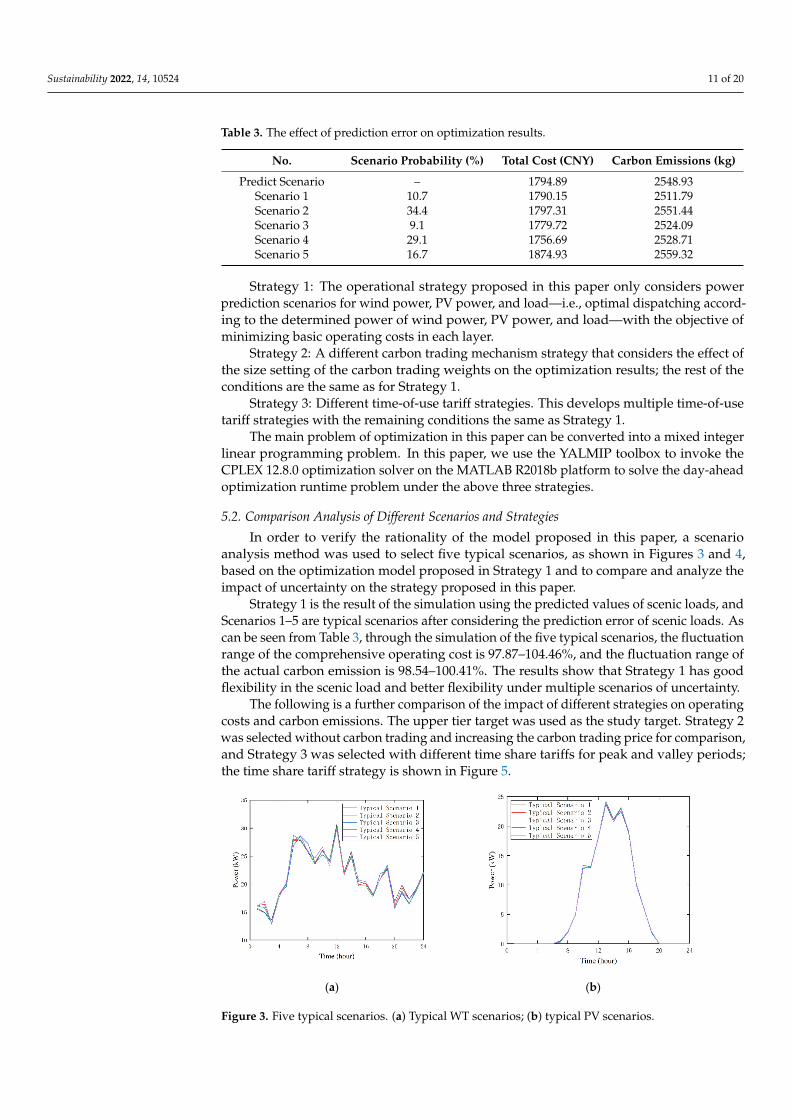
In order to verify the rationality of the model proposed in this paper, a scenarioanalysis method was used to select five typical scenarios, as shown in Figures 3 and 4,based on the optimization model proposed in Strategy 1 and to compare and analyze theimpact of uncertainty on the strategy proposed in this paper.

Strategy 1 is the result of the simulation using the predicted values of scenic loads, andScenarios 1–5 are typical scenarios after considering the prediction error of scenic loads. Ascan be seen from Table 3, through the simulation of the five typical scenarios, the fluctuationrange of the comprehensive operating cost is 97.87–104.46%, and the fluctuation range ofthe actual carbon emission is 98.54–100.41%. The results show that Strategy 1 has goodflexibility in the scenic load and better flexibility under multiple scenarios of uncertainty.

The following is a further comparison of the impact of different strategies on operatingcosts and carbon emissions. The upper tier target was used as the study target. Strategy 2was selected without carbon trading and increasing the carbon trading price for comparison,and Strategy 3 was selected with different time share tariffs for peak and valley periods;the time share tariff strategy is shown in Figure 5.

Sustainability 2022, 14, x FOR PEER REVIEW 12 of 20

(a) (b)

Figure 3. Five typical scenarios. (a) Typical WT scenarios; (b) typical PV scenarios.

(a) (b)

Figure 4. Five typical scenarios. (a) Typical AC load scenarios; (b) typical DC load scenarios.

Strategy 1 is the result of the simulation using the predicted values of scenic loads, and Scenarios 1–5 are typical scenarios after considering the prediction error of scenic loads. As can be seen from Table 3, through the simulation of the five typical scenarios, the fluctuation range of the comprehensive operating cost is 97.87–104.46%, and the fluc-tuation range of the actual carbon emission is 98.54–100.41%. The results show that Strat-egy 1 has good flexibility in the scenic load and better flexibility under multiple scenarios of uncertainty.

The following is a further comparison of the impact of different strategies on operat-ing costs and carbon emissions. The upper tier target was used as the study target. Strat-egy 2 was selected without carbon trading and increasing the carbon trading price for comparison, and Strategy 3 was selected with different time share tariffs for peak and valley periods; the time share tariff strategy is shown in Figure 5.

Figure 3. Five typical scenarios. (a) Typical WT scenarios; (b) typical PV scenarios.

Sustainability 2022, 14, 10524 12 of 20

Sustainability 2022, 14, x FOR PEER REVIEW 12 of 20

(a) (b)

Figure 3. Five typical scenarios. (a) Typical WT scenarios; (b) typical PV scenarios.

(a) (b)

Figure 4. Five typical scenarios. (a) Typical AC load scenarios; (b) typical DC load scenarios.

Strategy 1 is the result of the simulation using the predicted values of scenic loads, and Scenarios 1–5 are typical scenarios after considering the prediction error of scenic loads. As can be seen from Table 3, through the simulation of the five typical scenarios, the fluctuation range of the comprehensive operating cost is 97.87–104.46%, and the fluc-tuation range of the actual carbon emission is 98.54–100.41%. The results show that Strat-egy 1 has good flexibility in the scenic load and better flexibility under multiple scenarios of uncertainty.

The following is a further comparison of the impact of different strategies on operat-ing costs and carbon emissions. The upper tier target was used as the study target. Strat-egy 2 was selected without carbon trading and increasing the carbon trading price for comparison, and Strategy 3 was selected with different time share tariffs for peak and valley periods; the time share tariff strategy is shown in Figure 5.

Figure 4. Five typical scenarios. (a) Typical AC load scenarios; (b) typical DC load scenarios.

Sustainability 2022, 14, x FOR PEER REVIEW 13 of 20

Figure 5. Electricity price plan.

As can be seen from Table 4, comparing Strategy 2, the integrated operating cost without carbon trading is CNY 84.38 less than in Strategy 1, whereas the actual carbon emission is 132.7 kg more than in Strategy 1; meanwhile, the integrated operating cost and the actual carbon emission keep the same trend after increasing the carbon trading price. Comparing the objective function in the upper model, it can be concluded that the increase in carbon trading price makes the system adjust the energy allocation and the cost of elec-tricity purchase and the cost of the DC sub-microgrid increase, whereas the cost of the AC sub-microgrid decreases, indicating that the AC sub-microgrid has a larger share in car-bon emissions. Comparing Strategy 3, the combined operating costs and actual carbon emissions are greater under a constant tariff than in Strategy 1. Time-sharing Tariff 2 changes the peak and trough periods of the tariff, which in turn changes the microsource output for each period, while time-sharing Tariff 3 changes the size of the tariff for each period, causing the microsource output to increase and both the combined operating costs and actual carbon emissions to increase. The difference in operating costs between the different time-sharing tariff strategies chosen is mainly reflected in the cost of purchasing electricity. The uncertainty of the time-sharing tariff mainly affects the operating profit in the hybrid AC–DC microgrid model, whereas a large amount of historical information and reliable and publicly available data sources exists.

Table 4. The influence of different operation strategies on optimization results.

No. CACyx (CNY) CDCyx (CNY) CGRID (CNY) Total Cost (CNY) Ed (kg) Strategy 1 976.17 459.47 232.96 1794.89 2548.93

Strategy 2 a 986.91 560.23 120.49 1710.51 2681.63 b 945.24 459.47 263.61 1876.71 2516.68

Strategy 3 a 975.27 273.75 489.02 1835.54 2564.42 b 900.41 460.34 287.75 1760.53 2512.18 c 989.14 591.77 166.37 1876.62 2721.64

In addition to studying the economics of AC–DC hybrid microgrids, this paper also analyzes their flexibility. The upward and downward flexibility are used to characterize the flexibility of the microgrid system and to reflect the ability of the microgrid system to use the existing schedulable resources to respond to source–load uncertainty. The upward and downward flexibility are shown in Figure 6. The upward flexibility adjustment reaches the maximum value of 200kW in hours 1–7, whereas the downward flexibility adjustment reaches the maximum value in hours 19–21, and the remaining period has a sufficient margin.

Figure 5. Electricity price plan.

As can be seen from Table 4, comparing Strategy 2, the integrated operating costwithout carbon trading is CNY 84.38 less than in Strategy 1, whereas the actual carbonemission is 132.7 kg more than in Strategy 1; meanwhile, the integrated operating costand the actual carbon emission keep the same trend after increasing the carbon tradingprice. Comparing the objective function in the upper model, it can be concluded that theincrease in carbon trading price makes the system adjust the energy allocation and thecost of electricity purchase and the cost of the DC sub-microgrid increase, whereas thecost of the AC sub-microgrid decreases, indicating that the AC sub-microgrid has a largershare in carbon emissions. Comparing Strategy 3, the combined operating costs and actualcarbon emissions are greater under a constant tariff than in Strategy 1. Time-sharing Tariff 2changes the peak and trough periods of the tariff, which in turn changes the microsourceoutput for each period, while time-sharing Tariff 3 changes the size of the tariff for eachperiod, causing the microsource output to increase and both the combined operating costsand actual carbon emissions to increase. The difference in operating costs between thedifferent time-sharing tariff strategies chosen is mainly reflected in the cost of purchasingelectricity. The uncertainty of the time-sharing tariff mainly affects the operating profit inthe hybrid AC–DC microgrid model, whereas a large amount of historical information andreliable and publicly available data sources exists.

Sustainability 2022, 14, 10524 13 of 20

Table 4. The influence of different operation strategies on optimization results.

No. CACyx (CNY) CDCyx (CNY) CGRID (CNY) Total Cost (CNY) Ed (kg)

Strategy 1 976.17 459.47 232.96 1794.89 2548.93

Strategy 2 a 986.91 560.23 120.49 1710.51 2681.63b 945.24 459.47 263.61 1876.71 2516.68

Strategy 3a 975.27 273.75 489.02 1835.54 2564.42b 900.41 460.34 287.75 1760.53 2512.18c 989.14 591.77 166.37 1876.62 2721.64

In addition to studying the economics of AC–DC hybrid microgrids, this paper alsoanalyzes their flexibility. The upward and downward flexibility are used to characterizethe flexibility of the microgrid system and to reflect the ability of the microgrid systemto use the existing schedulable resources to respond to source–load uncertainty. Theupward and downward flexibility are shown in Figure 6. The upward flexibility adjustmentreaches the maximum value of 200kW in hours 1–7, whereas the downward flexibilityadjustment reaches the maximum value in hours 19–21, and the remaining period has asufficient margin.

Sustainability 2022, 14, x FOR PEER REVIEW 14 of 20

Figure 6. The upward and downward flexibility.

In summary, the operation scheme developed according to Strategy 1 has more ob-vious economic benefits and higher flexibility and is more adaptable to fluctuations in scenic load power, thus verifying the effectiveness of this paper’s scenario-analysis-based AC–DC hybrid microgrid operation optimization method on a one-hour time scale.

5.3. Day-Ahead Forecast Optimization Results Analysis The results of the AC–DC hybrid microgrid operation using Strategy 1 are shown in

Figures 7–11. The composition of the AC/DC load before and after the demand response is shown in Figure 7, from which it can be seen that load in the peak and valley hours before and after the demand response has a more obvious change. The load curve is smoothed out and the effect of peak and valley reduction is achieved. Figures 12–15 show the optimized operation results of the AC and DC sub-microgrids without considering the carbon trading mechanism and without considering the time-of-use electricity price, i.e., Strategy 2a and Strategy 3a.

The power output of each DG of the AC and DC sub-microgrids is shown in Figures 8 and 9, respectively. The wind power generation power is basically at a more average level within 24 h. The controllable microsources in the AC sub-microgrid include diesel generators and microcombustion turbines. The diesel generators are basically at their low-est power generation state due to their high-power generation cost and only play a backup role when the AC load is high (19:00~22:00). Microgas turbines, with their lower power generation costs, give full play to their power generation advantages during the hours when the gap between wind power and AC load is too large (9:00~24:00), thus meeting the demand, and the power generated by them in 24 h accounts for about 49.31% of the AC load. The AC sub-microgrid purchases power from the grid at a lower price during the valley load hours (24:00 to 08:00) and continues to purchase power from the grid dur-ing the peak load hours (16:00 to 18:00) to meet the load demand.

Figure 6. The upward and downward flexibility.

In summary, the operation scheme developed according to Strategy 1 has more obviouseconomic benefits and higher flexibility and is more adaptable to fluctuations in scenicload power, thus verifying the effectiveness of this paper’s scenario-analysis-based AC–DChybrid microgrid operation optimization method on a one-hour time scale.

5.3. Day-Ahead Forecast Optimization Results Analysis

The results of the AC–DC hybrid microgrid operation using Strategy 1 are shown inFigures 7–11. The composition of the AC/DC load before and after the demand response isshown in Figure 7, from which it can be seen that load in the peak and valley hours beforeand after the demand response has a more obvious change. The load curve is smoothed outand the effect of peak and valley reduction is achieved. Figures 12–15 show the optimizedoperation results of the AC and DC sub-microgrids without considering the carbon tradingmechanism and without considering the time-of-use electricity price, i.e., Strategy 2a andStrategy 3a.

Sustainability 2022, 14, 10524 14 of 20Sustainability 2022, 14, x FOR PEER REVIEW 15 of 20

Figure 7. Consequence of demand response.

Figure 8. Power output curves of AC sub-microgrid under Strategy 1.

Figure 9. Power output curves of DC sub-microgrid under Strategy 1.

PV power generation increases and then decreases from 8:00 to 18:00. The controlla-ble microsource in the DC sub-microgrid is the fuel cell. During the period from 9:00 to 24:00, the load demand starts to gradually increase, and the fuel cell output also starts to gradually increase, becoming the main source of electricity for the DC sub-microgrid. The power generated by it in 24 h accounts for about 64.15% of the DC load, and due to the emergence of PV, the fuel cell does not reach its maximum power at first. The battery is charged during the valley tariff and when the load level is not high (1:00 to 7:00) and discharged during the higher load hours (13:00, 19:00 to 23:00), if it meets the requirements

Figure 7. Consequence of demand response.

Sustainability 2022, 14, x FOR PEER REVIEW 15 of 20

Figure 7. Consequence of demand response.

Figure 8. Power output curves of AC sub-microgrid under Strategy 1.

Figure 9. Power output curves of DC sub-microgrid under Strategy 1.

PV power generation increases and then decreases from 8:00 to 18:00. The controlla-ble microsource in the DC sub-microgrid is the fuel cell. During the period from 9:00 to 24:00, the load demand starts to gradually increase, and the fuel cell output also starts to gradually increase, becoming the main source of electricity for the DC sub-microgrid. The power generated by it in 24 h accounts for about 64.15% of the DC load, and due to the emergence of PV, the fuel cell does not reach its maximum power at first. The battery is charged during the valley tariff and when the load level is not high (1:00 to 7:00) and discharged during the higher load hours (13:00, 19:00 to 23:00), if it meets the requirements

Figure 8. Power output curves of AC sub-microgrid under Strategy 1.

Sustainability 2022, 14, x FOR PEER REVIEW 15 of 20

Figure 7. Consequence of demand response.

Figure 8. Power output curves of AC sub-microgrid under Strategy 1.

Figure 9. Power output curves of DC sub-microgrid under Strategy 1.

PV power generation increases and then decreases from 8:00 to 18:00. The controlla-ble microsource in the DC sub-microgrid is the fuel cell. During the period from 9:00 to 24:00, the load demand starts to gradually increase, and the fuel cell output also starts to gradually increase, becoming the main source of electricity for the DC sub-microgrid. The power generated by it in 24 h accounts for about 64.15% of the DC load, and due to the emergence of PV, the fuel cell does not reach its maximum power at first. The battery is charged during the valley tariff and when the load level is not high (1:00 to 7:00) and discharged during the higher load hours (13:00, 19:00 to 23:00), if it meets the requirements

Figure 9. Power output curves of DC sub-microgrid under Strategy 1.

Sustainability 2022, 14, 10524 15 of 20

Sustainability 2022, 14, x FOR PEER REVIEW 16 of 20

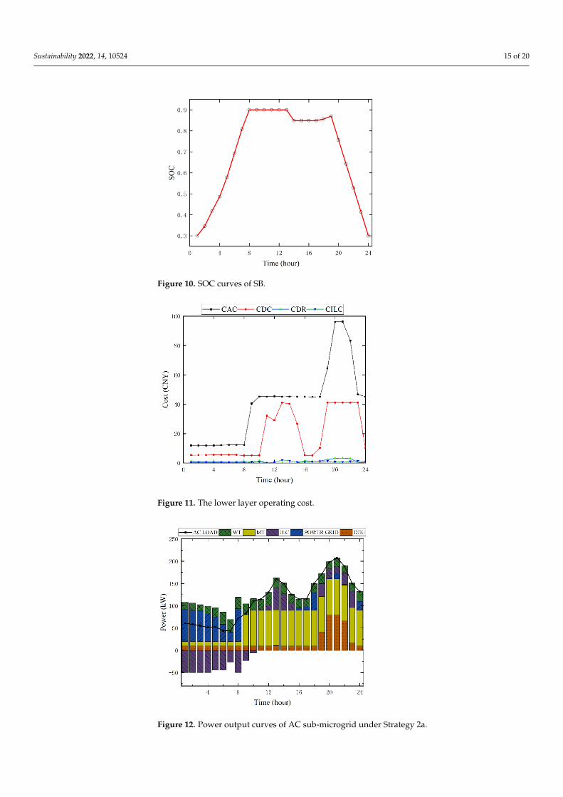
of the charge state. Figure 10 shows the charge state of the battery as a function of time. The battery acts as an energy buffer link to complement other distributed energy sources, playing a role in peak and valley reduction while also increasing the flexibility of the sys-tem.

The AC sub-microgrid and the DC sub-microgrid exchange power through a bidirec-tional power converter. The figure shows the interactive power between the sub-mi-crogrids, setting the input sub-microgrid as positive. Combining the two diagrams, it can be concluded that during the period from 1:00 to 7:00, the PV power is 0, the AC sub-microgrid delivers power to the DC sub-microgrid, and the DC sub-microgrid uses the resulting power to balance the load and charge the battery. During the period from 12:00 to 15:00, the PV output is larger, while the AC sub-microgrid experiences a peak load, and the DC sub-microgrid delivers power to the AC sub-microgrid to satisfy the power bal-ance. During the hours of 19:00~23:00, the AC and DC loads come to the peak hours of the day, the battery starts to discharge under the premise of meeting the requirements of the charge state, and the DC sub-microgrid transmits power to the AC sub-microgrid due to the overload of the AC sub-microgrid. The time curve of each cost in the lower layer ob-jective function is shown in Figure 11.

In contrast, as illustrated in Figures 12–15, Strategy 2a has a big difference in the out-put period of the MT and FC, whereas Strategy 3a has a significant decrease in the output of the FC due to the increase in electricity purchased from the grid, and the BS is not fully utilized.

Figure 10. SOC curves of SB.

Figure 11. The lower layer operating cost.

Figure 10. SOC curves of SB.

Sustainability 2022, 14, x FOR PEER REVIEW 16 of 20

of the charge state. Figure 10 shows the charge state of the battery as a function of time. The battery acts as an energy buffer link to complement other distributed energy sources, playing a role in peak and valley reduction while also increasing the flexibility of the sys-tem.

The AC sub-microgrid and the DC sub-microgrid exchange power through a bidirec-tional power converter. The figure shows the interactive power between the sub-mi-crogrids, setting the input sub-microgrid as positive. Combining the two diagrams, it can be concluded that during the period from 1:00 to 7:00, the PV power is 0, the AC sub-microgrid delivers power to the DC sub-microgrid, and the DC sub-microgrid uses the resulting power to balance the load and charge the battery. During the period from 12:00 to 15:00, the PV output is larger, while the AC sub-microgrid experiences a peak load, and the DC sub-microgrid delivers power to the AC sub-microgrid to satisfy the power bal-ance. During the hours of 19:00~23:00, the AC and DC loads come to the peak hours of the day, the battery starts to discharge under the premise of meeting the requirements of the charge state, and the DC sub-microgrid transmits power to the AC sub-microgrid due to the overload of the AC sub-microgrid. The time curve of each cost in the lower layer ob-jective function is shown in Figure 11.

In contrast, as illustrated in Figures 12–15, Strategy 2a has a big difference in the out-put period of the MT and FC, whereas Strategy 3a has a significant decrease in the output of the FC due to the increase in electricity purchased from the grid, and the BS is not fully utilized.

Figure 10. SOC curves of SB.

Figure 11. The lower layer operating cost. Figure 11. The lower layer operating cost.

Sustainability 2022, 14, x FOR PEER REVIEW 17 of 20

Figure 12. Power output curves of AC sub-microgrid under Strategy 2a.

Figure 13. Power output curves of DC sub-microgrid under Strategy 2a.

Figure 14. Power output curves of AC sub-microgrid under Strategy 3a.

Figure 12. Power output curves of AC sub-microgrid under Strategy 2a.

Sustainability 2022, 14, 10524 16 of 20

Sustainability 2022, 14, x FOR PEER REVIEW 17 of 20

Figure 12. Power output curves of AC sub-microgrid under Strategy 2a.

Figure 13. Power output curves of DC sub-microgrid under Strategy 2a.

Figure 14. Power output curves of AC sub-microgrid under Strategy 3a.

Figure 13. Power output curves of DC sub-microgrid under Strategy 2a.

Sustainability 2022, 14, x FOR PEER REVIEW 17 of 20

Figure 12. Power output curves of AC sub-microgrid under Strategy 2a.

Figure 13. Power output curves of DC sub-microgrid under Strategy 2a.

Figure 14. Power output curves of AC sub-microgrid under Strategy 3a. Figure 14. Power output curves of AC sub-microgrid under Strategy 3a.

Sustainability 2022, 14, x FOR PEER REVIEW 18 of 20

Figure 15. Power output curves of DC sub-microgrid under Strategy 3a.

5.4. The Impact of Carbon Trading Price on System Operation The carbon trading price can be regarded as the weight of the objective function, so

the change of the carbon trading price will affect the carbon emission, carbon trading cost, and energy purchase cost and thus affect the total operating cost of the system. In order to further study the impact of carbon trading price on system operation, the relationship between total operating cost and actual carbon emissions with carbon price was drawn, as shown in Figure 16.

Figure 16. Carbon price relationship curve.

The actual carbon emission generally decreases with the increase in the carbon trad-ing price. A carbon trading price between CNY 10–20 and 70–80 leads to a large change in the actual carbon emission, and the rest of the changes are basically the same. The total operating cost increases with the increase in the carbon trading price, and the growth rate is basically the same. From the above analysis, setting a reasonable carbon trading price can promote the synergy of system economy and low carbon.

6. Conclusions In this paper, a two-layer optimization model has been designed for AC–DC hybrid

microgrid, which considers the carbon trading mechanism and the prediction uncertain-ties of renewable energy and load. Through the analysis of three strategies considering the uncertainties in multiple scenarios, the following conclusions can be drawn up: (1) The optimization model proposed in this paper has good results in terms of the eco-

nomic benefits of microgrids as well as carbon emissions, realizing a reasonable

Figure 15. Power output curves of DC sub-microgrid under Strategy 3a.

Sustainability 2022, 14, 10524 17 of 20

The power output of each DG of the AC and DC sub-microgrids is shown in Figures 8 and 9,respectively. The wind power generation power is basically at a more average level within24 h. The controllable microsources in the AC sub-microgrid include diesel generatorsand microcombustion turbines. The diesel generators are basically at their lowest powergeneration state due to their high-power generation cost and only play a backup role whenthe AC load is high (19:00~22:00). Microgas turbines, with their lower power generationcosts, give full play to their power generation advantages during the hours when the gapbetween wind power and AC load is too large (9:00~24:00), thus meeting the demand, andthe power generated by them in 24 h accounts for about 49.31% of the AC load. The ACsub-microgrid purchases power from the grid at a lower price during the valley load hours(24:00 to 08:00) and continues to purchase power from the grid during the peak load hours(16:00 to 18:00) to meet the load demand.

PV power generation increases and then decreases from 8:00 to 18:00. The controllablemicrosource in the DC sub-microgrid is the fuel cell. During the period from 9:00 to 24:00,the load demand starts to gradually increase, and the fuel cell output also starts to graduallyincrease, becoming the main source of electricity for the DC sub-microgrid. The powergenerated by it in 24 h accounts for about 64.15% of the DC load, and due to the emergenceof PV, the fuel cell does not reach its maximum power at first. The battery is charged duringthe valley tariff and when the load level is not high (1:00 to 7:00) and discharged duringthe higher load hours (13:00, 19:00 to 23:00), if it meets the requirements of the charge state.Figure 10 shows the charge state of the battery as a function of time. The battery acts as anenergy buffer link to complement other distributed energy sources, playing a role in peakand valley reduction while also increasing the flexibility of the system.

The AC sub-microgrid and the DC sub-microgrid exchange power through a bidirec-tional power converter. The figure shows the interactive power between the sub-microgrids,setting the input sub-microgrid as positive. Combining the two diagrams, it can be con-cluded that during the period from 1:00 to 7:00, the PV power is 0, the AC sub-microgriddelivers power to the DC sub-microgrid, and the DC sub-microgrid uses the resultingpower to balance the load and charge the battery. During the period from 12:00 to 15:00,the PV output is larger, while the AC sub-microgrid experiences a peak load, and theDC sub-microgrid delivers power to the AC sub-microgrid to satisfy the power balance.During the hours of 19:00~23:00, the AC and DC loads come to the peak hours of theday, the battery starts to discharge under the premise of meeting the requirements of thecharge state, and the DC sub-microgrid transmits power to the AC sub-microgrid dueto the overload of the AC sub-microgrid. The time curve of each cost in the lower layerobjective function is shown in Figure 11.

In contrast, as illustrated in Figures 12–15, Strategy 2a has a big difference in the outputperiod of the MT and FC, whereas Strategy 3a has a significant decrease in the output of theFC due to the increase in electricity purchased from the grid, and the BS is not fully utilized.

5.4. The Impact of Carbon Trading Price on System Operation

The carbon trading price can be regarded as the weight of the objective function, sothe change of the carbon trading price will affect the carbon emission, carbon trading cost,and energy purchase cost and thus affect the total operating cost of the system. In orderto further study the impact of carbon trading price on system operation, the relationshipbetween total operating cost and actual carbon emissions with carbon price was drawn, asshown in Figure 16.

The actual carbon emission generally decreases with the increase in the carbon tradingprice. A carbon trading price between CNY 10–20 and 70–80 leads to a large change inthe actual carbon emission, and the rest of the changes are basically the same. The totaloperating cost increases with the increase in the carbon trading price, and the growth rateis basically the same. From the above analysis, setting a reasonable carbon trading pricecan promote the synergy of system economy and low carbon.

Sustainability 2022, 14, 10524 18 of 20

Sustainability 2022, 14, x FOR PEER REVIEW 18 of 20

Figure 15. Power output curves of DC sub-microgrid under Strategy 3a.

5.4. The Impact of Carbon Trading Price on System Operation The carbon trading price can be regarded as the weight of the objective function, so

the change of the carbon trading price will affect the carbon emission, carbon trading cost, and energy purchase cost and thus affect the total operating cost of the system. In order to further study the impact of carbon trading price on system operation, the relationship between total operating cost and actual carbon emissions with carbon price was drawn, as shown in Figure 16.

Figure 16. Carbon price relationship curve.

The actual carbon emission generally decreases with the increase in the carbon trad-ing price. A carbon trading price between CNY 10–20 and 70–80 leads to a large change in the actual carbon emission, and the rest of the changes are basically the same. The total operating cost increases with the increase in the carbon trading price, and the growth rate is basically the same. From the above analysis, setting a reasonable carbon trading price can promote the synergy of system economy and low carbon.

6. Conclusions In this paper, a two-layer optimization model has been designed for AC–DC hybrid

microgrid, which considers the carbon trading mechanism and the prediction uncertain-ties of renewable energy and load. Through the analysis of three strategies considering the uncertainties in multiple scenarios, the following conclusions can be drawn up: (1) The optimization model proposed in this paper has good results in terms of the eco-

nomic benefits of microgrids as well as carbon emissions, realizing a reasonable

Figure 16. Carbon price relationship curve.

6. Conclusions

In this paper, a two-layer optimization model has been designed for AC–DC hybridmicrogrid, which considers the carbon trading mechanism and the prediction uncertaintiesof renewable energy and load. Through the analysis of three strategies considering theuncertainties in multiple scenarios, the following conclusions can be drawn up:

(1) The optimization model proposed in this paper has good results in terms of theeconomic benefits of microgrids as well as carbon emissions, realizing a reasonableallocation and use of resources and effectively coordinating the economy and lowcarbon of system operation.

(2) In this paper, the impact of various uncertainties on the system was verified bysimulating and analyzing the uncertainties of wind, PV, load, and tariff. A reasonabletime-sharing tariff strategy can not only reduce system operating costs but also reducecarbon emissions to a certain extent.

(3) By comparing the impact of the price of carbon trading costs on the optimized opera-tion results, this paper concludes that the total operating cost of the system steadilyincreases with the increase in carbon trading price, and the carbon emissions showa phased decrease with the change of carbon trading price; furthermore, setting areasonable carbon trading price can synergize low carbon and economy.

Follow-up work will consider the feasibility of optimizing the operation on a timescale of minutes and conduct a more in-depth study of the impact of a stepped carbontrading mechanism on the operation of the system.

Author Contributions: L.Y. and Y.Z. conceived the research. Y.Z. participated in the analysis ofthe data and in writing the initial manuscript. T.X., N.M., Z.L. and Z.Y. revised the manuscriptand adjusted the data presentation. All authors have read and agreed to the published version ofthe manuscript.

Funding: This research received no external funding.

Informed Consent Statement: Not applicable.

Conflicts of Interest: The authors declare no conflict of interest.

Sustainability 2022, 14, 10524 19 of 20

References1. Kumar, P.P.; Saini, R.P. Optimization of an off-grid integrated hybrid renewable energy system with different battery technologies

for rural electrification in India. J. Energy Storage 2020, 32, 101912. [CrossRef]2. Zhu, L.; Tong, Q.; Yan, X.; Liu, Y.; Zhang, J.; Li, Y.; Huang, G. Optimal design of multi-energy complementary power generation

system considering fossil energy scarcity coefficient under uncertainty. J. Clean. Prod. 2020, 274, 122732. [CrossRef]3. Zahraoui, Y.; Alhamrouni, I.; Mekhilef, S.; Basir Khan, M.R.; Seyedmahmoudian, M.; Stojcevski, A.; Horan, B. Energy Management

System in Microgrids: A Comprehensive Review. Sustainability 2021, 13, 10492. [CrossRef]4. Wang, K.; Niu, D.; Yu, M.; Liang, Y.; Yang, X.; Wu, J.; Xu, X. Analysis and Countermeasures of China’s Green Electric Power

Development. Sustainability 2021, 13, 708. [CrossRef]5. Azeem, O.; Ali, M.; Abbas, G.; Uzair, M.; Qahmash, A.; Algarni, A.; Hussain, M. A Comprehensive Review on Integration

Challenges, Optimization Techniques and Control Strategies of Hybrid AC/DC Microgrid. Appl. Sci. 2021, 11, 6242. [CrossRef]6. Li, P.; Zheng, M. Multi-objective optimal operation of hybrid AC/DC microgrid considering source-network-load coordination. J.

Mod. Power Syst. Clean Energy 2019, 7, 1229–1240. [CrossRef]7. Jiang, K.; Wu, F.; Zong, X.; Shi, L.; Lin, K. Distributed Dynamic Economic Dispatch of an Isolated AC/DC Hybrid Microgrid

Based on a Finite-Step Consensus Algorithm. Energies 2019, 12, 4637. [CrossRef]8. Wei, B.; Han, X.; Wang, P.; Yu, H.; Li, W.; Guo, L. Temporally Coordinated Energy Management for AC/DC Hybrid Microgrid

Considering Dynamic Conversion Efficiency of Bidirectional AC/DC Converter. IEEE Access 2020, 8, 70878–70889. [CrossRef]9. Li, Y.; Yang, Z.; Li, G.; Zhao, D.; Tian, W. Optimal Scheduling of an Isolated Microgrid With Battery Storage Considering Load

and Renewable Generation Uncertainties. IEEE Trans. Ind. Electron. 2018, 66, 1565–1575. [CrossRef]10. Hosseini, S.M.; Carli, R.; Dotoli, M. Robust Optimal Energy Management of a Residential Microgrid Under Uncertainties on

Demand and Renewable Power Generation. IEEE Trans. Autom. Sci. Eng. 2021, 18, 618–637. [CrossRef]11. Jabr, R.A. Mixed-Integer Convex Optimization for DC Microgrid Droop Control. IEEE Trans. Power Syst. 2021, 36, 5901–5908. [CrossRef]12. Deng, X.; Lv, T. Power system planning with increasing variable renewable energy: A review of optimization models. J. Clean.

Prod. 2019, 246, 118962. [CrossRef]13. Jiang, Y.; Kang, L.; Liu, Y. The coordinated optimal design of a PV-battery system with multiple types of PV arrays and batteries:

A case study of power smoothing. J. Clean. Prod. 2021, 310, 127436. [CrossRef]14. Mbungu, N.T.; Naidoo, R.M.; Bansal, R.C.; Vahidinasab, V. Overview of the Optimal Smart Energy Coordination for Microgrid

Applications. IEEE Access 2019, 7, 163063–163084. [CrossRef]15. Qiu, H.; Gu, W.; Xu, Y.; Zhao, B. Multi-Time-Scale Rolling Optimal Dispatch for AC/DC Hybrid Microgrids with Day-Ahead

Distributionally Robust Scheduling. IEEE Trans. Sustain. Energy 2018, 10, 1653–1663. [CrossRef]16. Liang, Z.; Chen, H.; Wang, X.; Chen, S.; Zhang, C. Risk-Based Uncertainty Set Optimization Method for Energy Management of

Hybrid AC/DC Microgrids with Uncertain Renewable Generation. IEEE Trans. Smart Grid 2020, 11, 1526–1542. [CrossRef]17. Li, Q.; Li, A.; Wang, T.; Cai, Y. Interconnected hybrid AC-DC microgrids security enhancement using blockchain technology

considering uncertainty. Int. J. Electr. Power Energy Syst. 2021, 133, 107324. [CrossRef]18. Zhang, L.; Yang, Y.; Li, Q.; Gao, W.; Qian, F.; Song, L. Economic optimization of microgrids based on peak shaving and CO2

reduction effect: A case study in Japan. J. Clean. Prod. 2021, 321, 128973. [CrossRef]19. Li, F.; Qin, J.; Kang, Y. Closed-Loop Hierarchical Operation for Optimal Unit Commitment and Dispatch in Microgrids: A Hybrid

System Approach. IEEE Trans. Power Syst. 2020, 35, 516–526. [CrossRef]20. Li, L.; Yu, S. Optimal management of multi-stakeholder distributed energy systems in low-carbon communities considering

demand response resources and carbon tax. Sustain. Cities Soc. 2020, 61, 102230. [CrossRef]21. Su, J.; Li, Z.; Jin, A.J. Practical Model for Optimal Carbon Control with Distributed Energy Resources. IEEE Access 2021, 9,

161603–161612. [CrossRef]22. Saeed, M.H.; Wang, F.; Salem, S.; Khan, Y.A.; Kalwar, B.A.; Fars, A. Two-stage intelligent planning with improved artificial bee

colony algorithm for a microgrid by considering the uncertainty of renewable sources. Energy Rep. 2021, 7, 8912–8928. [CrossRef]23. Kharrich, M.; Kamel, S.; Hassan, M.H.; ElSayed, S.K.; Taha, I.B.M. An Improved Heap-Based Optimizer for Optimal Design of a

Hybrid Microgrid Considering Reliability and Availability Constraints. Sustainability 2021, 13, 10419. [CrossRef]24. Lu, H.; Ma, X.; Huang, K.; Azimi, M. Carbon trading volume and price forecasting in China using multiple machine learning

models. J. Clean. Prod. 2020, 249, 119386. [CrossRef]25. Zakeri, A.; Dehghanian, F.; Fahimnia, B.; Sarkis, J. Carbon pricing versus emissions trading: A supply chain planning perspective.

Int. J. Prod. Econ. 2015, 164, 197–205. [CrossRef]26. Cao, K.; Xu, X.; Wu, Q.; Zhang, Q. Optimal production and carbon emission reduction level under cap-and-trade and low carbon

subsidy policies. J. Clean. Prod. 2017, 167, 505–513. [CrossRef]27. Zhu, L.; Zhou, X.; Zhang, X.; Yan, Z.; Guo, S.; Tang, L. Integrated resources planning in microgrids considering interruptible

loads and shiftable loads. J. Mod. Power Syst. Clean Energy 2018, 6, 802–815. [CrossRef]28. Wu, N.; Wang, H.; Yin, L.; Yuan, X.; Leng, X. Application Conditions of Bounded Rationality and a Microgrid Energy Management

Control Strategy Combining Real-Time Power Price and Demand-Side Response. IEEE Access 2020, 8, 227327–227339. [CrossRef]29. Hu, M.; Xiao, F.; Wang, S. Neighborhood-level coordination and negotiation techniques for managing demand-side flexibility in

residential microgrids. Renew. Sustain. Energy Rev. 2021, 135, 110248. [CrossRef]

Sustainability 2022, 14, 10524 20 of 20

30. Liu, Z.; Liu, S.; Li, Q.; Zhang, Y.; Deng, W.; Zhou, L. Optimal Day-ahead Scheduling of Islanded Microgrid Considering Risk-basedReserve Decision. J. Mod. Power Syst. Clean Energy 2021, 9, 1149–1160. [CrossRef]

31. Faraji, J.; Hashemi-Dezaki, H.; Ketabi, A. Optimal probabilistic scenario-based operation and scheduling of prosumer microgridsconsidering uncertainties of renewable energy sources. Energy Sci. Eng. 2020, 8, 3942–3960. [CrossRef]

32. Cen, B.; Cai, Z.; Liu, P.; Chen, Y.; Sun, Y.; Hu, K.; Zeng, X. Characteristic matching of stochastic scenarios and flexible resourcecapacity optimisation for isolated microgrids. IET Gener. Transm. Distrib. 2020, 14, 6009–6018. [CrossRef]

33. Li, P.; Xu, D.; Zhou, Z.; Lee, W.; Zhao, B. Stochastic optimal operation of microgrid based on chaotic binary particle swarmoptimization. IEEE Trans. Smart Grid 2016, 7, 66–73. [CrossRef]

34. Mohamed, F.A.; Koivo, H.N. System modelling and online optimal management of microgrid using mesh adaptive direct search.Int. J. Electr. Power Energy Syst. 2010, 32, 398–407. [CrossRef]

35. Pipattanasomporn, M.; Willingham, M.; Rahman, S. Implications of on-site distributed generation for commercial/industrialfacilities. IEEE Trans. Power Syst. 2005, 20, 206–212. [CrossRef]