Trophic modelling of a New Zealand rocky reef ecosystem using simultaneous adjustment of diet,...

Journal of Experimental Marine Biology and Ecology 367 (2008) 189–203

Contents lists available at ScienceDirect

Journal of Experimental Marine Biology and Ecology

j ourna l homepage: www.e lsev ie r.com/ locate / jembe

Trophic modelling of a New Zealand rocky reef ecosystem using simultaneousadjustment of diet, biomass and energetic parameters

M.H. Pinkerton a,⁎, C.J. Lundquist b, C.A.J. Duffy c, D.J. Freeman d

a National Institute of Water and Atmospheric Research (NIWA), Private Bag 14-901, Kilbirnie, Wellington, New Zealandb NIWA, P.O. Box 11-115, Hamilton, New Zealandc Department of Conservation (DoC), Aquatic and Threats Unit, Private Bag 68-908, Newton, Auckland, New Zealandd DoC, Aquatic and Threats Unit, P.O. Box 10-420, Wellington, New Zealand

⁎ Corresponding author.E-mail address: [email protected] (M.H. Pinke

0022-0981/$ – see front matter © 2008 Elsevier B.V. Aldoi:10.1016/j.jembe.2008.09.022

a b s t r a c t
a r t i c l e i n f o
Article history:
We present a balanced mod Received 2 July 2007Received in revised form 18 September 2008Accepted 23 September 2008
Keywords:Carbon fluxEcopathInverse methodMass balanceNew ZealandRocky reefTemperate coastal ecosystemTrophic model

el of organic carbon flows through a temperate coastal ecosystem in New Zealand.The Te Tapuwae o RongokakoMarine Reserve is a 2452 ha no-take area including both rocky reef platforms andsoft sediment, and covering the intertidal and subtidal communities to depths of approximately 50 m. Themodel includes 22 trophic groups, including birds, predatory and grazing invertebrates, detritivores, fivegroups of fish, microphytes, macroalgae, zooplankton, phytoplankton, bacteria and detritus. Initialparameterisations of the model were developed from video, diver and quadrat surveys in the study area,augmented by parameters derived from simple population models and scientific literature. A novel two stagebalancing methodology is presented which adjusts biomasses, diet fractions, and energetic parameters of alltrophic groups simultaneously, taking into account estimated parameter uncertainties and the highly variablemagnitudes of flows through different groups (6 orders of magnitude). Most adjustments to the initialparameters necessary to balance the trophic model were b20%, but large adjustments were needed for poorlyobserved groups such as bacteria, sponge, and phytoplankton. The balanced model is recognised as being onesolution amongst many. In the model, 94% of the primary production remained ungrazed and formedparticulate and dissolved organic detritus. The balanced model indicated that the reserve is relativelyimpoverished in terms of grazers and predators relative to New Zealand rocky reefs to the north. The modelsuggests that lobsters, which have increased in numbers since the reserve was established, are responsible forsubstantial predation on invertebrate groups which make up their prey (grazing, predatory, phytal/infaunalinvertebrates). The level of predation on invertebrates by lobster in the model depends significantly on theextent to which lobsters in TTMR are consuming macroalgae.

© 2008 Elsevier B.V. All rights reserved.

1. Introduction

Rocky reefs are a common coastal habitat throughout temperatewaters and occur around much of the coast of New Zealand (Andrewand Francis, 2005). Their ubiquity and accessibility means that theirecosystems are often extensively studied (e.g. Taylor,1998a,b,c; Mengeet al., 1999; Shears and Babcock, 2003, 2004a). The fact that temperaterocky reefs often occur close to human habitationmean that they tendto be vulnerable to anthropogenic disturbance at the local level(e.g. fisheries, sedimentation, pollution). Protection of coastal areasthrough the establishment of no-take areas often leads to changes incommunity structure through indirect trophic cascade effects (Shearsand Babcock, 2003). Changes can be unexpected, take some time tooccur, and differ between areas (Davidson et al., 2002; Kelly et al.,2000, 2002; Shears and Babcock, 2003; Willis et al., 2003; Langloisand Ballantine, 2005). Considerable interest lies in assessing to what

rton).

l rights reserved.

extent we can use numerical ecosystem models to describe coastalecosystems with a view to predicting how ecosystems will respond tovarious disturbances and management activities.

A variety of coastal ecosystem models are available. At oneextreme, ecosystem models are “biologically-realistic” in that theyare based on detailed, often non-linear, parameterisations of indivi-dual species, interactions and processes (e.g. ERSEM: Baretta et al.,1995; InVitro: Gray et al., 2006; ATLANTIS: Fulton et al., 2003, 2004).The complexity of thesemodels tends to lead to complex relationshipsbetween model inputs and outputs, and the robustness of predictionsto input uncertainties and stochastic effects is often difficult to assess.Time series of measurements of ecosystems at the level needed tovalidate such ecosystem models are rare. At the other extreme,stylised models have been developed to investigate the generalcharacteristics of complex ecosystems, without being specific to anyone area (e.g. May, 1973; Martinez and Dunne, 1998). These stylisedmodels can generate hypotheses that can be tested in particularsystems using field data (e.g. Bertness and Callaway, 1994; Mengeet al., 1994; Brose et al., 2005). Between these two extremes are

mailto:[email protected]

http://dx.doi.org/10.1016/j.jembe.2008.09.022

http://www.sciencedirect.com/science/journal/00220981

190 M.H. Pinkerton et al. / Journal of Experimental Marine Biology and Ecology 367 (2008) 189–203

models which aim to provide a relatively simple, quantitative descrip-tion of the structure, particularly trophic structure, of a particularecosystem.

Mass-balance models bring together varied field data andliterature information to provide a self-consistent picture of thetrophic structure of a given ecosystem. Ecosystem function anddynamics are closely but not simply related to ecosystem structure(Pascual and Dunne, 2006), so that a model of the trophic structure ofa particular ecosystem is not sufficient to predict its dynamics, but isan extremely valuable precursor to developing dynamic or mechan-istic ecosystem models. Given that parameters in such models areimperfectly known, a number of studies have used inverse methods toreconstruct flux through an ecosystem based on incomplete knowl-edge (e.g. Polovina,1984; Vezina and Platt, 1988; Jackson and Eldridge,1992; Niquil et al., 1998; Donali et al., 1999). The Ecopath/EcoSimsoftware (Christensen and Pauly, 1992; Christensen and Walters,2004; Christensen et al., 2004) has become a commonly usedapproach to the inverse modelling problem (e.g. Mendoza, 1993;Wolff, 1994; Jarre-Teichmann et al., 1998; Arreguin-Sanchez et al.,2002; Jiang and Gibbs, 2005). The general scheme is to obtain a set ofmodel parameters from fieldmonitoring data and the literature. Theseparameters will have varying levels of uncertainty associated withthem, and, in general, will not lead to a self-consistent (balanced)model. Expert opinion and numerical techniques are typically used toadjust the initial set of parameters to obtain balance. The need forautomated adjustment of parameters led to the development ofEcoranger, available within Ecopath/EcoSim (Kavanagh et al., 2004)which adjusts biomass and diet fractions to achieve a plausiblebalanced model, and allow the effects of parameter uncertainty to beinvestigated (Plagányi, 2007). Here, we present an alternative toEcoranger in the form of a novel technique which allows all keyparameters, including energetic parameters, to be adjusted simulta-

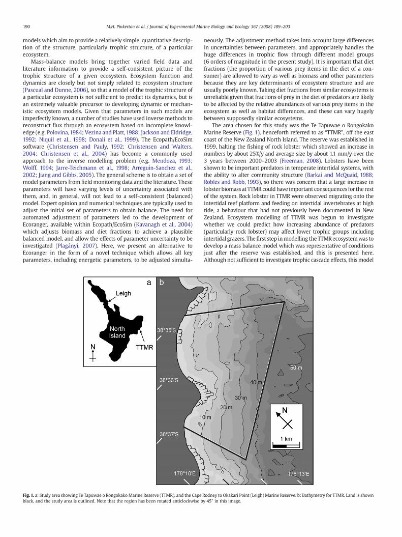
Fig. 1. a: Study area showing Te Tapuwae o Rongokako Marine Reserve (TTMR), and the Capeblack, and the study area is outlined. Note that the region has been rotated anticlockwise b

neously. The adjustment method takes into account large differencesin uncertainties between parameters, and appropriately handles thehuge differences in trophic flow through different model groups(6 orders of magnitude in the present study). It is important that dietfractions (the proportion of various prey items in the diet of a con-sumer) are allowed to vary as well as biomass and other parametersbecause they are key determinants of ecosystem structure and areusually poorly known. Taking diet fractions from similar ecosystems isunreliable given that fractions of prey in the diet of predators are likelyto be affected by the relative abundances of various prey items in theecosystem as well as habitat differences, and these can vary hugelybetween supposedly similar ecosystems.

The area chosen for this study was the Te Tapuwae o RongokakoMarine Reserve (Fig. 1), henceforth referred to as “TTMR”, off the eastcoast of the New Zealand North Island. The reserve was established in1999, halting the fishing of rock lobster which showed an increase innumbers by about 25%/y and average size by about 1.1 mm/y over the3 years between 2000–2003 (Freeman, 2008). Lobsters have beenshown to be important predators in temperate intertidal systems, withthe ability to alter community structure (Barkai and McQuaid, 1988;Robles and Robb, 1993), so there was concern that a large increase inlobster biomass at TTMRcould have important consequences for the restof the system. Rock lobster in TTMR were observed migrating onto theintertidal reef platform and feeding on intertidal invertebrates at hightide, a behaviour that had not previously been documented in NewZealand. Ecosystem modelling of TTMR was begun to investigatewhether we could predict how increasing abundance of predators(particularly rock lobster) may affect lower trophic groups includingintertidal grazers. Thefirst step inmodelling the TTMRecosystemwas todevelop a mass balance model which was representative of conditionsjust after the reserve was established, and this is presented here.Although not sufficient to investigate trophic cascade effects, this model

Rodney to Okakari Point (Leigh) Marine Reserve. b: Bathymetry for TTMR. Land is showny 45° in this image.

191M.H. Pinkerton et al. / Journal of Experimental Marine Biology and Ecology 367 (2008) 189–203

improves understanding of the system and has involved developing anovel model balancing technique that could be applied elsewhere.

2. Methods

2.1. Study area

The focus of the current work, Te Tapuwae o Rongokako MarineReserve (TTMR) is a 2452 ha area including both rock platforms and softsediment, and covering the intertidal and subtidal communities todepths of approximately 50 m (Stephens et al., 2006). Several distincthabitats are found in the reserve including sandy beaches, intertidal reefplatforms, shallow weed zones, urchin barrens, kelp forest, deep reefslope, sedimentflats, and deepmudflats (Ngati Konohi andDepartmentof Conservation,1998). There are a suite of grazing, predatory, and sessileinvertebrates, including gastropods, bivalves, crabs, sponges, sea urchin,and the rock lobster (Jasus edwardsii). Monitoring of the abundance oforganisms in the TTMR ecosystem has been ongoing since 1990, butincreased in intensity for theperiod 2000–2003. These lattermonitoringdata form the basis of the currentwork.We alsouseddata from the best-studied no-take area in New Zealand (Cape Rodney to Okakari PointMarine Reserve near Leigh, hereafter referred to as “Leigh”, Fig. 1) as asimple reality-check on data collected in TTMR.

2.2. Model structure

The trophic model developed here quantifies the transfer of organicmaterial through a highly stylised view of the ecosystem to provide asystem-level overview of its structure. The model used the main mass-balance identities of the Ecopath trophic model (Pauly et al., 2000;Christensen and Walters, 2004; Christensen et al., 2004) (Eqs. (1)–(3)below). The fact that this approach is commonly used around the worldfacilitates intercomparison of model structure, parameters and output.The balance currency in the model is organic carbon: biomass ispresented in units of organic carbon density (gCm−2), and trophic flowspresented in units of gC m−2 y−1. We used 22 trophic groups which aredescribed below. The model was not spatially resolved horizontally orvertically. A time step of one year was used, with the model designed torepresent the average state of the system in the period 2000–2003.

Transferof organicmaterial betweenTTMRand the surroundingareawill occur by both passive (advection, diffusion), and active (movementof animals) processes. Only the long-term net transfer of material isimportant to the model: does more material leave the system thanenters it over a typical year? The study area is set on a coastline amongstsimilar habitats and, except for lobster, abundances of organisms inTTMRare similar to thoseoutside it (DoC, unpublishedmonitoringdata).Along-shore, we would hence expect the net residual import/export ofbiomass from TTMR to be small. The study area includes the intertidalarea up to mean high water springs and beach cast seaweed, so nettransfer of material from the study area to land will only be possible forbirds and is likely to be small. There is potential for net transfer ofmaterial between the study area and offshore waters. However, thestudy area includes a wide area of soft sediment between the reef areasand offshore waters which is likely to intercept most of the detritusadvected off the reef. In addition, few species are thought to consistentlymigrate from the study area to deeper waters with soft sediments. It ishence reasonable to assume for the purposes of this study that the net,long-term transfer of material between TTMR and surrounding area issmall for all groups. For lobster, this assumption is supported byecological studies and tagging results (Annala, 1981; Booth, 1997, 2003;Kelly et al., 2002; Kendrick and Bentley, 2003; Freeman, 2008).

Carbon flow through a given trophic group per year is balancedaccording to Eq. (1) where Bi is the biomass (gC m−2) of trophic groupi, Pi/Bi is the production/biomass ratio (y−1), Qj/Bj is the consumption/biomass ratio (y−1), Dji is the fraction of prey i in the average diet ofpredator j (dimensionless), Ei is the ecotrophic efficiency (see below),

Xi is the net export of material from the group (due to advection,movement, fishing, macroalgal beach cast), Ai is the accumulation ofbiomass over a year, and (n–1) is the total number of non-detritustrophic groups. Autotrophs are defined as having exactly zeroconsumption (Q/B=0), and their production is net of respiration.

BiPB

� �iEi− ∑

n−1

j¼1Bj

QB

� �jDji−Xi−Ai ¼ 0 ð1Þ

For heterotrophs (Q/BN0), carbon flow is assumed to follow Eq. (2).

Qi 1−Uið Þ ¼ Pi þ Ri ð2Þ

Here, Ui is the fraction of food consumed by component i that is notassimilated but rather transformed into detritus rather than produc-tive potential due to “messy eating” (incomplete or non-consumption)and faecal excretion; Ri is the loss of organic carbon in the system dueto respiration by component i (gC m−2 y−1). The nth group is assumedto be the only detritus group, and this accumulates all “lost” pro-duction (that which is not available to other trophic groups) from theother (n–1) non-detrital groups, according to Eq. (3).

∑n−1

i¼1Bi

PB

� �i1−Eið Þ þ Q

B

� �iUi

� �− ∑

n−1

j¼1Bj

QB

� �jDjn−Xn−An ¼ 0 ð3Þ

2.3. Ecotrophic efficiency

Ecotrophic efficiency is defined as the fraction of production that isnot remineralised, being instead consumed by other groups, exported,fished or accumulated. Values of ecotrophic efficiencymust lie between0 and 1, and are typically adjusted to establish a balance point where allflows of organic carbon in the system are accounted for. Whereas mostlabile detritus that originated from small organisms dying from reasonsother than direct predation (e.g., disease, injury) may undergo bacterialand fungal decomposition, we suggest that the majority of largerorganisms that die in cold-water coastal ecosystems are likely to beconsumed by scavenging fauna. Here, as a start to accounting forcarcasses reasonably, we assume that all remains of larger species areconsumed by similar organisms that predate on the species. Therefore,except for groups that are known to be largely abraded rather thanconsumed (macroalgae), and for bacteria, ecotrophic efficiency isdefined to be exactly 1. This represents a view of the system wherebacterial decomposition of carcasses and detritus plays the smallestfeasible ecological role, and differs from the standard Ecopath approachthat assumes all labile detritus is decomposed by bacterial action.

2.4. Ontogenetic splitting of groups

The trophic role and energetic parameters of most organisms in areef ecosystemwill change with life stage. For example, most benthicinvertebrates include a planktonic larval stage which has a differenttrophic role (feeding strategy, prey, and predators) to the adult stage.As in many mass-balance trophic models (e.g. Ecopath version 5 andearlier), we did not explicitly separate different life stages of species.We note that Ecopath version 6 includes capability for multiple lifestages. Here, we included invertebrate adults in one group (e.g. mobilecarnivorous invertebrates), larvae implicitly in another (e.g. themacro/meso zooplankton group), and assumed that transfers between groupsbalance or are small compared to intrinsic growth of the groups.

2.5. Balancing methodology: stage 1

We first obtained initial estimates of the large number of param-eters needed for the model (see summary below). The parametersrequired for each group include biomass, energetic parameters (pro-duction, consumption, respiration, unassimilated consumption), accu-mulation, and diet fractions. In addition to these best initial estimates,


we estimated upper and lower bounds on all the parameters. Someparameters were fixed by setting the upper and lower bounds to equalthe best estimate. Values of ecotrophic efficiency (E) were heldconstant at unity for most groups as explained previously. Net export(X) was set to zero to reflect the assumption that the ecosystem isassumed to be in dynamic balancewith its surroundings. Therewas nofishing in the study area. We estimated an accumulation rate forlobster in TTMR, and assumed that biomasses of all other groups werenot accumulating from year to year.

The balance equations (Eqs. (1) and (3)) provide a number of equalityconstraints to the system. Other equality constraints are provided by thefact that diet fractions of each predator sum to unity. The number ofvariable parameters is greater than the number of constraints so this isan under-constrained system and we expect a number of solutions.Some or none of these solutions may be within the feasible parameterspace defined by our upper and lower bounds on variable parameters.Theproblemat this stage is non-linearandweadopt a two stage strategyto test whether there are any feasible solutions, and if so, what we cansay about the feasible ranges of the parameters.

The first step in the balancing methodology is to exclude impos-sible ranges of diet fractions, using two tests. First, a diet fraction isimpossible if it pushes another diet fraction outside its feasible range.For example, if a predator can consume two prey groups, and thefraction of one prey is known to be b0.1, the fraction of the other preymust be N0.9. Second, we calculate the upper limit on the amount of agiven prey item that a predator can consume (i.e. available preybiomass) using the highest possible production rate of the prey andthe lowest total consumption of the prey by other predators. Thehighest fraction for prey i in the diet of predator j is then given by thehighest available biomass of prey i divided by the lowest possibleconsumption rate of the predator j. A lower limit for the diet fraction isobtained in a similar way.

The feasible range of each diet fraction is adjusted in turn usingthese two tests and the process is repeated until there are no furtherchanges. The remaining ranges will not necessarily give a balancedsolution, but we consider the parts excluded to be definitelyimpossible. If the entire range of a diet is excluded this implies thatthere is no feasible solution to the system. In this case, the initialparameter estimates are inconsistent with the model structure, andthe derivation of offending parameter(s) must be re-evaluated.

Where diet ranges were changed, we used the mid-point of theadjusted diet range. All diet fractions of a predator were then divided bythe total so that they summed to unity. Having obtained an estimate ofeach energetic parameter and diet fraction that are not fatallyinconsistent, we go on to stage 2 which employs Singular ValueDecomposition (SVD: Press et al.,1992) to search for the closest solutionwhere all the equality constraints are fulfilled - the balance point.

2.6. Balancing methodology: stage 2

The second stage of the balancing process involved simultaneouslyadjusting biomass (B), production ratio (P/B), consumption ratio (Q/B),accumulation (A), and all diet fractions (D). The challenge was toensure even adjustment across all groups given that the magnitude ofcarbon flows across the ecosystem span many orders of magnitude.The system was linearised to allow this adjustment to be carried outby SVD (Press et al., 1992). The SVD algorithm used returned thesmallest adjustment vector, defined as the solution which minimisesthe cost function, Δ (Eq. (4)).

Δ2 ¼ ∑all i

δBið Þ2þ ∑all i

δPB

� �i

� �2þ ∑

all iδ

QB

� �i

� �2

þ ∑all i; j

δDij� �2þ ∑

all iδAið Þ2 ð4Þ

Changes in parameters (δBi, δ(P/B)i, …) are assumed to be small.These changes are defined in Eqs. (5)–(9). Using biomass as an example,

B’ is the value of biomass that causes the model to balance, and B is thestarting value.

Biomass B′i ¼ Bi � 1þ KBi d δBi

� � ð5Þ

ProductionPB

� �′i¼ P

B

� �id 1þ KP

i d δPB

� �i

� �ð6Þ

ConsumptionQB

� �′i¼ Q

B

� �id 1þ KQ

i d δQB

� �i

� �ð7Þ

Diet fractions D′ij ¼ Dij þ KD

ij d δDij ð8Þ

Accumulation A′i ¼ Ai þ KAi d Bi

PB

� �i

� �dδAi ð9Þ

The dimensionless coefficients KB, KP, KQ, KD, and KA allow for thefact that initial values of different parameters have varying levels ofuncertainty. High values of K indicate high uncertainty and vice versa.The KB, KP and KQ coefficients were applied to the changes inparameters relative to their starting values to account for the largerange in magnitude of these values. The KD factors were applied toactual changes in diet fractions because these diet fractions are ofsimilar magnitudes (0–1). The KA coefficients were applied to changesin accumulation as a fraction of the annual production of the group asour initial estimates of accumulation are generally zero.

Relative uncertainty between parameters is difficult to assess. Weassumed that production and consumption rates for most fauna arelikely to be better known than biomass, as they will be relativelyconsistent between regions and so literature values may be reason-able. We initially set KB=1 (all groups), KA=0 (all groups exceptlobster), KA=1 (lobster), and KP=KQ=0.4 (all groups). Some of these KB

and KP values were altered during the balancing as explained later.Group-specific values can be used for KB, KA, KP, KQ in the future. Fordiet, we set KD=[(high limit minus low limit)/(best estimate)]1/2. Thesquare root transformation was used to dampen the KD factors andprevent them having an over-riding effect on the balancing procedure.

After adjustment by SVD, the set of equality constraints are typicallynot exactly satisfied because the minimisation works on a linearisedversion of the constraints. We hence repeat the process and stop whenthe total residual error (mean square departure from balance asproportion of production across all groups except detritus) is less thana preset (small) amount. This typically took fewer than 4 iterations.

2.7. Trophic groups

After assessment of the biota present and their relative biomass,we based the trophic model on 22 trophic groups. There was one non-fish, vertebrate group (birds). There were fur seal haul outs in thevicinity of the reserve but seals feed out of the study area.We included7 groups of benthic invertebrates: lobster, mobile herbivorousinvertebrates, mobile carnivorous invertebrates, sea cucumber, phy-tal/infaunal invertebrates, sponges, and sessile invertebrates. Grazinggastropods were divided between two groups: mobile herbivorousinvertebrates and phytal/infaunal invertebrates.

Fishwere divided into 5 groups. Cryptic reef fishwere first separatedfromother species, and thenon-crypticfishwere thendividedaccordingto feeding preference: invertebrate feeders, piscivores, planktivores andherbivores. Extensive examination of stomach contents of commerciallyimportant pelagic, demersal and reef-associated fish species in NewZealand underpinned this division, (e.g., Thompson, 1981; Clark, 1985;Clark et al., 1989), but for some species the appropriate group wasambiguous. For example, trevally (Pseudocaranx dentex) is usually amidwater (planktivorous) feeder, but occasionally feeds by grubbing inthe bottom sediments (Thompson,1981). In such cases, we assigned the

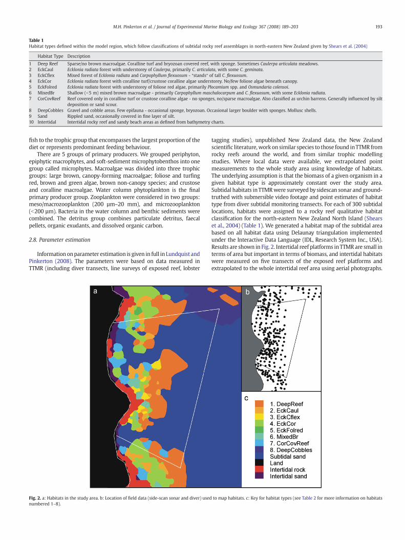
Table 1Habitat types defined within the model region, which follow classifications of subtidal rocky reef assemblages in north-eastern New Zealand given by Shears et al. (2004)

Habitat Type Description

1 Deep Reef Sparse/no brown macroalgae. Coralline turf and bryozoan covered reef, with sponge. Sometimes Caulerpa articulata meadows.2 EckCaul Ecklonia radiata forest with understorey of Caulerpa, primarily C. articulata, with some C. geminata.3 EckCflex Mixed forest of Ecklonia radiata and Carpophyllum flexuosum - qstandsq of tall C. flexuosum.4 EckCor Ecklonia radiata forest with coralline turf/crustose coralline algae understorey. No/few foliose algae beneath canopy.5 EckFolred Ecklonia radiata forest with understorey of foliose red algae, primarily Plocamium spp. and Osmundaria colensoi.6 MixedBr Shallow (b5 m) mixed brown macroalgae - primarily Carpophyllum maschalocarpum and C. flexuosum, with some Ecklonia radiata.7 CorCovReef Reef covered only in coralline turf or crustose coralline algae - no sponges, no/sparse macroalgae. Also classified as urchin barrens. Generally influenced by silt

deposition or sand scour.8 DeepCobbles Gravel and cobble areas. Few epifauna - occasional sponge, bryozoan. Occasional larger boulder with sponges. Mollusc shells.9 Sand Rippled sand, occasionally covered in fine layer of silt.10 Intertidal Intertidal rocky reef and sandy beach areas as defined from bathymetry charts.


fish to the trophic group that encompasses the largest proportion of thediet or represents predominant feeding behaviour.

There are 5 groups of primary producers. We grouped periphyton,epiphytic macrophytes, and soft-sediment microphytobenthos into onegroup called microphytes. Macroalgae was divided into three trophicgroups: large brown, canopy-forming macroalgae; foliose and turfingred, brown and green algae, brown non-canopy species; and crustoseand coralline macroalgae. Water column phytoplankton is the finalprimary producer group. Zooplankton were considered in two groups:meso/macrozooplankton (200 µm–20 mm), and microzooplankton(b200 µm). Bacteria in the water column and benthic sediments werecombined. The detritus group combines particulate detritus, faecalpellets, organic exudants, and dissolved organic carbon.

2.8. Parameter estimation

Information onparameter estimation is given in full in Lundquist andPinkerton (2008). The parameters were based on data measured inTTMR (including diver transects, line surveys of exposed reef, lobster

Fig. 2. a: Habitats in the study area. b: Location of field data (side-scan sonar and diver) usednumbered 1–8).

tagging studies), unpublished New Zealand data, the New Zealandscientific literature,work on similar species to those found inTTMR fromrocky reefs around the world, and from similar trophic modellingstudies. Where local data were available, we extrapolated pointmeasurements to the whole study area using knowledge of habitats.The underlying assumption is that the biomass of a given organism in agiven habitat type is approximately constant over the study area.Subtidal habitats inTTMRwere surveyed by sidescan sonar and ground-truthed with submersible video footage and point estimates of habitattype from diver subtidal monitoring transects. For each of 300 subtidallocations, habitats were assigned to a rocky reef qualitative habitatclassification for the north-eastern New Zealand North Island (Shearset al., 2004) (Table 1). We generated a habitat map of the subtidal areabased on all habitat data using Delaunay triangulation implementedunder the Interactive Data Language (IDL, Research System Inc., USA).Results are shown in Fig. 2. Intertidal reef platforms inTTMR are small interms of area but important in terms of biomass, and intertidal habitatswere measured on five transects of the exposed reef platforms andextrapolated to the whole intertidal reef area using aerial photographs.

to map habitats. c: Key for habitat types (see Table 2 for more information on habitats


Bird abundances and model parameters were based on directobservations in TTMR (A. Bassett, DoC, pers. comm.; Bert Lee, TolagaBay East Cape Charters, pers. comm.), combined with weights fromHeather and Robertson (1986), diets from Medway (2000), andenergetic parameters from Cummings et al. (1997) and Lundquist et al.(2004), based on estimated metabolic rates for 12 species.

Abundances of the red rock lobster (Jasus edwardsii) were estimatedfromdiver transects and extrapolated to the studyarea based on habitat.Sampling of lobster by baited pots and tagging were consistent withthese numbers. A simple population model using measurements of tailwidth, sex, carapace length and weight in TTMR, combined withliterature studies (Annala, 1978, 1980; Taylor, 1998a) allowed us toestimate anaverage lobsterweight.Workon the energetic parameters oflobster since Lundquist and Pinkerton (2008) gave initial energeticparameters of P/B=0.44 y-1 and Q/B=4.4 y−1. Measurements of lobsterdiet in other parts of New Zealand (S. Kelly, Auckland Regional Council,unpublished data) were combined with local information from stableisotope analysis (Freeman, 2008) to initialise lobster diet in the model.

Mobile herbivorous and detrivorous invertebrates in the regioninclude kina/sea urchin (Evechinus chloroticus), paua/abalone (Haliotisaustralis, H. iris), chitons, and grazing gastropods (including Cookiasulcata, Trochus viridis, and Turbo smaragdus). Their abundances wereestimated by localmeasurements in intertidal and subtidal reef surveys,and extrapolated across the whole study area. Grazing herbivores lessthan approximately 5 mm in size may be undersampled in these data,and instead they are included in the phytal/infaunal invertebrate groupdescribed below. Density and size-frequency measurements of manyinvertebrates (e.g. paua, kina)were collected inTTMR.Abundances, dietsand energetic parameters were obtained from the literature: Ayling(1978), Schiel (1982), Raffaelli (1985), Creese (1988), Schiel and Breen(1991), McShane and Naylor (1995), Marsden and Williams (1996),Freeman (1998), Taylor (1998a), Lamare and Mladenov (2000), Barker(2001), Shears and Babcock (2004a), Brey (2005).

The mobile carnivorous invertebrate group consists of rock crabs,hermit crabs, octopus, predatory gastropods (mainly whelks), andseastars/brittlestars. Crab densities in three New Zealand subtidalhabitats (intertidal and subtidal reef, soft sediment) were combinedwith local measurements of abundance in the intertidal zone, andlocal information on crab size, to estimate biomass. Densities,energetic parameters and typical diets for crabs were taken fromWear and Haddon (1987), McLay (1988), Taylor (1998a), Smith (2003),Shears and Babcock (2004a). By-catch rates of octopus in lobster potswere used to estimate total octopus numbers (Brock and Ward, 2004;Hunter et al., 2005). Nudibranchs are considered rare in northern NewZealand coastal rocky reefs (Willan, 2005). Gastropod and asteroid/ophiuroid abundances and energetic parameters were based onintertidal and subtidal monitoring surveys of the region and theliterature (Town, 1980; McShane and Naylor, 1995; Taylor, 1998a;Shears and Babcock, 2004a; Stewart and Creese, 2004; Brey, 2005).

Holothuroids (sea cucumber) are not thought to be common in theTTMR, though no night-time surveys were carried out. Abundances,weights, and energetics were taken from day-time surveys of otherNew Zealand reef areas (Sewell, 1990; Smith, 2003; Shears andBabcock, 2004a). The commonest New Zealand holothuroid (Stichopusmollis) is known to be cryptic during the day, so abundance based onday-time counts is likely to be underestimated. It remains ambiguousto what extent holothuroids and other detritivores consume detritusitself rather than bacteria feeding on the detritus (Moriarty, 1982;Uthicke, 1999). Here, we nominally assumed that detritivores aresolely bacteria-eaters, an assumption that ultimately has little effecton the final model (see discussion).

The phytal/infaunal invertebrate group included epifauna living in,on, or amongst macroalgae, as well as soft sediment infauna with size20 µm–5 mm (methodological size division). Taxa include micro-crustaceans (amphipods, isopods, ostracods, harpacticoid copepods,tanaids, cumaceans), gastropods, bivalves, nematodes, platyhelminthes,

and polychaetes. Information on phytal invertebrate abundance andproductivity inNewZealandwaterswas taken from the literature (TaylorandCole,1994;Williamson andCreese,1996; Taylor,1998a,b,c; Andersonet al., 2005), noting that abundances of cryptic species may beunderestimated. Estimates of phytal invertebrate abundance by habitatwere combinedwithhabitatmapsof TTMR to estimate total abundances.Individual weights and trophic parameters were combined with NewZealand estimates of relative abundances of phytal groups withinmacroalgae to convert abundances to biomass (Donovaro et al., 2002;C. Duffy, DoC, pers. comm.). Benthic macrofauna biomass in sedimentswas enumerated from nine subtidal cores in TTMR. Mean weights,production rates, P/Q anddiet values formacrofaunaandmeiofauna, andbiomass estimates formeiofauna, were taken from the literature (Bouvy,1988; Edgar, 1990; Cummings et al., 1997; Taylor, 1998a).

Sponges (Porifera) were common and considered separately fromother sessile encrusting invertebrates because of very differentindividual weights and energetic parameters. Percent coverages ofsponge in TTMRwere surveyed by diver transects in each habitat type.Sponge areal coverage was converted to biomass using Shears andBabcock (2004a). Productivity was estimated from New Zealandmeasurements (Ayling, 1983; Bell, 1998; Smith and Gordon, 2005).

Sessile invertebrates in TTMR includemussels, anemones, barnacles,hydroids, bryozoans, corals, ascidians, and epifaunal bivalves. Biomass ofsessile invertebrates was estimated using local measurements of thearea coverage by each group of sessile invertebrates in each habitat typeand extrapolated to the whole study area using triangulation. Averageweights per unit area were estimated based on Shears and Babcock(2004a). Energetic values and diets were taken from the literature(Edgar, 1990; Ortiz and Wolff, 2002; Zeldis et al., 2004).

The most abundant species of cryptic reef fish in the region aretriplefins. Biomasses of subtidal cryptic reef fish were estimated basedon studies of rocky reef habitats in north-eastern New Zealand (Duffy,1989; Smith, 2003; Willis and Anderson, 2003). The average size ofcryptic fish in the region of 1.0 g followed Glassey (2002). Diet ofcryptic fish was taken from Thompson (1981). Abundances of non-cryptic fish species over the subtidal reef were estimated using datafrom 85 diver monitoring surveys. Abundances of 34 species of fishsighted on these surveys were calculated for each habitat, andextrapolated to the entire model region. Additional information ondemersal and pelagic fish biomasses were estimated using NewZealand research trawls and New Zealand Ministry of Fisheries aerialsurveys in the surrounding region. Maximum fish sizes were takenfrom one or more of: Ministry of Fisheries data (e.g., Sullivan et al.,2005); research from local and northeastern New Zealand (Thompson,1981; Taylor and Willis, 1998); FishBase (Froese and Pauly, 2005); alength-weight relationship based on other fish in the area. Fishlength-frequency data collected in the study area for 6 species gave anestimate of the ratio of average to maximum length in TTMR. Foodconsumption followed Palomares and Pauly (1998). Fish diets weretaken from, inter alia, Thompson (1981), Russell (1983), Clark (1985),Clark et al. (1989), Jones (1988), Stevens et al. (2007). Information onfish diets were not obtained locally, and much (especially Thompson,1981) is relatively rudimentary, emphasizing the need to allowestimates of diet fractions to vary during model balancing.

We combined microphytobenthos on soft sediment, erect epiphyticmacrophytes (ranging from small encrusting species to larger epiphytessuch as Ulva sp. and Laurencia sp.), and microphytes (periphyton),typically diatoms, into a single trophic group in the model. Benthicmicroalgal biomass and primary productivity was estimated fromworkby Gillespie et al. (2000) and Cahoon and Safi (2002). Epiphyte biomassandprimary productivitywas estimated fromworkbyD'Antonio (1985),Smith et al. (1985) and Klumpp et al. (1992).

Subtidal abundance estimates of macroalgae in each habitat typewere obtained from transect surveys across north-eastern NewZealand (Shears et al., 2004). Abundances were converted to wetweights using length-weight relationships from Shears and Babcock


(2004a). Algal coverage and density in the intertidal zone wererecorded on 5 transects of the reef platforms. Topographic maps andaerial photographs were used to extrapolate these survey data to thewhole intertidal reef area. Weights were converted to carbon biomassusing Lamare andWing (2001), and unpublished data from R.B. Taylor(University of Auckland). Primary productionwas estimated followingTaylor et al. (1999), Chisholm (2003), Shears and Babcock (2004b),Schiel (2005), and Miller and Dunton (2007).

Zooplankton biomass was estimated using New Zealand measure-ments (Foster and Battaered, 1985; Bradford-Grieve et al., 1993) and

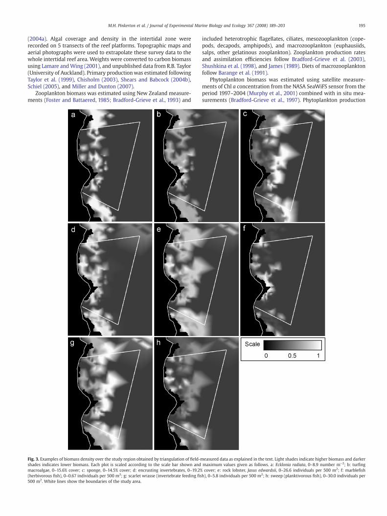
Fig. 3. Examples of biomass density over the study region obtained by triangulation of field-mshades indicates lower biomass. Each plot is scaled according to the scale bar shown andmacroalgae, 0–15.6% cover; c: sponge, 0–14.5% cover; d: encrusting invertebrates, 0–19.2%(herbivorous fish), 0–0.67 individuals per 500 m2; g: scarlet wrasse (invertebrate feeding fis500 m2. White lines show the boundaries of the study area.

included heterotrophic flagellates, ciliates, mesozooplankton (cope-pods, decapods, amphipods), and macrozooplankton (euphausiids,salps, other gelatinous zooplankton). Zooplankton production ratesand assimilation efficiencies follow Bradford-Grieve et al. (2003),Shushkina et al. (1998), and James (1989). Diets of macrozooplanktonfollow Barange et al. (1991).

Phytoplankton biomass was estimated using satellite measure-ments of Chl a concentration from the NASA SeaWiFS sensor from theperiod 1997–2004 (Murphy et al., 2001) combined with in situ mea-surements (Bradford-Grieve et al., 1997). Phytoplankton production

easured data as explained in the text. Light shades indicate higher biomass and darkermaximum values given as follows. a: Ecklonia radiata, 0–8.9 number m−2; b: turfingcover; e: rock lobster, Jasus edwardsii, 0–26.6 individuals per 500 m2; f: marblefish

h), 0–5.8 individuals per 500 m2; h: sweep (planktivorous fish), 0–30.0 individuals per

Table 2Common fish in the study area

Group New Zealandcommon name

Scientific name Biomass (group)a Abundance (total)b P/B Q/B

% % y−1 y−1

Invert feeder Red moki Cheilodactylus spectabilis 33.0 1.6 0.32 2.7Scarlet wrasse Pseudolabrus miles 17.8 9.8 0.60 4.6Leatherjacket Parika scaber 14.0 2.4 0.44 2.9Blue moki Latridopsis ciliaris 9.2 0.5 0.33 3.4Porae Nemadactylus douglasi 8.6 0.8 0.37 5.1Snapper Pagrus auratus 5.8 0.3 0.32 3.8Spotty Notolabrus celidotus 5.2 4.5 0.67 4.9Banded wrasse Notolabrus fucicola 3.4 0.9 0.49 3.8Goatfish Upeneichthys lineatus 1.6 0.3 0.45 5.0

Piscivore Kahawai Arripis trutta 35.3 2.6 0.42 3.9Rock cod Lotella rhacinus 27.9 2.7 0.36 2.4Blue cod Parapercis colias 27.9 2.7 0.45 2.9Kingfish Seriola grandis 5.2 0.3 0.38 6.8Spiny dogfish Squalus acanthias 1.7 0.0 0.31 2.7Red-banded perch Hypoplectrodes huntii 0.4 0.4 0.81 5.8Jack mackerel Trachurus novae-zelandiae 0.4 0.1 0.50 3.9

Planktivore Sweep Scorpis lineolatus 35.8 28.3 0.52 7.9Trevally Pseudocaranx dentex 37.7 21.0 0.47 6.0Blue maomao Scorpis violceus 13.6 10.6 0.52 4.9Butterfly perch Caesioperca lepidoptera 12.8 11.2 0.53 4.6

Herbivore Marblefish Aplodactylus arctidens 86.8 0.4 0.40 9.4Butterfish Odax pullus 13.2 0.1 0.43 10.1

a Biomass as a proportion of the group biomass. See Table 3 for total group biomass (gC m−2).b Abundance (number of fish per m2) as a proportion of the abundance of all the non-cryptic fish.


was estimated using the model of Behrenfeld and Falkowski (1997)and in situ data from Bradford et al. (1982), taking into accountchanges in light availability, water column depth and estimates ofnutrient availability between the inshore and offshore areas (Lund-quist and Pinkerton, 2008).

In the absence of local measurements, bacterial biomass andproductivities were taken from the literature (inter alia, Pomeroy,1979; Sorokin,1981,1999; Poremba and Hoppe,1995; Bradford-Grieveet al., 2003), and large uncertainty was attached to these parameters.We did not estimate detrital biomass or flow.

Values for unassimilated consumption, U, followed previous trophicmodels (e.g., Christensen and Pauly, 1992; Bradford-Grieve et al., 2003)as 0.2 for birds, and 0.3 for other trophic groups. We nominally set U=0for bacteria.

Table 3Trophic group parameters for TTMR estimated from local data and literature

# Group B P/B

gC m−2 y−1

1 Birds 0.00022 (0.00016–0.00028) 0.10 (0.08–0.12)2 Lobster 0.16 (0.11–0.20) 0.44 (0.35–0.52)3 Mobile_inverts_herb 0.11 (0.078–0.13) 1.30 (1.04–1.56)4 Mobile_inverts_carn 0.094 (0.065–0.11) 1.76 (1.41–2.12)5 Sea cucumber 0.29 (0.21–0.37) 0.60 (0.48–0.72)6 Phytal/infaunal inverts 0.26 (0.19–0.54) 3.05 (2.44–3.67)7 Sponge 7.45 (5.22–9.32) 0.20 (0.08–0.24)8 Sessile_inverts 1.37 (0.97–1.72) 1.50 (1.20–1.80)9 Fish_cryptic 0.064 (0.045–0.080) 2.40 (1.92–2.88)10 Fish_invert 0.35 (0.25–0.44) 0.41 (0.33–0.50)11 Fish_pisc 0.12 (0.090–0.16) 0.43 (0.34–0.51)12 Fish_plank 0.86 (0.61–1.08) 0.50 (0.40–0.60)13 Fish_herb 0.013 (0.0088–0.016) 0.40 (0.32–0.48)14 Microphytes 8.52 (5.97–10.6) 21.0 (16.8–25.2)15 Macroalgae_canopy 132 (92.5–165) 2.87 (2.29–3.44)16 Macroalgae_foliose 8.76 (6.13–10.9) 13.0 (10.4–15.7)17 Macroalgae_crustose 0.35 (0.25–0.44) 25.4 (20.3–30.5)18 Meso/Macrozooplankton 0.19 (0.14–0.24) 17.7 (14.1–21.2)19 Microzooplankton 0.069 (0.048–0.086) 220 (176–264)20 Phytoplankton 0.23 (0.17–0.29) 324 (129–389)21 Bacteria 0.60 (0.19–1.80) 100 (80.0–150)

Ranges estimated as feasible are used as inputs to stage 1 of the balancing process as descrA=Accumulation, X=Export and fishery, U=Unassimilated consumption. N/A=Not applicab

2.9. Trophic levels

We calculated trophic levels (Lindeman, 1942; Christensen andPauly, 1992) in the balanced model using matrix inversion based ontwo rules: (1) primary producers, detritus and bacteria are defined ashaving a trophic level of 1; (2) consumer's trophic level is the sum ofthe trophic levels of their prey items, weighted by diet fraction, plusone. Bacteria are defined as being at the same trophic level as primaryproducers.

3. Results

Habitats produced by the mapping are shown in Fig. 2. The area ofintertidal reef in the reserve was estimated from topographic maps as

Q/B E A X U

y−1 %B y−1 gC m−2 y−1

89.8 (71.8–135) 1 0 0 0.20 (0.16–0.24)4.35 (3.48–6.53) 1 10 (0–30) 0 0.30 (0.24–0.36)7.94 (6.35–11.9) 1 0 0 0.30 (0.24–0.36)7.47 (5.97–11.2) 1 0 0 0.30 (0.24–0.36)3.40 (2.72–5.10) 1 0 0 0.30 (0.24–0.36)12.0 (9.66–18.1) 1 0 0 0.30 (0.24–0.36)0.80 (0.64–1.20) 1 0 0 0.30 (0.24–0.36)6.00 (4.80–9.00) 1 0 0 0.30 (0.24–0.36)15.6 (12.5–23.5) 1 0 0 0.30 (0.24–0.36)3.59 (2.87–5.39) 1 0 0 0.30 (0.24–0.36)3.62 (2.90–5.44) 1 0 0 0.30 (0.24–0.36)6.33 (5.06–9.50) 1 0 0 0.30 (0.24–0.36)9.52 (7.61–14.3) 1 0 0 0.30 (0.24–0.36)N/A 1 (0–1) 0 0 N/AN/A 1 (0–1) 0 0 N/AN/A 1 (0–1) 0 0 N/AN/A 1 (0–1) 0 0 N/A51.5 (41.2–77.3) 1 0 0 0.30 (0.24–0.36)624 (499–940) 1 0 0 0.30 (0.24–0.36)N/A 1 0 0 N/A400 (320–600) 1 0 0 0

ibed in the text. B=Biomass, P=Production, Q=Consumption, E=Ecotrophic efficiency,le.


821,000m2, approximately 4% of the total study area. About 48% of theintertidal area in TTMR and 21% of the subtidal area is reef and theremainder sand. In spite of the small area, the intertidal reef isimportant because it contains high concentrations of macroalgaeincluding Hormosira banksi, Cystophora spp. and coralline turf.

3.1. Parameter results

The abundances of some example trophic groups as estimatedfrom the habitat-based mapping approach are shown in Fig. 3. Fishbiomass and energetic parameters for important species in TTMR aregiven in Table 2 to illustrate how species were combined into trophicgroups.

3.2. Model balancing

Tables 3 and 4 show the biomass, energetic parameters and dietfractions obtained from the analysis of the local data and literaturereview. The balancing process started from this point.

Stage 1 of the balancing procedure involved excluding parts of theranges of energetic parameters and diet proportions that prevent abalanced solution being found. The most obvious result was that thevast majority of primary production by macrophytes and microphytescannot be consumed in the system. The maximum consumption rate

Table 4Diet matrix estimated from local data and literature, with ranges showing input to stage 1

# Group 1 2 3 4 5 6 7 8

1 Birds 0.01(0–0.2)

2 Lobster 0.10(0.01–0.5)

3 Mobile_inverts herb 0.25 0.26 0.30(0.1–1) (0.01–0.7) (0.1–1)

4 Mobile_inverts carn 0.30 0.14 0.25(0.1–1) (0.01–0.5) (0.1–1)

5 Sea cucumber 0.01(0–0.2)

6 Phytal/infaunal inverts 0.35 0.28 0.08(0.1–1) (0.01–1) (0–1)

7 Sponge 0.10(0.01–0.5)

8 Sessile_inverts 0.15(0.10–1)

9 Fish_cryptic 0.10(0.01–0.5)

10 Fish_invert

11 Fish_pisc

12 Fish_plank

13 Fish_herb

14 Microphytes 0.25 0.25(0.1–1) (0.1–1)

15 Macroalgae canopy 0.19 0.35 0.25(0.05–0.7) (0.1–1) (0.1–1)

16 Macroalgae foliose 0.20(0.1–1)

17 Macroalgae crustose 0.13 0.20(0.05–1) (0.1–1)

18 Meso/Macro zooplankton

19 Micro-zooplankton 0.30 0.3(0.1–1) (0.

20 Phytoplankton 0.25 0.40 0.4(0.1–1) (0.1–1) (0.

21 Bacteria 1.00 0.25 0.30 0.3(0.1–1) (0.1–1) (0.

22 Detritus

Predators are shown on the x-axis and prey on the y-axis.

of algal grazers in the system account for only a small proportion ofthe minimum production rates of macroalgae and microphytes. Bygroup, maximum grazing could account for 2.8% production bymicrophytes, 1.5% production by canopy macroalgae, 0.8% productionby foliose macroalgae, and 16% production by crustose and corallinealgae. The majority of macroalgal primary production is channelled todetritus (including abraded material and algal exudants) via very lowecotrophic efficiencies for all four algal groups.

Three other trophic groups in the TTMR system also haveinsufficient predation for their production to be accounted for bydirect consumption based on our initial estimates of parameters: seacucumber (27% of production may be directly consumed), sponges(27%), and phytoplankton (42%). The production rates of all thesegroups in TTMR are poorly known, so that rather than accounting forthe mismatch between estimated production and estimated con-sumption using ecotrophic efficiency (E), we held E=1 and allowedtheir production rates to vary (KP=5). For phytoplankton and bacteria,we also allowed biomass to vary substantially (KB=5) becauseinformation on these groups is particularly poor.

Only 3 of our 59 initial estimates of diet fractions were found to lieoutside the feasible ranges estimated a priori. We initially suggestedthat bird carcasses made up 1% of the diet of scavenging mobileinvertebrates (such as crabs), but given the small biomass of birdsrelative to invertebrates, this could only be b0.1%. We estimated that

of the balancing process

9 10 11 12 13 18 19 21

0.16(0.1–1)0.30(0.1–1)

0.64 0.17 0.22(0.1–1) (0.1–1) (0.1–1)

0.04(0.01–0.5)

0.21 0.32(0.1–1) (0.1–1)

0.09(0.01–0.5)0.21(0.1–1)0.09(0.01–1)0.53(0.1–1)0.09(0.01–0.5)

0.24(0.1–1)0.66(0.1–1)0.09(0.01–0.50)

0.15 0.72 0.20(0.1–1) (0.1–1) (0.1–1)

0 0.70 0.101–1) (0.1–1) (0.01–0.5)0 0.10 0.651–1) (0.01–0.5) (0.1–1)0 0.06 0.25 0.501–1) (0.01–0.5) (0.1–1) (0.1–1)

0.50(0.1–1)

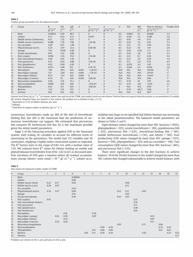
Table 5Trophic group parameters for the balanced model

# Group B P/B Q/B E A X U P/Q R/B Flow to detritus Trophic level

gC m−2 y−1 y−1 gC m−2 y−1 gC m−2 y−1 y-1 gC m−2 y−1

1 Birds 0.00022 0.10 89.7 1 0 0 0.2 0.0011 72 0.0040 3.52 Lobster 0.15 0.43 4.13 1 0.0161 0 0.3 0.105 2.5 0.180 2.63 Mobile inverts (herbivores) 0.13 1.32 8.13 1 0 0 0.3 0.16 4.4 0.31 2.04 Mobile inverts (carnivores) 0.088 1.78 7.08 1 1.5E-08 0 0.3 0.25 3.2 0.19 3.35 Sea cucumber 0.30 0.51 3.40 1 0 0 0.3 0.15 1.9 0.30 2.06 Phytal/infaunal inverts 0.29 3.07 12.4 1 6.0E-08 0 0.3 0.25 5.6 1.07 2.07 Sponge 7.14 0.018 0.80 1 0 0 0.3 0.02 0.54 1.71 2.38 Sessile invertebrates 0.97 1.43 6.00 1 0 0 0.3 0.24 2.8 1.74 2.39 Fish (cryptic) 0.058 2.36 15.8 1 1.5E-08 0 0.3 0.15 8.7 0.28 3.210 Fish (invertebrate feeders) 0.28 0.41 3.42 1 0 0 0.3 0.12 2.0 0.29 3.411 Fish (piscivores) 0.16 0.43 4.08 1 7.5E-09 0 0.3 0.11 2.4 0.19 4.512 Fish (planktivores) 0.65 0.49 6.20 1 0 0 0.3 0.078 3.9 1.20 3.413 Fish (herbivores) 0.013 0.40 9.6 1 4.7E-10 0 0.3 0.042 6.3 0.036 2.014 Microphytes 7.99 20.9 N/A 0.010 −1.2E-07 0 N/A N/A N/A 165.04 12

15 Macroalgae (canopy) 123 2.84 N/A 0.005 −1.2E-07 0 N/A N/A N/A 347.05 12

16 Macroalgae (foliose) 8.53 13.0 N/A 0.003 0 0 N/A N/A N/A 110.93 12

17 Macroalgae (crustose) 0.34 25 N/A 0.058 3.0E-08 0 N/A N/A N/A 8.08 12

18 Macro/meso zooplankton 0.20 17.8 51.3 1 0 0 0.3 0.35 18 3.07 2.919 Microzooplankton 0.069 220 626 1 -9.5E-07 0 0.3 0.35 218 12.94 2.120 Phytoplankton 0.16 221 N/A 1 3.8E-06 0 0 N/A N/A 0.00 12

21 Bacteria 1.59 134 535 1 0 0 0 0.25 401.2 0.00 12

22 Detritus N/A N/A N/A 1 0 0 N/A N/A N/A 6553 12

System-level flows (gCm−2 y−1) of organic matter into and out of the TTMR, and trophic levels are also shown. Positive flows are exports from the system, or accumulations (A) withinthe system. Negative flows are imports to the system. All symbols are as defined in Eqs. (1)–(3).1 Equivalent to 11.1% of lobster biomass per year.2 Defined.3 Total flow of organic matter to detritus (gC m-2 y-1).


carnivorous invertebrates made up 30% of the diet of invertebratefeeding fish, but 26% is the maximum that the production of car-nivorous invertebrates can support. We estimated that piscivorousfish consume 9% herbivorous fish but 3% is the maximum possiblegiven the initial model parameters.

Stage 2 of the balancing procedure applied SVD to the linearisedsystem, with scaling (K) variables to account for different levels ofuncertainty in the parameters. The model had 112 variables and 36constraints, implying a highly under-constrained system as expected.The KD factors were in the range of 0.82–4.4, with a median value of1.55. We reduced three KD values for lobster feeding on mobile andphytal/infaunal invertebrates from 0.92–1.62 to 0.5 as discussed later.Four iterations of SVD gave a solution where all residual accumula-tions (except lobster) were small (b10−5 gC m−2 y−1). Lobster accu-

Table 6Diet matrix for balanced trophic model of TTMR

# Group 1 2 3 4 5 6

1 Birds 0.000042 Lobster 0.083 Mobile inverts (herb) 0.22 0.17 0.044 Mobile inverts (carn) 0.28 0.075 Sea cucumber 0.246 Phytal/infaunal inverts 0.34 0.27 0.007 Sponge 0.108 Sessile invertebrates 0.549 Fish (cryptic) 0.1610 Fish (invertebrate feeders)11 Fish (piscivores)12 Fish (planktivores)13 Fish (herbivores)14 Microphytes 0.18 0.3915 Macroalgae (canopy) 0.16 0.30 0.3916 Macroalgae (foliose) 0.2317 Macroalgae (crustose) 0.33 0.2818 Meso/macrozooplankton19 Microzooplankton20 Phytoplankton 0.1121 Bacteria 1.00 0.1122 Detritus

Predators are shown on the x-axis and prey on the y-axis.

mulationwas larger aswe specified that lobster biomasswas increasingin the initial parameterisation. The balanced model parameters areshown in Tables 5 and 6.

Eight biomass values changed by more than 10%: bacteria (+165%),phytoplankton (−32%), sessile invertebrates (−30%), planktivorous fish(−25%), piscivorous fish (+22%), invertebrate-feeding fish (−19%),mobile herbivorous invertebrates (+13%), and lobster (−10%). Fourproductivity (P/B) values changed by more than 10%: sponge (−91%),bacteria (+34%), phytoplankton (−32%) and sea cucumber (−14%). Twoconsumption (Q/B) values changed bymore than 10%: bacteria (−46%),and piscivorous fish (+12%).

There were significant changes to the diet fractions to achievebalance: 19 of the 59 diet fractions in themodel changed bymore than10%. Lobster diet changed substantially to achievemodel balance, with

7 8 9 10 11 12 13 18 19 21

0.040.11

0.52 0.11 0.030.07

0.43 0.670.210.180.110.490.01

0.230.670.11

0.05 0.71 0.060.30 0.30 0.72 0.100.40 0.40 0.21 0.670.30 0.30 0.26 0.23 0.23

0.77


more feeding on crustose macroalgae (+20%), and less feeding onherbivorous mobile invertebrates (−9%) and carnivorous mobileinvertebrates (−6%). Three groups consumed more sessile inverte-brates in the balanced model than we proposed (mobile carnivorousinvertebrates +39%, invertebrate-feeding fish +35%, and cryptic fish+22%. For cryptic fish, more feeding of sessile invertebrates wasbalanced with less feeding on phytal/infaunal invertebrates (−12%)and meso/macrozooplankton (−9%). For invertebrate-feeding fish,more feeding of sessile invertebrates was balanced with less feedingon mobile carnivorous invertebrates (−19%) and mobile herbivorousinvertebrates (−13%). Planktivorous fish feeding on bacteria wasincreased (+20%), while that on phytal/infaunal invertebrates wasreduced (−19%). The balanced model showed piscivorous fishconsuming more cryptic fish than anticipated (+12%), and consumingless of the other fish groups. The diet of mobile carnivorousinvertebrates was substantially changed with more feeding on seacucumber (+23%), and less feeding on carnivorous mobile inverte-brates (−25%) and herbivorous mobile invertebrates (−26%). Phytalinvertebrates in the balancedmodel consumedmore microphytes andcanopy macroalgae (+14% in both cases), and less bacteria andphytoplankton (−14% in both cases) than originally proposed. Meso/macrozooplankton feeding on other meso/macrozooplankton wasreduced (−13%), while feeding on phytoplankton was increased(+11%). Finally, the balancing process reduced the consumption ofphytal/infaunal invertebrates by carnivorous mobile invertebrates tozero. This model result is within the range of information in theliterature and is considered ecologically possible.

3.3. Trophic levels

Particular organisms may be expected to have broadly similartrophic levels (TL) in similar types of ecosystems where they arefeeding on similar prey. Trophic levels were calculated for the finalmodel (Table 5) and compared with other trophic models that usedcompatible methodologies for estimating trophic level. Comparingtrophic levels in this way is a fairly crude way of comparing models,but may highlight major inconsistencies in the parameters or dietsused here. Some models did not model bacteria explicitly, and insteaddefined detritus as having TL=1 (e.g. Jarre-Teichmann et al., 1998;Arreguin-Sanchez et al., 2002; Jiang and Gibbs, 2005). This will notaffect trophic levels as detrivores are assumed to consume detritusrather than bacteria. Trophic levels for the groups in the TTMR agreewell with those from trophic models of rocky reefs elsewhere. Forexample, for birds TL=3.5 compares reasonably well with 3.8(Arreguin-Sanchez et al., 2002) but less well with 4.5 (Jarre-Teichmann et al., 1998). Birds in the Benguela system modelled byJarre-Teichmann et al. (1998) are different species and are likely to befish-eaters rather than invertebrate feeders as in TTMR. Mobilecarnivorous invertebrates at TL=3.3 compares with values for crabsand predatory invertebrates: 3.3–3.4 (Wolff, 1994) and 2.4–2.8(Arreguin-Sanchez et al., 2002). Mobile herbivorous invertebrateshave TL=2.0 compared with 2.1–2.5 (Wolff, 1994), and 2.0–2.1 (Jiangand Gibbs, 2005). Trophic levels for invertebrate-feeding fish andplanktivorous fish at 3.4 agree well with values for similar fish: 3.3(Jarre-Teichmann et al., 1998); 2.7–3.5 (Wolff, 1994); 3.2–3.9 (Men-doza, 1993); 3.1–3.8 (Jiang and Gibbs, 2005). Finally, meso/macro-zooplankton and microzooplankton here have TL=2.1–2.9 comparedto values of 2.2–2.4 (Jarre-Teichmann et al., 1998); 2.0 (Mendoza,1993;Jiang and Gibbs, 2005); 2.2 (Arreguin-Sanchez et al., 2002).

4. Discussion and Conclusions

We have shown how a balanced trophic model of a temperaterocky reef ecosystem can be obtained from incomplete and imperfectinitial estimates of biomass, energetic parameters and diet fractions.The model structure was based on a simplified but widely-used

conceptual picture of organic carbon flux through ecosystems. Thereare a number of ecological issues that are not explicitly or realisticallyconsidered inmass balancemodels of the type presented here, andwemade some typical assumptions: we ignored seasonal variations inecosystem function and considered flows averaged over an annualperiod; we included data from different years assuming that the basicstate of the ecosystem was similar from year to year; we did notexplicitly model different life stages of biota; we grouped organismsinto a relatively small number of model compartments; we assumedthere was no net import/export of material from any groups; and,except for lobster, we assumed that biota were not accumulating inthe study area. We also assumed that animal carcasses in the systemwere scavenged rather than decomposing (E=1), and that thescavengers and predators of a given group were similar. Theseassumptions are justified in testing data for consistency and obtainingan initial system-level view of ecosystem structure, but many wouldneed to be reconsidered to develop a dynamic model.

Field data from a monitoring programme in TTMR between 2000and 2003 were used to estimate biomass of key ecosystem groups. Formany species, we combined sparse local measurements of abundancewith knowledge of the habitat distributions in the study area toestimate total biomass. Local data were augmented with unpublisheddata from New Zealand, information from the scientific literature, andexpert opinion to obtain a starting set of biomass and energeticparameters for modelling. Estimating uncertainties on these para-meters was almost entirely subjective as there is much that is simplynot known about the biology and ecology of some species.

There have been no long-term measurements of diet compositionin TTMR and starting estimates of diet fractions were necessarily takenfrom the literature. We suggest that diet may vary considerablybetween different rocky reef ecosystems because of changes inrelative prey abundance and suitability of habitats for differentgroups. Stable isotope data was useful in informing possible diets oflobster, and more extensive application of this method in the futuremay be able provide useful information on various diet linkages in thesystem (Peterson and Fry, 1987). Even so, diets in complex trophicmodels will generally be poorly known.

The starting set of parameters did not lead to a balancedmodel andwe found it necessary to develop novel inverse modelling techniquesto adjust parameters, including allowing diet fractions to vary. Thisinversemodelling (balancing) procedure should not, and cannot, be anentirely automated exercise. Valuable insights often arise fromplayingwith a model during balancing and there is a danger of losing this byover-reliance on automated fitting methods. The process we havedescribed combined expert-driven parameter adjustment and power-ful statistical and numerical modelling techniques. The first stage ofthe balancing procedure allowed us to identify gross problems withthe parameters and model structure, and the second stage introduceda method to adjust all parameters taking into account both variationsof scale between trophic groups and variations in uncertaintybetween parameters. Applying these inverse modelling techniquesled to a balanced and self-consistent model of the TTMR ecosystemthat is consistent with both the local survey data and literature. This isencouraging, but we emphasise that this balanced model is not theonly feasible solution and it is highly likely that we could obtain analternative balanced model with substantially different parameters.

Most adjustments to the initial parameters necessary to balance thetrophicmodelwere b20%, and large adjustmentswere needed only fora few poorly observed groups, such as bacteria, sponge, sea cucumber,and phytoplankton. These groups have poorly quantified productionrates and biomass in the study region, and generally weak directpredation pressure. The ability of sponge to change its production ratein response to grazing pressure (e.g. Ayling,1983; Bell,1998) presents achallenge to simple trophicmodels. The very large reduction in the P/Bparameter for sponge in the balanced model suggests that sponge inTTMR is overestimated in terms of biomass, is very slow growing, has


more consumers than thought, or loses substantial material to thedetrital pool by abrasion or other damage. A combination of thesefactors is likely. More information on sponge biology and ecology inTTMR is needed to improve modelling of the group.

Many initial estimates of diet fractions were changed duringmodelbalancing, though, generally, the changes were relatively small.Wherewe combined organisms that are not in contact with each otherbecause of habitat disconnects into a single trophic group (forexample, phytal invertebrates and infauna), we took this into accountwhen estimating initial diet fractions. We do not believe that changesto diet fractions made during balancing led to unrealistic diet fractionsin the balanced model because of this habitat disconnection.

The model presented here suggests low predation pressure on allprimary producers except phytoplankton. In the model, 94% of totalprimary production was not directly consumed. The proportion isN99% if phytoplankton are excluded. This is consistent with previouswork showing that in some coastal systems the majority of primaryproduction is transferred to higher trophic levels via detrital pathways(e.g. Berry et al., 1979; Manickchand-Heileman et al., 1998). In ourmodel, 28% of material transferred to higher trophic levels wasthrough the detrital pathway, and 72% was transferred via directconsumption of primary producers. The proportion transferred via thedetrital pathway increased to 79% when consumption of phytoplank-tonwas excluded. Surveys of beach cast macroalgae indicate that up to25% of annual production is deposited on the beach as detritus(Zemke-White et al., 2004) which is then broken down by bacterialaction. The remainder of ungrazed macroalgal production forms partof the water column detrital pool, from where it may be depositedover the reef and broken down by bacterial action. Studies have shownhigh grazing pressure on epiphytes and periphyton relative to theirhost (D'Antonio,1985; Smith et al., 1985; Klumpp et al., 1992).We havepoor information on biomass and primary production rates forepiphytes and periphyton in TTMR and are unable to separate thetrophic role of epiphytes, microphytobenthos and periphyton. How-ever, the model shows low direct predation pressure on the combinedepiphytes and periphyton trophic group, as on macroalgae. Overalllow grazing pressure on macroalgae, epiphytes and periphyton isconsistent with low biomass of grazing invertebrates and herbivorousfish in TTMR.

Many coastal trophic models do not explicitly include either watercolumn or benthic bacteria as separate trophic groups, often with therationale that the appropriate parameters for these groups are poorlyknown (e.g., Arreguin-Sanchez et al., 2002; Rybarczyk and Elkaim,2003; Jiang and Gibbs, 2005). Although we had separate bacteria anddetritus groups in the model presented, and balanced these groupsindividually, the lack of information on biomass, production, andconsumption of bacteria makes it difficult to derive any benefit fromhaving this additional detrital-bacterial closure constraint. The totalconsumption by detrivores in the model is equivalent to only 2.4% ofthe flow of material into the detrital pool, so bacterial respiration, notdetrivorous consumption, is the ultimate fate of most detrital materialin the model.

Compared to Leigh and other northern New Zealand rocky-reefecosystems, the balanced model of the TTMR ecosystem suggests thatit is impoverished in terms of invertebrate biomass (e.g. Choat andSchiel, 1982). At Leigh, Taylor (1998a) estimated that crabs were 2.6%of the total biomass of the rocky reef system. We estimate them tomake up about 0.4% of the invertebrate biomass at TTMR (excludingsponges). Taylor (1998a) estimated that grazing gastropods were 28%of the total faunal biomass in the Leigh ecosystem and contributedroughly 12% of the total production. We estimate grazing gastropodsto comprise 1.5% of the invertebrate biomass, and 1.9% of theinvertebrate production (excluding sponges). This matches anecdotalobservations by divers of very few mobile invertebrates on reefs nearto the study area compared to similar New Zealand habitats elsewhere(Shears and Babcock, 2004a).

We compared fish abundances in Leigh just after protection withthose estimated in the present study, after correcting for differences incoverage of various habitats (data not shown). Fish abundances inLeigh were extensively studied just after the reserve was established(Thompson, 1981), and the habitats are similar though TTMR is moreexposed. For many of the fish species compared (15 of 23), there wasrelatively good agreement between the fish abundance in Leigh andTTMR. Usually, the numbers estimated on the basis of densities inLeigh are higher than those measured in TTMR, but by less than anorder of magnitude. The other 8 species of fish were much rarer orentirely absent in TTMR compared to Leigh. These were parore (Girellatricuspidata), silver drummer (Kyphosus sydneyanus), red bandedperch (Hypoplectrodes huntii), red pigfish (Bodianus unimaculatus),snapper (Pagrus auratus), goatfish (Upeneichthys lineatus), hiwihiwi(Chironemus marmoratus) and John dory (Zeus faber). TTMR is moreexposed than Leigh, and water temperatures are lower, which maylead to reduced fish abundances. Is it possible that food availabilitycould also be responsible for differences in fish densities andassemblages in TTMR compared to Leigh? Better information on thediets of these fish in TTMR is needed to settle this question, but we canmake some initial observations. Within the herbivorous fish group,parore and silver drummer are rarer at TTMR compared to Leigh thanmarblefish and butterfish, but are likely to have similar diets. In themodel, macroalgae and periphyton are abundant at TTMR comparedto the demand of herbivores, so at this coarse level, food does notseem to explain the difference in herbivorous fish density betweenLeigh and TTMR. For piscivorous fish, there is little evidence of adifference in diet between the species that are relatively common inTTMR (kahawai, rock cod, blue cod) compared to those that arerelatively scarce (red banded perch, John dory). However, the mostcommon piscivore in TTMR (kahawai) is thought to be able to feedeffectively on zooplankton whereas most of the other species in thisgroup cannot. With respect to invertebrate feeding fish, the scarcerfish in TTMR (snapper, hiwihiwi, goatfish, red pigfish) have similardiets to the more common fish (red moki, scarlet wrasse, leather-jacket, blue moki), but there may be subtle differences in diet. Unlikethe scarcer species, some of the more common species of invertebratefeeding fish in TTMR are thought to be able to feed on red macroalgae,sponge, and sessile invertebrates. There is also some evidence in theliterature (e.g. Thompson, 1981) that the scarcer species in TTMR aremore dependent on crab and grazing invertebrates for food than themore common species, and so could be more limited by preyavailability. Further work on the diets of these fish is needed to testthese hypotheses as habitat structure, in addition to relative abun-dances of prey, will alter the relative availability of prey to differentpredators.

Does the relative paucity of invertebrates in TTMR mean thatlobster predation on invertebrates is particularly intense? In themodel presented, lobster diet fractions are 17% mobile herbivorousinvertebrates, 7% carnivorous invertebrates, and 27% phytal/infaunalinvertebrates, the remainder being macroalgae (16% canopy macro-algae, 33% crustose/coralline algae). This implies that lobsters con-sume considerable proportions of the annual production of theseinvertebrate groups (61%, 28% and 18% respectively). In the model,invertebrate-eating fish consume about the same biomass of mobileinvertebrates as lobster, whereas cryptic reef fish consume nearly 3times as much phytal/infaunal invertebrate biomass as lobster. Itappears from this model therefore, that at present, predation pressureby lobster in TTMR on invertebrates is high but not excluding otherinvertebrate feeders.

However, this result is sensitive to the amount of variability allowedin the diet of lobster during model balancing (the KD factors). Higherflexibility (KD=1.0 rather than 0.5 for lobster feeding on invertebrategroups) leads to much lower proportions of mobile herbivorous andcarnivorous invertebrates in lobster diet (3% and 0% respectively). Lowerflexibility (KD=0.2) leads to more mobile herbivorous and carnivorous


invertebrates in lobster diet (25% and 12% respectively), which cor-responds to 84% and 47% of the annual production of these groups beingconsumed by lobster. The proportion of phytal/infaunal invertebrates inlobster diet (27%), and the accumulation rates of lobster (11%B y−1) arealmost entirely unchanged between scenarios. Such changes to themodel balance point have important consequences for other groups. Forexample, invertebrate-eating fish are forced to consume more phytal/infaunal invertebrates (from 8 to 14%) if lobsters consumemore macro-invertebrates.

Macroalgae is a major (35–70%) diet component for lobster inTTMR in all three versions of themodel (KD=1.0, 0.5, 0.2). Lobster havenot been found to consume large quantities of macroalgae in otherparts of New Zealand (S. Kelly, Auckland Regional Council, unpub-lished data) but limited local information from stable isotope analysissuggested this is the case in TTMR (Freeman, 2008). Such unusualbehaviour, if genuine, may indicate that a paucity of invertebrates inTTMR is forcing lobster to seek alternative prey. Lobster diet in TTMRremains poorly known and should clearly be an important focus offuture study. In particular, whether lobster can switch predation frommobile macro-invertebrates to phytal/infaunal invertebrates and/oralgae is likely to determine what will happen in TTMR if lobster bio-mass continues to increase.

This discussion focussed on lobster emphasises that a parameter setincluding considerable uncertainties does not imply a unique balancedecosystem model. Nevertheless, the trophic model of TTMR presentedhere gives a system-level view of ecosystem structure that has beenuseful in investigating its particular characteristics, identifying potentialcompetition between groups, and prioritising future monitoring andresearch. Integration of monitoring data into a trophic model hasprovided insights that were not apparent in the field data alone. Futurework should aim to systematically quantify, and preferably mitigate,excessive ambiguity in the structure and linkages of the ecosystembefore going on to develop a dynamic model based on mass-balanceidentities. Investigation of the role of spatial and seasonal structure inecosystem functioning could usefully happen in parallel.

Acknowledgements

This work was funded by the Department of Conservation (“MaoriMethods and Indicators of Marine Protection”), with assistance fromFoundation for Research, Science and Technology projects C01X0027and C01X0004. We thank the following for access to and interpreta-tion of unpublished data: Ministry of Fisheries, DoC, NIWA, N. Shears,F. Smith, S. Kelly, R. Taylor, A. MacDiarmid, J. Leathwick, P. Taylor, M.Francis, M. Kelly, M. Gibbs, J. Grieve, B. Lee, and A. Bassett. The projectbenefited from discussions with K. Hogan, E. Villouta, and J. Holborow,and useful comments by four anonymous reviewers. [RH]

References

Anderson, M.J., Diebel, C.E., Blom, W.M., Landers, T.J., 2005. Consistency and variation inkelp holdfast assemblages: Spatial patterns of biodiversity for the major phyla atdifferent taxonomic resolutions. J. Exp. Mar. Biol. Ecol. 320, 35–56.

Andrew, N., Francis, M. (Eds.), 2005. The Living Reef: The ecology of NewZealand's rockyreefs. Craig Potton Publishing, Nelson, New Zealand, pp. 92–99.

Annala, J.H., 1978. Mortality estimates for the New Zealand rock lobster, Jasus edwardsii.Fish. B-NOAA 77 (2), 471–480.

Annala, J.H., 1980. Mortality estimates for the rock lobster, Jasus edwardsii, nearGisborne, New Zealand. New Zeal. J. Mar. Fresh. 14 (4), 357–371.

Annala, J.H., 1981. Movements of rock lobsters (Jasus edwardsii) tagged near Gisborne,New Zealand. New Zeal. J. Mar. Fresh. 15, 437–443.

Arreguin-Sanchez, F., Arcos, E., Chavez, E.A., 2002. Flows of biomass and structure in anexploitedbenthic ecosystem intheGulf of California,Mexico. Ecol.Model.156,167–183.

Ayling, A.L.,1978. The relation of food availability and foodpreferences to thefielddietof anechinoid Evechinus chloroticus (Valenciennes). J. Exp. Mar. Biol. Ecol. 33, 223–235.

Ayling, A.L., 1983. Growth and regeneration rates in thinly encrusting Demospongiaefrom temperate waters. Biol. Bull. 165, 343–352.

Barange, M., Gibbons, M.J., Carola, M., 1991. Diet and feeding of Euphausia hanseni andNematoscelis megalops (Euphausiacea) in the northern Benguela Current: ecologicalsignificance of vertical space partitioning. Mar. Ecol. Prog. Ser. 73, 173–181.

Baretta, J.W., Ebenhöh, W., Ruardij, P., 1995. The European Regional Seas EcosystemModel, a complex marine ecosystem model. Neth. J. Sea Res. 33, 233–246.

Barkai, A., McQuaid, C., 1988. Predator-prey role reversal in a marine benthic ecosystem.Science 242, 62–64.

Barker, M.F., 2001. The ecology of Evechinus chloroticus. In: Lawrence, JM (Ed.), EdibleSea Urchins: Biology and Ecology. Elsevier Science, pp. 251–260.

Behrenfeld, M.J., Falkowski, P.G., 1997. Photosynthetic rates derived from satellite-basedchlorophyll concentration. Limnol. Oceanogr. 42 (1), 1–20.

Bell, A.H., 1998. The feeding dynamics of the sponge Polymastia croceus (Porifera:Demospongiae: Hadromerida) and implications for its ecology and aquacultureMSc Thesis University of Auckland, Auckland, New Zealand.

Berry, P.F., Hanekom, P., Joubert, C., Joubert, I., Schleyer, M., Smale, M., van der Elst, R.,1979. Preliminary account of the biomass and major energy pathways through aNatal nearshore reef community. S. Afr. J. Sci. 75 (12), 564.

Bertness, M.D., Callaway, R.M., 1994. Positive interactions in communities. Trends Ecol.Evol. 9, 191–193.

Booth, J.D., 1997. Long-distance movements in Jasus spp. and their role in larval recruit-ment. B. Mar. Sci. 61 (1), 111–128.

Booth, J.D., 2003. Research sampling design for rock lobsters in Te Tapuwae o RongokakoMarine Reserve. DOC Science Internal Series, vol. 128. 25 pp.

Bouvy, M., 1988. Contribution of the bacterial and microphytobenthic microflora in theenergetic demand of the meiobenthos in an intertidal muddy sediment (KerguelenArchipelago). Mar. Ecol. 9, 109–122.

Bradford, J.M., Heath, R.A., Chang, F.H., Hay, C.H., 1982. The effect of warm core eddies onoceanic productivity off northeastern New Zealand. Deep-Sea Res. 29 (12),1501–1516.

Bradford-Grieve, J.M., Murdoch, R.C., Chapman, B.E., 1993. Composition of macrozoo-plankton assemblages associated with the formation and decay of pulses within anupwelling plume in greater Cook Strait, New Zealand. NewZeal. J.Mar. Fresh. 27,1–22.

Bradford-Grieve, J.M., Chang, F.H., Gall, M., Pickmere, S., Richards, F., 1997. Size-fractionated phytoplankton standing stocks and primary production during australwinter and spring 1993 in the Subtropical Convergence region near New Zealand.New Zeal. J. Mar. Fresh. 31, 201–224.

Bradford-Grieve, J.M., Probert, P.K., Nodder, S.D., Thompson, D., Hall, J., Hanchet, S.,Boyd, P., Zeldis, J., Baker, A.N., Best, H.A., Broekhuizen, N., Childerhouse, S., Clark, M.,Hadfield, M., Safi, K., Wilkinson, I., 2003. Pilot trophic model for sub Antarctic waterover the Southern Plateau, New Zealand: a low biomass, high transfer efficiencysystem. J. Exp. Mar. Biol. Ecol. 289, 223–262.

Brey, T., 2005. Population Dynamics in Benthic Invertebrates: A Virtual Handbook.Alfred Wegener Institute. http://www.awi-bremerhaven.de/Benthic/Ecosystem/FoodWeb/Handbook/main.html.

Brock, D.J., Ward, T.M., 2004. Maori octopus (Octopus maorum) bycatch and southernrock lobster (Jasus edwardsii) mortality in the South Australian rock lobster fishery.Fish. B-NOAA 102, 430–440.

Brose, U., Berlow, E.L., Martinez, N.D., 2005. Scaling up keystone effects from simple tocomplex ecological networks. Ecol. Lett. 8 (12), 1317–1325.

Cahoon, L.B., Safi, K.A., 2002. Distribution and biomass of benthic microalgae inManukau Harbour, New Zealand. New Zeal. J. Mar. Fresh. 36, 257–266.

Chisholm, J.R.M., 2003. Primary productivity of reef-building crustose coralline algae.Limnol. Oceanogr. 48 (4), 1376–1387.

Choat, J.H., Schiel, D.R., 1982. Patterns of distribution and abundance of large brownalgae and invertebrate herbivores in subtidal regions of northern New Zealand.J. Exp. Mar. Biol. Ecol. 60, 129–162.

Christensen, V., Pauly, D., 1992. The ECOPATH II - a software for balancing steady-stateecosystem models and calculating network characteristics. Ecol. Model. 61, 169–185.

Christensen, V., Walters, C.J., 2004. Ecopath with Ecosim: methods, capabilities andlimitations. Ecol. Model. 172, 109–139.

Christensen, V., Walters, C.J., Pauly, D., 2004. Ecopath with Ecosim: a users' guide.Fisheries Centre, University of British Columbia, Vancouver, Canada.

Clark, M.R., 1985. The food and feeding of seven fish species from the Campbell Plateau,New Zealand. New Zeal. J. Mar. Fresh. 19, 339–363.

Clark, M.R., King, K.J., McMillan, P.J., 1989. The food and feeding relationships of blackoreo, Allocyttus niger, smooth oreo, Pseudocyttus maculates, and 8 other fish speciesfrom the continental slope of the south-west Chatham Rise, New Zealand. J. FishBiol. 35, 465–484.

Creese, R.G., 1988. Ecology of molluscan grazers and their interactions with marinealgae in north-eastern New Zealand: a review. New Zeal. J. Mar. Fresh. 22, 427–444.

Cummings, V.J., Schneider, D.C., Wilkinson, M.R., 1997. Multiscale analysis ofaggregative responses of mobile predators to infaunal prey. J. Exp. Mar. Biol.Ecol. 216, 211–227.

D'Antonio, C., 1985. Epiphytes on the rocky intertidal red algae Rhodomela larix (Turner)C. Agardh: negative effects on the host and food for herbivores. J. Exp. Mar. Biol.Ecol. 86, 197–218.

Davidson, R.J., Villouta, E., Cole, R.G., Barrier, R.G.F., 2002. Effects of marine reserveprotection on spiny lobster (Jasus edwardsii) abundance and size at Tonga IslandMarine Reserve, New Zealand. Aquat. Conserv. 12, 213–227.

Donali, E., Olli, K., Heiskanen, A.-S., Andersen, T., 1999. Carbon flow patterns in theplanktonic food web of the Gulf of Riga, the Baltic Sea: A reconstruction by theinverse method. J. Marine Syst. 23, 251–268.

Donovaro, R., Gambi, C., Mirto, S., 2002. Meiofaunal production and energy transferefficieincy in a seagrass bed Posidonia oceanica bed in the western Mediterranean.Mar. Ecol. Prog. Ser. 234, 95–104.

Duffy, C.A.J., 1989. The fish fauna of subtidally fringing macroalgae sampled at WairepoFlats, Kaikoura: species composition, distribution and abundance. M.Sc. thesis,University of Canterbury, Christchurch.

Edgar, G.J., 1990. The use of the size structure of benthic macrofaunal communities toestimate faunal biomass and secondaryproduction. J. Exp.Mar. Biol. Ecol.137,195–214.

http://www.awi-bremerhaven.de/Benthic/Ecosystem/FoodWeb/Handbook/main.html

http://www.awi-bremerhaven.de/Benthic/Ecosystem/FoodWeb/Handbook/main.html


Foster, B.A., Battaered, W.R., 1985. Distribution of zooplankton in a coastal upwelling inNew Zealand. New Zeal. J. Mar. Fresh. 19, 213–226.

Freeman, D., 1998. Ecological interactions between three herbivourous gastropods andEcklonia radiata (Laminariales) in northeastern New Zealand kelp forests. M.Sc.thesis. University of Auckland.

Freeman, D.J., 2008. The ecology of spiny lobsters (Jasus edwardsii) on fished andunfished reefs. PhD thesis, University of Auckland, New Zealand.

Froese, R., Pauly, D., 2005. FishBase: concepts, design and data sources. ICLARM, LosBaños, Laguna, Philippines. (www.fishbase.org/home.htm).

Fulton, E.A., Smith, A.D.M., Johnson, C.R., 2003. Effect of complexity on marineecosystem models. Mar. Ecol. Prog. Ser. 253, 1–16.

Fulton, E.A., Fuller, M., Smith, A.D.M., Punt, A.E., 2004. Ecological Indicators of theEcosystem Effects of Fishing: Final Report. Australian Fisheries ManagementAuthority Report, R99/1546.

Gillespie, P.A., Maxwell, P.D., Rhodes, L.L., 2000. Microphytobenthic communities ofsubtidal locations in New Zealand: taxonomy, biomass, production, and food-webimplications. New Zeal. J. Mar. Fresh. 34, 41–53.

Glassey, N.J., 2002. The composition and resilience of rockpool fish assemblages on theCentral Hawke's Bay coast, New Zealand. M.Sc. thesis, Massey University,Palmerston North.

Gray, R., Fulton, E.A., Little, L.R., Scott, R., 2006. Operating Model SpecificationWithin anAgent Based Framework. NorthWest Shelf Joint Environmental Management StudyTechnical Report - Vol 16. CSIRO, Hobart, Tasmania.

Heather, B., Robertson, H., 1986. The field guide to the birds of New Zealand. PenguinBooks, New York, p. 432.

Hunter, C.M., Haddon, M., Sainsbury, K.J., 2005. Use of fishery-dependent data forthe evaluation of depensation: case study involving the predation of rock lobster(Jasus edwardsii) by octopus (Octopus maorum). New Zeal. J. Mar. Fresh. 39,455–469.

Jackson, G.A., Eldridge, P.M., 1992. Food web analysis of a planktonic system offSouthern California. Prog. Oceanogr. 30, 223–251.

James, M.R., 1989. Role of zooplankton in the nitrogen cycle off the west coast of theSouth Island, New Zealand, winter 1987. New Zeal. J. Mar. Fresh. 23, 507–518.

Jarre-Teichmann, A., Shannon, L.J., Moloney, C.L., Wickens, P.A., 1998. Comparing trophicflows in the southern Benguela to those in other upwelling ecosystems. S. Afr. J.Mar. Sci. 19, 391–414.

Jiang, W., Gibbs, M.T., 2005. Predicting the carrying capacity of bivalve shellfish cultureusing a steady, linear food web model. Aquaculture 244, 171–185.

Jones, G.P., 1988. Ecology of rocky reef fish of north-eastern New Zealand: a review. NewZeal. J. Mar. Fresh. 22, 445–462.

Kavanagh, P., Newlands, N., Christensen, V., Pauly, D., 2004. Automated parameteroptimization for Ecopath ecosystem models. Ecol. Model. 172 (2-4), 141–149.

Kelly, S., Scott, D., MacDiarmid, A.B., 2002. The value of a spillover fishery for spiny lobstersaround a marine reserve in northern New Zealand. Coast. Manage. 30, 153–166.

Kelly, S., Scott, D., MacDiarmid, A.B., Babcock, R.C., 2000. Spiny lobster, Jasus edwardsii,recovery in New Zealand marine reserves. Biol. Conserv. 92, 359–369.

Kendrick, T.H., Bentley, N., 2003. Movements of rock lobsters (Jasus edwardsii) tagged bycommercial fishers around the coast of New Zealand from 1993. New ZealandFisheries Assessment Report No. 2003/55. 48 pp.

Klumpp, D.W., Salita-Espiosa, J.S., Fortes, M.D., 1992. The role of epiphytic periphytonand macroinvertebrate grazers in the trophic flux of a tropical seagrass community.Aquat. Bot. 43, 327–349.

Lamare, M.D., Mladenov, P.V., 2000. Modelling somatic growth in the sea urchinEvechinus chloroticus (Echinoidea: Echinometridae). J. Exp. Mar. Biol. Ecol., 243,17–43.

Lamare, M.D., Wing, S.R., 2001. Calorific content of New Zealand marine macrophytes.New Zeal. J. Mar. Fresh. 35, 335–341.

Langlois, T.J., Ballantine, W.J., 2005. Ecological research using fully-protected marinereserves: Conclusions from northern New Zealand. Conserv. Biol. 19, 1763–1770.

Lindeman, R.L., 1942. The trophic-dynamic aspect of ecology. Ecology 23 (4), 399–418.Lundquist, C., Chiaroni, L., Halliday, J., Williston, T., 2004. Identifying areas of

conservation value in the Waikato coastal marine environment. NIWA ClientReport HAM2004-039 prepared for the Department of Conservation. 98 pp.

Lundquist, C.J., Pinkerton, M.H., 2008. Collation of data for ecosystem Modelling of TeTapuwae o Rongokako Marine Reserve. Science for Conservation 288, Department ofConservation, Wellington, New Zealand. 103 pp.

Manickchand-Heileman, S., Arreguin-Sanchez, F., Lara-Dominguez, A., Soto, L.A., 1998.Energy flow and network analysis of Terminos Lagoon, SW Gulf of Mexico. J. FishBiol. 53, 179–197.

Marsden, I.D., Williams, P.M.J., 1996. Factors affecting the grazing rate of the NewZealand abalone Haliotis iris Martyn. J. Shellfish Res. 15 (2), 401–406.

Martinez, N.D., Dunne, J.A., 1998. Time, space and beyond: Scale issues in food webresearch. In: Peterson, D., Parker, V.T. (Eds.), Ecological Scale: Theory andApplications. Columbia University Press, New York, pp. 207–226.

May, R.M., 1973. Stability and Complexity In Model Ecosystems. Princeton UniversityPress. reprinted in 2001 as a “Princeton Landmarks in Biology” edition.

McLay, C.L., 1988. Crabs of New Zealand. Leigh Laboratory Informal Bulletin 25/33-3002.463 pp.

McShane, P.E., Naylor, J.R., 1995. Small-scale spatial variation in growth, size at maturity,and yield- and egg-per-recruit relations in the New Zealand abalone Haliotis iris.New Zeal. J. Mar. Fresh., 29, 603–612.

Medway, D.G., 2000. The Reed Field Guide to Common New Zealand Shorebirds. ReedPublishing (NZ) Ltd., Auckland, New Zealand. 155 pp.

Mendoza, J.J., 1993. A preliminary biomass budget for the northeastern Venezuela shelfecosystem. In: Christensen, V., Pauly, D. (Eds.), Trophic models of aquaticecosystems. ICLARM Conference Proceedings, 26, pp. 285–297.

Menge, B.A., Berlow, E.L., Blanchette, C.A., Navarrete, S.A., Yamada, S.B., 1994. Thekeystone species concept: variation in interaction strength in a rocky intertidalhabitat. Ecol. Monogr. 64, 249–286.

Menge, B.A., Daley, B.A., Lubchenco, J., Sanford, E., Dahlhoff, E., Halpin, P.M., Hudson, G.,Burnaford, J., 1999. Top-down and bottom-up regulation of New Zealand rockyintertidal communities. Ecol. Monogr. 69, 297–330.

Miller, H.L., Dunton, K.H., 2007. Stable isotope (13C) and O2micro-optode alternatives formeasuring photosynthesis in seaweeds. Mar. Ecol. Prog. Ser. 329, 85–97.

Moriarty, D.J.W., 1982. Feeding of Holothuria atra and Stichopus chloronotus on bacteria,organic carbon and organic nitrogen in sediments of the Great Barrier Reef. Aust. J.Mar. Freshw. Res. 33 (2), 255–263.

Murphy, R.J., Pinkerton, M.H., Bradford-Grieve, J.M., Boyd, P.W., 2001. Phytoplanktondistributions around New Zealand derived from SeaWIFS remotely-sensed oceancolour data. New Zeal. J. Mar. Fresh. 35, 343–362.

Ngati Konohi and Department of Conservation, 1998. Te Tapuwae o Rongokako MarineReserve application. 66 pp.

Niquil, N., Jackson, G.A., Legendre, L., Delesalle, B., 1998. Inverse model analysis of theplanktonic foodwebof TakapotoAtoll (FrenchPolynesia).Mar. Ecol. Prog. Ser.165,17–29.

Ortiz, M., Wolff, M., 2002. Spatially explicit trophic modelling of a harvested benthicecosystems in Tongoy Bay (central northern Chile). Aquat. Conserv. 12, 601–618.

Palomares, M.L.D., Pauly, D., 1998. Predicting food consumption of fish populations asfunctions of mortality, food type, morphometrics, temperature and salinity. Mar.Freshw. Res. 49, 447–453.

Pascual, M., Dunne, J.A., 2006. Ecological Networks: Linking Structure to Dynamics infood Webs. Oxford University Press. 371 pp.

Pauly, D., Christensen, V., Walters, C., 2000. Ecopath, Ecosim, and Ecospace as tools forevaluating ecosystem impact of fisheries. ICES J. Mar. Sci. 57, 697–706.

Peterson, B.J., Fry, B., 1987. Stable isotopes in ecosystem studies. Annu. Rev. Ecol. Syst.18,293–320.

Plagányi, E.P., 2007. Models for an ecosystem approach to fisheries. FAO FisheriesTechnical Paper 477. FAO, Rome (Italy).

Polovina, J.J., 1984. Model of a coral reef ecosystem. Part I: the ECOPATH model and itsapplication to French Frigate Shoals. Coral Reefs 3, 1–11.

Pomeroy, L.R., 1979. Secondary production mechanisms of continental shelf commu-nities. In: Livingston, R.J. (Ed.), Ecological processes in coastal and marine systems.Plenum Press, New York, pp. 163–186.

Poremba, K., Hoppe, H.G., 1995. Spatial variation of benthic microbial production andhydrolytic enzymatic-activity down the continental slope of the Celtic Sea. Mar.Ecol. Prog. Ser. 118, 237–245.

Press, W.H., Teukolsky, S.A., Vetterling, W.T., Flannery, B.P., 1992. Numerical Recipes in C,Second Edition. Cambridge University Press. 994 pp.

Raffaelli, D.R., 1985. Functional feeding groups of some intertidal molluscs defined bygut content analysis. J. Molluscan. Stud. 51, 233–239.

Robles, C., Robb, J., 1993. Varied carnivore effects and the prevalence of intertidal algalturfs. J. Exp. Mar. Biol. Ecol. 166, 65–91.

Russell, B.C., 1983. The food and feeding habits of rocky reef fish of north eastern NewZealand. New Zeal. J. Mar. Fresh. 17, 121–145.

Rybarczyk, H., Elkaim, B., 2003. An analysis of the trophic network of a macrotidalestuary: the Seine Estuary (Eastern Channel, Normandy, France). Estuar. Coast. ShelfSci. 58, 775–791.

Schiel, D., 2005. Common kelp and giant kelp. In: Andrew, N., Francis, M. (Eds.), TheLiving Reef: The ecology of New Zealand's rocky reefs. Craig Potton Publishing,Nelson, New Zealand, pp. 64–79.

Schiel, D.R., 1982. Selective feeding by the echinoid, Evechinus chloroticus, and the removalof plants from subtidal algal stands in northern New Zealand. Oecologia 54, 379–388.

Schiel, D.R., Breen, P.A., 1991. Population structure, ageing and fishing mortality of theNew Zealand abalone Haliotis iris. Fish. B-NOAA 89, 681–691.

Sewell, M.A., 1990. Aspects of the ecology of Stichopus mollis (Echinodermata:Holothuroidea) in north-eastern New Zealand. New Zeal. J. Mar. Fresh. 24, 97–103.

Shears, N.T., Babcock, R.C., 2003. Continuing trophic cascade effects after 25 years of no-take marine reserve protection. Mar. Ecol. Prog. Ser. 246, 1–16.

Shears, N.T., Babcock, R.C., 2004a. Quantitative classification of New Zealand's shallowsubtidal reef communities. Report to Department of Conservation, Science andResearch Unit. 158 pp.

Shears, N.T., Babcock, R.C., 2004b. Indirect effects of marine reserve protection on NewZealand's rockycoastalmarinecommunities.DOCScience Internal Series, vol.192. 48pp.

Shears, N.T., Babcock, R.C., Duffy, C.A.J., Walker, J.W., 2004. Validation of qualitativehabitat descriptors commonly used to classify subtidal reef assemblages in north-eastern New Zealand. New Zeal. J. Mar. Fresh. 38, 743–752.

Shushkina, E.A., Vinogradov, M.E., Lebedeva, L.P., 1998. Biotic balance in the ocean andestimation of the organic matter flux from epipelagic zones on the basis of satelliteand expeditionary data. Oceanol. (translated from Okeanologiya) 38 (5), 628–635.

Smith, B.D., Cabot, E.L., Foreman, R.E., 1985. Seaweed detritus versus benthic diatoms asimportant food sources for two dominant subtidal gastropods. J. Exp. Mar. Biol. Ecol.92, 143–156.

Smith, F., 2003. Marine environment classification: physical influences on rocky reefassemblages in the Hauraki Gulf. 62 pp.

Smith, F., Gordon, D., 2005. Sessile invertebrates. In: Andrew, N., Francis, M. (Eds.), TheLiving Reef: The ecology of New Zealand's rocky reefs. Craig Potton Publishing,Nelson, New Zealand, pp. 80–91.

Sorokin, Y.I., 1981. Microheterotrophic organisms in marine ecosystems. In: Longhurst,A.R. (Ed.), Analysis of marine Ecosystems. Academic Press, London, pp. 293–342.

Sorokin, Y.I., 1999. Aquatic microbial ecology. Backhuys Publishers, Leiden.Stephens, S.A., Broekhuizen, N., MacDiarmid, A.B., Lundquist, C.J., McLeod, L., Haskew, R.,

2006. Modelling transport of larval New Zealand abalone (Haliotis iris) along anopen coast. Mar. Freshw. Res. 57, 519–532.

http://www.fishbase.org/home.htm


Stevens, D.W., Hurst, R.J., Bagley, N.W., 2007. A review of literature on feeding of NewZealand fish and additional data from research trawls. Draft NIWA Technical Report.

Stewart, M.J., Creese, R.G., 2004. Feeding ecology of whelks on an intertidal sand flat innorth-eastern New Zealand. New Zeal. J. Mar. Fresh. 38, 819–831.

Sullivan, K.J., Mace, P.M., McL. Smith, N.W., Griffiths, M.H., Todd, P.R., Livingston, M.E.,Harvey, S.J., Key, J.M., Connell, A.M., 2005. Report from the Fishery AssessmentPlenary, May 2005: stock assessments and yield estimates, Parts 1 and 2.Ministry ofFisheries, Wellington, New Zealand. 792 pp.

Taylor, R.B., 1998a. Density, biomass and productivity of animals in four subtidal rockyreef habitats: the importance of small mobile invertebrates. Mar. Ecol. Prog. Ser.172,37–51.

Taylor, R.B., 1998b. Seasonal variation in assemblages of mobile epifauna inhabiting threesubtidal brown seaweeds in northeastern New Zealand. Hydrobiologia 361, 25–35.

Taylor, R.B., 1998c. Short-term dynamics of a seaweed epifaunal assemblage. J. Exp. Mar.Biol. Ecol. 227, 67–82.

Taylor, R.B., Cole, R.G., 1994. Mobile epifauna on subtidal brown seaweeds innortheastern New Zealand. Mar. Ecol. Prog. Ser. 115, 271–282.

Taylor, R.B., Willis, T.J., 1998. Relationships amongst length, weight and growth of north-eastern New Zealand reef fishes (note). Mar. Freshw. Res. 49, 255–260.

Taylor, M.W., Taylor, R.B., Rees, T.A.V., 1999. Allometric evidence for the dominant role ofsurface cells in ammonium metabolism and photosynthesis in northeastern NewZealand seaweeds. Mar. Ecol. Prog. Ser. 184, 73–81.

Thompson, S., 1981. Fish of the marine reserve: a guide to the identification and biologyof commom coastal fish of north eastern New Zealand. Leigh Laboratory BulletinNo. 3. University of Auckland New Zealand. 364 pp.

Town, J.C., 1980. Diet and food preference of intertidal Astrostole scabra (Asteroidea:Forcipulata). New Zeal. J. Mar. Fresh. 14 (4), 427–435.

Uthicke, S., 1999. Sediment bioturbation and impact of feeding activity of Holothuria(Halodeima) atra and Stichopus chloronotus, two sediment feeding holothurians, atLizard Island, Great Barrier Reef. Bull. Mar. Sci. 64 (1), 129–141.

Vezina, A.F., Platt, T., 1988. Food web dynamics in the oceans. 1. Best-estimates of flownetworks using inverse methods. Mar. Ecol. Prog. Ser. 42, 269–287.

Wear, R.G., Haddon, M., 1987. Natural diet of the crab Ovalipes catharus (Crustacea,Portunidae) around central and northernNew Zealand.Mar. Ecol. Prog. Ser. 35, 39–49.

Willan, R., 2005. Nudibranchs. In: Andrew, N., Francis, M. (Eds.), The Living Reef: Theecology of New Zealand's rocky reefs. Craig Potton publishing, Nelson, New Zealand,pp. 100–107.

Williamson, J.E., Creese, R.G., 1996. Small invertebrates inhabiting the crustose algaPseudolithoerma sp. (Ralfsiaceae) in northern New Zealand. New Zeal. J. Mar. Fresh.30, 221–232.

Willis, T.J., Anderson, M.J., 2003. Structure of cryptic reef fish assemblages: relationshipswith habitat characteristics and predator density. Mar. Ecol. Prog. Ser. 257, 209–221.

Willis, T.J., Millar, R.B., Babcock, R.C., 2003. Protection of exploited fish in temperateregions: high density and biomass of snapper Pagrus auratus (Sparidae) in northernNew Zealand marine reserves. J. Appl. Ecol. 40, 214–227.

Wolff, M., 1994. A trophic model for Tongoy Bay – a system exposed to suspendedscallop culture (Northern Chile). J. Exp. Mar. Biol. Ecol. 182, 149–168.

Zeldis, J., Robinson, K., Ross, A., Hayden, B., 2004. First observations of predation by NewZealand Greenshell mussels (Perna canaliculus) on zooplankton. J. Exp. Mar. Biol.Ecol. 311 (2), 287–299.

Zemke-White, W.L., Speed, S., McClary, D., 2004. Beach cast seaweed review: Environ-mental impacts of harvesting beach-cast seaweeds in New Zealand. Kingett-MitchellLtd.

Trophic modelling of a New Zealand rocky reef ecosystem using simultaneous adjustment of diet,...

Documents

Transcript of Trophic modelling of a New Zealand rocky reef ecosystem using simultaneous adjustment of diet,...