TreeMig: A forest-landscape model for simulating spatio-temporal patterns from stand to landscape...

Autho

r's

pers

onal

co

py

e c o l o g i c a l m o d e l l i n g 1 9 9 ( 2 0 0 6 ) 409–420

avai lab le at www.sc iencedi rec t .com

journa l homepage: www.e lsev ier .com/ locate /eco lmodel

TreeMig: A forest-landscape model for simulatingspatio-temporal patterns from stand to landscape scale

Heike Lischkea,∗, Niklaus E. Zimmermanna, Janine Bolligera,Sophie Rickebuscha, Thomas J. Lofflerb

a Swiss Federal Research Institute WSL, Zurcherstr. 111, CH-8903 Birmensdorf, Switzerlandb Geological Institute, Swiss Federal Institute of Technology, Universitatsstr. 6, CH-8049 Zurich, Switzerland

a r t i c l e i n f o

Article history:

Published on line 6 September 2006

Keywords:

Landscape patterns

Dynamic forest-landscape model

Spatially explicit

Spatially linked

Pattern formation

Tree migration

Distribution-based approach

a b s t r a c t

Landscape patterns result from complex endogenous dynamics and heterogeneity of envi-

ronmental drivers. Landscape models are appropriate tools for analysing such patterns.

We present the dynamic, spatially explicit, grid-based and spatially linked forest-landscape

model TreeMig. In each grid cell, the forest dynamics is simulated with a multi-species,

height structured forest model, based on growth, competition and death of the trees in

each height class. Within-cell heterogeneity is accounted for by assuming that trees are

randomly distributed resulting in Poisson distributions of tree densities and light. Repro-

duction is modelled explicitly by seed production, seed bank dynamics, germination and

sapling development. The forests in the different cells interact spatially through seed dis-

persal. The model is flexible and can be applied on a range of spatial scales, from single

stands to entire regions.

The model’s ability to generate patterns was tested in two case studies with different

spatial resolutions. The first case study shows simulations of pattern formation by endoge-

nous dynamics on a small spatial scale. The simulations are conducted under spatially and

temporally homogenous environmental conditions, initialized with seeds of all species in

the centre cell. The simulation shows transiently several types of patterns in the species

biomasses: circular standing waves, patch structures and homogenous spread of dominant

species. In the second, large-scale case study, the tree species’ spread since the last Ice Age

in the Alpine region of the Valais is simulated, under temporally and spatially heterogeneous

environmental conditions. The simulated spatio-temporal pattern consists of immigration

waves of new species into empty or already forested areas, fast die-backs after sharp, strong

temperature decreases, slower recolonization after temperature increases and spatial sep-

aration of the species according to the environmental conditions. The simulation indicates

that the environment forms the basis for the endogenous dynamics, primarily migration and

competition, which play a particular role during the transient phases after drastic changes

in the boundary conditions (immigration and climate change).

We conclude that the forest-landscape model TreeMig is able to produce landscape pat-

terns resulting from both, endogenous dynamics and exogenous drivers and is suitable for

a range of different applications.

© 2006 Elsevier B.V. All rights reserved.

∗ Corresponding author. Tel.: +41 1 739 2533; fax: +41 1 739 2215.E-mail address: [email protected] (H. Lischke).

0304-3800/$ – see front matter © 2006 Elsevier B.V. All rights reserved.doi:10.1016/j.ecolmodel.2005.11.046

Autho

r's

pers

onal

co

py

410 e c o l o g i c a l m o d e l l i n g 1 9 9 ( 2 0 0 6 ) 409–420

1. Introduction

1.1. Patterns and processes in forest landscapes

Various traits of natural landscapes, e.g. vegetation type, cov-erage, species composition, biomass, show spatial patterns(Bolliger et al., 2003; O’Neill et al., 1988; Turner, 1990).

In natural forest landscapes, patterns may appear at dif-ferent spatial scales: at the stand scale, e.g. as the mosaic ofpatches with tree groups of different age structures in tem-perate virgin forests (Koop and Hilgen, 1987; Korpel, 1995;Remmert, 1991), at the regional scale, as forest-vegetationbelts along altitudinal or climatic gradients or treelines or atcontinental scales as different biomes along latitudinal andcontinentality gradients.

Landscape patterns are not static, but undergo more or lessobvious changes, thus they are spatio-temporal or spatiallydynamic. The drivers for landscape patterns and their changesarise from various processes that (inter)act at different spa-tial and temporal scales. Such processes include, for instance,non-linear interactions and feedbacks, which act within thesystem boundaries and may be referred to as endogenous,whereas exogenous drivers include abiotic or biotic environ-mental factors (Bolliger et al., 2005, 2003).

Endogenous drivers for pattern generation at the singleplant level include various demographic processes, such asreproduction (seed production, seed bank dynamics, germi-nation), development (growth, maturation) and mortality(age-related). Interactions between individual plants at smallspatial scales consist of competition for space or resources(nutrients, water, light), for instance, through shading ordifferent use efficiency. Negative feedbacks exist in the formof intra-specific competition or specific antagonists. Posi-tive feedbacks consist for example of reproduction or localmodifications of the stand climate, e.g. by trees increasingtemperature which in turn enhances tree growth. At the standor community level, these endogenous plant level processesand interactions manifest themselves as gap dynamicsand autogenic succession. At intermediate spatial scales,interactions between biotic landscape elements occur bymovement, primarily dispersal (Clark and Ji, 1995; Neilson etal., 2005), either of plants or their antagonists, e.g. pathogens,herbivores or even higher order consumers (Malanson, 1997).

Landscape patterns can also be driven exogenously, i.e. bypatterns of environmental factors such as nutrients, water,climate and anthropogenic forces. Environmental factors acteither continuously (e.g. temperature), as rare extreme eventsor as disturbances (floods, droughts, fires, windstorms). Bioticfactors such as pests, herbivores and pathogens also representexogenous drivers for natural landscape patterns.

In most cases, natural landscapes are influenced by acombination of both endogenous processes and externalfactors and it is not clear how these interact. The relativeimportance of each driver for pattern generation is scaledependent. Endogenous drivers for landscape patterns maybe considered more relevant at small spatial and temporalscales, as the environment may be considered constant.Exogenous drivers, however, dominate pattern generation atlarge spatial and temporal scales (e.g. ecosystem, biome).

It is important to understand the mechanisms behind theformation of natural landscape patterns and their dynam-ics, because although today human land use is certainly thestrongest driver of landscape change, it cannot be considereddetached from the natural background. Disentangling the dif-ferent natural causes of observed patterns in the past andpresent improves the understanding of the landscape system.More specifically, the analysis of landscape patterns is impor-tant for projecting future landscape development, particularlyin the context of global change (e.g. for assessing speciesmigration in the temperate and boreal zones), or testingscenarios of human intervention in landscape development,such as management and conservation activities. Analysingand projecting pattern dynamics at large landscapes involvesthe application of scaling (Lischke et al., in press-b). Under-standing the mechanisms causing the patterns enhances thearray of techniques for and the accuracy of such scalingapproaches.

1.2. Dynamic landscape models

The aforementioned interactions at the ecosystem and land-scape level, and the resulting spatio-temporal patterns, arecomplex and cannot be studied by observing characteristicsof ecosystems or their proxies, such as pollen data, alone. Inthis situation, dynamic spatial models are useful instruments,because they incorporate essential processes, interactions anddependences on environmental factors.

Various modelling approaches are available to simulateforest-landscape dynamics, including: (i) cellular automata,(ii) individual-based position dependent forest models, (iii)interlinked gap models, (iv) frame-based models, (v) biogeog-raphy models, (vi) biogeochemical process models and (vii)dynamic global vegetation models (see reviews in Bolligeret al., 2005; Lischke et al., in press-a). The approaches dif-fer significantly with respect to the aims they were designedfor. Differences include the organizational levels (physiology,organ, individual, whole canopy) at which the models operate(Lischke, 2001), the level of detail in which the observed pro-cesses are modelled (inherent detail of mechanisms), the waythey include information (empirical, process based) and theway they treat time (dynamic, static) and space (local, aggre-gated, distributed or spatially linked).

The inclusion of spatial interactions between landscapeelements is a prerequisite for realistic dynamic landscape-pattern simulations. There are several existing dynamicspatio-temporal landscape models that include spatial inter-actions. Examples of these interactions are lateral shading,as in some individual-based, position-dependent forestmodels (e.g. SORTIE, Pacala et al., 1993; Picard et al., 2001;SILVA, Pretzsch, 2002), interaction rules, as in generic cellularautomata (Bolliger, 2005; Bolliger et al., 2003), and seed dis-persal processes, as in the models LANDSIM (Roberts, 1996)and LANDIS (He and Mladenoff, 1999; He et al., 1999), whichare both based on presence/absence of tree age cohorts andalso incorporate disturbances such as fire, wind, insects andforest management.

Several aspects have been identified as crucial in forest-landscape modelling: (a) structure, in terms of populationdensities of several species and within-stand horizontal and

Autho

r's

pers

onal

co

py

e c o l o g i c a l m o d e l l i n g 1 9 9 ( 2 0 0 6 ) 409–420 411

vertical heterogeneity (Harvey, 2000; Loffler and Lischke, 2001;Moorcroft et al., 2001; Pacala and Deutschman, 1995; Strayeret al., 2003), (b) sufficient detail in population dynamics, par-ticularly with respect to recruitment (seed production, dis-persal and seed bank dynamics) (Finegan, 1984; Price et al.,2001) and (c) computational efficiency to simulate large areasat a sufficiently fine resolution. None of the spatio-temporalforest-landscape models existing to date fulfils all of theserequirements simultaneously.

We present a new forest-landscape model named TreeMig,which is based on multi-species population dynamics,describes recruitment processes, includes spatial interactionsby seed dispersal and efficiently accounts for within-standheterogeneity. The model is designed for simulations of forest-landscape dynamics on scales ranging from single stand tosubcontinent.

Additionally, as a first step of model evaluation, we presenta plausibility check to test the qualitative model behaviour.This implies that parameter values, boundary conditions andsimulation results are within a plausible range, but do not nec-essarily reflect a specific real situation.

We investigate in two case studies which kind of forest-landscape patterns the model is able to produce at differentscales. One case study works at fine spatial resolution witha constant environment and the other at coarse resolutionunder varying environmental conditions.

2. The TreeMig model

2.1. Requirements and concept

We chose a flexible model approach for TreeMig, to be able toadapt the model to new applications with their specific bioticand abiotic conditions by adjusting the drivers, parameters orsingle process functions, while the model structure remains.

One requirement we put in first place was the applica-bility of TreeMig at a range of spatial scales. For example,species migration operates at spatial extents ranging fromregion to continent and over centuries to millennia, whereasstand dynamics is restricted to a few hectares for a coupleof decades to centuries. The spatial resolution has to capturethe spatial heterogeneity of the relevant environmental fac-tors, intrinsic processes and resulting patterns. TreeMig allowsto adapt it to the heterogeneity of the area to be simulated.For example, in a rugged terrain such as the Alps, the grainshould not be much above 1 km, which is the standard resolu-tion of TreeMig. In addition to the forest population processes(growth, mortality, competition and establishment) TreeMigincludes processes and interactions essential for landscapedynamics, i.e. reproduction, including seed production, seeddensity regulation and, most importantly, seed dispersal. Fur-thermore, within-stand heterogeneity, in terms of species andvertical and horizontal stand structure, is included. Other fac-tors, such as bioclimate, are usually assumed to be homoge-nous within each cell. The state variables, i.e. the mean treedensities, are also assumed to be homogenous within a cell,which introduces a discretization error.

Finally, the model has to include the explicit dependenceon external drivers relevant for the systems studied. Since cli-

mate, and its change, is a primary driver for the formation ofpatterns and shifts in species composition, the basic modelprocesses are formulated as temperature and precipitationdependent. Additionally, nutrient supply and disturbances areaccounted for.

TreeMig (Fig. 1) is formulated as a set of time discrete dif-ference equations with a yearly time step. The state variablesare the population densities of seeds in the seed bank Sbs,x,y,t

and of trees Ns,i,x,y,t in height class i (of height hi) of species s incell (x, y) at time t. The change in N and Sb between t and t + 1consists of local dynamics L and LSb ((3)–(5)) and spatial inter-actions, i.e. seed inflow I (6). (For a detailed model descriptionand the parameter values see the online appendix.)

Ns,i,x,y,t+1 = Ns,i,x,y,t + Ls,i,x,y,t (1)

Sbs,x,y,t+1 = Sbs,x,y,t + LSb,s,x,y + Is,x,y,t (2)

2.2. Local dynamics

The local tree dynamics of TreeMig is based on thedistribution-based, height-structured tree population modelDisCForM (Lischke et al., 1998; Loffler and Lischke, 2001), whichin turn uses the process functions and parameters of the well-tested gap model ForClim (Bugmann, 1994).

The local dynamics L is determined by ingrowth IG intoheight class i from the height class below, outgrowth OG intothe next class above and fatalities D.

Ls,i,x,y,t = IGs,i,x,y,t(Ns,i−1,x,y,t, Nj≥i−1,x,y,t)

− OGs,i,x,y,t(Ns,i,x,y,t, Nj≥i,x,y,t)

− Ds,i,x,y,t(Ns,i,x,y,t, Nj≥i,x,y,t), i = 1, . . . , 15 (3)

Outgrowth and fatalities of height class i are propor-tional to the population density in this height class, whileingrowth is proportional to the population density of theheight class below. Growth and survival are reduced due toshading by all higher trees Nj≥i,x,y,t of all species. All pro-cess rates depend on the bioclimatic variables degree-day sum(above 5.5 ◦C), minimum of monthly mean temperatures anddrought stress index. They are calculated in advance accord-ing to the ForClim-E (Bugmann and Cramer, 1998).

To include within-stand variability, the distribution-basedapproach assumes that the trees in each height class are ran-domly distributed over the stand, which results in a Poissondistribution of tree population densities per unit area (833 m2);frequency distributions of light intensity and light-dependentestablishment, growth and mortality rates in each height classare calculated from the tree distributions of all higher heightclasses (Lischke et al., 1998; Loffler and Lischke, 2001). In thisway, competition through shading and its spatial variability isincluded.

2.2.1. ReproductionTreeMig explicitly simulates seed production, seed dispersal,seed bank Sb dynamics and the recruitment and developmentof seedlings and saplings Ns,0,x,y,t (Lischke and Loffler, 2006) (5).The number of seeds S produced per year by each tree dependson its height, species and mast seeding period. The seed inflow

Autho

r's

pers

onal

co

py


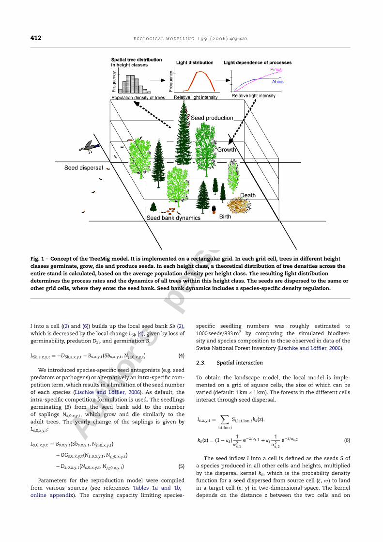
Fig. 1 – Concept of the TreeMig model. It is implemented on a rectangular grid. In each grid cell, trees in different heightclasses germinate, grow, die and produce seeds. In each height class, a theoretical distribution of tree densities across theentire stand is calculated, based on the average population density per height class. The resulting light distributiondetermines the process rates and the dynamics of all trees within this height class. The seeds are dispersed to the same orother grid cells, where they enter the seed bank. Seed bank dynamics includes a species-specific density regulation.

I into a cell ((2) and (6)) builds up the local seed bank Sb (2),which is decreased by the local change LSb (4), given by loss ofgerminability, predation DSb and germination B.

LSb,s,x,y,t = −DSb,s,x,y,t − Bs,x,y,t(Sbs,x,y,t, Nj≥0,x,y,t) (4)

We introduced species-specific seed antagonists (e.g. seedpredators or pathogens) or alternatively an intra-specific com-petition term, which results in a limitation of the seed numberof each species (Lischke and Loffler, 2006). As default, theintra-specific competition formulation is used. The seedlingsgerminating (B) from the seed bank add to the numberof saplings Ns,0,x,y,t, which grow and die similarly to theadult trees. The yearly change of the saplings is given byLs,0,x,y,t:

Ls,0,x,y,t = Bs,x,y,t(Sbs,x,y,t, Nj≥0,x,y,t)

− OGs,0,x,y,t(Ns,0,x,y,t, Nj≥0,x,y,t)

− Ds,0,x,y,t(Ns,0,x,y,t, Nj≥0,x,y,t) (5)

Parameters for the reproduction model were compiledfrom various sources (see references Tables 1a and 1b,online appendix). The carrying capacity limiting species-

specific seedling numbers was roughly estimated to1000 seeds/833 m2 by comparing the simulated biodiver-sity and species composition to those observed in data of theSwiss National Forest Inventory (Lischke and Loffler, 2006).

2.3. Spatial interaction

To obtain the landscape model, the local model is imple-mented on a grid of square cells, the size of which can bevaried (default: 1 km × 1 km). The forests in the different cellsinteract through seed dispersal.

Is,x,y,t =∑

lat,lon,i

Si,lat,lon,tks(z),

ks(z) = (1 − �s)1

˛2s,1

e−z/˛s,1 + �s1

˛2s,2

e−z/˛s,2 (6)

The seed inflow I into a cell is defined as the seeds S ofa species produced in all other cells and heights, multipliedby the dispersal kernel ks, which is the probability densityfunction for a seed dispersed from source cell (�, �) to landin a target cell (x, y) in two-dimensional space. The kerneldepends on the distance z between the two cells and on

Autho

r's

pers

onal

co

py


the species’ mean dispersal distance ˛s. The direction is nottaken into account. Due to the modular formulation of themodel code, the dispersal kernels can easily be exchanged.Currently, a combination of two negative exponentials, onefor short-distance transport (e.g. ballistic, normal wind, smallanimal transport) and one for long-distance transport (e.g.by birds, large mammals, uplifting by wind) is implemented.The species-specific values of �s, ˛s,1 and ˛s,2 were roughlyassigned (Tables 1a and 1b of the online appendix), for thewind-dispersed species based on terminal velocities and windspeed distributions (Lischke and Loffler, 2006). These valuesrange from 25 to 200 m. The seed transport, defined by seedproduction and the dispersal kernel, can be simulated eitherdeterministically or stochastically. For stochastic transport,the number of seeds reaching a sink cell from a source cellis sampled from a binomial distribution.

3. Case studies

We present here two case studies to test the model’s ability toform patterns in different situations. Under the assumptionthat patterns depend on spatial resolution, one comparativelyfine and one coarser resolution were chosen for the two casestudies. Moreover, in order to test the influence of endogenousversus exogenous drivers on patterns, the first case study isset up in a temporally and spatially constant environment,the second one in a strongly heterogeneous and variable envi-ronment.

3.1. Case study 1: “local pattern formation”

The first case study represents a theoretical model applica-tion, which tests the influence on the simulated patterns ofthe model processes alone.

The simulation was run for 800 years on a grid consist-ing of 50 × 50 cells of 100 m side length. The bioclimaticdrivers were kept constant in space and time, at valuescorresponding to a temperate, humid climate (degree-daysum of 1564 ◦C, minimum winter temperature of −2.7 ◦C andabsence of drought stress). The simulation was run with the30 most important Central European species (for a list seeTables 1a and 1b of the online appendix). It was initializedin a spin-up run of 5 years, during which all cells were empty,except the centre one, where the simulation was run with aconstant seed supply but without seed dispersal. In this way,all species that can establish under these conditions form aninitial low forest in the centre cell. After the spin-up, the modelwas switched to its standard configuration, i.e. seed produc-tion, seed loss (predation, loss of germinability, germination)and stochastic seed dispersal were activated and the constantseed supply was disabled.

The simulation results are presented in Fig. 2 as contourplots of species biomasses for selected time steps (for an ani-mation of the simulation, see online appendix).

The spatio-temporal pattern is determined by: (a) com-plementary quasi-standing waves of Betula pendula, Populustremula and Populus nigra in the first 100–200 years, (b) outliersand fringe spread of species with few seeds (Quercus petraea,Sorbus aucuparia, Fagus silvatica) and (c) homogenous spread

of dominant species that produce large seed quantities (Piceaabies). The patterns of less dominant species are overlaid bythose of more dominant species. The patterns are not stablethroughout the whole simulation, but eventually reach a moreor less homogenous spatial distribution of all species towardsthe end of the simulation, with P. abies and F. silvatica domi-nating the other species.

The wave-like pattern formation is due to the interactionof similar early-successional tree species with slightly differ-ent competitive behaviour. While P. tremula is slightly strongerin the competition for resources, B. pendula disperses moreseeds. At distant locations, the latter is thus able to escapethe competition with aspen by building up new populations.Closer to the source cell, the amount of seeds is limited by thecarrying capacity, which gives a competitive advantage to P.tremula. When the trees of the first cohort of a species reachthe age of first seed production, B. pendula forms a new colo-nization ring, whereas P. tremula follows behind in an anotherring. These initial ring structures persist for a long time, buteventually vanish, i.e. the wave pattern is not stable. Even ina simulation (not shown) with only P. tremula and B. pendula,both species end up coexisting homogenously in space.

A transient patch structure is created by the stochasticlong distance transport of the comparatively fewer seeds ofQ. petraea, S. aucuparia, A. incana and F. silvatica. New satel-lite populations establish away from the main populationcentre, originating from a few seeds that arrive there at ran-dom. The satellite populations then again spread regularlyand merge with the original population after several hundredyears of simulation. These species obviously produce too fewseeds (compared to their seed dispersal capability) to domi-nate homogenously across the newly invaded areas.

This simplified case study demonstrates the ability of theTreeMig model to produce a number of different endogenouslydriven patterns as a result of seed production, dispersal andregeneration, as well as species competition for resources andmortality.

3.2. Case study 2: “Holocene tree-species migration inan Alpine region”

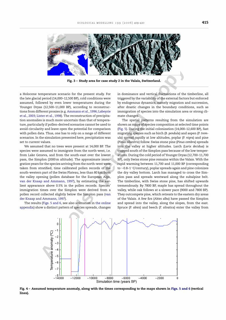
The topic of the case study is the potential spatio-temporalvegetation development in the Alpine region of the Valaissince the last Ice Age. It is an example of large-scale spatio-temporal landscape dynamics. The region has defined immi-gration paths for each tree species, which is important for sim-ulating migration. Furthermore, the strong climatic hetero-geneity, due to the topography and continentality gradients,makes it particularly suitable for evaluating the combinedeffects of external drivers and model processes on spatio-temporal patterns.

The central Alpine region of the Valais (Fig. 3) spans a largerange of environmental conditions, with altitudes stretchingfrom 400 to 4600 m, yearly mean temperatures between −10and 11 ◦C and yearly precipitation sums between 350 mm inthe eastern parts of the valley and clearly above 2000 mm athigh altitudes. The central Alps separate the main valley fromthe glacial refuges of many species in the south and east. Thefew paths where species could enter the region are the north-ern opening of the valley and several lower mountain passes

Autho

r's

pers

onal

co

py


Fig. 2 – Biomass of selected species (out of 30) in a simulation with constant environmental conditions (temperate humidclimate) at selected time points. Each square corresponds to the biomass of one species in 50 × 50 cells of 100 m × 100 meach. The simulation was initialized with all species in the centre cell and empty cells everywhere else. For an animation ofthe spatio-temporal dynamics see “LocalPatternFormation.avi” in the electronic appendix.

in the south-east. The simulation was carried out on an areaof 50 km × 110 km (Fig. 3) with 1 km × 1 km grid cells and ranfrom the end of the last Ice Age, ∼14,000 before present (BP),to present.

The scenario of past climate change used in this studywas derived from current climate data and assumptions aboutthe temperature anomalies. Bioclimatic variables (degree-daysum above 5.5 ◦C, minimum of monthly mean temperaturesand a drought stress index (between 0 and 1)) were generatedfor each cell and each year in the simulation period. For this weused current monthly temperature and precipitation values,

interpolated from climate stations (Zierl, 2001). Past climatethroughout the simulation period was obtained by adding ananomaly scenario to current temperature values.

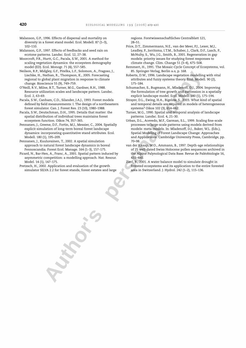
The temperature anomaly (Fig. 4) has been reconstructedusing chironomids in Alpine lakes for the period from 11,000BP to present (for details, see Heiri et al., 2005). This recordis one of the few continuous quantitative climate reconstruc-tions for the Central Alps. The smoothed, 62-sample July airtemperature reconstruction (as described in Heiri et al., 2003)was used with the revised age-scale for the Hinterburgseesediment record (described in Heiri et al., 2004) to produce

Autho

r's

pers

onal

co

py


Fig. 3 – Study area for case study 2 in the Valais, Switzerland.

a Holocene temperature scenario for the present study. Forthe late glacial period (14,000–12,500 BP), cold conditions wereassumed, followed by even lower temperatures during theYounger Dryas (12,500–11,000 BP), according to reconstruc-tions from different proxies (e.g. Ammann et al., 1996; Labeyrieet al., 2003; Lister et al., 1998). The reconstruction of precipita-tion anomalies is much more uncertain than that of tempera-ture, particularly if pollen-derived scenarios cannot be used toavoid circularity and leave open the potential for comparisonwith pollen data. Thus, one has to rely on a range of differentscenarios. In the simulation presented here, precipitation wasset to current values.

We assumed that no trees were present at 14,000 BP. Thespecies were assumed to immigrate from the north-west, i.e.from Lake Geneva, and from the south-east over the lowestpass, the Simplon (2000 m altitude). The approximate immi-gration years for the species arriving from the north-west weretaken from stratified, time calibrated pollen records of thesouth-western part of the Swiss Plateau, less than 80 km fromthe valley opening (pollen database for the European Alps,van der Knaap and Ammann, 1997), by estimating the ear-liest appearance above 0.5% in the pollen records. Species’immigration times over the Simplon were derived from apollen record collected slightly below the Simplon pass (vander Knaap and Ammann, 1997).

The results (Figs. 5 and 6, see also animation in the onlineappendix) show a distinct pattern of species spreads, changes

in dominance and vertical fluctuations of the timberline, alltriggered by the variability of the external factors but enforcedby endogenous dynamics, namely migration and succession,after drastic changes in the boundary conditions, such asimmigration of species into the simulation area or strong cli-mate changes.

The spatial patterns resulting from the simulation areshown as maps of species composition at selected time points(Fig. 5). During the initial colonization (14,000–12,600 BP), fastmigrating species such as birch (B. pendula) and aspen (P. trem-ula) spread rapidly at low altitudes, poplar (P. nigra) and pine(Pinus silvestris) follow. Swiss stone pine (Pinus cembra) spreadsinto the valley at higher altitudes. Larch (Larix decidua) istrapped south of the Simplon pass because of the low temper-atures. During the cold period of Younger Dryas (12,700–11,700BP), only Swiss stone pine remains within the Valais. With therapid warming between 11,700 and 11,000 BP (correspondingto ∼0.8–1 ◦C/century), poplar spreads again and pine colonizesthe dry valley bottom. Larch has managed to cross the Sim-plon pass and spreads westward along the subalpine belt.The timberline, with Swiss stone pine, has shifted upwardstremendously. By 7800 BP, maple has spread throughout thevalley, while oak follows at a slower pace (9000 and 7800 BP).They outcompete pine, which retreats to the eastern dry areasof the Valais. A few firs (Abies alba) have passed the Simplonand spread into the valley, along the slopes, from the east.Spruce (P. abies) and beech (F. silvatica) enter the valley from

Fig. 4 – Assumed temperature anomaly, along with the times corresponding to the maps shown in Figs. 5 and 6 (verticallines).

Autho

r's

pers

onal

co

py


Fig. 5 – TreeMig simulation (13,800–11,000 BP) of tree species spread on a 1 km × 1 km grid, over a 100 km × 50 km area inthe region of the Valais, Switzerland. In each cell, the species biomasses (t/ha) are drawn as stacked columns. A completelyfilled cell corresponds to 435 t/ha total biomass. For an animation of the spatio-temporal pattern, see“HoloceneTreeMigration.avi” in the electronic appendix.

the north-west. By 6000 BP, spruce and beech have spreadalmost throughout the Valais. Many species still coexist attheir eastern limits, in the valley. This spread of spruce andbeech continues until present, when spruce dominates in theregion, particularly on the slopes. It reduces fir, oak and beechto low biomasses at medium altitudes and pushes Swiss stonepine and larch up to high elevations. Only in the valley bot-

tom do pine, oak and beech co-exist. Pine dominates in the dryeastern region. This pattern corresponds largely to the currentspecies composition in the Valais, as recorded on the plots ofthe first Swiss National Forest Inventory (EAFV, 1988), whichshow beech and oak in the west and pine in the east of thevalley bottom, spruce at medium to high altitudes, some fir atintermediate altitudes on the northern slopes and larch with

Autho

r's

pers

onal

co

py


Fig. 6 – TreeMig simulation of tree species spread for years 9000 BP to today. For explanations, see Fig. 5.

some Swiss stone pine at the timberline. The main deviationbetween simulation and data lies in the under-representationof larch and fir (particularly in the north).

The large-scale spatio-temporal pattern is dominated byfive aspects: (1) the initial colonization of the empty habi-tats, (2) the disappearance of most species during the verycold Younger Dryas, (3) the recolonization after Younger Dryas,(4) the immigration waves of various new species with theinvaders partly co-existing (Pinus, Populus and Quercus) andpartly outcompeting the formerly established trees (Picea and

Fagus) and (5) the spatial separation of the species accordingto environmental conditions. The importance of each of thesefactors differs between times and locations. The dynamicsand spatial patterns of the exogenous drivers influence thesimulated patterns directly (aspects (2) and (5)) and initiatetransient phases of strong spatio-temporal endogenous pat-tern formation (aspects (1), (3) and (4)). At this coarse scale(grain = 1 km × 1 km), no pattern types such as those in thelocal, fine-scale case study (quasi-standing waves, patches)could be observed. This might be because the resolution is

Autho

r's

pers

onal

co

py


too coarse with respect to the interaction ranges and becauseof the strong gradients of the environmental variables.

The same simulation with a different temperature anomaly(up to 5.5 ◦C higher temperatures in the first period(14,000–11,000 BP), ca. 0.35 ◦C lower temperatures afterwards,Lischke, 2005), differs mainly in the species composition andspread until 11,000 BP. There, Larix manages to pass the Sim-plon already in the first centuries, spreads and dominates onthe slopes, before being suppressed by Swiss stone pine. Theclimatic bottleneck at the pass is therefore not as narrow asin the simulation presented here. Later, oak immigration isslower and that of spruce faster than in the simulation wepresent here. This is probably due to the slightly cooler cli-mate influencing migration speed through growth and com-petition, which affect mean annual seed production. The finalspecies composition, however, is nearly identical between thetwo simulations. This indicates that the (spatial) transientbehaviour is more sensitive to changes in driving variablesthan the equilibrium state and corroborates the conclusionin Lischke (2005), that changes in boundary conditions have aparticularly strong influence, via species’ migrations, on thespatio-temporal pattern.

4. Discussion of the model

The forest-landscape model TreeMig accounts for within-cellstructure in terms of horizontal and vertical heterogeneitywithin the forest stand and in terms of species. Reproductionis modelled in a detailed way, including seed production byadult trees, seed dispersal, seed bank dynamics, germinationand sapling development. The case studies demonstrate thatthe model can successfully be applied to various situations,with, for instance, different spatial (region to continent) ortemporal (centuries to millennia) scales. Additionally, the casestudies illustrate that the model can produce several types ofpatterns, including regular or stochastic patchy patterns onthe small scale and a combination of exogenously and endoge-nously generated patterns in the large-scale simulation on theother hand.

4.1. Comparison with other spatially dynamiclandscape modelling approaches

TreeMig is similar to some other landscape model approaches,in that it simulates multi-species forests which are spatiallylinked. It differs in the way the population dynamics andreproduction are implemented and particularly in the within-cell heterogeneity.

In the model LandClim, Schumacher et al. (2004) replacedthe presence/absence of species cohorts of the LANDIS modelwith species biomass dynamics. However, this model includesonly presence/absence of seeds and does not link seed num-bers to adult tree density and maturity. Thus, it biasesthe inter-specific competition. Pennanen et al. (2004) andPennanen and Kuuluvainen (2002) also developed LANDIS fur-ther. As in TreeMig, seed production and dispersal were linkedto seed sources. Similarly to the intra-specific seed densityregulation of TreeMig, this model limits the seed numbers ofstrong seed producers. The limitation is modelled by a rule

which forces shade intolerant species to establish in open gapsonly. Also similarly to TreeMig, the landscape model LandMod(Garman, 2004) was scaled up from a gap model to acceleratethe computation. It includes seed production and dispersal.Growth and mortality functions, as well as bioclimatic values,were fitted by meta-modelling (Urban et al., 1999) to gap modelsimulations. In contrast to TreeMig however, none of thesemodels account for within cell variability. As demonstrated insimulations with LandMod (Garman, 2004), this can lead to asignificant underestimation of the density of shade-intolerantspecies.

4.2. Potential and limitations of the model

TreeMig is a model for studying vegetation dynamics at a broadrange of spatial and temporal scales, ranging from stands toregions with resolutions of 100–1000 m. Because the essentialprocess functions are included, the model is general in thesense that it can be used for different topics and in differ-ent regions without changing its structure. Beyond that, mostparameters and functions of this model are interpretable andmeasurable.

The inclusion of antagonists or a carrying capacity for seedsmakes the model formulation similar to that of traditionalgap models: the supply of saplings of each species is lim-ited. However, in TreeMig this supply depends on the pres-ence or absence of parent trees, as in the spatial gap-modelMOSEL (Malanson, 1996). Moreover, the seed supply in TreeMigincreases continuously depending on the number of parenttrees, i.e. the positive feedback “more seeds–more trees–moreseeds” acts, as long as the number of seeds produced remainbelow the carrying capacity.

The flexibility of TreeMig is demonstrated by the differentapplications for which the model is currently being used as abasis: the simulation of riparian forest dynamics in the contextof the restoration of the Rhone river (Glenz et al., submittedfor publication), land use and climate change at the Alpineand boreal treelines and the assessment of human influenceon vegetation composition in the Holocene by comparing themodel simulations to pollen sequences.

TreeMig is computationally efficient in comparison withmodels of a similar level of ecological and environmentaldetail, thus it allows simulations at the regional scale. Thesimulation time is about 2/30 ms per grid cell and year on aSun Blade 1000 workstation with an UltraSparc III cu 900 MHzCPU with 1 GB RAM, what amounted to 48 h for the Holocenestudy, which encompasses 6050 grid cells and 14,000 years.

The computing time will be limiting if very large areas, e.g.the entire Alpine Arch or entire Europe, are to be simulatedwith a fine resolution. Increasing the grain to values greaterthan 1 km would however increase discretization errors, dueto assumptions about the distribution of species inside cells.The spatial resolution of the model should also not be smallerthan 100 m, otherwise the distribution-based approach, whichassumes a theoretical distribution over patches of 833 m2.For such resolutions an individual-based, position-dependentapproach is more suitable.

Some uncertainties remain in the model, including thefinal shape of the dispersal kernel. Most parameters for thetree dynamics were taken from a well-tested gap model (For-

Autho

r's

pers

onal

co

py


Clim, Bugmann, 1994). However, the new parameters for repro-duction and seed dispersal were compiled from the literature,and some of them contained large uncertainties. Others werefitted by eye or derived using best estimates. Therefore, theshape of the dispersal kernel in particular, but also the esti-mated parameter values have to be considered as preliminaryand will be tested in a sensitivity analysis.

Despite these uncertainties, the species compositions sim-ulated in both case studies for current conditions largely cor-respond to empirical evidence, such as forest inventory data.The simulations, however, differ from observations in thatthey show high biomasses of P. abies and low biomasses ofA. alba (not shown in case study 1) and F. silvatica.

This implies that in a next step the model should be testedthoroughly by a validation against local and spatio-temporaldata and by a comprehensive sensitivity analysis of its spatialbehaviour.

Acknowledgements

This project has been supported by the Swiss National ScienceFoundation, Grant number 31-55958.98 and partly through the5th framework Programme of the European Union (Contractnumber EVK2-CT-2002-00136).

Appendix A. Supplementary data

Supplementary data associated with this article can be found,in the online version, at 10.1016/j.ecolmodel.2005.11.046.

r e f e r e n c e s

Ammann, B., Gaillard, M.-J., Lotter, A.F., 1996. PalaeoecologicalEvents During the Last 15000 Years: Regional Syntheses ofPalaeoecological Studies of Lakes and Mires in Europe. JohnWiley & Sons Ltd., Switzerland.

Bolliger, J., 2005. Simulating complex landscapes with a genericmodel: sensitivity to qualitative and quantitativeclassifications. Ecol. Complexity 2, 131–149.

Bolliger, J., Lischke, H., Green, D.G., 2005. Simulating the spatialand temporal dynamics of landscapes using generic andcomplex models. Ecol. Complexity 2 (2), 107–116.

Bolliger, J., Sprott, J.C., Mladenoff, D.J., 2003. Self-organization andcomplexity in historical forest landscape patterns. Oikos 100,541–553.

Bugmann, H., 1994. On the ecology of mountainous forests in achanging climate: a simulation study. Dissertation Nr 10638.Environmental Sciences, Swiss Federal Institute ofTechnology, Zurich.

Bugmann, H., Cramer, W., 1998. Improving the behaviour of forestgap models along drought gradients. Forest Ecol. Manage. 103(2–3), 247–263.

Clark, J.S., Ji, Y., 1995. Fecundity and dispersal in plantpopulations: implications for structure and diversity. Am. Nat.146 (1), 72–111.

EAFV, 1988. Schweizerisches Landesforstinventar. Ergebnisse derErstaufnahme 1982–1986. Berichte Eidgenossische.Forschungsanstalt fur Wald, Schnee und Landschaft. 305.Eidgenossische Anstalt fur das forstliche Versuchswesen inZusammenarbeit mit dem Bundesamt fur Forstwesen undLandschaftsschutz, Birmensdorf.

Finegan, B., 1984. Forest succession. Nature 312, 109–114.Garman, S.L., 2004. Design and evaluation of a forest landscape

change model for western Oregon. Ecol. Modell. 175 (4),319–337.

Glenz, C., Iorgulescu, I., Lischke, H., Kienast, F., Schlaepfer, R.RIFOD: a spatially-explicit riparian forest dynamics model.Forest Ecol. Manage., submitted for publication.

Harvey, L.D.D., 2000. Upscaling in global change research. Clim.Change 44 (3), 225–263.

He, H.S., Mladenoff, D.J., 1999. The effects of seed dispersal on thesimulation of long-term forest landscape change. Ecosystems2 (4), 308–319.

He, H.S., Mladenoff, D.J., Boeder, J., 1999. An object-oriented forestlandscape model and its representation of tree species. Ecol.Modell. 119 (1), 1–19.

Heiri, O., Lotter, A.F., Hausmann, S., Kienast, F., 2003. Achironomid-based Holocene summer air temperaturereconstruction from the Swiss Alps. Holocene 13 (4), 477–484.

Heiri, O., Tinner, W., Lotter, A.F., 2004. Evidence for coolerEuropean summers during periods of changing melt-waterflux to the North Atlantic. Proc. Natl. Acad. Sci. U.S.A. (PNAS)101, 15285–15288.

Heiri, C., Bugmann, H., Tinner, W., Heiri, O., Lischke, H., 2005. Amodel-based reconstruction of Holocene treeline dynamics inthe Central Swiss Alps. J. Ecol. 94, 206–216.

Koop, H., Hilgen, P., 1987. Forest dynamics and regenerationmosaic shifts in unexploited beech (Fagus sylvatica) stands atFontainebleau (France). Forest Ecol. Manage. 20, 135–150.

Korpel, S., 1995. Die Urwalder der Westkarpaten. Gustav Fischer,Stuttgart, Jena, New York.

Labeyrie, L., Cole, J., Alverson, K., Stocker, T., Allen, J., Balbon, E.,Blunier, T., Cook, E., COritjo, E., D’Arrigo, R., Gedalov, Z.,Lambeck, K., Paillard, D., Turon, J.L., Waelbroeck, C.,Yokohama, U., 2003. The history of climate dynamics in thelate quaternary. In: Alverson, K.D., Bradleyand, R.S., Pedersen,T.F. (Eds.), Paleoclimat, Global Change and the Future.Springer, Berlin a.o., pp. 33–61.

Lischke, H., 2001. New developments in forest modeling:convergence between applied and theoretical approaches.Nat. Resour. Model. 14 (1), 71–102.

Lischke, H., 2005. Modelling of tree species migration in the Alpsduring the Holocene: what creates complexity? Ecol.Complexity 2 (2), 159–174.

Lischke, H., Bolliger, J., Seppelt, R. Dynamic spatio-temporallandscape models. In: Kienast, F., Ghoshand, S., Wildi, O.(Eds.), A Changing World: Challenges for Landscape Research.Kluwer, Dordrecht, in press.

Lischke, H., Loffler, T.J., Thornton, P.E., and Zimmermann, N.E.Up-scaling of biological properties and models to thelandscape level. In: Kienast, F., Ghoshand, S., Wildi, O. (Eds.), AChanging World: Challenges for Landscape Research. Kluwer,Dordrecht, in press.

Lischke, H., Loffler, T., 2006. Intra-specific density dependence isrequired to maintain diversity in spatio-temporalforest simulations with reproduction. Ecol. Modell.198, 341–361.

Lischke, H., Loffler, T.J., Fischlin, A., 1998. Aggregation ofindividual trees and patches in forest successionmodels—capturing variability with height structured randomdispersions. Theor. Popul. Biol. 54 (3), 213–226.

Lister, G., Livingstone, D.M., Ammann, B., Ariztegui, D., Haeberli,W., Lotter, A.F., Ohlendorf, C., Pfister, C., Schwander, J.,Schweingruber, F., Stauffer, B., Sturm, M., 1998. Alpinepalaeoclimatology. In: Cebon, P., Dahinden, U., Davies, H.,Imbodenand, D., Jaeger, C. (Eds.), A View From the Alps:Regional Perspectives on Climate Change. MIT Press, Boston.

Loffler, T.J., Lischke, H., 2001. Incorporation and influence ofvariability in an aggregated forest model. Nat. Resour. Model.14 (1), 103–137.

Autho

r's

pers

onal

co

py


Malanson, G.P., 1996. Effects of dispersal and mortality ondiversity in a forest stand model. Ecol. Modell. 87 (1–3),102–110.

Malanson, G.P., 1997. Effects of feedbacks and seed rain onecotone patterns. Landsc. Ecol. 12, 27–38.

Moorcroft, P.R., Hurtt, G.C., Pacala, S.W., 2001. A method forscaling vegetation dynamics: the ecosystem demographymodel (ED). Ecol. Monogr. 71 (4), 557–585.

Neilson, R.P., Midgley, G.F., Pitelka, L.F., Solomon, A., Fragoso, J.,Lischke, H., Nathan, R., Thompson, K., 2005. Forecastingregional to global plant migration in response to climatechange. Bioscience 55 (9), 749–759.

O’Neill, R.V., Milne, B.T., Turner, M.G., Gardner, R.H., 1988.Resource utilization scales and landscape pattern. Landsc.Ecol. 2, 63–69.

Pacala, S.W., Canham, C.D., Silander, J.A.J., 1993. Forest modelsdefined by field measurements: I. The design of a northeasternforest simulator. Can. J. Forest Res. 23 (10), 1980–1988.

Pacala, S.W., Deutschman, D.H., 1995. Details that matter: thespatial distribution of individual trees maintains forestecosystem function. Oikos 74, 357–365.

Pennanen, J., Greene, D.F., Fortin, M.J., Messier, C., 2004. Spatiallyexplicit simulation of long-term boreal forest landscapedynamics: incorporating quantitative stand attributes. Ecol.Modell. 180 (1), 195–209.

Pennanen, J., Kuuluvainen, T., 2002. A spatial simulationapproach to natural forest landscape dynamics in borealFennoscandia. Forest Ecol. Manage. 164 (1–3), 157–175.

Picard, N., Bar-Hen, A., Franc, A., 2001. Spatial pattern induced byasymmetric competition: a modelling approach. Nat. Resour.Model. 14 (1), 147–175.

Pretzsch, H., 2002. Application and evaluation of the growthsimulator SILVA 2.2 for forest stands, forest estates and large

regions. Forstwissenschaftliches Centralblatt 121,28–51.

Price, D.T., Zimmermann, N.E., van der Meer, P.J., Lexer, M.J.,Leadley, P., Jorritsma, I.T.M., Schaber, J., Clark, D.F., Lasch, P.,McNulty, S., Wu, J.G., Smith, B., 2001. Regeneration in gapmodels: priority issues for studying forest responses toclimate change. Clim. Change 51 (3–4), 475–508.

Remmert, H., 1991. The Mosaic-Cycle Concept of Ecosystems, vol.85. Springer-Verlag, Berlin a.o, p. 168.

Roberts, D.W., 1996. Landscape vegetation modelling with vitalattributes and fuzzy systems theory. Ecol. Modell. 90 (2),175–184.

Schumacher, S., Bugmann, H., Mladenoff, D.J., 2004. Improvingthe formulation of tree growth and succession in a spatiallyexplicit landscape model. Ecol. Modell. 180 (1), 175–194.

Strayer, D.L., Ewing, H.A., Bigelow, S., 2003. What kind of spatialand temporal details are required in models of heterogeneoussystems? Oikos 102 (3), 654–662.

Turner, M.G., 1990. Spatial and temporal analysis of landscapepatterns. Landsc. Ecol. 4, 21–30.

Urban, D.L., Acevedo, M.F., Garman, S.L., 1999. Scaling fine-scaleprocesses to large-scale patterns using models derived frommodels: meta-models. In: Mladenoff, D.J., Baker, W.L. (Eds.),Spatial Modeling of Forest Landscape Change: Approachesand Applications. Cambridge University Press, Cambridge, pp.70–98.

van der Knaap, W.O., Ammann, B., 1997. Depth-age relationshipsof 25 well-dated Swiss Holocene pollen sequences archived inthe Alpine Palynological Data Base. Revue de Paleobiologie 16,433–480.

Zierl, B., 2001. A water balance model to simulate drought inforested ecosystems and its application to the entire forestedarea in Switzerland. J. Hydrol. 242 (1–2), 115–136.

This article was originally published in a journal published byElsevier, and the attached copy is provided by Elsevier for the

author’s benefit and for the benefit of the author’s institution, fornon-commercial research and educational use including without

limitation use in instruction at your institution, sending it to specificcolleagues that you know, and providing a copy to your institution’s

administrator.

All other uses, reproduction and distribution, including withoutlimitation commercial reprints, selling or licensing copies or access,

or posting on open internet sites, your personal or institution’swebsite or repository, are prohibited. For exceptions, permission

may be sought for such use through Elsevier’s permissions site at:

http://www.elsevier.com/locate/permissionusematerial

http://www.elsevier.com/locate/permissionusematerial

TreeMig: A forest-landscape model for simulating spatio-temporal patterns from stand to landscape...

Documents

Transcript of TreeMig: A forest-landscape model for simulating spatio-temporal patterns from stand to landscape...