Transportation Forecasting: Analysis and Quantitative Methods
160
TRANSPORTATION RESEARCH RECORD 944 Transportation Forecasting: Analysis and Quantitative Methods TRANSPORTATION RESEARCH BOARD NATIONAL RESEARCH COUNCIL NATIONAL ACADEMY OF SCIENCES WASHING TON. D C 1983
-
Upload
khangminh22 -
Category
Documents
-
view
0 -
download
0
Transcript of Transportation Forecasting: Analysis and Quantitative Methods

I.r
8 —c
TRANSPORTATION RESEARCH RECORD 944
Transportation Forecasting:Analysis andQuantitative Methods
TRANSPORTATION RESEARCH BOARD
NATIONAL RESEARCH COUNCILNATIONAL ACADEMY OF SCIENCESWASHING TON. D C 1983

TransportationResearchRecord944Price$18.20EditedforTRB by ScottC,Herman
modes1 highwaytransportation2 publictransit4 airtransportation
subjectareas12 planning13 forecasting
LibraryofCongressCataloginginPublicationDataNationalResearchCouncil.TransportationResearchBoard.Transportationforecasting.
(Transportationresearchrecord;944)1.Transportation-Forecasting-Mathematicalmodels-Con-
~esses.2. Transportation-Planning-Mathematicalmodels-Con-gresses.L NationalResearchCouncil(U.S.)TransportationR&searchBoard.II.NationalAcademy ofSciences(U.S.)111.Series.TE7.H5 no.944 380.5S 84-18963[HE1l] [380.5]ISBN 0-309-03665-8 ISSN0361-1981
SponsorshipofthePapersinThisTransportationResearchRecord
GRCXJP I-TRANSPORTATION SYSTEMS PLANNING ANDADMINISTRATIONKenneth W. Heath ington, University of Tennessee, chairman
TransportationForecastingSectionGeorgeV. Wickstrom, Metropolitan Washington Councilof Govern-ments, chairman
Committeeon PassengerTravelDemand ForecastingFrank S. Koppelman, Northwestern University, chairmanMoshe E. Ben-Akiva, Werner Brog, William A. Davidson, ChristopherR. Fleet, Susan Hanson, Joel L. Horowitz, Stephen M. Howe, TerryKraft, Steven Richard Lerman, Eugene J. Lessieu, En”cJ. Miller,Eric Ivan Pas, Martin G. Richards, Aad Ruhl, Earl R. R uiter, JamesM. Ryan, Bruce D. Spear, Timothy J, Tardiff
Committeeon TravelerBehaviorandValuesDavid T. Hartgen, New York State Department of Transportation,
chairmanPeter M. Allarnan, Julian M. Benjamin, Katherine Patricia Burnett,Melvyn Cheslow, David Damm, Michael A. Florian, Thomas F.Golob, David A. Hensher, Joel L. Horonitz, Frank S. Koppelman,Steven Richard Lerrnan, Jordan J. Louviere, Amim H. Meyburg,Richard M. Michaels, Alfred J. Neveu, Robert E. Paaswell, Earl R.Ruiter, Yosef Sheffi, Peter R. Stopher, Antti Talvitie, Mary LynnTischer
JamesA.Scott,TransportationResearchBoardstaff
Sponsorshipisindicatedby a footnoteattheendofeachreport.The organizationalunits,officers,andmembersareasofDecember31,1982.

Contents
DEVELOPMENT OF SURVEY INSTRUMENTS SUITABLE FOR DETERMININGNONHOME ACTIVITY PATTERNS
Werner Brog, Arnim H. Meyburg, and Manfred J. Wermuth . . . . . . . . . . . . . . . . . . . . . . . . . . . . . . 1
SEQUENTIAL, HISTORY-DEPENDENT APPROACH TO TRIP43-IAINING BEHAVIORRyuichi Kitamura . . . . . . . . . . . . . . . . . . . . . . . . . . . . . . . . . . . . . . . . . . . . . . . . . . . . . . . . . . . . . .13
IDENTIFYINGTIME AND HISTORY DEPENDENCIES OFACTIVITYCHOICERyuichi Kitamura and Mohammad Kermanshah . . . . . . . . . . . . . . . . . . . . . . . . . . . . . . . . . . . . ...22
EQUILIBRIUM TRAFFIC ASSIGNMENTON ANAGGREGATED HIGHWAY NETWORKFORSKETCHPLANNING
R.W. Eash, K.S. Chon, Y.J. Lee,and D.E. Boyce . . . . . . . . . . . . . . . . . . . . . . . . . . . . . . . . . . . ...30
NETWORK DESIGN APPLICATIONOF ANEXTRACTION ALGORITHM FORNETWORKAGGREGATION
Ali E. Haghani andMark S. Daskin . . . . . . . . . . . . . . . . . . . . . . . . . . . . . . . . . . . . . . . . . . . . . . ...37
QUICK-RESPONSE PROCEDURES TO FORECAST RUlV4L TRAFFICAlfred J. Never . . . . . . . . . . . . . . . . . . . . . . . . . . . . . . . . . . . . . . . . . . . . . . . . . . . . . . . . . . . . . . . .47
RESPONDENTTRIP FREQUENCY BIAS INON-BOARDSURVEYSLawrence B. Doxsey . . . . . . . . . . . . . . . . . . . . . . . . . . . . . . . . . . . . . . . . . . . . . . . . . . . . . ..”” ””.54
BUS,TAXI,ANDWALK FREQUENCYMODELS THAT ACCOUNT FORSAMPLE SELECTIVITY ANDSIMULTANEOUS EQUATION BIAS
Jesse Jacobson . . . . . . . . . . . . . . . . . . . . . . . . . . . . . . . . . . . . . . . . . . - . . . . . . . . . . . . .””-...”” .57
EFFECTOFSAMPLE SIZE ONDISAGGREGATE CHOICEMODEL ESTIMATIONAND PREDICTION
Frank S. Koppelrnan andChaushie Chu b. . . . . . . . . . . . . . . . . . . . . . . . . . . . . . . . . ..- . . ..”” ..60
MOBILITY ENTERPRISE: ONEYEARLATERMichael J. Doherty and F.T. Sparrow . . . . . . . . . . . . . . . . . . . . . . . . . . . . . . . . . . . ..”. ”””” .””.70
PERSON-CATEGORY TRIP-GENERATION MODEL-.>
Janusz Supemak, AnttiTalvitie,md Anthony DeJohn . . . . . . . . . . . . . . . . . . . . . . . . . . . . . . . . . . 74 /Y
TRIPGENERATIONBYCROSS-CLASSIFICATION: ANALTERNATIVEMETHODOLOGYPeter R. Stopher and KathieG. McDonald . . . . . . . . . . . . . . . . . . . . . . . . . . . . . . . . . . . . . . . . . . .
~4,/(~:~,‘\J
SOMECONTRARY INDICATIONS FOR THEUSEOFHOUSEHOLD STRUCTUREINTRIP-GENERATION ANALYSIS
Kathie G. McDonald and Peter R. Stopher . . . . . . . . . . . . . . . . . . . . . . . . . . . . . . . . . . . . . . . . . . . /g~ @/.
...111

iv
MAXIMUM-LIKELIHOOD AND BAYESIAN METHODS FOR THE ESTIMATION OFORIGIN-DESTINATION FLOWS
Itzhak Geva, Ezra Hauer, and Uzi Landau. . . . . . . . . . . . . . . . . . . . . . . . . . . . . . . . . . . . . . . . ...101
TRIP TABLE SYNTHESIS FOR CBD NETWORKS: EVALUATION OF THE LINKODMODELAnthony F. Hanand Edward C. Sullivan. . . . . . . . . . . . . . . . . . . . . . . . . . . . . . . . . . . . . . . . . ...106
ESTIMATING TRIP TABLES FROM TRAFFIC COUNTS: COMPARATIVE EVALUATION OFAVAILABLE TECHNIQUES
Yehuda J. Gus . . . . . . . . . . . . . . . . . . . . . . . . . . . . . . . . . . . . . . . . . . . . . . . . . . . . . . . . . . . . . ...113
TRIP DISTRIBUTION USING COMPOSITE IMPEDANCEWilliam G. Allen, Jr . . . . . . . . . . . . . . . . . . . . . . . . . . . . . . . . . . . . . . . . . . . . . . . . . . . . . . . . . ...118
DEVELOPMENTOF ATRAVEL-DEMAND MODELSETFOR THENEWORLEANSREGION
Gordon W. Schultz . . . . . . . . . . . . . . . . . . . . . . . . . . . . . . . . . . . . . . . . . . . . . . . . . . . . . . . . . . . . 128
ESTIMATION AND USEOFDYNAMIC TRANSACTION MODELS OFAUTOMOBILE OWNERSHIP
Irit Hocherrnan, Joseph N. Prashker, and Moshe Ben-Akiva . . . . . . . . . . . . . . . . . . . . . . . . . . . . . 134
EXPERIMENTS WITH OPTIMAL SAMPLING FORMULTINOMIAL LOGITMODELSYosef Sheffiand ZviTarem. . . . . . . . . . . . . . . . . . . . . . . . . . . . . . . . . . . . . . . . . . . . . . . . . . . . ..141
PROCEDURE FOR PREDICTING QUEUES ANDDELAYSON EXPRESSWAYSINURBANCOREAREAS
Thomas E. Disco . . . . . . . . . . . . . . . . . . . . . . . . . . . . . . . . . . . . . . . . . . . . . . . . . . . . . . . . . . . . ..148
Authors of the Papers in This Record
Allen,WilliamG., Jr., Volvo of America, 1 Volvo Drive, Building B, Rockleigh, NJ. 07647; formerly with Barton-AschmanAssociates, Inc.
Ben-Akiva, Moshe, Department of Civil Engineering, Massachusetts Institute of Technology, 77 Massachusetts Avenue,Room 1.178, Cambridge, Mass.02139
Boyce, D.E., Transportation Planning Group, Department of Civil Engineering, University of Illinois at Urbana-Champaign,208 N. Rornine Street, Urbana, Ill. 61801
Brog, Werner, Socialdata, GmbH, Hans-Grassel-Weg 1,8000 Miinchen 70, West GermanyChon, K.S., Department of Civil Engineering, State University of New York at Buffalo, Buffrdo, N.Y. 14260Chu, Chaushie, Department of CivilEngineering, University of Petroleum and Minerals, Dhahran, Saudi ArabiaDaSkin, Mark S., Department of CivilEngineering, Northwestern University, Evanston, Ill. 60201DeJohn, Anthony, Bureau of Statewide Planning, New Jersey Department of Transportation, 1035 Parkway Avenue,
Trenton, N.J. 08625Doherty, Michael J., Institute for Interdisciplinary Engineering Studies, Room 304 Potter, Purdue University, West
Lafayette, Ind. 47906Doxsey, Lawrence B., Transportation Systems Center, U.S. Department of Transportation, Kendall Square, Cambridge,
Mass.02142Eash, R.W,, Chicago Area Transportation Study, 300 W, Adams-Street, Chicago, Ill. 60606Geva, Itzhak, Department of Civil Engineering, University of Toronto, Toronto, Ontario, Canada M5S 1A4Gur, Yehuda J., Transportation Research Institute, Technion-Israel Institute of Technolo~, Haifa, IsraelHaghani, Ali E., Department of Civil Engineering, Northwestern University, Evanston, Ill. 60201Han, Anthony F., Institute of Transportation Studies, 109 McLaughlin Hall, University of California, Berkeley, Calif. 94720Hauer, Ezra, Department of Civil Engineering, University of Toronto, Toronto, Ontario, Canada M5S 1A4Hocherman, hit, Transportation Research Institute, Technion–Israel Institute of Technology, Haifa, IsraelJacobson, Jesse, 1382 Beacon Street, Brookline, Mass. 02 146; formerly with Transportation Systems Center, U.S.
Department of TransportationKermanshah, Moharnmad, Department of Civil Engineering, University of California at Davis, Davis, Calif. 95616Kitamura, Ryuichi, Department of Civil Engineering, University of California at Davis, Davis, Calif. 95616Koppelman, Frank S., Department of Civil Engineering, Northwestern University, Evanston, Ill. 60201Landau, Uzi, Department of Civil Engineering, Technion-Israel Institute of Technology, Haifa, IsraelLee, Y,J., Transportation Planning Group, Department of Civil Engineering, University of Illinois at Urbana-Champaign,
208 N. Romine Street, Urbana, Ill. 61801Iisco, Thomas E., Central Transportation Planning Staff, 27 School Street, Boston, Mass. 02108McDonald, Kathie G,, Research and Analysis, Planning Division, Metropolitan Dade County Planning Department, 44 West
Flagler Street, Suite 1100, Miami, Fla. 33130; formerly with Schimpeler-corradinoMeyburg, Arnim H., Department of Civil and Environmental Engineering, Cornell University, Hollister Hall, Ithaca, N.Y.
14853Neveu, Alfred J., Transportation Data and Analysis Section, Planning Department, New York State Department of
Transportation, 1220 Washington Avenue, State Campus, Albany, N.Y, 12232Prashker, Joseph N., Transportation Research Institute, Technion–Israel Institute of Technology, Haifa, IsraelSchultz, Gordon W., Barton-Aschman Associates, Inc., 1400 K Street, N.W., Washington, D.C. 20005Sheffi, Yosef, Center for Transportation Studies, Massachusetts Institute of Technology, 77 Massachusetts Avenue, Room
1-131, Cambridge, Mass. 02139Sparrow,F.T., Institute for InterdisciplinaryEngineeringStudies, Room 304 Potter, Purdue University,WestLafayette, Ind
47906Stopher, Peter R., Schimpeler-CorradinoAssociates,300 PalermoAvenue,CoralGables,Fla. 33134Sullivan,EdwardC., Institute of TransportationStudies, 109McLaughlinHall,Universityof California,Berkeley,Calif.
94720Supernak,Janusz, Departmentof CivilEngineering,San Diego State University, San Diego, Calif. 921 82; formerly with
Drexel University

, .
vi
Talvitie, Antti, Department of Civil Engineering, State University of New York at Buffalo, Buffalo, N.Y. 14260Tarem, Zvi, Center for Transportation Studies, Massachusetts Institute of Technology, 77 Massachusetts Avenue, Room
14350, Cambridge, Mass.02139Wermuth; Manfred J., Institute fur Stadtbauwesen, Technische Universitat Braunschweig, Postfach 3329,3300
Braunachweig, West Germany

Transportation Research Record 944
Development of Survey Instruments Suitable for
Determining Nonhome Activity Patterns
WERNER BROG,ARNIM H.MEYBURG,AND MAN FRED J.WERMUTH
Generation of travel behavior dats by means of empirical surveys is an impor-tant element of transportation planning. At the same time, relatively Iitdeattention has been paid to the rules for collecting and determining themethodological quality of the data. The methodological design of suchsurveys is relatively oompiiaated beaauseof a number of influenaefartors that may ultimet.dy be reflected in the validity of the results. Theissueof survey instrument design is discussedin detail. A number of msthod-dogiczl tests are examined that wera intendad to improve one of the weakpoints in surveys of tsaval behavior-tha design of suds instruments. Initially,it was concluded that a diary-type instrument would haw to be used to en-sure proper reaording of tiip dataiis. An ideal diary was davalopad that wasused in savaral survays. Sut it becems evident that this instrument design, inspite of its high msthodokrgieel quality, was unsuitable for Iarge+oda surveys,suah as those frequently used in transportation planning, becauseof Organira-tiorsal and cost problams. Tharefore, an additional seriesof teats was deval-oped to simplify these diaries and to transform them into a form suitable foriarga+cale mail-back surveys. Each tast serieswas tested empiriadly with de-taileddocumentationofraportirrgdafiaenaaa. Thus it was fmaible to presentin an undarstendabla manner tha development of a survey instrument of da-sirable quality. The final varsion of the instrument design, wtsish was theoutgrowth of the empirisal tests, has been usad subsaquarstlyin numerouslarge-male applications in several countrias. In the course of these applica-tions the methodological quality of the desi~ was ronfirmed, vvhiah ulti-mately justified the development rests.
The influence of measurement procedures and measure-ment (survey) instruments on measurement results hasto be recognized at the outact of any empirical sur-vey. Therefore, the survey procedure has to be in-cluded as part of the overall research approach(J). Typicallyr a measurement process (i.e., surveyprocedure) is composed of a number of elements thatcan be subsumed under the following categories (2,3):--
1. Problem formulation, theoretical referenceframe, analyais concept:
2. Base population, sampling unit, sampling pro-cedure, weighting, population values;
3. Survey method and instrument(s);4. Survey implementation,response rates; and5. Data preparation, evaluation, and analysis.
The third and fourth categories are the subjects of
this paper. The development and use of survey in-struments designed to meaaure actual nonhome activ-ity patterns are described in this paper.
Empirically measured travel behavior is the mostimportant input to transportation planning decisionsbecauae it constitutes the basis for explanation andprediction of future travel activities. Methodolog-ical deficiencies of this measure have direct conse-quences for all aubaequent phases of the transporta-tion planning process.
Meanwhile, the mail-back household survey, whichmeasures nonhome activity patterns, has become astandard compnent of transportation planning. Gen-erally, the survey instruments used in this processare the result of years of developmental work. Inthis paper such a developmental process ia retracedin terms of content and chronology on the basis ofthe KONTIV design (~).
Two aspects will be emphasized. First, the la-borious path of such developmental work, includingits accompanying setbacks, is illustrated. Second,it will be shown that basic methodological researchalso can produce, as by-products, fundamental andsubstantive analytical and theoretical insights.
1
EARLY DEVELOPMENTS
When preliminary developmental work toward the iae-provement of methods for measuring nonhome activitypatterna started in Germany in 1972, the qenerally
accepted method for empirical surveys was the per-sonal interview. For example, in an intensive per-sonal interview survey (~), the course of the dailytrips to work or schml was investigated in additionto various other aspects. Three main basee forcriticism arose out of such survey efforts:
1. The survey measured average rather than ac-tual travel behavior;
2. Information (e.g., abOUt fXWSl time) was es-timated by the interviewee)and
3. Only a segment of the individual’s mobilitywas investigated.
Consequently, the results of such interview in-formation were unsatisfactory when validated on thebasis of objectively measured values for traveltime, distance, and cost. For example, only three-quarters of automobile drivers estimated theirtravel time within a tolerance level of *25 per-cent. (Admittedly,the generation of objective com-parative data is difficult 1ss this instance.) Onaverager travel time was underestimated by 11 per-cent Q).
For the transit user the situation was quite dif-ferent. Although the share of respondents with re-ports of travel tiraewitbin the tolerance level of*25 percent was greater (naaaely,79 percent), theaverage error was substantially higher and in the
opposite direction, namely an average overestimationof 36 percent [see Table 1 (~)1.
The strong distortions caused by these roisesti-mates are describ+d in Table 2 (~), which gives abreakdown of trips into their sccess, S9ress, andtravel-time components. Automobile drivers claim tohave spent, on average, only a total of 6 min on ac-cess and egress, including the search for parkingspaces, whereas tranait users recorded 62 min foraccessr egress, waiting, and transfer times.
The methodologically oriented reader of such re-sults could draw two significant conclusions.Firstr the reported travel behavior and characteris-tics deviated substantially from reality even thoughthese respondents experienced the real values ofthese trip elements twice during each working
(school) day. Second, the biases are of a system-atic nature and apparently are related to the user’sattitude toward the respective travel mode. Hence,in the caae of public transit, the particularly dis-turbing access, egressr waiting, and transfer timesare overestimated drastically.
From a conceptual point of view, these resulta[which were substantiated in several other studies(~)1 indicated that the subjective perception ofnuch measures constitutes an important determinantof travel modal choice. l%is concept has foundentry into the relevant models under the terms per-ception and perceived values (~). The method0l09-ical analysis of these findings leads to two conclu-sions. First, data about travel behavior must notbe collected (inquired about) in a 9eneral form

Transportation Research Record 944
Table 1. Acrurscy of travel-tirns estimates for automobiles and transit (~).
Reported (interview) Travellime for
Item Automobde Public Transit
8ample size 800 520Correct estimates (within t25 percent error) (%) 72 79Incorrect estimates (> 25 percent error) (%) 28 21Index of average demation from the correct travel ttme 89 136
(objective time = 100)
Table2.Reportedzstirnatasof travai-tints components for automobile andtransit users (~).
Travel
ItemT]me(rein)
Automobile users (n = 800)Walk from residence topwking; from parking to destination 6In-vehicle travel time 41Search for parking at destination 1—Total 48
Transit users (n= 520 )Walk from residence to boarding stop; from alighting stop to 28
destinationIn-vehicle travel time 22Total waiting and transfer time 34
TotaI 84
(i.e., not in terms of average values); they need tohave a concrete temporal reference. Second, activ-ities cannot be viewed in isolation. Instead, can-plete daily activity patterns are needed to consti-tute the basis of analysis.
It could be shown, for example, that the record-ing of beginning and termination times of a trip ismore accurate than the direct reporting of triplengths. The implicationsof this for further meth-
orological considerations are as follms. First,the data about travel behavior need to be collectedfor specific survey days. Second, a diary-type sur-
vey instrument should be used, which requires en-tries about complete daily activity sequences.Third, a written survey form is preferable to thepersonal interview. However, this does not indicateby what means the survey instrument should be de-livered to the respondents, i.e., by mail or bymeana of an interviewer.
DEVEMPMENT OF AN ACTIVITIES DIARY
Based on the recognition that surveys about general(or average) travel behavior and of estimated infor-mation lead to invalid results, an activity diary(Q) was developed in 1972, in which the target popu-lation (sample) waa asked to record in writing itscomplete daily activity set for specific surveydates.
This diary (see Figures 1-4) was a brochure ofabout 8 x 6 in. in size, the cover of which listedthe name of the target person, the day of the week,and the date of the respective survey day. On theinside cover were 12 numbered lines for trip en-triesr where the odd-numbered trips were designatedby a different color in order to make this page ofthe diary visually clearer and more appealing. Onthis page the respondents were supposed to enter the
I Day of
I the Week

Transportation Research Record 944
Fi~mZ Inside oftripdiwy.
3
Fiwra3. Trip rogistirof diawforrwpoodent.
I /
/ //’@=-
..—. ———

4Transportation Research
FiWra 4. Trip register for ascompsrrying pemm(~).—
1) /
P’- —.xn
\tz
.-=J--BEti
Record 944
most important aspects of their sequence of activ- fornrfor the accompanying person contained informa-itiea during that day; i.e., location of the day’afirst activity (usually home), starting time of thefirst trip, activity aaaociated with that trip(e.g., work), and time of arrival at destination.
All subsequent tripa for that day were recordedaccording to the same pattern on the inside cover.Thus the temporal sequence of activities and thereasons (trip purposes) for the diverse nonhome ac-tivities were determined. At the same time, theformat and layout of the instrument ensured thatthis rough record of daily activities could be out-
lined in the course of the day (i.e., en route,cloee to the time of the occurrence of any partic-ular activity). This constituted the basis for theadditional questions in the activities diary.
Separate survey sheets for each trip were afixedto the top ,of the inside right cover. There weretwo sheets for each trip; the first was to be usedby the target person who was completing the diary.The second trip sheet referred to any possible ac-
~nyin9 traveler. These individual survey sheetswere equipped with a register that made it simple tolocste quickly the two sheets that belonged to anyone trip. A color code waa used for each trip thatcorresponded to the color scheme of even- versusodd-numbered trips recorded on the left inside cover.
The survey form for a specific trip performed bythe respondent contained the following information:
1. Accurate address of destination,2. Specification of up to three accompanying
parsona (e.g., neighbor, son, uncle),3. All travel modes used on a particular trip,
and4. Detailed description of the destination ac-
tivity.
A window was cut in the space where the specifi-
cation of the accompanying person waa recorded sothat this specification appeared on both sheets (forthe respondent and the accompanying person) withoutthe need to record the same information twice. The
tion aa to whether that person had accompanied therespondent from the start of the trip, whether theperson stayed with the respondent at the destina-tion, and, if applicable, what the person did subse-quently.
ORGANIZATIONAL PROCESS FOR USE OF ACTIVITY DIARY
The diary was intended to be completed by the re-s~ndents, but the demands on the respondents bothin terms of time and contents comprehension weresubstantial, especially for first-time use. Thenecessary instructions could not be transmittedeasily in writing to the respondent. fiencethe useof interviewers was necessary, but they played therole of adviaora rather than interviewers.
The procedure went as follows. First, the inter-viewer conducted a preinterview with the respondent,collecting the relevant aociodemographic data. Theinterviewer●xplained the structure of the diary and
helped fill in the sequence of activities for theday before the interview. Then the diaries werehanded to the respondent for subsequent unassistedre~rting of activities on the specified survey days.
Finally, a postinterview was arranged to discussthe respondents” experiences with the diaries, toreview the completed diariesi to make any correc-tions or additions that came to light at that time,and to collect the completed diaries. By this tech-nique it was possible to determine how well respon-dents had fared with the diaries and how completethe recorded information was.
The technique of a personal trip diary repre-sented significant progress both in terms of contentand method. With respect to content, the diary,which required the reporting of entire activity se-quencee, by necessity alao provided information forthe transportation planner about walk and bicycletripa that had been ignored typically up to thattime. The high share of nonmotorized travel intotal individual mobility was registered with some

Transportation Research Record 944
*.5. n~fof~ti~
5
I .. VlsitlngDates.. SubstltutaLhtM I
m : , II I I I 1r
Tdaa hdkmnreeflntewlevmronlepcwmdlnlmbareftrifm(#.
AVS No. of MobilityIndexmy Trips (ri dKY. 100.0)
5.14;
100.04.90 95.3
3 4.66 90.7Visjtby ioterviewcr
S.02 97.75 4.66 90.76 4.76 92.67 4.43 86.2
VM by intrrviewxr8 4.82 93.89 4.45 86.610 4.67 90.911 4.74 92.2
Vit byinterviewer12 4.83 94.013 4.S2 87.914 4.48 87.2
surprise, at least in the ?aderal Republic ofGermany.
Pros ● methodological point of via9, progress wasachievad because trave1 behavior had not baan re-corded in general ●nd ●verage terms, but rather w-cording to actual ●ctivities, ●nd ●mtlmates had baanreplaced by ●ethodologically mperior teohniquos.Navarthelesa, the problama ramalnad that one surveyday prwtded only ● sagmnt of ●n individualta mo-bility behavior, ●nd that traval bahavior could varyfrom day to day.
Baaed on these problems it was decided to inves-tigate the travel ●ctivities of a population for twoconsecutive waaka, with ●ach day re@ring the wpletion of ● ●aparate diary. Bacauae it could be•~tti that the motivation for completing these
diariaa would deoraasa with tima, tho Interviewerstook on the ●dditional tamk of viaitittgthe ●axplehouaaholds ●d providing tha raapondants with re-nawad ●noauragaaant. Also, roqondenta wara handeddiarias for only 3 to 4 daya at ● tin, which werethen chaokad ●nd ●xchangad againat new onaa for thenext aet of daya. Only highly qualified ●nd aanmi-tive interviewers aould ba uaad for this difficulttask. Tfmrefore tha sampla wam divided into severalaubaamplaa for which the survay waaka wara ●tag-gerad. Hance the intorviawara did not have to con-duct all preinterviawa ●nd pomtintarviawa on the●ama days. :natoad, they racaivad a rathar ~li-oated work plan (aaa Figura 5) aocording to whichthey had to conduct tha preinterviawa, the rapaatvisits, ●nd tha poatinterviawa on ●paolfic daya forSWCifiC houaaholda.
This forx of ●urvoy organisation parmits ● tima-aariea investigation with diarioa. It ia alear,however, that ●uoh ●urveya hava to M linlted intarma of. s~le sise bacauaa of organisational andfinancial conatrainta.
Tho ●valuation of the data collected by xeana ofthese diarie8 indicetoa that the ●xpmmiva ●dviwryfunction parformad by the interviawera waa abso-lutely necessary. Aa indicated by the data in Table3 (g), the n-r of trips recorded fOr the firotday was highest, with ●ll ●ubaaquent daym showing adacl ine. This continuity wa8 interrupted only forthe daya following ● visit by ●n interviewer, i.e.,the number of raportad trips inoreaaad only to da-creaae ●gain until tha naxt visit.
It boa- clear that, from ● methodological point ofview, this diary ●pproach constituted the beat in-

Transportation Research Record 944
strument in the early 1970s. However,suitable for use in large-scale surveyslarge geographical or time dimensions.
it wan notthat coverThe objec-
tives for further developmental work were the elitni-nation of the interviewer (adviaor) and the simpli-fication of the diary to such a degree thatself-administered, mail-back surveys would becomefeaaible.
In the course of a new prete8t series, the dia-riea were still delivered by interviewee. But theinterviewers would only hand out an instructionsheet to the sample houeeholdm, rather than provid-ing d’etailedverbal explanations. The completed di-aries were returned by mail, thus eliminating thepoaaibility of checking the diaries for accuracy andcompleteness.
The these reawna, this preteet wae subjected toa systematic ●rror analysia of each diary, which re-vealed the following reeultsr
1. About one-third of the diariee did not con-tain any recognizableerrors,
2. About one-fifth contained mistakea that couldbe corrected subsequently by taeanmof careful datapreparation (e.g., miesing return trips hams, inac-curate destination addrese), and
3. Another fifth showed niatakes of such sever-ity that the diary wae unueable or only partly u8-able [eee Table 4 (~), Version 1].
A more detailed analysis of the miatakee indicatedthat
1. Forty percent of the errors pertained to thetrip destination addrem, mst of which could becorrected subsequently;
2. Approximately 25 percent of the errore oc-curred in the trip-purpose specification, meet ofwhich could be corrected; and
3. A little less than one-quarter of the defi-ciencies pertained to incomplete information, aontlymiaaing trips~ only 14 percent of these could be re-constructed in the data preparation phame [ace Table5 (~), Version 11.
Tzblo4.Rzqxwwquzli4vtmrecdvitvdizYv@.
Item Vzniorl1‘ Version 2b
8axnple tie 118 133Usable diaries (%)
Without mistakaa 62 60WithsmaUmiatakea 18 20— —Total 80 ~o
Unuzableoronlyputlyu$ablediarica(%) 20 20
‘Evsry activityreprawm a trip. bzvary modswad comtituteas trip.
Tsb406.RzportinazrromforzzUVItYdlW(@.
Overall, about three-quarteraof the recognizableerrors could be corrected (Table 5). Thie resultwaa considered ●atiafactory. In principle, it ap-peared feaaible to conduct such aurveya with purelywritten inatructiona accompanying the survey instru-ment. The relatively high nuxber of unueable oronly partly usable survey reaponaea were attribut-able to the c~lexity of the required recordingprocedure that had not been altered up to this stagein the development of the survey lnatrument.
Before tackling this particular iaaue, anotherproblen had to be ●ddreaaed, which pertained to thecontant of the survey inatrumentr namely the defini-tion of the tern trip and the recording of travelxodea. Up to this vemion of the diary, a trip wasunderstood aa the activity that links two geographi-cally ●eperate placam where the respondent pursued●ctivities. Therefore, it waa necea8ary to recordall modes of travel that were necessary to overcomethe spatial separation. This aa~t reeulted in thefollwing iasueac
1. It wa8 possible that respondents did not re-cord walk trips that were necessary in conjunctionwith the use of individual or public trana~rtationmodes\
2. If a travel mode had to be used repeatedly(e.g., different subway, bus, or street car lines),this mode could only be recorded once; and
3. The sequence of use for the different modeswaa not hsediately diacernable from the diary en-tries.
The methodological solution that eliminated theseimsues completely could only lie in the definitionof trip aa cmprising each individualmode used on aapacific travel eegment. ~io meant that a separatesurvey sheet would have to be used for each changeof mode. The obvious diaadvantege was the increasedreporting effort required of the respondent.
tie reaulta of a teat with a diary that used thetrip definition just outlined were as follws.
1. The number of usable diaries did not change.2. The nuxber of diaries with correctable minor
errora increaaed slightly (see Table 4, Version 2).3. The number of recorded trips per diary in-
creased fra 4.21 to 4.79, as was to be expected.of course, this increaae was directly related to thechange in trip definition. In fact, when the numberof tripa were compared on the basis of the same tripdefinition, the second, more work-intensive versionof the diary led to a reduction in the number oftrips by about 10 percent.
4. The total number of errors per diary de-creased from 3.41 in the pretest to 3.05, which wasattributable mainly to improvements in the reportingof destination addresses. This is plausible becausethis addresa now was the parking 9ara9e~ the busstop, and so forth.
Total(n=2,S22) Varsiorrl’(n=402) Vrraion2b(n=405)
Correctable @’rzctrble[tern
CkwrtwtablePercent Errorr (%) Pzrcrnt ErYon (%) Percent Errors
Errorindeatixiation addrrss 60 46 40 36 26)lrrorirrtrippurposc 20 16 28 24 52 ::Error in mode used 4 2 3 1Error in specification oftime 5 2 5 ;Incomplete reporting 11 6 23 14 2; 8“
— — — — —
Total 100 72 G 77 101 72
‘Every ●CtMty rcpmsenta● trip. bEVUYmod?-d constltuta a trip.
7Transportation Research Record 944
5. The number of uncorrectablefrom 0.78 to 0.85 per daily diary.
errors increasedNore than half
ol! the errors pertained to trip-purpose information(see Table 5, Version 2).
These results suggested a return to the former tripdefinition because the problems that gave rise to achange in trip definition could be overcome by othermeana:
1. Walk trips as access and egress elementscould be supplemented at the time of data prepara-tion (verification);
2. The sequence of travel mode used and multipleuse of a mode on a single trip could be constructedeasily on the basis of origin-destination informa-tion, in case this is important information for aspecific study~ and
3. The majority of investigations that deal withexplanation and prediction of, and the ability toinfluence, travel behavior are mainly directed to-ward the main mode used on a trip.
FRQM ACTIVITY DIARY TO PERSONAL SURVEY POW
From a methodological and theoretical point of view,it can be concluded that the diary met the require-ments of methodological quality extremely WS1l.Nevertheless, as stated previously, the use Of adiary becomes problematic for large, possibly widelydispersed, populations. The financial and organiza-tional costs for the necessary interviewer advicean~ for the instrument layout make it somewhat ques-tionable.
This implied that a survey instrument had to bedeveloped for larqe-scale surveYs that maintainedhigh ,nethodologicalquality while at the same timewas technically simpler and more aultable for self-
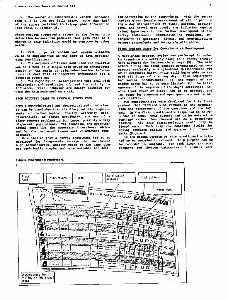
FiWm6. Rowvsmionofqussdomnsha.
administration by the respondents. with the survey
content given (namely measurement of all trips dur-ing a day characterize?iby times, purpose, destina-tion, and travel mode used), the following aspectsgained importance in the further development of the
survey instrument: formulation of questions, ar-rangement of questions, layout, and cowaunicationsbetween respondents and survey administrators.
First Pretest Phase for Questionnaire Develoment
A multiphase pratest series was performed in orderto transform the activity diary ko a survey instru-ment suitable for large-scale surveys (~). The main
effort during the first pretest concentrated on gen-erating preferably a single-sheet questionnaire outof an extensive diary, while still being able to re-cord all trips of a survey day. This requirement
had several consequences: (a) the number of re-
corded trips had to be more limited~ (b) the briefsumnary of the sequence of the dayls activities (in-side front cover of diary) had to be deleted, and(c) space for comments and open questions was to be-come limited.
Tw questionnaires were developed for this firstpretest that differed with respect to tha formula-tion and arrangement of the questions and the lay-out. In the first questionnaire trips had to be re-corded in rows. Trip purpose had to be entered inlonghand rather than checked off on a preprintedlisting. All trip characteristics could only belisted once. Each trip row contained fields formaking longhand entries and square’s for checkoffmarka (Fi9ure 6).
In the second varsion of this questionnaire tripshad to be recorded in columns. Trip purpose had to
be recorded in longhand. For each block the moatfrequent and obvious categories of answers were
HInstructions II Date
—— —~ ~FirstName HOestlnation
AddressI
Instructions
II I I
~ ModesUsed
I- —-
.

8 Transportation Research Record 944
given for eaay checkoff~ all other anawera had to beprovided in longhand (Figure 7).
The reaulta of this first pretest atage can besunnnarizedaa follows.
1. The percentage of usable forma for the columnversion of the questionnaire waa higher (97 percent)than the row version (92 percent) [ace Table 6 (~)].
2. Sixty-two percent of the reported trips con-tained incorrect or hcomplete inforsaation$ 46.4percent were correctable [see Table 7 (~,~, FirstPretest Phaae].
Fi~m7. Colurnnveraionofquassionstaire.
3. Moat deficiencies in reporting pertain to thedestination addreas (41.9 percent of all trips), butmost of them are minor problems because the majority
of the addreaaea can be located, given the geograph-ical aggregation level typically used in transporta-tion planning (see Table 7, First Pretest Phase).
4. In the row version an increasing number oferrors occurred with respect to trip purpose for thereturn trip home. This ia attributable to the openform of the question used in this version.
5. The average number of daily trips meaaured inthis pretest was 3.59 trips per person compared with
I Enroute TripItinerary I
Destination/Purpose M 4
Pracise r~DestinationMdress
UaableQue8tioMzircs (%)Unuaabk.or
Questionnaire Sample Wlthuut ComectableVersion Size
Partly UsableError Questionnaire Total Questionnaire (%)
COlumn layout 59 88 9 97 3Row layout 58 89 3 92 8

Transportation ResearCh Record 944 9
Tat407.lnoormct●d incomplete reporting (&~).
Incorrect Reports Per 100 Trips by Trip Characteristic
Timing of DepartureDestination Address Purpose Mode
Incomplete Reportsand Arrival
Pretestper 100 Trips
Phsse Total NoncorrectableTotal Noncorrectable Total Noncorrectable Total Noncorrectsble Total Noncorrectable
Fust 41.9 2.9 4.4Second
2.6 1.6 1.0 5.529.6
3.68.1 4.7
8.6 551,6 1.9 0.8 0.8 0,4 2.0 0.4
4.21 trips reported in the diary. The reasons forthis lie in the absence of an interviewer providingadditional motivation for respatding and in the lay-out of the questionnaire.
Second Pretest Phase
The second pretest again made use of the row andcolumn versions of the questionnaire (see Figures 6and 7). However, this time the layout was improvedsubstantially. Oual color printing made the ques-tionnaire more readable and visually more appeal-ing. In the column version the fields and squaresfor recording answers and checkmarks, and in the rowveraion all odd-numbered trips, appeared in a dif-ferent color from that used on the rest of theform. Also, emphasis of certain important informa-tion wss achieved through varying letter size andthickness.
These changes in layout were supposed to improvethe results of the first pretest phase in two re-spects. First, the clearer distinction between in-dividual trips impresses more on the respondent thatall trips for a day were to be recorded. Second,the visual emphasis was supposed to reduce the shareof unanswered questions because the respondent couldsee i~iately where entries were expected to bemade.
The second pretest phase ia distinguishable fromthe first one mainly because the questionnaires wereto be tested under the conditions of a mail-backsurvey; i.e., respondents had to master the ques-tionnaire responses exclusively on the basis of thewritten instructions provided, and the respondentshad to be motivated in writing to participate in thesurvey.
TWO variations of the column version, distin-guished by their different spatial arrangements,were developed for purposes of a mail-back survey.
Seth variations were printed on one sheet, one ofthem a folded version where all trips could be re-corded across that page. The other version wasprinted on both sides of a smaller sheet, with theimplication that the sheet had to be turned overafter the first four trips had been recorded on thefront. l%is laat version, of course, had a postagecost advantage.
The results of this second pretest phase were asfollows.
1. The number of reported trips increased from3.59 during the first phase to 3.97 trips, which canbe attributed to the improved layout. The remainingdiscrepancy with respect to the 4.20 trips per per-son per day obtained in the diary is explainable be-cause no control and immediate corrections functioncan be provided in the mail-back questionnaires.
2. The row version contained the largest numberof incomplete answers (39.9 percent of all trips),whereas the front and back column version containedthe fewest (37.9 percent). These differences arenot dramatic, but it should be emphasized that thenumber of errors was successfully reduced for allquestionnaire versions compared with the first pre-test phase [see Table 8 (~,~)].
3. The number of mistakes with respect to thedestination address decreased from 41.9 to 29.6 #sr-cent. Unfortunately, the share of noncorrectableerrors increased from 2.9 to 8.1 percent (see Table7, Second Pretest Phase). It is worth mentioningthat the first pretest phase was conducted in 14u-nich, where a greater amount of professional deci-phering of address information could lx provided bythe administering agencies (Socialdata GIsM3 andTechnical University Munich) than in the case of thesecond pretest phase, which took Place in otherGerman cities. Of course, the three questionnaireversions usad were identical; i.e., the destinationaddress had to be provided in longhand [see Table 9(9,10)].‘~ The row veraion had more errors in the trippurposes, aa was the case in the first pretestphase. Again, the reason was because of the openanswer format (Table 9).
5. The number of unusable questionnaires andnoncorrectableentries increased with the age of therespondent. Older people had particular difficul-ties with the accurate reporting of trip purposes.
6. For complicated trip sequences (i.e., thosethat involve more than travel to and from a singledestination or involve several intermediate activi-ties), the number of unusable responses was high.Trip purpose and destination address aeeeared tocause the most difficulties.
TrbloS.Inaormstandinaon@@tsrepotingoftripsitsmlathtodiffamntquastionnzimversioew(~~).
Incorrect and Incomplete Incorrect and IncompleteTrip Reports Reports per 100 Trips
ReportedQuestionnaire Version Trips Total Noncorrectable Total Noncorrectable
Columnversionwith foldout 1,384 540 146 39.0 10.6Column version with front-to-back printing 1,148 436 138 37.9 12.1
Rowversion 1,253 Soo 144 39.9 11.5—.
Total 3,785 1,476 428 39.0 11.3

10 Transportation Research Record 944
Table9. lncorr=t andinm~lem ttipm~m ~ttiphatidtic and@mti~ntim Wmim(~~).
Incorrect Reports per 100 Trips by Trip Characteristic
Timing of Departure incomplete ReportsDestination Address Purpose Mode and Arrival psr 100 Trips
Questmnnaue Versmrr Total Noncorrectable Total Noncorrectable Total Noncorrectable Total Noncorrectable Total Noncorrectable
Column version with foldout 29.7 7.8 4.0 0.9 1.9 1.1 1.4 0.8 2,0Column version with front-to- 29.7 9.7 4.0
0.01.0 1.1 0.4 0.6 0.1 2.5 0,9
back printingRow versmn 29.5 7.3 6.1 2.9 2.7 0.7Total
0.2 1.429.6 8.1 4,7 1.6
0.41.9 0.8 ;:: 0.4 2.0 0.4
In summary It can be concluded that the column
version resulted in higher reporting accuracy. Thedecisive impetus to use this version in future sur-veys, however, was provided by a second criterionthat was investigated in this pretest phase--will-ingness to respond.
The front-to-back variation on the column versionled to a better response rate: approximately 80percent as compared with the row version of about 70percent.
CommunicationBetween Survey Aqency and Respondent
In the previous sections a distinction was made be-tween two forms of communication: personal deliveryand pickup of the survey forms (first pretest) andself-administered mall-back surveys (second pre-test). The impact of these two methods on response
accwacy was investigated. However, comrnunicat ionstill has two additional important implications:response rate and survey cost per respondent.
These two aspects were investigated In anotherpretest series. Eight different forms of communica-tion were tested, including a mix of personal andpostal delivery and pickup. For the case of postalservice use, additional distinctions were made as towhether prior notification by postcard was provided,and whether the recipients of the survey instrumentreceived reminders by telephone on the actual pre-scribed survey day.
The results of these methodological tests wereclear [Table 10 (Q)]. Even the simplest postal ser-vice method (method 1) resulted In a better responserate (73 percent) than the most costly personal at-tention method (method 7) by meana of interviewera(7o percent response rate). A response rate df 81percent was achieved by means of the most expensivepostal method [i.e., Including notification and re-minder by telephone (method 4)]. Even this methodis less expensive than the least-expensive personalmethod (method 5).
On the basis of these results it waa decided toconduct such surveys in writing by the mail-backprocess and to ensure as good a response rate aspossible by written notification and remindepnotices (~).
Further Aspects of Survey Instrument Dealgn
Three additional aapecta of questionnaire designthat often are relevant In specific practical appli-cations are as follows: (a) ease of coding for com-puter analysis, (b) consistency of questionnairecontents, and (c) surveys for foreign nationals.
Questionnaire Design for Computer Processing
Frequentlyt questionnaires were and are designedsuch that they meet the demands of researchers Inthe best possible manner. These demands and stan-dards, however, often run counter to the needs ofthe survey respondent. Outstanding examples forthis are the attempts to design the eurvey queetlon-naires in machine-readable form. A comparison oftwo substantially identical questionnaires, one inmachine-readable format and the other with a normallayout, produced the following results (~:
1. The machine-readable form produced 10 percentfewer activities,
2. The number of deficient questionnaires wasalmost 3 times aa high,
3. The number of unusable questionnaires was al-most 4 times as high, and
4. With identical strategies for irtcreaeingtheresponse rate, the machine-readable form produced a66 percent rate and the normal layout a 79 percentrate.
Consistency of Questionnaire Content
In addition to the design and layout, the question-naire content hae a significant ●ffect on the will-ingness to respond. The logic of the questionnairecontent (as perceived by the respondent) rather thanthe length la important. In thie context It can beahown that It Is feaeible to transmit to the respon-dent the necessity of answering related and inter-nally consistent eets of queotiona, but that the re-spondents Comprehension and willingness to respondis reduced markedly when this rule Is violated.
TableIO. Respa*ramsadsuwey~ttiafintiaofqutimntimtiti~tiarnddltia msdtods(~.
Response Cost-Index Sample Size
Distribution and Collection Method Rate (%) per Response (households)
Method l-postal distribution andretum 73 100 1,188
Method 2- not]ficatmn, postal distribution and return 78 101 1,196
Method 3-post al distribution, reminder on survey daY, postal return 77 104 1,193
Method 4-notification, postal distribution, reminder on survey day, postal return 81 113 1,191
Method 5- postal distribution, personal pickup 64 188 544
Method 6-personal delivery, post al return 63 215 517
Method 7-personal delivery. personal pickup 70 278 1,071

Transportation Research Record 944
Fi~N8. Columnvanionofqmrti0nmair8forforei~m.
11
lTrii)Number. IDrawn in-Ti& ofDeparture
~M
Mode u--k
I-4---&I 111-
I 1
Destination / Time ofAddress Departure
This point is illustrated in the following table.on the basis of three surveys (~) with differentdegrees of internally logical sets of questions:
Version1: 2: 3:Complete Partial NOInternal Internal Internal
ItemSample size
Logic Logic Logic55,107 19,380 12,091
Response rate (8) 81 77 67
Version 1 contained queationa about demographic andnonhoma activities (i.e., the internal logic wasfully recognizable). Version 2 included additional,somewhat related queationa (i.e., a logical unit waspresent, in part). Finally, in version 3 sets ofquestions of entirely different content were added(i.e., the logical unity wae lost). The data in thetable indicate that the response rate was affectedquite substantially.
Surveys for Foreign Nationals
In several countries with sizable groupa of foreignnationals it is zometimes neceesary to survey thispopulation segment of a specific study area. TyPi-cally, one of the following eurvey tachniquea iaused. Either the foreigners receive the standardlocal-language form aa it is dietributad to the do-mestic population sample in the hopes that they haveacquired sufficient local-language facility, or theyreceive a version prepared in their native language.
The second method obviously is the better ap-proach, but it ie not sufficient to generate ade-quate response in terms of numbers and quality. Be-cause foreigner do not only differ in their native
language but alao in terms of mentality (e.g., ~r-ception of time), forma of expreasione, and ~ni-catione, a straight technical translation of thesurvey instrument cannot suffice to prwide themwith a eurvey form adequate for their needm (aceFigure 8). In order to generate a questionnaire ofequal content it was neceanary to conduct similartypes of pretemt series ae were described for thedevelo~nt of the local-language questionnaire inearlier aactionm of this paper. Different tech-nique and presentation had to be teated.
Such a questionnaire waa developed for Turkishand Yugoalav residents of Berlin, Germany, and itwas used in the context of a large-scale murvey inthat city (U). A meaningful ~riaon of the re-mponme quality between the German and foreign-language vereions of the questionnaire can be madefor the reporting of trip deetinationa because thatampact was probably meet difficult for foreigner toanswer accurately. The reaultm indicated that thedifference in response accuracy was insignificant,and it was certainly much better than had been ob-served in other eurveye involving foreign remidents[see ‘fable11 (12J].
Tsbloll. Exam@aof rwporma quality for Garrnsn and TurkishawlYusINIavresidsntsofSsrlin,Gsrnrmy(@
German TurkishandYugoslsvItem Residents Residents
Sample size 19,000 2,000Reporting quality ofdestination
address (%)Directly usable 78 72Usablewithextra effort 20 18Not usable 2 10
Responserate (%) 77 71

12 Trans~rtatiOn Research Record 944
The questionnaire design for foreigners alao hasa direct impact on the response rate. A 13 percentdifference in response rates could be observed be-tween a straight technical translation and a spe-cially designed survey form. According to the datain the following table (~, an additional increaseof 9 percent was possible by means of specialforeign-language telephone and written assistanceand information:
Sample Response
WJ!sYStraight technical
Size Rate (%)
translation 3,000 49Specially designed
survey form 1,084 62Specially designed survey
form with specialassistance provided 2,712 71
The detaila of the developmental process involved ingenerating a survey instrument that meets criteriaof high methodological quality, high expected re-sponse rates, suitability for large-scale surveysinto travel behavior, and relatively low costs havebeen described. Through a number of real-worldtests it waa demonstrated that a variety of designaspects can have substantial influence on one ormore of the preceding criteria. Each test series
was tested empirically, with detailed documentationof reporting deficiencies.
The tests revealed how important methodologicalresearch into improved survey design can pay off interms of better and more complete survey resultsand, hence, in terms of more reliable and valid in-puts into travel modeling and transportation plan-ning. Uncritical use of unproven survey instrumentscan have a profound influence on the efforts bytransportationplanners and policy decision makers.
In this paper the evolution of better travel sur-vey instruments based on diary-generated informationthrough research performed in Germany has been dis-cussed. It should be made clear that many of themethodological insights gained In the course ofthese developments have been implemented in sophis-ticated trsvel data-collection efforts in the UnitedStates. Excellent examples of such efforts havebeen presented in two recent papers (13,14).——
1. A.E. Meyburg and w. BrW. validity Problems inEmpirical Analyses of Nonhome Activity Pat-terns. TRB, Transportation Research Record
807, 1981, PP. 46-50.2. W. Brbg. Mobility and LifestYle--Sociolo9icsl
Aspects. Repxt of the 8th International Euro-pean Conference of dinisters of Trsnsport Symp-osium on Theory and Practice in Transport Eco-nomics (ECMT Publications Department of the
3.
4.
5.
6.
7.
8.
9.
10.
11.
12.
13.
14.
Organization for Economic Cooperation and De-velopment), Istanbul, SePt. 1979.M.J. Wermuth. Effects of .Survey Methods andMeeiSUretIIetIt Techniques on the Accuracy ofHousehold Travel Behavior Surveys. ~ NewHorizons in Travel Behavior Research (P.R.Stopher, A.H. Meyburg, and W. Br59~ eds.), Lex-ington Books, Lexington, Mass., 1981, Chapter28.Sozialforschung Br5g. KONTIV 75-773 Continu-ous Survey of Travel Behavior (KontinuierlicheErhebung zum Verkehrsverhalten), Summary Vola.1-3. Ministry of Transport, Munich, Germany,1977 (in German).W. Br6g and W. Schwerdtfeger. Considerationson the Design of Behavioral Oriented Modelsfrom the Point of View of Empirical Social Re-search. ~ Transport Decisions in an Age ofUncertainty (E.J. Visser, ad.), Kluwer AcademicPublishers, Hingham, Mass., 1977.W. Brdg. Latest Empirical Findinge of Individ-ual Travel Behavior as a Tool for EstablishingBetter Policy-Sensitive Planning Models. Pre-sented at World Conference on Transport Re-search, London, England, April 1980.W. Br?3g. Application of Situational Approaahto Depict a Model of Personal Long-DistanceTravel. TRB, Transportation Research Record890, 1982, pp. 24-33.Sozialforschung Br&g. Travel Behavior in Con-nection with the Munich Commuter Train System(Verkehrsverhalten im S-Bahn-Bereich). UrbanDevelopment Office, Munich, Germany, Jan. 1973(in German).Sozialforschung Br~. Comprehensive Transpor-tation Plan for Nuremberg (GesemtverkehrsplanNUrnberg). Government of Middle Franconia, Mu-nich, Germany, Preparatory Studies, vo1. 3,1974 (in German).M.J. Wermuth and G. Meerschalk. Representa-tiveness of Written Mail-Back Household Surveys(Zur Repr&3entanz Schriftlicher flaushaltsbe-fragungen). German Ministry of Transport, Mu-nich, Germany, 1981 (in German).Sozialforschung Brdg. Investigation of Workand School Trips (8tudie ZWI Berufs-und fNAS-bildungsverkehr). German Ministry of Trans-port, Munich, Germany, 1976 (in German).Sozialforschung Brdg. Transport DevelopmentPlan for Berlin [Verkehrsentwicklungsplan(VEP)Berlin]. Senator for Construction and Housing,Berlin, Germany, Final Rept., 1977 (in German).P.R. Stopher and I.M. Sheskin. Toward ImprovedCollection of 24-E Travel Record. TRB, Trans-portation Research Record B91, 1982, PP. 10-17.P. Rei, P.R. Stopher, and C. Brown. Origin-
Oestinstion Travel Survey for Southeast Mich-igan. TRB, Transportation Research Record 886,1982, pp. 1-8.
Publicationofthis papersponroredby Cbmm”tteeonPo.$.$engw7?avelDematiForecasting.
Transportation Research Record 944
Sequential, History-Dependent Approach toTrip-Chaining Behavior
RYUICHI KITAMURA
The charerteristirs of trip-purpose chains ● re examined, ●nd ● gsquentislmodeloftripchaining,whioh oonsistsof hhtorydependemt probabilitiesof wtivity choice, is developed. Ststistial mmlyee$of the study indicstethet there is ● consistent hierwohial order in eequenoingmotivitiesin ●
okminwhera less-flexible srtivitiss tend to be pursued first. The atalyeesdeo indiozte that the at of motivitiespursued ins shsin tends to behomogeneous. Thus activity trmssitionswe more organized snd systematicthan whet ● Msrkovian model wuld depict. Basedon these findings, asequantiel nsdel of ●ctivity ohoise is formulated that, in spite of its simpli-fied representation of the history of ● olmin, satisfactorily represent$ thaobserved behavior. Althou@ the focus of the model is on direct linkagesbetween activities, the model is rapable of representing those charmterie-tics ●ssociated with the entire set of activities in a chain. The results of thestudy etrongly support the sequential modeling ●pproach ●nd indicata itsprsctial usefulness in tha analysis of trip-draining behavior.
The importance of understanding trip-chaining be-havior has long been recognized in connection withnonresidential trip generation (l_)or with urbanland use development (~). Underlying this is thedissatisfaction with the way tripmaking has beendealt with in the conventional transportation plan-ning process or in location theory (~). As planningemphases in transportation shifted from infrastruc-ture construction toward systems management and pol-icy development, it was recognized that there was anincreased need for a more fundamental understandingof travel.behavior (4-6). The responses of urbanresidents to the rece-nt-oil crises (7,8) have madeevident the importance of investigate-ng-trip-chain-ing behavior. Its importance is clearly seen whenconsidering how the temporal and spatial distribu-tion of trips in an urban area is affected by theway people organize their daily schedule of activi-ties and combine trips. Statistical analyaes havebeen accumulated to form a substantial body of em-pirical evidence [reviews of previous works on re-lated subjects can be found in Hanson (~) and Damss(2)1. Yet many questions that have arisen in model-building efforts of trip-chaining behavior remain tobe answered.
In this study one of the criticsl issues in tripchain modeling is addressed: representation of thedecision structure involved in trip chaining. Frcmthe viewpoint that pabple plan and schedule before-hand a set of activities to be pursued in a tripchain, the decision process can be best representedas a simultaneous one that concerns the entire act.However, only few studies (~ have taken this ap-proach in the past becauae of enormous difficultiesinvolved in developing a practical simultaneousmodel of trip chaining. Moat previous studies tookse9UentiSl modeling approached, which include theMarkovian approach that hss been traditionally usedin trip chain analysis (1,3,11-14). The validity of——the Merkovian models, h-~ver, has not been thor-oughly examined in the past, although several ●rmpir-ical observations (15-18) have indicated thet trip——chaining is not Nerkovlan.
The objective of this study is to demonstratethat the inadequacy of previous sequential models iscaused by their failure to represent patterns ofactivity sequencing and activity set formation intrip chaining, and further to detaonstrstethat trip-chaining behavior can be adequately deecrltasd bysequential probabilities of activity choice thatincorporate the history dependence of the behavior
13
in a simple manner. The sequential approach has anobvious advantage because it represents the behaviorby a simple model structure while avoiding combina-torial and other problems that may otherwise arise.At the same time, the approach may appear to be in-consistent with the viewpoint that trip chains areplanned and scheduled beforehand while consideringthe entire set of activities, and not the transi-tions between activities. Nhether a sequentialanalysis can adequately describe the behavior is,therefore, a critical question to be examined, be-cause if the sequential approach is proven to bevalid, it will lead to practical models of tripchaining that can be developed for a wide range ofstudy objectives. This study is an effort to estab-
lish a basis for such development.In examining the adequacy of the sequential ap-
proach, two aspects are discussed: sequencing ofactivities in a trip chain, and tendencies or pref-erences in formation of the set of activities to bepursued in a trip chain. (This study is concernedwith types and sequences of activities in a chain,
but not with their spatial or temporal attributes.A modeling effort that extends the present study
into the temporal dimension can be found in a paperby Kitemura and Kermanshah presented elsewhere inthis Record.) How these two aspects affect sequen-tial probabilities of activity choice is demon-strated. Following this, empirical observationa aremade, and the nature of trip-chaining behavior ischaracterized.
BACKGROUND
The equivalence of the sequential and simultaneousapproaches can be found in the following identity.By letting ~ be the nth activity in a trip chainfor the case of three activities,
Pr(Xi =A,X2=B,X3= C)=Pr(X3=ClX,=A,X2=B)Pr@2‘91X1
=A)Pr(X,=A) (1)
The probability that a given set of activities ischosen and pursued in a given order can be repre-sented by a set of sequential and conditional proba-bilities. (The same identity has been used in re-lating simultaneous and sequential formulations ofdiscrete choice.) Nhen the conditionality in Equa-tion 1 is appropriately represented in sequentialprobabilities, then the sequential approach isequivalent to the simultaneous approach to triPchaining.
It may be argued that activity choice cannot beadequately described by probabilities that are con-ditioned only on the past; activity choice may alsobe dependent on future activities because a set ofactivities to be pursued may have been planned be-forehand. Nevertheless, it can be seen that thebackward dependency on the PSat imPlies forwarddependency on the future-as well. By using Bayes’a
rule,
[ 1pr(XilX2)= [WX21X1)W%)l/ :lpr@21X1WXi)(2)

14 Transportation Research Record 944
Pr(X1 [X2,X3)=[Pr(X31Xl,X2) WX21XI)MXI)1
[ 1+ Z Pr(X31Xt, X~)Pr(X21X1)Pr(X1)xl
(3)
and so forth. A forward dependent probability canbe always exprea.aedas a function of backward depan-dent probabilities. That a choice is conditioned onthe past implies that it is also conditioned on thefuture.
The preceding discussion indicates that the prob-lems of previous sequential analysea, many of whichused Markov chains, do not lie in their sequentialstructure, but rather they lie in their inadequaterepresentation of the conditionality. In the fol-lowing discussion it is assumed that there are pat-terns in sequencing activities in a set, and alsothat the choice probability of a given activity setis predetermined. The intensity of direct linkagesbetween activities, or transition probabilities,which have been the main focus of previous studies,is viewed as a consequence of the patterns and pref-erences in chmsing activity sets and sequencingactivities. It is then shown that these patternsand preferences can be represented by the condi-tional transition probability, whereas the twoMarkovian assumptions--hLetory dependence and sta-tionarity (or time homogeneity)--are inadequate.
Suppose the number of activities in the set (de-noted by k) is fixed and the individual is com-pletely indifferent to the sequence of activities.Conaider an activity set (w) and two activitytypes (A and B). Because the sequencing is com-pletely random, all the sequences obtained by parmu-tating the activities in w have the identicalprobability. Accordingly, for all w,
Pr(Xn=A,Xn+l= Blti)=Pr(Xm=A,X~+,=Blo) (4)
and
Pr(Xn=Alw)=Pr(Xm =Alo) m,n=l,2, . . .. l-l (5)
Then, if A is included in at least one activity set,
Pr(Xn+l = BIX.L
=A)= ZPr(Xn=A,Xn+l=B/ti)Pr(w) 1[u 1+2Pr(Xn=Alti)Pr(ti)
=Pr[Xm,l =B\Xm = A] (6)
Namely, the pairwise activity transition probabili-ties are stationary. Note that this conclusion isnot affected by the probability with which u ischosen [Pr(w)], i.e., it does not depend on thepreferences in activity set choice.
Although the pairwise activity transition proba-bilities are stationary, they are not history inde-pendent even in this simplified case of randomactivity sequencing. Suppose that the choice proba-bilities of sets that include activities A, B, and Dare zero, while those of other sets are positive.Then
Pr(Xn+l=B1....XQ=C, Xn=A)>=A)> O (7)
and
Pr(Xn+l =Bl, ... X*= D,. ... &= A)=O (8)
Therefore, pr(Xn+~lXl, X2, . . “J xn) # Pr(xn+llxn).For the activity transitions to be Markovian, theprobabilities with which respective activity Setsare chosen must conform with those depicted by thetransition matrix of a Markov chain, a conditionrather groundless to asauma.
The pattern of sequencing activities in a tripchain ia another source of history dependence, which
also yields nonstationarity. Suppose activity Atends to be pursued before B, but the individual isindifferent to the sequencing of activity C. Thenfor u that involves A, B, and C, the probabilityPr(X+l = BI .
{... q-c,kr) variea depending on
whet er A has been pursued before C. Now supposeboth A and B tend to be pursued earlier in a chain,but again C is equally likely to be pursued in anyorder. Then, Pr(Xm+l =AI~=C, U) > Pr(Xn+l=AIXn = c, w) ifm<n. The first example indicatesthat sequencing patterns cause history dependence,and the latter indicates that palrwise transitionsbecome nonstationary.
Any Markov chain exhibits certain patterns ofactivity set formation and sequencing. But the re-versal is not always true~ i.e., given patterns ofset formation and sequencing cannot always be repre-sented by a Markov chain. The discussion in thissection also implies that sequencing and activityset formation can be representad when the condi-tional probabilities of activity transitions areappropriately specified. The failure of Markovchain models is caused by their invalid representa-tion of the conditionality. In the following sec-tions characteristics of trip chaining are firstobserved, and then a sequential model is proposed.
DATA SETS
Empirical observations of this study are made by
using the 1965 Detroit area transpcmtation and landuse study (TALUS) data set, the 1977 Baltimoretravel demand data set, and published transitionfrequency matrices from Chicago, Buffalo, and Pitts-burgh [reported by Hemmens (~)]. The TALUS dataset is most extensively analyzed, whereas the othersets are used to examine the generality of the re-sults obtained. A significant advantage of the
TALUS data set--a conventional origin-destinationsurvey result--is its ample sample size, which iscrucial for the analysis carried out in this study.
The original TALUS data file, which contain~records of 320,090 trips made by 82,050 individuals~was screened to exclude those individuals who didnot have a closed series of trips that originatedand terminated at home (which may include intermedi-ate returns to home)? who had no car available tothe household or did not hold a driver’s license,who were younger than 18 years old, who used travelmodes other than car, and those who made work tripson the survey day (walk triPS are ~t r~rd~ ‘nthe TALUS data unless they were work trips). Thelast criterion is introduced because of the substan-tial differences in travel and time use patternsbetween those who worked and those who did not onthe survey day (20,21). As a result of this screen-ing, the aemple<n~yzed includes 76,025 trips and27,901 trip chains made by 16,520 individuals [.sgeographical subsample of this was usad in previousstudies (~,~~~)].
All screening criteria are also applied to theBaltimore data set, and a sample of 1,789 trips and697 trip chains made bY 435 individuals is o~tained. The transition frequency matrices fr09 theother three metropolitan areas include all observa-tions without comparable screening. Aa is clearfrom the screening criteria, the internal h_e-neity of the sample is emphasised in this studY~whereaa some aspects of travel behavior are placedout of its scopes such as the effect of travel -eon trip chaining. Individuals with tranait tripsare eliminated for this reason, and they are notanalyzed because their sample size is too small forstatistical analysis.
The 27,901 trip chains in the sample frm theTALUS data set contain 48,124 sojourns with an aver-

Transportation Research Record 944 15
age chain length (average number of sojourns perchain) of 1.725. Although 62.2 percent of the totalchains are single-eojourn chains, they account foronly 36.0 percent of the total sojourns, and approx-imately two-thirds of the aojourne belong to multi-aojourn chaina. The significance of multieojournchains ie evident. The average chain length of theBaltimore sample ie 1.57, approximately 10 percentleas than that of the TALOS sSMple. The averagenumber of chains per pergon is 1.60, which compareswith 1.689 of the TALUS sample.
The direct traneitione between activities in tripchains in the TALUS and Baltimore samples were firotanalyzed by ueing a transition matrix, with the aa-suakptionthat trip chaining can be represented by astationary and hietory-independent Markov chain.These two eemplea are different from thoee of otheratudiee in that the individual who made work tripsare excluded. Nevertheless, this preliminary anal-yaie of the pooled transition matrices indicatedthat the present samples share many of the trip-purpoae linkage patterna reported in the literature(L,Q,E).
NONSTATIONARITYOF ACTIVITY TRANSITIONS
Although traditional Narkov chain analysis (whichuses the pooled transition matrix) offers a conve-nient means of data sunnnarization,the implicit sta-tionarity assumption that the same transition matrixapplies to all transitions in a trip chain is toorestrictive for rigorous analysis of the behavior.In thie section the nature of trip chaining is ex-plored by using a nonstationary Markov chain, whereeach step of transition has ite own transition me-trix that ie not necessarily identical to those ofother steps (the first step of transition refers tothe transition from the first purpose to the second,the second step of transition is the one from thesecond purpose to the third, and so forth).
Nonstationarity in Trip-PurposeChains
Nonstationarity in the observed trip-purpoee transi-tions ie etatj.aticallyexamined by applying thelikelihood-ratio test (~. The result,sare e.uznaa-rized in Table 1. TO eliminate empty cells in thefrequency matrices for as many steps as possible,
Tabh 1.Likelihood-ratio test of atztiotwfity in tfippufpoae trsmitiona.
Fors=l, ...,9 Fors= 2,...,9
Row column Row ColumnTrip Purpose Totsla Totalb Tot d’ Totald
Home — 357.6’ 77.9=Personal businesqf 337.6” 155.2’ 4;.@ 39.9Socisl-recreationh 603.? 157.4’Shopping 374.1’Serve passengers m“
Totali
38.8 65.7’36.5 93.0” 26.9
8787’ &2” &6e-1,585.4eJ 1,585.4’J 310.oe’k310.oe’k
Note: in places Were dsgrest of freedom are imthted, the df for the column totatcannot be definedIn theconventiorulmanner;thereforethe ratio ((total df) + (no.of columns)1 ispresentedhere.
adf = 32.
bdf = 2S.6.
Cdf= 28.‘df = 12.4.~ignificsnt N a = 0.00S.Includesschool.
‘Signifimnt ~ta = 0.0S.h.Includesem.medtrips.‘A definitionof the Ioa-likelihoodratio statisticu givenin hderwn and G.wdrnn.(=).
‘df = 128.‘df= 112,
two trip purposes with fewer observed frequenciesare merged with others, as indicated in the table.The test is Conducted for the firet nine transitionmetricee, and aleo for the eight matrices from steps2-9. The null hypothesis is strongly rejected inboth ’casee.
Together with the overall chi-square values, thedata in Table 1 present chi-equare statistics forthe row and column of each trip purpose, where therow total represents the nonstationarity in thetransition probabilities from the trip purpoee, andthe column total represent8 that to the trip pur-pose. For the first caee (steps = 1, 2, . . ., 9),all rowe and columns have significant statistics,except the column total for shopping, which indi-catee that shopping is pursued with a relativelystationary probability throughout a chain. Thelarge chi-equare value associated with the transi-tions to serve-passenger trips and that from social-recreation tripe are also noted.
The second test excludes the transition matrix ofthe first step. The drastic reduction in the over-all chi-equare value from the first test indicatesthe extreme distinctiveness of the matrix for thefirst transition. Note that the firat transitiondetermines whether the individual pursues only oneor more than one sojourn in a trip chain. The datain Table 1 also indicate that the variation in link-ages with serve-pesaenger trips is a major source ofnonstationarity in the second step and thereafter.
The peirwise distinctiveness of two successivetransition matrices wae also tefated,and the firstfour metricee were found to be significantly differ-ent from each other (with chi-square values of 783.3between the first and second stepe, 92.1 betweensecond and third, and 38.9 between third and fourth,all with df = 16). NO significant difference wasfound after the fourth step. This ia at leastpertly caused by the reduced sample size in thetransition frequency matrices of later stepe. Atthe same time, the implication of the result thatthe transition probabilities are stabilized in latersteps of a trip chain is intuitivelyagreeable.
Variation in Linkage Patterne
The nonetationarity in trip-purpose transitions im-plies that a pair of activities my have strengthen-ing or weakening linkages with each other, and thatsotaeactivities tend to be pursued earlier or laterin a chain. The data in Table 2 indicate by step oftransition those trip-purpoee pairs for which morethan expected transitions are observed in respectivesteps. Neny of the diagonal cells are significantin all steps, which indicates that activities of thesame type continue to have strong linkages amongthemselves throughout the chain. There are alsoseveral trip-purpoee combination that are signifi-cant only in the first few steps or in later atepe.
category HOME PBNS SREC MEAL SHOP SCHL SVPS
PBNS 1,2,3,4 1SREC 1 1,2,3,4 1,2,3MSAL 1,2,3 3SHOP 1,2 1,2,3,4SCHL 1 2SVPS 3 1. 1 1,2,3,4
Note: Steps i through 4 indkate the step of trmwition for whkh the celi hss ● chi-muue value of 7.879 or meater with m ●xpected frsquency of s or ar-ta. Ab-breviations for Irip-purposs mteaories me u follows! PBNS= Pmonal business,SREC = social-recreation, MEAL = eatmed. SHOP= shopping,SCHL= -hool.and SVPS=sewe p~uenger%
16 Transportation Research Record 944
Eaeecially noted is the transition from eerve-passenger trips to home in the third step. The sig-nificance of this trip-purpose _ination in thisparticular step ia caused by the dominance of thetrip-purpose sequence: serve passengers to otheractivity to serve passengers to home (a later sec-
tion indicates that this is a typical sequence whena trip chain involves serve-paasenger trips). Thusthe result suggests that the observed nonstationar-ity is partly caused by the sequencing by the triD-maker of the activities within a trip chain.
The variations in trip-purpose linkages were fur-ther characterized by ●valuating for respectivesteps the mean first passage times (MFPTs)”;that ia,the expected number of transitions from an originstate until a destination state is visited for thefirst time (~). The result indicated that thelinkages to personal business become weaker in latersteps of a chain. On the other hand, the MFPTs toserve-passenger and social-recreation trips revealedstrengthening linkages between these activities andothers in later steps.
This analysis of nonstationsrity in trip-purposechains strongly suggests the existence of patternsin sequencing activities. An earlier section indi-cated that another possible source of the observednonststionarity is the dependence of activity choiceon the set of activities already pureued, which isclosely zelated with the preferences in the choiceof activity set. In the following sections thesetwo aspects are discussed, and the ressons why suchnonstationarity exists in trip-chaining behavior areilluminated.
ACTIVITY SEQUENCING IN A TRIP CHAIN
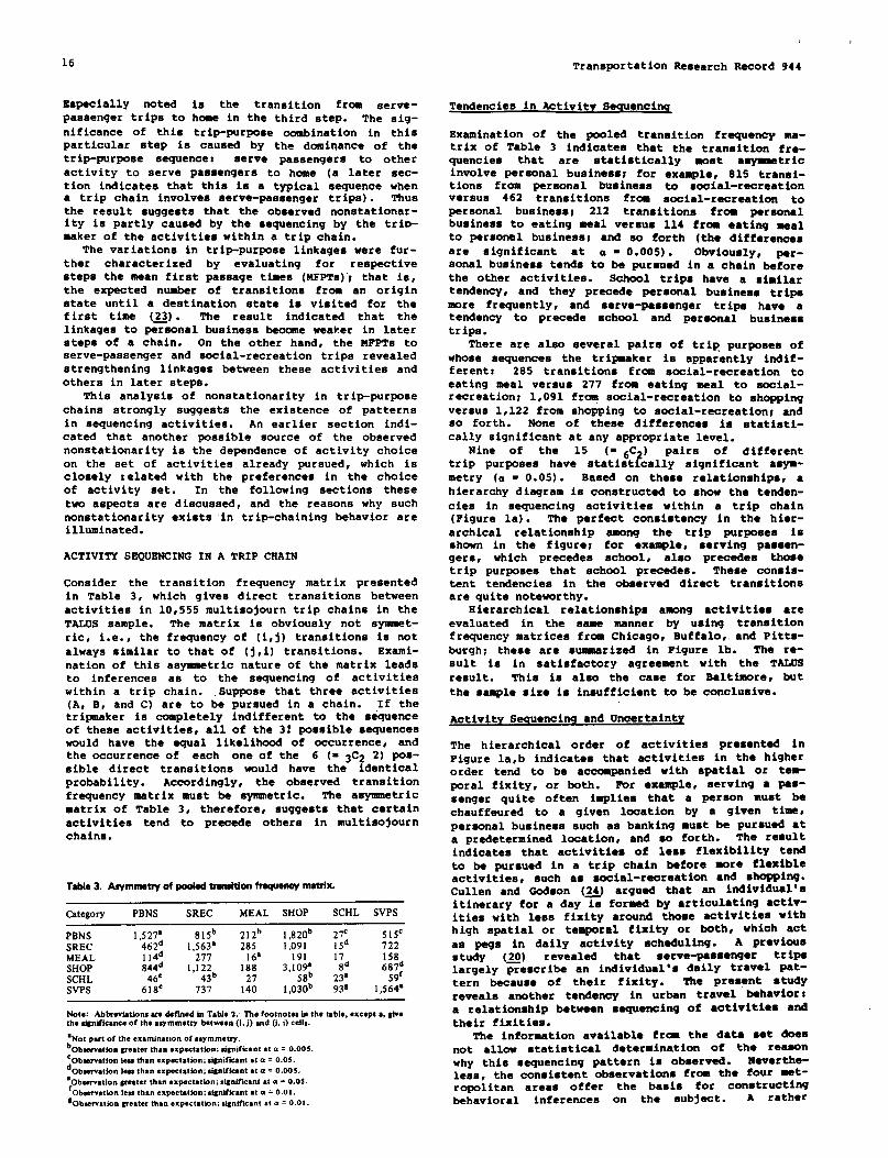
Consider the transition frequency matrix presentedin Table 3, which gives direct transitions betweenactivities in 10,555 multisojourn trip chains in theTALUS sample. The matrix is obviously not syfttmet-ric, i.e., the frequency of (i,j) transitiona is notalways similar to that of (j,i) transitions. Exami-nation of this asymmetric nature of the matrix leadsto inferences aa to the sequencing of activitieswithin a trip chain. ,Suppoee that three activities(A, B, and C) are to be pursued,in a chain. If thetripmaker is completely indifferent to the sequenceof these activities, all of the 3: possible sequenceswould have the equal likelihood of occurrence, andthe occurrence of each one of the 6 (= 3C2 2) PoS-sible direct transitions would have the identicalprobability. Accordingly, the observed transitionfrequency matrix must be sytmnatric. The asytmftetric●atrix of Table 3, therefore, suggests that certainactivities tend to precede others in multisojournchains.
Tsbla3. Arymmstryofpaa16ritfztniUonffaq~m*ix.
category PBNS SREC MEAL SHOP SCHL SVPS
PBNS 1,527’ Slsb 212’J ; ,;~~b 27= S15CSREC 462~ 1,563’ 285 ,yt 722MEAL 114’4 277 ,& ’191 17 158SHOP 844: 1,122 188 3,1O!Y 8~ 687dSCHL 43b 27 ~~b 23’ s9fSVPS 618= 737 140 1,030b 93s 1,564”
f’iote: AbbrcvlM&nsaredeflnedinTtble 2. l%efootnotesinthet~ble,excopt &cIvethe Wniftcsnceof theasymmetryhetwmen(1,j) tnd 0, I) ceUs.
‘Not partof the ex~minmmnof asymme fry.bObservation greater than expectation; sisnifkant ●t a = 0.00S.
cObmrvatlon Ies than expectation; s@ifkant st a = 0.05.d
Obae?vatkm lest than expectation; sirnlftcant at a = 0.005.~nwation mester than expectatk.n; slrnificsnt ●t a = 0.05.
Observation Iett than expectation; dgnifkant at a = 0.01.
‘Observation treater thm ●xpectation; signiflcam at a = 0.01.
Tendencies in Activltv Set7uencinq
Examination of the pooled transition frequencyzta-trix of Table 3 indicatea that the transition fre-quenties that are statistically xost a~tricinvolve personal business; for example, 815 transi-tions from personal business to social-recreationversus 462 transitions from social-recreation topersonal business; 212 transitions froa personalbusiness to eating meal versus 114 froa eating sealto personal business; and so forth (the differencesare significant at a - 0.005). Obviously, per-sonal business tenda to be pursued in a chain beforethe other activities. School trips have a similartendency, and they precede personal business tripemore frequently, and serve-passenger trips have atendency to precede school and personal businesstrips.
There are also several pairs of trip purposes ofwhose sequences the tripmeker is apparently indif-ferent: 285 transition from social-recreation toeating meal versus 277 from eating meal to aocial-recreation; 1,091 from social-recreation to shoppingversus 1,122 from shopping to social-recreation;andso forth. None of these differences ia statisti-cally significant at any appropriate level.
Nine of the 15 (- 6C )?
pairs of differenttrip purposes have statist tally significant asym-metry (a = 0.05). Based on these relationships, ahierarchy diagram is constructed to show the tenden-cies in sequencing activities within a trip chain(Figure la). The perfect consistency in the hier-archical relationship among the trip purposes isshown in the figure; for ●xample, serving passen-gers, which precedes school, also precedes thosetrip purposes that school precedes. These consis-tent tendencies in the observed direct transitionsare quite noteworthy.
Hierarchical relationships among activities areevaluated in the same manner by using transitionfrequency matrices from Chicago, Buffalo, and Pitts-burgh; these are summarized in Figure lb. The re-sult is in satisfactory agreement with the TALUSresult. This is also the case for Baltimore, butthe sample size is insufficient to be conclusive.
ActivitY Serruencingand Uncertainty
The hierarchical order of activities presented inFigure la,b indicates that activities in the higherorder tend to be accompanied with spatial or ten-poral fixity, or both. For example, serving a pas-senger quite often implies that a person must bechauffeured to a given location by a given timerpersonal business such as banking must be pursued ata predetermined location, and w forth. The resultindicates that activities of less flexibility tendto be pursued in a trip chain lxnforemore flexibleactivities, such as social-recreation and shopping.Cullen and Godson (~ argued that an individual’sitinerary for a day is foraiedby articulating activ-ities with less fixity around those activities withhigh spatial or temporal fixity or both, which actaa pegs in daily activity achaduling. A previousstudy (4) revealed that serve-passenger tripalargely prescribe an individual’s daily travel pat-tern because of their fixity. The present studyreveals another tendency in urban travel behavior:a relationship betwean sequencing of ●ctivities andtheir fixities.
The information available fra the data set doeanot allow statistical determination of the reasonwhy this sequencing pattern is observed. Neverthe-less, the consistent observations from the four met-ropolitan areas offer the basis for constructingbehavioral inferences on the subject. A rather

t
Transportation Research Record 944 17
Figurel.Himrchyinactivitya.quandngintsipchains:TALUS (Oatroit),Suffdo,Chizapo,mdpRMaur@.
a. TALUS (Oetroit) b. Buffalo, ChiCd.gO, and pittsburghl
SERVE PASSENGERS
I
:UORK
I
kl$.$:?
1
‘ A solid arrow indicates that the hierarchicalrelationship is observed in all three rnatro-pol itan areas. A broken arrow indicates that
SHOPPING the relationship is observed in the area
I
Indicated by the initial (e. g., “B” for Buffalo).
‘Includes eating meals. Serving passengers isexcluded from the original tabulation
SHOPPING SOCIAL-RECREATION [AT MEAL SOCIAL-RECREATION* Note: Transit frequerscy tsbleaare reportad in Hammns {~.
straightforward conjecture postulated here is thatthe sequencing pattern observed In this study is aresult of individuals consideration of uncertaintyin activity planning.
Consider the case where an individual is combin-ing both fixed and flexible activities into achain. Quite typically, the exact amount of therequired to accomplish an activity is not known tothe individual beforehand. If a flexible activityis pursued first, and if it takes longer than ini-tially thought, then the individual may not be ableto attend the fixed activity in time. Note that anactivity with spatial and temporal fixity by defini-tion demands the individual to be at a certain loca-tion by a certain time. On the other hand, if theflexible activity takes less time, an unexpectedblock of time must be somehow spent. In eithercase, if the individual recognizes this uncertainty,it appears logical for him to pursue the fixed ac-tivity first. The observed activity .sequencingpattern thus suggests that uncertainty plays a sig-nificant role in the activity planning of an indi-vidual. The pattern is perhaps a result of an indi-viduals effort to minimize risks because of theuncertainty and to pursue a set of activities effi-ciently in a trip chain.
HISTORY DEPENDENCE IN ACTIVITY CHOICE
An earlier section indicated that preferences in
activity set choice in general make activity transi-tions history dependent. The sequencing pattern ob-
served in the previous section implies that activitychoice depends on the series of activities alreadypursued in a trip chain. The strong direct linkagesamong activities of the same type also suggest his-tory dependence. However, little ●xploration of thenature of history dependence in trip chaining hasbeen”made in the past, and most analyses were con-cerned only with direct linkages between pairs ofactivities. The analysis of this section, whichfocuses on tbe entire series of activities in tripchains, reveals additional characteristics of activ-ity set forsaationand activity sequencing.
Although there are many possible ways of statis-tically examining the history dependence in tripchaining [e.g., triples used by Parkes and Wallies(&S); also see Anderson and Goodman (~)1, ~st ofthem encounter problems with sample size because ofthe scarcity in the sample of chains with a largenumber of sojourns. Accordingly, this study takeson an approach of tabulating the frequency of chains
by the trip-purpose sequence and directly examiningthe history-independence assumption by using a con-tingency table analysis technique.
History Dependence of Three-SojournChains
Consider those trip chains with three sojourns,namely, Xl, X2* and X3 $ home, and X4 = home. Thehistory-independence assumption can be stated forthese chains as
Pr(X3=klX,=i,X2=j)=Pr(X3=klX2=j) (9)
for all i, j, and k # hcme. Namely, the conditionalprobability that the third activity is k given thesecond activity (= j) is independent of the firstactivity (= i). This null hypothesis can be testedby tabulating, for given X2, the frequencies ofthe third activity categories by the first catego-ries, then by examining the independence of the re-sulting two-way contingency table. This contingencysnalysis is equivalent to applying a nonstationaryMsrkov chain of the first order to test the historyitiepenslenceof three-sojourn chains. The resultsfor 2,760 three-sojourn chains found in the TALUSswle are given in Table 4. To ensure a sufficientnumber of observations for each sequence of trippurposes, the original six trip-purpose categoriesare collapsed into four, as in Table 1.
In part A og Table 4 the results for those three-sojourn chains whose secondtrip purpose is personalbusiness (including school) are presented. The rowrepresents the first trip purpose, and the columnrepresents the third trip purpose. If the history-independent assumption holds, then every row shouldhave the seseedistribution of cell frequencies. Theexpected cell frequencies under this independenceassumption are shown in parentheses.
As expected, the four contingencytables (partsA-D, Table 4) are all highly significant, which in-dicates that the conditional probability that a cer-tain activity is pursued as the third activitY#given the second one, does depend on the firSt ac-tivity pursued in the chain. Especially notable arethe much higher-than-expected frequencies of thediagonal cells; tripmekers tend to repeat the smetype of activity as the first and third activitiesin a trip chain. ‘I%isrecurrence of the same activ-ity type is particularly noticeable for serve-pessenger trips when the eecond purpose is not SerV-ing passengers (see parts A-C of Table 4). Thediagonal cell for serving passengers alone accounts

18 Transportation Research Record 944
Table4.Frequenciesof three-sojourn chains by sequenw of trip Purpms.
A X2 = PBNS——x,,
xl PBNS SREC SHOP SVPS Tot al
PBNS 107 38 .37 13 245(66.2) (42.5) (84.6)
SREC(51.7) [50.7]
(2:.’3) (13?0) (25:9)SHOP
(I5:) [513
O& (12112
(3%SVPS
(23.1) (31.51
(4:.;)103 179
m’:) (6?i (37.8) [1$3.11
Total 165 211[44.0] [:9%]
611[28.51 [1;9?1 [280.9]
B X2 = SREC
X3x, PBNS SREC SHOP SVPS Total
PBNS(17rn6) (6%
167(35?9)
SREC(47*7) [85.31
183(2;.?)
278(109.5) (5;.1) (79?4)
SHOP[87.8]
(12.?) (4:.’5)118
(25*4) (33%SVPS
[44.9]
(21.:)2oa
(8:.;) (4;.!) (;8?2) [249.91
C X2=SHOP.—X3
xl PBNS SREC SHOP SVPS Total
PBNS 163(4::)
311(66?1) (153.2) (4;.?) [65.21
SREC(24.1) (3:.:)
m“(90:6) (2%
SHOP[73.91
(576) (889) (1:7?6) (6i:)SVPS
[6%
(25.:)114
(3;:) (9:!6) (30.0) [2;0%
Total 144 524 170[61.91 [6% [59.51 [294.01 [4iR]
D X. = SVPSxl,
x, PBNS SREC SHOP SVPS Total
PBNS
SREC
SHOP
SVPS
(:.’8)
(6.:)
(6.:)
(2;.’5)
(:.!) (10!)(2 (9.%)
():9) (a
(311 (3:.2)
(2Y5)
(21’.’t)
(21:)107(80.3)
[4!:][7%[14?1
[1%
Total 165 219[80%]
767[9%1 [47.4] [243.11 [467.81
Total 1k9[3?1 [18?1
31s[3% [15.61 [f40.7]
Personal business (PBNS) inrlude$ SCINWLand serial.recreatira (SRIK) includes eating meal. For other abbreviati~s, see Table 2.
( k Exper@d cell frequenryt ]: Row, r-alumn, w grand total of chi-square values.
for 40.0 percent of the total chi-square value ofpart A where the second purpose is personal busi-ness. The corresponding values are 38.1 percent forpart B (X2 = social-recreation), and 48.8 Percentfor part C (3$ = shopping). The sequence of servepassengers to other activity to serve passengers isobserved much more frequently than the expectationunder the history-independenceassumption, and it isfound in 12.2 percent of the all three-sojournchains, or in 36.6 percent of those three-sojournchains that involve serve-paesenger trips at all.The corresponding statistics from the Baltimore sam-ple are 14 and 36 percent, respectively. This se-quence pattern is obviously cauaed by the typicalrequirement that a person chauffeured and droppedoff at a place haa to be picked up later. The exam-ination of individual cells of parts A-C also indi-cates that the probability that the third purpose isserving passengers is significantly smaller than the-PeCtation when the first and eecond purposee arenot serving peeaengers.
The data in Table 4 also indicate that the activ-ities pursued in a chain quite often all fall withinone trip-purpose category. For example, the se-quences shopping to shopping to shopping And social-recreation to social-recreation to social-recreationare the most frequently observed sequences. Thie,together with the recurring tendency previously dis-cussed, indicates that the activities pursued in achain tend to be homogeneous. Of the 2,760 chains,61.9 percent involve only one trip-purpose category,23.6 percent involve two, and only 14.5 percent in-volve three different trip-purpose categories asdefined here. These observations differ substan-tially from the expected values obtained by assumingcoaplete independence in trip-purpose transitions(i.e., Markov chain of the Oth order): 6.9, 56.8,and 35.3 percent, respectively.sample 72 percent of chains withjourns involve only one or twgories.
The sequences of activities
In the Baltimorethree or more so-trip-purpose cate-
in these three-
aojourn chains showed exactly the same hierarchicalorder as in Figure 1. Note that this analysia takeainto consideration the sequences of indirectlylinked activities. Thie can be seen in part byexamining the aaymmetry of the matrices presented inTable 4.
Similar tabulations and analyses were done for1,164 four-sojourn chains in the TALUS sample withthe aasseclassification of trip purposes into fourcategories. However, of the 256 (= 4*) possiblesequences of trip purposes, 150 had observed fre-quencies of 3 or less, which warranted only limitedstatistical examination of these chaine. Even adata set of 76,025 trip records appeare insufficientfor rigorous statistical investigation of historydependence in trip chains. Nevertheless, availablestatistic indicate that the inferences made for thethree-sojourn chains are likely to aeely to thefour-sojourn chains. For example, 547 (47 percent)of the all four-sojourn chains involved only one ort- trip-purpose categories. Again, trlpmakers tendto pursue only a few types of activities in achian. Of the 292 chains that contain two or threeserve-passenger trips, 220 (75.3 percent) in~lvethe eequences of serve passengers to other activityto serve passengers, or serve passengers tO otheractivity to other activity to serve paesengera.
Possible Explanation of Homogeneity
Obviously, the temporal and spatial distribution ofopportunities are among the factors that contributeto the hraaogeneityof activity types pursued in atrip chain. For example, pureuing personal businessis not likely in the evening because businesses orshops are typically closed, and chains made in theevening tend to be social-recreation oriented. CcaS-mercial corridor developsaentyrovidea many shoppingopportunities in close proximity, thus making shop-ping trip chains convenient and economical.
It may also be hypothesized that the individualhas clear perception as to the compatibility of dif-
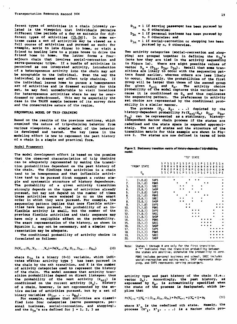
Transportation Research Record 944
ferent typa of activities in a chain [closely re-lated is the Vhstpmht that individual perceivedifferent tixe periods of a day as suitable for dif-ferent types of activities (~,~]. In some ex-treme cases a set of activities may be viewed as afull course of activities and pursued aa such; forexample, movie to late dimer to h-, or viait afriend to bowling lane to a pizza house to drive thefriend home to home. The latter forms a four-sojourn chain that involves saial-recreation andserve-passenger trips. If a bundle of activities isperceived as one integrated activity, introductionof a heterogeneous activity into the chain may notbe acceptable to the individual. Even the way theindividual ia dressed may affect trip chaining. Ifthe individual leaves home to pursue a homogeneousaet of activities and is dresamd suitably for thisset, he may feel uncomfortable to visit locationsfor heterogeneous activities where he may be over-dressed or underdressed. This may be especially thecase in the TALUS sample because of its survey dateand the conservative nature of the region.
SEQUENTIAL ~EL OF TRIP CHAINING
Sased on the results of the previous sections, whichexamined the nature of trip-chaining behavior fromvarious viewpoints, a simple model of the behavioris developed and tested. The key issue in thexodeling ●ffort is how to represent the past historyof a chain in a simple and practical form.
Model Framework
The model development effort is based on the premisethat the observed characteristics of trip chainingcan be adequately represented by making the transi-tion probabilities dependent on the past history ofthe chain. The findings that activities in a chaintend to be hcaogeneous and that inflexible activi-ties tend to be pursued first suggest a rather sh-ple and systematic structure of history dependence.The probability of a given activity transitionstrongly depends on the types of activities alreadypursued, but may not depend on the number of timesthese activities were engaged in or on the exactorder in which they were pursued. For example, thesequencing pattern implies that once flexible activ-ities have been pursued, the probability of an in-flexible activity is small, but the number of theprevious flexible activities and their sequence mayhave only a negligible ●ffect on the probability.The exact representationof the history, as shown inEquation 1, may not be necessary, and a simpler rep-resentation my be adequate.
The conditional probability of activity choice isformulated as follows:
M%+llxl, xz, . . ..)(n) =Pf&+il&. D,n, D2n, . .. DKm) (lo)
where D n is a binary (O-1) variable, which indi-2cates w ether activity type j has been pursued in
the chain by the nth transition, and K is the numberof activity categories used to represent tlsehistoryof the chain. The model assumes that activity tran-sition probabilities depend on direct linkages; thusthe probability of the next activity (Xn+l) isconditioned on the current activity (Xn). Historyof a chain, however, la not represented by the en-tire series of activities pursued, but by a set ofbinary variables (Din, . . .t DKn).
For example, suppose that activities are classi-fied into four categories (serve passengers, per-sonal business, social-recreation, and shoppizsq)~and the Djn”s are defined for j = 1, z, 3 aS
‘ln =lifn, O
‘2n -lifn, O
serving passengerotherwise;personal businessOtherwise) and
Dam = 1 if social-recreation
19
has bean pursued by
has been pursued by
or shopping has beenpursued by n, O otherwise.
Two activity categories (social-recreationand shop-Ping) are grOUped together in defining the D ‘s
rn!?ng(note how they are tied in the activity sequein Figure la). There are eight possible values ofvector Dn = (Din, D2n, D3n). Recall that ~ tran-sitions are likely to occurwith the sequencingpat-tern found earlier, whereas others are less likelyto occur. Naturally, the probabilities of the firstgroup will be larger than those of the second groupfor given X + and Xn. The activity choiceprobability oft?se model captures this variation be-cause it is conditioned on Dn and thus replicatesthe sequencing pattern. The preferences in activityset choice are represented by the conditional prob-ability in a similar manner.
The Process (Xl, X ,i
. . .) depicted by thehistory-dependentprobab lity Pr(~+lt~\ Din, D2n,
D3 ) can be represented ● s ● stationary, history-inaependent Uarkov chain process if the states areredefined and the state space is expanded appropri-ately. The aet of states and the structure of thetransition matrix for this example are shown in Fig-ure 2. The states are now defined in terms of both
Fiwu2. Ststiswmrytwmitionsmasrixafhiatorydepmsdaisf6i@aWiInodal.
“TO” STATE
SPSSSPSSSPSSSPS SSPSSH“FROW STATE VBRHVBRHVBVRHBRH VBRHO
PNEOPNEOPNPEONE OPNEOMon SSCPSSCPSSSCPSCP SSCPE
—.—.— —— .——— .—— -— ___ ___(1,0,0) SVPS ● ‘ ● * ●
;: (0,1 ,0) PBNS ● * ● * ●
(0,0,1) SREC ● *** ●
:; (0,0,1) SHOP ● *** ●
5. (1,0,0) SVPS * ● ● ●●
6. (0,1,0) PBNS ** ● * ●
(0,0,1) SREC ● *** ●
:: (0,0,1) SHOP ● *** ●
(1,1,0) SVPS ● * ● **1:: (1,1,0) PENS ● * ● **
11. (1,0,1) y: ● ** ● *
12. (1,0,1) ● ** ● *
(1,0,1) p: ● ** ● *
ii (0,1.1) ● *** ●
15. (0,1,1) SREC ● *** ●
16. (0,1,1) SHOP **** ●
17. (1,1,1) SVPS ● *.**.*18. (1,1,1) PBNS ● ****
(1,1,1) SREC *+***
;:: (1,1,1) SHOP ● ****
Note: States 1 through 4 are only for the first transition.A “*” indicates that the transition probabil ity betweenthe states are positive; otherwise the probability is zero.
PBNS includes personal business and school, SREC includessocial-recreation and eating meals, SHOP represents shop-ping, and SVPS represents serving passengers.
activity type and past history of the chain (i.e.,vector Dn). Accordingly, the past history, asexpressed by Dn, ia au~tically specified whenthe state of the process is designated, which i-plies that
Pr&+, =jl&=i;D1.,Dz.,Dsnj=Pf(Xi+l‘jIXA=i)=Pu (11)
where X’n is the redefined nth state. NSQSIYI the
process (X’l, X’2, . . .) is a Markov chain pro_
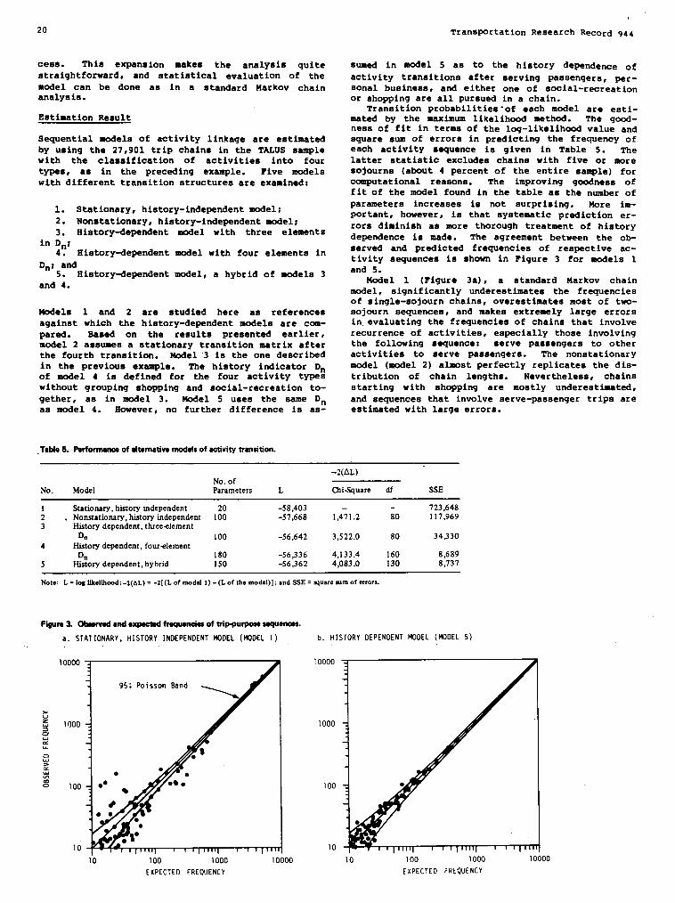
20 Transportation Research Record 944
cess. ‘1’hisexpennion makea the analyais quitestraightforward, and atatiatical evaluation of themodel can be done as in a standard Markov chainanalyaia.
Estimation Result
Sequential aodela of activity linkage are estimatedby ueiingthe 27,901 trip chaina in the TALUS samplewith the classification of activities into fourtypes., as in the preceding example. Five modelswith different transition structures are examined:
1. Stationary, history-independentmodel;2. Nonstationary, history-independentmodel;3. History4ependent mcdel with three elements
in Dn;4. History-dependentmodel with four elements in
Dn; and5. History-dependentmodel, a hybrid of models 3
and 4.
Models 1 and 2 are studied here aa referencesagainat which the history-dependentmodels are cosss-pared. Based on the results presented earlier,model 2 assumes a stationary transition matrix afterthe fourth transition. h@del’3 ia the one describedin the previous example. The history indicator Dnof model 4 is defined for the four activity typeswithout grouping shopping and social-recreation to-gether, as in model 3. Model 5 uses the same Dnas model 4. However, no further difference is as-
.Table5. Perfonstanoaof alternativemodelsofaotivitytransition.
smed in model 5 as to the history dependence of
activity transitions after serving passenger, per-sonal business, and either one of social-recreationor ahopping are all pursued in a chain.
Transition probabilities-of each model are esti-mated by the maximum likelihood method. The good-ness of fit in terms of the log-likelihood value andsquare sum of errora in predicting the frequency ofeach activity sequence ia given in Table 5. Thelatter statiatic excludes chains with five or moresojourns (about 4 percent of the entire sample) forcomputational reasons. The improving goodness offit of the model found in the table as the number ofparameters increaaes is not surprising. Nore im-portant, however, is that systematic prediction er-rors diminish as more thorough treatment of historydependence is made. The agreement between the ob-served and predicted frequencies of respective ac-tivity sequences ia shown in Figure 3 for models 1and 5.
Model 1 (Figure 3a), a standard Markov chainmodel, significantly underestimates the frequenciesof single-sojourn chains, overestimate most of two-sojourn sequences, and makes extremely large errorsin. evaluating the frequencies of chains that involverecurrence of activities, especially those involvingthe following sequence: serve passengers to otheractivities to serve passengers. The nonstationarymodel (mcdel 2) almost perfectly replicates the dis-tribution of chain lengths. Nevertheless, chainsstarting with shopping are mostly undereatissated,and sequences that involve serve-pasaenqer trlpa areestimated with large errors.
-2(AL)No.of
No. Model Parameters L C3ii-Square df SSE
1 Stationary, history independent 20 -58,403 723,6482. Nonstationary, history independent 100 -57,6683
1,4;1 .2 80 117,969Niatory dependent, three-element
Dn 1004
-S6,642 3,522.0 80 34,330Nistory dependent, four-element
Dn 180 -56,336 4,133.4 160 8,6895 History dependent, hybrid 150 -56,362 4,083.0 130 8,737
Note: L = log Ukelltmod;-2( AL) = -2[(L of model 1) -(L of the model)] ; and SSE = wuare 8umof errors.
F~m3, Oteamadmslesqseamdfmqtsanaiesoftrip-pssrpoeeaasfuenaee.
a STAT 10NARY , HISTORY INDEPENDENT k!ODEL (MODEL 1 )
I 00004
952 Poisson 8and
z0 100 ~ ●* ●
&● *
h
b. HISTORY DEPENDENT MOOEL (MOOEL 5)
10000
1000
100
10
10 100 1000 I 000010 100 I 000 I 0000
EXPECTEO FREQuENCY ExPECTEO FREQUENCY

Transportation Research Record 944
The history-dependentmOdelS (models 3-5) largelyimprove these defects. Wodel 3, however, stillshows significant errors for chains that involvesocial-recreation or shopping trips, which Suggeststhat grouping these two activity typea when repre-senting the history of a chain is not adequate.Examination of the log-likelihood value between thismodel and models 4 and 5 also indicates this. Theperformances of models 4 and 5 (Figure 3b) are sat-isfactory, and only few activity sequences are pre-dicted with significant errors. Note that model 5performs almost as well as model 4, even though ithas 30 less parameters. The satisfactory agreementbetween the observed and predicted frequencies im-plies that the patterns in activity sequencing andactivity set formation are well represented by themodel, and also that the model adequately capturesthe history of a chain. A simple representation ofthe hietory of a trip chain by means of a set ofbinary varjables makes ~aaible a satisfactory rep-
lication of trip-chaini~ behavior.
CONCLUSIONS
The atatfatfcal analyais of this study found thatthere is a conaiatent hierarchical order in sequenc-ing activities where less-flexible activities tendto be pursued first. It was also found that the setof activities pursued in a trip chain tends to hehomogeneous. Thus activity transitions are moreorganized and systematic than what a Markovian pro-cess would depict. The homogeneity of activitytypes, patterns in sequencing activities, historydependence, and nonatationarity in activity transi-tions are all closely interrelated. Accordingly, itwas possible to develop a sequential, hiatory-dependent model of activity transition that, inspite Of ita simplified representation of the his-tory of a chian, well replicated the observation.Although the focus of the model was on direct tran-sitions of activities, the model was capable of rep-resenting those characteriatica found for the entirechain (e.g., homogeneity and recurrence of activi-ties and patterns in indirect tranaitiona). Theresult strongly aupporta the sequential modelingapproach adopted in this study. The uaefulnesa ofthe model can be ●nhanced when the history-dependentprobabilities are related to exogeneoua factors.This ia another step that nuat be taken before thesequential model can be applied to practicalproblems.
Although the focus of this study waa on the basiccharacteristics of trip chaining and ita representa-tion by sequential probabilities, the study resultshave aoma practical implication. The strong regu-larity implied by the ~eneity of trip chainssuggeata that Peopless reaponaea to changea in thetravel ●nvironment may be limited, as far as tripchaining ia concerned. People organize their tripchaina while considering the typea of activities,but they nay not necessarily minimize travel dis-tance or coat. The importance of uncertainty inactivity scheduling suggested by the observed se-quencing pattern also implies this. Thus travelpatterna may be less sensitive to travel cost thanwhat was expected. The rather eurprlaing resultthat the peat-energy criaia Baltimore sample hae amean chain length that is 10 percent shorter thanthat of the 1965 Oetroit sample also aupporta thisclaim. This conjecture, however, ia subject to fur-ther investigation. Additional subjects that can besuggested for future investigation include examina-tion of hierarchical relationahipa in time alloca-tion and spatial choices for activities in a tripchain, extension of the analysia to incorporate tem-poral and spatial aspecta and verifying the present
21
findings in that context, and investigation of thecharacteristics of all trip chaina made by an indi-vidual within the study period and of the interde-pendence among these chaina.
A~
This study was partly supported by a grant from theNational Science Foundation to the University ofCalifornia, Davia.
REFERENCES
1.
2.
3.
4.
5.
.6.
-r.
8.
9.
10.
11.
12.
13.
14.
F.E. Horton and P.W. Shuldiner. The Analysisof Land-Uae Linkages. RF@, Highway ResearchRecord 165, 1967, pp. 96-107.J.D. Nyatuen. A Theory and Simulation of Intra-urban Travel. ~ Quantitative Geography--PartI: Economic and Cultural Topics (W.L. Garrisonand D.F. Marble, eds.), Department of Geogra-phy, Northwestern Univ., Evanaton, Ill., Stud-ies in Geography 13, 1967, pp. 54-83.S. Hanaon and D.F. Marble. A Preliminary Ty-pology of Urban Trip Linkages. The East LakesGeographer, Vol. 7, 1971, pp. 49-59.P.M. Jones. Methodology for Assessing Trans-portation Policy Impacts. TRS, TransportationResearch Record 723, 1979, pp. 52-58.S. Hanson. Urban-Travel Linkagea: A Review.In Behavioral Travel Modelling (D.A. Hensher—and P.R. Stopher, eds.), Grorsn Helm, London,England, 1979, pp. 81-100.W. Br8g and E. Erl. Application of a Model ofIndividual Behavior (Situational Approach) toExplain Household Activity Patterns in an UrbanArea and to Forecaat Behavioral Changes. InRecent Advancea in Travel Demand Analysis (~Carpenter and P.M. Jones, eda.), Gower, Alder-ahot, England, 1983, pp. 350-370.D.T. Hartgen, A.J. Neveu, J.M. Brunao, J.S.Banaa, and J. Miller. Changes in Travel Duringthe 1979 Energy Crisis. Planning ResearchUnit, New York State Department of Tranaporta-tlon, Albany, Prelim. Res. Rept. 171, 1980.R.L. Peskin. Policy Implications of UrbanTravel Response to Recent Gasoline Shortages.Presented at Energy Users Conference, San An-tonio, Tex., 1980.D. D-. Theory and Results of Estimation: AComparison of Recent Activity-Sased Research.~ Recent Advancea in Travel Demand Analysis(s. Carpenter and P.M. Jones, ede.), Gower,Aldershot, England, 1983, pp. 3-33.T. Mler and M.E. Ben-Akiva. A Theoretical andBmpirical Model of Trip Chaining Behavior.Transportation Research, Vol. 13B, 1979, PP.243-257.J.O. Wheeler. Trip Purposes and Urban ActivityLinkages. Annals of the Association of Ameri-can Geographers, Vol. 62, 1972, pp. 641-654.S.R. Lermen. The Uae of Disaggregate ChoiceModels in Semi-Markov Process Models of TripChaining Behavior. Transportation Science,Vol. 13, 1979, pp. 273-291.D. Swiderski. A Model for Simulating Spatiallyand Temporally Coordinated Activity Sequenceson the Beaia of Mental Mepa. In Recent Ad-—vances in Travel Demand Analyais (S. Carpenterand P.M. Jones, ads.), Gower, Aldershot* En9-land, 1983, pp. 313-334.R. Kitamura and T.N. Lam. A Time DependentMarkov Renewal k!odelof Trip Chaining. In Pro-ceedings of the Eighth International Sn—wsiumon Transportation and Traffic Theory (v.F.Hurdle, E. Hauer, and G.N. Steuart, ads.), ~-

22 Transportation Research Record 944
15.
16.
17.
18.
19.
20.
ronto University Preaa,ada, 1983, pp. 376-402.
Toronto, Ontario, Can-
D. Damns. fnterdependenciea in Activity Behav-ior. TRB, Transportation Raaearch Record 750,1980, pp. 33-40.R. Kitemura, L.P. Koatyniuk, and M.J. Uyeno.Baaic Properties of Urban Time-Space Paths:Empirical Teata. TRB, Transportation ResearchRecord 794, 1981, pp. 8-19.V. Vidakovic. A Study of Individual JourneySeries: An Integrated Interpretation of theTransportation Proceaa. In Traffic Flow andTransportation (G.F. Neweil, cd.), Elaevier,New York, 1972, pp. 57-70.K. Kondo. Estimation of Person Trip Patterna
and Modal Split. In Transportation and Traffic—Theory (D.J. Buckley, cd.), Elsevier, New York,1974, pp. 715-742.G.C. IIerreeens.The Structures of Urban ActivityLinkagea. Center for Urban and Regional Stud-ies, Univ. of North Carolina, Chapel Hill, Ur-ban Studiee Rea. Nonograph, 1966.R. Kitaetura. ‘Serve-Pasaenger= Trips aa a De-terminant of Travel Behavior. ~ Recent M-
21.
22.
23.
24:
25.
vances In Travel Demand Analysis (S. Carpenterand P.M. Jones, eda.), Gower, Alderahot, Eng-land, 1983, pp. 137-162.L.P. Kostyniuk and R. Kitazrrura.Life Cycle andHousehold Time-space Paths: Empirical Investi-gation. TRB, Transportation Research Record879, 19828 pp. 28-37.T.W. Anderson and L.A. Goodman. StatisticalInferences About Merkov Chaina. Annala ofMathematical Statistics, vol. 28, 1957, pp.89-110.J.C. Kemeny and J.L. Snell. Finite MarkwChains. Van Nostrand, Princeton, N.J., 1960.I. Cullen and V. Godson. Urben Networks: TheStructure of Activity Patterns. PergaeronPress, London, England, 1975.D. Parks and W.D. Wallia. Graph Theory and theStudy of Activity Structure. In Timing Spaceand Spacing Time--Volume 2: H-—n Activity andTime Geography (T. Carlstein et al., eds.),Edward Arnold, London, England, 1978, pp. 75-99.
IWblicarwnofthispapersponwred by@nrrsitteecm ~awlerBehcvwrand Values.
Identifying Time and History Dependencies of
Activity ChoiceRYUICHI KITAMURA AND MOHAMMAO KERMANSHAH
Inthisstudyasequentialmodelofactivitypctrarnsisforrrwlctedthatcerr-sistsoftires-andhistorvdapertdantmcdal$ofactivitycfroica.Thisanalyticalframeworkisusedtoidwrtifytime-cfdaywrdhistorydspendantchcractsris-ticeofactivitychoicabystatisticallytestingaesriesofhypcthosss.There-eultsindicatathatthasimplestexprassicnofthehistoryofactivityangagementsisanadsqrmtadsswiptor,●nd●lsothatnon-homeAcaadcotivitychcioaisconditionallyindependentoftheactivitiesintheprsvissuschain%givwr theactivities pursusd inthecurrent trip chain. Interdqsendsnoiasof activitytypes acrosstrip chcirw ● ra also characterized by aetimctsd model mafficiants.The rasults of the study indissta thst tha dscisions aeeociatad with tha entireactivity pattarn can bsdsccmposed into interrelctsd activity choices whosaconditional dapemdemciescan be statistically waluated.
The way individuals schedule their daily activitiesand organize their itineraries has irrenediateimpactson the spatial and temporal distribution of tripa,or needs for trips, in an urban area. Therefore,representing how the choice and scheduling of activ-ities are done and how travel patterns are formedare critical elements in travel-demand forecastingaa well as in baaic travel-behavior research (l-3).This ia especially so when attempting to for~c<atthe impacts of novel changee in the travel environ-ment or when seeking a transportation policy thatwill accomplish given objectives moat effectively.
The mechanism by which trips as induced demandare qenereted is complex. Even when only schedulingia considered (i.e., when and in what order a givenaet of locations ia visited and how these vieits arearranged into trip chains), there are numerousscheduling poaaibilities. Choice of activities andtheir locations further complicates the problem.Constrainta that govern the behavior are not limitedto monetary and time budgets as in the Claasicalutility maximization framework in economics, but
include spatial and temporal fixity constraints as-sociated with the respective activities (~), inter-paraonal linkage constraints (~), and other types ofconstraint that portray the travel environment ofeach individual (~). The interrelated activitychoices underlying an activity-travel pattern aredependent on the time of day, as many previous etud-ies on tiresuse have indicated (7,8). Previous em-pirical evidence (~, and paper by-~itemura elsewherein this Record) at the aareetime indicatea that thechoices are dependent on history, i.e., the aet ofactivities already pursued on that day.
These aspecte of daily activity and travel be-havior are all of particular importance for the un-derstanding and forecasting of the behavior. Inparticular, the time-of-day and history dependenciesof activity choice may be viewed as the most funda-mental elements, whose adequate representation willlead to repreeentationof other important aspects ofthe behavior as well. For example, the preferencesin forming a set of activities in a trip chain canbe described by sequential probabilities of activity
choice when their history dependencies are appropri-ately incorporated (see paper by Kitamura elsewherein this Record). BY apectfying the structure of thetime-of-day and history dependencies and estimatingthe model statistically, an important objective canhe accomplished: characteri~ation of activity andtravel patterna along the time dimension. When themodel includes exogenous factore that are related tochanges in the travel enviroiucentor in the popula-tion characteristics, then the model serves as atool for forecasting possible changes in activitYand travel behavior.

.Transportation Research Record 944
An extension Of a previouS sequential analYsis ofactivity linkagea is described in this study (see
P@sr by KitSMUra elsewhere in this Record), and anattempt ia made to identify the structure of timeand history dependencies of activity choice. Theobjective ia to demonstrate that the conditionaldependency of activity choice can be properly repre-sented by a simple model structure that can be sta-tistically estimated and conveniently applied topractical problems. The dependency is examined bytesting a set of hypotheses and by inferring itscharacteristics. Alternative model specificationsare examined, and home-based and non-home-baaedactivity-choicemodels are estimated.
The reaulta of hypotheaia testing and model esti-mation indicate that a simple indicator of the his-tory of the behavior--a aet of binary variables eachrepresenting whether an activity of a given type haabeen pursued--beat explains the activity choice.Iicme-basedchoice that determines the first activityin a trip chain ia shown to be dependent on the pestactivity engagement, but non-home-baaed choice iaconditionally independent of the activities in theprevious chaina, given the activities pursued in thepresent chain. Strong time-of-day dependencies inactivity choice, whose temporal variations are wellcaptured by the model, are also shown in the study.The results of the study consistently indicate thatthe time and history dependencies of the behaviorcan be represented by a simple model structure, andsuggest that a set of sequential activity-choicemodels can be developed to represent and forecaatthe characteristics of daily activity and travelbehavior.
BACKGROUND
Becauae individuals develop their daily itineraries
while considering the set of activities to be pur-sued during a certain period, activity choices (ortrsvel choices) cannot be analyzed individually, butthe interdependenciea among them must be adequatelyaccounted for. Such interdependencies have beennoted acrosa different time pericds of a day (~), oramong activity choices in a trip chain (see paper byKitamura elsewhere in this Record). Another aspectof activity and travel behavior is the existence ofvarious types of constrsinta that govern behavior(S,g,g). Many constraints are unobservable if typ-ical survey data are the only information sources.All these characteristic of tripmeking make causalrepresentationof the behavior quite complex.
A poaaible representation of activity- andtravel-choice behavior uses the concept of optimiza-tion together with the assumption that the observedactivity-travel pattern is the one preferred themost by the individual (n). Let ~ be the typeof nth activity, tn be its starting time, dn beita duration, and tn be the location where theactivity ia pursued. For simplicity, only thesefour aapecta are considered here. By letting a =
~~~~i:~e$~;in~ndbe~~i$r~~ & f~~~~~. a~~follows:
MaxindreU = U(a, t,d,l) (1)
Subjectto tn+i-(t. +d.)=s(%,%+i,tn+d.)
O<to, . . ..tn+l <T. tO=?N+, =homr
O<dn
~~C,~eE n=l, . . ..N
gi(a,t,d,Q)=Oi=l,...,G
where
s(i,j,a) = travel time between locations i and jwhen the trip begins at time a,
N-
C=E=
23
total number of sojourns (including in-termediate sojourns at home),set of activity types, andaet of opportunity locations.
The first constraint simply represents the temporalcontinuity condition, the second repreaenta the con-dition where the individual’s path nust originateand terminate at home within time T, and the thirdcondition is the nonnegativity of activity dura-tions. Additional conatrainta are represented in ageneral form by function g in this formulation.Function U, which may be called a utility function,includes not only the t- and duration of each ac-tivity but also its starting time. This ia becausethe regularity and rhythms in time uae patternsstrongly auggeat that the utility of an activity ofa 9iven type iS a function of the time when it ispursued.
Not quite obvious from this formulation is thediscrete nature of the optimization problem, i.e.,resources are not always allocated to all activitiesand srsmsactivities simply may not be pursued at allduring a given period. Accordingly, the classicalconstrained optimization approach (12,13) la not——applicable to this problem if this formulation is tobe applied to disaggregate data where behavior dur-ing a relatively short period (e.g., 1 day) is re-corded. The problem is also much more complex thanthat of a traveling salesman. Not only the order ofvisits, but also the number of visite, their loca-tions, the way these visits are organized into tripchaina, and their timing must be endogenously deter-mined. When this complexity aa a mathematical pro-graznoingproblem is combined with the additionalconstraints, the task involved in representing thebehavior as an optimization problem and obtainingits solution appaara to be prohibitive. Perhaps thenumber of poasfble activity-travel patterns recog-nized by the individual is relatively small (~) be-cause of the constraints and limited information theindividual has, but this ia not the case for theobserver who attempts to analyze and predict the be-havior without comparable knowledge on microscopicfactors that influence each individual.
[The approach taken by Mler and Ben-Akiva (~)avoids these difficulties and at the same time re-tains the simultaneous structure of analyaia bymodeling the behavior as a discrete choice among al-ternative activity-travel patterna. The approach iaquite effective in analyzing characteristics ofactivity-travel choice. Determining the probabilitywith which a given pattern will be chosen, however,requirea that all feasible patterns be enumerated.]
An alternative approach to the analymie of activ-ity and travel petterna is a sequential one, whichis based on the following identityf
pr(a, t.d, ~)=n~opr[%+l, tn+l, ~+1, %+ll%),
t(n), d(n), f(n)] (2)
where a(n) is a vector of the firat (n + 1) elementsof a, i.e., a
and ‘$)are sg\;r~;~$;;;Is~;i~Zp~&LI ~~~~
choic a are analyzed one by one in a sequence, repre-sents the preferences in choosing patterns 9iventhat, if u(a,t,d,t) ~u(a’,t’,d’,t’), then pr(a,t~d~L) ~pr(at,tt,do,t~). The approach has an advantage
in that it reducesthe size of the problemto a MM-ageableone, and the preferences to the entire pat-tern can be correctly represented if the conditionaldependencies of the sequential probabilities areproperly incorporated. A recent study indicatedthat the sequence of activities in a trlP chain canbe adequately reereaented by a siwle seWential
24
model, whereaa failure to capture the conditional
dependency leada to erroneous results (ace paper byKitamura elsewhere in this Record).
An interesting example of a sequential approachcan be found in Horowitz (lS), where the concept oftime-dependent utility in used. A similar conceptis used in the present etudy, but emphasis is on theidentification of time and history dependencies ofthe behavior. The works by D- (~), Damo and Ler-man (~), and Jacobson (~ are noted here becausecertain facets of the complex behavior are carefullyselected in these studies zo that the size of theproblem can be reduced and the analysis can be car-ried out meaningfully and effectively by usingeconometric aaethoda.
There are two taaks involved in developing asequential model of activity and travel f?r fore-casting purposes. The first is the identificationof the structure of the conditional dependency,which ia a prerequisite for proper functioning ofthe model. Because representing the history as inEquation 2 will not serve practical purposes becauseof its excessive information requirements, some sim-ple yet accurate forma must be sought. The secondtaak is to relate the aequentlal probabilities toexogenous factors, ●specially those that clomelyrepresent plaming options and policies.
The time factor is of critical importance in de-veloping sUch a probabillatic model of activitychoice becauae of the strong correlation betweentime of day and activity, as noted earlier. Incor-porating the time variable is aleo important becauseit will make probabilistic representation of theconstraints that affect the behavior more meaningfuland accurate. In particular, the ●ffect of timeconstraints cannot be appropriately representedwithout the time variable [e.g., Iiageratrandgsprlam1s approximat~ by time-dependent probabilities ofspatial choice (~]. A previous study (~ indi-cated that married women who are not employed andwho are in the childbearing stage tend to returnhme early in the evening; this can be viewed aabeing a result of the constraint imposed by familyrespnmibilitiem. The aaquentlal probabilities candepict such constralnta when they are specified astime-of-day dependent and when they include appro-priate variablea that represent individuals’ at-tributes.
APPRDACH
In this study the activity choice along the timedimension ia analyzed, and the main focus of thestudy is on the identification of the time- andhistory-dependentnature of the choice. The spatialaepect is suppressedin this study. The model spec-ificationand estimationeffort is baaed on the fol-lowing formulationof the sequential probability:
~[%+1 . tn+l Ia(n), t(n)l
=Pr[~+llt”+l;atn),t{n)] dpf[tn+ll~n). t(n)l
‘Pr[~+l ltn+l; a(”), Qn)l ~r[%+l
-tnl%,tn;a(n.l),t(n.l)l (3)
where alt . . .? ~) as before,and ~+:(~)( ‘;~’called the sojourn duration inthe nth atate that, in this formulation, includesthe duration of the nth activity and trip time toita location (the activity duration and trip timeare treated separately in the empirical analysispresented in later sections). The aequentlal prob-
ability is expressed aa a product of activity-choiceprobability given the time of the choice and theprobability density of the duration of the nth eO-
Transportation Research
journ. The fodus of this study ia on
element: time- and history-dependentchoice probability.
~$
Record 944
the firstactivity-
The activity-choice probability is formulated aaa function of time, history, and other factora.byusing the multinominallogit structure, i.e.,
Pr[%+l=jltn:l =t;qn),qn).yl
‘exP{vj [t. ~n)$ t(n)t Yl}/~ @xP{vk [t, a(n), t(n), Yl} (4)
where y 1s a vector of socioeconomic attributes of
the individual and t Is the the of day. The condi-tional dependence in Equation 3 is now representedin the model by its explanatory variables that rep-resent the history of the’behavior and the time ofday. It is therefore aasumed that the random errorterms of the model poaseem all the desirable proper-ties, including their statistical independenceacross the choices in the sequence. Although it iapoaelble to use more elaborate formulation of therandom elements (20,21), which may lead to an in-——tereating examination of history dependence, thisstudy doea not extend its scope to analysis of thedependence structure of the unobservable. [Notethat the validity of the error term specificationdepends on mcdel apeclfication, and it ia an empiri-cal issue in that sense (~).]
The time dependency of activity choice is repre-sented by introducing time variables into the logitfunction. For example, suppose that the effect oftime of day on relative activity-choice odds can beerrpreaaedby ganweafunctions, i.e.,
exp[Vj(t, . ..)exp[Vi(t .t) ]..)] ‘[iCtaeXP(-bt)l+[t’exp(dt)] a,b,c,d~ >0 (5a)
(Note that neither the numerator nor the denominatoris necessarily a distribution function.) Then,
Vj(t,...Vi(t.t)=!2nK+(aKc)!Znt!Znt-(tr-d)t (5b)
Although it is not poeaible to determine these pa-rameter values unlguely, the time effecte can berepresented simply by introducing t and kn(t) intofunction V. The model specification effort in thefollowing sections aleo considers polynomial andexponential functions of t.
By using this framework, varioua hypotheses re-garding the nature of the conditional dependenciescan be examined statistically and the model can bespecified subaeguently. l%is study rejects withoutexamination the null hypothesis that activity choiceis independentof time of day. The critical hypoth-eses that need to be examined statistically includethe following:
1. Activity choice is independent of the set ofactivities pursued in the pastr
2. Activity choice is conditionally independentof the met of activities pursued in Previous triechainm, given the activities pursued in the currentchain;
3. Given whether activities of respective typeshave been pursued or not, activity choice ia condi-tionally independent of the number of times the-ac-tivitiea were Pureuedl
4. Given whether activiti~s of respective typeshave been pursued or not, activity choice ia CO~i-tionally independent of the amount of time apent inthe peat for each type of activity;
5. Activity choice ia independent of the numberof trip chains made in the peat; and
6. Activitychoice does not depend on the ti~apent since the individual left home.

.
Transportation Research Record 944 25
An appropriate representation of the historY of anactivity pattern is sought through the examinationof these hypotheses, and the nature of history de-pendency is inferred from the reeults.
DATA Sfm AND VARIABLEG
In this study the statistical analysis of a samplefrom the 1977 Baltimore travel demand data eet isused. Analysis of nonwork activities is the mainsubject of this study, and only those individualswho did not make work trips on the survey day areanalyzed. The records h the data set are screened,and individuals who were younger than 18 years old,who did not hold a driver’s license, and whosehouseholds did not have a car available are elimi-nated. A detailed description of the screening crl-terfa used can be found in Kitamura (see papar else-where in this Re@xd). The screened sample used inthis study includes 927 activity choices in 356 tripchains made by 217 individuals.
Activities are defined in terms of the trip-purpose categories in the data set, which aregrouped into four types: personal businese, social-recreation, shopping, and serve passengers. fiome-beaed activity-choice models are estimated withthese activity typea as alternative. TWO addi-tional categories enter models of non-hcme-basedchoice: temporary return to home and permanent re-turn to home for the day [similar binary classifica-tion of the home state can be found in Lerman(Q) ]. Accordingly, the non-home-based models areestimated with six alternatives.
As variables representing individuals’ attri-butes, the age, sex, education, employment status,household income, household size, number of chil-dren, family life cycle, household role, and carownership are examined in this study. The house-hold-role variable is defined in terms of the sexand employment status of the individual. The life-cycle-stage variable is defined in terms of themarital status of the adult members,their ages, andthe age of the youngest child. The definitions ofthose variables that appear in the ssodelapresentedin this paper are given in Table 1.
RCUE-BASED ACTIVITY-C~IC13MODEL
Because the examination of alternative hypothesesregarding the structure of time and history depen-dencies is an important concern of the study, aseries of. models, each being developed to test aspecific hypothesis, is presented in this section.The first in the series involves only socioeconomicattributes of the individual as its explanatoryvariables (model 1 of Table 2). The mcdel as awhole is significant with a = 0.005, but theamount of variation explained by the model is rela-tively emell (0: - 0.0256). Nevertheless, mean-ingful relationships are found from the eatiaetionresult. The coefficient of the variable that repre-sents the presence in the household of children agedbetween 5 and 12 (SCHLAG) indicates a possitivecon-tribution of this variable to the engagement ofserve-peesenger trips. The role variable (ROLE),which has a value of 1 when the individual is femaleand not employed, indicatea that these individualscarry out shopping and serve-peasenger trips moreoften than do the others. The coefficient of thenumber of children (CELDRN) indicates the negativeeffect that the presence of children ham on the en-gagement in social-recreationby the adult members.
The fit of the model improves when time variableaare introduced into the model with six additionalcoefficients (model 2). The log-likelihood ratiostatistic has a value of ~z = 46.14, with degreea
TabieI.~lnitiondoxmti~vtiatiindv~ww~ls.
Variable and Abbreviation Oefmition
Schoolagedchifdren(SCHLAG)
Householdrole(ROLE)
No. of children (CHLDRN)
Household incnme(INCOME)
No. of cars (CARS)
Time of day (t)
Activity engagement in pretious chains inPersonal business (PBNSO1H)social-recreation (SRECU 1H)Shopping (SHOPO1H)Serve pasaangers (SVPSO1H)
Activity engagementin the current chain inPersonaJ business (PBNSO1C)Social-recreation (SRECO1C)Shopping (SHOPO1C)Servepassengers(SVPSO1C)
Out*f-home time (OHTIME)
No.of chains (CHAINS)
Current activityPeraonal business(PBNS)Social-recreation (SREC)Shopping ( SHOP)Serve paaaengers (SVPS)
Birraryvariable: 1 iftheageof the youngeat child in thehousehold is between 5 and12,00therwiae
Binary variable: 1 if the in-dividual ia a female and notemployed, Ootherwise
No. of household membenswho are 17yearsoldoryounger and not married
Median value of the houae-hold’sannualg.msv incomecategory (S)No,of cars available to the
householdTime of daya in hours; the
study period begins at 4:00sm. when t = 4.0, and endsat 4:00 a.m. the next daywhen t = 28.0
Binary variable: 1 if activi-ties of the indicated typewerepurauedinthe tripchainsprevioualy made
Binary variable: 1 if activi-ties of the indicated typehave been pursued in thecurrent trip chain
simulative amount of timespent so far outside homefor both trips and activities
Cumulative number ofhome-baaed trip chains made sofar
Binary variable: 1 if thecurrent activity is of theindicated type
of freedom (df) = 6 for the six new coefficients.Clearly the tine of day haa a substantial influenceon activity engagesaent. The nature of the time de-pendency of activity choice ia presented later inthis section,by using a history-dependentmodel.
Examination of the history dependence of home-besed choice uses the following variables to repre-sent the past history of activities: O-1 binaryvariables, each representing whether an activity ofa given type has been pursued in the past; the num-ber of sojourns made for each activity type; and thecusmalativeamount of time spent for each activitytype. These variables are used because of theirconciseness as e~ry variables of the history.The possible effects on activity choice of the exactsequence of the past activities, their respectivedurations, and their occurrence times are consideredto be negligible.
Each set of history variablea ia tested, and onthe basis of its aigniflcance the nature of historydependence ia inferrti. The results indicate thatthe simplest representation of the history--the setof binary indicators of activity engagement--explains the choice better than any other aeta ex-amin&i here (saodel3). Although the other sets ofvariables are all significant, they do not explainas large a portion of variations as doee the set ofbinary variablee. Whether the individual has pur-sued an activity of a given type or not doaeeaffectthe home-based activity choice, but how many timesand how long the activities were engaged in do nothave aa decisive an effect. This rather unexpectedreeult ia encouraging because of ita implication
that the history of behavior can be exeressed inquite a simple manner in representing the condi-

26 Transportation Research Record 944
Tabla 2. Horns-bMwJ activity~ie models.
Activity Type
personal Business Social-Remeation Shopping Ser9e Passengers
Variable Coefficient t-Statistic Coefficient t-Statistic COefficient t-Stat istic Coefficient t-Statiatic
Model l‘
ConstantSCHLAG
+.5797 -0.86 -43.0485 A3.08 0.0698 0.11
ROLE0.8583 2.76
0.4968 1.99 0.5702CHLDRN
1.924.1895 -2.02
!hr(INCOME) 0.2877 1.23 0.5893 2.37 0.2801 1.23
Model 2b
Constant -3.3830SCHLAG
-5.s5 -10.984 -2.01 S.0561 1.01
ROLE0.8585 2.76
CHLDRN0.4787 1.89
-0.24690.s743 1.93
-2.52QrI(INCOME) 0.3299 1.37 0.5063 2.02 0.2136 0.92t -0.4240 -1.57!Ar(t)
43.2050 -0.76 -0.7928 -2.854.1127 1.21 0.4227 1.18 10.498 2.90
Model 3C
constant -3.7499 -0.65 -11.876 -2.10 4.8241SCHLAG
5.25
ROLE0.6289 1.89
0.3895 1.44 0.6413 1.96CHLDRN J3.2086 -2.07hr(INCOME) 0.3542 1.42 0.5169 1.97 0.2093t
0.87-0.3S22 -1.22 -0.1310 -0.46 -0.7315
!ln (t )-2.56
3.7260 1.04 4.0236 1.08 10.634 2.89PBNSOIH -0.8605 -1.98 -1.6576 -3.34SRECO1H
-1.0187 -1.900.6166 0.91 0.8793
SHOPO1H1.25 1.5780 2.20
+.2300 4.47 -0.5662SVPSOIH
-1.09 +.2014 4.360.3252 0.52 0.9638 1.67 1.8125 3.14
Note: ti@e=3S6home.bMd actltitychokex L@)=log4ikelfiood tihthemdd cmfflcients, L(C) =log4kelfiwd Wthoutexpkmtow whMes(contiant terms done), L(O)= log41kelfiood Mthout."y coeK~ients,.nd g2=1-L@)/L(C). lltechi-qumev atuesprerenteda redefineda s-2[L(C)-
W)l.
:UO) = 493.52, L(C)= -490.27, L(J)= -477.70, X2= 2S.14 (df = 7), and P2 = 0.02S6.
L(#)= A54.63, x2=71 .29(df= 13), P2=0.0727, andx2f0r thewtOfthe Whbl-=46.l4(df=6).CL(8) =434.36,X2= 111.81 (df=25), #2=0.114, andx2for theset of activity indicators =40. S4(df= 12).
tional dependency of activity choice. Another his-tory descriptor--the number of chains ccaopletedinthe past--was found to be insignificant.
These models aredeveloped primarily to examinealternative hypotheses; thus the selections of ex-planatory variables are not necessarily finalized asthey are presented in Table 2. A similar model isestimated sfter eliminating some of the insignifi-cant variables of model 3, and its coefficients forthe binary variables are given in Table 3 to indi-cate how the past engagement in an activity of onetype affects the choice of another activity type.In the table the estimated set of coefficients isadjusted by adding a constant to the coefficientsfor each activity type. The value of the constantis arbitrary, and that value that ntakesthe row sumof the adjusted coefficients zero is used in devel-oping the table.
The result indicates that engagement in personal
Tabla3. Effaotaofaativhyangegzmentainpfaviousahainaonhoma-bawdactivi2yohoiw.
First Activity of Current Chain
Activity Engagement Personal sOcial- Serwinpreviouschains’ Buainesa Recreation Shopping Pa.wngers
Personal business 0.8278 0.0602 4.7S64 4.1317Social-recreation -0.4109 -0.4109 0,0612 0.7606Shopping 0.1024 0.1024 -0.3072 0.1024Serve passengers -0.6059 -0.6059 0.1782 1,0336
‘1 ifenaaged, Ootherwlae.
business in the past has a positive influence on thechoice of the same activity type later. The sametendency can be found for serving passengers;choices of personal business or serve-peseengertrips are positively correlated acroas trip chains.The negative diagonal value for shopping indicatesthat people tend not to pursue shopping in two orattoretrip chains; it suggests that people have beenconsolidating their shopping trips into fewer tripchains. A negative coefficient of social-recreationon personal business indicates that there are pat-terns in sequencing activities across trip chains,arqipareonal business tends not to be pursued if theprevious chains included social-recreation trips.The pattern found here is quite similar to thatfound ●arlier as to the sequencing of activitieswithin a trip chain (see paper by Kitafauraelsewherein this Record).
The time-dependent nature of home-based activitychoice can be seen in Figure 1, which presentsagainst the time axis both the observed relativefrequencies of chosen activity types and the choiceprobabilities depicted by the ❑odel. The observedshopping frequency coincides naturally with the typ-ical stores’ hours, and it peaks in the ●arly after-noon. Personal business tends to be Pureued in themorning, whereas the relative frequency of eocial-reoreation increases toward the end of the day. Theserve-passenger activity has a rather irregular pet-tern with peaks in the early morning (chauffeuringchildren or workers, perhaps)? ,earlY after~n~ andlate evening.
The data in the figure indicate that the observedtendencies are well replicated by the estimted
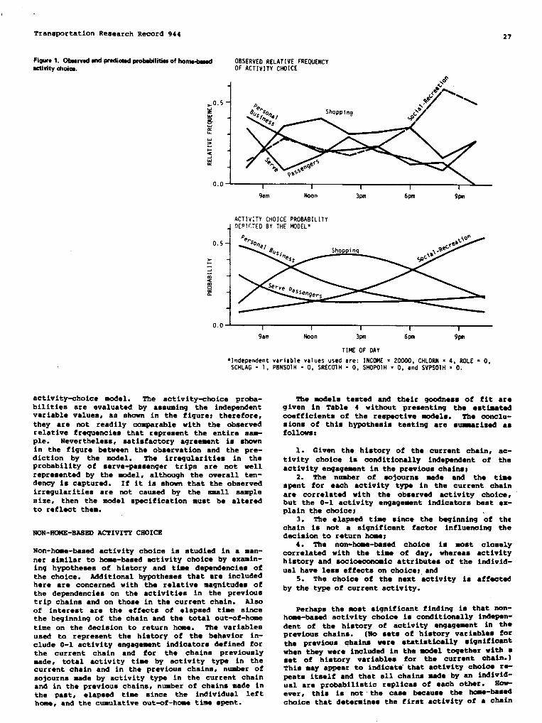
Transportation Research Record 944 27
F@ml. Obaervedendpradkadprobzbilitieaofkj~ OBSERVED RELATIVE FREQUENCYactivity dloire. OF ACTIVITY CHOICE
0.0 i \I I I 1 I
9am Noon 3pm 6PM 9pm
ACTIVITY CHOICE PROBABILITY
i
DEPICTED BY THE POOEL*
9am Moon 3pm 6Pn
TIME OF OAY
●independent variable values used are: INCOME = 20000, CHLORN = 4, ROLE = O,SCHLAG = 1, PBNSOIH = O, SRECOIH = O, SHOPOIH = O, and SVPSOIH = O.
activity-choice model. The activity-choice proba-bilities are evaluated by aasuming the independentvariable valuea, aa shown in the figurel therefore,they are not readily comparable with the observedrelative freguenciea that represent the ●ntire aem-ple. Nevertheless, aatiafactory agreement ia shownin the figure between the observation and the pre-diction by the model. The irregularities in theprobability of serve-paasenger trips are not wellrepresented by the model, although the overall ten-dency ia captured. If it is shown that the observedirregularities are not caused by the small samplesize, then the model apacification must be alteredto reflect them.
~N-NOME-BASED ACTIVITY CKOICE
Non-home-baaed activity choice is studied in a man-ner similar to home-based activity choice by ●xemin-ing hypotheses of history and time dependencies ofthe choice. Mditlonal hypotheses that are includedhere are concerned with the relative magnitudes ofthe dependencies on the activities in the previoustrip chainm and on those in the current chain. Alsoof interest are the effects of elapsed time mincethe beginning of the chain and the total out-of-hazetine on the decision to return home. The variablesused to represent the history of the behavior in-clude O-1 activity engagement indicators definedforthe current chain and for the chains previouslymade, total activity time by activity type in thecurrent chain and in the previous chains, number ofaojourna made by activity type in the current chainand in the previous chains, number of chains made inthe paat, elapsed time since the individual lefthoaoe,and the cumulative out-f-home time spent.
The models tested end their goodness of fit aregiven in Table 4 without presenting the ●stimatedcoefficients of the respective mdela. The conclu-sions of this hypothesis testing are sumerized aafollowsx
1. Given the history of the current chain, ac-tivity choice is conditionally independent of theactivityengagementin the previouschaine~
2. The number of eojournm made and the timespent for each activity type in the current chainare correlated with the obmerved activity choice,but the O-1 activity engage~nt indicator best ex-plain the choicet
3. The elapmed time since the beginning of thechain is not a significant factor influencing thedeoiaion to return has;
4. The non-home-based choice is moat clomelycorrelated with the time of day, whereas activityhistory and aociomoomomic attribute of the individ-ual have leaa effects on choice;,and
5. The choice of the next activity ia affectedby the type of current activity.
Perhaps the momt significant finding is that non-home-baeed activity choice is conditionally itiapan-dent of the history of activitY en9a9emant in theprevious chains. (No setm of history variables forthe previous chains were statistically mignifi-twhen they were included in the model togetherwith aset of himtory variables for the current chain.)This may appear to indicate”that activity choioe ra-paatm itself and that all chains made by an individ-ual are probabilistic replicaa of each other. H-ever, this is not the case because the home-basedchoice that determines the first activity of a chain

28 TranaportathnReaearah Record 944
Tsbfs4. Attommfvsspsdffoattonsofnon~ Ssdvky+mks e
Hi3toryIndbtomu llmeof
ModelNo. Iodicator Lky Socioscenomic Sst 1 sot 2 w) X2 (df - 4)
1“ x x x2 x x
-S13.585 -bx
3x
x x-810.396 -c
x x4 x
No.ofSojoufns,pastx x x
407.6S9 5.474
sActivMytime,ps3t
x x x-806.258 8.276
x6 x
o-lWttvity,putx x
-808.649 3.494
xNo.ofmjoums,ountufstive-803.366 14.060
x : x:
Activitytime,cumulstiwx x x x
-807.694
9No.ofSojouflts,prosont
x x-S00.499 1::%
x x10
Aotivitytime,Pfssbntx x x x
-805.467 9.8580-1sotivity,Pfossnt -797.013
11’ x x26.:~
0-1●ctivity,pfssont -842.98i12’ x x : 0-lactiyity.Ofosent 408.820 _a
Note: Thi orlsln Indkator Inciudos Ibrea bhuy v~hblw PBNS, SRCC, and SVPS. Tboc of &y k roPNnotd by threelad8p,ndatlvdk●bl- t, ●xP(t), snd axIJ(-t). The sot of socioeconomlcs incktdoc four vukbh: numbs of cbbldma,o-1 bkuy vukbh foc Prwoacoof @!oal.uat ehlfdrm, Income.MM numbu of arg. l’lw hktary indkamrsbtcludotwo #@sof vukbkw mf 1mukts of camuhtlw out.of.koae time,damodilme, andnumbwof chdm m~ pmvbmdy;●ndscf2 Inctuda Ilw mrkbh ladkat.d la tha labl.. X Indkalu ttut thevwkble II h.ckudmd In the model.
~em modeb we teuad acahs modet 10; lb. othu models U. mstod asshnt modo! 2.
EJfecl of hhtory, X2 = 33.14, df = 7.
CRofesence mod@L‘F.ikt Of tbzIi0fd9Y, Xa = 91.94, df = S.
‘Ef?ect of dkect Ilnbascs, X2 = 23.61, df = 10.
is depandont of the past history, u dicousaad intho pZOViOUS 800ti031. ThY3S the history dopandenosof the non-ham-baaed choice is indirectly repro-sontad throuqh the history dopandmco of tho homa-baaad Ohoice.
The strong tbe dapandenoy of nott-homa-bacadchoice aust be notad. Tho contribution of the fiv.tin coafficionts to the explanatory power of themodal. ia represented by ● ahi-square statiatie of91.9 (df = 5) , whoreaa that of the ●ooi~icvariablea ia 16.1 (df . 4) , ●nd that of the historyvariabloa ia 33.1 (df - 7). Obviously, time of dayia tho moat critical determinant of the non-ham-baaad choice.
The final form of the non-hma-bacad ●ctivity-choice model that waa selected on the basis of thehypothea~a teatittgroaulta ia givettin Table 5. Acot of three binary variablea (PBWS, SR6C, S180P)isuaad to repeeaent the type” of current ●ot ivity,i.e., the activity just ~letad ●t the time of thotranaithn to the choaan ●ctivity. Many of the ninecoafflaienta that ●pply to theea variablem ●re ●ig-nifiaant and indicate the strength of diraot link-
aqes batuaan aotivity typea. Caqbared with thehae+aead ahoioe wdala, fever aocioeoona ic ●t-tribute variablea ●re used in the wdel. The nudtarof children ●nd the preaanoa of aohool-agad childrenhave the cane ●ffaota on aotivity choioa ●s in theh~ ahoioa model.
The coefficients of the oar-ounerahip variable●re poaitiva(butnot ●iqftificant) for the temporary
return to haa, and they ●re negative for the par-Mnant return to hae. The hdioation ia that theindividuals froa households with more aara tend tosake more trip ahaina, but the nubar of ●ojourna in● ohaln may tend to be fewer. A ●tiilar tendencywee found in ● previous study that ●nalyaed ● 196SDetroit data cot (2 . The nagetiva voefficientm of
Pthe atnulative ott-f-hma tin ●nd the mmbar ofohains ●re quite notauorthy, ●lqh theY ●re ~t●tati8tioally ●iqnifieant ●t e = 0.05. Tho ooaf-fieienta ●pply to the Pemnattt return to home ●nd*1Y thet the sore tine the individual has apantoutcida hnma and the mm. ehaina he has made, theless likely he is to terminate hia out-of-hone ac-tivity pursuit of the day. The result ●uweats that
Act* ‘w@
Mfmlolkuf3teu 8ocfsl-Rscv@bn Sboppbu ssYYsPsomWOn fio3m Abawbhu Nome
cosm- 030m. *m-
Vsrisbto Cbnt t-stotiuk Cbnt t-8tstMIs cbot t-stotbtkSb3tt taafMk Chat t-stotfstkCbflt t-8tstMk
Constsltt +.s306 -1.01 -2.4408 -3.08 -2.7799 -3.19 -2.s840 -2.89 0.9237 1.17PENS 1.4074 1.59 1.7789 2.17 2.7420 2.57 IJS98 I.U t.1598 I.USREC 1.11S6 l.% 1.821S 2.2s 0.5169SHOP 0.9220 t.29
0.S169 1.0943812 .::: 43812 -1.to
t 0.1809 3.23 0.0884 1.74 0.1490 2.s2exp(+lo) 13261 0.77em w 10) 0.0520 6.04&~Rf 4.2116 -1.66
nAO09 131
CAR8PBN8011-Smcolc8HOP01
-u ------ .-.0.0580 0.s9 -0.2478 -232
!C 1.2327 2.62 0.4349 1.160.6284 1.s1 0.6789 1.76
SvP80t’: I.4726 3.s3i.2009 2.83
Of’f2’fm -O- -1.30
CHAINS 4.1498 -1.26

.
Transportation Research Record 944
individual pursue ●ither very few or very many ac-tivities on a given day. This may be a result ofactivity scheduling over a longer time span, e.g., aweek.
In summary, the hypothesis testing and modelspecification efforts presented in these two sac-tions have indicated that the activity choice isdependent on both the time of day and the history ofthe activity. But the structure of!the history de-pendency is rather simple. The binary history indi-cators that represent whether activities of respec-tive types have been pursued in the past or not arecorrelated with the activity choice more stronglythan is the number of sojourns or the time spent foreach activity type in the past. Furthermore, non-home-based activity choice is found to be condition-ally independentof the activity history in the pre-vious chains, given the history in the currentchain. It appears that activity choice is dependentmore strongly on nsxe recent activities. The sig-nificance of the variables that represent the directlinkages also indicates this.
DISCUSSION OF RESULTS
Identifying the dependencies across a series of ac-tivity choices is critically important for the de-velopment of a practical tool for analyzing andforecasting daily activity and travel behavior. Inthis study the structural form of a sequential modelof activity patterns was formulated, and conditionalprobabilities of activity choice that used the mul-tinominal logit structure were specified. Thisframework was then used to examine the nature oftime and history dependencies in activity choicewith the assumption that time of day and the historyof the behavior are the most fundamental factorsthat influence activity choice.
The examination of a series of hypotheses indi-cated that the simplest representation of the his-tory of the behavior--a set of binary activity en-gagement indicators—is an adequate descriptor andbest explains activity choice. Non-home-based ac-tivity choice is strongly affected by time of dayand also by current activity type, but socioeconomicattributes of the individual and history variableshave less influence on non-home-based choice than onhome-based choice. Non-home-based activity choicewas also found to be conditionally independent ofthe activity history in the previous chains, giventhe activity history in the current chain, whereashome-based activity choice had interdependencies inthe activity types across trip chains. The resultsof the study are encouraging and indicate that a setof simple models that can be conveniently estimatedis capable of representing individuals’ “daily ac-tivity and travel behavior together with the inter-dependencies acrossthe choices involved. The studyhas indicated that the decisions associated with theentire activity pattern can be decomposed into in-terrelated activity choices whose conditional de-pendencies can be statisticallyevaluated.
The models presented in this study, however, arenot immediately applicable to practical problems be-cause the types of ●xogenous variables included arelialited. This limitation is mainly caused by theaspetial nature of the study. The models must beextended to spatial activity-choice models with landuse and transportation network variables introducedas explanatory variables. Note that the land usevariables in this context must be defined in termsof &th the spatial distribution of opportunitiesand their availabilities along the time dimension.When land use variables are defined in this manner,then the activity choice can be related to the
availabilities of varioustime periods of a day.
opportunities
29
in different
Such effort of modeling the activity choice inthe spatial dimension will encounter a new problem:representation of the attractiveness of an oppor-tunity, or a group of opportunities such as a zone.This is not a trivial task when the assumption ofthe conventional approach that a travel choice canbe separated from the rest and can be analyzed inde-pendently is discarded, and when the interdependen-cies across the choices are acknowledged. Theinterdependencies imply that a choice of an oppor-tunity ie influenced by both the past and intendedfuture behavior. The conventional formulation ofthe attractiveness of a zone that uses the attri-butes of that zone alone is not adequate when theindividual has in mind additional activities to bepursued elsewhere. In other worde, when trip chain-ing is considered, the traditional definition of theattraction becomes inadequate, and the attractive-ness of a zone as an origin from which the next ac-tivity site will be reached must be evaluated andincorporated into the attraction measure. This canbe done by ueing the concept of expected utility, inwhich the attractiveness of a zone is a function ofnot only its own attributes but also those of otherzones. Another aspect, which was not emphasized inthis study, is the structural relationship betweenthe activity duration and actiivitychoice. It maybe the case that the relationship varies dependingon the time of day or on the past history of the be-havior. Examination of the interdependence struc-ture of the unobservable also remains as a subjectof future research.
AC~T
This study was partly supported by a grant from theNational Science Foundation to the University ofCalifornia, Davis.
REFERENCES
1.
2.
3.
4.
5.
6.
7.
8.
P.M. Jones, M.C. Dix, M.I. Clarke, and I.G.Iieggie. Understanding Travel Behavior. Trans-port Studies Unit, Oxford Univ., Oxford, Eng-land, 1982.K.P. Burnett and S. Haneon. Rationale for anAlternative Nathemetical Approach to Ibvementas Complex Human Behavior. TRB, TransportationReeearch Record 723, 1979, pp. 11-24.W. Brog and E. Erl. Application of a Nodel onIndividual Behavior (Situational Approach) toExplain Household Activity Patterns In an UrbanArea and to Forecast Behavioral Changes. ~Recent Advances in Travel Demand Analysis (S.Carpenter and P.M. Jones, ads.), Gower, Alder-shot, England, 1983, pp. 350-370.I. Cullen and V. Godeon. Urban Networks: TheStructure of Activity Patterns. PergamonPress, London, England, 1975.I.G. Heggie and P.M. Jones. Defining Dc4aainsfor Nodels of Travel Demand. Transportation,vol. 7, 1978, pp. 119-135.T. Hagerstrand. What About People in RegionalScience? Papers, Regional Science Association,Vol. 24, 1970, pp. 7-21.J. Toalinson, N. Bullock, P. Dickens, P. Stead-man, and E. Taylor. A Model of Students’ DailyActivity Patterns. Environment and Planning,Vol. 5, 1973, pp. 231-266.M. Shapcott and P. Steadman. Rhythms of UrbanActivity. In Timing Space and Spacing Time--VOIUDS 28 =&zan Activity and Time Geo9raPhY(T. Carlstein et al., eds.), Edward Arnold,London, England, 1978, pp. 49-74.
Transportation Research Record 94430
9.
10.
11.
12.
13.
14.
15.
16.
17.
18.
D. Damm. Interdepandencies in Activity Be-havior. TRE, Transportation Research Record750, 1980, pp. 33-40.J. Supernak. Travel-Time Budget: A Critique.TRB, Transportation Research Record 079, 1982,pp. 15-28.G.S. Root and W.W. Reeker. Toward a DynamicModel of Individual Activity Pattern Forms-tion. & Recent Advances in Travel DemandAnalysis (S. Carpenter and P.M. Jones, eds.) ,Gower, Aldershot, England, 1983, pp. 371-382.M.J. Beckraann and T.F. Golob. A Critique ofEntropy and Gravity in Travel Forecasting. In—Traffic Flow and Transportation (G.E. Newell,cd.), Elsevier, New York, 1972, pp. 109-117.J.H. Niedercorn and B.V. Bechdolt. An EconomicDerivation of the Gravity Law of Spatial Inter-action. Journal of Regional Science, Vol. 9,No. 2, 1969, pp. 273-282.T. Mler and M. Ben-Akiva. A Theoretical andEmpirical Model of Trip Chaining Behavior.Transportation Reeearch, Vol. 13B, 1979, pp.243-257.J. Horowitz. A Disaggregate Demand Model ofNon-Work Travel that Includes Multi-DestinationTravel. TRB, Transportation Research Record673, 1978, pp. 65-71.D. Damm and S.R. Larmen. A Theory of ActivityScheduling Behavior. Environment and PlanningA, Vol. 13, 1981, pp. 703-718.J. Jacobson. Nodels of Non-Work Activity Dura-tion. Department of Civil Engineering, Massa-chusetts Institute of Technology, Cambridge,Ph.D thesis, 1978.R. Kitemura and M. Hioki. A Time Dependent
19.
20.
21.
22.
23.
24.
stochastic Model of Spatial Interaction: NodelFramework and Properties. Presented at AnnualMidContinent Meeting of the Regional scienceAssociation, Vail, Colo., June 1982.L.P. Kostyniuk snd R. Kitamura. Life Cycle andHousehold Tima-SpaCe Paths: EI@KiCal Investi-gation. TRB, Transpxtation Reeearch Record879, 1982, pp. 28-37.J.J. Iieckmen. Statistical 140dels for DiscretePanel Data. ~ Structural Analyeia of DiecreteData with Econometric Application (C.F. Nanskiand D. McFadden, eds.), MIT Preae, Cambridge,NSSS., 1981, PP. 114-178.C.F. Daganzo and Y. Sheffi. Multincmial Probitwith Time-Series Data: Unifying State Depen-dence and Serial Correlation Models. Environ-ment and Planning A, Vol. 14, 1982, pp. 1377-1388.D. McFadden, K. Train, and W.B. Tye. An Appli-cation of Diagnostic Tests for the Independencefrom Irrelevant Alternative Property of theMultinrsnialLogit Nodel. TRB, TransportationResearch Record 637, 1977, pp. 34-46.S.R. Lermsn. The Use of Disaggregate ChoiceModels in Semi-Markov Process Nodela of Trip
Chaining Behavior. Trana~rtation Sc fence,Vol. 13, 1979, pp. 273-291.
R. Kitamura, L.P. Kostyniuk, and !4.J.Uyeno.Baeic PropertiesEmpirical Tests.Record 794, 1981,
of Urban Time-Space Paths:TRB, Transportation Researchpp. 8-19.
fiblicatwnofthis wrxrwonsoredby ~mrrritteeon~a=lm BetibratiValues.
Equilibrium Traffic Assignment on an Aggregated HighwayNetwork for Sketch PlanningR.W. EASH, K.S. CHON-,Y.J. LEE, AND D.E. BOYCE
An●ppllzstionofth.Squilibdumtrafficswi@mmntdgorlthmon● dmplifizdhighwaynetwork,woh asmi@rtbzwadforskstdrplanning,h dzsoribzd.Ansly8i:rone9inth.swi~rnentus zlsautmtsntldiyIsrgzrthq [email protected] qullibfiumtrafficz9-slgmnsntisintroduced,foilewvdbysdboumlon01ttwproblsnwwithqui-Iibriumtrzfficsssigrwnsmtinssks@@snningsppliastion.Noxt,thznetworkwalingproasdurzs for the ssm study wz wwmirwd. Raultr of tlw skotsh-phnning zwigrwnent W9 than svdustzd againsts zompsrablo regional msiiwr-ment of the sznm trips. Finally, thzrz is a dbzussion of how this rwssroh fitsinto the Programs of a trsnspwtztion pimrning ●gsnoy.
An application of equilibrium traffic assignment tosketch planning ia presented in this paper. Tripsare assigned onto an aggregated network with a1imited number of links, nodes, and zone centroids.One arterial link in the sketch-planning network isequivalent to a number of links in a conventionallycoded ragional highway network, and one sketch-plan-ning zone is substantially larger than a zone in theragiona1 assignment at the aema location. Thetraffic assignment algorithm US- in the studyconverges to approximately equal path travel timesfor multiple paths between origin-destination zonepairs. The algorithm is available to most transpor-tation planning agencies.
A majorparison of
portion of the paperthis sketch-Dlannin9
ia spent on a com-assignmant with a
regional traffic assign&t of- a larw trip tableonto s detailed coded highway netwrk. This comperi-aon ia complicated by the different number of intra-zonal tripe in the two traffic assignments1 there-fore, a procedure waa developad to determine theaignificance of the additional intrazonal trips inthe sketch-planning assignment. Vehicle miles ofcapacity and travel, vehicle hours# and avera9espeeds predicted by the tw assignments are susmte-rized at the regional and zonal levels.
In the introductory sections of the paper theequilibrium traffic assignment algorithm and thenetwrk coding procedures for the sketch-plann~n9netwrk are documented. A simple method for aggre-gating linka and summing regional link capacitiesinto sketch-planning link capacities is then de-scribed. The question of the beat network a99re9a-tion procedure is not considered. Moreover, a eolu-tion of this netwr k aggregation problem was not anobjective of the research, but rather a data re-quirement. The PCincipel concern of this paper isto demonstrate a satisfactory correspondence between

,Transportation Research Record 944
traffic assignments on the sketch plan and regionalnetworka. Finally, a few implications of this re-search for work programs of transportation planningagenciea are diecuased.
MSTHOOOLGGICAL APPROAC?I
The equilibrium concept was first formulated forminimum time-path traffic assignment by Wardrop(&). Given that travel times on a network linkincreaae with traffic, a highway network is inequilibrium if the travel times along all patha thatare used between esch origin-destination are equal,and no unused path has a lower time. In other words,no driver has an incentive to change paths.
Several algorithms were developed in the early1970s to determine the equilibrium traffic flows,and one version of the algorithm is now available inthe Urban Transportation Planning system (UTPs)computer ero9rema for transportation planning SUp-
pOK@d by UMTA and FHWA Q). The formulation of thealgorithm discussed here follows the work of Wguyen(~) and LeBlanc et al. (~) and is consistent withthe algorithm available in the UTPS program OROAD.
For a given trip table, the equilibrium aeaign-ment of traffic MSy be found by solving a nonlinearmathematical programming problem. The solution tothie problem is that set of traffic flows on networklinks that minimizes a nonlinear convex mathematicalfunction (called an objective function), the valueof which depends on the traffic flows. These flowsmuet alao satisfy a second set of linear equationscalled constraints. In general terms, the con-straints on the objective function ensure that allsolutions are feasible trip aasignmenta; that is,all trips in the trip table are assigned to thenetwork, and negative link flows are prohibited.
The objective function is to minimize the aum ofthe areas under each link’s travel-time and trafficvolume congestion function from zero to the assignedflow. To understand the interest in minimizing theaum of these areas requires some mathematical analy-sis beyond the scope of this paper. It is onlyimportant to understand that the link flows thatcorrespond to the minimum value of this objectivefunction are those that satisfy the equilibriumconditions.
Summery of Equilibrium Traffic Assignment Algorithm
The algorithm to solve the equilibrium traffic as-signment problem is based on a nonlinoar optimiza-tion techn@ue developed by Frank ●nd Wolfe (5).Theirs is an iterative ●pproaah that starta with ●ninitial feaaible aolutfon that ●atisfias the con-straints, determines a feasible direction to movathat improves the objective function, and then cal-culates how far to move in this direction. Thisresults in a new feasible solution, and the proce-dure itaratea until the objective function cannot beimproved.
A network composed of links with congestion func-tions, a trip table for aasignmant, snd a firsteolution that is a feasible saaigmment of trips tothe network are given. The equilibrium conditionsare normally not met by this firet trip assignment.Application of the method by Frank and Wolfe theninvolves the following steps.
1. Compute the travel time on each link by usingvolumes in the current solution.
2. Trace minimum time-path trees from eachorigin to all destinations by using the link timescomputed in step 1.
3. Assign all trips for each origin to eachdestination to the minimum psthe computed in step 2
31
this produces an all-or-nothing trip assignment).4. Linearly combine the current link volumes
Vs) of the solutionink volumes (wa) of
new current solutionobjective function;
and the new all-or-nothingthe ,assignment to obtain a
(va) that minimizes the
where
v; = (l-A)Va + iwa = new currentsolution volume on link a,
Sa(x) = link congestion function forA = constant between O and 1.
5. If the solution haa convergedstop; otherwise return to step 1.
The sequence of program steps is shownchart in Figure 1.
Fiws1. EquiliMumdporlUimpropm~.
~
HighwayNatwork
First Wh forUnconpastad
limes
&I Triptobla i.oodTram I
link a
auffic
(i)
and
ently,
in the flow-
0Naw Pathfor100dad
btatwrklimes
&Equilibrium Traffic Assignment and Sketch Planninq
The obvious probleme in applying equilibrium trafficassignment to sketch plenning are how to slmplifYthe traffic assignment network and analysia zonesand the nature of the travel-time and traffic volumecongestion function for Su-ch a network. Previously
researchers have constructed sketch-planning net-works either by eliminating minor and lightly
traveled links (~) or by aggregating links in a

32 Transportation Research Record 944
detailed network into summary links (~). The sketch-planning network for this project combines these two
approaches and includes all freeway and expresswaylinks with a grid network of aggregate llnka forarterial streets.
A number of time and volume relationships havebeen developed for traffic assignment when the codednetwork resembles an actual highway network (~).The most wjdely used is the Bureau of Public Roads(BPR) formula available in the program UROAP:
T=TO [1+0.15(v/c)4] (2)
where
To = uncontested (zero traffic flow) traveltime on the link,
T - estimated link travel time, andv/c - ratio of link traffic volume to link
capacity.
In a conventionally coded highway assignmentnetwork, each link is a street or highway segment,the attributes of which can be observed. TO illus-trate the detail coded into these networks, onlylocal streets and rural roads used principally forland access are omitted in the regional network usedby the Chicago Area Transportation Study (CATS). Itis reasonable, therefore, to assert that the codednetwork built from all these individual links re-flects the supply characteristics of the regionalhighway network.
If the regional network links to be combined in asketch-planning link can be identified and accept-able regional network link congestion functionsexist, then two methods for developing aggregatecongestion functions appear plausible. First, theregional time and volume relationships can be mathe-matically combined to form an aggregate congestionfunction. Alternatively, a general link congestionfunction can be applied to a surmnarylink, the at-tributes of which are aggregate quantities. Bothmethods were attempted in this project.
Further problems in using equilibrium assignmentfor sketch planning are caused by the larger analy-sis zones and the corresponding smaller trip table.For a conventional regional assignment, an analystmight have a trip table with a thousand or morezones. By comparison, no more than a few hundredzones can be used in a sketch-planningapplication.
More trips occur within a zone when larger zonesare used in a traffic assignment. Because intrazonaltrips are not assigned to the highway network, thismeans that estimated traffic is reduced. This under-assignment of trips, in turn, affects congestion inthe highway network and the travel times predictedby the link congestion functions. The effect ofthis larger number of intrazonal trips on thesketch-planning assignment was evaluated in thisprojact.
The smaller trip table causes cell values toincrease, and more trips are loaded onto the networkat zone centroids. The links immediately adjacentto centroids are then loaded with all the trafficfrom the larger area covered by the sketch-planningzone. These links tend to be overassigned, whichalso affects the travel times predicted by the linkcongestion functions. Fortunately, this problem ismitigated by running more iterations of the equilib-rium algorithm to load more paths in the sketch-planning network.
Coding the Sketch-PlanningNetwork
The first step in coding the sketch-planning networkwas selection of the system of analysis zones. The
zone system usqd in the project was developed bycombining the CATS regional zones into a suitablenumber of areal units. Each sketch-planning zoneusually includes four to nine regional zones. Theresulting zone system covers the eight-county north-eastern Illinois (six counties) and northwesternIndiana (two counties) region; it iS shown in Figure2. There are 317 sketch-planning zones compared tothe 1,797 zones used in the CATS regional trafficassignments.
Fiwme2.Skstch+Asnningzonesystem.
The basic areal unit in the region is the surveytownehip, a roughly 6-mile2 land unit originallysurveyed in the mid-1800s. All of the CATS zonesystems, including the sketch-planning zones, makeuse of these survey townships. A majority of thesketch-planning zones are quarter-townships (approx-imately 9 mileaz), with full townships as the nextlargest group of zones. At the state line betweenIndiana and Illinois, a few zones are slightlylarger than full townships, and several s~llerodd-sized zones are along the lakefront.
zonee are covered by a network of bidirectionalarterial and freeway links (~). Each ZOne’s centroidis located at,the center of a zone and is connectedby two to four arterial street links to Produce afairly regular grid network over the region. Freewayand expressway links are then coded on top of thisregular grid of arterial street links, with inter-changes placed approximately at their actual loca-tions. A portion of the sketch-planning netmrk isahown in Figure 3.
Links are coded as either arterials or freeways(expressways). Attributes coded for each sketch-planning link include beginning and ending n~enumbers, link length, type of area where link iSlocated, link free speed, and link CaPacitY. Thetype of area where the link is located is coded byusing municipal boundaries and zone populations.Link free speed is then estimated for each link byusing the area and facility t~e. All ceding wasdone in the usual lJTPSformat, except that the traf-fic count field waa used for link capacity and uROADwaa altered to accept link capacities in this field.
Arterial Link Capacity and Congestion Functions
The original approach in the Project to develoe

r
Transportation Research Record 944
Figurs3. Exampleofgketi@~ingm~~~ng.
I I
I I
I
I I
I I LEGEND
Freeway ~
I IArterial ~
I Zone Border -----
/ Zone Ctitroid 0
+
I
1- .I
I
sketch-planning arterial street. network congestionfunctions was to aggregate mathematically the BPRformula congestion functions used in the regionalnetwork, as described by Norlok (3&). This approachcan straightforwardly be applied for two or moreconsecutive links, or for two parallel links between
the same two nodes. The intent was to construct thesketch plan arterial network congestion functionsfrom~the regional network congestion functions byrepeated aggregation using these two relationships.This approach proved far too time consuming to be
c-leted MnuallY~ and it waa believed that prepar-ing suitable software to accomplish the work re-quired substantial efforts beyond the scope of theproject.
Given the gaometry of the sketch-planning networkand the arrangement of zones (two regular grid pat-terns offset so that each zone boundary is usuallycrossed by only one summary arterial street link),
an obvious method for estimatingarterial link capacities was to sum
33
sketch-planninqreqional arte-
rial network capacities along the edge of a sketch-
Planning zone. This was accomplished by firat over-laying the sketch-planning zones on the regionalhighway network to identify the regional arterialstreet links crossing a zone boundary, and thenWzmIing the appropriate regional link capacities.This procedure is shown in Figure 4. Note that inthis example the capacity of the first regional linkis shared with the adjacent zone.
EVALUATION OF SIU2’2CN-PUING ASSIGNMENT
Because there are separate zone systems in the re-qional traffic assignment and in the sketch-planningtraffic assignment, intrazonal tripa in the twoassignments are different. This makes it difficultto compare the tm sssignmente because fewer tripzare assigned onto the sketch-planning network andfewer vehicle miles of travel are produced. Toremove this biae from the comparison of the regionaland sketch-planning assignments, an estimate ofthese added intrazonal trips and missing vehiclemiles was needed.
A second aeeignment of trips onto the reqionalhighway network was performed with a trip table thatcontsined only the additional intrazonal trips inthe sketch-planning assignment, i.e., the trips thatbecame intrazonal when the reqional zones were ag-gregated. This partial trip table was created byscanning the regional trip table and eliminating allentries that would be intrazonal in the eketch-plan-ning zone eystem. The resulting intrazonal triptable was then assigned onto the same minimum timepaths used in the regional traffic assignment. Theproportion-of the intrazonal trip table assigned toeach minimum time path was the same as the propor-tion of the full trip table aasigned to that minimumthe path. Link volumes from the intrazonal tripassignment were then aubtractad from the originallink volumes of the regional assignment to produce arevised vehicle mile estimate.
Another difference between the two assignments isthe number of iterations of the equilibrium algo-rithm. In the regional traffic assignment, fiveseparate all-or-nothing assignments are completed,
Fiwwz4.Estitimofsbti@mningatifidlink~W
Ra@iondAssi~mentNetwork Sk.khPlOnNat*rk
- --4---4-+---------iI--LI I ●
, ●
I I I
F=I
p--— ———-—- ————. ———-Jz-wggzv
Regionol Sketch PlonLink Qf@!Y Link Q2@!l’
1 cl a +C,+ca+cs
2 c~
3 c~

34 Transportation Research Record 944
which correspond to four Iteration of the equilib-rium algorithm. For tbe sketch-plannlng asaigruktent,10 all-or-nothing aaaignments are prepared (9 itera-tions of the equilibrium algorithm): therefore, eachinterchange has the opportunity to travel 5 addedpaths. However, the sketch-planning assignment isstill less expensive in computer costs. This pointsout the trade-off between detail in the assignmentnetwork and the number of paths that can be practi-cally loaded in the equilibrium algorithm. As thenetwork becoroeamore detailed, the cost of buildingminimum time patha increaaea, thereby restrictingthe number of iterations of the equilibrium algo-rithm that can be completed.
The CATS regional and sketch-plannlng assignmentsin the project are given in Table 1. Both assign-ments are for a l-hr 1975 trip table in the morningpeak period. The sketch-planning network is lessthan one-tenth the size of the regional network,even allowing for the fact that tbe regional networkextends slightly beyond the eiqht-county areacovered by the sketch-planningnetwork. The data inTable 1 indicate that the number of trips In the twoassignments is slightly different because of round-ing during the allocation of the regional trip tableinto sketch-planning zones. There are an additional137,000 intrazonal trips in the sketch-planningassignment.
Tdhl. Summzsyofr@ondrndsketah-pfmni~nztwosirzssipwrsants.
Sketch-PlanningItem
RegionalNetwork Net works
Analysis zonesNetwork nodesOne-way IinkaAwignedirrterzonal tripsUnassigned intrazonal tripsNumber of iterations (all-or-nothing aaaign-
ments)Computing timeb (CPU)
Memoryrequiredb (maximum bytes)
3178202,4221,016,900192,80010
3min,45sec
600K
1,797
12,04037,0651,140,40055,8005
163 min.7 aec
540K
%eredonalnetwmrk coversaslightly luger mMthsntheeight.co.nty Clricaroregion.
bISM 3033, Operating System VS2.
The laat two items in Table 1 give the relativecomputer coata of the two assignments. The aketch-planning assignment was accomplished with the OTPS“program UROAD (slightly modified to use link capac-ities from the network link file and an efficientline-search procedure), whereas the regional assign-ment made use of the PLANPAC programs originallyprepared in the nid-1960s by the FRWA (n), with aseparate program for the equilibrium algorithm (~.Different programs are required because of the sizeof the regional network, which is too large for theversion of the UROAD program used in the project.Identical functions (path building, assignment, linesearch between all-or-nothing assignments, and cal-culation of link times) are carried out in bothcases.
Computer memory requirements for the two assign-ments are atroutequal becauee UROAD allocates memoryspace according to the largest node number (morethan 6,000 in this caae) instead of the number ofnodes in the network, and also because the individ-ual PLAWPAC programs can be written more efficientlyfor memory use because each program performs only asingle function. The computer time required to runthe sketch-planning aaaignsnentis almost insignifi-cant compared with the regional assignment, even
though twice as many iterations are performed forthe sketch-planningassignment.
RSgiOtIal Travel Comparison
The results of the regional and sketch-planningassignments within the eight counties are given inTables 2-5. Becauae the sketch-planning networkdoes not include any rempe between freeways or be-tween freeways and arterials, ramps are not includedin the regional vehicle miles of capacity (Table2). Even without rempa, slightly more capacity isavailable in the regional network than in thesketch-planning network. Total arterial capacity inthe two networka ia surprisingly close, however,considering the crude method used to estimate thecapacity of the sketch-planning arteriallinks.
street
Several reasons can be cited for the discrepancybetween the freeway capacities in the two networks.A few short freeway segments, most only a mile or soin length, are omitted from the sketch-planningnetwork. Another reason is that the sketch-planningfreeway links are coded somewhat abstractly asstraight links between freeway interchanges. Thistends to understate the actual length of these links.
The data in Table 3 give vehicle miles of travelfor the two netmrks. Vehicle miles on ramps areincluded in the regional assignments, even thoughtheir capacity was omitted. Although rampe are notcoded in the sketch-planning network, the vehiclemiles of travel that would occur on rempe are ap-proximated by additional travel to reach the singleinterchange node. Vehicle miles on rampe that con-nect freeways are included in the freeway category,and vehicle miles on ramps between freeways andarterials are split evenly between both route typea
in the regional assignment figures. Only vehiclemiles within the eight countiee are tabulated.
The data in Table 3 also describe the impact ofthe intrazonal trips in a comparison of the twoassignments. When the sketch-planning and regionalassignments are first compared, there is a differ-ence of 4 percent in the division of vehicle milesbetween freeways and arterials. ltsenty-ninepercentof the unadjusted regional vehicle miles are as-signed to freeways, whereas 31 Percent of thesketch-planning vehicle miles occur on freeways.When the regional assignment is adjusted for thedifferent number of intrazonal tripsr part of thisdifference is explained. The great majority oftrips in the intrazonal trip table is assigned ontoarterials because these trips are short and are notlikely to uee a freeway.
The difference between the total vehicle miles inthe sketch-planning assignment and the adjusted
regional assignment is about 5 percent, and theextra vehicle miles on sketch-planning network free-ways account for nearly all of the difference.After reviewing the coding of the two networks, itis clear that freeways in the sketch-planning net-work have some advantages that freeways in the re-gional network do not have. In addition to theslight undercoding of distance along sketch-planningfreeway links noted earlier, the onlY radial linkeincluded in the sketch-planning network are freewaylinke, so paths made up only of arterial links muetbe longer than comparable paths in the regionalassignment network.
Vehicle houre of travel for the assignment aregiven in Table 4. These estimatee follow the patternestablished in Table 3. Although total vehiclehoure in the sketch-planning assignment and in theadjueted regional assignment are nearly equal, thedistribution of the vehicle hours between freewaysand arterlals is somewhat different. rn the sketch-
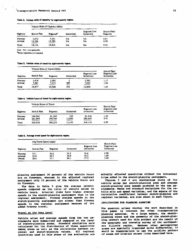
. #Transportation Research Record 944 35
Tzbk2. VohidcdlmOf~WfWsi@twnW@~.
Vehicle hfklesof CapaatY (000s)
Regional lawHighway Sketch Plan
Sketch Plan/Regionala Intrazonal Intraronal Regional
Freeway 3,870 4,241 NA NA 0.91Arterial 14,286 14,584 NA NA 0.98
Total 18,156 18,825 NA NA 0.96
Note: NA=notspplicable.%rampCapacities not included.
Tab103. Vzhido dlsa of trzvsl ftw ●ight~nty rejon.
Vehicle Miles of Travel (000s)Sketch Plan/
Regional Less Regional LessHighway Sketch Plan Regionzk Irrtrazonal Intrazorral Intrzzonal
Freeway 3,476 2,98S 3 2,982 1.17Arterisf 7,001 7,315 289 7,026 1.00
Total 10,477 10,300 G 10,008 1.05
Table4. Vzhidaham oftrzvzlforsi~t~ty rsglon.
Vehicle Hours of TravelSketch Plan/
Regional Less Regional LessHkghway Sketch Plsrr Regional Intrazorml Intrazonal lntrazOnal
Freeway 104,962 81,549 103 81,446 1.29Artarial 261,048 298,704 12,040 286,664 0.91
Totsl 366,010 380,253 12,143 368,110 0.99
TsIAo6. Awaw travd spszdfor Zidtt-nty region.
Avg TravelSpeed (mph)Sketch Plan/
Regional Less Regional LessHLghway Sketch Plan Regional hrtrazonal Intrazonal Intrazonzl
Freeway 33.1 36.6 33.3 36.6 0.90ktrrid 26.8 24.5 24.0 24.5 1.09Overall 28.6 27.1 24.1 27.2 1.05
planning assignment 29 percent of the vehicle hoursare on freeways, whereas in the adjusted regionalassignment only 22 percent of the vehicle hours areon freeways.
The data in Table 5 give the average network
speeds c-ted as the ratio of vehicle miles tovehicle hours. Arterial links have higher averageaPSeda in the sketch-plannin9assignment than in theregional aaaignment. Freeway average speeds in thesketch-planning assignment are slower than freewaYapeeda in the regional assignment because of theadded freeway travel.
Travel at the Zone Level
Vehicle miles and average ●peedm frm the two aa-aignmenta were summarized and compared at the levelof sketch-planning zones. Standard mtatiatics werecalculated for the distribution of these quantitiesamong zonea aa well as the correlation between re-gional and sketch-planning valuee. All regionalquantities used in this phaee of the evaluation are
actually adjusted quantities without the intrazonaltrips added in the sketch-plannittgassignment.
Figures 5 and 6 are zcattergram plots of thevehicle miles per sketch-planning zone and averagesketch-planning zone speeds produced by the two as-sigrtaents.Meanm and etandard deviations for the ve-hicle mile and zpeed variablee, and the equare of thecorrelation coefficient between sketch-planning andregional variablee, are aleo abown in each figure.
IMPLICATIONS FOR PLANNING AGENCIES
The question ariaes whether the work deeorlbed inthis paper ia relevant for other tranapbrtationplanning agenciea. TO a large extent, the sketoh-planning zones and the geaetry of the sketch_plan-ning network used for this project are the result ofthe geography and townehip murvey of the northeast-ern Illinoie region. SeOauae other metropolitanareas are apetially organized quite differently, itwould be inappropriate to uee the gridlike petternof zonee and arterial street links dezcribed here.
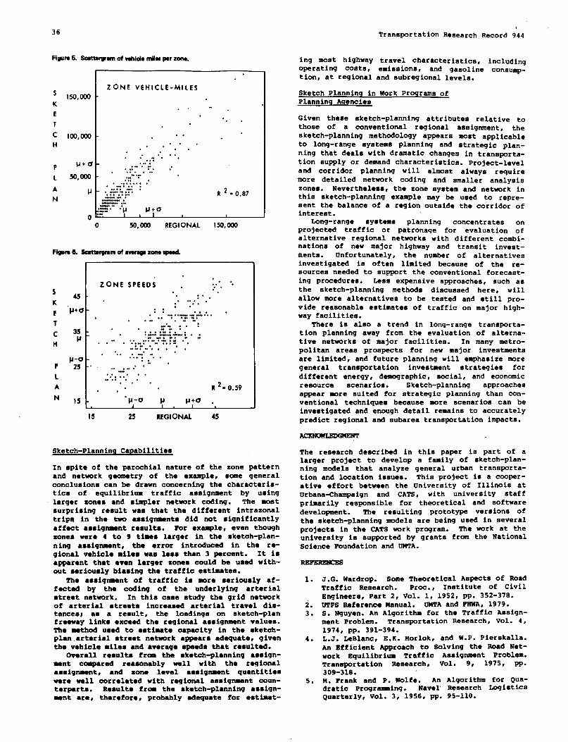
36
Fi~m 6.
s 150,K
E
T
cH
P
L
A
N
Saette**m ofwhichMNazpsr zonz. i rig most highwayoperating coats,t
IZONE VEHICLE-MILESOoo
IOo,ooo
p+a
50,000
P
o
.,- ..
“..
. . ... ”””
.“. ““..” .,:”.” “.
. .. .,“. . .
., . ...”“““’...“ ““!“n “. .. . . . . . ..
“.. n”””:. . . .. .7. R 2 =0.87,, ...”... . “. .. . ,—. ....-Y.-.....” :IJ p+o.“
0 50,000 REGIONAL 150,000
Fiwrz S. ~m of we- rens spsed.
s
K
f
T
c
H
P
L
A
N
4s
“p+e-
35SJ -
p-o -25 -“
ZONE SPEED; .“..,. ..“ “
. . . .. “. ...”.”
:.””:: . . . .
. “ . . Y “”?%--.-” ““.“ .“-
. ..”-..:“o...--:.. - . . . :..
“ . . . .,. .”....,. .- -
..- .“.”. ”.-. . . . .-: ;””...” .
. “......”-. . . ...””.: .. .
““d-”“.”...”””
“.. ...”...” R 2= 0.59
15 25 REGlONAL 45
Sketch-PlanningCapabilitIes
In spite of the parochial nature of the zone patternand network geometry of the example, some generalconclusions can be drawn concerning the characteris-tics of equilibrium traffic assignment by usinglarger zonea and simpler network coding. The mostsurprialng result wan that the different intrazonaltrips in the two ●mmignmentm did not S19nlfiCant2Yaffectassignment reaulta. For ●xample, even thoughzones were 4 to 9 timem larger in the sketch-plan-ning aasignmant, tho error introduced in the re-gional vehicle milee wam leas than 3 percent. It iSapparent that even larger sones could be used with-out aerioualy biasing the traffic eetimates.
The aemignment of traffic ie wre merioualy af-fected by the coding of the underlying arterialetreet network. In this case etudy the grid networkof arterial ●treets increamed arterial travel die-tances; as a result, the loadings on sketch-planfreeway links exceed the regional assignment valuea.The method uead to eetimate capacity in the mketch-plan ●rterial ●treet network ●ppeareadequate,giventhe vehicle milee ●nd ●veragespeedmthat resulted.
Overall results from the sketch-planning aeaign-mant compared reasonably well with the reqionalamaignment, ●nd zone level aamignment quantitieswere well correlated with regional assignment coun-terpart. Results from the sketch-planning ae8ign-ment ●re, therefore, probably ●dequate for estimat-
ion, at regional
Transportation Rezearch Record 9’44
travel characteriatica, including●miasiona, and gasoline cona~-and subregional levels.
Sketch Planning in Work Programs ofPlanning Agencies
Given these sketch-planning attribute relative to
those of a conventional regional assignment, thesketch-planning methodology appears most applicable
to long-range ayetems planninq and strategic plan-
ning that deala with dramatic changez in transporta-tion supply or demand characteristic. Project-1eveland corridor planning will almoat always requiremore detailed network ceding and smaller analysiszones. Nevertheless, the zone system and network inthis sketch-planning example may be used to repre-sent the balance of a region outside the corridor ofinterest.
Long-range systems planning concentrates onprojected traffic or patronaqe for evaluation ofalternative regional netwrrrkawith different combi-nation of new major highway and transit invest-ments. Unfortunately, the number of alternativeainvestigated is often limited because of the re-sources needed to support the conventional forecast-ing procedures. Less expensive approaches, such asthe sketch-planning methcds discussed here, willallow more alternatives to be tested and still pro-vide reasonable estimates of traffic on major high-way facilities.
There is also a trend in long-range transporta-tion planning away from the evaluation of alterna-tive networks of major facilities. In many metro-politan areas prospects for new major investmentsare limited, and future planning will emphasize moregeneral transportation investment strategies fordifferent energy, demographic, social, and economicreaource scenarios. Sketch-planning approaches
appear mre suited for strategic planning than con-ventional techniques because more scenarios can beinvestigated and enough detail remains to accuratelypredict regional and subarea transportationimpacts.
Ac~
The research described in this paper is part of alarger project to develop a family of sketch-plan-ning models that analyze general urban transporta-tion and location issues. This project ia a cooper-ative effort between the University of Illinois atUrbana-Champaign and CATS, with university staffprimarily responsible for theoretical and softwaredevelopment. The resulting prototype versiona ofthe sketch-planningmodels are being used in severalprojects in the CATS work program. The work at theuniversity ia supported by grants from the NationalScience Foundation and UMTA.
RBPBRENCBS
1.
2.3.
4.
5.
J.G. Wardrop. Some Theoretical Aspects of RoadTraffic Research. Proc.r Institute of CivilEngineers, Part 2, Vol. lr 1952, Pp. 352-378.UTPS Reference Uanual. UMTA and ~A# 1979.S. Nguyen. An Algorithm for the Traffic Assign-ment Problem. Transportation Research, Vol. 4,1974, pp. 391-394.L.J. LeBlanc, E.K. Morlok, and W.P. Pierskalla.AQ Efficient Approach to Solving the Road Net-work Equilibrium Traffic Aaai9=nt Problem.Transportation Research, vol. 9, 1975, pp.309-318.M. Frank and P. Wolfe. An Algorithm for Qua-dratic Programing. Navel Research LogisticsQuarterly, Vol. 3, 1956, pp. 95-110.
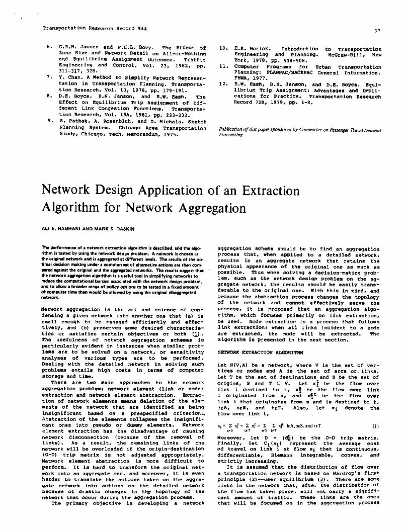
Transportatkan Research Record 944 3-1
6.
7.
8.
9.
G.R.M. Jansen and P.H.L. Bevy. The Effect ofZone Size and Network Detail on All-or-Nothing
and Equilibrium Assignment Outcomes. TrafficEngineering and Control, Vol. 23, 1982, pp.311-317, 328.Y. Chan. A Method to Simplify Network Represen-tation in Transportation Planning. Transporta-tion Research, Vol. 10, 1976, pp. 179-191.D.E. Boyce, B.N. Janson, and R.w. Eatsh. TheEffect on Equilibrium Trip Assignment of Dif-ferent Link Congestion Functions. Transporta-tion Research, Vol. 15A, 1981, pp. 223-232.S. Pathak, A. Rosenbluh, and D. Michals. Sketch
Planning System. Chicago Area TransportationStudy, Chicago, Tech. Memorandum, 1975.
10.
11.
12.
E.K. Morlok. Introduction to TransportationEngineering and Planning. McGraw-Hill, NewYork, 1978, pp. 504-508.Computer Programs for Urban TransportationPlanning: P~Ac~CKPAC General Information.FNwA, 1977.R.W. Eash, B.N. Janson, and D.E. Boyce. )fqui-
librium ‘l’rip Assignment: Advantages and Impli-cations for Practice. Transportation ResearchRecord 728, 1979, PP. 1-8.
fiblication of thispapersponsoredby CommitteeonPassengernavel DemandForecasting.
Network Design Application of an ExtractionAlgorithm for Network Aggregation
ALI E. HAGHANI AND MARK S. DASKIN
llre ~rformanra of a network extreation algorithm is described, and the algo.rithm is tested by using the network design problem. A network is chosen asthe original natwork and is aggregated at differant Ievals. l%e results of the op-timal dsasion making under a mmmon aat of alternative actions are than aom-parsd against tha original and the aggregatednetworks. The rasulta suggestthatthe natwork a~sgation algorithm is a useful tool in simplifying networks toredura the computational burden associated with the network design problem,and to allow a breeder mnga of poliay options to be tested in a fixad amountof computer time than would be allowad by usingtha original diasggregatednatwrsk.
Network aggregation is the art and science of con-
densing a given network into another one that (a) is
small enough to be managed efficiently and effec-tively, and (b) preserves some desired characteris-tics or satisfies certain objectives or both (~).The usefulness of network aggregation schemes iaparticularly evident in instances when similar prob-lems are to be solved on a network, or sensitivityanalyses of various types are to be performed.Dealing with the detailed network In solving suchproblems ●ntails high costs in terms of computerstorage and time.
There are two main approaches to the network
a99re9ation Problems network element (link or node)extraction and network element abstraction. 13xtrac-tion of network elements means deletion of the ele-ments of the network that are identified as beinginsignificant based on a prespecified criterion..Abstraction of the elemente collapsee the insignifi-cant ones into pseudo or dummy elements. Networkelement extraction has the disadvantage of causing
network disconnection (because of the removal of1inks). As a result, the remaining links of thenetwork will be overloaded if the origin-destination(O-D) trip matrix is not adjusted appropriately.Network element abstraction is more difficult toperform. It is hard to transform the original net-work into an aggregate one, and moreover, it is evenharder to translate the actions taken on the aggre-gate network into actions on the detailed networkbecause of drastic changes in t~ topology of thenetwork that occur during the aggregation process.
The primary objective in developing a network
a99re9ation scheme should be to find an aggregationprocess that, when applied to a detailed network,results in an aggregate network that retains thephysical appearance of the original one as much aspossible. Thus when solving a decision-making prob-lem, such as the network design problem on the ag-gregate network, the results should be easily trans-ferable to the original one. With this in mind, andbecauae the abstraction process changes the topologyof the network and cannot effectively serve theprocess, it is proposed that an aggregation algo-rithm, which focuses primarily on link extraction,be used. Node extraction is a process that followslink extraction; when all links incident to a nodeare extracted, the node will be extracted. Thealgorithm is presented in the next section.
NETWORK EXTRACTION ALGORITSM
Let N(V,A) be a network, where V is the set of ver-tices or nodes and A is the aet of arcs or links.Let T be the set of destinations and S be the set oforigins, Sand TCV. Let xl be the flow overlink i destined to t, X? be the flow over linki originated from a, and x~t be the flow overlink i that originates from s and ia destined to t,icA, m~S, and tcT. Also, let xi denote theflow over link i,
xi= ~ x!= X X/= ~ ~ x~, icA, seS, andtcT (1)ses teT scS WT
Moreover, let D = (d~ep;~se:~e O-D trip matrix.Finally, let Ci (xi) the average costof travel on link i at flow xi that is continuous,differentiable, Riemann integrable, convex. and
strictly increasing.It is assumed that the distribution of flow over
a transportation network is based on Wardrop’s firstprinciple (~)--user equilibrium Q). There are somelinks in the network that, after the distribution ofthe flow haa taken place, will not carry a signifi-cant amount of traffic. These links are the onesthat will be focused on in the aggregation process

Trant3portation Research Record 944
to be described. The criterion used for the identi-fication of Insignificant 1inks is defined asfollows.
A link in a network Is Inalgnificant if the cor-responding equilibrium flow IS below a percent ofthe maximum equlllbrlum link flow in the network.The level of network aggregation changes, dependingon the value of a; as a increaaea, the networkbecomes more aggregated and vice versa.
The reason for choosing the level of flow in thellnks as a criterion for identifying the insignifi-cant llnks la that many transportation problems dealwith the equllibriw flow levels in the networklinks. It has already been proved (~) that theequilibrium flow level in the significant or nonex-tracted links remains unchanged when the aggregationscheme Is used. By preserving the level of equilib-rium flow in the nonextracted links, the aggregationscheme should produce an aggregate network that ismore representative of the detailed network than Isan aggregation process that failed to preserve theseflow levels. This should be particularly importantIn solving problems In which the objective functionla baaed on the level of equilibrium flow in thelinks. The network design problem is one suchproblem.
Thus the network extraction algorithms as it hasbeen coded, Is presented. A more rlgoroua presenta-tion is included elsewhere (~). The inputa to thealgorithm are the specification of the originalnetwork N(V,A), the average link coat functionsCi(xi), ieA, and the O-D trip matrix D. Eitherthe maximum number of llnka to be extracted or themaximum a percentile denoting the cutoff pointbetween the insignificant and significant link flatsshould also be given. Through this process certainprespecified links in the aggregate network can bemaintained; also, specificlinks can be extracted.Furthermore, the algorithm extracts the llnka one byone and provides the reaulta after each iteration.As a result, several different aggregate networksare obtained. The principle la to extract insignifi-cant links and to update the trip matrix such thatthe flow level in the remaining llnka of the aggre-gate network remains unchanged. The algorithm Is asfollows.
Step 1: Specify a or the maximum number oflinks that may be extracted (M). Solve the equilib-rium flow problem. Let xi, itA be the equilibriumflow on link i.
Step 2: Identify the unextracted link k with theminimum flow. Let t(k) and h(k) denote the tall andhead nodes of link k. Compute
(2)
Ifak>a ZiS specified In step 1, or if the numberof extracted links la greater than the maximumnum-ber of links that may be extracted (aPecifi* instep 1), atop. Otherwise disaggregate the flow onlink k by specifying the origin and destination ofall flow on the link, which is done by solving theaqullibrlum flow problam on the most aggregate net-work generated. [An outline of how the O-D specificlink flow (xft) maY be obtained from the solutionprocedure to the equilibrium flow problem, and theproblems associated with the nonuniqueness of thisquantity, are discussed elsewhere (~).] Go to step3.
Step 3: Discard link k. Declare t(k) a destina-tion (if it is not already such a node) and h(k) anorigin (if it la not already such a node).
Step 4: Update the trip matrix as follows: (a)type I entry, where t(k) Is a deatlnation, i.e.,
,&k)=d:(k)+x{ (3)
where d:(k) IS the original O-D matrix element and
Is taken to be zero If the t(k) is a new destination,.
and ~t(k) Is the updated O-D trip matrix element;(b) type II entry, where h(k) la an origin, i.e.,
(4)
where ~(kk
la the original O-D trip matrix elementand is ta en to be zero if h(k) is a new origin, and.dfik ie the updated O-D trip ma:rix element; and(cl ~ypa III ●ntriea, where all remaining entries of
.are substituted by d~ -
~ ‘(~ll~t?act~n~i~r~?l~ the part of the demandfrom s to t that is now deetined to a new destina-tion and that will reoriginate from a new origin).
Certain properties of the algorlthm are worth
mentioning. First, as previously noted, the algo-rithm preservea the level of equllbrlum flow In the
llnks of the network that are not ●xtracted. Second,In casea In which all of the nodes of the networkara not both origins and destinations, the algorithmwill Increase the number of origins and destinationsin the aggregate network. This In turn might haveadverse effects on tha computation time of the net-work design problem by increasing the number oforigins and the asaoclated time for computation ofthe minimum patha in the network. This situationhas not been examined In this paper. However, thisincrease in computation tlake should be offsetthrough other meana.
Third, the result of the ●xtraction process maybe a set of disconnected subnetworka. If this oc-curs, the analysis of the aggregate network, now aset of subnetworks, will be much easier to under-take. In fact, In cases in which link extractionwill increase the number of origins and destinations(and thereby increase the computation time for the
network design problem), specification of the linksto be extracted can force the aggregate network to
be a aet of dlaconnected subnetworka. In this waythe computational savings obtainable by having dis-connected aubnetworks may be used to offset theIncreaaed time that results from additional originsand destinations.
Finally, in the network design problem It isshown thst for a given budget level? the total costto the usera of the network, aa measured on thedetailed network, la overestimated by the solutionto the network design problem that uses the aggre-,.gate network (~).
In the next section this algorithm is applied toan original network, and the network design problemIs solved on the original detailed network and on aseries of aggregatenetworka.
.APPLICATIONS OF NBTUORR EXTRACTION ALGQRITNN TONB’lWRK DESI@l PROB_
Problem Description
The network design problem is that of finding a setof feaaible actiona or projects from =n9 a Collec-tion of aucb actions that, when implemented oPti-mise the objective function(s) beiw considered.The feasibility of a aet of actions is determined byresource, physical, and environmental constraints(~). Traditionally, the objective function in thenetwork design problem has been formulated as theminimization of the total number of vehicle hours oftravel on the network, with flows and travel times

Transportation Research Record 944 39
computed based on user equilibrium. This is repre-sented as
Subject to budget constraint on the cost of implemented projects p
where X* is the user equilibrium flow on link i,and P !s a set of projects (p) under considerationfor implementation. In solving the network designproblem, a ssodifiedobjective function, which wassuggested by Poorzahedy (~) in his algorithm I, hasbeen used. This form is as follows:
.M% Z ~i Ci(Vi~Vi
irA(6)
Subject to budget constraint on the cost of implemented projects p
where x; is the user equilibrium &w on link i.The modified form of the problem was selected
because of the availability of a computer code tosolve this problem. Also, solving this form of theproblem has been found to be more efficient thansolving the traditional formulation and generallyresulte in similar actions being taken on the net-work (~).
Thus the results of a set of experiments designedto test the effectiveness of the proposed NA algo-
rithm in solving the modified network design problemcan be presented. For the detailed network, theSioux Falla, South Dakota, network is used in theexperiments because it ie a well-documented networkand has been used by other researchers (4,6,7) inanalyzing network design problems.
.-
The detailed network, which consists of 24 nodesand 76 links (or 38 link pairs, allowing two-waytraffic movements), is ehown in Figure 1 (~). Thelink travel costs [c~(xi)l are given by func-tions of the form
G (XI)=q +b Cd’ (7)
The conetants ai and bi for each of the existinglinks in the network, aa well aa for the aix candi-date links, are given in Table 1 (~). Also providedin the table Is the cost of implementingeach of thecandidate links. The first five projects representImprovements on existing links, whereas the sixthproject is an entirely new link. Two different setsof experbenta were considered. In the first, onlythe five improvement projects are used; in the sec-ond, all six candidate projects are used. The O-Dmatrix for this network is given in Poorzahedy (~).
Five aggregate networks are developed, whichresult from the extraction of 6, 12, 18, 24, and 30links. The aggregate networks are shown in Figures
[email protected](~). 2
Legend:
o i Node i
+$, Link Pair
~*Candidate
~ti Candidata
@ Project Numbe.
j,j+l
Project on Existing
Project,New Lirdc
Links

Trans~rtation Research Record 94440
Tdie 1.Linkpemme~ oftestnmwqrkIll(~).
ink
1,2 I 5.96 0.00023 1
=l=m=l3S,36 2.98
IO.00011
d=bi3,4 4.34 0.00011
5,6 5.17 0.12408
7,8 4.31 0.00069 I
9,10 4.14 0.00016
*
I21,22 9.61 0.23064
*
EEE=
2+29,30 8.04 0.19296
31,32 6.46 0.15504
33,34 4.42 0.10608
39,40 3.50I
o. 00L04
II 43,44 1.67 I 0.04008
W49,S0 4.46 0.00017
51,!32 3.99 0.09576
53,54 5.72 0.13728
IEEE55,56 4.71 0.11304
57,58 L.67 0.0400~
I61,62 4;00 O.0960(
a(xU3-2b(x10-4)
9,70 2.17 0.05206
1,72 3.72 0.08928
3,74 2.s0 O.ol.lss
177,78 - -
l-FF--~67,66 I 1.60 10.00037
cost $625.x103
I 69>70 1.30 0.01562
I cost $650.ti03
I 71,72 2.20 0.02678
‘-kl.xkw
Note: I parameters are given in hours, and b pmameten are riven In hours + (1 ,000 vehicles per do’)4
2-6; the reaultinq O-D matrices are given in Ilaghani(J).
Results for the A9!lregation Uodel
The five aggregatenetwrks shown in Figures2-6 andthe detailednetwork shown in Figure 1, along withtheir corresponding O-D matrices, constitute thebaais for the experiments. On each of these sixnetworks, two nettmrk design problems were solved:one with the first five candidate projects, and thesecond with all six projects. The initial budgetwas set at $2,000,000 in all cases, and a completesensitivity analysis (with respect to increases inthe budget) was performed for all six networks andboth design probleme.
Results of the Five-Project Experiment
The results of the five-project experiment are eum-
merized in Table 2. Nore detailed resulte are givenin Haghani (~). The data in the table repcmt (a)
the percentage error in the total number of vehiclehours on the aggregate networke as compared with thedetailed network, and (b) the number Of PKojectethat are selected differently when the network de-sign problem is solved on the detailed and aggregatenetworks. Note that there are 18 unique bud9etlevels that must be considered in performing thesensitivity analyses, be9innin9 with a bud9et of$2,000,000 and ending with a bud9et of $4,325,000,which allows the implementation of all five pKoj-ects. Of the 18 budget levels, 5 result in differ-ent solutions for the network design problem on theoriginal and aggregate networks in the worstcase.
The data in Table 2 indicate that with six linksdeleted frcm the original network, the solutions tothe network design problem on the original networkand the aggregate network are identical for allbudget levels. For higher. levels of a99re9ation#discrepancies occur between the solution using theaggregate network and that found using the originalnetwork. Aleo note that most of the errors occurwhen the ratio of the budget level to the total cost
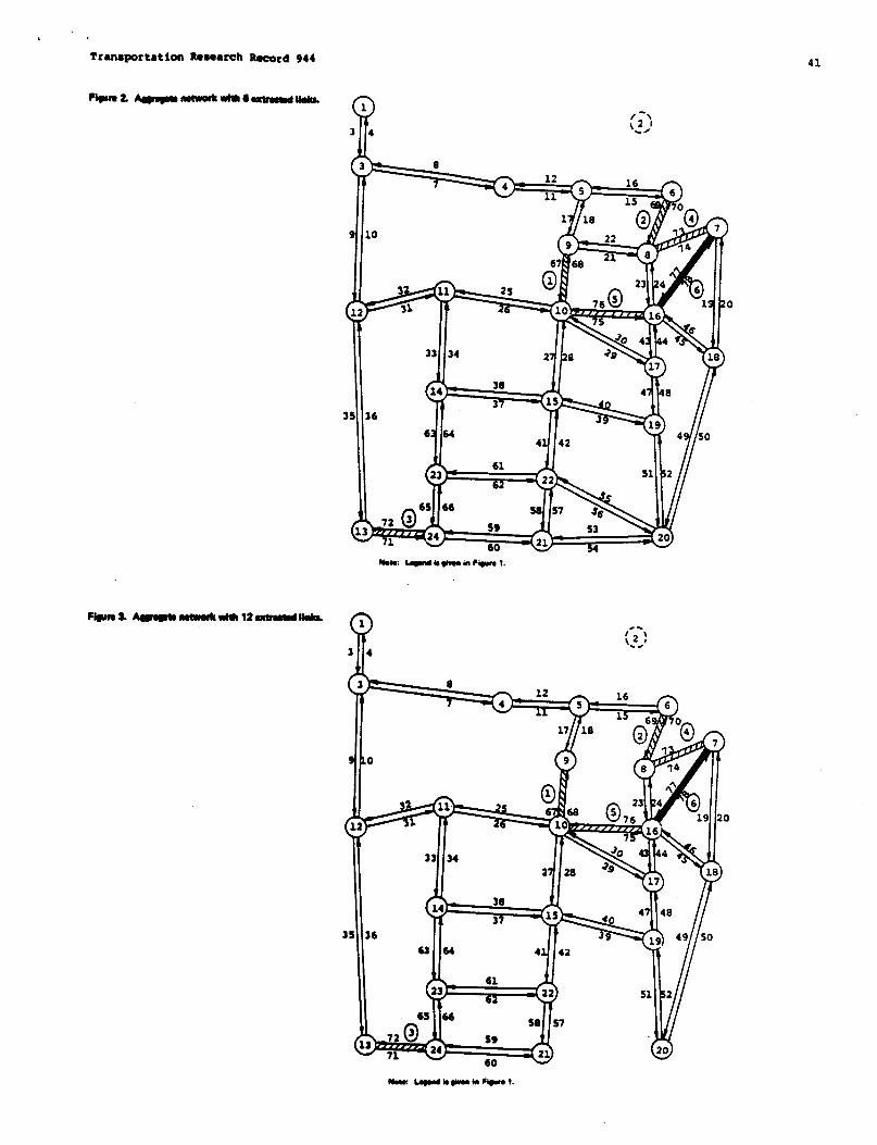
Tranaportmtion Re8earch~rd 944 41
ND- Lcgmdisgh,minflglwl.
7134
- slc@nllln%u91.

42
FiwIra4. Aggregatenetworkwith 18 ax~ti links.(
35
Fi~ra5.AggmgatanetworkwiUr24.xtractsdlinks.
NC.t.: Lqnd ,ssivm m Figure 1.
Q1
Transportation Research Record 944
[:2>

43
i’4 50
20
Not.: L6gmd is OIWIIm Fqum 1.
Tablc2, Pwwentagmel vshido hour ● rrum md numbsr of miaehcted ~ for fivqmject ~.
No. of Extracted Links
6 12 18 24 30
Budget No. of Vehicle No. of Vehicle No. of Vehicle No. of VehicleLxels Budget
No. of VehicleHoor hfissclected Hour Missclected Hour
No. of
($000s) LevelsMisselectedHour Miasclected Hour
Error (%) Rojecta Error (%) ProjectsMimelected
Error (%) Rejects Error (%) Projects Error (%) Rejects
B=2,000 1 0 0 3.11 1 3.11 1 0 0B=2,050 1 0 0
3.11 I6.73 6.73 6.73 1
2J25<B 3 0 0 0 i6.73
0 i o 0 0 :<2,475
2,475< B 2 0 0 3.82 1 3.82 1 3.82 1 3.82 1< 2,675
B = 2,675 1 0 0 7.95 7.95 7.95 1 7.952,700< B 5 0 0 0 : 0 ; o 0 0 ;
< 3,3253,325< B 4 0 0 0 0 0 0 0 0 0 0
<4,325B=4,325 I o 0 0 0 0 0 0 0 0 0
of all candidate links ie low. In all cases inwhich the eolution on the aggregate netwozk differedfrom the solution on the detailed network, the num-ber of misselected links was. only one. By usingvehicle hours as the measure of effectiveness, themaximum percentage error is 7.95 percent. The iden-tity of the errors, the equality of their severity,and the similarity of their frequency acroee thevarioue levels of aggregation euggest that the sizeof the network may be reduced significantly withoutincreasing the magnitude of the errors. This phenom-enon ie also apparent in the case of six projects.
{Note that the maximum percentage error of 7.95percent is computed as follows. At a given budgetlevel, let ~a and ~. be the optimal solutions to the
network design problem for the aggregate and original
networks, respectively,where z = (Yi) and Yi = (0~1)if project i (is not, is) chosen to be In the optiBslset. Aleo, let V(x) represent the deoreaee in the to-tal number of vehicle hour. in the original networkthat results from implementing project set~. Thepercentage error is defined as [V(= - V(~)/V(~]Q 100.}
Note also that the total travel time on the net-
work 1s werestimated by the solution to the designproblem on the aggregate networke as Cc9PSred witi
the total time found when using the detailed net-work. This is also shown in the six-projectexperi-ment and, ae noted at the end of the section onNetwork Extraction Algorithm, may be shown to be ageneral property of the aggregation process.
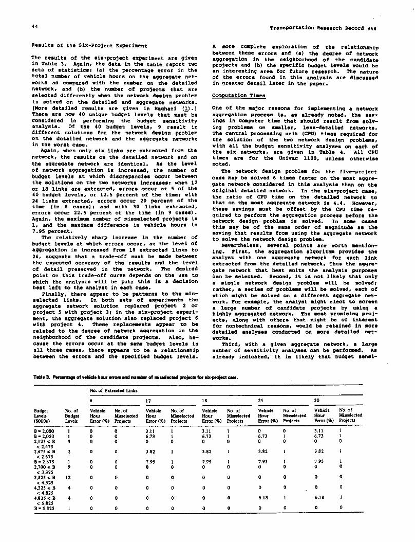
44 TranapOKtaticm Research Record 944
Results of the Six-Project Experiment
The results of the six-project experiment are givenin Table 3. Again, the data in the table report twoaeta of atatiatica: (a) the percentage ●rror in thetotal number of vehicle hours on the aggregate net-works aa compared with the number on the detailednetwork, and (b) the number of projects that areselected differently when the network design problemia solved on the detailed and aggregatenetworks.[More detailed results are given in Haghani (~).]There are now 40 unique budget levels that mat beconsidered in performing the budget menaitivityanalysia. Of the 40 budget levels, 9 result indifferent solutions for the network design problemon the detailed network and the aggregate networkain the worst case.
Again, when only aix links are extracted from thenetwrk, the reaulta on the detailed network and onthe aggregate network are identical. As the levelof network aggregation ia increaaad, the number ofbudget levels at which diacrepenciea occur betweenthe aolutiona on the two networka increasea: when 12or 18 links are extracted, errors occur at 5 of the40 budget levels, or 12.5 percent of the time; with24 links extracted, errors occur 20 percent of thethe (in 8 caaea); and with 30 links extracted,errorsoccur 22.5 percentof the time (in 9 caaea).Again,the maximumnumberof miaselectedprojectsia1, and the maximum difference in vehicle hours is7.95 percent.
The relatively aharp increaae in the number ofbudget levels at which errors occur, as the level ofaggregation ia increaaed from 18 ●xtracted links to
24, auggeata that a trade-off must be made betweenthe expected accuracy of the results and the level
of detail preserved in the network. The desiredpoint on this trade-off curve depends on the use towhich the analyaia will be put; this ia a decisionbest left to the analyst in ●ach case.
Finally, there appear to be patterna to the mia-aelected linka. In both sets of experiments theaggregate network solution replaced project 2 orproject 5 with project 3; in the six-project experi-ment, the aggregate solution also replaced project 6with project 4. These replacement appear to berelated to the degree of network aggregation in theneighborhood of the candidate projectm. Also, be-cauae the errors occur at the aama budget levels inall three cases, there appaara to be a relationshipbetween the errors and the specified budget levels.
A core Complete exploration of the relationshipbetween these errors and (a) the degree Of networkaggregation in the neighborhood of the candidateprojects and (b) the specific budget levels would bean interesting area for future research. The natureof the errors found in this analysia are diacuaeedin greater detail later in the paper.
Computation Times
One of the major reaaons for implementing a network
a99re9ation Process is, aa already noted, the aav-inga in coaputer time that should result from solv-ing problems on smaller, less-detailed net~rka.The central proceaslng unit (CPU) times requiredforthe solution of the two network design problems,with all the budget sensitivity analyaes on each ofthe aix networks, are given In Table 4. All CPUtiMaS are for the Univac 1100, unless otherwisenoted.
The network design problem for the five-projectcase may be solved 6 timaa faater on the moat aggre-gate network considered in this analyais than on theoriginal detailed network. In the aix-projact case,the ratio of CPU time on the detailed network tothat on the xost aggregate netmrk ia 4.4. iIowever,these aavinga must be offset by the CPU time re-quired to performthe aggregation prcsceasbefore thenetwork design- problem ia solved. In some casesthis may be of the same order of raagnitudeas thesaving that reaulta from using the aggregate networkto solve the network design problem.
Nevertheless, several points are worth mention-ing. First, the aggregation algorithm provides theanalyat with one aggregate network for each linkextracted from the detailed network. Thus the aggre-gate network that beat auita the analyaia purposescan be selected. Second, it ia not likely that onlya single network design problem will be solved)rather,a seriesof problems will be solved, ●ach ofwhich might be solved on a different aggregate net-work. ?or example, the analyst might elect to screena large number of candidate projects by using ahighly aggregated network. The most promising proj-ects, along with others that might be of interestfor nontechnical reaaona,would be retained in moredetailed analyaea conducted on more detailed net-works.
Third, with a given aggregatenetwork, a largenumber of sensitivity analysea can be performed. Aaalready indicated,it ia likely that budget ●enai-
TabloS. ~dw~~ahmr~tim~dd~~~tiw~~.
No.ofExtracted Links
6 12 18 24 30
Budget NO.of Vehicle No.of Vehicle No.of Vehicle No. of Vehicle No. of Vehicle No. ofLevels Budget Hour Misselected Hour Misselected Hour Missrlected Hour Misselected Hour(4000s) Lavels
MissclectedError (%) Projects &rOr (%) Projects Error (%) Projects Brror (%) Projects Srror (%) mje~~
B = 2,000 1 0 0 3.11 1 3.11 1 0 0 3.11 1
B = 2,050 1 0 0 6.73 1 6.73 6.73 1 6.732,125<B 5 0 0 0 0 0 A o 0 0 :
< 2,4752,475< B 2 0 0 3.82 1 3.82 1 3.82 1 3.82 1
< 2,67SB= 2,675 0 0 7.95 1 7.95 7.9s 7.95 12,700< B ; o 0 0 0 0 i o A o 0
< 3J253,325< B 12 0 0 0 0 0 0 0 0 0 0
<43254>25< B 4 0 0 0 0 0 0 0 0 0 0
<4,8254,825<B 4 0 0 0 0 0 0 6.18 1 6.18 1< 5,82SB=S,825 1 0 0 0 0 0 0 0 0 0 0

Transportation Research Record 944 45
CFUTree’(see)
ND.of Five six~@On Extracted Candidate Candidate
Links Prolects PrOiects
o Ob 50’0
79~Ob 3]4.384 514.598
0.2797 6 246.2800.3352
398.48712 249.677 409.988
0.3413 18 249.002 417.0270.3564 24 207.315 378.4810.3780 30 51.496 124.228
●AM figures, except those noted in footnote c, are from t UNIVAC1100.
bWCInal network.
cFkures ●re from ~ CDC 66oo, u reported by Poorzahedy @,
tivity analyses will be performed. In addition, thesensitivity of the eolution to additional con-straints that require eelacted projects to be in-cluded in (or excluded frc@ the optimal solutionmay need to be analyzed. In all of theee cases thenetwork aggregation algorithm needs to be solvedonly once. Thue the CPU time for the networkaggre-gationalgorithm ie best viewed as a fixed coet thatmay be distributed over a large number of analyses.
Finally, note that the CPU time involved in solv-ing the network deeign problem dacreasea signifi-cantly ae a result of extracting six links from thenetwork in both the five- snd six-project experi-ments. The CPU times for the casea of 6, 12, and 18extracted links are comparable. A elight decreasein CPO time is experienced aa a result of extracting24 link=, and a significant dacrea8e is found when30 linke are extracted. This result, combined withthe resulte outlined in the section Resultefor theAggregation Model, which deecribes the accuracy ofthe results at varioun levels of aggregation,clearly auggeetn that there ia an important trade-off to be made between decreased computation coats(and greater network aggregation) on one hand andimproved eolution accuracy on the other hand.
In the aemple probleme previously discunsed, itappears that desirable aggregation levels wouldcorrespond to either the extraction of 6 links (re-sulting in a moderatedecreasein computertime anda high level of accuracy) or the extractionof 30linke (resulting in a large decrease in computertine at the expense of decreaaedsolution accuracy).Intermediate levels of ●ggregation appesr to resultin relatively large eolution errors without largecomperk8ationain termsof solutiontimes. An inter-●sting ●rea of future research would be to determinewhether or not the network aggregation algorithmresults in such identifiable choices tktween aggre-gation and solution accuracy in other net~rk designproblem, and more generally, in other network prob-lems.
SOURCES OF DISCRSPAIKY BETWSRf AGGREGATS NslWXtKANO DSTAILSD ~RS RSSULTS
The results preeented in the previous sectione onthe application of the propoeed network aggregationalgorithm to the network deeign problem are gener-ally promising. In no case ia the difference in theimprovement in vehicle hours between the aolutionaon the detailed and the aggregatenetworks greaterthan 7.95 percent. Also, the two aolutiona differby at mat one candidate link in all caaes. Never-
theleaa, there are several differewea that warrantfurtherexplanation. As indicated in the followingparagrapha, the teat caee eelactad is likely toexaggerate the extent of the differences that arelikely to result in a more realiatic planning con-text.
Two characterlatica of the teat problem will tendto reeult in an Overemtination of the errors thatresult from using the network aggregation scheme.?irat, the Sioux ?alla network being used ia alreadya highly aggregate representation of the actual roadnetwork. This ia ●violentwhen the range in equilib-rium flowe on the original network under the do-nothing option is examinedt i.e., the maximum linkflat is leaa than 4 times the minim link flow.The average link flow Is 12,989 vehicles and themaximum flow is 24,901 vehiclee. The flow in the30th link extracted frox the network ia 9,839 vehi-cles, or almoet 40 percent of the maximum link flow.A real network is likely to exhibit a much qreaterrange in equilibrium flows. If the extracted linkstruly carry an insignificant level of flow comparedwith the flow on the maximum flow link, the solu-tions to design problems on the aggregate networksare likely to be much better than they were in theteat problem in which the flow levels on the ex-tracted links were actually quite large and sig-nificant.
Second, the number of candidete links in thedesign problem waa large relative to the total num-ber of linke in the detailed network. There are 6two-way candidate links on a network with only 38links. In the aggregate networka the situation iseven mre dramatic. Nhen 30 (one-way) links areextracted, 26 percent of the links are being con-sidered aa candidate links. Thus the changea underconsideration for the network are quite radical whencompared with more reallatic situations in whichonly 1 or 2 percent of the links are likely to beconsidered candidate links. Again, if the ratio ofthe nuaber of candidate links to the number of linksin the detailed network is small, the solution tothe design problem on an aggregate network ia mrelikely to replicate the solution on the .detailadnetwork than waa found in the teat problem, in whichalmost 16 percent of the links in the detailed net-work were candidate links.
In a~ry, the teet network chosen for study isalready a highly aggregate network that exhibits arelatively small range in equilibrium link flows.Also, the number of candidate links ia extremelylarge relative to the total number of links in thenetwork. It ia expected that, if a more realiaticdetailed network is used, the solution to the net-work design problem using an aggregate network willmore closely approximate the solution using thedetailed network than waa found in the small testnetwork.
Finally, note that the aggregation process ex-tracta links sequentially, thereby propagating com-putational errors and accumulating them in the finalaggregate network. The reeuiting O-D trip matrixcarries these errors to the decision-making mdel--in this case the network design model. Had a simul-taneoua ●xtraction process been developed, thisxource of error would have been eliminated. TOdate, however, a simultaneous extraction processthat circumvents the multiple counting danger hasnot been impleaentad.
CONCLUSIONS ANO RX@9WNDATIONS FOR FUTURE ~RK
A network●xtractionalgorithm for the network ag-gregationproblem haa been presented. The algorithm
is based on the extraction of those links in a de-tailed network whose equilibrium link flows are less

46 Transportation Research Record 944
than a user-apecifiad fraction of the IIIaXiIUnn equi-librium link flow. The algorithm ia sufficientlyflexible to allow the analyst either to force cer-tain links out of the detailed network or to retainparticular links in the resulting aggregate network.Links are sequentially extracted from the networkand, after each ●xtraction, a modified O-D matrix isderived. The revision in the O-D trip matrix pre-serves the level of equilibrium flow in the nonex-tracted links. By extracting links sequentially,the a190rithm provides the analyst with multiplea99re9ate networks--one after each link extraction.
The network aggregation algorithm was tested byexamining the performance of a network design algo-rithm (~) on both a detailed network and five aggre-
gate networks derived from the detailed network.The results are quite encouraging. The maximumpercentage error,in the improvement in vehicle hoursof travel between a solution using the detailednetwork and a solution using an aggregate networkwas 7.95 percent. In most cases the same projectswere selected for implementationwhen using both thedetailed and the aggregate networks; when the solu-tions differed, at most one link was misselectedwhen using the aggregate network. As suggested inthe previous section, it ia anticipated that evenbetter results will occur when the algorithm is
applied to networks that are larger and more realis-tic than is the 76-link, 24-node test network pre-sented here.
Several promising areas for future research aresuggested by this study. First, links are extractedfrom the network in increasing order of the ratio ofthe equilibrium flow in the link to be extractedtothe maximum equilibrium link flow. Other criteriashould also be investigated. For example, in cer-tain contexts it may be desirable to extract linksbased on the ratio of the equilibrium flow in thelink to the capacity of the- link.hybrid criteria might be developed.the traditional formulation of theproblem, the objective function is
MinimireZ= z x;c,(x;)alllinks
Iwhich may be rewritten as
Alternatively,For example, innetwork design
(8)
matrices on the aggregate networks and on the usesto which those aggregate networks are put ia worthyof additional research.
Third, to avoid multiple counting problems, asequential link extraction procedure has been imple-mented. Research should be devoted to the develop-ment of a simultaneous link extraction procedure.Such a procedure would probably be faster than the
sequential Pr@edure that has been used and would beless prone to accumulating and propagating round-offerrors from one aggregate network to the next.
Fourth, based on the network design experiments,it it suspected that the quality of the networkdesign solution that uses an aggregate network isrelated to the degree of network aggregation in theneighborhood of the candidate links and to the ratioof the available budget to the budget required toimplement all candidate links. Additional researchshould explore these relationships.
Finally, the algorithm should be tested on net-works that have a limited number of origins anddestination to determine whether or not the in-crease in the size of the O-D matrix that resultsfrcm the extraction algorithm increases the computa-tion time more than the time is reduced because ofthe deletion of links. Recall that this did notoccur in the network used in the set of experimentsbecause all nodes were origins and destinations. Ifthis does occur, it might limit the usefulness ofthe proposed approach to cases in which the increasein the size of the O-D matrix can be predicted to besmall.
We would like to acknowledge ?IoussainPoorzahedy,whose ideaa and assistance contributed significantlyto this research. We would also like to acknowledgeHedayat Aashtiani, who helped secure a c-Puteraccount for the camponent of the research conductedin Iran, aa well as the computer staff of theIsfahan University of Technology in Iran for theirtechnical assistance. Funds for this research werepartly provided by a National Science Foundationgrant; this support is also greatly appreciated.
Minimi2eZ= z x; Ci(*’)+ Z ~“Ci(X:) (9)links ii“~ggreg.te deleted
net work links i
In solving a network design problem on an aggre-gate network, it is hoped that changes in the net-work caused by the actions taken will not signifi-cantly affect the second term of the objectivefunction and that it may, therefore, be treated as aconstant and omitted from the calculations. Thissuggests that the rate of change in the objectivefunction from a change in the flow on link i can becomputed, and that links for which changes in theflow will only marginally change the objective func-tion can be deleted. Specifically, the rate ofchange in the objective function because of a changein the flow of link (which is denoted Wi) is
aziaxi = Wi = Ci (x;) + %“C; (N”) (10)
where,C~(x~) is the derivative of C (x) evaluated atx = xi. kA hybrid strategy would be o compute Wi forall links and to deleteless than a ~x (Wi).
those links for which Wi is
Second, the O-D trip matrix that is derived aftereach link iz extracted is not unique because it isbased on the O-D specific flows in the extractedlink, which are not unique. The effect of other O-D
1.
2.
3.
4.
5.
6,
7.
A.E. Iiaghani. A Network Extraction Approach tothe Network Aggregation Problem. NorthwesternUniv., Evanston, Ill., M.S. thesis, June 1982.J.G. Wardrop. Some Theoretical Aspects of RoadTraffic Research. ProC., Institute of CivilEngineers, Part II, Vol. 1, 1952, pp. 352-37B.M.C. Beckmann, B. McGuire, and C. Winston.
Studies in the Bconomics of Transportation.Yale Univ. Press, New Haven, Corm., 1956.?I.Poorzahedy. I$fficientAlgririthmafor Solvingthe Network Design Problem. NorthwesternUniv.1Bvanston,Ill., Ph.D. dissertation,June 19B0.H. Poorzahedy and 14.A.Turnquist. Approximate
Algorithms for the Discrete Network Design Prob-lem. Transportation Research, Vol. 16B, No. 1,1982, pp. 45-55.11.Z.Aashtiani. The Multimodal Traffic Assign-ment Problem. Massachusetts Institute of Tech-nology, Cambridge, Ph.D. dissertation, May 1979.L.J. LeBlanc. An Algorithm for the Discrete
Network Design Problem.. Transportation scie~e~vol. 9, woo 3, 1975, pp. 183-199.
%
Rdlicationofthis popersponwredby CbnwnitteeonRnsenger lhrvelllemawlForemrting.

Transportation Research Record
Quick-Response
ALFRED J. NEVEU
944
Procedures to Forecast Rural Traffic
47
The dwdopmsnt of ● quidwwpcrrssmsthcd to forsrast traffic wolumwzt projast sites loomed on ths rursl highway network is disoussed. By usingtrwd dsta from Now York Stats’s continuous count ststicns in rural bos-tion$ wrd various stzte., county., andtown-lwrddemographicdzta,aw of.Iasticity-bwsdmodelsi$derived.Thwsmodolsan forsoenfutureysarwrnudsv.ragzdailytrzffic(AADT)n afunstionofbwzyewAADT modi-fiid by various dzmogrsphic faotora. Thws moddsarswtimstzd basedonthz typs of ssrvirz the roadway carriw: interurban, urbsn to rural, wtdrural to rural. NoM~phs ●nd a user’s manual that dworibw ● simpleseven-stepproozm to U$Zthe model werz dwebpzd wrd distributed to re-gional offkzs throughout Now York Stste.
For highway improvements, the gap between availablefunds and potential projects is becoming wider asrevenues from various sources ( including gasolinesales taxes, vehicle registration fees, and driver’slicense fees) fall becauae of economic pressure orgovernment-enforced conservation (although the $0.05gasoline tax increaae will ease some of the pres-sure). Costs of labor and materials are escalatingfaster than the national rate of inflation. At thesame time, compounding the problem, increasingtravel demands are placing an even greater burden onthe U.S. highway system than in the past, thus wcrs-ening an already difficult situation.
These trends mean that the need for construction,rehabilitation,and regular maintenance of the high-way network is greater than ever. Each year a largenumber of such projects, ranging from simple inter-section improvements to large-scale facility con-struction,.are identified as candidates for the lim-ited financial resources available. Even in thebest of times, not all projects can be funded; now,with reduced mnies to fund projects, it is evenmore imperative that programming decisions be madein the most effective and efficient manner possible.
The selection of projects to be implemented isgenerally based on some evaluation process in whichthe costs and benefits of each project are ccm-pared. The various evaluation processes considermany factors in weighing each alternative, includingsafety, noise, air pollution, and energy. Each ofthese factors is, in turn, based on an estimate ofthe traffic volume that will use the facility underconsideration. Thus the volume estimate determines,to a significant degree, which of the many projectswill be implemented.
Travel forecasting methodology is highly advancedat the urban area level. Most large metropolitanareas have developed and implemented a fairly so-phisticated set of computer-based travel simulationmodels based on the traditional four-step process.In a nonurban context, however, this process is notnearly so advanced. With many of the projects com-peting for the scarce funds coming from nonurhnareas, it is important to improve and streamlineforecasting procedures for rural travel needs. Inthis way it would be possible to evaluate many ruralprojects quickly and accurately, thus providing gov-ernment officials with better inforraationon whichto base their programming decisions.
TO fulfill this need, research waa initiated bythe Transportation Statistics and Analysis Bectionof the New York State Department of Transportation(NYSDDT) to develop a quick-respcnae procedure toforecast traffic volumes on rural roads. The pri-mary focus of this effort was the design and testingof a simple, fast method to forecast rural trafficvolumes. In this paper previous efforts aimed at
forecasting rural traffic are examined, the chosenmethodology is described, and the results of theanalyaia are presented. Finally, acme of the limi-tation of the procedure are discussed, and scaepossible solutions to the limitationsare provided.
PAST BXPERIBNCE
Little attention has been focused on the topic offorecasting volumes on rural roada. Much of the re-search that deals with the rural highway system hasbeen in the area of design and construction of lcw-voluma roada, travel to recreation facilities, orrural public transportation. An extensive litera-ture review uncovered only two studies specificallyconcerned with forecasts of rural traffic volumes.
In 195S Mcrf and Houska (~) examined the varia-tion of traffic growth patterns on rural highways.They hypothesized that four factors were responsiblefor the variations in growth patterns observed onthe Illinois rural highway network: geographic lc-cation, type and width of pavement, proximity to anurban area, and type of service provided by theroadway. This last factor was subdivided into fourcategories: interurban, interregional, urban torural, and rural to rural.
The authora noted that the growthtrends in sitesclose to urban areas were primarily a function ofthe expansion of the city. Therefore, the remaininganalysis focused on rural highways outside the in-fluence of an urban area.
A co~arizcn by geographic location indicatedminor differences in grwth petterns. Slightlygreater traffic increases were noted in northernrather than southern Illinois. Roadways with widerwidths had correspondingly greater increaeea intraffic, but the authors believed that the widerroads were an effect of the volume increaaes, not acause of tham.
The only factor that had an appreciable effect ontraffic growth rates was the characteristic of typeof service. Highways with the greatest percentageof interurban or interregional service generally hadthe largest increases in travel. Roads that servedlargely urban-to-rural or rural-to-urban travel hadthe smallest increasea. Based on these results, theauthors projected volume trends on the rural highwaynetwork in Illinois for the different road typesseparately.
The study by Tennant (~) used the land use andtraffic generation principle to outline a procedureto estimate rural road traffic in developing ccun-ties. By using various eccncdc# social, land use,and travel data from the Mgunt Kenya rqion inKenya, several trip-generation equations were esti-mated for both urban and rural zones in the studyregion. The results are almost identical in bothcases employment is a hatter predictor of trip gen-eration than is vehicle ownership. The correlationcoefficients that uae either variable in the ~a-tion are all in the range of 0.5 to 0.9. Thus even
vehicle. ownership does a fair job of Predictingtrips per person. Examining traffic generation fromdifferent land uses revealed that 75 percent of thetripa were generated by one of three land usetypesz retail and c~rcial; government adminis-tration, and road transport. Agricultural and resi-dential land uae areas did not generate many triPsin this region. The author concluded that, obvi-

48 Transportation Research Record 944
ouely, more detailed research waa needed, andt as a
first-cut analyaia, either vehicle ownership or em-ployment could be used to forecast future rural tripgeneration.
DEVELOPING TSE METHODOLOGY
Current practice at NYSDOT to forecaat travel onrural highway links aaaumea that travel, representedaa vehicle miles of travel (VMT), is directly pro-portional to population (note that theee data arefr~ an internal memo from W.S. Caawell to J.Shafer, ‘V?4TGrowth Factora for Minor Civil Divi-s ione,8 January 14, 1975).’ Travel forecaate forurbanized areaa are obtained from the network aa-aignmenta for each area. In areaa outside thosegeographic boundaries, a different procedure wasdeveloped. By using V14T per capita estimates byarea from the 1972 National T~anaportation Study andpopulation eathetea for each town and county in thestate from the New York State Department of Com-merce, annual V?4T growth ratea by town were derived
for the years 1972-1990. These rates were developedby first estimating total VMT for each area by usingthe VMT per capita data and the population esti-mates, then calculating the annual growth rates foreach area.
Several problems surfaced as these VMT growthratee were ueed by the Department. Firet, it waerecognized in the beginning that there Is not necee-aarily a correlation between W4T and population.Inaccurate eatimatea of VMT may result from largeamounts of nonresident travel drawn into or throughthe area. This is especially true in popular recre-ation areas. Second, although the population in NewYork atate may decline (and did ao between 1970 and1980), the number of households may (and did) rise;thus thie procedure would fdrecaet a decline in VNTfrom 1970 to 1980 when, in actuality, travel waastill increasing. Finally, there wae no sensitivityto energy price or supply in this method.
Because of these shortcomings, the NYSDOT Trans-portation Statietice and Analysia Section initiateda research project to develop a procedure sensitiveto these factors to forecast rural traffic to beused in the development and evaluation of highway-related projects. This new methodology was designedto meet several criteria. First, the procedure mustbe simple enough to be used on simple desk-top orhand-held calculators, which are generally availablein most planning organization offices. It was be-lieved that a large, cumberaane computer model wouldbe inappropriate in this study. Second, the dataused in the procedure must be easily available tothe local or regional planner. This includes bothhistorical trenda and future predictions. Finally,it wae believed that to be of maximum use to theproject development staff, the procedure would fore-cast annual average daily traffic (MDT) at theproject site, rather than WIT as waa done previously.
An elasticity model formulation was selected asthe appropriate 8odel. In this model future yearAADT is related to present year AADT and modified bychanges in any number of background factors. Thegeneral form of the model is as follows:
A4DTf=AADTP{l.0+el[(Xl,~- X,,P)/Xl,P]+...} (1)
where
AADTf * AADT in the future year,A% = AADT in the present year,Xl,f = value of variable X1 in the future year,Xl,p = value of variable Xl in the present
year,el = elasticity of AADT with respect to Xl.
The elasticity model was selected for several
reasona. Secauee it was believed that the range ofvolumes over which the model would be applied wouldbe much greater than that available in the calibra-tion data set, a simple linear regression model thatrelates AADT to the background factora directly wasdeemed inappropriate. second, the use of presentyear AAOT to eetimete future year M (ae a sort ofpivot point) would reduce the problem of nonresidenttravel. Finally, the ●lasticity portion of themodel calculate a growth factor directly, so theprocedure can be easily transformed into a set ofnomography, thus further simplifying the work re-quired by the user.
The elaaticitiea and the appropriate backgroundfactors are derived from a linear equation that re-lates AADT to s variety of local, county, and etate-wide factora. It can be ahown mathematically thatgiven an equation of the form
Y=a+a1x1+a2x2+... (2)
elasticity measuree can be estimated by
ei = ai(Zi/V) (3)
Thus the background factore that best estimate AADTand their respective elasticities can be derived byueing multiple linear regreeaion.
Data for the estimation of the background factorsand elasticities came from a variety of sources.The AADT values were obtained from the continuouscount program at NYSDOT. Only thoee stations clas-sified aa rural in nature were selected for use inthe study. This yielded a total of 32 stationsthroughout the state (Figure 1). By using the townand county in which the station ia located, the var-ious background factora were collected. Informationat the atate, county, or town level waa obtainedfrom a variety of demographic factora, includingpopulation, households, automobile ownership, andemployment. Some of these data were collected atmore than one level of detail. A summary of thebackground factors collected at each level is aafollows:
1. Town level--population, housing units, andhouaeholdal
2. County level--population, housing units,households, automobile registrations, employment,labor force, personal income, and income per capita;and
3. State level--gaaolinesales.
These data wera collected for several years (1974-1978) and yielded a total of 5 observations for eachstation and 160 observationsoverall. These years
were chosen to avoid any cazplicationa introduced bythe energy emergency situation experienced duringthe pact decade. Although the first energy crisisdid encompeaa the ●arly months of 1974, it was be-lieved that the emergency had eaaed enough ao thatyearly totals for the variables would not be signif-icantly affected.
The equationa developed to uncover the moat im-portant background factors and to estimate theirelasticities related each year’a AADT for ●ach eta-tion to the corresponding year’s data for the back-ground variablea for that station’a location. Byusing the results from the earliar study in Illinois(~),’threa different claaaes of roads were examinedseparately. These road classes were based on thetype of aervlce the road providea. By using func-
tional claas aa the determinant, the three servicetypes were InterStates (representing interurban andinterregional service), principal arterials (repre-

Transportation Research Record 944
F@rel. Rurdtitinuws count stition$.
49
(t..—..,,..+—j‘j.=..l.
Acd\* .-.J
I il
k&._.–...# +.-/‘Li ~--!
I —1 > ‘~l #
A Comt stations (RuralOS_dy)
senting rural-to-urban service), and minor arterials R2 values, t-atatiatics, and elaaticitles are asand major collectors (representing rural-to-rurslservice). Thus three sets of elasticities and threeforecastingmcdela were derived.
Several regression analyses were performed’ byusing a stepwise linear regression program. In theinitial runs, one of the income variables was en-tered into the nodel. ?Iowever,future values foreither of those income variables are difficult toforecast, especially in an economy that is under-going such rapid changee. Given the esrlier crite-rion for using variables that are easily availableand simple to forecast, all further anslyses elimi-nated any incrsmavariables from consideration.
In addition, throughout the remainder of theanalyses, town or county housing units appeared inmany of the equations. In this caae, although therelationship haa statistical significance, thecausal relationship to travel must be questioned.It was believed that households (sometimes definedas occupied housing units) were a better determinantof travel. Therefore, whenever housing units at anylevel entered the equationa, the correapondin7household value was aubstltuted. This resulted in●xtremely small reduction in explanatory power ofthe models, but the models had a much better causalfoundation.
The final regression equations, along with the
follows. For Interstate,
MDT =-1097S70+O.051 county automobiles
+ 9.042 town households
R2= 0.65 t=2.49 t=6.86F =25.13 e=O.228 e=O.t332
For principal arteriala,
MDT = -3013.145 + 0.125 county households
+0.866town population
(4)
(5)
R’= 0.77t=4.98 t=7.27F =45.75e=O.572e=O.760
For minor arterisls and major collectors,
AADT = 2867. 129+ 0.619 town households (6)
R*= 0.20 t=4.95F =2452 e=0314
Each of the models are relatively simple, with onlyone or two variables in” each. The equations usevsrisbles that are easily available to 100al plan-ners from a variety of sources for both historicaland future trenda. Each of the variables is aignif-

50 TransportationResearchRecord944
icant at the 95 percent confidence level, and allfunction in the properdirection; i.e., ●s the vari-ables increame, travel increases. Bquations 4 ●nd 5exPlain much xore of the variance than Bquation 6,but thie ie an expectedresult. The last type ofrural road is much more ●bundant ●nd serves aanysore purposes than the other, ~re specialized,typae of roads. Therefore, it is expected thatthere would be much ~re variability in the data andmuch less explanatory power in ● simple model. Thisvariabilityia probably caused by local factorsbe-low the twn level. Large trafficgeneratorssuchas malls,drive-infast food restaurants, or schoolsin the proximity of the counting station are ex-amplesof such a local●ffect.
There are severalitemsof interestin Equations4-6. First, in only one equationdoes a populationvariableenter, whereas a householdvariable is in●very equation. This supportsthe contentionthathouseholds, not population, ●re a better deter~inantof travel. This is especially significant becaueethe previous procedure at NYBDOT relied exclusivelyon population as the determinant of future trafficvolumes. Second, it is interesting to note that theenergy variable did not ●nter ●ny of the equations.In fact, ite correlationwith ~ was extr~lysmall. This variable was a statewidevalue,whereasthe reet of the data was of ● finer detail. Unfor-tunately,nore detailed information on fuel supplywas not available. Perhapswith xore detailaddataenergyfactorsmay becomesignificantin theee aque-tions.
By using the elasticitiesderived from the re-
Fipe2. Intsntmsnomopmph.
lSTERSTAT~
Given: MOT (19S0) - 25.600
&XlllCYAut08, 1960- 52,000
County hItOa, 1990 - 69,160
Town Ml, 1960 - 2.200
Town till, 1990 - 2,620
ZtIComty Autom -69,160-52.000
52,000
- 33%
%ATouolllf. 2,620-2.200
2,200
Prom
AAoT
- 19X
the mmograph - Z ● 1.23
(1990)- z x AAfYT(19so)
- 1.23x 25,600
- 31,46s
9reSsiOnaguatione,it is now possible to ~letethe devel~nt, of the forecastingmodel by substi-tuting those elasticitiesinto Equation 1. Thismodel ia preeentad in Equations 7-9. For Inter-state,
AADT1=AADTP [1+0.228(%Acmmty automobiles)
+ 0.832 (%A town households)] (7)
For principal arterials,
AADTf=AADTP [1+0.572 (%lcounty houzrholds)
+0.670(%Atown population)]
For ■inor●rterialsand majorcoUectors.
(8)
AADTf=AADTp[ 1+0.314(%Atown households) (9)
~ make the procedureeven easier to use, nomo-grapher were developedto prwide fasterestimateeofthe growth factor (called Z), that portion of theequation ●ncoapaqing only the elasticities(l+elA8xl+. . .). These nomography ●re showninFigures 2-4, ●long with ●xa8plecalculationsde~n-stratingtheir uee.
TO use theee nowgraphs, the user needs to com-pute the percentagechange in the appropriatevari-ablee at the projectsite fra the base year to thehorizonyear. By using Figure 2 (Interstetes) as anexaaple, the variableswould be county automobileregistrationand town householda.The intersectionof those lines in the graph yields the growth fac-tor. In the example,a 35 percentchange in county
9MM
1.7
1.6
1.s
1.4
1.3
1. 2
1. 1
z-1. c
o. 9
-5 c
o. 8
0. 1
0.
-50
2.0
1.9
l.a
1.7
1.6
1.5
1.4
1.3

Transportation Research R~rd 944 51
Fiem3.P14nd2Nluelhlm-wlh.1.2
PRINCIPALARTZX3M
Givul: MOT (19s0)
TOunPOP,1920
TOuOPOP,1990
- 7,600
- 5,700
- 8,120
CXUltyiliio1980- 15,500
county WI, 1990- 24.500
- 53%
24 500- 15,5001A (bunty IUi - ‘ 15
,
- 58x
From tha -graph, Z - 1.73
MOT (1990)- z x AAoT(19@3)
- 1.73x 7,600
- 13.494
1.1
2-1.0
0.9
0.8
0.7
0.6
-5C
o.!
0.1
-50
Given: MOT (1980) - 1,500
TOvn illi, 1980- 10750
Town till, 1990- 2,485
“’-””-w- 42Z
?rm thanowcrsph.Z - 1.13
MOT (1990)- z x MoT(lMO
- 1.13x 1,500
- 1,695
1.s
7
1.4
1.3
1.2;
z1.1.
PA
0.8
L_0.7
0.6
0.1d
7
. .
-50 -40 -30 -20 -1001020304050 w708090100
, ● 1 I u . 8
zATouliuu

52 Transportation Research Record 944
automobile registrations and a 20 percent change intown households give a growth factor of approxi-mately 1.23, which implies a 23 percent growth intraffic from the present to the future year.
These models satisfy all of the criteria speci-fied earlier. The procedure is easily used by any-one with a hand-held calculator; no large computersyetea is necessary. With the nomography,the fore-castingprocedurebecomes●ven easier to use. Thedata needed to predict rural traffic volumes withthese models are readily available at the local andregional levels. Historical trenda for populationand households are found in census publications, andautcmmbile registration data are generally availablefrom either the state transportation or motor vehi-cle department. In addition, recent work at NYSOOThas been directed toward compiling a reference di-rectory for gathering transportation and energy dataat all levels of detail (~). Thie directory pro-vides guidelines and euqgestions for collecting thistype of information at the local, regional, andstate levels.
To use the forecasting procedure, a eimple seven-step outline was developed:
1. Determine functional class of roadway,2. Determine town and county of roadway,3. Collect baae year AADT,4. Collect base and horizon year data for re-
quired variables,5. Calculate percentage change for each variable,6. Calculate (or uae ncaograph to estimate) z
factor, and7. Calculate horizon year AADT.
The user’e manual that describes this procedure wasdevelop@ and distributed to the regional offices ofWYSOOT (~). This manual included etep-by-step ins-tructions for using the procedure, the nomography,an example calculation, and the necessary data touse the methodology.
TSSTING THE KSTHODOIOGY
A sample of 100 sections from the state highway sye-tem were selected to test this procedure. Thesesections were selected because they were propor-tional to the total number of sections for ●ach ofthe three service types, and each section had atraffic count performed in 1975 and 1980. By usingthe appropriate town and county values for the back-ground variables, foreoasta of AADT for 1980, basedon 1975 AADTs, were computed and coapared with theactual 1980 AADTs for each section.
The results indicated‘that the tiels performedsatisfactorily.
AvqForecast Avq
SOadway Error (t) AADTInterstates -4.54 iziaoPrincipal arterials 14.49 5,415Minor arterials and 6.93 3,865major collectors
The larger errors (for principal arterials, andminor arterials and major collectors) are associatedwith the smaller valuee of AADT. Errors of theseeizes will not have a large hpact on any design de-cimions.
The models overestimate future AADT on moat ofthese sections, but it must be remembered that inthe 1975-19S0 time period an energy shortage causeda drop in travel of 5 percent or more. Therefore,the estimate of future AADT should be high. By ad-justing the forecasts to account for the 1979 fuelshortage, the models would perform even better.
APPLICATIONS
There are many potential uses for the rural travel
forecasting model. Several poaeible applicationsare preeented in this section, and these deal pri-marily with the project development process, whichis the main task for many state highway agencies.
The most obvious ~nd direct uee of this procedureis for the ●stimation of the benefits for specifichighway system improvements. These projects canrange from relatively simple road widenings tolarge-scale reconstruction of highway eections. Theprocedure estimates future traffic volumes reason-ably quickly and accurately, and thus allowe theanalyat to examine many alternative projects with
minimal expenditures of time and money.A second, related application would be ae an aid
in the eelection of the appropriate design for aproject. Answere to questions such as the number oflance and type of traffic control required are alsodetermined by the volumes on that highway segment.The engineer can gain some insight into the futureneedn of the area in order to scale the project tomeet those criteria.
The final application for the rural traffic fore-casting model is the use of the procedure as a guidein the identification of potential problem segmentsof the state highway syetem (at leaet the rural por-tion). SeCause the model is based on town- andcounty-level variablea, it is possible to identifythe towns and counties where traffic growth will bethe greatest and to focus on these areas for moredetailed examination. This will be of great assis-tance in helping the planner estimate where the fu-ture problems will be. Ae a corollary to this use,it is possible to key the traffic counting programto thie information by concentrating on the areasthat show rapid growth (or decline) and by eliminat-ing frequent counte in the areae that ahow a stablesituation. As the available funds for all phases ofhighway work decline, this could be one of severalways to reduce the cost of the traffic count programwithout sacrificingmuch of its information.
PROB= AND LIMITATIONS
Perhape the meet serious problem with the procedureie one that is coamon to all forecasting tools: theaccuracy of the model is determined to a large de-gree by the accuracy of the inputs, especially forfuture values of the background variables. Thestate provides a set of forecasts for county popula-tion and households for 5-year intervals, but thereis little information available for the other vari-ables required in the procedure. Thus the queetionis how to eeth.zte future values for county autcmw-bile registrations and town population and house-holds.
There are several ways to obtain future year es-timates of the number of automobile registered inthe county. The first and most obvioue way ie tocheck with the state department of transportationor motor vehicles to see if they have some forecastsof that sort. If that fails, or the local plannerwiahea to check thoee forecasta, there are otherwaye to forecast future automobile registrations.The eaeiest is to calculate the average annualgrowth rate from the historical data (in thie case,1973-1980 data), and aesume an increasing, decreas-ing, or constant rate for the future. Thie method
does not incorporate any concern about reaching asaturation point, but it may be reflected by alter-ing the projected growth rate. Another way, which
accounts for the eaturatlon problem, ie to examinethe trend of historical automobile per pereon inthe county, and then carry that trend out to the fu-

Transportation Research Record 944 53
ture until this value reaches a predefine 6atura-tion point. Then, by multiplying this trend by thecounty population, estimates of future year countyautomobile registration are developed.
The varioua ways to obtain future values for bothtown population and households are virtually identi-cal, and will be considered together. These methodsalso parallel the ones used to eatimete county auto-mobile registration in the futurel The first andsimplest way is to calculate an average annualgrowth rate for the town and carry it over into thefuture. Of course, the analyst can adjust this rateto more closely reflect the local situation. Thismethod, however, does not guarantee that the sum ofthe town values will equal the county total (pro-vided already) for a given year. This is not a realproblem for localized projects, but it could proveto be a significant error in larger undertakings.Therefore, a somewhat more complex way may be con-sidered. In this method, the town’s proportion ofthe county total is calculated for two points intime. Depending on the difference between them, itmay be assumed that the town’s proportion increases,decreases, or remains constant out to the horizonyear. Although these procedures are not elegant,they do provide eeveral options for the local ana-lyst to usa to meet the data requirements of therural travel forecasting models.
One other major problem encountered while usingthis new forecasting tool deals with the applicabil-ity of the model in various areaa. Row does theanalyst decide that the project area ia rural enoughfor the model? Obviously, the model should not beused to estimate future traffic volumes in the cen-tral city, but what about the rest of the areas? Itia difficult to develop guidelines to assist in thisdecision. Perhaps the beet advice to give here isto use this model In conjunction with any othertravel forecasts (e.g., from the assignment networkin the fringe of the urbanized area) that deal withthe acme area. If no other forecast exists, thenthe area may be assumed to be adequately representedby this model. As experience is gained in the useof this pr=edure, better guidelines may be de-veloped.
Finally, the model formulation asaumes that theelasticities are constant over time, but the regres-sion derivations do not ensure this. Historically,travel has been growing at a fairly constant ratefor many years. After the interruptions caused bythe two fuel shortages, travel growth resumed thatrate in a short time. Therefore, it was believedthat assuming constant elasticities would not intro-duce any substantial errors.
In addition, a log-linear form to estimate theelasticities, which ensures constant elasticities,was tested. The form of the equation ia
Y=~+a, lnX,+a21nX2+... (lo)
where al, a2~ . . . are the elasticities. Theresults were not significantly different from theoriginal models (as shown in the following table) ,
and this provides further evidence to support theassumption of constant elasticities from the linearregression formulation.
RoadwayInterstate
ElasticitiesLinear Log-Linear-4.54 9.98
Principal arteriala 14.49 13.19Minor arterials and 6.94 6.50major collectors
Overall, few probleme have been identified duringthe Initial uses of these modele. The problems pre-viously identified were the only significant onesexperienced to date. As local planners begin to usethis procedure more often, some of the subtlershortcomings may surface, but they are not expectedto be major concerns. It must be kept in mind thatthe end uae for the forecasted volumes ia the designof rural highway projects. These volumes are gen-erally low enough ao that large errora (on the orderof 20 to 50 percent) will not cause a significantchange in the design criteria.
Finally, it is important to note here that thismodel Is not intended to be the perfect forecastingtool, if such a thing could ever exist. Rather, itis to be used by the analyat as one way, among many,to estimate future travel on the rural highway sys-tem. The user is expected to weigh the results interms of the local situation, and adjust them ac-cording to his judgment of the specific area and ap-plication.
AC~T
1 wish to thank all thosa who provided assistance inthis project, especially David T. Hartgen for hishelpful guidance and comments during this study.Special thanks to Judy Khachadourlan, Dianne DeVoe,Tedi Toca, and Charron Many for their excellant typ-ing of tbe manuscript.
RE3’BRENCE5
1.
2.
3.
4.
T.F. Morf and F.V. Houska. Traffic Growth Pat-terne on Rural Highways. HRS, Bull. 194, 1958,pp. 33-41.B. Tennant. Forecasting Rural Road Travel inDeveloping Countries from Land Use Studies. ~Tranaport Planning in Developing Countries,Proc., Sumner Annual Meeting, Planning andTransport Research and Computation Company,Ltd., Univ. of Warwick, Coventry, Warwickshire,England, July 1975.N. Erlbaum. Data Sources and Reference Direc-tory of Transportation and Energy Data. Plan-ning Division, New York State Department ofTransportation, Albany, Prelim. Res. Rept. 199,Oct. 1981.A.J. Neveu. Quick Procedure to Forecast RuralTraffic: User’s Manual. Planning Division, NewYork State Department of Transportation, Albany,Oct. 1981.
fiblicatwn of thispapersponsoredby Conmittee on Rsssenger?%rvelDe-ntand Forecasting.
Notice: The author is responsiblefor any errorsof fact or omisswn.

54 Transportation Research Record 944
Respondent Trip Frequency Bias in On-Board Surveys
LAWRENCE B. DOXSEY
In this paper it is shown that on-board grwveys are burdsn~ with an in.herent and serious ssmpling bias. Tha rouraa and implications of this biasare pressntad, and a simple statistical correction proceshm is developed.An example is used in which the bias leash to a 50 percent overestimateof aversga tripmaking by usarsand ● 33 percent undarastimste of thenumber of trsnsit usersin the population.
On-board surveys are the most commonly used mecha-nism for the collection of disaggregate data aboutpublic transit patrona. For many operators, on-board aurveya are conducted on an annual baaia andprovide them with their only source of informationon the users of their systems. The attractions ofthis survey technique are both strong and obvious.
Compared with other survey procedures, on-board sur-veys are inexpensive to both develop and administerand they guarantee that all respondents will betransit users. Thus fairly modest resource expendi-ture can generate a substantial volume of user in-formation.
Unfortunately, on-board surveys are also burdenedwith a number of disadvantages. Frequently acknowl-edged among these is the general low response rate,often 25 to 50 percent, with the poaaibility of se-vere nonresponae bias. Also widely recognized isthe inherent need for brevity and hence the relativepaucity of information on each respondent. Otherdifficulties relating both to the method of adminis-
tration and to limitations on the information re-
ceived have been identified and could be mentionedhere. However, one fundamental and potentially se-rious drawback to on-board surveys has been quitegenerally overlooked. This ia the problem of selec-tion biasr which results from using transit passen-ger trips as the sampling frame for interviewingtranait users. This particular form of selectionbias is referred to in this paper as respondent tripfrequency biaa. It is the purpose of this paper toisolate the source and implicationsof respondenttrip frequencybias in on-boardsurveysand to offera simple statistical weighting procedure that cancorrect it.
SELECTIOW BIAS
Selection biaa results when the probabilities withwhich sample units aro actually drawn differ fromthe probabilities with which they are believed orperceived to have been drawn. The relationship ofthe sample to the population consequently differsfrom what it is thought to be and, in turn, esti-mates based on the sample are biased. Selectionbiaa conmtonlyoccurs either if the pattern of nonre-sponae is such that the actual probability of an in-dividual unit appearing in the sample is unknowinglycorrelated with variablea under study, or if the ac-tual sampling prccedure differs from the samplingdesign. Selection biaa constitutes a broad class ofproblems in survey sampling (~). The on-board sur-vey respondent trip frequency biaa addressed herebelongs to the latter category. In other applica-tions, identification of and correction for selec-tion bias are routine stepa in the analysis of sur-vey data. However, with the exception of a fewspecific and sophisticated application (~), thepresence and implications of selection bias in on-board surveys has been conmtonlyoverlooked.
In an on-board survey the sampling frame is theset of passenger trips taken during the sample pe-
riod. However, much of the subsequent analysis, andmuch of the motivation for conducting a survey atall, involves identifying the characteristics of theusera of the system. It is significant that in con-ducting the analyaia, the observation are treatedaa if the sampling frame had been system usersrather than system trips, and each res~ndent istreated as if he had an equal probability of appear-ing in the sample. This is in error because theprobability of an individual user appearing in the
sample is directly proportional to the number of
tranait tripa that user makes during the sampleperiod.
Individuals who take many trips are far ~relikely to appear in the aemple than are individualswho take few trips. Potentially severe selectionbias occurs because the asaumed design probabilities(i.e., those implicit in the analysis) differ mark-edly and systematically from the actual probabili-ties. From a sampling viewpoint, the relationshipbetween trips and users can be regarded as an im-plicit stratification of users on the basis of theirrespective individual trip rates. This interpreta-tion allows viewing respondent trip frequency biasin the endogenous variable stratification context ofHauaman and Wise (~), although their work is couchedin terms of explicit rather than implicit stratifi-cation.
WHAT RESPONDENT TRIP FREQUENCY BIAS NEANS FORON-BOARD SURVEY R33SULTS
Because differences in individual travel frequenciesgive rise to the bias, it may be intuitively clearthat its most critical impact is on ●stimates ofpatronsr mean transit use. Relative to the popula-tion, the sample has an overrepresentation of fre-quent users and an underrepresentationof infrequentusers. A linear average of responees to the ques-tion of frequency of use will provide an estimate ofthe population mean that is biased sharply upward.An ●stimate of mean frequency of travel based on anon-board survey is often used with total boardingcounts to estimatethe total numberof patronsandhence the market penetration of the tranait ayatem.An upward bias to the mean frequenoy esthete willimply a downwardbias to the aatimated total numberof users and the degreeof market ~netratloni
Althoughthe consequencesare greatestfor esti-mates of mean travel frequency, biaa also reSUltt3for any characteristic that is correlated withtravel frequency. For example, if an analyst wantsto determine the income distribution Of transitusersr and if low-income people generally take fewertransit trips than do middle-income people, then theestimated income distribution of users will be
biased from those with low incomes and toward thosewith middle incomes. Overall, the distortions canbe large enough that the on-board survey provides amisleading picture of the user population.
CORRECT WSIGHTING PROCEDURS
Although the problem of respondent trip frequencybias in on-board surveys is serious, application ofa relatively simple statistical correction can elim-inate the bias. The correction involves the use ofindividual travel frequencies to develop weights for●ach observation, whereby observations are weighted

Transportation Research Record 944
by the ratio of their relative frequency in the POP_ulation to their relative frequency in the sample.The individualweights are as followa~
(1)
where
Wi = weight aaalgned to the ith observation,fi = transit travel frequency of the ith respon-
dent, andn . total sample eize.
The weights calculated from Squation 1 takelarger values for observations on infrequent travel-ers and smaller values for observations on frequenttravelers. In calculating the relative frequency ofthe occurrence of various characteristics in ‘theuser population, an observation contribute a share
e~al to the valUe of its weight rather than con-tributing a unit amount. ~us an unbiased estimateof the share of the user population in a given in-come bracket ia equal to the sum of the weights forall respondents in that income bracket divided bythe sum of the weights for all respondents. It maybe worth noting that the weighting procedure iaself-normalizingin that
; wi=n.i=,
That is, the sum of the weights taken over all re-spondents equals the number of respondents.
For variables that are not categorical, estimsteaof population values are made by using the weightsmultiplicatively with the variables. For example,if the on-board survey had continuousdata on incxmaratherthan categoricalvariables,an unbiasedesti-mate of the mean income level of users would be madeby suming all observations of the product of theindividual weight values and income level and thendividing this sumsation by the total number of us-ers. This is also the procedure by which the meantransit trip frequency is calculated. Thus the fol-lowing equation provides an unbiased estimate of av-erage number of trips taken by users:
()u= ,},fiwih (2)
where u is the mean frequency..~is compareswithan estimate of the mean calculated aa
in instances where the ●ffect of respondent tripfrequency biasthe mean tripfied to
()u =n/ ; l/fli= 1
is ignored. As a direct estimate offrequency, Squation 2 can be eimpli-
(3)
It should be evident that with nearly any analy-sia, software package calculation and application ofweights to correct for res~ndent trip frequencybias can be easily accomplished. In the next sec-tion an example that should underscore the impor-tance of this correction is given.
55
ILWSTRATIVE EXAMPLE
In this ex-le data are used from an on-board sur-vey conducted in Atlanta during 14ay1979 as part ofa PrOjSct sponsored under the Service and MethodsDemonstration program of OMTA. ‘i%e demonstrationproject was designed to study the impacts of fareintegration of a mcnthly transit pass that had beenintroducedto the MetropolitanAtlantaRapidTransitAuthority(MARTA)system in March 1979. Interviewswere conductedwith 4,672people during the on-boardsurvey.
The survey results provide clear evidence of theimportance of correcting for respondent trip fre-quency bias. When the observations are properlyweighted, the average user is estimated to takeeight trips per week on MARTA. If the weighting isIgnored, the estimate is 12 trips per week. Thus inthis example the Influence of respondent trip fre-quency bias ia to overstate the mean trip frequencyby 50 percent. Bias of 30 to 60 percent could wellbe found in most on-board surveye.
Bias in estimating mean user trip frequency isreflected in esttites of the total number of us-ers. For May 1979, UARTA counts indicated a totalof 5.4 million boardings. If the unbiased estimateof mean trip frequency is used, a total of 161,000persons are estimated to use the system. The uncor-rected estimate of the mean implies an estimate of107,000 system ueers. The indicated market penetra-tion of the MARTA system differs substantially be-tween the two eetimates. The former suggests that8.7 percent of the area’s population are system us-ers, whereas the latter indicatesthat only 5.8 per-cent are users (note that these data are based onU.S. Census estimates of 1.852 million people in theAtlanta standard metropolitan statistical area as ofJuly 1, 1978).
The data in Table 1 give a further illustrationof the effect of respondent trip frequencybias. Inthe table the household income distrtbuttons of us-ers are presentedbasedon unweighed, and hence in-correct, data and on the same data properlyweighted. Also in the table are the respectivewithin-group mesn weekly transit trip frequencies.Although the share of riders in any one income groupis not more than a few percentage points wrong, theincome distribution calculated without correctingfor respondent trip frequency bias Is biased towardlower-income people. when corrected, people withhousehold incomes of 815,000 ●nd greater appear tocOmPoSe 28 percent of the users as oompared with the22 percent they appear to compose with the un-weighed data. !rhisbias in the income distributionin the dirsot aonssquence of a lower ●verage transittrip frequency at higher incomes.
It is also worth observing that the impact of re-spondent trip frequency bias is not wnstant acrossincome groups. The overstatement effect of the biason the within-group trip frequencies ranges from 39
Tabhl.lnoonmdistribwtkmofMARTA8Ystsmussn.
Without Weights to With Weights to Cor-Correct for Respon- rect for Respondentdent Trip Frquency TripFrequoncyBias Bias
HouseholdIncome Ueen MeanWeekly Users MeanWeeklyRange (S) (%) TriPs (%) TriP8
< 5,000 23 12.3 23 8.05,000-9,999 32 12.s 28 9.010,000-14,999 23 12.5 21 8.815,000-24,999 15 10.8 18 6.7>25,000 7 10.0 10 5.7

56 Transportation Research Record 944
percent for the 85,000 to S9,999 group to 75 percentfor the $25,000 and greater group. The differenceresults from differences among the groups in theunderlyingtrip frequency distributions. In gen-eral, the greater the disparaion of trip frequenciesacross group members, the greater will be the rela-tive bias.
BONE aIDBLIWSS ?OR WEB
Although no great difficulty is presented in calcu-lating weighta to correct for respondent trip fre-quency bias, the survey instrupant must be writtento provide information on individual trip fre-quency. A precise count of tranait trips taken dur-ing the survey peziod is the ideal situation. Com-plete accuracy is, however, too much to expect, andan adequate alternativeis the,number of transittrips taken within the previous 7 daya ar the numbertypically taken in a week. It can be an aid to thethought process of the respondent to aak for totaluse through questions about ita components. Thus asurvey form could ask for the number of transittrips to work during the previous 7 days, the numberof transit trips from work during the previous 7days, and the numbzr of transit trips to or fromplacea other than work during the same time period.Note that although measurement error creeps in withany form 0$ question, the need ia not so much todistinguish the person who takee 8 trips from theone who takes 10 trips aa it is to distinguish thepereon who takes 2 or 3 trip= from the one who takes10, 12, or more trips. Furthermore, even if ques-tions are written precisely, the accuracy of re-aponsee to on-board murveys ia sufficiently unsatis-factory, especially with the ~n practice ofeelf-administration, so that it is unrealistic toexpect the instrument to distinguish fine grada-tiona. *US substantial improvement can be madeeven when working with four or five categorical re-sponaea.
Lest the case appear to have been made toostrongly, there are instances when unweighed dataare appropriate. when the analyst’s interest liesnot with the uaera of the systembut with the triPa*then the unweighed data provide an unbiased pic-ture. Nevertheless, care should be taken to dis-tinguish between reporting that s- 55 percent ofall system trips are taken by people with household
i~s less than $1,0,000 (which is the case inTable 1) and reportingthat 55 percentof users havehousehold incomee less than $10,000 (which excaedathe unbiased estimate by 4 percentage points). TOthe extent that the role Of a transit system is theprovision of eerviceto a region’spopulation, un-derstanding the user population and measuring ●arketpenetration are crucial. Neither can be accom-plished with unwaighted on-board data.
FINAL CamsNTs
The focu9 of thie paper has been exclusively on onefundamental and dramatic eource of bias in on-boardsurveys. This im not to suggest that on-board sur-veys are otherwise ●bove reproach. Among the ave-nues for hprwemants to on-board eurveya areoptimal use of the clustering implicit In drawingobaervationa through bus runs, development of tech-niques to increase response ratea, ●nd applicationof procedures for efficient stratification so as tominimize the variance of estimates. Nevertheless,incorporation of the weighting procedure presentedin thim paper can do much to increaae the validityof on-board surveys conducted, even without benefitof eophiaticatedsampling techniques.
Work on this paper was sponsored by the Office ofService and Nenagemant Demonstrations,Dt4TA.
1. W.Ii.Williams. Row Bad Can ‘Goodm Data Be? TheAmericanStatistician,Vol. 32, No. 2, Nay 1978,pp. 61-65.
2. S. Larman ●nd S. Gonaalez. Poiazon RagresaionAnalysis Under Alternate Sampling Strategies.Transportation Science, Vol. 14, No. 4, 1980.
3. J. Iiauamanand D. Wise. Stratificationon l$n-dogenoua Variables. Q StructuralAnalysis ofDiscreteData with Econometric Applications (C.klanskland D. ,M?adden, eda.), MIT Press, Cem-bridge, Uses., 1981.
Fubliratwnofthis paperaponaw.rdby (2vwnittsronliuxngrr i%avrllkmmdForerasting.

Transportation Research Record 944
Bus, Taxi, and Walk Frequency
57
Models That Account forSample Selectivity and Simultaneous
JESSEJACOSSON
A 2-year utor+ti subsidy wqsgrimwstthat providzd tho hasdiappod ●wl thszldwly with disoountzd coupons to k uszd on busm ●nd tasis was amductzdin a wmdl nofieastzrn m.tropolitznoity.Tha .ffzot of the uozr-aishsubsidy
@xWimwst on bswati t=i trzvd bY *C ddzfly population i: describzd. ASWS~. *O SUISIWoxwiment imwzaud tha number of trips taken by busznd by taxi. Futizrmom, ●ble-bdzd elderly por&rss who do not own msto-rnobilas and hzrrdimppod.Idwfy personswho ● m oitfszr employed or stud.ntiarc morzIikcty to pwrofwr disosrurrtrdbus coupons than the population ofddorly pznons & a wtrok Alxo, tho numbsr of wzlk trips wzs not zffemzd bytho number of bus end tzxi trips taken. Therzforej pwpfa who hzvo pzrtici-pztzd in the subsidy prwam hzw.njoyzd● notinoreauinmobilityOntheformofzdditiondbus●sdtaxi trips) Iszoeuw bus wrd taxi trips hwo notsimply rzpkad wdk trips.
Starting in July 1978 and for 24 consecutive monthsthereafter, the U.S. Department of Transportation(DOT) conducted an experiment of user-side subsidiesfor public transportation in Lawrence, Masaachu-●ottar a small metropolitan city north of Eoaton. Aselect group of individuala--the elderly (65 yearsand oldor) and the handicapped of all agea--waa eli-gible to receive fissancialasaistenoe in the form of● r~uced bun fare (theregular bua fare for elderlyand handicapped persons waa ~0. 15, but only SO.01 ifprojectcouponswere used)and a 50 percentdiscounton taxi rides (the discountwaa limitedto $1.25 perride and $20 per month). To establiaheligibilityindividual were to register at a downtownoffice,whichwaa aleo the only locationwhere discountcou-pons for bua and taxi rideacould be purchaaed.
In conjunctionwith the experiment,a sample ofindividual who were eligibleto receivethe aaais-tartcewaa wntected and ●aked to report aooiodetno-graphic informationand to recorda diary of travelfor Uey 1978 and May 1979 (beforethe experimentandduring the tenth month of the experiment) . Althoughthe total sampleincluded lwth elderlyand transpor-tation-handicappedpereona, only the aubaample ofthe elderly (handicappedand able-bodiedperzona)was selectedfor this study. From this groupr 130~leted returnm were available; 48 percent oftheee returna were from tranaportetion-handicappedperaorm,●nd 40 percent of the returnawere fron in-dividual who choseto bacon projectuaerm.
The purpo8e8 of this paper ●re to ~aaure thetravel impact of the experiment on the ●lderly popu-lationand to understandthe reaaonsthat attractedsome of the ●ligible populationto purchase dis-counted ooupona●nd to uee bua ●nd taxi for theirtravel.
There i= a problemin measuringthe impactof theproject becauae the purchaaeof the discountedcou-pons is promptedby expectedbenefitsand other ex-ogenous factorsthat are not fully measurable. Ifthe incidenceof theme factorswas known, the vari-ablea that identify them could be used in the analy-sia. Unfortunately,theme variablesare often notknown or measured! thus in this paper ● aathod torepresent their●ffectia preeented.
In the followingsectionstwo nodela that measurebum ●nd taxi trip fraguencyr ●nd a model that mea-●ures the numberof walk trips, ●re presented. Thelattertiel ia used to determine whetherwalk tripeare beingreplacedby bus or taxi trips.
PROB- OF
Equation Bias
SELF-SELFCTION TO ~~
Although the goal of this research ia to meaaure theeffectiveness of the project in increasing travelmobility,it ia rarsognizedthat the inevitablelimi-tation of the data generate iaaueathat the modelhaa to deal with explicitly. This ia ao, in partic-ular, becauae the choice of becoming a project user(i.e., registeringin the projectand purchasingthedhcount coupma) rests ●ntirely on the individualwho participate in the survey. Therefore,a defini-tion has to be found for the follwing dichot~avariable for individual t,
1
lifindividuslpurchasrsdiscountedcouposud,= (1)
Oothenvisr
and for the follwing model of travel demand,
yt=6%+64+et (2)
where
Yt =6=
$=6-
~t =
number of tripatakenby individualt;columnvectorof coefficients;columnvectorof independentvariables;a scalar,which is the coefficientof thedichotmua variabled t anda.tochaaticcomponento~ the model.
At first glance it would appear that 6 would rep_resent the effect of the project. Hwever, thosewho baceneprojectusers did zo bacauae,aa a gen-eral rule, they expectedtheir travel demand to behigher than otherwiaerand those who chose not tobacrma ueera did ao becauae they did not expecttheir travel to increase by becoming users. Inother words, the benefits that users derive frompurchasingthe diaoountedcoupons are larger thanthe benefits foregone by nonuaere. This impliezthat dt and ct are correlated;thucrthe modelof trip generationthat wan propomd could not beeatimeted either by ordinary regreaaion or by con-ventional croaa-claaaification,a method that aa-auaea,much like ordinary regreamion, independentlydistributedstochasticcomponents.
As nentionedpreviously,if it Waa Possible tomeaaure all the variables that determine projectparticipation,the variableacould be incorporatedin the analyainexplicitly. However, becauae someof these variable=are unmeaauredrit im neceaearyto consider dt am being an endogenouavariable.Thus the estimationof a model that reoognizeathisendogessicity,which is aleo calledselectivitybias,is presented. The theoreticaljustificationforsuch a aodel ia straightforward,and the reader iareferred to the extensiveliteratureon the subject(1,2) for =re detail.--
BUS FSEQOI$WY -L
Purchase of diacountad-coupons for bua travel iaclearly a major factor In the fremency with whichindividual.take bu8 tripn. ROwever,as diacusaedearlier,the uae of the variablethat repreaentathe

58
observed purchase decision in the model could yieldinconsistent●atimetea of the projecteffectbecauaeof the likely presence of sample aelectlvlty. Ac-cordingly, the bua frequency model h estimated by atwo-stage procedure first proposed by Maddala andLee (~). The Pr=edure r-irea estimation of aprobit model of the decivsionto purchase discountedbua coupons, and esthation of a model (which incor-porate as an independent variable the expectedvalue of the dependent variable of the probit) ofbus trip frequency.
The probit model of purchase of discounted busfarea is estimated from data on the actual purchaaeof these fares in May 1979. The observed dependentvariable of the model is ●qual to one if bus couponswere purchased (in f4ay 1979) and zero otherwise.The probability of purchasing discounted bue coupons(i.e., the expected value of the dependent variable)is equal to *(y’zt)# wher● Zt is a columnvector of independent variables, Y is a columnvector of coefficients, and o(.) is the cumulativeof the standard normal distribution. The estimatedCoefficients (y), together with some goodness-csf-fit measuree, are given in Table 1. Although theprobit waa formulated as a single-equation model,different coefficients were estimated for able-bodied and transportation-handicappedpersona.
Tablal. Probite$timates ofuaaofbuacoupons.
AsymptoticUser Coefficient t-Statiatic
Ablebodied personConstant -0.945 3.2Zero automobiles in household 0.711 1.7Bus trips in May 1978 0.0678 2.5
Transportation-handicap ped personc0nst3nt -0.856 3.1Ernploytd or student 2.09 2.9BUS trips in hfay 1978 0.281 3.6
Note: br-Mkahood tithdhted cMmcieati= -S0.16, ks~~~dtitha~nti Ane=-74J6, 10~WWwdmtiosmtkic (4df)=49.4, mtmbsrofobaarvatkona- 13o, SS.4pmcant ofsampls wascocractly clasdffed, 10.8 parcsntofmmplaw~on-~yedunon~,ud 3.8 pareont ofaampla waswronaouslyckuakfked asuaer.
For able-bodied elderly persons, automobile own-ership (a zero-one variable) wae found to affect thepurchase of bue coupons significantly, whereas fortransportation-handicappedpereons, the most hpor-tant variable was that of employment and etudentstatus, again a zero-one variable. The log-likeli-hood ratio statisticie equal to 49.4, a value thatallowsrejection,with a large level of confidence~of the hypothesis of no effect of the independentvariables.
The second-stage model--a limited dependent vari-able model of the number of bus trips--iseatimetedfrcevbus trips reported in the May 1979 diary sur-vey. As discussed earlier, instead of including azero-one variable for actual coupon purchase (ornonpurchaee), the probability of being a projectuser ie included in this model, i.e., the expectedvalue of the dependent variable from the probitmodel. This ensures that the coefficient for thebua coupon purchase variable is aonaietent becauses.@pie selectivity is accounted for. A eingle-equa-tion specification ia again used for the groups ofable-bodied and transportation-handicappedpereone.Th6 eetimated coefficients are given in Table 2.
To teat the ●ffectiveness of the program, furtherstatistical tests are performed on the subsample ofactual project ueers. specifically, the expectednumber of bus trips of project usere, had they been
Transportation Research Record
TableZ Estimatesof Mw 1979 bustrips (limitsd dopandent variablemodd).
UserAsymptotic
Coefficient t-Statiatic
Able-bodied personConstant -6.07 2.sProbability of being a user for 28.7 2.2
individuala who are neither studentsnor employed
No. of bus trips in May 1978 0.791 1.9Transportation-bandkapped person
Constant -10.1 3.9Probability of being a user 23.4 4.3No.ofbuatripsin May1978 0.630 4.2
0 10.4 10.6
Note: y*= X’#+e
y ~{o. If Y*<0.sy otharwisa
snd loa4Skadihood with sattnmted coaftlckents= -270.36, Iovlkkeiihood withconstants akone = -31s.01, Ioa.likelihood ratio statkatlc (4 df) = 9S.3, ●nd mm.berof obser’vatioru= 130.
nonuaera, is compared with the actual number of
944
bustrips taken. Bgause the distribution of the numberof trips f.struncated normal, the probability thatthe expected number of bus trips (conditional onnonpurchase of the project coupons ie lower than theactual number of bus trips) is written as (X88 - u)/a, where B is a column vector of coefficients, Xis a vector of independent variables, u is the ac-tual number of bus tripe taken in May 1979, and aie the standard deviation of the underlying non-truncated distribution of the stochastic componentof the model. For the subsesopleof program users,this probability averages 80 percent, and the Pear-songs PL is 252.90 with 70 df, a value thatclearly permits rejection of the null hypothesis ofno-project effect on bus travel. Note aleo that themean number of bus trips for the individuals whopurchased discounted bus coupone in May 1979 is16.51, whereae the mean expected number of busstripsfor the same individuals, had they been ttonusera,is4.70, a difference of approximately 12 monthly trips.
TAXI FREQOENCY MODEL
The estimation of a probit model of taxi coupon pur-chases did not yield acceptable resmlts. specifi-
cally, standard statistical teate pointed to the lowexplanatory power of the model. Several different
Swifications of the probit model were tested, butthoee also met with little euccess. Althoqh itwould have been poseible to investigate the failureof the probit formulation to yield a satisfactorymodel, doing eo would have been beyond the scope ofthis research. As a consequence,the two-stagepro-cedure adoptedfor the bus frequencymodel wae re-placed by a simpler model. This’model, which mea-sures the monthly taxi trips taken, includes ae anindependentvariable the actual purchaee (or ~nNr-chase) of taxi coupons in May 1979 (a zer~ne vari-able) and not the expected value from a probit model.
It ia recognized that the coefficient eetimste ofthe coupon purchase variable will be biaeedbecauseof its endogenicity. ffowever, it should be aten-tioned that this endogenicity is expect~ !O ~ muchlese severe in the taxi model than in the bus model,particularly becaume the subsidy is only 50 percent(versus93 percent for bum tripe) and it ie morelimited in availability (the maximum taxi subsidy is$1.25 per trip and S20.00 per month per pereon).Accordingly, although the model Preeented in thefollowingparagraphahae some evident limitation.it wae decidedto includeit in this paper for com-pleteness.

.’!
Transportation Research ~cord 944
The taxi frequencymodel, like the model for bustravel, la ● li.xiteddependent variable Xodel. Anfor the previoue xodel, the taxi trip rate cannot benegative, and 79 of the 130 persons in the sample(61 percent) did not take any taxi trips in MSy1979. In addition to the zero-one variable for in-dividuals who purchased taxi coupons, the number ofhouseholdautomobilesbaa, aa expected,a signifi-cant effecton taxi trip frequency(ace Table 3).
T6131c3.E6timataaofMzyl979tartitr@s(limit6ddapandcntvti~.modal).
Asymptoticltcm Coefficient t-static
Constant -7.54 4.6No. ofhousehold●utomobiles 3.48 2.1No.oftaxitip;inMay1978 0.812 8.SPurchaaadtaxicoupons(1ifyes, 9.10 5.3
0 otherwhe)a 6.91 9.6
Note: y*= X’#+@,.{;egou~
and lo@ke613mod with Utimsted coefflcionts = -199.36, lo@koUhood withCowtaat done = -247.3S, lo@ke13hood ratko ststbtic (3 dYJ = 9S .6, and own.* of Observatloru = 130.
To teat the effectivenessof the prograx in in-creasingtaxi travel,statisticaltasts identical tothe onea used for the bu8 travel xodel are appliedhere. Specifically, PearaonSs P
+ tkh?: tr&id~valueof 167.92for the aubaaxpleouals who are taxi coupon purchasers)sllowa rejec-tion of the null hypothesisof no increasein taxitravelbecauaeof projectparticipation.The analy-sis also indicatesthat tha mean nuxber of taxitripstaken %n Jtay1979 by taxicouponpurchaser is8.6, whereas the expectedvalue conditionalon non-
purchaeeis 3.45 taxi trips for the aaxe group ofindividual, a difference of approximately5 tripeper xonth.
Although vehiculartripe in general, and bus andtaxi trips in Mrtioular, increaseda. a resultoftha user-sideeubsidy,it was hypothesized that ameof the new vehiculartrips might have replaced whatwere forxerly walk trips. TO test this hypothesis awalk fraquenoy mdel tbet includes hue and taxi tripfrequency as explanatoryvariablesis estimated.
Because bus and taxi trips ●re ●ndogenousto thewalk trips xodel (i.e., the xodels for eaoh travelxrtdeare pert of ● ayateaof structuralequations),it was decided to use the ●xpected trip rates fromthe modelspresentedin the previous two aeotionsasinstrumentsinsteadof using tha observedtrip ratefor bus and taxitrips.
The specificationchosen for the astimtion isagain a limited dependentvariablemodel. As forthe previctua models, the walk trip rate cannot benegative,and 17 of the 130 pereona in the sample(13 percent) did not take any walk tripe in MaY1979. The coefficient●stixatea for the xrtdel aregiven in Table 4. If bus and taxi trips were ●ctu-ally replacingpotential walk tripe, the coeffi-cients of tha frequency of bus and taxi tripe wouldbe negative (and statistically significant). z13eresults, however, reveal these coefficient to bepositiveand not statisticallydifferent frox Xeroewhich indicatesthat the hypothesisof modal substi-tutionia unlikelyto be valid. ,
59
[twoAsymptotic
Coafficiantt-awiatic
Colutant 0.40 0.13Expcctrdno. of bua hips in May 19?9 0.15 0.85Expwtcdno.oftaxitripsinMay 1979 0.43No. of W6fk tiPS in hfay 1978 0.79 1:::U 20.7 15.0
NO*,:y**x’#+*y.{;og~s@ 10@k4313100d with66t&06t0d406ffldentS--S1S.862, loc-Uk6113mod vdtbcomtant done [email protected] S8, lo&W@&md rstk@stik(3d0- 173.19, andnum.kofobawmuolls =130.
COIWLUSIONS
The tiels presented in this paper have confirxedquite strongly the a priori hypothesis regardingtravelby bus, taxi, and walk. The large increasesin bus and taxi travel observed in May 1979 by thoeeindividual who purchaaed dieoounted couponscan bedirectlyattributedto the project. Aleo, it wasehown that the irtcreaae in bua and taxi trips wasnot achieved at the expense of walk trips. Rether,the additionalbus and taxi tripe were tripe thatwould have not been takan in the absenceof the sub-sidy projeot.
Tha data in Table 5 furtharconflrxthe findingsof the xodels. Note in particularthe incraase (be-tween 1978 and 1979) in bus trips for bus aubmidyusers (i.e.,for those individual who purchasedbuscoupons),and the increasein taxi trips for taxisubsidyusers. These increasesare xuch larger thanthe inoraaaesfor the aaxpla aa a whole and for thesubaampleof nonusersof tha prograx.
Td3106. Triprstoabvmod.mdp rohctpartidpatior.ststus
Project Participation Statua
ProjectUaara,Taxi Roj6ct Prqact
Month AU Sample and Bua Bua Uaera Taxi U3rrIMode and Yaar (n=130) (32-49) (n-35) (n- 30)
Bus M3y1978 3.52May 1979 6.22
Taxi tiy1978 2.43May 1979 3.22
walk ~~y 1978 40.27May 1979 37.12
Ml May 1978 109.05modaa May 1979 106.69
7.1812.82
3.695.57
49.2744.98
100.0099.61
9.9716.51
3.834.37
54.5449.69
103.63104.14
8,2711.77
5.338.6
42.939.93
100.6799.37
Walk tripe are mostly unaffected by programuseewhich confirm the findings of the model of walktrips. Wote that only bua subsidy users take alarger number of walk tripsthanothergroups.
This paper was prepared” aa part of an exploratorystudy of the travelbehaviorof the elderlyand thehandicapped; it was sponsoredbY the Service atiUethods Demonstrationprograx of ~A. I wish tCJ
●cknowledge various c~nts by Lawrence B. D=seYof the TransportationSystems Center.

60 TranspcxtationResearchRecord 944
REFERENCES Publishing Company, CSMbCidge, Ma#s.. 1976.3.
.— --G.S. Ueddela ant- L.-S’.k.”
1. B.S. Barnow, G.G. Cain, and A..S.Goldberg. Ia-Reour9ive ~ela
with Qualitativelmdogenows Variables.sues in the Analysis of Selectivity Bias. In
Annelaof Eco-ic and social Measurement,
Evaluation Studies Review Annual, volume 5 (E.=vol. 5,
1976, Pp. 525-545.Stromsdorfer and G. Parkas, eds.), Sage Publica-tions, Beverly Hills, Calif., 1980.
2. J. Heckmen. Simultaneous Equation Models withBoth Continuous and Discrete EndogestouaVari- Publieationof thts paper sponsored by Gwrsrrritteeon PassaragwlkveiDerrromi
Forecasting.ables with or Without Structural Shift in theEquations. ~ Studies in Nonlinear Estimation Notice:i%ispaperrqrresentstheviewsofthe~thor&mtnme&y those(S.M. Goldfeld and R.E. Quandt, eds.), Ballinger of.US.Departmen tofTmrrsportation
Effect of Sample Size on Disaggregate Choice ModelEstimation and Prediction
FRANKS. KOPPELMAN ANDCHAUSHIECHU
8amplhsperrorisoneofaevaraitypasofarmrin aconomatricrnodaling. Thamlatiormhipbetwean samplingarrorand samplaaizaiswell knowmforboth aa-tintetiomandpradiction. l%eobjaotiwofthi$papari stoprovidaanampiriaalfoundation for usingdsasemletionships to guide masarshan ●nd ptenners in thatitarrninationofsampl esizeformodal davalopmsnt Analyticrelatiossshipaem formulated for sampla size, praaision of paramatar aatirrratas,replication of~rnt~lad~, mdm@i~donof maltermtiva (~ntiw)~~lti~. Ap-plication of these ralationshipa to an ampirioai ozseindiaatas that the samplesizesre~irad to obtain reasonably praaiaa fmramater estimates are substantiallylarger dsmsthe sampla sizas generally considzmd to be needed for diaagpmpatamodel aatirnatiom. Nawrtfrelwa, these sample sizesappear to be adequate forobtaining reasonably aaossratampiiaation of observed ahoire behavior in the*mt population. 7ha aorrasponding results for prediction to a dtiamnt pop-uhtiols ● re eomrpliratad bv tha issueof intrapopulatimr twmfwebility. Al-thMsph the MSUIU reported in this papar should be validated in odrar contexts,~ appears that aamwzta estimation raquiraa tha use of samplesthat are aub-stmrtially Iarpar than formerly baliewd. samples on tha order of 1,000 to
..2,000 obwrwtidns may be needed for aatimatlon of reletivaly simpla diaappra-gate rhoira models. Althou~ sormsraduotion in this raquirarnant may be ob.tainad by improved szmpla design, it is unlikaly that the final aampla require.nrsntt m be reduced to leasthan 1,000 observations.
Econometric model development is subject to errorsin samplingr model spscification, and measurement(1,2). In this paper the effect of sampling errori; ‘examined for model parameter estimates, predic-tion to.the parent population, and transfer predic-tion to alternative populations. Sampling error canbe avoided only by observation and analysis of theentire population. In practice, the resourcesneeded to collect data for an entire population andto analyze such extensive data are not available.Thus there is concern with tt.emagnitude of the er-rors that are introduced by use of samples of thepopulation.
EXPECTEDEPPECTS OF SAMPLE SIZE
The precision of parameter estimates for a givenmodel structure depends on the estimation methodusedr the multidimensional distribution of the ex-planatory variables of the modelr the range of ob-served &havior, the quality of model specification,and the sample eize of the eatimetion data set.Maximum likelihood estimation obtaine consistentestimators of the parameters of disaggregate choicemodels and provides eetimetes of the precision withwhicheel paremetereare estimated(3-5).--
The relationship betweensample eize is well known.
parameterprecisionandThe variance-covariance
matrix of ●stimated parametersin linear models isinverselyproportionalto sample size (J,x). Thevariance-covariancematrix of maximum likelihoodeetimetedparameters for quantal choice models isa$rymptoticallyequal to the negative inverse of theHessian of the log-likelihoodfunction (3,7). Theasymptoticexpectationof this matrix is-~nverselyproportionalto sample size. Thus the error var-iance-covariancematrix for maximumlikelihoodesti-mationsfor quentalchoice models is also inverselyproportionalto samplesize.
Predictionaccuracydescribeshow well the choicemodel replicatesobservedpopulationbehavior. Pre-diction performance of discretechoice models is afunctionof the validityof model theoryrthe valid-ity of the derivedMel structure,the qualityofmodel specification,the quality of variablemea-surementand prediction,and the accuracyof eeti-mated parameters(8). As noted earlier,precisionof model parameter estimates ia proportional tosample size. It follows that the portion of predic-tion error attributableto errore in parameter esti-mation is inverselyproportionalto s~le size.Specificallyrthe ●xpected squaredpredictionerrorcaused by errors in parameter estimate.is inverselyproportionalto sample size (~, p. 189). Uodelsestimatedfr- large semplea are more likelyto ac-curatelydescribe the behavioral prooassin the gen-eral population,and consequentlysuch models willhave satisfactory predictionperformance. Thus itis expectedthat increasedsamplesize in model es-timation will yield improved prediction precision.When excessively emell samples are used, both perem-eter estimates and parent population predictionswill be highly variable.
Trenaferebility of disaggregatediscrete choicemodels ie based on the argumentthat choice mcdeladescribe the underlyingbehavioralrespotsaemecha-nisms or dedsion rules of decisionmekerm in theselectionamong availablealternatives(9,10). Ifthe behavioralresponseor decision rule;~ deci-sionmekere is conatent aor6sa contexts, models thatdescribethis behaviorwill be transferable.KOP-pelm.snand Wilmot (~) define transferabilityofchoicemodele as ‘the degree of successwith which

. .
Transportation Research Record 944 61
the predictions obtained by model transfer describebehavior in the prediction context.” Transferabilityis a function of the quality of the model beingtransferred and similarity of behavior between theestimation and application contexts.
If choice behavior in the estimation and applica-tion contexts is baeed on the same behavioral pro-cess, the transfer predictive accuracy will be in-creased with increasing estimation sample size. Inthis case a model that is able to provide an accu-rate description of choice behavior in the estima-
tion context will be able to provide an accuratedescription in the transfer qr prediction context.However, if the behaviors are different between con-texts, increasing sample size will not overcomethese differences.
The objective of this paper is to examine the ef-fect of eample size on parameter etability, parentpopulation replication, and transferability of dis-a99re9ate discrete choice models of multinominallogit structure. In each case the expected rela-tionship is formulated, an empirical analysis toscale the relationship is executed, the implicationsof the results obtained are identified, and the con-clusions are stated. Also described in the paperare the data used and the structure of the empiricalanalya’isundertaken.
DATA DESCRIPTION AND EXPERIMENTAL DESIGN
Data
The data used in this study are drewn from the Wash-ington Council of Governments travel to work modal-choice data collected in Washington, D.C., in 1968.The data used describe the central business district(CSD) work trips of 2,236 persons. A total of 1,768persons have drive-alone, shared-ride, and transitalternatives available, and 468 persons have onlythe shared-ride and transit alternatives because ofa lack of driver’s license or cars available in thehousehold.
The data set is partitioned into three geographicsectors of the region according to worker residen-tial location. Each sector includes approximately
one-third of the sample observations. The partitionallows for the examination of the first two rela-tionships (parameter precision and parent populationreplication) within each sector and the investiga-tion of the transferability prediction relationshipfor six possible transfers between sectors.
EXperimental Design
The experiment is constructed by defining the fullsample in each sector as the population of interest,and then subsamples of varying size are selected.These subsemples are used to estimate multinominallogit model parameters, predict choice behavior forthe population from which each sample is drawn, andpredict choice behavior in each of the other popula-tions (different sectors). The flowchart of thisexperimental design is shown in Figure 1, which de-scribes the sampling and estimation process and alsothe data used in each step.
The first task of the experiment is to obtainsubsamples of each data set with varying samplesizes. Forty-five eets of random subsamples areindependently generated within each of the threesectors. within each sector the number of individ-uals in samples varies from approximately 50 to ap-proximately 700.
The second task is to estimate travel modal-choice models for each data sample. A nine-variablemodel previously used in a related study of modeltransferability (11) is used in this study. Thesevariables are de~ribed in Table 1. By using asingle-model specification, it is poseible to ex-amine the effect of sample size without any con-founding effects caused by differences in modelspecification. The estimation results for thesemodels that use the full set of cases (the popula-tion) in each sector, as well as additional data,are reported in Tables 2 and 3. These estimationresulta serve as a reference point for the modelsestimated with each data subsemple. The subsampleestimation results are discussed later in this paper.
The third step in this study is to use the 45
models estimatti-in each sector to predict travelchoices for the full population in each of the three
F~re 1. Flowchart for experimental design. FLOWS OF OPERATION
[FWT,
f?f!j$flPOPULATION POPULATION POPULATION
PREDICTIONS PREDICTIONS PREDICTIONS
SECTOR 1 SE~OR 2 SECXOR 3
NATURE OF DATA STATISTICAL TASK
~~
- ------ - .-: 775 NODE CHOICE !
1 OBSERVATIONS IN :
; EACH SECTOR I- - - .- --- -1
,----- ----
, sANPLE SIZEI
, RANGING FM !
, 50-700 CASES IN [
t EACH SECKORl-__--_--J
~__— -----1
I NINE ~DEL PARA-II ~E~ LISTED 1
t IN TASLZ 2I
i-------- --
~__-–_–-_,, PiCSDIC1’EDCHOICEI, LOG LIKELIHOOD I, FOR EACH 1
t APPLICATION I
I------ - I,NAscoN I
I SANPLING !k----.--~
,---- ---tNAXINOM ]
ILIKELIHOOD :
t ESTIMATION ,4 --.-----
------ -I I, CHOICZ II PNOSASILITY:
lPREDICTICSi ,1. --- - - -
--- -----:PLOT AND :
IANALKSElWZ:c----- - -- -- J IRSSULTS 4
I ----- -
NOKATIORS: represents 45 predictions to parent population
---------- represents 45 predlctiOns to transfer application

62
.’.
Transportation Research Record 944
sectors. Thus each estimated model is USed forthree predictions (one local and two tranafer pre-dictions). Population replication performance andtransferability measures are developed for each ofthese predictions and used to interpret the modelaccuracy relationships.
EFFECT OF SAMPLE SIZE ON PARAMETER PRECISION
Parameter precision is the inverse of the varianceof parameter estimates obtained in repeated sam-ples. In this section the effect of sample size onparameter precision is evaluated by ca~ring esti-mated parameter values for each sample with the Pp-ulation parameters reported in Tables 2 and 3.
Relation Between Parameter Precision and Sample Size
The total available data sample is treated as the
population of interest, and the difference betweenmodels estimated on subsamples and models obtainedfrom the population (full sample) is examined. Asall the data included in each eubsemple are also in-cluded in the full sample, the parameter estimatesobtained from samples are not independent of param-eter estimates obtained from the full dsta. The
Tat4el. Model aparif~tions.
Variable Name Variable Description
DAD, SRD
CPDDA,CPDSR
OPTCINC
TVTT
OVTTD
GWSR
NWORKSR
Dummy variable specific to drivedone and shared-ridealternative; measures average bias bet wemr pairs of al-ternatives other than that represented by the includedvariables
Cars per driver included separately as alternative specificvariables from the drive-alone and shared-ride modes;measures the change in bias among modes caused bychanges in automobile awilability within the household
Round trip outof-pocket tmvel coat divided by income(cents/$1,000peryeer~ meaaurestheeffect oftmvelcost on mode utility with wst effect modified byhousehcddincome level
Roundtriptotal tmveltime inmirrutes; measures thelinear effect of combined in- and out-of-vehicle traveltime in mode utility
Round trip outaf-vehicle tmvel time divided by tripdistance (minutes/mile); measures the additional effectof out~f.vehicle tmvel time in utility in addition to theeffect represented in TVIT; this added effect is struc-tured to decline with increasing trip distance
Dummy variable that indicatesifthe breadwinnerisagovernment worker specific to the shared-ride akerna-tive; measures the effect on aharedwide utilit y of ahared-ride irrcentivesfor government workers
Number of workera iri the household specific to theshared-rfdealternative; measures the change in utility ofshared ride when there is an opportunity to share ridewith a householdmember
Variance-covariance matrix of estiraetesof the dif-ference between sets of psrarnsterestimates is
Z.,=2=+ZP-2XW (1)
where
ZZ = error Variance-covariance matrix for dif-ference between subsesple and full sampleparameters (i.e., z = 86 - 13~;
Zs, Zp = error variance for subssmple and fullsample parameter estimates, respectively;and
Z~p = covarianc~matrixof errorbetweensub-sampleand fullsampleparameteresti-mates.
When the subsampleis a subset of the full sample&sp = ts (see Appendix),
Zz=z$-zp (2)
which is a positive semidefietitecovariance matrixof the differences between parameter estimates ob-tained from the full and partial samples. The ex-pected relationship between the full and partialsample error variancea is
~p=~s~s/Np) (3)
Thus, from Equations 2 and 3,
&=[(Np-NJ/Np] Z, (4a)
and
Z. = [(NP - Ns)/N,l ~p (4b)
A standardized variable of differences is formulatedin parameter estimates (Q) by dividing obeerved dif-ferences (z) by the standard error in populationestimates (Sp)f i.e., square root of diagonalelements in Zp.
Q = Z/Q (5)
where Q is the difference between sample parameterand population parameter values in units of standard
error of estimate for population parameters. Then
the variance and 95 percent confidence interval of Qare
V(Q) = (NP - NM, (6a)
and
-1.96[(NP - NJ/N, ] % < Q* < 1.96 [(NP - Ns)/Nsl H (6b)
Table 2. Paramater eatimatea mwfatmxl~d errors.
Sector 1 Sector 2 Sector 3 Region
Estimated Standard Estimated Standard Estimated Standard Estimated StandardVariable Parameter Error Parameter Error Parameter Error Parameter Error
DAD -3.30 0.425 -1.44 0.388 -2.73 0.402 -2.67 0.226
SRD -2.62 0.321 -1.92 0.277 -2.52 0.345 -2.35 0.175
CPDDA 4.06 0.426 2.70 0.382 3.58 0.396 3.41 0.227
CPDSR 2.06 0.319 1.67 0.235 1.59 0.315 1.77 0.159
OPTCINC -0.0138 0.0155 -0.0282 0.0139 -0.0280 0.0163 -0.0297
TVTT
0.0084
-0.0459 0.0070 -0.0110 0.0050 -0.0223 0.0049 -0,0233 0.0031
OVTTD -0.0019 0.0668 -0.1068 0.0666 -0.0421 0.0781 -0.0588
GWSR 0.775
0.0393
0.179 0.481 0.166 0.680 0.163 0.648 0.096
NWORKSR 0.133 0.128 0,27S 0.110 0.502 0.123 0.308 0.067


.Transportation Research Record 944 65
gate choice models. The eample size required issubatentially greater than the 300 to 500 observa-tions that are commonly believed to be adequate forestimation of disaggregate choice mdele (13,~ formore than half of the model paremater.e. Use of thesmaller samples can be expected to produce parameterestimates that have a high probability of being dif-ferent from the true parameters. This problem ismost serious for level-of-serviceparameters in thisdata act.
Conclusions
Two important observations are drawn from these re-sults. First, as expected from sampling theory, thevariability of parameter estimates is inverselyrelated to sample size in a nonlinear fashion. Thisrelationship is described in Equation 6a and isshown In Figure 3. Second, the sample size neededto obtain a reasonable degree of precision for mana-gerial policy analysis may be substantially largerthan is commonly suggested for the estimation ofdisaggregate choice models. The ~nly held be-lief that 300 to 500 observations are satisfactoryseriously underestimates the eemple size suggestedin this analysis to be needed to obtain eetimetorswith a reasonable level of precision, especially for
service variables. The importance of these results,if verified in other studies, is heightened by not-ing that many studies use samples of 1,000 or lessobservationa (l&20J, whereas this study suggests aneed for at least 1,000 observations to estimate theinfluence of travel time--a most important vari-able--within an error of 25 percent with 80 percentconfidence.
EFFBCT OF SANPLS SIZE ON REPLICATION OF PARENTPOPULATION BBNAV20R
In thLe study an examination was made of the ac-
curacy with which a model, based on a data “SS28Ple,will replicate the choice behavior in the parentpopulation.
Relation Between Replication Precisionand Sample Size
A prediction test statistic was formulated to testthe hypothesis that the subsample model 68 iSequivalent to the population model SP8
This statistic, which is approximately chi-equared,
can be exprassed as a quadratic function of the dif-ference in parameter vectors (S)2
PTsp(&)-(Bp-A)’x;&.-Jz) (14b)
Entering the relationships of z=6E-g~andZz=
[(Np - NE)/NEIZp into mation ldb~
PTSP((3,)- [(NP- N,)/N,]z’~; z (15)
where the quadratic term has a chi-square distribu-tion. fius the mean, variance, and 1 - a confi-dence limit of PTS are
E(P’TS)= [(NP-MN,] xDF (16)
V(PTS)= 2 [(NP-N,)/N,]2X DF (17)
and
ITS=< [(NP-WhL]~iF,. (18)
Thus both the average and the varia~e of PTS de-crease at deczeaaing rates as eatimetion sample sizeincreaaes and are asymptotic to zero ●n sample sizeapproaches population size.
~irical Population Replication Analysis
To empirically demonstrate the results derived inthe previous subsection, the predicted populationlog-likelihood by subseaple models was compared withthe maximum population log-likelihood by the fullaemple mdel in each sector by using llquation14a.,To examine the distribution and the 95 percent con-fidence limit of the prediction test statistic,scattergreme were plotted of the prediction teatstatistic against the size of eatimetion mubeemplesin Figure 4, and different syubols were umed to rep-
resent observation in three different sectors. Theresults were aa follows. First, ● s expected, PTd iasubject to large variance when estimation samplesize is smell. The variance decreamea quickly asestimtion sample size increases for observations inall three sectors. Second, the curve that repre-aente the expected value of PTS appears to fit thedate well in ●ll three ●ectors. Third, it appearsthat ●pproxinetely 95 percent of the observationsare within the 95 percent confidence limit shown inthe figure. Thus these observation ●re consistentwith the analytic results in the previous subsection.
Next, a prediction index was formulated that de-fines the degree to which the model ●stimated froathe sample describes the population choice behaviorrelative to a model baaed on the full population.First, the comon sample-based rho-square measurewas conaideredt
P:=[LU4)-LL OW1/[LL”-LOWl=1-[L~(J?J/L~(NM)] (19)
and then the corresponding population-baaed rbo-equare meaaure based on senple ●atimetes waa oon-sidereda
P&=[%W-LLP @W/[L~-L~@Wl=1-[L~@J/L~(NM)] (20)
Baaed on population estLmetes,
P;P=[%16%)-%1 OW1/[L~-LLV@’Wl=1- [L~(L$J/LLv(NW (21)
Next, the prediction index as the ratio of Bquations20 and 21 were formulated to obtain
FI=[Lb@)-~(W]/[L~ (&)-~@M)] (22)
The degree to which the sample-beaed model prwides
information ●bout population behavior relative to
that prwided by the population-based 60del (whenboth referred to a c~ bees or null model) is de-scribed by this ratio. To interpret this index, itwae reformulated in terms of the population testatatiatic defined in Equation 14,
PI=l-{~@)/2[L~(&)- L~(NM)]} (23)
Note that the denominator in the ●aoond term is
fixed for any population ●nd model ●peoification.Further, this term is the population wdel likeli-hood ratio atetiatic reported in Table 3 for ●ach ofthe population models. Theme results can be used toobtain the expected value of the predictim indexfor fixed population ●ize ●s
E(M)=l-{[(Np-NJ/Ns]“DF/LRs} (24)

66
Fipum4.%at@rgmmofpredictionteetttatietioswitheatirnationsampleeke.
Transportation Research Record
A ZECTOKl
m zrclw2
x zEcTou3
—Mm&4
— -aaXc.l.
o 100200300400500 600 700 8
Number of Cases in Estimation Sample
o
944
Finally, these results are modified for populations resented by the value of the likelihod ratio sta-of varying size but otherwise identical characteris-tics by defining the likelihood ratio statistic perindividual in the population (obviously, populationdata from which to compute the ppulation modellikelihood ratio statistic are not generally avail-able; however, LR& can be estireatedby dividingsample likelihood ratio statistics by sample size):
LRS.=LRS/NP (25)
to obtain
E(H)= 1- {[(NP- N,)/N,]DF/(NPXLRS.)} (26)
which, when population size ia much greater thansample size, ia
E&’I)=1-(l~,)(DF/LRS.) (27)
The expected values of the prediction index for thethree Washington sectors for different sample sizesare given in Table 5. The proportion of informationprovided by models eatimeted on samples of differentsizes depends on the ability of the model to prwideinformation about the behavior under sthdy, as rep-
Tnble5.ExpeatedwalueofpredktionksIex(larlPPVJltibnms).
ExpectedValueofRedictianIndex
.%moleSize sector1 sector2 SaCtor3
50 0.62 0.21 0.34100 0.81 0.61 0.67200 0.90 0.80 0.83300 0.94 0.87 0.89500 0.96 0.92 0.93
1,000 0.98 0.96 0.97
tistic per person. Sectors in which estireatedmod-els provide a higher level of information requiresmaller samples to achieve a specified level of rel-ative accuracy. The results reported in Table 5 in-dicate that samples of 500 observations will provide90 percent of the potential model information ineach of the three Washington sectors.
Conclusions
The theoretical relationship between sample size andpopulation description accuracy in the form of theprediction teat statietic is developed in Equations14-18. The empirical results reported in Table 4are consistent with those relationships. The pre-diction index provides a somewhat more intuitivedescription of the relationship between sample sizeand descriptive accuracy. ‘l’hisrelationship sug-gests that, in terms of descriptive accuracy alone,disaggregate samples of approximately 500 observa-tion may be adequate. It is important to recognizethe distinction between the ability to describeparent population choice behavior and prediction ofbehavior under different travel service conditionerwhich is meet closely related to the precision ofestimated parameters discussed previously.
EFFECT OF SAMPLE SIZE OW TRAWSPERASILITY
StatisticalMeaaure and General Expectation
Model transferability at the disaggregate level canbe measured by indices formulated as a function ofthe difference in log-likelihood for the applicationsample of a transferred model [LLi (8 )1 and the cor-
4 estimated onresponding log-likelihood of a modethat sample [(LLi (8i)]. The transfer test statisticformulated by Koppelman and Wilmot (Q) is usad toevaluate the transferabilityof disaggregate models.
The transfer test statistic
L’.
Transportation Research Record 944 67
l’rs,(/jJ)=-2[L~@j)-L~W] (28)
is chi-squarad distributed with degrees of freedomequal to the number Of model parameters under theassumption of fixed values of parameters for thetransferred model. The smaller this statistic is,the more applicable is the transferred model to the
application population.This transfer test statistic is used to evaluate
each of the sample-based models for transfer predic-tion of the population in each of the other eec-tors. Based on the results given previously, it isexpected that the sample size of estimation subsam-ples will affect both the prediction accuracy andvariability of a transferred model in the applica-tion context, according to a function that has aterm of (Np - N8)/Ne to reflect the samplingeffect in the estimation context. It is also ex-pected that there is a constant term in the transfertest statistic that reflects the real difference be-tween the population of estimation and the popula-tion of prediction. These relationships are devel-oped in the following subsection.
Relation Between Transfer Test Statistics andEstimation Sample Size
The transfer test statistic of a subsample-basedmodel ( .), predicted on an alternative popula-tion, is defined as
l-rsu=-2[L~(d,)-L~(p;)] (29a)
which is approximately (~),
TTSti=(8”-8j)’Z~@/-6j) (29b)
Let TTS~j represent the transfer test statisticof the population-basedmodel,
~s; .@“ -~;)’z; (&”-p;) (30)
which is nonstochastic, and assume that Npi x ~pi =
NPj x ~Pj(i.e., the underlying model parameter co-
variance matrices are equivalent) for the two popu-lations; thus (ZJ,
~%j =~si +(NPi/NPj)[(NPj- N%)/N%][2W“ -B;)’G; Zj
+ z;z;;Zj] (31)
That is, the transfer test statistic for a modelestimated on a sample from population ~ and used topredict population i is ccnnposedof a deterministicterm that describes the difference between the twopopulations and a randcsovariate composed of twoterms. The first term, which is random because ofthe inclusion of zj, is normally distributed withmean zero and variance-covariancematrix rzj. The
second term, which is random because of the inclusion
of z; r;;zj, is a chi-equare variate with DF de-
grees of freedom. Thus TTSij is the sum of afixed term, a normal variate and a chi-square vari-ate. (Note that this breakdown of TTSij ignoresthe interaction between terms and the constraintrequired to ensure that ‘r’rSiexpected value and variance of?~~~~~?ative”) ‘he
E(TTS)=TTS~+(Npi/Npj)x[(NPj-N,j)/N3]DF (32a)
and
v (’rxs)=4(Npi/Npj)X{[(Npj-N5)PJ31TT%}
+2(NPi/Npj)X[(Npj-N%)/N,j]xDF (32b)
Thus both the mean and variance of the transfer teStstatistic increaae with the difference between thetwo populations involved in the transfer process anddecrease with the semple size of the estimation dataSet so that increased estimation sample size im-proves model transferability.
Empirical Analysis
The relationship between the transfer test statisticand sample size is examined empirically.of the population transfer test statisticgiven in the following table:
Transfer Test StatisticsEstimation by,Prediction SectorsSector 1 2 31 -- 67.2 F2 48.6 -- 29.03 52.6 27.2 --
The values(TTS*) are
A scattergrem of the transfer test statistic isplotted with varying estimation sample size fortransfers from sectors 1 and 3 to sector 2. Thisscattergrem (Figure 5) can be used to examine theexpected values and variances that were derived. Inthis figure, the expected value of the transfer teatstatistic, as defined by Equation 32a, is included.Ae expected, these lines fit the data in the respec-tive transfer conditions satisfactorily. It wasalso observed that the variance of the transfer teststatistic decreases as the estimation sample sizeincreases, as suggested by Equation 32b. Further,it was noted that the sample values of TM fortransfers from sector 3 with the smaller value ofTTS* have both lower mean and variance than the
transfer from sector 1.
Conclusions
The expected relationship between sample size andtranafer prediction accuracy is confirmed by theanalytic decompaition of the transfer test statis-tic into a deterministic component that is indepen-dent of sample size and a stochastic component, thedistribution of which Is related to sample size forany given pair of populations. Empirical transfer-ability tests are consistent with these analyticallyformulated relationships.
Increases in sample size cannot be used to offsetreal differences in the behavior of two populationsreflected in TTS*. However, they can reduce thestochastic component. Additional analysis my beuseful to clarify these relationships, but the em-pirical results suggest that samples in excess of500 observations may be necessary to obtain transferpredictive accuracy that is close to that fiichmight be obtained by a population-basedmodel.
SUMMARY OF CONCLUSIONS
The conclusions reported in the pr~eding sectionsare summarized as follows.
1. Increased size of estimation samples leads to(a) parameter estimates that are likely to be closerto the true population parameters, (b) smeller stan-dard errors of such parameter estimates, and (c)more accurate prediction “of population choice be-havior.
2. The sample size required to obtain choicemodel parameter estimates that are reasonably close
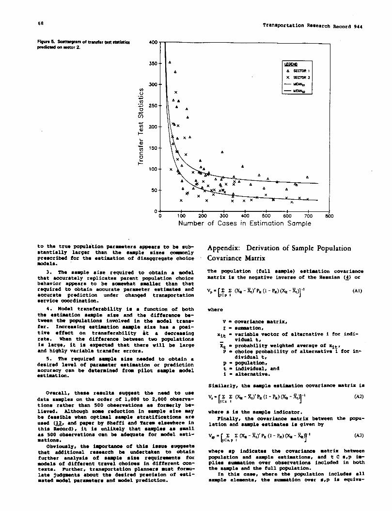
68 Transportation Research Record 944
Fiwrz6.~rzmoftrmfirrnfi-ltihprediatadonnztor2.
400-
350- -
3oo- -(n0.-+
.: 250- -
z
A
x
AAAA
A
\x\ A
WE?iQAZEC?OR1x ZECloR.1
— ~%— M%
A
/ \~
100 x ‘AA
xA A
A AXAA
s.XA
AXX A &
A
50
t
AA”” A A–x x x
x x x )(x R x
040 100 200 300 400 500 600 700 8i
Number of Cases in Estimation Sample
to the true population parameters appears to be sub-stantially larger than the seaple sizes ~nlyprescribed for the ●stlxetion of disaggregate choiceaodela.
3. The sample size required to obtain a aodelthat accurately replicates parent population choicebehavior appears to be saewhat smeller than thatrequired to obtain accurate parameter egti~tes and●ccurate prediction under changed transportationservice coordination.
4. Model trenaferability ia a function of both
the estimation ●aaple size ●nd tha difference be-tween the populations involved in the model trana-fer. Inorea8ing emtimetion ●enple size has a posi-tive effeot on transferability it a dacreaaingrate. When the difference between two populationia large, it ia expected that there will be largeand highly variable tranafer ●rrora.
5. The required sample ●ixe needed to obtain adesired level of perenter estimation or predictionaccuracy can be determined from pilot sample model●etimetion.
Overall, these reaulta ●uggeat the need to usedata mmplea on the order,of 1,000 to 2,000 observa-tions rather then 500 observat~ona as formerly ba-lieved. Although come reduction in eample ●ize Mybe feamible when optiael sample stratifications areused (12, ●nd paper by Sheffi ●nd Tarem ●leawhere inthis Reoord), it is unlikely that ●-lea as smellaa 500 observation can be adequate for model eeti-nations.
Obviously, the ~rtanoe of this ismue wgqestathat ●dditional reeearch be undertaken to obtainfurther ●nalyais of ●eaple size requirannto formodelm of different travel choices in different wn-texts. Further, transportation plannere auat forxu-late judgmarttaabout the deeired preoiaion of eati-●atad mdel paramatera ●nd xodel prediction.
o
Appendix: Derivation of Sample Population
Covariance Matrix
The population (full eample) eetlmetion covariancematrix is the negative inverse of the Eeasian (~) or
(Xt-%)’pito-%)(xit -%)”1
(Al)
covariance matrix,auznation,variable veotor of alternative i for indi-vidual t,probability weighted average of xit,choioe probability of alternative i for in-dividual t,population,individual,andalternative.
Similarly, the sample estimation oovariance matrix ia
“% ~ ‘%- X’)’P’(’‘p’)&- “!-’(A2)
where a ia the aaaple indicator.
Finally, the oovariance matrix between the popu-lation and sample estimatem ia given by
vm=[,~p;&-xt)’P, (l-P.)&-%~”’ (A3)
where ap indicatea the covarianoa matrix betweenpopulation and ample estimations, and t C a.p ix-pliea s~tion over obaervatione inoluded in boththe ●aple and the full population.
In this caea, where the population includes allsample elemante, the aumation wer SVP ie U@Va-

>Transportation Research Record 944 69
lent to the stumation over s and Vsp = Va OK, byusing the notation in the body of the paper, =Sp =“
AClRWlLEDQ4ENT
We acknowledge the support of the Office of Univer-sity Research, U.S. Department of Transportation,for support of this work under a contract to inves-tigate “Conditions for Effect\ve Transferability of‘disaggregateChoice Blodela”v and Jemes Ryan of UMTA,who as contract aonitor has provided substantialstimulation to this research effort.
We also acknowledge earlier analysia undertakenby Joseph N. Prashker of Technion University in col-laboration with Koppelmen, and valuab~e discussionswith Eric I. Pas of Duke University. Finally, wethank our colleagues at the Worthwestern UniversityTrenaportat~on Center for intellectual and analyticsupport in the research. These colleague includeChester G. Wilmott Peter Kuah, and Albert Lunde.
1.
2.
3.
4.
5.
6.
7.
8.
9.
C.F. Manski. The Analysis of QualitativeChoice. Neasachuaetta Institute of Technology,Cambridge, Ph.D. dissertation, 1973.C. Chu. Structural Issues and Sources of Biasin Residential Location and Travel Mode ChoiceModels. Department of civil Engineering,Worthweetern Univ., Evanston, Ill., Ph.D. dis-sertation, 1982.E. Theil. Principles of Econranetrics. WileyrNew York, 1971.D. McFadden. Conditional Logit Analysis ofQualitative Choice Sehavior. ~ Frontiers inEconometrics (P. Zarembka, cd.), AcademicPress, New York, 1973.C. Daganzo. Multinominal Probit. AcademicPress, New York, 1979.G. Neddala. Econometrics. McGraw-Hill, NewYork, 1977.c. Rae. Linear Statistical Inference and ItsApplication. Wiley, New York, 1965.F.S. Koppelman. Methodology for Analyzing Er-rors in Prediction with Disaggregate ChoiceModels. TRB, Transportation Research Record592, 1976, PP. 17-23.T.J. Atherton and M.E. Ben-Akiva. Transfer-ability and Updating of Disaggregate Travel De-mand Nodels. TF03,Transportation Research Rec-ord 610, 1976, pp. 12-1S.
10.
11.
12.
13.
14.
15.
16.
17.
1s.
19.
26.
21.
D. NcFadden. Properties of MultinominalLogitNodel. Univ. of California, Sarkeley, WorkingPaper 7617, 1976.F.S. Koppalman and C.G. ffil~t. Transferabil-ity ~alysis of Disaggregate Choice Models.TRS, Transportation Research Record 895, 1982,pp. 1S-24.C. Daganzo. Optimal Sampling Strategies forStatistical Nodels with Diecrete Dependent Var-iablea. Traneportetion Science, Vol. 14, No.4, 1980.M.F. Richards. Application of DisaggregateTechniques to Calibrate a Trip Distribution andModal-Split Model. TRB, Transportation Re-search Record 592, 1976, pp. 29-34.M. Richards and M. Ben-Akiva. A DisaggregateTravel Demand Nodel. Sexon Rouse and LexingtonBooks, Lexington, Mace., 1975.A.P. Talvitie and D. Kirschner. Specification,Transferability, and the Effect of Data Out-liers in Modeling the Choice of Mode in UrbanTravel. Transportation, Vol. 7, No. 3, 1978.K.L. SObel. Travel Demand Forecasting by Usingthe Neeted Multhomial Logit Mcdel. TRB,Transportation Research Record 775, 1980, pp.48-55.D. McFadden. The Theory and Practice of Disag-gregate Demand Forecasting for Various Modes ofUrban Transportation. In Emergency Transporta-tion Planning t4ethods-(W.F. Brown et al.,eds.), U.S. Department of Transportation, Rept.DOT-RSPA-DPB-50-78-2,197S.K. Train. A Validation Test of a DisaggregateMode Choice Model. Transportation Research,Vol. 12. 1978, PP. 167-174.C.F. Manski and L. Sherman. An EmpiricalAnalysis of Household Choice Among Motor Vehizcles. Trans~rtation Research, Vol. 14A, No;5-6, Oct.-Dee. 19S0. ,,
T.A. Domencich and D. McFadden. Urban TravelDemand: A Behavioral Analysis. Worth-Holland,Amsterdam, 1975.F. Koooelmen and C. Chu. Samole Size Effects.-on Parameter Stability, Prediction Precision,and Transferability of MultinominalLogit Mod-els. ~ Identification of Conditions for theEffective Transferability of DisaggregateChoice Nodels, Transportation Center, North-western Univ., Evanston, Ill., 1982.
Rddkwionofthispuper sponwredbyCbnmittee onTmvekrBehavkw ondvalues

70
Mobility Enterprise: One Year Later
MICHAELJ.DOHERTY AND F.T.SPARROWo
A mobilityenterpriseisanewtrarwpcrtztionconcept .im~ at increasing SISeproductivityoftheautomobilethroughuseofmini0smicroautomobilesinconjunctionwithe$heredfleetofintermediatemadfull-sizedvshidet.Themainobjectiveoftheenterpri$ei$toprovideabettermatchingofvahicleat.tributestotriprequirementsandKillmaintainthepersonalfreedomthatappear$tobe$ohighlyvaluadbytheAmericzndrivar.Althoughthisconceptwaspresentedin dateii in an earlierTRB Record(TRR8S2),aviewofthaprogress that has been made in taking the mobility enterprise from an innwa-tive concept to an actual experiment is presented in this paper. The majority ofthe information deals with metheds for observing consumer attitudas, design-ing the actual mobility enterprise, and measuring mini and micro autemoblleperformance.
In January 1982 the Automotive Transportation Centerat Purdue University unveiled an innovative trans-portation concept called the mobility enterprise(~). Briefly stated, the research examined the ef-fects of mini and micro class automobiles andshared-vehicle fleets on the overall productivity ofthe personal automobile. This paper is designed toprovide an update of the progress made during thelast year and to discuss the experimental design andpreliminary findings.
After years of promoting public transit and car-pooling to conserve energys it appears that the av-erage consumer still prefers the convenience of thepersonal automobile. At the same time, althoughautomobile efficiency (fuel economy) has undergonesignificant improvement, automobile productivity hasremained disturbingly low (2S3). The concept pre-sented here for improving pr~~ctivity is batsedon abetter matching of the trip requirements of an indi-vidual to the characteristicsof the vehicle. Threeinterrelated features of a mobility enterprise--retained autonomy, easy access to an expanded fleet,and reduced expenditures--are the inferred keys toits success. An enterprise membersa minimum attri-bute vehicle (a mini or micro automobile in theseexperiments) provides hiresby definition, with themost economical means of accomplishing hie most fre-quent trips. When a memberss mini or micro automo-bile is inappropriate for a desired trips he mustseek access to an appropriate vehicle from theshared fleet. This process may involve delaya, someadvanced planning, paperwork, and out-of-pocketcosts, depending on the procedures of the enter-prise. A general description of the mobility enter-prise that has been set up at Purdue University isas follows.
1. The following items are included in a setmonthly fee: (a) an individually garaged mini ormicro class vehicle that will satisfy most comcnutingand around-town driving, (b) access to a sharedfleet of intermediate and full-sized vehicles fortrips that the mini or micro vehicle would be un-suitable, (c) all insurance costs, (d) all mainte-nance costs, (e) all registration and licensingcosts, and (f) taxes.
2. Gasoline costs are not covered in the monthlyfee.
3. Cost per participating household for experi-ments is $165 per month.
The concept of a mobility enterprise requirescareful examination of several behavioral parametersof the American as a driver. Judging from theunderutilization of public transit systems and ride-sharlng programs, it appears that personal freedomand independence are highly valued attributes. If
Transportation Research Record 944
it is imperative that this independence be pre-served, a key step in the design of proposed experi-ments must be an inventory of the current patternsof the U.S. driver and the use of his personal vehi-cle. The shape of the enterprise must come as closeas possible to’ satisfying travel demands, with aslittle inconvenience as possible. However, becausethere may be come inconvenience (changes in travelbehavior), it is important to gauge the value driv-ere place on the quality of travel provided by theshared fleet available through the enterprise. Inother words, what would be the trade-offs betweenthe current condition of automobile ownership andparticipation in a mobility enterprise?
Two key tools that have been used to acquire datapertaining to consumer acceptance and current travelbehavior are the focus-group interview and a surveyinstrument (questionnaire). In addition to consumerand travel-behavior studies, a microprocessor-baseddata acquisition system, under development at PurdueUniversity, will measure the stress on these smallautomotive engines when subjected to real-world mis-sions. Such a system is necessary to determine thefeasibility of using mini or micro automobiles forpersonal transportation in the United States.
FOCUS-GROUP INTERVIEWS
Focus-group interviews are predicated on the assump-tion that the mobility enterprise will be better un-derstood and more efficiently designed when thereare more data on how potential users, supporters,and detractors define its advantages and disadvan-tages and its significant and modifiable attributes(~). The content of each interview was analyzed forrecurring themes. The attributes that account fordecisions to join or not join the enterprise wereschematized, and questions measuring the characterand quality of these attributes were developed forthe larger general survey instrument.
Focus-group interviews began in West Lafayette,Indiana, in March 1982. The length of the focus-group interviews varied from 1 to 1.5 hr. Therewere seven focus groups: one group of Purdue Univer-sity faculty and staff, one group of Purdue Univer-sity faculty and staff couples, one group of PurdueUniversity faculty and staff as new car intenders(intention to buy a new car within 2 months), twogroups of college students, and two groups of teen-agers (one consisting of all male and one consistingof all female). A total of 62 individual partici-pated.
Data from the focus-group interviews were ana-lyzed for issues raiseds opinions expressed, and ex-periences reported and were then examined for recur-rent significant themes. The fbcus-group interviewsand subsequent analyses were based on the aeeumptionthat the study of coneumer attitudes and interactionand the emphasie on analysis of themes should pro-vide insight into the consumer decision-making pro-cess of automobile ownership, mini and micro vehi-cles, and the mobility enterprise (5s6). This in
turn should improve the capability f~r-planning anddeveloping the mobility enterprise. The focus 9rouPinterviews were divided into four content areas: (a)vehicle ownership and use~ (b) the expense of ownin9and operating cars, (c) the mini or micro autmo-bile, and (d) the mobility enterprise. The major
findings in each of these content areas were as fol-lows.
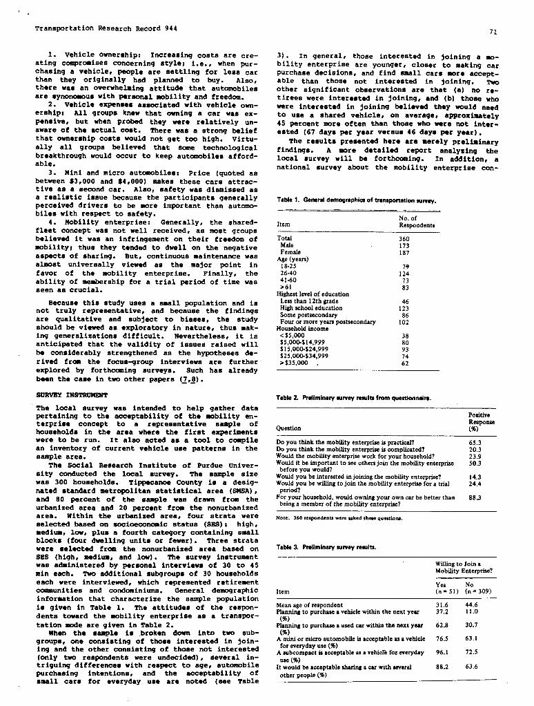
Transportation Research Record 944
1. Vehicle ownership: Increasing costs are cre-ating comprcaises concerning style; i.e., when pur-chasing a vehicle, people are settling for less carthan they originally had planned to buy. Also,there wae an overwhe2xing attitude that automobilesare synoncaous with personal mobility and freedom.
2. Vehicle expenses associated with vehicle own-ership: All groups knew that owning a car was ex-pensive, but when probed they were relatively un-aware of the actual coat. There was a strong beliefthat ownership coataiwould not get too high. Virtu-ally all groups believed that some technologicalbreakthrough would occur to keep automobiles afford-able.
3. Mini and micro automobile: Price (quoted asbetween $3,000 and $4,000) makes these cars attrac-tive aa a second car. Also, safety was dismissed asa realistic issue because the participants generallyperceived drivers to be more important than automo-biles with respect to safety.
4. Nobility enterprise: Generally, the shared-fleet concept was not well received, as most groupsbelieved it was an infringement on their freedom ofmbility; thus they tended to dwell on the negativeaspects of sharing. But, continuous maintenance wasalmost universally viewed as the major point infavor of the mobility enterprise. Finally, theability of membership for a trial period of time wasseen as crucial.
Because this study uses a small population and isnot truly representative, and because the findingsare qualitative and subject to biases, the studyshould be viewed as exploratory in nature, thus mak-ing generalisations difficult. Nevertheless, it isanticipated that the validity of issues raised willbe considerably strengthened as the hypotheses de-rived from the focus-group interviews are further
explored by forthcoming surveys. Such has alreadybeen the case in two other papers (7,8).. .
SURVEY INSTRUMENT
The local survey was intended to help gather datapertaining to the acceptability of the -bility en-terprise concept to a representative sample ofhouseholds in the area where the first experimentswere to be run. It also acted as a tool to compilean inventory of current vehicle use patterns in thesample area.
The Social Research Institute of Purdue Univer-sity conducted the local survey. The sample sizewas 300 houaebolds. Tippecanoe County is a desig-nated standard metropolitan statistical area (Sf4SA),and 80 percent of the sample was drawn from theurbanized area and 20 percent from the nonurbanizedarea. Within the urbanized area, four strata wereselected based on eocioeconoxic status (SSS): high,medium, low, plus a fourth category containing smallblocks (four dwelling units or fewer). Three stratawere selected from the nonurbanizad area based onSES (high, medium, and low). The survey instrumentwas administered by personal interviews of 30 to 45min each. TWO additional eubgroups of 30 householdseach were interviewed, which represented retirementcenmnunitiesand condominiums. General demographicinformation that characterize the sample populationis given in Table 1. The attitudes of the respon-dents toward the mobility enterprise as a transpor-tation mode are given in Table 2.
When the sample is broken down into two aub-groupe, one consisting of those interested in join-ing and the other consisting of those not interested(only two respondents were undecided), several in-triguing difference with reepect to age, automobilepurchasing intentions, and the acceptability ofemall cars for everyday use are noted (see Table
3). In general,bility enterprise
71
those interested in joining a mo-are younger, closer to making car
purchase decisions, and find small cars more accept-able than those not interested in jolnlng. TWOother significant obaervatkms are that (a) no re-tirees were interested in joining, and (b) those whowere interested in joining believed tbeY would needto use a shared vehicle, on average, approximately45 percent more often than thoee who were not inter-ested (67 days per year vereue 46 days per year).
The results presented here are merely preliminaryfindings. A more detailed report enalyzing thelocal survey will be forthcoming. In addition, anational survey about the mobility enterprise con-
Table1.Gmserddemographioroftransportationsurvey..— ---—.— . . ___
No.ofItem Respondents
TotalMaleFemale
Age (yeara)16-2526-4041-60>61
Nighest level of educationLess tkan 12th gradeHigh school educationSome postsecondsryFour ormore yearapost.vecondsry
Housaholdincome<$5,000s5,00@$14,999$15,000-S24,999$25,00G$34,999●$35,000 .
360173187
791247383
4612386
102
3880937462
Tabla2 Preliminarysurveyresultsfromqueationnzira.
PositiveResponse
Question (%)
Do you think the rnobiJityenterprise is practical? 65.3Do you tfdnk the mobility enterprise is complicated? 20.3Would the mobility enterprise work for your household? 23.9Woulditbairnportant toseeothersjoin themobilityenterpriae .50.3
before ynu would?Would you be interested in joining the mobility enterptie? 14.3Would you be willing to join the mobility enterprise for a trial 24.4
period?Foryourhousehold, wouldowrringyour owncarbebetter than 883
being a member of the mobility enterprise?
Now: 360rmpondmea were asked these questions,
Tabla3.Preliminarysurveyresults.
WiUirrgtoJoinaMobility Enterprise?
YesItem (rr= 51) $=309)
Mean age of respondent 31.6 44.6Planning to purchase a vehicle within the next year 37.2 11.0
(%)Plarminatoourchaaeausedcarwithio the next year 62.8 30.7(%) - -
A mini or micro automobile is acceptable sa a vehicle 76.5 63.1for weryday use (%)
A subcompact is acceptableasavehicf6for.everyday 96.1 72.5Uae(%)Itwouldbeacceptableahasingacarwithaaveral 88.2 63.6otherpeople (%)

Transportation Research Record 94472
ceptWest
TRIP
will be conducted by J.D. Power & Associates ofLake Village, California.
DIARIES
Although focus-group interviews and transportationsurveys are helpful in ident~fyittgthe inclinationtoward acceptance of a mobility enterprise conceptand zome of its critical attributes, another snoredirect measure of acceptance based on actual be-havior was also needed. For this reazon, the col-lection of trip diaries from potential experimentalsubjects began in August 1982. Thus nearly 6 monthsof actual travel behavior was collected before theinitial experiments.
Because participation in the mobility enterpriseinvolves changes in vehicle use, it is important toknow whether the enterprise fits into the currenttravel behavior of the participants. Because thetravel patterns of the participants both as a groupand as a household are known up to this point, thisdata should prove to be extretttelyvaluable. Signif-icant changes in travel patterns caused by the ac-cormaodation of the operating system and restrictionsof the mobility enterprise are detected with thesedata. A meaningful control group of trip diary par-ticipants who will not be enterprise members is be-ing maintained for the duration of the experiments.
Trip diary results to date have revealed a re-markable degree of consistency for the test popula-tion from week to week. A summary of trip typea andmileage for the first 12 weeks of the study is givenin Table 4. The trip occupancy pattern for the pop-ulation for the first 12 weeks is given in Table 5.
Table4. Pretest tripdiary resulta oftriptypa andmileaga.
Trips Mean Mileageper per Trip
Trip Type Week (one way)
Shopping(grocery andnongrocery) 2.66 4.97Commuting(work orschool) 5.19 7.64Social-recreation 3,49 14.65Peracmalbuainesa(errands,paaaengerferry,andsoon) 5.75 5.14Return home 9.05 9.24
Note: 65.36 percent were muttipurpmetfirn. Raault8cdver a12-weekparkod.
Table5.Pretaattripdiawraaultsoftripoeaufaency.
Occupancy per Trip(%) by No. ofOccupants
Trip Type <2 >3
Shopping (grocery and norrgrocery) 89.7 10.3Commuting (work or school) 99.0 1.0Social-recreation 79.1 20.9Personal buairreas(errands, passenger ferry, and ao on) 91.2 8.8
AU trips 91.1 8.9
ing four or more occupants. By using these cri-teria, the expected use of shared vehicles for thefirst 12 weeks of the study ie ahown in Figure 1.Extrapolation of these data for a 20-member”enter-prise, run under the restrictions assumed here, ap-peara to indicate that the enterprise is umt effi-cient if it owns two vehicles in its shared fleetand uses an outside vendor for those times when ad-ditional vehicles would be needed. Eowever, thesequestions must be more thoroughly examined duringthe actual experiment.
F@wal. Hypotheticalahm’s&ffastkras.
,’,,l,qusl
l!40 6( 8(
September ctober
4100
TimeNote: Datigtic ax~d Afwtiud vtikloforfi*12ti&triodisrvstudica. Thmodmsuabnadonwhtdiavrawltsfromffrattimfiariodfor ●hypotfratkafantamrisa of24membarhou~
TBCNNICAL DATA ACQUISITION SYSTEN
All mini and micro vehicles in the experiment are tobe equipped with a data acquisition system (DAS) tocollect information on the performance characteris-tics of these vehicles. The DAS has a standard con-figuration, with sensors mounted on the power plantthat pass signals to the crsaputer. The processorpasses the data or processes it and sends the infor-mation to a digital recording device. Oefaignspeci-
fications were developed to sccoamodate the harshautomotive environment. ~is work is not new; it is
an extension of the basic work on internal combus-tion vehicles already perfomed for instrumentationof electric vehicles st Purdue University @).
A mission use pattern will be developed through aseries of plots, such as vehicle speed histograms(percentage of time spent in various vel-ityranges), trip length histograms, number of trips perday versus day of the week, and so forth.
A mission severity index will be used to calcu-late the energy required for acceleration, constantspeed, and idle periods. Data fr- engine fUel_COn-sumption maps will also be used to characterize fuelconsumption during s mission. A general schematic
of this system is shown in Figure 2.
Note: Resuttsc-av=a 11-weekpwiod.INITIAL EXPERIMKSTS
A final purpose for which the.trip diary data maybe ueeful is in the design of the ehared fleet. Oneof the most critical design charscteristtcs of a mrr-bility enterprise is the size of the shared fleetfor a given size of enterprise. HOW many cars wouldbe tw many? HOW many would be too few? For thepurposes of the experiments currently bein9 con-ducted, assume that a shared vehicle iS r~ired for
a trip greater than 30 milee (one way) or transport-
The first mobility enterprise experiment became areality on January 22* 1983. The enterprise ini-
tially consisted of seven participeti$W households.The basic service included an individually ga-
raged, mini or micro automobile and access to a
shared fleet of one vehicle. Because of insurancerestrictions resulting from-the lack of safety dateon the mini and micro automobilee~ all such vehi-cles are prohibited from use on Interetaatehi9h-ways. All operating costs (excludi~ gasoline) are

,’.
Transportation Research Record 944 73
Fiwe2 FicwzhwofDAS.
IOPEP.ATOR INPUTS OATA
I
IFROM KEYPAD
(No. of Occupants, TripI. D., Cargo Code, AmOUnt Of Fuel, etc. )
II
F==7DATA CdLLECTED nORINC MISSION IS
(Date, Time, Full Flow, Vehicle Speed,
Oil Pressure, Manifold Pressure, Grade,
Temperatures, Engine Knock and Speed)I
I OATABASESTORAGEI
included in the monthly fee. In addition, each mem-ber receives approximately 10 coupons for use of theshared fleet. The coupone have a caah value of ap-proximately 87.00. The basic rate for shared-fleetuse varioa ●ccording to peak or off-peak perictda.The coupon ●xchange rate for shared vehicles is twocoupons per weekday and three coupons per weekendday. Coupons m@ be accumulated for use at a latertime, traded among mmbera, or turned in at the endof the month for a credit toward their next wnth”abill. Maintenance of all vehicles and shared-fleetoperations ia administered through the Purdue Uni-versity Tranepcrtation Bervicea Department.
Trip diariea are being ●aintained for all vehi-cles in the mobility enterprise ae well aa in a con-trol group of nonenterprise members. In April 1983the mini and micro vehicles were equipped with theon-board DAS that meaeures varioua factore in engineperformance. All teat aubjecte are being cloeelymonitored throughout the experiments.
tion of the travel demands of the potential partici-pants. This is particularly noteworthy because thedata from the trip diary include AUgUSt (a high va-cation month) and September (Labor Day weekend).The fccua-group interviews imply that there is noaversion to mini or micro automobiles (also indi-cated in the survey) and that continuous maintenanceia a significant factor in favor of the mobility en-terprise concept. The survey and focus groups havealso indicated that the mobility enterprise, to besuccessful, must coma close to the current state ofautrsnobileownership. Other work currently underway deala with determining optimal shared-fleet eize(~, which is crucial to the ultimate economic auc-cesa of such a venture.
In addition to the data presented here, a greatdeal of the first year’a effort haa dealt with lo-gistical considerations, such as obtaining waiversfor importing the mini and micro automobiles, ar-ranging insurance coverage and maintenance deliveryaystemar procuring vehicles for the shared fleet,and calculating costs to the participants. Althoughsuch efforta yield no experimental data, they areboth time consuming and crucial to the performanceof the actual exparimenta. Thus, bacauae of thework described in this paper, the Purdue Universitymobility enterprise experiments were able to beginin January 1983.
This work has truly been of an interdisciplinaryna-ture, and special thanks are due to Harry Potter(Department of Sociology), Richard Feinberg andThelma Snuggs (Departmentof Consumer Sciences), JonD. Frlcker (Department of Civil Engineering), andPatrick McCarthy (Department of Economics) for allof their intereat and active participation in theearly and tedious data-gathering phasee of theatudy. A apaclal thanks ia elao due to LoriSerthold and Pat Sandere, without whose diligentwork and akilla this paper would not have been pos-sible.
Thanks is also due to the three research teamsthat have asaiated in the formulation of the focus-group interviews: the Purdue University teem(headed by Richard Feinberg and Thelma Snuggs of theDepartment of Consumer Sciences), Avis Rent-A-Car ofGarden City, Hew York (headed by Al Dold, executivevice president for marketing), and J.D. Power & As-zociatee, consulting spacialiata in autmobile mer-keting (headed by John Hemphill, executive vicepresident).
The purpose of this paper ia to describe the prog-rees that has been made in the paat year in bringingthe mobility enterprise frm a hypothetical conceptto a set of actual ●xperiments designed to test iteviability as a transportationmode. Many of the re-sulte presented here deal with research activitiesthat must precede the actual exparimenta. The re-search emphaeie to date has been in the area of con-sumer acceptance of the mobility enterprise concept,recruitment of experimental subjects, operationaldesign of the Purdue University experiments, andmethods for measuring mini ,and micro vehicle per-formance under U.S. driving conditions.
Thus far the data are encouraging becauee mrethan 20 percent of the random sample would be will-ing to try ● mobility enterprise for a trial periodand more than 10 percent said they would be willingto join euch ●n organisation. The data from thetrip diariee a~ar to indicate that a mobility en-terprise operation could aatiafy a significant por-
1.
2.
3.
4.
5.
F.T. Sparrow, J.D. Fricker, and R.K. Whitford.The Mobility Enterpriaer Improving AutomobileProductivity. TRS, Transportation ResearchRecord BS2, 1982, pp. 19-24.The U.S. Automobile Industry, 19S0. Re~rt tothe Preeident, Secretary of the U.S. Departmentof Transportation.Jan. 1981.A. Altechuler, J.P. Womeck, and J.R. Pucher.The Urban TranepQrtation System: Politics andPolicy Innovation. MIT Press, Cambridge,f4aea.,1979.J. IIiggenbottomand K. Cox. FOCUS Group Inter-views. American Marketinq Association, ~i-cago, 1979.E. Fern. Why Do Focus Groups Work...A Reviewend Integration of Smell Group Prccese Theo-ries. In Advancee in Consumer Research (S.Mitchell. ed.), Univ. of Michigan Prees, -nArbor (in preparation).

74 TransportationReeearch Record 944
6. R.A. Feinbar9 and T.L. Snugga. The MobilityEnterprise: FOCUS Group Interviews. Automo-tive Transportation Center, Purdue univ., WestLafayette, Ind., July 1982.
7. R.A. Feinberg and T.L. Snugga. The MobilityEnterprise as Innovation. Automotive Transpor-tation Center, Purdue Univ., West Lafayette,Ind., May 1982.
8. R.A. Felnberg and T.L. Snuggs. PsychologicalPricing and the Mobility Enterprise. Automo-tive Transportation Center, Purdue Univ., WestLafayette, Ind., June 1982.
9. W.G. Blom et al. High Speed Digital Data Ac-
quisition System for Electric Vehicles. Prmo,Electric Vehicle Council Symposium VI, BVCPaper 8120, Oct. 1981.
10. J.D. Pricker and J.K. Cochran. A Queuing w-mand MOdel to Optimize Economic Policymakingfor a Shared Vehicle Enterprise. Presented atthe Operation Research Society of America(ORSA) and The Institute of Menaqement science(TIHS) Conference, San Diego, Oct. 25, 1982.
Fublirationofthu papersponsoreriby ComrnMteeon Truvdar BdraviorarsdValues.
Person-Category Trip-Generation Model
JANUSZ SUPERNAK, ANTTI TALVITIE, AND ANTHONY OeJOHN
A pereon%etegorymodalof trip generation is presented as an altarnativotohoueehold-beted trip-psneration models. In this modal a homogeneous groupof persons is used m en analysis unit. The final daedption of the person wte-gories is not wbitracy but results from the multistage, multivariate analyeis ofmmsypotentially significant variables. The variableeege, ●mployment status,and automobile availability were found to be the most signifiint deeoriptorsof a person’s mobility. The final version of the model ia based on ●ight pesemsoategoriet. Both theoretical discussion and empiriad findings favor the pro-posedversion of the pereon-oztegory model over houeehold-beeed models be-oause it is more preatiral at tha foreazet stage, requires eignifkantly Iaeedata,has Mter behavioralbackground, and is more compatible with the ●ntire eyetam of individually oriented trzveldemarwl models.
The development and evaluation of a person-categorytrip-generation model as an alternative to house-hold-based models are discussed in this paper. Theindividual-levelapproach was chosen for the follow-ing reasons. First, a person-level trip-generationmodel ia compatible with other components of thefour-step travel-deinandmodel system that is basedon tripmekers rather than on households. Second, itis extremely difficult to devise a household-basedcross-classification scheme that uses all importantvariables and has a manageable number of classes[e.g., a British household cross-classificationmodel (&) haa 108 categories]. Predicting represen-tations in so many classes is difficult.
Third, the sample size for the person-ate90rYmodel can be much smaller (10 to 40 times) than forthe household-category model. Fourth, demographicchangea can be more easily accounted for in thepereon- rather than household-category model, andsome demographic variablea (such as age) are virtu-ally nondefinable for households. Finally, personcategories are eaaier to forecast to the future thanthe household categories, which require forecaetsabout houeehold formation and family size. With theperson categories these tasks are altogetheravoided. More importantly, because the bulk of thetripz will be made by people older than 18 years ofage, the task of predicting the tripmakinq popula-tion 15 to 20 years ahead is much easier.
There are of course scme limitations that a per-son-category model may have. Foremost among theseis the difficulty of introducing household-interac-tion effects and household money costs and moneybudgets into the model. On the other hand, it isnot clear how.vital these considerations are and howthey can effectively be introduced even in a house-hold-category model. The methodology of the develop-
ment and testing of the person-category uslel waabased on previous work from Europe (2-6), where theperson level of data aggregation w~s-found to besuccessful for travel-demandanalysie.
DATA AWD DEFINITIONS
Date
The data used in preparing this paper were from theBaltimore home interview survey conducted in 1977 bythe FHWA and from Minneapolis-St. Paul hoeea inter-view data collected in 1970. Before the enalyses,data were superficiallycleaned. .Workday recordswere separated from weekend-day records, and somepersons were excluded froa the original saeeple. Forexample, if in the original file a significant in-consistency was found (e.g., number of cars in thefemily = 7 and number of drivers = O), the parsonwas excluded. Outliers were also excluded. If thenumber of trips done by a pereon was greater than 10and if total time spent on traveling during the dayexceeded 150 rein,then this person was suspected tobe a professional driver (or similar category) andwas excluded from the sample.
Definitions
The following definitions are used in the analyses:
Ni = trip rate, that is, the daily number ofone-way trips made by (aVera9e)eer~n incategory i; and nqi = triP rate to Pur-pose q in category i;
Ti = daily travel time; that ia, the time (inminutes) spent by (avera9a)Per-n in cate-gory i on traveling during the daifz
Yj - total number of trips made anywhere by theinbabitenteof sone j (all categories t-gether);
q . nuraberof zone j inhabltantsrand
aij = percentage of inhabitant of zone j belonging to category i.
Thus the following basic relationship is given:
(1)

.’.
Transportation Research Record 944 75
The method of calculating zonal Productions (P )and 1attractions (A ) is not presented in th spaper. iThis method s briefly presentad in Supernak(s).
In analyzing and calculating trip rates, tripsare divided into
1. Hcae-based (RS) trips if origin (NBO) ordestination (NBD) of the trip is the place of resi-dence of the traveler, and
2. Non-home-based (NSB) trips if neither originnor destination of the trip is at home.
Trips are further divided by trip purpose (q) asfollows: work (W), education (E), shopping (S),personal business (Pb), and social-recreational andother purposes (Sr). This trip-purpose classifica-tion applies to both NB and NHS trips. Work andeducation trips are called obligatory trips, and allother trips are called discretionary trips. Thetraditional description of the trip links (insteadof sojourns of trips) was chosen because it clearlyrelates the number of outside-the-home activities tothe number of trips made (6,7).
An example of trip rat&-for category i is givenin Table 1. Fifteen-elementvectors of partial triprates
9i (i.e., separated by purpose, direction,
and base may be derived from the data, as shown inTable 1; they served as the trip characteristic ofcategory i.
Tsblsl. ExarnplaoftriprztsoharrctsristicNforrategoryi.
Obligatory Discreti0n2ry
Triu w E s Pb Sr Total’
HBO 0.86 0.02 0.10 0.21 0.05 1.33HBD 0.86 0.05 0.21 0.19 0.02 1.33NHB 0.02 005 0.14 0.14 0.07 043—-Total’ ~bl=l.86 N:isc=].24 Ni=3.10
aNotethatmmecolumnswillnot totalbecau=of rounding.
ANALYSIs mwcmoRs
The model development was done in four stages:
Stage l--(a) arbitrary choice of many variables,which are expected to be important for explainingdifferences in a person’? mobility, and definitionof plausible person categories by using these vari-ables; and (b) preliminary analysis of trip rates(Ni) and trip times (Ti) to find which variables havethe least explanatory power and can be excluded fromthe model~
Stage 2--(a) detailed analysis of trip character-istics to find variables that define similar cate-gories for stage 3; variables that do not givesubstantial explanation of the data variance orvariables that duplicate an explanation of otherbetter variables are excluded; (b) proposal for thefinal trip-generation categories the number ofwhich should not ●xceed a certain practical maximum(for example, 10); and (c) analysis of dependency oftrip rates between trip purposes [not reported inthis paper, see Supernak et al. (g)];
Stage 3--(a) final trip-generation characteris-tics of each category, as determined in stage 2, areanalyzed in detail; and (b) transferability of theresults within different sections of Baltimore andto other cities is exeminadr and
Stage 4--comparieon with household-based trip-
generation model, aa presentad in detail in DeJohnQ) .
The statistical methods used in the analyses aresimple and straightforward. At all times thesestatistical methods are supplemented by visual anal-ysis of data that try to find petterns in the datathat a blind application of statistical methods maynot find.
In stage 1 of the model develo~nt only a peir-wieiecomparison of total trips rates is performed.The Z-statistic for the trip rates of two categoriesi and j, which are differentiated by the analyzedvariable only, is computed and compared with thecritical Z-value at the 0.01 level of significance.
In the remaining stages three additional measuressupportad by histograms and analyses of variance areused. These three measures are the correlationcoefficient, slope (m), and intercept (b) of ther~ression Nqt = bij + mi Nqj.
The categories i and 1 may be treated as similarif (a) the correlation coefficient between vectorsof the partial trip rates (i.e.,poee and base) ~i and
7j, and
of the regression coeff cientsintercept),-satisfy
ru>0.900
0.75<q< 1.25
Ibul<0.10
the following
trip rates by pur-(b) the parameters(m~ - slope,
4-con itions:bij -
(2)
(3)
(4)
These conditions are arbitrarily chosen and arequite demanding.
These three measures can be used to analyze theappropriate categories for both pareons and trippurposes, as shown in Figure 1. The Q-type regres-
sion and correlation analysis is used for analyzingthe best grouping of persons, and the R-type analy-sis is used for grouping trip purposes. These anal-yses are useful for both travel-demand analysis(~,~) as well as for nontransportation applications(~) .
Fiwws1. @~patiR-WpadytiMwipr*Nqi.
ProwlCaqws{2 n~4a
:lnpRater:
N
El
mm MmCt’uuctcrilllcs
*=45
STAGS 1: CHOICE OF VARIABLES AND DSVEL@MENT OFCATSGORIEB
For stage 1, the following variables (and strata)were used to form the categories.
1. Sex: The obvious “choice of strata here ismale and female.
2. Age: Age was used to describe the main activ-ity at a given age (primary school pupilsr high
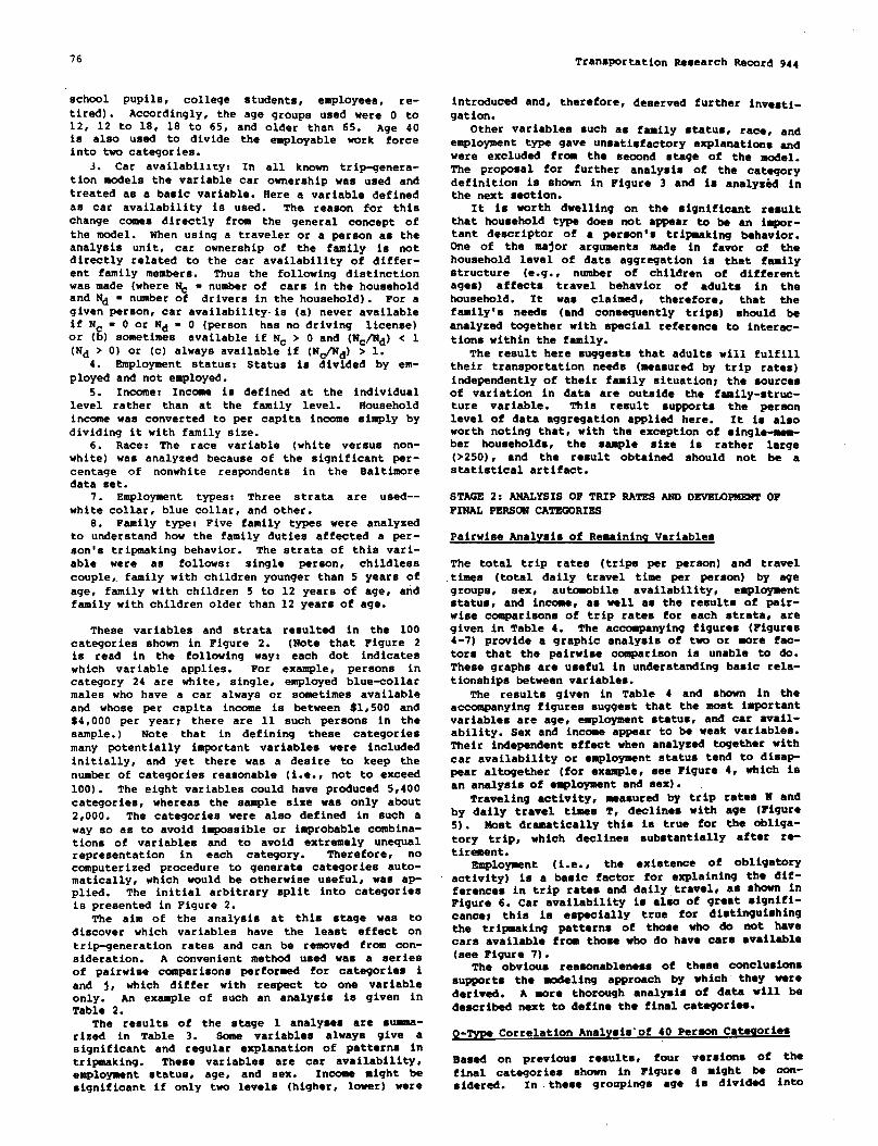
76 Transportation Research Accord 944
school pUpilS, college students, employees, re-tired) . Accordingly, the age groups used were O to12, 12 to 18, 18 to 65, and older than 65. Age 40is also used to divide the employable work forceinto two categories.
3. Car availability: In all known trip-genera-tion models the variable csr ownership was used andtreated as a baaic variable. Here a variable definedaa car availability is used. The reason for thischange comes directly from the general concept ofthe model. When using a traveler or a person as theanalysia unit, car ownership of the family is notdirectly related to the car availability of differ-ent family members. Thus the following distinctionwas made (where ~ = number of cars in the householdand Nd = number of drivers in the household). For agiven person, car availability-is (a) never availableif Nc = O or Nd = O (person haa no driving license)or (b) sometimes available if Nc > 0 and (Ncfld) < 1(Nd > O) or (c) always available if (N&Nd) > 1.
4. Employment status: Status la divided by em-ployed and not employed.
5. Income: Income is defined at the individuallevel rather than at the family level. Householdincome was converted to per capita income eimply bydividing it with family size.
6. Race: The race variable (white versus non-white) was analyzed because of the significant per-centage of nonwhite respondents in the Baltimoredata set.
7. Employment types: Three strata are used--white collar, blue collar, and other.
8. Family type: Five family types were analyzedto understand how the family duties affected a per-son’s tripmeking behavior. The strata of this vari-able were as follows: single person, childlesscouple,.family with children youn9er than 5 Years ofage, family with children 5 to 12 yeara of age, andfamily with children older than 12 years of age.
These variables and strata resulted in the 100categories shown in Figure 2. (Note that Figure 2is read in the following way: each dot indicateswhich variable applies. For example, persons incategory 24 are white, single, employed blue-collarmales who have a car always or sometimes availableand whose per capita income is between $lt500 and$4,000 per year; there are 11 euch persone in thesample.) Note that in defining these categoriesmany potentially important variables were includedinitially, and yet there was a desire to keep thenumber of categories reasonable (i.e., not to exceed100). The eight variables could have produced 5,400categories, whereas the aemple size was only about2,000. The categories were also defined in such away so as to avoid impossible or improbable combina-tions of variables and to avoid extremely unequalrepresentation in each category. Therefore, nocomputerized procedure to generate categories auto-matically, which would be otherwise useful, was ap-plied. The initial arbitrary split into categoriesis presented in Figure 2.
The aim of the analysia at this stage was todiscover which variables have the least effect ontrip-generation ratea and can be reawved from con-sideration. A convenient method used was a seriesof pairwise compsriaons performed for categories iand j, which differ with respect to one variableonly. An example of such an analysis ie given inTable 2.
The results of the stage 1 analysea are summa-rized in Table 3. Some variables always give asignificant and regular explanation of patterns intripmaking. These variables are car availability,employment status, age, and sex. Income sight besignificant if only two levels (higher, lower) were
introduced and, therefore, deserved further inveati-gation.
Other variables euch as family status, race, andemployment type gave unsatisfactory explanations andwere excluded from the eecond stage of the model.The proposal for further analysis of the categorydefinition is shown in Figure 3 and ia analys&d inthe next section.
It is worth dwelling on the significant resultthat household type does not appear to be an iapor-tant descriptor of a person’s tripmeking behavior.One of the major arguments made in favor of thehousehold level of data aggregation ia that familystructure (e.g., number of children of differentages) affecta travel behavior of adults in thehousehold. It was claimed, therefore, that thefemily’s needs (and consequently trips) should beanalyzed together with special reference to interac-tions within the family.
The result here suggests that adults will fulfilltheir transportation needs (meaaured by trip ratea)independently of their family situation! the sourcesof variation in data are outside the family-struc-ture variable. This result supports the personlevel of data aggregation applied here. It is alaoworth noting that, with the exception of single-mem-ber households, the sample size is rather large(>250), and the result obtained should not be astatistical artifact.
STAGE 2: ANALYSIS OF TRIP RATSS AND DEVBLO~ OFFINAL PERSON CATEGORIES
Pairwiae Analysis of Remaining Variablee
The total trip rates (trips per person) and traveltimes (total daily travel time per person) by agegroups, sex, automobile availability, employmentstatus, and income, as well as the results of peir-wise comparisons of trip rates for each strata, aregiven in Table 4. The accompanying figures (Figures4-7) provide a graphic analysis of ttm or more fac-
tors that the peirwiee comparison ia unable to do.These graphs are useful in understanding basic rela-tionships between variables.
The results given in Table 4 and shown in theaccompanying figures suggeet that the meet importantvariables are age, employment status. and car avail-ability. Sex and income appear to be weak variablea.Their independent effect when analysed together withcar availability or employment status tend to disap-pear altogether (for example, see Figure 4, which isan analysis of employment and sex).
Traveling activity, measured by trip rates W andby daily travel times T, declines with age (Figure5). lbst dramatically thie ia true for the obliga-tory trip, which declines substantially after re-tirement.
Employment (i.e., the existence of obligatoryactivity) is a beeic factor for explaini~ the dif-ferences in trip rates and daily travel, as ahown inFigure 6. Car availability ie also of great mignifi-cance~ this is especially true for distinguishingthe tripmaking petterns of those who do not havecare available from those who do have cara available(eee Figure 7).
The obvious reasonableness of theee conclusionssupporta the modeling approach by which they werederived. A uore thorough analysis of date will bedescribed next to define the final categories.
!2-- Correlation Analyeis-of 40 Pereon Categories
Baeed on previous results, four versions of the
final categories shown in Figure 8 might be con-sidered. In these groupings age is divided in~

!’
Transportation Research Record 944
Fiwwe2. PvhnazysplitintolOOc ategor&.
VN2AS2X.9
VNIASLS‘W2AlZ0?LI?S
c3nLmm6<5PHKUY scmo3,
POVILS
$-lY
scPloa
Pom3a
STWS~S
01R2sP3.JXED
MAK
mu
sPm.aYsEs
PmlALs
S2mmm3s
.—
Ss16u.S
(Ikmmmfss)
UTIBSD
PSOPLS
Ss
~~s,—.-.
1.J
9
.
.
.
●
J
.
.
T●
D
!-.●
.●
.●
.,.,..D●
.
.,,.
D,,,
;,,I4,,14
J,,
,
;
●
●
●
8
●
?APIILYSTA2VSCMAVA12AJ1LZF
● I..
:1
L i.. be● ☛
● ☛☛ 1
● ● I,C
●
✎
●
✎
✎
✎
✎
●
●
✎
✎
●
.0. .● *. .. ..0.C. .● ●,.*● *. ..*● *. .. .● *● *
●
●
●
●
●
●
●
●
✃
✎
��✎ � ✎☎✎✎
.—
● ✎☛✎
● ✎☛☛
● ✎☛☛
● ✎☛☛
● *9*● ***● **...**
1
1“
,.
●
●
✎
●
..
●
✎
✎
✌
●
.●
●
●
●
✎
●
✎
●
✎
.●
.●
.●
✎
●
●
●
●
●
.
.●
●
✌
✌
✎
✎
●
.*● ☛
s●
● *● *
●
●
,)
.
.●
9,.I*
●
2
,
.●
●
9s.
—
●
●
—
.
.
.●
●
●
9..●
●
A
—
,
●
●
●
●
✎
●
●
—
.9
.
.
.●
●
.
.●
.---
●
—
●
●
●
●
●
●
77
!~II
I
e
05
*
6628233432341545~172s
+
506
~1113
103061
:;9
:231240151
5s3*6
5?1195D6221055
i“-2‘2!01116,9,6!3,2!616~113112126239176
188
3227’29231826
+
325
:172647
61
1334

78 TranaportatkrrtRfa.eearchRecord 944
Figures. stsps2dsacriPtion ofps~MtsgorisI.three strata: younger than 18, 18 to 65, and olderthan 65. The pairwise analysis suggested that theage groups younger than 40, 40 to 65, and older than65 may be most appropriate. However, plots in Fig-ures 4-7, which consider more than one variable, aswell as practical considerations, favor the firat-tnentionedage strata. The first stratum consists of(mostly) unemployable students, the second stratusnincludes the labor pool, and the third stratuztitt-cludes retired people.
Four versions of category descriptions were ana-lyzed (Figure 8). Version D is preferred because itis a parsitaoniousgrouping of people into only eight
CAT-012
AGE Szx AOTO mP INC
1223333333333333333444.4444b44444h4b555555
1211111112222222221111111222222222111222
3456789
10U1213141516171819202122232425262728293031323334353637383940—
123123
123123123123123
123123
:3123123
111111211111
:221111112111111
:2
1112
:
111222
111222
111222
—
categories; however, it must be based on a more
Tatde2. Andysisofvariebloagz: trip rzteaforyourrgervsnuaolderhou3ewivsa.
Trip Rstes N,Category No.
Age c 40 Age >40Age <40 Age >40 (n = 21S) (n = 190)
Variable Levels:
ME 1. <122. 12-183. 19-404. 41-655. >65
SEZ 1. Haze2. Fenle
717375777981838587
727476788082848688
3.363.001.422.181.891,123.862.721.50
2.812.330.851.501.130.703.652.271.52 mu 1. Never
WAILASILITY 2. ti~ti~’2.1l’,b 1.73’”3. Nways
~T 1. @loyad2. Nen-aPloyed
‘Mereof totsl triprate.bz,,~=4.oo.cZ~,~, = 2.30. mx6rz 1. < $3000/cap
2. ~ W3001eap
TotsS Trip Rate’Z-Veluesb(Zo.ol =
1 2 3 4 2.57,2..0S = 1.96)
Variable Category Mean No. Mesn No, Mean No. Mesn No. 1,2 13 2,3 Comments
sex We, fe- 2.65mde
811 2.20 1,093
1,661 1.23
190
289 3.23
478
163 2.83
176
171 2.92
246 2.82
7.89
—
0.42
0.2I
26.3
3.8
8.W3
0.83
0.32
8iinifkmrt difference in trip occur-redordyforpersons >6S;thiagroup alone may not wmrantstrztifxationby sex
Younger persons tmvel more4.82
4,00
15.4
Age 12-18,18- 2.9265,>65<40,>40 2.11
482
215
309
2.56
1.73
2.78
243
341
206
27
276
Youngerpersom travelmoreAge, hou3e-Wive$Onsy
car avail-abilityy
L3ifferenceabetween cm never, some-times, and aSwaysavaiSablearesignifirant;grester csravailsbilitymesrrsmore trips
Whetheraperann isemployednrnotinssrextremely sigrritlcantvsriable
Never, 1.38sometimes,shays
Employmentstatus
EnapSoyed, 2.85not em-ployed
kW, mid- 1.89die, high
White, non- 2.25white
1,183
187
398
1.85
1.85
1.98
17.0
0.40
2.88
Trip rates between lrisSSand otherincome groups are different
Thinu sn extremely erratic variable;viauaSexmnination of data did notsusgeat atratificstion by race; dif.ference.cauaedby fourcateisnries(46, 59,94, 98)
Notnaigrdficaratvariable
Income
Race
2.28Employmenttype
White col- 3.05hr. bluecdsr,other
Single, 2.90couple,couple withchildren<5, rouplewith chil-dren >5
133 2.67
2.80 591 0.62 Farnilytypeisnot significant
(23,4= 0.10)Household
type70 2.78
%ocolumnsh this=thn w.redufoUow. me*tcfme* w@bletied&d .nd=tie V-bbkati Gt~wc~umnsi c4., c=sw~bMY+~r, ~m"th_. ~Y'._dth`*lPmtah cO1umns1,2, md3ptiti tothexamts lnthcco&smow(l.e-l forneva, 2forsometlmm, snd3fm~aW).
bZ-vstuosus cskulsted by comwlm ttw mean tip rstcsforthecotumnsshown.

Table4. f%wisa comparison of tripstttributasby catagory (stage 2).
Characteristicsof AttributesZ-Valueof PairwiseComparison
1 2 3 4 of Means of AttributesAttri-
Variable category bute Mean SD No. Mean SD No. Mean SD No. Mean SD No. z,,.’ Z,,3 Z,,4 z~,, Comments
Age <18, ]840,41- N 2.88 2.0s 347 2.77 2.01 698 2.40 1.76 586 1.2s 1.67 195 0.82 3.65 3.50 3.50 Z2,4 = 10.72, Z3,4 = 8.2365, >65 T 51.8 37.2 347 52.8 38.0 698 47.9 35.2 586 22.0 31.2 195 0.40 1.17 9.94 2.40
Sex Male, female N 2.69 2.05 816 2.37 1.98 1,010 3.37 – – –T 53.8
Sex sfone is a significant variable,38.9 816 42.7 36.5 1,010 6.S7 – – – but when plntted together with
employment status its signifi-
Automobile Never, wmetimes N 1.55 1.58 501 2.86 2.05 349 3.23 1.95 483availabihty always T 32.6 36.1 501 54.8 35.8 349 60.6 38.2 483
Employment Employed, not N 3.05 0.19 1,086 1.71 1.43 740Status employed T 61.4 39.4 1,086 27.8
fncome34.7 740
bW, high N 2.78 2.05 217 3.27 2.23 522T 62.8 39.1 217 67.2 42.3 522
carrce disappaam10.05 14.80 – 4.23 lmpnrtant variable8.86 11.80 – 2.23
21.18 – - – Impurtantvariable19.22 – – –2.88 Income is not a strong variable; for1.42 Tit is not a aigrrK1cantstratified
even when considered slone
Note: ‘EIIistabte is read in the same msnmw8$Table 3. N = trip rate and T = total trawl time.
Figure4. Vduas of N and T as rfapersdantan.WIW-L -x, ~ w of Pa-s-
n
4
L____3 ---w::;;:,,,: =--y:;:;:’,.Aa’
10 30 3s 40 69 so 70 40 V,*1S
‘t[*4
j --k:,,,,.
Figura5. Values of N and T for obfigatorvand disamticrnarytrip puvposas as depavrdanton age of par30ns.
j_lE25LE10 20 30 40 40 co 10 80 vun
T[mm
10.
60
~,9r-l-- –--l--- --1-1-
40 II, lSU13s4s,,I
30 1;
20I lDIBcmsiHo/r10 II At[
o 10 20 30 40 bo no 70 Doham
Figura6. Values of N and T as depandent on ageof parxmrsand employment status.
Figure 7. Vafrrasof N and T avdependentcurcar availability and sga nf panons.
m
4
l-x
Alwq83 S*N*,WS
2““*’ -------
I
AI’o 1s 20 30 40 50 10 ?0 coV,wt
L. AGEo 10 2s 30 49 ho 60 70 00 vows

Transportation *s@arch Record 94480
F@m 8. Four vmcionc of psrcon~tzgory definition.
1<18
14 cat8g*1i88
Vfnslon cA@f/f MP/lMWSEX
m
91@
la#
[m,. ~
10Cntngafias 8 cat*wl**
detailed examination of the data using the 15-ele-ment trip rate vector (Nqi) shown in Table 1 andcalculated for each category.
For all four versions of the final category defi-nition, respective triangle matrices of rij, mij, andbij were found (the Q-type analysis). From the analy-sis point of view, the interesting parts of thesematrices are those near the hypotenuse, where thevalues of ri , mij, and bij areconditions o~ similarity given~~~~~~~~~~2-4) for those old categories i, j,..., m, whichwill be combined in one new category C (Figure 9).
Figum9. &ncmlidca ofmatingandavdudngncwfinalpcmon ostzgoricc.
rij, bi s and mij ledFirst, there are three ~ai~~&s?%’i&e-z~have clearly different trip-generation characteris-tics: people under the age of 18 (mostly students),employed adults (age 18 to 65), snd not employedadults and retired people. Second, the conditionstaken as a measure of similarity (ri > 0.900, 0.75 <m~
1< 1.25, bi
i1< 10.1OI) are sat sfied for most
pa rs of old ca egories, which are consolidated intothe final new categories. These criteria are bettermet by the etudent snd eaployed sdult categoriesthan by the not employed snd retired categories. Itmeans that the exlatence of an obligatory activity(work, school) makes travelers’ behavior more regu-lar. Third, unsatisfactory valuea of ri , mij, andbij observed 1in aoee cases were regular y sccompa-niad by emall size in the categories.
The correlation analyses and the pairwiae com-parisons strongly suggest tihatthe final categoriesshould be based on age (younger than 18, 18 to 65,older than 65) and ecoploymentetatus (employed, notemployed). Of the remaining variables, either caravailability or sex and inocae could be used. Forpractical reasons, to keep the numbers of categorieslow and variablea compatible with other models, caravailability was chosen to complete the list ofvariables for defining trip-generation categories.A two-dimensional analysie of variance was done toprovide quantitative support for this choice; theresults indicated that sex and income do not havemuch explanatory power when analyzed together withcar availability.
STAGE 3: FURTHSR ANALYSIS OF FINAL TRIP-GENERATIONCATEGORIES
The final eight person categories were baeed onthree variables: age, employment etatua, and caravailability. These ●ight categories are analyzedin more detail.
Car availability data may be replaced in themodel by car ownership, the latter in some caseebeing more readily available. The results of aversion A (using car availability) and those of aversion B (using car ownership) are compared InFigure 10. .For practical model applications, bothversions require estimation of category representa-
ACE
The shadowed triangles in Figure 9 that were nearhypothenusee of the matrices rij, m~j, and b~j wereexamined carefully. As one of the possible measuresof appropriateness for each four versions of thefinal category description, the average regressionfor pairs of categories in the shadowed sreas waecalculated.
The results of the regressions [see Supernak etal. (~) for details] indicated that a 14-categoryvereion is only slightly better than the 8-categoryversion. This conclusion is aleo supported by visualinspection of the triangular matrices for rij, bij,
and;;lh;~) hetailed examination of the matricee for
F~ro10. Twovmcioncoffinalpeno~ dc4cription and theirmpmcsntationin tfceseltirnorsdcca.
vEnslon I Vfmslcm9
rzwl
tmm-’EN?LCVCDEMS-UP.
6!910.3s
#b% 1I.t71,
1.8% 1 1.1%843
17.*% Iccn11.6!I

,’.
Transportation Research Record 944
tiona at the zonal level. This can be achieved byapplying the parson-category car-availability andownership model, which is presented in detail inSupernak et al. (~. This model uses land uae andlevel-of-service variables and thus takes into con-sideration the influence of these variables on boththe category representationsand final trip ratea inthe given area.
Figure 10 compares these two versions of thefinal trip-generation categories in the availablesample. The weekday trip-generation rates for thetwo versions are given in Table 5 for all trips and
Tab4e5.Trip.ganarationrates (tripsperpersan) forei@tperaanatagorias,wakdaysonly(sw#2),
Home BasedNon-Home
Obligatory biscretionmy Based TotalWezovNo. A B A B A B A B
1 1.47 1.472 1.40 1.273 1.77 1.694 1.67 1.72s 0.13 0.156 0.34 0.237 0.30 0.278 0.12 0.12
Wei@ted 1.01avg ofpopulation
1.13 1.130.59 0.700.85 0.851.05 0.900.89 0.931.74 1.392.10 1.660.93 0.93
1.07
0.38 0.380.51 0.570.55 0.590.76 0.680.31 0.350.47 0.430.59 0.430.43 0.43
0.50
2.98 2.982.50 2.543.17 3.233.48 3.301.33 1.432.55 2.052.99 2.361.48 1.48
2.59
Note: QtwMstivmtinsAmdBwedeftiedh Fwure10.
in Table 6 for vehicular trips only. The data indi-cate that there ia little difference whether caravailability or car ownership is used. The biggestdifference is in discretionary trips by car-owningpersona. Generally, version A of the model formula-tion is reconuoanded because it clearly refers to theperson (a real or potential traveler) and hia accessto transportation models and hia individual travelchoices. The person-category car-availability model(~ is a direct input to the person-category trip-generation model. Both models require only routinelyavailable data and are easy in practical application.
A crartperissonof the data in Tables 5 and 6 indi-cates the importance of walk and other nonvehicular
Table&Tfi~rn~~(tiidoti~~r~~}foroi@t~mnZ-@-I -kdw *.
Home BasedNon-Home
Obli@ory OiscretionsryCdtegory
Based Totsl
No. A B A B A B A B
0.63 0.63 0.48 0.48 0.15 0.1s 1.26 1.26; 1.15 0.98 0.28 0.28 0.28 0.27 1.713
1.531.64 1.57 0.76 0,83 0.49 0.52 2.89 2.91
4 1.61 1.61 0.96 0,82 0.71 0.63 3.285
3.090.06 0.06 0.40 0.31 0.14 0.11 0.60 0.48
6 0.28 0.16 1.39 1.04 0.38 0.32 2.057
1.520.24 0.21 2.03 1.50 0.57 0.39 2.84 2.10
8 0.12 0.12 0.60 0.60 0.28 0.28 1.00 1.00
Weighted 0.80 0.7s 0.36 1.91avg ofpeculation
Note: Categ.orleiinversionsA ●.d B ●re defined in Fiswe 10.
trips (e.g., bike,parsons not Ownina
81
horse, boat). For example, forcars these trips account for 40
to 60 percent Of all tK@3. For young people thispercentage ia greater. This is important becausethere clearly exist substitution possibilities be-tween walk and bike and vehicular modes, and theseshould be accounted for in the models. It alsoappears that there is a distinct difference betweenemployed and not employed persone~ trip ratea~ thesame is true for the car-ownership and car-avail-ability groups.
For example, non-home-based vehicle trips (duringweekdays) are more numerous far employed persons andincrease with higher automobile availability level,which is an expected finding.
Also, modal choice ia strongly related to theperson category for both obligatory and discretion-ary trips. Employed persons are more likely todrive than not employed persons; public transit israrely used by those with car always available, andthe same applies to discretionary trips by personswith any access to a cart also the percentage ofwalk trips increases with decreasing car availabil-ity and is larger for discretionary trips. Again,the walk tripsare more ccwronrrn
TRANSFERABILITY
TO examine thetrip-generationferent areas of
are of no smell significance;‘theythan the transit trips (~, Figure 3).
OF MODEL WITNIN TNB BALTIMORE AREA
performance of the person-categorymodel, it was applied to three dif-the Baltimore region. Area 1 is the
central urban area (628 Persons)r area 2 is theremainder of the urban area (617 persons), and area3 is the suburban area (622 persona)
Figure11.BaltirnoraregiondividedintoUrraearaas.
A transferabilityerror analysiarates, nonwork vehicle trip rates,
(see Figure 11).
of areawide tripand the autceto-
blle drive portion of modal split for subareas 1 and3 ia given in Table 7. The data indicate that thecategorization of persons reduces the percentageerror in the average trip rate, and thus in travel-demend prediction often by more than SO Percent,which leaves the remaining error rather low. The re-
maining errors for total trip rates (N, NObl, I@isc)are smeller for the r~nded version A of themodel formulation than for version B. The data alsoindicate that person cat_qories provide a satisfac-tory explanation of automobile driver modal-selitpercentages (it can even be argued that these arebetter results than the results obtained with a
sophisticatedmodal-split model).

82 Trans~rtation Research ~rd 944
T-Mo 7.Corrtpzriweroftretwfwabilitywrmerfor au- 1-3 hr Bzltirrrorzwith end without zztzpory division,
fine 1:Central Urban Zone 3: Suburban
Percentage Percentage Percentage PercentageCategory Errorwith- Errorwith Errorwith- ErrorwithSplit out Category cat Ory
Yout Category Cate ory
No, Value %Veraktn Splita Split split’ split
1 N AB
~ i@’ A
Ndi,r B3
:4 ~onwatk A
B5 PercentageofdiscretionaryA
nonwalk trips B6 Percentageof drive-alone A
trips B
+10.5+23.3 -14.2
-6.6+12.8 -8.6
+29 .1+9.3
-11.2-3.2
+8.1 -3.2
+19.4 +11.9-16.4
-1.7+19.4 -15.8
+57 .0+26.5
-26.4-14.3
+18.7 -1 s ,4+31.2 -13.3+s 1.9 +29.9 -18.2 -16.0
+86.8+7.4
-37.6-15.3
+16.9 -11.4
‘Calculated as (Nave - Nj)/Nj, where j = area.
(U:ibCalculated as Za.. N.. . N. INi, wirere ad = percentage of rample in cat.?gory i Ao reside in area J.
The numbers in Table 7 also call for caution intreating walk trips. The data indicate that thereia an overprediction of nonwalk trips in the urbanarea by about 30 percent, and an underprediction ofnonwalk trips in the suburban area by about 15 per-cent, even when pereon categories are used; thuswalking is an importantmode.
Overall, this analysis demonstrate the useful-neaa of categorization of the population into eightaagmkants. The conclusion from the data in Table 7,howeverr should not be that trip-generation fore-casts based on person categories provide a substan-tial improvement over trip-generation forecaatabaaed on average (one category) trip rates. Thiswould be a trivial finding. Rether, the conclusionis that the remaining transferability errors arelow, keeping in mind that sample size in Baltimoresubereaa is only attout600.
Another transferability teat was performed be-tween Baltimore and the Twin Cities of St. Paul-Minneapolis (~). Unfortunatelyr this comparisoncould be made for travelers only and their vehiculartrips becauae the data records in the Twin Citieswere not complete. The trip rates of eight cate-gories appeared to be similar for those two cities,and the transferability errors were low. ffoweverrbecause the analysis unit traveler is not recont-mended for trip-generation analyses, this part ofthe research is not presented in this paper. Moredetails about transferabilityof the person-categorytrip-generationmodel are given in Supernak (~).
CONPARIBON WITB ROUS~LD CATEGORY NODEL ANDCONCLUDING ~
For comparison purposes, a household-category modelwas developed in the aerzeway as the person-categorymodel (~). Because there were only 609 households(but 1,825 individuals) in the Baltimore data (week-days), the analyses lacked the richneaa of the per-son-categorymodel.
Baaed on previous research (&,~,~), three vari-ables were chosen for the analyses: household size(one, two, three, four, five or core), car ownership(zero, one, two or more), and number of employedhousehold merzbers(one, two, three or more). Unfor-tunately, other variablea such as income and racecould not be included because the chosen variablesalready yielded 51 categories, and the sample sizewas only 609.
Some results of the pairwise comparison of trip
rates are given in Table B. One unexpected resultis noticed. The household-size variable is the onlyone that gives expected, consistent reaulta. Rouae-hold size appears to overshadow all other differ-ences; this of course is a trivial finding (i.e.,more people, therefore more trips). This result issubstantial becauae it indicstea the inefficiencyand simplicity of the household-categorymodel. Theperson-category model totally avoida these types oftrivialities and the difficulty of predicting house-hold size [for substantial errors in predictinghousehold size, see Talvitie et al. (16)].—
VariableExamined Stratumi Stratumj Zij
Carownerahip o 1 2.241 2+ 4.24
Housrhold workers o1
12
1.481.76
2 3+ 4.17Household size 1 4.80
; 2.70: 4 3.394 5+ 3.89
Note:ZO,o,=2.S7,
The two models discussed next are two-dimensionalcombination of the three variables. The firstmcxiel,model A, has 15 categories of household size(one, two, three, four, five or more) and car owner-ship (zeror one, two or more). Model B has ninecategories of workera (zero, one, two or more) sndcar ownership (zero, one, two or more). Trip ratesfor these models are shown in Figure 12. Model Ashows consistency; that is, trip rstes increase withcar ownership and family size. Model B does notshow consistency that is, the trip rate for one-carfamilies ie lese than the zero-car households whenthere are zero or two or more workers in the house-hold. This outcotrtais difficult to ●xplain andsuggests that model A is the better model becauseintroduction of one more variable (e.g., householdsize) would increase the number of categories tomake the model impractical. It may be recalled that

.’.
Transportation Reeearch Record 944
Fipure12.l+ou~hddmoddtripr~te8.
MODEL A
IIOUSEHOLOS12[
MOOf L B
134fJ- z, CARS
,, Io ! 2’.OF[MPLOVEES
employment etatus wae the key variable in the psr -son-category model.
Examination of the performance of model A waedifficult. Becauee of reaeone of data incompatibil-ity, a transferability check with Minneapolis-St.Paul data was impoeeible. The ecarcity of data
rquired that the Baltimore region be divided onlyinto two areae, inetead of the three ueed with thepereon-category model, to examine the transferabil-ity propertied of the model. The remaining trans-ferability error between the two zonee wae approxi-mately 15 percent, or eliqhtly more than for thepereon-category model (6 to 12 percent for the rec-onmsendedvereion). Nevertheleee, the findinge arenot comparable becauee the Baltimore eubareae weredefined differently.
Principally, then, the pereon-category model iefavored for the following reasons. Firet, it clae-eifiee people in a manner that ie logical and elimi-nates the neceeeity of predicting houeehold forme-tion and, especially, houeehold eize with theirattendant difficulties. The research also indicatedthat houeehold type was an unhportant variable inexplaining pereon trip generation. Second, data areueed much more efficiently in the pereon-categorynwxielthan in houeehold-categorymodel, or, alterna-tively, less data are needed for developing thepereon-category model. Third, fewer categories maYbe used in the pereon-category model. Becauee houee-hold size ie the key variable in houeehold-categorymodel, it precludes the introduction of real behav-ioral variablee (euch ae age, esnploymentetatue, andothere) if the number of categories ie to be keptwithin practical limite. This rendere the houee-hold-cateqoryrsodeltrivial.
Finally, the pereon-category model haa a betterbehavioral background bscauee the analysis unit ieidentical with the traveling unit. This makee thepereon-category trip-generation model compatiblewith other modele in the entire travel-dessendmodeleyetern. The pereon-category car-availability meltwhich ie fully compatible with the person trip-gen-eration mcdel, makes references to the land use andlevel-of-eervice variablee that where found to besignificant in previous aggregate modele, but werenot present in ssoethoueehold-category trip-genera-tion modele. Therefore, the person-category tKip-generation model reported in this paper ie con-sidered to be ueeful and practical and superior to ahoueehold-categorymodel.
ACKNWI@XMENT
The research deecrlbed in this paper waa eupportedin part by a contract from the FRWA, U.S. Departmentof Traneportation, to the State University of NewYork at Buffalo. We wieh to thank Preeton Luitweiler
83
and MarilYn Macklin for their help in preparing thiepaper.
REPEN=CBS
1.
2.
3.
4.
5.
6.
7.
8.
9.
10.
11.
12.
13.
14.
15.
16.
E.Y. Wooton and G.W. Pick. A Model fOK TripeGenerated by Houeeholde. Journal of TraneportEconomics and Policy, Wo. 1, 1967.u. B&ma. Grundlagen zur Berechnung dea etlidt-iachen Pereonenverkehre. Technieche UniveraitStDresden, Dresden, German DsssocraticRepublic,Ph.D dissertation, 1970.E. Kutter. Demographieche DeterrslnantenetSdt-iachen Personenverkehre. Technische UnivereiditBraunechweig, Braunechweig, Federal Republic ofGermany, 1972.J. Supernak. Travel Demand Models for PolishCities. Technical University of Wareaw, Wareaw,poland, Ph.D dissertation, 1976 (in Polish).J. Supernek. A Behavioral Approach to TripGeneration Modeling. Preeented at the 7thPlanning and Traneport Research and Computa-tion, Ltd. S-r Annual Meeting, Univ. ofWarwick, Coventry, Warwickshire, England, 1979.J. Supernak. Travel Demand Models. WI(IL,Warsaw, Poland, 1980 (in polish).J. Supernak. Travel-Tiae Budget: A Critique.TRB, Transportation Reeearch Record 879, 1982,pp. 15-28.J. Supernak, A. Talvitie, and A. DeJohn. Anal-ysis of the Pereon Category Trip Generation--Split Into Forty Categories. State Univ. ofNew York, Buffalo, Working Paper 782-11, 1980.A. DeJohn. The CoaspartsonBetween the Householdand Pereon Category Trip Generation Modele.State Univ. of New York, Buffalo, M.S. theeie,1981.K. bberla. Faktorenanalyee. Sprissger-Verlag,Berlin, New York, 1971.J. Supernak, A. Talvitie, and B. Bogan. APereon Category Car Availability@wnershipModel. State Univ. of New York, Buffalo, Uork-ing Paper 782-17, 1981.J. Supernak, A. Talvitie, and A. DeJohn. Trans-ferability of the Person Category Trip Genera-tion Model Between Baltimore and Twin Citiee.State Univ. of New York, Buffalo, working Paper782-13, 1980.J. Supernak. Transferability of the PereonCategory Trip Generation Model. Presented atthe 9th Planning and Transport Research andComputation, Ltd. Sumser Annual Meeting, Univ.of Warwick, Coventry, Warwickehire, I!n@and,1981.C.R. ?leet and A.B. Soselair. Trip GenerationProcedures Ass Improved Design for Today’SNeeds. Traffic Engineering, Arlington, Vs.,NOV. 1976, PP. 17-25.D.Y. Ashley. The Regional Highway TrafficModel: The Nome-Based Trip End Model. Presentedat the Planning and Transport Reeearch andComputation, Ltd. SurronerAnnual Meeting, Univ.of Warwick, Coventry, Warwickshire, En91and#1978.A. Talvitie, M. Morris, and M. Assdereon. AnAeeessssaentof Land Uee and Socioeconomic Pore-casts in the Baltimore Region. State Univ. ofWew York, Buffalo, Working Paper 782-04, 1980.
&blicatwnofthis Wperqwnwredby C%mmilteeonlirswlw &havioratsdValues.
Notice: Theviewse.rpretwdinthiswpwwethowoftheauthorsatimtnecesauily those of the FH WA.

84
Trip Generation by Cross-Classification:
An Alternative Methodology
PETER R. STOPHER AND KATHIE G. McDONALD
An alternative methodology for calibrating cross-daaaifiaetion medals, namelymultiple daaaification enelysis (MCA), it deaaribad. This tadrnique, which hesbean aveilable in the secial saienaes for acme time, does not appasr to havebean used in trwwpc+tation planning before, although it appears to be able toeverrome moat of the disadventagatnormally eaaoaietadwith atsndard cross-dassifiation ralibretion tedwsiquas. The MCA prooadure is deearibad briefly,end its merits-in terms of stetiatiod aaaaesmant,ebility to permit comparisonsamong alternative models, end leek of susaaptibllity to smell asmples in in-dividual aalls-ere disaueaadin detail. In addition, the method ie IMS~ onendysis of variersoa(ANOVA), whiah provides e atmeturad proaadure fordrooairrgemong alternative irrde~ent variablesend eltarrtativegroupings ofthe values of eaoh independent verieble. Thaaeprooaduravwe oontmsted withstandard proaadurasfor cross-dassifiation that aatimate sell valuee by obtain-ing the averagevalue of the dapandant variabla(a.g., a tip rata) for those tam.plas that fall in the all and ara unable to use any information from any otharodl. Tha proaas of salarting indapandent variablasand sderting groupings ofthe rlroaanvariables by ANOVA is illustrated with a mea study. In this studythe wey in whiah this prooasaworka, and the dagrw to whidr thara is stetistiadinformation provided to ~ida the analyst’s judgment, is shown. In the caeastudy tha aorrfirmationof intuitiva sdeatiom of variables is noted, andalsoamere surpri$irtgresult is produmd that shows that thabesthousehold groupingis one that oombtnee two- and thres-parsrwrhouseholds. A aaoend csee studyillustrates the use of MCAto aaloulatatripretas.A aornpsriaonoftheconven-tionalproredura of cdl-by-all everaging,a MCA design that doas not arreuntfor intaraations among the indepandant variables, and a MCA design thet rer-raotafor intarartions is given. It is ahown that the MCAallows trip rates to beoomputad for soma cells that are ampty of data, and that MCA ramovassomepesaibly spurious rates that erisa in tha mnventiorrai mathod from gmall templeproblems in soma oalb. It is concluded tfrat MCA provides a strong meth-odology for arosa-dasaificationmodaling and that the prooadure is effadva insurmounting most of the drawfmrksof eorrventionalaatimation of suds medals.
In the 1950s and 1960s most of the transportationplanning studies developed trip-generation equationsthat used linear regression, particularly for pereontrip-production models. Linear regression wae eostrongly favored that it was the central reethcdinthe FNWA guide to. trip-generation analysie (~).Initially, most of the trip-production models wereformulated to provide an estimate of zonal trips asa function of zonal variables that descrbe house-holds. These models were increasingly the subjectof criticiem, particularly because of the lees ofvariance from the extremely aggregate nature Ofthese models (2,3) . As a result, household modelsof tr1P produc~i~n were developed, in which the de-pendent variable be@MVS average daily tries Perhouseholdr possibly by purpose, as a futtction of at-tributea of the household. These models remainedrhowever, predominantly linear-regressionmodels.
In a few instances an alternative method of
modeling trip generation appared. This method wasknown in the United States as cross-classificationand in the United Kingdom as category analysis(1,4). Thia method went through the same develop----meritaz the linear-regressionmodels, with the ear-liezt procedures being zonal trip estimators andsubsequent models being based on household rates.For the most part, however, the household-basedcrose-classification models were still aggregate inthat the classes were defined by average zonal val-ues for household characteristics, and the tripratez were applied simply to the total number ofhouseholds in the zone. Thus a cross-classificationmodel beared on household size and car ownershipmight have the first variable classified intoranges, such as less than 1.5 persons per household,1.5 to 2.5 persons per household, 2.5 to 3.5 pereons
TranspxtatiOn Research Record 944
per household, and more than 3.5 permns per houee-hold; car ownership was defined similarly inranges. Then the average zonal values of each vari-able would be determined and a look-up table wouldbe used to eelect one cell rate for the zone basedon these average values.
Although the cross-classification method waswidely used in Europe, it was used in relatively fewinstances In North America. Howeverr with the grow-ing interest in and use of disaggregate modal-choicemodels, there has been a resurgence of interest inthe cross-classification model, formulated now in asubstantially more disaggregate form. Currently,the saodeluses categorized variables, such as house-hold sizer vehicle ownership, and so on, as integervalues to describe individual households. The ratesin the cells of the table are then average rates forhouseholds of that type. The correct application ofthe model is to estimate the number of households ineach category within a zone and to multiply the triprates by those numbers of households. In general,this procedure leads to greater disaggregation thanany other nethod of modeling trip generation, andhas the potential to provide more policy responsive-ness than alternative methods.
It is important to note that the standard methodfor computing cell rates is to group households inthe calibration data to the individual cell group-ings and total, cell by cellr the observed trips bypurpose groups. The rate is then the total trips ina cell by purpose divided by the number of house-holds in the cell. In mathematical fom it is asfollows:
& =T~n/Hmn (1)
where
tP *m
Tpm =
‘mn =
trip rate for the pth purpose for households
of type mn,observed tripe made by households of type
mttfor purpose p, andobserved number of households of type mn.
The advantages that can be claimed for the disag-gregate cross-classificationmethods are as follows:
1. Cross-classification methods are independentof the zone system of a region,
2. They do not require prior assumption aboutthe shape of the relationships (which do not evenneed to be monotonic, let alone linear)?
3. Relationships can differ in form from classto class of any one variable (e.g., the effect ofhousehold size changes for zero car-ownin9 house-holds can be different from that of one car~inghoueeholdvs),end
4. The cross-classification model does not per-mit extrapolation beyond its calibration classesnalthough the highest or lowest class of a variablemay be open-ended.
The models also have several disadvantages, whichare ~n to all traditional cross-classificationmethodss

Transportation Research Record 944 85
1. There ia no statistical goodnessi-of-fitmea-aure for the model, ao that closeness to the cali-bration data cannot be ascertained;
2. Cell values vary in reliability becauae ofdifferent numbers of houaeholda being available ineach cell for calibration!
3. For the same reason as the preceding problem,the leaat-reliable cells are likely to be those atthe extremes of the matrix, which nay also be themost critical cells for forecasting;
4. There is no ●ffeotive way to choose amongvariablea for classification or to choose beatgroupings of a given variable, except to use an ex-tensive trial-and-error procedure not usually con-sidered feaaible in practical atudlea) and
5. The procedure auppresaes information on vari-ancea within a cell (~).
AII alternative computational method is put for-ward and illustrated in the balance of this paper.This method--multiple classification analysis(NCA)-is well known to quantitative social scien-tists, but appears not to have been used by trans-portation analysts. As will be shown, MCA overcomesmost of the disadvantages of cross-classificationmodels without ccmpromiaing their advantages.
MULTIPLE CLASSIFICATION ANALYSIS
14CA ia based on a simple extension of analysis ofvariance (ANOVA), and AWOVA (g) alao provides a sta-tistically powerful procedure for selecting the var-iables and their categories for the cross-classifi-cation models. 14CA is a rather simple develo~ntout of ANOVA, with application primarily for two-wayand greater ANOVA problems.
Although a number of alternative methods havebeen suggested for analyzing cross-classificationmodels and for determining cell values (~), thereramaina little change in the practice of estimatingcross-classification cell values. Generalized lin-ear models and regressions with duzmy variables havebeen suggested aa alternative methods, but they havenot found wide acceptance in practice. The methodsuggested here is rnre readily accessible than meetothers because it is contained in some statisticalpackagea that are available to transportation plan-nera. Nevertheless, like many of the other methodsthat have been suggested recently, there la notreatment of this method in the statistical textsmeet frequently used by engineers and by Couraeataken by transportation planners. Indeed, no refer-ence to the Bsthod could be found in any of the ata-tiatical texts most likely to be found on the book-shelf of a transportation planner or an en9ineer.Therefore, a brief description of the method ia pro-vided here.
Consider a two-way A!SIVAdesign in which the de-pendent variable is a continuous variable, euch aa atrip rate, and the two independent variablea are twointeger variablea that describe houeeholda, such aahousehold size and vehicle ownership. First, agrand mean can be estimated for the dewndent vari-able, where this grand mean Is estimated over theentire sample of houaeholda. Second, group meanscan be estimated for each group of each independentvariable, without regard for the other; in otherwords, meana are computed from the row and columnauma of the cross-claaeification matrix. Each of
the group meana can be expressed aa a deviation fromthe grand mean. Observing the signs of the devia-tion, a cell value can now be eetimated by addingthe row and column deviations of the cell to thegrand mean.
An ●xample may help to Clarify this. Suppose thedependent variable ia home-based work trips, and theindependent variablea are cars owned and householdsize. The grand mean is 1.49 trips per household.Deviations for cars owned are -0.97 for zero cara,-0.26 for one car, and +0.88 for t- or more cars.Deviations for household size are -1.06 for one per-son, -0.33 for two persons, +0.49 for three persona,+0.55 for four persona, and +0.70 for five or morepersona. For a household with one car and three~1~4; the trip rate would be estimated as 1.72
- 0.26 + 0.49). That ia, it la the grandmean plus the deviation for one car plus the devia-tion for three persona. Note that, in contraat tostandard transportation cross-claaaificationmodels,the deviations are computed not only for householdsin the cell three persons with one car, but ratherthe car deviation are computed over all householdsizes, and the bouaehold deviations are computedover all car ownerships.
If interactions are present, then theaa devia-tions need to be adjuated to account for the inter-active effects. This ia done by taking a weightedmean for each of the group meana of one independentvariable over the groupings of the other independentvariables, rather than a simple mean, which aasumesthat variation is random over the data in a group.Theee weighted means will decreaae the sizes of tbeadjustments to the grand mean when Interaction arepresent. The cell meana of a multiway classifica-tion are still based on means estimated from all theavailable data, rather than being baaed on onlythose data pointa that fall in the multiway cell.Furthermore, there ia no over-compensation resultingfran a false assumption of total lack of correlationbetween the independentvariablea.
Because it ia baaed on ANOVA, MCA also haa sta-
tistical gmdness-of-fit meaaures aaaociated withit. Primarily, these consist of an F statistic toaaaeas the entire cross-classification scheme, aneta-square atatiatic (~) for aaaessing the contribu-tion of each classification variable, and anR-square for the entire cross-classification model.These measurea provide a means to compare among al-ternative cross-classificationschemes and to aaaeasthe fit to the calibration data.
Without pursuing come further advantagea offeredby the statistical context within which MCA ia ap-plied, It is apparent that NCA overcomes effectivelyseveral of the disadvantages cited for other typesof cross-classification models. First, there arestatistical goodneaa-of-fit meaaures available forthe 14CAnodele that permit selection from among al-ternative claaaification schemes and that permitoverall aaaesanent of fit to the calibration data.Second, the cell values are no longer baaed only onthe size of the data sample within a given cell;rather the call values are based on a grand meanderived from the entire data act, and two or -reolasa meana are derived from all data in each clasaof the classification variablea, where the inters--tion of those claaaea defines the cell of intereat.tiis aleo tends to reduce the uncertainty of fore-casting outlying households. For example, if acritical cell ia the five or more person householdwith two or more cars available, for which the orig-inal data might have provided less than 2 percent ofthe ample, WA will provide a cell rate that iabaaed on the grand mean (from all the data) adjustedby.deviationa for all five or more person householdsand all two or more car .households~where the firstof these miqht comeriae 10”Percent or ‘Ke ‘f ‘hedata and the second more than 20 ~rcent. Clearly,
there is far greater reliability in this cell ratethan would be obtained from traditionalmethods.
86 Transportation Research Record 944
SELECTING CLASSIFICATIONVARIABLES AND CIJissES
In current computer Software packages that compute anMCA Q), the MCA is USUally provided after perform-ing ANWA. In turn the use of ANOVA provides theappropriate method for selecting variables andclaesee within variables. After developing a seriesof hypotheses about possible variablea and classesof variablee that might be used for the cross-clasaification scheme, a series of ANOVAs can beperformed, from which several pieces of informationare obtained that indicate better or worse classifi-cation echemea.
Several piecee of information are provided by astandard ANOVA that enable this evaluation to bemade. First, there is an F statistic available foreach main effect and for the interaction effects. Ahighly significant F statistic for the main effectsindicatee that the variable is strongly associatedwith the trip-rate variations in the data. A highlysignificant F etatietic for the interaction effectssuggests that the independent variables may be toohighly intercorrelated to be useful, and it islikely to be necessary to choose among alternativeindependent variablee and reduce as much as possiblethe interaction effects. There ie also an overall Fstatistic for the entire crose-classification schemethat indicates the extent of covariation between thetrip rates and the eet of classified independentvariables.
By trial-and-error procedures, or neeted hypothe-ses, it is also poesible to compare alternative in-dependent variablee and to compare alternative clae-sificatione. Of course, as the number of classes ischanged, there is a consequent change in the numberof degrees of freedom of the ANOVA problem and aconsequent change in the expected F etatistic. Ob-viously, this must be taken into account in aesess-ing alternative schemee, but it then becomes possi-ble to determine the amunt of information lossoccurring by aggregating clasees, or the amount ofadded informationobtained by disaggregatingclassea.
Thue ANOVA provides a structured and statisti-cally sound procedure for eelecting both the inde-pendent variablee and the beet groupings of thosevariablee from those available. There ie no claimof optimality in this, and clearly there are coun-tervailing tendencies from aggregating and disaggre-gating variables, which demand the application ofjudgment to the results rather than blind acceptanceof the statistical indicstore. Aleo, the method isonly as good as the initial and subsequent hypothe-eee of model structure. lhis may be interpreted asan advsntage to the method over linear regreaeion.The latter method permits too readily the abrogationof judgment to stepwise or similar regression pro-cedures that may build mdels that appear to performwell, baeed on statistical measuree and the R-squarevalues, but which make no ‘conceptualsense, whereasthe application of ANOVA is far more demanding ofthe structuring of conceptually sound hypotheses,particularly becauee of its rather low efficiency inselecting gcc.dstructures from blind application.
Finally, with each ANOVA it is poesible to obtainthe MCA reeulte. Theee can also be revealing be-cause they provide the additional statistics of anR-square and the eta-squsre for each variable, andthey indicate the eize of the deviations from thegrand mean provided by each claee of each indepen-dent variable. These data items msy illuminate,clsrify, or support the resulta from the ANOVA andshould generally lesd to a more rapid closure on agood structure for tbe model.
In eunenary,the use of the ANOVA that accompaniedthe @lCA procedure resolves the remsining disadvan-tage of traditional cross-claseificstion methods,
namely the lack of a eound method for choosing a~ng
alternative variables and alternative claeses withina variable.
There is, bowever, one disadvantage incurred as aresult of the use of MCA. MCA averages the effectof the relationships of one variable over classee ofthe other variables. Becauee the deviations arebased on row and column means, there is no longerthe capability for the shape of the relationship todiffer from clase to clase Of each variable ae ex-ists in traditional cross-classification methods.There does remain, however, no limitation on the av-erage shape of the relationship for each independentvariable, which etill is not required even to bemonotonic, let alone linear. This appeare to be arelatively small price to pay for the advantages ob-tained, particularly when taking into account thatmany of the variations in functional form betweenclaeses in traditional models may derive from spuri-ous emall-sample effects.
USE OF ANOVA TO SELFK!TVARIABLES ANO CIABSES
A case study application of this method used data on2,446 households from, a metropolitan area in theMidwest. For initial variable eelection, severalcandidates were identified and classifications wereproposed for each of these variables. As a pre-cureor to the multiway anslyses, one-way ANOVAe wereperformed between trip rates and each candidate var-iable.
There are two bases for selecting variablee intravel-forecasting models that hold true for anymodel. This firet ie conceptual or behavioral jus-tification that the variable hae a causal effect onthe phenomenon being modeled, and the eecond is sta-tistical justification that the variable chows asignificant and measurable empirical associationwith the phenomenon being modeled.
Given 30 years of travel forecasting at the re-gional level, considerable experience and informa-tion exists now on variables that affect trip pro-duction, so that exteneive concept formulation isnot neceaeary. Based on past experience, the fol-lowing variables were considered:
1.2.3.4.5.6.7.8.
Household sise (pereoneper household),Automobile ownership or availability,Housing type,Iioueeholdlife cycle or etructure,Number of workers,Number of licensed drivere,Income, endArea type.
Each of these variablee is described briefly, to-gether with ite espected effects on trip production.
Household size is defined ae the number of per-sons in the household without regard to age. Rouse-
hold size ia expected to csuse increases in tripmak-ing for all trip purposee, although not in a uniformmanner. Trips per person is expected and has beenshown to be relatively etable; hence the more peoplein the household, the more trips are likely to bemade by the household.
Automobile ownership or availability ie measuredas the number of automobiles, vans, or lightweighttrucks usable for personal travel by household mem-bers, either owmed by the household or available tomembers of the household. A well-documented phenom-enon ie that acquisition of a vehicle increasee sub-stantially the number of tripe and motorized tripsmade by a housebold. Thie arises both from substi-tution of vehicular trips for wslk trips and fromsatisfaction of previously unsatisfied demand fortravel. The tripmaking rate of increase is nonlin-

Transportation Research Record 944
ear, with a decreasing rate of increaae withcreaahg autowbilea. Vehicle availability
in-ia
likely to be the more appropriate meaaure than own-ership because it ie a more accurate meaeure of thepotential to satisfy demand for vehicular trips.
Housing type is usually defined as single-familyor multifamily dwellings, and hotel and motel unitswhen tourists and nonresidents are to be included.It has a weak conceptual link, deriving principallyfrom density consideration and some aspects of ve-hicle availability associated with vehicle storageapece.
Recent research (10) suggests that a household-structure variable correlates more strongly withtrip rates than almost any other variable. Thecategories of this variable are described elsewhere(see paper by McDonald and Stopher elsewhere in thisRecord), as are the arguments for its conceptual ef-fect on tri~king ~), and they are not describedin this paper.
Number of workers may be defined as all workers,or as full-time workers only, where worker is re-stricted to work outside the hems. Clearly, thenumber of workers will be in direct proportion toand is causative of the number of household worktrips. Aleo, as more members of a housebold of agiven size work, the number of trips for all otherpurposes is likely to be fewer, except for non-home-based trips, because nore activities are likely tobe undertaken on the way to or frca work.
To the extent that a household has more licenseddrivers than vehicles, more licensed drivers thanworkers, and more vehicles than workers, the numberof licensed drivers would be expected to have a pos-itive relationship to all nonwork trip purposes.
Income is usually defined as incme groups of
fairly broad income ranges. As income increases(all other things being equal), it is expected thattri~king would increase because purchasing tripsrequires available monetary budgets and, as theseincreaae, ao doea the potential to satisfy pre-viously unsatisfied demand.
Area type has been defined in a variety of wayaand is designed to differentiate between areas withmarkedly different intensities of development andactivity. Therefore, either explicitly or implic-itly, It is related to employment and residentialdensities. Where densities are higher, xotorizsdtrips ere likely to be fewer because opportunitiesfor satisfying activities are closer and both con-gestion and perking price may be significantlyhigher, whereaa parking availability is lower. Inaddition, various services and home deliveries maybe more available, thus reducing the need for sometrips. The effect of area type is likely to begreatest on discretionary travel (home-based social-recreational, hone-based other) and least on mnda-tory travel (hone-baaedwork or school).
The purpose of the one-way ANOVAs was both to de-termine which variables appeared to have the stron-gest relationships to tripmaking by purpose and todetermine the best grouping of data to use. The re-sults of these procedures were as follows.
1. Number of care available waa consistently oneof the most significant variablea for all trip pur-poses. It always performed better than number ofcars owned.
2. Household size was also consistently a sig-nificant variable for all trip purposes.
3. Area type, which was defined as tw groups—high density of either residences or employment, andlow density of both residences and employnnt-~asranked third in significance across most trip pur-poses.
4. ilousingtype, denoted as single family and
87
multifaxlily, ranked about fourth in significanceacross most trip purposes.
5. Household structure, which was defined interms of the relationships enong household members,presence or absence of children, and some aspects of
both household size and ages of members, was foundto be inferior to household size alone and to numbar
of cars available.6. Other variables examined included number of
workers, number of licensed drivers, and incoaie.Each of these variables was significant for at leastone purpose in the most dieaggregated form of thevariables, but they did not perform satisfactorilyacross a majority of the purposes.
In experiments on groupings, the results were asfollowe.
1. Vehicle ownership or availability could bespecified as zero, one, and two or more without sig-nificant loss of Power of the variable.
2. The optimal grouping of household size ap-peared to be one, two and three, four, and five ormore. Exeaination of some other recent models (n)revealed a smell difference in trigmaking rates formost purposes between two- and three-person house-holds, which tended to confirm this grouping.
3. Income is best grouped into low (less then$15,000). medium ($1S,000 to S34,999), and high(more than $35,000) categories.
4. Household structure abould be grouped intofive categories: single-person households, one-parent households. adult households with childrenand more than one adult, adult households withoutchildren and more than one adult, and households ofunrelated individuals.
5. Number of workers can be grouped so as to ag-gregate households of four or more workers into oneclass, yielding categories of zero, one, two, three,and four or more.
6. Number of licensed drivers can also be aggre-gated to a aet comprising zero, one, two, three, andfour or more.
These results should not be considered indicativeof general rules of classification. They are forthe case study data and are provided here to illus-trate the way in which ANOVA can be used for thistype of anelysia. Details of the runs are not pro-vided here, because the results were derived fromuse of six trip purposes and involved running arather large number of AIUWAs. Furthermore, it isnot the purpose of this paper to produce specificrecommendations on the structure of trip-generationmodels or to develop conclusions about the inclusionof one or another variable in the model. This isleft to other papers that may use the approach de-scribed here to xeke more detailed studies of theperforaence of alternative variables. Despite thenumber required to be run, neither setup time to runthem nor central processing unit (cPu) tine on thecomputer to ~lete them were large.
The results of some of the mUltiWaY ANOVAe usedto select the cross-claeeification scheme are givenin Tables 1-4. The data in Table 1 give five pur-poses by using car ownershiP, housing tYPeO endhousehold size, whereas the data in Table 2 are theseas except for the use of car availability in placeof ownership. For all purposes except shopping, theF statistics are higher, although not significantlyso, in most cases. The R--area for the MA tablesand the eta-squares for the vehicle variable followthe sane pettern. There are also two fewer signifi-cant interaction teras for car availability than forcar ownership. This led to the selection of car

88 Transportation Research R-d 944
availability In preference to car ~er~hi~, thusconfirming the results from the one-way ANOVAa.
The data in Table 3 give the replacement of thepartly insignificant housing type by total ●raploy-raent. Only the home-based work model la clearlybetter in this specification, the tiels for allother purposes being virtually indistinguishablefroafthe SkOdOlwith housing type. The data in Table4 give the uae of income in place of housing type.
Confirming the ~ results (~, income to ap-parently able to add little once vehicle availtiil-ity is included. In all purpoees, none Of the sta-tistical meamurea for the ~ ia aa good for thisspecification aa for the on. that uses housing type.
An additional interesting result ia given inTable 5. In the ~s presented in Tablea 1-4,houeehold size was left disaggregate for t- andthree-pereon households. In Table 5 the best ●peci-
Teblel. ANOVAraasltaformodelsticturo 1.
Purpose
Statistic HBWORK HBSHOP HBSCXR HBOTHR NHB
F 28.0 6.0df
5.7 33.8 10.5
Within group 2,240 2,240 2,240 2,240 2,240Between groups 29 29 29 29 29
Si nitlcantR!
–~ –~ –~ –* –~0.255 0.065 0.059 0.291 0.103
Eta-squareVehicles owned o.34b o.14b o.09b O.lob
0.06b0.16b
Housing type o.05b 0.01 0.02o.25b
o.05bHousehold size 0.16b o.2ob O,Sob o.22b
Signifkant interactions Vehicles owned and Ncme None Vehicles owned and Vehicles owned andhousehold size houaahold size; household sire
housing type andhooaeholdsize
Note: Independent vwhblm Uevehicles owed, ho~gtyp, andhouholdtize. F. F.ccore, df=degseaa of freadom, HBWOItK=hom+buad work, HBSHOP= home. baaadahoppjns, HB~R. home.bWd wcM.remeation, HBOTHR= bonw.baasd otber, snd NHB. non-home.baaed trips.
● ✎S@ fic4ntat 99 percent or beyond. bSlanUi*nt st 9S percent or bayond
Table2 ANOVAreaultaforcaravaildsility.
h-pose
Statistic HBWORK HBSHOP HBSOCR HBOTHR NHB
F 29.5 5.9 6.0 35.1 11.4df
Within group 2,292 2,292 2,292 2,292 2,292Betwarngroups 29 29 29 29 29
S#ificant –~ –~ –~ –~ –a0.261 0.062 0.060 0.295 0.113
Eta-squareVehicles avai3able 0.36b o.12b O.1o1’ O.llb o.2obHousing type O.osb O.osb 0.00 0.01 0.04Household sire 0.24b 0.16b o.191’ O.Sob o.21b
Signifhxnt interactions None None Vehicleaavaildble and Houaingtyprand Nonehouashold SiZO household size
Noto: lndeWtiontvfiblamvohM#.mUblo, ho~typa,andhmuaholddae. Statiatkcsand p~aradeffnsd lnT1blal.
‘Slanincm●t99pbramlt or bayond. b$bifk.Mat95P@SSaIStorbayond.
TdleS. ANOVAnaultswithsrn@oyrnarrt
Purpoaa
Statistic HBWORK HBSHOP HBSOCR HBOTHR NHB
F 37.0 4.3 5.2 25.9 9.sdf
Within group 2,402 2,402 2,402 2,402 2,402Between groups 42 42 42 42 42
:F”nt–~ –~ –~ -a –~0.376 0.058 0.061 0.295 0,126
Eta-squareVehiclesavsilable o.22b O.lsb O.llb ::3b O.16bWorkers o.4ob 0.04 0.02 o.14bHouseholdaiae 0.16b 0.171’ 0.2($’ o.49b o.19b
Signifkactt interactions Workecaand vehick?s None Householdsiseand Workersand household Workeaaandhouaaholdavailable:workers workers: household sire siseand houaeholdaize siseand’vehicles
available
Note: hdcPadmttibl-mvtiklmstiblc,wrkm,mdhowtiMti. StatmbsndpV=uodofiedbTobb 1.
●Sk@ffcant●t99Parcant or beyond. bB@kflunt at 9S parcamtocbayomi.
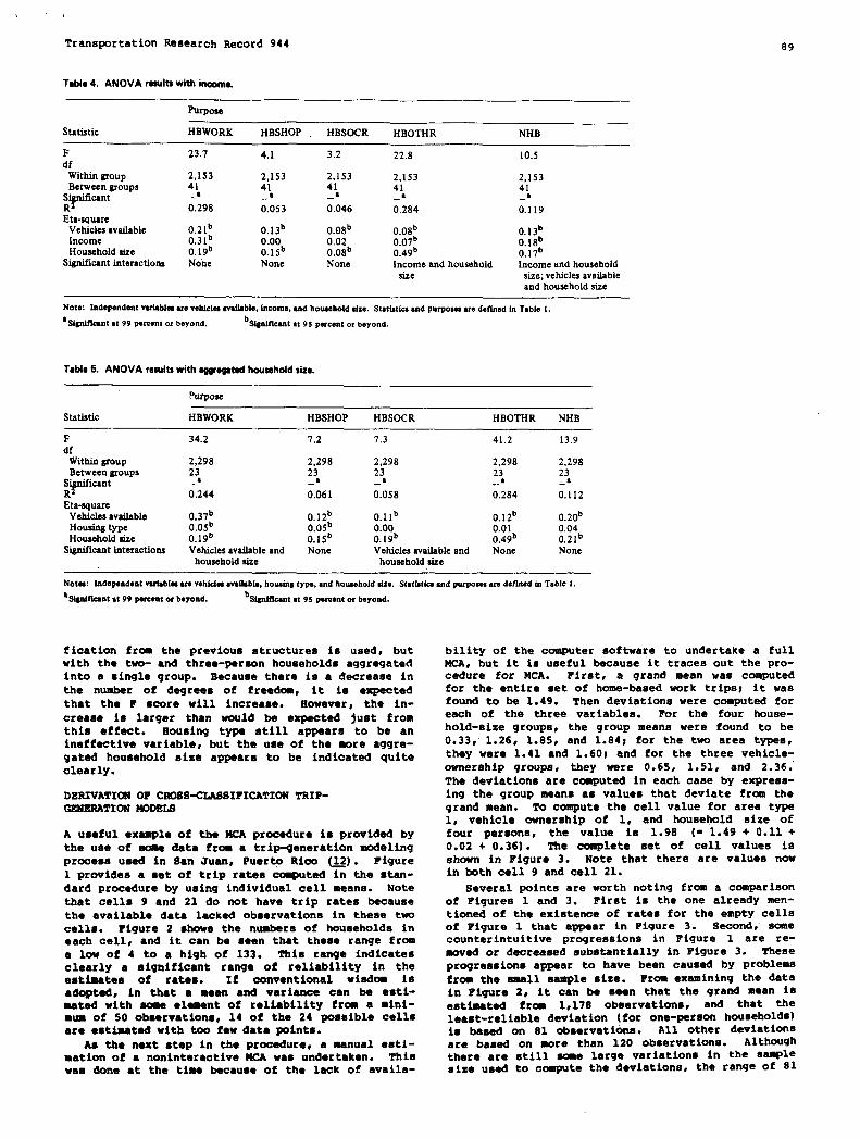
Transportation Research Record 944 89
Tablo4. ANOVAre$ultswith ittoosme.
Purpose
Statistic HBWORK HBSHOP HBSOCR HBOTHR NHB
F 23.7 4.1 3.2df
22.8 10.5
‘Within gxoup 2,1S3 2,153 2,153 2,153Between groups 41
2,15341 41 41 41
S“ “ficsntR~
-~ -a –~ –~ –~0.298 0.053 0.046
Eta-square0,284 0.119
Vehicles available o.21b o,13b 0.08b 0.08bInwme o.31b
o.13b0.00 0.02 o.07b
o.19bo.18b
Household sire 0.15’J 0.08b o.491’ o.17bNgrrificantinteractions None None None income and household Income and household
size size; vehicles availsbleand household size
Note: hdependsnt tibl~me veMclStw~bl., hcome, Mdhowhold~ze. Statktim andpu~om Uedefiedln Table 1.
‘ S@Mssnt tt 99 pwcsnt or bsyond. bS@fICSnt M 95 percent or beyond.
Table5.ANOVA resultswithaggrzgztrdhouseholdsize.
Statistic HBWORK HBSHOP HBSOCR HBOTHR NHB
F 34.2 7.2df
Witbin gxoup 2,298 2,298Between groups 23 23
:icant –~ -a0.244 0.061
Eta-squareVehicles avsilsble o.37b o.121’Housing type O.osb O.osbHousehold sire o.19b 0.15’J
Signifhnt interactions Vehicles avsilsble and Nonehousehold sise
7.3 41.2 13.9
2,298 2,298 2,29823 23–~ :: –a0.058 0.284 0.112
O.llb o.12b O.zob0.00 0.01 0.04o.19b o.49b o.21bVehicles avsilable and None None
household sire
Notss: $ndepsndem Vulsblss srs vehlsb wsilsble, houslns type, snd household she. Ststistiwsnd purposessre defined in Table 1.
●SIudflcaatst99permnt or b. yond. b~t at 9S percent or beyond.
fication frcsathe previous structures is.used, butwith the two- and three-person households aggregatedinto a single group. Because there is a decrease inthe number of degrees of freedom, it is expectedthat the F score will increase. However, the in-crease is larger than would be expected just fromthis effect. Housing type still appears to be anineffective variable, but the use of the more aggre-gated household size appears to be indicated quiteclearly.
DERIVATION OF CROSS-CLASSIFICATIONTRIP-~TION ~DSLB
A useful exaaple of the MCA procedure is provided bythe use of some data from a trip-generationeodelingprocess used in San Juan, Puer~ Rico ~2). Figure1 provides a set of trip rates coaputed in the sten-dard procedure by using individual cell means. Notethat cells 9 and 21 do not have trip rates becausethe available data lacked observations in these twocells. Figure 2 shows the numbers of households ineach cell, and it can be seen that these range frenaa low of 4 to a high of 133. This range indicatesclearly a significant range of reliability in theestimates of rates. If conventional wisdom isadoetsd, in that ● ●ean and variance can be esti-mated with some ●lement of reliability from a ●ini-mun of 50 observations, 14 of the 24 possible cellsare ●stimated with too few data points.
AZ the next step in the procedure, a menual esti-mation of a noninteractlve14CAwas undertaken. Thiswas done at the time because of the lack of availa-
bility of the computer software to undertake a fullMCA, but it is useful because it traces out the pro-cedure for MCA. First, a grand mean was computedfor the entire set of home-based work trips~ it waafound to be 1.49. Then deviations were computed foreach of the three variables. For the four house-hold-size groups, the group means were found to be0.33,’1.26, 1.85, and 1.848 for the two area types,they were 1.41 and 1.60$ and for the three vehicle-ownerahip groups, they were 0.65, 1.51, and 2.36;The deviations are conputed in each caae by express-ing the group means as values that deviate from thegrand mean. To compute the cell value for area typz1, vehicle ownership of 1, and household size offour pereons, the value is 1.98 (= 1.49 + 0.11 +0.02 + 0.36). The complete set of cell values iashown in Figure 3. Note that there are values nowin both cell 9 and cell 21.
Several points are worth noting from a crwnperisonof Figures 1 and 3. First is the one already men-tioned of the existence of rates for the empty cellsof Figure 1 that appear in Fiqure 3. Second, somecounterintuitive progressions in Figure 1 are re-aoved or decreaaed substantially in Figure 3. These
progressions appear to have been caused by problemsfrcm the zsaellsample size. From examinirw the datain Figure 2, it can be seen that the grand mean ieestimated froa 1,178 observations, and that the
least-reliable deviation (for one-person households)is based on 81 observatibs. All other deviationare baaed on snore than 120 observations. Althou9h
there are etill some large variations in the e.smplesize used to ccmpute the deviations, the range of 81

90
F@ra 1.Conwntiond tripmtw: honwbawdwork.
= Vehicl=Area Tvne /DU 1 ~ 4 5+
40.30‘..48,:.35?.39
‘ FFEEEIRural LowDensity 2 . .
—.
2 1 ‘o.~ ‘1.29 ~5$ ~69
Urban High
Density 2+ 4- 42.19?.70?.59
Fiwm 2 Numb4r of households by cell of orow-olawification.
:rossclass Persons/DU
Vehicle4 I I I i
Area Tvoe
1
Rural LowDensity
2Urban High
Density
‘w
‘OR7=F711‘1 ‘2,y,’,-1‘9,,-120,3
-12+ 4’ ~s’
I 1‘“ 24”—
to 609 obaervatione represents a much lesa-aiqnifi-cant variation in reli&bility than in the data usedfor Figure 1.
Figure 4 presents the reaulte from a full-inter-action MCA for the aama data. There are clearlyama aajor interaction in this apacificatlon of themodel, aa shown by the differences in the ratea be-tween ?igurea 3 and 4. The anomaloua decreaee inrate between four and five or more paraon householdsremaina and ia of a similar order of rnagnituderwhich auggeata that this result ia etructurad in thedata. For the remaining differences, some ratee arehigher than before, whereas others are lower. Ar’is
Transportation Research Record 944
Fi~m3. NonintemctivO~tiprati: horru-bwedwark.
crossclass Persons/DU
Vehicle$:
Area Tvne /Du 1 ~ 4 5+--J
o 4000“Q ‘1.12:.10
1 1 ‘o” ““ 4’; +“Rural Low - - g-- ~ ~ ~
[+ d
Density 2 1.30 2.23 2.83 2.81
— . . .
0 ’3000p“”” 50” +“’1
2 ‘1 - ~z: ““ ‘“9 ?J7Urban High
‘ensity 2+ 4’.” 9- 92.64:.62~. 1 I 1 1 i
Fiwre4. FullMCA triprata%honw-bewdwork.
:rossclassI I Persons/ DU I
Vehickd)
14reaTvDe /DU 1 ~ 4 5+
40.12 ~0.62 :.o1 ?.96
-1 J1 1 ‘O.M ‘ 4 ‘
Rural Low — ‘--~ ~’”3’ ~“75 J’”Density 2+ 1.63 2.13 2.52 2.47
‘---i-o~2
Urban HighDensity
—-J J J
1 +’4“1“3’‘V’”7320’”67J J 23 24
2+ a’1.6, ‘22.11 2.50 2.45
expected from the theory, the range of trip rates ialower in Fiaure 4 than in Figure 3 bacauae account-ing for in~eractions dacrea~ea the net effect ofeach variable. Thus the higheet trip rate in Figure3 is 2.83, whereaa the higheat rate in Fi9ure 4 ia2.52. Similarly, the loweet value hae inz?reaaadfrom 0.00 in Figure 3 to 0.10 in Figure 4. Perhapathe moat marked difference in the two figures ia betwaen the one and two or -more vehicle households.The large differences at all -houeehold-size valueabetween these two have dacreamad markedly in Figure4, and the valuea of the one-vehicle households areaubatantlally higher in the one-paraon Itouseholda,

,’,
TransportationReeearch Record 944 91
and lower in the largeet households for Figure 4qared with Figure 3.
Some etatiatical comparisons among the resultsserve to illustrate the differences better than canba seen from a visual inspection. Pirat, root meansquare (sMB) errore were calculated between Figures1 and 3, ?igures 1 and 4, and Figures 3 and 4. ForFiguree 1 and 3, it ia 0.47; between Figuras 1 and 4it increasee to 0.51; but it ia only 0.24 betweanFiguraa 3 and 4. This 10 about aa expected. Thelargeet difference is between the conventional rateeand the 14CArates with full intecactiona. The dif-ference between BKA with full interactlone and with-out is by far the leaet of the differencaa. Givenan average trip rate of around 1.45, the diffarenceebetween the conventional method and the NCA methodeare on the order of one-third of the average triprate.
Chi-square contingency tests between values closeto 1.0 are notoriously misleading because the valueof chi-square la nacesearily small in ouch a caae.This case is no exception, with the three c~ri-aone producing chi-squares of 1.88, 4.22, and 1.30,●ach with 21 degrees of freedom. These values wouldnot be conaiderad significant. ikmmver, if theratae ara multiplied by the number of houaeholda inthe sample (Figura 2), the chi-square teat would befor differences in the numbers of trips produced forwork. In this caae the chi-aquaree are 55.5, 19.0,and 41.4, reapactively. The degraee of freedom arethe eama ae before, and all valuee except the ●acondone are significant beyond 95 percent. The low chi-aquare between Figures 1 and 4 appeare to arisepurely by chance, where two of the larger groupe ofhousehold are associated with a small difference intrip retee, fortuitously. It ia not clear whetherthie reeult should leed to a conclusion of no sig-
nificant difference in trip ratee between the twocasee. ~us thesa reaulte indicate some real dif-ference in trip ratee that are likely to lead tosignificant differences in forecasts.
Tha two caee studies presented in this paper serveto illustrate the potential prwidad by the NCAmethod ●nd ~ from which it stems. This proca-dure overcomee ● number of the criticisms that havabean made before about cross-classification modele.Specifically, the method permits a statimtlcallybaeed selection of variablee for the croee-claaeifi-cation model, and also allowe oompariaottmto be mdebetween alternative groupings of any given vari-able. Frcm this it ie possible to provide a modelstructure that has both conceptual ●nd statisticalmerit, rather than relying only on a conceptual se-lection.
Second, the method prwides a etatistioally soundprocedure for ●stimating cell means, which reducesthe inherent variability of rates computed from dif-
ferent size samples of households and is capable ofproviding estimates for eon cells where data may belacking in the base data set (although the use ofthie capability does reduce eons of the availablestatistical information). Third, there are good-
neSe*f-fit atatistice frm all of thase steps inthe procees that permit more epecific mmparhrme tobe made, good hypothesis-teeting procedure to befolhwed, and results to be aaeeaaed in terms of theamount of the variability of the dependent variablethat is captured in the model. Finally, and mostimportant, the method takea into account the inter-action among the alternative independent variablea,which have never been taken into account in standardcroee-classificationmodels.
It should be noted that similar modelo have beendeveloped for predicting vehicle availability, aswall as for trip productions by a variety of pur-poses. There is no reason why euch crose-claeeifi-cation models ehould not be built for any otherphenomenon that ia appropriately modeled by thisprocedure. Principally, any phenomenon that has anonlinear, and poesibly discontinuous, functionalform, and that ie meet readily ralatad to variableathat are categorical in nature, would be a primacandidate for the method.
1.
2.
3.
4.
5.
6.
7.
8.
9.
10.
11.
12.
Guideline for Trip Generation Analyeis. FRWA,U.S. Oepartaent of Transportation,1967.G.M. NcCarthy. Multiple+egreaeion Analysis ofSouaehold Trip Generation-A Critigue. RRB,IiighwayResearch Record 297, 1969, pp. 31-43.H. Kasaoff and E.D. Ueutachman. Trip Ganera-tion: A Critical Appraisal. EBB, Highway Re-search Record 297, 1969, pp. 15-30.R. Lane, T.J. Powell, and P. Prestwood-Smith.Analytical Transport Planning. ?IalatedPrese,Wiley, New York, 1973.P.R. Stopher and A.R. Ueyburg. Urban Transpor-tation Modeling and Planning. D.C. Reath andCo., Lexington Booke, Lexington, Maae., 1975.N.L. Johnson and P.C. Leone. Statistics andExperimental Deeign: Volume II. Wiley, NowYork, 1964.D. Segal. Discrete Nultivariate Uodel of Work-Trip Node Choice. TRS, Transportation ResearchRecord 728, 1979, pp. 30-35.P.R. Stopher. Goodneaa-of-Fit Heaauras forProbabilistic Travel Demand Nodels. Transpor-tation, Vol. 4, 1975, pp. 67-83. —
l?.ii.Nie, C.H. Rull, J.G. Jenkins, K. Stein-brenner, and H.D. Bent. Statistical Packagefor the Social Sciences, 2nd ad. McGraw-Hill,New York, 1975.P.M. Allaman, T.J. Tardiff, and F.C. Dunbar.wow Approached to Understanding Travel Be-havior. NCBRP, Rept. 250, Sept. 1982, 147 pp.Schimpeler-corradino ASSOCiOtee. Review andRefinement of Standard Trip Generation Model.Florida Department of Transportation, Talla-haeaee, Final Report Task B, June 1980.Bchimmeler-rradino Associates. Urban Trane-porta~ion Planning Ncdels. Department ofTransportation and Public works, ~nwaalthof Puerto Rico, San Juan, Final Rept., July1982.
Pwblicatfonofthiapzp.rrrponsoredby GwnmitteeonTwelw Behavwrandvaluer.

92
Some Contrary Indications
Household Structure
KATHIE G. MoDONALOAND PETER R. STOPHER
Transportat ~on Rea@arch R_rd 944
for the Use of
in Trip-Generation Analysis
The variables used to predict household trip-generation ratas hava long been anareaof eonoarn for transportation plannars;these variablaaindudzd householdsiza, number of vahidas owned, and ineoma. Howavar, a raaznt NCHRP studythat used linear repression analysis hee proposed thet a houeehold-scruztrsravarizblawould corraleta mow strondy with trip rates than almost ●ny otharvariabla,axrept vehiola ownarship. In particular, this should improva tha modalsignificantly tiara it is mmbined with vahicla ownarship and used es a substi-tute for houaahold siza. Tha results of a trip-penerationarrdyd$ performed ondata from tha Miiwast by using multipla dsssificetion analysis (MCA) inron-lraettolinearregressionaradewribed.Tha household-struoture verizbla wasteetsd by using both analysis of varianoeand MCAto datermins how wall tlravarisbla performs in various modal struoturaswhan compared with other vari-.sblas.Theothervariablestestedwaranumberof oarsor vahiclesavailable totha household, houwhold size, housing type, total numlwr of amployzd per-sons, houwhold inoonsa, and total number of licensed drivars. It wee oondudedthat tha househdd-struotura variabiadid not perform sigrtifioantlybatter thanthe other variablw tasted.
With the increasing acceptance into practice of tre-havioral mcdela for travel forecasting, recent re-search by the NCHRP has focused on enriching travel-forecasting atodelswith theories and procedures fromthe behavioral sciences. [Note that these researchresults are from work done at Boston College forNCWNP Project 8-14 (New Approaches to UnderstandingTravel Behavior); the report Is available on re-guest from NCHNP.] One of the first potential di-rections examined for translation into practice isthe incorporation of behavioral concepts in trip-generation modeling at the household level. As partof this research, Charles River Associates (-)proposed that a household-structure variable woulderignificantly improve the performance of such amodel (~).
This proposal was based on the premise thathouseholds with differing structures, in terms ofadults, children, and personal roles, would havediffering activity requirements, arobility COtt-straints, and opportunities for trade-offs withother household members or for trip chaining. Thusproposed changes in household structure, such as anincreasing percentage of single and single-parenthouseholds as well as adult households with nochildren, as is expected within the next decade,would have a significant effect on trip-generationrates within a population. It is argued that such avariable should add behavioral content that is lack-ing frca traditional trip-generation models, whichgenerally have included such variables ae householdsise, nuraberof vehiclee owned, and incoaaeto pre-dict houeehold trip rates. Furthermore, a house-hold-structure variable would be more significant incapturing changes in the future than many of themore traditional variables used.
The household-etructure categories proposed werebased on the age, gender, marital status, and lastnames of each household member. These variables de-termined the presence or absence of dependentswithin the household, the number and type of adultspresent, and the relationships eraong and of houze-hold members.
The results of an application of this household-structure variable in trip-generation analysis in aMidweet study area are described. The value of thisvariable is compared with other variables that weretested at this the by using multiple claeaificat~onanalyeis (MCA) (see paper by Stopher and mcDcmald
elsewhere in this Record). WA is ●n ●xtension ofanalysis of variance (AlS3VA)that, for ● eat ofclaeaified data, expreeses group means ●s deviationfroa the grand mean.
HmsEsOLD—smucTvRECowcEPT
The household-structurevariable defined by CRA ~Prh3e0 eight household Cat~Orha8 male ●nd female
single-person households, single-parent households,couplee, nuclear families, adult familiem with chil-dren, adult families without children, ●nd unrelatedindividuals. Age 20 was used ●s the cutoff to dia.tinguiah between children and ●dultm. The8e catego-ries were determined by using the method shown inFigure 1.
It was expected that these categories would havevarying effects on trip rates. Mults living ●lonewould be less 8cbility constrained then those ●dultsliving with children; but they would have acme ofthe opportunities for trip coordination produced byliving with other adult members. Single-parentf.zxilieswould have both increaeed mobility ccm-straints as well ae no opportunities for trip ocor-dination, whereas couples would have the ●dvantegeaof the opposite of both of theee. ~ ●dult feBilywould have further increased opportunities for tripcoordination, but would perhaps differ from ●n adulthousehold of unrelated individual where individualactivities would possibly be less influenced byother houzehold members.
More specifically, when tripgeneration rates ●reanalyzed by purpose groups, differences between thetrip-generation ratee of these household categor~eowould be expected. Those households with ohildrenwould be expected to have ● greater proportbn ofschool tripe end trips eervittgpassengers than thosehouseholds without children, whereao the lattertmuld probably have a greater proportion of zooial-recreation tripe.
CRA examined this houeeftcld-structureconcept byusing Baltimore survey date with regression anely-SLS, where the dependent variables were trip-genera-tion rates by purpose mode, and the indePendent VU-
iables tested included, in ●ddition to hcueaholdstructure, vehicles owned, income, numkm Of pemormolder than 12, age etructure of hcueehold, hou8imgtype, number of preschoolers preeestt, n-r of
gradeeohoclere preeent, ●mployment •~tus, r-,population per residential eoret ● aity M8it alu-sifioetion, and length of reeidenoe ●t that ad-drese. The trip-purpcee groups defined ●e the de-pendent variables were as follows: totalh~~eedtripe, home-based work tripe, hcme+aeed ~in9tripe, home-based pereortal businese tripe* has_based entertainment and ~unlty tripe, home-baaedvisit and social tripe, and home-based ●wvice andaccrmpany-travelertripe.
CRA concluded that tne Itoueehold-etructurevari-able was 8ignificent in predicting trip frequestcY.It should be noted, however, that tbe regreeeicnewere constrained to use all independent variablee topermit comparability, even’tbcpgh veryistg numbere ofindependent variables were highly insignificant.Potentially, intercorrelationaamong variables couldhave masked acme of the true underlying relation-

,
Trans~rtatiOn Research Record 944 93
F~ml. CRAflovmhart ofhousahold typologf.
HOUSSHOLL)
- lAND MARRIED=
y.
P II HOUSSHOLD I
Nll# FEMALES = 1
=
N
v
HOUSEHOLDTYPE-UNRSLATEDINDIVIDU&Sw w
SOURCE: CharlesRiver Associates, 10 SO.
ships. CRA concluded that, of two camaonly usedtrip-generation variables--number of vehicles ownedand income--only number of vehicles owned out-per-formed the household-structurevariable.
CASE STUDY
The analysis of travel dats collected in the Midwestexamined the household-structure concept. The datawere collected from a stratified random sample ofthe population in seven counties (~). The principalpurposes of the survey were to provide
1. The means to update trip-generation rates andmodal-split aodels,
2. Attitudes of the population tmtard transpor-tation and energy,
3. Attitudes toward possible changes in thetransit system, and
4. Preferred methods of obtaining information oncarpooling.
The data were collected by using an in-hose inter-view and a 24-hr travel diary snd Included the vari-sbles age, gender, possession of a driver’s license,employment status, and income of household members,all of which were avsilsble for use in tr@-genera-tion analysis.
The final data set consisted of 2,446 house-holds. Of these households, the average householdsize was 2.9 persons per household, where less than50 percent (1,656) of all households had two or lesspersonst 60 percent (1,483) had no children; and 53percent (1,300) were two adult person households.In addition, alaost 80 percent (1,952)of all house-holds had at least one car available for use, and 30percent (734) had more than one; 80 PSrCent (1,875)occupied single-family dwellings; and 87 percent(2,124) of all households had at least one licenseddriver. Seventy percent (1,724) of all householdshad at least one person eaployed, 63 percent (1,537)had at least one person employed full-time, and 60percent (1,468) of all households had 19S0 incomesgreater than $15,000, with 14 percent (341) greaterthan $35,000.
The household-structure variable defined by CRAwas derived from the data by the method shown inFigure 2. ~is differs slightly froa the CRA flow-chart because of the definition of the variableswithin the Southeastern Michigan TransportationAuthority (SR9TA) dsta set. These differences in-clude the following: (a) the cut-off age betweenchildren and adults is 1S years instead of 20, and(b) relationship codes were uned to distinguish be-tween adult fadlies without children and householdsof unrelated adults; the last name of each pereonwss not ascertained in the survey.

94
Figure 2. Flowchart of household typeslogyused in analyzing SEMTA data.
1~ousehold
‘“e “ 0Single)-fale
HouseholdType= Single Type= Single
‘are”’ @Female
@
TransportationResearch Record 944
Type =
I pm,,, @) ,-
1 1 J
Household Type= Adult Family
N
% Except Reapondant( i.e. Oo Not Check Person # 1)
I I I
Table 1. Householef-strurtwe characteristics of SEMTA data.
Household-Structure No. of Percentage of
Category Households Households
Single male 200 8.3Single female 2S4 10.5Single parent 1so 6.2Couple 502 20.8Nuclear family 483 20.0Adults with children 347 14.4Adults with no children 420 17.4Unrelated individuals 56 2.3Missing ~Total 2,446
The final breakdown of the data into these house-hold categories is given in Table 1. Abost 19 Per-cent are single-pereon households, with ali9htlYmore single females than single males (2 percent).Single-parent households comprise only 6 percent,whereas couples and nuclear families comprise 21 and20 percent, respectively. Adults with children makeup #lightly fewer households than those withoutchildren (14 percent compared with 17 percent), buthouseholds of unrelated individuals form the small-est category--2 percent of all households. Thirty-four households could not be classified. These in-cluded 17 eingle-person households where the personwas younger than 18 years old.
lb analvze the role ofvariable in trip-generation
the household-structureanalyeis, this variable
and seven other-variables that ware also thought toplay a significant role in trip-generation rateswere selected from the data set. The other vari-ables eelected were car ownership, household size,housing type, licensed drivers, houeehold income,and total number of employed persons in the house-hold (see Table 2). These eight variablee werefirst analyzed by using one-way ANOVAe to determinehow well they performed against the household-struc-ture variable. Subsequently, the variables were
analyzed by using one-way ~s to determine theeffects of varying grouping strategies on thecategories within ●ach variable.
The household-structure variable was grouped inthree ways. The least-aggregate grouping oombinedthe single-male and single-female categories becauseit wae believed that there would be no significantdifference between the overall tripmeking charac-teristics by gender, although there might be smelldifferences for specific trip purposes. The least-aggregate grouping also combined nuclear familieswith adult families with children~ based on the
theory that additional adult members in the house-hold would not significantly change the pattern oftripmeking. The second grouping strategy furthercombines all edult households,-except single personsand couples. This assumes that adult householdsthat consist of related pereons will have littledifference in tripmeking characteristics than those

,..
Transportation Research Record 944
Table 2. Variable grouping strategies used in SEMTA tripgeneration anzlysie.
Variable Name Grouping No. Categories Used in Groupirsg
LIFE I (householdstructure)
LIFE 11(householdstructure)
1-6 123456
12
1-5
LIFE III (household 1-3structure)
NUMCAR(numberofcan O-2availabk to household)
HHSIZ I (household size) 1-5
HHSIZ 11(household size) 1-4
HOUSTYP (housisrgtype)
TOTEMP (total number ofemployed persons)
INC80 ( 1980 householdincome)
TOTLIC (total number oflicensed drivers)
34s
o12
12345
12
34
0-1 01
0-2 012
1-3 123
&2 o12
SinglepersonsSingle parentacouplesFamilies with childrenAdult families without childrenUnrelated individual
Single personaSingle parentsCouplesFamiliea with childrenOther adult households with no
children
Single personsFarni&a with childrenHouseholds with no children
No cars availableOne car availableTwo or mnre cars available
One-person householdTwc-person household
Thre&person household
Four-perann household
Five or more person houa6hnld
One-persnn householdTwn- and thre~person house-
holdFour-person householdFive or more persmrhousehold
MultifamilySingle family
No employed personsOne employed personTwo nrmoreemployedpenona
S3-$14,999S15,00GS34,999>s35,000
No licensed drivenOne licensed driverTwo or more I&naed drivers
.households that consist of unrelated individuals.Thus the theory of a coordination of tripmaking de-cisions between related household rnetira waa ex-amined. The moat severe grouping strategy eeperateshouseholds with children from households withoutchildren, identifying thin characteristic as themoat important in trip decision making. onlysingle-person houmeholda are further dietirtguiahedto reflect unique trip-generationcharacteriatica.
Other variable groupittgaare alao given in Table2. The model II household size grouping, which craa-birtestwo- and threa-pereoethouaeholda, waa examinedafter initial analyaia indicated little differencein trip rataa of these households. Income waagrouped into high-, medium-, and low-inccreacatego-riea.
Finally, UCA (3, and paper by Stopher and Mc-Donald elsewhere in this Record) was used to comparedifferent coeabinationaof these grouped variablea intrip-generation analyaia. MCA derives trip rateawithin a standard trip-generation matrix by usingdeviation from the grand mean of the data act.Thus it improvaa on the traditional method of coas-puting individual cell meana becauaa it permits es-timation of trip ratea for cells that contain nodata. In addition, WA, by using version 6, 7, or Sof the Statistical Package for the Social Sciencen(S2SS) {~), is able to take into account the inter-active ●ffects between independent variablea wherethese variablea have nonzero correlation with eachother. This corrects for the overestimation of ad-juateeentsfrom the grand mean when these correlationsare ignored. This uae of MC!Aand the croaa-claaai-fication structure is different from the CRA ap-
proach, which waa to uae least-aguaresanalyaia to predict the trip-generation
95
regressionmeasures.
The effects of household structure were analyzedboth in terms of the additional level of varianceexplained by the household-structure variable aswell as the level of variance ●xplained when substi-tuting household structure for another variable.
The models examined in trip-generation analysisare given in Table 3. It can be seen that the num-ber of vehicles (NUMVEE) available to the householdwas substituted for number of cara in some modelsbecause this variable performed significantly betteracross all purpose groups.
Table Z. MCAmodels used in SEMTAtrirge.neration analysis.
Trip Purpose
Home-baaedwork ,home-baaedshopping home-baaed aocial-recreation, homa-baSedother,and non-homa-baaadtrips
Home-baaedwnrk, homebsaedshopping, home-based other,and non-homebssed trips
No.
123
12345
MCAModeh
NUMCAR,HHSIZ I,HOUSTYPNUMVEH,HHSIZ l,HOUSTYPNUMCAR,LIFEH, HOUSTYP
NUMVEH,HHSIZ 11NUMVEH,HHSIZ II,LIFEIINUMVEH,HHSIZ II,HOUSTYPNUMVEH,HHSIZ H,TOTEMPNUMVEH, HHSIZ II, INC80
In all three typaa of analysis previously dis-cussed, trip-generation models were examined formotorized trips by specific trip purpose. Initialanalyais distinguished social-recreation trips, butthe final trip-purpose categories examined werehome-based work, home-based shopping, home-basedschool, home-baaed other, and non-home-baaed trips.These final trip-purpqae categories differ from thecategories used by CRA that (a) do not examine non-hrme-beaed trips, and (b) break down the other cate-gory into more specific purpose groupa.
DESCRIPTION OF RESULTS
The reaulta of the ANOVA for ungrouped variables aregiven in Table 4$ the results indicate that acrossall purpose groups the number of cara available tothe household explaina more variation than any othervariable. This result is consistent with resultsobtained by CSA. Rousehold size and housing typeare the next most significant variables acroas allpurpose groups; and whereas the number of employeeein the household explaina the moat variation forhome-based work trips, it does not perform well forall other purpose groupa. Household structure andincoae appear to be of equal strength, although theyperfom better on different purpose groups. Incrsaeie most effective in explaining the total number ofnon-hm-baaed trips, whereas household structure ismoat effective in ●xplaining the number of home-baaed school tripa. The licensed-driver variableranks no better than third in ●xplained variationfor any purpose group.
The ANOVA results of the grouping atratsrgieaper-formed on the household-structurevariable are givenin Table 5. The moat effective grouping is themodel II grouping: single-person households,
single-parent householdat couples, other families
with children, and other adult Stouaeholda. There
appeara to be little difference between the travelconsiderations of adult families that consist ofrelated individual and ttioaethat conaiat of unre-lated individuals, because there is a large increasein the F-ratio acrosa all purpose groups when theseare combined, whereaa the change in the within-group
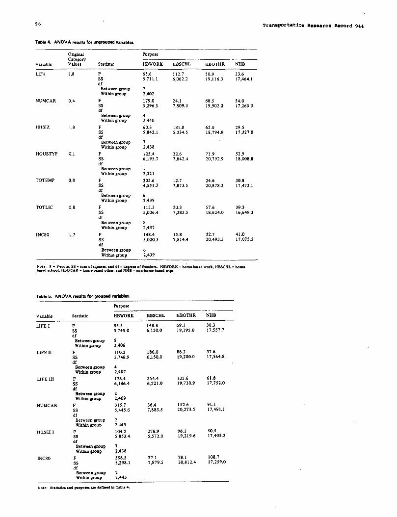
96 TransportationResearch Record 944
Tabie4. ANOVAmwlti fwuWrm@variaM~.
original Purposecategory
Variable values Statistic HBWORK HBSCHL HBOTHR NHB
LIFE
NUMCAR
1,8 FSsdf
Between soupWithin group
0,4 FSsdf
Between groupWithin group
FSsdf
Between groupWithin group
0,1 FSsdf
Between groupWithin group
65.65,711.1
72,402
179.05,296.5
42,440
60.35,842.1
72,438
125.46,195.7
12,321
112.76,062.2
50.919,116.3
23.617,464.1
54.017,265.3
29.517,327.0
52.918,008.8
30.817,472.1
39.316,649.3
41.017,075.2
24.17,809.3
68.519,902.0
HHSIZ 1,8 181.85.334.5
62.018,794.9
HOUSTYP
TOTEMP
TOTLIC
INC80
22.67,842.4
73.920,792.9
0,8 FSs
205.64,551.3
12.77,873.5
24.620,878.2
dfBetween groupWithin group
0,8 FSsdf
Between groupWithin group
1,7 FSsdf
Between groupWithin group
62,439
112.35,006.4
82,437
148.45,020.3
62,439
30.37,383.5
57.618,624.0
15.87,814.4
32.720,493.5
Note: F= F.score, SS=sumof quare&snd df. degre~ of freedom. HBWORK. home-ba#ed work, HB8CHL=homt-based 8chool, HBOTHR = home-bssed othat, ●nd NHB - non-borne-bawd trips.
Table 5. ANOVA rewlta for groupad variablee.
Purpose
Variable statistic HBWORK HBSCHL HBOTHR NHB
LIFE I FSs
85.55,745.0
148.86,150.0
69.119.195.0
30.317,557.7
37.617,564.8
61.817,752.0
91.117,491.1
50.517,405.2
108.717,259.0
dfBetween groupWithin group
s2,406
LIFE 11 FSs
110.25,748.9
186.06,150.0
86.219,200.0
dfBetween SKOUp
Wlthiu group42,407
128.46,146.4
354.46,221.0
135.619,730.9
LIFE111 FSsdf
Between groupWmin group
22,409
315.75,445.6
36.47,883 ..5
112.620,273.5
NUMCAR FSsdf
Between gIoupWitldn group
22,443104.25,853.4
27S.95,572.0
98.219,219.6
HHSIZ 1 FSsdf
Between groupWithin group
72,438
3.58.55,298.1
37.17,879.5
78.120,812.4
1NC80 FSsdf
Between groupWithin group
22,443
Note:StatiseiaandPIM’POSNare defiaod In Ttblo 4.

1,
TransixKtation Research Record 944 97
variance is small. This contrasts with the modelIII grouping (single persons, families with chil-dren, and other families without children) where,although there is a large increase in the F-ratioacross all purpome groups, and most particularlywith home-based school trips, this is accompanied bya significant increase in the within-oroup variance.
The ANOVA results of the other grouped variablesare alao given in Table 5. It is clear thst thenumber of cara available to the household remainmthe most significant variable in household trip-generation analysis. Once again, the F-scores aresubstantially greater across all purpose groups,even taking into account the difference in the de-grees of freedom. Model II household size, whichcombines two- and three-person households, improveson model I household size by increasing substan-tially the F-ratio without increasing substantiallythe within-group variance. Household income (1980)is also effective in explaining trip-generationrates for all purpose groups except hcme-basedschool and home-based other, and thus nay be usefulwhen applied to specific trip-purpose models. Thetotal number of licensed drivers, a variable thatperformed so poorly in earlier analysen, was nottested as a grouped variable.
The NCA results for the two sets of trip-purposegroups are given in Tables 6 and 7. From the firstset of purpose groups (Table 6)? the basic modelconsists of number of cars or vehicles available tothe household and model I household size. Of thevariables used as additions to this basic model,housing type clearly performs the best across allpurpose groups. In addition, this model performsbetter than the model that uses number of cars,household structure, and housing type, where houme-hold structure is used as a substitute for householdsize, an alternative suggested by CRA (~). Furtherimprovements are made by using number of vehiclesavailable to the household instead of number of carsavailable.
The results of the models analyzed for the secondset of trip purpose groups are given in Table 7. Aninitial examination of these MCA results gives theimpression that the model that uses household struc-ture, household stie, and number of vehicles ia thebest model, particularly from sn examination of theF-ratios. This is, however, a misleading impres-
sion. The ?-ratio for an entire model is usuallybased on all main effects and interactions. If data
are missing in some cells of the matzix that definethe ANOVA problem, SPSS Q) is unable to calculatethe interactions and computes an ?-ratio on the main
effects only. This ?-ratio has substantially fewerdegrees Of freedom than one on the main ●ffects ●ndinteractions, and therefore it must be a larger nu-meric value for the same significance level.
The household-structure model generated ●-tycells for some combinations of household structure,household size, and vehicle availability (e.g., thehousehold structure of a couple can occur only fortwo-person households) and resulted in suppressionof interactions in the AZ?OVA. The model that uaeahousehold structure is the only model in Table 7 forwhich this happened, and leads to an inflated F-ratio compared with all other models. When F-ratiosare calculated on main effects only for the othermodels (as indicated by a footnote in Table 7), theF-ratios are almost all larger than those for thehousehold-structure model. Thus the addition ofhousehold structure to the baolc model of number ofvehicles available to the household ●nd householdsize does not improve its performance for ●ny trip-purpose group.
Of the other variables examined as additiona tothe model, the total number of workers in the house-“hold improves the model for home-based work tripe.Household income (1980) and the model II houaehold-aize variable are both improvements over the house-bold-structure variable. Income is better in ex-plaining home-based work trips and non-home-basedtrips, and housing type Is better in explaining theother trips. Thus, unless a separate model is de-veloped for home-based work trips by using the em-
ployment variable, the model of number of vehiclesper household, household size, and housing typestill remains the best approach. These concluaionasupport those found with the previous set of purposegroups, with the exception that the model 11 house-hold size performs better than, and thus replsces~the model I household size.
~SIONS
In the trip-generation analysis of the case studydata, the household-structure variable did not per-
Tzble6. MCAra8ultzef8ztlmedslsu@in~ziwSEMTA*.
Furpozz
Model Statiztic HBWORK HBSHOP HBSOC HBOTHR NHB
NUMCAR, HHSIZI,HOUSTYP F 29.5 s .9 6.0 35.1 11.4df‘Betwezn ~oup 29Within group 2,292
SIG 0.000 0.000 0.000 0.000 0.000R2 0.261 0.062 0,060 0.295 0.113
NUMVEH, HHSIZI,HOUSTYP F 29.1 5.6 5.0 3s .5 11.5df
Between group 29Withingoup 2,244SIG 0.000 0.000 0.000 0.000 0.000R2 0.261 0.060 0.053 0.29S 0.116
NUMCAR, LIFEI1,HOUSTYP F 2S.3 5.2 5.1 26.4 9.5df
Betwzen group 29Within group 2,259
SIG 0.000R2 0.254
0.0000.056
0.0000.054
0.000 0.0000.238 0.096
Not.: SIG- slznltlcance, HSSHOP = homo-hued SIIOPPIIUT,HSSOC = hom~bawd mclal+.c?ation, snd the rat are defined In Tabla 4.

98 TranSpOrt~tiOn Research Record 944
Tsbie7. MCAresults ofszsll modolsusad inanzlyzi~ SEMTAdats.
Purpose
Model Statistic HBWORK HBSHOP HBOTHR NHB
NUMVEH, HHSIZ 11
NUMVEH’, HHSIZ II, LIFE II
F 74.1 14.0 15.9 29.1df
Between sroupWltbin group
SIGR2
112,4340.0000.246
94.194.lb
0.0000.057
16.516.5b
0.0000.060
21.021.ob
0.0000.109
34.034.ob
F
dfBetween groupWithin group
SIG~z
92,4020.0000.261
34.8127.2b
0,0000.058
0.0000.073
0.0000.113
NUMVEH, HHSIZ II, HOUSTYP F 7.024.9b
7.324,2b
13.947.3b
dfBetween groupWithin group
SIG~2
232,2990.0000.246
0.0000.061
0.0000.059
0.0000.108
9.738.6
NUMVEH, HHSIZ U, TOTEMP F 38.7176.2b
5.019.2b
5.514.2b
dfBetween group 33Witf2is2group 2,268SIG 0.000R2 0.348
0.0000.057
0.0000.055
0.0000.105
10.444.3b
5.221.lb
5.622.3b
NUMVEH, HHSIZ 11,INC80 F 32.4148.1b
dfBetween KOUpWithin group
SIG
332,4120.0000.298
0.0000.057
0.0000.060
0.0000.112R2
Note:Ststlst{csandpurposesdefhdinTables4and6.
‘ImmctlonaSuppressed. bF-ratioscdcussted on main effects only.
torily in this trip-generation analysis, there wouldbe problems implementing it in trip-generationmodels. When presented with a possible tr@-genera-tion design that used the household-structurevari-able, a metropolitan planning organization (MPO) wasreluctant to implement it. Although CRA stated thatthe household-structurevariable could be easily ob-tained from census data, the !4p0 expressed doubtsthat it could be. Forecasting at a zonal level,particularly to obtain distribution of households byhousehold-structure category, appears fraught withproblems. Possibly, forecasts could be made at theregional level of the constituent elements of house-hold structure, but current analysis-zone forecastsin most metropolitan areas do not include theee com-ponents and would possibly be difficult to add tocurrent forecasts. In addition, household structurecannot be used as a policy variable, whereas othervariables, particularly housing type, could beused. l%is aleo helped itsthe decision to excludethe household-structure variable from the S~TAtrip-generationmodels.
form as well as was expected from the CRA analysisof Baltimore data. ‘rhismay, however, be a resultof the different methodologies that were used in thetwo analyses. The analysis reported in this paperapplied traditional cross-classificationmodels thatused 14CA to predict cell-by-cell trip rates. Thefinal model consisted of number of vehicles, house-hold size, and housing type. However, subsequentanalysis not discussed in this paper has revealedthat the use of an area-type variable instead ofhousing type may improve the models even further.
Figures 3 and 4 show the resulte of the automaticinteraction detection (AID) analysis performed on1973 Niagara Frontier Transportation Committee (Buf-falo) and a 1974 Genesee transportation travel sur-vey (Rochester) date for all trips and for homa-based nonwork trips (~). The nufnbarof vehiclesrepresents the first cluster. This supports boththe conclusions drawn by CRA and by the authors.This is followed by number of children (usually afunction of household size) and age of the oldestchild. The final clusters are based on houeeholdsize, vehicles per licen.zeddriver (a function ofboth vehicles per household and household size),household employment status, and number of vehiclesavailable to the household. Although the variousage classifications may be a function of householdstructure, they may also be a function of other var-iablea (for example, household size).
xt is also pertinent to note that even had thehousehold-structure variable performed satisfac-
RBPERBNCBB
1. P.M. Allaman, T.J. Tardiff, and F.C. Dunber.New Approaches to UesderetandingTravel Behav-ior. NCERP, Rapt. 250, Sept. 1982, 147 pp.
2. R. Parvataneni, P. Stopher, and c. Br~. Ori-gin-Destination Travel Survey for Southeast
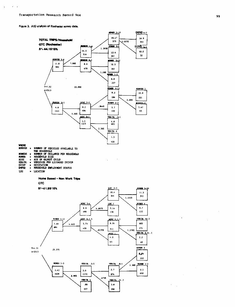
,,, ,
Transportation Research Record 944 99
amJs5-1o m 6.7t
TOTAL mnlouehm16.17
\ J
16.9
1.027X .341
GT’c @0d9eeter)IK66m 3-4 a ,* ,.
R*.44.1S15% IA.S12.6 10.2
314241 32
NIWW 2-6 1 1
11.6 0.6 10.3
678 241J
- 1-2
//Y-7.52
A-2513\
22.99X
Y 6.0237 I
m4- 1
9.2 m.4ym#_&l AGx 2-s
4.0 8.2
1521 606 122 635.16:
%
o-l 92WOL.3-1
3.5 &.8l\15 683
2. ‘367,vEH/oL o
1.5
432
WUIRSMMVEN . NUW2?R DP WICLES AVAILASL.ETO
THEINX2SSNCU2~ : =o~ CHXL3RSDPERNDUSEJKILD
AGcJc s AGEW CO&ST CNILD~DL = VEHICLESPSRLICSNSSD DRIVEROXIJP z DCCUPATI~
* SOUSUWD R9PLOWWT STATIJSI.lx = IC22ATXX
Home Bssed-NoaIWork Tr@
GTC
LOr 2-1
1“1 m
o
11.5
i211
I
AcOc3-4 Lnrl
> m4
8.9 5.14 8.7
400 136 133
NIJmlll4-II Acw 0-2.5 .Au3c 0.2 5 vmloL -4-2
7.49 5.71 6.2k 683
884 &09 311
JLGQc1 vrwm o. 0-.1
4.0
93
/ 1 I L L
Y-&.2125.17X
A-2513
\
rJu70rH3
xl
4#9
212
V2WDL .3-5 9ZWOL .&S1
3.0 2.7
1629 1172 652
VVllOL e 9U!IOL.3-.7
.00I
H

100 Transportation Research Record 944
FiWN 4.
UHERENUMVEH :
tWWDS =N(R4iN :AGOC=VWDL :OCCUP =D4PHD:
m=
AIDanalydsofMO data. M12?UHk-9 ~ 6-7
28.87
TOTAL ~ 7
m WfdO) 2,6,7,1cOcct,? NIJ?SIH1-3R8.~7@% ~ L3U.*% ~ !?%wl
!4.1961 ‘r ““-p L I I I
\NLM4H3-9
NIWVEH0-1 mlvm 1 w/mlr5,5 n-1 6.8 3,4
1189n79
b56 28!
I,EHI1)L0-5 Amc1-5a.~
NUk@ER OF VSNICLES AVAILASLETO h2> 11 0THE NDUSENOLD 310NWER of CHILDRED PER HOUSEHOLDHOUSEHOLD SIZEAGE W OLDEST CHILDvEHICLES PSR LICENSED DRIVERDCCUPAT[ON~LD WLOT?SHT STATUS
KCATKN
HoeneDeead-Non Wti TmM=lcR2.34.06D4% Xlxi
/ L 4 I IV-4.49 19.W2II-1962 2WN00.1,2b,? Koc2-5
\8
-7 m1
l&7 2.9 2.73Z42 bA2
2.9732
mH o
.84ZAY
Michigan. TRB, Transportation Re66earchRecord tical Application to Transportation PlanniM.
886, 1982, pp. 1-8. New York State Department of Transportation,
3. N.Ii.Nie. C.E. Hull, J.G. Jenkine, K. Stein- Albany, Draft Paper, Aug. 1982.
brenner, and D.II. Sent. Statistical Package forthe social Sclencea, 2nd ed. McGraw-Hill, NewYork, 1975. R6blieationofthia paperspomoredby GnnmitteeonTr@eler Behavwrand
4. J. Chicoine. The Life Cycle Concept: A Prac- Valuex

Transportation Reeearch Record 944
Maximum-Likelihood and Bayesian Methods for the
Estimation of Origin-Destination Flows
ITZHAK GEVA, EZRA HAUER, AND UZI LANDAU
The design of trti!c management erhamae usually requires knowledgo ofttw pattern of trips on the eyetom under scrutiny. This pattern is ordi.nzrilydescribed by an origindeetinetion (O-D) flow matrix. On. common*of this type of mstrix is the .etimetion,of flows tin the interw~ onapprmohes on ● stretch of road. Estimation is based on intersection flow00unts that we supplemented by ● Iirerssz-plstesurvey. In this paper ● pm-oedure is daveloped to obtain the rnogtlikely O-D flow zetimetes by usingboth intersection counts ●sd resulti of the liowm@@e Uwey. Theprmredure is described in detail on the baeisof ● numzrioel example. An eerlierPSPWreported ● method of zetimztion that rolkk on intersection counts onlyand does not require the oonduzt of ● sample Iioznee-plete’eurvey. An ern-piriral wmminetion is ronduoted to test how astirnstiorr●roumzy inorezsaswhen the edded information from the lirense.@ete survey is used. Thisexamination revzek that wfrenthe supplementary Iioenez-platesurvey is smell,the maximum.likelihood method yields urtsetiefeotofy estimates. This defi-cim’wyis rectified by the use of ● Wyeshn method. TIMrmuki~ m[utionpmredure is simple, and satisfactory estimates ●e prodmad.
A variety. of!transportation planning and managementtasks require the knowledge of the pattern of tripflows between origins and destinations. This pat-tern is usually deacrihed by an origin-destination(O-D) flow matrix. One common task of this type ofmatrix ia the estimation of flows between the inter-section approaches on a stretch of road. The esti-mation is based on a license-plate survey that isfactored up to match counts of intersection flows.
In recent years attention has been given to theproblem of estimating an O-D matrix by using trafficCounts as the main source of information (1-4). Arecent paper (~) descrIbes a method that‘d~partsfrrx! previous workr in that travel behavior isbrought into estimation by information contained insmall O-D samples obtained by a survey. It iStherefore not necessary to rely on speculative mi-crostates (as in entropy models) or to assume thatactual route choice is correctly captured by avail-able models. Rather, the purpose Is to find thatmatrix of O-D flows that is consistent with the ob-served traffic counts and that is most probable inview of the O-D samples observed.
This approecb Is used in the present paper, inwhich a procedure to estimate flows between the in-tersection approached on a stretch of road is devel-
oped ~sed on intersection flow counts and a li-cense-plate survey. The effect of sample size onestimation accuracy is explored in a real-life ex-ample.
In the first section of the paper two alternativelikelihood models, which capture the manner in whichdata are obtained in the field, are presented. Thenormal equations that identify the maximum-likeli-hood estimate are obtained, and an algorithm fortheir numerical solution is described. A numericalexample is presented in the second section. The ex-a~le is intended to illustrate the how-to of themethod and to assist the practitioner in its appli-cation. As noted earlier (~), estimates of O-Dflows can be obtained from traffic counts alone,without having to resort to tedtous license-platesurveys. The increase in estimation accuracy ob-tained as a function of sample size is examined inthe third section. The results of this examinationlead to the development of a new procedure based onBayesian ztatiztics. This procedure is presentedand examined in the fourth section.
101
pRoBxm FO~TION AND SOLUTION
Consider a street section as shown in Figure 1. Theintersection approaches are thought of as originsand destinations. Estimates of O-D flows are de-sired.
Figuml. Exernpleofetreatseotionwitie~tiflo~.
~ @ @
The method most commonly used for this purpose intraffic ●ngineering practice is to count trafficvolumes at every intersection and to conduct a li-cense-plate survey of a sample of vehicles enteringand exiting the street of interest. Usually severaldigits of the license-plate number are recorded andlater matched so as to obtain a sample O-D pattern.The sample ia later factored up in an attempt tomake tbe appropriate sums of O-D flow ●stimatesmatch the corresponding volume counts. The purposeof this paper is to suggest an estimation procedureto replace the arbitrary and often ambiguous factor-ing. The merit of the procedure is that it identi-fies the O-D flows that are mst likely in view ofthe results of the license-plate eurvey and the in-tersection volume counts.
In formulating the problem, tbe following basicnotations are used:
o~ -
Dj =
tij -
T~j =
number of vehicles entering the street atentry approach i (i = lr2,...,m) during aspecified period of time,number of vehicles leaving the street atexit approach j (j = 1,2,...,n) during thesame period of time,number of license plates matched betweenrecords obtained at entry approach i andexit approach j, andnumber of vehicles that enter the street byapproach i and exit it by approach j.
The objective of the exercise is to obtain esti-mates of Tij by using the data Oi, Dj, andtij. The estimation logic is of the customarymaximum-likelihood kind. Thus the O-D sample matrix
(tij) obtained from license-plate matching isthought to be a random sample drawn from the matrixof O-D flows (Ti ).this sample can ~ cap~~~p~~~~i~~~~i~~~~metical model. A search is made for the estimatesof Ti that maximize this probability and at theseme~ime fit all the intersection volume counts.These are the most likely O-D flowerto have pre-vailed at the time of the license-plate survey andintersectionvolume counts.

102 Transportation Research Record 944
llto points deserve mention. First, fOr trafficplanning and management purposes, O-D flow estimatesare needed that represent average conditions ratherthan estimates of flows that have prevailed at thetime of the survey.and D., K ‘0 ‘0’ ‘itl ~~~rlc#s;aZ~would have to be regardedables ](~). Because the focus in this paper is theeffect of the sampling ratio for the license-platesurvey on O-D estimation accuracy, the estimation ofO-D flows that prevailed at the time of the surveyare sought. This is what practitioners have beendoing anyway. The second point has to do with adiscrepancy between the model and the practicalitiesof traffic surveys. In the model the analyst pre-tends that the intersection volume counts, as wellas the license-plate survey, are conducted duringthe same time period. But because of personnel lim-itations, this is seldom true. With these qualifi-cations, the random nature of the license-plate sem-ple is described by using an appropriate probabilitymodel.
The probability model chosen must fit the mannerin which the random sample is selected from the pop-ulation. Thus the essential details of the li-cense-plate survey procedure used have to bestated. To reduce survey personnel requirements andto keep errors of recording in check, it is usuallybest to specify beforehand some part of the li-cense-plate number to serve as the sampling cri-terion. Thus if all even-numbered plates are re-corded, the sampling ratio is 50 percent; if allplates ending with the digit O are recorded, thesampling ratio is 10 percent: and so forth. Pro-vided that the digits selected to serve as a sam-pling criterion are uniformly distributed in thepopulation of license plates, the sampling ratio isestablished when the sampling criterion is specified.
Two alternative probability models are suggestedto capture the stochastic nature of this survey pro-cedure. First, each license-plate match can beviewed as a success of a Bernoulli trial in whichthe probability of success is dictated by the ssm-pling ratio and the rate of errors of recording andcoding. The unknown flows Tij correspond here tothe number of Bernoulli triale. Thus the likelihoodfunction is a product of binomial probability massfunctions. Second, the license plates recorded at acertain survey point can be viewed as a random sam-ple drawn (with replacement) from the constituentO-D flows passing that point. This leads to themultinominalprobability model. Both models are con-sidered and their merits are discussed.
Starting with the binomial model, let Uij de-note the number of license plates within Ti
1.that
satisfy the sampling criterion. The proba ilitydistribution of Uij can be described by the bi-nomial model. Thus
()~Ujj)= ~j r‘U(l-r)TU-uU (1)
where r is the sampling ratio.Equation 1 would be a reasonable description of
the state of affairs if observers in the field wereable to record all license platea that should berecorded and do so without error. In reality, er-rors occur. Thus instead of obtaining Uij match-ing license plates for e stream of vehicles, onlYtij(tij ~ uij) is obtained.
Now the conditional probability mase function(M) of tij is given by
p(tijlU~)=()‘ijqti’ (1 - q)ui’ - ‘i’
t ii
(2)
where q is the probability that nothing goes wrongand the license plate is obtained and processed cor-rectly at both entry and exit.
This case ia known in the literature as partialascertainment (g). In such a case the oriqinal dis-tribution will be distorted. If the rmcdelunderly-ing the partial destruction of original observations(or the survival distribution) is known, the distri-bution of the observed values can be derived. Itwae shown that where the original distributions arePoiaeon, binomial, or negative binomial, the modi-fied distribution is of the same form.
Therefore, the PMF Of tij ia also binomial andgiven by
()Tii (q)ti(l.rq)Tti-tij
fltij)= ~ti (3)
An expression analogous to Squation 3 can bewritten for every possible flow. It can be shown(~) that if Xl,...,% are binomial variates withsamPle size Nl~...vNt* respectively, and a commonprobability of success in each trial, then the dis-
ttribution of X = (Xl,...,Xt) conditional on rx~=
i=ln is multivariate hypergeometric with parameters n,N, and (N1...~). Therefore, the probability ofobtaining a matrix of (tij)if the matrix of flowsis (Tij) is given by
(4)
The identificationof the array T: for which this\probability (or the logarithm of th e probability)
ia maximum ia needed. However, the solution mustsatisfy the traffic count constraints
~ TU=Oi fori=l,2,. ... m (5)j=*
and
; Tij=Dj forj=l,Z.. .,ni=*
(6)
BY forming the Lagrangean, using Stirlin9’s for-mula, taking derivatives, and ●quating to zero (~),the following equation ia formulated:
T;=tu/(l-@j) ;j;;’:”::’;.,
(7)
‘m obtain numerical values for the estimates T; ,the unknown values Al,A2*...#Am Jand B1,B2~...? n
first must be found. ~is can be accomplished by asimple algorithm deecribad in the next section.
The alternative manner of describing the surveyby a probability model ie to consider the randomsample til,tiz,...,tinobtained at etation i as drawnfrom the flows Til,Ti2~.../Tin# which are unknown.Only their sum (Oi) is 9iven. The probability ofobserving this sample is given by the multinominalmodel:
(8)
(The multinominalmodel is only approximate becauseit assumea sampling with replacement. As long aa
the sample is a smell fraction of the population,the assumption appears proper.)

Transportation Research Record 944
Accordingly, the probability of observing all(tij) when the matrix of flows is (Tij) is given by
(9)
The zolution must satisfy the same constraints(Equations 5 and 6). By forming the Lagrangean andtaking derivatives (~), the following eauation is—given:
T;=tti/(~+ ~)
The nextsimultaneousknowns: AI,.
i=l,2 ,..., mj=l,2, . . ..n
(10)
task ia to solve a system of (m + n)nonlinear equations with (m + n) un-..,&; Bl,...,&. The aimpleat solution.
algorithm conaista of-repeat& balancing of the vec-tors Ai and Bj and is named after Kruithof (~. Thealgorithm ia described and illustrated by a numeri-cal example In the following section.
NUMSRICAL SXAMPLE
To illustrate the procedure, consider the road sec-tion described in Figure 1, on which the ●asttoundflows are obtained from ordinary intersectioncounts. A license-plate survey is conducted with asampling ratio of 50 percent (r = 0.5). To achievethis sampling ratio, only vehicles with even licensenumbers were recorded. The number of vehicles thatwere matched in the survey (tij) are shown in the
uPPer left corner of ●ach of the 16 cells in Figure2.
Fiwra2.~DlllStdXZom8pmdlngtortrazt8aationinFi~rel.
m4’347’~’l
j“l’lR
ElE 50] 30 ] 70
BIi ’50 Y’OEEl
0.75130.6430 o.6a67
The flows T12, T13, and T79 are 50, 30, and200, respectively, because these values can be ob-tained directly from the counts. Therefore, the es-timation problem consists of the 13 empty cells thathave to be filled with eatimatea so as to satisfythe 8 row and column sums. These sums are listedunder the heading ~ and obtained from the inter-section counts.
The solution algorithm begins by obtaining ini-tial estimates of Ai. A starting guess may beAi = 1.0. By using these tentative values forAi, the first estimates of each Bj can be ob-
tained. For example, for j = 4, the aum T14 + T24 +T34 must be 70. Thus by using SquatIon 7,
[14/(1 - B4)] + [2/(1 - B4)] + [1/(1 - B4)] = 70.
In this case B4 = 0.7571. The valuea of ~and B9 are obtained similarly by using Equation 7to fit the given sums of columns 7 and 9. Then newestimates for Ai are calculated from the givensums of the appropriate rows and the current esti-
103
mates of Bj. The new estimates of Ai are com-pared with the previous ones. Unless the desiredCIOaUKe is attained, a new round of computations iscarried out. In this example, after a few itera-tions, the solution in Figure z is reached. Thevalues of Ai and B
2are shown in the rightmost
column and the lowes row, respectively. The finalestimates of Tij are ahown in the lower rightcorner of each of the 13 cells. (A listing of aFORTRAN prcqrem for this procedure la available.)
The solution for the.multinomial model (Equation10) is obtained by the same algorithm. Both modelsprcduced slightly different results, which vanishafter rounding to integers. Therefore, it Is inmls-terial which model is used for the estimation.
ESTIMATION ACCURACYAND EFFECT OF SANPLING RATIO
One of the purposes of this work has been to explorethe accuracy of estimates obtainable by the methodas a function of sample size. This ia done empiri-cally by comparing estimates obtained when differentsampling ratioa are used with the 100 percent sam-ple. The information waa provided by a detailedlicense-plate survey conducted on a section of afour-lane collector road with five intersections inToronto. In the survey four digits of the license-plate Code were recorded for 2 hr. The matched li-cense-plate records were converted into O-D flows.For this investigation, these results were consid-ered as the true matrix. It had to be pretendedfirst that the survey waa conducted with different
semPlin9 ratioa by considering only license platesending with certain digits. Flow estimates obtainedby the suggested method are then ~red with thetrue matrix.
Esthetes were obtained for different samplingratios and alao for the case of zero sample [i.e.,from ths t~ffic counts only by the method describedby Hauer and Shin (~]. The error measure chosenwas the average absolute error (M), which is de-fined as follows:
AAE=(l/N)~ IT;-Ttil (11)
where
T;j - estimated flow from i to j,= true flow frcm i to j, and
‘id = nu*r of nonzero cells.
The results are shown in Figure 3 (similar re-sults were found when other error measures wereused). Some observations follow.
First, as expected, estimation accuracy increaseswith sample size. Initially, the improvement in ac-curacy is considerable. As higher sampling ratioaare reached, the law of diminishing returns exertsstrong influence.
Second, even without an O-D sample, reasonableflow estimates can be obtained. In this case noneof the models described here can be used. The ana-lyat haa to rely on the assumption of equally likelymicrostates and use the method described by Iiauerand Shin (~,~. The accuracy of estimation in thiscaae (sampling ratio = O) la shown by a square andis ~rable to what can be obtained by using Equa-tions 7 and 10 with a 20 percent O-D sample.
The reason for the unsatisfactory performancewhen the sample Is smell ia inherent in Equations 7and 10. Nben the flow between an O-D pair (ij) isnot captured by tbe semple;(i.e., tinecessity, the ●atimete Tij = O. d: :;; ;Z; ::license plates recorded is sufficiently small forthis to occur often, estimation accuracy ia likelyto suffer. Thus it is not so much the sampling

104
P@trz 3. Effartofaan@ingretiO m ME ofaazirmatadtnetriXudngzhzmzximum.iikalihoodproredum.
16I
14
12
10
AAE
et
6 –
4 –
2 –
o
0 I I I I I I 1 I I 40 10 20 30 *O 50 60 ?0 60 90 100
Maximum likelihood procedure
Zero samole
0
0
Q
SAMPLINS2 RATlO (%)
ratio as the absolute sample size that governs esti-IOSt~031accuracy. When the sample size is small, theanalyet can do better by ignoring it altogether be-cause it uncovers a deficiency in the maximum-likeli-hood method of estimation described in the sectionProblem Formulation and solution! it forces theanalyst to assign zero values to flows, ●ven thoughit is known that this is highly unlikely to be asatisfactory estimate. It ie unwiee to disregardthis prior knowledge. A method that makes use ofboth the prior knowledge and the information con-tained in the O-D sample should be sought. The nextsection is aimed at developing such a procedure thatbridges the existing discontinuity and improves esti-mation accuracy when relatively small samples areused.
BAYESIAN APPROACH TO ESTIMATION
The essence of Bayesian methods (~ is to apply theinformation contained in the outcome of an expari-etentto the knowledge about the probability distri-bution of some parameters that are available before
the experiment in order to generate a new, posteriorprobability distribution function about these pa-rameters.
In the preeent case the experiment is the li-cense-plate survey that yields the sample realiza-tions (tij). The prior probability distribution,denoted by PO(Tij), describes the probability ofobtaining the ●atrix of flows Ti .
1With this, and
using Bayes’ theorem, the poster or probability isgiven by
PUij)a ~tij ITu)P” (’1’u) (12)
The conditional probability component of Equation12 has already been stated by Equation 4 (for thebinomial model) or Equation 9 (in the case of themultinominalmodel). Thue the prior probability dis-tribution component pO(Ti ) must be specified.
AIn the absence of ot er information, it may beassumed that the probability of observing a certainmatrix (Ti )
2is proportional to the number of ele-
mentary ev nta (microstates)from which it can arise(~). If all elementary events are equally likely,it can be shown.that
(13)
Transportation Aesearch Record 944
Therefore, the posterior probability distributionfunction can be written as
p(TU)a ; f [l/(Tij-tU)!] (binomial model) (14)i=l j=l
or
P(TU)= fi ~ (Tijtu/Tij!) (multinomisl model)i=l j=l
(15)
Frcm here on, the procedure follows the logic ex-plained in the section Problem Formulation and Solu-tion. A search is made for that matrix T;atakesthe posterior probability in Equations 14 ‘%:15 as large as possible. Again, by ueing the methodof Lagrange multipliers and Stirling’s approximation,
T~=tti+~~ (binomialmodel) (16)
and
T~=exp(tJT~)~q (mukinomialmodel) (17)
Note that when tij = O, both equations prrwiucethe same result (Tij = AiBj), which is also the gen-eral solution for zero aemple (6,11). In this man-ner the discontinuity problem n~a~the origin (Fig-ure 3) is eliminated.
Examination of Equations 16 and 17 reveals thatthe first is easily solved. squation 17 requires accmplex iterative algorithm. Seth equations wereused to obtain O-D estimates for the case of thestreet section described in the previous section.For sampling rates of up to 50 percent, both modelsproduced almost identical estimates. For highersampling rates, however, there is a difference be-tween them. This can be illustrated by consideringthe extreme case of a 100 percent sample. At thispoint, Squation 16 givee the natural result T~j = tij(which is the same as Equations 7 and 10). However,Equation 17 leads to different estimates.
The effect of sampling rate on the level of ac-curacy, by using the maximum-likelihood procedure(Equations 7 or 10) and the Bayesian procadure(Bquations 16 or 17), ia presented in Figure 4. Itcan be seen that for sampling rates of up to 30 per-cent, the Bayesian method improves estimation accu-racy. The maximum-likelihood procedure is appropri-ate for the higher sampling rates.
Fl~m4. EffectoframvlimsralioonMEofti-*@nfJtimaximunwdihoodemdd2eBsyzdemprooedura.
Is
a o Maximumllkef8roodprocedure
● SayeaLanmcsdse
L ● zaroaamvtze
14
m
oo~SAMPLING RATIO (%)
o

Transportation Research Record 944 105
mnwhRY
TWO coherent methods for the estimation of O-D flowsfroa traffic count ●nd license-plate survey informa-tion are presented. The first astlmetion methodidentifies the momt likely aet of flowe that agreeewith the obmerved intersection approach flow countson a stretch of road and the results of a sample li-cense-plate survey.
The effect of the saaple size on the accuracy ofO-D flows obtained by this procedure ia examined byusing data froa ● comprehensive license-plate surveyconducted on a stretch of road in Toronto. As was●xpected, ●ccuracy increases with sample size. How-ever, for ●all ●saple#t better accuracy can be ob-tained by estlmting from traffic counts only.Therefore, a second procedure baaed on the Bayesianapproach haa been developed. This procedure signif-icantly Improves the accuracy of O-D flow eatimateaobtained froa traffic count and small eample li-cenme-plate survey information. The procedure izcapable of producing relatively aatiafactory eati-aates froa saall samples and thus is an aid in theperformance of a coaaon taak In practice.
It appeara that this procedure ia preferable be-cause of it8 conaiatency and capability, whereaa themaximum-likelihood procedure should be used whenhigh sampling rates are available at all survey ata-tions. The Baye8ian procedure described here was●pplied only to simple ayatama, such a= street sec-tions, freeway ●ecttons, and subway or bua lines.Further research ia required for the application ofthe procedure to cameo in which there are multiplepetha between an O-D pair.
1.
2.
L.G. Willumsen. Estimation of an” O-D Matrixfrom Traffic Counts--A Review. Institute forTransport Studies, Univ. of Leeds, Laeda, En-gland, Working Paper 99, 197S.V.K. Chan, R.G. DOWling, and A.E. Willis. De-riving O-D Information from Routinely CollectedTraffic Counts: Phaee 1, Review of Current Re-search and Application. Institute of Tranapor-
3.
4.
5.
6.
7.
8.
9.
10.
11.
12.
tation Studies, Univ. Of California, Berkeley,1980.Y. Gur et al. Determining an O-D Trip TableBased on Observed Volumes. Presented at theOperation Research Society of America (ORSA)
and The Institute of Management Science (TIME)Annual Meeting, New York, 1978.H.J. Van Zuylen and L.G. Willumsen. The NoatLikely Trip Matrix Estimated frOm TrafficCounts. Transportation Research, Vol. 14B,1980, pp. 281-293.U. Landau, E. Hatser, and I. G.eVa. Estimationof Cross-Cordon Origin-Destination Flows fromCordon Studies. TRB, Transportation ResearchRecord 891, 19S2, pp. 5-1o.E. Hauer and B.T. Shin. Estimation of O-D Ma-tricee from observed Flowe: Simple Syetems.Univ. of Toronto/York Univ. Joint Program inTransportation, Toronto, Ontario, Canada, Res.Rept. 65, 1980.H.R. Kirby and J.D. Murchland. Gravity ModelFitting with Both Origin-Destination Data andModeled Trip Engineering Estimates. ProC., 8thInternational SyI&Osium on Transportation andTraffic Theory, Toronto, Ontario, Canada, June1981.C.R. RSO. On Discrete Distribution Arising Outof Methods of Ascertainment. ~ Clasaical andContagious Distributions (G.P. Patil, cd.),Statistical Publishing society, Calcutta, 1965.Y.M.M. Bishop, S.E. Feinberg, and P.w. Hol-land. Discrete Multivariate Analysis: Theoryand Practice. MIT Press, Cambridge, Haas.,1975.J. Kruithof. Calculation of Telephone Traf-fic. De Ingenieur, Vol. 52, No. 8, 1937.E. Rauer and B.T. Shin. Origin-Oeatination Ma-trices from Traffic Counts: Application andValidation on Simple Systems. Traffic Engi-neering and Control, vol. 22, No. 3, 19S1.L.D. Phillips. Bayeaian Statistics for SocialScientists.- -Thomas Nelson and Sons, London,England, 1972.
Atblicatwn of this paper gronsored by Cbmmittee on Passenger Tmvellkrnarsd Forecast@.

106 Transportation Research Record 944
Trip Table Synthesis for CBD Networks:
Evaluation of the LINKOD Model
ANTHONY F. HAN andEDWARD C.SULLIVAN
Oriiindzstinztion(0-0)synthesismetfrrslsdezlwithtfwproblemofderivissgtripO.Dpztternsfromtrzfficoorsnts.A rzlidsleO-Dsynthwismodelforsmellwss[e.g.,osntrdbwsinwrdistrkt(Cm)]spplkatierwhe,greet~n-tisltohzlpwziuetedtwnztivetrenrportationsystemnw~snt msetures.Amensv~ri~s*I$ rwiti, LIFJKODwes8dwtedforirr4mfrevsfudvnbsczuseofitsqrpzrentsuitsbil~forCBD epplkatbnt.A 1976SanJose,Glifornia.CBD O-DdetzsetwithtrzffkrountrsstintstedbythomkruzrsigwrnentmodelwasusedtotesttheperfermmnwofLINKOD.Signifiszntdiffer.awes*m foundbztienthzsynthesizedtriptsbbwtdtheWe triptsb(e;nsvzrttwbss,Men zssigrwdtothenetworkbydw misrezmipnnwntmodal,bth triptzbbsprsdiotzdsimilzrflowpsttsrrw.Bswdw thtiWW, LINKODw hk# tobs●nszwptabbtoolforprewssztksppliratbnsinCBDS.Anextensivemrwitivitymtzly$isofthepsrformznszofLINKODww elsomsdetoinvestigatetheeffwtsofdifferentinitialtergettriptsbleszndimzornpktelinkvohrnwqtmts.Altktou@LINKODperfonmadbeatwithdateon100pzr.rantofthetumi~movements,itwasfoundthstwith2Speresntsovsrzgz(PIUSailzordon-stationvdunwammtdthereexitionly● 10to20psrosntlossinsyntheticO-Dtzblezcourzq.ItwsszhodstermirwdthatthePpmphicpztternofthztrsffiscounttiztezffssmdtheoutaomssonsirhrsbiy.BsseurzabetterCBO detaM isinditpenssMeforoondr@rtg● morezorn.PIetavzlidztionofO-Dsynthesisrnodzlsw wellzrodwrtrzffkmodds,s=rWzhensiwCBD travddsts-zohotiorreffortsppewswarrzntsd.
In the past the standard technique to obtain origin-destination (O-D) information was to conduct an O-Dfield survey. These O-D surveys were expansive andsometimes disruptive.. Such difficulties caused manydifferent investigators to seek techniques forderiving O-D information from routinely collectedfield data such as traffic counts. These substituteapproaches, which do not require an O-D field sur-vey, are generally called O-D ayntheeis techniques.
Potential applications of O-D synthesis tach-niques can be divided into three categories (~)asingle-path, corridor, and multipath applications.This categorization ia based on the relative com-plexity of the route-choice problem. For a single-path network, such as a section of urban freeway,there is only one path between each O-D pair; thusthese O-D synthesis techniques do not have to con-sider route choice. A multipeth network, such asthe street system of a central business district(cSD), contains a large number of paths for each @Dpair and thus requires an O-D synthesis techniquewith a carefully selected route-choice assumption.Corridor application are between these two ex-tremes, and solution techniques are often hybrids ofthe single-path and multipeth approaches.
Among multipath applicationsr the CBD is amongthe most complex of operating environments for ap-plying an O-D synthesis technique. It ia a smell,heterogeneous study area with a potential for eig-nificant congestion, numerous route and modal-choiceoptions, and a hIgh percentage of external tripeamong the total trips observed within the study area.
The recent emphasis of plannere and traffic en-gineers on improving the performance of the CBDtransportation system has caused a great dermandforimproved analytical tools. High-impact transporta-tion system management (~M) measures, such as busmalls and automobile-free zones, must be evaluatedwith respect to their impacts on local circulationand ultimately in terms of the ●economic health ofthe CBD. However, available tools for analyzing theperformance of the CBD street system [such as micro-assignmant (~-~)1 require a great deal of detailedO-D information. This requirement has inhibited the
wide use of such analytical tools. Thus an O-D syn-thesis technique appropriate for CSD applicationshas great potential to help imprwe decision makingfor TBN measures.
Among the many existing O-D synthesis models thatwere reviewed (9-13), a model called LINKOD, whichwas developed f=r-the FSWA, waa selected for in-depth ●valuation, pristcipelly because it wasslesignedspecifically for smell and congested aresanalysis (~). The objective of this study was toevaluate the performance”of LINICODfor CSD applics-tions. The study considered only the ability ofLINKOD to synthesize an O-D table of vehicle tripsfrom available trip-generation estimates and to linkvehicular traffic counts.
The remainder of this papar is organized as fol-lowe. First, the etructure of the LINKOD model isbriefly reviewed. Second, the validation of LINKODby using a 1975 San Jose, Callforniar CSD O-D dataset together with traffic counts ●stimated by themicroassigttmantmodel is described. Third, a sensi-tivity analyais of the performance of LINROD Is pre-sented. Finally, conclusions and suggestions forfurther research are qiven.
LINKOD NODEL STROCTUM
The overall structure of the LINKOD computer pro-grams Is ehown in Figure 1. As input data, the user
F~rsl. LINKODntedsletswaSIm.
m-MTA
m-&l
-=5Iaivd
Emust vrovide a coded network, contain~ in a load-node file and s link file. The load-node file qivesthe node types (e.g., boundary or internal) and aB-eociated trip productions and attractions. The link
file includes the length, t~r n-r of lanee~ andobserved traffic volume for each link. Although thetheory underlying LINKOD calls for traffic VOIU~information on 100 percent of the links, the modelhas the ability to insert artificial counts forthose links where actual counts are unavailable.(The impact of using incomplete link count data willbe discussed in a later section.)

>,, ,
Transportation Research Record 944
Three principal steps are involved in usingLINKOD to develop a trip table from available data.
1. Prepare a network representation of the studyarea transportation system. Optionally, thisinvolves coding turning movements aa network links(program PRNP).
2. Create a target trip table that subaaguentlywill be adjusted to confors to the observed trafficcounts. This step is performed by using a special-ized small area gravity model that incorporatenumerous adjustment factors to deal with high pro-pxtions of external and through travel (programsTRES and SMALD).
3. Through an iterative procedure, uae availablelink counts to adjust the target trip table suchthat observed link counts are reproduced when theadjusted trip table is assigned to the transporta-tion network by using an equilibrium traffic assign-ment procedure (prcqramODLINK).
LINKOD alao contains two utility prcqrama(CONVERT and ODEVAL), which are used for managinqdata files and generating printed reports, reapec-tively. FSNA documents (6,7) should be consultedfor details of the LINKOD ~l~orithma and their theo-retical baaes.
INITIAL VALIDATION
A 1975 San Jose, California, CBD data base was usedto evaluate the performance of L2NKOD. Secause of alack of full coverage of actual traffic counts andturning movements, a well-validated set of trafficcounts estimated by the microassignment model (3,4)was used to create the input link file. A 1975 ~r~ptable that contained data updated from a 1964 O-D.
FiwJre2.SmJonCSDnetwork.
Legend:
A loadnodso nstworknode— street link---- turninglink
,s?
1+1,#s tll
106 : *?9 v,,’ ‘, ,‘. ,“ .\ ,’
.1.’ ‘.SO
+ . ●/\,,/’ ‘,/,.”,
& \ )’ s.,
eurvey was used aamode1. Because this
input to thewas considered
107
microasSi9rUnntto be the best
available estimate of the true trip table, it wasused as the base table against which the synthetictrip table .waacompared.
The San Jose CBD network is shown in Figure 2. Itincludes about 69 city blocks and cwers about 1miles. To convert the data from the microassign-ment format to the LINKOD format consistently andcorrectly, turning movamenta were defined as sepa-rate links. These are indicated by the dotted linksin Figure 2. The coded network includes S57 one-waylinks, 233 netmrk nodes, and 156 load nodes. Amongthem, 113 are internal load nodes, each of whichrepresenta a block face. The network includes botharterials and local streets, many of which are one-way streeta. For the initial validation, 100 percentof link counts and turning movements were providedas input. Trip productions and attractions used toestimate the target trip table were obtained by sum-ming the rows and columns of the base trip table,respectively.
Several goodness-of-fit statistics were used tomeasure the cell-to-cell differences between thesynthetic LINKOD table and the base table. Specifi-cally, four cell-by-cell comparison statistics usedare defined as follows. For the mean absolute errorper cell (MABSE\cell),
MABSE/ceU=~ ~(lTij_T~l/F4) (1)
For the mean absolute error per trip (NABSEltriP),
MABSE/ttii=ZZ(lTij -T~l/T) (2)ij

108 TransportationResearch Record 944
For the root mean square
RMSE ={[ 1}2Z(Tu-T:)2/N %
ii
error (R14SE),
(3)
And for the M4S3?,aa a ratio of average cell value(SU4SE/AVGT),
RhSSE/AVGT=(RMSE/T) XN (4)
where
Tij =
Tfj -
N=AVGT =
value (numberof trips in the ijth cellin the base table),correspondingcell value in the pro-duced table,total number of cells in both tables, andaverage number per cell for the bane table.
In addition, a chi-square atatiatic waa used to nea-sure the difference between two trip length distri-butions. This statiatic ia defined aa follows:
X2=:, [(oi- T pi)2iTpi] (s)
where
Oi = number of trips in the comparison triptable with length in the ith group (the fullrange of trip lenqth ia divided into 11groups),
T = total number of tripa in the comparisontable, and
Pi = percentage of tripa in length group i forthe base trip table.
To detect any ayatematic distortions in themodel, comparisons were made aeperately for differ-ent O-D groupings baaed on whether one or both loadnodes were internal or on the study area boundary.The results, which ara given in Table 1, were not
aatiafactory. Significant differences existed be-tween tha two trip tables. However, without knowingtha true O-D table, a definite conclusion cannot bereached.
As a second besia for comparison, both the syn-thesized O-D table and the baae O-D table ware inputto the sticroeaaignmentmodel and the differences inthe aaaiqned traffic flows ware meanured. The datagiven in Table 2 indicate that the aaaigned trafficflows from tha two O-D tablea were close to eachother. From thie viewpoint, the LINKOD softwarepackage ia crwtaideredto be an acceptable tool forpragmatic application. Detailed descriptions of tbedata and results of this case study can be found inHan et al. Q).
SENSITIVITY ANALYSIS
Sensitivity analysis wae performed to determinewhich featuree of the model are most critical tosuccessful application and to assess how the modelreacts to variations in input. The San Jose dataaet was used to investigate the sensitivity ofLIlll(~ to different aodel parameter values, tochanges in the initial target trip table, and to theextent and coverage pattern of available trafficcounts.
Sensitivity to Control Parameters andAdlustmant Factors
Four runs were mada to find appropriate values forthe control parameters that determine the number ofprogram iterations. Little improvement, In terms of
eynthetic trip table accuracy compared with the baaeO-D table, resulted from all-ing the program to ex-ceed 3 equilibrium assignment iterations and 10 linkflow correction iteration. Tbeae parameter settingscan save appreciab& computer time relative to thevalues proposed in the published documentation (~).
Six runs were made to test model sensitivity toadjuatmant factors of the small area gravity model(SMALD) used to creata the target trip tebla. Vary-ing fixed penalties and directional change factorswere found to have little impact on tbe final triptable. However, the dafault valuee for these adjust-ment factors appeared to be slightly bettar thanother values tasted.
Sensitivity to Different Target Trip Tables
The accuracy impact of different target trip tableswas aleo investigated. The modular structure ofLINROD (Figuie 1) makes it an eaay matter to run theprogram with other than the built-in gravity model.For convenience, T5 and T7 are used to denote thetarget trip table and the final trip table, respec-tively [these notationa are adopted from the LINKCDuser”a manual (~)]. Sesides tbe internally generatedT5, denoted by S- T5, two alternative target triptablas, GSAV T5 and AVG T5, were used and evaluated.GRAV T5 denotes an O-D table generated by a simpleorigin-constrainedgravity modal that uses the inputtrip production and attraction data as internallycalculated node-to-node travel times. AVG T5 denoteaa trip table in which all cell values are equal tothe average number of trips per call.
Let SMALD T7, GRAV T7, and AVG T7 denote thefinal trip tablea created fra the tar9et triPtables SMALD T5, GRAV T5, and AVG T5, respactivaly.The performance of theea final trip tables, in termsof the four error measures defined earlier, is shownin Figure 3. As seen in the figure, SMALD T7, thefinal trip table that results from the internally
Tzblel.G00d2tae.0f4ttstztbt!=2@t2tiCWM21bSIStdPtZbi0.
No,ofTripsMeanAbsoluteError RootMcznSquurError
Saee Satio’ C12i-square
TriP Table ODLS10 (%) (Ilf=lo) PzrCell PzrTrip RMSE RMSE/AVGT
Internel-to-boundary3,977 3,s44 89.1 122.2 1.6441 1.0096 4.0019 2.4634Internal+ointemd 141 1,039 736.9 196.9 0.0982 8.0426 0.U7S 36.6398
Scwrdery+o-htrt.iary10,309 10,234 99.3 516.8 15.283S 0.6849Sourrdary404ntornel
34.8227 1.56061,753 1,599 91.2 309.8 1,0302 1.2835 4,9478 6.1643
Total trips 16,180 16,416 101.5 480.4 0.8694 0.8937 6.2770 6.4S24
%latlo= (ODLS 10/bass tsble)X100Percent.

s,, ,
Transportation Research Record 944 109
Tsble 3. Synthetic link fiowr versus goundcounts:theSecondStrsatscrwntins.
DifferenceDirec- Base O-D
StreetLINKOD
tion’ Table O-D Tableb No. Percent
Reed EB 27s 282 +7 2w 261 285 +24 9
Wdliam EB 24 14WB
-10 4220 19 -1 5
San Salvador EB 92 68WB
-24 26200 213 -13
San Carlos EB 633 521 -112 1:WB 358 353 -5
San Fernando WB 410 368 42 liSanta Clara EB 785 816 +31 4
WB 492 494St. Johns
+2 0WB 304
St. James285
EB-19 6
1,019 1,0~6JuJian
+57 6WB 522 473
Subtotal49 9
2,828 2,777 -51 2E 2&7 2*O 33
Total 5,395 5,267 -128 2
~LXrect&n b divided into eastbound (EB) and westbound (wB).
LINKOD O-D table with 100 percent tumins movements.
Fipirs3.Acurrsryimpsctoftargsttriptablesenfinaltripfables.
LegandraAmcf7WOSA17mswMof7
kiAB3E/calluABsf/?r~ RUSE
although incomplete, can generate satlafactory solu-tions.
Note that in a micronized network, such as thatshown in Figure 1, each link represents a singlethrough or turning movement. For simplicity, theterms turning movements (which also include throughmovements) and links are used interchangeably in thefollowing discussion.
To define a strategy for collecting link-countdata from a network, two factors must be included:location (where the surveyed links are) and coverage(the percentage of links counted). Relative to loca-tion, three sampling strategies were considered:random sampling (R), major link selection (M), andgeographic pattern schemes (GP). R means that thecounted links are randomly selected from all linksof the network. When the M scheme is used, onlylinks that carry the highest traffic flows areselected. Links selected by a GP scheme form a par-ticular geographic pattern, e.g., a cordon or screenline(s), or a combination of these two.
These three link selection schemes, together withdifferent coverage levels, were used to define the16 experiments sutmnarizedin Table 3. Here the nurz-ber associated with each experiment specifies thepercentage of links for which link volumes were in-put. For example, R30 is the experiment that used alink file that contained turning movement volumesfor a randomly selected 30 percent of the links ofthe network. Brief descriptions of the geographicpatterns associated with the six GP experiments aregiven in Table 4.
Accuracy measured by ItMl? and by NABSE/trip forthe final trip tables produced in the 16 experimentsare plotted in Figures 4 and 5. As shown in thesefigures, the GP scheme is the preferred samplingstrategy because it yields the closest match to thebase O-D table for almost all link coverage levels.
Tdle3.Expsrimsrrt$withdiffsrentzsnrplingst’mtssies.
PercentageofObserved Turning Random MajorLink Geographic PatternMovements’ Samphng Selection Schemeb
0-15 –c -c GP1316-29 –c M25 GP2530-39 R30 M3O GP3740-59 R50 M50 GP506049 R60 M60 GP6070-79 R75 M75 GP7580-89 -c M85 –c
generated target trip table, 18 consistently andsignificantly closer to the base O-D table than theothers. The trip length distributions of the finaltrip tables were also ccmpared with that of the basetrip table. Results again showed that SMALD T7yielded the closest comparison.
Therefore, it wes concluded that the internalSMALD performs better than alternatives such as thesimpler gravity model and the maximum entropy modelused in this study. Until a more cost-effective al-ternative is found, the user is advised to use theinternal model.
Sensitivity to Incomplete Link Data
The accuracy impact of incomplete link data has beenanalyzed for the.single-path network case (~ andfor small multipath networks (~). HoWaver, practicalguidelines for real-world application have not beendeveloped. Thue a systematic investigation of thesensitivity of LINKOD to incomplete link volume datawan made in this study to provide guidelines to helpusers collect and prepare efficient data sets that,
lTuroins movements Include through mowmemhb
See Ttble 4 for a more detailed descriptkm of aach GP experiment.cNot tested.
Tabfo4.hs0ri@kww0ftfIssix~ptS2trtM2.
Experiment Description of Geographic Pattern
GP13 A broken cordon including some turning linksGP25a A complete cordon with about half of thetumingliiscon-
nectingto the cordon
GP37 GP25 plus thethmugh movements onthree screenlirres
(Mafktt, SanCarlos, andSantaClara)
GP50 GP37 plus one more screenline (San Fernando), alJ the
turning movements between the four screenlines, and theotherfrsJfoftumin6Iirrka●ttJtecordon
GP60 GP60plus three more screenlirres(Vine, Almaden, andNotre Dame) andallturning movements btween tiesthree streets and sII other acreerdines
GP75 GP60 plus three more screenJines (St. James, William,andThird) with theif turning links
“see Fipre 8 for Iocatiom of the links selected.

110 TransportationReeearch Record 944
On this basis, the MOE is defined as follows:
r3-
-$M-.T&._.-._._.-.-,
9- ‘aRANDOM SAMPLING
0-
7-
60 43 k Ki& oflumingcowra Data
MOEi=@ercentage improvement irrRMSE) + (percentage
improvement in MABSE/trip)
={ [(~SEo - RMSE,)/RJiSEO]+ [(MABSEO
-MABS~)/MABSEo]} X I@)%
where
140Ei. cmbined MOE for eXPSritIMnt i,
RMSEi = RMSE of the final trip tsble producedby experiment i,
~EIJ = 9.5438 = SMSE of SMALD T5,MASSEi = MESE\trip of the final trip table
produced by experiment i, andMAESEO = 0.9527 = MASSE\trip of E@fALDT5.
It was also found that when the link file con-tains turning counts for more than 60 percent of thelinks, the final table T7 produced by the GP experi-ment is closer to the base table in both -E andMAEBE/trip than the target trip table SMALD T5.However, when the link file containe less thsn 60percent of the total turning counts, the reeults areambiguous. In such cases the final table has a bet-ter R14BEand yet a worse MAESE/trip than the SMALDTS. This is shown in Figures 4 and 5. It implieethat a target trip table generated from a completeload-node file BSy be even better than a final triptable adjusted to correspond to a ecanty link file.
When comparing the final trip table (T7) againstthe target trip table (SMALD T5) within the range of40 to 60 percent availabla turning counts, the gainin the RMSE measure is much larger than the loss inthe MSSE/trip meaeure. It implies that, in thisrange, the correction procedure tende to correct thebad cells in the trip table while sacrificing comeoverall goodness of fit.
Because both error measures are meaningful, thealternative data-collection schemes beeed on asingle measure cannot be evaluated. Although thetrade-off between these two error measures is stillunclear, a combined ueasure of effectiveness (~~)wae defined based on the following assumptions:
1. The users are more concerned with the rela-tive (percentage) improvement rather than the abeo-lute improvement in the error measures, and
2. Seth error meaaures are of equal importance.
(6)
The combined t40Eafor the various experiments areplotted in Figure 6. It is clear that the geographicpattern scheme is the zmst effective data-collectionscheme among the three teated. It can also be ob-served that, when using this link aalection scheme,a minimum of 15 percent turning count data is re-quired to produce a better final trip table than theinitial SMALD T5.
Suppose that the data-collection coet is propor-tional to the number of links for which counts areavailable. The horizontal axis of Figure 6 theneerves as a proxy for cost. The effectivenesslcost(E\C) ratio can thus be illustrated for each experi-ment, as ehown in Figure 7. Again the six GP experi-ment are more coet effective than the others. ~ngthese experiments, GP13 haa a negative E/C ratio,presumably because less information is contained inthe link file than ia provided in the complete load-
Q 2s 54 75Porcmtagooflumirm COuntsOti
100
~m6. OverdleffeaUvansncfdWhfentdtstivSS.
D
Fi~re7.E/CreticfordterruUvodetz-aoll~*-
0.6-
04
-0.6-
& ofTumisrgCwntx OUSo

,,.
Transportation Research Record 944 111
node file. Finally, the alternative GP25, in whichthe selected links located along the cordon of thestudy area are emphasized by black lines in Figure8, is found to be the most cost-effective data-col-lection scheme.
The ccmplete results of each experiment and a de-tailed description of this sensitivity analysis canbe found in Ran et al. (~, Chapter 7).
SUl@lARY AND CONCLUSIONS
O-D synthesis techniques deal with the problem ofderiving trip O-D patterns from traffic counts.Among the many applications considered for O-D syn-thesis, the CSD is among the most complex because ofthe potential for congestion and its varied choicealternatives (Including routes, modes, and vehicleoccupancy). In this study the performance of aleading O-D synthesis technique was examined when itwas applied to the estimation of vehicle trips in a1 miles portion of a major California CSD.
Among various models reviewed, the LINKOD modelthat was designed primarily for small and congestedarea analysis was selected for in-depth evaluation.A 1975 San Jose CSD O-D data set with traffic countsestimated by the microassignment model was used inthe ●valuation. Significant differences were foundbetween the synthetic LINKOD trip table and the basetrip table. However, when ansigned to the networkthat used the microassignmentmodel, both O-D tablesproduced similar flow patterns. LINKOD is thus con-sidered as an acceptable tool for pragmatic applica-tions in CBDS.
An extensive sensitivity analysis was also made.Among three alternative target trip tables, the in-ternal SMALD performed much better than a simpler
gravity model and a naive maximum entropy distribu-tion. It wss concluded that the trip-distributionmodel internal to LINKOD should be used wheneverpossible. The sensitivity of the model to incom-plete link volume sampling strategies was tested tofind the most effective way to collect this tYp8 ofdata. The alternative that ueed traffic countssolely along the study area cordon was found to bethe most cost-effective data-collection scheme ofthose tested.
In the realm of future research, there are sev-eral topics that merit further investigation.
1. A comprehensive data-collection effort shouldbe launched for a CBD study area. The data collat-ion should include a field survey of vehicular O-Dpatterns and simultaneous collection of travel timeand traffic volume information. Such a data setwould be vastly superior to the San Jose data setused in this study, which was model derived. Withthis improved data set, the following topics can beinvestigated in greater detail.
2. Further research should be undertaken regard-ing O-D patterns of external vehicle trips travelingthrough a CBD. Techniques for estimating the ●xter-nal trip O-D based on minimal external network datashould be investigated, aa well as techn@ues forforecasting the changes in external trip O-D pat-terns that result from TSM measures in the internalnetwork.
3. A cost-effective combination of manual turn-ing movement counts and machine volume counts needsto be determined. The current research focused onturning counts on,ty.Initial attempts to investigatethe trade-off between turning counts snd machinecounts were inconclusive and require further inves-tigation.
Fiwm8. LinkssslsctedinHrunGP2S.

112 Transportation Research Record 944
4. The effect of inaccurate traffic counts onthe accuracy of the synthetic O-D table needa to beexamined. The current research dealt with consis-tent, accurate count informationonly.
5. Finally, research ia needed to expand theequilibrium framework to permit estimation of multi-modal trip tablea and the analyaia of ahifta invehicle occupancy.
ACKNCWUDQ4ENT
The work described in this paper waa performed”undercontract with the Division of Transportation Plan-ning, California Department of Transportation(Caltrana). The data in this paper are adapted fromthe project final report produced by a research teamthat included Rick Dowling, Alan Willis, and AdolfD. May, the project’s principal investigator. Wewould like to expreaa our appreciation to numerousindividual in Caltrana, the U.S. Department ofTransportation, and elsewhere who offered their ad-vice and assistance during the course of this study.
REPSRJ3NCES
1.
2.
3.
4.
5.
v. Chan, R. Dowling, and A. Willis. DerivingOrigin-Destination Information from RoutinelyCollected Traffic Counts--Phase I: Review ofCurrent Research and Application. lnatitute ofTransportation Studies, Univ. of California,Berkeley, Working Paper 80-1, Jan. 1980.Y.-P. Chan. Inferring an Origin-DestinationMatrix Directly from Network Flow Sampling.Pennsylvania Transportation Institute, Pennsyl-vania State Univ., University Park, WorkingPaper, 1981.D.C. Chenu. San Jose Central Buainesa DistrictProject Validation of Microaasignment and Eval-uation of Two Loading Procedures. Division ofTransportation Planning, California Departmentof Tranaportatlon,Sacramento, June 1977.S.M. Easa, T.-L.A. Yeh, and A.D. May. TrafficManagement of Dense Networks--Volume I: Analy-sis of Traffic Opsrationa in Residential andDowntown Areas. Institute of TransportationStudies, Univ. of California, Berkeley, Rsa.Rept. 80-5, June 1980.s. Easa, T.-L.A. Yeh, and A.D. May. TrafficManagement of Dense Networks--Volume II:User’a Guide of the Refined MicroaasignmentModel. Institute of Transportation Studies,
6.
7.
8.
9.
10.
11.
12.
13.
Univ. of California, Berkeley, Ree. Rept. 80-6,June 1980.Y.J. Gur, H. Turnquiat, n. Schneider, L.Lsblanc, and D. Kurth. !!atimationof an Origin-Deetinatlon Trip Table Baaed on Observed LinkVolumee and TUKning Movements-Volume 1: Tsch-nical Report. FSWA, Rept. FBWA/RD-80/034, May1980.Y.J. Gur, P. Eutsebat, D. Kurth, H. Clark, andJ. Caatilia. Eatimetion of ap Origin-Destina-tion Trip Table Baaed on Observed Link Volumesand Turning 140vementa--Voluae11: Userls Man-ual. FNWA, Rept. FRNA/RD-80/035,May 1980.A. Han, R. Dowling, E. Sullivan, and A. nay.Deriving Origin-Osstination Information fr~Routinely Collected Traffic Counts—volume II:Trip Table Syntheaia for Uultlpath Networka.Institute of Transportation Studiee, Univ. ofCalifornia, Berkeley, Rea. RePt. 81-9, Aug.1981.P. Hogberg. Eathation of Parameters in Modelfor Traffic Prediction: A Nonlinear RegreaaionApproach. Transportation Research, Vol. 10,1976, PP. 263-265.J. Helm, T. Jensen, S. Neilaen, A. Christensen,B. Johnson, and G. Ronby. Calibrating TrafficModels on Traffic Census Results Only. TrafficEngineering and Control, Vol. 17, April 1976.A.E. Willis and V.K. Chan. Deriving Origin-Deatination Information frca Routinely Col-lected Traffic Counts--Phaae 11: Comparison ofTechniguea for Single-Path and Multipath Net-work. Institute of Transportation Studies,Univ. of California, Berkeley, Working Paper80-10, Sept. 1980.L.G. Willumeen. Estimation of an O-D Matrixfrom Traffic Counts: A RSVieW. Institute forTranaport Studies, Univ. of Leeds, Leeds, GreatBritain, Paper 99, Aug. 1978.H.J. Van Zuylen. The Information MinimizingMethod: validity and Applicability to Trans~port Planning. In New Developmsnta in modelingTravel Demand an~Urban Syatsms (G.R. Janmen etal., eds.), Gower Publishing, Ltd., Brookfield,Vt., 1979.
fiblication of thispaper qortsored by Cbrrsrnitteeon PassengerTravelDe-rnandForecosting.
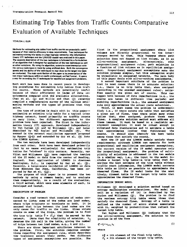
,,, ,
Transportation Research Record 944 113
Estimating Trip Tables from Traffic Counts: Comparative
Evaluation of Available Techniques
YEHUDAJ. GUR
Methods for estimating trip tsbles from trsffic aounts are potentially usefulbecause of their relative efficiency in data requirements. Two techniques forestimating existing trip tables in urban highway networks-the informationtheory (IT) teshnique and the LINKOD modal-ara msalysed in this paper.The eeparatadwrription of the tw techniques is followd by a formulationof ●n algorithm that is designed for ●pplication of the two tedwsquas as wellm othar variations. BYusing the algorithm, axtansiva axperimentstion withthe various tedwriques is mada by using artificial data. Seth tha convergencespeeds and the ability of tha techniques to stay dose to tha target trip tableare waluated. Tha main contribution of the paper is its presentation of thatwo major terhniquas within an aasily understood, unifiad format. It opansa WSYfor extending tha IT techniques for equilibrium assignment problams.
Much work has been done In recent years in develop-ing procedures for estimating trip tables from traf-fic counts. These methods are potentially usefulbecause of their efficiency in terms of data re-quirements compared with the available alternatives.Chan et al. (~) and Willis and Chan (~) recentlycompiled a comprehensive survey of tha various esti-mating methods and the types of problems that theysolve.
One type of problem is dealt with in this paper--estimating an existing trip table for a typical urbanhighway network, based primarily on traffic countson many links. Two different approaches to theproblem have been reported. The first is the infor-mation theory (IT) approach, developed independentlyby Van Zuylen (~) and by Willumsen (~), and laterdescribed by Van Zuylen and Willumsen (~). Thesecond is the network equilibrium approach proposedby Nguyen (6-8) and extended by Gur et al. (~) intothe LINKOD ~y~tem.
The two methods have been developed independentlyfrom each other. Both have been developed primarily(but by no means exclusively) for estimating triptables for “windowsm in city centers. Recently, vanVliet and Willumsen (10) have reported the testingof the IT model on data from the center of Reading,England. Test application of LINKOD in downtownWashington, D.C., is reported by Gur et al. (~).Recently, a large-scale validation of LINKOD on datafrom downtown San Jose, Cal~fornia, has been re-ported by Han et al. (11).
The purpose of thi~paper is to present the twomethods by using a ccsmaonbasis, and to evaluatethem comparatively. As a result of the evaluation,a third methccl, which uses some elements of each, isdeveloped and tested.
DESCRIPTION OF PROB~
Consider a road network that consists of nodes con-nected by links; some of the nodes are load nodes,where trips originate or terminate or both. It iSasaumed that trips between the load ncdes are theonly cause for traffic on the links. Given volumecounts on some of the links, the problem ie to find
the true trip table ; = (~i) that is served by thenetwork. (Note that for simplicity of notation, tidenotes the ith cell in the table, givin9 the numrof tripa between two load nodes, e.q., k and (t).
There are three important attribute inherent tothe problem. First, the solution requires assump-tions regarding the assignment rule, which describeshow travelera aelsct their paths. TWO differenttypes of assignment assumptions are possible. The
first is the proportional assignment where linkvolumes are directly proportional to the inter-changes served by them. This happena where pathselection does not depend on link volume, as in anall-or-nothing assignment. Alternatively, withnonproportional assignment rules, path selection isa function of link volumes as in equilibrium assign-ment. Proportional assignment aasumptiona make thesolution process simpler, but this assumption mighthe unrealistic in congested networks. The main bodyof this paper deals with all-or-nothingassignments.
A second important attribute of the problem isthat in most cases there is no accurate solution;i.e., there is no trip table that, when assigned(according to the assumed assignment rules), satis-fies exactly the given set of counts. This canhappen both because of data imperfections (e.g., thecounts are taken in different time periods) andmodeling imperfections (e.g., the aaaumed assignmentrule only approximates the actual route selection).
Third, in moat cases the problem is underspeci-fied; i.e., if there exists one table that satisfiesa given set of flows, then there exist many othertables that, when assigned, produce those sameflows. A complete solution method must address allthese issues. It must be based on a realistic as-signment assumption~ it must be robust enough towithstand data inaccuracies and to estimate a tablethat approximates (rather than duplicate) thecounts. It should alao identify the best tableamong those that satisfy the counts.
Both the IT and the LINXOD models satisfy theserequirements; although LINKOD can operate for bothproportional and equilibrium assignment aaauraptiona,the current version of the IT model operates onlyfor proportional aaaignment. The problem of multi-plicity of solutions is addressed in the two modelein a similar way, i.e., the input to the model in-cludes a target trip table--a trip table that de-scribes the best estimate of the true table witbouttraffic count information. The LINKOD a8)delCOrrSCtSthis table as little as possible to approximate theobserved flows. The IT model looks for the mostlikely, closest table to the target trip table thatapproximates the observed flows.
INFORMATION TNEORY -EL
Willumsen (~) developed a solution method based onentropy maximization considerations. The model (aswell as a variation of it) is described by Van!zuylenand Willumsen (:). The problem is to findthe maximum entropy trip table among those thatsatisfy the observed flows. Entropy of a table iadefined as the number of micro states associatedwith it, weighted by probabilities that reflect thetarget trip table.
van Zuylen and Willumsen (~) indicate that forthe all-or-nothing assignment, the solution to theproblem in of the form
tr=fl ● rrscr,Xs (1)
where
t? - ith element of the final trip table,fi = ith element of the target trip table,

114
r~ -
‘a =
set of links that are included in the pathof the ith interchange,andlink-specificperimeters.
Van Zuylen and Willunaen auggeet that Equation 1can be solved [i.e., the valuea of x = (xa) can befound] by using iterative proportional fitting andan algorithm that will be described later. Theynote that even though the convergence of the methodhas not been proven, numerous experiments with arti-ficial data failed to show a case of nonconvergence.Aa will be shownfound, which wanalgorithm.
LINKOD APPROM2H
The LINROD modelby Turnquiat andby Nguyen (6,7).--
later, a case of nonconvergence waarectified by a minor change to the
is described by Gur ●t al. (~) andGur (~. The theory was developedNquyen specifies a nonlinear opti-
mization problem; it is ahown that any solution tothat problem ia a trip table that, when asaigned byusing equilibrium assignment, replicates the ob-served flows. The optimization problem is similarto the problem connected to equilibrium aaaignmentwith elaatic demqnd.
As in any other equilibrium aaslgnment problem,the LINKOD model uses volume-delay functions. Iiow-ever, here both the link volume and the impedance atload are known. It can be shown that the correctsolution to the problem la arrived at regardless ofwhat function is used aa the volume-delay function,aa long as it ia a strictly increaeinq function andit gives the correct impedance at the observed load.For convenience, LINKOD uses linear, or bilinear,functions,e.g.,
c,(v,)=t.+b,(t.-Va) (2)
whereCa(v) -
ea =&a -
ba .
hpedence of link a at voluam v,observed voluxe,Ca(?a) = impedence at the observedvolume, anda peraxeter.
Those functions operate like error functions, wherethe error measure ~a - Ca(v) is directly related tothe difference between the observed and assignedvolumes●
Another @ortant ●ttribute of the xodel is thatthe theory does not prwide for a unique solution tothe problems) i.e., ●ll the trip tablea that satisfythe observed flows have exectly the s- value aathe objective function. To overccme this problemthe solution algorithm wae designed to keep thefinal trip table as close as possible to an inputtarget trip table. T%us the LINKOD nodel ●ctuallycorrects the target trip table ao that it approxi-mate, as close ae possible, the observed flows.
AWoRITNM FOR SOLVING TNE ALL-oR-tWTNINGPROBH
In spite of the different theoretical beckqrounds ofthe IT and LINKOD xodela, their solution algorithmsare similar. The following algorithm describes thesolution process by the two nodels and various pos-sible combinations of thex. This versien of the
LINKOD model is a special case, where it can beaasumed that only one path is used for ●ach origin-destination (O-D) pair (for ●xample, traVel on anexpressway).
1. Given the target trip table (P), the observed
volumes (~), the link impedence at load (~), and the
TransportationResearch Record 944
link error (voluae-delay) functions [Ca(0)],deter-aine the minimum impedence path for each O-D pair.Denote by ri the set of all links that serve the
ith O-D pair and determine the skim trees at load ~:
Ui=2.,,,c- (3)
Assign the target trip table to the network andobtain Vn.
2. Setm=O, vO=0,Tn =F, andTO.O.3. Svaluate the solution (Vn,Tn). If it iS
satisfactory,go to step 10.4.Set 9 = n + 1, @ . p, TO . Tn, and
Cn = C(vn).5. Calculate for each link the link error mea-
sure2
Y.=Y[f.,#,cao] (4)
(The definition of y ia given later.)6. Calculate a correction factor for each in-
terchange:
si=s(y,;=ri) (5)
That is, the interchange correction factor (s) is afunction of the volume errors of the links along thepath that serves the interchange. Calculate a cor-rected or a correction trip table:
t; =t(sJ (6)
7. Assign @ and get *.8. Find x such that
W=(I-A)V”+AV’ (8)
where o < I < 1 and i minimizes the value of
the objective function.9. Go to step 3.10. The solution to the problem is the trip
table +. Stop.
In the LINKOD xodel, steps 5 and 6 uae linear re-lations:
Y}=15.-c.(fl) (9)
In cases where c(*) is linear (Squation2):
(9a)
(lo)
and
tf=t;{l+2*[sJ(ui-lli”-$J]} (11)
where ~ ia the akin trees that use the imped-ances
c:=c,(o) (12)
In WilluDzen’s IT aodel, rzultiplicativerelation-ships are used, i.e.,
(13)
%w=%eri)f (14)
(15)

,,,
120 TransportationResearch Record 944
This formula is simply the reciprocal of the aum
of the modal impedances, scaled to represent suit-able values. The second formulation nuns the expo-nential of the disutility function for all modes?takes the reciprocal of the sum, and takea the nat-ural logarithm of this reciprocal. l%is is calledthe log aum method, and is described as follows:
Income Coefficients
Group AutomobileAutomobile Drive Alone (1, I) (G, I)
Income Accezz PenaltyGroup’ (I) Coefficient Coefficient t-Ratio Coefficient t-Ratio
IC.I.=K*lzt C/i~,exp[-A(i)]I
(2)Home-basedwork trips1234
Hems-bssedother trips1
1.4]651.06830.4943
-0.2245
1.40140,7979
-0.0750-0.6783
13.748.24
-0.32-6.59
1.67331.26770.89390.6140
21.1418.8910.017.83
Both of these functions meet the criteria previ-OUSly described, but little was known about theability of either to perform as a meaaure of spatialseparation. Therefore, both measures were tested bycalibrating the home-baaed work trip-diatributionfnodel twice, each time by using a different nea-sure. The choice would then be made on the basis ofwhichever formulation provided the closer match to
observed conditions, based on average trip lengthand other such measures.
CALIBRATION TECHNIQUE
The Ne”wOrleans distribution model uses the standardgravity model form (~). This model postulates thatthe number of trips for a given zone interchange iaproportional to the number of trip productions atthe origin zone and the number of trip attractionsat the destination zone, and invereely proportionalto the travel impedance between the two zonea. Therelationship with impedance is generally deecriktedby a nonlinear function that relatea impedance to anondimensional F factor (also called frictionfactor).
The usual calibration process involves determin-ing the relationship between the impedance valuesand the F factors such that the distribution of es-timated trips by impedance matches that of the ob-served trips. Additional adjustment factors (K fac-tors) are used to help match observed and estimatedtrips by geographic stratification (such as dis-tricts). For this project, separate models were de-veloped for each trip purpose and for each of fourincome levels. Observed person trips came from thehome interview survey.
Initially, it waa assumed that the UTPB programAm, operating in the so-callti SAC mode, would beable to automatically calculate the proper F fac-tors. However, this function of program AGN was notoperating correctly at that time and an ad-hocmethod of calibrating the F factors waa [email protected] method ueed essentially the same technique aadescribed in the AGN program documentation. F fac-tora are calculated by using a gamma function, i.e.,
F(l)=A*IB*EXP(G*l) (3)
2.96612.30951.93051.4125
0.0934-1.1802-2.1397-2.9294
9.06-21.00-30.61-38.33
-1.5281-2.2168-2.7419-3.1109
-24.40-35,62-44.41-50.70
234
Non-home-baaedtrips1 -1.3447
-1.9311-2.6904-3.0689
-11.73-17.53-24.48-27.S7
-1.3496-2.]027-2.5040-2.7298
–11.52-17.19-21.67-2335
234
Note: See Table 1 forequstions used for bizscoefflcienta.
●Income g?oup8are divided ufoUowz: 1 =Iow, 2=low.middle, 3=high-middle, and4= hi@
TW03. Vari&laauszdinmod.a14miozral ibrztion.
Acronym Description of Variableunits ofMeasure
Transit variablesTRN RUN hr-vehicle time from the transit network, not
including automobile access timeAutomobile access time from the transit
networkWaikaccess time from the transit networkTransitboardizzgtimeforthefmt transitvebi-
clefrornthetramdt networkTime spent transferring from the transit
networkNumber of transfers from the transit networkTransit fareDummyvariableaignifying ifanautomobile
was required to access the transit system(Oisno,lisyes)
Percentage of regional employment within 25minof total tranaittime from destinationzone
Minutes
Minutes
Minutez
AUTO ACC
WALKWA2T1
WAIT2
TXFERFAREAUTO CONN
Cents—
Percent
Minutes
Minutes
Cents
CentsCentsCentsMinutes
TRNDACC25
Highway varizbleaH~ RUN 1 Highwayizr-vehicle timefromhighway network
for one person per car (drive alone) tripsHighway in-vehicle time for group automobile
trips(sameasHWY RUN1 pluaanadditionaltime for each passenger)
Highwayopcrating costforonepersrm percartrips
Highway operating cost for group tripsAvg parking cost for one person per car tripsAvgpazkingcost forgrouptzipsTimespentparkbrg andunparkingan automo-
bile; the sum of highway terminal time at theorigin zone and the destination zone (alsocalled highway excess or terminal time)
HWY RUNG
HWYCSTI
HWYCSTGPRK CST1PRK CSTGHWY EXC where
F(I) = F factor for impedance value I,
A,B, and G = calibrated coefficients, andEXP = exponential function.
This function was judged to be adequate becausethere is considerable documentation that it siztu-lates the relationship between F factors and imped-ance adequately. Calibration of a distributionmodel consists mainly of fitting this curve. Thiswae done an follows.
C.L=Wi~,[A(i)+C] (1)
where
C.I. =A(i) -
c=
K=
value of composite impedance,modal choice disutility function for mode i(i = 1,2,3),constant chosen such that all A(i)gs arepoeitive, andconstant chosen such that all C.I.’S arebetween 1 and 127, inclusive.
1. Apply program Am in-the apply-and-calibrate(AC) mode, which reports the observed and estimatedtrips stratified by each unit of impedance.
2. The observed and estimated tripe and the F

TC&nSpCtrtAt~On Research Record 944 119
Tablea 1 and 2. Aa the equations in Table 1 indi-cate, travel disutility itIa linear function of thetime and coat of the transit, drive alone, and groupautcsnobilemodes, and other service characteristicssuch as number of tran8fers and transit accessibil-ity. Also, the income level of the traveler ie aprime influence on perceived dleutility. The dif-ferential effect of walk accese to transit versusautomobile access to transit on modal choice la de-fined through the uee of an automobile access pen-alty dummy coefficient in the transit disutilityequation. The variablee are described in more de-tail in Table 3. For the work trip purpose, peak-hour impedance valuee were uaad; for home-based
other and non-home-ttaeadpurposes, off-peak valueswere used.
The mode and variable definitions for these equa-tions are similar to other modal-choice models re-cently developed for Minneapolis-St. Paul (~), Seat-tle (I&), Houston (~, St. Louis (~, and BuenosAires (13). The group mode coneiets of persons in—automobiles with two or more occupants. A separatelogit eubmodel ia used to estimate the proportion oftwo-person, three-person, and four or more persontripa in.order to determine the average group occu-pancy for each interchange. The transit and highwayvariables are created from standard Urban Transpor-tation Planning System (~PS) network analysis pro-grasta (~) and special submdels are used to esti-mate accessibility, terminal time, and parkingcost. The calibration data consisted of a compre-hensive, home interview origin-destination surveyconducted in the New Orleans region in 1960.
The coefficients and the final list of variableewere developed by using ~IT on a eample of thesurvey file, followed by disaggregate validation andadjustment by using the full survey file. The coef-ficients are comparable to coefficients from othercitiei, exhibit internal consistency, and have ac-ceptable t-ratios (see Tablea 1 and 2). The “follow-ing observation support the reasonableness of theseequations:
1. The out-of-vehicle time coefficients ●xceed
those for in-vehicle time~2. The model is much more sensitive to aut~-
bile access time to tranait than to time spent onthe transit vehicle$
3. The ratio of the time coefficient to the costcoefficient, which is the implied value of traveltime, ia approximately one-third to one-half the av-erage 1960 regional income in cents per atinuteland
4. The inctnne bias Coefficient itiicate that asincome level increaaes, there is a lower propensity
to use transit, and within the automobile mode, ahigher propensity to be a driver rather than a pas-senger.
COMPOSITE IMPEDANCB CALCULATION
The previous section describes how impedance is de-fined for each mode. The remaining challenge is tocombine the three impedance into one value. rnrthis task, the following condition must be ❑et.
1. The combined value must decrease as any ofthe modes becomes better, i.e., declines in time orcost.
2. The combined value must increase if a mode isnot available [i.e., an interchange with even unsat-isfactory transit service must have a better (lower)impedance than one with no service at all].
3. The value must lie between 1 and 127, inclu-sive. The OTPS program Am assumed that the inputimpedance values are stored as l-byte matrix ele-❑ents. The highest value that can be represented inthis format is 127.
4. The distribution of values within this rangeshould @ reasonable; i.e., they should not be con-centrated at the top or bottom of the range.
It was ascertained that at least two mathematicalformulation meet these criteria. One formulationis a variation of the harmonic mean function:
T6M01.Modsl+aedisutilitysquation,.
Mode Eutmtion
Honae-baaedwork tfipSTransit disutility
Drive-alone disutility
Group automobile disutility
Home-baaed other tripsTranaitdkutility
Drive-alone disutility
Group automobile disutility
Norr-hom&baaed tfipaTranait disutility
Driwrlone disutility
Group automobile disutility
0.0332 ● WALK+ 0.0769● WA2T1+0.0319● WA1T2+0.0078● FARE+ 0.014S● TRN RUN+ 0.1005● AUTO ACC(4.07) (20.21) (8.S5) (10.45) (6.72) (2.59)
+0.0588.TXFER + Auto Access Penalty (I) ● AUTO CONN(3.59)
0.0693● HWY EXC +0.0]45.HWY RUN1 +0.0078*HWY CSTI+0.02145● PRK CST1 + Income Coefficient (1, 1)(4.94) (6.72) (10.45) (10.45)
0.0174*HWYEXC +0.0145 *HWYRfiG +0.0078 *HWYCSTG +0.02145 *PRKCSTG +lncomeCocfficient (G,l)(1.74) (6.72) (10.45) (10.45)
0.0165*(WALK+WAITI+WA1T2)+0.0116*FARE+0.0066●(TRNRUN+AUTO ACC)-O.0183*TRNDACC25(7.45) (9.55) (-22.91)
+AutoAc~Peraalty(I)oAUTOCONN
0.3403● HWY EXC +0.0066● HWY RUN1 +0.0116● HWY CST1+0.0319● PRK CST1 + Income Coefficient(1,1)(25.98) (7.45) (9.55) (9.55)
0.2828*HWYEXC +0.0066*HWYRUNG +0.0116 .HWYCSTG +0.0319*PRKCSTG +lnromeCoefficient (G,l)(28.50) (7.45) (9.55) (9.55)
0.0328*(WALK +WAfTl+WAIT2) +0.0047* FARE+O.O131O (TRNRUN+AUTO ACC)+O.0750* TXFER(9.41) (2.75) (9.41)
+2.7472*AUT0 CONN(4.91)..
0.2423● HWY EXC+0.0131● HWY RUN1 +~O04J● HWY CSTI+ fzo~:;● PRK CST1+ IncomeCMffi~t (1.1)(20.14) (9.41)
0.3048.HWYEXC+0.0131.HWYRUNG +0.0047*HWYCSTG +0.0291”PRKCSTG +lncomeCoeffiient(G,l)(25.58) (9.41) (2.75) (2.75)
Note: DkautUltiaa must ba muttlpliad by -1 bcfora tabinc the expcmwntkal in the torkt aquatkon. Numb- kn parenthaaaa mpraaant t-ratlm T-ratiaawarenot calcutsted far theWrk and othar automobile sccu psnalt y coefflckanas, or the non-home-baud coefficient on TX FER. Sae Table 2 for oxpluutkomof bku coaffidenaa uaadfortha ●W@kOU.
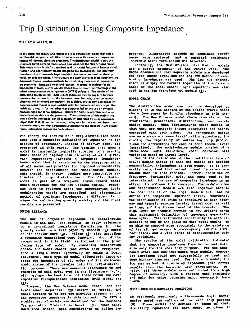
.r,
118 Transportation Research Record 944
Trip Distribution Using Composite Impedance.
WILLIAM G. ALLEN, JR.
In this papar the thaorv ●nd results of a trip-distribution modal that uses amultimoshl romposite definition of impadwsw as its mazsrm of wpsmtion,instead of highway tima, ●re praantad. Tha diatribwtionmodal is part of acmmplste traveldemmwl model chain developedfor the New Orleansregion.This model chain is briefly described, and its special fssturas of inaome strati-fication assl connartivity among programs ara cmphaaizad. The disutilityfunctions of a thraa-mode Iogit modd-choica modal are uaad to developmodal impadanra values. The structure and coefficients of these equations ●rediscussed. Two ●lternative methods for combining these modal impedances●re presented: harmonic mean and log sum. A special technique for cali-brating tho F faotor curves was developed to circumvent shortcomings in theurban transportation planning system (UTPS) software. The results of thealibration are prwantml. Thaaaresults indiwted that the log sum formulaproduczd batter results than the harmonic mean formula, baaed on variousobserved and estimated comparisons. In addition, the log sum mmposite im-psdmma-bsaad model prosed suitable only for homa-bsaad work trips. Un-sztiafaotory results for tha other trip purposes lad to the use of off-peakhighwsy time for those purposes. Rssulta for home-based other ●nd non-homa-baaadmodels ere also presented. The conclusions of this analysis ●rethat ● distribution modol can be suoaaaafullycalibrated by using compositeimpedance; that. at last in this case, the log sum formula worked better thanharmonic mean; ●nd that a successful alternative to the standard AGM gravitymodol calibration process can be deve(~.
The theory and results of a trip-distribution modelthat uaen a composite definition of impedance as itsmeasure of sreparation, instead of highway time, arepresented in this paper. The premise that such amodel is inherently logically superior to a gravitymodel baaed on highway time ia accepted as a given.This superiority involves a composite impedance-based model that is sensitive to the characteristicsof all modes and provides for improved connectivitybetween the distribution and modal-choice models.This should, in theory, produce more reasonable ●s-timates of trip distribution. The dietributionmodel is part of a complete travel-deazandmodelchain developed for the New Orleans region. Previ-ous work is reviewed here~ the accompanying logitmodal-choice models are deacribed; and alternativemethods of conrhining.impedances, a diffarent tech-nique for calibrating gravity models, and the finalresults are presented.
PRIOR RESEARCS
The use of composite impedance in distributionmodels is not new. For example, an early referenceto a generalized rasistanca formulation for thegravity model is a 1973 paper by Nenheim (~) basedon hla earlier work (~). Wilson s) also describesa composite generalized coat function. Much of therecent work in this field has focused on the jointchoice type of model. By combining destinationchoice and modal choice (and often triP frWuencY)into a single model (generally by using a logitstructure), this type of model effectively incorpo-rate the impedances of all zrrsdeaand the socioeco-nomic etatua of the traveler into the trip-distribu-tion process. There are numaroua references to andexamples of this model type in the literature (~,~),with perhaps the beat known of these being the Met-ropolitan Transportation Crmvmiasion (MTC) model aet(3).
However, the New Orleans model chain uses thetraditional sequential application of models, andthere appears to be but one previous attempt at us-ing composite impedance in this context. In 1975 asimilar aet of models was developed for the RegionalTransportation District in Denver (~). That studyused modal-choice logit coefficients to define im-
pedance. Alternative methodsantes were reviewed, and a(harmonic mean) formulation waa
of combining imped-parallel resistanceselected.
Basically, the New Orleans distribution medalsare a direct extension of the Denver ~rk. Themajor changes are that separate models are developedfor each income level and the log sum method of com-bining impedances was used. The log sum method,which is simply the natural logarithm of the denonti-nator of the modal-choice logit equation, was alsoused in the San Francisco NTC models (~).
NODEL CSAIN
The distribution model can beat be described byplacing it In the setting of the entire travel modelchain (see paper by Schultz elsewhere in this Rac-ord). The New Orleans model chain consists of thetraditional generation, distribution, and modal-choice nsodela. What distinguishes these models isthat they are entirely income atratified and highlyconnected with each other. The generation mrsdelause an elaborate cross-classification structure, in-cluding the capability of aatimating trip produc-tions and attraction for each of four income levels(quartiles). The modal-choice models conaiat of athree-mode logit structure, which contains biasvariables baaed on Income level.
One of the criticisms of the traditional type oftravel-demand models 1s that the models are appliedsequentially, independent of each other. It ia gen-erally recognized that actual travel decisions areseldom made in this faahion. Rather, decisions onfrequency, destination, mode, and route tand to beinterrelated. The uae of composite impedance ie anattempt to address this concern. The modal-choiceand distribution models are tied together becausethe coefficients of the logit models are used todefine the composite impedance value. Therefore,the distribution of trips ia sensitive to both high-way and transit service levels, travel cost as wellas time, and the income level of the traveler. Thehigh level of transit service in New Orleans makeathis multimodal definition of impedance especiallymeaningful. This multimodal sensitivity ia also es-sential to one of the goals of this model chain: tobe able to respond more accurately to the existenceof transit guidewaya, high-occupancy vehicle (IK3V)facilities, and a wide range of transportation pol-icy variablea.
The rasults of the model calibration indicatedthat the composite impedance formulation was suit-able only for the work trip purprrae. For the home-based other and non-home-based trip models, composi-te impedance could not successfully be used, andthus highway time was used. For the work model, thelog sum method of combining impedance gave betterresults than the harmonic mean formulation. Fi-nally, all three modele were calibrated to a highdegree of accuracy, with K factora used sparinglyand only for trips creasing major geographic bar-riera.
MODAL-CHOICE DISUTILITY FONCTIONS
Aa previously mentioned, a three-mode logit zsodal-choice model was calibrated for each trip purpose(~). These models are defined in terms of theirdisutility equations for each tie, as 9iven ‘n

TranaportatiOn Research Record 944
residual of 70 after 6 iterations, and a residual of15 after 15 iterations.
4. The three multiplicative versione of themodel always resulted in similar trip tablea, whichtended to be slightly different than that of theLINKOD algorithm.
5. Adding the 1 weighting (Equation 8, model3) increased the convergence speed only slightly.
CLOSENESS OF FINAL TRIP TABLE TO TARGST TRIP TABLE
The data in Table 3 give the value of t for thefinal and target trip tables for the different algo-rithms and target trip tables. Figure 3 shows theratios of c for LIWKOD (model 1) and the squareroot vereion of the IT algorithm (model 4).
1. All the algorithms succeed in producing finaltrip tables that are close to the target tables.Different target trip tables result in completelydifferent final trip tables that, nevertheless, aresimilar in their ability to reproduce the obeervedflows.
2. The different multiplicative algorithms re-sult in final trip tables whose distances from thetarget trip-tables are similar. This is particularlysignificant relative to the algorithm with the iweighting (model 3); its divergence from the basicform of the IT model (Equation 1) does not appear toharm its performance.
3. In most cases the multiplicative algorithmsresult in final trip tables that are elightly closerto the target trip table compared to LIWKOD. Thiscan be seen clearly in Figure 3.
4. In caaes where the algorithms show conver-gence difficulties (Table 2f), the final trip tableis not the feasible solution closest to the target.TO confirm this point, a systematic eearch for theclosest solution was made by using linear combina-tions of the eight basic solutions. The best triptable had @ = 0.274 compared with @ = 0.553 forthe final trip table of the algorithm. In all caseswithout convergence difficulties, only slight dif-ferences between the two t’s were found.
CONCLUSIONS
In this paper the two major models for estimatingtrip tables baeed on traffic counts that have beenverified in full-scale applications are compared.The analysis concentrates on all-or-nothing assign-ment problems. It is ehown that the two models aresimilar, both in the structure of their algorithmsand in their performance. LIWKOD uses additiveterms for the table correction.steps,whereas the ITmodels use multiplicative terms. The differentversione of the IT model produce eimilar reeults.They tend to produce final trip tables that areelightly closer to the target tables when comparedwith LIWKOD.
The target trip table is shown to have majoreffects on all aepects of the eolution. It dictatesthe structure of the final trip table and the speedof convergence. In any application of the model,the eelection of a target trip table should be madewith care.
The standard IT algorithm (model 2) failed toconverge in one case. It should be used with care.All the other algorithm performed satisfactorily inall cases.
A significant reeult is the successful perfor-mance of model 3--multiplicativecorrection with Aweighting (Equation 8). The a weighting step isan essential element in any equilibrium aseiqnmentalgorithm; the success of the model that includesthis step gives a strong itW3iCati0nthat it can
117
perform Successfully under equilibrium assignmentaeeumptions. Development work in this direction isunder way.
REFERENCES
1.
2.
3.
4.
5.
6.
7.
8.
9.
10.
11.
12.
13.
V. Chan, R. Dowling, and A. Willis. DerivingOrigin-Destination Information frcm RoutinelyCollected Traffic Counte--Phase I: Review ofCurrent Research and Applications. Instituteof Transportation Studies, Univ. of California,Berkeley, Working Paper 80-1, 1980.A.E. Willis and V.K. Chan. Deriving Origin-Destination Information from Routinely Col-lected Traffic Counte--Phase II: Comparisons ofTechniques for Single-Path and Multipath Net-works. Institute Of Transportation Studies,Univ. of California, Berkeley, Working Paper80-10, 1980.H.J. Van Zuylen. A Method to Estimate Trip Ma-trix from Traffic Volume Counts. Preeented atPlanning and Transport Research and ComputationCompany, Ltd. S~r Annual Meeting, Univ. of
Warwick, Coventry, Warwickshire, England, 1978.L. Willumaen. Estimation of an O-D Matrix fromTraffic Counts: A Review. Institute for Trans-port Studiee, Univ. of Leeds, Leeds, England,Working Paper 99, 1978.X.J. Van Zuylen and L.G. Willumsen. The MostLikely Trip Matrix Estimated from TrafficCounts. Transportation Research, Vol. 14B,1980, PP. 281-293.S. Nguyen. Estimating an O-D Matrix from Net-work Data: A Network Equilibrium Approach.Centre de Recherche eur les Traneport, Univer-sity de Uontreal, Montreal, Quebec, Canada,Publ. 60, 1977.S. Nguyen. On the Estimation of an O-D TripMatrix by Equilibrium Methods Using PeeudoDelay Functions. Centre de Recherche sur lesTransport, Univereite de Montreal, Montreal,Quebec, Canada, Publ. 81, 1977.S. Nguyen. On Estimating O-D Matrices fromTraffiC Date. Presented at the Canadian Trans-port Research Forum Meeting, Winnipeg, Mani-toba, Canada, June 12-14, 1978.Y. Gur, M. Turnquist, M. Schneider, L. Leblanc,and D. Kurth. Estimation of an O-D Trip TableBased on Observed Link Volumes and TurningMovement, Volumes 1-3. FSWA, Rept. FSWA/RD-
80/035, 1980.D. van Vliet and L.G. Willumeen. Validation ofthe ME2 Model for Estimating Trip Matrices fromTraffic Counts. Presented at the 8th Interna-tional Symposium on Transportation and TrafficTheory, Univ. of Toronto, Toronto, Ontario,Canada, 1981.A.F. Ran, R.G. Dowling, E.C. Sullivan, andA.D. May. Deriving O-D Information from Rou-tinely collected Traffic Counte--Volume II:Multipath Networks. Institute of TransportationStudies, Univ. of California, Berkeley, 1981.M. Turnquist and Y. Gur. Estimation of Trip
Tables from Observed Link Volumes. TSB, Trans-
portation Research Record 730, 1979, PP. 1-6.A.B. Willis and A.D. Hay. Deriving O-D Infor-mation from Routinely collected TrafficCounts--VolutaS 1: Trip Table Synthesis forSingle-Path Networks. Institute of Transporta-tion Studies, Univ. of California, Berkeley,1981.
Rtblieatwnofthis paperqoonwredby bnrnitteeonlbsse~w TravelDe-tmrmdForecattitrg.

. . .116 Transportation Research Record 944
small enough to permit complete analytical solu-tions.. Out of the 15 cells in the trip table, 4 arealways zero because of the 8tructure of the network.The 10 volume counts provide 8 independent equa-tions. Those equations, when combined with non-n~ativity constraints on the cells of the triptable, can be solved with eight different basic triptables, each with eight positive cells, which sat-isfy the observed flows. The data in Table 2b markthe cells that can be zero. The data in Table 2Care an example of a basic solution. Every scaledlinear combination of the eight basic tables alsosatisfies the observed flas.
There exist a nuatberof measures for the distancebetween two matrices. These measures are describedby Willis and May (lJ). For the present project,the following distance measure was selected:
4J=(l/zj~)zi[tr* lloE(ti’/fi)ll (18)
where F is the target trip table and ~ is thefinal trip table. This measure is a normalizedequivalent to the distance measure used in develop-ing the IT model.
The extent to which the final trip table approxi-mates the observed flows was measured by two vari-ables: the LINKOD objective function and the sum ofabsolute volume errors, i.e.,
For the main body of the experiments, a number ofdifferent target trip tables were specified, and aset number of iterations (5 or 15) were run by usingthe different models. The statistics of the dif-ferent runs were used for model evaluation. Themajor results are shown in Figures 2 and 3 and aregiven in Table 3.
Fi!#Jm2.cmvwgmczlpeodforfhedifferen2elgorithtnh
500
\“’’’’’’’’””4
RL.< \
so ‘\.\mTARoET~2(f)
awd
‘\ “> TAReET=2(@)
‘1 “ ,M20
‘\, b
\\
10‘\
\
‘Y\
‘Y.,’\
Q
)
\ \5 \
‘\.e
2 L
\, -iI I I I \ I 1 1 1 1. I I 1 I 1
-o I 234 S67891011 I’131415ITERATION
CDNVt?~ CNARACTSRISTICS
The data in Table 3 give the values of the variouserror measures that use different target trip ta-bles. Residual errors after each iteration for twosample tables are shown in Figure 2. The main con-clusions are as follows.
1. At least in one case (target table as speci-fied in the data in Table 2d), the simple IT algo-ritluh (number 2) failed to converge. The otherthree algorithms always converged.
2. The LINKOD algorithm tends to improve thesolution more than the IT algorithms during thefirst one or two iterations. However, the multipli-cative algorithms tend to be more efficient when theerrors are small. In general, after five or moreiterations, all the algorithms show similar residualerrors.
3. The speed of convergence depends strongly onthe target trip table. It is interesting to notethat all of the algorithms display convergence dif-ficulties exactly for the same target trip tables.The data is Tables 2e and f give the two targettables whose convergence patterns are shown in Fig-ure 2; these patterns display that behavior. Al-though the data in Table 2e give a residual of about4 after 6 iterations, the data in Table 2f give a
Fi~ra3. Dirfancemt400for LlNKODandlT models.
. I
Residual Srror (VOLER’) Distance from Target (@b)
Ir [rT6rget IT (square IT (squ6reTable LINKOD with root ) LINKOD with root)
25 22 28 0.159 0.157 0.158k 29 28 31 0.154 0.138 0.1383 20 15 15 0.289 0.284 0.2844 60 56 56 0.426 0.410 0.4155 13 4 0.300 0.292 0.2926 26 17 2: 0.363 0.371 0.3567 16 10 0.476 0.488 0.481
4 : 4 0.131 0.131 0.131: 12 4 13 0.553 0.555 0.557
10 70 66 65 0.467 0.446 0.452II 9 8 7 0.195 0.195 0.195
Note: netable prewntsvdues of thepefiormance meWrmafiw~efi_8t~~
%OLERlsthe aumofabmlute linkvolume~&s. VOLER= Z1.. -.:l.
bOisdeflned stdescrlbed in24uat&n 1S.
CBY uskng malytkat techrdques, Solutions with @of 0.130 and 0.268 mm found fortartet trip tables 8md 9,respectkvely.

Transportation Research Record 944 115
Another difference between the two algorithms isthe need for the i weighting (step 8). In theLINROD model the table T= is a correcting triptable that points to the direction of the neededcorrection in any iteration. Therefore, the iweighting is an ●ssential part of the algorithm. Inthe IT algorithm # is a corrected trip tabletthus the x wetghting is not s necessary part ofthe algorithm; it might ●ven be harmful.
Note that in the IT algorithm, without i weight-ing (x from Equation 1) is
TheFigure 1. Tsst nstwswk. was
~==my:.m (16)
where ~Cm is the value of y from Equation 13at the mth iteration. However, if i weighting isused, then the wlution trip table (Tn) cannot beexpressed in terms of Equation 1. Thus it im doubt-ful whether the solution with the A weighting isthe best solution, ●s specified by the IT criteria.In the pure IT MOdel, 1 in Equation 8 iS always 1.
EXPERIMENTATION
Tst401. Tettnotworkattrbtaa.
Node A NodeB c, b, %
4566778888
8 6.98 9,2s 31.07 19.6I 8.08 13.92 13.53 12.04 11.45 6.5
0.03 1300.04 1300.05 200.04 2900.05 600.03 2300.05 1700.03 2000.06 900.05 30
TablaZ TtitriPtsbkh
algorithm as described in the previous sectionprogramed, and a set of experiments with the
a. Asolution (anexsmple) b. Structureofa solution
!M :ii+!
60 170 200 90 so 570
Note: -meansit muslbezero.Omewu iican be zafo, and x msana it must be positive.
d. A targetthatcannotronws’gewithc. Abasicsolution(anexampie) algorithm 2
‘w ‘me,A quickly converging target f. Aslowly mnvergingtsrget
~w ‘m
two models and some other variations were performed.
The ●xperiments were designed to answer the follow-ing questions.
1. How do the various algorithms perform interms of speed of convergence to a trip table thatapproximates the observed flowm? Are there caseswhere the algorithms fail to converge?
2. ROW do the various algorithms perform interms of finding a solution that is close to thetarget trip table?
The experimentation started with three models:(a) LINKOD, (b) IT with a = 1, and (c) IT withoptimal i (step 8 of the algorithm). After a fewexperiments, it was found that in certain circum-stances the standard IT model overcorrectm the triptable and fails to converge. A fourth version ofthe model was added, where Equation 13 was replacedby Equation 4:
Y:’=SQRT(%M) (17)
and A - 1.
The experiments use the network shown in Figure1, with the link attributes given in Table 1. Thedats in Table 2a give an example of a trip tablethat satisfiem the observed flows. The problem is

,,.
Transportation Research Record 944 121
factors used in that run were then keypunched into afile that could be used by Statistical Package forthe Social Sciences (SPBS) program (MJ.
3. The SPSS subprogram REGRESSION was then usedto obtain a leaat aquare8 fit for the coefficientsA, B, and G (after auitablg transformation of thevarieblea).
4. Mew ? factora were calculated by using thenew coefficients, and program A= waa reapplied.The obeerved and eatimeted trip lengths were then~redr and if the re3SUltawere inadequate, atepa2-4 were performed again.
Tzbie6,Compssisonoftwocompo4itzimpsduNaforsarS~ higlmrzyrurwti~urns (mIn).
HsrrrronicMem Log Sum
Income E3ti-Percent Esti- PercsntGroup’ Observed mated Error Observed mated Error
1 10.17 10.67 4.92 10.17 10.82 6.3910.18 11.02 8.25 10.18
:10.59 4.03
10.87 11.59 6.62 10.87 10.97 0.924 11.16 11.87 6.36 11.16 11.26 0.90
AU income 10.68 11.39 6.65 10.68 10.94 2.43groups
Note: Ttwsemlu= reprmwrtthe hrrme-bswd work purpose srwttYm odelmm,w WhorrtKfactors.‘Jnarmesroups aredMdedssfoUoww l=low,2= lowmid~e, 3-tih.middle, ad4=lrl@.
The results were judged by a visual inspection ofthe impedance distribution and by CoaParing the av-erage values for coapoaite impedance and triplength. By using this technique, a satisfactory aetof ? factors could be obtained in between aix andnine iteration.
Tti6. Comparbonofmvocornpoditzimpedmosforfnulss: hirJtwzy&tznaa (mild.RESULTS
The reoulta of the impedance calculation are givenin Table 4. The ~aite impedance valuea differmarkedly by income level and are biaaed in theproper direction. That ia, the lower-inmme levelsare associated with higher impedance. This reflectsthe fact that lower-i~ persona tend to havelower mobility (for example, they are leaa likely toown automobile). The ccapoaite valuea also indi-cate a larger apreed than the the valuea, which uayauggeat more specific relationshlpa between com-posite hpedance and ? factora. These atatiaticsindicate that the crezpoaite iapedance formulationbehavea mathematically. This increaaea the confi-dence with which it can be used in gravity model de-velopment.
HannoNcMean Log Sum
Income Esti- Percent Esti- PercentGroupa Observed mrrted Error Obs.med mated Error
1 4.29 4.53 5.59 4.29 4.64 8.162 4.29 4.70 9.56 4.29 4.52 5.363 4.72 5.15 9.11 4.72 4.80 1.694 4.91 5.29 7,74 4.91 4.96 1.02
AUincome 4.61 4.99 8.24 4.61 4.75 3.04groups
Note: ~~@uwrew*ntthetim*b-Wrkpur~UtfitYmdelm~ withoutKfsctorx.%womesrouparedtvld~ssfolioww l=low,2=low-mlddle, [email protected], -d
4=bl@.
Tzblz4.Stsmrtmryofobtamzdhnpzdznavztuss.Tabi07.Compzriwnoftwowrnpodtzimpodanre formulas:numbsrofintrzrmdtfip4.
—.HarnronicMesn Log Sum
Income Esti- Percent Es& PercentGroupa Observed mated Error Observed mated Error
Purpomutdhrcome Aversge Lowest Hipbest StandardIx@’ Vslueb Vsluec Vthrec Dcvistion
Home.bascdwork trips1234
Homc+ssedothsr trips1
62.18956.33847.17138.063
44382921
111988477
9.9088.6958.5968.670
936 882 -5.77 936 857 -8.44: 2,202 1,854 -15.80 2,202 2,396 8.813 2,89S 2,471 -14.6S 2,895 3,437 18.724 3,113 2,374 -23.74 3,113 2,866 -7.93
AU income 9,146 7,581 -17.11 9,146 9,556 4.48groups
Note: Theuva3ues reprWntthe hom*basedwork purpase CrWitymodelruna.tithoutK fmton.
‘brnme~uwmdtidadufoUow. l=low,2=low-mAddle, 3=hlsk-midrUe,mId4=rd#rr.
7.s797.9658.2147.692
1111
43394444
4.9425.3346.1185.679
,4
34
Non-homebssed trips1 5.263
5.4515.3925.130
7.7207.6717.7107.520
1111
36433939
224
.lnr.ornelmlkdMdcdssfdow#: 1=low.2=low-nddrUo. 3=hktr-nriddle,snd4=highway travel the and distance considerably betterthan did the harzmnic mean formulation, except forthe lowest inccae quartile. When intrazonal tripeare ~redt the log aum anrmch iS superior fortotal trip estimation, but slightly inferior for thelow and high-middle income quartilea. In comparin9major trip patterna, such aa tripa acroas the Mia-aissippi River, the harmonic mean model overesti-mated the observed data by 69 percent, whereaa thelog am model overestimated by only 44 percent (be-fore K factora were applied, in both caaea). Inadditione a cotaperiaonwaa tie of the n-r ofdistrict interchange (there are 20 diatricta) fOrwhich the difference between observed and emtimetedtripe wan greater than 100 tripe and the percentagedifference waa greater than 15 Percent. The har-
monic ■ean model had 68 such district interchan9ea*whereaa the log aum tiel had 56.
wbl’bovsluuforbom+bsacd workmpmwatlnssumronrpodtainrtredmm..Ulothorvshrumprowmtk34fswsytlrrraAf31dghvmytirmsrwodwsreoff-p.skhlshwaytimaWhbouttarmiasl Urrlm
cN3sbutsndlowat nlucsthstcantdrr obswvdtrips.
The reaulta of calibrating the home-based work●odel with both acts of c~aite impedance func-tions are given in Teblem 5-7. These compariaonaindicate that the log sux re8ulta are superior tothoee obtained with the harwnic mean fornula. Thebaaic philosophy of theme comparieona waa that, if
the model oould be calibrated by using one type ofimpodanoe ●nd could be shown to properly replicatethe mmna of a different (but related) tYPe of ~-pedance, the calibration would be considered ●uc-ceaaful. The log ●um formulation eathatea average

122 Transportation Re8earch Record 944
Based on this analysis, the log sum formulationwas chosen to complete the calibration of the dis-tribution model. Because the log sum formula workedwell for home-based work trips, this method waa usedfor home-based other and non-home-based tripa aswell. An F factor equation for home-based othertrips was calibrated, and the model was applied fora validation check. However, in this case, in com-paring observed and estimated tripa with respect tohighway time and distance, the estimated tripsshowed a much higher trip length. The estimatedtrips were considerably less than the observed tripsin the 1-, 2-, and 3-reintime range and considerablyhigher in the 4-, 5-, and 6-rein time range. Attimes greater than approximately 7 rein,the two dis-tributlona were similar. Considerable thought wasgiven to correct this imbalance in distribution, butno methodology appeared to offer any reasonablechance of successful calibration. Because of theseresults, the hcme-baaed other distribution atcdel wascalibrated by using off-peak highway travel timerather than composite impedance.
Similar results were obtained for the non-home-based avxlel calibration, leading to the same solu-tion; uae of off-peak highway time instead of com-posite impedance. Off-peak highway time was alsoused for the remaining models (taxi, internal-external, and truck).
There is speculation that the lack of success inusing composite impedance in the nonwork models is
related to the nature of nonwork trips compared withwork trips. Work trips are methodical and repeti-tive, and the commuter may actually have more knowl-edge than the nontwxk traveler about his modal op-tions and their associated impedances. Wonworktripa are less structured, and perhapa less thoughtis given to alternative modes for such trips. Thatis, coat considerations and the availability oftransit service may not strongly affect nottworkdes-tination choice.
The calibrated F factor equations for all trippurposes are given in Table 8, with the F factorsbeing defined by the three coefficients of the gartmadistribution. All coefficients are statisticallysignificant, and the correlation coefficient (Rz),which comparea the required F with the calculated P,
was greater than 0.90. The regression program equa-tions have been adjusted, where necessary, to ensurethat the highest F value is not storethan 999,999,in order for the data to be acceptable to A@l.
Tsblc8.Ffzsforequztiorv:.
EquationCoefficientValuesbPurposeandIncomeGroup’ A B G
Home-basrdwork trips1 4,296,752 0 -0.093003972 EXP(26.82271) -3.153498 -0.08367553 EXP (34.10976) -6.800698 -0.0248414 EXP(28.39026) -4.819197 -0.041024
Home-based other trips1 1,064,302 -1.0s55592
-0.10540661,070,772 -1.292004
3-0.09307232
647,077 -1.8388364
-0.037013911,033,560 -1.838298 -0.05231526
Nort-hom*based trips1 663,504 -0.6655663 -0.12315752 869,1143
-0.9009789 -0.1125171267,378 -0,9540237 -0.1127642
4 371,881 -0.7850539 -0.138105
‘Income mourn am dMded u foUoW: 1 = low. 2 = low-middle, 3 = hkh-middla, ●rd4=hEdr: “
bF fmtom sre ulctited by udnr the equation: F(I) = A*lB*EXp(G*I); where 1 b thecompodte Impedance for work trips and hL@waY tkme f.x the other trip Purpoceh
The primary reason for calibrati~ the distriti-tion models by income quartile waa the hypothesisthat tripmakera in different income levels wouldreact differently to the impedance measure. Al-though the gazssafunction coefficients are differentfor the four income levels, It is hard to ascertainthe true difference because the F factors are rela-tive, and the mean composite istpedanoevalues aredifferent by income level. lb test the hypothesisthat the F factors are truly different by incomelevel, a set of normalized F factors were calculatedby using the mean composite impedance values and thestandard deviation from the mean. Wornalized Ffactors were developed by adjusting the constantterm (the A coefficient in the g.ztmnaequation) sothat the F factor would (arbitrarily)equal 100,000at a composite impedance value, which waa 2.5 stan-dard deviations less than the mean value. This com-parison is shown in Figure 1. In essence, the ~-parison shows that F factors for the lower incamsare less sensitive to the impedance values. Itwould not appear reasonable, though, to use thisccsoperisonto draw the conclusion that poorer peoplelike to travel sore than richer people. Perhaps abetter explanation is that the lower-income travelerhas fewer destinations to choose fron, thereby re-ducing the impact of travel impedance on travel be-havior, at least on diatrihution.
Most calibration reports on distribution modelsgive the observed and estimated trips stratified byhighway travel time. For distribution models cali-brated by using highway time, these comparisons nor-
100.OOO
W.oao
10,OW
5.000
I,ma
~
<m..0~
i
#ml
AW lNcoMf
UEOIUULOWwCOWE
—WEolw ttlGMISCOM
~“,o” MxM
I 1 I I I I3 4 1 0 t a 3
NuWS6R OF STANOAnO MVIATIM FnOW MEAN~Te IWEOAWCE

.,.
Transportation Research Record 944 123
reallyindicate a great deal of agreement between theobserved and ●stimated trips, which is only reason-able because the F factors are directly related tohighway time. Becauae the spatial measure used inthis model was ccaposite impedance, of which highwaytravel time was only one caponent, a comparison ofthe observed and eathated trips meaaured againathighway travel tine would be a useful validationtest, am mentioned previously. These comparisonare shown graphically in Figures 2-6. AS can beseen from the data in these figures, the estimated
Figum2.Comps2i30noft2ipdi3tributionafo210wiwmshome—bamdworktips.
6,000
5,000
Fieum3.Compuisos30ft2ipdistfibsstiomsfor~iuminsomshonwbmed worktriw. 9,0C0
am
1,WR7
6,030
5,W0
4.WO
K’E.
trips agree with the observed trips extremely veil.The ccmpsrieons by income level are similar to nor-mal gravity model trip-distribution comparisons.When the trips for all incomes are combined (Fi9ure6), the observed trip pattern is much smoother andthe estimated trips compare extremely well with theobserved trips.
After calibrating the F factora, the next step inthe calibration procedure was to aacertain the tripmovements that were inadequately simulated and thathad specific attributes that would be identifiable
ESTIMATEDTRIPS
~OESERVED
I
I I I I I I I
5 10 15 m 25 30 35
PEAK HOUR HIGHWAY TRAVEL TIME (MINUTES)
k..‘b
I I I i I I I5 10 15 30 3s 30 3s
PEAK HOUR HIGHWAY TRAVEL TIME (MINuTESI

124 Transportation Research R~rd 944
Figum4.Um~dmnoftrip tifihdonstihi@#uminoonw horno-bawd work trips.
U-#-l
moo
7!2C0
6,000
5,000
Figure 5. Comparison of trip distributions for hi#r inmrnehomebnsed work trips.
-.I\
‘\
!#
i
‘!
‘,f1 ‘1\
I\
! I\
:
/ \
;
t\
I — ESTIMATEDI
/
‘,
‘1
‘\
,\
I \
I
-.$
‘\
.
I I I I I I I5 10 15 20 25 2a 35PEAK HOUR HIGHWAY TRAVEL TIME (MINUTESI
Y \\7‘\-.,..
---
-5 ;0 15 m 25 30 35PEAK HOUR HIGHWAV TRAVEL TIME (MINUTES)

,1.
Transportation Research Record 944 125
35,0W
30,W0
25SO0
m,ooo
15.000
in the future. The two most important movementsmeeting theme criteria were the water crossings,specifically the trip movements across the Missis-sippi River and the Navigational Canal. Aa can beseen from the data in Tablen 5-7, even the log sumapproach overestimated these trip movements for worktrips. River crossings are traditionally difficultto estimate because there ia a psychological factorassociated with crossing this type of barrier. Thecalibration method to estimate the K values was tos~rize the observed and estimated tripe crossingthe barrier and calculate the K value as a rstio ofthese two values. Because the K value appears trothin the numerator and the denominator of the distri-bution formula, this formulation does not estimate acorrect K ‘factor in one iteration. Several itera-tions were required to develop K factors that pro-duced adequate results. The final K factors aregiven in Table 9.
TaMe9. Finzl Kfaz@n.
,
\I
--—ESTIMATED TRIPS
.-_ OBSERVEO TRIPS
I I
K Factors
Purpose=dlnoome Aorom AcrossGroup’ MiniaippiRiver Navigational Canal
Home-bascdwork1234
Home-bamdother1.L
34
Non-horn-based
12
34
0.4960,4630.7030.660
0.1970.1840.2410.241
0.3650.3160.3680.351
0.7980.9620.8960.895
0.9720.8970.8991.000
0.7020.8600.8180.805
Note: Fortripc thstcrom bc.thwnt~y8, tlu MHpQl K’arnuMd.
‘b-marouwue&ddufoUow: l=low,2=low-mlddle,3 =Malr-msddle,and4 = hlrh.
5 10 15 20 25 3a 35
PEAK HOUR HIGHWAY TRAvEL TIME(MINUTESI
Once the F factors and K values were calibrated,the full distribution model was applied by usingA(W. The resulting trip table was then comparedwith the observed trip table by using severaltests. The results of these tests for the work trippurpose are given in Tables 10-12. A primary checkon the distribution model was to ascertain if tbeestimated trips had the same distribution as the ob-served trips when the impedance rrteaaurewas highwaytime or highway distance or both. For the work tripmodel, this comparison was excellent. Total esti-mated work trips had an average highway travel timeand highway distance that differed from observedtrips by lese than 0.2 percent. When the averagetravel time was compared by income level, the re-sults were slightly less accurate but well withinnormal limits of acceptability. The number of irt-trazonal trips was also compared, and the resultswere favorable. Three screen-line checks weremade: trips across the Mississippi River, tripsacross the Navigational Canal, and trips betweenOrleans Parish and Jefferson Pariah. The modeloverestimated the latter by L.44 percent, and mostof this error was in the lowest income quartile.
The hcae-based other and non-home-based resultsare given in Table 13. The average travel time anddistance for observed and estimated trips were sim-ilar. The model tended to undereatimete intrazonaltrips, but estimated travel acrosa both major water-ways (the Mississippi River and the NavigationalCanal) ●xtremely well. However, the movements be-tween Orleans Parish and Jefferson Parish were over-estimated.
The income-related sensitivity of the home-basedother models to travel time is similar to that ofthe work models in that low-income travelers areless sensitive than hi9h-income travelers, as sh~in Figure 7. However, this sensitivity is less pro-nounced than for work trips.
Similsr models were calibrated for ir3ternal-externel person tripe, taxi vehicle trips, internal-externel truck trips, and internal-internal trucktripn. They are discussed in the more detailed re-port on distribution models for New Orleans (~).

126 Tranapxtation Research Record 944
Table 10. Firrslcalibrationreurltaofhorns-basedworkgravitymodal:averagaim~-.— .—
Highway Running Time Highway Distance Composite Impedance—
Percentage Percentage PercentageIncome Groupa Observed Estimated Error Observed Estimated Error Obsen’ed——
Estimated Error
1 10.17.
10.562
3.8310.18
4.2910.31
4.49 4.661.28
62.194,29
62.184.35
-0.02
3 10.87 10.771.40
-0.9256.34
4.7256.14
4.68-0.35
4 11.16 11.04-0.85
-1.0847,17 46.85
4.91 4.84-0.68
-1.43 38.06 37.8SAll income gIOUPS 10.68 10.70
-0.550.19 4,61 4.62 0.22 48.94 48.73 -0.43
‘Income group$ are divided ssfoito.us: 1 = low, 2 = Iow.middle, 3 = hiah. middle, and4 = hish.
Table11.Finelcelibrationramdtaofhome.baaad ——— —.— ——__
vmrkgravitymodel:numberofintrazonaitripa. hrtrazonal Tripsm aPercentage
Incomeof “rOtalTrips
PercentageGroup’ Observed Estimated Error Total Trips Observed Estimated
1 936 884 -5.56~
61,994 1.512,202 2,438
1.4310.72 105,327
3 2,8952.09
3,4772.31
20.10 120,1914 3,113 2,906
2.41-6.65
2.89127,533 2.44 2.28
Allincome 9,146 9,705 6.11 415,045 2.20groups
2.34
—— —___aIncome asoupsare divided as follows: 1 =Iow, 2=low. middle, 3 ‘high-middle, arrd4= high.
Tabla 12. Final calibration resulti of horns-bzaadwork gravity nrodel: majormovement comparison.
Observed Estimated PercentageMovement Trips Trips Error
Across Mississippi River 25,269 26,639 5.42Across Navigational Canal 38,770 39,985 3.13BetweenOrleans and 71,143 72,164 1.44
Jefferacm Parishes
SUMMARY
A complete set of distribution models was calibratedfor the New Orleans region. The original intent ofthis calibration waa to prepare a set of distribu-tion models stratified by inccinelevel and using acombined impedance measure that would adequately re-flect the travel time and coat of all models. Thisdesign proved to be feaaible for home-baaed worktrips, thus producing an excellent trip-distributionmodel. The log sum method of combining irapedanceayielded batter results than the harmonic mean method.
For home-based other and non-home-baaed trips,ehe use of a combined impedance measure produced amodel that overestimated long tripa. For this rea-son, these models were calibratti by using off-peakhighway times. For the hosze-basedwork and horrte-based other distribution models, the income strati-
fication produced F factors that were substantiallydifferent by income level, but were logical, in thatthe higher income strata were more aenaitive totravel impedance. The F factora for the non-home-baaed model showed only minor differences among in-ccme strata. In all casea the F factors were cali-brated by using the function described in thedocumentation of program AQ4 and by using standardstatistical regression techniques. A set of Kvalues was required for all models for trip move-ments across the Mississippi River and the Naviga-tional Canal. The final screen-line checks werequite accurater with the exception of the hoese-besedother trip movements between Orleans and Jefferson
Tabla13.Finalaalibratfonmsultaofho~ otharandnon4rome-baaadgravitymodeb.
pariehes.With respect to model validation, the results of
aPPlYin9 the models to 1980 conditions proved quitesatisfying. As reported by Schultz (see paper else-where in this Record), the changes between 1960 and1980 in New Orleans have been aubetantlal. Nonethe-less, the 1980 eetimates of vehicle miles of travelwere within 5 percent of the observed data, whichindicate that the distribution (and modal-choice)models performed adequately.
ACRWWLEO-T
The results given in this paper are frcm a study
performed for the Regional Planning Coanziasion(SW)of Jefferson, Orleana, St. Bernard, and St. Tammanyparishes, Louisiana, which waa funded in part by
Homo-BasedOther Non-Home Baaed
Percentage PercentageMeasure observed Estimated Error Observed EstimatedError
Highwaymnningtime (mist) 7.891 7.864 -0.34 7.630 7.642 0.16Highwaydiatance (mile) 3.186 3.225 1.22 3.089 3.118 0.94No. of intrazonal tripa 90,632 72,593 -19.90 17,827 17,817 -0.06Major movements
Across Mississippi River 14,941 15,022 0.54 5,520 5,575 1.00
Across Navigetiorra.1Canal 39,288 39,51s 0.58 7,746 7,825 1.02Between Orleans and Jefferson Parishes 56,631 68,044 20.15 21,512 23,678 10.07

,,.
Transportation Research RWord 944 127
Fi9urz7.Home-bNedothzrnownalizedF IOo,ooofzotorsplotteda@rwthighwaytrwoltimz.
50.C03
10.000
5,000
1mo
500
200
rI I 1 I I I5 1015mB30
HIGHWAY TIME (MINUTESI
UUTA, U.S. Department of Transportation. I wouldlike to thank Dennis D. Striz of the RPC and Posterde la Houssaye of the Office of Transit Administra-tion, city of New “Orleans, for their a9SiStStto.*c~nts, and support in the completion of the workreported herein.
REPBRmcEs
1. kl.L.Manheim. Practical Implications of SowFundamental Properties of Travel-OemzndModels. RI@, liighway Researah Reoord 422s1973, PP. 21-38.
2. M.L. Uanheim. ?undaaental Properties of Sys-
3.
4.
5.
6.
7.
8.
9.
10.
11.
12.
13.
14●
152
16.
teas of ~d Models. Oepartaant of Civil BIS-gineeristg, Massachusetts Institute of Tech-nology, Cambridge, 1970.A.G. Wilson. Travel-Danand Forecasting:Achieveszenta●nd Problems. ~ Urban Travel Ue-mand, tIRB,Special Rapt. 143, 1973, pp. 283-306.D.A. Hensher and P.R. Stopher, ada. BehavioralTravel Nodellistg. Croom Helm, I#ndon, England,1979.T. Doaencich and D. McFadden. Urban Travel De-nandt A Behavioral Analysis. North-?lolland,Ameterdam, 1975.Cambridge Systematic, Inc. Travel Model Da-velop9ent Project. Metropolitan TransportationComission, San Francisco, 1977.System Managenant Contractor. smc Multi-HodalPatronage llodel. Regional Transportation Dis-trict, Denver, 1975.Barton-Azchman Associates, Inc. Developmentand Calibration of the New Orleans Mode ChoiceModels. Ragional Planning Ccnmnieaion, NOWOrleans, 1981.R.H. Pratt and Aseociatea, and D~, Inc. De-velopment and Calibration of Mode Choice Modelsfor the Tuin Cities Area. Twin Cities Metro-politan Council, Uinneapolie-St.Paul, 1976.Barton-Aschman Associates, Inc. (under subcon-tract with Paraone, Brinckerhoff Quade, andDouglaa in Seattle). Developnt and Calibra-tion of the Mde Choice 140dela. Municipalityof Metropolitan Seattle, Seattle, 1979.Serton-Aachman Aezociatea, Inc., and TexasTransportation Institute. Development and Cal-ibration of Travel De9end Modele for theXouston-Galveston Area. Metropolitan TransitAuthority, Houston, 1979.Barton-Aachmen Aezociates, Inc. Calibration of
the St. tiia Mode Choice Uodels. l?ast+iestGateway Coordinating Council and the Bi-StateDevelopment Agency, St. Louis, 1982.Barton-Aschmn Associates, Inc. (under s:~-tract to ATBC, S.A., in Buenos AirOS).sis de Nternativas para la Ampliacion de laRSS3de Subterraneos de la Ciudad. Municipalityof Buenos Aires, Buenos Aires, Argentina, 1981.Urban Transportation Planning System. f34TAandFRWA, 1972.Barton-Aschmast Aasociatest Inc. Development
and Calibration of the New Orleans Distribution)lodels. Regional Planning Coamiasion, NewOrleans, 1981.N.11.Nie et s1. SPSS: Statistical Package forthe Social sciences, 2nd ~. MoGraw-Eill, NewYork, 1975.
fiblicationofthti pepe?rporuoredby CommitteeonPasreWw TrovelDemad Forecasting.
128 Trana~rtation Research Record 944
Development of a Travel-Demand Model Set for the
New Orleans Region
GORDON W.SCHULTZ
A completesetof travalderrramimodels wze cslibrzted for the New Orleansregion by using the 1S60 origindwtinstion survey. The general form of themodel set was szquentizl, with zzre being taken to iiwlude trenepotiionsystem ohzrzzteristics in all submodsls of the modeling sat. Other unique fee-tures of the model sat ware thzt (a) ell submodeis ware strztifii by incomequartilee; (b) the distribution modal used a composite impederrw that rom-bined treval time and rests for sll modes, (c} the generation model used ac-cessibility wsd Iozationel maeeuree,end (d) the exogenous input date, mquirzdin forecasting, were limited to six dats items. The zalilemted models were ep-plied to 1SS0 oondition$, and the resdting trzvel ●etimzses were temperedwith ground counts. This comperieon indiated dszt the model set oouldproduze reaeonzbly ecaurate 20-year forezaets.
In 1980 the New Orleans Regional Planning Commission(RpC) decided to update its travel-demend W.Slingprocedures to support ongoing transportation plan-ning in the New Orleans region. A previous set ofmodels was developad in 1972. A review of thesemodels indicated a number of deficiencies that madethem inappropriate for the current planning environ-ment, especially with respect to the modeling ofsubstantial new transit service and high-occupancyvehicle (IN3V)incentives.
Because of limited resources available for thismodel update, it was necessary to use an existinghome interview survey, which was taken in 1960,rather than to conduct a limited new or igin-destina-tion survey. A conservative estimate of the cost ofa limited survey Indicated that more than a third ofthe available resources would be required to conductthis survey. It waa alao observed that a set ofmodels based on the 1960 survey would allow thestudy “teem to immediately make a 20-year forecast,i.e., to 1980, which could be validated by usingexisting ground counts.
It was judged that the available resources weresufficient to develop a set of sophisticated modelsthat could be applied by using the standard trans-portation planning computer programs. An initialdecision was made that the model aet would be imple-mented by using the Urban Transportation PlanningSystem (UTPS) developed by UMTA and FEWA. Anotherinitial decision was that the general model struc-ture would be the sequential model form (generation,distribution, mode choice). It was believed thatthis model structure gave the best assurance of suc-cessfully calibrating the model set within the re-sources available, and that by proper specificationmost of tbe shortcomings of a sequential modelstructure could be overcome or minimized.
In this paper the general philosophy and struc-ture of the New Orleans travel-demand model set aredescribed, and the results of applying this modelset to the 1980 conditions are presented.
MODEL STRUCTUSX AND PHILOSOPIW
The goals of the New Orleans travel-demand model up-date were to develop a model set that would includetransportation system characteristics for all majortravel functions, would be reasonably easy to applyin the forecast mode, and would require a minimalamount of ●xogenou.edata in the forecast mode. Thegoal of incorporating transportation syetem char-acteristics into all major travel function submodels(i.e., generation, distribution, and mode choice) is
a fairly standard objective for a travel-demand act,but in many cases the goal is not realized. Theease-of-application goal is reasonable and obvious,but there are many urban area umdel acts that re-quire extremely large amounts of computer resourcesand person hours to implement.
In many waye the goal of minimizing exogenous in-put data is the key to producing logical forecastawith a reasonable amount of resources. Model aetathat require extremely detailed exogenous datasimply shift the possibility for errors to othermodeling efforts, impose a large expenditure of re-sources on other planning groups, and contribute tothe phenomenon of adjusting the data so that theanswer is correct. It was the objective of thisstudy to constrain the ●xogenous input data to ele-ments that are normally forecasted and can be eval-uated for reaeonableneas by using other forecasts orby using standard reasonableness checks.
The stated goals for the New Orleans travel-de-mand model update led to the establishment of thefollowing objectives:
1. The trip-generation element of the model aetshould include not only socioeconomic and land uaedata, but it should also include locational measuresthat describe the transportation system and the ur-ban form of the area;
2. The distribution element of the model setehould incorporate all relevant transportation sye-tem characteristics for all ❑odes of travel;
3. The modal-choice element of the model setshould be properly sensitive to transportation sys-tem characteristics, socioeconomic measures, andland use form, and the model should be applicable toplanned HOV incentives;
4. All elements of the model set should bestratified by a socioeconomic characteristic thatmeasures the wealth of the traveler;
5. The model set should require a minimal amountof exogenous data in the forecast mode, and thisdata should lend itself to reasonablenesschecksf ancl
6. The procedures for forecasting with the modelset should use straightforward computer progrsme,either UTPS programs or programs compatible with theUTPS systeee,and these programs should be relativelyeasy and inexpensive to apply.
There are two general types of model forma that meetthe first three objectives and that have beendevelopad in other urban ●reas: direct-demandmodels and sequential modele. The direct-demandstructure is theoretically the better etructure forincluding transportation system characteristics inall elements of the model set. For this study,though, it was believed that the resources requiredto calibrate a direct-demand model set.would prob-ably exceed the project’s budget, and that a sequen-tial structure could be developed to meet all theobjectives. In addition, the sequential structureallowed the project to have a fallback position inthe event that the initial-model spacificstions wereimpossible to implement within the budget con-straints (the fallbeck position being the standardsequential model specification).

,,, ,
Transportation Research Record 944
The objective tO Stratify allments--generation, distribution, anda socioeconomic characteristic that
the model ele-mode choice--bymeasures wealth
is not a unique proposal. Most trip-generation pro-duction models use this type of stratification, andmany modal-choice models also have a stratificationbased on wealth. The deficiency with most of thesemodel sets is that the distribution model is notstratified by the weslth measure, and thereforethere is no connectivity among the submodels withrespect to the wealth measure. By performing a ccm-plete stratification by the wealth measure, themodel set would have complete connectivity with re-spect to this measure. That is, low-wealth trip endswould be distributed by using a low-wealth impedancemeasure, and these person trips could then be allo-cated to each ❑ode by using a low-wealth modal-choice formulation. The development of a distribu-tion model stratified by a measure of wealthpresented no theoretical or practical problems. Themajor impediment in the development of a fullystratified set of travel-demand models was thedevelopment of a stratified trip-generation attrac-tion model. It was hypothesized at the beginning ofthe project, though, that a wealth-stratified at-traction model could be developed if proper atten-tion was given to locational variables.
The last two objectives--minimal data inPUt andease in application--wereessential if the model set
was to be frequently used in the forecasting mode.Model sets that require extremely large resources,both in person hours and computer costs, have littleusefulness, regardless of their level of accuracy,because most planning organizations have constrainedresources and tend to implement these expensivemodel sets only once every 2 or 3 years. It shouldbe the intent of all organizations developingtravel-demand models that these models can be rea-sonably used at least three or four times a year.
In summary, the philosophy for developing the NewOrleans travel-demandmodel set was to (a) develop asequential set of models completely stratified by ameasure of wealth, (b) have transportation systemcharacteristics present in each submodel, and (c)require a minimal amount of exogenous input data.Locational measures were anticipated to be signifi-cant varisbles in the trip-generation model, andmeasures representing time and cost for all modeswere to be explored as independentvariables for thedistribution model. Care was to be taken in thedevelopment of the models to ensure a reeource-effi-cient application methodology.
MODEL DEVELOPMENT
The final New Orleans travel-demand model set con-sisted of three major models--generation, distribu-tion, and mode choice--and six auxiliary models. Thestudy team was able to develop a model set by usingonly six socioeconomic and land use data items alongwith the normal set of transpatation system dataitems. The following list gives a summary of theexogenous dats input items:
1. Socioeconomic and land use data (at the zonelevel)--population, households, retail ●mel-ntfnonretail employment, area of zone~ and mean zonalhousehold income;
2. uighway system data (link 8Pecific)-~is-tance, facility type, number of lanes, and toll; and
3. Transit system data--distance (link spe-cific), facility type (link se=ific)~ travel timefor norrlocalroute links, headway (route specific),and fares (interchangespecific).
129
The use of Population and household to estimat~travel demand is normal. The study teem would havepreferred to use a more detailed classification foremployment than retail and nonretail, but the baaeyear data did not allow any finer stratification.Traffic analysis zones were used to calculate grosedensity measures, such as employment par acre. Themean household income of a zone was chosen as theonly exogenous socioeconanic variable and was pri-marily used to estimate the number of household ineach income quartile by zone. The project team con-sidered whether to use income or automobile owner-ship as the primary socioeconomic variable. Althoughautomobile ownership appears to have a greater ef-fect on tripmeking and mode choice than income,automobile ownerehlp was not choeen for the follow-ing reasons.
1. There are many variables that influence auto-mobile ownership. Some of the obvious variables are
household income, the availability and magnitude ofthe transit system, the structure of the city in
terms of density, and general economic conditions.The uee of automobile ownership aa a variable wouldrequire a fairly detailed forecasting model (includ-ing the use of an income measure), which was con-sidered to be a difficult model to calibrate.
2. There are a considerable number of indepen-dent forecasta of national and regional incrmelevels that can be used to evaluate the income esti-mates used in the forecasts.
3. A recent study (~) hae indicated that houee-hold trip rates are declining over time for a givenlevel of automobile ownership. In SOSIS casea thedecline ie more than 30 percent in a 10-year period.This lack of temporal stability suggests that auto-mobile ownership and trip generation may not be asfirmly related as previous studies indicated.
Becauee the model set requires only six eocbeco-nomic and land use data items, the effort requiredto develop forecaats should be minimized, therebyallowing for a more rigorous asaesament of the inputdata.
The specification of minimal exogenous data meansthat this model set had to include a set of auxil-iary models that would estimate values of variablesthat in other model sets are simply specified as re-quired data inputs. A suimary of these auxiliarymodels is given in Table 1. The data developed fr~these models include parking cost, highway terminaltime, an area-type classification, the stratifica-tion of households by income quartile and familysize, and network speeda. Perhaps the moat importantauxiliary model was the procedure to stratify zonalhouseholds by family size and income quartile. Thismodel was calibrated by using data from the 1960origin-destination study and the 1960 census; themodel consisted of a set of stratified curves and aprocedure to ensure that the regional household andpopulation totals were balanced. The area-typemodel claaaified zones into five urban area types:central business dietrict (cBD), csD frin9e, urbanresidential, suburban residential, and exurban. Thetechnique used to assign area types to zones wasdeveloped with the sid of discriminant analysis (~)and a standard statistical computer software package(~). These area types were used in developing high-way and transit link seeeda. The auxiliarY ~elsalso contained procedures to estimate both highwayand transit link speeds. The highway network usedthe UTPB program UROAD speed-capacity tables, whichallowed the user to specify highwsy speeds by areatype and highway fscility type. Transit speeds weredeveloped siailarly, in that local transit speedewere a function of area type and the highway facil-

130 Transportation Research Record 944
Tabla 1. 8umrnaryofWxUieryrnodals.
Model Measures Estimated Independent Variables Estimated Meaaures Are Usedin
Parking cost model Daiiy smd hourly parking cost Employment densityHighway terminal tune model
Modal~hoice modelProduction and attraction terminal Employment and population Modal+hoice model
times densityArea-type model Stratification of zones into five Employment and population Highway and transit speed models
types of areas densityIncome and family size stratification Stratification for each zone of Households, population, and Tripgeneration model
model households by income quartde mean household incomeand family size
Transit speed model Peak and off-peak transit speeds Area type and highway facility Preparation of transit networksfor local transit routes type and travel times
Highway speed model Offjreak highway speeds Area type and highway facilky Preparation of h~hway networkstype and travel times
ity type. A special program was required to imple-ment this model.
The trip-generation models were calibrated byusing a combination of cross-classificationanalysisand regression analysia. The normal socioeconomicand land use data were used In the model, but ac-cessibility and locational variables were also foundto be aignlficant. The accessibility measurea weredefined as the number of jobs or households within agiven highway or transit travel time. The loca-tional variable used waa the number of jobs orhouseholda within 0.75 mile. This waa interpretedas a meaaure of the potential of a traveler to use anoruttotorizedmode, i.e., walk. Obviously, as thepotential for using a nofuftotorizedmode is in-
creased, the probability for using a motorized modeshould decrease. It was found that for almost allof the trip-generation submodes, this locationalvariable had to be Included in the model to obtainlogical coefficients on the accessibility measures.It was also found that the accessibility and loca-tional measures were essential in estimating attrac-tions by income level.
A detailed deacrlption of the trip-generationmodel would be too long for this paper, but a shortdescription of the final home-based work trip equa-tions will illustrate the use of the locational andaccessibility measures. The home-based vmtrk produc-tion equations are given in Table 2. There are fivelinear equations, one for each household size qroup;each contains a constant, three income quartile dutst-my variables, and three locational variables. Theconstant and dummy variables are analogous to across-classificationmodel with family size and in-come quartiles being the independent variables. Thelocational variables are (a) the number of jobs(employees) within walking distance of the house-hold, with the walking distance being defined as0.75 mile; (b) the percentage of all joba within 30min of highway drivinq tlme~ and (c) the percentage
Talrla2. l+omz-basadwor kprodurtio nzqtsztions.
of all jobs within 25 mln of transit travel time.
The walk potential measure (i.e., employees withinwalking distance) will reduce the number of motor-ized trips as the number of entployeee increase,whereaa the two accesalbillty measures will chow anincrease in the trip rate as the accessibility in-creases.
Point elasticities were calculated for each ofthe three locational variablee for each strata ofhoueehold size and income. Although these elastici-ties varied for each strata, In general the walk po-tential variable and the transit accessibility mea-sure had the same elasticity (with, of course,oPPosite si9nS)r whereae the highway accessibilityelasticity was approximately 3 times as large as theother two elaaticitles.
To estlatate home-baeed work attraction by incomequartile, it was firet neceaaary to estimate theemployment by income quartile. The equatlone for ea-timeting thie employment are ae followe (note thatin application, eetimated employees by incomenormalized to total employment):
ESTIEMP(l)=TOTEMP X 0.09562+0.02S532[DURAT(I)]+0.046435[ACRAT3(1)]
EST1EMP(2)=TOTEMP X 0.19560+0.021294[DURAT(2)]+0.056881[ACRAT1(2)]
ESTIE~3) =TOTEMP X 0.25138+0.073811[DURAT(3)]-0.028823(DURAT)+0.052197[ACRAT1(3)]
EST1EMP(4)=TOTEMP X 0.21657-0.004334(DUILiT)+0.042297[ACRAT4(4)]
where
ESTIEMP(i) =ToTm4P =
DURAT(i) =
eetimate of income i employees;total zonal employment (mean =881.15);ratio of income i dwelling unitswithin 0.75 mile to employtnent
Income Dummy Varmbles’FamdySi2e Constant 1 2 3 EMPwK2b PHWYACC3’ PTRNACC1*
are
(1)
(2)
(3)
(4)
I 0.1215 -0.20750 0.01960 -0,07919 -43.000001949 0.0040951 0.00385081.2614 +.73882 -0.23995 -0,03878 -0.000012201
:0.0040951 0,0038508
1.8393 -1.07462 +.45938 4.24010 -0.000019252 0.0040951 0.0038508
4 1.7926 43.94112 -0.25897 4.16738 -0.000012401 0.0040951 0.0038508
>5 1.9193 -0.87939 -0.50307 4.24072 43.000014707 0.0040951 0.0038508
‘Income dummy vuiables redefined as follows: 1 =Iowest income quartile, 2=medium-tow mcnmequsMle,and 3=me.dium.high income q”uejke.
b EMPWK2 = eMploYeEs within 0.75 mfle (mem = 5962.2).~PHWACC3= percentage ofr~ti”al employment within 30.m~peak h&bwaythe (man= 92.77).
aPTRNACCl =percentaae ofreaioml employ me"ttithti 25.mtipesktranut time (mean =22.38).

,,,
Transportation Research Reccxd 944 131
DURAT =
ACRATl(i) ●
ACRAT3
ACRAT4
i) =
i) =
wlthln 0.75 mile (weighted means:
income 1 = 0.2172, income 2 =0.2077, Income 3 = 0.1932);ratio of dwelling units within 0.75mile to employment within 0.75 mile(weightedmean = 0.8082);ratio of percentage of income idwelling units within 25-reinpeak-hour transit time to percentage ofall dwelling units within 25-reinpeak-hour transit time (weightedmeans: income 2 = 1.0449, income3 = 0.9113);same as ACRAT1(I), except for 35-reinpeak-hour transit time (weightedmeanfor income 1 = 1.1253); andsame as ACRATl(i), except for 40-minpeak hour transit time (weightedmeanfor Income 4 = 0.9273).
These equations use two types of locational vari-ables: (a)-the ratio of dwe~~ing units within walk-ing distance (0.75 mile) to the number of employeeswithin walking distance, and (b) the ratio of oneincome strata of household to all households withina given transit travel time range. These independentvariables are relative variables In that they de-scribe the mix of land use rather than the absolutevalue of the land use. The walk petentlal variable--the ratio of dwelling units to employees withinwalking distance--deacrlbes the mix of residentialunits and employment within a given area. For thelower income categories, the employment for thesecategories increases as the number of households inthese categories increases, whereas for the highestincome quartile the employment will decrease forthis category when the number of total householdsincreases. In other words, the model is showing thatthere Is a relationship between low-income employ-ment and low-income households, but the high-lnccmee~lo~nt tends to be In areas with little or noresidential units. The accessibility variable--theratio of one income strata of households to allhouseholds for a given transit travel time range--isalways positive; that la, as the number of house-holds for a given inccme group increases, the numberof employees for the same income qroup increases.
When the number of employees for each incomequartile is known, estimating home-based work at-tractions by income quartile is fairly simple. Theequations for this model are as follows:
ESTATR(l)=EMP(l)X{1.3279-2.6367x10-’[DUWLK(1)]}
EsTATR(2)=EMP(2)x{l.3463-1.4483X10-S[DUWLK(2)]}
●ES’TATR(3)=EMP(3)X{I.3419-5.8307x10+[DUWLK(3)]}
ESTATR(4)=EMP(4)X{I.3573-1.7085X1O-5[DUWLK(4)]}
where
ESTATR(i) =
EMF
DUWLK
i) =
i) =
estimated work attractions byi employees,
(5)
(6)
(7)
(8)
income
number of income i employees (weiqhtedmeans: inccsne1 = 132.59, income 2 =225.14, Income 3 = 254.20, income 4 =269.22), andnumber of income i dwellinq unitawithin 0.75 mile (weiqhtedmeans:income 1 = 2604.3, income 2 = 1140.7,income 3 = 1075.6, income 4 = 1122.5).
This model Is a set of linear equations that con-tains a constant and a locational varisble--percent-age of dwelling units within walking distance. Theconstant can be considered the average number of at-tractlona per employee if no households are within
walking distance. The locational variable has thecorrect sign, in that, as the number of householdsinCreaSeS, the number of motorized work attractiondecreases, but it does not contribute significantlyto the trip rate; at the mean, the change in thetrip rate is less than 2 percent.
The distribution model was specified as a normalgravity model. Attempts were made to use the modal-choice model equations to calculate a compositeimpedance by combining travel times and costs forall modes. This attempt was extremely successfulfor the home-based work tripa, but it was not ccal-pletely successful for other trip purposes. Highwaytravel time was thus used as the impedance measurefor these other purposes. All the distributionmodels were stratified by Income quartiles, and itwas found that the low-income travelers were lesssensitive to the impedance meaeure than were thehigh-income travelers. The modal-choice model was amultinominalloqit model that used three modes: tran-sit, drive alone, and qroup automobile. A submodelwas used to split the group mode Into integer auto-mobile occupancies (two persons per automobile,three persons per automobile, and so forth). Theinitial modal-choice model was calibrated on a dis-aggregate level by usinq the UTPS program OLOGIT andthen validated at the aggregate level. The use ofinteger automobile occupancies allowed the applica-tion methodology to be configured in a manner thatwould allow HOV incentives to be explicitly con-sidered.
Because of the model specification, the normalforecasting procedure sequence (i.e., generation,distribution, and mode choice) was not applicable.For the New Orleans model set, the modal-choicemodel must be applied before distribution in orderto generate the composite impedances; the generalflow of the model application is shown in Figure 1.The modal “probabilities, generated by the modal-choice model, can be saved and used to split theperson trip distribution or, if computer time isless costly than storage, the modal-choice model canbe applied again after the distribution model. Al-though the entire model set Is fairly Intricate, Itdoes not use excessive computer resources. Thecentral processing unit (CPO) time for the entirechain (468 traffic analysis zones) Is approximately1.5 hr on an ISW system 370 model 158.
In summary, the New Orleans travel-demand modelswere developed within the framework of the goals andobjectives specified for the model act. The de-veloped models are unique in that all models arestratified by Income quartiles, the generation modelincludes accessibility and locational measures, andthe hrsue-beeadwork distribution mmdel uses a ccm-posite impedance measure. The goal of using trans-portation system characteristics in all major sub-models was essentially met, although the inabilityto use the composite impedance measures for the non-work trip-diatribution models was somewhat disap-pointing. The development of six auxiliary mcdelsminimized the number of exogenous data items re-quired for the model set, thereby reducin9 the ef-fort required to apply the models and maximizing theobjectivity of the forecasts.
K)OEL APPLICATION RESULTS
A practical advantage of calibrating a travel-demandmodel set by using an old origin-destination surveywas that the first forecast could use data for thepresent year and this forecast could be validated byusing ground counts and other data sources. The Wew
Orleans model set, which was calibrated by using the1960 origin-destination survey, was aePlied for theyear 1980. The resultinq estimates compared quite

132
favorably with actualcensus data.
The comparison of
Transportation Research Record 944
ground counts and preliminary The Louisiana Department of Transportation andDevelopment developed a 1978 estimate of daily ve-
the 1980 estimated data with hicle miles of travel (vMT) primarily from groundobserved data ia given in Table 3. The number of counts, and this estimate ie approximatelyhouseholds and the population for 1980 had been es- higher than the model estimates. The modeltimeted before the publication of the preliminary mated traneit tripe by approximately 31980 census data, and theee eetimetee appear to be Theee rather gross comparisons indicateslightly low (approximately5 percent for households model aet waa able to forecaat trips forand 1 percent for population). time period with a reasonable degree of
t \
MOOECHOICEMOOEL
I
1( 1
t t
TRIPDISTRIBUTION
MODEL
I
LEGEND:
a COMPUTERPROGRAM(SI
O lNPUT/OUTPUTOATA
NOTE:Norrmi~mrminp proceama,ruchaa~ buiA$iw,us mt *W.
L-)PERSONTRIPTABLES
f I4
c)MOOALTRIP
TABLES
5 &rcentovereeti-percent.that thea 20-yearaccuracy,
Data from PercentageItem Emimate Other Sources Difference Sources
Households 365,1S2 385,351 -5.2 Preliminary 1980 censusPopulation 1,064,876 1,076,171 -1.1 Preliminary 1980 censusDaily vehicle miles of travel 7,922,045 8,325,000 -5.1(VMT)
1978eatirnateby LouisianaDepartment.
Tranaittripa (not including
of Transportation and Ikvelopment
197,577 191,542 +3.1 Office of Tranait Adrniniatration, cityschool tripa) of New Orleana

1,, ,
Transportation Research Record 944 133
although there is some indication thatslightly underestimated.
In the past 20 years there has been achange in travel patterns in most urban
VMT may be
significantareas. The
data in Table 4 present some travel measures indica-tive of these changes. The estimated increase intravel per person is approximately 16 percent,whereas the average trip length has increased bymore than 20 percent. More significantly, the aver-age VNT per person is estimated to have increased by
aeeroximatelY 100 Percent during the past 20 years.
Table4.Comparinwrof1880datawith1880d-m.
PercentageItem 1960 1980 Change
Perrnntripsper personPerson trips per household
Avg trip length (miputes
ofhighwaytime)DailyVMT perpersonPercentagetransit(total)Percentage transit (CBD)Vehicle occupancy (total)
Vehicle occupancy (CBD)
1.41 1.63 +1 5.64,62 4.75 +2.68.44 10.36 +22.7
3,71 7.44 +100,525.43 12.53 -50.754.14 36.71 -32.21.477 1.480 +0.21.487 1.365 -a .0
This growth, which represents approximately a 3.5percent per year increase, was so substantial thatgrowth rates from other urban areas were obtained toascertain the reasonableness of this increase. Theannual growth rate of VMT per person for the Vir-ginia suburbs of Washington, D.C. (the counties ofArlington, Fairfax, and Prince William) was deter-mined to be approximately 2.3 percent per year be-tween 1968 and 1978 (4,5). This increase is notquite as large as the–f&tcasted New Orleans in-crease, but It is in the same range. Transit rider-ship as a proportion of the total travel marketdecreased significantly between 1960 and 1980. Thepercentage of transit for the region decreased by 50percent, whereas the percentage of transit to theCBD decreaaed by more than 30 percent. The model es-timated only minor changes in vehicle occupancy,which was unexpected. Higher gasoline and parkingcoste probably account for the stable vehicle occu-pancies, in spite of rising incomee.
Vehicle assignments were compared with groundcounts for five screen lines. In all casee the as-signment volumes were lower than the ground counts.‘fhisoccurred, in pert, because highway assignmentscannot always replicate double screen-line croseingsand short (intrazonal) trips; the 1960 survey datarevealed a 10 percent difference in assignment ver-sus ground counts for one of these screen lines. Theavailable ground counts were also simple tubecounts, with no correction factor for multiaxle ve-hicles. The study teem identified a range of errorethat could be associated with the ground counts andthe computer assignments, and two sets of error cor-rections were prepared. The ratio of assignments toground counts for five screen lines, with the twoerror ranges, is given in Table 5. Perhaps the sig-nificant element of the screen-line compariaone iathat the ratio of assigned volumes to ground countsare similar, which indicates that the model eet es-timated the distribution of travel correctly.
In summery, the Wew Orleane model eet, calibratedon 1960 data, wae used to estimate 1980 travel. Thisis equivalent to a 20-year forecast. The reeultingtravel patterne were similar to obeerved data,thereby providing regional planners with greater ae-eurance that this model aet could be ueed to fore-cast future travel.
Tablg5. ~Wn.line cempari~n$.
Assigned VolumetoGroundCountRatio
With f-east With NighestScreen-Line Forecast/ Error Cor- Error COr-Deacription Ground Count rection rection
MisaissipplIUvercrossings0.870 1.086 1.206Navigational Canal 0.746 0.930 1.034Jefferson Pariah– 0.717 0.894 0.993
OrIeansPariahBOundawon East Bank
Harveycanal 0.603 1 0.753 0.836DOnnerCanal 0.714 0.890 0.989
CONCLUSIONS
A complete set of travel-demand models was cali-brated for the New Orleans region by using 1960travel data. These models were successfully appliedto 1980 conditions within a reasonable degree of ac-curacy, although the observed data were only avail-able at an aggregate level. Although the physicalchanges in the transportation system between 1960and 1980 were not radical (consistingprimarily of afew freeway additions), the changes in aggregatetravel patterne were substantial. The average VNTper person increased by approximately 100 percent,whereas the transit market share decreased by 50percent. There was also a substantial change ineconcmic conditions between 1960 and 1980. The con-sumer price index increased by more than 170 per-cent, whereas per capita income increased by morethan 60 percent, in constant dollars. Most as-suredly, changes of this magnitude would be con-sidered significant changes for any forecast. Thesuccessful application of the model to 1980 condi-tions, coupled with the substantial changes in thetravel petterns and economic conditions between 1960and 1980, would imply that an appropriately speci-fied travel-demand model set may indeed be tempo-rarily stable (within reason), and that the use ofold eurvey data is not appropriate in investigatingtravel behavior and in calibrating travel-demandmodels.
The calibrated travel-demand model set is fairlyunique in that all submodels were stratified by in-ccme quartiles. Other noteworthy especta of themodel were the use of a composite impedance measurein the distribution model, the use of accessibilityand locational factore in the tr@-generation rncdel,and the uee of minimal exogenous input data.
A~
The data in this paper are based on the results of astudy performed by the RPC of Jefferson, Orleans,St. Bernard, and St. Tammeny parishes in Louisiana.This research was funded in part by U14TA,U.S. De-partment of Transportation. I would like to thankDennis 1).Striz of the RPC and Poster de la Housaayeof the Mayorcs Office of Transit Administration,city of New Orleane, for their aeeistance, comments,and support in the completion of the work reportedherein.
REFERENCES
1.
2.
3.
G.S. Cohen and M.A. “Kocie. Components of Changein urban Travel. New York State Department OfTransportation,Albany, July 1979.M.M. Tatsouka. Multivariate Analysis. Wiley, NewYork, 1971.N.H. Nie et al. SPSS: Statistical Package for the

,,
134 Transportation Reeearch Record 944
Social Sciences, 2nd ed. McGraw-Rill, New York, Arterial, and primary Routes. Traffic and safety1975. Division, Virginia Department of Highways and
4. Average Daily Traffic Volumes on Interstate, Transportation,Richmond, 1978.Arterial, and Primary Routes. Traffic and SafetyDivision, Virginia Department of Highways andTransportation,Richmond, 1968. hblkntkwofthis pap.rrporrmuedby Gwrrrritteeonhsmrgrr TmvelDe-
5. Average Daily Traffic Volumes on Interstate, rrrandForscartirrg.
Estimation and Use of Dynamic Transaction Models ofAutomobile Ownership
IRITHOCHERMAN, JOSEPHN.PRASHKER,AND MOSHE BEN.AKIVA
ModdsofautomabihownorsMplevelwd typodroioaaredcssribadbyu.ingadynamictrarmaotiommcdd struaturz.l%.funotionsiformofthomodelistwmstassnwtsdIogit:thshigherled inthohiorarrhissldaokionprcoamis●decisiononthetypzoftrwwaotionintft.-r marks~Thsl~+v~ d~~nisontypzofzar,wtIiohisscnditiowalonthodedsiontobwy● oar.Autcrncbilstypedternstiw●m dofinsdbymaks,model,vintage,●ndbodytype.Tfwmodalwa8●stimatedwithdamfromthsHaifaurban●rszinIwasl.TIMsamploOCndStd of a 0hO&bZ8ed (rtratifi~)UM@S of600h~+~s thstd~ ~tbuyarerin197Smrl800hcuszhddsthatboqht● zarduringthzurnsysar.EazhstratumwasdrawnatrandomfromUror-o populationofthoHdfsurbanizzd●rea.Themodelscstimatadintfrigpzpsr●rsszndtii.tcattributztofthetypeofosr,housaholdZlrarsoteriatizs,sndaooarribilitybypublictrantitW@ privatzcar.Thsmcdolstzkscxplieit8ooountofthswzrwzationocrtithatareinwrrsdwhwropzrztirrgintfrsoarmarlmt.
The purpose of this paper is to develop and test adynamic demand model for automobiles. Understandingthe demand for cars has always been an importantconsideration in transportation studies. In recentyears the crmpcsition of the car market has become akey factor in the evaluation of energy-consumptionpolicies. The relative roles of purchase price andusage costs in determining car choice are of inter-est to policy decision makers. This is especiallytrue in a country such as Israel, where cara andfuel are taxed at high levels. ~us changes in thestructure of these taxes can be used to achievepolicy goals, such as increasing the share of smellcars. In Israel, car purchase and use also affeetthe balance of payments, because almost all the carssold and all the oil consumed are imported.
The market for private cars in Israel is charac-terized by two major aspecta. First, the level ofownership ia relatively low compared with NorthAmerica and Western Europe, where a third of thehouseholds (40 percent in the major urban areas) owncars, and of these only about 6 percent (2 to 3percent of the total population) own more than onecar. Growth of the private car fleet still occursmainly by purchase of a first car.
The second important characteristic of theIsraeli car market lies in the ccmpcaition of thecar stock. Most of the cars in Israel are smallEuropean cara, with only a smell percentage of U.S.made cars, one popular Japsneae brand (Subaru)~ andtwo domestic models that are asaetabled in Israel.The Israeli car fleet ia heterogeneous and includesscores of different makes. The typical car in Israelis older than in the United States. About 60 percentof all cars are more than 5 years old, with 20 per-cent more than 10 years old.
These characteristics imply that the usual cate-gorization of cars into subcompact, compact, and so
forth, used in some models of car type choice (~,~)is not valid for the Israeli market, as almost allcars fall in the subcompact category. Also, therelevant ownership levels are zero and one. Owner-ship of two or more cars may become of interest inthe future, but any attempt to model this phenomenonnow will require special data-collectionefforta.
In ~ry, a practical model of the Israeli carmarket may confine itself to zero- and l-car house-holds should deal with holding or purchase of allcars, new or old; and should be able to describe thedeterminants of growth in the market.
MODELING APPROACH
The model developed in this study is a disaggregate,dynamic transactions model for level of ownershipand type of car owned. As its name implies, thedecision process involved in buying or replacing acar at the household level is the model studied.The model is dynamic in the sense that level ofownership and type of car owned during the previoustime period are assumed to influence decisions abouttransactions made during the current (modeled) timeperiod.
The key aspecta of the model developed here areaa follows.
1. The model is dynamic. It uses data on pre-vious car holdings and includes a detailed treatmentof transaction costs.
2. It ia a transaction model that concentrateson changea in automobile holdings.
3. It Is a nested lcgit model of the decision totransact and then the choice of car type given atransaction.
4. It describes the Israeli ●arket, which may bemore representative of conditions in some Europeanor developing countries than in North America interms of type, composition, and levels of ownership.
THEORETICAL ~Rl(
Previous Disaggrwate Automobile ownership Models
The development of the discrete choice econometrictechniques facilitated a disaggregate approach tothe modeling of car ownership. The first studiesdealt with level of ownership, usually as a jointdecision with mode to wrk ~-~).
Leve and Train (4) studied the choice of newvehicles by size clasm. Manski and Sherman (~)
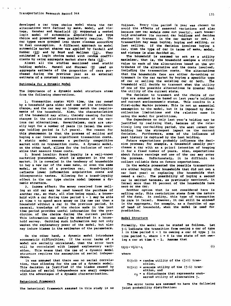
,,.
Transportation Research Record 944 135
developed a car type choice model where the caralternatives were defined by make, model, and vin-tage. ?lenaherand J4anefield(~) suggested a nestedlogit model of automobile acquisition and typechoice and presented some preliminary results. Thecar types were grouped into three claases accordingto fuel consumption. A different approach to modelautomobile market shares was applied by Cardell andDunbar (~ and by Soyd and MeUmen (~. Theyestimated a logit choice model with random coeffi-cients by using aggregate market share data (~.
Almost all the studies mentioned used etaticholding models. Manski and Sherman” (Q) used an
a99re9ate estimate of the proportion of cars pur-chaaed during the previoue year as an externalestimate of a conntant transactioncost.
Rationale for a Dvnemic Model
The importance of a dynamic model structure stemsfrom the following observations.
1. Transaction coats: With time, the car ownedby a household gete older and come of ita attributeschange, and the car may no longer match the require-ment of the household. Also, the characteristicsof the household may alter, thereby causing furtherchanges in the relative attractiveneee of the var-ious car alternatives. Nevertheless, cars are usu-ally kept for a number of years (in Israel the aver-age holding period is 3.5 years). The reaaon forthis phenomenon ia that the process of selling andbuying a car involves significant transaction costs.A static model assumes a perfectly competitivemarket with no transaction costs. A dynamic model,on the other hand, allows for the inclusion of vari-ables that measure these costs.
2. Brand loyalty: Brand loyalty is a well-knownmarketing phenomenon, which is apparent in the carmarket. It is revealed in the tendency of householdsto buy a new car of the same make, or ●ven the samemodel, as that of a previous car. Brand-loyaltyreflects lower information acquisition coete andidiosyncratic tastes. Allowing for a brand-loyaltyeffect in the car type choice model imposes a dy-namic structure.
3. Income ●ffect: The money received from sell-ing an old car may be used toward the purchase ofanother car, ao that, all else being equal, a house-hold with a car during time period t - 1 may be ableat the t to spend more money on its new car than ahousehold without a car in the previous period. Ingeneral, knowledge of the choice made in the lasttime period provides useful information for the pre-diction of the choice during the current period.This information can easily be obtained in a house-hold survey. Omitting such information may not onlyweaken the explanatory power of the mode~, but alsomay induce biases in the esthetes of the parameters.
on the other hand, a dynamic model introduceseconometric difficulties. If the error terms of amodel are serially correlated, then the error termwill be correlated with lagged explanatory vari-ables. This means that the use of a dynamic modelstructure requires the assumption of serial indepen-dence.
It was assumed that there was no serial correla-tion, thus allowing for the use of a dynamic model.This decision ia justified if the biases caused byviolation of serial independence are small comparedwith the advantagea of a dynamic characterization.
Behavioral Framework
follows. Every time period (a year was chosen toavoid the effects of seasonal variationa and alsobecause new car models come out yearly), each house-hold evaluates its current car holdings and decideswhether to tranaact in the car market or not. Atransaction may mesn buyhg, buytng and selling, orjust selling. If the decision involves buying acar, then the type of car in terms of make, model,and vintage is also decided on.
The household is assumed to act as a utilitymaximizer, that is, the household assigns a utilityvalue to each of the alternatives based on the at-tributes of the alternative and the costs involved,including the transaction costs. The alternativesthat the households face are either do-nothing ortransact in the car msrket by buying a specific typeof car or selling the exieting car or both. Thehousehold will decide to transact when the utilityof one of the poaaible alternative is greater thanthe utility of the current state.
The decision to transact and the choice of cartype are aaaumed to be based on last year’s holdingsand current socioeconomic status. This results in afirst-order Merkov process. This is not an essentialassumption to the model, but it is imposed by data-collection limitations and the relative eaee inusing the model for predictions.
The dependence on only last year’a holding may bejustified by realizing that, because of the rela-tively long car-holding period, the most recent carholding has the strongest impact on the currentdecision. Furthermore, some of the influence ofpast history is captured by the laat holding.
Future expectations probably influence the deci-sion process; for example, a household ueually pur-chases a car with an a priori intention of keepingit for a fixed number of yeare. Also, expectationsabout future earnings and use of the car may enterthe process. Unfortunately, it is difficult tocollect reliable data on future expectations.
In the models presented the possible transactionsare either buying (for households that did not own acar last year) or replacing (for households thatowned a car). The possibility of buying a secondcar is omitted because, aa previously mentioned, inIsrael more than 95 percent of the households havezero or one car.
Another option that is not considered here isselling only. l%is restriction stems from the natureof the data. In reality, this type of transactionis rare in Israel. However, it can still be allowedin the aggregate, for example, as a function of ageof head of household, when the model is used forprediction.
Model Structure
Formally, the model can be stated as follows. Letjli ’indicatethe transition from owning a car of typei in time period t - 1 to owning a car of type j intime period t, where i = O is the state of not own-ing a car at time t - 1. Assume that
Ufi@=V~li)+6J (1)
where
u(jti) = random utility of the (jIi) tran-sition,
V(jli) = average utility of the (jli) tran-sition, and
rj = a disturbance that represents unob-served utility-of alternative j.
The error terms are assumed to have the following
The behavioral framework assumed in this study is as joint probability distribution:
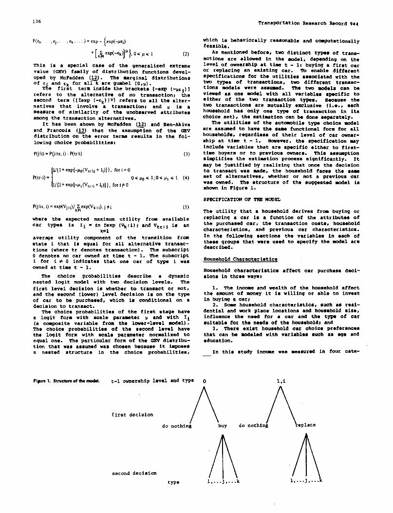
136 Transportation Research Record 944
Nei,,ej,. .,ck$...)=CX{CXp(ppC~C~
(2)
This is a apaclal case of the generalized ●xtreme
value (GEV) family of distribution functions devel-
oped by McFadden (~. The marginal distributionsof c
kand ck for all k are guabel (0,11).
T e firat term inside the brackets [-exp (-IICi)lrefers to the alternative of no transaction; thesecond term ([.texp(-ck)]u)refera to all the alter-natives that involve a transaction~ and u is ameasure of similarity of the unobserved attributesamong the transaction alternatives.
It has been shown by McFadden (1.2)and Ben-Aklvaand Francola (13J that the assumption of the GBVdistribution on the error terms results letthe fol-lowing choice probabilities:
FYjli)= P(jltr, i) P(trli) (3)
Il/{l+exp[-*(V~,lO+ IJ]),fOri=O
P(trli)= o</.4)<l;o<ul<l (4)
l/{lieXP[-P~(V~~li+I,)]J,fori*O
~ Itr, 1) = eXp(vj lL)/k~iCXP(vk I i), J # i
where the expected maximumcar types is Ii = in Zexp
Ir#l
(5)
utility from available(vkli); and Vtrli is an
averqe utility component of the transition fromstate i that is equal for all alternative transac-tions (where tr denotes transaction). The subscriptO denotes no car owned at time t - 1. The subscripti for i # O indicates that one car of type i wasowned at time t - 1.
The choice probabilities describe a dynamicnested logit model with two declslon levels. Thefirst level decision la whetter to transact or not,and the second (lower) level decision ia on the typeof car to be purchased, which la conditional on adaciaion to transact.
The choice probabilities of the first stage havea logit form with scale parameter u and with Ii(a composite variable frorsthe lower-level model).The choice probabilities of the second level havethe logit form with scale parameter normalized toequal one. The particular form of the GNV distribu-tion that was assumed was chosen because it imposesa nested structure in the choice probabilities,
which la behaviorally reasonable and computationallyfeasible.
Aa mentioned before, two distinct typSS Of trans-actions are allowed in the model, depending on thelevel of ownership at time t - 1: buying a first caror replacing an existing car. To enable differentspecifications for the utilities associated with thetwo types of transactions, two different tranaac-tiona models were assumed. The two models can beviewed as one aodel with all variables specific toeither of the two transaction types. Because thetwo transactions are mutually exclusive (i.e., eachhousehold has only one type of transaction in itschoice act), the estimation can h done separately.
The utilities of the automobile type choice modelare assumed to have the same functional form for allhouseholds, regardless of their level of car owner-ship at time t - 1. However, the specification mayinclude variables that are specific either to first-time buyers or to previous owners. Thh assumptionsimplifies the estimation process significantly. ItIMY he justlfled by realizing that once the decisionto transact was made, the household faces the sameset of alternatives, whether or not a previous carwas owned. The structure of the suggested model isshown in Figure 1.
SPECIFICATIONOF TRE MODEL
The utility that a household derives from buying orreplacing a car 1s a function of the attributes ofthe purchased car, the transaction costs, householdcharacteristics, and previous car characteristics.In the following sections the variables in each ofthese groups that were used to specify the model aredescribed.
Household Characteristics
Household characteristics affect car purchase deci-
sions in three ways:
1. The income and wealth of the household affectthe amount of money it ia willing or able to investin buying a car)
2. Some household characteristics, such as resi-dential and work place locations and household size,influence the need for a car and the type of carsuitable for the need8 of the Iiousohold\and
3. There exist household car choiea preferencesthat can be modeled with variables such as age andeducation.
In this study in-e was measured in four cate-—
Figulvl.Stnkctursoftlwrrkodzl. t-1 ownership level and type o l,i
,onothin~udonothiq~eplace
first decision
A htype 1....j....k
second decision

,,, ,
TranBpxtation Research Record 944137
gories. Also used were proxy variables for incomeand wealth, such as education, age, and work status.
Household characteristics that affect the needfor a vehicle can be divided into two groupa: vari-ables that affect the relative utility of owning acar compared with not owning one, and variables thatinfluence the relative utilities of different typesof vehicles. The first group consists mainly ofaccessibility measures for work and other trips.The characteristics that affect the type of carchosen are household size and composition and theneed to use a car for work-related purposes. Indi-vidual preferences were characterized mainly byinteracting age and education of the car user withcar attributes such as performance and age.
Attributes of Previous Car
The attributes of the care owned during the previoustime period affect the decision to replace a car andthe choice of car type. The replacement model in-cludes the following attributes of the previous car:age, engine size, number of years owned by thehousehold, and average mileage. Engine size servesas a meaeure of durability, and mileage is a measureof use.
Attributes of the previous car were also aseumedto affect the car type choice. Purchase price foreach type was defined as its market price minus thesale price of tbe exieting car. Brand loyalty wascaptured by a dummy variable, which is set to 1 ifthe type is of the same make as the previous car.
Attributes of Alternative Cars
The car attributes are of special interest becausethey characterize the alternatives that a householdfaces when choosing a car, thus enabling predictionsof the effects of policy and technological changeeon the market. The car attributes were selectedAccording to two criteria: (a) the attribute has tobe familiar to prospective car buyers, and (b) areliable data source for the attribute exists forall the alternative car types. The following attri-butes were selected: cost--retail price and fuelefficiency; size-dimensions, weight, luggage space,and engine size; performance-acceleration (measuredby HP/kg) and maximum speed; and other--age, manu-facturing country, and number of cars of the sametype in the market.
The alternative-size variable (i.e., the numberof cars of the same type in the market) is also ofspecial interest. In the type choice model, eachtype represents a group of elemental alternatives--all the cars of the same make, model, year, and bodytype on the market. All of these cars have identicalobserved attributes. In this case it is necessaryto add to the utility of an alternative a normaliza-tion term equal to the logarithm of the number ofelemental alternatives (fJINj).The coefficient ofUINj is a measure of the variation of the unobservedattributes among cars of the eeme type. It is rea-sonable to aesume that ae cars get older, the heter-ogeneity among them increases. To enable differentcoefficients for car types of different agee. thealternative-eize variable wae introduced in themodel as a group of age-specific variablee. Fourtype size variables were ueed for cars: 2 to 5, 6 to9, 10 to 14, and 15 or more years old. The type-sizevariable ie not used for new car types. The choiceprobability for new cars does not depend on InNj
becausa the buyer faces only one new car that heorders from the dealer. AS described in the nextsection, the type-size variable ie also a proxy forsearch cost so that the coefficients of these vari-
ables capture the total affect of alternative sizeon the utility.
Transaction Costs
Transaction costs arise from two main sources:search costs in terms of time and money that areincurred in the process of searching for a car, andinformation costs that are caused by inc~leteknowledge of the attributes of alternative cars.Thie model includes a detailed specification of thetransaction costs, eqreesed as functions of the
attributes of the previous car, the purchased car,and the nature of the transaction.
In the process of teeting alternative model spec-ifications, some simplifying and generalizingassumptions had to be made with respect to the spec-ification of transaction costs (TC). The specifica-tion of TC in the car type utility function is asfollows:
where
6j,i =
:; :
‘~ -
6v~=j
! 1, if make (j) = make (i)
[O, otherwisenumber of cars of same make as j,number of cars of same type ae j,age of car j,
{
1, if vintage of car j belongs tovintage group 1
0, otherwise
and al, a2, a3t and a41 are unknown parameters.The first term represents brand loyalty. The
second term captures the market-size effect of allcars of the same make. The third term captures theeffect of the number of cars of the same type onsearch costs and the basic correction for alterna-tive size of the utility. These effects are allowedto vary with the age of the vehicle. The fourthterm represents the effect of the age of the vehicleon the information acquisition costs through a num-ber of age-specific dummy variablee. This effect ismeasured relative to new cars.
The average TC for each of the two types oftransactions appears in the respective transactionmodele as pert of the alternative specific constante.
SAMPLING STRATEGY ANO ESTIMATION PROC!SDORE
The estimation of the models was carried out byusing the data from a sample of households that werecollected in the Haifa urban area during 1979. Thenested etructure of the model dictated the samplingstrategy. The upper-level (transaction) model re-quires a sample of buyers and nonbuyers, with andwithout a previous car. The lower-level (car type)model requires for its estimation the householdsthat bought a car during the study year. A randomsample of households would not provide enough suchpurchases unless it is large, because only 40 per-cent of the households own care and less than one-third of these houeeholde are expected to purchase acar in a given year.
The eempling strategy used was choice based orendogenously stratified, where the stratificationwas based on the transaction decision. The total
se.mpleconsisted of a random sample with one sem-pling quotient of households that did not transactin the car market during the study year, and anothers~le with a greater quotient of households thatpurchaeed a car during that year. About 500 houee-holde that did not buy a car during the study year
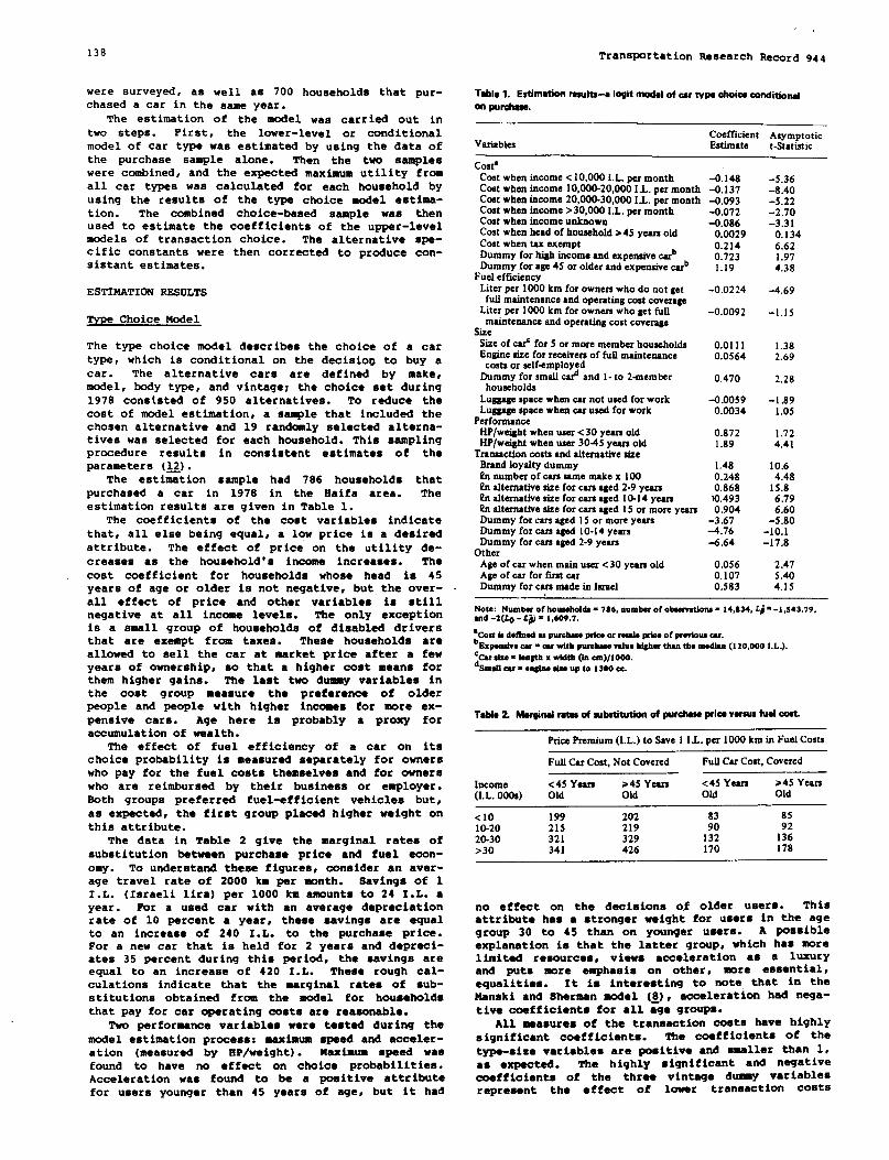
138
were surveyed, aa well as 700 households that pur-chased a car in the same year.
The estimation of the model was carried out intwo atepa. First, the lower-level or conditionalmodel of car type wae estimated by using the data ofthe purchase sample alone. Then the two sampleswere combined, and the expected maximum utility fromall car types waa calculated for each household byusing the results of the type choice model estima-tion. The combined choice-baaed sample was thenused to estimate the coefficients of the upper-levelmodels of transaction choice. The alternative spe-cific constants were then corrected to produce con-sistent estimates.
ESTIMATION RESULTS
TYPS Choice Model
The type choice model describes the choice of a cartype,which ie conditional on the decisio~ to buy acar. The alternative cars are defined by make,model, body type, and vintage; the choice set during1978 consisted of 950 alternatives. To reduce thecost of model estimation, a sample that included thechosen alternative and 19 randomly selected alterna-tives was selected for each household. This samplingprocedure results in consistent estimates of theparameters (~).
The eatireation sample had 786 households thatpurchased a car in 1978 in the Haifa area. Theestimation results are given in Table 1.
The coefficients of the cost variables indicatethat, all else being equal, a low price is a desiredattribute. The effect of price on the utility de-creases as the householdra income increases. Thecost coefficient for households whose head is 45years of age or older is not negative, but the over-all effect of price and other variables is stillnegative at all income levels. The only exceptionis a small group of households of disabled driversthat are exempt from taxes. These households areallowed to sell the car at market price after a fewyears of ownership, so that a higher cost means forthem higher gains. The last two d- variables inthe cost group measure the preference of olderpeople and people with higher incomes for more ex-pensive cars. Age here is probably a proxy foraccumulationof wealth.
The effect of fuel efficiency of a car on itschoice probability is measured separately for ownerswho pay for the fuel costs themselves and for ownerswho are reimbursed by their business or employer.Seth groups preferred fuel-efficient vehicles but,as expected, the first group placed higher weight onthis attribute.
The data in Table 2 give the marginal rates ofsubstitution between purchase price snd fuel eoon-
Ov ● To understand these figures, consider an aver-age travel rate of 2000 km per month. Savings of 1I.L. (Israeli lira) per 1000 km amounte to 24 I.L. ayear. Por a used car with an average depreciationrate of 10 percent a year, these savings are equalto an increase of 240 I.L. to the purchase price.For a new car that is held for 2 years and depreci-ates 35 percent during this period, the savings areequal tO an increase Of 420 I.L. These rough cal-culations indicate that the marginal rates of sub-stitutions obtained from the model for householdsthat pay for car operating costs sre reasonable.
TWO performance variables were tested during themodel estimation prrtcesa:maximum speed and acceler-ation (measured by lIP/weight). 14eximum speed waafound to have no effect on choice probabilities.Acceleration was found to be a positive attributefor users younger than 45 years of age, but it had
Transportation Research Record
TabIeI.Enimatia wlti-alwitticldar tvpachmiacortditbd
on w-.
944
coefficient A$ymptc.tkvarisblee Estimate t-Statimic
cost’Coatwhen income <10,000 I.L.per month -0.148Cost whenimcome l0,000-20,0001L. permontlr -0.137Cost whenincome 20,000.30.0001 .L. oermonth -(.093Coatwhenincome>30,000I~L.per m&rthCoatwhenincome unknownCost when head of household> 45 years oldCost when tas exemptDummy forhighincome sndexpermivecerbDummyforage45 orolderandexpenaive carb
Fuel efficiencyLiterper1000km forowncrawhodo notget
full maintenance and opemting coat coverageLiterper1000km forownarswhoget full
maintenanceaod operating cost coverageSise
SizeofcarCfor5 ormorememberhouaaholdsEngineaire forreceivem offuflmaintensnce
coatsoraelf+mployedDummyforsmall cd snd l-to2-rrremher
householdsLuggagespats when car not used for workLuggagespace whencaruavdforworkPerformanceHP/weightwhen user <30 years oldHP/weightwhenuaer 3045yearsold
Transaction costs and alternative sireBrandloyaltydummy!?rrnumberofcaranme makex100Qrralternative sire for cars aged 2-9 yrara!?nalternativeaise fOrcanaged10-14 yean!hralternstivesire formaged150r moreyedrrDummyforcars aged 150rmoreyearsDummyforcsra aged 10-14yearsDummyforcarsaged 2-9yeara
OtherAge of w when main user< 30 years oldAgeofcarforfti carDummyforcararnade inlmsel
-0,072-0.086
0.00290.2140.7231.19
-0.0224
-0.0092
0.01110.0564
0.470
-0.00590.0034
0.8721.89
1.48
0.2480.868
K).4930.904
-3.67-4.76
-6.64
0.0S60.1070.583
-5.36-8.40-5.22-2.70-3.31
0.1346.621.974.38
-4.69
-1.15
1.382.69
2,28
-1.891.05
1.724.41
10.64.48
15.86.796.60
-5.80-10.1-17.8
2.47S.404.15
Note: NumWrofhounholds .786, rntmber ofobwrvmt&ru =14,834, C~=-l,S43.79,and-2(20-f@ =1,609.7.
%ostiadcllrwdss purchanprktor rmdep#iaoofprcvIous SM.bExp.mtvsrar.au Wfthpsrahswvafu@3d6hertlmntbcma31u!(120,000LL.).~Cudm. kr13thx wfdtb(in cm)/1000.smst3ar=*r@n*duupt01300ss.
Price Premium (1.L.) to Save 1 IL per 1000 km in Fuel Costs
FuUCarCrmt,Not Covered Full CarCoat, Covered
Income <45 Yeua >45 YVUX <45 Yesra >45 Yesrs(LL. 000s) Old old Old Old
<IO 199 202 83 8510-20 215 219 9020-30 321 329 132 1?:>30 341 426 170 178
no effect on the decisions of older users. Thisattribute has a stronger weight for users in the agegroup 30 to 45 than on younger users. A possibleexplanation is that the latter group, which has morelimited resources, views acceleration as a luxuryand puts more emphasis on other, more essentialequalities. It is interesting to note that in the14anskiand Sherman model (~), acceleration had nega-tive coefficients for all age groups.
All measures of the transaction ooeta have highlysignificant coefficients. The coefficients of thetype-sise variables are positive and smaller than 1,as expected. The highly significant and negativecoefficients of the three vintage dumy variablesrepresent the effect of lower trsneaction costs

,.2,
Transportation Research Record 944 139
involved in purchasing a new car, as well as theeffects of other desired qualities of a new car,such as reliability and prestige. The differentmagnitudes of the three coefficients represent theeffects of unmeasured attributes that are related toeither age or vintage of the cara.
The other two age variablea meaaure the prefer-ence for old cars dieplayed by young buyers and byfirst-time buyera. In part this represents morelimited resources, but it may also indicate a leeserconcern for reliability on the part of inexperiencedbuyers and young users.
The last dummy variable for locally assembledcara represents a preference for these cars thatcannot be explainad by their lower prices.
To examine the goodness of fit between the eeti-fnetad and obaervad aggregate choice probabilitiesfor the sample, the 95o car types were groupad ac-cording to engine size and vintage. Generally, asatisfactory fit between the estimated and observedprobabilities was revealed, and none of the differ-ences was greater than 3 percent.
Purchase Model for Households Without a Vehicle
The purchase model for households without a vehicledescribes the purchase decision in year t for house-holds that did not own a car in year t - 1. Themodel was estimated with a sample of 618 households,about half of which came from a random sample ofhouseholds in the fiaifaarea and the other half froma random sample of car buyers from the sensearea.The eatiraationresults are given in Table 3. Allcoefficients In the model have the expected signs.
Tds103.Etimtionr-lti+lWitmddofmrWtiawd-isiaforhouseholds without vahidsa.—
Coefficient AsymptoticNo. Variable Estimate t-Statistic
One-adult hou8ehol& -1.04 -2.96; Income >10,000 LL. 0.498 1.923 Income not reported, head of household -0.06 -0.15
employed4 Hradofhouashold self-employed 0.699 1.525 Occupation of hsad of houarhold- 0.624 2.31
academicormsnagerkal6 Educetionofhaad ofhouashold-more 0.416 1.88
than 12 ysara7 Age of head ofhousehold when older -0.0093 -2.56
thsn 508 Use of car on Saturday (1 = ysaand -0.409 -1.63
2 = no)9 Travel time to work by bus 0.0185 3.S6
10 Traveltimetoworkbycar -0.0131 -1.7011 Walkingdiatanceto busstop (inrninutes) 0.142 4.4112 0rrmmyf0rpurd2asa alternative -6.5 -3.55
(rorrected)-13 Expected maximum utikity from the car 0.512 3.22
type choice (!2s3sum)
Note: Number of obsssvstlnns = 618; t~ = -339.S6; ●nd -2(f,0 - t~) = 177.60, df.13.
Attributes 1-6 represent the financial ability topurchase a car; they include income and some socio-d.amographic descriptors that are correlated withpotential earninga. Attributes 8-12 represent theneed for a car. They include the following accesal-bility measures: travel time to work by car and bybus, walking distance to the nearest bus stop, and aproxy to the need for a car for leisure trips, thatis, traveling on the Sabbath, when public transpor-tation service is significantly reduced.
The variable age of head of household when olderthan 50 representa the tendancy to change that isassociated with age as well as the increasing dif-
ficulty of acquiring a driver’s license. The lastvariable ia the expected maximum utility that thehousehold derives from the car choice, given that adecision is made to own a car.
The data in Table 4 demonstrate the influence ofsocioeconomic and accessibility attributes on pur-chase probabilities. The effect of the relativeaccessibility by bus and by car ie especially sig-nificant; for example, when travel time to work ia10 min by car and 30 min by bus, the purchase proba-bility for a blue-collar employee (column 3 in Table4) iS 0.08. When travel time to work by car in-creaaes to 20 min and by bus to 60 rein,the proba-bility that the same household will purchase a carmore than triples to 0.26 (column 6 in Table 4).
Ttble 4. Expactad purahzaaprobabilities rnmputad for hwaahohks withvariousattribtttas ttmtdidnotown arzrirrthepravinus period.—
Attribute Values by Household Number
Attribute 1 234567
No. of adults in house-hold
HouaeholdincomeWorkstatus of head of
householdOccupation of hesd of
householdEducation of hsad of
householdAge of head of
householdUse of car on SaturdayTravel time to work by
busTravel time to work by
carWalkingdistance to bus
stopInclusive value
Purchass probability
2
;E
AM
15
45
Yeso
0
2
6
0.14
2
;E
AM
15
45
Yes30
10
3
6
0.22
2 12
1 1EMP EMP ;E
BC BC AM
10 10 15
45 55 45
Yes Yes Yes30 30 60
10 10 20
33 10
666
0.08 0.02 0.54
2 1
1 1EMP EMP
BC BC
10 10
45 55
Yes Yre60 60
20 20
10 10
66
0.26 0.07
Note: SE . sstf employed, AM = ●UdemIc or msmgsrlst, EMP=employee, andLW=bluecolisr.
Purchase f40delfor Households AlreadyOwning a Vehicle
The purchase model for households already owning avehicle describes the probability that a householdwill replace its car during a certain year, giventhe socioeconomic descriptors of the household andattributes of the existing car. The estimationresults are given in Table 5.
AW unexpected finding waa that high income re-ducee the probability of replacing a car. This
result is strengthened by the negative coefficientsof other attribute that are correlated with @xx6e,such aa ●duration, work atatusp and =vera9e of caroperating and maintenance coste.
Age of head of household hae a negative effect onthe probability of replacing the car. So does being
a one-adult household, especially if this adult is awoman. It is possible that women and older parsonsface higher transaction coats. As expected, house-hold that are exempt from taxes have a higher pur-chase probability. The exemption ie generally givento disabled people who need a reliable vehicle andtherefore replace it often. Accessibility measureswere found to have no effect on the replacementdecision. This iS expectadn becauee reelacin9 a carwill have only a small effect on accessibility.
The attributes that deecribe the previous carhave the expected effect on replacement choice. The
replacement probability increaees with age and use

140 Transportation Reaestrch Record 944
Table5.AnimationreW1O-elqitmAd ofrarpur~wdwi$ionforhouseholdwithavehicle.
Coefficient AsymptoticVariable Estimates t-Statistic
One-adult houaehoidWoman head of householdIncome <10,000 I.L., head of householdemployedlncoore>20,000I,L.,head of household
employedIncome not reported, head of household
employedHead of household self-employedFull car maintenance coat coveredExemption from car taxesEducation ofheadof household–more than 12
yearsAgeofhead ofhousehold35 years of youngerAge of head of household 50 years or olderMonthly Irilometerage exceeds 2000 kmPrevious car charscteriatics
YearEngirre size smsller than 1300ccEngine size larger thsn 1800ccNo, of years car was owned by householdDummy for purchase alternative (corrected)Expected msximum utility from car type choice
-1.52-1.23
0.45s
-0.550
-0.919
-0.0654
-0.1501.51
-0.494
0.816-0.721
0.960
-0.09070.699
-0.8290.0766.5
-0.092
-2,3S-1.77
0.816
-2.00
-2.15
-0.14-0.30
2.03-2.18
2.71-2.65
2.37
-2.552.30
-1.591.493.67
-0.625
Note: Number ofobUmation. =582; lu=-267; and-2 (L~-[6)=271, d.f. 17.
of the vehicle and with duration of holding, anddecreases with engine size (a proxy for durability).The positive effect of duration of holding on re-placement reflects the decrease in relative utilityof the existing vehicle with time.
The coefficient of the expected maximum utilityin this model is negative but smell. It ie notsignificantly different from zero. This means thatgiven the aocioeconoeeic characteristics of thehousehold and the attributes of the existing car,the utility from the car type choice waa not foundto have an effect on the replacement deci6ion. Inother words, the decision to replace a car is inde-pendent of the type choice.
This result deserves an explanation because it isexpected that the replacement decision would bedependent on the characteristics of available cars.Two reasons may account for this effectr and bothreasons are related to the fact that this model isbased on cross-sectional data. First, exogenousvariables such aa fuel coats and microecon~ic con-ditions do not vary across the sample. Thus anypossible effect of the variables is contained in thetransaction-specificconstant. Second, technologicalchanges in the car industry are not so dramatic asto cause a major shift in choice from one period toanother. Thus the expected maximum utility from allcar types is well represented by the attributes ofthe existing car and household characteristics, andthose attribute are represented in the replacementmodel.
Forecasting Results
The model developed in this study was used to eval-uate the automobile-demand effects of the followingtwo scenarios:
1. A change in tax rates that will result in anincrease of 20 percent in the price of new largecars with an engine size larger than 1900 ccr and adecrease of 20 percent in the prices of new smallcars with an engine size smaller than 1300 cc (it ISassumed that the changes in the prices of new carawill cause price changea of similar proportions inthe used car market), and
2. An increase of 100 percent in fuel prices.
As expected, the price changee CKeated a relativeadvantage for small cars, which resulted in an in-crease in purchases of these cars and a correspond-ing decrease in purchases of larger cars. An inter-esting finding is that the increase occurs mainly inthe purchases of new cars in the engine-size cate-gory that benefited most from the tax changes,namely, cars with engine sizes of 1100 to 1300 cc.Apparently, for households that intended to buy asmall car, the price reduction enabled the purchaseof a newer or a bigger car within the ssme category.On the other hand, the price changes caused scarepotential buyers of intermediate or large cars tochoose a smaller car, and the savings thus gainedcould be used to purchase a newer car. The neteffect of theee shifts is an increaee of 38 percentin the category of new cars with engine sizes be-tween 1100 and 1300 cc, and a 10 percent decrease inthe demand for cars with engine size larger than1400 cc.
The assumed changes in car prices did not affectthe purchase decision. Thie result ia obvious forhouseholds that already own a car and considerwhether to replace it, because according to themodel the replacessentdecision is independent of thecar type decision. For households without cars, thepurchase decision is affected by the expected maxi-mum utility from all car types. However, thesevalues are not changed much by the proposed pricechanges, and the predicted aggregate effect is neg-ligible.
The increaee of 100 percent in fuel price in-creased the demand for fuel-efficient vehiclee (withengine volumes of up to 1000 cc) by 16 percent andcaused a corresponding decrease In the demand forbigger cars, especially for gas-guzzelers in the1900 cc or larger category. The choice of a smallercar ●nabled the buyer to purchaee a newer car withthe same budget, so that the overall demand for newcars increased by 7 percent.
The 100 percent increase in fuel price was foundto have a strong impact on the probability of buyinga first car. The estimated number of purchasesdecreased by 47 percent as a reeult of the fuelprice hike. However, the implied assumption thatthe car prices will remain unchanged in the face ofsuch changes in demand is unrealistic, and the realeffect of a large increase in fuel price on purchaseprobabilities of first care is expected to besmaller.
S~Y AND fX3NCLUSIONS
In this work dynamic transaction models for carownership were defined and ●stimated. The mainadvantage of theee modele is their dynamic struc-ture-+arkovian of the first order-which providesfor a direct account of transaction costs and char-
acteristics of the previous ownership level as wellaa the attributes of cars in the choice set. Thenested structure of the logit model used in thisstudy provides for an efficient data-collectioneffort and ●ases the estimation procees.
Specification of the models includes @icy-sen-sitive variables such as characteristics of cartypes, socioeconomic variables, and accessibilityvariables.
The use of the wdele to support policy decisionswas demonstrated for two scenarios involving changesin purchase and operating costs. For a more compre-hensive policy analysis, the models developed herecan be easily supplemented to includ. all the trans-actions that are possible -in the car market (e.g.,transaction in multicar households and transactionsthat result in a reduction in level of car owner-ship). A full set of such models can be incorporated

,.!
Transportation Research Record 944 141
into a system of equatiorm to represent equilibriumconditions in a car market. A general structure ofouch equations is deecribed by Manski (~. It isbelieved that the uee of the dynamic models devel-oped in thie work, in the framework of equilibriumequatione, can provide a ueeful system for the anal-ysis of policiee that affect the car market.
The research reported here wae performed at theTransportation Reeearch Institute, Technion--IeraelInstitute of Technology, Haifa. The study was epon-sored by the Israeli Ministry of Transport, and wewould like to thank @!uritStraue, the project mon-itor, for her continuing support. Partial supportwas also provided by a grant froa the National Sci-ence Foundation to the Naeaachueette Institute ofTechnology to study the demand for autcaobiles. Wealeo greatly benefited from the enlightening discus-sion we had with Charlea Manski.
REFSRENCEB
1.
2.
3.
4.
5.
C. Lave artd.K.Train. A Behavioral DisaggregateNodef of Auto ~ Choice. TransportationResearch, Vol. 13A, 1979, pp. 1-9.Wharton Econometric Forecasting Associates. AnAnalyaia of the Automobile Narket: Modeling theLong Run Determinant of the Demand for Automo-bile. Transportation Systems Center, Us.Department of Transportation, Cambridge, Maas.,1977.M. Sen-Akiva” and S. Lerman. Some EstimationResults of a Simultaneous Model of Auto Owrter-ship and Node Choice to Nork. Transportation,Vol. 3, 1976, pp. 357-376.S.R. Leraan and M. Ben-Akiva. DisaggregateBehavioral Nodel of Automobile Chmerehip. TRB,Transportation Reeearch Record 569, 1976, pp.34-55.L.D. Burns, T.F. tilob, and G.C. Nicolaidis.
6.
7.
8.
9.
10.
11.
12.
13.
14.
Theory of Urban Eousehold Automobile OwnershipDeciaiotta. TRB, ‘TransportationReeearch Record569, 1976, n 56-75.J. Kain and.G. Fauth. Forecasting Auto Owner-ship and Mrrde Choice for U.S. MetropolitanAreaa. Department of City and Regional Plan-ning, Harvard univ., Cambridge, M8SS.I WorkingPaper, 1977.R.R. Johnson. Aggregation and the Demand forNew and Used Automobiles. Review of SconcdcStudiee, Vol. 45, 1978, pp. 311-327.C.F. Wanski and L. Sherman. An ~irical Anal-yeia of Household Choice Among Motor Vehicles.Transportation Research, Vol. 14A, 1980, pp.349-366.D.A. Henaher and T. Manefield. A StructuredLogit Nodel of Automobile Acquisition and meChoice. ProC., Australian Trannport ResearchForum, Hobart, Tasmania, Australia, 1982.N.S. Cardel and F. Dunbar. Measuring the Soci-etal Impact of Automobile Downsizing. Trans-portation Research, Vol. 14A, 1980, pp. 423-434.J.H. Soyd and R.E. Mellman. The Effect of FuelEconq Standards on the Ues. AutomobileNarket: An Hedonic Demand Analysis. Transporta-tion Research, Vol. 14A, 1980, pp. 367-378.D. McFadden. 14udellingthe Choice of Residen-tial Location. ~ Spatial Interaction Theoryand Residential Location (A. Karlquist et al.,eds.), North-Holland, Amsterdam, 1978.M. Ben-Akiva and B. Francois. v Homogene@sGeneralized Extreme Value Model. Department ofCivil Engineering, Massachusetts Institute ofTechnology, Cambridge, Working Paper, 1981.C.F. Manski. Short Run Equilibrium in theAutomobile Market. The Maurice Falk Institutefor Economic Research in Israel, Jerusalem,Discussion Paper 8018, 1980.
Riblicationofthia papersponsoredby Committeeon TrrrvelerBehoviorandValues
Experiments with Optimal Sampling for Multinominal
Logit Models
YOSEFSHEFFIAND ZVITAREM
Inthispspsr● rsssntlypublidredmethodforoptimklngtheszmpleusedinsotinratingdieatete4roissmodelsb tested.7hetwwkieintendedtoidenttiwd oxplorcthzdzntwrt8thatirrflusrwstheeffsztivsnssrofthkmethodologyindesigningsamplingprossdumforzstltnztirtpImpitmodels.llrzirwatipz-tioninolude9bothwwlyt&el●ndnunreridtests.l%emuttsindkztcthettlrassmplooptimizationmethodssnimprovothesoourseyoftheresultingntirnztes,m aompzmlwithrwdom tampk.
Data collection is, in many cases, the major costitem in studies that involve the estimation of econ-ometric models. Technique for sample deeign havetherefore been developed for many econometric andstatistical models (~). In this paper discretechoice mrrdela,which are extensively used in travel-demand analysis, are examined, and, in particular,the multinominallogit (MNL) model is discussed. The
focus here is on a method for optimizing the sampleused to estimate discrete-choice models. The ap-
plicability of this sample optimization approach tothe collection of the sample points (the data) usedto estimate WNL models ie examined. Also examined
is the appropriate amount of effort that should beinvested in the sample optimization process.
The original development of the sample optimiza-tion method, which is the subject of this PaPer~ isfrom Daganzo (~). Daganzo’a method is a stratifiedsampling technique. It assumes that the Populationto be sampled frcincan be partitioned into separategroups (or strata) and that observations can be sam-pled independently from each group. The objective
of the eaapling method is to determine how many ob-servations should be drawn fr~ each 9rouP so that

142 Transportation Research Record 944
the total estimation error ia minimized. The esti-mation error ia a composite meaaure of the error inall the model parameters. Naturally, this minimiza-tion ia subject to a budget constraint. This sam-pling method attempta to determine the best alloca-tion of the sampling budget. (The companionproblem, that of determining the minimum budget re-quired to achieve a certain accuracy, is somewhatmore difficult. Ite solution, however, can be in-ferred from the solution of the problem under con-sideration.)
Three main points are diacuaaed in this paper.The firat point ia the applicability of the approachin terms of potential. The question examined inthis context is the sensitivity of the sampling er-ror to different sample deqigns. The second pointia that the solution of the eample optimization (SO)problem requires prior estimates (or guesses) of thevaluea of the parameters of the model to be esti-mated. The applicability of the whole concept de-pends, naturally, on the required accuracy of theseprior estimates. The tests described in this paperexplore this point in some detail. The third pointis related to the first point. It has to do withthe question of the amount of effort that should beinvested in obtalninq these prior estimates. Suchan effort should be judged in comparison to thelevel of effort of the entire study, which meansthat the relevant question is the allocation of ef-fort between obtaining the prior estimates and theestimation itself.
This paper ia organized as follows. First,DaganzoQs SO method is outlined. Then the applica-tion of this method to the MNL model is reviewed.Next, the question of the applicability of the SOmethod is explored by looking at a simple one-param-eter model and a two-parametermodel. Then the afore-mentioned issue of resource allocation in the frame-work of a small case study is diacuased, and finallyconclusions are given.
It should be noted that the conclusions of thispaper are baaed on numerical experiments, whichmeans that not all the results can be generalized inall circumstances. The experiments are deecribed infurther detail by Sheffl and Tarem (~).
SAMPLE OPTIMIZATION PROORAM
Daganzogs SO method attempts to minimize the errorassociated with the estimation of the parameters ofa discrete-choice model. The optimization problemis formulated as a mathematical minimization pro-gram, where a composite measure of the estimationerror serves as the objective function and the sam-ple group sizes are the decision variables. ThisaPProach assumes that the model under considerationis estimated by using the maximum likelihood (ML)method. It alao assumee that the distribution ofexplanatory variables in each group is known. [Thisinformation may not be available, In which case themethods discussed by Lerman and ktanski (~) may beused.]
The objective function of the SO program relatesthe sampling error to the sample group sizes. Thisexpression can be derived from the Kramer-Rao lowerbound on the covariance matrix of ML estimators.Lettinq ~ be a vector of explanatory variablee, y bethe dependent variable, and ~ he the vector of param-eters for some model, this bound (z;) iS 9iven by
(1)
where L(”IO,O) is the *log-likelihoodof the sample(Y,z) evaluated at ~, VeL(”) iS the e-~essian ofL(”). and E[*I denotes the expectation operator
that, in Equation 1, is carried out with respect toboth y and ~.
For stratified sampling, where all observationsare independent, the sample log-likelihood is givenby the eum
where
L (~
(2)
log-likelihoodof sample point n fromgroup k,observed values at this point,number of obaervatione in group k,andnumber of groups in the sample.
The FIeasianof this function ia
(3)
In stratified sampling it is assumed that all ob-servations from a 9iven 9roup [k) are realization ofsome underlying distribution f ‘)(y,JC)%x that charac-terizes the group. Thus all t @Be observations havethe same expectation. The expectation of Equation 3is therefore
(4)
where E(k) [o] denotes the expectation taken over thedistribution ~k~(y,~), and the designations n andk are omitted ~rom the notation of the likelihoodfunction in order to clarify the presentation. Thefinal expression for the bound on the parameter co-variance matrix is obtained by combininq Equation 4with Equation 1, I.e.,
(5)
To minimize the estimation error, a scalar mea-sure of the size of the parameter covarlance matrixhas to be defined. A family of such measures can bedefined by using a quadratic form of the covariancematrix with a (column)vector of constants, ~, i.e.,
where F is the estimation error, ~ ia the trueparameter covariance matrix, and the superscript Tdenotes the transposition operation. Because thetrue covariance matrix ia not known, the approxima-tion in Squation 5, which holds asymptotically formaximum likelihood estimators, is used instead. Thus
F(y) =~TZ~(tJ)Z, where~ = (...rNk)...). The form of
the error measure used in thie paper uses a vectorz - (1,1,...,1), i.e., F(E) is the sum of the ele-ments of the parameter covariance matrix.
The Optimal sample composition is derived ““v min-imizing F(s) with KeSpSCt to the Nk’s. Tk ncon-strained solution to the minimization is, ok XIsly,to sample an infinitely large number of obse ationsfrom each group. The estimation error t -n ap-
proaches zero. The sample sise, houever~ is Imdedby the budget available for sampling, and ~auiblyby sops other physical sise constraints. The total
budget constraint may be expressed by
: ckNk<Bk=l
(7)

.,,Transportation Research Record 944
where ck iS the COSt Of sampling One Unit fKOIIIgroup k, and B is the total budget available. Phys-ical group size constraints may be expressed as
Nk < N~ax forwmegroupsk (8)
In addition, the constraint set should always in-clude nonnegativityof the group sizes.
The SO program can be summarized as follows:
I I-1
Min F=zT - f NkE(k)~:L@lY,&)] ZNk k=l
Subject to
JCkNk<Bk=l
(9a)
(9b)
O< Nk<N~’x forallk (9C)
Daganzo (~) indicates that this proqram has a uniquelocal minimum for any constant vector ~ and any formof the log-likelihcd function L(qly,~). Thismeans that the problem can be solved by usinq stan-dard nonlinear, constrained optimization methods.The algorithm used in this work is baaed on the qra-dient projection (~) method.
The exact form of the objective function dependaon the specific model for which the sample is de-signed. Sheffi and Tarem (~) formulate and solvethis program for several nmdel forms. In the nextsection the derivation of this expression for MNLmodels is reviewed. The remainder of the paper isaimed at evaluating the usefulness and applicabilityof the approach.
SAMPLE OPTIMIZATION FOR LOGIT MODELS
The logit formula is the most widely used discrete-choice model because of the simplicity of its form.A detailed description of the model can be found inDomeneich and McFadden (~).
The logit model can be used to quantify some as-pects of individuals’choice among a set of alter-natives. The model can be interpreted In the freme-work of random utility maximization by assuming thateach decision maker attaches a measure of utility toeach alternative and chooses the one with the largestutility. The utility of alternative j to an individ-ual randomly drawn from the population (Uj) iS
modeled as the sum of a systematic utility term(Vj) and an error term that is assumed to be ran-domly distributed across the population. The system-atic utility captures the model specification interms of the relationships between the utility andthe explanatory variables; thus Vj = vj(g,x). The
specification of the random part determines thefamily of models to be used. If these random termsare aasumed identically and independently Gumbsldistributed, the resulting model is the MNL mode.The WNL model gives the probability that each avail-able alternative is chosen (i.e., it has the highestutility)--Pj(&,E)—as
P1@,~)=eXp[Vj@,&)]/,~l ew[v,(g,~)l (lo)
where I is the index set of the available alterna-tives. In most cases the systematic utility is as-sumed to be linear in the paremetera, and thusVj(g,~) = ~~~.
To develop the SO objective function for the MNLmodel, the e-?lessianof the log-likelihti func-tion has to be derived for such models. The likeli-hood of a sample point n can be written as
143
(11)
where ~ ia an indicator variable vector that con-tains the observed choice, i.e., a = 1 if alter-native j is chosen by the nth d~~ision maker inthe sample, and ~
t?= O otherwise. The vector
% ‘n-cludes the explan tory varisbles for the nth o ser-vation. The choice probabilities are given by Equa-tion 10. The logarithm of Equation 11 is simply
L@lgn,&n)=i: %jkwp”] (12)
= p (~,~) for ease of notation. The sample~~~~~jih~ includes the sum over n of .(~lfin,~),i.e.,
(13)
where N is the total sample size.The derivation of the e-Hessian of the sample
log-likelihood function is simple but somewhatlengthy (~). The final result of applying theHessian operator to the log-likelihoodfunction is
V2L@lg,1)=-WT QW (14)
where W is the matrix of attribute differences foran individual randomly drawn from the population,i.e., row j of W is the difference ~j - ~1, where Iis the index of the last alternative (any other al-ternative can be chosen as a base). Q is a squarematrix with the elemente,
[Q]ij=Pi(tiu-Pj)fori,j=l,2,....I-l (15)
where 6ij = 1 ifi=j, and O otherwise. Afterinserting Equation 14 into the objective function ofthe sample optimization program (Equation 9a), thisfunction becomes
-1
F=ZT -: NkE(kJ[-WTQW] z~.,
(16)
Computing the expectations of E(k)[”l in Equation16 requires prior knowledge of both the distributionof the attributes in all groups and the values ofthe unknown parameter vector (y). The latter is
required for computing the choice probabilities thatappear in the elements of Q. As previously men-
tioned, it is assumed in this paper that the attri-bute distributions are known before semple optimiza-tion. The main concern of this paper is with therequired accuracy of the initial parameter guesses.
Because the function under the expectation opera-tor is complicated, a numerical Monte Carlo approachfor computing these expectations was adopted. Withthis approach, M observations were drawn from thedistribution of the attributes and the average, where
(l/M)m~,[-WA QmWnrl (17)
was used as an approximation of the true expecte-tions.
INACCURACIES IN INITIAL GUESSES: ONE-PARAME~R MODEL
In this section two of the issues that determine theapplicability of the SO approach are examined.These questions are addreseed in the Context of asimple logit model that includes only two alterna-tive and a single parameter.
The usefulness of the SO method depends on twoseparate questions. The first is whether SO actu-
144 TransportationResearch Record 944
ally improves the accuracy of the resulting parema-ter estimates. Although SO asaures minimum error inestimation, the improvement relative to other sampledesigns may be insignificant. In this case the op-timization process is not cost effective. The sac-ond question is the dependence of the optimizationresults on the accuracy of the initial parameterguesses used in the optimization. If the optimiza-tion process requires accurste parameter values toyield satisfactory sample composition, its useful-ness will be limited because having such accurateparameter values obviates the need for the estima-tion process.
Thus, for the SO method to be useful, it is nec-essary that the estimation error will decrease whenan optimal sample is used, but also that this opti-mal composition may be obtained without an accurateinitial parameter guess.
The tests described In the following sections aredesigned to determine if and when these conditionscan be met for a simple logit model, where the issuecan be addressed analytically. The simple logitmodel chosen for this analysis includes two alterna-tives and one parameter. The systematic utilities ofthese alternativesare x18 and x29, respectively.Thechoice probabilities have the form
P, = exp[(xl- xz)6]/{1 + exp[(xl- X2)OI]
= exp (WO)/[1 + exp(WO)]; P2 = 1 - P,
= 1/[1 +exp~fl)]
and the optimization objective16) for this model is given by
.
F(N)= 1/; NkE(k)[W2Q]= 1/; NkEtkJk., k.,
+ [1+ exp(we)]’}
(18)
function (Equation
{W2 ex~WO)
(19)
The minimization of F(x) in Equation 19 is equiva-lent to the maximization of the reciprwal of F(H),i.e.,
MinF@) = MaxF’(~)= ; NkE(k)[W2Q]Nk Nk k= I
(20)
For a problem with a simple budget constraint (suchas ~ation 9b), the solution of this SO program isto sample all observations fran the group (k) withthe largest value of
~(k)= E(k)[W2Q]/Ck (21)
The total sample size will, of course, be B/ct,where I ie the group sampled. From Equation 21 itia clear that if the expectations E(k)[.] are similarin all groups, the sample should include observa-tions from the group with the lowest sampling cost.If the expectations differ considerably, however, agroup with higher sampling cost may contribute moreto the estimation accuracy and should therefore bechosen for eampling.
The accuracy of the initial parameter guess, de-noted by 9., needed in computing the a(k)~s Is impor-tant only if it can cause the sampling from thewrong group. In other words, as long ae the valuesof a(k) computed by ueing 80 suggest the same choiceof group as would happen with the true parameter (0),the optimal sample composition is not affected byinaccuracies in e~.
For example, aeeume that there are only twogroups, and that the sam ling costs are the same inboth . %If the true E(l)[W Q] is 10 times larger thanthe true E(2)[ldQl, computing a(k) with even a badgueee of e will still probably sugqeet samplinq
from~(l)~wYoup 1“
If, on the other hand, the true
true )3(~~[$:], %~liti &~~cyl;~?~ m~h~v~~the choice initiated by Equation 21. In thie case,however, the contribution of both groupe to the es-timation accuracy is similar, and sampling from thewrong group would not introduce a large increaee inthe estimation error (F).
In sunsnary,Squation 21 indicates that if thegroup attribute distributions (and hence the groupexpectations) are considerably dissimilar, samplingfrom the wrong group may cause a large eetimetionerror, but the correct group for eampling may berelatively easy to determine. In casee when thisdetermination ia more difficult (i.e., when thegroups are similar), the cost of an error is nothigh. Thue this analysie leads to the conclusionthat SO should be useful in this case, even withquestionable prior estimates of 8.
TNO-PARANETERMODEL
A eimilar analysis can be applied to a slightly more
c-licated tiel~ which includes two alternativesand two parameter. In this case the choice pro-b.s-bilities have the form
PI = exp(W181+ W202)/[1+ exp(wldl+ W202)];
P2 = 1/[1+ exp(W161+ W20J] (22)
where WI and W7 are the two elements of attributedifferen&es va&or ~ = (W1,W2). Theftmction (Equation16) in this case is
where the single element of the matrix
SO objsctivegiven by
(23)
Q iS
(Q),,, = exp(w,d,+ w2L9,)/[1 + w(w,O, + WT9Z)12 (24)
The general analysie of this case cannot be car-ried out analytically because of the complexity ofEquation 24. The approach followed here was to ana-lyze a specific sample design caee with known trueparameters. The problem eetup included two groupswith the following attribute distributions:
wfl)=~z)= ~;w~l) - N(05,0.25);W\2) - N(~,5,0.25)
The true parameters (see Equation 22) were set toel = 02 - 1.0. The true group expectation can becalculated by using the emulation method, explainedby Bquation 17, as follows:
E(I)[@w] =[ 10.14960.0549;E(2)[QWTW] =
[0.22344.122
0.05490.0545 4.122 0.11761
The budget constraint was set to t41+ N2 < 1, whichimplies that c1 = C2 = 1 and that the N~s can belooked on as sample shares rather than number of ob-servations. Because the budget constraint is alwaysbinding in theee probleme, the sample compositioncan be represented by the single variable NII andN2 can be replaced by 1 - N1.
The dependence of the ●stimation error on thesample composition was determined by evaluating theobjective func,tion(Equation 23) at different valuesof N1. Tbe resultinq curve ie ehown aa the dottedline on Figure 1. The estimation error has a die-tinct minimum at N1 = 0.908, which corresponds tothe value Pa = 17.567. It rieee sharply for valuesof N1 less than 0.69 (the 10 percent deviationmark).
Each sample composition is associated with a

,., !
Trans~rtation Research Record 944
Fiptrel. lnWmdSF *UFmOti Ve~8tiCt~~i~WW~
F
60
S(
4
3
2
I
\\\\\\
\\\\
\ I\
\\
\
un@ue value of the objective function in Figure 1.The sampling process, however, introduces a random-ness that may cause the actual eetimetion error todeviate from the one indicated in Fiqure 1. This isbecause once the group size is determined, the ac-tual observations are still randomly sampled withineach group. Thus different samples with the samecomposition may result in different estimation er-rors. To verify the relationships shown in Figure1, a simulated data set was generated. Attributeobservations were generated from the previously men-tioned distribution of the explanatory variableswithh each group. The chosen alternative was de-termined by simulating the total utilities of thealternatives to each individual and recording thealternative with the largest utility as the choeenone. This simulation was carried out by generatinga Gumbel-dietrlbuted random variable (by USinq thecumulative distribution inversion method) and add-ing it to the observed utility.
The logit estimation routine computes, apart fromthe parameter esthetes, an estimate of the parametercovariance matrix baeed on the sample. An approxi-mate estimation error may be computed by suming theelements of this matrix (see squation 6). Five dif-fereti”sempleswere generated for each selected com-position, and the estimation error wae computed foreach one by using that procedure. An interval ofprobable values for the estimation ● rror wan de-
rived from the mean and
five measurements (i.e.,average and Qw is the
145
standard deviation of the
F=~+uF, where ~ is thestandard deviation of the
five values). “ These intervals are also plotted inFigure 1. As demonstrated in the figure, the sem-pling results depict the same relation between theestimation error and the sample composition as shownby the analytical curve.
In the particular example solved here, Figure 1demonstrates that the SO ia worthwhile even when therandomness of the sampling prccedure is accountedfor. In general, however, this may not be the caseif the variance of the attribute distribution islarge. Such a case means that the groups are, sta-tistically, quite similar. As in the one-parametercase, this means that SO ia not cost effective be-cause the (expected)cost of an error in the groups’composition is not large.
The dependence of the optimal solution on the ac-curacy of the initial guesses was determined bysolving the SO problem by ueing different values ofthe initial Parameter 9uesses (SO) around the trueparameters (1). Figure 2 shows contours of equal com-position over a range of values of ~ around the truevalue of ~ = (1.0,1.0). The fiqure shows that inmost of the region, except for the upper right cor-ner, the optimal coropoeitionis within 10 percent ofthe best composition. The best composition is givenby Nl = 0.908, which was ccinputed by using thetrue parameter values.
Figure 3 demonstrate the same point from a dif-ferent angle. The relationships between the eetime-tion error and the initial guessee used in the op-timization procees can be derived by reading, fromFigure 1, the vslues of F that correspond to thesample compositions shown in Figure 2. These valueecan then be transformed to percentage differencesfrom the minimum error, F* = 17.567. Figure 3 de-picts contours of equal percentage differences overthe same range of &o used in Figure 2. Ae shownin Figure 3, most of the region analyzed lies within10 percent of the minimum error. In summery, it canbe concluded that although arbitrary sample composi-tions may yield lsrge estimation errors (as eeen inFigure 1), the uee of SO, even with a wide range ofpossible initial parameter guesses, limits the errorto small deviations from the minimum error obtainedby using the true parameter values.
es
t
1,0
w et. 1. 9.0 LO ‘ 2.0’ a.0
-ho

.--
146
Fipm 2,Contermofzqd mm (F)ovor lha ranqr of intitdPsrsrnzterpmlssa 00.
fJ
! u , \o \ \I \
I \ \
& \ ‘ Q\t \&- \ \
\‘\II
, <*
‘-\ --- “
Lo ~,w0>.
\.<%-
------------
-1.0 0.0 1.01 ad SOl●
I-.‘ .:+.
OPTIMAL BODGET ALLOCATION
The initial parameter gueaaestion rrroceaamav come from
used in the optimiza-two distinct eourcea.
The f~rat one ia”an external source, such aa anotherstudy or a aet of atudiea conducted elsewhere or inthe paat. The second one la an internal source,such aa a pilot study conducted on the current popu-lation. In this caae a small presample may he ran-domly drawn in order to estimate lo. The finalparameter ●atimetion will be baaed on a combinedsample, including the obaervationa of the preaampleand the main sample. The relevant question here Iswhat irJthe appropriate relative investment in theinitial sample that will yield the beat accuracy ofeatimetion when using the combined sample.
The procedure followed in this research for de-termining the optimal allocation of the aemplingbudget waa to first allocate some prescribed amount(~) to an initial randa sample. The parameterestimates baaed on this aemple were used aa initialguesses in determining the optimal sampling schemefor the main sample, subject to the remaining budqet
The main sample waa then drawn and combined~?~h the initial one and used to estimate themodel. The estimation error waa computed from theestimated parameter covariance matrix of thismodel. The optimal allocation was determined byparametrically varying the amount spent on the lnl-tial sample.
The existence of an optimal allocation stems fromthe fact that when the budget (Bl) spent on theinitial random sample ia emallr the resulting esti-mates of the parameters are not accurate. Thus themain aemple will not be close to optimelity, and theestimation error can be expected to be larqe. Onthe other hand, when most of the budget is spent onthe Initial sample, the resulting initial estimateswill be accurate, and the smell main sample ia closeto being optimal. The combined sample, however,will include primarily the randan, nonoptimal asm-ple, and the estimation error is again expected tobe larqe. Therefore, there may be some optimal al-location of the budget such that the size of therandom semple is sufficient to prwide relativelyaccurate estimates, but the remaining optimized sam-ple is sufficiently large to reduce the error mea-sure.
Transportation Research Record 944
This procedure was carried out by using a largedata set as a population. The data were extractedfrom the 1977 National Personal Travel Study (NpTs)data base. A simple model of automobile ownershiplevels was used aa an example model in these tests.The model included three alternatives: owning twoor more cars, owning one car, and owning no car.The syatemstic utilities of the alternatives werespecified as
U,=e, +eq lNCOME +64 HHSIZE
U2 =@2 +03 INCOME
Uq = 0.0
where INCOME ia measured in $10,000 units, andHSSIZE is the number of members in the household.The population data set contained 7,393 observationapartitioned into three groups along the income di-mension, according to the following ranges:
Income
SzQ!4E Range ($) Observations1 0-7,500 2,5652 7,500-20,000 3,3313 >20,000 &49JTotal 7r393
The diatributiona of the attributes (INCOME andNNSIZE) were estimet’edfrom the data.
A budget size of ~, varying between 40 and
200, was allocated to the initial random sample (as-auming a cost of one unit for all observations).The composition of the main sample was determined bysolving the optimization problem with the constraintN1 + N2 + N3 ~B2, where B2 = 200 - B1. The two sem-ples were then combined to yield a sample of size200, and the ●stimation error waa computed from thecombined sample. This procedure was repeated five
times for each value of B1. The interval ~ t uF ofthe five measurements is plotted versus B1 in Figure4. A shallow minimum can be observed around B1 =80, which means that 80 observations should be sam-pled at random. The results of this estimationshould be used to optimize the composition of theremaining 120 observations. The ahape of the rela-tionship shown in Figure 4 auqgeats, however, twohypotheses.
1. The optimal size of the initial sample isfixed, probably because it corresponds to the mini-mum sample size that yields reasonable initial eati-metes for the optimization. In this case the opti-mal initial sample size (~) ia independent of thetotal sample sise (B).
2. Optimizing a larger sample requires more ac-curate initial guesses, which implies a larger ini-tial sample. In this case the optimal initial saro-ple size (Bl) is a fixed proportion of the totalsample size (B).
To test these hypotheses in the context of theexamples analyzed in this sectionr the test proce-dure used in this case study waa repeated for totalSemple Sizes Of B = 400 and 600 observations. Themeana of the five estimation error measures computedfor each selected value of B1 are plotted in Fig-ure 5. The horizontal axis of the graph is the ra-tio ~/B, and the vertical axia represents the ea-timstion ● rror. The measurements obtained from eachvalue of B (i.e., 200, 400, and 600) were normalizedfor comparison purposes. The flqure shows that forall total sample size values, the ●stimation errordoes not have a distinct minimum but is flat overthe region up to B1/B = 0.5 and rises thereafter.
Thus it can only be concluded that the initial

1
045
o.2~
als
0.1
II
I 1 I b 0,) 40 0’0 I20 160 20’=
F@m 5.Wan dnutionerrorversusratioofinitialurmphsirstototslssnrphwire.
FoB
50
40
30
.,~.
A
~ 8s200
, 08/81 I I 1
0.2 0.4 0.6 0.0 1.0
147

148 Transportation Research Record 944
semple size for this example should be less thanone-half of the total sample size. This appears tosuggest that, in general, the initial random samplecan be small, regardless of the total sample size.The size of this sample may in fact be dictated bythe requirements on the estimation of the distribu-tion of the explanatory variables in all thegroups. This point was not addressed in this peper,which assumed that this distribution is known.
COWCLUSI(X4S
The two major conclusions from the work describedhere may be stated as follows:
1. The SO procedure can introduce a significantincrease In parameter estimation accuracy, and
2. This optimization need not be based on accu-rate initial parameter guesses; only a small pilotsample ia needed to produce sufficiently accurateguesses.
It should be emphasized, however, that these con-clusions result from a specific set of tests per-formed on prespecified models. Even though thesemodels were chosen without any regard to the finalresults, these results can be generalized only withcaution. The results are, however, encouraging inthat the SO procedure appears to be worthwhile incases where it can be applied. It requires nonlin-ear optimization software, which may not be easilyused in many environments.
REFERENCES
1. W.G. Cochran. Sampling Techniques. Wiley, NewYork, 1963.
2. C.F. Deganzo. Optimal Sampling Strategies forStatistical Models with Discrete Dependent Vari-ables. Transportation Science, Vol. 14, Wo. 4,NOV. 1980.
3. Y. Sheffi and Z. Tarem. Experiments with Opti-mal Sampling for Discrete Choice Models. Officeof University Research, Us. Department ofTransportation,Aug. 1982.
4. S.R. Lerman and C.F. Manski. Sample Design forDiscrete Choice Analysis of Travel Behavior:The State of the Art. Transportation Research,Part A, Vol. 13A, Wo. 1, Feb. 1979.
5. C.F. Daganzo. On the Uniqueness and Globalityof Optimal Data Gathering Strategies. Transpor-tation Science, Vol. 16, No. 2, May 1982.
6. E. Polak. Theory of optimal Control and Mathe-matical Programming. McGraw-Hill, New York,1979.
7. T. Domeneich and D. McFadden. Urban Travel De-mand: A Behavioral Approach. Worth-Holland,Amsterdam, 1975.
fiblicatwnofthis papergronsoredby CommitteeonPassenger TravelDe-rrrandForecasting.
Procedure for Predicting Queues and Delays on
Expressways in Urban Core AreasTHOMAS E. LISCO
A proaaduro that prodiots morning inbound and waning outbound queuing dz-Lsyson expraas hi~way faalitias in downtown ●raas is digausaad. lha proaa-dura k basedon tha relationships wnong hourly traffic zspadtias at bottlanackpoints, daily volumes at thoaa points, and assodatad queues and dslayx. Thanaad for s@! a psoaedure arose from diffiaultios in usingtraffic agdplmerrt orother existing analysis tadmiqsseato pradiat queues and delays moaiatad withaltarnativa higlsway plasm Esss@kel delay data for davolopirrgtha proceduraasnsefrom naarly 800 apaed nma ausdustad on the axpraas hi@way system inand naar downtown Sostoss. Fourteassqueuing and potantial quauing situa-tions wara analyrad. l%a ralationdslpe dsrivad ●ppaar to ba ganardizabl.,mwlthaspsaific raaulta from the Soeton maa should apply to other urban araas oforrmparabia siza.
A procedure that predicts peak-period queuing anddelays on express highway facilities in downtownareas is discussed. The procedure is beeed on therelationships among hourly traffic capacities atbottleneck points, daily volumee at those points,and associated peak-period queues and delays. (Inthis paper the term daily volume refers to averageweekday traffic.) The procedure wae developed bycompering observed bottleneck capacities with empir-ical delay data for traffic upstream of the bottle-necks. Capacities were derived from traffic countsat bottleneck locations. The delay data were from
almost 600 speed runs conducted on express highwayfacilities in and near downtown Boston, mostly dur-ing 1978 and 1979. The procedure was developed foruse in detailed evaluations of potential traffic izl-pects and benefits of alternative highway invest-ments in downtown areas.
The need for such a procedure arisee initiallyfrom difficulties in using the output from trafficassignment models to predict peak-period operatingconditions and cost-benefit statistics associatedwith alternative highway plans. The baeic problemis that the regional traffic assignment processderives speeds for individual 1inks separately baaedon their individual volume/capacity (v/c) ratios anddoes not consider the queuing effacte of bottlenecklccations. Thus in typical downtown area gISeUin9e ituations, where one bottleneck highway seqment cancreate queues stretching into many other segments~traffic assignments cannot indicate the locationsand extents of queues or the delays associated withthem. Because queuing can be of major importance inpeak-perhd expressway operations in downtown areas,the assignment can be grossly inaccurate in pre-dicting peak-period operating speeds. Similarly,the associated coet-benefit statistics can miss muchof the phenomenon they are intended to measure.

. . . .
Transportation Research Record 944 149
I
A potential solution to this problem would be toattempt a queuing analysis based on peak-periodtraffic assignment results. Such an analyais wouldfail for two reaaona. First, by ita very nature atraffic aaaignment is balanced, with all highwaylinks clearing all traffic assigned ‘to them for thetime period of analysis. Thus there is no possibil-ity of an aaaignment producing for a bottleneck linkthe different vehicle arrival and service ratea nec-eaaary to perforra a queuing analyais. Second, awell-calibrated traffic assignment will indicate allbottleneck links operating exactly at capacity dur-ifigpeak periods, with no indication of which aremajor and minor bottlenecks. In some cases the as-signments will indicate volumes greater than actualcapacities at bottlenecks, but the degree to whichsuch volumes are indicated ia related more to thendture of the capacity constraint in the assignmentprogram than to the queuing phenomenon. Therefore,these greater-than-capacityvolumes are not particu-larly helpful in predicting the extents of potentialqueues.
An alternative solution would be to perform aqueuing analysis based on daily traffic assignmentvolumes”with given fractions of daily traffic as-signed to peak hours. The traffic assigned to peakhours would be compared with capacities at bottle-neck pointa. Again there would be severe problems.One problem is that different bottlenecks processdifferent fractions of daily traffic during the peakperiods, with lower fractions being handled by se-vere bottlenecks. Thus a given fraction applied toall bottlenecks would underestimate the effects ofsmell bottlerteckaand overeatimeke the effects oflarge ones. A more important consideration ia thatqueues rarely contain more than several hundrad ve-hicles at one time. Thus any procedure that at-tempts to predict queues through calculating dif-ferences between arrival and service rates “mustproject flossswith a great deal of accuracy. Cer-tainly, this cannot be done by allocating fractionsof daily traffic to hourly flows at bottleneckpoints. AS before, the delays calculated will re-late far more to the assumptions used in the alloca-tion than to the queuing phenomenon.
Because of the difficulties involved in predict-ing vehicle arrival and service ratea from trafficaasignmenta and, more generally, the problems of ac-curately predicting these ratea by any method (~-~),the procedure documented in this paper follows anapproach that predicts queuing delaya directly with-out calculating the difference between arrival andservice ratea. Specifically, the analysis approachaasumea that there ia a consistent relationship be-tween daily traffic voluare at a bottleneck pointc~rti with capacity, and typical peak-period de-lays upstream of the bottleneck.
TO search for such a relationship, an extensiveanalysis waa conducted of the complex expresswayqueuing phenomenon in and near downtown sost~n. De-lay data were coapared with volumes and capacitiesat bottleneck pointe, and a set of rules was devel-oped that operatee in the formation of queues andappears to explain the interrelationships amongthem. ultimately, a procedure waa developed thatpredicts morning inbound qreuea and evening outboundqueues for downtown area expreaaways. The procedureia in two parts. In the firat part the average max-imum peak-period delaya are predicted by using acomparison of daily bottleneck volumes with hourlycapacities. In the second part queue speeds arederived from hourly VIC ratios of queue sections,and queue lengths are calculated frotnqueue speedsand delaya.
In this analysia no attempt has been made to pre-dict outbound morning delays or inbund evening de-
laya, or delays on highttayS that are not downtownoriented. Also, no consideration has been given topredicting delays caused by heavy stop-and-go traf-fic with no explicit bottleneck points. Such cir-cumstances were not adequately represented in thedata. Further, the procedure as presented does notinclude any consideration of the variation of queuelengths during the peak period. Patterns of within-peak variations tend to be similar among queuea andcan be adjusted aa circumstances require.
BASIC RELATIONSHIPS ~VERNING NORNING AND EVENINGPEAR-PERIOD QUEUING DELAYS
The baaic relationships between average maximumpeak-period delays and daily traffic related tohourly bottleneck capacity are ahown in Figures 1and 2 for morning and evening peak periods. Therelationship ahown are manually fitted curves fromthe Boston speed-run data. Six data points are forthe morning peak period, and eight data points arefor the evening peak period. The data in the fig-ures indicate that peak-period queues and delays be-gin to materialize when daily traffic volumes reachthe vicinity of S to 10 times the hourly capacity atbottleneck ~inta. Evening peak-period delays aregreater than morning delays for any given daily vol-ume relative to hourly bottleneck capacity becauseevening peak-period traffic tends to be heavier thanmorning peak-period traffic. Similarly, evening de-lays increase more quickly than morning delays forgiven increases in daily volumes relative to bottle-neck capecitiea.
In evaluating the curves shown in Figures 1 and
2, it can be seen that their shapes are quite regu-lar and sensible. Also, the relationships between
the fitted curves and the data points are close. Inno case does the predicted delay from the curves
Figurel. Dailytraffiivolurneeeamultiploofhourly oapaaity etlxrttheckverauszverage maximum morningpszk+sriod delay.
1s1
Figure2. Daily trafficvolums asamultipleofhmrly cepzcityat bottleneckversusaverage maximum evening peak-period delay.
181 /

150 Transportation Research Record 944
differ from the experienced average delay of thespeed cuns by more than 1 min. Thie difference rep-reaenta less than 15 vehicles per lane in a typicalqueue.
Of the 14 data points, only 2 are irregular intheir derivation. Theee data points are circled inFigure 2. The circled point with the greater delayis for travel from Logan Airport to downtwn Bostonthrough the Sumner Tunnel, an inbound rather than anoutbound route. This data point was included in theevening outbound statistic becauae Logan Airport isa major traffic generator in the Boston core area,and because evening peak-period traffic from LoganAirport can be considered to be outbound, regardlessof its direction.
The second irregulsr data point, which shws lessdelay, is the data point for I-93 and the BostonCentral Artery southbound during the evening peakperiod. In the derivation of delay data, the seg-ment of this route considered is aesumed to have one
long queue, even though it has an intermediate sec-tion that does not become solidly queued every even-ing. Because this section ia quite short, it wasnot considered to substantially affect the vslidityof the data point.
There is one major drawback in the data: thereare so few data points; i.e., a total of 14 to fittwo curves. Boston has only a few explicit bottle-neck points on its express highway system in andnear the downtwn area; thus data were taken for s1lof them.
CALCULATING QUEOB LSNGTHS FROM DELAYS
To calculate queue lengths from the delay curvesshwn in Figures 1 and 2, it is necesssry to comparequeue speeds on highway segments with speeds on thesame segments under uncontested conditions. Whenthe delay per unit distance that the difference be-tween queue apeed and congested apeed implies isknown, as well as the total delay in the queue,queue length can be determined by calculating thedistance of travel necessary to accumulate the totaldelay.
Information on queue speeds is shown in Figure3. The data in thie figure relate queue speeds toconventional hourly V[C ratios and also indicatewhat ia, in effect, a level-of-service F curve forqueuea. The input speed data for the figure wereactual speeds from speed runs for all segments ofall morning and evening queues on the highway systemin the downtown Boston area. As the data in thisfigure reveal, almost all of the observed apseds are
Figure3.Rolationvhip bstwwsnhourly v/c ratio and qtiauo spsad: morningand avsning quouav.
— ESTIMATED CURVE: BOSTON QUEUE DATA
---- CURVE FOR LQa. ‘F” (HIGHWAY CAPACITV MANUAL, P.2S4)
I ; :?%%%Z;Z:E:O::E AREA /’,,,8
Vf3LUME/CAPACITY RATIO
within 1 or 2 mph of what would be predicted by theestimated curve.
Also shown in Figure 3 is the level-of-service Fcurve from the 1965 Righway Capacity Manual (~, p.264). It is interesting to note that the estimatedcurve for queues in the downtown Boeton area hasspeeds less than those of the curve in the HighwayCapacity Manual. Although the reason for this isnot clesr, it appears that the level-of-service Fcurve in the Highway Capacity Manual was derivedfrcm statistics for stop-and-go conditions, with no
explicit kttlenack points and no explicit queues.There is support for this notion becauae the onlythree Soeton data points that are near the curve inthe Highway Capacity Manual (the points circled inFigure 3) are those for I-93 and the Central Artery(southbound) in the evening. As notad previously,this section of highway has a segment that ia notsolidly queued every evening. Thus average speedsare higher. In any caae, the fitted Boston curve isappropriate for estimatin9 existing and future queuespeeds and lengths.
The follwing ia a hypothetical delay and queue-length calculation. Suppose an expressway haa threetravel lsnes inbound, ●ach of which has a capacityof 2,000 vehicles per hour. Total inbound capacityof the highway is 6,000 vehicles per hour. At onepoint there is the constriction of a lane beingdropped. Beyond this point two lanes remain with atotal capacity of 4,000 vehicles per hour. SupposeSISO that the average weekday traffic inbound at thebottleneck Is 50,000 vehicles, or 12.5 times thehourly capacity at that point. Finally, supposethat the highway operates at 55 mph during uncen-gested periods.
The questions to be answered are ae followe: (a)What will be the average maximum morning delay up-stream of the bottleneck? and (b) How long will theaverage maximum morning queue be in which that delaywill be experienced? The anawer to the first ques-tion comes directly from Figure 1. With an aversgedaily traffic volume 12.5 timee the hourly bottle-neck capacity, the average maximum morning delaywill be about 5.7 min.
The calculation of queue length is a little morecomplicated. In the queue area the VIC ratio is0.67 (4,000 vehicles per hour traveling on threelanes that could handle 6,000 vehicles if it werenot for the bottleneck). lhis correspond with aqueue speed of 9.5 mph (as shown in Figure 3). Atthis speed it takes 6.316 min to travel a mile(1/9.5 X 60). In uncongeeted conditions it takes1.091 min to trsvel a mile (1/55 x 60). Thus a ve-hicle traveling 1 mile in the queue will incur 5.225min of delay (6.316 - 1.091). Because the total de-lay in the queue waa calculated to be 5.7 rein,theaverage maximum queue length will be 1.091 miles(5.700/5,225),or 5,760 ft.
Clearly, the procedure for calculating queue de-lays and lengths is quite simple. A little morework is required if there are on-ramps and off-rampeor variations in capacity within the queued eec-tion. In such cases v/c ratioa and speeds must becalculated separately by segments of the hi9hwaYsection (moving upstream from the bottleneck) anddelaya added up by segment until the total qweuedelay is achieved.
One final note is appropriate concerning the ap-plication of the model. In determining hourly bot-tleneck capacity for the determination of delaY, theactual peak-period capacity of the bottleneck shouldbe used, including vehicle mix, weaves, and 9scQet-rics. Alternatively, counts.may be used. Iiowever,
for determining queue length, capacities should beconsidered to be approximately 2,OOO vehicles perlane per hour becauee vehicle mix, weaves, and geo-

Transportation Research
metrics become largelywaiting in line.
Record 944
irrelevant when vehicles are
D~INING IDCATIONS OF ~ POINTS
Before the procedure for predicting queue delays andlengths can be carried out, the exact locations ofthe bottleneck pointe relevant to the given queuesmust be identified. This task can be more complexthan the application of the procedure. During thecourse of the development of the ba~c model in thisstudy, a number of methcds of selecting bottleneckpoints were tested in an attempt to develop consis-tent relationships between peak-period delays anddaily volumes relative to hourly capacities at bot-tlenecks. Ultimately, the best relationships wereestablished by using data that resulted from defin-ing and selecting bottlenecks according to the rulesset forth in the following sections. In performingthe queuing analysia, the same rules should be usedfor determining the locations of the bottleneckpoints.
Simple Queue
When a queue forms on an express highway with heavytraffic, the location of the queue will be upstreamof the point with the highest daily volume relativeto capacity, which point is the bottleneck point.Such a point may be at a constriction, such as abridge or a lane drop, or at a merge or diverge of amajor flow of traffic.
A simple queue is shown in Figure 4, which showsa bottleneck point and the queue upetreem of it.Also shown in Figure 4 are areas upstream of thequeue and downstream from the bottleneck where freeflows of traffic are maintained.
‘IWOQueues in Succession
In some circumstances a highway may have two bottle-
Fieure4. Shn@eqwus. DOWNSTREAM
In FREE FLOW
Flgure6. Twoqueuesin~on.
DOWNSTREAM ‘
T
BOTTLENECK B
TBOTTLENECK A
DOWNSTREAM
TBOTTLENECK S
l’SOTTLENECKA
1s1
neck points in succession. Such a circumstance isshown in Figure 5, which depicts an upstream bottle-neck A and a downstream bottleneck B. Here queuesand delays depend primarily on which ie the greaterbottleneck (higher daily volume relative to capec-ity). If bottleneck A is the greater bottleneck, aqueue will develop upstream of bottleneck A but noqueue will develop at bottleneck B, because bottle-neck A will meter traffic to bottleneck B, so thatno queue can develop there. Similarly, if bottle-neck B is the greater bottleneck, a queue will formthere but none will form at bottleneck A, becaueetraffic will meter itself in anticipation of thequeue downstream.
The only circumstance in which queues will de-velop at both locations will be where the bottle-necks are relatively far apert and substantial vol-umes of traffic enter and leave the highway betweenthem. In this circumstance traffic at the twbottlenecks ia mostly ccaposed of different vehi-cles, and delays at the two bottlenecks should bepredicted separately by ueing the volume relative tocapacity at each.
Split at Iieadof Queue
Where a highway divides at the head of a queue,three potential bottleneck pointa may be consideredfor predicting queue length and delay. This circum-stance is ahown in Figure 6, which chows bottleneckA before the diverge point and bottlenecks B and Cto the left and right after the diverge point.Hypothetical queues predicted from the bottlenecksare shown in the figure, where each queue is baeedon the daily volume relative to capacity of thegiven bottleneck.
In the case shown, bottleneck A would generatetbe smallest queues and delays, bottleneck B wouldgenerate the largest queuea and delays, and bottle-neck C would generate queues and delays of inter-mediate length and duration. Because it producesthe largest queues and delays, bottleneck B shouldbe ueed for prediction. Potential queuee formed bybottlenecks A and C would simply be submerged in thebottleneck B queue.
Split Near Head of Queue
A somewhat similar circumstance to that of a splitat the head of a queue is that of a major divergepoint near the head of a queue, with the divergingtraffic entering a bottleneck itself shortly afterthe diverge point. This circumstance Is shown inFigure 7, which again shows the potential bottle-necks for use in queue and delay prediction. Aeshown in the figure, bottleneck A in on the mainline just before the diverge point, bottleneck B ia
DOWNSTREAM
TBOTTLENECK
TBOTTLENECKA
UPSTREAM
BOTTLENECK A GREATER
UPSTREAM
BOTTLENECK BGREATER
UPSTREAM
SEPARATED BOTTLENECKS

152
~
TransportationResearch Record 944
FiWro6. Splitzthoed ofquaue.
DOWNSTREAM
Y60TTLEt4ECKA
UPSTREAM
BOTTLENECK AQUEUE
Figure 7. Split near head of queue.
RELEVANT BOTTLENECK
DOWNSTREAM
T
BOTTLENECK B
UPSTREAM
BOTTLENECK B QUEUE
RELEVANT 60TTLENECK120wNSTREAM DOWNSTREAM
SOTTLENECKA
7
BOTTLENECK
u u
UPSTREAM UPSTREAM
SOTTLENECKAOUEUE SOTTLENECKB QUEUE
on the main line downstream of the diverge point,and bottleneck C is on the route used by the diverg-ing traffic.
Also shown in Figure 7 are hypothetical queuelengths implied by the three bottlenecks individ-ually. Bottleneck A would generate the shortestqueue, bottleneck B the longest queue, and bottle-neck C a queue of intermediate length. In this caseit is the bottleneck that produces the queue thatstretches to the point farthest upstream that shouldbe used for prediction. In the example the relevantqueue is from bottleneck B. As before, potentialqueues from the other bottlenecks would simply besubmerged in the bottleneck B queue.
Two Queues Joining at Bottleneck
Yet another circumstance is that of two major high-way flows joining and encountering a bottleneck atthe merge point. Such a situation is shown In Fig-ure 8. In this case the question is whether thedaily volume relative to capacity of the joined flow
at bottleneck A should be used to predict equivalentqueues and delays for the two merging flows of traf-fic, or whether the two flows at bottlenecks B and Cshould be considered separately. In this circum-stance the flows should be coneiderad separately.The daily volumes to be used are those at bottle-necks B and C. The capacities to be used, hcuever,are not those at bottlenecks B and C, but the frac-tiona of the capacity at bottleneck A availablethrough channelization to the traffic flows frombottlenecks B and C.
00WNSWHM
TBOTTLENECK C
UPSTREAM
BOTTLENECK C OUEUE
DOWNSTREAM
r
60TTLENECKC
UPSTREAM
SOTTLENECKCOUEUE
Queue Joining Queue Near Bottleneck
A final circumstance is that of two major highwayflows joining upstream of a bottleneck on one ofthem. This circumstance is shown in Figure 9 by
three hypothetical cases. In all three cases a mainline queue is generated from bottleneck A. Three
different possible queues are illustrated from bot-tleneck B, which is upstream from bottleneck A andapplies to the merging traffic where it enters themain flow.
In case 1 bottleneck B createa a smell queue forthe entering traffic. l%is is the circumstance inwhich the entering traffic is a relatively smellfraction of the traffic on the main line and canmerge into the main flow without difficulty. Pre-
sumably, the relationship between daily traffic andpotential merge capacity at bottleneck B wuldcreate only a minor queue. In case 2 a queue iaformed upstream of bottleneck B equal in length tothat on the main line. Here both flows are deter-mined effectively by bottleneck A, and there isreally one queue with two equivalent tails. In case3 bottleneck B creates a queue longer than that ofthe main line upstream of the merge point. Here the
queues are probably separate in cauae and operation.Nhich of these three casee appliea in any given
situation ia difficult to determine becauae the gen-eral circumstance ia, in pert, equivalent to twoqueuea in aucceesion. The following guidelines,however, may help determine which caae applies. Ifthe traffic flows through bottlenecks A and B arelargely composed of different vehicles, the queuin9

Transportation Research Record 944 153
Figwz8. Twoqueuas ioiningetbotUmeck.
DOWNSTREAM
nRELEVANTBOTTLENECK
DOWNSTREAM
n
RELEVANT BOTTLENECK
00WN91REAM
.nLENEc~wTTLENEcK~ ~mLENEcKcn
UPSTREAM UPSTREAM
BOTTLENECK A QUEUE BOTTLENECK BQUEUE
Figure9. Clueueioiningqueueneerbotdeneok.
DOWNSTREAM OWNSTREAM
Lk
BOTTLENECKA SOTTLENECKA
BOTTLENECKS BOTTLENECK B
UPSTREAM UPSTREAM
CASE 1 CASE 2
prediction can probably be accomplished separatelyfor the two bottlenecks, as in cases 1 and 3. Ifmost vehicles from both routes are destined for bot-tleneck A, however, the queuing should probably bepredicted by assuming one queue with equivalenttails from bottleneck A, as in case 2.
Summary
The rules just discussed for bottlenecks would indi-cate that
1. The relationship between queue delays anddaily volumes compared with hourly capacities per-tains only to unbroken stretches of congestedtraffic;
2. The ratio to apply is that of the point withthe highest daily volume compared with hourly capac-ity, the point of which will be at the head of thequeue; and
3. The delay to apply is that to the most dis-tant end of the queue.
There are qualifications, and the rules need tobe applied with careful attention paid to actualcircumstances. But with adequate consideration ofgeomatrics and traffic flows, followin9 the rulespreviously described yields clear relationships be-tween queue delays and daily volumes relative tohourly capacities at bottleneck points.
STSENGTNB AND LIMITATIONSOF TNE PROCEOURE
The procedure descrhed in this paper has a number
UPSTREAM
SOTTLENECKC QUEUE
DOWNSTREAM
k
BOTTLENECKA
BOTTLENECKS
.
UPSTREAM
CASE 3
of strengths. Primary among these are its abilityto use traffic assignment data as input, its sim-
plicity, and its generally reasonable and consistentresults. The procedure appears to solve success-fully the extremely difficult problem of predictingvehicle arrival and service rates. At the sametime, however, the relationships developed for theprocedure are based on data collected for only a fewqueues. Only six data points for morning inboundqueues and eight data points for evening outboundqueues could be derived from observations of trafficin the Soston core area. Further, some of thesedata points are subject to question.
An additional limitation of the procedure is itsnarrow range of applicability: morning inbound andevening outbound queues in the cores of urban areasabout the same size ai Boston. ?40attempt was madeto calibrate proceduretifor queues in reverse flowsor in nondirectional flows (such as on circumferen-tial routes), for temporary queues where construc-tion projects are under way, or for queues in urbanareas of different sizes. Nevertheless, the basic
aeeroach appears to be applicable to these circum-stances, and analogous procedures could be derivedfor them with further data collection and analysis.
Certainly, addressing problems of queuing is cen-tral to imprwing the operations of many urban ex-pressway systems. To the extent that the basicapproach can be applied to other cities and circum-stances, the prediction of queuing from relation-ships between daily traffic and bottleneck capaci-ties may provide a powerful analysis tool. It couldenhance considerably the analyst”s ability to pre-

154
diet and evaluate the potential impacts of urban ex-pressway projects.
AC~T
The preparation of this paper was financed through acontract with the Massachusetts Department of PublicWorks and with the cooperation of the FRWA, U.S. De-partment of Transportation.
RSFBRENC13S
1. M. Wohl. Notes on Transient Queuing Behavior,Capacity Constraint Functions, and Their Rela-tionship to Travel Forecasting. ~ The Regional
2.
3.
4.
TransportationResearch Record 944
Science Association Papers (M.D. Thomas, ad.),Regional Science Associationt The WhartonSchool, Philadelphia, 1968, pp. 191-202.D.R. Drew. Traffic Flow Theory and control.t4cGraw-Hill,New York, 1968.W.A. stock, R.C. Blankenhorn, and A.D. May. The‘FNBQ3” Freeway Model. Institute of Transporta-tion and Traffic Engineering, Univ. of Califor-nia, Berkeley, Rapt. 73-1, 1973.Highway Capacity Manual. HRB, Special Rept. 87,1965, 411 PP.
hb[imtionofthis papersponwredby CommitteeonPassersger lhsvelknondForeassting.