Transport of large woody debris in the presence of obstacles
13
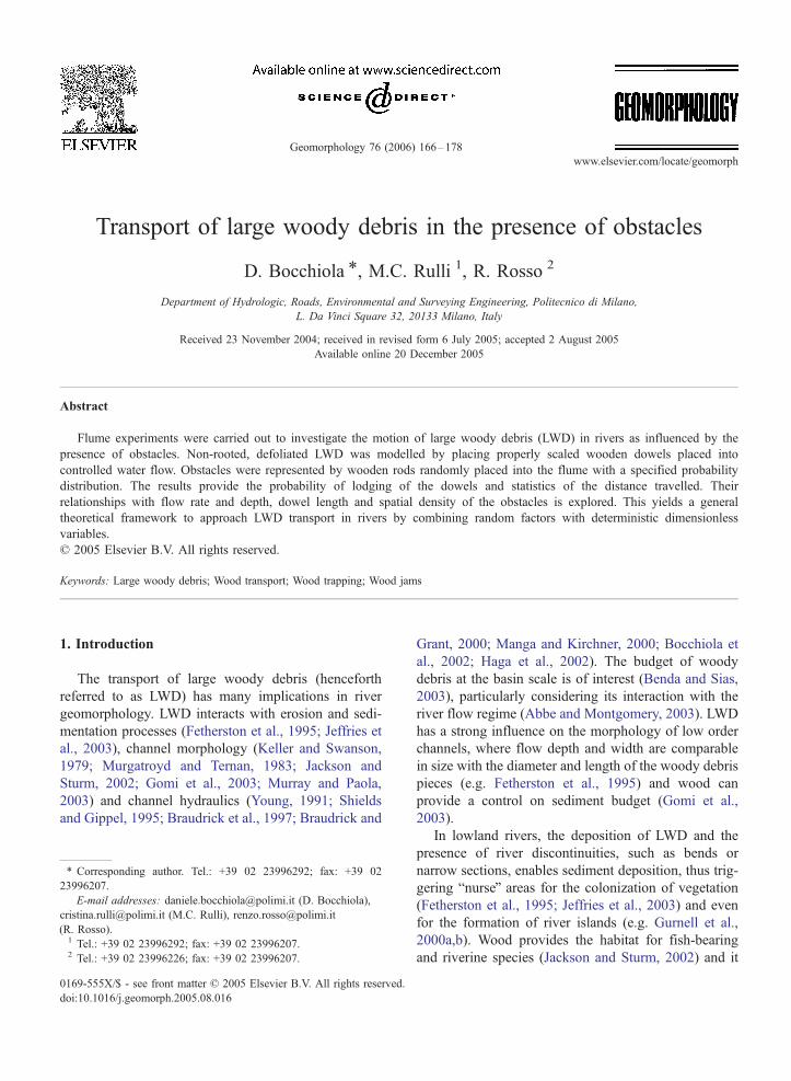
Transport of large woody debris in the presence of obstacles D. Bocchiola * , M.C. Rulli 1 , R. Rosso 2 Department of Hydrologic, Roads, Environmental and Surveying Engineering, Politecnico di Milano, L. Da Vinci Square 32, 20133 Milano, Italy Received 23 November 2004; received in revised form 6 July 2005; accepted 2 August 2005 Available online 20 December 2005 Abstract Flume experiments were carried out to investigate the motion of large woody debris (LWD) in rivers as influenced by the presence of obstacles. Non-rooted, defoliated LWD was modelled by placing properly scaled wooden dowels placed into controlled water flow. Obstacles were represented by wooden rods randomly placed into the flume with a specified probability distribution. The results provide the probability of lodging of the dowels and statistics of the distance travelled. Their relationships with flow rate and depth, dowel length and spatial density of the obstacles is explored. This yields a general theoretical framework to approach LWD transport in rivers by combining random factors with deterministic dimensionless variables. D 2005 Elsevier B.V. All rights reserved. Keywords: Large woody debris; Wood transport; Wood trapping; Wood jams 1. Introduction The transport of large woody debris (henceforth referred to as LWD) has many implications in river geomorphology. LWD interacts with erosion and sedi- mentation processes (Fetherston et al., 1995; Jeffries et al., 2003), channel morphology (Keller and Swanson, 1979; Murgatroyd and Ternan, 1983; Jackson and Sturm, 2002; Gomi et al., 2003; Murray and Paola, 2003) and channel hydraulics (Young, 1991; Shields and Gippel, 1995; Braudrick et al., 1997; Braudrick and Grant, 2000; Manga and Kirchner, 2000; Bocchiola et al., 2002; Haga et al., 2002). The budget of woody debris at the basin scale is of interest (Benda and Sias, 2003), particularly considering its interaction with the river flow regime (Abbe and Montgomery, 2003). LWD has a strong influence on the morphology of low order channels, where flow depth and width are comparable in size with the diameter and length of the woody debris pieces (e.g. Fetherston et al., 1995) and wood can provide a control on sediment budget (Gomi et al., 2003). In lowland rivers, the deposition of LWD and the presence of river discontinuities, such as bends or narrow sections, enables sediment deposition, thus trig- gering bnurseQ areas for the colonization of vegetation (Fetherston et al., 1995; Jeffries et al., 2003) and even for the formation of river islands (e.g. Gurnell et al., 2000a,b). Wood provides the habitat for fish-bearing and riverine species (Jackson and Sturm, 2002) and it 0169-555X/$ - see front matter D 2005 Elsevier B.V. All rights reserved. doi:10.1016/j.geomorph.2005.08.016 * Corresponding author. Tel.: +39 02 23996292; fax: +39 02 23996207. E-mail addresses: [email protected] (D. Bocchiola), [email protected] (M.C. Rulli), [email protected] (R. Rosso). 1 Tel.: +39 02 23996292; fax: +39 02 23996207. 2 Tel.: +39 02 23996226; fax: +39 02 23996207. Geomorphology 76 (2006) 166 – 178 www.elsevier.com/locate/geomorph
Transcript of Transport of large woody debris in the presence of obstacles
www.elsevier.com/locate/geomorph
Geomorphology 76 (
Transport of large woody debris in the presence of obstacles
D. Bocchiola *, M.C. Rulli 1, R. Rosso 2
Department of Hydrologic, Roads, Environmental and Surveying Engineering, Politecnico di Milano,
L. Da Vinci Square 32, 20133 Milano, Italy
Received 23 November 2004; received in revised form 6 July 2005; accepted 2 August 2005
Available online 20 December 2005
Abstract
Flume experiments were carried out to investigate the motion of large woody debris (LWD) in rivers as influenced by the
presence of obstacles. Non-rooted, defoliated LWD was modelled by placing properly scaled wooden dowels placed into
controlled water flow. Obstacles were represented by wooden rods randomly placed into the flume with a specified probability
distribution. The results provide the probability of lodging of the dowels and statistics of the distance travelled. Their
relationships with flow rate and depth, dowel length and spatial density of the obstacles is explored. This yields a general
theoretical framework to approach LWD transport in rivers by combining random factors with deterministic dimensionless
variables.
D 2005 Elsevier B.V. All rights reserved.
Keywords: Large woody debris; Wood transport; Wood trapping; Wood jams
1. Introduction
The transport of large woody debris (henceforth
referred to as LWD) has many implications in river
geomorphology. LWD interacts with erosion and sedi-
mentation processes (Fetherston et al., 1995; Jeffries et
al., 2003), channel morphology (Keller and Swanson,
1979; Murgatroyd and Ternan, 1983; Jackson and
Sturm, 2002; Gomi et al., 2003; Murray and Paola,
2003) and channel hydraulics (Young, 1991; Shields
and Gippel, 1995; Braudrick et al., 1997; Braudrick and
0169-555X/$ - see front matter D 2005 Elsevier B.V. All rights reserved.
doi:10.1016/j.geomorph.2005.08.016
* Corresponding author. Tel.: +39 02 23996292; fax: +39 02
23996207.
E-mail addresses: [email protected] (D. Bocchiola),
[email protected] (M.C. Rulli), [email protected]
(R. Rosso).1 Tel.: +39 02 23996292; fax: +39 02 23996207.2 Tel.: +39 02 23996226; fax: +39 02 23996207.
Grant, 2000; Manga and Kirchner, 2000; Bocchiola et
al., 2002; Haga et al., 2002). The budget of woody
debris at the basin scale is of interest (Benda and Sias,
2003), particularly considering its interaction with the
river flow regime (Abbe and Montgomery, 2003). LWD
has a strong influence on the morphology of low order
channels, where flow depth and width are comparable
in size with the diameter and length of the woody debris
pieces (e.g. Fetherston et al., 1995) and wood can
provide a control on sediment budget (Gomi et al.,
2003).
In lowland rivers, the deposition of LWD and the
presence of river discontinuities, such as bends or
narrow sections, enables sediment deposition, thus trig-
gering bnurseQ areas for the colonization of vegetation
(Fetherston et al., 1995; Jeffries et al., 2003) and even
for the formation of river islands (e.g. Gurnell et al.,
2000a,b). Wood provides the habitat for fish-bearing
and riverine species (Jackson and Sturm, 2002) and it
2006) 166–178

D. Bocchiola et al. / Geomorphology 76 (2006) 166–178 167
has an influence on water temperatures, water flows and
nutrient fluxes (e.g. Welty et al., 2002). Several studies
have been carried out to map the spatial distribution of
LWD using in situ surveys (Wing et al., 1999; Kraft and
Warren, 2003) and remote sensing (Aspinall, 2002;
Marcus et al., 2002). Some pioneering attempts have
been made to assess the relationship between wood
accumulation processes and river geomorphology
(Jackson and Sturm, 2002; Abbe and Montgomery,
2003) and to investigate some statistics of the observed
LWD distribution (e.g. to test their randomness or
spatial organization, see Kraft and Warren, 2003). Brau-
drick and Grant (2000), Manga and Kirchner (2000),
Bocchiola et al. (2002) and Hygelund and Manga
(2003), among others, investigated the interaction of
wood and water flow in rivers. Additionally, Smith et
al. (1993) and Manga and Kirchner (2000) have studied
the influence of LWD transport on water shear stress
and sediment erosion.
During a flood LWD is swept and redistributed
throughout the river network. The redistribution pro-
cess depends on the hydraulic characteristics and ge-
ometry of the individual channels, this including in-
channel structures, such as steps, pools, large boulders
and wood jams. Therefore, the interaction of LWD with
irregular channel patterns plays a major role in deter-
mining LWD dynamics in rivers.
The present paper deals with the interaction of
LWD with channel obstacles. These are associated
with multifaceted bed morphology of braided rivers
and with boulders and vegetation in mountain rivers.
The presence of obstacles also affects the LWD trans-
portation in the floodplain. Here, vegetation is often
poorly managed, so it can grow undisturbed during
periods of low flows, but it can obstruct the transport
of wood pieces during large flood events that occur
with low frequency.
The key factor here is the interaction of the moving
logs with the obstacles, as conditioned by water depth
and velocity. This is approached here by developing
controlled experiments in a laboratory flume. These are
accurately designed in order to investigate the process
of LWD lodging and the distance travelled by the logs.
The results from these experiments are used to develop
a simple theoretical framework capable of providing
quantitative estimates of the complex interaction of
LWD with channel obstacles.
2. Previous studies on LWD transport in rivers
LWD consists of wood pieces 1 m or more in length
or 0.1 m or more in diameter (see Jackson and Sturm,
2002 for the definition of LWD). The initiation of
motion and redistribution of LWD throughout the
river network during flood events was studied by Brau-
drick et al. (1997), Braudrick and Grant (2001) and
Haga et al. (2002), who investigated the relationship
between the distance travelled by a single LWD piece
and the local properties of the flow. Travel distance
depends on LWD size (i.e. its representative length and
diameter and also the presence of rootwads) and den-
sity, the water depth and velocity, and the channel bed
roughness. The presence of bends, changes in channel
conveyance (i.e. channel width) and/or obstacles to
motion also have a significant influence on the path
of LWD.
LWD generally moves further in high order streams
(i.e. larger streams) and shorter pieces move further
than longer ones (e.g. Nakamura and Swanson, 1994).
In headwater streams, the logs longer than the bank-full
width tend to be stable and are removed only during
large flood events or due to decay (e.g. Haga et al.,
2002). Also, large boulders can interact with the trans-
port of the logs by trapping key pieces, leading to the
formation of jams (e.g. Faustini and Jones, 2003). The
major control of LWD transport in headwater streams is
the greatest water depth achieved during a flood event
(e.g. Braudrick and Grant, 2001; Haga et al., 2002). If it
exceeds the bfloating thresholdQ, the logs are more
likely to travel out of the reach. Following Abbe et
al. (1993), a log tends to stop and reside when the water
depth is lower than about half log diameter.
Channel morphology is a key factor in LWD dy-
namics. In straight reaches with deep water the wood
pieces flush rapidly, as they do not touch the bed and,
therefore, they do not encounter noticeable energy dis-
sipation. In sinuous reaches, the wood pieces can be
deposited due to frequent contact with the banks or to
the secondary flows in the outside of the channel bends
(Fetherston et al., 1995). In braided lowland rivers, the
presence of bars tends to bcaptureQ the wood pieces
(e.g. Gurnell et al., 2000a,b), because of the presence of
areas with shallow water and, in case, of the formation
of river islands.
Braudrick and Grant (2001) introduced the concept
that the probability of LWD to be deposited depends on
some particular flow variables and on the piece size.
They investigated the motion and the deposition pat-
terns of wood dowels (1.27–2.54 cm in diameter, 0.3 to
0.9 m in length) in a 7 m long, 1.22 m wide gravel bed
flume, with meanders and alternate bars. They intro-
duced a bdebris roughnessQ parameter, defined as a
weighted average of three variables, namely the ratio
between the piece length and the average channel width
D. Bocchiola et al. / Geomorphology 76 (2006) 166–178168
(Llog /wav), the ratio between the piece length and the
average channel radius of curvature (Llog /Rc) and the
ratio between the bbuoyantQ depth to the average chan-
nel depth (db /dav). This roughness has been related to
the distance travelled by the dowels. Haga et al. (2002)
carried out a field experiment in a mountain stream in
Japan, monitoring the distance travelled by regularly
shaped logs, depending on the flood history for 1 year.
They considered Small Coarse Woody Debris, i.e. logs
with length smaller than the stream width, and showed
that the distance travelled by the logs is strictly related
to the water depth at the peak flow. A log deposited
during an event with given water depth generally
moves only once a new event with a greater water
depth occurs. When the flow depth is smaller than the
log diameter, the logs are usually transported for a short
distance. Finally, the logs are transported further when
the water depth exceeds their diameter.
3. Key issues in transport of LWD
3.1. Stability of wood
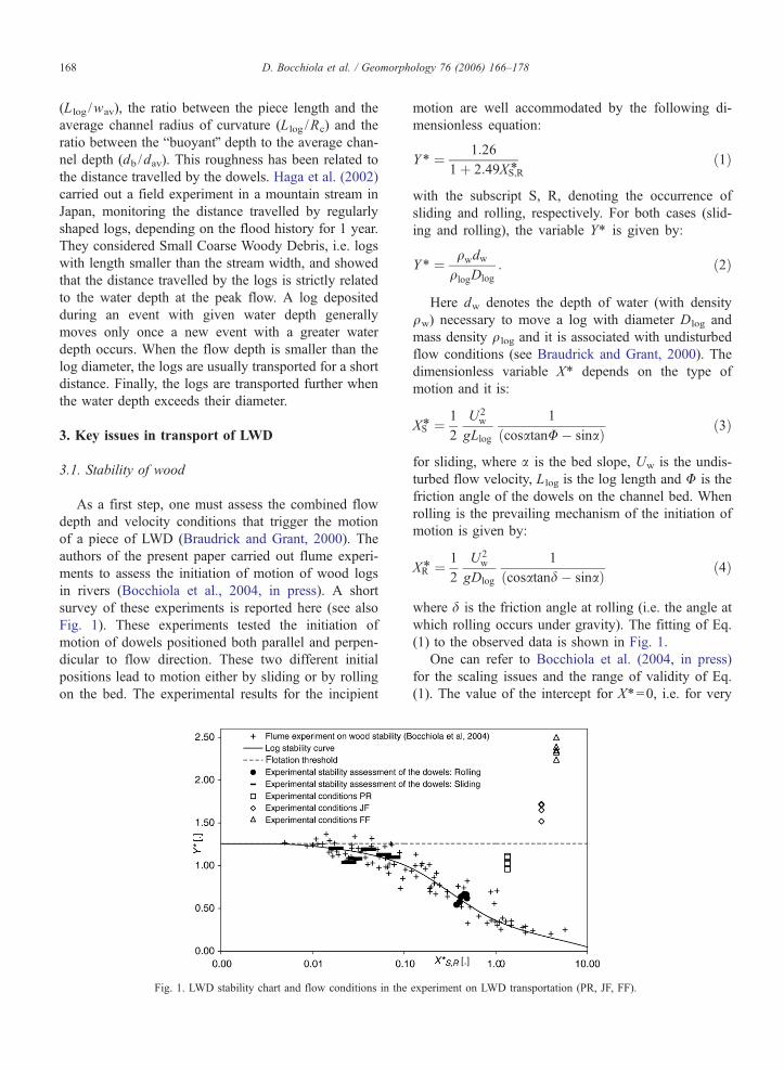
As a first step, one must assess the combined flow
depth and velocity conditions that trigger the motion
of a piece of LWD (Braudrick and Grant, 2000). The
authors of the present paper carried out flume experi-
ments to assess the initiation of motion of wood logs
in rivers (Bocchiola et al., 2004, in press). A short
survey of these experiments is reported here (see also
Fig. 1). These experiments tested the initiation of
motion of dowels positioned both parallel and perpen-
dicular to flow direction. These two different initial
positions lead to motion either by sliding or by rolling
on the bed. The experimental results for the incipient
Fig. 1. LWD stability chart and flow conditions in the
motion are well accommodated by the following di-
mensionless equation:
Y4 ¼ 1:26
1þ 2:49XS;R4ð1Þ
with the subscript S, R, denoting the occurrence of
sliding and rolling, respectively. For both cases (slid-
ing and rolling), the variable Y* is given by:
Y4 ¼ qwdw
qlogDlog
: ð2Þ
Here dw denotes the depth of water (with density
qw) necessary to move a log with diameter Dlog and
mass density qlog and it is associated with undisturbed
flow conditions (see Braudrick and Grant, 2000). The
dimensionless variable X* depends on the type of
motion and it is:
XS4 ¼1
2
U2w
gLlog
1
cosatanU� sinað Þ ð3Þ
for sliding, where a is the bed slope, Uw is the undis-
turbed flow velocity, Llog is the log length and U is the
friction angle of the dowels on the channel bed. When
rolling is the prevailing mechanism of the initiation of
motion is given by:
XR4 ¼1
2
U2w
gDlog
1
cosatand� sinað Þ ð4Þ
where d is the friction angle at rolling (i.e. the angle at
which rolling occurs under gravity). The fitting of Eq.
(1) to the observed data is shown in Fig. 1.
One can refer to Bocchiola et al. (2004, in press)
for the scaling issues and the range of validity of Eq.
(1). The value of the intercept for X*=0, i.e. for very
experiment on LWD transportation (PR, JF, FF).

Fig. 2. Example of dowel rolling inside the flume.
Table 1
Properties of the dowels
Dowel qlog,d Llog D log U d
[kg m�3] [m] [m] [8] [8
D1 750 0.050 0.014 34 11
D2 728 0.075 0.014 34 11
D3 798 0.100 0.014 34 11
D4 834 0.125 0.014 34 11
D5 787 0.150 0.014 34 11
D6 780 0.250 0.014 34 11
D. Bocchiola et al. / Geomorphology 76 (2006) 166–178 169
low flow velocity, is Y*=1.26. The multiplier for Y* in
Eqs. (2) and (3) is found by best fitting of the flume
experiments, and the estimated value of 2.49 is an
estimate of the drag coefficient exerted by the water
flow on the log. These results provide rules for wood
motion initiation that differ notably from those intro-
duced by Braudrick and Grant (2000), mainly in the
case of rolling (i.e. when the logs are perpendicular to
flow).
3.2. Types of motion of LWD
Two major modes occur in the motion of a piece of
LWD driven by river flow (e.g. Braudrick et al., 1997;
Braudrick and Grant, 2001; Haga et al., 2002). First, the
piece of wood can move in contact with the bed, by
rolling or sliding. Second, floating occurs when water is
deep enough to achieve wood buoyancy. One needs a
criterion to discriminate these two different situations,
depending on water depth and flow velocity. Haga et al.
(2002) followed the approach by Braudrick and Grant
(2000) and introduced the dimensionless variable
h*=qwdw /qlogdlog as the controlling factor discrimi-
nating between floating and rolling or sliding. One
notes that h*=Y*. The associated bflotation threshold’’
is h*=1; when h* exceeds unity, motion occurs by
floating. This is obviously associated with the expected
buoyancy force in hydrostatic conditions. One notes
that the above mentioned experiments (see Fig. 1)
yield a larger value of the flotation threshold, i.e.
Y*=1.26. This occurs because of the local perturbation
of the flow profile induced by the log. In fact, the log
raises the water depth upstream, and it lowers the water
depth downstream (Bocchiola et al., 2004, in press).
Therefore, the log is immersed to an average depth
lower than the undisturbed dw. As a result, the buoy-
ancy force is less than that occurring under hydrostatic
conditions, so flotation occurs for a larger flow depth.
Therefore, one assumes here that wood moves in con-
tact with bed for Y*V1.26 and by flotation for
Y*N1.26.
4. The experiments
4.1. Flume settings
Fig. 2 shows a picture of the experimental set-up,
where a dowel mimics the motion of a piece of LWD
under the influence of water flow in a straight channel
with known bed slope and roughness. The experimental
flume is 1 m wide and 30 m long, with a bed slope of
0.006. A 2 m panel is fixed to the flume bed, covered
with sand (D50=2 mm). One notes that sediment trans-
port interacts with wood transport in rivers. This inter-
action is neglected here, because one must first assess
the mechanics of log motion in absence of sediment
load. Accordingly, these experiments were carried out
using a fixed channel bed. The 2 m panel was mounted
in a position so that the water depth and velocity were
almost constant along its whole extent; this was
assessed using flow profile calculations and it was
further tested by local measurements. No relevant
back water effect was observed due to the gate at the
flume’s end.
4.2. Adopted dowels and validity of the incipient motion
criterion
The simple case of non-rooted, defoliated LWD is
considered here, well represented by handmade dowels.
Table 1 shows the major features of the test dowels.
These are made of Beech (Fagus sylvatica) with aver-
age dry density qL=779 kg m�3. Six different lengths
were used to conduct the experiments (see Table 1). A
set of experiments was carried out to check the accu-
racy of Eq. (1) in predicting the initiation of motion for
]

Fig. 3. Distribution of the obstacles in plane.
able 3
ummary of the experimental hydraulic conditions
ydraulic
onditions
owel
dw Uw XR* Re Fr Y* Xe* LL*
[m] [ms�1] [d ] [d ] [d ] [d ] [d ] [d ]
R D1 0.013 0.27 1.34 1.4E +04 0.76 1.03 1.25 0.19
R D2 0.013 0.27 1.34 1.4E +04 0.76 1.09 1.28 0.29
D. Bocchiola et al. / Geomorphology 76 (2006) 166–178170
the test dowels. The incipient motion of the dowels was
detected by eye (as in Bocchiola et al., in press and
similarly to Braudrick and Grant, 2000) and the asso-
ciated values of X* and Y* were computed from flow
measurements. The results are shown in Fig. 1 and also
reported in Table 2. One notes that Eq. (1) provides a
reasonable fit of the results.
4.3. Obstacles
Wood rods are placed vertically into the water and
mounted onto some drilled wood beams, so that they
can be pulled out of the water when necessary. The
spacing among the obstacles was set according to
observations of the spatial density of near channel
standing trees in a field survey of the Branega
River, Liguria (Northern Italy), within the framework
of the bINTERREG 3B DESERNETQ project (see
Rulli et al., 2004). Based on the available dowels’
size and the constraints given by the flume size, the
linear scale ratio for trees’ spatial density was assumed
to be 1 :19. This yields a scaled average inter-obstacle
distance in the flume of L0=0.26 m. This is the
average value of the distance between a rod and its
nearest neighbour, or the average available room for a
dowel across two adjacent rods. The obstacles are
randomly distributed in space (i.e. their coordinates
are extracted independently from a bivariate uniform
distribution, see Fig. 3). Although the spatial distribu-
tion of the trees in nature is likely to be more com-
plex, the uniform probability distribution is taken here
for simplicity. Specific analysis of the vegetation pat-
terns is needed to assess more complex distributions.
Also, different settings of the obstacles (i.e. different
randomly generated distributions of the obstacles)
could be considered.
The obstacle rods have a diameter of 0.01 m, so the
obstruction caused by the obstacle is negligible as
compared with channel width (1 /100).
Table 2
Stability of the dowels
Dowel dw Uw dw Uw
Sliding Sliding Rolling Rolling
[m] [ms�1] [m] [ms�1]
D1 0.016 0.24 0.011 0.14
D2 0.014 0.22 0.011 0.15
D3 0.013 0.22 0.012 0.16
D4 0.014 0.23 0.011 0.15
D5 0.016 0.24 0.012 0.16
D6 0.014 0.23 0.012 0.16
4.4. Scaling issues
Some scaling issues need to be discussed. The
Froude number, Fr, and the Reynolds number, Re, of
the flow field are to be considered (see Table 3). The
first ranges from 0.76 to 0.95, while the second ranges
from 1.4�104 to 5.3�104. These provide conditions
similar to those observed in lowland rivers for low
water depths (e.g. Braudrick and Grant, 2000; Hyge-
lund and Manga, 2003). Also, Fr and the Re are
consistent with those used to build the stability curve
(Bocchiola et al., in press) therefore assuring validity of
the stability criteria. Applying the scale ratio of the
flume to the dowels (1 :19), the rescaled length of the
shortest dowel (0.05 m) is about 1 m (0.95 m). This is
consistent with the lowest limit for LWD (e.g. Jackson
and Sturm, 2002). The length of the other, longer
dowels is scaled accordingly; the length of 0.25 m for
the longest dowel corresponds to about 5 m (4.75 m)
R D3 0.013 0.27 1.34 1.4E +04 0.76 1.02 1.25 0.38
R D4 0.013 0.27 1.34 1.4E +04 0.76 0.96 1.22 0.48
R D5 0.013 0.27 1.34 1.4E +04 0.76 1.11 1.28 0.58
F D1 0.020 0.41 3.15 3.3E +04 0.93 1.65 3.15 0.19
F D2 0.020 0.41 3.15 3.3E +04 0.93 1.65 3.15 0.29
F D3 0.020 0.41 3.15 3.3E +04 0.93 1.65 3.15 0.38
F D4 0.020 0.41 3.15 3.3E +04 0.93 1.52 3.15 0.48
F D5 0.020 0.41 3.15 3.3E +04 0.93 1.72 3.15 0.58
F D6 0.020 0.41 3.15 3.3E +04 0.93 1.71 3.15 0.96
F D1 0.027 0.49 4.58 5.3E +04 0.95 2.24 4.58 0.19
F D2 0.027 0.49 4.58 5.3E +04 0.95 2.35 4.58 0.29
F D3 0.027 0.49 4.58 5.3E +04 0.95 2.35 4.58 0.38
F D4 0.027 0.49 4.58 5.3E +04 0.95 2.50 4.58 0.48
F D5 0.027 0.49 4.58 5.3E +04 0.95 2.39 4.58 0.58
F D6 0.027 0.49 4.58 5.3E +04 0.95 2.33 4.58 0.96
T
S
H
c
d
P
P
P
P
P
J
J
J
J
J
J
F
F
F
F
F
F
D. Bocchiola et al. / Geomorphology 76 (2006) 166–178 171
for the prototype. Therefore, the experiment can be
thought representative of the behaviour of pieces of
LWD as observed in field surveys.
When considering the dynamic equilibrium of the
logs, one must account for the scaling in the vertical
direction (i.e. related to the dowels’ diameter). From
Eq. (1), the scaling is obtained by taking proper values
of X* and Y*, so the experiments are essentially at 1 :1
scale (i.e. the diameter of the log, the flow velocity and
depth and the bed friction angle need not to be scaled,
but through X* and Y*). When the logs start moving,
the interaction between the vertical and plane scales
depends on the logs’ velocity. As a first approximation,
the result (i.e. stop or not) of the bcollisionQ between a
dowel and an obstacle depends on the velocity reached
by that dowel. For given flow depth and velocity (i.e.
X* and Y*), the moving dowel will reach its highest
(limit) velocity and no more acceleration will occur.
This requires the dowel to travel a given distance. If this
distance is less than the average distance between the
obstacles, the experimental set-up is capable of repro-
ducing the impact of the dowels with the obstacles.
Because some preliminary tests showed the dowels
looked to reach a steady (limit) velocity after covering
a few centimetres, one assumes that these experiments
can mimic reasonably well the real situation occurring
in nature.
4.5. Methods of observation
The procedure for the wood transport experiment
was as follows. Steady values of depth and velocity
were established using the flume circulation facility.
Then, each dowel was positioned inside the channel
and left free to move under the action of the flowing
water. The dowels were positioned perpendicular to
main flow direction, as they were observed to be capa-
ble of self pivoting in a few centimetres, so self asses-
sing their motion very quickly. To mimic a random
effect with respect to the placement of the obstacles,
fifteen different starting positions were examined, tak-
ing different distances from the right side wall of the
flume (i.e. fifteen different values of the abscissa in Fig.
3). These were taken at steps of 5 cm, starting from 15
cm and stopping at 85 cm, to avoid the side effect of the
flume walls. Three runs were carried out for each
starting position.
Three mechanisms of LWD transport are examined.
These are bpure rollingQ (PR), i.e. when the dowel is
touching the channel bed (Y*b1.26); bjust floatingQ(JF), i.e. a condition when the dowel is floating but
the value of Y* is close to the flotation threshold
(Y*i1.26); and bfully floatingQ (FF), i.e. when the
water depth exceeds notably the floating threshold
(Y*N1.26). Three different modes of LWD motion
are associated with the values of X* and Y* shown in
Fig. 1.
A total number of 810 runs were carried out in order
to investigate the different modes of LWD motion and
the different lengths of the dowels. In Table 3 a sum-
mary is given of the experimental conditions.
5. Experimental results
5.1. Observed motion patterns
When the motion of the dowels is in contact with
the bed (for Y*V1.26), the motion mainly occurs by
rolling; and sliding only occurs as a transient process
with very short duration. When the dowel is initially
placed perpendicular to flow, it simply starts rolling.
When the dowel is placed stream-wise, it starts mov-
ing by sliding, until it pivots against some obstacle, or
more likely, because of bed grain roughness. Pivoting
makes the dowel turn perpendicular to the flow. In
case of floating, if the dowel is initially oriented
parallel to the flow, it simply starts floating, acceler-
ating until it reaches a steady state velocity, equating
the surface flow velocity (Braudrick and Grant, 2001).
Conversely, if the dowel is perpendicular to flow,
rolling or standing, it is lifted by the current and it
starts turning, driven by the uneven distribution of
velocity across the flow section. Then, it self-adjusts
its direction to match the flow direction and it con-
verges towards the centreline (see Braudrick and
Grant, 2001, Fig. 2).
5.2. Lodging against obstacles
Two different types of lodging mechanism are ob-
served. These are shown in Fig. 4 and will be referred
to as bbridgingQ and bleaningQ. The first occurs when a
dowel stops by literally bridging between two different
rods. This is a somewhat stable position and it is likely
that, unless some further perturbation occurs (i.e. wood
breaking or very high flows), the wood is going to be
bstoredQ for a long period. With the second option,
bleaningQ occurs when a dowel just leans against a
single rod. This usually occurs when the dowel
approaches the rod at about its centre of gravity, so
achieving a balance of the pivoting forces. Leaning of
the dowels was observed to last in time. In fact, in no
case was a leaning dowel seen to move away after it
had stopped. Therefore, one can assume that leaning is

Fig. 4. Deposition of the wood dowels. Flow direction from right to
left (a) Bridging, Br. (b) Leaning, Le.
able 4
ummary of the experimental results
odging dowel L* rL* Br Le Stop Out
[d ] [d ]
R D1 4.02 2.05 0 43 43 2
R D2 2.93 1.48 0 45 45 0
R D3 2.04 1.01 0 45 45 0
R D4 2.00 0.43 2 43 45 0
R D5 1.96 0.35 0 45 45 0
F D1 4.10 2.12 2 9 11 34
F D2 3.72 1.97 1 15 16 29
F D3 3.80 1.96 3 18 21 24
F D4 3.49 1.66 5 15 20 25
F D5 3.05 1.42 4 24 28 17
F D6 2.51 1.55 17 14 31 14
F D1 – – 0 3 3 42
F D2 – – 1 5 6 39
F D3 – – 1 4 5 40
F D4 3.79 1.95 4 6 10 35
F D5 3.29 1.79 8 9 17 28
F D6 2.67 1.64 8 8 16 29
D. Bocchiola et al. / Geomorphology 76 (2006) 166–178172
an effective lodging mechanism. However, the wood is
expected to move as soon as a perturbation (i.e. an
increase in flow depth or velocity) occurs.
These two different modes of lodging can lead to
different processes in rivers. For instance, a bridging
LWD can provide a possible bkey logQ for the formation
of jams. Qualitative experiments showed that when a
moving dowel meet a bridging bkey logQ, the latter is
seldom moved away and in the long run, it leads to the
formation of a jam. In contrast, when a moving dowel
encounters a leaning bkey logQ, the latter can be swept
away or not, depending on the size and momentum of
the moving dowel. In the case where a bkey logQ stands,an accumulation of LWD can start.
The chance that a dowel is deposited by bridging is
associated with its length. A short dowel is not likely to
bridge, as it is unlikely that it meets two rods separated
by a distance smaller than its length. A longer dowel
instead can meet two rods that are separated by a
distance smaller than its length and bridge them.
In the present paper, the events of bleaningQ and
bbridgingQ are assumed to be equivalent from the per-
spective of searching for the probability of lodging,
because they both lead to the deposition of a dowel.
However, these two modes must be approached sepa-
rately in order to understand the lodging process.
5.3. Probability of lodging and lodging position
In Table 4 some statistics are given about the ob-
served lodging dowels. These are the number of stops
(i.e. of retained dowels), divided into leaning (Le) and
bridging (Br). In some cases the dowel travels out of the
obstacle area (Out). In the case of rolling, PR, the dowel
D6 is not reported because it moves for a short track
and, therefore, no significant results can be obtained.
Dowel D6 was used only in the case of floating because
it was capable of travelling for a significant distance.
One notices that the number of stops due to bridging
increases with the dowel’s length. Also, the bridging
mode of LWD capture is observed mainly in case of
floating, JF and FF (31 and 22 cases, respectively) and
only two cases occurred for rolling, PR. This means
that when a log is rolling, the simple touch of an
obstacle is sufficient to stop it. In case of floating,
touching only one obstacle is sometimes insufficient
to stop the log, which can pivot and stop only if another
obstacle is found. Notice further that the number of
boutflowsQ of the dowels (Out in Table 4) is practically
null for the rolling case, while it increases noticeably
T
S
L
P
P
P
P
P
J
J
J
J
J
J
F
F
F
F
F
F

Fig. 5. Spatial distribution of the observed stops and related proba
bility for increasing dowels’ length (top-down) in case of pure rolling
PR. The area of the light circles is proportional to the probability dtostopT (also given in the labels). Unlabelled dots are rods where dnostopT happens for the considered dowel’s length in PR conditions
Notice the spatial sparseness of the stopping of short length dowels
(Llog=0.05 m top) and the increasing segregation effect (i.e. spatia
concentration of the stopping points) as L log increases (see Llog=0.15
m, bottom). Dowel D6 is not considered as it practically always stops
at the first obstacle (explained in the text).
D. Bocchiola et al. / Geomorphology 76 (2006) 166–178 173
for the JF and FF cases. This indicates that in case of
floating, i.e. for high water depth, logs tend to travel at
length. This is consistent with previous studies on LWD
(e.g. Haga et al., 2002).
Figs. 5–7 show the stopping position of the retained
dowels. For each obstacle, the table reports the proba-
bility that a dowel retained inside the domain stops
there. Consider first the case of PR shown in Fig. 5.
Here, almost all the dowels were retained, therefore
providing a somewhat higher number of samples (45
or so for each dowel). For the shortest dowel (D1, top)
the probability of stopping is quite constant in the
whole domain; this means that the dowel has more or
less the same probability of stopping against each of the
obstacles. Moving towards longer dowels (e.g. D5,
bottom), the probability of stopping increasingly con-
centrates towards the first obstacles. Given equivalent
hydraulic conditions (i.e. the same, or very similar, X*
and Y*), longer dowels have a higher probability to
impact on some obstacle, stopping thereby.
A smaller number of samples is available in the case
of Just Floating, JF, because the dowels often flowed
out of the measuring area (see Fig. 6 and Table 4).
However, one sees a behaviour similar to that shown in
Fig. 5. For the shortest dowels (D1, D2 and D3, top) the
stopping probability is evenly distributed in space. For
the longest dowels (D4, D5 and D6, bottom), the area
with the highest stopping probability shifts progressive-
ly towards the first obstacles. Particularly, dowel D6
(0.25 m), stops with a probability of 70% against the
first obstacles (LTb1 m). Neither is this effect due to a
low amount of samples, as the number of retained
dowels increases with length (e.g. for D6, 31 stop
events are observed). This finding means that increas-
ing the force for motion, a smaller number of dowels is
retained but the longest dowels tend to stop with the
highest frequency (see Table 4 for total number of
stops) close to the starting point (i.e. travelling for
short distances). The result for the fully floating dowels
(FF) are shown in Fig. 7. One notes that the shortest
dowels are seldom retained (Table 4, dowels D1, D2,
D3) and a significant sample (at least 10 stop events) is
available only for the dowels D4, D5 and D6. Increas-
ing the dowel length results in the highest stopping
probability shifting upstream towards the first obsta-
cles. Namely, while D4 (Llog=0.125 m) stops in the
first half of the track (LTb1 m) with a probability of
50%, D5 (Llog=0.15 m) stops thereby with a probabil-
ity of 59% or so and D6 (Llog=0.25 m) with a proba-
bility of 88%.
From Figs. 5–7, one notes that the distance travelled
by a dowel of a given length is not constant under the
-
,
.
l
same flow conditions, but it can be represented only as
a random variable with a specified probability distribu-
tion. Neither is this effect due to different starting

D. Bocchiola et al. / Geomorphology 76 (2006) 166–178174
positions (e.g. value of x in Fig. 3) as dowels starting
from the same positions generally stop in different
places.
ig. 7. Spatial distribution of the observed stops and related proba-
ility for increasing dowel length (Top-down) in case of Fully Float-
g, FF. The area of the light circles is proportional to the probability
o stopT (also given in the labels). Unlabelled dots are rods where dnotopT happens for the considered dowel’s length in FF conditions.
gain here a segregation effect is spotted as Llog increases, witnessed
y the highest probabilities observed for the closest rods (see
log=0.25 m, bottom), meaning that the longest dowels tend to travel
r the shortest distances. Dowels D1–D3 are not considered as they
re seldom retained and, therefore, no significant percentages can be
iven (explained in the text).
F
b
in
dts
A
b
L
fo
a
g
One notes that the parameterization of this probability
distribution would require a much larger sample size
than that presented in this preliminary study. This is
because one must assess the dependence of the para-
meters on the flow conditions, dowel size and obstacle
density.
Fig. 6. Spatial distribution of the observed stops and related proba-
bility for increasing dowel length (Top-down) in case of Just Floating,
JF. The area of the light circles is proportional to the probability dtostopT (also given in the labels). Unlabelled dots are rods where no stophappens for the considered dowel’s length in JF conditions. Notice
again the segregation effect as Llog increases, witnessed by the highest
probabilities observed for the closest rods (see Llog=0.25 m, bottom),
meaning that the longest dowels tend to travel for the shortest
distances.

Fig. 8. Average distance travelled by the dowels trapped into the
domain L*.
D. Bocchiola et al. / Geomorphology 76 (2006) 166–178 175
6. Theoretical approach
6.1. Key variables
The definition of a representative distance is neces-
sary in the interpretation of the dowels’ motion into the
flume. In principle, one could consider the length (ab-
solute value) of the vector linking the starting point to
the lodging one. However, here, only the stream-wise
coordinate is considered (i.e. LT in Fig. 3). This implies
that different starting and lodging position are regarded
as equivalent as far as they possess the same LT, irre-
spective of their x coordinate is. Here, only the stream-
wise travelled distance is considered, independently
from the lateral migration of the LWD. The presence
of clustering zone is also neglected in this case. The
travelled distance is assumed here to be a function of
the characteristic distance between obstacles, L0, of the
dowel’s length, LLog, and of the force applied by the
flow. Three dimensionless groups are therefore intro-
duced. The first is:
L4 ¼ LT=L0 ð5Þ
i.e. the ratio between the travelled distance LT and the
average inter-obstacles distance L0. The second is the
bobstruction ratioQ between the log’s length Llog and L0:
L4 ¼ Llog=L0: ð6Þ
The third group is the excess of force with respect to
the critical equilibrium condition. This can be written
as:
Xe4 ¼ XR4� Xc4
¼ XR4�1:26
Y4� 1
�=2:49 Y4V1:26
�
Xe4 ¼ XR4 Y4N1:26: ð7Þ
For Y* smaller than 1.26, the dowels move by roll-
ing on the bed. The greater the value of X* with respect
to its critical value, the stronger the dowel is pushed by
the flow. When Y* exceeds the floating threshold, 1.26,
the dowel starts floating. Because there is no friction
force exerted by the bed on the floating dowel, the
equilibrium statement of Eq. (1) no longer holds.
Under the assumption that the dowel moves at a thresh-
old flow velocity, the variable describing its motion is
Uw. However, in the group XR* of Eq. (2) the denom-
inator is constant; therefore, considering X* is tanta-
mount as considering Uw, apart from a pure scaling
factor. In case of floating the critical value Xc* is zero.
The idea here is that the dimensionless distance trav-
elled by the dowel L* is a function of LL* and Xe*.
Here, only L0 is taken to be representative of the
distance between the obstacles. One assumes that the
distribution of such distances influences the lodging
probability and location. Here, however, the authors
tentatively try to analyse the dependence of the lodging
process on L0. Notice also that it is not straightforward
that one can easily provide a full description of the
distribution of the observed obstacles in channels (e.g.
the distribution of boulders in rivers, or the distribution
of trees and bushes in floodplains) and a parsimonious
approach, using one only variable, seems appropriate.
6.2. Analysis
The random path of a dowel in a river in presence
of obstacles can be represented in terms of the aver-
age L* and the standard deviation rL* of the dimen-
sionless travelled length L* and of the probability and
type of lodging. Their relationship with the excess of
force Xe* and the log’s obstruction ratio LL* can be
assessed using exploratory statistics of observed data.
Here, a linear regression analysis is carried out, not to
determine the best fitting functions but rather to ex-
plore the capability of the selected variables of
explaining the observed variability of the process,
thus providing a basis for further modelling studies.
Due to the relatively small amount of data here
considered, there is no point in undertaking compar-
isons between complex fitting models, which would
not be conclusive anyway.
Table 3 shows the values of Y*, XR* and the excess of
force, Xe*; these are spatial averages along the flume.
Also, the obstruction ratio of the logs LL* is reported.
Table 4 reports the values of L* for the three examined
flow conditions, PR, JF and FF and the corresponding
standard deviation, rL*. The average L* and the stan-

Fig. 11. Observed probability dto stopT and stop type, depending on
LL*, FF.Fig. 9. Mean square error of the distance travelled by the dowels
trapped into the domain rL*.
D. Bocchiola et al. / Geomorphology 76 (2006) 166–178176
dard deviation rL* of the distance travelled by the
retained dowels are plotted against LL* in Figs. 8 and
9, respectively. One notes that the higher the force Xe
(i.e. going from PR to FF), the longer the average
travelled distance L*. Also, an increasing obstruction
ratio LL* is associated with decreasing L*. This shows
that the average distance travelled by LWD in the
presence of obstacles depends on the force exerted by
the water and on the length of the LWD, scaled to the
average distance between obstacles. The standard devi-
ation rL* increases as Xe increases, while it decreases
with increasing LL* (see Fig. 9). Here, the range of
distances travelled widens with an increase of the
water force and narrows with an increase of the length
of the LWD piece.
For JF and FF, the probability that a dowel stops
inside the study area is plotted against LL* in Figs. 10
and 11. This tends to one with increasing dowel’s
length. This is consistent with the idea that long logs
are deemed to stop (i.e. probability close to one).
Conversely, short logs are likely to travel out of the
domain. For increasing force, i.e. increasing Xe*, the
probability that a dowel travels out of the area tends to
increase as well. However, the values of this probability
Fig. 10. Observed probability dto stopT and stop type, depending on
LL*, JF.
are possibly dependent on the size (length) of the
domain adopted here (i.e. 2 m).
The percentage of the observed lodging modes (Br
or Le) is plotted against LL* in Figs. 10 and 11, for Br
and Le, respectively. Although the data show a certain
degree of scatter, it is seen that the percentage of Br
increases with dowel length LL* and that the percentage
of Le decreases consequently. Notice that the two prob-
abilities are bound to intercept the y axis at a value of 0
for Br and of 1 for Le because a very short log can stop
only by leaning.
Table 5 shows the result of data regression analysis
under the present approach. It is seen that the values of
R2 (from 0.61 to 0.94) are quite high, thus indicating
that the association of dimensionless variables adopted
here can provide an insight of the investigated process-
es. The highest values of R2 are associated with the
prediction of the lodging probability. These indicate
that one could consider the wood accumulation process
in rivers using a rather simple dimensionless approach
involving a small set of variables. One notes that Brau-
drick and Grant (2001) investigated the average trav-
able 5
egression analysis of the observed statistics with respect to the force
e* and the dowels’ length LL*
ariable/reg. Coeff. [d ] St. Er. [d ] p-val [d ] R2 [d ]
* Intercept 3.128 0.302 1.0E�04
Xe* 0.461 0.097 6.1E�04
LL* �2.693 0.529 3.5E�04 0.75
L* Intercept 1.211 0.272 9.9E�04
Xe* 0.365 0.088 1.6E�03
LL* �1.432 0.478 1.2E�02 0.61
top Intercept 1.000 – –
Xe* �0.245 0.012 1.0E�04
LL* 0.419 0.080 1.0E�04 0.94
e Intercept 1.000 – –
Xe* �0.312 0.120 2.0E�02
LL* �0.023 0.018 2.2E�01 0.76
T
R
X
V
L
r
S
L

D. Bocchiola et al. / Geomorphology 76 (2006) 166–178 177
elled distance (m) of the dowels by visual correlation
with Llog /wav, Llog /Rc and db /dav (see page 273, Fig.
8a, b, c). They also performed a linear regression
analysis between the bdebris roughnessQ and the dis-
tance travelled by the wood dowels, but they found
somewhat poor determination coefficient R2 (less than
0.1, see page 272, Table 5). Also, Braudrick and Grant
(2001) visually correlated the percentage of retained
wood into the flume (number of trials with retained
wood) with Llog /wav, Llog /Rc and db /dav (pag. 277,
Fig. 9a, b, c). They did not find any significant corre-
lation (see page 276). Although the experiment by
Braudrick and Grant (2001) is somewhat different
from the present one, it is noted that the theoretical
approach presented here improves substantially the pre-
vious approaches to LWD transportation in rivers. In
this sense, this study represents an improvement in the
field of LWD transport models and can be considered a
reliable basis for further research.
7. Conclusions
The transport of LWD into a reach where obstacles
are present is a complex process, involving a combina-
tion of random factors and deterministic mechanisms.
The present approach involves a simplified sketch of
vegetation, river geomorphology and hydraulic geom-
etry of stream flows, in order to describe the situation
when dead or living in-channel vegetation is present, or
morphologic constraints provide altered conveyance.
The distance travelled by a piece of LWD is a random
variable, whose expectation and variance depend on the
length of the piece, the inter-obstacle spacing and the
force exerted by the current. The probability that a
piece of LWD is stopped and also its stopping mode,
either by leaning against one obstacle or by bridging
two obstacles, also depends on the length of the LWD
and on the flow conditions. The simple theoretical
framework presented in Section 6 shows that LWD
transport process can be explored using an appropriate
dimensionless approach based on well-defined physical
quantities. As compared with previous investigations,
this approach provides a more comprehensive descrip-
tion of the key variables involved, also introducing a
simple and effective theoretical framework for model-
ling and predictive purposes. Because the distribution
of LWD influences the formation of wood structures in
rivers, these results are of interest for both researchers
and river managers.
Further developments will include the definition of
the general shape of the travelled length distributions
and of their dependence on the control variables
introduce here. Also, the study of more complex
LWD geometry, including roots and foliage, should
be considered. Further, the formation of jams requires
specific focus, because of its high potential in en-
hancing flood risk, especially in those rivers where
man-made structures yield supplementary obstacles to
the water flow and to LWD. Eventually, the present
results, although preliminary, can provide an interest-
ing insight of LWD transport in rivers and, more
generally speaking, can contribute to the understand-
ing of the interaction between woody debris and river
morphology.
Acknowledgments
The authors kindly acknowledge Eng. Davide
Motta, Chiara Narciso and Alessandro Greppi for
their contribution to this research, in partial fulfillment
of their Master’s thesis at Politecnico di Milano. Also,
the authors thank Dr. Silvia Bozzi and Dr. Matteo
Spada for their contribution in the research. This
work was supported by the GNDCI of the National
Research Council (CNR) of Italy (contract n.
00.00545.PF42), by INRM through the project
bAnalysis of hydrological and sedimentological re-
sponse in burned areasQ and by the Liguria region
through the bINTERREG 3B DESERNETQ project.
Funding for the present work was also granted from
the European Community, through the project
bIRASMOSQ (Contract FP6-2004-Global-3-018412).
The authors acknowledge two anonymous reviewers
for their accurate work that helped to improve the
quality of the paper.
References
Abbe, T.B., Montgomery, D.R., 2003. Patterns and processes of wood
debris accumulation in the Queets River Basin, Washington.
Geomorphology 51, 81–107.
Abbe, T.B., Montgomery, D.R., Featherston, K., McClure, E.,
1993. A process-based classification of woody debris in a
fluvial network; preliminary analysis of the Queets River,
Washington. EOS Transaction of the American Geophysical
Union 74, 296.
Aspinall, R.J., 2002. Use of logistic regression for validation of maps
of the spatial distribution of vegetation species derived from high
spatial resolution hyperspectral remotely sensed data. Ecological
Modelling 157, 301–312.
Benda, L.E., Sias, J.C., 2003. A quantitative framework for evaluating
the mass balance of in stream organic debris. Forest Ecology and
Management, vol. 172. Elsevier, pp. 1–16.
Bocchiola, D., Catalano, F., Menduni, G., Passoni, G., 2002. An
analytical–numerical approach to the hydraulics of floating debris
in river channels. Journal of Hydrology 269/1–2, 65–78.

D. Bocchiola et al. / Geomorphology 76 (2006) 166–178178
Bocchiola, D., Rulli, M.C., Rosso, R., 2004. Woody debris dynamics
in fire–floods environment. Proceedings: bThe 6th Int. Conf. on
Hydroscience and Engineering (ICHE-2004)Q, 165/1–14, May
31–June 3, Brisbane, Australia.
Bocchiola, D., Rulli, M.C., Rosso, R., in press. Flume experiments
on wood entrainment in rivers. Advances in Water Resources
(December).
Braudrick, C.A., Grant, G.E., 2000. When do logs move in rivers?
Water Resources Research 36 (2), 571–583.
Braudrick, C.A., Grant, G.E., 2001. Transport and deposition of large
woody debris in streams: a flume experiment. Geomorphology 41,
263–283.
Braudrick, C.A., Grant, G.E., Ishikawa, Y., Ikeda, H., 1997. Dynam-
ics of wood transport in streams: a flume experiment. Earth
Surface Processes and Landforms 22, 669–683.
Faustini, J.M., Jones, J.A., 2003. Influence of large woody debris on
channel morphology and dynamics in steep, boulder-rich moun-
tain streams, western Cascades, Oregon. Geomorphology 51,
187–205.
Fetherston, K.L., Naiman, R.J., Bilby, R.E., 1995. Large woody
debris, physical process and riparian forest development in Mon-
tane river networks of the Pacific Northwest. Geomorphology 13,
133–144.
Gomi, T., Sidle, R.C., Woodsmith, R.D., Bryant, M.D., 2003. Char-
acteristics of channel steps and reach morphology in headwater
streams southeast Alaska. Geomorphology 51, 225–242.
Gurnell, A.M., Petts, G.E., Harris, N., Ward, J.V., Tockner, K.,
Edwards, P.J., Kollman, J., 2000a. Large wood retention in river
channels: the case of the Fiume Tagliamento, Italy. Earth Surface
Processes and Landforms 25, 255–275.
Gurnell, A.M., Petts, G.E., Hannah, D.M., Smith, B.P.G., Edwards,
P.J., Kollman, J., Ward, J.V., Tockner, K., 2000b. Wood storage
within the active zone of a large European gravel-bed river.
Geomorphology 34, 55–72.
Haga, H., Kumagai, T., Otsuki, K., Ogawa, S., 2002. Transport and
retention of coarse woody debris in mountain streams: an in situ
field experiment of log transport and a field survey of coarse
woody debris distribution. Water Resources Research 38 (8),
1029–1044.
Hygelund, B., Manga, M., 2003. Field measurement of drag co-
efficients for model large woody debris. Geomorphology 51,
175–185.
Jackson, C.R., Sturm, C.A., 2002. Woody debris and channel mor-
phology in first and second order forested channels in Washing-
ton’s coast ranges. Water Resources Research, 38, 9, 16-1, 16-14.
Jeffries, R., Darby, S.E., Sear, D.A., 2003. The influence of vegetation
and organic debris on flood-plain sediment dynamics: case study
of a low order stream in the New Forest, England. Geomorphol-
ogy 51, 61–80.
Keller, E.A., Swanson, F.J., 1979. Effects of large organic material on
channel form and fluvial processes. Earth Surface Processes and
Landforms 4, 361–380.
Kraft, C.E., Warren, D.R., 2003. Development of spatial pattern in
large woody debris and debris dams in streams. Geomorphology
51, 127–139.
Manga, M., Kirchner, J.W., 2000. Stress partitioning in streams
by large woody debris. Water Resources Research 36 (8),
2373–2379.
Marcus, W.A., Marston, R.A., Colvard Jr., C.R., Gray, R.D., 2002.
Mapping the spatial and temporal distributions of large woody
debris in rivers of the Greater Yellowstone Ecosystem, U.S.A.
Geomorphology 44, 323–335.
Murgatroyd, A.L., Ternan, J.L., 1983. The impact of afforestation on
stream bank erosion and channel form. Earth Surface Processes
and Landforms 8, 357–369.
Murray, B., Paola, C., 2003. Modelling the effect of vegetation on
channel pattern in bedload rivers. Earth Surface Processes and
Landforms 28, 131–143.
Nakamura, F., Swanson, F.J., 1994. Distribution of coarse woody
debris in a mountain stream, western Cascades Range, Oregon.
Canadian Journal of Forest Research 24, 2395–2403.
Rulli, M.C., Bozzi, S., Spada, M., Bocchiola, D., Rosso, R., 2004.
The effect of forest fires on erosion and runoff in Mediterranean
environment area. Proceedings: bThe 6th Int. Conf. on Hydro-
science and Engineering (ICHE-2004)Q, 168/1–13, May 31–June
3, Brisbane, Australia.
Shields, D.F., Gippel, C.J., 1995. Prediction of effects of woody
debris removal on flow resistance. ASCE Journal of Hydraulic
Engineering 121, 341–354.
Welty, J.J., Beechie, T., Sullivan, K., Hyink, D.M., Bilby, R.E.,
Andrus, C., Pess, G., 2002. Riparian aquatic interaction simulator
(RAIS): a model of riparian forest dynamics for the generation of
large woody debris and shade. Forest Ecology and Management
162, 299–318.
Wing, M.G., Keim, R.F., Skaugset, A.E., 1999. Applying geostatistics
to quantify distributions of large woody debris in streams. Com-
puters and Geosciences 25, 801–807.
Young, W.J., 1991. Flume study of the hydraulic effects of large
woody debris in lowland rivers. Regulated Rivers: Research and
Management 6, 203–211.
Smith, R.D., Sidle, R.C., Porter, P.E., Noel, J.R., 1993. Effects of
experimental removal of woody debris on the channel morphol-
ogy of a forest, gravel-bed stream. Journal of Hydrology 152,
153–178.