This article was downloaded by: [Ingenta Content Distribution (Publishing Technology)]On: 13 October 2014, At: 13:58Publisher: Taylor & FrancisInforma Ltd Registered in England and Wales Registered Number: 1072954 Registered office: Mortimer House,37-41 Mortimer Street, London W1T 3JH, UK

Aerosol Science and TechnologyPublication details, including instructions for authors and subscription information:http://www.tandfonline.com/loi/uast20

Transport and Deposition of Angular Fibers in TurbulentChannel FlowsHaifeng Zhang a , Goodarz Ahmadi a & Bahman Asgharian ba Department of Mechanical and Aeronautical Engineering , Clarkson University , Potsdam,New York, USAb Chemical Industry Institute of Toxicology Research , Triangle Park, North Carolina, USAPublished online: 08 May 2007.

To cite this article: Haifeng Zhang , Goodarz Ahmadi & Bahman Asgharian (2007) Transport and Deposition of Angular Fibersin Turbulent Channel Flows, Aerosol Science and Technology, 41:5, 529-548, DOI: 10.1080/02786820701272004

To link to this article: http://dx.doi.org/10.1080/02786820701272004

PLEASE SCROLL DOWN FOR ARTICLE

Taylor & Francis makes every effort to ensure the accuracy of all the information (the “Content”) containedin the publications on our platform. However, Taylor & Francis, our agents, and our licensors make norepresentations or warranties whatsoever as to the accuracy, completeness, or suitability for any purpose of theContent. Any opinions and views expressed in this publication are the opinions and views of the authors, andare not the views of or endorsed by Taylor & Francis. The accuracy of the Content should not be relied upon andshould be independently verified with primary sources of information. Taylor and Francis shall not be liable forany losses, actions, claims, proceedings, demands, costs, expenses, damages, and other liabilities whatsoeveror howsoever caused arising directly or indirectly in connection with, in relation to or arising out of the use ofthe Content.

This article may be used for research, teaching, and private study purposes. Any substantial or systematicreproduction, redistribution, reselling, loan, sub-licensing, systematic supply, or distribution in anyform to anyone is expressly forbidden. Terms & Conditions of access and use can be found at http://www.tandfonline.com/page/terms-and-conditions

Aerosol Science and Technology, 41:529–548, 2007Copyright c© American Association for Aerosol ResearchISSN: 0278-6826 print / 1521-7388 onlineDOI: 10.1080/02786820701272004

Transport and Deposition of Angular Fibers in TurbulentChannel Flows

Haifeng Zhang,1 Goodarz Ahmadi,1 and Bahman Asgharian2

1Department of Mechanical and Aeronautical Engineering, Clarkson University, Potsdam, New York, USA2Chemical Industry Institute of Toxicology Research, Triangle Park, North Carolina, USA

Transport and deposition of angular fibrous particles in tur-bulent channel flows were studied. The instantaneous fluid velocityfield was generated by the direct numerical simulation (DNS) of theNavier-Stokes equation via a pseudo-spectral method. An angularfibers was assumed to consist of two elongated ellipsoids attachedat their tips. For a dilute suspension of fibers, a one-way couplingassumption was used in that the flow carries the fibers, but the cou-pling effect of the fiber on the flow was neglected. The particle equa-tions of motion used included the hydrodynamic forces and torques,the shear-induced lift and the gravitational forces. The hydrody-namic interactions of the high aspect ratio linkage were assumedto be negligibly small. Euler’s four parameters (quaternions) wereused for describing the time evolution of fiber orientations. En-sembles of fiber trajectories and orientations in turbulent channelflows were generated and statistically analyzed. The results werecompared with those for spherical particles and straight fibers andtheir differences were discussed. Effects of fiber size, aspect ratio,fiber angle, turbulence near wall eddies, and various forces werestudied. The DNS predictions were compared with experimentaldata for straight fibers and a proposed empirical equation model.

INTRODUCTIONTransport and deposition of fibers in turbulent flows oc-

curs in numerous industrial, technological, physiological, andgeological processes. Air pollution control, pneumatic trans-port, coal transport and combustion, inhalation toxicology,cleanrooms, textiles, and atmospheric aerosols are just a fewexamples.

Extensive experimental and computational studies related tospherical particle transport in turbulent flows were reported in

Received 30 March 2006; accepted 9 February 2007.The authors would like to thank Professor John McLaughlin for

many helpful discussions. Financial support of various stages of thiswork by the U.S. National Institute of Occupational Safety and Health(NIOSH) under Grant R01 OH03900, and U.S. Environmental Protec-tion Agency (EPA) is gratefully acknowledged.

Address correspondence to Goodarz Ahmadi, Department of Me-chanical and Aero Engineering, Clarckson Univeristy, MAE—Box5725, Potsdam, NY, USA. E-mail: ahmadi@clarckson.edu

the literature (Hinze 1975; Hinds 1982; Wood 1981a,b; Ahmadi1993). Papavergos and Hedley (1984) and McCoy and Hanratty(1977) reviewed the available experimental measurements of thedeposition rates of particles and droplets in turbulent gas flowsin pipes. Correlations relating the deposition velocity to particlerelaxation time and particle Schmidt numbers were suggested byWood (1981a,b) and Papavergos and Hedley (1984). A sublayermodel for particle resuspension and deposition in turbulent flowswas proposed by Cleaver and Yates (1973, 1975, 1976), Fichmanet al. (1988), and Fan and Ahmadi (1993).

In the past two decades, transport of elongated particles hasreceived increasing attention. Gallily and co-worker (Gallily andEisner 1979; Gallily and Cohen 1979; Schiby and Gallily 1980;Eisner and Gallily 1982; Krushkal and Gallily 1984) conducteda series of theoretical and experimental studies on the orderly, aswell as stochastic motions of ellipsoidal particle in laminar flows.Asgharian et al. (1988), Asgharian and Yu (1989), Chen and Yu(1990), and Johnson and Martonen (1993) studied the depositionof fibers in the pulmonary track of humans and animals. Detailedanalysis of ellipsoidal particle motion in shear flows was per-formed by Hinch and Leal (1976), Koch and Shaqfeh (1990),and Shaqfeh and Fredrickson (1990). Massah et al. (1993) stud-ied the motion of fibers in transient rheological flows and in aturbulent flow. Foss et al. (1989) and Schamberger et al. (1990)analyzed the collection process of prolate spheroids by spheri-cal collectors. Gradon et al. (1989) considered the deposition offibrous particles on a filter element.

Recently, Krushkal and Gallily (1988) described the orienta-tion density function of ellipsoidal particles in turbulent shearflows and discussed its application to atmospheric boundarylayer. Fan and Ahmadi (1995b) studied the dispersion of el-lipsoidal particles in an isotropic pseudo-turbulent flow field. Aprocedure involving Euler’s four parameters, which avoids theinherent singularity of using Euler angles, was also adopted byFan and Ahmadi (1995b,1995c). Fan et al. (1997), Soltani et al.(1997), and Soltani and Ahmadi (2000) evaluated the hydrody-namic forces and torques acting on a multi-link fiber by treatingeach link as an elongated ellipsoid. Recently Asgharian and Ah-madi (1998) analyzed the motion and deposition of two-linkangular fibers in small passages of human lung.

529

Dow

nloa

ded

by [

Inge

nta

Con

tent

Dis

trib

utio

n (P

ublis

hing

Tec

hnol

ogy)

] at

13:

58 1

3 O

ctob

er 2

014

530 H. ZHANG ET AL.

Direct numerical simulations (DNS) of particle depositionin wall bounded turbulent flows were performed by McLaugh-lin (1989) and Ounis, Ahmadi, and McLaughlin (1991, 1993).These studies were concerned with clarifying the particle depo-sition mechanisms. Brooke et al. (1992) performed detailed DNSstudies of vortical structures in the viscous sublayer. Pendinottiet al. (1992) used the DNS to investigate the particle behaviorin the wall region of turbulent flows. The DNS simulation wasused by Soltani and Ahmadi (1995) to study particle entrainmentprocess in a turbulent channel flow. They found that the wall co-herent structure plays a dominant role in the particle entrainmentprocess.

Squires and Eaton (1991a) simulated a homogeneousisotropic nondecaying turbulent flow field by imposing an ex-citation at low wave numbers, and studied the effects of inertiaon particle dispersion. They also used the DNS procedure tostudy the preferential micro-concentration structure of particlesas a function of Stokes number in turbulent near wall flows(1991b). Kulick et al. (1994) studied the particle response andturbulence modification in a fully developed turbulent channelflow. Rashidi et al. (1990) performed an experiment to studythe particle-turbulence interactions near a wall. They reportedthat the particle transport is mainly controlled by the turbulenceburst phenomena.

Recently, Zhang et al. (2001) studied the motion of ellip-soidal particles in turbulent channel flows using the DNS of theflow field. They also proposed an empirical equation for evalu-ating the deposition velocity for ellipsoids. Studies of the curlyfiber motion in turbulent flows are, however, rather scarce. Onlyrecently, Soltani and Ahmadi (2000) numerically analyzed thedispersion of multi-link fibers in turbulent flows and calculatedthe deposition velocities. Most natural fibers, however, are curlyand/or angular. In the first approximation, a fiber may be as-sumed to be made of several rigidly attached straight links.

In this work, transport and deposition of two-link fibers inturbulent channel flows were studied. The instantaneous fluidvelocity field was generated by the direct numerical simulation(DNS) of the Navier-Stokes equation. The links of the angularfiber were modeled as elongated ellipsoids. The hydrodynamicdrag and torque, the shear-induced lift and gravitational forceswere included in the governing equations pf particle motion. Thehydrodynamic interactions of the rigidly attached links were ne-glected. Therefore, the analysis is suitable for fibers with highaspect ratios, and when the angle between the links is not toosmall (Asgharian and Ahmadi 1998). It was assumed that thefiber concentration was sufficiently dilute that the coupling ef-fects of fibers’ drag and torque on the flow can be neglected.The motion of angular fibers in turbulent flows were evaluatedand statistically analyzed. The deposition rate of two-link fibersunder various conditions was evaluated and the results werecompared with the experimental data for straight fibers, the ear-lier simulation results for spherical and ellipsoidal particles, andthe prediction of a proposed empirical equation. The effects offiber shape (angle), size, aspect ratio, and turbulence near wall

eddies on their transport and deposition processes were studied.Statistics of various forces acting on the angular fibers were alsodiscussed.

TURBULENT FLOW FIELD VELOCITYThe instantaneous fluid velocity field in the channel under

the assumption of one way coupling is evaluated by the directnumerical simulation (DNS) of the Navier-Stokes equation. It isassumed that the fiber concentration is sufficiently dilute suchthat their effects on the flow field are negligible. The fluid is as-sumed to be incompressible and a constant mean pressure gradi-ent in the x-direction is imposed. The corresponding governingequations of motion are:

∇ · u = 0 [1]∂u∂t

+ u · ∇u = ν∇2u − 1

ρ f∇ P [2]

where u is the fluid velocity vector, P is the pressure, ρ f isthe density, and ν is the kinematic viscosity. The fluid velocityis assumed to satisfy the no slip boundary conditions at thechannel walls. In wall units, the channel has a width of 250, anda 630 × 630 periodic segment in x and z directions is used inthe simulations. A 16 × 65 × 64 computational grid in the x ,y, z-directions is also employed. The grid spacings in the x andz-directions are constant, while the variation of grid points in they direction is represented by the Chebyshev series. The distanceof the i th grid point in the y direction from the centerline is givenas

yi = h

2cos(π i/M), 0 ≤ i ≤ M [3]

Here M = 65 is the total number of grid points in the y-direction.

The channel flow code used in this study is the one developedby McLaughlin (1989). To solve for the velocity componentsby pseudospectral methods, the fluid velocity is expanded in athree-dimensional Fourier-Chebyshev series. The fluid veloc-ity field in the x and z direction is expanded by Fourier series,while in the y-direction the Chebyshev series is used. The codeuses an Adams-Bashforth-Crank-Nickolson (ABCN) scheme tocompute the nonlinear and viscous terms in the Navier-Stokesequation and performs three fractional time steps to forward thefluid velocity from time step (N) to time step (N + 1). The de-tails of the numerical techniques were described by McLaughlin(1989). In these computer simulations, wall units are used andall variables are nondimensionalized in terms of shear velocityu∗ and kinematic viscosity ν.

MacLaughlin (1989) showed that the near wall root-mean-square fluctuation velocities as predicted by the present DNScode are in good agreement with the high resolution DNS codeof Kim et al. (1987). Zhang and Ahmadi (2000) showed that the

Dow

nloa

ded

by [

Inge

nta

Con

tent

Dis

trib

utio

n (P

ublis

hing

Tec

hnol

ogy)

] at

13:

58 1

3 O

ctob

er 2

014

TRANSPORT AND DEPOSITION OF ANGULAR FIBERS 531

FIG. 1. (a) Sample velocity vector plot in the y-z plane. (b) x-y plane. (c) x-zplane.

present DNS with a grid size of 16 × 64 × 64 can produce first-order and second-order turbulence statistics that are reasonablyaccurate when compared with the results of high resolution gridsof 32 × 64 × 64 and 32 × 128 × 128. In this article, for the sakeof computational economy, the coarser grid is used.

Figure 1 shows sample instantaneous velocity vector plotsat t+ = 100 in different planes. Random deviations from themean streamwise velocity profile, near wall turbulence eddystructures and flow streams towards and away from the wall canbe observed from this figure.

ANGULAR FIBER MODEL AND EQUATIONOF MOTION

This section describes the two-link angular fiber model andits kinematics and dynamics.

Angular Fiber ModelIn this study, angular fibers that are made of two identical,

elongated ellipsoids attached with an angle of γ at their tip areconsidered. Features of the two-link fiber and the correspondingcoordinate systems are shown in Figure 2. The origin of the an-gular fiber coordinate system x = [x, y, z] is set at the centroidof the two-link fiber. The centroid is on the line of symmetry ata distance of b cos(γ ) from the fiber tip. The y-axis is along thesymmetric axis of the fiber system pointing from the centroidtowards the fiber tip, and the z-axis is in the fiber plane perpen-dicular to the y-axis. The x-axis is perpendicular to both y and zaxes, so that the x , y, z form a right-handed coordinate system.The links coordinates, x1 = [x1, y1, z1] and x2 = [x2, y2, z2] areset on each link with their zi -axes being along the ellipsoid ma-jor axes pointing away from the connected fiber tip. It should beemphasized that these three coordinates are attached to the fiberand move and rotate with it. In Figure 2, ˆx = [ ˆx, ˆy, ˆz] is theco-moving coordinate system, which translates with the fiber,and is set with its origin at the fiber centroid but its axes beingparallel to those of the inertial (laboratory) frame, x = [x, y, z].The total fluid dynamic forces and torques for an angular fiberare the sum of the forces and torques acting on its links. Thehydrodynamic forces and torques acting on a link are assumedto be equal to those for a single ellipsoid in free flow. For fibers

FIG. 2. Angular fiber model and the corresponding coordinate systems.

Dow

nloa

ded

by [

Inge

nta

Con

tent

Dis

trib

utio

n (P

ublis

hing

Tec

hnol

ogy)

] at

13:

58 1

3 O

ctob

er 2

014

532 H. ZHANG ET AL.

having a large aspect ratio, which are of concern in this study,hydrodynamic interactions of the fiber links that are expected tobe negligibly small are ignored in the subsequent analysis.

KinematicsThe transformation between the co-moving frame coordi-

nates and the particle frame coordinates as shown in Figure 2 isgiven by the linear relation

x = Aˆx [4]

Here, a boldfaced capital letter denotes a matrix while a bold-faced lower-case letter denotes a vector. According to Goldstein(1980) and Hughes (1986), the transformation matrix A = [ai j ]may be expressed in terms of Euler angles or Euler’s four pa-rameters (quaternions), i.e.,

A

=

cos ψ cos φ cos ψ sin φ sin ψ sin θ

− cos θ sin φ sin ψ + cos θ cos φ sin ψ

− sin ψ cos φ − sin ψ sin φ cos ψ sin θ

− cos θ sin φ cos ψ + cos θ cos φ cos ψ

sin θ sin φ − sin θ cos φ cos θ

[5]

or

A =

1 − 2(ε2

2 + ε23

)2(ε1ε2 + ε3η) 2(ε1ε3 − ε2η)

2(ε2ε1 − ε3η) 1 − 2(ε2

3 + ε21

)2(ε2ε3 + ε1η)

2(ε3ε1 + ε2η) 2(ε3ε2 − ε1η) 1 − 2(ε2

1 + ε22

) [6]

where φ, θ , and ψ are the Euler angles (the x-convention ofGoldstein, 1980), while ε1, ε2, ε3, η, are Euler’s four parameters.In this study, due to the inevitable singularity in evaluating thetime rates of changes of Euler angles (Fan and Ahmadi 1995b,c),Equation (6) is used in the numerical simulation for evaluatingthe fiber orientations. However, Euler angles which are mutuallyindependent variables and Equation (5) are used to assign theinitial fiber orientations.

The most general rotation of a rigid body has three degreesof freedom. Therefore, Euler’s four parameters are subject to aconstraint given as

ε21 + ε2

2 + ε33 + η2 = 1 [7]

The four parameters may also be expressed in terms of the ele-ments of the transformation matrix or the Euler angles. That is,for η �= 0,

η = ±1

2(1 + a11 + a22 + a33)1/2

= ±1

2[(1 + cos θ )(1 + cos(φ + ψ)]1/2 [8]

ε1

ε2

ε3

= 1

4η

a23 − a32

a31 − a13

a12 − a21

= 1

4η

sin θ (cos φ + cos ψ)

sin θ (sin φ − sin ψ)

(1 + cos θ ) sin(φ + ψ)

[9]

For η = 0,

ε1 = ±√

1 + a11

2[10]

ε2 = a12

2ε1[11]

ε3 = a23

2ε2[12]

where aij (elements of A) are the direction cosines.The time rates of change of [ε1, ε2, ε3, η] are related to the

particle angular velocities with respect to the particle frame,[ωx , ωy, ωz], i.e.,

dε1/dt

dε2/dt

dε3/dtdη/dt

= 1

2

ηωx − ε3ωy + ε2ωz

ε3ωx + ηωy − ε1ωz

−ε2ωx + ε1ωy + ηωz

−ε1ωx − ε2ωy − ε3ωz

[13]

where t is the time.The transformation matrices between the link coordinates

and the fiber coordinate are given as

x1 = 0

0−b sin(γ )

+ A1x [14]

x2 = 0

0b sin(γ )

+ A2x [15]

where b is the semi-major length of one link and

A1 =

−1 0 0

0 sin γ − cos γ

0 − cos γ − sin γ

[16]

A1 =

−1 0 0

0 sin γ − cos γ

0 − cos γ − sin γ

[17]

Here, γ is the angle between the two fiber links as shown inFigure 2.

The translational displacement of the particle is described by

dxdt

= v [18]

Dow

nloa

ded

by [

Inge

nta

Con

tent

Dis

trib

utio

n (P

ublis

hing

Tec

hnol

ogy)

] at

13:

58 1

3 O

ctob

er 2

014

TRANSPORT AND DEPOSITION OF ANGULAR FIBERS 533

where v is the translational velocity vector of the fiber masscenter.

DynamicsFor a two-link fiber moving in a general flow field, the transla-

tional motion (in the laboratory frame) and the rotational motionsin the particle frame are governed by

m p dvdt

= (m p − m f )g + fh + fL [19]

Ixdωx

dt− ωyωz(Iy − Iz) = T h

x [20]

Iydωy

dt− ωzωx (Iz − Ix ) = T h

y [21]

Izdωz

dt− ωxωy

(Ix − Iy

) = T hz [22]

In these equations, the following notations are used:

mp = mass of the fiber,m f = mass of the fluid the fiber displaces,t = time,v = [vx , vy, vz] = translational velocity vector of the fiber mass

center in the laboratory frame,g = [gx , gy, gz] = acceleration of gravity,fh = [ f h

x , f hy , f h

z ] = hydrodynamic drag acting on the fiber,fL = [ f L

x , f Ly , f L

z ] = shear-induced lift force acting on thefiber,

Ix , Iy, Iz = fiber moments of inertia about the fiber axes(x, y, z, ),

ωx , ωy, ωz = fiber angular velocities with respect to the fiberaxes,

Thx , T h

y , T hz = hydrodynamic torque acting on the fiber with

respect to the fiber axes.

It should be emphasized that, in Equations (19)–(22), the trans-lation motion is expressed in the inertial (laboratory) framex = [x, y, z], while the rotational motion is stated in the fiberframe, x = [x, y, z].

Moments of inertia for the angular fiber in the fiber frame isgiven by

Ix = 4πρ pβa5

15[β2(7 − 5 cos 2γ ) + 2] [23]

Iy = 4πρ pβa5

15[6β2(1 − cos 2γ ) + 3 + cos 2γ ] [24]

Iz = 4πρ pβa5

15[β2(1 + cos 2γ ) + 3 − cos 2γ ] [25]

where ρ p denotes the material densities of the particle, and β =b/a is the link aspect ratio (ratio of the semi-major axis, b, tothe semi-minor length axis, a).

Hydrodynamic DragThe hydrodynamic drag force acting on a link (ellipsoid) in a

general flow field under Stokes flow condition was obtained byBrenner (1964) in the form of an infinite series of fluid velocityand its spatial derivatives. The higher-order terms are propor-tional to higher-order powers of ellipsoidal minor axis. Retain-ing only the first term of the series for small particles and addingthe nonlinear correction, it follows that

fhj = µπa ˆK j · (u − v) [26]

where subscript j denotes the j th link, µ is the dynamic viscosityof the fluid, u = [ux , uy, uz] is the fluid velocity vector at thecentroid of one ellipsoidal link in the absence of the fiber. In thisequation, the translation dyadic (also known as the resistancetensor) is given by

ˆK j = A−1A−1j K j A j A [27]

The particle-frame translation dyadic K j for an ellipsoid of rev-olution along the z j -axis is a diagonal matrix with

kxx =kyy = 16(β2 − 1)

[(2β2 − 3) ln(β +√

β2 − 1)/√

β2 − 1] + β[28]

kzz = 8(β2 − 1)

[(2β2 − 1) ln(β +√

β2 − 1)/√

β2 − 1] − β[29]

where A and A j are given by Equations [6], [16], and [17].

Shear-Induced LiftThe shear-induced lift force acting on an arbitrary-shaped

particle was obtained by Harper and Chang (1968) as

fLj = π2µa2

ν1/2∂ux/∂y

|∂ux/∂y|1/2 ( ˆK j · L · ˆK j ) · (u − v) [30]

where

L =

0.0501 0.0329 0.00

0.0182 0.0173 0.00

0.00 0.00 0.0373

[31]

For the limiting case of a spherical particle, Equation (30) re-duces to

fLj = 36π2µa2

ν1/2

∂ux/∂y

|∂ux∂y|12L · (u − v) [32]

Dow

nloa

ded

by [

Inge

nta

Con

tent

Dis

trib

utio

n (P

ublis

hing

Tec

hnol

ogy)

] at

13:

58 1

3 O

ctob

er 2

014

534 H. ZHANG ET AL.

Note that the y-component lift force induced by the velocitydifference in the x-direction as evaluated from Equation (32)agrees with the result of Saffman (1965, 1968).

Hydrodynamic TorqueThe hydrodynamic torque acting on an ellipsoidal particle

suspended in a linear shear flow was obtained by Jeffery (1922).The flow near a small particle may locally be approximated as alinear shear. Consequently, the result of Jeffery (1922) may beused.

For an ellipsoidal link with its major axis along the z j -axis,the expressions for hydrodynamic torques are given as

T hx j

= 16πµa3β

3(β0 + β2γ0)[(1 − β2)dzy j + (1 + β2)(wzy j − ωx j )] [33]

T hy j

= 16πµa3β

3(α0 + β2γ0)[(β2 − 1)dzy j + (1 + β2)(wzy j − ωy j )] [34]

T hz j

= 32πµa3β

3(α0 + β0)(wyz j − ωz j ) [35]

where

dzy j = 1

2

(∂uz j

∂y j+ ∂uy j

∂z j

), dxz j = 1

2

(∂ux j

∂z j+ ∂uz j

∂x j

)[36]

wzy j = 1

2

(∂uz j

∂ y j− ∂uy j

∂z j

), wxz j = 1

2

(∂ux j

∂ z j− ∂uz j

∂ x j

),

wyx j = 1

2

(∂uy j

∂x j− ∂ux j

∂ y j

)[37]

are the elements of the deformation rate and the spin tensors inthe j th fiber link coordinate. The dimensionless parameters inEquations (33)–(35) were given by Gallily and Cohen (1979) as

α0 = β0 = β2

β2 − 1+ β

2(β2 − 1)3/2ln

[β −

√β2 − 1

β +√

β2 − 1

][38]

γ0 = − 2

β2 − 1− β

(β2 − 1)3/2ln

[β −

√β2 − 1

β +√

β2 − 1

][39]

The velocity gradient in the particle frame needed in Equations(36) and (37) may be obtained using the transformation

G j = A j AˆGA−1A−1

j [40]

where G j and ˆG stand for dyadic (e.g., ∇v) expressed in thefiber link and the co-moving frames, respectively.

Note that the hydrodynamic torque given by Equations (33)–(35) is stated in the link coordinate systems, and should be trans-formed to the fiber coordinate system for analyzing the fiber

rotation. The total hydrodynamic drag and lift forces acting onthe fiber are the sum of the corresponding forces for the linksexpressed in the laboratory frame x = [x, y, z] or the auxiliaryframe ˆx = [ ˆx, ˆy, ˆz]. The resultant torques are the summationof the torques acting on the links expressed in the fiber framex = [x, y, z].

It is advantageous to introduce a suitable equivalent relax-ation time for the angular fibers. Shapiro and Goldenberg (1993)suggested using a relaxation time for ellipsoidal particle basedon the assumption of isotropic particle orientation and the av-eraged mobility dyadic (inverse of the translation dyadic). Fanand Ahmadi (1995b) used the orientation averaged translationdyadic instead of the mobility dyadic. For the two-link fibermodel in this study, the following equivalent relaxation time isintroduced. i.e.,

τ+eq = 8βS(a+)2

Rxx + Ryy + Rzz[41]

here Rxx , Ryy , Rzz are the diagonal components of the matrix Rgiven by

R = A−11 K1A1 + A−1

2 K2A2 [42]

where A1, A2 are given by Equations (16) and (17). In Equation(41) and subsequent analysis, a superscript + indicates the useof wall units. That is, the symbol superscript + is nondimension-alized with the use of kinematic viscosity, ν, and shear velocityu∗.

For the angular fiber used in this study, the equivalent particlerelaxation time given by Equation (41) is the same as that of eachellipsoidal link reported by Fan and Ahmadi (1995b).

DEPOSITION VELOCITY AND EMPIRICAL MODELThe dimensionless deposition velocity for particles with a

uniform concentration C0 near a surface is defined as

u+d = J/C0u∗ [43]

where J is the particle mass flux to the wall per unit time. Inthe computer simulation, the particle deposition velocity is es-timated as:

u+d = Nd/t+

d

N0/y+0

[44]

where N0 is the initial number of particles uniformly distributedin a region within a distance of y+

0 from the wall, and Nd is thenumber of deposited particles in the time duration t+

d . In practice,the time duration should be selected in the quasi-equilibriumcondition when Nd/t+

d becomes a constant.Shapiro and Goldenberg (1993) proposed several empiri-

cal equations for predicting the effect of fiber length on the

Dow

nloa

ded

by [

Inge

nta

Con

tent

Dis

trib

utio

n (P

ublis

hing

Tec

hnol

ogy)

] at

13:

58 1

3 O

ctob

er 2

014

TRANSPORT AND DEPOSITION OF ANGULAR FIBERS 535

deposition velocity in vertical and horizontal ducts. Kvasnakand Ahmadi (1995) modified Wood’s equation along the line ofShapiro and Goldenberg to obtain an improved empirical modelfor the deposition velocity of straight fiber given as

u+d = 4.5 × 10−4(τ+

eq )2 + 5 × 10−3(L+)2 + τ+eq g+ [45]

where L+ = Lu∗/ν = 2a+β is the nondimensional particlelength. The first term in Equation (47) is the ellipsoidal parti-cle deposition induced by eddy diffusion impaction. The sec-ond term is due to the interception mechanism and the thirdterm corresponds to the gravitational sedimentation in horizontalducts.

Fan and Ahmadi (1993) developed a semi-empirical equa-tion for deposition velocity of spherical particle on smooth andrough surfaces in vertical ducts. Fan and Ahmadi (1997) ex-tended their equation to cover Brownian diffusion of straightfibers in turbulent flows. Soltani and Ahmadi (2000) also pro-vided a modified equation for application to fiber depositionon smooth surfaces in the absence of gravitational effects andlift force. When gravitational effects are present, Zhang et al.(2001) proposed an empirical equation for ellipsoidal particlesdeposition on smooth surface. That is,

u+d =

0.0185 × βL+2

β+3 + 4βτ+2eq g+ L+

10.01085(β+3)(1+τ

+2eq L+

1 )

3.42+ τ+2eq g+ L+

10.01085(1+τ

+2p L+

1 )

1/(1+τ+4β/(1+β)eq L+

1 )

×[1 + 8e−(τ+

eq−10)2/32]

1

1−τ+2eq L+

1

(1+ g+

0.037

)0.14 otherwise

i f u+d < 0.14 [46]

where the nondimensional lift coefficient is defined as

L+1 = 3.08

Sd+eq

= 0.725√Sτ+

eq

[47]

In Equation (46), the equivalent particle diameter is given as

d+eq =

√18τ+

eq

S[48]

and g+ is the nondimensional acceleration of gravity given by

g+ = ν

u∗3g. [49]

Note that Equation (46) was developed for vertical flows withacceleration of gravity being also vertical. For downward ductflows, g+ is positive and for upward flows, g+ is negative. Fora horizontal channel, g+ must be set equal to zero in Equation(46), but the gravitational sedimentation velocity τ+

eq g+ shouldbe added to the empirical equation for evaluating the depositionvelocity on the lower surface of the channel.

Equation (46) may be used for predicting the deposition ve-locity of angular fibers by replacing the nondimensional particlelength L+ by

L+ =

2a+β γ <π

6

4a+β sin γ γ ≥ π

6

[50]

Note that L+ is the largest dimension of the angular fiber. Forγ < π

6 , the largest dimension is the link length. For γ > π6 ,

however, the distance between the link tips as given by Equation(50) is the largest dimension. The suitability of Equation (46)together with Equation (50) is tested in the next section whencomparison with the DNS results is made.

SIMULATION PROCEDUREA computer program for solving the translation and rotation

of a two-link fiber in the three-dimensional turbulent flow fieldsgenerated by the DNS is developed. The computational algo-rithm consists of the following steps:

1. Initial positions and orientations (Euler’s angles φ, θ , and ψ)of fibers are specified.

2. Initial velocity conditions for fiber velocities and angular ve-locities are prescribed. Here these are set equal to those offluid velocities and angular velocities at the fiber centroids.

3. Parameters ε1, ε2, ε3, and η are evaluated using Equations(12)–(16).

4. Equations (5) or (6) and (16) and (17) are applied to obtainthe transformation matrix A, A1, A2.

5. The fluid velocity, u+, and the fluid velocity gradient tensor,∂u+

k /∂x+l , at each link centroid are evaluated and Equations

(27) and (40) are used to obtain the resistance and velocitygradient matrices ˆK and G.

6. The resultant hydrodynamic force and torque in the labora-tory and the fiber coordinate systems are evaluated.

7. Equations (17)–(22) are integrated numerically and the newparticle position and Euler’s parameters are determined.

8. The computational algorithm returns to step 4 and the proce-dure is continued until the desired time period or the termi-nation condition is reached.

The fourth-order Runge-Kutta scheme is used for numer-ical integration of Equation (17) and the Adams scheme isused to forward the particle position. The implicit Euler back-ward scheme is used in Equations (18)–(22) for evaluating thenew velocity and angular velocity of each angular fiber. Here,�t+ = 0.2 (i.e., �t = 3.33 × 10−5sec for u∗ = 0.3 m/s andν = 1.5 × 10−5m2/s) is used for integrating the fiber equationsof motion.

Dow

nloa

ded

by [

Inge

nta

Con

tent

Dis

trib

utio

n (P

ublis

hing

Tec

hnol

ogy)

] at

13:

58 1

3 O

ctob

er 2

014

536 H. ZHANG ET AL.

SIMULATION RESULTSIn this section, results concerning transport and deposition of

two-link fibers in turbulent channel flows are presented. In thesimulation, a temperature of T = 298 K, a kinematic viscosityof ν = 1.5 × 10−5 m2/s, and a density of ρ f = 1.12 kg/m3 forair are assumed. In this case, the Reynolds number based on theshear velocity, u∗, and the half-channel width is 125, while theflow Reynolds number based on hydraulic diameter and cen-terline velocity is about 8000. This condition corresponds to achannel width of 3.75 mm. The curvature angle γ and the shearvelocity are varied and a range of diameters and aspect ratios areused in the simulation. Ensembles of 8192 fibers are used forevaluating the particle trajectory statistics and the correspond-ing deposition velocity. It is assumed that the fiber deposits ona wall when one of the three nodes of fibers touches the wall.

In the first set of simulations, particles are initially distributedwith a uniform concentration between 1 to 30 wall units andparticle trajectories are evaluated for duration of 100 wall unitsof time. The streamwise direction is along the x-coordinate andy+ = ±125 are the locations of the side walls. For u∗ = 0.3m/s, S = 1000, β = 10 and γ = 45◦ in the absence of gravity,sample variations of the number of deposited fibers versus timefor different link radius are shown in Figure 3. It is observed thatthe number of deposited fibers increases with the link radius inthe size range shown in this figure. Also the number of depositedparticle reaches its equilibrium limit after about 30 wall unitsof time. (Equilibrium here is meant leading to a roughly linearvariation with time so that a constant slope could be evaluated.)

Initial Location of Deposited FibersHinze (1975) and Smith and Schwartz (1983) summarized the

well known streaky structures of turbulent near wall flows. In theearlier works, Ounis et al. (1993), Soltani and Ahmadi (1995),

FIG. 3. Variations of the number of deposited angular fibers versus time.

Zhang and Ahmadi (2000), and Zhang et al. (2001) showed thatthe turbulence near wall coherent eddies play a dominant roleon particle deposition and resuspension processes. To study theeffect of coherent eddy structures on angular fiber deposition,a simulation is performed with fiber initial positions being uni-formly distributed in a region with a width of 12 wall units fromthe wall, which covers the peak fluctuation energy productionregion. Here, the effect of gravity is neglected and S = 1000,u∗ = 0.3 m/s are assumed in the simulations. Figures 4a, 4b,

FIG. 4. Distribution of the initial locations of deposited fibers in the x-z plane.a = 5 µm. (b) a = 6 µm.

Dow

nloa

ded

by [

Inge

nta

Con

tent

Dis

trib

utio

n (P

ublis

hing

Tec

hnol

ogy)

] at

13:

58 1

3 O

ctob

er 2

014

TRANSPORT AND DEPOSITION OF ANGULAR FIBERS 537

respectively, show the initial locations of the deposited fiberswith a = 5 µm, β = 5, γ = 45◦, and a = 6 µm, β = 5,γ = 45◦, in a time duration of 0–100 wall units. It is observedthat the initial locations of fibrous particles in the x-z plane areconcentrated on certain bands which are about 100 wall unitsapart. This observation is consistent with the results reported byZhang et al. (2001) for ellipsoidal particles. Therefore, the nearwall streamwise eddies play an important role for depositionof both ellipsoidal and angular fiber particles. This figure alsoshows that the number of the deposited particles increases withfiber diameter.

FIG. 5. Distribution of the angular fibers. (a) y-z plane at t+=50. (b) y-z plane at t+=100. (c) y-z plane at t+=200.

A set of simulations is performed to analyze the preferentialconcentration of fibrous particles in the viscous sublayer. Fibersare initially uniformly distributed in the computational regionwithin 30 wall units from the lower wall. That is, at the start ofthe simulation the fibers are uniformly distributed in the region0 < x + <630, −125 < y + < −95, 0 < z + <630. In thesesimulations, S = 1000, u∗ = 0.3 m/s and the absence of gravityare assumed, and an ensemble of 8192 fibers with a = 4.94 µm,β = 5, and γ = 45◦ are used. The instantaneous locationsof fibers in y-z plane at different times are plotted in Figures5a–5c. These figures show that the fiber concentration in y-z

Dow

nloa

ded

by [

Inge

nta

Con

tent

Dis

trib

utio

n (P

ublis

hing

Tec

hnol

ogy)

] at

13:

58 1

3 O

ctob

er 2

014

538 H. ZHANG ET AL.

plane is nonuniform and that the fibers tend to accumulate incertain regions near the wall due to the turbulence coherent eddystructures. In Figure 5b, high concentration regions seem to formnear the wall, and the fibers tend to concentrate in bands at z+

of about 100, 200, 300, 420, and 550. The distances betweenthe nearby bands are about 100–130. Similar patterns are stillnoticeable at t+ = 200 in Figure 5c in the viscous sublayerregion. These results are similar with the results for ellipsoidsreported by Zhang et al. (2001).

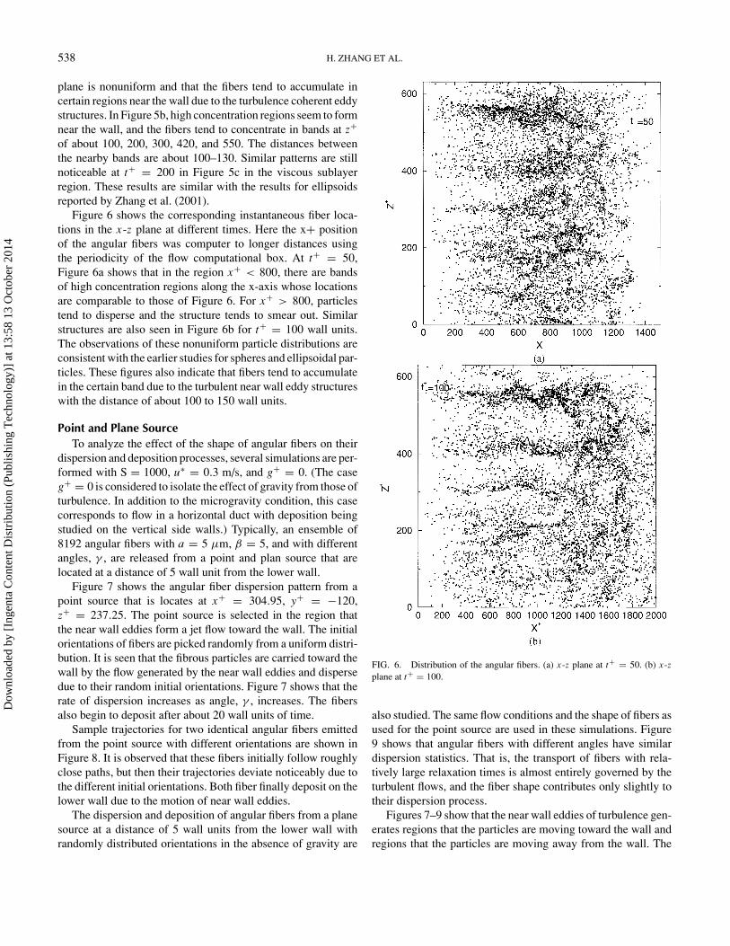
Figure 6 shows the corresponding instantaneous fiber loca-tions in the x-z plane at different times. Here the x+ positionof the angular fibers was computer to longer distances usingthe periodicity of the flow computational box. At t+ = 50,Figure 6a shows that in the region x+ < 800, there are bandsof high concentration regions along the x-axis whose locationsare comparable to those of Figure 6. For x+ > 800, particlestend to disperse and the structure tends to smear out. Similarstructures are also seen in Figure 6b for t+ = 100 wall units.The observations of these nonuniform particle distributions areconsistent with the earlier studies for spheres and ellipsoidal par-ticles. These figures also indicate that fibers tend to accumulatein the certain band due to the turbulent near wall eddy structureswith the distance of about 100 to 150 wall units.

Point and Plane SourceTo analyze the effect of the shape of angular fibers on their

dispersion and deposition processes, several simulations are per-formed with S = 1000, u∗ = 0.3 m/s, and g+ = 0. (The caseg+ = 0 is considered to isolate the effect of gravity from those ofturbulence. In addition to the microgravity condition, this casecorresponds to flow in a horizontal duct with deposition beingstudied on the vertical side walls.) Typically, an ensemble of8192 angular fibers with a = 5 µm, β = 5, and with differentangles, γ , are released from a point and plan source that arelocated at a distance of 5 wall unit from the lower wall.

Figure 7 shows the angular fiber dispersion pattern from apoint source that is locates at x+ = 304.95, y+ = −120,z+ = 237.25. The point source is selected in the region thatthe near wall eddies form a jet flow toward the wall. The initialorientations of fibers are picked randomly from a uniform distri-bution. It is seen that the fibrous particles are carried toward thewall by the flow generated by the near wall eddies and dispersedue to their random initial orientations. Figure 7 shows that therate of dispersion increases as angle, γ , increases. The fibersalso begin to deposit after about 20 wall units of time.

Sample trajectories for two identical angular fibers emittedfrom the point source with different orientations are shown inFigure 8. It is observed that these fibers initially follow roughlyclose paths, but then their trajectories deviate noticeably due tothe different initial orientations. Both fiber finally deposit on thelower wall due to the motion of near wall eddies.

The dispersion and deposition of angular fibers from a planesource at a distance of 5 wall units from the lower wall withrandomly distributed orientations in the absence of gravity are

FIG. 6. Distribution of the angular fibers. (a) x-z plane at t+ = 50. (b) x-zplane at t+ = 100.

also studied. The same flow conditions and the shape of fibers asused for the point source are used in these simulations. Figure9 shows that angular fibers with different angles have similardispersion statistics. That is, the transport of fibers with rela-tively large relaxation times is almost entirely governed by theturbulent flows, and the fiber shape contributes only slightly totheir dispersion process.

Figures 7–9 show that the near wall eddies of turbulence gen-erates regions that the particles are moving toward the wall andregions that the particles are moving away from the wall. The

Dow

nloa

ded

by [

Inge

nta

Con

tent

Dis

trib

utio

n (P

ublis

hing

Tec

hnol

ogy)

] at

13:

58 1

3 O

ctob

er 2

014

TRANSPORT AND DEPOSITION OF ANGULAR FIBERS 539

FIG. 7. Trajectory statistics for fibers released from a point source. (a) angular fibers with γ = 0. (b) angular fibers with γ = 45◦. (c) angular fibers withγ = 90◦.

locations of these regions vary with time as the flow evolves. Forshort duration of times of the order of one hundred wall units,which are much larger than the time scale for particle deposition,these regions remain unchanged and control the bulk of the par-ticle deposition (and resuspension) processes. Figure 7 clearlyshows that the near wall eddies are control the transport and de-position of the particles that region. Figure 9 shows that whenthe entire region is considered, the expected random dispersionis observed.

Deposition Velocity

In this section, a series of simulations for two-link angularfiber deposition in vertical and horizontal ducts are performed.Effects of fiber angle, link aspect ratio, and gravity on the fiberdeposition velocity are studied. Three cases when gravity is ab-sent, a vertical duct with gravity in the flow direction, and ahorizontal channel with gravity toward the lower wall are stud-ied. The simulation results are also compared with the empiricalequation results.

Dow

nloa

ded

by [

Inge

nta

Con

tent

Dis

trib

utio

n (P

ublis

hing

Tec

hnol

ogy)

] at

13:

58 1

3 O

ctob

er 2

014

540 H. ZHANG ET AL.

FIG. 8. Samples of trajectories for angular fibers. (a) y-z plane. (b) x-y plane.

Figure 10a shows variations of the deposition velocity of an-gular fibers with γ = 45◦ versus equivalent relaxation time.In these simulations, u∗ = 0.3 m/s, S=1000, the equivalent re-laxation time as defined by Equation (41) and different gravitydirections are used. The DNS results for deposition velocity ofspherical particles as reported by Zhang and Ahmadi (2000) andthe empirical equation predictions given by Equation (46) arealso reproduced in Figure 10a for comparison. It is observedthat the DNS results for the angular fiber are in close agreementwith the empirical equation. In the absence of gravity, Figure

FIG. 9. Trajectory statistics for fibers released from a plane source.

10a clearly shows that as the link aspect ratio increases, the de-position velocity for 0.5 < τ+

eq < 10 increases significantly.This is because the deposition by the interception mechanismbecomes very efficient for angular fibers; thus, fibers with largeaspect ratios have higher deposition rate when compared with thespherical particles with the same relaxation time. Figure 10a alsoshows that the deposition velocity for fibers with β = 5 is some-what larger for downflow conditions than that in the absence ofgravity. For the floor deposition in a horizontal channel, Fig-ure 10a shows that the gravitational sedimentation significantlyenhances the deposition rate.

The computer simulation results for variations of depositionvelocity with equivalent relaxation time for angular fibers witha curvature angle of γ = 45◦ for flows with u∗ = 0.1 m/s areshown in Figure 10b. The cases that gravity is absence and whenthe gravity is in the flow direction or perpendicular to the lowerwall are studied. The earlier DNS results of Zhang and Ahmadi(2000) for spherical particles and predictions of Equation (46)are also shown in this figure for comparison. It is observed thatthe empirical model is in good agreement with the present DNSresults. Similar to the case of u∗ = 0.3 m/s in Figure 10a, the in-crease of fiber aspect ratio leads to an increase in the depositionvelocity, and gravity enhances the deposition rate. Figure 10aand 10b show that the differences in the deposition velocitiesfor β = 5 and β = 10 for flows with u∗ = 0.1 m/s are muchlarger than those for u∗ = 0.3 m/s. This implies that the effectof fiber aspect ratio is more pronounced at low shear velocities.The effect of gravity is also more significant at lower shear ve-locities for both vertical and horizontal channels. In particular,the gravitational sedimentation significantly increases the depo-sition velocity in the horizontal channel at low shear velocities.

Dow

nloa

ded

by [

Inge

nta

Con

tent

Dis

trib

utio

n (P

ublis

hing

Tec

hnol

ogy)

] at

13:

58 1

3 O

ctob

er 2

014

TRANSPORT AND DEPOSITION OF ANGULAR FIBERS 541

FIG. 10. Variations of deposition velocity with particle relaxation time and aspect ratios. (a) u∗ = 0.3 m/s. (b) u∗ = 0.1 m/s. (c) u∗ = 0.6 m/s.

These observations are consistent with the results of Zhang andAhmadi (2000) for spherical particles and Zhang et al. (2001)for ellipsoidal particles.

There are no available experimental data for the two-link fibermodel, and the available experimental data for deposition ratesof straight fibers are also rather limited. Here, the simulationresults for angular fibers with γ = 45◦ and β = 5 are compared

with the experimental data reported by Shapiro and Goldenberg(1993) for straight fibers in Figure 10c. A shear velocity of u∗ =0.6 m/s, g+ = 0, S = 1820, and a = 0.93 µm, which arethe experimental conditions, are used in the simulation. Theprediction of the empirical equation given by Equation (46) isalso shown in this figure for comparison. While the simulationresults for the angular fiber follow the trend of the experimental

Dow

nloa

ded

by [

Inge

nta

Con

tent

Dis

trib

utio

n (P

ublis

hing

Tec

hnol

ogy)

] at

13:

58 1

3 O

ctob

er 2

014

542 H. ZHANG ET AL.

FIG. 11. Variations of deposition velocity with fiber curvature angle.

data for straight fibers, they show somewhat higher depositionrate. It should be emphasized that the total (tip-to-tip) lengthof the angular fibers with γ = 45◦ are about 1.4 times that ofthe straight fibers used in the experiment. The simulation resultsare also in good agreement with the prediction of the empiricalequation for smaller relaxation time. The deviation increases atlarger relaxation time.

To study the effect of the fiber shape on the deposition ve-locity, additional simulations are performed and the results forangular fibers are compared with the results for elongated el-lipsoidal particles reported by Zhang et al. (2001). Figure 11shows variations of the deposition velocity with the fiber an-gle, γ , for different size fibers for flows with a shear velocity ofu∗ = 0.3 m/s. Here the effect of gravity is neglected. While thereare some scatters, an increasing trend of the deposition velocitywith fiber angle is noticed from this figure. This is because thefibers with larger angle have larger effective aspect ratios. Asa result, the interception deposition mechanism becomes moreeffective.

Figures 12a and 12b compares the simulation results for de-position velocity of angular fibers with γ = 45◦ with those forellipsoids reported by Zhang et al. (2001). Here, the equivalentrelaxation time as defined by Equation (41) is used. Figures 12aand 12b show that the simulated deposition velocities of angu-lar fibers behave very similarly to those of straight ellipsoidswhen plotted versus equivalent relaxation time. That is, thesethe deposition data for straight and angular fibers collapse to thesame curves with the use of τ+

p . Thus, it may be concluded thatEquation (41) is indeed a proper expression for the equivalentrelaxation time for angular fibers.

FIG. 12. (a) Comparison of deposition velocity for ellipsoids and angularfibers at u∗ = 0.3 m/s. (b) u∗ = 0.1 m/s.

Motion StatisticsIn this section the orientation and the angular velocity distri-

bution of angular fibers in turbulent channel flows are studied.Several simulations are performed and an ensemble of 8192 an-gular fibers with a = 4.94 µm, β = 5, S = 1000, and γ = 22.5◦,45◦ and 67.5◦ for flows with u∗ = 0.3 m/s are used. Fibers areinitially uniformly distributed with random orientations in theregion within 30 wall units from the lower wall. All statisticalvalues are evaluated using an ensemble of fibers that are moving

Dow

nloa

ded

by [

Inge

nta

Con

tent

Dis

trib

utio

n (P

ublis

hing

Tec

hnol

ogy)

] at

13:

58 1

3 O

ctob

er 2

014

TRANSPORT AND DEPOSITION OF ANGULAR FIBERS 543

FIG. 13. Variations of orientation density functions for angular fibers. (a) cos(θ1). (b) cos(θ2). (c) cos(θ3).

in the viscous sublayer and part of buffer layer (within 12 wallunits from the lower wall) in time duration of 0–100 wall units.

For the case that the gravity is absent, variations of orientationdensity functions for angular fibers are shown in Figure 13. Thedensity function is computed using f (ξ ) = Nξ

N , where ξ =cos (θi ), and θi for i =1, 2, 3 being the angle between the x , y,and z-axis and the flow direction ˆx . Here, Nξ is the number offibers with ξ being in the region [ξ , ξ + �ξ ] , �ξ = 0.0025and N is the total number of samples used. Note that the densityfunction satisfies the normalization condition,

∑200i=1 f (ξi ) = 1.

Figure 13a shows the density function of the cosine value ofthe angle between x-axis (perpendicular to the plane of fiber)and the flow direction (co-moving coordinate axis ˆx) for fiberswith angles of γ = 22.5◦, 45◦, and 67.5◦. It is observed thatthe distribution of cos(θ1) is roughly symmetric and has a no-ticeable peak near the origin. This indicates that θ1 ≈ 90◦ isthe most likely value and the plane of angular fiber tends to be-come align with the flow direction. The alignment of the fiberplane with the flow direction becomes more pronounced as γ

decreases.

Dow

nloa

ded

by [

Inge

nta

Con

tent

Dis

trib

utio

n (P

ublis

hing

Tec

hnol

ogy)

] at

13:

58 1

3 O

ctob

er 2

014

544 H. ZHANG ET AL.

Figure 13b shows the orientation density function as a func-tion of cos(θ2). As noted before, θ2 is the angle between thedirection of angular fiber (line connecting the fiber centroid toits tip) with the flow direction. It is observed that there are twopeaks for cos(θ2) = ±1 (θ2 = 0, θ2 = 180◦) for γ of 22.5◦ and45◦. That is, fibers with small curvature angle tend to align theirtips (their y-axis) with the flow direction. For γ = 67.5◦, how-ever, the peaks at θ2 = 0, 180◦ disappears and the distribution isroughly uniform with a broad peak near cos(θ2) = 0 (θ2 = 90◦).This implies that the angular fibers tend to align their longestdimension with the mean flow velocity field.

Figure 13c shows that for the orientation distribution of thefiber z-axis has peaks at cos(θ3) = ±1 and these peaks arethe highest for γ = 67.5◦. As noted before, fibers with large

FIG. 14. Variations of angular velocity density functions for angular fibers. (a) γ = 22.5◦. (b) γ = 45◦. (c) γ = 67.5◦.

curvature angle tend to align their z-axis (elongated direction)with the flow direction. For γ = 22.5◦ and γ = 45◦, Figure13c shows that the peaks at θ3 = 0, 180◦ become smaller and abroad peak near θ3 = 0 appears. Figure 13 indicates that angularfibers suspended in the turbulent boundary layer near a wall tendto align their elongated direction with the flow direction. Forsmall γ , the arrow shape fibers align their y-axis along the flowdirection, while for large γ , the bow shape fibers align theirz-axis with the flow direction.

Distribution functions of the absolute value of angular ve-locities for fibers with γ = 22.5◦, 45◦, and 67.5◦ in the wallregion (within 12 wall units from the lower walls) are shown inFigure 14. The method used for evaluating the density functionof angular velocity is the same as that used for the orientation

Dow

nloa

ded

by [

Inge

nta

Con

tent

Dis

trib

utio

n (P

ublis

hing

Tec

hnol

ogy)

] at

13:

58 1

3 O

ctob

er 2

014

TRANSPORT AND DEPOSITION OF ANGULAR FIBERS 545

distribution. (Here, a value of�ω = 0.005 is used.) Figure 14shows that the angular velocity about the z-axis is the largest forγ = 22.5◦,45◦, and 67.5◦. This indicates that the angular fibersrotate fastest about the z-axis due to the streamwise mean shearfield, which is consist with the results for ellipsoids reported byZhang et al. (2001). Figure 14a and 14b show that the angularvelocity about x-axis is the smallest for fibers with γ = 22.5◦

and 45◦. For γ = 67.5◦, however, Figure 14c shows that theangular velocity about y-axis is the smallest.

Velocity and Force StatisticsIn this section, the velocity and force statistics of angular

fibers are presented. An ensemble of 8192 angular fibers withfixed relaxation time of τ+

eq = 5.0, S = 1000, γ = 45◦, and

FIG. 15. Variations of mean velocities of fluid and particles near the wall at (a) u∗ = 0.3 m/s. (b) u∗ = 0.1 m/s. (c) u∗ = 0.3 m/s. (d) u∗ = 0.1 m/s.

different gravity directions are used in the simulation. Specifi-cally, a = 4.95 µm, β = 5 for flows with u∗ = 0.3 m/s, anda = 14.8 µm, β = 5 for u∗ = 0.1 m/s are used. The same initialconditions as described in the previous section are also appliedhere.

Figures 15a and 15b show variations of the mean stream-wise velocities of fluids and angular fibers in the wall region.The mean streamwise velocities for ellipsoidal particles withthe same relaxation time of τ+

eq = 5.0 as reported by Zhanget al. (2001) are also reproduced in these figures for comparison.For ellipsoidal particles, a = 4.95 µm, β = 5 for flows withu∗ = 0.3 m/s, and a = 14.8 µm, β = 5 for u∗ = 0.1 m/swere used by Zhang et al. (2001). It is observed from Fig-ure 15a that the mean velocity of angular fibers in the streamwise

Dow

nloa

ded

by [

Inge

nta

Con

tent

Dis

trib

utio

n (P

ublis

hing

Tec

hnol

ogy)

] at

13:

58 1

3 O

ctob

er 2

014

546 H. ZHANG ET AL.

direction is slightly larger than that of the fluid even in the ab-sence of gravity. The reason is that the fibers are drifting towardthe wall (perhaps by the down sweep motion of the coherenteddies), and they carry their larger streamwise velocities com-pared to that of the surrounding fluid. Figure 15a also showswhen acceleration of gravity is in the flow direction, the meanfiber velocity in the streamwise direction is almost the same asthat in the absence of gravity. As noted before, at large shearvelocity (greater than 0.3 m/s), the effect of gravity is negli-gible. Figure 15b shows the slip velocity increases for gravityin the flow direction at low shear velocities. It is observed foru∗ = 0.1 m/s that the effect of gravity in the flow direction issignificant, and it makes fibers move faster than the case in theabsence of gravity. A similar behavior for ellipsoidal particleswas reported in the earlier work of Zhang et al. (2001). It is alsoobserved from these figures that the mean streamwise velocityfor angular and ellipsoidal particles in the flows of u∗ = 0.3 m/sare quite similar, while the ellipsoidal particles move slightlyfaster than the angular fibers for flows with u∗ = 0.1 m/s.

In these simulations, the mean forces acting on the angularfibers and ellipsoids are also evaluated. At every time step, en-semble averages of the y-component of drag and the lift forcesacting on the angular fibers that are moving in the region within12 wall units from the lower wall are computed. (Positive signdenotes the direction is away from the lower wall.) The simu-lation results for the time duration of 20 to 100 wall units areshown in Figures 15c and 15d (i.e., the time after the startupto 20 wall units is omitted to eliminate the effect of initial con-ditions). As noted before, the simulation results for ellipsoidalparticles with the same relaxation time reported by Zhang et al.(2001) are also plotted here for comparison.

Figures 15c and 15d show the variations of the mean forcesin y-direction versus time for different shear velocities. As wasnoted before, angular fibers move faster than the fluid in thewall region; therefore, they experience a mean lift force towardthe wall. For u∗ = 0.3 m/s, Figure 15c shows that the meanlift force is negative, which causes the fibers to move towardthe wall. The positive lateral drag force in this figure clearlyindicates that there is a trend of angular fiber migration towardthe wall. Figure 15c also shows that the variation of mean forcesdue to different gravity conditions is negligible at such high shearvelocities and various forces acting on fibers and ellipsoids havealmost the same magnitudes.

For u∗ = 0.1 m/s, Figure 15d shows that the magnitudes ofmean drag and lift forces are much larger for downward flows(with g in the flow direction) than those in the absence of gravity.As was noted before, the slip velocity of fiber increases whengravity is in the flow direction, thus the lift force toward thewall increases. Figure 15d also shows that for the same particlerelaxation time, ellipsoids experience larger lift forces in com-parison to fibers, especially when gravity is in the flow direction.This is due to the larger slip velocity experienced by ellipsoidsas shown in Figure 15b. The increased magnitude of drag forcealso indicates that the migration toward the wall for ellipsoidal

particles is more pronounced than that for fibers when gravity isin the flow direction.

CONCLUSIONSIn this work, transport and deposition of angular fibers in tur-

bulent channel flows are studied. The instantaneous fluid veloc-ity field is generated by the direct numerical simulation (DNS) ofthe Navier-Stokes equation. The hydrodynamic drag and torque,the shear-induced lift and gravitational forces acting on each linkof the fiber are included in the governing equations. The motionof fibers in turbulent flows are evaluated and statistically an-alyzed, and the deposition velocities under various conditionsare computed. On the basis of the present results, the followingconclusions are drawn:

• The turbulent near wall coherent vortical structureplays an important role on the fiber transport and de-position processes.

• Angular fibers tend to accumulate in certain bands inthe viscous sublayer with the spacing of about 100 to150 wall units due to the turbulent near wall eddy struc-tures.

• The dispersion of fibers with relatively large relaxationtimes is almost entirely governed by the turbulent flows,and the fiber shape contributes only slightly to theirdispersion process.

• The present DNS simulation results for deposition ve-locity of angular fibers are in good agreement with theproposed empirical equation.

• As link aspect ratio increases, the deposition velocityfor 0.5 < τ+

eq < 10 increases sharply due to the in-crease in the efficiency of the interception mechanism.

• The enhancement effect by the gravitational force fordeposition velocity is significant at low shear velocities.

• Angular fibers with larger curvature angle have higherdeposition velocity due to the more effective intercep-tion mechanism.

• Angular fibers tend to align their longest dimensionwith the mean flow direction. For small γ , the arrowshape fibers align their y-axis along the flow direction,while for large γ , the bow shape fibers align their z-axiswith the flow direction.

• Angular fibers generally rotate fastest about the z-axisdue to the streamwise mean shear field.

• Angular and straight fibers generally move faster thanthe fluid in the streamwise direction in the wall regionand the slip velocity increases when gravity is in theflow direction.

• The slip velocity decreases as shear increases, and theeffect of gravity on fiber transport and deposition inthe viscous sublayer becomes negligible for flows withhigh shear velocities.

• The effect of gravity becomes quite significant at lowshear velocities.

Dow

nloa

ded

by [

Inge

nta

Con

tent

Dis

trib

utio

n (P

ublis

hing

Tec

hnol

ogy)

] at

13:

58 1

3 O

ctob

er 2

014

TRANSPORT AND DEPOSITION OF ANGULAR FIBERS 547

• Angular fibers experience a lift force toward the wallin the wall region. The migration toward the wall trendincreases when gravity in the flow direction especiallyfor flows with low shear velocities.

REFERENCESAhmadi, G. (1993). Overview of Digital Simulation Procedures for Aerosol

Transport in Turbulent Flows. In Particle in Gases and Liquids 3: Detection,Characterization, and control, K.L. Mittal (ed.). Plenum, New York, p. 1.

Asgharian, B. and Ahmadi, G. (1998). Effect of Fiber Geometry on Depositionin Small Airways of the Lung, Aerosol Sci. Technol., 29:459–474.

Asgharian, B., Yu, C. P., and Gradon, L. (1988). Diffusion of Fiber in a TubularFlow, Aerosol Sci. Technol., 9:213–219.

Asgharian, B. and Yu, C. P. (1989). Deposition of Fibers in the Rat Lung, J.Aerosol Sci., 20:355–366.

Brenner, H. (1964). The Stokes Resistance of an Arbitrary Particle-IV, ArbitraryFields of Flow, Chem. Eng. Sci., 19:703–727.

Brooke, J. W., Kontomaris, K., Hanratty, T. J., and McLaughlin, J. B. (1992).Turbulent Deposition and Trapping of Aerosols at a Wall, Phys. Fluids A4:825–834.

Chen, Y. J. and Yu, C. P. (1990). Sedimentation of Charged Fibers from a Two-Dimensional Channel Flow, Aerosol Sci. Technol., 12:786–792.

Cleaver, J. W. and Yates, B. (1973). Mechanism of Detachment of Colloid Par-ticles from a Flat Substrate in Turbulent Flow, J. Colloid Interface Sci., 44:464–474.

Cleaver, J. W. and Yates, B. (1975). A Sublayer Model for Deposition of theParticles from Turbulent Flow, Chem. Eng. Sci., 30:983–992.

Cleaver, J. W. and Yates, B. (1976). The Effect of Re-entrainment on ParticleDeposition, Chem. Eng. Sci., 31:147–151.

Eisner, A. D. and Gallily, I. (1982). On the Stochastic Nature of the Motion ofNonspherical Aerosol Particles IV. General Convective Rotational Velocitiesin a Simple Shear Flow, J. Colloid Interface Sci. 88, 185–196.

Fan, F.-G. and Ahmadi, G. (1993). A Sublayer Model for Turbulent Depositionof Particles in Vertical Ducts with Smooth and Rough Surfaces, J. AerosolSci., 24:45–64.

Fan, F. G. and Ahmadi, G. (1995a). Analysis of Particle Motion in the Near-Wall Shear Layer Vortices-Application to the Turbulent Deposition Process,J. Colloid Interface Sci., 172:263–277.

Fan, F. G. and Ahmadi, G. (1995b). Dispersion of Ellipsoidal Particle in anIsotropic Pseudo-Turbulent Flow Field, ASME J. Fluids Eng., 117:154–161.

Fan, F. G. and Ahmadi, G. (1995c). A Sublayer Model for Wall Deposition ofEllipsoidal Particles in Turbulent Streams, J. Aerosol Sci., 26:813–840.

Fan, F. G. and Ahmadi, G. (1997). Wall Deposition of Small Ellipsoids fromTurbulent Air Flows-A Brownian Dynamics Simulation, Clarkson Universityreport No. MAE-327.

Fan, F. G., Soltani, M., Ahmadi, G., and Hart, S. C. (1997). Flow-induced Resus-pension of Rigid-link Fibers from Surfaces, Aerosol Sci. Technol., 27:97–115.

Fichman, M., Gutfinger, C., and Pnueli, D. (1988). A Model for Turbulent De-position of Aerosols, J. Aerosol Sci., 19:123–136.

Foss, J. M., Frey, M. F., Schamberger, M. R., Peters, J. E., and Leong, K. M.(1989). Collection of Uncharged Prolate Spherical Aerosol Particles by Spher-ical Collectors I: 2D motion, J. Aerosol Sci., 20:515–532.

Galliy, I. and Cohen, A. H. (1979). On the Orderly Nature of the Motion of Non-spherical Aerosol Particles II. Inertial Collision Between a Spherical LargeDroplet and Axially Symmetrical Elongated Particle, J. Colloid InterfaceSci., 68:338–356.

Gallily, I. and Eisner, A. D. (1979). On the Orderly Nature of the Motion of Non-Spherical Aerosol Particles I. Deposition from a Laminar Flow, J. ColloidInterface Sci., 68:320–337.

Goldstein, H. (1980). Classical Mechanics, 2nd Edition. Addison-Wesley, Read-ing, MA.

Gradon, L., Grzybowsk, P. and Pilacinsk, W. (1989). Analysis of Motion andDeposition of Fibrous Particles on a Single Filter Element, Chem. Eng. Sci.,43:1253–1259.

Harper, E. Y. and Chang, I. D. (1968). Maximum Dissipation Resulting fromLift in a Slow Viscous Shear Flow, J. Fluid Mech., 33:209–225.

Hinch, E. J. and Leal, L. G. (1976). Constitutive Equations in Suspension Me-chanics. Part 2. Approximate forms for a Suspension of Rigid Particles Af-fected by Brownian Rotations, J. Fluid Mech., 76:187–208.

Hinds, W. C. (1982). Aerosol Technology, Properties, Behavior, and Measure-ment of Airborne Particles, J. Aerosol Sci., 19:197–211.

Hinze, J. O. (1975). Turbulence. McGraw-Hill, New York.Hughes, P. C. (1986). Spacecraft Attitude Dynamics. Wiley, New York.Jeffery, G. B. (1922). The Motion of Ellipsoidal Particles Immersed in a Viscous

Fluid, Proc. R. Soc. A 102:161–179.Johnson, D. L. and Martonen, T. B. (1993) Fiber Deposition Along Airway

Walls: Effects of Fiber Cross-Section on Rotational Interception, J. AerosolSci., 24:525–536.

Kim, J., Moin, P., and Moser, R. (1987). Turbulent Statistics in Fully DevelopedChannel Flow at Low Reynolds Number, J. Fluid Mechanics, 177:133–166.

Koch, D. L. and Shaqfeh, S. G. (1990). The Average Rotation Rate of a Fiberin the Linear Flow of a Semidilute Suspension, Phys. Fluids A 2:2093–2102.

Krushkal, E. M. and Gallily, I. (1984). On the Orientation Distribution Functionof Nonspherical Aerosol Particles in a General Shear Flow, I. The LaminarCase, J. Colloid Interface Sci., 99:141–152.

Krushkal, E. M. and Gallily I. (1988). On the Orientation Distribution Functionof Nonspherical Aerosol Particles in a General Shear Flow, II. The TurbulentCase, J. Aerosol Sci., 19:197–211.

Kulick, J. D., Fessler, J. R., and Eaton, J. K. (1994). Particle Response andTurbulence Modification in Fully Developed Channel Flow, J. Fluid Mech.,277:109–134.

Kvasnak, W. and Ahmadi, G. (1995). Fibrous Particle Deposition in a TurbulentChannel Flow: An Experimental Study, Aerosol Science and Technology,23:641–652.

Massah, H., Kontomaris, K., Schowalter, W. R., and Hanraty, T. J. (1993). TheConfigurations of a FENE Bead-Spring Chain in Transient Rheological Flowsand in a Turbulent Flow, Phys. Fluids A 5:881–889.

McCoy, D. D. and Hanratty, T. J. (1977). Rate of Deposition of Droplets inAnnular Two-Phase Flow, Int. J. Multiphase Flows 3:319–331.

McLaughlin J. B. (1989). Aerosol Particle Deposition in Numerically SimulatedTurbulent Channel Flow, Phys. Fluids A 1:1211–1224.

Ounis, H., Ahmadi, G., and McLaughlin, J. B. (1991). Dispersion and Depositionof Brownian Particles from Point Sources in a Simulated Turbulent ChannelFlow, J. Colloid Interface Sci., 147:233–250.

Ounis, H., Ahmadi, G., and McLaughlin, J. B. (1993). Brownian Particle Depo-sition a Directly Simulated Turbulent Channel Flow, Phys. Fluids A 5:1427–1432.

Papavergos, P. G. and Hedley, A. B. (1984). Particle Deposition Behavior fromTurbulent Flows, Chem. Eng. Res. Des., 62:275–295.

Pendinotti, S., Mariotti, G., and Banerjee, S. (1992). Direct Numerical Simula-tion of Particle Behavior in the Wall Region of Turbulent Flows in HorizontalChannels, Int. J. Multiphase flow 18:927–941.

Rashidi, M., Hetsroni, G., and Banerjee, S. (1990). Particle-turbulence Interac-tion in a Boundary Layer, Int. J. Multiphase Flow 16:935–949.

Saffman, P. G. (1965). The Lift on a Small Sphere in a Slow Shear Flow, J.Fluid Mech., 22:385–400.

Saffman, P. G. (1968). Corrigendum to The Lift on a Small Sphere in a SlowShear Flow, J. Fluid Mech., 31:624.

Schamberger, M. R., Peters, J. E., and Leong, K. H. (1990). Collection of ProlateSpherical Aerosol Particles by Charged Spherical Collectors, J. Aerosol Sci.,21:539–554.

Schiby, D. and Gallily, I. (1980). On the Orderly Nature of the Motion of Non-spherical Aerosol Particles III. The Effect of the Particle-Wall Fluid-DynamicInteraction, J. Colloid Interface Sci., 77:328–352.

Dow

nloa

ded

by [

Inge

nta

Con

tent

Dis

trib

utio

n (P

ublis

hing

Tec

hnol

ogy)

] at

13:

58 1

3 O

ctob

er 2

014

548 H. ZHANG ET AL.

Shapiro, M. and Goldenberg, M. (1993). Deposition of Glass Fiber Particlesfrom Turbulent Air Flow in a Pipe, J. Aerosol Sci., 24:65–87.

Shaqfeh, S. G. and Fredrickson, G. H. (1990). The Hydrodynamic Stress in aSuspension of Rods, Phys. Fluids A, 2:7–24.

Smith, C. R., and Schwartz, S. P. (1983). Observation of Streamwise Rotation inthe Near-Wall Region of a Turbulent Boundary Layer, Phys. Fluids, 26:641–652.

Soltani, M. and Ahmadi, G. (1995). Direct Numerical Simulation of ParticleEntrainment in Turbulent Channel Flow, Phys. Fluids, 7:647–657.

Soltani, M. and Ahmadi, G. (2000). Direct Numerical Simulation of Curly Fibersin Turbulent Channel Flow, Aerosol Sci. Technol., 33:392–418.

Soltani, M., Fan, F. G., Ahmadi, G., and Hart, S. C. (1997). Detachment ofRigid-Link Fibers with Linkage Contact in a Turbulent Boundary Layer Flow,J. Adhesion Sci. Technol., 11:1017–1037.

Squires, K. D. and Eaton, J. K. (1991a). Measurements of Particle Disper-sion Obtained from Direct Numerical Simulations of Isotropic Turbulence,J. Fluid Mechan., 226:1–35.

Squires, K. D. and Eaton, J. K. (1991b). Preferential Concentration of Particlesby Turbulence, Physics of Fluids, A, 3:1169–1178.

Wood, N. B. (1981a). A Simple Method for the Calculation of Turbulent Depo-sition to Smooth and Rough Surfaces, J. Aerosol Sci., 12:275–290.

Wood, N. B. (1981b). The Mass Transfer of Particle and Acid Vapor to CooledSurfaces, J. Institute of Energy, 76, 76–93.

Zhang, H. and Ahmadi, G. (2000). Aerosol Particle Transport and Deposition inVertical and Horizontal Turbulent Duct Flows, J. Fluid Mechan., 406:55–80.

Zhang, H., Ahmadi, G., Fan, F.-G., and McLaughlin, J. B. (2001). EllipsoidalParticles Transport and Deposition in Turbulent Channel Flows, Intl. J. Mul-tiphase Flows, 27:971–1009.

Dow

nloa

ded

by [

Inge

nta

Con

tent

Dis

trib

utio

n (P

ublis

hing

Tec

hnol

ogy)

] at

13:

58 1

3 O

ctob

er 2

014