Traditional and geometric morphometrics for studying skull ...

Traditional and geometric morphometrics for studying skullmorphology during growth in Mastomys natalensis (Rodentia: Muridae)

MATTEO BRENO,* HERWIG LEIRS, AND STEFAN VAN DONGEN

Evolutionary Ecology Group, Department of Biology, University of Antwerp, Groenenborgerlaan 171, B-2020 Antwerp,

Belgium (MB, HL, SVD)

Danish Pest Infestation Laboratory, Department of Integrated Pest Management, Faculty of Agricultural Sciences,

University of Aarhus, Skovbrynet 14, DK-2800 Lyngby, Denmark (HL)

* Correspondent: [email protected]

Geometric morphometrics is a powerful tool for the study of morphological variation that possesses numerous

advantages over the more traditional approach based on linear measurements. We analyzed skull morphology,

comparing traditional with geometric morphometrics, of 3 different developmental pathways in Mastomys

natalensis (Rodentia: Muridae) from a single population. During early development growth patterns were

influenced by environmental factors, specifically rainfall pattern, consistent with previous reports that growth

trajectories vary according to the amount and distribution of rain. Results confirmed that early growth rate is

one of the main determinants of size and shape differences in the skull in the 3 developmental pathways

(generation types) of M. natalensis. Other factors, such as food quality and consistency, also could play an

important role. Overall, geometric morphometrics appeared more sensitive than the traditional method in

detecting variation in skull morphology, but both approaches led to very comparable conclusions. Phenotypic

plasticity is an alternative explanation to local adaptations for ecogeographical morphological variation.

Key words: geometric morphometrics, growth, phenotypic plasticity, skull morphology, traditional morphometrics

E 2011 American Society of Mammalogists

DOI: 10.1644/10-MAMM-A-331.1

Morphometrics, the quantitative approach to the study of

morphological variation, combines tools for the description

and the statistical analysis of many relevant biological

questions (Rohlf 1990). It is used in a broad range of

disciplines from paleontology to quantitative genetics. Com-

monly, the field of morphometrics is divided into traditional

or multivariate morphometrics and geometric morphometrics

(Rohlf and Marcus 1993). The former term refers to the

application of multivariate statistics to linear measurements

and ratios, whereas the latter concerns the development of

coordinate-based methods begun in the 1970s (Bookstein

1991; Dryden and Mardia 1998; Zelditch et al. 2004).

Traditional morphometrics has been shown to have certain

limitations when compared to geometric morphometrics. In

the former, data consist of lengths, depths, and widths

containing little information about the geometry of the

structure being studied (Zelditch et al. 2004). Geometric

relationships among the variables are not retained so that it is

not possible to depict graphical representations of shape

(Adams et al. 2004). In addition, overlap of variables occurs

frequently, making it difficult to describe local shape changes.

Within the traditional framework a formal distinction between

size and shape is difficult, and little agreement is found among

the many methods of size correction proposed (Klingenberg

1996, 1998; Zelditch et al. 2004). To overcome these

limitations a new method was developed starting in the

1970s. The results of the morphometrics synthesis (Bookstein

1996) led to what is now known as the morphometrics

revolution (Rohlf and Marcus 1993). Geometric morphomet-

rics methods capture the geometry of an object using

coordinate-based data. A statistical theory of shape has been

developed allowing ‘‘… the combined use of multivariate

statistical methods and methods for the direct visualization in

biological form’’ (Adams et al. 2004:6).

Direct and indirect comparisons between traditional and

geometric morphometrics have been few but generally have

shown the advantages of geometric morphometrics compared

to the traditional approach. For example, Maderbacher et al.

(2008) reported that both traditional and geometric morpho-

metrics were able to discriminate among 3 populations of the

w w w . m a m m a l o g y . o r g

Journal of Mammalogy, 92(6):1395–1406, 2011

1395

Dow

nloaded from https://academ

ic.oup.com/jm

amm

al/article/92/6/1395/961102 by guest on 11 September 2022

www.mammalogy.org

cichlid fish Tropheus moorii, but a landmarks approach

permitted a far better quantification and visualization of

among-population differences. Abdel-Rahman et al. (2009)

found a statistically significant sexually dimorphism in

the skull of the African Nile rat (Arvicanthis niloticus) that

was not detected in previous studies based on traditional

morphometrics, and Bernal (2007) showed that a considerable

amount of information was added by using landmarks-based

methods in a study of variation in molar shape in humans.

Finally, Blanco and Godfrey (2006) used geometric morpho-

metrics to show that ontogenetic scaling is insufficient to

describe sexual dimorphism in the mantled howling monkey

(Alouatta palliata).

The aim of this work is to explore within-population

morphological pattern in the skull of Mastomys natalensis

using both traditional and geometric morphometrics. Tradi-

tional and geometric approaches are applied to data collected

in the field with a 2-fold purpose: a nontechnical comparison

between multivariate and geometric morphometrics and the

study of morphological variation in relation to environmental

conditions. In a recent paper Fadda and Leirs (2009) showed

that environmental conditions affect growth trajectories of the

skull within a population of M. natalensis in Tanzania. The

peculiarity of this population is that it presents different

growth patterns related to the amount of rainfall. Three

different generation types (developmental pathways) have

been identified according to the presence and the length of a

period of reduced growth (Leirs et al. 1993). Generation a is

born in the middle of the year (main breeding season) and

shows the longest period of reduced growth, reaching the

maximum size in the next breeding season. Alternatively,

generation b is born in the main breeding season as well, but

due to abundant off-season rain (October–December) it has a

shorter period of reduced growth and is able to mature at the

very beginning of the next year. Its offspring, generation c,

appear in the off-season period (January–March) and reach

maturity in the main breeding season of that same year. A

growth stop phase has been identified as a major determinant

of skull shape, and its duration relates to the achievement of

target skull morphology (Fadda and Leirs 2009).

Among the many studies about within-species variation

in the morphology of the skull, most are concerned with

ecogeographical variation (Lawing and Polly 2009), whereas

studies investigating the direct effect of environment (mainly,

quality and consistency of food) on shape often are performed

in the laboratory (Kiliaridis 2006). For example, effects of

habitat on skull morphology in M. natalensis have been

reported, where 2 populations existing in different environ-

ments differed significantly in morphology (Lalis et al.

2009a). In studies like the latter it often is assumed that the

observed ecogeographical variation in morphology represents

a local adaptation and not differential reaction to different

environments (i.e., plasticity). However, laboratory studies have

shown an important role of plasticity (Myers et al. 1996).

Because we studied a single genetically homogeneous population

(Van Hooft et al. 2008) under varying developmental conditions,

we have the opportunity to study phenotypic plasticity in the

field.

MATERIALS AND METHODS

The data we analyzed come from the same trapping

campaign as in Fadda and Leirs (2009). However, we

considered only a subset of individuals for which a precise

age estimation was available. For this subset landmark data of

the skull were collected in addition to linear measurements.

Specimens were collected in Morogoro, Tanzania, between

September 1987 and October 1988. Animals were aged using

eye lens weight (Leirs 1995) and then assigned to generation

types and age classes according to their estimated date of birth

and age. Three 2-month age classes (0–2, 2–4, and 4–6 months)

were established, but a individuals belonging to the 3rd age

class were not available. In total, 856 skulls were used, of which

111, 563, and 182 were assigned to generation types a, b, and c,

respectively. Division into age classes resulted in the assign-

ment of 233 skulls to the 1st age class, 290 to the 2nd age class,

and 333 to the 3rd age class. Dermestid beetles were used to

skeletonize skulls, after which 22 cranial linear parameters were

measured to the nearest 0.05 mm with digital calipers (Fig. 1).

A subset of the original data set was investigated by using

geometric morphometrics; 292 (62 of generation a, 125

of generation b, and 105 of generation c) specimens were

photographed in dorsal view, and 23 landmarks (Fig. 1) were

registered twice using ImageJ (Rasband 2010). Numbers of

specimens were 95, 126, and 71 for the 1st, 2nd, and 3rd age

classes, respectively. Other studies have applied geometric

morphometrics to the study of skull morphology in M.

natalensis (Lalis et al. 2009a, 2009b); however, it was not

possible to locate exactly the same landmarks on the dorsal

side of the skull. All analyses were performed using MorphoJ

(Klingenberg 2011) and R (R Development Core Team 2009).

Analysis of linear measurements.—Univariate analysis of

variance and multivariate analysis of variance (MANOVA)

were carried out to identify sources of morphological variation

between or among generation types, age classes, and sex. Data

were graphically inspected for outliers and normality by QQ

plots. Proportional contributions of the sum of squares

(%SSQ) of each source of variation to the total SSQ were

reported (Bronner et al. 2007; Leamy 1983) for each variable.

In comparison to morphological differences observed between

age classes (Pillai’s trace 5 0.69, F44,1,646 5 19.80, P ,

0.001) and generation types (Pillai’s trace 5 0.77, F44,1,646 5

23.48, P , 0.001), sexual dimorphism was relatively small but

significant (Pillai’s trace 5 0.124, F22,822 5 5.30, P , 0.001).

The %SSQ identified age and generation type as the 2

major sources of variation for almost all variables (variation

explained by age class and generation type ranged from 1.6%

to 75% and 0.8% to 6%, respectively). For sexual dimorphism,

however, this range was between 0.1% and 1.2%. Because no

interactions with sex were observed, males and females were

pooled for all further analyses (sex*age class: Pillai’s trace 5

0.07, F44,1,646 5 1.45, P 5 0.03; sex*generation type: Pillai’s

1396 JOURNAL OF MAMMALOGY Vol. 92, No. 6

Dow


ic.oup.com/jm

amm


trace 5 0.06, F44,1,646 5 1.06, P 5 0.36). A significant

interaction was observed between age class and generation type

(Pillai’s trace 5 0.15, F66,2,472 5 1.94, P , 0.001), indicating

that morphological differences between generation types

changed with age.

Next, we performed a principal component analysis (PCA)

on untransformed data based on the correlation matrix for

each generation type separately. Age-related changes in size

were visualized by plotting the 1st principal component

(PC1) against age. This approach is common in traditional

FIG. 1.—Linear measurements made on skulls of Mastomys natalensis. 1, Greatest length of the skull (GL); 2, condylonasal length (CL);

3, henselion–basion distance (HB); 4, henselion–palation distance (HP); 5, length of palatal foramen (PL); 6, length of diastema (DL); 7,

distance alveolus M1–upper incisor (MoID); 8, smallest interorbital breadth (IB); 9, zygomatic breadth (BB); 10, smallest palatal breadth (PB);

11, length of upper cheek-teeth alveoli (UAL); 12, breadth of upper dental arch (UDB); 13, greatest breadth of M1 (Mo1); 14, breadth of

zygomatic plate (ZPB); 15, greatest breadth of nasals (NB); 16, greatest length of nasals (NL); 17, distance M1–M3 (MoJ); 18, length of bulla

(TBL); 19, greatest breadth of braincase (BrB); 20, rostrum height (RH); 21, greatest rostrum breadth (RB); 22, greatest jaw height (JH). Open

black squares represent landmarks.

December 2011 BRENO ET AL.—TRADITIONAL AND GEOMETRIC MORPHOMETRICS 1397

Dow


ic.oup.com/jm

amm


morphometrics, and PC1 usually is interpreted as a size com-

ponent if all of the coefficients of the 1st eigenvector have the

same sign and similar magnitude (Bever 2008; Krystufek

2002; Smith 1998; but see Sundberg 1989 for a discussion of

the topic). PC2 and PC3 were inspected by plotting them

against PC1 to explore differences between age classes and

generation types not associated with the main vector of

variation (i.e., PC1). To further explore differences in shape

between the 3 generation types a discriminant analysis was

performed for each age class. To visualize the dimensions that

optimally divide generation types within each age class,

canonical variate analysis (CVA) was conducted, and the 1st

and 2nd canonical variates (CVs) were plotted. Mahalanobis

distances were calculated among generation types for each age

class and were compared using permutation tests (10,000

permutations). To compare each trait among different

generation types allometric trajectories of both the c and bgeneration types were described using bivariate and multivar-

iate analysis (described below). Generation a was excluded

from the following analyses because it did not contain any

individual older than 4 months. In the bivariate case overall

size was estimated by means of total skull length. The relation

between each variable and skull length was studied using the

allometry equation: log y 5 log b0 + b1 + log e (derived from

power equation y~b0xb1 e—Abdala et al. 2001; Bever 2008;

Giannini et al. 2004). Deviations from isometry were tested by

constructing confidence intervals of the slopes (b1). Slopes

significantly . 1 indicate fast development relative to total

skull length, and slopes , 1 are indicative of a relative slow

growth. Analysis of covariance was used to test for differences

in allometric patterns between generation types for all traits. A

multivariate generalization of the allometry equation was

proposed by Jolicoeur (1963) as the PC1 from the variance–

covariance matrix of the log-transformed data. In this case

isometry is expressed by the isometric vector 1/n0.5, where

n is the number of variables. Values of the 1st eigenvector

represent the allometric coefficients of each variable. A

bootstrap procedure (with 5,000 resamples) was used to obtain

confidence intervals for each allometric coefficient where

differences in allometric coefficients between generation types

were tested by subtracting the bootstrap values of 1 generation

type from those of the other. If the confidence intervals of

these differences did not include zero, the 2 coefficients were

considered different between generation types.

Analysis of landmark data using geometric morphomet-

rics.—Several geometric methods exist, and among them the

Procrustes method (Goodall 1991) is the most widespread.

Procrustes superimposition involves 3 steps to eliminate all

nonshape variation. First, configurations of landmarks are

translated so that their centroid is placed at the origin of the

coordinate system. Next, they are scaled to a common unit

size. Finally, configurations are rotated around their centroid

to minimize the squared distance between corresponding

landmarks. When .2 configurations exist the process

becomes iterative, and all of the configurations are rotated

repeatedly to fit a temporal consensus. The procedure ends

when 2 subsequent average configurations match. Within- and

between-species variation is one among the many phenom-

ena that can be addressed with a morphometric approach.

Ultimately, Procrustes allows a more straightforward distinc-

tion between shape and size variations. Statistical analyses can

be applied to both sources of variation, and variation in shape

can be visualized easily (Zelditch et al. 2004).

The presence of outliers and the distribution of the data

were inspected graphically by plotting the cumulative

distribution of the squared Mahalanobis distance against a

multivariate normal distribution fitted to the data as imple-

mented by MorphoJ (Klingenberg 2011). Overall shape

variation and variation within age classes were visualized by

PCA of Procrustes superimposed landmark configurations of

the entire data set and for each age class. Relative warps (PC

scores of Procrustes coordinates) extracted from Procrustes

superimposition performed separately for each age class were

used to test for morphological differences among generation

types within age classes. The advantage of using relative

warps is that, in contrast to Procrustes coordinates, they

possess the correct number of dimensions and can be

submitted to further analyses without correcting for degrees

of freedom. However, a modified version of MANOVA for

Procrustes data implemented in MorphoJ (Klingenberg 2011)

and MANOVA of relative warps gave the same results.

Preliminary analyses were conducted on the entire data set

by means of MANOVA of relative warps, with age class,

generation type, sex, and their interactions as effects. Sig-

nificant differences were found for generation type (Pillai’s

trace 5 0.68, F42,520 5 6.49, P , 0.001) and age class (Pillai’s

trace 5 0.75, F42,520 5 7.44, P , 0.001) but not for sex

(Pillai’s trace 5 0.11, F21,259 5 1.56, P 5 0.06). Moreover, an

interaction between age class and generation type was found

(Pillai’s trace 5 0.44, F63,783 5 2.16, P , 0.001), and because

no significant interactions involving sex were present (sex*age

class: Pillai’s trace 5 0.12, F42,520 5 0.82, P 5 0.78;

sex*generation type: Pillai’s trace 5 0.17, F42,520 5 1.14, P 5

0.26), males and females were pooled. CVA then was

performed on Procrustes coordinates for each age class using

generation type as a grouping factor. Mahalanobis distances

and Procrustes distances among generation types were

computed in each age class and tested by a permutation test

(10,000 permutations).

RESULTS

Analysis of linear measurements.—Differences among

generation types were highly significant in each age class

(age class 1: Pillai’s trace 5 0.78, F2,123 5 3.02, P , 0.001;

age class 2: Pillai’s trace 5 0.71, F2,323 5 7.65, P , 0.001;

age class 3: Pillai’s trace 5 0.33, F1,224 5 4.68, P , 0.001).

Univariate analyses of variance revealed a number of

differences in all age classes, especially in the 2nd age class

(Table 1). PC1 explained 73% of the total variance. PC1 could

be interpreted as a size vector because the factor loadings

of this 1st eigenvector all had the same sign and similar


Dow


ic.oup.com/jm

amm


TA

BL

E1

.—A

nal

ysi

so

fv

aria

nce

tab

leo

fth

eco

mp

aris

on

of

lin

ear

mea

sure

men

ts(X

6S

D)

amo

ng

gen

erat

ion

typ

es(a

lph

a,b

eta,

and

gam

ma)

wit

hin

each

age

clas

s.S

eeF

ig.

1fo

r

def

init

ion

so

fm

easu

rem

ents

.*

P,

0.0

5;

**

P,

0.0

01

.

Ag

ecl

ass

1A

ge

clas

s2

Ag

ecl

ass

3

Alp

ha

Bet

aG

amm

aF

2,1

23

Alp

ha

Bet

aG

amm

aF

2,3

23

Bet

aG

amm

aF

1,2

24

GL

2,5

35

.86

75

.22

,532

.36

11

2.8

2,5

81

.66

95

.53

.57

*2

,608

.66

92

.22

,71

0.2

61

23

.62

,805

.96

12

6.2

38

.27

**

2,8

88

.56

11

5.0

2,9

47

.56

75

.71

0.1

9*

*

CL

2,3

26

.46

91

.02

,341

.76

10

9.0

2,3

59

.26

10

5.9

1.3

42

,419

.46

94

.22

,51

7.4

61

26

.22

,610

.86

12

7.4

34

.90

**

2,6

96

.36

12

1.0

2,7

49

.96

84

.67

.55*

*

HB

1,9

78

.86

84

.71

,983

.06

92

.82

,00

6.6

69

5.2

1.1

62

,064

.26

87

.42

,14

5.5

61

16

.32

,236

.46

11

8.4

34

.88

**

2,3

17

.76

11

2.5

2,3

69

.06

75

.68

.06*

*

HP

1,1

15

.66

44

.81

,127

.06

58

.11

,12

5.2

65

4.8

0.6

41

,161

.86

48

.31

,20

2.6

66

0.4

1,2

43

.96

64

.22

7.4

1*

*1

,286

.66

55

.21

,30

5.3

64

2.8

4.3

6*

PL

60

7.4

63

1.0

59

9.3

62

7.8

61

1.8

63

7.7

0.7

66

36

.56

34

.16

50

.66

33

.86

65

.56

41

.39

.55*

*6

93

.86

34

.96

98

.76

32

.90

.70

DL

63

5.1

63

0.4

64

2.0

63

5.8

64

7.4

63

3.3

1.8

26

69

.76

30

.97

00

.46

41

.37

26

.56

45

.22

6.6

2*

*7

62

.26

40

.27

77

.46

34

.75

.26*

Mo

ID6

65

.86

32

.96

87

.36

37

.86

87

.76

36

.75

.97

**

70

4.0

63

6.0

75

9.6

64

5.7

78

2.7

64

9.9

36

.15

**

82

8.5

64

4.0

84

1.8

63

3.8

3.4

7

IB3

92

.66

16

.44

01

.06

12

.63

94

.16

13

.31

.92

40

0.5

61

5.4

41

3.1

61

5.5

41

3.6

61

4.9

10

.48

**

42

1.3

61

3.7

41

7.2

61

3.2

3.2

0

BB

1,2

21

.26

48

.71

,231

.96

42

.41

,25

0.5

63

9.2

4.7

8*

1,2

47

.06

47

.31

,30

4.4

65

2.7

1,3

37

.16

54

.53

7.5

4*

*1

,381

.26

60

.31

,39

9.6

65

1.3

3.4

1

PB

22

7.2

61

4.5

23

8.0

61

0.5

23

6.7

61

3.1

7.7

4*

*2

36

.66

13

.12

52

.76

14

.12

51

.16

14

.81

8.2

3*

*2

65

.26

16

.22

61

.66

13

.31

.85

UA

L4

80

.66

16

.54

87

.36

13

.94

89

.76

14

.04

.41

*4

82

.46

18

.34

93

.96

18

.05

03

.96

17

.92

0.1

5*

*5

04

.96

19

.75

11

.96

15

.84

.65*

UD

B5

34

.76

15

.85

47

.06

15

.35

49

.86

11

.81

4.0

3*

*5

44

.26

17

.55

65

.06

18

.55

71

.66

18

.32

7.5

9*

*5

89

.06

18

.85

85

.56

14

.11

.32

Mo

11

46

.16

5.7

14

6.3

64

.81

50

.26

5.9

6.1

8*

*1

46

.86

4.1

14

7.8

66

.91

51

.06

5.8

9.8

2*

*1

48

.86

6.3

15

1.6

66

.37

.08*

*

ZP

B2

63

.36

14

.32

66

.36

15

.92

66

.76

17

.50

.65

27

1.1

61

8.2

28

4.6

61

9.3

29

4.6

61

9.8

20

**

30

1.5

61

8.5

31

7.4

61

5.6

27

.30

**

NB

28

6.5

61

5.6

27

5.7

61

2.9

28

3.6

61

2.0

3.5

7*

29

2.9

61

4.0

29

1.4

61

8.7

30

0.2

61

5.6

8.4

7*

*3

10

.86

19

.33

09

.56

16

.30

.15

NL

94

3.6

64

9.9

96

0.0

64

8.4

98

1.2

65

2.0

6.6

7*

*9

88

.06

52

.31

,06

3.2

66

9.8

1,1

01

.76

69

.23

5.3

5*

*1

,155

.26

60

.61

,17

4.9

65

1.6

3.8

7

Mo

J4

28

.66

12

.54

33

.36

8.4

43

7.9

61

1.4

7.3

5*

*4

30

.26

13

.84

35

.96

14

.64

45

.26

17

.01

7.1

28

**

44

3.7

61

7.5

44

8.5

61

5.2

2.6

9

TB

L4

61

.66

19

.34

64

.06

18

.14

73

.46

17

.34

.70

*4

61

.56

18

.94

66

.86

18

.94

81

.06

20

.82

1.1

9*

*4

76

.86

17

.24

84

.76

16

.37

.31*

*

BrB

1,1

20

.96

35

.61

,116

.76

30

.61

,13

7.1

62

8.0

3.2

6*

1,1

36

.66

28

.51

,15

1.8

62

7.9

1,1

72

.56

32

.32

4.7

7*

*1

,183

.16

30

.01

,18

0.3

63

5.8

0.2

8

RH

56

2.5

62

5.5

57

3.7

62

1.6

57

7.3

62

8.2

4.2

5*

58

7.1

62

2.3

61

6.2

63

1.3

64

1.8

63

2.7

43

.25

**

66

6.7

63

3.9

67

0.9

62

7.8

0.5

9

RB

43

1.9

62

3.5

43

9.3

62

1.2

44

7.3

61

6.2

6.0

1*

44

5.3

62

2.5

46

4.2

62

6.0

48

5.1

62

8.9

34

.25

**

49

9.0

62

7.7

51

2.3

62

2.8

8.6

1*

*

JH6

96

.06

44

.77

00

.06

23

.27

00

.86

34

.20

.19

72

3.8

62

8.4

76

4.9

65

2.6

78

6.6

64

9.8

20

.24

**

82

6.4

64

9.5

84

2.9

63

2.6

4.3

3*


Dow


ic.oup.com/jm

amm


magnitude. Variation represented by PC2 was mainly within

a, and removing the a generation before performing PCA led

to a PC1 containing 93% of the total variance; thus only PC1

was considered for further analysis. This interpretation also

was confirmed by plotting the individual scores for PC1

against age (Fig. 2), where highest scores were related to

oldest individuals. Finally, plotting PC1 against PC2 (explain-

ing 7% of the total variance) led to a subdivision between the

youngest and oldest individuals (figure not shown).

Analysis of the PC1 scores showed significant differences

among generation types in all 3 age classes (1st age class:

F2,123 5 5.18, P , 0.01; 2nd age class: F2,323 5 38.19, P ,

0.001; 3rd age class: F1,224 5 4.49, P , 0.05). Pairwise

comparisons (after Bonferroni’s correction) showed a signif-

icant difference only between a and c in the 1st age class (P ,

0.01), with b intermediate. The strongest differences were

found in the 2nd age class, where all generation types differed

significantly from each other (always P , 0.001; Fig. 2). In

the 1st age class (Fig. 3) the 2 CVs explained 64% and 36% of

the between-group variance, respectively. The measurements

showing highest loadings were smallest palatal breadth,

distance between M1 and the upper incisor, and greatest

breadth of the nasals. In the 2nd age class (Fig. 3) the 1st CV

described 52% of the between-group variance, and the 2nd CV

explained 48%. The highest loadings were observed for

smallest palatal breadth, smallest interorbital breadth, and

greatest breadth of M1 (Fig. 3). In the 1st age class the 2 CVs

contained a different amount of variance, but in the 2nd age

class they accounted for nearly the same amount.

Plotting the 1st CV against the 2nd one for the first 2 age

classes highlighted the presence of 3 distinct, although

overlapping, groups corresponding to the generation types.

In the 1st age class the 1st CV separated a from b and c. The

2nd CV differentiated between b and c. In age class 2 the 1st

CV separated b and c, and the 2nd separated b and c from a

(Fig. 3). The axis of group separation that divides a from band c was always perpendicular to the one that divides b from

c, although the relative importance of the 2 axes changes from

the 1st to 2nd age class. Observing CV loadings and the

FIG. 2.—Average scores of the 1st principal component (PC1 scores)

based on linear measurements for the 3 generation types in the different

age classes. Group scores on PC1 were significantly different (see

‘‘Results’’). Lines connecting the points represent growth trajectories

for the 3 generation types. Vertical bars depict SEs.

FIG. 3.—First and 2nd canonical variates (CVs) for the 1st and 2nd age classes (linear measurements). Although some overlap can be

observed, 3 groups are distinguishable. Lines represent the direction and importance of each measurement in discriminating among groups.

Ellipses represent 90% confidence levels. Dashed black line represents a, gray line b, and dotted black line c generations.


Dow


ic.oup.com/jm

amm


amount of variation accounted for by the 1st CV and 2nd CV

in both age classes, it is appears that differences among

generation types seem to be led by the same measurements

in both 1st and 2nd age class, and in the 2nd age class

morphological differences between c and b become more

prominent in comparison to the 1st age class.

In the 3rd age class (Fig. 4)—containing only individuals

from the b and c generation such that only 1 linear discriminant

function could be determined—the measurements that contrib-

uted most were greatest breadth of M1, breadth of zygomatic

plate, and breadth of upper dental arch measured on M1.

Permutation tests indicated that all Mahalanobis distances were

significant (Table 2). Bivariate allometry coefficients were

mostly consistent with their multivariate counterparts (Table 3).

All measurements had the same allometric pattern in the 2

generation types considered, except for breadth of zygomatic

plate (isometric in b and positively allometric in c), breadth of

the nasals (isometric in b and negatively allometric in c), and

greatest rostrum breadth (positively allometric in b and

isometric in c). Among the measurements that showed the

same allometric pattern zygomatic breadth and breadth of the

upper dental arch were more negative in c individuals.

Multivariate allometry coefficients (Table 3; Fig. 5) showed 7

variables—condylobasal length, henselion–basion distance,

henselion–palation distance, diastema length, M1–upper incisor

distance, nasals length, and jaw greatest height—to be

positively allometric in both generation types. Negative

allometry was shown by 7 measurements in both generation

types: interorbital breadth, length of upper cheek-teeth alveoli,

breadth of the upper dental arch, greatest breadth of the 1st

upper molar, M1–M3 distance (jaw), length of the bulla, and

greatest breadth of braincase. Differences in allometric patterns

between b and c individuals were found for 5 measurements:

length of palatal foramen, zygomatic breadth, breadth of

zygomatic plate, greatest breadth of nasals, and greatest rostrum

breadth. Length of palatal foramen was isometric in b and

slightly positively allometric in c; zygomatic breadth showed

isometry in b and negative allometry in c. Both generation types

showed positive allometry for breadth of zygomatic plate but

near isometry in b individuals; the greatest breadth of nasals

was slightly positively allometric in b and negatively allometric

in c. Finally, the greatest rostrum breadth was isometric in c and

positively allometric in b. The confidence intervals for the

difference between the 2 bootstrap tables showed that the

coefficients differed not only for the traits with different

FIG. 4.—Canonical variate (CV) scores for the 3rd age class (linear

measurements). Because only the b and c generations are represented

in this age class, only 1 CV is estimated.

TABLE 2.—Mahalanobis distances among generation types for each

age class for traditional (linear) and geometric (landmarks)

morphometrics data. See ‘‘Results’’ for details on statistical significance.

Linear Landmarks

Alpha Beta Alpha Beta

Age class 1

Beta 2.5609 1.8587

Gamma 1.9831 2.4004 1.8062 1.8198

Age class 2

Beta 2.4820 2.4503

Gamma 2.640 1.6916 3.1636 1.8372

Age class 3

Gamma 1.8061 2.1546

TABLE 3.—Allometry and bivariate and multivariate allometric

coefficients for each linear measurement. Symbols used indicate

different trends in the allometric pattern: +, positive allometry;

5, isometry; 2, negative allometry. * P , 0.05. See Fig. 1 for

definitions of measurements.

Multivariate Bivariate Coefficients

Beta Gamma Beta Gamma Beta Gamma

GL 5 5 0.219 0.219

CL + + + + 0.244 0.255

HB + + + + 0.268 0.273

HP + + + + 0.238 0.253

PL 5 + 5 5 0.221 0.242

DL + + + + 0.289 0.305

MoID + + + + 0.304 0.321

IB 2 2 2 2 0.087 0.089

BB 5 2* 2 2* 0.213 0.173

PB 2 2 2 2 0.177 0.177

UAL 2 2 2 2 0.092 0.081

UDB 2 2* 2 2* 0.135 0.110

Mo1 2 2 2 2 0.027 0.023

ZPB + +* 5 +* 0.234 0.287

NB + 2* 5 2* 0.228 0.152

NL + + + + 0.279 0.289

MoJ 2 2 2 2 0.071 0.053

TBL 2 2 2 2 0.091 0.077

BrB 2 2 2 2 0.089 0.077

RH + + + + 0.254 0.251

RB + 5* + 5* 0.269 0.227

JH + + + + 0.289 0.294


Dow


ic.oup.com/jm

amm


allometric patterns but also for a few that had similar allometry:

condylobasal length, length of diastema, M1–upper incisor

distance, and breadth of the upper dental arch.

Geometric morphometrics.—Multivariate analysis of vari-

ance of relative warps showed differences among generation

types for each age class (age class 1: Pillai’s trace 5 0.72,

F2,92 5 1.96, P 5 0.001; age class 2: Pillai’s trace 5 0.91,

F2,123 5 4.11, P , 0.001; age class 3: Pillai’s trace 5 0.54,

F1,69 5 2.74, P 5 0.001). The first 5 PCs explained 70% of

the total variance of the entire data set. Age classes divided

along the 1st axis, whereas other PCs did not show any pattern

related to generation types or any other grouping factors

(details not shown). PCA performed separately for each age

class showed a separation between a and c generations along

PC1, with b individuals distributed all along the axis in the

2nd age class (Fig. 6), whereas c specimens tended to cluster

together along PC2 in the 3rd age class (Fig. 6) with no clear

pattern detected in the 1st age class (details not shown). Shape

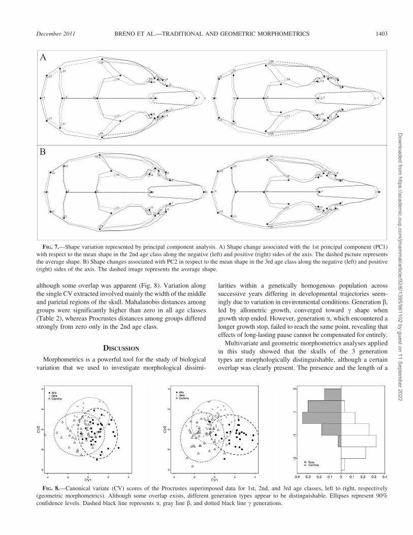
transformations relative to PC1 in the 2nd age class showed a

longer rostrum and a narrower and shorter neurocranium in

the positive side of the axis (Figs. 6 and 7A). Shape changes

associated with PC2 (Fig. 7B) in the 3rd age class were related

to the length and breadth of rostrum and breadth of the frontal

bone, depicting a narrower skull in the middle and anterior

region. First and 2nd CV axes for the 1st age class (Fig. 8)

contained 54% and 46% of among-group variation, respec-

tively. Generations a and c tended to be separated along the

1st axis, and the b generation differed from a and c along the

2nd axis (Fig. 8). Variation retained by the 1st CV was

manifested mainly in the length of the parietal region, whereas

variation in the 2nd CV involved primarily length and breadth

of the middle and anterior regions. This analysis for the 2nd

age class showed a similar pattern as in 1st age class (Fig. 8),

but the 1st CV explained more variation than the 2nd (72%

compared to 28%). Shape variation associated with the 1st

CV referred to the length of the rostrum and width of

neurocranium. Variation in the 2nd shape transformation

involved primarily a posterolateral–anteromedial shift of

maxillary bone in the region of the infraorbital fissure. CVA

in the 3rd age class showed a separation between b and c,

FIG. 5.—Multivariate allometric coefficients (linear measure-

ments) for each trait. Vertical bars represent 95% bootstrapped

confidence intervals. The horizontal line represents the pure

isometric vector. See Fig. 1 for definitions of measurements.

FIG. 6.—Plot of the 1st and 2nd principal component scores (PC1 versus PC2) in the 2nd (left graph) and 3rd (right graph) age classes

(geometric morphometrics). The 3 generation types separate along PC1 in the 2nd age class. PC2 appears to separate the b and c generations in

the 3rd age class.


Dow


ic.oup.com/jm

amm


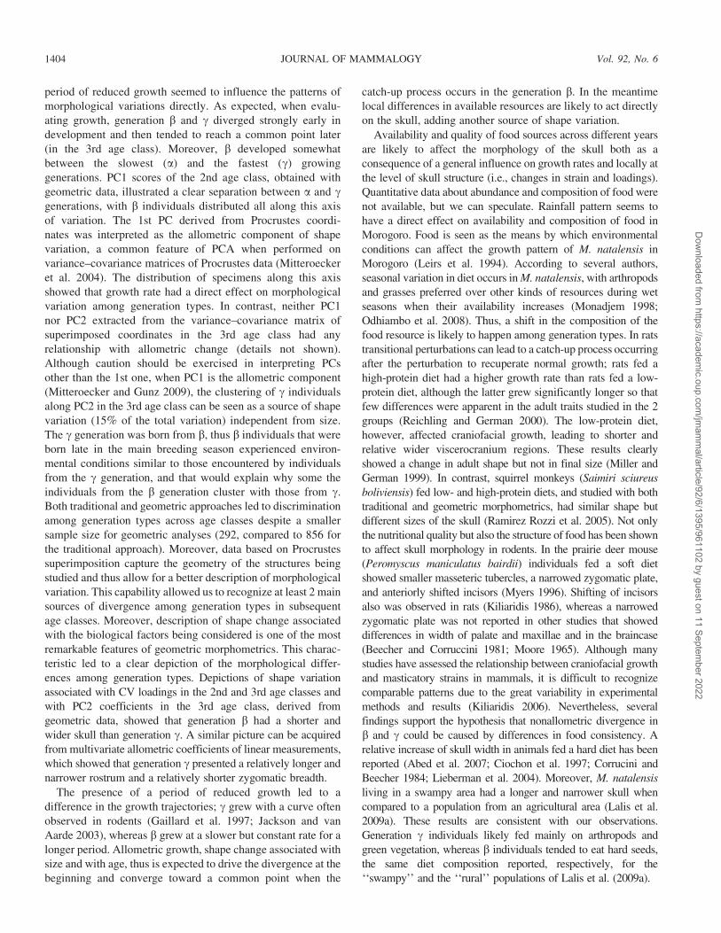
although some overlap was apparent (Fig. 8). Variation along

the single CV extracted involved mainly the width of the middle

and parietal regions of the skull. Mahalanobis distances among

groups were significantly higher than zero in all age classes

(Table 2), whereas Procrustes distances among groups differed

strongly from zero only in the 2nd age class.

DISCUSSION

Morphometrics is a powerful tool for the study of biological

variation that we used to investigate morphological dissimi-

larities within a genetically homogenous population across

successive years differing in developmental trajectories seem-

ingly due to variation in environmental conditions. Generation b,

led by allometric growth, converged toward c shape when

growth stop ended. However, generation a, which encountered a

longer growth stop, failed to reach the same point, revealing that

effects of long-lasting pause cannot be compensated for entirely.

Multivariate and geometric morphometrics analyses applied

in this study showed that the skulls of the 3 generation

types are morphologically distinguishable, although a certain

overlap was clearly present. The presence and the length of a

FIG. 8.—Canonical variate (CV) scores of the Procrustes superimposed data for 1st, 2nd, and 3rd age classes, left to right, respectively

(geometric morphometrics). Although some overlap exists, different generation types appear to be distinguishable. Ellipses represent 90%

confidence levels. Dashed black line represents a, gray line b, and dotted black line c generations.

FIG. 7.—Shape variation represented by principal component analysis. A) Shape change associated with the 1st principal component (PC1)

with respect to the mean shape in the 2nd age class along the negative (left) and positive (right) sides of the axis. The dashed picture represents

the average shape. B) Shape changes associated with PC2 in respect to the mean shape in the 3rd age class along the negative (left) and positive

(right) sides of the axis. The dashed image represents the average shape.


Dow


ic.oup.com/jm

amm


period of reduced growth seemed to influence the patterns of

morphological variations directly. As expected, when evalu-

ating growth, generation b and c diverged strongly early in

development and then tended to reach a common point later

(in the 3rd age class). Moreover, b developed somewhat

between the slowest (a) and the fastest (c) growing

generations. PC1 scores of the 2nd age class, obtained with

geometric data, illustrated a clear separation between a and cgenerations, with b individuals distributed all along this axis

of variation. The 1st PC derived from Procrustes coordi-

nates was interpreted as the allometric component of shape

variation, a common feature of PCA when performed on

variance–covariance matrices of Procrustes data (Mitteroecker

et al. 2004). The distribution of specimens along this axis

showed that growth rate had a direct effect on morphological

variation among generation types. In contrast, neither PC1

nor PC2 extracted from the variance–covariance matrix of

superimposed coordinates in the 3rd age class had any

relationship with allometric change (details not shown).

Although caution should be exercised in interpreting PCs

other than the 1st one, when PC1 is the allometric component

(Mitteroecker and Gunz 2009), the clustering of c individuals

along PC2 in the 3rd age class can be seen as a source of shape

variation (15% of the total variation) independent from size.

The c generation was born from b, thus b individuals that were

born late in the main breeding season experienced environ-

mental conditions similar to those encountered by individuals

from the c generation, and that would explain why some the

individuals from the b generation cluster with those from c.

Both traditional and geometric approaches led to discrimination

among generation types across age classes despite a smaller

sample size for geometric analyses (292, compared to 856 for

the traditional approach). Moreover, data based on Procrustes

superimposition capture the geometry of the structures being

studied and thus allow for a better description of morphological

variation. This capability allowed us to recognize at least 2 main

sources of divergence among generation types in subsequent

age classes. Moreover, description of shape change associated

with the biological factors being considered is one of the most

remarkable features of geometric morphometrics. This charac-

teristic led to a clear depiction of the morphological differ-

ences among generation types. Depictions of shape variation

associated with CV loadings in the 2nd and 3rd age classes and

with PC2 coefficients in the 3rd age class, derived from

geometric data, showed that generation b had a shorter and

wider skull than generation c. A similar picture can be acquired

from multivariate allometric coefficients of linear measurements,

which showed that generation c presented a relatively longer and

narrower rostrum and a relatively shorter zygomatic breadth.

The presence of a period of reduced growth led to a

difference in the growth trajectories; c grew with a curve often

observed in rodents (Gaillard et al. 1997; Jackson and van

Aarde 2003), whereas b grew at a slower but constant rate for a

longer period. Allometric growth, shape change associated with

size and with age, thus is expected to drive the divergence at the

beginning and converge toward a common point when the

catch-up process occurs in the generation b. In the meantime

local differences in available resources are likely to act directly

on the skull, adding another source of shape variation.

Availability and quality of food sources across different years

are likely to affect the morphology of the skull both as a

consequence of a general influence on growth rates and locally at

the level of skull structure (i.e., changes in strain and loadings).

Quantitative data about abundance and composition of food were

not available, but we can speculate. Rainfall pattern seems to

have a direct effect on availability and composition of food in

Morogoro. Food is seen as the means by which environmental

conditions can affect the growth pattern of M. natalensis in

Morogoro (Leirs et al. 1994). According to several authors,

seasonal variation in diet occurs in M. natalensis, with arthropods

and grasses preferred over other kinds of resources during wet

seasons when their availability increases (Monadjem 1998;

Odhiambo et al. 2008). Thus, a shift in the composition of the

food resource is likely to happen among generation types. In rats

transitional perturbations can lead to a catch-up process occurring

after the perturbation to recuperate normal growth; rats fed a

high-protein diet had a higher growth rate than rats fed a low-

protein diet, although the latter grew significantly longer so that

few differences were apparent in the adult traits studied in the 2

groups (Reichling and German 2000). The low-protein diet,

however, affected craniofacial growth, leading to shorter and

relative wider viscerocranium regions. These results clearly

showed a change in adult shape but not in final size (Miller and

German 1999). In contrast, squirrel monkeys (Saimiri sciureus

boliviensis) fed low- and high-protein diets, and studied with both

traditional and geometric morphometrics, had similar shape but

different sizes of the skull (Ramirez Rozzi et al. 2005). Not only

the nutritional quality but also the structure of food has been shown

to affect skull morphology in rodents. In the prairie deer mouse

(Peromyscus maniculatus bairdii) individuals fed a soft diet

showed smaller masseteric tubercles, a narrowed zygomatic plate,

and anteriorly shifted incisors (Myers 1996). Shifting of incisors

also was observed in rats (Kiliaridis 1986), whereas a narrowed

zygomatic plate was not reported in other studies that showed

differences in width of palate and maxillae and in the braincase

(Beecher and Corruccini 1981; Moore 1965). Although many

studies have assessed the relationship between craniofacial growth

and masticatory strains in mammals, it is difficult to recognize

comparable patterns due to the great variability in experimental

methods and results (Kiliaridis 2006). Nevertheless, several

findings support the hypothesis that nonallometric divergence in

b and c could be caused by differences in food consistency. A

relative increase of skull width in animals fed a hard diet has been

reported (Abed et al. 2007; Ciochon et al. 1997; Corrucini and

Beecher 1984; Lieberman et al. 2004). Moreover, M. natalensis

living in a swampy area had a longer and narrower skull when

compared to a population from an agricultural area (Lalis et al.

2009a). These results are consistent with our observations.

Generation c individuals likely fed mainly on arthropods and

green vegetation, whereas b individuals tended to eat hard seeds,

the same diet composition reported, respectively, for the

‘‘swampy’’ and the ‘‘rural’’ populations of Lalis et al. (2009a).


Dow


ic.oup.com/jm

amm


Although with the current data we could not assess any

specific relationship between diet and morphological variation

among generation types, quality and composition of food

likely are the major determinants of the observed differences

in skull growth and skull shape among successive generations

of M. natalensis in Morogoro. This argues for plasticity being

an important source of shape variation, and one that should be

considered in studies of intraspecific ecogeographic variation.

ACKNOWLEDGMENTS

Fieldwork was carried out by different Tanzanian and visiting

staff at the SUA Pest Management Center, Sokoine University of

Agriculture, Morogoro, Tanzania. Financial support was provided by

the Belgian Directorate-General for Development Cooperation and

the Flemish Interuniversity Council–University Development Coop-

eration. C. Bogaerts and W. Wendelen cleaned and measured all the

skull material for this work. MB holds a Ph.D. Fellowship from the

Research Foundation–Flanders.

LITERATURE CITED

ABDALA, F., D. A. FLORES, AND N. P. GIANNINI. 2001. Post weaning

ontogeny of the skull of Didelphis albiventris. Journal of

Mammalogy 82:190–200.

ABDEL-RAHMAN, E. H., P. J. TAYLOR, G. CONTRAFATTO, J. M. LAMB,

P. BLOOMER, AND C. T. CHIMIMBA. 2009. Geometric craniometric

analysis of sexual dimorphism and ontogenetic variation: a case

study based on two geographically disparate species, Aethomys

ineptus from southern Africa and Arvicanthis niloticus from Sudan

(Rodentia: Muridae). Mammalian Biology 74:361–373.

ABED, G. S., P. H. BUSCHANG, R. TAYLOR, AND R. J. HINTON. 2007.

Maturational and functional related differences in rat craniofacial

growth. Archive of Oral Biology 52:1018–1025.

ADAMS, D. C., F. J. ROHLF, AND D. E. SLICE. 2004. Geometric

morphometrics: ten years of progress following the ‘revolution.’

Italian Journal of Zoology 71:5–16.

BEECHER, R. M., AND R. S. CORRUCCINI. 1981. Effects of dietary

consistency on craniofacial and occlusal development in the rat.

Angle Orthodontist 51:61–69.

BERNAL, V. 2007. Size and shape analysis of human molars:

comparing traditional and geometric morphometric techniques.

Homo—Journal of Comparative Human Biology 58:279–296.

BEVER, G. S. 2008. Comparative growth in the postnatal skull of the

extant North American turtle Pseudemys texana (Testudinoidea:

Emydidae). Acta Zoologica (Stockholm) 89:107–131.

BLANCO, M. B., AND L. R. GODFREY. 2006. Craniofacial sexual

dimorphism in Alouatta palliata, the mantled howling monkey.

Journal of Zoology (London) 270:268–276.

BOOKSTEIN, F. L. 1991. Morphometric tools for landmark data: geometry

and biology. Cambridge University Press, Cambridge, United Kingdom.

BOOKSTEIN, F. L. 1996. Biometrics, biomathematics and the morpho-

metrics synthesis. Bulletin of Mathematical Biology 58:313–365.

BRONNER, G. N., M. VAN DER MERWE, AND K. NJOBE. 2007.

Nongeographic cranial variation in two medically important

rodents from South Africa, Mastomys natalensis and Mastomys

coucha. Journal of Mammalogy 88:1179–1194.

CIOCHON, R. L., R. A. NISBETT, AND R. S. CORRUCCINI. 1997. Dietary

consistency and craniofacial development related to masticatory

function in minipigs. Journal of Craniofacial Genetics and

Developmental Biology 17:96–102.

CORRUCINI, R. S., AND R. BEECHER. 1984. Occlusofacial morphological

integration lowered in baboons raised on soft diet. Journal of

Craniofacial Genetics and Developmental Biology 4:135–142.

DRYDEN, I. L., AND K. V. MARDIA. 1998. Statistical analysis of shape.

John Wiley & Sons, Inc., New York.

FADDA, C., AND H. LEIRS. 2009. The role of growth stop as morphogenetic

factor in Mastomys natalensis (Rodentia: Muridae). Biological Journal

of the Linnean Society 97:791–800.

GAILLARD, J. M., D. PONTIER, D. ALLAINE, A. LOISON, J. C. HERVE, AND

A. HEIZMAN. 1997. Variation in growth form and precocity at birth

in eutherian mammals. Proceedings of the Royal Society of

London, B. Biological Sciences 264:859–868.

GIANNINI, N. P., F. ABDALA, AND D. A. FLORES. 2004. Comparative

postnatal ontogeny of the skull in Dromiciops gliroides (Marsupi-

alia: Microbiotheriidae). American Museum Novitates 3460:1–17.

GOODALL, C. 1991. Procrustes methods in the statistical analysis of shape.

Journal of the Royal Statistical Society, B. Methodological 53:285–339.

JACKSON, T. P., AND R. I. VAN AARDE. 2003. Sex- and species-specific

growth patterns in cryptic African rodents: Mastomys natalensis

and M. coucha. Journal of Mammalogy 84:851–860.

JOLICOEUR, P. 1963. The multivariate generalization of the allometry

equation. Biometrics 19:497–499.

KILIARIDIS, S. 1986. The relationship between masticatory function and

cranial morphology: the eruption pattern of the incisors in the growing

rat fed a soft diet. European Journal of Orthodontics 8:71–79.

KILIARIDIS, S. 2006. The importance of masticatory muscle function in

dentofacial growth. Seminars in Orthodontics 12:110–119.

KLINGENBERG, C. P. 1996. Multivariate allometry. Pp. 23–49 in

Advances in morphometrics (L. F. Marcus, M. Corti, A. Loy,

G. J. P. Naylor, and D. E. Slice, eds.). Plenum Press, New York.

KLINGENBERG, C. P. 1998. Heterochrony and allometry: the analysis of

evolutionary change in ontogeny. Biological Reviews 73:79–123.

KLINGENBERG, C. P. 2011. MorphoJ: an integrated software package for

geometric morphometrics. Molecular Ecology Resources 11:353–357.

http://www.flywings.org.uk/MorphoJ_page.htm. Accessed 13 July 2011.

KRYSTUFEK, B. 2002. Cranial variability in the eastern hedgehog

Erinaceus concolor (Mammalia: Insectivora). Journal of Zoology

(London) 258:365–373.

LALIS, A., M. BAYLAC, J. F. COSSON, R. H. MAKUNDI, R. S. MACHANG’U,

AND C. DENYS. 2009a. Cranial morphometric and fine scale genetic

variability of two adjacent Mastomys natalensis (Rodentia:

Muridae) populations. Acta Theriologica 542:171–181.

LALIS, A., A. EVIN, AND C. DENYS. 2009b. Morphological identification

of sibling species: the case of West African Mastomys (Rodentia:

Muridae) in sympatry. Comptes Rendus Biologies 332:480–488.

LAWING, A. M., AND P. D. POLLY. 2009. Geometric morphometrics:

recent applications to the study of evolution and development.

Journal of Zoology (London) 280:1–7.

LEAMY, L. 1983. Variance partitioning and effects of sex and age on

morphometric traits in random bred house mice. Journal of

Mammalogy 64:55–61.

LEIRS, H. 1995. Population ecology of Mastomys natalensis (Smith,

1834). Implications for rodent control in Africa. Administration for

Development Cooperation, Agricultural Editions, Scientific Pub-

lications, Brussels, Belgium.

LEIRS, H., R. VERHAGEN, AND W. VERHEYEN. 1993. Productivity of

different generations in a population of Mastomys natalensis in

Tanzania. Oikos 68:53–60.

LEIRS, H., R. VERHAGEN, AND W. VERHEYEN. 1994. The basis of

reproductive seasonality in Mastomys rats (Rodentia: Muridae) in

Tanzania. Journal of Tropical Ecology 10:55–66.


Dow


ic.oup.com/jm

amm


LIEBERMAN, D. E., G. E. KROVITZ, F. W. YATES, M. DEVLIN, AND M. ST.

CLAIRE. 2004. Effects of food processing on masticatory strain and

craniofacial growth in a retrognathic strain and face. Journal of

Human Evolution 46:655–677.

MADERBACHER, M., C. BAUER, J. HERLER, L. POSTL, L. MAKASA, AND

C. STURMBAUER. 2008. Assessment of traditional versus geometric

morphometrics for discriminating populations of the Tropheus

moorii species complex (Teleostei: Cichlidae), a Lake Tanganyika

model for allopatric speciation. Journal of Zoological Systematics

& Evolutionary Research 46:153–161.

MILLER, J. P., AND R. Z. GERMAN. 1999. Protein malnutrition affects

the growth trajectories of the craniofacial skeleton in rats. Journal

of Nutrition 129:2061–2069.

MITTEROECKER, P., AND P. GUNZ. 2009. Advances in geometric

morphometrics. Evolutionary Biology 36:235–247.

MITTEROECKER, P., P. GUNZ, M. BERNHARD, K. SCHAEFER, AND F. L.

BOOKSTEIN. 2004. Comparison of cranial ontogenetic trajectories

among great apes and humans. Journal of Human Evolution

46:679–697.

MONADJEM, A. 1998. Reproductive biology, age structure, and diet of

Mastomys natalensis (Rodentia: Muridae) in a Swaziland grass-

land. Zeitschrift fur Saugetierkunde 63:347–356.

MOORE, W. J. 1965. Masticatory function and skull growth. Journal of

Zoology (London) 146:123–131.

MYERS, P., B. L. LUNDRIGAN, B. W. GILLESPIE, AND M. L. ZELDITCH.

1996. Phenotypic plasticity in skull and dental morphology in the

prairie deer mouse (Peromyscus maniculatus bairdii). Journal of

Morphology 229:229–237.

ODHIAMBO, R. O., R. H. MAKUNDI, H. LEIRS, AND R. VERHAGEN. 2008.

Dietary selection in Mastomys natalensis (Rodentia: Muridae) in

the maize agro-ecosystem of central and southwestern Tanzania.

Mammalia 72:169–177.

RAMIREZ ROZZI, F. V., R. GONZALES-JOSE, AND H. P. PUCCIARELLI. 2005.

Cranial growth in normal and low-protein-fed Saimiri: an environ-

mental heterochrony. Journal of Human Evolution 49:515–535.

RASBAND, W. S. 2010. ImageJ. 1997–2010. United States National

Institutes of Health, Bethesda, Maryland. http://rsb.info.nih.gov/ij/.

Accessed 13 July 2011.

R DEVELOPMENT CORE TEAM. 2009. R: a language and environment for

statistical computing. R Foundation for Statistical Computing,

Vienna, Austria. http://www.R-project.org. Accessed 13 July 2011.

REICHLING, T. D., AND R. Z. GERMAN. 2000. Bones, muscles and

visceral organs of protein-malnourished rats (Rattus norvegicus)

grow more slowly but for longer durations to reach normal final

size. Journal of Nutrition 130:2326–2332.

ROHLF, F. J. 1990. Morphometrics. Annual Review of Ecology and

Systematics 21:299–316.

ROHLF, F. J., AND L. F. MARCUS. 1993. A revolution in morphometrics.

Trends in Ecology & Evolution 8:129–132.

SMITH, J. I. 1998. Allometric influence on phenotypic variation in

the song sparrow (Melospiza melodia). Zoological Journal of the

Linnean Society 122:427–454.

SUNDBERG, P. 1989. Shape and size-constrained principal component

analysis. Systematic Zoology 38:166–168.

VAN HOOFT, P., J. F. COSSON, S. VIBE-PETERSEN, AND H. LEIRS. 2008.

Dispersal in Mastomys natalensis mice: use of fine-scale genetic

analyses for pest management. Hereditas 145:262–273.

ZELDITCH, M. L., D. L. SWIDERSKI, H. D. SHEETS, AND W. L. FINK. 2004.

Geometric morphometrics for biologists: a primer. Elsevier,

Amsterdam, Netherlands.

Submitted 28 September 2010. Accepted 15 May 2011.

Associate Editor was Elizabeth R. Dumont.


Dow


ic.oup.com/jm

amm


Traditional and geometric morphometrics for studying skull ...

Documents

Transcript of Traditional and geometric morphometrics for studying skull ...