TRADE AND LABOR MARKETS: EVIDENCE FROM THE

COLOMBIAN TRADE LIBERALIZATION PROCESS*

CHRISTIAN JARAMILLOa JORGE TOVARb

Abstract

The objective of this paper is to measure the impact of trade on the sectoral labor markets. Using the Colombian National Household Survey and comparable trade-related data, we study how changes in trade policy affect the sectoral demands for labor, as measured by the change in wages and employment. We develop a structural model and estimate its reduced form specification to determine an elasticity between measures of sectoral tariffs and labor demand, correcting for tariff endogeneity. The data used covers the period of 1984 through 1999. This allows us to take advantage of the natural experiment represented by the Colombian trade liberalization process of the early nineties. The results suggest that sector tariff levels over the period are positively correlated with their employment levels, but only for tradable sectors. In the case of wages, there is no evidence that they were affected by the trade reform. Keywords: Labor markets, trade liberalization, development, trade policy, Colombia JEL Classification: F13, F14, F16, J08, J38

* We thank Angelica Franco, Bibiana Taboada and Miguel Espinosa for their excellent research assistantship. We are grateful to participants at the conference on Job Reallocation, Productivity Dynamics and Trade Liberalization" at the Universidad de los Andes (2005), especially to Carmen Pagés of the World Bank, for their useful comments. We are also thankful to participants at the American Economic and Finance Meeting held in Houston, TX February 2006. All remaining errors are ours. a Department of Economics, Universidad de los Andes. Cra. 1 No18A-10 Bloque A, Bogotá – Colombia. Tel.:+57 1 3394949 Ext. 2439. Fax +57 1 3324021 E-mail: chjarami@uniandes.edu.co b Department of Economics, Universidad de los Andes. Cra. 1 No18A-10 Bloque A, Bogotá – Colombia. E-mail: jtovar@uniandes.edu.co

CEDE

DOCUMENTO CEDE 2006-28ISSN 1657-7191 (Edición Electrónica) AGOSTO DE 2006

COMERCIO Y MERCADO LABORAL: EVIDENCIA DEL PROCESO DE APERTURA COMERCIAL COLOMBIANO

Resumen

El objetivo de este trabajo es medir el impacto del comercio internacional en el Mercado laboral sectorial. Utilizamos la Encuesta Nacional de Hogares e información de comercio comparable para estudiar como cambios en la política comercial incide en los niveles salariales y de empleo. Para este fin desarrollamos un modelo estructural de la economía y estimamos su forma reducida para determinar la elasticidad entre aranceles sectoriales y demanda laboral, teniendo en cuenta la endogeneidad de los aranceles. La información utilizada cubre el período que va de 1984 a 1999. Esto nos permite explotar la apertura comercial colombiana de principios de los noventa como un experimento natural. Los resultados sugieren que los aranceles sectoriales están positivamente correlacionados con el nivel de empleo, pero sólo en los sectores transables. No encontramos evidencia de efectos sobre salarios ni sobre sectores no transables. Palabras clave: Mercado laboral, apertura comercial, desarrollo, política comercial, Colombia Clasificación JEL: F13, F14, F16, J08, J38

1. Introduction The increasing globalization over the past 25 years has led to many unresolved questions in international trade. One of the main concerns in developing countries has to do with the expected effects of increasing international trade on the labor market. Despite an abundant literature, whether trade liberalization will benefit the levels of employment and wages remains an open empirical question.1 Previous studies have found diverse answers, and no robust conclusion can yet be extracted. Most of the existing work concentrates on the effects of trade on the manufacturing sector, mainly due to the availability of data. This paper attempts to estimate such effects over the entire economy. The 1990s trade reform in Colombia offers an excellent experiment to test the effects on the labor market because the reforms were implemented over a very short period of time. As a measure of trade reforms we use tariff data, the most direct approach available. In Colombia, high tariffs predominated in the period from 1984 to 1991, followed by significantly lower levels in the 1990s. After deriving a structural model based on the firms profit maximization problem, we derive a reduced form to estimate the impact of tariffs on the level of employment and wages. Our results suggest positive effects of average tariffs reduction on the level of employment for tradable sectors. We were unable to find a corresponding effect on wages.

1.1. Effects of trade on the labor market: Theory and evidence One of the major issues when deciding whether to open an economy, particularly in developing countries, has to do with the effects that reduction in tariffs and non-tariff barriers may have on the labor market. Two main strands of research deal with this issue. One has to do with the (puzzling) increase in wage inequality in trade-reformist developing countries. The other is focused directly on the effects of trade on employment. Although this paper belongs to the latter literature, we review the results of both. In its simplest form, the Hecksher-Ohlin model states that a country will tend to export goods whose production is intensive in those factors it has in abundance. The model argues that trade produces a convergence in relative prices, which in turn is linked with relative factor prices through the Stolper-Samuelson theorem. Thus, trade affects wages through changes in product prices. The simple 2x2 model assumes that a developed country has relatively abundant skilled labor, while the developing country has relatively abundant unskilled labor. If the developing country engages in trade reforms, prices of skilled-labor-intensive goods (imported goods) will drop. The wages of skilled workers will then decrease relative to

1 See for example Attanasio et alter (2004), Curie and Harrison (1997), Fajnzylber and Maloney (forthcoming), Goldberg and Pavcnik (2005), Hanson and Harrison (1999), Rama (1994) or Verhoogen (2004)

those of unskilled workers (employed intensively by the export sector). Simultaneously, as relative prices increase in the export sector, demand for unskilled labor will increase. Provided there is enough labor mobility, workers will move towards the unskilled-labor intensive sector as their salaries rise.2 In summary, as developing countries are expected to be unskilled-labor abundant, trade reforms are supposed to reduce wage inequality. In addition to the wage effects, the Hecksher-Ohlin model predicts a change in the level of employment across sectors. For this to be a significant effect, it is implicitly necessary that there be either an increase in the workforce or enough labor mobility. So far, the empirical evidence does not support these predictions. In several Latin American countries, trade reforms have led to an increase in the skill premium and higher wage inequality (Arbache, 2001). This may not be a fault of the model: Hanson and Harrison (1999) and Attanasio et al. (2004) argue that in Mexico and Colombia this result is perfectly consistent with the Stolper-Samuelson theorem, given the circumstances of their respective trade liberalization processes. They note that the largest tariff reductions happened in sectors that employed a higher fraction of unskilled workers. In consequence, they claim, the corresponding prices and relative factor prices fell, thus increasing wage inequality. This, of course, leads to the disturbing prediction that trade liberalization in developing countries will cause wage inequality to increase. As for the second theoretical prediction, the empirical research, using mostly manufacturing data, has found little evidence of employment effects of trade across sectors. However, the focus on manufactures neglects the potential impact on industries indirectly affected by trade policy. In the Colombian case, for instance, the retail trade sector is of particular importance because it employs an important share of the workforce, but it is not directly affected by tariffs. Thus, we argue that by considering all sectors of the economy we can better test whether trade policy matters for labor markets. 3 Trade policy and wage inequality Goldberg and Pavcnik (2005) analyze the Colombian case and find that wage premiums fell in sectors with large tariff reductions.4 They argue that unskilled workers were thus hit twice. First, skill premiums were rising in the 1980s and 1990s; and second, tariff cuts were concentrated in sectors with a majority of unskilled labor, causing the wage premiums of unskilled-intensive industries to drop relative to those of skilled-intensive industries. Attanasio et al. (2004) also find that trade reforms affected the wage distribution but only in a very small magnitude. They argue that the increase in wage premiums was due to other factors, particularly skill-biased technological change. 2 The predictions of a 2x2 model are not necessarily robust when it is extended. However, the example serves the purpose here. 3 During the period of analysis the retail trade sector represented on average over 25% of employment. 4 Goldberg and Pavcnik (2005) define wage premium as \the portion of individual wages that cannot be explained by worker, firm, or job characteristics, but can be explained by the worker's industry affiliation"

Other relevant papers include Hanson and Harrison (1999) and Verhoogen (2004) who show that wage inequality increased drastically in Mexico following trade reforms. The former, as in Goldberg and Pavcnik (2005), explains this behavior arguing that Mexico had higher protection in sectors intensive in the use of unskilled labor. Correspondingly, tariff reductions were greatest in these sectors and the price of unskilled-labor intensive goods fell more than that of skill-intensive ones. This, they claim, is consistent with the Stolper-Samuel theorem. Verhoogen follows a different approach. Taking into account product differentiation and firm heterogeneity he argues that such wage inequality might obtain because the most productive firms enter the export market, and they pay higher wages. Trade policy and the level of employment At best, there is only weak evidence of direct effects of trade on the level of employment. Harrison and Hanson (1999) show in a short survey how the linkages are relatively weak in developing countries. Most studies, like those cited below, use data on the manufacturing industry. In a highly unionized Uruguayan labor market, Rama (1994) finds that trade reforms had a significant impact on the level of employment across manufacturing sectors. He finds, however, very little impact on real wages. Using plant level data for Morocco, Curie and Harrison (1997) find very little impact of trade reforms on the level of employment. They justify such sluggish behavior by arguing that instead of adjusting the employment levels, many firms chose to reduce profit margins and increase productivity. Revenga (1997) uses aggregate data for the Mexican case and finds that tariffs and employment are negatively related: as tariffs fall, employment increases in the industry. She does not find any statistically significant relation between the level of employment and tariffs when using plant level data. However, she does find a negative and significant effect between the reduction of quotas and firm level employment. In their paper on the effects of tariff reductions on wage inequalities in Colombia, Attanasio et al. (2004) found no evidence of labor reallocation across sectors. They reached this conclusion by regressing industry employment shares on industry tariffs and other controls. In summary, how trade influences the labor market across industries remains mostly unexplored. Moreover, as Behrman (1999) notes, one of the issues that need to be explored is the impact of trade reform on the total labor force, not only on the manufacturing sector. Our paper addresses these two questions. While Attanasio et al. (2004) have reviewed aspects of the first question for the Colombian case in a limited way; our paper differs from theirs in several aspects. First, we explicitly develop a model in order to determine the proper estimation equation. Second, our focus is on the level of employment as opposed to the employment shares exercise that they run. Third, as Goldberg and Pavcnik (2005) note, it is important to account for general equilibrium effects when analyzing the effect on the labor market.5 We attempt to capture these effects in two ways. On one hand, we had 5 In order to do so, they propose to take into account tariff changes in other industries as a way to capture the intermediate input linkages across industries

access not only to nominal but also to effective tariff rates, which allow us to capture −indirectly− the intermediate input linkages. On the other hand, as discussed in detailed in the data section, we attach tariffs to sectors for which no tariff data was available previously.

1.2. Trade reforms in Colombia Colombia's economy −like the rest of Latin America's− was affected by the financial crisis of the early 1980s.6 The main consequence was that access to international loans was suspended and Colombia's government was forced to engage in negotiations with several multilateral organizations, particularly the IMF and the World Bank. By 1985, Colombia reached an agreement with both organizations. In exchange for a one billion dollar loan, the IMF would monitor Colombia's quarterly macroeconomic indicators, while the World Bank would monitor its trade policy. The decision to engage in tariff reduction was due to the Barco administration (1986-1990). In 1989 the government decided to implement several structural economic reforms, trade and labor reforms among them. However, the political situation −including the assassination of several presidential candidates and the collapse of the international coffee agreement− prevented the reforms to actually take place that year. Early 1990, still under the Barco administration, the idea of the trade reform was retaken, and the government decided to begin a gradual liberalization program. According to this program, non tariff barriers would progressively be eliminated during a first phase that should last two years starting in February 1990. This increment in international exposure would be compensated with tariff increases and especially with a depreciation of the exchange rate. The second phase would last three years and would reduce tariffs gradually until they reached an average of 25%. The expected nominal depreciation of the exchange rate happened in 1990, but early in 1991 the real exchange rate began an appreciation process that would last several years. The Gaviria administration that came into power in August 1990 decided in the last quarter of that year that the trade reforms had to be pushed forward in a more decisive way. By October 1990, the government argued that both nominal and effective tariffs were still too high and rescheduled the trade liberalization program. As a consequence, by 1990 over 96% of the tariff universe had no import license requirements. The government also decided to simplify the tariff structure, reducing the number of levels from seven to four in a three-year period. Finally, it decided to gradually lower tariffs aiming at an average level of 12% by the end of the Gaviria administration in 1994. However, a year later, in August 1991, the situation was not as expected. Inflation was high; imports and particularly exports were not behaving as they were supposed to. Average imports had fallen, in terms of nominal dollars, by 11%. Only imports of retail goods had increased (10%). This, of course, was not the objective of the structural trade reform, as exports were stagnant and the share of trade variable in GDP was not increasing. 6 The discussion in this section follows closely that of Garay et alter (1998).

Furthermore, due to the behavior of imports, there seemed to be no significant advance in the access of domestic firms to foreign inputs and technology. Policymakers argued at the time that the reason for the imports' behavior was the decision of the private sector to postpone investment until the time when tariffs were at its lowest. Moreover, there was a significant inflow of capitals to Colombia due in part to interest rate differentials. As a consequence, the government finished the gradualism in the liberalization process and abruptly decided, in the last quarter of 1991, to adjust the tariff levels to those originally planned for 1994, the last year of the Gaviria administration.7 Nominal tariffs dropped by 1992 to an average of just below 11% and effective rates decreased to 17.5%. Since then, tariffs have remained relatively constant. Nevertheless, there has been some activity, mainly related to the reactivation of the Andean pact and the trade agreement between Colombia, Mexico and Venezuela. 2. A model of sectoral labor markets The model derived is similar in spirit to those in Grossman (1986), Grossman (1987) and Curie and Harrison (1997). We are trying to measure the effects on the level of employment across all sectors in the economy, so we must emphasize that we have no plant-level information. We are aware that industry-level employment and wage responses might hide significant variations at the firm level, but neither plant-level nor firm-level data sets are available beyond the manufacturing sector for Colombia. Therefore, we derive reduced-form expressions for labor and wages which we estimate using aggregate industry data at the 2-digit ISIC level In the rest of this section we present this paper's underlying theoretical model, a corresponding structural empirical specification and, finally, the reduced-form specifications for employment and wages.

2.1. Theoretical model Our theoretical model has three types of elements: firms, a labor market and product demand functions. The firms in our model are indexed by i, and each one belongs to an economic sector, indexed by j. Within each sector, the product of the firms is assumed homogeneous. Each firm uses capital K and labor L sell an output q according to a Cobb-Douglas function8

jj

ijijjij KLAq 21 ββ= (1)

7 There was no reelection in Colombia at the time. 8 Notice that this is not a production function in the usual sense, as the firm may have imported the good rather than actually made it. This is most evident in the case of retail commerce, where the goods sold may be home or foreign made, and one would like to isolate the value added by its seller

A firm may have some degree of market power in its product market. It takes the price of capital r as given, but it faces an upward sloping labor supply given by

jj

ijjij Lww 43~ ββ= (2) where wij is the wage paid by the firm and w~ j is the alternative wage: the wage that the firm's employees could earn somewhere else. The subscript j allows for the possibility that this alternative wage, as well as the labor supply parameters j

3β and j4β , be different for

firms in different sectors. The firm's objective function is then ijijijijjjL

rKLwqQPij

−−)(max (3)

where Qj is the aggregate demand for the sector. The product demand for sector j is similar to that of Grossman (1986, 1987) and is given by9

jj

jj

jjtij P

PP

EPDeQ

21)1(* ηη

π τ

⎥⎥⎦

⎤

⎢⎢⎣

⎡

⎥⎥⎦

⎤

⎢⎢⎣

⎡ += (4)

here, E is the exchange rate, Pj is the price of the product of sector j, Pj

* is the price of the same product abroad, τj is the prevailing tariff for imports of this product and P is the domestic aggregate price level, π is the rate of secular demand shift and D is a constant. The demand parameters η1j and ηj2 could in principle differ across sectors. The first order condition for the firm's problem is:

0=∂

∂−−

∂

∂+

∂

∂

∂ij

ij

ijij

ij

ijjij

ij

j

j

j LLw

wLq

PqLQ

QP

(5)

Using equations (1) through (5) one can reach

[ ]jij

ij

ij

ijj

ij

ij

ij

jj w

Ls

sq

Lq

P 4111 βεε

+=⎥⎥⎦

⎤

⎢⎢⎣

⎡

∂

∂−

∂

∂

⎥⎥⎦

⎤

⎢⎢⎣

⎡+

where j

ijij Q

qs = is the share of sector j's output produced by firm i, and εj is the own-price

9 The interpretation of this demand is somewhat ambiguous. Ideally, this is the demand for the output of the domestic firms in the sector, and that is how we treat it in this paper. While this is straightforward in the case of manufacturing, the aggregate output price of a sector like retail commerce embodies a mix of home and foreign elements.

elasticity of sector j's market demand. At this point, it is necessary to assume that the firms within each sector are symmetric in order to be able to aggregate their output into a sector output. This assumption implies ijjj LnL = ijjj KnK = jij ww = jij qq = (6)

and a more useful form of (5)

[ ]jj

jj

j

j

ijj

jj

j wPnK

nL

A

jj

4

1

1 11121

βε

βββ

+=⎥⎥⎦

⎤

⎢⎢⎣

⎡+

⎥⎥⎦

⎤

⎢⎢⎣

⎡

⎥⎥⎦

⎤

⎢⎢⎣

⎡−

(7)

Equations (1) through (4) together with (7) are the basis for our empirical specifications.

2.2. Empirical model

In what follows we derive first a structural specification. Then we eliminate the endogenous variables Pj, Qj and wj to get a reduced form model for Lj. Finally, we specify an analogous model for wj.

2.2.1. Structural form The central equation for our empirical specification is a log-linearized version of (7)

[ ]

[ ] [ ]jjjj

jjj

jj

jjjj

An

KwPL

4121

21

1lnlnlnln1ln

lnlnlnln1

ββββµ

ββ

++−−−++−

−=−+− (8)

where we have defined a mark-up parameter 11+≡

jj ε

µ and rearranged the terms so that

all the endogenous variables are on the left hand side. A second equation comes from (4) [ ] ( ) PEPtDPQ j

jj

jj

jjj

j ln1lnlnlnlnln 21*

121 ητηηπηη +++++=++ (9)

A third equation comes from (1) and (6) j

jjjj

jj KAnLQ lnlnlnlnln 21 ββ ++=− (10)

From (2) and (6) we get a fourth equation:

jj

jj

j wLw ~lnlnln 34 ββ =− (11)

Finally, to complete our system, we add three empirical equations of a structural nature that reflect the impact of trade reform: ( ) jj

jj v~1lnln 1 ++= τγµ (12)

( ) jjj

j vA ++= τγ 1lnln 2 (13)

( ) jjj

j vn ˆ1lnln 3 ++= τγ (14)

2.2.2. Reduced form Solving (8) through (14) for Lj yields

[ ][ ]

[ ] [ ][ ] ( )[ ] [ ]

[ ] D

vvv

wEPK

PtL

jjj

jjjj

jjj

jj

jjjj

jj

j

jj

jjjj

j

jjjj

ln1lnln

ˆ1~1

1ln11

~lnlnln1

ln1ln

41

21

32121

3*

2

φββ

φββφ

τγφββγφγϕ

βϕβφ

ϕπφ

−++−

−+++−+−

+−+++−−+−

+−−+

−−=Ω

(15)

where we have defined for simplicity

jjj21

1ηη

φ+

≡ jj

j

j21

1

ηηηϕ+

≡

[ ] 11 41 −−−≡Ω jj

jj βφβ

For purposes of estimation, one must decide which parameters are common to all sectors, and which are different across them. There are two sets of production function parameters

j1β , j

2β , two sets of labor supply parameters j3β , j

4β , two sets of sector demand parameters j

1η , j2η (or equivalently jφ and jϕ ) and three sets of trade liberalization

parameters j1γ , j

2γ and j3γ . There are also fixed effects stemming from the empirical

equations (13)-(14). We assume that all these parameters are common to all sectors, i.e. ( ) ( )32143213214321 ,,,,,,,,,,,,,,,, γγγϕφββββγγγϕφββββ =jjj

jjjjjj .

This assumption of common parameters across sectors could be strong, since the reason to aggregate the economy by sectors is presumably that they differ in technology, market demand and, if labor is not fully mobile, labor supply. However, with respect to the trade liberalization parameters −the focus of this paper−, there is no clear prediction for these parameters in any direction. Thus, the assumption that they are homogeneous across sectors is simply a place to start.

The same is not true of the fixed effects ( )jjj vvv ˆ~, , as it is likely that market power, number of firms and technological advances differ from sector to sector due to unobservable factors unrelated to trade. The issue here is the maximum level of aggregation one can afford before this biases the results. The model does not make any clear prescriptions in this regard. These considerations and equation (15) translate into the following reduced-form model for Lj:10

jjj

jjjj

fen

wEPKPtL

+++

+++++=

ln

~lnlnlnlnln

87

6*

53210

ατα

αααααα (16)

and an analogous reduced-form specification for wj, derived from (15) and (11):

jjj

jjjj

fen

wEPKPtw

+′+′+

′+′+′+′+′+′=

ln

~lnlnlnlnln

87

6*

53210

ατα

αααααα (17)

According to our model, the expected signs of the kα and kα ′ depend on the sign of Ω. Thus, nothing can be said a priori about the effect of trade on employment and wages. Moreover, due to the need to control for macroeconomic events and tariff endogeneity, we replace the time trend with year fixed effects. These year dummies remove then the need for any variables that show no cross-sector variation for given year. Our baseline empirical specification for both wages and employment is then: jtjjjjj fefenwEPKdep +++++++= ln~lnlnlnvarln 543

*210 θτθθθθθ (18)

We also include a number of demographic control variables in our regressions, to be described in the next sections. 3. Data The paper uses two datasets. One is the National Household Survey (NHS), originated in the Colombia's national statistical agency, DANE. The survey is prepared quarterly and although it is currently representative at the national level, historically it is not. In order to have a consistent dataset for the period 1984 to 1999 we use the NHS data for the seven major cities.11 The NHS survey provides us with information on employment, wages and several demographic characteristics at a 2-digit ISIC level. It also allows us to determine whether workers are skilled or unskilled depending on their years of education.

10 We have set ln (1 + τj ) = τj 11 The cities included are Bogotá, Cali, Medellín, Barranquilla, Bucaramanga, Pasto and Manizales.

The dependent variables in our models are the log of employment (logemploy) and the log of wages (logWi), both at the 2-digit level. We use two approaches to define the alternative wages. For most regressions we use the log of the simple average of wages at a one digit ISIC level (logaltW), but we also consider the log of the average wage of the economy (logaltW_agg), which varies only year to year. The data on tariffs (both nominal and effective) was provided by the National Planning Department (DNP) and was available at an eight-digit NANDINA level.12 Each NANDINA code was correlated with its corresponding 4-digit ISIC. We organized the data so that it represents the maximum number of sectors possible. Initially, the raw data had no tariffs for some 4-digit ISIC sectors prior to 1991. The reason is that after 1991 some NANDINA sectors were reclassified in different ISIC sectors and showed up under new codes. For example, some activities that, starting 1991, are sub sectors of the wholesale trade sector are typically embedded in some manufacturing codes prior to that year. We take advantage of the level of disaggregation of the dataset to identify the corresponding NANDINA sectors that appear in the dataset after 1991 but did not show up prior to 1991. Once identified, these NANDINA sectors are matched with the corresponding 4-digit ISIC prior to 1991. Using this approach, the DNP data is pulled back to the 1980s. We call this dataset the DNP tariff database. It appears in Fig.1 as DNP tariffs.13 To take into account the effects of a trade liberalization process on all possible sectors of the economy we also impute tariffs to sectors that had no explicit tariffs before. For example, sector ISIC 62, retail trade, has no tariffs assigned in the original database −not surprising, since it is mostly a services sector. However, Fig.2 shows that this sector is one of the main employment generators in Colombia. We argue that there should be effects of tariff reductions on such sectors. An example makes our argument easier to understand. The tariff of an imported car is classified in sector SIC 3843, manufacture of motor vehicles. The imported car clearly was not built in Colombia, but still the tariff is classified in the manufacturing sector, not in the retail trade sector. Normally this is not much of an issue, but we believe it is an issue when we deal with the labor market and the potential effects of a trade reform. In the particular case of cars, Tovar (2005) shows that there were no imports prior to the 1990s trade reforms. This implies that there were no car retailers beyond those of the three existing domestic firms. However, as imported cars flooded the market, new retailer centers selling only imported cars opened. This means that new personnel had to be hired. This kind of effect is in no way captured when regressing employment on tariffs if these are assigned in the usual manner. Following this idea, we have attached to each sector the relevant tariffs that affect those sectors that have no tariffs per se. In the example above, we have classified the tariff of an

12 NANDINA is the Andean equivalent of the harmonized international trade classification 13 Rigorously speaking there was one classification for the harmonized system in the 1980s (NABANDINA) and one in the 1990s (NANDINA). The correlation between both was done using (Valderrama 1990).

imported car as relevant for the manufacturing sector and the retail trade sector. This is necessary in order to adequately capture the effects of the trade reforms on the level of employment taking into account the totality of the labor force. This type of tariff measure is hereafter referred to as JT. We also use a measure of effective tariff rate provided by the DNP. In this case, given the definition of effective rates, it made no sense to reorganize the data and so we limited ourselves to pull back tariffs to the 1980s whenever possible. As robustness checks, we used simple and weighted averages for nominal and effective tariffs at the 2-digit level in the regression exercises. The latter is weighted by imports at the 4-digit level. These were also provided by the National Planning Department. Although the dataset set is rich in variation and information, it has one important restriction that has to do with the level of disaggregation available at the NHS, our source for employment measures. While tariff data (both nominal and effective) is available at the 4-digit ISIC level, employment data is only available at the 2-digit ISIC level. We are therefore forced to aggregate tariff data to match the employment data. In order to test the robustness of our measure of tariffs we present a set of regressions with several tariff measures. The tariff variables included in our regressions are tariff_wnJT, tariff_wnDNP, tariff_nJT, tariff_DNP, and tariff_neffDNP. tariff_wnJT stands for weighted (by imports) nominal tariff using the JT methodology described above. tariff_wnDNP stands for the weighted nominal tariff using the DNP methodology also described above. tariff_nJT and tariff_DNP are simple averages of the nominal tariffs. tariff_neffDNP are the DNP effective tariffs as constructed by the DNP. Other explanatory variables in the regressions are the alternate wage and standard control variables. alternate wage is calculated as the simple average of industry wages excluding this industry.14 The controls are the percentage of women in the sector employment (woman), the log of the average number of years of education of the sector workers (logeduc), and the log of their average age (logage). In all cases, sectors are at 2-digit ISIC. We do not include the log of the Consumer Price Index (logcpi) because it has no variation across sectors, so that the year dummies make it redundant. Capital stock, foreign prices and number of firms by sector are not included as explanatory variables because of the absence of sectoral data.15

3.1. Descriptive statistics

The liberalization process in Colombia was radical. The data in Figures 1, 2 and 3 is clear evidence of this. Figure 1 shows that the simple and weighted average prior to the liberalization process was above 25%, no matter what measure of tariffs we use. The

14 The average is calculated using ISIC 1-digit, not 2-digit, sectors. 15 We do have aggregate data on capital stock and foreign prices, but without the sectoral variation these effects are also captured by the year dummies.

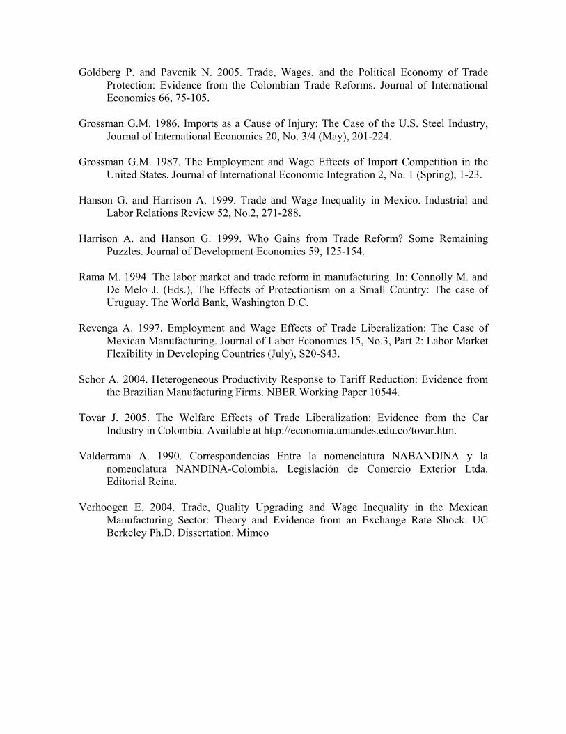
effective tariffs at this time were above 40%. Once the reforms were implemented, nominal tariffs dropped to less than 11% on average, leaving the effective tariffs at 15%. Figure 1 also shows that our constructed tariff measure is similar on average to the one provided by DNP, both before and after the reforms. The main difference, of course, has to do with those sectors that had no direct tariff data. Analyzing each sector at an 8-digit NANDINA level, we assigned tariffs at a corresponding 4-digit ISIC to retail trade, transport and storage, communications, financial institutions and social and related community services. As with the other sectors, the data shows that tariffs dropped substantially with the trade reforms. According to our estimates, the sectors with the largest tariffs are transport and storage and the more traditional textile, apparel, wood, and food in the manufacturing sector. Nominal tariffs for the transport and storage sector, prior to the trade reforms, are on average extremely high. In fact, the average for 1984 through 1989 is 116%, much higher than the rest of the economy. This sector includes some vehicles that had, for some years, nominal tariffs of over 700%. An interestingly counterintuitive sector is recreational and cultural services where tariffs actually increased. With respect to trade −but not to employment−, this sector essentially includes motion picture products. In terms of weighted average of tariffs some sectors had particularly high levels in the 1980s. Among these are the manufacture of food, beverages and tobacco with over 100% and textiles with an effective tariff of 94%. After the reforms, these two sectors retained the highest effective tariffs but the overall dispersion was much smaller. On average the effective rate dropped from 41.5% to 15.5%. Figures 3 and 4 show that prior to the reforms tariffs −either JT or DNP weighted tariffs− were much more disperse than after. If one defines tariff structure as the relative ordering of tariff levels, the graphs show that this is essentially maintained after the reforms were implemented, with consumer goods still having the highest rates. The evolution of employment and wage is displayed at a 1-digit level in Figure 5. The left vertical axis stands for number of employed individuals, while the right vertical axis represents the wage in 1994 constant Colombian pesos. Three sectors stand out in terms of employment levels: manufacturing; wholesale and retail trade; and community, social and personal services. The latter includes public administration and defense, social and related community services and personal and household services. Together, these three sectors represent around 70% of the total employed population. Other relevant sectors are transport and storage, and financing, insurance, real estate and business services. Not surprisingly, the sector with the highest wages is mining. Included here are the capital-intensive coal and petroleum sectors. However, in terms of the number of employed

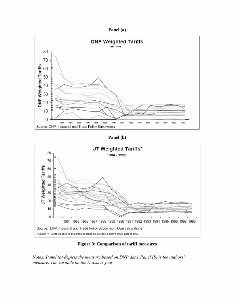
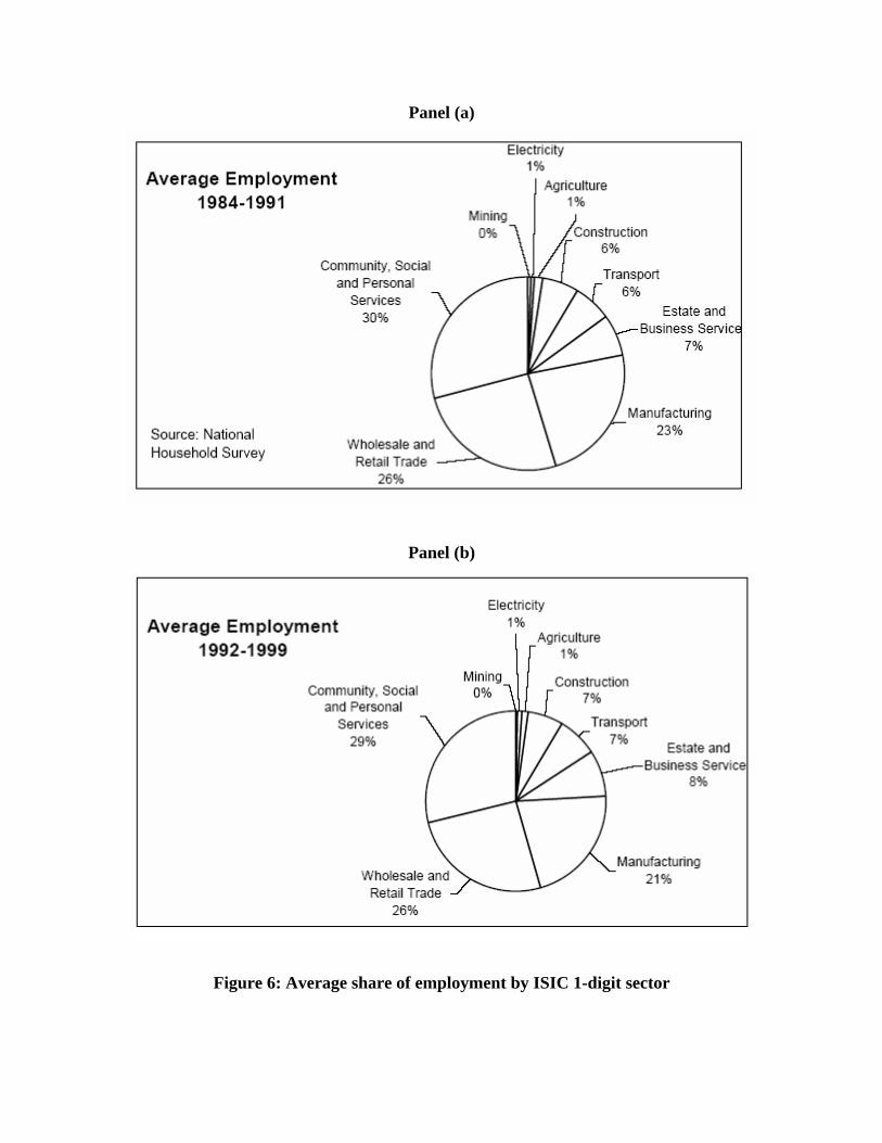
individuals it is one of the smallest in the sample, just ahead of the agricultural and hunting sector. 16 For ease of comparison across sectors, the right axis in Figure 5 is top-normalized to 500.000 pesos, except for the petroleum sector. Other than this outlier, the graphs show that the financing sector tends to be the best paid, while the agricultural sector has the highest volatility. Figure 6 presents the employment share of each sector before and after the trade reforms were implemented. It clearly illustrates that the three largest sectors remain around 70% of total employment over the entire period of analysis. More interestingly, these pies show no evidence, at least at an aggregate level, of a significant reallocation of labor across sectors. Finally, Figures 2 and 7 present some summary statistics for the control variables included in the regressions. Women participation is high in the textile industry, the restaurant and hotels sector and in social and related community services. There is no apparent significant variation of either average age per sector or women participation before and after the reforms. Education, on the other hand has strong dispersion across sectors, and the years of education increase slightly in the post reform period. In summary, the tariff data clearly shows the effect of the structural changes that took place in the late 1980s and early 1990s. The same overview, however, does not reveal any structural effects on the level of employment or on the real wages.

3.2. Endogeneity issues and instruments Goldberg and Pavcnik (2005) and Schor (2004) argue that the tariffs on the right hand side of equation (18) may pose an endogeneity problem. Overall tariff levels might be correlated with other macroeconomic policy changes. In the specific Colombian case, other structural changes took place in the early 1990s −in particular labor and fiscal reform and a new constitution. We control for such macroeconomic events with year dummies and drop the trend suggested by our structural model. These time dummies account for any year-specific economy-wide events other than tariffs, as the latter are explicitly included. The second source of endogeneity has to do with the political economy of tariff reduction. Specifically Goldberg and Pavcnik (2005) argue that it is possible that certain sectors had stronger influence over the way tariffs were reduced. This is true in most trade reform episodes across countries, but we argue that the Colombian 1991 trade reform was essentially unexpected and hence free of endogeneity. Moreover, Figure 3 suggests that tariffs dropped to their target levels in a short period of time and that the correlation of the pre- and post-reform tariff rankings is high. Nevertheless, we account for this possible endogeneity, as we include industry fixed effects to control for any time-invariant industry characteristics.

16 The small number of workers in the agricultural sector should be of no surprise, as the NHS is representative of the seven main cities.

According to Goldberg and Pavcnik (2005) at least two sources of endogeneity remain. On one hand, there could be unobserved time-varying political economy factors that simultanously affect tariffs and industry wages (or labor demands). On the other hand −and quite plausible for the Colombian economy−, workers could choose certain industries over others based on time-varying unobserved characteristics. The example given by Goldberg and Pavcnik (2005) clarifies the point. If for example trade liberalization causes the more able (or more productive) workers to leave sectors that experience large tariff cuts, so that the remaining workers represent a less able (in terms of unobserved characteristics) sample, we would expect the estimated tariff coefficient to be biased upwards. The instruments proposed exploit both the abruptness of Colombia's reforms and the way in which tariff levels were set. Since the original plan to reduce tariffs was suddenly changed and the final rate was set at a low average of 11% with no more than four tariff levels, there was little room for industry lobbying. Sectors with higher pre-reform tariffs had thus the highest tariff reduction. Therefore, in order to instrument for exogenous trade policy changes we use the information contained in the lags of the tariff levels per industry. We construct two variables that embody this information:

=1jtz tariff of sector j in 1984

+= 1984,

2jjtz τ total change of the simple tariff mean

since 1984 (excluding sector j)

Both variables use the 1984 industry tariffs to generate variation across industries. However, collinearity with the industry dummies (in the case of 1

jtz ) and the lack of time variation require that they be interacted with some other exogenous, relevant time-varying series. Thus, we interact each of them with annual exchange rates to obtain our instruments,

tmjt

mjt EzZ *= . The first instrument, 1

jtZ is the one Goldberg and Pavcnik (2005) use for their estimations. While we estimate our regression with both to check for robustness, we focus on the results with 2

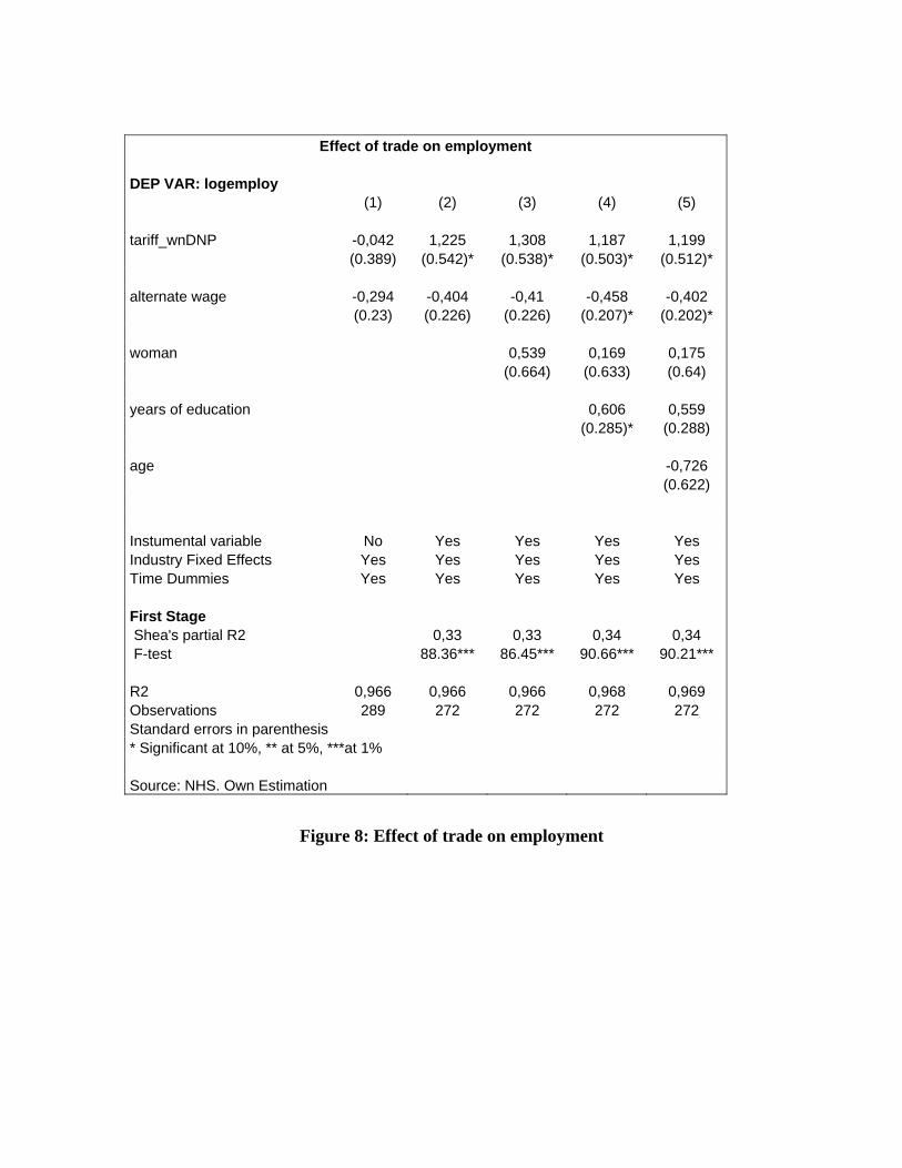
jtZ for the analysis of trade policy effects on labor markets. 4. Estimation results We present the results of five sets of reduced-form regressions based on equation (18). The first three sets include the natural logarithm of employment (logemploy) as the dependent variable; the last two use the wage on the left-hand side. In all cases, we use the Huber (robust) estimator to calculate confidence levels and report the standard errors. The first set of regressions, in Figure 8, introduces the right-hand-side variables used in this paper. In all columns, the dependent variable is logemploy, the measure of tariffs used is tariff_wnDNP, and we include year and ISIC 2-digit-sector fixed effects. The regression in column (1) is an OLS estimation without instruments. Compare the coefficient on the tariff with the corresponding one in column (2), where the tariff measure

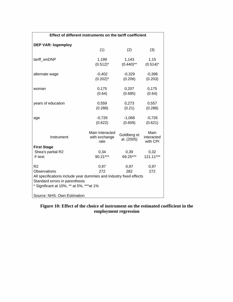
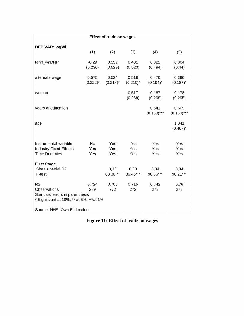
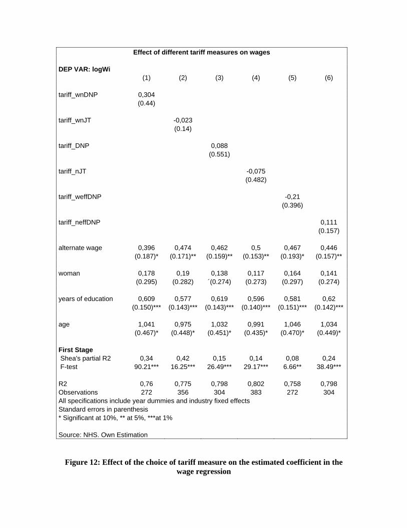
is instrumented with Z2, endogeneity is indeed an issue, and the instrument allows us to find a significant effect. In columns (3)-(5) the controls woman, logeduc, logage are successively added. None of the controls has a large impact on the tariff coefficients, but they do make the coefficient on the alternate wage statistically significant. Throughout the analyses in this section, our main specification is the one in column (5). Figure 9 compares the performance of the six alternative measures of tariffs described in the data section. Again, the dependent variable is logemploy, the measure of tariffs used is instrumented with Z², and we include year and ISIC 2-digit-sector fixed effects in all cases. The baseline tariff measure used for our analyses is tariff_wnDNP, in column (1). According to this specification, a reduction in tariffs of 1% corresponds to a drop in the sector employment of approximately 1.20%. Only this measure of tariffs is statistically significant (at the 10% level). Also, the choice of tariff measure affects the significance of the coefficient on the alternate wage. We run (but do not report) an analogous set of regressions using the instruments Z¹ to check the robustness of our choice of instrumental variable. They show similar results: tariff_wnDNP has a positive and significant coefficient in all cases. Also, with one exception, no other measure has a statistically significant coefficient. The one exception is the DNP measure of effective tariffs, tariff_neffDNP, which has a coefficient of 0.4, significant at the 10% level, when instrumented with Z¹. Figure 10 shows the regression results under different instruments when the tariff measure is tariff_wnDNP. Column (1) is the baseline specification. Column (2) uses Z¹, and column (3) uses the interaction of z² with the log of the Consumer Price Index, logcpi, in order to check the robustness of our choice of macroeconomic variable. The results are similar in all cases, both in magnitude and in level of significance, indicating that a 1% drop in tariff levels corresponds to a 1.14% to 1.20% drop in sector employment. In the last two tables, Figure 11 and Figure 12 the dependent variable is logWi, the log of sector wages. The first column in Figure 11 is an OLS estimation, without instruments, of the empirical specification (18). Column (2) adds the instrument for tariffs, Z². Columns (3)-(5) show the effects of the control variables. As was the case for the employment regressions, column (5) is the baseline specification for wages. While the instrument does have an impact on the tariff coefficient, the exercise yields no statistically significant effect of tariffs on sector wages. The alternate wage, on the other hand, has a positive and significant effect on the sector wage. In Figure 12 we run the baseline specification using various measures of tariffs, instrumented with Z² in all cases. None of the tariff measures has a significant effect on the wage. However, the alternate wage has a positive and significant effect in all cases.17

17 Several comments have pointed out that one should expect a differential effect of trade liberalization depending on the skilled-labor intensity in each sector. While our basic specification controls for education, this does not allow for non-linearities in the effect of education. It could be the case that the effect of one extra year of education, say from six to seven, be very different from the effect of increasing from twelve to

5. Concluding remarks This paper analyzes the impact of the 1990s Colombian trade liberalization process on labor and wages. As a measure of liberalization we use the most direct measure of trade policy available to us, namely tariff rates by economic sector. We extend the existing literature by analyzing the simultaneous impact of trade policy on the labor markets in all sectors of the economy. We use two datasets: the Colombian National Household Survey, which provides us with employment and wage series; and tariff data from the Colombian National Planning Department. We match them to generate time series of tariffs, employment and wages for each 2-digit ISIC sector of the economy. The resulting dataset includes also a number of relevant sector characteristics and demographic controls. The trade reforms took place in Colombia in 1991; our data spans the period between 1984 and 1999. Our tariff data is at the 4-digit ISIC level of aggregation, but our analysis uses 2-digit ISIC economic sectors. Thus, we construct several measures of tariffs for each ISIC 2-digit sector of the economy, aiming to capture the different ways in which trade policy might impact sectoral labor markets. We use simple and weighted averages of nominal tariffs, and simple averages of effective tariffs. We also construct a measure that imputes tariffs to sectors that count typically as non-tradable but include activities affected by tariffs. The analysis is built on a structural model: within each sector, firms maximize profits; across sectors they compete for supply of labor. We then regress reduced-form specifications with wages and employment as dependent variables, instrumenting the tariff measures to control for endogeneity. This allows us to estimate the impact of exogenous tariff variation on labor markets in all sectors of the economy, not only in the manufacturing industry. For the level of employment, our regression results are robust to the choice of instrumental variable but depend on the tariff measure used. In particular, when using nominal tariffs weighted by imports, the tariff coefficient is positive and significant: a 1% drop in tariff rates corresponds to a 1.20% decrease in the level of sectoral employment. In other words, a tariff reduction program would imply a reduction in the number of workers employed by the economy. However, no statistically significant effect is estimated for the other tariff measures. The results are suggestive in several ways. First, trade reforms have an impact on tradable sectors, i.e. those included in the tariff measure weighted by imports. Second, the impact on non-tradable sectors is small at best, as evidenced by the lack of significant coefficients of thirteen years. The specification does not allow either for differential effects of trade policy depending on the skill of the workers, so that a skilled worker may benefit while an unskilled one loses. In response to the comments, we explored several alternate specifications to check for the robustness of our results when the skilled/unskilled labor distinction is allowed. In all cases, the regressions confirmed that the direct effect of trade liberalization on wages and employment was small when the entire economy is taken into account.

the imputed tariff measures. Third −and perhaps less remarkable−, the effects are on actually traded (rather than tradable) sectors, as attested by the statistically insignificant coefficients of the simple tariff averages. Therefore, it seems that the direct effects of trade liberalization imply a reduction in labor, but only to sectors of traded goods and services. The model derived also allowed us to estimate the effect of the trade reform on wages. We were unable to find any evidence that linked trade, as measured by tariffs, to wage levels. Given the results, the policy implications should be interpreted with caution. The liberalization process analyzed here was essentially unilateral, as Colombia did not negotiate reciprocal tariff reductions from its trade partners. This may be reflected in the small effects estimated. Moreover, Colombia had very high tariffs in the 1980s. Any free-trade agreement negotiated today −like the one currently under way with the United States− would imply tariff reductions from a much lower base. Even if the direction of the effects remained, the absolute value of such effects should be smaller. Finally, although we control and instrument for several sources of endogeneity and selection, one important concern remains. To the extent that workers of higher unobservable ability prefer some sectors, our estimates may be incorporating this self-selection, given the use of aggregated sectoral data. If, for instance, traded sectors attract higher-ability workers, the aggregate employment level understates the impact of trade policy on labor markets. It is not clear how acute this concern is in this study, given the length of the panel. However, further analysis should use microdata to endogenize the workers' choice of economic sector to correct for this potential problem. References Arbache J. 2001. Trade Liberalization and Labor Markets in Developing Countries: Theory

and Evidence. Working Paper 853 University of Brasilia Attanasio O, Goldberg P, and Pavcnik N. 2004. Trade Reforms and Wage Inequality in

Colombia. Journal of International Economics 74; 331-366. Behrman J. 1999. Labor Markets in Developing Countries. In Ashenfelter and Card (Eds.),

Handbook of Labor Economics, Volume 3B; 2859-2939. Curie J. and Harrison A. 1997. Sharing the Costs: The Impact of Trade Reform on Capital

and Labor in Morocco. Journal of Labor Economics 15, S44-S71. Fajnzylber P. and Maloney W.F. (forthcoming). Labor Demand and Trade Reforms in Latin

America, Journal of International Economics. Garay L, Quintero L, Villamil J. and Tovar J. 1998. Colombia: Estructura Industrial e

Internacionalización (1967-1996). DNP-COLCIENCIAS-MINCOMEX.

Goldberg P. and Pavcnik N. 2005. Trade, Wages, and the Political Economy of Trade Protection: Evidence from the Colombian Trade Reforms. Journal of International Economics 66, 75-105.

Grossman G.M. 1986. Imports as a Cause of Injury: The Case of the U.S. Steel Industry,

Journal of International Economics 20, No. 3/4 (May), 201-224. Grossman G.M. 1987. The Employment and Wage Effects of Import Competition in the

United States. Journal of International Economic Integration 2, No. 1 (Spring), 1-23. Hanson G. and Harrison A. 1999. Trade and Wage Inequality in Mexico. Industrial and

Labor Relations Review 52, No.2, 271-288. Harrison A. and Hanson G. 1999. Who Gains from Trade Reform? Some Remaining

Puzzles. Journal of Development Economics 59, 125-154. Rama M. 1994. The labor market and trade reform in manufacturing. In: Connolly M. and

De Melo J. (Eds.), The Effects of Protectionism on a Small Country: The case of Uruguay. The World Bank, Washington D.C.

Revenga A. 1997. Employment and Wage Effects of Trade Liberalization: The Case of

Mexican Manufacturing. Journal of Labor Economics 15, No.3, Part 2: Labor Market Flexibility in Developing Countries (July), S20-S43.

Schor A. 2004. Heterogeneous Productivity Response to Tariff Reduction: Evidence from

the Brazilian Manufacturing Firms. NBER Working Paper 10544. Tovar J. 2005. The Welfare Effects of Trade Liberalization: Evidence from the Car

Industry in Colombia. Available at http://economia.uniandes.edu.co/tovar.htm. Valderrama A. 1990. Correspondencias Entre la nomenclatura NABANDINA y la

nomenclatura NANDINA-Colombia. Legislación de Comercio Exterior Ltda. Editorial Reina.

Verhoogen E. 2004. Trade, Quality Upgrading and Wage Inequality in the Mexican

Manufacturing Sector: Theory and Evidence from an Exchange Rate Shock. UC Berkeley Ph.D. Dissertation. Mimeo

Figure 1: Descriptive statistics of tariffs (1984-1999)

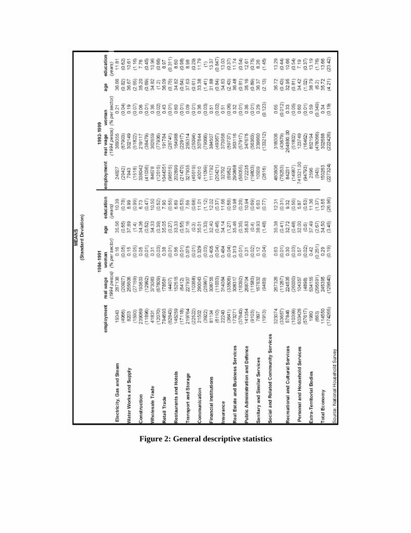
Figure 2: General descriptive statistics

Panel (a)

Panel (b)

Figure 3: Comparison of tariff measures

Notes: Panel (a) depicts the measure based on DNP data. Panel (b) is the authors' measure. The variable on the X-axis is year

Panel (a)

Panel (b)

Figure 4: Average tariff levels before and after the trade liberalization

Notes: Panel (a) depicts the measure based on DNP data. Panel (b) is the authors' measure. The variable on the X-axis is year

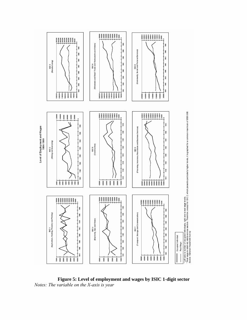
Figure 5: Level of employment and wages by ISIC 1-digit sector

Notes: The variable on the X-axis is year

Panel (a)

Panel (b)

Figure 6: Average share of employment by ISIC 1-digit sector

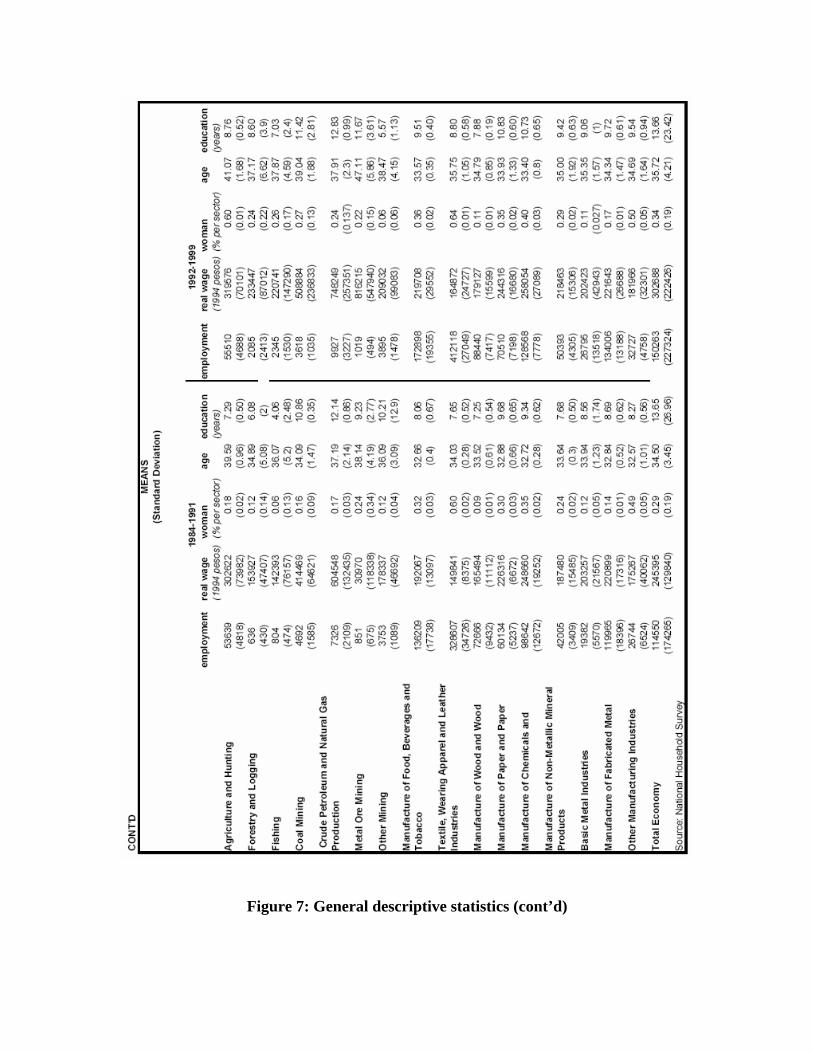
Figure 7: General descriptive statistics (cont’d)

Effect of trade on employment

DEP VAR: logemploy (1) (2) (3) (4) (5) tariff_wnDNP -0,042 1,225 1,308 1,187 1,199 (0.389) (0.542)* (0.538)* (0.503)* (0.512)* alternate wage -0,294 -0,404 -0,41 -0,458 -0,402 (0.23) (0.226) (0.226) (0.207)* (0.202)* woman 0,539 0,169 0,175 (0.664) (0.633) (0.64) years of education 0,606 0,559 (0.285)* (0.288) age -0,726 (0.622) Instumental variable No Yes Yes Yes Yes Industry Fixed Effects Yes Yes Yes Yes Yes Time Dummies Yes Yes Yes Yes Yes First Stage Shea's partial R2 0,33 0,33 0,34 0,34 F-test 88.36*** 86.45*** 90.66*** 90.21*** R2 0,966 0,966 0,966 0,968 0,969 Observations 289 272 272 272 272 Standard errors in parenthesis * Significant at 10%, ** at 5%, ***at 1% Source: NHS. Own Estimation

Figure 8: Effect of trade on employment

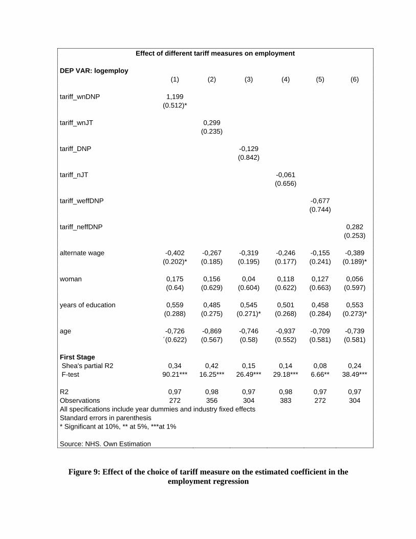
Effect of different tariff measures on employment DEP VAR: logemploy (1) (2) (3) (4) (5) (6) tariff_wnDNP 1,199 (0.512)* tariff_wnJT 0,299 (0.235) tariff_DNP -0,129 (0.842) tariff_nJT -0,061 (0.656) tariff_weffDNP -0,677 (0.744) tariff_neffDNP 0,282 (0.253) alternate wage -0,402 -0,267 -0,319 -0,246 -0,155 -0,389 (0.202)* (0.185) (0.195) (0.177) (0.241) (0.189)* woman 0,175 0,156 0,04 0,118 0,127 0,056 (0.64) (0.629) (0.604) (0.622) (0.663) (0.597) years of education 0,559 0,485 0,545 0,501 0,458 0,553 (0.288) (0.275) (0.271)* (0.268) (0.284) (0.273)* age -0,726 -0,869 -0,746 -0,937 -0,709 -0,739 ´(0.622) (0.567) (0.58) (0.552) (0.581) (0.581) First Stage Shea's partial R2 0,34 0,42 0,15 0,14 0,08 0,24 F-test 90.21*** 16.25*** 26.49*** 29.18*** 6.66** 38.49*** R2 0,97 0,98 0,97 0,98 0,97 0,97 Observations 272 356 304 383 272 304 All specifications include year dummies and industry fixed effects Standard errors in parenthesis * Significant at 10%, ** at 5%, ***at 1% Source: NHS. Own Estimation

Figure 9: Effect of the choice of tariff measure on the estimated coefficient in the employment regression

Effect of different instruments on the tariff coefficient

DEP VAR: logemploy (1) (2) (3) tariff_wnDNP 1,199 1,143 1,15 (0.512)* (0.440)** (0.514)* alternate wage -0,402 -0,329 -0,398 (0.202)* (0.206) (0.203) woman 0,175 0,207 0,175 (0.64) (0.685) (0.64) years of education 0,559 0,273 0,557 (0.288) (0.21) (0.288) age -0,726 -1,068 -0,726 (0.622) (0.659) (0.621)

Instrument Main Interacted with exchange

rate

Goldberg et al. (2005)

Main interacted with CPI

First Stage Shea's partial R2 0,34 0,39 0,32 F-test 90.21*** 69.25*** 121.11*** R2 0,97 0,97 0,97 Observations 272 282 272 All specifications include year dummies and industry fixed effects Standard errors in parenthesis * Significant at 10%, ** at 5%, ***at 1% Source: NHS. Own Estimation

Figure 10: Effect of the choice of instrument on the estimated coefficient in the

employment regression

Effect of trade on wages

DEP VAR: logWi (1) (2) (3) (4) (5) tariff_wnDNP -0,29 0,352 0,431 0,322 0,304 (0.236) (0.529) (0.523) (0.494) (0.44) alternate wage 0,575 0,524 0,518 0,476 0,396 (0.222)* (0.214)* (0.210)* (0.194)* (0.187)* woman 0,517 0,187 0,178 (0.268) (0.298) (0.295) years of education 0,541 0,609 (0.153)*** (0.150)*** age 1,041 (0.467)* Instrumental variable No Yes Yes Yes Yes Industry Fixed Effects Yes Yes Yes Yes Yes Time Dummies Yes Yes Yes Yes Yes First Stage Shea's partial R2 0,33 0,33 0,34 0,34 F-test 88.36*** 86.45*** 90.66*** 90.21*** R2 0,724 0,706 0,715 0,742 0,76 Observations 289 272 272 272 272 Standard errors in parenthesis * Significant at 10%, ** at 5%, ***at 1% Source: NHS. Own Estimation

Figure 11: Effect of trade on wages

Effect of different tariff measures on wages

DEP VAR: logWi (1) (2) (3) (4) (5) (6) tariff_wnDNP 0,304 (0.44) tariff_wnJT -0,023 (0.14) tariff_DNP 0,088 (0.551) tariff_nJT -0,075 (0.482) tariff_weffDNP -0,21 (0.396) tariff_neffDNP 0,111 (0.157) alternate wage 0,396 0,474 0,462 0,5 0,467 0,446 (0.187)* (0.171)** (0.159)** (0.153)** (0.193)* (0.157)** woman 0,178 0,19 0,138 0,117 0,164 0,141 (0.295) (0.282) ´(0.274) (0.273) (0.297) (0.274) years of education 0,609 0,577 0,619 0,596 0,581 0,62 (0.150)*** (0.143)*** (0.143)*** (0.140)*** (0.151)*** (0.142)*** age 1,041 0,975 1,032 0,991 1,046 1,034

(0.467)* (0.448)* (0.451)* (0.435)* (0.470)* (0.449)* First Stage Shea's partial R2 0,34 0,42 0,15 0,14 0,08 0,24 F-test 90.21*** 16.25*** 26.49*** 29.17*** 6.66** 38.49*** R2 0,76 0,775 0,798 0,802 0,758 0,798 Observations 272 356 304 383 272 304 All specifications include year dummies and industry fixed effects Standard errors in parenthesis * Significant at 10%, ** at 5%, ***at 1% Source: NHS. Own Estimation

Figure 12: Effect of the choice of tariff measure on the estimated coefficient in the wage regression