Regional convergence, trade liberalization and Agglomeration of

activities: an analysis of NAFTA and MERCOSUR cases∗

Nicole Madariaga† Sylvie Montout‡and Patrice Ollivaud§

Octobre 2003

Abstract

This study examines empirically and theoretically the existing link between economic integration,the density of activities and income per capita convergence within NAFTA members during the 1980-2000 period and within MERCOSUR partners from 1985 to 2000. In our empirical approach, we referto two different convergence concepts: homogenization and catch-up. We firstly evaluate activitiesconcentration trends within each trade agreement according to different measures of agglomeration.Then, we introduce some of theses measures in estimations to control for their influence on incomeper capita convergence. Our analysis of the sigma, absolute beta-convergence concluded to thenon existence of a process of convergence between the two partners of the NAFTA. ConcerningMERCOSUR, we observe a process of convergence between 1985 and 1995 even if this process appearsto slow down after 1995 whatever the concept of convergence. Moreover, agglomeration plays asignificant role between 1994 and 2000 on the narrowing in the percentage gap between the laggardand leading countries’ performance.

JEL Classification: F43, R11, R12, O40Key words: Growth, Regional convergence, Economic geography, Trade integration.

1 Introduction

The North American Free Trade Agreement (NAFTA) and the Mercado Comun del Sur (MERCOSUR)agreements seem to have accelerated the regional integration process respectively within the North andthe South of the American continent. The signature of the NAFTA in 1994 widened the free trade areabetween Canada and the United States to Mexico. Besides, in March 1991, the signature of the Treaty ofAsuncion by Argentina, Brazil, Paraguay and Uruguay initiated the creation of a common market called

∗We are very grateful to the CEPAL Office in Buenos Aires, to Ricardo Martinez who provided us Argentina data andto ProvInfo department from the Secretarıa de Provincias in Buenos Aires. We also want to thank Guillaume Gaulier forhis helpful technical comments.

†TEAM-CNRS, Universite Paris 1 Pantheon Sorbonne. Maison des Sciences Economiques, 106-112 Bd de l’Hopital,75647 Paris Cedex 13. nicole.madariaga@malix.univ-paris1.fr

‡TEAM-CNRS, Universite Paris 1 Pantheon Sorbonne. Maison des Sciences Economiques, 106-112 Bd de l’Hopital,75647 Paris Cedex 13. sylvie.montout@univ-paris1.fr

§OECD, Economic Department. Patrice.OLLIVAUD@oecd.org

1

MERCOSUR. The NAFTA represents a North-South regional integration which is leaded by the UnitedStates while MERCOSUR is a South-South regional agreement where Brazil has a major influence. Thegovernments of developing countries hoped that the creation of those trade areas would contribute to ahigher economic growth and income convergence between partners.

Over the last decades, the study of convergence in regional incomes has gradually gained importancein the economic literature. Growth theory in its neo-classical form implies convergence between poorand rich regions. In these models, convergence is due to decreasing returns to scale to capital: countrieswith a low endowment of capital and per capita income have a higher marginal return to capital andthus a larger marginal product. Therefore, capital is more accumulated and income grows faster in poorregions. This type of convergence (Barro and Sala-i-Martin (1995)) implies that one should found anegative relation between initial GDP and average growth rate across a sample of regions.

Nevertheless, endogenous growth and economic geography models cast doubt over these optimisticresults. For Lucas (1988), if long term growth is driven by the endogenous accumulation of experiencethrough learning-by-doing with a tendency for decreasing returns in the long term, then trade betweenregions can lead one region to specialize in industries in which it has a comparative advantage (e.g.traditional economic activities), but for which the opportunities to learn are relatively small, so that thegrowth rate in that region may be lower precisely because of trade integration.

In economic geography, a core-periphery pattern (Krugman (1991)) may appear with economic inte-gration. Fujita and Thisse (1996) insist on some of the economic efficiency gains that can be producedthrough the agglomeration of economic activities. Martin and Ottaviano ((1999), (2001)) present a modelintegrating a new growth framework to a new geography model, then the possibility of a trade-off betweenaverage growth and regional convergence emerge. Trade integration leads to more agglomeration alongthe lines of the new geography and agglomeration of economic activities favours innovation because itlowers costs of investment in the core. A mechanism of higher growth in the core than in the peripherytherefore emerge inducing increasing income inequality.

Industrial development in Canada, Mexico and the United States was accompanied by a specificdistribution of economic activities inducing an agglomeration process. The effects of economic integra-tion on Canada and the United States may have been probably much weaker than on Mexico. Theeconomic activity in the United States remains highly geographically concentrated. Nevertheless, since1950 employment growth relative to the nation as a whole has been strongly negative in North-Easternand Midwestern states, and strongly positive in southern and western states such as California, Florida,Georgia and Texas (Hanson (2001)). Under Import Substitute Industrialization (ISI) in Mexico, theindustrial development was illustrated by an agglomeration of economic activities in Mexico City. Afterseveral decades of ISI, Mexico opened its economy and joined the General Agreement on Trade andTariffs in 1986. Therefore, Mexico government adopted a new policy eliminating trade and investmentrestrictions. Given Mexico’s proximity to the United States and relatively low US trade barriers, tradeliberalization for Mexico is tantamount to economic integration with its northern neighbour. Since 1980,industrial activity in Mexico has shifted to states on the US-Mexico border diminishing Mexico city’s rolein the national economy. These developments have coincided with the opening of the Mexican economyto foreign trade and investment. Between 1980 and 1993, the Mexico city’s share of national manufactur-ing employment fell from 44,4% to 28,7%. Mexico’s new industrial centres are located in northern citiessuch as Ciudad Juarez, Monterrey, and Tijuana, which are physically close to the United States (Hanson(1998)). Krugman and Livas (1996) identified two kinds of industry centres emerged: a main centre inMexico city and a smaller centre in Northern Mexico.

In the MERCOSUR area, the most relevant concentration of activity is the one delimitating theSouthern Brazilian regions (Rio Grande Do Sul, Santa Catarina and Parana) and the Metropolitan -Pampas Argentinean regions (Buenos Aires province, Santa Fe, La Pampa, Cordoba and Entre Rıos).Many of the largest urban centres in the MERCOSUR are concentrated in this geographical pattern

2

(Terra and Vaillant (1997)). In 1989, about 87% of Brazilian population and manufacturing activity isconcentrated in Southern, East Southern and East Northern regions which represent only 36% of the totalcountry area. In 1990-1992, whereas the South has an income per capita relatively equal to the countrymean, the East North income per capita is 60% of the country mean. In Argentina, the Metropolitan -Pampas regions count for 70% of the population in 17% of the territory but concentrate more than 80%of the manufacturing activity in 1989 (Gatto and Centrangolo (2003)). The degree of concentration inmanufacturing production remains highly concentrated during the nineties. According to Volpe Martincus(2000), the removal of bilateral trade barriers between Argentina and Brazil has increased intra industrytrade. This specialization of trade seems to have enhanced the spatial concentration of manufacturingemployment in Argentina. This centripetal tendency put the stress on a possible divergence between thedifferent regions of both countries.

The effect of economic integration and trade liberalization on per capita income convergence hasoften been explored in the empiric literature1. Nevertheless, although Barro (1998) included a LatinAmerica dummy variable, the existing literature that clearly tackles the issue of convergence and tradeliberalization in Latin America is rather sporadic. Bowman and Felipe (2001) examined the effect ofeconomic integration and trade liberalization on per capita or per worker income convergence in theAmerican continent with a particular interest in Latin America. They find that incomes in the hemisphereas a whole and in Central America and the Caribbean has become more dispersed, while in South Americathe long term trend has been stable with a considerable process of convergence in the 1970-1992 period.Actually, South America has been the only region to exhibit beta-convergence in per worker and per capitaincome as well as sigma-convergence for the considered period. Caceres and Sandoval (2000) examinedthe behaviour of seventeen countries in Latin America and Dobson and Ramlogan (2002) found evidenceof beta convergence for Latin America in the 1960-1990 period. A new wave of regional trade agreementsspread in the last decade: the MERCOSUR and the NAFTA are the most significant in terms of surface,economy and population. Further, the Free Trade Area of the Americas (FTAA) initiative aims to createan area with all American nations. Then disparities will play a major role in this integration process andgovernments will have to pay attention to them in order to smoothen the transition.

At present, most of the empirical works concentrates on the European Union case like Barro (1991),Barro and Sala-i-Martin (1992), Dan (1993), Sanchez-Reaza and Rodriguez-Pose (2002). Concerning theparticular cases of NAFTA and MERCOSUR countries, previous literature focuses on convergence withineach partner but not among all members2. Studies on convergence in Argentina have been performed byMarina (1998), Garrido and alii (2001), Utrera and Koroch (1998) while Azzoni (1997, 2001) and Ferreiraand Diniz (2000) studied income disparities in Brazil. See Mallick and Carayannis (1994), Esquivel (1999),Andalon and Lopez-Calva (2002) for the Mexico case.

The convergence process has substantial implications for the welfare of nations and for the prospectfor reduction and even the elimination of poverty in the international community. Vamvakidis (1998)examines whether the openness, market size and level of development of countries in a same regionfaster growth. The results show that the economies near large and opened countries grow faster. Thelevel of development among neighbouring economies is also significant, especially when they are open,because it intensifies positive spillover effects. Therefore, these results assess that trade agreementsbetween developing and developed countries may lead to faster growth. Given that no country has zerotrade barriers, if a regional trade agreement improves the market accessibility of the developed countriestowards developing members, their growth should be promoted.

The aim of this article is to define both empirically and theoretically the existing link between eco-nomic integration, density of activities and convergence. As a consequence, we firstly build an economicgeography model with elements from endogenous growth theory. We are interested in determining if

1See for instance Padoa-Schioppa (1988), Young (1991), Krugman and Venables (1990), Venables (1999).2With the notable exception of Ramon-Berjano (2002) study on the MERCOSUR.

3

incomes per capita tend to converge in the NAFTA and the MERCOSUR. This analyze is particularlyinteresting and almost non existent in the literature because we compare two different types of tradeagreements. The NAFTA involving two countries with very different levels of development (North-Southtreaty) and the MERCOSUR composed by two countries which are less contrasted in terms of development(South-South treaty). In our empirical approach, we refer to two convergence concepts: homogenization(sigma-convergence) and catch-up (conditional and unconditional beta-convergence). The first one refersto a reduction in the dispersion among a set of countries (or regions). The second one corresponds to anarrowing in the percentage gap between the laggard and leading countries’ performance. We also includedifferent measures of agglomeration in our conditional convergence estimations to check its impact onper capita income catch-up. We proceed to estimations on the regional convergence between Mexico andthe United States inside the NAFTA, and between Argentina and Brazil within the MERCOSUR. Aninternational perspective is also adopted questioning the convergence of income per capita between thefour selected members of the two treaties.

The reminder of this paper proceeds as following. In the second section, we display an economicgeography model introducing elements from endogenous growth theory. In the third section, we proposedifferent measure of agglomeration and compare industrial pattern in the NAFTA and the MERCOSUR.The section four discusses the empirical methodology, i.e. the sigma and beta convergence analysis, andreports econometric method and results of convergence estimations. Finally, the fifth section concludes.

2 A two region model with different productivities in the tra-ditional sector

Our model is based on Martin and Ottaviano (1999) which combines an endogenous framework similarto Romer (1990) and Grossman and Helpman (1991) to a geography framework similar to Krugman(1991). We introduce Jacobs spillovers since the number of varieties already created is a key factor ofthe spillovers. In this case, the benefits from local spillovers are due to “the direct observation of theproduction process: researchers observe the production process and fit it easier to invent how new goodscan be produced”.

We consider two regions, the North and the South. The north is better endowed in a fixed amountof labour than the South (L > L∗). Besides, labour is immobile between regions. The two regions areidentical except for their initial level of human or physical capital named K0 in the North and K∗

0 inthe South and for their traditional sector productivity equals to 1 in the North and to α (α < 1) in theSouth. The North is then richer than the South. We therefore describe the economy only in the Northsince the South is almost symmetric. An asterisk refers to the variables of the South.

The utility function of a representative consumer is:

U =∫ ∞

0

log[D(t)µY (t)1−µ]e−ρtdt. (1)

Where ρ is the time preference parameter, D is a CES composite of N varieties and Y is the con-sumption of the traditional good and is the numeraire good. Following Dixit and Stiglitz (1977), thecomposite good consists of a number of different varieties:

D(t) =

[∫ N(t)

i=0

Di(t)1−1/σdi

] 11−σ

, σ > 1. (2)

where N is the total number of varieties produced in the North and in the South and σ is the elasticityof substitution between varieties. It increases with the substitutability between varieties. Growth isinduced by an increase in the number of varieties.

4

The representative consumer maximize its utility under the expenditure constraint:∫

i∈n

piDidi +∫

j∈n∗τp∗i Djdj + Y = E (3)

Where n is the number of firms in the north, N = n + n∗. pi and p∗i are the producer prices in theNorth and in the South. τ (τ > 1) represents transaction costs which are supposed to be iceberg costsas in Samuelson(1954). These costs may be interpreted as both transport costs and transaction costs.Only a fraction 1/τ of differentiated goods will be provided to abroad consumer.While goods are traded(D and Y ), factors (L and K) are not. We adopt the simplifying assumption (Krugman (1991) andKrugman and Venables (1995)) that Y trade is costless then traditional production prices and incomesare the same in both regions.

The manufacturing sector

The differentiated goods are produced with identical technologies under increasing returns to scale.One unit of capital, assimilated to a patent, is needed to start the production of one variety. This input isspecific to the firm that produces the new variety but does not need to be located where the productionprocess takes place since patents are freely traded. If one unit of capital is required to start the productionof a new variety then N = n + n∗ = K + K∗. This manufacturing sector require β units of labour perunit of output.

We can determine mark-up prices by maximizing operating profits which is the difference betweenthe value of sales and labour costs:

πi = pixi(pi)− wβxi(pi) =wβx

σ − 1. (4)

where x is the size of production. The mark-up price is then: pi = p∗i = wβσσ−1 . A the equilibrium, the

ratio σσ−1 is the ratio of mean cost to marginal cost, then, as in Krugman(1991), σ may be interpreted

as an reversed indicator of scale economies.

The Traditional sector

Good Y is produced under constant return to scale using one unit of labour to produce one unitof output. In our model, we assume a productivity difference only in the traditional sector and not inthe manufacturing sector to simplify the legibility of analytical results. Then the North has a higherproductivity in the traditional sector than the South. As the production capacity of the economy islimited, one region cannot satisfy the traditional goods demand on its own for the whole economy. Thenboth regions have to produce traditional good. As usually in economic geography, the good Y is chosenas the numeraire and wages are equal to the unity in the North and to α in the South (α < 1). Byintroducing this assumption, we are able to observe the impact of lower labour costs in the South as wellas the impact of a higher purchasing power in the North. This imply that pi > p∗i .

We may now identify two opposite effects:

A market effect : Northerners earn more than Southerners, then incomes are higher in the North. Itsmarket size is higher and entails a wider demand exerting a pull effect on firms location choices.

A competitiveness effect : having lower labour costs, producers in the South may claim more competitiveprices than producers in the North. Entrepreneurs may then be attracted by southern wages.

5

In contrast to firms, consumers are immobile so that their incomes are geographically fixed even iffirms are not. This implies that no cumulative agglomeration process can be due to workers mobility.

Solving the first order conditions for the consumers, we get the following individual consumer demands:

Di =σ − 1βσ

µE

n + n∗δλ(5)

Dj =σ − 1βσ

µE(τα)−σ

n + n∗δλ(6)

Y = (1− µ)E (7)

Where δ = τ1−σ (0 < δ < 1) measures the freeness of trade and λ = α1−σ(λ > 1)) measures theSouth competitiveness effect. Then, when southern labour costs converge to northern ones, λ goes downto 1.

It is possible to save in the form of a riskless asset that pays an interest rate r or in the form ofinvestment in shares of firms. K is the number of firms owned by the North and K∗ by the South. A firmthat buy a patent has a perpetual monopoly on the production of the variety. To produce a new variety,the entrepreneur needs to invest either in innovation or in physical investment. In the first case, thecapital is immaterial, i.e. a patent, in the second case, the capital is a machine. When an entrepreneurinvests and locates its plant in a region, he can perfectly repatriate its profits without costs. As capitalis mobile, operating profits are equal in both regions. If v is the value of a firm, the condition of noarbitrage opportunity between shares and the safe asset is:

r =v

v+

π

v(8)

This condition indicates that the return on an investment of size v is equal to the operating profitsplus the change in the value of capital. Because of free entry and zero profits condition on investments,the value of a firm is equal to the marginal cost of the unit of capital needed for the production of avariety, v = η/n in the North and v∗ = ηα/n∗ in the South. The creation of a new variety in a region isthen decreasing with the future R&D costs in both countries so that spillovers are global but the cost ofR&D is higher in the North than in the South.

From the inter temporal optimization, we also know that at steady state, E = 0 in both nations, thenthe Euler equations imply that r = ρ 3.

2.1 The equilibrium location of firms

The equilibrium of firms is determined by equalization of profits, π = π∗, then x = αx∗. We firstly haveto equalize demands in both regions to supplies in the North and in the South:

x = µσ − 1βσ

[EL

n + n∗δλ+

E∗L∗δασ

α(nδλ−1 + n∗

)]

(9)

x∗ = µσ − 1βσ

[ELδα−σ

n + n∗δλ+

E∗L∗

α(nδλ−1 + n∗)

](10)

Recording that N = n + n∗ = K + K∗, solving equations (9) and (10), we determine the optimal sizeof each firm for a given level of expenditures:

x = µσ − 1βσ

EL + E∗L∗α

N(11)

3See Baldwin and Forslid (1997) for more details on why E = 0 in steady state.

6

We now can define γ = nN which represents the share of firms (and varieties) in the North and

measures the extent of agglomeration of the manufacturing sector. The equilibrium location is then:

γ =θE(1− δλ)− (1− θE)(1− δλ−1)δλ

(1− δλ)(1− δλ−1)(12)

where θE = ELEL+E∗L∗ is the Northern share of total expenditure. As entrepreneurs and workers are

immobile no agglomeration forces operate when firms location is modified. The equation (12) indicatesthat when a firm locates in the other region, it automatically decreases the return difference that initiallymotivated its mobility. It then deters other firm from moving to another region. The equilibrium is stableand both countries have the same profits. Our assumption on productivity adds a new opposite forceto the ”home market effect” (Krugman (1980)). Now, entrepreneurs have to make a trade-off betweenthe larger market in the North and the price competitiveness of the South. Let us briefly observe theinfluence of a variation in the productivity differential. When the productivity in the South (when α)increases, We observe two opposite effects on γ. Analyzing the market effect, we find that:

∂γ

∂α=

∂γ

∂θE

∂θE

∂α< 0 with

∂γ

∂θE|δλ constant> 0 and

∂θE

∂α< 0

The two components of the derivative explain the market effect. ∂γ∂θE

indicates that as the share in theNorth of expenditures rises, the share of firms in this regions increases since entrepreneurs are attractedby the size of the market. However, as wages in the South converge to Northerners ones, the share ofexpenditures in the North decreases.

The impact of an α variation on the price competitiveness is:

∂γ

∂α|θE constant> 0

As the productivity in the traditional sector increases, labour costs rise and the price competitivenessdecreases. This fall in price competitiveness reduces the entrepreneurs’ incentive to locate in the South.

2.2 Equilibrium growth

To find the growth rate of the economy, we have to determine how capital is endogenously accumulated.Following Grossman and Helpman (1991), one unit of capital is needed to start the production of a newvariety. An entrepreneur must employ η/n units of labour in the North and η/n∗ units of labour in theSouth. We then introduce Jacobs (1969) local spillovers since the cost of innovation is not decreasingwith the presence of other researchers from the same industry but with the number of producers ofdifferent varieties already created in this region. As identified by Glaeser and al (1992), local spilloversmay be either assimilated to Marshall-Arrow-Romer (MAR) or to Jacobs. MAR spillovers are dueto the concentration of a whole industry in one city. It induces knowledge spillovers between firms, andtherefore the growth of that industry and of that city. Jacobs knowledge transfers, unlike MAR spillovers,come from other industries. Then, variety and diversity of geographically proximate industries promoteinnovation and growth. As reported by Gleaser and al., ”these theories of dynamic externalities areextremely appealing because they try to explain simultaneously how cities form and why they grow”.Their findings only validate Jacobs spillovers since their results show that industries grow slower in citieswhere they are over represented. This kind of spillovers has already been explored in the empiricalliterature by Ciccone and Hall (1996), Jaffe and al. (1993) and Henderson and al. (1995).

It is less costly to invest in a region where there are more firms. Investors are then urged to locatetheir activity in this region. Actually, if the cost of innovation is lower in one region, there is no reason

7

to do R&D activities in the other region. As the capital is perfectly mobile, its price and its costs isthe same in both regions. Capital holders from the South may invest as well as Northern ones. At theequilibrium, more firms are present in the North than in the South because K0 > K∗

0 . Investment benefitsfrom being located in the North.

At the steady state, the share of firms located in the North at the equilibrium is constant, then n, n∗

and N grow at the same rate g = N/N. The growth rate of both regions will be determined in the North.We now have to analyze the incentive to create new varieties. Recording equation (8) and the equilibriumvalue of a firm v = η/n in the North. We can rewrite the latter expression so that v = η/γN whichimplies that v decreases at the same rate as N increases. We conclude that:

g = N/N = n/n = −v/v (13)

Per capita income levels in each region are the sum of the earned wage plus the capital income. Thecapital income is equal to revenues obtained by owning a firm multiplied by the propensity to consume:ρv K

L . Actually, the incentive to have a firm is equal to the capital per capita multiplied by the valueof the firm. Aggregate income level is equal to: EL + E∗L∗ = L + αL∗ + ρNv. The value of the firmis given by the arbitrage condition in equation (8) that is the discounted sum of future profits. Profitsdecrease with growth rate, because a rise in g means new firms in the market and higher competition.Aggregate income level can then be rewritten:

EL + E∗L∗ = L + L∗ + ρµ

σ(ρ + g)

(EL +

E∗L∗

α

)(14)

In equilibrium, the world labour market must clear. Workers will either be working in the R&D sector(ηN/n), the traditional sector (LY +L∗Y ∗) and the two manufacturing sectors (Nβx). Introducing (??),we find:

L + L∗ = ηg

γ+ (1− µ)(L + αL∗) + (E +

E∗

α)

µL

σ(ρ + g)[ρ(σ − µ) + g(σ − 1)] (15)

Then using equation (11) expressing the equilibrium volume of production per firm, x, and thearbitrage condition in equation (8):

EL +E∗L∗

α=

ρ + g

µγησ (16)

Introducing (16) in (15), we finally determine the growth rate:

g =[µL + [1− α(1− µ)] L∗]

ησγ − σ − µ

σρ (17)

Some of the usual determinants of growth in endogenous models are present in the expression. Thelarger is the population, the higher is the growth rate because of scale effect. A higher elasticity of substi-tution between varieties (σ) decreases the monopoly power of each firm and the incentive to create newfirms. When ρ decreases, then present consumption increases at the expense of savings and investments.The higher is the cost of innovation, the lesser entrepreneurs invest in the R&D sector and therefore thelesser is the growth rate. The introduction of local spillovers implies that the share of firms in the Northhas a decreasing effect on the cost of innovation then improving investment and the growth rate. Wealso note that the higher is the difference between Northern and Southern productivity in the traditionalsector, the lower is the growth rate.

8

2.3 Equilibrium income inequality

In the previous sections, we have expressed the share of firms in the North γ in function of incomeinequality θE and the growth rate g in function of γ. We now want to determine θE in function of thegrowth rate of the economy.

Using equations (1), (4) and (11), we determine income per capita in the North and in the South:

EL = L +kρ

L

µL + [1− α(1− µ)] L∗

σg + ρ(σ − µ); E∗L∗ = αL∗ +

(1− k)ρL∗

µL + [1− α(1− µ)] L∗

σg + ρ(σ − µ)(18)

where k is the share of capital owned by the North. We note that this share is constant over timesince K, K∗, n, n∗ and N grow at the same rate in the two regions. Now, we can determine the share ofexpenditure in the North:

θE =Lσ(g + ρ) + ρ {k[µL + L∗(1− α(1− µ))]− µL}

(L + αL∗)σ(g + ρ) + ρL∗(1− α)(19)

This expression reveals that as k > LL+αL∗ , that is, as long as the share of capital owned by the North

is higher than the relative Northern market size, then θE > 1/2, that is, income per capita is higher inthe North than in the South4. Since we assumed that K0 > K∗

0 , then the North is always better endowedin capital than the South. We also note that when growth rate increases, then the share of expenditurein the North decreases. This is due to the growing competition generated by a larger number of firmsin the North that influence negatively the monopoly power of entrepreneurs. In this case, returns oncapital decrease. We can conclude that when the growth rate rises, the income inequality decreases.We now determine thanks to equations (16) and (18) the relation between agglomeration, γ and incomeinequality:

θE =Lγ + ρηh

(L + αL∗)γ + ρη(20)

We notice in equation (19) that the share of expenditure in the North is decreasing with γ. We mayexplain by that fact that when γ increases, the cost of innovation falls and the growth rate rises. Thenfollows the competition effect inducing income convergence between the North and the South. Thanks tothis competition effect, the geographic equilibrium is stable. Actually, the competition effect encouragesfirm owners in the North to relocate in the South where there is less competition. Moreover, as capitalis freely mobile, then Southerners can invest in the North and repatriate returns to capital. Then evenif the South does not have an innovation sector, it can earn returns on capital. This is why there is notself-sustaining divergence in capital accumulation.

After having demonstrated the relation between growth and agglomeration, the purpose of this articleis also to highlight the link between convergence and economic integration. Thus, we analyze the impactof trade liberalization (δ increases) on income inequality (θE) by splitting up the derivative of θE intotwo derivatives:

∂θE

∂δ=

∂γ

∂δ

∂θE

∂γ> 0

With:∂γ

∂δ< 0 and

∂θE

∂γ< 0

When trade liberalization increases, then the share of firms in the North decreases because the fall oftransaction costs allows the price competitiveness of the South to overcome the higher market size in the

4The real condition is as h > 1/2 and h > 1/(1+α), then θE > 1/2, but as 1/2 < 1/(1+α), the condition h > 1/(1+α)is sufficient.

9

North. Entrepreneurs are therefore urged to locate in the South. As the number of firms in the Northdecreases, the cost of innovation rises and equation (16) shows that a higher cost of innovation decreasesthe growth rate. Finally, as we note in equation (18), income inequality increases as the growth ratefall. As the North is initially richer than the South (h > 1/2), the North becomes even more richer thanthe South since the growth rate cannot overcome disparities. Finally, liberalization increases inequalitiesbetween the North and the South if capital endowment is unequal.

As for Martin (1999), when geography and growth are jointly determined in a model, then the pos-sibility of a trade-off between average growth and regional convergence emerges. However, in our model,trade integration leads to less agglomeration and to less growth rate. Indeed, agglomeration of economicactivities favours innovation by lowering costs of investment in the core. Thus, agglomeration is necessaryto improve the growth rate that allows a regional income convergence. If our model leads to lower den-sity of economic activities in the North, then trade liberalization is not sufficient to bring about incomeconvergence between the two regions.

Our model reveals strong relation between agglomeration, growth and convergence in income withina trade area between two countries with different levels of economic development. In the third section,we evaluate and compare with our theoretical conclusions, agglomeration tendencies in the NAFTA andthe MERCOSUR members. Then we will introduce our agglomeration indicators in our convergenceestimations.

3 Agglomeration in the NAFTA and in the MERCOSUR

The regional integration illustrated by a gradual decline in internal transaction costs may affect firms’strategies. Therefore regional agreements seem to modify the specialization and the distribution of eco-nomic activities. Brulhart (2001) confronts three schools in international economic theory. Firstly, inneoclassical models characterized by perfect competition, homogeneous products and non-increasing re-turns to scale, location is determined exogenously. Natural endowments, technologies and productionfactors determine the location of activities. The reduction in transaction costs favours the specializationand limits the dispersion. Secondly, in the new trade theory characterized by increasing returns, differen-tiated products and imperfect competition, the market size plays a key role in determining the locationof activities. In this context, the reduction in transaction costs tends to encourage the economic activ-ities concentration near the core market and increases the specialization. Finally, in the new economicgeography, firms location becomes entirely endogenous. Many models in economic geography literaturepioneered by Krugman (1991) emphasize sectoral agglomeration economies providing an incentive forfirms to locate near each others. Krugman raises the importance of the interaction of increasing returnsto scale and transport costs creating a self-reinforcing process of industry agglomeration. In order toreduce both transport costs and fixed production costs, firms tend to locate near large consumer market.As more firms locate in an industry centre, the centre becomes more attractive. For example, in the caseof European Union, the empirical literature demonstrated that European economic geography displays acore-periphery structure (Gaulier (2002), Martin (1998)). The richest regions are clustered in the northwestern part of the continent.

Nevertheless, our model introduced differences in price competitiveness derived from different labourcosts and market sizes. When price competitiveness counterbalances market size effect, a core-peripherystructure may emerge with trade liberalization but firms rather concentrate inside the smaller country.Therefore regional agreements may modify the specialization and the distribution of economic activities.To test empirically the relation between trade liberalization and agglomeration, we firstly evaluate twodifferent measures.

10

3.1 Two measures of the agglomeration

Our study wonders whether the NAFTA and the MERCOSUR have influenced the spatial organizationof production in Mexico and the United States on the one hand and, in Argentina and Brazil on theother hand. Then, we evaluate the degree of agglomeration in those countries thanks to a GINI and acentrality measure of agglomeration.

3.1.1 A GINI measure of the agglomeration

The GINI index resumes information on the inequality of the distribution between two variables. Itcorresponds to the area between the Lorenz curve and the bisector. When the distance between theLorenz curve and the bisector increases, the distribution between the two variables becomes more unequal.The GINI index illustrating the inequality then increases. To compute the GINI index, Krugman (1991)proposes:

G =2

N2Z×

[∑

i=1

θi(Zi − Z)

](21)

Where Zi = Xi/Yi, Xi and Yi are respectively the values of the concentration variable and thereference variable for the entity i. N is the number of entities. θi is the rank of the entity i for Z. Zis the mean of Zi. This index varies between 0 (no concentration) and 1 (maximal concentration whichmeans that 100% of the activities is concentrated in a single location).

Different variables of reference are used. We select three of them:- The distribution of the land area: the share of the country land area in each entity.- The distribution of the population: the share of the country population in each entity.- When referring to a sector, the reference series may be the share of the activity with respect to all

sectors in each entity (it is a sectoral index as developed by Brulhart (2001)).

3.1.2 A measure of the centrality

Studying agglomeration and then the inequality of the distribution of activities can be linked to theanalysis of the centrality of each location. Taking into account the core-periphery dimension, the questionis to know whether a sector is clustered at the economic core location or at the periphery. Core andperiphery are defined by their relative market access. Following the ”market potential” concept of Harris(1954) and Brulhart (2001), the centrality measure is:

CENTRALcd =1N

[∑

d

∑Eid

∂cd+

∑i Eic

∂cc

](22)

Where c and d denote entities, N is the number of entities and ∂ stands for geographical distance.Finally E represents the employment level .This definition takes into account each country’s own economicsize and area as well as its distance from other market (in terms of employment). Bilateral distances∂cd are defined as the distances between capital cities. Intra-entity distances ∂cc are computed followingLeamer (1997) as one third of the radius of a circle with the same area as the entity in question. Thus,∂cc =

([Areac/π]0.5

)/3.

To conclude in the existence of a core-periphery structure, a correlation between the centrality andBalassa index is established. The Hoover-Balassa index of revealed comparative advantage is the followingexpression:

11

BALASSAict =

Eic∑

cEic

/

∑i

Eic

∑i

∑c

Eic

t

(23)

Where E is the employment level and i, c, t are respectively industries, entities and time. This indextakes values between zero and infinity and relates positively to a country’s specialization in a particularindustry.

3.2 Data and agglomeration indices analysis

We evaluate the distribution of economic activities on employment data as generally done in the literature(Hanson (2001), Hanson (1998), Brulhart (2001)). It appears to be the most directly policy relevant andintuitive measure of the size of an industrial sector. The Mexico analysis, drawn on INEGI (InstitutoNacional de Estadistica Geografia e Informatica) database, is built on employment per state and persector in 1985, 1990, 1995 and 2000. INEGI also makes available data on population and land area. TheBEA (Bureau of Economic Analysis) database for the United States contains employment per states andper sector in 1985, 1990, 1995 and 2000. The population and the land area data are collected from theUS Census. Argentinean employment per state and per sector in 1985, 1990, 1995 and 2000 are providedby the Ministerio del Interior Argentino (ProvInfo - Unidad de Informacion Integrada, Secretarıa deProvincias) and data on population and lan area by the INDEC (Instituto de Estadıstica y Censos).Unfortunately, the IBGE (Instituto Brasileiro de Geografia e Estatıstica) provides data on employmentper state and per sector only for the years 1990, 1995 and 2000 for Brazil. Then, we could not take theyear 1985 into account in the Brazilian analysis. Data on population and land area also come from theIBGE.

The table 1 displays the evolution of GINI index values in Mexico, the United States, Argentina andBrazil in 1985, 1990, 1995 and 2000, considering all sectors, the manufacturing, the financial and the nonfinancial services sectors. GINI index with in reference the land area variable for GINI (1), the populationvariable for GINI (2) and the total employment as Brulhart for GINI (3). Because of unavailability ofdata, we cannot distinguish financial and non financial services for Argentina and Brazil nor BrazilianGINI indices in 1985. Thus, we evaluated the GINI index values for the services as a whole. We observethe following tendencies:

3.2.1 GINI indices evaluation

First GINI Index: land areas are the reference variable. Whatever the considered sector, this indicatorhas an important value in the United States, Mexico and Argentina but it is slightly higher in thetwo latter. This index is generally stable over the time despite a very slight decrease. These resultsdemonstrate that relatively to the land area, economic activities have been strongly concentratedin specific regions. Besides, we observe that after 1995, that is after the signature of the NAFTAtreaty, concentration in Financial services raises up in Mexico. Surprisingly, the GINI index issubstantially lower in Brazil even if it reveals an important level of concentration of employmentin Financial services sector. This is probably due to the fact that there is less disparity betweenregional employment in Brazil than in other countries.

Second GINI Index: population is the reference variable. The figures are largely inferior to previousones and almost always lesser than 0,5. This indicator is a proxy of the agglomeration of economic

12

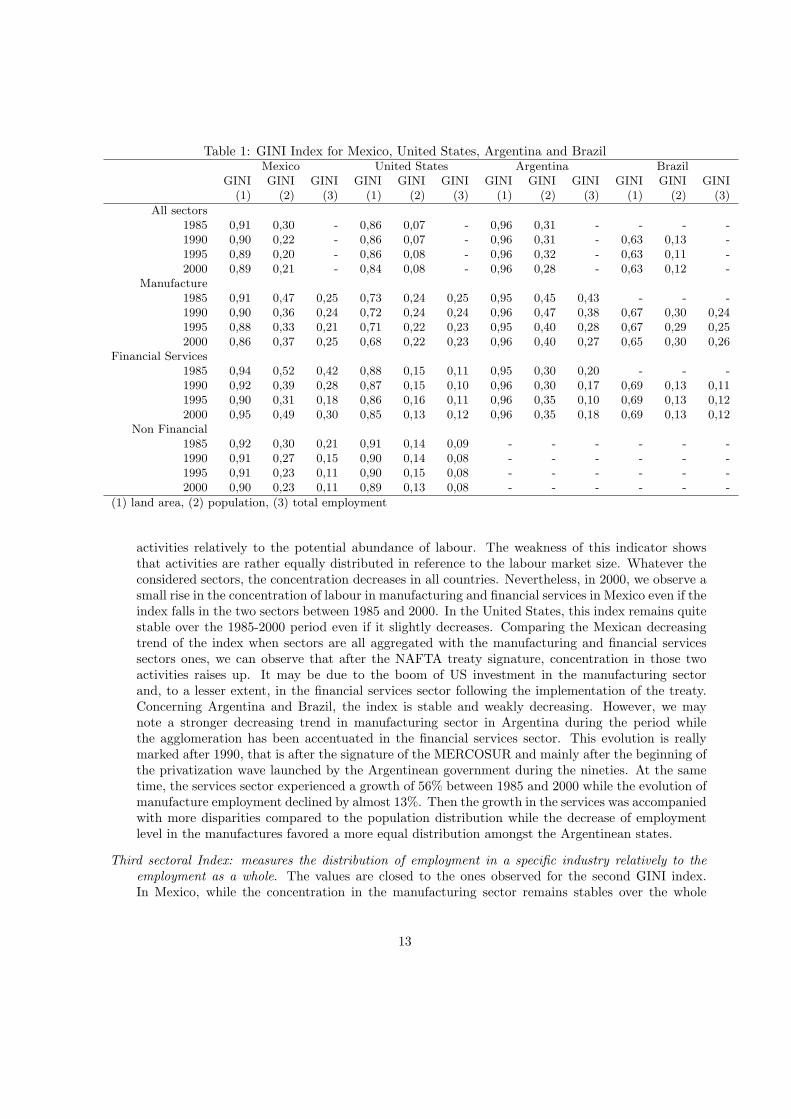
Table 1: GINI Index for Mexico, United States, Argentina and BrazilMexico United States Argentina Brazil

GINI GINI GINI GINI GINI GINI GINI GINI GINI GINI GINI GINI(1) (2) (3) (1) (2) (3) (1) (2) (3) (1) (2) (3)

All sectors1985 0,91 0,30 - 0,86 0,07 - 0,96 0,31 - - - -1990 0,90 0,22 - 0,86 0,07 - 0,96 0,31 - 0,63 0,13 -1995 0,89 0,20 - 0,86 0,08 - 0,96 0,32 - 0,63 0,11 -2000 0,89 0,21 - 0,84 0,08 - 0,96 0,28 - 0,63 0,12 -

Manufacture1985 0,91 0,47 0,25 0,73 0,24 0,25 0,95 0,45 0,43 - - -1990 0,90 0,36 0,24 0,72 0,24 0,24 0,96 0,47 0,38 0,67 0,30 0,241995 0,88 0,33 0,21 0,71 0,22 0,23 0,95 0,40 0,28 0,67 0,29 0,252000 0,86 0,37 0,25 0,68 0,22 0,23 0,96 0,40 0,27 0,65 0,30 0,26

Financial Services1985 0,94 0,52 0,42 0,88 0,15 0,11 0,95 0,30 0,20 - - -1990 0,92 0,39 0,28 0,87 0,15 0,10 0,96 0,30 0,17 0,69 0,13 0,111995 0,90 0,31 0,18 0,86 0,16 0,11 0,96 0,35 0,10 0,69 0,13 0,122000 0,95 0,49 0,30 0,85 0,13 0,12 0,96 0,35 0,18 0,69 0,13 0,12

Non Financial1985 0,92 0,30 0,21 0,91 0,14 0,09 - - - - - -1990 0,91 0,27 0,15 0,90 0,14 0,08 - - - - - -1995 0,91 0,23 0,11 0,90 0,15 0,08 - - - - - -2000 0,90 0,23 0,11 0,89 0,13 0,08 - - - - - -

(1) land area, (2) population, (3) total employment

activities relatively to the potential abundance of labour. The weakness of this indicator showsthat activities are rather equally distributed in reference to the labour market size. Whatever theconsidered sectors, the concentration decreases in all countries. Nevertheless, in 2000, we observe asmall rise in the concentration of labour in manufacturing and financial services in Mexico even if theindex falls in the two sectors between 1985 and 2000. In the United States, this index remains quitestable over the 1985-2000 period even if it slightly decreases. Comparing the Mexican decreasingtrend of the index when sectors are all aggregated with the manufacturing and financial servicessectors ones, we can observe that after the NAFTA treaty signature, concentration in those twoactivities raises up. It may be due to the boom of US investment in the manufacturing sectorand, to a lesser extent, in the financial services sector following the implementation of the treaty.Concerning Argentina and Brazil, the index is stable and weakly decreasing. However, we maynote a stronger decreasing trend in manufacturing sector in Argentina during the period whilethe agglomeration has been accentuated in the financial services sector. This evolution is reallymarked after 1990, that is after the signature of the MERCOSUR and mainly after the beginning ofthe privatization wave launched by the Argentinean government during the nineties. At the sametime, the services sector experienced a growth of 56% between 1985 and 2000 while the evolution ofmanufacture employment declined by almost 13%. Then the growth in the services was accompaniedwith more disparities compared to the population distribution while the decrease of employmentlevel in the manufactures favored a more equal distribution amongst the Argentinean states.

Third sectoral Index: measures the distribution of employment in a specific industry relatively to theemployment as a whole. The values are closed to the ones observed for the second GINI index.In Mexico, while the concentration in the manufacturing sector remains stables over the whole

13

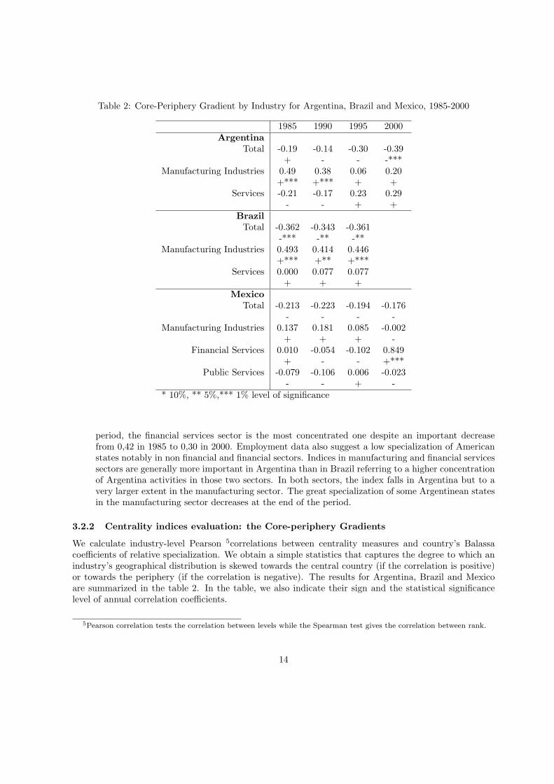
Table 2: Core-Periphery Gradient by Industry for Argentina, Brazil and Mexico, 1985-2000

1985 1990 1995 2000Argentina

Total -0.19 -0.14 -0.30 -0.39+ - - -***

Manufacturing Industries 0.49 0.38 0.06 0.20+*** +*** + +

Services -0.21 -0.17 0.23 0.29- - + +

BrazilTotal -0.362 -0.343 -0.361

-*** -** -**Manufacturing Industries 0.493 0.414 0.446

+*** +** +***Services 0.000 0.077 0.077

+ + +Mexico

Total -0.213 -0.223 -0.194 -0.176- - - -

Manufacturing Industries 0.137 0.181 0.085 -0.002+ + + -

Financial Services 0.010 -0.054 -0.102 0.849+ - - +***

Public Services -0.079 -0.106 0.006 -0.023- - + -

* 10%, ** 5%,*** 1% level of significance

period, the financial services sector is the most concentrated one despite an important decreasefrom 0,42 in 1985 to 0,30 in 2000. Employment data also suggest a low specialization of Americanstates notably in non financial and financial sectors. Indices in manufacturing and financial servicessectors are generally more important in Argentina than in Brazil referring to a higher concentrationof Argentina activities in those two sectors. In both sectors, the index falls in Argentina but to avery larger extent in the manufacturing sector. The great specialization of some Argentinean statesin the manufacturing sector decreases at the end of the period.

3.2.2 Centrality indices evaluation: the Core-periphery Gradients

We calculate industry-level Pearson 5correlations between centrality measures and country’s Balassacoefficients of relative specialization. We obtain a simple statistics that captures the degree to which anindustry’s geographical distribution is skewed towards the central country (if the correlation is positive)or towards the periphery (if the correlation is negative). The results for Argentina, Brazil and Mexicoare summarized in the table 2. In the table, we also indicate their sign and the statistical significancelevel of annual correlation coefficients.

5Pearson correlation tests the correlation between levels while the Spearman test gives the correlation between rank.

14

Mexican Pearson statistics almost never show significance in table 2. Only in 2000, the financialservices sector reveal a significant concentration in core regions. This sector appears to be the mostconcentrated as observed in table 1. We note two clear trends concerning all aggregated sectors wherethe statistic is negative during the whole period and the manufacturing sector showing a positive sign from1985 to 1995, but the gradients are generally not significant. We also found information on concentrationin the different Mexican sectors. Results are presented in table 3. In 1986, 8 out of 18 sampled industriesexhibit negative centre periphery gradients but only one is significant. This phenomenon is less persistentin 1999 because half of all sectors sampled exhibit a positive centre-periphery gradient but 5 of themare significant (4 significant positive statistics in 1986). This last year, only one sector is significantlyconcentrated in the periphery: food and kindred, and tobacco products. Besides, three sectors areconcentrated in core regions from 1989 to 1999: paper and products and printing industries, chemicaland plastics products, administration services. Confirming previous results, in 1999, financial servicesand repairing sectors also have joined centre regions.

In Argentina, core periphery gradients are generally not significant and specially in the case of theservices sector. However, until 1990, Pearson statistics indicate a significant manufacturing concentrationin core regions. Even if the statistics is not significant anymore in 1995 and 2000, it remains positive.Finally, we note a negative and significant sign in 1995 when all sectors are aggregated highlighting adispersion tendency of labour as demonstrated by Index (2) in table 1. Brazilian statistics are generallymore significant except in services sectors as in the Argentinean case. The Pearson statistic highlights ageographical distribution towards periphery (that is dispersion) when looking at all aggregated sectors.Nevertheless, centre periphery gradients exhibit a continuous manufacturing concentration in core regions.

Comparing tables 1 and 2, we may conclude that when all sectors are aggregated, the concentrationof economic activities is relatively low in three of our sampled countries where GINI (2) indices are verysmall and Pearson statistics show negative signs and significant in the Brazilian case. These results followthe conclusion of our model concerning the reversed relation between liberalization and agglomeration.Only the GINI (1) index insists on a strong concentration of labour by reference to the surface areaspecially in Mexico, Argentina and the United States. Those contrasting conclusions put the stress on theimportance of the chosen reference to evaluate concentration levels. Moreover, both tables 1 and 2 reveal astronger manufacturing agglomeration in Argentina and in Brazil than in other sectors even if decreasingover the time in the Argentinean case. Contrary to our model conclusions, the concentration trend inmanufacturing sector is stronger in the larger and richer country after the MERCOSUR implementation.Looking at NAFTA countries we notice that concentration is largely higher in Mexico than in the UnitedStates whatever the sector is. However, except in the case of financial services in Mexico , labour wasdispersing during the 1985-2000 period in both countries mainly when all sectors are aggregated. If weconsider that Mexican policies in favour of trade liberalization with the United States began in the midof the eighties, GINI index levels generally follow our model results despite the dispersion observed inboth countries in all sectors (except of course financial services).

We have observed two different trends in agglomeration process within the NAFTA and the MERCO-SUR. We now want to analyze the existing link between trade liberalization, agglomeration and incomeper capita convergence.

4 Regional convergence and agglomeration

We are particularly interested in the impact of the MERCOSUR and the NAFTA on Argentinean,Brazilian Mexican, and US GDP per capita convergence. The NAFTA is the first free trade area whichincludes developed and developing countries. Disparities in terms of economic development and market

15

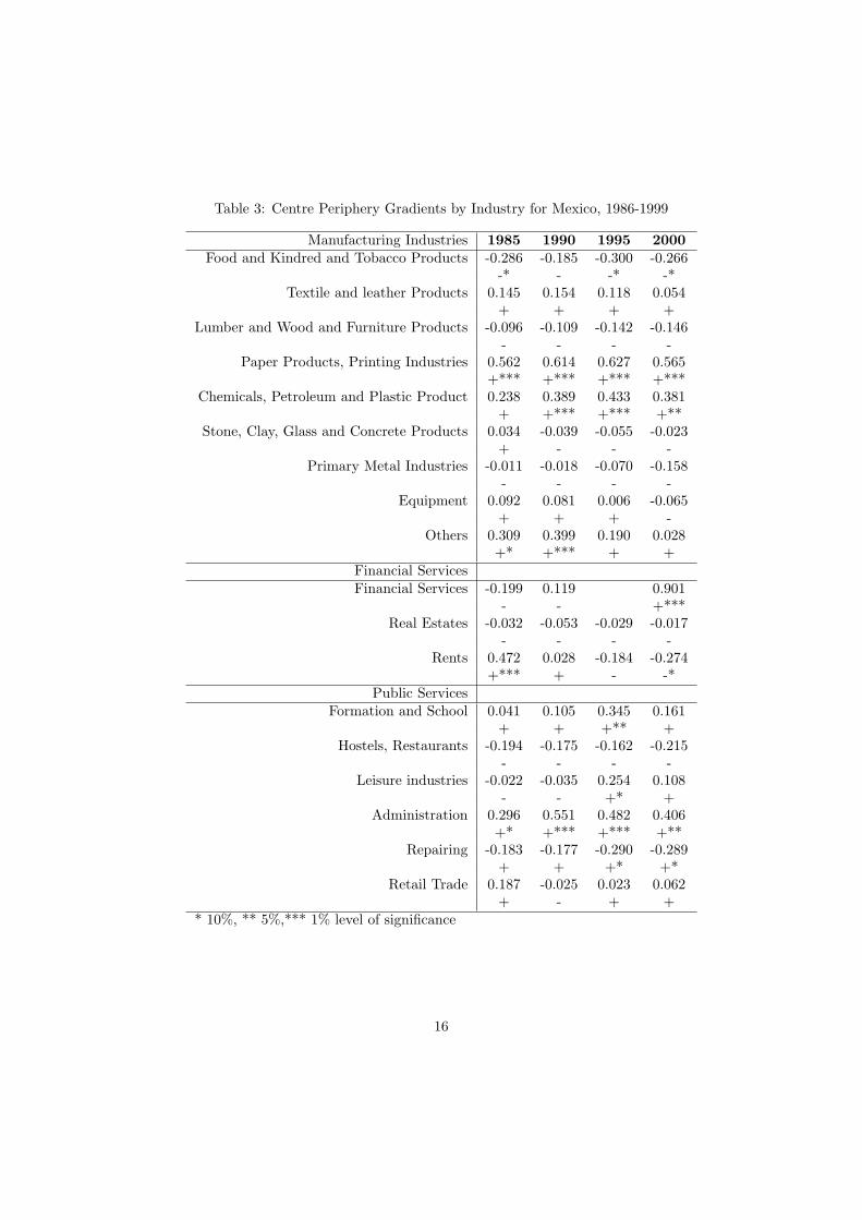
Table 3: Centre Periphery Gradients by Industry for Mexico, 1986-1999

Manufacturing Industries 1985 1990 1995 2000Food and Kindred and Tobacco Products -0.286 -0.185 -0.300 -0.266

-* - -* -*Textile and leather Products 0.145 0.154 0.118 0.054

+ + + +Lumber and Wood and Furniture Products -0.096 -0.109 -0.142 -0.146

- - - -Paper Products, Printing Industries 0.562 0.614 0.627 0.565

+*** +*** +*** +***Chemicals, Petroleum and Plastic Product 0.238 0.389 0.433 0.381

+ +*** +*** +**Stone, Clay, Glass and Concrete Products 0.034 -0.039 -0.055 -0.023

+ - - -Primary Metal Industries -0.011 -0.018 -0.070 -0.158

- - - -Equipment 0.092 0.081 0.006 -0.065

+ + + -Others 0.309 0.399 0.190 0.028

+* +*** + +Financial ServicesFinancial Services -0.199 0.119 0.901

- - +***Real Estates -0.032 -0.053 -0.029 -0.017

- - - -Rents 0.472 0.028 -0.184 -0.274

+*** + - -*Public Services

Formation and School 0.041 0.105 0.345 0.161+ + +** +

Hostels, Restaurants -0.194 -0.175 -0.162 -0.215- - - -

Leisure industries -0.022 -0.035 0.254 0.108- - +* +

Administration 0.296 0.551 0.482 0.406+* +*** +*** +**

Repairing -0.183 -0.177 -0.290 -0.289+ + +* +*

Retail Trade 0.187 -0.025 0.023 0.062+ - + +

* 10%, ** 5%,*** 1% level of significance

16

size notably between the laggard and the leading countries confirm the strong heterogeneity of those freetrade areas. Actually, in 2000, Mexican population accounts for 35% of the US population, and the grossnational product in Mexico is only equivalent to 5% of the US one. The labour costs and the level oflabour productivity show strong disparities: the Mexican average hourly wage only represents 30% ofthe US one in 2000. There are no such differences between Argentina and Brazil but if the ArgentineanPPP GDP represents 35% of the Brazilian one, Argentinean population is only 21% of the Brazilian.The NAFTA and the MERCOSUR established a gradual reduction in trade barriers, the elimination ofinvestments’ restrictions and an increasing competition resulting from improved market accessibility. Asa result, Mexico has also increased its share in US international trade and is currently the third largesttrading partner after Canada and Japan. Trade between MERCOSUR partners represented almost 15billion of US dollars in 1997 and 1998. Since the beginning of the crisis in 1999, trade has fallen by15 billions of US dollars but intra regional trade has grown by 12,7% per year between 1990 and 1999.Trade composition between Brazil and its partners is closed to developed countries one. Brazil exportsmanufactures and imports raw materials and foods with low added value.

In the light of such contrasts between each pair of countries, we want to check whether Mexican(Argentinean) states, experienced a process of convergence relatively to the United States (Brazil) ones.We also question the convergence between the four sampled countries. The process of convergence isfirstly analyzed by two traditional concepts: beta- and sigma-convergence. The beta (β)-convergenceindicates whether the growth in per capita income is positively correlated with the initial gap betweencountries. The sigma (σ)-convergence assumes a reduction in the dispersion of per capita income orproduction. Secondly, contrasted levels of economic development between NAFTA and MERCOSURpartners may produce a strong heterogeneity between countries steady states. In previous section, westated that concentration of activities in the four selected countries is important (notably if we refer tothe first GINI index). In this section, we check if it played any significant role on the convergence processof studied countries. Then, we also proceed to a conditional convergence analysis adding agglomerationvariables in our regressions to control for the relation between convergence and agglomeration. Then, wemay answer to the following questions: do preferential trade agreements have an incidence on income percapita convergence? What is the influence of agglomeration on this convergence?

4.1 The unconditional β convergence

The absolute or unconditional β convergence supposes that, at long term, economies tend to the sameequilibrium path. The unconditional β-convergence evaluates a convergence in levels. It is defined by thereduction of GDP per capita gaps in the concerned area. Absolute β convergence exists when there is anegative relation between growth and the level of initial per capita income or, what is the same thing,that during this period the poorer economies have grown on average at higher rates than richer ones.Thus, absolute β convergence exists when the b coefficient is significant and positive in the followingregression:

[log (yit)− log (yi0)] /t = a− b log (yi0) + ui (24)

where yit and yi0 are the level of per capita income of economy i in years t and 0 respectively and ui

is a stochastic error with the usual characteristics.Data on GDP per capita on Argentina come from the INDEC (Instituto Nacional De Estadistica y

Censos) and from the CEPAL in Buenos Aires. The IBGE provided data on Brazilian states. Data onMexico and the United States were respectively collected from the INEGI and the BEA.

Most of the results in table 4 are not significant except for Argentina and Brazil between 1985 and2000. Indeed, the rate of convergence is equal to 0.6% during this period. Moreover, this rate increases byalmost 3 points in the 1995-2000 period corresponding to the implementation of the MERCOSUR treaty.

17

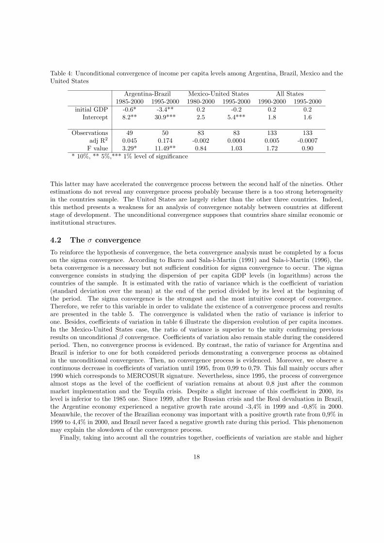
Table 4: Unconditional convergence of income per capita levels among Argentina, Brazil, Mexico and theUnited States

Argentina-Brazil Mexico-United States All States1985-2000 1995-2000 1980-2000 1995-2000 1990-2000 1995-2000

initial GDP -0.6* -3.4** 0.2 -0.2 0.2 0.2Intercept 8.2** 30.9*** 2.5 5.4*** 1.8 1.6

Observations 49 50 83 83 133 133adj R2 0.045 0.174 -0.002 0.0004 0.005 -0.0007

F value 3.29* 11.49** 0.84 1.03 1.72 0.90* 10%, ** 5%,*** 1% level of significance

This latter may have accelerated the convergence process between the second half of the nineties. Otherestimations do not reveal any convergence process probably because there is a too strong heterogeneityin the countries sample. The United States are largely richer than the other three countries. Indeed,this method presents a weakness for an analysis of convergence notably between countries at differentstage of development. The unconditional convergence supposes that countries share similar economic orinstitutional structures.

4.2 The σ convergence

To reinforce the hypothesis of convergence, the beta convergence analysis must be completed by a focuson the sigma convergence. According to Barro and Sala-i-Martin (1991) and Sala-i-Martin (1996), thebeta convergence is a necessary but not sufficient condition for sigma convergence to occur. The sigmaconvergence consists in studying the dispersion of per capita GDP levels (in logarithms) across thecountries of the sample. It is estimated with the ratio of variance which is the coefficient of variation(standard deviation over the mean) at the end of the period divided by its level at the beginning ofthe period. The sigma convergence is the strongest and the most intuitive concept of convergence.Therefore, we refer to this variable in order to validate the existence of a convergence process and resultsare presented in the table 5. The convergence is validated when the ratio of variance is inferior toone. Besides, coefficients of variation in table 6 illustrate the dispersion evolution of per capita incomes.In the Mexico-United States case, the ratio of variance is superior to the unity confirming previousresults on unconditional β convergence. Coefficients of variation also remain stable during the consideredperiod. Then, no convergence process is evidenced. By contrast, the ratio of variance for Argentina andBrazil is inferior to one for both considered periods demonstrating a convergence process as obtainedin the unconditional convergence. Then, no convergence process is evidenced. Moreover, we observe acontinuous decrease in coefficients of variation until 1995, from 0,99 to 0,79. This fall mainly occurs after1990 which corresponds to MERCOSUR signature. Nevertheless, since 1995, the process of convergencealmost stops as the level of the coefficient of variation remains at about 0,8 just after the commonmarket implementation and the Tequila crisis. Despite a slight increase of this coefficient in 2000, itslevel is inferior to the 1985 one. Since 1999, after the Russian crisis and the Real devaluation in Brazil,the Argentine economy experienced a negative growth rate around -3,4% in 1999 and -0,8% in 2000.Meanwhile, the recover of the Brazilian economy was important with a positive growth rate from 0,9% in1999 to 4,4% in 2000, and Brazil never faced a negative growth rate during this period. This phenomenonmay explain the slowdown of the convergence process.

Finally, taking into account all the countries together, coefficients of variation are stable and higher

18

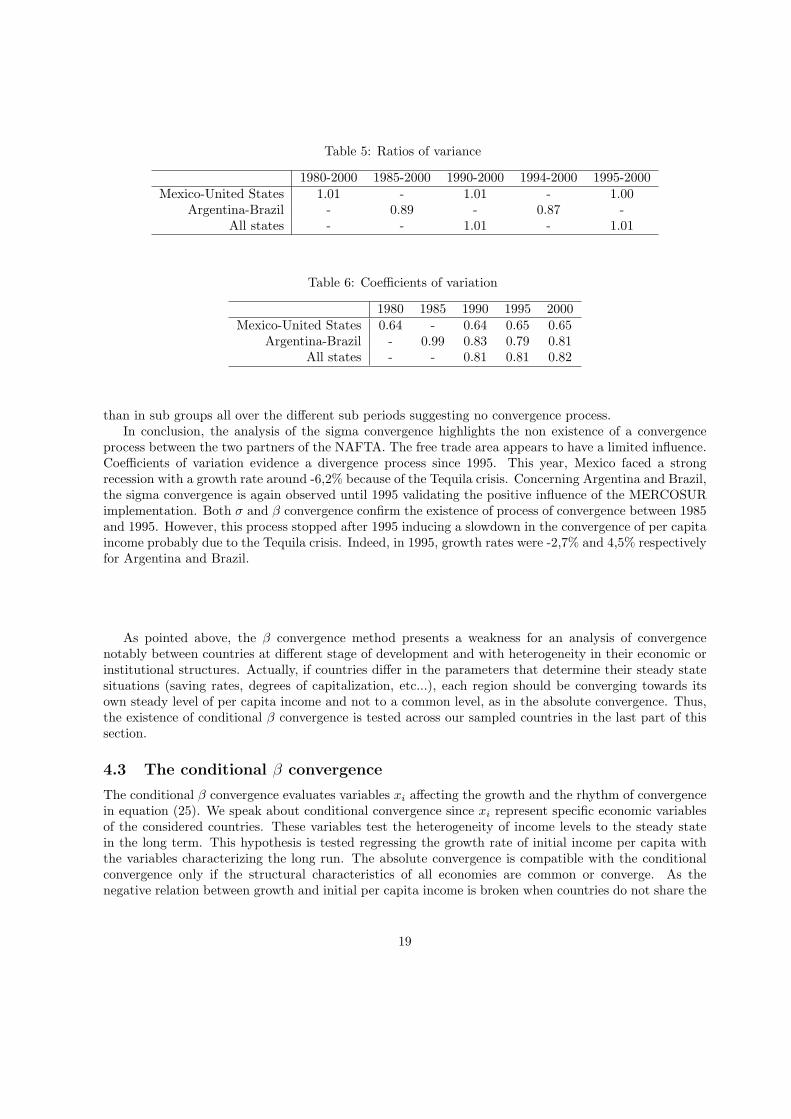
Table 5: Ratios of variance

1980-2000 1985-2000 1990-2000 1994-2000 1995-2000Mexico-United States 1.01 - 1.01 - 1.00

Argentina-Brazil - 0.89 - 0.87 -All states - - 1.01 - 1.01

Table 6: Coefficients of variation

1980 1985 1990 1995 2000Mexico-United States 0.64 - 0.64 0.65 0.65

Argentina-Brazil - 0.99 0.83 0.79 0.81All states - - 0.81 0.81 0.82

than in sub groups all over the different sub periods suggesting no convergence process.In conclusion, the analysis of the sigma convergence highlights the non existence of a convergence

process between the two partners of the NAFTA. The free trade area appears to have a limited influence.Coefficients of variation evidence a divergence process since 1995. This year, Mexico faced a strongrecession with a growth rate around -6,2% because of the Tequila crisis. Concerning Argentina and Brazil,the sigma convergence is again observed until 1995 validating the positive influence of the MERCOSURimplementation. Both σ and β convergence confirm the existence of process of convergence between 1985and 1995. However, this process stopped after 1995 inducing a slowdown in the convergence of per capitaincome probably due to the Tequila crisis. Indeed, in 1995, growth rates were -2,7% and 4,5% respectivelyfor Argentina and Brazil.

As pointed above, the β convergence method presents a weakness for an analysis of convergencenotably between countries at different stage of development and with heterogeneity in their economic orinstitutional structures. Actually, if countries differ in the parameters that determine their steady statesituations (saving rates, degrees of capitalization, etc...), each region should be converging towards itsown steady level of per capita income and not to a common level, as in the absolute convergence. Thus,the existence of conditional β convergence is tested across our sampled countries in the last part of thissection.

4.3 The conditional β convergence

The conditional β convergence evaluates variables xi affecting the growth and the rhythm of convergencein equation (25). We speak about conditional convergence since xi represent specific economic variablesof the considered countries. These variables test the heterogeneity of income levels to the steady statein the long term. This hypothesis is tested regressing the growth rate of initial income per capita withthe variables characterizing the long run. The absolute convergence is compatible with the conditionalconvergence only if the structural characteristics of all economies are common or converge. As thenegative relation between growth and initial per capita income is broken when countries do not share the

19

same steady in the neoclassical growth model, we use the definition of conditional β convergence whichis confirmed when beta is positive in the following regression:

1T

log(

Yi,to+ T

Yi,to

)= ai −

(1− e−βT

T

)log (Yi,to) + µi,to+T (25)

with ai = xi +(1− e−βT

)log(y∗i )

By estimating conditional convergence, we may confront our theoretical conclusions with empiricaldata and estimations. In order to assess the agglomeration of economic activities impact, we includeconcentration indexes in our regressions. By construction, the GINI index is calculated by country andnot by states. Thus, in order to integrate an agglomeration indicator by state, Zi from the GINI indexcalculation described above is used instead (in equation (21)). Fujita and Thisse (1996) insist on someof the economic efficiency gains that can be produced through the agglomeration of economic activities.As for Martin (1999), when geography and growth are jointly determined in a model, then the possibilityof a trade-off between average growth and regional convergence emerges. However, in our model, tradeintegration leads to a dispersion of economic activity. Agglomeration of economic activities favoursinnovation because it lowers costs of investment in the core. It is then necessary to improve the growthrate allowing a regional income convergence. In the previous section, GINI indices and Pearson statisticshave resulted in two contrasting concentration trends in the NAFTA and in the MERCOSUR normallyinducing two different convergence process. These distinct behaviours could be explained by a strongerdifference between economic development levels in the NAFTA than in the MERCOSUR.

As observed before, contrasts in economic development imply important structural differences betweenanalyzed countries. This is the reason why we include fixed effects in the model. These differences couldbe transmitted into disparate steady states. We also introduce two variables derived from GINI indexrelative to the surface area (column (1) in table 1) and from GINI index relative to the population (column(2) in table 1). They are respectively named agglo1 and agglo2.

4.3.1 Mexico and the United States

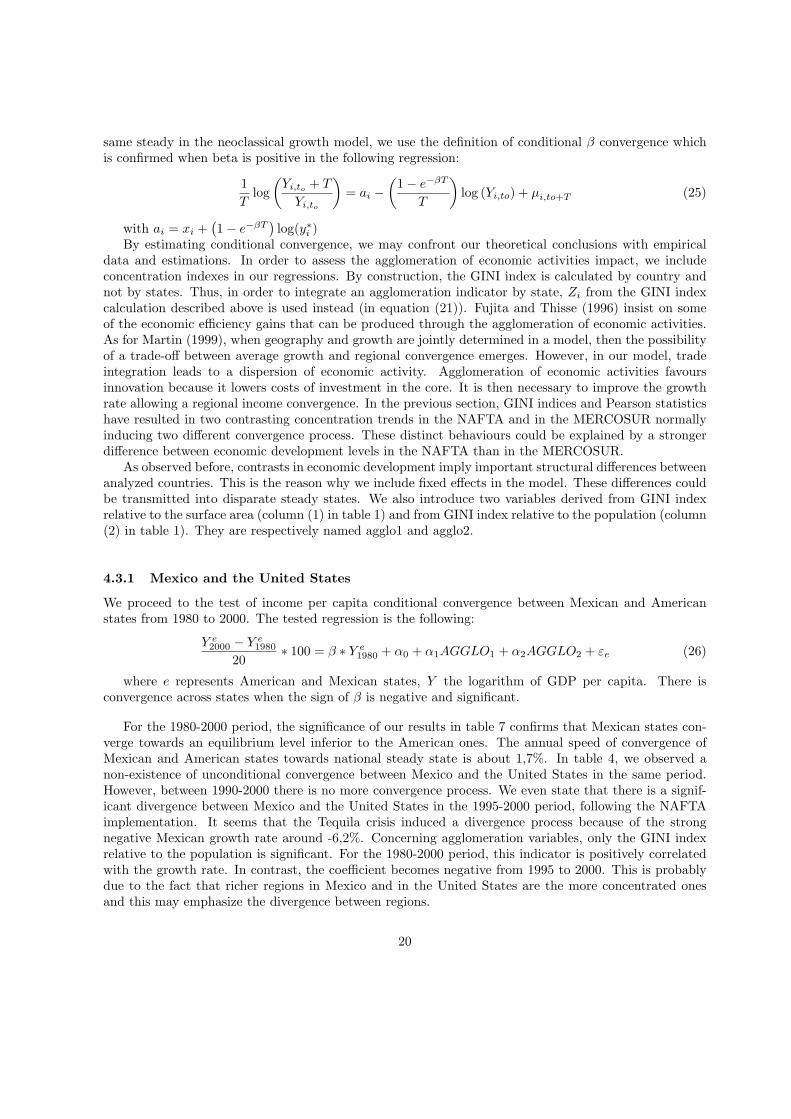
We proceed to the test of income per capita conditional convergence between Mexican and Americanstates from 1980 to 2000. The tested regression is the following:

Y e2000 − Y e

1980

20∗ 100 = β ∗ Y e

1980 + α0 + α1AGGLO1 + α2AGGLO2 + εe (26)

where e represents American and Mexican states, Y the logarithm of GDP per capita. There isconvergence across states when the sign of β is negative and significant.

For the 1980-2000 period, the significance of our results in table 7 confirms that Mexican states con-verge towards an equilibrium level inferior to the American ones. The annual speed of convergence ofMexican and American states towards national steady state is about 1,7%. In table 4, we observed anon-existence of unconditional convergence between Mexico and the United States in the same period.However, between 1990-2000 there is no more convergence process. We even state that there is a signif-icant divergence between Mexico and the United States in the 1995-2000 period, following the NAFTAimplementation. It seems that the Tequila crisis induced a divergence process because of the strongnegative Mexican growth rate around -6,2%. Concerning agglomeration variables, only the GINI indexrelative to the population is significant. For the 1980-2000 period, this indicator is positively correlatedwith the growth rate. In contrast, the coefficient becomes negative from 1995 to 2000. This is probablydue to the fact that richer regions in Mexico and in the United States are the more concentrated onesand this may emphasize the divergence between regions.

20

Table 7: Conditional convergence of income per capita levels across Mexico and the United States

1980-2000 1990-2000 1995-2000(1) (2) (3)

initial GDP -1.7*** -0.4 1.0*agglo1 0.0 0.0 0.0*agglo2 2.8*** 0.9* -2.0**

intercept 17.6*** 6.95* -4.9

Observations 82 82 82adj R2 0.245 0.024 0.076

F value 9.89*** 1.68 3.26*ratio of variance 1.01 1.01 1.01* 10%, ** 5%,*** 1% level of significance

Table 8: Conditional convergence of income per capita levels across Argentina and Brazil

1985-2000 1994-2000(1) (2)

initial GDP -0.7** -3.9**agglo1 0.0*** -0.0agglo2 -0.3 4.7*

intercept 9.9*** 31.3**

Observations 48 50adj R2 0.154 0.237

F value 3.91*** 6.17*** 10%, ** 5%,*** 1% level of significance

4.3.2 Argentina and Brazil

As in the previous estimation, we include agglomeration variables. The corresponding tested regressionis now:

Y e2000 − Y e

1985

15∗ 100 = β ∗ Y e

1985 + α0 + α1AGGLO1 + α2AGGLO2 + εe (27)

The estimation results in table 8 column (1) evidence a process of convergence with a significant annualspeed of convergence equals to 0,7%. Besides, during the 1994-2000 period that is after the MERCOSURsignature, the rate of convergence reaches 3,9% (column (2)). Those results may be interpreted as apositive impact of MERCOSUR implementation on convergence between Argentina and Brazil. We nowlook at the impact of agglomeration on the convergence rate. The second agglomeration variable (agglo2)has a significant and positive impact. Agglo1 that refers to land area is almost equal to zero while agglo2,referring to the population, has a positive and important coefficient. During the 1994-2000 period, the

21

convergence rate highly improves since it become five times larger than the one observed in the 1985-2000 period. It is a very important result since in the Mexico-United States case, table 7 indicates adivergence process after the NAFTA signature even if there is a slow convergence rate between 1980 and2000. We could interpret this acceleration of the convergence process as a consequence of the MERCOSURimplementation. Moreover, capturing the concentration disparities enhances the convergence rate by twopoints.

4.3.3 Convergence across NAFTA and MERCOSUR members?

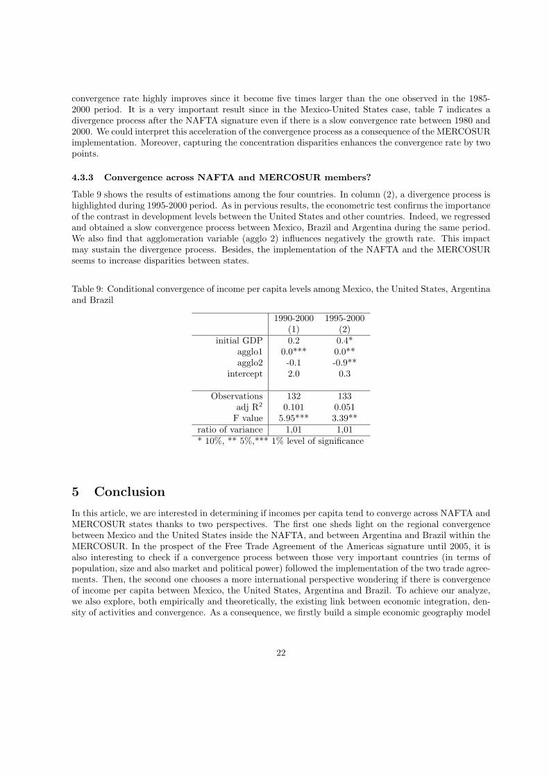
Table 9 shows the results of estimations among the four countries. In column (2), a divergence process ishighlighted during 1995-2000 period. As in pervious results, the econometric test confirms the importanceof the contrast in development levels between the United States and other countries. Indeed, we regressedand obtained a slow convergence process between Mexico, Brazil and Argentina during the same period.We also find that agglomeration variable (agglo 2) influences negatively the growth rate. This impactmay sustain the divergence process. Besides, the implementation of the NAFTA and the MERCOSURseems to increase disparities between states.

Table 9: Conditional convergence of income per capita levels among Mexico, the United States, Argentinaand Brazil

1990-2000 1995-2000(1) (2)

initial GDP 0.2 0.4*agglo1 0.0*** 0.0**agglo2 -0.1 -0.9**

intercept 2.0 0.3

Observations 132 133adj R2 0.101 0.051

F value 5.95*** 3.39**ratio of variance 1,01 1,01* 10%, ** 5%,*** 1% level of significance

5 Conclusion

In this article, we are interested in determining if incomes per capita tend to converge across NAFTA andMERCOSUR states thanks to two perspectives. The first one sheds light on the regional convergencebetween Mexico and the United States inside the NAFTA, and between Argentina and Brazil within theMERCOSUR. In the prospect of the Free Trade Agreement of the Americas signature until 2005, it isalso interesting to check if a convergence process between those very important countries (in terms ofpopulation, size and also market and political power) followed the implementation of the two trade agree-ments. Then, the second one chooses a more international perspective wondering if there is convergenceof income per capita between Mexico, the United States, Argentina and Brazil. To achieve our analyze,we also explore, both empirically and theoretically, the existing link between economic integration, den-sity of activities and convergence. As a consequence, we firstly build a simple economic geography model

22

with elements from endogenous growth theory. We then define, work out and include different measuresof agglomeration in our empirical approach on income per capita convergence.

Our theoretical model shows a relation between agglomeration, growth and convergence in incomewithin a trade area of two countries with different levels of economic development. Trade liberalizationleads to less agglomeration and to less growth rate because agglomeration of economic activities favoursinnovation by lowering costs of investment in the core. Thus, agglomeration is necessary to improve thegrowth rate that allows a regional income convergence. Then trade liberalization is not sufficient to bringabout income convergence between the two regions.

In our empirical work, we wonder whether the NAFTA and the MERCOSUR have influenced thespatial organization of production in Mexico and the United States on one hand and in Argentina andBrazil on the other hand. Contrary to our model conclusions, agglomeration measures indicate that theconcentration trend in manufacturing sector is stronger in Brazil, the larger country, after the MERCO-SUR implementation. At the opposite and following our theoretical conclusions, the concentration inNAFTA countries is largely higher in Mexico than in the United States whatever the sector is. However,except in the case of financial services in Mexico, we observe that labour was slightly dispersing duringthe 1985-2000 period in both countries.

Our analysis of the sigma- and absolute beta-convergence concluded to the non existence of a processof convergence between the two partners of the NAFTA. Thus, the free trade agreement seems to haveplayed a limited influence. We evidence a divergence process since 1995. This year, Mexico faced a strongrecession with a growth rate around -6.2% because of the Tequila crisis. Concerning MERCOSUR, thisstudy reveals a strong process of convergence between 1985 and 1995. However this process appears toslow down after 1995 in terms of GDP per capita dispersion. It seems that the MERCOSUR signaturefirstly accelerated the convergence process that was barely slacken of following the Tequila crisis in 1994and the common market implementation. Since 1999, after the Russian crisis and the Real devaluationin Brazil, the Argentine economy experienced a negative growth rate around -3,4% in 1999 and -0,8% in2000. Meanwhile, the recover of the Brazilian economy was important with a positive growth rate from0,9% in 1999 to 4,4% in 2000, and Brazil never faced a negative growth rate during this period. Thisphenomenon may explain the slowdown of the convergence process.

In order to assess the influence of agglomeration of economic activities on the convergence, we includein our regressions variables derived from GINI indices calculation. By this way, we try to check our modelconclusion on the negative relation between trade liberalization and the density of economic activities inthe richer country. This phenomenon could be interpreted as income convergence between regions doesnot follow trade liberalization.

In previous results, we reveal the non-existence of unconditional convergence between Mexico and theUnited States between 1980 and 2000. Nevertheless, we observe a conditional convergence between 1980and 2000 but not between, 1995 and 2000, indicating that the NAFTA has not played a role in convergenceprocess. Only the agglomeration variable referring to the population has a significant impact whateverthe analyzed period. However, its positive impact until the beginning of the 90s becomes negative since1995. Estimations on MERCOSUR members evidence a process of convergence with a significant annualspeed of convergence equals to 0,7% over the 1985-2000 period. Besides, during the 1994-2000 period, thatis after the MERCOSUR signature, the rate of convergence reaches 3,7%. The agglomeration variablereferring to the population has a positive and significant impact on the growth rate between 1994 and2000.

Empirical estimations on NAFTA countries seem to confirm our theoretical conclusion whereas MER-COSUR countries performed a convergence process after the implementation of the treaty in 1991. More-over, agglomeration plays a significant role on the narrowing in the percentage gap between the laggardand leading countries’ performance. Then, our model better explains the relation between the UnitedStates and Mexico than between Argentina and Brazil. It may be explained by the major difference

23

across NAFTA economic development levels than among MERCOSUR ones.

References

[1] Andalon M.L., Lopez-Calva L.F., (2002), ”The Many Mexicos: Income Inequality and Polar-ization in Urban Mexico During the 90s”, Working Paper presented at the Cornell-LSE-WIDERConference on Spatial Inequality, June 28-29-30th.

[2] Azzoni C., (1997), “Concentracao regional e dispersao das rendas per capita estaduais: analise apartir de series historicas estaduais de PIB (1939-1995)”, Estudos Economicos, 27(3), pp.341-393.

[3] Azzoni C., (2001), “Economic Growth and Regional Income Inequalities in Brazil ”, The Annalsof Regional Science, 35, pp.133-152.

[4] Baldwin R.E., Forslid R., (2000), “Trade Liberalization and Endogenous Growth: A Q-TheoryApproach”, Journal of International Economics, 50(2), pp.497-517.

[5] Barro R.J., (1991), “Economic Growth in a Cross-section of Countries”, Quarterly Journal ofEconomics, 106(2), p.407-443.

[6] Barro R., (1998), Determinants of Economic Growth: A Cross-Country Empirical Study, Cam-bridge, MA: MIT Press.

[7] Barro R., Sala-i-Martin, (1991), “Convergence Across States and Regions”, Brooking Papers onEconomic Activity, 1, pp. 107-158.

[8] Barro R.J. & Sala-i-Martin X., (1992), “Convergence”, Journal of Political Economy, 100,p.223-251.

[9] Barro R.J., Sala-i-Martin X., (1995), Economic Growth, Mc GrawHill.

[10] Ben-David D. (1993), “Equalizing Exchange:Trade Liberalization and income Convergence”,Quaterly Journal of Economics, 108, pp. 653-679.

[11] Bowman K. and Felipe J.,(2001), “Economic Convergence and Trade Integration in Latin Amer-ica”, 2001 Annual Meeting of the Political Science Association, San Francisco.

[12] Brulhart M. (2001),“Evolving Geographical Concentration of European Manufacturing Industries”,Weltwirtschaftliches Archiv, 137(2), pp. 215-243.

[13] Caceres L.R., Sandoval O.N., (1999), “Crecimiento Economico y Divergencia en AmericaLatina”, El Trimestre Economico, 264, pp. 781-796.

[14] Ciccone A. and Hall R, (1996), Productivity and the Density of Economic Activity”, AmericanEconomic Review, 87(1), p.54-70.

[15] Dan, B.D. (1993), “Equalizing Exchange: Trade Liberalization and Income Convergence”, Quar-terly Journal of Economics, 108(3), p.653-676.

[16] Dobson S., Ramlogan, (2002), Economic Growth and convergence in Latin America, The Journalof Development Studies, 38(6), pp.83-104.

24

[17] Esquivel G., (1999), “Convergencia Regional en Mexico, 1940-1995”, Trimestre Economico, 264,pp 725-761.

[18] Ferreira A., Diniz , (1995), Convergencia entre les rentas per capita estaduales en Brasil”, RevistaLatino Americana de Estudios Urbanos Regionales, XXI(62), pp.17-31.

[19] Fujita M., Thisse J.F., (1996), “Economics of Agglomeration”, Journal of the Japanese andInternational Economics, 10, pp. 339-378.

[20] Garrido N., Marina A., Sotelsek D., (2001), “Crecimiento y Convergencia: un ejercicio empıricosobre las rtegiones espanolas y las provincias argentinas”, Anales de la XXXVIa Reunion Anual dela Asociacion Argentina de Economia Polıtica.

[21] Gatto and Centrangolo, (2003), “Dinamica productiva provincial a fines de los anos noventa”,Serie Estudios y Perspectivas de la CEPAL, n◦14.

[22] Gaulier G., (2002), “Integration economique et convergences reelles”, These de Doctorat en SciencesEconomiques, Paris I, Novembre.

[23] Glaeser E.L., Kallal H., Scheinkman J. and Schleifer A., (1992), “Growth in Cities”, Journalof Political Economy, 100, p.1126-1152.

[24] Grossman G. and Helpman E., (1991), Innovation and Growth in the World Economy, MITPress, Cambridge MA.

[25] Hanson G., (1998), “North American Economic Integration and Industry Location”, Oxford Reviewof Economic Policy, 14, pp. 30.44.

[26] Hanson G., (2001), “US-Mexico Integration and Regional Economies: Evidence from Border-CityPairs”, NBER Working Paper, 5425.

[27] Harris C.D., (1954), “The Market as a Factor in the Localization of Industry in the United States”,Annals of the Association of American Geographers, 44, pp.315-348.

[28] Henderson V., Kuncoro A. and Turner M., (1995), “Industrial Development in Cities, Journalof Political Economics, 103(5), p.1067-1090.

[29] Jacobs J., (1969), Economy of Cities, New York Vintage.

[30] Jaffe A., Trajtenberg and Henderson R., (1993), “Geographic Localization of KnowledgeSpillovers as Evidenced by Patent Citations”, Quarterly Journal of Economics, 108, p.577-598.

[31] Krugman P.R. (1991), Geography and Trade, Leuven University Press MIT Press.

[32] Krugman P.R., Livas R. (1996),“Trade Policy and the Third World Metropolis”, Journal ofDevelopment Economics, 49, pp. 137-150.

[33] Krugman P.R., Venables A. (1990), Integration and the Competitiveness of Peripheral Industry,dans Unity with Diversity within the European Economy: the Community’s Southern Frontier, Ed.Braga de Macedo & Bliss, Cambridge University Press.

[34] Krugman P.R., Venables A.J., (1995), “Globalization and the Inequality of Nations”, TheQuarterly Journal of Economics, 110, p.857-880.

25

[35] Leamer E. (1997), Access to Western Markets and Eastern Efforts Levels, in S. Zecchini (ed.),Lessons from the Economic Transition, Kluwer, Boston.

[36] Lucas R., (1988), “On the Mechanics of Economic Development”, Journal of Monetary Economics,22, p. 3-42.

[37] Mallick R., Carayannis E.G. (1994), ”Regional Economic Convergence in Mexico: An Analysisby Industry”, Growth and Change, Vol.25, pp. 325-334, Summer.

[38] Marina A., (1998), “Convergencia Economica en la Argentina: ¿Que nos dice la evidenciaempırica?”, Anales de la XXXIIIa Reunion Anual de la Asociacion Argentina de Economia Polıtica.

[39] Martin P., (1998), “Can Regional Policies Affect Growth and Geography in Europe?”, WorldEconomy, 21(6), p. 757-774.

[40] Martin P., (1999), “Public Policies, Regional Inequalities and Growth”, Journal of Public Eco-nomics, 73(1), pp.85-105.

[41] Martin P. and Ottaviano G.I.P., (1999), “Growing Locations : Industry Location in a Model ofendogenous Growth”, European Economic Review, 43(2), p. 281-302.

[42] Martin P. and Ottaviano G.I.P., (2001), “Growth and Agglomeration”, International EconomicReview, 42(4), p. 947-968.

[43] Padoa-Schioppa T. (1988), “Effizienz, Stabilitat und Verteilungsgerechtigkeit. Eine Entwick-lungsstrategie fur das Wirtschaftssystem der Europaischen Gemeinschaft”, Wiesbaden.

[44] Puga D., Venables A.J. (1998), “Trading Arrangements and Industrial Development”, WorldBank Economic Review, 12 (2), Mai, pp. 221-249.

[45] Rodrıguez-Pose, A.,Sanchez-Reaza, J., (2002), “Economic polarisation through trade: the im-pact of trade liberalisation on Mexico’s regional growth”, paper presented at the Cornell/LSE/WiderConference on Spatial Inequality and Development, LSE.

[46] Ramon-Berjano C.B., (2002), “Convergence of Regional Disparities in Argentina and Brazil: TheImplications for MERCOSUR”, The Royal Institute of International Affairs Paper.

[47] Romer P., (1989), “Capital accumulation and the Long Run Growth”, in: R.J. Barro Ed., ModernBusiness cycle Theory, Harvard University Press, Cambridge, MA, pp. 51-127.

[48] Sala-i-Martin X., (1996), “Regional Cohesion: Evidence and Theories of Regional Growth andConvergence”, European Economic Review, 40, 1325-1352.

[49] Samuelson P., (1954), “The Transfer Problem and Transport Costs, II: Analysis of Effects of TradeImpediments”, Economic Journal, 64, pp. 264-289.

[50] Vaillant, M.,Terra I., (1997), “Polıticas comerciales versus polıticas de infraestructura: un ejerciciode simulacion de los impactos regionales en el MERCOSUR”, submitted to Pesquisa y PlanejamientoEconomico, IPEA Journal (Brasil).

[51] Utrera G.E. and Koroch J.A., (1998), “Convergencia: evidencia empirica para las provinciasargentinas (1953-1994)”, Anales de la XXXIIIa Reunion Anual de la Asociacion Argentina de Econo-mia Poltica.

26

[52] Vamvakidis A. (1998), “Regional Integration and Economic Growth”, The World Bank EconomicReview, 12(2), pp. 251-270.

[53] Venables A. (1999), “Regional Integration Agreements: a force for Convergence or Divergence?”,The World Bank Policy Research Working Paper, 2257.

[54] Volpe Martincus C., (2000), “Integracion economica y localozacion de la actividad productiva:el caso del MERCOSUR”, Documento de trabajo, 23, Departamento de Economia, Univesidad de laPlata.

[55] Young A. (1991), “Learning by Doing and the Dynamic Effects of International Trade”, QuarterlyJournal of Economics, 106, pp.369-405

27