An Inquiry on General Equilibrium Effects of MERCOSUR—An Intertemporal World Model

An Inquiry on General Equilibrium Effectsof MERCOSUR—An IntertemporalWorld Model

Xinshen Diao, International Food PolicyResearch Institute

Agapi Somwaru, U.S. Department of Agriculture,Economic Research Service

A multiregion dynamic computable general equilibrium model is constructed to analyzeeffects of the Southern Common Market (MERCOSUR) on the member countries aswell as third-party nonmember countries. The model is based on intertemporal optimizationbehaviors of consumers and firms with eight endogenously specified regions. By takinginto account dynamic general equilibrium adjustments, we observe significant shifts oftrade diversion away from the nonmember trading partners to the member countries. Wealso find that, following the MERCOSUR’s common external tariffication, growth ofintraregional trade would likely be accompanied by increases in trade between MERCO-SUR and other countries. In this case, not only MERCOSUR member countries gainmore, but also the nonmember countries are better off in terms of their production,consumption, and consumer welfare. 2000 Society for Policy Modeling. Publishedby Elsevier Science Inc.

1 AFTA, ASEAN Free Trade Agreement, came into effect in January 1993 to cover330 million people, with an aggregate GNP of over US$ 300 billion. The ASEAN consistsof Brunei, Indonesia, Malaysia, the Philippines, Singapore, and Thailand (Bowles andMacLean, 1996).

2 European Union-Extended Free Trade Agreement includes, in addition to the regular12 members, Finland, Austria, and Sweden.

Address correspondence to Dr. Xinshen Diao, Trade and Macroeconomics Division,International Food Policy Research Institute, 2033 K St., NW, Washington, DC 20006.E-mail: [email protected]

We are grateful to Jean Mercenier, Erinc Yeldan, and Terry Roe for their helpfulcomments and critical suggestions.

Received May 1997; final draft accepted September 1997.

Journal of Policy Modeling 22(5):557–588 (2000) 2000 Society for Policy Modeling 0161-8938/00/$–see front matterPublished by Elsevier Science Inc. PII S0161-8938(98)00006-4

558 X. Diao and A. Somwaru

1. INTRODUCTION

There is a growing interest on the economics of formation ofcustoms unions and trade blocs, given the second wave of regionalintegrations with the emergence of NAFTA, AFTA,1 EU-EFTA,2

MERCOSUR (Southern Common Market including four SouthAmerican countries), and negotiation on APEC (Asian PacificEconomic Association) in the recent years. Most studies to assessthe effects of these regional integration agreement (RIAs) ontrade and welfare have generally focused on the participated mem-ber countries. Examples are Francois and Shiells (1994) onNAFTA, Mercenier (1995) on EU, Adams and Park (1995) onASEAN, and Behar (1995) on MERCOSUR. The formation ofregional trading blocs, however, will not solely affect trade flowsand welfare of the member countries, it will likely substantiatesignificant trade diversion from the nonmember trading partnersand affect nonmember countries’ welfare. In this paper, we studysuch third party spillover effects in the context of a newly createdcommodity trade bloc, the Southern Common Market, and itsprevious major trading partners.

MERCOSUR was launched by the Treaty of Asuncion signedin March 1991, with the purpose of creating a free trade area anda custom union among Brazil, Argentina, Uruguay, and Paraguay.Before that in 1960, countries in South America established theLatin American Free Trade Association (LAFTA), the largestand most ambitious integration scheme. The failure of LAFTAto attain its main objective, namely, the complete elimination oftrade barriers among the member countries, led to its reorganiza-tion into a more flexible scheme, the Latin American IntegrationAssociation (LAIA) in 1980. The LAIA agreements includedprovisions for negotiating reductions in tariffs on intraregionaltrade on a global basis, the regional preferential tariff, but at thesame time, they allowed the liberalization of tariff barriers amongmembers on a bilateral basis. An example of the bilateral basis oftrade liberalization is provided by the 1988 economic cooperationagreement between the two largest South American countries,Argentina and Brazil, which stipulated the elimination of all barri-ers to reciprocal trade over a 10-year period. The advancementsin economic integration made by these two countries, as well asthe importance they have for the entire region compelled Uruguayand Paraguay to join the Argentine–Brazilian trade agreement inMarch 1991. The new cooperation treaty, the Treaty of Asuncion,

GENERAL EQUILIBRIUM EFFECTS OF MERCOSUR 559

was signed by the four countries, and the time schedule for achiev-ing tariff-free trade established by Brazil and Argentina was main-tained. At the same time, the countries committed themselves toinitiating a process of tariff alignment. The objectives include toeliminate tariff and non-tariff barriers for trade among membercountries and to converge toward a low common external tariff(CET) between zero and 20 percent for third-country importswith some exceptions.

The agreement of MERCOSUR represents the nature of therecent RIAs, which is different from earlier wave of postwar RIAs,as it is “more defensive than integrationist in nature, with smallercountries seeking “safe-haven” trade agreement with larger coun-tries” (Srinivasan et al., 1994, p. 52). The newly formed MERCO-SUR comprises 200 million people, who generated a GDP ofUS$670 billion in 1996 and accounted for about 50 percent ofLatin American industrial output and total exports. In the periodof 1990–94, the value of intra regional trade nearly tripled, fromUS$4.1 billion to US$10.7 billion. This growth partly reflects theprogress made under the trade liberalization program, as well asthe gradual elimination of non-tariff restraints on reciprocal trade.As the second largest trading bloc in the western hemisphere afterNAFTA, MERCOSUR will not only affect its member countries’economies, but also nonmember countries that have high tradeshares with it.

Discussion of welfare and trade effects of custom unions hasbeen one of the staples of trade theorists over the postwar years.3

The seminal contribution to the literature on the effects of RIAsis that of Viner (1950). He distinguishes between the effects oftrade creation in which trade between partner countries expandsin accordance with international comparative advantage, and tradediversion in which trade between countries expands as a result ofthe preferential treatment given to imports from within the regionas compared to those from the rest of world. While this categoriza-tion is a useful description of the effects of customs–union forma-tion, it is inappropriate as a basis for measuring the welfare effectsof a RIA. In this paper we employ a global model to analyze bothtrade effects and welfare effects of MERCOSUR on the member

3 For example, from Viner (1950), through Meade (1955) and Lipsey (1957), to Berglas(1979), Wonnacott and Wonnacott (1981), and Wooton (1986).


countries, and on the nonmember trading regions alike. The wel-fare effects are not only measured by changes in trade, but alsoby other macroeconomic indicators.

Previous CGE modeling work on regional integration and tradereform has been generally done within a static framework. Gainsfrom trade in static models stem from the increased efficiencyof resource allocation and improved consumption possibilities.However, such traditional CGE analysis fails to account for thepositive relationship between trade, investment, and growth, alinkage that is fairly well established empirically and theoretically.On the later, neoclassical growth theory suggests the potential fora medium-run growth or accumulation effect through inducedchanges in savings and investment patterns. But, the incorporationof saving and investment decisions by way of “fixed” parametersand ad hoc “closure” roles in the traditional CGE approachesoften led to nonrobust policy results with arbitrary dependenceon modeling specification (Devarajan and Go, 1996; Srinivasan,1982). In the current model, we incorporate explicit intertemporaloptimizing behavior on the part of rational agents and explorethe interaction between trade policy and capital accumulation ina multisector, miltiregion setting. As expected, we are able toinvestigate dynamic gains or losses in production or welfare.

Our model draws in many ways upon the recent contributionsof dynamic CGE modeling by Ho (1989), McKibbin (1993), Mer-cenier and Sampaı̈o de Souza (1994), Mercenier (1995), and Go(1994). We utilize the model to simulate both the short-run (uponimpact) and the medium-run, interregional transitional dynamiceffects of trade reforms in the context of a global economy. Webase our simulation experiments on the recent version of theGlobal Trade Analysis Project database (GTAP).4 The paper isorganized as follows: Section 2 presents the structure of the model.In Section 3, we analyze the dynamic effects of alternative MER-COSUR tariff reform scenarios on MERCOSUR member coun-tries, and as well as on the third-party trading partners. Finally,Section 4 summarizes the conclusions.

2. THE MODEL

2A. Overview

The model is based on the intertemporal general equilibriumtheory with multiregion specification. There are eight regions,

4 Hertel (1996).


each of which produces six commodities from the same numberof production sectors. The eight regions include: (1) the UnitedStates, (2) Argentina, (3) Brazil, (4) Chile, (5) the Rest of theWestern Hemisphere countries, (6) European Union, (7) all Asiancountries, and (8) the Rest of the World; while the six aggregateproduction sectors are: (1) agriculture, (2) processing food, (3)textile, (4) intermediates, (5) manufacturing, and (6) services. Allthese eight regions, including the Rest of World, are fully endoge-nous in the model. In a multiregion multisector framework, it isnecessary to keep track of the trade flows by their geographicaland sectoral origin and destination. Following the traditional CGEspecification structure, countries are linked by an Armington sys-tem so that commodities are differentiated in demand by theirgeographical origin.

Firms in each region produce goods and install capital so as tomaximize firm’s valuation. Infinitely-lived households consumehome produced and imported goods to maximize an intertemporalutility function. Household’s income is consumed or saved in theform of equity in domestic firms or foreign bonds. Home firmequities and foreign bonds are assumed to be perfect substitutes.Through equity purchases by households, the world “pool” ofsavings is channeled to profitable investment projects withoutregard to the national origin of savings. The detailed descriptionof the each agent within this framework is as follows.

2B. Firms and Investment

We assume that firms within each sector of every region canbe aggregated into a representative firm. The representative firmoperates with constant returns to scale technologies. The valueadded production function for labor and capital is of Cobb-Doug-las, while the intensities of intermediate goods are fixed. Therepresentative firm chooses, at each time period, the input levelsof labor and intermediate goods and makes investment decisionto maximize the value of the firm. We assume that the firm financesall its investment outlays by retaining profits so that the numberof equities issued by the private sector remains unchanged.

A starting point for specifying the firm’s optimizing behavioris the condition of asset market equilibrium, i.e., the expectedreturns from holding the equity in the firms must be in line withthose from holding a “safe” asset, such as foreign bonds, at anytime period:


r 5divi

Vi

1DVi

Vi

,

where r is the world interest rate, Vi is the market value of firmi, divi is the current dividend payments, and DVi 5 Vi,t11 2 Vi,t isthe expected annual capital gain on the firm equity. Assuming anefficient world financial capital market, each region faces the sameworld interest rate.

Firm’s intertemporal decision problem can be restated morerigorously as follows: in each region’s sector i, i 5 1, 2, . . . , 6,the representative firm chooses the optimal investment and laboremployment strategies, {Ii,t, L,ti}t51, . . . , ∞, to maximize the presentvalue of all future dividend payments, taking into account expectedfuture prices of output and sectoral specific capital equipment,and labor wage, {Pi,t, PIi,t, wt}t51, . . . , ∞, and the capital accumulationconstraint. Formally:

Max Vi 5 o∞t51Rtdivi,t ; o∞

t51Rt[Pi,t fi(Li,t,Ki,t) 2 wtLi,t 2 wiPi,tI 2

i,t

Ki,t

2 PIi,tIi,t],

subject to:

Ki,t11 5 (1 2 di)Ki,t 1 Ii,t,

where Rt 5 Pts511/(1 1 rs), represents the discount factor, and di

is a positive capital depreciation rate. The term, wiPiI 2i /Ki, repre-

sents the capital adjustment costs. Because of the presence ofadjustment costs on capital, marginal products of capital differacross sectors, resulting in unequal although optimal rates of in-vestments. We assume that labor is perfectly mobile across sectors(but immobile internationally), and firms never face any quantityconstraints. Also, the structure of investment goods, in terms ofsectoral origin, is of Cobb-Douglas form. Hence, PIi is a functionof Armington composite good prices:

PIi 5 P6j PCdj

j , i 5 1, 2, . . . , 6,

where PCi is the price for the composite good i, 0 , di , 1, andoidi 5 1.

2C. The Households and Consumption/Savings

In each region the representative household owns labor and allfinancial assets, namely, the equity in domestic firms and foreignbonds, and allocates income to consumption and savings to max-imize an intertemporal utility function over an infinite horizon:


Max o∞t50 1 1

1 1 r2t

u(TCt),

subject to the following budget constraint:

SAVt 5 wtLt 1 TIt 1 divt 1 rtBt21 2 PtctTCt

where r is the positive rate of time preference, TCt is the aggregateconsumption, SAVt is household savings, Bt21 is foreign assets andrrBt21 is interest earnings from foreign bond, Ptct is the consumerprice index, and TInt is the lump sum transfer of governmentrevenues. We assume no independent government saving–investment behavior. “Government” spends all its tax revenueson consumption or transfer to households and, hence, fiscal deficitis ignored.5 TCt, the instantaneous aggregate consumption, is gen-erated from the consumption of final goods by maximizing a Cobb-Douglas function:

TCt 5 PiCbii,t ,

subject to

o6i51PCi,tCi,t 5 PtctTCt,

where Ci,t is the final consumption for good i, 0 , bi , 1, andoibi 5 1.

The flow of savings, SAVt, is the demand for foreign new bondsissued by the other regions,6 which, in the equilibrium, reflectscurrent account imbalance of this region:

SAVt ; Bt 2 Bt21 5 rtBt21 1 FBORt

where a positive FBORt implies a surplus in this region’s foreigntrade.

2D. Equilibrium

Intratemporal equilibrium requires that at each time period,(1) in each region, demand for production factors equal their

5 Government budget deficits in some countries of MERCOSUR, such as Brazil andArgentina, are high, and any drastic reduction of tariff protection will have importantfiscal effects on their economies. Because we will focus our attention on the future bor-rowing behavior of the aggregated national economy as a whole, the behavior of thegovernment of each country and, hence, government budget deficit are ignored by theanalysis.

6 Because we assume that the number of equities of the firms in each region remainsconstant.


supply; (2) in the world, total demand for each sectoral good equalto its total supply; (3) in the world, the aggregate household savingsequal zero. In the steady state equilibrium, the following con-straints must also be satisfied for each region:

rss 5divss

Vss

Iss 5 dKss

FBORss 1 rssBss 5 0.

3. ANALYSIS OF ALTERNATIVE SIMULATIONS

3A. An Overview of MERCOSUR Trade and Protectionin 1992

The data for the calibration and the base-run are drawn primar-ily from the Global Trade Analysis Project (GTAP) version 3database. Initial trade protection data, for the present application,are representative of the world as of 1992 (i.e., pre-UruguayRound). A closer look at the data of trade flows indicates thatMERCOSUR has a comparative advantage in the trade of agricul-tural goods and agricultural related goods. In 1992, MERCOSURexports 13 to 22 percent of its different agricultural commoditiesto the world markets, and its world market shares for these com-modities vary from 6.2 to 12.5 percent.

The two important trading partners of MERCOSUR are U.S.and EU. In 1992, MERCOSUR shipped 16 and 31 percent of itstotal exported goods to the U.S. and EU, respectively, and itsimports from U.S. and EU account for 25 of 24 percent of its totalimported goods. Some Asian countries, such as Japan and China,are also important trading partners for MERCOSUR. MERCO-SUR’s exports to Asia account for 16 percent of its total exports,and its imports from Asia amount to 11 percent. In the model,the Rest of the Western Hemisphere ranks fourth from MERCO-SUR’s export point of view, and fifth regarding its imports (seeTable 1 for detail).

Table 1a,b,c also presents MERCOSUR’s import/export sharesof each commodity from different regions. While the Rest of theWestern Hemisphere countries are major suppliers of MERCO-SUR’s imports of agricultural and processing food products, EUis an important supplier regarding nonagricultural commodities.


Tab

le1a

:(M

erco

sur

Sect

oral

Impo

rtan

dE

xpor

tSh

ares

(Tot

alSe

ctor

alIm

port

s/E

xpor

tsA

re10

0,19

92)

1.M

erco

sure

impo

rtsh

ares

byre

gion

s

Exp

orti

ngF

ood

coun

trie

sA

gric

ultu

repr

oces

sing

Tex

tile

Inte

rmed

iate

sM

anuf

actu

ring

Serv

ices

USA

7.9

8.4

14.6

19.8

33.4

26.5

AR

G31

.59.

19.

01.

92.

12.

9B

RA

6.5

8.1

11.7

8.1

8.9

4.3

CH

L3.

07.

23.

94.

21.

22.

5R

WH

26.3

26.3

17.5

12.5

3.8

8.8

E_U

9.8

26.1

16.7

18.5

29.4

26.8

ASA

6.7

3.5

24.4

3.4

16.8

12.7

RO

W8.

311

.22.

231

.74.

315

.5

2.M

erco

sur

expo

rtsh

ares

byre

gion

s

Impo

rtin

gF

ood

coun

trie

sA

gric

ultu

repr

oces

sing

Tex

tile

Inte

rmed

iate

sM

anuf

actu

ring

Serv

ices

USA

9.7

11.8

40.4

14.8

19.8

12.4

AR

G1.

81.

13.

86.

616

.66.

6B

RA

8.6

1.2

2.9

1.5

4.0

4.5

CH

L1.

51.

32.

63.

46.

03.

2R

WH

6.6

7.5

11.7

13.7

24.6

8.9

E_U

45.3

43.4

26.0

25.8

16.5

31.6

RO

W14

.122

.95.

510

.37.

012

.2


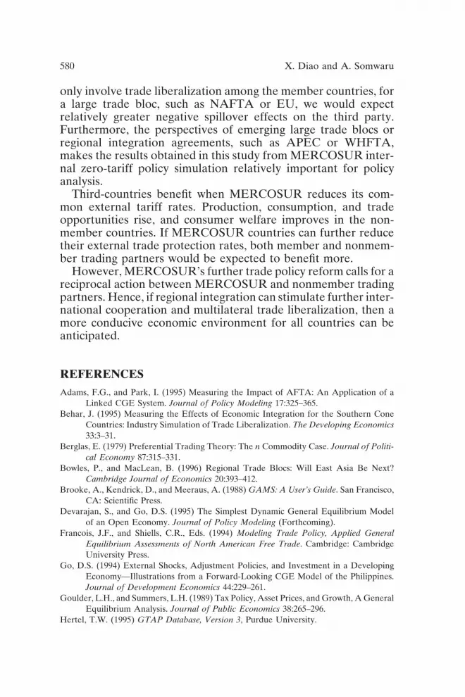
Table 1b: Mercosur Total Import and Export Shares by Regions (TotalImports/Exports Are 100, 1992)

USA ARG BRA CHL RWH E_U ASA ROW

Imports 25.1 4 7.4 2.7 9.7 24.1 11.1 15.9Exports 15.8 6.4 3.5 3.1 12.5 30.8 15.7 12.2

Asia, the Rest of the Western Hemisphere, and the U.S. haverelative large shares in MERCOSUR’s textile imports.

Regarding to sectoral exports, EU absorbed the largest sharesof MERCOSUR’s exports for agricultural, food processing, inter-mediate goods, and services, and is the second largest demanderfor MERCOSUR’s textile exports. MERCOSUR’s agriculturaland processing food products shipped to EU account for 45.3and 43.4 percent of MERCOSUR’s total exports in the respectcommodities.

Turning into intraregional trade in MERCOSUR, this can onlybe partially captured by the trade between Argentine and Brazildue to data limitation. In aggregate terms, intraregional tradeaccounts for 11.4 and 10 percent of MERCOSUR’s total importsand exports, respectively. Shares of the intraregional trade vary bysectors, but intraregional imports of agricultural and agricultural-related goods dominate total intraregional trade in MERCOSUR,with the highest share of 55 percent.

Even though Argentina and Brazil started their tariff reformsbefore the establishment of MERCOSUR, their 1992s tariff levelswere still high compared with other regions recognized in themodel. In 1992, the weighted average tariff rates7 for Argentinaand Brazil were 21.3 and 19.2 percent, respectively, which are thehighest two among the eight regions.

Following the formation of MERCOSUR, two important poli-cies that would affect both the member countries and the third-party economies are: (a) elimination of all restrictions to the freetrade among the member countries; and (b) gradual specificationof a common external tariff (CET) in the range of zero and 20percent on imports from third countries. We now turn to an analy-sis of MERCOSUR tariff reform policies from the point of view

7 Each country/region’s tariff rates on the goods imported from different countries arecalculated from GTAP database. For the average sectoral or total import tariff rates, theweights used are the values of 1992’s sectoral imports from different countries/regions.


Table 1c: Mercosur Market Shares in the World Trade (Total Exports/Importsin the World Are 100, 1992)

FoodAgriculture processing Textile Intermediates Manufacturing Services

Imports 1.7 1.3 0.7 1.9 1.7 1.8Exports 6.3 10.1 2.2 2.3 0.9 1.2

of adjustment processes of trade creation and trade diversion andwelfare gains/losses of the countries inside and outside MERCO-SUR. For this objective, we consider the following two alternativetariff reduction scenarios: under experiment EXP-1, we focus onthe trade liberalization among MERCOSUR member countriesby fully eliminating all internal tariffs of them; while under experi-ment EXP-2, we combine EXP-1 with MERCOSUR’s externalpolicy. Here, in addition to EXP-1, we harmonize MERCOSUR’sexternal tariffs for the third-country imports, with the commonexternal tariff rates lowered than the base levels are chosenroughly at the world average rates for comparable goods.

Our discussion strategy of the two experiments is as follows:we first analyze the adjustment processes of trade and productionamong MERCOSUR member countries in response to their tariffreforms; then we analyze the spillover effects of MERCOSURtariff reforms on its major nonmember trading partners. Facinga newly formed trade bloc, third countries’ interests mainly reflectconcern with potential trade and investment opportunities. Hence,our investigation will be focused on the effects on those countries’terms of trade, real exchange rates, and sectoral exports.

3B. Effects on MERCOSUR Member Countries

In general, a trade union in which tariffs are lowered or elimi-nated among its member countries creates trade opportunity forthe members. Our simulation for “zero-tariff” among MERCO-SUR member countries does capture this result. We observe thatupon impact (the first year in the simulation), Argentine andBrazilian total exports (in 1992 prices) increase by 33 and 9 per-cent, respectively, from their base-run levels (1992). When thenew steady state is approached, the aggregate exports rise by 39and 12 percent in Argentina and Brazil, respectively. In the second


Figure 1. Aggregate Investment in MERCOSUR Countries (Ratios to Base-Run Steady State). a) Argentina, b) Brazil.

experiment where not only tariffs are eliminated among the mem-ber countries, but also MERCOSUR’s external trade policy (Com-mon External Tariff) is fully implemented, aggregate exports growmore in the member countries (40 and 20 percent in year 1, and50 and 30 percent in the steady state for Argentina and Brazil,respectively).

In the conventional static approach, an increase in the membercountries’ trade is generated from a once-and-for-all reallocationof factors of production. As tariff elimination among the membercountries correct price distortion partially, current production fac-tors start to be reallocated relatively more efficiently. However,the process of resource reallocation continues over time, i.e., thenew trade policy would also affect firms’ investment decisionthrough its impact on firms’ expected returns of capital invest-ments. The intertemporal property of our model directly capturethe capital accumulation effects. The reduction of tariffs stimulatesinvestment (Figure 1a,b), and capital flows into MERCOSURcountries (under the assumption of a perfect world financial capital


Table 2: Dynamic Results of Alternative Mercosur Tariff Policies on theMember Countries (% Changes from Base-Run Steady State)

Experiment 1 Experiment 2

New steady New steadyYear 1 state Year 1 state

ArgentinaConsumer welfare

(equivalent variation) 0.318 0.171Gross domestic product 0.000 1.357 20.002 2.098Private consumption 0.792 1.996 0.255 2.099Aggregate investment 3.928 2.754 6.017 4.275Aggregate exports 32.741 39.319 39.757 50.426Aggregate imports 27.824 26.403 32.071 30.413Foreign trade deficit 10.638 214.090 15.728 221.352

BrazilConsumer welfare

(equivalent variation) 0.311 0.406Gross domestic product 0.000 0.759 0.000 2.259Private consumption 0.838 1.501 0.940 2.662Aggregate investment 1.663 1.409 5.278 4.213Aggregate exports 9.222 12.129 21.099 31.039Aggregate imports 18.000 17.820 34.366 32.427Foreign trade surplus 24.147 4.563 215.447 16.195

market). Thus, the regional economy experiences growth alongthe transition path. Of course, if MERCOSUR’s tariffs on thenonmember countries are reduced (as in EXP-2), growth of theregional economy will be more pronounced. We document partof our simulation results in Table 2, in which changes in MERCO-SUR member countries’ macroeconomic indicators are presentedfor both year 1 and the steady state. Real GDP and aggregatetrade are reported in the base year (1992) prices. Equivalentvariation is used to measure both transitional and long-term effectsof the policy on the household’s well-being (see for instance,Mercenier, 1995, for detail).

MERCOSUR significantly expands trade among its membercountries. In our simulations, increase in trade between Argentinaand Brazil is observed to be higher than the increase in twocountries’ total trade. Compared with the base year, under EXP-1,Argentine exports to Brazil increase by almost 200 percent in thefirst year and more than 200 percent in the new steady state, whileexports from Brazil to Argentina are more than doubled. As


intraregional trade grows faster than the total trade, shares ofintraregional trade with respect to MERCOSUR’s total tradeincrease significantly. Compared with the base year’s shares (inTable 1), shares of intraregional exports/imports in MERCO-SUR’s total exports and imports rise from 10 and 11 percent to30 and 33 percent in the new steady state, respectively.

When the common external tariff rates are reduced in EXP-2,MERCOSUR’s total exports rise more than that in EXP-1 (seeTable 2). However, its intraregional trade rises less than that incase of EXP-1, i.e., compared with the increases in the intra-regional trade between Argentina and Brazil observed in EXP-1,in EXP-2, exports from Argentina to Brazil and from Brazil toArgentina fall by 35 and 30 percent, respectively. The compari-son of simulation results suggest that, if MERCOSUR’s bothinternal and external trade policies are fully implemented, tradeopportunity for MERCOSUR member countries enlarges more.Increases in the member countries’ exports are not limited bythe rise in intraregional trade alone. Furthermore, the growth ofMERCOSUR’s real GDP and welfare gains are more pronounced(Table 2).

3C. Spillover Effects on Non-MERCOSUR Member Countries

Regional trading bloc will not be limited solely to the tradecreation effects between member countries, but also leads to spill-over effects over the third-party trading countries as well. Duringthe processes of gradual transition due to regional integration,the impact of initial adjustment on all parties involved may giverise to international retaliation by those stayed outside the group,but nevertheless affected. The possible counteractions may evenbe strong enough to halt the future of the bloc. In this subsection,we focus our study on the effects of MERCOSUR tariff reformson its major trading partners.

An important phenomenon observed from our simulations isthat spillover effects on third-country are quite different underthe different scenarios. We use changes in nonmember countries/regions’ consumer welfare index, total consumption, and real GDPto illustrate this (see Table 3). As most regions recognized in ourmodel are either highly aggregated or much larger than MERCO-SUR, trade between them and MERCOSUR only accounts forless than 1 percent of their total trade (except for Chile). Thus,


Table 3: Aggregate Spillover Effects of Mercosur on Third-Country TradingPartners in the New Steady States (% Changes from Base-RunSteady State)

Consumer welfare Gross domestic(EV) Total consumption product

EXP-1 EXP-2 EXP-1 EXP-2 EXP-1 EXP-2

USA 20.0043 0.0006 20.0034 0.0348 20.0014 0.0016CHL 20.0487 0.0596 20.1439 0.4389 20.1799 0.3786RWH 20.0065 0.0024 20.0074 0.0678 20.0101 0.0224E_U 20.0066 0.0064 20.0095 0.0563 20.0012 0.0075ASA 20.0032 0.0017 20.0011 0.0460 20.0046 0.0143ROW 20.0016 20.0071 0.0104 0.0125 0.0035 20.0171

the aggregate effects on the large nonmember regions due toMERCOSUR, no matter positive or negative, cannot be expectedto be large. If MERCOSUR only eliminates tariffs among itsmember countries, the aggregate effects on the other regions aremainly negative, i.e., total consumption and real GDP fall, andconsumer welfare deteriorates. If MERCOSUR eliminates inter-nal tariffs together with the reductions of its common externaltariffs on all imports from nonmember countries, consumer wel-fare improves, total consumption and real GDP rise in the newsteady state for the nonmember regions, except for the Rest ofthe World.

Reasons used to explain the difference in the spillover effectson the third country can be mainly drawn on the dynamic changesin these countries’ terms of trade. In general, a country’s termsof trade are defined as the price of its exports in terms of itsimports. Simulation results indicate that terms of trade deterioratein EXP-1 and improve in EXP-2 for all non-MERCOSUR coun-tries along the transitional paths (see Figure 2a-d). Similarly, thesecountries’ real exchange rates (price index of import goods interms of home produced commodities) appreciate in EXP-1, anddepreciate in EXP-2. Consequently, in response to the differentchanges in terms of trade and real exchange rates, firms reduceinvestment, when the terms of trade deteriorate, and increaseinvestment, when the terms of trade improve. Simulation resultsdo reveal that investments slightly fall in EXP-1 and rise in EXP-2for most nonmember regions (Figure 3a,b).


Fig

ure

2.T

erm

sof

Tra

dein

Sele

cted

Non

-Mem

ber

Reg

ions

(Rat

ios

toB

ase-

Run

Stea

dySt

ate)

.a)

USA

,b)

EU

,c)

Res

tof

Wes

tH

emis

pher

e,d)

Asi

a.


Figure 3. Aggregate Investment in Selected Non-Member Regions (Ratios toBase-Run Steady State). a) USA, b) EU.

In response to the deteriorated terms of trade in EXP-1, thirdcountries’ trade situation worsens. When tariffs among MERCO-SUR member countries are eliminated, nonmember countries’total exports fall along the transitional path.8 Among all nonmem-ber regions, the total exports decline more in the new steady statethan upon impact. Such negative effect is larger for the smallnonmember countries, such as Chile, than that for the large re-gions. Chile is experienced a decline in its total exports rangingfrom 0.14 percent upon impact to 0.55 percent in the steady state;while for the large regions, such declines rank from less than 0.05percent upon impact to 0.1 percent in the steady state.

Drastic declines in the exports to MERCOSUR are the reasonthat causes nonmember countries’ total exports to fall (Table 4a,and Figure 4a,b for U.S.). Under scenario EXP-1, exports from

8 The Rest of World total exports rise slightly (by 0.01 percent) in the first year, butfall by 0.02 percent in the new steady state.


Tab

le4a

:Sp

illov

erE

ffec

tsof

Mer

cosu

ron

Thi

rd-C

ount

ryT

otal

Exp

orts

(%C

hang

esfr

omB

ase-

Run

Stea

dySt

ate)

Exp

erim

ent

1E

xper

imen

t2

Yea

r1

Stea

dyst

ate

Yea

r1

Stea

dyst

ate

Tot

alto

Mer

c.T

otal

toM

erc.

Tot

alto

Mer

c.T

otal

toM

erc.

USA

20.

0237

28.

8232

20.

1017

29.

5381

0.15

4711

.904

42

0.04

298.

1022

CH

L2

0.14

122

7.37

072

0.55

222

9.15

220.

3208

9.84

411.

0418

7.24

25R

WH

20.

0217

26.

5350

20.

0862

28.

0585

0.11

277.

8240

0.05

934.

3334

E_U

20.

0475

29.

0253

20.

1049

210

.786

50.

1961

22.2

101

0.05

8017

.986

8A

SA2

0.00

892

13.0

058

20.

0708

214

.939

70.

1446

46.5

588

0.04

0540

.720

0R

OW

0.01

262

0.20

772

0.01

802

1.34

880.

0458

29.

4897

20.

1281

211

.667

4


Tab

le4b

:Sp

illov

erE

ffec

tsof

Mer

cosu

ron

Thi

rd-C

ount

rySe

ctor

alE

xpor

tsin

the

New

Stea

dySt

ates

(%C

hang

esfr

omba

se-r

unst

eady

stat

e)

All

non-

Mer

cosu

rco

untr

ies

U.S

.

EX

P-1

EX

P-2

EX

P-1

EX

P-2

Tot

alto

Mer

c.T

otal

To

Mer

c.T

otal

toM

erc.

Tot

alT

oM

erc.

Agr

icul

ture

20.

352

17.1

40.

192

19.2

30.

092

17.1

02

0.51

230

.44

Pro

cess

ing

food

20.

352

7.89

0.92

20.

140.

272

8.97

21.

012

12.4

4T

exti

le2

0.30

238

.96

0.55

51.8

12

0.44

239

.08

0.12

36.1

6In

term

edia

tes

20.

112

2.22

0.28

4.23

0.07

22.

860.

0315

.13

Man

ufac

turi

ng2

0.37

222

.38

0.56

31.0

92

0.32

220

.05

0.15

13.3

6Se

rvic

es0.

033.

482

0.01

25.

270.

133.

552

0.18

25.

22

Chi

leT

here

stof

the

Wes

tern

hem

isph

ere

EX

P-1

EX

P-2

EX

P-1

EX

P-2

Tot

alto

Mer

c.T

otal

To

Mer

c.T

otal

toM

erc.

Tot

alT

oM

erc.

Agr

icul

ture

0.22

212

.50

20.

652

8.50

20.

272

18.2

02

0.74

214

.02

Pro

cess

ing

food

0.00

26.

531.

7630

.06

0.04

27.

390.

9732

.55

Tex

tile

28.

522

36.5

66.

2123

.45

20.

852

38.9

91.

1253

.28

Inte

rmed

iate

s2

0.17

24.

552

0.17

28.

660.

072.

802

0.18

25.

85M

anuf

actu

ring

219

.37

235

.43

37.1

166

.48

20.

212

23.5

00.

5139

.41

Serv

ices

0.67

3.74

20.

222

5.01

0.11

3.29

20.

182

5.53

(Con

tinue

d)


Tab

le4b

:C

ontin

ued

Eur

opea

nU

nion

Asi

a

EX

P-1

EX

P-2

EX

P-1

EX

P-2

Tot

alto

Mer

c.T

otal

To

Mer

c.T

otal

toM

erc.

Tot

alT

oM

erc.

Agr

icul

ture

20.

012

16.0

22

0.69

225

.57

0.06

217

.65

20.

982

23.2

2P

roce

ssin

gfo

od0.

152

8.04

21.

092

26.7

40.

342

7.80

21.

178.

38T

exti

le2

0.13

240

.24

0.18

88.9

02

0.02

238

.29

20.

3743

.80

Inte

rmed

iate

s0.

082

4.74

0.29

38.6

60.

062

4.17

20.

0840

.10

Man

ufac

turi

ng2

0.40

222

.94

0.31

24.8

82

0.19

225

.24

0.37

72.1

5Se

rvic

es0.

093.

312

0.21

25.

640.

103.

552

0.26

25.

27

The

rest

ofth

ew

orld

EX

P-1

EX

P-2

Tot

alto

Mer

c.T

otal

To

Mer

c.

Agr

icul

ture

0.08

216

.46

20.

412

18.3

5P

roce

ssin

gfo

od0.

242

7.67

21.

272

27.7

8T

exti

le2

0.04

240

.13

20.

041.

14In

term

edia

tes

0.02

0.39

20.

352

20.8

3M

anuf

actu

ring

20.

262

20.5

00.

4933

.17

Serv

ices

0.01

3.69

0.08

24.

60


Figure 4. U.S. Total Exports and Exports to MERCOSUR (Ratios to Base-RunSteady State). a) Total Exports, b) Exports to MERCOSUR.

the nonmember regions (except for the Rest of World) to MER-COSUR fall between 6.5 percent (for EU) and 13 percent (forAsia) in the first year, and fall between 8 percent (for the Restof the Western Hemisphere) and 15 percent (for Asia) in thesteady state. To compensate for the losses in MERCOSUR mar-kets, the nonmember countries raise trade among themselves.However, increases in exports to the non-MERCOSUR countriesare smaller than the decreases in the exports to MERCOSURand, hence, we observe that total exports fall in the nonmembercountries.

In contrast, when MERCOSUR combines its common externaltariff policy with its internal trade policy, terms of trade improvefor the nonmember countries (in EXP-2). Thus, four non-MER-COSUR regions raise their aggregate exports either along thetransition or in the new steady state. Besides these four regions,U.S. and Rest of the World raise their exports during first fewyears after tariff reduction in MERCOSUR. Also, we observe that


increases in the exports from nonmember regions to MERCOSURare larger than the increases in their total exports, except for theRest of the World (Table 4a). For example, Asia and EU raisetheir exports to MERCOSUR by 47 and 22 percent, respectively,in the first year, and 41 and 18 percent, respectively, in the steadystate.

Now we turn to analyze MERCOSUR’s effects on third-coun-trys’ sectoral trade. We first calculate changes in sectoral exportsof the nonmember countries as a group, and report the results inthe first columns of Table 4b. We notice that under EXP-1, sectoralexports of all nonmember countries as a group fall between 0.1and 0.4 percent (except for services). Similar as the changes in totalexports, declines in sectoral exports are caused by the significantdecreases in the exports to MERCOSUR. Nonmember countries’exports to MERCOSUR fall as high as 40 percent for the textilesector to 2 percent for the intermediate sector in the steady state.However, if MERCOSUR implements its lower common externaltariff policy, sectoral exports of the nonmember countries risefrom 0.2 percent in agriculture to almost 1 percent in processingfoods. Increases in the exports of textile, intermediates, and manu-facturing can be explained by the increases in trade with MERCO-SUR. We observed that exports of nonmember countries to MER-COSUR significantly rise in these three sectors (52, 30, and 4percent for textile, manufacturing, and intermediates, respectively;see Table 4b). However, exports of agricultural and processingfoods of nonmember countries to MERCOSUR fall by 19 and0.14 percent, respectively. Thus, increases in nonmember coun-tries’ total exports of these two sectors are the results of tradeexpansion among themselves.

In general, the spillover effects of MERCOSUR on third-coun-try textile and manufacturing sectors are much greater than thoseon the other sectors, regardless of such effects being positive ornegative. This is due to the different levels of trade protectionrates among MERCOSUR’s sectors. The data (of 1992) indicatethat, for Argentina and Brazil, the textile and manufacturing im-port tariff rates are almost 100 percent higher than other sectors’tariff rates. Hence, when the internal tariffs are eliminated be-tween these two countries, or MERCOSUR’s common externaltariff on third-country are reduced to the world average levels,textile and manufacturing sectors are affected the most. Theseresults imply that, for the sectors with higher levels of protection


in MERCOSUR, trade-diverting effects are larger when MERCO-SUR only eliminates the internal tariffs. However, when MERCO-SUR also reduces its external tariffs, opportunities for the non-member countries to raise their exports to MERCOSUR are alsohigher in those sectors where MERCOSUR has higher levels oftrade protection.

Even though the sectoral exports fall in the nonmember coun-tries as a group under the scenario EXP-1, changes in their sectoralexports vary across regions. Table 4b also presents changes ineach nonmember region’s sectoral exports and exports to MER-COSUR and such variation can be easily observed.

4. CONCLUSIONS

In this paper we employ a dynamic global general equilibriummodel to analyze trade effects and welfare effects of MERCOSURon both its member countries and as well as on the nonmembertrading regions. The model is global in the sense that all regions,including the rest of world, are fully endogenous. The model ischaracterized by the nature of dynamics in the sense that weincorporate explicit intertemporal optimizing behavior of con-sumption, savings, and investment for the agents in each region.

The simulation results indicate that the regional trade agree-ment raises MERCOSUR member countries’ welfare by stimulat-ing their investment, production, and consumption. While tradeopportunities of the member countries increase, growth of intrare-gional trade is much faster than that of the total trade for themember countries. Furthermore, lowering MERCOSUR commonexternal tariff for third-country import allows MERCOSUR mem-ber countries to benefit more from their trade agreement thanthat if they only eliminated their internal tariffs. In this case, themember countries’ real GDP grows more and their welfare gainsmore. Also the total exports increases more, and the fast growthof their intra regional trade is accompanied by the increases intrade with their major third-country trading partners.

The negative spillover effects on the third-country trading part-ners are observed in terms of third-country’s investment, consumerwelfare, and national products, when MERCOSUR only carriesout internal trade reforms. However, as trade with MERCOSURhas a relative small share with respect to the large third-region’stotal trade, such negative effects are small. If trade agreements


only involve trade liberalization among the member countries, fora large trade bloc, such as NAFTA or EU, we would expectrelatively greater negative spillover effects on the third party.Furthermore, the perspectives of emerging large trade blocs orregional integration agreements, such as APEC or WHFTA,makes the results obtained in this study from MERCOSUR inter-nal zero-tariff policy simulation relatively important for policyanalysis.

Third-countries benefit when MERCOSUR reduces its com-mon external tariff rates. Production, consumption, and tradeopportunities rise, and consumer welfare improves in the non-member countries. If MERCOSUR countries can further reducetheir external trade protection rates, both member and nonmem-ber trading partners would be expected to benefit more.

However, MERCOSUR’s further trade policy reform calls for areciprocal action between MERCOSUR and nonmember tradingpartners. Hence, if regional integration can stimulate further inter-national cooperation and multilateral trade liberalization, then amore conducive economic environment for all countries can beanticipated.

REFERENCESAdams, F.G., and Park, I. (1995) Measuring the Impact of AFTA: An Application of a

Linked CGE System. Journal of Policy Modeling 17:325–365.Behar, J. (1995) Measuring the Effects of Economic Integration for the Southern Cone

Countries: Industry Simulation of Trade Liberalization. The Developing Economics33:3–31.

Berglas, E. (1979) Preferential Trading Theory: The n Commodity Case. Journal of Politi-cal Economy 87:315–331.

Bowles, P., and MacLean, B. (1996) Regional Trade Blocs: Will East Asia Be Next?Cambridge Journal of Economics 20:393–412.

Brooke, A., Kendrick, D., and Meeraus, A. (1988) GAMS: A User’s Guide. San Francisco,CA: Scientific Press.

Devarajan, S., and Go, D.S. (1995) The Simplest Dynamic General Equilibrium Modelof an Open Economy. Journal of Policy Modeling (Forthcoming).

Francois, J.F., and Shiells, C.R., Eds. (1994) Modeling Trade Policy, Applied GeneralEquilibrium Assessments of North American Free Trade. Cambridge: CambridgeUniversity Press.

Go, D.S. (1994) External Shocks, Adjustment Policies, and Investment in a DevelopingEconomy—Illustrations from a Forward-Looking CGE Model of the Philippines.Journal of Development Economics 44:229–261.

Goulder, L.H., and Summers, L.H. (1989) Tax Policy, Asset Prices, and Growth, A GeneralEquilibrium Analysis. Journal of Public Economics 38:265–296.

Hertel, T.W. (1995) GTAP Database, Version 3, Purdue University.


Ho, M.S. (1989) The Effects of External Linkages on U.S. Economic Growth: A DynamicGeneral Equilibrium Analysis. Unpublished Ph.D. thesis submitted to HarvardUniversity.

Lipsey, R. (1957) The Theory of Customs Unions: Trade Diversion and Welfare. Econom-ica 24:40–46.

McKibbin, W.J. (1993) Integrating Macroeconometric and Multi-Sector Computable Gen-eral Equilibrium Models. Brookings Discussion Papers in International Economics,No. 100.

Meade, J. (1955) The Theory of Customs Unions. Amsterdam: North-Holland.Mercenier, J. (1995) Can ‘1992’ Reduce Unemployment in Europe? On Welfare and

Employment Effects of Europe’s Move to a Single Market. Journal of Policy Model-ing 17:1–37.

Mercenier J., and Sampaı̈o de Souza, M. (1994) Structural Adjustment and Growth in aHighly Indebted Market Economy: Brazil. In Applied General Equilibrium Analysisand Economic Development (J. Mercenier and T. Srinivasan, Eds.). Ann Arbor:University of Michigan Press.

Mercenier J., and Michel, P. (1994) Discrete-Time Finite Horizon Approximations ofInfinite Horizon Optimization Problems with Steady-State Invariance. Economet-rica 62:635–656.

Mercenier J., and Yeldan, E. (1997) On Turkey’s Trade Policy. Is a Customs Union withEU Enough? European Economic Review 41:871–880.

Srinivasan, T. (1982) General Equilibrium Theory, Project Evaluation, and EconomicDevelopment. In The Theory and Experience of Economic Development (M. Ger-sowitz, C.F. Diaz-Alejandro, G. Ranis, and M. Rosenzweig, Eds.). London: GeorgeAllen and Unwin.

Srinivasan, T., Whalley, J., and Wooton, I. (1993) Measuring the Effects of Regionalismon Trade and Welfare. In Regional Integration and the Global Trading System (K.Anderson and R. Blackhurst, Eds.). New York: St. Martin’s Press.

Viner, J. (1950) The Customs Union Issue. New York: Carnegie Endowment for Interna-tional Peace.

Wonnacott, R., and Wonnacott, P. (1967) Is Unilateral Tariff Reduction Preferable to aCustoms Union? The Curious Case of the Missing Foreign Tariffs. American Eco-nomic Review 71:704–713.

Wooton, I. (1986) Preferential Trading Arrangements: An Investigation. Journal of Inter-national Economics 21:81–97.

APPENDIX I: EQUATIONS AND VARIABLES IN THEDYNAMIC CGE MODEL

A.1. List of Equations

The time-discrete intertemporal utility:

Un,1 5 o∞t511 1

1 1 r2t

ln(TCn,t)

TCn,t 5 PiCDbn,in,i,t.

Intertemporal value of firms:


Vn,i,1 5 o∞t51

1us5t(1 1 rs)t

[PVAn,i,tLan,in,i,t K

12an,in,i,t

2 wln,tLn,i,t 2 Fn,iPVAn,i,tI2

n,i,t

Kn,i,t

2 PIn,i,tIn,i,t]

Kn,i,t11 5 (1 2 dn,i)Kn,i,t 1 In,i,t.

Within period equations (time subscript t is skipped).

A.1.1. Armington functions:

PMMn,i 51

Yn,i3osu

smn,is,n,i 11 1 tms,n,i

1 2 tes,n,i

PXs,i212smn,i

41

(12smn,i)

PCn,i 51

Ln,i

bsmmn,in,i PMM12smmn,i

n,i 1 (1 2 bn,i)smmn,iPX12smmn,in,i ]

1

(12smmn,i)

Ms,n,i 5 Y11smn,in,i [

us,n,iPMMn,i

11 1 tms,n,i

1 2 tes,n,i2PXs,i

]smn,iMMn,i

MMn,i 5 L11smmn,in,i 3bn,i

PCn,i

PMMn,i4smmn,i

Cn,i

Dn,i 5 L11smmn,in,i 3(1 2 bn,i)

PCn,i

PXn,i4smm,ni

Cn,i.

A.1.2. Value added and output prices:

PVAn,i 51

An,iaan,in,i (1 2 an,i)12an,i

wlan,in wk12an,i

n,i

PXn,i 5 PVAn,i 1 ojPCn,jIOn,i,j.

A.1.3. Factor market equilibrium:

oian,iPVAn,iXn,i 5 wlnLBn

(1 2 an,i)PVAn,iXn,i 5 wkn,iKn,i.

A.1.4. Demand system:

CDn,i 5bn,i(Yn 2 SAVn)

PCn,i

GDn,i 5

cn,i1oiosten,s,iPXn,i

1 2 ten,s,i

Mn,s,i 1 oiostms,n,iPXs,i

1 2 es,n,i

Ms,n,i2PCn,i


INTDn,j,i 5 IOn,j,iXn,i

INVDn,i,j 5dn,i,jPIn,jIn,j

PCn,i

.

A.1.5. Household income:

Yn 5 wlnLBn 1 oidivn,i 1 rBn

divn,i 5 wkn,iKn,i 2 PVAn,iFn,iI2

n,i

Kn,i

2 PIn,iIn,i.

A.1.6. Commodity market equilibrium:

Cn,i 5 CDn,i 1 GDn,i 1 ojINVDn,i,j 1 ojINTDn,i,j.

A.1.7. Trade surplus:

FBn 5 oios1 PXn,i

1 2 ten,s,i

Mn,s,i 2PXs,i

1 2 tes,n,i

Ms,n,i2

Dynamic Difference Equations

A.1.8. Euler equation for consumption:

Yn,t11 2 SAVn,t11

Yn,t 2 SAVn,t

51 1 rt11

1 1 r

A.1.9. No-arbitrage condition for investment:

qn,i,t 5 PIn,i,t 1 2PVAn,i,tFn,iIn,i,t

Kn,i,t

(1 1 rt)qn,i,t21 5 wkn,i,t 1 PVAn,i,tFn,i1 In,i,t

Kn,i,t2

2

1 (1 2 dn,i)qn,i,t

A.1.10. Capital accumulation:

Kn,i,t11 5 (1 2 dn,i)Kn,i,t 1 In,i,t

A.1.11. Foreign assets:


Bn,t11 5 (1 1 rt)Bn,t 1 FBn,t

A.1.12. Terminal conditions (steady-state constraints):

dn,iKn,i,ss 5 In,i,ss

rssVn,i,ss 5 divn,i,ss

rssBn,ss 1 FBn,ss 5 0

rss 5 r

A.1.13. Welfare criterion (equivalent variation index):

o∞t50 1 1

1 1 r2t

ln(TC

l

n(1 1 wn)) 5 o∞t50 1 1

1 1 r2t

ln(TCnt)

where TC

l

n is base year’s total consumption. That is, welfare gainresulting from the policy change is equivalent from the perspectiveof the representative household to increasing the reference con-sumption profile by wn percent.

A.2. Glossary

A.2.1. Parameters:

gni shift parameter in Armington import function for goodi in region n

Kni shift parameter in Armington composite function for goodi in region n

Ani shift parameter in value added function for sector i inregion n

Anik shift parameter in capital good production function forsector i in region n

bni share parameter in household demand function for goodi in region n

cni share parameter in government demand function for goodi in region n

ani share parameter in value added function of sector i for laborin region n

usni share parameter in Armington import function for goodi in region n imported from s

bni share parameter in Armington function for compositegood i imported by region n


dnij share parameter in capital good production function forinput i in sector j and region n

smni elasticity of substitution in Armington import function forgood i in region n

smmni elasticity of substitution in Armington composite functionfor good i in region n

IOnij input-output coefficient for good i used in sector j andregion n

r rate of consumer time preferencedni capital depreciation rate in sector i region nwni a constant in capital adjustment function in sector i

A.2.2. Exogenous variables:

LBnt labor supply in region ntmsnit tariff rate for good i imported by region n from region stensit export tax rate for good i in region n exporting to region s

A.2.3. Endogenous variables:

PMMnit composite import price for good i in region nPXnit producer price for good i in region nPCnit composite good price for good i in region nPVAnit price of value added for good i in region nPInit unit price of investment quantity in sector i region nqnit shadow price of capital in sector i region ndivnit dividend in sector i region nwlnt wage in region nwknit marginal product of capital in sector i region nrt world interest rateXnit output of good i in region nCnit total absorption of composite good i in region nDnit own good i in region nMnsit trade flow of good i exported from region n to the

destination region sMMnit composite import good i in region nTCnt household aggregate consumption in region nCDnit household demand for composite good i in region nGDnit government demand for composite good i in region nINVDnjit investment demand for composite good j in sector i

region n


INTDnjit intermediate demand for composite good j in sector iregion n

Ynt household income in region nSAVnt household savings in region nKnit capital stock in sector i region nInit investment quantity in sector i region nFBnt trade surplus of region nBnt foreign assets in region n

APPENDIX II. DATA AND CALIBRATION STRATEGY

The GTAP database used for the calibration and the base-runare aggregated into a eight region, six sector data set. The sixaggregate production sectors/commodities are: (1) agriculture, (2)processing food, (3) textile, (4) intermediates, (5) manufacturing,and (6) services; while the eight aggregate regions include: (1) theUnited States, (2) Argentina, (3) Brazil, (4) Chile, (5) the Restof West Hemisphere countries, (6) European Union, (7) all Asiancountries, and (8) the Rest of World. Due to data limitation forthe other two member countries (Uruguay and Paraguay), MER-COSUR is represented approximately by the Argentine and Bra-zilian data, which, in terms of national domestic product, comprises97 percent of the total MERCOSUR’s economy. All regions,including the ROW, are fully specified, in the sense that produc-tion, consumption, investment, and trade decisions are the resultof well-defined optimization problems.

Calibration of the model involves specifying values for certainparameters based on outside estimates, and deriving the remainingones from restrictions posed by the equilibrium conditions. As ina static CGE model where calibration begins with the assumptionthat data obtained for the domestic economy reflect-period equi-librium, we assume that the world is evolving along a balanced(equilibrium) growth path.9 Hence, some of the assumptions onthe model calibration concerning the economy’s exogenous envi-ronment are arbitrary. However, as we are interested in deviationswith respect to a reference path in our counterfactual experiments,this specification can be regarded as robust.

9 The steady-state assumption, though questionable for most developing economies, issystematically adopted in applied intertemporal general equilibrium models due to itsextreme convenience for calibration. For example, Goulder and Summers (1989), Go(1994), and Mercenier and Yeldan (1997).


The method used to calibrate parameters or initial values ofvariables associated with intratemporal economic activities arequite standard as that used in most static CGE models. We onlysketch the more subtle dynamic calibration. Starting from thesteady-state assumption, the household time discount rate, r,equals the world interest rate, r, which can be chosen from outsidedata. GTAP database further provides both the values of eachregion’s stock of capital and the flows of capital. Thus, with thedata of the value of total investment, including capital adjustmentcosts, it is easy to calculate the initial level of total dividendpayments (div 5 value of capital flows 2 value of total investment).The aggregate steady state value of the firms, V, and hence themarginal value of capital, Tobin’s q, are then obtained, i.e., V 5div/r; q 5 V/K. The values of capital depreciation rate, d, and thecoefficient in the capital adjustment costs, w, have to be chosenconsistently with the steady-state condition. We can first eitherchoose d or w and then calculate the other one from the steady-state equations presented in Section 2. If w is chosen first, then dis calculated from the following equation derived from the steady-state conditions:

d 5q

2Pw2 3rq 2 wk

Pw1 1 q

2Pw22

41⁄2

.

The quantity of total investment, I, can be determined via I 5dK. The capital adjustment costs, and the price for investment,PI, then can be easily obtained.

In a dynamic general equilibrium model the analyst is typicallyinterested in the adjustments generated in the finite time periodsin response to parametric changes of selected exogenous variables.Hence, imposition of a terminal condition becomes pertinent fora discrete time dynamic model when there are out-of-steady statetransitional paths for the endogenous variables. Since the so-calledterminal conditions are, in fact, conditions for the steady state,an ideal terminal period should be chosen when a steady state isasymptotically approached. In administering the dynamic experi-ments, two criteria can be adhered to select the “convergence”of a steady state: the first is the time horizon when 99.99 percentof the transitional life of the main variables is realized; and thesecond is the time period when all endogenous variables cease tochange by less than 0.000001 percent. However, for a large sizeglobal model, the computation ability of the software or computer


used may restrict the application of these two criteria. Implement-ing the time-aggregation techniques of Mercenier and Michel(1994) reduces required aggregate number of time periods and,hence, reduce the size of the numerical model. This method isapplied in our simulation experiments.

An Inquiry on General Equilibrium Effects of MERCOSUR—An Intertemporal World Model

Documents

Transcript of An Inquiry on General Equilibrium Effects of MERCOSUR—An Intertemporal World Model