Yale University Yale University

EliScholar – A Digital Platform for Scholarly Publishing at Yale EliScholar – A Digital Platform for Scholarly Publishing at Yale

Discussion Papers Economic Growth Center

1-1-1989

Current Account and Budget Deficits in an Intertemporal Model of Current Account and Budget Deficits in an Intertemporal Model of

Consumption and Taxation Smoothing. A Solution to the Consumption and Taxation Smoothing. A Solution to the

‘Feldsteinn-Horioka Puzzle’? ‘Feldsteinn-Horioka Puzzle’?

Nouriel Roubini

Follow this and additional works at: https://elischolar.library.yale.edu/egcenter-discussion-paper-series

Recommended Citation Recommended Citation Roubini, Nouriel, "Current Account and Budget Deficits in an Intertemporal Model of Consumption and Taxation Smoothing. A Solution to the ‘Feldsteinn-Horioka Puzzle’?" (1989). Discussion Papers. 577. https://elischolar.library.yale.edu/egcenter-discussion-paper-series/577

This Discussion Paper is brought to you for free and open access by the Economic Growth Center at EliScholar – A Digital Platform for Scholarly Publishing at Yale. It has been accepted for inclusion in Discussion Papers by an authorized administrator of EliScholar – A Digital Platform for Scholarly Publishing at Yale. For more information, please contact elischolar@yale.edu.

ECONOMIC GROWTH CENTER

YALE UNIVERSITY

Box 1987, Yale Station New Haven, Connecticut 06520

CENTER DISCUSSION PAPER NO. 569

CURRENT ACCOUNT AND BUDGET DEFICITS IN AN INTERTEMPORAL MODEL

OF CONSUMPTION AND TAXATION SMOOTHING.

A SOLUTION TO THE "FELDSTEIN-HORIOKA PUZZLE"?

Nouriel Roubini

Yale University

and

NBER

January 1989

Notes: Center Discussion Papers are preliminary materials circulated to stimulate discussion and critical comments. References in publications to Discussion Papers should be cleared with the authors to protect the tentative character of these papers.

Current Account and Budget Deficits in an Intertemporal Model of Consumption and Taxation Smoothing.

A Solution to the "Feldstein-Horioka Puzzle"?

ABSTRACT

This paper presents an infinite horizon model of consumption and

taxation " smoothing" that implies a simple relation between current

accounts, budget deficits, investment rates and transitory output

shocks. It is argued that such a model could explain the "Feldstein­

Horioka puzzle" of the apparent lack of international capital mobility.

Traditional regressions of the savings rate on the investment rate, as

performed in the literature, are shown to be incorrect tests of the

hypothesis of capital mobility because they do not control for the

independent role of budget deficits and temporary o~tput shocks in the

current account and savings equations. Empirical tests of the model for

a sample of 18 OECD countries present good evidence that international

capital markets are widely integrated and that the "Feldstein-Horioka

puzzle" might be explained by the important role of fiscal deficits in

the determination of the current account and the saving behavior.

1

1. Introduction

The relation between the current account and budget deficits in

open economies has been for a long time a central topic of open economy

macroeconomics. The traditional "absorption approach" 1 to the current

account determination was subject to criticism for the absence of

intertemporal considerations that are central in the determination of

the trade balance and the current account. The recognition of these

dynamic aspects has led to a wide literature on "the intertemporal

approach to the current account" that has significantly increased our

understanding of the process of current account determination 2 •

This intertemporal approach applies the "consumption smoothing"

idea of Modigliani, Friedman and Hall (1978) to the optimal external

borrowing problem of open economies and derives relations between the

current account and temporary versus permanent economic disturbances.

In particular, transitory shocks to public expenditures and the output

level are shown to affect the current account while permanent

disturbances are usually adjusted through movements in private

consumption that leave the current account unaffected. From a normative

point of view, this intertemporal approach suggests that countries

should finance temporary shocks through external borrowing while they

1For recent surveys of this approach see Kenen (1985) and Frenkel and Razin (1988).

2 This approach, pioneered in the studies of optimal external borrowing by Bardhan (1969), Hamada (1969) and Bruno (1976), has been developed more recently by Svennson and Razin (1981, 1983), Sachs (1981, 1982), Buiter (1981), and extended by Lucas (1982), Persson and Svensson (1985), Frenkel and Razin (1986, 1988), Stockman and svensson (1987) and Buiter (1988) among the othe~s.

2

should adjust to permanent ones.

In spite of its theoretical appeal, systematic empirical tests of

the intertemporal current account model have been very preliminary

because hampered by the necessity to distinguish correctly between

transitory and permanent components of spending and output. In fact,

a standard formulation of these models expresses the current account

as a function of temporary versus permanent components of government

spending and output leaving open the complex econometric issue of

distinguishing between these temporary and permanent components 3•

In coincidence with the development of the intertemporal approach

to the current account, the idea of "smoothing" has been fruitfully

applied to another optimization problem: the issue of the optimal

choice of taxation and deficits in the presence of distortionary

taxation. The so-called "equilibrium approach to fiscal policy",

developed by Barro (1979, 1981, 1985, 1986) for a closed economy and

recently summarized by Aschauer (1988), argues that actual tax rates

and deficit policies are a reflection of an intertemporal optimization

over a long horizon by the budgetary authorities, who choose their

policies to reduce the excess burden of taxation for any given path of

government expenditures. This "tax smoothing" hypothesis of government

budgetary policy implies that budget deficits will be the optimal

outcome of the government decision to smooth distortionary taxes in the

3 Ahmed (1986, 1987) tests a version of the intertemporal theory of the current account for the United Kingdom by considering only the optimal "consumption smoothing" part of the problem. This leads him to the complex exercise of separating public expenditures in permanent and temporary components.

4

3

presence of temporary shocks to public expenditures and output •

Empirical tests of the "tax smoothing" hypothesis depend on the correct

distinction between temporary and permanent components of public

spending 5•

The "tax smoothing" model has been derived for the case of a

closed economy and the open economy implications of the hypothesis have

not been discussed. At the same time, the "consumption smoothing" model

of the current account has taken as given exogenously the path of

public spending and taxes without analyzing the optimal borrowing

choices of a government faced with distortionary taxes.

The objective of this paper is to bridge the two approaches by

presenting a model of an open economy where the current account is

determined by the "consumption smoothing" objective of the social

planner and the budget deficit is the result of the "tax smoothing"

problem of the fiscal authority. It will be shown that the joint

consideration of the two optimization problems leads to a very simple

relation between the current account, the budget deficit and the

investment rate that can be tested empirically without recourse to

4 For a critical empirical test of the tax smoothing hypothesis see Roubini and Sachs (1988 a, b).

5 Barro (1981, 1982, 1985) and Sahasakul (1986) test the "tax smoothing" theory in a closed economy setting and have to distinguish between temporary and permanent components of spending. Some of the results of Sahasakul, however, leave the doubt that these two components might have not been correctly identified econometrically.

4

unobserved variables such as transitory expenditure shocks 6•

The approach taken in this paper might also shed some additional

light on the paradox of the lack of international capital mobility

first found by Feldstein and Horioka (1980) and Feldstein (1983) and

then confirmed in numerous other studies of the issue 7• These studies

have systematically found a lack of correlation between the current

account and the investment ratio for the OECD countries in a number of

periods (or equivalently, a very high correlation between savings rates

and investment rates) leading to the paradoxical suggestion that

8international capital mobility might be very low • However, in all

these studies, the independent (and exogenous) role of the budget

6 Razin and Svensson (1983) consider a consumption and taxation smoothing problem in a two period model and show the optimal response of the current account and the government debt to a permanent and temporary real disturbance (a productivity shock). Anderson and Young (1988) considers a similar problem in a finite horizon setting. Here, instead, we will stress the role of temporary versus permanent fiscal disturbances and derive a explicit relation between budget deficits and current accounts in an infinite horizon framework.

7 See, among ·the others, Caprio and Howard (1984), Fieleke (1982), Frankel, Dooley and Mathieson (1987), Murphy (1984), Obstfeld (1986a, 1986b), Penati and Dooley (1984), Sachs (1981, 1983), Summers (1985). See also the comments of Tobin (1983) and Westphal (1983) to Feldstein (1983) and the critical observations of Harberger (1980) on the Feldstein-Horioka puzzle.

8 As observed by Obstfeld (1986 a), among others, the substantial evidence in favor of the equalization of domestic and foreign (or on-shore and off-shore) interest rates for the industrial countries is also at odds with the idea of a large degree of capital immobility. Frankel (1985) and Frankel, Dooley and Mathieson (1986), however, argue that equalization of the returns on financial assets might not be equivalent with the integration of the markets for physical capital and interpret the high correlations between saving and investment rates as evidence of an "apparent isolation of national markets physical capital".

5

deficits, that we will derive in this paper, has been disregarded and

regressions equations have estimated only the relation between the

current account (or the savings rate) and the investment rate . The

solution of the model presented in this paper suggests, however, that

the traditional estimated current account equations might be

misspecified because they do not control for the independent role of

budget deficits (in addition to the investment rate) in determining the

current account. Estimated savings equations present the same problem

since they do not control for the effects of fiscal deficits on the

level of national savings. The "Feldstein-Horioka paradox" might then

be due to this misspecification of the equation determining the current

account (and/or the savings behavior). This observation suggests that

the hypothesis of international capital mobility can be tested by

estimating the coefficients of the investment rate and the budget

deficit in a current account equation. Alternatively, .the hypothesis

that savings are not correlated with investment rates can be tested

only after controlling for the role of fiscal deficits.

The plan of the paper is the following. Section 2 presents the

model of the intertemporal choice of the current account and the budget

deficit. Section 3 introduces investment in the model. Section 4 tests

empirically the theoretical implications of the model. Section 5

presents some conclusions.

2. The Model

Consider a small open economy producing one tradeable good and

able to borrow in the international capital markets. It is convenient

to begin the analysis from an accounting framework where the dynamic

6

budget constraints of the private and public sector are described.

The change in the external indebtedness of the private sector (Dpt

- oPt-i> is given by:

= IP - sP (1)t t

where IPt represents private investment, Qt is GDP, Tt are taxes, ct is

private consumption, r is the exogenously given world real interest

rate and (Qt - Tt - r oPt-l - Ct) are private savings. The similar

expression for the public sector budget constraint is 9:

I 9= t - (Tt

= Ig - g9 (2)t t

9 It is assumed for accounting simplicity that the government finances its budget deficits through external borrowing and does not issue domestic bonds. This simplification does not change any result of the model because in the consolidation of the budget constraint for the entire economy (equation (3) below) domestic bonds issued by the government and held by the private sector would cancel out leaving the budget constraint identical to expression (3). Including domestic bonds in the model would modify equations (1) and (2) in the following way:

oPt - oPt-1 =Ipt - (Qt -Tt -ct -r oPt-1 -r Bft-1) + Bdt - Bdt-1 (l')

(Bdt -Bdt-1>+(B\ -B\_1)=I9t+Gt+r Bt-1 -Tt =I\ -(Tt -Gt -r Bt-1> (2 ')

where (Bdt - Bdt-i> represents the domestic bond finance of the public sector der-icit and (B\ - a\_1 ) the foreign financing component.

7

Here S9t represents the current account savings of the public sector,

Gt are exhaustive public expenditures on goods and services, and (I\ -

s\) gives the overall fiscal deficit (or surplus) of the public

sector. Adding up (1) and (2) we get the change in the net external

debt for the country that is equivalent to the current account deficit:

( 3)

In other terms the current account deficit, that is equivalent to the

change in the net external indebtedness of the country, is equal to the

excess of total (private and public) investment over savings:

= (4)

Imposing the standard transversality (solvency) condition that insures

that the country has the resources to service its debt and is not

borrowing forever to pay the interest on it we get the budget

constraint of the economy where the discounted value of its future

consumption is less than or equal to its productive wealth minus

initial external debt or:

~ ct+j ( l+r) · j (5) j=O

In order to concentrate on the role of the fiscal variables investment

(both private and public) is disregarded for the moment and the time

00

8

path of output is taken as exogenously given 10

Imposing a similar solvency condition on the public sector budget

constraint (2) get that the discounted value of public expenditurewe

on goods and services must be equal to the present value of taxes minus

the initial stock of public debt:

00 (6)I: Gt+j (l+r)-j

j=O

In this economy the social planner has to solve two maximization

problems:

(a) Maximize an intertemporal social welfare function in the

consumption level subject to the overall budget constraint of the

economy ("consumption smoothing" problem).

(b) Choose an optimal path of taxes and public debt such that the

distortionary effects of income taxation are minimized ("tax smoothing"

problem.

· ·:The "consumption smoothing" problem is represented by 11

(7)Max ct+j

subject to:

00 00

( 5 I)I: ct+J· (l+r)-j S ~ (Qt+J' - Gt+J') (l+r) -j - (l+r) Dt-1 j=O J=O

10 Investment will be introduced in section 3.

11see Sachs (1982) for a presentation of this problem in the continuous time.

9

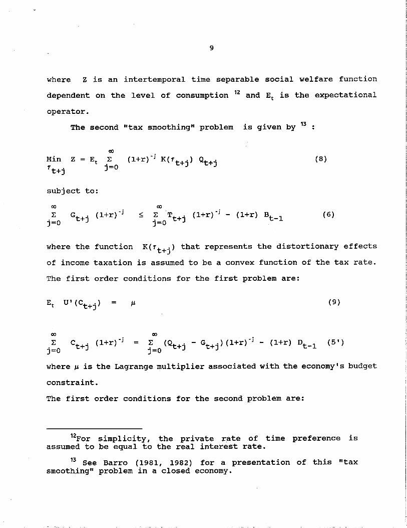
where Z is an intertemporal time separable social welfare function

12dependent on the level of consumption and Et is the expectational

operator.

The second "tax smoothing" problem is given by 13 :

(8)

subject to:

00

~ Gt+j (l+r) -j (6)

j=O

where the function K(Tt+j> that represents the distortionary effects

of income taxation is assumed to be a convex function of the tax rate.

The first order conditions for the first problem are:

= µ (9)

00 00

~ ct+j (l+r)-j = ~ (Qt+· - Gt+J·> (l+r)-j - (l+r) Dt-1 ( 5 I) j=O J=O J

whereµ is the Lagrange multiplier associated with the economy's budget

constraint.

The first order conditions for the second problem are:

12For simplicity, the private rate of time preference is assumed to be equal to the real interest rate.

13 See Barro (1981, 1982) for a presentation of this "tax smoothing" problem in a closed economy.

10

= (10)

00 00

( 6 I):E = ~ Tt+J' (l+r) ·j - (l+r) Bt-1 j=0 J=0

where¢ is the Lagrange multiplier associated with the public sector

budget constraint.

The first order conditions (9) (10) are the classic martingale

conditions for consumption and tax rates in these smoothing problems

(see Hall (1978) and Barro (1979, 1986)). In order to get explicit

solutions for our problem we assume particular functional forms for

U(Ct+j> and K(rt+j>• In particular we assume that U is a logarithmic

function of consumption and K is a quadratic function of the tax rate:

(11)log ct+j

(12)

Given assumption (11) is straightforward to show that Ct will be equal

to:

r C = (13)t

1 + r

where Wt or national wealth is equal to:

(14)= :E (Qt+J'j=0

00

11

The implications of this model are clear:

(a) The consumption path is determined by the "smoothing

principle" according to which external borrowing and lending should be

used to smooth the marginal utility of consumption over time.

(b) Condition (5') implies that the private sector internalizes

the government intertemporal budget constraint when choosing its

consumption path. In this sense "Barro-Ricardian" equivalence holds:

the optimal consumption path depends on the present value of government

expenditures but not on the path of government taxes and borrowing.

The major normative implication of the model is that a country

should finance transitory shocks through current account deficits

(external borrowing) and adjust to permanent shocks.

To highlight the implications for the current account of this

distinction between transitory and permanent shocks, it is convenient

to define the permanent values of output (QP) and government

expenditures (GP) :

00 00 1 + r (l+r) •j = ~ Qp (l+r) ·j = Qp (15)~ Qt+'

j=O J j=O r

and:

00 00 1 + r ~ Gt+J' (l+r) •j = ~ GP (l+r) ·j = GP (16)

j=O j=O r

Substituting (15) and (16) in (14) we get:

12

1 + r - (l+r) Dt-l (17)

r

By definition the current account is:

(18)

that can be rewritten as:

{18 I)

Substituting (17) in (13) and (13) in (18 1 ) we obtain:

(19)

Equation {19) is the basic equation of the intertemporal approach to

the current account. According to this equation:

{l)'If the output falls temporarily below its permanent level it

is optimal to borrow abroad in order to maintain a smooth path of

consumption; temporary negative (positive) shocks to output will

therefore cause current account deficits (surpluses) . Conversely,

permanent changes in the level of output will have no effect on the

current account.

(2) Given the output and optimal consumption path, transitory

increases in public expenditures will cause a deterioration of the

current account. Conversely permanent changes in government

expenditures will lead corresponding and equivalent reductions in

consumption (because of debt neutrality) with no effects on the current

account. In other terms, the implication of the "Barro-Ricardian

13

equivalence" for the current account is that the current account will

be invariant to the path of taxes, given the path of government

expenditure.

Equation (19) show a link between the current account and the

temporary components of public expenditure and output but it is not yet

a relation between the current account and the budget deficit. In order

to get such a relation we have to consider again the second leg of our

"smoothing model", the smoothing of taxes.

Given the quadratic assumption (12) about the costs of

distortionary taxation we can easily show that the tax rate will be

equal to:

for j = o, 1, ... , 00 (10 I)

or:

for j = 1 (10 1 ')Et 'ft+l = 'ft

In other terms the tax rate will follow a random walk without drift.

Take now the government budget constraint (6) where total taxes are

equal to the tax rate times output (Tt = .,. t Qt)

00

( 6 I)= l: Gt+J' (l+r) ·j + (l+r) Bt-1 } J=0

From (10') the best forecast of future tax rates is equal to the

current tax rate; then (6') becomes:

00 00

( 6 II)Et { I: Qt+J· (l+r) •j = I: Gt+' (l+r)·j + (l+r) Bt-1 } j=0 j=0 J

14

We can then use our definitions of permanent income and permanent

spending in (15) and (16) and substitute them in (6") to obtain:

1 + r 1 + r (20)=

r r

that implies:

r t = (21)

In other terms, smoothing of taxes will imply that the optimal tax rate

is constant and equal to the permanent value of expenditures plus the

interest payments on the debt divided by the permanent value of output

(i.e. the constant tax rate is equal to the permanent spending to

output ratio).

Then, given the government budget constraint:

(2')

and the definition of total taxes (Tt = 'ft Qt) we can substitute (21) in

(2') to obtain:

DEFt = (22)

15

where DEFt is the real budget deficit (equal to the change in the stock

of public debt held by the public). According to (22), temporary shocks

to public expenditures will lead to budget deficits because the tax

rate will be smoothed while permanent changes in expenditures will be

adjusted with higher taxes and no deficits. Similarly, temporary

negative shocks to output will result in budget deficits (because the

fixed tax rates will lead to lower tax collections following an output

fall) while permanent output shocks will leave the deficit unchanged.

We can finally combine the equilibrium solution for the current

account (equation (19)) with the solution for the budget deficit

(equation (22)) to obtain the following relation:

CAt = - DEFt (23)

or:

CAt = - DEFt (24)

Equation (24) is the crucial equation of the model and implies that,

if "consumption smoothing" and "tax smoothing" are holding, there

will be a simple one-to-one relation between current accounts and

budget deficits. In particular:

(1) A budget deficit will lead to a corresponding and equivalent

worsening of the current account because the same temporary spending

16

disturbance that leads to a budget deficit in (22) will worsen the

current account as in (19).

(2) Temporary positive (negative)° output shocks will lead to a

current account surplus (deficit). In fact, according to (22) a

temporary output shock, improves the budget balance by a fraction of

the shock ( .,. t> while it improves the current account by the full

amount of the shock. On net the current account will improve by a share

(1 - 'ft) of the output shock, for any given level of fiscal deficits.

In the particular case in which output follows a random walk, we

obtain from the definition of permanent income (equation (15)) that

permanent output will be equal to the current output (QP = Qt) so that

(24) simplifies to:

CAt = - DEFt (25)

i.e. if output follows a random walk, current account and budget

deficit will have a perfect negative relation.

Equation (24) or (25) simplifies by a large degree the problem of

testing the intertemporal theory of the current account. In the

traditional formulation (equation (19)) the current account is

expressed as a function of temporary versus permanent components of

government spending leaving open the complex econometric issue of

distinguishing between these temporary and permanent components; in

particular, systematic tests of the intertemporal current account model

have been very preliminary because hampered by the necessity to

distinguish correctly between transitory and permanent component of

17

spending 14 • Here, instead, the joint consideration of the two smoothing

problems allows to derive a relation between current account and budget

deficits that can be tested without any recourse to a distinction

between permanent and temporary components of expenditure 15 ; this

because the underlying, and unobserved temporary shock to expenditures

that leads to an observable budget deficit will also lead to a current

account imbalance.

Econometric tests of equation (24) will then be joint tests of the

intertemporal model of the current account and the equilibrium approach

to fiscal policy. Rejection of equation (24) might be caused by the

failure of either one of the two hypothesis 16

3. Introducing investment

In order to simplify the analysis we disregarded the role of

capital accumulation in the previous section. We now introduce

investment in the model to see how the relation between the current

account and the budget deficit is modified by the presence of capital

14 Ahmed (1986, 1987) tests a version of the intertemporal theory of the current account for the United Kingdom by considering only the optimal "consumption smoothing" part of the problem. This leads him to the complex exercise of separating public expenditures in permanent and temporary components. Similarly, Barro (1981, 1982, 1985) and Sahasakul (1986) test the "tax smoothing" theory in a closed economy setting and have to distinguish between temporary and permanent components of spending.

15 However, the problem of distinguishing between permanent and transitory components of output remains in this approach.

16 Roubini and Sachs (1988 a, b) find strong evidence against the "tax smoothing" model in the experience of the OECD countries.

18

17formation •

In the presence of investment the consumption smoothing problem

can rewritten as:

(l+r)-j (7)

subject to:

. 00

~ ct+J· ( l+r) · j (5) j=O

(26)

= I - 6 K (27)t t

where (26) represents the production function for the tradeable good

produced in the country (labor supply is normalized to one); and (27)

defines net capital accumulation as investment minus depreciation of

capital (6 is the coefficient of geometric depreciation).

Then, the first order condition of this problem become:

= µ, (9)

(28)

00 00

~ ct+j (l+r) ·j = ; (Qt+J· - Gt+J' - It+J') (l+r) ·j - (l+r) Dt-l (5 1 •)

j=O J=O

17In this section we lump together private and public capital formation.

19

(9) replicates the consumption smoothing rule seen in the previous

section; (28) states that in each period investment should be

undertaken so as to equate the marginal product of capital with the

world cost of capital (r+6).

These first order condition lead to the same consumption function

as in (13) but now national wealth wt in (14) must be redefined as:

(14 I)=

(14') can be rewritten ih terms of permanent values of Q and G by

observing that, given the optimal investment rule (28), present and

future changes in investment do not change the present value of Wt as

expressed in (14'). Then (14') can be rewritten as:

00

(14 I I= :E { Qt+J' (Kt) - Gt+j} (l+r)-j - (l+r) Dt-1 )

j=O

and (14' ') can be expressed in terms of permanent output and spending

as in (17).

The current account is now defined as:

(18 I)

Then, combining (13), (17), (18') we can write the final expression

for current account as:

20

(19 I)

The main difference between (19') and the previous expression for the

current account is the presence of investment in addition to the

temporary shocks to output and spending. (19') implies that any change

in investment will be fully financed through a current account deficit.

Combining this solution for the current account with the solution

for the budget deficit derived from the "tax smoothing" problem

18(equation (22)) , we finally get:

(29)

The main difference between equation (29) and (24) is the presence of

the investment variable among the determinants of the current account.

As in the case the budget deficit, the investment rate has a one-to­

one negative effect on the current account, i.e. investment shocks are

financed through capital inflows.

Equation (29) is important because it highlights the potential

shortcomings of the empirical studies of the degree of international

capital mobility following the seminal contributions of Feldstein and

18 The tax smoothing problem is not modified in the presence of investment.

21

Horioka (1980) and Feldstein (1983). In all these studies 19 , the

independent role of the budget deficits has been disregarded and

regressions equations have estimated only the relation between the

current account (as a share of GDP) and the investment rate (as a share

of GDP). These studies have systematically found a lack of correlation

between the current account and the investment ratio for the OECD

countries in a number of periods. Equation (29), however, suggest that

the traditional specification of the estimated equation might be

misspecified because it does not control for the independent role of

budget deficits (in addition to the investment rate) in determining the

current account. The "Feldstein-Horioka puzzle" might then due to this

misspecification of the equation determining the current account. In

fact, equation (29) suggest that the hypothesis of international

capital mobility can be tested by estimating the coefficients of the

investment rate and the budget deficit in a current account equation.

An alternative way to test the theory is to derive a saving

equation and show that, in the presence of international capital

mobility, saving rates are uncorrelated with the investment rate. This

approach, rather than the estimation of a current account equation, has

been preferred (starting from the contributions of Feldstein and

Horioka) by most studies of the capital mobility puzzle 20 • However, the

19 See, among the others, Caprio and Howard (1984), Fieleke (1982), Frankel, Dooley and Mathieson (1987), Murphy (1984), Obstfeld (1985, 1986), Penati and Dooley (1984), Sachs (1981, 1983), Summers (1985).

20 See, for example, Caprio and Howard (1984), Fieleke (1982), Frankel, Dooley and Mathieson (1987) , Murphy (1984) , Obstfeld (1985, 1986), Penati and Dooley (1984), Summers (1985).

22

model presented in this paper suggests that the standard savings

equations used in these studies might be misspecified as well. To show

this point, one can derive the savings equation implied by the model

above. We know that national savings are equal to investment plus the

current account:

(30)

Then, combining (29) with (30) we obtain that:

- DEFt + (31)

Equation (30) implies that total savings are a negative function of

the budget deficit and a positive function of transitory shocks to

output. In particular, budget deficits have a one-to-one negative

effect on total savings or, in other terms, that private savings (sPt)

are solely a function of transitory output shocks, i.e.:

5Pt

= (32)

where private savings are by definition:

(33)

It then follows that, the relation between national savings and

investment should be zero only after we control for the effects on

23

savings of budget deficits and temporary output shocks. Equation (31)

then suggests that traditional test of the capital mobility hypothesis

might be misspecified because they simply regress the savings rate on

the investment rate only without controlling for the fiscal and

cyclical determinants of the savings rate. The equation also suggests

that an alternative test is to regress the savings rate on the budget

deficit, the temporary components of output and the investment rate:

(34)

Then the null hypothesis of "smoothing" and capital mobility implies

that:

i.e. the coefficient on the investment rate should be equal to zero

only after having controlled for the ~ffects of budget deficits and

transitory output. Alternatively, the model might be tested, under the

maintained assumption of tax smoothing, by regressing private savings

on transitory output and investment:

5P = (35)t

Then the null hypothesis of "smoothing" and capital mobility implies

that:

= oa 1

24

i.e. private savings should not be affected by the investment rate.

4. Empirical Tests

In this section we will test the theoretical results obtained in

the previous sections. We will first start with the estimation of

current account equations like (29) and then move to the estimation of

savings equations like (31).

As seen in the previous section, equation (29) suggests that one

should regress current account equations on measures of budget

deficits, investment rate and transitory output. In particular, the

joint hypothesis of "consumption smoothing", "tax smoothing" and

"international capital mobility" implies that the estimated

coefficients of these two variables should be equal to minus one in the

estimated equations.

To begin with, current account equations are regressed on the

investment rate and the budget deficits disregarding the role of

transitory shocks to output. Given the wide empirical evidence on the

existence of unit roots in output and GNP 21 , the estimation of equation

(29) without a measure. of transitory output is correct (under the

random walk hypothesis output shock are all permanent and the

transitory output term in equation (29) disappears).

21 See Nelson and Plosser (1982), Campbell and Mankiw (1987, 1988), Cochrane (1988), Mankiw and Shapiro (1985) for some tests of unit roots in GNP.

25

Table 1 present the results of regressions of the current account

to GDP ratio on the budget deficit to GDP ratio and the investment to

GDP ratio for 18 OECD countries in the 1960-1985 period. Some

observations on the data used in the regressions are useful before the

discussion of the results. First, as derived in the theoretical part

of the paper, the correct measure of deficit to be used in the

regressions is the real inflation adjusted budget deficit that is

equivalent to the change in the net debt of the public sector. Data on

net debt for the OECD countries have been obtained from the OECD for

limited periods of time (for most of the 18 countries considered the

data go back only to 1970 .and are available since the early 1960s for

only eight countries). The sample period of the regressions in table

1 is therefore limited by the availability of the figures for the

public sector net debt. Second, the investment to GDP ratio used in the

regressions includes the fixed capital formation and the change in

inventories, i.e. inventories are considered a form of investment.

We can now discuss the results of the regressions presented in

table 1. In 12 out of the 18 countries considered, the coefficient on

the deficit variable has the right sign (negative) and is significant:

budget deficits lead to a current account worsening. Also, the

coefficient on the investment ratio has the right sign and is

significant in 13 out of 18 countries: increases in investment ratios

cause current account deficits. One can also observe that in 11

countries both variables are significant, i.e. the sample of 18

countries can be almost precisely divided between countries in which

the model works better (both variables are significant) and countries

26

in which the theory does not work at all (both variables are

insignificant) . However, even in the group of countries where the

explanatory variables are significant, the estimates of the

coefficients on the deficits and investment are almost always different

from the theoretical value of minus one. The exceptions are Italy,

Norway, Ireland, Greece and Spain where the coefficient on the

investment ratio is not significantly different from minus one. In no

country, however, the coefficient on the budget deficit variable gets

close to the theoretical value of minus one.

If one compares these results with previous tests of

22"international capital mobility" for the OECD countries , one

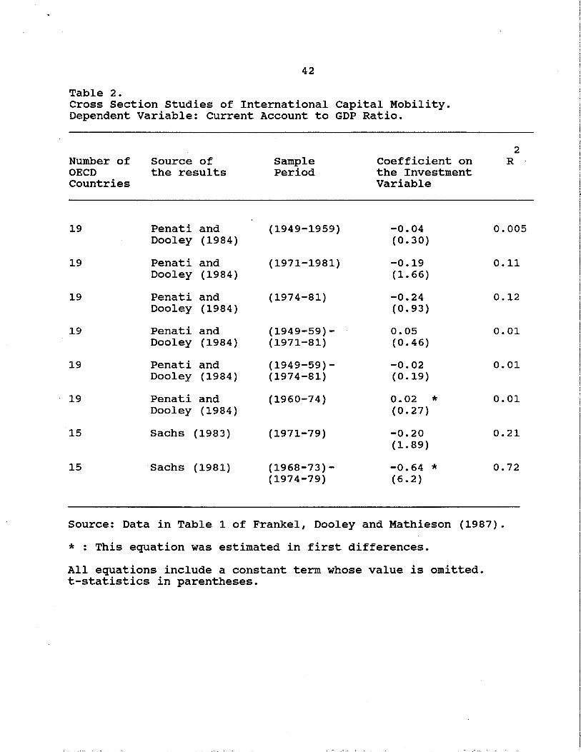
observes some striking differences. Table 2 summarizes the results of

previous studies on the relation between the current account and the

investment rate for the OECD countries. As the table shows Penati and

Dooley (1984), Frankel, Dooley and Mathieson (1987) found no relation

between current accounts and investment rates for the OECD countries

while Sachs (1981, 1983) finds a weak and almost not significant

relation. our results in Table 1, instead show a strongly negative and

significant relation for most of the countries in the sample and

suggest that international capital mobility might be much higher than

assumed on the basis of the previous studies of this issue.

How to reconcile the differences in results between table 1 and

table 2? There are two main explanations:

22 See Feldstein and Horioka (1980), Feldstein (1983), Sachs (1981, 1983), Penati and Dooley (1984), Frankel, Dooley and Mathieson (1987) for example.

27

1) Many of the previous studies considered only cross-section

regressions for a set of OECD countries while table 1 presents single

23country time series regressions • This means that previous studies

mixed in the same regressions countries for which the theory appears

to work with countries in which the theory is not supported reducing

therefore the fitness of the regressions. If one considers that

countries might differ in their degree of capital mobility (either

because of capital controls and/or other capital markets imperfections)

cross-section studies will bias downward the degree of capital mobility

for the entire sample. The time series approach followed in table 1,

instead, allows to estimate for each country separately the degree of

capital mobility.

2) All the previous studies have disregarded the separate and

independent role of budget deficits in affecting the current account

in addition to the investment rate. In this sense, previously estimated

equati~ns were misspecified in that the role of fiscal deficit was not

considered. This might have been an independent cause of the weak

relation between current account and investment rate. This explanation

is supported by the results of table 3 where the current account is

regressed on the investment rate only , the equation traditionally

estimated in the literature. Compared to the results in table 1 where

the investment variable was significant in 13 countries, in table 3

this variable is significant only in 5 countries. In other 8 countries

The main cross-section studies are those by Feldstein and Horioka (1980), Feldstein (1983), Fieleke (1982), Penati and Dooley (1984), Murphy (1984), Caprio and Howard (1985), Summers (1985) and Frankel Dooley and Mathieson (1986).

23

28

(U.S., Japan, Germany, France, Italy, Belgium, Sweden and Spain) the

investment variable does not appear as significant in the simple

bivariate (and incorrectly specified) regressions of table 3 while is

significant in the table 1 regressions that include the fiscal deficit.

This means that disregarding the role of budget deficits creates a

serious specification error and significantly bias downward the

through the exclusiveestimates of capital mobility obtained

consideration of investment rates.

The above results suggest that the lack of international capital

mobility obtained in previous studies of the issue might be seriously

biased by the cross-section technique used and the incorrect exclusion

of the fiscal variable from the current account equation.

The results obtained here, while being consistent with the

mobility than previouslyhypothesis of greater degree of capital

thought do not, however, completely confirm the joint hypothesis of

"consumption smoothing", "taxation smoothing" and "international

capital mobility". In particular, the theory does not work for a number

both explanatoryof countries and, even in the countries where

variables are significant, the estimated coefficients diverge from

their theoretically expected values. Which one of the three components

of the joint hypothesis is the source of these results?

One might suspect that the "tax smoothing" hypothesis is the weak

link in the model. Barro (1979, 1985, 1986) has found evidence in favor

of the tax smoothing model for the United States and the United Kingdom

but the tax smoothing model has been substantially rejected for most

of the other OECD countries by Roubini and Sachs (1988 a, 1988 b). One

29

can also observe that, while the investment variable is not

significantly different from its theoretical value in a number of

countries (Italy, Norway, Ireland, Greece and Spain) and very large in

many others, only one country (Spain) shows a coefficient of the

deficit variable close to the theoretical value of minus one.

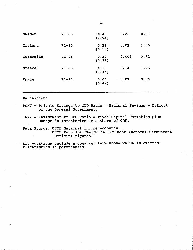
We can now move to the estimates of the savings equation. As shown

in the previous section, under the joint hypothesis of consumption and

taxation smoothing and international capital mobility, national savings

should be related only to the budget deficit and the transitory

components of output with no additional effect of the investment rate

(see equation (34)). Alternatively, and equivalently, private savings

should be only a function of transitory shocks to output with no role

of the investment rate (equation (35)). As discussed in the previous

section, simple bivariate regressions of national savings on the

investment rate, as usually performed in the literature, are not

correct tests of the hypothesis of international capital mobility

because they do not control for the effects on savings of fiscal

deficits and temporary output shocks. In this sense the high and

positive correlations between total savings and investment rates found

in the literature do not provide evidence for the absence of capital

mobility.

We will start the empirical test of the savings equation by

regressing the private saving rate (as a share of GDP) on the

30

investment rate (as a share of GDP) 24 This is the specification

suggested by equation (35) where the theoretical restriction of a minus

one coefficient on the budget deficit in the saving equation (see

equation (34)) is imposed 25 • Under the null hypothesis, we expect that

investment rate is not correlated with the savings rate. Table 4

presents the results of the regressions of the private saving rate on

the investment rate for 18 OECD countries. The results of the table

strongly confirm the hypothesis of no correlation between private

savings and investment rates: in 13 out of 18 countries the coefficient

on the investments rate is not significant and/or has a negative sign.

Only in 5 countries in the sample (Japan, Germany, France, Austria,

Norway) there is a statistically significant positive correlation

between private savings and investment. Moreover, even in the 5

countries where a statistically significant correlation is found the

estimated coefficient on the investment rate is significantly below

minus one (usually in the -0.30 to -0.40 range 26), i.e. the estimated

coefficient is much smaller (in absolute value) than the one found in

the numerous studies on the degree of international capital immobility.

These results suggest that the degree of international capital mobility

might be much larger than the one implied by previous studies and that

the "Feldstein-Horioka puzzle" might be the partial result of an

~ As explained above in the discussion of the current account equation, we disregard for the moment the role of transitory output shocks in the saving equation.

25 We will test below whether this restriction is confirmed by the data.

26 France is the only exception with a coefficient of -0.70.

31

incorrect specification of the savings equation. Once we control for

the role of budget deficits, the correlation between savings and

investment disappears in most of the OECD countries considered in our

sample.

The regressions in table 4 have imposed the theoretical

restriction of a minus one coefficient on the deficit variable in the

savings equation instead of testing it • Is such a restriction

warranted ? We can test this restriction by estimating directly

equation (34) that relates total savings to the budget deficit rather

than equation (35) that imposes a priori the above restriction.

The results of the regressions of total savings on the budget

deficit are presented in table 5. As shown in the table, in 16 out of

the 18 countries, the deficit variable has the correct negative sign

and is significant (the only exceptions being the U.K. and Australia

where the sign is correct but not statistically significant at the 5%

confidence level). Also, in 10 out of the 16 countries with a

significant coefficient, the estimated of the fiscal deficit

coefficient is not statistically different from its theoretical value

of minus one. In the other 6 countries, the estimate significantly

differs from the one implied by the maintained hypothesis. These

results then provide support for the restriction imposed in equation

(35) and the saving equation tested in table 4 only for over half of

countries in the sample.

The results in table 5 then suggests that we should estimate a

saving function as in equation (34) where the restriction- on the

deficit variable is not imposed a priori and the assumed zero effect

32

of investment is tested explicitly as well. Table 6 present the results

of the regressions of the total savings rate on the budget deficit and

the investment rate. The results in table 6 can be summarized as

following:

(a) in 12 out of 18 countries the deficit variable is significant

and has the correct negative sign; in the other 6 countries the sign

is correct but statistically not significant at the 5% confidence

level.

(b) In all the countries, with the exception of Spain, the

coefficient on the deficit variable is statistically different from its

theoretical value of minus one.

(c) The investment variable enters significantly in the savings

in 11 countries out of 18 even after controlling for the effects of

fiscal deficits.

(d) However, only in 5 countries (Italy, Norway, Ireland, Greece

and Spain) the coefficient on the investment rate is close to positive

27 one (the case of "capital immobility") • In the other countries the

.coefficient is either insignificant (7 countries) or significant but

much smaller than unity (6 countries) suggesting a large degree of

capital mobility 28

27 With the exception of Norway, these are also the OECD countries in the sample with the highest degree of capital controls.

28 It should be remembered that studies in the Feldstein­Horioka tradition have usually found correlation coefficients between savings and investment rates above 0.80. See, for example, Caprio and Howard (1984), Frankel, Dooley and Mathieson (1987), Murphy (1984), Obstfeld (1985, 1986), Penati and Dooley (1984), Summers (1985).

33

The implications of the results in table 6 are twofold. On one

side, they confirm the hypothesis of a large degree of capital mobility

for most OECD countries and contrast with earlier results in the

literature about a low degree of international mobility of capital. On

the other side, the results are partially at odds with those found in

table 4 where a much smaller number of countries showed a positive

relation between the private savings rate and the investment rate

(evidence of a very high degree of capital mobility) • Also, the large

negative coefficients on the deficit variable found in table 4 are not

replicated in table 6 where the number of countries with a deficit

coefficient equal to the theoretical value of minus one is much

smaller.

How to explain the persistent, even if modest, effect of

investment rate on savings, residually found in table 6 ? One

explanation, that substantially rejects the optimizing and Ricardian

paradigm of the paper, is to suppose that investment rates are

negatively correlated with budget deficits, i.e. budget deficits crowd­

out investment. Under the Ricardian and tax smoothing assumption,

temporary expenditure shocks that generate fiscal deficits should have

no effect on the real interest rate and therefore on the investment

rate •.

Suppose now, instead, that budget deficits actually crowd-out

investment. In this case, fiscal deficit would on one side generate

directly a fall in national savings (public savings become negative)

and would also cause a fall in the investment rate. We would then

observe that, in correspondence with fiscal shocks, there will be a

34

positive correlation between savings and investment rates even under -

the assumption of perfect capital mobility.

This explanation stresses again · the important role of fiscal

disturbances in explaining the capital mobility puzzle and allows to

reconcile the results in table 4 with those in table 6. If budget

deficits crowd-out investment estimates of the savings equation like

(34) where savings are regressed on budget deficits and an endogenous

investment rate will bias downward the estimates of the deficit

coefficient and will show a positive correlation between investment and

saving rates even under the hypothesis of perfect capital mobility.

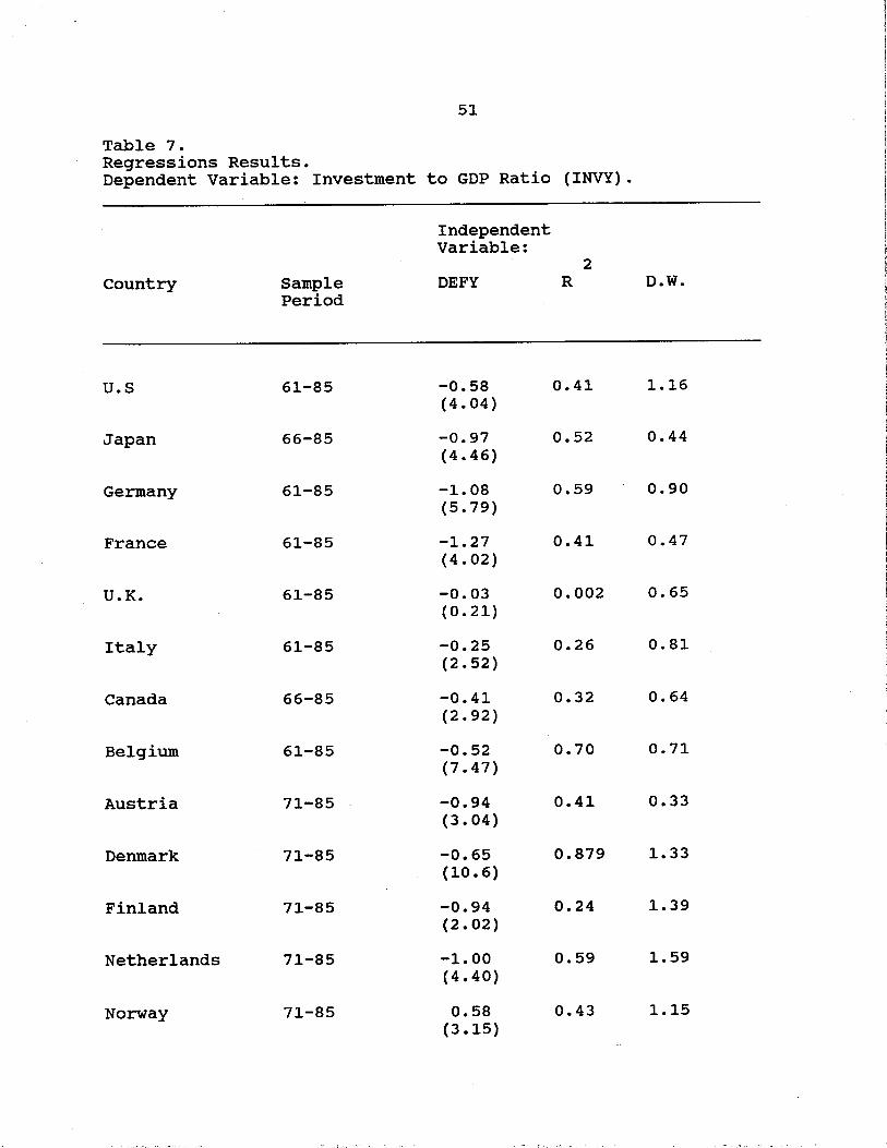
How likely is such an hypothesis of a crowding-out? While this

study cannot answer specifically such a question, it is possible to

test the hypothesis of a negative correlation between investment rate

and budget deficits. Table 7 presents the results of simple bivariate

regressions of the investment rate on the budget deficit for the 18

OECD countries in the sample. In 14 out of 18 countries table 7 shows

a strong negative and significant relation between budget deficits and

investment rates (the coefficients are usually above 0.50 (in absolute

value) and in a number of countries close to negative one).

One interpretation of this strong result is, as suggested above,

the crowding-out hypothesis. This hypothesis could explain the

significant role of the investment rate in some of the results in table

6 and the weakening of the coefficient on the budget deficits in that

table compared to the results of table 4. An alternative view could

interpret the negative correlation between budget deficits and

investment rates in terms of common underlying disturbances (such as

35

negative real shocks) that lead simultaneously to budget deficits and

falls in the investment rate. This alternative explanation would also

be consistent with the hypothesis of capital mobility and interpret the

correlation between savings and investment in terms of this common

underlying disturbances.

5. Conclusions.

This paper presented an infinite horizon model of consumption and

taxation smoothing that implies a simple relation between current

accounts, budget deficits, investment rates and transitory output

shocks. It was argued that such a model could explain the "Feldstein­

Horioka puzzle" of the apparent lack of international capital mobility.

Simple regressions of the savings rate on the investment rate were

shown to be incorrect tests of the hypothesis of capital mobility

because they do not control for the independent role of budget deficits

and temporary output shocks in the current account and savings

equations. Empirical tests of the model for a sample of 18 OECD

countries present good evidence that international capital markets are

widely integrated and that the "Feldstein-Horioka puzzle" might be

explained by the important role of fiscal deficits in the determination

of the current account and the saving behavior.

36

References

Ahmed, s. (1986), "Temporary and Permanent Government Spending in an Open Economy", Journal of Monetary Economics, 17, 197-224.

(1987) "Government Spending, The Trade Balance and the Terms of Trade in British History", Journal of Monetary Economics, 20, 195-220.

Anderson, J. and L. Young (1988) "Optimal Taxation and Debt in an Open Economy", Working Paper no.170, Boston College.

Aschauer, D.(1988), The Equilibrium Approach to Fiscal Policy, Journal of Money. Credit and Banking, February, 41-62.

Bardhan, P.K. (1967), "Optimum Foreign Borrowing", in K. Schell ed. Essays in the Theory of Economic Growth, MIT Press, Cambridge.

Barro, R. (1979), On the Determination of Public Debt, Journal of Political Economy. 87, October, 940-971.

(1981), Output Effects of Government Purchases, Journal of Political Economy. 89, December, 1086-1121.

(1985), Government Spending, Interest Rates, Prices and Budget Deficits in the United Kingdom, 1730-1918, Working Paper No.1 Rochester Center for Economic Research, March.

(1986) "U.S. Deficits since World War I", Scandinavian Journal of Economics, 88, 195-222.

Bruno, M. (1976) "The Two-Sector Open Economy and the Real Exchange Rate", American Economic Review, 66, 566-577.

Buiter, W. (1981), "Time Preference, and Intergenerational Lending and Borrowing in an Overlapping Generations Model", Journal of Political Economy, 89, no.4, 768-797.

(1988) Budgetary Policy, International and Intertemporal Trade in the Global Economy. forthcoming, North Holland.

?. IICampbell, J. and G. Mankiw (1988) "Are output Fluctuations Transitory , Quarterly Journal of Economics.

(1987) "Permanent and Transitory Components in Macroeconomic Fluctuations", American Economic Review, May 111-117.

Caprio, G. and D. Howard (1984) "Domestic Saving, Current Accounts, and International Capital Mobilityll, International Finance Discussion Papers

37

no.244, Federal Reserve Board, Washington, D.C., June.

Cochrane, J. (1988) "How Big is the Random Walk in GNP ?II Journal of• I

Political Economy.

Feldstein, M. (1983) "Domestic Saving and International Capital movements in the Long Run and the Short Run", European Economic Review, 21, 129-151.

Feldstein, M. and c. Horioka (1980), "Domestic Saving and International Capital Flows", Economic Journal, no.90, 314-329.

Fieleke, N. (1982) "National Saving and International Investment", in Saving and Government Policy, Conference Series no.25, Federal Bank of Boston, Boston.

Frankel, J. (1985) "International Capital Mobility and Crowding Out in the U.S. Economy: Imperfect Integration of Financial Markets or of Goods Markets?", in How Open is the U.S. Economy?, R. Hafer, ed., Lexington Books, Lexington.

Frankel, J., M. Dooley and D. Mathieson (1986) "International Capital Mobility in Developing Countries vs. Industrial Countries: What Do Saving-Investment Correlations Tell Us?", NBER Working Paper no. 2043, October.

Frenkel, J. and A. Razin (1986) "Fiscal Policies in the World Economy", Journal of Political Economy, 94, June, 564-594.

(1988) Fiscal Policies and the World Economy: An Intertemporal Approach, MIT Press, Cambridge, Mass.

Hall, R. (1978) "Stochastic Implications of the Life-cycle Permanent Income Hypothesis: Theory and Evidence;;, Journal of Political Economy, 86, 971-988.

Hamada, K. (1969) "Optimal Capital Accumulation by an Economy Facing an International Capital Market", Journal of Political Economy, 77, 684-697.

Kenen, P. (1985) "Macroeconomic Theory and Policy: How the Closed Economy was Opened", in R. Jones and P. Kenen, eds., Handbook of International Economics, vol.II, MIT Press, .Cambridge, Mass. ·

Lucas, R.E. Jr. (1982) "Interest Rates and Currency Prices in a Two-country World", Journal of Monetary Economics, 10, 355-359.

Mankiw, G. and M. Shapiro (1985) "Trends, Random Walks and Tests of the Permanent Income Hypothesis", Journal of Monetary Economics, 16, 165-174.

Murphy, R. (1984) "Capital Mobility and the Relationship between Savings and

38

Investment in the OECD Countries", Journal of International Money and Finance, vol.3, 327~342.

Nelson, C. and c. Plosser (1982) "Trends and Random Walks in Macroeconomic Time Series", Journal of Monetary Economics, 10, 139-162.

in the World Economy: Theory andObstfeld, M. (1986 a) "Capital Mobility Measurement", in Carnegie-Rochester Conference Series on Public Policy, Vol.24, 55-103.

(1986 b) "How Integrated Are World Capital Markets? Some New Tests", NBER Working Paper no.2075, November.

Penati, A. and M. Dooley (1984) "Current Account Imbalances and Capital Formation in Industrial Countries, 1949-1981" IMF staff Papers, vol.31, 1-24.

Persson, T. and L. Svensson (1985) "Current Account Dynamics and the Terms of Trade: Harberger-Laursen-Metzler Two Generations Later", Journal of Political Economy, 94, 43-65.

Razin, A. and L. Svensson (1983) "The Current Account and Optimal Government Debt", Journal of International Money and Finance, 2, 215-224.

(1988 a) "Political and Economics Determinants ofRoubini, N. and J. Sachs Budget Deficits in the Industrial Economies", NBER working Paper no.2682, forthcoming in European Economic Review.

(1988 b) "Government Spending and Budget Deficits in the Industrial Countries" presented at the Economic Policy panel fall 1988 meeting, October 20-21, Turin, Italy.

Sachs, J. (1981) "The Current Account and Macroeconomic Adjustment in the 1970s", Brookings Papers on Economic Activity, Vol.12, 201-268e

(1982) "The Current Account in the Macroeconomic Adjustment Process", Scandinavian Journal of Economics •

(1983) "Aspects of the Current Account Behavior of OECD Economies", in E. Classen and P. Salin, eds., Recent Issues in the Theory of Flexible Exchange Rates, Amsterdam, North Holland.

on Optimal Taxation over Time",Sahasakul, C. (1986) "The U.S. Evidence Journal of Monetary Economics, 18, November, 251-275.

Stockman, A. and L. svensson (1987) "Capital Flows, Investment and Exchange Rates", Journal of Monetary Economics, vol.19, no.2, 171-201.

Summers, L. (1985) "Tax Policy and International Competitiveness", in UniversityInternational Aspects of Fiscal Policies, J. Frenkel, ed.,

of Chicago Press.

39

Svensson, L. and A. Razin (1983) "The Terms of Trade and the Current Account: The Harberger-Laursen-Metzler Effect", Journal of Political Economy, 91, 97-125.

Tobin, J. (1983) "Comments on Domestic Saving and International Capital movements in the Long Run and the Short Run", European Economic Review, vol.21, 153-156. ·

40

Table 1. Regressions Results. Dependent Variable: current Account to GDP Ratio.

Independent Variables

Country

u.s

Japan

Germany

France

U.K.

Italy

Canada

Belgium

Austria

Denmark

Finland

Netherlands

Norway

Sample Period

61-85

66-85

61-85

61-85

61-85

61-85

66-85

61-85

71-85

71-85

71-85

71-85

71-85

DEFY

-0.61 (4.00)

-0.36 (2.61)

-0.44 (3.31)

-0.65 (3.84)

-0.14 (2.19)

-0.51 (5.83)

-0.23 (4.33)

-0.51 (4.22)

-0.37 (1.73)

-0.27 (1.43)

-0.18 (0.91)

-0.51 (1.23)

-0.45 (5.19)

INVY

-0.51 (3.06)

-0.33 (3.23)

-0.35 (3.70)

-0.11 (1. 31)

-0.57 (5 .14)

-1.00 (5.56)

-0.57 (7.78)

-0.41 (2 .10)

-0.30 (2.04)

-0.28 (0.99)

-0.62 (5.92)

-0.54 (1.69)

-0.97 (9.76)

2 R

0.42

0.38

0.39

0.47

0.54

0.71

0.78

0.53

0.27

0.21

0.77

0.19

0.96

D.W.

0.86

1.18

0.80

2.15

0.92

1.62

1.71

0.53

1.44

1.75

1.54

0.43

1.71

41

Sweden 71-85 -0.49 -0.61 0.61 0.87 (4.21) (2.71)

Ireland 71-85 -0.32 -0.91 0.69 1.42 (2.63) (4.14)

Australia 71-85 -0.15 0.31 0.09 0.72 (0.30) (0.005)

Greece 71-85 -0.25 0.90 0.36 1.65 (1.44) (0.04)

Spain 71-85 -0.89 (2.07)

-0.86 0.37 0.62 (2.59)

Definitions:

DEFY= General Government Deficit as a Share of GDP= Change in the Net Debt of the General Government as a share of GDP.

INVY = Investment to GDP Ratio= Fixed Capital Formation plus Change in Inventories as a Share of GDP.

Data Source: OECD National Income Accounts. OECD Data for Net Debt figures.

All equations include a constant term whose value is omitted. t-statistics in parentheses.

42

Table 2. Cross Section Studies of International Capital Mobility. Dependent Variable: Current Account to GDP Ratio.

Number of OECD Countries

19

19

19

19

19

19

15

15

Source: Data

Source of the results

Penati and Dooley (1984)

Penati and Dooley (1984)

Penati and Dooley (1984)

Penati and Dooley (1984)

Penati and Dooley (1984)

Penati and Dooley (1984)

Sachs (1983)

Sachs (198lj

Sample Period

(1949-1959)

(1971-1981)

(1974-81)

(1949-59)-(1971-81)

(1949-59)-(1974-81)

(1960-74)

(1971-79)

(1968-73)-(1974-79)

Coefficient on the Investment Variable

2 R

-0.04 (0.30)

0.005

-0.19 (1.66)

0.11

-0.24 (0.93)

0.12

0.05 (0.46)

0.01

-0.02 (0.19)

0.01

0.02 * (0.27)

0.01

-0.20 (1.89)

0.21

-0.64 (6.2)

* 0.72

in Table 1 of Frankel, Dooley and Mathieson (1987).

*: This equation was estimated in first differences.

All equations include a constant term whose value is omitted. t-statistics in parentheses.

43

Table 3. Regressions Results. Dependent Variable: Current Account to GDP Ratio.

Country

u.s

Japan

Germany

France

U.K.

Italy

Canada

Belgium

Austria

Denmark

Finland

Netherlands

Norway

Sample Period

61-85

66-85

61-85

61-85

61-85

61-85

66-85

61-85

71-85

71-85

71-85

71-85

71-85

Independent Variable:

INVY

-0.08 (0.47)

-0.13 (1.69)

-0.11 (1.50)

-0.09 (1.20)

-0.56 (4.67)

-0.46 (1. 77)

-0.39 I It i:;:g \ \-s'•-''-J/

0.28 (2 .10)

-0.13 (1.12)

0.10 (1.09)

-0.58 (6.32)

-0.23 (1.14)

-1.31 (10.1)

2 R

0.01

0.13

0.09

0.05

0.48

0.14

0.53

0.15

0.08

0.08

0.75

0.09

0.88

D.W.

0.31

0.70

0.84

1.32

0.75

0.42

1.11

0.53

1.03

2.03

1.38

0.54

1.10

44

Sweden 71-85 0.15 0.04 1.23 (0.76)

Ireland 71-85 -0.98 0.51 0.70 (3.69)

Australia 71-85 0.07 0.001 0.72 (0.15)

Greece 71-85 0.26 0.25 1.37 (2.08)

Spain 71-85 -0.23 (1.52)

0.15 0.66

Definition:

INVY = Investment to GDP Ratio= Fixed Capital Formation plus Change in Inventories as a Share of GDP.

Data Source: OECD National Income Accounts.

All equations include a constant term whose value is omitted. t-statistics in parentheses.

45

Table 4. Regressions Results. Dependent Variable: Private Savings to GDP Ratio (PSAV).

Country

u.s

Japan

Germany

France

U.K.

Italy

Canada

Belgium

Austria

Denmark

Finland

Netherlands

Norway

Sample Period

61-85

66-85

61-85

61-85

61-85

61-85

66-85

61-85

71-85

71-85

71-85

71-85

71-85

Independent Variable:

INVY

0.20 (1.40)

0.31 (3. 06)

0.33 (4.29)

0.70 (9.49)

0.36 (1.13)

-0.46 (1.77)

-0.18 (0.84)

-0.09 (0.72)

0.42 (2.97)

-0.26 (2.02)

0.16 (1.19)

0.16 (0.80)

0.42 (2.96)

2 R

0.08

0.34

0.44

0.78

0.05

0.14

0.04

0.02

0.40

0.23

0.10

0.05

0.40

D.W.

1.28

1.08

1.23

1.64

1.07

1.05

0.51

0.57

1.46

0.99

1.62

0.63

1.78

46

Sweden 71-85 -0.40 0.22 0.81 (1.95)

Ireland 71-85 0.21 0.02 1.56 (0~53)

Australia 71-85 0.18 0.008 0.71 (0.32)

Greece 71-85 0.26 0.14 1.96 (1.46)

Spain 71-85 0.06 0.02 0.64 (0.47)

Definition:

PSAV = Private Savings to GDP Ratio= National Savings+ Deficit of the General Government.

INVY = Investment to GDP Ratio= Fixed Capital Formation plus Change in Inventories as a Share of GDP.

Data Source: OECD National Income Accounts. OECD Data for Change in Net Debt (General Government Deficit) figures.

All equations include a constant term whose value is omitted. t-statistics in parentheses.

47

Table 5. Regressions Results. Dependent Variable: National savings to GDP Ratio (SAVY).

Country

u.s

Japan

Germany

France

U.K.

Italy

Canada

Belgium

Austria

Denmark

Finland

Netherlands

Norway

Sample Period

61-85

66-85

61-85

61-85

61-85

61-85

66-85

61-85

71-85

71-85

71-85

71-85

71-85

Independent Variable:

DEFY

-0.92 (7.08)

-1.00 (5.86)

-1.14 (7. 99)

-1.60 (5.25)

-0.15 (1.84)

-0.47 (7. 31)

-0.39 (5.29)

-0.80 (10.7)

-1.03 (3.79)

-0.74 (9.62)

-0.53 (2.22)

-0.97 (3.56)

-0.44 (7.14)

2 R D.W.

0.68 1.16

0.65 0.72

0.73 0.83

0.54 0.42

0.13 0.66

0.74 1.43

0.60 0.83

0.83 0.59

0.52 0.46

0.87 0.98

0.27 1.69

0.49 0.61

0.79 1.65

48 ·

Sweden 71-85 -0.65 0.85 0.77 (8.85)

Ireland 71-85 -0.31 (2.70)

Australia 71-85 -0.38 (0.83)

Greece 71-85 -0.94 (5.76)

Spain 71-85 -1.05 (6.23)

Definitions:

DEFY= General Government Deficit as a

Debt of the General Government

SAVY = National Savings to GDP Ratio.

0.36 1.37

0.05 0.48

0.71 1.72

0.74 0.63

Share of GDP= Change in the Net

as a share of GDP.

Data Source: OECD National Income Accounts. OECD Data for Net Debt figures.

49

Table 6. Regressions Results. Dependent Variable: National Savings to GDP Ratio (SAVY).

Independent Variables

2 Country Sample DEFY INVY R D.W.

Period

u.s 61-85 -0.67 0.43 0.75 0.94 (4.38) (2.57)

Japan 66-85 -0.36 0.66 0.89 1.18 (2.61) (6.37)

Germany 61-85 -0.47 0.62 0.91 0.80 (3.52} (6.55)

France 61-85 -0.48 0.87 0.92 1.92 (2.91) (10.5)

U.K. 61-85 -0.14 0.42 0.47 0.89 (2. 16} (3. 81)

Italy 61-85 -0.45 0.10 0.75 1.61 (5.84) (0.68)

Canada 66-85 -0.22 0.42 0.85 1.51 (3.93} (5.47)

Belgium 61-85 -0.49 0.58 0.87 0.58 (4.18} (3.06)

Austria 71-85 -0.36 0.70 0.83 1.42 (1.65) (4.71)

Denmark 71-85 -0.24 0.76 0.92 1.75 (1.22) (2.60)

Finland 71-85 -0.18 0.36 0.64 1.55 (0.93} (3.52)

Netherlands 71-85 -0.51 0.45 0.56 0.42 (1.24) (1.42)

Norway 71-85 -0.46 0.03 0.79 1.71 (5.39) (0.30)

50

Sweden 71-85 -0.49 0.38 0.88 0.88 (4.22) (1.72)

Ireland 71-85 -0.32 0.07 0.36 1.42 (2.63) (0.35)

Australia 71-85 -0.16 0.59 0.12 0.37 (0.32) (1.00)

Greece 71-85 -0.25 1.00 0.90 1.65 (1.42) (4.77)

Spain 71-85 -0.87 (2.03)

0.15 (0.46)

0.75 0.63

Definitions:

DEFY= General Government Deficit as a Share of GDP= Change in the Net Debt of the General Government as a share of GDP.

INVY = Investment to GDP Ratio= Fixed Capital Formation plus Change in Inventories as a Share of GDP.

SAVY = National Savings (Private and Public) as a Share of GDP.

Data Source: OECD National Income Accounts. OECD Data for Net Debt figures.

51

Table 7. Regressions Results. Dependent Variable: Investment to GDP Ratio (INVY).

Country

u.s

Japan

Germany

France

U.K.

Italy

Canada

Belgium

Austria

Denmark

Finland

Netherlands

Norway

Sample Period

61-85

66-85

61-85

61-85

61-85

61-85

66-85

61-85

71-85

71-85

71-85

71-85

71-85

Independent Variable:

DEFY

-0.58 (4.04)

-0.97 (4.46)

-1.08 (5.79)

-1.27 (4.02)

-0.03 (0.21)

-0.25 (2.52)

-0.41 (2.92)

-0.52 (7.47)

-0.94 (3.04)

-0.65 (10.6)

-0.94 (2.02)

-1.00 (4.40)

0.58 (3.15)

2 R

0.41

0.52

0.59

0.41

0.002

0.26

0.32

0.70

0.41

0.879

0.24

0.59

0.43

D.W.

1.16

0.44

0.90

0.47

0.65

0.81

0.64

0.71

0.33

1.33

1.39

1.59

1.15

52

Sweden 71-85 -0.41 0.65 1.46 (4.91)

Ireland 71-85 0.06 0.01 0.92 (0.39)

Australia 71-85 -0.36 0.18 3.01 (1.69)

Greece 71-85 -0.68 0.67 1.56 (5.22)

Spain 71-85 -1.17 (8.09)

0.83 0.99

Definitions:

INVY = Investment to GDP Ratio= Fixed Capital Formation plus Change in

Inventories as a Share of GDP.

DEFY= General Government Deficit as a Share of GDP= Change in the Net

Debt of the General Government as a share of GDP.

Data Source: OECD National Income Accounts. OECD Data for Net Debt figures.