,17(57(0325$/�68%67,787,21�$1'�7+(�/,48,',7<�())(&7,1�$�67,&.<�35,&(�02'(/�� �

J. Andrés(1), J.D. López-Salido(2) and J. Vallés(2)

(1) %DQFR�GH�(VSDxD��DQG�8QLYHUVLGDG�GH�9DOHQFLD�(2) %DQFR�GH�(VSDxD��5HVHDUFK�'HSDUWPHQW�

September 1999

$EVWUDFW

The liquidity effect, defined as a decrease in nominal interest rates in response to a monetary

expansion, is a major stylized fact of the business cycle. This paper seeks to understand under

what conditions such an effect can be explained in a general equilibrium model with sticky prices

and capital adjustment costs. The paper first confirms that, with separable preferences, a low

degree of intertemporal substitution in consumption is a necessary condition for the existence of

the liquidity effect. Contrary to this result, in a model with non-separable preferences and capital

accumulation it takes an implausibly high degree of intertemporal substitution to produce a

liquidity effect. The robustness of these results to alternative degrees of nominal rigidities, money

demand properties and real rigidities is also analyzed.

.H\ZRUGV� intertemporal substitution, liquidity effect, price and capital adjustment costs.

-(/�&ODVVLILFDWLRQ� E32, E43.

&RUUHVSRQGLQJ� DXWKRU� Javier Vallés, Research Department Banco de España, Alcalá 50,28014 Madrid, Spain. E-mail: valles@bde.es

� ��We owe special thanks to Larry Christiano, Jordi Galí, Robert Kollmann and Sergio Rebelofor very helpful comments and suggestions. We also thank Isabel Correia, Olivier Jeanne, AlbertMarcet, Stephanie Smitt-Grohé and Pedro Teles for insightful conversations, and seminarparticipants at Banco de Portugal, CEPR 1999 European Summer Symposium inMacroeconomics (Sintra), and the Society for Economic Dynamics 1999 Annual Meeting(Alghero) for comments. The views expressed in this paper are the authors' and do notnecessarily reflect those of the %DQFR�GH�(VSDxD.

1

��� ,QWURGXFWLRQ

The negative correlation between money growth and the nominal interest rate is one of the most

salient features of the monetary transmission mechanism. Most researchers seek to identify

positive monetary policy shocks as those innovations to money growth that exert a positive

influence on output (RXWSXW�HIIHFW), a positive one in prices (SULFH�HIIHFW) and reduce the nominal

interest rate on impact (OLTXLGLW\�HIIHFW). In fact, the confidence of the profession in this scheme is

such that failure to produce any of those effects is taken as a puzzle that calls into question the

identification procedure. Our reading of this literature is that the liquidity effect is a nominal

feature that any well-defined monetary model of the business cycle must be able to produce

under fairly general circumstances (see Christiano, Eichembaum and Evans (1998)).

Following the Lucas (1980) program for business cycle research, two broad classes of

models aim to account for those effects emphasizing different parts of the monetary policy

transmission mechanism. On the one hand, limited participation models generate a liquidity

effect by allowing restrictions in the adjustment of agents’ portfolios which break down the

intertemporal allocation of consumption (see, Fuerst (1992) and Christiano, Eichenbaum and

Evans (1997) -CEE, henceforth-). On the other hand, an alternative line of research has pointed

to the role of price rigidities and capital adjustment costs as the main factors determining the

behavior of nominal and real interest rates after a money supply shock (see, for instance, King

and Watson (1996)). Contrary to the previous one, the liquidity effect is far from granted in this

class of models since it depends on how the nominal interest rate is affected by the intertemporal

allocation of wealth.

In this paper we revisit the liquidity issue within a general equilibrium model with sticky

prices and capital accumulation in which money services provide utility to consumers. We show

that with separable preferences, a positive money shock induces a fall in interest rates if the

2

intertemporal elasticity of substitution of consumption is low enough, thus generating a large

impact response of current consumption relative to future consumption. This result has been

pointed out by Jeanne (1994) and CEE (1997) among others. In addition we show that a low

income elasticity of money demand goes in the same direction, making the liquidity effect more

likely without requiring a extremely high degree of risk aversion.

The previous results are obtained with separable preferences between consumption and

leisure. Although separable preferences have been used in many monetary models, they can be

hardly reconciled with the balanced growth properties unless some parametric restrictions are

satisfied (see Chari, Kehoe ank McGrattan (1998)). In a model with non-separable preferences

things are different since a high intertemporal substitution is needed to produce the liquidity

effect. This is so because after a monetary shock consumption and leisure move in opposite

directions inducing counteracting effects on the marginal utility of consumption that break down

out the negative link between intertemporal substitution and the impact response of the nominal

interest rate. Furthermore, if there is no capital accumulation, the model does never produce a

correctly signed liquidity effect within the range of positive risk aversion values.

In order to obtain a liquidity effect we have to bring capital accumulation in the

economy. But, in doing so the interest rate response to a positive monetary innovation is only

negative for very high values of the elasticity of intertemporal substitution. The impact

response of the nominal interest rate also depends on other parameters of the model like the

degree of nominal (price) and real (capital adjustment costs) inertia. Nevertheless, these

parameters are of secondary importance as compared with that of preferences as regards the

ability of the model to generate the liquidity effect. Then, in this kind of models a very high

intertemporal substitution is a necessary condition to generate a fall in the nominal interest

rate following a monetary shock. This is most unfortunate since it generates implausibly large

3

impact responses in output, employment and investment. Thus, we conclude that accounting

for the observed liquidity effect still remains as an unresolved puzzle for sticky price models.

The rest of the paper is organized as follows. Section 2 presents the model and defines

the equilibrium. In section 3 the model is calibrated to be compatible with a well behaved

steady state. Section 4 contains the main results of the paper. Section 5 concludes with some

additional remarks.

��� 7KH�0RGHO

Households (indexed by L) maximise their expected lifetime utility 0

~L

8 , defined as the present

discounted value of the momentary utility 8LW conditional on the information available at W ��

They choose a joint plan for consumption (&), leisure (��/) and end-of-period real balances

(0�3), where the utility of real balances stems from the transaction services provided by money:

∑∞

==

0),,(0

~

W LW/W3LW0

LW&LW8W(LR8 β [1]

Each household accumulates capital and rents it to firms at the cost =. The accumulation

of capital is driven by,

1)1(1 −−+−= LW.LW,LW. δ [2]

where is the rate of depreciation, . is capital and , investment. Adjusting capital to its desired

level is costly for the households who own it; the function of adjustment costs is chosen to

produce non-zero costs in the steady state:1

LW,LW.LW,N.

LW$&

2

2

=

φ[3]

1 These real adjustment costs are paid though the purchase of a CES basket of all the produced goods of theeconomy (see, Hairault and Portier (1993)).

4

with φ.

as the adjustment cost scale parameter for capital.

Households decide how to allocate savings between money (0), public sector debt (%)

and capital. They receive dividends from their share ( ) of profits ( ), nominal wage earnings

(3:), income derived from renting capital, interest payments from bonds and transfers (7) from

the government. The budget constraint faced by each household can be written as follows:

∑=

+−−+−+++

=++++

-

M MWLMW3LW%WULW0LW.W=W3LW/W:W3LW7W3

LW.

LW,.LW,W3LW%LW0LW&W3

1111

2

21

πω

φ

[4]

There are�-�firms indexed by M. An aggregator transforms heterogeneous goods (<M) into a

composite good (<), thus generating a demand schedule in terms of relative prices. More

formally, the problem faced by the aggregator can be stated as follows:

)1/(

1

)1(11/1;1}{

−

∑=

−−=∑=

−

θθ

θθ

θ -

M M<-<ZKHUH

-

M M<M33<M<

0D[

where �is the elasticity of substitution among the different produced goods (<M) and 3MW and 3W are

the individual and aggregate output prices respectively. Since the elasticity of substitution

between the different goods is finite and higher than one, each firm has some monopoly power

and cares about its own price relative to the aggregate one. The first order conditions of this

problem with respect to <M yield the following demand schedule:

θ/1−

=

W<

MW-<W3MW3 [5]

using this result and the zero profit condition for the aggregator yields:

)1/(11)

1()/1(

θθ

−−∑

==

-

M MW3-W3

5

The representative firm produces at a marginal cost that is increasing in aggregate output.

With flexible prices, these functional forms imply that, in steady state, firms charge a markup of

price over marginal cost equal to �� ���. The representative firm chooses a plan for production,

labour demand and capital as to maximise the expected present value of its profits:

∑∞

=

=0

00W

MWWWM 3( πρπ , where W is a pricing kernel representing the marginal utility value to the

representative household of an additional unit of profits accrued in period�W�W

WW Λβρ = .2 Profits

and technology are given by the following expressions:

<MW$&W3MW.W=W3MW/W:W3MW<MW3MWW3 −−−=π [6]

Φ−−= )1( ααMW/MW.W$MW< [7]

where�$W�describes the economy-wide state of technology at period W and� represents a fixed

cost; its existence makes it possible for a firm to earn zero profit in the long run.

The monopolistic competition environment makes it possible to incorporate sticky prices

into the model. We introduce nominal price rigidity following Rotemberg (1982), by assuming

that firms face convex costs of adjusting prices. Specifically, these costs are expressed as

follows:

W<MW3

MW3<MW$&

\

2

12

−

−= µ

φ[8]

2 Where

WΛ represents the marginal utility of consumption.

6

where φ\measures the degree to which firms dislike to deviate in their price setting

EHKDYLRU�IURP�WKH�FRQVWDQW�LQIODWLRQ�UDWH� �3

The public sector budget constraint is given by the following equation:

W7W3W%WUW%W0W0 =−−−+−− )11(1 [9]

The government derives revenue from issuing money and debt, which it uses to make transfers to

the households and to pay interest on outstanding debt. �The monetary policy can be described by

the following exogenous process for the growth of money: WW0W0 µµ=−1/ ; where represents

the steady state money growth. A shift in monetary policy takes the form of an unexpected

permanent rise in money: }{exp1 WWW µεµρµµ −= , where

Wµε is a normally distributed L�L�G. zero mean

shock with standard deviation µσ . Finally, the fiscal policy reaction function has no stochastic

component. We specify the following rule in terms of the transfers and real bonds: 1−−= W%W7W3 τ ;

where is a positive constant. Thus, transfers are determined to maintain dynamic stability of

the model. This specification is in the spirit of Leeper (1991) and guarantees a Ricardian regime

characterised by a combination of active monetary policy and passive fiscal policy.

We define a V\PPHWULF�PRQRSROLVWLF�FRPSHWLWLRQ�HTXLOLEULXP as the set of decision rules of

household L and firm M such that:

D��The set of quantities:�<MW��&LW��,LW��/LW��.LW����0LW��%LW� maximise the constrained present value

stream of utility of the representative household and the constrained present value of

profits earned by the representative firm,

E� The set of prices (3W��:W��=W��UW) clear the goods markets, the labor market and the money,

bonds and capital markets.

3 As noted by Woodford (1996) this model leads to a Phillips trade-off in which future inflation expectationsplay a crucial role in the joint dynamics of inflation and output.

7

An extensive representation of the symmetric equilibrium is obtained from the first order

conditions of both the LWK household and the MWK firm. Aggregating over L and M yields a set of

equations which define the symmetric equilibrium of the economy (see Appendix 1 for details).

Nominal variables grow at the rate . To solve the model we first write the equilibrium

equations in terms of stationary variables ( µ�; ;WW

~). Second, since an exact expression for

the equilibrium cannot be found analytically, we approximate the solution by log-linearizing the

equilibrium around the steady state. Then, following Sims (1995), we write the system of

transformed equations as: WWWW

[[ ζε µ 32110 Γ+Γ+Γ=Γ − ; where [W� is the vector of percentage

deviations of endogenous variables with respect to their steady state; µW is the monetary policy

shock, and the last term ζW �[W�(W���[W� defines expectational errors.4 The parameter matrices L

(i=0,1,2,3) are non-linear transformations of the structural parameters.

���6SHFLILFDWLRQ�RI�3UHIHUHQFHV�DQG�&DOLEUDWLRQ

����3UHIHUHQFHV

We consider three different momentary utility functions that have been extensively used in the

business cycle literature and which differ from each other in the within period separability

between consumption and leisure. Although separable preferences have been advocated in many

monetary models with money in the utility function, such preferences can hardly be reconciled

with balanced growth properties unlike non-separable preferences (King, Plosser and Rebelo

(1988)). As will become clear later, the liquidity effect depends heavily on the cross derivative

8&/ once we allow for the presence of significant substitution and income effects in the labor

supply. Thus, the following three alternative specifications of equation [1] have been considered:

4 This solution method is based on generalized eigenvalue decomposition and it extends the one described byBlanchard and Khan (1980).

8

ε

ε

κ

σσσ

σ /11

/11)1(2

/)1

1(

2

11

1

+

+−

−Γ

+

−

= +

LW/

W3

LW0

ELW

&LW8 �� [10]

)1

1()1(

2/)

11(

2

11

1 σψσσ

σ

σ

−−

−Γ

+

−

=

LW/

D

W3

LW0

ELW

&LW8 �� [11]

11

0

2/1

2

σ

ψ

σσ

−

−

Γ

+=

Y

LW/

W3

LW0

ELW

&LW8 � [12]

The usual restrictions imposed on the parameters ensure that the utility is concave, & and 0�3

are normal goods, and the interest elasticity of money demand is strictly negative.5 We can think

of the instant utility function as depending on a composite good, which is a flexible CES

aggregator of consumption and real balances. This allows us to make our exercises across

alternative preferences comparable in terms of the specification of the money demand leaving

the money demand properties unrestricted. In particular, the log-linear approximation of the first

order conditions yields the following expression for the money demand: WUUWFFWSWP εε −=− ,

where )1/()1( 2 Γ−−= σεF

, )1)(1/(1 UU

−Γ−=ε , and U is the steady state nominal interest

rate. Finally, notice that setting 2σ=Γ yields a unit income elasticity of money demand.

Equation [10] represents separable preferences as the ones recently used by CEE

(1997) where �!� characterizes risk aversion and is the labor supply elasticity. Equation

[11] is a general form of two alternative preference specifications. On the one hand, if we set

��D, we obtain the standard Cobb-Douglas preference specification (CD, henceforth). On

the other hand, if D � we obtain the preferences used by Chari, Kehoe and McGrattan (1996)

5 When 2σ=Γ we get the usual CES aggregator. The sign of Ucm equals the sign of 1- �� � (where m=(M/P)).

9

from which it is easy to compute the labor supply elasticity. The third class of utility functions

(expression [12]) is the one advocated by Greenwood, Hercowitz and Huffman (1988) (GHH,

henceforth). These preferences have two properties that may be relevant to understanding the

liquidity effect: (i) first, the elasticity of intertemporal substitution of leisure is zero; and (ii)

the number of hours worked (L) is a function of the current wage, and so there is no income

effect on labor supply. The elasticity of labor supply implied by these preferences is �� ��

(with Y>1). Finally, the parameters κ and � will be chosen so that the total hours worked by

agents are a given proportion of their time endowment.

����&DOLEUDWLRQ

This section describes the benchmark values used to compute the response of the economy to

monetary shocks. These parameters together with the steady state of the economy are reported in

Table 1. We set the discount parameter to ��������� which implies that the real interest rate is

equal to � percent per annum. The nominal interest rates, U, and the inflation rate (money growth

rate, ) were set at ���� and ����, respectively. Our benchmark value for the risk aversion

parameter ( �) is equal to �. With separable and GHH preferences the elasticity of labor supply

with respect to real wages was set equal to �. When we use non-separable preferences as in [11],

the share parameter (parameter D�or ) is set as to ensure that agents work ���percent of their

time endowment. Finally, the benchmark parameters in the money demand function are F � and

U ����. The former is essentially the long run elasticity estimate by Lucas (1988). Nevertheless,

10

following King and Watson (1996) we choose a much lower value for the interest rate

elasticity.6 Next, we consider the technology and capital adjustment cost parameter. The labor

income share ( ) is equal to ����, and the annual depreciation rate is equal to ���percent. The

capital adjustment cost parameter, φ.

, is set equal to ��. This value implies that the installation

of capital involves a ���� percent cost in terms of investment, and a capital-output ratio of ���.

These values are consistent with microeconometric estimates (see, for instance, Whited 1992).

Nevertheless, we will also analyze the effects of changing the capital adjustment costs in terms

of the liquidity effect.

We turn now to the consideration of the parameters , and φ\. The elasticity of

demand is chosen ( �� such that the markup in a flexible price economy is �� percent (say,

���). Assuming zero profits in the steady state, the previous assumption is equivalent to making

the value of �< ��� �$�N /��� �� also equal to 20 percent. Although these values are

conventional in the literature, our results do not change when a lower markup is used (say, 5

percent) as suggested by the evidence in Basu and Fernald (1997). The price adjustment cost

parameter (φ\) cannot be calibrated using steady state information. To choose a value we follow

recent estimates of the new-keynesian Phillips trade-off by Sbordone (1998). In particular, we set

φ\ ���� � ���, which implies that firms change prices every � months.7 Finally, we set ���

corresponding to the estimated value for M1 growth in the US (Cooley and Hansen (1995)).

6 This low value is consistent with a low degree of substitution in money demand over the business cycle.Moreover, the empirical evidence reported by Goldfeld and Sichel (1990) is consistent with such a value. Indeed,those authors advocated a lower value for the income elasticity. We will analyze how our results depend onsetting

F equal to 0.2 as an alternative to unit elasticity.

7 As can be seen from the previous expression, holding the time between price adjustments constant, a lowermarkup (higher ) implies a much higher cost of adjusting prices.

11

���7KH�(IIHFWV�RI�3HUPDQHQW�8QDQWLFLSDWHG�0RQH\�6XSSO\�6KRFNV

In this section we assess the role of preferences, capital accumulation and other features of our

model in shaping the response of interest rates to money shocks, or the OLTXLGLW\� HIIHFW. We

proceed step by step, first working with a version of the model with separable preferences, then

introducing non-separable preferences and finally adding capital into the model. We show that

for a given exogenous money growth rule the existence of a liquidity effect depends critically on

the interaction of these elements with the rest of the model. With the complete model we analyze

the properties of the parameterizations that generate the liquidity effect, discussing the

importance of the real and nominal rigidities and of the persistence of the money growth shock

for obtaining the liquidity effect.

�����(FRQRP\�ZLWKRXW�FDSLWDO��6HSDUDEOH�3UHIHUHQFHV

Let us consider a simple version of the model presented in section 2, where preferences are

separable as expressed by [10], and without capital, so that the production function is defined as

Φ−= − )1( αMWWMW

/$< . Figure 1A shows that positive and persistent money shocks generate a

positive and persistent response of consumption, real balances and output. Since prices are

sticky, a positive nominal shock increases nominal demand and marginal costs but lowers the

markup. Labor demand, output and consumption increase. Following the rise in real wages,

labor supply also increases, pushing the economy closer to the competitive equilibrium.

Eventually, the price level adjusts to its new level, restoring the initial reduction in the markup

and returning the economy to its steady state.

Nevertheless, these real effects occur along with a positive impact on the nominal interest

rate. This impact effect is characterized by two equilibrium equations representing the

intertemporal allocation of consumption and the demand of money balances:8

8 These are derived from expression [A1], [A3] and [A4] in Appendix 1.

12

)/(/ 11,, ++=WWFWWWWF38(U38 β [13]

−=W

WFWP U88 11/ ,, [14]

where equation [13] represents the intertemporal Euler equation of consumption, and

equation [14] determines the optimal allocation between consumption and real balances

within period (i.e. it represents a money demand equation). CEE (1997) combines

equation [13] with a cash-in-advance constraint obtaining an expression of the type:

[ ])//()( 211,1, ++++=WWWFWWWWFW

008&(U8& β . They show that the expectational term becomes a

constant (say, A) in the event that prices are set one period in advance and money growth follows

an LLG process. Under these assumptions, after a positive money growth shock, the only way to

generate a liquidity effect is through a reduction in FWW

8& . Under separability between

consumption and leisure, then βσ $&UWW

/11−= . Thus, after an increase in the money supply that

leads to a rise in Ct, the nominal interest rate will fall if and only if the risk aversion parameter is

greater than one ( �!�).

Unfortunately, this result cannot be so easily obtained once we relax some of the CEE’s

assumptions regarding the price setting and the money growth process. Nevertheless, we can still

log-linearize the above expressions [13] and [14] around the steady state to obtain:9

)( 111 WWWWWWFF(S(U −=∆− ++ σ [13a]

WUUWFFWSWP εε −=− [14a]

9 Notice that to get this expression we are also assuming that the parameter b in expressions [10]-[12] approachesto zero so real the balances disappear of [13a]. We recall that this is not a bad approximation if we calibrate themodel by looking at the average velocity for M1 in US (see Chari et al. (1996) and Kim (1998)). Nevertheless, inall the simulations we eliminate this assumption.

13

where lower case letters represent deviations from their steady state value. Solving now for the

nominal interest rate in these two expressions and assuming that money demand only responds to

movements in consumption �εU ��:10

∆

−+∆ ++= 1

11

1111 WW

F

WW

F

S(P(WU

εσεσ � [15]

For a given degree of money and price persistence the monetary shock generates an impact

increase in money and prices that is expected to continue in the future. Under these fairly general

circunstances two results follow from the above expression. The first is that, for given values of εF

and , high risk aversion (i.e. a low intertemporal elasticity of substitution (��σ�)) is needed for

the existence of the liquidity effect.

The intuition behind this result can also be cast in terms of the impact effect on the right

hand side of expression [13a], i.e. the real interest rate. After a positive money shock,

consumption rises at time W and rises further in W�� to decline from W�� onwards (see Figure 1A).

Thus, the impact effect on the real interest rate is positive and it is given by σ�=2 times the

expected increase in consumption. This increase is further reinforced by the rise in expected

inflation. A lower degree of intertemporal substitution of consumption induces a lower expected

rise in consumption from W to W��, which will eventually become negative for very large values of

σ�. Thus, this produces a substantial reduction in the real interest rate (by an amount equals to

)( 11 WWWFF( −+σ ) which, if strong enough, might compensate the increase in inflation

10 When εr is different from zero we solve forward for the nominal interest rate and obtain:

++

∆−+++

∆Σ

∞

=

=1

1

1

1

1

1

0MW

SW

(

F

MWP

W(

F

M

M

IWU

εσεδ where

1

1

1;;

1

1

−

+==

+

=

κσε

ε

κ

κσ

κδ I

F

U .

Setting εr=0 yields expression [15] that it is easier to interpret. In our simulations we will consider that εr =0.01.

14

expectations.11 The real interest rate moves to match the expected change in the marginal utility

between period W and W��. Since consumption is the only argument of marginal utility, it is the

expected change in consumption what matters for the liquidity effect. Thus, a substantial decrease

in FW��� as compared with FW� is needed to obtain a decline in the real interest rate; this is only

possible if households are willing to smooth consumption over time, i.e. if (��σ�) is low enough.

The second result is that for sufficiently low money demand elasticity with respect to

consumption (εc), the liquidity effect may also be obtained without requiring a high value for risk

aversion. In our model, money is introduced as an argument in the utility function and the short

run consumption elasticity is left free so that a low value of F favors an impact fall in the nominal

rate. The lower the income elasticity of money demand the smaller the substitution away from

bonds and thus the more likely the impact fall in the interest rate following the initial increase in

the supply of real money balances.

To put some numbers to these results, we simulate in Figure 1B the impact effect on the

nominal interest rate and real balances of a money growth shock under different values of the risk

aversion parameter. This Figure confirms the previous surmise. Thus, in sticky price models if

preferences are separable, the higher the risk aversion the more likely is the liquidity effect.

Notice that the existence of price and money growth persistence implies an implausibly large

degree of risk aversion in order to generate the liquidity effect. When the income elasticity of real

balances is less than one a lower value of the risk aversion will generate that effect.

11 In a cash-in-advance economy without capital Jeanne (1994) also gets this result.

15

�����(FRQRP\�ZLWKRXW�FDSLWDO��1RQ�6HSDUDEOH�3UHIHUHQFHV

When preferences are non-separable, things are different. In particular, expression [15] no longer

represents the interest rate response since the intertemporal allocation of consumption depends

on other features of the model. Figure 2A shows the response of the main variables in the model

to a persistent money shock. The results correspond both to Cobb-Douglas preferences and to

GHH preferences. At first glance, the impulse response functions look very similar in this

economy as compared with those in a world with separable preferences (i.e. those depicted in

Figure 1A): a positive monetary shock increases output, consumption and real balances, while

the nominal interest rate still increases on impact. Nevertheless, a closer look at the results shows

an interesting departure from the general proposition enunciated above. As the sensitivity

analysis in Figure 2B makes clear, a higher risk aversion is no longer a necessary condition for

the existence of the liquidity effect. Indeed the opposite is true.

To give some intuition for this latter result, we consider the non-separable preferences

given by expression [11], when D �. Proceeding at in the previous section, the log-linear

equation for the intertemporal consumption allocation [13] takes now the following form:

( )( ) )(11

11111 WWWWWWWWWFF((

/

/S(U −+−−

−

=∆− +++ σσψll [13b]

This expression states that the real interest rate moves as to ensure the equalization of the

marginal utility of consumption between W and W��, but now the ratio of marginal utilities not

only depends on the expected change in consumption but also on the expected response of labor

supply. As the elasticity of intertemporal substitution, (��σ�), falls both (W∆FW�� and

1+∆WW

( l become smaller and eventually negative, exerting opposite effects upon the ratio of

marginal utilities; the leisure effect dominates making the liquidity effect less rather than more

likely for given inflation expectations.

16

An additional result is that in this case the liquidity effect is never obtained for positive

values of σ�. This result also relies heavily on the fact that in a model without capital

consumption is proportional to labor (i.e.WW

F lα≈ ). Thus, for the benchmark values of the

parameters the expected increase in consumption and leisure roughly compensate each other in

expression [13b] leaving the nominal interest rate almost unchanged, for a given expected

inflation, as we move towards higher values of the risk aversion.

As noted in section 3, the CD preferences impose strong income and substitution effects

on leisure after a positive money shocks. Thus, we now analyze how allowing for a zero

intertemporal substitution effect on leisure and a zero income effect on labor supply affect our

previous result. We use the GHH preferences that imply the following (log-linear) expression for

the intertermporal consumption allocation:

( ) ( )[ ]WWWWWWWWW

(FF(S(UY ll −−−=∆−

− +++ 1111 )(1 ηση [13c]

where the steady state solution imposes ��� ���F�\��12 Whith these preferences households

smooth (WW

F lη− ) over time instead of FW�and, unlike with CD preferences, the parameter is

independent of the intertemporal substitution. The absence of an income effect on the labor

supply makes the movements in consumption and leisure roughly proportional and such

proportion is independent of the degree of intertemporal substitution. Moreover, increases in the

risk aversion (σ�) affect the nominal interest rate more significantly than in the case of CD

preferences but always in the opposite direction that required for a liquidity effect.

Since this is a most unfortunate feature of the model we may ask at this point what does it

take to obtain a proper liquidity effect in a sticky price model with non-separable preferences.

12 In general this parameter is close to one in market economies.

17

What we need is a mechanism that drives the response of labor supply and consumption

significantly apart so that the real interest rate could fall substantially on impact.

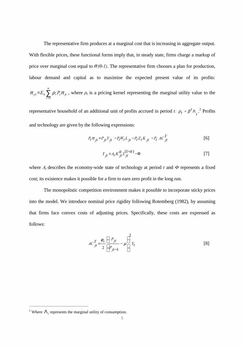
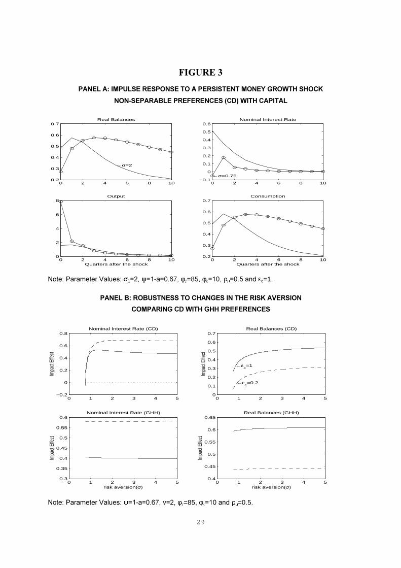
�����(FRQRP\�ZLWK�FDSLWDO��1RQ�VHSDUDEOH�3UHIHUHQFHV

Capital accumulation is a key feature of the model that is expected to have a major effect on the

way some endogenous variables respond to a monetary shock. In particular, current consumption

can be made less responsive to the money shock for a given output response, since households

devote part of their income to invest in capital goods (in addition to bonds and real balances). We

will show that in order to generate the liquidity effect the mere presence of capital is not enough,

what is needed is strong incentive to accumulate it. This can be obtained in the model previously

discussed by means of high degree of intertemporal substitution (say, 1/σ�) and low adjustment

costs of capital (φN). The reason why we need a high intertemporal substitution stems from the

fact that with low intertemporal substitution the response of consumption after a persistent

money shock is similar to that in output so that the pattern of impulse-responses resemble very

much that of an economy without capital.13

The impulse responses in Figure 3A of an economy with capital accumulation show that

the previous surmise is correct. Still, in the case of high risk aversion values there are not

incentives to save and accumulate capital, and therefore the allocation of real balances and

consumption has not undergone a significant change with respect to the model without capital.

Thus the money market equilibrium generates the same path in terms of interest rates: an

increase on impact followed by a smooth decrease over time. Nevertheless, the money shock

simulation when σ� is low generates a large substitution effect that is reflected in a huge output

and labor responses on impact but only a small change in consumption. For σ� ���� the interest

13 A similar reasoning applies to a high value of the capital adjustment costs (φN).

18

rate response generates a liquidity effect. We can explain the impact response of interest rates in

terms of the expression [13b]: if the risk aversion parameter is less than one, then there is a large

expected fall in labor after the first period that moves the current interest rates down.14

The impulse responses in Figure 3A also highlight the role of capital in this model. Since

��σ� (1/0.75) is large, consumers have the incentive to postpone consumption which, unlike the

model without capital, does not necessarily implies postponing production (and so employment)

too. On the contrary, as the real rate falls the initial jump in the expected shadow price of capital

leads to a sharp increase in the demand for investment. Since, given the existence of sticky

prices, output is demand determined the increase in investment translates into output so

increasing labor demand alongside.15 As can be seen in expression [13b], now the sharp expected

reduction in labor ( 1+∆WW

( l ) more than compensates the expected consumption increase ((W FW���

to produce a strong fall in the real interest rate. Why do households postpone consumption and

work harder today despite the fact that the real rate has fallen? The reason is that there is a new

asset, capital, which makes very profitable any additional amount of resources devoted to

accumulate it. As ��σ� gets smaller all these effects become smaller too and the economy

resembles very much the one without capital in which consumption and labor balance each other

its effect on the marginal utility of the household so leaving no room for movements in the real

interest rate.

14 In Appendix 2 we show the implications of such a risk aversion parameter in terms of the labor supplyelasticity.15 Notice that the additional output demand in period W must be entirely met by a rise in employment since .W ispredetermined.

19

To sum up, when preferences are non-separable and there is capital accumulation the liquidity

effect is more likely the smaller the risk aversion parameter, just the opposite of what happens

in an economy with separable preferences. Nevertheless the range of values for which such an

effect exists is very small and is always for risk aversion values lower than one (see Figure

3B). That generates implausibly large movements in output and labor whereas consumption

movements remain very low after a monetary shock.

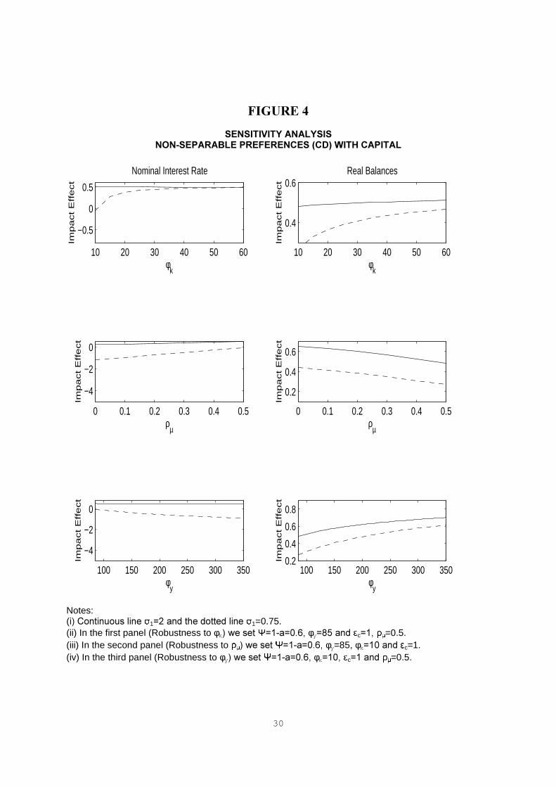
To get a more complete picture of the features shaping the initial response of the nominal

interest rate in this model, we check the robustness of our results with respect to the remaining

parameters of the model. Figure 4 depicts the results of sensitivity analyses with regard to

nominal and real rigidities as well as to the money shock persistence. Within the low risk

aversion region (dotted line) the liquidity effect is more likely the lower the adjustment cost of

capital, the lower persistence of the money growth shock and the higher the price stickiness. The

cost of adjusting capital is borne by households and the lower this cost the higher the incentive to

accumulate capital, leading to the stronger output and employment responses needed to

guarantee the liquidity effect. The impact response of the nominal interest rate is always higher,

and that of real balances lower, the higher the value of ρµ. Similarly, as expected, real balances

rise and the interest rate falls more, the higher the value of φ<, i.e. the liquidity effect is more

likely the higher the degree of price inertia. Within the region of higher risk aversion

(continuous), the sensitivity of the interest rates and real balances to this parameter is much

lower. Therefore, under non-separability and capital accumulation the risk aversion parameter is

the crucial one, as compared with those reflecting the intensity of price inertia and capital

adjustment costs, in shaping interest rate movements.

20

��� &RQFOXVLRQV

Although neither the output nor the price effects of a monetary expansion need to be preceded by

a fall in the nominal interest rate, the liquidity effect is viewed by many economists as one of the

well established empirical facts in monetary economics. General equilibrium models aimed at

representing such mechanism face the challenge of reproducing the liquidity effect along with

other business cycle features of market economies. In this paper we have discussed under what

conditions a general equilibrium model with costs of adjusting prices and capital is capable of

generating a downwards movement of the nominal rate following a positive monetary innovation.

In a world without capital and separable preferences, the logic of the intertemporal

allocation of wealth leads to the following result: it takes a low elasticity of intertemporal

substitution for the nominal rate to fall on impact. We show that it is also possible to get the same

result by reducing the income elasticity of money demand over the business cycle. This is so

because the marginal utility of consumption is just driven by the dynamics of consumption. When

preferences are not separable the previous result does not apply. Now, the impact response of

nominal interest rate is not sensitive to changes in the intertemporal substitution. The reason is

also straightforward: now consumption and labor supply movements balance each other its effect

on the marginal utility of the household so leaving no room for movements in the real interest

rate.

In an economy with non-separable preferences and capital accumulation the liquidity

effect is not achieved unless the intertemporal substitution is very high and the capital adjustment

costs are not high. In such a case, this intertemporal substitution effects leads households to

postpone consumption investing in capital and so increasing current output and labor demand by

21

an amount large enough to reduce the real interest rate by more than the expected increase in

prices.

The logic of this result can be analyzed in the light of the monetary transmission

mechanism of the simplest limited participation model. In this kind of models, restrictions on

the adjustment of consumer’s portfolios make it possible that the additional liquidity of the

system is not necessarily devoted to consumption. The additional savings must be devoted to

increase the demand of productive factors, which firms are willing to do if the interest rate

falls. In sticky price models where the marginal utility of consumption depends upon

consumption and leisure we can get a similar result imposing a strong bias towards the

intertemporal substitution and low adjustment costs of capital. Nevertheless, in this latter

model this comes at the cost of generating implausibly large impact responses in output,

employment and investment.

Finally, the impact response of the nominal interest rate also depends on other

parameters of the model like the degree of nominal (price) and real (capital adjustment costs)

inertia. Nevertheless, these parameters are of secondary importance as compared with that of

preferences as regards the ability of the model to generate the liquidity effect. Thus, we

conclude that accounting for the observed liquidity effect still remains as an unresolved

puzzle for sticky price models of the monetary transmission mechanism.

22

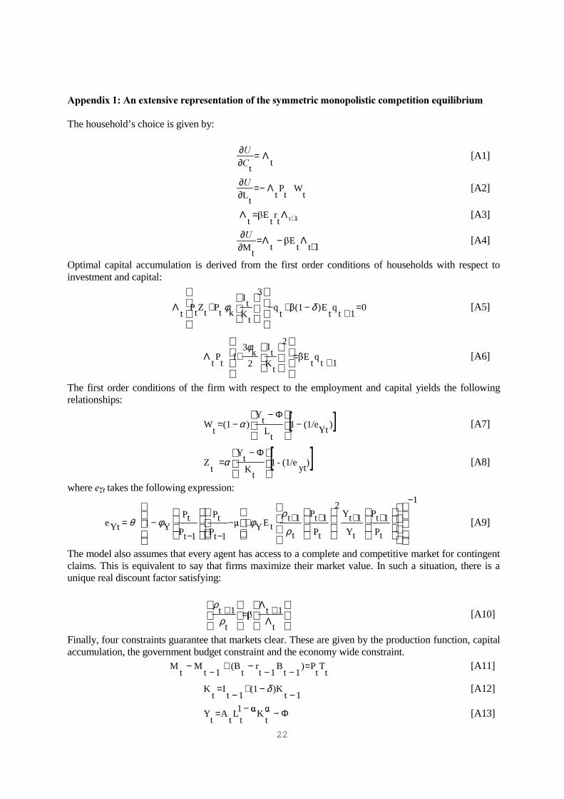
$SSHQGL[����$Q�H[WHQVLYH�UHSUHVHQWDWLRQ�RI�WKH�V\PPHWULF�PRQRSROLVWLF�FRPSHWLWLRQ�HTXLOLEULXP

The household’s choice is given by:

tt

Λ=∂∂&8 [A1]

tW

tP

tt

LΛ−=

∂∂8 [A2]

1ttr

tE

t +Λ=Λ [A3]

1ttE

tt

M +Λ−Λ=

∂∂8 [A4]

Optimal capital accumulation is derived from the first order conditions of households with respect toinvestment and capital:

01t

qt

E)(1t

q

3

tK

tI

ktP

tZ

tP

t=

+−+−+Λ

δφ [A5]

1tq

tE

2

tK

tI

2k

31

tP

t +=+Λ

φ[A6]

The first order conditions of the firm with respect to the employment and capital yields the followingrelationships:

[ ])Yt

(1/e1t

Lt

Y)(1

tW −

Φ−−=

α [A7]

[ ])yt

(1/e-1t

Kt

Y

tZ

Φ−=α [A8]

where H<W takes the following expression:

1

tP

1tP

tY

1tY2

tP

1tP

t

1ttEY

1tP

tP

1tP

tPY1Yte

−

+++++−−−

−=

ρ

ρφφθ [A9]

The model also assumes that every agent has access to a complete and competitive market for contingentclaims. This is equivalent to say that firms maximize their market value. In such a situation, there is aunique real discount factor satisfying:

Λ+Λ

=+

t

1t

t

1tρ

ρ[A10]

Finally, four constraints guarantee that markets clear. These are given by the production function, capitalaccumulation, the government budget constraint and the economy wide constraint.

tT

tP)

1tB

1tr

t(B

1tM

tM =

−−−+

−− [A11]

1t)K(1

1tI

tK

−−+

−= δ [A12]

Φ−−=t

K1t

Lt

At

Y [A13]

23

to obtain the economy wide constraint we proceed as follows. Using the definition of profitsYt

ACt

Ktt

Lt

Wt

Yt

−−−= =π

and imposing the government budget constraint in the household budget constraint yields:

Yt

ACt

Y

2

tK

tI

2K1

tI

tC −=++

φ[A14]

Price adjustment costs take the following quadratic expression:

tY

2

1tP

tP

2YY

tAC

−

−

=φ

[A15]

We specify the following fiscal policy in terms of the transfers:

1tB

tT

tP

−−= τ [A16]

Where τ is a positive constant. Thus, transfers are determined to maintain dynamic stability of the model.The equation for the monetary policy completes the system of 17 dynamic equations with 17 endogenousvariables: 7 prices (3W��:W��=W��ΛW��ρW��TW��UW), 5 quantities (<W��&W��,W��/W��7W), 3 stocks (0W��%W��.W), the mark-up((1-(1/H<W))

-1) and the price adjustment costs ($&<

W).

24

$SSHQGL[����/LTXLGLW\�(IIHFW�DQG�/DERU�6XSSO\�(ODVWLFLW\

To give some additional insights as to why do we need an economy with low risk aversion and capital we performed

the following exercise. The Panel A of Table A2 presents how changes in the risk aversion translate into: (i)

alternative intertemporal (Frisch) labor supply elasticities; and (ii) different impact effects on nominal interest rates

(rt) and labor (Lt). In the economy without capital, changes in the intertemporal elasticity of substitution leaves

practically unchanged the initial impact effect on /W, and thus on UW. The same exercise in an economy with capital

reveals two interesting features: first there is a dramatic increase in the output and employment response; second, and

most important, this effect is five times as large when σ� equals ��� as compared with σ� ���. In the economy without

capital there is no evidence of liquidity effect. This result is robust to alternative Frisch labor supply elasticities and

steady state hours worked. In an economy with capital, low values of risk aversion still translate into high enough

Frisch labor supply elasticities. Both circumstances imply that very small changes in the real wages are associated

with very important impact effects on labor.16

Since with these preferences both intertemporal substitution and

income effects play a very important role in tracing out the impact response of labor, the result translate into a huge

expected reduction in the marginal utility of consumption and so in an important liquidity effect.

7$%/(�$���/,48,',7<�())(&7�$1'�/$%25�6833/<�(/$67,&,7<�&'�35()(5(1&(6�

(&2120<�:,7+287�&$3,7$/σ1 0.5 0.65 0.70 0.75 0.80 1.00

$��/ �����D �����

Frisch Labor Supply - 3.09 2.94 2.80 2.68 2.33r Impact Effect - 0.47 0.47 0.47 0.47 0.47L Impact Effect - 0.92 0.92 0.92 0.92 0.92%��/ �����D �����Frisch Labor Supply 6.90 5.56 5.24 4.97 4.72 4.00r Impact Effect 0.47 0.47 0.47 0.47 0.47 0.47L Impact Effect 0.94 0.94 0.94 0.94 0.94 0.94

(&2120<�:,7+�&$3,7$/σ1 0.5 0.65 0.70 0.75 0.80 1.00

$��/ �����D �����Frisch Labor Supply - 3.18 3.00 2.85 2.72 2.33r Impact Effect - ����� ����� ����� 0.18 0.47L Impact Effect - 20.65 14.60 11.17 9.05 5.34%��/ �����D �����Frisch Labor Supply 7.12 5.68 5.34 5.00 4.78 4.00r Impact Effect ����� ����� 0.16 0.28 0.35 0.47Limpact Effect 23.07 11.63 9.95 8.71 7.78 5.55

1RWH��The impact effects correspond to expansionary money shocks. The rest of the parameters aretaken from Table 1. The letters r, L corresponds to nominal interest rate and labor, respectively.

16 In the economy with capital under � ���� and / ��� the impact response of real wages is �����

25

5HIHUHQFHV

Basu, S. and J.G. Fernald (1997): "Returns to Scale in US Production: Estimates and

Implications", -RXUQDO�RI�3ROLWLFDO�(FRQRP\, 105, 249-283.

Blanchard O.J. and C.M. Khan (1980): "The solution of Linear Difference Models under Rational

Expectations", (FRQRPHWULFD 48, 1305-13.

Chari, V.V., P.J. Kehoe and E.R. McGrattan (1996): "Sticky Price Models of the Business Cycle:

Can the Contract Multiplier Solve the Persistence Problem?”, NBER WP 5809.

Chari, V.V., P.J. Kehoe and E.R. McGrattan (1998): "Monetary shocks ad real interest rates in

sticky price models of international business cycle”, Federal Reserve Bank of Minneapolis,

Research Dpt. Staff Report 233.

Christiano, L., M. Eichenbaum and C. Evans (1997): "Sticky Price and Limited Participation

Models: A Comparison", (XURSHDQ�(FRQRPLF�5HYLHZ, 41 (6), 1201-1249.

Christiano, L., M. Eichenbaum and C. Evans (1998): "Monetary Policy Shocks: What Have we

Learned and to What End?" NBER WP 6400.

Cooley, T. and G. Hansen (1995): "Money and the Business Cycle", in T. Cooley (editor)

)URQWLHUV�RI�%XVLQHVV�&\FOH�5HVHDUFK, Princeton Universtity Press, Princeton, New Yersey,

175-216.

Fuerst,T.(1992):"Liquidity, Loanable Funds and Real Activity",-RXUQDO�RI�0RQHWDU\�(FRQRPLFV

29, 3-24.

Hairault, J. and F. Portier (1993): "Money, New-Keynesian Macroeconomics and the Business

Cycle",�(XURSHDQ�(FRQRPLF�5HYLHZ 37, 1533-1568.

Jeanne, O, (1994): "Nominal Rigidities and the Liquidity Effect", mimeo ENCP-CERAS.

Goldfeld, S. and D. Sichel (1990): "The Demand for Money", in B. Friedman and F. Hahn (eds.),

+DQGERRN�RI�0RQHWDU\�(FRQRPLFV� vol. I Amsterdam: North Holland, 299-356.

26

Greenwood, J.; Zvi Hercowitz and G. Huffman (1988): "Investment, Capacity of Utilization and

the Real Business Cycle", $PHULFDQ�(FRQRPLF�5HYLHZ, 78, 402-417.

Kim, J. (1998): "Monetary Policy in a Stochastic Equilibrium Model with Real and Nominal

Rigidities". Divisions of Research & Statistics and Monetary Affairs. Federal Reserve

Board, IRUWKFRPLQJ�-RXUQDO�RI�0RQHWDU\�(FRQRPLFV

King, R.G.; Plosser, G. and S. Rebelo (1988): "Production, Growth and Business Cycles I: The

Basic Neoclassical Model", -RXUQDO�RI�0RQHWDU\�(FRQRPLFV, 21, 195-232.

King, G.R. and Watson, M. (1996): “Money, Prices, Interest Rates and the Business Cycle´�

5HYLHZ�RI�(FRQRPLFV�DQG�6WDWLVWLFV, 78, 35-53.

Leeper, E. (1991): " Equilibria under "Active" and "Passive" Monetary and Fiscal Policies",

-RXUQDO�RI�0RQHWDU\�(FRQRPLFV 27, 129-147.

Lucas, R.E. (1980): "Methods and Problems in Business Cycle Theory", -RXUQDO�RI�0RQH\�&UHGLW

DQG�%DQNLQJ, 12 (4), 696-715.

Lucas, R.E: (1988):"Money Demand in the United States: A Quantitative Review���&DUQHJLH

5RFKHVWHU�&RQIHUHQFH�6HULHV�RQ�3XEOLF�3ROLF\, 29, 137-167.

Rotemberg, J.(1982): "Sticky Prices in the United States", -3(� 90, 1187-1211.

Sbordone, A.(1998):"Price and Unit Labor Costs: A New Test of Price Stickiness",IIES.WP 653.

Sims, C. (1995): "Solving Linear Rational Expectations Models", mimeo, Yale University.

Whited, T. (1992): "Debt, Liquidity Constraints and Corporate Investment: Evidence from Panel

Data", 7KH�-RXUQDO�RI�)LQDQFH 47, 1425-60.

Woodford, M. (1996): "Control of the Public Debt: A Requirement for Price Stability", NBER

WP 5684.

27

),*85(��3$1(/�$��,038/6(�5(63216(�72�$�3(56,67(17�021(<�*52:7+�6+2&.

6(3$5$%/(�35()(5(1&(6�:,7+287�&$3,7$/

0 2 4 6 8 100

0.1

0.2

0.3

0.4

0.5

0.6

0.7Real Balances

0 2 4 6 8 10−0.2

0

0.2

0.4

0.6

0.8Nominal Interest Rate

0 2 4 6 8 10−1.5

−1

−0.5

0Markup

Quarters after the shock0 2 4 6 8 10

0

0.1

0.2

0.3

0.4

0.5

0.6

0.7Consumption

Quarters after the shock

1RWH��3DUDPHWHU�9DOXHV�� 1 ��� ���φY ���� ����DQG� c=1.

3$1(/�%��52%8671(66�72�&+$1*(6�,1�7+(�5,6.�$9(56,21

0 5 10 15−2

−1.5

−1

−0.5

0

0.5

1Nominal Interest Rate

risk aversion(σ)

Impa

ct E

ffect

←εc=1

←εc=0.2

0 5 10 150.1

0.2

0.3

0.4

0.5

0.6

0.7

0.8Real Balances

risk aversion(σ)

Impa

ct E

ffect

1RWH��3DUDPHWHU�9DOXHV�� ���φY ���DQG� =0.5.

28

),*85(��

3$1(/�$��,038/6(�5(63216(�72�$�3(56,67(17�021(<�*52:7+�6+2&.

121�6(3$5$%/(�35()(5(1&(6��&'�*++��:,7+287�&$3,7$/

0 2 4 6 8 100

0.2

0.4

0.6

0.8Real Balances

0 2 4 6 8 100

0.1

0.2

0.3

0.4

0.5Nominal Interest Rate

0 2 4 6 8 100

0.2

0.4

0.6

0.8Output

Quarters after the shock

CD→

←GHH

0 2 4 6 8 100

0.2

0.4

0.6

0.8Consumption

Quarters after the shock

1RWH��3DUDPHWHU�9DOXHV�� 1 ��� ��D ������Y ���φY ���� ����DQG� c=1.

3$1(/�%��52%8671(66�72�&+$1*(6�,1�7+(�5,6.�$9(56,21

0 5 10 150.4

0.42

0.44

0.46

0.48

0.5Nominal Interest Rate (CD)

Impa

ct E

ffect

0 5 10 15

0.3

0.4

0.5

0.6Real Balances (CD)

Impa

ct E

ffect

0 5 10 150.3

0.4

0.5

0.6

0.7

0.8

0.9

1Nominal Interest Rate (GHH)

risk aversion(σ)

Impa

ct E

ffect

←εc=1

←εc=0.2

0 5 10 150.2

0.3

0.4

0.5

0.6Real Balances (GHH)

risk aversion(σ)

Impa

ct E

ffect

1RWH��3DUDPHWHU�9DOXHV� ��D �����Y ���φY ���DQG� =0.5.

29

),*85(��

3$1(/�$��,038/6(�5(63216(�72�$�3(56,67(17�021(<�*52:7+�6+2&.

121�6(3$5$%/(�35()(5(1&(6��&'��:,7+�&$3,7$/

0 2 4 6 8 100.2

0.3

0.4

0.5

0.6

0.7Real Balances

←σ=2

0 2 4 6 8 10−0.1

0

0.1

0.2

0.3

0.4

0.5

0.6Nominal Interest Rate

←σ=0.75

0 2 4 6 8 100

2

4

6

8Output

Quarters after the shock0 2 4 6 8 10

0.2

0.3

0.4

0.5

0.6

0.7Consumption

Quarters after the shock

1RWH��3DUDPHWHU�9DOXHV�� 1 ��� ��D ������φY=85, φk ���� ����DQG� c=1.

3$1(/�%��52%8671(66�72�&+$1*(6�,1�7+(�5,6.�$9(56,21

&203$5,1*�&'�:,7+�*++�35()(5(1&(6

0 1 2 3 4 5−0.2

0

0.2

0.4

0.6

0.8Nominal Interest Rate (CD)

Impa

ct Ef

fect

0 1 2 3 4 50

0.1

0.2

0.3

0.4

0.5

0.6

0.7Real Balances (CD)

Impa

ct Ef

fect

←εc=1

←εc=0.2

0 1 2 3 4 50.3

0.35

0.4

0.45

0.5

0.55

0.6Nominal Interest Rate (GHH)

risk aversion(σ)

Impa

ct Ef

fect

0 1 2 3 4 50.4

0.45

0.5

0.55

0.6

0.65Real Balances (GHH)

risk aversion(σ)

Impa

ct Ef

fect

1RWH��3DUDPHWHU�9DOXHV�� ��D ������Y ���φY=85, φk ���DQG� =0.5.

30

),*85(��

6(16,7,9,7<�$1$/<6,6121�6(3$5$%/(�35()(5(1&(6��&'��:,7+�&$3,7$/

10 20 30 40 50 60

−0.5

0

0.5

Nominal Interest Rate

φk

Imp

act

Eff

ect

10 20 30 40 50 60

0.4

0.6Real Balances

φk

Imp

act

Eff

ect

0 0.1 0.2 0.3 0.4 0.5

−4

−2

0

ρµ

Imp

act

Eff

ect

0 0.1 0.2 0.3 0.4 0.5

0.2

0.4

0.6

ρµ

Imp

act

Eff

ect

100 150 200 250 300 350

−4

−2

0

φy

Imp

act

Eff

ect

100 150 200 250 300 3500.2

0.4

0.6

0.8

φy

Imp

act

Eff

ect

Notes:(L��&RQWLQXRXV�OLQH� 1 ��DQG�WKH�GRWWHG�OLQH� 1=0.75.(ii) In the first panel (Robustness to φk��ZH�VHW� ��D �����φy ���DQG� c ��� =0.5.(iii) In the second panel (Robustness to ��ZH�VHW� ��D �����φy=85, φk ���DQG� c=1.(iv) In the third panel (Robustness to φy��ZH�VHW� ��D �����φk ���� c ��DQG� =0.5.

31

7$%/(��$��%$6(/,1(�9$/8(6�)25�&$/,%5$7,21�3$5$0(7(56

DescriptionParameter Value

Discount Factor β (0.97)1/4

3UHIHUHQFHV

D���6HSDUDEOHV

/DERU�VXSSO\�HODVWLFLW\ 1.00

Risk aversion σ1 2.00E��1RQ�6HSDUDEOHV��&REE�'RXJODV�&'��Risk aversion σ1 2.00F���1RQ�6HSDUDEOHV��*UHHQZRRG�+HUFRZLW]+XIIPDQ��*++��Labor supply elasticity ��� ��� 1.00

0RQH\�'HPDQG�3URSHUWLHVConsumption elasticity ( c) (1-σ2����� � 1.00Interest rate semi-elasticity ( r) ����� ����U� 0.01

7HFKQRORJ\�DQG�&DSLWDO�$FFXPXODWLRQCapital income share α 0.33Depreciation rate δ (0.10)1/4

Capital adjustment cost parameter φk 10

3ULFH�6HWWLQJ

6WHDG\�6WDWH�0DUNXS �� ��� 1.20

3ULFH�$GMXVWPHQW�FRVW�SDUDPHWHU φy 85

0RQHWDU\�3ROLF\Autocorrelation of Money Growth Shocks ρµ 0.50

%��67($'<�67$7(

DescriptionValues

(in annual terms)

µ 1.05R 1.08M/B 0.33L 0.30C/Y 0.74K/Y 2.50I/Y 0.25Φ/Y 0.20Price Adjust.Cost/Y (%) 0.70Capital Adjust.Costs/I (%) 1.74