
NAFTA and Industrial Adjustment: A Specific-Factors Model of Production
26
Growth and Change Vol. 27 (Winter 1996) pp. 3-28 NAFTA and Industrial Adjustment: A Specific-Factors Model of Production HENRY THOMPSON The North American Free Trade Agreement (NAFTA) will continue to attract political debate as U.S. manufacturing industries adjust in the face of increased import competition and export opportunities. This study applies the specific factors model of production to manufacturing industries in Alabama to examine the pending adjustment. As industrial prices change, there will be small output adjustments in the short run and downward pressure on the wages of production workers. Projected changes in industrial investment will lead to substantial long-run output adjustments. his paper focuses on predicting industrial adjustments and income redistribu- T tion in Alabama manufacturing. The critical question is what will happen to industrial prices. Some industries will experience increasing import competition and falling prices, some will experience rising prices through increased export demand, while others will experience increased intraindustry (two way trade and no predictable price trend. The present study applies the specific factors model of production in which each industry has its own particular capital input. Manufacturing survey data are used to derive factor shares and industry shares for production workers, nonproduction workers, and capital in seventeen manufacturing industries. Factor intensity is used as a basis for projecting the direction of trade and price changes, which cause outputs to adjust as labor moves between industries. These short run output changes are predicted to be small by the specific factors model. In the long run, investment will shift across industries. The return to capital in an industry is positively related to the price of output in the industry. Henry Thompson is a professor of economics at Auburn University, AL 36849. The preliminary research for this paper was sponsored by a grant from the Auburn Policy Research Center. The author wishes to thank Paul Pecorino and Harris Schlesinger for comments at a seminar at the University of Alabama. Richard Gift and two referees of this journal provided comments which substantially improved the final product. Submitted Oct. 1994; revised May 1995 0 1996, College of Business and Economics, University of Kentucky. Published by Blackwell Publishers, 238 Main Street, Cambridge, MA 02142 US, and 108 Cowley Road, Oxford, OX4 IJF, UK
Transcript of NAFTA and Industrial Adjustment: A Specific-Factors Model of Production
Growth and Change Vol. 27 (Winter 1996) pp. 3-28
NAFTA and Industrial Adjustment: A Specific-Factors Model
of Production HENRY THOMPSON
The North American Free Trade Agreement (NAFTA) will continue to attract political debate as U.S. manufacturing industries adjust in the face of increased import competition and export opportunities. This study applies the specific factors model of production to manufacturing industries in Alabama to examine the pending adjustment. As industrial prices change, there will be small output adjustments in the short run and downward pressure on the wages of production workers. Projected changes in industrial investment will lead to substantial long-run output adjustments.
his paper focuses on predicting industrial adjustments and income redistribu- T tion in Alabama manufacturing. The critical question is what will happen to industrial prices. Some industries will experience increasing import competition and falling prices, some will experience rising prices through increased export demand, while others will experience increased intraindustry (two way trade and no predictable price trend.
The present study applies the specific factors model of production in which each industry has its own particular capital input. Manufacturing survey data are used to derive factor shares and industry shares for production workers, nonproduction workers, and capital in seventeen manufacturing industries. Factor intensity is used as a basis for projecting the direction of trade and price changes, which cause outputs to adjust as labor moves between industries. These short run output changes are predicted to be small by the specific factors model.
In the long run, investment will shift across industries. The return to capital in an industry is positively related to the price of output in the industry.
Henry Thompson is a professor of economics at Auburn University, AL 36849. The preliminary research for this paper was sponsored by a grant from the Auburn Policy Research Center. The author wishes to thank Paul Pecorino and Harris Schlesinger for comments at a seminar at the University of Alabama. Richard Gift and two referees of this journal provided comments which substantially improved the final product.
Submitted Oct. 1994; revised May 1995 0 1996, College of Business and Economics, University of Kentucky. Published by Blackwell Publishers, 238 Main Street, Cambridge, MA 02142 US, and 108 Cowley Road, Oxford, OX4 IJF, UK
4 GROWTH AND CHANGE, WINTER 1996
Investment will follow rising capital returns, causing substantial output adjust- ment in the long run. These long run output adjustments are predicted to be in the range of ten to twenty percent.
There will also be some redistribution of income both toward and away from nonproduction labor . Also, owners of capital are projected to experience some large changes in the return to capital across industries.
Review of the Literature Computable general equilibrium (CGE) models are based on a
microeconomic structure of production. Brown et al. (1992) present a version of the University of Michigan CGE model to study the effects of NAFTA. The model has a competitive structure with increasing returns to scale and an input- output format. Demand for final products drives results, with prices fixed at world levels. They predict that the effects of NAFTA on gross domestic output will be small in both countries, and that wage changes will be very small in the U.S. Outputs of stone, clay and glass, primary metals, and electrical equipment are projected to fall in the US. , while outputs of textiles, apparel, furniture, chemicals, plastics, and miscellaneous manufactures are projected to rise. (See Tables 1 and 2 for full names of industries and SIC codes.)
A similar CGE model (Inforum 1990) prepared at the University of Maryland predicts that U.S. industries which will add jobs under NAFTA are chemicals, rubber, metals, and machinery, while the losing industries will be apparel and furniture. In another CGE model, Peat Marwick (1991) predicts little effect in either the U.S. or Mexico unless investment enters Mexico. With incoming foreign investment, Mexico gains substantially and the U S . benefits by having cheaper imports. Industries which are projected to expand in the U.S. are chemicals, machinery, and transport equipment, while textiles, apparel, furniture, stone, and electrical equipment are projected to decline.
There are also a few computable models which are less detailed. Hinojosa and Robinson (1991) produce a highly aggregated CGE model without detailed industrial structure, and predict small overall gains in the U.S. with increased output in the capital goods industries. Young and Romero (1991) utilize a dynamic model with no industrial detail which allows investment to adjust. They find small effects on aggregate U.S. manufacturing, but industrial output in Mexico is projected to increase significantly with investment. Boyd et al. (1991) examine the effects of tariff removal in the U.S. in a highly aggregated model with no industrial detail, and find very small industrial effects.
Other studies use general economic analysis. The U.S. International Trade Commission (ITC 1991) presents an informal model with a good deal of regional
NAFTA AND INDUSTRIAL ADJUSTMENT 5
analysis. Little immediate impact on the U.S. is projected, but as Mexico grows U.S. exports will increase. Southwestern states will benefit from NAFTA, but other regions may suffer as resources relocate. The ITC model predicts that chemicals, machinery, and electrical equipment will expand, while textiles, apparel, and stone suffer. Hufbauer and Schott (1992a, 1992b, 1993) use similar general economic analysis to study the impact of NAFTA on specific industries, and predict that results will vary by industry with textiles and apparel the only clear losers. Hansen (1994) uses similar analysis to predict the regional effects of NAFTA, and foresees benefits for the border states and the Midwestern states, with losses forecast for the Southeastern states. Overall, Hansen expects small effects in the aggregate U.S., but noticeable effects in particular states and considerable variation across locales inside states.
Still other studies have focused on particular industries. Hunter et al. (1995) examine the pattern of trade in automobiles, and find little net effect on the U.S. auto industry. Imports from Mexico of car parts and light trucks are projected to increase, while exports of cars to Mexico increase. Investment would create larger changes, but they predict no large investment shifts. Baer and Erb (1991) study automobiles and electronics, and foresee integration between countries. Gains for both countries are predicted in autos, and ultimate gains in electronics are seen after costly transition. Trela and Whalley (1991) discuss textiles, apparel, and steel, predicting that imports from Mexico will rise with prices falling in the U.S.
Using another approach, Wientraub et al. (1991) present chapters written by specialists and business people in the automobile, petrochemical, pharmaceutical, textiles, apparel, computer, and food industries. These practitioners differ in their opinions, some predicting decline in the U.S., especially in automobiles and petrochemicals. Others think the U.S. and Mexican industries are already integrated to a large extent, and that NAFTA will have minimal impact. International patent protection is thought to be important in pharmaceuticals, and should encourage integration. Lustig et al. (1992) present a collection of nontechnical articles by different authors on NAFTA, including a survey of CGE models, labor issues, and industrial effects.
Regarding overall policy, Prestowitz and Cohen (I99 I ) suggest structuring NAFTA so that production in Mexico using U.S. capital and skilled labor and Mexican labor is exported to the rest of the world, not back into the U.S. Mexico would thus become an export zone for the U.S., an arrangement Mexican industry and U.S. consumers would definitely not favor. Morici (1991) proposes to limit Mexican exports in sensitive industries to cushion the shock of transition.
The Department of Commerce (1993) analyzes the effects of NAFTA on industries under the headings of legal requirements, current structure, standards,
6 GROWTH AND CHANGE, WINTER 1996
government procurement, rules of origin, customs administration, intellectual property rights, and foreign investment. Discussion focuses on the growth potential in every industry. Even apparel, universally seen as facing stiff import competition, is pictured with increased export opportunities in particular lines.
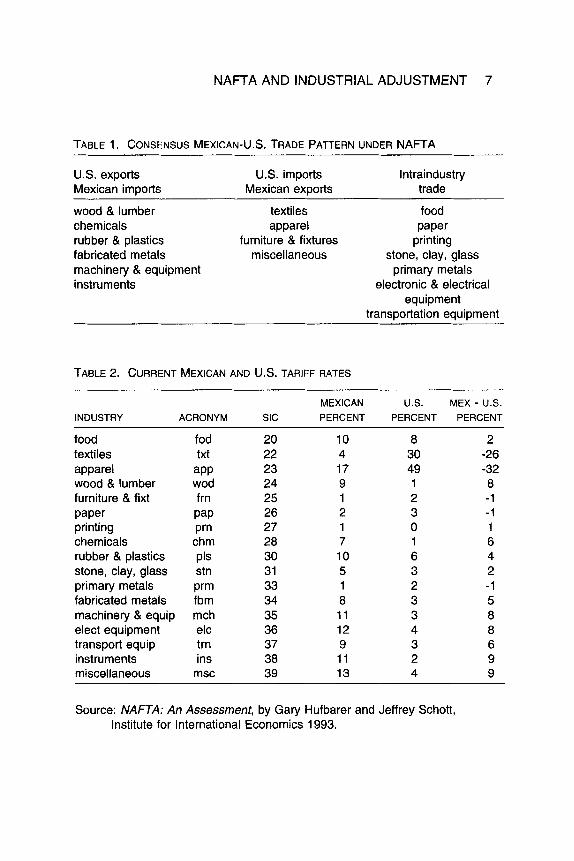
Table 1 reports the “consensus” projected trade pattern. Textiles and apparel industries stand out as import competing industries. Furniture is not highly protected, but increased imports are expected. Intraindustry trade occurs with imports and exports in the same classification. There is variation in both the types and qualities of goods in each of these industries. In the food industry, for instance, the U.S. will import cattle to feed lots and export frozen ground beef. In transport equipment, the U.S. will export cars and heavy machinery, while importing car parts and light trucks. Differences in quality may also explain intraindustry trade. The US. will, for instance, export higher quality primary metal alloys and import lower quality metal products.
Industries which currently are protected from imports will experience falling prices. Current U.S. tariff rates by industry from Hufbauer and Schoff (1993) are listed in Table 2. These rates are tariffs plus equivalent protection from quotas and other nontariff barriers. Note that the highest U.S. tariffs are in textiles and apparel. These two industries can expect import competition to increase substantially, unless they can maintain protection. Mexico has historically protected its industry from imports, and to a much higher level, with average tariffs in the 30 to 50 percent range only 10 years ago. The Mexican government had for years tried to build its economy on the principle of import substitution, encouraging domestic industry to produce what could have been imported. The most highly protected Mexican industries are apparel, miscellaneous, electrical equipment, machinery, instruments, food, and plastics.
Table 2 also reports the difference between Mexican and U.S. tariffs. A positive number represents an industry with higher protection in Mexico, suggesting the potential for U.S. exports. The largest positive differences occur in instruments, miscellaneous, wood, machinery, electrical equipment, chemicals, transport equipment, fabricated metals, and plastics. Negative numbers indicate industries which are more protected in the U.S., suggesting increased imports and falling prices. Apparel and textiles will feel pressure, but also furniture, paper, and primary metals could see increased imports.
Tables 1 and 2 tell a similar story. The list of potential U.S. exports to Mexico in the first column of Table 1 is similar to those in Table 2 with the largest tariff differences, except for the missing electrical equipment, transport equipment, and miscellaneous. These three industries appear in the intraindustry trade column in Table 1. Two industries with negative signs in Table 2, paper and primary metals, in Table 1 are projected to experience intraindustry trade.
NAFTA AND INDUSTRIAL ADJUSTMENT 7
TABLE 1. CONSENSUS MEXICAN-US. TRADE PATTERN UNDER NAFTA
U.S. exports Mexican imDorts
U.S. imports lntraindustry Mexican exDorts trade
wood & lumber textiles food chemicals apparel paper rubber & plastics furniture & fixtures printing fabricated metals miscellaneous stone, clay, glass machinery & equipment primary metals instruments electronic & electrical
equipment transportation equipment
TABLE 2. CURRENT MEXICAN AND U.S. TARIFF RATES
MEXICAN U.S. MEX - U.S. INDUSTRY ACRONYM SIC PERCENT PERCENT PERCENT
food fod textiles txt apparel aPP wood & lumber wod furniture & fixt frn paper Pap printing Prn chemicals chm rubber & plastics pls stone, clay, glass stn primary metals Prm fabricated metals fbm machinery & equip mch elect equipment elc transport equip trn instruments ins miscellaneous msc
20 22 23 24 25 26 27 28 30 31 33 34 35 36 37 38 39
10 8 2 4 30 -26 17 49 -32 9 1 8 1 2 -1 2 3 -1 1 0 1 7 1 6 10 6 4 5 3 2 1 2 -1 8 3 5 1 1 3 8 12 4 8 9 3 6 1 1 2 9 13 4 9
Source: NAFTA: An Assessment, by Gary Hufbarer and Jeffrey Schott, Institute for International Economics 1993.
8 GROWTH AND CHANGE, WINTER 1996
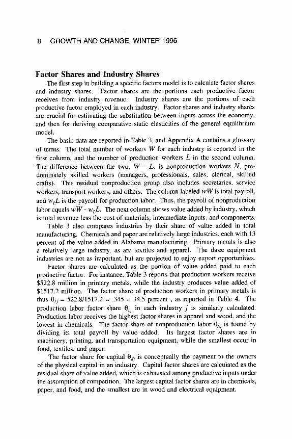
Factor Shares and Industry Shares The first step in building a specific factors model is to calculate factor shares
and industry shares. Factor shares are the portions each productive factor receives from industry revenue. Industry shares are the portions of each productive factor employed in each industry. Factor shares and industry shares are crucial for estimating the substitution between inputs across the economy, and then for deriving comparative static elasticities of the general equilibrium model.
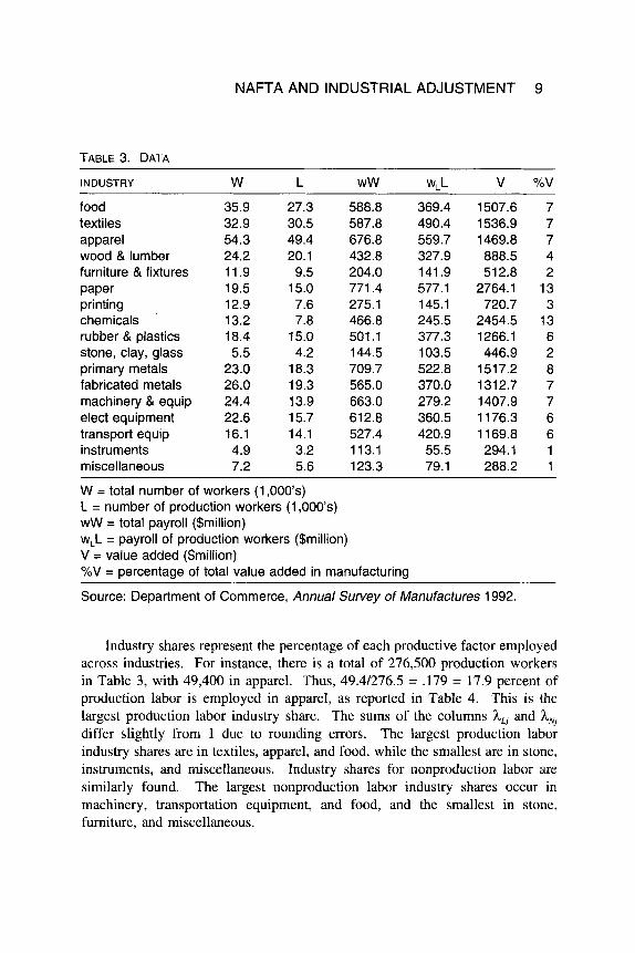
The basic data are reported in Table 3, and Appendix A contains a glossary of terms. The total number of workers W for each industry is reported in the first column, and the number of production workers L in the second column. The difference between the two, W - L, is nonproduction workers N , pre- dominately skilled workers (managers, professionals, sales, clerical, skilled crafts). This residual nonproduction group also includes secretaries, service workers, transport workers, and others. The column labeled wWis total payroll, and wLL is the payroll for production labor. Thus, the payroll of nonproduction labor equals WW - wLL. The next column shows value added by industry, which is total revenue less the cost of materials, intermediate inputs, and components.
Table 3 also compares industries by their share of value added in total manufacturing. Chemicals and paper are relatively large industries, each with 13 percent of the value added in Alabama manufacturing. Primary metals is also a relatively large industry, as are textiles and apparel. The three equipment industries are not as important, but are projected to enjoy export opportunities.
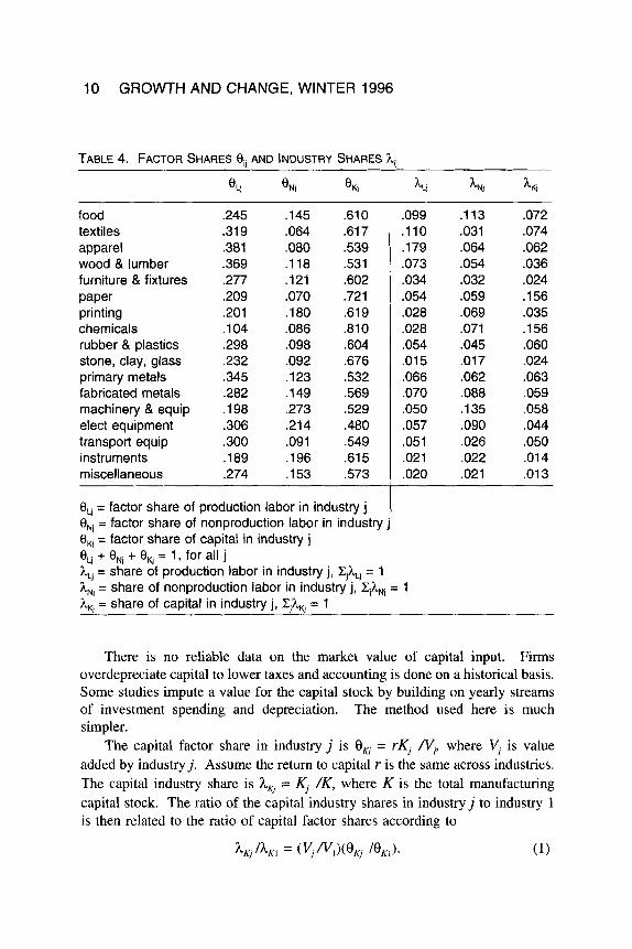
Factor shares are calculated as the portion of value added paid to each productive factor. For instance, Table 3 reports that production workers receive $522.8 million in primary metals, while the industry produces value added of $1517.2 million. The factor share of production workers in primary metals is thus 0, = 522.8/1517.2 = .345 = 34.5 percent , as reported in Table 4. The production labor factor share 8, in each industry j is similarly calculated. Production labor receives the highest factor shares in apparel and wood, and the lowest in chemicals. The factor share of nonproduction labor 8, is found by dividing its total payroll by value added. Its largest factor shares are in machinery, printing, and transportation equipment, while the smallest occur in food, textiles, and paper.
The factor share for capital 8, is conceptually the payment to the owners of the physical capital in an industry. Capital factor shares are calculated as the residual share of value added, which is exhausted among productive inputs under the assumption of competition. The largest capital factor shares are in chemicals, paper, and food, and the smallest are in wood and electrical equipment.
NAFTA AND INDUSTRIAL ADJUSTMENT 9
TABLE 3. DATA
INDUSTRY W L w w w, L u %V
food textiles apparel wood & lumber furniture & fixtures paper printing chemicals rubber & plastics stone, clay, glass primary metals fabricated metals machinery & equip elect equipment transport equip instruments miscellaneous
35.9 27.3 588.8 32.9 30.5 587.8 54.3 49.4 676.8 24.2 20.1 432.8 11.9 9.5 204.0 19.5 15.0 771.4 12.9 7.6 275.1
I 8.4 15.0 501.1 5.5 4.2 144.5
26.0 19.3 565.0 24.4 13.9 663.0
16.1 14.1 527.4 4.9 3.2 113.1 7.2 5.6 123.3
13.2 7.8 466.8
23.0 18.3 709.7
22.6 15.7 612.8
369.4 490.4 559.7 327.9 141.9 577.1 145.1 245.5 377.3 103.5
370.0 279.2 360.5 420.9 55.5 79.1
522.8
1507.6 1536.9 1469.8 888.5 512.8 2764.1 720.7 2454.5 1266.1 446.9 151 7.2 131 2.7 1407.9 1176.3
294.1 288.2
1 169.8
7 7 7 4 2 13 3 13 6 2
7 7 6 6 1 1
a
W = total number of workers (1,000’s) L = number of production workers (1,000s) WW = total payroll ($million) w,L = payroll of production workers ($million) V = value added ($million) %V = percentage of total value added in manufacturing
Source: Department of Commerce, Annual Survey of Manufactures 1992.
Industry shares represent the percentage of each productive factor employed across industries. For instance, there is a total of 276,500 production workers in Table 3, with 49,400 in apparel. Thus, 49.4/276.5 = .179 = 17.9 percent of production labor is employed in apparel, as reported in Table 4. This is the largest production labor industry share. The sums of the columns hLj and hNj differ slightly from 1 due to rounding errors. The largest production labor industry shares are in textiles, apparel, and food, while the smallest are in stone, instruments, and miscellaneous. Industry shares for nonproduction labor are similarly found. The largest nonproduction labor industry shares occur in machinery, transportation equipment, and food, and the smallest in stone, furniture. and miscellaneous.
10 GROWTH AND CHANGE, WINTER 1996
. I10 .031 ,179 .064 .073 .054 ,034 .032 .054 .059 .028 ,069 ,028 .071 .054 .045 ,015 ,017 .066 .062 .070 .088 .050 .I35
I ,057 .090 .051 ,026
.020 .021 1 .021 .022
TABLE 4. FACTOR SHARES e,, AND INDUSTRY SHARES h,,
food textiles apparel wood & lumber furniture & fixtures paper printing chemicals rubber & plastics stone, clay, glass primary metals fabricated metals machinery & equip elect equipment transport equip instruments miscellaneous
.245
.319 ,381 .369 ,277 .209 .201 .I04 ,298 .232 .345 ,282 .I98 ,306 .300 .I89 ,274
.145
.064 ,080 . I 18 .121 .070 .I80 .086 ,098 ,092 ,123 ,149 .273 .214 .091 .I96 .I53
.610
.617
.539
.531
.602 ,721 .619 .810 ,604 .676 .532 .569 .529 ,480 .549 .615 .573
.072
.074
.062
.036
.024
.156
.035
.156
.060
.024
.063 ,059 ,058 .044 .050 .014 .013
8 , = factor share of production labor in industry j 1 8,, = factor share of nonproduction labor in industry j 8 , = factor share of capital in industry j eLj + 8, + 8, = 1, for all j h, = share of production labor in industry j, ZjhLl = 1 hNI = share of nonproduction labor in industry j , ClhNj = 1 hKl = share of capital in industry j, CJhKJ = 1
There is no reliable data on the market value of capital input. Firms overdepreciate capital to lower taxes and accounting is done on a historical basis. Some studies impute a value for the capital stock by building on yearly streams of investment spending and depreciation. The method used here is much simpler.
The capital factor share in industry j is 9, = rKj N,, where V, is value added by industryj. Assume the return to capital r is the same across industries. The capital industry share is h, = Kj /K, where K is the total manufacturing capital stock. The ratio of the capital industry shares in industryj to industry 1 is then related to the ratio of capital factor shares according to
NAFTA AND INDUSTRIAL ADJUSTMENT 11
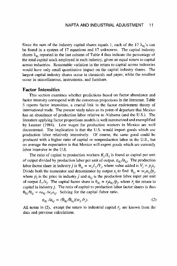
Since the sum of the industry capital shares equals 1, each of the 17 hKj’s can be found in a system of 17 equations and 17 unknowns. The capital industry shares h, reported in the last column of Table 4 thus indicate the percentage of the total capital stock employed in each industry, given an equal return to capital across industries. Reasonable variation in the return to capital across industries would have only small quantitative impact on the capital industry shares. The largest capital industry shares occur in chemicals and paper, while the smallest occur in miscellaneous, instruments, and furniture.
Factor Intensities This section examines whether predictions based on factor abundance and
factor intensity correspond with the consensus projections in the literature. Table 5 reports factor intensities, a crucial link in the factor endowment theory of international trade. The present study takes as its point of departure that Mexico has an abundance of production labor relative to Alabama (and the U.S.). The literature applying factor proportions models is well summarized and exemplified by Learner (1984). Low wages for production workers in Mexico are well documented. The implication is that the U.S. would import goods which use production labor relatively intensively. Of course, the same good could be produced with a higher ratio of capital or nonproduction labor in the U.S., but on average the expectation is that Mexico will export goods which are currently labor intensive in the U.S.
The ratio of capital to production workers Kj/Lj is found as capital per unit of output divided by production labor per unit of output, aKj/aLf The production labor factor share in industryj is 8, = wLLjN,, where value added is V, = p,+ Divide both the numerator and denominator by output xj to find 8, = wLaL/pj, where p j is the price in industry j and aLj is the production labor input per unit of output Lj/xj. The capital factor share is 8, = r,uKj/pj, where rj the return to capital in industry j . The ratio of capital to production labor factor shares is thus 8, /8, = ruKj /wLu,. Solving for the capital /labor ratio,
am /a, = (8m/BLj)(wL/rj).
All terms in (2) , except the return to industrial capital rj, are known from the data and previous calculations.
12 GROWTH AND CHANGE, WINTER 1996
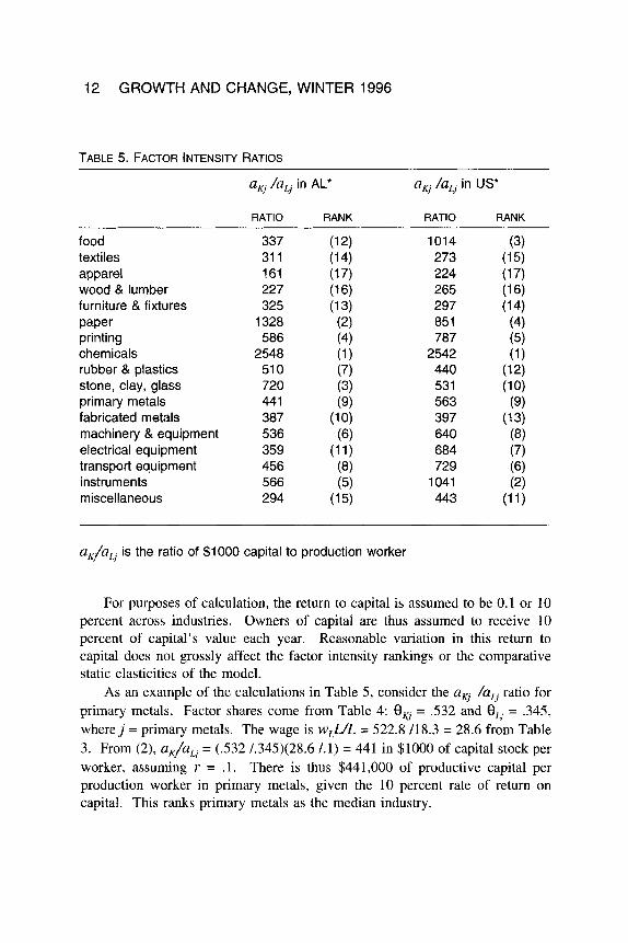
TABLE 5. FACTOR INTENSITY RATIOS
aa /a, in AL* a4 /a, in US*
RATIO RANK RATIO RANK
food textiles apparel wood & lumber furniture & fixtures paper printing chemicals rubber & plastics stone, clay, glass primary metals fabricated metals machinery & equipment electrical equipment transport equipment instruments miscellaneous
337 31 1 161 227 325 1328 586 2548 51 0 720 44 1 387 536 359 456 566 294
1014 273 224 265 297 851 787 2542 440 53 1 563 397 640 684 729 1041 443
a,/u, is the ratio of $1000 capital to production worker
For purposes of calculation, the return to capital is assumed to be 0.1 or 10 percent across industries. Owners of capital are thus assumed to receive 10 percent of capital’s value each year. Reasonable variation in this return to capital does not grossly affect the factor intensity rankings or the comparative static elasticities of the model.
As an example of the calculations in Table 5, consider the am /a, ratio for primary metals. Factor shares come from Table 4: 8, = .532 and 8, = -345, wherej = primary metals. The wage is w,UL = 522.8 /18.3 = 28.6 from Table 3. From (2), aK/aLj = (.532 /.345)(28.6 1.1) = 441 in $1000 of capital stock per worker, assuming Y = . l . There is thus $441,000 of productive capital per production worker in primary metals, given the 10 percent rate of return on capital. This ranks primary metals as the median industry.
NAFTA AND INDUSTRIAL ADJUSTMENT 13
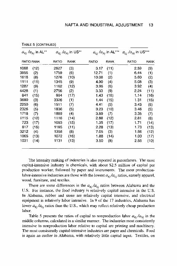
TABLE 5 (CONTINUED)
aKj /aw in AL'* aKj /aNj in US** aLj /aNj in AL*" aLj /a, in US"'
RATIO RANK RATIO RANK RATIO RANK RATIO RANK
1068 (12)
1618 (8)
1287 (9) 4428 (1) 841 (15)
3680 (3) 2250 (6) 2326 (5) 1718 (7) 1115 (10) 723 (17) 817 (16)
3212 (4) 1065 (13) 1031 (14)
3955 (2)
1111 (11)
2627 1759 1276 1345 1162 2756
894 3326 151 1 1836 1889 1116 1093 1185 1356 1072 1131
3.17 12.71 10.08 4.90 3.96 3.33 1.43 1.44 4.41 3.23 3.89 2.88 1.35 2.28 7.05 1.88 3.50
2.59 6.44 5.60 5.08 3.92 2.24 1.14 1.31 3.43 3.46 3.35 2.81 1.71 1.73 1.86 1.03 2.55
The intensity ranking of industries is also reported in parentheses. The most capital-intensive industry is chemicals, with about $2.5 million of capital per production worker, followed by paper and instruments. The most production- labor-intensive industries are those with the lowest aq/aLj ratios, namely apparel, wood, furniture, and textiles.
There are some differences in the aKj/aLj ratios between Alabama and the U S . For instance, the food industry is relatively capital intensive in the U.S. In Alabama, rubber and stone are relatively capital intensive, and electrical equipment is relatively labor intensive. In 9 of the 17 industries, Alabama has lower aq/aLj ratios than the U.S., which may reflect relatively cheap production labor.
Table 5 presents the ratios of capital to nonproduction labor a,/aNj in the middle columns, calculated in a similar manner. The industries most consistently intensive in nonproduction labor relative to capital are printing and machinery. The most consistently capital-intensive industries are paper and chemicals. Food is again an outlier in Alabama, with relatively little capital input. Textiles, on
14 GROWTH AND CHANGE, WINTER 1996
the other hand, is highly capitalized but employs relatively little nonproduction labor in Alabama.
Table 5 finally reports the ratios of production labor to nonproduction labor, U N . From the definition of factor shares,
(3)
The ratio of unit inputs, uLj/uw can be solved directly. In machinery and equipment, for instance, the ratio of factor shares from Table 4 is 8, /0,=.198/.273 = .725. Nonproduction wages are calculated as w, = (wW - wLL) /(W-L) = (663.0 - 279.2) /(24.4 - 13.9) = 37.3. The ratio wN/wL is then 37.3 /20.1 = 1.86, and uLj/u, is .725 x 1.86 = 1.35, which ranks machinery and equipment as the least intensive in production to nonproduction labor. Also, uLj/uNj = (uKj/uLj) + (uKj/uNj) directly from the first two sets of columns in Table 5.
Industries which employ production labor intensively relative to nonproduction labor are textiles, apparel, wood, and furniture. Industries which are clearly intensive in nonproduction labor relative to production labor are printing, instruments, chemicals, and electrical equipment. Transport equipment in Alabama is extremely intensive in production labor relative the U.S., but this may change with the coming Mercedes plant. In fourteen of the industries, Alabama has high production-labor inputs relative to the U.S.
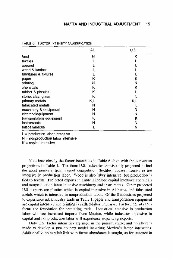
Table 6 summarizes factor intensities, classifying each industry as intensive in one of the inputs. This classification relies on the rankings in Table 5. Each input appears in two rankings. When an industry is ranked higher than the median in both rankings, it is classified as intensive in that input. For instance, chemicals is ranked (1,l) in the uKj/uLj ratios in (AL, U.S.) and (3,l) in the uq/u, rankings. Chemicals is thus called capital intensive (K) . As another example, fabricated metals is intensive in L relative to K in Table 5 (10,13), intensive in N relative to K (10,14), intensive in N relative to L in Alabama (12), but slightly intensive in L relative to N in the U S . (8). The industry is thus classified as intensive in nonproduction labor. Primary metals is ambiguous in this scheme, the median in uKj/aLj ratios, slightly K intensive relative to N , and slightly L intensive relative to N .
Textiles, apparel, wood, and furniture are intensive in production labor. Industries which are clearly intensive in nonproduction labor are printing, machinery, electrical equipment, and instruments. Capital intensive industries are paper, chemicals, and transportation equipment. Food, plastics, stone, primary metals, fabricated metals, and miscellaneous manufacturing are all ambiguous in this ranking scheme.
0, m, = W L u L j / W ~ N .
NAFTA AND INDUSTRIAL ADJUSTMENT 15
TABLE 6. FACTOR INTENSITY CLASSIFICATION
AL U.S.
food N K textiles L L apparel L L wood & lumber L L furnitures & fixtures L L paper K K printing N N chemicals K K rubber & plastics K L stone, clay, glass K L primary metals K,L K,L fabricated metals N L machinery & equipment N N electricalequipment N N transportation equipment K K instruments N N miscellaneous L N
L = production labor intensive N = nonproduction labor intensive K = capital intensive
Note how closely the factor intensities in Table 6 align with the consensus projections in Table 1. The three U.S. industries consistently projected to feel the most pressure from import competition (textiles, apparel, furniture) are intensive in production labor. Wood is also labor intensive, but production is tied to forests. Projected exports in Table 1 include capital intensive chemicals and nonproduction-labor-intensive machinery and instruments. Other projected U.S. exports are plastics which is capital intensive in Alabama, and fabricated metals which is intensive in nonproduction labor. Of the 8 industries projected to experience intraindustry trade in Table 1, paper and transportation equipment are capital intensive and printing is skilled-labor intensive. Factor intensity thus forms the foundation for predicting trade. Industries intensive in production labor will see increased imports from Mexico, while industries intensive in capital and nonproduction labor will experience expanding exports.
Only U.S. factor intensities are used in the present study, and no effort is made to develop a two country model including Mexico’s factor intensities. Additionally, no explicit link with factor abundance is sought, as for instance in
16 GROWTH AND CHANGE, WINTER 1996
Moroney (1970). One goal of the present study is to show how commonly available production data can be fashioned into a general equilibrium model of production. Clearly, many other influences will come into play in determining regional industrial adjustment. The present model makes many simplifying assumptions, but arrives at a set of unambiguous results.
While many contend that factor intensity plays a decreasing role in explaining international trade, it is striking that Table 1 and Table 6 basically agree. Predictions of trade based on factor abundance and factor intensity agree with the consensus projections from the literature, which include numerous types of models and a variety of analysis. Industries intensive in production labor in the U.S. can be transferred to Mexico, which has abundant and cheap production labor.
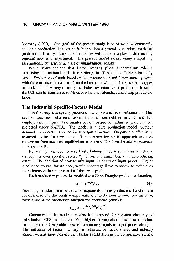
The Industrial Specific-Factors Model The first step is to specify production functions and factor substitution. This
section specifies behavioral assumptions of competitive pricing and full employment, and presents estimates of how output will adjust to price changes projected under NAFTA. The model is a pure production model, without demand considerations or an input-output structure. Outputs are effectively assumed to be final products. The comparative static approach assumes movement from one static equilibrium to another. The formal model is presented in Appendix B.
By assumption, labor moves freely between industries and each industry employs its own specific capital Kj. Firms minimize their cost of producing output. The decision of how to mix inputs is based on input prices. Higher production wages, for instance, would encourage firms to switch to techniques more intensive in nonproduction labor or capital.
Each production process is specified as a Cobb-Douglas production function,
x- I = L"iPK,'. (4) Assuming constant returns to scale, exponents in the production function are factor shares and the positive exponents a, b, and c sum to one. For instance, from Table 4 the production function for chemicals (chm) is
- LlwN086K ,810 xchrn - chin .
Outcomes of the model can also be discussed for constant elasticity of substitution (CES) production. With higher (lower) elasticities of substitution, firms are more (less) able to substitute among inputs as input prices change. The influence of factor intensity, as reflected by factor shares and industry shares, weighs more heavily than factor substitution in the comparative statics.
NAFTA AND INDUSTRIAL ADJUSTMENT 17
Thus, improved estimates of production functions as in Moroney and Toevs (1977) would not make large differences in the projected comparative static output adjustments.
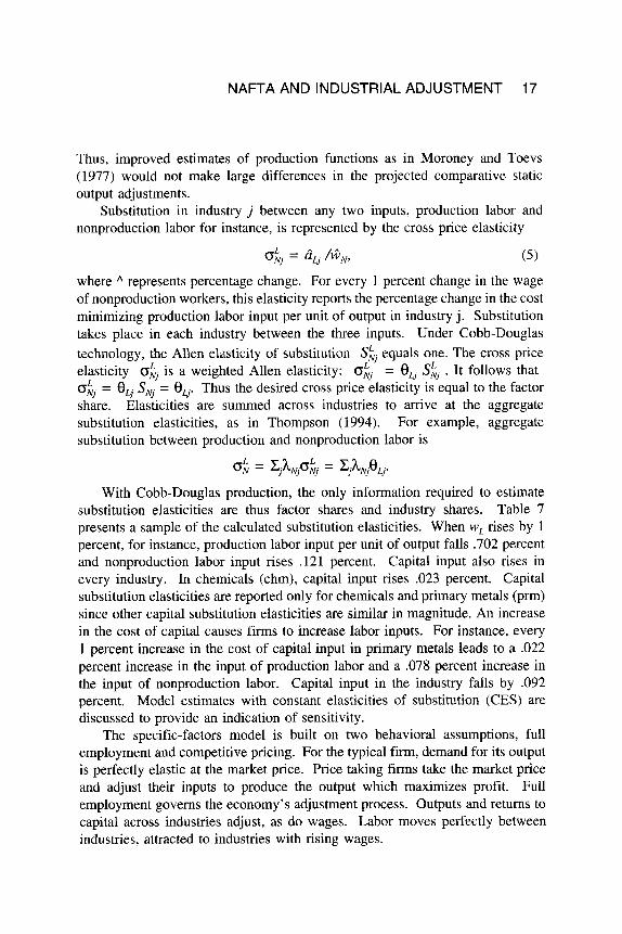
Substitution in industry j between any two inputs, production labor and nonproduction labor for instance, is represented by the cross price elasticity
( 5 ) ON, - aL, / @ N ,
where represents percentage change. For every 1 percent change in the wage of nonproduction workers, this elasticity reports the percentage change in the cost minimizing production labor input per unit of output in industry j. Substitution takes place in each industry between the three inputs. Under Cobb-Douglas technology, the Allen elasticity of substitution S;, equals one. The cross price elasticity o;, is a weighted Allen elasticity: oh, = 8, Sk, . It follows that o;, = 8, SNJ = 8,. Thus the desired cross price elasticity is equal to the factor share. Elasticities are summed across industries to arrive at the aggregate substitution elasticities, as in Thompson (1 994). For example, aggregate substitution between production and nonproduction labor is
L - *
0; = c$wo;, = c,4tqj0Lj.
With Cobb-Douglas production, the only information required to estimate substitution elasticities are thus factor shares and industry shares. Table 7 presents a sample of the calculated substitution elasticities. When wL rises by 1 percent, for instance, production labor input per unit of output falls .702 percent and nonproduction labor input rises .121 percent. Capital input also rises in every industry. In chemicals (chm), capital input rises .023 percent. Capital substitution elasticities are reported only for chemicals and primary metals (prm) since other capital substitution elasticities are similar in magnitude. An increase in the cost of capital causes firms to increase labor inputs. For instance, every 1 percent increase in the cost of capital input in primary metals leads to a .022 percent increase in the input of production labor and a .078 percent increase in the input of nonproduction labor. Capital input in the industry falls by .092 percent. Model estimates with constant elasticities of substitution (CES) are discussed to provide an indication of sensitivity.
The specific-factors model is built on two behavioral assumptions, full employment and competitive pricing. For the typical firm, demand for its output is perfectly elastic at the market price. Price taking firms take the market price and adjust their inputs to produce the output which maximizes profit. Full employment governs the economy’s adjustment process. Outputs and returns to capital across industries adjust, as do wages. Labor moves perfectly between industries, attracted to industries with rising wages.

18 GROWTH AND CHANGE, WINTER 1996
TABLE 7. COBB-DOUGLAS SUBSTITUTION ELASTICITIES IN ALABAMA MANUFACTURING
YoAL %AN %AKchm ~ O A K p r l l l
l % A wL -.702 ,121 .023 .035 WN .261 -.848 ,057 ,033
rprrn .022 .078 0 -.092 rchrn ,016 .013 -.030 0
Capital is treated as industry specific in the short run, with each industry’s endowment of capital Kj exogenously held fixed. An alternative is to assume perfect capital mobility between industries. An advantage of using the assumption of industry specific capital is that variation in the return to capital by industry can occur. Subsequent long run changes in investment by industry are then projected, based on these changes in industrial capital returns. The model formally assumes a uniform return to industrial capital across industries in a pre-NAFTA equilibrium, then examines changes in the pattern of capital returns due to projected price changes. In a model with homogeneous capital, the return to capital would be the same across industries.
Comparative Static Adjustments When price in an industry changes, outputs adjust as summarized in Table
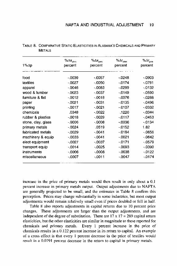
8. Price changes in each industry lead to reported output adjustments in chemicals (x,,,) and primary metals (x,,,). There are 17 x 17 = 289 price elasticities of outputs, and the others are similar in magnitude. Columns report output adjustments for 1 percent price changes in each sector. As an example, every 1 percent increase in the price of primary metals (prm) results in a 0.0024 percent decline in the output of chemicals. Other industrial outputs also decline slightly, contributing to the 0.05 19 percent increase in the output of primary metals.
The striking characteristic of the output elasticities in Table 8 is their inelasticity. The Cobb-Douglas specification contributes to this small magnitude. With a higher degree of CES production, these elasticities change proportionately. When CES = 2, for instance, every 1 percent change in the price of inputs causes a 2 percent change in inputs per unit of output, and the elasticities in Table 8 would be doubled. Empirical studies seldom find CES estimates larger than 2. Even with CES = 2, the largest output elasticity, which is in primary metals, would be only 2 x 0.0519 = 0.1038. Every 1 percent
NAFTA AND INDUSTRIAL ADJUSTMENT 19
TABLE 8. COMPARATIVE STATIC ELASTICITIES IN ALABAMA’S CHEMICALS AND PRIMARY
METALS
1 YoAp %AXchm %AX,,, % Archm %Arpr, percent percent percent percent
food textiles apparel wood & lumber furniture & fixt paper printing chemicals rubber & plastics stone, clay, glass primary metals fabricated metals machinery & equip elect equipment transport equip instruments miscellaneous
-.0039 -.0027 -.0046 -.0023 -.0012 -.0021 -.0017 .0348
-.0018 -.0006 -.0024 -.0029 -.0033 -.0027 -.0014 -.0006 -.0007
-.0057 -.0050 -.0083 -.0037 -.0018 -.0031 -.0021 -.0022 -.0029 -.0008 .0519
-.0041 -.0041 -.0037 -.0025 -.0008 -.0011
-.0248 -.0174 -.0299 -.0149 -.0076 -.0135 -.0107 ,1220
-.Oil7 -.0036 -.0152 -.0184 -.0021 -.0171 -.0093 -.0038 -.0047
-.0903 -.0791 -.0132 -.0590 -.0288 -.0496 -.0332 -.0344 -.0453 -.0134 1.82 -.0656 -.0642 -.0579 -.0390 -.0122 -.0174
increase in the price of primary metals would then result in only about a 0.1 percent increase in primary metals output. Output adjustments due to NAFTA are generally projected to be small, and the estimates in Table 8 confirm this perception. Prices may change substantially in some industries, but most output adjustments would remain relatively small even if prices doubled or fell in half.
Table 8 also reports adjustments in capital returns due to 10 percent price changes. These adjustments are larger than the output adjustments, and are independent of the degree of substitution. There are 17 x 17 = 289 capital return elasticities, but the other elasticities are similar in magnitude to these reported for chemicals and primary metals. Every 1 percent increase in the price of chemicals results in a 0.122 percent increase in its return to capital. An example of a cross effect is that every 1 percent decrease in the price of textiles would result in a 0.0791 percent decrease in the return to capital in primary metals.
20 GROWTH AND CHANGE, WINTER 1996
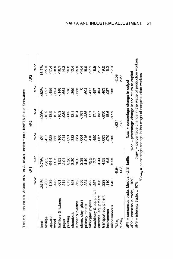
Elasticities in Table 8 are based on the assumption that only one price changes with all other prices (and factor endowments) held constant. NAFTA, however, will introduce a range of price changes across industries. Table 9 reports adjustments in outputs and returns to capital under three different price scenarios. The first price scenario AP1 is based on the consensus trade pattern in Table 1 and the differences between U.S. and Mexican tariffs in Table 2. The difference between tariffs is used as the projected price change in Alabama. For instance, chemicals is projected by Table 1 to be a U.S. export, and Table 2 indicates a difference of 6 percent in tariffs. The price of chemicals is thus projected to rise 6 percent under API. For the U.S. imports in Table 1, price declines are projected to be 26 percent in textiles, 32 percent in apparel, and 1 percent in furniture. For industries projected to experience increased intraindustry trade, projected price changes are set to zero. Export and price changes for the U.S. are thus projected onto Alabama.
Under AP1, only textiles and apparel output fall, both only by about 1 percent. Other outputs rise slightly, typically less than half of 1 percent. Returns to capital, however, are grossly affected in some industries, with significant declines in textiles and apparel.
A further assumption leads to projected long run output adjustments. Suppose capital moves in proportion to the change in its return. Under this assumption, every 1 percent change in the return to capital causes a 1 percent long run adjustment in the capital stock. Under APl, for instance, the capital stock in plastics would rise by 10.0 percent, while the capital stock in apparel would fall by 54.5 percent. When levels of capital adjust, outputs also adjust. In the specific-factors model with CRS, the percentage adjustment in output is about equal to the percentage change in the industry’s capital stock. Thus, the columns labeled percent Ar can be interpreted as approximate long run output changes. Output in apparel is thus projected to fall more than 50 percent in the long run under APl, and in textiles by close to 40 percent. Industries projected by AP1 to expand more than 10 percent in the long run are wood, rubber, fabricated metals, machinery, and instruments. Every industry except textiles and apparel would expand in the long run under API.
Production labor suffers falling wages under API, with production wages falling 6.94 percent. The decrease in production wages for Alabama is larger than generally projected for the entire U.S. Alabama is a relatively heavy producer of goods intensive in production labor, namely textiles apparel, wood, and miscellaneous manufacturing. The large impact on production wages is thus explained by Alabama’s pattern of production.
TA
BLE
9.
INDU
STRI
AL A
DJU
STM
EN
T IN A
LAB
AM
A
UN
DE
R T
HR
EE
NA
FT
A P
RICE
SCE
NARI
OS
AP 1
A
P2
AP
3 %
AX
YoAr
YO
AX
%A
r %
AX
YoAr
food
.2
01 Yo
text
iles
-.930
ap
pare
l -1
.39
woo
d .4
49
furn
iture
& fi
xtur
es
.061
pa
per
,314
pr
intin
g ,0
79
chem
ical
s .3
58
rubb
er &
pla
stic
s .3
62
ston
e, c
lay,
gla
ss
,056
pr
imar
y m
etal
s ,2
84
fabr
icat
ed m
etal
s ,4
22
mac
hine
ry &
equ
ipm
ent
.567
el
ectri
cal e
quip
men
t ,1
96
trans
port
equi
pmen
t .2
29
inst
rum
ents
,1
10
mis
cella
neou
s ,0
43
%A
WL
YoAW
.,
2.79
%
-38.
5 -5
4.4
20.6
1.
53
2.01
2.
26
8.30
10
.0
2.38
4.
49
12.2
17
.7
4.44
4.
55
16.8
3.
33
-6.9
4 ,0
03
0%
-.457
-.5
28
.332
-.1
66
-.014
-.0
21
.332
.3
84
-.004
-.0
15
,418
,4
50
-.037
-.0
03
,079
-.
lo2
-.40
9%
-16.
2 -1
8.5
19.3
-1
6.9
-.089
-.6
02
12.1
16
.4
-.161
.2
36
17.1
17
.7
-.837
-.
050
15.6
-1
7.9
-.621
2.
75
.482
%
-.397
-.
459
-.304
-.1
48
,664
.2
16
.369
-.3
53 0
-.504
-.4
17
.497
,4
94
.463
.0
87
. 1 02
16.7
%
-15.
3 -1
7.4
-1 8.
9 -1
6.1
14.3
16
.2
12.4
-1
5.9
-14.
4 -1
8.0
-17.
1 18
.5
21.2
19
.2
16.2
17
.9
-2.0
9 2.
27
AP
1 =
cons
ensu
s tra
de, M
exic
an-U
.S. t
ariff
s A
P2
= co
nsen
sus
trade
, f 1
0%
AP
3 =
inte
nsity
trad
e, f 1
0%
%Ax
i =
per
cent
age
chan
ge in
out
put
%A
w, =
per
cent
age
chan
ge in
the
wag
e of
pro
duct
ion
wor
kers
%
Ari =
per
cent
age
chan
ge in
the
retu
rn to
cap
ital
%Aw,
= p
erce
ntag
e ch
ange
in th
e w
age
of n
onpr
oduc
tion
wor
kers
4
D - z 0 c cn -I n F e 2 D
C
cn rn Z
22 GROWTH AND CHANGE, WINTER 1996
The columns labeled AP2 use the same consensus trade pattern, but set price changes at +I0 percent for exports and -10 percent for imports. These are larger price increases for exports, and smaller price decreases for imported textiles and apparel. Again, price changes in intraindustry trade industries are set to zero. Output adjustments are again all less than 1 percent in the short run, but long run changes are more striking. Compared to API, declines in long run output in textiles and apparel are less radical, while declines in furniture and miscellaneous are more than 15 percent. Export industries are again projected to enjoy small output increases in the short run under AP2. Returns to capital all rise more than 10 percent, inducing subsequent investment and long run increased output. Chemical output would rise 12.1 percent in the long run under AP2. Some of the long run output changes are close to 20 percent. Production labor loses under AP2, but by less than under APl. Textiles and apparel employ large shares of production labor, and changes in these two prices drive production wages.
The price scenario AP3 is based directly on the U.S. factor intensities in Table 6. Industries which are intensive in production labor are treated as import competing, with price declines set at 10 percent. Primary metals is included as production labor intensive. Outputs fall in the import competing industries, but by less than 1 percent in the short run. Returns to capital fall in the range of 15 percent to 20 percent. Industries which are intensive in nonproduction labor and capital are treated as export industries, with price increases set at 10 percent. Output increases by less than 1 percent in the short run in each of these industries. Capital returns rise substantially in each export industry, signalling increased investment and long run output increases in the range of 15 percent to 20 percent. Wages of production workers fall, while nonproduction labor enjoys gains. All of the gains from trade are thus distributed to nonproduction workers and some capital owners.
Conclusion Some industries will decline under NAFTA, but short run output adjustments
will be negligible. As changing returns to capital alter investment, however, long run output adjustments will be substantial in particular industries. Projecting the results from Alabama to the entire U.S., this paper reaches the consensus opinion that downward pressure on the wages of production labor will continue, increasing the incentive to obtain education and training. The return to education is underestimated if historical wages are used.
Every price scenario has differences, but there are similarities. Under every assumption, Alabama’s textiles and apparel industries decline, wages of production workers fall, and wages of nonproduction workers rise. Other likely
NAFTA AND INDUSTRIAL ADJUSTMENT 23
industrial losers are furniture and primary metals. Industrial winners in Alabama under every scenario are chemicals, machinery, and instruments. Other likely winning industries are food, wood, paper, printing, electrical equipment, and transportation equipment. Industries which are “too close to call” are plastics, fabricated metals, and miscellaneous.
First, industries can be disaggregated. Estimation of production or cost functions can be refined. The model can be applied to other states, regions, or the entire U.S. Final demand and an input-output structure can be added. Varying degrees of labor and capital mobility can be included. Factor intensity and production can be modelled explicitly in Mexico. International capital flows can be introduced. The influence of factor intensity, however, is strong enough that the basic results presented here would continue to hold.
The present line of research can be extended in various ways.
REFERENCES Baer, D., and G. Erd, eds.
Boyd, R., K. Krutilla, and J. McKinney.
1991. Strategic sectors in Mexican - US. free trade. Washington DC: Center for Strategic and International Studies .
1991. The impact of tariff liberalization between the United States and Mexico: A general equilibrium analysis, Baylor University, working paper.
Brown, D., A. Deardorff, and R. Stern. 1992. A North American free trade agreement: Analytical issues and a computational assessment. The World Economy, 11-29.
Department of Commerce. 1992. Annual survey of manufactures, Washington DC. . 1993. North American Free Trade Agreement: Opportunities for U.S.
industries, NAFTA industry sector reports, Washington DC. Hansen, N. 1994. NAFTA: Implications for U.S. regions, The Survey of Regional
Literature, 4-22. Hinojosa, R. and S. Robinson. 1991. Alternative scenarios of U.S.-Mexico integration:
A computable general equilibrium approach. University of California, Berkeley, working paper.
Hufbauer, G., and J. Schott. 1992a. North American free trade: Issues and recommendations, Washington DC: Institute for International Economics.
. 1992b. Prospects for North American free trade. Washington DC: Institute for International Economics.
. 1993. NAFTA: An assessment. Washington DC: Institute for International Economics.
Hufbauer, G., and K. Elliott. Measuring the cost of protection in the US. Washington DC: Institute for International Economics.
Hunter, L., J. Markusen, and T. Rutherford. 1995. Trade liberalization in a multinational-dominated industry, Journal of International Economics, 95- 1 I 7.
1994.
24 GROWTH AND CHANGE, WINTER 1996
Inforum. 1990. Industrial effects of free trade agreement between Mexico and the U.S.A, prepared for the U.S. Department of Labor. College Park: University of Maryland.
International Trade Commission. 199 I . The likely impact on the United States of a free trade agreement with Mexico, Washington DC.
Kehoe, P., and T. Kehoe. Capturing NAFTA’s impact with applied general equilibrium models, Quarterly Review, Federal Reserve Bank of Minneapolis, Spring.
Learner, E. 1984. Sources of comparative advantage: Theory and evidence. Cambridge: The MIT Press.
Lustig, N., B.P. Bosworth, and R.Z. Lawrence (eds). 1992. North American free trade: Assessing the impact. Washington DC: Brookings Institution.
Morici, Peter. 1991. Trade talk with Mexico: A time for realism. Washington DC: National Planning Association.
Moroney, J. 1970. The strong factor-intensity hypothesis: A multisectoral test, Journal of Political Economy, 241-89.
Moroney, J . , and A. Toeus. 1977. Factor costs and factor use: An analysis of labor, capital, and natural resource inputs, Southern Economic Journal, 222-39.
Peat Marwick. The effects of u free trade agreement between rhe U.S. and Mexico. Washington DC: U.S. Council of the Mexico-U.S. Business Committee.
Prestowitz, C., and R. Cohen. 1991. The new North American order: A win-win strategy for US.-Mexican trade. Washington DC: University Press of American.
Thompson, H. 1994. An investigation into the quantitative properties of the specific factors model of international trade, Japan and the World Economy pp. 378-88.
Trela, I., and J. Whalley. 1992. Bilateral trade liberalization in quota restricted items: U.S. and Mexico and textiles and steel. The World Economy.
Weintraub, S., L. Rubio, and A. Jones. 1991 U S . - Mexican industrial integration: The road to free trade. Boulder CO: Westview Press.
Young, L., and J.J. Romero. 1991. A dynamic dual model of the Free Trade Agreement. University of Texas, working paper.
1994.
1991.
NAFTA AND INDUSTRIAL ADJUSTMENT 25
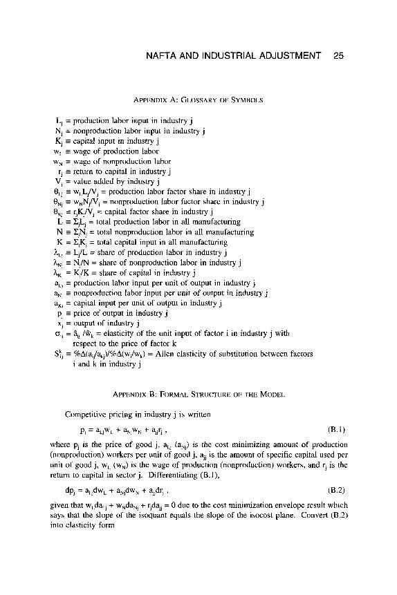
APPENDIX A: GLOSSARY OF SYMBOLS
Lj = production labor input in industry j Nj = nonproduction labor input in industry j K, = capital input in industry j wL = wage of production labor wN = wage of nonproduction labor
rJ = return to capital in industry J
Vj = value added by industry j eLj = wLL,/VJ = production labor factor share in industry j 0 , = w,NjN, = nonproduction labor factor share in industry J
0, = rjK,/VJ = capital factor share in industry j L = CjLJ = total production labor in all manufacturing N = CJN, = total nonproduction labor in all manufacturing K = CjK, = total capital input in all manufacturing
h,, = Lj/L = share of production labor in industry j h, = Nj/N = share of nonproduction labor in industry J
h , = K,/K = share of capital in industry j aLj = production labor input per unit of output in industry j a,, = nonproduction labor input per unit of output in industry J aKj = capital input per unit of output in industry J
p, = price of output in industry j xJ = output of industry j oil = gi, / ~ k = elasticity of the unit input of factor i in industry j with
respect to the price of factor k
i and k in industry j s! 1J = y oA(a,jla,)/%A(w,/w,) = Allen elasticity of substitution between factors
APPENDIX B: FORMAL STRUCTURE OF THE MODEL
Competitive pricing in industry J is written
Pj = ~ L J W L + ~ N ~ W N + 7 (B. 1 )
where p, is the price of good j, aLJ (a,) is the cost minimizing amount of production (nonproduction) workers per unit of good j, aJ, is the amount of specific capital used per unit of good j, wL (w,) is the wage of production (nonproduction) workers, and r, is the return to capital in sector j. Differentiating (B.l),
(B.2)
given that w,daLJ + w,da,, + r,dau = 0 due to the cost minimization envelope result which says that the slope of the isoquant equals the slope of the isocost plane. Convert (B.2) into elasticity form
dp, = aLJdwL + a,,dw, + a,drJ ,
26 GROWTH AND CHANGE, WINTER 1996
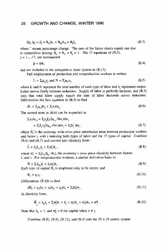
dp, /pJ = 0, = 0,2, + 9NJ2N + eJ,tJ, (B.3)
where A means percentage change. The sum of the factor shares equals one due to competitive pricing: 8, + 8, + 0, = 1. The 17 equations of (B.3), j = 1, ..., 17, are summarized
p = 0*, 03.4)
and are included in the comparative static system in (B.13). Full employment of production and nonproduction workers is written
L = XJaLJxJ and N = CJaNJx,. 03.5)
where L and N represent the total number of each type of labor and xJ represents output. Labor moves freely between industries. Supply of labor is perfectly inelastic, and (B.5) says that total labor supply equals the sum of labor demands across industries. Differentiate the first equation in (B.5) to find
dL = ZJaLJdx, + ZJxJdaL, . The second term in (B.6) can be expanded as
CJxJdaL, = ZJxJZ,(aaLJ IawJdw,
= C,ZJxJ(da,, ldw,)dw, = C,S; dw, , 03.7)
where S; is the economy wide cross price substitution term between production workers and factor i , with i indexing both types of labor and the 17 types of capital. Combine (B.6) and (B.7) and convert into elasticity form:
L = Zjkj2j i- C p ; q ,
N = ZJ&j?J + zio;2, .
where 0; = ZJkLJ(iiLj /*J, the economy’s cross price elasticity between factors L and i . For nonproduction workers, a similar derivation leads to
Each type of capital K, is employed only in its sector, and
K. = a.x. J J J J .
Differentiate (B.lO) to find
dKj = ajjdxj + xJdaJ = ajjdxl + ZiS;dwi.
In elasticity form,
K, = + = Xj + o p L + G;*N + 0jfJ . 1
Note that hjj = 1, and 06 = 0 for capital when n # j.
Combine (B.8), (B.9), (B.12), and (B.4) into the 35 x 35 matrix system
(B.8)
(B.9)
(B.lO)
(B.11)
(B.12)
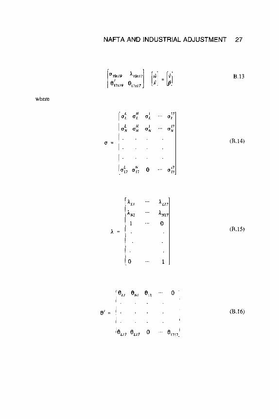
NAFTA AND INDUSTRIAL ADJUSTMENT 27
L N 1 17' O L OL OL .'. OL
ON aN oN aN ..* L N 1 17
. . .
. . .
. . .
where
a =
a =
0 -
B.13
(B.14)
(B.15)
(B.16)
28 GROWTH AND CHANGE, WINTER 1996
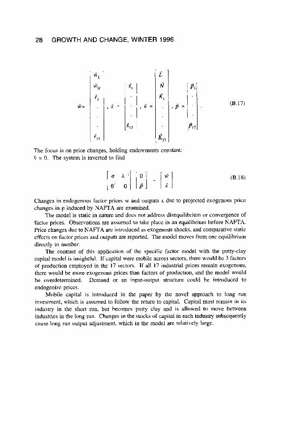
, v = ,P =
The focus is on price changes, holding endowments constant: G = 0. The system is inverted to find
P i
$1,
(B.17)
(B.18)
Changes in endogenous factor prices w and outputs x due to projected exogenous price changes in p induced by NAFTA are examined.
The model is static in nature and does not address disequilibrium or convergence of factor prices. Observations are assumed to take place in an equilibrium before NAFTA. Price changes due to NAFTA are introduced as exogenous shocks, and comparative static effects on factor prices and outputs are reported. The model moves from one equilibrium directly to another.
The contrast of this application of the specific factor model with the putty-clay capital model is insightful. If capital were mobile across sectors, there would be 3 factors of production employed in the 17 sectors. If all 17 industrial prices remain exogenous, there would be more exogenous prices than factors of production, and the model would be overdetermined. Demand or an input-output structure could be introduced to endogenize prices.
Mobile capital is introduced in the paper by the novel approach to long run investment, which is assumed to follow the return to capital. Capital must remain in its industry in the short run, but becomes putty clay and is allowed to move between industries in the long run. Changes in the stocks of capital in each industry subsequently cause long run output adjustment, which in the model are relatively large.