Columbia Program on Indian Economic

Policies

Working Paper No. 2010-3

Trade Liberalization and Poverty Reduction:

New Evidence from Indian States

J.Salcedo Cain, Rana Hasan

and

Devashish Mitra

2

Trade Liberalization and Poverty Reduction:

New Evidence from Indian States

J.Salcedo Cain

University of Missouri

jsc535@mail.missouri.edu

Rana Hasan

Asian Development Bank

rhasan@adb.org

Devashish Mitra

Syracuse University

dmitra@maxwell.syr.edu

November 2010

Abstract: As is widely acknowledged, the incidence of poverty in India has declined steadily over the

last several decades. What is debated, however, is the pace at which poverty has declined and its

relationship with India's economic reforms. In particular, a key concern among policymakers and

researchers alike is that trade liberalization undertaken in the early 1990s may have slowed the progress

made in reducing poverty. In this paper, we update our previous econometric analysis on the links

between trade liberalization and poverty reduction in India. By incorporating measures of poverty based

on the 2004-05 consumer expenditure survey carried out by India's National Sample Survey Organisation,

we are able to sidestep the controversy-ridden poverty measures based on the 1999-2000 survey. Our

new results are in line with the earlier ones in Hasan, Mitra and Ural (2007): States, and regions within

states, that were more exposed to trade liberalization on account of their employment structures did not

experience slower reduction in poverty; on the contrary, to the extent that we find a statistically

significant relationship between trade liberalization and poverty reduction, the evidence points to faster

poverty reduction in states and regions experiencing greater increases in exposure to trade. Moreover,

this relationship is typically stronger in states with more flexible labor regulations, better quality

transportation infrastructure, and more developed financial systems.

# Work on this paper has been supported by Columbia University‘s Program on Indian Economic Policies, funded

by a generous grant from the John Templeton Foundation. The opinions expressed in the paper are those of the

authors and do not necessarily reflect the views of the John Templeton Foundation or the Asian Development Bank,

its Executive Directors, or the countries that they represent.

Corresponding author: Department of Economics, The Maxwell School, Syracuse University, Eggers Hall,

Syracuse, NY 13244. Phone: (315) 443-6143, Fax: (315) 443-3717.

3

1. Introduction

International trade leads to gains in aggregate welfare or average real incomes through various channels.

It generates efficiency gains from specialization and exchange based on comparative advantage. It also

leads to higher welfare and productivity due to the availability of larger varieties of final and intermediate

goods. These are aggregate effects and do not automatically translate into a reduction in poverty, as trade

does create winners and losers.

Under fairly plausible conditions, trade theory tells us that the winners from trade liberalization are the

owners of the factor(s) of production a country is relatively abundant in and the losers are the owners of

the scarce factor(s). Most poor countries are actually relatively abundant in unskilled labor. This fact

should lead us to expect that unskilled workers will benefit from trade liberalization in such countries. As

a result, trade reforms should help with poverty reduction in poor, unskilled labor abundant countries.

However, what can come in the way of the prediction regarding the poverty reducing effect of trade to

hold is the lack of mobility of factors, including labor, from one sector to another. The reasons are two-

fold. Firstly, the gains from specialization work through the reallocation of factors from one sector to

another. Secondly, the prediction that all unskilled workers gain from trade in a country that is abundant

in them requires the equalization of their wages across sectors. In the absence of intersectoral labor

mobility, such equalization will not take place and workers, who are not able to get out of sectors that are

forced to shrink upon trade liberalization, will see a decline in their incomes (and even an adverse change

in their employment status in the presence of other labor market rigidities).

Based on arguments above, the effect of trade on poverty becomes an empirical question. This paper is an

update and an extension of the earlier empirical study by Hasan, Mitra and Ural (2007) that uses Indian

state-level and region-level poverty data from India. For updating the study, we construct, from

individual-level data from the latest round of the National Sample Survey (NSS Round 61), the standard

poverty measures both at the state and region-levels. In terms of extending the analysis, we try to see how

4

the effects of trade liberalization on poverty vary by the degree of labor market flexibility in the various

states, which was also done in the earlier study, but this time we experiment with alternative measures. In

addition, we also for the first time look at how the gains in poverty reduction from trade liberalization will

vary by road connectivity and financial development. While roads will determine how changes in prices

at the border translate into local prices, financial development determines how well the banking system

responds to the changes in the needs of the producers for credit in response to trade reforms. In the face of

greater competition through trade liberalization, domestic producers might have to increase their scale of

production or invest in more modern techniques, for which they need access to credit.

The two studies so far on the impact of trade reforms on poverty are Topalova (2005) and Hasan, Mitra

and Ural (2007). Topalova examined the impact of trade liberalization on district level poverty in India.

Her main findings can be summarized in three short quotes from her paper: (1) ―rural districts where

industries more exposed to trade liberalization were concentrated experienced a slower progress in

poverty reduction‖; (2) ―compared to a rural district experiencing no change in tariffs, a district

experiencing the mean level of tariff changes saw a 2 percentage points increase in poverty incidence and

a 0.6 percentage points increase in poverty depth. This setback represents about 15 percent of India‘s

progress in poverty reduction over the 1990s‖; (3) there is ―no statistically significant relationship

between trade exposure and poverty in urban India‖, but with point estimates still in the same direction as

in the case of rural poverty.

The results from the Hasan-Mitra-Ural study are quite different from Topolova‘s. In no case do they find

reductions in trade protection to have worsened poverty at the state or region level. Instead, they find that

states whose workers are on average more exposed to foreign competition tend to have lower rural, urban

and overall poverty rates (and poverty gaps), and this beneficial effect of greater trade openness is more

pronounced in states that have more flexible labor market institutions. They also find that trade

liberalization has led to poverty reduction to a greater degree in states more exposed to foreign

5

competition by virtue of their sectoral composition. Their results hold, at varying strengths and

significance, for overall, urban and rural poverty. In addition, they find some evidence that industrial

delicensing has had a more beneficial impact on poverty reduction in states with flexible labor institutions

consistent with the findings of Aghion et al (2008) on the relationship between delicensing and

performance of registered manufacturing sector across Indian states.

Unlike Topalova who restricts her analysis to tariffs, Hasan, Mitra and Ural look at both tariffs and non-

tariff barriers (NTBs). Just the way Topalova arrives at her district-level measure of tariffs, Hasan, Mitra

and Ural weight tariffs and alternatively NTBs by sectoral employment to arrive at the state level inverse

measure of the trade exposure of the labor force. But unlike Topalova, they refrain from using

nontradable employment weights (where Topalova sets zero sectoral tariffs) in the aggregation of

protection since a commodity not being traded means the trade costs are prohibitive (not zero). They

allow for the transmission of changes in protection rates to domestic prices to vary by state in some of

their analysis. Third, in order to avoid sampling related issues, they, in contrast to Topolova‘s approach

of using district-level measures of urban and rural poverty, work with state-level measures of urban, rural,

and overall poverty (See Hasan, Mitra and Ural, 2007 for details).1 They also complement their analysis

with robustness checks using region-level measures of poverty, where regions are the ones defined as in

the National Sample Survey (NSS). Like in Topolova‘s analysis, the poverty measures used in the

Hasan-Mitral-Ural study are based on the poverty lines recommended by Deaton and Dreze (2002;

henceforth, DD) and their approach for adjusting poverty estimates for a change in the questionnaire

design of the 1999-2000 NSS household expenditure survey. However, as robustness checks, Hasan,

Mitra and Ural also use two additional sets of poverty measures: Government of India (GOI) estimates of

poverty with an adjustment made for the new questionnaire adopted in 1999-2000 and a longer series (10

years of data for the 1990s and late 1980s) of state-level poverty rates created by Ozler, Datt and

1 The NSSO sampling methodology is not constructed with the aim of making the sample within a district random.

In addition, it is extremely difficult, if not impossible, to keep controlling for changes district boundaries that keep

happening ever so often.

6

Ravallion (1996) (ODR) using both the ―thick‖ and ―thin‖ rounds of the NSS in India.2 Finally, while

the ―thick-round‖ analysis in Hasan, Mitra and Ural is based on poverty estimates for three years -- i.e.

corresponding to the latest three available "thick" rounds of the NSS (i.e., 1987-88, 1993-94 and 1999-

2000) for which protection data are available -- Topalova‘s analysis is restricted to two thick rounds,

those for 1987-88 and 1999-2000, While she justifies her approach based on the uncertainty regarding

whether the 1993-94 poverty is driven by post or pre-reform policies, Hasan, Mitra and Ural include

1993-94 in their thick round analysis since after all the state-level trade exposure measure is being used as

a regressor.

In this new study, we continue to rely on state- and NSS region-specific poverty estimates based on the

poverty lines developed by Deaton (2003a). However, since the latter only cover the years 1987-88,

1993-94 and 1999-2000 (referred to as Deaton and Dreze or the DD poverty measures in Hasan, Mitra

and Ural), we incorporate in our analysis poverty estimates for 2004-05 by using the poverty lines

updated by Amoranto and Hasan (2010) for that year using the procedures of Deaton (2003a). In addition,

we check the robustness of our results by using a second set of state- and NSS region-specific poverty

estimates, namely those from the Government of India‘s Expert Group (2009) for the years 1993-94 and

2004-05, with observations generated for 1987-88 by extrapolating the Expert Group‘s poverty lines for

the year 1987-88 using Deaton‘s (2003a) Fischer prices indexes. For the analysis with the Expert Group

poverty measure, we omit 1999-2000 for the problems of comparability arising from the unusual survey

design for that particular round as described above. All our poverty rate estimates are at the state and

region levels and are calculated for the rural and urban sectors separately as well for the overall state or

region.

2 While in theory the Deaton and Dreze (DD) measure is superior to both the Government of India and the Ozler,

Datt and Ravallion measures, in practice in a world with imperfect data it is possible that it is not so. This could be

due to the high demands placed on the wide variety of data required to compute the DD measure. Also, the ODR

provides with a much longer series,.

7

The protection measures are the same as those used in Hasan, Mitra and Ural (2007) but extended to the

year 2003 which serves as the lagged protection for the year 2004-05 (NSSO Round 61). They are

weighted by employment in different industries to create overall, rural and urban protection (tariff, NTB

and a principal component combination of the two) from the industry-level protection measures at the

national level. Since we want to see whether the trade-poverty nexus is affected by labor-market

flexibility, we use the measure of labor market flexibility used in Hasan, Mitra and Ural (2007), which

was also used in Hasan, Mitra and Ramaswamy (2007), which partitions the set of major Indian states

into the subset of flexible labor market states and the rigid labor market states. Since there is disagreement

on this partitioning, we use two alternative partitionings. Our results are robust to all three measures,

indicating that that the four common states in the flexible subset across the measures (relative to the six

common states in the rigid subset) might be driving the results regarding the differential effects of trade

on poverty in flexible versus rigid states.

These effects could also be different because the degree of transmission of international prices and

protection can differ by state depending on road connectivity. We control for that in our regressions using

road density by state. This also allows us to see how the effects of exposure to foreign trade on poverty

could vary as road connectivity changes across states and over time. Another state characteristic that can

lead to a differential effect is financial development. We use a survey based measure capturing the

proportion of firms facing difficulties in obtaining credit and alternatively, a principal component measure

based on credit-deposit ratios in nationalized banks and the post office to population ratio among other

things from Ghosh and De (2004). Finally, we also want to control for and analyze the impact of another

component of globalization, namely foreign direct investment (FDI), which we do by using the ratio of

foreign direct investment to the gross domestic product of a state.

We find that on average for every percentage point reduction in the weighted tariff rate, there was a 0.57

percent reduction in poverty which implies that a 38 percent reduction in poverty during 1987-2004 can

8

be attributed to change in the exposure to foreign trade. An alternative interpretation is that a state that

experienced a percentage point higher reduction in employment-weighted tariff than another state

experienced 0.57 percent greater reduction in poverty. Since our regressions use time controls and poverty

all across the country has been declining over time, we can infer that trade liberalization (and the greater

exposure of the labor force to foreign competition) actually speeded up poverty reduction. Qualitatively

similar but quantitatively much larger estimates result from the use of NTBs, possibly additionally

capturing the effects of other correlated policy and institutional variables.

In the case of urban poverty, we find that not only have reductions in tariff rates been associated with

reductions in urban poverty across India's states, the extent of this poverty reduction has been larger in

states with flexible labor regulations. In addition, we find that reductions in urban poverty induced by

trade liberalization have been faster in states with higher road density and more advanced banking and

financial systems. In the case of rural poverty, while the overall effect of protection on poverty is

qualitatively similar , the evidence for differential effects based on labor-market flexibility, road density

and financial development is quite weak.

The remainder of this paper is organized as follows. Section 2 reviews the literature on the relationships

between trade, growth, and poverty. Section 3 describes key elements of the Indian policy framework

relating to trade, labor regulations, and the industrial licensing regime over the 1980s and 1990s. Section

4 discusses data issues concerning poverty and measures relating to the policies described in Section 3.

Section 5 presents the results of our empirical work while Section 6 concludes.

2. Trade and Poverty: Review of Related Literature

It has been argued by Bhagwati (2004) that trade, by fostering growth, leads to higher incomes and in turn

a reduction in poverty. Therefore, we first review the literature on the effects of trade barriers on growth

and income, which have been empirically studied since the early 1990s. Various cross-country, macro

9

studies, using different measures of openness, have showed positive effects of trade on growth (See for

instance Dollar (1992), Sachs and Warner (1995) and Edwards (1998)). However, these papers have been

strongly criticized by Rodriguez and Rodrik (2001) for the problems with their openness and protection

measures, their econometric techniques and the difficulty in establishing the direction of causality. While

the measure of openness used by Sachs and Warner (1995), as argued by Rodriguez and Rodrik (2001),

captures many aspects of the macroeconomic environment in addition to trade policy, Baldwin (2003) has

recently defended that approach on the grounds that the other policy reforms captured in the measure

accompany most trade reforms. Therefore, the use of such a measure tells us the value of the entire

package of trade and accompanying reforms. Wacziarg and Welch (2003) have updated the Sachs-Warner

dataset and have again shown the positive growth effects of such reforms.

The more recent papers look at the effects of trade on income levels rather than growth rates. Frankel and

Romer (1999), using gravity and geography based predicted trade flows as instruments, find positive

effects of trade on income levels that are greater than the estimates produced by ordinary least squares.

Irwin and Tervio (2002) demonstrate the robustness of these results, with the same approach applied to

cross-country data from various periods in the twentieth century.

Rodrik, Subramanian and Trebbi (2002) have looked at the simultaneous effects of institutions,

geography and trade on per capita income levels. Using a measure of property rights and the rule of law

to capture institutions and the trade-GDP ratio to capture openness in trade, and appropriately

instrumenting them, they find that ―the quality of institutions trumps everything else‖. However, trade and

institutions have positive effects on each other, so trade does have indirect effects on income.

10

The literature on the direct determinants of poverty rates and changes (or rather reductions) in them is

much smaller.3 Dollar and Kraay (2002), in a cross-country study of 92 countries over the last four

decades, find that the growth rates of average incomes of people in the bottom quintile are no different

from the growth rates of overall per capita incomes, with the former growth always associated with the

latter. Also policies that promote overall growth promote growth in the incomes of the poor. These

policies include trade openness, macroeconomic stability, moderate government size, financial

development, and strong property rights and the rule of law. In another paper, Dollar and Kraay (2004),

based on data from the post-1980 ―globalizing developing economies‖, argue that per capita income

growth arising from expansion in trade in those countries has led to a sharp fall in absolute poverty in the

past 20 years.

Similarly, Ravallion (2001) finds that an increase in the per capita income by 1 percent can reduce the

proportion of people below the $1-a-day poverty line by about 2.5 percent on average. This varies across

countries, depending how close the poor are to the poverty line. Research by Ravallion and Datt (1999)

on the determinants of poverty reduction across India‘s major states between 1960 and 1994 also shows

empirically the importance of initial conditions. They find that a one percent increase in non-agricultural

state domestic product leads to a 1.2 percent decline in poverty rates in the states of Kerala and West

Bengal versus only 0.3 percent decline in Bihar. The fact that growth of non-farm output was also

relatively meager in Bihar over the period under consideration exacerbated the poverty problem in Bihar.

Ravallion and Datt find that more than half of the differential impact of non-farm output on poverty rates

is attributable to Kerala‘s much higher levels of initial literacy. Their results suggest that while the

transition from (low-wage) agriculture to (higher wage) non-farm sectors may be key for the removal of

poverty, making the transition is not easy or automatic for the poor. In other words, there are pecuniary

3 For an excellent, comprehensive survey of the evidence on the globalization-poverty linkage, see Harrison (2006).

11

costs as well as non-pecuniary ones associated with investments in minimum levels of education,

nutrition, and health to be incurred on the part of a poor agricultural worker to making the transition.

Finally, Hasan, Quibria and Kim (2003) argue, using cross-country evidence, that ―policies and

institutions that support economic freedom are critical for poverty reduction.‖ Economic freedom

indicators used by these authors include, government size, price stability, freedom to trade with

foreigners, absence of over-regulations of markets and civil liberties as reflected in property rights, rule of

law etc.

We end this literature review with two cautionary notes. Firstly, most of these studies are cross country.

Such studies, despite using numerous controls, cannot control for the institutional diversity across the

world. Secondly, some of the poverty studies use a uniform ―$1-a-day‖ definition of poverty across.

Although the conversion of local currencies into the US dollar is made using purchasing power parities,

there are some well known limitations of these for the purposes of comparing poverty across countries

and even within them (ADB, 2008)

.

3. Indian Policy Framework

3.1 Trade Policy Reforms in India

From independence all the way through the early 1980s, India pursued a development strategy of import

substitution. While some liberalization began in the 1980s, by far the most decisive break with the trade

policies of the past came in 1991 in response to a balance of payments crisis resulting from a rapid rise in

the fiscal deficit to GDP ratio, in foreign commercial debt, and in the debt service ratio. These problems

were further accentuated into a crisis-like situation by the dramatic oil price rise originating from the Gulf

War. The government approached the International Monetary Fund (IMF) for financial assistance, which

came attached with the strong conditionality of major economic reforms. These reforms were initiated

12

almost immediately. Given several earlier attempts to avoid IMF loans and the associated conditionalities,

these reforms came as a surprise.

The main objectives of the reform program included simplification of rules, the removal over time of

import and export barriers (that included both price and quantity restrictions) and the eventual full

convertibility of the Indian rupee for foreign exchange transactions. The maximum tariff was reduced

from 400 percent to 150 percent in July 1991 and to roughly 45 percent by 1997-98. Mean tariffs, which

were 128 percent before July 1991 had fallen to roughly 35 percent by 1997-98. The mean manufacturing

tariff fell to under 15 percent by 2005. The reductions in mean tariffs were also accompanied by

significant reductions in tariff dispersion. Nontariff barriers were also reduced. Prior to 1991, there were

quantitative restrictions on 90 percent of the value added in the manufacturing sector. In April 1992, all

the twenty-six import-licensing lists were eliminated, along with the introduction of a ―negative list‖

(from which most intermediate and capital goods were excluded) of prohibited import items. This

eliminated many of the licensing procedures and discretionary aspects of the previous import regime. The

reductions in tariffs and nontariff barriers to trade were also accompanied by significant devaluations of

the Indian rupee in 1991 and 1992.

3.2 Labor Markets: Regulations and Rigidity

A comprehensive review of labor regulations in India is beyond the scope of this paper. 4

However, two

features of India's labor regulations are noteworthy. First, under the Indian constitution, both the central

(federal) government as well as individual state governments have the authority to legislate on labor

related issues and even amend central legislations. And enforcement of all labor regulations is mainly

performed by the state governments.

4 See Anant et al (2006) for a detailed discussion of India‘s labor-market regulations.

13

Second, there is considerable debate among observers of the Indian economy regarding the impact of

labor market regulations on the various dimensions of economic performance. Consider Chapter VB of

the Industrial Disputes Act (IDA) which makes it compulsory for employers with more than 100 workers

to seek the prior approval of the government before workers can be dismissed. In practice, governments

have often been unwilling to grant permission to retrench (Datta-Chaudhuri, 1996).5 Therefore, critics of

these labor laws argue that they have created a strong disincentive to hire (additional) workers, and a bias

against hiring (abundant) labor relative to (scarce) capital, leading to weak employment growth. Similar

arguments have been made for other elements of labor regulations, including specific provisions of the

Industrial Employment (Standing Orders) Act and the Trade Union Act (TUA).6

Not all analysts agree with the above view. Their counter-argument is that most of India‘s labor

regulations have been either ignored (see Nagaraj, 2002) or circumvented through the increased usage of

temporary or contract labor (see, in particular, Datta, 2003, and Ramaswamy, 2003). Ultimately, whether

India‘s labor laws have created significant rigidities in labor markets or not is therefore an empirical

question.

4. Data

4.1 Poverty

Our main measure of (absolute consumption) poverty is the headcount index, or poverty rate. This

measures the proportion of the population with consumption expenditures below a given threshold, or

5 The term layoff refers to a temporary or seasonal dismissal of a group of workers due to slackness of current

demand. Retrenchments, on the other hand, denote permanent dismissals of a group of workers. Both terms may

be distinguished from ―termination‖ which refers to separation of an individual from his or her job.

6 As per the Standing Orders Act, worker consent is required to modify job descriptions or move workers from one

plant to another. While the goal of promoting worker consent is certainly an important one, Anant (2000) argues

that rigidities can creep in on account of how one defines or establishes worker consent. With the Trade Union Act

allowing multiple unions within the same establishment and rivalries common across unions, a requirement of

worker consent for enacting changes ―can become one of consensus amongst all unions and groups, a virtual

impossibility‖ (page 251).

14

poverty line. We also consider an alternative measure of poverty, the poverty gap index (PGI). The PGI,

unlike the poverty rate, gives a sense of how poor the poor are. It is equivalent to the shortfall of

consumption below the poverty line per head of the total population, and is expressed as a percentage of

the poverty line.7

In principle, the official poverty lines of the Government of India and the large-scale, or quinquennial-

round consumer expenditure surveys carried out by the National Sample Survey Organisation (henceforth

referred to as NSS surveys) approximately every five years provide an excellent basis for estimating

measures of rural and urban poverty at the national, state, and NSS region level8 over 1987-2004, the

period of interest to us in this paper. In practice, however, there has been considerable controversy about

the estimates of poverty that these data yield. There are two main points of contention.9 First, the

information on food expenditures obtained by the NSS survey carried out in 1999-2000 has been deemed

by many researchers to be incomparable with expenditure data from other large-scale NSS surveys carried

out before and since then. Given the large share of food in total expenditures – almost 2/3rds of total

expenditures on average even for households in the 5th decile of the distribution of per capita expenditures

in 2004-05 – any incomparability in the food expenditures data would translate into incomparability of

poverty estimates.10

7 The PGI can be expressed as:

m

i

i

z

yz

nPGI

1

1

where yi represents consumption of the i-th poor person, z is the poverty line, n the total population, and m the

number of poor. The poverty rate, or head count index, is simply m/n, of course.

8 NSS regions are geographically contiguous areas within states sharing common agro-climatic conditions.

9 There are other points of contention. For example, Bhalla's (2003) comparisons of consumption expenditure totals

from the NSS surveys with their national accounts analogues has led him to argue that the NSS surveys under state

consumption expenditures in India. Moreover, he argues that this understatement also takes place for poorer

households and thereby results in an overstatement of poverty in India.

10

Since the 1950s NSS consumption expenditure surveys have used a 30-day recall period in canvassing

information on households‘ food expenditures. The 55th round of the survey, undertaken in 1999-2000, adopted

two recall periods for food, one based on a 7-day recall and the other on the standard 30-day recall. Since the

15

Second, and more generally, many researchers have raised concerns about the official poverty lines used

to generate official estimates of poverty. To understand these concerns, it is useful to briefly describe the

official methodology for estimating poverty lines and poverty used currently (but under review as of the

writing of this paper). The current procedures, developed by the Expert Group 1993 (Government of

India, 1993) and adopted since March 1997 by India's Planning Commission, take as their starting point

separate ―all-India‖ poverty lines of Rs. 49.09 per person per month in rural India and Rs. 56.64 in urban

India at 1973-74 prices. These poverty lines, developed originally by a specially constituted task force

(Government of India, 1979), represent the monthly per capita consumption expenditures required on

average to satisfy food consumption corresponding to specified calorie norms (2400 kcal per capita per

day in rural areas and 2100 kcal per capita per day in urban areas) and some minimum of nonfood

requirements (such as clothing, shelter, etc.). Crucially, the computation of these poverty lines is based

on the observed expenditure patterns of households as captured by the NSS consumer expenditure survey

of 1973-74. These all-India rural and urban poverty lines are then adjusted in two ways. First, state- and

sector-specific price indexes for 1973-74 are used to come up with state-and sector-specific poverty lines

to capture interstate price differentials (as they existed in 1973-74). Second, the state-specific poverty

lines are updated for later years using price indexes based on the state-specific CPI of Agricultural

Laborers (CPI-AL) in rural areas and CPI of Industrial Workers (CPI-IW) for urban areas to capture

changes in the cost of living over time.11

These poverty lines are then used against the NSS surveys to

identify the poor as those whose monthly per capita expenditures fall below the poverty lines appropriate

to their state and sector.

question on the 7-day recall came before the 30-day recall (columns for the two recalls appear side-by-side against

each consumption item in the questionnaire), most researchers agree that the consumption expenditures recorded are

driven by the 7-day recall (i.e., the 30-day recall is essentially a prorated version of the 7-day recall). Pilot surveys

have strongly suggested that the shorter recall period yields on average higher consumption expenditures (on a

prorated basis, of course) quite possibly due to a tendency for respondents to forget some items of consumption the

longer the recall period. A comprehensive discussion of this and related issues in the context of the NSS

consumption expenditure surveys is provided by the papers in Deaton and Kozel (2005). 11

These price indexes re-weight the components of the CPI-AL and CPI-IW to reflect the expenditure shares of the

consumption basket of the poor in 1973-74 at the all-India level.

16

There are three main concerns with these procedures. First, 1973-74 consumption patterns are likely to

have at best a weak relationship with consumption patterns of the poor today in both rural and urban

areas. Second, as argued by Deaton (2003a), the CPIs used to adjust the state specific rural and urban

poverty lines over time yield implausible estimates of poverty. For example, the official urban poverty

lines of Andhra Pradesh and Karnataka have been around 70% higher than the corresponding rural lines

in recent years and resulted in official estimates of urban poverty being much higher than rural poverty in

these states, a situation deemed by many to be unreasonable. Indeed, the rural-urban price differentials

implicit in the poverty lines have gone from an average of a little under 15% in 1973-74 to between 35%-

40% during 1987-1999. According to Deaton, such large price differentials reflect not so much real

differences in the cost of living across rural and urban areas but the use of defective price indexes (which

themselves arise on account of either defective price data and/or the use of outdated weights in

aggregating prices) and a failure to consider changes in patterns of consumption across states over long

periods of time. Finally, on the assumption that health care and education would be adequately provided

by the state, the price indexes used to update the official poverty lines take no account of the price of

obtaining health and educational services – an omission which is serious given the increasing private

expenditures on health and education over-time (Government of India, 2009).

We deal with the criticisms of the official poverty lines by using for our analysis poverty estimates based

on two alternative sets of poverty lines. The first set of poverty lines are those developed by Deaton

(2003a) covering the years 1987-88, 1993-94, and 1999-2000 and updated by Amoranto and Hasan

(2010) for 2004-05 using the procedures of Deaton (2003a). In particular, Amoranto and Hasan extend to

2004-05 the Deaton poverty lines, which are specific to each state and rural/urban sector and anchored to

17

the official all-India rural poverty line of 1987-88 (Rs. 115.70), using Törnqvist temporal and spatial price

indexes calculated and used exactly along the lines of Deaton (2003a).12

In order to deal with the potential contamination of expenditure data caused by the use of 7- and 30-day

recall periods in the 1999-2000 NSS survey, we use the adjustments of Deaton (2003a) and Deaton

(2003b) applied to data at the state and NSS region level, respectively, as in Hasan, Mitra, and Ural

(2007).13, 14

This adjustment is designed to make the 1999-2000 expenditure information comparable with

other large sample NSS rounds.15

As for the second set of state and sector specific poverty lines, we use the poverty lines (or poverty rates

when available for the year or level of aggregation used in our analysis) developed by the Expert Group

2009 (Government of India, 2009) for the years 1993-94 and 2004-05. Given the controversy

12

The steps taken by Amoranto and Hasan include identifying food and fuel items which are common across the

NSS surveys of 1999-2000 and 2004-05 and for which unit values (i.e., expenditures divided by quantities

purchased as a proxy for prices) satisfy various consistency checks, and using median unit values and average

budget shares (weighted by population or household weights as appropriate) to estimate three sets of price indexes:

a price index for 2004-05 relative to 1999-2000 for rural India; sector-specific price indexes for states relative to all

India rural for 2004-05; and price indexes for urban relative to rural sectors by state for 2004-05. Armed with these

price indexes and taking as their starting point Deaton's all-India rural poverty line for 1999-2000 of Rs.303.52,

Amoranto and Hasan derive state and sector specific poverty lines for 2004-05 as follows. First, they scale up the

1999-2000 all-India rural poverty line reported in Deaton (2003a) by the Tornqvist price index for the 61st round

relative to the 55th round (rural sector) to get an all-India rural poverty line for the 61st round (Rs.340.8). Next, they

obtain rural poverty lines for each state by multiplying the all-India rural poverty line by the rural price indexes for

each state relative to all India. Finally, they derive urban poverty lines for each state from the state-specific rural

poverty lines by using states' urban relative to rural price indexes.

13

Poverty estimates based on the Deaton (2003a) poverty lines were referred to as the Deaton-Dreze (or DD)

poverty estimates in Hasan, Mitra, and Ural (2007).

14

Deaton (2003a) reports adjusted estimates of poverty only at the state level. In order to work with the region

level, we also need region-specific estimates of poverty for 1999-2000. We obtain these using the state- and sector-

specific poverty lines of Deaton (2003a) and applying a simplified parametric version of the methods of Deaton

(2003a) to adjust for the changes in the 1999-2000 NSS questionnaire. Deaton (2003b) describes this simplified

parametric version and also reports the corresponding poverty estimates at the region level.

15

The adjustment exploits the fact that the 1999-2000 expenditure survey used a 30 day recall period exclusively for

a number of items, including fuel and light, non-institutional medical care, and various miscellaneous goods and

services. Deaton and Dreze (2002) find that the expenditure on these items turns out to be highly correlated with

total expenditures and therefore use these to estimate total expenditures comparable with those of previous thick

sample rounds.

18

surrounding the NSS survey for 1999-2000, we drop this year from our analysis entirely when using the

Expert Group's poverty lines and poverty estimates. However, this still leaves us with the task of

estimating poverty in 1987-88 using poverty lines that would be at least roughly consistent with the

Expert Group's poverty lines for 1993-94. To do so, we use Deaton's (2003a) Fischer price indexes for

1993-94 relative to 1987-88 to translate the Expert Group's state and sector specific poverty lines for

1993-94 to come up with their corresponding 1987-88 values. (The Expert Group 2009 relies on the

Fischer price index for their temporal and spatial price indexes.) We then use these poverty lines against

the expenditure data reported in the 1987-88 NSS survey to estimate poverty rates in that year. In doing

so, we are careful to follow the procedures of the Expert Group so that, rather than use household

expenditures reported on a uniform 30-day basis for our computations, we use ‗mixed reference period‘

expenditures whereby the 30-day expenditures for high-frequency consumption items (food, fuels, etc.)

are combined with 365-day expenditures for low-frequency consumption items (clothing, footwear and

durables) duly prorated to 30 days.16

Admittedly, our approach for extending the Expert Group poverty lines back to 1987-88 is imperfect as

the Deaton (2003a) temporal price indexes are based on unit values of food, fuel and intoxicants while the

Expert Group's price indexes also include information from unit values for clothing, bedding, and

footwear based on the NSS surveys. The Expert Groups price indexes also incorporate information on the

costs of education health care expenditures among others. Nevertheless, the common use of unit values

for food and fuel items – a large part of the budget share of many Indian households – and an approach to

controlling for temporal and spatial variations in prices that are similar in spirit across Deaton (2003a) and

the approach of the Expert Group 2009 suggests this exercise is defensible -- consider the use of much

16

The Expert Group‘s procedures for estimating poverty in 1993-94 and 2004-05 rely on monthly per capita

expenditures based on a ‗mixed reference period‘ of 365 days for ‗low frequency‘ items of consumption (pro-rated

to 30 days and covering clothing, footwear, durables, and expenditures on education and health (institutional)) and

30 days for the remaining items, including food. The NSS survey for 1987-88 collected expenditures on a 365-day

basis for three of the low frequency groups, i.e., clothing, footwear and durables; education and health expenditures

were only collected on a 30-day basis. However, this is unlikely to raise serious comparability issues vis-à-vis the

other two rounds since the weight of these items in total consumption expenditures is not very high.

19

cruder national level CPIs used to update international poverty lines (such as the $1.25 a day poverty line

in 2005 PPPs) over time and used routinely in cross-country analysis of poverty (for example, Chen and

Ravallion, 2008).

In summary, our estimates of poverty are based not on the Government of India's official poverty lines,

but rather the poverty lines of Deaton (2003a) and the Expert Group 2009 (Government of India, 2009)

adjusted to cover 2004-05 in the case of the former and 1987-88 in the case of the latter. Both sets of

poverty estimates are available for rural and urban areas separately by state.17

In addition, it may be noted

that some of our analysis entails estimating the relationship between poverty and trade liberalization at the

NSS region level. For this, we rely on state and sector specific poverty lines to estimate poverty for the

corresponding regions. In addition, we employ the adjustment outlined in Deaton (2003a and 2003b) to

deal with problems associated with the 1999-2000 NSS survey when using poverty estimates based on the

Deaton poverty lines. Finally, some of our analysis is carried out by combining rural and urban areas.

Combined rural and urban poverty estimates for any given state are simple averages of the corresponding

rural and urban poverty estimates, each weighted by the sector's share in the combined population (as

derived from NSS data). The time plots of the various estimates of poverty by state are described in

Figures 1 and 2.

4.2 Protection

We follow Hasan, Mitra, and Ural (2007) for constructing state-level measures of trade protection at three

levels of aggregation—i.e., the state as a whole, as well as for urban and rural sectors within states. In

17

Appendix Tables 1 and 2 provide the Deaton poverty lines and poverty estimates at the state and sector level,

respectively, from 1987-2004 while Appendix Tables 3 and 4 provide the Expert Group 2009 poverty lines and

poverty estimates at the state and sector level, respectively, for 1987-93 and 2004-05.

20

particular, industry-level tariff rates and non-tariff barrier (NTB) coverage rates for agricultural, mining,

and manufacturing industries are weighted by state and sector specific employment shares as follows:18

(2) k

kt

j

ik

j

it TariffIndTariff _*1993,

(3) k

kt

j

ik

j

it NTBIndNTB _*1993,

where j

ik 1993, is the employment share of industry k in broad sector j of state i derived from the 1993

employment-unemployment survey.19

ktTariffInd _ and ktNTBInd _ are industry-specific tariff rates

and non-tariff coverage rates that are measured at the 2-digit industry level for each year t. 11993, mk

j

ik

where k represents tradable 2-digit industries (comprising agricultural, mining, and manufacturing

industries). Non-tradable industries were excluded from the calculations.20

A multicollinearity problem arises when tariffs and non-tariff barriers are simultaneously used on the

right-hand side of our regressions. This is due to the strong correlation between the two protection

measures and it prevents the precise estimation of their individual effects. To get around this problem, a

combined measure of tariffs and non-tariff barriers is calculated using principal component analysis

(PCA). PCA is commonly used to reduce the dimension of a matrix of correlated variables by combining

them into a smaller set of variables that contains most of the variation in the data. In our case, the first

18

The information on industry-level tariff rates and NTB coverage rate are from Pandey (1999) and Das (2008).

Pandey reports these for various years over 1988 to 1998. Das updates these for various years up to 2003 using the

methodology of Pandey. Simple linear interpolation is used to account for years from 1988 to 2003 for which there

is no information on trade protection. As explained, the estimation strategy requires protection-related data for

1986. This is estimated by assuming that tariff and NTB coverage rates grew at the same annual rate from 1986 to

1988 as they did from 1988 to 1989. The NTB coverage rates estimated for 1986 are bounded at 100%.

19

The year 1993-94 is one of the middle years in the data and is thus treated as the base (reference) year in the

construction of state-level openness index. Like in the case of any good index, the weights therefore are not allowed

to change from one year to another. 20

Similar employment-weighted protection measures have been used in other recent studies. One such example is

Edmonds, Pavcnik and Topalova (2008). The idea is that there is an interaction between the industry-level tariff

vector and the employment vector in determining various outcomes.

21

principal component contains approximately 90% of the variation in the protection data for all industry

groups, and hence is used as a combined measure. Figures 3 and 4 show the plots of tariff rates and NTB

coverage ratios by state for the combined rural and urban sector.

4.3 Labor-Market Flexibility

As noted in Section 2, India‘s states can be expected to vary in terms of the flexibility of their labor

markets and this may have implications for the relationship between trade liberalization and poverty

reduction. We use two approaches to partition states in terms of whether they have flexible labor markets

or not. A first approach starts with Besley and Burgess‘ (2004) coding of amendments to the Industrial

Disputes Act (IDA) from 1958 to 1992 as pro-employee, anti-employee, or neutral, and extends it to

2004.21

Five states are found to have had anti-employee amendments (in net year terms, as defined in

Besley and Burgess, 2004): Andhra Pradesh, Karnataka, Kerala, Rajasthan, and Tamil Nadu.22

Since

anti-employee amendments are likely to give rise to flexible labor markets, a natural partition of states

would be to treat these five states as having flexible labor markets. 23

These states are termed Flex1 states

in our empirical analysis. For these states the variable Flex1 equals 1, while it takes the value of 0 for

other states.

This partition has some puzzling features, however. Maharashtra and Gujarat, two of India‘s most

industrialized states, are categorized as having inflexible labor markets on account of having passed pro-

employee amendments to the IDA. However, businesses in India typically perceive these states to be

21

Besley and Burgess (2004) consider each state-level amendment to the IDA from 1958 to 1992 and code it as a 1,

–1, or 0 depending on whether the amendment in question is deemed to be pro-employee, anti-employee, or neutral.

The scores are then cumulated over time with any multiple amendments for a given year coded to give the general

direction of change. See Besley and Burgess (2004) for details. (The Besley and Burgess coding is available at

econ/lse/ac.uk/staff/rburgess/#wp.) 22

With the exception of Karnataka, these anti-employee amendments took place in 1980 or earlier. For Karnataka

the anti-employee amendments took place in 1988.

23

An alternative measure of labor-market flexibility and/or rigidity would have been to use the cumulative scores on

amendments. This is the approach of Besley and Burgess (2004). Using these scores in place of our labor-market

flexibility dummy variable leaves our results qualitatively unchanged.

22

good locations for setting up manufacturing plants. It is questionable whether businesses in India would

consider Maharashtra and Gujarat to be especially good destinations for their capital if their labor markets

were very rigid. Conversely, Kerala is categorized as having a flexible labor market despite an industrial

record that is patchy compared with that of Maharashtra and Gujarat. Moreover, few businesses in India

would consider it a prime location for setting up manufacturing activity.

An alternative partition of states arises by including Maharashtra and Gujarat in the list of states with

flexible labor markets while dropping Kerala. A World Bank research project on the investment climate

faced by manufacturing firms across 10 Indian states lends strong support to such a switch (see Dollar,

Iarossi, and Mengistae, 2002 and World Bank, 2003).24

First, rankings by managers of surveyed firms

lead Maharashtra and Gujarat to be the two states categorized as ―Best Investment Climate‖ states; Kerala

was one of the three ―Poor Investment Climate‖ states. Second, the study reports that small and medium-

sized enterprises receive twice as many factory inspections a year in poor climate states (of which Kerala

is a member) as in the two best-climate states of Maharashtra and Gujarat. This suggests that even if IDA

amendments have been pro-employee in Maharashtra and Gujarat, their enforcement may be weak.

Finally, a question on firms‘ perceptions about ―over-manning‖—i.e., how the optimal level of

employment would differ from current employment given the current level of output—indicate that while

over-manning is present in all states, it is lowest on average in Maharashtra and Gujarat.25

Thus, we

consider a modified partition in which Maharashtra and Gujarat are treated as states with flexible labor

markets while Kerala is treated as a state with inflexible labor markets. The six states with flexible labor

markets as per this modification are termed Flex2 states (i.e., Andhra Pradesh, Gujarat Karnataka,

24

Over 1,000 firms were surveyed across 10 states. Over 900 belong to the manufacturing sector.

25

A supplement to the original World Bank survey carried out in two good investment climate states and one poor

investment climate state was aimed at determining the reasons behind over-manning. The results indicated that over-

manning was partially the result of labor hoarding in anticipation of higher growth in the future in the good

investment climate states but hardly so in the poor investment climate state. In fact, labor regulations were noted as

a major reason for over-manning in the poor investment climate state. This lends indirect support to the notion that

given Maharashtra and Gujarat‘s ranking as best investment climate states, labor regulations have in effect been less

binding on firms than the amendments to the IDA may suggest.

23

Maharashtra, Rajasthan, and Tamil Nadu). For these states, the variable Flex2 equals 1, while it takes the

value of 0 for other states.

We also consider a final alternative partition of states that has recently been used by Gupta, Hasan, and

Kumar (2009). This partition is based on combining information from Besley and Burgess (2004),

Bhattacharjea (2008), and OECD (2007).26

Bhattacharjea focuses his attention on characterizing state-

level differences in Chapter VB of the IDA (which relates specifically to the requirement for firms to seek

government permission for layoffs, retrenchments, and closures). However, Bhattacharjea considers not

only the content of legislative amendments, but also judicial interpretations to Chapter VB in assessing

the stance of states vis-à-vis labor regulation. He also carries out his own assessment of legislative

amendments as opposed to relying on that of Besley and Burgess. The OECD study uses a very different

approach and relies on a survey of key informants to identify the areas in which states have made specific

changes to the implementation and administration of labor laws (including not only the IDA but other

regulations as well). The OECD study aggregates the responses on each individual item across the

various regulatory and administrative areas into an index that reflects the extent to which procedural

changes have reduced transaction costs vis-à-vis labor issues. Gupta et al take each of the three studies,

partition states into those with flexible, neutral, or inflexible labor regulations and then finally come up

with a composite labor market regulation indicator variable using a simple majority rule across the

different partitions. Based on their work, we define Flex3, which takes a value of 1 for five states deemed

to have flexible labor regulations (Andhra Pradesh, Karnataka, Rajasthan, Tamil Nadu, and Uttar

Pradesh) and 0 for the remaining states.27

26

See also Bhattacharjea (2006) for a critique of the Besley-Burgess coding.

27

While, as is obvious from our discussion above, we believe that Gujarat and Maharashtra are the states most likely

to have relatively flexible labor markets and labor laws, ongoing debates on coding of some states include these two.

We therefore use the third measure to show the robustness of our results to using all existing measures, allowing the

reader to pick the preferred measure.

24

4.4 Other Variables

In addition to labor regulations, there may be other characteristics of states that influence the effects of

trade liberalization in poverty. Two important characteristics pertain to the quality of the transportation

infrastructure and financial system across states. The transmission of changes in protection rates to

domestic prices may vary across states for a variety of reasons, an important one being the quality of the

transportation infrastructure. To allow for this possibility, we use information on road density by state

(total kilometers of surfaced road divided by total state area in kilometers) to construct a proxy for

transportation costs. Data on total kilometers of surfaced road is taken from the official web site of the

Ministry of Road Transport and Highways.28

Data is available for the years 1987, 1993, and 1998 to 2002.

As is noted below, we introduce measures of protection and state characteristics (such as road density)

with a one year lag in our poverty regressions. Since the years for which we have poverty measures are

1987, 1993, 1999, and 2004 we use simple linear interpolation and extrapolation to generate values for

road density for the years 1986, 1992, and 2003 (1998 being available).

Similarly, it has been argued that the welfare effects of trade liberalization can depend crucially on the

ability of households and enterprises to access credit, which in turn will depend on how well developed

the financial system is at the state level (see Sundaram, 2010 for details). Accordingly, we use an index

of states' financial development created by Ghosh and De (2004) using information from 1981-1997 on

credit/deposit ratios in nationalized banks, share of state tax revenue in net state domestic product, and the

number of post offices per 10,000 of the population. Since the Ghose and De index is available for 1981,

1991, and 1997, we again use simple linear interpolation and extrapolation to generate values for the

financial development index for the years 1986, 1992, 1998, and 2003. Interestingly, this measure is

highly correlated with an interpolated and extrapolated measure of states' financial development proposed

by Hasan, Jandoc, and Khor (2010). This measure uses information from the NSS survey of unregistered

enterprises carried out in 2000 and 2005. In particular, it uses the responses from a question on whether a

28

http://morth.nic.in

25

firm was facing difficulties obtaining capital or not and uses these to compute at the state level the

proportion of firms complaining about difficulties obtaining capital. States in which this proportion is

relatively low are deemed to have a better developed financial system than others. The two measures are

generally highly correlated. Thus pairwise correlations range from -0.40 to -0.75 while Spearman rank

correlations range from -0.42 to -0.75. The negative correlations make perfect sense since states with

high values on the financial development index can be expected to be states where a smaller share of

firms would be expected to deem capital to be a problem and vice versa. This gives us confidence that

our two measures, despite relying on interpolation and extrapolations are capturing something very real

regarding financial development.

We also introduce state GDP per capita and per capita development expenditures at the state level as

controls in our econometric analysis. State GDP and population data are obtained from the official web

site of the Ministry of Statistics and Programme Implementation29

, while state development expenditures

are obtained from the official web site of Reserve Bank of India30

.

Finally, we consider the relationship between poverty and another aspect of globalization, namely foreign

direct investments (FDI). We do this by introducing the share of state specific FDI in states‘ gross

domestic product in place of protection in our regression analysis. Since we only have state-specific FDI

data from 1994-2002, we extrapolated the value for FDI at the state level back to 1991 using the growth

rate between 1994 and 1997. We then introduce the share of FDI to GDP at the state level lagged by two

years to analyze its effect on poverty from 1993 to 2004.

29

http:// www.mospi.gov.in

30

http:// www.rbi.org.in

26

Table 1 provides some summary statistics for our measures of poverty and protection by state for the

initial and final years we work with. To save space, we only report combined rural and urban figures. As

can be seen, there is considerable variation in poverty rates across states and over time. This is true for

poverty rates based on both the Deaton poverty lines as well as the Expert Group 2009 poverty lines.

Interestingly, while the two sets of poverty rates look quite different – those of the Expert Group being

considerably higher – they are highly correlated. Qualitatively speaking, states with very high (low)

poverty tend to be the same across both measures.31

(Pearson correlation coefficients are 0.95 in both the

initial and final years. Spearman rank correlations are also high: 0.94 and 0.93 in 1987 and 2004,

respectively.) Interestingly, the extent of poverty reduction is similar according to both the Deaton and

Expert Group 2009 poverty lines. As will be seen later, the correlation coefficient between reductions in

the two sets of poverty rates over 1987 and 2004 is 0.82.

Table 2 provides by state the values taken by the three different measures of labor market flexibility we

consider and measures of the quality of the transportation infrastructure and financial system. For the last

three variables, which are time-variant, we only show the values of first and last years used in our

econometric analysis (1986 and 2003, respectively, given that these are variables are introduced with one

year lags as noted below).

5. Estimation Strategy

We estimate variants of the following basic specification for the various measures of poverty, trade

protection, labor market flexibility, transportation infrastructure, and financial development, with and

without controls:

ittiitit

j

itit

j

it

j

it ZXprotectionXprotectiony 41311211 (4)

31

There is more disagreement in the middle, but with the exception of Uttar Pradesh, that does not seem to be too

serious.

27

where yjit is the logarithm of poverty in state i and sector j (overall, urban, and rural), protection

jit-1 refers

to one of our three measures of trade protection lagged once,32

Xit is a measure of a state characteristic,

possibly time-invariant, that may influence how reductions in protection affect poverty (for example,

labor regulations, the quality of transportation infrastructure, or the financial system), Zit denotes a time-

varying state-level control variable (for example, per capita development expenditures), i represents

fixed state effects, t represents year dummies, and εit is an error term assumed to satisfy the usual

properties. In some of our analysis we work with measures of poverty and protection at the NSS region

level.

While our specification is a fairly standard one, a couple of points need to be noted on the inferences that

can be drawn from our estimated coefficients, especially as they concern the impact of trade liberalization

on poverty. First, the inclusion of year dummies means that the effects of any factor which changes over

time but is common across states will be subsumed in the estimated coefficients on the year dummies.

Crucially, and borrowing the terminology of Topalova, this includes the "level" effects of trade

liberalization on poverty. Thus, with year dummies included in our estimation, the coefficient on the

trade liberalization term will capture the differential impact of liberalization on poverty across

geographical areas depending on how open they are to trade and on how the degree of openness changed

differentially across states and regions. While the effects of trade liberalization on poverty that are

common across the country will get subsumed in the coefficient on the year dummies, these years

dummies will also control for the effects of macroeconomic shocks.

Second, the interaction terms involving trade liberalization are used to capture the possibility that the

effects of trade liberalization are contingent on state-level characteristics. Consider, for example, a case

32

We experimented with using contemporaneous protection on the right-hand side in our previous paper. The

overall message remained unchanged: trade liberalization reduces poverty on average and at times, more so in

flexible labor market states. We therefore decided to work exclusively with lagged protection measures here.

28

where the state characteristic being considered is labor regulations and the estimate of β2 is positive (and

statistically significant at conventional levels). This implies that a reduction in protection is associated

with bigger reductions (or smaller increases) in poverty rates in states with more flexible labor

regulations. A negative estimate of β2 can be interpreted as a reduction in protection to be associated with

smaller reductions (or larger increases) in poverty rates in states with more flexible labor regulations.

6. Results

6.1 Main Results

Table 3 describes pair-wise correlations involving reductions in the two sets of poverty estimates (i.e.,

those based on the Deaton, 2003a and the Expert Group 2009 poverty lines33

) and our two main

protection measures (i.e., tariff rates and NTB coverage rates) over 1987 and 2004. The correlation

coefficient involving reductions in the two sets of poverty rates are 0.82. The correlations between

reductions in poverty and reductions in protection are also high and fairly similar for both sets of poverty

estimates: around half to almost two thirds in the case of tariffs and around three fourths in the case of

nontariff barriers. These correlations are consistent with the notion that trade liberalization has been

beneficial for poverty reduction. Of course, these correlations may simply reflect the fact that India's

economy has opened up considerably to trade over the last two decades and that poverty has been

declining for reasons that have little to do with trade liberalization. We therefore turn to our econometric

analysis which allows us to carry out a more nuanced assessment of the links between trade liberalization

and poverty reduction.

To conserve space, we describe results based mainly on Deaton poverty lines/rates. (A complete set of

results based on the Expert Group poverty rates is available from us upon request.) Table 4 presents

results for a simple version of equation (4). The right hand side variables include state-level protection

33

The Deaton (2003a and 2003b) adjustment to expenditure data for 1999-2000 is always used in conjunction with

the Deaton poverty lines.

29

measures, state and year fixed effects, and state-level per capita development expenditures. As noted

earlier, the state-level protection measures used are tariffs and NTB coverage rates weighted by state and

industry-specific employment shares across the different tradable sectors, as well as a principal-

components combination of the two. Columns 1-3 pertain to the overall (i.e., urban and rural combined)

state-level poverty rates while columns 4-6 and 7-9 pertain to the urban and rural state-level poverty rates,

respectively.

Focusing first on results for the overall poverty rates, the positive and statistically significant coefficients

on each of the three protection terms suggests that controlling for time, trade liberalization has contributed

to poverty reduction. A more conservative interpretation is that states experiencing bigger reductions in

the employment-weighted protection experienced faster reductions in poverty. The estimates of column 1

imply that controlling for time, for every percentage point reduction in the weighted tariff rate, there was

a 0.57 percent reduction in poverty. During the period 1987-04, the average value across states of the

weighted tariff rate (lagged) went down by about 68 percentage points, which implies the actual tariff

reduction that took place would have been associated with a 38 percent reduction in poverty during this

period. An alternative interpretation is that a state that experienced a percentage point higher reduction in

employment-weighted tariff than another state experienced 0.57 percent greater reduction in poverty.

Since our regressions use time controls and poverty all across the country has been declining over time,

we can infer that trade liberalization (and the greater exposure of the labor force to foreign competition)

actually speeded up poverty reduction.

The estimates of column 2 are qualitatively similar. Controlling for time, they imply that there is a 4

percent reduction in poverty corresponding to every percentage point reduction in the NTB coverage

ratio. The impact of trade liberalization on poverty indicated by these estimates is probably an

overestimate, as there could be several other factors, correlated with trade reforms, that may be driving

poverty. Moreover, the estimates of columns 1-3 may be masking important differences in the way trade

30

liberalization has affected poverty in urban and rural areas. An examination of the remaining columns

strongly suggests that this is the case. For example, comparing the coefficients on the tariff terms across

columns 4 and 7, we see that though tariff reductions can have large effects on poverty, these are

imprecisely estimated. On the other hand, the effects of tariffs on poverty are lower in rural areas but

they are precisely estimated. These results suggest that it is important to consider the effects of trade

liberalization on urban and rural sectors, separately. They also suggest that there may be considerable

variation in how trade liberalization has affected poverty across states, especially in the urban sector.

Accordingly, in what follows we introduce interactions involving protection and various state-level

characteristics. We also carry out our analysis separately for the urban and rural sectors.

Table 5 presents the results for equation (4) using urban sector poverty rates as the dependent variable. In

addition to the various controls, the protection measures are introduced directly as well as in interaction

with various state-level characteristics. Columns 1-3 of the top panel reveal that both the direct and

interaction terms involving tariff rates are positive and statistically significant. In other words, not only

have states experiencing bigger reductions in weighted tariff rates been associated with bigger reductions

in urban poverty, the extent of this poverty reduction has been larger in states with flexible labor

regulations. This result holds regardless of which of the three measures of flexibility we use. Somewhat

similarly, columns 4-6 suggest that poverty reductions induced by trade liberalization have been faster in

states with better quality transport infrastructure and more developed financial systems. The last

relationship follows from the finding that states with fewer complaints about difficulties in obtaining

capital by unregistered enterprises experience a larger reduction in poverty for a given reduction in tariff

rates, as captured by the negative sign of the interaction between tariff and KPROB (column 5). The

positive sign on the interaction between tariff and FINDEV (where a higher value of FINDEV represents

a state with a relatively well-developed financial system) leads to qualitatively the same conclusion

(column 6). In addition, the sign of the coefficients of the level terms in these variables, namely roads,

KPROB and FINDEV (labeled as state characteristic), in combination with their estimated interaction

31

coefficient multiplied by the actual protection rate, clearly shows that states experiencing greater financial

development saw bigger reductions in poverty.

The results based on NTBs as our measure of protection are not quite as strong (middle panel of Table 5).

In particular, the interaction terms involving NTBs and Flex1, Flex3, and Roads fail to be significant at

the 10% level. However, the interaction terms involving NTBs and Flex2 and both measures of the

financial system remain statistically significant and have the same signs as in the case of tariff rates.

Critically, these results, as well as those of the first principal components measure of protection show no

indication that trade liberalization has had an adverse impact on urban poverty in Indian states (bottom

panel of Tables 5). In fact, they suggest a beneficial impact of trade liberalization on urban poverty in the

right institutional setting. Also, financial development has a poverty reducing effect both by itself and in

interaction with poverty. There is also some weak evidence that greater road density leads to bigger gains

from trade in terms of poverty reduction.

Table 6 presents the rural analog of Table 5. While a number of the own, direct protection terms are

positive and statistically significant at the 10% level or lower, none of the interactions with the labor

market flexibility variables are significant. There are only a couple of interaction terms that are

statistically significant. Both have the same sign as in the previous table. The first of these is the term

involving tariff rates and roads. It is positively signed so that in states with better quality transportation,

trade liberalization has been associated with reduction in rural poverty. In addition, the negative sign of

the interaction between tariff and KPROB shows that relatively financially developed states saw bigger

reductions in rural poverty.

Tables 7 and 8 present results based on estimating specifications that are nearly identical to those of

Tables 5 and 6, respectively. The main difference is that the various versions of equation 4 are now

estimated at the region level. That is, the dependent variables are urban and rural poverty across the

32

various regions of the 15 major states we work with. Similarly, our measures of protection are tariffs and

NTB coverage rates weighted by region and industry-specific employment shares across the different

tradable sectors, as well as a principal-components combination of the two. The remaining right hand

side variables are as before -- i.e., they are state-specific.

The overall flavor of the results is similar. As Table 7 shows, states with bigger reductions in

employment-weighted tariff rates are associated with larger reductions in urban poverty (top panel).

Moreover, states with more flexible labor regulations, better quality of transportation infrastructure and

more developed financial systems experience larger reductions in urban poverty as a result of tariff

reductions. Results for NTB coverage rates the first principal component are weaker in that none of the

own terms are significant (middle panel). However, even here, the evidence suggests that states with

more flexible labor regulations as measured by Flex1 and Flex2, and states with better road connectivity

see larger reductions in urban poverty on account of trade liberalization.

Interestingly, the results of Table 8, pertaining to rural poverty at the regional level, lend more support to

a beneficial impact of trade liberalization on rural poverty than the results of Table 6: In so far as tariff

reductions are concerned, the results are consistent with trade liberalization reducing rural poverty in

states with flexible labor regulations (in terms of the Flex1 and Flex2 measures), better quality

transportation infrastructure and a more developed financial system. In addition, and unlike previous

results, we see in several specifications that increases in per capita development expenditures at the state

level are associated with statistically significant reductions in rural poverty at the region level.

What happens if we include all of our state characteristics together? Tables 9 and 10 describe the results

at the state level for the urban and rural sectors, respectively. Estimates of the direct protection measures

are always positive and significant in five cases (all of them being with the first principal component) so

that trade liberalization is associated with reductions in poverty in the specifications. As for the

33

statistically significant interaction terms involving our various protection measures, the results generally

indicate that trade liberalization has been associated with reductions in poverty in urban sectors of states

with flexible labor regulations as measured by Flex2 and Flex3. The results are weaker in the rural sector.

Here, the only interaction terms that are sometimes significant are those involving roads. Conducting this

analysis at the region level yields similar results (though fewer terms are statistically significant). The

main difference is that the interaction term involving protection and financial development is significant

in a couple of cases for the urban sector so that there is some evidence that financial development and

trade liberalization are complements in reducing poverty.

Taken together, the results lend no support to the notion that trade liberalization has been inimical to

poverty reduction. On the contrary, they suggested trade liberalization has been good for poverty

reduction especially in institutional environments characterized by more flexible labor regulations, better

quality transportation infrastructure, and more developed financial systems.

6.2 Robustness Checks

In what follows, we explore the robustness of these results in three ways. First, we examine whether our

results are robust to dropping data from 1999-2000 from the analysis. As may be recalled from Section

3, there are concerns at the comparability of poverty estimates based on the 1999-2000 NSS survey of

household expenditures with those of other rounds. Although our poverty estimates incorporate

adjustments due to Deaton 2003a and 2003b, it is useful to check whether the 1999-2000 numbers are

somehow driving our key results. Second, we consider whether our results hold up if we use an

alternative set of poverty estimates, namely those recently proposed by the Expert Group 2009. Finally,

we consider an alternative measure of poverty. In particular, we substitute the poverty rate (or headcount

index) with the poverty gap index.

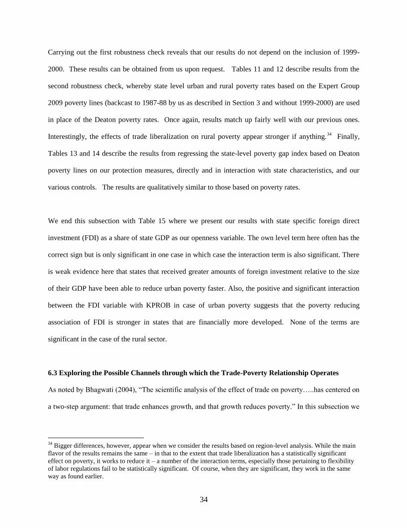
34

Carrying out the first robustness check reveals that our results do not depend on the inclusion of 1999-

2000. These results can be obtained from us upon request. Tables 11 and 12 describe results from the

second robustness check, whereby state level urban and rural poverty rates based on the Expert Group

2009 poverty lines (backcast to 1987-88 by us as described in Section 3 and without 1999-2000) are used

in place of the Deaton poverty rates. Once again, results match up fairly well with our previous ones.

Interestingly, the effects of trade liberalization on rural poverty appear stronger if anything.34

Finally,

Tables 13 and 14 describe the results from regressing the state-level poverty gap index based on Deaton

poverty lines on our protection measures, directly and in interaction with state characteristics, and our

various controls. The results are qualitatively similar to those based on poverty rates.

We end this subsection with Table 15 where we present our results with state specific foreign direct

investment (FDI) as a share of state GDP as our openness variable. The own level term here often has the

correct sign but is only significant in one case in which case the interaction term is also significant. There

is weak evidence here that states that received greater amounts of foreign investment relative to the size

of their GDP have been able to reduce urban poverty faster. Also, the positive and significant interaction

between the FDI variable with KPROB in case of urban poverty suggests that the poverty reducing

association of FDI is stronger in states that are financially more developed. None of the terms are

significant in the case of the rural sector.

6.3 Exploring the Possible Channels through which the Trade-Poverty Relationship Operates

As noted by Bhagwati (2004), ―The scientific analysis of the effect of trade on poverty…..has centered on

a two-step argument: that trade enhances growth, and that growth reduces poverty.‖ In this subsection we

34

Bigger differences, however, appear when we consider the results based on region-level analysis. While the main

flavor of the results remains the same – in that to the extent that trade liberalization has a statistically significant

effect on poverty, it works to reduce it – a number of the interaction terms, especially those pertaining to flexibility

of labor regulations fail to be statistically significant. Of course, when they are significant, they work in the same

way as found earlier.

35

first examine the evidence for the two-step argument using our measures of poverty, trade liberalization

and state per capita incomes (gross state domestic product per capita).

Table 16 presents results from regressions of state per capita incomes on state-level employment-

weighted tariffs and their interactions with state characteristics such as labor-market flexibility, road

density and our two measures of financial development. Clearly trade protection has a negative effect on

per capita incomes. In other words, trade openness increases per capita incomes. Alternatively, we can

interpret our results as follows: states whose workers were more exposed to foreign competition (states in

which employment was concentrated in the relatively less protected sectors) and saw greater reduction in

their employment-weighted average tariff grew faster than others. Using our various alternative measures

of labor market flexibility, we find this effect of trade openness to be stronger for states with relatively

more flexible labor markets. Also, using both our measures of financial development, we find very strong

evidence of this effect being stronger in the financially more developed states. Thus, the first step in

Bhagwati‘s two step argument certainly works very well. We next empirically investigate the second step

of this argument.

Did higher state economic growth help reduce poverty faster? If yes, then after accounting for this effect,

did trade have an additional role in poverty reduction possibly through its redistributive effect in favor of

workers. Table 17 describes results for regressions of state (overall) poverty on state per capita incomes

and then additionally on employment-weighted tariffs. Clearly from columns (1) and (2), we see that

states that have been growing faster are also the ones that have reduced their poverty faster. For a one

percent increase in per capita income, we get a 0.42 percent reduction in poverty. When we additionally

control for protection in column (3) this effect falls to 0.35 and the significance of the log of GSDP per

capita falls somewhat. In addition, tariff still enters with a positive sign even though it is only very

marginally significant. This indicates the possibility that trade, in addition to reducing poverty through an

increase in average incomes, also works to reduce poverty through redistributing incomes. From column

36

(7), it is very clear that this effect is stronger in states with better road connectivity, possibly due to better

transmission of trade policies and border prices in such states

The regression results examined in this subsection identify possible channels through which the trade-

poverty nexus, that we have found evidence for, works. The results suggest that reductions in trade

protection may, through their positive impact on per capita income, have contributed to reducing poverty.

For trade liberalization to generate economic growth and at the same time reduce poverty, it is essential

that reductions in trade protection do not significantly worsen income distribution. In fact, we find that

trade liberalization has an additional beneficial effect on poverty reduction, over and above its effect

through enhancing growth.

7. Conclusions

Our empirical investigation of the impact of trade liberalization shows that there is a fair amount of

evidence in support of their poverty reducing effects. The most conservative interpretation of our results

is that poverty reduction was greater in states and NSS regions that were more open by virtue of the

exposure of their labor force to foreign competition, measured by the employment weighted average tariff

at the state or region level. There is also some weak evidence that states that received more FDI relative to

their domestic output fared better with poverty reduction.

We find that the beneficial effects of openness are typically larger in states with more flexible labor

market institutions (especially in the urban sectors of such states), better connectivity through

transportation, and more developed financial systems. Compared to a state with rigid labor market

institutions, we find that a state with flexible labor market institutions, that experienced a percentage point

higher reduction in employment-weighted tariff, would have experienced a 1.5 percent greater reduction

in urban poverty. Similarly, we find that a state with a greater degree of financial development would

have experienced greater reduction in urban poverty as a result of trade liberalization. The results are

37

qualitatively similar with road connectivity. These results help to underscore the importance of

improving physical mobility within India by upgrading the transportation infrastructure and improving

banking and financial infrastructure in fully reaping the benefits of globalization. By globalization, we do

not limit ourselves to trade liberalization. We have also considered FDI in our paper. There again, we find

that the gains from FDI are best exploited in the presence of better developed financial institutions.

38

References

Aghion, P., R. Burgess, S.J. Redding, and F. Zilibotti. (2008). ―The Unequal Effects of Liberalization:

Evidence from Dismantling the License Raj in India,‖ American Economic Review, 98:4, 1397–1412.

Amoranto, G. and R. Hasan. (2010). ―A Note on Updating Poverty Lines over Time: An Application to

India,‖ mimeo, Economics and Research Department, Asian Development Bank.

Anant, T.C.A. (2000). ―Reforming the labour market,‖ in: Gangopadhyay, S., Wadhwa, W. (Eds.),

Economic Reforms for the Poor, Konark, Delhi.

Anant, T.C.A., R. Hasan, P. Mohapatra, R. Nagaraj, and S. K. Sasikumar (2006). ―Labor Markets in

India: Issues and Perspectives,‖ in Jesus Felipe and Rana Hasan, eds., Labor Markets in Asia: Issues and

Perspectives Palgrave Macmillan.

Asian Development Bank (2008). ―Comparing Poverty Across Countries: The Role of Purchasing Power

Parities,‖ Key Indicators 2008.

Baldwin, Robert. (2003). ―Openness and Growth: What is the Empirical Relationship?,‖ NBER Working

Paper No. 9578.

Besley, T. and R. Burgess. (2004). ―Can Labor Regulation Hinder Economic Performance? Evidence

from India,‖ Quarterly Journal of Economics 19(1), 91-134.

Bhagwati, Jagdish. (2004). In Defense of Globalization, Oxford University Press, New York.

Bhalla, S. (2003). ―Recounting the Poor: Poverty in India 1983-99‖. Economic and Political Weekly.

Vol. 37, pp. 25-31, January.

Bhattacharjea, A. (2006). ―Labour Market Regulation and Industrial Performance in India: A Critical

Review of Empirical Evidence,‖ The Indian Journal of Labour Economics, 49(2):211-32.

__________. (2008). ―How do Indian firms respond to employment protection legislation?‖ mimeo.

Chen, S. and M. Ravallion. (2008). ―The Developing World is Poorer than we Thought,

But no Less Successful in the Fight Against Poverty ‖ World Bank Policy Research Paper 4703.

Das, D. (2008). "Trade Barriers Measurement: A Methodological Overview,‖ mimeo.

Datta, R. (2003). ―Labor Market, Social Institutions, Economic Reforms, and Social Costs,‖ in S.

Uchikawa, ed., Labour Market and Institution in India, 1990s and Beyond, Manohar, New Delhi.

Datta-Chaudhuri, M. (1996). ―Labor Markets as Social Institutions in India,‖ IRIS-India Working Paper

no. 10, University of Maryland at College Park.

Deaton, A. (2003a). ―Prices and poverty in India, 1987-2000,‖ Economic and Political Weekly 25, 362-

68.

Deaton, A. (2003b). ―Regional Poverty Estimates for India, 1999-2000,‖ Research Program in

Development Studies, Princeton University, 22 August.

39

Deaton, A. and J. Dreze. (2002). ―Poverty and Inequality in India – A Re-examination,‖ Economic and

Political Weekly 7, 3729-48.

Deaton, A. and V. Kozel. (2005). ―Data and Dogma: The Great Indian Poverty Debate,‖ MacMillan India.

Dollar, D. (1992). ―Outward-Oriented Developing Economies Really Do Grow More Rapidly: Evidence

from 95 LDCs, 1976-1985,‖ Economic Development and Cultural Change, 40(3), 523-44.

Dollar, D. and A. Kraay. (2002). ―Growth is Good for the Poor,‖ Journal of Economic Growth 7(3), 195-

225.

__________. (2004). ―Trade, Growth, and Poverty,‖ Economic Journal 114(493), F22-F49.

Dollar, D., G. Iarossi, and T. Mengistae. (2002). ―Investment Climate and Economic Performance: Some

Firm Level Evidence from India,‖ mimeo, The World Bank.

Edmonds, E.V., N. Pavcnik, and P. Topalova. (2008). ―Trade Adjustment and Human Capital

Investments: Evidence from Indian Tariff Reform.‖ NBER Working Paper no. 12884.

Edwards, Sebastian. (1998). ―Openness, Productivity and Growth: What Do We Really Know,‖ The

Economic Journal 108(447), 383-98.

Frankel, Jeffrey and David Romer. (1999). ―Does Trade Cause Growth?,‖ American Economic Review

89(3), 379-399.

Ghosh, B. and P. De. 2004. ―How Do Different Categories of Infrastructure Affect Development?

Evidence from Indian States.‖ Economic and Political Weekly, October 16, 2004: 4645-4657.

Government of India. (1979). Report of the Task Force on Projections of Minimum Needs and Effective

Consumption Demand. Perspective Planning Division, Planning Commission.

__________. (1993). Report of the Expert Group on Estimation of Proportion and Number of Poor.

Perspective Planning Division, Planning Commission.

__________. (2009). Report of the Expert Group to Review the Methodology for Estimation of Poverty.

Planning Commission.

Gupta, P., R. Hasan, and U. Kumar. 2009. "Big Reforms but Small Payoffs: Explaining the Weak Record

of Growth in Indian Manufacturing." India Policy Forum, 5.

Harrison, Ann. (2006). ―Globalization and Poverty,‖ mimeo, University of California – Berkeley.

Hasan, R., K.R. Jandoc, and N. Khor (2010). ―Do Constraints to Growth Vary by Firm Size? Evidence

from India Over a Period of Trade Liberalization,‖ mimeo, Economics and Research Department, Asian

Development Bank.

Hasan, R., M.G. Quibria, and Y. Kim. (2003). ―Poverty and Economic Freedom: Evidence from Cross-

Country Data,‖ East-West Center Working Paper.

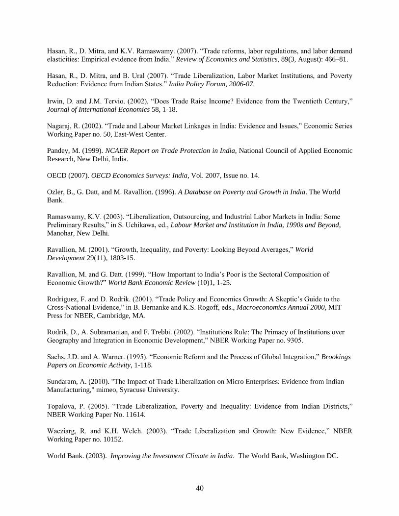
40

Hasan, R., D. Mitra, and K.V. Ramaswamy. (2007). ―Trade reforms, labor regulations, and labor demand

elasticities: Empirical evidence from India.‖ Review of Economics and Statistics, 89(3, August): 466–81.

Hasan, R., D. Mitra, and B. Ural (2007). ―Trade Liberalization, Labor Market Institutions, and Poverty

Reduction: Evidence from Indian States.‖ India Policy Forum, 2006-07.

Irwin, D. and J.M. Tervio. (2002). ―Does Trade Raise Income? Evidence from the Twentieth Century,‖

Journal of International Economics 58, 1-18.

Nagaraj, R. (2002). ―Trade and Labour Market Linkages in India: Evidence and Issues,‖ Economic Series

Working Paper no. 50, East-West Center.

Pandey, M. (1999). NCAER Report on Trade Protection in India, National Council of Applied Economic

Research, New Delhi, India.

OECD (2007). OECD Economics Surveys: India, Vol. 2007, Issue no. 14.

Ozler, B., G. Datt, and M. Ravallion. (1996). A Database on Poverty and Growth in India. The World

Bank.

Ramaswamy, K.V. (2003). ―Liberalization, Outsourcing, and Industrial Labor Markets in India: Some

Preliminary Results,‖ in S. Uchikawa, ed., Labour Market and Institution in India, 1990s and Beyond,

Manohar, New Delhi.

Ravallion, M. (2001). ―Growth, Inequality, and Poverty: Looking Beyond Averages,‖ World

Development 29(11), 1803-15.

Ravallion, M. and G. Datt. (1999). ―How Important to India‘s Poor is the Sectoral Composition of

Economic Growth?‖ World Bank Economic Review (10)1, 1-25.

Rodriguez, F. and D. Rodrik. (2001). ―Trade Policy and Economics Growth: A Skeptic‘s Guide to the

Cross-National Evidence,‖ in B. Bernanke and K.S. Rogoff, eds., Macroeconomics Annual 2000, MIT

Press for NBER, Cambridge, MA.

Rodrik, D., A. Subramanian, and F. Trebbi. (2002). ―Institutions Rule: The Primacy of Institutions over

Geography and Integration in Economic Development,‖ NBER Working Paper no. 9305.

Sachs, J.D. and A. Warner. (1995). ―Economic Reform and the Process of Global Integration,‖ Brookings

Papers on Economic Activity, 1-118.

Sundaram, A. (2010). "The Impact of Trade Liberalization on Micro Enterprises: Evidence from Indian

Manufacturing," mimeo, Syracuse University.

Topalova, P. (2005). ―Trade Liberalization, Poverty and Inequality: Evidence from Indian Districts,‖

NBER Working Paper No. 11614.

Wacziarg, R. and K.H. Welch. (2003). ―Trade Liberalization and Growth: New Evidence,‖ NBER

Working Paper no. 10152.

World Bank. (2003). Improving the Investment Climate in India. The World Bank, Washington DC.

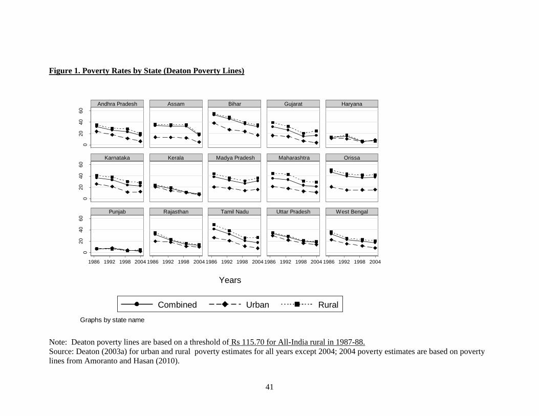
41

Figure 1. Poverty Rates by State (Deaton Poverty Lines)

0

20

40

60

02

04

06

00

20

40

60

1986 1992 1998 2004 1986 1992 1998 2004 1986 1992 1998 2004 1986 1992 1998 2004 1986 1992 1998 2004

Andhra Pradesh Assam Bihar Gujarat Haryana

Karnataka Kerala Madya Pradesh Maharashtra Orissa

Punjab Rajasthan Tamil Nadu Uttar Pradesh West Bengal

Combined Urban Rural

Perc

ent

Years

Graphs by state name

Note: Deaton poverty lines are based on a threshold of Rs 115.70 for All-India rural in 1987-88.

Source: Deaton (2003a) for urban and rural poverty estimates for all years except 2004; 2004 poverty estimates are based on poverty

lines from Amoranto and Hasan (2010).

42

Figure 2. Poverty Rates by State (Expert Group 2009 Poverty Lines)

20

40

60

80

20

40

60

80

20

40

60

80

1986 1992 1998 2004 1986 1992 1998 2004 1986 1992 1998 2004 1986 1992 1998 2004 1986 1992 1998 2004

Andhra Pradesh Assam Bihar Gujarat Haryana

Karnataka Kerala Madya Pradesh Maharashtra Orissa

Punjab Rajasthan Tamil Nadu Uttar Pradesh West Bengal

Combined Urban Rural

Perc

ent

Years

Graphs by state name

Note: Expert Group poverty lines are based on a threshold of Rs 578.8 for All-India urban in 2004-05.

Source: Government of India (2009) for 1993 and 2004, except for Bihar, Madhya Pradesh, and Uttar Pradesh which were calculated

from unit-level data using poverty lines provided in Appendix Table 3. 1987 poverty estimates calculated from NSS unit-level data

using poverty lines from Amoranto and Hasan (2010).

43

Figure 3. Tariff Rates (Lagged) by State

0

50

10

01

50

05

01

00

15

0

05

01

00

15

0

1986 1992 1998 2004 1986 1992 1998 2004 1986 1992 1998 2004 1986 1992 1998 2004 1986 1992 1998 2004

Andhra Pradesh Assam Bihar Gujarat Haryana

Karnataka Kerala Madya Pradesh Maharashtra Orissa

Punjab Rajasthan Tamil Nadu Uttar Pradesh West Bengal

Perc

ent

Years

Graphs by state name

Source: Based on tariff rates reported in Pandey (1999) and Das (2008) and employment weights derived from NSS employment-

unemployment survey for 1993-94.

44

Figure 4. NTB Coverage Ratios (Lagged) by State

05

01

00

05

01

00

05

01

00

1986 1992 1998 2004 1986 1992 1998 2004 1986 1992 1998 2004 1986 1992 1998 2004 1986 1992 1998 2004

Andhra Pradesh Assam Bihar Gujarat Haryana

Karnataka Kerala Madya Pradesh Maharashtra Orissa

Punjab Rajasthan Tamil Nadu Uttar Pradesh West Bengal

Perc

ent

Years

Graphs by state name

Source: Based on NTB coverage ratios reported in Pandey (1999) and Das (2008) and employment weights derived from NSS

employment-unemployment survey for 1993-94.

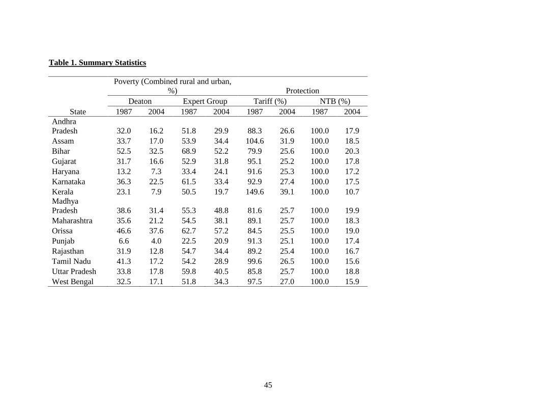
45

Table 1. Summary Statistics

State

Poverty (Combined rural and urban,

%) Protection

Deaton Expert Group Tariff (%) NTB (%)

1987 2004 1987 2004 1987 2004 1987 2004

Andhra

Pradesh 32.0 16.2 51.8 29.9 88.3 26.6 100.0 17.9

Assam 33.7 17.0 53.9 34.4 104.6 31.9 100.0 18.5

Bihar 52.5 32.5 68.9 52.2 79.9 25.6 100.0 20.3

Gujarat 31.7 16.6 52.9 31.8 95.1 25.2 100.0 17.8

Haryana 13.2 7.3 33.4 24.1 91.6 25.3 100.0 17.2

Karnataka 36.3 22.5 61.5 33.4 92.9 27.4 100.0 17.5

Kerala 23.1 7.9 50.5 19.7 149.6 39.1 100.0 10.7

Madhya

Pradesh 38.6 31.4 55.3 48.8 81.6 25.7 100.0 19.9

Maharashtra 35.6 21.2 54.5 38.1 89.1 25.7 100.0 18.3

Orissa 46.6 37.6 62.7 57.2 84.5 25.5 100.0 19.0

Punjab 6.6 4.0 22.5 20.9 91.3 25.1 100.0 17.4

Rajasthan 31.9 12.8 54.7 34.4 89.2 25.4 100.0 16.7

Tamil Nadu 41.3 17.2 54.2 28.9 99.6 26.5 100.0 15.6

Uttar Pradesh 33.8 17.8 59.8 40.5 85.8 25.7 100.0 18.8

West Bengal 32.5 17.1 51.8 34.3 97.5 27.0 100.0 15.9

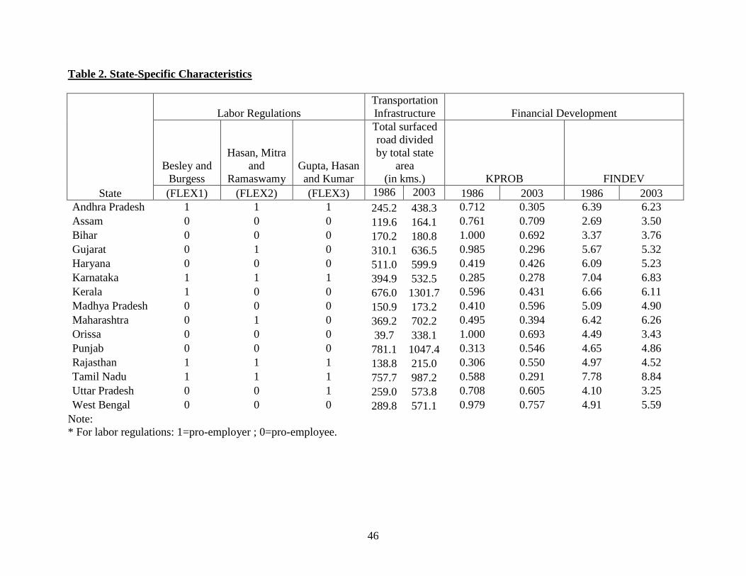
46

Table 2. State-Specific Characteristics

State

Labor Regulations

Transportation

Infrastructure Financial Development

Besley and

Burgess

Hasan, Mitra

and

Ramaswamy

Gupta, Hasan

and Kumar

Total surfaced

road divided

by total state

area

(in kms.)

KPROB

FINDEV

(FLEX1) (FLEX2) (FLEX3) 1986 2003 1986 2003 1986 2003

Andhra Pradesh 1 1 1 245.2 438.3 0.712 0.305 6.39 6.23

Assam 0 0 0 119.6 164.1 0.761 0.709 2.69 3.50

Bihar 0 0 0 170.2 180.8 1.000 0.692 3.37 3.76

Gujarat 0 1 0 310.1 636.5 0.985 0.296 5.67 5.32

Haryana 0 0 0 511.0 599.9 0.419 0.426 6.09 5.23

Karnataka 1 1 1 394.9 532.5 0.285 0.278 7.04 6.83

Kerala 1 0 0 676.0 1301.7 0.596 0.431 6.66 6.11

Madhya Pradesh 0 0 0 150.9 173.2 0.410 0.596 5.09 4.90

Maharashtra 0 1 0 369.2 702.2 0.495 0.394 6.42 6.26

Orissa 0 0 0 39.7 338.1 1.000 0.693 4.49 3.43

Punjab 0 0 0 781.1 1047.4 0.313 0.546 4.65 4.86

Rajasthan 1 1 1 138.8 215.0 0.306 0.550 4.97 4.52

Tamil Nadu 1 1 1 757.7 987.2 0.588 0.291 7.78 8.84

Uttar Pradesh 0 0 1 259.0 573.8 0.708 0.605 4.10 3.25

West Bengal 0 0 0 289.8 571.1 0.979 0.757 4.91 5.59

Note:

* For labor regulations: 1=pro-employer ; 0=pro-employee.

47

Table 3. Pairwise Correlations: Reductions in Poverty and Lagged Protection, 1987 and

2004

Reductions in Poverty Reductions

in Lagged

Tariffs Deaton

Expert

Group

Reductions

in Expert

Group

Poverty

0.8179***

(0.0002)

Reductions

in Tariffs

0.6216** 0.4940*

(0.0134) (0.0612)

Reductions

in NTB

0.7536*** 0.7530*** 0.7357***

(0.0012) (0.0012) (0.0018)

Note: Actual significant levels in parenthesis.

48

Table 4. Dependent Variable: Log of Deaton poverty rates, State-level

Regressors

Combined Rural + Urban Urban Rural

NRP NTB FPC NRP NTB FPC NRP NTB FPC

(1) (2) (3) (4) (5) (6) (7) (8) (9)

L. Protection 0.0057 0.0395 0.3142 0.0125 0.0175 0.7051 0.0047 0.0359 0.2436

[2.26]** [2.77]*** [3.08]*** [1.66] [1.46] [2.19]** [1.72]* [2.74]*** [2.43]**

L. Log DEVEXP

PC -0.0919 0.0209 -0.0690 0.1321 0.1360 0.1644 -0.1771 -0.0973 -0.1675

[0.44] [0.12] [0.33] [0.56] [0.55] [0.71] [0.83] [0.49] [0.78]

Constant 3.4606 1.9400 3.9978 0.4664 0.3341 2.4924 4.2378 2.9898 4.7188

[2.39]** [1.44] [2.66]** [0.24] [0.15] [1.51] [2.89]*** [1.95]* [3.06]***

R-squared 0.8 0.83 0.81 0.79 0.78 0.8 0.72 0.75 0.73

Robust t statistics in brackets. Also included as regressors but not shown are year and state dummy variables.

Number of observations: 60; Number of states: 15.

* significant at 10%; ** significant at 5%; *** significant at 1%

49

Table 5. Dependent Variable: Log of Deaton poverty rates, State-level (Urban)

Regressors

State Characteristics

FLEX1 FLEX2 FLEX3 ROAD KPROB FINDEV

Tariff (1) (2) (3) (4) (5) (6)

L. Protection 0.0145 0.0125 0.0186 0.0082 0.0148 0.0044

[1.97]* [1.96]* [2.63]** [0.94] [2.07]** [0.52]

L. Protection interaction 0.0029 0.0031 0.0033 0.0014 -0.0067 0.0008

[2.63]** [2.63]** [3.02]*** [1.88]* [2.35]** [2.22]**

L. State characteristic -0.0790 1.2602 -0.2621

[0.74] [2.75]*** [3.11]***

L. Log of DEVEXP per

capita 0.1613 0.1283 0.1825 0.2156 0.1008 0.0072

[0.76] [0.59] [0.80] [0.93] [0.43] [0.03]

Constant -0.1203 0.3301 -0.8133 0.5101 0.1293 3.1616

[0.07] [0.18] [0.43] [0.26] [0.07] [1.41]

R-squared 0.81 0.82 0.81 0.8 0.82 0.83

Non-tariff barriers (7) (8) (9) (10) (11) (12)

L. Protection 0.0164 0.0182 0.0187 0.0133 0.0243 0.0073

[1.37] [1.54] [1.49] [0.99] [1.91]* [0.62]

L. Protection interaction 0.0028 0.0037 0.0023 0.0013 -0.0083 0.0009

[1.64] [2.05]** [1.28] [1.30] [1.88]* [1.79]*

L. State characteristic -0.1364 1.2709 -0.2440

[1.21] [2.63]** [3.15]***

L. Log of DEVEXP per

capita 0.1453 0.1344 0.2094 0.2028 0.1488 -0.0307

[0.64] [0.59] [0.84] [0.77] [0.63] [0.13]

Constant 0.2827 0.1271 -0.3543 0.3070 -0.7120 3.3039

[0.13] [0.06] [0.15] [0.12] [0.32] [1.43]

R-squared 0.8 0.81 0.79 0.8 0.82 0.82

First principal component (13) (14) (15) (16) (17) (18)

L. Protection 0.8614 0.7298 1.0061 0.5270 0.8336 0.4176

[3.00]*** [2.58]** [3.43]*** [1.59] [2.43]** [1.29]

L. Protection interaction 0.0909 0.0862 0.0970 0.0328 -0.2042 0.0208

[2.80]*** [2.44]** [2.81]*** [1.60] [2.40]** [2.02]*

L. State characteristic 0.0056 0.7290 -0.1702

[0.04] [2.34]** [1.86]*

L. Log of DEVEXP per

capita 0.1997 0.1630 0.2855 0.2173 0.1562 0.0296

[0.98] [0.76] [1.29] [0.92] [0.69] [0.13]

Constant 2.6447 2.6325 2.3430 1.7350 2.2396 3.9733

[1.92]* [1.85]* [1.58] [1.09] [1.35] [2.32]**

R-squared 0.83 0.83 0.82 0.81 0.83 0.83

Robust t statistics in brackets. Also included as regressors but not shown are year and state

dummy variables. Number of observations: 60; Number of states: 15.

* significant at 10%; ** significant at 5%; *** significant at 1%

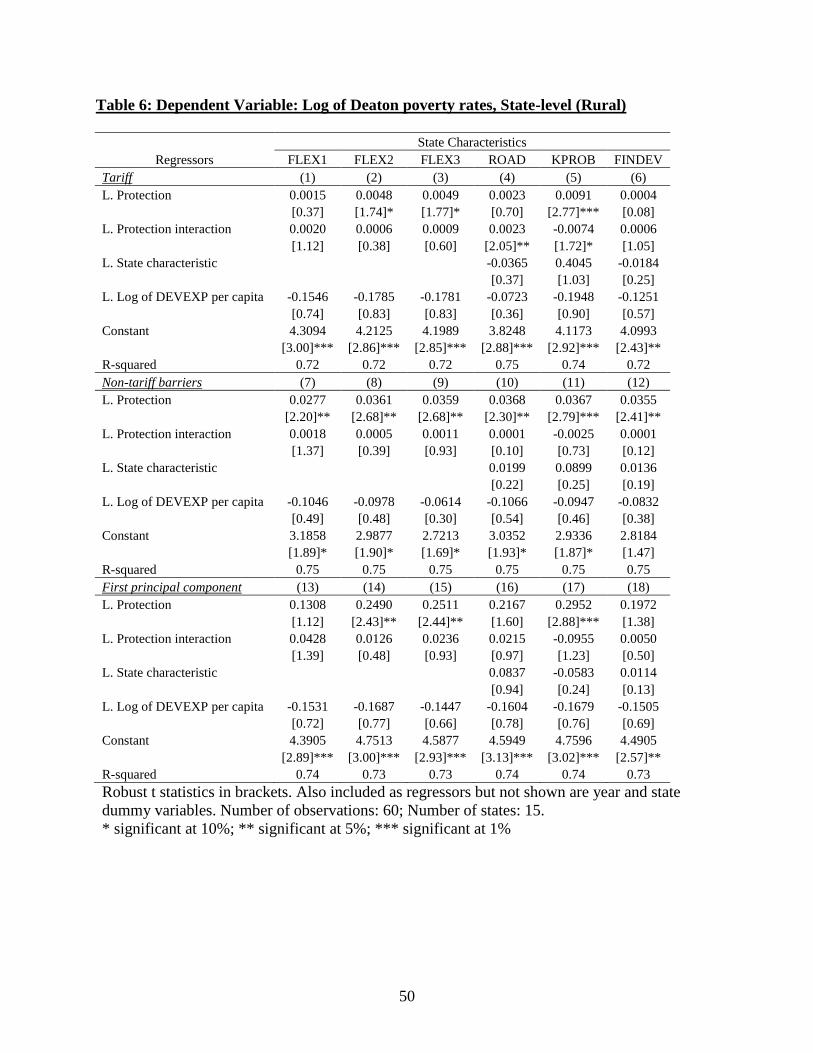
50

Table 6: Dependent Variable: Log of Deaton poverty rates, State-level (Rural)

Regressors

State Characteristics

FLEX1 FLEX2 FLEX3 ROAD KPROB FINDEV

Tariff (1) (2) (3) (4) (5) (6)

L. Protection 0.0015 0.0048 0.0049 0.0023 0.0091 0.0004

[0.37] [1.74]* [1.77]* [0.70] [2.77]*** [0.08]

L. Protection interaction 0.0020 0.0006 0.0009 0.0023 -0.0074 0.0006

[1.12] [0.38] [0.60] [2.05]** [1.72]* [1.05]

L. State characteristic -0.0365 0.4045 -0.0184

[0.37] [1.03] [0.25]

L. Log of DEVEXP per capita -0.1546 -0.1785 -0.1781 -0.0723 -0.1948 -0.1251

[0.74] [0.83] [0.83] [0.36] [0.90] [0.57]

Constant 4.3094 4.2125 4.1989 3.8248 4.1173 4.0993

[3.00]*** [2.86]*** [2.85]*** [2.88]*** [2.92]*** [2.43]**

R-squared 0.72 0.72 0.72 0.75 0.74 0.72

Non-tariff barriers (7) (8) (9) (10) (11) (12)

L. Protection 0.0277 0.0361 0.0359 0.0368 0.0367 0.0355

[2.20]** [2.68]** [2.68]** [2.30]** [2.79]*** [2.41]**

L. Protection interaction 0.0018 0.0005 0.0011 0.0001 -0.0025 0.0001

[1.37] [0.39] [0.93] [0.10] [0.73] [0.12]

L. State characteristic 0.0199 0.0899 0.0136

[0.22] [0.25] [0.19]

L. Log of DEVEXP per capita -0.1046 -0.0978 -0.0614 -0.1066 -0.0947 -0.0832

[0.49] [0.48] [0.30] [0.54] [0.46] [0.38]

Constant 3.1858 2.9877 2.7213 3.0352 2.9336 2.8184

[1.89]* [1.90]* [1.69]* [1.93]* [1.87]* [1.47]

R-squared 0.75 0.75 0.75 0.75 0.75 0.75

First principal component (13) (14) (15) (16) (17) (18)

L. Protection 0.1308 0.2490 0.2511 0.2167 0.2952 0.1972

[1.12] [2.43]** [2.44]** [1.60] [2.88]*** [1.38]

L. Protection interaction 0.0428 0.0126 0.0236 0.0215 -0.0955 0.0050

[1.39] [0.48] [0.93] [0.97] [1.23] [0.50]

L. State characteristic 0.0837 -0.0583 0.0114

[0.94] [0.24] [0.13]

L. Log of DEVEXP per capita -0.1531 -0.1687 -0.1447 -0.1604 -0.1679 -0.1505

[0.72] [0.77] [0.66] [0.78] [0.76] [0.69]

Constant 4.3905 4.7513 4.5877 4.5949 4.7596 4.4905

[2.89]*** [3.00]*** [2.93]*** [3.13]*** [3.02]*** [2.57]**

R-squared 0.74 0.73 0.73 0.74 0.74 0.73

Robust t statistics in brackets. Also included as regressors but not shown are year and state

dummy variables. Number of observations: 60; Number of states: 15.

* significant at 10%; ** significant at 5%; *** significant at 1%

51

Table 7. Dependent Variable: Log of Deaton poverty rates, Region-level (Urban)

Regressors

Own-

term

State Characteristics

FLEX1 FLEX2 FLEX3 ROAD KPROB FINDEV

Tariff (1) (2) (3) (4) (5) (6) (7)

L. Protection 0.0074 0.0068 0.0044 0.0079 0.0061 0.0106 0.0006

[1.76]* [1.68]* [1.09] [1.88]* [1.46] [2.17]** [0.14]

L. Protection interaction 0.0037 0.0038 0.0025 0.0018 -0.0087 0.0011

[2.72]*** [3.33]*** [1.87]* [2.94]*** [2.75]*** [2.34]**

L. State characteristic -0.1165 1.4468 -0.2540

[1.21] [3.57]*** [2.93]***

L. Log of DEVEXP per capita -0.1224 -0.1032 -0.1311 -0.0892 -0.0356 -0.1714 -0.2274

[0.54] [0.47] [0.59] [0.39] [0.15] [0.74] [1.04]

Constant 2.8866 2.7301 2.9809 2.6081 2.3093 2.5517 5.0229

[1.72]* [1.68]* [1.81]* [1.55] [1.37] [1.52] [2.87]***

R-squared 0.52 0.55 0.55 0.53 0.54 0.55 0.55

Non-tariff barrier (8) (9) (10) (11) (12) (13) (14)

L. Protection 0.0093 -0.0102 0.0050 0.0056 -0.0042 0.0109 -0.0024

[0.34] [0.38] [0.18] [0.20] [0.15] [0.39] [0.09]

L. Protection interaction 0.0047 0.0042 0.0030 0.0016 -0.0074 0.0007

[2.36]** [2.33]** [1.48] [1.67]* [1.37] [0.99]

L. State characteristic -0.1651 1.2221 -0.2543

[1.57] [2.47]** [2.78]***

L. Log of DEVEXP per capita -0.0995 -0.1422 -0.1478 -0.0016 -0.0982 -0.0986 -0.3159

[0.42] [0.61] [0.62] [0.01] [0.41] [0.42] [1.34]

Constant 2.7410 4.8335 3.2926 2.3594 4.0815 2.2732 6.3604

[0.82] [1.48] [0.95] [0.67] [1.24] [0.68] [1.72]*

R-squared 0.51 0.53 0.53 0.52 0.53 0.54 0.53

First principal component (15) (16) (17) (18) (19) (20) (21)

L. Protection 0.3949 0.3102 0.2794 0.4131 0.2657 0.3764 0.2147

[1.59] [1.33] [1.14] [1.62] [1.06] [1.40] [0.91]

L. Protection interaction 0.0887 0.0922 0.0665 0.0379 -0.1885 0.0190

[2.25]** [2.77]*** [1.68]* [2.07]** [1.92]* [1.44]

L. State characteristic 0.0045 0.7104 -0.1829

[0.04] [2.69]*** [1.92]*

L. Log of DEVEXP per capita -0.0955 -0.0932 -0.1326 -0.0062 -0.0622 -0.1200 -0.2657

[0.42] [0.41] [0.58] [0.03] [0.27] [0.51] [1.18]

Constant 3.8344 3.6797 3.9303 3.2845 3.3115 3.3894 5.8527

[2.23]** [2.17]** [2.28]** [1.91]* [1.86]* [1.90]* [3.37]***

R-squared 0.52 0.54 0.54 0.53 0.54 0.55 0.54

Robust t statistics in brackets. Also included as regressors but not shown are year and region

dummy variables. Number of observations: 232; Number of regions: 58.

* significant at 10%; ** significant at 5%; *** significant at 1%

52

Table 8. Dependent Variable: Log of Deaton poverty rates, Region-level (Rural)

Regressors Own-term

State Characteristics

FLEX1 FLEX2 FLEX3 ROAD KPROB FINDEV

Tariff (1) (2) (3) (4) (5) (6) (7)

L. Protection 0.0057 0.0012 0.0054 0.0054 0.0029 0.0116 -0.0009

[1.79]* [0.32] [1.70]* [1.72]* [0.87] [3.18]*** [0.22]

L. Protection interaction 0.0030 0.0024 0.0022 0.0026 -0.0109 0.0009

[1.92]* [1.70]* [1.51] [3.21]*** [2.67]*** [2.04]**

L. State characteristic -0.0478 0.7854 -0.0115

[0.66] [2.16]** [0.17]

L. Log of DEVEXP per

capita -0.2863 -0.2770 -0.2900 -0.2817 -0.2213 -0.3384 -0.2269

[1.70]* [1.68]* [1.74]* [1.70]* [1.32] [2.02]** [1.23]

Constant 4.9426 4.9561 4.9484 4.8976 4.5482 4.8751 4.6281

[4.24]*** [4.33]*** [4.27]*** [4.26]*** [3.96]*** [4.25]*** [3.15]***

R-squared 0.46 0.47 0.47 0.47 0.49 0.48 0.47

Non-tariff barrier (8) (9) (10) (11) (12) (13) (14)

L. Protection 0.0248 0.0168 0.0236 0.0232 0.0215 0.0253 0.0256

[1.53] [1.00] [1.42] [1.42] [1.23] [1.53] [1.55]

L. Protection interaction 0.0019 0.0012 0.0012 0.0004 -0.0022 0.0000

[1.32] [0.88] [0.90] [0.53] [0.57] [0.10]

L. State characteristic -0.0419 0.2152 0.0180

[0.54] [0.53] [0.26]

L. Log of DEVEXP per

capita -0.2365 -0.2539 -0.2499 -0.1953 -0.2353 -0.2412 -0.2211

[1.45] [1.52] [1.49] [1.13] [1.42] [1.45] [1.20]

Constant 2.6349 3.4888 2.7874 2.4743 2.9494 2.6145 2.3789

[1.29] [1.64] [1.33] [1.16] [1.39] [1.26] [1.00]

R-squared 0.46 0.47 0.47 0.47 0.46 0.46 0.46

First principal component (15) (16) (17) (18) (19) (20) (21)

L. Protection 0.2427 0.1222 0.2315 0.2308 0.1767 0.2916 0.1883

[2.01]** [0.90] [1.89]* [1.88]* [1.26] [2.31]** [1.35]

L. Protection interaction 0.0477 0.0341 0.0337 0.0250 -0.1185 0.0063

[1.58] [1.31] [1.26] [1.65] [1.50] [0.70]

L. State characteristic 0.0562 0.1025 0.0272

[0.70] [0.45] [0.35]

L. Log of DEVEXP per

capita -0.2696 -0.2749 -0.2815 -0.2316 -0.2619 -0.2923 -0.2537

[1.62] [1.65] [1.66]* [1.37] [1.55] [1.72]* [1.38]

Constant 5.5351 5.3319 5.6329 5.2588 5.3284 5.6272 5.2271

[4.39]*** [4.20]*** [4.39]*** [4.15]*** [4.05]*** [4.35]*** [3.28]***

R-squared 0.46 0.47 0.47 0.47 0.47 0.47 0.46

Robust t statistics in brackets. Also included as regressors but not shown are year and region

dummy variables. Number of observations: 232; Number of regions: 58.

* significant at 10%; ** significant at 5%; *** significant at 1%

53

Table 9. Dependent Variable: Log of Deaton poverty rates, State-level (Urban)

Regressors

FLEX1 FLEX2 FLEX3

KPROB FINDEV KPROB FINDEV KPROB FINDEV

Tariff (1) (2) (3) (4) (5) (6)

L. Protection 0.0101 [1.20] 0.0076 [0.80] 0.0047 [0.51] 0.0087 [1.06] 0.0119 [1.49] 0.0101 [1.11]

L. Protection * FLEX 0.0019 [1.50] 0.0018 [1.26] 0.0027 [1.51] 0.0038 [2.19]** 0.0026 [2.20]** 0.0026 [2.50]**

L. Protection * ROAD 0.0011 [1.07] 0.0004 [0.38] 0.0016 [1.59] 0.0013 [1.35] 0.0013 [1.32] 0.0005 [0.51]

L. Protection *

KPROB/FINDEV -0.0015 [0.33] 0.0002 [0.33] 0.0016 [0.27] -0.0006 [0.79] -0.0008 [0.18] 0.0002 [0.42]

L. Road (Own-term) -0.0168 [0.19] -0.0839 [0.80] -0.0833 [0.82] -0.1806 [1.48] -0.0511 [0.57] -0.1159 [1.07] L. KPROB/FINDEV (Own

term) 0.7417 [1.13] -0.2288 [2.47]** 0.2394 [0.28] -0.1727 [1.96]* 0.6676 [1.03] -0.2304 [2.44]**

L. Log of DEVEXP per capita 0.1891 [0.82] 0.0286 [0.12] 0.2302 [0.96] 0.0279 [0.12] 0.2367 [0.95] 0.0673 [0.29]

Constant 0.0266 [0.01] 2.9077 [1.45] 0.4588 [0.24] 2.7883 [1.27] -0.5745 [0.30] 2.1428 [0.93]

R-squared 0.84 0.84 0.84 0.85 0.84 0.84

Non-tariff barriers (7) (8) (9) (10) (11) (12)

L. Protection 0.0149 [0.89] 0.0099 [0.74] 0.0072 [0.40] 0.0147 [1.19] 0.0153 [0.93] 0.0115 [0.88]

L. Protection * FLEX 0.0017 [0.86] 0.0020 [0.90] 0.0039 [1.61] 0.0056 [2.41]** 0.0024 [1.42] 0.0025 [1.44]

L. Protection * ROAD 0.0010 [0.70] 0.0006 [0.50] 0.0018 [1.20] 0.0018 [1.61] 0.0013 [0.90] 0.0008 [0.68]

L. Protection *

KPROB/FINDEV -0.0025 [0.36] 0.0000 [0.05] 0.0045 [0.51] -0.0014 [1.43] -0.0017 [0.24] 0.0000 [0.04]

L. Road (Own-term) -0.0818 [0.88] -0.1588 [1.33] -0.1160 [1.21] -0.2360 [2.10]** -0.1154 [1.25] -0.1948 [1.66] L. KPROB/FINDEV (Own

term) 0.7939 [1.11] -0.2209 [2.70]** 0.0443 [0.05] -0.1532 [1.89]* 0.7295 [1.02] -0.2210 [2.73]***

L. Log of DEVEXP per capita 0.1880 [0.73] 0.0211 [0.08] 0.1879 [0.71] 0.0270 [0.11] 0.2736 [1.01] 0.1117 [0.42]

Constant -0.1475 [0.05] 2.9473 [1.15] 0.5813 [0.20] 2.6417 [1.03] -0.7914 [0.27] 2.1561 [0.83]

R-squared 0.83 0.83 0.84 0.85 0.83 0.83

First principal component (13) (14) (15) (16) (17) (18)

L. Protection 0.7252 [1.84]* 0.6085 [1.76]* 0.4553 [1.00] 0.5086 [1.74]* 0.7960 [2.08]** 0.6826 [2.05]**

L. Protection * FLEX 0.0638 [1.58] 0.0723 [1.53] 0.0723 [1.36] 0.1162 [2.43]** 0.0806 [2.18]** 0.0841 [2.42]**

L. Protection * ROAD 0.0167 [0.52] 0.0106 [0.38] 0.0354 [1.12] 0.0374 [1.53] 0.0236 [0.78] 0.0147 [0.57]

L. Protection *

KPROB/FINDEV -0.0719 [0.51] -0.0016 [0.09] 0.0225 [0.12] -0.0233 [1.15] -0.0587 [0.43] 0.0009 [0.06]

L. Road (Own-term) 0.0278 [0.25] -0.0631 [0.45] 0.0232 [0.22] -0.0834 [0.67] -0.0020 [0.02] -0.0997 [0.72]

L. KPROB/FINDEV (Own

term) 0.6054 [1.75]* -0.1849 [1.99]* 0.3593 [0.85] -0.2050 [2.21]** 0.5918 [1.75]* -0.1826 [1.96]*

L. Log of DEVEXP per capita 0.2005 [0.89] 0.0677 [0.29] 0.2117 [0.88] 0.0522 [0.22] 0.3018 [1.22] 0.1727 [0.70]

Constant 1.9359 [1.29] 4.0131 [2.41]** 1.5216 [0.97] 3.8370 [2.42]** 1.4025 [0.87] 3.4518 [2.12]**

R-squared 0.85 0.84 0.85 0.86 0.85 0.85

Robust t statistics in brackets. Also included as regressors but not shown are year and state dummy variables.

Number of observations: 60; Number of states: 15.

* significant at 10%; ** significant at 5%; *** significant at 1%

54

Table 10. Dependent Variable: Log of Deaton poverty rates, State-level (Rural)

Regressors

FLEX1 FLEX2 FLEX3

KPROB FINDEV KPROB FINDEV KPROB FINDEV

Tariff (1) (2) (3) (4) (5) (6)

L. Protection 0.0028 [0.42] 0.0046 [0.84] 0.0052 [0.90] 0.0078 [0.93] 0.0043 [0.84] 0.0059 [1.04]

L. Protection * FLEX 0.0006 [0.27] 0.0027 [1.10] -0.0007 [0.29] 0.0015 [0.61] 0.0001 [0.05] 0.0011 [0.69]

L. Protection * ROAD 0.0019 [1.30] 0.0032 [1.78]* 0.0017 [1.18] 0.0032 [1.72]* 0.0019 [1.29] 0.0030 [1.73]*

L. Protection *

KPROB/FINDEV -0.0021 [0.36] -0.0011 [1.03] -0.0047 [0.61] -0.0008 [0.68] -0.0030 [0.54] -0.0006 [0.67]

L. Road (Own-term) -0.0441 [0.45] -0.0612 [0.60] -0.0400 [0.41] -0.0580 [0.55] -0.0445 [0.45] -0.0500 [0.49] L. KPROB/FINDEV (Own

term) 0.0617 [0.12] 0.0945 [1.10] 0.2730 [0.37] 0.0924 [0.96] 0.1228 [0.25] 0.0732 [0.89]

L. Log of DEVEXP per capita -0.0824 [0.36] -0.0432 [0.22] -0.1007 [0.45] -0.0518 [0.26] -0.0921 [0.41] -0.0465 [0.23]

Constant 3.8865 [2.78]*** 3.3484 [2.21]** 3.8440 [2.76]*** 3.0695 [2.00]* 3.8421 [2.75]*** 3.1875 [2.06]**

R-squared 0.75 0.76 0.75 0.75 0.75 0.75

Non-tariff barriers (7) (8) (9) (10) (11) (12)

L. Protection 0.0288 [1.64] 0.0276 [1.90]* 0.0399 [2.17]** 0.0384 [2.15]** 0.0380 [2.19]** 0.0372 [2.27]**

L. Protection * FLEX 0.0019 [1.25] 0.0030 [1.85]* -0.0002 [0.11] 0.0008 [0.42] 0.0007 [0.58] 0.0013 [1.03]

L. Protection * ROAD -0.0001 [0.10] 0.0003 [0.29] -0.0002 [0.20] 0.0003 [0.21] -0.0001 [0.09] 0.0003 [0.24]

L. Protection *

KPROB/FINDEV 0.0001 [0.03] -0.0007 [0.93] -0.0037 [0.52] -0.0002 [0.21] -0.0019 [0.42] -0.0002 [0.31]

L. Road (Own-term) 0.0107 [0.11] -0.0156 [0.15] 0.0270 [0.26] 0.0153 [0.14] 0.0135 [0.13] 0.0009 [0.01] L. KPROB/FINDEV (Own

term) -0.1211 [0.30] 0.0502 [0.67] 0.2079 [0.30] 0.0352 [0.41] 0.0526 [0.13] 0.0328 [0.43]

L. Log of DEVEXP per capita -0.1077 [0.51] -0.0939 [0.42] -0.0979 [0.48] -0.0873 [0.39] -0.0744 [0.34] -0.0398 [0.17]

Constant 3.2447 [1.89]* 2.9065 [1.48] 2.8438 [1.68] 2.6932 [1.32] 2.7688 [1.63] 2.3851 [1.14]

R-squared 0.76 0.76 0.75 0.75 0.75 0.75

First principal component (13) (14) (15) (16) (17) (18)

L. Protection 0.1385 [0.70] 0.1516 [0.93] 0.2689 [1.63] 0.3040 [1.38] 0.2510 [1.60] 0.2690 [1.59]

L. Protection * FLEX 0.0329 [0.87] 0.0677 [1.68] -0.0031 [0.07] 0.0286 [0.65] 0.0135 [0.50] 0.0297 [1.06]

L. Protection * ROAD 0.0155 [0.58] 0.0322 [1.03] 0.0127 [0.44] 0.0320 [0.93] 0.0151 [0.55] 0.0295 [0.93]

L. Protection *

KPROB/FINDEV -0.0103 [0.10] -0.0187 [1.02] -0.0720 [0.48] -0.0114 [0.49] -0.0435 [0.42] -0.0080 [0.48]

L. Road (Own-term) 0.0488 [0.47] 0.0666 [0.61] 0.0540 [0.54] 0.1031 [1.03] 0.0541 [0.55] 0.0883 [0.90]

L. KPROB/FINDEV (Own

term) -0.0984 [0.39] 0.0147 [0.17] -0.0490 [0.14] 0.0301 [0.34] -0.0758 [0.29] 0.0277 [0.31]

L. Log of DEVEXP per capita -0.1466 [0.67] -0.1187 [0.57] -0.1656 [0.75] -0.1393 [0.65] -0.1477 [0.66] -0.1033 [0.48]

Constant 4.3864 [2.74]*** 3.9076 [2.37]** 4.6941 [2.94]*** 4.3743 [2.62]** 4.5845 [2.86]*** 4.0849 [2.48]**

R-squared 0.74 0.75 0.74 0.74 0.74 0.74

Robust t statistics in brackets. Also included as regressors but not shown are year and state dummy variables.

Number of observations: 60; Number of states: 15.

* significant at 10%; ** significant at 5%; *** significant at 1%

55

Table 11. Dependent Variable: Log of Expert Group 2009 poverty rates, State-level

(Urban)

Regressors

Own-

term

State Characteristics

FLEX1 FLEX2 FLEX3 ROAD KPROB FINDEV

Tariff (1) (2) (3) (4) (5) (6) (7)

L. Protection 0.00784 0.0103 0.00759 0.01229 0.00389 0.00838 0.00191

[1.80]* [2.94]*** [2.01]* [2.94]*** [0.85] [1.92]* [0.43]

L. Protection interaction 0.00281 0.0018 0.00263 0.00069 -0.00348 0.00066

[3.54]*** [2.01]* [2.56]** [0.90] [1.34] [2.83]***

L. State characteristic -0.1306 0.79606 -0.17437

[1.68] [2.85]*** [3.56]***

L. Log of DEVEXP per capita -0.00516 0.02476 -0.0033 0.172 0.08529 0.00971 -0.17751

[0.03] [0.16] [0.02] [1.08] [0.49] [0.06] [0.93]

Constant 2.62551 1.98148 2.55128 0.75711 2.5257 2.24037 5.0107

[1.78]* [1.75]* [2.00]* [0.57] [2.08]** [1.83]* [3.08]***

R-squared 0.74 0.83 0.78 0.8 0.78 0.81 0.83

Non-tariff barriers (8) (9) (10) (11) (12) (13) (14)

L. Protection 0.00749 0.00525 0.00894 0.00788 0.00001 0.01333 -0.00178

[0.65] [0.48] [0.74] [0.67] [0.00] [1.03] [0.17]

L. Protection interaction 0.00237 0.00213 0.00164 0.00084 -0.00482 0.00078

[2.25]** [1.98]* [1.36] [1.02] [1.70] [3.20]***

L. State characteristic -0.13772 0.86659 -0.16945

[1.56] [3.81]*** [3.79]***

L. Log of DEVEXP per capita -0.0201 0.0035 -0.03292 0.075 0.09585 -0.00631 -0.19092

[0.09] [0.02] [0.20] [0.36] [0.53] [0.04] [1.10]

Constant 3.00588 2.99496 2.86076 2.28304 2.96323 2.08495 5.5529

[1.79]* [2.30]** [2.00]* [1.36] [2.30]** [1.46] [3.52]***

R-squared 0.72 0.77 0.76 0.74 0.78 0.81 0.82

First principal component (15) (16) (17) (18) (19) (20) (21)

L. Protection 0.39048 0.49008 0.4115 0.55808 0.17155 0.42642 0.16129

[1.83]* [2.77]** [2.44]** [2.95]*** [0.75] [2.15]** [0.80]

L. Protection interaction 0.06624 0.04859 0.05865 0.01678 -0.10428 0.01691

[3.18]*** [2.19]** [2.41]** [0.91] [1.65] [2.98]***

L. State characteristic -0.07441 0.54157 -0.11283

[0.59] [3.79]*** [1.97]*

L. Log of DEVEXP per capita -0.03236 -0.01582 -0.03872 0.10947 0.07011 -0.00935 -0.18498

[0.16] [0.12] [0.25] [0.68] [0.40] [0.07] [1.04]

Constant 3.08397 2.74023 3.04826 1.78639 2.80795 2.64578 4.96377

[2.23]** [2.86]*** [2.80]*** [1.58] [2.53]** [2.61]** [3.25]***

R-squared 0.74 0.82 0.79 0.79 0.78 0.82 0.83

Robust t statistics in brackets. Also included as regressors but not shown are year and state

dummy variables. Number of observations: 45; Number of states: 15.

* significant at 10%; ** significant at 5%; *** significant at 1%.

56

Table 12. Dependent Variable: Log of Expert Group 2009 poverty rates, State-level (Rural)

Regressors

Own-

term

State Characteristics

FLEX1 FLEX2 FLEX3 ROAD KPROB FINDEV

Tariff (1) (2) (3) (4) (5) (6) (7)

L. Protection 0.00969 0.00259 0.01021 0.00998 0.00938 0.01396 0.00248

[3.80]*** [1.10] [3.47]*** [3.34]*** [2.77]** [4.20]*** [0.61]

L. Protection interaction 0.00456 0.00284 0.00336 0.00018 -0.0078 0.00094

[3.97]*** [2.32]** [2.84]*** [0.13] [2.15]** [2.20]**

L. State characteristic -0.01051 0.69804 -0.04648

[0.11] [2.07]** [0.83]

L. Log of DEVEXP per

capita -0.13242 -0.03204 -0.13728 -0.0065 -0.1189 -0.07629 -0.05181

[0.77] [0.17] [0.72] [0.03] [0.65] [0.41] [0.22]

Constant 4.00102 3.8249 3.88776 3.04478 3.94115 3.24788 3.90684

[3.58]*** [3.11]*** [3.17]*** [2.51]** [3.43]*** [2.76]** [2.27]**

R-squared 0.77 0.84 0.8 0.81 0.77 0.8 0.8

Non-tariff barriers (8) (9) (10) (11) (12) (13) (14)

L. Protection 0.03132 0.01282 0.03206 0.03092 0.02762 0.03222 0.02184

[1.89]* [0.87] [1.83]* [1.78]* [1.37] [1.97]* [1.30]

L. Protection interaction 0.00342 0.00177 0.00212 -0.0001 -0.00595 0.00075

[3.06]*** [1.85]* [2.17]** [0.09] [2.35]** [1.92]*

L. State characteristic -0.06634 0.68582 -0.01516

[0.51] [2.46]** [0.25]

L. Log of DEVEXP per

capita -0.02615 -0.00459 -0.03391 0.0835 -0.00168 0.01161 0.03846

[0.21] [0.03] [0.22] [0.60] [0.01] [0.07] [0.17]

Constant 1.03966 2.63378 0.94669 0.28416 1.21426 0.64252 1.24131

[0.57] [1.35] [0.47] [0.15] [0.59] [0.33] [0.50]

R-squared 0.74 0.81 0.76 0.77 0.74 0.78 0.77

First principal component (15) (16) (17) (18) (19) (20) (21)

L. Protection 0.42893 0.25199 0.44913 0.43645 0.49516 0.46818 0.30645

[7.98]*** [4.77]*** [7.54]*** [7.23]*** [4.30]*** [8.95]*** [3.61]***

L. Protection interaction 0.05843 0.04323 0.04905 0.0001 -0.112 0.01209

[3.39]*** [2.48]** [2.84]*** [0.01] [2.14]** [1.79]*

L. State characteristic 0.07346 0.22757 0.00872

[0.72] [1.20] [0.14]

L. Log of DEVEXP per

capita -0.14113 -0.07541 -0.15199 -0.01998 -0.18943 -0.0932 -0.09505

[0.89] [0.43] [0.83] [0.12] [1.06] [0.53] [0.43]

Constant 4.18406 4.01932 4.19194 3.34204 4.42031 3.77796 3.93194

[3.98]*** [3.47]*** [3.51]*** [2.97]*** [3.87]*** [3.25]*** [2.41]**

R-squared 0.81 0.85 0.84 0.84 0.81 0.84 0.83

Robust t statistics in brackets. Also included as regressors but not shown are year and state

dummy variables. Number of observations: 45; Number of states: 15.

* significant at 10%; ** significant at 5%; *** significant at 1%.

57

Table 13. Dependent Variable: Log of Deaton poverty gap index, State-level (Urban)

Regressors

Own-

term

State Characteristics

FLEX1 FLEX2 FLEX3 ROAD KPROB FINDEV

Tariff (1) (2) (3) (4) (5) (6) (7)

L. Protection 0.0114 0.0147 0.0114 0.0219 0.0043 0.0165 -0.0002

[1.27] [1.66] [1.47] [2.57]** [0.42] [1.79]* [0.02]

L. Protection interaction 0.0048 0.0048 0.0056 0.0021 -0.0090 0.0012

[3.01]*** [3.17]*** [3.58]*** [2.11]** [2.15]** [2.01]*

L. State characteristic -0.1485 1.2627 -0.3759

[1.08] [2.00]* [3.36]***

L. Log of DEVEXP per

capita -0.1654 -0.1181 -0.1713 -0.0795 -0.0259 -0.2074 -0.3434

[0.42] [0.33] [0.47] [0.22] [0.07] [0.53] [0.98]

Constant 0.9601 0.0108 0.7477 -1.2225 1.0210 0.5251 4.8208

[0.33] [0.00] [0.27] [0.42] [0.35] [0.18] [1.63]

R-squared 0.79 0.83 0.83 0.83 0.82 0.81 0.84

Non-tariff barriers (8) (9) (10) (11) (12) (13) (14)

L. Protection 0.0078 0.0061 0.0088 0.0098 -0.0011 0.0178 -0.0080

[0.48] [0.39] [0.55] [0.59] [0.06] [1.00] [0.53]

L. Protection interaction 0.0045 0.0051 0.0037 0.0025 -0.0114 0.0013

[2.14]** [2.35]** [1.60] [1.87]* [1.86]* [1.92]*

L. State characteristic -0.1615 1.2856 -0.3748

[1.32] [2.04]** [3.54]***

L. Log of DEVEXP per

capita -0.1771 -0.1624 -0.1794 -0.0624 -0.1009 -0.1632 -0.4325

[0.42] [0.42] [0.46] [0.15] [0.24] [0.41] [1.17]

Constant 1.7585 1.6766 1.4756 0.6820 2.1877 0.5781 6.3151

[0.50] [0.51] [0.44] [0.19] [0.57] [0.17] [1.99]*

R-squared 0.79 0.81 0.81 0.8 0.81 0.81 0.83

First principal component (15) (16) (17) (18) (19) (20) (21)

L. Protection 0.5043 0.7291 0.5398 0.9286 0.1915 0.7406 0.0554

[1.05] [1.67] [1.27] [2.01]* [0.38] [1.43] [0.12]

L. Protection interaction 0.1308 0.1242 0.1368 0.0578 -0.2703 0.0319

[3.15]*** [2.88]*** [2.96]*** [2.11]** [2.22]** [2.06]**

L. State characteristic 0.0116 0.5726 -0.2719

[0.08] [1.36] [2.22]**

L. Log of DEVEXP per

capita -0.1481 -0.0973 -0.1501 0.0227 -0.0555 -0.1573 -0.3648

[0.37] [0.27] [0.41] [0.06] [0.14] [0.40] [1.00]

Constant 2.5241 2.7433 2.7260 2.3135 1.1971 2.5213 4.9069

[0.87] [1.08] [1.05] [0.86] [0.44] [0.89] [1.79]*

R-squared 0.79 0.82 0.83 0.82 0.82 0.82 0.83

Robust t statistics in brackets. Also included as regressors but not shown are year and state

dummy variables. Number of observations: 60; Number of states: 15.

* significant at 10%; ** significant at 5%; *** significant at 1%

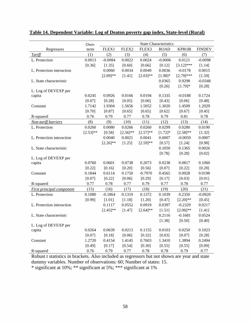
58

Table 14. Dependent Variable: Log of Deaton poverty gap index, State-level (Rural)

Regressors

Own-

term

State Characteristics

FLEX1 FLEX2 FLEX3 ROAD KPROB FINDEV

Tariff (1) (2) (3) (4) (5) (6) (7)

L. Protection 0.0013 -0.0084 0.0022 0.0024 -0.0006 0.0121 -0.0098

[0.36] [1.35] [0.60] [0.66] [0.12] [3.12]*** [1.14]

L. Protection interaction 0.0060 0.0034 0.0049 0.0036 -0.0178 0.0015

[2.09]** [1.41] [2.03]** [1.98]* [2.79]*** [1.59]

L. State characteristic 0.0365 0.9298 -0.0348

[0.26] [1.70]* [0.28]

L. Log of DEVEXP per

capita 0.0245 0.0926 0.0166 0.0194 0.1335 -0.0188 0.1724

[0.07] [0.28] [0.05] [0.06] [0.43] [0.06] [0.48]

Constant 1.7142 1.9304 1.5656 1.5052 1.3020 1.4509 1.2029

[0.70] [0.87] [0.65] [0.65] [0.62] [0.67] [0.45]

R-squared 0.76 0.79 0.77 0.78 0.79 0.81 0.78

Non-tariff barriers (8) (9) (10) (11) (12) (13) (14)

L. Protection 0.0260 0.0080 0.0266 0.0260 0.0299 0.0280 0.0190

[2.53]** [0.58] [2.56]** [2.57]** [1.72]* [2.58]** [1.32]

L. Protection interaction 0.0040 0.0021 0.0041 0.0007 -0.0059 0.0007

[2.26]** [1.25] [2.59]** [0.57] [1.24] [0.98]

L. State characteristic 0.1050 0.1365 0.0026

[0.78] [0.28] [0.02]

L. Log of DEVEXP per

capita 0.0760 0.0601 0.0738 0.2073 0.0238 0.0817 0.1060

[0.22] [0.16] [0.20] [0.56] [0.07] [0.22] [0.28]

Constant 0.1844 0.6114 0.1750 -0.7970 0.4565 0.0928 0.0198

[0.07] [0.22] [0.06] [0.29] [0.17] [0.03] [0.01]

R-squared 0.77 0.78 0.77 0.79 0.77 0.78 0.77

First principal component (15) (16) (17) (18) (19) (20) (21)

L. Protection 0.1080 -0.1864 0.1319 0.1372 0.1039 0.2350 -0.0920

[0.99] [1.01] [1.18] [1.20] [0.47] [2.20]** [0.45]

L. Protection interaction 0.1117 0.0552 0.0919 0.0397 -0.2329 0.0217

[2.45]** [1.47] [2.64]** [1.51] [2.06]** [1.41]

L. State characteristic 0.2116 -0.1681 0.0524

[1.38] [0.50] [0.40]

L. Log of DEVEXP per

capita 0.0264 0.0639 0.0213 0.1155 0.0103 0.0250 0.1023

[0.07] [0.18] [0.06] [0.32] [0.03] [0.07] [0.28]

Constant 1.2720 0.4154 1.4145 0.7603 1.3410 1.3894 0.2494

[0.49] [0.17] [0.54] [0.30] [0.55] [0.55] [0.09]

R-squared 0.76 0.79 0.77 0.78 0.78 0.79 0.77

Robust t statistics in brackets. Also included as regressors but not shown are year and state

dummy variables. Number of observations: 60; Number of states: 15.

* significant at 10%; ** significant at 5%; *** significant at 1%

59

Table 15. Dependent Variable: Log of Deaton poverty rates, State-level

Regressors

Own-

term

State Characteristics

FLEX1 FLEX2 FLEX3 ROAD KPROB FINDEV

Urban (1) (2) (3) (4) (5) (6) (7)

L2. FDI share to GDP -0.0056 -0.0052 -0.0052 -0.0052 -0.0008 -0.0734 0.0354

[0.44] [0.41] [0.43] [0.41] [0.06] [2.22]** [1.29]

L2. FDI share interaction -0.0166 -0.0264 -0.016 0.0026 0.0709 -0.0097

[0.69] [1.02] [0.66] [0.17] [1.86]* [1.44]

L2. State characteristics -0.2123 0.4326 -0.2856

[1.23] [0.59] [2.51]**

L. Log of DEVEXP per

capita 0.3988 0.3762 0.3757 0.3745 0.4324 0.3005 0.1116

[1.46] [1.36] [1.36] [1.35] [1.43] [1.17] [0.39]

Constant 0.0783 0.2324 0.2364 0.2441 -0.1935 0.1888 3.4631

[0.04] [0.12] [0.12] [0.13] [0.09] [0.10] [1.51]

R-squared 0.68 0.68 0.69 0.68 0.69 0.71 0.74

Rural (8) (9) (10) (11) (12) (13) (14)

L2. FDI share to GDP 0.0019 0.0015 0.0018 0.0015 0.0038 -0.0245 0.0078

[0.25] [0.18] [0.22] [0.18] [0.40] [0.72] [0.34]

L2. FDI share interaction 0.0179 0.0085 0.0188 -0.0146 0.0289 -0.0014

[0.94] [0.39] [0.96] [0.87] [0.87] [0.24]

L2. State characteristics -0.0734 -0.2031 -0.0304

[0.38] [0.50] [0.29]

L. Log of DEVEXP per

capita -0.0627 -0.0382 -0.0552 -0.0341 -0.0333 -0.0796 -0.0944

[0.27] [0.17] [0.24] [0.15] [0.14] [0.36] [0.35]

Constant 3.764 3.5972 3.7129 3.5692 3.5488 3.7089 4.1321

[2.40]** [2.29]** [2.34]** [2.28]** [2.16]** [2.44]** [1.89]*

R-squared 0.57 0.57 0.57 0.58 0.58 0.58 0.57

Robust t statistics in brackets. Also included as regressors but not shown are year and state

dummy variables. Number of observations: 45; Number of states: 15.

* significant at 10%; ** significant at 5%; *** significant at 1%

Table 16. Dependent Variable: Log of State GDP per capita (Combined Urban and Rural)

Regressors

Own-

term

State Characteristics

FLEX1 FLEX2 FLEX3 ROAD KPROB FINDEV

(1) (2) (3) (4) (5) (6) (7)

L. Tariff -0.0051 -0.0017 -0.0058 -0.0057 -0.0024 -0.0046 0.0008

[2.32]** [0.72] [3.46]*** [2.81]*** [0.79] [2.40]** [0.63]

L. Tariff interaction -0.0023 -0.0028 -0.0013 -0.0006 0.0047 -0.0012

[3.51]*** [6.09]*** [1.84]* [1.22] [2.80]*** [8.15]***

L. State characteristic 0.0727 -0.7997 0.0133

[1.04] [4.09]*** [0.35]

L. Log of DEVEXP per capita 0.219 0.1955 0.2235 0.2051 0.1572 0.245 0.0566

[1.02] [1.13] [1.43] [0.96] [0.88] [1.34] [0.60]

Constant 7.8543 7.7843 8.0423 8.0571 8.0094 7.7469 9.1432

[5.21]*** [6.34]*** [7.31]*** [5.46]*** [6.10]*** [6.02]*** [12.73]***

R-squared 0.88 0.91 0.94 0.89 0.89 0.91 0.95

Robust t statistics in brackets. Also included as regressors but not shown are year and state dummy variables.

Number of observations: 60; Number of states: 15.

* significant at 10%; ** significant at 5%; *** significant at 1%

61

Table 17. Dependent Variable: Log of Deaton poverty rates, State-level (Combined Urban and Rural)

Regressors

Own-term

Trade

protection

State characteristics

FLEX1 FLEX2 FLEX3 ROAD KPROB FINDEV

(1) (2) (3) (4) (5) (6) (7) (8) (9)

L. Log of GSDP per capita -0.41911 -0.42162 -0.35228 -0.24913 -0.30054 -0.29729 -0.22257 -0.17814 -0.18621

[2.03]** [2.15]** [1.66] [1.21] [1.05] [1.38] [1.06] [0.73] [0.65]

L. Tariff 0.0039 0.00204 0.00425 0.00446 0.00084 0.00801 0.00038

[1.54] [0.62] [1.47] [1.70]* [0.28] [2.25]** [0.06]

L. Tariff interaction 0.00146 0.0005 0.00097 0.00218 -0.00601 0.00053

[1.07] [0.31] [0.81] [2.39]** [1.47] [0.77]

L. State characteristic (own-

term) -0.05316 0.40758 -0.07937

[0.65] [1.04] [1.14]

L. Log of DEVEXP per capita 0.01132 -0.00954 -0.02077 -0.02255 -0.02219 0.06414 -0.06699 -0.05475

[0.06] [0.05] [0.11] [0.12] [0.12] [0.36] [0.35] [0.27]

Constant 6.71356 6.65467 6.18867 5.47933 5.76704 5.70505 4.90167 4.74695 5.51223

[3.45]*** [2.64]** [2.36]** [2.09]** [1.81]* [2.11]** [1.93]* [1.64] [1.70]*

R-squared 0.8 0.8 0.81 0.81 0.81 0.81 0.84 0.82 0.82

Robust t statistics in brackets. Also included as regressors but not shown are year and state dummy variables.

Number of observations: 60; Number of states: 15.

* significant at 10%; ** significant at 5%; *** significant at 1%

Appendix Table 1. Deaton Poverty Lines (Rupees)

Sector/State

43rd

Round 50th

Round 55th

Round 61st Round

(1987-88) (1993-94) (1999-2000) (2004-05)

Rural Urban Rural Urban Rural Urban Rural Urban

Andhra Pradesh 108.8 120.4 192.4 212.6 309.6 344.8 342.3 379.1

Assam 123.5 133.3 214.8 239.7 339.9 379.0 372.5 411.5

Bihar 121.0 130.8 192.8 216.9 296.9 321.6 331.5 370.3

Gujarat 127.8 134.8 228.9 240.8 337.3 369.4 383.4 424.3

Haryana 114.4 128.3 203.0 234.7 310.8 358.4 360.2 413.9

Karnataka 114.9 126.4 203.4 224.9 322.6 367.2 349.5 399.2

Kerala 121.4 125.6 221.5 230.8 373.9 386.2 381.8 399.7

Madhya Pradesh 109.0 123.2 185.1 214.3 288.9 321.3 321.4 378.4

Maharashtra 120.1 137.0 207.7 245.5 319.9 385.4 360.5 429.4

Orissa 111.8 123.2 182.4 201.5 300.3 312.3 309.2 340.3

Punjab 109.0 123.4 206.3 235.6 316.5 350.5 371.8 414.0

Rajasthan 120.2 128.3 207.3 230.7 323.9 353.2 349.7 389.0

Tamil Nadu 122.1 133.0 210.3 230.6 336.5 366.1 365.5 405.0

Uttar Pradesh 105.7 124.9 180.4 210.2 280.5 320.4 317.0 374.9

West Bengal 114.8 129.4 189.9 223.0 306.8 343.5 347.9 394.0

Source: Deaton (2003a) for rounds 43-55; Amoranto and Hasan (2010) for 61st round.

63

Appendix Table 2. Deaton Poverty Rates (Percent)

Sector/State

43rd

Round 50th

Round 55th

Round 61st Round

(1987-88) (1993-94) (1999-2000) (2004-05)

Rural Urban Rural Urban Rural Urban Rural Urban

Andhra Pradesh 35.0 23.4 29.2 17.8 27.9 11.3 19.9 6.4

Assam 36.1 13.6 35.4 13.0 35.7 12.1 18.9 5.0

Bihar 54.6 38.1 48.6 26.7 39.3 23.5 34.9 16.9

Gujarat 39.4 16.4 32.5 14.7 20.4 6.6 24.6 3.9

Haryana 13.6 11.8 17.0 10.6 6.5 5.1 6.7 8.7

Karnataka 40.8 26.0 37.9 21.4 30.3 11.5 28.2 12.1

Kerala 23.8 21.0 19.5 13.9 11.6 10.5 8.2 7.2

Madhya Pradesh 43.7 20.7 36.7 18.5 31.2 14.1 36.5 16.3

Maharashtra 44.3 21.2 42.9 18.2 30.8 13.0 29.1 11.2

Orissa 50.4 20.8 43.5 15.2 41.3 15.6 41.7 15.7

Punjab 6.6 6.6 6.2 7.8 2.8 4.0 5.0 2.2

Rajasthan 35.3 19.8 23.0 18.3 16.2 10.6 13.7 9.7

Tamil Nadu 49.0 26.2 38.5 20.9 25.6 11.1 26.2 7.5

Uttar Pradesh 34.9 29.3 28.7 21.7 20.8 16.5 18.9 14.0

West Bengal 36.3 22.3 25.1 15.5 22.7 11.4 20.6 8.0

Source: Deaton (2003a) for rounds 43-55; 61st round poverty rates estimated using NSS unit

level data based on poverty lines from Amoranto and Hasan (2010).

64

Appendix Table 3. Expert Group 2009 Poverty Lines (Rupees)

Sector/State

43rd

Round 50th

Round 61st Round

(1987-88) (1993-94) (2004-05)

Rural Urban Rural Urban Rural Urban

Andhra Pradesh 138.9 159.2 244.1 282.0 433.4 563.2

Assam 153.4 172.7 266.3 306.8 478.0 600.0

Bihar* 147.8 161.7 236.1 266.9 433.4 526.2

Gujarat 163.8 193.9 279.4 320.7 501.6 659.2

Haryana 168.7 175.7 294.1 312.1 529.4 626.4

Karnataka 152.4 166.6 266.9 294.8 417.8 588.1

Kerala 166.5 166.9 286.5 289.2 537.3 584.7

Madhya Pradesh* 135.3 160.7 232.5 274.5 408.4 532.3

Maharashtra 155.5 181.9 268.6 329.0 484.9 632.9

Orissa 136.1 166.4 224.2 279.3 407.8 497.3

Punjab 150.5 183.0 286.9 342.3 543.5 642.5

Rajasthan 163.0 174.9 271.9 300.5 478.0 568.2

Tamil Nadu 150.7 169.2 252.6 288.2 441.7 559.8

Uttar Pradesh* 145.5 170.1 244.3 281.3 435.1 532.1

West Bengal 141.4 173.0 235.5 295.2 445.4 572.5

Note: * Bihar poverty lines for round 61 are population-weighted averages of Bihar and Jharkand

poverty lines; Madhya Pradesh poverty lines are population-weighted averages of Madhya

Pradesh and Chattisgarh poverty lines; and Uttar Pradesh poverty lines are population-weighted

averages of Uttar Pradesh and Uttaranchal poverty lines.

Source: Amoranto and Hasan (2010) for 43rd

round; Government of India (2009) for 50th

and 61st

rounds.

65

Appendix Table 4. Expert Group 2009 Poverty Rates (Percent)

Sector/State

43rd

Round 50th

Round 61st Round

(1987-88) (1993-94) (2004-05)

Rural Urban Rural Urban Rural Urban

Andhra Pradesh 54.7 41.3 48.1 35.2 32.3 23.4

Assam 56.2 28.9 54.9 27.7 36.4 21.8

Bihar 70.8 55.3 63.1 43.5 54.8 35.5

Gujarat 57.8 40.1 43.1 28.0 39.1 20.1

Haryana 35.3 26.2 40.0 24.2 24.8 22.4

Karnataka 69.5 41.9 56.6 34.2 37.5 25.9

Kerala 53.1 37.1 33.9 23.9 20.2 18.4

Madhya Pradesh 60.2 34.6 51.1 31.1 54.0 33.7

Maharashtra 64.6 34.0 59.3 30.3 47.9 25.6

Orissa 65.8 38.6 63.0 34.5 60.8 37.6

Punjab 21.5 25.0 20.3 27.2 22.1 18.7

Rajasthan 58.7 39.4 40.8 29.9 35.8 29.7

Tamil Nadu 62.2 39.6 51.0 33.7 37.5 19.7

Uttar Pradesh 62.2 49.3 50.3 37.3 42.4 33.6

West Bengal 55.1 41.8 42.5 31.2 38.2 24.4

Source: Calculated from NSS unit-level data using poverty lines from Amoranto and Hasan

(2010) for 43rd

round; Government of India (2009) for 50th

and 61st rounds, except for Bihar,

Madhya Pradesh, and Uttar Pradesh which were calculated from unit-level data using poverty

lines provided in Appendix Table 3.