International Journal of Solids and Structures 43 (2006) 3739–3769

www.elsevier.com/locate/ijsolstr

Towards a multiscale analysis of periodic masonrybrickwork: A FEM algorithm with damage and friction

Giuseppina Uva a,*, Ginevra Salerno b

a Department of Sciences of Civil Engineering and Architecture, Politechnical University of Bari, via Orabona n. 4, 70125 Bari, Italyb Department of Structures, University of ‘‘Roma Tre’’, via Vito Volterra n. 62, 00146 Roma, Italy

Received 12 May 2005; received in revised form 2 June 2005Available online 22 December 2005

Abstract

The aim of this paper is to present an effort towards a multiscale model of the inelastic behaviour of masonry brickpanels and the relative solution algorithm. The essential features of the inelastic behaviour, such as the damagedevelopment within the bed joints and the frictional dissipation over cracks’ faces, are taken into account. Micromechan-ical solutions are adopted in order to trace the guidelines for modelling the mentioned phenomena, and FEM analyses oflarge-scale panels are shown.� 2005 Elsevier Ltd. All rights reserved.

Keywords: Periodic masonry brickwork; In-plane behaviour; Damage and plasticity; Multiscale analysis; Homogenization; FEM analysis

1. Introduction

The mechanical behaviour of masonry structures is one of the most complex and challenging matters of themodern structural engineering. Indeed, masonry is a composite material, highly inhomogeneous and aniso-tropic because of the presence of mortar joints acting as weak points within the structure (Page, 1981;Syrmakezis and Asteris, 2001). The mechanical response, as a consequence, exhibits significant non-linear,irreversible and dissipative phenomena, which cannot be neglected by a structural model aimed at the predic-tion of the ultimate load and of the response under cyclical loads for masonry structures. The relevantmechanical phenomena that should be considered in order to describe the material behaviour (such as cracks’nucleation and growth within mortar layers or mortar–brick interfaces; frictional sliding at the contactbetween opposite cracks’ faces; rocking of indented cracks edges) actually take place at a very small scale.On the other side, the structure is governed, in its peculiar overall response, by its global geometrical and mor-phological configuration. For instance, in masonry buildings the distribution of the loads among the different

0020-7683/$ - see front matter � 2005 Elsevier Ltd. All rights reserved.

doi:10.1016/j.ijsolstr.2005.10.004

* Corresponding author.E-mail addresses: g.uva@poliba.it (G. Uva), salerno@uniroma3.it (G. Salerno).

3740 G. Uva, G. Salerno / International Journal of Solids and Structures 43 (2006) 3739–3769

structural elements is deeply influenced by the effectiveness of the box-like behaviour, whereas for historicalmasonry bridges, fundamental is the load path developed through the arc-effect.

In the early stages, the research studies developed in this field produced two different and antithetic visions,which for a long time have been the centre of a lively cultural debate within the scientific community (Hughesand Pande, 2001). On one side there was a continuous idea of masonry structures, in which the different struc-tural elements (masonry piers, slabs, . . .) were modelled by means of classical continuous elements (plates,shells, panels, . . .) endowed with agile constitutive functions and then assembled in order to provide the finaloverall response of the structural system (Italian Ministry of Public Works, 1981). On the other side, a differ-ent approach was followed, by interpreting each of the constituents in the masonry assembly (i.e. each blockand mortar joint) as an individual body, endowed with specific geometric and mechanical properties, andaccordingly performing the analysis for the actual assemblage of elements (Hart et al., 1988).

Each of the two mentioned visions has indeed a high theoretical dignity and presents a number of advan-tages (among others things, we could recall the affordable computational cost for the first one, and the solidphysical basis for the second one). However, when these two approaches are proposed as completely self-sufficient, they reveal irremediable defects. Actually, the one just possess the qualities the other is lackingof. In the last few years, the rigidity of such a dichotomy has been softening, and the scientific communityhas progressively realized that between the two antithetical extremes it is necessary to find a reasonable com-promise, in order to avoid excessive computational efforts when facing real case studies, but endowing contin-uous approaches with a well-founded mechanical basis (Hughes and Pande, 2001; Sutcliffe et al., 2001; Asterisand Tzamtzis, 2003). The literature about this questions is really wide: some references are given in the bib-liography of the paper, to which the reader is also addressed in order to find a more exhaustive state of the artreview (Hughes and Pande, 2001; Asteris, 2003; Sutcliffe et al., 2001; Asteris and Tzamtzis, 2003; Kouznetsovaet al., 2001; Kouznetsova et al., 2004; Kouznetsova et al., 2002; Kouznetsova, 2002; Massart, 2003).

Many modern modelling approaches and algorithms are actually continuous models enriched with a verydeep micromechanical insight, and could be defined, in the wide meaning of the word, ‘‘multiscale’’approaches according to Phillips (1998), that is to say, algorithms in which different scales of observationof the same physical phenomenon interact, exchanging information. It is our opinion that a reflection and dis-cussion should be promoted about multiscale algorithms in order to precise, for instance, the theoretical rela-tionships with research fields like non-linear homogenization or damage mechanics, in which a geometric linkwith lower scales is hiddenly kept every time that stabilizing procedures for the finite element are adopted,aimed at the sanitization of mesh dependency. The authors’ idea of multiscale is presented in Salerno andUva (2002) and is referred to the use of a hierarchic strategy in which a clear and precise definition is madeboth for the physical-mathematical models and for the scaling operators among different physical scales.

This paper does not completely belong to the philosophy presented in Salerno and Uva (2002) (whose effec-tiveness is actually still being tested), but nevertheless represents an effort in that direction, and in this senseshould be intended the word ‘‘towards’’ mentioned in the paper title. The objective is not only to give a micro-mechanical foundation for the definition of the inelastic part of the constitutive response (i.e. Eshelby’s solu-tion), but also to allow the interaction of the macroscopic scale, which is characterized by the finite elementdiscretization of an equivalent homogeneous body obtained through standard homogenization techniques(Sanchez Palencia, 1992; Suquet, 1983), with the lower scales, where the discontinuous nature of masonryis perceived, and the mathematical variables usually introduced to measure the damage level and the frictionalsliding do assume a precise physical meaning. The idea is that in quasi-fragile materials like mortars, macro-scopic non-linear phenomena are an effect of nucleation and growing of cracks at the microstructural level,and that a significant role is played by friction. A consistent micromechanical derivation of the constitutiveprescription would lead to a law with internal damage variables, endowed with proper multisurface domainsand flow rules (even non-associative). It is well known that the integration of such a constitutive law is quitecumbersome. In order to reduce algorithmic difficulties and to exploit at the best the advantages of the iter-ative arc-length strategy employed in the evolution path-following analysis, the constitutive law has beenreformulated within a scheme of localization–updating–averaging consistent with the classical homogeniza-tion method. Indeed, the framework for a real multiscale algorithm is then outlined. The research that is herepresented belongs to this general framework, and is focused on the in-plane behaviour of periodic masonrybrickwork. The aim is to predict the structural response both under monotonical and cyclical loading condi-

G. Uva, G. Salerno / International Journal of Solids and Structures 43 (2006) 3739–3769 3741

tions with sufficient accuracy but reasonable computational costs. The fulfillment of this objective is to be real-ized through progressive steps. In a first stage, the following two simplifying assumptions are made: (i) Onlybed joints are supposed to suffer decohesion and frictional sliding, head joints are completely neglected andblocks are considered as perfectly elastic; (ii) Nucleation and propagation of cracks is always considered asconfined within a plane and governed by opening and sliding modes, that are supposed to be uncoupled (thatis to say, dilatancy is not modeled). Of course, the description that is obtained is slightly rough, but the aim ofour research work is to consolidate a numerical basis for the analysis, pointing out the direction for futuredevelopments. Some experimental and numerical tests solved by different authors (Anthoine et al., 1994;Lagomarsino et al., 1995; Raijmakers and Vermeltfoort, 1992; Lourenco et al., 1994) have been selectedfor testing the model and the performance of the numerical strategy.

The paper is organized as follows: Section 2 is entirely devoted to provide a theoretical foundation of theconstitutive choices, within the spirit of Eshelby’s micromechanical solution, completed by the classical Mohr–Coulomb law and by Griffith’s criterion. Then, in Section 3 the theoretical model is re-formulated for the sakeof the computational management and the algorithm solution is outlined. Finally, in Section 4 results are pre-sented and compared with benchmarks. Conclusions follow.

2. Constitutive modelling

2.1. Preliminary remarks

The resistance of masonry buildings to horizontal actions and seismic input is usually considered very lowand unreliable. Indeed, this belief must be somewhat incorrect, since many ancient buildings still survivetoday, although they had not been intentionally and consciously designed to face unexpectedly strongearthquakes.

In order to explain this fact, it should be remembered that a proper structural organization encourages thespatial behaviour and allows the distribution of actions to the proper supporting elements. This is the primarycondition under which an optimum development of the shear strength and of frictional dissipation effects canoccur. During a seismic shaking, an evolution of cracks takes place and consequently there is an increase in theenergy dissipation related to frictional phenomena. The effect is the enhancement of structural ductility, andeven a material intrinsically brittle like masonry can adjust itself to face stresses that would otherwise be toostrong for it.

It is then evident that it is very important to devote attention to the non-linear and inelastic part of theconstitutive law, in order to obtain a satisfactory representation of the behaviour of masonry-like materials.In front of the complexity briefly outlined, descriptions based upon a pure linear elastic framework (tradi-tional elastic perfectly brittle model, no-tension model) are a drastic reduction.

Experimental research has pointed out that the constitutive behaviour of masonry is basically a softeningone, characterized by a progressive crack growth and by degradation in stiffness and strength. Moreover, ithas been definitely shown that the amount of inelastic deformations and hysteretic dissipation is not so neg-ligible. All these irreversible and dissipative phenomena make the structural response anisotropic and historydependent, but at the same time allow the development of plastic resources and the dissipation of part of theenergy related to seismic events. For all these reasons, aiming at reconstructing the post-critical, non-linearbranch of the equilibrium path, we have decided to pay attention to the mechanics of the events occurringat the microscopic scale.

Before getting into the heart of the matter, it is necessary to spend a few words and point out that we aredealing with a complex phenomenon where the structural response is governed by spatial scales that are verydifferent one from the other, and vary from the level of the single mortar joint to that of the whole wall. Withthis idea, we will distinguish three different scales that will be referred to as macro, meso and micro scales. Atthe macroscopic scale we see the continuum model of the masonry panel (obtained through a proper homog-enization of the lower scales), whereas at the mesoscopic level we see a non-homogenous, discrete system, com-posed of bricks and mortar joints. At the microscopic scale we finally get inside the mortar joint, where therelevant micromechanical phenomena we are interested in (such as crack’s growth and frictional sliding)can be observed.

3742 G. Uva, G. Salerno / International Journal of Solids and Structures 43 (2006) 3739–3769

2.2. The micromechanical approach

Nucleation and growth of cracks at the microscopic scale (with a possible development of contact frictionon the cracks’ faces) play a crucial role in the structural response of masonry panels and are to be accuratelydescribed.

Damage Mechanics is able to explain the deterioration occurring at the mesoscale, where the informationabout the microscopic complexity is lost. The effects of the evolution of microcracks can be recovered by usinga continuum internal variable controlling the damage, whose definition and evolution should somehow keeptrace of the micromechanics of the problem.

The basis on which the choice and definition of the internal variables is made is a micromechanical modelfor quasi-brittle materials proposed by Alpa and Gambarotta (1990), Gambarotta (1995), Gambarotta andLagomarsino (1993), Gambarotta and Lagomarsino (1994b). In order to develop this model, a graduatedapproach is followed, starting from the solution of the simpler problem involving a single crack, and then pro-gressively enriching it.

During the loading process, microdefects can grow up: by adopting the classical reference framework of theFracture Mechanics, their propagation can be basically traced back to three ‘‘crack modes’’ (Fig. 1): (I) Open-ing mode; (II) Sliding mode; (III) Tearing mode. These phenomena are the reason for the apparent drop off inthe stiffness and strength of the material. After choosing a proper reference elementary volume (REV), theeffect of the development of a single plane, penny-shaped crack (denoted by the index i) immersed in an elasticmatrix and having a generic orientation singled out by a normal versor ni (Fig. 2) can be analysed as a bound-ary problem in which an external far stress field is assigned for the loading condition.

The starting point for solving such a boundary problem and obtaining the elastic state induced by the crackin the REV (displacement, strain and stress fields) is represented by the Eshelby solution of the ellipsoidalinclusion problem (Eshelby, 1968a,b). An infinite solid containing an ellipsoidal inhomogeneity and subjectedto a remote stress field is considered. Remarkably, supposing that both the matrix and the inclusion are madeof elastic and homogeneous materials, it turns out that the strain and stress fields inside the inclusion (and onthe interface as well) are uniform. Furtherly, the solution fields averaged over the REV can be expressed as thesum of two terms: the state induced by the far stress imagining that the solid were homogeneous with elasticconstants corresponding to the matrix, plus an ‘‘inelastic’’ correction due to the presence of the inclusion.

If the inclusion is actually a hole (that is to say, stress free), its displacement and strain fields, in particularon the boundary (where they are actually meaningful), can still be computed, and the expression of the fieldsinduced in the REV keeps the same additive form as before.

Since a crack can be simply generated by properly collapsing one of the semi-axes of an ellipsoidal cavity,the particularization of the above mentioned results suggests the way for computing the displacements of thetwo opposite sides of the crack u�i and provides the expression for the strain field induced in the REV by theopening of the single crack.

Finally, by adding the contributions of all the cracks embedded in the REV (the assumption that microde-fects do not interact one with the other allows to superpose elastic states), the overall inelastic contribution E*

Fig. 1. Elementary crack propagation modes.

Fig. 2. A single microcrack immersed in the REV.

G. Uva, G. Salerno / International Journal of Solids and Structures 43 (2006) 3739–3769 3743

to the mesoscopic strain field E is evaluated (C compliance matrix; ni normal versor to the plane of the ithcrack, N total number of microcracks contained in the REV):

E ¼ CTþ E� ¼ CTþXNi¼1

e�i ni � ni þ sym c�i � ni

� �� �. ð1Þ

According to the previous remarks, the inelastic contributions of the crack opening displacements to themesoscopic strain field can be explicited by following the procedure sketched by Eshelby. It can be seen thatthey are a function of: the far stress solved in the crack plane (ti = Tni), the mechanical parameters of thematrix, the geometry and the initial dimension of the crack (Budiansky and O’Connell, 1976; Hoenig,1979; Hoenig, 1978; Nemat-Nasser and Horii, 1983). The ‘‘solved stress’’ can be split into two uncoupledcomponents: ti = rini + si, where ri = Tni Æ ni and si = Tni � rini.

However, it is necessary to take into account the presence of the contact actions acting through the crack’sfaces (Fig. 3): in fact, the stresses applied to the crack plane can not be fully engaged for the crack’s growth: atthe beginning, the contact actions are opposed and dissipate by friction a part of the elastic energy of the exter-nal loads, that is no more available for the fracture propagation.

Hence, the solved stresses are turned into ‘‘effective stresses’’:

e�i ¼ cniaiHðriÞri ¼ cniairi;eff ;

c�i ¼ ctiaiðsi þ f iÞ ¼ ctiaisi;eff .

�ð2Þ

Fig. 3. Effective stresses over the crack’s faces.

3744 G. Uva, G. Salerno / International Journal of Solids and Structures 43 (2006) 3739–3769

Hð�Þ ¼ Heaviside step function:Hð�Þ ¼ 1 if � > 0;Hð�Þ ¼ 0 if � 6 0;ri;eff ¼HðriÞri;si,eff = (si + fi);f i ¼ �siHð�riÞ ¼ friction force; kf ik � l j ri j6 0;l = friction coefficient;cni = normal compliance;cti = tangential compliance.

Eshelby’s solution in terms of effective stresses (2) depends also on the variable ai, which is function only ofthe actual dimension of ith crack and assumes the role of internal damage variable, whose evolution will be fol-lowed during the loading process. The two mechanical parameters cni and cti are to be provided in the model.

Eq. (2)1 shows that the normal strain e�i , for a given ai, is determined once the normal effective stress ri,eff isassigned. Actually, it is an unilateral constitutive constraint: the inelastic contribution vanishes if the crack isunder a compression state, that is to say, if it is closed. In Eq. (2)2 the friction is explicitly introduced in theform of the effective tangential stress si,eff. The presence of friction involves a problem of plasticity, and makesit necessary to keep a trace of the residual plastic tangential sliding, that becomes a further internal variable ofthe model: cri.

The definition of the limit domains and the evolution laws for the internal variables ai and cri is madeaccording to the principles of Damage Mechanics (Krajicinovic, 1989; Krajicinovic and Fonseka, 1981;Lemaitre, 1984; Lemaitre, 1992). First of all, the static associated variables Gi and fi (thermodynamic general-ized forces) related to the internal variables should be defined, by means of the dissipated powerD ¼ �f i � _cri þ Gi _ai. Trivially, the static variable associated to the residual plastic sliding cri is �fi. With regardto the damage state, the associated variable Gi can be defined according to the principles of FractureMechanics (Broek, 1984) as the energy release rate involved by the crack growth:

Gi½ti; ai� ¼dwe½ti; ai�

dai

����ti¼cost

¼ 1

2HðriÞri

oe�ioaiþ 1

2si þ f ið Þ � oc�i

oai; ð3Þ

where we is the elastic strain energy stored in the REV in presence of the ith crack, characterized by the dam-age measure ai, and under the constant stress state ti.

Now, it is necessary to properly choose some criteria governing the evolution of each ai and the correspond-ing frictional sliding cri. For the frictional sliding a classical Coulomb–Mohr law is adopted, while for thedamage development an energetically based criterion is employed, following the approach suggested byGriffith. It is supposed that the propagation of a crack can take place when the energy released with the infin-itesimal crack increment dai (this is just the function Gi previously defined) becomes greater than the toughnessR of the material, that is to say, the intrinsic strength opposed by the material to the crack growth (Broek,1984):

Gi½ti; ai� �R½ai� 6 0. ð4Þ

We will deal with a concrete-like material: according to Broek (1984), we will choose for it a toughness func-tion containing all the meaningful features of the behaviour of a quasi-brittle material: an initial linearly elasticbranch; a critical peak ðacr;RcrÞ; an unstable softening phase. The critical state defined by ðacr;RcrÞ can beidentified through uniaxial tests (pure tension or shear) on the material.

After all, the problem for a generic crack identified by ai is expressed by the following system of plasticadmissibility conditions and loading/unloading conditions:

Udi½ti; ai� ¼ Gi �R½ai� 6 0 ) 1

2cniHðriÞr2

i þ1

2ctiksi þ f ik2 �R½ai� 6 0;

Usi½ti; cri� ¼ kf ik � ljrij 6 0 ) ksik � ljrij 6 0;

Udi _ai ¼ _Udi _ai ¼ 0; _ai P 0;

Usi_ki ¼ _Usi

_ki ¼ 0; _ki ¼ 0; _cri ¼ vi_ki; vi ¼ �

f i

kf ik.

ð5Þ

G. Uva, G. Salerno / International Journal of Solids and Structures 43 (2006) 3739–3769 3745

For further details on the micromechanical model, the interested reader is addressed to the specific literature(Gambarotta and Lagomarsino, 1993; Gambarotta and Lagomarsino, 1994b).

The constitutive law defined by (5) is quite complex, and can be properly described within the framework ofmultisurface plasticity. The type of hardening occurring depends on the particular stress states: (1) pure tensilestress; pure shear; tension and shear; (2) compression and shear.

The first group of stress combinations is depicted in Fig. 4, where the evolution of the limit damagedomains Ud[a] for 0 < a < acr (top) and for a P acr (bottom) is shown: for loading paths confined in thehalf-plane r P 0, the material exhibits an isotropic hardening that is positive for 0 < a < acr and negativefor a P acr. In the same figure, even if not active, the limit damage surfaces under compression are shownin the left shadowed half-plane and will be discussed later.

For fixed values of a, in the half–plane r P 0 the limit curve is the semi-ellipse defined by the equationUþd ½a� ¼ 1

2cnr2 þ 1

2ctksk2 �R½a� ¼ 0.

The second group of stress combinations (compression and shear—Fig. 5) is more complex. The simulta-neous presence of shear and compression generates a frictional behaviour that is not merely governed by theCoulomb law. In fact, because of the interaction between plastic frictional sliding and damage, a combinationof kinematical and isotropic hardening is triggered. With regard to the mathematical expressions, the damagedomain U�d ½a� ¼ 1

2ctksþ fk2 �R½ai� ¼ 0 in the half-plane r < 0 is represented by two lines having a slope

defined, respectively, by �l and l, and parallel to the classical Coulomb friction cone. Phenomenologically,

Fig. 4. Evolution of the limit domains for tension/shear loading paths: (a) a < acr, (b) a > acr.

Fig. 5. Evolution of the limit domains for compression/shear loading paths.

3746 G. Uva, G. Salerno / International Journal of Solids and Structures 43 (2006) 3739–3769

the plastic sliding is actually bounded by the finite dimension of the crack and by the presence of theuncracked material fraction, so it can increase only when the crack dimension grows up.

In other words, this means that the damage limit domain and the frictional admissible surface are alwayslinked on one side: every time that _a and _cr are simultaneously positive, the limit damage surface is activated

G. Uva, G. Salerno / International Journal of Solids and Structures 43 (2006) 3739–3769 3747

and starts to expand (a < acr) or contract (a P acr), while a translation of the Coulomb cone (kinematicalhardening) occurs. When _cr < 0, such an interaction is not activated, since _a is always non-negative: healingis not admitted by our damage model.

A further comment on Fig. 5 is useful for a better understanding of the constitutive model. In the left side ofthe figure, the actual mesoscopic stress state for the typical material point is represented in the stress domain(r,s). In the right side, instead, the different constitutive behaviour of the cracked fraction and of theuncracked one is traced in the plane (c,s) (the relevant quantities are denoted, respectively, with the super-scripts ‘‘c’’ and ‘‘u’’). This information, actually, is lost at the mesoscopic level and is here recalled in orderto define the internal damage variable.

For each loading path in the mesoscopic stress domain (identified by capital letters), the correspondingplastic path for the cracked fraction (distinguished by capital letters with the superscript ‘‘c’’) can be readin the stress/strain domain. Also the ‘‘elastic’’ uncracked stress (superscript ‘‘u’’) is plotted in this graph, incorrespondence of the actual value of the total tangential sliding c.

Let us follow the loading path OAB/OABc shown in the top of Fig. 5. The line OA is characterized by aconstant normal compression r and by the closure of the crack because of friction: macroscopically, thebehaviour is perfectly elastic. At point A, the initial limit surface is reached. The tangential stress s becomesequal to lr (i.e., to the limit sliding threshold for the contact actions on the crack’s surface). The Mohr–Cou-lomb constitutive law states that no increment of the tangential stress is possible on the cracked fraction: fromnow on (A–B), any additional external work will be entirely spent in the development of the inelastic sliding cr,while the microscopic tangential stress sc will remain frozen at the value lr. Correspondently, an increment inthe size of the crack’s surface has to occur: together with the plastic sliding increment _cr, an increment _a takesplace, and the limit domain consequently expands.

For example, at point B, the tangential stress of the cracked fraction sc is frozen at lr (Bc), while the inelas-tic sliding cr occurs. In the stress domain, this situation is represented by a vertical shifting of the initial cone,driven by the increments of both a and cr.

Now, if the representative stress point is driven back following the initial path and inverting the sign of thetangential stress (branch BCDEFG/BcCcDcEcFcGc in Fig. 5-middle), the cracked fraction undergoes the elas-tic unloading BcCcDc until the microscopic stress sc attains the value �lr. At this point (D/Dc), the develop-ment of a plastic sliding cr in the opposite direction starts. In the stress plane, all this happens within theinstantaneous elastic domain, that is to say, with no increment of the internal variable a: there is a ‘‘free’’ spacewithin which the sliding of the crack can take place at no extra-cost in terms of damage increase.

At the point G/Gc, the plastic sliding cr previously accumulated is completely recovered, and a further pro-gress can only proceed if the crack’s size accordingly grows up: _cr > 0 and _a > 0. So, for example, the pathGH/GcHc (Fig. 5-bottom) is characterized by the gain of a negative inelastic sliding Dcr and by a new expan-sion of the limit damage surface, measured by Da.

2.3. Continuum modelling of masonry brickwork

As stated at the beginning, in order to avoid excessive computational costs, a macromodelling approach hasbeen here adopted: instead of describing in detail the texture of a masonry panel, an equivalent Cauchy con-tinuum has been defined, and its ideal mechanical properties have been obtained starting from those of its con-stituents. This operation is fulfilled by considering the masonry as made up of alternate layers of brick andmortar (Fig. 6b) and by homogenizing (Fig. 6c) this layered composite by standard techniques (Anthoine,1994).

Head joints are neglected, although they are present in the initial topology (Fig. 6a), and this has allowedus to consider the homogenized continuum as transversely isotropic rather then orthotropic, at least in theelastic state. This could seem quite a rough assumption; however, the observation of existing structuresand experimental testing seems to suggest that their influence plays only a secondary role in collapse mech-anisms: ruptures are mostly localized in mortar bed joints (whose thickness is usually very small with respectto the other dimensions), at the contact surface between mortar and blocks rows, whereas the propagation ofcracks more significantly involves bed joints (with the characteristic diagonal pattern) only in the late post-critical branch.

Fig. 6. Homogenization of the masonry panel seen as a transversely isotropic composite.

3748 G. Uva, G. Salerno / International Journal of Solids and Structures 43 (2006) 3739–3769

The micromechanical model briefly sketched in the previous paragraph can be fruitfully used for themodelling of masonry panels, as it was shown by some authors (Gambarotta and Lagomarsino, 1994a;Gambarotta et al., 1995). Of course, further simplifications will have to be introduced, if we do not wantto loose sight of the practical exigencies of the analysis, aimed at the solution of large structures. Hence, beforehomogenizing, some additional hypotheses will be done.

First of all, we have chosen to deal with plane systems, and to focus the attention only on their in-plane

behaviour. It is then supposed that the rupture within the horizontal mortar joints can only take place alongan ‘‘interface’’ plane, whose position within the thickness of the bed is unimportant to the aim of the overallanalysis. Hence, microcracks are described as a set of equi-oriented segments laying on the interface plane andgoverned by a unique scalar measure of damage, in the form of an internal variable controlling the cracks’length. Hence, from now on, the subscript i will be left out.

One more consequence is that the nucleation and propagation of cracks is only governed by opening andsliding elementary modes, supposed to be uncoupled (that is to say, dilatancy cannot be modelled). Actually,damage affects also the bricks, but in the proposed model this will be completely neglected: indeed the exper-imental evidence shows that it becomes significant only when a high compression state is attained (usually inthe late post-critical branch, Ballio et al., 1993).

According to these assumptions, the micromechanical model (1) and (2) assumes a very simple form:only one scalar damage variable is introduced in each material point, able to account for the damage ofthe bed joints, whereas the bricks are supposed to remain elastic throughout all the loading process. Dur-ing the loading process, the microdefects within the mortar interfaces split open—according to the open-ing mode and sliding mode (Section 2.2)—and are subjected to contact actions as a consequence of theharshness of the cracks’ faces. As an effect of these mechanisms, inelastic deformations arise (Eq. (2)) andcontribute to the macroscopic strain field E (Eq. (1)) of the equivalent continuum. In the elastic phase, theglobal response is described by the compliance matrix obtained by homogenizing the layered composite intoa linear elastic transversely isotropic Cauchy material. In Fig. 6, axis 2 is the transverse isotropy axis. In theplane case, only four independent constants appear in the constitutive elastic coefficient matrix, that is, E1, E2,m and G:

e1

e2

c

8><>:

9>=>; ¼

1E1

� mE1�

� mE1

1E2

�� � 1

G

2664

3775 ¼

r1

r2

s

8><>:

9>=>;; ð6Þ

r1

r2

s

8><>:

9>=>; ¼

E1 þ m2

1E2�m2

E1

h i m

1E2�m2

E1

h i �

m

1E2�m2

E1

h i 1

1E2�m2

E1

h i �

� � G

2666664

3777775¼

StE11 StE

12 �StE

12 StE22 �

� � StE33

264

375 ¼

e1

e2

c

8><>:

9>=>;; ð7Þ

G. Uva, G. Salerno / International Journal of Solids and Structures 43 (2006) 3739–3769 3749

where the stiffness coefficients Stij are defined, and E1, E2, m and G assume the following form in terms of mor-tar and bricks elastic moduli (Em, Eb, Gm, Gb) and of their volume fractions (gm,gb):

E1 ¼ gmEm þ gbEb;

m ¼ gmmm þ gbmb;

E2 ¼1

gmm2m þ gbmb

E1

� gmm2m

Em

þ gbm2b

Eb

þ gm

Em

þ gb

Eb

;

G ¼ GmGb

gmGb þ gbGm

.

ð8Þ

Let us now homogenize the anelastic contribution. The REV will be chosen in order to contain just one bedjoint. In that case, and considering that the tangential strain has only one component, the inelastic deforma-tion in Eq. (1), only dependent on mortar bed joints, is specified as follows:

E�m ¼ e�mn� nþ c�mm � ne�m ¼ cnaHðrÞr;

c�m ¼ ctaðsþ f Þ;

�a ¼

XNi¼1

ai. ð9Þ

The notations and parameters used are the same introduced in Section 2.2, specifying that the material is themortar. In particular, cn and ct are the normal and tangential compliance parameters governing the crackopening in the mortar bed joints.

The overall strain field in the masonry (variables referring to the homogenized masonry have been denotedwith the index M), after the Reuss homogenization, becomes:

EM ¼ CM TM þ gmE�m. ð10Þ

Actually, while homogenization techniques for periodic media have been extensively and successfully appliedin linearized elasticity, when the constituents are endowed with a non-linear behaviour there are not widelyaccepted and firmly stated homogenization procedures, and only in very simple cases, like this, it is possibleto obtain a closed form for the solution.

3. Computational model

3.1. Preliminary remarks

Until now, an effort has been done in order to provide a preparatory theoretical background for the fol-lowing analysis. The result is condensed in Eq. (9), that defines the constitutive law for the material‘‘masonry’’. This formula actually describes a material that, after the homogenization procedure, is homoge-neous everywhere except for a set of extremely localized inelastic singularities.

A natural procedure for the analysis could be, at this point, to write the incremental constitutive law start-ing from (9) and (5), and to integrate them with a standard predictor–corrector algorithm. Nevertheless, it isall the same natural to exploit the apriori knowledge about the geometrical position of the points where inelas-tic phenomena happen.

The selected theoretical model assumes that such inelastic events are localized within the mortar joints: it isthen natural and wise, when performing a discretized numerical analysis, to place the sampling points justthere. Since the chosen discretization method is a FEM one, this leads us to adjust the mesh so that the Gaussintegration points lie within the mortar bed joints (Fig. 7). Furthermore, since these points are the place wherethe most relevant mechanical phenomena occur, not only they will be the sampling points for the stress state,but also they will provide the updated values of the internal variable, keeping the memory of the inelasticevents.

On this subject, it is now worth spending some words about the opportunity of performing a ‘‘down-scaling’’ into the micromechanics, in order to have a more conscious and less empirical control over theevolution of the internal variables. Such a scale switching is performed by applying a Voigt homogenization

Fig. 7. Location of the sampling-Gauss points within the FEM discretization for two different masonry patterns.

3750 G. Uva, G. Salerno / International Journal of Solids and Structures 43 (2006) 3739–3769

just at each Gauss point, that becomes the doorway for a ‘‘material’’ universe (Fig. 8), where we try to discernwithin the complessity of microcracking in order to simplify it.

Let us look at Fig. 8. In a REV centered at the generic Gauss-point P we can imagine a horizontal surfaceon which microcracking phenomena are localized. Let A be the area of that surface, Ac be the total area of thecracks and Au = A � Ac be the area of the uncracked zone. Whatever is the distribution of the microcracks onthat surface, the first hypothesis is to merge them in order to create two rectangular separate but contiguoussubregions, both as deep as the REV itself. Let b be the ‘‘measure’’ of microcracks, defined as the ratio ofthe cracked area Ac with respect to the total area A. According to the first hypothesis, in a planar view, b

Fig. 8. The typical cracked material point as a system reacting in parallel: Voigt homogenization.

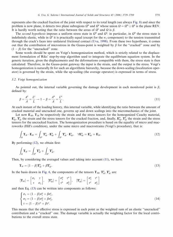
G. Uva, G. Salerno / International Journal of Solids and Structures 43 (2006) 3739–3769 3751

represents also the cracked fraction of the joint with respect to its total length (see always Fig. 8) and since theproblem is now plane, it detects two plane subregions Xu and Xc whose union X = Xu [ Xc is the plane REV.It is hardly worth noting that the ratio between the areas of Xc and X is b.

The second hypothesis imposes a uniform stress state in Xu and Xc: in particular, in Xu the stress state isindefinitely elastic, while in Xc it is practically equal (except for the r1 component) to the tension transmittedthrough the crack’s faces into unilateral frictional contact (Uva, 1998). From these two hypotheses, it comesout that the contribution of microstress in the Gauss-point is weighted by b for the ‘‘cracked’’ zone and by(1 � b) for the ‘‘uncracked’’ zone.

Some words should be spent on Voigt’s homogenization method, which is strictly related to the displace-ment formulation of Riks’ step-by-step algorithm used to integrate the equilibrium equation system. In thegeneric iteration, given the displacements and the deformations compatible with them, the stress state is thencalculated. Therefore, in the Gauss-point gateway the input is the strain, and the output is the stress. Voigt’shomogenization is naturally fit for such an algorithmic hierarchy, because the down-scaling (localization oper-ator) is governed by the strain, while the up-scaling (the average operator) is expressed in terms of stress.

3.2. Voigt homogenization

As pointed out, the internal variable governing the damage development in each monitored point is b,defined by:

b ¼ Ac

A¼ Lc

L! 1� b ¼ Au

A¼ Lu

L. ð11Þ

At each instant of the loading history, this internal variable, while identifying the ratio between the amount ofcracked material and uncracked one, governs up and down scalings into the micromechanics of the joint.

Let now EM, TM be respectively the strain and the stress tensors for the homogenized Cauchy material,Ec

M ;TcM the strain and the stress tensors for the cracked fraction, and, finally, Eu

M ;TuM the strain and the stress

tensors for the uncracked fraction. The homogenization procedure is based on the equality of micro and mac-roworks (Hill’s condition), under the same micro and macrostrains (Voigt’s procedure), that is:

Z

XTM � EM ¼

ZXu

TuM � Eu

M þZ

XcTc

M � EcM ; 8Eu

M ¼ EcM ¼ EM . ð12Þ

By performing (12), we obtain first:

ZX

TM ¼Z

XuTu

M þZ

XcTc

M .

Then, by considering the averaged values and taking into account (11), we have:

TM ¼ ð1� bÞTuM þ bTc

M . ð13Þ

In the basis drawn in Fig. 6, the components of the tensors TM, TuM ;T

cM are:

½TM � ¼r1 s

s r2

� ; ½Tu

M � ¼ru

1 su

su ru2

� ; ½Tc

M � ¼rc

1 sc

sc rc2

�

and then Eq. (13) can be written into components as follows:

r1 ¼ ð1� bÞru1 þ brc

1;

r2 ¼ ð1� bÞru2 þ brc

2;

s ¼ ð1� bÞsu þ bsc.

8><>: ð14Þ

This means that the effective stress is expressed in each point as the weighted sum of an elastic ‘‘uncracked’’contribution and a ‘‘cracked’’ one. The damage variable is actually the weighting factor for the local contri-butions to the overall stress state.

3752 G. Uva, G. Salerno / International Journal of Solids and Structures 43 (2006) 3739–3769

3.2.1. The microscopic constitutive laws

In this paragraph the constitutive behaviour of the two material fractions is described: the starting point isthe elastic law expressed by (6) and (7), here adapted to take into account the presence of inelastic deforma-tions. The given macro deformation is EM and the microdeformation is governed by the localization choiceimplied by Voigt’s procedure, that is Eu

M ¼ EcM ¼ EM . In the vector basis drawn in Fig. 6, the components

of EM are:

½EM � ¼e1 c

c e2

� .

3.2.1.1. ‘‘Uncracked’’ stresses. The behaviour of the uncracked fraction is linearly elastic in every step of theloading process, that is:

TuM ¼ KEEM !

ru1 ¼ StE

11e1 þ StE12e2;

ru2 ¼ StE

12e1 þ StE22e2;

su ¼ StE33c

8><>: ð15Þ

with the coefficients explicited in Eq. (7).

3.2.1.2. ‘‘Cracked’’ stresses. For the ‘‘cracked’’ fraction, we suppose that the constitutive behaviour dependson whether the crack is open or closed, that is, whether the macrostrain e2 is positive or negative. The mic-rodeformation is always equal to the macrodeformation: the problem is to state which components are elasticand which are inelastic.

If the crack is closed, the material fraction behaves as it is intact and elastic (15); if appropriate, it willdevelop inelastic deformations in the shear direction, involving frictional phenomena. This means that themacroshear strain will be partly plastic (cr) and partly elastic (c � cr), according to Coulomb’s frictionallaw. As pointed out in Section 2.2, cr represent the ‘‘memory’’ of the non-holonomic frictional time history.

rc1 ¼ StE

11e1 þ StE12e2;

rc2 ¼ StE

12e1 þ StE22e2;

sc ¼ StE33ðc� crÞ

8><>: closed crack. ð16Þ

under the condition:

US ¼j sc j þlrc2 6 0 ð17Þ

If the crack is open, the idea is that e2 and c are both anelastic and not involving plastic phenomena, while e1 isentirely elastic (see Fig. 9).

This elementary difference arises from simple considerations: even if open, the interface cracks are placedalong direction 1 and divide the material in a set of parallel layers that allow the transmission of e1. Hence,according to the (7), sc is zero, rc

1 is non-zero for the part depending on e1. Also rc2 would be non-zero

for the part depending on e1, that is, rc2 ¼ StE

12ec1. However, since Voigt’s homogenization is based on displace-

Fig. 9. The selective transmission of the elastic deformations for an open crack.

G. Uva, G. Salerno / International Journal of Solids and Structures 43 (2006) 3739–3769 3753

ments and implies approximation in stresses and equilibrium errors, rc2 6¼ 0 should be considered as an equi-

librium error (it does not satisfy a natural boundary condition on the open crack faces) and is thereforeneglected.

Hence, for an open crack, the constitutive law is the following:

rc1 ¼ StE

11e1

rc2 ¼ 0

sc ¼ 0

8><>: open crack. ð18Þ

3.3. The damage evolution law

It is now necessary to represent in an explicit form the cracks’ evolution law as a function of the chosendamage variable b, according to the energetic criterion (4) sketched in Section 2.2:

G½t; b� �R½b� 6 0. ð19Þ

Until this condition is satisfied, b does not evolve and the cracks within the sampled joint do not propagate.The situation G ¼ R represents a critical condition and is to be considered as the starting point for the growthof the crack, proceeding by adjacent equilibrium states.

According to (3), the explicit computation of G involves the elastic strain energy expressed as a function ofthe damage variable through the inelastic contributions e* and c* (9), that will be now specified for the mortarmaterial and for the new damage variable b. It should be clear that solution (2) has to be re-scaled in terms ofthis new variable and this implies a redefinition of the compliance parameters, to be experimentally tuned.

�� ¼ bcmnr2;eff ¼ bcmnHðr2Þr2;

c� ¼ bcmtseff ¼ bcmtðsþ f Þ;

�ð20Þ

where, with the same notation used in Section 2.2:

cmn, cmt = normal and tangential compliance for the mortar;f ¼ �signðsÞHðr2Þl j r2 j¼ friction force.

By applying (3), the expression of the energy release rate G as a function of b becomes:

G ¼ 1

2

dW e

db

����r2;s¼cost

¼ 1

2Hðr2Þr2 �

o��2obþ ðsþ f Þ � oc�

ob

� ¼ 1

2cmnHðr2Þr2

2 þ cmtðsþ f Þ2h i

. ð21Þ

Let us now explicitly express the contributions of the cracked and uncracked fractions by introducing in (21)the homogenized Cauchy stress components (14):

G ¼ 1

2cmnHðr2Þ ð1� bÞru

2 þ brc2

� �2 þ cmt ð1� bÞðsþ f Þu þ bðsþ f Þc½ �2n o

.

Under tension (e2 P 0), the average operator provides that all the stress components of the cracked fractionactually appearing in G vanish. Hence, we will have:

Gþ ¼ 1

2ð1� bÞ2 cmnr

u2

2 þ cmtsu2

�open crack ðe2 P 0Þ.

Under compression (e2 < 0), the expression of the energy release rate G deserves more attention. First of all, Gdoes not include the contribution of the compressive normal stress, because in our damage model compressivestress does not spend work for opening the cracks. The tangential stress has to be slightly manipulated in orderto show the role played by Voigt’s homogenization:

s ¼ bsc þ ð1� bÞsu ¼ blrc2 þ ð1� bÞsu ¼ blrc

2 þ ð1� bÞlru2 � ð1� bÞlru

2 þ ð1� bÞsu

¼ lr2 þ ð1� bÞðs� lr2Þu ! s� lr2 ¼ ð1� bÞðs� lr2Þu;

3754 G. Uva, G. Salerno / International Journal of Solids and Structures 43 (2006) 3739–3769

so, we will have:

G� ¼ 1

2ð1� bÞ2cmtðsþ f Þu2 closed crack ðe2 < 0Þ.

In a concise form, we can express the two previous equations in the following formula:

G ¼ 12ð1� bÞ2 cmnHðr2Þru

22 þ cmtðsþ f Þu2

n o. ð22Þ

Still it has to be explicited the expression for R, which will contain the mechanical response of the materialwith respect to fracture. The equation of R½b� is chosen on a semi-empirical base, following the classical guide-lines for concrete-like materials, which can be found in the literature (Broek, 1984). The chosen R-functionrepresents the essential behaviour of a quasi-brittle material, which typically includes an initial stable branchand an unstable softening phase, separated by a critical state ðbcr;RcrÞ which is experimentally identified:

R½b� ¼Rmcr

b1� b

0 6 b 6 bcr;

Rmcrb

1� b

� ��qm

bcr 6 b 6 1;

8>><>>:

ð23Þ

qm ¼ 0:8. ð24Þ

The plot of this function is shown in Fig. 10. The maximum of the function is:

Rmcr ¼ cmnr2lim ¼ cmts

2lim ð25Þ

and is attained for b = bcr = 1/2.Now, the relation GðbÞ �RðbÞ ¼ 0 allows to associate at each value of the total strain E the damaged state

b of the material point under investigation. A few manipulations of (22) and (23) lead to the following equa-tions, the first of which is valid in the stable branch 0 6 b 6 1/2, the second in the unstable one 1/2 6 b 6 1:

y ¼ Rmcrb

ð1� bÞ30 6 b 6

1

2;

y ¼ Rmcr

1

bqmð1� bÞ2�qm

1

26 b 6 1;

8>>><>>>:

ð26Þ

where it has been set y ¼ 12

cmnru2

2 þ cmtsu2� �

.

The two functions have been plotted in Fig. 11 in the whole domain 0 < b < 1: however, the branches of ourinterest are only those drawn by continuous line.

Fig. 10. Toughness function RðbÞ.

Fig. 11. Plot of the diagram b–y.

G. Uva, G. Salerno / International Journal of Solids and Structures 43 (2006) 3739–3769 3755

Eq. (26)1 can be easily inverted, obtaining an explicit expression for b. Function (26)2, instead, does notadmit an analytic inverse function and, from an algorithmic point of view, it is convenient to perform a piece-wise linearization. Another algorithmic drawback is the presence of the cusp for b = 0.5, which can be con-veniently smoothed.

We have used an elastoplastic constitutive model with damage. In order to calibrate the macroscopicalmodel, a set of micromechanical parameters, both elastic and inelastic, have to be identified.

Roughly speaking, in the literature there are two different classes of experimental tests aimed at the iden-tification of the micromechanical parameters of masonry. A first category directly involves the individual con-stituents of the masonry (i.e. mortar and bricks), and includes standard tests for the determination of theirelastic coefficients (the constituents are supposed to have an isotropic, elastic behaviour).

A second class of tests, instead, is aimed at the specific characterization of the ‘‘mortar joint’’ (intended asthe assembly of mortar beds and bricks), which is deeply governed by the presence of interface layers.

In the literature about the constitutive modelling of masonry, a frequent choice is to introduce the micro-mechanical parameters belonging to the first group into a linear homogenization procedure, in order to obtainthe elastic properties of the composite material at the macroscopic level. For the description of the inelasticbehaviour of the mortar joint, a wide variety of constitutive models can be used. Anyway, recurrent param-eters are: the ultimate strength of the joint under tension and shear, the friction coefficient, the dilatancy.These parameters are measured from specific tests on small combinations of bricks and mortar (coupletsand triplets).

In our model, mortar joints are very thin if compared to the bricks’ height and it is quite intuitive to con-sider as crucial the role of the mortar–brick interfaces. Therefore, we have chosen to use the constitutiveparameters provided by the tests on couplets and triplets rather then those measured on mortar specimens.

More specifically, the damage law we have used (19) involves four different mechanical parameters: the ulti-mate strength under tension (rlim); the ultimate strength under shear (slim); the axial compliance of the mortarjoint (cmn); the tangential compliance of the mortar joint (cmt). Actually, only three of these coefficients can beindependently assigned (see Eq. (25)). Hence, according to the specific test to be simulated, the axial or thetangential compliance of the joint is deduced from the experimental tests, while the other one is numericallydefined by Eq. (25): Rmcr ¼ cmnr2

lim ¼ cmts2lim.

The development of damage and frictional sliding are, at this point, uncoupled: the former is directlydetermined from the total strain assigned at the beginning of the load step; the latter only involves the cracked

3756 G. Uva, G. Salerno / International Journal of Solids and Structures 43 (2006) 3739–3769

portion of the material, whose amount is measured by the actual value of b (which can be immediately cal-culated, according to the previous remark). Since the frictional law is non-holonomic, the inelastic residualsliding cr must be known throughout all the loading process. In order to do this, we will store at each stepthe difference between the uncracked tangential stress and the cracked one, that is an information perfectlyequivalent to the accumulated residual sliding, as shown in Fig. 16.

3.4. FEM numerical analysis

3.4.1. Integration strategy

The mechanical behaviour of the masonry material described in the last sections is now inserted within aFEM integration strategy, driven by a scalar loading parameter k. The equilibrium equations of the discretizedproblem:

s½u� � p½k� ¼ 0;

where ðs; u; pÞ 2 Rn and k 2 R, are highly non-linear and actually governed by the constitutive behaviour ofthe mortar joints.

The solution algorithm chosen is a step-by-step evolutive one, consisting in a linear elastic prediction fol-lowed by an iterative correction phase (see Fig. 12), based on Modified Newton Raphson strategy. The controlparameter is the arc-length, which is able to avoid the loss of convergence at the limit load configurations(Riks, 1979, 1984).

In Fig. 13 the flow chart of a single step of the arc-length iterative algorithm is pictured.Starting from the two last known equilibrium configurations (0 and 1 in initial point), a linear extrapolation

is performed (predictor) driven by a parameter x which takes into account the non-linear behaviour of theprevious steps. Then, starting from a first trial configuration ~2, an iterative correction phase begins, aimedat zeroing the equilibrium residual. Such a phase consists in the calculation of the elasto-plastic response(s[uj] in structural response), of the residual vector (rj in equilibrium residual), of the primary variable correctionvectors ( _uj; _kj in corrector), and finally in the updating step (uj+1, kj+1 in updating). At each iteration of thecorrection phase, the constitutive information of each mortar joint is updated. This is done in the routinecalled ‘‘elastoplastic structural response’’, discussed in Section 3.4.3, where the global stress state, the currentvalues of the internal variables and the structural response at four Gauss integration points for each elementare calculated (Fig. 7).

3.4.2. High-continuity FEM discretization

With regard to the FEM discretization, the algorithm handles a mesh of rectangular compatible finite ele-ments, for which a High Continuity interpolation (see Aristodemo, 1985) is chosen. Each finite element has asingle node, located at the center of the element itself, with two parameters. However, the displacement fields

Fig. 12. The reconstruction of the equilibrium path: step-by-step evolutive analysis and arc-length iterative strategy.

Fig. 13. Flow chart of the integration strategy.

G. Uva, G. Salerno / International Journal of Solids and Structures 43 (2006) 3739–3769 3757

of the element are interpolated by quadratic splines, by using all the parameters of the eight surrounding ele-ments. This guarantees a C1-continuity to the displacements and a C0-continuity to the deformations, even if arelatively small number of parameters is used, and enables the use of the element in computational elastoplas-tic problems. Moreover, the regularity of a rectangular mesh is fairly suitable for the analysis of masonry pan-els with a standard geometry.

Let us now refer to Fig. 14 in order to present further details of the finite element in the case of a two-dimensional problem. Each internal finite element is surrounded by a grid of eight elements, from which itgains the parameters needed for the interpolation of the displacement fields in its domain. For example, inthe grid of nine elements shown in Fig. 15(a) numbered like the entries of a 3 · 3 numerical matrix, the element2,2 uses nine nodal parameters dij, i, j: = 1,3 (one for each element) for each displacement fields. For example,the variation law of u(n,g), expressed in terms of the natural coordinates n ¼ x

a and g ¼ yb (where a and b are

respectively the width and the height of the element), of the nodal parameters dij and of the shape functions Ui,assumes the following form:

uðn; gÞ ¼X3

i;j¼1

UiðnÞUjðgÞuij;

Fig. 14. (a) Nodes’ position for a standard HC grid; (b) Natural coordinates.

Fig. 15. (a) Nodes’ position for the FE at the boundary; (b) Displacement interpolation for the one-dimensional case.

3758 G. Uva, G. Salerno / International Journal of Solids and Structures 43 (2006) 3739–3769

where the Ui, obtained by imposing the continuity condition on u and on its derivatives along directions x andy, are:

U1ðnÞ ¼1

8� n

2þ n2

2U1ðgÞ ¼

1

8� g

2þ g2

2;

U2ðnÞ ¼3

4� n2 U2ðgÞ ¼

3

4� g2;

U3ðnÞ ¼1

8þ n

2þ n2

2U3ðgÞ ¼

1

8þ g

2þ g2

2.

This ‘‘cellular’’ structure, although privileged among the compatible elements of the same computational cost,implies some drawbacks. In fact, the overall management becomes somewhat cumbersome because of the ele-ments at the boundary. These are special elements, since they lack some of the nodes that are needed in theinterpolation. Therefore, just for the elements at the boundary, further nodes are introduced along the bound-ary itself (see Fig. 15(a)), and there is a specialized treatment with respect to the standard elements. In partic-ular, depending on which part of the boundary they do share, the shape functions assume specific definitions(see Aristodemo, 1985).

G. Uva, G. Salerno / International Journal of Solids and Structures 43 (2006) 3739–3769 3759

3.4.3. The elastoplastic structural response algorithm

With reference to Fig. (13), it will be now better precised how the structural response is constructed at eachiteration of the correction phase:

1. A first trial displacement field u is assigned and the correspondent compatible deformation field EM isdefined. Starting from this, it is immediately computed the local stress state TM, split into two fractions(‘‘uncracked’’–‘‘cracked’’): Tu

M;TcM. In this phase, also the increment of the internal damage variable b is

evaluated, by using (26).

Fig. 16. Frictional model and residual sliding.

3760 G. Uva, G. Salerno / International Journal of Solids and Structures 43 (2006) 3739–3769

2. At this point, it is faced the truly plastic part of the constitutive law: the elastic stress prediction, when vio-lating the plastic admissibility condition, is corrected in order to bring back the actual elasto-plastic stressstate within the limit domain (according to a typical return algorithm). As previously specified, only thecracked portion of the material (singled out by b) is involved, and moreover the nature of the plastic defor-mations is purely tangential. The plastic condition to be checked is represented by Eq. (17), that identifiesthe classical Mohr–Coulomb cone. According to the classical framework of the Theory of Plasticity, elasticand inelastic strain contributions are supposed to follow an additive law (where the plastic variable govern-ing the evolution of the limit domain is the accumulated plastic sliding cr):

cEP ¼ cE þ cr. ð27ÞSo, when the plastic condition (17) is activated, the final admissible stress state is recovered and the plasticvariable cr is updated by (27).

Calculation of the final state:c1 ¼ cE;

s1 ¼ maxð�lr;minðsE � Gcro; lrÞÞ;

�

Updating of the residual sliding:cr1 ¼ ðsE � s1Þ=G:

If we plot the elastoplastic law in the s–c plan, a geometrical interpretation tells us that the elastic predictionpoint (E) and the elastoplastic solution (A1) are on the same vertical line, that is to say, correspond to thesame total tangential sliding c. In Fig. 16, this graphical interpretation of the inelastic tangential sliding andof the final elastoplastic state is shown, with regard to three different initial states.

Fig. 17. Flow chart showing the computation of the elastoplastic structural response.

G. Uva, G. Salerno / International Journal of Solids and Structures 43 (2006) 3739–3769 3761

3. The ‘‘homogenized’’ stress is recovered by adding up the uncracked and the cracked contributions, properlyweighted by the actual value of b (Eqs. (13) and (14)).

The routine for the calculation of the elastoplastic structural response, as it is implemented in the numericalcode is summarized in the flow chart of Fig. 17.

4. Numerical tests: results and discussion

The computational model previously described allows a quite simple mechanical description of the exam-ined phenomena. First of all, this has made the FE numerical implementation simple, and has provided a toolfor explaining some characteristic phenomenological evidences, assessing a set of benchmarks and preliminarytests, in view of the future tuning of both the mechanical and the computational model.

In the following paragraphs, a number of simple tests are presented, in order to show how the behaviourunder simple tension, compression and shear is reproduced for small representative elements. Then, two exper-imental tests for masonry brick specimens have been chosen to be numerically reproduced. The scope was toinvestigate the potentiality and accuracy of the followed approach, making also clear the limits and problemsto be furtherly faced. Results are encouraging enough, showing a satisfactory reconstruction of the main fea-tures of the structural behaviour, with a fairly cheap computational cost.

4.1. Basic benchmarks: cyclical tensile and shear tests for small panels

As first reference examples, in order to assess the basic performances of the code, simple tests (cyclical uni-axial tension and cyclical shear under constant compression) for a small structural element are presented (themechanical parameters used are the same listed in Table 2). In Fig. 18, the masonry geometric pattern, loadingand constraint schemes are drawn, together with the chosen mesh (4 HC elements). The left bottom element isenlightened in order to make clear that the computational model is different from the initial geometric schemebecause of the neglection of head joints. The symbol k identities the varying load. At the bottom of the samefigure, stress–strain diagrams in a specific Gauss-point (the one marked in bold) are drawn. As expected, in thecyclical shear test the presence of hysteresis loops is observed: at the beginning, sliding is inhibited by thefriction force, and the unloading follows the line tangent to the curve at the origin (the apparent tangentialmodulus is the same than the initial structure); when the applied stress exceeds the friction force, a slidingtakes place, and there is a sudden change in the slope of the line. As a consequence, a permanent tangentialdeformation arises, and a part of the elastic energy is dissipated.

4.2. Monotonic shear test on a masonry panel

A larger numerical test has been performed on a test proposed by Raijmakers and Vermeltfoort inRaijmakers and Vermeltfoort (1992), in which a masonry periodic brickwork has been experimentally testedunder a monotonic load.

The pier is a one-wythe running bond masonry, built using 20.4 cm · 9.8 cm · 5.0 cm clay blocks and mor-tar joints of thickness s = 1.0 cm, according to the arrangement shown in Fig. 19. The overall dimensions ofthe pier are: B = 100 cm, H = 100 cm, T = 100 cm, and the loading set-up and pattern are schematized inFig. 19.

The numerical simulation of this test has been performed with our algorithm, by using a mesh of 40 HCelements and 66 nodes. The geometrical scheme and the mesh are shown in Fig. 20.

It is worth noting that, in order to fit the actual dimensions of the specimen with the reference cell adaptedto the specific brick pattern (see Fig. 7, bottom), a small variation in the geometry has been adopted(B = 108 cm, H = 98 cm). In the report describing the benchmarks (Raijmakers and Vermeltfoort, 1992),the uniaxial tests on mortar, bricks and masonry specimens are also presented. As pointed out in Section3.3, the mechanical parameters used in the algorithm proposed by the authors are just identified by meansof these simple reference values. The mentioned data have been provided in the reference: the corresponding

Fig. 18. Basic benchmark tests for tension (left) and shear (right): schemes of the masonry elements, mesh and stress–strain diagrams forthe Gauss-point marked in bold.

Fig. 19. Geometry and loads of the experimental test of Raijmakers and Vermeltfoort (1992): vertical load (left) and horizontal quasi-static load (right).

3762 G. Uva, G. Salerno / International Journal of Solids and Structures 43 (2006) 3739–3769

coefficients, according to the identification scheme indicated in Section 3.3, and used in our model, are listed inTable 1.

It is worth making some comments on the results of the numerical analysis, shown in the next three figures.Fig. 21 presents a comparison among two experimental curves (one for each specimen shown in Fig. 22), theequilibrium curve provided by our algorithm and the numerical curve provided by Lourenco et al. in

Fig. 20. Numerical simulation of the test of Raijmakers and Vermeltfoort (1992): geometrical scheme and FE mesh.

Fig. 21. Comparison among the experimental curves, the results provided by our algorithm and the results of Lourenco et al.

Table 1Mechanical parameters of the constituents

Mortar Bricks

Em = 780 MPa Eb = 16,700 MPamm = 0.125 mb = 0.15rlim = 0.25 MPaslim = 0.35 MPal = 0.75gm = 0.167

cmn = 0.0154 MPa�1

qm = 0.8

G. Uva, G. Salerno / International Journal of Solids and Structures 43 (2006) 3739–3769 3763

Lourenco et al. (1994) by a discrete approach, based on 648 finite elements. The simulation based on ourmodel showed some numerical swaying in the reconstruction of the post-critical branch of the equilibriumcurve; nevertheless, a satisfactory matching with the experimental results of Raijmakers and Vermeltfoort

Fig. 22. The experimental crack pattern for two of the specimens.

3764 G. Uva, G. Salerno / International Journal of Solids and Structures 43 (2006) 3739–3769

and the numerical results of Lourenco et al. has been obtained, also considering that the recorded numericaldrifting is comparable to the scattering of the available experimental results.

In Fig. 23 the progressive development of the damage (as reproduced by our algorithm and represented bythe value of the damage variable b) is shown in correspondence of the five points A, B, C, D, E of the equi-librium curve. In Fig. 22, the qualitative experimental failure patterns are drawn, and they can be comparedwith the numerical damage maps. It should be clear that our algorithm in unable of reproducing the brickcrushing and the development of cracks within head joints. However, the progressive diagonal crack patternsand the progressive horizontal sliding patterns of the first and the last rows are well reproduced.

Fig. 23. Damage distribution at points A–E of Fig. 21.

G. Uva, G. Salerno / International Journal of Solids and Structures 43 (2006) 3739–3769 3765

4.3. Cyclical shear test on a masonry panel

The results presented in this subsection are relative to a famous benchmark due to Anthoine et al. (1994)and performed at ISPRA. The geometry of the analyzed panel is shown in Fig. 24, together with the test set-upand load pattern. After applying a constant vertical preload, the panel has been subjected to a cyclical shearloading. The results provided by our algorithm have been compared not only with the experimental ones butalso with the numerical results obtained by Gambarotta et al. (1995) through the micromechanical modeldescribed in Gambarotta and Lagomarsino (1994a), Gambarotta (1995), Gambarotta and Lagomarsino(1993, 1994b).

The numerical simulation of the benchmark has been performed with our algorithm, by using a mesh of 70HC elements and 104 nodes. The geometrical scheme and the mesh are shown in Fig. 25.

The parameters for the materials constituting the brickwork are listed in Table 2 (the volume fraction of themortar is qm = 0.154).

Fig. 24. Schematic testing set-up and crack pattern of the experimental test of Anthoine et al.

Fig. 25. Numerical simulation of the test with the proposed algorithm: schemes of the panel and FE mesh.

Table 2Mechanical parameters (Anthoine et al., 1994)

Mortar Bricks

Em = 650 MPa Eb = 3000 N/mm2

mm = 0.15 mb = 0.25rl,m = 0.1 MPa rlb = 5 N/mm2

sl,m = 0.25 MPa slb = 2 N/mm2

cmn = 0.0154 MPa�1 cbt = 0.5 MPa�1

qm = 0.16 qb = 0.16bm = 0.8 bb = 0.9

Fig. 26. Comparison of the results obtained with our algorithm (right), experimental tests (center) and Gambarotta’s algorithm (left).

Fig. 27. Normal stress and damage distribution.

3766 G. Uva, G. Salerno / International Journal of Solids and Structures 43 (2006) 3739–3769

A first comparison among the results provided by our algorithm, the experimental results and Gambar-otta’s numerical results can be made in terms of equilibrium paths, as shown in Fig. 26. It is immediately clearthat there is a significant difference between the numerical simulations and the experimental results: in fact the

G. Uva, G. Salerno / International Journal of Solids and Structures 43 (2006) 3739–3769 3767

latter involve a larger number of cycles and longer post-critical branch. Therefore, the comparison is neces-sarily partial. However, by the observation of the figure it can be deduced that both the numerical algorithmsreproduce the limit configuration with a sufficient accuracy, even if with a slight overestimation of the limitload, probably because of the compatibility of both FE discretizations. In our algorithm, moreover, it shouldbe noticed that the infinite strength of the bricks can be a further cause of the overestimation of the limit load,whereas the inability in following the hysteresis cycles in the advanced post-critical branch could depend onthe numerical instability produced by the integration of the damage law.

A final comment has to be made about the crack patterns exhibited by the experimental test and those pro-vided by the proposed model. In Fig. 27 the damage map and the stress state for the last equilibrium config-uration obtained are reported. The damage map can be compared with the failure mechanism depicted inFig. 24, which shows a crossed diagonal cracking due to the inversion of the load sign, plus a sliding shearcracking concentrated at the four corners of the panel. Within the capabilities of our model, whose limits havealready been discussed, the figure demonstrate a fair good agreement with the experimental evidence.

5. Conclusions

The analysis we have performed has produced results quite satisfactory, and represents a starting point tobe furtherly improved, under the key idea that both the model and the algorithm for the integration of thesolution equations should be developed.

In the presented analysis, we have proposed three different levels, which are hierarchically interconnectedone with the other: to each level a specific mathematical model corresponds, even if it is not always explicitlyformulated. The three models are: the macroscopic model, which sees a Cauchy homogeneous continuumcrossed by planes on which inelastic deformations develop; the mesoscopic level, in which the contributionsof the mortars and the blocks can be clearly distinguished; the microscopic model, inside the cracked joint,where the dissipative phenomena (that are recorded in terms of stress state and internal damage and plastic slid-ing variables) occur. Of course, in each these levels, a well-founded mechanically improvement could beintroduced.

With regard to the macroscopic level, the choice of a Cauchy continuum is maybe not the best possible,above all in a long perspective. In fact, if until now we have worked with a fixed mesh, using a Gauss samplingpoint at each mortar joint, varying the mesh size we would probably encounter mesh-dependence phenomena,that are well known in the literature (de Borst, 1991) and invariably affect a FEM analysis every time that asoftening constitutive behaviour in introduced.

This is the first aspect that has to be improved in order to make the model more reliable and effective at thesame time. Some steps forward in this direction have already be taken, by introducing at the macroscopic levela Cosserat Model (see Masiani et al., 1995; Salerno and Uva, 2002).

At the mesoscopic level, while neglecting head joints (that has been made for the sake of the mechanical andalgorithmic simplicity) we have actually ignored the influence of the masonry texture on the solution. In thecase of shear tests, the presence of head joints makes the real difference, for example, between a running bondmasonry and a stack bond one (see di Carlo, 1999; Berto et al., 2004). This is an aspect to be improved, as well.

At the microscopic level, our idea is that the main part of the phenomenology involved has been taken intoaccount (that is to say, the two crucial phenomena of damage and friction). Anyway, a deeper comprehensionof the micromechanics could lead to a better-founded damage evolution law and, above all, to a smootherformulation, able to avoid the difficulties actually encountered in the integration of the law. With regard tothis last aspect, a necessary improvement concerns the management of internal variables as primary variablesof the problem (at the same level as displacement variables), as shown in Formica et al. (2003). This wouldallow, in our opinion, a fair good improvement in the stability of the algorithm.

Besides the enrichment of the model at the different levels, our primary forthcoming objective is to make themultiscale strategy more clear, expliciting the operators for the scale switching. Homogenization theory rep-resents in this sense a very well assessed framework, able to suggest wise choices and carefully control theapproximations and errors involved in every down or up-scaling that is performed (see Salerno and de Felice,2000). It is indeed this aspect that has driven us in the choice of the paper title, with the purpose of pointingout that we really feel ourselves on a long road.

3768 G. Uva, G. Salerno / International Journal of Solids and Structures 43 (2006) 3739–3769

References

Alpa, G., Gambarotta, L., 1990. Mechanical models for frictional materials. In: Proc. of International Meeting on New Developments inStructural Mechanics, Catania.

Anthoine, A., 1994. Research on unreinforced masonry at the joint research center of the European commission. In: Proc. of the US ItalyWorkshop on Guidelines for Seismic Evaluation and Rehabilitation of Unreinforced Masonry, Pavia, pp. 427–432.

Anthoine, A., Magenes, G., Magonette, G., 1994. Shear compression testing and analysis of brick masonry walls. In: Proc. of 10thEuropean Conference on Earthquake Engineering, Vienna, pp. 1657–1662.

Aristodemo, M., 1985. A high continuity finite element model for two-dimensional elastic problems. Comput. Struct. 21 (5), 987–993.Asteris, P.G., 2003. Lateral stiffness of brick masonry infilled plane frames. J. Struct. Eng.: Amer. Soc. Civil Eng. (ASCE) 129.Asteris, P.G., Tzamtzis, A.D., 2003. On the use of a regular yield surface for the analysis of unreinforced masonry walls. Electron. J.

Struct. Eng. 3, 23–42.Ballio, G., Calvi, G.M., Magenes, G., 1993. Experimental and numerical research on a brick masonry building prototype. Report 2.0,

CNR-GNDT, Dipartimento di Meccanica Strutturale del’Universita di Pavia.Berto, L., Saetta, A., Scotta, R., Vitaliani, R., 2004. Shear of masonry panel in parametric FE analyses. Int. J. Solids Struct. 41, 4383–

4405.Broek, D., 1984. Elementary Engineering Fracture Mechanics, third ed. Martinus Nijhoff Publishers, The Hague, The Netherlands.Budiansky, B., O’Connell, J., 1976. Elastic moduli of a cracked solid. Int. J. Solids Struct. 15, 81–97.de Borst, R., 1991. Simulation of strain localization: a reappraisal of the cosserat continuum. Eng. Comput. 8, 317–332.di Carlo, A., 1999. A memo of mortar modelling: what could be beyond a bonafide rigid bock-elastic interface models. In: Private

Communication to the Authors, Roma.Eshelby, J.D., 1968a. The elastic behaviour of an elliptical crack. J. Mech. Phys. Solids 17, 177–199.Eshelby, J.D., 1968b. The elastic field of a crack extending non-uniformly under general anti-plane loading. J. Mech. Phys. Solids 17, 177–

199.Formica, G., Sansalone, V., Casciaro, R., 2003. A mixed strategy for the nonlinear analysis of brick masonry walls. Comput. Meth. Appl.

Mech. Eng..Gambarotta, L., 1995. Stati limite di resistenza per materiali fragili a danneggiamento isotropo. In: Atti del XII congresso nazionale

dell’Associazione Italiana di Meccanica Teorica ed Applicata, Napoli.Gambarotta, L., Lagomarsino, S., 1993. A microcrack damage model for brittle materials. Int. J. Solids Struct. 30 (2), 117–198.Gambarotta, L., Lagomarsino, S., 1994. Damage in brick masonry shear walls. In: Proc. Europe–US Workshop on Fracture and Damage

in Quasi-brittle Structures, Praga.Gambarotta, L., Lagomarsino, S., 1994. Micromechanically based constitutive equations for concrete-like materials. In: Proc. EURO-C

International Conference, Innsbruck, Austria, pp. 223–322.Gambarotta, L., Lagomarsino, S., Morbiducci, R., 1995. Two-dimensional finite element simulation of a large scale brick masonry wall

through a continuum damage model. Internal report.Hart, V.R., Cundall, P., Lemos, J., 1988. Formulation of a three-dimensional distinct element model—Part ii: Mechanical calculations for

motion and interaction of a system composed of many polyhedral blocks. Int. J. Rock Mech., Min. Sci. Geomech. Abstr. 25, 117–126.Hoenig, A., 1978. The behaviour of a flat elliptical crack in an anisotropic elastic body. Int. J. Solids Struct. 14, 925–934.Hoenig, A., 1979. Elastic moduli of a non-randomly cracked body. Int. J. Solids Struct. 12, 137–154.Hughes, Pande (Eds.), 2001. Computer methods in structural masonry—v. In: Proc. STRUMAS V.Italian Ministry of Public Works, 1981. Instruction for the application of the technical code for the repair and retrofitting of existing

buildings damaged by earthquakes. In: Circolare n. 21745.Kouznetsova, V.G., 2002. Computational homogenization for the multi-scale analysis of multi-phase materials. PhD thesis, Department

of Engineering, Technische Universiteit Eindhoven.Kouznetsova, V.G., Brekelmans, W.A.M., Baaijens, F.P.T., 2001. An approach to micro–macro modeling of heterogeneous materials.

Comput. Mech. 27, 37–48.Kouznetsova, V.G., Geers, M.G.D., Brekelmans, W.A.M., 2002. Multi-scale constitutive modeling of heterogeneous materials with a

gradient-enhanced computational homogenization scheme. Int. J. Numer. Meth. Eng. 54, 1235–1260.Kouznetsova, V.G., Geers, M.G.D., Brekelmans, W.A.M., 2004. Multi-scale second-order computational homogenization of multi-phase

materials: a nested finite element solution strategy. Comput. Methods Appl. Mech. Eng.Krajicinovic, D., 1989. Damage mechanics. In: Mechanics of Materials, vol. 8, p. 117.Krajicinovic, D., Fonseka, G.U., 1981. The continuous damage theory of brittle materials. J. Appl. Mech. (48), 809–824.Lagomarsino, S., Gambarotta, L., Morbiducci, R., 1995. Brittle-ductile response of in-plane loaded brick masonry walls. In: Proc. 10th

European Europe Conference on Earthquake Engineering, Vienna, pp. 1663–1668.Lemaitre, J., 1984. How to use the damage mechanics. Nucl. Eng. Des. (80), 233–245.Lemaitre, J., 1992. A Course on Damage Mechanics. Springer Verlag, Berlin, Germany.Lourenco, P.B., Rots, J.G., Blaauwendraad, J., 1994. Implementation of an interface cap model for the analysis of masonry. In: de Borst,

R., Mang, H., Bicanic, N. (Eds.), Proc. International Conference on Computational Modelling of Concrete Structures, EURO-C, pp.123–134.

Masiani, R., Rizzi, N.L., Trovalusci, P., 1995. Masonry as structured continuum. Meccanica 30, 673–683.Massart, T.J., 2003. Multi-scale modeling of damage in masonry structures. PhD thesis, Department of Engineering, Technische

Universiteit Eindhoven.

G. Uva, G. Salerno / International Journal of Solids and Structures 43 (2006) 3739–3769 3769

Nemat-Nasser, S., Horii, H., 1983. Overall moduli of solids with microcracks: load-induced anisotropy. J. Mech. Phys. Solids 31 (2), 155–171.

Page, A.W., 1981. The biaxial compressive strength of brick masonry. In: Proc. Inst. Civ. Eng.Phillips, R., 1998. Multiscale modeling in the mechanics of materials. Curr. Opin. Solid State Mater. Sci. 3, 526–532.Raijmakers, T.M.J., Vermeltfoort, A.T., 1992. Deformation controlled tests in masonry shear walls. In: Report B-92-1156, TNO-Bouw,

Delft, The Netherlands (in Dutch).Riks, E., 1979. An incremental approach to the solution of snapping and buckling problems. Int. J. Solids Struct. 15, 529–551.Riks, E., 1984. Bifurcation and stability, a numerical approach. In: WAM Symposium on Innovative Methods for Non-linear Problems,

New Orleans.Salerno, G., de Felice, G., 2000. Continuum modelling of discrete systems: a variational approach. In: Proc. ECCOMAS2000—the Fifth

World Congress on Computational Mechanics, Barcellona, 2000.Salerno, G., Uva, G., 2002. A two-scale algorithm for the nonlinear analysis of damaged masonry brickwork. In: Proc. WCCM V—the

Fifth World Congress on Computational Mechanics, Vienna, 2002.Sanchez Palencia, E., 1992. Introduction aux methodes asymptotique et a I’homogeneisation. Masson.Suquet, P.M., 1983. Une metode duale en homogenisation: application aux milieux elastiques. J. Mecanique appliquee.Sutcliffe, D.J., Yu, H.S., Page, A.W., 2001. Lower bound limit analysis of unreinforced masonry shear walls. Comput. Struct. 79, 1295–

1312.Syrmakezis, C.A., Asteris, P.G., 2001. Masonry failure criterion under biaxial stress state. J. Mater. Civil Eng. 13.Uva, G., 1998. A constitutive model with damage and friction for masonry structures: theoretical and numerical aspects. In: Proc. of the

Workshop on Seismic Performance of Monuments Monument-98, Lisbona.