�����������������

Citation: Jamrozik, W.; Górka, J.;

Wygledacz, B.; Kiel-Jamrozik, M.

FEM-Based Thermogram Correction

for Inconel 625 Joint Hardness

Clustering. Materials 2022, 15, 1113.

https://doi.org/10.3390/

ma15031113

Academic Editor: Paolo Ferro

Received: 29 November 2021

Accepted: 28 January 2022

Published: 31 January 2022

Publisher’s Note: MDPI stays neutral

with regard to jurisdictional claims in

published maps and institutional affil-

iations.

Copyright: © 2022 by the authors.

Licensee MDPI, Basel, Switzerland.

This article is an open access article

distributed under the terms and

conditions of the Creative Commons

Attribution (CC BY) license (https://

creativecommons.org/licenses/by/

4.0/).

materials

Article

FEM-Based Thermogram Correction for Inconel 625 JointHardness ClusteringWojciech Jamrozik 1,* , Jacek Górka 2 , Bernard Wygledacz 2 and Marta Kiel-Jamrozik 3

1 Department of Fundamentals of Machinery Design, Silesian University of Technology, Konarskiego Str. 18a,44-100 Gliwice, Poland

2 Department of Welding Engineering, Silesian University of Technology, Konarskiego Str. 18a, 44-100 Gliwice,Poland; jacek.gorka@polsl.pl (J.G.); bernard.wygledacz@polsl.pl (B.W.)

3 Department of Biomaterials and Medical Devices Engineering, Silesian University of Technology, RooseveltaStr. 40, 41-800 Zabrze, Poland; marta.kiel-jamrozik@polsl.pl

* Correspondence: wojciech.jamrozik@polsl.pl

Abstract: Assessing the temperature of the joint in on-line mode is a vital task that is demanded tocharacterize the formations of terns formations that are taking place in a joint and result in reachingnecessary properties of the joint. Arc welding generates a high amount of heat that is reflected by themetallic surface of the welded object. In the paper, a temperature measurement credibility increasemethod is described and evaluated. The proposed method is used to reduce the influence of thereflected temperature of the hot torch and the arc on the temperature distribution observed on thesurface of the welded joint using an infrared camera. The elaborated approach is based on comparisonbetween infrared observation of the solidifying weld and precisely performed finite element method(FEM) simulation. The FEM simulations were calibrated according to the geometry of the fusion zone.It allows to precisely model heat source properties. The best-reflected temperature correction mapwas selected and applied to obtain a temperature representation that differs from the FEM baselineby less than 10 ◦C. Precise temperature values allowed us to cluster welded joints in 3D feature space(temperature, hardness, linear energy). It was found that by using the k-means clustering method it ispossible to distinguish between correct and faulty (in terms of too low mechanical properties) joints.

Keywords: welding; TIG; thermography; reflected temperature; hardness; clustering

1. Introduction

Inconel nickel-chromium superalloys contain approximately 15 to 20% chromium andiron additives up to approximately 18%, molybdenum up to approximately 16%, niobiumup to approximately 5% and other elements (Co, Cu, W). They are characterized by highcorrosion resistance and high durability at temperatures up to approximately 1000 ◦C. Theyare used in the most thermally loaded parts of jet engines, accounting for nearly 50% oftheir mass [1]. Inconel 625 (EN 2.4856-NiCr22Mo9Nb) being a trademark of the SpecialMetals Corporation group [2] is a nickel-chromium-molybdenum alloy with an addition ofniobium that acts with the molybdenum to stiffen the alloy matrix and thereby provide highstrength without strengthening heat treatment. This alloy resists a wide range of severelycorrosive environments and is especially resistant to pitting and crevice corrosion. Usedin chemical processing, aerospace and marine engineering, pollution control equipment,and nuclear reactors. Inconel 625 is a solid solution-reinforced superalloy. Additionally,strengthening of this material may be derived by precipitation of carbides or intermetallicphases [3]. The solidus temperature of Inconel 625 is 1290 ◦C and the liquidus temperatureis 1350 ◦C [4].

In the welding of nickel-based alloys, alloy elements segregate mainly at grain bound-aries and form low melting point phases such as eutectic γ–γ′, Laves phase, and MC

Materials 2022, 15, 1113. https://doi.org/10.3390/ma15031113 https://www.mdpi.com/journal/materials

Materials 2022, 15, 1113 2 of 22

carbides along solidified grain boundaries. The presence of intergranular liquid films re-sults in microfissures because the liquid films cannot withstand the thermal and mechanicaltensile stresses generated in the gas tungsten arc welding (GTAW) process. Consequently,solidification cracking and liquation cracking occur due to the solid–liquid interface sep-aration in the brittle temperature range (BTR), which is lower than the melting point ofnickel-based alloys. It is one for the critical factors of high hot cracks. Furthermore, there isa ductility dip temperature range (DTR) between solidus temperature (TS) and 0.5TS [5]. Toperform the welding process correctly, it is necessary to know exact values of temperature.

As Inconel 625 material is a rather expensive one and is often applied in criticalapplications, it is necessary to ensure the high quality of any made joints. It is especiallydesirable to use on-line/in-line monitoring methods to reduce/avoid post productionquality checks that can result in revealing of systematic weld failures in large productionbatches. To allow this type of monitoring, a credible, properly calibrated measurementmethod is needed. One of such approaches can consist of temperature measurementsusing infrared (IR) cameras. The application of thermography (IR imaging) to monitor anddiagnosing welding and welded joints is an engineering and scientific task that has beenexplored for more than sixty years. The concept of infrared application for nickel alloywelding monitoring emerged in 1966 when work on establishing relationships betweeninfrared radiation (IR) emitted during the weld pulse cycle and the relative tensile strengthof the weld was started [6]. Practical considerations on passive and active thermographyapplications for the evaluation of weld quality were described in the 1970s when commercialdevices for IR observation became available [7]. Several interesting phenomenon werefound covering connection between temperature and process parameters. One of findingswas that current plays an important role in cooling rates (measured with IR camera) andtensile strength of welded joint [8]. Also IR detection was applied to control the weldingprocess by measuring the width of the weld bead, the depth of penetration and the positionof the torch [9,10]. However, the main branch of the developed methods is devoted toonline monitoring of the weld geometry [11,12] and the temperature distribution in thewelding pool [13] using a passive approach. Various image processing techniques andnovelty/anomaly detection algorithms were utilized to detect weld defects. Even in manypromising results achieved, thermography remains a method that is rarely applied in anindustrial environment.

The use of an infrared camera for welding process monitoring is relatively simple, butit is a non-trivial task to get measurement results that are valid. This is due to the nature ofinfrared radiation. The IR-based temperature measurement is an indirect one, and severalfactors must be set to calculate temperature from the infrared radiation emitted by an object.Additionally, the welding process requires a large amount of heat that is needed to meltthe edges of material pieces to produce the joint. One of the welding techniques, that isoften applied for the joint of a wide group of metallic materials is tungsten inert gas (TIG).It can be applied to join dissimilar materials. Nickel alloys can also be welded with otheriron alloys, e.g., nonalloy steels, with duplex stainless steels and other alloy steels [14]. TheTIG method is also commonly used for joining stainless steels [15]. In general TIG weldedjoints can be characterized by the presence of undercutting and burn-through. The otherdefect that can appear during TIG joining is a lack of penetration. It was observed thatweld depth can be increased by welding with the flux activated tungsten inert gas (ATIG)method [16,17].

In TIG welding, the torch introduces a high thermal noise into the measurementsetup. Metal surfaces (including surfaces of nonferrous alloys and superalloys) have asmall absorptivity and thus a weak emissivity in the wavelength range covered by typicaluncooled IR cameras, totalling about 5% of the black-body emissivity. The radiance emittedby the metallic surfaces is weak. Consequently, the infrared images are blurry and faint.Additionally, there is the possibility of grease patches or oxidized zones and spatter thathave different (higher) emissivity levels than the base material surface. In [18] this wasthe case for the water glass used to protect thermocouples from high temperature. These

Materials 2022, 15, 1113 3 of 22

areas are often interpreted as hot spots that are considered damaged zones. Moreover, thehigh reflectivity of the metallic surface causes the phenomenon of parasitic reflection. Inthe case of welding, the heat from the hot torch, electrode, and welding arc is reflectedby the surface, which acts as a mirror in the infrared spectrum. Reflected hot areas maskthe real temperature on the material surface and complicate the interpretation of acquiredthermograms. Some experts attempt to weaken any interference by using the shield plate orfilter [19]. However, interference cannot be completely avoided. As the vast majority of newmetallic materials, alloys and superalloys are used in harsh environments, are characterizedby low thermal expansion coefficients, have relatively good weldability (cobalt, titanium,and nickel) and have low emissivity in the wavelength band used mainly by longwaveinfrared (LWIR) cameras (8–14 µm), so there is a constant demand for novel acquisitionand processing methods that will limit these drawbacks.

Modelling of temperature distribution in welded joints by the finite element method(FEM) is widely applied. The main way to correlate and bound the simulation resultswith the experimental ones is the use of contact temperature measurements with the useof thermocouples [18]. It is a convenient method, but it has several drawbacks, suchas a limited number of measurement points that can be set up on one workpiece and asmall repeatability of thermocouple positioning. Additionally, use of thermocouples isnot allowed in the production environment, because it requires previous preparation ofsamples and affects the quality of further product.

Large thermal gradients generated during welding due to localized heating by mov-ing concentrated heat sources are causes of metallurgical changes, welding stresses, anddistortion and can allow the formation of welding defects. 3D transient FEM numerical sim-ulation is a proven and reliable method of analysis of thermo-metallurgical and mechanicaleffects of welding processes. 3D transient FEM welding simulations are computationallyintensive, but offer a more detailed solution and greater application elasticity than analyti-cal methods. Welding simulations do not converge 100% convergent with experimentalresults. However, the use of correct simulation methods, material models that factor in thechange of thermal and mechanical parameters in the temperature range, and the correctsimulation methodology significantly increase the accuracy of simulation [20–23].

In the paper a study on the possibility of clustering welded joint properties accordingto hardness and IR-based temperature measurements is presented. The key issue is theexact temperature measurement of the temperature that is proposed. According to wellcalibrated FEM simulation results, a valid ground truth temperature distribution wasgenerated. Based on those distributions, a method of reflected temperature correctionwas proposed. Using corrected IR images, the condition of welded joints was clustered todifferentiate the correct and incorrect joints from the hardness point of view.

2. Materials and Methods

The tests were carried out on thin sheets with a thickness of 1 mm of nickel super-alloys type Inconel 625, welded by the TIG method. The sheets used to make the weldswere from the Huntington Alloys Corporation industrial process (Huntington, WV, USA),which involved treating the material in a vacuum furnace. Next, a plastic processing wasperformed by cold rolling with intermediate heat treatment (recrystallization annealing).The chemical composition of the tested sheets is shown in Table 1.

Table 1. Chemical composition of the investigated Inconel 625 superalloys.

Super-Alloy

Element Concentration, wt %

Ni Cr Fe Mo Nb Co Mn Cu Al Ti Si C S P

Inconel625 * 60.7 21.76 4.27 8.96 3.56 0.07 0.07 - 0.14 0.18 0.08 0.01 0.0003 0.007

* Nb+Ta—3.56%, N—0.01%.

Materials 2022, 15, 1113 4 of 22

The Casto TIG 2002 device (Castolin GmbH, Kriftel, Germany, Figure 1a) was used toweld sheets from the investigated Inconel nickel superalloy. The TIG welding of sheets wascarried out under laboratory conditions with the following constant parameters: shieldgas of Ar 12 L/min, ridge shield gas of Ar 3 L/min, tungsten electrode (thoriated) andWT20 with a diameter of 2.4 mm. Measurement of the temperature distribution on thesurface of the welded joints was conducted with the FLIR A655sc infrared camera (IRCAM, spectral range of 7.5–14.0 µm) equipped with a 25 mm lens (Teledyne FLIR LLC,Wilsonville, OR, USA, Figure 1b). The spatial resolution of the camera was 640 × 480 pxand the temporal resolution, as well as the acquisition frequency, was 60 Hz (60 fps). Theoptical axis of the sample camera was inclined to the plane of the sample at an angle of30 degrees, and the distance between the camera and welded sample was 300 mm. For thislength, the instantaneous field of view (IFOV) or size of one detector element in millimetersis 0.21. On the thermograms, the welding pool as well as the solidified and cooling jointarea was acquired.

Figure 1. Welding device and TIG torch used during studies: (a) Casto-TIG 2002 device front panel,(b) TIG welding torch and FLIR A655sc IR camera mounted on the test stand.

For the IR camera, a dedicated software, namely FLIR ResearchIRx64, (TeledyneFLIR LLC, Wilsonville, OR, USA) was used. The custom in house build PC used for thecalculations was equipped with the following features: Intel Core i7-7700K, 4.2 GHz, ASUSTUF Z270 MARK 2 motherboard, and Corsair Vengeance LPX 16 GB DDR4 3000 MHzRAM. FEM simulations were performed in Visual-Weld 16.0 (SYSWELD core, ESI Group,Paris, France). Data post-processing and analysis was performed in the MATLAB R2021aenvironment with the use of an additional Teledyne FLIR Science File SDK (to read andprocess IR sequences).

Metallographic examination was performed in five stages: visual inspection of weldedjoints, macroscopic metallographic tests, observations of the structure on a light microscope,observations of the structure in a scanning electron microscope, hardness measurements.Visual tests of macroscopic welding imperfections of TIG-welded joints were carried outwith the naked eye or at magnification up to 10×. The observed welding inconsistenciesof the type: lack of penetration, burnout, undercut, etc. were classified according tothe PN–EN ISO 6520-1 standard. Macroscopic metallographic tests were carried out onsamples of joints cut perpendicularly to the weld line of the welded sheets. The cut sampleswere mechanically ground on abrasive papers with different granulations of the abrasive,successively from 100 to 800, and polished on cooled polishing wheels with water. Toreveal the joint zone (JT) and the heat affected zone (HAZ), as well as the base materialarea (BM), the joint surfaces were etched with Adler’s reagent. with the following chemical

Materials 2022, 15, 1113 5 of 22

composition: 3 g (NH4)3(CuCl4), 20 mL of distilled water, 50 mL of hydrochloric acid HCl,15 g of iron chloride FeCl3. The etching of the samples was carried out in stages for 10 to15 s at room temperature. Macroscopic observations of the etched joint samples were madeusing an OLYMPUS GX71 light microscope (Olympus Corporation, Tokyo, Japan) with amagnification of up to 50×. The width of the heat-affected zone and the dimensions ofthe face and ridge of the welded joints were determined by the metallographic methodwith a microscope magnification, which ensures the measurement with an accuracy of±0.1 mm. Microscopic metallographic tests were performed on samples of welded jointsperpendicular to the longitudinal axis of the weld. The samples were embedded in DuracrylPlus self-hardening resin (Metalogis S.C., Warszawa, Poland) and then mechanically groundon water-based abrasive papers with abrasive granulation of 320 to 1000. With each changeof paper, the grinding direction was changed by 90◦. The polished parts were polishedon a Planopol-3 polishing machine (Struers A/S, Ballerup, Denmark) using a felt discand a water suspension of Al2O3 (Struers A/S, Ballerup, Denmark). Polished samplesof Inconel 625 superalloy joints were etched in a reagent containing, apart from HCl andHNO3 acid, approximately 2% HF acid. Etching was carried out several times at roomtemperature for 15 to 25 s. Metallographic observations were made on the OLYMPUS GX71light microscope with a magnification in the range of 100 to 400×. All chemicals used forsamples etching were manufactured by POCH, Avantor Performance Materials PolandS.A., Gliwice, Poland.

The hardness of the cross sections was measured using a Struers DuraScan 50 andHauser hardness tester (Henri Hauser AG, Biel, Switzerland) with a force of 9.807 N, thusthe hardness of 1 HV (or HV) was measured.

Correct assessment of the temperature for clustering is required. To overcome dynamicchanges of apparent temperature caused by presence of reflected heat resulting in reflectedtemperature being a noise covering the correct temperature distribution. The heat sourcefor this correct distribution is only the heated workpiece, and not the hot welding electrode,torch, and welding arc. The idea of a correction process is presented in Figure 2. Theprocess requires information about the parameters of already made joints, thermogramsequences of those joints (taken during the process), and the topology of IR observingdevices. Test joints are needed to make an FEM simulation that will reflect the results of thereal process as best as possible.

Figure 2. Diagram of reflected temperature correction in the IR image of TIG welding.

FEM welding analysis is very susceptible to changes in simulation parameters inputand, as such concept of heat source fitting—a process where parameters of moving heatsource are determined based on some experimental data such as dimensions and shape ofthe fused zone, welding thermal cycle, or surface temperature distribution. TIG 3D weldingsimulations are most often carried out with a double ellipsoidal volumetric heat source(Goldak heat source) [24]. This heat source model accurately describes the temperature

Materials 2022, 15, 1113 6 of 22

distribution in arc welding processes. The input parameters for the Goldak heat sourceare: power (given by welding energy per unit length multiplied by efficiency) and shapeparameters width length and depth of the heat source [23,25].

The 3D FEM model was composed of 298,006 elements and 379,776 nodes. The 3Delements mesh had an increase in element density and a uniform hexahedron element sizeof 0.2 × 0.2 × 0.2 mm in the area where the heat source was applied. The value was chosento fit the IFOV of IR image. The sides of the model were composed of 0.33 × 0.33 × 0.33 mmhexahedral elements and the transition layers were formed from pentahedral elements.The 3D element mesh and the area of mesh density are presented in Figure 3. The thermalboundary conditions were set to 20 ◦C free air of 20 ◦C exchange on all faces of the openelement faces. The Goldak heat source was used. Energy per unit length was calculatedfrom the registered TIG welding parameters. The heat source parameters resulting fromthe fitting of the heat source to the shape of the fused zone. Additional simulations withheat source thermal efficiency of 0.4 and 0.6 were performed. Other parameters of the heatsource were the same as for each considered sample (welding parameters combination)regardless the thermal efficiency. The Inconel 625 material database used in simulationtakes into account changes in thermal parameters such as density, thermal conductivityand specific heat in the range of 20–1300 ◦C. The commercial database provided with theSYSWELD software was used (database version/date 5 November 2014).

Figure 3. View of the meshed model and on the denser mesh in the area where the heat source modelis applied.

To apply results of FEM modelling to estimate the reflected temperature and, further,to calibrate IR images, it is necessary to remove the perspective that is introduced to imagesby the topology of the image acquisition setup. Perspective distortion (also called keystonedistortion) is a common problem. It is especially apparent in an image with dominantvertical lines & shapes. The distortion is caused by the camera’s digital sensor (the focalplane) not being parallel to an object’s surface and/or not level with the centre of the object.If you shoot horizontally and level (perpendicular) with the centre of an object, its verticallines will appear straight. If the camera is tilted up, it will bend inward towards the topof the picture. If the camera is tilted down, they will bend inward towards the bottom

Materials 2022, 15, 1113 7 of 22

of the picture. The idea of this kind of transform is presented in Figure 4. It can be seenthat after transformation in the resulting image, horizontal parallel lines are kept parallel.Vertical parallel lines are not parallel to each other after transformation. To achieve thisresult, a set of corresponding points must be found in both images. Then using a lineartransform [26] the image is corrected. After this transform, a geometric alignment betweenthe FEM based image of the temperature distribution and the IR image was set in order toproduce a quality overlay of both images.

Figure 4. Idea of a projective (perspective) transform on the example of welding of two plates(marked as A and B). The piece on the original IR image is distorted, and after perspective transformthe view is rectified (the viewing axis is perpendicular to the workpiece surface).

Thermograms after correction can be used to elaborate a reflected temperature cor-rection map. For this operation, a constant emissivity ε = 0.13 was used. According toprevious research, the emissivity of the Inconel 625 alloy is below ε = 0.2 [18]. After ad-ditional evaluations, it was found that it is even lower. The emissivity was checked atroom temperature (20 ◦C) and at elevated temperature (100 ◦C). The test procedure consistsof the painting a part of sample a black paint with known high emissivity (ε = 0.98). Toperform measurements in the elevated temperature, the sample was heated in a controllablefurnace. The temperature was then measured in a specially designed dark chamber, toavoid reflexes from external heat sources. Then the emissivity of the unpainted area wasthen changed iteratively to the moment, when the temperature of both material parts(painted and unpainted) was the same. The reflected temperature correction map was thencalculated by minimizing the difference, understood as a mean squared error, betweenthe FEM simulation results and the IR image. The range of possible reflected temperatureTR was also narrowed down TR ∈ 〈50; 1500〉 ◦C. Then, according to a greedy/exhaustiveoptimization algorithm, a parameter set consisting of the emissivity value and ten valuesof the reflected temperature were found. For the search procedure, the temperature stepwas set to ∆TR = 1 ◦C. According to this procedure, a set reflected temperature-calibratedmaps was defined. First maps were calculated for each test image, differing in the thermalefficiency of the reference FEM images. Additionally, an average map of all test sampleswas for consecutive thermal efficiencies (correct, that is, various for each sample, η = 0.4and η = 0.6).

The corrected and rectified thermograms are then assessed. The distribution of temper-ature in a thermogram calculated over a line profile that is perpendicular to the weld axisis bounded with changes in hardness measured on a cross section of the joint taken at thesame location as temperature. The third parameter is the welding liner energy calculatedfor a constant value of thermal efficiency, which is taken from previous experiments [18].Linear energy of welding was calculated, using the following equation:

E = ηUIv

(J/mm) (1)

where: η—thermal efficiency coefficient of the process (0.6 for the TIG process), U—weldingcurrent (A), I—arc voltage (V), v is the welding speed (mm/s).

All these values are then normalized to the range 〈0; 1〉. It is needed to make distancesbetween various quantities need to be comparable, because the range of temperature,

Materials 2022, 15, 1113 8 of 22

hardness, and liner energy is different, thus a quantity with the largest span could sig-nificantly influence the clustering process. All this can lead to poor results of clustering.One of the open issues that needs to be solved is the number of clusters. The ability todistinguish correct joints, form incorrect ones, having e.g., low hardness in HAZ or jointis desired. Also, it is wanted to distinguish between joint and base material zones. Thek-means clustering method was applied and the Manhattan distance metric was used [27].Manhattan distance is preferred over the Euclidean distance metric as the dimension ofthe data increases; thus, for 3D data used in the clustering process of welded joints, it wasapplied. Both considered distances are used to measure the similarity of weld samples inthe 3D space described by process parameters and joint properties. The Euclidean distanceis a shortest, straight-line distance between two points in the 3D space (in considered case).It is calculated as the square root of the sum of the squared differences between two points.The Manhattan distance (called also city block distance) is the sum of the lengths of theprojections of the line segment between the points onto the coordinate axes. It is calculatedas the distance between real vectors using the sum of their absolute difference.

3. Results

There were two sets of test joints used in the investigation. The first was used to createa baseline for further clustering and to elaborate reflected temperature correction maps(Figure 5). The second was used for joint condition clustering.

Figure 5. Weld faces made on Inconel 625 sheets, with current: (a) S2–40A, (b) S3–35A, (c) S4–45A.

3.1. Metalographic Examination

To model the heat source, which reflects real conditions and welding results, a reg-istration process was carried out. Based on the geometry of the fused zone, simulationparameters were calibrated for three different samples made with different process param-eters (Table 2). The heat-affected zone in the joints of Inconel 625 superalloys does notchange significantly with the change in the linear energy of the arc. The estimated width ofthis zone is approximately 0.20 mm in the entire range of linear energy from approximately68 J/mm to approximately 94 J/mm (Figure 6). On the other hand, the width of the weldface in this range of linear welding energy increases, respectively, from about 3.0 to about4.9 mm, and the root from about 2.2 to about 4.1 mm (Figure 6). All energy values werecalculated for constant thermal efficiency value η = 0.6.

Table 2. Parameters of the welding processes selected to make sample joints.

Sample ID Current (A) Welding Speed (mm/s) Linear Energy (J/mm)

S2 40 3 81.6S3 35 3 68.58S4 45 3 94.5

Materials 2022, 15, 1113 9 of 22

Figure 6. Macrostructure of cross-section of welded samples: (a) S2; (b) S3; (c) S4.

For the purpose of hardness clustering, a second set of samples was used. Theseworkpieces were also made from Inconel 625 alloy, but the thickness of the samples was1.2 mm. Process parameters used to make those samples are gathered in Table 3. It can beseen, that those samples are characterized with higher linear energy, as it was the case forcalibration sample (Table 2).

Table 3. Parameters of the welding processes selected to make sample joints.

Sample ID Current (A) Welding Speed (mm/s) Estimated Energy per UnitLength (J/mm)

S14 60 3 132S17 70 3 256.6S18 70 5 154.7S19 70 5 154.7S20 70 7 110

The minimum HAZ hardness of approximately 208 HV is demonstrated by weldedjoints with the highest linear arc energy of approximately 94 J/mm. With these weldingparameters, a minimum hardness of the weld of approximately 240 HV was also achieved.In the intermediate zones of the tested joints, the hardness generally shows a differentiateddependence on the welding parameters that can be regarded as averaged values for thehardness of the adjacent zones.

In the joint structure, the occurrence of narrow zones of columnar dendrites elongatedin the direction of the fusion line and passing through is observed in them in large colonies

Materials 2022, 15, 1113 10 of 22

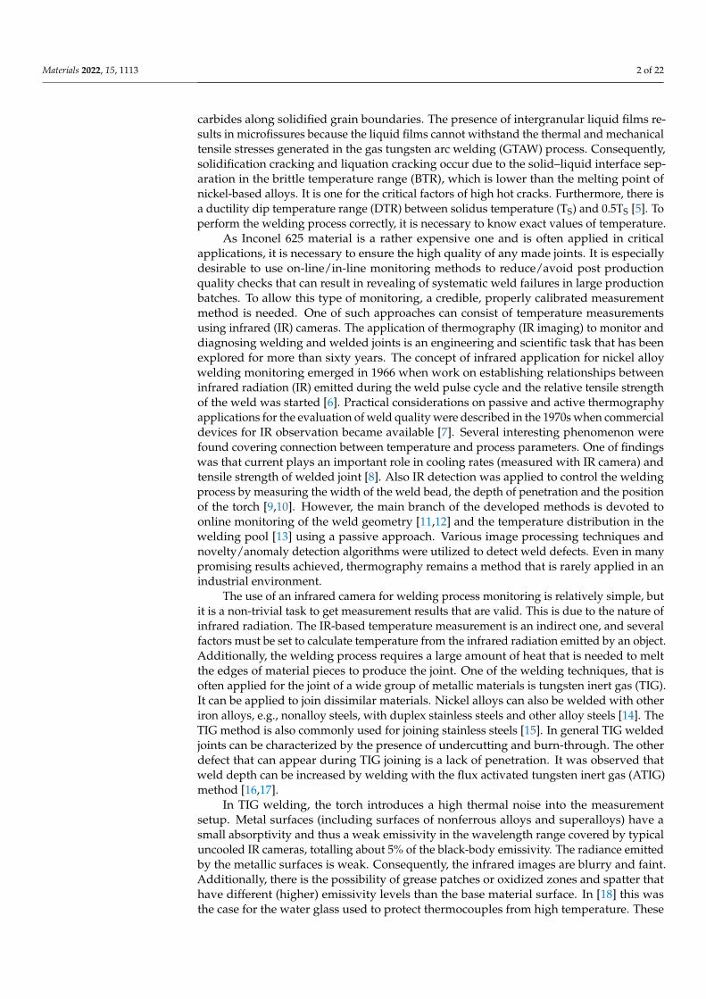
of dendritic grains in the weld area of the weld (Figure 7a). On the other hand, in theheat-affected zones of these joints, the presence of fine grains of austenite was revealed.In the Inconel 625 superalloy sheets, a similar matrix structure is observed; however, thetwin-austenite is finer-grained. The size of austenite grains determined by the microscopicmethod in Inconel 625 superalloy sheets is approximately 15 to 25 µm. In the heat-affectedzone of the joints of Inconel 625 superalloys welded with a linear energy of approximately68 J/mm, the austenite grain size of austenite is approx. 10 µm. On the other hand, weldingthese sheets with an energy of about 94 J/mm causes further, slight grain grinding in thiszone. Fragmentation of the HAZ structure is undoubtedly related to the separation ofintermetallic phases that block the movement of grain boundaries and thus inhibit theirgrowth (Figure 7a).

Figure 7. Structure of the joint made between Inconel 625 sheets (S3 sample): (a) HAZ—joint; zoom200×; (b) joint, zoom 200×.

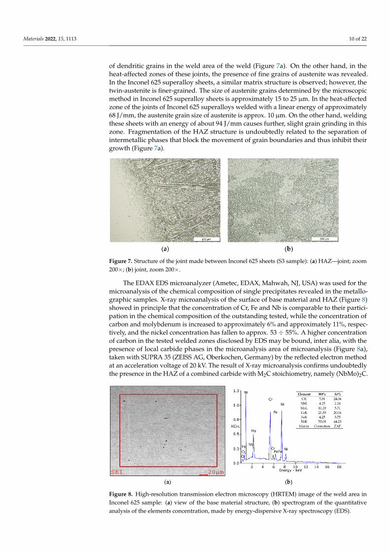
The EDAX EDS microanalyzer (Ametec, EDAX, Mahwah, NJ, USA) was used for themicroanalysis of the chemical composition of single precipitates revealed in the metallo-graphic samples. X-ray microanalysis of the surface of base material and HAZ (Figure 8)showed in principle that the concentration of Cr, Fe and Nb is comparable to their partici-pation in the chemical composition of the outstanding tested, while the concentration ofcarbon and molybdenum is increased to approximately 6% and approximately 11%, respec-tively, and the nickel concentration has fallen to approx. 53 ÷ 55%. A higher concentrationof carbon in the tested welded zones disclosed by EDS may be bound, inter alia, with thepresence of local carbide phases in the microanalysis area of microanalysis (Figure 8a),taken with SUPRA 35 (ZEISS AG, Oberkochen, Germany) by the reflected electron methodat an acceleration voltage of 20 kV. The result of X-ray microanalysis confirms undoubtedlythe presence in the HAZ of a combined carbide with M2C stoichiometry, namely (NbMo)2C.

Figure 8. High-resolution transmission electron microscopy (HRTEM) image of the weld area inInconel 625 sample: (a) view of the base material structure, (b) spectrogram of the quantitativeanalysis of the elements concentration, made by energy-dispersive X-ray spectroscopy (EDS).

Materials 2022, 15, 1113 11 of 22

In the weld zone of the assumed welded joint, a primary, dendritic microstructurewith clearly marked main axes of dendrites and precipitations in the form of eutectic, isrevealed in interdendritic areas (Figure 9). The results of X-ray microanalysis from thejoint surface of the joint showed basically identical distribution of the elements analysed,as in the case of the base material and HAZ of the tested joint (Figures 8b and 9b). Onthe other hand, results of point X-Ray microanalysis of the structural components of thewelds showed in the case of separation in the area of a dendrite, in the form of a localeutectic inflated concentration of carbon at 5.83%, niobium up to 18.40% and Mo up to16.84% and Ti up to 0.77% at low Cr concentration of approx. 17%, Fe approx. 3% andNi approx. 38%. Eutectic in this case can form an intermetallic phases of stable nitride(TiN) and more numerous MC composite carbides such as Nb(TiMo)C or M6C, such as, forexample Mo(Ni)6C with an isomorphic structure (FCC) of isomorphic to the solution γ, butwith a lower crystallization temperature.

Figure 9. High resolution transmission electron microscopy (HRTEM) image of the weld area inInconel 625 sample: (a) view of the dendritic structure in the joint, (b) spectrogram of the quantitativeanalysis of element concentration, made by energy-dispersive X-ray spectroscopy (EDS).

3.2. FEM Modelling

According to the procedure described in Section 2 a set of simulations was elaborated.First, for samples S2–S4, the simulation (properties of heat source) was calibrated in a waythat reflects real welding conditions in the model. The simulation parameters were changediteratively to obtain the geometry of the temperature field cross section, which will havethe best correspondence to the weld and HAZ areas. The fusion zone (FZ) was representedas a diagram of the maximum temperature value on the cross section, located midwayalong the length of the joint. In this case, the white area representing the temperaturethat exceeds the weld melting point marks the boundary of the weld (Figure 10). Both theshape and size of FZ and HAZ computed for samples T2 and T3 are in good agreementwith the measurements. The T4 sample differs from the original real sample mainly in theshape of FZ on the weld root side. The width of HAZ is also correctly reflected in the FEMresults, because for all considered samples it was measured on a level of 0.2 mm. Takinginto consideration that the temperature distribution only on the weld face side will beconsidered, the obtained correspondence can be regarded as sufficient.

The heat source parameters for consecutive simulations are gathered in Table 4. It canbe seen that for different samples the thermal efficiency varies from η = 0.43 to η = 0.505. Itis a relatively large span. Furthermore, it differs from the commonly used value for TIG(η = 0.6). For each sample, results were taken, when the heat source was in 25, 50 and 75%of workpiece length.

Materials 2022, 15, 1113 12 of 22

Figure 10. Macrostructure of the cross section of welded samples: (a) S2; (b) S3; (c) S4.

Table 4. The heat source parameters resulting from the fitting of the heat source fitting to the shapeof the fused zone.

Simulated Variant Energy per Unit Length(J/mm) Thermal Efficiency (η) Width (mm) Length (mm) Depth (mm)

S2 136.0 0.43 3.5 3.5 0.25S3 114.3 0.44 3.0 3.0 0.25S4 157.5 0.505 4.5 4.5 0.25

The simulation results were the temperature distribution in the 3D model in specifictime points (time cards), Figure 11. The length of each time card was automatically adjustedautomatically based on thermal gradients, and the results were in the range 121–187 timecards long. All simulation results were exported from SYSWELD and later processed inthe MATLAB environment. In Figure 12 a comparison of simulation results generated forthe S2 sample parameters. The temperature pattern depends on the thermal efficiency. Itcan be seen that for higher efficiency, more heat from source is transferred to the materialand a higher temperature can be observed on the material surface. The difference betweenmaximal temperature for the most extreme values of thermal efficacy exceeds 500 ◦C(Figure 11).

Materials 2022, 15, 1113 13 of 22

Figure 11. Exemplary result from FEM simulation results in SYSWELD software; S2 with thermalefficiency η = 0.6.

Figure 12. FEM simulation results for S2: (a) calibrated thermal efficiency η = 0.43, (b) η = 0.4,(c) η = 0.6. Results from SYSWELD visualized in MATLAB.

3.3. Reflected Temperature Maps Generation and IR Image Correction

To generate reflected temperature correction distribution map, first it was necessary, tounwarp the IR image to reduce the influence of perspective on geometry of objects visibleon each image. The necessary coefficients were calculated according to the geometry ofthe vision system geometry. The results of image rectification are presented in Figure 13. Itcan be seen that after rectification the face surface of welded workpiece is ideally projectedon the image pane (Figure 13b). Moreover, the right metal part that was used to hold andstabilize the welded elements is ideally parallel to the joint axis.

Materials 2022, 15, 1113 14 of 22

Figure 13. Exemplary IR image from the S2 sequence: (a) raw, (b) rectified.

Figures 14 and 15 present correction maps for thermograms coming from one sequence(S2) and averaged maps. In both, there is a general pattern visible. Because of the way thewelded workpiece was mounted, namely, it was sealed on both sides, with metal plates, arelatively large reflection is on both sides of a joint. In the middle there was an insert withdrilled holes through which gas was supplied to protect the root of the weld. This area iscooler than areas on both sides. As was supposed, most of the reflections are concentratedin the immediate distance from the welding torch outlet. Averaging of correction mapstends to produce a more complex solution that can be treated as a more general solution. Itis visible, that it generalizes sequence-dependent artifacts, like disturbances by tor outlet orspecific shape of gas nozzles in the middle of the welding pad (Figure 16).

Figure 14. Calibration maps for S2–M2: (a) calibrated thermal efficiency (η = correct), (b) η = 0.4,(c) η = 0.6.

Results of the FEM simulation were generated for three time points in which theelectrode tip reached the position at 25%, 50% and 75% of the workpiece length. Knowingthe moment of welding start in the IR sequence and the welding speed, thermogramscorresponding to specific timepoints were found. For all sequences (Table 2), three testimages were selected and later subjected to reflected temperature correction.

Two reflected temperature correction strategies were evaluated. In the first one foreach sequence that reflects a certain set of process parameters (S2/S3/S4), a dedicatedcorrection map was used. In this case, each image tends to be as close to the FEM imageas possible. From the qualitative point of view, this approach is susceptible to decreasingof artifact distinctness. It can be seen that small hot spots that are visible in the solidifiedweld area (Figures 17a and 18a) are barely visible in corrected thermogram (Figures 17b,cand 18b,c). On the other hand, as the span between hottest and the coolest points in a

Materials 2022, 15, 1113 15 of 22

thermogram decreases after correction, the change of the representation range, and theredrawing of IR images in the new scale reveal most of artifacts that justify presence ofweld defects and inconsistencies. The second strategy consist of applying an averagingover all calibration maps and using this averaged reflected temperature distribution map(Figure 19). It is noticeable that the shape of area with increased temperature is not assmooth as it was in the case of map dedicated for one sample. The small asymmetry oftemperature near the torch is preserved and the temperature is in a similar range as it is inFigure 18. For both types of correction maps extracted for ground truth FEM simulationsgenerated for heat effectiveness, 0.4, 0.6 and the correct value were used.

To quantify the results of thermogram correction, a mean absolute error (MAE) wasused. It measures the difference between thermogram (original/raw or corrected) and FEMsimulation result:

MAE =1n

n

∑i=1|TOBS,i − TFEM,i| (2)

where: TOBS,i is the temperature in pixel i in thermogram and TOBS,i is the temperature inpixel i in temperature map, being the result of FEM simulation.

Figure 15. Averaged calibration maps for S2/S3/S4 sequences—MAVG: (a) calibrated thermal effi-ciencies (different for each IR test IR image sequence, η = correct), (b) η = 0.4, (c) η = 0.6.

Figure 16. Location of artifacts caused by (a) holders and (b) gas nozzles.

Materials 2022, 15, 1113 16 of 22

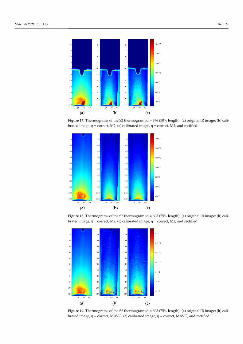
Figure 17. Thermograms of the S2 thermogram id = 376 (50% length): (a) original IR image; (b) cali-brated image, η = correct, M2, (c) calibrated image, η = correct, M2, and rectified.

Figure 18. Thermograms of the S2 thermogram id = 603 (75% length): (a) original IR image; (b) cali-brated image, η = correct, M2, (c) calibrated image, η = correct, M2, and rectified.

Figure 19. Thermograms of the S2 thermogram id = 603 (75% length): (a) original IR image; (b) cali-brated image, η = correct, MAVG, (c) calibrated image, η = correct, MAVG, and rectified.

Materials 2022, 15, 1113 17 of 22

All results were collected in Table 5. It can be seen that it was possible to obtain an errorlevel less than 10 ◦C. Having the map calculated for valid thermal efficacies (η = correct,MAVG) it was possible to obtain a best average MAE for all thermograms tested. Theaverage ˆMAE = 8.9 ◦C, what is a more than a satisfactory result. It has to be emphasizedthat all results regardless of the correction map using which they were generated werecompared to FEM simulations performed with experimentally tuned parameters.

Table 5. Mean absolute error (MAE) of the temperature distribution in IR images sets compared toideal distribution in the FEM simulation results.

η = Correct η = 0.4 η = 0.6

MAVG MS2 MS3 MS4 MAVG MS2 MS3 MS4 MAVG MS2 MS3 MS4

S2 9.9 11.7 7.4 12.9 11.0 18.1 12.9 33.0 31.9 46.6 23.9 9.9S3 11.0 23.8 29.5 16.5 70.9 58.7 73.2 115.9 7.4 5.2 2.2 9.8S4 5.7 17.0 15.9 7.2 14.9 23.9 10.1 19.6 13.1 12.3 16.9 44.7

avg. 8.9 17.5 17.6 12.2 32.3 33.6 32.1 56.2 17.5 21.4 14.3 21.5

The application of the correction map that gives best results is visualized in Figure 20.There are two plots in each axis: FEM temperature (blue) and corrected IR temperature(red). It can be easily assessed that applying map (η = correct, MAVG) leads to a temperaturedistribution that is close to the ideal distribution. There are two main reasons for theoccurrence of deviations:

• presence of point or area temperature disturbances that are the results of weldingprocess instabilities or weld faults,

• uneven distribution on the reflected temperature in certain regions of the correctionmap caused by temperature artifacts occurring on the surface of samples that wereused for correction maps generation.

Figure 20. Comparison of the temperature profiles of IR image and FEM simulation for η = correctMAVG mapping for the 75% of the length for samples: (a) S2; (b) S3; (c) S4.

Finding that the averaged correction map is less selective in preserving small, pointchanges in temperature but still having the low overall MAE, it was decided to apply it ona second set of IR images, gathered for a different set samples. These samples were alsomade from Inconel 625 but all sheets were 1.2 mm thick. For that, a different set of weldingparameters was used to create joints (Table 3). For all samples, hardness was measured inrow, and consecutive idents were separated by 0.4 mm. Exemplary identifications for basematerial, HAZ, and joint are presented in Figure 21.

To compare hardness results with the temperature, a part of measurements coveringthe limited number of samples counting form the weld axis (Figure 20) is covered. Itcan be seen that for the S14 and S20 hardness is almost the same in all zones. Thus,for combinations of parameters: 60 A, 3 mm/s and 70 A, 7 mm/s, the amount of heattransferred into the welding pool is similar. For 70 A welding speed, decreasing leads towidening of joint zone and slight decrease of hardness in joint and HAZ.

Materials 2022, 15, 1113 18 of 22

Figure 21. Idents for Vickers hardness measurements made in different areas of sample S17, magnifi-cation 10×: (a) base material; (b) HAZ; (c) joint.

The clustering process was applied to distinguish automatically between the correctand incorrect processes that is resulting with excessive lowering of the hardness in joint.To group the measurement values of hardness, temperature were bounded. To do this,consecutive hardness measurements (Figure 22) were connected with corresponding tem-perature values measured on the surface of welded sample (Figure 19). For each sample,22 value pairs for two positions were obtained. Moreover, the third parameter, the linerenergy was applied. As the voltage remains almost constant, it was set to 11 V. The thermalefficiency was set to η = 0.4 according to previous results (rounded down thermal efficiencyobtained for considered test samples S2–S4, Table 4). All triplets {t, HV, E} were projectedinto 3D space (Figures 23b and 24b). It can be seen that differences between individualtest samples are visible. In general, higher linear energy results in higher temperature andlower hardness in joint. Applying the clustering for two clusters leads to the creation oftwo groups (Figure 23a). Those groups reflect only base material and joint. Adding thethird cluster, an additional separate group can be formed. After that, joints can be differedin terms of properties corrections is joints (Figure 23b). Groups for correct (OK joint) andincorrect (NOK joint) are almost perfectly gathering valid samples. Only two points of thebase material (marked purple oval, Figure 23a) are incorrectly clustered. Adding the fourthcluster is not a solution to overcome this drawback. For this clustering procedure, addingnew sample will lead to assignment to proper cluster. Thus, an easy way of distinguishingbetween correct and incorrect joints is possible.

Figure 22. Hardness distribution for samples S14, S17–S20 for 25% of length as a function of offsetfrom the joint axis.

Materials 2022, 15, 1113 19 of 22

Figure 23. Clustering results for two groups on temperature, hardness and linear energy estimate µ(a) and class distribution (b).

Figure 24. Clustering results for three groups on temperature, hardness and linear energy estimate µ(a) and class distribution (b).

4. Summary and Conclusions

In the paper a method of correction that is based on the calculation of the differencebetween results of the FEM simulation and IR images is described and validated. Withhighly accurate temperature distributions on the workpiece surface it was possible toautomatically cluster weld conditions in the joint areas. When clustering to three groups adifferentiation between base material and proper and improper joint was possible.

In [18] a regressive model was elaborated and used to predict the hardness values injoints. The mean prediction error for the hardness of joint area at the level of err = 1.25%.Nevertheless, based only on the relative temperature changes, it is difficult to obtain anexact correspondence between process parameters and joint properties. Moreover, it wasproven that relying only on a constant and collected form literature review value of thermalefficiency to calculate linear energy of welding can be misleading. It was found during FEMmodelling that for wrong setup of heat source parameters, like thermal effectiveness, errors

Materials 2022, 15, 1113 20 of 22

in the temperature field distribution can exceed several hundred ◦C. Generally, from thepractical point of view, it can be stated the key issue is the elaboration of high quality FEMmodel, that address all properties of correct weld made to join elements made of certainmaterial using chosen technology. In the paper a limited approach was used, that was basedonly on bounding the simulation results with the shape of real welded joint and HAZ cross-section. As FEM modelling is generally used to predict the stress distribution in weldedjoints [28,29], it was applied in the research to obtain a reliable and accurate temperaturedistribution on the surface of the workpiece. Even using this limited approach it wasfound, that naïve application of theoretic values of thermal efficiency can lead unexpectedresults, when the temperature distribution remains unreliable. Nevertheless correctionof the reflected temperature based on FEM simulation was found to be more accuratethan using thermocouples [18,30]. Using the reflected temperature calibration methodbased on optimal FEM simulation that was proposed in this paper allows temperaturemeasurements in solidified welded joint area with an average MAE lower than 10 ◦C.Such a small measurement error makes it possible to perform further investigations onadditional properties of joint clustering and predictions, such as impact strength or residualstress. For performed studies clustering error for faulty weld was on a level of about 7%.There were no faulty samples clustered as correct ones, but further investigation is neededto confirm the generalization ability of the proposed approach.

The proposed approach has also several drawbacks limiting the applicability. Firstit is strongly dependant on the geometry of the measurement system. To ensure a propercorrespondence between the temperature distribution in FEM nodes and IR images aperspective transform is required. To get correct results the parameters of this transformmust be tuned carefully, which is difficult because there is no generally no reference imagethat can be used to evaluate the quality of the projective transform. Only the desireddimensions of welded workpiece can be calculated analytically and used as a groundtruth for any performed transformation. On the other hand, the quality and validity ofsummation results should be proven using temperature measurements. As it was alreadymentioned the use of thermocouples is problematic. Other possible solution is use of two-colour pyrometers, that are measuring temperature for unknown emissivity of materialssurface. This demands a special device to perform the measurements, that can oftenonly measure temperature in one spot at the time, what can be insufficient to confirmthe correctness of FEM-based temperature distributions. In addition, a FEM simulationhas to be made for each combination of material type, workpiece dimension and processparameters. This operation must always be preceded by the fabrication of reference welds.

Author Contributions: Conceptualization, W.J. and J.G.; methodology, W.J. and J.G.; software, W.J.and B.W.; validation, W.J. and J.G.; formal analysis, W.J.; investigation, W.J., B.W., M.K.-J. and J.G.;resources, W.J.; data curation, W.J., B.W. and M.K.-J.; writing—original draft preparation, W.J. andB.W.; writing—review and editing J.G.; visualization, W.J.; project administration, W.J.; fundingacquisition, W.J. All authors have read and agreed to the published version of the manuscript.

Funding: This research study was funded by the National Science Centre (NCN), Miniatura 3 project,grant number 2019/03/X/ST8/00422.

Institutional Review Board Statement: Not applicable.

Informed Consent Statement: Not applicable.

Data Availability Statement: The data presented in this study are available on request from thecorresponding author. The data are not publicly available because the authors do not wish to publishadditional material.

Conflicts of Interest: The authors declare that they have no conflicts of interest. The funders had norole in the design of the study; in the collection, analyses, or interpretation of data; in the writing ofthe manuscript, or in the decision to publish the results.

Materials 2022, 15, 1113 21 of 22

References1. Shankar, V.; Bhanu Sankara Rao, K.; Mannan, S.L. Microstructure and mechanical properties of Inconel 625 superalloy. J. Nucl.

Mater. 2008, 288, 222–232. [CrossRef]2. Special Metals Corporation. INCONEL® Alloy 625; Special Metals Corporation: New Hartford, NY, USA, 2013.3. Dubiel, B.; Sieniawski, J. Precipitates in Additively Manufactured Inconel 625 Superalloy. Materials 2019, 12, 1144. [CrossRef]

[PubMed]4. Inconel 625, Bibulmetals, Material Datasheet. Available online: https://www.bibusmetals.pl/fileadmin/editors/countries/

bmpl/Data_sheets/Inconel_625_karta_katalogowa.pdf (accessed on 28 November 2021).5. He, M.; Jianing, Q.; Zhentai, Z.; Fen, S.; Yunfeng, L. Numerical simulation of nickel-based alloys’ welding transient stress using

various cooling techniques. High Temp. Mater. Process. 2020, 39, 633–644. [CrossRef]6. Snedeker, D.A. Study on Development of Techniques for Resistance Welding, Phases I and II Final Report; Martin Marietta Corp.:

Orlando, FL, USA, 1967.7. Bobo, S. Infrared radiation as a tool in non-destructive evaluation of welding and bonding. Non-Destr. Test. 1970, 3, 345–350.

[CrossRef]8. Naksuk, N.; Nakngoenthong, J.; Printrakoon, W.; Yuttawiriya, R. Real-Time Temperature Measurement Using Infrared Ther-

mography Camera and Effects on Tensile Strength and Microhardness of Hot Wire Plasma Arc Welding. Metals 2020, 10, 1046.[CrossRef]

9. Nagarajan, S.; Banerjee, P.; Chen, W.; Chin, B. Control of the welding process using infrared sensors. IEEE Trans. Robot. Autom.1992, 8, 86–93. [CrossRef]

10. Wilik, H.C.; Kottilingam, S.; Zee, R.H. Infrared sensing techniques for penetration depth control of the sub-merged arc weldingprocess. J. Mater. Process. Technol. 2001, 113, 228–233.

11. Thomas, K.R.; Unnikrishnakurup, S.; Nithin, P.V.; Balasubramaniam, K.; Rajagopal, P.; Prabhakar, K.V.P.; Padmanabham, G.;Riedel, F.; Puschmann, M. Online monitoring of cold metal transfer (CMT) process using infrared thermography. Quant. InfraredThermogr. J. 2016, 14, 68–78. [CrossRef]

12. Al-Habaibeh, A.; Parkin, R. An autonomous low-cost infrared system for the on-line monitoring of manufacturing processesusing novelty detection. Int. J. Adv. Manuf. Technol. 2003, 22, 249–258. [CrossRef]

13. Bicknell, A.; Smith, J.S.; Lucas, J. Infrared sensor for top face monitoring of weld pools. Meas. Sci. Technol. 1994, 5, 371–378.[CrossRef]

14. Rogalski, G.; Swierczynska, A.; Landowski, M.; Fydrych, D. Mechanical and Microstructural Characterization of TIG WeldedDissimilar Joints between 304L Austenitic Stainless Steel and Incoloy 800HT Nickel Alloy. Metals 2020, 10, 559. [CrossRef]

15. Tomków, J.; Sobota, K.; Krajewski, S. Influence of tack welds distribution and welding sequence on the angular distortion of TIGwelded joint. Facta Univ. Ser. Mech. Eng. 2020, 18, 611–621. [CrossRef]

16. Ghetiya, N.; Pandya, D. Mathematical Modeling for the Bead Width and Penetration in Activated TIG Welding Process. InProceedings of the International Conference on Multidisciplinary Research & Practice, Gujarat, India, 30 November 2014;Volume 1, pp. 247–252.

17. Tseng, K.-H.; Hsu, C.-Y. Performance of activated TIG process in austenitic stainless steel welds. J. Mater. Process. Technol. 2011,211, 503–512. [CrossRef]

18. Jamrozik, W.; Górka, J.; Kik, T. Temperature-Based Prediction of Joint Hardness in TIG Welding of Inconel 600, 625 and 718 NickelSuperalloys. Materials 2021, 14, 442. [CrossRef] [PubMed]

19. Farson, D.; Richardon, R.; Li, X. Infrared measurement of base metal temperature in gas tungsten arc welding. Weld. Res. Suppl.1998, 77, 396.

20. Kik, T.; Moravec, J.; Nováková, I. Application of Numerical Simulations on 10GN2MFA Steel Multilayer Welding. In DynamicalSystems Theory and Applications; Awrejcewicz, J., Ed.; Springer International Publishing: Cham, Switzerland, 2018; pp. 193–204.

21. Thejasree, P.; Manikandan, N.; Binoj, J.S.; Varaprasad, K.C.; Palanisamy, D.; Raju, R. Numerical Simulation and ExperimentalInvestigation on Laser Beam Welding of Inconel 625. Mater. Today Proc. 2021, 39, 268–273. [CrossRef]

22. Flint, T.; Yates, J.; Francis, J. Analytical Solutions of the Transient Thermal Field Induced in Finite Bodies with Insulating andConvective Boundary Conditions Subjected to a Welding Heat Source. In Proceedings of the 22nd International Conference onStructural Mechanics, San Francisco, CA, USA, 18–23 August 2013.

23. Kik, T. Computational Techniques in Numerical Simulations of Arc and Laser Welding Processes. Materials 2020, 13, 608.[CrossRef] [PubMed]

24. Goldak, J.; Chakravarti, A.; Bibby, M. A New Finite Element Model for Welding Heat Sources. Metall. Trans. B 1984, 15, 299–305.[CrossRef]

25. Kik, T. Heat Source Models in Numerical Simulations of Laser Welding. Materials 2020, 13, 2653. [CrossRef]26. Woods, R.P. Spatial Transformation Models. In Biomedical Engineering, Handbook of Medical Imaging; Bankman, I.N., Ed.; Academic

Press: Cambridge, MA, USA, 2000; pp. 465–490.27. Aggarwal, C.C.; Hinneburg, A.; Keim, D.A. On the Surprising Behavior of Distance Metrics in High Dimensional Space. In

Proceedings of the International Conference on Database Theory; Van den Bussche, J., Vianu, V., Eds.; Springer: Berlin/Heidelberg,Germany, 2001; Volume 1973. [CrossRef]

Materials 2022, 15, 1113 22 of 22

28. Vemanaboina, H.; Gundabattini, E.; Kumar, K.; Ferro, P.; Babu, B.S. Thermal and Residual Stress Distributions in Inconel 625Butt-Welded Plates: Simulation and Experimental Validation. Adv. Mater. Sci. Eng. 2021, 2021, 3948129. [CrossRef]

29. Saha, R.; Biswas, P. Temperature and Stress Evaluation during Friction Stir Welding of Inconel 718 Alloy Using Finite ElementNumerical Simulation. J. Mater. Eng. Perform. 2021, 1–10. [CrossRef]

30. Górka, J.; Jamrozik, W. Enhancement of Imperfection Detection Capabilities in TIG Welding of the Infrared Monitoring System.Metals 2021, 11, 1624. [CrossRef]