Wavenumber-explicit hp-FEM analysis for Maxwell’sequations with impedance boundary conditions

J.M. Melenk∗ S.A. Sauter†

January 10, 2022

Abstract

The time-harmonic Maxwell equations at high wavenumber k in domains with ananalytic boundary and impedance boundary conditions are considered. A wavenumber-explicit stability and regularity theory is developed that decomposes the solution intoa part with finite Sobolev regularity that is controlled uniformly in k and an analyticpart. Using this regularity, quasi-optimality of the Galerkin discretization based onNedelec elements of order p on a mesh with mesh size h is shown under the k-explicitscale resolution condition that a) kh/p is sufficient small and b) p/ ln k is bounded frombelow.

Contents

Symbols and Notation ii

1 Introduction 1

2 Setting 32.1 Geometric setting and Sobolev spaces on Lipschitz domains . . . . . . . . . . . 32.2 Sobolev spaces on a sufficiently smooth surface Γ . . . . . . . . . . . . . . . . 42.3 Trace operators and energy spaces for Maxwell’s equation . . . . . . . . . . . . 62.4 Regular decompositions . . . . . . . . . . . . . . . . . . . . . . . . . . . . . . . 72.5 The Maxwell equations with impedance boundary conditions . . . . . . . . . . 11

3 Stability analysis of the continuous Maxwell problem 123.1 Well-posedness . . . . . . . . . . . . . . . . . . . . . . . . . . . . . . . . . . . 123.2 Wavenumber-explicit stability estimates . . . . . . . . . . . . . . . . . . . . . 12

4 The Maxwell equations with the “good”sign 184.1 Norms . . . . . . . . . . . . . . . . . . . . . . . . . . . . . . . . . . . . . . . . 184.2 Maxwell problem with the good sign . . . . . . . . . . . . . . . . . . . . . . . 20

∗(melenk@tuwien.ac.at), Institut fur Analysis und Scientific Computing, Technische Universitat Wien,Wiedner Hauptstrasse 8-10, A–1040 Wien, Austria.

†(stas@math.uzh.ch), Institut fur Mathematik, Universitat Zurich, Winterthurerstr. 190, CH–8057 Zurich,Switzerland

1

arX

iv:2

201.

0260

2v1

[m

ath.

NA

] 7

Jan

202

2

5 Regularity theory for the Maxwell equation 245.1 Finite regularity theory . . . . . . . . . . . . . . . . . . . . . . . . . . . . . . . 245.2 Analytic regularity theory . . . . . . . . . . . . . . . . . . . . . . . . . . . . . 25

6 Frequency splittings 266.1 Frequency splittings in Ω: HR3 , LR3 , HΩ, LΩ, H0

Ω, L0Ω . . . . . . . . . . . . . . 26

6.2 Frequency splittings on Γ . . . . . . . . . . . . . . . . . . . . . . . . . . . . . . 276.3 Estimates for the frequency splittings . . . . . . . . . . . . . . . . . . . . . . . 29

7 k-Explicit regularity by decomposition 327.1 The concatenation of S+

Ω,k with high frequency filters . . . . . . . . . . . . . . 337.2 Regularity by decomposition: the main result . . . . . . . . . . . . . . . . . . 34

8 Discretization 388.1 Meshes and Nedelec elements . . . . . . . . . . . . . . . . . . . . . . . . . . . 388.2 hp-Approximation operators . . . . . . . . . . . . . . . . . . . . . . . . . . . . 398.3 An interpolating projector on the finite element space . . . . . . . . . . . . . . 42

9 Stability and convergence of the Galerkin discretization 449.1 Splitting of the consistency term . . . . . . . . . . . . . . . . . . . . . . . . . . 459.2 Consistency analysis: the term T1 in (9.9) . . . . . . . . . . . . . . . . . . . . 46

9.2.1 hp-Analysis of T1 . . . . . . . . . . . . . . . . . . . . . . . . . . . . . . 479.3 Consistency analysis: the term T2 in (9.9) . . . . . . . . . . . . . . . . . . . . 48

9.3.1 hp-Analysis of T2 . . . . . . . . . . . . . . . . . . . . . . . . . . . . . . 489.4 h-p-k-explicit stability and convergence estimates for the Maxwell equation . . 51

10 Numerical results 53

A Analytic regularity with bounds explicit in the wavenumber ( [39,45] revis-ited) 54A.1 Analytic regularity near the boundary . . . . . . . . . . . . . . . . . . . . . . 57A.2 Interior analytic regularity . . . . . . . . . . . . . . . . . . . . . . . . . . . . . 65A.3 Proof of Theorem A.1 . . . . . . . . . . . . . . . . . . . . . . . . . . . . . . . 66

B Details of the proof of Lemma 8.3 67

Acknowledgements 70

References 70

i

Symbols and Notation

general

k ≥ 1 > 0 wavenumberi imaginary unit

√−1

A . B there exists C independent of k, h, p, and independent offunctions that possibly appear in A and B so that A ≤ CB holds,

a+ a+ := maxa, 0 for a ∈ RN positive integers: N = 1, 2, 3 . . .

caveat: in Appendix A, wefollow the “French” convention N = 0, 1, . . .

N0 N = 0, 1, . . .N≥p n ∈ N |n ≥ pN≤p n ∈ N |n ≤ p

geometry

B1(0) unit ball in R3

B+r half-balls in R3

Ω domain in R3

Γ = ∂Ω boundary of Ωn unit normal vector on Γ pointing into Ω+

n∗ constant extension of n to tubular neighborhood of Γ

spaces

X := H(Ω, curl) (2.3)Ximp Ximp := u ∈ H0(Ω, curl) |ΠTu ∈ L2(Γ); (2.28)Ximp,0 Ximp,0 := u ∈ Ximp | curl u = 0 = ∇ϕ |ϕ ∈ H1

imp(Ω);Ximp(Ω) Ximp(Ω) := (H1(Ω))

′ ∩X′imp,0; (4.1)

Ximp(Γ) Ximp(Γ) :=(H−1/2T (Γ)

)′∩H−1

T (Γ, divΓ) (4.2)

H(Ω, curl), H(Ω, div) (2.3), (2.4)H0(Ω, curl) H0(Ω, curl) = u ∈ H(Ω, curl) | γTu = 0 on ∂ΩH(Ω, div0) divergence-free functionsL2(Ω) space of vector-valued L2-functionsHs(Ω), Hs(Γ) scalar-valued Sobolev spaces on Ω, Γ, Sec. 2.1Hs(Ω) vector-valued Sobolev spaces on ΩH1

imp(Ω) H1imp(Ω) = ϕ ∈ H1(Ω) |ϕ|∂Ω ∈ H1(∂Ω), Def. 2.5

H(curl,Ω) norm ‖ curl u‖L2(Ω) + ‖u‖L2(Ω)

H(div,Ω) norm ‖ div u‖L2(Ω) + ‖u‖L2(Ω)

L2T (Γ), Hs

T (Γ) Sobolev space of tangential fields on Γ, (2.14), (2.16)

H−1/2div (Γ) (2.19)

H−1/2curl (Γ) (2.19)

ii

H−1(Γ, divΓ) (4.2)Vk,0 u ∈ Vk,0 ⇐⇒ ((u,∇ϕ))k = 0 for all ϕ ∈ H1

imp(Ω); (8.22)Vk,0,h u ∈ Vk,0,h ⇐⇒ ((u,∇ϕh))k = 0 for all ϕ ∈ Sh; (8.27)A(C1, γ1, ω), class of analytic fcts., Def. 2.1; C1, γ1 are independent of k

functions

E, H, E+, H+ electric and magnetic fields in Ω and in Ω+

Y m` , λ` eigenfunctions of Laplace-Beltrami, Remark 6.1ι` index set of indices for eigenvalue λ`, Rem. 6.1gk Helmholtz fundamental solution, (3.6c)

sesquilinear forms, norms

‖ · ‖imp,k ‖u‖2imp,k = ‖ curl u‖2 + k2‖u‖2 + |k|‖u‖2

L2(Γ), (2.29)

‖ · ‖k,+ ‖u‖2k,+ = k2‖u‖2 + |k|‖u‖2

L2(Γ), (2.29)

‖ · ‖X′imp(Ω),k supv∈Ximp

|(f ,v)|‖v‖imp,k

; (4.3); Lemma 4.1

‖ · ‖X′imp(Γ),k supv∈Ximp

|(gT ,vT )L2(Γ)|‖v‖imp,k

; (4.4); Lemma 4.1

(·, ·) (u, v) =∫

Ωuv is the L2(Ω) innerproduct/duality pairing

‖ · ‖ = ‖ · ‖L2(Ω) L2(Ω)-norm; Sec. 2.1(·, ·)L2(Γ) L2(Γ)-inner prod. (or duality pairing)Ak, sesquilinear form associated with

Maxwell’s equations, (2.42), (2.48)A+k , sesquilinear form associated with

Maxwell’s equations with the “good” sign, (4.15)((·, ·))k ((·, ·))k = k2(·, ·)L2(Ω) + i k(ΠT (·),ΠT (·))L2(Γ) ; see (2.47)‖ · ‖−1/2,curlΓ ,

‖ · ‖−1/2,divΓnorms on H

−1/2curl (Γ), on H

−1/2div (Γ), (2.19)

|v|H`(Ω),k |v|H`(Ω),k := k−`|v|H`(Ω); see (2.6)

‖v‖Hm(Ω),k ‖v‖Hm(Ω),k :=(∑m

`=0 |v|2H`(Ω),k

)1/2; see (2.6);

‖v‖2Hm(Ω),k = ‖v‖2

H0(Ω) + k−2|v|2H1(Ω) + · · ·+ k−2m|v|2Hm(Ω)

‖v‖H−m(Ω),k ‖v‖H−m(Ω),k := km‖v‖H−m(Ω); see (2.7)‖v‖H−1/2(Γ,divΓ),k |k|‖ divΓ gT‖H−1/2(Γ) + k2‖gT‖X′imp(Γ),k; see (4.5) and Lemma 4.2

‖v‖H(Ω,div),k ‖v‖H(Ω,div),k :=(k−2m| div v|2Hm(Ω) + k2‖v‖2

Hm(Ω),k

)1/2; (2.8)

‖v‖2H(Ω,div),k = k−2m| div v|2Hm(Ω) + k2‖v‖2

L2(Ω) + · · ·+ k2−2m|v|2Hm(Ω)

‖v‖H(Ω,curl),k ‖v‖H(Ω,curl),k :=(k−2m| curl v|2Hm(Ω) + k2‖v‖2

Hm(Ω),k

)1/2; (2.8)

‖v‖2H(Ω,curl),k = k−2m| curl v|2Hm(Ω) + k2‖v‖2

L2(Ω) + · · ·+ k2−2m|v|2Hm(Ω)

‖gT‖Hν(Γ),k ‖gT‖Hν(Γ),k :=

(2ν∑`=0

|k|1−` |gT |2H`/2(Γ)

)1/2

;see (2.21)

‖gT‖Hν(Γ),k ∼ k1/2‖gT‖L2(Γ) + |gT |H1/2(Γ) + k1/2|gT |H1(Γ)

+ · · ·+ k1/2−ν |gT |Hν(Γ)

‖gT‖H−1/2(Γ),k ‖gT‖H−1/2(Γ),k := k‖gT‖H−1/2(Γ); see (2.21)

iii

‖gT‖Hν(Γ,divΓ),k ‖gT‖2Hν(Γ,div),k = | div gT |2Hν(Γ),k + k|gT |2Hν(Γ),k; see (2.22)

‖gT‖Hν(Γ,curlΓ),k ‖gT‖2Hν(Γ,curl),k = | curl gT |2Hν(Γ),k + k|gT |2Hν(Γ),k; see (2.22)

‖ · ‖H,ω ‖ · ‖2H,ω = ‖∇ · ‖2

L2(ω) + k2‖ · ‖2L2(ω)

|·| Euclidean norm〈·, ·〉 bilinear form on Cn: 〈a,b〉 =

∑ni=1 aibi; Sec. 2.1

| · |p,q,B+R

, [[·]]p,q,B+R

,

ρ2∗[[·]]p,q,B+

R, ρ

32∗ [[·]]p, 1

2,ΓR

,

ρ12∗ [[·]]p, 3

2,ΓR

, seminorms to control high order derivatives, Appendix A, p. 58

discrete spaces, meshes

K reference tetrahedronTh, FK , FK , AK triangulation, element maps, Sec. 8.1, Ass. 8.1Sh (discrete) subspace of H1(Ω);

we require ∇Sh ⊂ Xh and exact seq. property (8.8)Xh (discrete) subspace of H(Ω, curl)h, hK , p global and local meshwidth (Assumption 8.1, (8.1)), polyn. deg. pPp, Pp space of R-valued and R3-valued polynomials of degree p, (8.3)

N Ip(K) Nedelec type I space on reference tetrahedron K, (8.5)

Sp+1(Th), N Ip(Th), polyn. spaces on Th: H1(Ω)-, H(curl,Ω)-conforming

operators

curl, div 3D curl and divergence operatorscurlΓ, divΓ 2D scalar curl and divergence operators on the surface Γ, (2.11)−−−→curlΓ, ∇Γ, 2D vectorial curl and surface gradient operators on Γ, (2.10)∆Γ surface Laplace-Beltrami operator, (2.12)Ecurl, Ediv, lifting operators (see Thm. 2.3)F Fourier transformation, (6.1)γ standard trace operator: γu = u|Γ and γu = u|ΓΠT , γT trace operators (2.25); Thm. 2.3;

ΠTu = n× (u× n), γTu = u× n,(·)T subscript T indicates tangential trace: uT = Πτu(·)high, (·)low vhigh = HΩv, vlow = LΩv,(·)∇ gradient part of Hodge decomp. of functions on Γ, (2.15), (6.12)(·)curl curl part of Hodge decomp. of functions on Γ, (2.15), (6.12)R1, R2 operators of order −1 of the regular decomp. in Lemma 2.6;

by (2.33), R2 is (up to a smoothing operator)a right inverse inverse of curl for divergence-free functions

K operator of order −∞ of the regular decomp. in Lemma 2.6S f = H0

Ωf + L0Ωf + Sf ;

for div f = 0 we have Sf ∈ C∞(Ω); see (6.5)

iv

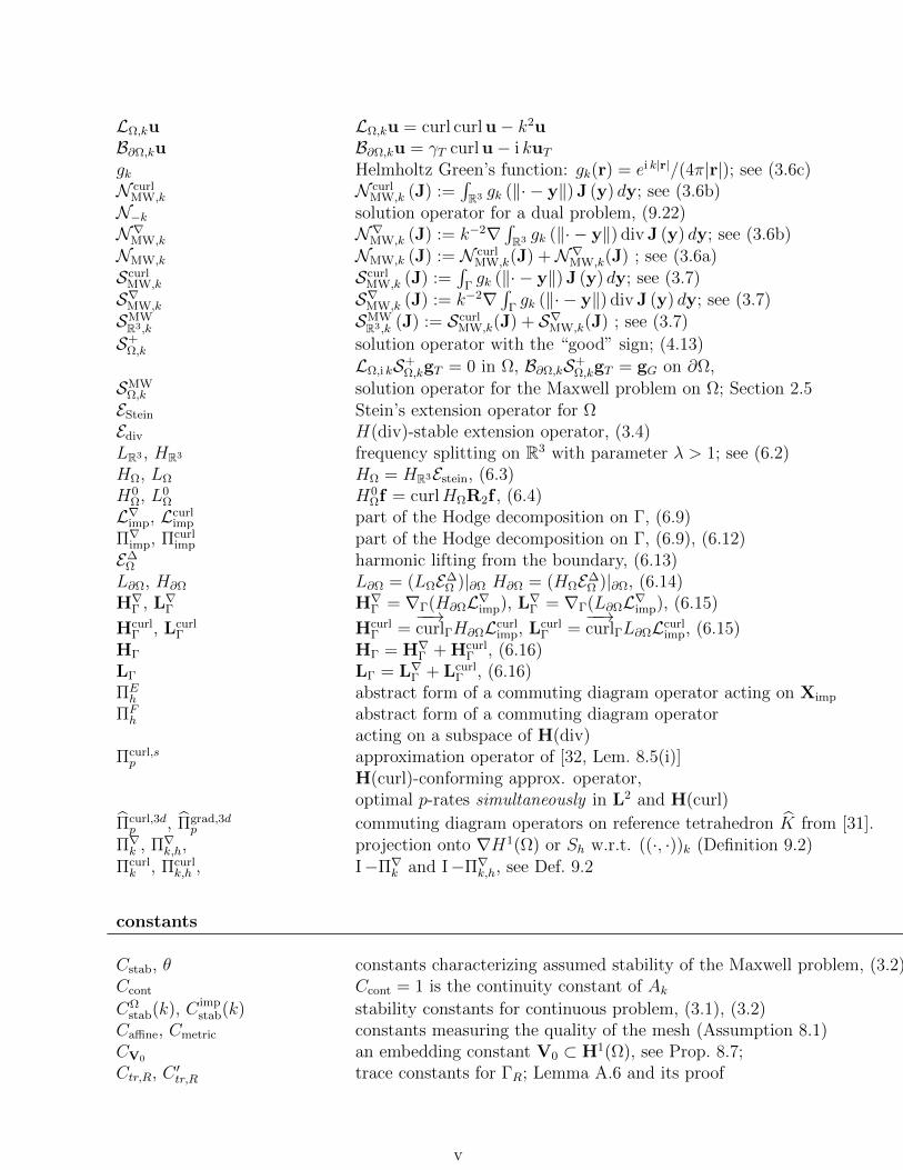
LΩ,ku LΩ,ku = curl curl u− k2uB∂Ω,ku B∂Ω,ku = γT curl u− i kuTgk Helmholtz Green’s function: gk(r) = ei k|r|/(4π|r|); see (3.6c)N curl

MW,k N curlMW,k (J) :=

∫R3 gk (‖· − y‖) J (y) dy; see (3.6b)

N−k solution operator for a dual problem, (9.22)N∇MW,k N∇MW,k (J) := k−2∇

∫R3 gk (‖· − y‖) div J (y) dy; see (3.6b)

NMW,k NMW,k (J) := N curlMW,k(J) +N∇MW,k(J) ; see (3.6a)

ScurlMW,k Scurl

MW,k (J) :=∫

Γgk (‖· − y‖) J (y) dy; see (3.7)

S∇MW,k S∇MW,k (J) := k−2∇∫

Γgk (‖· − y‖) div J (y) dy; see (3.7)

SMWR3,k SMW

R3,k (J) := ScurlMW,k(J) + S∇MW,k(J) ; see (3.7)

S+Ω,k solution operator with the “good” sign; (4.13)

LΩ,i kS+Ω,kgT = 0 in Ω, B∂Ω,kS+

Ω,kgT = gG on ∂Ω,

SMWΩ,k solution operator for the Maxwell problem on Ω; Section 2.5EStein Stein’s extension operator for ΩEdiv H(div)-stable extension operator, (3.4)LR3 , HR3 frequency splitting on R3 with parameter λ > 1; see (6.2)HΩ, LΩ HΩ = HR3Estein, (6.3)H0

Ω, L0Ω H0

Ωf = curlHΩR2f , (6.4)L∇imp, Lcurl

imp part of the Hodge decomposition on Γ, (6.9)Π∇imp, Πcurl

imp part of the Hodge decomposition on Γ, (6.9), (6.12)E∆

Ω harmonic lifting from the boundary, (6.13)L∂Ω, H∂Ω L∂Ω = (LΩE∆

Ω )|∂Ω H∂Ω = (HΩE∆Ω )|∂Ω, (6.14)

H∇Γ , L∇Γ H∇Γ = ∇Γ(H∂ΩL∇imp), L∇Γ = ∇Γ(L∂ΩL∇imp), (6.15)

HcurlΓ , Lcurl

Γ HcurlΓ =

−−→curlΓH∂ΩLcurl

imp, LcurlΓ =

−−→curlΓL∂ΩLcurl

imp, (6.15)HΓ HΓ = H∇Γ + Hcurl

Γ , (6.16)LΓ LΓ = L∇Γ + Lcurl

Γ , (6.16)ΠEh abstract form of a commuting diagram operator acting on Ximp

ΠFh abstract form of a commuting diagram operator

acting on a subspace of H(div)Πcurl,sp approximation operator of [32, Lem. 8.5(i)]

H(curl)-conforming approx. operator,optimal p-rates simultaneously in L2 and H(curl)

Πcurl,3dp , Πgrad,3d

p commuting diagram operators on reference tetrahedron K from [31].Π∇k , Π∇k,h, projection onto ∇H1(Ω) or Sh w.r.t. ((·, ·))k (Definition 9.2)Πcurlk , Πcurl

k,h , I−Π∇k and I−Π∇k,h, see Def. 9.2

constants

Cstab, θ constants characterizing assumed stability of the Maxwell problem, (3.2)Ccont Ccont = 1 is the continuity constant of AkCΩ

stab(k), C impstab(k) stability constants for continuous problem, (3.1), (3.2)

Caffine, Cmetric constants measuring the quality of the mesh (Assumption 8.1)CV0 an embedding constant V0 ⊂ H1(Ω), see Prop. 8.7;Ctr,R, C ′tr,R trace constants for ΓR; Lemma A.6 and its proof

v

dual problems andapproximationproperties

N−k solution operator for an adjoint problem; (9.22),

ηalg6 (9.14)

ηalg2 (9.24)

a tilde indicates that an adjoint sol. operator N is involved;η indicates a pure approximation property,superscript “alg” indicates that algebraic convergenceof hp-FEM is expected

vi

1 Introduction

The time-harmonic Maxwell equations at high wavenumber k are a fundamental component ofhigh-frequency computational electromagnetics. Computationally, these equations are chal-lenging for several reasons. The solutions are highly oscillatory so that fine discretizationsare necessary and correspondingly large computational resources are required. While condi-tions to resolve the oscillatory nature of the solution appear unavoidable, even more stringentconditions on the discretizations have to be imposed for stability reasons: In many numericalmethods based on the variational formulation of the Maxwell equations, the gap between theactual error and the best approximation error widens as the wavenumber k becomes large.This “pollution effect” is a manifestation of a lack of coercivity of the problem, as is typicalin time-harmonic wave propagation problems. Mathematically understanding this “pollutioneffect” in terms of the wavenumber k and the discretization parameters for the model problem(1.1) is the purpose of the present work.The “pollution effect”, i.e., the fact that discretizations of time-harmonic wave propagationproblems are prone to dispersion errors, is probably best studied for the Helmholtz equation atlarge wavenumbers. The beneficial effect of using high order methods was numerically observedvery early and substantiated for translation-invariant meshes [2, 3]; a rigorous mathematicalanalysis for unstructured meshes was developed in the last decade only in [15, 33, 34]. Theseworks analyze high order FEM (hp-FEM) for the Helmholtz equation in a Garding settingusing duality techniques. This technique, often called “Schatz argument”, crucially hinges onthe regularity of the dual problem, which is again a Helmholtz problem. The key new insightof the line of work [15,33,34] is a refined wavenumber-explicit regularity theory for Helmholtzproblems that takes the following form (“regularity by decomposition”): given data, thesolution u is written as uH2 + uA where uH2 has the regularity expected of elliptic problemsand is controlled in terms of the data with constants independent of k. The part uA is a(piecewise) analytic function whose regularity is described explicitly in terms of k. Employing“regularity by decomposition” for the analysis of discretizations has been successfully appliedto other Helmholtz problems and discretizations such DG methods [29], BEM [22], FEM-BEMcoupling [24], and heterogeneous Helmholtz problems [5, 9, 20,21].In this paper, we consider the following time-harmonic Maxwell equations with impedanceboundary conditions as our model problem:

curl curl E− k2E = f in Ω, (1.1a)

(curl E)× n− i kET = gT on ∂Ω (1.1b)

on a bounded Lipschitz domain Ω ⊂ R3 with simply connected boundary ∂Ω. We study anH(curl)-conforming Galerkin method with elements of degree p on a mesh of size h and showquasi-optimality of the method under scale resolution condition

|k|hp≤ c1 and p ≥ c2 ln |k| , (1.2)

where c2 is arbitrary and c1 is sufficiently small (Theorem 9.7). The resolution condition|k|h/p ≤ c1 is a natural condition to resolve the oscillatory behavior of the solution, and theside constraint p ≥ c2 ln |k| is a rather weak condition that suppresses the “pollution effect”.Underlying this convergence analysis is a wavenumber-explicit regularity theory for (1.1) akinto the Helmholtz case discussed above of the form “regularity by decomposition” (Theo-rem 7.3). Such a regularity theory was developed for Maxwell’s equation in full space in the

1

very recent paper [32], where the decomposition is directly accessible in terms of Newtonpotential and layer potentials. For the present bounded domain case, however, an explicitconstruction of the decomposition is not available, and the iterative construction as in theHelmholtz case of [34] has to be brought to bear. For this, a significant complication in theMaxwell case compared to the Helmholtz case arises from the requirement that the frequencyfilters used in the construction be such that they produce solenoidal fields if the argument issolenoidal.While our wavenumber-explicit regularity result Theorem 7.3 underlies our proof of quasiop-timal convergence of the high order Galerkin method (cf. Theorem 9.7), it also proves usefulfor wavenumber-explicit interpolation error estimates as worked out in Corollary 9.8.The present paper analyzes an H(curl)-conforming discretization based on high order Nedelecelements. Various other high order methods for Maxwell’s equations that are explicit in thewavenumber can be found in the literature. Closest to our work are [10, 39]. The work [39]studies the same problem (1.1) but uses an H1-based instead of an H(curl)-based variationalformulation involving both the electric and the magnetic field. The proof of quasi-optimalityin [39] is based on a “regularity by decomposition” technique similar to the present one. [38]studies the same H1-based variational formulation and H1-conforming discretizations for (1.1)on certain polyhedral domains and obtains k-explicit conditions on the discretization for quasi-optimality. Key to this is a description of the solution regularity in [38] in terms cornerand edge singularities. The work [10] studies (arbitrary, fixed) order H(curl)-conformingdiscretizations of heterogeneous Maxwell problems and shows a similar quasi-optimality resultby generalizing the corresponding Helmholtz result [9]; the restriction to finite order methodscompared to the present work appears to be due to the difference in which the decompositionof solutions of Maxwell problems is obtained. High order Discontinuous Galerkin (DG) andHybridizable DG (HDG) methods for (1.1) have been presented in [16] and [23] together witha stability analysis that is explicit in h, k, and p. A dispersion analysis of high order methodson tensor-product meshes is given in [3].The outline of the paper is as follows. Section 2 introduces the notation and tools such asregular decompositions (see Section 2.4) that are indispensable for the analysis of Maxwellproblems. Section 3 (Theorem 3.6) shows that the solution of (1.1) depends only polynomi-ally on the wavenumber k. This stability result is obtained using layer potential techniques inthe spirit of earlier work [15, Thm. 2.4] for the analogous Helmholtz equation. While earlierstability estimates for (1.1) in [16,19,47], and [38, Thm. 5.2] are obtained by judicious choicesof test functions and rely on star-shapedness of the geometry, Theorem 3.6 does not requirestar-shapedness. Section 4 analyzes a “sign definite” Maxwell problem and presents k-explicitregularity assertions for it (Theorem 4.3). The motivation for studying this particular bound-ary value problem is that, since the principal parts of our sign-definite Maxwell operator andthat of (1.1) coincide, a contraction argument can be brought to bear in the proof of Theo-rem 7.3. A similar technique has recently been used for heterogeneous Helmholtz problemsin [5]. Section 5 collects k-explicit regularity assertions for (1.1) (Lemma 5.1 for finite reg-ularity data and Theorem 5.2 for analytic data). The contraction argument in the proof ofTheorem 7.3 relies on certain frequency splitting operators (both in the volume and on theboundary), which are provided in Section 6. Section 7 presents the main analytical result,Theorem 7.3, where the solution of (1.1) with finite regularity data f , g is decomposed intoa part with finite regularity but k-uniform bounds, a gradient field, and an analytic part.Section 8 presents the discretization of (1.1) based on high order Nedelec elements. Section 9shows quasi-optimality (Theorem 9.7) under the scale resolution condition (1.2). Section 10

2

concludes the paper with numerical results.

2 Setting

2.1 Geometric setting and Sobolev spaces on Lipschitz domains

Let Ω ⊂ R3 be a bounded Lipschitz domain which we assume throughout the paper to have asimply connected and sufficiently smooth boundary Γ := ∂Ω; if less regularity is required, wewill specify this. We flag already at this point that the main quasi-optimal convergence result,Theorem 9.7 will require analyticity of Γ. The outward unit normal vector field is denoted byn : Γ→ S2.The Maxwell problem in the frequency domain involves the wavenumber (denoted by k) andwe assume that1

k ∈ R\ (−k0, k0) for k0 = 1. (2.1)

Let L2(Ω) denote the usual Lebesgue space on Ω with scalar product (·, ·)L2(Ω) and norm

‖·‖L2(Ω) := (·, ·)1/2

L2(Ω). As a convention we assume that the complex conjugation is applied to

the second argument in (·, ·)L2(Ω). If the domain Ω is clear from the context we write short(·, ·), ‖·‖ for (·, ·)L2(Ω), ‖·‖L2(Ω). By Hs(Ω) we denote the usual Sobolev spaces of index s ≥ 0with norm ‖·‖Hs(Ω). The closure of C∞0 (Ω) functions with respect to ‖·‖Hs(Ω) is denoted by

Hs0(Ω). For s ≥ 0, the dual space of Hs

0(Ω) is denoted by H−s(Ω). For s ≥ 0, the spaces Hs(Ω)of vector-valued Sobolev spaces are characterized by componentwise membership in Hs(Ω).For details, we refer to [1]. We write (·, ·) also for the vectorial L2(Ω) inner product given by(f ,g) =

∫Ω〈f ,g〉. Here, we introduce for vectors a,b ∈ C3 with a = (aj)

3j=1, b =(bj)

3j=1 the

bilinear form 〈·, ·〉 by 〈a,b〉 :=∑3

j=1 ajbj. For m ∈ N0, we introduce the seminorms

|f |Hm(Ω) :=

∑α∈N3

0 : |α|=m

|α|!α!

(∂αf , ∂αf)

1/2

(2.2)

and the full norms ‖f‖2Hm(Ω) :=

∑mn=0 |f |2Hn(Ω). For the Maxwell problem the space H(curl) is

key to describe the energy of the electric field. For m ∈ N0 we set

Hm (Ω, curl) := u ∈ Hm (Ω) | curl u ∈ Hm (Ω) and X := H (Ω, curl) := H0 (Ω, curl) .(2.3)

The space H(Ω, div) spaces is given for m ∈ N0 by

Hm (Ω, div) := u ∈ Hm (Ω) | div u ∈ Hm (Ω) (2.4)

with H(Ω, div) := H0(Ω, div). We introduce

H(Ω, div0) := u ∈ H (Ω, div) | div u = 0 . (2.5)

1We exclude here a neighborhood of 0 since we are interested in the high-frequency behavior – to simplifynotation we have fixed k0 = 1 while any other positive choice k0 ∈ (0, 1) leads to qualitatively the same resultswhile constants then depend continuously on k0 ∈ (0, 1) and, possibly, deteriorates as k0 → 0.

3

For ρ ∈ R\ 0 and m, ` ∈ N0 we define the indexed norms and seminorms by

|v|H`(Ω),ρ := |ρ|−` |v|H`(Ω) and ‖v‖Hm(Ω),ρ :=

(m∑`=0

|v|2H`(Ω),ρ

)1/2

(2.6)

and corresponding dual norms

‖v‖H−m(Ω),ρ := |ρ|m ‖v‖H−m(Ω) . (2.7)

We define for D ∈ curl, div

‖f‖Hm(Ω,D),ρ :=(ρ−2m |D f |2Hm(Ω) + ρ2 ‖f‖2

Hm(Ω),ρ

)1/2

=

(ρ−2m |D f |2Hm(Ω) +

m∑`=0

ρ2−2` |f |2H`(Ω)

)1/2

and introduce the shorthands:

‖f‖Hm(Ω,D) := ‖f‖Hm(Ω,D),1 ,

‖f‖H(Ω,D),ρ := ‖f‖H0(Ω,D),ρ =(‖D f‖2 + ρ2 ‖f‖2)1/2

, (2.8)

‖f‖H(Ω,D) := ‖f‖H0(Ω,D) . (2.9)

We close this section with the introduction of the spaces of analytic functions:

Definition 2.1 For an open set ω ⊂ R3, constants C1, γ1 > 0, and wavenumber |k| ≥ 1, weset

A(C1, γ1, ω) :=

u ∈ (C∞(ω))3 | |u|Hn(ω) ≤ C1γn1 max n+ 1, |k|n ∀n ∈ N0

.

2.2 Sobolev spaces on a sufficiently smooth surface Γ

The Sobolev spaces on the boundary Γ are denoted by Hs(Γ) for scalar-valued functions andby Hs(Γ) for vector-valued functions with norms ‖·‖Hs(Γ), ‖·‖Hs(Γ) (see, e.g., [25, p. 98]).Note that the range of s for which Hs(Γ) is defined may be limited, depending on the globalsmoothness of the surface Γ; for Lipschitz surfaces, s can be chosen in the range [0, 1]. Fors < 0, the space Hs(Γ) is the dual of H−s(Γ).For a sufficiently smooth scalar-valued function u and vector-valued function v on Γ, theconstant extensions (along the normal direction) into a sufficiently small three-dimensionalneighborhood U of Γ is denoted by u∗ and v∗. The surface gradient ∇Γ, the tangential curl−−−→curlΓ, and the surface divergence divΓ are defined by (cf., e.g., [37], [7])

∇Γu := (∇u?)|Γ ,−−−→curlΓu := ∇Γu× n, and divΓ v = (div v∗)|Γ on Γ. (2.10)

The scalar counterpart of the tangential curl is the surface curl

curlΓ v := 〈(curl v∗)|Γ ,n〉 on Γ. (2.11)

The composition of the surface divergence and surface gradient leads to the scalar Laplace-Beltrami operator (see [37, (2.5.191)])

∆Γu = divΓ∇Γu = − curlΓ−−−→curlΓu. (2.12)

4

From [37, (2.5.197)] it followsdivΓ (v × n) = curlΓ v. (2.13)

Next, we introduce Hilbert spaces of tangential fields on the compact and simply connectedmanifold Γ and corresponding norms and refer for their definitions and properties to [37, Sec.5.4.1]. We start with the definition of the space L2

T (Γ) of tangential vector fields given by

L2T (Γ) :=

v ∈ L2(Γ) | 〈n,v〉 = 0 on Γ

. (2.14)

Any tangential field vT on Γ then can be represented in terms of the Hodge decomposition2as

vT = v∇T + vcurlT with v∇T := ∇ΓV

∇ and vcurlT :=

−−−→curlΓV

curl (2.15)

for some scalar potentials

V ∇ ∈ H1(Γ) and V curl ∈ H(Γ,−−−→curlΓ) :=

φ ∈ L2(Γ) |

−−−→curlΓφ ∈ L2

T (Γ).

In particular, this decomposition is L2T -orthogonal:(

v∇T ,vcurlT

)L2(Γ)

=(∇ΓV

∇,−−−→curlΓV

curl)L2(Γ)

= 0 ∀vT as in (2.15).

Hence, the splitting (2.15) is stable:

‖vT‖L2(Γ) =

(∥∥∇ΓV∇∥∥2

L2(Γ)+∥∥∥−−−→curlΓV

curl∥∥∥2

L2(Γ)

)1/2

,∥∥∇ΓV∇∥∥

L2(Γ)≤ ‖vT‖L2(Γ) and

∥∥∥−−−→curlΓVcurl∥∥∥L2(Γ)

≤ ‖vT‖L2(Γ) .

Higher order spaces are defined for s > 0 by

HsT (Γ) :=

vT ∈ L2

T (Γ) | ‖vT‖Hs(Γ) <∞

(2.16)

and for negative s by duality.The Hs(Γ)-norm of curlΓ (·) and divΓ (·) can be expressed by using the Hodge decomposition

‖curlΓ vT‖Hs(Γ) =∥∥curlΓ vcurl

T

∥∥Hs(Γ)

=∥∥∥curlΓ

−−−→curlΓV

curl∥∥∥Hs(Γ)

=∥∥∆ΓV

curl∥∥Hs(Γ)

, (2.17)

‖divΓ vT‖Hs(Γ) =∥∥divΓ v∇T

∥∥Hs(Γ)

=∥∥divΓ∇ΓV

∇∥∥Hs(Γ)

=∥∥∆ΓV

∇∥∥Hs(Γ)

. (2.18)

We define

‖vT‖H−1/2(Γ,curlΓ) :=(∥∥curlΓ vcurl

T

∥∥2

H−1/2(Γ)+ ‖vT‖2

H−1/2(Γ)

)1/2

=(∥∥∆ΓV

curl∥∥2

H−1/2(Γ)+ ‖vT‖2

H−1/2(Γ)

)1/2

,

(2.19a)

‖vT‖H−1/2(Γ,divΓ) =(∥∥divΓ v∇T

∥∥2

H−1/2(Γ)+ ‖vT‖2

H−1/2(Γ)

)1/2

=(∥∥∆ΓV

∇∥∥2

H−1/2(Γ)+ ‖vT‖2

H−1/2(Γ)

)1/2

.

(2.19b)

2Throughout the paper we use the convention that if vT , v∇T , vcurl

T , V ∇, V curl appear in the same contextthey are related by (2.15).

5

The corresponding spaces H−1/2T (Γ, curlΓ) and H

−1/2T (Γ, divΓ) are characterized by

vT ∈ H−1/2T (Γ, divΓ) ⇐⇒ vT is of the form (2.15) and ‖vT‖H−1/2(Γ,divΓ) <∞,

vT ∈ H−1/2T (Γ, curlΓ) ⇐⇒ vT is of the form (2.15) and ‖vT‖H−1/2(Γ,curlΓ) <∞.

(2.20)

We also introduce indexed norms for functions in Sobolev spaces on the boundary: for ν ∈ Rwith 2ν ∈ N0, we formally set

‖gT‖Hν(Γ),k :=

(2ν∑`=0

|k|1−` ‖gT‖2H`/2(Γ)

)1/2

and ‖gT‖H−ν(Γ),k := |k|ν+1/2 ‖gT‖H−ν(Γ) .

(2.21)For DΓ ∈ curlΓ, divΓ, we introduce

‖gT‖Hν(Γ,DΓ),k :=(‖DΓ gT‖2

Hν(Γ),k + k2 ‖gT‖2Hν(Γ),k

)1/2

. (2.22)

In particular, we have

‖gT‖H0(Γ),k = |k|1/2 ‖gT‖Γ and ‖gT‖Hν(Γ) ≤ C |k|−1/2+ν ‖gT‖Hν(Γ),k . (2.23)

We remark that the special dual norms ‖ ·‖H−1/2(Γ,divΓ),k and ‖ ·‖X′imp(Γ),k on the boundary will

be defined later in (4.4) and in (4.5). By using standard interpolation inequalities for Sobolevspaces we obtain the following lemma.

Lemma 2.2 For m ∈ N0, there holds

‖gT‖Hm+1/2(Γ),k ≤ C

(m+1∑r=0

|k|1−(2r−1)+ ‖gT‖2H(r−1/2)+ (Γ)

)1/2

= C

(|k| ‖gT‖2

L2(Γ) +m+1∑r=1

k2−2r ‖gT‖2Hr−1/2(Γ)

)1/2

≤ C

(m+1∑r=0

k2−2r ‖gT‖2Hr−1/2(Γ)

)1/2

and

‖gT‖Hm+1/2(Γ),k ≤ C(|k| ‖gT‖2

L2(Γ) + k−2m ‖gT‖2Hm+1/2(Γ)

)1/2

(2.24)

≤ C(k2 ‖gT‖2

H−1/2(Γ) + k−2m ‖gT‖2Hm+1/2(Γ)

)1/2

.

2.3 Trace operators and energy spaces for Maxwell’s equation

We introduce tangential trace operators ΠT and γT , which map sufficiently smooth functionsu in Ω to tangential fields on Γ

ΠT : u 7→ n× (u|Γ × n) , γT : u 7→ u|Γ × n. (2.25)

The following theorem shows that H−1/2T (Γ, divΓ) and H

−1/2T (Γ, curlΓ) are the correct spaces

for the continuous extension of the tangential trace operators to Hilbert spaces.

6

Proposition 2.3 ( [8], [37, Thm. 5.4.2]) The trace mappings ΠT and γT in (2.25) extendto continuous and surjective operators

ΠT : X→ H−1/2T (Γ, curlΓ), γT : X→ H

−1/2T (Γ, divΓ).

Moreover, for theses trace spaces there exist continuous divergence-free liftings EΓcurl : H

−1/2T (Γ, curlΓ)→

X and EΓdiv : H

−1/2T (Γ, divΓ)→ X.

For a vector field u ∈ X, we will employ frequently the notation

uT := ΠTu.

From [37, (2.5.161), (2.5.208)] and the relation ΠT∇u= n× (∇u|Γ × n) = ∇u|Γ − (∂nu) n weconclude

ΠT∇u = ∇Γ (u|Γ) (2.26)

γT∇u = (ΠT∇u)× n = ∇Γ (u|Γ)× n. (2.27)

Remark 2.4 For gradient fields ∇ϕ we have (∇ϕ)curlT = 0 and (∇ϕ)∇T = ∇Γϕ.

Definition 2.5 Let Ω ⊂ R3 be a bounded domain with sufficiently smooth Lipschitz boundaryΓ as described in Section 2.1. The energy space for Maxwell’s equation with impedanceboundary conditions on Γ, real wavenumber k ∈ R\ (−k0, k0) is

Ximp :=u ∈ X : ΠTu ∈ L2

T (Γ)

(2.28)

with corresponding norm

‖u‖imp,k :=(‖curl u‖2 + ‖u‖2

k,+

)1/2

with ‖u‖k,+ :=(k2 ‖u‖2 + |k| ‖uT‖2

L2(Γ)

)1/2

. (2.29)

Its companion space of scalar potentials is

H1imp(Ω) :=

ϕ ∈ H1(Ω) | ϕ|Γ ∈ H

1(Γ). (2.30)

2.4 Regular decompositions

We will rely on various decompositions of functions into regular parts and gradient parts.The following Lemma 2.6 collects a key result from the seminal paper [14]. The operator R2,which is essentially a right inverse of the curl operator, will frequently be employed in thepresent paper.

Lemma 2.6 Let Ω be a bounded Lipschitz domain. There exist pseudodifferential operatorsR1, R2 of order −1 and K, K2 of order −∞ on R3 with the following properties: For each m ∈Z they have the mapping properties R1 : H−m(Ω) → H1−m (Ω), R2 : H−m(Ω) → H1−m (Ω),and K, K2 : Hm (Ω)→ (C∞(Ω))3 and for any u ∈ Hm (Ω, curl) there holds

u = ∇R1 (u−R2 (curl u)) + R2 (curl u) + Ku. (2.31)

For u with div u = 0 on Ω there holds

curl R2u = u−K2u. (2.32)

7

Proof. In [14, Thm. 4.6], operators R1, R2, R3, K1, K2 with the mapping properties

R1 : H−m(Ω)→ H1−m (Ω) ,R2 : H−m(Ω)→ H1−m (Ω) ,R3 : H−m(Ω)→ H1−m (Ω) ,K` : Hm (Ω)→ (C∞(Ω))3, ` = 1, 2

are constructed with

∇R1v + R2(curl v) = v −K1v,

curl R2v + R3 (div v) = v −K2v. (2.33)

We note that (2.33) implies (2.32). It is worth stressing that the mapping properties given in(2.33) express a locality of the operators, which are pseudodifferential operators on R3: on Ω,the operators depend only on the argument restricted to Ω and not on the values on R3 \ Ω.Selecting v = u−R2(curl u) in the first equation we obtain

∇R1(u−R2(curl u))+R2(curl(u−R2(curl u))) = u−R2(curl u)−K1(u−R2(curl u)). (2.34)

Since curl u is divergence free, we obtain from the second equation

R2(curl(u−R2 (curl u))) = R2 (curl u)−R2(curl u−K2 curl u)

= R2(K2(curl u)) =: K3u,

where, again, K3 is a smoothing operator of order −∞. Inserting this into (2.34) leads to

∇R1 (u−R2 (curl u)) + R2 (curl u) = u−K1 (u−R2 (curl u))−K3u.

By choosing Ku := K1 (u−R2 curl u) + K3u the representation (2.31) is proved.

Lemma 2.7 Let Ω be a bounded, connected Lipschitz domain.

(i) There is C > 0 such that for every u ∈ X there is a decomposition u = ∇ϕ+ z with

div z = 0, ‖z‖H1(Ω) ≤ C ‖curl u‖ , ‖ϕ‖H1(Ω) ≤ C ‖u‖H(Ω,curl) . (2.35)

(ii) Let m ∈ Z. For each u ∈ Hm (Ω, curl) there is a splitting independent of m of the formu = ∇ϕ+ z with ϕ ∈ Hm+1 (Ω), z ∈ Hm+1 (Ω) satisfying

‖z‖Hm+1(Ω) ≤ C ‖u‖Hm(Ω,curl) and ‖z‖Hm(Ω) + ‖ϕ‖Hm+1(Ω) ≤ C ‖u‖Hm(Ω) . (2.36)

(iii) There is C > 0 depending only on Ω such that each u ∈ Ximp can be written as u =∇ϕ+ z with ϕ ∈ H1

imp(Ω), z ∈ H1(Ω) with

‖∇ϕ‖imp,k + ‖z‖H1(Ω) + |k|‖z‖L2(Ω) + |k|1/2‖z‖L2(Γ) ≤ C‖u‖imp,k. (2.37)

Proof. Proof of (i): Let u ∈ X. The point is to choose z in the splitting u = ∇ϕ + z suchthat it can be controlled by curl u. To this end, we set v = curl u ∈ L2(Ω) and observe that

8

div v = 0 and therefore (1, 〈n,v〉)L2(Γ) = 0. By [35, Thm. 3.38], this allows us to conclude theexistence of z ∈ H1(Ω) with div z = 0, v = curl z and

‖z‖H1(Ω) ≤ C ‖v‖ .

Since curl(u− z) = 0, we have u− z = ∇ϕ for a ϕ ∈ H1(Ω), which trivially satisfies

(∇ϕ,∇ψ) = (u− z,∇ψ) ∀ψ ∈ H1(Ω).

By fixing ϕ such that∫

Ωϕ = 0, the estimate of ϕ follows by a Poincare inequality.

Proof of (ii): With the operators of Lemma 2.6, we define

z := R2(curl u) + Ku, ∇ϕ := ∇R1(u−R2(curl u)).

Lemma 2.6 implies u = z + ∇ϕ as well as the bounds by the mapping properties given inLemma 2.6.Proof of (iii): Multiplying the second estimate in (2.36) for the decomposition of (ii) and m =0 by |k| leads to |k| ‖z‖L2(Ω) + |k| ‖∇ϕ‖L2(Ω) ≤ C |k| ‖u‖L2(Ω) and ‖z‖H1(Ω) ≤ C‖u‖H(Ω,curl).The multiplicative trace inequality gives |k|‖z‖2

L2(Γ) ≤ C |k| ‖z‖L2(Ω)‖z‖H1(Ω) ≤ Ck2‖z‖2L2(Ω) +

C‖z‖2H1(Ω). Hence, ‖z‖imp,k ≤ C‖u‖H(Ω,curl),k ≤ C‖u‖imp,k. The triangle inequality then also

provides ‖∇ϕ‖imp,k ≤ ‖u‖imp,k + ‖z‖imp,k ≤ C‖u‖imp,k.The following result relates the space H(Ω, curl)∩H(Ω, div) to classical Sobolev spaces. Thestatement (2.39) is from [12]; closely related results can be found in [4].

Lemma 2.8 Let ∂Ω be smooth and simply connected. Then there is C > 0 such that for everyu ∈ H (Ω, curl) ∩H (Ω, div) there holds

‖u‖ ≤ C(‖curl u‖+ ‖div u‖+ ‖〈u,n〉‖H−1/2(Γ)

), (2.38a)

‖u‖ ≤ C(‖curl u‖+ ‖div u‖+ ‖γTu‖H−1/2(Γ)

). (2.38b)

We assume3 〈u,n〉 ∈ L2(Γ) or γTu ∈ L2T (Γ). Then, there holds

‖u‖H1/2(Ω) ≤ C(‖curl u‖+ ‖div u‖+ ‖〈u,n〉‖L2(Γ)

), (2.39a)

‖u‖H1/2(Ω) ≤ C(‖curl u‖+ ‖div u‖+ ‖γTu‖L2(Γ)

). (2.39b)

Proof. We use the regular decomposition u = ∇ϕ + z, of Lemma 2.7(i) where z ∈ H1(Ω)satisfies

‖z‖H1(Ω) ≤ C ‖curl u‖ . (2.40)

Since div z = 0 we have ∆ϕ = div u. Concerning the boundary conditions for ϕ, we considertwo cases corresponding to (2.38a), (2.39a) and (2.38b), (2.39b) respectively.Case 1.The function ϕ satisfies the Neumann problem

∆ϕ = div u, ∂nϕ = 〈n,∇ϕ〉 = 〈n,u− z〉 ,3In [12], it is shown that these conditions are equivalent for u with u ∈ H(Ω, curl) ∩H(Ω,div).

9

and we note that the condition div z = 0 implies that the solvability condition for this Neu-mann problem is satisfied. We estimate

‖〈n,u− z〉‖H−1/2(Γ) ≤ ‖ 〈n,u〉 ‖H−1/2(Γ) + ‖〈n, z〉‖H−1/2(Γ) ≤ ‖ 〈n,u〉 ‖H−1/2(Γ) + ‖z‖H1(Ω) .

An energy estimate for ϕ provides

‖∇ϕ‖ ≤ C(‖div u‖+ ‖∂nϕ‖H−1/2(Γ)

).

The combination of these estimates lead to (2.38a). We also note that if 〈u,n〉 ∈ L2 (Γ), thenwe get by the smoothness of Γ that ϕ ∈ H3/2(Ω) with ‖ϕ‖H3/2(Ω) ≤ C(‖ div u‖+ ‖∂nϕ‖L2(Γ)),which shows (2.39a).Case 2. We observe −−−→

curlΓϕ = γT∇Γϕ = γT (u− z)

and therefore∆Γϕ = − curlΓ

−−→curlϕ = − curlΓ (γT (u− z)) .

Hence, by smoothness of ∂Ω (and the fact that ∂Ω is connected) we get

‖ϕ‖H1/2(Γ) ≤ C ‖∆Γϕ‖H−3/2(Γ) = C ‖curlΓ (γT (u− z))‖H−3/2(Γ) ≤ C ‖γT (u− z)‖H−1/2(Γ)

≤ C(‖γTu‖H−1/2(Γ) + ‖z‖H1(Ω)

).

Hence, ‖ϕ‖H1(Ω) ≤ C(‖ div u‖ + ‖ϕ‖H1/2(Γ)), which shows (2.38b). By similar reasoning,γTu ∈ L2(Γ) implies ϕ|∂Ω ∈ H1(∂Ω) with ‖ϕ‖H1(Γ) ≤ C(‖γTu‖L2(Γ) + ‖z‖H1(Ω)) so thatϕ ∈ H3/2(Ω) and thus (2.39b).The following lemma introduces some variants of Helmholtz decompositions.

Lemma 2.9 Let Ω be a bounded sufficiently smooth Lipschitz domain with simply connectedboundary. For any u ∈ Ximp ∩ H (Ω, div), there exists ϕ ∈ H1

0 (Ω) and z ∈ H1 (Ω) withdiv z = 0 such that u = ∇ϕ + curl z. The function u belongs to H1/2(Ω) and we have theestimates

‖∇ϕ‖H1/2(Ω) ≤ C ‖u‖H1/2(Ω) , (2.41a)

‖curl z‖H1/2(Ω) ≤ C(‖curl u‖+ ‖γTu‖L2(Γ)

). (2.41b)

Proof. The Helmholtz decomposition was considered in [43, Thm. 4.2(2)], [42, Thm. 28(i)].Since div curl = 0 and ϕ ∈ H1

0 (Ω), we have

∆ϕ = div u and ϕ|∂Ω = 0.

In [12] it is proved that the conditions on u imply u ∈ H1/2(Ω). A standard shift theorem forthe Poisson equation leads to

‖ϕ‖H3/2(Ω) ≤ C ‖div u‖H−1/2(Ω) ≤ C ‖u‖H1/2(Ω) .

10

Next, we estimate z. Note that ϕ ∈ H10 (Ω) implies ∇Γϕ = 0 so that also γT∇ϕ = 0 on Γ.

Lemma 2.8 then implies

‖ curl z‖H1/2(Ω) ≤ C(‖curl curl z‖+ ‖γT curl z‖L2(Γ)

)≤ C

(‖curl u‖+ ‖γTu‖L2(Γ) + ‖γT∇ϕ‖L2(Γ)

)γT∇ϕ=0

= C(‖curl u‖+ ‖γTu‖L2(Γ)

).

This finishes the proof of (2.41).

2.5 The Maxwell equations with impedance boundary conditions

We have introduced all basic ingredients to formulate the electric Maxwell equation for con-stant wavenumber k ∈ R\ (−k0, k0) with impedance boundary conditions on Γ. We define thesesquilinear form Ak : Ximp ×Ximp → C by

Ak(u,v) := (curl u, curl v)− k2 (u,v)− i k (uT ,vT )L2(Γ) . (2.42)

The variational formulation is given by: For given electric current density and boundary data

j ∈ L2(Ω), gT ∈ H−1/2T (Γ, divΓ) ∩ L2

T (Γ) (2.43)

find E ∈ Ximp such that

Ak(E,v) = (j,v) + (gT ,vT )L2(Γ) ∀v ∈ Ximp. (2.44)

Note that the assumptions (2.43) on the data are not the most general ones (see (4.1), (4.2)and (4.17) below) but they reduce technicalities in some places. By integration by parts it iseasy to see that the classical strong form of this equation is given by

LΩ,kE = j in Ω,B∂Ω,kE = gT on Γ

(2.45)

with the volume and boundary differential operators LΩ,k and BΩ,k, defined by

LΩ,kv := curl curl v − k2v in Ω and B∂Ω,kv := γT curl v − i kΠTv on Γ.

We denote bySMW

Ω,k : X′imp → Ximp (2.46)

the solution operator that maps the linear functional Ximp 3 v → (j,v) + (gT ,v)L2(Γ) to thesolution E of (2.45) and whose existence follows from Proposition 3.1 below.In our analysis, the sesquilinear form

((u,v))k := k2 (u,v) + i k (uT ,vT )L2(Γ) (2.47)

will play an important role. We note

Ak(u,v) = (curl u, curl v)− ((u,v))k , (2.48)

Ak(u,∇ϕ) = − ((u,∇ϕ))k ∀u ∈ Ximp, ∀ϕ ∈ H1imp(Ω), (2.49)

((u,v))k = ((v,u))−k. (2.50)

11

3 Stability analysis of the continuous Maxwell problem

In this section we show that the model problem (2.44) is well-posed and that the norm of thesolution operator is O(|k|θ) for suitable choices of norms and some θ ∈ R.

3.1 Well-posedness

The continuity of the sesquilinear form Ak(·, ·) is obvious; it holds

|Ak(u,v)| ≤ Ccont ‖u‖imp,k ‖v‖imp,k with Ccont := 1.

Well-posedness of the Maxwell problem with impedance condition is proved in [35, Thm. 4.17].Here we recall the statement and give a sketch of the proof.

Proposition 3.1 Let Ω ⊂ R3 be a bounded Lipschitz domain with simply connected andsufficiently smooth boundary. Then there exists γk > 0 such that

γk ≤ infu∈Ximp\0

supv∈Ximp\0

|Ak(u,v)|‖u‖imp,k ‖v‖imp,k

.

Proof. Step 1. We show uniqueness. If Ak(u,v) = 0 for all v ∈ Ximp then

0 = ImAk(u,u) = −k ‖uT‖2L2(Γ) .

Hence, uT = 0 on Γ and the extension of u by zero outside of Ω (denoted u) is in H(Ω, curl)

for any bounded domain Ω ⊂ R3. This zero extension u solves the homogeneous Maxwellequations on R3. An application of the operator “div” shows that div u = 0 and thus u ∈H1(R3). Using curl curl = −∆+∇ div we see that each component of u solves the homogeneousHelmholtz equation. Since u vanishes outside Ω, the unique continuation principle assertsu = 0.Step 2. From [17, Thm. 4.8] or [6] it follows that the operator induced by Ak is a compactperturbation of an isomorphism and the Fredholm Alternative shows well-posedness of theproblem.

3.2 Wavenumber-explicit stability estimates

Proposition 3.1 does not give any insight how the (positive) inf-sup constant γk depends onthe wavenumber k. In this section, we define the stability constants CΩ

stab(k), C impstab(k) and

estimate their dependences on k under certain assumptions.

Definition 3.2 Let Ω ⊂ R3 be a bounded Lipschitz domain with simply connected boundary.Let C imp

stab(k) denote the smallest constant such that for j = 0 and any given gT ∈ L2T (Γ) the

solution E of (2.44) satisfies

‖E‖imp,k ∼ ‖E‖H(Ω,curl),k + |k|1/2 ‖ET‖L2(Γ) ≤ C impstab(k) ‖gT‖L2(Γ) .

Let CΩstab(k) denote the smallest constant such that for all j ∈ L2(Ω) and gT ∈ L2

T (Γ) thesolution E of (2.44) satisfies

‖E‖imp,k ∼ ‖E‖H(Ω,curl),k + |k|1/2 ‖ET‖L2(Γ) ≤ CΩstab(k) ‖j‖L2(Ω) + C imp

stab(k) ‖gT‖L2(Γ) . (3.1)

12

The behavior of the constants CΩstab(k) and C imp

stab(k) with respect to the wavenumber typicallydepends on the geometry of the domain Ω. Our stability and convergence theory for conform-ing Galerkin finite element discretization as presented in Sections 9 requires that this constantgrow at most algebraically in k, i.e.,

∃θ ∈ R, Cstab > 0 such that maxC imp

stab(k), CΩstab(k)

≤ Cstab|k|θ ∀k ∈ R\ (−k0, k0) .

(3.2)

Remark 3.3 A more fine-grained characterization of the stability could involve two possiblydifferent exponents θ1, θ2 that measure the growth of the stability constants separately. How-ever, in the hp-FEM application below, the term |k|θ will be mitigated by an exponentiallyconverging approximation term so that the benefit of such a refined stability description wouldbe marginal.

Remark 3.4 If Assumption (3.2) holds, then Ak satisfies the inf-sup condition

infu∈H(Ω,curl)

supu∈H(Ω,curl)

|Ak(u,v)|‖u‖imp,k‖v‖imp,k

≥ 1

1 + |k|CΩstab(k)

≥ 1

1 + Cstab|k|θ+1. (3.3)

This result is shown in the same way as in the Helmholtz case, see, e.g., [33, Thm. 4.2], [15,Thm. 2.5], [26, Prop. 8.2.7].

In the remaining part of this section, we prove estimate (3.2) for certain classes of domains.The following result removes the assumption in [19] for the right-hand side to be solenoidal.

Proposition 3.5 Let Ω ⊂ R3 be a bounded C2 domain that is star-shaped with respect to aball. Then, assumption (3.2) holds for θ = 0.

Proof. Let ϕ ∈ H10 (Ω) satisfy

−∆ϕ = div j in Ω.

Then,

‖k−2∇ϕ‖imp,k = |k|−1‖∇ϕ‖L2(Ω) ≤ C|k|−1‖ div j‖H−1(Ω) ≤ C|k|−1‖j‖L2(Ω),

‖j +∇ϕ‖L2(Ω) ≤ ‖j‖L2(Ω) + C‖ div j‖H−1(Ω) ≤ C‖j‖L2(Ω).

Noting that ϕ vanishes on Γ, the difference SMWΩ,k (j,gT )− k−2∇ϕ satisfies

LΩ,k

(SMW

Ω,k (j,gT )− k−2∇ϕ)

= j +∇ϕ, B∂Ω,k

(SMW

Ω,k (j,gT )− k−2∇ϕ)

= gT ,

and div(j +∇ϕ) = 0. [19, Thm. 3.1] implies

‖SMWΩ,k (j,gT )− k−2∇ϕ‖imp,k ≤ C

(‖j +∇ϕ‖L2(Ω) + ‖gT‖L2(Γ)

)≤ C

(‖j‖L2(Γ) + ‖gT‖L2(Γ)

).

The estimate estimate for SMWΩ,k (j,gT ) follows from a triangle inequality.

For the more general situation where the domain may not be star-shaped we require somepreliminaries. For a bounded domain Ω with smooth boundary we know, e.g., from [18,Cor. 4.1] that there exists a continuous extension operator Ediv : Hm (Ω, div)→ Hm (R3, div)

13

for any m ∈ N0. In particular this extension can be chosen such that for a ball BR of radiusR with Ω ⊂ BR there holds

supp (Edivh) ⊂ BR ∀h ∈ H(Ω, div). (3.4)

This operator allows us to extend the right-hand side j in (2.45) to a compactly supportedfunction J := Ediv(j) ∈ H(R3, div). Next we introduce the solution operator for the full spaceproblem

curl curl Z− k2Z = J in R3,|∂rZ (x)− i kZ (x)| ≤ c/r2, as r = ‖x‖ → ∞ (3.5)

via the Maxwell potential

Z = NMW,k (J) := N∇MW,k (J) +N curlMW,k (J) , (3.6a)

where4

N curlMW,k (J) :=

∫R3 gk (‖· − y‖) J (y) dy

N∇MW,k (J) := k−2∇N curlMW,k (div J)

in R3 (3.6b)

with the fundamental solution of the Helmholtz equation in R3

gk (r) :=ei kr

4πr. (3.6c)

Note that the adjoint full space problem is given by replacing k in (3.5) by −k with solutionoperator NMW,−k (J).The layer operators S∇MW,k, Scurl

MW,k map densities on the boundary Γ to Ω by

ScurlMW,k (µ) :=

∫Γgk (‖· − y‖)µ (y) dy

S∇MW,k (µ) := k−2∇ScurlMW,k (divΓµ)

in R3\Γ, (3.7)

and we set SMWR3,k := S∇MW,k + Scurl

MW,k.

Theorem 3.6 Let Ω ⊂ R3 be a bounded Lipschitz domain with simply connected, analyticboundary. Then

CΩstab(k) ≤ |k|σ+5/2

√1 + ln |k| and C imp

stab(k) ≤ C |k|σ+2√

1 + ln |k| for σ = 1.

Remark 3.7 The analyticity requirement of ∂Ω can be relaxed. It is due to our citing [28],which assumes analyticity.

Proof. We estimate SMWΩ,k (j,gT ) (see (2.46)) for given (j,gT ) ∈ L2(Ω)× L2

T (Γ).Step 1. (reduction to solenoidal right-hand side) Let ψ ∈ H1

0 (Ω) be the weak solution of

−∆ψ = div j. As in the proof of Proposition 3.5, we write SMWΩ,k (j,gT ) = SMW

Ω,k (j,gT )−k−2∇ψwith j := j +∇ψ. As in proof of Proposition 3.5, we have

‖k−2∇ψ‖imp,k ≤ C‖j‖L2(Ω), ‖j‖L2(Ω) ≤ C‖j‖L2(Ω), div j = 0. (3.8)

4With a slight abuse of notation we write N curlMW,k (v) :=

∫R3 gk (‖· − y‖) v (y) dy also for scalar functions v.

This is the classical acoustic Newton potential.

14

In particular,

‖j‖H(Ω,div) ≤ C‖j‖L2(Ω). (3.9)

Step 2. (reduction to homogeneous volume right-hand side) We set

gT := gT − B∂Ω,kuj with uj :=(NMW,kEdivj

)∣∣∣Ω

(3.10)

so that E = u0 + uj with u0 being the solution of the homogeneous problem

curl curl u0 − k2u0 = 0 in Ω,γT (curl u0)− i k (u0)T = gT on Γ.

(3.11)

To estimate uj, we rely on the following estimate from [33, Lem. 3.5]

|k|‖N curlMW,k(f)‖L2(Ω)+‖N curl

MW,k(f)‖H1(Ω)+|k|−1‖N curlMW,k(f)‖H2(Ω) ≤ C‖f‖L2(R3) ∀f ∈ L2(R3).

(3.12)

Abbreviate Ncurl := N curlMW,k(Edivj) and N∇ := N curl

MW,k(div Edivj). (3.12) implies

|k|‖Ncurl‖L2(Ω) + ‖Ncurl‖H1(Ω) + |k|−1‖Ncurl‖H2(Ω) ≤ C‖j‖L2(Ω), (3.13)

|k|‖N∇‖L2(Ω) + ‖N∇‖H1(Ω) + |k|−1‖N∇‖H2(Ω) ≤ C‖ div Edivj‖L2(R3) ≤ C‖j‖L2(Ω). (3.14)

For uj = Ncurl + k−2∇N∇ we get by a multiplicative trace inequality:

‖uj‖imp,k ≤ C(|k|‖Ncurl‖L2(Ω) + ‖Ncurl‖H1(Ω) + |k|1/2‖Ncurl‖1/2

L2(Ω)‖Ncurl‖1/2

H1(Ω)

+ |k|−1‖N∇‖H1(Ω) + |k|−3/2‖∇ΓN∇‖L2(Γ)

)≤ C

(‖j‖L2(Ω) + |k|−1‖j‖L2(Ω) + |k|−3/2‖N∇‖1/2

H1(Ω)‖N∇‖1/2

H2(Ω)

)≤ C‖j‖L2(Ω). (3.15)

Arguing similarly, we get for gT = gT − B∂Ω,kuj

‖gT‖L2(Γ) ≤ ‖gT‖L2(Γ) + ‖B∂Ω,kuj‖L2(Γ) ≤ C(‖gT‖L2(Γ) + |k|1/2‖j‖L2(Ω)

). (3.16)

Step 3. (Estimate of γT curl u0, γTu0.) To estimate the function u0, we employ theStratton-Chu formula (see, e.g., [11, Thm. 6.2], [37, (5.5.3)-(5.5.6)])

u0 = curlScurlMW,k (γTu0) + SMW

R3,k (γT curl u0) in Ω.

The weak formulation (2.44) implies

‖curl u0‖2 − k2 ‖u0‖2 − i k ‖(u0)T‖2L2(Γ) = (gT , (u0)T )L2(Γ)

from which we obtain by considering the imaginary part

|k| ‖(u0)T‖L2(Γ) ≤ ‖gT‖L2(Γ) . (3.17)

For the real part, we then obtain by a Cauchy-Schwarz inequality∣∣‖ curl u0‖2 − |k|2 ‖u0‖2∣∣ ≤ C |k|−1 ‖gT‖2

L2(Γ). (3.18)

15

Next, we estimate the traces γT curl u0 and γTu0. Since ΠTu0 ∈ L2T (Γ) we may employ

γTu0 = (ΠTu0)× n and (3.17) to obtain

‖γTu0‖L2(Γ) = ‖ΠTu0‖L2(Γ) ≤1

|k|‖gT‖L2(Γ). (3.19)

The boundary conditions (second equation in (3.11)) lead to

‖γT curl u0‖L2(Γ) ≤ ‖gT‖L2(Γ) + |k| ‖(u0)T‖L2(Γ) ≤ 2 ‖gT‖L2(Γ) . (3.20)

The estimate (3.20) also implies

‖divΓ γT curl u0‖H−1(Γ) ≤ ‖γT curl u0‖L2(Γ) ≤ 2 ‖gT‖L2(Γ) . (3.21)

Step 4. (Mapping properties of Maxwell Layer Potentials.)The mapping properties of curlScurl

MW,k, ScurlMW,k, and S∇MW,k are well understood due to their

relation with the acoustic single layer potential. We conclude from [28, Lem. 3.4, Thm. 5.3]:∥∥ScurlMW,kµ

∥∥Hs(Ω)

≤ Cs |k|s+1 ‖µ‖Hs−3/2(Γ) for s ≥ 0.

Hence, the Stratton-Chu formula leads to the estimate

‖u0‖H−1/2(Ω) ≤∥∥curlScurl

MW,k(γTu0)∥∥H−1/2(Ω)

+∥∥Scurl

MW,k(γT curl u0)∥∥H−1/2(Ω)

(3.22)

+∥∥S∇MW,k(γT curl u0)

∥∥H−1/2(Ω)

≤∥∥Scurl

MW,k(γTu0)∥∥H1/2(Ω)

+∥∥Scurl

MW,k(γT curl u0)∥∥+ k−2

∥∥ScurlMW,k(divΓ γT curl u0)

∥∥H1/2(Ω)

≤ C(|k|3/2 ‖γTu0‖L2(Γ) + C |k| ‖γT curl u0‖H−3/2(Γ) + |k|−1/2 ‖divΓ γT curl u0‖H−1(Γ)

).

Inserting (3.19), (3.20), (3.21) in (3.22), we get

‖u0‖H−1/2(Ω) ≤ C |k|σ ‖gT‖L2(Γ) with σ = 1. (3.23)

Step 5. Let R2 and K2 be as in Lemma 2.6 and consider

u := r0 − curl u0 for r0 := R2 (curl curl u0) . (3.24)

Since u0 ∈ Ximp, we have u0 ∈ L2(Ω) and the relation curl curl u0 − k2u0 = 0 impliescurl curl u0 ∈ L2(Ω). Hence, r0 ∈ H1(Ω) together with the k-explicit bound

‖r0‖H1/2(Ω) = k2 ‖R2(u0)‖H1/2(Ω) ≤ Ck2 ‖u0‖H−1/2(Ω)

(3.23)

≤ C |k|σ+2 ‖gT‖L2(Γ) . (3.25)

By the same reasoning and the mapping properties of R2, we obtain

‖r0‖H1(Ω) ≤ Ck2 ‖u0‖ . (3.26)

Furthermore, we compute with Lemma 2.6

curl u(3.24)= curl R2(curl curl u0)− curl curl u0

Lem. 2.6= − curl K2 curl u0. (3.27)

16

We employ the Helmholtz decomposition of u in the form u = ∇ϕ+curl z given in Lemma 2.9with ϕ ∈ H1

0 (Ω), z ∈ H1(Ω), and div z = 0. Since div u = div r0 we obtain from (2.41a)

‖ϕ‖H3/2(Ω) ≤ C ‖r0‖H1/2(Ω)

(3.25)

≤ C |k|σ+2 ‖gT‖L2(Γ) . (3.28)

Next, we estimate z. The definition of r0 in (3.24) gives

γT u = γT r0 − γT curl u0 = γT r0 − gT + i k(u0)T ∈ L2T (Γ). (3.29)

Lemma 2.9 then implies

‖ curl z‖H1/2(Ω) ≤ C(‖curl u‖+ ‖γT u‖L2(Γ)

)(3.27)= C

(‖curl K2 (curl u0)‖+ ‖γT u‖L2(Γ)

)(3.29), Lem. 2.6

≤ C(‖u0‖H−1/2(Ω) + ‖γT r0‖L2(Γ) + |k| ‖(u0)T‖L2(Γ) + ‖gT‖L2(Γ)

)(3.23), (3.17)

≤ C(|k|σ ‖gT‖L2(Γ) + ‖γT r0‖L2(Γ) + ‖gT‖L2(Γ)

). (3.30)

Step 6. The combination of Step 5 with a trace inequality leads to

‖u‖H1/2(Ω) ≤ ‖∇ϕ‖H1/2(Ω) + ‖curl z‖H1/2(Ω)

(3.28), (3.30)

≤ C(|k|σ+2 ‖gT‖L2(Γ) + ‖γT r0‖L2(Γ)

).

(3.31)

Let B1/22,1 (Ω) denote the Besov space as defined, e.g., in [46]. Then the trace map γT :

B1/22,1 (Ω)→ L2

T (Γ) is a continuous mapping (see [46, Thm. 2.9.3]), and we obtain from (3.31)

‖u‖H1/2(Ω) ≤ C(|k|σ+2 ‖gT‖L2(Γ) + ‖r0‖B1/2

2,1 (Ω)

). (3.32)

This allows us to estimate

‖curl u0‖H1/2(Ω)

(3.24)

≤ C(‖r0‖H1/2(Ω) + ‖u‖H1/2(Ω)

) (3.25), (3.32)

≤ C(|k|σ+2 ‖gT‖L2(Γ) + ‖r0‖B1/2

2,1 (Ω)

).

(3.33)To estimate ‖r0‖B1/2

2,1 (Ω)we use the fact (see [46]) that the Besov space is an interpolation space

B1/22,1 (Ω) = (L2 (Ω) , H1 (Ω))1/2,1 (via the so-called real method of interpolation). For t ∈ (0, 1]

select (r0)t ∈ H1(Ω) as given by Lemma 3.8 and estimate with the interpolation inequality(by using the notation as in Lemma 3.8)

‖r0‖B1/22,1 (Ω)

≤ ‖r0 − (r0)t‖B1/22,1 (Ω)

+ ‖(r0)t‖B1/22,1 (Ω)

≤ C(‖r0 − (r0)t‖

1/2 ‖r0 − (r0)t‖1/2

H1(Ω) + ‖(r0)t‖B1/22,1 (Ω)

)Lem. 3.8

≤ C(t1/4 ‖r0‖1/2

H1/2(Ω)

(‖r0‖1/2

H1(Ω) + t−1/4 ‖r0‖1/2

H1/2(Ω)

)+ ‖(r0)t‖B1/2

2,1 (Ω)

)(3.36), (3.37)

≤ C(‖r0‖H1/2(Ω) + t1/2‖r0‖H1(Ω) +

√1 + | ln t|‖r0‖H1/2(Ω)

)≤ C

(t1/2 ‖r0‖H1(Ω) +

√1 + |ln t| ‖r0‖H1/2(Ω)

)(3.25), (3.26)

≤ C(t1/2k2 ‖u0‖+

√1 + |ln t|k2‖u0‖H−1/2(Ω)

).

17

Using (3.18) we get

|k| ‖u0‖ ≤ C(‖curl u0‖2 +

∣∣(|k| ‖u0‖)2 − ‖curl u0‖2∣∣)1/2

≤ C(|k|−1/2 ‖gT‖L2(Γ) + ‖curl u0‖

) (3.33)

≤ C(|k|σ+2 ‖gT‖L2(Γ) + ‖r0‖B1/2

2,1 (Ω)

)≤ C

(|k|σ+2 ‖gT‖L2(Γ) + t1/2k2 ‖u0‖+

√1 + |ln t|k2 ‖u0‖H−1/2(Ω)

)(3.23)

≤ C(√

1 + |ln t| |k|σ+2 ‖gT‖L2(Γ) + t1/2k2 ‖u0‖).

Selecting t ∼ 1/k2 sufficiently small implies

|k| ‖u0‖ ≤ C |k|σ+2√

1 + ln |k| ‖gT‖L2(Γ) .

We conclude from this and (3.33)

‖curl u0‖H1/2(Ω) + |k| ‖u0‖ ≤ C |k|σ+2√

1 + ln |k| ‖gT‖L2(Γ) . (3.34)

Combining (3.34) and (3.17) yields

‖u0‖imp,k ≤ C |k|σ+2√

1 + ln |k| ‖gT‖L2(Γ)

(3.16)

≤ C |k|σ+2√

1 + ln |k|(‖gT‖L2(Γ) + |k|1/2‖j‖L2(Ω)

). (3.35)

Step 7. Combining (3.8), (3.15), and (3.35), we have arrived at

‖SMWΩ,k (j,gT ) ≤ ‖k−2∇ψ‖imp,k+‖uj‖imp,k+‖u0‖imp,k ≤ C |k|σ+2

√1 + ln |k|

(‖gT‖L2(Γ) + |k|1/2‖j‖L2(Ω)

),

which is the claimed estimate.

Lemma 3.8 ( [30, Prop. 4.14]) Let Ω ⊂ R3 be a bounded Lipschitz domain. Then there isC > 0 such that for every w ∈ H1/2(Ω) and every t ∈ (0, 1] there exists some wt ∈ H1(Ω)such that

‖w − wt‖+ t ‖wt‖H1(Ω) ≤ Ct1/2 ‖w‖H1/2(Ω) , (3.36)

‖wt‖B1/22,1 (Ω)

≤ C√

1 + |ln t| ‖w‖H1/2(Ω) . (3.37)

4 The Maxwell equations with the “good” sign

4.1 Norms

We consider the Maxwell equations with the “good” sign and first describe the spaces for thegiven data. By using the usual notation V ′ for the dual space of a normed vector space V wedefine

Ximp,0 := w ∈ Ximp : curl w = 0 = ∇ϕ |ϕ ∈ H1imp(Ω),

X′imp(Ω) :=(H1(Ω)

)′ ∩X′imp,0, (4.1)

H−1T (Γ, divΓ) :=

w ∈ H−1

T (Γ) | divΓ w ∈ H−1T (Γ)

,

X′imp(Γ) := H−1/2T (Γ) ∩H−1

T (Γ, divΓ) . (4.2)

18

and equip the dual spaces X′imp(Ω) and X′imp(Γ) with the norms (cf. also Lemma 4.1 below)

‖f‖X′imp(Ω),k := supv∈Ximp\0

|(f ,v)|‖v‖imp,k

, (4.3)

‖gT‖X′imp(Γ),k := supv∈Ximp

|(gT ,vT )L2(Γ)|‖v‖imp,k

. (4.4)

We also introduce for gT ∈ H−1/2T (Γ, divΓ) (cf. (2.20))

‖gT‖H−1/2(Γ,divΓ),k := |k|‖ divΓ gT‖H−1/2(Γ) + k2‖gT‖X′imp(Γ),k. (4.5)

An equivalent norm that is more naturally associated with the intersection spaces X′imp(Ω)and X′imp(Γ) is given in the following lemma.

Lemma 4.1 The spaces X′imp(Ω) and X′imp(Γ) can be viewed in a canonical way as subspacesof X′imp, and there holds the norm equivalences

‖f‖X′imp(Ω),k ∼ supϕ∈H1

imp(Ω):∇ϕ 6=0

|(f ,∇ϕ)|‖∇ϕ‖imp,k

+ supz∈H1(Ω)\0

|(f , z)||k|‖z‖L2(Ω) + ‖z‖H1(Ω)

, (4.6)

‖gT‖X′imp(Γ),k ∼ supϕ∈H1

imp(Ω):∇ϕ 6=0

|(gT ,∇Γϕ)L2(Γ)|‖∇ϕ‖imp,k

+ supz∈H1(Ω)\0

|(gT , zT )L2(Γ)||k|‖z‖L2(Ω) + ‖z‖H1(Ω)

, (4.7)

with constants implied in ∼ that are independent of |k| ≥ k0.

Proof. Proof of (4.6): Since ∇ϕ ∈ Ximp for ϕ ∈ H1imp(Ω) and H1(Ω) ⊂ Ximp, the right-hand

side of (4.6) is easily bounded by the left-hand side. For the reverse estimate, we decomposeany element v ∈ Ximp with the aid of Lemma 2.7 as v = ∇ϕ+ z with ‖∇ϕ‖L2(Ω) + ‖z‖L2(Ω) ≤C‖v‖L2(Ω) and ‖z‖H1(Ω) ≤ C‖v‖H(Ω,curl). Hence,

‖∇ϕ‖imp,k + |k|‖z‖H1(Ω),k ≤ C(|k|1/2(‖vT‖L2(Γ) + ‖zT‖L2(Γ)) + ‖v‖imp,k

)≤ C‖v‖imp,k, (4.8)

where, in the last step we used the multiplicative trace estimate ‖zT‖2L2(Γ) ≤ C‖z‖L2(Ω)‖z‖H1(Ω).

This implies that the left-hand side of (4.6) can be bounded by the right-hand side.Proof of (4.7): The proof is analogous to that of (4.6).Note that L2(Ω) ⊂ X′imp(Ω) and L2

T (Γ) ⊂ X′imp(Γ) with continuous embeddings as can be seenfrom the following reasoning. For m ∈ N0 and f ∈ L2(Ω) or f ∈ Hm(Ω) or f ∈ Hm(Ω, div) and

for gT ∈ L2T (Γ) or gT ∈ H

m+1/2T (Γ) or gT ∈ H

m+1/2T (Γ, divΓ), we have by direct estimations

‖f‖X′imp(Ω),k ≤ C|k|−1‖f‖L2(Ω) ≤ C|k|−1‖f‖Hm(Ω),k ≤ C|k|−2‖f‖Hm(Ω,div),k, (4.9)

‖gT‖X′imp(Γ),k ≤ C|k|−1/2‖gT‖L2(Γ) ≤ C|k|−1‖gT‖Hm+1/2(Γ),k ≤ Ck−2‖gT‖Hm+1/2(Γ,divΓ),k,

(4.10)

‖gT‖H−1/2(Γ,divΓ),k ≤ C|k|‖gT‖H1/2(Γ),k. (4.11)

We also have the following result for ‖gT‖H−1/2(Γ,divΓ),k:

Lemma 4.2 There is C > 0 depending only on Ω such that

‖gT‖H−1/2(Γ,divΓ),k ≤ C‖ divΓ gT‖H−1/2(Γ),k + |k|‖gT‖H−1/2(Γ),k.

19

Proof. We use the minimum norm lifting E∆Ω from (6.13) with the property ‖∇ϕ‖L2(Ω) ≥

‖∇E∆Ω (ϕ|Γ)‖L2(Ω) for arbitrary ϕ ∈ H1

imp(Ω). By continuity of the trace mapping, we getinfc∈R ‖ϕ− c‖H1/2(Γ) ≤ C‖∇E∆

Ω (ϕ|Γ)‖L2(Ω) ≤ C‖∇ϕ‖L2(Ω). An integration by parts shows forarbitrary ϕ ∈ H1

imp(Ω) and arbitrary c ∈ R

|(gT ,∇Γϕ)L2(Γ)| = |(divΓ gT , ϕ− c)L2(Γ)| ≤ ‖ divΓ gT‖H−1/2(Γ)‖ϕ− c‖H1/2(Γ).

Taking the infimum over all c ∈ R yields, for arbitrary ϕ ∈ H1imp(Ω),

|(gT ,∇Γϕ)L2(Γ)| ≤ C‖ divΓ gT‖H−1/2(Γ)‖∇ϕ‖L2(Ω),

and we conclude

supϕ∈H1

imp(Ω):∇Γϕ6=0

|(gT ,∇Γϕ)L2(Γ)||k|1/2‖∇Γϕ‖L2(Γ) + |k|‖∇ϕ‖L2(Ω)

≤ C|k|−1‖ divΓ gT‖H−1/2(Γ).

Similarly, for z ∈ H1(Ω) we estimate |(gT , zT )L2(Γ)| ≤ C‖gT‖H−1/2(Γ)‖z‖H1(Ω). Hence,

‖gT‖X′imp(Γ),k ≤ C(|k|−1 ‖ divΓ gT‖H−1/2(Γ) + ‖gT‖H−1/2(Γ)

). (4.12)

The result follows.

4.2 Maxwell problem with the good sign

Maxwell problem with the good sign: Given f ∈ X′imp(Ω) and gT ∈ X′imp(Γ), findv ∈ Ximp such that

LΩ,i kv = f in Ω and B∂Ω,kv = gT on Γ. (4.13)

The weak formulation is:

find z ∈ Ximp s.t. A+k (z,w) = (f ,v) + (gT ,vT )L2(Γ) ∀v ∈ Ximp, (4.14)

where the sesquilinear form A+k is given by

A+k (u,v) := (curl u, curl v) + k2 (u,v)− i k (uT ,vT )L2(Γ) . (4.15)

The solution operator is denoted (f ,gT ) 7→ S+Ω,k(f ,gT ). In this section, we develop the regular-

ity theory for problem (4.13). Indeed, as the following Theorem 4.3 shows, (4.14) is uniquelysolvable.

Theorem 4.3 Let Ω be a bounded Lipschitz domain with simply connected boundary. Thenthere is C > 0 independent of k such that the following holds:

(i) The sesquilinear form A+k satisfies ReA+

k (v, σv) = 2−1/2‖v‖2imp,k for all v ∈ Ximp, where

σ = exp(π i4

sign k).

(ii) The sesquilinear form is continuous: |A+k (u,v)| ≤ ‖u‖imp,k‖v‖imp,k for all u, v ∈ Ximp.

20

(iii) The solution u ∈ Ximp of (4.13) satisfies

‖u‖imp,k ≤ C(|k|−1 ‖f‖L2(Ω) + |k|−1/2 ‖gT‖L2(Γ)

), (4.16)

‖u‖imp,k ≤ C(‖f‖X′imp(Ω),k + ‖gT‖X′imp(Γ),k

), (4.17)

provided (f ,gT ) ∈ L2 (Ω)×L2T (Γ) for (4.16) and (f ,gT ) ∈ X′imp (Ω)×X′imp (Γ) for (4.17).

(iv) Let m ∈ N0. If Γ is sufficiently smooth and f ∈ Hm(Ω, div), gT ∈ Hm+1/2T (Γ), then

‖u‖Hm+1(Ω),k ≤ C |k|−3(‖f‖Hm(Ω,div),k + ‖gT‖Hm−1/2(Γ,divΓ),k

), (4.18a)

‖u‖Hm+1(Ω,curl),k ≤ Ck−2(‖f‖Hm(Ω,div),k + |k| ‖gT‖Hm+1/2(Γ),k

). (4.18b)

Proof. Proof of (i), (ii): For (i) we compute

Re(A+k (v, σv)

)= Re

(σ ‖v‖2

H(Ω,curl),k + i σk ‖vT‖2L2(Γ)

)=

√2

2‖v‖2

imp,k .

The continuity assertion (ii) follows by the Cauchy-Schwarz inequality.Proof of (iii): The estimate (iii) follows directly from a variant of the Lax-Milgram lemma:We choose v = u in the weak form (4.14) and estimate

√2

2‖u‖2

imp,k = ReA+(u, σu) = Re(

(f , σu) + (gT , σuT )L2(Γ)

)≤(‖f‖X′imp(Ω),k + ‖gT‖X′imp(Γ),k

)‖u‖imp,k (4.19)

from which (4.17) follows. Estimate (4.16) is then obtained from (4.17) and (4.9), (4.10).Proof of (iv): From now on, we assume that Γ is sufficiently smooth. We proceed by inductionon m ∈ N0 and show that if the solution u ∈ Hm(Ω, curl), then u ∈ Hm+1(Ω, curl). Specifi-cally, after the preparatory Step 1, we will show u ∈ Hm+1(Ω) in Step 2 and curl u ∈ Hm+1(Ω)in Step 3. Step 4 shows the induction hypothesis for m = 0 including the norm bounds. Step 5completes the induction argument for the norm bounds.Step 1. Taking the surface divergence of the boundary conditions we get by using thedifferential equation

− i k divΓ uT = divΓ gT − divΓ (γT curl u)[37, (2.5.197)]

= divΓ gT + curlΓ curl u

= divΓ gT + 〈curl curl u,n〉 = divΓ gT +⟨f − k2u,n

⟩. (4.20)

We note that div(f − k2u) = 0 so that

‖〈f − k2u,n〉‖Hm−1/2(Γ) ≤ C‖f − k2u‖Hm(Ω). (4.21)

Inserting this in (4.20) yields

‖divΓ uT‖Hm−1/2(Γ) ≤ C|k|−1(‖divΓ gT‖Hm−1/2(Γ) + ‖f‖Hm(Ω) + k2 ‖u‖Hm(Ω)

). (4.22)

21

It will be convenient to abbreviate

Rm := |k|−1(‖divΓ gT‖Hm−1/2(Γ) + ‖f‖Hm(Ω) + |k|−1 ‖f‖Hm(Ω,div) + k2 ‖u‖Hm(Ω) + |k| ‖u‖Hm(Ω,curl)

).

(4.23)Step 2. (Hm+1(Ω)-estimate) With the aid of Lemma 2.7(ii), we write u = ∇ϕ + z withϕ ∈ Hm+1(Ω) and z ∈ Hm+1(Ω) and

‖ϕ‖Hm+1(Ω) + ‖z‖Hm(Ω) ≤ C‖u‖Hm(Ω) ≤ C|k|−1Rm, (4.24)

‖z‖Hm+1(Ω) ≤ C‖u‖Hm(Ω,curl) ≤ CRm. (4.25)

Step 2a: We bound

‖divΓ zT‖Hm−1/2(Γ) ≤ C‖zT‖Hm+1/2(Γ) ≤ C‖z‖Hm+1(Ω)

(4.25)

≤ CRm. (4.26)

Step 2b: Applying divΓ ΠT to the decomposition of u leads to

∆Γϕ|Γ = divΓ∇Γϕ = divΓ uT − divΓ zT (4.27)

with

‖divΓ uT − divΓ zT‖Hm−1/2(Γ)

(4.22),(4.26),(4.23)

≤ CRm. (4.28)

Together with (4.27), we infer ϕ|Γ ∈ Hm+3/2(Γ). Since Γ is connected, ϕ|Γ is unique up to aconstant. We select this constant such that ϕ|Γ has zero mean. Elliptic regularity implies

‖ϕ‖H3/2+m(Γ) ≤ C ‖divΓ uT − divΓ zT‖H−1/2+m(Γ)

(4.28)

≤ CRm.

The function ϕ satisfies the following Dirichlet problem:

−∆ϕ = div u− div z = k−2 div f − div z ∈ Hm(Ω), ϕ|Γ ∈ H3/2+m (Γ)

from which we get by elliptic regularity

‖ϕ‖H2+m(Ω) ≤ C(‖ϕ‖H3/2+m(Γ) + k−2‖ div f‖Hm(Ω) + ‖div z‖Hm(Ω)

)≤ CRm.

We conclude‖u‖Hm+1(Ω) ≤ CRm. (4.29)

Step 3. (Hm+1 (curl,Ω)-estimate) We set w := curl u. Since u ∈ Hm+1 (Ω) (cf. (4.29)) weknow that w ∈ Hm (Ω). As in Step 2 we write w = ∇ϕ+ z and obtain

‖ϕ‖Hm+1(Ω) + ‖z‖Hm(Ω) ≤ C‖w‖Hm(Ω) ≤ C‖u‖Hm+1(Ω)

(4.29)

≤ CRm,

‖z‖Hm+1(Ω) ≤ C‖w‖Hm(Ω,curl) ≤ C(‖ curl w‖Hm(Ω) + ‖w‖Hm(Ω)

)≤ C

(‖ curl curl u‖Hm(Ω) + ‖u‖Hm+1(Ω)

)≤ C

(‖f − k2u‖Hm(Ω) +Rm

).

To estimate ϕ, we employ the boundary condition satisfied by u, i.e.,

∇Γϕ = n× γT∇ϕ = n× (γTw − γT z) = n× (gT + i kuT − γT z) .

22

In view of gT ∈ Hm+1/2T (Γ), this implies ϕ|Γ ∈ Hm+3/2 (Γ) with

‖∇Γϕ‖Hm+1/2(Γ) ≤ C(‖gT‖Hm+1/2(Γ) + |k| ‖uT‖Hm+1/2(Γ) + ‖γT z‖Hm+1/2(Γ)

)≤ C

(‖gT‖Hm+1/2(Γ) + |k|‖u‖Hm+1(Ω) + ‖z‖Hm+1(Ω)

)≤ C

(‖gT‖Hm+1/2(Γ) + |k|Rm

).

The function ϕ solves the Dirichlet problem

∆ϕ = div(w − z) = − div z in Ω, ϕ|Γ ∈ Hm+3/2 (Γ) . (4.30)

Since ϕ|Γ is determined up to a constant, we may assume that ϕ|Γ has vanishing mean. Ellipticregularity theory for (4.30) tells us that

‖∇ϕ‖Hm+1(Ω) ≤ C(‖∇Γϕ‖2

Hm+1/2(Γ) + ‖div z‖2Hm(Ω)

)1/2

≤ C(‖gT‖Hm+1/2(Γ) + |k|Rm

).

We obtain w ∈ Hm+1(Ω) with

|curl u|2Hm+1(Ω) = |w|2Hm+1(Ω) ≤ C(|∇ϕ|2Hm+1(Ω) + |∇z|2Hm(Ω)

)≤ C

(‖gT‖Hm+1/2(Γ) + |k|Rm

)2.

(4.31)Step 4: We ascertain the bounds (4.18a), (4.18b) for m = 0. We have

‖u‖imp,k

(4.17), (4.9), (4.5)

≤ Ck−2(‖f‖H(Ω,div),k + ‖gT‖H−1/2(Γ),divΓ),k

),

‖ divΓ gT‖H−1/2(Γ)

(4.5)

≤ |k|−1‖gT‖H−1/2(Γ,divΓ),k.

This implies for R0 from (4.23)

R0 ≤ Ck−2(‖f‖H(Ω,div),k + ‖gT‖H−1/2(Γ,divΓ),k

)(4.32)

and in turn from (4.29)

‖u‖H1(Ω),k ≤ C(‖u‖L2(Ω) + |k|−1‖u‖H1(Ω)

) (4.29),(4.23)

≤ C|k|−1R0

≤ C|k|−3(‖f‖H(Ω,div),k + ‖gT‖H−1/2(Γ,divΓ),k

),

which is formula (4.18a) for m = 0. Next,

‖u‖H1(Ω,curl),k ≤ C(|k|−1‖ curl u‖H1(Ω) + |k|‖u‖H1(Ω),k

) (4.31)

≤ C(|k|−1‖gT‖H1/2(Γ) +R0

)(4.32)

≤ C(|k|−1‖gT‖H1/2(Γ),k + k−2‖f‖H(Ω,div),k

),

which is formula (4.18b) for m = 0.We now assume that the estimates (4.18a), (4.18b) holds up to m and show that they holdfor m+ 1. Introduce the abbreviations

T1(m) := ‖f‖Hm(Ω,div),k + ‖gT‖Hm−1/2(Γ,divΓ),k,

T2(m) := ‖f‖Hm(Ω,div),k + |k| ‖gT‖Hm+1/2(Γ),k.

23

It is easy to verify thatT1 (m) ≤ CT2 (m) ≤ CT1 (m+ 1) . (4.33)

By the induction hypothesis, we have

|k|‖u‖Hm+1(Ω) + ‖u‖Hm+1(Ω,curl) ≤ C|k|m+1‖u‖Hm+1(Ω,curl),k

≤ C|k|m−1T2(m) ≤ C|k|m−1T1(m+ 1). (4.34)

Hence,

|k|−(m+2)Rm+1 ≤ C|k|−(m+2)(|k|−1‖ divΓ gT‖Hm+1/2(Γ) + |k|−1‖f‖Hm+1(Ω) (4.35)

+|k|−2‖f‖Hm+1(Ω,div) + |k|‖u‖Hm+1(Ω) + ‖u‖Hm+1(Ω,curl)

)≤ C|k|−3

(‖ divΓ gT‖Hm+1/2(Γ),k + ‖f‖Hm+1(Ω,div),k + T1(m+ 1)

)≤ C|k|−3T1(m+ 1)

and therefore by the induction hypothesis and (4.29)

‖u‖Hm+2(Ω),k ≤ C(‖u‖Hm+1(Ω),k + |k|−(m+2)|u|Hm+2(Ω)

)ind. hyp., (4.29)

≤ C(|k|−3T1(m) + |k|−(m+2)Rm+1

)(4.35)

≤ C|k|−3T1(m+ 1), (4.36)

which completes the induction step for formula (4.18a).Again from the definition of Rm+1, the induction hypothesis, and (4.33), we have

|k|−(m+2)Rm+1 ≤ C(|k|−2‖gT‖Hm+3/2(Γ),k + |k|−3‖f‖Hm+1(Ω,div),k + |k|−3T2(m)

)≤ C|k|−3T2(m+1).

The combination of this with (4.36) and (4.33) leads to

‖u‖Hm+2(Ω,curl),k ≤ C(|k| ‖u‖Hm+2(Ω),k + |k|−(m+2)| curl u|Hm+2(Ω)

)(4.36),(4.31)

≤ C(k−2T2(m+ 1) + |k|−(m+2)

(‖gT‖Hm+3/2(Γ) + |k|Rm+1

))≤ C

(k−2T2(m+ 1) + |k|−1‖gT‖Hm+3/2(Γ),k + k−2T2(m+ 1)

)≤ Ck−2T2(m+ 1),

which completes the induction argument for (4.18b).

5 Regularity theory for the Maxwell equation

In this section, we collect regularity assertions for the Maxwell model problem (2.45). Inparticular, the case of analytic data studied in Section 5.2 will be a building block for theregularity by decomposition studied in Section 7.

5.1 Finite regularity theory

The difference between Maxwell’s equations with the “good” sign and the time-harmonicMaxwell equations lies in a lower order term. Therefore, higher regularity statements for thesolution of Maxwell’s equation can be inferred from those for with the “good” sign, i.e., fromTheorem 4.3. The following result makes this precise.

24

Lemma 5.1 Let Ω be a bounded Lipschitz domain with simply connected, sufficiently smoothboundary Γ. Let m ∈ N0. Then there is C > 0 (depending only on m and Ω) such that for f ∈Hm(Ω, div), gT ∈ H

m+1/2T (Γ) the solution u of (2.45) (for j := f) satisfies u ∈ Hm+1(Ω, curl)

and

‖u‖Hm+1(Ω),k ≤ C|k|−3(‖f‖Hm(Ω,div),k + ‖gT‖Hm−1/2(Γ,divΓ),k

)+ C‖u‖L2(Ω), (5.1)

‖u‖Hm+1(Ω,curl),k ≤ Ck−2(‖f‖Hm(Ω,div),k + |k|‖gT‖Hm+1/2(Γ),k

)+ C |k| ‖u‖L2(Ω). (5.2)

If assumption (3.2) holds, then ‖u‖L2(Ω) ≤ C|k|θ−1(‖f‖L2(Ω) + ‖gT‖L2(Γ)

). In particular,

‖u‖H1(Ω,curl),k ≤ Ck−2‖ div f‖L2(Ω) + |k|max1,θ+2‖f‖L2(Ω) (5.3)

+ |k|‖gT‖H1/2(Γ) + |k|max3/2,θ+2‖gT‖L2(Γ)

.

Proof. The weak solution u of (2.45) exists by Proposition 3.1 and depends continuously onthe data. In particular, u ∈ L2(Ω). From the equation LΩ,ku = f , we have −k2 div u = div fso that u ∈ H(Ω, div). The function u solves

LΩ,i ku = f + 2k2u, B∂Ω,ku = gT . (5.4)

It is easy to see that Theorem 4.3 is inductively applicable. We get

‖u‖Hm+1(Ω),k ≤ C(|k|−3‖f + 2k2u‖Hm(Ω,div),k + |k|−3‖gT‖Hm−1/2(Γ,divΓ),k

)≤ C

(|k|−3‖f‖Hm(Ω,div),k + |k|−3‖gT‖Hm−1/2(Γ,divΓ),k + ‖u‖Hm(Ω),k

). (5.5)

We see that we may successively insert (5.5) into itself to arrive at (5.1). The statement (5.2)follows from (5.1) and Theorem 4.3 and the observation ‖gT‖Hm−1/2(Γ,divΓ),k ≤ C|k|‖gT‖Hm+1/2(Γ),k.

5.2 Analytic regularity theory

In this section, we consider the Maxwell problem (2.45), i.e.,

LΩ,kE = f in Ω, B∂Ω,kE = gT on Γ (5.6)

with analytic data f and gT and analytic boundary Γ. We show in Theorem 5.2 that the solu-tion is analytic, and we make the dependence on k explicit. In Appendix A we generalize thetheory in [39,45] to the case of inhomogeneous boundary data. The key idea is to reformulatethe problem (5.6) as an elliptic system and then to apply the regularity theory for ellipticsystems with analytic data to this problem (see [13]). Here, we summarize the main results.The problem (5.6) can be formulated as an elliptic system for U = (E,H), where E is theelectric and H := − i

kcurl E the magnetic field (see Appendix A):

L (U) :=

(curl curl E−∇ div Ecurl curl H−∇ div H

)= F + k2U in Ω,

T (U) := H× n− ET = − ikgT on Γ,

B (U) :=

div Ediv H

γT curl H + (curl E)T

= kGU + GΓ on Γ

(5.7)

25

for

F :=

(f + 1

k2∇ div f− ik

curl f

), GU :=

00

i (HT − γTE)

, GΓ :=

− 1k2 (div f)|Γ

0− ikγT f

.

In Appendix A, we show that this system is elliptic in the sense of [13]. For the special caseGΓ = 0 and gT = 0, the analytic regularity theory for this problem has been developedin [39, 45]. The following Theorem 5.2 generalizes their result to the case of inhomogeneousboundary data gT , GΓ. To describe the analyticity of gT and GΓ we assume that thesefunctions are restrictions of analytic functions g∗ and G∗ on an open neighborhood UΓ ofΓ and satisfy gT = γg∗ and GΓ = γG∗ for the standard trace operator γ (see (A.1+1/3),(A.1+2/3)). We write gT ∈ A(Cg, λg,UΓ ∩ Ω) if g∗ ∈ A(Cg, λg,UΓ ∩ Ω).

Theorem 5.2 Let Ω ⊂ R3 be a bounded Lipschitz domain with a simply connected, analyticboundary. Let UΓ be an open neighborhood of Γ. Let f ∈ A(Cf , λf ,Ω) and gT ∈ A(Cg, λg,UΓ∩Ω). Then there are constants B, C > 0 (depending only on Ω, UΓ, and λf , λg) such that thesolution E of (5.6) satisfies

E ∈ A(CCE, B,Ω), (5.8)

where CE = Cfk−2 + Cg |k|−1 + 1

|k| ‖E‖H1(Ω,curl),k. If assumption (3.2) holds, then

CE ≤ C(Cfk

−2|k|max0,θ+1 + Cg|k|−1|k|max0,θ+1/2) . (5.9)

Proof. The statement of the theorem follows from Corollary A.2 and more details can befound there. The existence u ∈ Ximp is implied by Proposition 3.1, and finite regularityassertions for E are provided in Lemma 5.1. In particular, E ∈ H2(Ω). In turn, U = (E,H) ∈H1(Ω, curl) solves the elliptic system (5.7). This makes Theorem A.1 applicable, which showsthe corresponding result for U by a boot-strapping argument and an explicit tracking of thewavenumber k to arrive at the result of Corollary A.2, which reads

|E|Hp(Ω) ≤ CCEBp max(p, |k|)p, ∀p ∈ N≥2 (5.10)

with CE as given in the statement. A direct calculation shows ‖E‖H1(Ω) ≤ CE and ‖E‖L2(Ω) ≤|k|CE so that (5.10) also holds for p = 0 and p = 1. This shows (5.8).The estimate (5.9) follows from (5.3) of Lemma 5.1 and the definition of the analyticity classestogether with the trace estimates ‖gT‖H1/2(Γ) ≤ CCg|k| and ‖gT‖L2(Γ) ≤ CCg|k|1/2.

6 Frequency splittings

As in [15,28,29,32–34] we analyze the regularity of Maxwell equations (2.45) via a decompo-sition of the right-hand side into high and low frequency parts.

6.1 Frequency splittings in Ω: HR3, LR3, HΩ, LΩ, H0Ω, L0

Ω

In order to construct the splitting, we start by recalling the definition of the Fourier transformfor sufficiently smooth functions with compact support

u (ξ) = F (u) (ξ) = (2π)−3/2

∫R3

e− i〈ξ,x〉 u (x) dx ∀ξ ∈ R3 (6.1)

26

and the inversion formula

u (x) = F−1 (u) (x) = (2π)−3/2

∫R3

ei〈x,ξ〉 u (ξ) dξ ∀x ∈ R3.

These formulas extend to tempered distributions and in particular to functions in L2(R3).Next, we introduce a frequency splitting for functions in R3 which depends on k and a pa-rameter λ > 1 by using the Fourier transform. The low- and high frequency part is givenby

LR3u := F−1(χλ|k|F (u)

)and HR3u := F−1

((1− χλ|k|

)F (u)

), (6.2)

where χδ is the characteristic function of the open ball with radius δ > 0 centered at the origin.We note the splitting HR3 +LR3 = I. By using Stein’s extension operator EStein, [44, Chap. VI]this splitting induces a frequency splitting for functions in Sobolev spaces in Ω via

LΩf := (LR3ESteinf)|Ω and HΩf := (HR3ESteinf)|Ω , (6.3)

where, again, LΩf +HΩf = f in Ω.In general, the condition div f = 0 neither implies divLΩf = 0 nor divHΩf = 0. We thereforeintroduce another lifting (instead of EStein) for functions in Sobolev spaces on Ω that inheritsthe divergence-free property to the full space and allows for alternative frequency splittingsL0

Ω, H0Ω at the expense that L0

Ω + H0Ω is not the identity but the identity plus a smoothing

operator. With the operator R2 of Lemma 2.6, which has been constructed in [14], we set

H0Ωf := curlHR3ESteinR2f and L0

Ωf := curlLR3ESteinR2f (6.4)

and define the operator S by

Sf : = f −(H0

Ωf + L0Ωf)∣∣

Ω. (6.5)

In view of (2.32), we have for f with div f = 0 that Sf = K2f |Ω so that in particular for all s,s′

‖Sf‖Hs(Ω) ≤ Cs,s′‖f‖Hs′ (Ω) ∀f ∈ Hs′(Ω) : div f = 0. (6.6)

6.2 Frequency splittings on Γ

For the definition of the Hodge decompositions and frequency splittings of this section, werecall that Ω has a simply connected, analytic boundary.

Remark 6.1 The Laplace-Beltrami operator ∆Γ is self-adjoint with respect to the L2(Γ) scalarproduct (·, ·)L2(Γ) and positive semidefinite. It admits a countable sequence of eigenfunctions

in L2(Γ) denoted by Y m` such that

−∆ΓYm` = λ`Y

m` for ` = 0, 1, . . . and m ∈ ι`. (6.7)

Here, ι` is a finite index set whose cardinality equals the multiplicity of the eigenvalue λ`,and we always assume that the eigenvalues λ` are distinct and ordered increasingly. We haveλ0 = 0 and for ` ≥ 1, they are real and positive and accumulate at infinity. Since we assumedthat Γ is simply connected we know that λ0 = 0 is a simple eigenvalue.

27

According to [37, Sec. 5.4.1], any tangential field hT ∈ L2T (Γ) on the bounded, simply con-

nected manifold admits an expansion

hT =∞∑`=1

∑m∈ι`

(αm` ∇ΓY

m` + βm`

(−−−→curlΓY

m`

)). (6.8)

The functions∇ΓY

m` ,−−−→curlΓY

m` : ` ∈ N≥1, m ∈ ι`

constitute an orthogonal basis in L2

T (Γ)

and hence the coefficients αm` , βm` are uniquely determined via (6.8). We set

L∇imphT :=∞∑`=1

∑m∈ι`

αm` Ym` , Lcurl

imphT :=∞∑`=1

∑m∈ι`

βm` Ym` ,

Π∇imp := ∇ΓL∇imp, Πcurlimp := I − Π∇imp =

−−−→curlΓLcurl

imp,

(6.9)

where I denotes the identity operator.

Remark 6.2 L∇imphT and LcurlimphT are characterized by(

∇ΓL∇imphT ,∇Γψ)L2(Γ)

= (hT ,∇Γψ)L2(Γ) ∀ψ ∈ C∞(Γ), (6.10)(−−−→curlΓLcurl

imphT ,−−−→curlΓψ

)L2(Γ)

=(hT ,−−−→curlΓψ

)L2(Γ)

∀ψ ∈ C∞(Γ), (6.11)

and the condition (L∇imphT , 1)L2(Γ) = 0 and (LcurlimphT , 1)L2(Γ) = 0. In strong form, we have in

view of curlΓ−−−→curlΓ = −∆Γ that ∆ΓL∇imphT = divΓ hT and ∆ΓLcurl

imphT = − curlΓ hT .

In summary, we have introduced a Hodge decomposition:

hT = Π∇imphT + ΠcurlimphT = ∇Γϕ+

−−−→curlΓψ for ϕ = L∇imphT and ψ = Lcurl

imphT (6.12)

(for further details see [37, Sec. 5.4.1]).Next, we introduce the harmonic extension E∆

Ω : H1/2 (Γ) → H1 (Ω) of Dirichlet boundarydata defined by

∆(E∆

Ω ϕ)

= 0 in Ω, E∆Ω ϕ∣∣Γ

= ϕ. (6.13)

(Later, we will use that E∆Ω extends to a continuous operator Hs(Γ)→ H1/2+s(Ω) for s ≥ 0.)

This allows us to define boundary frequency filters L∂Ω and H∂Ω based on this Dirichlet liftingby

L∂Ωϕ :=(LΩE∆

Ω ϕ)∣∣

Γand H∂Ωϕ :=

(HΩE∆

Ω ϕ)∣∣

Γ. (6.14)

The vector valued versions for tangential fields on the surface are used to define

H∇Γ (hT ) := ∇Γ

(H∂ΩL∇imphT

), L∇Γ (hT ) := ∇Γ

(L∂ΩL∇imphT

),

HcurlΓ (hT ) :=

−−−→curlΓ

(H∂ΩLcurl

imphT), Lcurl

Γ (hT ) :=−−−→curlΓ

(L∂ΩLcurl

imphT),

(6.15)

and we setHΓ := H∇Γ + Hcurl

Γ and LΓ := L∇Γ + LcurlΓ . (6.16)

28

6.3 Estimates for the frequency splittings

Lemma 6.3 Let Ω be a bounded Lipschitz domain with simply connected, analytic boundary.The operators L∇imp and Lcurl

imp can be extended (uniquely) to bounded linear operators HsT (Γ)→

Hs+1(Γ) for any s ∈ R and

‖L∇imphT‖Hs+1(Γ) ≤ Cs‖ divΓ hT‖Hs−1(Γ), ‖LcurlimphT‖Hs+1(Γ) ≤ Cs‖ curlΓ hT‖Hs−1(Γ). (6.17)

For every s > −1, there is Cs > 0 independent of λ > 1 such that for any hT ∈ HsT (Γ) there

holds hT = H∇Γ hT + HcurlΓ hT together with∥∥H∇Γ hT

∥∥Hs(Γ)

+∥∥Hcurl

Γ hT∥∥Hs(Γ)

≤ C ‖hT‖Hs(Γ) .

Proof. The mapping properties for L∇imp, Lcurlimp, follow directly from elliptic regularity theory

on smooth manifolds in view of Remark 6.2. For the stability of the operators H∇Γ , HcurlΓ

we use the stability of the operator HΩ : Hs′(Ω) → Hs′(Ω) for s′ ≥ 0 and the stabilityof the trace operator γ : H1/2+s′(Ω) → Hs′(Γ) for s′ > 0 as in [34, Lem. 4.2] to get thathT 7→ γHΩE∆

Ω L∇imphT maps continuously H−1+ε(Γ) → Hε(Γ) for any ε > 0 with continuity

constant independent of λ > 1. Since ∇Γ : Hε(Γ) → H−1+εT (Γ), the result follows. The case

of HcurlΓ is handled analogously.

We recall some properties of the high frequency splittings that are proved in [34, Lem. 4.2].

Proposition 6.4 Let λ > 1 be the parameter appearing in the definition of HR3 in (6.2).Let HΩ, H0

Ω, and HΓ be the operators of (6.3), (6.4), and (6.16). There are constants Cs′,sindependent of λ > 1 such that the following holds.

(i) The frequency splitting (6.2) satisfies for all 0 ≤ s′ ≤ s the estimates

‖HR3f‖Hs′ (R3) ≤ Cs′,s (λ |k|)s′−s ‖f‖Hs(R3) ∀f ∈ Hs(R3), (6.18)

‖HΩf‖Hs′ (Ω) ≤ Cs′,s (λ |k|)s′−s ‖f‖Hs(Ω) ∀f ∈ Hs(Ω), (6.19)∥∥H0

Ωf∥∥Hs′ (Ω)

≤ Cs′,s (λ |k|)s′−s ‖f‖Hs(Ω) ∀f ∈ Hs(Ω). (6.20)

The estimates hold also for Lipschitz domains.

(ii) Let 0 ≤ s′ < s or 0 < s′ ≤ s. Then the operator H∂Ω satisfies

‖H∂Ωg‖Hs′ (∂Ω) ≤ Cs′,s (λ |k|)s′−s ‖g‖Hs(∂Ω). (6.21)

(iii) Let −1 ≤ s′ < s or −1 < s′ ≤ s. Then the operator HΓ satisfies for gT ∈ HsT (Γ)

‖HΓgT‖Hs′ (Γ) ≤ Cs′,s (λ |k|)s′−s ‖gT‖Hs(Γ), (6.22a)

‖divΓ HΓgT‖Hs′−1(Γ) ≤ Cs′,s (λ |k|)s′−s ‖ divΓ gT‖Hs−1(Γ), (6.22b)

‖curlΓ HΓgT‖Hs′−1(Γ) ≤ Cs′,s (λ |k|)s′−s ‖ curlΓ gT‖Hs−1(Γ). (6.22c)

29

Proof. Proof of (i): Estimates (6.18) and (6.19) are shown in [34, Lem. 4.2]. To see (6.20),we bound H0

Ω as follows∥∥H0Ωf∥∥Hs′ (Ω)

= ‖curlHR3ESteinR2f‖Hs′ (Ω) = ‖HR3 curl ESteinR2f‖Hs′ (Ω)

(6.18)

≤ Cs′,s (λ |k|)s′−s ‖curl ESteinR2f‖Hs(R3)

≤ Cs′,s (λ |k|)s′−s ‖ESteinR2f‖Hs+1(R3) ≤ Cs′,s (λ |k|)s

′−s ‖R2f‖Hs+1(Ω)

≤ Cs′,s (λ |k|)s′−s ‖f‖Hs(Ω) .

Proof of (ii): For s′ > 0 the definition of H∂Ω in (6.14) implies

‖H∂Ωg‖Hs′ (∂Ω) =∥∥HΩE∆

Ω g∥∥Hs′ (∂Ω)

≤ C∥∥HΩE∆

Ω g∥∥Hs′+1/2(Ω)

(6.19)

≤ Cs′,s (λ |k|)s′−s ∥∥E∆

Ω g∥∥Hs+1/2(Ω)

.

The regularity theory for the Laplace problem (6.13) leads to (6.21). For the case s′ = 0, wehave s > 0 and the multiplicative trace inequality

‖H∂Ωg‖L2(∂Ω) ≤ C‖HΩE∆Ω g‖

1−1/(2s+1)

L2(Ω) ‖HΩE∆Ω g‖

1/(2s+1)

Hs+1/2(Ω),

and the properties of HΩ lead to the result.Proof of (iii): We have

HΓgT = ∇Γ

(H∂ΩL∇impgT

)+−−−→curlΓ

(H∂ΩLcurl

impgT).

A triangle inequality leads to

‖HΓgT‖Hs′ (Γ) ≤∥∥H∂ΩL∇impgT

∥∥Hs′+1(Γ)

+∥∥H∂ΩLcurl

impgT∥∥Hs′+1(Γ)

(6.21)

≤ Cs′,s (λ |k|)s′−s(∥∥L∇impgT

∥∥Hs+1(Γ)

+∥∥Lcurl

impgT∥∥Hs+1(Γ)

)(6.17)

≤ Cs′,s (λ |k|)s′−s ‖gT‖Hs(Γ) ,

which shows (6.22a). For (6.22b) we start from

divΓ HΓgT = divΓ

(∇Γ

(H∂ΩL∇impgT

)+−−−→curlΓ

(H∂ΩLcurl

impgT))

= ∆Γ

(H∂ΩL∇impgT

).

Hence, we may apply the previous estimate (6.21) to get

‖divΓ HΓgT‖Hs′−1(Γ) =∥∥∆Γ

(H∂ΩL∇impgT

)∥∥Hs′−1(Γ)

≤ C∥∥H∂ΩL∇impgT

∥∥Hs′+1(Γ)

≤ Cs′,s (λ |k|)s′−s ∥∥L∇impgT

∥∥Hs+1(Γ)

.

From (6.10), we obtain ∆ΓL∇impgT = divΓ gT so that

‖divΓ HΓgT‖Hs′−1(Γ) ≤ Cs′,s (λ |k|)s′−s ∥∥∆ΓL∇impgT

∥∥Hs−1(Γ)

= Cs′,s (λ |k|)s′−s ‖divΓ gT‖Hs−1(Γ) .

This shows (6.22b). The proof of (6.22c) follows along the same lines by using curlΓ−−−→curlΓ =

−∆Γ and curlΓ∇Γ = 0.The following lemma concerns the parameter-explicit bounds for the low frequency operators.

30

Lemma 6.5 Let λ > 1 be fixed in the definition (6.2) of LR3. There exists a constant C > 0independent of λ such that for all p ∈ N0, v ∈ L2(R3), w ∈ L2(Ω), there holds

|LR3v|Hp(R3) ≤ C (λ|k|)p ‖v‖L2(R3) , (6.23a)

|LΩw|Hp(Ω) +∣∣L0

Ωw∣∣Hp(Ω)

≤ C (λ|k|)p ‖w‖ . (6.23b)

For the boundary frequency filter we have, due to the analyticity of Γ, the existence of C >0 and a neighborhood UΓ ⊂ R3 of Γ (depending only on Ω) and some γ > 0 (depending

additionally on λ) such that for each zT ∈ H−1/2T (Γ) there exists a function

Z ∈ A(C ‖zT‖H−1/2(Γ) , γ,UΓ

)such that Z|Γ = LΓzT .

Proof. From [33, (3.32b)] for the full space and from [34, Lem. 4.3] for bounded domains theestimates (6.23a) and the first one in (6.23b) follow. For the operator L0

Ω, recall the liftingoperator R2 as in (2.6). Then, for any w ∈ L2 (Ω) and p ∈ N0, the second estimate in (6.23b)follows from∣∣L0

Ωw∣∣Hp(Ω)

≤∣∣L0

Ωw∣∣Hp(R3)

= |curlLR3ESteinR2w|Hp(R3) = |LR3 curl ESteinR2w|Hp(R3)

(6.23a)

≤ C(λ|k|)p ‖curl ESteinR2w‖ ≤ C(λ|k|)p ‖w‖ .

Finally, we consider the boundary low frequency operator. For zT ∈ H−1/2(Γ), we definefunctions in the volume Ω via

Φ := LΩE∆Ω L∇impzT , Ψ := LΩE∆

Ω LcurlimpzT

so that

LΓzT = ΠT∇Φ + ΠT∇Ψ× n

= n× (φ|Γ × n) + ψ|Γ × n

for φ := ∇Φ and ψ := ∇Ψ. Let n∗ denote an analytic extension of the normal vectorfield into the domain Ω; due to the analyticity of the domain we may assume that thereare constants Cn, γn > 0 and a tubular neighborhood U∂Ω ⊂ Ω with ∂Ω ⊂ U∂Ω such thatn∗ ∈ A∞ (Cn, γn,U∂Ω). Let

N∗ :=

0 n∗3 −n∗2−n∗3 0 n∗1n∗2 −n∗1 0

.Then,

ψ|Γ × n = (N∗ψ)Γ and n× (φ|Γ × n) = −(N2∗φ)

Γ,

i.e.,LΓzT = Gz|Γ for Gz := N∗ (ψ −N∗φ) . (6.24)

We further have for p ∈ N0

|φ|Hp(U∂Ω) =∣∣∇LΩE∆

Ω L∇impzT∣∣Hp(U∂Ω)

≤∣∣LR3∇ESteinE∆

Ω L∇impzT∣∣Hp(U∂Ω)

≤ C(λ|k|)p∥∥∇ESteinE∆

Ω L∇impzT∥∥L2(R3)

≤ C(λ|k|)p∥∥E∆

Ω L∇impzT∥∥H1(Ω)

≤ C (λ|k|)p∥∥L∇impzT

∥∥H1/2(Γ)

≤ C1 (λ|k|)p ‖zT‖H−1/2(Γ) .

31

The proof of the estimate

|ψ|Hp(U∂Ω) ≤ C2 (λ |k|)p ‖zT‖H−1/2(Γ)

follows along the same lines. Next we use [27, Lem. 4.3.1] (an inspection of the proof shows that

this lemma also holds for d = 3) to deduce that N∗ψ, −N2∗φ ∈ A

(C ‖zT‖H−1/2(Γ) , γ,U∂Ω

),

where C depends only on C1, C2, Cn, γn, while γ depends additionally on λ.

7 k-Explicit regularity by decomposition

In this section, we always assume that the bounded Lipschitz domain Ω ⊂ R3 has a simplyconnected, analytic boundary Γ = ∂Ω. We consider the Maxwell problem (2.45) with data f ,gT with finite regularity.For the regularity analysis of the operator SMW

Ω,k it is key to understand that the solutions forhigh-frequency right-hand sides have low order regularity but well-behaved stability constant(with respect to the wavenumber) while solutions corresponding to low-frequency right-handsides are analytic but with possibly growing stability constant. This different behavior isreflected in the regularity theory, which decomposes the solution z = SMW

Ω,k (f ,gT ) into apart with finite regularity that can be controlled uniformly in k and an analytic part thatcan be controlled explicitly in k. This is achieved in Theorem 7.3. The main idea of theproof is to exploit that the operators LΩ,k and LΩ,i k have the same leading order differentialoperator. With the filter operators of the preceding Section 6 and recalling I = H0

Ω +L0Ω +S =

H0Ω + L0

Ω +HΩS + LΩS as well as I = HΓ + LΓ one can write

SMWΩ,k (f ,gT ) = S+

Ω,k(H0Ωf +HΩSf ,HΓgT ) + SMW

Ω,k (L0Ωf + LΩSf ,LΓgT ) + z′

for a remainder z′. One then makes the following observations:

1. If div f = 0 (which may be achieved by subtracting a suitable gradient field), then theoperator S is smoothing by (6.6).

2. The term S+Ω,k(H

0Ωf +HΩSf ,HΓgT ) has finite regularity properties given by Theorem 4.3.

An effect of the high frequency filters H0Ω and HΓ is that they improve the k-dependence

of lower-order terms in the indexed norms such as ‖ · ‖Hm(Ω),k (see Lemma 7.1 below).

3. SMWΩ,k (L0

Ωf + LΩSf ,LΓgT ) is an analytic function and can be estimated with the aid ofTheorem 5.2.

4. The function z′ satisfies

LMWΩ,k z′ = r, B∂Ω,k = 0

where, by suitably choosing the cut-off parameters λ in the frequency operators, theresidual r satisfies ‖r‖∗ ≤ q‖f‖∗ for some q ∈ (0, 1) and a suitable norm ‖ · ‖∗. Hence,the arguments can be repeated for z′ and the decomposition can be obtained by ageometric series argument.

32

7.1 The concatenation of S+Ω,k with high frequency filters

The following lemma analyzes the mapping properties of the concatenation of the solutionoperator S+

Ω,k with the high frequency filter operators H0Ω and HΓ.

Lemma 7.1 Let m ∈ N0, ` ∈ N0. Provided the right-hand sides are finite, the followingestimates hold:

|k|m∥∥H0

Ωf∥∥Hm(Ω,div),k

≤ C |k| ‖f‖Hm(Ω) , (7.1)

|k|`−1‖H0Ωf‖H`−1(Ω,div),k ≤ Cλ−1/2‖f‖H`(Ω), ` = 1, . . . ,m, (7.2)

|k|‖H0Ωf‖X′imp(Ω),k ≤ Cλ−1/2‖f‖L2(Ω) (7.3)

|k|m+2‖S+Ω,k(H

0Ωf , 0)‖Hm(Ω),k ≤ Cλ−1/2‖f‖Hm(Ω), (7.4)

|k|m−1‖HΓgT‖Hm−1/2(Γ,divΓ),k ≤ C(λ|k|)−`(|k|‖gT‖Hm−1/2+`(Γ) + ‖ divΓ gT‖Hm−1/2+`(Γ)

),

(7.5)

|k|m+2‖S+Ω,k(0,HΓgT )‖Hm(Ω),k (7.6)

≤ C(λ|k|)−`λ−1

(|k|‖gT‖Hm−1/2+`(Γ) + ‖ divΓ gT‖Hm−1/2+`(Γ)

), m ≥ 1,(

|k|‖gT‖Hm−1/2+`(Γ) + ‖ divΓ gT‖Hm−1/2+`(Γ)

), m = 0.

For f ∈ L2(Ω) with div f = 0 and the operator S of (6.5) we have for any n ∈ N0

|k|n‖HΩSf‖Hm(Ω),k ≤ Cnλ−n‖f‖L2(Ω), (7.7)

|k|n‖S+Ω,k(HΩSf , 0)‖Hm+1(Ω),k ≤ Cnλ

−n‖f‖L2(Ω). (7.8)

Proof. Proof of (7.1): (7.1) follows from the fact that divH0Ωf = 0 and Proposition 6.4.

Proof of (7.2) and (7.3): For ` ≥ 1, we estimate

‖H0Ωf‖H`−1(Ω),k ≤ C

(‖H0

Ωf‖L2(Ω) + |k|−(`−1)|H0Ωf |H`−1(Ω)

)Prop. 6.4

≤ C((λ|k|)−` + |k|−(`−1)(λ|k|)−1

)‖f‖H`(Ω) ≤ Cλ−1|k|−`‖f‖H`(Ω).

Noting that divH0Ωf = 0, the estimate (7.2) follows for ` ≥ 1. For ` = 0, recall the definition

of ‖ · ‖X′imp(Ω),k in (4.3) and observe with the multiplicative trace inequality

‖γTHR3ESteinR2f‖L2(Γ) ≤ C(λ|k|)−1/2‖ESteinR2f‖H1(R3) ≤ C(λ|k|)−1/2‖f‖L2(Ω). (7.9)

Since H0Ωf = curlHR3ESteinR2f , we get with an integration by parts ( [35, Thm. 3.29]) for

v ∈ Ximp ∣∣(H0Ωf ,v)

∣∣ =∣∣(γTHR3ESteinR2f ,vT )L2(Γ) + (HR3ESteinR2f , curl v)

∣∣≤ C(λ|k|)−1/2‖f‖L2(Ω)‖vT‖L2(Γ) + (λ|k|)−1‖f‖L2(Ω)‖ curl v‖L2(Ω)

≤ Cλ−1/2|k|−1‖f‖L2(Ω)‖v‖imp,k.

By the definition (4.3) of ‖ · ‖X′imp(Ω),k, we conclude |k|1∥∥H0

Ωf∥∥X′imp(Ω),k

≤ Cλ−1/2‖f‖L2(Ω),

which is the statement (7.3).Proof of (7.4): For m ≥ 1, we obtain (7.4) from (7.2) and Theorem 4.3, (4.18a). Form = 0, (7.4) follows from Theorem 4.3, (4.17) and (7.3) and since ‖S+

Ω,k(H0Ωf , 0)‖L2(Ω) ≤

|k|−1‖S+Ω,k(H

0Ωf , 0)‖imp,k ≤ C|k|−1‖H0

Ωf‖X′imp(Ω),k.

33

Proof of (7.5): We distinguish the cases m = 0 and m ≥ 1. For m ≥ 1, the statement followsfrom the approximation properties of HΓ given in Proposition 6.4. For m = 0, in addition toProposition 6.4 on invokes invokes Lemma 4.2.Proof of (7.6): For m ≥ 1, the estimate (7.6) follows from combining Proposition 6.4 with(7.5) to get

‖S+Ω,k(0,HΓgT )‖Hm(Ω),k ≤ C|k|−3‖HΓgT‖Hm−1−1/2(Γ,divΓ),k

(7.5)

≤ C|k|−3−m+2(λ|k|)−1−` (|k|‖gT‖Hm−1/2+`(Γ) + ‖ divΓ gT‖Hm−1/2+`(Γ)

).

For m = 0, we use Theorem 4.3, (4.17)to get

‖S+Ω,k(0,HΓgT )‖L2(Ω) ≤ C|k|−1‖S+

Ω,k(0,HΓgT )‖imp,k ≤ C|k|−1‖HΓgT‖X′imp(Γ),k

(4.12)

≤ Ck−2(|k|‖HΓgT‖H−1/2(Γ) + ‖ divΓ HΓgT‖H−1/2(Γ)

)Prop. 6.4

≤ Ck−2(λ|k|)−`(|k|‖HΓgT‖H−1/2+`(Γ) + ‖ divΓ HΓgT‖H−1/2+`(Γ)

).

This completes the proof of (7.6).Proof of (7.7), (7.8): For f with div f = 0 we have Sf ∈ C∞(Ω) by (6.6). Hence, (7.7), (7.8)follow from Proposition 6.4 and (6.6) and again Theorem 4.3.

Lemma 7.2 Let m ∈ N0, div f ∈ Hm−1(Ω), divΓ gT ∈ Hm−3/2(Γ). Then there exists ϕf ∈Hm+1(Ω) ∩H1

0 (Ω) and ϕg ∈ Hm+1(Ω) such that for ` = 0, . . . ,m

‖ϕf‖H`+1(Ω) ≤ C‖ div f‖H`−1(Ω), div∇ϕf = div f , B∂Ω,k∇ϕf = 0,

‖ϕg‖H`+1(Ω) ≤ C‖ divΓ gT‖H`−3/2(Γ), div∇ϕg = 0, divΓ∇Γϕg = divΓ g.

Proof. Define ϕf ∈ H10 (Ω) as the weak solution of

∆ϕf = div f .

By elliptic regularity, we then have ϕf ∈ Hm+1(Ω) and the stated bounds. The function ϕg isdefined in two steps: First, let ϕ ∈ H1(Γ) with

∫Γϕ = 0 denote the weak solution of

∆Γϕ = divΓ gT ,

which satisfies ‖ϕ‖Hm+1/2(Γ) ≤ C‖ div gT‖Hm−3/2(Γ). Then, ϕg is defined on Ω as the harmonicextension from Γ, i.e., ϕg ∈ Hm+1(Ω) solves

∆ϕg = 0, ϕg|Γ = ϕ.

Again, the bounds follow from elliptic regularity theory.

7.2 Regularity by decomposition: the main result

Theorem 7.3 Let Ω ⊂ R3 be a bounded Lipschitz domain with a simply connected, analyticboundary Γ = ∂Ω. Let the stability Assumption 3.2 be satisfied. Then there is a linear mappingL2(Ω)×H

−1/2T (Γ, divΓ) 3 (f ,gT ) 7→ (zH2 , zA, ϕf , ϕg) such that the solution z := SMW

Ω,k (f ,gT ) ∈Ximp of (2.45) can be written as z = zH2 + zA + k−2∇ϕf + i k−1∇ϕg.The linear mapping has the following properties: For any m, m′ ∈ N0, there are constants C,B > 0 (depending only on Ω and m, m′) such that for (f ,gT ) ∈ Hm(Ω) × H

m−1/2T (Γ) with

(div f , divΓ gT ) ∈ Hm′−1(Ω)×Hm′−3/2(Γ) the following holds:

34

(i) The function zH2 satisfies

‖zH2‖Hm+1(Ω),k ≤ C|k|−m−2(|k|‖gT‖Hm−1/2(Γ) + ‖f‖Hm(Ω)

). (7.10)

If gT ∈ Hm+1/2T (Γ), then

‖zH2‖Hm+1(Ω,curl),k ≤ C |k|−m−1(‖gT‖Hm+1/2(Γ) + ‖f‖Hm(Ω)

)(7.11)

and in (7.10) the term |k|‖gT‖Hm−1/2(Γ) can be replaced with ‖gT‖Hm+1/2(Γ).

(ii) The gradient fields ∇ϕf and ∇ϕg are given by Lemma 7.2 and satisfy, for ` = 0, . . . ,m′:

‖ϕf‖H`+1(Ω) ≤ C ‖div f‖H`−1(Ω) , (7.12)

‖ϕg‖H`+1(Ω) ≤ C ‖divΓ gT‖H`−3/2(Γ) . (7.13)

(iii) The analytic part zA satisfies

zA ∈ A(C|k|−2+max(0,θ+1)(‖f‖+ |k|‖gT‖H−1/2(Γ)), B,Ω). (7.14)

Proof. By linearity of the solution operator SMWΩ,k , we consider the cases SMW

Ω,k (f , 0) andSMW

Ω,k (0,gT ) separately. The fact that the right-hand sides in (7.10), (7.11), (7.14) do notcontain the divergence of f or gT is due to the fact that we suitably choose the functions ϕf ,ϕg in the course of the proof.Step 1: (reduction to divergence-free data) Let the functions ϕf , ϕg be given by Lemma 7.2.These functions have the regularity properties given in (ii). The function z′ := z− k−2∇ϕf −i k−1∇ϕg satisfies

LΩ,kz′ = f −∇ϕf − i k∇ϕg =: f ′ in Ω,

B∂Ω,kz′ = gT −∇Γϕg =: g′T in Ω.

By construction, div f ′ = 0 and divΓ g′T = 0. Furthermore, using ‖ div f‖Hm−1(Ω) ≤ C‖f‖Hm(Ω)

and ‖ divΓ gT‖Hm−3/2(Γ) ≤ C‖gT‖Hm−1/2(Γ) we obtain

‖f ′‖Hm(Ω) ≤ C(‖f‖Hm(Ω) + C|k|‖gT‖Hm−1/2(Γ)

), (7.15)

‖g′T‖Hm−1/2(Γ) ≤ C‖gT‖Hm−1/2(Γ). (7.16)

Step 2: (Analysis of SMWΩ,k (f ′, 0) with div f ′ = 0) We claim that

SMWΩ,k (f ′, 0) = zH2,f + zA,f (7.17)

for some functions zH2,f and zA,f satisfying the estimates (7.11) (and therefore also (7.10))

and (7.14). We have div f ′ = 0 and assume gT = 0, which implies g′T = 0. Set f ′0 := f0 := f ′

and define, with the mapping f 7→ ϕf of Lemma 7.2, recursively for n = 0, 1, . . . ,

zH2,n := S+Ω,k(H

0Ωfn, 0) + S+

Ω,k(HΩSfn, 0) (7.18)

zA,n := SMWΩ,k (L0

Ωfn, 0) + SMWΩ,k (LΩSfn, 0)

f ′n+1 := 2k2zH2,n,

fn+1 := f ′n+1 −∇ϕf ′n+1.

35

We also note that div fn = 0 for all n and estimate with Lemmas 7.1 and 7.2: if fn ∈ Hm (Ω),then

|k|m+2‖S+Ω,k(H

0Ωfn, 0)‖Hm(Ω),k ≤ Cλ−1/2‖fn‖Hm(Ω). (7.19)

Recursively we obtain

‖∇ϕf ′n‖H`(Ω) ≤ C‖ div f ′n‖H`−1(Ω) ≤ C‖f ′n‖H`(Ω), ` = 0, . . . ,m, (7.20)

‖f ′n+1‖H`(Ω)

(7.19)

≤ Cλ−1/2‖fn‖H`(Ω) ≤ Cλ−1/2‖f ′n‖H`(Ω), ` = 0, . . . ,m, (7.21)

‖fn+1‖Hm(Ω) ≤ C‖f ′n+1‖Hm(Ω) ≤ Cλ−1/2‖fn‖Hm(Ω). (7.22)

From the equation that defines zH2,n and since divH0Ωfn = 0 we get(

2k2)−1

div f ′n+1 = div zH2,n = k−2 divHΩSfn. (7.23)

Since S is a smoothening operator, the first estimate in (7.20) holds for any ` ∈ N0. The

functions fn and fn decay in geometric progression as n increases if λ > 1 is chosen suchthat Cλ−1/2 =: q < 1. Fixing such a λ > 1, a geometric series argument implies for anyµ ∈ 0, 1, . . . ,m

∞∑n=0

‖fn‖Hµ(Ω) ≤ C‖f ′‖Hµ(Ω). (7.24)

We also get from Theorem 4.3 and Lemma 7.1

‖zH2,n‖Hm+1(Ω,curl),k

Thm. 4.3

≤ Ck−2(‖H0

Ωfn‖Hm(Ω,div),k + ‖HΩSfn‖Hm(Ω,div),k

)(7.1)

≤ C|k|−(m+1)‖fn‖Hm(Ω).

Lemma 6.5 shows that L0Ωfn, LΩSfn ∈ A(C1‖fn‖L2(Ω), C2λ|k|,Ω) for some C1, C2 depending

only on Ω. From Theorem 5.2, we infer

|zA,n|Hp(Ω) ≤ Cz|k|−2+max0,θ+1‖fn‖L2(Ω)γp max (p, |k|)p ∀p ∈ Np≥2 (7.25)

for some Cz, γ independent of k and n; γ depends on λ, which has been fixed above. Uponsetting

zH2,f ′ :=∞∑n=0

zH2,n, ∇ϕ :=∞∑n=1

∇ϕf ′n , zA,f :=∞∑n=0

zA,n,

we have by (7.24)

‖zH2,f ′‖Hm+1(Ω,curl),k≤ C|k|−(m+1)‖f ′‖Hm(Ω) ≤ C|k|−(m+1)‖f‖Hm(Ω),

zA,f ∈ A(C|k|−2+max(0,θ+1)‖f‖L2(Ω), γ,Ω).

For the term ∇ϕ, we get∥∥k−2∇ϕ∥∥Hm+1(Ω,curl),k

= |k|−1 ‖∇ϕ‖Hm+1(Ω),k ≤ C |k|−1∞∑n=1

‖div f ′n‖Hm(Ω),k

(7.23)= C |k|−1

∞∑n=0

‖2 divHΩSfn‖Hm(Ω),k

≤ C

∞∑n=0

‖HΩSfn‖Hm+1(Ω),k ≤ C |k|−(m+1)∞∑n=0

‖fn‖L2(Ω),

36

where we used (7.7) with n← m+1 for the last estimate. The combination with (7.24) shows

k−2 ‖∇ϕ‖Hm+1(Ω,curl),k ≤ C |k|−(m+1) ‖f ′‖L2(Ω) .

We setzH2,f := zH2,f ′ − k−2∇ϕ.

That is, the terms zH2,f and zA,f satisfy the estimates given in the statement of the theorem.We compute

LΩ,k(zH2,f + zA,f ) =∞∑n=0

f ′n − f ′n+1 = f ′0 = f ′, B∂Ω,k(zH2,f + zA) = 0.

By the uniqueness assertion of Proposition 3.1, we have identified zH2,f + zA,f = SMWΩ,k (f ′, 0).

Step 3: (Analysis of SMWΩ,k (0,g′T ) with divΓ g′T = 0) We define

zH2,g := S+Ω,k(0,HΓg′T ), zA,g := SMW

Ω,k (0,LΓg′T ).

From Theorem 4.3 and the properties of HΓ given in Proposition 6.4 we get

‖zH2,g‖Hm+1(Ω),k ≤ C|k|−3‖HΓg′T‖Hm−1/2(Γ,divΓ),k

(7.5),divΓ g′T=0

≤ C|k|−1−m‖gT‖Hm−1/2(Γ),

(7.26)

‖zH2,g‖Hm+1(Ω,curl),k

Prop. 6.4

≤ C|k|−(m+1)‖gT‖Hm+1/2(Γ). (7.27)

That is, zH2,g satisfies the estimates given in the statement of the theorem. For zA,g weobserve that Lemma 6.5 ensures5 LΓg′T ∈ A(C‖g′T‖H−1/2(Γ), γ,Ω) for some C depending onlyon Ω and γ > 0 depending on Ω and λ. We note ‖g′T‖H−1/2(Γ) ≤ C‖gT‖H−1/2(Γ) by (7.16).From Theorem 5.2 we obtain

zA,g ∈ A(C|k|−1+max(0,θ+1/2)‖gT‖H−1/2(Γ), γ,Ω).

Since max(0, θ + 1/2) ≤ max(0, θ + 1), the function zA,g satisfies the estimate stated in thetheorem. Finally, we observe that z := SMW

Ω,k (0,g′T )− (zH2,g + zA,g) satisfies

LΩ,kz = 2k2S+Ω,k(0,HΓg′T ) =: f , B∂Ω,kz = 0.

From Lemma 7.1 we get using divΓ g′T = 0

‖f‖Hm(Ω) ≤ C|k|‖g′T‖Hm−1/2(Γ), ‖f‖Hm(Ω) ≤ C‖g′T‖Hm+1/2(Γ), ‖f‖L2(Ω) ≤ C|k|‖g′T‖H−1/2(Γ).(7.28)

We note that div f = 0 and that Step 2 provides a decomposition of z in the form z =zH2 ,f + zA,f . By Step 2, the term zH2 ,f can be controlled in terms of ‖f‖Hm(Ω) in thus in therequired form. For zA,f , we note that Step 2 yields

zA,f ∈ A(C|k|−2+max(0,θ+1)‖f‖L2(Ω), γ,Ω) ⊂ A(C|k|−1+max(0,θ+1)‖gT‖H−1/2(Γ), γ,Ω),

5We write LΓg′T instead of introducing a new symbol Z with Z|Γ = LΓg

′T

37

which is an analytic function with the desired estimate. We summarize that zH2 , zA in thestatement of the theorem are given by

zH2 = zH2,f − k2∇ϕ+ zH2,g + zH2 ,f and zA = zA,f + zA,g + zA,f

and the summands have been estimated in Step 1-3.Step 4: The proof is now complete with the exception of the statement in (i) that |k|‖gT‖Hm−1/2(Γ)

can be replaced with ‖gT‖Hm+1/2(Γ). However, this follows directly from (7.11) via

|k| ‖zH2,g‖Hm+1(Ω),k≤ ‖zH2,g‖Hm+1(Ω,curl),k

(7.27)

≤ C |k|−m−1 ‖gT‖Hm+1/2(Γ) .

and for the control of z in Step 3 via the bound ‖f‖Hm(Ω) . ‖g′T‖Hm+1/2(Γ) in (7.28).

8 Discretization

In this section, we describe the hp-FEM based on Nedelec elements.

8.1 Meshes and Nedelec elements

The classical example of curl-conforming FE spaces are the Nedelec elements, [36]. We restrictour attention here to so-called “type I” elements (sometimes also referred to as the Nedelec-Raviart-Thomas element) on tetrahedra. These spaces are based on a regular, shape-regulartriangulation Th of Ω ⊂ R3. That is, Th satisfies:

(i) The (open) elements K ∈ Th cover Ω, i.e., Ω = ∪K∈ThK.

(ii) Associated with each element K is the element map, a C1-diffeomorphism FK : K → K.

The set K is the reference tetrahedron.

(iii) Denoting hK = diamK, there holds, with some shape-regularity constant γT ,

h−1K ‖F

′K‖L∞(K) + hK‖(F ′K)−1‖L∞(K) ≤ γT . (8.1)

(iv) The intersection of two elements is only empty, a vertex, an edge, a face, or they coincide(here, vertices, edges, and faces are the images of the corresponding entities on the

reference tetrahedron K). The parametrization of common edges or faces are compatible.

That is, if two elements K, K ′ share an edge (i.e., FK(e) = FK′(e′) for edges e, e′ of K)

or a face (i.e., FK(f) = FK′(f′) for faces f , f ′ of K), then F−1

K FK′ : f ′ → f is an affineisomorphism.

The maximal mesh width is denoted by

h := max hK : K ∈ Th . (8.2)

The following assumption assumes that the element map FK can be decomposed as a compo-sition of an affine scaling with an h-independent mapping. We adopt the setting of [33, Sec. 5]and assume that the element maps FK of the regular, γ-shape regular triangulation Th satisfythe following additional requirements:

38

Assumption 8.1 (normalizable regular triangulation) Each element map FK can bewritten as FK = RK AK, where AK is an affine map and the maps RK and AK satisfyfor constants Caffine, Cmetric, γ > 0 independent of K:

‖A′K‖L∞(K) ≤ CaffinehK , ‖(A′K)−1‖L∞(K) ≤ Caffineh−1K ,

‖(R′K)−1‖L∞(K) ≤ Cmetric, ‖∇nRK‖L∞(K) ≤ Cmetricγnn! ∀n ∈ N0.

Here, K = AK(K) and hK > 0 is the element diameter.

Remark 8.2 A prime example of meshes that satisfy Assumption 8.1 are those patchwisestructured meshes as described, for example, in [33, Ex. 5.1] or [27, Sec. 3.3.2]. These meshesare obtained by first fixing a macro triangulation of Ω; the actual triangulation is then obtainedas images of affine triangulations of the reference element.

On the reference tetrahedron K we introduce the classical Nedelec type I and Raviart-Thomaselements of degree p ≥ 0 (see, e.g., [35]):

Pp(K) := spanxα | |α| ≤ p, (8.3)

RTp(K) := p(x) + xq(x) |p ∈ (Pp(K))3, q ∈ Pp(K), (8.4)

N Ip(K) := p(x) + x× q(x) |p,q ∈ (Pp(K))3. (8.5)

The spaces Sp+1(Th), RTp (Th), N Ip(Th) are then defined as in [35, (3.76)] by transforming

covariantly N Ip(K):

Sp+1(Th) := u ∈ H1(Ω) |u|K FK ∈ Pp+1(K), (8.6a)

RTp(Th) := u ∈ H(Ω, div) | (detF ′K)(F ′K)−1u|K FK ∈ RTp(K), (8.6b)

N Ip(Th) := u ∈ H(Ω, curl) | (F ′K)Tu|K FK ∈N I

p(K). (8.6c)

We set

Xh := N Ip(Th) ∩Ximp = N I

p(Th), (8.7)

Sh := Sp+1(Th) ∩H1imp (Ω) = Sp+1(Th)

and recall the well-known exact sequence property

Sh∇−→ Xh

curl−→ curl Xh. (8.8)

The hp-FEM Galerkin discretization for the electric Maxwell problem (2.44) is given by:

find Eh ∈ Xh such that Ak (Eh,v) = (j,v) + (gT ,v)L2(Γ) ∀v ∈ Xh. (8.9)

8.2 hp-Approximation operators

We will use polynomial approximation operators that are constructed elementwise, i.e., foran operator Ip on the reference element K, a global operator Ip is defined u by setting

(Ipu)|K := Ip(u FK)) F−1K . If Ip maps into Pp+1(K), we say Ip admits an element-by-

element construction, if the operator Ip defined in this way maps into Sp+1(Th). Analogously,

39

if Ip maps into N Ip(K), then we say that Ip admits an element-by-element construction if the

resulting operator Ip maps into N Ip(Th).

For scalar functions (or gradient fields), we have elemental approximation operators with theoptimal convergence in L2 and H1:

Lemma 8.3 Let K ⊂ Rd, d ∈ 2, 3, be the reference triangle or reference tetrahedron and

t ≥ (d + 1)/2. Then there exists for every p ∈ N0 a linear operator Πp : H t(K) → Pp+1 thatpermits an element-by-element construction such that for all p ≥ t− 2

(p+ 1)‖u− Πpu‖L2(K) + ‖u− Πpu‖H1(K)+ (8.10)

(p+ 1)1/2‖u− Πpu‖L2(∂K) + (p+ 1)−1/2‖u− Πpu‖H1(∂K) ≤ C(p+ 1)−(t−1)|u|Ht(K)

for a constant C > 0 that depends only on t, d, and the choice of reference triangle/tetrahedron.For the case d = 3, the condition on t can be relaxed to t > d/2.

Proof. The operator Πp may be taken as the operators Πgrad,3dp+1 for d = 3 or Πgrad,2d

p+1 for d = 2

of [31]. The volume estimates follow from [31, Cor. 2.12, 2.14]. For the estimates on ∂K, one

notices that the restriction of Πgrad,3dp+1 to a boundary face f is the operator Πgrad,2d

p+1 on that

face and that the restriction of Πgrad,2dp+1 to an edge of the reference triangle is the operator

Πgrad,1dp+1 discussed in [31, Lem. 4.1].

For d = 3 an operator Πp with the stated approximation properties is constructed in [33,

Thm. B.4] for the case t > d/2 = 3/2. The statement about the approximation on ∂K followsby a more careful analysis of the proof of [33, Thm. B.4]. For the reader’s convenience, theproof is reproduced in Theorem B.5.

The fact that Πp in Lemma 8.3 has the element-by-element construction property meansthat an elementwise definition of the operator Π∇,sp : H t(Ω) → Sp+1(Th) by (Π∇,sp ϕ)|K =

(Πp(ϕ FK)) F−1K maps indeed into Sp+1(Th) ⊂ H1(Ω).

In the following we always assume for the spatial dimension d = 3. By scaling arguments weget the following result:

Corollary 8.4 Let d = 3. For m ∈ N>3/2 and p ≥ m − 2 the operator Π∇,sp : Hm(Ω) →Sp+1(Th) has the approximation properties for all K ∈ Th:

‖ϕ− Π∇,sp ϕ‖L2(K) +hKp+ 1

‖ϕ− Π∇,sp ϕ‖H1(K) ≤ C

(hKp+ 1

)m‖ϕ‖Hm(K), (8.11)

‖ϕ− Π∇,sp ϕ‖H1(∂K) ≤ C

(hKp+ 1

)m−3/2

‖ϕ‖Hm(K). (8.12)

In [32, Lem. 8.2] approximation operators Πcurl,sp : H1(K, curl) → N I

p(K) and Πdiv,sp :

H1(K, div) → RTp(K) on the reference tetrahedron K are defined with certain elementwise

approximation properties. Global versions of these operators Πcurl,sp : X∩

∏K∈ThH

1(K, curl)→N I

p(Th) and Πdiv,sp : H (Ω, div)∩

∏K∈ThH

1(K, div)→ RTp (Th) are characterized by lifting theoperators on the reference element by (cf. [32, Def. 8.1])

(Πcurl,sp u)|K FK := (F ′K)−T Πcurl,s

p ((F ′K)>u FK), (8.13)

(Πdiv,sp u)|K := (det(F ′K))−1F ′K(Πdiv,s

p (detF ′K)(F ′K)−1u FK)) F−1K . (8.14)

40

The approximation properties of Πcurl,sp are inferred from those of Πcurl,s

p given in [32, Lem. 8.2].We obtain:

Lemma 8.5 Let m ∈ N>3/2 and p ≥ m−1. Let C, B > 0. Then there are constants C, σ > 0

depending only on C, B, m, and the constants of Assumption 8.1 such that the following holdsfor the operator Πcurl,s

p : Hm(Ω)→ N Ip(Th) and all K ∈ Th:

(i) If u ∈ Hm(K) then

p

hK‖u− Πcurl,s

p u‖L2(K) + ‖u− Πcurl,sp u‖H1(K) ≤ C

(hKp

)m−1

‖u‖Hm(K), (8.15)

‖u− Πcurl,sp u‖L2(∂K) ≤ C

(hKp

)m−1/2

‖u‖Hm(K). (8.16)

(ii) If u ∈ A(Cu(K), B,K) for some Cu(K) > 0 and if

hK + |k|hK/p ≤ C (8.17)

then

h1/2K ‖u− Πcurl,s

p u‖L2(∂K) + ‖u− Πcurl,sp u‖L2(K) + hK‖u− Πcurl,s

p u‖H1(K)

≤ CCu(K)

((hK

hK + σ

)p+1

+

(|k|hKσp

)p+1). (8.18)

(iii) If u ∈ A(Cu, B,Ω) for some Cu > 0 and if (8.17) holds, then

‖u− Πcurl,sp u‖imp,k ≤ Cu|k|

((h

h+ σ

)p+

(|k|hσp

)p).

Proof. The result follows from modifications of the procedure in [32, Sec. 8.3]. We recallthe structure FK = RK AK of the element maps by Assumption 8.1. For K ∈ Th we defineK := AK(K) and the transformed functions v := (F ′K)>v FK on K and v := (R′K)>v RK

on K. We note that v = (A′K)>v AK . By Assumption 8.1 and the fact that AK is affine,we have

‖v‖Hj(K) ∼ ‖v‖Hj(K), ‖v‖L2(∂K) ∼ ‖v‖L2(∂K), (8.19)

|v|Hj(K) ∼ h1+j−3/2K |v|Hj(K), ‖v‖L2(∂K) ∼ h1−1

K ‖v‖L2(∂K), (8.20)

where the implied constant depends only on j and the constants of Assumption 8.1.Proof of (i): From [32, Lem. 8.2], we have for

p‖u− Πcurl,sp u‖L2(K) + ‖u− Πcurl,s

p u‖H1(K) ≤ Cp−(m−1)|u|Hm(K). (8.21)

This approximation result and the scaling argument expressed in (8.19), (8.20) produce (8.15).The multiplicative trace inequality of the form ‖v‖2

L2(∂K)≤ C‖v‖L2(K)‖v‖H1(K) applied to

(8.21) and similar scaling arguments produce (8.16).

41

Proof of (ii): By [32, Lem. 8.4], the pull-back u satisfies A(CCu(K)h1−3/2K , hKB

′, K) for someB′ depending only on B and the constants of Assumption 8.1. By [32, Lem. 8.2] there areconstants depending only on B and the constants of Assumption 8.1 such that

‖u− Πcurl,sp u‖W 2,∞(K) ≤ Ch

1−3/2K Cu(K)

((hK

hK + σ

)p+1

+

(|k|hKσp

)p+1).

With similar scaling arguments as in the proof of (i), we obtain the stated estimate.Proof of (iii): For each K ∈ Th, we define

C2u(K) :=

∞∑n=0

|u|2Hn(K)

(2B)2n max(n+ 1, |k|)2n

and noteu ∈ A(Cu(K), 2B,K) with

∑K∈Th

C2u(K) ≤ 2C2

u.

We then sum the elementwise error estimates provided by (ii).

8.3 An interpolating projector on the finite element space

For the error analysis, the following subspaces of H1(Ω) will play an important role:

Vk,0 :=u ∈ Ximp | ((u,∇ϕ))k = 0 ∀ϕ ∈ H1

imp (Ω). (8.22)

Proposition 8.6 Let Ω be a bounded Lipschitz domain with simply connected boundary. Thespace Vk,0 can alternatively be characterized by

Vk,0 = u ∈ Ximp | div u = 0 ∧ i k 〈u,n〉+ divΓ uT = 0 on Γ . (8.23)

The proof of this proposition is standard and uses the same arguments as, e.g., [32, Lem. 4.10].

Proposition 8.7 Let Ω be a bounded Lipschitz domain with simply connected boundary. Itholds Vk,0 ⊂ H1(Ω), and there exists c > 0 independent of k such that

c |k| ‖v‖H1(Ω),k ≤ ‖v‖H(Ω,curl),k ≤ ‖v‖imp,k ∀v ∈ Vk,0.

Proof. The estimate ‖v‖H(Ω,curl),k ≤ ‖v‖imp,k follows directly from the definition of the norms.For the lower bound, we employ the Helmholtz decomposition as in Lemma 2.7(i) to v ∈ Vk,0

and take into account div v = 0. Hence, there exists w ∈ H1(Ω) and ϕ ∈ H1(Ω) with

v = ∇ϕ+ w

and‖w‖H1(Ω) ≤ C ‖curl v‖ . (8.24)

Since div v = 0 we conclude ‖v‖H(Ω,div) = ‖v‖ so that a trace theorem gives us

‖〈v,n〉‖H−1/2(Γ) ≤ C ‖v‖H(Ω,div) = C ‖v‖ .

42

It holds∆Γ (ϕ|Γ) = divΓ (vT −wT )

Prop. 8.6= − i k 〈v,n〉Γ − divΓ wT =: v.

The function v can be controlled by

‖v‖H−1/2(Γ) ≤ ‖divΓ wT‖H−1/2(Γ) + |k| ‖〈v,n〉‖H−1/2(Γ) ≤ C(‖wT‖H1/2(Γ) + |k| ‖v‖

)≤ C

(‖w‖H1(Ω) + |k| ‖v‖

) (8.24)

≤ C ‖v‖H(Ω,curl),k . (8.25)

Hence, by the smoothness of the closed manifold Γ and the shift properties of the Laplace-Beltrami operator we conclude that

‖ϕ‖H3/2(Γ) ≤ C ‖v‖H−1/2(Γ) ≤ C ‖v‖H(Ω,curl),k .

Since ϕ solves−∆ϕ = div w in Ω,

the shift theorem for the Laplace operator on smooth domains leads to

‖∇ϕ‖H1(Ω) ≤ C(‖div w‖+ ‖ϕ‖H3/2(Γ)

)≤ C

(‖curl v‖+ ‖v‖H(Ω,curl),k

). (8.26)

The combination of (8.24) and (8.26) shows that v ∈ H1 (Ω) and

‖v‖H1(Ω) ≤ C ‖v‖H(Ω,curl),k ≤ C ‖v‖imp,k .

Since we have trivially |k| ‖v‖ ≤ ‖v‖H(Ω,curl),k, the assertion follows.A discrete version of the space Vk,0 is given by

Vk,0,h := v ∈ Vk,0 | curl v ∈ curl Xh . (8.27)

The operator Πcurl,sp in (8.13), (8.14) has (p-optimal) approximation properties in ‖ · ‖curl,Ω,k

as it has simultaneously p-optimal approximation properties in L2 and H1. However, it is nota projection and does not have the commuting diagram property. Since this is needed for theestimate of the consistency term in Section 9.2 we employ operators, Πcurl,c

p , Πdiv,cp , which enjoy

these properties. They were constructed in [31] in an element-by-element fashion and usedin [32, Thm. 8.2]. The choice ΠE

h : Vk,0,h + Xh → Xh as Πcurl,cp and the companion operator

ΠFh : H(Ω, div) ∩

∏K∈Th H1(K, div) → curl Xh as Πdiv,c

p allows us to derive quantitativeconvergence estimates in Section 9.

Lemma 8.8 The operators ΠEh := Πcurl,c

p and ΠFh := Πdiv,c

p satisfy the following properties:ΠEh : Vk,0,h+Xh → Xh and ΠF

h : H(Ω, div)∩∏

K∈Th H1(K, div)→ curl Xhare linear mappingswith

(i) ΠEh is a projection, i.e., the restriction ΠE

h

∣∣Xh

is the identity on Xh.

(ii) The operators ΠEh have the commuting property: curl ΠE

h = ΠFh curl.

Proof. Since Πcurl,cp is based on an element-by-element construction it is well defined on

H(Ω, curl) ∩∏

K∈ThH1(K, curl). Since Vk,0,h + Xh is a subspace of this space, the mapping

properties follow. The projection property of ΠEh and the commuting property of ΠE

h and ΠFh

are proved in [31, Thm. 2.10, Rem. 2.11].

43

9 Stability and convergence of the Galerkin discretiza-

tion

The wavenumber-explicit stability and convergence analysis for the Maxwell equation withtransparent boundary conditions has been developed recently in [32] and generalizes the theoryin [35, Sec. 7.2]. A key role is played by the term (curl u, curl v) − Ak(u,v), where the fullsesquilinear form Ak for the Maxwell equation with transparent boundary conditions differsfrom our sesquilinear form Ak (see (2.42)) in the terms related to the boundary conditions.In this section, we develop a stability and convergence theory for the Maxwell equation withimpedance boundary conditions, see Sect. 2.5. Recall the definition of the sesquilinear form((·, ·))k of (2.47) and of the norm ‖·‖k,+ in Definition 2.5.We introduce the quantity δk : Ximp → R by δk (0) := 0 and for w ∈ Ximp\ 0 by

δk(w) := supvh∈Xh\0

(2

|((w,vh))k|‖w‖imp,k‖vh‖imp,k

), (9.1)

which will play the important role of a consistency term.

Proposition 9.1 (quasi-optimality) Let E ∈ Ximp and Eh ∈ Xh satisfy

Ak(E− Eh,vh) = 0 ∀vh ∈ Xh.

Assume that δk(eh) < 1 for eh := E − Eh. Then, eh satisfies, for all wh ∈ Xh, the quasi-optimal error estimate

‖eh‖imp,k ≤1 + δk(eh)

1− δk(eh)‖E−wh‖imp,k .

Proof. The definitions of the sesquilinear forms Ak and ((·, ·))k imply

‖eh‖2

imp,k= |Ak(eh, eh) + 2 ((eh, eh))k| . (9.2)

We employ Galerkin orthogonality for the first term in (9.2) to obtain for any wh ∈ Xh

‖eh‖2imp,k ≤ |Ak(eh,E−wh) + 2 ((eh,E−wh))k|+ δk (eh) ‖eh‖imp,k ‖Eh −wh‖imp,k︸ ︷︷ ︸

≤‖eh‖imp,k+‖E−wh‖imp,k

.

We write Ak in the form (2.48) so that

(1− δk(eh)) ‖eh‖2imp,k ≤ |(curl eh, curl (E−wh)) + ((eh,E−wh))k| (9.3)

+ δk(eh) ‖eh‖imp,k ‖E−wh‖imp,k .

The sesquilinear form ((·, ·))k is continuous and we have

((u,v))k ≤ ‖u‖k,+ ‖v‖k,+ ∀u,v ∈ Ximp. (9.4)

Hence,

(1− δk(eh)) ‖eh‖2imp,k ≤ ‖eh‖imp,k ‖E−wh‖imp,k + δk(eh) ‖eh‖imp,k ‖E−wh‖imp,k ,

and the assertion follows.

44

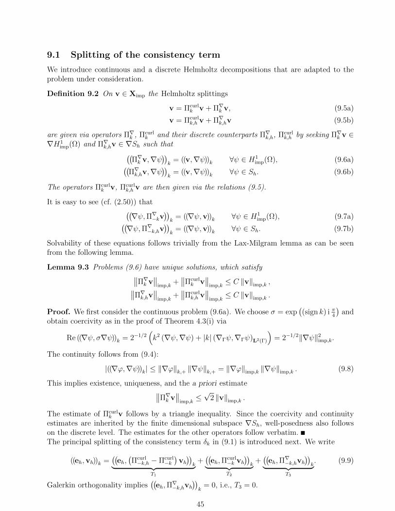
9.1 Splitting of the consistency term

We introduce continuous and a discrete Helmholtz decompositions that are adapted to theproblem under consideration.

Definition 9.2 On v ∈ Ximp the Helmholtz splittings

v = Πcurlk v + Π∇k v, (9.5a)

v = Πcurlk,h v + Π∇k,hv (9.5b)

are given via operators Π∇k , Πcurlk and their discrete counterparts Π∇k,h, Πcurl

k,h by seeking Π∇k v ∈∇H1

imp(Ω) and Π∇k,hv ∈ ∇Sh such that((Π∇k v,∇ψ

))k

= ((v,∇ψ))k ∀ψ ∈ H1imp(Ω), (9.6a)((

Π∇k,hv,∇ψ))k

= ((v,∇ψ))k ∀ψ ∈ Sh. (9.6b)

The operators Πcurlk v, Πcurl

k,h v are then given via the relations (9.5).

It is easy to see (cf. (2.50)) that((∇ψ,Π∇−kv

))k

= ((∇ψ,v))k ∀ψ ∈ H1imp(Ω), (9.7a)((

∇ψ,Π∇−k,hv))k

= ((∇ψ,v))k ∀ψ ∈ Sh. (9.7b)

Solvability of these equations follows trivially from the Lax-Milgram lemma as can be seenfrom the following lemma.

Lemma 9.3 Problems (9.6) have unique solutions, which satisfy∥∥Π∇k v∥∥

imp,k+∥∥Πcurl

k v∥∥

imp,k≤ C ‖v‖imp,k ,∥∥Π∇k,hv

∥∥imp,k

+∥∥Πcurl

k,h v∥∥

imp,k≤ C ‖v‖imp,k .

Proof. We first consider the continuous problem (9.6a). We choose σ = exp((sign k) i π

4

)and

obtain coercivity as in the proof of Theorem 4.3(i) via

Re ((∇ψ, σ∇ψ))k = 2−1/2(k2 (∇ψ,∇ψ) + |k| (∇Γψ,∇Γψ)L2(Γ)

)= 2−1/2‖∇ψ‖2

imp,k.

The continuity follows from (9.4):

|((∇ϕ,∇ψ))k| ≤ ‖∇ϕ‖k,+ ‖∇ψ‖k,+ = ‖∇ϕ‖imp,k ‖∇ψ‖imp,k . (9.8)

This implies existence, uniqueness, and the a priori estimate∥∥Π∇k v∥∥

imp,k≤√

2 ‖v‖imp,k .

The estimate of Πcurlk v follows by a triangle inequality. Since the coercivity and continuity

estimates are inherited by the finite dimensional subspace ∇Sh, well-posedness also followson the discrete level. The estimates for the other operators follow verbatim.The principal splitting of the consistency term δk in (9.1) is introduced next. We write

((eh,vh))k =((

eh,(Πcurl−k,h − Πcurl

−k)

vh))k︸ ︷︷ ︸

T1

+((

eh,Πcurl−k vh

))k︸ ︷︷ ︸

T2

+((

eh,Π∇−k,hvh

))k︸ ︷︷ ︸

T3

. (9.9)

Galerkin orthogonality implies((

eh,Π∇−k,hvh

))k

= 0, i.e., T3 = 0.

45

9.2 Consistency analysis: the term T1 in (9.9)

The continuity of the sesquilinear form ((·, ·))k (cf. (9.4)) implies

|T1| ≤ ‖eh‖k,+∥∥(Πcurl

−k,h − Πcurl−k)

vh∥∥k,+

. (9.10)

The definition of the discrete and continuous Helmholtz decomposition applied to a discretefunction vh leads to (cf. Def. 9.2, (9.7))((

∇ψh,(Πcurl−k,h − Πcurl

−k)

vh))k

= 0 ∀ψh ∈ Sh. (9.11)

We use (9.5) to get curl Πcurl−k = curl Πcurl

−k,h = curl on Xh and thus

curl(Πcurl−k,hvh − ΠE

h Πcurl−k vh

) Lem. 8.8(ii)= curl

(Πcurl−k,hvh

)− ΠF

h curl(Πcurl−k vh

)= curl vh − ΠF

h curl vhLem. 8.8(ii)

= curl vh − curl ΠEh vh

Lem. 8.8(i)= curl (vh − vh) = 0.

(9.12)

By the exact sequence property (8.8), the observation (9.12) implies that Πcurl−k,hvh−ΠE

h Πcurl−k vh =

∇ψh for some ψh ∈ Sh and(Πcurl−k,h − Πcurl

−k)vh = ∇ψh +

((ΠEh − I

)Πcurl−k)

vh. (9.13)

For the second factor in (9.10) we get by the Galerkin orthogonality (9.11) and (9.13)∥∥(Πcurl−k,h − Πcurl

−k)vh∥∥2

k,+= Re

((((ΠEh − I

)Πcurl−k)

vh,(Πcurl−k,h − Πcurl

−k)vh))k

+ (sign k) Im((((

ΠEh − I

)Πcurl−k)

vh,(Πcurl−k,h − Πcurl

−k)

vh))k

≤2∥∥((ΠE

h − I)

Πcurl−k)

vh∥∥k,+

∥∥(Πcurl−k,h − Πcurl

−k)

vh∥∥k,+

so that ∥∥(Πcurl−k,h − Πcurl

−k)vh∥∥k,+≤ 2

∥∥((ΠEh − I

)Πcurl−k)vh∥∥k,+

.

This leads to the estimate of T1

|T1| ≤ 2 ‖eh‖k,+∥∥(I − ΠE

h

)Πcurl−k vh

∥∥k,+

.

We set

ηalg6 := ηalg

6

(Xh,Π

Eh

):= sup

w∈V−k,0\0 :curlw∈curlXh

∥∥w − ΠEhw∥∥k,+

‖w‖H1(Ω)

(9.14)

and obtain

|T1| ≤ 2 ‖eh‖k,+ ηalg6

∥∥Πcurl−k vh

∥∥H1(Ω)

≤ 2C ‖eh‖k,+ ηalg6

∥∥Πcurl−k vh

∥∥imp,k

≤ C ‖eh‖k,+ ηalg6 ‖vh‖imp,k .

(9.15)

46

9.2.1 hp-Analysis of T1

In [32, (4.72)] it was proved that for our choice ΠEh := Πcurl,c

p with Πcurl,cp as in [31], [32, §8]

(see Lem. 8.8), one has

supw∈V−k,0\0 :curlw∈curlXh

|k|∥∥w − ΠE

hw∥∥

‖w‖H1(Ω)

≤ C|k|hp. (9.16)

For the boundary term in the norm ‖ · ‖k,+ we study the approximation properties of the

operator Πcurl,cp of [31] on the boundary of the reference tetrahedron K more carefully.

Lemma 9.4 Let Πcurl,3dp be the operator introduced in [31]. For all u ∈ H1(K) with curl u ∈(

Pp(K))3

, there holds with the tangential component operator ΠT,∂K∥∥∥ΠT,∂K

(u− Πcurl,3d

p u)∥∥∥

L2(∂K)≤ Cp−1/2 ‖u‖H1(K) .

Proof. We follow the proof of [31, Lem. 6.15] and employ the notation used there. From [31,proof of Lem. 6.15] and [31, (6.42)], we can decompose u = ∇ϕ+ v with

‖ϕ‖H2(K) + ‖v‖H1(K) ≤ C‖u‖H1(K). (9.17)

Since curl u ∈(Pp(K)

)3we have v − Πcurl,3d

p v = 0. We conclude

u− Πcurl,3dp u = v +∇ϕ− Πcurl,3d

p (v +∇ϕ) = ∇(ϕ− Πgrad,3dp+1 ϕ)

with Πgrad,3dp+1 as in [31]. The construction of the projection-based interpolation operators

Πcurl,3dp , Πgrad,3d

p is such that facewise, they reduce to corresponding 2D operators. That is, for

each face f ⊂ ∂K we have

ΠT,∂K

(u− Πcurl,3d

p u)∣∣∣

f= ΠT,∂K

(∇(ϕ− Πgrad,3d

p+1 ϕ))∣∣∣

f= ∇f

(I− Πgrad,2d

p+1

)(ϕ|f).

We apply [31, Thm. 2.13] to obtain∥∥∥ΠT,∂K

(u− Πcurl,3d

p u)∥∥∥

L2(f)=∥∥∥∇f

(I− Πgrad,2d

p+1

)(ϕ|f)∥∥∥

L2(f)≤ Cp−1/2 ‖ϕ‖H3/2(f)

≤ Cp−1/2 ‖ϕ‖H2(K)

(9.17)

≤ Cp−1/2 ‖u‖H1(K) .

For the boundary part of ‖w‖imp,k for w ∈ V−k,0 with curl w ∈ curl Xh, we get, by applyinga scaling argument to Lemma 9.4:

|k|∥∥ΠT

(w − ΠE

hw)∥∥2

L2(Γ)= |k|

∑K∈Th|K∩Γ|>0

∥∥ΠT

(w − ΠE

hw)∥∥2

L2(K∩Γ)(9.18)

≤ C|k|hp

∑K∈Th|K∩Γ|>0

‖w‖2H1(K) ≤ C

|k|hp‖w‖2

H1(Ω) .

The combination of (9.16) with (9.18) leads to

ηalg6 ≤ C

(|k|hp

)1/2(

1 +

(|k|hp

)1/2). (9.19)

47

9.3 Consistency analysis: the term T2 in (9.9)

Recall the definition of T2 = ((eh,v0))k for v0 := Πcurl−k vh. The function v0 belongs to Ximp

and by combining (9.5a) and (9.6a) we find that v0 belongs to V−k,0. Proposition 8.7 impliesv0 ∈ H1(Ω) and

‖v0‖H1(Ω) ≤ |k| ‖v0‖H1(Ω),k ≤ C ‖v0‖H(Ω,curl),k ≤ C ‖v0‖imp,k . (9.20)

The characterization (8.23) of V−k,0 implies

divΓ (v0)T = i k 〈v0,n〉 . (9.21)

To estimate the term T2 we consider the dual problem: Given v0 ∈ V−k,0, find z ∈ Ximp suchthat

Ak(w, z) = ((w,v0))k ∀w ∈ Ximp.

The operator N−k : V−k,0 → Ximp is defined by N−kv0 := z. The strong formulation is givenby

LΩ,−kz = k2v0 in Ω,B∂Ω,−kz = − i k (v0)T on Γ

(9.22)

and hence, N−kv0 := SMWΩ,−k (k2v0,− i k (v0)T ). By Galerkin orthogonality satisfied by eh, we

have for any wh ∈ Xh

|((eh,v0))k| = |Ak(eh,N−kv0 −wh)| ≤ ‖eh‖imp,k ‖N−kv0 −wh‖imp,k . (9.23)

We set

ηalg2 (Xh) := sup

v0∈V−k,0\0inf

wh∈Xh

‖N−kv0 −wh‖imp,k

‖v0‖imp,k

(9.24)

so that|T2| = |((eh,v0))k| ≤ ηalg

2 (Xh) ‖eh‖imp,k ‖v0‖imp,k . (9.25)

9.3.1 hp-Analysis of T2

Next, we estimate the approximation property ηalg2 (Xh). We employ the splitting given by

Theorem 7.3, viz.,N−kv0 = z = zH2 + zA + k−2∇ϕf − i k−1∇ϕg. (9.26)

Note that these four functions z, zH2 , zA, ϕf , ϕg depend on v0 but we suppress this in thenotation. From Theorem 7.3 with m = m′ = 1 we have

‖ϕf‖H2(Ω) ≤ Ck2‖ div v0‖L2(Ω)divv0=0

= 0,

‖ϕg‖H2(Ω) ≤ C|k|‖ divΓ(v0)T‖H−1/2(Γ) ≤ C|k|‖(v0)T‖H1/2(Γ)

(9.20)

≤ C|k|‖v0‖imp,k,

‖zH2‖H2(Ω) ≤ k2‖zH2‖H2(Ω),k

(7.10)

≤ Ck2|k|−3(‖k2v0‖H1(Ω) + |k|‖k(v0)T‖H1/2(Γ)

)(9.20)

≤ C|k|‖v0‖imp,k,

zA ∈ A(CCz, B,Ω),

Cz = |k|−2+max(0,θ+1)(‖k2v0‖+ |k|‖k(v0)T‖H−1/2(Γ)

)i k(v0)T=divΓ v0,(9.20)

≤ C|k|−1+max(0,θ+1)‖v0‖imp,k. (9.27)

48

We note that ϕf = 0. For the approximation of ∇ϕg, we use the elementwise defined operatorΠ∇,sp of Corollary 8.4 with m = 2 there to get

∥∥k−1(∇ϕg − Π∇,sp ∇ϕg

)∥∥imp,k

≤ C|k|−1

(|k|hp

+ |k|1/2(h

p

)1/2)‖ϕg‖H2(Ω)

≤ C

(|k|hp

)1/2

‖v0‖imp,k. (9.28)

For the approximation of zH2 , we employ the elementwise defined operator Πcurl,sp : H2(Ω)→

Xh as in Lemma 8.5. By summing over all elements the estimates of Lemma 8.5(i) we get∥∥zH2 − Πcurl,sp zH2

∥∥2

H(Ω,curl),k=∑K∈Th

∥∥zH2 − Πcurl,sp zH2

∥∥2

H(K,curl),k(9.29)

≤ C∑K∈Th

h2K

p2

(1 +

k2h2K

p2

)‖zH2‖2

H2(K) ≤ Ch2

p2

(1 +

k2h2

p2

)‖zH2‖2

H2(Ω)

≤ Ck2h2

p2

(1 +

k2h2

p2

)‖v0‖2

imp,k .

For the boundary part of the ‖·‖imp,k norm we proceed similarly with Lemma 8.5(i) to arriveat

|k|1/2‖zH2 − Πcurl,sp zH2‖L2(Γ) ≤ C|k|1/2

(h

p

)3/2

‖zH2‖H2(Ω) ≤ C

(|k|hp

)3/2

‖v0‖imp,k.

In summary, we have proved∥∥zH2 − Πcurl,sp zH2

∥∥imp,k

≤ Ch |k|p

(1 +

(h |k|p

)1/2

+h |k|p

)‖v0‖imp,k . (9.30)

Next, for the analytic part zA we get from Lemma 8.5(iii) in view of (9.27) under the (mild)resolution condition

h+|k|hp≤ C (9.31)

that

‖zA − Πcurl,sp zA‖imp,k ≤ CCz |k|

((h

h+ σ

)p+

(|k|hσp

)p)(9.32)

≤ C ‖v0‖imp,k |k|max(0,θ+1)

((h

h+ σ

)p+

(|k|hσp

)p).

This derivation is summarized in the following lemma.

Lemma 9.5 Assume hypothesis (3.2) and let Ω be a bounded Lipschitz domain with simplyconnected, analytic boundary. Assume the hypotheses on the mesh as in Assumption 8.1. Letc2, ε > 0 be given. Then there exists c1 > 0 (depending only on the constants of (3.2), Ω,the parameters of Assumption 8.1, and c2, ε) such that for h, k, p satisfying the resolutioncondition

|k|hp≤ c1 and p ≥ max 1, c2 ln |k| (9.33)

there holdsηalg

2 (Xh) ≤ ε. (9.34)

49

Proof. We combine (9.28), (9.30), and (9.32) with the resolution condition to arrive at

ηalg2 (Xh) ≤ C

((h |k|p

)1/2

+ |k|max(0,θ+1)

[(h

σ + h

)p+

(|k|hσp

)p]). (9.35)

Note that C in (9.35) is independent of ε. We fix ε′ := 2−max(0,θ+1)

2 max1,3C,εε so that 0 < ε′ <

2−max(0,θ+1) min ε, ε/ (3C) , 1. Let dΩ := diam Ω and choose p0 ≥ 1 such that

2max(0,θ+1)

(dΩ

σ + dΩ

)p0

<ε

3C

holds. Finally, let c1 be small enough such that 2max(0,θ+1)c1p0/σ ≤ ε′ < 1 and c1/21 < ε′ are

satisfied. In particular we then have |k|h/ (σp) < 1.We first consider the case 1 ≤ |k| ≤ 2. Then,

ηalg2 (Xh) ≤ C

(c

1/21 + 2max(0,θ+1)

[(h

σ + h

)p+(c1

σ

)p]).

Since σ > 0, the function x → xσ+x

is monotone increasing for x ∈ R>0. Since |k| ≥ 1, we

have 0 < h ≤ h := min c1p, dΩ and h/ (σ + h) ≤ h/(σ + h

). If p ≥ p0 we estimate

2max(0,θ+1)

(h

σ + h

)p≤ 2max(0,θ+1)

(dΩ

σ + dΩ

)p0

<ε

3C,

while for 1 ≤ p ≤ p0 it holds

2max(0,θ+1)

(h

σ + h

)p≤ 2max(0,θ+1) c1p0

σ< ε′ <

ε

3C.

Thus,

ηalg2 (Xh) < C

(c

1/21 +

ε

3C+ 2max(0,θ+1)

(c1

σ

)p)< ε′ +

ε

3C+ ε′ < ε.

It remains to consider the case |k| > 2. We employ [32, Lem. 8.7] to see that for any c2 > 0and given ε > 0, there exists some c1 > 0 such that the resolution condition (9.33) implies

|k|max(0,θ+1)

(h

σ + h

)p≤ ε′. (9.36)

For the last term in (9.35) we get

|k|max(0,θ+1)

(|k|hσp

)p= |k|max(0,θ+1) exp

(p ln

(|k|hσp

))≤ |k|max(0,θ+1)+c2 ln( |k|hσp ) ≤ |k|max(0,θ+1)+c2 ln(c1/σ) .

By choosing c1 sufficiently small (depending on θ, c2, and σ) we have max(0, θ + 1) +c2 ln (c1/σ) < 0 and

|k|max(0,θ+1)

(|k|hσp

)p≤ 2max(0,θ+1)+c2 ln(c1/σ) < ε/ (3C) , (9.37)

where the last inequality follows from taking c1 sufficiently small. Hence, we have proved

ηalg2 (Xh) ≤ C

(c

1/21 + ε′ +

ε

3C

)≤ C

(2ε′ +

ε

3C

)< ε, (9.38)

and this is (9.34).

50

9.4 h-p-k-explicit stability and convergence estimates for the Maxwellequation

We begin with the estimate of the consistency term δk.

Lemma 9.6 Let the assumptions in Lemma 9.5 hold. Let ε, c2 > 0 be given. Then, one canchoose a constant c1 > 0 sufficiently small such that the resolution condition (9.33) implies

δk(eh) ≤ ε.

Proof. Let v0 := Πcurl−k vh. We combine estimates (9.8), (9.9), (9.15), (9.19), (9.25), (9.34) in

a straightforward way to obtain

|((eh,vh))k| ≤ C(c

1/21 + c1 + ε

)‖eh‖imp,k ‖vh‖imp,k

and thus δk(eh) ≤ 2C(c1/21 + c1 + ε). We may assume that

√c1 ≤ ε ≤ 1 so that δk(eh) ≤ 6Cε.

Since the constant C > 0 does not depend on ε, the result follows by adjusting constants.This estimate allows us to formulate the quasi-optimality of the hp-FEM Galerkin discretiza-tion and to show h-p-k-explicit convergence rates under suitable regularity assumptions.

Theorem 9.7 Let Ω ⊂ R3 be a bounded Lipschitz domain with a simply connected, analyticboundary. Let the stability Assumption 3.2 be satisfied. Let the finite element mesh with meshsize h satisfy Assumption 8.1, and let Xh be defined by as the space of Nedelec-type-I elementsof degree p (cf. (8.7)).Then, for any j, gT satisfying (2.43), the variational Maxwell equation (2.44) has a uniquesolution E.For any fixed c2 > 0 and η ∈ (0, 1) one can select c1 > 0 (depending only on Ω and theconstants of (3.2) and Assumption 8.1) such that the resolution condition (9.33) implies thatthe discrete problem (8.9) has a unique solution Eh, which satisfies the quasi-optimal errorestimate

‖E− Eh‖imp,k ≤1 + η

1− ηinf

wh∈Xh

‖E−wh‖imp,k . (9.39)

Proof. Existence and uniqueness of the continuous variational Maxwell problem follow fromProposition 3.1. From Lemma 9.6 we know that c1 can be chosen sufficiently small such thatδ(eh) < η. As in the proof of Theorem [32, Thm. 4.15] (which goes back to [22, Thm. 3.9])existence, uniqueness, and quasi-optimality follows.The quasi-optimality result (9.39) leads to quantitative, k-explicit error estimates if a k-explicit regularity of the solution E is available. In the following corollary, we draw on theregularity assertions of Theorem 7.3. We point out, however, that due to our relying on theoperator Πcurl,s

p and the regularity assertion Theorem 7.3, the regularity requirements on thedata j, gT are not the weakest possible ones.

Corollary 9.8 Let the hypotheses of Theorem 9.7 be valid. Given η ∈ (0, 1) and c2 > 0let c1 be as in Theorem 9.7. Then, under the scale resolution condition (9.33) the following

51

holds: Let m, m′ ∈ N0 and (j,gT ) ∈ Hm(Ω) × Hm−1/2(Γ) together with (div j, divΓ gT ) ∈Hm′(Ω)×Hm′−1/2(Γ). If p ≥ max(m,m′ + 1), then

‖E− Eh‖imp,k ≤ C1 + η

1− η

Cj,g,m

(h

p

)m+ Cj,g,m′ |k|−3/2

(h

p

)m′+1/2

(9.40)

+ |k|Cj,g,A

((h

h+ σ

)p+

(|k|hσp

)p),

where

Cj,g,m := |k|−1‖j‖Hm(Ω) + ‖gT‖Hm−1/2(Γ), (9.41)

Cj,g,m′ := ‖ div j‖Hm′ (Ω) + |k|‖ divΓ gT‖Hm′−1/2(Γ), (9.42)

Cj,g,A := |k|−2+max0,θ+1 (‖j‖L2(Ω) + |k|‖gT‖H−1/2(Γ)

). (9.43)

Proof. For the error estimate (9.40), we employ the solution decomposition provided byThm. 7.3:

E = EH2 + EA + k−2∇ϕj + i k−1∇ϕg

with

‖EH2‖Hm+1(Ω) ≤ CCj,g,m,

‖ϕj‖Hm′+2(Ω) + |k|‖ϕg‖Hm′+2(Ω) ≤ CCj,g,m′ ,

EA ∈ A(CCj,g,A, B,Ω)

for k-independent constants C, B. With the operators Π∇,pp and Πcurl,sp of Corollary 8.4 and

Lemma 8.5 we get

‖EH2 − Πcurl,sp EH2‖imp,k ≤ CCj,g,m

((h

p

)m+ |k|

(h

p

)m+1

+ |k|1/2(h

p

)m+1/2)

≤ CCj,g,m

(h

p

)m,

k−2‖∇ϕj −∇Π∇,sp ϕj‖imp,k ≤ CCj,g,m′k−2

(|k|(h

p

)m′+1

+ |k|1/2(h

p

)m′+1/2)

≤ CCj,g,m′k−2|k|1/2

(h

p

)m′+1/2

,

|k|−1 ‖∇ϕg −∇Π∇,sp ϕg‖imp,k ≤ CCj,g,m′k−2|k|1/2

(h

p

)m′+1/2

,

‖EA − Πcurl,sp EA‖imp,k ≤ C|k|Cj,g,A

((h

h+ σ

)p+

(|k|hσp

)p).

52

DOF per wavelength

1 10 20 50 80

rel.

errorin

‖·‖curl+

k‖·‖

10-1

100

k=10

k=20

k=30

k=40

O(h)

DOF per wavelength

10 20 50

rel.

errorin

‖·‖curl+

k‖·‖

10-2

10-1

100

k=10

k=20

k=30

k=40

O(h 2 )

DOF per wavelength

10 20 50 80

rel.

errorin

‖·‖curl+

k‖·‖

10-4

10-2

100

k=10

k=20

k=30

k=40

O(h 3 )

Figure 10.1: Ω = (−1, 1)3, smooth solution; left to right: p ∈ 1, 2, 3

1 10 20 50

DOF per wavelength

10-1

100

k=20

k=40

k=80

O(h)

1 10 20 50

DOF per wavelength

10-2

10-1

100

k=20

k=40

k=80

O(h 2)

10 20 50

DOF per wavelength

10-2

100

k=20

k=40

k=80

O(h 3)

Figure 10.2: Ω = (−1, 1)3 \ [−1/2, 1/2]3, smooth solution; left to right: p ∈ 1, 2, 3

10 Numerical results

We illustrate the theoretical findings of Theorem 9.7 and Corollary 9.8 by two numericalexperiments. All computations are performed with NGSolve, [40, 41] using Nedelec type IIelements, i.e., full polynomial spaces. We show in Figs. 10.1, 10.2 the relative error in thenorm ‖ curl ·‖L2(Ω) + k‖ · ‖L2(Ω) ∼ ‖ · ‖H(Ω,curl),k versus the number of degrees of freedom perwavelength

Nλ =2πDOF1/3

|k||Ω|1/3,

where DOF stands for the dimension of the ansatz space.

Example 10.1 We consider Ω = (−1, 1)3 and impose the right-hand side and the impedanceboundary conditions such that the exact solution is E (x) = curl sin(kx1)(1, 1, 1)>. Fig. 10.1shows the performance for the choices k ∈ 10, 20, 30, 40 and p ∈ 1, 2, 3 as the mesh isrefined quasi-uniformly. The final problem sizes were DOF = 18, 609, 324 for p = 1, DOF =9, 017, 452 for p = 2, and DOF = 23, 052, 940 for p = 3.We observe the expected asymptotic O(hp) convergence. We also observe that the onset ofasymptotic quasi-optimal convergence is reached for smaller values of Nλ for higher ordermethods. This is expected in view of Theorem 9.7, although the present setting of a piecewiseanalytic geometry is not covered by Theorem 9.7.

Example 10.2 We consider Ω = (−1, 1)3\[−1/2, 1/2]3 and Maxwell’s equation with impedanceboundary conditions on ∂(−1, 1)3 and perfectly conducting boundary conditions on ∂(−1/2,−1/2)3.We prescribe the exact solution E (x) = k cos(kx1)(x2

1 − 1/4)(x22 − 1/4)(x2

3 − 1/4)(0,−1, 1)>.Fig. 10.2 shows the performance for the choices k ∈ 20, 40, 80 and p ∈ 1, 2, 3 as the

53

mesh is refined quasi-uniformly. The final problem sizes were DOF = 43, 598, 374 for p = 1,DOF = 168, 035, 046 for p = 2, and DOF = 54, 063, 558 for p = 3.We observe the expected asymptotic O(hp) convergence. We also observe that the onset ofasymptotic quasi-optimal convergence is reached for smaller values of Nλ for higher ordermethods.

A Analytic regularity with bounds explicit in the wavenum-

ber ( [39, 45] revisited)

In this appendix, we reproduce [39, Appendix A] and add parts (marked in red color that arerequired to account for the addition of right-hand sides in Theorem 5.2. We will also followthe numbering in [39, Appendix A] and indicate insertions by “+1/2”, “+1/3” etc.To be consistent with [39], we follow in this appendix the “French” convention and denote

N = 0, 1, 2, . . . and N∗ = 1, 2, . . ..

Furthermore, we assume as in [39] that k ≥ k0 > 0, while the estimates for negative k ≤ −k0 <0 follow by replacing k by |k| in all estimates. For a bounded open set ω, the seminorms | · |p,ωare defined by

|u|2p,ω =∑

α∈Nn : |α|=p

|α|!α!‖∂αu‖2

L2(ω), ‖u‖2p,ω =

p∑l=0

|u|2l,ω. (A.0)

We assume that f is an analytic function satisfying

|f |p,Ω ≤ Cfλpf max(p, k)p ∀p ∈ N. (A.1)

Additionally, given a tubular neighborhood T of ∂Ω and (analytic) functions GD : T → CN1

GB : T → CN0 that satisfy

‖GD‖p,T ≤ CgDλpgD

max(p, k)p ∀p ∈ N, (A.1+1/3)

‖GB‖p,T ≤ CgBλpgB

max(p, k)p ∀p ∈ N. (A.1+2/3)

We consider the two traces gD := γGD and gB := γGB. Then, we can formulate in analogyto [39, Thm. A.1]

Theorem A.1 Let Ω ⊂ Rn, n ≤ 3, be a bounded domain with an analytic boundary ∂Ω,and let (L,D,B) be an elliptic system in the sense of [13, Def. 2.2.31, Def. 2.2.33] with L(resp. D and B) an N×N (resp. N0×N and N1×N with N0, N1 ∈ N such that N0 +N1 = N)system of differential operators of order 2 (resp. 0 and 1) with analytic coefficients, N ∈ N∗and k > 1. Let f , gD, gB be analytic functions verifying (A.1) and (A.1+1/3), (A.1+2/3)and G a matrix with analytic coefficients (in a tubular neighborhood of ∂Ω) . If u∈ H2(Ω)

is a solution of L(u) = f + k2u in Ω,D(u) = gD on ∂Ω,B(u) = kGu+gB on ∂Ω,

(A.2)

54

then we have|u|p,Ω ≤ CuK

p max(p, k)p, ∀p ∈ N, p ≥ 2

with Cu = (k−2Cf + CgD + k−1CgB+‖u‖Ω + k−1‖u‖1,Ω).

Remark A.1+1/3 The point of Theorem A.1 is the tracking of the k-dependence. The keyingredient of the proof below is the appeal to [13, Prop. 2.6.6] and [13, Prop. 2.6.7], which inturn rely on

(a) local H2-estimates of the form [13, (2.47)]. These local H2-estimates result from theellipticity of the operator L and the covering condition of the boundary conditions (cf. [13,Cor. 2.2.16]);

(b) the condition [13, (2.50)]. Condition [13, (2.50)] is satisfied by the ellipticity of the oper-ator L (see footnote 3 in [13, p. 97]).

Example A.1+2/3 We transform the problem

curl curl E− k2E = f in Ω, (A.2+1/5)

γT curl E− i kET = gT on ∂Ω, (A.2+2/5)

for sufficiently smooth f , gT to the form considered in Theorem A.1. We proceed as in [39] andwrite the Maxwell equations as a first order system for the electric field E and the magneticfield H := − i

kcurl E and set u = (E,H). The function u solves the elliptic system

L (u) :=

(curl curl E−∇ div Ecurl curl H−∇ div H

)= F + k2u in Ω,

D (u) := H× n− ET = − ikgT on Γ,

B (u) :=

div Ediv H

γT curl H + (curl E)T

= kGu + GΓ on Γ

(A.2+3/5)

for

F :=

(f + 1

k2∇ div f− ik

curl f

), Gu :=

00

i (HT − γTE)

, GΓ :=

− 1k2 (div f)|Γ

0− ikγT f

.

(A.2+4/5)Elliptic systems of the form (A.2+3/5) are considered in [39, Thm. A1] for gT = GΓ = 0.We now show that (A.2+3/5) is indeed an elliptic system in the sense of [13, Def. 2.2.31]. Theoperator L is simply the block Laplacian since curl curl = ∇ div−∆ and clearly elliptic. To seethat the boundary conditions are covering at a boundary point x0, we first consider the system(A.2+3/5) in a half space x3 > 0 with boundary x3 = 0. We assume that x0 = (0, 0, 0)>.The principal part Lpr of L coincides with L. In the notation of [13, Notation 2.2.1], thespaces M[L; ξ′] and M+[L; ξ′] (with ξ′ ∈ R2) can be computed explicitly due to the simplestructure of L:

M[L; ξ′] = u(t) = ηe−|ξ′|t + βe|ξ

′|t |η,β ∈ C6,

M+[L; ξ′] = u(t) = ηe−|ξ′|t |η ∈ C6.

55

In particular, the operator L is properly elliptic, [13, Def. 2.2.3]. The boundary operators

are obtained by inserting u(x′, t) = eix′·ξ′e−|ξ′|tη into the boundary conditions and afterwards

removing the factor eix′·ξ′ and setting (x′, t) = (0, 0, 0) = x0, which gives

D(u) =

(η5 − η1

−η4 − η2

)

B(u) =

i ξ′1η1 + i ξ′2η2 − |ξ′|η3

i ξ′1η4 + i ξ′2η5 − |ξ′|η6

− i ξ′1η6 − |ξ′|η4 + i ξ′2η3 + |ξ′|η2

− i ξ′2η6 − |ξ′|η5 − i ξ′1η3 − |ξ′|η1

.

In matrix form, we have−1 0 0 0 1 00 −1 0 −1 0 0

i ξ′1 i ξ′2 −|ξ′| 0 0 00 0 0 i ξ′1 i ξ′2 −|ξ′|0 |ξ′| i ξ′2 −|ξ′| 0 − i ξ′1−|ξ′| 0 − i ξ′1 0 −|ξ′| − i ξ′2

︸ ︷︷ ︸

=:M

η1

η2

η3

η4

η5

η6

.

A direct calculation shows det M = |ξ′|4. Hence, M is invertible for every ξ′ 6= 0. Thismeans that the set of boundary conditions satisfies the covering condition. According to [13,Def. 2.2.31], this covering condition has to be satisfied for every x0 ∈ ∂Ω and the “tangent”model system. Locally flattening the boundary at x0 in such a way that the Jacobian is orthog-onal at x0 leads to “tangent” systems that are of the same form as above. Hence, the system(A.2+3/5) is elliptic.While [39, Cor. A.2] focuses on the regularity of u, we formulate the following corollarydifferently by giving a regularity assertion for for E.

Corollary A.2 Let Ω ⊂ R3 be a bounded domain with an analytic boundary. Let the functionf satisfy (A.1). Let the function g : T → C3 satisfy for a tubular neighborhood T of ∂Ω

|g|p,T ≤ Cgλpg max(p, k)p, ∀p ∈ N.

Let E ∈ H2(Ω, curl) solve (A.2+1/5), (A.2+2/5). Then, we have

|E|p,Ω ≤ CEKp max(p, k)p ∀p ∈ N, p ≥ 2,

where, for some C, K > 0 independent of k,

CE = C

(Cfk

−2 + |k|−1Cg +1

|k|‖E‖H1(Ω,curl),k

).

Proof. We note that the analyticity of ∂Ω implies that the normal vector n has an analyticextension n? to a tubular neighborhood of ∂Ω. Since the operators γT , ΠT have the form

56

γTv = γ(v × n?), ΠTv = γ(n? × (v × n?)), we see that Gu and GΓ of (A.2+4/5) can bewritten as

Gu = γGu, GΓ = γGΓ, GΓ :=

− 1k2 div f

0− ikf × n?

,

where the matrix-valued function G is analytic in a tubular neighborhood of ∂Ω. Likewise,the boundary data gT = γ(n? × (g × n?)) = γg for some g that is analytic in a tubular

neighborhood of ∂Ω. By, e.g., [32, Lemma 2.6], we get by setting GB := GΓ, GD := − i k−1g

for suitable Kf , λg independent of k

‖F‖p,Ω ≤ CCfKpf max(p, k)p, ∀p ∈ N,

‖GB‖p,Ω ≤ k−1CCfKpf max(p, k)p, ∀p ∈ N,

‖GD‖p,Ω ≤ k−1CCgλpg max(p, k)p, ∀p ∈ N.

We may apply Theorem A.1 with G = G and F given by (A.2+3/5). To that end, we observethat the regularity assumption E ∈ H2(Ω, curl) implies u = (E,H) =

(E,− i

kcurl E

)∈ H2 (Ω)

so that Thm. A.1 is indeed applicable.

Remark A.3 See [39, Rem. A.3].

A.1 Analytic regularity near the boundary

Denote B+R = BR(0, R) ∩ x|xn > 0 and ΓR = x ∈ B+

R |xn = 0, with R ∈ (0, 1]. Weemphasize that in the following developments, most estimates will not be sharp in theirdependence on R.

Let f be an analytic function and G be a matrix with analytic coefficients defined on B+R such

that

‖∂αf‖B+R≤ Cfλ

|α|f max(|α|, k)|α| ∀α ∈ Nn, (A.3)

‖∂αG‖∞,B+R≤ CGλ

|α|G max(|α|, k)|α| ∀α ∈ Nn (A.4)

as well as the functions gD := GD|ΓR and gB := GB|ΓR with

‖∂αGD‖B+R≤ CgDλ

|α|gD

max(|α|, k)|α| ∀α ∈ Nn, (A.4+1/3)

‖∂αGB‖B+R≤ CgBλ

|α|gB

max(|α|, k)|α| ∀α ∈ Nn (A.4+2/3)

for some k ≥ 1 for some positive constants Cf , λf , CG, λG, CgD , λgD , CgB , λgB . Letu ∈ H2(B+

R) be a solution of L(u) = f + k2u in B+

R ,D(u) = gD on ΓR,B(u) = kGu+gB on ΓR,

(A.5)

57

where (L,D,B) is an elliptic system with analytic coefficients (in the sense above), with D(resp. B) an operator of order 0 (resp. 1). For further purposes, we define a few norms6

|u|p,q,B+R

:= max|α|=pαn≤q

‖∂αu‖B+R,

[[u]]p,q,B+R

:= max0≤ρ≤R/(2p)

ρp|u|p,q,B+R−pρ

, for all p > 0,

[[u]]0,0,B+R

:= ‖u‖B+R,

ρ2∗[[u]]p,q,B+

R:= max

0≤ρ≤R/(2(p+1))ρp+2|u|p,q,B+

R−(p+1)ρ,

|u|p, 12,ΓR

:= maxα′∈Nn−1 : |α′|=p

‖∂α′u‖ 12,ΓR,

ρ32∗ [[u]]p, 1

2,ΓR

:= max0≤ρ≤R/(2(p+1))

ρp+32 |u|p, 1

2,ΓR−(p+1)ρ

,

|u|p, 32,ΓR

:= maxα′∈Nn−1 : |α′|=p

‖∂α′u‖ 32,ΓR,

ρ12∗ [[u]]p, 3

2,ΓR

:= max0≤ρ≤R/(2(p+1))

ρ12

+p|u|p, 32,ΓR−(p+1)ρ)

,

for all p, q ∈ N with q ≤ p.We will first estimate the norm of the tangential derivatives (and the normal derivative upto 2) by using the standard analytic regularity of elliptic systems. Then, we will be able toestimate the complete norm [[u]]p,q,B+

R. So we start with an estimation of the norm of tangential

derivatives [[u]]p,2,B+R

. Before, let us prove the next technical results that allow to pass from a

sum on the multi-indices to a sum on their lengths.

Lemma A.4 Let h be a mapping from N into [0,∞) and a multi-index α′ ∈ Nn−1, for n = 2or n = 3. Then we have ∑

β′∈Nn−1 : β′≤α′h(|β′|) ≤ 2

|α′|∑p=0

h(p)e|α′|−p. (A.6)

Proof. See [39, Lemma A.4].

Corollary A.5 Let h be a mapping from N into [0,∞) and a multi-index α ∈ Nn with αn ≤ 1.Then we have ∑

β∈Nn : β≤α

h(|β|) ≤ 2(1 +1

e)

|α|∑p=0

h(p)e|α|−p. (A.8)

Proof. See [39, Cor. A.5].

Lemma A.6 There exists a positive constant C (depending on n), a positive constant Ctr,R(depending only on R ≤ 1), and a positive constant λ′G ≥ λG such that for all l ∈ N and anyu ∈ Hl+1(B+

R), we have

ρ32∗ [[Gu]]l, 1

2,ΓR≤ CCtr,RCG

l+1∑p=0

(λ′G)l+1−p max(l + 1, k)l+1−p[[u]]p,2,B+R. (A.9)

6cf. [13, Notation 2.6.5] and [13, Notation 2.5.1]

58

Additionally, the constant Ctr,R may be assumed to satisfy the trace estimate

‖v‖ 12,ΓR≤ Ctr,R‖v‖1,B+

R∀v ∈ H1(B+

R).

Proof. See [39, Lemma A.6].Noting the trace estimate (cf. [39, (A.10)]), we obtain from (A.4+1/3), (A.4+2/3) for thetraces gD and gB for suitable C ′tr,R

ρ12∗ [[gD]]l, 3

2,ΓR≤ C ′tr,R

[[[GD]]l,0,B+

R+ [[GD]]l+2,2,B+

R

](A.13+1/4)

(A.4+1/3)

≤ 2C ′tr,RCgDλl+2gD

max(l + 2, k)l+2,

ρ32∗ [[gB]]l, 1

2,ΓR≤ Ctr,R

[[[GB]]l,0,B+

R+ [[GB]]l+1,1,B+

R

](A.13+1/2)

(A.4+2/3)

≤ 2Ctr,RCgBλl+1gB

max(l + 2, k)l+1,

‖v‖ 32,ΓR≤ C ′tr,R‖v‖2,B+

R∀v ∈ H2(B+

R). (A.13+3/4)

Here, we have implicitly assumed λgD ≥ 1 and λgB ≥ 1. We also emphasize that the constantsCtr,R and C ′tr,R depend on R, which could be tracked by a more careful application of the traceestimates.

Lemma A.7 Let u ∈ H2(B+R) be a solution of (A.5) with f , gD, gB, G analytic and satis-

fying (A.3)—(A.4+2/3). Then there exist K > 1 and CR > 1 such that for all p ≥ 2

[[u]]p,2,B+R≤ Cu(B+

R)Kp max(p, k)p

with Cu(B+R) = CR(Cfk

−2 + CgD + k−1CgB + ‖u‖B+R

+ k−1‖u‖1,B+R

).

Proof. We will prove this result by induction, by applying a standard analytic regularityresult (i.e., [13, Prop. 2.6.6]), which gives us a real number A ≥ 1 such that for all p ≥ 2

[[u]]p,2,B+R≤

p−2∑l=0

Ap−1−l(ρ2∗[[L(u)]]l,0,B+

R+ ρ

32∗ [[B(u)]]l, 1

2,ΓR

+ ρ12∗ [[D(u)]]l, 3

2,ΓR

)+Ap−1

1∑l=0

[[u]]l,l,B+R.

(A.14)Initialization: For p = 2, by (A.14) we have

[[u]]2,2,B+R≤ A

(ρ2∗[[L(u)]]0,0,B+

R+ ρ

32∗ [[B(u)]]0, 1

2,ΓR

+ρ12∗ [[D(u)]]0, 3

2,ΓR

)+ A

1∑l=0

[[u]]l,l,B+R

≤ A(ρ2∗[[f + k2u]]0,0,B+

R+ ρ

32∗ [[kGu+gB]]0, 1

2,ΓR

+ρ12∗ [[gD]]0, 3

2,ΓR

)+ A

1∑l=0

[[u]]l,l,B+R

R≤1

≤ A(‖f‖B+

R+ k2‖u‖B+

R+ k‖Gu‖ 1

2,ΓR

+‖gB‖ 12,ΓR

+‖gD‖ 32,ΓR

)+ A

1∑l=0

[[u]]l,l,B+R

(A.13+1/4),(A.13+1/2)

≤ A(‖f‖B+

R+ (k2 + 1)‖u‖B+

R+ kCtr,R‖Gu‖1,B+

R+Ctr,R‖GB‖1,B+

R

+C ′tr,R‖GD‖2,B+R

+ ‖u‖1,B+R

)59

with the constants Ctr,R, C ′tr,R introduced before. By noticing that

kCtr,R‖Gu‖1,B+R≤ CkCtr,RCG

(‖u‖1,B+

R+ λG‖u‖B+

R

),

‖GB‖1,B+R≤ CCgBλgBk,

‖GD‖2,B+R≤ CCgDλ

2gDk2

we then have

[[u]]2,2,B+R≤ A

(‖f‖B+

R+ (k2 + 1 + CCtr,RCGλGk)‖u‖B+

R+ (CCtr,RCGk + 1)‖u‖1,B+

R

)+A(CCtr,RCgBkλgB + CC ′tr,RCgDk

2λ2gD

)≤ Ak2

[k−2Cf+k

−1CCtr,RCgBλgB + CC ′tr,RCgDλ2gD

+

(2 + CCtr,RCGλGk−1)‖u‖B+

R+ (CCtr,RCG + k−1)k−1‖u‖1,B+

R

]≤ Ak2 max(2 + CCtr,RCGk

−1λG, CCtr,RCG + k−1, CCtr,RλgB , CC′tr,Rλ

2gD

)×(Cfk

−2 + k−1CgB + CgD + ‖u‖B+R

+ k−1‖u‖1,B+R

)≤ CRCu(B+

R) max(2, k)2 ≤ Cu(B+R)K2 max(2, k)2,

with CR ≥ Amax(2 +CCtr,RCGk−1λG, CCtr,RCG + k−1, CCtr,RλgB , CC

′tr,Rλ

2gD

) ≥ 1 and sinceK ≥ 1.Induction hypothesis: For all 2 ≤ p′ ≤ p, we have

[[u]]p′,2,B+R≤ Cu(B+

R)Kp′ max(p′, k)p′. (A.15)

We will show this estimate for p+ 1: Using (A.14), we may write

[[u]]p+1,2,B+R≤

p−1∑l=0

Ap−l(ρ2∗[[L(u)]]l,0,B+

R+ ρ

32∗ [[B(u)]]l, 1

2,ΓR

+ ρ12∗ [[D(u)]]l, 3

2,ΓR

)+ Ap

1∑l=0

[[u]]l,l,B+R.

(A.16)We now need to estimate each term of this right-hand side. We start by estimating ρ2

∗[[L(u)]]l,0,B+R

for l ≤ p− 1: First we notice that

ρ2∗[[L(u)]]l,0,B+

R

R≤1

≤ [[f + k2u]]l,0,B+R≤ [[f ]]l,0,B+

R+ k2[[u]]l,2,B+

R.

By the induction hypothesis (A.15), we then have

ρ2∗[[L(u)]]l,0,B+

R≤ Cfλ

lf max(l, k)l + k2Cu(B+

R)K l max(l, k)l

≤ k2 max(l, k)lCu(B+R)K l

(λlfK l

+ 1

).

As l + 2 ≤ p+ 1, this estimate directly implies that

ρ2∗[[L(u)]]l,0,B+

R≤ max(p+ 1, k)p+1Cu(B+

R)K l

((λlfK

)l+ 1

)≤ 2 max(p+ 1, k)p+1Cu(B+

R)K l,

60

for K > λf . Multiplying this estimate by Ap−l and summing on l, one gets

p−1∑l=0

Ap−lρ2∗[[L(u)]]l,0,B+

R≤ Cu(B+

R)Kp+1 max(p+ 1, k)p+1 2

K

p−1∑l=0

Ap−lK l−p

≤ Cu(B+R)Kp+1 max(p+ 1, k)p+1 2

K

p−1∑l=0

(A

K

)p−l.

If K ≥ 2A, then∑p−1

l=0 (AK

)p−l ≤∑∞

l=1(AK

)l ≤ 1, which yields

p−1∑l=0

Ap−lρ2∗[[L(u)]]l,0,B+

R≤ Cu(B+

R)Kp+1 max(p+ 1, k)p+1 2

K. (A.17)

Estimation of ρ32∗ [[B(u)]]l, 1

2,ΓR

: By the boundary condition on u, we have

ρ32∗ [[B(u)]]l, 1

2,ΓR≤ kρ

32∗ [[Gu]]l, 1

2,ΓR

+ρ32∗ [[gB]]l, 1

2,ΓR

and by the estimate (A.9) and (A.13+1/2) , we get

ρ32∗ [[B(u)]]l, 1

2,ΓR≤ kCCtr,RCG

l+1∑p′=0

(λ′G)l+1−p′ max(l + 1, k)l+1−p′ [[u]]p′,2,B+R

(A.18)

+2Ctr,RCgBλl+1gB

max(l + 2, k)l+1 =: I + II.

For the first term, I, the induction hypothesis (A.15) then leads to

I ≤ kCCtr,RCGCu(B+R)

l+1∑p′=0

(λ′G)l+1−p′Kp′ max(l + 1, k)l+1−p′ max(p′, k)p′

≤ kCCtr,RCGCu(B+R) max(l + 1, k)l+1K l+1

l+1∑p′=0

(λ′GK

)l+1−p′

.

Hence, for K ≥ 2λ′G and K ≥ λgB (recalling that l+2 ≤ p+1 and that∑l+1

p′=0

(λ′GK

)l+1−p′≤ 2),

we deduce

ρ32∗ [[B(u)]]l, 1

2,ΓR≤ I + II ≤ 2CCtrCGCu(B+

R)K l+1 max(p+ 1, k)p+1

+2Ctr,Rk−1CgBλ

l+1gB

max(l + 2, k)l+1

≤ 2Ctr,R(CCG+1)Cu(B+R)K l+1 max(p+ 1, k)p+1.

Multiplying this estimate byAp−l and summing on l, we get

p−1∑l=0

Ap−lρ32∗ [[B(u)]]l, 1

2,ΓR≤ Cu(B+

R)Kp+1 max(p+ 1, k)p+12Ctr,R(CCG+1)

p−1∑l=0

Ap−lK l−p

≤ Cu(B+R)Kp+1 max(p+ 1, k)p+12Ctr,R(CCG+1)

A

K

∞∑l=0

(A

K

)l.

61

Again, for K ≥ 2A, we arrive at

p−1∑l=0

Ap−lρ32∗ [[B(u)]]l, 1

2,ΓR≤ Cu(B+

R)Kp+1 max(p+ 1, k)p+1 4Ctr,R(CCG+1)A

K. (A.19)

Estimation of ρ12∗ [[D(u)]]l, 3

2,ΓR

:

ρ12∗ [[D(u)]]l, 3

2,ΓR

= ρ12∗ [[gD]]l, 3

2,ΓR

(A.13+1/4)

≤ 2C ′tr,RCgDλl+2gD

max(l + 2, k)l+2

l+2≤p+1

≤ 2C ′tr,RCgDλl+2gD

max(p+ 1, k)p+1.

Multiplying this estimate by Ap−l and summing on l, we get for K ≥ λgD and K ≥ 2A

p−1∑l=0

Ap−lρ12∗ [[D(u)]]l, 3

2,ΓR≤ CgD max(p+ 1, k)p+12C ′tr,Rλ

2gD

p−1∑l=0

Ap−lλlgD

λgD≤K≤ CgD max(p+ 1, k)p+12C ′tr,Rλ

2gD

p−1∑l=0

Ap−lK l

≤ CgD max(p+ 1, k)p+12C ′tr,Rλ2gDKp

p−1∑l=0

Ap−lK l−p

≤ CgD max(p+ 1, k)p+12C ′tr,Rλ2gDKp A

K

∞∑l=0

(A

K

)l≤ CgD max(p+ 1, k)p+1Kp+1

4C ′tr,RAλ2gD

K2

≤ Cu(B+R) max(p+ 1, k)p+1Kp+1

4C ′tr,RAλ2gD

K2. (A.19+1/3)

Finally using the definition Cu(B+R), we directly check that

1∑l=0

[[u]]l,l,B+R≤ k

CRCu(B+

R) (A.19+2/3)

and therefore (since we assume that K ≥ 2A)

Ap1∑l=0

[[u]]l,l,B+R≤ 1

CRCu(B+

R)Kp max(p+ 1, k)p+1.

In summary, using this estimate (A.17), (A.19), and (A.19+1/3), in (A.16) we have obtained

[[u]]p+1,2,B+R≤ Cu(B+

R)Kp+1 max(p+ 1, k)p+1

(2 + 4Ctr,R(CCG+1)A+ 1

CR

K+

4C ′tr,RAλ2gD

K2

).

This yields (A.15) for p+ 1 if

K ≥ max

(λf , λgD , 2A, λ

′G, 2 + 4Ctr,R(CCG + 1)A+

1

CR+ 4C ′tr,Rλ

2gDA

).

62

Now, we will show an equivalent lemma but which also estimates the norm of the normalderivatives of higher order.

Lemma A.8 Let u ∈ H2(B+R) be a solution of (A.5) with f , G, GD, and GB analytic and

satisfying (A.3), (A.4), (A.4+1/3), (A.4+2/3). Then there exist K1, K2 ≥ 1 such that forall p, q ≥ 2 with q ≤ p, we have

[[u]]p,q,B+R≤ Cu(B+

R)Kp1K

q2 max(p, k)p,

with Cu(B+R) = CR

(Cfk

−2 + k−1CgB + CgD + ‖u‖B+R

+ k−1‖u‖1,B+R

).

Proof. Again, we will show this lemma by induction and by using a standard analyticregularity result for elliptic problems (i.e., [13, Prop. 2.6.7]), which gives us

[[u]]p,q,B+R≤

p−2∑l=0

Ap−1−l

min(l,q−2)∑

ν=0

Bq−1−νρ2∗[[L(u)]]l,ν,B+

R+Bq−1

(ρ

32∗ [[B(u)]]l, 1

2,ΓR

+ρ12∗ [[D(u)]]l, 3

2,ΓR

)+ Ap−1Bq−1

1∑l=0

[[u]]l,l,B+R

(A.21)

for some positive constants A and B ≥ 1. The induction is done on q, the initialization stepq = 2 is obtained from Lemma A.7 by taking K1 ≥ K and K2 ≥ 1. The induction hypothesisis: For all p ≥ 3, 2 ≤ q′ ≤ p− 1, it holds

[[u]]p,q′,B+R≤ Cu(B+

R)Kp1K

q′

2 max(p, k)p. (A.22)

We use the estimate (A.21) to get

[[u]]p,q+1,B+R≤

p−2∑l=0

Ap−1−l

min(l,q−1)∑

ν=0

Bq−νρ2∗[[L(u)]]l,ν,B+

R+Bqρ

32∗ [[B(u)]]l, 1

2,ΓR

+Bqρ12∗ [[D(u)]]l, 3

2,ΓR

+ Ap−1Bq

1∑l=0

[[u]]l,l,B+R. (A.23)

Estimate of ρ2∗[[L(u)]]l,ν,B+

R. By the induction hypothesis (A.22) we may write

ρ2∗[[L(u)]]l,ν,B+

R≤ [[f ]]l,ν,B+

R+ k2[[u]]l,ν,B+

R

≤ Cfλlf max(l, k)l + k2Cu(B+

R)K l1K

ν2 max(l, k)l

≤ Cu(B+R)K l

1Kν2k

2 max(l, k)l

((λfK1

)l1

Kν2

+ 1

)l≤p−2

≤ Cu(B+R)Kp

1Kq+12 max(p, k)p

2

K1K2

K l−p+11 Kν−q

2

63

if K1 ≥ λf . Multiplying this estimate by Ap−1−lBq−ν and summing on ν and l, one gets

p−2∑l=0

Ap−1−lmin(l,q−1)∑

ν=0

Bq−νρ2∗[[L(u)]]l,ν,B+

R

≤ Cu(B+R)Kp

1Kq+12 max(p, k)p

2

K1K2

p−2∑l=0

Ap−1−lmin(l,q−1)∑

ν=0

Bq−νK l−p+11 Kν−q

2

≤ Cu(B+R)Kp

1Kq+12 max(p, k)p

2

K1K2

p−2∑l=0

(A

K1

)p−1−l min(l,q−1)∑ν=0

(B

K2

)q−ν.

Choosing K1 ≥ 2A and K2 ≥ 2B, we conclude that

p−2∑l=0

Ap−1−lmin(l,q−1)∑

ν=0

Bq−νρ2∗[[L(u)]]l,ν,B+

R≤ Cu(B+

R)Kp1K

q+12 max(p, k)p

8

K1K2

. (A.24)

Estimation of ρ32∗ [[B(u)]]l, 1

2,ΓR

for l ≤ p − 2: We use the estimate (A.9) and the induction

hypothesis (A.22) and (A.13+1/2) to get

ρ32∗ [[B(u)]]l, 1

2,ΓR≤ ρ

32∗ [[kGu]]l, 1

2,ΓR

+ ρ32∗ [[gB]]l, 1

2,ΓR

≤ kCCtr,RCGCu(B+R)K2

2

l+1∑p′=0

(λ′G)l+1−p′Kp′

1 max(l + 1, k)l+1−p′ max(p′, k)p′

+2Ctr,RCgBλl+1gB

max(l + 2, k)l+1.

In the above right-hand side as l + 2 ≤ p and p′ ≤ p− 1, we obtain

ρ32∗ [[B(u)]]l, 1

2,ΓR≤ CCtr,RCGCu(B+

R)K22 max(p, k)pK l+1

1

l+1∑p′=0

(λ′GK1

)l+1−p′

+2Ctr,Rk−1CgBλ

l+1gB

max(p, k)p.

For K1 ≥ 2λ′G and K1 ≥ λgB we deduce that

ρ32∗ [[B(u)]]l, 1

2,ΓR≤ 2Ctr,RCu(B+

R)(CCGK22 + 1) max(p, k)pK l+1

1 . (A.25)

Multiplying this estimate by Ap−1−lBq and summing on l, as before one gets (since K1 ≥ 2Aand K2 ≥ B )

p−2∑l=0

Ap−1−lBqρ32∗ [[B(u)]]l, 1

2,ΓR≤ Cu(B+

R)Kp1B

q max(p, k)p2Ctr,R(CCGK22 + 1)

p−2∑l=0

Ap−1−lK l+11 K−p1

K2≥B≤ Cu(B+

R)Kp1K

q+12 max(p, k)p

(4Ctr,RA(CCGK

22 + 1)

K1K2

).

64

Estimation of ρ12∗ [[D(u)]]l, 3

2,ΓR

: From (A.13+1/4) and l + 2 ≤ p we have

ρ12∗ [[D(u)]]l, 3

2,ΓR≤ 2C ′tr,RCgDλ

l+2gD

max(l + 2, k)l+2

≤ Cu(B+R)2C ′tr,Rλ

pgD

max(p, k)p. (A.25+1/2)

Finally, using (A.19+2/3), one has

Ap−1Bq

1∑l=0

[[u]]l,l,B+R≤ Cu(B+

R)Kp1K

q+12 max(p, k)p

1

CRK1K2

.

Inserting this estimate and the estimates (A.24), (A.25), (A.25+1/2) into (A.16), we canconclude that

[[u]]p,q+1,B+R≤ Cu(B+

R)Kp1K

q+12 max(p, k)p

(8

K1K2

+4Ctr,RA(CCGK

22 + 1)

K1K2

+1

CRK1K2

+2C ′tr,R

Kq+12

(λgDK1

)p)≤ Cu(B+

R)Kp1K

q+12 max(p, k)p

for K1 and K2 large enough.

Remark A.9 In Lemma A.8, if we take p = q, we obtain

[[u]]p,p,B+R≤ Cu(B+

R)Kp max(p, k)p

with K = K1K2.

A.2 Interior analytic regularity

Let BR = B(0, R), L an elliptic system of order 2 defined in BR, and k > 1. Here, we considera solution u of

L(u) = f + k2u in BR. (A.26)

We now define the following semi-norms

[[u]]p,BR := max0<ρ< R

2p

max|α|=p

ρp‖∂αu‖BR−pρ ,

ρ2∗[[u]]p,BR := max

0<ρ< R2p

max|α|=p

ρp+2‖∂αu‖BR−pρ .

We suppose that f is analytic with

‖∂αf‖BR ≤ Cfλpf max(|α|, k)|α|, ∀α ∈ Nn, (A.27)

for some positive constants Cf and λf independent of k.

Lemma A.10 Let u ∈ H2(BR) be a solution of (A.26) with f satisfying (A.27). Then thereexists K ≥ 1 such that

[[u]]p,BR ≤ Cu(B+R)Kp max(p, k)p

with Cu(B+R) = CR(Cfk

−2 + ‖u‖BR + k−1‖u‖1,BR) for suitable CR ≥ 1.

Proof. The proof is exactly the same as the one of Lemma A.7 when we use [13, Prop. 1.6.3](a standard interior regularity result) instead of [13, Prop. 2.6.6].

65

A.3 Proof of Theorem A.1

According to a standard procedure, see for instance [13, p. 105], the first step of the proof isto consider a covering of Ω by some open sets, which verifies

Ω ⊂ ∪Nj=1Bj ⊂ ∪Nj=1Bj,

where

1. Bj = B(xj, ξj) and Bj = B(xj,ξj2

), with ξj > 0 small enough such that B(xj, ξj) ⊂ Ω,if xj ∈ Ω,

2. while in the case xj ∈ ∂Ω, Bj is a sufficiently small neighborhood of xj such that thereexists an analytic map φj from Bj onto the ball B(0, ξj) (for some ξj > 0 such that

φj(Bj ∩ Ω) = B+j , and φj(Bj ∩ ∂Ω) = Γξj . In that case, we set Bj = φ−1

j (B+ξj/2

).

This yields

|u|p,Ω .N∑i=1

|u|p,Bj∩Ω .∑

1≤i≤N : xi∈Ω

|u|p,Bj +∑

1≤i≤N : xi∈∂Ω

|u|p,Bj∩Ω.

In the case of an interior ball, namely, for i such that xi ∈ Ω, we simply perform a translationto apply Lemma A.10. Hence, the operator L does not change, and we directly have7

|u|p,Bi . np/2[[u]]p,p,Bi . np/2Cu(Bi)Kp max(p, k)p.

By the definition of Cu(Bi), we then arrive at

|u|p,Bi .(Cfk

−2 + ‖u‖Bi + k−1‖u‖1,Bi

)(n1/2K)p max(p, k)p. (A.28)

In the case when the open set intersects the boundary of Ω, namely, for each i such thatxi ∈ ∂Ω, we apply the change of variables x = φi(x), which allows us to pass from Bi ∩ Ω toB+ξi

and transforms the system (A.2) restricted to Bi ∩Ω into an elliptic system with analytic

coefficients of the form (A.5) with other operators L, D, B, which D (resp. B) an operator oforder 0 (resp. 1). First thanks to a Faa-di-Bruno formula, we obtain (see [13, (1.b)])

|u|p,Bi∩Ω . cp+1i

p∑l=0

p!

l!|u|l,B+

ξi/2,

with a positive constant ci which depends only on the transformation that allows us to passfrom Bi ∩ Ω to B+

ξi. Then, we can apply Lemma A.8 (see Remark A.9) and get

|u|p,Bi∩Ω . np/2cp+1i Cu(B+

ξi)

p∑l=0

p!

l!K l max(l, k)l.

Using [39, (A.11)], i.e.,p!

q!≤ pp−q, ∀p, q,∈ N : q ≤ p,

7We employ the multinomial formula and the definition of the norm | · |p,Bigiven in (A.0) so that the

formula deviates from [39]

66

and a change of variables (in Cu(B+ξi

) and again Faa-di-Bruno formula) we obtain

|u|p,Bi∩Ω . np/2cp+1i

(Cfk

−2 + ‖u‖Bi∩Ω + k−1‖u‖1,Bi∩Ω

)max(p, k)p

p∑l=0

K l.

This yields

|u|p,Bi∩Ω .ciK

K − 1

(Cfk

−2 + ‖u‖Bi∩Ω + k−1‖u‖1,Bi∩Ω

)(cin

1/2K)p max(p, k)p.

The combination of this estimate with (A.28) yields the result.

B Details of the proof of Lemma 8.3

In this section, we give some details of the proof of Lemma 8.3. The estimates of the volumeterms ‖·‖L2(K), ‖·‖H1(K) in (8.10) are proved in [33, Thm. B.4] and it remains to estimate the

boundary norms in (8.10). For this, we first reproduce the arguments given in [33, Appendix B]to make our proof for the boundary norms (Theorem B.5) self-contained.

Before proceeding we recall the definition of the Sobolev space H1/200 (Ω). If Ω is an edge or a

face of a triangle or a tetrahedron, then the Sobolev norm ‖ · ‖H

1/200 (Ω)

is defined by

‖u‖2

H1/200 (Ω)

:= ‖u‖2H1/2(Ω) +

∥∥∥∥∥ u√dist(·, ∂Ω)

∥∥∥∥∥2

L2(Ω)

, (B.1)

and the space H1/200 (Ω) is the completion of C∞0 (Ω) under this norm.

Definition B.1 (element-by-element construction, [33, Def. 5.3]) Let K be the refer-ence simplex in Rd, d ∈ 2, 3. A polynomial π is said to permit an element-by-element

construction of polynomial degree p for u ∈ Hs(K), s > d/2, if:

(i) π(V ) = u(V ) for all d+ 1 vertices V of K,

(ii) for every edge e of K, the restriction π|e ∈ Pp is the unique minimizer of

π 7→ p1/2‖u− π‖L2(e) + ‖u− π‖H

1/200 (e)

(B.2)

under the constraint that π satisfies (i); here the Sobolev norm H1/200 is defined in (B.1).

(iii) (for d = 3) for every face f of K, the restriction π|f ∈ Pp is the unique minimizer of

π 7→ p‖u− π‖L2(f) + ‖u− π‖H1(f) (B.3)

under the constraint that π satisfies (i), (ii) for all vertices and edges of the face f .

Lemma B.2 ( [33, Lemma B.1]) Let K2D be the reference triangle in 2D. Vertex and edgelifting operators can be constructed with the following properties:

67

1. For each vertex V of K2D there exists a polynomial LV,p ∈ Pp that attains the value 1

at the vertex V and vanishes on the edge of K2D opposite to V . Additionally, for everys ≥ 0, there exists Cs > 0 such that ‖LV,p‖Hs(K2D) ≤ Csp

−1+s.

2. For every edge e of K2D there exists a bounded linear operator πe : H1/200 (e)→ H1(K2D)

with the following properties:

(a) ∀u ∈ Pp ∩H1/200 (e) : πeu ∈ Pp,

(b) ∀u ∈ H1/200 (e) : πeu|∂K2D\e = 0,

(c) ∀u ∈ H1/200 (e) : p‖πeu‖L2(K2D) + ‖πeu‖H1(K2D) ≤ C

(‖u‖

H1/200 (e)

+ p1/2‖u‖L2(e)

).

Lemma B.3 ( [33, Lemma B.2]) Let K3D be the reference tetrahedron in 3D. Vertex, edge,and face lifting operators can be constructed with the following properties:

(i) For each vertex V of K3D there exists a polynomial LV,p ∈ Pp that attains the value 1at the vertex V and vanishes on the face opposite V . Additionally, for every s ≥ 0 thereexists Cs > 0 such that ‖LV,p‖Hs(K3D) ≤ Csp

−3/2+s.

(ii) For every edge e of K3D there exists a bounded linear operator πe : H1/200 (e)→ H1(K3D)

with the following properties:

(a) πeu ∈ Pp if u ∈ Pp ∩H1/200 (e)

(b) (πeu)|f = 0 for the two faces f with f ∩ e = ∅(c) for the two faces f adjacent to e (i.e., f ∩ e = e)

p‖πeu‖L2(f) + ‖πeu‖H1(f) ≤ C‖u‖H

1/200 (e)

+ p1/2‖u‖L2(e),

‖πeu‖H1/2(∂K3D) ≤ C(p−1/2‖u‖

H1/200 (e)

+ ‖u‖L2(e)

),

p‖πeu‖L2(K3D) + ‖πeu‖H1(K3D) ≤ C(p−1/2‖u‖

H1/200 (e)

+ ‖u‖L2(e)

).

(iii) For every face f of K3D there exists a bounded linear operator πf : H1/200 (f)→ H1(K3D)

with the following properties:

(a) πfu ∈ Pp if u ∈ Pp ∩H1/200 (f)

(b) (πeu)|f ′ = 0 for the faces f ′ 6= f

p‖πfu‖L2(K3D) + ‖πfu‖H1(K3D) ≤ C(‖u‖

H1/200 (f)

+ p1/2‖u‖L2(f)

).

Lemma B.4 ( [33, Lemma B.3]) Let K be the reference triangle or the reference tetrahe-

dron. Let s > d/2. Then there exists for every p a bounded linear operator πp : Hs(K)→ Ppand for each t ∈ [0, s] a constant C > 0 (depending only on s and t) such that

‖u− πpu‖Ht(K) ≤ Cp−(s−t)|u|Hs(K), p ≥ s− 1. (B.4)

68

Additionally, we have ‖u−πpu‖L∞(K) ≤ Cp−(s−d/2)|u|Hs(K). For the case d = 2 we furthermore

have ‖u − πpu‖Ht(e) ≤ Cp−(s−1/2−t)|u|Hs(K) for 0 ≤ t ≤ s − 1/2 for every edge. For the case

d = 3 we have ‖u− πpu‖Ht(f) ≤ Cp−(s−1/2−t)|u|Hs(K) for 0 ≤ t ≤ s− 1/2 for every face f and

‖u− πpu‖Ht(e) ≤ Cp−(s−1−t)|u|Hs(K) for 0 ≤ t ≤ s− 1 for every edge.

The following theorem is a slight modification of [33, Thm. B.4] and expresses the statementof Lemma 8.3.

Theorem B.5 (Lemma 8.3/ [33, Thm. B.4]) Let K ⊂ R3 be the reference tetrahedron.Let s > 3/2. Then there exists C > 0 (depending only on s) and for every p a linear

operator π : Hs(K) → Pp that permits an element-by-element construction in the sense ofDefinition B.1 such that

p‖u− πu‖L2(K) + ‖u− πu‖H1(K) ≤ Cp−(s−1)|u|Hs(K) ∀p ≥ s− 1, (B.5)

p1/2‖u− πu‖L2(∂K) + p−1/2‖u− πu‖H1(∂K) ≤ Cp−(s−1)|u|Hs(K) ∀p ≥ s− 1. (B.6)

Proof. We also mention that (B.5) is shown in [33, Thm. B.4] so that our reproducing theproof focuses on ensuring that (B.6) holds.We will construct πu for a given u; inspection of the construction shows that u 7→ πu is infact a linear operator.Let π1 ∈ Pp be given by Lemma B.4. Then, for p ≥ s− 1 there holds

‖u− π1‖Ht(K) ≤ Cp−(s−t)|u|Hs(K), 0 ≤ t ≤ s (B.7)

‖u− π1‖Ht(f) ≤ Cp−(s−t−1/2)|u|Hs(K), ∀ faces f, 0 ≤ t ≤ s− 1/2 (B.8)

‖u− π1‖Ht(e) ≤ Cp−(s−t−1)|u|Hs(K), ∀ edges e, 0 ≤ t ≤ s− 1 (B.9)

‖u− π1‖L∞(K) ≤ Cp−(s−3/2)|u|Hs(K). (B.10)

From (B.10) and the vertex-lifting properties given in Lemma B.3, we may adjust π1 by vertexliftings to obtain a polynomial π2 satisfying (B.7)–(B.10) and additionally the condition (i)of Definition B.1. We next adjust the edge values. The polynomial π2 coincides with u inthe vertices and satisfies (B.9). By fixing a t ∈ (1/2, s − 1), we get from an interpolationinequality:

p1/2‖u− π2‖L2(e) + ‖u− π2‖H

1/200 (e)

≤ p1/2‖u− π2‖L2(e) + C‖u− π2‖1−1/(2t)

L2(e) ‖u− π2‖1/(2t)Ht(e)

≤ Cp−(s−3/2)|u|Hs(K).

Hence, for an edge e, the minimizer πe of the functional (B.2) satisfies p1/2‖u − πe‖L2(e) +‖u−πe‖

H1/200 (e)

≤ Cp−(s−3/2)|u|Hs(K); the triangle inequality therefore gives that the correction

πe− π2 needed to obtain condition (ii) of Def. B.1 likewise satisfies p1/2‖πe− π2‖L2(e) + ‖πe−π2‖

H1/200 (e)

≤ Cp−(s−3/2)|u|Hs(K). We conclude that the edge lifting of Lemma B.3 allows us to

adjust π2 to get a polynomial π3 ∈ Pp that satisfies the conditions (i) and (ii) of Def. B.1.Additionally, we have

p‖u− π3‖L2(K) + ‖u− π3‖H1(K) ≤ Cp−(s−1)|u|Hs(K),

p‖u− π3‖L2(f) + ‖u− π3‖H1(f) ≤ Cp−(s−3/2)|u|Hs(K) for all faces f.

69

Since π3|e = πe for the edges, the minimizer πf of the functional (B.3) for each face f has tosatisfy p‖u− πf‖L2(f) + ‖u− πf‖H1(f) ≤ p‖u− π3‖L2(f) + ‖u− π3‖H1(f) ≤ Cp−(s−3/2)|u|Hs(K).From the triangle inequality, we conclude

p‖π3 − πf‖L2(f) + ‖π3 − πf‖H1(f) ≤ Cp−(s−3/2)|u|Hs(K), together with π3 − πf ∈ H10 (f).

Hence, the face lifting of Lemma B.3 allows us to correct the face values to achieve alsocondition (iii) of Definition B.1. Lemma B.3 also implies that the correction is such that(B.5) is true.

Acknowledgements

We cordially thank Claudio Rojik (TU Wien) for assistance with the numerical computationsin Section 10. Financial support by the Austrian Science Fund FWF (through grants P28367-N35 and F65) is gratefully acknowledged.

References

[1] R. A. Adams and J. J. F. Fournier. Sobolev spaces, volume 140 of Pure and AppliedMathematics (Amsterdam). Elsevier/Academic Press, Amsterdam, second edition, 2003.

[2] M. Ainsworth. Discrete Dispersion Relation for hp-Finite Element Approximation atHigh Wave Number. SIAM J. Numer. Anal., 42(2):553–575, 2004.

[3] M. Ainsworth. Dispersive properties of high-order Nedelec/edge element approximationof the time-harmonic Maxwell equations. Philos. Trans. R. Soc. Lond. Ser. A Math.Phys. Eng. Sci., 362(1816):471–491, 2004.

[4] C. Amrouche, C. Bernardi, M. Dauge, and V. Girault. Vector potentials in three-dimensional non-smooth domains. Math. Methods Appl. Sci., 21(9):823–864, 1998.

[5] M. Bernkopf, T. Chaumont-Frelet, and J. Melenk. Wavenumber-explicit convergenceanalysis for heterogeneous Helmholtz problems. Technical report, in prep.

[6] A. Buffa. Remarks on the discretization of some noncoercive operator with applicationsto heterogeneous Maxwell equations. SIAM J. Numer. Anal., 43(1):1–18, 2005.

[7] A. Buffa, M. Costabel, and D. Sheen. On traces for H(curl,Ω) in Lipschitz domains. J.Math. Anal. Appl., 276(2):845–867, 2002.

[8] M. Cessenat. Mathematical methods in electromagnetism. World Scientific PublishingCo., Inc., River Edge, NJ, 1996.

[9] T. Chaumont-Frelet and S. Nicaise. Wavenumber explicit convergence analysis for finiteelement discretizations of general wave propagation problems. IMA J. Numer. Anal.,40(2):1503–1543, 2020.

[10] T. Chaumont-Frelet and P. Vega. Frequency-explicit approximability estimates for time-harmonic Maxwell’s equations. Technical report, 2021. https://hal.infria.fr/hal-03221188.

70

[11] D. Colton and R. Kress. Inverse acoustic and electromagnetic scattering theory, volume 93of Applied Mathematical Sciences. Springer-Verlag, Berlin, 1992.

[12] M. Costabel. A remark on the regularity of solutions of Maxwell’s equations on Lipschitzdomains. Math. Methods Appl. Sci., 12(4):365–368, 1990.

[13] M. Costabel, M. Dauge, and S. Nicaise. Corner Singularities and Analytic Regularity forLinear Elliptic Systems. Part I: Smooth domains. Technical Report https://hal.archives-ouvertes.fr/hal-00453934, HAL arxives-ouvertes.fr, 2010.

[14] M. Costabel and A. McIntosh. On Bogovskiı and regularized Poincare integral operatorsfor de Rham complexes on Lipschitz domains. Math. Z., 265(2):297–320, 2010.

[15] S. Esterhazy and J. M. Melenk. On stability of discretizations of the Helmholtz equation.In I. Graham, T. Hou, O. Lakkis, and R. Scheichl, editors, Numerical Analysis of Mul-tiscale Problems, volume 83 of Lect. Notes Comput. Sci. Eng., pages 285–324. Springer,Berlin, 2012.

[16] X. Feng and H. Wu. An absolutely stable discontinuous Galerkin method for the indefinitetime-harmonic Maxwell equations with large wave number. SIAM J. Numer. Anal.,52(5):2356–2380, 2014.

[17] G. N. Gatica and S. Meddahi. Finite element analysis of a time harmonic Maxwellproblem with an impedance boundary condition. IMA J. Numer. Anal., 32(2):534–552,2012.

[18] R. Hiptmair, J. Li, and J. Zou. Universal extension for Sobolev spaces of differentialforms and applications. J. Funct. Anal., 263(2):364–382, 2012.

[19] R. Hiptmair, A. Moiola, and I. Perugia. Stability results for the time-harmonic Maxwellequations with impedance boundary conditions. Math. Models Methods Appl. Sci.,21(11):2263–2287, 2011.

[20] D. Lafontaine, E. A. Spence, and J. Wunsch. Wavenumber-explicit convergence of the hp-fem for the full-space heterogeneous helmholtz equation with smooth coefficients, 2020.arXiv:2010.00585.

[21] D. Lafontaine, E. A. Spence, and J. Wunsch. Decompositions of high-frequency helmholtzsolutions via functional calculus, and application to the finite element method, 2021.arXiv:2102.13081.

[22] M. Lohndorf and J. M. Melenk. Wavenumber-explicit hp-BEM for high frequency scat-tering. SIAM J. Numer. Anal., 49(6):2340–2363, 2011.

[23] P. Lu, H. Chen, and W. Qiu. An absolutely stable hp-HDG method for the time-harmonicMaxwell equations with high wave number. Math. Comp., 86(306):1553–1577, 2017.

[24] L. Mascotto, J. M. Melenk, I. Perugia, and A. Rieder. FEM-BEM mortar coupling forthe Helmholtz problem in three dimensions. Comput. Math. Appl., 80(11):2351–2378,2020.

71

[25] W. McLean. Strongly Elliptic Systems and Boundary Integral Equations. Cambridge,Univ. Press, 2000.

[26] J. M. Melenk. On Generalized Finite Element Methods. PhD thesis, University of Mary-land at College Park, 1995.

[27] J. M. Melenk. hp-Finite Element Methods for Singular Perturbations. Springer, Berlin,2002.

[28] J. M. Melenk. Mapping properties of combined field Helmholtz boundary integral oper-ators. SIAM J. Math. Anal., 44(4):2599–2636, 2012.

[29] J. M. Melenk, A. Parsania, and S. A. Sauter. General DG-methods for highly indefiniteHelmholtz problems. J. Sci. Comput., 57(3):536–581, 2013.

[30] J. M. Melenk and A. Rieder. On superconvergence of Runge-Kutta convolution quadra-ture for the wave equation. Numer. Math., 147(1):157–188, 2021.

[31] J. M. Melenk and C. Rojik. On commuting p-version projection-based interpolation ontetrahedra. Math. Comp., 89(321):45–87, 2020.

[32] J. M. Melenk and S. Sauter. Wavenumber-explicit hp-FEM analysis for Maxwell’s equa-tions with transparent boundary conditions. Found. Comput. Math., 21:125–241, 2021.

[33] J. M. Melenk and S. A. Sauter. Convergence Analysis for Finite Element Discretizationsof the Helmholtz equation with Dirichlet-to-Neumann boundary condition. Math. Comp,79:1871–1914, 2010.

[34] J. M. Melenk and S. A. Sauter. Wave-Number Explicit Convergence Analysis for GalerkinDiscretizations of the Helmholtz Equation. SIAM J. Numer. Anal., 49(3):1210–1243,2011.

[35] P. Monk. Finite element methods for Maxwell’s equations. Oxford University Press, NewYork, 2003.

[36] J.-C. Nedelec. Mixed finite elements in R3. Numer. Math., 35(3):315–341, 1980.

[37] J. C. Nedelec. Acoustic and Electromagnetic Equations. Springer, New York, 2001.

[38] S. Nicaise and J. Tomezyk. The time-harmonic Maxwell equations with impedanceboundary conditions in polyhedral domains. In U. Langer, D. Pauly, and S. Repin,editors, Maxwell’s Equations: Analysis and Numerics, Radon Series on Computationaland Applied Mathematics 24, pages 285–340, Berlin, 2019. De Gruyter.

[39] S. Nicaise and J. Tomezyk. Convergence analysis of a hp-finite element approximation ofthe time-harmonic Maxwell equations with impedance boundary conditions in domainswith an analytic boundary. Numer. Methods Partial Differential Eq., 36:1868–1903, 2020.

[40] J. Schoberl. Finite Element Software NETGEN/NGSolve version 6.2.https://ngsolve.org/.

72

[41] J. Schoberl. NETGEN - An advancing front 2D/3D-mesh generator based on abstractrules. Computing and Visualization in Science, 1(1):41–52, Jul 1997.

[42] J. Schoberl. Numerical methods for Maxwell Equations. Technical Report Via WWW-address: http://www.asc.tuwien.ac.at/ schoeberl/wiki/lva/notes/maxwell.pdf, Technis-che Universitat Wien, 2009.

[43] B. Schweizer. Friedrichs inequality, Helmholtz decomposition, vector potentials, andthe div-curl lemma. INdAM-Springer series, Trends on Applications of Mathematics toMechanics, 2018.

[44] E. M. Stein. Singular Integrals and Differentiability Properties of Functions. Princeton,University Press, Princeton, N.J., 1970.

[45] J. Tomezyck. Resolution numerique de quelques problemes du type Helmholtz avec con-ditions au bord d’impedance ou des couches absorbantes (PML). PhD thesis, UniversitePolytechnique Hauts-de-France, 2019.

[46] H. Triebel. Interpolation theory, function spaces, differential operators. Johann Ambro-sius Barth, Heidelberg, second edition, 1995.

[47] B. Verfurth. Heterogeneous multiscale method for the Maxwell equations with highcontrast. ESAIM Math. Model. Numer. Anal., 53(1):35–61, 2019.

73