Variable Resolution Coding with JPEG 2000 Part 10

Manuel N. Gamitoa and Miguel Salles Diasa

aADETTI/ISCTE, Av. das Forcas Armadas, 1600–086 Lisboa, Portugal

ABSTRACT

JPEG 2000 Part 10 is a new work part of the ISO/IEC JPEG Committee dealing with the extension of JPEG 2000 technolo-gies to three-dimensional data. One of the issues in Part 10 is the ability to encode non-uniform data grids having variableresolution across its domain. Some parts of the grid can be more finely sampled than others in accordance with some pre-specified criteria. Of particular interest to the scientific and engineering communities are variable resolution grids resultingfrom a process of adaptive mesh refinement of the grid cells. This paper presents the technologies that are currently beingdeveloped to accommodate this Part 10 requirement. The coding of adaptive mesh refinement grids with JPEG 2000 worksas a two step process. In the first pass, the grid is scanned and its refinement structure is entropy coded. In the secondpass, the grid samples are wavelet transformed and quantized. The difference with Part 1 is that wavelet transformationmust be done over regions of irregular shape. Results will be shown for adaptive refinement grids with cell-centered orcorner-centered samples. It will be shown how the Part 10 coding of an adaptive refinement grid is backwards compatiblewith a Part 1 decoder.

Keywords: JPEG 2000 standard, JP3D standard, Variable Resolution Coding, Adaptive Mesh Refinement, Physical Sim-ulation

1. INTRODUCTION

JPEG 2000 Part 10 was approved as a new work item of the JPEG committee during the 25th WG1 meeting in Sydney,Australia.1 The main purpose of Part 10, which became informally known as JP3D, is to extend the coding abilities ofJPEG 2000 to three dimensional data. Part 2 of the standard can already provide a limited form of three dimensional codingby having a multi-component sequence of 2D slices. Cross-component correlation from Part 2 can then be applied, priorto compression. The problem with this approach is that a different compression strategy is applied along the third axisdimension relative to the other two axes. For example, the concepts of tiles, precincts and code blocks do not extend to thethird dimension, for which only the coding facilities of Part 2, Annex J, are defined.2 For these reasons, it was decided thata new standard was necessary to isotropically encode all three dimension axes, by extending the Part 1 coding technologyto volume data.

The ability of JP3D to provide isotropic compression of three dimensional data answers many use cases in the medicalimaging community but additional goals were defined to address the scientific and engineering communities also.3 Theseadditional goals for JP3D are:

• The coding of floating point data.

• The coding of data over variable resolution grids.

This paper will focus on the facilities of JP3D for the coding of data over variable resolution grids. A companion to thispaper will focus on the aspects of floating point data coding.4 Variable resolution data grids are commonly used for physicalsimulation in both scientific and engineering contexts. In physical simulation, one often has to find a numerical solutionfor some quantity over space that verifies a physical model embodied by a set of equations. The space is discretized intoa mesh of samples and a numerical solution is found for those samples. If the solution is known to have localized regionsof rapid change then it is advantageous to have an increased sampling rate over those regions compared to the remainderof the solution domain. The rationale is to achieve higher precision by placing samples closer to each other only wherenecessary and thus without incurring a significantly greater memory cost.

E-mail: mag@iscte.pt & jmd@iscte.pt, Telephone: +351 21 7903064, Fax: +351 21 7935300

There are two methods for creating variable resolution sampling grids: by triangulation of the sampling domain andby adaptive mesh refinement of rectangular grid cells. The triangulation method is commonly used for Finite ElementAnalysis and when it is known a priori the regions where increased resolution will be necessary. The study of optimaltriangulation algorithms for Finite Element Analysis is a research topic on its own but the underlying principle is alwaysto generate a triangular mesh coverage of the solution domain with smaller triangles where higher resolution is necessaryand larger triangles elsewhere.5 The method of adaptive mesh refinement, on the other hand, is commonly used when itis not possible to know a priori where higher resolution will be necessary. The solution domain is initially covered witha rectangular sampling grid at an initially constant sampling rate. As the simulation iterates towards the final solution, theaccuracy is checked over each rectangular grid cell. If it is found that higher resolution is necessary, that cell is subdividedinto four smaller cells (if in two dimensions) or eight smaller cells (if in three dimensions) and the computation progressesfrom there. The adaptive mesh refinement process is driven by the solution itself, based on an initially supplied subdivisioncriterion that is applied recursively to each grid cell at the end of every iteration of the simulation.

Because the JPEG 2000 standard is only applicable over logically rectangular sampling grids, it was realized earlyon that variable resolution grids which resort to triangulation methods could not be encoded with Part 10. Triangulationmethods place samples arbitrarily over the solution domain and do not generate rectangular arrays that could then beprocessed with the JPEG 2000 coding methods. Compression methods for arbitrary triangular meshes do exist but theseare not compatible with the JPEG 2000 technology.6 This leaves only adaptive mesh refinement methods (or AMRmethods, for short) for variable resolution coding, which, as will be seen in the next section, generate a hierarchy of nestedrectangular sampling grids of increasing resolution. This type of variable resolution grids can therefore be compressedwith a suitable extension of the JPEG 2000 standard.

Examples of AMR methods can be found in the fields of Computational Fluid Dynamics7, 8 and Computer Visualiza-tion.9, 10 The coding of AMR grids with JPEG 2000 was originally presented in a 2003 paper.11 This current papergives an overview of the Part 10 coding technology for AMR grids in Section 2 and presents in Section 3 new results andextensions that have been developed since the original 2003 paper.

2. CODING OF ADAPTIVE MESH REFINEMENT GRIDS

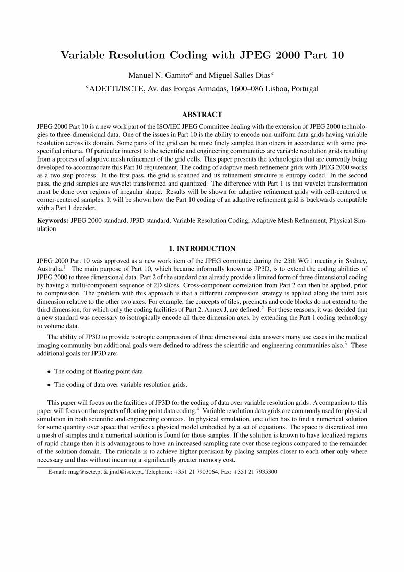
Part 10 will be able to code two types of AMR grids. These are classified in terms of the position of the samples relative tothe subdivision cells in the grid. The two types of grid are:

• Cell-centered grids. The samples are placed at the center of each grid cell. There is a direct one-on-one correspon-dence between a grid cell and its associated sample.

• Corner-centered grids. The samples are placed at the corners between adjacent grid cells. This means that a samplemay be shared among a maximum of four or eight grid cells (depending on the dimensionality and the refinementstructure of the grid).

Fig. 1 shows examples of the two types of grids. The construction of an AMR grid begins with a base grid of uniformresolution over which successively finer subgrids are superimposed during each refinement step. This creates a sequence ofgrids {Gn, Gn−1, . . . , G1, G0} for n refinement steps, where Gn is the initial base grid and G0 is the highest resolution grid∗.The samples belonging to any grid Gi, with i < n, will have originated from samples of grid Gi+1 that were subdivided.Fig. 1, again, shows, for both types of grid, the extent of each subgrid, using a darker grey for the higher resolution subgrid.The refinement structure is the same in both the left and right grid, only the sample placement changes. The subgrids areseen to be nested for increasing resolution levels and this is true for any type of AMR grid.

The shape of any gridGi is irregular, and it may even be disconnected, because any arbitrary set of cells from the parentgrid Gi+1 may have been subdivided, depending on the particular criteria that was used to perform the subdivision. Also,any row or any column of samples from a grid Gi is always going to have an even number of samples, for a cell-centeredgrid, or an odd number of samples, for a corner-centered grid. This is because refinement in two dimensions alwaysintroduces new grid cells in groups of four arranged in a square (eight arranged in a cube, if in three dimensions), and sothe samples will increase in a regular way along the horizontal and vertical directions.

∗The reason for using lower indices for higher resolutions is to make them compatible with the indices for the decomposition levelsof the wavelet transform, as will be seen shortly.

(a) Cell-centered grid. (b) Corner-centered grid.

Figure 1. Two AMR grids with the same refinement structure and with different sample placement strategies. The extent of the tworesolution levels, within each grid, is shown with different shades of grey.

A Part 10 encoder must perform two tasks: encode the refinement structure of the grid, i.e., signal in the codestreamwhich grid cells have been subdivided and to which depth, and encode the quantities stored in the grid samples. The firsttask is explained in Section 2.1 and the second in Section 2.2.

2.1. Signalling of the Adaptive Refinement Structure

The refinement structure of an AMR grid can be coded as a sequence of binary digits. All the cells of the grid, at allresolution levels, are scanned, in breadth-first order, with a symbol “0” being output if a cell is further subdivided and asymbol “1” being output if the cell has no descendants. The MQ binary arithmetic coder of JPEG 2000 is used to insert thesample symbols into the bitstream. This coder prevents the words in the range 0xFF90 to 0xFFFF from ever being inserted.This is because those words are reserved for the markers defined by the standard. By using the MQ coder to signal theadaptive structure of the AMR grids, it is ensured that the AMR part of the bitstream will be free from words that might bemistakenly interpreted as JPEG 2000 markers.

The bitstream resulting from refinement structure coding is encapsulated inside a proposed new SOG (Start of Grid)marker segment, which must be present in the main header. If the bitstream is larger than the maximum allowed markersegment length of 65534 bytes, it can be split into several consecutive SOG markers segments. The complete bitstreamwill then be reconstructed by a Part 10 decoder.

Coding of the refinement structure in a breadth-first manner is shown in the following pseudo-code. Sorted lists areused to keep track of which grid cells need to be checked for subdivision at the next higher subdivision level. This methodfor the coding of adaptive refinement structures was inspired by the quadtree wavelet coding method, where the waveletcoefficients are encoded according to a hierarchical structure that is similar to the one used here.12

initialize list to empty

for every cell of Grid(n)

add cell to list

call Breadth_Encode(list)

Procedure Breadth_Encode(list):

initialize new list to empty

for every cell in list

if the cell is subdivided

output "0"

for all four children of cell

add child to new list

else

output "1"

call Breadth_Encode(new list)

2.2. Wavelet Transformation of Adaptive Mesh Refinement Grids

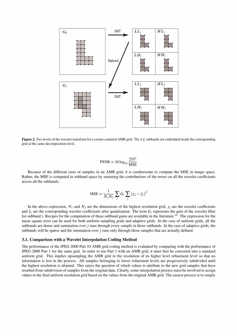
Similarly to the Part 1 specifications, the wavelet decomposition in Part 10 is done with a one-dimensional separabletransform. For clarity of explanation, the decomposition procedure will be explained in this section for a two-dimensionalAMR grid. The extension to a three-dimensional AMR grid is trivial. The wavelet decomposition is first applied along thecolumns and then along the rows of the image, for each decomposition level. It starts at decomposition level LL0, whichis considered to be the original image, and proceeds to decompose it into low-pass and high-pass subbands of the formLL1, HL1, LH1 and HH1. The process is then repeated a number of steps NL, where each wavelet decomposition startsalways with the low-pass subband LLi from the previous decomposition. In the case of AMR grids, the samples from eachlow-pass band LLi must be embedded inside the grid residing at decomposition level i before performing the next step ofthe wavelet transform. The process begins with grid G0, which is the finest resolution grid and the starting data for thewavelet transform sequence. The pseudo-code for the wavelet transform is:

LL(0) = Grid(0)

for each i between 1 and NL

{LL(i),HL(i),LH(i),HH(i)} = DWT(LL(i-1))

if i <= n

LL(i) = Embedding of LL(i) inside Grid(i)

if n > NL

for each i between n - NL + 1 and n

Upsample Grid(i) to the resolution of NL

LL(NL) = Embedding of LL(NL) inside Grid(i)

Figure 2 exemplifies the algorithm for two levels of wavelet decomposition of a corner-centered AMR grid. Thealgorithm embeds each LLi subband inside the grid Gi at the corresponding sampling resolution. This is because the gridsare nested and, so, subband LLi, which originates from grid Gi−1, is nested inside grid Gi. If there are more decompositionlevels than subgrids, i. e., if n < NL, then the algorithm will stop embedding grids after reaching the lowest grid Gn andwill start passing the LLi subbands unchanged to the next wavelet decomposition level. If, on the other hand, there aremore subgrids than decomposition levels, i. e., if n > NL, then all the remaining grids, after the wavelet transform sequencehas finished, are upsampled to the sampling resolution of subband LLNL

and embedded in it.

Every subband LLi has an irregular boundary which is the same as the boundary of the grid Gi, since this grid embedsinside it everything coming from lower decomposition levels. Because of this irregularity in the boundary of the low-passsubbands, the one-dimensional wavelet transforms will have to be applied over spans of samples whose limits will alwaysbe changing from column to column and from row to row. It may even happen, if the grid Gi is disconnected into severalpieces, that the one-dimensional wavelet transform will be applied to two or more spans of samples along one given rowor column of the subband. The study of wavelet transforms over irregular shapes has lead to the development of the ShapeAdaptive Discrete Wavelet Transform by Li and Li.13 The SA-DWT, for the case of odd-length symmetric biorthogonalwavelets, is used in Part 10, since both the 9/7 and the 5/3 wavelet filters specified in JPEG 2000 Part 1 fall under thatcategory. The symmetric boundary extension method, specified in Part 1, is applied, as needed, at the extremities of eachspan of pixels.

3. RESULTS

Several features of the coding of AMR grids with JPEG 2000 Part 10 will be discussed in this section. Except for the discus-sion of backwards compatibility with Part 1, in Section 3.2, all features are applicable to both two and three-dimensionalapplications. The current state of development of the Part 10 Verification Model, however, does not yet allow the fullthree-dimensional coding of data. For this reason, the AMR coding features will be shown with two-dimensional gridsonly.

One of the measures of performance for the coding of AMR grids is the peak signal to noise ratio (PSNR). The PSNR,in turn, is computed from the mean square error (MSE) after coding the data:

PSfrag replacements

LL1 HL1

LH1 HH1

LL2 HL2

LH2 HH2

G0

G1

DWT

DWT

Embed

Figure 2. Two levels of the wavelet transform for a corner-centered AMR grid. TheLL subbands are embedded inside the correspondinggrid at the same decomposition level.

PSNR = 10 log102552

MSE

Because of the different sizes of samples in an AMR grid, it is cumbersome to compute the MSE in image space.Rather, the MSE is computed in subband space by summing the contributions of the errors on all the wavelet coefficientsacross all the subbands:

MSE =1

N1N2

∑

i

Gi∑

j

(

yj − yj)2

In the above expression, N1 and N2 are the dimensions of the highest resolution grid, yj are the wavelet coefficientsand yj are the corresponding wavelet coefficients after quantization. The term Gi represents the gain of the wavelet filterfor subband i. Recipes for the computation of these subband gains are available in the literature.14 The expression for themean square error can be used for both uniform sampling grids and adaptive grids. In the case of uniform grids, all thesubbands are dense and summation over j runs through every sample in those subbands. In the case of adaptive grids, thesubbands will be sparse and the summation over j runs only through those samples that are actually defined.

3.1. Comparison with a Wavelet Interpolation Coding Method

The performance of the JPEG 2000 Part 10 AMR grid coding method is evaluated by comparing with the performance ofJPEG 2000 Part 1 for the same grid. In order to use Part 1 with an AMR grid, it must first be converted into a standarduniform grid. This implies upsampling the AMR grid to the resolution of its higher level refinement level so that noinformation is lost in the process. All samples belonging to lower refinement levels are progressively subdivided untilthe highest resolution is attained. This raises the question of which values to attribute to the new grid samples that haveresulted from subdivision of samples from the original data. Clearly, some interpolation process must be involved to assignvalues to the final uniform resolution grid based on the values from the original AMR grid. The easiest process is to simply

attribute the value from any original sample to all the samples that are subsequently subdivided from it. This amounts toa simple constant interpolation strategy. A more clever approach consists of using the wavelet transformation basis of thePart 10 encoder to interpolate the data onto the uniform grid before performing the Part 10 encoding. Wavelet interpolationminimizes the energy, during the Part 10 encoding, of spurious wavelet coefficients that result from the interpolationprocess and that do not represent the original AMR data. The process of wavelet interpolation can be seen as a standardinverse DWT transform, which computes the final high resolution data from all the orignal LLi subbands and where thecoefficients in the HLi, LHi and HHi subbands, for all resolution levels i, are set to zero. The pseudo-code for thiswavelet interpolation strategy is:

LL(n) = Grid(n)

for each i between n-1 and 0

LL(i) = INVDWT(LL(i+1),0,0,0)

LL(i) = Embedding of LL(i) inside Grid(i)

It could be argued that wavelet interpolation of an AMR grid onto a uniform resolution grid, followed by a conventionalPart 1 coding, could be seen as a better approach for the representation of AMR grids since only Part 1 technology would berequired for decoding the codestream. The adaptive refinement structure of the original AMR grid could be considered asmeta-data for this Part 1 codestream and transmitted through secondary channels. However, and as will be demonstrated,this coding strategy performs better than the Part 10 AMR coding technology only for low resolution data and at lowbitrates and therefore cannot be considered as a general coding method for adaptive refinement grids.

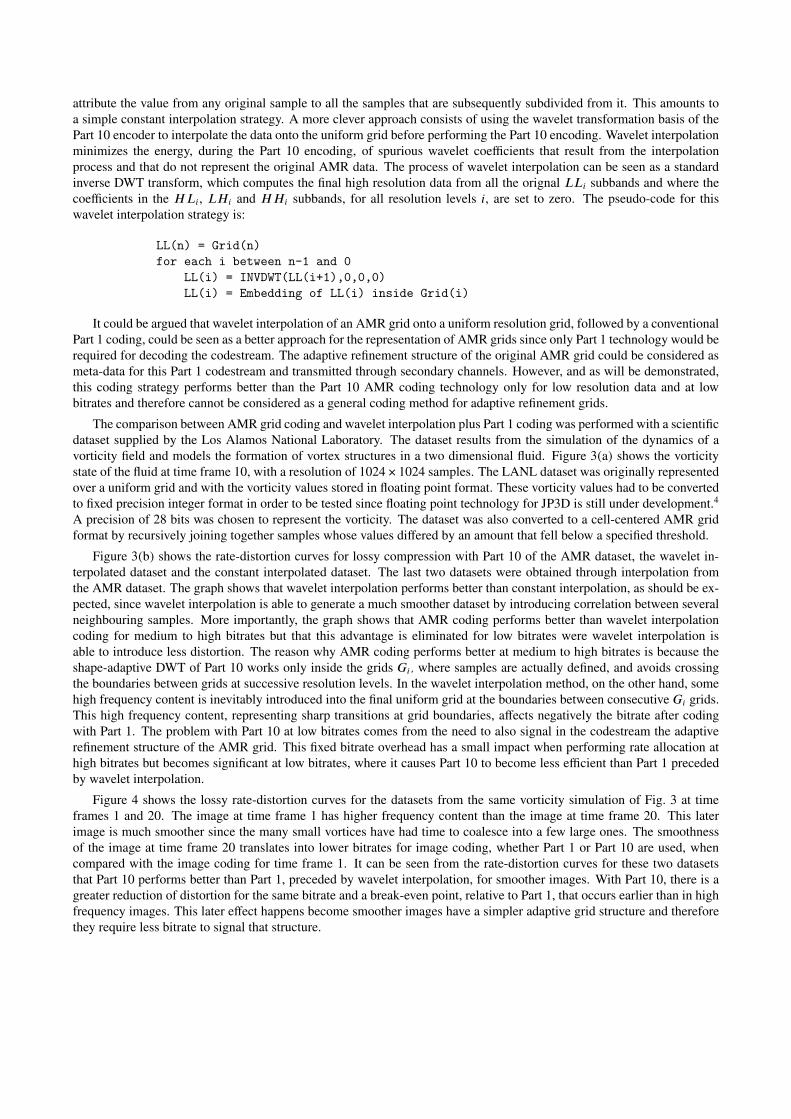
The comparison between AMR grid coding and wavelet interpolation plus Part 1 coding was performed with a scientificdataset supplied by the Los Alamos National Laboratory. The dataset results from the simulation of the dynamics of avorticity field and models the formation of vortex structures in a two dimensional fluid. Figure 3(a) shows the vorticitystate of the fluid at time frame 10, with a resolution of 1024×1024 samples. The LANL dataset was originally representedover a uniform grid and with the vorticity values stored in floating point format. These vorticity values had to be convertedto fixed precision integer format in order to be tested since floating point technology for JP3D is still under development.4

A precision of 28 bits was chosen to represent the vorticity. The dataset was also converted to a cell-centered AMR gridformat by recursively joining together samples whose values differed by an amount that fell below a specified threshold.

Figure 3(b) shows the rate-distortion curves for lossy compression with Part 10 of the AMR dataset, the wavelet in-terpolated dataset and the constant interpolated dataset. The last two datasets were obtained through interpolation fromthe AMR dataset. The graph shows that wavelet interpolation performs better than constant interpolation, as should be ex-pected, since wavelet interpolation is able to generate a much smoother dataset by introducing correlation between severalneighbouring samples. More importantly, the graph shows that AMR coding performs better than wavelet interpolationcoding for medium to high bitrates but that this advantage is eliminated for low bitrates were wavelet interpolation isable to introduce less distortion. The reason why AMR coding performs better at medium to high bitrates is because theshape-adaptive DWT of Part 10 works only inside the grids Gi, where samples are actually defined, and avoids crossingthe boundaries between grids at successive resolution levels. In the wavelet interpolation method, on the other hand, somehigh frequency content is inevitably introduced into the final uniform grid at the boundaries between consecutive Gi grids.This high frequency content, representing sharp transitions at grid boundaries, affects negatively the bitrate after codingwith Part 1. The problem with Part 10 at low bitrates comes from the need to also signal in the codestream the adaptiverefinement structure of the AMR grid. This fixed bitrate overhead has a small impact when performing rate allocation athigh bitrates but becomes significant at low bitrates, where it causes Part 10 to become less efficient than Part 1 precededby wavelet interpolation.

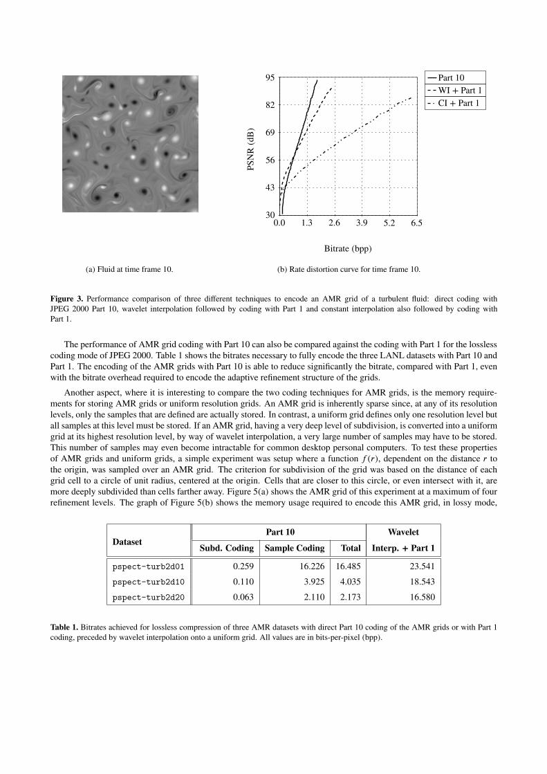
Figure 4 shows the lossy rate-distortion curves for the datasets from the same vorticity simulation of Fig. 3 at timeframes 1 and 20. The image at time frame 1 has higher frequency content than the image at time frame 20. This laterimage is much smoother since the many small vortices have had time to coalesce into a few large ones. The smoothnessof the image at time frame 20 translates into lower bitrates for image coding, whether Part 1 or Part 10 are used, whencompared with the image coding for time frame 1. It can be seen from the rate-distortion curves for these two datasetsthat Part 10 performs better than Part 1, preceded by wavelet interpolation, for smoother images. With Part 10, there is agreater reduction of distortion for the same bitrate and a break-even point, relative to Part 1, that occurs earlier than in highfrequency images. This later effect happens become smoother images have a simpler adaptive grid structure and thereforethey require less bitrate to signal that structure.

Bitrate (bpp)PS

NR

(dB

)

30

43

56

69

82

95

0.0 1.3 2.6 3.9 5.2 6.5

Part 10WI + Part 1CI + Part 1

(a) Fluid at time frame 10. (b) Rate distortion curve for time frame 10.

Figure 3. Performance comparison of three different techniques to encode an AMR grid of a turbulent fluid: direct coding withJPEG 2000 Part 10, wavelet interpolation followed by coding with Part 1 and constant interpolation also followed by coding withPart 1.

The performance of AMR grid coding with Part 10 can also be compared against the coding with Part 1 for the losslesscoding mode of JPEG 2000. Table 1 shows the bitrates necessary to fully encode the three LANL datasets with Part 10 andPart 1. The encoding of the AMR grids with Part 10 is able to reduce significantly the bitrate, compared with Part 1, evenwith the bitrate overhead required to encode the adaptive refinement structure of the grids.

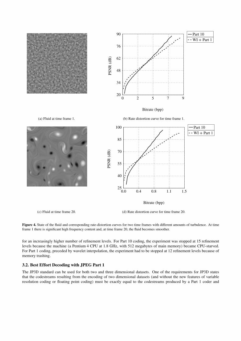
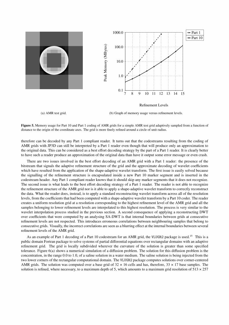
Another aspect, where it is interesting to compare the two coding techniques for AMR grids, is the memory require-ments for storing AMR grids or uniform resolution grids. An AMR grid is inherently sparse since, at any of its resolutionlevels, only the samples that are defined are actually stored. In contrast, a uniform grid defines only one resolution level butall samples at this level must be stored. If an AMR grid, having a very deep level of subdivision, is converted into a uniformgrid at its highest resolution level, by way of wavelet interpolation, a very large number of samples may have to be stored.This number of samples may even become intractable for common desktop personal computers. To test these propertiesof AMR grids and uniform grids, a simple experiment was setup where a function f (r), dependent on the distance r tothe origin, was sampled over an AMR grid. The criterion for subdivision of the grid was based on the distance of eachgrid cell to a circle of unit radius, centered at the origin. Cells that are closer to this circle, or even intersect with it, aremore deeply subdivided than cells farther away. Figure 5(a) shows the AMR grid of this experiment at a maximum of fourrefinement levels. The graph of Figure 5(b) shows the memory usage required to encode this AMR grid, in lossy mode,

Part 10 WaveletDataset

Subd. Coding Sample Coding Total Interp. + Part 1

pspect-turb2d01 0.259 16.226 16.485 23.541

pspect-turb2d10 0.110 3.925 4.035 18.543

pspect-turb2d20 0.063 2.110 2.173 16.580

Table 1. Bitrates achieved for lossless compression of three AMR datasets with direct Part 10 coding of the AMR grids or with Part 1coding, preceded by wavelet interpolation onto a uniform grid. All values are in bits-per-pixel (bpp).

Bitrate (bpp)PS

NR

(dB

)

20

34

48

62

76

90

0 2 5 7 9

Part 10WI + Part 1

(a) Fluid at time frame 1. (b) Rate distortion curve for time frame 1.

Bitrate (bpp)

PSN

R(d

B)

25

40

55

70

85

100

0.0 0.4 0.8 1.1 1.5

Part 10WI + Part 1

(c) Fluid at time frame 20. (d) Rate distortion curve for time frame 20.

Figure 4. State of the fluid and corresponding rate-distortion curves for two time frames with different amounts of turbulence. At timeframe 1 there is significant high frequency content and, at time frame 20, the fluid becomes smoother.

for an increasingly higher number of refinement levels. For Part 10 coding, the experiment was stopped at 15 refinementlevels because the machine (a Pentium 4 CPU at 1.8 GHz, with 512 megabytes of main memory) became CPU-starved.For Part 1 coding, preceded by wavelet interpolation, the experiment had to be stopped at 12 refinement levels because ofmemory trashing.

3.2. Best Effort Decoding with JPEG Part 1

The JP3D standard can be used for both two and three dimensional datasets. One of the requirements for JP3D statesthat the codestreams resulting from the encoding of two dimensional datasets (and without the new features of variableresolution coding or floating point coding) must be exactly equal to the codestreams produced by a Part 1 coder and

Refinement LevelsPe

akM

emor

y(M

Byt

es)

0.1

1.0

10.0

100.0

1000.0

7 8 9 10 11 12 13 14 15

Part 1Part 10

(a) AMR test grid. (b) Graph of memory usage versus refinement levels.

Figure 5. Memory usage for Part 10 and Part 1 coding of AMR grids for a simple AMR test grid adaptively sampled from a function ofdistance to the origin of the coordinate axes. The grid is more finely refined around a circle of unit radius.

therefore can be decoded by any Part 1 compliant reader. It turns out that the codestreams resulting from the coding ofAMR grids with JP3D can still be interpreted by a Part 1 reader even though that will produce only an approximation tothe original data. This can be considered as a best effort decoding strategy by the part of a Part 1 reader. It is clearly betterto have such a reader produce an approximation of the original data than have it output some error message or even crash.

There are two issues involved in the best effort decoding of an AMR grid with a Part 1 reader: the presence of thebitstream that signals the adaptive refinement structure of the grid and the approximate decoding of wavelet coefficientswhich have resulted from the application of the shape-adaptive wavelet transform. The first issue is easily solved becausethe signalling of the refinement structure is encapsulated inside a new Part 10 marker segment and is inserted in thecodestream header. Any Part 1 compliant reader knows that it should skip any marker segments that it does not recognize.The second issue is what leads to the best effort decoding strategy of a Part 1 reader. The reader is not able to recognizethe refinement structure of the AMR grid nor is it able to apply a shape-adaptive wavelet transform to correctly reconstructthe data. What the reader does, instead, is to apply a standard reconstructing wavelet transform across all of the resolutionlevels, from the coefficients that had been computed with a shape-adaptive wavelet transform by a Part 10 coder. The readercreates a uniform resolution grid at a resolution corresponding to the highest refinement level of the AMR grid and all thesamples belonging to lower refinement levels are interpolated to this highest resolution. The process is very similar to thewavelet interpolation process studied in the previous section. A second consequence of applying a reconstructing DWTover coefficients that were computed by an analysing SA-DWT is that internal boundaries between grids at consecutiverefinement levels are not respected. This introduces erroneous correlations between neighbouring samples that belong toconsecutive grids. Visually, the incorrect correlations are seen as a blurring effect at the internal boundaries between severalrefinement levels of the AMR grid.

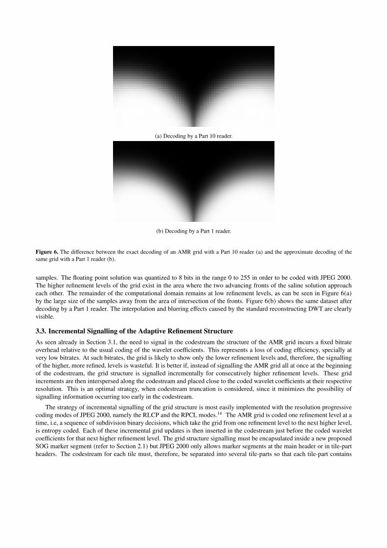
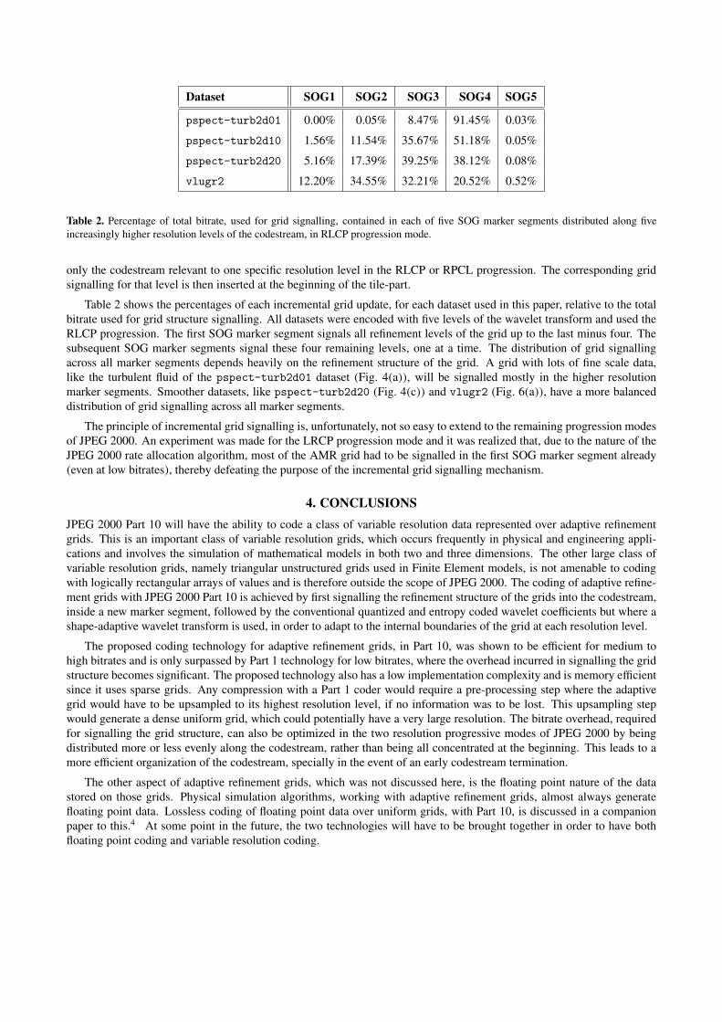
As an example of Part 1 decoding of a Part 10 codestream for an AMR grid, the VLUGR2 package is used.15 This is apublic domain Fortran package to solve systems of partial differential equations over rectangular domains with an adaptiverefinement grid. The grid is locally subdivided wherever the curvature of the solution is greater than some specifiedtolerance. Figure 6(a) shows a numerical simulation of a diffusion problem. The solution for this diffusion problem is theconcentration, in the range 0.0 to 1.0, of a saline solution in a water medium. The saline solution is being injected from thetwo lower corners of the rectangular computational domain. The VLUGR2 package computes solutions over corner-centeredAMR grids. The solution was computed over a base grid of 32 × 16 cells and has, therefore, 33 × 17 base samples. Thesolution is refined, where necessary, to a maximum depth of 5, which amounts to a maximum grid resolution of 513× 257

(a) Decoding by a Part 10 reader.

(b) Decoding by a Part 1 reader.

Figure 6. The difference between the exact decoding of an AMR grid with a Part 10 reader (a) and the approximate decoding of thesame grid with a Part 1 reader (b).

samples. The floating point solution was quantized to 8 bits in the range 0 to 255 in order to be coded with JPEG 2000.The higher refinement levels of the grid exist in the area where the two advancing fronts of the saline solution approacheach other. The remainder of the computational domain remains at low refinement levels, as can be seen in Figure 6(a)by the large size of the samples away from the area of intersection of the fronts. Figure 6(b) shows the same dataset afterdecoding by a Part 1 reader. The interpolation and blurring effects caused by the standard reconstructing DWT are clearlyvisible.

3.3. Incremental Signalling of the Adaptive Refinement Structure

As seen already in Section 3.1, the need to signal in the codestream the structure of the AMR grid incurs a fixed bitrateoverhead relative to the usual coding of the wavelet coefficients. This represents a loss of coding efficiency, specially atvery low bitrates. At such bitrates, the grid is likely to show only the lower refinement levels and, therefore, the signallingof the higher, more refined, levels is wasteful. It is better if, instead of signalling the AMR grid all at once at the beginningof the codestream, the grid structure is signalled incrementally for consecutively higher refinement levels. These gridincrements are then interspersed along the codestream and placed close to the coded wavelet coefficients at their respectiveresolution. This is an optimal strategy, when codestream truncation is considered, since it minimizes the possibility ofsignalling information occurring too early in the codestream.

The strategy of incremental signalling of the grid structure is most easily implemented with the resolution progressivecoding modes of JPEG 2000, namely the RLCP and the RPCL modes.14 The AMR grid is coded one refinement level at atime, i.e, a sequence of subdivision binary decisions, which take the grid from one refinement level to the next higher level,is entropy coded. Each of these incremental grid updates is then inserted in the codestream just before the coded waveletcoefficients for that next higher refinement level. The grid structure signalling must be encapsulated inside a new proposedSOG marker segment (refer to Section 2.1) but JPEG 2000 only allows marker segments at the main header or in tile-partheaders. The codestream for each tile must, therefore, be separated into several tile-parts so that each tile-part contains

Dataset SOG1 SOG2 SOG3 SOG4 SOG5

pspect-turb2d01 0.00% 0.05% 8.47% 91.45% 0.03%

pspect-turb2d10 1.56% 11.54% 35.67% 51.18% 0.05%

pspect-turb2d20 5.16% 17.39% 39.25% 38.12% 0.08%

vlugr2 12.20% 34.55% 32.21% 20.52% 0.52%

Table 2. Percentage of total bitrate, used for grid signalling, contained in each of five SOG marker segments distributed along fiveincreasingly higher resolution levels of the codestream, in RLCP progression mode.

only the codestream relevant to one specific resolution level in the RLCP or RPCL progression. The corresponding gridsignalling for that level is then inserted at the beginning of the tile-part.

Table 2 shows the percentages of each incremental grid update, for each dataset used in this paper, relative to the totalbitrate used for grid structure signalling. All datasets were encoded with five levels of the wavelet transform and used theRLCP progression. The first SOG marker segment signals all refinement levels of the grid up to the last minus four. Thesubsequent SOG marker segments signal these four remaining levels, one at a time. The distribution of grid signallingacross all marker segments depends heavily on the refinement structure of the grid. A grid with lots of fine scale data,like the turbulent fluid of the pspect-turb2d01 dataset (Fig. 4(a)), will be signalled mostly in the higher resolutionmarker segments. Smoother datasets, like pspect-turb2d20 (Fig. 4(c)) and vlugr2 (Fig. 6(a)), have a more balanceddistribution of grid signalling across all marker segments.

The principle of incremental grid signalling is, unfortunately, not so easy to extend to the remaining progression modesof JPEG 2000. An experiment was made for the LRCP progression mode and it was realized that, due to the nature of theJPEG 2000 rate allocation algorithm, most of the AMR grid had to be signalled in the first SOG marker segment already(even at low bitrates), thereby defeating the purpose of the incremental grid signalling mechanism.

4. CONCLUSIONS

JPEG 2000 Part 10 will have the ability to code a class of variable resolution data represented over adaptive refinementgrids. This is an important class of variable resolution grids, which occurs frequently in physical and engineering appli-cations and involves the simulation of mathematical models in both two and three dimensions. The other large class ofvariable resolution grids, namely triangular unstructured grids used in Finite Element models, is not amenable to codingwith logically rectangular arrays of values and is therefore outside the scope of JPEG 2000. The coding of adaptive refine-ment grids with JPEG 2000 Part 10 is achieved by first signalling the refinement structure of the grids into the codestream,inside a new marker segment, followed by the conventional quantized and entropy coded wavelet coefficients but where ashape-adaptive wavelet transform is used, in order to adapt to the internal boundaries of the grid at each resolution level.

The proposed coding technology for adaptive refinement grids, in Part 10, was shown to be efficient for medium tohigh bitrates and is only surpassed by Part 1 technology for low bitrates, where the overhead incurred in signalling the gridstructure becomes significant. The proposed technology also has a low implementation complexity and is memory efficientsince it uses sparse grids. Any compression with a Part 1 coder would require a pre-processing step where the adaptivegrid would have to be upsampled to its highest resolution level, if no information was to be lost. This upsampling stepwould generate a dense uniform grid, which could potentially have a very large resolution. The bitrate overhead, requiredfor signalling the grid structure, can also be optimized in the two resolution progressive modes of JPEG 2000 by beingdistributed more or less evenly along the codestream, rather than being all concentrated at the beginning. This leads to amore efficient organization of the codestream, specially in the event of an early codestream termination.

The other aspect of adaptive refinement grids, which was not discussed here, is the floating point nature of the datastored on those grids. Physical simulation algorithms, working with adaptive refinement grids, almost always generatefloating point data. Lossless coding of floating point data over uniform grids, with Part 10, is discussed in a companionpaper to this.4 At some point in the future, the two technologies will have to be brought together in order to have bothfloating point coding and variable resolution coding.

ACKNOWLEDGMENTS

The authors would like to thank Chris Brislawn, the editor of JP3D, for his guidance. The authors would also like to thankMark Taylor, at Los Alamos National Laboratory, for graciously allowing the use of the various pspect-turb2d datasetsfor the purpose of testing JP3D technologies.

REFERENCES1. C. Brislawn, “JP3D: Proposal for work item subdivision.” ISO/IEC JTC1/SC29/WG1 document #2379, 2001.2. M. Boliek, “JPEG 2000 Part 2: Final draft before international standard.” ISO/IEC JTC1/SC29/WG1 docu-

ment #2679, July 2002.3. C. Brislawn and P. Schelkens, “JP3D: Scope and requirements document, version 5.0.” ISO/IEC JTC1/SC29/WG1

document #3022, 2003.4. M. Gamito and M. Dias, “Lossless coding of floating point data with JPEG 2000 Part 10,” in Applications of Digital

Image Processing XXVII, A. Tescher, ed., SPIE Proceedings, 2004.5. J. C. Cavendish, “Automatic triangulation of arbitrary planar domains for the finite element method,” International

Journal for Numerical Methods in Engineering 8, p. 679, 1974.6. I. Salomie, A. Munteanu, A. Gavrilescu, G. Lafruit, P. Schelkens, R. Deklerck, and J. Cornelis, “Meshgrid - a com-

pact, multi-scalable and animation friendly surface representation,” IEEE Trans. on Circuits and Systems for VideoTechnology , June 2004.

7. M. Berger and P. Colella, “Local adaptive mesh refinement for shock hydrodynamics,” J. Computational Physics 82,pp. 64–84, May 1989. Lawrence Livermore Laboratory Report No. UCRL-97196.

8. G. L. Bryan, “Fluids in the universe: Adaptive mesh refinement in cosmology,” Computing in Science and Engineer-ing 1, pp. 46–53, Mar./Apr. 1999.

9. S. Phillips, A. Worrall, C. Willis, and D. Paddon, “Adaptive mesh refinement for the radiosity method,” in Proceedingsof Third International Conference on Computational Graphics and Visualization Techniques (Compugraphics ’93),pp. 178–186, GRASP, December 1993.

10. Y. Wu, Y. Liu, S. Zhan, and C. Gao, “Efficient view-dependent rendering of terrains,” in Proceedings of the GraphicsInterface 2001 (GI-01), pp. 217–222, Canadian Information Processing Society, (Toronto, Ontario), June 7–9 2001.

11. M. Gamito and M. Dias, “JPEG 2000 coding of data over adaptive refinement grids,” in Visual Communication andImage Processing, T. Ebrahimi and T. Sikora, eds., pp. 752–763, SPIE Proceedings, 2003. ISBN: 0-8194-5211-4.

12. A. Munteanu, J. Cornelis, G. van der Auwera, and P. Cristea, “Wavelet image compression – the quadtree codingapproach,” IEEE Trans. on Information Technology in Biomedicine 3, pp. 176–185, September 1999.

13. S. Li and W. Li, “Shape-adaptive discrete wavelet transforms for arbitrarily shaped visual object coding,” IEEE Trans.on Circuits and Systems for Video Technology 10, pp. 725–743, August 2000.

14. D. Taubman and M. Marcellin, JPEG2000 Image Compression: Fundamentals, Standards and Practice, KluwerAcademic Publishers, 2002.

15. J. G. Blom, R. A. Trompert, and J. G. Verwer, “Algorithm 758: VLUGR2: a vectorizable adaptive-grid solver forPDEs in 2D,” ACM Transactions on Mathematical Software 22, pp. 302–328, September 1996.