Titel of Thesis - Montanuniversität Leoben

Chair of Applied Geophysics

Master's Thesis

Comparison of fracture detection methods applied on the

Kerry 3D seismic, Taranaki Basin, New Zealand

November 2018

Sharadiya Rasarani Kozak, BSc

II

Die Eidesstattliche Erklärung muss unterschrieben und mit Datum versehen in Ihre Abschlussarbeit eingebunden werden.

EIDESSTATTLICHE ERKLÄRUNG

Ich erkläre an Eides statt, dass ich diese Arbeit selbständig verfasst, andere als die angegebenen Quellen und Hilfsmittel nicht benutzt, und mich auch sonst keiner unerlaubten Hilfsmittel bedient habe.

Ich erkläre, dass ich die Richtlinien des Senats der Montanuniversität Leoben zu "Gute wissenschaftliche Praxis" gelesen, verstanden und befolgt habe.

Weiters erkläre ich, dass die elektronische und gedruckte Version der eingereichten wissenschaftlichen Abschlussarbeit formal und inhaltlich identisch sind.

Datum 07.11.2018

Unterschrift Verfasser/in Sharadiya Rasarani, Kozak

Matrikelnummer: 01135004

III

Acknowledgement I would first like to thank my thesis advisor Dipl.-Ing. Johannes Amtmann of Geo5 GmbH and

Ao.Univ.-Prof. Dr.phil. Robert Scholger of the Chair of Applied Geophysics at the Montanuniversität

Leoben for their advice, supervision and review of this thesis. Further, I would like to thank Christiane

Pretzenbacher for her unfailing assistance with the paper work.

Further, I would like to thank the Austrian Research and Promotion Agency (FFG) for funding the

GeoSegment3D research project, Geo5 GmbH for supervision inputs and the New Zealand

Government for the allowance to use the New Zealand Petroleum Exploration Data Pack 2015.

Finally, I must express my very profound gratitude to my parents and friends for providing me with

unfailing support and continuous encouragement throughout my years of study. This

accomplishment would not have been possible without them.

Sharadiya Rasarani Kozak

IV

Abstract The extraction of faults in a 3D seismic volume is done in different ways and this step is one of the

most important steps in seismic interpretation. Each method has advantages and disadvantages.

Some methods are standard approaches, and some are more recent technologies. To get a better

understanding of the different methods and to verify those, was the goal of this master thesis.

In this thesis four different fracture detection methods were tested: Manual fault interpretation, the

Ant-Tracking Workflow, the Grey-Level-Co-Occurrence Matrix (GLCM) and the Fuzzy K-Means

Clustering method.

Analysis was performed on a sub-crop of the 3D seismic cube Kerry in the Kupe area (Taranaki Basin,

offshore Western New Zealand). Testing of the four fault detection methods focussed on the

comparison of the methodologies, the resulting faults and their characteristics, the influences on the

results, improvements in fault detection and suggestions for the selection of the right method.

Considering the difficulties in fault extraction in the Tangahoe Formation, which is characterized by

weak and discontinuous seismic reflections, Fuzzy K-Means Clustering was able to mostly

differentiate faults from other seismic facies, whereas Ant-Tracking and GLCM showed great

difficulty to do so. Additionally, Ant-Tracking falsely extracted faults, when to close or crossing each

other. Through cognition, manual fault interpretation was of no great difficulty in the Tangahoe

Formation, but is proven ineffective regarding its processing time.

Thus, Manual Fault Interpretation is effective, if the factor time is subordinate. Ant-Tracking and

GLCM are excellent quick look methods. Precaution should be taken, before relying on the

automatically extracted faults of the Ant-Tracking result, because often incorrect fault paths are

tracked. Generally, Fuzzy K-Means Clustering has been proven to be the most effective and detailed

method to detect fracture zones and could be of use in future to automate the fault extraction

process.

V

Kurzfassung Die Extraktion von Störungen in einem 3D-seismischen Volumen erfolgt auf unterschiedliche Weisen

und dieser Schritt ist einer der wichtigsten Schritte bei der seismischen Interpretation. Jede Methode

hat Vor- und Nachteile. Einige Methoden sind Standardansätze und andere sind neuere

Technologien. Um die verschiedenen Methoden besser zu verstehen und zu verifizieren, wurde eine

Masterarbeit gefertigt.

In dieser Arbeit wurden vier verschiedene Methoden zur Erkennung von Störungen getestet:

Manuelle Störungsinterpretation, der Ant-Tracking-Workflow, die Grauwertematrix (GLCM) und die

Fuzzy-K-Means-Clustering Methode.

Die Analyse wurde an einem Ausschnitt der Kerry 3D-Seismik der Kupe Region (Taranaki-Becken,

Offshore-West-Neuseeland) durchgeführt. Die Prüfung der vier Störungsdetektionsmethoden

konzentriert sich auf den Vergleich der Methodik, der daraus resultierenden Störungen und ihrer

Eigenschaften, die Einflüsse auf die Ergebnisse, Verbesserungen bei der Störungsdetektion und

Vorschläge für die richtige Methodenauswahl.

Angesichts der Schwierigkeiten bei der Störungsextraktion in der Tangahoe-Formation, die durch

schwache und diskontinuierliche seismische Reflexionen gekennzeichnet ist, konnte das Fuzzy-K-

Means-Clustering Störungen im Wesentlichen von anderen seismischen Fazies unterscheiden. Ant-

Tracking, sowie GLCM hatten teils große Schwierigkeiten damit. Zusätzlich hat Ant-Tracking

Störungen inkorrekt extrahiert, wenn sie zu nahe beieinander sind oder sich kreuzen. Durch

Kognition war die manuelle Störungsinterpretation in der Tangahoe-Formation erleichtert, hat sich

jedoch hinsichtlich der Bearbeitungszeit als ineffektiv erwiesen.

Somit ist die manuelle Störungsinterpretation effizient, wenn der Faktor Zeit von untergeordneter

Bedeutung ist. Ant-Tracking und GLCM sind exzellente Quick-Look-Methoden. Es sollte jedoch

Vorsicht getroffen werden, bevor man sich auf die automatisch extrahierten Störungen des Ant-

Tracking-Workflows verlässt, da häufig inkorrekte Störungspfade verfolgt werden. Im Allgemeinen

hat sich das Fuzzy-K-Means-Clustering als die effektivste und detaillierteste Methode zur Erkennung

von Bruchzonen erwiesen und könnte in Zukunft zur Automatisierung des

Störungsextraktionsprozesses von Nutzen sein.

VI

Table of Contents Acknowledgement.................................................................................................................................. III

Abstract .................................................................................................................................................. IV

Kurzfassung ............................................................................................................................................. V

1. Introduction ..................................................................................................................................... 1

1.1. Study Area ............................................................................................................................... 1

2. Geological Overview ........................................................................................................................ 5

2.1. Regional Geology ..................................................................................................................... 5

2.2. Geology of the Taranaki Basin ................................................................................................. 7

2.3. Structural Geology of the Kupe Area in the Taranaki Basin .................................................. 11

3. Methodology ................................................................................................................................. 13

3.1. Data Set ................................................................................................................................. 13

3.2. Software Used ....................................................................................................................... 15

3.3. Fault Detection ...................................................................................................................... 16

3.3.1. Seismic Attributes for Fault Detection .......................................................................... 16

3.3.1.1. 3D Edge Enhancement .......................................................................................... 16

3.3.1.2. Chaos ..................................................................................................................... 16

3.3.1.3. 3D Curvature ......................................................................................................... 17

3.3.1.3.1. Contour Curvature.............................................................................................. 17

3.3.1.3.2. Maximum Curvature .......................................................................................... 17

3.3.1.3.3. Minimum Curvature ........................................................................................... 17

3.3.1.3.4. Most Extreme Curvature .................................................................................... 17

3.3.1.3.5. Most Negative Curvature ................................................................................... 17

3.3.1.3.6. Strike Curvature ................................................................................................. 17

3.3.1.4. RMS Amplitude ...................................................................................................... 18

3.3.1.5. Variance (Edge Method) ........................................................................................ 18

3.3.2. Manual Fault Interpretation .......................................................................................... 19

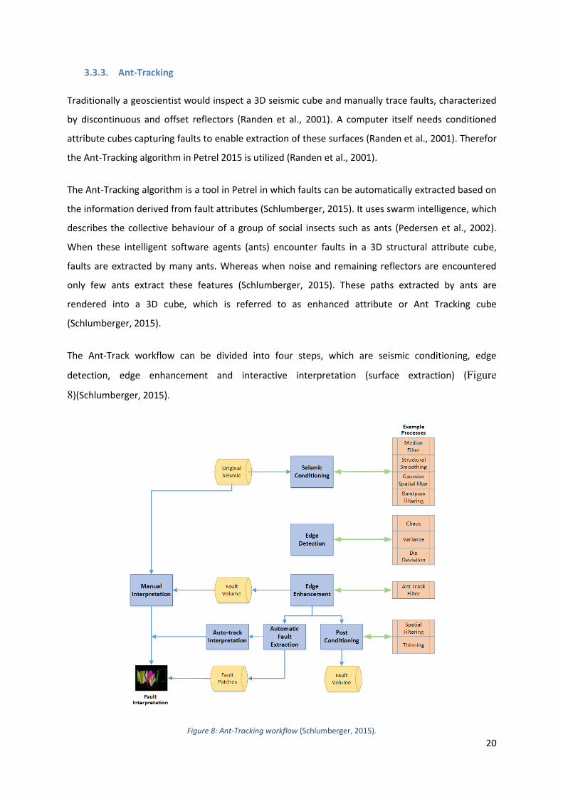
3.3.3. Ant-Tracking .................................................................................................................. 20

3.3.4. Grey-Level Co-Occurrence Matrix (GLCM) .................................................................... 23

3.3.5. Fuzzy K-Means Clustering .............................................................................................. 25

VII

4. Results ........................................................................................................................................... 28

4.1. Fault Detection ...................................................................................................................... 28

4.1.1. Manual Fault Interpretation .......................................................................................... 28

4.1.2. Ant-Tracking .................................................................................................................. 32

4.1.3. Grey-Level Co-Occurrence Matrix (GLCM) .................................................................... 48

4.1.4. Fuzzy K-Means Clustering .............................................................................................. 57

5. Discussion ...................................................................................................................................... 76

5.1. Manual Fault Interpretation .................................................................................................. 76

5.2. Ant-Tracking .......................................................................................................................... 76

5.3. Grey-Level Co-Occurrence Matrix (GLCM) ............................................................................ 77

5.4. Fuzzy K-Means Clustering ...................................................................................................... 78

5.5. Comparison of Fault Detection Results of the Kerry 3D Subcrop ......................................... 79

6. Conclusion ..................................................................................................................................... 92

7. Outlook .......................................................................................................................................... 93

8. Literature ....................................................................................................................................... 94

1

1. Introduction The study focuses on the extraction of faults in a 3D seismic volume which is one of the most

important steps in seismic interpretation. To get a better understanding of the different methods

and to verify those four different fracture detection methods were tested: Manual fault

interpretation, the Ant-Tracking Workflow, the Grey-Level-Co-Occurrence Matrix (GLCM) and the

Fuzzy K-Means Clustering method.

Analysis was performed on a sub-crop of the 3D seismic cube Kerry in the Kupe area (Taranaki Basin,

offshore Western New Zealand) (Figure 1, Figure 2, Figure 3, Figure 6). Testing of the four fault

detection methods focussed on the comparison of the methodologies, the resulting faults and their

characteristics, the influences on the results, improvements in fault detection and suggestions for the

selection of the right method.

1.1. Study Area

The Taranaki Basin is situated west of New Zealand’s North Island on the Australasian Plate and is

behind a convergent margin to the east, where the Pacific Plate is subducted beneath the Australian

Plate Figure 1, Figure 2)(Adams et al., 1977; Walcott, 1978; DeMets et al., 1994). The basin partially

lies onshore, but is mostly offshore and continues westwards into deep-water area of the North

Caledonian Trough (Figure 1, Figure 2)(Isaac et al., 1994).

The South Taranaki Basin is structurally complex, with multiple phases of deformation including

episodes of rifting, passive margin formation and convergence (Figure 4)(King et al., 1996). This plate

margin evolution has controlled the geometry and sedimentary infill of New Zealand’s basins,

including the Taranaki Basin.

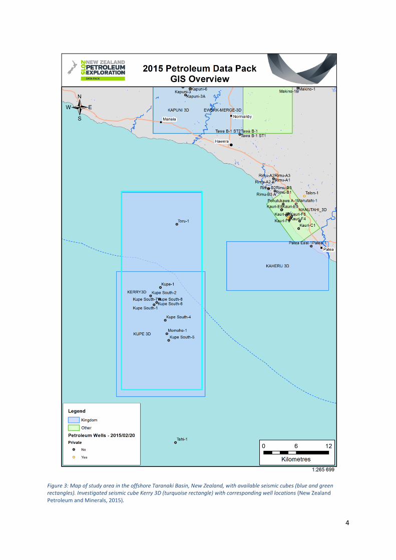
The Kupe Area, which contains the Kerry and Kupe seismic cube, is in the South Taranaki Basin, which

covers an area of approximately 100000 km2 (Figure 3, Figure 6). The Kupe and Kerry seismic cube lie

offshore in the Southern Taranaki Bay, 8.9 km of the coast from Hawera and 70 km of the coast of

Whanganui (Figure 2, Figure 3). The Kupe area is delimited by the coast in the north, the Taranaki

Fault in the east, by the Otakeho High in the west and the 2D seismic line MohoA-dsir in the south

(Figure 2, Figure 3, Figure 6)(Fohrmann et al., 2012).

Ten wells lie within the study area of the Kerry 3D seismic and are all located offshore, on the crest of

the Manaia Anticline (Figure 3, Figure 6).

2

Figure 1: Map of study area in the offshore Taranaki Basin (turquoise) and surrounding basins, New Zealand (New Zealand Petroleum and Minerals, 2015).

3

Figure 2: Map of study area in the offshore Taranaki Basin, New Zealand, with available seismic cubes (blue and green rectangles). Investigated seismic cube Kerry 3D is located South of Hawera and West of Whanganui (black rectangle) (New Zealand Petroleum and Minerals, 2015).

Fig. 3

4

Figure 3: Map of study area in the offshore Taranaki Basin, New Zealand, with available seismic cubes (blue and green rectangles). Investigated seismic cube Kerry 3D (turquoise rectangle) with corresponding well locations (New Zealand Petroleum and Minerals, 2015).

5

2. Geological Overview

2.1. Regional Geology

In Palaeozoic and early Mesozoic time, New Zealand´s basement rocks were part of the Pacific

margin of Gondwana, joined to Australia and Antarctica (Figure 4)(King et al., 1996). Subduction

continued until the Early Cretaceous at the active continental margin of Gondwana (Figure 4)(King et

al., 1996). Then the onset of extensional tectonics led to the break-up of Gondwana, with one

margin-parallel rift opening the Tasman Sea, subsequently separating New Zealand from Gondwana

(Figure 4)(Bradshaw, 1989; King et al., 1996; Laird et al., 2004). At that time New Zealand was part of

the Pacific Plate, compared to now where the northern part of New Zealand is on the Australian

Plate and the southern on the Pacific Plate (Figure 4)(King et al., 1996). When New Zealand was

tectonically stable, active seafloor spreading in the Tasman Sea and southern Pacific Ocean

dominated the Late Cretaceous to the earliest Eocene, with the Taranaki Basin becoming a passive

margin (Figure 4)(King et al., 1996). Until the Late Eocene post-rift thermal subsidence and formed

rift basins were flooded through associated marine transgression (King et al., 1996).

In the Early Eocene seafloor spreading ended in the Tasman Sea, but progressed in the southern

Pacific Ocean (King et al., 1996). Then a new Australia-Pacific plate boundary formed south of New

Zealand, opening the Emerald Basin and thus resulting in anticlockwise rotation of eastern New

Zealand relative to the west (King et al., 1996; King, 2000). By the Late Oligocene, New Zealand´s

landmass was completely submerged, and sediment starved, reaching maximum inundation between

Oligocene and earliest Miocene (Figure 4)(Nelson et al., 1994; King et al., 1996). The new plate

boundary formed a range of structures, through differential compaction and deformation during this

time (King et al., 1996).

A southwest-dipping subduction zone was present in northern New Zealand by the earliest Miocene

(Figure 4)(King et al., 1996). Large volcanoes were active west of what is now Northland, which is a

part of the overriding Australian Plate (Figure 4)(King et al., 1996). The Reinga Basin, which was

originally a rift, transformed into an intraplate back-arc basin (Figure 4)(King et al., 1996). Cretaceous

to Oligocene passive margin sediments, which accumulated northeast of New Zealand, were

obducted part-way into the Reinga, East Coast and Raukumara basins as thrust sheets (King et al.,

1996). Southwest-directed subduction in northernmost New Zealand was short-lived (King et al.,

1996). Southwest-directed oblique subduction east of North Island at the Kermadec Ridge continues

at present (King et al., 1996). The Kermadec Trench continues south as Hikurangi Trough and ends at

Chatham Rise just south of Cook Strait (King et al., 1996). In South Island, there is strike-slip

deformation on the Alpine Fault (Figure 4)(King et al., 1996). The acceleration of plate boundary

convergence since the Middle Miocene, resulted in rapid uplift and erosion of Northland volcanoes,

6

and uplift of the Southern Alps (King et al., 1996). This resulted in a vast amount of sediment supply

and progressive infilling of marine basins and progradation of continental shelves (King et al., 1996).

Figure 4: Paleogeographic maps of New Zealand from the Early Cretaceous till present. Green areas are above sea-level (New Zealand Petroleum & Minerals, 2014).

7

2.2. Geology of the Taranaki Basin

Sedimentation in the Taranaki Basin reflects a general 1st-order (100 my) transgressive-regressive

megacycle, common to stratigraphic sequences in other New Zealand Basins from the Cretaceous to

Quaternary (King et al., 1999). This resulted in complex spatial and temporal distribution of

sediments in the Taranaki Basin (Grain, 2008). The Taranaki Basin initially formed during Late

Cretaceous rifting between Australia and New Zealand (Figure 4, Figure 5)(King et al., 1996).

The oldest sediments in the north-eastern Taranaki Basin are in the Middle Cretaceous terrigenous

Taniwha Formation (Figure 5)(Shell BP Todd Oil Services Ltd., 1986). The Mid Cretaceous Taniwha

Formation is deposited over basement rocks, which consist of meta-sedimentary and cratonic

accretionary terranes formed on the Gondwana Margin (Bradshaw, 1989; King et al., 1996;

Mortimer, 2004). The Taniwaha Formation is then unconformably overlain by the Late Cretaceous

Pakawau Group (Figure 5)(King et al., 1996). Grabens and half-grabens accumulated terrestrial

sediments of the Pakawau Group, which is divided into the Raikopi and the North Cape Formations

(Figure 5)(King et al., 1996; Grain, 2008). The Late Cretaceous Raikopi Formation is formed of

interbedded coal measures and terrestrial sandstone sequences (Figure 5)(Thrasher, 1992; Wizevich

et al., 1992; Palmer et al., 1993; King et al., 1996). The lithofacies of the Raikopi Formation is

indicative of swamp and overbank deposition on a fluvial flood plain (King et al., 1996). The Late

Cretaceous North Cape Formation is the more marine influenced strata of the Pakawau Group

(Figure 5)(Thrasher, 1992; Wizevich et al., 1992). It was deposited in shallow marine, paralic, and

terrestrial environments (Figure 5)(King et al., 1996). The North Cape Formation is comprised of

siltstone, sandstone and conglomerate, with minor coal seams (Figure 5). Namely the Pupuonga

Member, Wainui Member and the Fresne Conglomerate Member (Thrasher, 1992; King et al., 1996).

The Deposition of the Raikopi Formation was then followed by a passive margin phase in the

Palaeocene and Eocene in which the sea transgressed, depositing terrestrial to marginal-marine

sequences (Figure 5)(King et al., 1996). The Palaeocene to Eocene succession is subdivided into two

groups, the Kapuni Group and Moa Group (Figure 5)(King et al., 1996). The sediments are comprised

of terrestrial to shallow marine coals and clastic sediments of the Kapuni Group and their marine age

equivalent of the Moa Group (Figure 5)(King et al., 1996; Sykes et al., 2010). The increasing marine

influence recorded in the Moa Group express the gradual subsidence of the basin and south-

eastward marine transgression, and encompasses a series of fine-grained, calcareous siltstones and

sandstones (Figure 5)(Hayward et al., 1989; King et al., 1992, 1996). The Kapuni Group is further

subdivided into the Farewell, Kaimiro, Mangahewa and McKee Formations (Figure 5)(King et al.,

1996). The Moa Group consists of the Turi and Tangaroa formations (Figure 5)(King et al., 1996). Late

Eocene and Early Oligocene sediments are absent, which marks a period of clastic detrital starvation

8

(Figure 5)(King et al., 1996). The absence of sediments near the Kapuni field, which is directly North

of the Kerry field and onshore, might indicate a paraconfomity or tectonic uplift (King et al., 1996).

The Ngatoro Group of the Oligocene to Early Miocene overlies the Kapuni and Moa Group, in which

maximum subsidence of the basin and its hinterland leads to widespread deposition of calcareous

muds, limestones, with reduced clastic supply (Figure 5)(King, 1988a, 1988b; Hayward et al., 1989;

King et al., 1999). The Ngatoro Group further comprises the Matapo Member, Otaraoa, Tikorangi and

Taimana Formations (Figure 5)(King et al., 1996). Although carbonate sedimentation signifies tectonic

quiescence and low terrigenous input, major tectonic changes accompanied the deposition of the

Ngatoro Group (King et al., 1996). The Oligocene Matapo greensand represent the onset of

subsidence and marine inundation (King et al., 1996). The Manaia sub-basin, in which the Kerry and

Kupe seismic cubes are located, subsided from sub-aerial and shallow marine environment to a

bathyal foredeep setting (King et al., 1996). The Otaraoa Formation was then deposited in outer shelf

to upper bathyal waters (Figure 5)(King et al., 1996). The Taimana Formation represents an influx of

clastic sediments into the carbonate-dominated foredeep, which is associated with overthrusting on

the Taranaki Fault and uplift of the hinterland (King et al., 1996).

Increasing occurrence of clastic sediments imply the onset of the regressive sequence with a

westward prograding shelf margin since the middle Miocene (King et al., 1992). The regressive

sequence is divided into the Miocene Wai-iti and the Plio-Pleistocene Rotokare Group (Figure 5),

ultimately caused by high sediment supply and tectonism associated with the Neogene convergent

plate boundary (King et al., 1992, 1996). The Wai-iti Group directly overlies the Ngatoro Group and is

comprised of the Manganui, Moki, Mohakatino, Mount Messenger, Urenui and Ariki Formation

(Figure 5)(King et al., 1992). The Manganui Formation comprises of more than 1000 m of bathyal

mudstone and dominates the Miocene interval, which is interrupted by several interbedded

sandstone and mudstone packages (Figure 5)(Palmer et al., 1993; King et al., 1996). The Rotokare

Group unconformably overlies the Wai-iti Group and is further subdivided into the Matemateaonga,

Tangahoe, Mangaa and Giant Foresets Formations (Figure 5)(King et al., 1992). Near the Manaia

Anticline, the boundary between the Wai-iti and Rotokare groups is represented by an angular

unconformity and marks the final growth of the anticline in the Late Miocene (King et al., 1992). In

the Kupe area the Late Miocene is associated with the Mangaoapa Member, a member of the Kiore

Formation of the Wai-iti Group (Bland et al., 2013) and often acts as a replacement for the “Kiore

Formation-equivalent” (Roncaglia et al., 2008). The Late Miocene to Early Pliocene Matemateaonga

Formation, predominantly consists of sandstone, and includes limestone, mudstone, shell beds and

coal (Figure 5)(King et al., 1996). The Early to Mid-Pliocene Tangahoe formation is a fine-grained shelf

deposit overlying the Matemateaonga Formation (Figure 5)(King et al., 1996). The Plio-Pleistocene

9

shelf strata overlying the Tangahoe Formation is often described as “Undifferentiated”, but is

sometimes correlated with the Whenuakura Group (Figure 5)(Fleming, 1953).

Deposition of large clinoform sequences of the Giant Foresets Formation took place in the Plio-

Pleistocene (Figure 5)(Beggs, 1990). The fine-grained lithologies of this sedimentary wedge are

punctuated by coarser-grained gravity-flow deposits of the late Early to Middle Miocene Moki, Late

Miocene Mount Messenger, and Pliocene Mangaa Formation (Figure 5)(King et al., 1996). Volcanics

and volcaniclastic sediments of the Late Miocene to Quarternary lie in the north-eastern and central

parts of the basin, outside the study area (King et al., 1996).

10

Figure 5: Stratigraphy of the Taranaki Basin (Baur (2012) modified after King & Thrasher (1996)). The international and New Zealand chronostratigraphic ages are depicted on the left (Cooper, 2004; Hollis et al., 2010). The central column shows the lithostratigraphic formations in the Taranaki Basin (Baur ,2012). Seismic horizons mapped by Baur (2012), used as a guide for the horizon interpretation in this thesis, and their relationship with Late Cretaceous to Pleistocene stratigraphic groups are depicted on the right (Baur,2012). Position of well Toru-1 (position on map in Figure 6) is indicated with a total measured depth of 4150.8 m and depth bellow rotary table of 4158 m. Investigated formations of the Kerry 3D sub-crop in red box.

Toru-1

11

2.3. Structural Geology of the Kupe Area in the Taranaki Basin

The major faults in the Kupe area are the Taranaki, Manaia, Rua and Motumate Fault, which are

explained in the following paragraphs (Figure 6).

The Kupe field is delimited by the north-south oriented crustal-scale Taranaki fault in the east, and

north-south oriented Manaia fault in the west (Figure 6)(Cope et al., 1967). The Taranaki fault is a

remnant antithetic back-thrust to the Hikurangi subduction margin, which has been episodically

active since the Mid Oligocene (Stagpoole et al., 2008). The Taranaki Fault signifies a basement

terrane boundary with the western Brook Street terrane thrusting over the eastern Murihiku terrane

(King et al., 1996; Mortimer et al., 1997). In the North-Eastern Kupe area, the Taranaki Fault uplifts

basin-fill in wedges, which are characterised by shallow-dipping planes steepening upwards

(Fohrmann et al., 2012). Towards the south the Taranaki Fault becomes a steeply dipping reverse

fault (Fohrmann et al., 2012).

The north-south oriented Manaia Fault is a significant inversion lineament in the Kupe field (Figure

6)(Fohrmann et al., 2012). Movement was initially normal from the Cretaceous to Late Paleocene,

reversed during the latest Eocene–Oligocene and peaked in the Late Miocene, with formation of the

Manaia Anticline (Stagpoole et al., 2008; Fohrmann et al., 2012). The Manaia anticline is a north-

south trending and north plunging, reverse-faulted inversion structure which formed through

inversion of the Cretaceous rift-related Manaia Fault (Figure 6)(King et al., 1996). The Kerry Field

itself is situated at the southern end of the Manaia Anticline and is segmented by a series of NW-SE

striking normal faults, with the largest one being the Kupe South Fault (Figure 6)(Schmidt et al.,

1990).

The Rua Fault forms the eastern splay off of the Manaia Anticline in the south and is a Miocene piggy

back thrust fault (Schmidt et al., 1990). Subsequently the Rua fault was deformed by the Manaia fault

(Clayton, 2017). The Manaia Anticline, forming the trap for the Kupe South Field, is the result of

overlap of the Manaia and Rua Fault (Figure 6)(Clayton, 2017).

Located in the west of the Kupe area the Motumate Fault is a westward dipping inverted Cretaceous

rift fault (Figure 6)(Schmidt et al., 1990; King et al., 1996). It is antithetic to the Rua Fault and

separated from the Manaia Fault by the Waiokura Syncline (Figure 6)(Fohrmann et al., 2012).

12

Figure 6: Schematic map of the KUP area (yellow polygon) with seismic cube Kerry 3D (grey polygon), 2D seismic lines (grey lines), well locations (circles) and main structural features (black lines) (Fohrmann et al., 2012).

13

3. Methodology

3.1. Data Set

The data used to carry out this research is a 3D seismic cube named BO_Kerry3D.sgy which was

provided by New Zealand Petroleum and Minerals (NZP&M). This data set was prepared and

compiled by New Zealand Petroleum and Minerals (NZP&M) in 2013 in the Kupe area of the Taranaki

Basin. The original cubes inlines extend from 58 to 510 and the cross lines from 510 to 792 (Figure 7,

Table 1). Respectively, the width of the cube is about 14.32 km and the length is about 36.70 km.

Further, the z-range of the cube extends from 0 to 5004 ms (Table 1). The projects original projection

is NZTM (New Zealand Transverse Mercator) and the datum is NZGD2000 (New Zealand Geodetic

Datum 2000) (Table 1).

AREA Taranaki_Basin – KERRY-3D Migration/PEGI

SURVEY KERRY 3D

INLINE 510 – 796

CROSSLINE 58 – 792

CDP 510058 - 796792

SAMPLE RATE 4000

RECORD LENGTH 5004

CLASS 3D SEISMIC

PROJECTION NZTM

DATUM NZGD2000

DATE APRIL 2013 Table 1: Acquisition parameters from seismic cube Kerry 3D header (New Zealand Petroleum and Minerals, 2015).

Although seismic cube Kupe 3D overlaps Kerry 3D, Kerry 3D was chosen for this thesis due to better

resolution of seismic amplitudes and minor acquisition noise, compared to Kupe 3D (Figure 7).

For faster processing, seismic cube Kerry 3D was cropped into a small sub-cube (Figure 7). The new

cube expands from inline 599 to 687, from cross line 508 to 721 and from 0 to -1620 ms along the z-

axis (Figure 7). This results in a length of 10.67 km, width of 4.42 km and a depth of -1620 ms (Figure

7).

14

Figure 7: To the left the position of the Kerry 3D and Kupe 3D seismic amplitude cubes are displayed. The subcrop that was chosen for the thesis is highlighted by the turquoise rectangle and the figure to the right.

15

3.2. Software Used

ArcMap 10.6.1 by Esri was used to display, edit and construct the ArcMap project of New Zealand

provided by New Zealand Petroleum & Minerals.

Petrel 2015 by Schlumberger was used to display the seismic cube and calculate attributes. Further,

it was used to manually track faults and to automatically extract faults on attribute cubes.

OpendTect by dGB Earth Sciences was utilized to display the seismic. For the calculation of the Grey-

Level Co-Occurrence Matrix-based attributes, the plugin FracTex from Geo5 GmbH was used.

Matlab by MathWorks was used to classify the seismic attribute data, previously calculated in Petrel,

into a matrix to then test the Fuzzy K-Means Clustering algorithm. The data output can then be

viewed in OpendTect.

16

3.3. Fault Detection

The interpretation of faults in a 3D seismic volume is performed through four different fracture

detection methods: Manual fault interpretation, the Ant-Tracking Workflow, the Grey-Level-Co-

Occurrence Matrix (GLCM) and the Fuzzy K-Means Clustering method. Thus, the prerequisites, such

as seismic attributes and the basics of each method are presented here.

3.3.1. Seismic Attributes for Fault Detection

Seismic attributes are quantities derived from post-stack seismic data and are used to improve

geological and geophysical interpretation by analysing and enhancing the seismic data. In Petrel 2015

seismic attributes are available as surface and volume attributes. In this thesis, only volume

attributes are in use. As input for the volume attribute generation for the Ant-Tracking-, GLCM- and

Fuzzy K-Means Clustering method the Kerry 3D seismic crop was used. The following seismic

attributes were calculated.

3.3.1.1. 3D Edge Enhancement

3D Edge Enhancement is a filter to enhance edges, such as faults and discontinuities, within a seismic

data volume (Schlumberger, 2015). To do so, the filter is applied in planes in three dimensions

(Schlumberger, 2015). These are then rotated to filter along all directions and angles (Schlumberger,

2015).

Edge detection is improved along a plane of an edge-detected cube through comparison and

summation of surrounding pixel values (Schlumberger, 2015). This is repeated for all pixels,

directions and angles (Schlumberger, 2015). The resulting cube displays mean values and thus only

enhances larger features, whereas smaller features are smoothed (Schlumberger, 2015). Compared

to other methods 3D edge enhancement, vastly reduces noise levels, and improves edge continuity

(Schlumberger, 2015).

3.3.1.2. Chaos

Seismic data contains chaotic signal patterns, which are a measure of the lack of organization of the

dip and azimuth estimation method (Schlumberger, 2015). These chaotic signal patterns can be used

to highlight faults and discontinuities, for seismic classification of chaotic textures or geologic

features (Schlumberger, 2015).

17

3.3.1.3. 3D Curvature

In 2D, curvature describes how bent a curve is at a specific point, in other words how much it

deviates from a straight line (Roberts, 2001). In 3D, curvature is the amount by which a surface

deviates from a flat plane (Roberts, 2001). In this thesis various types of curvature attributes were

used as input for the Fuzzy K-Means Clustering method.

3.3.1.3.1. Contour Curvature

Contour Curvature differs from Normal Curvature and is similar to Strike Curvature. This attribute

represents the curvature of map contours of the surface (dGB Earth Sciences, 2017). Large values

occur at the crest of synclines, anticlines, ridges and valleys (dGB Earth Sciences, 2017).

3.3.1.3.2. Maximum Curvature

Maximum Curvature defines the largest absolute curvature and is calculated orthogonal to the plane

of the Minimum Curvature (dGB Earth Sciences, 2017). This attribute is effective at delimiting faults

and their geometries (dGB Earth Sciences, 2017).

3.3.1.3.3. Minimum Curvature

Minimum Curvature defines the smallest absolute curvature and is calculated orthogonal to the

plane of the Maximum Curvature (dGB Earth Sciences, 2017). The Minimum Curvature is diagnostic

in identifying fracture zones but is noisier then Maximum Curvature (dGB Earth Sciences, 2017).

3.3.1.3.4. Most Extreme Curvature

Extreme curvature is the absolute Maximum Curvature at a certain azimuth in which the curve shape

is its tightest (Gao et al., 2015). The term “extreme” is used to represent the signed absolute

maximum curvature value (Chopra et al., 2010).

3.3.1.3.5. Most Negative Curvature

Most Negative Curvature highlights faults and lineaments (dGB Earth Sciences, 2017). The lineaments

magnitude is preserved, at loss of shape information, thus the attribute can be compared to first

derivative based attributes (dGB Earth Sciences, 2017).

3.3.1.3.6. Strike Curvature

Strike Curvature, also known as Tangential Curvature, is orthogonal to the Dip Curvature (dGB Earth

Sciences, 2017). It returns the curvature of the intersection between a vertical plane in strike

direction and the curved surface (dGB Earth Sciences, 2017). The attribute is commonly used in

terrain analysis and shows how shapes, such as ridges, are connected (dGB Earth Sciences, 2017).

18

3.3.1.4. RMS Amplitude

The Root-Mean-Square (RMS) attribute is calculated as the square root of the sum of squared

amplitudes, divided by the number of samples within the chosen time window (Equation 1) (Koson et

al., 2014; Schlumberger, 2015):

𝑥𝑅𝑀𝑆 = √1

𝑁∑𝑤𝑛𝑥𝑛

2

𝑁

𝑛−1

Equation 1: Root Mean Square (RMS) Amplitude with N samples as the square root of the sum of all the trace values x squared in which w and n are window values (Koson et al., 2014).

RMS Amplitude measures the reflectivity of sediments, to find amplitude anomalies in the seismic

volume, thus the attribute is also sensitive to noise (Koson et al., 2014; Schlumberger, 2015).

3.3.1.5. Variance (Edge Method)

The Variance attribute is used to detect edges, through estimation of the local variance of the signal

(Van Bemmel et al., 2000; Schlumberger, 2015). The attribute can be used to isolate edges, meaning

discontinuities in the horizontal continuity of amplitudes, from the seismic input (Schlumberger,

2015).

To calculate the Variance following equation is applied (Equation 2)(Van Bemmel et al., 2000):

𝑉 = 𝜎2 = ∑ [𝑤𝑗−𝑡∑ (𝑥𝑖𝑗 − �̅�𝑗)

2𝐼𝑗=1

∑ (𝑥𝑖𝑗)2𝐼

𝑗=1

]

𝑗=𝑡+𝐿 2⁄

𝑗=𝑡−𝐿 2⁄

Equation 2: Variance of sample with amplitude x at time t of cell (i, j), search length L and weighting factor w Modified after Van Bemmel and Pepper (2000).

In Equation 2 the mean seismic amplitude within the chosen search radius is calculated, which is than

subtracted from the investigated seismic sample (Van Bemmel et al., 2000). The then squared sum is

divided by the total squared sum and multiplied by a weighting function (Equation 2)(Van Bemmel et

al., 2000).

Variance, run with a short window, is typically used to illuminate stratigraphic features such as

depositional features, reefs, channels, splays, etc (Schlumberger, 2015). This is typically calculated

without dip-guidance (Schlumberger, 2015). Dip guided variance is useful when wanting to highlight

structural features such as faults (Schlumberger, 2015).

19

3.3.2. Manual Fault Interpretation

Faults are digitized in Petrel by directly interpreting on a seismic intersection, either by drawing fault

segments in the 2D seismic interpretation window or by modelling faults on a 3D seismic cube

through fault framework interpretation (Schlumberger, 2015).

The first method uses traditional Manual Fault Interpretation by creating fault segments in 2D with

the addition of fault plane triangulation in 3D, thus creating a fault surface (Schlumberger, 2015). A

fault segment can consist of an indefinite number of points in the 2D seismic section (Schlumberger,

2015). A fault surface is than created by triangulating the points from adjacent fault segments

(Schlumberger, 2015). A new fault segment is simply created by moving to the next seismic

intersection (Schlumberger, 2015). Manual interpretation can be done on the original amplitude

seismic or any edge enhancing seismic attribute volume (Schlumberger, 2015).

The second method uses the regular manual interpretation process and automatically adds faults to

the fault framework as interpretation progresses (Schlumberger, 2015). In this thesis only the first

Manual Fault Interpretation method is used.

20

3.3.3. Ant-Tracking

Traditionally a geoscientist would inspect a 3D seismic cube and manually trace faults, characterized

by discontinuous and offset reflectors (Randen et al., 2001). A computer itself needs conditioned

attribute cubes capturing faults to enable extraction of these surfaces (Randen et al., 2001). Therefor

the Ant-Tracking algorithm in Petrel 2015 is utilized (Randen et al., 2001).

The Ant-Tracking algorithm is a tool in Petrel in which faults can be automatically extracted based on

the information derived from fault attributes (Schlumberger, 2015). It uses swarm intelligence, which

describes the collective behaviour of a group of social insects such as ants (Pedersen et al., 2002).

When these intelligent software agents (ants) encounter faults in a 3D structural attribute cube,

faults are extracted by many ants. Whereas when noise and remaining reflectors are encountered

only few ants extract these features (Schlumberger, 2015). These paths extracted by ants are

rendered into a 3D cube, which is referred to as enhanced attribute or Ant Tracking cube


The Ant-Track workflow can be divided into four steps, which are seismic conditioning, edge

detection, edge enhancement and interactive interpretation (surface extraction) (Figure

8)(Schlumberger, 2015).

Figure 8: Ant-Tracking workflow (Schlumberger, 2015).

21

After generating an ant-track attribute volume fault patches, signifying parts of faults, can be

extracted through the automatic fault extraction tool (Figure 8)(Schlumberger, 2015). These fault

patches represent areas of high confidence of connectedness and can be merged and smoothed into

larger fault surfaces (Schlumberger, 2015).

In the first step seismic data is conditioned by reducing noise in the signal (Figure 8)(Schlumberger,

2015). This can be done by using structural smoothing with the fault edge preservation option

(Figure 8)(Schlumberger, 2015). In the second step spatial discontinuities are enhanced in the seismic

by using an edge detection method (Figure 8)(Schlumberger, 2015). Typical attributes for edge

detection are the structural attributes such as chaos and variance on which edge enhancement,

namely Ant-Tracking, is performed (Figure 8)(Schlumberger, 2015).

The variance attribute itself is the estimation of local variance in the signal. It is useful for edge

detection (Figure 8)(Schlumberger, 2015). The Variance attribute isolates edges, which represent

discontinuity in horizontal continuity of amplitude (Schlumberger, 2015). Thus, if the amplitude in a

reflection layer is continuous, variance is small (Randen et al., 2001). Faults are represented by

amplitude change within a reflection layer and result in larger variance (Randen et al., 2001). By

using dip guided variance structural features such as faults are further accentuated (Schlumberger,

2015). Optionally vertical smoothing can be applied to reduce noise in the seismic data

(Schlumberger, 2015). The chaos attribute, and thus the chaotic signal pattern in a seismic volume,

represents the lack of organization in the dip and azimuth estimation method (Schlumberger, 2015).

Since the variance attribute results in more enhanced faults, it is better suited as input for the ant

tracking algorithm (Silva et al., 2005).

In the third step, the fault attributes are significantly improved by the Ant-Tracking algorithm which

reduces noise and cancels events that do not represent faults (Figure 8) (Schlumberger, 2015). This is

done by imitating the behaviour of ant colonies, where pheromones are used to track paths in the

search of food (Schlumberger, 2015). Ants are deployed as seeds to look for discontinuities in the

seismic volume and when a discontinuity is encountered virtual pheromones highlight these paths

related mostly to fault zones (Schlumberger, 2015). The resulting attribute cube displays the faults in

a sharper and more detailed manner than other edge enhancing attributes (Schlumberger, 2015).

This cube can then be used as an input for Petrel´s automatic fault extraction (Figure

8)(Schlumberger, 2015). In automatic fault extraction 3D fault patches can be extracted from an ant

tracking, variance, chaos attribute volume etc. (Figure 8)(Schlumberger, 2015). The extracted fault

patches are typically incomplete fault surface segments, which can give the interpreter an overview

22

of the present fault systems and their orientation within the data (Pedersen et al., 2002;

Schlumberger, 2015). Following, corresponding fault patches can be merged and smoothed into fault

surfaces (Silva et al., 2005). Surfaces created by acquisition footprint or other coherent noise can be

verified, and if necessary, deleted (Schlumberger, 2015).

23

3.3.4. Grey-Level Co-Occurrence Matrix (GLCM)

The Grey-Level Co-Occurrence Matrix (GLCM) is a statistical texture classification method where its

derived attributes are used to semi-automatically produce a description to characterize the spatial

arrangement of amplitude values (Haralick et al., 1973).

GLCM is a commonly used method for the texture classification of 2D images such as satellite-, sea-

ice-, magnetic resonance- or computed tomography (Eichkitz, Schreilechner, et al., 2015). In the past

20 years GLCM has also been applied to seismic data (Vinther et al., 1996; Gao, 2009, 2011, 1999,

2003, 2007, 2008b, 2008a; West et al., 2002; Chopra et al., 2005, 2006b, 2006a; Yenugu et al., 2010;

de Matos et al., 2011; Eichkitz et al., 2013). Since GLCM-based attribute calculation was used for 2D

applications only, it is now necessary to adapt the workflow for 3D seismic data (Eichkitz et al., 2013).

Textural attributes, such as GLCM, can characterize the spatial arrangement of neighbouring

amplitudes, rock units, depositional facies and reservoir properties (Gao, 2011). In general, GLCM is a

measure for how often different combinations of neighbouring pixel brightness values occur in an

image (Eichkitz et al., 2012).

GLCM analysis in 2D images uses calculation in four directions (0°, 45°, 90°, and 135°) for

neighbouring pixels (Eichkitz, Schreilechner, et al., 2015). If averaging the four directions to form an

average GLCM, influences of bed dip and azimuth can be reduced (Gao, 2007). For the 3D case it is

easiest to imagine a Rubik’s cube which is made up of 27 small cubes (Eichkitz, Schreilechner, et al.,

2015). The central cube, which signifies the reference point for which calculations are made, is

surrounded by 26 neighbouring cubes (Eichkitz, Schreilechner, et al., 2015). If lines are drawn from

the centre point to all neighbouring cubes, the resulting space directions for calculation are thirteen

(Eichkitz, Schreilechner, et al., 2015).

When integrating dip steering into the GLCM calculation, the 3D input volume is warped along the

seismic stratigraphy (Eichkitz, Schreilechner, et al., 2015). Dip steering avoids mixing of signals from

different seismic packages, resulting in sharper, easier to interpret, images (Eichkitz, Schreilechner, et

al., 2015). Dip-guidance also results in a wider value range in GLCM attributes, making features more

visible (Eichkitz, Schreilechner, et al., 2015).

The first step in the GLCM workflow is the transformation of the seismic amplitude volume into a

grey-level cube (Eichkitz et al., 2012). For calculation on a seismic amplitude cube 16 or 32 grey levels

are adequate, because more grey levels do not result in considerable improvements in the resulting

attributes and rather result in longer computation times (Chopra et al., 2006a; Gao, 2007).

Regardless, a higher number of grey levels results in improvement of the signal-to-noise ratio,

24

important for delineating geological features (Eichkitz, Schreilechner, et al., 2015). Up to 512 grey

levels, improvement of the signal-to-noise ratio is visible (Eichkitz, Schreilechner, et al., 2015).

To improve computing time FracTex uses a linked-list approach in which nonzero matrix entries are

skipped (Eichkitz, Schreilechner, et al., 2015). Thus, computing time is no longer determined by the

number of grey levels, but the size of the analysis window (Eichkitz, Schreilechner, et al., 2015). Next

each GLCM entry is divided by the sum of all entries, transforming it into a probability matrix

(Eichkitz, Schreilechner, et al., 2015).

Followingly, several textural attributes, namely GLCM-based attributes, can be derived and used to

determine isotropic and anisotropic areas in the data (Eichkitz, Amtmann, et al., 2015).

These attributes can be divided into the contrast-, orderliness- and statistics-group. The contrast-

group encompasses the contrast, homogeneity, and cluster tendency attributes, which are functions

of matrix entry probabilities and differences between grey levels (Haralick et al., 1973; Wang et al.,

2010; Eichkitz, Schreilechner, et al., 2015). The orderliness-group includes energy and entropy as

attributes and measure how regularly grey-level values are distributed in a given search window

(Haralick et al., 1973; Eichkitz, Schreilechner, et al., 2015). Attributes of the orderliness-group are

merely a function of GLCM probability entries (Eichkitz, Schreilechner, et al., 2015). The statistics-

group includes mean and variance as attributes (Haralick et al., 1973).

The results of the GLCM-based attributes can then be used as a fracture intensity measure, as well as

for strike and dip determination of fractures due to the directional dependency of the attributes to

the strike of the main feature (Eichkitz, Schreilechner, et al., 2015). The calculated attribute values

are assigned to the central point of the analysis window and the procedure is repeated for all points

within the seismic cube (Eichkitz, Schreilechner, et al., 2015).

25

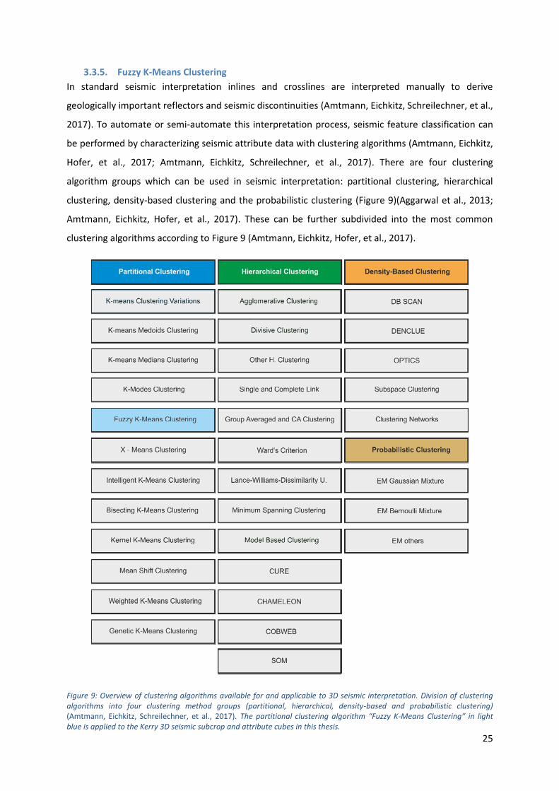
3.3.5. Fuzzy K-Means Clustering

In standard seismic interpretation inlines and crosslines are interpreted manually to derive

geologically important reflectors and seismic discontinuities (Amtmann, Eichkitz, Schreilechner, et al.,

2017). To automate or semi-automate this interpretation process, seismic feature classification can

be performed by characterizing seismic attribute data with clustering algorithms (Amtmann, Eichkitz,

Hofer, et al., 2017; Amtmann, Eichkitz, Schreilechner, et al., 2017). There are four clustering

algorithm groups which can be used in seismic interpretation: partitional clustering, hierarchical

clustering, density-based clustering and the probabilistic clustering (Figure 9)(Aggarwal et al., 2013;

Amtmann, Eichkitz, Hofer, et al., 2017). These can be further subdivided into the most common

clustering algorithms according to Figure 9 (Amtmann, Eichkitz, Hofer, et al., 2017).

Figure 9: Overview of clustering algorithms available for and applicable to 3D seismic interpretation. Division of clustering algorithms into four clustering method groups (partitional, hierarchical, density-based and probabilistic clustering) (Amtmann, Eichkitz, Schreilechner, et al., 2017). The partitional clustering algorithm “Fuzzy K-Means Clustering” in light blue is applied to the Kerry 3D seismic subcrop and attribute cubes in this thesis.

26

In this thesis the focus is on the partitional clustering group, more specifically the Fuzzy K-Means

Clustering algorithm, which is a variant of the k-means algorithm (Figure 9)(MacQueen, 1967;

Amtmann, Eichkitz, Hofer, et al., 2017).

The fuzzy k-means algorithm is not commonly used for 3D seismic data, but in Paasche and Tronicke

(2007), who used this algorithm on 3D Ground Penetrating Data, proposed the possible applicability

to 3D seismic data (Amtmann, Eichkitz, Hofer, et al., 2017).

The workflow consists of 3D seismic attribute calculation and selection in Petrel, Fuzzy K-Means

Clustering of groups of three 3D seismic attribute cubes in Matlab and display of the resulting Fuzzy

K-Means Clustering cubes in OpendTect.

In general, fuzzy clustering algorithms are used for characterizing multidimensional datasets

(Höppner et al., 1999). The advantage is that no prior knowledge of interrelationships of the different

datasets is required (Paasche et al., 2007). When using the fuzzy k-means algorithm an objective

function is iteratively minimized for a predefined number of clusters (Paasche et al., 2006, 2007). This

results in optimized cluster centre locations for defining the degree of membership of clustered data

points to the predefined number of clusters (Paasche et al., 2007). The cluster membership of data

points is based on the distances to cluster centres (Bauckhage, 2015).

Mathematically speaking, Fuzzy K-Means Clustering is based on the minimization of the objective

function (Equation 3) (Bezdek, 1981):

𝐽𝑚 =∑∑𝜇𝑖𝑗𝑚‖𝑥𝑖 − 𝑐𝑗‖

2𝑁

𝑗=1

𝐷

𝑖=1

Equation 3: Objective function Jm. D is the number of data points; N is the number of clusters; m is the fuzzy partition matrix exponent controlling the degree of fuzzy overlap (m>1); xi is the ith data point; cj is the centre of the jth cluster; µij is the degree of membership of xi in the jth cluster (Σµij=1) (Bezdek, 1981).

The Fuzzy K-Means Clustering workflow consists of five steps. In the first step random cluster

memberships µij are chosen. In the second step cluster centres are calculated as follows (Equation 4)

(Bezdek, 1981):

𝑐𝑗 =∑ 𝜇𝑖𝑗

𝑚𝑥𝑖𝐷𝑖=1

∑ 𝜇𝑖𝑗𝑚𝐷

𝑖=1

Equation 4: Cluster centre cj. D is the number of data points; xi is the ith data point; µij is the degree of membership of xi in the jth cluster (Σµij=1); m is the fuzzy partition matrix exponent controlling the degree of fuzzy overlap (m>1) (Bezdek, 1981).

In the third step µij is than updated according to Equation 5 (Bezdek, 1981):

27

𝜇𝑖𝑗 =1

∑ (‖𝑥𝑖 − 𝑐𝑗‖‖𝑥𝑖 − 𝑐𝑘‖

)

2𝑚−1

𝑁𝑘=1

Equation 5: Degree of membership µi of xi in the jth cluster (Σµij=1); N is the number of clusters; xi is the ith data point; m is the fuzzy partition matrix exponent controlling the degree of fuzzy overlap (m>1); xi is the ith data point; cj is the centre of the jth cluster; ck is the centre of the kth cluster (Bezdek, 1981).

In the fourth step the calculated parameters from step two and three are used in Equation 3 to

calculate the objective function Jm (Bezdek, 1981).

In step five, step two to four are repeated until Jm reaches a specified maximum number of iterations

or until Jm improves by less than a specified minimum threshold value (Bezdek, 1981).

Compared to “hard” clustering algorithms, fuzzy or “soft” algorithms allow for partial memberships,

meaning that a data point may be mostly part of a certain cluster, but may also be a partial member

of another cluster (Paasche et al., 2007). By use of “hard” clustering algorithms data points can only

belong to one cluster, even if it is optically not obvious which cluster they belong to (Bauckhage,

2015).

Depending on the chosen seismic attributes, number of predefined clusters and fuzzy k-means

parameters, seismic facies models with different solutions are generated (Amtmann, Eichkitz,

Schreilechner, et al., 2017).

28

4. Results

4.1. Fault Detection

4.1.1. Manual Fault Interpretation

In Manual Fault Interpretation the seismic volume is investigated for discontinuities in the reflectors.

To aid with the Manual Fault Interpretation, a horizon interpretation was performed in Petrel (Figure

10, Figure 11, Figure 12, Figure 13, Figure 14). The horizon interpretation makes it easier to detect

discontinuities in the reflectors, indicative of faults (Figure 10, Figure 11, Figure 12, Figure 13, Figure

14). Further, it helps to make sense of the geological timing of faulting.

The interpretation of formation tops was done with help of well reports and seismic interpretations

of 2D seismic lines in the Kupe area (Baur, 2012; Fohrmann et al., 2012; New Zealand Petroleum and

Minerals, 2015). The formation tops extracted in the Kerry 3D subcrop includes the seafloor (Figure

11), Top Whenuakura (Figure 12), Top Tangahoe (Figure 13) and Top Matemateaonga (Figure 14).

Especially the Tangahoe Formation was easy to delimit due to its weak reflection character and

dipping reflectors (Figure 10).

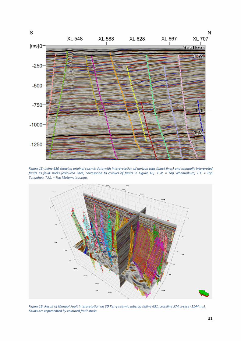
The result of the fault interpretation is presented in an exemplary 2D seismic inline (Figure 15) and as

a 3D fault model (Figure 16).

Figure 10: Inline 630 showing original seismic data with interpretation of horizon tops (black lines). T.W. = Top Whenuakura, T.T. = Top Tangahoe, T.M. = Top Matemateaonga.

29

Figure 11: Top Seafloor horizon interpretation on amplitude seismic of Kerry 3D subcrop.

Figure 12: Top Whenuakura horizon interpretation on amplitude seismic of Kerry 3D subcrop.

30

Figure 13: Top Tangahoe horizon interpretation on amplitude seismic of Kerry 3D subcrop.

Figure 14: Top Matemateaonga horizon interpretation on amplitude seismic of Kerry 3D subcrop.

31

Figure 15: Inline 630 showing original seismic data with interpretation of horizon tops (black lines) and manually interpreted faults as fault sticks (coloured lines, correspond to colours of faults in Figure 16). T.W. = Top Whenuakura, T.T. = Top Tangahoe, T.M. = Top Matemateaonga.

Figure 16: Result of Manual Fault Interpretation on 3D Kerry seismic subcrop (inline 631, crossline 574, z-slice -1144 ms). Faults are represented by coloured fault sticks.

32

4.1.2. Ant-Tracking

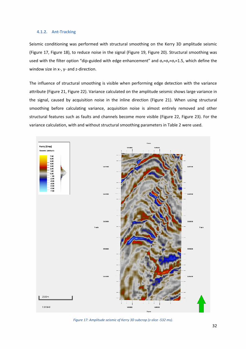
Seismic conditioning was performed with structural smoothing on the Kerry 3D amplitude seismic

(Figure 17, Figure 18), to reduce noise in the signal (Figure 19, Figure 20). Structural smoothing was

used with the filter option “dip-guided with edge enhancement” and σx=σy=σz=1.5, which define the

window size in x-, y- and z-direction.

The influence of structural smoothing is visible when performing edge detection with the variance

attribute (Figure 21, Figure 22). Variance calculated on the amplitude seismic shows large variance in

the signal, caused by acquisition noise in the inline direction (Figure 21). When using structural

smoothing before calculating variance, acquisition noise is almost entirely removed and other

structural features such as faults and channels become more visible (Figure 22, Figure 23). For the

variance calculation, with and without structural smoothing parameters in Table 2 were used.

Figure 17: Amplitude seismic of Kerry 3D subcrop (z-slice -532 ms).

33

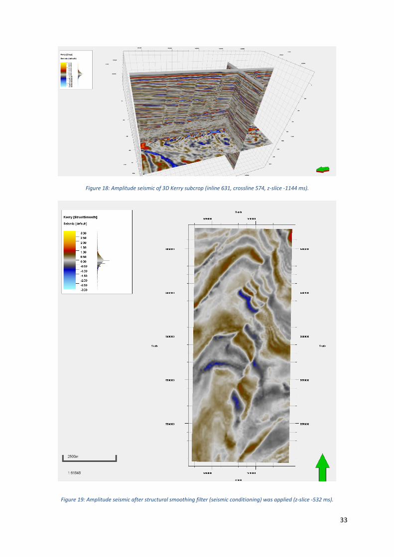
Figure 18: Amplitude seismic of 3D Kerry subcrop (inline 631, crossline 574, z-slice -1144 ms).

Figure 19: Amplitude seismic after structural smoothing filter (seismic conditioning) was applied (z-slice -532 ms).

34

Figure 20: Amplitude seismic after structural smoothing filter (seismic conditioning) was applied (inline 631, crossline 574, z-slice -1144 ms).

Inline range 3

Crossline range 3

Vertical smoothing 15

Dip correction On

Inline scale 1.5

Crossline scale 1.5

Vertical scale 1.5

Plane confidence threshold 0.6

Dip guided smoothing Off

Table 2: Settings used for variance attribute calculation on Kerry 3D amplitude seismic with and without structural smoothing.

35

Figure 21: Variance attribute (edge detection) without structural smoothing filter (seismic conditioning) on z-slice -532 ms. Acquisition noise is very prominent in N-S-direction.

Figure 22: Variance attribute (edge detection) with structural smoothing filter (seismic conditioning) on z-slice -532 ms. Acquisition noise in N-S-direction was removed by use of seismic conditioning.

36

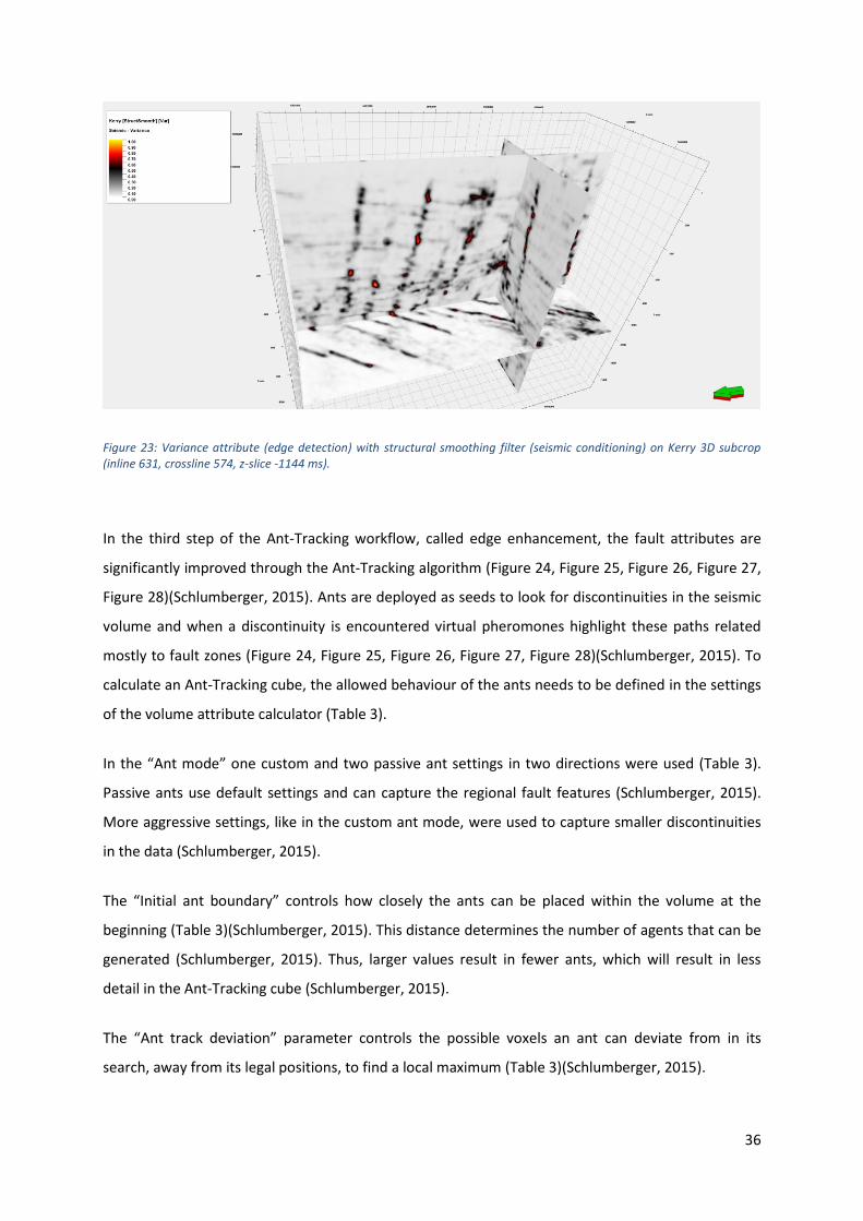
Figure 23: Variance attribute (edge detection) with structural smoothing filter (seismic conditioning) on Kerry 3D subcrop (inline 631, crossline 574, z-slice -1144 ms).

In the third step of the Ant-Tracking workflow, called edge enhancement, the fault attributes are

significantly improved through the Ant-Tracking algorithm (Figure 24, Figure 25, Figure 26, Figure 27,

Figure 28)(Schlumberger, 2015). Ants are deployed as seeds to look for discontinuities in the seismic

volume and when a discontinuity is encountered virtual pheromones highlight these paths related

mostly to fault zones (Figure 24, Figure 25, Figure 26, Figure 27, Figure 28)(Schlumberger, 2015). To

calculate an Ant-Tracking cube, the allowed behaviour of the ants needs to be defined in the settings

of the volume attribute calculator (Table 3).

In the “Ant mode” one custom and two passive ant settings in two directions were used (Table 3).

Passive ants use default settings and can capture the regional fault features (Schlumberger, 2015).

More aggressive settings, like in the custom ant mode, were used to capture smaller discontinuities

in the data (Schlumberger, 2015).

The “Initial ant boundary” controls how closely the ants can be placed within the volume at the

beginning (Table 3)(Schlumberger, 2015). This distance determines the number of agents that can be

generated (Schlumberger, 2015). Thus, larger values result in fewer ants, which will result in less

detail in the Ant-Tracking cube (Schlumberger, 2015).

The “Ant track deviation” parameter controls the possible voxels an ant can deviate from in its

search, away from its legal positions, to find a local maximum (Table 3)(Schlumberger, 2015).

37

“Ant step size” defines how far an ant advances in its search (Table 3)(Schlumberger, 2015). Large

values will allow ants to search further, thus finding more connections, at cost of resolution


“Illegal steps allowed” allows to search beyond edges, when tracking discontinuous faults and thus

creates more continuous faults (Table 3)(Schlumberger, 2015).

“Legal steps required” requires a selected number of valid steps after an illegal step was taken (Table

3)(Schlumberger, 2015). Lower values are thus less restrictive and allow for more continuous faults


“Stop criteria” is used to stop ants advancing further, when too many illegal steps were taken (Table

3)(Schlumberger, 2015). Larger values allow ants to advance further (Figure 24)(Schlumberger, 2015).

Thus, following parameters were used to calculate the Ant-Tracking volumes (Table 3):

Custom 1st Direction 2nd Direction

Ant mode Custom Passive Passive

Initial ant boundary 7 7 7

Ant track deviation 2 2 2

Ant step size 3 3 3

Illegal steps required 2 1 1

Legal steps required 3 3 3

Stop criteria 15 5 5

Table 3: Settings used for calculation of one custom and two passive and directionally dependent Ant-Tracking volumes.

38

Figure 24: Custom Ant-Track filter (edge enhancement) calculated on a structurally smoothed variance cube (z-slice -532 ms).

39

Figure 25: Passive Ant-Track filter (edge enhancement) calculated on a structurally smoothed variance cube (z-slice -532 ms).

Figure 26: Passive Ant-Track filter (edge enhancement) calculated on a structurally smoothed variance cube (inline 631, crossline 574, z-slice -1144 ms).

40

Figure 27: Passive Ant-Track filter (edge enhancement) calculated on a structurally smoothed variance cube (z-slice -532 ms).

Figure 28: Passive Ant-Track filter (edge enhancement) calculated on a structurally smoothed variance cube (inline 631, crossline 574, z-slice -1144 ms).

41

Ant-Tracking volumes (Figure 24, Figure 25, Figure 26, Figure 27, Figure 28) were used as input for

the automatic extraction of fault patches (Figure 29, Figure 32). To automatically generate fault

patches, following parameters need to be defined (Table 4).

The fault patch “extraction sampling distance” defines the minimum distance between extraction

seed points (Table 4)(Schlumberger, 2015).

“Extraction sampling threshold” characterizes the minimum signal level from which to create

extraction points from (Table 4). Thus, a value of 3 % uses only the highest data values


“Extraction background threshold” specifies the minimum signal level to be included into a fault

estimate (Table 4)(Schlumberger, 2015).

The value “Deviation from a plane” controls how far a fault can deviate from a plane surface, to fit

the data (Table 4)(Schlumberger, 2015).

“Connectivity constraint” specifies the voxel connectivity on 1 to 3 faces to be included in the fault

patch (Table 4)(Schlumberger, 2015).

“Minimum fault patch size” (points) defines the minimum number of points that is needed to extract

fault patches (Table 4)(Schlumberger, 2015).

The parameter “Patch down sampling” specifies the density of points and how close these points can

be within a fault patch, measured in voxels (Table 4)(Schlumberger, 2015).

Custom 1st Direction 2nd Direction

Extraction sampling distance 25 25 25

Extraction sampling threshold 3 3 3

Extraction background threshold 7 7 7

Deviation from a plane 15 15 15

Connectivity constant 1 1 1

Minimum patch size 200 200 200

Patch down sampling 8 8 8

Table 4: Settings used for automatic fault extraction within one custom and two passive and directionally dependent Ant-Tracking volumes.

42

Because Ant-Tracking was calculated in two directions on both passive Ant-Tracking cubes, excluding

all signals in the stereonet dipping in inline and crossline direction, no acquisition noise is visible

(Figure 25, Figure 26, Figure 27, Figure 28). Thus, acquisition noise cannot be falsely extracted as fault

surfaces in the Automatic Fault Extraction workflow (Figure 29, Figure 30).

As for the custom Ant-Tracking cube the “Stop criteria” was set rather high, allowing ants to advance

further (Table 3). Hence, acquisition noise shows the same intensity in the custom Ant-Tracking cube

as the faults (Figure 24). This explains why Automatic Fault Extraction extracts these “faults” in inline

direction (Figure 32, Figure 37). These falsely extracted faults were removed in the stereonet and

“dip azimuth” histogram window (Figure 33, Figure 37, Figure 38).

After removing fault patches in the inline direction, the corresponding fault patches were merged

and smoothed to create even and continuous fault surfaces (Figure 30, Figure 34, Figure 35).

Automatic Fault extraction on the custom Ant-Tracking cubes, faces problems when dealing with

faults that are very close and cross each other (Figure 36). When two high angle faults cross each

other, they appear as one merged surface in automatic fault extraction (Figure 36). This problem was

not faced, when using the passive Ant-Tracking cubes calculated in different directions (Figure 31).

This made the extraction of fault patches for crossing faults easier (Figure 31).

Figure 29: Automatically extracted fault patches calculated on both passive Ant-Track cubes. Displayed in amplitude seismic cube (inline 631, crossline 574, z-slice -1144 ms).

43

Figure 30: Automatically extracted fault patches calculated on both passive Ant-Tracking cubes, which were filtered, merged and smoothed. Displayed in amplitude seismic cube (inline 631, crossline 574, z-slice -1144 ms).

Figure 31: Detailed view of automatically extracted fault patches calculated on both passive Ant-Tracking cubes, which were filtered, merged and smoothed. Crossing faults are of no difficulty for the Automatic Fault Extraction when calculated on Ant-Tracking cubes, which were conditioned in two directions.

44

Figure 32: Automatically extracted fault patches calculated on custom Ant-Tracking cube.

Figure 33: Automatically extracted fault patches calculated on custom Ant-Tracking cube. Falsely extracted faults (acquisition noise) were filtered in the stereonet settings of the fault patch folder.

45

Figure 34: Automatically extracted fault patches calculated on custom Ant-Tracking cube. Grey fault patch to the right is the result of merging 3 fault patches.

Figure 35: Automatically extracted faults, calculated on custom Ant-Tracking cube, after filtering, merging and smoothing all fault patches.

46

Figure 36: Detailed view of automatically extracted fault patches calculated on custom Ant-Tracking cube, which was filtered, merged and smoothed. Crossing faults are of difficulty for the Automatic Fault Extraction when calculated on an Ant-Tracking cube, which was not directionally conditioned.

Figure 37: Resulting stereonet displays of automatically extracted faults which were filtered, merged and smoothed. From left to right: Automatic Fault Extraction on custom Ant-Tracking cube, on passive Ant-Tracking cube and on passive Ant-Tracking cube. Dark grey zones are filtered fault patches after faults were extracted and which follow the crossline direction.

47

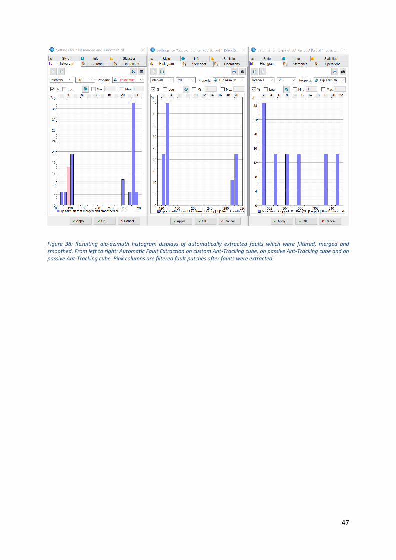
Figure 38: Resulting dip-azimuth histogram displays of automatically extracted faults which were filtered, merged and smoothed. From left to right: Automatic Fault Extraction on custom Ant-Tracking cube, on passive Ant-Tracking cube and on passive Ant-Tracking cube. Pink columns are filtered fault patches after faults were extracted.

48

4.1.3. Grey-Level Co-Occurrence Matrix (GLCM)

Firstly, an edge-preserving smoothing filter with basic settings was used on the Kerry 3D seismic

subcrop (Figure 39, Figure 40). For the batch execution process “single process” was used.

To calculate GLCM attributes the FracTex plugin for OpendTect designed by Geo5 GmbH was utilized.

As input for the calculation of all GLCM attributes the Kerry 3D seismic subcrop (Figure 39),

conditioned with the edge-preserving smoother (Figure 40), was used. In the process of GLCM

attribute generation calculation the amplitude cube is transformed into a grey level cube (dGB Earth

Sciences, 2018). For the calculation of the GLCM attributes parameters in Table 5 were used.

The number of “grey levels” is utilized for the transformation of an amplitude into a grey level cube

(Table 5)(dGB Earth Sciences, 2018). Higher grey level values result in improved quality of the GLCM

attribute output (dGB Earth Sciences, 2018).

“Min/ Max of Input Data” defines the range of the amplitude values to be used in the transformation

process (Table 5)(dGB Earth Sciences, 2018).

The number of traces to be used in the calculation are characterized by the “horizontal search

window” (Table 5)(dGB Earth Sciences, 2018). If the value one, three traces, one trace left and one

right of the centre trace, are used (Table 5)(dGB Earth Sciences, 2018).

The number of samples included in the search window are characterized by the “vertical search

window” (Table 5)(dGB Earth Sciences, 2018).

“Grey-Level Transformation” defines the type of transformation to be used in generation of the grey-

level cube (Table 5)(dGB Earth Sciences, 2018). Logarithmic transformations emphasise negative

amplitudes and exponential transformations positive amplitudes (Eichkitz et al., 2018). Linear

transformations equally emphasise the amplitude range (Eichkitz et al., 2018).

The calculation of the GLCM attribute volume can be performed with or without “steering” (Table 5).

Dip steering can improve the signal-to-noise ratio in GLCM attribute calculation (dGB Earth Sciences,

2018).

49

Contrast Dissimilarity Energy Energy Entropy Homogeneity

Grey Levels 64 64 64 64 64 64

Min/ Max of Input Data

-2.911/ 2.911

-3.0566/ 3.0566

-2.0282/ 2.0282

-2.0232/ 2.0232

-0.3919/ 0.3919

-3.0326/ 3.0326

Horizontal Search Window

Inl:1, Crl:1 Inl:1, Crl:1 Inl:1, Crl:1 Inl:1, Crl:1 Inl:1, Crl:1 Inl:1, Crl:1

Vertical Search Window

5 5 5 5 5 5

Output Anisotropy Factor

Anisotropy Factor

Anisotropy Factor

Anisotropy Factor

Anisotropy Factor

Anisotropy Factor

Grey-Level Transformation

Linear Linear Exponential Exponential Logarithmic Linear

Steering None None Full (PG Steer)

None None None

Table 5: Settings used for calculation of GLCM attributes with the FracTex plugin.

Figure 39: Amplitude seismic display of Kerry 3D subcrop (z-slice -468 ms).

50

Figure 40: Amplitude seismic with edge-preserving smoother on Kerry 3D subcrop (top: z-slice -468 ms; bottom: inline 615, crossline 643, z-slice -468 ms).

51

In the contrast cube the faults are marked by very low contrast values, which are clearly visible as

NE-SW striking features in Figure 41. Strong amplitude regions (Figure 39) result in an especially high

contrast region (Figure 41). Acquisition noise is slightly visible in N-S direction (Figure 41). The low

contrast layer between 750 and 100 ms, is clearly bound to a geological layer and thus makes faults

hard to detect in this region (Figure 41). The majority of the contrast cube shows lower values (Figure

41).

Figure 41: FracTex attribute “contrast” calculated on amplitude seismic with edge-preserving smoother (top: z-slice -468 ms; bottom: inline 615, crossline 643, z-slice -468 ms).

52

In the dissimilarity cube the faults are marked by lower contrast values, which are clearly visible as

NE-SW striking features in Figure 42. Strong amplitude regions (Figure 39) result in very high

dissimilarity values and in this case rather weak reflectors in very low dissimilarity values (Figure 42).

Acquisition noise is not evident (Figure 42). The medium to low and high to very high dissimilarity

values follow the shape of crosscutting reflectors, when compared to Figure 39 and Figure 40. The

low dissimilarity layer between 750 and 100 ms, is clearly bound to a geological layer and thus makes

faults harder to detect in this region (Figure 42). Reflector layering is apparent in Figure 42.

Figure 42: FracTex attribute “dissimilarity” calculated on amplitude seismic with edge-preserving smoother (top: z-slice -468 ms; bottom: inline 615, crossline 643, z-slice -468 ms).

53

In the energy cube with PG steering the faults are marked by low to very low energy values, which

are clearly visible as NE-SW striking features in Figure 43. Strong amplitude regions (Figure 39) result

in very high energy values (Figure 43). The medium to low and high to very high energy values follow

the shape of crosscutting reflectors when compared to Figure 39 and Figure 40. Acquisition noise is

slightly visible along the western edge of the cube in N-S direction (Figure 43). The low energy layer

between 750 and 100 ms, is clearly bound to a geological layer and thus makes faults harder to

detect in this region (Figure 43). Compared to the other GLCM attributes (Figure 41, Figure 42, Figure

45, Figure 46) the influence and disturbance of this layer is the least prominent. Reflector layering is

apparent in Figure 43.

Figure 43: FracTex attribute “energy with PG steering” calculated on amplitude seismic with edge-preserving smoother (top: z-slice -468 ms; bottom: inline 615, crossline 643, z-slice -468 ms).

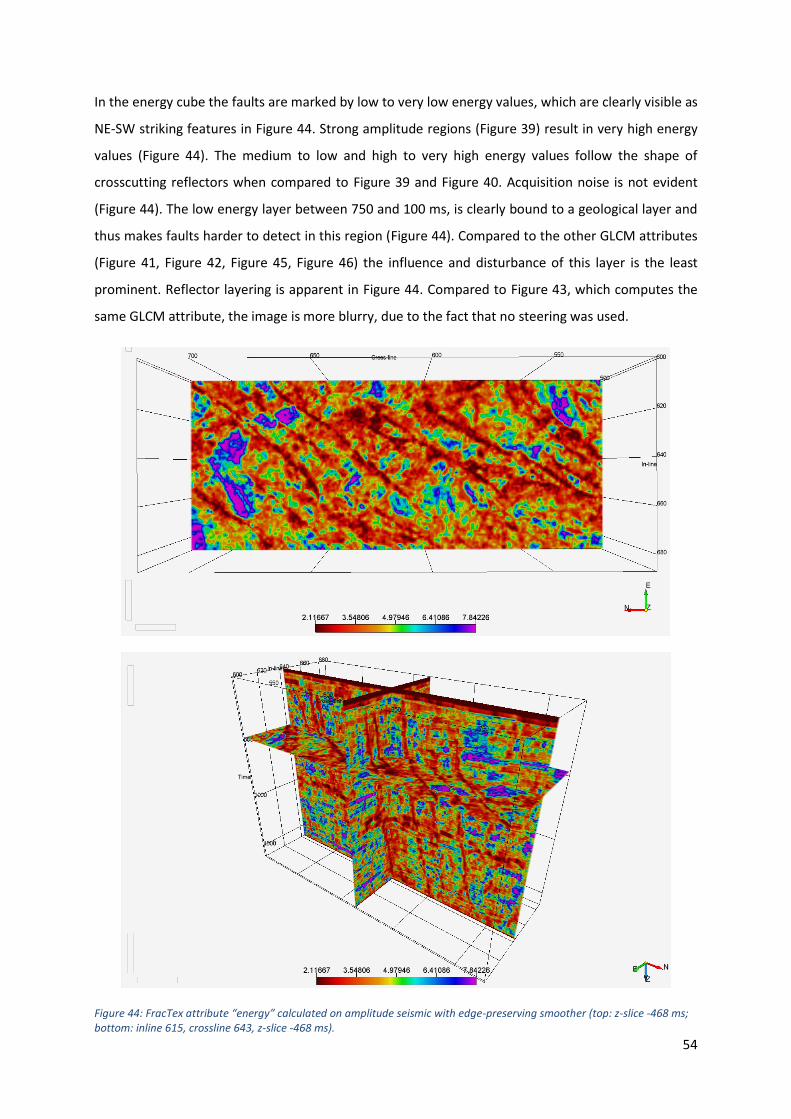
54

In the energy cube the faults are marked by low to very low energy values, which are clearly visible as

NE-SW striking features in Figure 44. Strong amplitude regions (Figure 39) result in very high energy

values (Figure 44). The medium to low and high to very high energy values follow the shape of

crosscutting reflectors when compared to Figure 39 and Figure 40. Acquisition noise is not evident

(Figure 44). The low energy layer between 750 and 100 ms, is clearly bound to a geological layer and

thus makes faults harder to detect in this region (Figure 44). Compared to the other GLCM attributes

(Figure 41, Figure 42, Figure 45, Figure 46) the influence and disturbance of this layer is the least

prominent. Reflector layering is apparent in Figure 44. Compared to Figure 43, which computes the

same GLCM attribute, the image is more blurry, due to the fact that no steering was used.

Figure 44: FracTex attribute “energy” calculated on amplitude seismic with edge-preserving smoother (top: z-slice -468 ms; bottom: inline 615, crossline 643, z-slice -468 ms).

55

In the entropy cube the faults are marked by low to very low energy values, which are clearly visible

as NE-SW striking features in Figure 45. Strong amplitude regions result in very high entropy values

and in this case rather weak reflectors in very low entropy values (Figure 39, Figure 45). The medium

to low and high to very high entropy values follow the shape of crosscutting reflectors when

compared to Figure 39 and Figure 40. Acquisition noise is not evident (Figure 45). The low energy

layer between 750 and 100 ms, is clearly bound to a geological layer and thus makes faults harder to

detect in this region (Figure 45). Reflector layering is apparent in Figure 45. Compared to other GLCM

attributes the image shows more detail regarding its features, although no steering was used (Figure

45).

Figure 45: FracTex attribute “entropy” calculated on amplitude seismic with edge-preserving smoother (top: z-slice -468 ms; bottom: inline 615, crossline 643, z-slice -468 ms).

56

In the homogeneity cube the faults are marked by low to very low energy values, which are visible as

NE-SW striking features in Figure 46. The faults appear blurrier than in the other GLCM attribute

cubes (Figure 46). Strong amplitude regions result in very high homogeneity values (Figure 39, Figure

46). The medium to low and high to very high entropy values follow the shape of crosscutting

reflectors when compared to Figure 39 and Figure 40. Acquisition noise is not evident (Figure 46).

The low energy layer between 750 and 100 ms, is clearly bound to a geological layer and thus makes

faults harder to detect in this region (Figure 46). Reflector layering is apparent in Figure 46.

Figure 46: FracTex attribute “homogeneity” calculated on amplitude seismic with edge-preserving smoother (top: z-slice -468 ms; bottom: inline 615, crossline 643, z-slice -468 ms).

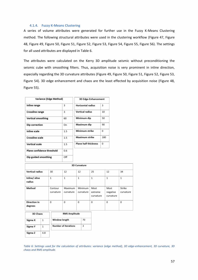
57

4.1.4. Fuzzy K-Means Clustering

A series of volume attributes were generated for further use in the Fuzzy K-Means Clustering

method. The following structural attributes were used in the clustering workflow (Figure 47, Figure

48, Figure 49, Figure 50, Figure 51, Figure 52, Figure 53, Figure 54, Figure 55, Figure 56). The settings

for all used attributes are displayed in Table 6.

The attributes were calculated on the Kerry 3D amplitude seismic without preconditioning the

seismic cube with smoothing filters. Thus, acquisition noise is very prominent in inline direction,

especially regarding the 3D curvature attributes (Figure 49, Figure 50, Figure 51, Figure 52, Figure 53,

Figure 54). 3D edge enhancement and chaos are the least effected by acquisition noise (Figure 48,

Figure 55).

Table 6: Settings used for the calculation of attributes: variance (edge method), 3D edge-enhancement, 3D curvature, 3D chaos and RMS amplitude.

58

Figure 47: 3D edge enhancement attribute calculated on amplitude seismic (top left: z-slice -468 ms, top right: crossline 668, inline 630).

59

Figure 48: Chaos attribute calculated on amplitude seismic (top left: z-slice -468 ms, top right: crossline 668, inline 630).

60

Figure 49: Contour curvature attribute calculated on amplitude seismic (top left: z-slice -468 ms, top right: crossline 668, inline 630).

61

Figure 50: Maximum curvature attribute calculated on amplitude seismic (top left: z-slice -468 ms, top right: crossline 668, inline 630).

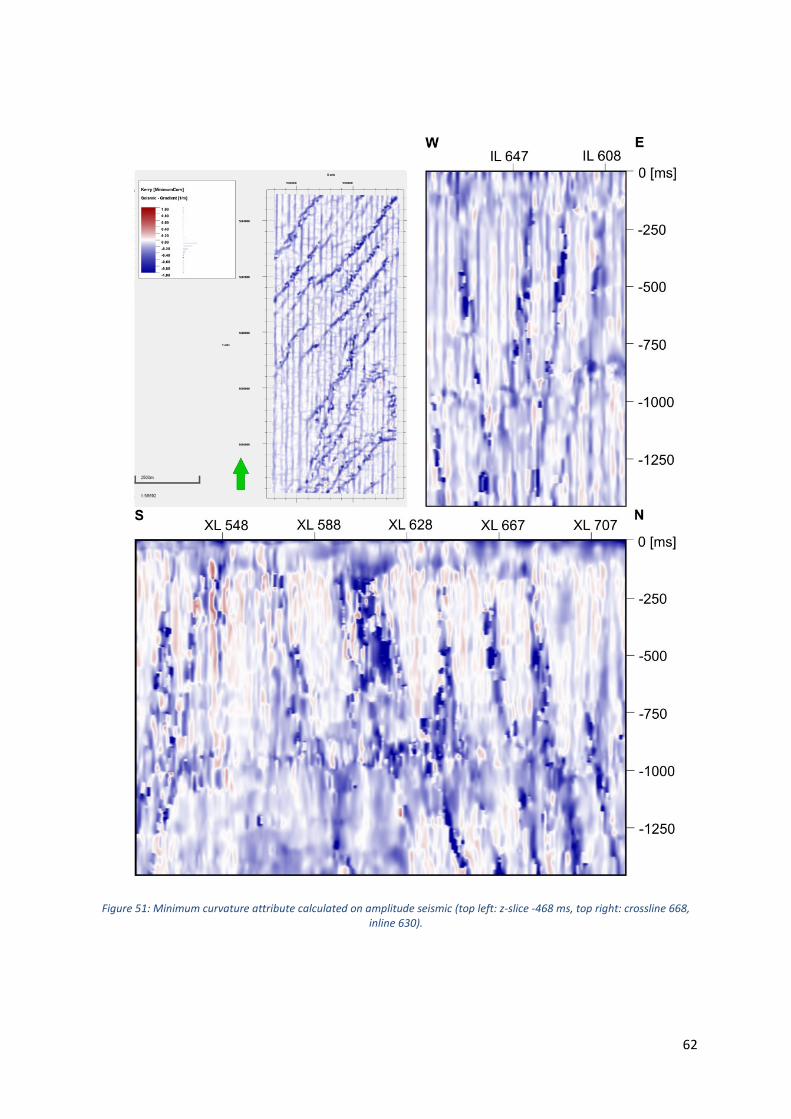
62

Figure 51: Minimum curvature attribute calculated on amplitude seismic (top left: z-slice -468 ms, top right: crossline 668, inline 630).

63

Figure 52: Most extreme curvature attribute calculated on amplitude seismic (top left: z-slice -468 ms, top right: crossline 668, inline 630).

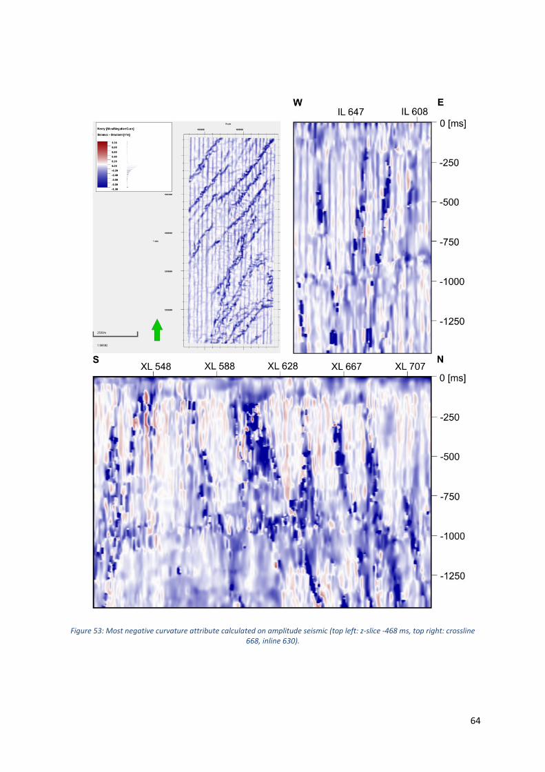
64

Figure 53: Most negative curvature attribute calculated on amplitude seismic (top left: z-slice -468 ms, top right: crossline 668, inline 630).

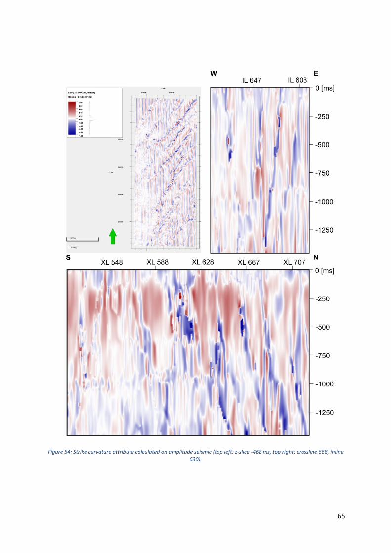
65

Figure 54: Strike curvature attribute calculated on amplitude seismic (top left: z-slice -468 ms, top right: crossline 668, inline 630).

66

Figure 55: RMS amplitude attribute calculated on amplitude seismic (top left: z-slice -468 ms, top right: crossline 668, inline 630).

67

Figure 56: Variance attribute calculated on amplitude seismic without structural smoothing (top left: z-slice -468 ms, top right: crossline 668, inline 630).

68

The cube in Figure 57 is the result of clustering 3 volume attributes, namely 3D edge-enhancement

(Figure 47), chaos (Figure 48) and contour curvature (Figure 49). For clustering a number of five

clusters were used, represented by five colours (Figure 57). The faults are marked in red and yellow

and strike NE-SW (Figure 57). Within the faults layering in red and yellow is visible, outside of the

faults layering is represented by dark red and grey colours (Figure 57). The layers which are yellow

inside of the faults continue as dark red layers outside of the faults (Figure 57). The largest portion of

the cube is represented by grey colour (Figure 57). Acquisition noise is not evident (Figure 57). The

red layer between 750 and 100 ms, is clearly bound to a geological layer and thus makes faults

harder to detect in this region (Figure 57).

Figure 57: Fuzzy K-Means Clustering result with five clusters, when using following volume attributes: 3D edge enhancement, chaos and contour curvature.

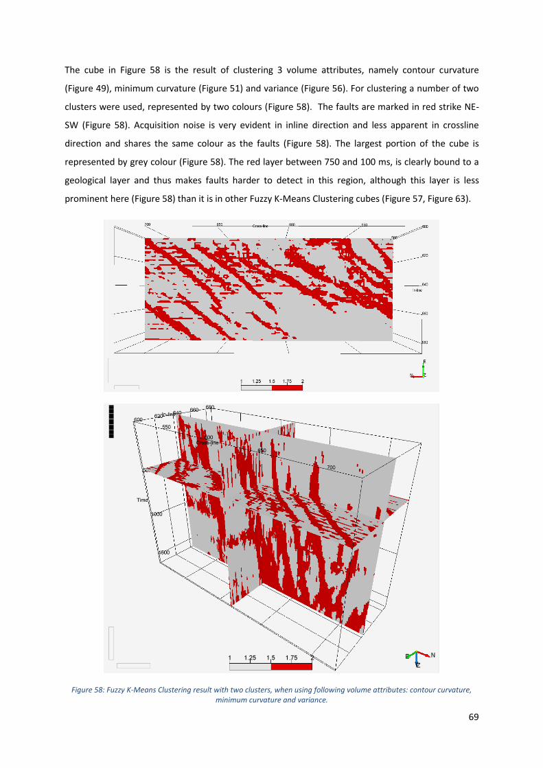
69

The cube in Figure 58 is the result of clustering 3 volume attributes, namely contour curvature

(Figure 49), minimum curvature (Figure 51) and variance (Figure 56). For clustering a number of two

clusters were used, represented by two colours (Figure 58). The faults are marked in red strike NE-

SW (Figure 58). Acquisition noise is very evident in inline direction and less apparent in crossline

direction and shares the same colour as the faults (Figure 58). The largest portion of the cube is

represented by grey colour (Figure 58). The red layer between 750 and 100 ms, is clearly bound to a

geological layer and thus makes faults harder to detect in this region, although this layer is less

prominent here (Figure 58) than it is in other Fuzzy K-Means Clustering cubes (Figure 57, Figure 63).

Figure 58: Fuzzy K-Means Clustering result with two clusters, when using following volume attributes: contour curvature, minimum curvature and variance.

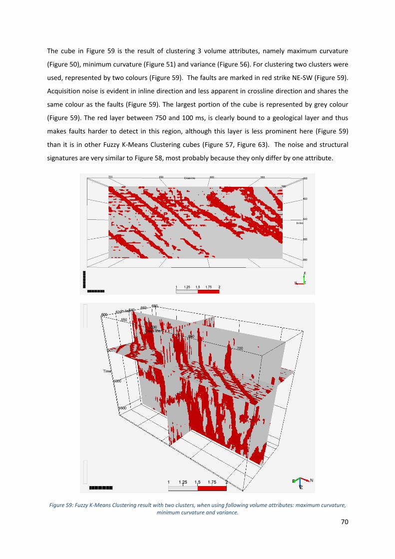
70

The cube in Figure 59 is the result of clustering 3 volume attributes, namely maximum curvature

(Figure 50), minimum curvature (Figure 51) and variance (Figure 56). For clustering two clusters were

used, represented by two colours (Figure 59). The faults are marked in red strike NE-SW (Figure 59).

Acquisition noise is evident in inline direction and less apparent in crossline direction and shares the

same colour as the faults (Figure 59). The largest portion of the cube is represented by grey colour

(Figure 59). The red layer between 750 and 100 ms, is clearly bound to a geological layer and thus

makes faults harder to detect in this region, although this layer is less prominent here (Figure 59)

than it is in other Fuzzy K-Means Clustering cubes (Figure 57, Figure 63). The noise and structural

signatures are very similar to Figure 58, most probably because they only differ by one attribute.

Figure 59: Fuzzy K-Means Clustering result with two clusters, when using following volume attributes: maximum curvature, minimum curvature and variance.

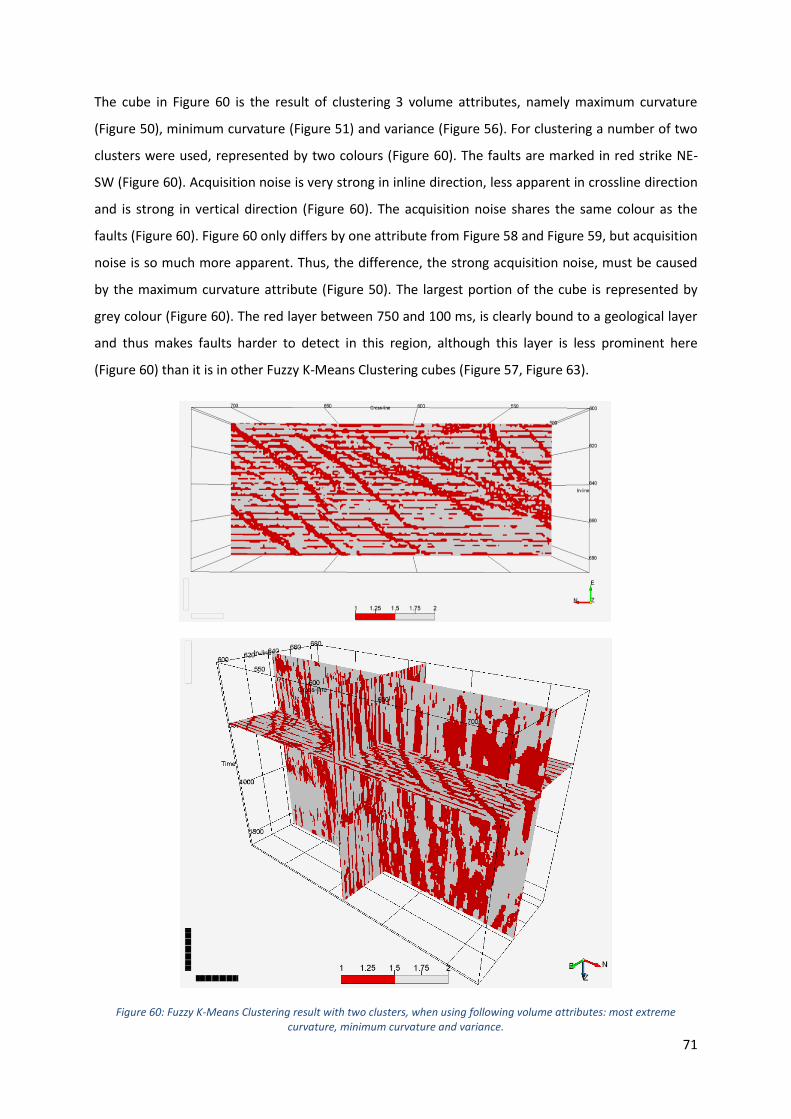
71

The cube in Figure 60 is the result of clustering 3 volume attributes, namely maximum curvature



SW (Figure 60). Acquisition noise is very strong in inline direction, less apparent in crossline direction

and is strong in vertical direction (Figure 60). The acquisition noise shares the same colour as the

faults (Figure 60). Figure 60 only differs by one attribute from Figure 58 and Figure 59, but acquisition

noise is so much more apparent. Thus, the difference, the strong acquisition noise, must be caused

by the maximum curvature attribute (Figure 50). The largest portion of the cube is represented by

grey colour (Figure 60). The red layer between 750 and 100 ms, is clearly bound to a geological layer

and thus makes faults harder to detect in this region, although this layer is less prominent here

(Figure 60) than it is in other Fuzzy K-Means Clustering cubes (Figure 57, Figure 63).

Figure 60: Fuzzy K-Means Clustering result with two clusters, when using following volume attributes: most extreme curvature, minimum curvature and variance.

72

The cube in Figure 61 is the result of clustering 3 volume attributes, namely most extreme curvature

(Figure 52), minimum curvature (Figure 51) and variance (Figure 56). For clustering five clusters were

used, represented by five colours (Figure 61). The faults are marked in red strike NE-SW (Figure 61).

Acquisition noise is very strong in inline direction, less apparent in crossline direction and strong in

vertical direction (Figure 61). This time the acquisition noise mostly shares a different colour to the

faults and makes it distinguishable. The red layer between 750 and 100 ms, is clearly bound to a

geological layer and makes faults harder to detect in this region, although this layer is less prominent

here (Figure 61) than it is in all other Fuzzy K-Means Clustering cubes (Figure 57, Figure 63).

Figure 61: Fuzzy K-Means Clustering result with five clusters, when using following volume attributes: most extreme curvature, minimum curvature and variance.

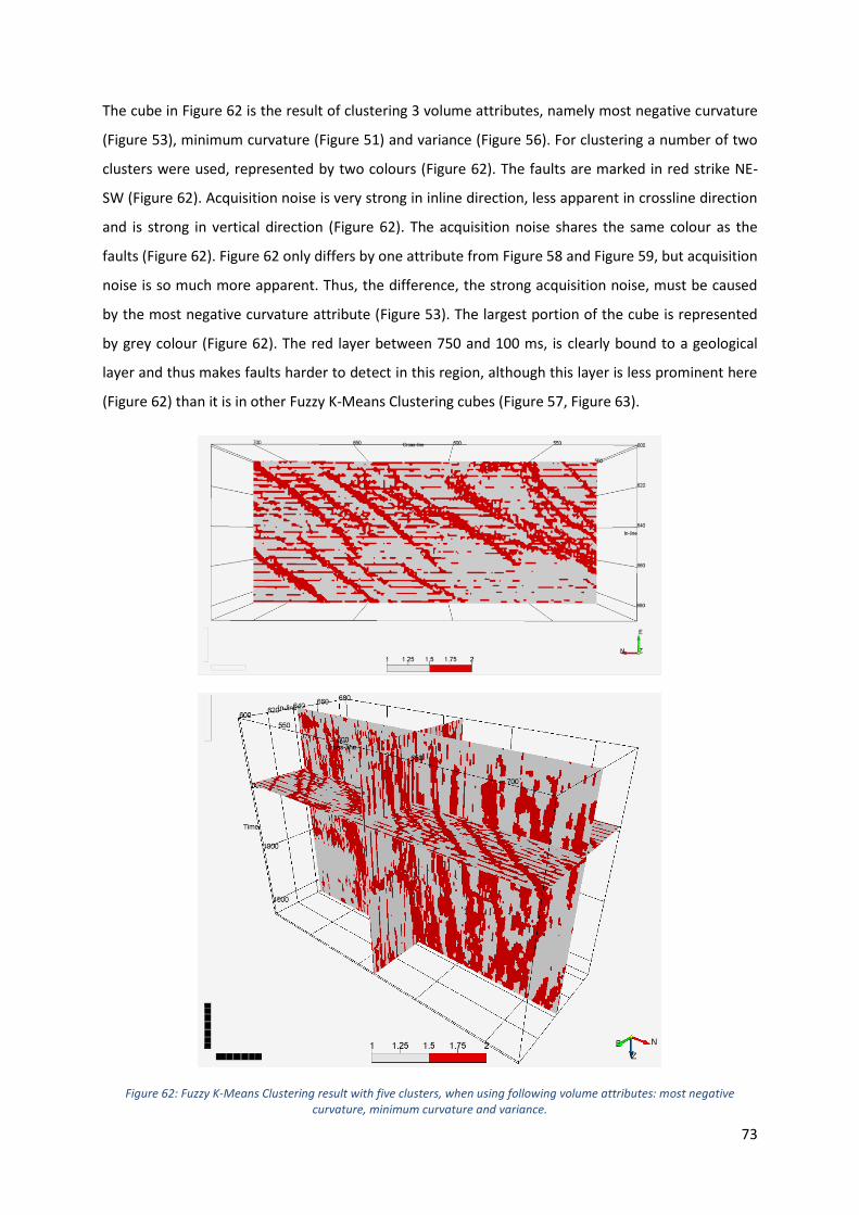
73

The cube in Figure 62 is the result of clustering 3 volume attributes, namely most negative curvature



SW (Figure 62). Acquisition noise is very strong in inline direction, less apparent in crossline direction

and is strong in vertical direction (Figure 62). The acquisition noise shares the same colour as the

faults (Figure 62). Figure 62 only differs by one attribute from Figure 58 and Figure 59, but acquisition

noise is so much more apparent. Thus, the difference, the strong acquisition noise, must be caused

by the most negative curvature attribute (Figure 53). The largest portion of the cube is represented

by grey colour (Figure 62). The red layer between 750 and 100 ms, is clearly bound to a geological

layer and thus makes faults harder to detect in this region, although this layer is less prominent here

(Figure 62) than it is in other Fuzzy K-Means Clustering cubes (Figure 57, Figure 63).

Figure 62: Fuzzy K-Means Clustering result with five clusters, when using following volume attributes: most negative curvature, minimum curvature and variance.

74

The cube in Figure 63 is the result of clustering 3 volume attributes, namely RMS amplitude (Figure

55), strike curvature (Figure 54) and variance (Figure 56). For clustering two clusters were used,

represented by two colours (Figure 63). The faults are marked in red strike NE-SW (Figure 63).

Acquisition noise is strong in inline direction, less apparent in crossline and in vertical direction

(Figure 63). The acquisition noise shares the same colour as the faults (Figure 63). Further faults are

masked by big red areas, that most likely stem from the RMS amplitude attribute (Figure 55). It

shows the same signature in the central eastern edge of the cube (Figure 55, Figure 63). The largest

portion of the cube is represented by grey colour (Figure 63). The red layer between 750 and 100 ms,

is bound to a geological layer and makes faults harder to detect due to its prominence (Figure 63).

Figure 63: Fuzzy K-Means Clustering result with two clusters, when using following volume attributes: RMS amplitude, strike curvature and variance.

75

The cube in Figure 64 is the result of clustering 3 volume attributes, namely RMS amplitude (Figure

55), strike curvature (Figure 54) and variance (Figure 56). Compared to Figure 63 five, instead of two,

clusters were used (Figure 64). The faults are marked in red strike NE-SW (Figure 64). Acquisition

noise is strong in inline direction, less apparent in crossline and in vertical direction (Figure 64). The

colour signature of the acquisition noise completely differs from the faults (Figure 64). Due to the

higher number of clusters, compared to Figure 63, faults are not masked by the RMS amplitude

attribute response (Figure 55). The largest portion of the cube is represented by brown and grey

colour (Figure 64). The red layer between 750 and 100 ms, is clearly bound to a geological layer, but

is not very evident. Thus, fault detection is simplified (Figure 64).

Figure 64: Fuzzy K-Means Clustering result with five clusters, when using following volume attributes: RMS amplitude, strike curvature and variance.

76

5. Discussion In this chapter, observations and interpretations of the four fault detection methods Manual Fault

Interpretation, Ant-Tracking, GLCM and the segmentation tool Fuzzy K-Means Clustering are

discussed for the seismic dataset Kerry 3D. The discussion focuses on the used methodologies, the

comparison of the methodologies, the resulting faults, the influences on the results, improvements

in fault detection and suggestions for further proceedings.

5.1. Manual Fault Interpretation

Seismic interpretation still needs a lot of manual work and requires an experienced interpreter to

determine relevant fault paths. In Manual Fault Interpretation the seismic volume is investigated for

discontinuities in the reflectors. It is a very well-established method for fault detection.

In the Tangahoe Formation seismic reflectors are very faint, so that discontinuities are very difficult

to detect with the naked eye. Only through the use of logic and human cognition it is obvious that

faults must continue underneath the Tangahoe Formation, if a line from the overlying to the

underlying formations can be traced and the discontinuity has the same offset on both sides of the

formation. Often faults are also missed or are wrongly traced by the interpreter. In Manual Fault

Interpretation Petrel tries to assist the interpreter, through suggesting fault paths, as soon as a few

fault sticks were created. If the interpreter relies on the computer-aided manual interpretation, it

often happens that wrong fault paths are traced. Especially when it comes to cross-cutting faults,

branching faults or complex fault systems. Regarding computational time or speed of workflow,

Manual Fault Interpretation tends to be very tedious and time-consuming, especially in complex fault

systems.

5.2. Ant-Tracking

Ant-Tracking is sufficient in extracting the fault information, but it is visible that the ant colony does

not highlight faults as strongly in the Tangahoe Formation as in the remaining cube. When using a

very aggressive ant tracking algorithm the faults are highlighted very well, at the cost of also

highlighting acquisition noise, which the structural smoothing filter was not able to remove.

Additionally, the problem with the more aggressive algorithm is visible when automatic fault

extraction is used. Although the faults are highlighted more clearly, the automatic fault extraction

function seems to have difficulties regarding faults that cross or are very close to each other.

Especially if faults cross each other at a very small angle. When extracting fault patches, it seems that

the algorithm is confused of which fault path to follow and ends up creating very uneven and merged

77

surfaces. To avoid difficulties with cross cutting faults it is best to calculate an ant tracking cube in

two directions on the structurally smoothed variance cube. By doing so only the information in the

chosen dip and azimuth are considered. This also makes it possible to extract different fault systems

in structurally even more complex cubes, making the interpretation of tectonic and geologic history

in a seismic cube easier. By using the ant tracking algorithm in a certain dip and azimuth fields at a

time, cancels out a lot of noise the algorithm would otherwise track. This is especially the case for the

acquisition noise in the Inline direction. Although the use of the structural smoothing filter cancelled

out most of the acquisition noise, some remains. To cancel the remaining acquisition noise the

corresponding dip and azimuth values are excluded for automatic fault extraction in the stereonet

display of the Ant Tracking window. Whether extracting faults on a custom, more aggressive, ant

tracking cube or in two different dip and azimuth directions of the faults, both approaches seem to

face the same difficulties in the Tangahoe Formation. In the Tangahoe Formation the weak amplitude

character makes discontinuities harder to detect and to trace completely. The incompletely traced

faults in the ant tracking cube results in patches with missing zones in automatic fault extraction. This

can be compensated for by merging and smoothing faults after fault patches were extracted. In the

incompletely extracted regions, fault surfaces can be interpolated through merging of the

corresponding fault patches.

Automatic fault extraction doesn´t take too long, but the problems faced with faults that are too

close to each other and thus merge, can dramatically change the interpretation of fault systems, if

heavily relying on its results. Thus, quality control of the result or even removing wrongly extracted

faults, is necessary. Wrongly extracted faults should be removed and the correct paths added

manually with Manual Fault Extraction, to save time.

5.3. Grey-Level Co-Occurrence Matrix (GLCM)

Before attempting to calculate GLCM-attributes OpendTect´s Edge-Preserving Smoother filter was

applied to the amplitude seismic. The Edge-Preserving Smoother filter, is designed to make it easy for

interpreters to visualize, pick and map the faults. Furthermore, the filter was utilized to reduce the

acquisition noise in the inline direction and to enhance and improve seismic data visualization for

structural interpretation. Afterwards the GLCM-attributes contrast, dissimilarity, energy, energy with

PG Steering, entropy and homogeneity were calculated.

All attributes highlight faults, which are characterized by low GLCM-attribute values and are mostly

continuous. Most GLCM-attributes show high attribute values in regions were z-slice cross-cutting

reflectors show stronger amplitude values, visible in the far north, south-eastern corner and the

78

central to western region of the amplitude and GLCM cubes. Thus, if the amplitudes of the seismic

cube could be normalized, the influence of the strongly varying reflector strengths on the GLCM-

attribute results would be reduced. Through normalization of the amplitude values the GLCM-

attribute value range could be reduced and therefore the faults enhanced. This might also help to

reduce the influence of weak seismic reflectors of the Tangahoe Formation on the GLCM-attribute

results. The Tangahoe Formation results in low GLCM-attribute values, which mask the low GLCM-

attribute values of the faults. The GLCM-attribute, which seem to be the least influenced by the weak

reflectors of the Tangahoe Formation, is the energy attribute, regardless if steering was used or not.

5.4. Fuzzy K-Means Clustering

To conduct Fuzzy K-Means Clustering a series of fault enhancing attribute volumes were calculated,

such as 3D Edge Enhancement, Chaos, 3D Curvature (contour, maximum, minimum, most extreme,

most negative, strike), RMS Amplitude and Variance. The seismic amplitude volume was not filtered

or enhanced before the calculation of the volume attributes. Therefor not only faults, but also

acquisition noise is visible in the attribute volumes. Features such as channels, and strong offlaps and

downlaps of the Tangahoe Formation are enhanced by the volume attributes. For Fuzzy K-Means

Clustering three different volume attributes were used as input and either two or five clusters

defined.

What is immediately visible, is where variance was used in the attribute combinations for Fuzzy K-

Means Clustering faults are depicted more clearly and continuous. Further, faults are better

distinguished in the results, when more clusters were used for the calculation. Where only two

clusters were used, features such as acquisition noise and irregularities in formations are highlighted

in the same colour as the faults. Through use of five clusters most of the acquisition noise in the

inline direction can be discriminated from faults. Thus, increasing the number of clusters might be of

use to filter acquisition noise, without having to pre-process seismic data using smoothing.

Nevertheless, irregularities remain in the Tangahoe Formation, after the number of clusters were

increased.

79

5.5. Comparison of Fault Detection Results of the Kerry 3D Subcrop

For better comparison of the four fault detection methods the 2D sections of inline 630 (Figure 67),

inline 658 (Figure 68), crossline 540 (Figure 69), crossline 668 (Figure 70), z-slice at -468 ms (Figure

71) and -960 ms (Figure 72) are displayed with the corresponding interpretations. Further a

geological (Figure 74) and seismic facies profile (Figure 75) of inline 630 were made.

Figure 65: Positions of investigated and interpreted inlines (630 and 658), crosslines (540 and 668) and z-slice -468 (displayed) of all four methods.

Acquisition noise is not a major hindrance when it comes to Manual Fault Interpretation. Spectral

enhancement or structural smoothing can improve the ability to detect faults for the interpreter.

This might be necessary in cubes with stronger acquisition noise than in the Kerry 3D seismic cube.

Ant-Tracking is affected by acquisition noise, although structural smoothing was used prior to the

Ant-Tracking algorithm. In automatic fault extraction on the Ant-Tracking cube, remaining acquisition

noise is even strong enough to be falsely extracted as a fault (Figure 24, Figure 32). The interpreter is

then responsible to remove the wrongly extracted fault within the stereonet or histogram display of

80

the extracted fault patches (Figure 37, Figure 38). In the GLCM-method acquisition noise in the inline

direction is enhanced but is almost completely removed when using OpendTect´s Edge-Preserving

Smoother (Figure 40). As for the Fuzzy K-Means Clustering cubes, when five clusters are used,

acquisition noise almost completely falls within different clusters than the faults (Figure 61, Figure

64). When using two clusters in the Fuzzy K-Means Clustering method acquisition noise and faults fall

within the same clusters (Figure 58, Figure 59, Figure 60, Figure 62, Figure 63). So, it is advised to use

five instead of two clusters, when wanting to prevent mixing of noise and fault responses or using

smoothing filters on the amplitude seismic.

The major regional fault in the Kupe area is the north-south oriented Manaia Fault, which is a

significant inversion lineament in the Kupe field (Figure 6)(Fohrmann et al., 2012). Movement was

initially normal from the Cretaceous to Late Paleocene, reversed during the latest Eocene–Oligocene

and peaked in the Late Miocene, with formation of the Manaia Anticline (Stagpoole et al., 2008;

Fohrmann et al., 2012). The Manaia anticline is a north-south trending and north plunging, reverse-

faulted inversion structure which formed through inversion of the Cretaceous rift-related Manaia

Fault (Figure 6)(King et al., 1996). The Kerry Field itself is situated at the southern end of the Manaia

Anticline and is segmented by a series of NW-SE striking normal faults, with the largest one being

the Kupe South Fault (Figure 6, Figure 71, Figure 72)(Schmidt et al., 1990). The offsets along the

faults in the Kerry 3D subcrop are minor and reach a maximum of about 70 ms (TWT).

Manual Fault Interpretation of an experienced interpreter, GLCM-attributes and the Fuzzy K-Means

Clustering algorithm have no difficulty determining fault paths (Figure 67, Figure 68, Figure 69, Figure

70, Figure 71, Figure 72). Ant-Tracking on the other hand, selects evidently erroneous fault paths,

especially when faults are very close, cross each other at very small angles or when faults have to be

extracted in regions with disturbed or discontinuous reflectors (Figure 67, Figure 68, Figure 69, Figure

70, Figure 71, Figure 72).

Detected faults are clearly outlined and continuous in Manual Fault Interpretation, although

discontinuities where hard to identify in the Tangahoe Formation, which is characterized by very

weak and chaotic reflectors (Figure 67, Figure 68, Figure 69, Figure 70, Figure 71, Figure 72). Through

the help of cognitive thinking of the interpreter, faults which are visible above and below the

Tangahoe Formation and show the same offset, belong to the same fault. Although Ant-Trackings

automatic fault extraction is capable of extracting faults in a very continuous manner, the extraction

encounters difficulties in the Tangahoe Formation (Figure 67, Figure 68, Figure 69, Figure 70, Figure

72). This is compensated for by merging and smoothing faults after fault patches were extracted. The

GLCM-attributes are rather effective at extracting continuous fault, which are characterized by

medium to low GLCM-attribute values (Figure 67, Figure 68, Figure 69, Figure 70, Figure 71, Figure

81

72). The only obstacle is the Tangahoe Formation, which shows very similar GLCM-attribute values as

the faults (Figure 67, Figure 68, Figure 69, Figure 70, Figure 71, Figure 72). In fact, GLCM is the

method most effected by the response of the Tangahoe Formation (Figure 67, Figure 68, Figure 69,

Figure 70, Figure 72). Concerning Fuzzy K-Means Clustering, the algorithm performs quite well in

respect to fault continuity (Figure 67, Figure 68, Figure 69, Figure 70, Figure 71, Figure 72).

Between cross lines 680 and 550 Manual Fault Interpretation, Ant-Tracking and GLCM seem to have

difficulties extracting faults that resemble a fault bound gas chimney structure (Figure 67). Fuzzy K-

Means Clustering is the only method able to completely extract the structure missed by all other

methods (Figure 67). In general, Fuzzy K-Means Clustering appears to be the method most capable of

extracting fault zones. The Fuzzy K-Means Clustering algorithm identifies several faults which were

missed by all other methods (Figure 67, Figure 68, Figure 69, Figure 70, Figure 71, Figure 72). The

faults which were additionally extracted by the Fuzzy K-Means Clustering algorithm are plausible,

when investigating the original seismic section (Figure 73).

The results of all methods imply that fault detection and extraction is the most difficult in the

Tangahoe Formation (Figure 67, Figure 68, Figure 69, Figure 70, Figure 71, Figure 72). Thus, the

geology of the formation needs to be investigated (Figure 74). The Tangahoe Formation is

characterized by poorly bedded sandy mudstones (Arnold, 1957) and is easily distinguished from the

Giant Foresets Formation above and Matemateaonga Formation below, through its bland character

in the 3D amplitude seismic (Figure 73, Figure 75)(Baur, 2012). The overlying Giant Foresets and the

underlying Matemateaonga Formation are characterized by high amplitudes and continuous

reflection patterns (Figure 73, Figure 75)(Baur, 2012). This observation indicates that the impedance

contrast between the Giant Foresets and Tangahoe, and Tangahoe and Matemateaonga Formation

are very high. Thus, the Tangahoe Formation must be homogeneous from lithology, poorly bedded

and the impedance contrast to its over- and its underlying formations large to result in its bland

reflection character (Figure 73, Figure 75). In detail the Tangahoe Formation is characterized by low-

to medium-amplitude discontinuous off-lapping reflectors (Figure 73, Figure 75) described as shelf,

outer shelf, and slope claystones and siltstones (Baur, 2012). Then there are relatively continuous,

off-lapping clinoform north-east dipping reflectors with medium to high amplitudes which

periodically subdivide these and are interpreted as progradational shelf foresets (Figure 73, Figure

75)(Ogilvie, 1993; King et al., 1996). Further, discontinuous medium- to high-amplitudes incise the

higher amplitude reflectors indicating fluvial channels (Figure 67, Figure 73)(Baur, 2012). The flat

clinoform bottomsets, made up of fine-grained sediment and sand, show medium to high amplitudes

fading into low amplitude reflectors towards the basin centre (Figure 73, Figure 75)(Baur, 2012). To

summarize, the Tangahoe Formation, comprises offlapping, progradational shelf topsets which

82

accumulated after rapid and tectonically-driven subsidence in the late-Early Pliocene (Figure

75)(Hayton et al., 1997; Kamp, 1999; Bland et al., 2013).

The seismic facies classification for all formations within the Kerry 3D seismic subcrop (Figure 73),

was characterized by a simplified seismic sequence stratigraphy, reflection configuration, reflection

continuity and reflection strength (Figure 75). The Matemateaonga Formation (Figure 74) is

characterized by parallel, continuous to semicontinuous and strong reflectors (Figure 75.8). The

overlying Tangahoe Formation (Figure 74) comprises of three seismic facies (Figure 75.5, Figure

75.6, Figure 75.7). The base is defined by parallel, continuous to semicontinuous reflectors which are

weaker to the south and become stronger towards the north (Figure 75.7). Overlapping is a

progradational section with oblique, semicontinuous and weak reflectors terminating at the base

with downlaps (Figure 75.6). This is followed by a contorted to mound-shaped, discontinuous section

with weak reflectors onlapping the previous section (Figure 75.5). The overlying Giant Foresets

Formation (Figure 74) is divided into three seismic facies sections (Figure 75.2, Figure 75.3, Figure

75.4). The base is characterized by parallel, continuous to semicontinuous, strong reflectors (Figure

75.4). Onlapping is a progradational section defined by oblique, continuous to semicontinuous

reflectors which are weaker towards the south and stronger when onlapping further north (Figure

75.3). This is followed by the Giant Foresets Formation, which is thickest section, with parallel,

continuous and strong reflectors (Figure 75.2). The uppermost section is the Late Pleistocene

Formation (Figure 74) with parallel, continuous to semicontinuous, weak reflectors (Figure 75.1).

When considering the varying reflection character of the Tangahoe Formation, also if its overall

character is weaker than the over- and underlying formations (Figure 73), it is evident that not the

whole formation is responsible for the difficulties in fault interpretation in this zone (Figure 75).

When outlining the medium to weak amplitude zone in the amplitude seismic it is evident in the

GLCM-attribute section that all disturbances where caused by the corresponding zone (Figure 67,

Figure 68, Figure 69, Figure 70, Figure 72). All features in the Fuzzy K-Means Clustering method which

cannot indistinguishably be assigned to faults, fall within the bland reflection zone of the Tangahoe

Formation (Figure 67, Figure 68, Figure 69, Figure 70, Figure 72). The disturbed zones, which fall

within the same cluster as the faults, towards the right in the inline displays of the Fuzzy K-Means

Clustering method, are most probably caused by downlaps and clinoforms with stronger amplitude

values (Figure 67, Figure 68). Especially the strong amplitude downlaps of the prograding Tangahoe

Formation are visible in variance attribute cubes.

Concerning display of faults, Manual Fault Interpretation and Ant-Tracking display faults as surfaces,

whereas GLCM and Fuzzy K-Means Clustering algorithms display faults as volumes (Figure 67, Figure

68, Figure 69, Figure 70, Figure 71, Figure 72). Faults are to be considered as fault or fracture zones

83

and not surfaces without volumes. When creating reservoir models, faults as created in Manual Fault

Interpretation and Ant-Tracking, are of no direct use, since flow is not possible along a surface with

no volume. The GLCM and Fuzzy K-Means Clustering method result in fracture volumes, better suited

for reservoir engineering models, since they portray a more realistic geological model. Parameters

important for flow, such as porosity and permeability, can thus be realistically populated onto a

reservoir model.

Regarding computational time or speed of workflow Manual Fault Interpretation tends to be very

tedious and time-consuming, especially in complex fault systems. For small seismic volumes Ant-

Tracking with automatic fault extraction and the GLCM-method are very fast. When processing big

seismic volumes computers need considerably more computing power to calculate the Ant-Tracking

or GLCM-attribute cube in an adequate amount of time. Fuzzy K-Means Clustering is quite fast once

the attribute sets are brought into a, for Matlab, processible form.

Figure 66: Legend for Figure 67, Figure 68, Figure 69, Figure 70, Figure 71 and Figure 72.

84

Figure 67: Interpretation of all four fault detection methods on inline 630. a. Manual Fault Interpretation: Interpreted fault colour correspond with colours in Figure 16, weak reflector zone of Tangahoe Formation (white dotted line), strong amplitude channels (yellow arrows), gas chimney-like structure or fault (white area). b. Fuzzy K-Means Clustering: recognizes more faults than other methods (yellow area), some of the red zones in the weak amplitude zone of the Tangahoe Formation (white dotted line) might be related to channels (yellow arrows). c. Ant-Tracking: Results of automatic fault extraction with passive (green and yellow lines) and custom Ant-Tracking cube (blue lines), falsely extracted fault paths (red area). d. GLCM-Method (dissimilarity attribute): weak reflector zone of the Tangahoe Formation very prominent (white dotted line) and correlates to the low dissimilarity zone, missed a few faults (white area).

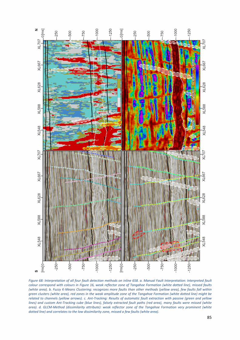
85

Figure 68: Interpretation of all four fault detection methods on inline 658. a. Manual Fault Interpretation: Interpreted fault colour correspond with colours in Figure 16, weak reflector zone of Tangahoe Formation (white dotted line), missed faults (white area). b. Fuzzy K-Means Clustering: recognizes more faults than other methods (yellow area), few faults fall within green clusters (white area), red zones in the weak amplitude zone of the Tangahoe Formation (white dotted line) might be related to channels (yellow arrows). c. Ant-Tracking: Results of automatic fault extraction with passive (green and yellow lines) and custom Ant-Tracking cube (blue lines), falsely extracted fault paths (red area), many faults were missed (white area). d. GLCM-Method (dissimilarity attribute): weak reflector zone of the Tangahoe Formation very prominent (white dotted line) and correlates to the low dissimilarity zone, missed a few faults (white area).

86

Figure 69: Interpretation of all four fault detection methods on crossline 540. a. Manual Fault Interpretation: Interpreted fault colour correspond with colours in Figure 16, weak reflector zone of Tangahoe Formation (white dotted line), many faults were missed (white area). b. Fuzzy K-Means Clustering: recognizes more faults than other methods (yellow area), red zones in the weak amplitude zone of the Tangahoe Formation (white dotted line). c. Ant-Tracking: Results of automatic fault extraction with passive (green and yellow lines) and custom Ant-Tracking cube (blue lines), falsely extracted fault paths (red area), many faults were missed (white area). d. GLCM-Method (dissimilarity attribute): weak reflector zone of the Tangahoe Formation very prominent (white dotted line) and correlates to the low dissimilarity zone, missed many faults (white area).

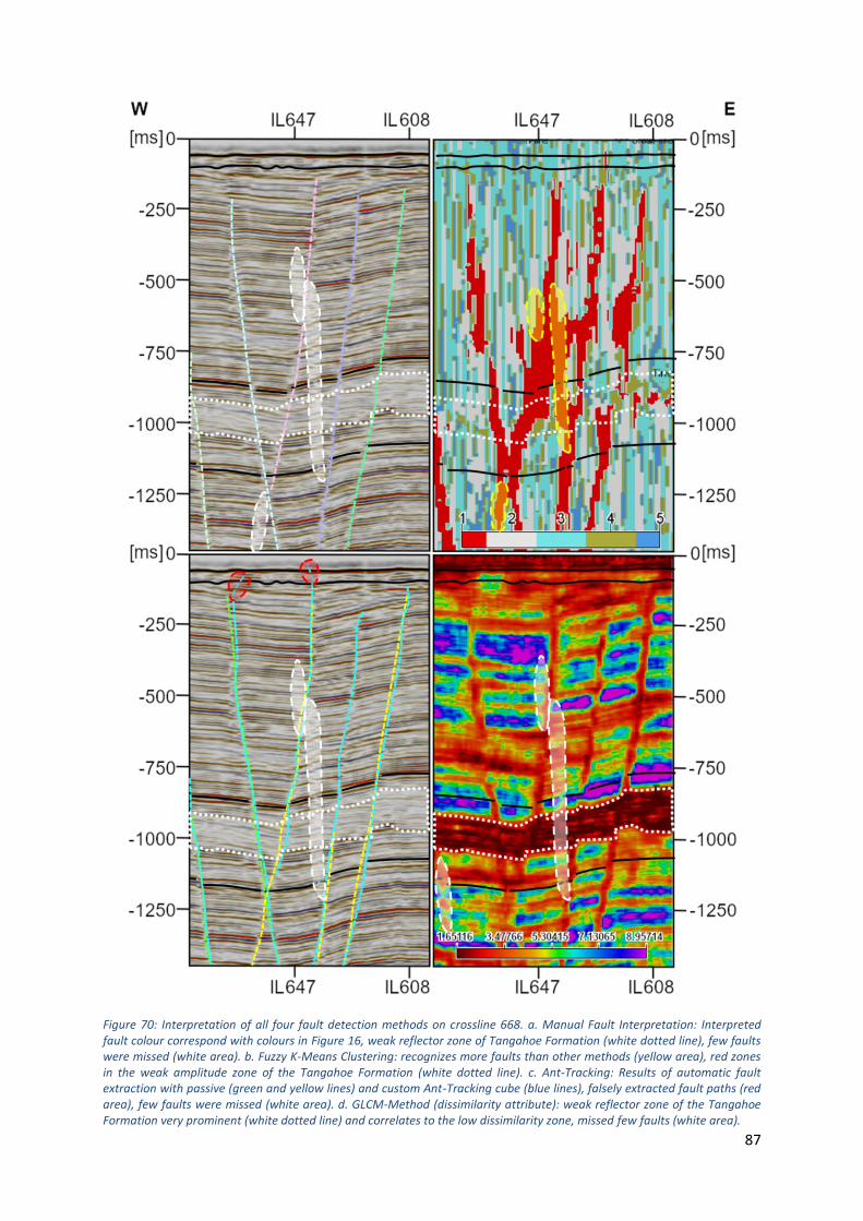
87

Figure 70: Interpretation of all four fault detection methods on crossline 668. a. Manual Fault Interpretation: Interpreted fault colour correspond with colours in Figure 16, weak reflector zone of Tangahoe Formation (white dotted line), few faults were missed (white area). b. Fuzzy K-Means Clustering: recognizes more faults than other methods (yellow area), red zones in the weak amplitude zone of the Tangahoe Formation (white dotted line). c. Ant-Tracking: Results of automatic fault extraction with passive (green and yellow lines) and custom Ant-Tracking cube (blue lines), falsely extracted fault paths (red area), few faults were missed (white area). d. GLCM-Method (dissimilarity attribute): weak reflector zone of the Tangahoe Formation very prominent (white dotted line) and correlates to the low dissimilarity zone, missed few faults (white area).

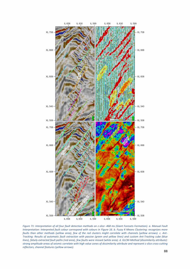
88

Figure 71: Interpretation of all four fault detection methods on z-slice -468 ms (Giant Foresets Formation). a. Manual Fault Interpretation: Interpreted fault colour correspond with colours in Figure 16. b. Fuzzy K-Means Clustering: recognizes more faults than other methods (yellow area), few of the red clusters might correlate with channels (yellow arrows). c. Ant-Tracking: Results of automatic fault extraction with passive (green and yellow lines) and custom Ant-Tracking cube (blue lines), falsely extracted fault paths (red area), few faults were missed (white area). d. GLCM-Method (dissimilarity attribute): strong amplitude areas of seismic correlate with high value zones of dissimilarity attribute and represent z-slice cross-cutting reflectors, channel features (yellow arrows).

89

Figure 72: Interpretation of all four fault detection methods on z-slice -960 ms (Tangahoe Formation). a. Manual Fault Interpretation: Interpreted fault colour correspond with colours in Figure 16. b. Fuzzy K-Means Clustering: recognizes few more faults than other methods (yellow area), very prominent red zones in the weak amplitude zone of the Tangahoe Formation (white dotted line). c. Ant-Tracking: Results of automatic fault extraction with passive (green and yellow lines) and custom Ant-Tracking cube (blue lines), falsely extracted fault paths (red area), few faults were missed (white area). d. GLCM-Method (dissimilarity attribute): weak reflector zone of the Tangahoe Formation very prominent (white dotted line) and correlates to the low dissimilarity zone, due to response of Tangahoe Formation fault response masked (white area).

90

Figure 73: Kerry 3D amplitude seismic at inline 630.

Figure 74: Geological profile of Kerry 3D subcrop at inline 630. Black lines represent faults and red arrows indicate the direction of motion of hanging wall block.

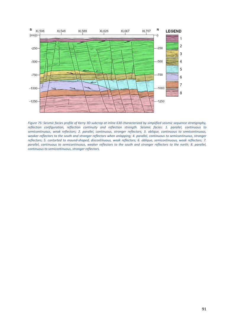
91

Figure 75: Seismic facies profile of Kerry 3D subcrop at inline 630 characterized by simplified seismic sequence stratigraphy, reflection configuration, reflection continuity and reflection strength. Seismic facies: 1. parallel, continuous to semicontinuous, weak reflectors; 2. parallel, continuous, stronger reflectors; 3. oblique, continuous to semicontinuous, weaker reflectors to the south and stronger reflectors when onlapping; 4. parallel, continuous to semicontinuous, stronger reflectors; 5. contorted to mound-shaped, discontinuous, weak reflectors; 6. oblique, semicontinuous, weak reflectors; 7. parallel, continuous to semicontinuous, weaker reflectors to the south and stronger reflectors to the north; 8. parallel, continuous to semicontinuous, stronger reflectors.

92

6. Conclusion Seismic interpretation still requires a lot of manual work, specifically in regard to the Manual Fault

Interpretation and the Ant-Tracking workflow. Thus, it would be of advantage, if the fault detection

workflows could be automated or improved by use of the GLCM or the Fuzzy K-Means Clustering

workflow.

Manual Fault Interpretation of an experienced interpreter, GLCM-attributes and the Fuzzy K-Means

Clustering algorithm have no difficulty determining fault paths. Ant-Tracking on the other hand,

selects evidently erroneous fault paths, especially when faults are very close, cross each other at very

small angles or when faults have to be extracted in regions with disturbed or discontinuous

reflectors. Acquisition noise is only a hinderance in Ant-Tracking as remaining noise is even strong

enough to be falsely extracted as a fault.

Detected faults are clearly outlined and continuous in Manual Fault Interpretation, although

discontinuities where sometimes hard to identify in the Tangahoe Formation, which is characterized

by very weak and chaotic reflectors. The GLCM-attributes are rather effective at extracting

continuous fault, with the only obstacle being the Tangahoe Formation, showing the same GLCM-

attribute values as the faults. Fuzzy K-Means Clustering was able to mostly differentiate faults from

other seismic facies.

The Fuzzy K-Means Clustering algorithm identifies several faults which were missed by all other

methods. The faults which were additionally extracted by the Fuzzy K-Means Clustering algorithm are

plausible, when investigating the original seismic section.

Since faults are to be considered as fault or fracture zones and not surfaces without volumes. The

GLCM and Fuzzy K-Means Clustering method result in fracture volumes, better suited for reservoir

engineering models, since they portray a more realistic geological model. Fuzzy K-Means Clustering is

so far the most effective and detailed method to detect fracture volumes, but is only as good and

effective as the attributes that were used as input.

To further improve fault detection methods, a more detailed investigation of the workflows on other

seismic data sets, in combination with geological and geophysical well data, is advised. Especially in

geologically more complex settings.

Concluding, Manual Fault Interpretation is effective, if the factor time is subordinate. Ant-Tracking

and GLCM are excellent quick look methods. Generally, Fuzzy K-Means Clustering has been proven to

be the most effective and detailed method to detect fracture zones and could be of use in future to

automate the fault extraction process.

93

7. Outlook Manual Fault Interpretation and Ant-Tracking are established methods for fault detection, but the

Fuzzy K-Means Clustering workflow itself requires further validation. The Fuzzy K-Means Clustering

workflow should be tested on other data sets to identify, if clustering is convenient and efficient for

other, especially more complex data sets. It would be interesting to examine the outcome of Fuzzy K-

Means Clustering, if an Ant-Tracking cube was used as input. Since Fuzzy K-Means Clustering

combinations that include the variance cube show the best results, the use of an Ant-Tracking cube

might show more defined results, since it displays faults in a clearer manner, compared to other

structural volume attributes. Compared to the variance attribute, Ant-Tracking can remove the

signature of channels, strong onlapping reflectors and most of the acquisition noise.

Since certain GLCM-attributes also detect more faults than other methods, GLCM-attributes should

also be tested with Fuzzy K-Means Clustering, regardless of the difficulties in the Tangahoe

Formation. One should remember, that the Fuzzy K-Means Clustering method is only as good and

effective in detecting fracture zones, as the attributes that were used as input. Thus, further

attributes should be tested as calculation input. Further test of different clustering algorithms is

advised to see, if other clustering algorithms would result in more realistic fault and reservoir

models. Attribute validation should also be done on horizon slices, to see if a more direct correlation

between attributes, fracture detection methods, geology and stratigraphy can be found. Validating

the fracture detection methods through well data is also of great importance. Unfortunately, the well

data of well Toru-1 in the Kerry 3D subcrop is not enough to create detailed statements about

fracture zones and geologic characteristics of the whole cube. The lack of well data creates

limitations in interpretation, because assumptions about the geology of a well are only reliable one

meter around well, as far es well logs go. Additionally, one well is not enough for a reliable well tie. If

a sufficient number of wells would be present to create a reliable velocity model, the seismic cube

could be converted from time to depth. With a depth-converted seismic cube more quantitative

statements can be made about the geology of the subcrop. Thereafter, it is suggested to perform the

fault detection methods, specifically Fuzzy K-Means Clustering, on a seismic cube with a sufficient

number of wells.

Farther, to create better assumptions about fault zones and volumes in Fuzzy K-Means Clustering

optical borehole imager logs should be investigated. Consequently, fault thicknesses generated from

the Fuzzy K-Means Clustering and GLCM workflow could be matched with fracture zone thicknesses

of the optical borehole imager logs. This might also lead to a correlation between Fuzzy K-Means

Clustering and GLCM volumes with parameters such as permeability and porosity which are also

related to faults and fault zones.

94

8. Literature Adams, R. D., and D. E. Ware, 1977, Subcrustal earthquakes beneath new zealand; locations

determined with a laterally inhomogeneous velocity model: New Zealand Journal of Geology and Geophysics, v. 20, no. 1, p. 59–83, doi:10.1080/00288306.1977.10431592.

Aggarwal, C. C., and C. K. Reddy, 2013, Data Clustering Algorithms and Applications: Chapman and Hall/ CRC, 1-23 p.

Amtmann, J., C. G. Eichkitz, D. Hofer, and M. G. Schreilechner, 2017, Clustering of seismic attributes for automatic seismic interpretation - First tests on synthetic geological models: First Break, v. 35, no. 5, p. 65–69.

Amtmann, J., C. G. Eichkitz, M. G. Schreilechner, D. Hofer, N. Gegenhuber, and M. Jud, 2017, Testing of Clustering Algorithms on Different 3D Seismic Models, in 79th EAGE Conference & Exhibition 2017: p. 1–4.

Arnold, H. C., 1957, The Pliocene stratigraphy of central and South Taranaki.

Bauckhage, C., 2015, Lecture Notes on Data Science : Soft k-Means Clustering: 1-7 p., doi:10.13140/RG.2.1.3582.6643.

Baur, J. R., 2012, Regional seismic attribute analysis and tectono-stratigraphy of offshore South-Western Taranaki Basin, New Zealand: Victoria University of Wellington, 431 p.

Beggs, J. M., 1990, Seismic Stratigraphy of the Plio-Pleistocene Giant Foresets, Western Platform, Taranaki Basin: New Zealand Oil Exploration Conference, p. 201–207.

Van Bemmel, P. P., and R. E. F. Pepper, 2000, Seismic Signal Processing Method and Apparatus for Generating a Cube of Variance Values, US 6,151,555: United States.

Bezdek, J. C., 1981, Pattern Recognition with Fuzzy Objective Function Algorithms: New York, Plenum Press, 1-256 p.

Bland, K. J., D. P. Strogen, M. Fohrmann, and K. F. Kroeger, 2013, Cretaceous – Recent lithostratigraphy of the Kupe mapping area (4D Taranaki Project), southeastern Taranaki Basin.

Bradshaw, J. D., 1989, Cretaceous Geotectonic patterns in the New Zealand region: Tectonics, v. 8, no. 4, p. 803–820.

Chopra, S., and V. Alexeev, 2005, Application of texture attribute analysis to 3D seismic data: 75th SEG meeting, p. 767–770.

Chopra, S., and V. Alexeev, 2006a, Applications of texture attribute analysis to 3D seismic data: The Leading Edge, v. 25, no. 8, p. 934–940, doi:10.1190/1.2335155.

Chopra, S., and V. Alexeev, 2006b, Texture Attribute Applications To 3D Seismic Data: 6th International Conference & Exposition on Petroleum Geophysics “Kolkata 2006,” p. 874–879, doi:10.1190/1.2335155.

Chopra, S., and K. J. Marfurt, 2010, Integration of coherence and volumetric curvature images: The Leading Edge, no. 9, p. 1092–1107.

Clayton, S., 2017, 3-D Geometry and Kinematic Evolution of the Kupe Inversion Structure, Southern Taranaki Basin, New Zealand: University of Oklahoma, 87 p.

Cooper, R. A., 2004, The New Zealand Geological Timescale: Institute of Geological and Nuclear

95

Sciences.

Cope, R. N., and J. J. Reed, 1967, The Cretaceous Paleogeology of the Taranaki - Cook Strait Area: Proceedings of the Australasian Institute of Mining and Metallurgy, v. 222, p. 63–72.

DeMets, C., R. G. Gordon, D. F. Argus, and S. Stein, 1994, Effect of Recent Revisions to the Geomagnetic Reversal Time Scale on Estimates of Current Plate Motions: Geophysical Research Letters, v. 21, p. 2191–2194, doi:10.1029/94GL02118.

dGB Earth Sciences, 2017, OpendTect 6.0 [User Guide]: <http://doc.opendtect.org/6.0.0/doc/dgb_userdoc/Default.htm#dip- steering/attributes_with_steering/curvature_analysis.htm%253FTocPath%253D3%252520Dip- Steering%257C3.5%252520Attributes%252520with%252520Steering%257C3.5.1%252520Curvature%252520Analysis%25 7> (accessed November 8, 2018).

dGB Earth Sciences, 2018, OpendTect 6.2 [User Guide]: <http://doc.opendtect.org/6.2.0/doc/od_userdoc/Default.htm#appendix_a- attributes_and_filters/texture-directional.htm%3FTocPath%3D11%2520Appendix%2520A%2520- %2520Attributes%2520and%2520Filters%7C_____28> (accessed November 13, 2018).

Eichkitz, C., and J. Amtmann, 2018, GLCM-based anisotropy estimation - the influence of computation parameters on the results: First Break, no. June, p. 47–52.

Eichkitz, C. G., J. Amtmann, and M. G. Schreilechner, 2013, Calculation of grey level co-occurrence matrix-based seismic attributes in three dimensions: Computers and Geosciences, v. 60, p. 176–183, doi:10.1016/j.cageo.2013.07.006.

Eichkitz, C. G., J. Amtmann, and M. G. Schreilechner, 2015, Directional Grey Level Co-occurrence Matrix- based Attributes for Fracture Detection, in 77th EAGE Conference & Exhibition: p. 1–4, doi:10.13140/RG.2.1.4837.2643.

Eichkitz, C. G., J. Amtmann, and M. G. Schreilechner, 2012, Facies Characterization by Seismic Texture Analysis Using Grey Level Co-occurrence Matrix Based Attributes, in 74th EAGE Conference & Exhibition: p. 1–5.

Eichkitz, C. G., M. G. Schreilechner, P. de Groot, and J. Amtmann, 2015, Mapping directional variations in seismic character using gray-level co-occurrence matrix-based attributes: Interpretation, v. 3, no. 1, p. T13–T23, doi:10.1190/INT-2014-0099.1.

Fleming, C. A., 1953, The Geology of Wanganui Subdivision; Waverley and Wanganui Sheet Districts (N137 and N138): 361 p.

Fohrmann, M., P. R. King, D. P. Strogen, E. Reid, H. Zhu, L. Roncaglia, M. G. Hill, K. J. Bland, and G. P. L. Scott, 2012, Seismic reflection character, mapping and tectono-stratigraphic history of the Kupe area (4D Taranaki Project), south-eastern Taranaki Basin: 1-62 p.

Gao, D., 1999, 3-D VCM seismic textures : A new technology to quantify seismic interpretation SEG 1999 Expanded Abstracts SEG 1999 Expanded Abstracts.

Gao, D., 2009, 3D seismic volume visualization and interpretation: An integrated workflow with case studies: Geophysics, v. 74, no. 1, p. W1–W12, doi:10.1190/1.3002915.

Gao, D., 2008a, Adaptive seismic texture model regression for subsurface characterization: Oil & Gas Review, v. 6, no. 11, p. 83–86.

96

Gao, D., 2008b, Application of seismic texture model regression to seismic facies characterization and interpretation: The Leading Edge, v. 27, no. 3, p. 394, doi:10.1190/1.2896632.

Gao, D., 2007, Application of three-dimensional seismic texture analysis with special reference to deep-marine facies discrimination and interpretation: offshore Angola, West Africa: AAPG Bulletin, v. 91, no. 12, p. 1665–1683.

Gao, D., 2011, Latest developments in seismic texture analysis for subsurface structure, facies, and reservoir characterization: A review: Geophysics, v. 76, no. 2, p. W1–W13, doi:10.1190/1.3553479.

Gao, D., 2003, Volume texture extration for 3D seismic visualizatioin and interpretation: Geophysics, v. 68, no. 4, p. 1294–1302, doi:10.1190/1.1598122.

Gao, D., and H. Di, 2015, Extreme curvature and extreme flexure analysis for fracture characterization from 3D seismic data: New analytical algorithms and geologic implications: Geophysics, v. 80, no. 2, p. IM11-IM20, doi:10.1190/geo2014-0185.1.

Grain, S. L., 2008, Palaeogeography of a Mid Miocene Turbidite Complex , Moki Formation , Taranaki Basin , New Zealand: Victoria University of Wellington, 1-182 p.

Haralick, R. M., K. Shanmugam, and I. Dinstein, 1973, Textural features for image classification: IEEE Transactions on Systems, Man, and Cybertinetics, v. 3, no. April, p. 610–621.

Hayton, S., P. J. J. Kamp, and C. S. Nelson, 1997, Lithostratigraphy of the Pliocene Wanganui River section, Wanganui Basin, New Zealand, in Geological Society of New Zealand Annual Conference.

Hayward, B. W., and R. A. Wood, 1989, Computer-Generated Geohistory Plots for Taranaki Drillhole Sequences, New Zealand Geological Survey Report PAL 147: Lower Hutt, New Zealand, 73 p.

Hollis, C. J., A. G. Beu, J. S. Crampton, C. M. Jones, M. P. Crundwell, H. E. G. Morgans, J. I. Raine, and A. F. Boyes, 2010, Calibration of the New Zealand Cretaceous- Cenozoic Timescale to GTS2004: Institute of Geological and Nuclear Sciences, v. 43.

Höppner, F., F. Klawonn, R. Kruse, and T. Runkler, 1999, Fuzzy cluster analysis: Methods for classification, data analysis and image recognition: John Wiley & Sons, Inc., 300 p.

Isaac, M. J., R. H. Herzer, F. J. Brook, and B. W. Hayward, 1994, Cretaceous and Cenozoic sedimentary basins of Northland, New Zealand, Monograph 8: Lower Hutt, New Zealand, 230 p.

Kamp, P. J. J., 1999, Tracking Crustal Processes by FT Thermochronology in a Forearc High (Hikurangi Margin, New Zealand) Involving Cretaceous Subduction Termination and Mid-Cenozoic Subduction Initiation: Tectonophysics, no. 307, p. 313–343.

King, P. R., 2000, New Zealand’s changing configuration in the last 100 million years: plate tectonics, basin development and depositional setting: 2000 New Zealand Petroleum Conference Proceedings. Ministry of Economic Development.

King, P. R., 1988a, Well Summary Sheets Offshore Taranaki: 18 p.

King, P. R., 1988b, Well Summary Sheets Onshore Taranaki: 14 p.

King, P. R., T. R. Naish, G. H. Browne, B. D. Field, and S. W. Edbrooke, 1999, Cretaceous to Recent sedimentary patterns in New Zealand: Lower Hutt, New Zealand, Folio Series 1.

King, P. R., and G. P. Thrasher, 1996, Cretaceous-Cenozoic Geology and Petroleum Systems of the

97

Taranaki Basin, New Zealand.: Lower Hutt, New Zealand, 1-242 p.

King, P. R., and G. P. Thrasher, 1992, Post-Eocene Development of the Taranaki Basin, New Zealand : Convergent Overprint of a Passive Margin, in Geology and Geophysics of Continental Margins: American Association of Petroleum Geologists, doi:https://doi.org/10.1306/M53552C7.

Koson, S., P. Chenrai, and M. Choowong, 2014, Seismic attributes and seismic geomorphology: Bulletin of Earth Sciences of Thailand, v. 6, no. 1, p. 1–9.

Laird, M. G., and J. D. Bradshaw, 2004, The break-up of a long-term relationship: the Cretaceous separation of New Zealand from Gondwana: Gondwana Research, v. 7, no. 1, p. 273–286, doi:10.1016/S1342-937X(05)70325-7.

MacQueen, J., 1967, Some Methods for Classification and Analysis of Multivariate Observations, in Proceedings of 5-th Berkeley Symposium on Mathematical Statistics and Probability: University of California Press, p. 281–297.

de Matos, M. C., M. (Moe) Yenugu, S. M. Angelo, and K. J. Marfurt, 2011, Integrated seismic texture segmentation and cluster analysis applied to channel delineation and chert reservoir characterization: Geophysics, v. 76, no. 5, p. P11–P21, doi:10.1190/geo2010-0150.1.

Mortimer, N., 2004, New Zealand’s geologic foundations: Gondwana Research, v. 7, no. 1, p. 261–272.

Mortimer, N., A. J. Tulloch, and T. R. Ireland, 1997, Basement geology of Taranaki and Wanganui Basins, New Zealand: New Zealand Journal of Geology and Geophysics, v. 40, no. 2, p. 223–236, doi:10.1080/00288306.1997.9514754.

Nelson, C. S., P. J. J. Kamp, and H. R. Young, 1994, Sedimentology and petrography of mass‐emplaced limestone (Orahiri Limestone) on a late Oligocene shelf, western North Island, and tectonic implications for eastern margin development of Taranaki Basin: New Zealand Journal of Geology and Geophysics, v. 37, no. 3, p. 269–285, doi:10.1080/00288306.1994.9514621.

New Zealand Petroleum & Minerals, 2014, New Zealand Petroleum Basins: Wellington, New Zealand, New Zealand Petroleum & Minerals, 36 p.

New Zealand Petroleum and Minerals, 2015, 2015 Petroleum Exploration Data Pack (External HDD).

Ogilvie, M. J., 1993, The Pliocene-Pleistocene seismic stratigraphy of part of the offshore south Taranaki and South Wanganui Basins: Victoria University of Wellington.

Paasche, H., and J. Tronicke, 2007, Cooperative inversion of 2D geophysical data sets: A zonal approach based on fuzzy c -means cluster analysis: Geophysics, v. 72, no. 3, p. A35–A39, doi:10.1190/1.2670341.

Paasche, H., J. Tronicke, K. Holliger, A. G. Green, and H. Maurer, 2006, Integration of diverse physical-property models: Subsurface zonation and petrophysical parameter estimation based on fuzzy c -means cluster analyses: Geophysics, v. 71, no. 3, p. H33–H44, doi:10.1190/1.2192927.

Palmer, J. A., and P. B. Andrews, 1993, Cretaceous-Tertiary sedimentation and implied tectonic controls on the structural evolution of Taranaki Basin. In: P.F. Balance ed. South Pacific Sedimentary Basin of the World: Amsterdam, Elsevier, 309-328 p.

Pedersen, S., T. Skov, T. Randen, and L. Sønneland, 2002, Automatic Fault Extraction Using Artificial Ants, in SEG International Exposition and 72nd Annual Meeting: p. 1–6.

98

Randen, T., S. I. Pedersen, and L. Sønneland, 2001, Automatic Extraction of Fault Surfaces from Three-Dimensional Seismic Data, in SEG International Exposition and Annual Meeting: p. 1–5.

Roberts, A., 2001, Curvature attributes and their application to 3D interpreted horizons: First Break, v. 19, no. 2, p. 85–100.

Roncaglia, L., H. E. G. Morgans, M. J. Arnot, J. Baur, H. Zhu, H. Bushe, C. M. Jones, P. R. King, and M. Milner, 2008, Stratigraphy, Well Correlation and Seismic-to-Well Tie in the Upper Cretaceous to Pliocene Interval in the Kupe Region, Taranaki Basin, New Zealand : Introduction to the Stratigraphic Database in Petrel: Lower Hutt, New Zealand.

Schlumberger, 2015, Petrel 2015 [Computer Program Manual].

Schmidt, D. S., and P. H. Robinson, 1990, The Structural Setting and Depositional History for the Kupe South Field, Taranaki Basin: New Zealand Oil Exploration Conference, p. 151–172.

Shell BP Todd Oil Services Ltd., 1986, Well Resume Te Ranga-1, Ppl 38107 Taranaki New Plymouth: Wellington, New Zealand, 809 p.

Silva, C. C., C. S. Marcolina, and F. D. Lima, 2005, Automatic Fault Extraction Using Ant Tracking Algorithm in the Marlim South Field, Campos Basin, in SEG/Houston 2005 Annual Meeting: p. 857–860.

Stagpoole, V., and A. Nicol, 2008, Regional structure and kinematic history of a large subduction back thrust: Taranaki Fault, New Zealand: Journal of Geophysical Research: Solid Earth, v. 113, no. 1, doi:10.1029/2007JB005170.

Sykes, R., K. G. Zink, and R. H. Funnell, 2010, Chemometric Analysis of Oil Families and Oil- Source Rock Correlations in New Zealand Basins: Implications for Source Kitchens and Migration Pathways: 2010 New Zealand Petroleum Conference: conference proceedings : transformation., Crown Minerals, Ministry of Economic Development, p. 20.

Thrasher, G. P., 1992, Late Cretaceous Geology of Taranaki Basin, New Zealand: Victoria University of Wellington, 281 p.

Vinther, R., K. Mosegaard, K. Kierkegaard, I. Abatzis, C. Andersen, F. If, and P. H. Nielsen, 1996, Seismic texture classification: A computer-aided approach to stratigraphic analysis: 65th SEG Meeting, p. 153–155.

Walcott, R., 1978, Present tectonics and late Cenozoic evolution of New Zealand: Geophysical Journal of the Royal Astronomical Society, v. 52, p. 137–164.

Wang, H., X.-H. Guo, Z.-W. Jia, Z.-G. Li, K.-C. Li, and Q. He, 2010, Multilevel binomial logistic prediction model for malignant pulmonary nodules based on texture features of CT image: European Journal of Radiology, v. 74, p. 124–129, doi:10.1016/j.ejrad.2009.01.024.

West, B. P., S. R. May, J. E. Eastwood, and C. Rossen, 2002, Interactive seismic facies classification using textural attributes and neural networks: The Leading Edge, v. 21, no. 10, p. 1042–1049, doi:10.1190/1.1518444.

Wizevich, M. C., G. P. Thrasher, M. R. Bussell, G. J. Wilson, and J. D. Collen, 1992, Evidence for marine deposition in the late cretaceous pakawau group, northwest Nelson: New Zealand Journal of Geology and Geophysics, v. 35, no. 3, p. 363–369, doi:10.1080/00288306.1992.9514529.

Yenugu, M. (Moe), K. J. Marfurt, and S. Matson, 2010, Seismic texture analysis for reservoir prediction and characterization: The Leading Edge, p. 1116–1121.

Titel of Thesis - Montanuniversität Leoben

Documents

Transcript of Titel of Thesis - Montanuniversität Leoben