Master Thesis
96
Sirindhorn International Institute of Technology Thammasat University Thesis EC-MS-2012-02 IDTSG: TIME-STABLE GEOCAST FOR POST CRASH NOTIFICATION IN VEHICULAR HIGHWAY NETWORKS Phuchong Kheawchaoom
Transcript of Master Thesis
Sirindhorn International Institute of Technology
Thammasat University
Thesis EC-MS-2012-02
IDTSG: TIME-STABLE GEOCAST FOR POST CRASH NOTIFICATION IN VEHICULARHIGHWAY NETWORKS
Phuchong Kheawchaoom
IDTSG: TIME-STABLE GEOCAST FOR POST CRASHNOTIFICATION IN VEHICULAR HIGHWAY
NETWORKS
A Thesis Presented
by
Phuchong Kheawchaoom
Master of ScienceElectronics and Communications Engineering Program
Sirindhorn International Institute of Technology
Thammasat UniversityApril 11, 2013
IDTSG: TIME-STABLE GEOCAST FOR POST CRASH NOTIFICATION INVEHICULAR HIGHWAY NETWORKS
A Thesis Presented
By
Phuchong Kheawchaoom
Submitted to
Sirindhorn International Institute of Technology
Thammasat University
In partial fulfillment of the requirement for the degree of
MASTER OF SCIENCE IN ENGINEERING
Approved as to style and content by
Advisor andChairperson of Thesis Committee Asst. Prof. Somsak Kittipiyakul, Ph.D.
Committee Member andChairperson of Examination Committee Assoc. Prof. Steven Gordon, Ph.D.
Committee MemberDr. Kannikar Siriwong Na Ayutaya
External Examiner : Asst. Prof. Kultida Rojviboonchai, Ph.D.
April 11, 2013
i
Acknowledgement
This thesis is partially supported by Thailand Graduate Institute of Science and Tech-nology (TGIST) under National Science and Technology Development Agency (NSTDA),contract no. TG-44-13-53-064M.
I express my gratitude to Dr. Somsak for supervising me. When I started the graduateprogram at SIIT, research in an area of computer network, especially in VANETs, was com-pletely new to me. Dr. Somsak helped me to overcome the initial hurdles and guided mepatiently. He also checked and corrected the fault of all publications including this thesis.
In addition, I am grateful for Asst. Prof. Dr. Steven Gordon and Dr. Kannikar sugges-tions and all their help.
Finally, my graduation would not be achieved without best wishes and supports frommy farther and my mother who help me everything and always give me greatest love, willpower,and financial support.
ii
Abstract
iDTSG: Time-Stable Geocast for Post Crash Notification in Vehicular Highway Networks
March 2013
by
Phuchong Kheawchaoom
B.Eng, Sirindhorn International Institute of Technology
Thammasat University, 2010
We study broadcasting of emergency messages in highways. A warning message mustbe disseminated to notify an accident to all incoming vehicles into a specific area. All thecars in the area must be aware of the emergency message for a certain time until the incidentis taken care of. Such emergency messages help to reduce further accidents by informing theincident to other drivers in time. This is especially useful when the cars are moving at highspeed and in low visibility environment such as at night or during rain. With fast-movingvehicles, the network topology changes rapidly and sometimes cars are too far apart fromeach other and result in partitioned networks. However, with slow-moving vehicles, the net-work may become too dense with many cars closed to each other. We propose a time-stablegeocast protocol, called iDTSG, which uses vehicular ad-hoc networks and works in bothsparse and dense car traffic. The protocol assumes each car is equipped with a GPS butdoes not require any knowledge of the neighbors. In sparse traffic scenario, the protocoluses opposite-direction vehicles to help relaying the message and hence connects the other-wise partitioned network. In dense scenarios, to avoid a broadcast storm problem resultedfrom a simple flooding scheme, the protocol uses a distributed relay selection mechanismthat requires no coordination among the neighboring cars. The mechanism is based on adistance-based defer time. We develop our protocol from an existing protocol but we intro-duce several improvements. In addition, to better evaluate the performance of the protocol,we perform more realistic simulations such as fading channels and car-movement model. Westudy the importance of several protocol parameters to the performance of the protocol. Thesimulations show that iDTSG performs better than the existing protocol in term of a bettermessage delivery while at a smaller number of message rebroadcasts. Furthermore, for theprotocol to work reliably in any car traffic density, it must be able to estimate the traffic den-
iii

sity and adapts its parameters accordingly. We propose a simple estimation algorithm andshow by simulation that the protocol performs well with such algorithm.
iv
Contents
Chapter Title Page
Signature Page i
Acknowledgement ii
Abstract iii
List of Figures viii
List of Tables xi
1 Introduction 1
1.1 Motivation and Objective . . . . . . . . . . . . . . . . . . . . . . . 2
1.2 Contribution . . . . . . . . . . . . . . . . . . . . . . . . . . . . . . 2
1.3 Thesis Organization . . . . . . . . . . . . . . . . . . . . . . . . . . 3
2 Background and Related Work 5
2.1 Vehicular Ad-Hoc Networks (VANETs) . . . . . . . . . . . . . . . . 5
2.2 Wireless Access in Vehicular Environment (WAVE) . . . . . . . . . 6
2.3 Broadcast and Dissemination Techniques . . . . . . . . . . . . . . . 9
2.4 Time-Stable Geocast Protocol . . . . . . . . . . . . . . . . . . . . . 11
3 VANET Simulation Tools 14
3.1 Network Simulator (NS-3) . . . . . . . . . . . . . . . . . . . . . . . 14
3.2 Highway Mobility . . . . . . . . . . . . . . . . . . . . . . . . . . . 17
4 iDTSG: Time-Stable Geocast for Post Crash Notification on Vehicular Ad HocHighway Networks 20
v
4.1 System Assumptions . . . . . . . . . . . . . . . . . . . . . . . . . 20
4.2 Protocol Description . . . . . . . . . . . . . . . . . . . . . . . . . . 21
4.2.1 Direction of Propagation of the Warning Message . . . . . . 23
4.2.2 Broadcast Storm Suppression Part of iDTSG . . . . . . . . . 23
4.2.3 Deterministic Distance-Based Defer Time . . . . . . . . . . 24
4.2.4 Store-Carry-Forward . . . . . . . . . . . . . . . . . . . . . . 25
4.2.5 Time-Stable Geocast Part of iDTSG . . . . . . . . . . . . . . 25
4.2.6 Dynamic Length of Extra Region . . . . . . . . . . . . . . . 26
4.3 Simulation Results . . . . . . . . . . . . . . . . . . . . . . . . . . . 28
4.3.1 Performance on Reliability . . . . . . . . . . . . . . . . . . 28
4.3.2 Performance on Efficiency . . . . . . . . . . . . . . . . . . . 30
5 Effects of Distance-Based Defer Times and Probabilistic Channel to Time-Stable Geocast 37
5.1 Introduction . . . . . . . . . . . . . . . . . . . . . . . . . . . . . . 37
5.2 Deterministic Distance-Based Defer Times . . . . . . . . . . . . . . 38
5.2.1 Bound on Minimum Deterministic Defer Times . . . . . . . 40
5.3 Stochastic Distance-Based Defer Times . . . . . . . . . . . . . . . . 41
5.4 Simulation Results . . . . . . . . . . . . . . . . . . . . . . . . . . . 42
5.4.1 Effect of Transmission Range in Probabilistic Channel . . . . 42
5.4.2 Effect of Maximum Defer Time . . . . . . . . . . . . . . . . 43
5.4.3 Effect of Varying the Shape of Defer Time . . . . . . . . . . 48
5.4.4 Minimum Deterministic Defer Times . . . . . . . . . . . . . 49
5.4.5 Effect of Stochastic Defer Time . . . . . . . . . . . . . . . . 49
6 Estimation of the Average Inter-Vehicle Spacing 52
6.1 Simple Estimation Mechanism . . . . . . . . . . . . . . . . . . . . 52
vi
6.2 Simulation Results . . . . . . . . . . . . . . . . . . . . . . . . . . . 53
7 Summary and Future Works 56
7.1 Summary . . . . . . . . . . . . . . . . . . . . . . . . . . . . . . . . 56
7.2 Recommendations and Future Works . . . . . . . . . . . . . . . . . 57
Appendices 60
A NS-3 code 60
A.1 Controller class . . . . . . . . . . . . . . . . . . . . . . . . . . . . 60
A.2 Vehicle class . . . . . . . . . . . . . . . . . . . . . . . . . . . . . . 67
A.3 Highway class . . . . . . . . . . . . . . . . . . . . . . . . . . . . . 75
References 77
Publications 83
vii
List of Figures
Figure Title Page
2.1 Illustration of a WAVE system showing the typical locations of the OBUsand RSUs, the general makeup of the WBSSs, and the way a WBSS canconnect to a WAN through a portal. . . . . . . . . . . . . . . . . . . . . . 7
2.2 The WAVE Protocol Stack and Its Associated Standards. . . . . . . . . . . 8
2.3 Illustration of the directional propagation communication model betweencluster groups of vehicles . . . . . . . . . . . . . . . . . . . . . . . . . . 11
2.4 Geobroadcast, the sender (S) initiate the multihop dissemination of a mes-sage within the area of interest. . . . . . . . . . . . . . . . . . . . . . . . 12
3.1 Wifi Architecture in ns-3 . . . . . . . . . . . . . . . . . . . . . . . . . . 14
3.2 Packet reception probabilities for the deterministic and probabilistic channels. 17
4.1 Problem model and an illustration of the intended, forwarding, and extraregions. . . . . . . . . . . . . . . . . . . . . . . . . . . . . . . . . . . . . 21
4.2 Illustration of the reception probability in one-hop transmission range basedon probabilistic channels . . . . . . . . . . . . . . . . . . . . . . . . . . 22
4.3 Illustration of the distance of opportunistic contact between two vehiclestoward each other . . . . . . . . . . . . . . . . . . . . . . . . . . . . . . 23
4.4 iDTSG protocol flow chart . . . . . . . . . . . . . . . . . . . . . . . . . 27
4.5 Loss Ratio for dense networks . . . . . . . . . . . . . . . . . . . . . . . . 29
4.6 Loss Ratio for sparse networks . . . . . . . . . . . . . . . . . . . . . . . 30
4.7 Over head for dense networks . . . . . . . . . . . . . . . . . . . . . . . . 31
4.8 Over head for sparse networks . . . . . . . . . . . . . . . . . . . . . . . . 32
4.9 Number of cumulative helping vehicles for dense networks . . . . . . . . 33
viii
4.10 Number of cumulative helping vehicles for sparse networks . . . . . . . . 34
4.11 The relative overhead of iDTSG with DTSG in dense networks . . . . . . 35
4.12 The relative overhead of iDTSG with DTSG in sparse networks . . . . . . 36
5.1 Different defer times TD: the inverse defer time TD,I in (4.1), TD in (5.1)with ε = 2, 1, 0.5, and 0.2, the probabilistic-channel defer time TD,opt in(5.2), for R = 300 and TDMAX = R = smax = 8.57 s. For this plot, weassume the receiving node is moving at the maximum speed (sr = smax)
and hence from (4.2) we have TN = 2R/2smax = TDMAX . . . . . . . . . 39
5.2 Loss ratio and overhead for deterministic and probabilistic channels withR = 180m and 300m, under dense scenario . . . . . . . . . . . . . . . . . 43
5.3 Loss ratio for deterministic withR = 180m and probabilistic channels withR = 300m, under dense scenario . . . . . . . . . . . . . . . . . . . . . . 44
5.4 Overhead for deterministic with R = 180m and probabilistic channels withR = 300m, under dense scenario . . . . . . . . . . . . . . . . . . . . . . 45
5.5 Loss ratio for deterministic withR = 180m and probabilistic channels withR = 300m, under sparse scenario . . . . . . . . . . . . . . . . . . . . . . 46
5.6 Loss rario and Overhead for deterministic withR = 300m and probabilisticchannels with R = 300m, under dense scenario . . . . . . . . . . . . . . 47
5.7 Performances of varying ε and shape of TD for dense scenario. . . . . . . 48
5.8 Performance of critical deterministic defer time TD for probabilistic chan-nel and dense scenario . . . . . . . . . . . . . . . . . . . . . . . . . . . 50
5.9 Performance of stochastic defer time TS and deterministic defer time TDfor probabilistic channel and dense scenario . . . . . . . . . . . . . . . . 51
6.1 Simple estimation of the average inter-vehicle spacing . . . . . . . . . . . 52
6.2 Performance metric for dense networks of iDTSG with estimation spacing. 54
6.3 Performance metric for sparse networks of iDTSG with estimation spacing. 55
7.1 Bounded defer times . . . . . . . . . . . . . . . . . . . . . . . . . . . . . 58
7.2 Performance of bounded deterministic defer time TD for probabilistic chan-nel and dense scenario . . . . . . . . . . . . . . . . . . . . . . . . . . . . 59
ix

A.1 Structure of the simulator . . . . . . . . . . . . . . . . . . . . . . . . . . 61
x
List of Tables
Table Title Page
3.1 Parameters of IEEE 802.11p . . . . . . . . . . . . . . . . . . . . . . . . . 15
3.2 IDM parameters used in simulations . . . . . . . . . . . . . . . . . . . . 18
xi
Chapter 1
Introduction
In this thesis, we propose and evaluate a time-stable geocast protocol which aims to dis-seminate a message about an emergency situation on a highway. Drivers should receive themessage before they encounter to the incident. The proposed protocol works well in bothhighly and sparsely density networks. An in-depth study of accidents by Thailand AccidentResearch Center shows that a main factor of road accidents is the driver behavior. The statis-tics of the National Police indicates that human behavior is the main cause of road accidentswhen drivers are driving faster than the rate prescribed or high speed access where this is notappropriate for the situation and variety of road conditions. This is the important factor thatincreases the likelihood of an accident. If the drivers use high speed driving, they will have ashort time to make decisions or respond to things around themselves. From the safe drivingspeed report [1], accidents often happened in the period from 06:00 p.m. to 01:00 a.m., espe-cially late at night with little traffic and low visibility. During that time, many drivers drovewith high speed, which increased the opportunity of crashing and reduces the available timeneeded to avoid a crash. The traffic accidents could be significantly avoided by informingthe drivers about the incident or emergency event so the drivers can make a proper reactionon time.
Many researchers have been interested in development vehicular communication sys-tems since IEEE Task Group has recently approved an IEEE 802.11p amendment to enableefficient short range communication for vehicular networks [2]. The IEEE 802.11p is de-signed for MAC and PHY layers to achieve low latency communication in short coverageareas. A collection of wireless vehicle nodes dynamically forming a temporary network iscalled Vehicular Ad Hoc Networks (VANETs). A conception of ad hoc networks is incor-porating of wireless communication systems and data sharing capabilities. In VANETs, agroup of vehicles forms a network providing similar services like mobile ad hoc networks(MANETs). VANETs are also similar to MANETs in the ways of multi-hop mobile networks(e.g., dynamic topology, no central entity, and nodes route data themselves across the net-work); however, VANETs differ from MANETs in many features. The differences are highlydynamic topology, frequently disconnected networks, sufficient energy and storage, mobilitymodeling and prediction, various communications environment, and hard delay constraints[3]. Due to the distinct features of the VANETs, different problems have interested manyresearchers (e.g., mobility modeling, routing protocol, MAC protocol, and its applications).
1
Conventional ad hoc routing protocols for MANETs (e.g., AODV and DSR) are not suitablefor VANETs [4]. Wireless communication among a vehicle-to-vehicle (V2V) or a vehicle-to-infrastructure (V2I) enhance driver’s safety and infotainment in the not-too-distant future.
1.1 Motivation and Objective
In data dissemination, broadcasting is common operation to disseminate such emer-gency information in VANETs. A simple method to disseminate the information is a flood-ing scheme. However, the flooding scheme results in serious redundant rebroadcasts, con-tention, and collision problems. These problems refer to a broadcast storm problem [5].The broadcast storm problem seriously occurs in highly density networks. The broadcastingin VANETs is unreliable in disconnected networks, especially in sparsely density networksduring off-peak hours and/or during initial deployment, due to high mobility caused by fastmoving vehicles, lacking of acknowledgment mechanisms, and lacking of the typical Re-quest to Sender/Clear to Sender (RTS/CTS) message. Hence, in this thesis, we focus on adesign and an evaluation of Time-Stable Geocast protocol which disseminates and keepsan alarm message to support post crash notification within a specific area, for a time dura-tion. This protocol is expected to be scalable in highly density networks and to be reliable insparsely density networks.
1.2 Contribution
In this thesis, a novel time-stable geocast protocol is proposed for the post crash no-tification in vehicular highway networks. This protocol is called Improved Dynamic TimeStable Geocast (iDTSG) which is an improvement of the proposed DTSG protocol in [6].The aim of iDTSG is to maximize the number of informed nodes in the specific area with afast and a reliable transmission while network loads are minimized. The proposed protocolcompares with DTSG in a ns-3 simulation. The iDTSG protocol improves upon DTSG inseveral significant ways:
• iDTSG suppresses the broadcast storm further than DTSG at least 20% and 30% indense density connected networks and sparse density connected networks, respectively.
• iDTSG modifies the length of the extra region (defined later in Chapter 4) which isused in the DTSG. This length is not fixed and depends on the estimate of the vehicle density,while the DTSG assumes that the vehicle density is known a priori.
• Compared to the simulation in [6], the performances of the proposed protocol and theDTSG are simulated in a more realistic car movement model and a more realistic channelmodel which includes the possibility of packet loss. These more realistic models are expectedto provide a better assessment of the performance of the protocols.
2
• Furthermore the effects of the three design parameters (TDMAX, ε, and R) in the pop-ular defer time given in [7], [8], [9], [10], and [11] are studied in both deterministic channeland probabilistic (i.e., fading) channel.
• For deterministic defer times in bi-directional single-lane highway, we analyze andshow that there is an optimal parameter design to avoid packet collisions and achieve the bestmessage dissemination time.
• We show that the stochastic defer times can give a better performance, comparingto the deterministic ones. The reason is that the randomness in the defer times introduces apossibility of a closer receiver to rebroadcast the received packet sooner than another furtherreceiver which may not receive the packet due to signal blocking by other vehicles. Thisbehavior should be included when selecting the defer time function.
• Finally, for the protocol to work reliably in any car traffic density, it must be ableto estimate the traffic density and adapts its parameters accordingly. We propose a sim-ple estimation algorithm and show by simulation that the protocol performs well with suchalgorithm.
1.3 Thesis Organization
The structure of this thesis is organized as follows:
• In Chapter 2, we present an overview of VANETs. We describe many unique chal-lenges and supported technologies in VANETs. We provide existing broadcast storm sup-pression mechanisms and dissemination techniques. At the end, we present an existing time-stable geocast protocol.
• In Chapter 3, we give the method to set up VANETs simulation on highway withrealistic mobility model and probabilistic channel assumption in ns-3 simulator.
• In Chapter 4 the main topic of this thesis, We describe the iDTSG protocol and makeperformances comparison.
• In Chapter 5, we show the effects of distance-based defer times and probabilisticchannel to time-stable geocast. The effects of different defer time shapes and parameters areshown via simulations.
• In Chapter 6, we discuss a method to estimate the average inter-vehicle spacing andgives the performance of this mechanism with iDTSG.
• In Chapter 7, we give a conclusion of the whole work and possible future research.
• In Appendix A, we show the modified codes of highway mobility in ns-3 network
3

simulator which is used in this thesis.
4
Chapter 2
Background and Related Work
2.1 Vehicular Ad-Hoc Networks (VANETs)
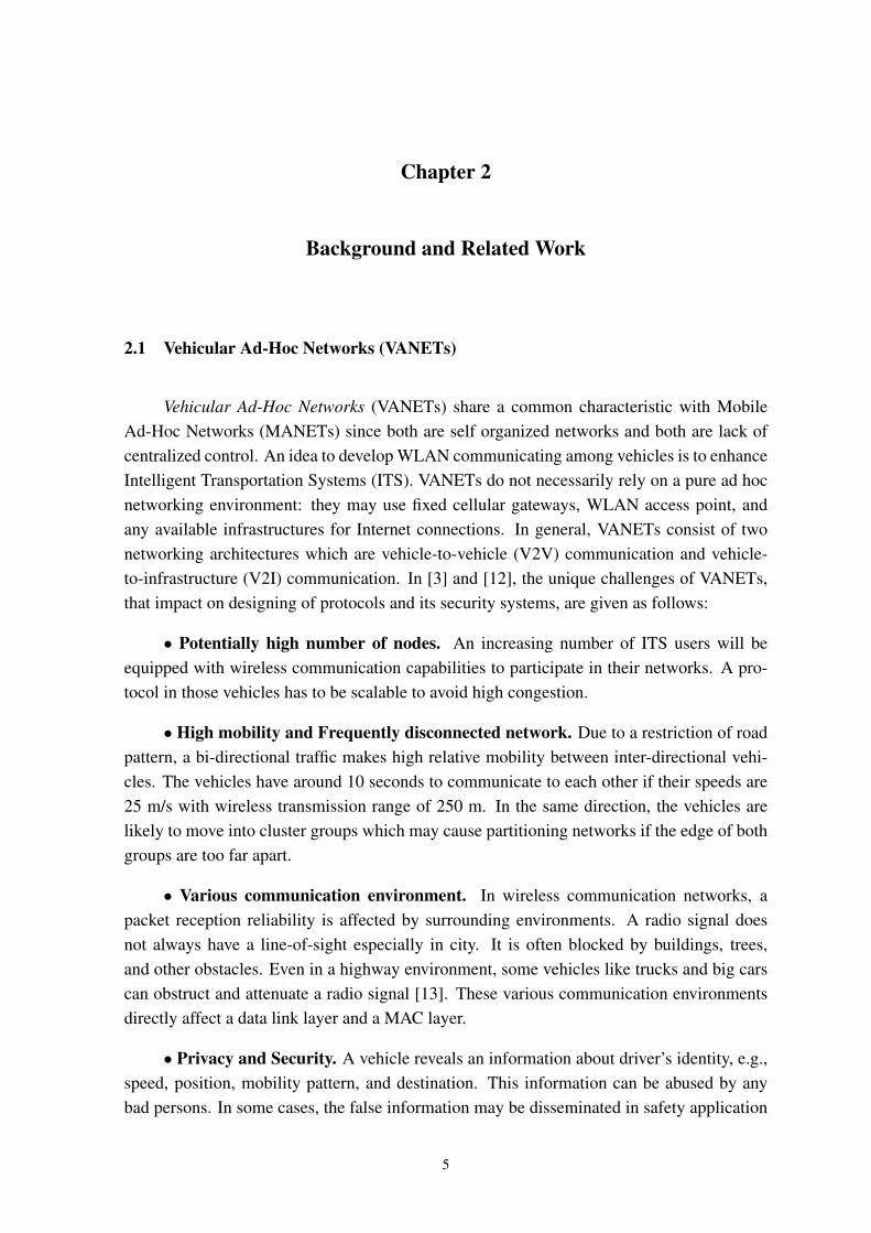
Vehicular Ad-Hoc Networks (VANETs) share a common characteristic with MobileAd-Hoc Networks (MANETs) since both are self organized networks and both are lack ofcentralized control. An idea to develop WLAN communicating among vehicles is to enhanceIntelligent Transportation Systems (ITS). VANETs do not necessarily rely on a pure ad hocnetworking environment: they may use fixed cellular gateways, WLAN access point, andany available infrastructures for Internet connections. In general, VANETs consist of twonetworking architectures which are vehicle-to-vehicle (V2V) communication and vehicle-to-infrastructure (V2I) communication. In [3] and [12], the unique challenges of VANETs,that impact on designing of protocols and its security systems, are given as follows:
• Potentially high number of nodes. An increasing number of ITS users will beequipped with wireless communication capabilities to participate in their networks. A pro-tocol in those vehicles has to be scalable to avoid high congestion.
• High mobility and Frequently disconnected network. Due to a restriction of roadpattern, a bi-directional traffic makes high relative mobility between inter-directional vehi-cles. The vehicles have around 10 seconds to communicate to each other if their speeds are25 m/s with wireless transmission range of 250 m. In the same direction, the vehicles arelikely to move into cluster groups which may cause partitioning networks if the edge of bothgroups are too far apart.
• Various communication environment. In wireless communication networks, apacket reception reliability is affected by surrounding environments. A radio signal doesnot always have a line-of-sight especially in city. It is often blocked by buildings, trees,and other obstacles. Even in a highway environment, some vehicles like trucks and big carscan obstruct and attenuate a radio signal [13]. These various communication environmentsdirectly affect a data link layer and a MAC layer.
• Privacy and Security. A vehicle reveals an information about driver’s identity, e.g.,speed, position, mobility pattern, and destination. This information can be abused by anybad persons. In some cases, the false information may be disseminated in safety application
5
for any bad objectives.
In general, applications in VANETs can be categorized into safety applications andnon-safety applications. Some safety applications of VANETs are surveyed in [14] and [15],where safety applications are ranged from low danger to high danger, e.g., approaching emer-gency vehicle warning, curve speed waring, work zone warning, pre-crash sensing, and postcrash notification. These applications are highly desirable in VANETs due to improvementof public road safety. In this applications, drivers are warned by emergency warning mes-sages about vehicles acting out of control due to an accident, mechanical breakdown, or someother failure. We focus on this type of applications, especially in post crash notification.
Such safety applications in VANETs require a broadcast protocol which must have lowimplementations and low operation cost. The protocol must be self-organized and propagatean alarm message within a small delay. Objectives of post crash notification are to notifyvehicles in an approaching area for avoiding the incident and traffic jams. Hence, the alarmmessage has to be kept in the approaching area until the highway is free. This applicationmust have low latency, high reliability, high scaling, and well-defined scope of receivers.Furthermore, the protocol should be designed to balance trade-off between reliability, mes-sage dissemination time, and efficiency.
2.2 Wireless Access in Vehicular Environment (WAVE)
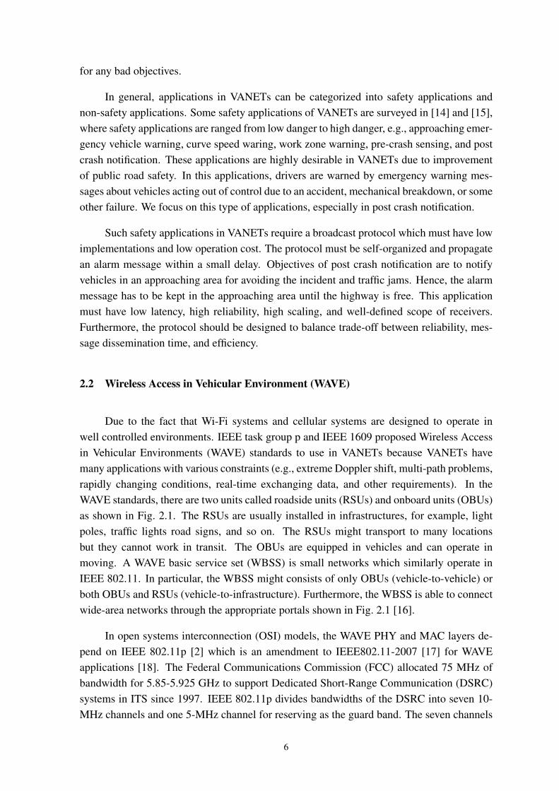
Due to the fact that Wi-Fi systems and cellular systems are designed to operate inwell controlled environments. IEEE task group p and IEEE 1609 proposed Wireless Accessin Vehicular Environments (WAVE) standards to use in VANETs because VANETs havemany applications with various constraints (e.g., extreme Doppler shift, multi-path problems,rapidly changing conditions, real-time exchanging data, and other requirements). In theWAVE standards, there are two units called roadside units (RSUs) and onboard units (OBUs)as shown in Fig. 2.1. The RSUs are usually installed in infrastructures, for example, lightpoles, traffic lights road signs, and so on. The RSUs might transport to many locationsbut they cannot work in transit. The OBUs are equipped in vehicles and can operate inmoving. A WAVE basic service set (WBSS) is small networks which similarly operate inIEEE 802.11. In particular, the WBSS might consists of only OBUs (vehicle-to-vehicle) orboth OBUs and RSUs (vehicle-to-infrastructure). Furthermore, the WBSS is able to connectwide-area networks through the appropriate portals shown in Fig. 2.1 [16].
In open systems interconnection (OSI) models, the WAVE PHY and MAC layers de-pend on IEEE 802.11p [2] which is an amendment to IEEE802.11-2007 [17] for WAVEapplications [18]. The Federal Communications Commission (FCC) allocated 75 MHz ofbandwidth for 5.85-5.925 GHz to support Dedicated Short-Range Communication (DSRC)systems in ITS since 1997. IEEE 802.11p divides bandwidths of the DSRC into seven 10-MHz channels and one 5-MHz channel for reserving as the guard band. The seven channels
6
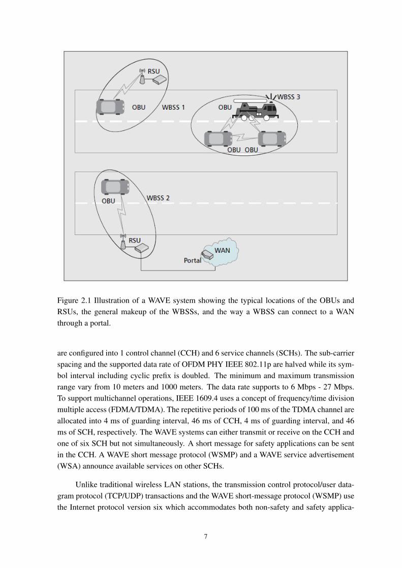
Figure 2.1 Illustration of a WAVE system showing the typical locations of the OBUs andRSUs, the general makeup of the WBSSs, and the way a WBSS can connect to a WANthrough a portal.
are configured into 1 control channel (CCH) and 6 service channels (SCHs). The sub-carrierspacing and the supported data rate of OFDM PHY IEEE 802.11p are halved while its sym-bol interval including cyclic prefix is doubled. The minimum and maximum transmissionrange vary from 10 meters and 1000 meters. The data rate supports to 6 Mbps - 27 Mbps.To support multichannel operations, IEEE 1609.4 uses a concept of frequency/time divisionmultiple access (FDMA/TDMA). The repetitive periods of 100 ms of the TDMA channel areallocated into 4 ms of guarding interval, 46 ms of CCH, 4 ms of guarding interval, and 46ms of SCH, respectively. The WAVE systems can either transmit or receive on the CCH andone of six SCH but not simultaneously. A short message for safety applications can be sentin the CCH. A WAVE short message protocol (WSMP) and a WAVE service advertisement(WSA) announce available services on other SCHs.
Unlike traditional wireless LAN stations, the transmission control protocol/user data-gram protocol (TCP/UDP) transactions and the WAVE short-message protocol (WSMP) usethe Internet protocol version six which accommodates both non-safety and safety applica-
7
Figure 2.2 The WAVE Protocol Stack and Its Associated Standards.
tions.
As described in [18] and [19],they summarized the following WAVE protocol architec-tures with its major components as shown in Fig. 2.2:
• IEEE 1609.1 “Trial Use Standard for Wireless Access in Vehicular Environments(WAVE) - Resource Manager.” This standard specifies the services and the interfaces for aWAVE Resource Manager application.
• IEEE 1609.2 “Trial Use Standard for Wireless Access in Vehicular Environments(WAVE) - Security Services for Applications and Management Messages.” This standarddefines secure message formats and the circumstances for secure message exchange.
• IEEE 1609.3 “Trial Use Standard for Wireless Access in Vehicular Environments(WAVE) - Networking Services.” This standard defines network service and transport layerservices.
• IEEE 1609.4 “Trial Use Standard for Wireless Access in Vehicular Environments(WAVE) - Multi-Channel Operations.” This standard describes enhancements to the IEEE802.11 MAC layer for multi-channel operations.
• IEEE P1609.11 “Over-the-Air Data Exchange Protocol for Intelligent TransportationSystems (ITS).”
8
2.3 Broadcast and Dissemination Techniques
For many safety applications, the time to access data through wireless infrastructures orroadside units is too high, comparing to that through ad-hoc networks. Furthermore, wirelessinfrastructures may be damaged in the event of a disaster; however, vehicle-to-vehicle vehic-ular ad hoc networks (V2V) can be formed dynamically. A simple dissemination mechanismfor V2V is a simple flooding protocol. In the flooding protocol, a node rebroadcasts every re-ceived packets which have not been transmitted before. Since each packet contains a uniquesequence number, the node drops the packet when it receives the same sequence packet. Sev-eral nodes may rebroadcast at the same time and cause collisions, which can immensely highfor dense networks. Since the typical request to sender/clear (RTS/CTS) message and an ac-knowledgment (ACK) mechanism are deactivated in the broadcasting mode. This is knownas a broadcast storm problem. While the network density may be very high in urban areasand during rush hours, it is low in rural areas and at night time. Furthermore, VANETs arehighly mobile and mostly partitioned into many clusters. The gaps between each cluster pre-vent a communication path between a source and a destination if these gaps are larger thanthe transmission range of the vehicles. Although the flooding protocol is highly inefficient indense networks scenario, the flooding ensures the reliability of broadcast packet. However,the flooding protocol is still unreliable in sparsely connected networks scenario. Hence,many researchers aim to design data dissemination protocols which are scalable, reliable,and efficient for safety applications in VANETs. Due to the dynamic characteristic of thechannel in VANETs, to know information about a nodes neighbor requires high overhead es-pecially for networks with high speed nodes. Consequently a neighbor-based scheme, wherenodes require neighbor topology information to decide whether to rebroadcast a message, isinadequate in ad hoc networks due to a difficulty of maintaining a neighboring list, a limitedbandwidth, and high link failures [4].
In summary, several broadcast storm suppression mechanisms for information dissem-ination are classified as follows [20]:
• Probability-based scheme. Each node makes a decision whether it will forward thepacket or not, depending on a probability p after a random back-off period. The node dropsthe packet with a probability 1 − p. Note that when p = 1, the scheme is equivalent tothe simple flooding protocol. The probability-based schemes are simple methods for denseenvironments broadcasting to mitigate broadcast storms. However, the configuration of pa-rameters for the probabilistic decisions in each node is difficult to achieve when the networkconfiguration dynamically changes.
• Counter-based scheme. There is a counter to count a duplicate message in eachnode. The counter increases when the node overhears any duplicated messages that are for-warded by its neighbor nodes. When each node receives a non-duplicate message, the nodeinitiates a random timer which is decremented afterwards. The node rebroadcasts the re-
9
ceived packet if the counter does not exceed a threshold called Max-count when the timerexpires. Depending on the sufficient threshold, this scheme works well even in partition net-works and dynamic networks. This scheme takes into account the network dynamics in mak-ing a decision on the forwarding then the node suppresses the forwarding by silently discard-ing the packet [10]. Hence the counter-based scheme is more robust in various network-widebroadcasting scenarios, However, it is not optimal in the network efficiency side because ofthe incomplete elimination of the packet redundancy.
• Location-based scheme. The principle of location-based scheme uses its locationinformation and transmission range for deciding to rebroadcast. When a node receives anon-duplicate message, the additional area that can be covered by the transmission range ofeach node is calculated. If the received node has the maximum additional area that exceeds apredetermined threshold, it forwards the packet otherwise, it drops the packet. For an omni-directional antenna, the closest node to the destination node is chosen to be the forwarder.This method reduces unnecessary forwarding by choosing the furthest forwarder. However,this method has several shortcomings. One of them is that the neighbor nodes, which havethe same threshold, will rebroadcast as they are able to cover the additional area. In verydense networks, this leads to the rebroadcast of hundreds of redundant packets because eachnode have no global knowledge in which nodes act as the forwarder. Another shortcomingis, due to sparsity of network, the next hop forwarder does not alway present. Thus, boththeir number and location of the forwarders are the key factors in designing the efficient andreliable location-based protocol.
• Distance-based scheme. The distance-based scheme is known as the contention-based forwarding (CBF) [21]. In this scheme, a received node starts a defer time after hear-ing the first message. The defer time is inversely proportional to a relative distance betweenitself and a sender. During the defer time, if a received node does not receive any dupli-cate messages, it rebroadcasts the received message. Due to the fact that further nodes waitshorter than closer nodes to the sender. Hence, the furthest node from the sender rebroad-casts first because its defer time is the shortest. This scheme achieves the lowest messagepropagation delay due to using minimum hops. CBF requires no information about neighborpositions and beacon exchanging. Since CBF selects nodes for multi-hop relays based ona distance-based defer time, it is suitable for broadcast storm suppression in highly mobileVANETs. However, it suffers from network partitioning problem in sparse networks becausethe next hop does not always present. The authors in [22] and [23] analyzed the effect ofprobabilistic channels on CBF in vehicular ad hoc networks. They stated that CBF is bene-ficial in probabilistic channel, but efficient suppression mechanisms are required to enhanceCBF in probabilistic channels. In addition, the node selection for multi-hop relays suffersfrom a reliability trade-off in probabilistic channels [24].
In sparse density networks, store-carry-forward and directional protocols are employedto deliver messages whenever the multi-hop connectivity among vehicles is not available. As
10
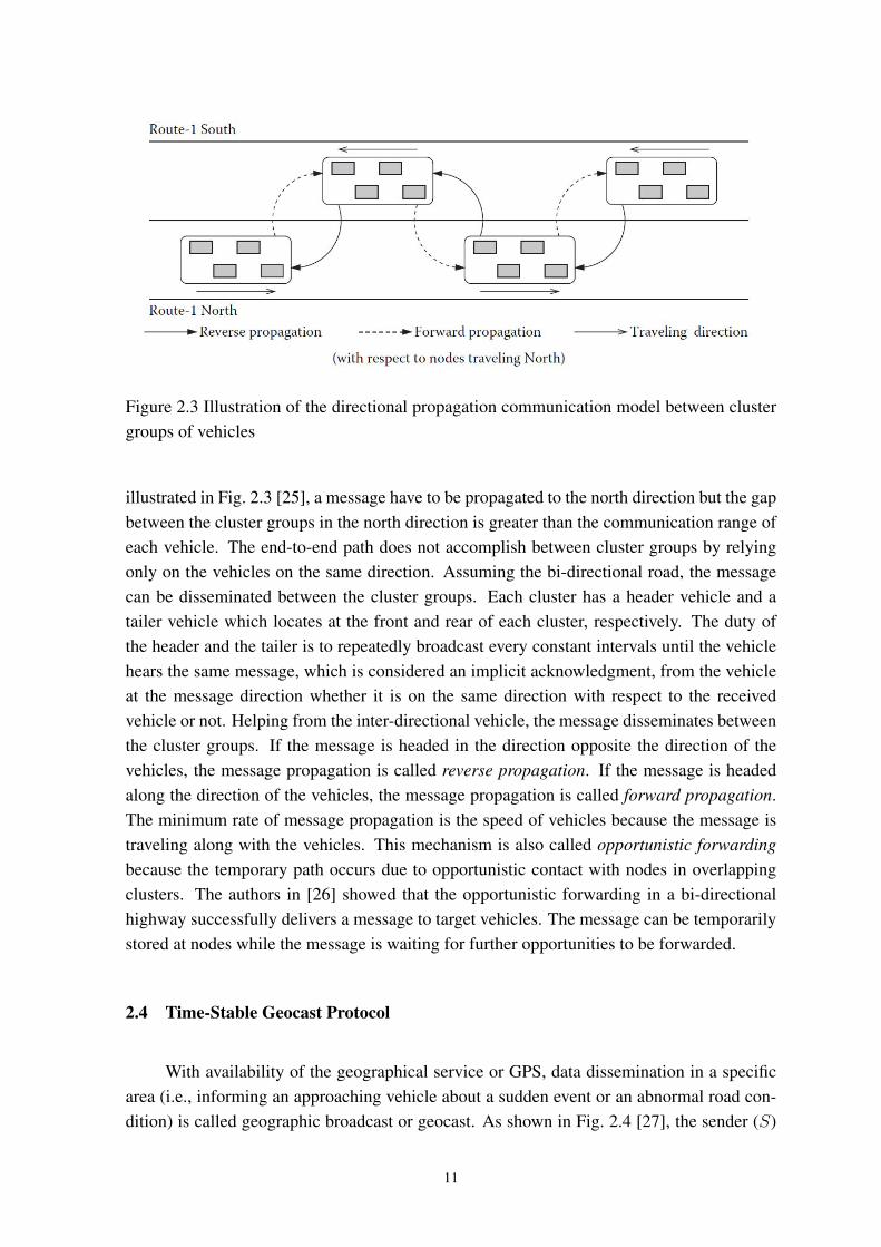
Figure 2.3 Illustration of the directional propagation communication model between clustergroups of vehicles
illustrated in Fig. 2.3 [25], a message have to be propagated to the north direction but the gapbetween the cluster groups in the north direction is greater than the communication range ofeach vehicle. The end-to-end path does not accomplish between cluster groups by relyingonly on the vehicles on the same direction. Assuming the bi-directional road, the messagecan be disseminated between the cluster groups. Each cluster has a header vehicle and atailer vehicle which locates at the front and rear of each cluster, respectively. The duty ofthe header and the tailer is to repeatedly broadcast every constant intervals until the vehiclehears the same message, which is considered an implicit acknowledgment, from the vehicleat the message direction whether it is on the same direction with respect to the receivedvehicle or not. Helping from the inter-directional vehicle, the message disseminates betweenthe cluster groups. If the message is headed in the direction opposite the direction of thevehicles, the message propagation is called reverse propagation. If the message is headedalong the direction of the vehicles, the message propagation is called forward propagation.The minimum rate of message propagation is the speed of vehicles because the message istraveling along with the vehicles. This mechanism is also called opportunistic forwardingbecause the temporary path occurs due to opportunistic contact with nodes in overlappingclusters. The authors in [26] showed that the opportunistic forwarding in a bi-directionalhighway successfully delivers a message to target vehicles. The message can be temporarilystored at nodes while the message is waiting for further opportunities to be forwarded.
2.4 Time-Stable Geocast Protocol
With availability of the geographical service or GPS, data dissemination in a specificarea (i.e., informing an approaching vehicle about a sudden event or an abnormal road con-dition) is called geographic broadcast or geocast. As shown in Fig. 2.4 [27], the sender (S)
11
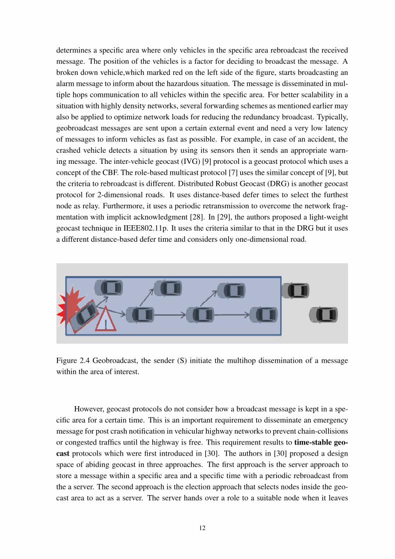
determines a specific area where only vehicles in the specific area rebroadcast the receivedmessage. The position of the vehicles is a factor for deciding to broadcast the message. Abroken down vehicle,which marked red on the left side of the figure, starts broadcasting analarm message to inform about the hazardous situation. The message is disseminated in mul-tiple hops communication to all vehicles within the specific area. For better scalability in asituation with highly density networks, several forwarding schemes as mentioned earlier mayalso be applied to optimize network loads for reducing the redundancy broadcast. Typically,geobroadcast messages are sent upon a certain external event and need a very low latencyof messages to inform vehicles as fast as possible. For example, in case of an accident, thecrashed vehicle detects a situation by using its sensors then it sends an appropriate warn-ing message. The inter-vehicle geocast (IVG) [9] protocol is a geocast protocol which uses aconcept of the CBF. The role-based multicast protocol [7] uses the similar concept of [9], butthe criteria to rebroadcast is different. Distributed Robust Geocast (DRG) is another geocastprotocol for 2-dimensional roads. It uses distance-based defer times to select the furthestnode as relay. Furthermore, it uses a periodic retransmission to overcome the network frag-mentation with implicit acknowledgment [28]. In [29], the authors proposed a light-weightgeocast technique in IEEE802.11p. It uses the criteria similar to that in the DRG but it usesa different distance-based defer time and considers only one-dimensional road.
Figure 2.4 Geobroadcast, the sender (S) initiate the multihop dissemination of a messagewithin the area of interest.
However, geocast protocols do not consider how a broadcast message is kept in a spe-cific area for a certain time. This is an important requirement to disseminate an emergencymessage for post crash notification in vehicular highway networks to prevent chain-collisionsor congested traffics until the highway is free. This requirement results to time-stable geo-cast protocols which were first introduced in [30]. The authors in [30] proposed a designspace of abiding geocast in three approaches. The first approach is the server approach tostore a message within a specific area and a specific time with a periodic rebroadcast fromthe a server. The second approach is the election approach that selects nodes inside the geo-cast area to act as a server. The server hands over a role to a suitable node when it leaves
12
from the geocast area. The third approach is the neighbor approach where all nodes insidethe geocast area can be a forwarder when a new node enters to the geocast area.
In [31], the authors ensure that a warning message disseminates to all affected vehi-cles in highway with high reliability and low overhead. The protocol uses the improvedpredicting interval of vehicles from [32]. It uses the CBF with a distance-based defer timeto suppress broadcast storm problems. It periodically rebroadcasts the message to counterwith a network fragmentation problems in vehicular ad hoc networks, similarly to [9] and[29]. The dynamic time-stable geocast (DTSG) protocol [6] is a time-stable geocast protocolwhich our proposed protocol is based on. The DTSG protocol is divided into two peri-ods: pre-stable and stable periods. During the pre-stable period, all vehicles use the CBF todisseminate the message to cover a specific area. When a helping vehicle moves to an extra-region, the helping vehicle rebroadcast again to start the stable period. In the stable period,the message is kept within the specific area, for a time duration via a diagonal disseminationin an extra-region. In DTSG, the defer time is
TD = TN ×R
d, (2.1)
whereTN =
2R
sr + sm. (2.2)
This defer time is called a dynamic sleep time (TD) because it depends on a speedof a receiver and a distance between a sender and a receiver. This dynamic sleep time isused to suppress broadcast storm problems. To counter the network partitioning problem, aheader of each cluster is selected to carry the received message and rebroadcast every TNintervals in (2.2). This interval TN considers that two vehicles moving toward to each otheris in each other’s transmission range. The worst scenario is that a vehicle comes toward aforwarder with a maximum allowance speed, say sm m/s. Hence, the interval TN equals toR/sm to guarantee that the message is successfully delivered to the coming vehicle. Theheader stops rebroadcasting when it receives three duplicate messages from inter-directionalvehicles in the pre-stable period. The DTSG protocol guarantees the message delivery with alow receiving cost without using any roadside units in sparsely density networks. However,the dissemination time is too long and not suitable for the emergency dissemination even inhighly density networks.
13

Chapter 3
VANET Simulation Tools
3.1 Network Simulator (NS-3)
In this section, we describe the network simulator which is used in this thesis. The Net-work Simulator-3 or ns-3 [33] is used as a discrete event network simulator for the wirelessnetworks in this thesis. When this thesis began, the available version was ns-3.12 which hasbeen used to perform the simulations. We assume that all vehicles are embedded with a wifidevice which communicates via the wifi architecture shown in Fig. 3.1
Figure 3.1 Wifi Architecture in ns-3
14
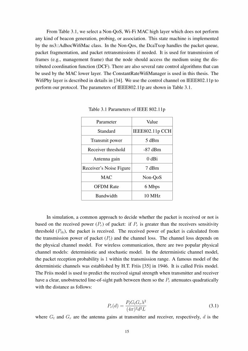
From Table 3.1, we select a Non-QoS, Wi-Fi MAC high layer which does not performany kind of beacon generation, probing, or association. This state machine is implementedby the ns3::AdhocWifiMac class. In the Non-Qos, the DcaTxop handles the packet queue,packet fragmentation, and packet retransmissions if needed. It is used for transmission offrames (e.g., management frame) that the node should access the medium using the dis-tributed coordination function (DCF). There are also several rate control algorithms that canbe used by the MAC lower layer. The ConstantRateWifiManager is used in this thesis. TheWifiPhy layer is described in details in [34]. We use the control channel on IEEE802.11p toperform our protocol. The parameters of IEEE802.11p are shown in Table 3.1.
Table 3.1 Parameters of IEEE 802.11p
Parameter Value
Standard IEEE802.11p CCH
Transmit power 5 dBm
Receiver threshold -87 dBm
Antenna gain 0 dBi
Receiver’s Noise Figure 7 dBm
MAC Non-QoS
OFDM Rate 6 Mbps
Bandwidth 10 MHz
In simulation, a common approach to decide whether the packet is received or not isbased on the received power (Pr) of packet: if Pr is greater than the receivers sensitivitythreshold (Pth), the packet is received. The received power of packet is calculated fromthe transmission power of packet (Pt) and the channel loss. The channel loss depends onthe physical channel model. For wireless communication, there are two popular physicalchannel models: deterministic and stochastic model. In the deterministic channel model,the packet reception probability is 1 within the transmission range. A famous model of thedeterministic channels was established by H.T. Friis [35] in 1946. It is called Friis model.The Friis model is used to predict the received signal strength when transmitter and receiverhave a clear, unobstructed line-of-sight path between them so the Pr attenuates quadraticallywith the distance as follows:
Pr(d) =PtGtGrλ
2
(4π)2d2L(3.1)
where Gt and Gr are the antenna gains at transmitter and receiver, respectively, d is the
15
distance between transmitter and receiver while λ is the wavelength corresponding to thecarrier frequency, L is the system loss factor not related to propagation loss (when L = 1
indicates no loss in the system hardware).
For the stochastic channel models, a popular model is the Nakagami-m distribution[36] which represents fading caused by interference between two or more versions of thetransmitted signal. When the receiver receives the two or more versions of the transmittedsignal at slightly different times, the combination of those transmitted signals affect the re-ceived signal by varying its amplitude and phase. Following the m-Nakagami distribution,the probability density function (PDF) of the received signal power Pr(x) is given as
Pr(x;m,ω) =2mm
Γ(m)ωmx2m−1e−
mωx2 , (3.2)
where m is the fading depth parameter, ω the average received signal power, Γ is the Gammafunction. Both m and ω depend on the distance between transmitter and receiver. For theaverage received signal power ω in VANETs, the authors in [37] recommend to use a logdistance path loss propagation model, which calculates the path loss in dB as follows:
L =
0 d < d0L0 + 10n0log10(
dd0
) d0 ≤ d < d1
L0 + 10n0log10(d1d0
) + 10n1log10(dd1
) d1 ≤ d < d2
L0 + 10n0log10(d1d0
) + 10n1log10(d2d1
) + 10n2log10(dd2
) d ≥ d2
(3.3)
where L is the resulting path loss (dB), d is the distance (m) between transmitter and receiver,L0 is the path loss at reference distance (dB), and n0, n1, and n2 are the path loss distanceexponents for distance d0, d1, and d2, respectively.
For highway environment, the authors in [38] show that the Nakagami-m distributionagrees with empirical propagation data, where m = 3, 1.5, and 1 for the transmission rangeless than 50 meters, between 50 meters and 150 meters and greater than 150 meters, re-spectively. For the pathloss, the authors in [39] recommend the log-distance pathloss modelwith the pathloss exponent of 2 and 4, for the range less than 225 meters and between 225and 1000 meters, respectively. Using ns-3 simulation and the same transmission power of 5dBm, Fig. 3.2 shows the reception probabilities versus distance for the deterministic channeland the probabilistic channel based on the Nakagami and the log-distance path loss. Wedenote the reception probability under the probabilistic channel as PR(·). The result showsthat the transmission range in probabilistic channel model is larger than deterministic chan-nel model; however, the reception probability decreases over the distance in probabilisticchannel model.
16
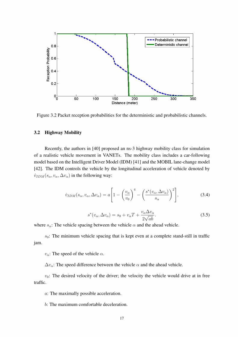
Figure 3.2 Packet reception probabilities for the deterministic and probabilistic channels.
3.2 Highway Mobility
Recently, the authors in [40] proposed an ns-3 highway mobility class for simulationof a realistic vehicle movement in VANETs. The mobility class includes a car-followingmodel based on the Intelligent Driver Model (IDM) [41] and the MOBIL lane-change model[42]. The IDM controls the vehicle by the longitudinal acceleration of vehicle denoted byvIDM(sα, vα,∆vα) in the following way:
vIDM(sα, vα,∆vα) = a
[1−
(vαv0
)4
−(s∗(vα,∆vα)
sα
)2], (3.4)
s∗(vα,∆vα) = s0 + vαT +vα∆vα
2√ab
. (3.5)
where sα: The vehicle spacing between the vehicle α and the ahead vehicle.
s0: The minimum vehicle spacing that is kept even at a complete stand-still in trafficjam.
vα: The speed of the vehicle α.
∆vα: The speed difference between the vehicle α and the ahead vehicle.
v0: The desired velocity of the driver; the velocity the vehicle would drive at in freetraffic.
a: The maximally possible acceleration.
b: The maximum comfortable deceleration.
17
T : The desired time headway to the ahead vehicle.
s∗(vα,∆vα): The desired distance to its predecessor.
We apply this model to a bi-directional single lane highway for the realistic vehiclemobility in this highway mobility class. Having the mobility simulator in ns-3, we cansimultaneously simulate the vehicular ad-hoc networks and the vehicle mobility with feed-back on driver behavior. The authors of [43] shows that the maximum deceleration of IDMis larger than the maximum deceleration of physical limit. Hence, they introduced the fol-lowing L-IDM equation:
a(t) = max(bmax, aIDM(t)), (3.6)
where bmax < 0 is the physical maximum deceleration of vehicle and aIDM(t) is the value ofacceleration taken from the IDM formula. This modification considers fundamental physicallimits hence it gives a more realistic model.
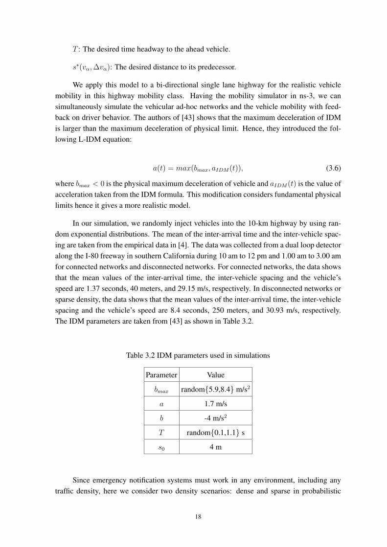
In our simulation, we randomly inject vehicles into the 10-km highway by using ran-dom exponential distributions. The mean of the inter-arrival time and the inter-vehicle spac-ing are taken from the empirical data in [4]. The data was collected from a dual loop detectoralong the I-80 freeway in southern California during 10 am to 12 pm and 1.00 am to 3.00 amfor connected networks and disconnected networks. For connected networks, the data showsthat the mean values of the inter-arrival time, the inter-vehicle spacing and the vehicle’sspeed are 1.37 seconds, 40 meters, and 29.15 m/s, respectively. In disconnected networks orsparse density, the data shows that the mean values of the inter-arrival time, the inter-vehiclespacing and the vehicle’s speed are 8.4 seconds, 250 meters, and 30.93 m/s, respectively.The IDM parameters are taken from [43] as shown in Table 3.2.
Table 3.2 IDM parameters used in simulations
Parameter Value
bmax random{5.9,8.4} m/s2
a 1.7 m/s
b -4 m/s2
T random{0.1,1.1} s
s0 4 m
Since emergency notification systems must work in any environment, including anytraffic density, here we consider two density scenarios: dense and sparse in probabilistic
18
channel. In the dense scenario, the mean, minimum, and maximum inter-vehicle spacingare 40 m, 7 m, and 150 m, respectively. In the sparse scenario, the mean, minimum andmaximum values are 250 m, 80 m, and 600 m, respectively. Note that, from Fig. 3.2, thepacket reception probability for the probabilistic channel at 40m and 250m are about 100%
and 10%, respectively. This means that in the dense scenario, we would expect severalvehicles in the same direction of traffic flow to receive the transmission and in the sparsescenario only one vehicle or none. Hence, in the dense scenario, we have a highly connectednetwork, while in the sparse scenario, a highly disconnected network.
In our simulation, we inject the source vehicle to the 10-km straight highway. Aftermoving for 6.5 km, the source starts broadcasting an alarm message until it receives the samemessage back from another vehicle. Since there is no any standard to evaluate a protocol forpost crash notification, the message in our simulation is required to be within the region D =3 km or D = 1 km for duration T = 30 minutes in sparse vehicle density networks and T = 10minutes in high vehicle density networks. The speed limit is sm = 35 m/s (= 126 km/h) andtransmission range parameter R = 300 m. The braking distance is 120 meters. The modifiedcodes are shown in Appendies A. For each simulation result, we run 10 independent runsand calculate the average values.
19
Chapter 4
iDTSG: Time-Stable Geocast for Post Crash Notification on VehicularAd Hoc Highway Networks
In this chapter, we describe in details the model of our problem. We also propose a time-stable geocast protocol, called Improved Dynamic Time Stable Geocast (iDTSG) [44], forpost crash notification in both dense and sparse vehicular highway networks. The iDTSGprotocol is an improvement of the DTSG protocol proposed in [6].
4.1 System Assumptions
Consider a portion of a two-way highway with L lanes per direction illustrated inFig. 4.1 for L = 31, there is a source vehicle (S), that after having an accident or hav-ing encountered an accident, immediately starts broadcasting an alarm message to behindvehicles traveling in the same direction. The alarm message warns about a location of theaccident. We assume that all vehicles equip with an omni-directional transceiver and a globalpositioning system device. We also assume that there is no roadside units available for mes-sage dissemination and hence the message must be disseminated only via the vehicular adhoc network. Due to a variety of network densities, the network densities may range fromhighly connected network at high densities to disconnected subnetworks at very low den-sities. As illustrated in Fig. 4.1, we divide all vehicles into intended and helping vehiclesexcept the vehicle S where this model is similar to [6]. We denote this region of D kmbehind the breaking distance B from the location of the accident as an intended region. Theintended vehicles (I) are the vehicles that are moving toward the accident. They are targetrecipients of the alarm message. The helping vehicles (H) are the vehicles that are movingin the opposite direction on the other lanes, with respect to the source. The helping vehiclescan carry the alarm message and disseminate the message to the intended vehicles when thepartitioning networks occur. To keep the message within the intended region, we define twoadditional regions: a forwarding region and an extra region. The intended region and theopposite region in the opposite lane are together called a forwarding region. Both ends ofthe two forwarding regions are extra regions. For simplicity, we assume that there is onlyone active alarm message to be disseminated. An objective of our protocol is that the alarm
1For illustration purpose, the figure shows three lanes per direction. In our simulation, we consider, however, one laneper direction.
20
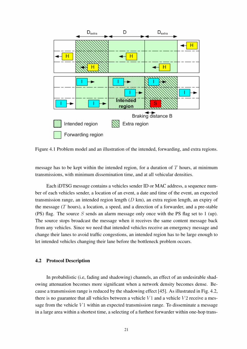
Figure 4.1 Problem model and an illustration of the intended, forwarding, and extra regions.
message has to be kept within the intended region, for a duration of T hours, at minimumtransmissions, with minimum dissemination time, and at all vehicular densities.
Each iDTSG message contains a vehicles sender ID or MAC address, a sequence num-ber of each vehicles sender, a location of an event, a date and time of the event, an expectedtransmission range, an intended region length (D km), an extra region length, an expiry ofthe message (T hours), a location, a speed, and a direction of a forwarder, and a pre-stable(PS) flag. The source S sends an alarm message only once with the PS flag set to 1 (up).The source stops broadcast the message when it receives the same content message backfrom any vehicles. Since we need that intended vehicles receive an emergency message andchange their lanes to avoid traffic congestions, an intended region has to be large enough tolet intended vehicles changing their lane before the bottleneck problem occurs.
4.2 Protocol Description
In probabilistic (i.e, fading and shadowing) channels, an effect of an undesirable shad-owing attenuation becomes more significant when a network density becomes dense. Be-cause a transmission range is reduced by the shadowing effect [45]. As illustrated in Fig. 4.2,there is no guarantee that all vehicles between a vehicle V 1 and a vehicle V 2 receive a mes-sage from the vehicle V 1 within an expected transmission range. To disseminate a messagein a large area within a shortest time, a selecting of a furthest forwarder within one-hop trans-
21
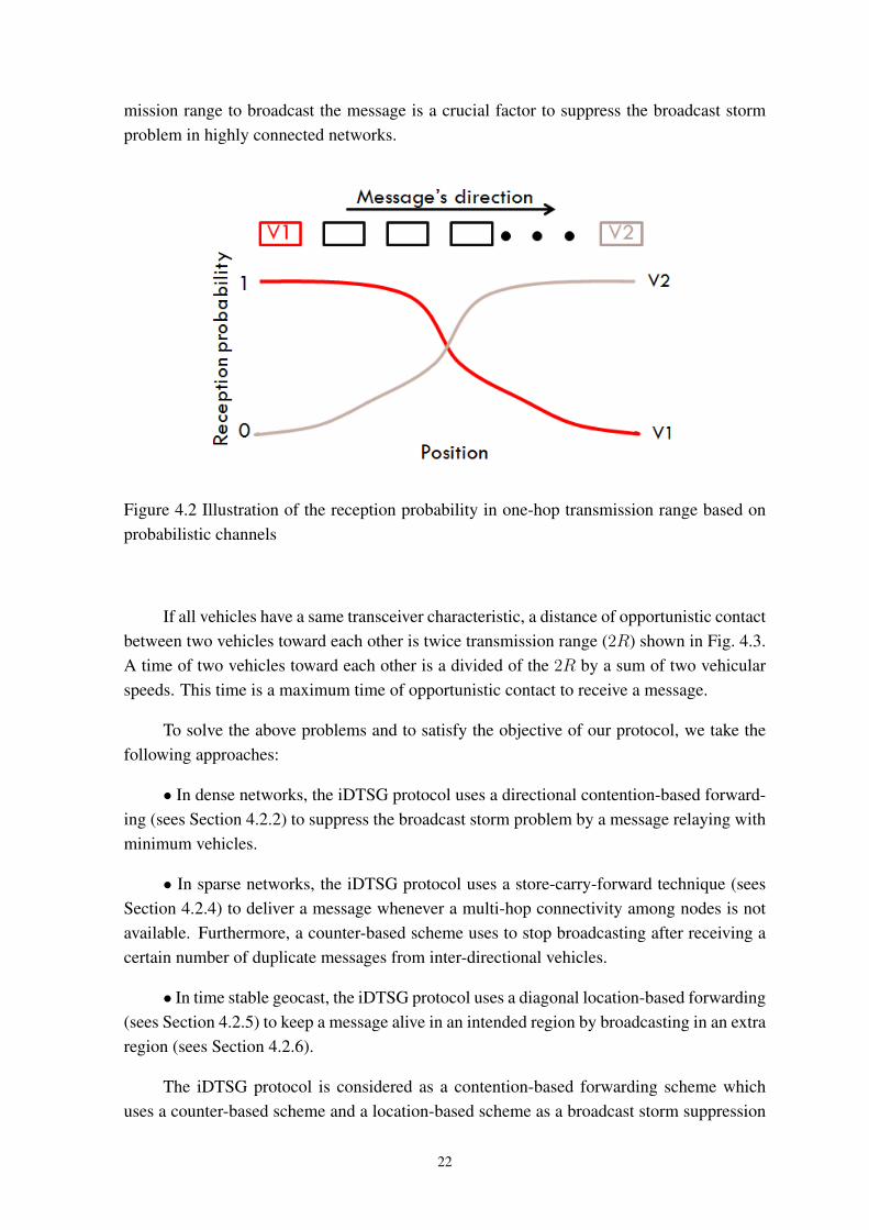
mission range to broadcast the message is a crucial factor to suppress the broadcast stormproblem in highly connected networks.
Figure 4.2 Illustration of the reception probability in one-hop transmission range based onprobabilistic channels
If all vehicles have a same transceiver characteristic, a distance of opportunistic contactbetween two vehicles toward each other is twice transmission range (2R) shown in Fig. 4.3.A time of two vehicles toward each other is a divided of the 2R by a sum of two vehicularspeeds. This time is a maximum time of opportunistic contact to receive a message.
To solve the above problems and to satisfy the objective of our protocol, we take thefollowing approaches:
• In dense networks, the iDTSG protocol uses a directional contention-based forward-ing (sees Section 4.2.2) to suppress the broadcast storm problem by a message relaying withminimum vehicles.
• In sparse networks, the iDTSG protocol uses a store-carry-forward technique (seesSection 4.2.4) to deliver a message whenever a multi-hop connectivity among nodes is notavailable. Furthermore, a counter-based scheme uses to stop broadcasting after receiving acertain number of duplicate messages from inter-directional vehicles.
• In time stable geocast, the iDTSG protocol uses a diagonal location-based forwarding(sees Section 4.2.5) to keep a message alive in an intended region by broadcasting in an extraregion (sees Section 4.2.6).
The iDTSG protocol is considered as a contention-based forwarding scheme whichuses a counter-based scheme and a location-based scheme as a broadcast storm suppression
22
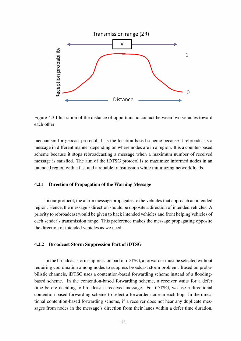
Figure 4.3 Illustration of the distance of opportunistic contact between two vehicles towardeach other
mechanism for geocast protocol. It is the location-based scheme because it rebroadcasts amessage in different manner depending on where nodes are in a region. It is a counter-basedscheme because it stops rebroadcasting a message when a maximum number of receivedmessage is satisfied. The aim of the iDTSG protocol is to maximize informed nodes in anintended region with a fast and a reliable transmission while minimizing network loads.
4.2.1 Direction of Propagation of the Warning Message
In our protocol, the alarm message propagates to the vehicles that approach an intendedregion. Hence, the message’s direction should be opposite a direction of intended vehicles. Apriority to rebroadcast would be given to back intended vehicles and front helping vehicles ofeach sender’s transmission range. This preference makes the message propagating oppositethe direction of intended vehicles as we need.
4.2.2 Broadcast Storm Suppression Part of iDTSG
In the broadcast storm suppression part of iDTSG, a forwarder must be selected withoutrequiring coordination among nodes to suppress broadcast storm problem. Based on proba-bilistic channels, iDTSG uses a contention-based forwarding scheme instead of a flooding-based scheme. In the contention-based forwarding scheme, a receiver waits for a defertime before deciding to broadcast a received message. For iDTSG, we use a directionalcontention-based forwarding scheme to select a forwarder node in each hop. In the direc-tional contention-based forwarding scheme, if a receiver does not hear any duplicate mes-sages from nodes in the message’s direction from their lanes within a defer time duration,
23
the receiver rebroadcasts the received message. The defer time is inversely proportional to arelative distance between a receiver and a forwarder and hence a furthest node in a message’sdirection has the shortest defer time. Then, the furthest node rebroadcasts the message firstand it is called a forwarder node. For example, an intended (or helping) vehicle receives analarm message at the first time and hence it defers the message broadcasting with the de-fer time. In the defer time duration, if the intended (or helping) vehicle hears any duplicatemessages from another back intended (or front helping) vehicles with respect to itself, the in-tended (or helping) vehicle drops the received message otherwise it rebroadcasts the receivedmessage. Furthermore, the intended (or helping) vehicle drops every received messages atthe first time if messages come from another back intended (or front helping) vehicles withrespect to their positions. Because those vehicles consider that they are not suitable to dis-seminate the alarm message. This scheme controls the message’s direction. It also limits re-dundant transmissions and wasting channel utilization in highly density networks. However,as shown in Fig. 4.2, some vehicles that receive a message from the vehicle V 1 cannot hearany duplicate messages from the furthest node (the vehicle V 2). On the other hand, somevehicles do not receive a message from the vehicle V 1 but they receive a message from thevehicle V 2 at first. Those vehicles will rebroadcast the received message until those receiveany duplicate messages from nodes in the message’s direction on their lanes. Hence, this isnot a optimal scale but it is a quasi-optimal scale for dissemination in probabilistic channelswith the distance-based defer time technique. This reduces the redundancy of rebroadcastmessages in highly density networks.
4.2.3 Deterministic Distance-Based Defer Time
Due to the fact that the defer time is inversely proportional to the relative distance be-tween a receiver and a forwarder, the greater the distance between a forwarder and a receiver,the shorter the defer time. Hence, only the furthest receiver broadcasts the message. The de-fer time in (4.1) which is called dynamic sleep time in [6] is applied in our iDTSG’s defertime as follows:
TD,I = TN ×R
d, (4.1)
whereTN =
2R
sr + sm. (4.2)
R is the expected transmission range, d is the distance between the forwarder and thereceiver, sr is the speed of the receiver, and sm is the maximum speed limit.
24
4.2.4 Store-Carry-Forward
Due to the directional contention-based forwarding scheme, if multi-hops connectivityamong nodes are not available, forwarders must be a tail vehicle among cluster groups ofintended vehicles and a head vehicle among cluster groups of helping vehicles. Since neigh-bor’s information is not known before receiving message, the forwarders must repeatedlyrebroadcast the received message to overcome network partitioning problem. The periodicrebroadcast time must be short enough such that there is any contact between a forwarder andan opposite receiver. However, the shorter the interval time, the higher the overhead. On theother hand, the longer the interval time, the higher the loss ratio. To be on a safe side, the for-warders can assume that a next hop node in an opposite direction moves with the maximumspeed allowed in the highway and hence the contact time inside the forwarder’s transmissionrange is twice the transmission range divided by the sum of both vehicle’s speed. The inter-val time in (4.2), called a normal sleep time, is applied to repeatedly rebroadcast the receivedmessage to ensure that all vehicles receive the alarm message.
4.2.5 Time-Stable Geocast Part of iDTSG
A mechanism to store a message in the intended region is broadcasting in separateregions. Firstly, the area surrounding the intended region names a forwarding region shownin Fig. 4.1. The vehicles inside the forwarding area rebroadcast the message to ensure thatall vehicles in the intended region receive the message. Secondly, the extra region (Dextra)where vehicles exit from the intended region. To keep the message alive in the intendedregion, the vehicles rebroadcast the message in both extra regions shown in Fig. 4.1. Thisensures that all incoming vehicles receive the message before they enter to the intendedregion. The similar concepts to keep a message alive in a specific area is found in [6] and[31].
As shown in Fig. 4.4, the iDTSG protocol contains two main parts: the broadcaststorm suppression part and the time-stable geocast part. In the time-stable geocast part, itis divided into a geocast period and a time-stable period depending on the purpose of PSflag. During the geocast period, if a forwarder is in the forwarding region, it rebroadcasts thereceived message with the interval TN given in (4.2) until the stop rebroadcast condition(C1)is satisfied. When a helping vehicle (be a forwarder) moves to the extra region, its PS flagturns down (0). Then, the protocol changes into the time-stable period and it initiates todisseminate the message again only in its extra region. When a receiver sees the turn down PSflag from its received message, the receiver changes into the time-stable period too. Duringthe time stable period, a forwarder repeatedly rebroadcasts the received message with theinterval (4.2) in theDextra region on its own lane until the stop rebroadcast condition (C2) issatisfied. The forwarders in two separate extra regions expect to inform the alarm message toother vehicles on the opposite direction before the other vehicles move to the intended region.
25
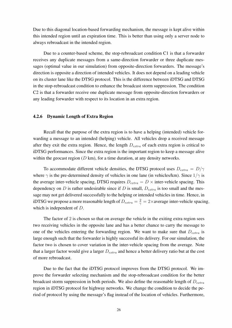
Due to this diagonal location-based forwarding mechanism, the message is kept alive withinthis intended region until an expiration time. This is better than using only a server node toalways rebroadcast in the intended region.
Due to a counter-based scheme, the stop-rebroadcast condition C1 is that a forwarderreceives any duplicate messages from a same-direction forwarder or three duplicate mes-sages (optimal value in our simulation) from opposite-direction forwarders. The message’sdirection is opposite a direction of intended vehicles. It does not depend on a leading vehicleon its cluster lane like the DTSG protocol. This is the difference between iDTSG and DTSGin the stop-rebroadcast condition to enhance the broadcast storm suppression. The conditionC2 is that a forwarder receive one duplicate message from opposite-direction forwarders orany leading forwarder with respect to its location in an extra region.
4.2.6 Dynamic Length of Extra Region
Recall that the purpose of the extra region is to have a helping (intended) vehicle for-warding a message to an intended (helping) vehicle. All vehicles drop a received messageafter they exit the extra region. Hence, the length Dextra of each extra region is critical toiDTSG performances. Since the extra region is the important region to keep a message alivewithin the geocast region (D km), for a time duration, at any density networks.
To accommodate different vehicle densities, the DTSG protocol uses Dextra = D/γ
where γ is the pre-determined density of vehicles in one lane (in vehicles/km). Since 1/γ isthe average inter-vehicle spacing, DTSG requires Dextra = D × inter-vehicle spacing. Thisdependency on D is rather undesirable since if D is small, Dextra is too small and the mes-sage may not get delivered successfully to the helping or intended vehicles in time. Hence, iniDTSG we propose a more reasonable length ofDextra = 2
γ= 2×average inter-vehicle spacing,
which is independent of D.
The factor of 2 is chosen so that on average the vehicle in the exiting extra region seestwo receiving vehicles in the opposite lane and has a better chance to carry the message toone of the vehicles entering the forwarding region. We want to make sure that Dextra islarge enough such that the forwarder is highly successful its delivery. For our simulation, thefactor two is chosen to cover variation in the inter-vehicle spacing from the average. Notethat a larger factor would give a larger Dextra and hence a better delivery ratio but at the costof more rebroadcast.
Due to the fact that the iDTSG protocol improves from the DTSG protocol. We im-prove the forwarder selecting mechanism and the stop-rebroadcast condition for the betterbroadcast storm suppression in both periods. We also define the reasonable length of Dextra
region in iDTSG protocol for highway networks. We change the condition to decide the pe-riod of protocol by using the message’s flag instead of the location of vehicles. Furthermore,
26
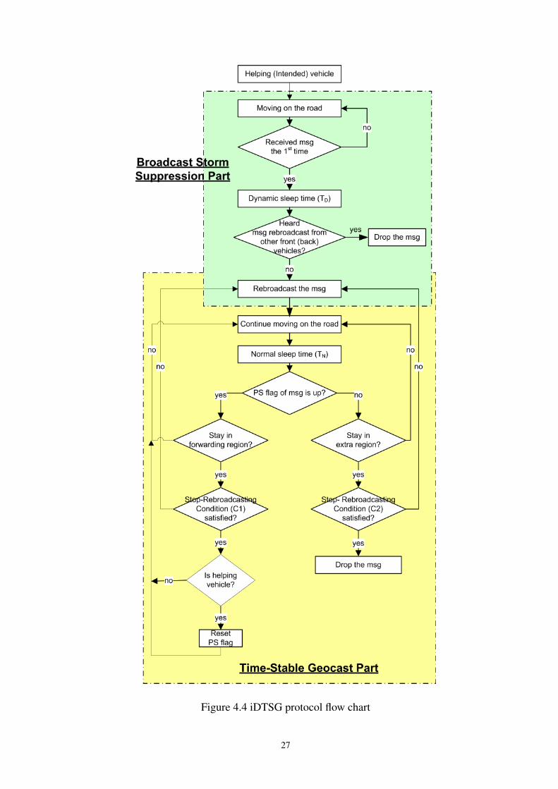
Figure 4.4 iDTSG protocol flow chart
27
the geocast area (intended region) in iDTSG is larger than the area in [31] to reduce trafficjams because of bottleneck problems .
4.3 Simulation Results
Since the objective of our time stable geocast protocol is informing an alarm messageto all vehicles in an intended region as fast as possible and keeping the message alive inthe intended region with minimum transmissions, we are interested in reliability and trans-mission efficiency which generally can be measured in multiple ways in broadcast protocolsincluding time-stable geocast protocols. In our work, the reliability is measured in term ofthe packet loss ratio while the the efficiency is measured via overhead.
Loss Ratio: Assuming the time of the first broadcast of the message as time t = 0, theloss ratio at time t is the ratio between i) the number of those intended nodes that have notreceived the message up to time t and ii) the total number of intended nodes up to time t. Inemergency notification scenario, we are also interested in the dissemination time, which isthe shortest time that the loss ratio reaches almost 0%.
Overhead: The overhead at time t is the total number of packet rebroadcasts up totime t. This number includes the collided rebroadcasts.
4.3.1 Performance on Reliability
With a priori known inter-vehicle spacing, the iDTSG protocol compares with theDTSG protocol in both dense networks and sparse networks. As mentioned in the previ-ous section, the reasonable length of Dextra is 2× average inter-vehicle spacing. This lengthshould be able to cover the spacing between vehicles. In this work, we believe that ourDextra length of iDTSG is more suitable than Dextra which depends on the length of D kmin [6]. In this section, we vary Dextra region from (1 × average inter-vehicle spacing) to(3× average inter-vehicle spacing) to verify our belief. Fig. 4.5 (a) and (b) illustrate the lossratio in dense networks where the lengthD is 1 and 3 km. For reliability, the length ofDextra
has no affect on the loss ratio in dense networks. Both D = 1 and D = 3 km, the loss ratioof iDTSG is similarly to the loss ratio of DTSG in dense networks.
However, the length of the Dextra affects on the loss ratio of iDTSG in sparse net-works. In D = 1 km, the loss ratio of the DTSG protocol is better than the loss ra-tio of the iDTSG protocol when the Dextra is 1 × average inter-vehicle spacing and 2 ×average inter-vehicle spacing. The loss ratio of DTSG and iDTSG (when the Dextra is3× average inter-vehicle spacing) are similar and less than 10%.
28
(a)Loss Ratio in dense networks when D = 1 km
(b)Loss Ratio in dense networks when D = 3 km
Figure 4.5 Loss Ratio for dense networks
InD = 3 km, the loss ratio of iDTSG (when theDextra is 2×average inter-vehicle spacingand 3× average inter-vehicle spacing) and the loss ratio of DTSG are similar. The loss ratioof iDTSG (when the Dextra is 1× average inter-vehicle spacing) is the worst.
As shown in Fig. 4.6 (a) and (b), the results show that the length of Dextra is such im-portant region to maintain the message in the intended region for sparsely density networks.Hence, the length of Dextra must be independent from the value of the D region and largerto ensure that new coming vehicles receive the message in the Dextra region. The iDTSGprotocol and the DTSG protocol also depend on the same D km region and the same defertime (TD) and hence the loss ratios in dense networks are similar. The area of D region hasno affect on the reliability of the DTSG protocol and the iDTSG protocol.
29
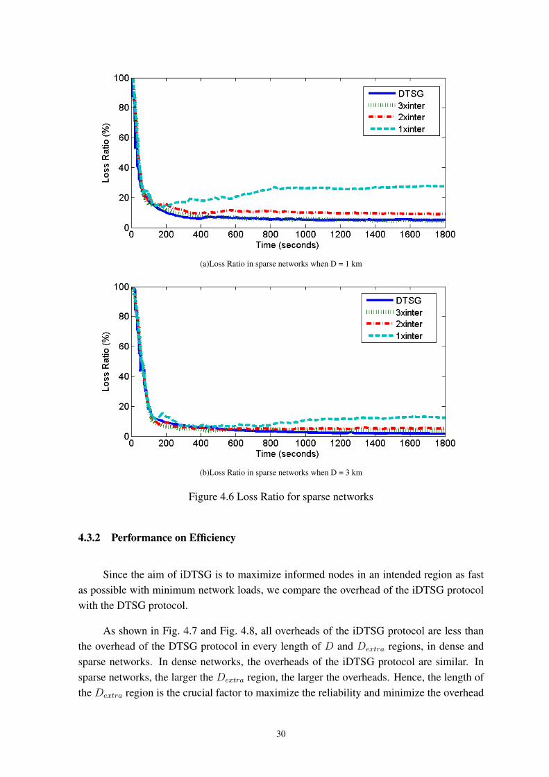
(a)Loss Ratio in sparse networks when D = 1 km
(b)Loss Ratio in sparse networks when D = 3 km
Figure 4.6 Loss Ratio for sparse networks
4.3.2 Performance on Efficiency
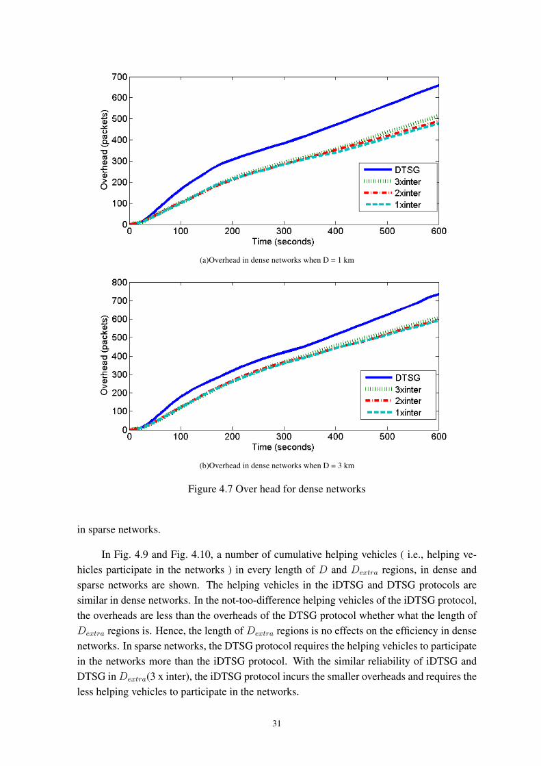
Since the aim of iDTSG is to maximize informed nodes in an intended region as fastas possible with minimum network loads, we compare the overhead of the iDTSG protocolwith the DTSG protocol.
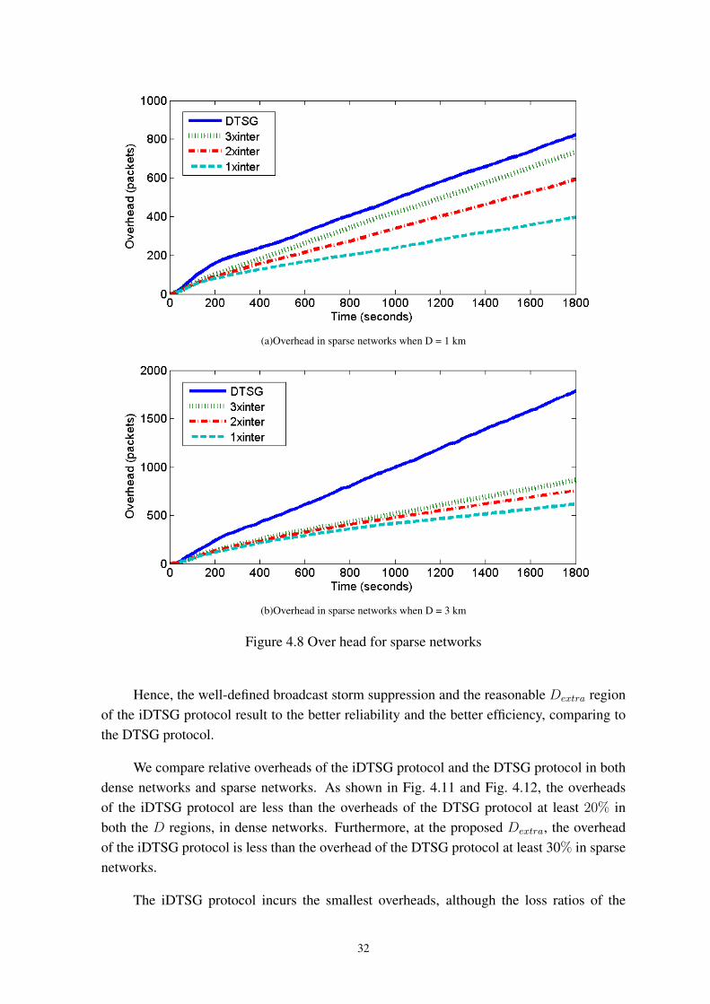
As shown in Fig. 4.7 and Fig. 4.8, all overheads of the iDTSG protocol are less thanthe overhead of the DTSG protocol in every length of D and Dextra regions, in dense andsparse networks. In dense networks, the overheads of the iDTSG protocol are similar. Insparse networks, the larger the Dextra region, the larger the overheads. Hence, the length ofthe Dextra region is the crucial factor to maximize the reliability and minimize the overhead
30
(a)Overhead in dense networks when D = 1 km
(b)Overhead in dense networks when D = 3 km
Figure 4.7 Over head for dense networks
in sparse networks.
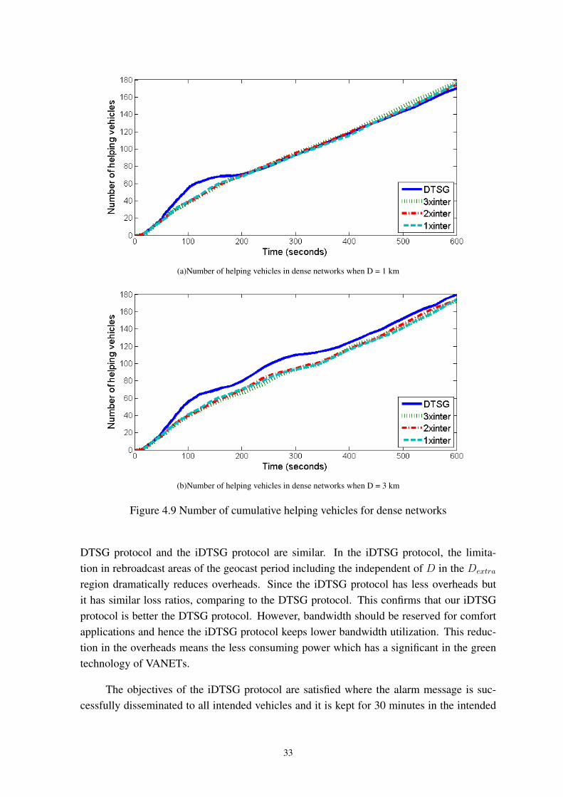
In Fig. 4.9 and Fig. 4.10, a number of cumulative helping vehicles ( i.e., helping ve-hicles participate in the networks ) in every length of D and Dextra regions, in dense andsparse networks are shown. The helping vehicles in the iDTSG and DTSG protocols aresimilar in dense networks. In the not-too-difference helping vehicles of the iDTSG protocol,the overheads are less than the overheads of the DTSG protocol whether what the length ofDextra regions is. Hence, the length of Dextra regions is no effects on the efficiency in densenetworks. In sparse networks, the DTSG protocol requires the helping vehicles to participatein the networks more than the iDTSG protocol. With the similar reliability of iDTSG andDTSG inDextra(3 x inter), the iDTSG protocol incurs the smaller overheads and requires theless helping vehicles to participate in the networks.
31
(a)Overhead in sparse networks when D = 1 km
(b)Overhead in sparse networks when D = 3 km
Figure 4.8 Over head for sparse networks
Hence, the well-defined broadcast storm suppression and the reasonable Dextra regionof the iDTSG protocol result to the better reliability and the better efficiency, comparing tothe DTSG protocol.
We compare relative overheads of the iDTSG protocol and the DTSG protocol in bothdense networks and sparse networks. As shown in Fig. 4.11 and Fig. 4.12, the overheadsof the iDTSG protocol are less than the overheads of the DTSG protocol at least 20% inboth the D regions, in dense networks. Furthermore, at the proposed Dextra, the overheadof the iDTSG protocol is less than the overhead of the DTSG protocol at least 30% in sparsenetworks.
The iDTSG protocol incurs the smallest overheads, although the loss ratios of the
32
(a)Number of helping vehicles in dense networks when D = 1 km
(b)Number of helping vehicles in dense networks when D = 3 km
Figure 4.9 Number of cumulative helping vehicles for dense networks
DTSG protocol and the iDTSG protocol are similar. In the iDTSG protocol, the limita-tion in rebroadcast areas of the geocast period including the independent of D in the Dextra
region dramatically reduces overheads. Since the iDTSG protocol has less overheads butit has similar loss ratios, comparing to the DTSG protocol. This confirms that our iDTSGprotocol is better the DTSG protocol. However, bandwidth should be reserved for comfortapplications and hence the iDTSG protocol keeps lower bandwidth utilization. This reduc-tion in the overheads means the less consuming power which has a significant in the greentechnology of VANETs.
The objectives of the iDTSG protocol are satisfied where the alarm message is suc-cessfully disseminated to all intended vehicles and it is kept for 30 minutes in the intended
33
(a)Number of helping vehicles in sparse networks when D = 1 km
(b)Number of helping vehicles in sparse networks when D = 3 km
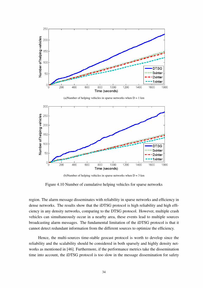
Figure 4.10 Number of cumulative helping vehicles for sparse networks
region. The alarm message disseminates with reliability in sparse networks and efficiency indense networks. The results show that the iDTSG protocol is high reliability and high effi-ciency in any density networks, comparing to the DTSG protocol. However, multiple crashvehicles can simultaneously occur in a nearby area, these events lead to multiple sourcesbroadcasting alarm messages. The fundamental limitation of the iDTSG protocol is that itcannot detect redundant information from the different sources to optimize the efficiency.
Hence, the multi-sources time-stable geocast protocol is worth to develop since thereliability and the scalability should be considered in both sparsely and highly density net-works as mentioned in [46]. Furthermore, if the performance metrics take the disseminationtime into account, the iDTSG protocol is too slow in the message dissemination for safety
34
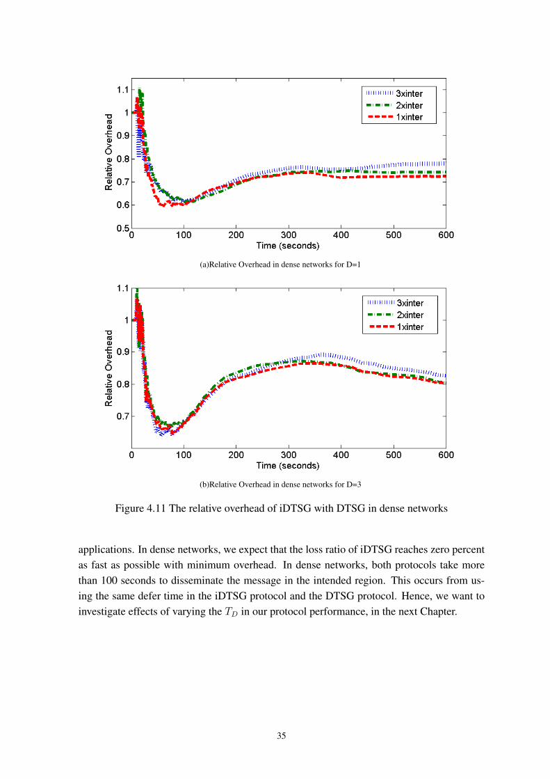
(a)Relative Overhead in dense networks for D=1
(b)Relative Overhead in dense networks for D=3
Figure 4.11 The relative overhead of iDTSG with DTSG in dense networks
applications. In dense networks, we expect that the loss ratio of iDTSG reaches zero percentas fast as possible with minimum overhead. In dense networks, both protocols take morethan 100 seconds to disseminate the message in the intended region. This occurs from us-ing the same defer time in the iDTSG protocol and the DTSG protocol. Hence, we want toinvestigate effects of varying the TD in our protocol performance, in the next Chapter.
35
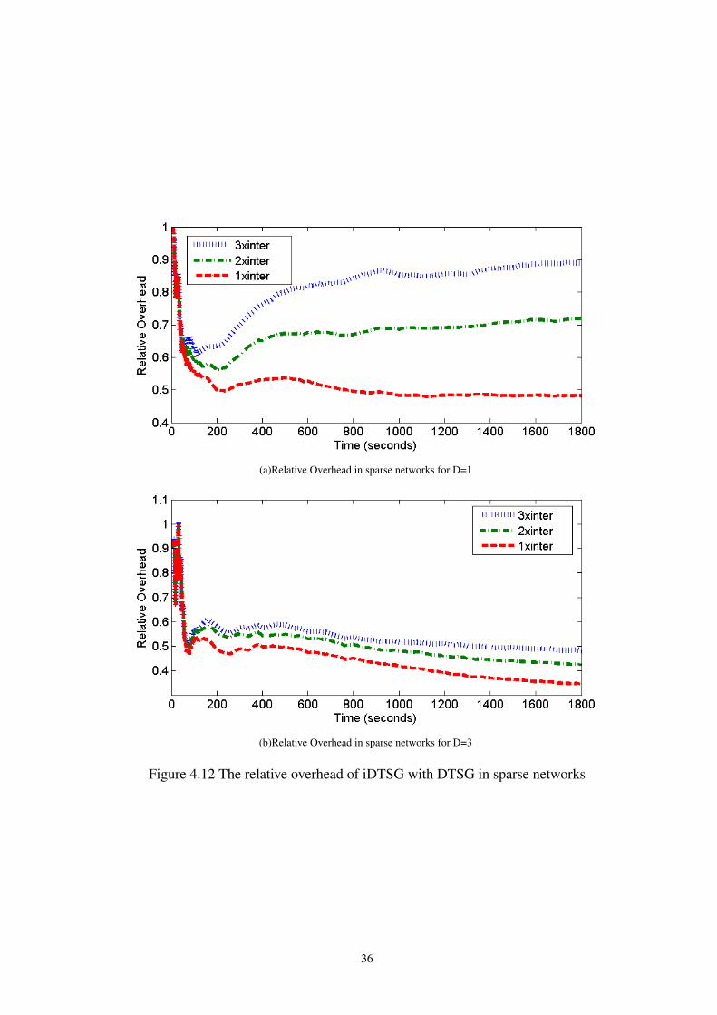
(a)Relative Overhead in sparse networks for D=1
(b)Relative Overhead in sparse networks for D=3
Figure 4.12 The relative overhead of iDTSG with DTSG in sparse networks
36
Chapter 5
Effects of Distance-Based Defer Times and Probabilistic Channel toTime-Stable Geocast
This chapter evaluates effects of some existing deterministic and stochastic distance-baseddefer times in both deterministic and probabilistic (i.e., fading and shadowing) channels.Parts of this chapter appear in [47].
5.1 Introduction
Many articles use contention-based forwarding protocols (e.g., [21]) for forwarder se-lection in VANETs. The contention-based forwarding protocol requires no information ofneighboring vehicles. In this protocol, receiver waits for a time duration, called defer time,before deciding to broadcast the received message. If the receiver does not receive any du-plicate messages during its defer time, the receiver broadcasts the received message after theend of its defer time, otherwise it drops the message. The defer time is used in a general ap-proach to suppress the broadcast storm problem in stateless broadcast protocols, where eachnode does not know or keep track of the locations of its neighbors [48]. The defer time isa crucial factor of contention-based forwarding protocols for broadcast storm suppression indense networks. It was shown in that contention-based forwarding protocols are better thanposition-based forwarding protocols in probabilistic channel [22]. However, an influence ofthe undesirable shadowing attenuation becomes more significant when the traffic becomesdense since the progress of transmission is reduced by the shadowing problem [45]. Withthe shadowing effect, the message dissemination time may be longer than desired for anemergency notification in VANETs.
Several proposed defer times (e.g., [7], [8], and [9]) depend deterministically on dis-tance. Hence, they are called distance-based defer times. The distance-based defer time isinversely proportional to the distance between sender and receiver. The further the distancefrom sender, the smaller the defer time of the receiver. If there are more than two receiversat the same distance from the sender, the receiver will broadcast with the same defer timeand hence a collision occurs. There are other defer times that depend not only on distance,but also angle [49] and link probabilistic [50]. In addition, stochastic defer times have beenproposed such as uniform and Gaussian random defer times [10], and bi-zone random defer
37
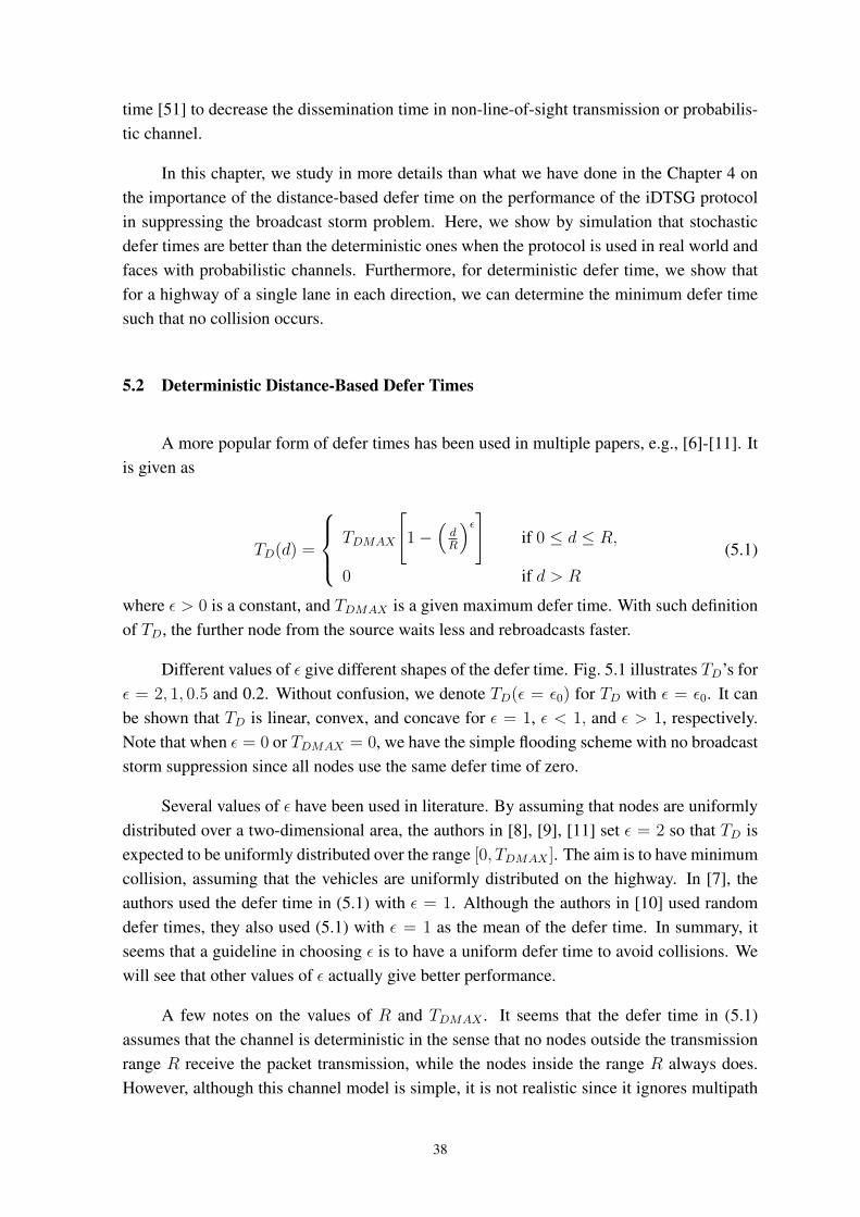
time [51] to decrease the dissemination time in non-line-of-sight transmission or probabilis-tic channel.
In this chapter, we study in more details than what we have done in the Chapter 4 onthe importance of the distance-based defer time on the performance of the iDTSG protocolin suppressing the broadcast storm problem. Here, we show by simulation that stochasticdefer times are better than the deterministic ones when the protocol is used in real world andfaces with probabilistic channels. Furthermore, for deterministic defer time, we show thatfor a highway of a single lane in each direction, we can determine the minimum defer timesuch that no collision occurs.
5.2 Deterministic Distance-Based Defer Times
A more popular form of defer times has been used in multiple papers, e.g., [6]-[11]. Itis given as
TD(d) =
TDMAX
[1−
(dR
)ε]if 0 ≤ d ≤ R,
0 if d > R
(5.1)
where ε > 0 is a constant, and TDMAX is a given maximum defer time. With such definitionof TD, the further node from the source waits less and rebroadcasts faster.
Different values of ε give different shapes of the defer time. Fig. 5.1 illustrates TD’s forε = 2, 1, 0.5 and 0.2. Without confusion, we denote TD(ε = ε0) for TD with ε = ε0. It canbe shown that TD is linear, convex, and concave for ε = 1, ε < 1, and ε > 1, respectively.Note that when ε = 0 or TDMAX = 0, we have the simple flooding scheme with no broadcaststorm suppression since all nodes use the same defer time of zero.
Several values of ε have been used in literature. By assuming that nodes are uniformlydistributed over a two-dimensional area, the authors in [8], [9], [11] set ε = 2 so that TD isexpected to be uniformly distributed over the range [0, TDMAX ]. The aim is to have minimumcollision, assuming that the vehicles are uniformly distributed on the highway. In [7], theauthors used the defer time in (5.1) with ε = 1. Although the authors in [10] used randomdefer times, they also used (5.1) with ε = 1 as the mean of the defer time. In summary, itseems that a guideline in choosing ε is to have a uniform defer time to avoid collisions. Wewill see that other values of ε actually give better performance.
A few notes on the values of R and TDMAX . It seems that the defer time in (5.1)assumes that the channel is deterministic in the sense that no nodes outside the transmissionrange R receive the packet transmission, while the nodes inside the range R always does.However, although this channel model is simple, it is not realistic since it ignores multipath
38
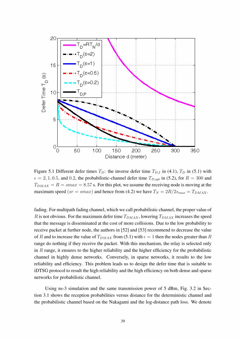
Figure 5.1 Different defer times TD: the inverse defer time TD,I in (4.1), TD in (5.1) withε = 2, 1, 0.5, and 0.2, the probabilistic-channel defer time TD,opt in (5.2), for R = 300 andTDMAX = R = smax = 8.57 s. For this plot, we assume the receiving node is moving at themaximum speed (sr = smax) and hence from (4.2) we have TN = 2R/2smax = TDMAX .
fading. For multipath fading channel, which we call probabilistic channel, the proper value ofR is not obvious. For the maximum defer time TDMAX , lowering TDMAX increases the speedthat the message is disseminated at the cost of more collisions. Due to the low probability toreceive packet at further node, the authors in [52] and [53] recommend to decrease the valueofR and to increase the value of TDMAX from (5.1) with ε = 1 then the nodes greater thanRrange do nothing if they receive the packet. With this mechanism, the relay is selected onlyin R range, it ensures to the higher reliability and the higher efficiency for the probabilisticchannel in highly dense networks. Conversely, in sparse networks, it results to the lowreliability and efficiency. This problem leads us to design the defer time that is suitable toiDTSG protocol to result the high reliability and the high efficiency on both dense and sparsenetworks for probabilistic channel.
Using ns-3 simulation and the same transmission power of 5 dBm, Fig. 3.2 in Sec-tion 3.1 shows the reception probabilities versus distance for the deterministic channel andthe probabilistic channel based on the Nakagami and the log-distance path loss. We denote
39
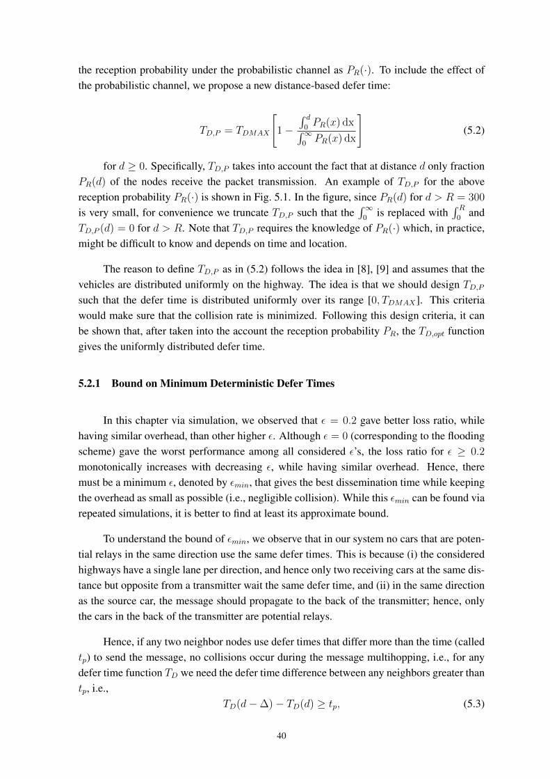
the reception probability under the probabilistic channel as PR(·). To include the effect ofthe probabilistic channel, we propose a new distance-based defer time:
TD,P = TDMAX
[1−
∫ d0PR(x) dx∫∞
0PR(x) dx
](5.2)
for d ≥ 0. Specifically, TD,P takes into account the fact that at distance d only fractionPR(d) of the nodes receive the packet transmission. An example of TD,P for the abovereception probability PR(·) is shown in Fig. 5.1. In the figure, since PR(d) for d > R = 300
is very small, for convenience we truncate TD,P such that the∫∞0
is replaced with∫ R0
andTD,P (d) = 0 for d > R. Note that TD,P requires the knowledge of PR(·) which, in practice,might be difficult to know and depends on time and location.
The reason to define TD,P as in (5.2) follows the idea in [8], [9] and assumes that thevehicles are distributed uniformly on the highway. The idea is that we should design TD,Psuch that the defer time is distributed uniformly over its range [0, TDMAX]. This criteriawould make sure that the collision rate is minimized. Following this design criteria, it canbe shown that, after taken into the account the reception probability PR, the TD,opt functiongives the uniformly distributed defer time.
5.2.1 Bound on Minimum Deterministic Defer Times
In this chapter via simulation, we observed that ε = 0.2 gave better loss ratio, whilehaving similar overhead, than other higher ε. Although ε = 0 (corresponding to the floodingscheme) gave the worst performance among all considered ε’s, the loss ratio for ε ≥ 0.2
monotonically increases with decreasing ε, while having similar overhead. Hence, theremust be a minimum ε, denoted by εmin, that gives the best dissemination time while keepingthe overhead as small as possible (i.e., negligible collision). While this εmin can be found viarepeated simulations, it is better to find at least its approximate bound.
To understand the bound of εmin, we observe that in our system no cars that are poten-tial relays in the same direction use the same defer times. This is because (i) the consideredhighways have a single lane per direction, and hence only two receiving cars at the same dis-tance but opposite from a transmitter wait the same defer time, and (ii) in the same directionas the source car, the message should propagate to the back of the transmitter; hence, onlythe cars in the back of the transmitter are potential relays.
Hence, if any two neighbor nodes use defer times that differ more than the time (calledtp) to send the message, no collisions occur during the message multihopping, i.e., for anydefer time function TD we need the defer time difference between any neighbors greater thantp, i.e.,
TD(d−∆)− TD(d) ≥ tp, (5.3)
40
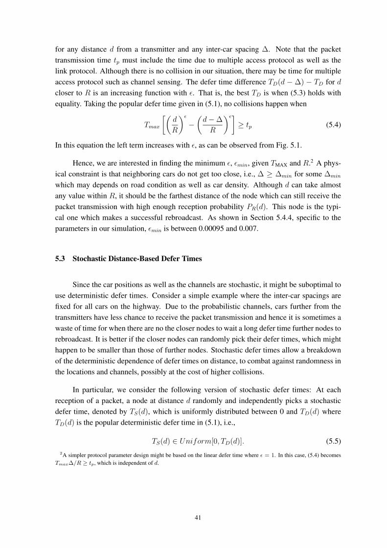
for any distance d from a transmitter and any inter-car spacing ∆. Note that the packettransmission time tp must include the time due to multiple access protocol as well as thelink protocol. Although there is no collision in our situation, there may be time for multipleaccess protocol such as channel sensing. The defer time difference TD(d − ∆) − TD for dcloser to R is an increasing function with ε. That is, the best TD is when (5.3) holds withequality. Taking the popular defer time given in (5.1), no collisions happen when
Tmax
[(d
R
)ε−(d−∆
R
)ε]≥ tp (5.4)
In this equation the left term increases with ε, as can be observed from Fig. 5.1.
Hence, we are interested in finding the minimum ε, εmin, given TMAX and R.2 A phys-ical constraint is that neighboring cars do not get too close, i.e., ∆ ≥ ∆min for some ∆min
which may depends on road condition as well as car density. Although d can take almostany value within R, it should be the farthest distance of the node which can still receive thepacket transmission with high enough reception probability PR(d). This node is the typi-cal one which makes a successful rebroadcast. As shown in Section 5.4.4, specific to theparameters in our simulation, εmin is between 0.00095 and 0.007.
5.3 Stochastic Distance-Based Defer Times
Since the car positions as well as the channels are stochastic, it might be suboptimal touse deterministic defer times. Consider a simple example where the inter-car spacings arefixed for all cars on the highway. Due to the probabilistic channels, cars further from thetransmitters have less chance to receive the packet transmission and hence it is sometimes awaste of time for when there are no the closer nodes to wait a long defer time further nodes torebroadcast. It is better if the closer nodes can randomly pick their defer times, which mighthappen to be smaller than those of further nodes. Stochastic defer times allow a breakdownof the deterministic dependence of defer times on distance, to combat against randomness inthe locations and channels, possibly at the cost of higher collisions.
In particular, we consider the following version of stochastic defer times: At eachreception of a packet, a node at distance d randomly and independently picks a stochasticdefer time, denoted by TS(d), which is uniformly distributed between 0 and TD(d) whereTD(d) is the popular deterministic defer time in (5.1), i.e.,
TS(d) ∈ Uniform[0, TD(d)]. (5.5)2A simpler protocol parameter design might be based on the linear defer time where ε = 1. In this case, (5.4) becomes
Tmax∆/R ≥ tp, which is independent of d.
41
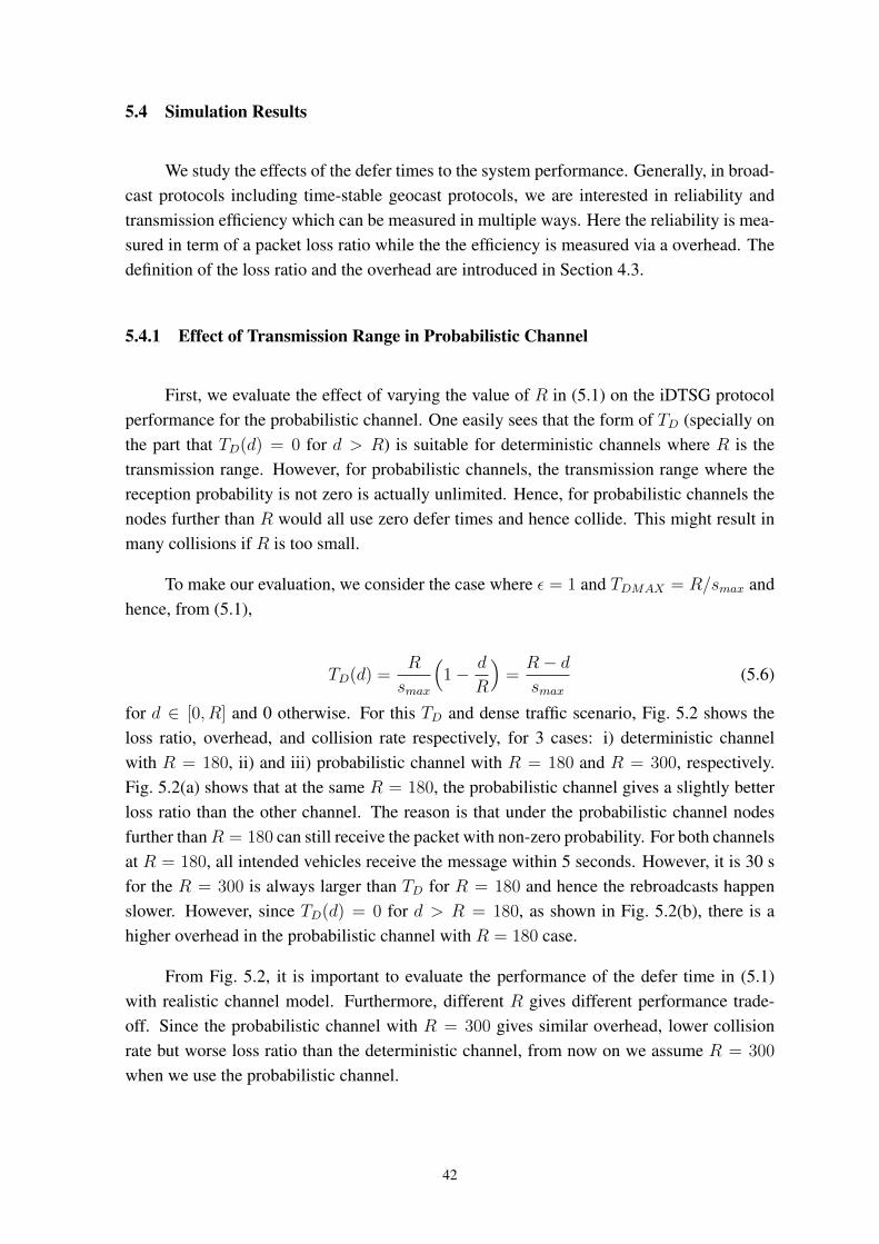
5.4 Simulation Results
We study the effects of the defer times to the system performance. Generally, in broad-cast protocols including time-stable geocast protocols, we are interested in reliability andtransmission efficiency which can be measured in multiple ways. Here the reliability is mea-sured in term of a packet loss ratio while the the efficiency is measured via a overhead. Thedefinition of the loss ratio and the overhead are introduced in Section 4.3.
5.4.1 Effect of Transmission Range in Probabilistic Channel
First, we evaluate the effect of varying the value of R in (5.1) on the iDTSG protocolperformance for the probabilistic channel. One easily sees that the form of TD (specially onthe part that TD(d) = 0 for d > R) is suitable for deterministic channels where R is thetransmission range. However, for probabilistic channels, the transmission range where thereception probability is not zero is actually unlimited. Hence, for probabilistic channels thenodes further than R would all use zero defer times and hence collide. This might result inmany collisions if R is too small.
To make our evaluation, we consider the case where ε = 1 and TDMAX = R/smax andhence, from (5.1),
TD(d) =R
smax
(1− d
R
)=R− dsmax
(5.6)
for d ∈ [0, R] and 0 otherwise. For this TD and dense traffic scenario, Fig. 5.2 shows theloss ratio, overhead, and collision rate respectively, for 3 cases: i) deterministic channelwith R = 180, ii) and iii) probabilistic channel with R = 180 and R = 300, respectively.Fig. 5.2(a) shows that at the same R = 180, the probabilistic channel gives a slightly betterloss ratio than the other channel. The reason is that under the probabilistic channel nodesfurther thanR = 180 can still receive the packet with non-zero probability. For both channelsat R = 180, all intended vehicles receive the message within 5 seconds. However, it is 30 sfor the R = 300 is always larger than TD for R = 180 and hence the rebroadcasts happenslower. However, since TD(d) = 0 for d > R = 180, as shown in Fig. 5.2(b), there is ahigher overhead in the probabilistic channel with R = 180 case.
From Fig. 5.2, it is important to evaluate the performance of the defer time in (5.1)with realistic channel model. Furthermore, different R gives different performance trade-off. Since the probabilistic channel with R = 300 gives similar overhead, lower collisionrate but worse loss ratio than the deterministic channel, from now on we assume R = 300
when we use the probabilistic channel.
42
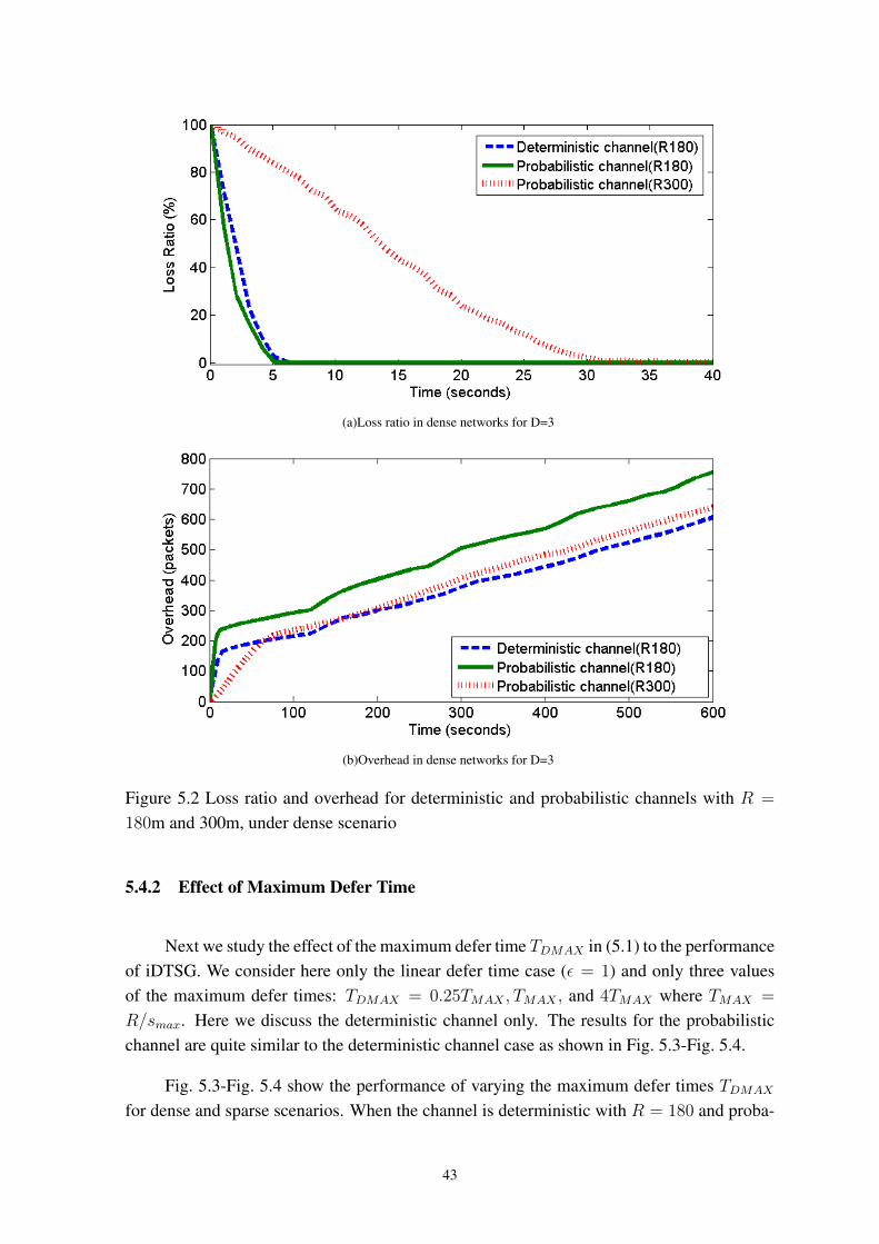
(a)Loss ratio in dense networks for D=3
(b)Overhead in dense networks for D=3
Figure 5.2 Loss ratio and overhead for deterministic and probabilistic channels with R =
180m and 300m, under dense scenario
5.4.2 Effect of Maximum Defer Time
Next we study the effect of the maximum defer time TDMAX in (5.1) to the performanceof iDTSG. We consider here only the linear defer time case (ε = 1) and only three valuesof the maximum defer times: TDMAX = 0.25TMAX , TMAX , and 4TMAX where TMAX =
R/smax. Here we discuss the deterministic channel only. The results for the probabilisticchannel are quite similar to the deterministic channel case as shown in Fig. 5.3-Fig. 5.4.
Fig. 5.3-Fig. 5.4 show the performance of varying the maximum defer times TDMAX
for dense and sparse scenarios. When the channel is deterministic with R = 180 and proba-
43
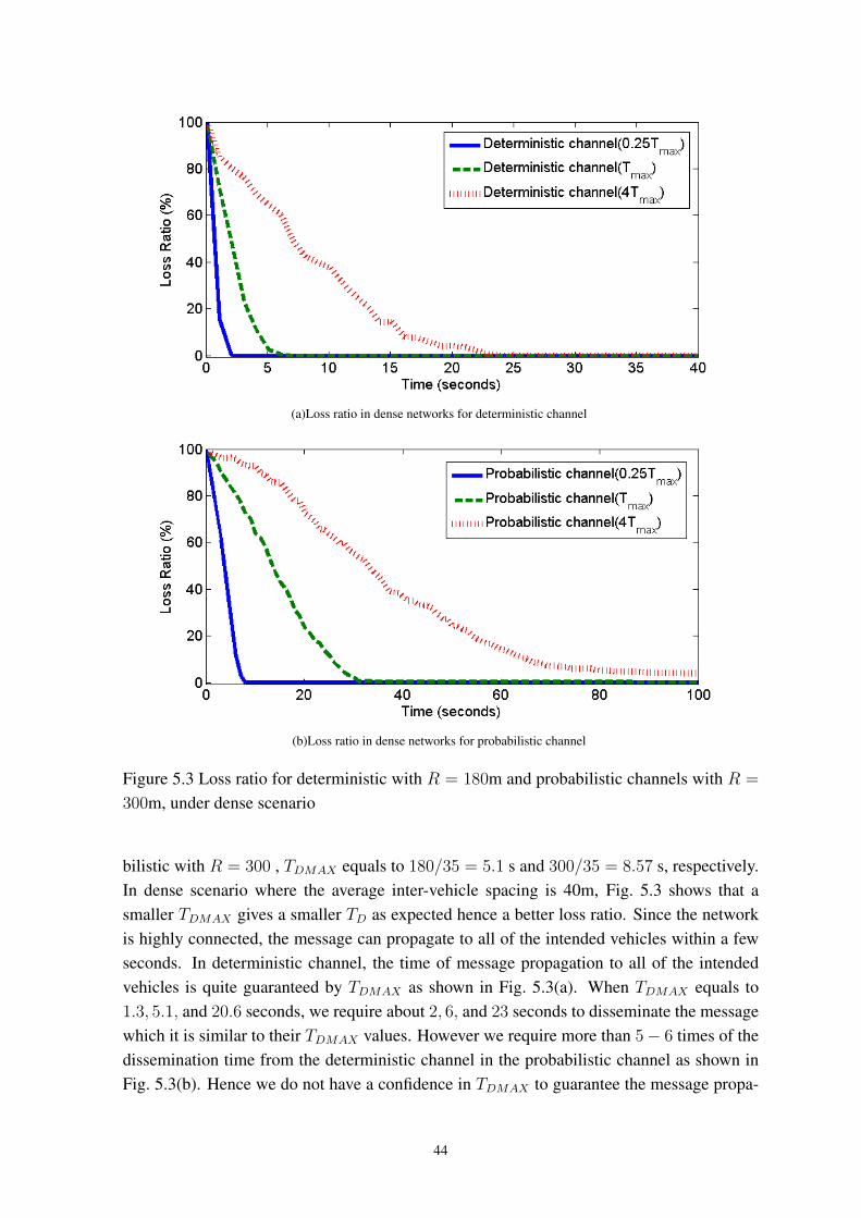
(a)Loss ratio in dense networks for deterministic channel
(b)Loss ratio in dense networks for probabilistic channel
Figure 5.3 Loss ratio for deterministic with R = 180m and probabilistic channels with R =
300m, under dense scenario
bilistic with R = 300 , TDMAX equals to 180/35 = 5.1 s and 300/35 = 8.57 s, respectively.In dense scenario where the average inter-vehicle spacing is 40m, Fig. 5.3 shows that asmaller TDMAX gives a smaller TD as expected hence a better loss ratio. Since the networkis highly connected, the message can propagate to all of the intended vehicles within a fewseconds. In deterministic channel, the time of message propagation to all of the intendedvehicles is quite guaranteed by TDMAX as shown in Fig. 5.3(a). When TDMAX equals to1.3, 5.1, and 20.6 seconds, we require about 2, 6, and 23 seconds to disseminate the messagewhich it is similar to their TDMAX values. However we require more than 5− 6 times of thedissemination time from the deterministic channel in the probabilistic channel as shown inFig. 5.3(b). Hence we do not have a confidence in TDMAX to guarantee the message propa-
44
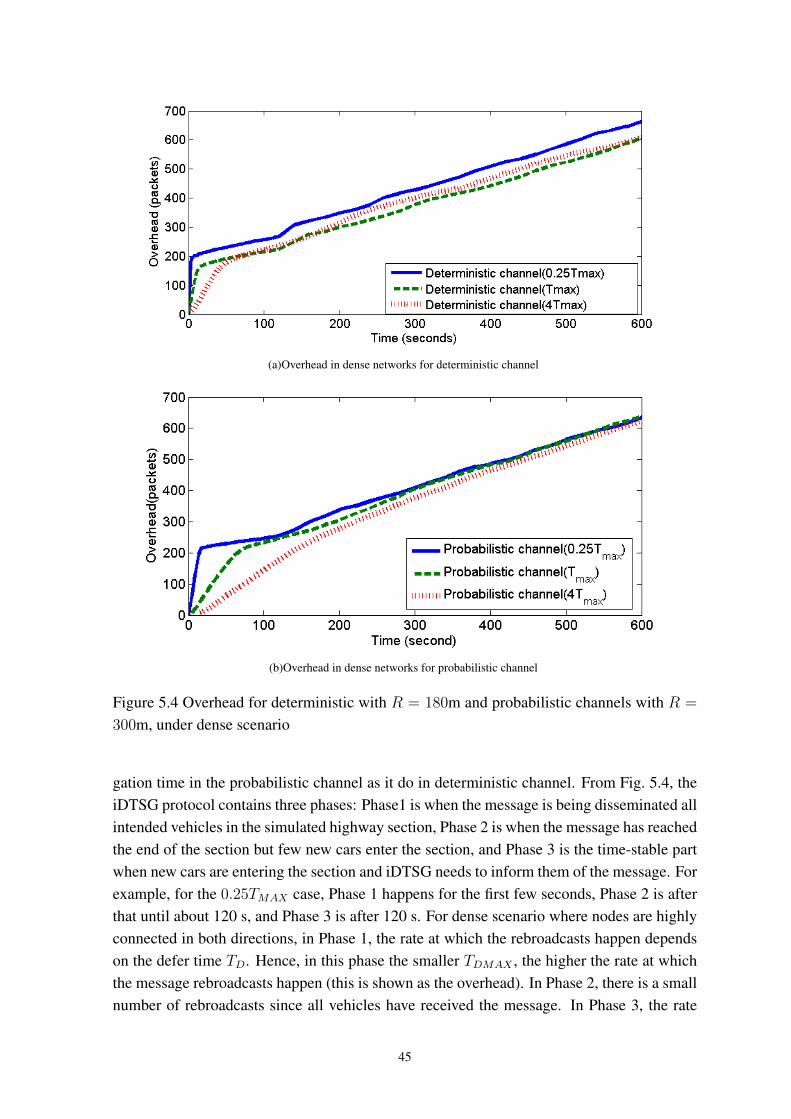
(a)Overhead in dense networks for deterministic channel
(b)Overhead in dense networks for probabilistic channel
Figure 5.4 Overhead for deterministic with R = 180m and probabilistic channels with R =
300m, under dense scenario
gation time in the probabilistic channel as it do in deterministic channel. From Fig. 5.4, theiDTSG protocol contains three phases: Phase1 is when the message is being disseminated allintended vehicles in the simulated highway section, Phase 2 is when the message has reachedthe end of the section but few new cars enter the section, and Phase 3 is the time-stable partwhen new cars are entering the section and iDTSG needs to inform them of the message. Forexample, for the 0.25TMAX case, Phase 1 happens for the first few seconds, Phase 2 is afterthat until about 120 s, and Phase 3 is after 120 s. For dense scenario where nodes are highlyconnected in both directions, in Phase 1, the rate at which the rebroadcasts happen dependson the defer time TD. Hence, in this phase the smaller TDMAX , the higher the rate at whichthe message rebroadcasts happen (this is shown as the overhead). In Phase 2, there is a smallnumber of rebroadcasts since all vehicles have received the message. In Phase 3, the rate
45
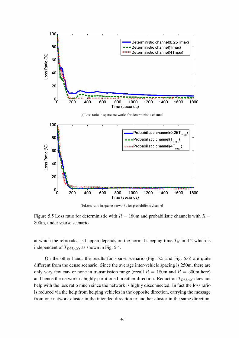
(a)Loss ratio in sparse networks for deterministic channel
(b)Loss ratio in sparse networks for probabilistic channel
Figure 5.5 Loss ratio for deterministic with R = 180m and probabilistic channels with R =
300m, under sparse scenario
at which the rebroadcasts happen depends on the normal sleeping time TN in 4.2 which isindependent of TDMAX , as shown in Fig. 5.4.
On the other hand, the results for sparse scenario (Fig. 5.5 and Fig. 5.6) are quitedifferent from the dense scenario. Since the average inter-vehicle spacing is 250m, there areonly very few cars or none in transmission range (recall R = 180m and R = 300m here)and hence the network is highly partitioned in either direction. Reduction TDMAX does nothelp with the loss ratio much since the network is highly disconnected. In fact the loss rariois reduced via the help from helping vehicles in the opposite direction, carrying the messagefrom one network cluster in the intended direction to another cluster in the same direction.
46
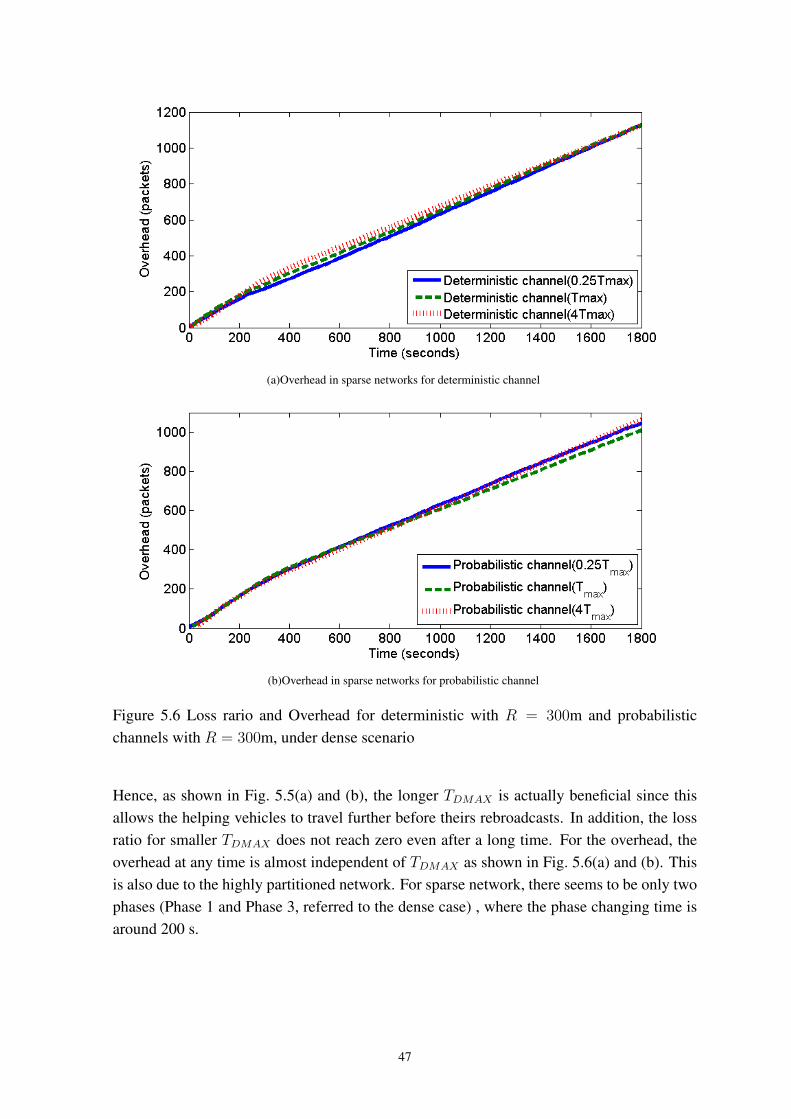
(a)Overhead in sparse networks for deterministic channel
(b)Overhead in sparse networks for probabilistic channel
Figure 5.6 Loss rario and Overhead for deterministic with R = 300m and probabilisticchannels with R = 300m, under dense scenario
Hence, as shown in Fig. 5.5(a) and (b), the longer TDMAX is actually beneficial since thisallows the helping vehicles to travel further before theirs rebroadcasts. In addition, the lossratio for smaller TDMAX does not reach zero even after a long time. For the overhead, theoverhead at any time is almost independent of TDMAX as shown in Fig. 5.6(a) and (b). Thisis also due to the highly partitioned network. For sparse network, there seems to be only twophases (Phase 1 and Phase 3, referred to the dense case) , where the phase changing time isaround 200 s.
47
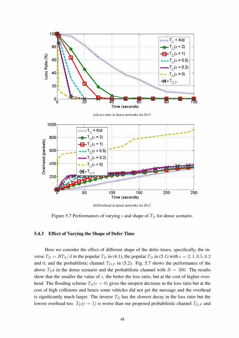
(a)Loss ratio in dense networks for D=3
(b)Overhead in dense networks for D=3
Figure 5.7 Performances of varying ε and shape of TD for dense scenario.
5.4.3 Effect of Varying the Shape of Defer Time
Here we consider the effect of different shape of the defer times, specifically, the in-verse TD = RTN/d in the popular TD in (4.1), the popular TD in (5.1) with ε = 2, 1, 0.5, 0.2
and 0, and the probabilistic channel TD,P in (5.2). Fig. 5.7 shows the performance of theabove TDs in the dense scenario and the probabilistic channel with R = 300. The resultsshow that the smaller the value of ε, the better the loss ratio, but at the cost of higher over-head. The flooding scheme TD(ε = 0) gives the steepest decrease in the loss ratio but at thecost of high collisions and hence some vehicles did not get the message and the overheadis significantly much larger. The inverse TD has the slowest decay in the loss ratio but thelowest overhead too. TD(ε = 1) is worse than our proposed probabilistic channel TD,P and
48
TD(ε = 0.5) and TD(ε = 0.2) since the overhead for all these cases are vary similar. Ourproposed probabilistic-channel TD,P is also worse than TD(ε = 0.2) in term of loss ratio.
5.4.4 Minimum Deterministic Defer Times
Here we evaluate our proposed a method in (5.4) to find a bound on deterministic defertimes. To avoid packet collision as discussed in Section 5.2.1, we consider the minimalinter-vehicle spacing (∆min) to be 6 m, which gives εmin to be 0.007 which is the minimumvalue to prevent flooding behavior. However, if ∆min is changed to 40 m (i.e., the averageinter-vehicle spacing in our simulation), the value of εmin becomes 0.00095 which leadsto flooding, as shown in Fig. 5.8(b). Since vehicles sometime get closer than the averagespacing of 40 m, a vehicle may not be able to hear its neighbor’s rebroadcast within its defertime and hence starts its own rebroadcast which results in collision. However, in probabilisticchannel, each transmission range is not exactly the same; the packet collisions occur onlyin the overlap transmission ranges. This is why the loss ratio of TD(ε = 0.00095) rapidlydecreases to 0% within 0.1 s. Since the disparity of defer times between two closest vehiclesin TD(ε = 0.007) and TD(ε = 0.05) exceeds the minimum packet transmission time, the lossratio of ε = 0.007 rapidly decreases in 0.2 s which it is faster than the ε = 0.05 while theoverhead is similar as shown in Fig. 5.8(a). For TD,P and TD(ε = 0.2), the longer the defertimes, the smaller the overhead and hence the slower the decline rate of the loss ratio. For thepurpose of choosing the value of ∆, we see that if the value of ∆ greater than the minimalinter-vehicle spacing is selected, there are many vehicles in this range and the defer time ofeach vehicle in this range is less than tp which leads to the packet collisions. The parameterε is inversely proportional to ∆. The distance d is proportional to ε. This criteria can beapplied to calculate other design parameters (e.g., TDMAX , R) while ε is fixed. TDMAX candecrease until the slope or the disparity between defer times of two closest neighbors is equalto tp.
5.4.5 Effect of Stochastic Defer Time
Finally, we compare the performance of stochastic defer times and deterministic defertimes. We select deterministic TD(ε = 1) and TD = 0 to compare with stochastic TD(ε = 1)
and TS = Tmax, respectively. As shown in Fig. 5.9(a), the stochastic defer times outper-form the deterministic defer times in reliability. The loss ratio of the stochastic defer timeTD(ε = 1) decreases faster than the deterministic defer time TD(ε = 1). The overhead of thestochastic Tmax is less than the deterministic TD = 0 and is similar to the others. The dis-semination time of Tmax is quite longer than the stochastic TD(ε = 1) because the varianceof the defer times for stochastic Tmax is much higher. Note that the shown plot is a result ofaveraging 10 independent runs. It happens that in some runs, many nodes pick small defertimes and hence the dissemination time is small, while in other runs, larger defer times are
49
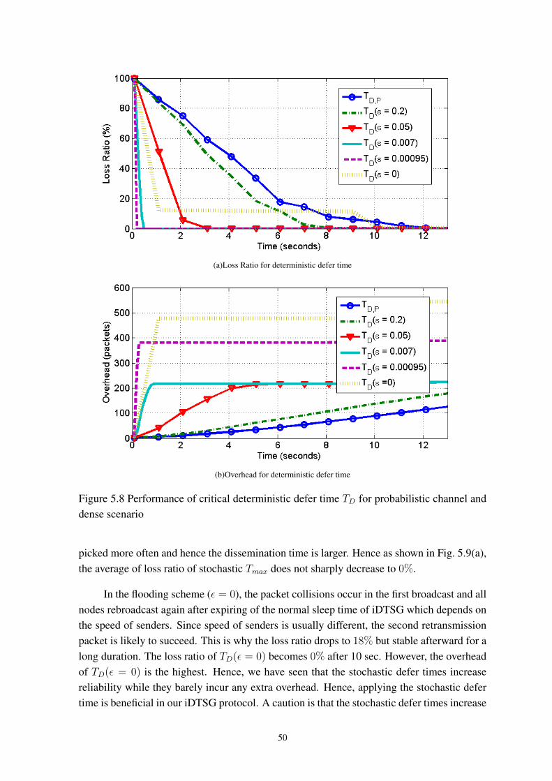
(a)Loss Ratio for deterministic defer time
(b)Overhead for deterministic defer time
Figure 5.8 Performance of critical deterministic defer time TD for probabilistic channel anddense scenario
picked more often and hence the dissemination time is larger. Hence as shown in Fig. 5.9(a),the average of loss ratio of stochastic Tmax does not sharply decrease to 0%.
In the flooding scheme (ε = 0), the packet collisions occur in the first broadcast and allnodes rebroadcast again after expiring of the normal sleep time of iDTSG which depends onthe speed of senders. Since speed of senders is usually different, the second retransmissionpacket is likely to succeed. This is why the loss ratio drops to 18% but stable afterward for along duration. The loss ratio of TD(ε = 0) becomes 0% after 10 sec. However, the overheadof TD(ε = 0) is the highest. Hence, we have seen that the stochastic defer times increasereliability while they barely incur any extra overhead. Hence, applying the stochastic defertime is beneficial in our iDTSG protocol. A caution is that the stochastic defer times increase
50
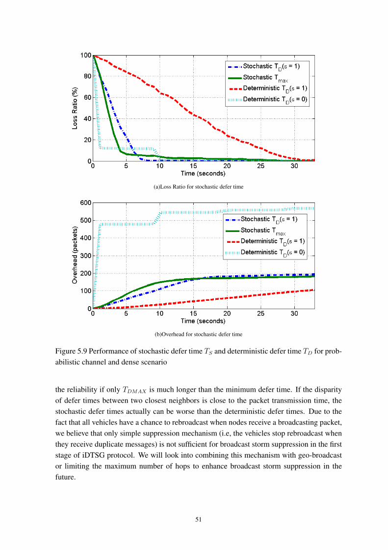
(a)Loss Ratio for stochastic defer time
(b)Overhead for stochastic defer time
Figure 5.9 Performance of stochastic defer time TS and deterministic defer time TD for prob-abilistic channel and dense scenario
the reliability if only TDMAX is much longer than the minimum defer time. If the disparityof defer times between two closest neighbors is close to the packet transmission time, thestochastic defer times actually can be worse than the deterministic defer times. Due to thefact that all vehicles have a chance to rebroadcast when nodes receive a broadcasting packet,we believe that only simple suppression mechanism (i.e, the vehicles stop rebroadcast whenthey receive duplicate messages) is not sufficient for broadcast storm suppression in the firststage of iDTSG protocol. We will look into combining this mechanism with geo-broadcastor limiting the maximum number of hops to enhance broadcast storm suppression in thefuture.
51
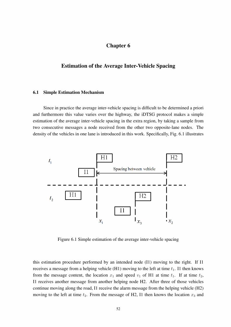
Chapter 6
Estimation of the Average Inter-Vehicle Spacing
6.1 Simple Estimation Mechanism
Since in practice the average inter-vehicle spacing is difficult to be determined a prioriand furthermore this value varies over the highway, the iDTSG protocol makes a simpleestimation of the average inter-vehicle spacing in the extra region, by taking a sample fromtwo consecutive messages a node received from the other two opposite-lane nodes. Thedensity of the vehicles in one lane is introduced in this work. Specifically, Fig. 6.1 illustrates
Figure 6.1 Simple estimation of the average inter-vehicle spacing
this estimation procedure performed by an intended node (I1) moving to the right. If I1receives a message from a helping vehicle (H1) moving to the left at time t1. I1 then knowsfrom the message content, the location x1 and speed v1 of H1 at time t1. If at time t2,I1 receives another message from another helping node H2. After three of those vehiclescontinue moving along the road, I1 receive the alarm message from the helping vehicle (H2)moving to the left at time t2. From the message of H2, I1 then knows the location x3 and
52
speed v2 of H2 at time t2. By assuming that H2 drives with a constant speed during time t1and t2, I1 can estimate the spacing between H1 and H2 as follows:
inter-vehicle spacing ≈ |x1 − x3 + v2(t2 − t1)|. (6.1)
Hence, the spacing between H1 and H2 can be calculated and taken as the estimate of theaverage inter-vehicle spacing. The average inter-vehicle spacing updates value as follows:inter-vehicle spacing = α(inter-vehicle spacing)old + (1−α)(inter-vehicle spacing)new. Theα is the parameter to balance the previous inter-vehicle spacing and the new inter-vehiclespacing information. This is likely to be valid for sparse scenarios. However, for densescenarios, there would likely be some other vehicles between H1 and H2 and hence thespacing between H1 and H2 would be larger than the actual inter-vehicle spacing. This isnot harmful to the loss ratio of the protocol since the extra region would just be longer thannecessary. In iDTSG, the initial value of Dextra is set to 20 m then an spacing estimation isdone. Dextra is updated as 2× inter− vehicle spacing. 3 If no estimation can be done doesnot happen, the extra region will be the same as that in the message content.
6.2 Simulation Results
After applying the simple estimation of the average inter-vehicle spacing to the iDTSGprotocol, we evaluate the performance by using the TD(RTN/d) and TD(ε = 0.2) in denseand sparse networks for D = 3 km and α = 0.5. The performance metrics are the lossratio and the overhead which are stated in the Chapter 5. As shown in Fig. 6.2 (a), the lossratio of the TD(RTN/d) does not reach 0% within 100 seconds in dense networks. Theloss ratio of the TD(ε = 0.2) reaches 0% within 10 seconds in dense networks. On theother hand, the overhead of the TD(ε = 0.2) is greater than the overhead of TD(RTN/d)
by 12% at 600 seconds. The overhead of the TD(ε = 0.2) is greater than the overhead ofthe TD(RTN/d) in dense networks, although the overhead of the TD(ε = 0.2) is less thanthe overhead of the TD(RTN/d) in sparse networks. Fig. 6.3 illustrates that the iDTSG lossratio of TD(ε = 0.2) saturates at 7% while the loss ratio of TD(RTN/d) keeps lower than5%. The simple estimation of the average inter-vehicle spacing is usable in both dense andsparse networks. Sometimes the estimation are too small so the loss ratio increases, while theoverhead decreases. However, the overhead (when the protocol uses the simple estimationof the average inter-vehicle spacing) is too high because the average inter-vehicle spacingis mostly overestimated. This simulation does not take an error from GPS into account andhence the average inter-vehicle spacing is not accurate. Since the iDTSG protocol uses aposition info from GPS, the accuracy of GPS would affect the performance of the iDTSGprotocol. Our simple estimation of the average inter-vehicle spacing has to be improved totolerate GPS errors and to be more accurate. This is left as a future work.
3A more accurate but more complicated estimate of the average inter-vehicle spacing would be a running average of allthe values of the inter-vehicle spacing that a node has observed so far.
53
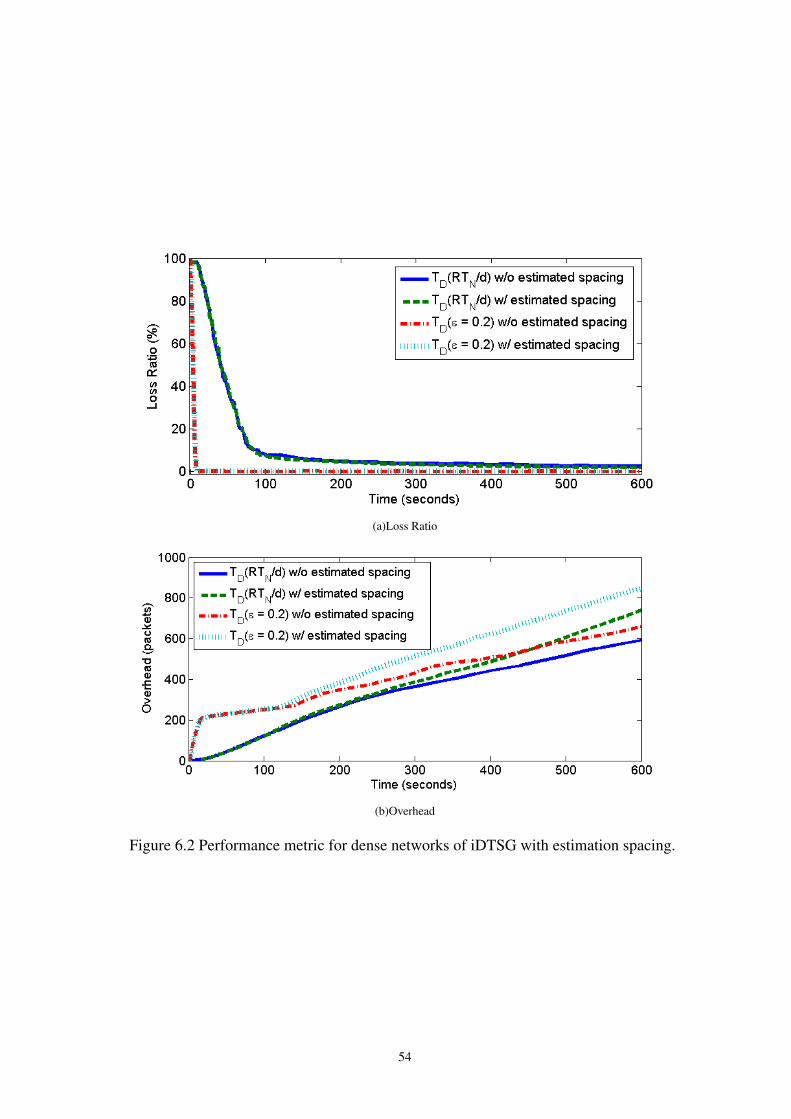
(a)Loss Ratio
(b)Overhead
Figure 6.2 Performance metric for dense networks of iDTSG with estimation spacing.
54
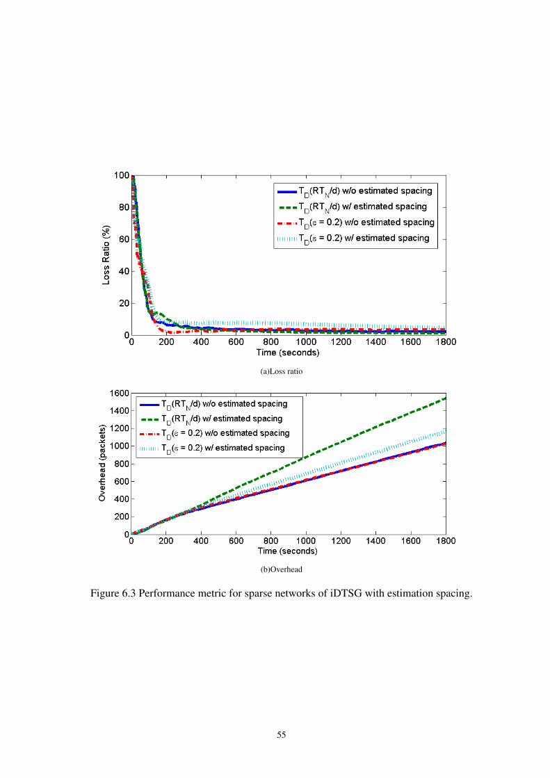
(a)Loss ratio
(b)Overhead
Figure 6.3 Performance metric for sparse networks of iDTSG with estimation spacing.
55
Chapter 7
Summary and Future Works
Vehicle ad-hoc networks enhance transportation safety at low implementation and operationcost. In such high speed movement of vehicles in highway environment, the vehicles areequipped with WAVE transceivers and GPS. Each driver make decision about the emergencyevents which have been informed by neighbor vehicles along the road in VANETs. In thepost crash notification, the emergency or warning message is disseminated to prevent chain-collision or congested traffic until the accident has been cleared from the highway. To meetthis objective, the time-stable geocast protocol is designed to disseminate and to maintainthe warning message for the sake of the new approaching vehicles in the specific area for acertain time.
7.1 Summary
In this thesis, we propose a new time-stable geocast protocol, called iDTSG. TheiDTSG protocol is the multi-hop broadcast protocol which considers the trade-off betweenreliability, dissemination time, and efficiency or redundancy of the message. The aim ofiDTSG is to maximize the number of informed nodes in the intended region with a fast and areliable transmission while network loads are minimized. iDTSG uses the contention-basedforwarding scheme to select forwarders, the counter-based scheme to suppress broadcaststorm problem, and the location-based scheme to keep the message alive in the intendedregion.
By simulation in ns-3, we compared the performance of the iDTSG protocol with theDTSG protocol in realistic channel and highway mobility models. Furthermore, we eval-uated the effects of the design parameters (TDMAX , ε, and R) for the distance-based defertimes and the shapes of the defer times with the iDTSG protocol. In addition to the evalu-ation of the previously proposed defer times, we proposed and evaluated a new defer timewhich is more appropriate with probabilistic channels. We also proposed the method forcalculating the deterministic defer time to avoid collisions for a bi-directional single lanehighway. We considered both dense and sparse traffic scenarios and both deterministic andprobabilistic channels. The simulation results show the following:
1.) Our iDTSG achieved almost 0% for the loss ratio, same as DTSG but at a much
56
lower cost of rebroadcast packets at least 20% and 30% in dense and sparse density connectednetworks, respectively. The reliability of iDTSG did not depend on the geocast region,
2.) Trade-offs between reliability and efficiency.
3.) Reducing the deterministic defer time (by reducing TDmax or ε) increases the relia-bility at the cost of the efficiency;
4.) The deterministic distance-based defer time has a optimal design value of ε to avoidcollision.
5.) Although our proposed defer time takes into account the different reception prob-ability at different distant and hence performs well, our proposed defer time can still beimproved in the future by considering the fact that nodes suppress their rebroadcasts if theyhear prior rebroadcasts.
6.) Furthermore, the stochastic distance-based defer time is more appropriate than thedeterministic distance-based defer time in case of increasing reliability if the parameter Tmaxis larger than necessary.
7.) iDTSG gives high reliability and high efficiency. Since iDTSG requires knowledgeof the local traffic density, we provided a simple density estimation algorithm. The resultsshowed that the estimation performed well.
7.2 Recommendations and Future Works
In the Chapter 5, we proposed the method to find a bound on minimum deterministicdefer times in a bi-directional single-lane highway. We showed that the ε = 0.007 andthe ε = 0.00095 are the bounded value for Tmax = R/smax. In this section, we applythe same method to find a bounded Tmax for ε = 1. The bounded Tmax are 0.09 and 0.02seconds. Fig. 7.1 illustrates defer times for Tmax = 0.09 seconds with varying ε values andTmax = 0.02 seconds.
The results in Fig. 7.2 show the trade-off between loss ratios and overheads. The lossratios of convex defer times are better than the linear defer time. The overheads of the TD,Pand the Tmax=0.09 are similar. Due to the fact that the TD(ε = 0.2) has a similar defer timeof the Tmax = 0.02 in a far distance. Hence, the TD(ε = 0.2) incurs the extra overhead thesame as the Tmax = 0.02. This means that the TD(ε = 1) with Tmax = 0.09 is not an optimalvalue as we think from the calculation. However, we are able to determine the bounded defertime in the bi-directional single-lane highway from the calculation.
Since the protocol has to work in bi-directional multiple-lane highways, our protocolhas to consider following issues:
57
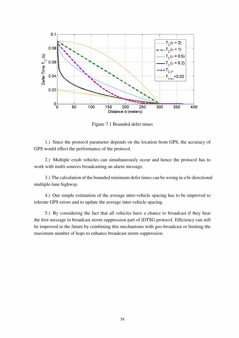
Figure 7.1 Bounded defer times
1.) Since the protocol parameter depends on the location from GPS, the accuracy ofGPS would effect the performance of the protocol.
2.) Multiple crash vehicles can simultaneously occur and hence the protocol has towork with multi-sources broadcasting an alarm message.
3.) The calculation of the bounded minimum defer times can be wrong in a bi-directionalmultiple-lane highway.
4.) Our simple estimation of the average inter-vehicle spacing has to be improved totolerate GPS errors and to update the average inter-vehicle spacing.
5.) By considering the fact that all vehicles have a chance to broadcast if they hearthe first message in broadcast storm suppression part of iDTSG protocol. Efficiency can stillbe improved in the future by combining this mechanisms with geo-broadcast or limiting themaximum number of hops to enhance broadcast storm suppression.
58
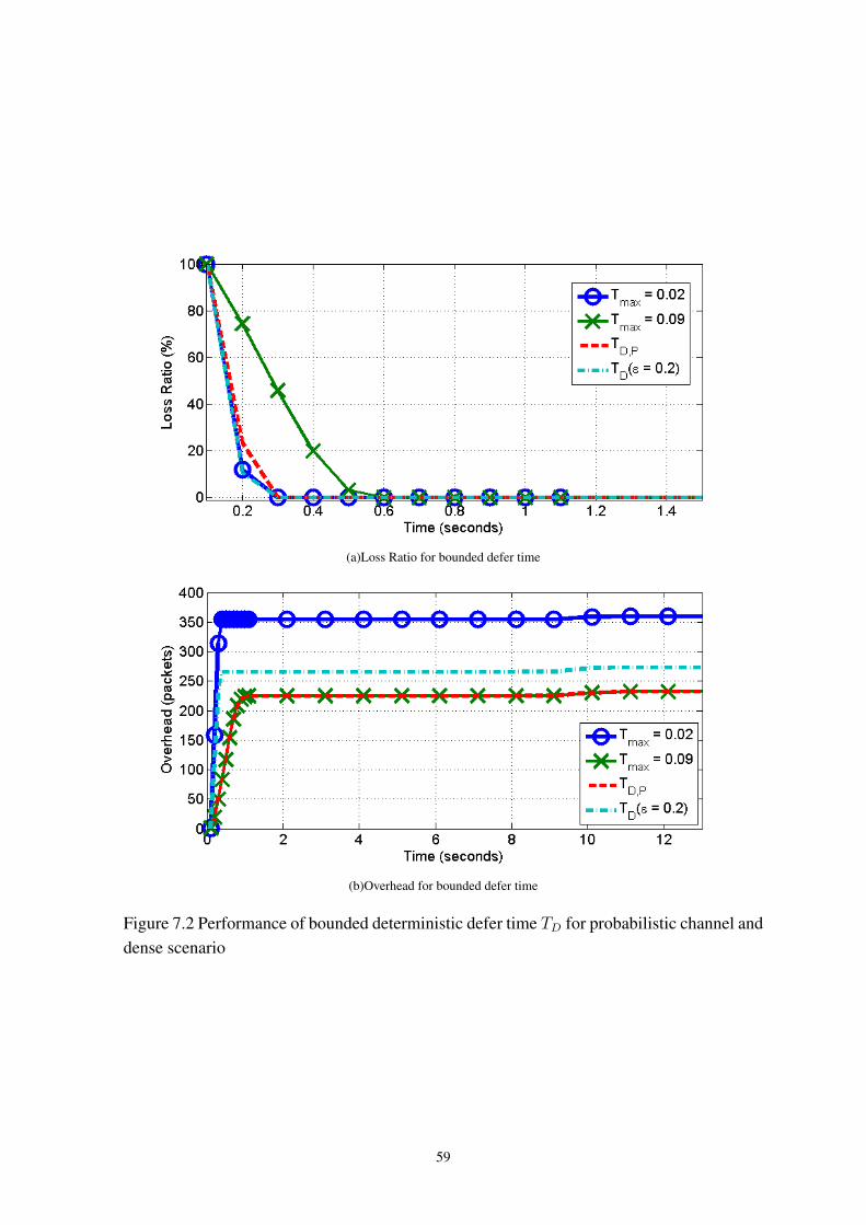
(a)Loss Ratio for bounded defer time
(b)Overhead for bounded defer time
Figure 7.2 Performance of bounded deterministic defer time TD for probabilistic channel anddense scenario
59
Appendix A
NS-3 code
Since H. Arbabi [40] proposed the highway mobility in ns-3, the simulations of vehicular adhoc networks do not require complicated interfaces between the network simulator and themobility simulator. A simplified schematization of the whole simulator is shown in Fig. A.1which we used to perform evaluations of our work. The highway mobility moves the nodesand changes their states following the rules given by the IDM mobility model and the MOBILlane-change model, while user-defined and a controller class are created to handle events andto create special vehicles. For example, after the vehicle is injected to the highway to act asthe source which initiates the disseminated message, the receivers call the iDTSG protocolin vehicle class. The following sections show in details C++ codes which are modified from[40].
A.1 Controller class
#include <iostream>#include <sstream>#include “Controller.h”using namespace stdusing namespace ns3namespace ns3{int all =0;int success = 0;int broadcast=0;int packeterror =0;int packetreceive=0;int packetsent=0;bool ch = false;int bID = 0;double fi =0;bool h = true;double nnn =0;
60
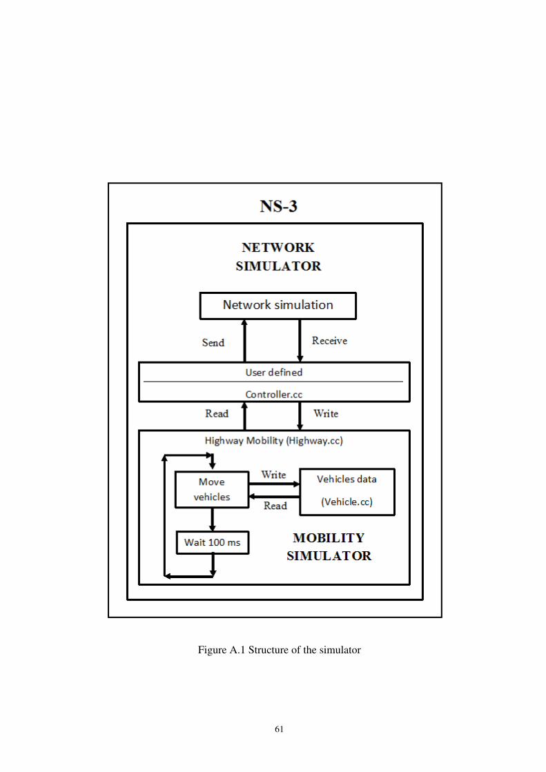
Figure A.1 Structure of the simulator
61

Controller::Controller(){T= −1.0;Plot=false; }Controller::Controller(Ptr<Highway> highway) {this->highway=highway; }void Controller::SetHighway(Ptr<Highway> highway) {this->highway=highway; }Ptr<Highway> Controller::GetHighway(){return this->highway; }bool Controller::Injectbroken(Ptr<Highway> highway, int& VID){ YansWifiPhyHelper sourcePhyHelper=YansWifiPhyHelper::Default();sourcePhyHelper.SetChannel(highway->GetWifiChannel());sourcePhyHelper.Set(“TxPowerStart”,DoubleValue(5));sourcePhyHelper.Set(“TxPowerEnd”,DoubleValue(5));sourcePhyHelper.Set(“TxPowerLevels”,UintegerValue(1));sourcePhyHelper.Set(“TxGain”,DoubleValue(0));sourcePhyHelper.Set(“RxGain”,DoubleValue(0));sourcePhyHelper.Set(“EnergyDetectionThreshold”, DoubleValue(-87.0));sourcePhyHelper.Set(“CcaMode1Threshold”, DoubleValue(-83));sourcePhyHelper.Set(“RxNoiseFigure”, DoubleValue(7));
Ptr<Vehicle> source = CreateObject<Vehicle>();source->SetupWifi(highway->GetWifiHelper(),sourcePhyHelper, highway->GetNqosWifiMacHelper());source->SetVehicleId(VID++);source->SetDirection(1);source->SetPosition(Vector(0.0, highway->GetYForLane(0,1), 0));source->SetVelocity(0.0);source->SetAcceleration(0.0);Ptr<Model> sourceModel=highway->CreateSedanModel();sourceModel->SetDesiredVelocity(30.93);source->SetModel(sourceModel);source->SetLaneChange(highway->GetSedanLaneChange());source->SetLength(4);source->SetWidth(2);source->SetReceiveCallback(highway->GetReceiveDataCallback());highway->AddVehicle(source);bID = source->GetVehicleId();highway->SetAutoInject(true);return false;}
62
bool Controller::InitVehicle(Ptr<Highway> highway, int& VID) {Simulator::Schedule(Seconds(500.0), &Controller::Injectbroken, this,highway, VID);return false;}
bool Controller::ControlVehicle(Ptr<Highway> highway, Ptr<Vehicle> vehicle, double dt){
if(Plot==true){ bool newStep=false;double now=Simulator::Now().GetDouble();
if(now > T){ T = now;newStep=true; }
if(newStep==true && ch == true ) { newStep=false; }
if(newStep==false && ch == true ){ Controller::DeliveryRatio(vehicle);}}
if(vehicle->GetVehicleId()==bID && vehicle->GetPosition().x >=6500 && ch ==
false){ double t = Simulator::Now().GetSeconds();
if (ch == false){ ch = true;Controller::BroadcastWarning(vehicle);Controller::DeliveryRatio(vehicle);Controller::Printresult(t) ;}return false;}return false;}
void Controller::BroadcastWarning(Ptr<Vehicle> veh)static double now=0;static int crash pos = veh->GetPosition().x ;
63
if (veh->GetSequencenumber() < 1){ veh->SetFlag(1);now=Simulator::Now().GetSeconds();}
if (veh->GetAckfirst(0) == true ){ f = veh->Getfirst(2); }if (veh->GetCount() < 1 && veh->GetPosition().x < 9600){ stringstream msg;msg << veh->GetVehicleId()<< “ ” << veh->GetSequencenumber()<< “ ” << veh->GetPosition().x<< “ ” << veh->GetDirection()<< “ ” << crash pos<< “ ” << veh->GetDirection()<< “ ” << veh->GetFlag()<< “ ” << 3000 // The D region is 3 km. << “ ” << now<< “ ” << 20 // The initial value of inter-vehicle spacing << “ ” << veh->GetVelocity();uint16 t packetSize = 800;Ptr<Packet> packet = Create<Packet>((uint8 t*) msg.str().c str(), packetSize);veh->SendTo(veh->GetBroadcastAddress(), packet);veh->SetSequencenumber();Simulator::Schedule(Seconds(veh->GetWaitingTime(true)),&Controller::BroadcastWarning,this,veh);}}
void Controller::ReceiveData(Ptr<Vehicle> veh, Ptr<const Packet> pk, Address ad-dress){ int direction = veh->GetDirection();int vid=veh->GetVehicleId();
if (veh->IsEquipped==false) {return;}uint8 t *buffer = new uint8 t[pk->GetSize()];pk->CopyData (buffer, pk->GetSize());stringstream ss (stringstream::in | stringstream::out);string data = string((char*)buffer);int sender id, message sequence, sender direction, event direction, period flag, D region ;double sender pos, event pos, event time, speed, inter spacing;ss << data;ss >> sender id;ss >> message sequence;
64
ss >> sender pos;ss >> sender direction;ss >> event pos;ss >> event direction;ss >> period flag;ss >> D region;ss >> event time;ss >> inter spacing;ss >> speed;
if(veh->GetDirection() == 1){ density1 = (density1*0.5)+(dense*0.5); }else if(veh->GetDirection() == -1){ density2 = (density2*0.5)+(dense*0.5); }fi = event pos − D region;veh->SetCount(veh ,pk);if (period flag==2){veh->SetFlag(2); }
if (direction == −1&& sender direction == 1 ){
if(veh->Checkccc() == 0){ veh->SetintiX(sender pos, now, sender id); veh->Setccc();}
if (veh->Checkccc() == 1 ){ veh->SetExtraRangehelping (sender pos, now, speed, sender id);veh->Setccc(); }} else if( direction == 1 && sender direction2 == −1 ){ if(veh->Checkccc() == 0) veh->SetintiX(sender pos, now, sender id);veh->Setccc(); }
if (veh->Checkccc() == 1 ){ veh->SetExtraRangeintended(sender pos, now, speed, sender id );veh->Setccc(); }}
if (vid=bID && veh->GetCount() ==1){ veh->SetWaitingTime(veh->GetVelocity(), sender x2, veh->GetPosition().x );if (period flag == 1)veh->SetFlag(1);veh->SetExtra(inter spacing);veh->iDTSG(veh, pk, address); }
if (veh->GetPosition().x > event pos && veh->GetDirection() == 1){if(sender direction2 == −1){veh->stableOpcount();}
65
else if (sender direction== 1 and space < 0){veh->FrontStableCount();}}else if(veh->GetPosition().x < fi && veh->GetDirection() == −1){ if(sender direction == 1){veh->stableOpcount();}else if (sender direction == −1 and space > 0){veh->FrontStableCount();}}}
void Controller::DeliveryRatio(Ptr<Vehicle> veh){ double veh pos = veh->GetPosition().x;
if(veh->IsEquipped==false){ return;}broadcast= veh->Broadcastcount();packeterror = veh->errorcount();packetreceive = veh->Macreceivecount();packetsent = veh->Macsentcount();
if (x <= 6381 && x >= 3501 && veh->GetDirection()==1 && veh->GetRange() ==false){ all = all+1;veh->SetRange(); }
if ( veh->GetCount()>=1 && x<= 6381 && x>= 3501 && veh->GetDirection()==1&& veh->GetRange() == true && veh-> GetSuccess() == false){ success = success+1;veh->SetSuccess(); }}
void Controller::Printresult(double Time){ double now=Simulator::Now().GetSeconds();now = (now-Time);int lost = all−success;
if(now >= 120){nnn = 20;}else if ( now >= 0.1 ){nnn = 1;}else{nnn = 0.1;}
std::cout<< now << “ ”<< lost << “ ”<< broadcast << “ ” << all << “ ” <<success << “ ” << packeterror << “ ” << packetreceive << “ ” << packetsent << ”;”<< endl;Simulator::Schedule(Seconds(nnn),&Controller::Printresult, this, Time);}}
66
A.2 Vehicle class
The following functions are added into the vehicle class of the [40]’ work.
namespace ns3 { int bc =0;int packeterror =0;int m packetsSent1 =0;int m packetReceive=0;
void Vehicle::SetSequencenumber(void) { sequencenum++; }
int Vehicle::GetSequencenumber(void) { return sequencenum; }
void Vehicle::SetFlag(int value1) { period flag = value1; }
int Vehicle::GetFlag(void) { return period flag; }
void Vehicle::SetRange(void) { range = true; }
void Vehicle:: SetSuccess(void) { success = true; }
bool Vehicle::GetRange(void) { return range; }
bool Vehicle::GetSuccess(void) { return success; }
bool Vehicle:: Checkccc(void) { return ccc; }
void Vehicle:: Setccc(void) { ccc = true; }
bool Vehicle::Getyyy(void) { return yyy; }
void Vehicle::SetExtraRangeintended(double x2, double t, double speed, int iid){
if(send id= iid){ int delta = t-ti;int dense = (inti x - (x2+(speed*delta)) ) ;if (dense < 0){dense = (0 - dense);}density = (0.5*dense)+(0.5*density) ;yyy=true;inti x = x2;ti = t;}}
void Vehicle::SetExtraRangehelping (double x2, double t, double speed, int iid) {
67
if (send id= iid){ int delta = t-ti;int dense = inti x - (x2-(speed*delta)) ;if (dense < 0){dense = (0 - dense);density = (0.5*dense)+(0.5*density) ; yyy=true;inti x = x2;ti = t;}}
void Vehicle::SetExtra(double duu) { density = duu; }
void Vehicle::SetintiX(double x,double t, int iid) { inti x = x;ti = t;send id = iid;}
int Vehicle::checkdensity(void) { return density ; }
void Vehicle::SetWaitingTime(void){ double speed = m velocity ;repeat Time = (600(speed+35)); }
double Vehicle::GetWaitingTime(bool value){ switch (value){ case true:return repeat Time;break;case false:return defer Time;break;default:NS FATAL ERROR (“No such value:” << value); }}
void Vehicle::SetWaitingTime(double speed, double position source,double position receiver){ int diff = position source - position receive;
if(diff <){diff = 0-diff;}if(diff > 10) { diff = diff; }else if (diff < 10) { diff = 10; } defer Time = ((600(speed+35))*(300((double)diff))); }
int Vehicle::GetBackCount(void) { return back count; }
68
int Vehicle::GetOpCount(void) { return op count; }
int Vehicle::GetLeaderCount(void) { return leader count; }
int Vehicle::GetCount(void) { count =leader count+op count+back count;return count; }
void Vehicle::SetCount(Ptr<Vehicle> veh, Ptr<const Packet> packet) { uint8 t *buffer= new uint8 t[packet->GetSize()];packet->CopyData (buffer, packet->GetSize());stringstream ss (stringstream::in | stringstream::out);string data = string((char*)buffer);int sender id, message sequence, sender direction, event direction, period flag, D region ;double sender pos, event pos, event time;ss << data;ss >> sender id;ss >> message sequence;ss >> sender pos;ss >> sender direction;ss >> event pos;ss >> event direction;ss >> period flag;ss >> D region;ss >> event time;int direction = veh->GetDirection();double space = ( veh->GetPosition().x - sender x);
if(direction == 1 and direction == sender direction and space < 0) { leader count++; }else if ( direction == 1 and direction == sender direction and space > 0 ) { back count++; }else if ( direction= sender direction) { op count++; }else if(direction == -1 and direction == sender direction and space < 0) { back count++; }else if ( direction == -1 and direction == sender direction and space > 0 ) { leader count++;}}
void Vehicle::helpingbroadcast(Ptr<Vehicle> v1, Ptr<const Packet> pk,Address ad-dress3) { uint8 t *buffer = new uint8 t[pk->GetSize()];pk->CopyData (buffer, pk->GetSize());stringstream ss (stringstream::in | stringstream::out);string data = string((char*)buffer);static int sender id, sequence number, sender direction, event direction, prestableflag, D region;static double sender pos, event pos, event time, dense, speed;
69
ss << data;ss >> sender id;ss >> message sequence;ss >> sender pos;ss >> sender direction;ss >> event pos;ss >> event direction;ss >> period flag;ss >> D region;ss >> event time;ss >> dense;ss >> speed;double D extra = event pos - D region - (2*dense);double finale = event pos - D region ;double bound = event pos + (2*dense);Vehicle::SetWaitingTime();
if (v1->GetPosition().x >250 && v1->GetPosition().x < 9600){ v1->Setprob();
if (v1->GetSequencenumber()==0 && v1->GetLeaderCount() < 1 ){ v1->SetSequencenumber();stringstream msgx;msgx << “ ” << v1->GetVehicleId()<< “ ” << v1->GetSequencenumber()<< “ ” << v1->GetPosition().x<< “ ” << v1->GetDirection()<< “ ” << event pos<< “ ” << event direction<< “ ” << v1->GetFlag()<< “ ” << D region<< “ ” << event time<< “ ” << v1->checkdensity()<< “ ” << v1->GetVelocity();uint16 t packetSize = 800;Ptr<Packet> packet = Create<Packet>((uint8 t*) msgx.str().c str(), packetSize);v1->SendTo(v1->GetBroadcastAddress(), packet);
Simulator::Schedule(Seconds(v1->GetWaitingTime(true)),&Vehicle::helpingbroadcast,this,v1,packet,address3);return;}
else if (v1->GetFlag()== 1 && v1-GetLeaderCount()< 1 && v1->GetOpCount()<3
70
&& v1->GetSequencenumber()> 0 && v1->GetPosition().x>D extra && v1->GetPosition().x< bound){ v1->SetSequencenumber();stringstream msgx;msgx << “ ” << v1->GetVehicleId()<< “ ” << v1->GetSequencenumber()<< “ ” << v1->GetPosition().x<< “ ” << v1->GetDirection()<< “ ” << event pos<< “ ” << event direction<< “ ” << v1->GetFlag()<< “ ” << D region<< “ ” << event time<< “ ” << v1->checkdensity()<< “ ” << v1->GetVelocity();uint16 t packetSize = 800;Ptr<Packet> packet = Create<Packet>((uint8 t*) msgx.str().c str(), packetSize);v1->SendTo(v1->GetBroadcastAddress(), packet);
Simulator::Schedule(Seconds(v1->GetWaitingTime(true)),&Vehicle::helpingbroadcast,this,v1,packet,address3);}
else if (v1->GetSequencenumber() >0){ if ( v1->GetPosition().x > finale) {
Simulator::Schedule(Seconds(v1->GetWaitingTime(true)),&Vehicle::helpingbroadcast,this,v1,pk,address3);return;}
else if ( v1->GetPosition().x <= finale && v1->GetPosition().x > D extra && v1->GetstableOpcount() < 1 && v1->GetFrontStableCount() < 1){ v1->SetFlag(2);v1->SetSequencenumber();stringstream msgx;msgx << “ ” << v1->GetVehicleId()<< “ ” << v1->GetSequencenumber()<< “ ” << v1->GetPosition().x<< “ ” << v1->GetDirection()<< “ ” << event pos<< “ ” << event direction<< “ ” << v1->GetFlag()
71
<< “ ” << D region<< “ ” << event time<< “ ” << v1->checkdensity()<< “ ” << v1->GetVelocity();uint16 t packetSize = 800;Ptr<Packet> packet = Create<Packet>((uint8 t*) msgx.str().c str(), packetSize);v1->SendTo(v1->GetBroadcastAddress(), packet);
Simulator::Schedule(Seconds(v1->GetWaitingTime(true)),&Vehicle::helpingbroadcast,this,v1,pack,address3); }}else return;} else return;}
void Vehicle::intendedbroadcast(Ptr<Vehicle> v17, Ptr<const Packet> pkv,Addressaddress4){ uint8 t *buffers = new uint8 t[pkv->GetSize()];pkv->CopyData (buffers, pkv->GetSize());stringstream ss (stringstream::in | stringstream::out);string data = string((char*)buffers);static int sender id, message sequence, sender direction, event direction, period flag,D region;static double sender pos, event pos,event time,dense,speed;ss << data;ss >> sender id;ss >> message sequence;ss >> sender pos;ss >> sender direction;ss >> event pos;ss >> event direction;ss >> period flag;ss >> D region;ss >> event time;ss >> dense;ss >> speed;double D extra = event pos +(2*dense);double fin = event pos-D region;double bound = event pos-D region -(2*dens);Vehicle::SetWaitingTime();
if (v17->GetPosition().x >250 && v17->GetPosition().x < 9600)
72
{ if (v17->GetSequencenumber()==0 && v17->GetBackCount() < 1 ){ v17->SetSequencenumber();stringstream msgx;msgx << “ ” << v17->GetVehicleId()<< “ ” << v17->GetSequencenumber()<< “ ” << v17->GetPosition().x<< “ ” << v17->GetDirection()<< “ ” << event pos<< “ ” << event direction<< “ ” << v17->GetFlag()<< “ ” << D region<< “ ” << event time<< “ ” << v17->checkdensity()<< “ ” << v17->GetVelocity();uint16 t packetSize = 800;Ptr<Packet> pacr = Create<Packet>((uint8 t*) msgp.str().c str(), packetSize);v17->SendTo(v17->GetBroadcastAddress(), pacr);
Simulator::Schedule(Seconds(v17->GetWaitingTime(true)),&Vehicle::intendedbroadcast, this,v17,pacr,address4);return;}
else if ( v17->GetFlag() == 1 && v17->GetBackCount() ¡ 1 && v17->GetOpCount()<3 && v17->GetSequencenumber() > 0 && v17->GetPosition().x < D extra && v17->GetPosition().x > bound){ v17->SetSequencenumber();stringstream msgp;msgp << “ ” << v17->GetVehicleId()<< “ ” << v17->GetSequencenumber()<< “ ” << v17->GetPosition().x<< “ ” << v17->GetDirection()<< “ ” << event pos<< “ ” << event direction<< “ ” << v17->GetFlag()<< “ ” << D region<< “ ” << event time<< “ ” << v17->checkdensity()<< “ ” << v17->GetVelocity();uint16 t packetSize = 800;Ptr<Packet> pacr = Create<Packet>((uint8 t*) msgp.str().c str(), packetSize);v17->SendTo(v17->GetBroadcastAddress(), pacr);
73
Simulator::Schedule(Seconds(v17->GetWaitingTime(true)),&Vehicle::intendedbroadcast,this,v17,pacr,address4);}
else if ( v17->GetSequencenumber() ¿ 0){ if (v17->GetPosition().x < event pos){
Simulator::Schedule(Seconds(v17-GetWaitingTime(true)),&Vehicle::intendedbroadcast,this,v17,pkv,address4);return;}
else if (v17->GetFlag() == 2 && v17->GetPosition().x>= event pos && v17->GetPosition().x< D extra && v17->GetstableOpcount() < 1 && v17->GetFrontStableCount() < 1 ){ v17->SetSequencenumber();stringstream msgc;msgc << “ ” << v17->GetVehicleId()<< “ ” << v17->GetSequencenumber()<< “ ” << v17->GetPosition().x<< “ ” << v17->GetDirection()<< “ ” << event pos<< “ ” << event direction<< “ ” << v17->GetFlag()<< “ ” << D region<< “ ” << event time<< “ ” << v17->checkdensity()<< “ ” << v17->GetVelocity();uint16 t packetSize = 800;Ptr<Packet> packq = Create<Packet>((uint8 t*) msgc.str().c str(), packetSize);v17->SendTo(v17->GetBroadcastAddress(), packq);
Simulator::Schedule(Seconds(v17->GetWaitingTime(true)),&Vehicle::intendedbroadcast,this,v17,packq,address4);}} else return;} else return;}
void Vehicle::iDTSG(Ptr<Vehicle> v6, Ptr<const Packet> pkt, Address address1){ if (v6->GetDirection() == -1){
Simulator::Schedule(Seconds(v6->GetWaitingTime(false)),&Vehicle::helpingbroadcast,
74
this,v6,pkt,address1);return; }
else if (v6->GetDirection() == 1){
Simulator::Schedule(Seconds(v6->GetWaitingTime(false)),&Vehicle::intendedbroadcast,this,v6,pkt,address1);return; }}
int Vehicle::Broadcastcount(void) { return bc; }
void Vehicle::stableOpcount(void) { Opstablecount++; }
int Vehicle::GetstableOpcount(void) { return Opstablecount; }
void Vehicle::FrontStableCount(void) { frontstablecount++; }
int Vehicle::GetFrontStableCount(void) { return frontstablecount; }
A.3 Highway class
The following configurations are modified in the Highway function.
Highway::Highway(){// Setup Wifi
m wifiHelper = WifiHelper::Default();
m wifiHelper.SetStandard (WIFI PHY STANDARD 80211p CCH);
m wifiMacHelper = NqosWifiMacHelper::Default();
m wifiPhyHelper = YansWifiPhyHelper::Default();
m wifiMacHelper.SetType (”ns3::AdhocWifiMac”);
m wifiHelper.SetRemoteStationManager (“ns3::ConstantRateWifiManager”,“DataMode”, StringValue (“OfdmRate6MbpsBW10MHz”),“ControlMode”, StringValue(“OfdmRate6MbpsBW10MHz”));
m wifiChannelHelper.SetPropagationDelay (“ns3::ConstantSpeedPropagationDelayModel”);
m wifiChannelHelper.AddPropagationLoss(“ns3::ThreeLogDistancePropagationLossModel”,
75
“Distance0”,DoubleValue(1.0), “Distance1”,DoubleValue(225.0), “Distance2”,DoubleValue(1000.0),“Exponent0”,DoubleValue(2) , “Exponent1”,DoubleValue(4), “Exponent2”,DoubleValue(4));
m wifiChannelHelper.AddPropagationLoss(“ns3::NakagamiPropagationLossModel”, “Dis-tance1”, DoubleValue(50.0) , “Distance2”,DoubleValue(150.0), “m0”, DoubleValue(3.0),“m1”, DoubleValue(1.5), “m2”, DoubleValue(1.0));
m wifiChannel = m wifiChannelHelper.Create();
m wifiPhyHelper.SetChannel (m wifiChannel);
m wifiPhyHelper.Set(“TxPowerStart”,DoubleValue(5));
m wifiPhyHelper.Set(“TxPowerEnd”,DoubleValue(5));
m wifiPhyHelper.Set(“TxPowerLevels”,UintegerValue(1));
m wifiPhyHelper.Set(“TxGain”,DoubleValue(0));
m wifiPhyHelper.Set(“RxGain”,DoubleValue(0));
m wifiPhyHelper.Set(“EnergyDetectionThreshold”, DoubleValue(-87.0));
m wifiPhyHelper.Set(“CcaMode1Threshold”, DoubleValue(-83));
m wifiPhyHelper.Set(“RxNoiseFigure”, DoubleValue(7)); }
76
References
[1] K. Kanitpong, Sirilan, S. Kachathong, S. Ponboon, N. Boontob, and P. Aniwat-takulchai, “Safe driving speed report,” tech. rep., Thailand Accident Research Center(TARC) Transportation Engineering, School of Engineering and Technology, AsianInstitute of Technology (AIT), July 2008.
[2] “Ieee standard for information technology– local and metropolitan area networks–specific requirements– part 11: Wireless lan medium access control (mac) and phys-ical layer (phy) specifications amendment 6: Wireless access in vehicular environ-ments,” IEEE Std 802.11p-2010 (Amendment to IEEE Std 802.11-2007 as amendedby IEEE Std 802.11k-2008, IEEE Std 802.11r-2008, IEEE Std 802.11y-2008, IEEEStd 802.11n-2009, and IEEE Std 802.11w-2009), pp. 1 –51, 15 2010.
[3] F. Li and Y. Wang, “Routing in vehicular ad hoc networks: A survey,” Vehicular Tech-nology Magazine, IEEE, vol. 2, pp. 12 –22, June 2007.
[4] N. Wisitpongphan, F. Bai, P. Mudalige, and O. Tonguz, “On the routing problem indisconnected vehicular ad-hoc networks,” in INFOCOM 2007. 26th IEEE Inter-national Conference on Computer Communications. IEEE, pp. 2291 –2295, May2007.
[5] S.-Y. Ni, Y.-C. Tseng, Y.-S. Chen, and J.-P. Sheu, “The broadcast storm problem ina mobile ad hoc network,” in Proceedings of the 5th annual ACM/IEEE internationalconference on Mobile computing and networking, MobiCom ’99, (New York, NY,USA), pp. 151–162, ACM, 1999.
[6] H. Rahbar, K. Naik, and A. Nayak, “Dtsg: Dynamic time-stable geocast routing invehicular ad hoc networks,” in Ad Hoc Networking Workshop (Med-Hoc-Net), 2010The 9th IFIP Annual Mediterranean, pp. 1 –7, june 2010.
[7] L. Briesemeister and G. Hommel, “Role-based multicast in highly mobile but sparselyconnected ad hoc networks,” in Mobile and Ad Hoc Networking and Computing, 2000.MobiHOC. 2000 First Annual Workshop on, pp. 45 –50, 2000.
[8] M.-T. Sun, W. Feng, and T.-H. Lai, “Location aided broadcast in wireless ad hoc
77
networks,” in Global Telecommunications Conference, 2001. GLOBECOM ’01.IEEE, vol. 5, pp. 2842 –2846 vol.5, 2001.
[9] A. Bachir and A. Benslimane, “A multicast protocol in ad hoc networks inter-vehiclegeocast,” in Vehicular Technology Conference, 2003. VTC 2003-Spring. The 57thIEEE Semiannual, vol. 4, pp. 2456 – 2460 vol.4, april 2003.
[10] S. Oh, J. Kang, and M. Gruteser, “Location-based flooding techniques for vehicu-lar emergency messaging,” in Mobile and Ubiquitous Systems: Networking Services,2006 Third Annual International Conference on, pp. 1 –9, july 2006.
[11] K. Ibrahim, M. Weigle, and M. Abuelela, “p-ivg: Probabilistic inter-vehicle geocastfor dense vehicular networks,” in Vehicular Technology Conference, 2009. VTCSpring 2009. IEEE 69th, pp. 1 –5, april 2009.
[12] A. Dahiya and R. K. Chauhan, “A comparative study of manet and vanet environment,”Journal of computing, vol. 2, pp. 87–92, July 2010.
[13] M. Boban, T. Vinhoza, M. Ferreira, J. Barros, and O. Tonguz, “Impact of vehiclesas obstacles in vehicular ad hoc networks,” Selected Areas in Communications, IEEEJournal on, vol. 29, pp. 15 –28, january 2011.
[14] E. Schoch, F. Kargl, M. Weber, and T. Leinmuller, “Communication patterns invanets,” Communications Magazine, IEEE, vol. 46, pp. 119 –125, november 2008.
[15] T. Willke, P. Tientrakool, and N. Maxemchuk, “A survey of inter-vehicle commu-nication protocols and their applications,” Communications Surveys Tutorials, IEEE,vol. 11, pp. 3 –20, quarter 2009.
[16] R. Uzcategui and G. Acosta-Marum, “Wave: A tutorial,” Communications Magazine,IEEE, vol. 47, pp. 126 –133, may 2009.
[17] “Ieee standard for information technology - telecommunications and information ex-change between systems - local and metropolitan area networks - specific requirements- part 11: Wireless lan medium access control (mac) and physical layer (phy) specifi-cations,” IEEE Std 802.11-2007 (Revision of IEEE Std 802.11-1999), pp. 1 –1076, 122007.
[18] Y. Li, “An overview of the dsrc/wave technology,” in Quality, Reliability, Securityand Robustness in Heterogeneous Networks (X. Zhang and D. Qiao, eds.), vol. 74 of
78
Lecture Notes of the Institute for Computer Sciences, Social Informatics and Telecom-munications Engineering, pp. 544–558, Springer Berlin Heidelberg, 2012.
[19] “http://www.standards.its.dot.gov/fact sheet.asp?f = 80.”
[20] M. Bakhouya, J. Gaber, and P. Lorenz, “An adaptive approach for information dissem-ination in vehicular ad hoc networks,” Journal of Network and Computer Applications,vol. 34, no. 6, pp. 1971 – 1978, 2011.
[21] H. Fußler, J. Widmer, M. Kasemann, M. Mauve, and H. Hartenstein, “Contention-based forwarding for mobile ad hoc networks,” Ad Hoc Networks, vol. 1, no. 4,pp. 351–369, 2003.
[22] M. Torrent-Moreno, F. Schmidt-Eisenlohr, H. Fubler, and H. Hartenstein, “Effectsof a realistic channel model on packet forwarding in vehicular ad hoc networks,” inWireless Communications and Networking Conference, 2006. WCNC 2006. IEEE,vol. 1, pp. 385 –391, april 2006.
[23] W. Zhang, “Analysis of packet forwarding in vanets using probabilistic channelmodel,” in Vehicular Technology Conference, 2009. VTC Spring 2009. IEEE69th, pp. 1 –5, april 2009.
[24] R. Chen, W.-L. Jin, and A. Regan, “Broadcasting safety information in vehicular net-works: issues and approaches,” Network, IEEE, vol. 24, pp. 20 –25, jan.-feb. 2010.
[25] Y. Shao, C. Liu, and J. Wu, Handbook on Vehicular Networks, ch. 10 Delay-TolerantNetworks in VANETs. M. Weigle and S. Olariu: Taylor & Frances, 2009.
[26] Z. D. Chen, H. Kung, and D. Vlah, “Ad hoc relay wireless networks over moving vehi-cles on highways,” in Proceedings of the 2nd ACM international symposium on Mobilead hoc networking & computing, MobiHoc ’01, (New York, NY, USA), pp. 247–250,ACM, 2001.
[27] M. Almeida, ed., Advances in Vehicular Networking Technologies. InTech, 2011.
[28] H. P. J. Maria Kihl, Mihail Sichitiu, “Design and evaluation of two geocast protocolsfor vehicular ad-hoc networks,” Journal of Internet Engineering, vol. 2, no. 1, pp. 127–135, 2008.
79
[29] M. Javed and J. Khan, “A geocasting technique in an ieee802.11p based vehicular adhoc network for road traffic management,” in Australasian Telecommunication Net-works and Applications Conference (ATNAC), 2011, pp. 1 –6, nov. 2011.
[30] C. Maihofer, T. Leinmuller, and E. Schoch, “Abiding geocast: time–stable geocast forad hoc networks,” in Proceedings of the 2nd ACM international workshop on Vehicularad hoc networks, VANET ’05, (New York, NY, USA), pp. 20–29, ACM, 2005.
[31] Q. Yu and D. Liu, “Disseminate warning message in vanets based on predicting theinterval of vehicles,” in Frontier of Computer Science and Technology (FCST), 2010Fifth International Conference on, pp. 559 –564, aug. 2010.
[32] Q. Yu and G. Heijenk, “Abiding geocast for warning message dissemination in vehic-ular ad hoc networks,” in Communications Workshops, 2008. ICC Workshops ’08.IEEE International Conference on, pp. 400 –404, may 2008.
[33] “http://www.nsnam.org/.”
[34] M. Lacage and T. R. Henderson, “Yet another network simulator,” in Proceeding fromthe 2006 workshop on ns-2: the IP network simulator, WNS2 ’06, (New York, NY,USA), ACM, 2006.
[35] H. Friis, “A note on a simple transmission formula,” Proceedings of the IRE, vol. 34,pp. 254 – 256, may 1946.
[36] M. Nakagami, “The m-distribution- a general formula of intensity distribution of rapidfading,” in Statistical Methods in Radio Wave Propagation, pp. 3–36, Pergamon Press,Oxford, U. K., 1960.
[37] Q. Chen, F. Schmidt-Eisenlohr, D. Jiang, M. Torrent-Moreno, L. Delgrossi, andH. Hartenstein, “Overhaul of ieee 802.11 modeling and simulation in ns-2,” in Pro-ceedings of the 10th ACM Symposium on Modeling, analysis, and simulation of wire-less and mobile systems, MSWiM ’07, (New York, NY, USA), pp. 159–168, ACM,2007.
[38] M. Torrent-Moreno, D. Jiang, and H. Hartenstein, “Broadcast reception rates and ef-fects of priority access in 802.11-based vehicular ad-hoc networks,” in Proceedingsof the 1st ACM international workshop on Vehicular ad hoc networks, VANET ’04,(New York, NY, USA), pp. 10–18, ACM, 2004.
80
[39] L. Cheng, B. Henty, F. Bai, and D. Stancil, “Highway and rural propagation channelmodeling for vehicle-to-vehicle communications at 5.9 ghz,” in Antennas and Prop-agation Society International Symposium, 2008. AP-S 2008. IEEE, pp. 1 –4, july2008.
[40] H. Arbabi and M. Weigle, “Highway mobility and vehicular ad-hoc networks in ns-3,”in Simulation Conference (WSC), Proceedings of the 2010 Winter, pp. 2991 –3003,dec. 2010.
[41] M. Treiber, A. Hennecke, and D. Helbing, “Congested traffic states in empirical ob-servations and microscopic simulations,” Phys. Rev. E, vol. 62, pp. 1805–1824, Aug2000.
[42] M. Treiber and D. Helbing, “Realistische mikrosimulation von straβenverkehr miteinem einfachen modell,” in 16th Symposium ”Simulationstechnik ASIM 2002” Ros-tock (D. Tavangarian and R. Grutzner, eds.), pp. 514–520, 2002.
[43] M. Segata and R. L. Cigno, “Emergency braking: a study of network and applicationperformance,” in Proceedings of the Eighth International Workshop on Vehicular AdHoc Networks, VANET 2011, Las Vegas, NV, USA, September 1, 2011, pp. 1–10, ACM,2011.
[44] P. Kheawchaoom, S. Kittipiyakul, and K. Ayutayay, “idtsg time-stable geocast forpost crash notification in vehicular highway networks,” in Electrical Engineer-ing/Electronics, Computer, Telecommunications and Information Technology (ECTI-CON), 2012 9th International Conference on, (Phetchaburi, Thailand), pp. 1 –4, may2012.
[45] P.-J. Wang, C.-M. Li, and H.-J. Li, “Influence of the shadowing on the informationtransmission distance in inter-vehicle communications,” in Personal, Indoor and Mo-bile Radio Communications, 2009 IEEE 20th International Symposium on, pp. 3015–3019, sept. 2009.
[46] Y.-W. Lin, Y.-S. Chen, and S.-L. Lee, “Routing protocols in vehicular ad hoc networks:A survey and future perspectives,” J. Inf. Sci. Eng., vol. 26, pp. 913–932, May 2010.
[47] P. Kheawchaoom and S. Kittipiyakul, “Effects of distance-based defer times and prob-abilistic channel to time-stable geocast,” in International Conference on Communica-tions Systems and Technologies (ICCST’12), (San Francisco, USA), October 2012.
81
[48] B. T. . W. M. . B. T. Heissenbuttel, M., “Optimized stateless broadcasting in wirelessmulti-hop networks,” in INFOCOM 2006. 25th IEEE International Conference onComputer Communications. Proceedings, (Barcelona, Spain), pp. 1–12, April 2006.
[49] H. Sadeghian, A. Farahani, and M. Abbaspour, “Dynamic forwarding delay incontention-based forwarding protocols,” in Computational Problem-Solving (ICCP),2011 International Conference on, pp. 688 –691, oct. 2011.
[50] Q. Yang and L. Shen, “A multi-hop broadcast scheme for propagation of emergencymessages in vanet,” in Communication Technology (ICCT), 2010 12th IEEE Interna-tional Conference on, pp. 1072 –1075, nov. 2010.
[51] F. Hrizi, C. Bonnet, J. Harri, and F. Filali, “Adapting contention-based forwarding tourban vehicular topologies for active safety applications,” Annals of Telecommunica-tions, pp. 1–19, 2012.
[52] M. Torrent-Moreno, “Inter-vehicle communications: assessing information dissemi-nation under safety constraints,” in Wireless on Demand Network Systems and Ser-vices, 2007. WONS ’07. Fourth Annual Conference on, pp. 59 –64, jan. 2007.
[53] L. Anchora, L. Casone, G. Ciccarese, M. De Blasi, P. Marra, and C. Palazzo, “An opti-mal setting for the parameters of an intelligent flooding scheme in vanets,” in WirelessConference (EW), 2010 European, pp. 332 –338, april 2010.
82
Publications
[1] P. Kheawchaoom and S. Kittipiyakul, “Effects of Stochastic and Deterministic DeferTimes on Time-Stable Geocast in VANETs,” IAENG International Journal of AppliedMathematics, Volume 43, Issue 1, pp. 30-36, 2013.
[2] P. Kheawchaoom and S. Kittipiyakul, “Effects of Distance-Based Defer Time and Prob-abilistic Channel to Time-Stable Geocast,” International Conference on Communica-tions Systems and Technologies (ICCST12), USA, Oct, 2012.
[3] P. Kheawchaoom, S. Kittipiyakul, and K. Siriwong Na Ayutaya, “iDTSG: Time-StableGeocast for Post Crash Notification in Vehicular Highway Networks,” 9th InternationalConference on Electrical Engineering/Electronics, Computer, Telecommunications andInformation Technology (ECTI-CON 2012), Thailand, May, 2012.
83