
DPhil Thesis
274
The Effect of Magnetic Fields on Autocatalytic Chemical Reactions A thesis submitted for the degree of Doctor of Philosophy at the University of Oxford by Robert Evans Worcester College & Inorganic Chemistry Laboratory Trinity Term 2007
Transcript of DPhil Thesis

The Effect of Magnetic Fields on
Autocatalytic Chemical Reactions
A thesis submitted for the degree of
Doctor of Philosophy at the
University of Oxford
by
Robert Evans
Worcester College &
Inorganic Chemistry Laboratory
Trinity Term 2007
CONTENTS Acknowledgements i Abstract ii
Physical constants, glossary iii
1: Introduction 1 1.1 Magnetic Fields 3 1.1.1 Bulk Properties 4 1.1.2 Microscopic Properties 5 1.2 Origins of Magnetic Field Effects 10 1.2.1 Lorentz Force 10 1.2.2 Magnetic Force 11 1.2.3 Radical Pair Mechanism 15 1.3 Feedback and Autocatalysis 22
PART I: MAGNETIC FIELD EFFECTS ON THE TRAVELLING WAVE REACTION BETWEEN CO(II)EDTA2− AND H2O2 2: Introduction 28 2.1 Magnetic Resonance Imaging 31 2.1.1 Basics of Magnetic Resonance 31 2.1.2 Spin Relaxation 33 2.1.3 Magnetic Resonance Imaging 36 2.2 Convective Effects and Chemical Fingering 43 3: Methods and Materials 47 3.1 Materials 47
3.2 Methods 47 3.2.1 Preliminary Experiments 47 3.2.2 MRI Experiments 51 4: Results 58 4.1 Preliminary Results 58 4.1.1 Magnetic Susceptibility Measurements 58 4.1.2 Magnetic Field Effect 59 4.1.3 Changes in Density and its Effect 61 4.1.3.1 Distortion of the Wavefront 62 4.1.3.2 Dilatometer Measurements 62 4.2 MRI Experiments 65 4.2.1 Application of Magnetic Field Gradients z/Bz ∂∂ 65 4.2.1.1 Flat Wave Fronts 66 4.2.1.2 Distorted Wave Fronts 67 4.2.1.3 Waves in a Porous Medium I 69 4.2.2 Application of Magnetic Field Gradients
x/Bz ∂∂ and 70 y/Bz ∂∂ 4.2.2.1 Formation of a Chemical Finger 71 4.2.2.2 Manipulation of a Chemical Finger 75 4.2.2.3 Waves in a Porous Medium II 82 5: Discussion 84 5.1 Interpreting the Effect 84 5.2 Future Work and Applications 94 5.2.1 Modelling 94 5.2.2 Velocity Imaging 106 5.2.3 Other Reactions 109
PART II: EFFECT OF MAGNETIC FIELDS ON THE OSCILLATIONS OF THE BELOUSOV-ZHABOTINSKY REACTION 6 Introduction 113 6.1 A Brief History of the Belousov-Zhabotinsky Reaction 113 6.2 Mechanism of the BZ 115 6.3 Possibility of a Magnetic Field Effect 123 7: Methods and Materials 127 7.1 Methods 127 7.1.1 Continuously-flowed Stirred Tank Reactor (CSTR) 127 7.1.2 Analysis 133 7.2 Materials 135 8. Results 139 8.1 Oscillations 139 8.2 Preliminary Results 145 8.2.1 Addition of Ag+ ions 146 8.2.2 Irradiation of Reaction 149 8.3 Application of Magnetic Field 153 8.4 Is there an effect? 156 8.4.1 Ferroin Catalysed Reaction 157 8.4.2 Cerium Catalysed Reaction 158 9. Discussion 161
PART III: USING SQUID MAGNETOMETRY TO FOLLOW CHEMICAL REACTIONS. 10 Introduction 171 10.1 Methods of Measuring Magnetic Properties 172 10.2 Other Methods of Following Chemical Reactions 175 10.2.1 Absorption Spectroscopy 175 10.2.2 Nuclear Magnetic Resonance 176 11: Methods and Material 177 11.1 Materials 177 11.2 Methods 178 11.2.1 pH Electrode Experiments 178 11.2.2 Absorption Spectroscopy Experiments 178 11.2.3 NMR Experiments 178 11.2.4 SQUID Experiments 179 11.2.5 Analysis 183 12: Results 185 12.1 Co(II)EDTA2−/H2O2 reaction 185 12.1.1 pH Electrode Experiments 185 12.1.2 Absorption Spectroscopy Experiments 187 12.1.3 NMR Experiments 194 12.1.4 SQUID Experiments 196 12.2 Other Reactions 203 12.2.1 Belousov-Zhabotinsky Reaction and Derivatives 203 12.2.1.1 Cerium-Catalysed Belousov-Zhabotinsky Reaction 204 12.2.1.2 Ferroin Clock Reaction 209 12.2.2 Vanadium Chemistry 214 13. Discussion 217 14: Summary and Conclusion 223

Appendices Appendix I: Corresponding to Introduction Systems of Magnetic Units I
Appendix II: Corresponding to Part I Derivation of Navier-Stokes equations IV Appendix III: Corresponding to Part II Data acquisition program X Appendix IV: Corresponding to Part III
SQUID Magnetometry XXVI References And Notes I

ACKNOWLEDGEMENTS
In spite of me being slightly more demanding for time than Fraser, Chris Timmel has
been a top class supervisor. I guess any apologies for being mental myself should go
here. Sorry.
Without Melanie Britton, I doubt there’d be this thesis in this form. There is really not
much more that can be added. You’ve been great. Yiannis Ventikos and Mike Heyward
have allowed me to use their time, space and resources and helped out whenever I hit a
brick wall in those pieces of work. Peter Hore has also added just the right advice, at the
right times. Nick Rees and Nick Green, as well. Both helpful whenever ambushed on
South Parks Road.
The rest of the CRT and PJH groups, from Kevin, Kim and Fillipo all the way to Part II
students that I’m really struggling to remember, have been great company. Certainly
Kevin and Kim have been a great help throughout. Janet, Wedge and Alex have all put
up with my rather skewed take on life. They deserve medals. Shiny ones.
I have to mention lab services and work shops, both in the PTCL and ICL. Friendly and
helpful, they have helped with the two, three lab moves as the group and I have roamed
across the science area. The football chat with the ICL guys when I was alone in the
basement there certainly made that year much more bearable. It’s the little things, the 1
day jobs, turned around immediately which really make life easy.
Away from labs? Well, that’d just be self-indulgent, wouldn’t it?
i
The Effect of Magnetic Fields on Autocatalytic Chemical Reactions
A Thesis Submitted for the Degree of Doctor of Philosophy
Robert Evans Worcester College Trinity Term 2007
ABSTRACT This thesis describes an experimental study into the effect of static magnetic fields on chemical reactions that display feedback and autocatalysis. Magnetic field effects have been observed in a variety of chemical systems. However, their small magnitudes (typically only a few percent) have caused justified scepticism about the likelihood of any such effects occurring in vivo. However it has been suggested that if any magnetic field effect could be amplified by non-linear kinetics, then magnetic field effects might indeed govern biological magnetic field effects such as the avian magnetic compass. It is the aim of this thesis to identify and study autocatalytic reactions that exhibit magnetic field dependence and investigate any effects observed in more detail. In the introductory chapter the different mechanisms by which a magnetic field can interact with a chemical system are introduced, such as the Lorentz force and the radical pair mechanism (RPM). A discussion as to why non-linear kinetics present in a reaction could amplify a smaller effect is also introduced. Part I of the thesis details the investigation of a travelling wave reaction manipulated by applied inhomogeneous magnetic fields. Magnetic resonance imaging techniques are used to follow the progress of the wave in a vertical tube. Magnetic field gradients of different geometries are applied to the reaction and the wavefront can be accelerated, decelerated and manipulated. The magnetic field effect can be understood by considering all of the magnetic fields and field gradients present. At the end of the section, there is discussion of potential future research on the topic. Part II focuses on the oscillating Belousov-Zhabotinsky reaction. The existence of a magnetic field effect on this reaction has been disputed in the literature and previously published data is inconclusive. Apparatus was designed and built specifically for the study of this reaction. Series of oscillations of the reaction catalysed by ferroin and cerium were produced. However, no magnetic field effect on the reaction was observed. The findings are discussed in the framework of the RPM. In the concluding section, Part III, the changes in magnetic susceptibility that occur as the reactions studied above proceed are used to investigate rather than manipulate the reactions. For the first time, SQUID magnetometry is used successfully to follow a liquid-phase chemical reaction. Applications of the technique, such as in observing magnetic field effects, are discussed.
ii

Physical Constants
Avogadro constant, NA 6.022 × 10²³ mol−1
Planck constant, h 6.626 × 10⁻³⁴ J s
2πh
=h
Boltzmann constant, k 1.381 × 10⁻²³ J K−1
Vacuum permeability, 0μ 4π × 10−7 H m−1
Bohr magneton Bμ 9.274 × 10⁻²⁴ J T−1
iii

Glossary
NMR Nuclear Magnetic Resonance
MRI
SQUID
rf
Magnetic Resonance Imaging
Superconducting Quantum Interference Device
Radiofrequency
Co(II)EDTA2−
Co(III)EDTA−
EDTA
(ethylenediaminetetraacetato)cobalt(II)
(ethylenediaminetetraacetato)cobalt(III)
Ethylenediaminetetraacetic acid (HO2CCH2)2NCH2CH2N(CH2CO2H)2
Ferroin
Ferriin
Iron(II) 1, 10 – phenanthroline
Iron(III) 1, 10 – phenanthroline
Phenanthroline
BZ
MA
CPMG
Belousov-Zhabotinsky
Malonic acid
Carr-Purcell-Meiboom-Gill sequence
O
iv
O
OH
N
O
N
HO
O OH
OH
N N

Chapter 1: Introduction
1
1: INTRODUCTION
The effects of magnetic fields on biological systems have been investigated since the early
seventies. The possibility of a detrimental effect to human health from a magnetic field has
driven this research. A link between childhood leukaemia and overhead power lines was
suggested by an early epidemiological survey of the problem1. A recent 6 year study of
possible links between mobile phone use and cancer has concluded that there is a “hint” of
higher cancer risk in the long term2. Furthermore, it has been shown that the Earth’s
magnetic field (a magnitude of ~ 50 μT) has a role in aiding animal migration3. These
investigations have prompted research into the effects of magnetic fields on biological
systems by considering relevant model systems and chemical reactions as well as probable
mechanisms which might govern such effects.
One argument against the existence of magnetic field effects is based on the fact that the
thermodynamic effects of magnetic fields on chemical reactions are typically very much
smaller than the thermal energy of any system considered. The energy difference between
the two states of an electron in a 1 T magnetic field, 11 J mol−1, is over 200 times smaller
than kT at room temperature, 2500 J mol−1. However, in reactions that feature
ferromagnetic materials, the significantly larger changes in magnetic energy that occur can
indeed lead to magnetic field effects at very high magnetic fields (> 10 T)4. Still, for the
vast majority of reactions, a magnetic field is unlikely to have much effect on the position
of equilibrium of a chemical reaction.
Chapter 1: Introduction However, it has been convincingly shown both experimentally and theoretically that even
small magnetic fields can have a pronounced effect on the kinetics of certain chemical
reactions. The well-established radical pair mechanism (RPM)5 produces magnetic field
effects by altering the rates of recombination of radical pairs. In inhomogeneous systems,
forces arise from the presence of magnetic fields and their gradients and convective flow
can develop. This flow can interact with a chemical reaction, leading to some striking
magnetic field effects, such as that observed in the reaction between Co(II)EDTA2− and
H2O26.
In discussion of the role of the radical pair mechanism in magneto-reception in birds7, Ritz
et al. argue the need for an effect to be amplified as not only are the magnetic field effects
likely to be small but the size of the effects may be limited by the complicated, biological
nature of the system. Biological systems also provide several examples of mechanisms
where a small initiating effect leads to a larger response. The reception of only a handful of
photons on one receptor in the eye is amplified enough to produce a response in the
nervous system8. Negative feedback, or inhibition, is a common feature of biological
processes, such as in regulation of body temperature or hormone levels. Calcium waves,
observed upon the fertilisation of eggs9, are a biological example of positive feedback.
Simpler chemical reactions showing similar kinetics could be suitable models for these
effects observed in biological systems.
The work presented in this thesis investigates simple chemical systems that involve some
form of feedback in their kinetics and could show magnetic field effects. Mechanisms for
the interaction between a magnetic field and a chemical reaction exist and are well known.
2

Chapter 1: Introduction Feedback is also a well-known phenomenon, observed in both chemical and biological
systems. Reactions which exhibit chemical feedback and could be manipulated by an
applied field can be identified. A range of experimental techniques could then be used to
determine if a magnetic field has an effect on a particular reaction and how that reaction,
and its non-linear kinetics, interacts with an applied magnetic field.
The following sections detail the magnetic properties of materials and the origins of
possible magnetic field effects. Non-linear kinetics, such as autocatalysis, are introduced at
the end of the section and the possibility of amplification is introduced.
1.1 Magnetic Fields
Although the properties of magnetic fields and materials have been observed throughout
history, study of the various phenomena was slow until the link between electricity and
magnetism was observed in 1819 by Oersted. Ampére, Biot and Savart expanded on this
discovery with experiments concerning magnetic forces acting between current carrying
wires10. Magnetic fields are produced by electric currents, from currents in wires, as first
observed in the 19th century, to those in atoms and molecules. A loop of current has a
magnetic dipole moment, μ (units of A m2), associated with it, and this magnetic dipole
interacts with a magnetic field of flux density, B (N A−1 m−1), in much the same way as an
electric dipole would interact with an electric field. A torque acts on the dipole to turn it
into the field, and a translational force acts on it in a magnetic field gradient. The properties
of materials in a magnetic field are determined by the interaction of microscopic magnetic
dipoles with an applied magnetic field.
3
Chapter 1: Introduction
1.1.1 Bulk Properties
When a material is placed within a magnetic field, the flux density, B, within it changes
relative to that in a vacuum. The extent of this change is indicated by the magnetisation, M,
induced in the material and determined by its magnetic susceptibility, χ, which is either
positive or negative. The magnetic flux density within the material is comprised of
contributions from the magnetic field strength, H, and the magnetisation, M, where:
)+(= 0 ΜΗB μ (1)
M is also defined as the magnetic dipole moment per unit volume, μ/V. For simple
materials, the magnetisation is proportional to the magnetic field strength:
(2) HM χ=
χ is the volume magnetic susceptibility, a dimensionless value. The mass magnetic
susceptibility, χw, and the molar magnetic susceptibility, χmol, are closely related. The
magnetisation is a response of the material to an applied magnetic field. There are two
contributions to the magnetic susceptibility of a simple material. For a material at a
temperature, T, the molar susceptibility is given by:
4
Chapter 1: Introduction
⎟⎟⎠
⎞⎜⎜⎝
⎛+=
3kTξ-μNχ
2
0Amolμ (3)
ξ is the induced diamagnetic magnetic moment and μ is the permanent magnetic dipole of
the material. The induced diamagnetic magnetic moment is found in all materials, as a
small magnetisation is directed against any applied magnetic field. Paramagnetism is
observed in materials that contain unpaired electrons and is the simplest form of
magnetisation. Unpaired electrons give rise to permanent dipole moments in atoms and
molecules. These dipoles will orientate with an applied magnetic field to give a positive
magnetisation. The diamagnetism of a material is considerably smaller than magnetism
arising from a permanent magnetic dipole. Both paramagnetism and diamagnetism are
small effects, with ~10−10 and ~10−8 m3 mol−1. Other types of magnetism,
such as ferromagnetism ( ~10−1 m3 mol−1) and antiferromagnetism ( ~10−9 m3
mol−1), occur in ordered materials due to the interactions between magnetic dipoles in the
material and are not considered here.
dia mol,χ para mol,χ
molχ molχ
1.1.2 Microscopic Properties
The bulk properties described above arise from the interactions of particles possessing spin
with magnetic fields. Spin is a quantum mechanical phenomenon and a measure of the
intrinsic angular momentum of a particle. Electrons, protons and therefore some nuclei
possess non-zero spin.
5
Chapter 1: Introduction A particle of spin quantum number, s, has a spin angular momentum, s, of magnitude.
h1)s(s +=s (4)
The particle has 2s + 1 magnetic substates determined and described by the spin projection
quantum number, =s, s−1, ..., −s. The component of this angular momentum along a
given direction is given by
sm
zs
(5) hsz ms =
For an electron, s = ½ and = ± ½, producing two possible states, designated as ‘up’ and
‘down’ or α and β. For systems with many electrons, a total angular momentum, S, can be
calculated. In the case of weak spin-orbit coupling, this can be obtained using a Clebsch-
Gordon series so that S = s1+s2, s1 + s2 −1, ... , s1 − s2. This has magnitude and projection
given by
sm
S and . zS
h1)S(S +=S (6)
hsz MS = , where = S, S−1, ..., −S (7) sm
The intrinsic spin of a charged particle produces a magnetic moment for that particle.
6
Chapter 1: Introduction
Sμ ⎟⎠
⎞⎜⎝
⎛−=h
Bs
μg (8)
g is the g-factor, approximately equal to 2 for an electron (ge for a free electron = 2.0023).
In the absence of an applied magnetic field, the different substates are degenerate.
However, this degeneracy is lifted by the application of a magnetic field, B, with the energy
of a magnetic dipole, μ, in the field, given by:
sM
(9) Bμ ⋅−=E
The energy of an electron in the magnetic field is then calculated from the projection of the
electron magnetic dipole onto the magnetic field.
(10) zBs ΒμgmE −=
For an electron, the two spin states give rise to two spin energy levels in a magnetic field.
The difference in energy levels for an electron is given as:
(11) zBΒgμE −=Δ
Absorption of a photon that has the same energy as the energy gap between the two states
will cause a transition between the two states. Given the relationship between the energy of
a photon and its wavelength, the resonance or Larmor frequency of the proton, Lν is found.
7
Chapter 1: Introduction
LhE ν=Δ
h
BgμhE zB
L =Δ
=ν (12)
This equation is important for resonance spectroscopy, such as NMR and ESR, as well as
the radical pair mechanism, described later in this section.
So how does the existence of spin give rise to properties such as paramagnetism? In the
absence of a magnetic field, the magnetic dipoles that make up the material are randomly
aligned and cancel each other. However, with an applied field, they become orientated and
the magnetic field within the material is now greater than that outside. The orientation is
limited by the effect of thermal noise, giving the paramagnetism inverse temperature
dependence. For a simple system, where spins are the only contribution to the
paramagnetism, a spin-only formula for the molar magnetic susceptibility can be produced.
3kTμN
3kTξ-μNχ
20A
2
0Amolμμ
=⎟⎟⎠
⎞⎜⎜⎝
⎛+=
3kT
1))(S(SμgμN3kT
μgμN 2B
2e0A
22
B2e0A +
=⎟⎠
⎞⎜⎝
⎛
=S
h (13)
Hence, the paramagnetism of a substance is directly related to the number of unpaired
electrons present per atom. The situation is complicated when there are contributions to the
angular momentum from electronic orbitals. This can be included in the expression for the
8
Chapter 1: Introduction magnetic moment, by considering the magnetic moment due to the orbital angular
momentum.
Lμ ⎟⎠
⎞⎜⎝
⎛−=h
Bo
μ (14)
( SLμμμ gμBos +⎟
⎠
⎞⎜⎝
⎛−=+=h
) (15)
There are contributions to the magnetic moment from both sources of angular momentum.
For heavier atoms, the situation gets further complicated by the effects of spin-orbit
coupling.
Analogous formulae to those given for electrons can be constructed for other particles with
intrinsic spin, such as nuclei with nuclear spin, I, and nuclear angular momentum, I. Many
important nuclei have I > 0, such as hydrogen and carbon-13 (both I = ½). As with
electronic spin, nuclear spin has magnitude and projection given by I and . zI
h1)I(I +=I (16)
hIz mI = , where = I, I−1, ..., −I (17) Im
The magnetic moments of magnetic nuclei can be derived in the same manner as for an
electron.
9

Chapter 1: Introduction
IIμ NN
N γμg =⎟⎠⎞
⎜⎝⎛=h
(18)
In Eqn. 18, and are the nuclear g-factor and nuclear magneton for the nucleus in
question. Much more commonly used is , the gyromagnetic ratio of the nuclei. This is
the ratio of its magnetic dipole moment to its angular momentum and is a property of a
given nuclei. It becomes important in magnetic resonance techniques, described in Part I.
Ng Nμ
Nγ
1.2 Origins of Magnetic Field Effects
There are several ways by which magnetic fields can interact with chemical reactions. The
effects can arise from the interaction of the bulk properties of the reagents and products
with an applied magnetic field, especially in inhomogeneous systems. They can also arise
from the interactions between electrons in reactive intermediates of a chemical reaction,
leading to a change in the kinetics of the reaction.
1.2.1 Lorentz Force
The movement of charged particles within a magnetic field exerts a force, FL, on a particle
with charge, q, moving with velocity, v, perpendicular to the magnetic field, B.
(19) BvF qL ×=
Chemical reactions often include ions. A flow of ions in the reaction would be affected by
this force. The force is proportional to B and, acting perpendicular to the direction of
10
Chapter 1: Introduction motion, induces rotational motion in affected particles. In solution, where ions and charged
particles collide with the solvent and other solutes, this leads to convection. The effects
produced by this force, known as magnetohydrodynamics11, tend to occur in
electrochemical systems where there exists a flow of current from an electrode into a bulk
solution. Reactions on solid-liquid interfaces give rise to some impressive magnetic field
effects. Helical crystals of silicates have been grown in magnetic fields12 and the precession
of silver dendrites as they precipitate out of solution onto a zinc surface can be observed13.
1.2.2 Magnetic Force
The forces acting on an electric or magnetic dipole in an electric or magnetic field can be
derived using the energy of a dipole, U, in the relevant field10.
(20) Ep ⋅−=EU
Bμ ⋅−=MU (21)
p is the electric dipole moment (units of C m) and E is the electric field strength (J C−1 or
more conventionally, V m−1). Pairs of analogous relationships can be produced, such as for
the torque of a dipole in a uniform field.
(22) EpT ×=E
BμT ×=M (23)
11

Chapter 1: Introduction Formulae for the force acting on a dipole in a non-uniform field can also be produced, by
calculating the gradient of the energy.
)(E EpF ⋅∇= (24)
)(M BμF ⋅∇= (25)
∇ is the vector differential operator. If the force is calculated by considering an electric
dipole, p, comprised of two equal but opposite charges, ±q, separated by a distance, l, in a
non-uniform electric field, a different expression is obtained.
EpF )(E ∇⋅= (26)
This is different to that obtained by the method described above, but the two expressions
are identical if , which is true in the absence of a magnetic field. However, a
magnetic dipole does not exist as a pair of magnetic monopolesI, but as a minute loop of
current. By considering the interaction of non-uniform magnetic fields on sections of the
current loop, an expression for the force acting on a magnetic dipole can be derived. It
requires that in order for the analogous force expression to be obtained.
0=×∇ E
0=× B∇
BμF )(M ∇⋅= (27)
12
Chapter 1: Introduction A force acting on a dipole can then be scaled up to a body of volume, V, and magnetisation,
M, as μ = MV. χ is assumed to be small enough that the field is not changed by the
presence of the body and an expression for force can then be obtained
BBF )(μ
Vχ
0
vM ∇⋅⎟⎟
⎠
⎞⎜⎜⎝
⎛= (28)
The equation is a simplification of one of Maxwell’s equations (Eqn. 1.31 from
the set of four equations below). This set of equations can be used to describe the various
relationships between magnetic fields, electric fields, charge and current.
0=×∇ B
t∂∂
−=×∇BE (29)
0ερ
=⋅∇ E (30)
t
εμε 000 ∂∂
+=×∇EJB (31)
(32) 0=⋅∇ B
J is the current density and is the electric charge density of the material. ρ
Other derivations for this magnetic force exist14. For example, the magnetic energy, U, of a
body in a magnetic field which has acquired a magnetic dipole moment of m in being
brought from infinity to a point where the magnetic field has the initial value, B, is
–m.B/2. The dipole moment is the integral of the magnetisation, M, over the volume of the
13
Chapter 1: Introduction body, V. We assume first that B and χ are constant across the body, and also that χ is small
enough that the field is not changed by the presence of the body. Given that M = χH, then
BHMm )Vχ/μVχV 0(=== and the energy is given as:
2
02μχVU B⎟⎟
⎠
⎞⎜⎜⎝
⎛−= (33)
The force acting on the body can be calculated from this expression, as F = −∇U.
)(2μχV 2
0
BF ∇⎟⎟⎠
⎞⎜⎜⎝
⎛= (34)
There is the possibility of a force that is dependent on the χ∇ term. The effect of this force
on a system and its existence has been discussed elsewhere15. There is also the possibility
of a magnetic torque forming for molecules which possess an anisotropic magnetic
susceptibility16. However, these forces are very unlikely to have much effect in the systems
studied in this thesis.
While the Lorentz force is proportional to the magnetic flux density, B, the magnetic force
is proportional to the product of the field and its gradient. Phenomena such as the levitation
of water and small animals in high magnetic fields, or the magneto-Archimedes effect17
result from the magnetic force. The force acting on a paramagnetic liquid can be used to
control convection in solution18. It can also move and separate transition metal ions
supported on a silica gel19.
14
Chapter 1: Introduction
1.2.3 The Radical Pair Mechanism
is well known that some chemical reactions proceed via the formation of radicals. When
pair of radicals is produced20. Such a pair can
igu illustratio bl the radical pair, depicted using
e vector mo . The spins precess around external field, Bz
state and the two electron spins
It
a chemical bond is broken homolytically, a
have two spin configurations, determined and described by the relative orientation of the
spins of the two radicals to one another. A radical pair can exist in a singlet state, where the
electron spins are arranged anti-parallel to one another so that the total spin quantum
number, S, is zero and the spin multiplicity is one, or a triplet state, where the electrons are
arranged parallel to one another with total spin quantum number, S, equal to one and spin
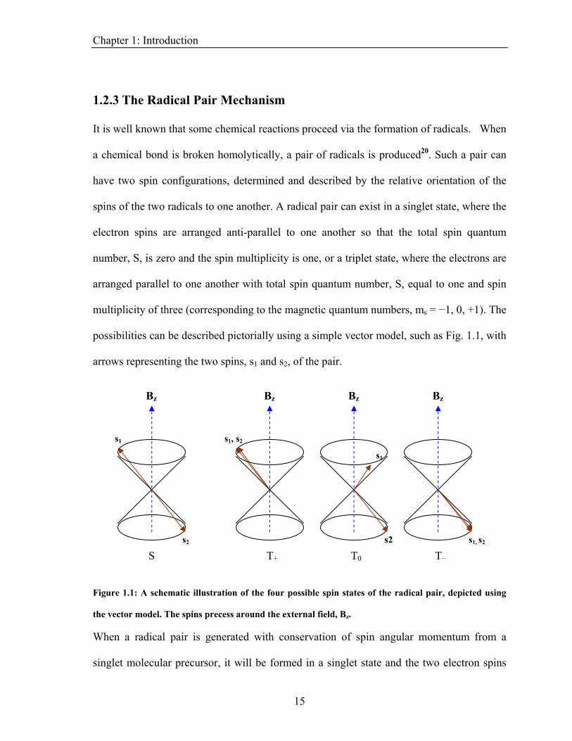
multiplicity of three (corresponding to the magnetic quantum numbers, ms = −1, 0, +1). The
possibilities can be described pictorially using a simple vector model, such as Fig. 1.1, with
arrows representing the two spins, s1 and s2, of the pair.
F re 1.1: A schematic n of the four possi e spin states of
th del the .
When a radical pair is generated with conservation of spin angular momentum from a
singlet molecular precursor, it will be formed in a singlet
T0
B z Bz Bz B z
s1 s1, s2
s1
s2 s1, s2s2
S T− T+
15
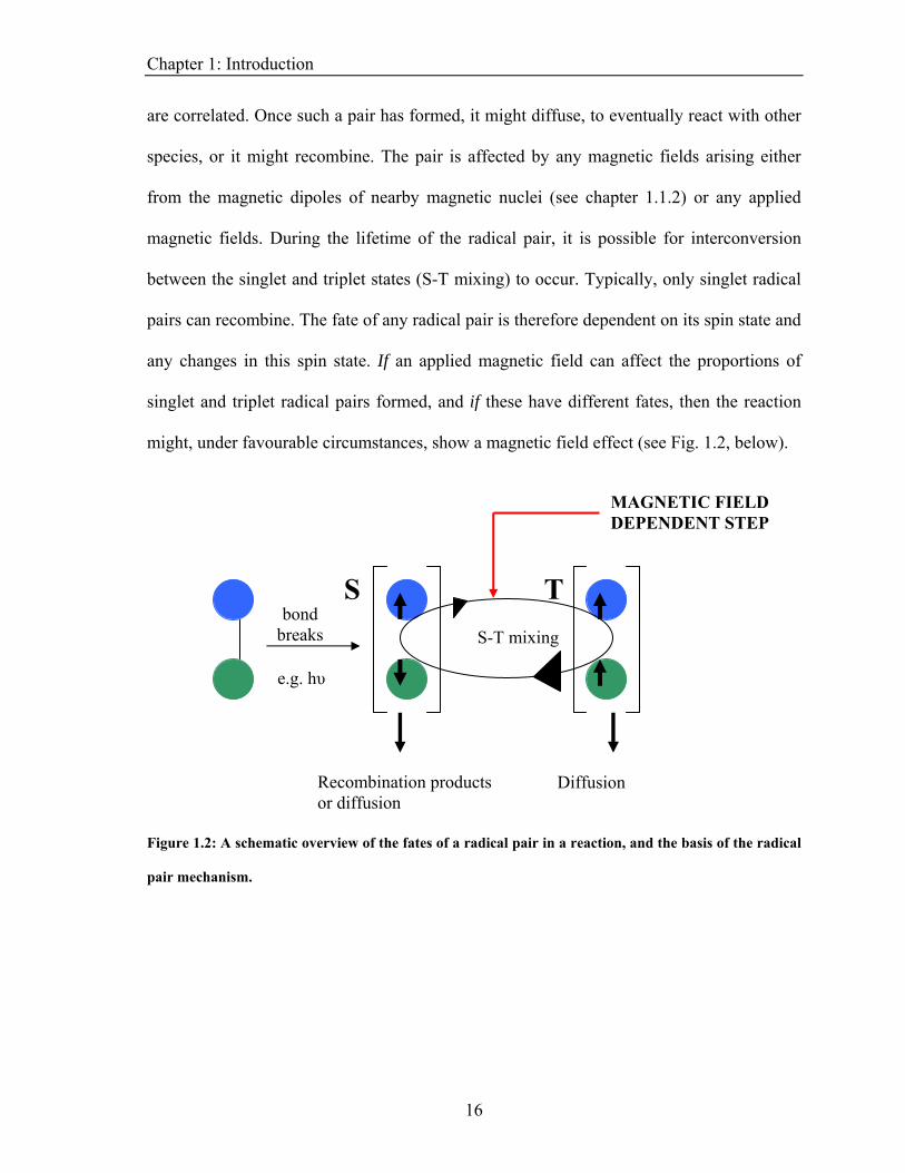
Chapter 1: Introduction are correlated. Once such a pair has formed, it might diffuse, to eventually react with other
species, or it might recombine. The pair is affected by any magnetic fields arising either
from the magnetic dipoles of nearby magnetic nuclei (see chapter 1.1.2) or any applied
magnetic fields. During the lifetime of the radical pair, it is possible for interconversion
between the singlet and triplet states (S-T mixing) to occur. Typically, only singlet radical
pairs can recombine. The fate of any radical pair is therefore dependent on its spin state and
any changes in this spin state. If an applied magnetic field can affect the proportions of
singlet and triplet radical pairs formed, and if these have different fates, then the reaction
might, under favourable circumstances, show a magnetic field effect (see Fig. 1.2, below).
Figure 1.2: A schematic overview of the fates of a radical pair in a reaction, and the basis of the radical
pair mechanism.
T
Diffusion Recombination products or diffusion
MAGNETIC FIELD DEPENDENT STEP
bond breaks
S
e.g. hυ
S-T mixing
16
Chapter 1: Introduction The radical pair is subject to several magnetic interactions, summarised below.
1: Dipole-dipole interaction
2: Exchange interaction
3: Hyperfine coupling
4: Zeeman splitting
The first two are inter-radical interactions. The dipole-dipole interaction arises from the
direct magnetic interaction between the two electron magnetic dipoles. It is an anisotropic
interaction can be assumed to average to zero in systems with rapid molecular motion. The
exchange interaction is a consequence of the Pauli Exclusion principle and arises from
fundamental differences between the singlet and triplet state. Overlap of the two
wavefunctions is forbidden in the triplet state, but not in the singlet state. The S and T
levels are not degenerate, even in the absence of an applied magnetic field. The energy gap
that exists between them is an ever-decreasing function of the separation of the two radicals
and becomes neglible at ~ 1 nm . Hence, there is no mixing of the singlet and triplet states
of the radical pair until the separation between the radicals is large enough for the exchange
interaction to be minimal.
The hyperfine interaction is intramolecular and occurs between the electron spin and any
magnetic nuclei (where I > 0) present in the radical. It can occur directly between the
magnetic dipoles (analogous to the dipole-dipole interaction described above) or through
bonds and electron spins, via the Fermi Contact interaction. The dipole-dipole interaction is
anisotropic and averages out through motion of the radical in solution, leaving the isotropic
21
17
Chapter 1: Introduction Fermi contact. The hyperfine coupling is the main driving force of S-T mixing in low to
moderate magnetic fields.
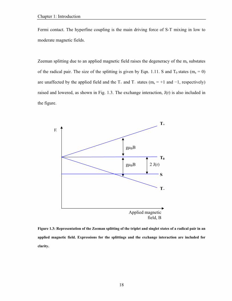
Zeeman splitting due to an applied magnetic field raises the degeneracy of the ms substates
of the radical pair. The size of the splitting is given by Eqn. 1.11. S and T0 states (ms = 0)
re unaffected by the applied field and the T+ and T− states (ms = +1 and −1, respectively)
igure 1.3: Representation of the Zeeman splitting of the triplet and singlet states of a radical pair in an
pplied magnetic field. Expressions for the splittings and the exchange interaction are included for
clarity.
a
raised and lowered, as shown in Fig. 1.3. The exchange interaction, J(r) is also included in
the figure.
T+
F
a
T0
S
T−
E
Applied magnetic field, B
2 J(r)
gμBB
gμBB
18
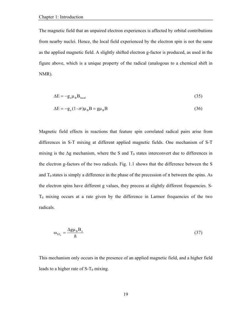
Chapter 1: Introduction The magnetic field that an unpaired electron experiences is affected by orbital contributions
from nearby nuclei. Hence, the local field experienced by the electron spin is not the same
as the applied magnetic field. A slightly shifted electron g-factor is produced, as used in the
figure above, which is a unique property of the radical (analogous to a chemical shift in
NMR).
(35) localBe
ΒμgE −=Δ
ΒgμΒ)μ-(1gE BBe =−=Δ σ (36)
ixing at different appl
mixing is the Δg mechanism, where the S and T0 states interconvert due to differences in
the electron g-factors of the two radicals. Fig. 1.1 shows that the difference between the S
and T0 states is simply a difference in the phase of the precession of π between the spins. As
the electron spins have different g values, they precess at slightly different frequencies. S-
T mixing occurs at a rate given by the difference in Larmor frequencies of the two
radicals.
Magnetic field effects in reactions that feature spin correlated radical pairs arise from
differences in S-T m ied magnetic fields. One mechanism of S-T
0
h
zBSTω
0= (37)
BΔgμ
his mechanism only occurs in the presence of an applied magnetic field, and a higher field
T
leads to a higher rate of S-T0 mixing.
19
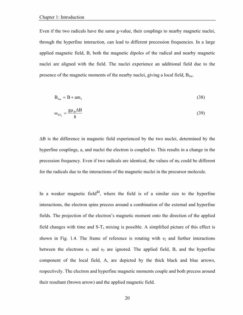
Chapter 1: Introduction Even if the two radicals have the same g-value, their couplings to nearby magnetic nuclei,
agnetic dipoles of the radical and nearby magnetic
uclei are aligned with the field. The nuclei experience an additional field due to the
through the hyperfine interaction, can lead to different precession frequencies. In a large
applied magnetic field, B, both the m
n
presence of the magnetic moments of the nearby nuclei, giving a local field, Bloc.
Iloc amBB += (38)
h
BgμBST0
Δω = (39)
B is the difference i
hyperfine couplings, a, and nuclei the electron is coupled to. This results in a change in the
ion frequency. E I
r the radicals due to the interactions of the magnetic nuclei in the precursor molecule.
ied
eld changes with time and S-T± mixing is possible. A simplified picture of this effect is
Δ n magnetic field experienced by the two nuclei, determined by the
precess ven if two radicals are identical, the values of m could be different
fo
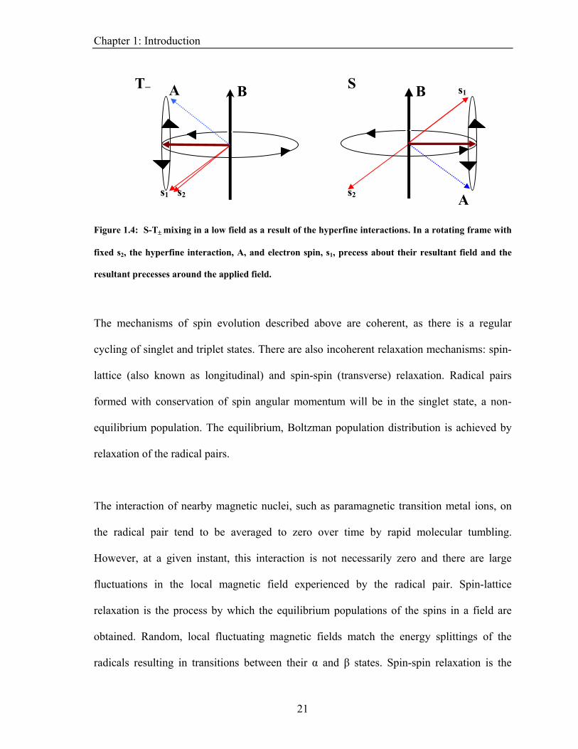
In a weaker magnetic field22, where the field is of a similar size to the hyperfine
interactions, the electron spins precess around a combination of the external and hyperfine
fields. The projection of the electron’s magnetic moment onto the direction of the appl
fi
shown in Fig. 1.4. The frame of reference is rotating with s2 and further interactions
between the electrons s1 and s2 are ignored. The applied field, B, and the hyperfine
component of the local field, A, are depicted by the thick black and blue arrows,
respectively. The electron and hyperfine magnetic moments couple and both precess around
their resultant (brown arrow) and the applied magnetic field.
20
Chapter 1: Introduction
Figure 1.4: S-T± mixing in a low field as a result of the hyperfine interactions. In a rotating frame with
xed s2, the hyperfine interaction, A, and electron spin, s1, precess about their resultant field and the
esses around the applied field.
The mechanisms of spin evolution described above are coherent, as there is a regular
d spin-spin (transverse) relaxation. Radical pairs
rmed with conservation of spin angular momentum will be in the singlet state, a non-
his interaction is not necessarily zero and there are large
uctuations in the local magnetic field experienced by the radical pair. Spin-lattice
fi
resultant prec
cycling of singlet and triplet states. There are also incoherent relaxation mechanisms: spin-
lattice (also known as longitudinal) an
fo
equilibrium population. The equilibrium, Boltzman population distribution is achieved by
relaxation of the radical pairs.
The interaction of nearby magnetic nuclei, such as paramagnetic transition metal ions, on
the radical pair tend to be averaged to zero over time by rapid molecular tumbling.
However, at a given instant, t
fl
relaxation is the process by which the equilibrium populations of the spins in a field are
obtained. Random, local fluctuating magnetic fields match the energy splittings of the
radicals resulting in transitions between their α and β states. Spin-spin relaxation is the
A s1 s2 s
s − 1T S B B A
2
21
Chapter 1: Introduction process by which the polarisation of the spins is lost. The radicals experience a range of
slightly different magnetic fields resulting in slightly different precession frequencies. In
both cases, it is fluctuations in the local magnetic field that lead to the spin mixing. If these
processes occur at fast enough rates compared to the coherent mechanisms of spin-mixing
then the spin system quickly attains thermal equilibrium. A magnetic field effect will not be
seen if the relaxation processes are faster than the processes of singlet-triplet mixing or
radical recombination of the pair.
If a reaction is to show a magnetic field effect by the radical pair mechanism then not only
must it have a step in the reaction which occurs via a radical pair intermediate, but there
must be a mechanism by which the two spin states can mix. Furthermore, the rate of
terconversion between the two states must be on a faster time scale than the rates of
their own production. This can be negative
positive feedback. In this latter case, the
a maximum rate at some later stage in the
in
reaction and relaxation of the two radicals and interactions between the radicals must be
small.
1.3 Feedback and Autocatalysis
Feedback arises in chemical reactions when the products of later steps in the reaction affect
earlier steps in the reaction and the rates of
feedback, where the reaction is self-inhibiting, or
rate of the reaction increases with time, with
reaction, and then falling to zero as the reaction approaches completion23. Autocatalysis is a
type of positive feedback, where the reaction product is itself the catalyst for the reaction.
22
Chapter 1: Introduction There are many examples of feedback in physical, chemical and biological systems. A fire
spreading through a dry field has heat as its autocatalyst – heating the fuel ahead of it until
it combusts and creates more heat. In solution phase reactions, the presence of autocatalysis
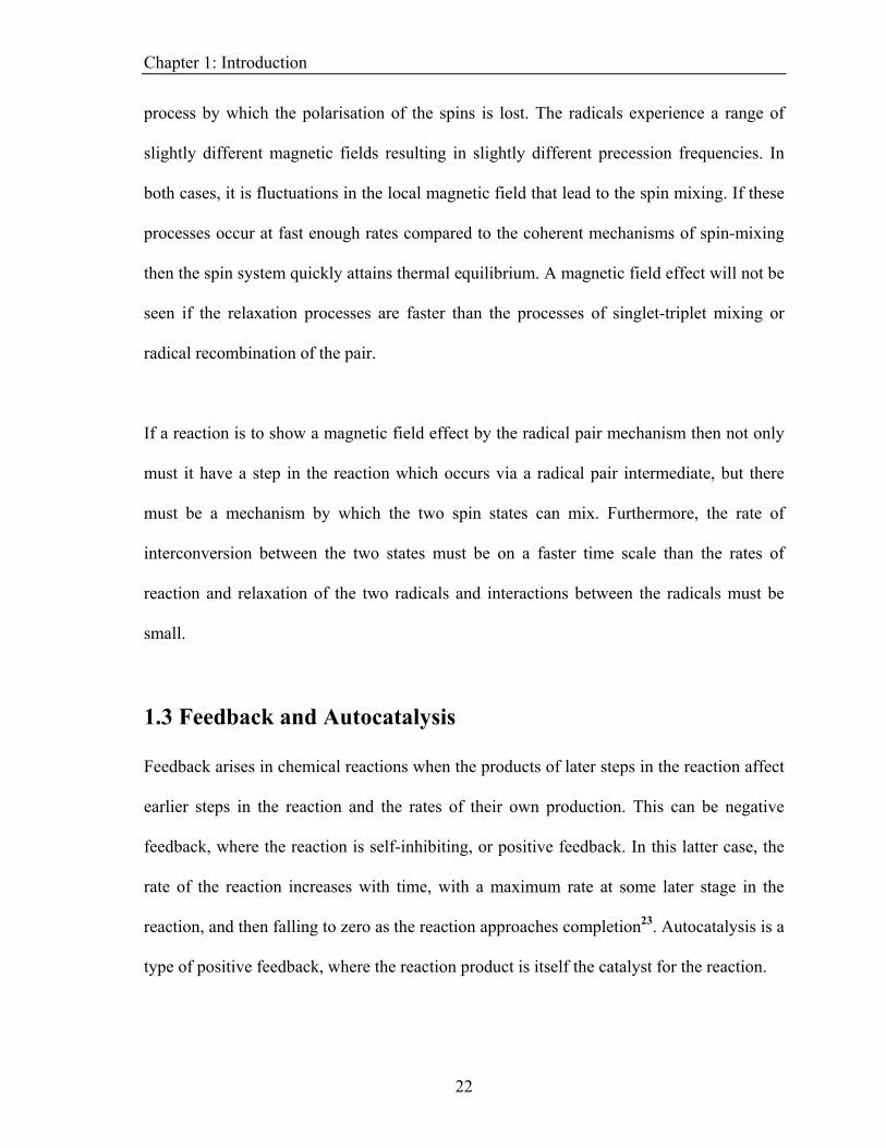
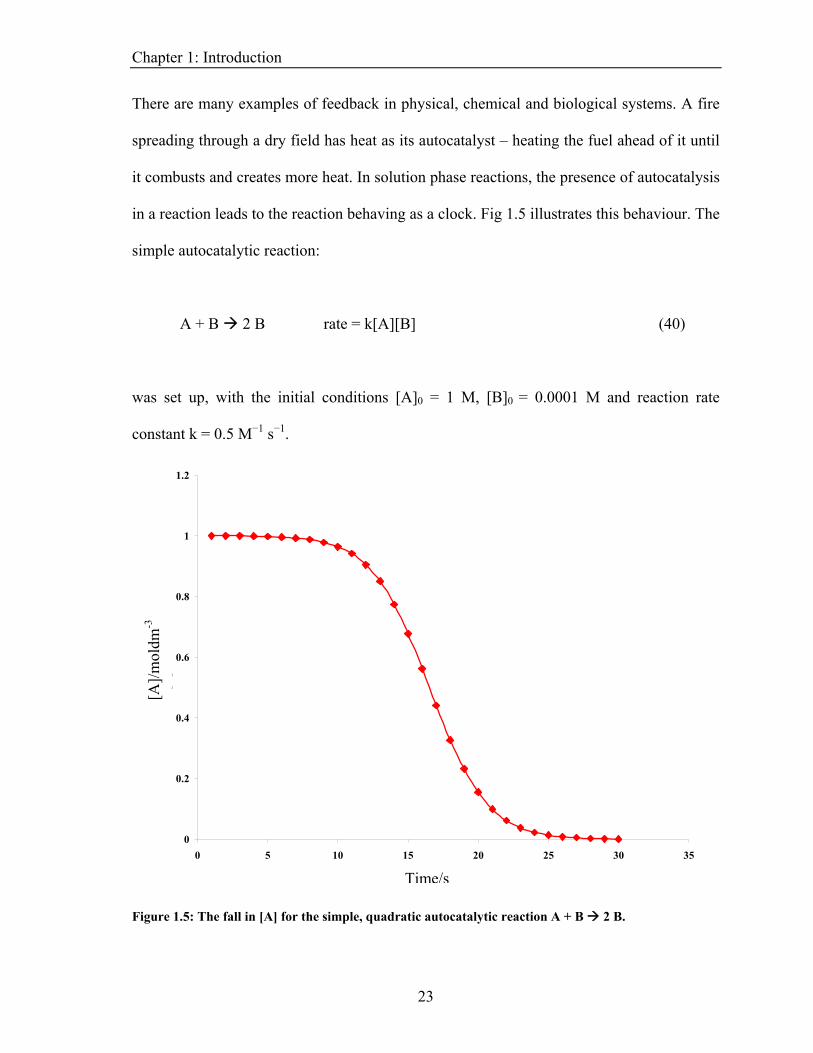
a reaction leads to the reaction behaving as a clock. Fig 1.5 illustrates this behaviour. The
onditions [A]0 = 1 M, [B]0 = 0.0001 M and reaction rate
onstant k = 0.5 M−1 s−1.
in
simple autocatalytic reaction:
A + B 2 B rate = k[A][B] (40)
was set up, with the initial c
c
0
0.2
0.4
0.6
0.8
1.2
1
0 5 10 15 20 25 30 35time/s
[A]/m
oldm
-3
Figure 1.5: The fall in [A] for the simple, quadratic autocatalytic reaction A + B 2 B.
[A]/m
oldm
-3
Time/s
23
Chapter 1: Introduction With a small amount of autocatalyst present at the start, the reaction rate is slow but
increases as more autocatalyst is produced by the reaction. After a certain amount of time,
the reaction rate reaches its peak before falling as the reagents are used up. This is seen by
the observer as a sharp change in the solution from one state to another.
When autocatalysis is coupled with diffusion, such as by initiation of the reaction with a
small amount of the autocatalyst in a shallow layer, chemical waves form24. The wave
travels at a constant velocity through the solution, with unreacted solution ahead of it and
fully reacted solution behind it. The boundary between the two regions, the wavefront, is a
narrow region where the reaction is occurring.
If the reaction features a mechanism by which the clock is reset, then oscillations in the
tions is the
elousov-Zhabotinsky reaction, studied in this thesis, but there are many other examples of
eroxidise-oxidase reaction27). Magnetic field effects have also been observed in the
waves forms. More exotic behaviour, such
solution are possible. One of the most famous oscillating chemical reac
B
reactions of this type, such as the Bray-Liebhafsky reaction25 (iodate catalysed
disproportionation of H2O2). Oscillations are not limited to solution-phase reactions, with
the behaviour observed in combustion reactions (oxidation of CO, oxidation of simple
hydrocarbon fuels26) and also in biological systems (for example, the horseradish
p
oscillations of the peroxidise-oxidase reaction28.
Complex behaviour arises when these oscillations couple with diffusion in unstirred
shallow layers. Instead of the simple front described above, a single wave, with both a
wave front and a wave back or a series of such
24
Chapter 1: Introduction as chaos, is also possible29. Such reactions can also exhibit excitability where the system
art I details the investigation of a magnetic field effect in a travelling wave reaction and
elousov-
habotinsky reaction is an attractive reaction for this study as there have been some reports
to this, behaviour similar to
has a stable steady state that when perturbed by a small amount quickly returns to its initial
concentrations30. When the perturbation exceeds a certain threshold, a single wave is
generated before the system returns to its original state. This amplification of a small effect
is a common phenomenon in this class of reactions, with small changes in the starting
concentrations often having large effects on the behaviour observed in a reaction.
The work presented in this thesis investigates magnetic field effects in chemical reactions
which display feedback. This thesis is split into three sections.
P
the use of magnetic resonance imaging techniques to study the effect. From a magnetic
field effect readily observed in a bench-top reaction using a Petri-dish and a horseshoe
magnet, the reaction was investigated in increasingly more detail, with magnetic resonance
imaging techniques used to study the effect of different geometry magnetic fields on the
reaction and the role of chemical fingering in the magnetic field effect.
The second section (Part II) details attempts to observe a magnetic field effect in an
oscillating reaction. The kinetics that give rise to wave reactions, as investigated in Part I of
this thesis, also give rise to oscillations, as described in chapter 1.3. The B
Z
of MFEs occurring in the reaction and the mechanism of the reaction suggests that the
reaction might show some magnetic field dependence. Further
25

Chapter 1: Introduction
26
ld be used for this
urpose, it was shown that the magnetometer could follow the changes in magnetic
that observed in this reaction has also seen in many biological systems, making the reaction
a possible model for biological oscillations and feedback.
The last section outlines an investigation into the use of SQUID magnetometers in
following chemical reactions, with an aim of using the high sensitivity of the technique in
observing magnetic field effects. In order to test that the SQUID cou
p
susceptibility of a solution phase chemical reactions. The clock behaviour of the
autocatalytic reactions was more than suitable for this study, as the important features such
as the rapid change in metal oxidation state occur some after the reaction has been initiated.
Part I: MAGNETIC FIELD EFFECTS ON THE
TRAVELLING WAVE REACTION BETWEEN CO(II)EDTA2− AND H2O2

Part I Chapter 2: Introduction
28
2. INTRODUCTION
The travelling wave reaction between Co(II)EDTA2−, and hydrogen peroxide, H2O2,
exhibits a change of colour, with pink Co(II)EDTA2− oxidised at ~ pH 4 to dark blue
Co(III)EDTA−. It also displays a striking visual magnetic field effect when performed in a
shallow layer in a Petri-dish1. The reaction can be initiated by a small amount of sodium
hydroxide solution and a wave moves out isotropically from the initiation site. However,
with only a small horseshoe magnet placed under the dish, the dark blue region forms a
dumbbell shape (Fig 2.1). No effect is seen if a non-magnetic blank is used instead of the
horseshoe magnet.
(a) (b)
Figure 2.1: Photographs of the reaction of Co(II)EDTA2− with H2O2 in a shallow layer in a Petri-dish in
the absence (a) and in the presence (b) of an applied inhomogeneous magnetic field. The position of the
poles of the horseshow magnet is shown by black lines in (b). The Petri dishes have a diameter of 90
mm, and the gap between magnet poles was 20 mm. Light, pink regions are areas of unreacted solution
and dark, blue regions are areas of reacted solution.
Part I Chapter 2: Introduction
The reacting solution used in Fig. 2.1 is a 9:1 by volume mixture of 0.02 M Co(II)EDTA2−
and 35 % H2O2, initiated with a small droplet of 0.016 M NaOH. A possible net reaction
mechanism, suggested by He et al.1, is shown here:
Co(II)EDTA2− + H2O2 → Co(II)EDTA. HO23− + H+ (1)
Co(II)EDTA. HO23− + Co(II)EDTA2− + H2O → 2 Co(III)EDTA− + 3 −OH
(2)
Hydroxide ions catalyse the reaction through the penetration of the peroxo-ligand into the
inner coordination sphere of the Co(II)EDTA2−. Dissociation of the first EDTA dentate site
is usually slow, but −OH ions readily penetrate this sphere, displacing one of the dentate
sites. This labilizes the chelate ring, facilitating further substitution1. The Co(II)EDTA2−
complex subsequently reacts with the H2O2. Since −OH is a product of the full reaction, the
reaction is autocatalytic. There is also formation of oxygen, observable after the reaction
has clocked. This results from the disproportionation of excess H2O2 in the alkaline,
Co(III)EDTA− product solution.
Accompanying the reaction is a change in magnetic susceptibility of the solution. The
Co(II) in the Co(II)EDTA2− complex has a d7 high spin electronic configuration, giving it
three unpaired electrons and making the ion paramagnetic. The product of the reaction,
Co(III)EDTA−, has a d6 low spin configuration, due to the increased charge on the cobalt
atom, and possesses no unpaired electrons. This ion is diamagnetic. This change in
magnetic property across the reaction wave front is the most probable cause of the
29
Part I Chapter 2: Introduction
sensitivity of this reaction to magnetic field gradients. He et al. suggests that the effect
observed occurs due to the different behaviours of Co(II)EDTA2− and Co(III)EDTA− in
inhomogeneous magnetic fields. The Co(II)EDTA2− ions are attracted up the magnetic field
gradient, where they react, and the diamagnetic Co(III)EDTA− ions formed are repelled
down the magnetic field gradient. A related reaction, the Co(II)-catalysed autoxidation of
benzaldehyde2, shows very similar behaviour suggesting that the magnetic field is acting on
the transport of the various solutions involved rather than on a specific part of the chemistry
of the reaction.
The Petri dish experiments give a clear illustration of the magnetic field effect but they are
not suitable for a quantitative analysis of the reaction. In order to get a better idea of the
nature of the magnetic field effect, a series of preliminary studies were undertaken. A
simplified apparatus was designed and built to study the movement of a reaction wavefront
in a shallow trough up or down a known magnetic field gradient. Subsequently, the reaction
was investigated in vertical tubes using both visual and magnetic resonance imaging (MRI)
techniques to follow the wave. These experiments allowed well-defined magnetic fields and
field gradients to be applied to the reaction. All experiments involving this reaction were
strongly affected by free convection around the boundary between the reacted and
unreacted solutions. This convection has an important role in explaining the origin and
magnitude of the magnetic field effect.
30

Part I Chapter 2: Introduction
2.1 Magnetic Resonance Imaging
The conversion of paramagnetic to diamagnetic ions across the reaction front allows a
study of the reaction using magnetic resonance imaging (MRI) techniques. The protons in
the water surrounding the Co(II)EDTA2− and Co(III)EDTA− ions show different relaxation
characteristics, due to the presence of unpaired electron spins in the Co(II)EDTA2− ions .
This difference can be exploited to produce relaxation contrast images of the travelling
wave. Not only do MRI techniques allow accurate measurement of the wave velocity, but
any pattern formation can be studied in terms of concentrations3. Furthermore, study is not
limited to contrast images. A variety of other techniques can be used to follow the wave.
Those that image the velocity profile of fluid flow in the sample are of particular interest.
The gradient coils used in imaging the wave can also be used to create linear, homogeneous
magnetic field gradients which can then be used to manipulate the wave.
2.1.1 Basics of Magnetic Resonance
Nuclear magnetic resonance (NMR)4 methods enable information about systems with
magnetic nuclei to be obtained by probing the energy splittings between nuclear spin states
in the presence of applied magnetic fields. In 1.1.2, a series of equations were produced that
describe the energy levels of electrons in an applied magnetic field. It was also shown that
nuclei with nuclear spin, I, form analogous systems. The equations are listed below, as a
reminder.
h1)I(I +=I (3)
, where = I, I−1, ..., −I (4) hIz mI = Im
31
Part I Chapter 2: Introduction
IIμ NN
N γμ
g =⎟⎠
⎞⎜⎝
⎛=h
(5)
(6) Bμ ⋅−=E
The gyromagnetic ratio, , has the value 4.258 × 10⁷ T−1 s−1 for 1H nuclei. In the presence
of a strong magnetic field, B, along the z-axis, the expression of the energy of a state with
magnetic quantum number mI is therefore:
Nγ
(7) zI γBmE h−=
For a proton, I = ½, the two values are +½ and –½. Transitions between the energy
levels are subject to the selection rule = ±1, and in the case of a proton, this gives an
energy gap of:
Im
IΔm
(8) γBΔE h=
Absorption of a photon that has the same energy as the energy gap between the two states
will cause a transition between the two states. Given the relationship between the energy of
a photon and its wavelength, the resonance or Larmor frequency of the proton, , is found. Lν
(9) LhνE =Δ
2πγB
hEνL =
Δ= (10)
32

Part I Chapter 2: Introduction
However, protons do not typically resonate at the determined by the applied magnetic
field. Small variations in the field experienced by the nuclei due to the local magnetic and,
therefore, chemical environment lead to range of resonant frequencies of the protons in the
sample (for example, protons in an organic molecule). Chemical shifts can be produced by
comparing these resonant frequencies with those from a known standard.
Lν
The principle underlying both NMR and MRI is that the resonance frequency of a spin is
proportional to the magnetic field it is experiencing. By applying magnetic field gradients
across a sample, the spins experience a field that is now also dependent on their position
within the sample as well as their chemical environment. This is key to MRI.
2.1.2 Spin Relaxation
Chemical shifts are not the only information that can be extracted from an NMR signal.
Differences in the relaxation of the induced magnetisation of the proton spins occur due to
the different environments, chemical and magnetic, experienced by the magnetic nuclei.
In an applied magnetic field, at thermal equilibrium, there is a Boltzmann distribution of
nuclear spins between the higher energy state ( = − ½ (β)) and the lower energy state
( = + ½ (α)):
Im
Im
⎟⎠⎞
⎜⎝⎛ Δ
=kT
E-expNN
α
β (11)
33
Part I Chapter 2: Introduction
Nα and are the populations of the two states and T is the temperature. In this case, ΔE
for 1H is 3.143 × 10⁻²⁶ J at a magnetic field of 7.0 T at 300 K and corresponds to a
difference of three or four spins in one million. This net alignment of the magnetic dipoles
in the magnetic field leads to a macroscopic magnetisation of the bulk sample, M0. The
applied magnetic field in the spectrometer is the static magnetic field due to the
superconducting magnet of the NMR spectrometer and directed along the z-axis. At
equilibrium, there is only magnetisation along the z-axis, Mz.
βN
By applying a radiofrequency (rf) pulse of frequency equal to the Larmor frequency, spins
can undergo transitions between their α and β states. The macroscopic magnetisation tilts
away from the direction of the applied field. The duration of the pulse determines the flip
angle of the macroscopic magnetization. In addition to the loss of magnetisation along the
z-axis, the magnetisation is focused in the phase of the applied rf pulse with a
corresponding increase in the magnetisation in the xy plane (transverse magnetisation Mxy).
After the excitation of the sample, the populations will return to equilibrium. In other forms
of spectroscopy, spontaneous emission, where the nuclei spontaneously drop from a higher
energy level to a lower one, occurs. In NMR this is too slow to have any effect.
Furthermore because the nuclear spins interact weakly with most external influences, they
are effectively decoupled from molecular motions and remain aligned with any applied
magnetic field. However the excited spins are not isolated from other spins in the system or
their surroundings and energy can be exchanged with both through magnetic interactions.
34
Part I Chapter 2: Introduction
There are two processes of relaxation, spin-lattice and spin-spin relaxation, which are
governed by the time constants T1 and T2 respectively. Spin-lattice relaxation is a process
by which nuclear spins flip between their excited state and their ground state, non-
radiatively. Energy is lost to the system as the Boltzmann distribution is regained. This is
an enthalpic process. Immediately after the pulse is applied, Mz starts to return to its
equilibrium value. The rate at which Mz returns to its equilibrium value M0 is governed by
the time constant T1 according to the equation:
⎟⎟⎠
⎞⎜⎜⎝
⎛⎟⎟⎠
⎞⎜⎜⎝
⎛−=
1z,0z T
t-exp1MM (12)
Spin-spin relaxation is the process by which spins lose their coherence over time. It is an
entropic process. The transverse magnetisation starts to dephase because the individual
spins experience slightly different magnetic fields due to the presence of other spins in the
sample, such as other protons in a water sample. This gives rise to a range of different
precession frequencies. The rate at which falls towards 0 is governed by the time
constant, T2, according to the equation:
xyM
⎟⎟⎠
⎞⎜⎜⎝
⎛⎟⎟⎠
⎞⎜⎜⎝
⎛=
2xy,0xy T
t-expMM (13)
As the spins move around in the solution, there are a number of temporary, random
interactions with the other spins in the sample and these have a cumulative effect. Any
35
Part I Chapter 2: Introduction
magnetic interaction can lead to relaxation and the presence of paramagnetic ions in the
sample further increase the rate of the dephasing due to their magnetic dipole moments.
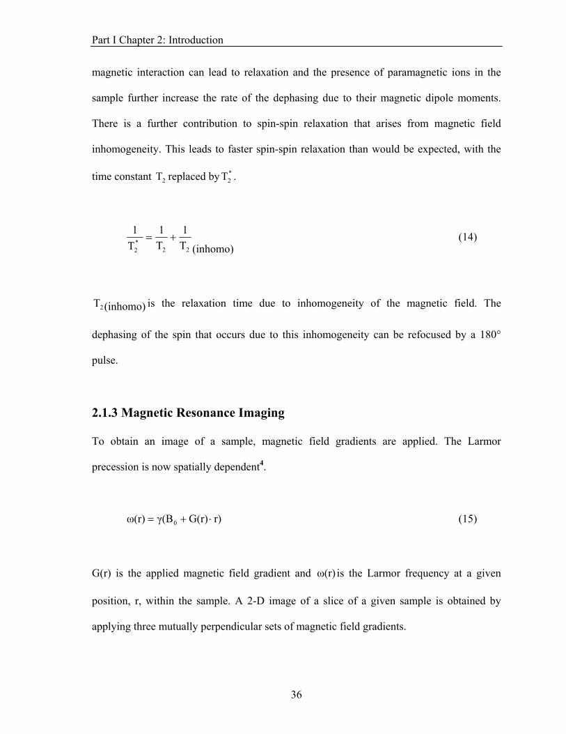
There is a further contribution to spin-spin relaxation that arises from magnetic field
inhomogeneity. This leads to faster spin-spin relaxation than would be expected, with the
time constant replaced by . 2T *2T
(inhomo)T
1T1
T1
22*2
+= (14)
(inhomo)T2 is the relaxation time due to inhomogeneity of the magnetic field. The
dephasing of the spin that occurs due to this inhomogeneity can be refocused by a 180°
pulse.
2.1.3 Magnetic Resonance Imaging
To obtain an image of a sample, magnetic field gradients are applied. The Larmor
precession is now spatially dependent4.
(15) r)G(r)γ(Bω(r) 0 ⋅+=
G(r) is the applied magnetic field gradient and is the Larmor frequency at a given
position, r, within the sample. A 2-D image of a slice of a given sample is obtained by
applying three mutually perpendicular sets of magnetic field gradients.
ω(r)
36
Part I Chapter 2: Introduction
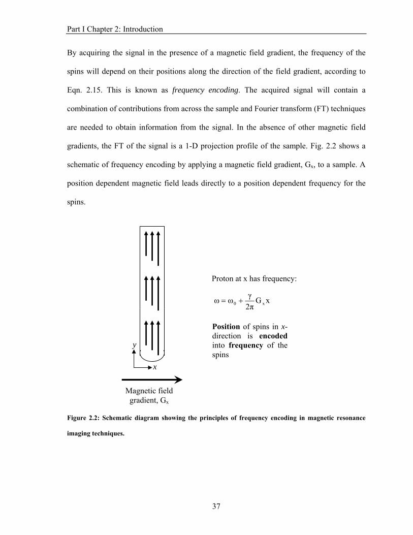
By acquiring the signal in the presence of a magnetic field gradient, the frequency of the
spins will depend on their positions along the direction of the field gradient, according to
Eqn. 2.15. This is known as frequency encoding. The acquired signal will contain a
combination of contributions from across the sample and Fourier transform (FT) techniques
are needed to obtain information from the signal. In the absence of other magnetic field
gradients, the FT of the signal is a 1-D projection profile of the sample. Fig. 2.2 shows a
schematic of frequency encoding by applying a magnetic field gradient, Gx, to a sample. A
position dependent magnetic field leads directly to a position dependent frequency for the
spins.
x
y
Proton at x has frequency:
xG2πγωω x0 +=
Position of spins in x-direction is encoded into frequency of the spins
Magnetic field
gradient, Gx
Figure 2.2: Schematic diagram showing the principles of frequency encoding in magnetic resonance
imaging techniques.
37
Part I Chapter 2: Introduction
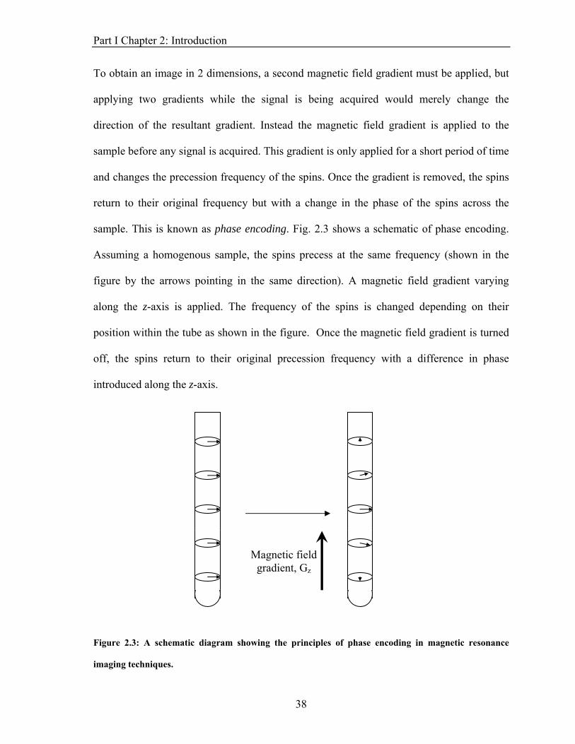
To obtain an image in 2 dimensions, a second magnetic field gradient must be applied, but
applying two gradients while the signal is being acquired would merely change the
direction of the resultant gradient. Instead the magnetic field gradient is applied to the
sample before any signal is acquired. This gradient is only applied for a short period of time
and changes the precession frequency of the spins. Once the gradient is removed, the spins
return to their original frequency but with a change in the phase of the spins across the
sample. This is known as phase encoding. Fig. 2.3 shows a schematic of phase encoding.
Assuming a homogenous sample, the spins precess at the same frequency (shown in the
figure by the arrows pointing in the same direction). A magnetic field gradient varying
along the z-axis is applied. The frequency of the spins is changed depending on their
position within the tube as shown in the figure. Once the magnetic field gradient is turned
off, the spins return to their original precession frequency with a difference in phase
introduced along the z-axis.
Magnetic field gradient, Gz
Figure 2.3: A schematic diagram showing the principles of phase encoding in magnetic resonance
imaging techniques.
38
Part I Chapter 2: Introduction
With the two sets of gradients applied so far, the image would be a 2-D profile of the whole
sample. Slices of the sample can be selected by applying a third magnetic field gradient. A
particular slice of the sample is selected by using a frequency selective rf pulse and a
magnetic field gradient. Only spins with the frequency of the selective pulse are excited.
This will correspond to a slice of the sample.
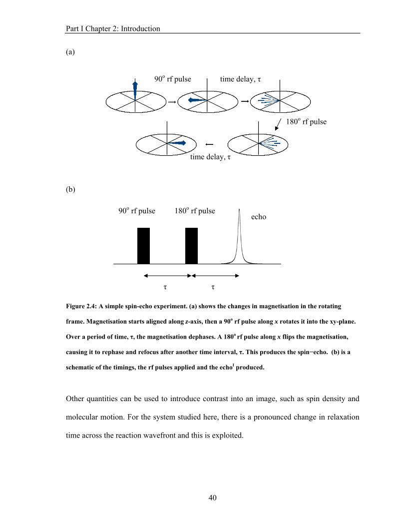
The imaging sequences used in these experiments are based on spin-echo images, as
depicted in Fig. 2.4. The 180o pulse used in this experiment refocuses the spins and
eliminates the effect of field inhomogeneities and chemical shifts. A 90o rf pulse produces
magnetisation in the xy plane, which dephases at a rate governed by the spin-spin relaxation
time, , of the spins in the sample. After a time delay, τ, an 180o pulse is applied and the
magnetisation flips and starts to rephase. This produces an echo at a time 2τ after the initial
pulse that has T2 dependence in its signal intensity.
*2T
39
Part I Chapter 2: Introduction
(a)
90o rf pulse time delay, τ
(b)
time delay, τ
90o rf pulse echo
180o rf pulse
180o rf pulse
τ τ
Figure 2.4: A simple spin-echo experiment. (a) shows the changes in magnetisation in the rotating
frame. Magnetisation starts aligned along z-axis, then a 90o rf pulse along x rotates it into the xy-plane.
Over a period of time, τ, the magnetisation dephases. A 180o rf pulse along x flips the magnetisation,
causing it to rephase and refocus after another time interval, τ. This produces the spin−echo. (b) is a
schematic of the timings, the rf pulses applied and the echoI produced.
Other quantities can be used to introduce contrast into an image, such as spin density and
molecular motion. For the system studied here, there is a pronounced change in relaxation
time across the reaction wavefront and this is exploited.
40
Part I Chapter 2: Introduction
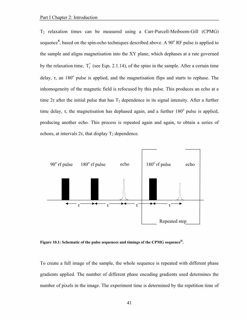
T2 relaxation times can be measured using a Carr-Purcell-Meiboom-Gill (CPMG)
sequence5, based on the spin-echo techniques described above. A 90o RF pulse is applied to
the sample and aligns magnetisation into the XY plane, which dephases at a rate governed
by the relaxation time, (see Eqn. 2.1.14), of the spins in the sample. After a certain time
delay, τ, an 180o pulse is applied, and the magnetisation flips and starts to rephase. The
inhomogeneity of the magnetic field is refocused by this pulse. This produces an echo at a
time 2τ after the initial pulse that has T2 dependence in its signal intensity. After a further
time delay, τ, the magnetisation has dephased again, and a further 180o pulse is applied,
producing another echo. This process is repeated again and again, to obtain a series of
echoes, at intervals 2τ, that display T2 dependence.
*2T
Figure 10.1: Schematic of the pulse sequences and timings of the CPMG sequenceII.
To create a full image of the sample, the whole sequence is repeated with different phase
gradients applied. The number of different phase encoding gradients used determines the
number of pixels in the image. The experiment time is determined by the repetition time of
90o rf pulse echo 180o rf pulse 180o rf pulse echo
Repeated step
τ τ τ τ
41
Part I Chapter 2: Introduction
the experiment and the number of phase encoding gradients used to produce the image.
This could be as long as a couple of minutes. For the imaging of a moving wave, a faster
imaging technique had to be used.
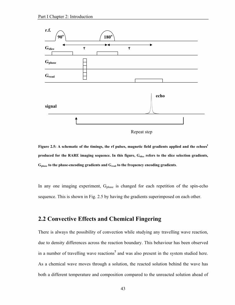
The imaging sequence used to obtain the images in this chapter was the fast imaging,
multiple spin-echo sequence Rapid Acquisition with Relaxation Enhancement, RARE6. A
single 90o excitation pulse is used to excite the spins in a sample. As with the basic spin-
echo imaging sequence (Fig. 2.4), a 180o pulse is applied. Once the echo is acquired, the
magnetisation is refocused and a different phase encoding gradient is applied. For each
excitation, multiple echoes are collected so the experiment time is a few hundred
milliseconds. T2 contrast is possible with this imaging sequence, where regions of longer T2
appear brighter than regions of shorter T2. The sampling time for the experiment is
comparable with the T2 relaxation time of the imaged solution, so there is a degree of
blurring, but this is not significant. Fig. 2.5 shows a schematic of the pulse sequence, with
frequency-encoding gradients, phase-encoding gradients, slice selection and the spin-echo
imaging technique all combining to produce the imaging sequence.
42
Part I Chapter 2: Introduction
Gslice
r.f. 90o
τ τ
180o
Gphase
Gread
echo
signal
Repeat step
Figure 2.5: A schematic of the timings, the rf pulses, magnetic field gradients applied and the echoesI
produced for the RARE imaging sequence. In this figure, Gslice refers to the slice selection gradients,
Gphase to the phase-encoding gradients and Gread to the frequency encoding gradients.
In any one imaging experiment, Gphase is changed for each repetition of the spin-echo
sequence. This is shown in Fig. 2.5 by having the gradients superimposed on each other.
2.2 Convective Effects and Chemical Fingering
There is always the possibility of convection while studying any travelling wave reaction,
due to density differences across the reaction boundary. This behaviour has been observed
in a number of travelling wave reactions7 and was also present in the system studied here.
As a chemical wave moves through a solution, the reacted solution behind the wave has
both a different temperature and composition compared to the unreacted solution ahead of
43
Part I Chapter 2: Introduction
the wave. Buoyant forces associated with these density differences will lead to fluid flow,
or free convection. A change in temperature of the solution will lead to a change in its
density. The change in density, ΔρT, due to the enthalpy change of the reaction is given by:
ΔρT = αρ0ΔT (16)
ΔT is the change in temperature in the reaction, α is the thermal expansion coefficient of
water, −(1/ρ)(∂ρ/∂T)P, and ρ0 is the initial density of the solution. There may also be a
change in density, ΔρC, due to the change in composition of the solution, if the partial molal
volumes of the products differ from those of the reactants. This is given by:
ΔρC = βρ0ΔC (17)
ΔρC is the change in density due to a given species, ΔC is the change in concentration of the
species being considered, β is the expansion coefficient of the solution for the species,
(1/ρ)(∂ρ/∂C) and ρ0 is the initial density of the solution. The overall change in density can
be related to a measured change in volume, ΔV, in a solution of initial volume V by:
Δρ = − (ΔV/V0)ρ0 (18)
The total change in density is the combination of the two different contributions.
Δρ = ΔρT + ΔρC (19)
44
Part I Chapter 2: Introduction
If the reaction is exothermic (and most travelling wave reactions are7) and there is an
isothermal increase in volume during the reaction, then the total density change is negative
and the reacted solution is less dense than the unreacted solution. If a reaction is initiated in
a tube, from the top, a descending wave front will form. In this example, Δρ is negative and
the wave front, with less dense reacted solution above a denser unreacted solution is stable.
Convection does not arise and the wave front formed is flat, independent of the width of the
tube. If the wave is initiated from the bottom of the tube, however, the wave front could be
unstable to distortion due to free convection.
If ΔρT and ΔρC are of opposite signs, then the two contributions to the change in density act
in different directions. A reaction wave front that appears, at first glance, to have a stable
density gradient can still distort under free convection. Imagine an exothermic travelling
wave reaction that also features an increase in density as it reacts, so ΔρT < 0 and ΔρC > 0.
A small perturbation to the wave front leaves a small amount of warm, reacted solution in
the unreacted solution. The diffusivity of heat is larger than the diffusivity of any of the
species in the reacted parcel, so the solution in the perturbated volume rapidly cools,
becomes denser than the surrounding solution and sinks. As there is also reaction occurring
across all interfaces between the solutions, this behaviour is seen as a finger of reacted
solution moving down from the reacted solution through the unreacted solution. This
convection is known as ‘double−diffusive’ convection and produces chemical fingers7. If
the reaction is performed horizontally, such as in a trough or in a Petri dish, there is always
the possibility of convection around the wavefront, as the stable configuration of the two
solutions will always be horizontal and the boundary is vertical7.
45

Part I Chapter 2: Introduction
46
It appears likely that the magnetic field effect observed will be associated with free
convection around the wave front. Free convection arises due to changes in the force acting
on the fluid, due to changes in density of the fluid. The magnetic force acting on the fluid is
simply be another force acting on the system.
Part I Chapter 3: Methods and Materials
47
3 METHODS AND MATERIALS
3.1 Materials
Sodium hydroxide, EDTA, cobalt chloride and hydrogen peroxide (35 % by volume) all of
ACS grade were obtained from Aldrich and used without further purification. A 0.02 M
Co(II)EDTA2− solution was made by dissolving a slight excess of EDTA with CoCl2 in de-
ionised water and then adjusting the pH to 4. The reacting solution used in the experiments
was made from the 0.02 M Co(II)EDTA2− and the hydrogen peroxide in a 9:1 ratio. The
H2O2 was stored in a fridge until needed.
3.2 Methods
3.2.1 Preliminary Experiments
The reaction was studied in a shallow trough held between the poles of an electromagnet.
Shaped pole pieces had been designed and built for a previous, preliminary study with
dimensions chosen so that the magnetic field generated had a constant magnetic field
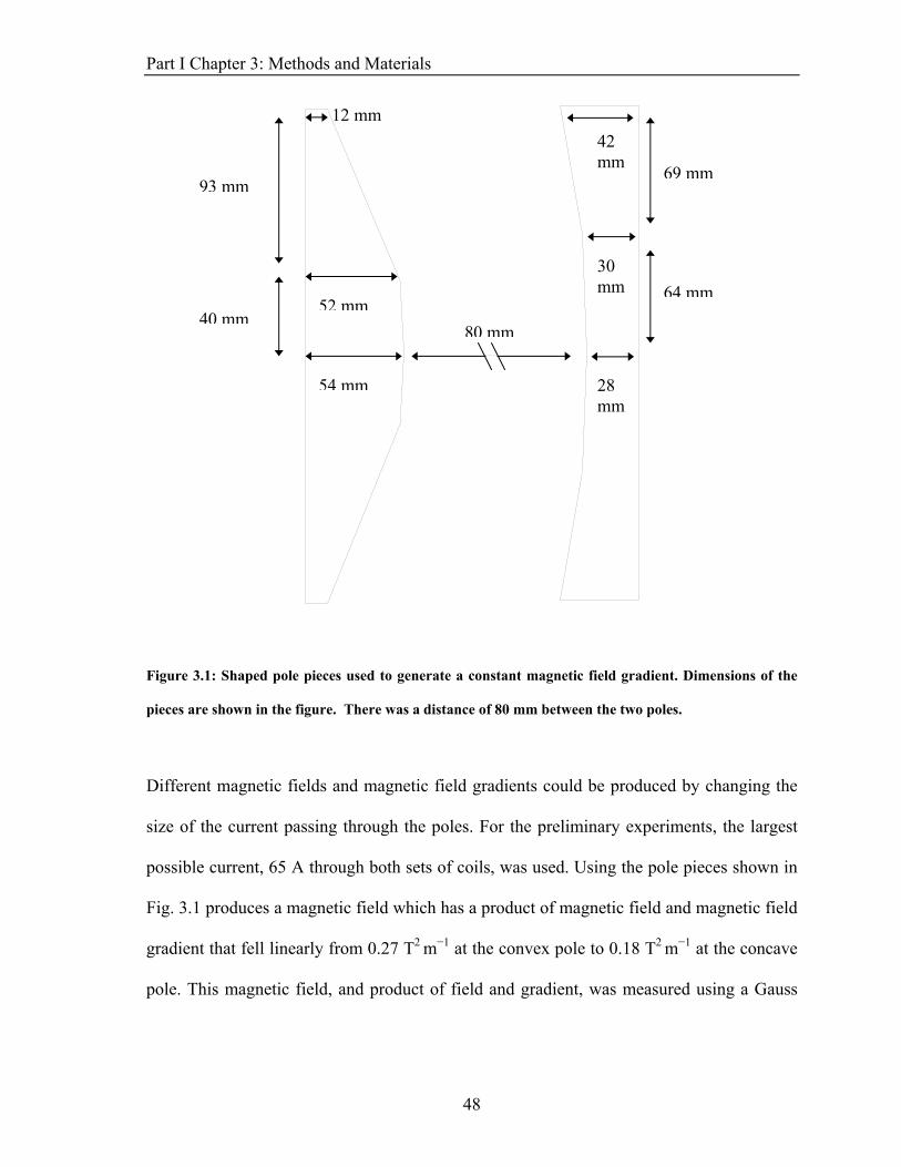
gradient8. Fig. 3.1 shows the dimensions of the two steel pole pieces.
Part I Chapter 3: Methods and Materials
12 mm 42 mm 69 mm
93 mm
30 mm 64 mm
52 mm40 mm
80 mm
Figure 3.1: Shaped pole pieces used to generate a constant magnetic field gradient. Dimensions of the
pieces are shown in the figure. There was a distance of 80 mm between the two poles.
Different magnetic fields and magnetic field gradients could be produced by changing the
size of the current passing through the poles. For the preliminary experiments, the largest
possible current, 65 A through both sets of coils, was used. Using the pole pieces shown in
Fig. 3.1 produces a magnetic field which has a product of magnetic field and magnetic field
gradient that fell linearly from 0.27 T2 m−1 at the convex pole to 0.18 T2 m−1 at the concave
pole. This magnetic field, and product of field and gradient, was measured using a Gauss
54 mm 28 mm
48
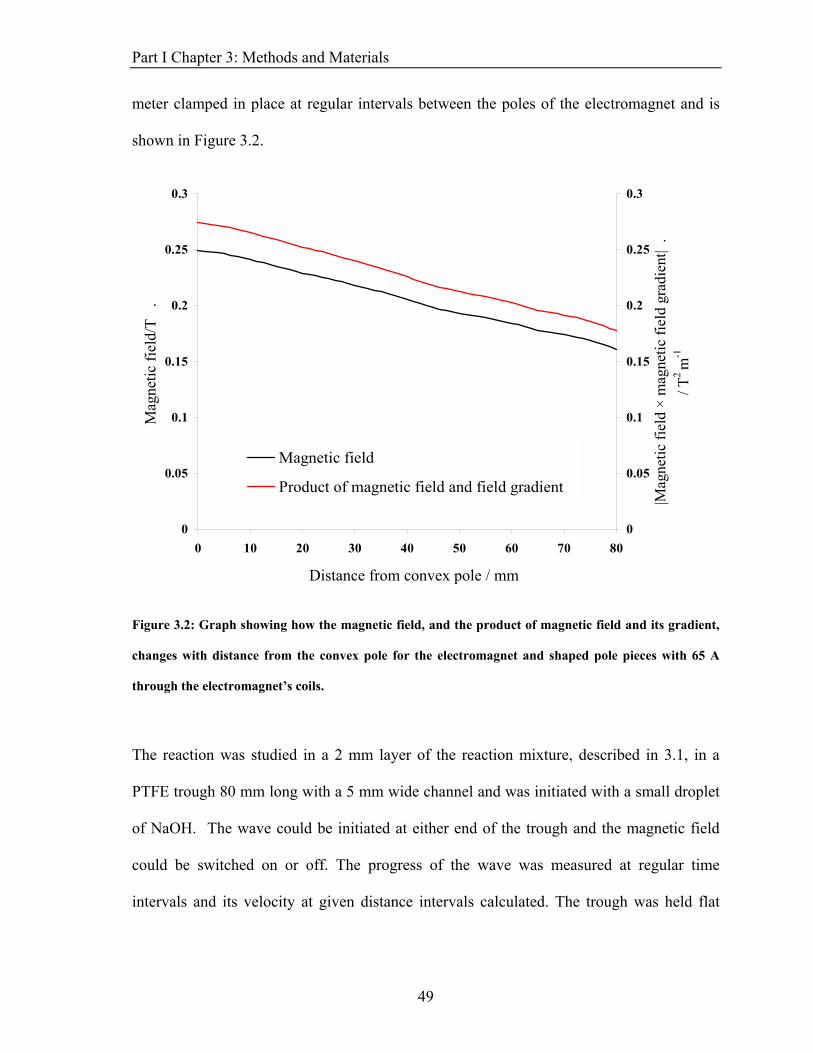
Part I Chapter 3: Methods and Materials meter clamped in place at regular intervals between the poles of the electromagnet and is
shown in Figure 3.2.
0
0.05
0.1
0.15
0.2
0.25
0.3
0 10 20 30 40 50 60 70 80
Distance from convex pole/mm
Mag
netic
fiel
d/T
.
0
0.05
0.1
0.15
0.2
0.25
0.3
|Mag
netic
fiel
d ×
mag
netic
fiel
d gr
adie
nt|
. / T
2 m
-1
Magnetic field
Product of magnetic field and field gradient
Distance from convex pole / mm
Figure 3.2: Graph showing how the magnetic field, and the product of magnetic field and its gradient,
changes with distance from the convex pole for the electromagnet and shaped pole pieces with 65 A
through the electromagnet’s coils.
The reaction was studied in a 2 mm layer of the reaction mixture, described in 3.1, in a
PTFE trough 80 mm long with a 5 mm wide channel and was initiated with a small droplet
of NaOH. The wave could be initiated at either end of the trough and the magnetic field
could be switched on or off. The progress of the wave was measured at regular time
intervals and its velocity at given distance intervals calculated. The trough was held flat
49
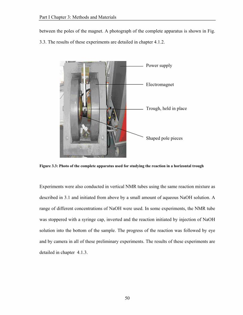
Part I Chapter 3: Methods and Materials between the poles of the magnet. A photograph of the complete apparatus is shown in Fig.
3.3. The results of these experiments are detailed in chapter 4.1.2.
Power supply
Electromagnet
Trough, held in place
Shaped pole pieces
Figure 3.3: Photo of the complete apparatus used for studying the reaction in a horizontal trough
Experiments were also conducted in vertical NMR tubes using the same reaction mixture as
described in 3.1 and initiated from above by a small amount of aqueous NaOH solution. A
range of different concentrations of NaOH were used. In some experiments, the NMR tube
was stoppered with a syringe cap, inverted and the reaction initiated by injection of NaOH
solution into the bottom of the sample. The progress of the reaction was followed by eye
and by camera in all of these preliminary experiments. The results of these experiments are
detailed in chapter 4.1.3.
50
Part I Chapter 3: Methods and Materials To confirm the differences in susceptibility between the reagents and the products of the
reaction, the magnetic susceptibilities of the Co(II)EDTA2− and Co(III)EDTA− were
measured using a Gouy balance. Co(II)EDTA2− solutions of concentrations 0.05, 0.04,
0.03, 0.02 and 0.01 M were prepared and measured. From these five solutions, a series of
9:1 by volume reacting mixtures with H2O2 were made up and left to react for ~ 24 hours.
These reacted solutions were measured in the Gouy balance. The Gouy balance
measurements gave a mass susceptibility in cgs units which needed conversion into SI units
and then into volume or molar susceptibilities. These measurements can be found in
chapter 4.1.1.
3.2.2 MRI Experiments
MRI experiments were conducted in Cambridge in collaboration with Dr. Melanie Britton
on a Bruker DMX-300 spectrometer equipped with a 7.0 T superconducting magnet
operating at a proton resonance frequency of 300 MHz. The reaction was studied in 5 mm
NMR tubes, using a 25 mm radiofrequency coil, with a maximum vertical observation
region of 30 mm.
Images were obtained using the fast-imaging, multiple echo sequence RARE. In the first set
of MRI experiments, described later in Chapter 4.2.1, the horizontal and vertical fields of
view were 10 mm and 50 mm, respectively, and comprised of a 256 × 64 pixel array. This
gave a pixel size of 195 μm (horizontal) by 156 μm (vertical). In the second set of MRI
experiments, described later in Chapter 4.2.2, the horizontal field of view was 13.5 mm
with a corresponding pixel size of 195 μm by 195 μm. Both vertical (in the zy plane) and
51
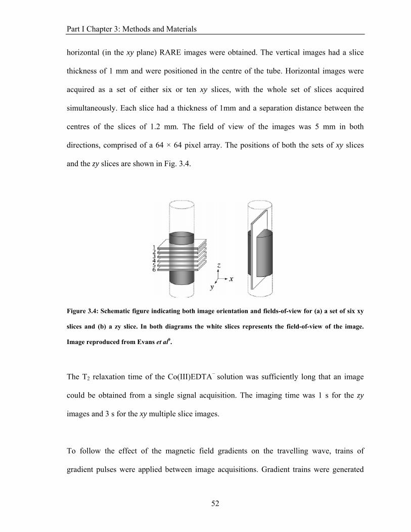
Part I Chapter 3: Methods and Materials horizontal (in the xy plane) RARE images were obtained. The vertical images had a slice
thickness of 1 mm and were positioned in the centre of the tube. Horizontal images were
acquired as a set of either six or ten xy slices, with the whole set of slices acquired
simultaneously. Each slice had a thickness of 1mm and a separation distance between the
centres of the slices of 1.2 mm. The field of view of the images was 5 mm in both
directions, comprised of a 64 × 64 pixel array. The positions of both the sets of xy slices
and the zy slices are shown in Fig. 3.4.
Figure 3.4: Schematic figure indicating both image orientation and fields-of-view for (a) a set of six xy
slices and (b) a zy slice. In both diagrams the white slices represents the field-of-view of the image.
Image reproduced from Evans et al9.
The T2 relaxation time of the Co(III)EDTA− solution was sufficiently long that an image
could be obtained from a single signal acquisition. The imaging time was 1 s for the zy
images and 3 s for the xy multiple slice images.
To follow the effect of the magnetic field gradients on the travelling wave, trains of
gradient pulses were applied between image acquisitions. Gradient trains were generated
52
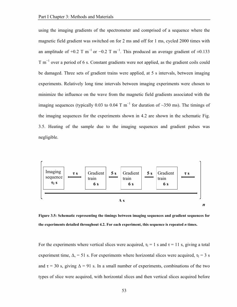
Part I Chapter 3: Methods and Materials using the imaging gradients of the spectrometer and comprised of a sequence where the
magnetic field gradient was switched on for 2 ms and off for 1 ms, cycled 2000 times with
an amplitude of +0.2 T m−1 or −0.2 T m−1. This produced an average gradient of ±0.133
T m−1 over a period of 6 s. Constant gradients were not applied, as the gradient coils could
be damaged. Three sets of gradient trains were applied, at 5 s intervals, between imaging
experiments. Relatively long time intervals between imaging experiments were chosen to
minimize the influence on the wave from the magnetic field gradients associated with the
imaging sequences (typically 0.03 to 0.04 T m−1 for duration of ~350 ms). The timings of
the imaging sequences for the experiments shown in 4.2 are shown in the schematic Fig.
3.5. Heating of the sample due to the imaging sequences and gradient pulses was
negligible.
Imaging sequence
τI s
5 s 5 sτ s Gradient train
6 s
Gradient train
6 s
Gradient train
6 s
τ s
Δ s
n
Figure 3.5: Schematic representing the timings between imaging sequences and gradient sequences for
the experiments detailed throughout 4.2. For each experiment, this sequence is repeated n times.
For the experiments where vertical slices were acquired, τI = 1 s and τ = 11 s, giving a total
experiment time, Δ, = 51 s. For experiments where horizontal slices were acquired, τI = 3 s
and τ = 30 s, giving Δ = 91 s. In a small number of experiments, combinations of the two
types of slice were acquired, with horizontal slices and then vertical slices acquired before
53
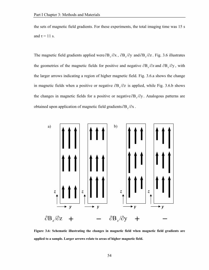
Part I Chapter 3: Methods and Materials the sets of magnetic field gradients. For these experiments, the total imaging time was 15 s
and τ = 11 s.
The magnetic field gradients applied were x/Bz ∂∂ , y/Bz ∂∂ and z/Bz ∂∂ . Fig. 3.6 illustrates
the geometries of the magnetic fields for positive and negative z/Bz ∂∂ and y/Bz ∂∂ , with
the larger arrows indicating a region of higher magnetic field. Fig. 3.6.a shows the change
in magnetic fields when a positive or negative z/zB ∂∂ is applied, while Fig. 3.6.b shows
the changes in magnetic fields for a positive or negative y/Bz ∂∂ . Analogous patterns are
obtained upon application of magnetic field gradients x/Bz ∂∂ .
Figure 3.6: Schematic illustrating the changes in magnetic field when magnetic field gradients are
applied to a sample. Larger arrows relate to areas of higher magnetic field.
z z z z
y y y
a) b)
+
y
z/Bz ∂∂ + − − y/Bz∂ ∂
54
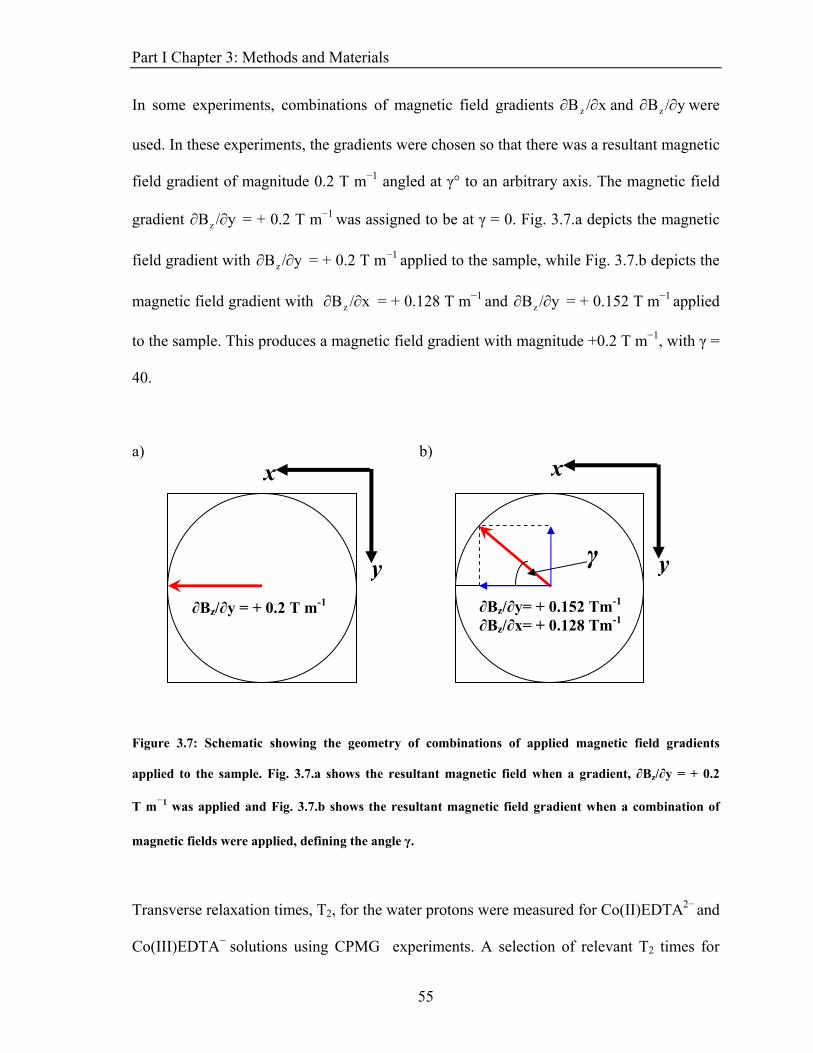
Part I Chapter 3: Methods and Materials
In some experiments, combinations of magnetic field gradients x/Bz ∂∂ and y/Bz ∂∂ were
used. In these experiments, the gradients were chosen so that there was a resultant magnetic
field gradient of magnitude 0.2 T m−1 angled at γ° to an arbitrary axis. The magnetic field
gradient = + 0.2 T m−1 was assigned to be at γ = 0. Fig. 3.7.a depicts the magnetic
field gradient with = + 0.2 T m−1 applied to the sample, while Fig. 3.7.b depicts the
magnetic field gradient with
y/Bz ∂∂
y/Bz ∂∂
x/Bz ∂∂ = + 0.128 T m−1 and y/Bz ∂∂ = + 0.152 T m−1 applied
to the sample. This produces a magnetic field gradient with magnitude +0.2 T m−1, with γ =
40.
Figure 3.7: Schematic showing the geometry of combinations of applied magnetic field gradients
applied to the sample. Fig. 3.7.a shows the resultant magnetic field when a gradient, ∂Bz/∂y = + 0.2
T m−1 was applied and Fig. 3.7.b shows the resultant magnetic field gradient when a combination of
magnetic fields were applied, defining the angle γ.
Transverse relaxation times, T2, for the water protons were measured for Co(II)EDTA2− and
Co(III)EDTA− solutions using CPMG experiments. A selection of relevant T2 times for
a) b) xx
∂Bz/∂y = + 0.2 T m-1
γ
∂Bz/∂y= + 0.152 Tm-1 ∂Bz/∂x= + 0.128 Tm-1
y y
55
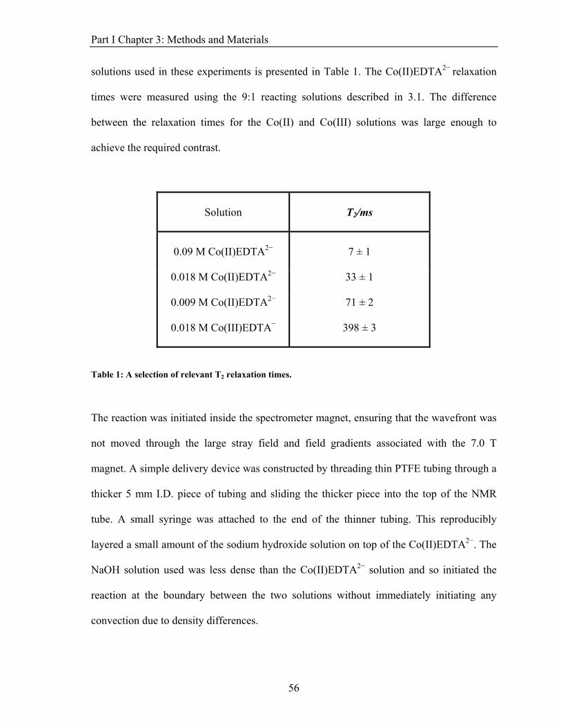
Part I Chapter 3: Methods and Materials solutions used in these experiments is presented in Table 1. The Co(II)EDTA2− relaxation
times were measured using the 9:1 reacting solutions described in 3.1. The difference
between the relaxation times for the Co(II) and Co(III) solutions was large enough to
achieve the required contrast.
Solution
T2/ms
0.09 M Co(II)EDTA2−
7 ± 1
0.018 M Co(II)EDTA2−
33 ± 1
0.009 M Co(II)EDTA2−
71 ± 2
0.018 M Co(III)EDTA−
398 ± 3
Table 1: A selection of relevant T2 relaxation times.
The reaction was initiated inside the spectrometer magnet, ensuring that the wavefront was
not moved through the large stray field and field gradients associated with the 7.0 T
magnet. A simple delivery device was constructed by threading thin PTFE tubing through a
thicker 5 mm I.D. piece of tubing and sliding the thicker piece into the top of the NMR
tube. A small syringe was attached to the end of the thinner tubing. This reproducibly
layered a small amount of the sodium hydroxide solution on top of the Co(II)EDTA2−. The
NaOH solution used was less dense than the Co(II)EDTA2− solution and so initiated the
reaction at the boundary between the two solutions without immediately initiating any
convection due to density differences.
56
Part I Chapter 3: Methods and Materials
57
To observe any effect of reducing convective flow, experiments were conducted in a porous
medium. A 7.5 mm I.D. tube was used for these experiments. Glass balls of various sizes
were used initially as a porous medium, but the reaction initiated on the surface of the balls.
Ion exchange resin interacted with the reacting solution and the reaction no longer initiated.
Packing foam proved not to initiate or interfere with the reaction, and plugs of it were cut
out of a strip and forced into the tube. Standard 5 mm I.D. tubes proved to be too thin. The
wider tube was filled with reacting solution and initiated in the same way as the
experiments in 5 mm I.D. NMR tubes.
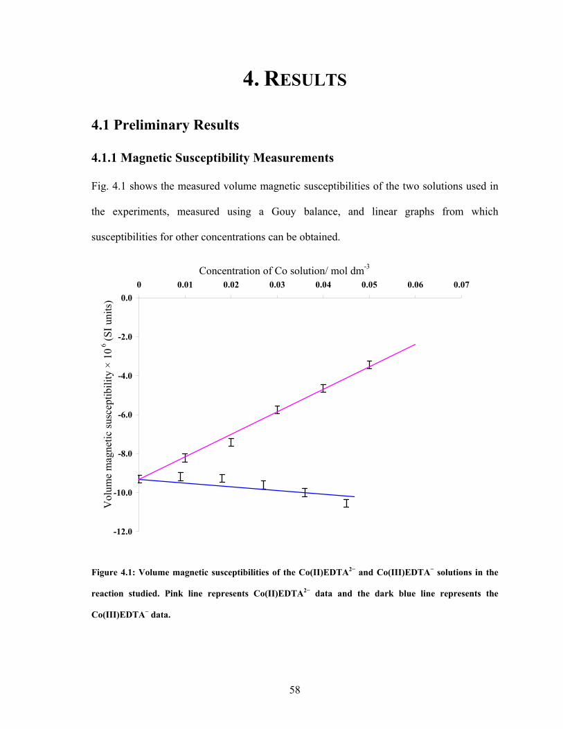
Part I Chapter 4: Results
4. RESULTS
4.1 Preliminary Results
4.1.1 Magnetic Susceptibility Measurements
Fig. 4.1 shows the measured volume magnetic susceptibilities of the two solutions used in
the experiments, measured using a Gouy balance, and linear graphs from which
susceptibilities for other concentrations can be obtained.
-12.0
-10.0
-8.0
-6.0
-4.0
-2.0
0.00 0.01 0.02 0.03 0.04 0.05 0.06 0.07
Concentration of Co solution/ mol dm-3
Vol
ume
mag
netic
susc
eptib
ility
× 1
0-6 (S
I uni
ts)
Figure 4.1: Volume magnetic susceptibilities of the Co(II)EDTA2− and Co(III)EDTA− solutions in the
reaction studied. Pink line represents Co(II)EDTA2− data and the dark blue line represents the
Co(III)EDTA− data.
58
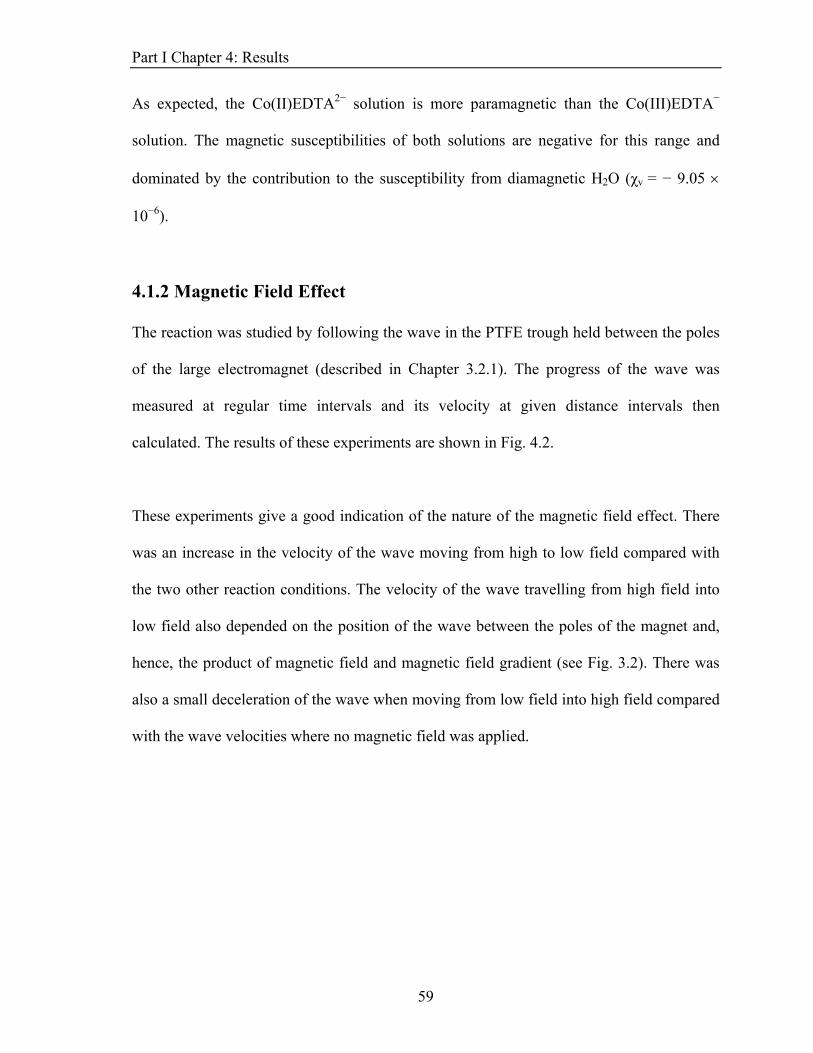
Part I Chapter 4: Results
As expected, the Co(II)EDTA2− solution is more paramagnetic than the Co(III)EDTA−
solution. The magnetic susceptibilities of both solutions are negative for this range and
dominated by the contribution to the susceptibility from diamagnetic H2O (χv = − 9.05 ×
10−6).
4.1.2 Magnetic Field Effect
The reaction was studied by following the wave in the PTFE trough held between the poles
of the large electromagnet (described in Chapter 3.2.1). The progress of the wave was
measured at regular time intervals and its velocity at given distance intervals then
calculated. The results of these experiments are shown in Fig. 4.2.
These experiments give a good indication of the nature of the magnetic field effect. There
was an increase in the velocity of the wave moving from high to low field compared with
the two other reaction conditions. The velocity of the wave travelling from high field into
low field also depended on the position of the wave between the poles of the magnet and,
hence, the product of magnetic field and magnetic field gradient (see Fig. 3.2). There was
also a small deceleration of the wave when moving from low field into high field compared
with the wave velocities where no magnetic field was applied.
59
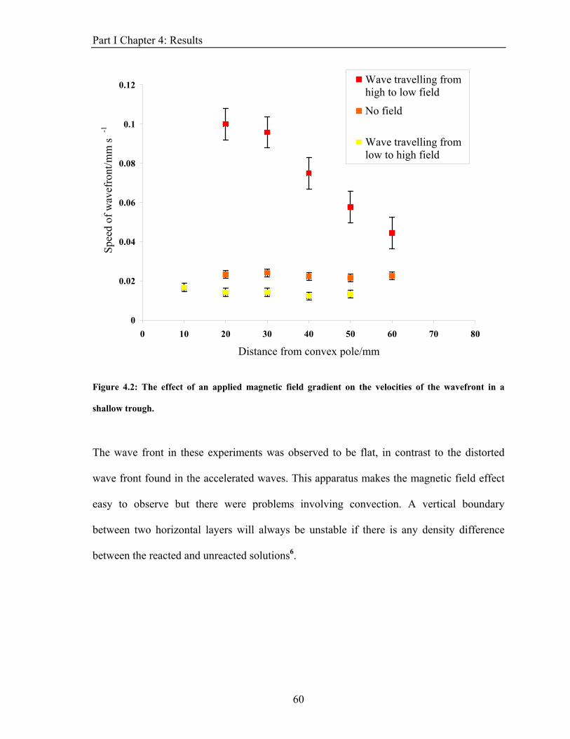
Part I Chapter 4: Results
0
0.02
0.04
0.06
0.08
0.1
0.12
0 10 20 30 40 50 60 70 8
Distance from convex pole/mm
Spee
d of
wav
efro
nt/m
m s
-1
0
Wave travelling fromhigh to low field
No field
Wave travelling fromlow to high field
Figure 4.2: The effect of an applied magnetic field gradient on the velocities of the wavefront in a
shallow trough.
The wave front in these experiments was observed to be flat, in contrast to the distorted
wave front found in the accelerated waves. This apparatus makes the magnetic field effect
easy to observe but there were problems involving convection. A vertical boundary
between two horizontal layers will always be unstable if there is any density difference
between the reacted and unreacted solutions6.
60
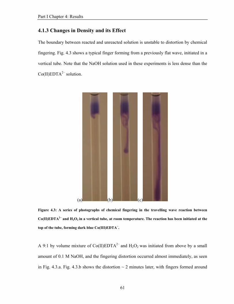
Part I Chapter 4: Results
4.1.3 Changes in Density and its Effect
The boundary between reacted and unreacted solution is unstable to distortion by chemical
fingering. Fig. 4.3 shows a typical finger forming from a previously flat wave, initiated in a
vertical tube. Note that the NaOH solution used in these experiments is less dense than the
Co(II)EDTA2− solution.
(a) (b) (c)
Figure 4.3: A series of photographs of chemical fingering in the travelling wave reaction between
Co(II)EDTA2− and H2O2 in a vertical tube, at room temperature. The reaction has been initiated at the
top of the tube, forming dark blue Co(III)EDTA−.
A 9:1 by volume mixture of Co(II)EDTA2− and H2O2 was initiated from above by a small
amount of 0.1 M NaOH, and the fingering distortion occurred almost immediately, as seen
in Fig. 4.3.a. Fig. 4.3.b shows the distortion ~ 2 minutes later, with fingers formed around
61
Part I Chapter 4: Results
the edge of the tube. These have pooled into a single larger finger which has started to
move down the tube. Note that the ‘head’ of the tendril is larger than the tail. Fig. 4.3.c
shows the finger ~ 5 minutes after the initiation of the wave. The head of the finger is still
larger than the tail and the whole finger has grown, due to reaction occurring across the
whole interface of the reacted solution.
4.1.3.1: Distortion of the Wavefront
When NaOH solutions which were much less dense than the Co(II)EDTA2− solution were
used to initiate the wave, the flat wave front still distorted in the same manner. Even
organic bases, such as ethylamine, that layered immiscibly on top of the Co(II)EDTA2−
solution produced a wave front that ultimately distorted to produce a finger. Using NaOH
made denser with addition of NaCl, the reaction could be initiated at the bottom of the
sample. In these experiments, flat wave fronts developed which did not distort. However,
there was distortion of the wavefront by O2 bubbles rising up from the reacted solution. The
bubbles drag reacted Co(III)EDTA− and –OH with them as they moved through the
unreacted solution. This is unrelated to chemical fingering.
4.1.3.2: Dilatometer Measurements
Following the change in density against time by measuring the mass of the reacting
solution in density bottles of a known volume at regular time intervals indicated that the
reacting mixture decreased in density as the reaction proceeded. A simple dilatometer was
constructed with a large stock of solution in a stoppered conical flask with a thin tube
inserted to measure changes in volume through changes in height of the column of fluid
62
Part I Chapter 4: Results
and a temperature sensor to measure changes in temperature. Measurement of the change in
density against time using this method was complicated by the formation of O2 by the
reaction of excess H2O2 with alkaline Co(III)EDTA− solution (around pH 9II). A typical set
of data from the dilatometer is shown in Fig. 4.4. A 9:1 by volume mixture of
Co(II)EDTA2− and H2O2 at pH 4.0 was used. The dilatometer had an initial volume of 325
cm3. The pink line shows the height of the column of fluid in a 1.0 mm I.D. tube and the
black line the temperature recorded by a small electronic thermometer.
Both measurements showed clock behaviour with an induction period preceding a larger
change in the quantities measured. The moment the reaction clocked, O2 formation would
occur in the bulk of the solution. Bubble formation was observed throughout the sample,
forcing the column of reacting solution up and out of the tube, limiting the amount of
information that could be gained from this method.
63

Part I Chapter 4: Results
0
5
10
15
20
25
0 10 20 30 40 50 60
Time/min
Hei
ght o
f col
umn/
mm
19.9
20
20.1
20.2
20.3
20.4
20.5
20.6
20.7
Tem
pera
ture
/o C
Drop in column height
Column HeightTemperature
Figure 4.4: A typical set of results from the dilatometer. A 9:1 by volume mixture of Co(II)EDTA and
H2O2 at pH 4 was used, with regular measurements of both the height of the column of fluid (pink line)
and temperature (black line).
The most important feature was the sudden drop in volume just before the formation of O2,
while the temperature of the solution kept rising. This corresponds to an increase in the
density due to the changes in composition accompanying a fall in density due to the
exothermicity of the reaction. The dip and the clock behaviour of the temperature and
column height were reproduced in every experiment using this apparatus, as was the
formation of O2 that hindered any attempts to record further data.
64
Part I Chapter 4: Results
Reasonable estimates of the sizes of the two contributions can also be made, before the O2
formation dominates the changes in height. There was a fall in the height of the column of
approximately 2 mm just before the reaction clocked. From Eqn. 2.18, this gives an
estimate for Δρ of ~ + 0.006 kg m−3. From Eqn. 2.16, ΔρT at this point can be estimated as ~
− 0.06 kg m−3. ΔρC is then given as ~ + 0.066 kg m−3. The different contributions to the
change in density can be seen though, with ΔρC > 0 and ΔρT < 0, conditions that can lead to
chemical fingering.
4.2 MRI Experiments
4.2.1 Application of Magnetic Field Gradients, z/Bz ∂∂
The preliminary work in the shallow trough was aimed at studying the effect of a linear
magnetic field gradient on the travelling wave reaction. The first MRI experiments used
magnetic field gradients of a similar geometry to the magnetic fields used in the
experiments detailed in 4.1.2 and were intended to investigate the effect of magnetic field
gradients parallel to the direction of the magnetic field, i.e. and zB z/Bz ∂∂ . The static field
of the superconducting magnet was 7 T and magnetic field gradients, = ± 0.2 T
m−1, were applied to the reaction. Fig. 3.6.a showed a schematic of the geometry of the
magnetic fields, with a positive gradient increasing the magnetic field from the bottom to
the top of the sample.
z/z ∂B∂
65
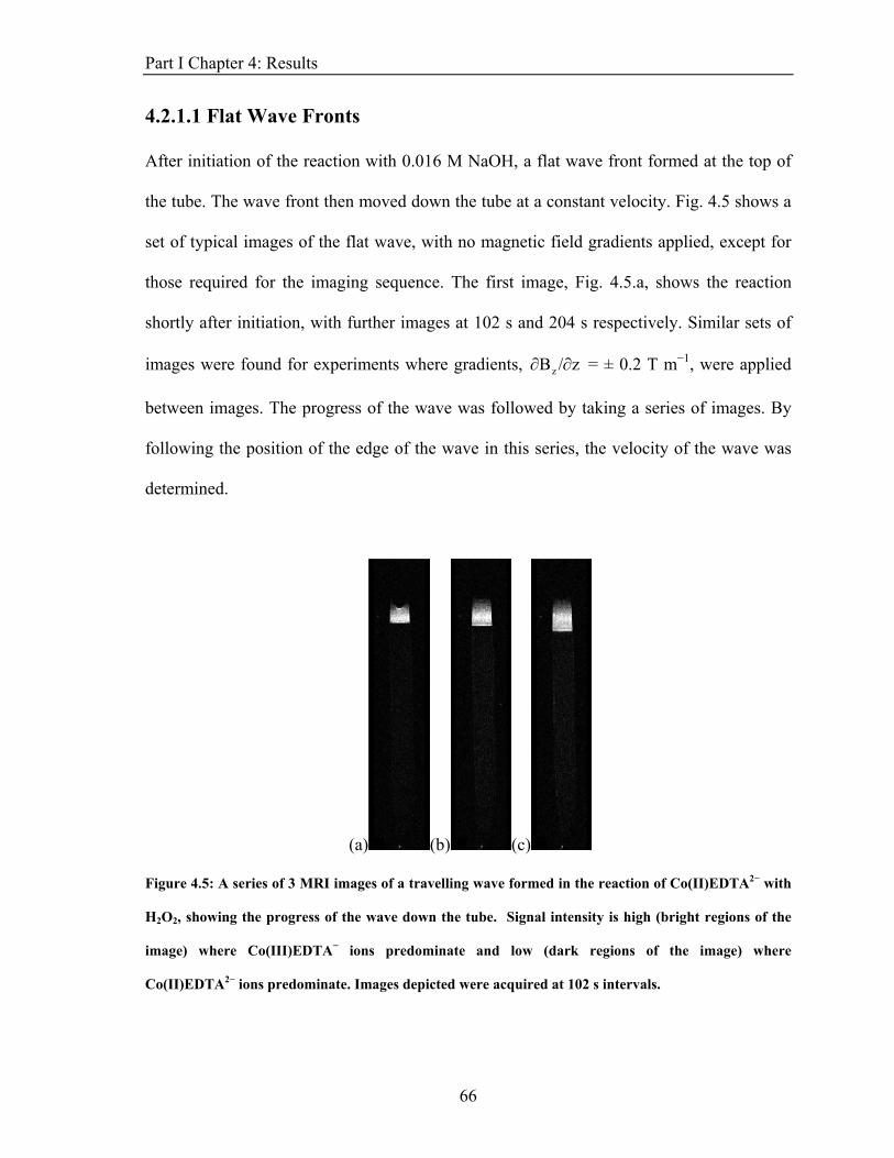
Part I Chapter 4: Results
4.2.1.1 Flat Wave Fronts
After initiation of the reaction with 0.016 M NaOH, a flat wave front formed at the top of
the tube. The wave front then moved down the tube at a constant velocity. Fig. 4.5 shows a
set of typical images of the flat wave, with no magnetic field gradients applied, except for
those required for the imaging sequence. The first image, Fig. 4.5.a, shows the reaction
shortly after initiation, with further images at 102 s and 204 s respectively. Similar sets of
images were found for experiments where gradients, z/Bz ∂∂ = ± 0.2 T m−1, were applied
between images. The progress of the wave was followed by taking a series of images. By
following the position of the edge of the wave in this series, the velocity of the wave was
determined.
(a) (b) (c)
Figure 4.5: A series of 3 MRI images of a travelling wave formed in the reaction of Co(II)EDTA2− with
H2O2, showing the progress of the wave down the tube. Signal intensity is high (bright regions of the
image) where Co(III)EDTA− ions predominate and low (dark regions of the image) where
Co(II)EDTA2− ions predominate. Images depicted were acquired at 102 s intervals.
66
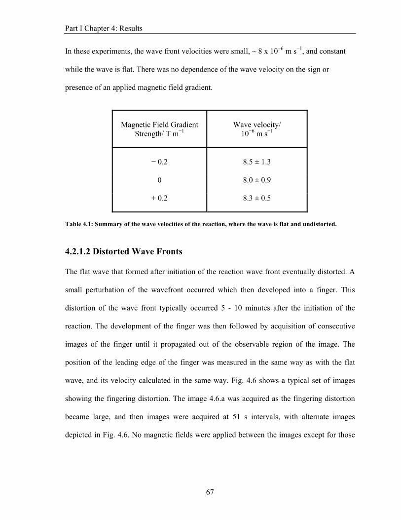
Part I Chapter 4: Results
In these experiments, the wave front velocities were small, ~ 8 x 10⁻⁶ m s−1, and constant
while the wave is flat. There was no dependence of the wave velocity on the sign or
presence of an applied magnetic field gradient.
Magnetic Field Gradient Strength/ T m−1
Wave velocity/
10−6 m s−1
− 0.2
8.5 ± 1.3
0
8.0 ± 0.9
+ 0.2
8.3 ± 0.5
Table 4.1: Summary of the wave velocities of the reaction, where the wave is flat and undistorted. 4.2.1.2 Distorted Wave Fronts The flat wave that formed after initiation of the reaction wave front eventually distorted. A
small perturbation of the wavefront occurred which then developed into a finger. This
distortion of the wave front typically occurred 5 - 10 minutes after the initiation of the
reaction. The development of the finger was then followed by acquisition of consecutive
images of the finger until it propagated out of the observable region of the image. The
position of the leading edge of the finger was measured in the same way as with the flat
wave, and its velocity calculated in the same way. Fig. 4.6 shows a typical set of images
showing the fingering distortion. The image 4.6.a was acquired as the fingering distortion
became large, and then images were acquired at 51 s intervals, with alternate images
depicted in Fig. 4.6. No magnetic fields were applied between the images except for those
67
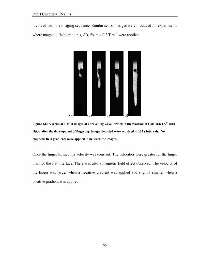
Part I Chapter 4: Results
involved with the imaging sequence. Similar sets of images were produced for experiments
where magnetic field gradients, z/Bz ∂∂ = ± 0.2 T m−1 were applied.
(a) (b) (c) (d)
Figure 4.6: A series of 4 MRI images of a travelling wave formed in the reaction of Co(II)EDTA2− with
H2O2, after the development of fingering. Images depicted were acquired at 102 s intervals. No
magnetic field gradients were applied in between the images.
Once the finger formed, its velocity was constant. The velocities were greater for the finger
than for the flat interface. There was also a magnetic field effect observed. The velocity of
the finger was larger when a negative gradient was applied and slightly smaller when a
positive gradient was applied.
68
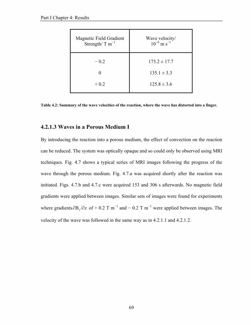
Part I Chapter 4: Results
Magnetic Field Gradient
Strength/ T m−1
Wave velocity/
10−6 m s−1
− 0.2
173.2 ± 17.7
0
135.1 ± 3.3
+ 0.2
125.8 ± 3.6
Table 4.2: Summary of the wave velocities of the reaction, where the wave has distorted into a finger.
4.2.1.3 Waves in a Porous Medium I
By introducing the reaction into a porous medium, the effect of convection on the reaction
can be reduced. The system was optically opaque and so could only be observed using MRI
techniques. Fig. 4.7 shows a typical series of MRI images following the progress of the
wave through the porous medium. Fig. 4.7.a was acquired shortly after the reaction was
initiated. Figs. 4.7.b and 4.7.c were acquired 153 and 306 s afterwards. No magnetic field
gradients were applied between images. Similar sets of images were found for experiments
where gradients of + 0.2 T m−1 and − 0.2 T m−1 were applied between images. The
velocity of the wave was followed in the same way as in 4.2.1.1 and 4.2.1.2.
z/Bz ∂∂
69
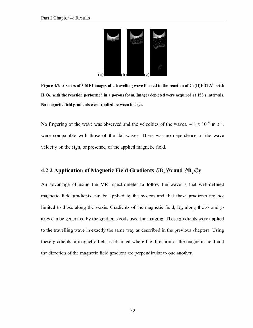
Part I Chapter 4: Results
(a) (b) (c)
Figure 4.7: A series of 3 MRI images of a travelling wave formed in the reaction of Co(II)EDTA2− with
H2O2, with the reaction performed in a porous foam. Images depicted were acquired at 153 s intervals.
No magnetic field gradients were applied between images.
No fingering of the wave was observed and the velocities of the waves, ~ 8 x 10⁻⁶ m s−1,
were comparable with those of the flat waves. There was no dependence of the wave
velocity on the sign, or presence, of the applied magnetic field.
4.2.2 Application of Magnetic Field Gradients x/Bz ∂∂ and y/Bz ∂∂
An advantage of using the MRI spectrometer to follow the wave is that well-defined
magnetic field gradients can be applied to the system and that these gradients are not
limited to those along the z-axis. Gradients of the magnetic field, Bz, along the x- and y-
axes can be generated by the gradients coils used for imaging. These gradients were applied
to the travelling wave in exactly the same way as described in the previous chapters. Using
these gradients, a magnetic field is obtained where the direction of the magnetic field and
the direction of the magnetic field gradient are perpendicular to one another.
70

Part I Chapter 4: Results
4.2.2.1 Formation of a Chemical Finger
As described in section 4.2.1, when the wave was initiated by a small amount of 0.016 M
NaOH, the initial wave front was horizontal and flat. After some time, the wave front
distorted and a finger formed. In the experiments where no magnetic field gradients other
than those used for imaging were applied, the position on the front at which the finger
develops was found to be around the edge of the tube, with the finger pooling into the
centre of the tube. Frequently, more than one finger would form. In order to follow the
movement of the wave out of the zy plane, horizontal images in the xy plane were obtained.
These imaging sequences apply a larger number of gradient pulses associated with the
imaging of the reaction, as gradients are needed for positioning in both the xy plane and in
the z axis. A smaller number of image slices were taken to limit the effect of these magnetic
fields on the reaction. Only a limited region of the tube could therefore be imaged at any
one time. Hence, the sets of images were moved down the tube with time following the
progress of the wave down the tube. All of the images in a set of horizontal images are
acquired simultaneously.
Fig. 4.8 depicts a wave which has distorted and a combination of vertical and horizontal
images showing the position of the fingering distortion in the tube. Note that the vertical
image was acquired after the series of horizontal images, so the tip of the finger has moved
down into the last slice between acquisitions of the two images. The figure shows the
formation of two fingers and also a distortion of the wave around the edge of the tube.
71
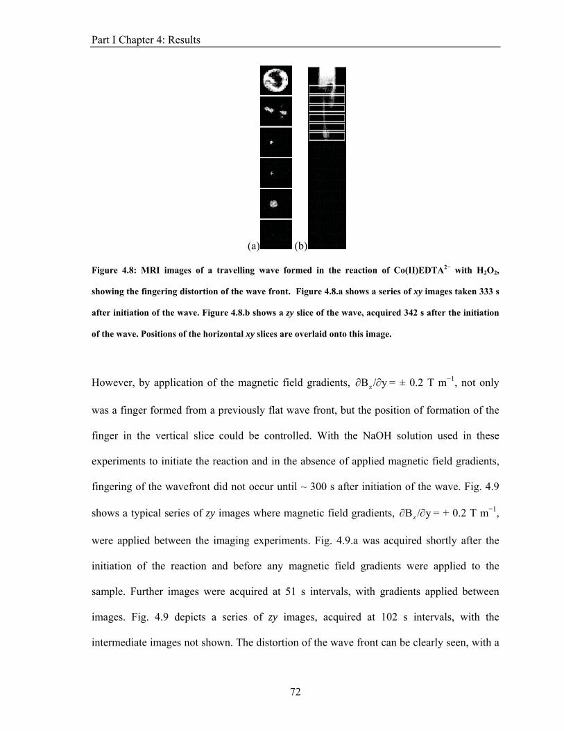
Part I Chapter 4: Results
(a) (b)
Figure 4.8: MRI images of a travelling wave formed in the reaction of Co(II)EDTA2− with H2O2,
showing the fingering distortion of the wave front. Figure 4.8.a shows a series of xy images taken 333 s
after initiation of the wave. Figure 4.8.b shows a zy slice of the wave, acquired 342 s after the initiation
of the wave. Positions of the horizontal xy slices are overlaid onto this image.
However, by application of the magnetic field gradients, y/Bz ∂∂ = ± 0.2 T m−1, not only
was a finger formed from a previously flat wave front, but the position of formation of the
finger in the vertical slice could be controlled. With the NaOH solution used in these
experiments to initiate the reaction and in the absence of applied magnetic field gradients,
fingering of the wavefront did not occur until ~ 300 s after initiation of the wave. Fig. 4.9
shows a typical series of zy images where magnetic field gradients, = + 0.2 T m−1,
were applied between the imaging experiments. Fig. 4.9.a was acquired shortly after the
initiation of the reaction and before any magnetic field gradients were applied to the
sample. Further images were acquired at 51 s intervals, with gradients applied between
images. Fig. 4.9 depicts a series of zy images, acquired at 102 s intervals, with the
intermediate images not shown. The distortion of the wave front can be clearly seen, with a
y/Bz ∂∂
72

Part I Chapter 4: Results
finger formed from a previously flat wave and this finger moving down the side of the
NMR tube.
(a) (b) (c) (d)
Figure 4.9: A series of 4 MRI images of a travelling wave formed in the reaction of Co(II)EDTA2− with
H2O2. Image 4.9.a was acquired shortly after the initiation of the reaction by NaOH introduced onto the
top of the Co(II)EDTA2− solution. Images 4.9.b, 4.9.c and 4.9.d were acquired 102, 204 and 306 s
afterwards, respectively. Magnetic field gradients, ∂Bz/∂y, = + 0.2 T m−1 were applied, with geometry as
described in 3.2.2.
Application of magnetic field gradients, y/Bz ∂∂ = − 0.2 T m−1, lead to the formation of a
finger on the opposite side of the tube. Fig. 4.10 shows a typical series of zy images where
magnetic field gradients, y/Bz ∂∂ = − 0.2 T m−1, were applied between the imaging
experiments. Fig. 4.10.a was acquired shortly after the initiation of the reaction and before
any magnetic field gradients were applied to the sample. Further images were acquired at
51 s intervals, with gradients applied between images. Fig. 4.10 depicts a series of alternate
images, at 102 s intervals. With the sign and, therefore, direction of the magnetic field
73
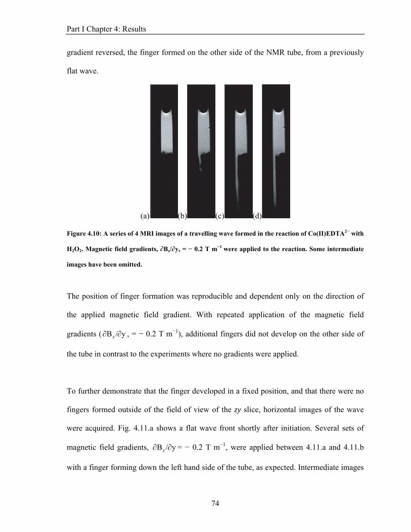
Part I Chapter 4: Results
gradient reversed, the finger formed on the other side of the NMR tube, from a previously
flat wave.
(a) (b) (c) (d)
Figure 4.10: A series of 4 MRI images of a travelling wave formed in the reaction of Co(II)EDTA2− with
H2O2. Magnetic field gradients, ∂Bz/∂y, = − 0.2 T m−1 were applied to the reaction. Some intermediate
images have been omitted.
The position of finger formation was reproducible and dependent only on the direction of
the applied magnetic field gradient. With repeated application of the magnetic field
gradients ( , = − 0.2 T m−1), additional fingers did not develop on the other side of
the tube in contrast to the experiments where no gradients were applied.
y/Bz ∂∂
To further demonstrate that the finger developed in a fixed position, and that there were no
fingers formed outside of the field of view of the zy slice, horizontal images of the wave
were acquired. Fig. 4.11.a shows a flat wave front shortly after initiation. Several sets of
magnetic field gradients, y/Bz ∂∂ = − 0.2 T m−1, were applied between 4.11.a and 4.11.b
with a finger forming down the left hand side of the tube, as expected. Intermediate images
74
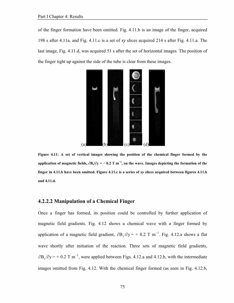
Part I Chapter 4: Results
of the finger formation have been omitted. Fig. 4.11.b is an image of the finger, acquired
198 s after 4.11a, and Fig. 4.11.c is a set of xy slices acquired 214 s after Fig. 4.11.a. The
last image, Fig. 4.11.d, was acquired 51 s after the set of horizontal images. The position of
the finger tight up against the side of the tube is clear from these images.
(a) (b) (c) (d)
Figure 4.11: A set of vertical images showing the position of the chemical finger formed by the
application of magnetic fields, ∂Bz/∂y = − 0.2 T m−1, on the wave. Images depicting the formation of the
finger in 4.11.b have been omitted. Figure 4.11.c is a series of xy slices acquired between figures 4.11.b
and 4.11.d.
4.2.2.2 Manipulation of a Chemical Finger
Once a finger has formed, its position could be controlled by further application of
magnetic field gradients. Fig. 4.12 shows a chemical wave with a finger formed by
application of a magnetic field gradient, y/Bz ∂∂ = + 0.2 T m−1. Fig. 4.12.a shows a flat
wave shortly after initiation of the reaction. Three sets of magnetic field gradients,
= + 0.2 T m−1, were applied between Figs. 4.12.a and 4.12.b, with the intermediate
images omitted from Fig. 4.12. With the chemical finger formed (as seen in Fig. 4.12.b,
y/Bz ∂∂
75
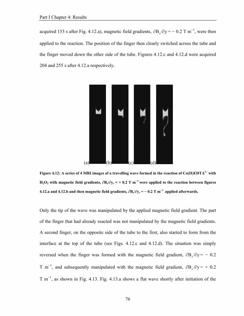
Part I Chapter 4: Results
acquired 153 s after Fig. 4.12.a), magnetic field gradients, y/Bz ∂∂ = − 0.2 T m−1, were then
applied to the reaction. The position of the finger then clearly switched across the tube and
the finger moved down the other side of the tube. Figures 4.12.c and 4.12.d were acquired
204 and 255 s after 4.12.a respectively.
(a) (b) (c) (d)
Figure 4.12: A series of 4 MRI images of a travelling wave formed in the reaction of Co(II)EDTA2− with
H2O2 with magnetic field gradients, ∂Bz/∂y, = + 0.2 T m−1 were applied to the reaction between figures
4.12.a and 4.12.b and then magnetic field gradients, ∂Bz/∂y, = − 0.2 T m−1 applied afterwards.
Only the tip of the wave was manipulated by the applied magnetic field gradient. The part
of the finger that had already reacted was not manipulated by the magnetic field gradients.
A second finger, on the opposite side of the tube to the first, also started to form from the
interface at the top of the tube (see Figs. 4.12.c and 4.12.d). The situation was simply
reversed when the finger was formed with the magnetic field gradient, = − 0.2
T m−1, and subsequently manipulated with the magnetic field gradient, = + 0.2
T m−1, as shown in Fig. 4.13. Fig. 4.13.a shows a flat wave shortly after initiation of the
y/Bz ∂∂
y/Bz ∂∂
76
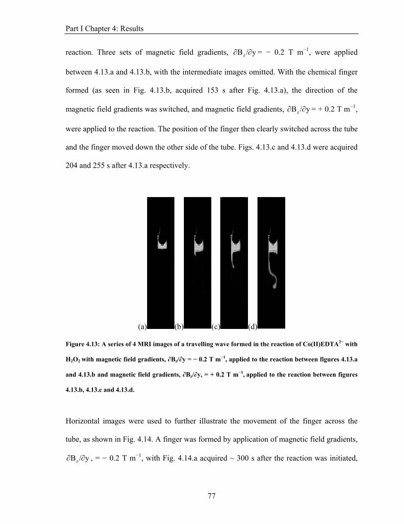
Part I Chapter 4: Results
reaction. Three sets of magnetic field gradients, y/Bz ∂∂ = − 0.2 T m−1, were applied
between 4.13.a and 4.13.b, with the intermediate images omitted. With the chemical finger
formed (as seen in Fig. 4.13.b, acquired 153 s after Fig. 4.13.a), the direction of the
magnetic field gradients was switched, and magnetic field gradients, = + 0.2 T m−1,
were applied to the reaction. The position of the finger then clearly switched across the tube
and the finger moved down the other side of the tube. Figs. 4.13.c and 4.13.d were acquired
204 and 255 s after 4.13.a respectively.
y/Bz ∂∂
(a) (b) (c) (d)
Figure 4.13: A series of 4 MRI images of a travelling wave formed in the reaction of Co(II)EDTA2− with
H2O2 with magnetic field gradients, ∂Bz/∂y = − 0.2 T m−1, applied to the reaction between figures 4.13.a
and 4.13.b and magnetic field gradients, ∂Bz/∂y, = + 0.2 T m−1, applied to the reaction between figures
4.13.b, 4.13.c and 4.13.d.
Horizontal images were used to further illustrate the movement of the finger across the
tube, as shown in Fig. 4.14. A finger was formed by application of magnetic field gradients,
, = − 0.2 T m−1, with Fig. 4.14.a acquired ~ 300 s after the reaction was initiated, y/Bz ∂∂
77
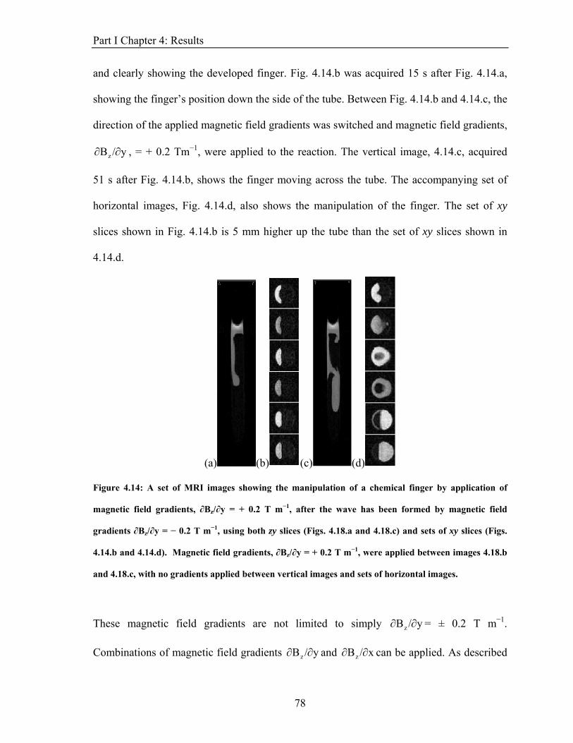
Part I Chapter 4: Results
and clearly showing the developed finger. Fig. 4.14.b was acquired 15 s after Fig. 4.14.a,
showing the finger’s position down the side of the tube. Between Fig. 4.14.b and 4.14.c, the
direction of the applied magnetic field gradients was switched and magnetic field gradients,
, = + 0.2 Tm−1, were applied to the reaction. The vertical image, 4.14.c, acquired
51 s after Fig. 4.14.b, shows the finger moving across the tube. The accompanying set of
horizontal images, Fig. 4.14.d, also shows the manipulation of the finger. The set of xy
slices shown in Fig. 4.14.b is 5 mm higher up the tube than the set of xy slices shown in
4.14.d.
y/Bz ∂∂
(a) (b) (c) (d)
Figure 4.14: A set of MRI images showing the manipulation of a chemical finger by application of
magnetic field gradients, ∂Bz/∂y = + 0.2 T m−1, after the wave has been formed by magnetic field
gradients ∂Bz/∂y = − 0.2 T m−1, using both zy slices (Figs. 4.18.a and 4.18.c) and sets of xy slices (Figs.
4.14.b and 4.14.d). Magnetic field gradients, ∂Bz/∂y = + 0.2 T m−1, were applied between images 4.18.b
and 4.18.c, with no gradients applied between vertical images and sets of horizontal images.
These magnetic field gradients are not limited to simply y/Bz ∂∂ = ± 0.2 T m−1.
Combinations of magnetic field gradients y/Bz ∂∂ and x/Bz ∂∂ can be applied. As described
78
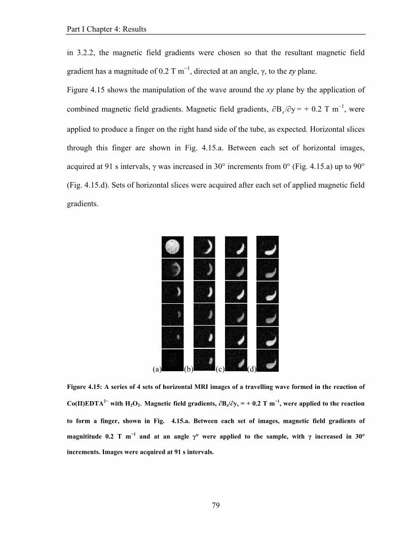
Part I Chapter 4: Results
in 3.2.2, the magnetic field gradients were chosen so that the resultant magnetic field
gradient has a magnitude of 0.2 T m−1, directed at an angle, γ, to the zy plane.
Figure 4.15 shows the manipulation of the wave around the xy plane by the application of
combined magnetic field gradients. Magnetic field gradients, y/Bz ∂∂ = + 0.2 T m−1, were
applied to produce a finger on the right hand side of the tube, as expected. Horizontal slices
through this finger are shown in Fig. 4.15.a. Between each set of horizontal images,
acquired at 91 s intervals, γ was increased in 30° increments from 0° (Fig. 4.15.a) up to 90°
(Fig. 4.15.d). Sets of horizontal slices were acquired after each set of applied magnetic field
gradients.
(a) (b) (c) (d)
Figure 4.15: A series of 4 sets of horizontal MRI images of a travelling wave formed in the reaction of
Co(II)EDTA2− with H2O2. Magnetic field gradients, ∂Bz/∂y, = + 0.2 T m−1, were applied to the reaction
to form a finger, shown in Fig. 4.15.a. Between each set of images, magnetic field gradients of
magnititude 0.2 T m−1 and at an angle γ° were applied to the sample, with γ increased in 30°
increments. Images were acquired at 91 s intervals.
79
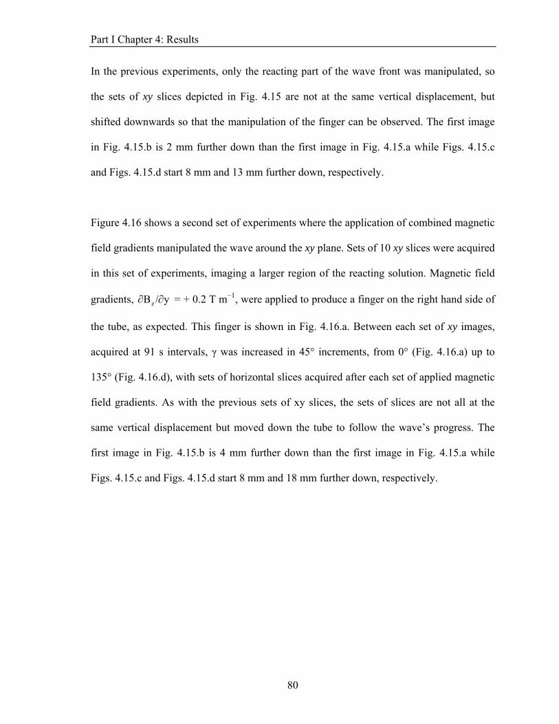
Part I Chapter 4: Results
In the previous experiments, only the reacting part of the wave front was manipulated, so
the sets of xy slices depicted in Fig. 4.15 are not at the same vertical displacement, but
shifted downwards so that the manipulation of the finger can be observed. The first image
in Fig. 4.15.b is 2 mm further down than the first image in Fig. 4.15.a while Figs. 4.15.c
and Figs. 4.15.d start 8 mm and 13 mm further down, respectively.
Figure 4.16 shows a second set of experiments where the application of combined magnetic
field gradients manipulated the wave around the xy plane. Sets of 10 xy slices were acquired
in this set of experiments, imaging a larger region of the reacting solution. Magnetic field
gradients, = + 0.2 T m−1, were applied to produce a finger on the right hand side of
the tube, as expected. This finger is shown in Fig. 4.16.a. Between each set of xy images,
acquired at 91 s intervals, γ was increased in 45° increments, from 0° (Fig. 4.16.a) up to
135° (Fig. 4.16.d), with sets of horizontal slices acquired after each set of applied magnetic
field gradients. As with the previous sets of xy slices, the sets of slices are not all at the
same vertical displacement but moved down the tube to follow the wave’s progress. The
first image in Fig. 4.15.b is 4 mm further down than the first image in Fig. 4.15.a while
Figs. 4.15.c and Figs. 4.15.d start 8 mm and 18 mm further down, respectively.
y/Bz ∂∂
80
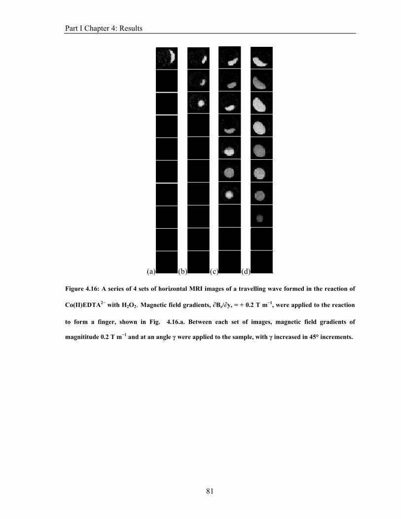
Part I Chapter 4: Results
(a) (b) (c) (d)
Figure 4.16: A series of 4 sets of horizontal MRI images of a travelling wave formed in the reaction of
Co(II)EDTA2− with H2O2. Magnetic field gradients, ∂Bz/∂y, = + 0.2 T m−1, were applied to the reaction
to form a finger, shown in Fig. 4.16.a. Between each set of images, magnetic field gradients of
magnititude 0.2 T m−1 and at an angle γ were applied to the sample, with γ increased in 45° increments.
81

Part I Chapter 4: Results
4.2.2.3 Waves in a Porous Medium II
In analogy to the experiments described in 4.2.1.3, the reaction was introduced into a
porous medium, reducing the effect of convection on the reaction. A series of experiments
were carried out with the solution in porous foam in a 7.5 mm I.D. tube. The system was
optically opaque and so could only be observed using MRI techniques. Fig. 4.17 shows a
typical series of zy images where magnetic field gradients, y/Bz ∂∂ = + 0.2 T m−1, were
applied between the imaging experiments. Fig. 4.17.a was acquired shortly after the
initiation of the reaction and before any magnetic field gradients were applied to the
sample. Further images were acquired at 51 s intervals with magnetic field gradients,
= + 0.2 T m−1, applied between images. The figure depicts a series of zy images,
acquired at 102 s intervals.
y/Bz ∂∂
(a) (b) (c) (d)
Figure 4.17: A series of 4 MRI images of a travelling wave formed in the reaction of Co(II)EDTA2− with
H2O2, with the reaction performed in a porous foam. Magnetic field gradients, ∂Bz/∂y = + 0.2 T m−1,
were applied to the reaction. The images shown were acquired at 102 s intervals.
Although there was some distortion of the wave in Figs. 4.17, comparison with Fig. 4.9
shows that the finger was much more developed in the earlier experiments than in the
experiments in the porous medium.
82
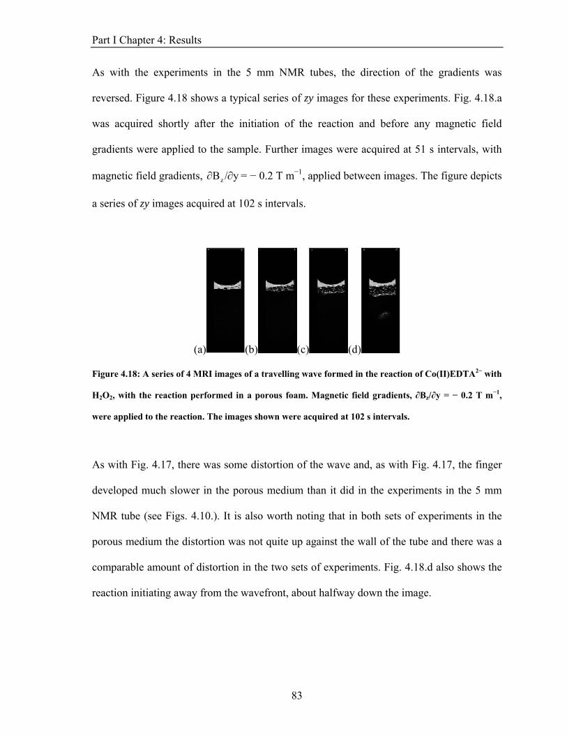
Part I Chapter 4: Results
As with the experiments in the 5 mm NMR tubes, the direction of the gradients was
reversed. Figure 4.18 shows a typical series of zy images for these experiments. Fig. 4.18.a
was acquired shortly after the initiation of the reaction and before any magnetic field
gradients were applied to the sample. Further images were acquired at 51 s intervals, with
magnetic field gradients, = − 0.2 T m−1, applied between images. The figure depicts
a series of zy images acquired at 102 s intervals.
y/Bz ∂∂
(a) (b) (c) (d)
Figure 4.18: A series of 4 MRI images of a travelling wave formed in the reaction of Co(II)EDTA2− with
H2O2, with the reaction performed in a porous foam. Magnetic field gradients, ∂Bz/∂y = − 0.2 T m−1,
were applied to the reaction. The images shown were acquired at 102 s intervals.
As with Fig. 4.17, there was some distortion of the wave and, as with Fig. 4.17, the finger
developed much slower in the porous medium than it did in the experiments in the 5 mm
NMR tube (see Figs. 4.10.). It is also worth noting that in both sets of experiments in the
porous medium the distortion was not quite up against the wall of the tube and there was a
comparable amount of distortion in the two sets of experiments. Fig. 4.18.d also shows the
reaction initiating away from the wavefront, about halfway down the image.
83
Part I Chapter 5: Discussion
5. DISCUSSION
5.1 The origin of the effect
The application of various combinations of magnetic field and magnetic field gradients on
the travelling wave reaction clearly has a large effect. The simple Petri dish reaction,
depicted in Fig. 2.1. shows that even a small magnet can produce a large effect.
The sensitivity of the reaction to applied magnetic fields should arise from the change in
magnetic susceptibility across the reaction wave front and the magnetic force acting on this
but the Lorentz force (Eqn 1.19) could also be acting on the reaction. However, this force
can soon be excluded as it has little effect. The Lorentz force acts in a different manner to
the magnetic force, operating at right angles to both the magnetic field and any flow of
ions. In simulations by Kinouchi et al.10 the Lorentz force acted to inhibit the diffusion of a
species similar to that present in these experiments. This would lead to a homogeneous
magnetic field possibly slowing down the wave’s velocity due to a smaller effective
diffusion constant. Further to the effect being one which would not speed up the reaction,
the fields as high as 106 T were required to have a significant effect on the diffusion
constants of the species involved in the reaction. The magnetic fields used in these
experiments ranged between 7 T for the MRI experiments and around 1 T, and lower, for
the Petri dish experiments. Hence, the Lorentz force does not drive the observed effects.
The preliminary results shown in Fig. 4.2 showed a strong dependence of the field effect on
the product of magnetic field and magnetic field gradient, when the wave is travelling from
84
Part I Chapter 5: Discussion
high to low field. While this does not necessarily exclude the effect of the Lorentz force,
the data suggests that the dominant force is the magnetic force. Previous work focused on
the manipulation of droplets of solutions of paramagnetic ions through a surrounding
diamagnetic solution7. This transport of paramagnetic ions also showed a strong
dependence on the product of the magnetic field and its gradient, as well as on the magnetic
susceptibilities of the fluids involved. Crucially, the magnetic field acted to move the
neutral radical 2,2,6,6-tetramethylpiperidine-1-oxy (TEMPO), so the Lorentz force could
not be acting in these experiments.
The magnetic force could affect the reaction in two possible ways. First, there is the
movement of paramagnetic solution through a diamagnetic solution or, in this case, a finger
of diamagnetic solution through a paramagnetic one. This would occur in the absence of
any reactions, as seen in previous work. There is also the possibility of mixing of the
solutions through convection of the paramagnetic solution into the diamagnetic solution,
where Co(II)EDTA2− comes into contact with the autocatalytic −OH ions, hence, increasing
the reaction rate and wavefront velocity.
The magnetic force is given as:
BBF )(μ
Vχ
0
vM ∇⋅= (20)
This force can be considered as the product of two factors. First, there is a magnetic field-
dependent term proportional to BB )( ∇⋅ which, when expanded, can be written as:
85
Part I Chapter 5: Discussion
( )
⎟⎟⎟⎟⎟⎟⎟
⎠
⎞
⎜⎜⎜⎜⎜⎜⎜
⎝
⎛
∂∂
+∂∂
+∂∂
∂
∂+
∂
∂+
∂
∂∂∂
+∂∂
+∂∂
=⎟⎟⎟
⎠
⎞
⎜⎜⎜
⎝
⎛
⎟⎟⎠
⎞⎜⎜⎝
⎛∂∂
+∂∂
+∂∂
=∇⋅
zBB
yBB
xBB
zB
By
BB
xB
B
zBB
yBB
xBB
BBB
zB
yB
xB
zz
zy
zx
yz
yy
yx
xz
xy
xx
z
y
x
zyxBB
(21)
Clearly, it is certain combinations of magnetic field and magnetic field gradient that lead to
magnetic forces in a given direction.
The force acting on any droplet or finger of solution is also proportional to the magnetic
susceptibility of the species and the amount of it present. There is a change in magnetic
susceptibility across the reaction wavefront in the MRI experiments where the wave is
initiated at the top of the tube and moves down through the tube. Both solutions are actually
diamagnetic, with a large contribution to the overall magnetic susceptibility from the water
solvent. However, the Co(II)EDTA2− solution is less diamagnetic than the Co(III)EDTA−
solution above it. The difference in the susceptibility across the boundary is the important
quantity as it leads to a resultant force acting on the solution across the boundary.
For the experiments where the magnetic field gradients, z/Bz ∂∂ = ± 0.2 T m−1, were applied
to the reaction, the sample inside the spectrometer is in the magnetic field:
zBzBB z
0z,z ∂∂
+= (22)
86
Part I Chapter 5: Discussion
0z,B =7.0 T is the homogeneous magnetic field produced by the vertical superconducting
magnet of the MRI spectrometer, z/Bz ∂∂ = ± 0.2 T m−1, is the magnetic field gradient
produced by the imaging coils and z is the distance along the z−axis from the centre of the
RF coil (0 - ~ 0.0125) m. Maxwell’s equation 0=⋅∇ B shows that a magnetic field gradient
cannot be produced independently and that the magnetic field gradients z∂/Bz∂ y/By ∂∂ and
must also be produced. These give rise to distance dependent magnetic fields
and .
x∂/Bx∂
xB yB
0z
By
Bx
B zyx =∂∂
+∂
∂+
∂∂
=⋅∇ B (23)
For the period that the magnetic field gradients are applied, the magnetic force acting on the
reaction is:
⎟⎟⎟⎟⎟⎟⎟⎟
⎠
⎞
⎜⎜⎜⎜⎜⎜⎜⎜
⎝
⎛
∂∂
⎟⎠
⎞⎜⎝
⎛∂∂
+
∂
∂⎟⎟⎠
⎞⎜⎜⎝
⎛∂
∂+
∂∂
⎟⎠
⎞⎜⎝
⎛∂∂
+
=
⎟⎟⎟⎟⎟⎟⎟
⎠
⎞
⎜⎜⎜⎜⎜⎜⎜
⎝
⎛
∂∂∂
∂∂∂
=∇⋅=
zB
zz
BB
yB
yy
BB
xB
xx
BB
μVχ
zBB
yB
B
xBB
μVχ
)(μ
Vχ
zz,0z
yyy,0
xxx,0
0
V
zz
yy
xx
0
V
0
VM BBF (24)
It is clear that there are distance dependent forces acting in the x- and y-direction, from the
terms and . However, these are small compared to the force acting in
the z-direction, due to the small distances (~ 0.0025 m) across the tube, and the absence of
x/BB xx ∂∂ y/BB yy ∂∂
87

Part I Chapter 5: Discussion
either or . With =7.0 T and 0xB , 0yB, 0z,B z/Bz ∂∂ = ± 0.2 T m−1 substituted in, an
expression for the force is obtained.
( )⎟⎟⎟⎟⎟⎟⎟⎟
⎠
⎞
⎜⎜⎜⎜⎜⎜⎜⎜
⎝
⎛
+
⎟⎟⎠
⎞∂
⎟⎠
⎞∂
4y
Bx
B
2y
2x
±
⎜⎜⎝
⎛ ∂
⎜⎝
⎛ ∂
=
0.04z1
y
x
μVχ
0
V
.
MF (25)
The size of the forces in the x- and y- directions are no larger than 1 × 10⁻⁴ T2 m−1. The z-
dependent term in the z- direction is no larger than 5 × 10⁻⁴ T2 m−1. Both of these terms are
much smaller than the ± 1.4 T2 m−1 term and can be safely ignored.
In control experiments, no gradients are applied and the product of magnetic field and
magnetic field gradient is zero, and no magnetic force acts on any of the sample. In the
other experiments, the dominant term in the magnetic force is ± 1.4 T2 m−1, depending on
the sign of the magnetic field gradient. This is a value that changes sign when the sign of
the applied magnetic fields is changed and is effectively constant over the area of the
reaction imaged.
With a magnetic field gradient, = − 0.2 T m−1, the magnetic field is higher at the top of the
tube than at the bottom. In much the same way as with the experiments in the shallow layer,
when the wave is travelling from high field to low, there is increased mixing of the
reagents. The diamagnetic reacted solution is forced away from the high field region and
88
Part I Chapter 5: Discussion
more paramagnetic unreacted solution is pulled up the magnetic field gradient, into contact
with the reacted solution and a higher [−OH]. The magnetic force could also act to simply
move the finger down through the solution. This leads to the greater wave velocity
observed.
When the magnetic field gradient is reversed, z/Bz ∂∂ = + 0.2 T m−1 and the magnetic field
is lower at the top of the tube. With the travelling wave moving down the tube, the wave
moves from low field to high, with the reacted solution always in a lower field region than
the more paramagnetic unreacted solution. This would mean that the force acting on the
reaction would keep the two regions separated, limiting the amount of mixing around the
wave front.
With application of the magnetic field gradients x/Bz ∂∂ and y/Bz ∂∂ , the z-component of
the magnetic field, , is given by: zB
yB
yx
BxBB zz
z,0z ∂∂
+∂∂
+= (26)
As with the previous experiments, these magnetic field gradients cannot be produced in
isolation. In the absence of electric currents in the sample or time dependent electric fields,
Maxwell’s equation (Eqn. 1.31) simplifies to 0=×∇ B and the magnetic field gradients are
related by:
89
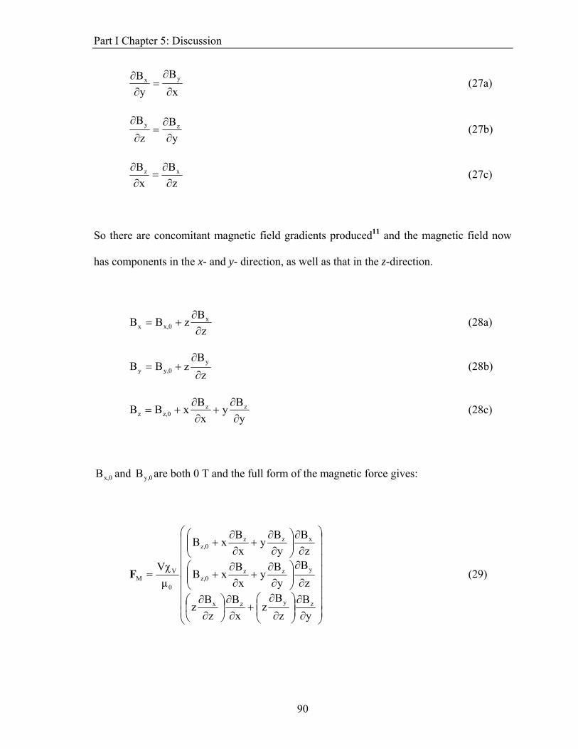
Part I Chapter 5: Discussion
x
By
B yx
∂
∂=
∂∂ (27a)
yB
zB zy
∂∂
=∂
∂ (27b)
zB
xB xz
∂∂
=∂∂ (27c)
So there are concomitant magnetic field gradients produced11 and the magnetic field now
has components in the x- and y- direction, as well as that in the z-direction.
z
BzBB xx,0x ∂
∂+= (28a)
z
BzBB y
y,0y ∂
∂+= (28b)
yBy
xBxBB zz
z,0z ∂∂
+∂∂
+= (28c)
x,0B and are both 0 T and the full form of the magnetic force gives: y,0B
⎟⎟⎟⎟⎟⎟⎟⎟
⎠
⎞
⎜⎜⎜⎜⎜⎜⎜⎜
⎝
⎛
∂∂
⎟⎟⎠
⎞⎜⎜⎝
⎛∂
∂+
∂∂
⎟⎠
⎞⎜⎝
⎛∂∂
∂
∂⎟⎟⎠
⎞⎜⎜⎝
⎛∂∂
+∂∂
+
∂∂
⎟⎟⎠
⎞⎜⎜⎝
⎛∂∂
+∂∂
+
=
yB
zB
zx
Bz
Bz
zB
yB
yx
BxB
zB
yBy
xBxB
μVχ
zyzx
yzzz,0
xzzz,0
0
VMF (29)
90
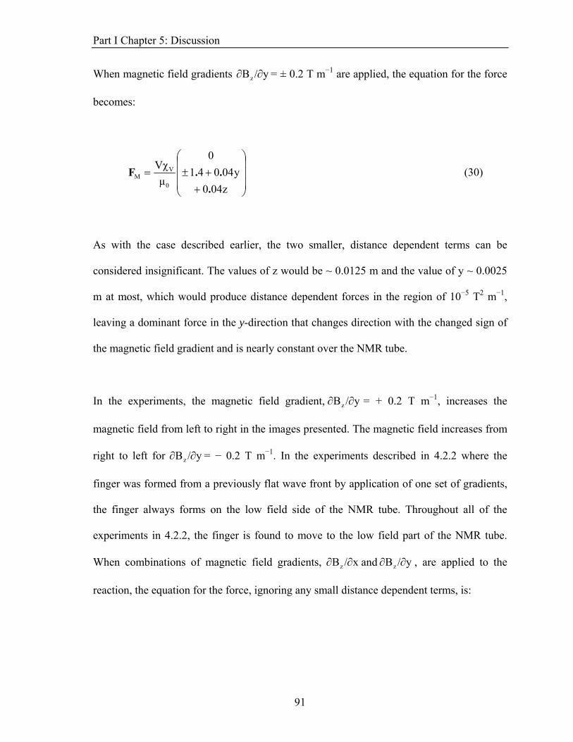
Part I Chapter 5: Discussion
When magnetic field gradients y/Bz ∂∂ = ± 0.2 T m−1 are applied, the equation for the force
becomes:
⎟⎟⎟
⎠
⎞
⎜⎜⎜
⎝
⎛
++±=
z040y04041
0
μVχ
0
VM
...F (30)
As with the case described earlier, the two smaller, distance dependent terms can be
considered insignificant. The values of z would be ~ 0.0125 m and the value of y ~ 0.0025
m at most, which would produce distance dependent forces in the region of 10−5 T2 m−1,
leaving a dominant force in the y-direction that changes direction with the changed sign of
the magnetic field gradient and is nearly constant over the NMR tube.
In the experiments, the magnetic field gradient, y/Bz ∂∂ = + 0.2 T m−1, increases the
magnetic field from left to right in the images presented. The magnetic field increases from
right to left for = − 0.2 T m−1. In the experiments described in 4.2.2 where the
finger was formed from a previously flat wave front by application of one set of gradients,
the finger always forms on the low field side of the NMR tube. Throughout all of the
experiments in 4.2.2, the finger is found to move to the low field part of the NMR tube.
When combinations of magnetic field gradients,
y/Bz ∂∂
x/Bz ∂∂ and y/Bz ∂∂ , are applied to the
reaction, the equation for the force, ignoring any small distance dependent terms, is:
91
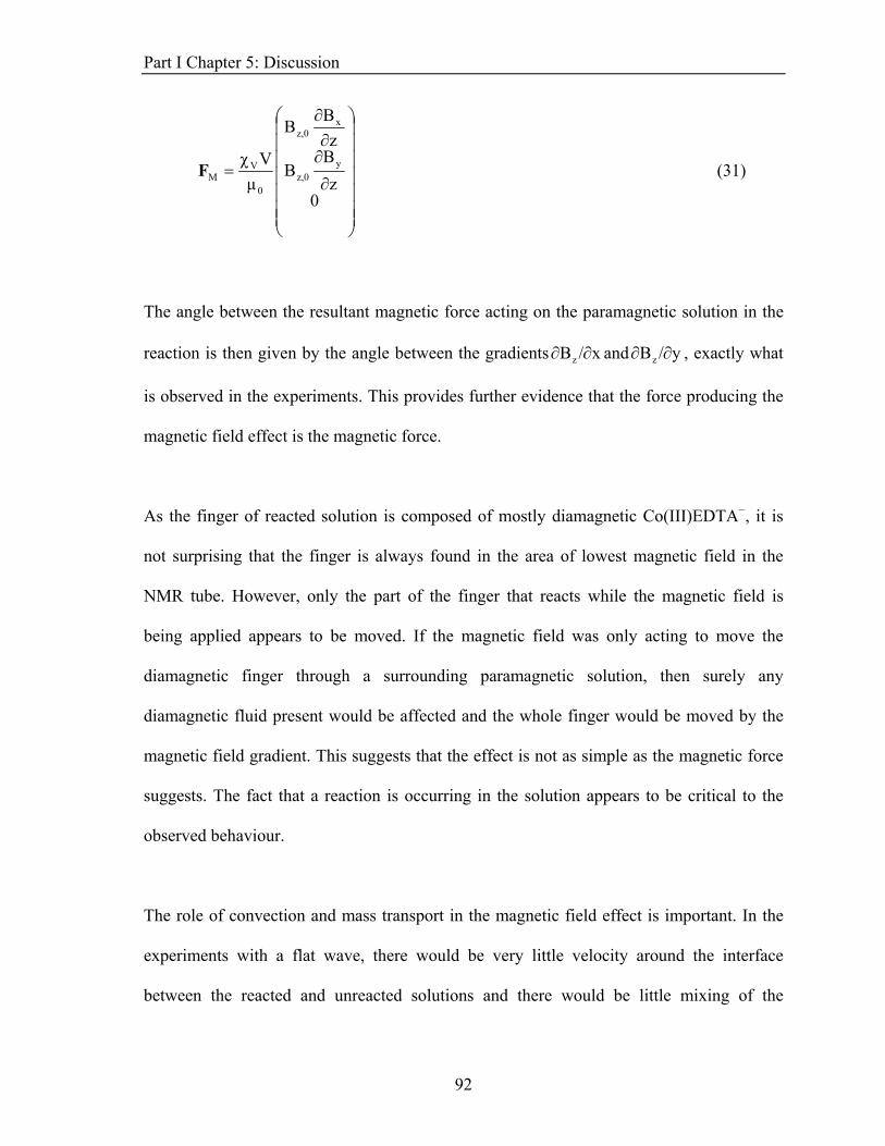
Part I Chapter 5: Discussion
⎟⎟⎟⎟⎟⎟⎟
⎠
⎞
⎜⎜⎜⎜⎜⎜⎜
⎝
⎛
∂
∂∂∂
=
0z
BB
zBB
μVχ y
z,0
xz,0
0
VMF (31)
The angle between the resultant magnetic force acting on the paramagnetic solution in the
reaction is then given by the angle between the gradients x/Bz ∂∂ and , exactly what
is observed in the experiments. This provides further evidence that the force producing the
magnetic field effect is the magnetic force.
y/Bz ∂∂
As the finger of reacted solution is composed of mostly diamagnetic Co(III)EDTA−, it is
not surprising that the finger is always found in the area of lowest magnetic field in the
NMR tube. However, only the part of the finger that reacts while the magnetic field is
being applied appears to be moved. If the magnetic field was only acting to move the
diamagnetic finger through a surrounding paramagnetic solution, then surely any
diamagnetic fluid present would be affected and the whole finger would be moved by the
magnetic field gradient. This suggests that the effect is not as simple as the magnetic force
suggests. The fact that a reaction is occurring in the solution appears to be critical to the
observed behaviour.
The role of convection and mass transport in the magnetic field effect is important. In the
experiments with a flat wave, there would be very little velocity around the interface
between the reacted and unreacted solutions and there would be little mixing of the
92
Part I Chapter 5: Discussion
unreacted solution and the reacted solution. In these experiments, the magnetic force
appeared to only act on a convective flow that was already present. With the reaction
performed in a porous medium, similar results were observed. No dependence on the
applied magnetic field was seen when magnetic field gradients were applied and the wave
velocities were of a similar size to those measured with a flat wave. This suggests that the
velocity of the wavefront is determined by reaction and diffusion only in these two cases.
The experiments described in this section start to quantify the magnetic field effects seen
previously. Well-defined magnetic field gradients are applied to the reaction. The reaction
can be sped up and slowed down by the application of magnetic field gradients z/Bz ∂∂
y/Bz
and
the magnetic field effect is highly dependent on the possibility of free convection around
the reaction wave front. The application of magnetic field gradients ∂∂ and
had a more striking effect, as chemical fingering could be induced in a previously
flat wave and then manipulated by the further application of magnetic fields. It was also
found that the wave front could not be driven upwards by a magnetic field gradient, as the
coupling of reaction and diffusion alone ensured that it would propagate away from the
point of initiation.
x/Bz ∂∂
93
Part I Chapter 5: Discussion
5.2 Future Work and Applications
With the results reasonably well understood in terms of the magnetic force acting on the
travelling wave reaction, where else can this work go? Not everything has been explained.
Two main questions remain unanswered: first, why is only the part of the finger that forms
while the magnetic field is being applied manipulated by the field and secondly, why do the
magnetic field gradients y/Bz ∂∂ and x/Bz ∂∂ produce a distortion in the wavefront
while needs a distortion in the wavefront to have an effect? Are there any
experiments or models that can give further insight into the difference in behaviour? Also,
is the phenomenon observed here restricted to this reaction, or can other reactions show
similar magnetic field dependence? Can this magnetic field dependence be put to any
practical use? This chapter aims to start answering those questions, or, at least, highlight
how these questions could be answered.
z/Bz ∂∂
5.2.1 Modelling
Modelling the travelling wave and the finger phenomena observed gives an insight into the
nature of the flow around the wavefront. Even if a full, accurate model of the reaction is not
developed, analysing the forces acting on the system and the convective flow they produce
in the reaction would certainly aid understanding of the magnetic field effect and how it
arises. The relationship between the reaction, velocities around the wave front and the
magnetic field effect seen can then be analysed. Even a simplistic model could give
important insight into the nature of chemical fingering and the magnetic field effect. The
aim of this section is to introduce some methods that could be used to model the reaction
and to show some preliminary simulations. The reaction and travelling wave could be
94
Part I Chapter 5: Discussion
modelled using a range of techniques, such as pseudospectral methods12 and computational
fluid dynamics (CFD). The latter technique formed the basis of a series of preliminary
studies modelling the effect of the magnetic field on the wave using the commercial
packages Femlab and CFD-ACE. In both programs, compressible Navier-Stokes flow was
coupled with changes in density of the fluid due to the autocatalytic reaction as a model of
the chemical fingering. It is the intention here to guide further, more theoretical, studies in
this area whilst a full investigation of the observed phenomena is beyond the scope of this
thesis.
In this series of simulations, a 2-D strip, scaled so that the width of the strip equalled the
diameter of the NMR tubes, was the geometry used throughout. A grid was added to the 2-
D strip, splitting the geometry up into a series of small cells. CFD-ACE uses a Finite
Volume AnalysisIII method to solve the equations. Time-dependent solutions were
obtained. Models in CFD-ACE could be made increasingly more complex by adding
different sub-routines modelling changes in different variables, increasing the complexity
of the reactions taking place and adding extra forces, if needed. Instead of starting with all
of the equations, the model was built up in a series of steps, increasing in complexity to
create an increasingly more accurate and realistic model.
A simple autocatalytic reaction can be easily modelled. A travelling wave is produced if an
autocatalytic reaction is coupled to diffusion of the species present in the reaction.
95
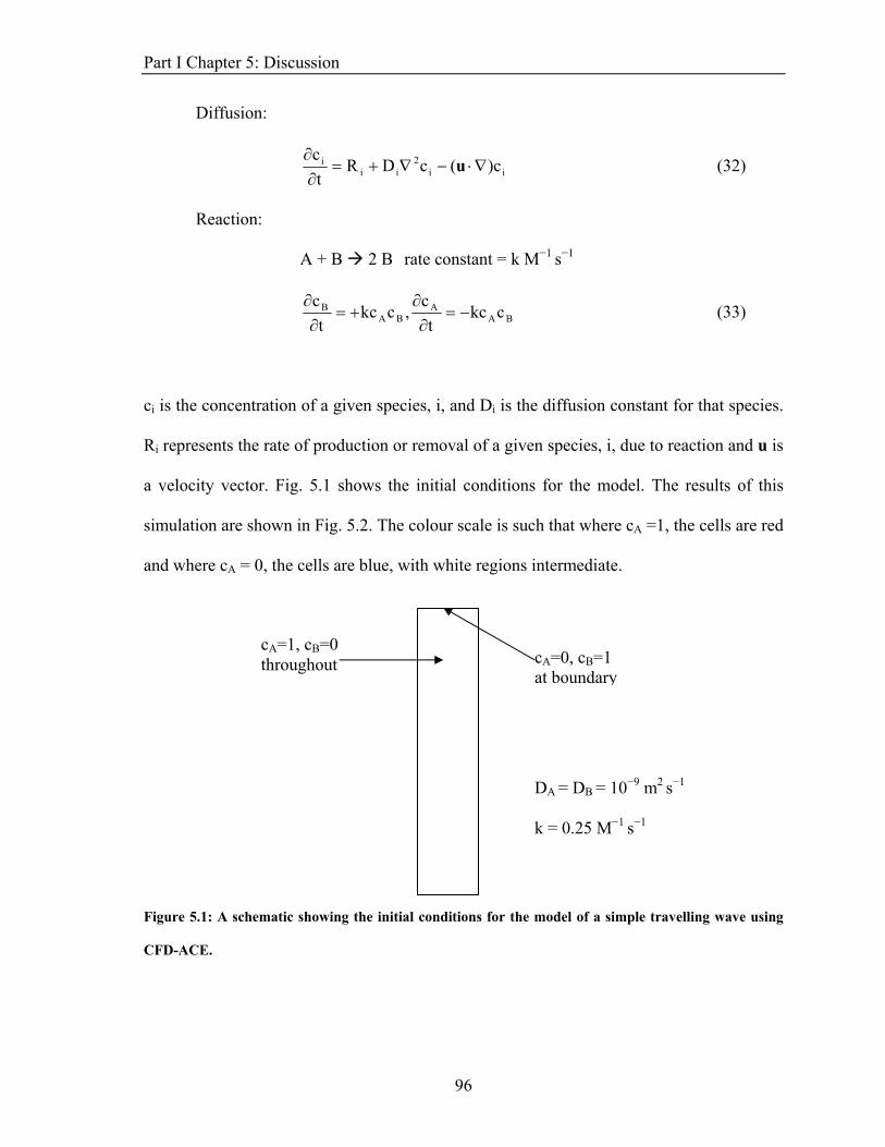
Part I Chapter 5: Discussion
Diffusion:
ii2
iii )c(cDR
tc
∇⋅−∇+=∂∂ u (32)
Reaction:
A + B 2 B rate constant = k M−1 s−1
BAA
BAB ckc
tc
,ckct
c−=
∂∂
+=∂∂ (33)
ci is the concentration of a given species, i, and Di is the diffusion constant for that species.
Ri represents the rate of production or removal of a given species, i, due to reaction and u is
a velocity vector. Fig. 5.1 shows the initial conditions for the model. The results of this
simulation are shown in Fig. 5.2. The colour scale is such that where cA =1, the cells are red
and where cA = 0, the cells are blue, with white regions intermediate.
cA=1, cthrough cA=0, cB=1
at boundary
B=0 out
DA = DB = 10−9 m2 s−1
k = 0.25 M−1 s−1
Figure 5.1: A schematic showing the initial conditions for the model of a simple travelling wave using
CFD-ACE.
96
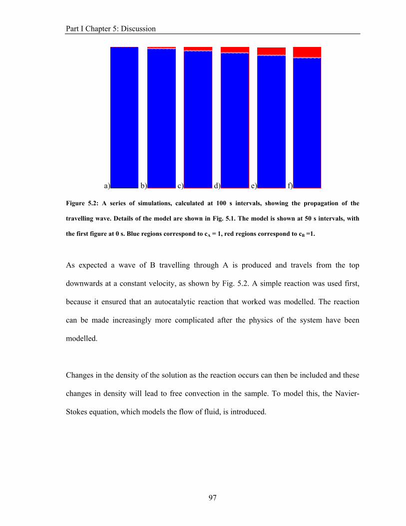
Part I Chapter 5: Discussion
a) b) c) d) e) f)
Figure 5.2: A series of simulations, calculated at 100 s intervals, showing the propagation of the
travelling wave. Details of the model are shown in Fig. 5.1. The model is shown at 50 s intervals, with
the first figure at 0 s. Blue regions correspond to cA = 1, red regions correspond to cB =1.
As expected a wave of B travelling through A is produced and travels from the top
downwards at a constant velocity, as shown by Fig. 5.2. A simple reaction was used first,
because it ensured that an autocatalytic reaction that worked was modelled. The reaction
can be made increasingly more complicated after the physics of the system have been
modelled.
Changes in the density of the solution as the reaction occurs can then be included and these
changes in density will lead to free convection in the sample. To model this, the Navier-
Stokes equation, which models the flow of fluid, is introduced.
97

Part I Chapter 5: Discussion
Navier-Stokes:
( )[ ] Fuuuuu=∇+∇+∇+∇⋅∇−
∂∂ p).ρ()()(η
tρ T (34a)
( ) 0ρtρ
=⋅∇+∂∂ u (34b)
where ρ is the density of the solution, dependent on the composition and the temperature of
the solution and η is the viscosity of the solution, p is the pressure of the solution and F is a
sum of all of the forces acting on the solution, such as gravity. A derivation of this equation
can be found in Appendix II. Eqn. 35 is based on equations featured in chapter 2.2.
Density:
ρ = ρ0 [1 + αΔT + βiΔci + ... ] (35)
ρ0 is the density of the solution at a given temperature and composition (T0, cA,0, cB,0). α
and βi were defined in chapter 2.2. In this first, simplest model, the only force acting on the
system is gravity. Changes in temperature were not modelled. Fig. 5.3 shows the initial
conditions for the model. Boundary conditions now become important. In these
simulations, u = 0 for all of the boundaries.
98
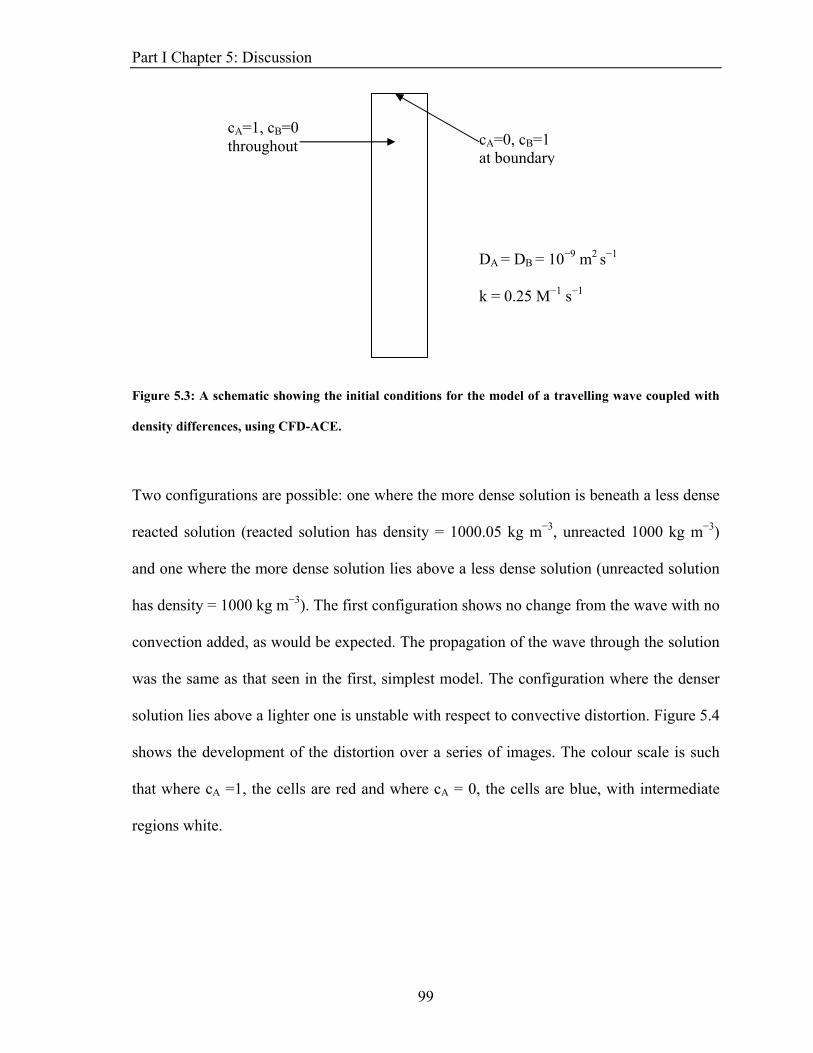
Part I Chapter 5: Discussion
cA=1, cthrough cA=0, cB=1
at boundary
B=0 out
DA = DB = 10−9 m2 s−1
k = 0.25 M−1 s−1
Figure 5.3: A schematic showing the initial conditions for the model of a travelling wave coupled with
density differences, using CFD-ACE.
Two configurations are possible: one where the more dense solution is beneath a less dense
reacted solution (reacted solution has density = 1000.05 kg m−3, unreacted 1000 kg m−3)
and one where the more dense solution lies above a less dense solution (unreacted solution
has density = 1000 kg m−3). The first configuration shows no change from the wave with no
convection added, as would be expected. The propagation of the wave through the solution
was the same as that seen in the first, simplest model. The configuration where the denser
solution lies above a lighter one is unstable with respect to convective distortion. Figure 5.4
shows the development of the distortion over a series of images. The colour scale is such
that where cA =1, the cells are red and where cA = 0, the cells are blue, with intermediate
regions white.
99
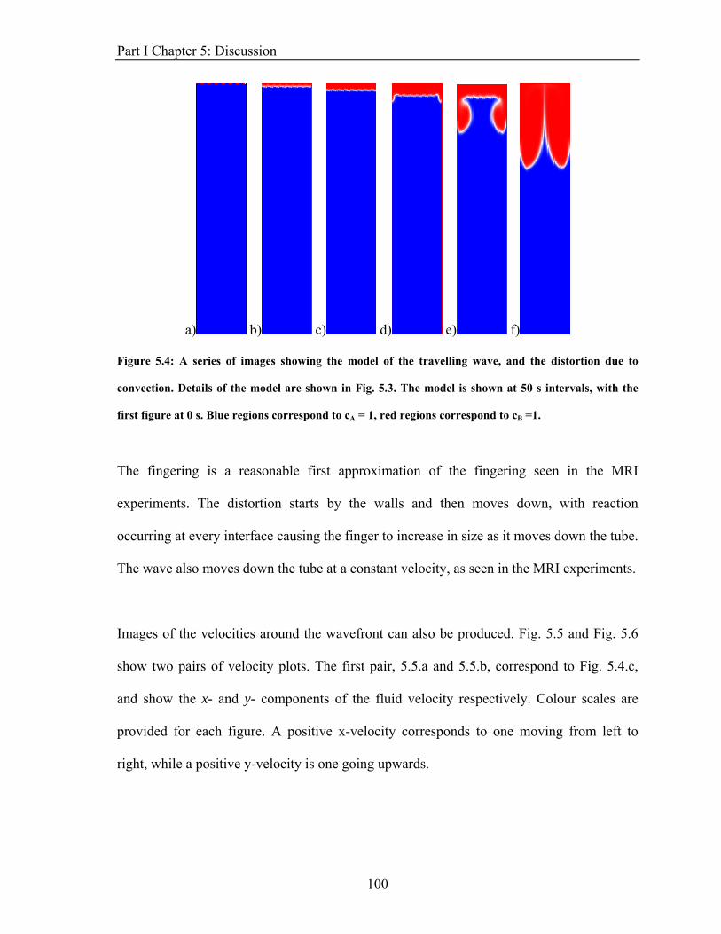
Part I Chapter 5: Discussion
a) b) c) d) e) f)
Figure 5.4: A series of images showing the model of the travelling wave, and the distortion due to
convection. Details of the model are shown in Fig. 5.3. The model is shown at 50 s intervals, with the
first figure at 0 s. Blue regions correspond to cA = 1, red regions correspond to cB =1.
The fingering is a reasonable first approximation of the fingering seen in the MRI
experiments. The distortion starts by the walls and then moves down, with reaction
occurring at every interface causing the finger to increase in size as it moves down the tube.
The wave also moves down the tube at a constant velocity, as seen in the MRI experiments.
Images of the velocities around the wavefront can also be produced. Fig. 5.5 and Fig. 5.6
show two pairs of velocity plots. The first pair, 5.5.a and 5.5.b, correspond to Fig. 5.4.c,
and show the x- and y- components of the fluid velocity respectively. Colour scales are
provided for each figure. A positive x-velocity corresponds to one moving from left to
right, while a positive y-velocity is one going upwards.
100
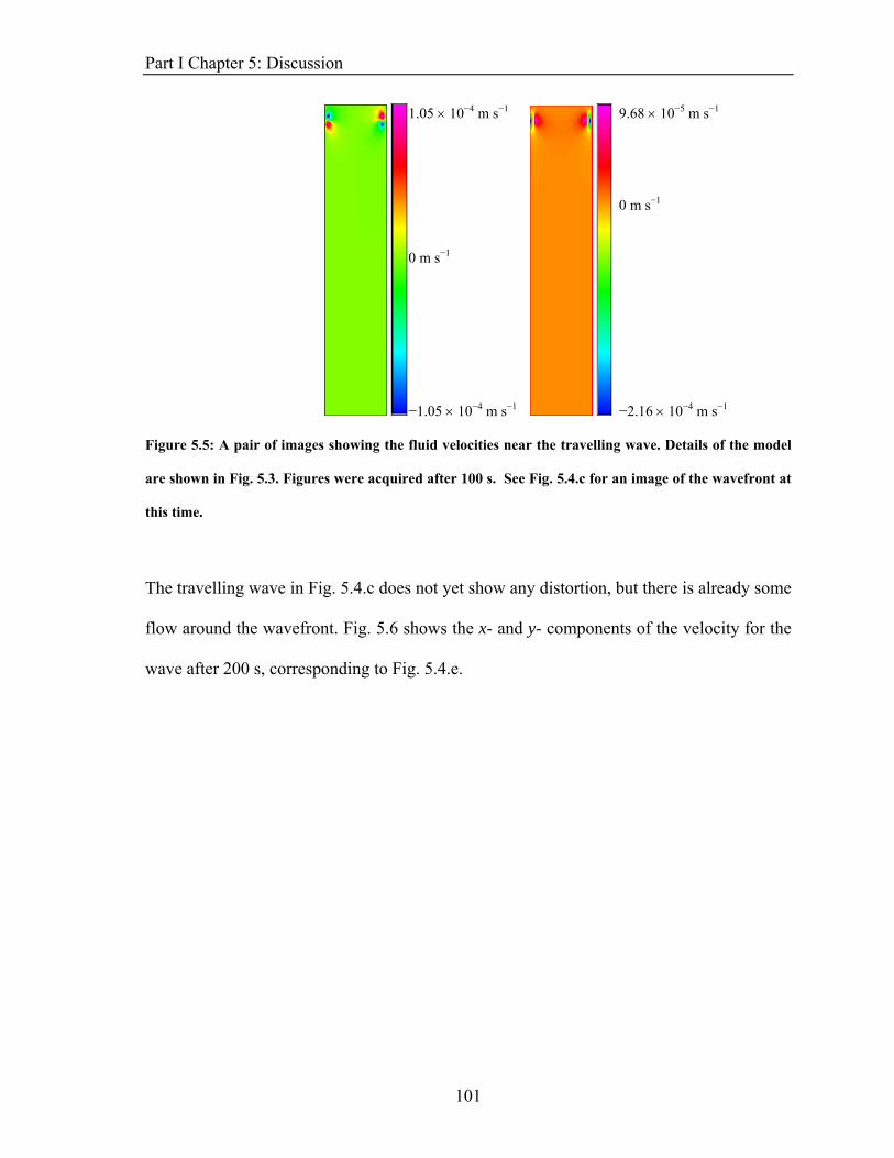
Part I Chapter 5: Discussion
1.05 × 10⁻⁴ m s−1
−1.05 × 10⁻⁴ m s−1 −2.16 × 10⁻⁴ m s−1
9.68 × 10⁻⁵ m s−1
0 m s−1
0 m s−1
Figure 5.5: A pair of images showing the fluid velocities near the travelling wave. Details of the model
are shown in Fig. 5.3. Figures were acquired after 100 s. See Fig. 5.4.c for an image of the wavefront at
this time.
The travelling wave in Fig. 5.4.c does not yet show any distortion, but there is already some
flow around the wavefront. Fig. 5.6 shows the x- and y- components of the velocity for the
wave after 200 s, corresponding to Fig. 5.4.e.
101
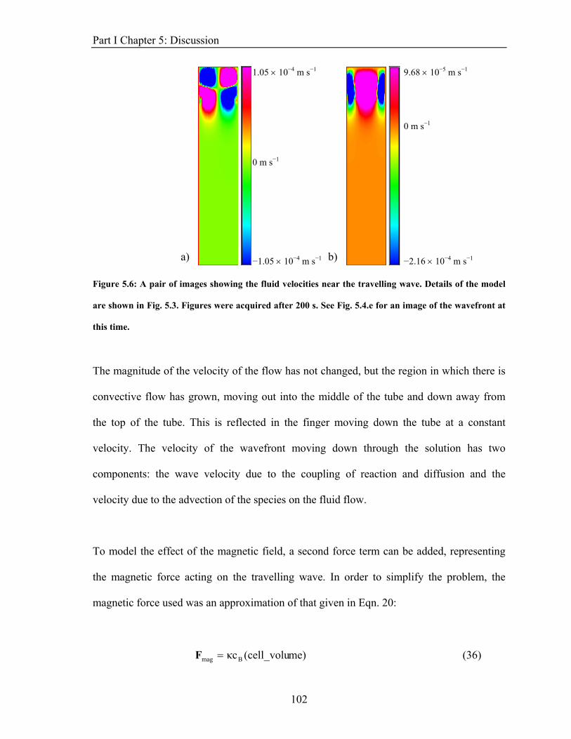
Part I Chapter 5: Discussion
1.05 × 10⁻⁴ m s−1
−1.05 × 10⁻⁴ m s−1
9.68 × 10⁻⁵ m s−1
−2.16 × 10⁻⁴ m s−1 a) b)
0 m s−1
0 m s−1
Figure 5.6: A pair of images showing the fluid velocities near the travelling wave. Details of the model
are shown in Fig. 5.3. Figures were acquired after 200 s. See Fig. 5.4.e for an image of the wavefront at
this time.
The magnitude of the velocity of the flow has not changed, but the region in which there is
convective flow has grown, moving out into the middle of the tube and down away from
the top of the tube. This is reflected in the finger moving down the tube at a constant
velocity. The velocity of the wavefront moving down through the solution has two
components: the wave velocity due to the coupling of reaction and diffusion and the
velocity due to the advection of the species on the fluid flow.
To model the effect of the magnetic field, a second force term can be added, representing
the magnetic force acting on the travelling wave. In order to simplify the problem, the
magnetic force used was an approximation of that given in Eqn. 20:
me)(cell_voluκcBmag =F (36)
102

Part I Chapter 5: Discussion
κ is a constant and cell_volume is the volume of one cell formed by the grid. The force is
calculated on a cell by cell basis at the start of each time step. This expression was chosen
as all of the important details of the original force could be included while it was simple
enough so that reasonable results could be obtained, quickly. The constant, κ, contains the
constant of proportionality between volume susceptibility and concentration, the product of
magnetic field and gradient (assumed to be constant) and μ0. In this expression, the force
was to act only on cB, rather than cA. This should make no difference to the model as a
force acting to drive the reacted solution down should be equal to one acting to drive the
unreacted solution up the tube.
Fig. 5.7 shows the initial conditions for the model. Some results of these simulations are
shown in Fig. 5.8.
cA=0, cB=1 at boundarycA=1, cB=0
throughout
DA = DB = 10−9 m2 s−1
k = 0.25
βA = 1 ×10⁻⁶ βB = 5 ×10⁻⁵ κ = ± 0.5
Figure 5.7: A schematic showing the initial conditions for the model of a travelling wave coupled with
density differences and with an extra force applied to the reaction, solved using CFD-ACE.
103

Part I Chapter 5: Discussion
Two possible configurations were modelled: one where the force acted alongside gravity (κ
−’ve) and one where it acted opposite to gravity (κ +’ve). For both simulations, the initial
conditions were set up with a denser solution propagating into a less dense solution. Fig.
5.8 shows some of the results of the simulation. Fig. 5.8.a shows the starting conditions for
the simulation and Fig. 5.8.b and Fig. 5.8.c contrast the different effects of the two applied
forces. In Fig. 5.8.b, the force was acting with gravity down the tube, and the travelling
wave was accelerated, while in Fig. 5.8.c, the force acted against gravity, so the distortion
of the wave was limited, leading to a flat wave and a slower wavefront velocity.
a) b) c)
Fmag F g ma
Figure 5.8: A set of images illustrating the effect of the additional force on the travelling wave. Image
5.8.a shows the initial conditions of the simulation. Both images 5.8.b and 5.8.c are of the wave 150 s
afterwards, but 5.8.b has a downwards magnetic force applied and 5.8.c has an upwards one applied.
Details of the model are shown in Fig. 5.7. Blue regions correspond to cA = 1, red regions correspond to
cB =1.
104
Part I Chapter 5: Discussion
It is immediately clear that these simulations do not model the behaviour observed in the
reaction that well. The finger is accelerated but a comparison with Fig. 4.6.b or 4.6.c shows
that the experimentally observed finger has a more well-defined shape.
One key difference between the models and experiments is that the experiments feature
short pulses of magnetic field with no extra force acting on the wave for most of the
experimental time. The expression for the force was simplified, with the smaller terms
ignored and κ estimated, so that some effect would be seen. As described earlier, the aim
was to make a model that worked and then gradually make it more accurate, so the
magnitude of the force could be made more precise in later simulations.
The effect of temperature changes need to be considered in order to fully model the
fingering. In this reaction, the fingering distortion only formed when the wave was
travelling downwards, suggesting that the change in density due to changes in composition
of the reaction dominate in the long term. In light of this, the addition of heat transfer to the
model was held off until a later stage. Heat would be modelled by using the Heat Transfer
option of CFD-ACE, which solved equations based on the conservation of energy.
Preliminary heat simulations including heat production and transfer produced
unsatisfactory results.
It was the aim of this short section to point the way towards potential simulations of this
highly complicated system using available software packages. These initial models do
provide some insight into the forces acting on the reaction, the flow of the fluid they
produce and how the wave distorts, without giving detailed answers. It does however
105
Part I Chapter 5: Discussion
provide a suitable platform for further work modelling both the phenomena of chemical
fingering and the effect of the magnetic force on the fingering.
5.2.2 Velocity Imaging
All of the images presented in Part I of the thesis were RARE images, contrasting the two
regions of the reacting system by exploiting the change of oxidation state across the
reaction wavefront. Variations on this technique exist, allowing the imaging of any velocity
flow in the sample. In the previous section, the simulations showed how convective flow
could interact with the travelling wave. By imaging the velocity of the solution in the
sample, detailed information about the mass transport around the wave front can be
obtained. The aim of this section is to briefly describe some techniques that could have
been used to image the velocity of fluid flow during the reaction, to show examples of the
images produced and what they show about the reaction and to discuss their use and,
ultimately, why they were not used.
The DANTE sequence13 overlays a grid of selective excitement before the image is
acquired and the image produced features a grid, distorted by any flow occurring in the
sample. An example of a DANTE image is shown in Fig. 5.9, with the grid clearly visible.
The image was acquired ~ 300 s after the initiation of the wave without magnetic field
gradients applied. The wave has distorted with fingers formed on both sides of the slice, but
the grid is only distorted close to the surface of the reaction.
106
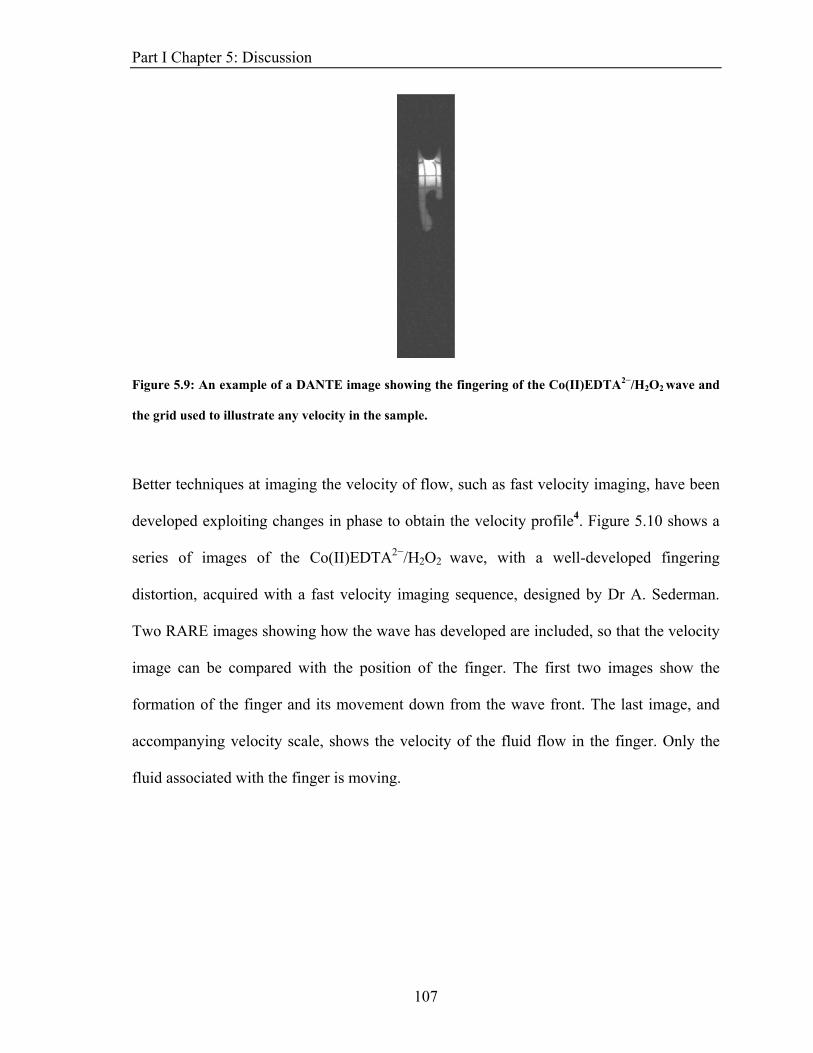
Part I Chapter 5: Discussion
Figure 5.9: An example of a DANTE image showing the fingering of the Co(II)EDTA2−/H2O2 wave and
the grid used to illustrate any velocity in the sample.
Better techniques at imaging the velocity of flow, such as fast velocity imaging, have been
developed exploiting changes in phase to obtain the velocity profile4. Figure 5.10 shows a
series of images of the Co(II)EDTA2−/H2O2 wave, with a well-developed fingering
distortion, acquired with a fast velocity imaging sequence, designed by Dr A. Sederman.
Two RARE images showing how the wave has developed are included, so that the velocity
image can be compared with the position of the finger. The first two images show the
formation of the finger and its movement down from the wave front. The last image, and
accompanying velocity scale, shows the velocity of the fluid flow in the finger. Only the
fluid associated with the finger is moving.
107

Part I Chapter 5: Discussion
0.7 mm s-1
a) b) c)
0 mm s-1
Figure 5.10: A series of images of a fingering distortion of the Co(II)EDTA2−/H2O2 reaction. Figs. 5.10.a
and 5.10.b are RARE images, with 51 s between the images. Fig 5.10.c is a velocity image of the same
finger, acquired 11 s after 5.10.b, with a colour scale showing the relevant velocities. Note that only
areas which have some signal intensity for the RARE image give information about their velocity.
In both sets of images, the velocity can only be measured in regions that produce a signal in
a RARE image. In these experiments, this means that only the velocity of regions of reacted
Co(III)EDTA− can be measured. The fast velocity imaging sequence also applied more
magnetic field gradients than the standard RARE imaging sequence and these gradients
manipulated the wave to a much greater extent. This limits the suitability of the technique
for analysis of the wave front but it still can be used to illustrate the velocities of flow in the
finger. Used in conjunction with the simulations described in the previous chapter, velocity
imaging could be a useful tool in observing and understanding the interactions between the
reaction, convective flow and the observed MFE. However, due to the increased
manipulation of the finger, a detailed study of the reaction using the technique was not
attempted.
108
Part I Chapter 5: Discussion
5.2.3 Other Reactions
The effects of inhomogeneous magnetic fields applied to travelling wave reactions should
not be limited to the reaction studied here. Any travelling wave reaction containing species
that exhibit a change in oxidation state and, hence, magnetic susceptibility across the
reaction wave front should show similar effects. MRI techniques used here can also be used
to image the reactions. Some reactions that have potential for further, similar, work are
briefly discussed here.
The Belousov-Zhabotinsky reaction would appear to be a prime candidate with waves of
changes in metal oxidation state being observed in an unstirred solution14. The change in
metal oxidation state also means that the reaction can be imaged by MRI techniques15,
although contrast between the oxidised and reduced forms of the catalyst might not always
be achieved, depending on the metal catalyst used16. There are also modifications of the
reaction, such as uncatalysed bromate oscillators that have been imaged using MRI
techniques17.
The reaction of iron(II) with concentrated nitric acid, the basis of the brown-ring test for
nitrates in qualitative analysis, can also produce a travelling wave18. The overall
stoichiometry of the reaction is given as:
3 Fe2+ + 4 H+ + NO3− 3 Fe3+ + 2 H2O + NO (37)
109
Part I Chapter 5: Discussion
HNO2 is the autocatalytic species for the reaction. There is a change in metal oxidation
state across the wave front, which could both be imaged and manipulated. This reaction
shows a large dependence of wave velocity on whether the wave is travelling up or down19,
suggesting that convection plays an important role in the propagation of the wave.
Radical chain polymerisation reactions are a further possibility. In these reactions, the
autocatalyst is not a chemical species but heat. Free-radical polymerisation reactions are
highly exothermic and thermal fronts, analogous to the chemical waves, can form20. The
changing concentrations of radicals in the reaction lead to changes in magnetic
susceptibility. It is also possible that large changes in viscosity could lead to better control
of the magnetic field effect and allow more dramatic manipulation of any wave.
Travelling waves are also found in biological systems. One possible system that exhibits
travelling wave behaviour and also contains paramagnetic species is the Ca2+ waves
observed in sea urchin eggs upon fertilisation. Importantly, the radical species NO is
involved in the signalling process21, with NO possibly acting as an autocatalytic species.
There has been some preliminary work investigating a possible magnetic field effect in this
system, but no magnetic field effect was seen and no further work has been attempted22.
The possibilities for further work on this reaction are not limited to this small section, with
better and different modelling techniques, a large range of possible, similar reactions and
velocity imaging techniques allowing more detailed investigation of the magnetic field
effect. This section should serve to act as an initial guide to any further work.
110
Part I Chapter 5: Discussion
111
At the start of the section, the magnetic field effect was introduced as a reaction in a
shallow layer in a Petri dish, with the magnetic field applied produced by a horseshoe
magnet placed underneath the dish. This effect can be quantitatively explained by
considering the magnetic field gradients around the magnet, with the wave accelerated out
from parallel to the sides of poles, but slowed down when travelling towards them. But the
work detailed here has developed from that initial problem. MRI experiments have shown a
wider range of behaviours, with different geometries of magnetic field having different
effects on the travelling wave. The mechanism by which the field interacts with the
travelling wave has also been investigated. Although not every detail of the magnetic field
effect is worked out and understood, this body of work goes a long way to understanding it
and opens up some interesting ideas for further research.

Part II: AN EXPERIMENTAL STUDY OF THE EFFECTS OF MAGNETIC FIELDS ON
THE OSCILLATIONS OF THE BELOUSOV-ZHABOTINSKY
REACTION
Part II Chapter 6: Introduction
113
6. INTRODUCTION
In Part I, the effect of an inhomogeneous magnetic field on an autocatalytic wave
reaction was observed, identified and investigated. In this section, the possibility that
the kinetics of a reaction could amplify a magnetic field effect is studied. The Belousov-
Zhabotinsky reaction between malonic acid and acidified bromate ions, catalysed by
metal ions, exhibits homogeneous oscillations in solution. A small body of work exists
suggesting that an applied magnetic field has an effect on the reaction, although there is
some doubt on the matter. Could the inherent autocatalysis of the reaction amplify any
magnetic field effect into one observable in the oscillations of the reaction? The sharp
changes in colour of the reacting solution allow for easy observation of the reaction, and
any potential effect on the reaction. The reaction also serves as a potential model of
biological systems as many of the features seen in this reaction are also observed in far
more complex systems.
6.1 A Brief History of the Belousov-Zhabotinsky Reaction
The Belousov-Zhabotinsky (BZ) reaction arose from attempts to replicate the Krebs
cycle using citric acid, a cerium salt and acidified bromate in 19511. The yellow colour
of the Ce4+ salt vanished, as expected, but then oscillations in the colour of the solution
between yellow and colourless were observed. These oscillations lasted for up to an
hour. And yet, even with recipes, photographs and an easily reproducible phenomenon,
referees refused to publish his results, saying that his “supposedly discovered
discovery”2 was impossible.

Part II Chapter 6: Introduction
There is a long history behind oscillating reactions, with oscillations in the combustion
of phosphorous observed by Boyle in the 1600s, but by the 1900s, it was assumed that
any oscillating reaction would pass through equilibrium on each oscillation and that the
Gibbs free energy of the system would decrease and then increase as the reaction took
place. The Bray reaction, a reaction between iodate and hydrogen peroxide3, first
attracted many more papers attempting to debunk the oscillations reported than trying to
explain their existence4. The BZ reaction was famously denied publication for several
years. It took further work by Zhabotinsky5 and theoretical work to show that the
reaction did not necessarily break the Second Law of Thermodynamics6. It was shown
that the oscillations are not of the reagents or products but of intermediate species such
as Br−, HBrO2 and the metal catalyst. Field, Körös and Noyes then produced a
mechanism for the reaction (the classic FKN mechanism7), which reproduced many of
the features of the reaction in particular its oscillations.
The BZ reaction shows a wide range of behaviour, from simple oscillations in a well-
stirred batch reaction, to series of wave trains when left unstirred, with more
complicated behaviour such as spiral patterns8 and chaotic oscillations9 also possible.
The reaction can be modified with a range of different metal catalysts and organic
substrates to provide an even greater range of behaviour. With the ruthenium salt
Ru(bipy)32+ as a catalyst, for example, oscillations in luminescence are observed under
ultraviolet irradiation10. This catalyst is also photosensitive, allowing manipulation of
the reaction using light11. Ce(III), Mn(II), Np(V) and ferroin (a complex of iron(II) and
1, 10 - phenanthroline) have all been investigated as catalysts of the reaction. The
organic substrate can also be modified. The first BZ reaction used citric acid, but
malonic acid is now more commonly used. Methyl-malonic acid and gallic acid have
114

Part II Chapter 6: Introduction
also been used in the reaction. More interesting is the use of compounds such as 1, 4-
cyclohexadione, which give rise to systems that do not need the metal catalyst12.
The change in colour of the metal catalyst provides an easy way to monitor the changes
in the state of the reaction but oscillations may also be observed in the redox potential
of the solution, determined by the ratio of metal in its oxidised and reduced forms, and
in the bromide ion concentration.
6.2 Mechanism of the BZ Reaction
The FKN mechanism, developed in 19727, was a key point in the history of the reaction.
It proposed a detailed mechanism for the reaction and gives a framework for
understanding the various phenomenon observed. It has been constantly updated, as
further experimental evidence has become available.
The overall reaction is driven by the oxidation of malonic acid by acidified bromate, but
the direct reaction between the two is slow.
3 BrO3− + 5 CH2(COOH)2 + 3 H+ → 3 BrCH(COOH)2 + HCOOH
+ 4 CO2 + 5 H2O (1)
The FKN mechanism is split into three sections: process A, the removal of bromide, an
inhibitor of the reaction, from the system, process B, the autocatalytic reaction that
oxidises the metal catalyst and process C, the regeneration of bromide and reduced form
of the metal catalyst by reaction with organic substrate. Processes A and B form the
115
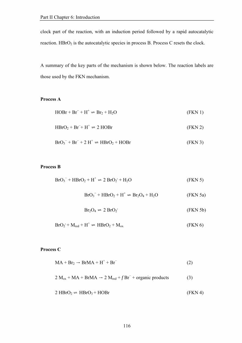
Part II Chapter 6: Introduction
clock part of the reaction, with an induction period followed by a rapid autocatalytic
reaction. HBrO2 is the autocatalytic species in process B. Process C resets the clock.
A summary of the key parts of the mechanism is shown below. The reaction labels are
those used by the FKN mechanism.
Process A
HOBr + Br− + H+ ⇌ Br2 + H2O (FKN 1)
HBrO2 + Br−+ H+ ⇌ 2 HOBr (FKN 2)
BrO3− + Br− + 2 H+ ⇌ HBrO2 + HOBr (FKN 3)
Process B
BrO3− + HBrO2 + H+ ⇌ 2 BrO2
. + H2O (FKN 5)
BrO3− + HBrO2 + H+ ⇌ Br2O4 + H2O (FKN 5a)
Br2O4 ⇌ 2 BrO2. (FKN 5b)
BrO2. + Mred + H+ ⇌ HBrO2 + Mox (FKN 6)
Process C
MA + Br2 → BrMA + H+ + Br− (2)
2 Mox + MA + BrMA → 2 Mred + f Br− + organic products (3)
2 HBrO2 ⇌ HBrO3 + HOBr (FKN 4)
116
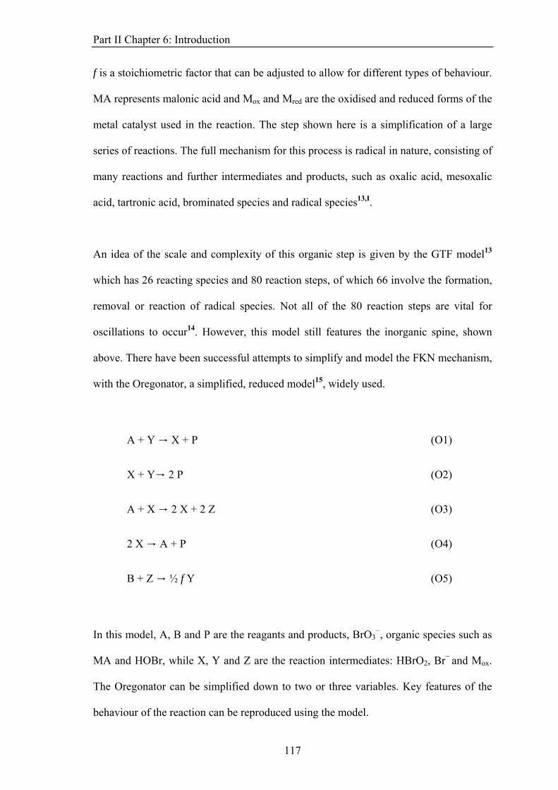
Part II Chapter 6: Introduction
f is a stoichiometric factor that can be adjusted to allow for different types of behaviour.
MA represents malonic acid and Mox and Mred are the oxidised and reduced forms of the
metal catalyst used in the reaction. The step shown here is a simplification of a large
series of reactions. The full mechanism for this process is radical in nature, consisting of
many reactions and further intermediates and products, such as oxalic acid, mesoxalic
acid, tartronic acid, brominated species and radical species13,I.
An idea of the scale and complexity of this organic step is given by the GTF model13
which has 26 reacting species and 80 reaction steps, of which 66 involve the formation,
removal or reaction of radical species. Not all of the 80 reaction steps are vital for
oscillations to occur14. However, this model still features the inorganic spine, shown
above. There have been successful attempts to simplify and model the FKN mechanism,
with the Oregonator, a simplified, reduced model15, widely used.
A + Y → X + P (O1)
X + Y→ 2 P (O2)
A + X → 2 X + 2 Z (O3)
2 X → A + P (O4)
B + Z → ½ f Y (O5)
In this model, A, B and P are the reagants and products, BrO3−, organic species such as
MA and HOBr, while X, Y and Z are the reaction intermediates: HBrO2, Br− and Mox.
The Oregonator can be simplified down to two or three variables. Key features of the
behaviour of the reaction can be reproduced using the model.
117
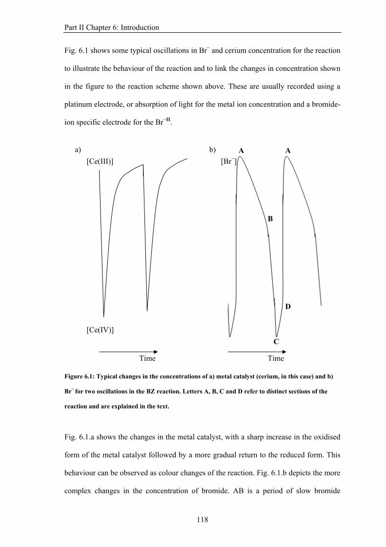
Part II Chapter 6: Introduction
Fig. 6.1 shows some typical oscillations in Br− and cerium concentration for the reaction
to illustrate the behaviour of the reaction and to link the changes in concentration shown
in the figure to the reaction scheme shown above. These are usually recorded using a
platinum electrode, or absorption of light for the metal ion concentration and a bromide-
ion specific electrode for the Br−II.
[Ce(III)]
[Ce(IV)]
[Br−] A
B
C
D
a) b) A
Time Time
Figure 6.1: Typical changes in the concentrations of a) metal catalyst (cerium, in this case) and b)
Br− for two oscillations in the BZ reaction. Letters A, B, C and D refer to distinct sections of the
reaction and are explained in the text.
Fig. 6.1.a shows the changes in the metal catalyst, with a sharp increase in the oxidised
form of the metal catalyst followed by a more gradual return to the reduced form. This
behaviour can be observed as colour changes of the reaction. Fig. 6.1.b depicts the more
complex changes in the concentration of bromide. AB is a period of slow bromide
118

Part II Chapter 6: Introduction
consumption, corresponding to process A (FKN 1-3), where Br− reacts with BrO3− and
HBrO2. When Br− falls to a certain, critical value, reaction FKN 2 is too slow to prevent
the reaction of HBrO2 with BrO3− and the autocatalytic FKN 5 dominates, with a large,
rapid increase in HBrO2. The section BC in Fig. 6.1.b corresponds to the sharp increase
in [Ce(IV)] in Fig. 6.1.a. The remaining small amount of Br− is rapidly consumed by the
rapidly increasing [HBrO2] and FKN 2. DA is a phase of rapid bromide production,
where the oxidised form of the metal catalyst reacts with BrMA to form Br−. The
reduced metal catalyst is regenerated, as seen in Fig. 6.1.a, and HBrO2 is removed by
reaction with Br− (FKN 2) and by disproportionation (FKN 4). A period of slow
bromide production, CD in Fig. 6.1.b, can appear in solutions with low concentrations
of MA present. Br2, produced in FKN 1, is removed by MA at too slow a rate and
accumulates, rather than reacting with the enol form of the MA to form Br−.
The original mechanism proposed by Field, Körös and Noyes7 has undergone some
revision since its publication. A revision of rate constants occurred as calculations
showed that some of the original set of rate constants were in error by several orders of
magnitude. These rate constants were calculated using the minimum amount of
thermodynamic and kinetic data, and as more information on the system was collected,
more accurate rate constants were produced. The key issue arose from estimating the
pK of HBrO2. A value of 2 can be assigned, based on the Pauling model of the strength
of oxyacids, but a value of ~ 4.9 was found to be more accurate16. A second set of rate
constants was developed, based on this change. The role of Br− in controlling the
reaction has also been put under some scrutiny. Addition of silver should suppress
oscillations as the formation of AgBr (solubility product at 25°C = 5 × 10⁻¹³ mol2 dm−6)
would quickly remove the Br− from the system. However, oscillations persisted, with no
119

Part II Chapter 6: Introduction
oscillations of Br− recorded by a bromide ion specific electrode17. This raised the
possibility of radicals, such as MA., being the control intermediate.
The inorganic oxybromine chemistry that makes up the backbone of the reaction has
remained essentially unchanged from its first formulation. The revised set of rate
constants developed in the years following the publication of the original FKN
mechanism are summarised in Table 1. Values in table obtained from Field et al18.
FKN step
Forward rate constant
k+
Reverse rate constant
k−
1
8 × 10⁹ M−2 s−1
110 s−1
2
3 × 10⁶ M−2 s−1
2 × 10⁻⁵ M−1 s−1
3
2 M−3 s−1
3.2 M−1 s−1
4
3 × 10³ M−1 s−1
1 × 10⁻⁸ M−2 s−1
5a
42 M−2 s−1
2.2 × 10³ s−1
5b
7.4 × 10⁴ M−2 s−1
1.4 × 10⁹ M−1 s−1
6
8 × 10⁴ M−2 s−1
8.9 × 10³ M−1 s−1
Table 1: Summary of the rate constants of FKN mechanism for the cerium-catalysed BZ reaction in
aqueous solution.
120
Part II Chapter 6: Introduction
Ferroin was used throughout the preliminary work to give an easy visual check on
whether oscillations were occurring. However, by changing the catalyst from cerium to
ferroin, several things are altered. In the experiments performed here, the key change is
that the BrO2. radical reacts with a different metal catalyst and this dramatically changes
the forward rate constant of that reaction18.
BrO2. + Ce(III) + H+ ⇌ Ce(IV) + HBrO2 (FKN 6)
k6+ = 8 × 10⁴ M−2 s−1
BrO2. + ferroin + H+ ⇌ ferriin + HBrO2 (FKN 6*)
k6*+ = 1.9 × 10⁹ M−2 s−1
There are other changes to the chemistry as the oxidised forms of the two metals react
with malonic acid in different ways. For the ferroin-catalysed reaction, this process is
very complicated19 and believed to feature radicals, due to the reaction
ferriin + MA ⇌ ferroin + MA. (4)
The BZ reaction is also sensitive to the addition of certain species which can interfere
with the oxybromine chemistry, leading to changes in the periods and even resulting in
the suppression of the oscillations. For example, Cl− ions interfere with the oxybromine
chemistry, by forming chlorous acid which reduces Ce(III) back to Ce(IV), to such an
extent that oscillations rapidly stop20. The addition of Ag+ has already been mentioned.
The low solubility product of AgBr means that Br− is precipitated out of the solution.
121
Part II Chapter 6: Introduction
This, in turn, means that process A is ‘short-circuited’ and the autocatalytic process B
occurs almost immediately as [Br−] falls rapidly below its critical level.
Irradiation of the reaction with light over a range of wavelengths has been observed to
have an effect on the reaction. The effect of visible light on the ferroin-catalysed
reaction has been studied, with the period and amplitude of the oscillations both
increasing, with suppression of the oscillations observed above a given intensity of
light21. However, irradiation using a laser flash at 632.8 nm has been shown to initiate
waves in a shallow layer22. The photosensitivity of the Ru(bipy)32+ catalysed reaction is
thought to be based on the formation of an excited species, *Ru(bipy)32+, which has a
significantly lower standard reduction potential than the ground state23. The question
now arises as to whether a similar effect could be observed with the reaction studied
here. Whatever effect irradiation of the reaction has depends on the wavelength and
intensity of the light used, the metal catalyst used and the particular state of the reaction,
due to the constantly changing concentrations of reagents as the reaction proceeds.
However, it could be an interesting method of perturbing the reaction without adding
extra solution into the cell. There is also a practical reason for investigating the effect of
light on the reaction. If the reaction is light sensitive then the light used to follow the
reaction could also be perturbing the reaction. These experiments can be used to check
whether the monitoring light used to follow the reaction is having any effect on its
oscillations.
In a shallow layer, the surface of the reaction does not feature any oscillations24.
Oxygen is known to be an inhibitor of the BZ reaction, although the precise effect
depends on the conditions of the reaction. Various methods of dealing with the presence
122
Part II Chapter 6: Introduction
of oxygen have been suggested, adjusting various sections of the Oregonator model.
Predictions of its effect on the reaction can be made by considering the oxygen to be
involved only in the organic part of the reaction (section C of the FKN mechanism)
interfering with the reaction of malonic acid with the oxidised form of the metal catalyst
by forming peroxyl radicals. Reacting solutions that minimise the effect of oxygen on
the reaction can be prepared25. In practical terms, flowing nitrogen through a degassed
solution throughout the experiment would ensure that the reaction is not affected by
oxygen.
6.3 Possibility of a Magnetic Field Effect
There exists a small body of published work detailing the effect of magnetic fields on
the BZ reaction. It is certainly an attractive system for such a study as the feedback
mechanism could allow for the amplification of any small effect. However, the work
published is contradictory as some papers report magnetic field effects in these systems
whilst others show no such effects.
No magnetic field effects were observed in the work of McLauchlan26, who expected
any change in the rate of the constituent reactions to have an amplified effect on the
period of the oscillations. However, several Russian researchers have reported a range
of effects, with static and oscillating fields used to reduce the wavelength of the
travelling waves in a shallow layer27, accelerate the rate of autocatalytic period of the
reaction, when performed as a clock with malonic acid absent28 and increase the
amplitude of the reaction29.
123
Part II Chapter 6: Introduction
More recently, Blank and Soo reported an acceleration of the ferroin-catalysed BZ
reaction when a weak oscillating electromagnetic field (ranging from 0 – 80 μT and 0 –
600 Hz) was applied to the reaction30. A small acceleration of the reaction (up to 10 %),
seen as a decreasing period of oscillation, was observed. This effect fell as the rate of
the reaction increased. The frequency dependence showed that a broad maximum effect
was observed around fields of frequency 250 Hz (for 5 μT fields). These experiments
were then used as a model for more complicated biological systems such as cytochrome
oxidase and Na, K-ATPase. Sontag, however, failed to reproduce the results seen in the
previous work, applying a range of magnetic fields at different field strengths and
frequencies (5 – 2700 μT, 10-250 Hz) to the reaction31. None of the experiments
showed a significant effect on the period of the reaction. Both of these sets of results
were performed in batch reactions.
So could this reaction exhibit a magnetic field effect? The first indication that a reaction
could be magnetic field dependent is the presence of a radical pair in the mechanism of
the reaction. The BZ reaction features many steps that involve radicals, mostly in the
reaction of the oxidised metal catalyst with the organic species present in the reaction.
However, one well-characterised step produces a pair of radicals with two possible
reaction fates – recombination to form the dimer or further reaction with the metal
species. Furthermore, the radicals form from a single precursor, Br2O4, so they should
be spin-correlated. There is also a potential spin selectivity of the radical pair, as the
singlet pair is capable of both recombination reaction or reaction with the metal, while
the triplet is only able to react with the metal species. The potential radical pair is
highlighted in the reaction scheme below.
124
Part II Chapter 6: Introduction
BrO3− + HBrO2 + H+ ⇌ 2 BrO2
. + H2O (FKN 5)
BrO3− + HBrO2 + H+ ⇌ Br2O4 + H2O (FKN 5a)
Br2O4 ⇌ 2 BrO2. (FKN 5b)
BrO2. + Mred + H+ ⇌ HBrO2 + Mox (FKN 6)
Importantly the radical pair highlighted above, 2 BrO2., is formed in the autocatalytic
step of the reaction, suggesting that even small changes in the reaction rates involved
could lead to an amplified effect on the period of the oscillations. It has to be pointed
out that this possible radical pair does not ensure that the whole reaction is magnetic
field dependent but its presence, particularly in the autocatalytic steps of the reaction, is
promising. It is possible that there are other reaction steps that feature radical pairs. For
the rest of this investigation though, discussion will focus on the radical pair identified
here and its properties.
The most likely mechanism by which S-T mixing occurs is through the hyperfine
coupling. With the identical pair of radicals predicted by this mechanism, the Δg
mechanism would have no effect on their spin evolution. Hyperfine constants for the
BrO2. molecule in solution can be estimated from the ESR of the species in an irradiated
K79BrO4 crystal32, which produces an average hyperfine coupling of 99 MHz. This
coupling corresponds to a magnetic field of 3.55 mT. The change in ‘solvent’ from the
solid state to aqueous solution could change the coupling, as any anisotropic
contributions to the hyperfine interaction would be averaged to zero leaving an isotropic
term. Both stable isotopes of bromine (79Br, 81Br) have magnetic nuclear spin quantum
number of 3/2, and are present in nearly equal proportions. Differences in the hyperfine
125
Part II Chapter 6: Introduction
126
couplings of the electron due to the different isotopes could occur, although they should
be small.
A field exceeding a few hundred mT should have a significant effect on a radical pair
with such hyperfine couplings, assuming that there are favourable conditions for
exhibition of a magnetic field effect. Slow relaxation, weak radical-radical interactions
and favourable diffusion increase the likelihood of an effect being observed. If an effect
was seen by a large field, then it is likely that the radical pair formed during the reaction
is being affected by the magnetic field, according to the RPM. If this first study reveals
any effect, further experiments can then be performed, using lower fields and oscillating
fields.
Part II Chapter 7: Methods and Materials
127
7. METHODS AND MATERIALS
7.1 Methods
7.1.1 Continuously-flowed Stirred Tank Reactor (CSTR)
The impact of a magnetic field on the rates of reaction can be studied using the most
obvious feature of the BZ reaction: the change in colour associated with any change in
metal oxidation state. Preliminary experiments were performed in the absence of
malonic acid and the clock behaviour observed using the changing absorption of light as
the reaction proceeds. However, it was very hard to perform the reaction reproducibly
as a single-shot clock as the timings and details of the reaction were observed to vary
hugely. Inhomogeneities such as defects on the cell wall can initiate the reaction and
cause the reaction to act as a wave rather than as a homogenous clock. Even without
such waves forming in the cell, the induction period was still found to be highly
variable, due to minute variations in the starting reaction mixture33.
Given that the full B-Z reaction resets itself by reaction of the organic species with the
oxidised form of the metal catalyst, a series of oscillations could be used to see if some
change to the system has an effect. Batch reactions can be studied but, even though the
oscillations produced can last for several hours, the oscillations eventually die out as the
reagents are consumed. There are also slight differences between consecutive
oscillations as the reaction proceeds, slowly but surely, towards equilibrium. If fresh
reagents are flowed into the cell, then a steady state can be reached where the loss of
reagents due to reaction is balanced by the inflow of reagents into the cell. The contents
of the cell have to be continuously stirred in order to prevent the formation of
Part II Chapter 7: Methods and Materials
inhomogeneities and concentration gradients in the cell. This apparatus is known as a
continuous-flow stirred tank reactor (CSTR)
Although more complicated behaviour can be observed using a CSTR to study the
reactionIII, the main reason for their use in this investigation is that a reacting mixture
can be maintained so that series of oscillations with periods that should not increase or
decrease with time can be produced. Once a series of oscillations is set up, any effect an
external perturbation has on the system can be studied via any observed changes in the
period, amplitude or shape of the oscillations.
A simple apparatus was designed and constructed in PTFE (polytetrafluoroethylene).
PTFE had to be used for two reasons: it is resistant to the highly acidic reacting
solution, unlike other plastics and metals, and also it is not magnetic. Fig. 7.1 shows two
diagrams of the apparatus, one from the front and one from the side. A pump to flow the
reacting solutions through the cell was also built. Two plastic syringes were pumped at
the same rate by a small electric motor attached to a gear box and rack and pinion gears,
with PTFE tubing connecting the two syringes to the cell holder. The overflow tube was
also a length of PTFE tubing, leading away from the cell holder. The reaction was
followed by absorption of light from an Oriel 66011 300 W lamp, with appropriate
filters used to select wavelengths of light. Light guides were used to direct the light into
and out of the cell to a photomultiplier tube (PMT), through a pair of aligned holes in
the cell holder (see Fig. 7.1).
128
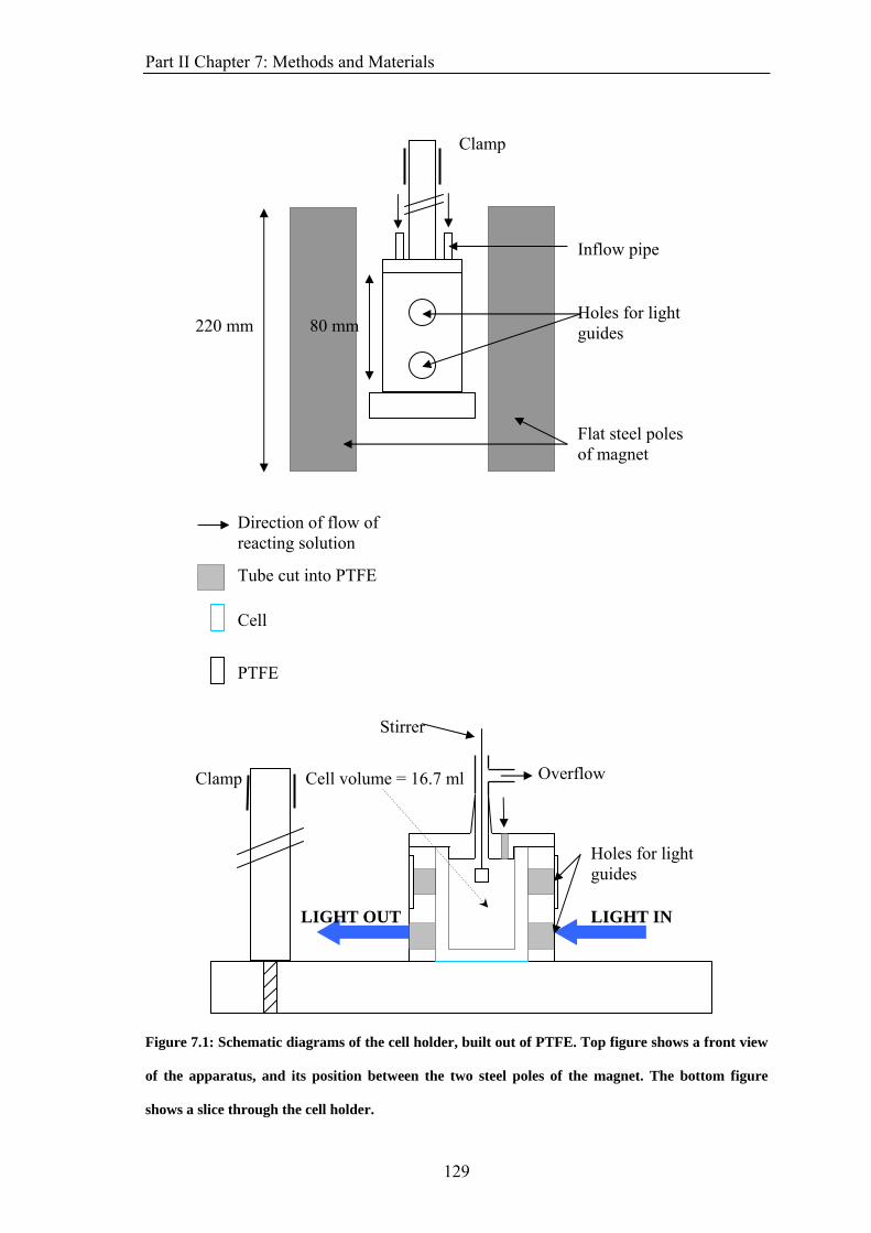
Part II Chapter 7: Methods and Materials
Clamp
Inflow pipe
Figure 7.1: Schematic diagrams of the cell holder, built out of PTFE. Top figure shows a front view
of the apparatus, and its position between the two steel poles of the magnet. The bottom figure
shows a slice through the cell holder.
Stirrer
LIGHT IN LIGHT OUT
Direction of flow of reacting solution
Tube cut into PTFE
Cell
PTFE
Flat steel poles of magnet
Clamp OverflowCell volume = 16.7 ml
220 mm 80 mm Holes for light guides
Holes for light guides
129
Part II Chapter 7: Methods and Materials
The lamp and PMT could be placed at a distance from the magnetic field so changes in
the magnetic field would have no effect on the voltage output of the PMT. The signal
produced by the PMT was recorded directly by a PCI 9112 data acquisition card using a
program written in Labview (see appendix IIIa). The oscillations were detected by
changes in the intensity of light passing through the cell, which can be related to
changes in the concentration of the metal catalyst.
Figs. 7.3 and 7.4 show the absorption spectra for the oxidised and reduced forms of
0.0025 M solutions of both ferroin and cerium solutions recorded in a cell with a path
length of 1 mm using a Unicam UV-2 UV/vis spectrometer. In both cases, the oxidised
form was produced by reacting 0.0025 M solution of the reduced metal solution with
0.35 M NaBrO3 and leaving overnight. For the ferroin experiments, a 510 nm filter was
used for the monitoring light and for the cerium experiments; a 380 nm filter was used.
Neither the bromate nor malonic acid used in the experiments absorbed at these
wavelengths.
130
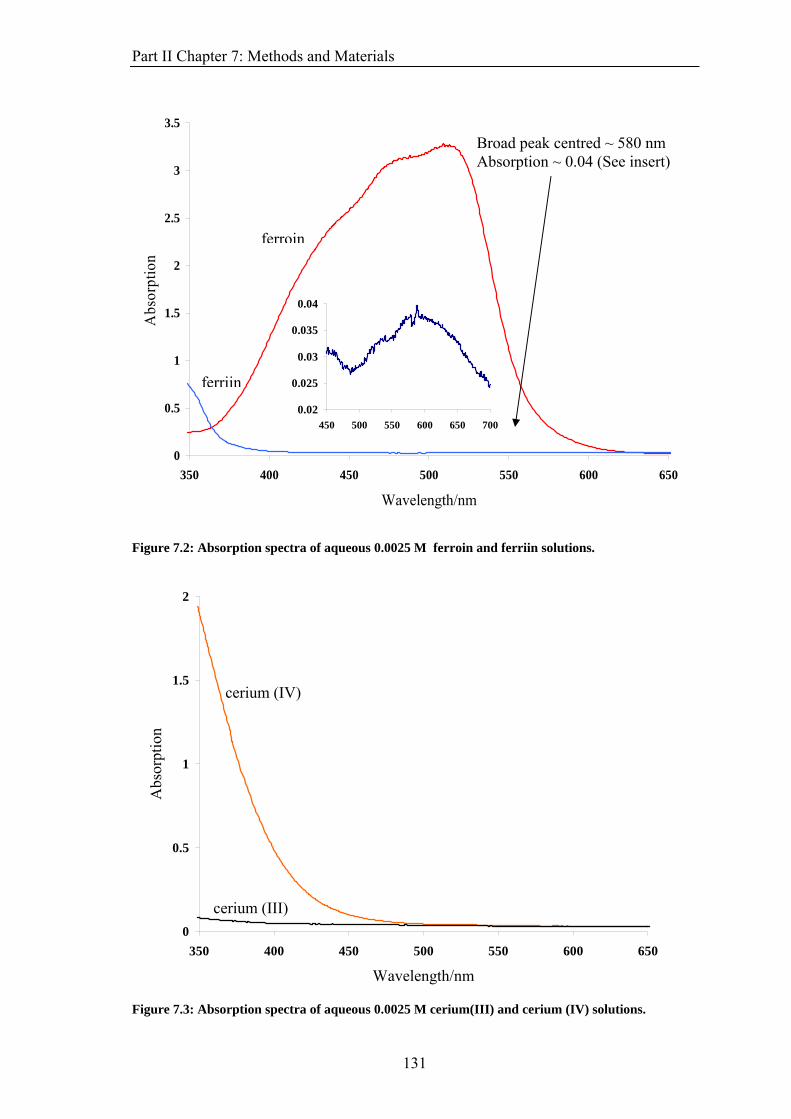
Part II Chapter 7: Methods and Materials
0
0.5
1
1.5
2
2.5
3
3.5
350 400 450 500 550 600 650
Wavelength/nm
Abs
orpt
ion
Broad peak centred ~ 580 nm Absorption ~ 0.04 (See insert)
ferroin
0.02
0.025
0.03
0.035
0.04
450 500 550 600 650 700
ferriin
Figure 7.2: Absorption spectra of aqueous 0.0025 M ferroin and ferriin solutions.
0
0.5
1
1.5
2
350 400 450 500 550 600 650
Wavelength/nm
Abs
orpt
ion
cerium (IV)
cerium (III)
Figure 7.3: Absorption spectra of aqueous 0.0025 M cerium(III) and cerium (IV) solutions.
131
Part II Chapter 7: Methods and Materials
The static magnetic field was generated by a large electromagnet with flat steel pole
pieces designed to produce a homogeneous field. The maximum field strength of the
magnet was 0.14 T and this was used in all of the magnetic field experiments. The cell
holder was designed to hold the cell in between the two flat poles, in middle of the
homogeneous region.
The BZ reaction is very sensitive to both changes in temperature and in stirring rate.
The period of oscillation can depend in a complex way on the stirring rate. Amongst
possible explanations are changes in the interaction between the gaseous and liquid
phases34 and incomplete mixing of the inflow of reagents into the CSTR leading to an
increased inhomogeneity within the reactor35. Any interaction between the stirring rate
and the reaction is going to be complicated. For the CSTR used in these experiments, a
fall in stirring rate lead to both a fall in amplitude and increasing period of oscillation.
Hence, it was crucial that the large static magnetic field would not affect the stirring
apparatus. The motor for the stirrer was placed in a μ-metal box. The arm of the stirrer
was long enough for the stirrer motor to be held away from the cell holder and the high
magnetic field produced by the flat magnetic poles. It was then shown in preliminary
experiments that the applied magnetic field had no effect on the stirring rate of the
stirrer.
The BZ reaction (and its derivatives) is sensitive to changes in temperature, with
increasing temperature leading to both reduced induction periods and periods of
oscillation36. A cell holder built from PTFE does not easily allow for the heating or
cooling of the mixture as the reaction proceeds. Instead, the temperature within the cell
was followed using a calibrated Pt100 and the changes in temperature as the reaction
132
Part II Chapter 7: Methods and Materials
itself proceeded were small, around 1° C. They also fell with time towards a steady
temperature in the cell, achieved after only a few minutes. The change in oscillation
period due to a change of 1° C was less than 1-2 s. The periods of oscillations observed
in the experiments ranged between 100 and 200 s, so the changes in period due to
changes in temperature would be no more than 1-2 % of the period.
Several experiments were performed to calibrate the apparatus. First, series of
oscillations were produced showing that the apparatus functioned as intended and that
oscillations in the metal catalysts could be observed. Subsequently, different
perturbations to the system were applied showing that changes in these oscillations
could be observed by the apparatus. For these experiments, Br− and UV light were used.
Addition of Br− was achieved by briefly removing the stirrer and pipetting 1 cm3 of
AgNO3 solution into the cell. For the irradiation experiments, a second lamp would be
used to irradiate the cell through the higher light guide hole, shown in Fig. 7.1. Finally,
the magnetic field would be applied, and any effect of this on the reaction could then be
determined.
7.1.2 Analysis
The experiments were conducted by flowing the reagent solutions through the apparatus
and obtaining a series of oscillations. After a number of oscillations, the magnetic field
would be turned on and further oscillations recorded before the magnetic field was
turned off. A small number of oscillations with no field applied were then recorded.
To analyse the period of the oscillations, a simple peak detection program was written
in Labview (see Appendix IIIb). This took the data recorded from the PMT and
133

Part II Chapter 7: Methods and Materials
calculated the first and second derivatives with respect to time. Negative peaks of the
second derivative under a certain threshold amount were then picked out and the period
of oscillation calculated by the difference in time between the two peaks. This is shown
in Fig. 7.4, with the red lines showing the raw PMT data of the oscillations, the blue
lines the first derivative with time of this data and the green lines the second derivative.
-5000
0
5000
10000
15000
20000
25000
30000
1020 1040 1060 1080 1100 1120 1140 1160 1180 1200
Time/s
PMT
outp
ut in
to c
ompu
ter
50
60
70
80
90
100
110
120
130
140
150
Osc
illat
ion
perio
d/s
.
raw PMT data
first derivative wrt time
second derivative wrt time
Period data point
Figure 7.4: Diagram showing the raw data, and first and second derivatives, for a pair of
oscillations in the ferroin-catalysed BZ reaction. The period of the oscillation is calculated and
shown as a black square between the two peaks. All data presented in Chapter 8 will consist of
series of oscillations recorded from the PMT and the periods of these oscillations in the same figure
(see Fig. 8.1 for an example).
To determine if a change had occurred, and if that change was statistically significant,
Student’s t-test was used to test if the results were statistically different from each other.
134

Part II Chapter 7: Methods and Materials
It was then proposed that if an effect was observed using the highest field possible using
the magnet, further experiments would be performed using lower fields and oscillating
fields to start to quantify any effect.
7.2 Materials
Sodium bromate, sulphuric acid, silver nitrate and malonic acid, of A.C.S. grade, were
obtained from Aldrich and used without further purification.
A stock ferroin solution was produced by dissolving iron sulphate (FeSO4.7H2O) and 1,
10 – phenanthroline in Analar water to produce a 0.025 M solution. Both the iron
sulphate and 1, 10 – phenanthroline were obtained from Aldrich and used without
further purification. Cerium (IV) ammonium nitrate (Ce(NH4)2(NO3)6) was obtained
from Aldrich and used without further purification.
Table 2 summarises the reacting solutions used in the experiments. A second set of
concentrations for the cerium-catalysed reaction were prepared to eliminate the effect of
oxygen on the reaction25. The original reaction mixture is based on one detailed in
Scott’s “Oscillations, Waves, and Chaos in Chemical Kinetics”.
135
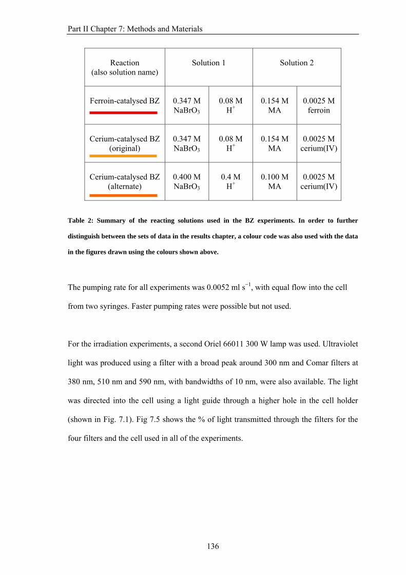
Part II Chapter 7: Methods and Materials
Reaction
(also solution name)
Solution 1
Solution 2
Ferroin-catalysed BZ
0.347 M NaBrO3
0.08 M
H+
0.154 M
MA
0.0025 M
ferroin
Cerium-catalysed BZ
(original)
0.347 M NaBrO3
0.08 M
H+
0.154 M
MA
0.0025 M
cerium(IV)
Cerium-catalysed BZ
(alternate)
0.400 M NaBrO3
0.4 M
H+
0.100 M
MA
0.0025 M
cerium(IV)
Table 2: Summary of the reacting solutions used in the BZ experiments. In order to further
distinguish between the sets of data in the results chapter, a colour code was also used with the data
in the figures drawn using the colours shown above.
The pumping rate for all experiments was 0.0052 ml s−1, with equal flow into the cell
from two syringes. Faster pumping rates were possible but not used.
For the irradiation experiments, a second Oriel 66011 300 W lamp was used. Ultraviolet
light was produced using a filter with a broad peak around 300 nm and Comar filters at
380 nm, 510 nm and 590 nm, with bandwidths of 10 nm, were also available. The light
was directed into the cell using a light guide through a higher hole in the cell holder
(shown in Fig. 7.1). Fig 7.5 shows the % of light transmitted through the filters for the
four filters and the cell used in all of the experiments.
136
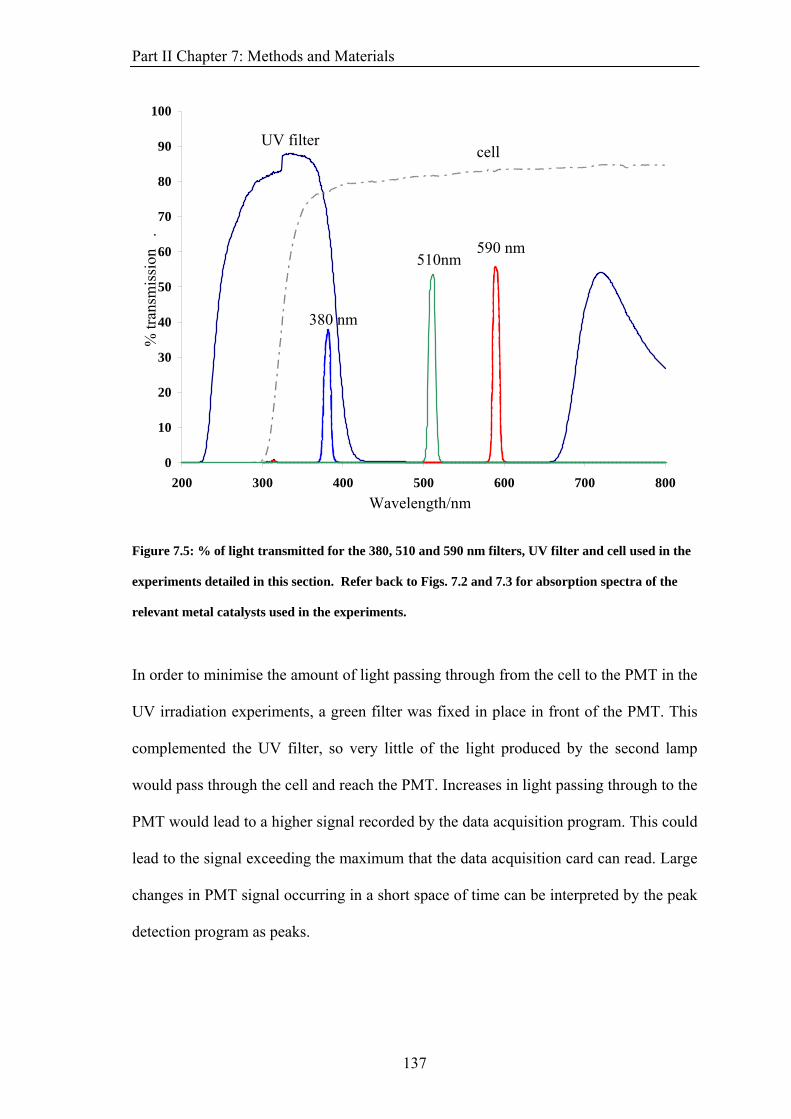
Part II Chapter 7: Methods and Materials
0
10
20
30
40
50
60
70
80
90
100
200 300 400 500 600 700 800
wavelength/nm
% tr
ansm
issi
on
.
cell UV filter
590 nm 510nm
380 nm
Wavelength/nm
Figure 7.5: % of light transmitted for the 380, 510 and 590 nm filters, UV filter and cell used in the
experiments detailed in this section. Refer back to Figs. 7.2 and 7.3 for absorption spectra of the
relevant metal catalysts used in the experiments.
In order to minimise the amount of light passing through from the cell to the PMT in the
UV irradiation experiments, a green filter was fixed in place in front of the PMT. This
complemented the UV filter, so very little of the light produced by the second lamp
would pass through the cell and reach the PMT. Increases in light passing through to the
PMT would lead to a higher signal recorded by the data acquisition program. This could
lead to the signal exceeding the maximum that the data acquisition card can read. Large
changes in PMT signal occurring in a short space of time can be interpreted by the peak
detection program as peaks.
137

Part II Chapter 7: Methods and Materials
138
A 0.0167 M AgNO3 solution was made for experiments where silver ions interfered
with the oxybromine chemistry of the reaction. 1 ml of this was pipetted into the middle
of the cell when required giving a concentration of Ag+ in the cell of 0.001 M.
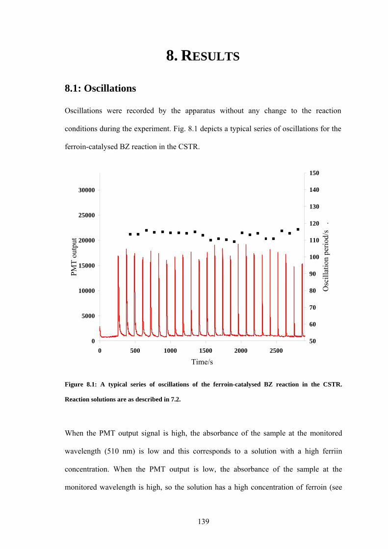
Part II Chapter 8: Results
139
8. RESULTS
8.1: Oscillations
Oscillations were recorded by the apparatus without any change to the reaction
conditions during the experiment. Fig. 8.1 depicts a typical series of oscillations for the
ferroin-catalysed BZ reaction in the CSTR.
0
5000
10000
15000
20000
25000
30000
0 500 1000 1500 2000 2500
Time/s
PMT
outp
ut
50
60
70
80
90
100
110
120
130
140
150
Osc
illat
ion
perio
d/s
.
Figure 8.1: A typical series of oscillations of the ferroin-catalysed BZ reaction in the CSTR.
Reaction solutions are as described in 7.2.
When the PMT output signal is high, the absorbance of the sample at the monitored
wavelength (510 nm) is low and this corresponds to a solution with a high ferriin
concentration. When the PMT output is low, the absorbance of the sample at the
monitored wavelength is high, so the solution has a high concentration of ferroin (see
Part II Chapter 8: Results
Fig. 7.4 for relevant absorption spectra). For the typical set of data depicted in Fig. 8.1,
the average period was 113.4 s with a standard deviation of ± 2.0 s. Similar sets of data
were produced, with the standard deviation of the data varying between 2 and 6 s. This
set of results is an indication that the apparatus could be used to follow any changes in
the period of oscillations of a reaction, as long as they are greater than the inherent noise
of our design (~ 5 s).
There is a small amount of noise in the period of oscillation but, given that it is not a
general trend (i.e. an increasing or decreasing period), it must arise from small and
random fluctuations in the temperature or flow rate of the reaction or transient
formation of small areas of inhomogeneity in the cell. These result in small changes in
the concentrations of the reagents inside the cell so that each oscillation is not quite be
the same as the one preceding it. A small fluctuation in the period of oscillation is
introduced. As long as this is only a random variation around a constant period, rather
than a drift in the period, the CSTR can be considered to be working well enough to
detect the effects of applying a magnetic field to the oscillations. An error of the size
observed is unlikely to arise from the peak detection program. A small error could arise
in the location where the peak detection program picks the peak of the second
derivative. However, this should not be more than the time between points (~ 0.4 s).
The difference in period of oscillation between sets of experiments was found to be
greater than the difference in period during an experiment. The BZ reaction is
notoriously sensitive to its initial conditions33, with slight changes in the autocatalyst
(HBrO2) and inhibitor (Br−) concentrations causing large differences in oscillation and
induction period. Other factors such as small differences in stirring rate, temperature
140

Part II Chapter 8: Results
and inhomogeneities on the cell wall can cause differences between experiments. As
explained previously, the nature of our apparatus made changing the temperature of the
solutions within it difficult, but once the reaction was running and the solutions flowing,
the temperature remained stable. Another factor that can influence the oscillations is the
presence of trace impurities. Attempts to remove them were taken by using the purest
water available, Analar water, and the chemicals of the purest grade possible. The
apparatus was thoroughly cleaned between experiments with concentrated nitric acid
and rinsed with Analar water.
Fig. 8.2 shows a typical series of oscillations for the cerium-catalysed BZ reaction in the
CSTR, obtained 2500 s into the reaction.
0
5000
10000
15000
20000
25000
30000
2500 3000 3500 4000 4500 5000 5500 6000Time/s
PMT
outp
ut
50
75
100
125
150
175
200
Osc
illat
ion
perio
d/s
.
Figure 8.2: A typical series of oscillations of the cerium-catalysed BZ reaction in the CSTR, using
the reacting solution, cerium-catalysed BZ I, as described in 7.2.
141
Part II Chapter 8: Results
Light of wavelength 380 nm was used to monitor the reaction. For this experiment, the
PMT output is high when the reacting solution has a high Ce(III) concentration, and the
PMT output is low when the reacting solution has a high Ce(IV) concentration (see Fig.
7.4 for relevant absorption spectra).
The same issues of reproducibility that affected the ferroin-catalysed reaction also
affected the cerium-catalysed one. For the typical set of data shown in the figure, the
average period of oscillation was 178.5 s with a standard deviation of ± 4.9 s. Similar
sets of data were produced with similar standard deviations in the period data. As with
the ferroin catalysed reaction, the difference in period of oscillation between sets of
experiments was found to be greater than the difference in period during an experiment.
The oscillations seen in both sets of experiments are as expected for the reaction
(compare with Fig. 6.1.a), with rapid production of the oxidised metal catalyst and a
more gradual return to the reduced form. The difference in period between the ferroin-
catalysed and cerium-catalysed reactions can be assigned to the large differences in rate
constant that arise when the catalyst is changed, such as in R6 (see discussion in chapter
6.2). Fig. 8.3 compares single oscillations from the two sets of data, drawn on the same
time-scale for clarity.
142
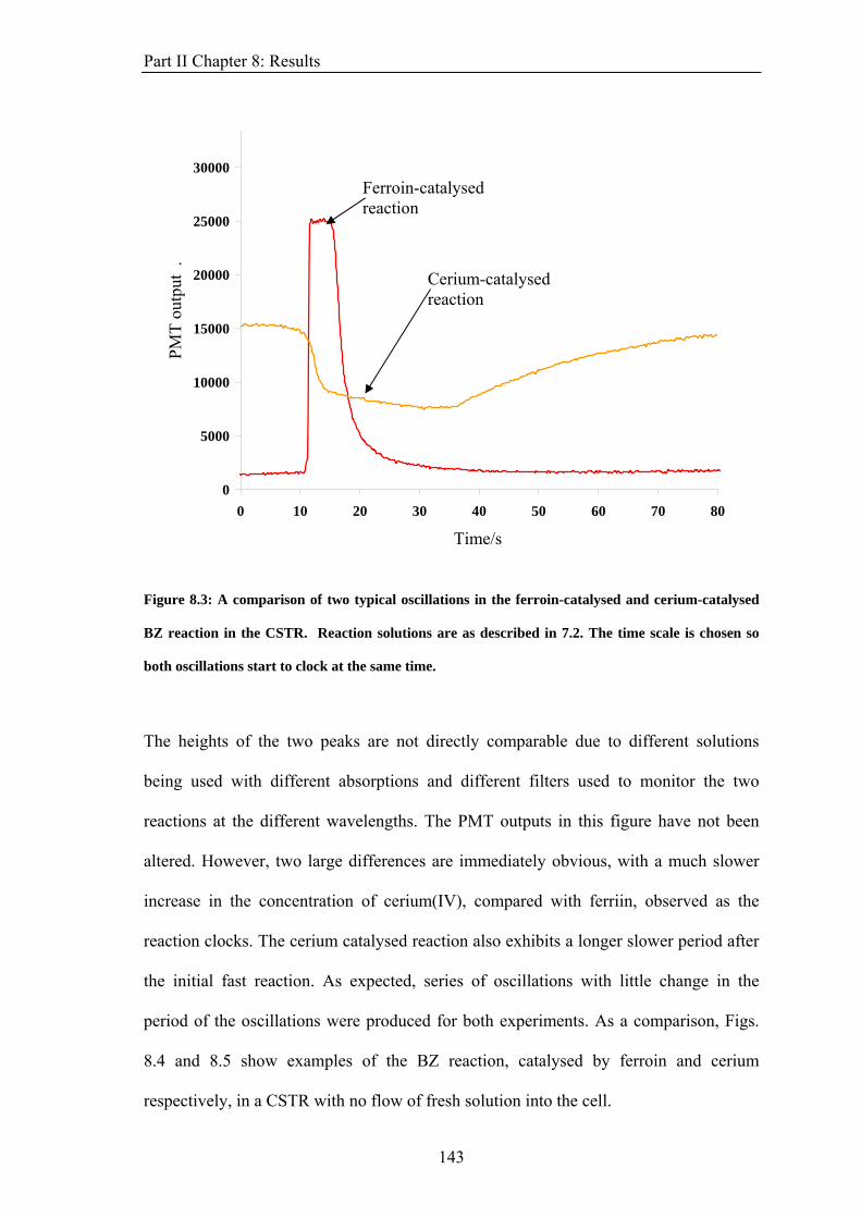
Part II Chapter 8: Results
0
5000
10000
15000
20000
25000
30000
0 10 20 30 40 50 60 70 80
Ferroin-catalysed reaction
PMT
outp
ut . Cerium-catalysed
reaction
time/sT ime/s
Figure 8.3: A comparison of two typical oscillations in the ferroin-catalysed and cerium-catalysed
BZ reaction in the CSTR. Reaction solutions are as described in 7.2. The time scale is chosen so
both oscillations start to clock at the same time.
The heights of the two peaks are not directly comparable due to different solutions
being used with different absorptions and different filters used to monitor the two
reactions at the different wavelengths. The PMT outputs in this figure have not been
altered. However, two large differences are immediately obvious, with a much slower
increase in the concentration of cerium(IV), compared with ferriin, observed as the
reaction clocks. The cerium catalysed reaction also exhibits a longer slower period after
the initial fast reaction. As expected, series of oscillations with little change in the
period of the oscillations were produced for both experiments. As a comparison, Figs.
8.4 and 8.5 show examples of the BZ reaction, catalysed by ferroin and cerium
respectively, in a CSTR with no flow of fresh solution into the cell.
143
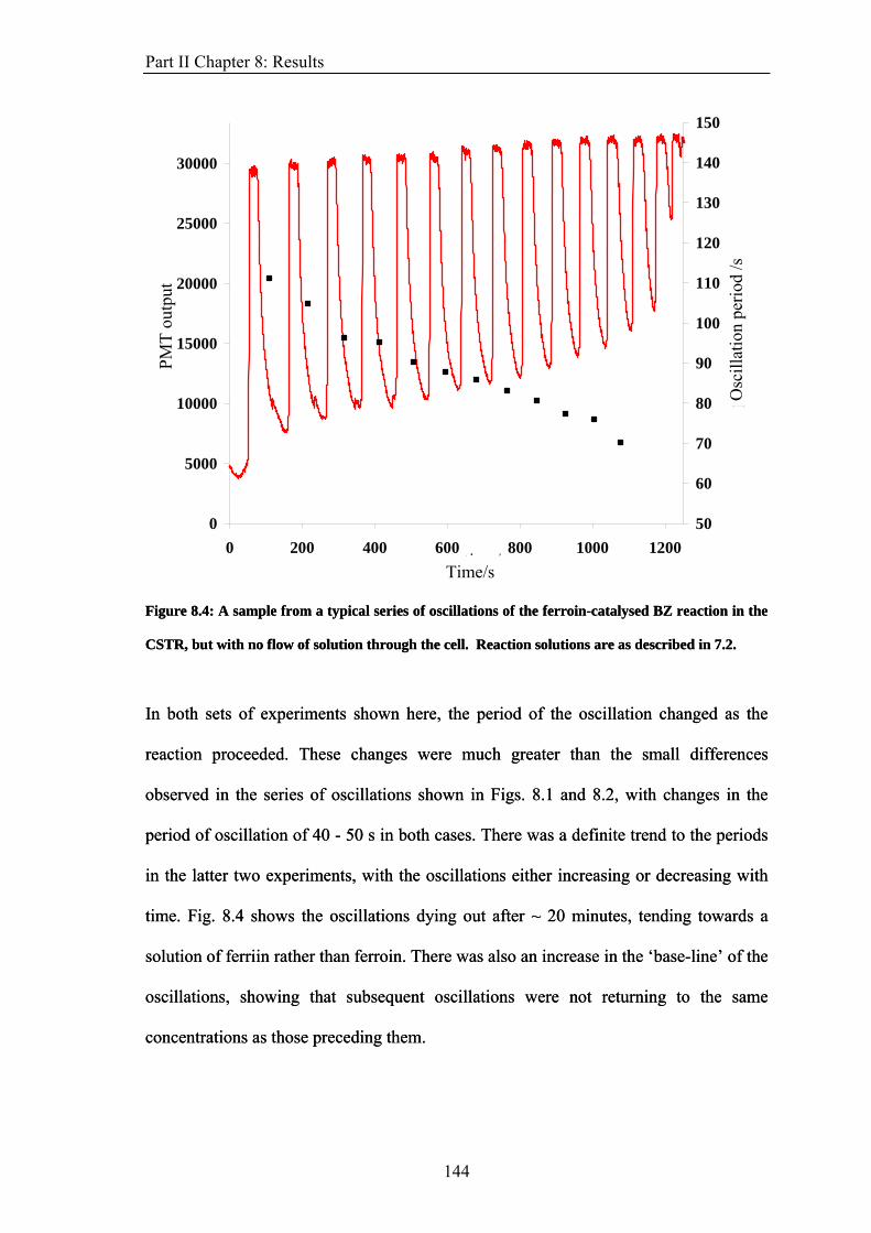
Part II Chapter 8: Results
0
5000
10000
15000
20000
25000
30000
0 200 400 600 800 1000 1200
PMT
outp
ut
50
60
70
80
90
100
110
120
130
140
150
llatio
ns/s
.pe
riod
of o
scill
atio
ns/s
.O
scill
atio
n pe
riod
/s
time/sTime/s
Figure 8.4: A sample from a typical series of oscillations of the ferroin-catalysed BZ reaction in the
CSTR, but with no flow of solution through the cell. Reaction solutions are as described in 7.2.
Figure 8.4: A sample from a typical series of oscillations of the ferroin-catalysed BZ reaction in the
CSTR, but with no flow of solution through the cell. Reaction solutions are as described in 7.2.
In both sets of experiments shown here, the period of the oscillation changed as the
reaction proceeded. These changes were much greater than the small differences
observed in the series of oscillations shown in Figs. 8.1 and 8.2, with changes in the
period of oscillation of 40 - 50 s in both cases. There was a definite trend to the periods
in the latter two experiments, with the oscillations either increasing or decreasing with
time. Fig. 8.4 shows the oscillations dying out after ~ 20 minutes, tending towards a
solution of ferriin rather than ferroin. There was also an increase in the ‘base-line’ of the
oscillations, showing that subsequent oscillations were not returning to the same
concentrations as those preceding them.
144

Part II Chapter 8: Results
0
5000
10000
15000
20000
25000
30000
710 910 1110 1310 1510 1710
time/s
PMT
outp
ut
.
50
75
100
125
150
175
200
..O
scill
atio
n Pe
riod
Pe
riod
O
scill
atio
n pe
riod/
s
Time/s
Figure 8.5: A sample from a typical series of oscillations of the cerium-catalysed BZ reaction in the
CSTR, but with no flow of solution through the cell. Reaction solutions are as described in 7.2.
Figure 8.5: A sample from a typical series of oscillations of the cerium-catalysed BZ reaction in the
CSTR, but with no flow of solution through the cell. Reaction solutions are as described in 7.2.
Fig. 8.5, on the other hand, shows the period of the oscillations growing with time.
These oscillations also, eventually, died out with time. With the CSTR apparatus
producing series of oscillations that changed little with time, the experiments could now
move on to studying the effect of known perturbations on the oscillating reaction.
8.2: Preliminary Results 8.2: Preliminary Results
With the apparatus producing suitable series of oscillations, it needed to be tested as to
whether changes in the period could be observed. Known perturbations on the reaction,
such as irradiation and the addition of certain chemicals, were used to further test the
experiment.
With the apparatus producing suitable series of oscillations, it needed to be tested as to
whether changes in the period could be observed. Known perturbations on the reaction,
such as irradiation and the addition of certain chemicals, were used to further test the
experiment.
145
Part II Chapter 8: Results
8.2.1: Addition of Ag+ ions
As described in Chapter 6.2, the addition of Ag+ to a reacting BZ solution can result in
the suppression of oscillations. With any Br− present removed by the Ag+, there should
be a sudden switch to a solution of Mox. Once all of the Br− is removed, then a
combination of the BZ reaction releasing Br− from brominated organic species and
reactions of other oxybromine species and the inflow of new solution increases the
concentration of Br− in the cell and oscillations resume.
For the experiments where AgNO3 solution was added to the system, the stirrer was
briefly removed and 1 cm3 of solution was pipetted into the bottom of the cell, before
the stirrer was replaced. A small series of preliminary experiments were performed,
showing that there was no effect on the reaction from removing the stirrer for a short
period of time, or from inserting a pipette into the solution. Fig. 8.6 shows the effect of
adding silver ions to the BZ reaction.
146
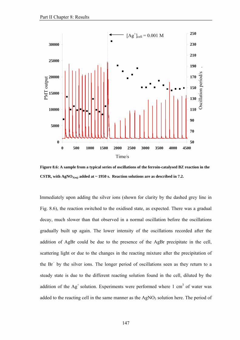
Part II Chapter 8: Results
0
5000
10000
15000
20000
25000
30000
0 500 1000 1500 2000 2500 3000 3500 4000 4500
PMT
outp
ut
50
70
90
110
130
150
170
190
210
230
250
Osc
illat
ion
perio
d/s
.
[Ag+]cell = 0.001 M
time/sTime/s
Figure 8.6: A sample from a typical series of oscillations of the ferroin-catalysed BZ reaction in the
CSTR, with AgNO3(aq) added at ~ 1950 s. Reaction solutions are as described in 7.2.
Immediately upon adding the silver ions (shown for clarity by the dashed grey line in
Fig. 8.6), the reaction switched to the oxidised state, as expected. There was a gradual
decay, much slower than that observed in a normal oscillation before the oscillations
gradually built up again. The lower intensity of the oscillations recorded after the
addition of AgBr could be due to the presence of the AgBr precipitate in the cell,
scattering light or due to the changes in the reacting mixture after the precipitation of
the Br− by the silver ions. The longer period of oscillations seen as they return to a
steady state is due to the different reacting solution found in the cell, diluted by the
addition of the Ag+ solution. Experiments were performed where 1 cm3 of water was
added to the reacting cell in the same manner as the AgNO3 solution here. The period of
147

Part II Chapter 8: Results
the oscillations was seen to increase. The residence time of the cell in this reaction was
~3200 s, so it is not surprising that the oscillations are starting to fall to a steady state
after a delay of a similar period.
Fig. 8.7 shows the effect of Ag+ ions on the cerium-catalysed reaction.
0
5000
10000
15000
20000
25000
30000
0 1000 2000 3000 4000 5000 6000 7000Time/s
PMT
outp
ut
50
70
90
110
130
150
170
190
210
230
250
Osc
illat
ion
perio
d/s
.
[Ag+]cell = 0.001 M
Figure 8.7: A sample from a typical series of oscillations of the cerium-catalysed BZ reaction in the
CSTR, with AgNO3(aq) added at ~ 1950 s. Reaction solutions are as described in 7.2.
The addition of the silver ions has a very similar effect, except that the PMT output
drops rapidly upon addition of the AgNO3, further than the lowest point observed
during the oscillations. This could be due to the formation of the AgBr(s) in the cell,
scattering light and preventing it from reaching the PMT. As with the ferroin catalysed
reaction, the oscillations do start again over time with a decrease in the maximum PMT
148
Part II Chapter 8: Results
output, possibly due to the presence of the precipitate in the cell. After a delay of around
3000 s, the oscillations have started to return to a steady state. This is probably due to
the concentration of Br− returning to a value that can support oscillations due to
formation by reaction of brominated organic species in the solution and reaction of
other oxybromine compounds in the cell, as well as inflow of fresh reagents.
Both sets of data show that large changes in the oscillations could be observed, through
changes in the height of the oscillations and in their periods. The amount of quantitative
information that can be obtained from these sets of data does look limited, with only the
qualitative effects of the perturbation easily obtained.
8.2.2: Irradiation of Reaction
The second method of perturbing the reaction was to irradiate the sample with light. The
effect of light on the BZ reaction is highly dependent on not only the metal catalyst used
but also on the state of the reaction when the light is applied. The oscillations mean that
the concentration of the reagents is constantly changing with time. In all of the
experiments carried out, the light was applied at the same point, at the peak of any
oscillation, so that the effects could be easily compared from experiment to experiment.
It was also applied continuously for several oscillations, so that all of the reaction was
irradiated.
149
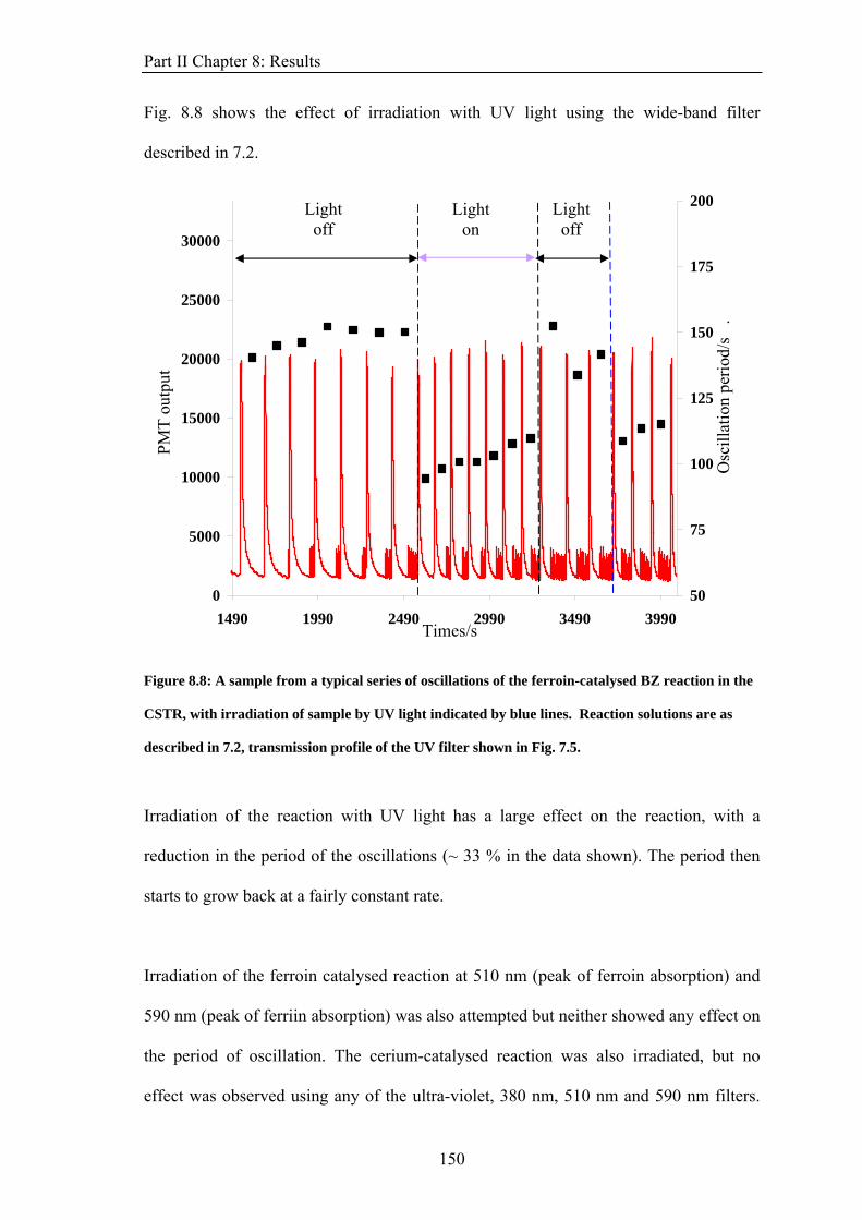
Part II Chapter 8: Results
Fig. 8.8 shows the effect of irradiation with UV light using the wide-band filter
described in 7.2.
0
5000
10000
15000
20000
25000
30000
1490 1990 2490 2990 3490 3990Times/s
PMT
outp
ut
50
75
100
125
150
175
200
Osc
illat
ion
perio
d/s
.
Light off
Light off
Light on
Figure 8.8: A sample from a typical series of oscillations of the ferroin-catalysed BZ reaction in the
CSTR, with irradiation of sample by UV light indicated by blue lines. Reaction solutions are as
described in 7.2, transmission profile of the UV filter shown in Fig. 7.5.
Irradiation of the reaction with UV light has a large effect on the reaction, with a
reduction in the period of the oscillations (~ 33 % in the data shown). The period then
starts to grow back at a fairly constant rate.
Irradiation of the ferroin catalysed reaction at 510 nm (peak of ferroin absorption) and
590 nm (peak of ferriin absorption) was also attempted but neither showed any effect on
the period of oscillation. The cerium-catalysed reaction was also irradiated, but no
effect was observed using any of the ultra-violet, 380 nm, 510 nm and 590 nm filters.
150
Part II Chapter 8: Results
These wavelengths of light were chosen as they correspond to absorption bands in both
metal catalysts used. If an effect is seen at one wavelength, or if an effect is seen in one
reaction but not when the catalyst has been changed, then it can be related to the
differences in absorption of the metal species. The absence of any effect observed when
the other filters were used could be due to the limited amount of light passing through
the cell when these narrow-band filters are used (see Fig. 7.4 for a comparison of the %
transmission spectra for the filters used).
Considering the effect of light on Ru(bipy)32+ in related reactions and proposed
mechanisms could give some insight into what effect irradiation has on the ferroin-
catalysed reactions studied here. The excited catalyst, *Ru(bipy)32+, is formed upon
irradiation with ultraviolet light and this can react directly with BrO3− to form the
BrO2.11.
Ru(bipy)32+ + hυ *Ru(bipy)3
2+
*Ru(bipy)32+ + BrO3
− + 2 H+ Ru(bipy)33+ + BrO2
. + H2O
The net result of this is a second mechanism by which the metal is oxidised, releasing
bromine dioxide radicals. These, in turn, react with any Ru(bipy)32+ that remains in the
cell, accelerating the autocatalytic part of the reaction. A similar effect could be
observed in the ferroin-catalysed reaction,
A second possibility is that visible light of ~ 630 nm is believed to catalyse the
reduction of ferriin to ferroin22. The second, high wavelength peak of transmission of
the filter used here is at ~ 720 nm (as shown in Fig. 7.5). This could also be a factor in
151
Part II Chapter 8: Results
the reduction of the period of oscillation, with two routes by which the concentration of
ferroin could be returned to its previous level. However, this mechanism would not
release Br− by reaction of ferriin with the brominated organic species. Both methods
would act to reduce the period of the oscillations, by either speeding up the autocatalytic
process or speeding up the regeneration of the metal catalyst after the autocatalytic
process.
UV light of 300 – 350 nm is ionising and there is the possibility of other radical species,
such as Br. and MA. forming in the cell. The role of MA. as a second control
intermediate in the reaction has already been discussed briefly in chapter 6.2. However,
the absence of any observable effect on the cerium-catalysed reaction suggests that the
effect arises due to an interaction between the light and the metal catalysts used, rather
than an interaction between the light and the oxybromine chemistry or the organic
species in the reaction.
The full effect of light on the reaction could be analysed by modification of a model of
the reaction and adding the relevant equations for irradiation by light, such as in both
Kadar et al.11. and Tóth et al.22. In this thesis, the irradiation of light was used as a
method of checking whether changes in the period of oscillation could be observed by
the CSTR and whether the light used to monitor the reaction was having any effect on
the reaction. There is an effect when UV light at ~ 350 nm was used to irradiate the
reaction. This can be explained qualitatively by considering the species in the reaction
and also similar light-sensitive BZ reactions. Furthermore, as there was no effect on the
reaction when irradiating with either 510 nm light (in the ferroin-catalysed case) or 380
nm (in the cerium-catalysed case), it could be safely assumed that the monitoring light,
152
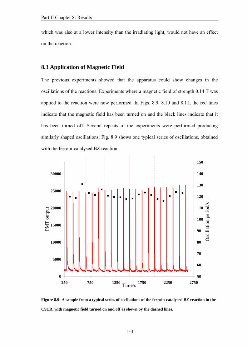
Part II Chapter 8: Results
which was also at a lower intensity than the irradiating light, would not have an effect
on the reaction.
8.3 Application of Magnetic Field
The previous experiments showed that the apparatus could show changes in the
oscillations of the reactions. Experiments where a magnetic field of strength 0.14 T was
applied to the reaction were now performed. In Figs. 8.9, 8.10 and 8.11, the red lines
indicate that the magnetic field has been turned on and the black lines indicate that it
has been turned off. Several repeats of the experiments were performed producing
similarly shaped oscillations. Fig. 8.9 shows one typical series of oscillations, obtained
with the ferroin-catalysed BZ reaction.
0
5000
10000
15000
20000
25000
30000
250 750 1250 1750 2250 2750Time/s
PMT
outp
ut
50
60
70
80
90
100
110
120
130
140
150
Osc
illat
ion
perio
d/s
.
Figure 8.9: A sample from a typical series of oscillations of the ferroin-catalysed BZ reaction in the
CSTR, with magnetic field turned on and off as shown by the dashed lines.
153
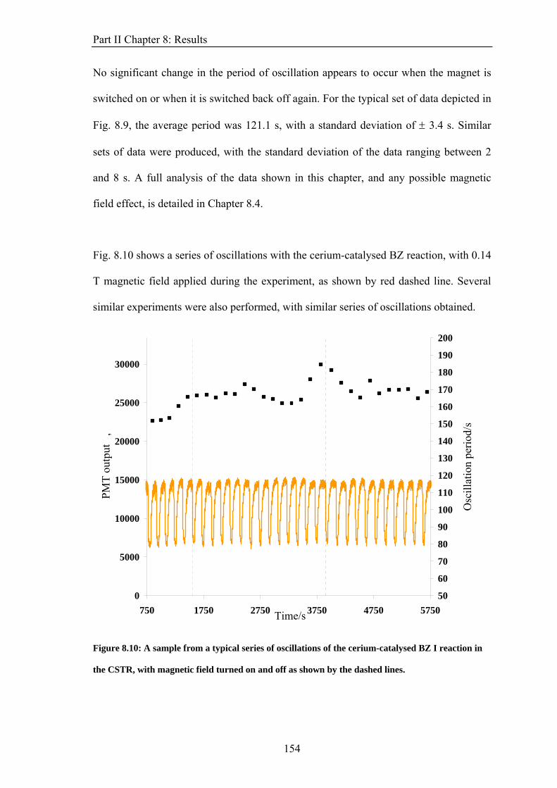
Part II Chapter 8: Results
No significant change in the period of oscillation appears to occur when the magnet is
switched on or when it is switched back off again. For the typical set of data depicted in
Fig. 8.9, the average period was 121.1 s, with a standard deviation of ± 3.4 s. Similar
sets of data were produced, with the standard deviation of the data ranging between 2
and 8 s. A full analysis of the data shown in this chapter, and any possible magnetic
field effect, is detailed in Chapter 8.4.
Fig. 8.10 shows a series of oscillations with the cerium-catalysed BZ reaction, with 0.14
T magnetic field applied during the experiment, as shown by red dashed line. Several
similar experiments were also performed, with similar series of oscillations obtained.
0
5000
10000
15000
20000
25000
30000
750 1750 2750 3750 4750 5750Time/s
PMT
outp
ut
,
50
60
70
80
90
100
110
120
130
140
150
160
170
180
190
200
Osc
illat
ion
perio
d/s
Figure 8.10: A sample from a typical series of oscillations of the cerium-catalysed BZ I reaction in
the CSTR, with magnetic field turned on and off as shown by the dashed lines.
154
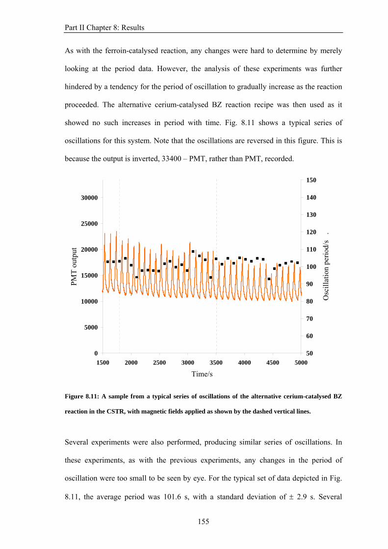
Part II Chapter 8: Results
As with the ferroin-catalysed reaction, any changes were hard to determine by merely
looking at the period data. However, the analysis of these experiments was further
hindered by a tendency for the period of oscillation to gradually increase as the reaction
proceeded. The alternative cerium-catalysed BZ reaction recipe was then used as it
showed no such increases in period with time. Fig. 8.11 shows a typical series of
oscillations for this system. Note that the oscillations are reversed in this figure. This is
because the output is inverted, 33400 – PMT, rather than PMT, recorded.
0
5000
10000
15000
20000
25000
30000
1500 2000 2500 3000 3500 4000 4500 5000
Time/s
PMT
outp
ut
50
60
70
80
90
100
110
120
130
140
150
Osc
illat
ion
perio
d/s
.
Figure 8.11: A sample from a typical series of oscillations of the alternative cerium-catalysed BZ
reaction in the CSTR, with magnetic fields applied as shown by the dashed vertical lines.
Several experiments were also performed, producing similar series of oscillations. In
these experiments, as with the previous experiments, any changes in the period of
oscillation were too small to be seen by eye. For the typical set of data depicted in Fig.
8.11, the average period was 101.6 s, with a standard deviation of ± 2.9 s. Several
155

Part II Chapter 8: Results
similar sets of data were produced, with the standard deviation of the data ranging
between 3 and 10 s.
The periods of oscillation in Fig. 8.11 are shorter than in those shown in Fig. 8.10, so
the alternate cerium catalysed reaction could have reached a steady state faster than the
original cerium catalysed reaction mixture. Further to this, the reaction was designed to
limit the effect of dissolved oxygen. This could also be a key reason for the changes
observed in the first cerium-catalysed experiments, with changes in the oxygen
concentration having an effect on the oscillation period. However, a similar effect
should have been observed in the ferroin-catalysed reaction.
8.4 Is there an effect?
The main question raised at the end of this study is “Is there a magnetic field effect on
the reaction?” The effects reported in other work was small – changes of a few seconds
within period of ~ 100s – so large differences in period were not expected. There does
appear to be very little effect of a magnetic field on the oscillations shown here.
Although a Student’s T-test could be performed on a single set of data, every oscillation
needs to be considered when trying to determine if the applied magnetic field had had
an effect or not. For each set of data (a series of oscillations, as shown in the figures
presented above), each period was recorded as a % difference from the mean value for
that particular set of data. All of the periods, recorded as % differences, for each field in
the set (i.e. field on or field off) were collated together, producing a mean % difference
and its standard deviation for field on or field off for each set of data. The means and
standard deviations can then be compared. To see if there is a significant effect, a T-test
156
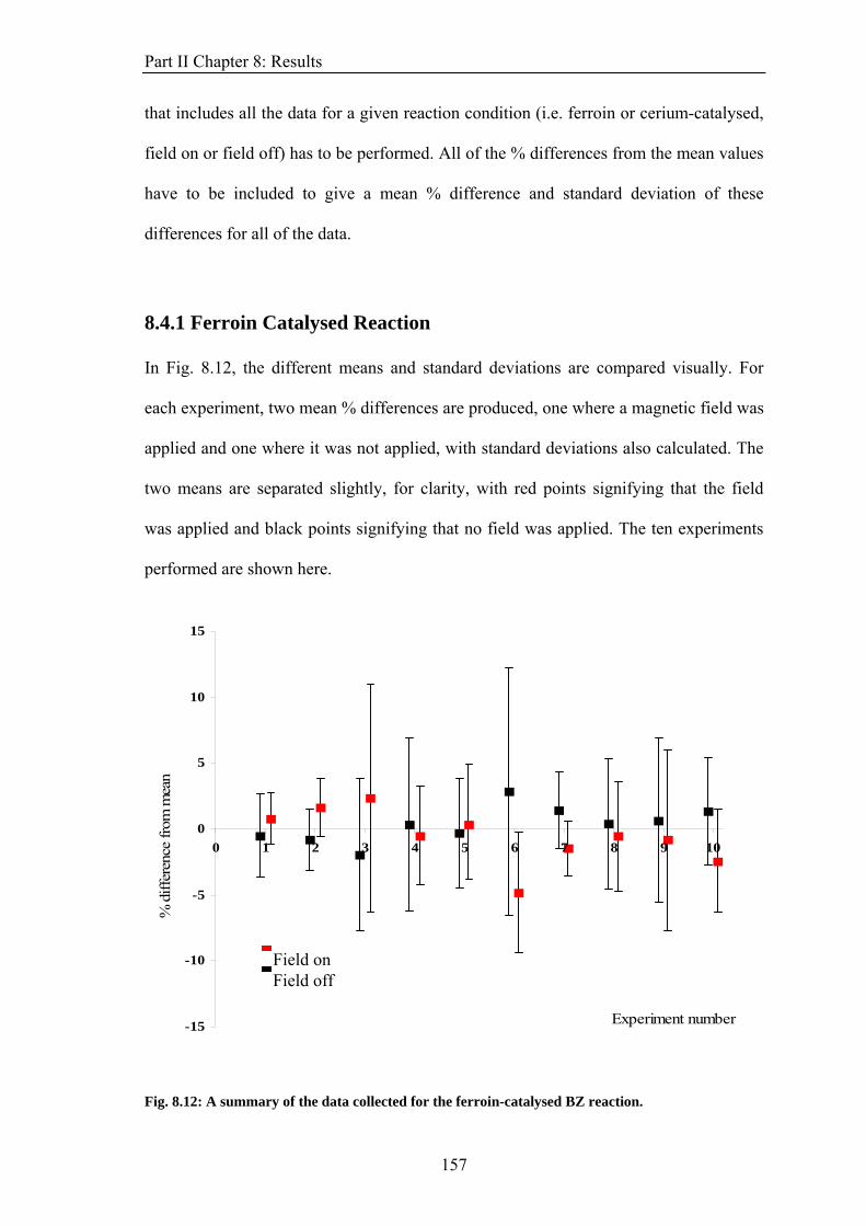
Part II Chapter 8: Results
that includes all the data for a given reaction condition (i.e. ferroin or cerium-catalysed,
field on or field off) has to be performed. All of the % differences from the mean values
have to be included to give a mean % difference and standard deviation of these
differences for all of the data.
8.4.1 Ferroin Catalysed Reaction
In Fig. 8.12, the different means and standard deviations are compared visually. For
each experiment, two mean % differences are produced, one where a magnetic field was
applied and one where it was not applied, with standard deviations also calculated. The
two means are separated slightly, for clarity, with red points signifying that the field
was applied and black points signifying that no field was applied. The ten experiments
performed are shown here.
-15
-10
-5
0
5
10
15
0 1 2 3 4 5 6 7 8 9 10
Experiment number
% d
iffer
ence
from
mea
n
Field on Field off
Fig. 8.12: A summary of the data collected for the ferroin-catalysed BZ reaction.
157
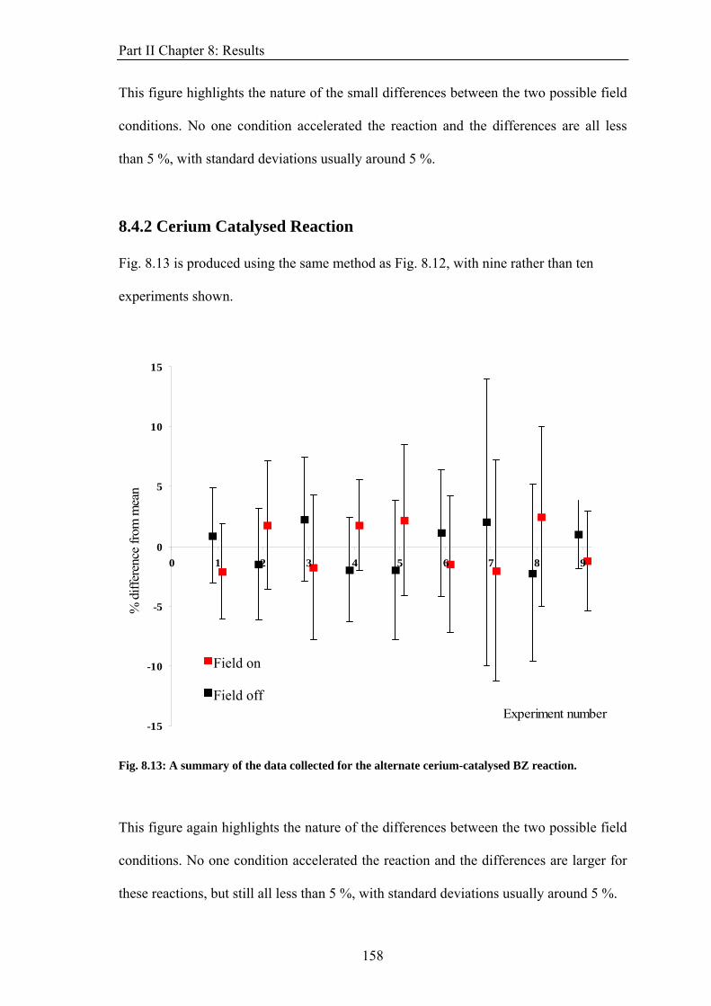
Part II Chapter 8: Results
This figure highlights the nature of the small differences between the two possible field
conditions. No one condition accelerated the reaction and the differences are all less
than 5 %, with standard deviations usually around 5 %.
8.4.2 Cerium Catalysed Reaction
Fig. 8.13 is produced using the same method as Fig. 8.12, with nine rather than ten
experiments shown.
-15
-10
-5
0
5
10
15
0 1 2 3 4 5 6 7 8 9
Experiment number
% d
iffer
ence
from
mea
n
Field on
Field off
Fig. 8.13: A summary of the data collected for the alternate cerium-catalysed BZ reaction.
This figure again highlights the nature of the differences between the two possible field
conditions. No one condition accelerated the reaction and the differences are larger for
these reactions, but still all less than 5 %, with standard deviations usually around 5 %.
158
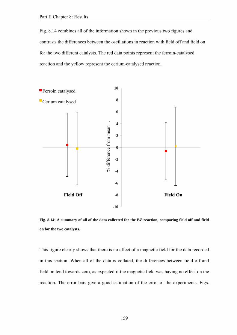
Part II Chapter 8: Results
Fig. 8.14 combines all of the information shown in the previous two figures and
contrasts the differences between the oscillations in reaction with field off and field on
for the two different catalysts. The red data points represent the ferroin-catalysed
reaction and the yellow represent the cerium-catalysed reaction.
-10
-8
-6
-4
-2
0
2
4
6
8
10
% d
iffer
ence
from
mea
n .
Ferroin catalysed
Cerium catalysed
Field Off Field On
Fig. 8.14: A summary of all of the data collected for the BZ reaction, comparing field off and field
on for the two catalysts.
This figure clearly shows that there is no effect of a magnetic field for the data recorded
in this section. When all of the data is collated, the differences between field off and
field on tend towards zero, as expected if the magnetic field was having no effect on the
reaction. The error bars give a good estimation of the error of the experiments. Figs.
159
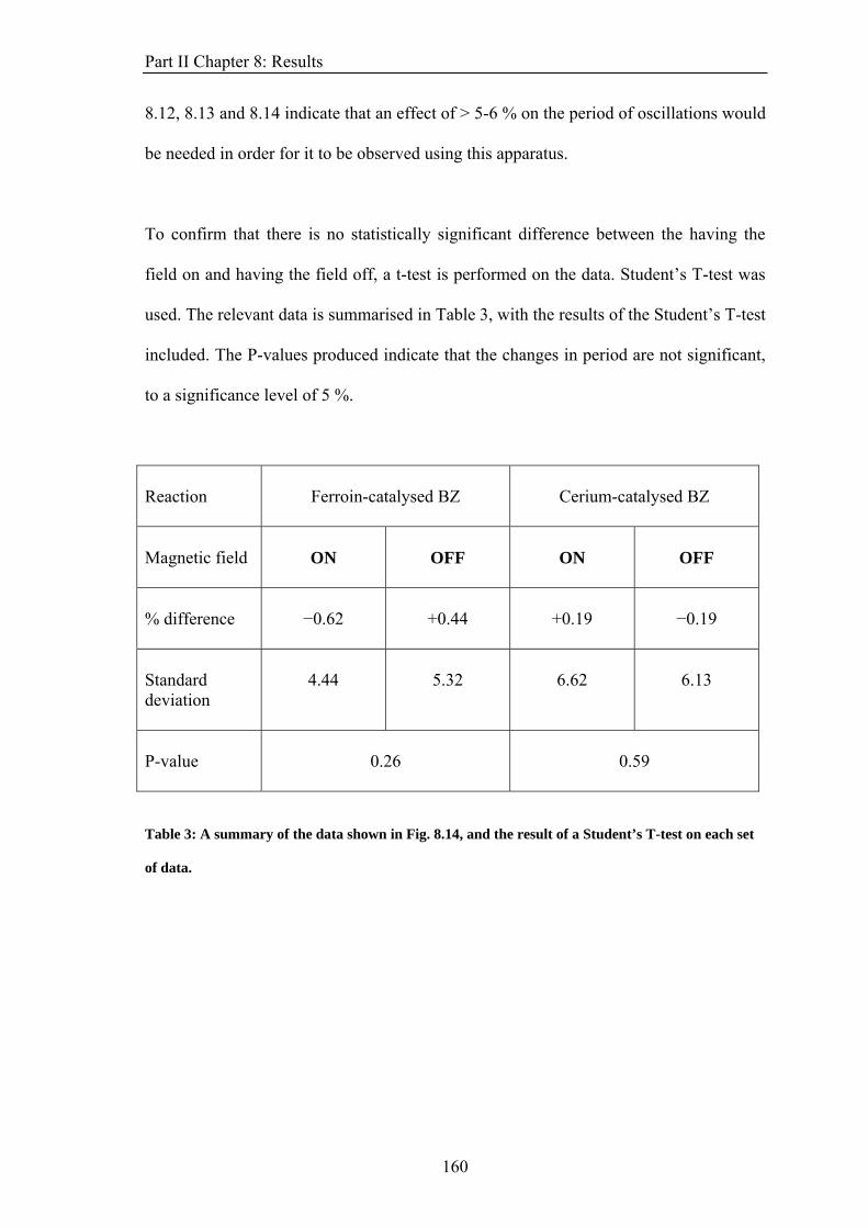
Part II Chapter 8: Results
160
8.12, 8.13 and 8.14 indicate that an effect of > 5-6 % on the period of oscillations would
be needed in order for it to be observed using this apparatus.
To confirm that there is no statistically significant difference between the having the
field on and having the field off, a t-test is performed on the data. Student’s T-test was
used. The relevant data is summarised in Table 3, with the results of the Student’s T-test
included. The P-values produced indicate that the changes in period are not significant,
to a significance level of 5 %.
Reaction
Ferroin-catalysed BZ
Cerium-catalysed BZ
Magnetic field
ON
OFF
ON
OFF
% difference
−0.62
+0.44
+0.19
−0.19
Standard deviation
4.44
5.32
6.62
6.13
P-value
0.26
0.59
Table 3: A summary of the data shown in Fig. 8.14, and the result of a Student’s T-test on each set
of data.
Part II Chapter 9: Discussion
161
9. DISCUSSION
The results presented here show that there is no statistically significant magnetic field
effect on the BZ reaction when a static field of 0.14 T was applied to the reaction. The
standard deviation produced in Fig. 8.14 gives an indication of the size of effect that
would need to be present in order for it to be observed by the apparatus. For the
apparatus used in these experiments, an effect of < 5-6 % on the period of the
oscillations would simply not be observed by the apparatus. One other problem with
this CSTR is that, because it was hard to reproduce the period of oscillations between
experiments, it could only be used to monitor changes in period within a series of
oscillations.
So why is no effect seen? First, assuming that there is some magnetic field
dependence, the effect could, simply, be too small to be observed by the apparatus. As
said earlier, an effect of less than 5 % on the period of oscillation would not be seen
by this apparatus. This error compares well with similar work conducted by Sontag31,
who also failed to see any effect on the reaction. If the apparatus was improved to
reduce the error between oscillations to only one or two percent, the error reported by
Blank and Soo, then a smaller effect could be more easily observed. But Figs. 8.11
and 8.12 show that neither “field on” nor “field off” consistently speds up or slowed
down the reaction. If one condition did accelerate the reaction, then there might be
some justification for trying to improve the accuracy of the apparatus in order to
better characterise the extent of this acceleration. However, that neither condition did
suggests strongly that there is no effect.
Part II Chapter 9: Discussion
It could also be possible that there was an effect on some individual rate constants but
the kinetics of the whole system act to minimise the effect. This behaviour was
possibly observed in Fig. 8.8, with the effect of irradiation of the reaction with UV
radiation decreased after an initial large fall in oscillation period. Similar behaviour is
also observed in a shallow layer when a perturbation that does not reach a certain
threshold does not produce a wave while one over that threshold does37. If this was
the case, then there could be some change in the rate of the autocatalytic part of the
reaction which is then compensated by changes in the rate of the regeneration of the
metal catalyst. Individual peaks could be compared but perhaps an easier method is to
show the first derivative with respect to time of the data plotted against time, as
shown in Fig. 9.1.
162
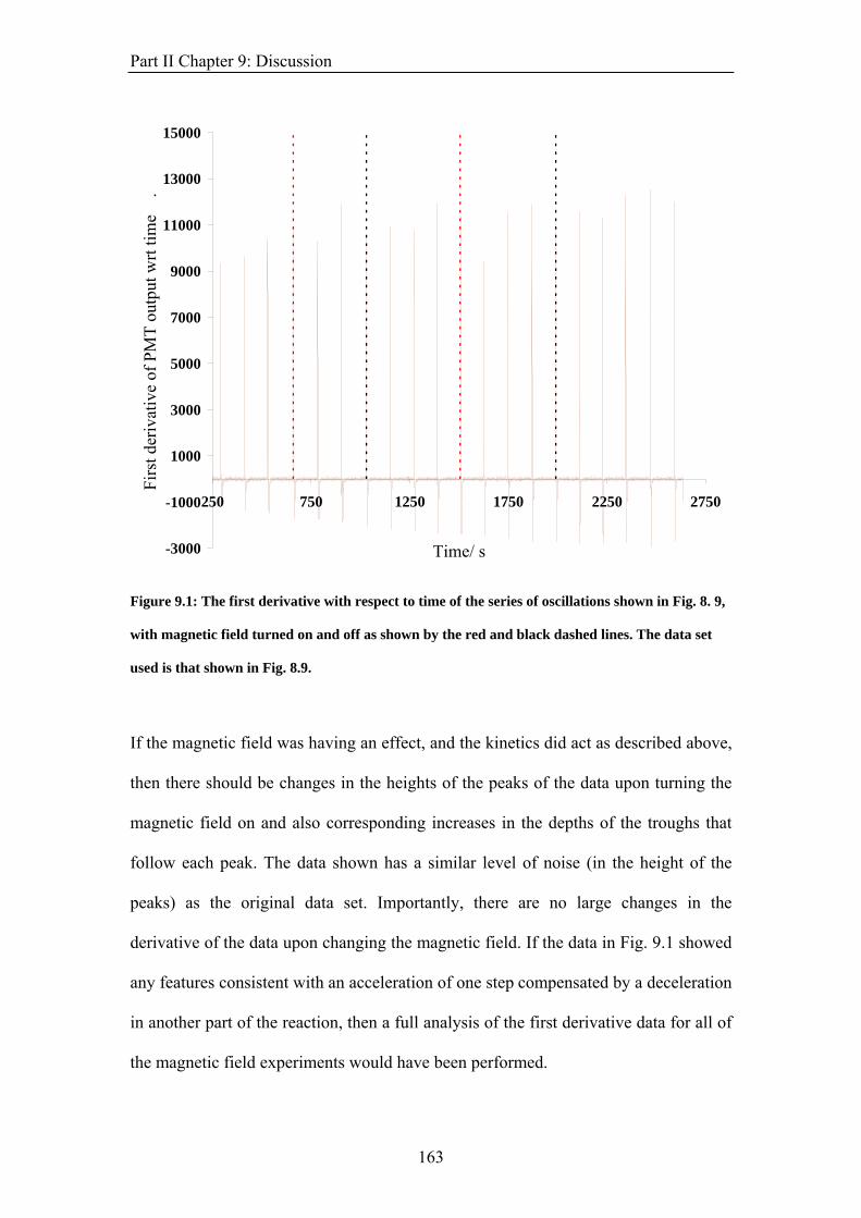
Part II Chapter 9: Discussion
-3000
-1000
1000
3000
5000
7000
9000
11000
13000
15000
250 750 1250 1750 2250 2750
Time/ s
Firs
t der
ivat
ive
of P
MT
outp
ut w
rt tim
e
.
Figure 9.1: The first derivative with respect to time of the series of oscillations shown in Fig. 8. 9,
with magnetic field turned on and off as shown by the red and black dashed lines. The data set
used is that shown in Fig. 8.9.
If the magnetic field was having an effect, and the kinetics did act as described above,
then there should be changes in the heights of the peaks of the data upon turning the
magnetic field on and also corresponding increases in the depths of the troughs that
follow each peak. The data shown has a similar level of noise (in the height of the
peaks) as the original data set. Importantly, there are no large changes in the
derivative of the data upon changing the magnetic field. If the data in Fig. 9.1 showed
any features consistent with an acceleration of one step compensated by a deceleration
in another part of the reaction, then a full analysis of the first derivative data for all of
the magnetic field experiments would have been performed.
163
Part II Chapter 9: Discussion
It is also possible that there was no effect on the reaction at this magnetic field
strength. Six criteria have been listed as necessary conditions for the observation of a
magnetic field dependent enzymatic reaction38. Although the BZ reaction is not an
enzymatic reaction, these criteria provide some insight into the likelihood of there
being a magnetic field effect. The six criteria are summarised below:
1) One reaction step must proceed via a radical-pair intermediate.
2) The radicals in the radical pair must be weakly coupled.
3) There must be a mechanism by which the singlet and triplet states of
the radical pair can mix.
4) The rate of the reaction must be sensitive to the concentration of the
radical pair.
5) The radical pair must be sufficiently long lived for significant
interconversion of the two states to occur.
6) The reaction step preceding the formation of the radical pair must be
reversible.
What criteria are fulfilled for the possible radical pair identified earlier? Certainly, the
formation of a pair of radicals in a known reversible step of the reaction, as suggested
by the FKN mechanism and identified earlier as a potentially magnetic field
dependent step, would meet criteria 1, 4 and 6. The remaining criteria can be dealt
with in turn.
Whether the radical can show interconversion between S and T states has been
discussed in Chapter 6.3, where coupling of the radical to Br nuclei, through the
164
Part II Chapter 9: Discussion
hyperfine interaction, allows mixing of the two states and can result in a magnetic
field effect. ‘Weak coupling’ of the radical pair refers to the exchange interaction and
its role in S-T mixing. At small separations, the singlet and triplet wavefunctions of
the radical pair cannot overlap, so the radical pair has to separate, by diffusion, until
the exchange interaction falls to a neglible amount, and then S-T mixing can occur
between the pair. The radical pair must then recombine.
The lifetime of a radical pair is perhaps the most important factor in determining
whether a magnetic field has an effect. If the reactions of the BrO2. radical, either with
another radical or with the metal catalyst occur at a faster rate than any spin-mixing, a
magnetic field effect will simply not have the time to occur. The reaction will not be
magnetic field dependent. There is only a build up of the radical during the
autocatalytic clocking section of the oscillation. This is backed up by data shown in
Försterling et al. and related papers 39. For the radical pair identified as potentially
important in this reaction, the isotropic hyperfine couplings are ~ 4 mT, leading to a
spin mixing on the timescale of nanoseconds while the references above suggest that
the radicals have a lifetime as long as seconds. These very different timescales of
reaction and S-T mixing may contribute to the absence of a magnetic field effect,
although an effect is only ruled out if the radical recombines on a faster rate than the
S-T mixing.
A large difference in rate constants of the reaction of the radical with the metal
catalyst that occurs when cerium is substituted with ferroin was identified in chapter
6.2, with the ferroin reacting with the radical at a rate 105 times faster than cerium.
The result of this is that, in the ferroin-catalysed reaction, any BrO2. formed reacts
165
Part II Chapter 9: Discussion
faster with the ferroin than it would react with another bromine dioxide molecule to
recombine. As the radical pair is no longer formed in a reversible reaction, any MFE
in this system is unlikely. In the cerium catalysed reaction, the rates of reaction with
metal catalyst and of recombination are similar18. An example of the lifetimes of the
bromine dioxide radical in solutions of metal ions typically used in the BZ reaction
can be found in Field et al.40 where BrO2. was formed by the radiolysis of solutions of
bromate. Although the experiments were performed in a different solution (neutral
solutions, no MA present, different metal catalysts), they show a marked difference in
the lifetimes of the radicals depending on the metal used. The reaction rate of BrO2.
with Fe(CN)64− is comparable with that of ferroin and the data presented by Field et
al. clearly shows how much faster the radical reacts with the metal catalyst than with
other radicals in recombination reactions.
The diffusion of the radicals is likely to be a key factor in whether a magnetic field
effect is observed. If the radical pair forms and then diffuses apart without a chance to
recombine then no magnetic field effect is ever going to be seen. The radical pair
consists of neutral radicals, so there is no coulombic attraction holding them together.
If a reacting solution could be prepared in a more viscous solution, then similar
experiments to those conducted here could easily be performed to check if there is
still no magnetic field effect observed.
There is also another mechanism which would remove any magnetic field effect. For
the system that was studied here, incoherent mixing must be having some effect on
the radical pair present produced. The presence of paramagnetic transition metals has
a large effect on the relaxation times of electron spins of radical pairs. A further effect
166
Part II Chapter 9: Discussion
is that of the bromine atom on the radical pair. This atom has large electric
quadropolar coupling41 and it is possible that the nucleus does not precess around the
applied field but a resultant of the applied field and this quadropole. This precession
may be affected by the rotation of the molecule but should be capable of inducing
incoherent S-T+ and S-T− transitions for the radical. These two relaxation processes
occur on a similar (or faster) timescale than the rate of reaction due to cerium or
recombination, so any coherence will be lost by the time the radical reacts with either
the metal or recombines. There could also be a spin-orbit coupling effect. In a
photolysis experiment, magnetic field effects observed in the reactions of dibenzyl
ketone were removed when Br was substituted into one of the aromatic rings42. In
these experiments, spin-orbit coupling was proposed to be dominating the mixing of
the singlet and triplet states of the radical pair. Given radicals formed in the radical
pair being considered here are bromine-centred, it is likely that there is also very fast
relaxation of the electron spins through this mechanism. No magnetic field effect is
observed because the rates of incoherent mixing, by a range of mechanisms, occur on
a faster time scale than the rates of reaction of the radical.
One key point is whether there are any other reactions in the mechanism that could be
magnetic field dependent. In chapter 6.3, a particular sequence of reactions was
identified as the most likely step to give rise to any magnetic field dependence.
Discussion of the results has focussed on one particular section of the reaction.
However, there could be other radical pairs formed, especially in the reactions
involving the organic species present. Looking at the GTF model12, there are 8
reactions that produce radicals, but 5 of these are reactions of Ce4+ with an organic
167

Part II Chapter 9: Discussion
species. The remaining 3 all produce bromine centred radicals, which are unlikely to
given any magnetic field effect for reasons given above.
Admittedly, this work is only concerned with the effect of a large static field on the
oscillating reaction, whereas some of the previous work had considered small,
oscillating magnetic fields. But in terms of the radical pair mechanism theory
considered here, an oscillating magnetic field effect can only be observed in a system
where there is already a known static magnetic field effect. The frequency of the
oscillating magnetic field would have to be the same size as the hyperfine couplings
in order for it to have an effect, so a MHz field would have to be used. The fields used
in the Blank and Soo experiments were in the Hz – kHz range30. This does raise the
question of whether there are other mechanisms by which an oscillating magnetic
field can influence a chemical reaction. Although there are other mechanisms by
which a magnetic field could interact with a chemical reaction29, only the RPM is well
accepted.
Modelling of the reaction could give more insight into what size an effect could be
expected and whether a reasonable change to key reaction rate constants, such as
those identified earlier, will lead to an observable effect in the reaction as a whole. If a
reasonable change in the rate constants or behaviour of key reactions does not produce
an observable effect in the overall reaction, then no effect on the whole reaction can
be expected. Various attempts to model the reaction and the effects observed in this
thesis were made with simulations42 based on the FKN model, the Oregonator and
sub-sets of the reaction, such as the autocatalytic clock taken in isolation. The larger
models added little to the problem due to difficulties in getting them to produce
168
Part II Chapter 9: Discussion
169
suitable sets of oscillations while the smaller sub-sections were limited by their very
nature, concentrating on one or two reactions and ignoring the changes in
concentration that occur during each oscillation. Theoretical work of this nature has
been conducted by Baxter43 who analysed the Brusselator model of the BZ reaction.
Some striking changes in behaviour of the simulated oscillations were produced. That
work gives further details into the sensitive kinetics of the reaction and also shows
how the whole reaction could be affected by changes in relevant rate constants.
However, the Brusselator is a much reduced version of the model, consisting of four
reactions. It could be used as a starting block for a more thorough investigation of the
kinetics. Given that no effect was observed in the experimental section and that the
absence of an effect can be explained by considering relaxation of the electron spins
due to both transition metals and the bromine atoms, a full kinetic analysis was not
attempted here.
The experimental evidence convincingly shows that no magnetic field effect was
present in the experiments conducted and the absence of any effect can be explained
using a well-established theory that describes magnetic field effects. The BZ reaction
remains an interesting reaction to investigate due to the wide range of phenomena
observed.

Part III: USING SQUID MAGNETOMETRY TO
FOLLOW CHEMICAL REACTIONS.
Part III Chapter 10: Introduction
171
10. INTRODUCTION
The change in magnetic susceptibility of a reaction, which was used in Part I to
manipulate a reaction, can also be used to monitor its progress. One potential
application utilising this change in susceptibility could be in following reactions which
proceed via a radical pair mechanism. The formation of the radical pair can be observed
by a range of methods such as UV/vis spectrophotometry1, fluorescence spectroscopy2
and time-resolved infrared spectroscopy3. However, there are some limitations to these
techniques. For example, the species involved might not be fluorescent or the spectra of
the precursor and the radical pair might overlap. Any changes in susceptibility will be a
direct result of any changes in the concentration of radicals, with no dependence on the
absorption or fluorescence properties of the radical molecule, making the technique
more universal. Using a suitably precise magnetometer, such as a superconducting
quantum interference device (SQUID), to measure the changes in magnetic
susceptibility could prove to be a further method available for the study of such
systems.
The technique could also be used to follow the progress of other suitable reactions with
time. The reaction between Co(II)EDTA2− and H2O2 at ~ pH 4 displays wave behaviour
when initiated locally by a small amount of NaOH solution (see Part I for more details),
but also displays clock behaviour when mixed, well-stirred and then left to stand4. The
reaction can be followed in a number of ways, with the striking change in colour and the
increase in the autocatalyst concentration, −OH, two main indicators of the reaction’s
progress. There is also a change in the magnetic susceptibility of the reacting solution,
as shown by the susceptibility data recorded using a Gouy balance in Fig. 4.1.1. It
Part III Chapter 10: Introduction
should be possible to follow the progress of the reaction by measuring this change in
magnetic susceptibility with respect to time.
In this chapter, SQUID magnetometry is used, for the first time, to measure the progress
of a solution phase reaction. The results acquired can then be compared and contrasted
with data collected using other methods such as absorption spectroscopy and previous
research to give further information on the reaction and on the presence and nature of
any intermediates formed during the reaction. The study is not limited to just the
Co(II)EDTA2−/H2O2 reaction described above. There are number of other reactions,
such as the Belousov-Zhabotinsky reaction (studied in detail in Part II), that could
possibly be followed using the technique introduced here. These are discussed in
Chapter 12.2. The work that follows is intended to show that the SQUID magnetometry
can be used to follow liquid phase reactions. The reactions chosen for the study have
relatively large changes in magnetic susceptibility and should be easily measured by the
SQUID magnetometer. If the SQUID can be used to follow these reactions, then it
could be used in the study of radical pair reactions and this section acts as a proof of
principle that the SQUID can be used to study solution phase reactions.
10.1 Methods of Measuring Magnetic Properties
There are various ways of measuring the magnetic properties of materials5. One can
measure the force acting on a sample of material in an inhomogeneous magnetic field.
The Gouy balance is an example of this method. There is a change in energy of a
material with magnetic moment, μ, as it is placed in a magnetic field of strength, H (see
Chapter 1.2.2). With an inhomogeneous magnetic field, there a force is generated on the
172
Part III Chapter 10: Introduction
sample. The change in weight due to this force can then be measured by a sensitive
balance.
(1) Hμ χV=
)(2χVμ 20 HF ∇⎟
⎠
⎞⎜⎝
⎛= (2)
One can also measure the net magnetic moment of the sample. The induction of a
current in a coil by a magnetic moment can be used to measure the size of the magnetic
moment. This is the basis of the vibrating sample magnetometer and similar techniques.
SQUID magnetometers are the most sensitive devices for measuring magnetic fields.
Conventionally, they are used to characterise the magnetic properties of solid materials,
particularly those with ordering of magnetic domains, looking at changes in magnetic
susceptibility as functions of temperature or applied magnetic field6. Other possible uses
include the measurement of minute magnetic fields in a range of applications, such as in
the brain, the heart, occurring during the corrosion of metals and geological magnetic
fields7.
The sensitivity of these devices arises from the use of superconducting materials, which
can conduct current without developing a potential difference across the material, and,
specifically, Josephson junctions, where superconducting material is separated by a thin
(~ 1 nm) layer of insulating material. With a sufficiently thin barrier, tunnelling occurs
and the wavefunctions of the two superconducting materials can interact across the
barrier. Appendix IV is a brief overview of how the sensitivity of a SQUID is obtained.
173
Part III Chapter 10: Introduction
This effect was predicted in 19628, with the first junction built in 19639 and the first
SQUIDs were built in the following years. Several superconducting components feature
in the magnetometer used: a superconducting magnet to produce large magnetic fields, a
set of superconducting detection coils through which the sample passes and a SQUID
connected to the superconducting detection coils. The SQUID used here has one
Josephson junction in the current path of a closed superconducting loop (a
radiofrequency (rf) SQUID). Properly calibrated, a SQUID magnetometer can be
capable of detecting a change in a magnetic field approaching 10−15 T.
The SQUID device in the magnetometer used in these experiments does not directly
detect the magnetic field from the sample. The junction is too small and too fragile for
this purpose. Instead, a sample moves through a set of superconducting coils which are
connected to the SQUID in a superconducting loop. Any change in magnetic flux
passing through the detection coils produces a proportional change in the persistent
current in the coils. This current is inductively coupled to a Josephson junction, which
acts as a highly sensitive flux-to-voltage converterI.
Measurements are made by moving the sample through the detection coils. The change
in the sample’s position changes the flux within the superconducting coil, changing the
current in the complete superconducting circuit. As the circuit is superconducting, the
current does not decay and produces a voltage output from the SQUID. The sample is
passed through the coils in a series of steps, which produces a series of voltage
measurements, from which the magnetic moment of the sample can be calculated by
reference to a calibration of the SQUID with a known mass of a material of a known
susceptibility.
174
Part III Chapter 10: Introduction
This technique is used in conjunction with other spectroscopic techniques, such as
uv/vis absorption spectrophotometry, NMR techniques and pH electrodes, to both
follow the reaction and, by comparing the various techniques, identify any intermediates
in the reaction.
10.2 Other Methods of Following Chemical Reactions
The results obtained using the SQUID magnetometer are supported by data acquired
using a range of other techniques. Hydroxide ions are known to be the autocatalyst in
the Co(II)EDTA2−/H2O2 reaction (see Chapter 2 and Eqns 2.1 and 2.2), so following the
reaction with a calibrated pH electrode was an obvious method. Other methods
employed probe changes in the oxidation state of the metal ions, allowing comparison
with the SQUID data.
10.2.1 Absorption Spectroscopy
The absorption spectra of solutions give information as to the electronic spectra of the
ions in the solution and changes in the intensity of light absorbed by a solution can be
used to follow changes in the concentrations of species in the solution. The Beer-
Lambert law shows the relationship between the intensity of light transmitted, I, and the
concentration of the sample, c, its molar absorption coefficient, ε, the incident light
intensity, I0, and the path length of the lightthrough the sample, l:
I = I010−(εcl) (3)
175
Part III Chapter 10: Introduction
176
The product of the three terms, ε, c and l, is the absorbance of the sample, A.
0IA=εcl=logI
⎛⎜⎝ ⎠
⎞⎟ (4)
The absorbance can be measured by the spectrometer, calculated from the light intensity
that passes through the sample. There is often a striking change in colour in reactions
where transition metal ions change oxidation states. In the Co(II)EDTA2−/H2O2 reaction
pink Co(II)EDTA2− is oxidised to dark blue Co(III)EDTA−. In the Belousov-
Zhabotinsky reaction, the colour change is determined by the catalyst used, with red to
blue oscillations observed for the ferroin-catalysed reaction. By following the changes
in absorbance of light at specific wavelengths passing through a sample, the changing
concentrations of the coloured metal ions in the solution can be followed.
10.2.2 Nuclear Magnetic Resonance
The changes in metal oxidation state can also be measured by magnetic resonance
techniques. Chapter 2.1.2 described how the presence of transition metal ions caused a
drop in the spin-spin relaxation time of protons in water. A Carr-Purcell-Meiboom-Gill
(CPMG) sequence is used to measure T2 times of protons in solution10.
Part III Chapter 11: Methods and Materials
177
11. METHODS AND MATERIALS
11.1 Materials
Sodium hydroxide, EDTA, cobalt chloride and hydrogen peroxide (35 % by volume),
all of ACS grade, were obtained from Aldrich and used without further purification. A
0.02 M Co(II)EDTA2− solution was made by dissolving equimolar quantities of EDTA
and CoCl2 in de-ionised water and then adjusting the pH to ~ 4. The reacting solution
used in all of the Cobalt experiments in Chapter 12 was a 9:1 by volume mixture of 0.02
M Co(II)EDTA2− at pH 3.9 and 35 % H2O2 solution.
Sodium bromate, sulphuric acid, silver nitrate and malonic acid, of A.C.S. grade, were
obtained from Aldrich and used without further purification. A stock ferroin solution
was produced by dissolving iron sulphate (FeSO4.7H2O) and 1, 10 – phenanthroline in
Analar water to produce a 0.025 M solution. Both the iron sulphate and 1, 10 –
phenanthroline were obtained from Aldrich and used without further purification.
Cerium (IV) ammonium nitrate (Ce(NH4)2(NO3)6) was obtained from Aldrich and used
without further purification. Concentrations of the reacting solutions for the BZ
reactions in Chapter 12.5 are described in the text. Ammonium metavanadate and
hydrochloric acid were obtained from Aldrich and used without further purification.
Any dilute acid solutions were made from concentrated stock solutions.
Part III Chapter 11: Methods and Materials
11.2 Methods
11.2.1 pH Electrode Experiments
A pH electrode was connected directly to a computer using a PCI 9112 data acquisition
card. A simple data acquisition program was written in Labview (see Appendix IIIa)
and the pH meter calibrated using buffer solutions (pH 4, 7 and 10). The measurement
of pH was taken from 50 ml of reacting mixture in a small flask, with measurements of
pH taken every 100 ms. The reacting mixtures were thermostatted at 22 oC using a
water bath.
11.2.2 Absorption Spectroscopy Experiments
Ultraviolet/visible light absorption spectra were obtained for the reacting mixture in a
Unicam UV-2 spectrometer. A thin path length (1 mm) cell was used as the absorption
of the Co(III)EDTA− product was too high for the spectrometer to record accurately
with longer path lengths. The clock reaction was followed in the spectrometer with full
spectra of the solution in a 1 mm path length cell from 350 to 700 nm acquired at 2
minute intervals, and the absorption of the solution at given wavelengths against time
taken from the full scans. The spectrometer could also record spectra at a given
wavelength by recording the absorption at that wavelength every 125 ms. No
temperature control of the reacting solutions was possible in the spectrometer.
11.2.3 NMR Experiments
MRI experiments were conducted on a Bruker DMX-300 spectrometer equipped with a
7.0 T superconducting magnet, operating at a proton resonance of 300 MHz, and at 295
K. The reacting solution was prepared outside of the magnet and a 5 mm ID NMR tube
178
Part III Chapter 11: Methods and Materials
was filled to a depth of a few centimetres of the reacting solution. The CPMG sequence
recorded 64 echoes with a τ of 2 ms. CPMG measurements of the reacting sample were
obtained at 30 s intervals. A small number of experiments were performed by acquiring
RARE images instead of using the CPMG sequence. As described in 2.1.3, the RARE
imaging sequence uses the difference in relaxation time to obtain contrast. These
experiments acquired RARE images of the clock reaction at 30 s intervals.
11.2.4 SQUID Experiments
The magnetic moment of the sample was measured using a Quantum Design MPMS5
magnetometer at 300 K. The SQUID magnetometer uses cgs units with the applied field
measured in oersteds, rather than tesla, and the moment in emu, as opposed to A m2 (see
Appendix I for a discussion of the different systems and units). A field of 50000 Oe was
used for all of the experiments in this chapter, and was converted into the equivalent SI
unit, A m−1, for calculations (see flow chart, Fig. 11.2). Other magnetic fields could be
produced by the superconducting magnet but this highest field possible was chosen. The
reaction was initiated outside of the SQUID magnetometer and a small, known mass
(around 100 mg) of the reacting solution placed inside a 5 mm NMR tube which was
then sealed. This sealed sample was loaded into a thin plastic tube and held in place
with empty gelatine capsules lodged into position. A typical sample tube is shown in
Fig. 11. 1. These prevent the sample from moving while it is passed through the coils.
179
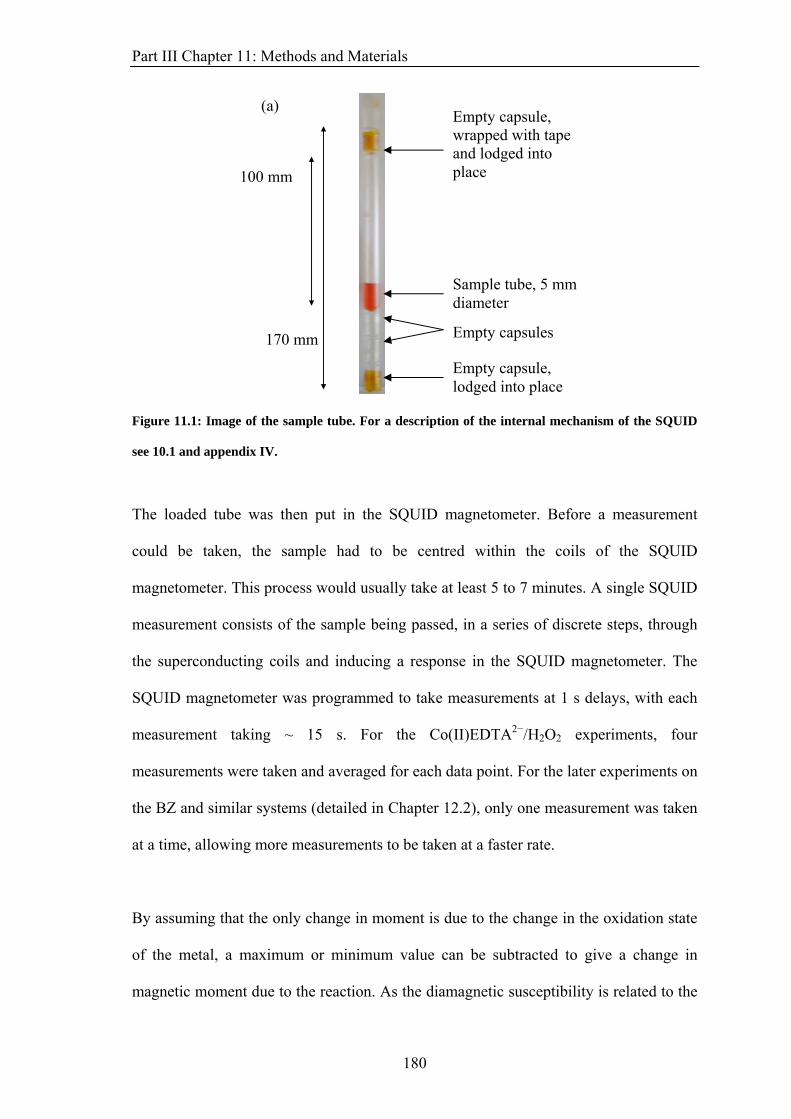
Part III Chapter 11: Methods and Materials
(a)
Empty capsule, wrapped with tape and lodged into place 100 mm
170 mm
Sample tube, 5 mm diameter
Empty capsule, lodged into place
Empty capsules
Figure 11.1: Image of the sample tube. For a description of the internal mechanism of the SQUID
see 10.1 and appendix IV.
The loaded tube was then put in the SQUID magnetometer. Before a measurement
could be taken, the sample had to be centred within the coils of the SQUID
magnetometer. This process would usually take at least 5 to 7 minutes. A single SQUID
measurement consists of the sample being passed, in a series of discrete steps, through
the superconducting coils and inducing a response in the SQUID magnetometer. The
SQUID magnetometer was programmed to take measurements at 1 s delays, with each
measurement taking ~ 15 s. For the Co(II)EDTA2−/H2O2 experiments, four
measurements were taken and averaged for each data point. For the later experiments on
the BZ and similar systems (detailed in Chapter 12.2), only one measurement was taken
at a time, allowing more measurements to be taken at a faster rate.
By assuming that the only change in moment is due to the change in the oxidation state
of the metal, a maximum or minimum value can be subtracted to give a change in
magnetic moment due to the reaction. As the diamagnetic susceptibility is related to the
180
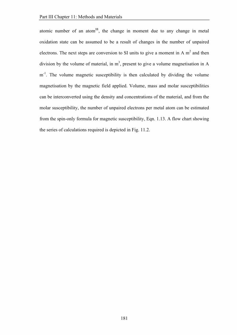
Part III Chapter 11: Methods and Materials
atomic number of an atom11, the change in moment due to any change in metal
oxidation state can be assumed to be a result of changes in the number of unpaired
electrons. The next steps are conversion to SI units to give a moment in A m2 and then
division by the volume of material, in m3, present to give a volume magnetisation in A
m-1. The volume magnetic susceptibility is then calculated by dividing the volume
magnetisation by the magnetic field applied. Volume, mass and molar susceptibilities
can be interconverted using the density and concentrations of the material, and from the
molar susceptibility, the number of unpaired electrons per metal atom can be estimated
from the spin-only formula for magnetic susceptibility, Eqn. 1.13. A flow chart showing
the series of calculations required is depicted in Fig. 11.2.
181
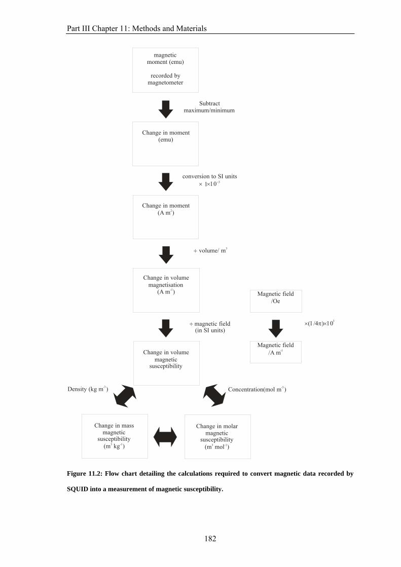
Part III Chapter 11: Methods and Materials
magneticmoment (emu)
recorded by magnetometer
Change in moment(emu)
Change in moment(A m )2
Cha ge in volume magnetisation
(A m )
n
-1
Change in volume magnetic
susceptibility
Change in molar magnetic
susceptibility(m mol )3 -1
Change in massmagnetic
susceptibility(m kg )3 -1
Concentration(mol m )-3Density (kg m )-3
÷ magnetic field (in SI units)
÷ volume/ m3
conversion to SI units 1× ×10−3
Subtract maximum/minimum
Magnetic field /Oe
Magnetic field /A m-1
×(1/4π)×103
Figure 11.2: Flow chart detailing the calculations required to convert magnetic data recorded by
SQUID into a measurement of magnetic susceptibility.
182
Part III Chapter 11: Methods and Materials
11.2.5 Analysis
In order to compare the various methods of following the reaction described above,
some methods of quantifying the features of the reaction are needed. One of the
distinctive features of autocatalysis in a reaction is a period of slow reaction rate
(sometimes known as the ‘induction period’) followed by one where the reaction rate
increases to a maximum value before slowing down again. This behaviour is
colloquially known as ‘clocking’, given that the reaction changes rapidly from
unreacted to reacted after a period of time. Fig. 1.5 is reproduced here, with the rate of
reaction added, in order to illustrate the behaviour and terms used.
0
0.2
0.4
0.6
0.8
1
1.2
0 5 10 15 20 25 30Time/s
[A]/m
oldm
-3
0
0.02
0.04
0.06
0.08
0.1
0.12
0.14
d[A
]/d t
/ m
oldm
-3s-1
Induction period ?
Clocking time
Unreacted solution
Reacted solution
Figure 11.3: The fall in [A] for the simple, quadratic autocatalytic reaction A + B 2 B. Figure is
based on a reproduction of Fig. 1.5.
183
Part III Chapter 11: Methods and Materials
184
Various features of the reaction could be chosen to be the indicator required, as long as
its use is consistent. The induction period is not a well-defined measure as it can be hard
to determine the state of the reaction and whether the reaction is slow or not. Likewise,
there is rarely a clear point when the reaction can be said to be finished. A first
derivative of the data with respect to time will show when the reaction reaches its
maximum rate, as shown in Fig. 11.3. This is the parameter used in this work to
quantify the clock reactions depicted in the next chapter and will be referred to as the
‘clocking time’ in this thesis. This measurement can also be used for every set of data.
Assigning the clocking time to some maximum or minimum value of the data may work
for some methods but not all methods produce convenient sets of data. Certainly, in the
experiments depicted in Chapter 12, the end of the reaction is often not clear as there are
further reactions of hydrogen peroxide in an alkali transition metal solution, as well as
the presence of an intermediate species. The maximum value of the first derivative
should correspond to the same point for all of the experimental methods used.
The values of this clocking time should not differ much between the methods, as the
same reaction is being observed in all cases. There will be slight variations in the
reaction conditions for each method used to follow reaction leading to small variations
in the clocking time of the reaction. What is interesting is how reproducible the clocking
time is for a particular method.
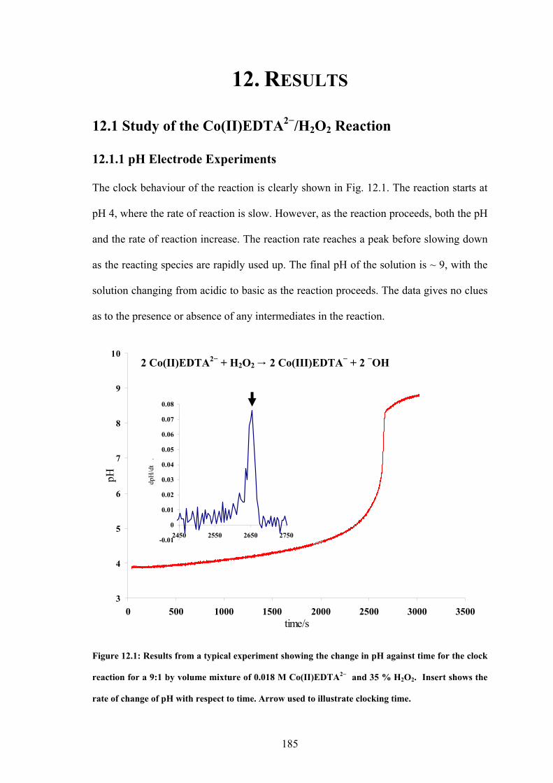
Part III Chapter 12: Results
185
12. RESULTS
12.1 Study of the Co(II)EDTA2−/H2O2 Reaction
12.1.1 pH Electrode Experiments
The clock behaviour of the reaction is clearly shown in Fig. 12.1. The reaction starts at
pH 4, where the rate of reaction is slow. However, as the reaction proceeds, both the pH
and the rate of reaction increase. The reaction rate reaches a peak before slowing down
as the reacting species are rapidly used up. The final pH of the solution is ~ 9, with the
solution changing from acidic to basic as the reaction proceeds. The data gives no clues
as to the presence or absence of any intermediates in the reaction.
3
4
5
6
7
8
9
10
0 500 1000 1500 2000 2500 3000 3500time/s
pH
2 Co(II)EDTA2− + H2O2 → 2 Co(III)EDTA− + 2 −OH
-0.01
0
0.01
0.02
0.03
0.04
0.05
0.06
0.07
0.08
2450 2550 2650 2750
Time/s
dpH
/dt
.
Figure 12.1: Results from a typical experiment showing the change in pH against time for the clock
reaction for a 9:1 by volume mixture of 0.018 M Co(II)EDTA2− and 35 % H2O2. Insert shows the
rate of change of pH with respect to time. Arrow used to illustrate clocking time.
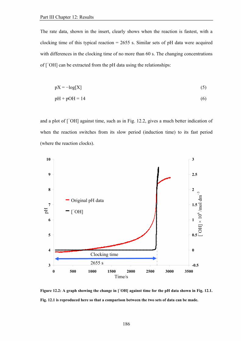
Part III Chapter 12: Results
The rate data, shown in the insert, clearly shows when the reaction is fastest, with a
clocking time of this typical reaction = 2655 s. Similar sets of pH data were acquired
with differences in the clocking time of no more than 60 s. The changing concentrations
of [−OH] can be extracted from the pH data using the relationships:
pX = −log[X] (5)
pH + pOH = 14 (6)
and a plot of [−OH] against time, such as in Fig. 12.2, gives a much better indication of
when the reaction switches from its slow period (induction time) to its fast period
(where the reaction clocks).
3
4
5
6
7
8
9
10
0 500 1000 1500 2000 2500 3000 3500Time/s
pH
-0.5
0
0.5
1
1.5
2
2.5
3
[−O
H]/m
oldm
−3
[−O
H] ×
106 /m
ol d
m−3
Original pH data [−OH]
Clocking time
2655 s
Figure 12.2: A graph showing the change in [−OH] against time for the pH data shown in Fig. 12.1.
Fig. 12.1 is reproduced here so that a comparison between the two sets of data can be made.
186
Part III Chapter 12: Results
This data shows the difference between the slow period and the fast period much more
clearly than the pH data, giving a clearer moment when the reaction ‘clocked’, but
shows little else. The period immediately after the reaction has clocked is not included
in the figure as not only is signal to noise (S/N) poor for this region, the change in
behaviour from slow to fast is more interesting. The transformation of the pH data into
[−OH] produced a data set with a poor S/N at higher pH as small differences in pH are
highly exaggerated by the calculation. The reactions of H2O2 with the basic, transition
metal after the reaction has clocked mean that there are still changes in pH after all of
the Co(II)EDTA2− has reacted.
12.1.2 Absorption Spectroscopy Experiments
Fig 12.3 shows absorption spectra for 0.018 M solutions of Co(II)EDTA2− and
Co(III)EDTA− between 350 nm and 700 nm. The Co(III)EDTA− solution was
produced by letting a 9:1 by volume mixture of Co(II)EDTA2− and H2O2 react
overnight. To check that the reaction has proceeded to completion, two spectra were
recorded several minutes apart, showing no change in the absorption of the solution.
187

Part III Chapter 12: Results
0
0.2
0.4
0.6
0.8
1
350 400 450 500 550 600 650 700Wavelength/ nm
Abs
orpt
ion/
nm
.
Co(II)EDTA2−
Co(III)EDTA−
Figure 12.3: absorption spectra from 350 nm to 700 nm for 0.018 M Co(II)EDTA2− and 0.018 M
Co(III)EDTA− solutions. Pink line shows the Co(II)EDTA2− solution and the blue line shows the
absorption of the Co(III)EDTA− solution.
There is large difference in absorption between the Co(II)EDTA2− and Co(III)EDTA−
solutions across all of the wavelengths, reflected in the large difference in colour
between the two solutions. The Co(II)EDTA2− solution has a broad peak at around 500
nm, while Co(III)EDTA− has two peaks of greater intensity, one at about 380 nm and
one at about 550 nm. Fig. 12.4 shows the changes in the absorption of the reacting
solution over the range of wavelengths, 300 nm to 700 nm, during the reaction. The
spectra are shown at 4 minute intervals. An initial Co(II)EDTA2− solution with no H2O2
added is shown here as the first spectrum. The oxidation of Co(II)EDTA2− to
Co(III)EDTA− is clear. The peak at 550 nm develops slowly at first, then quickly as the
reaction clocks. There is also a build up of absorption between 300 and 400 nm that
188
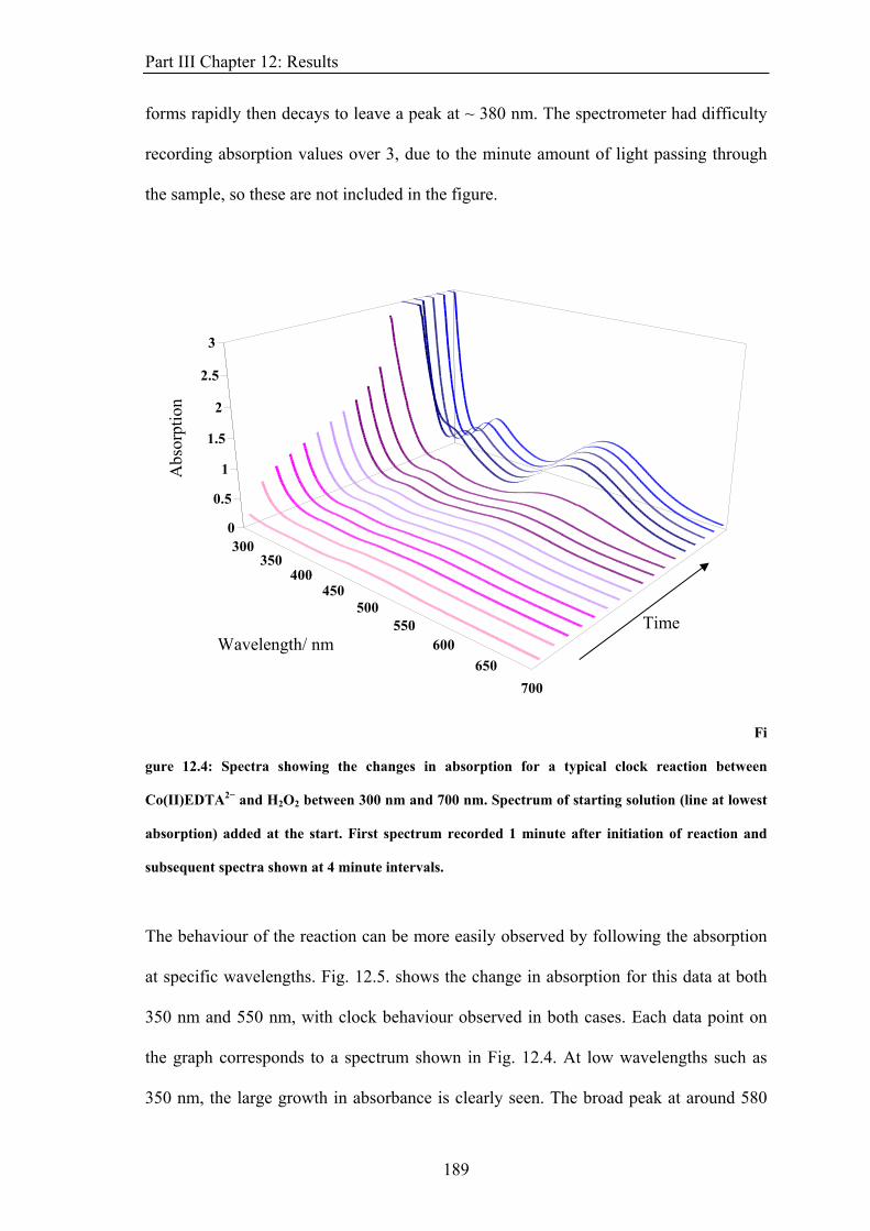
Part III Chapter 12: Results
forms rapidly then decays to leave a peak at ~ 380 nm. The spectrometer had difficulty
recording absorption values over 3, due to the minute amount of light passing through
the sample, so these are not included in the figure.
300350
400450
500550
600650
700
0
0.5
1
1.5
2
2.5
3
Abs
orpt
ion
Wavelength/ nm
Fi
gure 12.4: Spectra showing the changes in absorption for a typical clock reaction between
Co(II)EDTA2− and H2O2 between 300 nm and 700 nm. Spectrum of starting solution (line at lowest
absorption) added at the start. First spectrum recorded 1 minute after initiation of reaction and
subsequent spectra shown at 4 minute intervals.
Time
The behaviour of the reaction can be more easily observed by following the absorption
at specific wavelengths. Fig. 12.5. shows the change in absorption for this data at both
350 nm and 550 nm, with clock behaviour observed in both cases. Each data point on
the graph corresponds to a spectrum shown in Fig. 12.4. At low wavelengths such as
350 nm, the large growth in absorbance is clearly seen. The broad peak at around 580
189
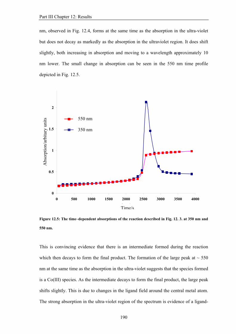
Part III Chapter 12: Results
nm, observed in Fig. 12.4, forms at the same time as the absorption in the ultra-violet
but does not decay as markedly as the absorption in the ultraviolet region. It does shift
slightly, both increasing in absorption and moving to a wavelength approximately 10
nm lower. The small change in absorption can be seen in the 550 nm time profile
depicted in Fig. 12.5.
0
0.5
1
1.5
2
0 500 1000 1500 2000 2500 3000 3500 4000time
350 nm
550 nm
550 nm 350 nm
Abs
orpt
ion/
arbi
tary
uni
ts
/sTime/s
Figure 12.5: The time–dependent absorptions of the reaction described in Fig. 12. 3. at 350 nm and
550 nm.
This is convincing evidence that there is an intermediate formed during the reaction
which then decays to form the final product. The formation of the large peak at ~ 550
nm at the same time as the absorption in the ultra-violet suggests that the species formed
is a Co(III) species. As the intermediate decays to form the final product, the large peak
shifts slightly. This is due to changes in the ligand field around the central metal atom.
The strong absorption in the ultra-violet region of the spectrum is evidence of a ligand-
190
Part III Chapter 12: Results
to-metal charge transfer band and such strong absorptions are found in peroxo-dicobalt
species12. This work is in agreement with data by Yalman4.
These spectra can be used to follow the concentrations of Co(II) and Co(III) species.
The total absorption measured at a given wavelength, λ, would be given by:
Atot, λ = (εCo(II)EDTA,λ×[Co(II)] + εCo(III)EDTA,λ×[Co(III)]) (7)
ε are absorption coefficients for the given species at a given wavelength. The path
length is constant throughout and can be ignored. The wavelength chosen is the
isosbestic point of the two Co(III) species involved, 578 nm, so that the formation of the
intermediate does not complicate matters. The calculation is made simpler by
considering that the total cobalt concentration, [Co(III)EDTA−] + [Co(II)EDTA2−], is
constant throughout. The change in the contribution of H2O2 to the absorption has been
neglected, given that it is a clear, colourless solution. However, the addition of peroxide
clearly has some effect on the solution, with an increase in absorption across all
wavelengths, and especially at lower wavelengths. To correct for this, the first point,
recorded 1 minute after the initiation of the reaction is corrected to give an absorption of
0 at 574 nm. Fig. 12.6 shows the results of this calculation.
191

Part III Chapter 12: Results
0
0.002
0.004
0.006
0.008
0.01
0.012
0.016
0.018
0.02
0 500 1000 1500 2000 2500 3000 3500 4000Time/s
[Co(
III)
]
Clocking time 2520s
-10123456789
10
0 1000 2000 3000 4000d[C
o(III
)]/d
t ×10
5 / m
oldm
−3
/mol
dm−3
0.014
Figure 12.6: Time-dependent changes in the concentration of Cobalt(III) species, calculated from
the absorption data shown in Fig. 12. 4. Insert shows the rate of change of concentration of cobalt
with clocking time identified.
The clock behaviour is quite clearly observed. The clocking time, 2520 s is easily
observed in the rate data although the precision of the value is limited entirely by the
time taken to take an individual spectrum.
It was also possible for the spectrometer to record the absorptions at one given
wavelength every 625 ms. Fig. 12.7 shows one such measurement, following the
reaction at 600 nm. As with all of the UV/vis spectroscopy, the clock behaviour of the
reaction is reproduced.
192
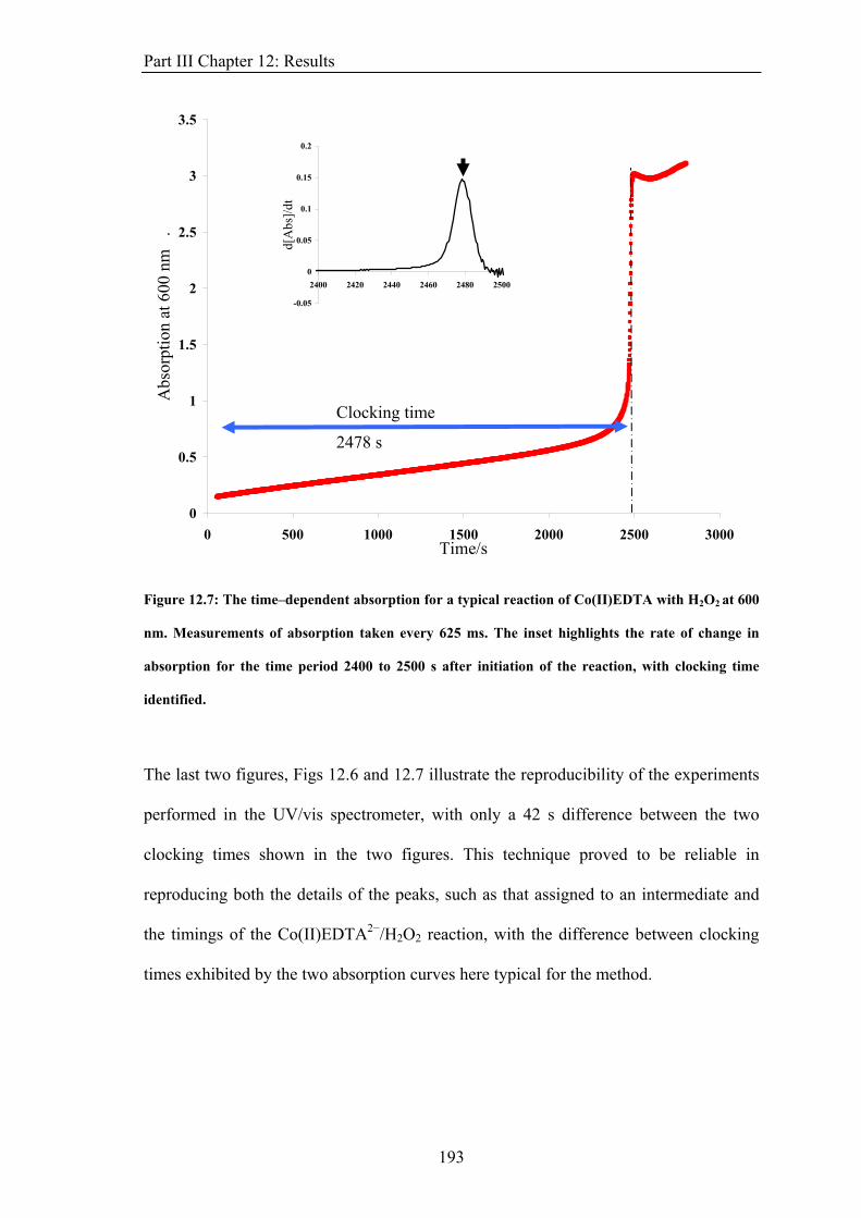
Part III Chapter 12: Results
0
0.5
1
1.5
2
2.5
3
3.5
0 500 1000 1500 2000 2500 3000Time/s
Abs
orpt
ion
at 6
00 n
m
.
-0.05
0
0.05
0.1
0.15
0.2
2400 2420 2440 2460 2480 2500d[
Abs
]/dt
2478 s
Clocking time
Figure 12.7: The time–dependent absorption for a typical reaction of Co(II)EDTA with H2O2 at 600
nm. Measurements of absorption taken every 625 ms. The inset highlights the rate of change in
absorption for the time period 2400 to 2500 s after initiation of the reaction, with clocking time
identified.
The last two figures, Figs 12.6 and 12.7 illustrate the reproducibility of the experiments
performed in the UV/vis spectrometer, with only a 42 s difference between the two
clocking times shown in the two figures. This technique proved to be reliable in
reproducing both the details of the peaks, such as that assigned to an intermediate and
the timings of the Co(II)EDTA2−/H2O2 reaction, with the difference between clocking
times exhibited by the two absorption curves here typical for the method.
193
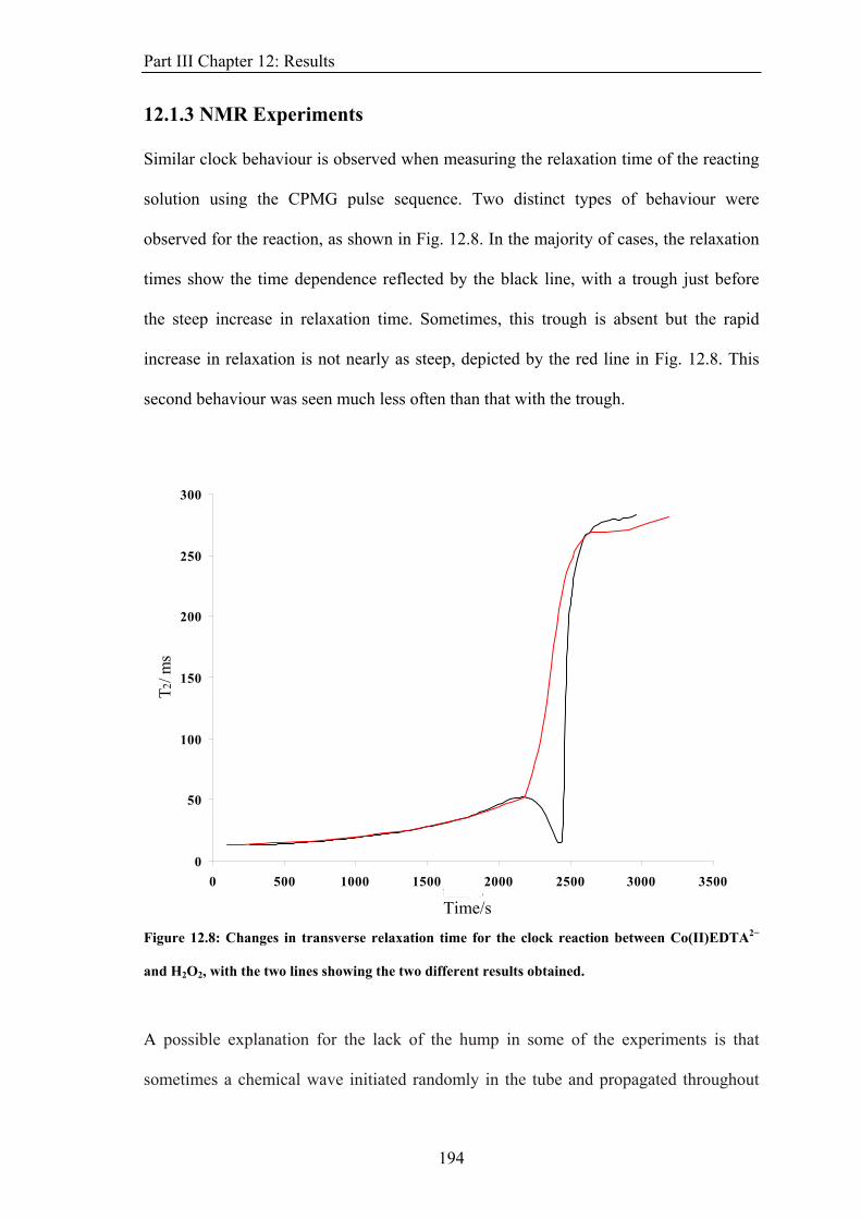
Part III Chapter 12: Results
12.1.3 NMR Experiments
Similar clock behaviour is observed when measuring the relaxation time of the reacting
solution using the CPMG pulse sequence. Two distinct types of behaviour were
observed for the reaction, as shown in Fig. 12.8. In the majority of cases, the relaxation
times show the time dependence reflected by the black line, with a trough just before
the steep increase in relaxation time. Sometimes, this trough is absent but the rapid
increase in relaxation is not nearly as steep, depicted by the red line in Fig. 12.8. This
second behaviour was seen much less often than that with the trough.
0
50
100
150
200
250
300
0 500 1000 1500 2000 2500 3000 3500time/ s
T 2/ m
s
Time/s
Figure 12.8: Changes in transverse relaxation time for the clock reaction between Co(II)EDTA2−
and H2O2, with the two lines showing the two different results obtained.
A possible explanation for the lack of the hump in some of the experiments is that
sometimes a chemical wave initiated randomly in the tube and propagated throughout
194
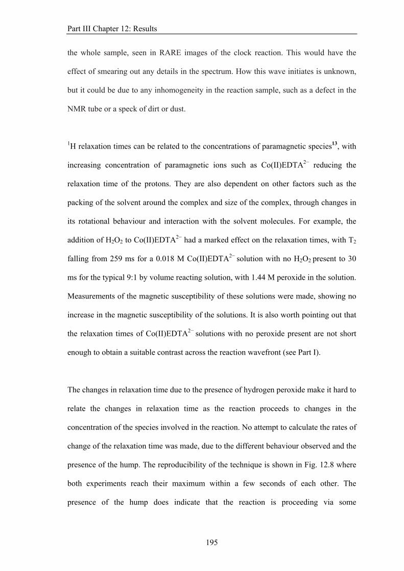
Part III Chapter 12: Results
the whole sample, seen in RARE images of the clock reaction. This would have the
effect of smearing out any details in the spectrum. How this wave initiates is unknown,
but it could be due to any inhomogeneity in the reaction sample, such as a defect in the
NMR tube or a speck of dirt or dust.
1H relaxation times can be related to the concentrations of paramagnetic species13, with
increasing concentration of paramagnetic ions such as Co(II)EDTA2− reducing the
relaxation time of the protons. They are also dependent on other factors such as the
packing of the solvent around the complex and size of the complex, through changes in
its rotational behaviour and interaction with the solvent molecules. For example, the
addition of H2O2 to Co(II)EDTA2− had a marked effect on the relaxation times, with T2
falling from 259 ms for a 0.018 M Co(II)EDTA2− solution with no H2O2 present to 30
ms for the typical 9:1 by volume reacting solution, with 1.44 M peroxide in the solution.
Measurements of the magnetic susceptibility of these solutions were made, showing no
increase in the magnetic susceptibility of the solutions. It is also worth pointing out that
the relaxation times of Co(II)EDTA2− solutions with no peroxide present are not short
enough to obtain a suitable contrast across the reaction wavefront (see Part I).
The changes in relaxation time due to the presence of hydrogen peroxide make it hard to
relate the changes in relaxation time as the reaction proceeds to changes in the
concentration of the species involved in the reaction. No attempt to calculate the rates of
change of the relaxation time was made, due to the different behaviour observed and the
presence of the hump. The reproducibility of the technique is shown in Fig. 12.8 where
both experiments reach their maximum within a few seconds of each other. The
presence of the hump does indicate that the reaction is proceeding via some
195
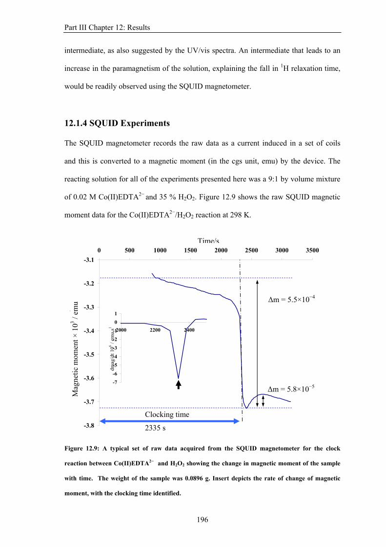
Part III Chapter 12: Results
intermediate, as also suggested by the UV/vis spectra. An intermediate that leads to an
increase in the paramagnetism of the solution, explaining the fall in 1H relaxation time,
would be readily observed using the SQUID magnetometer.
12.1.4 SQUID Experiments
The SQUID magnetometer records the raw data as a current induced in a set of coils
and this is converted to a magnetic moment (in the cgs unit, emu) by the device. The
reacting solution for all of the experiments presented here was a 9:1 by volume mixture
of 0.02 M Co(II)EDTA2− and 35 % H2O2. Figure 12.9 shows the raw SQUID magnetic
moment data for the Co(II)EDTA2−/H2O2 reaction at 298 K.
-3.8
-3.7
-3.6
-3.5
-3.4
-3.3
-3.2
-3.10 500 1000 1500 2000 2500 3000 3500
time/sTime/s
mag
netis
atio
n ×
103 /e
mu
Figure 12.9: A typical set of raw data acquired from the SQUID magnetometer for the clock
reaction between Co(II)EDTA2− and H2O2 showing the change in magnetic moment of the sample
with time. The weight of the sample was 0.0896 g. Insert depicts the rate of change of magnetic
moment, with the clocking time identified.
Δm = 5.5×10⁻⁴
Δm = 5.8×10⁻⁵
Clocking time
2335 s
-7
-6
-5
-4
-3
-2
-1
0
1
2000 2200 2400
dmag
/dt 1
06 / em
u s1
Mag
netic
mom
ent ×
103 /
emu
196
Part III Chapter 12: Results
Only the clock behaviour of the reaction is observed, although there is a rise in
magnetic moment of the sample after it has clocked. The change observed for this
experiment is 5.50 × 10⁻⁴ emu. The errors in individual measurements are around 1 ×
10−7 emu. From the data in Fig. 12.9, a clocking time of 2335 s can be found. The
precision of this value is limited by the time taken to acquire a measurement of
magnetic moment. The minimum value of magnetisation could be used as another
measure of the clocking time of the reaction. Compare Fig. 12.1 with Fig. 12.9 and it is
clear that not every method produces a clear maximum/minimum value of the data.
The change in the number of unpaired spins can be calculated from the flow chart (Fig.
11.1), and the results are summarised below:.
Δmagnetic moment/emu = 5.50 × 10⁻⁴
Δmagnetic moment/A m2 = 5.50 × 10⁻⁷
Δvolume magnetisation/A m−1 = 6.14
Δvolume magnetic susceptibility = 1.54 × 10⁻⁶
Δmolar magnetic susceptibility/m3 mol−1 = 8.57 × 10⁻⁸
From this change in molar susceptibility, the number of unpaired spins can be estimated
from the spin-only formula for susceptibility.
3kT
1))(S(SμμgNχ
2B0
2eA
m+
= (8)
For the data presented in Fig. 12.8, the change in the number of unpaired spins = 3.15,
slightly higher than the expected value of 3, but an error of only 5%. It is likely that
197
Part III Chapter 12: Results
there is some contribution to the susceptibility of the Co(II)EDTA2− solution due to
orbital contributions that arise from the d7( ) configuration of the ion. These
effects are largest when there is an unoccupied orbital of a similar energy to a singly
occupied orbital present in the ion (such as d1 and d2 configurations). The electron
configuration here should have an orbital magnetic contribution and such contributions
has been observed in some Co(II) complexes14. The Co(II)EDTA2− complex is likely to
have a higher magnetic moment than predicted by a simple spin-only model, so the
change in susceptibility as it reacts to form the Co(III)EDTA− complex
( configuration so no orbital contribution) should be larger than predicted.
52gt 2
ge
62gt
The later rise in recorded magnetic moment is probably due to the formation of
paramagnetic O2 from the disproportionation of excess H2O2 in the final reacted
solution:
2 H2O2 2 H2O + O2 (9)
This reaction is catalysed by transition metals and is also more rapid in solutions where
pH > 7. The maximum amount of O2 produced by the reaction can be estimated by
considering the amount of H2O2 present in a small reacting sample, and assuming that
all of it decomposes to form O2. For a typical reacting sample of 0.1 ml, there are 1.4 ×
10−4 moles present in the sample, and this will decompose to form 7 × 10⁻⁵ moles of
oxygen. The volume one mole of the gas will take can be estimated, using the molar
volume of a gas, approximately 2.4 × 10⁻² m3 mol−1, to give a volume of 1.7 × 10⁻⁶ m3.
There might be small differences in the molar volume, due to an increasing pressure
from produced gas, but this gives an answer in the range of cubic centimetres. With a
198
Part III Chapter 12: Results
suitably large space above the reacting solution, there should be no danger in the
pressure building up too much and breaking the tube.
Is this gas responsible for the rise in magnetic moment of the sample after the reaction
has clocked? Assuming that all of the gas remains in the sample space, the magnetic
moment of this volume of O2 can be calculated using the volume susceptibility of the
gas, 1.83 × 10⁻⁶ 15. This gives a potential rise in magnetic moment, in emu, at 50 kOe of
8.74 × 10⁻³. This is far larger than that seen in Fig. 12.9. However, the formation of
bubbles shows clearly that not all of the gas does remain in the sample. The saturation
concentration of oxygen in water is ~ 0.2 × 10⁻³ mol dm−3. Given a molar susceptibility
of O2 of 4.3 × 10⁻⁸ m3 mol−1, this gives rise to an increase in the magnetic moment of
the 0.1 ml sample of reacting solution, in a field of 50 kOe, of 6.84 × 10⁻⁶ emu,
approximately a power of ten smaller than that seen in the figure. The higher value
observed soon after the reaction has clocked could be due to a rapid production of O2 as
the reaction clocks then as the gas escapes from the solution and out of the measured
region of the sample, the magnetic moment of the sample falls towards that expected of
a saturated O2 solution. Not all of the oxygen that can be produced from the reactions of
H2O2 will be released at once. Bubbles of gas are observed in the reaction many hours
after the Co(II)EDTA2−/H2O2 has finished. Also, as the pressure in the sealed tube
increases, the saturation concentration of oxygen will increase, increasing the
contribution from the dissolved oxygen. Could the change in magnetic moment after the
reaction has clocked be related to the formation of the complex, as observed in the
UV/vis spectroscopy? In the UV/vis experiments, an intermediate formed which
decayed to form the final product. The SQUID experiments showed a rise in the
magnetic moment which is then followed by a subsequent fall. This is reproduced in all
199
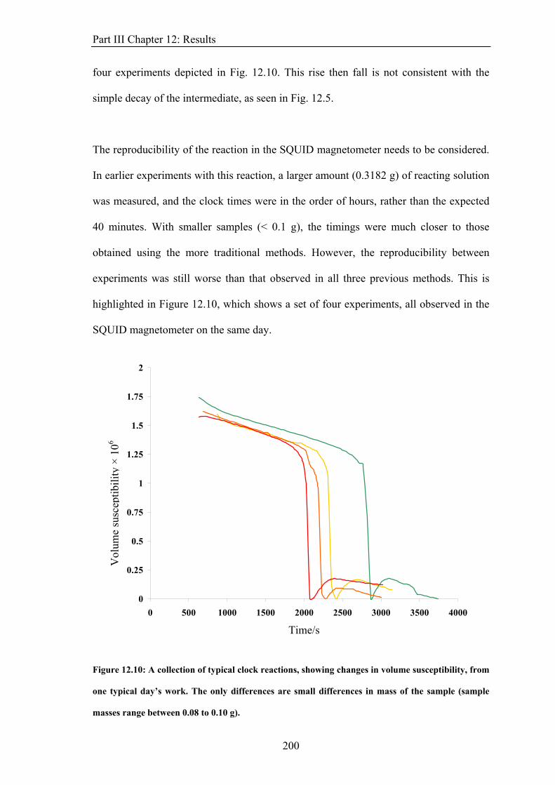
Part III Chapter 12: Results
four experiments depicted in Fig. 12.10. This rise then fall is not consistent with the
simple decay of the intermediate, as seen in Fig. 12.5.
The reproducibility of the reaction in the SQUID magnetometer needs to be considered.
In earlier experiments with this reaction, a larger amount (0.3182 g) of reacting solution
was measured, and the clock times were in the order of hours, rather than the expected
40 minutes. With smaller samples (< 0.1 g), the timings were much closer to those
obtained using the more traditional methods. However, the reproducibility between
experiments was still worse than that observed in all three previous methods. This is
highlighted in Figure 12.10, which shows a set of four experiments, all observed in the
SQUID magnetometer on the same day.
0
0.25
0.5
0.75
1
1.25
1.5
1.75
2
0 500 1000 1500 2000 2500 3000 3500 4000
Time/s
Vol
ume
susc
eptib
ility
×10
-6
.
/ 6
Vol
ume
susc
eptib
ility
× 1
0
Figure 12.10: A collection of typical clock reactions, showing changes in volume susceptibility, from
one typical day’s work. The only differences are small differences in mass of the sample (sample
masses range between 0.08 to 0.10 g).
200
Part III Chapter 12: Results
The measured moment has been converted into volume susceptibilities to enable easier
comparison of the data.
The four sets of data all show the same details – a slow induction period, which
gradually speeds up into a fast period before reaching a minimum of volume
susceptibility and then a smaller rise after the reaction has clocked. It is reassuring that
the smaller increases are similar in height for three of the four sets of data. As with the
data presented in 12.9, the clocking time is limited by the resolution of the technique
and there is little difference between the sets shown here. However, there is clearly a
difference in the clocking times of the reactions – for this set of data, the average
clocking time was 2400 s, similar to the clocking times observed in all of the techniques
shown, but, more importantly, the standard deviation was 340 s, almost 15 % of the
clocking time. This is larger than that seen in any of the previous experimental
techniques.
Further proof that the SQUID has followed the reaction can be obtained by comparing
typical sets of the SQUID and the electronic absorption data. Both techniques follow the
changes of the metal species in the reaction, and should produce very similar results.
201
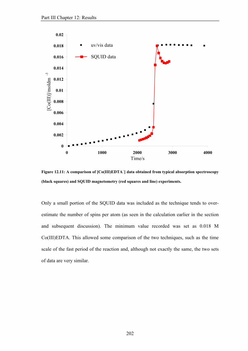
Part III Chapter 12: Results
0
0.002
0.004
0.006
0.008
0.01
0.012
0.014
0.02
0 1000 2000 3000 4000Time/s
[Co(
III)
]/mol
dm -3
uv/vis data SQUID data 0.016
0.018
Figure 12.11: A comparison of [Co(III)EDTA−] data obtained from typical absorption spectroscopy
(black squares) and SQUID magnetometry (red squares and line) experiments.
Only a small portion of the SQUID data was included as the technique tends to over-
estimate the number of spins per atom (as seen in the calculation earlier in the section
and subsequent discussion). The minimum value recorded was set as 0.018 M
Co(III)EDTA. This allowed some comparison of the two techniques, such as the time
scale of the fast period of the reaction and, although not exactly the same, the two sets
of data are very similar.
202
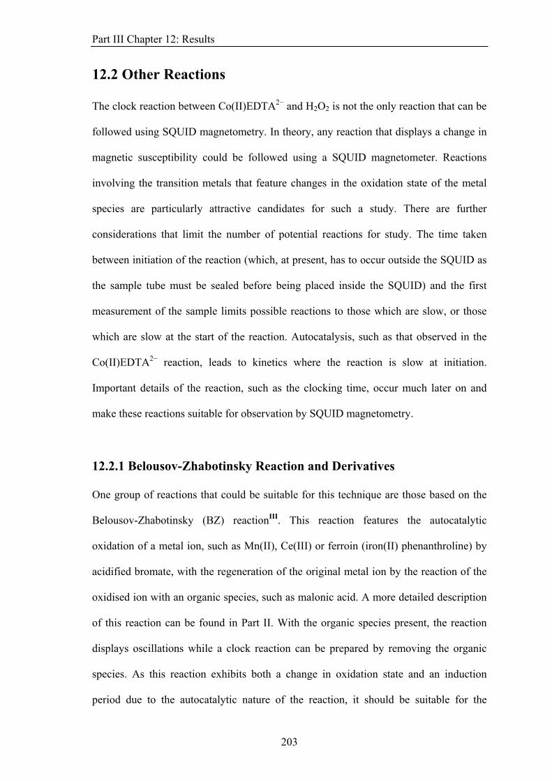
Part III Chapter 12: Results
12.2 Other Reactions
The clock reaction between Co(II)EDTA2− and H2O2 is not the only reaction that can be
followed using SQUID magnetometry. In theory, any reaction that displays a change in
magnetic susceptibility could be followed using a SQUID magnetometer. Reactions
involving the transition metals that feature changes in the oxidation state of the metal
species are particularly attractive candidates for such a study. There are further
considerations that limit the number of potential reactions for study. The time taken
between initiation of the reaction (which, at present, has to occur outside the SQUID as
the sample tube must be sealed before being placed inside the SQUID) and the first
measurement of the sample limits possible reactions to those which are slow, or those
which are slow at the start of the reaction. Autocatalysis, such as that observed in the
Co(II)EDTA2− reaction, leads to kinetics where the reaction is slow at initiation.
Important details of the reaction, such as the clocking time, occur much later on and
make these reactions suitable for observation by SQUID magnetometry.
12.2.1 Belousov-Zhabotinsky Reaction and Derivatives
One group of reactions that could be suitable for this technique are those based on the
Belousov-Zhabotinsky (BZ) reactionIII. This reaction features the autocatalytic
oxidation of a metal ion, such as Mn(II), Ce(III) or ferroin (iron(II) phenanthroline) by
acidified bromate, with the regeneration of the original metal ion by the reaction of the
oxidised ion with an organic species, such as malonic acid. A more detailed description
of this reaction can be found in Part II. With the organic species present, the reaction
displays oscillations while a clock reaction can be prepared by removing the organic
species. As this reaction exhibits both a change in oxidation state and an induction
period due to the autocatalytic nature of the reaction, it should be suitable for the
203
Part III Chapter 12: Results
technique. The cerium-catalysed BZ reaction exhibits both an induction time and
oscillations between Ce(III) and Ce(IV), making study of that reaction a very attractive
option.
12.2.1.1 Cerium-catalysed Belousov-Zhabotinsky Reaction
Fig. 12.12 shows a typical set of oscillations found in the cerium-cataysed BZ reaction,
with the reaction followed by absorption of light at 310 nm in a sealed 1 mm path length
cell in a Unicam UV-2 spectrometer.
0.07
0.08
0.09
0.1
0.11
0.12
0.13
0.14
0.15
0.16
0.17
0 500 1000 1500 2000 2500 3000time/s
abso
rptio
nA
bsor
ptio
n
Time/s
Fig 12.12: A typical set of oscillations for the cerium-catalysed BZ reaction, followed by the
absorption of light at 310 nm. Reagent concentrations are specified in the text.
204
Part III Chapter 12: Results
The reacting solution was made from a 1:1 by volume mix of 0.347 M NaBrO3 and
0.0025 M Ce(NH4)2(NO3)6 in 0.08 M H+ with 0.154 M malonic acid mixed then placed
in the cell. In order to attempt to replicate the conditions in the SQUID sample, the cell
was sealed shut with a plastic stopper.
There is an induction period with little change in the absorption of light which precedes
a series of oscillations that can last tens of minutes with only a small change in
amplitude and period. These changes occur because, as the reaction proceeds towards
equilibrium, small amounts of the reagents (BrO3−, MA) are consumed and each
oscillation takes place in a slightly different reacting solution. The period of the
oscillations is reproducible, although, as also noted elsewhere16, the induction time of
the reaction is much less reproducible.
For this reaction, the metal oscillates between colourless Ce(III) (electronic
configuration 4f1) and yellow Ce(IV) (electronic configuration 4f0). The lack of
unpaired electrons in Ce(IV) makes analysis simple. Oscillations between the two
oxidation states would be observed in the magnetometer as changes between a
paramagnetic solution and a diamagnetic one.
Compare the oscillations in Fig. 12.1 with those in Fig. 12.2, which shows a typical set
of oscillations observed in a ferroin-catalysed BZ reaction. The reaction was followed at
510 nm in a 1 mm path length cell, using a 1:1 by volume reaction mixture of 0.347 M
NaBrO3 in 0.08 M H+ mixed with 0.154 M malonic acid and 0.0025 M ferroin. In this
set of oscillations, there is no induction period17 and both the period and the intensity of
the oscillations clearly change with time. Observation of the reaction in an NMR tube
showed that the reaction tended to react as a series of waves travelling through the
205
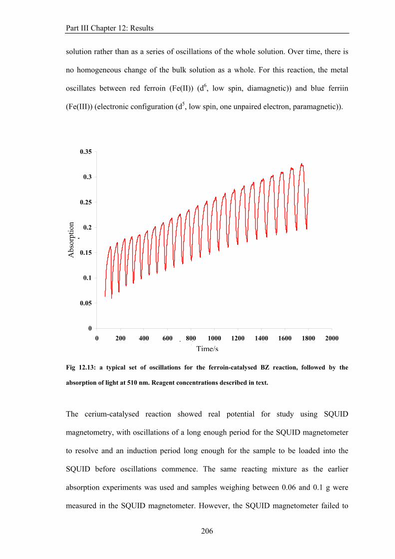
Part III Chapter 12: Results
solution rather than as a series of oscillations of the whole solution. Over time, there is
no homogeneous change of the bulk solution as a whole. For this reaction, the metal
oscillates between red ferroin (Fe(II)) (d6, low spin, diamagnetic)) and blue ferriin
(Fe(III)) (electronic configuration (d5, low spin, one unpaired electron, paramagnetic)).
0
0.05
0.1
0.15
0.2
0.25
0.3
0.35
0 200 400 600 800 1000 1200 1400 1600 1800 2000time/s
abso
rptio
nA
bsor
ptio
n
Time/s
Fig 12.13: a typical set of oscillations for the ferroin-catalysed BZ reaction, followed by the
absorption of light at 510 nm. Reagent concentrations described in text.
The cerium-catalysed reaction showed real potential for study using SQUID
magnetometry, with oscillations of a long enough period for the SQUID magnetometer
to resolve and an induction period long enough for the sample to be loaded into the
SQUID before oscillations commence. The same reacting mixture as the earlier
absorption experiments was used and samples weighing between 0.06 and 0.1 g were
measured in the SQUID magnetometer. However, the SQUID magnetometer failed to
206
Part III Chapter 12: Results
record data that showed any of the features of the absorption work. Often, the SQUID
recorded a magnet moment that simply fell gradually with time. This could have been a
result of the SQUID failing to correctly centre on the sample, perhaps due to its low
initial value. The SQUID also measured how well the data recorded fit an ideal point
magnetic moment. The graphs of this measure against time also showed it falling with
time, in much the same way as the magnetic data did. Attempts to use larger samples of
reacting solution (> 0.1 g) were not successful in recording any oscillations.
There were two further possible problems with this reaction that were not tested by this
SQUID work but are worth considering. First, the reaction sample, both in the SQUID
magnetometer and in the absorption work, is not stirred. In an unstirred vessel, the
reaction mixture does not remain homogeneous and travelling waves can form. The
motion of the sample as a measurement is made could mix the solution to some extent
but it is not vigorous to ensure that the solution is homogeneous. In this case, the bulk of
the mixture does not change oxidation state. The SQUID might also have problems with
a sample with magnetic susceptibility gradients present within it18.
The BZ reaction, like the Co(II)EDTA2−/H2O2 reaction, also produces gas: Br2 through
the reactions of oxybromine species in acidified aqueous solution and CO2 through the
reactions of malonic acid. This could be a problem in the sealed SQUID sample but, as
with the Co(II)EDTA2−/H2O2 reaction, the amount of gas can be calculated and the
space above the solution can be maximised. If the sample tube were to break within the
cryometer at the heart of the SQUID, further experiments using the apparatus would be
limited. Br2 is produced but is consumed by the malonic acid to produce bromomalonic
acid19, so the production of that should not be a problem.
207
Part III Chapter 12: Results
HOBr + Br− + H+ ⇌ Br2 + H2O (10)
Br2 + CH2(COOH)2 → BrCH(COOH)2 + Br− + H+ (11)
The overall reactions for the reaction of malonic acid with Ce(IV)17 are:
CH2(COOH)2 + 6 Ce(IV) + 2 H2O → HCOOH + 6 Ce(III) + 2 CO2 + 6 H+
(12)
BrCH(COOH)2 + 4 Ce(IV) + 2 H2O → Br− + 4 Ce(III) + HCOOH + 2 CO2 +
5 H+
(13)
Every mole of malonic acid that reacts will produce 2 moles of CO2 gas. In the SQUID
experiments, [MA] = 0.076 M and the sample volume was ~ 0.1 ml so there would be ~
7.6 × 10⁻⁶ moles of malonic acid in the sample. This would produce 1.52 × 10⁻⁵ moles
of CO2 gas. The volume of this gas can then be estimated, assuming that the molar
volume of a gas is ~ 24 ×103 cm3mol−1, as 0.36 cm3 of gas. With a large enough space
above the solution, the production of gas should not be a problem. Also, the gas is
produced in small amounts throughout the series of oscillations. Observation of the
reaction in a sealed tube revealed that only small bubbles of gas formed, and only after a
long time after the reagents were brought together.
208
Part III Chapter 12: Results
12.2.1.2 Ferroin Clock Reaction
An alternative reaction was the ferroin BZ reaction but without the malonic acid
present20. This reaction exhibited the autocatalytic oxidation of the ferroin to ferriin
without the regeneration of the metal catalyst. The reaction could be catalysed by an
alternative metal catalyst such as cerium or manganese, but, for a first attempt at
looking at the reaction, the change from red to blue exhibited by the ferroin-catalysed
reaction made its progress easily observable in NMR tubes outside of the SQUID.
The ferroin-catalysed reaction shows different reaction mechanisms depending on
different relative concentrations of ferroin and bromate ions. At concentrations of
ferroin, so that [ferroin] < [BrO3−], the key step is the autocatalytic oxidation of ferroin.
However, as the concentration of ferroin is increased, a second reaction pathway, the
dissociation of ferroin, becomes increasingly important. This change in behaviour could
be used to check whether the reaction was being followed or not by the SQUID
magnetometer.
The overall stoichiometry of the reaction is:
4 ferroin + BrO3− + 5 H+ → 4 ferriin + HOBr + 2 H2O (14)
While this does not look autocatalytic, the key sequence of steps in the reaction is the
same as for the BZ reaction. It assumed that there are small concentrations of HBrO2
and Br− present in the reaction mixture.
HBrO2 + BrO3− + H+ ⇌ Br2O4 + H2O (15)
209
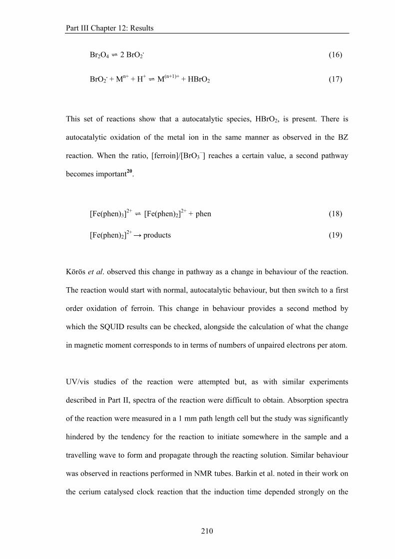
Part III Chapter 12: Results
Br2O4 ⇌ 2 BrO2. (16)
BrO2. + Mn+ + H+ ⇌ M(n+1)+ + HBrO2 (17)
This set of reactions show that a autocatalytic species, HBrO2, is present. There is
autocatalytic oxidation of the metal ion in the same manner as observed in the BZ
reaction. When the ratio, [ferroin]/[BrO3−] reaches a certain value, a second pathway
becomes important20.
[Fe(phen)3]2+ ⇌ [Fe(phen)2]2+ + phen (18)
[Fe(phen)2]2+ → products (19)
Körös et al. observed this change in pathway as a change in behaviour of the reaction.
The reaction would start with normal, autocatalytic behaviour, but then switch to a first
order oxidation of ferroin. This change in behaviour provides a second method by
which the SQUID results can be checked, alongside the calculation of what the change
in magnetic moment corresponds to in terms of numbers of unpaired electrons per atom.
UV/vis studies of the reaction were attempted but, as with similar experiments
described in Part II, spectra of the reaction were difficult to obtain. Absorption spectra
of the reaction were measured in a 1 mm path length cell but the study was significantly
hindered by the tendency for the reaction to initiate somewhere in the sample and a
travelling wave to form and propagate through the reacting solution. Similar behaviour
was observed in reactions performed in NMR tubes. Barkin et al. noted in their work on
the cerium catalysed clock reaction that the induction time depended strongly on the
210
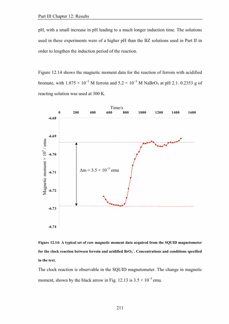
Part III Chapter 12: Results
pH, with a small increase in pH leading to a much longer induction time. The solutions
used in these experiments were of a higher pH than the BZ solutions used in Part II in
order to lengthen the induction period of the reaction.
Figure 12.14 shows the magnetic moment data for the reaction of ferroin with acidified
bromate, with 1.875 × 10⁻³ M ferroin and 5.2 × 10⁻³ M NaBrO3 at pH 2.1. 0.2353 g of
reacting solution was used at 300 K.
-6.74
-6.73
-6.72
-6.71
-6.70
-6.69
-6.680 200 400 600 800 1000 1200 1400 1600
time/sTime/s
mag
netis
atio
n
10-3
em
uM
agne
tic m
omen
t × 1
03 / em
u
Δm = 3.5 × 10⁻⁵ emu
Figure 12.14: A typical set of raw magnetic moment data acquired from the SQUID magnetometer
for the clock reaction between ferroin and acidified BrO3−. Concentrations and conditions specified
in the text.
The clock reaction is observable in the SQUID magnetometer. The change in magnetic
moment, shown by the black arrow in Fig. 12.13 is 3.5 × 10⁻⁵ emu.
211
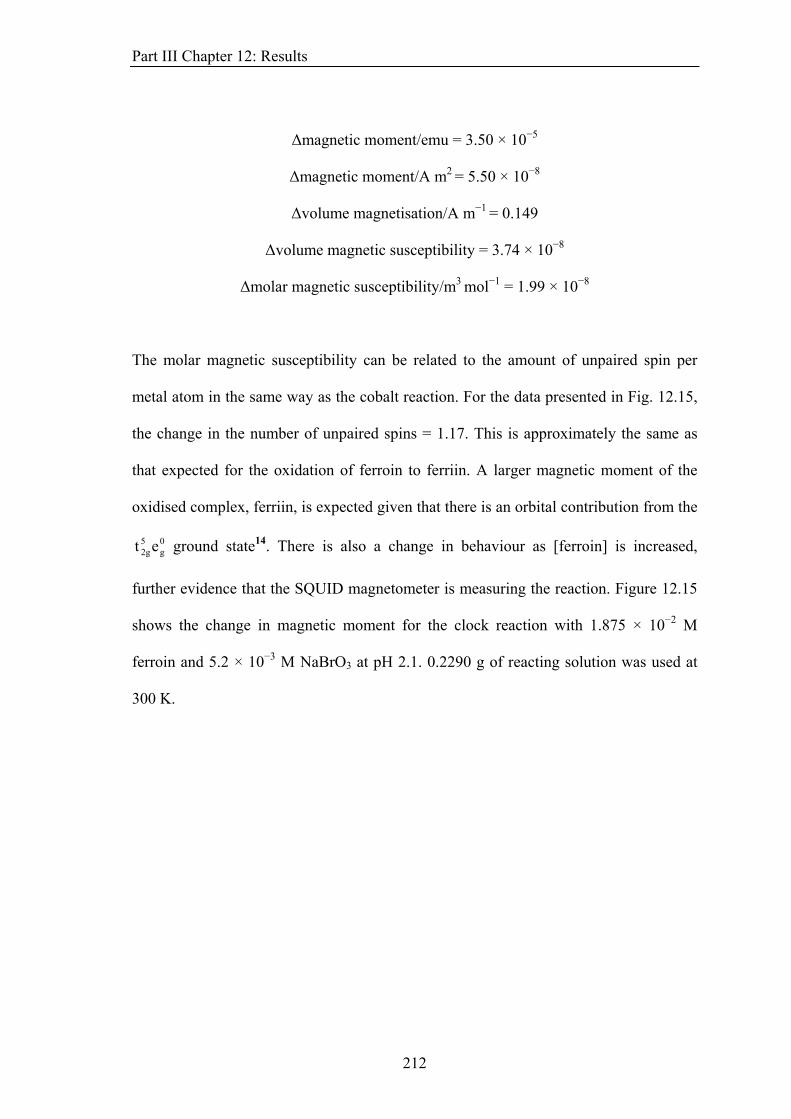
Part III Chapter 12: Results
Δmagnetic moment/emu = 3.50 × 10⁻⁵
Δmagnetic moment/A m2 = 5.50 × 10⁻⁸
Δvolume magnetisation/A m−1 = 0.149
Δvolume magnetic susceptibility = 3.74 × 10⁻⁸
Δmolar magnetic susceptibility/m3 mol−1 = 1.99 × 10⁻⁸
The molar magnetic susceptibility can be related to the amount of unpaired spin per
metal atom in the same way as the cobalt reaction. For the data presented in Fig. 12.15,
the change in the number of unpaired spins = 1.17. This is approximately the same as
that expected for the oxidation of ferroin to ferriin. A larger magnetic moment of the
oxidised complex, ferriin, is expected given that there is an orbital contribution from the
ground state14. There is also a change in behaviour as [ferroin] is increased,
further evidence that the SQUID magnetometer is measuring the reaction. Figure 12.15
shows the change in magnetic moment for the clock reaction with 1.875 × 10⁻² M
ferroin and 5.2 × 10⁻³ M NaBrO3 at pH 2.1. 0.2290 g of reacting solution was used at
300 K.
0g
52get
212
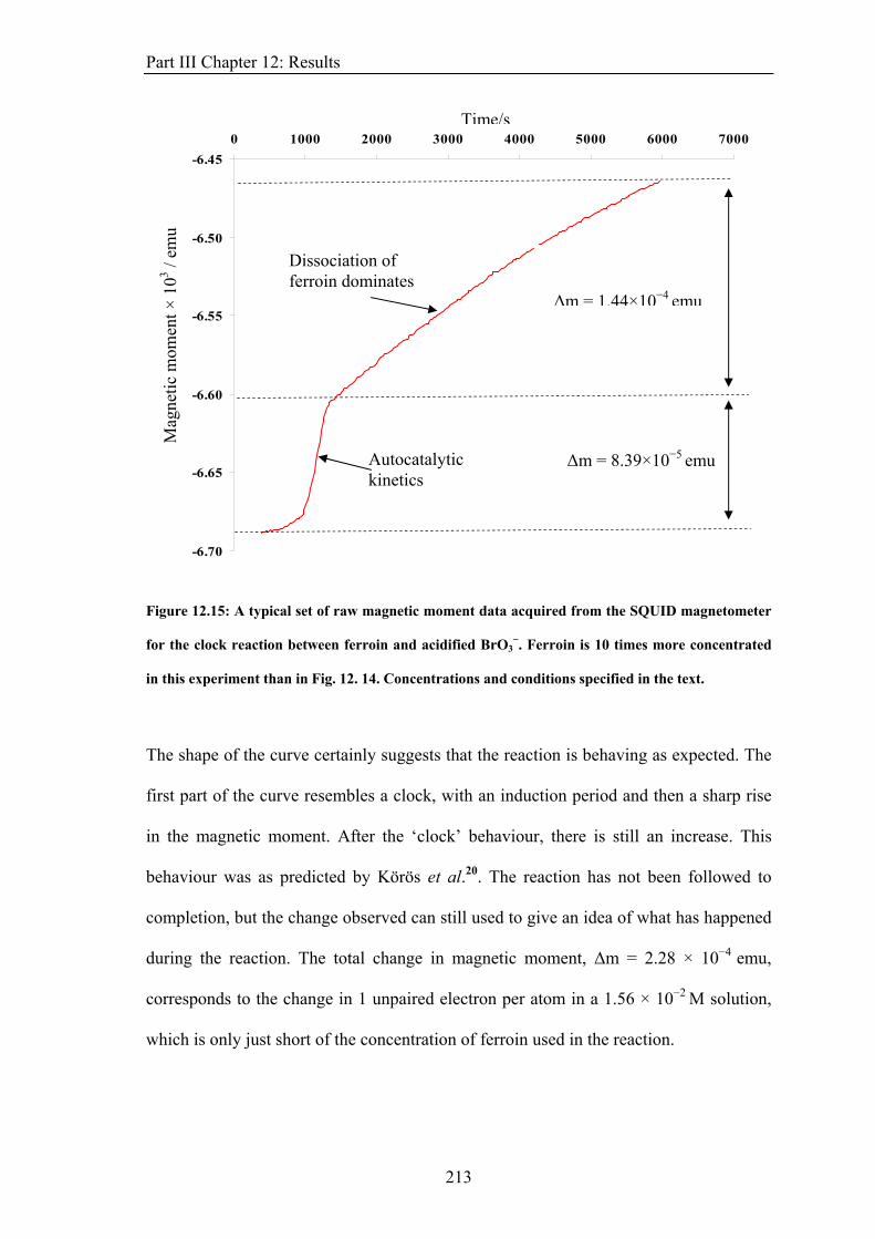
Part III Chapter 12: Results
-6.70
-6.65
-6.60
-6.55
-6.50
-6.450 1000 2000 5000 6000 70003000 4000
time/sTime/s
Mag
netis
atio
n
10
em-3
uM
agne
tic m
omen
t × 1
03 / em
u
Dissociation of ferroin dominates
Δm = 1.44×10⁻⁴ emu
Δm = 8.39×10⁻⁵ emu Autocatalytic kinetics
Figure 12.15: A typical set of raw magnetic moment data acquired from the SQUID magnetometer
for the clock reaction between ferroin and acidified BrO3−. Ferroin is 10 times more concentrated
in this experiment than in Fig. 12. 14. Concentrations and conditions specified in the text.
The shape of the curve certainly suggests that the reaction is behaving as expected. The
first part of the curve resembles a clock, with an induction period and then a sharp rise
in the magnetic moment. After the ‘clock’ behaviour, there is still an increase. This
behaviour was as predicted by Körös et al.20. The reaction has not been followed to
completion, but the change observed can still used to give an idea of what has happened
during the reaction. The total change in magnetic moment, Δm = 2.28 × 10⁻⁴ emu,
corresponds to the change in 1 unpaired electron per atom in a 1.56 × 10⁻² M solution,
which is only just short of the concentration of ferroin used in the reaction.
213
Part III Chapter 12: Results
As with the Co(II)EDTA2−/H2O2 reaction, there were issues with the reproducibility of
the reaction. The difference in timings of the reactions was similar to that observed in
the Cobalt reactions detailed in 12.4 with two added problems. The first was that in
order to obtain a set of data that showed that the reaction was actually taking place a
larger mass of solution had to be used. Smaller samples (< 0.1 g) failed to show any
behaviour. It was observed early in studying the Co(II)EDTA2−/H2O2 reaction that a
larger mass of solution could lead to much longer reaction times, with the reaction
sometimes taking several hours to react. In order to obtain data that showed the clock,
accurate measurement of the kinetics had to be sacrificed. The second was that the
reaction itself was inherently noisy, with a tendency for the reaction to form of the
surface of the cell. It was hard to get a set of reactions to clock at about the same time
outside of the SQUID. Placing these reactions in the cryostat of the magnetometer
added to the difficulty. In addition to this, there were still problems with measuring the
reaction using the SQUID magnetometer with many failed experiments.
12.5.2 Vanadium Chemistry
Vanadium chemistry was also considered as several oxidation states can be reached
through reaction. The reaction of vanadate solution with zinc metal in hot acid displays
a range of colours as the reaction oxidises the reduces the vanadium from a yellow
VO2+ (V(V)) solution to blue VO2+ (V(IV)) via a green solution, a mixture of the two.
Further reduction of the vanadium occurs, with formation of a green V(III) solution and
then purple V(II) possible. A simplified chain of equations for the reaction is shown
below, showing the changes in vanadium oxidation state.
214
Part III Chapter 12: Results
2 VO2+ + 4 H+ + Zn(s) 2 VO2+ + 2 H2O + Zn2+ (20)
VO2+ + 2 H+ + Zn(s) V3+ + H2O + Zn2+ (21)
2 V3+ + Zn(s) 2 V2+ + Zn2+ (22)
This sequence of reactions was confirmed by reaction of a 0.085 M V(V) solution at pH
1, reacting with 2-3 g of powdered zinc. However, the reaction conditions would be far
too vigorous for the SQUID magnetometer to cope with. To get the reaction to proceed
past the blue solution, it needed heating to ~ 40°C. The reverse reaction was also
considered, with an appropriate oxidising agent used to return the solution back up.
However, this was also not suitable, with the reaction quickly returning to higher
oxidation states in air, even upon transferring to another container. Hydrogen ions in
solution can oxidise the final V2+ solution back to V3+, producing hydrogen gas, and the
presence of air continues the oxidation of the vanadium ions.
The reaction of the VO2+ ion with d-fructose was another reaction that showed promise,
with work suggesting that the reaction showed suitable kinetics21. However, following
the reaction using absorption of light showed that the reaction was actually not suitable,
with no induction period observed. Fig 12.16 shows the change in absorption between
400 and 750 nm of a reacting solution. A 0.027 M solution of NH4VO3 at pH 1 was
mixed in a 1:1 by volume ratio with 0.26 M d-fructose solution. The original VO2+
solution was bright yellow/orange, which gradually turned green, then pale blue. The
first spectrum was acquired 30 s after initiation and subsequent spectra at 90 s intervals.
215
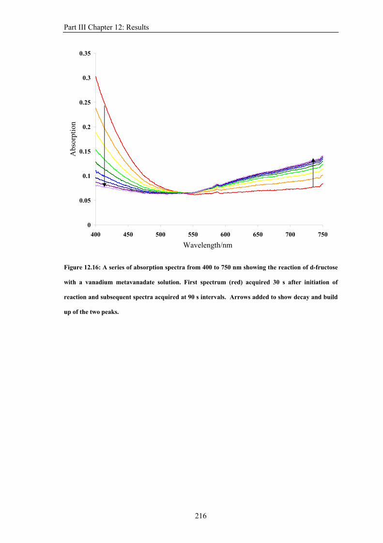
Part III Chapter 12: Results
216
0
0.05
0.1
0.15
0.2
0.25
0.3
0.35
400 450 500 550 600 650 700 750
Wavelength/nm
Abs
orpt
ion
Figure 12.16: A series of absorption spectra from 400 to 750 nm showing the reaction of d-fructose
with a vanadium metavanadate solution. First spectrum (red) acquired 30 s after initiation of
reaction and subsequent spectra acquired at 90 s intervals. Arrows added to show decay and build
up of the two peaks.

Part III Chapter 13: Discussion
217
13. DISCUSSION
The aim of this work was to show that solution phase chemical reactions can be
monitored using a SQUID magnetometer. The clock behaviour of the
Co(II)EDTA2−/H2O2 reaction as Co(II)EDTA2− is oxidised to Co(III)EDTA− is
observed. Data recorded on the SQUID magnetometer can be compared with that
acquired using more traditional techniques, such as absorption spectroscopy.
Calculations based upon the changes in metal species in the reaction confirm that the
magnetometer is recording the changes in magnetic susceptibility due to the clock
reaction. The timings of the reaction are similar for all of the techniques suggesting that
the applied magnetic field of the SQUID has no effect on the Co(II)EDTA2−/H2O2
reaction. The clock reaction between ferroin and acidified BrO3− is also observed in the
magnetometer, with an expected change in behaviour of the reaction as the
concentration of ferroin is increased.
Taken in isolation, the SQUID data from the Co(II)EDTA2−/H2O2 reaction, like the pH
data from the reaction, only shows the clock behaviour of this reaction. The difference
between the two techniques is that they follow two different species, transition metal
complex and hydroxide ions, present in the reaction. However, it is in combination with
all of the data acquired that the SQUID data can give further insight into the reaction.
There is an intermediate present in the reaction, as suggested by Yalman4, and
confirmed here in the UV/vis spectra. As the peak at 550 nm forms at the same time as
the strong absorbance in the ultra-violet (see Fig. 12.5.), the intermediate would
probably be Co(III) centred with a ligand-to-metal charge transfer absorption, such as
that due to a peroxo-ligand. The small change in the wavelength of the peak at 550 nm
Part III Chapter 13: Discussion
is then probably due to small changes in the ligand field as the peroxo-compound forms
and then decays. The magnetic resonance data adds more detail, with a fall in relaxation
time observed just before the reaction does clock. This fall in relaxation time could be
due to the change in oxidation state of the metal species. If this was the case, any
change in magnetic properties would be seen in the SQUID data. As the hump is absent
in the SQUID data, this fall in relaxation time must arise from some other change in the
complex. The T2 of a solution can depend on the ordering of the solvent around ions in
that solvent and, as there is some intermediate formed, this is a possible explanation for
the spectra seen. Further to this, the relaxation time of the Co(II)EDTA2− solution is
dependent on the presence of H2O2, so some interaction between these two species
could explain this. This data supports Yalman’s proposed intermediate – a peroxo-
dicobalt(III) species – as the SQUID data shows that the intermediate has the same
number of unpaired spins per atom as the final cobalt(III) product. A larger metal
complex formed with two metal centres bridged by a peroxo- group could also lead to
the change in relaxation time observed. Time-resolved electron spin resonance (ESR)
spectra of the reaction could give further information about the nature of the metal
complexes involved. A preliminary study has been attempted, with spectra of frozen
samples of the reacting solution acquired at known intervals, however further work is
required.
The use of SQUID magnetometry in following the ferroin-bromate clock fails to add
any further details to the reaction, but confirms that a clock reaction does occur and, as
the concentration of ferroin is increased, there is a change in behaviour, confirming
previous research. What these experiments do is confirm the potential of using the
technique to follow a reaction other than the Co(II)EDTA2−/H2O2 clock.
218
Part III Chapter 13: Discussion
As a method of following a reaction, the SQUID magnetometer has its uses but also its
limitations. As described in Chapter 12, there is a limitation as to what reactions can be
followed due to the time taken to load a sample into it and the limited number of
reactions that feature changes in magnetic properties. The kinetics of the reaction are an
important factor in the suitability of a reaction, with those exhibited by most
autocatalytic reactions suitable for study. The resolution of the technique is also a
limitation with a fastest possible speed of data acquisition of one measurement every ten
to fifteen seconds. With the reactions studied here, the changes in behaviour occur over
a similar time scale, but a faster reaction would not be able to be followed using the
reaction. There is the possibility of freezing the sample before placing it in the SQUID.
This can interfere with the reaction as ice crystals form inhomogeneities in the sample.
The ferroin clock reaction is observed to react completely upon freezing. If the samples
are frozen quick enough and the freezing does not interfere with the reaction, then the
SQUID can be used to follow a reaction by studying frozen samples taken at known
time intervals/reaction conditions. This approach has been used to characterise changes
in a Manganese-centred species22.
The reproducibility of the timings of the clock reaction in the SQUID reaction are worse
than the other techniques used to follow the reaction, as shown in Fig. 12.10. In
comparison, all the other techniques used give measurements to within 60 s of each
other, with the thermostatted pH measurement the most accurate method of following
the timing of the reaction. Although the reaction is thermostatted at the centre of the
SQUID coils, the sample has to pass through temperature gradients as it passes from the
outside into the superconducting magnet at the heart of the magnetometer. It may also
pass through temperature gradients as the sample is moved through the cryostat as the
219
Part III Chapter 13: Discussion
magnetic moment is measured. A larger volume of solution is more likely to pass
outside of the thermostatted region of the cryostat and into colder regions of the
magnetometer. This leads to cooling of the sample. These problems with temperature
gradients are not relevant for the typical use of the SQUID in measuring magnetic
properties of solid state compounds. Only the temperature of the sample as these
measurements of magnetisation is made is important. However, when following a
reaction, cooling the reaction does affect the rate of the reaction, changing the clocking
time, for example.
There may also be heating of the sample as it is sealed, although this can be limited by
sealing the tube as far away from the solution as possible. The SQUID treats the sample
as a point source magnetic dipole, which might cause problems with a larger sample as
the magnetisation of the sample is calculated by comparison with an ideal sample. Both
of these effects can be minimised by using as small an amount of material as possible.
Similar problems with the timings of the reaction occur with studies of reactions based
on the BZ reaction, with larger samples needed so that measurements could be made,
even though this makes the reaction slower. All of these factors limit the usefulness of
the technique in analysing the kinetics of the reaction.
The SQUID is different to the other methods of the reaction in a number of other ways.
The reaction is sealed, in the dark and in a large applied static magnetic field. The effect
of these conditions on the Co(II)EDTA2−/H2O2 reaction was replicated outside of the
SQUID with the reactions performed in 5 mm I.D. NMR tubes. No large effects on the
reaction were observed on the rate of reaction for any of the conditions. The staccato
motion of the sample as a measurement is made was also replicated. Again, this had no
220
Part III Chapter 13: Discussion
effect on the Co(II)EDTA2−/H2O2 reaction. However, it failed to mix the BZ and related
reactions enough to prevent the formation of waves dominating the changes in oxidation
state of the reaction. This raises an important point relevant to all of the techniques.
Inhomogeneities on the surface of the reaction vessel are known to initiate wave
reactions. The Co(II)EDTA2−/H2O2 reaction was a lot more robust than the BZ reaction,
with wave formation only observed in a small number of experiments performed in
NMR tubes (see 12.1.3). However, the BZ reaction was known, and observed, to be
very sensitive to inhomogeneities and waves formed on most glass surfaces. Reducing
the surface area relative to the volume of the solution could reduce the effect of these
waves on the reaction.
In spite of these caveats, this technique could be useful in systems where the reaction
proceeds with little change in either pH or absorption, such as in opaque solutions or
materials. It is non-invasive, so suitable for analysis of light- or air-sensitive materials.
It is a direct method of determining the concentration of any paramagnetic species
present during a reaction and very sensitive measurements of the species can be made.
The information obtained about a reaction can then be used in conjunction with other
spectra and data to produce a more detailed picture of the reaction and the presence (or
absence) of any intermediates and their nature. This study is the first time the SQUID
magnetometer has been used to follow the progress of a liquid phase chemical reaction.
The SQUID magnetometer lends itself to the study of magnetic field effects due to two
key aspects of the technique, and one modification. First, the magnetometer is contained
within a superconducting magnet, and the applied magnetic field within the
magnetometer can be easily, and quickly, changed from 0 up to 5 T. Second, there is the
221
Part III Chapter 13: Discussion
222
inherent sensitivity of the technique, so even small changes in the concentrations of
radicals in the sample can be seen through the change in magnetisation observed. The
concentration of radical pairs in a typical flash photolysis experiment will be ~ 1 × 10⁻⁵
M23. In the ferroin clock experiments, the change of 1 unpaired electrons per mole in a
1.875 × 10⁻³ M solution was clearly seen, with a change in moment of 5.5 × 10⁻⁴ emu.
The changes in the radical pair will be ~ 100 times smaller than this change. This is on
the limit of the sensitivity of the SQUID, as the errors for most measurements were ~ 1
× 10−7 emu. A second problem arises from the transient nature of the radical pairs
formed. A radical pair can have a lifetime of only nanoseconds while it takes the
SQUID seconds to make a measurement. Importantly, the SQUID can be modified so
that a light guide can be attached and a sample continuously irradiated within the
magnetic field. The applied magnetic field can then be changed, so any magnetic field
dependence on the concentration of radicals in the sample could be observed. An
example of this modification of the SQUID is shown by the SQUID study of the
irradiation of 2,4,6-triazo-3,5-dichloropyridine crystals to form paramagnetic centres24.
A liquid phase radical pair, formed by the continuous irradiation of a sample, and
subjected to changing magnetic fields, is not too many steps removed from this
experiment and certainly a possibility avenue for further use of the technique.
14. SUMMARY AND CONCLUSIONS
This thesis is based on the possibility that autocatalysis in a reaction mechanism may
play a role in amplifying any magnetic field effect present in a reaction. The possibility
of the kinetics of a reaction amplifying a small effect, such as that of an applied
magnetic field, is certainly an interesting topic of research and one with many possible
applications such as in biological systems.
Two particular reactions were investigated: the reaction between Co(II)EDTA2− and
H2O2 and the Belousov-Zhabotinsky reaction. The key features of the reactions,
travelling waves and clock behaviour/oscillations, were used to observe the effects of
magnetic fields on the reactions.
An investigation of the travelling wave that forms when Co(II)EDTA2− reacts with H2O2
forms the first section of the thesis. A series of preliminary experiments started to
quantify the reaction in terms of the forces acting on the wave front. Magnetic
resonance imaging techniques produced a series of striking images of the fingering
distortion. Both vertical and horizontal slices were used to image the wave, so that
manipulation of it around the xy plane could be observed.
The different effect of different geometry magnetic fields was also observed, with a
magnetic field gradient needing some convection around the wavefront in order
for it to have an effect on the reaction, while magnetic field gradients and
had a large effect on previously flat waves, initiating a distortion in the wave.
This distortion could be manipulated by the application of further magnetic field
z/Bz ∂∂
x/Bz ∂∂
y/Bz ∂∂
Chapter 14: Summary and Conclusion
gradients. By performing the reaction in porous foam, the role of convection as a key
factor in the magnetic field effect was identified. While the work presented here shows
a visually impressive magnetic field effect and provides an explanation for the magnetic
field effect, there is also great potential for future work, as described in chapter 5.2.
The Belousov-Zhabotinsky reaction was identified as a reaction that could show a
magnetic field dependency. In contrast to the Co(II)EDTA2−/H2O2 experiments, the
reaction itself was thought to be magnetic field dependent and that autocatalysis would
amplify any effect. Research done by other groups suggested that a magnetic field effect
on the reaction could be observed.
Apparatus was designed and built to observe the oscillations of the reaction. Solution
was continuously flowed through the cell and stirred to remove any inhomogeneities
from the solution. Series of oscillations were obtained using both cerium and ferroin as
the catalyst for the reaction, showing that the apparatus worked. Perturbations, such as
the addition of silver ions, were applied to the reaction and showed that changes in the
period of oscillations could be observed using the apparatus. Qualitative analysis of
these perturbations was also carried out.
When a magnetic field was applied to the reaction, no effect was observed in either the
ferroin-catalysed or the cerium-catalysed reactions. This was confirmed by analysis of
the data using Student’s T-test. The absence of any effect was explained by considering
the factors needed for a reaction to be magnetic field dependent. The lifetimes of the
radicals in the reaction were shown to be many powers of ten different to the timescale
224
Chapter 14: Summary and Conclusion
225
of any mixing of the radical state, while the presence of paramagnetic metal ions and
bromine atoms would remove any coherent spin-mixing through relaxation processes.
The final section of the thesis concerned not the manipulation of the reactions but the
analysis of the reactions using their changes in magnetic properties. SQUID
magnetometry is the most sensitive method of measuring magnetic fields and this
sensitivity could be used to measure tiny changes in concentration of radical species.
The work in the thesis used the reactions described previously to determine how
suitable SQUID magnetometry was for following chemical reactions and what details
the technique could show about a chemical reaction. Both reactions were successfully
followed with the technique, with the changes in magnetic susceptibility observed. The
data collected for the Co(II)EDTA2−/H2O2 reaction was compared and contrasted with
that obtained by more traditional methods, such as NMR and UV/vis spectroscopy. This
gave more information about intermediates that formed during the course of the reaction.
SQUID magnetometry proved to be another possible technique that can be used to
follow chemical reactions. Modification of the magnetometer to make it suitable for the
study of magnetic fields arising from the radical pair mechanism was discussed.
This thesis has shown how magnetic fields can be used to both manipulate and
investigate autocatalytic chemical reactions. A range of experimental techniques have
been used in this thesis. In particular, MRI techniques illustrated how magnetic field
gradients can manipulate and control travelling waves and SQUID magnetometry was
shown to be a potentially useful tool in observing chemical reactions. This thesis opens
up possibilities for detailed theoretical work that can supplement and complement these
investigations and further experimental work to build on the progress made here.
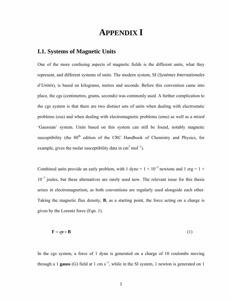
Appendix I
I
APPENDIX I
I.1. Systems of Magnetic Units
One of the more confusing aspects of magnetic fields is the different units, what they
represent, and different systems of units. The modern system, SI (Systèmes Internationales
d’Unités), is based on kilograms, metres and seconds. Before this convention came into
place, the cgs (centimetres, grams, seconds) was commonly used. A further complication to
the cgs system is that there are two distinct sets of units when dealing with electrostatic
problems (esu) and when dealing with electromagnetic problems (emu) as well as a mixed
‘Gaussian’ system. Units based on this system can still be found, notably magnetic
susceptibility (the 80th edition of the CRC Handbook of Chemistry and Physics, for
example, gives the molar susceptibility data in cm3 mol−1).
Combined units provide an early problem, with 1 dyne = 1 × 10⁻⁵ newtons and 1 erg = 1 ×
10−7 joules, but these alternatives are rarely used now. The relevant issue for this thesis
arises in electromagnetism, as both conventions are regularly used alongside each other.
Taking the magnetic flux density, B, as a starting point, the force acting on a charge is
given by the Lorentz force (Eqn. 1).
(1) BvF ×= q
In the cgs system, a force of 1 dyne is generated on a charge of 10 coulombs moving
through a 1 gauss (G) field at 1 cm s−1, while in the SI system, 1 newton is generated on 1
Appendix I
coulomb moving through a 1 tesla (T) field at 1 ms−1 (where 1 tesla = 104 gauss). These
units are interchanged freely, as 1 T is a large magnetic field. Alongside B, there is also the
magnetic field strength, H and magnetisation M (see chapter 1.1.1). The SI system defines
the three quantities B, H and M by
)(μ 0 MHB += (2)
whereas in the cgs emu system
MHB π4+= (3)
This would not be a problem, but magnetic fields measured in oersteds (cgs unit of H) are
still used, such as in the SQUID magnetometer used in Part III. To convert from oersted to
the SI equivalent, A m−1, a conversion factor of 1/4π × 103 is required. One advantage of
the latter system is that B and H have the same dimensions. This factor of 4π arises again in
measurements of susceptibility. A molar susceptibility of cm3 mol−1 requires a conversion
of 4π × 10−6 rather than 1 × 10⁻⁶, as the units might suggest.
These differences arise from the fact that electricity and magnetisation are linked through
and the values of ε0 and μ0 cannot be independent. The different systems simply
introduced different values for the two constants. These competing systems can easily add
confusion to any problem, with different units being used in different areas by different
people . In this thesis, SI units have been used wherever possible. Although the SQUID
dQ/dtI =
II

Appendix I
III
magnetometer measures in the cgs emu system, the measurements were converted to those
in the SI system as soon as possible and then SI units were used wherever possible. If cgs
units are used, they will be appropriately labelled.
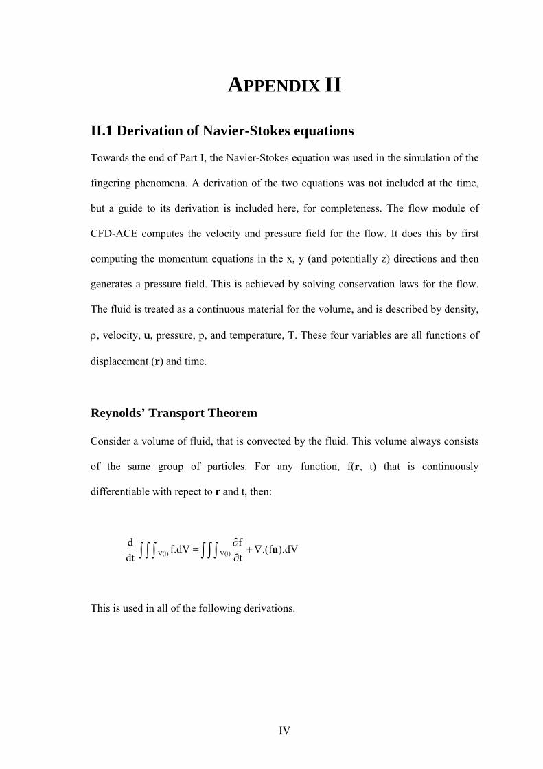
Appendix II
IV
APPENDIX II
II.1 Derivation of Navier-Stokes equations Towards the end of Part I, the Navier-Stokes equation was used in the simulation of the
fingering phenomena. A derivation of the two equations was not included at the time,
but a guide to its derivation is included here, for completeness. The flow module of
CFD-ACE computes the velocity and pressure field for the flow. It does this by first
computing the momentum equations in the x, y (and potentially z) directions and then
generates a pressure field. This is achieved by solving conservation laws for the flow.
The fluid is treated as a continuous material for the volume, and is described by density,
ρ, velocity, u, pressure, p, and temperature, T. These four variables are all functions of
displacement (r) and time.
Reynolds’ Transport Theorem
Consider a volume of fluid, that is convected by the fluid. This volume always consists
of the same group of particles. For any function, f(r, t) that is continuously
differentiable with repect to r and t, then:
).dV.(ftff.dV
dtd
V(t)V(t) u∇+∂∂
=∫ ∫ ∫∫ ∫ ∫
This is used in all of the following derivations.
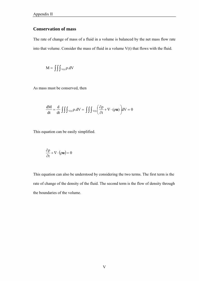
Appendix II Conservation of mass
The rate of change of mass of a fluid in a volume is balanced by the net mass flow rate
into that volume. Consider the mass of fluid in a volume V(t) that flows with the fluid.
∫ ∫ ∫= ρ.dVM V(t)
As mass must be conserved, then
0dV.)(ρtρρ.dV
dtd
dtdM
V(t)V(t) =⎟⎠⎞
⎜⎝⎛ ⋅∇+∂∂
== ∫ ∫ ∫∫ ∫ ∫ u
This equation can be easily simplified.
( ) 0ρtρ
=⋅∇+∂∂ u
This equation can also be understood by considering the two terms. The first term is the
rate of change of the density of the fluid. The second term is the flow of density through
the boundaries of the volume.
V
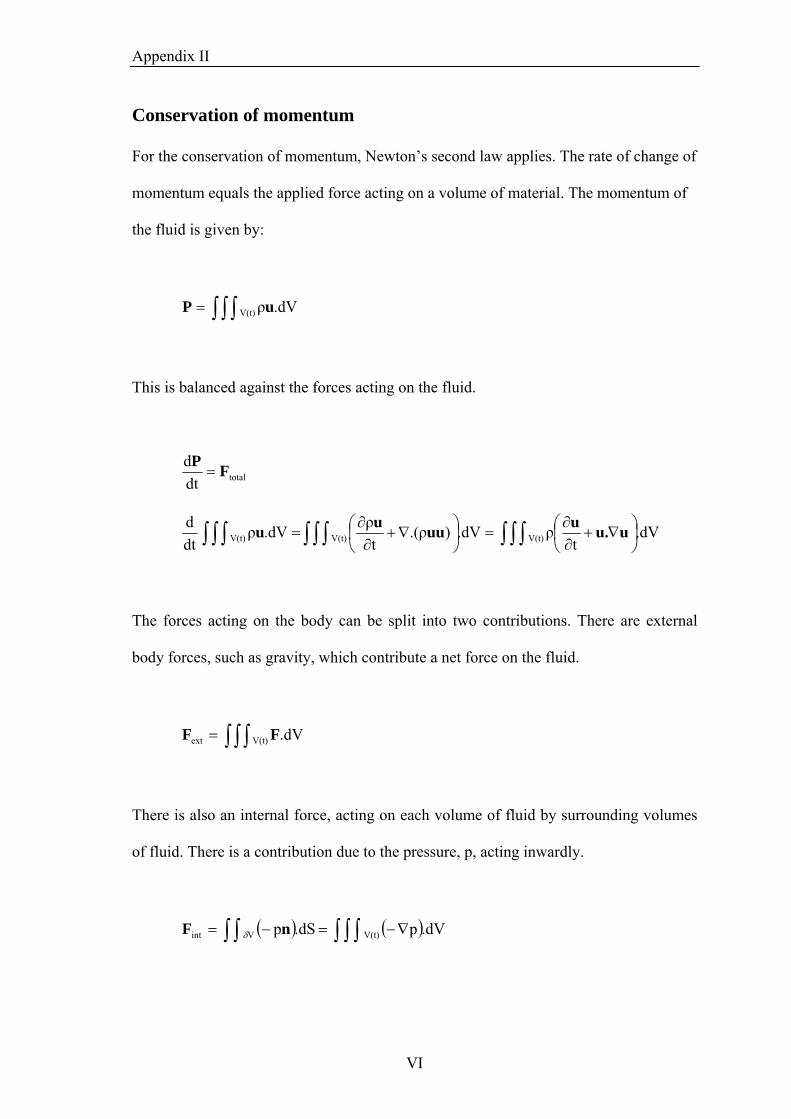
Appendix II Conservation of momentum
For the conservation of momentum, Newton’s second law applies. The rate of change of
momentum equals the applied force acting on a volume of material. The momentum of
the fluid is given by:
∫ ∫ ∫= .dVρV(t) uP
This is balanced against the forces acting on the fluid.
totaldtd FP
=
.dVt
ρ.dV).(ρtρ.dVρ
dtd
V(t)V(t)V(t) ∫ ∫ ∫∫ ∫ ∫∫ ∫ ∫ ⎟⎠⎞
⎜⎝⎛ ∇+∂∂
=⎟⎠⎞
⎜⎝⎛ ∇+∂∂
= uu.uuuuu
The forces acting on the body can be split into two contributions. There are external
body forces, such as gravity, which contribute a net force on the fluid.
∫ ∫ ∫= .dVV(t)ext FF
There is also an internal force, acting on each volume of fluid by surrounding volumes
of fluid. There is a contribution due to the pressure, p, acting inwardly.
( ) ( )∫ ∫ ∫∫ ∫ ∇−=−= .dVp.dSp V(t)Vint nF δ
VI
Appendix II There is also a contribution due to the viscosity of the fluid. In order to include these
forces, assumptions must be made about the nature of the fluid. If it is assumed that
viscosity is neglible, then:
( ).dVpρgdV.t
ρ V(t)V(t) ∫ ∫ ∫∫ ∫ ∫ ∇−=⎟⎠⎞
⎜⎝⎛ ∇+∂∂ uu.u
0dVρg.-pt
ρV(t) =∇+⎟⎠⎞
⎜⎝⎛ ∇+∂∂
∫ ∫ ∫ uu.u
The integrand must also equal 0, and the equation of fluid flow for a zero-viscosity fluid
is obtained. The presence of viscosity, μ, results in stresses within the fluid. In order to
include this in the equations, certain assumptions about the fluid must be made. In order
to produce the equation 5.34a, the stress tensor was assumed to have the form:
uuu .λδrr
μT iji
j
j
iij ∇+⎟
⎟⎠
⎞⎜⎜⎝
⎛
∂
∂+
∂∂
=
The second term arises due to the presence of a second coefficient of viscosity, λ,
associated with changes in volume. This term is normally neglible. The remaining term
is included in the equation as T⋅∇ , giving the equation used.
VII
Appendix II Conservation of energy
Equations of motion can also be calculated by considering that energy must be
conserved for the solution. If heat is to be included in the equations, then it can be
included in the equations of motion by considering that energy must be conserved. The
kinetic energy of a volume of the fluid is given by:
dVρ21 2
V u∫∫∫
The thermal energy of the volume of fluid is given by
TdVρcvV∫∫∫
where cv is the specific heat of the solution. Energy sources and sinks also have to be
included in the model. The same technique used above can be used to produce a third
equation.
There are now three equations, but four unknowns (ρ, u, p and T). A fourth equation is
needed, to link pressure, density and temperature, such as:
ρRTp =
In the model shown in the thesis, the relationships between concentration, temperature
and density are the relevant equation.
VIII

Appendix II
IX
Finite Volume Analysis
The technique used by CFD-ACE is known as finite volume analysis. The governing
equations are solved on discrete control volumes. A recommended book on the topic is
“Computational Methods for Fluid Dynamics” by Ferziger and Peric, Springer.
Appendix III
X
APPENDIX III
III.1 Data acquisition program
In order to monitor the output from the PMT, a simple data acquisition program was
written in Labview. The following pages show the program and its various subroutines,
with a brief description of how the program works.
False, false: The program is not yet running.
True, true 1-1: This image shows the key part of the program. A suitably large array
filled with zeros is produced. The relevant data (PMT output, time) fills it up and a final
array can be saved. The program also plots the data on a graph so that the progress of
the experiment can be followed. A number of individual measurements can be averaged
to produce a data point.
The various subroutines shown deal with the timing of the data acquisition.
0 : Records the starting time of the experiment
1-0 : Records the time of the first measurement in any set of averages 1-1 : Measurement of the PMT signal for N measurements and summation of the
measurements 1-2 : Timing of the data point calculated. Output is the total
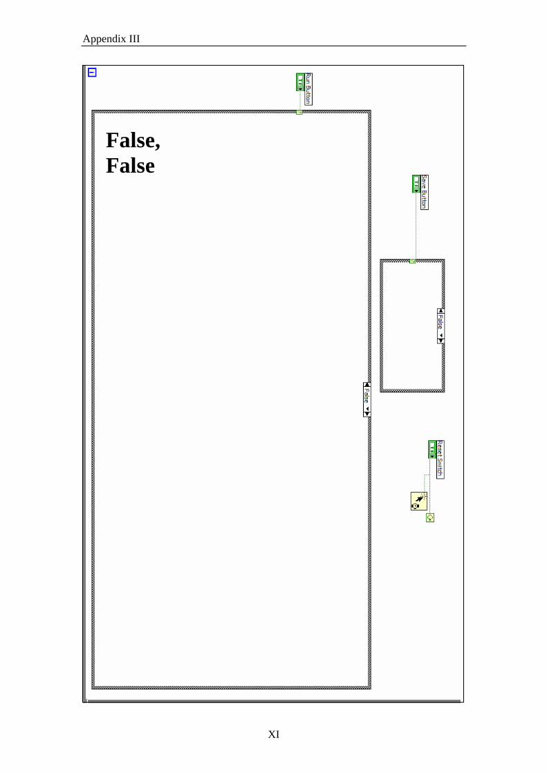
Appendix III
XI
False, False
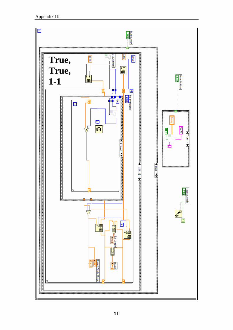
Appendix III
XII
True, True, 1-1
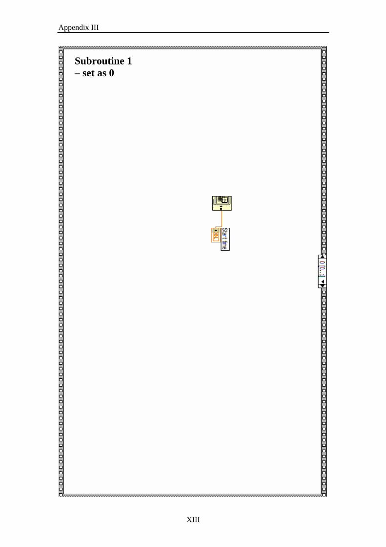
Appendix III
Subroutine 1 – set as 0
XIII
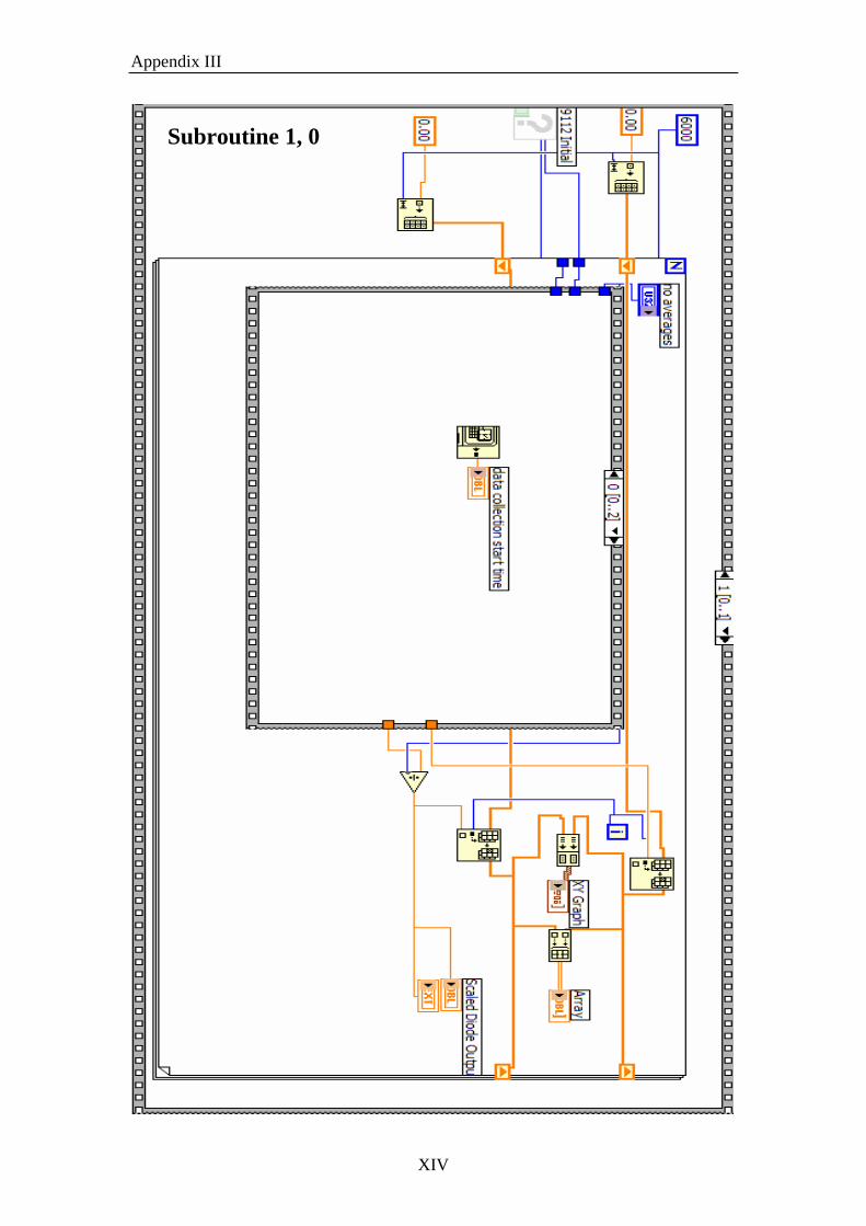
Appendix III
XIV
Subroutine 1, 0
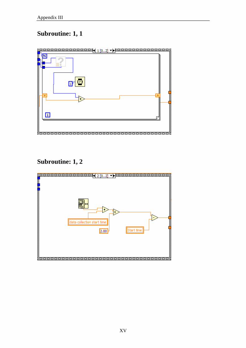
Appendix III
Subroutine: 1, 1
Subroutine: 1, 2
XV
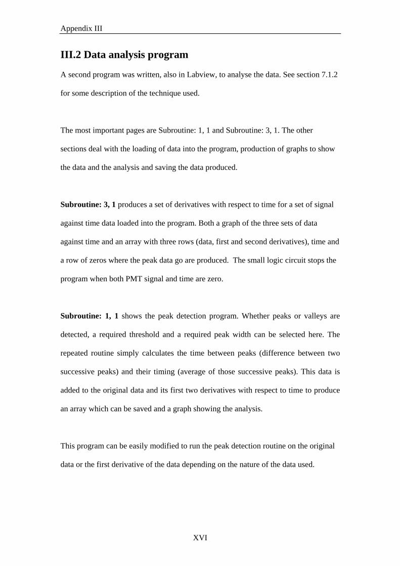
Appendix III
XVI
III.2 Data analysis program A second program was written, also in Labview, to analyse the data. See section 7.1.2
for some description of the technique used.
The most important pages are Subroutine: 1, 1 and Subroutine: 3, 1. The other
sections deal with the loading of data into the program, production of graphs to show
the data and the analysis and saving the data produced.
Subroutine: 3, 1 produces a set of derivatives with respect to time for a set of signal
against time data loaded into the program. Both a graph of the three sets of data
against time and an array with three rows (data, first and second derivatives), time and
a row of zeros where the peak data go are produced. The small logic circuit stops the
program when both PMT signal and time are zero.
Subroutine: 1, 1 shows the peak detection program. Whether peaks or valleys are
detected, a required threshold and a required peak width can be selected here. The
repeated routine simply calculates the time between peaks (difference between two
successive peaks) and their timing (average of those successive peaks). This data is
added to the original data and its first two derivatives with respect to time to produce
an array which can be saved and a graph showing the analysis.
This program can be easily modified to run the peak detection routine on the original
data or the first derivative of the data depending on the nature of the data used.
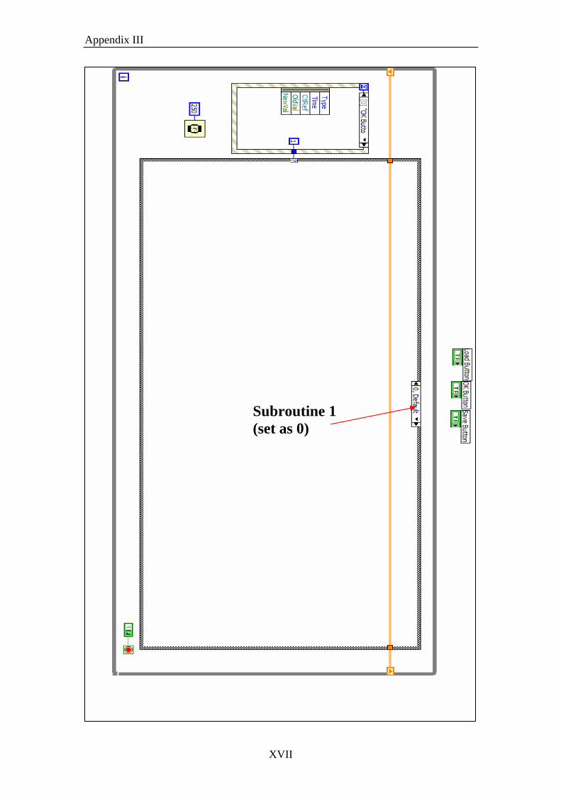
Appendix III
Subroutine 1 (set as 0)
XVII
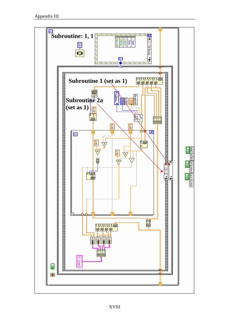
Appendix III
Subroutine: 1, 1
Subroutine 1 (set as 1)
Subroutine 2a (set as 1)
XVIII

Appendix III
Subroutine: 1, 0
XIX
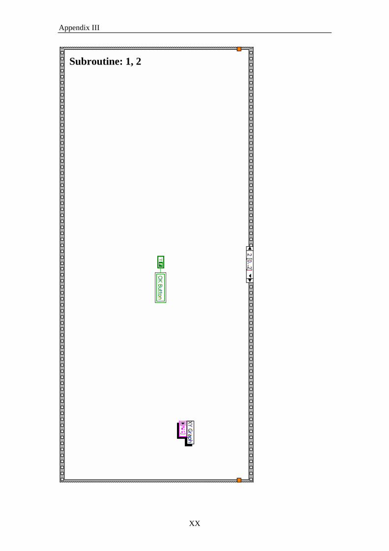
Appendix III
Subroutine: 1, 2
XX
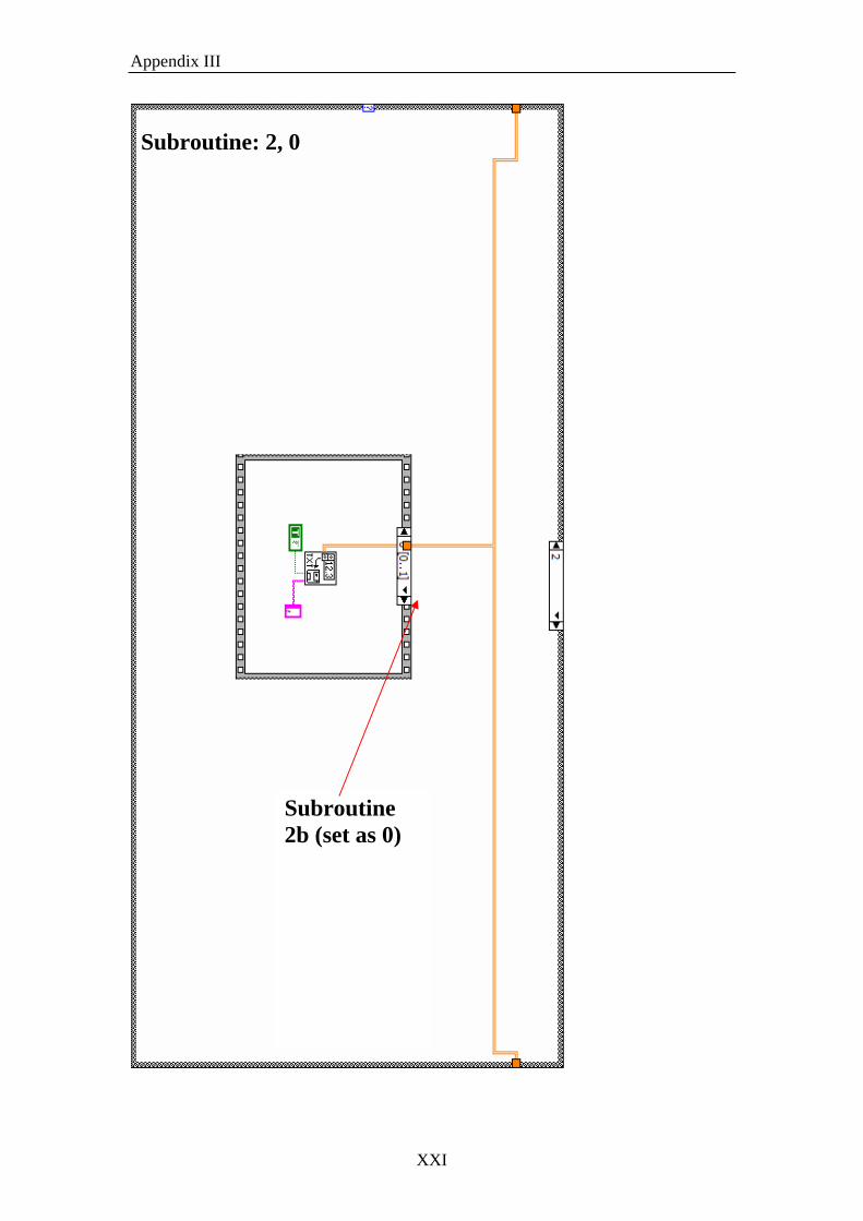
Appendix III
Subroutine: 2, 0
Subroutine 2b (set as 0)
XXI
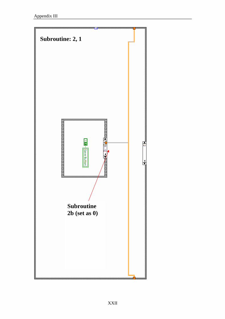
Appendix III
Subroutine: 2, 1
Subroutine 2b (set as 0)
XXII
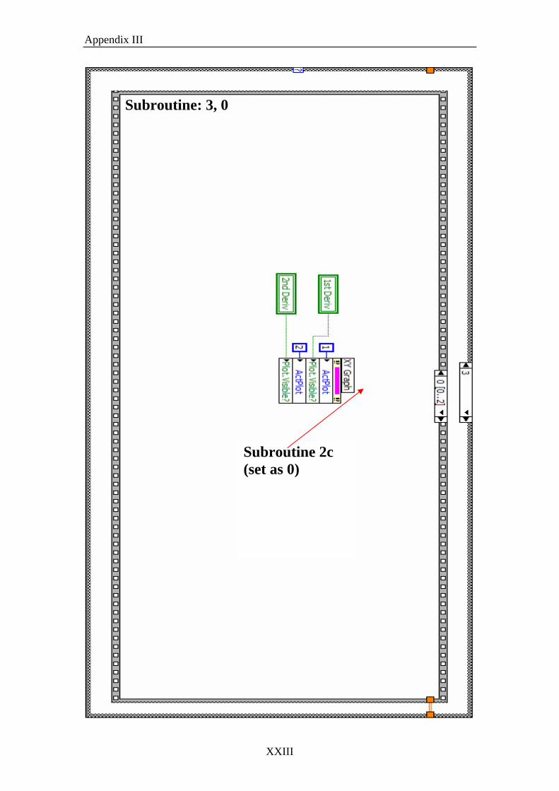
Appendix III
Subroutine: 3, 0
Subroutine 2c (set as 0)
XXIII
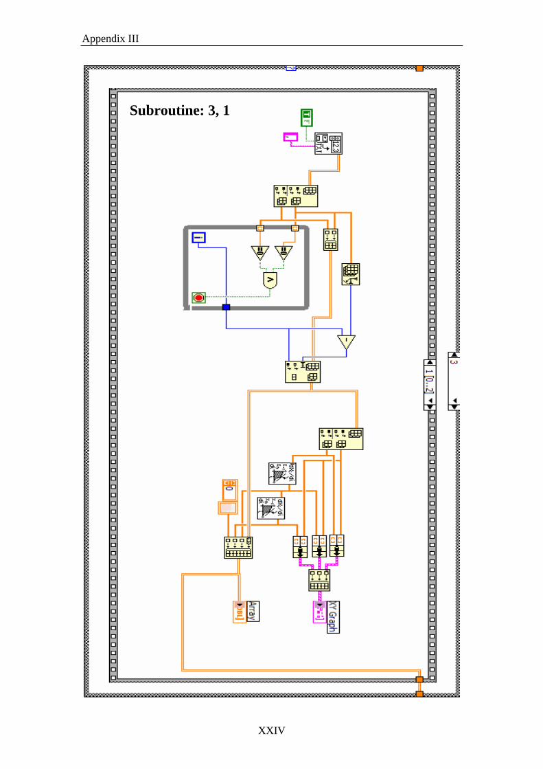
Appendix III
Subroutine: 3, 1
XXIV
Appendix III
XXV
Subroutine: 3, 2

Appendix IV
XXVI
APPENDIX IV
SQUID Magnetometry
The principles behind SQUID magnetometry are derived from the properties of
superconducting materials. This appendix is meant to serve as a brief guide explaining why
and how SQUIDs work as they do. For more detail, especially in terms of electronic
hardware and practical considerations, see Rev. Sci. Instrum., 77 (2006) 101101 and The
Squid Handbook, Wiley. Tinkham, M., Introduction to Superconductivity, McGraw-Hill is
a more detailed guide to all of the relevant theory of low-temperature/superconducting
physics.
Superconductivity
As certain materials approach absolute zero, their resistance can fall to practically zero.
This behaviour is theorised to be a result of weakly bound electron pairs (Cooper pairs).
The critical temperature, Tc, is a property of the material. There also exist critical current
densities (Jc) and critical magnetic fields (Hc), above which the superconducting behaviour
is lost. For example, mercury has a Tc = 4.153 K, Hc = 0.0412 T and can support a
current(Jc) of up to 108 A cm−2.
Another property of superconducing materials is the exclusion of magnetic fields from a
material held in a magnetic field as Tc is reached (Meissner effect). If the superconducting
material forms a ring and the applied magnetic field is turned off, then the flux becomes
trapped, threading through the ring. In a normal ring of material, this magnetic flux decays,

Appendix IV due to the resistance of the material. Howver, below Tc, there is no resistance and no decay
of the current or the magnetic flux. This current persists as long as the material stays below
Tc. One further, interesting property of this behaviour is that the flux contained within the
ring is quantised and only exists in multiples of Φ0 = 2.068 × 10⁻¹⁵ Wb.
Josephson Junctions
If a ring of superconducting material is interrupted, by a resistive region or even a
constriction in the ring, then it would be expected that the current would decay across the
gap and the persistent current would cease. However, tunnelling between the two regions
can occur, as predicted by Josephson and observed by Anderson and Powell. Below a
characteristic Ic for the junction, superconducting behaviour is observed. Above it, normal
current flow occurs with V = IR.
Superconducting State
Voltage
Ic Current
Fig. IV.1: The voltage-current (V-I) curve for a typical Josephson junction at a given T (T<Tc), showing
that a superconducting current can be maintained without applied voltage, until a certain critical
current flows. At this point, normal resistive behaviour occurs.
XXVII
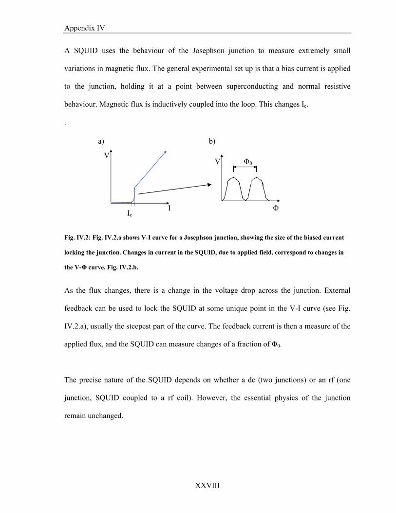
Appendix IV
XXVIII
A SQUID uses the behaviour of the Josephson junction to measure extremely small
variations in magnetic flux. The general experimental set up is that a bias current is applied
to the junction, holding it at a point between superconducting and normal resistive
behaviour. Magnetic flux is inductively coupled into the loop. This changes Ic.
.
a) b)
Ic
V
I
V Φ0
Φ Fig. IV.2: Fig. IV.2.a shows V-I curve for a Josephson junction, showing the size of the biased current
locking the junction. Changes in current in the SQUID, due to applied field, correspond to changes in
the V-Φ curve, Fig. IV.2.b.
As the flux changes, there is a change in the voltage drop across the junction. External
feedback can be used to lock the SQUID at some unique point in the V-I curve (see Fig.
IV.2.a), usually the steepest part of the curve. The feedback current is then a measure of the
applied flux, and the SQUID can measure changes of a fraction of Φ0.
The precise nature of the SQUID depends on whether a dc (two junctions) or an rf (one
junction, SQUID coupled to a rf coil). However, the essential physics of the junction
remain unchanged.
References
I
REFERENCES AND NOTES
The references are listed by section of the thesis. If a reference appears in more than one
section, then it will be repeated in each relevant section of the references.
INTRODUCTION
NOTES:
I: Given the analogous behaviour observed between magnetic and electric dipoles, it is
tempting to extend the analogy to the structure of the dipoles. A magnetic dipole could
consist of two poles of equal and opposite strength, ± p, separated by a small distance, l.
However, magnetic monopoles have not been found, while dipoles, consisting of loops
of current, have. The Maxwell equation 0=⋅∇ B can be interpreted as a statement that
there can be no magnetic monopoles as it indicates that magnetic field lines must be
closed lines.
REFERENCES:
1: Werthheimer, N. and Leeper, E., Am. J. Epidemiol., 109 (1979) 273
2: UK Mobile Telecommunications and Health Research Programme, Report 2007. Articles based on the report can be found at:
http://news.bbc.co.uk/1/hi/health/6990958.stm and http://www.guardian.co.uk/science/2007/sep/13/mobilephones.health
3: Schlichte, H. J. and Koenig, K., Proc. Nat. Acad. Sci. USA, 69 (1972) 2446-2447
Keeton, W. T., Proc. Nat. Acad. Sci. USA, 68 (1971)102-106 4: see Chapter 4, Tanimoto, Y. and Yamaguchi, M., Magnetoscience – Magnetic Field
effects on Materials: Fundamentals and Applications, Kodansha.
References
Relevent papers include Yamaguchi, M., Nomura, H., Yamamoto, I., Ohta, T. and Goto, T., Phys. Lett. A, 126 (1987) 133-135 and a summary/theoretical analysis of the magnetic field effects Yamamoto, I. et al., Jpn. J. Appl. Phys., 41 (2002) 416-424.
5: Steiner, U. E. and Ulrich, T., Chem. Rev., 89 (1989) 51-147 6: He, X., Kustin, K., Nagypál, I. and Peintler, G., Inorg. Chem., 33 (1994) 2077-2078 7: Ritz, T., Adem, S. and Schulten, K., Biophysical Journal, 78 (2000) 707-718 8: Bialek, W., Ann. Rev. Biophys. Biophys. Chem., 16 (1987) 455-78
Chapter 16, Essential Cell Biology, Garland also features a small but useful section on amplification processes in the eye.
9: McDougall, A., Shearer, J. and Whitaker, M., Biol. Cell., 92 (2000) 205-214
10: Orchard, A. F., Magnetochemistry, Oxford Chemistry Primers 75, OUP is a good place to start for an overview of this topic and its history.
Duffin, W. J., Electricity and Magnetism (4th Ed), McGraw-Hill is another good text. 11: see Chapter 3, Tanimoto, Y. and Yamaguchi, M., Magnetoscience – Magnetic Field
effects on Materials: Fundamentals and Applications, Kodansha. 12: Katsuki, A and Tanimoto, Y., Chem. Lett., 34 (2005) 726-727 13: Uechi, I., Katsuki, A., Dunin-Barkovskiy, L. And Tanimoto, Y., J. Phys. Chem.,
108 (2004) 2527-2530 14: Boyer, T. H., Am. J. Phys., 56 (1988) 688-692 15:Coey, J. M. D., Rhen, F. M. F., Dunne, P. and McMurry, S., J. Solid State
Electrochem., 11 (2007) 711-717 16: see Chapter 5, Tanimoto, Y. and Yamaguchi, M., Magnetoscience – Magnetic Field
effects on Materials: Fundamentals and Applications, Kodansha. 17: Ikezoe, Y, Hirota, N, Nakagawa, J. and Kitazawa, K., Nature, 393 (1998) 749-750 18: Braithwaite, D., Beaugnon, E. and Tournier, R., Nature, 354 (1991) 134-135 An application of this can be found at: Tanimoto, Y., Sueda, K. and Irie, M., Bull.
Chem. Soc. Jpn., 80 (2007) 491-494 19: Fujiwara, M. Kodoi, D., Duan, W. and Tanimoto, Y., J. Phys. Chem. B., 105 (2001)
3343-3345 Further papers on the topic: Chie, K., Fujiwara, M., Fujiwara, Y. and Tanimoto, Y.,
J. Phys. Chem. B, 107 (2003) 14374-14377
II
References
Fujiwara, M., Chie, K., Sawai, J., Shimizu, D. and Tanimoto, Y., J. Phys. Chem. B, 108 (2004) 3531-3534
Fujiwara, M., Mitsuda, K. and Tanimoto, Y., J. Phys. Chem. B, 110 (2006) 13965-13969
20: Steiner and Ulrich’s review (reference 5) is comprehensive.
Further reviews of the topic that could be useful are Brocklehurst, B., Chem. Soc. Rev., 31 (2002) 301-311 and Timmel, C. R. and Henbest, K. B., Phil. Trans. R. Soc. Lond. A, 362 (2004) 2573-2589
As with most of this chapter, Tanimoto, Y. and Yamaguchi, M., Magnetoscience – Magnetic Field effects on Materials: Fundamentals and Applications, Kodansha is recommended. Chapter 6 deals with the radical pair mechanism.
21: O’Dea, A. R., Curtis, A. F., Green, N. J. B, Timmel, C. R. and Hore, P. J., J. Phys.
Chem. A, 109 (2005) 869-873 22: predicted by Brocklehurst, B., J. Chem. Soc. Faraday Trans., 72 (1976) 1869-1884
23: A good place to start reading on the topic of non-linear kinetics and related
phenomena is Scott S. K., Oscillations, Waves and Chaos in Chemical Kinetics, Oxford Chemistry Primers 18, OUP.
Epstein, I. R. and Showalter, K., J. Phys. Chem., 100 (1996) 13132-13147 and Sagués, F. and Epstein, I. R., Dalton. Trans., 7 (2003) 1201-1217 are two fairly comprehensive reviews of the same topic.
24: Scott, S. K. and Showalter, K., J. Phys. Chem., 96 (1992) 8702-8711 25: Bray, W.C. and Liebhafsky, H. A., J. Am. Chem. Soc., 53 (1931) 38 26: Scott, S. K., Oscillations, Waves and Chaos in Chemical Kinetics, Oxford
Chemistry Primers 18, OUP, chapter 6 See also: chapter 9, Scott, S. K., Chemical Chaos, OUP 27: Møller, A. C., Hauser, M. J. B. and Olsen, L. F., Biophysical Chemistry, 72 (1998)
63-72 28: Møller, A. C. and Olsen, L. F., J. Phys. Chem. B, 104 (2000) 140-146
Møller, A. C., Lunding, A. and Olsen, L. F., Phys. Chem. Chem. Phys., 2 (2000) 3443-3446
29: Scott, S. K., Chemical Chaos, OUP is the best place to start. Chaotic behaviour is a
feature of the reactions studied in this thesis but no attempt to investigate the behaviour was attempted.
30: Page 37 and following, Scott, S. K., Chemical Chaos, OUP
III
References
PART I
NOTES:
I: The echo depicted in this image is an schematic illustration of the Lorentzian spin-
echo.
II: See chapter 12.1 for an illustration of the pH changes of the Co(II)EDTA2−/H2O2.
III: A description of the method of finite volume analysis is too broad a topic to be
dealt with in this thesis, but a brief description of the technique and a helpful text can be
found in Appendix II.
REFERENCES:
1: He, X., Kustin, K., Nagypál, I. and Peintler, G., Inorg. Chem., 33 (1994) 2077-2078
2: Boga, E, Kadar, S., Peintler, G. and Nagypál, I., Nature, 347 (1990) 749
3: Britton, M. M., J. Phys. Chem. A, 110 (2006) 2579-2582 Britton, M. M., J. Phys. Chem. A, 110 (2006) 13209-13214
4: For a detailed overview of both NMR and MRI, see Callaghan, P. T., Principles of
Nuclear Magnetic Resonance Microscopy , OUP.
Hore, P. J., Nuclear Magnetic Resonance, Oxford Chemistry Primers 18, OUP was also found to be useful.
Mantle, M. and Sederman, A., Prog. Nuc. Magn. Res. Spec., 43 (2003) 3–60 reviews the techniques from a chemical engineering point of view.
5: Meiboom, S and Gill, D., Rev. Sci. Instrum., 29 (1958) 688-691
6: Hennig, J., Naureth, A. and Freidburg, H., Magn. Reson. Med., 3 (1986) 823-833
7: Nagypál, I., Bazsa, G. and Epstein, I., J. Am. Chem. Soc., 108 (1986) 3635-3640 Pojman, J. A. and Epstein, I., J. Phys. Chem., 94 (1990) 4966-4972 follows on from the previous paper.
IV
References
There is a further series of papers: Pojman, J. A., Epstein, I. R., MacManus, T. J. and Showalter, K., J. Phys. Chem., 95 (1990) 1299-1306 Pojman, J. A., Nagy, I. P. and Epstein, I. R., J. Phys. Chem., 95 (1990) 1306-1311
8: Harris, G., Part II Thesis, 2001 9: Evans, R., Timmel, C. R., Hore, P. J. and Britton, M. M., J. Am. Chem. Soc., 128
(2006) 7309-7314 10: Kinouchi, Y., Tanimoto, S., Ushita, T., Sato, K., Yamaguchi, H. and Miyamoto, H., Bioelectromagnetics, 9 (1988) 159-166
11: Norris, D. and Hutchison, J., Magn. Reson. Imaging, 8 (1990) 33 12: De Wit, A. and Homsy, G., Physics of Fluids, 11 (1999) 949 - 951 13: Morris, G. and Freeman, R., J. Magn. Reson., 29 (1978) 433-462 14: Mori, E., Schreiber, I. and Ross, J., J. Phys. Chem., 95 (1991) 9359-9366 15: Su, S., Menziger, M., Armstrong, R., Cross, A. and Lemaire, C., J. Phys. Chem.,
98 (1994) 2494-2498 16: Gao, Y., Cross, A. and Armstrong, R., J. Phys. Chem., 100 (1996) 10159-10164 17: Britton, M., J. Phys. Chem. A, 107 (2003) 5033-5041
Britton, M., J. Phys. Chem., 110 (2006) 5075-5080 Taylor, A. F. and Britton, M., Chaos, 16 (2006) 37103-37111 18: Bazsa, G and Epstein, I., J. Phys. Chem., 89 (1985) 3050-3053 Póta, G., Lengyel, I. and Bazsa, G., J. Phys. Chem., 95 (1991) 4379-4381 19: Pojman, J. A., Nagy, I. and Epstein, I., J. Phys. Chem., 95 (1991) 1306-1311 20: Pojman, J. A., Ilyashenko, V. M. and Khan, A. M., J. Chem. Soc., Faraday Trans.,
92 (1996) 2825-2837 A useful review: Epstein, I. R. and Pojman, J. A., Chaos, 9 (1999) 255-259
21: Wilmott, N. Sethi, K. Walseth, T. F., Lee, H. C., White, A. M. and Galione, A. J.
Biol. Chem., 271 (1996) 3699-3705 22: Baxter, E., Part II Thesis, 2001
V
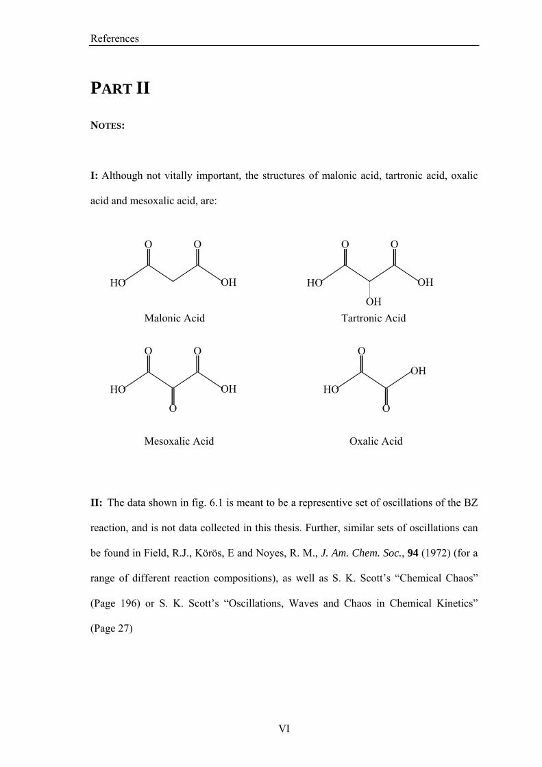
References
PART II
NOTES:
I: Although not vitally important, the structures of malonic acid, tartronic acid, oxalic
acid and mesoxalic acid, are:
II: The data shown in fig. 6.1 is meant to be a representive set of oscillations of the BZ
reaction, and is not data collected in this thesis. Further, similar sets of oscillations can
be found in Field, R.J., Körös, E and Noyes, R. M., J. Am. Chem. Soc., 94 (1972) (for a
range of different reaction compositions), as well as S. K. Scott’s “Chemical Chaos”
(Page 196) or S. K. Scott’s “Oscillations, Waves and Chaos in Chemical Kinetics”
(Page 27)
O O
OHHO
O O
OH HO
OH Tartronic Acid Malonic Acid
O O
OHHO
O
OH
HO
O
Oxalic Acid
O
Mesoxalic Acid
VI
References
III: Examples of chaotic oscillations observed in a CSTR can be found in S. K. Scott’s
“Chemical Chaos” (Page 200 and following)
REFERENCES:
1: Belousov, B. P. (translated by Field, R. J. and Burger, M.), Oscillations and Travelling Waves in Chemical Reactions, Wiley Interscience, NY, 1984
2: Winfree, A. J., J. Chem. Ed., 61 (1984) 661-663
3: Bray, W. C., J. Am. Chem. Soc., 43 (1921) 1262-1267
4: Shaw, D. H. and Pritchard, H. O., J. Phys. Chem., 72 (1968) 1403-1404. Reply to this letter: Degn, H and Higgins, J., J. Phys. Chem., 72 (1968) 2692-2693
Further reply: Shaw, D. H. and Pritchard, H. O., J. Phys. Chem., 72 (1968) 2693 5: Zaikin, A. N. and Zhabotinsky, A. M., Nature, 225 (1970) 535-537
6: Prigogine, I. and Le Fever, R. J. Chem. Phys., 48 (1968) 1695-1700
7: Field, R. J., Körös, E and Noyes, R. M., J. Am. Chem. Soc., 94 (1972) 8649-8664
8: Winfree, A. T., Science, 175 (1972) 634
9: Györgi, L. and Field, R. J., Nature, 355 (1992) 808-810
10: Bolletta, F. and Balzani, V., J. Am. Chem. Soc., 104 (1982) 4250-4251
11: Kádár, S., Amemiya, T. and Showalter, K., J. Phys. Chem. A, 101 (1997) 8200-8206
12: Szalai, I. and Körös, E., J. Phys. Chem. A, 102 (1998) 6892-6897
13: Györgi, L., Turanyi, T. and Field, R. J., J. Phys. Chem., 94 (1990) 7162-7170
14: Turanyi, T., Györgi, L. and Field, R. J., J. Phys. Chem., 97 (1993) 1931-1941
15: Field, R. J. and Noyes, R. M., J. Chem. Phys., 60 (1974) 1877-84
16: Noyes, R. M., J. Phys. Chem., 90 (1986), 5407-5409
17: Noszticzius, Z., J. Am. Chem. Soc., 101 (13): 3660-3663 1979
Further discussion of the results: Noyes, R. M., Field, R. J., Försterling, H. D., Körös, E and Ruoff, P. J. Phys. Chem., 93 (1989) 270-274
18: Field, R. J. and Försterling, H. D., J. Phys. Chem., 90 (1986) 5400-5407
VII
References
Zhabotinsky, A. M., Buchholtz, F., Kiyatkin, A. B. and Epstein, I. R., J. Phys. Chem., 97 (1993) 7578-7584
19: Noyes, R. M., J. Am. Chem. Soc., 102 (1980) 4644-4649 Further discussion and work: Rovinsky, A. B., J. Phys. Chem., 88 (1984) 4-5
Chou, Y-C, Lin, H-P, Sun, S. S. and Jwo, J-J, J. Phys. Chem., 97 (1993) 8450-8457 Ungvarai, J. Nagy-Ungvarai, Z, Enderlein, J. and Müller, S. C., J. Chem. Soc., Faraday Trans., 93 (1997) 69-71
20: Jacobs, S. S. and Epstein, I. R., J. Am. Chem. Soc., 98 (1976) 1721-1725
21: Gaspar, V., Bazsa, G. and Beck, M., Z. Phys. Chem. (Leipzig), 264 (1983) 43
22: Tóth, R., Gaspar, V., Belmonte, A., O’Connell, M. C., Taylor, A. and Scott, S. K., Phys. Chem. Chem. Phys., 2 (2000) 413-416 23: Ram Reddy, M. K., Szlavik, Z., Nagy-Ungvarai, Z. and Miller, S. C., J. Phys.
Chem., 99 (1995) 15081-15085 24: Taylor, A. F., Johnson, B. R. and Scott, S. K., J. Chem. Soc., Faraday Trans., 94
(1998) 1029-1033 25: Steinbock, O., Hamik, C. T. and Steinbock, B., J. Phys. Chem., 104 (2000) 6411-
6415 26: Broomhead, E. J. and McLauchlan, K. A., J. Chem. Soc., Faraday Trans., 74 (1978)
775-781 27: Kovalenko, A. S., Lugina, L. N., Andreev, E. A. and Tikhona, L. P., Teor. Eksp.
Khimiya, 25 (1989) 647-652 28: Agulova, L. P., Opalinskaya, A. M. and Kiryanov, V. S., Teor. Eksp. Khimiya, 26
(1990) 624-627 29: Agulova, L. P., Opalinskaya, A. M., Zhurnal Fizicheskoi Khimii, 59 (1985) 1513-
1516 30: Blank, M. and Soo, L., Bioelectrochemistry, 61 (2003) 93-97
31: Sontag, W., Bioelectromagnetics, 27 (2006) 314-319
32: Byberg, J. R. and Linderberg, J., Chem. Phys. Lett., 33 (1975) 612-615
33: Barkin, S., Bixon, M. Noyes, R. M. and Bar-Eli, K., Int. J. Chem. Kin., 11 (1977) 841-862 34: Menziger, M. and Jankowski, P., J. Phys. Chem., 94 (1990) 4123-4126
VIII
References
35: Schneider, F. W. and Münster, A. F., J. Phys. Chem., 95 (1991) 2130-2138 36:Dutt, A. K. and Müller, S. C., J. Phys. Chem., 97 (1993) 10059-10063
BZ with gallic acid: Dutt, A. K. and Menziger, M., J. Phys. Chem., 96 (1992) 8447-8449
37: Field, R. J. and Noyes, R. M, Faraday Symp. Chem. Soc., (1994) 21- 27
See also: Scott, S. K., Oscillations, Waves and Chaos in Chemical Kinetics (page 37)
38: Grissom, C. B., Chem. Rev., 95 (1995) 3-24 39: Försterling, H. D., Murányi, S. and Noszticzius, Z., React. Kinet. Catal. Lett., 42
(1990) 217 See also: Försterling, H. D., Murányi, S. and Noszticzius, Z., J. Phys. Chem., 94 (1990) 2915-2921
40: Field, R. J., Raghaven, N. V. and Brummer, J. G., J. Phys. Chem., 86 (1982) 2443-
2449 41: Symons, M. C. R., Free. Rad. Res., 32 (2000) 25-29
42: Turro, N. J., Chung, Ch-J, Jones, G and Becker, W. G., J. Phys. Chem., 86 (1982) 3677-3679
43: Modelling attempts used the Chemical Kinetics Simulator.
44: Baxter, E., Part II Thesis, 2001
IX
References
PART III
NOTES:
I: SQUID magnetometry is a practical application of quantum interference in
superconducting materials. A brief summary of the low-temperature solid state physics
that gives rise to the behaviour is described in Appendix IV. The SQUID was used
without modification, so a detailed understanding of the physics driving the phenomena
and the electronics used in the magnetometer was thought unnecessary. References for
further reading are also given.
II: As with the NMR/MRI sequences shown in Part I, the echo depicted in this image is
a schematic illustration of the Lorentzian. spin-echo.
REFERENCES:
1: Eveson, R.W. , Timmel, C. R., Brocklehurst, B., Hore P. J. and McLauchlan, K. A., Int. J. Rad. Biol., 76 (2000) 1509-1522.
See also: Thomas, P. G., DPhil Thesis, 2004 2: Henbest, K. B., Maeda, K., Athanassiades, E., Hore, P. J. and Timmel C. R., Chem.
Phys. Lett., 421 (2006) 571-576 See also: Norman, S. A., DPhil Thesis, 2006, Wedge, C., Part II Thesis, 2005.
Steiner, U. E. and Ulrich, T., Chem. Rev., 89 (1989) 51-147 is a comprehensive review, and features further examples of how reactions featuring radical pairs can be studied.
3: Vink, C. B. and Woodward, J. R., J. Am. Chem. Soc., 126 (2004) 16730-16731. 4: Yalman, R. G., J. Phys. Chem., 65 (1961) 556-560
5: Chapter 5.7, Blundell, S., Magnetism in Condensed Matter, OUP
6: Adkin, J. J. and Heyward, M. A., Chem. Mater., 19 (2007) 755-762
X
References
XI
7: An overview of the many applications of SQUIDs can be found in Fagaly, R. L., Rev. Sci. Instrum., 77 (2006) 101
Tinkham, M., Introduction to Superconductivity, McGraw-Hill is a more detailed guide to all of the relevant theory. See Appendix IV for a brief overview. Juzeliūnas, E. and Hinken, J. H., J. Electroanal. Chem., 477 (1999) 171-177
8: Josephson, B. D., Phys. Lett., 1 (1962) 251-253
9: Anderson, P. W. and Rowell, J. M., Phys Rev. Lett., 11 (1963) 230-232
10: Meiboom, S and Gill, D., Rev. Sci. Instrum., 29 (1958) 688-691
11: page 5, Orchard, A. F., Magnetochemistry, Oxford Chemistry Primers 75, OUP
12: Yalman, R. G. and Warga, M. B., J. Am. Chem. Soc., 80 (1958) 1011
13: Britton, M. M., J. Phys. Chem. A, 110 (2006) 13209-13214 14: Nicholls, D., Complexes and First Row Transition Elements, Macmillan
15: Handbook of Chemistry and Physics, 80th Edition, CRC Press
16: Barkin, S., Bixon, M. Noyes, R. M. and Bar-Eli, K., Int. J. Chem. Kin., 11 (1977) 841-862
17: Smoes M-L., J. Chem. Phys., 71 (1979) 4669-4679 18: McElfresh, M., Fundamentals of Magnetism and Magnetic Measurements ,
(Quantum Design’s guide to the SQUID magnetometer) 19: Field, R.J., Körös, E and Noyes, R. M., J. Am. Chem. Soc., 94 (1972) 8649-8664 20: Körös, E., Burger, M. and Kris, Á, React. Kinet. Catal. Lett., 1 (1974) 475-480
21: Khan, Z., Babu, P. S. S. and Kabir-ud-Din, Carbohydrate Research, 339 (2004) 133-140
22: Horner, O., Rivière, E., Blondin, G., Un, S., Rutherford, A. W., Girerd, J-J. and
Boussac, A., J. Am. Chem. Soc., 120 (1998) 7924-7928 23: Henbest, K. B. and Maeda, K., private communications 24: Morgunov, R. B., Berdinskii, V. L., Kirman, M. V., Tanimoto, Y. and Chapysev, S.
V., High Energy Chemistry, 41 (2007) 33-36