tidal and residual currents measured by an

TIDAL AND RESIDUAL CURRENTS MEASURED BY AN

ACOUSTIC DOPPLER CURRENT PROFILER AT THE

WEST END OF CARQUINEZ STRAIT, SAN FRANCISCO BAY,

CALIFORNIA, MARCH TO NOVEMBER 1988

By Jon R. Burau, Michael R. Simpsoa and Ralph T. Cheng

U.S. GEOLOGICAL SURVEY

Water-Resources Investigations Report 92-4064

Prepared in cooperation with

U.S. ARMY CORPS OF ENGINEERS,CALIFORNIA STATE WATER RESOURCES CONTROL BOARD, andCALIFORNIA DEPARTMENT OF WATER RESOURCES

ON

o m

Sacramento, California 1993

U.S. DEPARTMENT OF THE INTERIOR BRUCE BABBITT, Secretary

U.S. GEOLOGICAL SURVEY Robert M. Hirsch, Acting Director

Any use of trade, product, or firm names in this publication is for descriptive purposes only and does not imply endorsement by the U.S. Government.

For sale by theU.S. Geological SurveyEarth Science Information CenterOpen-File Reports SectionBox 25286, MS 517Denver Federal CenterDenver, CO 80225

For additional information write to: District Chief U.S. Geological Survey Federal Building, Room W-2233 2800 Cottage Way Sacramento, CA 95825

CONTENTS

Abstract 1 Introduction 1

Purpose and scope 3 Acknowledgments 3

Approach 4Description of the acoustic Doppler current profiler system 4 Period of data collection 6

Description and processing of the data 6 Data analysis 7

Harmonic analysis 7 Low-pass filter 11

Tidal and residual currents 11 Selected references 21 Appendix A.--ADCP error sources 71

Random error 71 Systematic error 71

Errors due to uncompensated pitch, roll, and heading 72 Errors due to improper beam geometry 72 Receiver chain effects 72Errors due to the mispositioning of receiver tracking filters 73 Error due to transmit filter mistuning 74

Effects of ADCP error on gross tidal and residual velocity data 75 Appendix B.--Doppler data formats 77

FIGURES

COVER: An instantaneous filtered vertical-velocity profile at 0000 hours, May 11, 1988, showing the effect of gravitational circulation.

1. Map showing location of acoustic Doppler current profiler in Carquinez Strait, San Francisco Bay 2

2. Sketch showing ADCP deployment configuration and beam pattern 53. Graphs showing power spectrum of bin2 84. Diagram of tidal-current ellipses 9

5-13. Graphs showing:5. Frequency and impulse response functions of four filters 126. Normalized major axis magnitude compared to depth 137. Three-dimensional vertical-velocity profiles, April 6, 1988 148. Delta discharge for the 1988 water year 159. Phase difference of the four principal tidal constituents compared to depth 16

10. Coherence phase spectrum and magnitude squared coherence between bin2 and bin 10 17

11. Three-dimensional vertical-velocity profiles of filtered data, May 11 and 18, 1988 1812. Simultaneous plots of the delta discharge and residual velocities at bin2 and bin 10 1913. Magnitude squared coherence plotted between daily discharge and filtered

velocities at bin2 and bin 10 2014. Time-series plots of tidal and residual currents 3515. Graph showing combined effects of acoustic Doppler current profiler bias errors on a

typical water-velocity profile taken from the study data 75

Contents

TABLES

1. Principal astronomical partial tidal constituents2. Harmonic analysis results 23

10

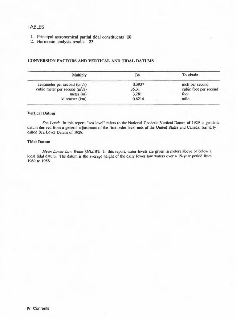
CONVERSION FACTORS AND VERTICAL AND TIDAL DATUMS

Multiply By To obtain

centimeter per second (cm/s)cubic meter per second (mVs)

meter (m)kilometer (km)

0.393735.31

3.2810.6214

inch per second cubic foot per second foot mile

Vertical Datum

Sea Level: In this report, "sea level" refers to the National Geodetic Vertical Datum of 1929~a geodetic datum derived from a general adjustment of the first-order level nets of the United States and Canada, formerly called Sea Level Datum of 1929.

Tidal Datum

Mean Lower Low Water (MLLW): In this report, water levels are given in meters above or below a local tidal datum. The datum is the average height of the daily lower low waters over a 19-year period from 1969 to 1988.

IV Contents

TIDAL AND RESIDUAL CURRENTS MEASURED BY AN ACOUSTIC

DOPPLER CURRENT PROFILER AT THE WEST END OF

CARQUINEZ STRAIT, SAN FRANCISCO BAY, CALIFORNIA

MARCH TO NOVEMBER 1988

By Jon R. Burau, Michael R. Simpsoa and Ralph T. Cheng

Abstract

Water-velocity profiles were collected at the west end of Carquinez Strait, San Francisco Bay, California, from March to November 1988, using an acoustic Doppler current profiler. These data are a series of 10-minute-averaged water velocities collected at 1-meter vertical intervals (bins) in the 16.8-meter water column, beginning 2.1 meters above the estuary bed. To examine the vertical structure of the horizontal water velocities, the data are separated into individual time-series by bin and then used for time-series plots, harmonic analysis, and for input to digital filters. Three-dimensional graphic renditions of the filtered data are also used in the analysis.

Harmonic analysis of the time-series data from each bin indicates that the dominant (12.42 hour or M2) partial tidal currents reverse direction near the bottom, on average, 20 minutes sooner than M2 partial tidal currents near the surface. Residual (nontidal) currents derived from the filtered data indicate that currents near the bottom are predominantly up-estuary during the neap tides and down-estuary during the more energetic spring tides.

INTRODUCTION

The long-term salinity distribution in San Francisco Bay, the transport of nonmotile organisms, the location of the "null zone" (Peterson and others, 1975), and the ability of the bay to move contaminants through the northern reach are principally functions of the long-term balance between tidal trapping (pumping) in the large shallow regions of Suisun and San Pablo Bays (fig. 1), freshwater discharge, and the effects of gravitational (estuarine) circulation caused by horizontal salinity gradients (Fischer, 1976). The relative magnitude of these mechanisms is time-varying, depending on the short- and long-term variability of freshwater discharge into San Francisco Bay.

In 1979, the U.S. Geological Survey, in cooperation with the National Ocean Survey/National Oceanic and Atmospheric Administration, began collecting water-level and velocity data to gain insight into the fundamental interactions among inflows from the delta, outflows to the ocean, and circulation within the San Francisco Bay system (Cheng and Gartner, 1984). Although this extensive circulatory survey went a long way in quantifying the overall spatial distributions of the currents in San Francisco Bay, relatively few data were collected in the vertical because of limitations in the current-measurement instrumentation. Certain important processes that appear only in a vertical plane, such as gravitational circulation (Fischer, 1976; Officer, 1976; Yih, 1980), the mass balance of wind forcing, and shear-induced mixing in the water column, are known to affect transport processes in estuaries.

Introduction 1

122-151 122-141 122-131

38°04' -

38°03' -

Areas where depth of water is less than 2 meters

0 5 10 15 KILOMETERS

Figure 1 . Location of acoustic Doppler current profiler in Carquinez Strait, San Francisco Bay.

2 Tidal and Residual Currents Measured by an Acoustic Doppler Current Profiler at San Francisco Bay

This study, done by the Geological Survey in cooperation with the U.S. Army Corps of Engineers, California State Water Resources Control Board, and California Department of Water Resources, takes a detailed first-time look at the vertical structure of the tidal and residual currents in San Francisco Bay. From the tidal currents, information about the shear stress distribution through the water column can be gained and extrapolated to estimate the shear at the channel bed. Knowing the shear stress at the channel bed provides insight into sediment deposition and resuspension. This knowledge is of particular interest to the U.S. Army Corps of Engineers, who are authorized by Congress to keep navigation channels open in San Francisco Bay. The tidally averaged residual or net current profile gives the magnitude, direction, and time-dependence of the gravitational circulation if other nontidal forcings are ignored. Gravitational circulation is the density-induced residual current, which causes a net up-estuary current near the channel bottom and a net down-estuary current at the water surface. The gravitational circulation plays an important role in the long-term salt balance in the estuary, in addition to providing an up-estuary transport mechanism for nutrients and nonmotile or feeble swimming organisms.

The development and refinement of acoustic Doppler current-measurement technology since 1979 has enabled a more detailed look at the vertical structure of water-velocity profiles than was previously possible. In 1986, the Geological Survey acquired an acoustic Doppler current profiler (ADCP) to collect vertically resolved water-velocity data in the San Francisco Bay estuary. The ADCP's accuracy, vertical resolution, and resistance to fouling (no moving parts) make it well suited for studying vertical variations in the tidal and residual currents in estuarine environments. ADCP's of the type used in this study typically are anchored on the estuary floor. Piezo-electric transducer elements on the ADCP project acoustic beams vertically into the water column. Part of the acoustic energy from each beam is reflected back toward the transducer elements by particulate matter (scatterers) moving with the water. The reflected energy is shifted in frequency because of the Doppler effect (Tipler, 1976), and the ADCP converts the frequency shifts into water-parcel speed. When multiple acoustic beams are used, the ADCP is capable of resolving both water speed and direction in several specified depth intervals, called bins, within the water column.

PURPOSE AND SCOPE

This report documents the first investigation of the vertical structure of long-term horizontal water- velocity measurements in the northern reach of San Francisco Bay, near the west end of Carquinez Strait (fig. 1). The purpose of the report is to present and summarize the unique data series collected by the ADCP, and to provide the reader with an understanding of the tools necessary to complete a data- collection and analysis effort of this type.

The scope of the work included: deployment and retrieval of the ADCP system, bin-by-bin data reduction of the three-dimensional ADCP velocity data into multiple sets of

time-series data, statistical, harmonic, and error analyses of the time-series data sets, application of digital filtering techniques to remove the tidal signal from the time-series data

sets, and computer animation and graphic rendition of the filtered and unfiltered data sets.

ACKNOWLEDGMENTS

The authors gratefully acknowledge the support provided by the San Francisco District of the U.S. Army Corps of Engineers, and appreciate the high degree of professionalism of the crew of the R/V Saul E. Rantz during instrument deployment and recovery. We also wish to acknowledge the Wickland Oil Company for the use of their facilities during this study. And finally, we are grateful to Dr. Jia Wang (visiting scientist from the Institute of Oceanology, Academia Sinica, Qingdao, Shandong, People's Republic of China) for providing the digital filtering computer codes used in preparing this report.

Introduction 3

APPROACH

The gravitational circulation, or density-induced residual current, is weak in San Francisco Bay compared with the tidal currents and can easily be affected by relatively minor perturbations in bottom bathymetry. Therefore, gravitational circulation is usually restricted to deeper areas with relatively smooth bottom topography where these vertical effects can develop. Walters and others (1985) described the effect of bottom topography in the areas surrounding the Pinole and San Bruno shoals in San Francisco Bay, and Gill (1982) discussed the general concept of "blocking" in stratified fluids. Because of these considerations, the ADCP was deployed in a bathymetrically smooth channel near the west end of Carquinez Strait (fig. 1) in 16.8 m of water, referenced to Mean Lower Low Water (MLLW). Mooring the instrument in a channel, where the flow is virtually bidirectional, avoids the complications of transverse flows. In 16.8 m of water, the ADCP was able to resolve 12 statistically reliable velocity measurements at 1.0-m intervals (bins) in the water column beginning at a height of 2.1 m above the estuary bed.

DESCRIPTION OF THE ACOUSTIC DOPPLER CURRENT PROFILER SYSTEM

A typical upward-looking ADCP system is anchored on the estuary floor and projects four acoustic beams vertically into the water column. These beams are positioned 30° from the vertical axis of the transducer assembly (fig. 2). The ADCP samples reflected signals from each beam at discrete time intervals during the progress of the advancing acoustic wave front to determine the water velocity. In practice, these bins lack distinct boundaries; however, the distance between bin centers is accurately controlled by timing circuits in the ADCP. The bins can be thought of as a series of overlapping vertical "windows" in the water column, each containing water-velocity information. The height of the bins can be adjusted by manipulation of the ADCP software.

ADCP transducers emit parasitic acoustic side lobes about 30° off their main axes. Because the main beams are directed 30° from the vertical (the optimum angle for data collection), these side lobes are strongly reflected off the water surface and interfere with the ADCP measured velocity profiles in the upper 15 to 20 percent of the water column. After transmitting the acoustic pulses, the transducers and associated electronics must recover for a short time-period before receiving incoming acoustic reflections. The acoustic pulses travel about 0.3 to 0.4 m during this recovery period, referred to as the blanking distance, and velocity data cannot be collected within this distance. The first measured bin center is 1 m beyond the blanking distance. During this study, the ADCP was deployed in 16.8 m of water and was suspended 0.7 m above the estuary floor. Therefore, the actual profile range started at 2.1 m above the estuary floor and ended at a depth of about 3.4 m below the water surface because of the blanking period and acoustic side lobe interference. In practice, this range is made even shorter because of water-surface disturbances, referred to as bubble clouds, caused by wind action. Consequently, the near-surface bin may be detectable only sporadically during periods of foul weather.

The ADCP system used for this study was a model RD-DR1200 ADCP manufactured by RD Instruments (RDI). This ADCP uses an acoustic frequency of 1200 kilohertz (kHz) and has a maximum range of 29 m. A 90° adaptor was used to mount the transducer assembly at a right angle or right angles to the pressure vessel to facilitate positioning of the instrument as close to the channel bed as possible. The ADCP electronics were housed in an aluminum pressure-resistant vessel attached to the transducer assembly (fig. 2).

A platform constructed of monel (copper-nickel alloy) tubing was used to suspend the ADCP above the estuary bed. Monel tubing was chosen because of its resistance to corrosion and fouling. Because of electrolytic incompatibility between monel and the aluminum used in the ADCP pressure vessel, the ADCP was electrically insulated from the platform. The platform was designed to provide stability to the ADCP during conditions of high water velocity and to protect the delicate transducer faces from damage. To aid in ADCP recovery, an acoustic release and buoy were attached to the ADCP platform with stainless steel cable and deployed approximately 30 m from the ADCP. An auxiliary cable was also attached to a nearby pier for retrieval of the ADCP if the acoustic release failed (fig. 2).


liSSlislsaisî^-ct^s^^^^^s^^MsfilSE^Ê^

AUUUtJIKJ ttiiBBaiBHEaa iJIJiÊlk^SjE AjJD FlrQAI

"LrufiM^-Wiifiir « «:ri:ri-.-.B-:s-«:

|5S|| ST'i'Htfl^î'fc!^:1.-*-"!^:*!:11--*! ?:$:H~» »-»:J'f fc=« .=3'ar:«T!'s5:a!t:!.5 ; *^'s H's: 3:nT:5 » s^ rj-r s E

ftK>£- ; " 'j^£gQftj|Kjjj>jj£-ij|i i- .g-ti;S"n -P'i Is TI

li^TRANSDUCER ASSEMBLY

?4.H:h!*if^P1?!§S5gF . "*" :!^£\r^j^^j*|l3 IjjjjIIJPggig

""""^^HMSmlJlsjimiH"-''^ -~?ir" k«/-Mvl[TI Dl ATCrtDll -"^"'^^L^LATroRM

:^-^n.- .- s=j iJ i. - . : J-L.^^: «. :j LJ ». . .£ v ^ «-- i :b"tiT« r--« *-«:iire?:« m:-r.n:r-fm-m:t.r r:; w WT ri r-« gi-a--: ^Lil^^ J L-^.-B.v.B.j-^rk.i ti'm-J U"L . .KJ-U-.C-B x j-u - m

Figure 2. ADCP deployment configuration and beam pattern. System is anchored to the channel bottom and beams are projected up toward surface, 30° off vertical.

Data from the ADCP were transmitted via a 367-m, six-wire telemetry cable to an on-shore computer using RS-422 serial communications protocol. Alternating current (AC) power was also supplied to the ADCP via this cable. The data were processed using software provided by the ADCP manufacturer and stored on a 20-megabyte hard disk drive.

The ADCP measures water velocities at each 1-m depth interval during the vertical traverse of a single acoustic pulse (ping). The standard deviation of a single-ping, water-velocity measurement is approximately 13 cm/s; therefore, numerous pings must be averaged to obtain an accurate measurement. The ADCP ping rate during the deployment period was approximately eight pings per second. This varied intermittently because of time used for data storage and ADCP self diagnostics. Eight measurements (pings) were averaged by the ADCP system and then were transmitted to the on-shore computer for processing. Additional data, such as backscattered amplitude, percent-good pings, platform attitude, and temperature, were also transmitted. This group of data is called an ensemble. The on-shore computer calculated a 10-minute average of these ensemble data before storing these data as a record on a hard disk drive. A typical record consists of 11 or 12 bins of averaged water-velocity data computed from a base of 272 data ensembles, along with error-checking data, averaged backscattered amplitude data, and averaged percent-good data.

Conventional current meters were not deployed during this study. A careful comparison of this type of ADCP with conventional current meters is described by Mangell and Signorini (1986). For additional reading on ADCP systems see Theriault (1986), Pettigrew and others (1986), and RD Instruments (1989). For a detailed description and additional readings on the errors associated with ADCP instrumentation, see appendix A.

Approach 5

PERIOD OF DATA COLLECTION

The ADCP was deployed on March 25, 1988, and data collection began on March 28, 1988. Several times during ADCP deployment, the on-shore computer lost contact with the ADCP and attempted each time to re-establish contact using an initialization sequence. These attempts were usually successful; however, short gaps occurred in the data. These short gaps are thought to be insignificant until November 4, 1988, when the ADCP began operating erratically. Complete ADCP failure occurred November 13. The ADCP was retrieved January 24, 1989, and found to be partly flooded. Electrolytic corrosion had produced a pin-hole leak at the connector end of the ADCP, introducing saline water into the pressure vessel. The saline water submerged a wire wrap connector and caused failure of the power supply. The electrically conductive path of the saline water provided an unwanted connection between the on-shore 115-volt commercial power and the ADCP pressure vessel, causing severe electrolytic corrosion of the aluminum pressure vessel and transducer assembly. The telemetry cable also was found to be partly flooded and was probably the cause of the intermittent communication failures experienced during the deployment. The period of usable data spanned from March 28 to November 4, 1988.

DESCRIPTION AND PROCESSING OF THE DATA

The data output from the RD Instruments post-processing software gives a series of velocity readings averaged over a 10-minute period for each bin as shown in appendix Bl. For each 10-minute sampling period, the time (reckoned to the end of the 10-minute period), ensemble number, and the number of ensemble averages used to calculate the velocities are given as a header line. Following the header, a series of data are output for each bin including: (1) bin number, (2) east velocity (U), (3) north velocity (V), (4) vertical velocity (W), (5) error beam check, (6) percent good, and (7) backscattered amplitude.

The bin number is related to the depth of a particular velocity measurement. In this report, binl corresponds to the first velocity reading from the bottom, bin2 is the next sampling point up the water column, and so on. The error beam check is calculated by the ADCP computer program from data provided by all four beams and is used as a measure of data validity. Percent good is also calculated by the ADCP computer program using several signal integrity indicators and is a measure of the quantity of valid data present in an ensemble average. Backscattered amplitude, a measure of the strength of the reflected acoustic signal, is obtained during received signal processing by the ADCP. Error beam check, percent good, and backscattered amplitude are used to determine if the data from a given bin are statistically reliable and thus usable.

Many of the velocity bins, particularly those near the surface, contain information that is not statistically meaningful. Therefore, the first step in data processing was to eliminate bins that contained velocity readings that were statistically unreliable. Two basic criteria were used to remove velocity readings. The first involved the error beam check. Data were not used if the absolute value of the error beam check contained a value greater than 65. The second criterion for data removal was the backscattered amplitude. The backscattered amplitude should steadily decrease up the water column. Velocity data were not used when the backscattered amplitude flattened or increased. Using these two criteria left 12 usable bins whose data were stored in a format given in appendix B2. In order to complete the analyses, the data were further separated into individual time-series by bin using the format given in appendix B3.

The vertical-velocity components from these data were not used because they appeared to have been affected by incorrect information regarding the orientation of the acoustic beams relative to vertical. It is unclear whether these uncertainties were due to incorrect instrument initialization or simply incorrect pitch and roll corrections. Nevertheless, in theory, these uncertainties should have very little effect in the horizontal velocities (estimated relative error to be less than 1 percent).


DATA ANALYSIS

The study of estuarine hydrodynamic processes can be broadly classified into three time scales. Going from small to large scale phenomena, the first time scale operates on scales of less than an hour and is concerned primarily with turbulence and small spatial scale variations. A second time scale, about 1-25 hours, involves the tidal cycle variations. About 80-90 percent of the variability in water levels and velocities in San Francisco Bay occurs at the tidal time scale. Third, processes that occur over a few tidal cycles, on the order of days, are related to residual currents, gravitational currents, and long-term transport processes. The short-period processes are beyond the scope of this investigation. In this report, harmonic analysis is used to quantify the tidal currents. The residual currents or longer term variations in these data are derived by digitally filtering the time-series data bin by bin.

HARMONIC ANALYSIS

Harmonic analysis of tides and tidal currents is a process in which the observed data are separated into independent harmonic constituents of different but known frequencies. The amplitudes and phases of simple cosine functions at the astronomically known tidal frequencies are known as the harmonic constants.

On a basic level, the tide is the periodic rise and fall of water that results from the balance of gravitational attraction of the Moon and Sun on the Earth and the centrifugal force due to the rotation of the Earth on its axis. The tidal currents are the accompanying horizontal movement of water resulting from spatial water-level differences. Discounting meteorological effects, tidal phenomena are strongly tied to astronomical forcing whose frequencies are confined to a relatively few forcing frequencies directly related to certain astronomical movements. By calculating the power spectrum of a time-series of a tide or tidal current record, it is clear that much of the energy is contained in distinct frequency packets or spectra (fig. 3) that directly correspond to the movements of the Earth, Moon, and Sun. It is convenient, therefore, to express the resultant tide as the sum of a number of simple harmonic (cosine) functions, each with its own characteristic amplitude, phase, and astronomically known frequency, as

- eg a 1-1

where£ = the water-surface elevation at time t,N = the total number of constituents used to determine the tidal signal, and each term in the

summation represents a tidal constituent with tidal angular frequency, C0j. Rt = the amplitudes derived from observed data, and a; = the initial phases of the i-th constituent reconciled to a reference time, when f=0.

In practice, a set of harmonic constants for tides and tidal currents is derived from analysis of field data for each geographic location. The method of harmonic analysis used to process the data in this report uses a least squares approach that is well documented in Schureman (1976) and Cheng and Gartner (1984).

Once the harmonic constants are derived, the results can be used to make predictions of the tide and tidal currents at any specified time. In the case of stage data, £, equation la can be rewritten for predictions as

C - E

Data Analysis 7

10 A, Diurnal frequency band

CO

109

108LJJ Q

< , EC 10'

&LJJ

85 106EC LJJ

10s

10?3x10:2 4x1 (T5 5x10'2 6x10'2 7x10'2

FRECJUEJNJCY, IN CYCLES PER HOUR \

1010 B, Semidiurnal frequency band

109

co 108

LJJ Q

a:

CO EC

oa.

107

106

105

104

103§x10'2 7x10'2 8x10'2 9x10;2^""1x10- 1

FREQUENCY, IN CYCLES,PER"HOUR

108

b 107 CO

LJJ Q

106

oUJ85 1 °5a:LJJ

O 10*

102

... .semidiurnal

11 .i IE

90-percent : confidence interval i<

11 mill i i 111 ml i MI10,-3 10

,-210

,-1 10 102

FREQUENCY, IN CYCLES PER HOUR

C, Complete power spectrum

Figure 3. Power spectrum of bin2. A and 8 show the power spectrum centered on the diurnal and semidiurnal frequencies, respectively, using 8,906 10-minute data points, with no smoothing. C represents the full spectrum at bin2 computed using 2,048 10-minute data points and a simple moving average to smooth the results. The peaks in the power spectrum are restricted to a relatively narrow frequency band, indicative of line spectra, and are centered roughly on the astronomically relevant 12- and 24-hour periods. A and Cuse more data in their computation and can therefore resolve (separate) the principal diurnal and semidiurnal tides, respectively.


where fi = the node factor,Hf = the mean tidal amplitude,0)j = the angular frequency,t = time,Kf = the local epoch, and£( = the local equilibrium argument reconciled to time t=0 for the i-th constituent.

Harmonic analysis of tidal currents proceeds similarly as with the stage except the velocity components are independently analyzed, giving two equations:

u = E//M,cos{°V ~ (2a)

v = E-//v,cos{°V - (2b)

where for the i-th tidal constituents the u, and v, are the tidal current amplitudes, and the (K ). and (Kj are the epochs for the u (east/west) and v (north/south) series, respectively (Cheng and Gartner" 1984) These two component series can be combined into a tidal current ellipse by a transformation of'the coordinate axes into the principal direction (u) and the normal to the principal direction (v') such that

"' = E /M (3a)

v/ = E /,t>i[a>; - <t>J (3b)

where Ut and V, are the magnitudes of the semimajor and semiminor axes of the tidal current ellipse for the Mh partial tide, the phase lag <t>- K, - E, (fig. 4). The results of harmonic analysis for each bin tabulated and given in table 2 (at back of report).

are

V

V North - South

L

V North - South

East - West

V

Semimajor axis

UEast - West

A B

Figure 4. Diagram of tidal-current ellipses. A Counterclockwise rotating tidal current ellipse B Clockwise rotating tidal current ellipse.

Data Analysis 9

The RMS current speed is a measure of the relative speed of the currents regardless of direction and is defined by the square root of the sum of the squared velocity amplitudes.

rms2X V,.) (4)

where / = 1,2 JV andN = number of data points.

The M and v series standard errors given in table 2 are calculated based on the differences between the data and predictions using the computed harmonic constants at each sampling point. The standard errors are used as measures of both the high and low frequency nontidal effects in the data. The tidal form number, F = (K1+O1)/(M2+S2), is the ratio of the major diurnal to semidiurnal tidal constituents (Defant, 1958). When F < 0.25 the tide is semidiurnal, when 0.25 < F < 1.5 the tide is mixed mainly semidiurnal, when 1.5 < F < 3.0 the tide is mixed mainly diurnal, and when F > 3.0 the tide is diurnal.

The limits for the spring and neap tidal currents have been estimated by assuming that the four major tidal constituents are either in phase or out of phase. That is, the maximum tidal current speed at spring tide is estimated by adding together the semimajor axis values for the following tidal constituents: (M2+S2)+(O1+K1). The maximum speed at neap tide is estimated to be not less than the semimajor axis components summed as follows: (M2-S2)+ (O1-K1) where M2, Kl,... are taken to be the magnitude of the semimajor axis, UM2, UK1, ... in equation 3a. See table 1 for a description of these tidal constituents.

The principal current direction is the semimajor axis weighted average of the directions of the major tidal constituents and is given in the flood direction.

The time-series mean, the Eulerian residual current, is defined as the vectorial average of the velocity data made over the maximum usable number of M2 tidal cycles included in the current-meter record (Cheng and Gartner, 1984). The Eulerian residual can be estimated by the mean of the time-series with the current-meter data sets truncated to an even number of M2 cycles before the mean is calculated. The M2 cycle (12.42 hours) is used because it is by far the most dominant tidal constituent (partial tide) in San Francisco Bay.

Table 1 . Principal astronomical partial tidal constituents

SymbolPeriod (solar hours)

Angular frequency (degrees per hour)

Species

MK3

M4

Diurnal species

Kl01PIQlJl

Ml

23.9325.8224.0726.8723.1024.83

15.041113.943014.958913.398715.585414.4967

Luni-solarPrincipal lunarPrincipal solarLarger lunar ellipticSmall lunar ellipticSmaller lunar elliptic

Semidiurnal species

M2S2N2K2

NU2L2T2

MU2

12.4212.0012.6611.9712.6312.1912.0212.87

28.984130.000028.439730.082128.512629.628529.958927.9682

Principal lunarPrincipal solarLarger lunar ellipticLuni-solarLarger lunar evectionalSmaller lunar ellipticLarger solar ellipticVariational

Terdiurnal species

8.18 44.0252 M2-K1 interaction

Quarter Diurnal species

6.21 57.9682 Lunar quarter diurnal


LOW-PASS FILTER

An extensive review of time-series analysis or filtering techniques is not included in this report, and the reader is referred to texts on this subject by Bloomfield (1976), Hamming (1983), and Press and others (1986). For oceanographic and estuarine applications of filtering techniques, see Walters and Heston (1982), Roberts and Roberts (1978), Thompson (1983), Evans (1985), and Forbes (1988). The filter used in this study is similar to the discrete Fourier "transform" filter (DFT) described in Walters and Heston (1982), except that a cosine taper was used between a specified stop frequency of 30 hours and pass frequency of 40 hours to reduce the ringing in the filtered results. Inherent in discrete Fourier transform algorithms is the potential "ringing" caused by the Gibbs phenomenon at the beginning and end of the filtered time series. In this filter the ringing is controlled by minimizing the step from zero to some finite data value at the record ends using a cosine bell taper applied to 40 data points on each end of the data record. The data affected by the cosine taper have been removed from the filtered results. The u and v velocity series were independently filtered and recombined to generate plotted results. The frequency and impulse response characteristics of this DFT filter were compared with several other filters commonly used for oceanographic applications (fig. 5). This filter has a comparatively sharp cut-off, allowing almost complete attenuation of the tidal signal while minimally affecting the lower frequency variations in the filtered results.

TIDAL AND RESIDUAL CURRENTS

The results of this investigation are graphically presented in figure 14 (at back of report) as time- series plots of the measured and residual (filtered) currents by bin number. As expected, the speeds associated with the measured currents are dominated by the tides and are much larger than the filtered or residual velocities. The residual or net flow is an order of magnitude smaller than the more energetic tidal flow. Plots of the measured currents show the typical twice daily bidirectional (roughly ±180°) flow pattern typical of the flood-ebb cycles of the tides as well as the 14-day spring-neap variations caused primarily by the constructive and destructive interference (beating) of the diurnal and semidiurnal tidal components. As one would expect, the tidal velocities increase with distance away from the bottom (fig. 6), where binl has an RMS current speed of 50.4 cm/s compared to an RMS value of 80.1 cm/s near the surface in bin 12. In general, the measured velocities are roughly aligned through the water column (fig. 7).

The results of harmonic analysis provide insight into the way the tides are modified in the vertical. The ADCP was deployed during a period when there was minimal freshwater discharge from the delta (fig. 8); consequently, relatively minor vertical stratification was present throughout the duration of the deployment. Thus, this data set provides an excellent opportunity to examine the effects of bottom friction on the tidal velocity variations near the channel bed. Figure 9 depicts the phase difference, relative to the phase of the surface bin, going from top to bottom, of the four principal tidal constituents computed from harmonic analysis results. From conservation of momentum, the tidal current should turn first near the bottom, which is consistent with the vertical phasing of the principal tidal constituents shown in figures 7 and 9. Because the velocities are greater near the surface (see figs. 6 and 7), there is a correspondingly greater inertia there, and thus it takes longer for these accelerations to take place. The turning of the M2 tidal current occurs, on average, 20 minutes earlier on the bottom than at the surface. These results are independently corroborated by computing the coherence and coherence phase, as shown in figure 10. Readers are referred to Marple (1987) for the computational details of the coherence and coherence phase. One additional feature of the tidal current is the rotation direction of the partial tidal current ellipses derived from the harmonic analysis. Near the bottom, all the computed partial tides maintain a clockwise rotation; however, as one moves up the water column, many of the partial tides change their rotation direction.

With the exception of M4, all the partial tides increase in amplitude (major axis) up the water column. The M4 tide is a compound tide resulting from the nonlinear interaction between the M2 tide and itself. Interestingly, M4 reaches its peak magnitude in bin3 near the bottom (where large nonlinearities are to be expected) and then decreases toward the water surface (fig. 6).

Tidal and Residual Currents 11

QZ OoHI CO

Uj£ QD.

is SHI <S

HI O

1.2

0.8

lM o *>

DFT filter with the cqsirie;tapef2 1201913 filter3 least squares filter4 Lancz-6

101 10*

PERIOD, IN HOURS

103

4.0

O OHI

QC HI Q.CO CC HI

UJ O

UJ COz oQ. CO HI CCHI CO

3.0

2.0

1.0

-1.0

1 DFT filter with the cosine taper2 1201913 filter3 leas] squares filter4 Lancz-6

101 201 301

TIME, IN HOURS

401 501

BFigure 5. Frequency and impulse response functions of four filters. A Frequency response function R(w) . The DFT filter with the cosine tapering the filter between the period of 40 and 30 hours; the 1201913 filter has a band width of 241 points; the least squares filter has the half-energy point at 35 hours with a band width of 129 points; Lancz-6 has a band width of 121 points. B, Impulse response functions. The input is a 512-point series of hourly values containing all zeros except point 200, which has a value of 50.


tCD

12

11r-

0> 10

cc in co

CD

CO

iLLI Q

I0.60 0.65 0.70 0.75 0.80 0.85 0.90 0.95 1.0

VELOCITY OF MAJOR COMPONENT (AT DEPTH BIN Z, DIVIDED BY VALUE FOR ENTIRE PROFILE), IN

CENTIMETERS PER SECOND

Figure 6. Normalized major axis magnitude compared to depth. With the exception of the M4 partial tide, all of the partial tides increase in magnitude with distance from the bed as predicted by simple hydraulic theory. The M4 partial tide, however, reaches its peak near the bed and gradually declines up the water column. When energy is shifted from the principal forcing frequencies (in this case M2) into the first-order harmonics (in this case M4) a relative increase in nonlinearity is indicated. The M4 profile in this figure seems to verify the notion of increased nonlinearity due to turbulent shear and other effects near the channel bottom.

Several notable patterns are apparent in the residual or filtered velocities. In the bottom velocity, bins 1-5, the flow directions change in concert with the spring-neap cycle. The flow near the bottom is basically up-estuary (directions of 90° true) during the neap tides and down-estuary (directions of -60°) during the more energetic spring tides (fig. 11). Presumably, this up-estuary circulation is due to a combination of gravitational circulation caused by salinity gradients in the estuary and the nonlinear coupling of the principal tidal forcings. The exact mechanisms controlling this vertical structure in the residual current is an area of active research. Nonetheless, the bottom-induced up-estuary flow was typically inhibited during spring tides throughout the deployment period in which there were no significant discharges (fig. 8).

Bin6 is typically the cross-over location in the vertical from up-estuary to down-estuary residual flow as seen in the slight changes in direction during very weak neap tides. The remaining upper bins become increasingly unidirectional moving up the water column, and the entire flow is directed down-estuary at -60° to -90° as a result of the net discharge from the Sacramento and San Joaquin Rivers.


A, 0800 hours, full ebb B, 1200 hours C, 1220 hours

c/> 56.2-

S -56.2-147.2 0 147.2

U-VELOCITY. IN CENTIMETERS PER SECOND

56.2

-56.2-147.2 I) 147.2

U-VELOCITY, IN CENTIMETERS PER SECOND"-147.2 6 147.2


G, Time-series plot ofbin6

bin12

56.2

gE!8=!sail

-147.2 0 1472U-VELOCITY. IN CENTIMETERS PER SECOND

D, 1230 hours

"-147.2 0 147.2 U-VELOCITY. IN CENTIMETERS PER SECOND

E, 1300 hours

-56.2-147.2 0 147.2U-VELOCITY. IN CENTIMETERS PER SECOND

F, 1530 hours, full flood

Figure 7. Three-dimensional vertical-velocity profiles, April 6, 1988. Profiles start at 0800 and end at 1530 hours. A-Fshow a typical turning of the tide from ebb to flood. The figure below each vertical-velocity profile represents the projection of the velocities onto the horizontal plane. G shows a 5-day,,time-series plot of bin6.


o oLU COCC LU Q_COtrinin

o2

ul CD tr

oCOQ

1,200

1.100 r-

1,000

900

800

700

600

500

400

300

200

100

-100 Jl J_SEPT 7 OCT2 OCT27 NOV21 DEC 16 JAN 10 FEB 4 FEB29 MAR 25 APR 19 MAY 14 JUNES JULY 3 JULY 28 AUG22 SEPT 16 OCT11

1987 1987 1988 1988

Figure 8. Delta discharge for the 1988 water year. Discharge computed by the California Department of Water Resources shows the lack of a typical significant (greater than 30,000 cubic meters per second) winter outflow event during 1988.


2.5 5 7.5 10 12.5 15 17.5

PHASE DIFFERENCE, IN MINUTES

20 22.5

Figure 9. Phase difference of the four principal tidal constituents compared to depth. Because of momentum effects, the timing of the tide occurs first at the channel bottom where the velocities are lower.


COBJCC OLJJ QzLJJ

OUJ

5 §LJJ O

LJJo: LJJXo o

wIQ.

20.0

COWUJCC 10.0OUJQ

-10.0 1.5

O LJJ

1.0OCO UJ O

£ °-5

O O

diurnal semidiurnal

A, coherence phase spectrum for the tidal frequency band

Bf magnitude squared coherence for the tidal frequency band

4x10"2

6x1 0'2 '2 ,10-1

REQUENCY, IN CYCLES PER HOUR

83.0

C, coherence phase spectrur for the entire bandwidth

JD, magnitude squared coherence for the entire bandwidth

ID


Figure 1 0. Coherence phase spectrum (CPS) and magnitude squared coherence (MSC) between bin2 and binlO. MSC is used to measure, as a function of frequency, the similarity between two signals. MSC of 1 is perfect coherence and MSC of 0 is no coherence. As expected, the diurnal and semidiurnal frequencies are perfectly coherent through the water column and the CPS of -4° for the diurnal and -9° for the semidiurnal signals agrees with the phase shifts of the Kl and M2 partial tides, respectively, computed by harmonic analysis.


A, Time-series plot ofbin6rawdata

00- 120 122 124 126 128 130 Apr 29 Mayl May 5 May 9

1:2 134 136 138 May13 May 17

B, Time-series plot of bin2 filtered data

Cf Time-series plot of bin2 filtered data

140 142 144 146 148 150 May 21 May 25 May 29

TIM E, IN CALENDAR DA\ S


-22 0 22

U-VELOCITY, IN CENTIMETERS PER SECOND

E, May 18, 0000 hours, Spring tideD, May 11, 0000 hours, Neap tide

Figure 11. Three dimensional vertical-velocity profiles of filtered data May 11 and 18, 1988. A shows a 30-day time-series plot of the tidal current speed at bin6 and B and C show the bin2 filtered time series (direction and speed). Figures D and Eshow a typical neap and spring residual profile, respectively. Below each vertical-velocity profile is a projection of the velocities onto the horizontal plane.


800 rAr Daily Delta discharge

700

<r eooLU Q.

£ 500 tnO 400 CD

2 300

LU

CC 200

80 100 120 140 160 180 200 220 240 260 280

TIME. IN CALENDAR DAYS

B, Filtered (residual) velocities for bin2150

S3 90z ^ "30 O(/j *" FLU$% -30

ig -*>-150

WQ 15

rli 10 !1^ s

80 100 120 140 160 180 200 220 240 260 280

TIME, IN CALENDAR DAYS

C, Filtered (residual) velocities for binlO

2 LU «>

z-| 30

Fffi -30O ILIUU£E £E C3 -90

-150

25

20

15

10aba:" Wo; c o &

80 100 120 140 160 180 200 220 240 260 280

TIME. IN CALENDAR DAYS

Figure 12. Simultaneous plots of the delta discharge and residual velocities at bin2 and binl 0. The minor spike in discharge on calendar day 115 has little effect on the residual velocities.


Finally, of major interest to biological, chemical, and hydrodynamic studies in the San Francisco Bay are the effects on the bay due to variations of delta discharge. The delta discharge for the 1988 water year shows the drought conditions that existed during this period (fig. 8). At the consistently low discharges during which the ADCP was deployed, there appears to be almost no noticeable effect of the delta discharge on the filtered velocities at bin2 or binlO (as shown in figs. 12 and 13). However, even at these relatively low discharges, a noticeable long-term coherence appears between the delta outflow and binlO that this "short" record was unable to resolve (fig. 13).

The ADCP provided an extremely clean data set in a difficult estuarine working environment. Gravitational circulation was verified at this site using digital filtering techniques, wherein the modulation of the gravitational circulation with the spring-neap cycle was noted. The effects of wind on these data were not examined because of difficulties in obtaining local wind data, but will be addressed in future studies. Future multiple deployments of this type of instrumentation could be tested to address the cross- channel variability in the gravitational circulation, wind, and stratification. Finally, multiple deployments along a channel cross section could possibly be used to determine the net mass flux through a given cross section.

1.0

0.5

Q HIcc <owHIozLU CC HI

O O

MAGNITUDE SQUARED COHERENCE BETWEEN DELTA DISCHARGE AND B1N2

l : .:;.! ( II 1:11

1.0B

I TJirriT ' T I ' III If H^ I f Mill '

MAGNITUDE SQUARED COHERENCE BETWEEN DELTA DISCHARGE AND BIN10

i i i -i nm

10'3 ID'2 10'1 10'°


Figure 13. Magnitude squared coherence plotted between daily discharge and filtered velocities at bin2 (A) and bin 10 (B).


Selected References

Appel, G.F., Gast, J.A., Williams, R.G, and Bass, P.D., 1988, Calibration of acoustic Doppler current profilers:Proceedings of Oceans '88, Baltimore, Maryland, October 31-November 1, 1988, IEEE Catalogue number88-CM2585-8, p. 346-352.

Bloomfield, Peter, 1976, Fourier analysis of time series--an introduction: New York, John Wiley, 258 p. Carter, R.W., and Anderson, I.E., 1963, Accuracy of current-meter measurements: American Society of Civil

Engineers, Journal of the Hydraulics Division, v. 89, no. HY 4, p. 105-115. Cheng, R.T., and Gartner, J.W., 1984, Tides, tidal and residual currents in San Francisco Bay, California - results

of measurements 1979-1980, parts I through V: U.S. Geological Survey Water-Resources Investigations Report84-4339, 747 p.

__1985, Harmonic analysis of tides and tidal currents in South San Francisco Bay, California: Estuarine, Coastaland Shelf Science, v. 21, p. 57-74.

Chereskin, T.K., Firing, Eric, and Gast, J.A., 1989, On identifying and screening filter skew and noise bias inacoustic Doppler current profiler instruments: Journal of Atmospheric and Oceanic Technology, v. 6,p. 1040-1054.

Defant, Albert, 1958, Ebb and flow: Ann Arbor, Michigan, University of Michigan Press, 121 p. Evans, J.C., 1985, Selection of a numerical filtering method convolution or transform windowing?: Journal of

Geophysical Research, v. 90, no. C3, p. 4991-4994. Fischer, H.B., 1976, Mixing and dispersion in estuaries, in Annual review of fluid mechanics, Volume 8, edited by

Van Dyke, Milton, Vincenti, W.G., and Wehausen, J.V., eds.: Palo Alto, California, Annual Reviews Inc.,418 p.

Forbes, A.M.G., 1988, Fourier transform filtering, a cautionary note: Journal of Geophysical Research, v. 93,no. C6, p. 6958-6962.

Gill, A.E., 1982, Atmosphere-ocean dynamics: International geophysics series: San Diego, California, AcademicPress, 662 p.

Gordon, R.L., 1989, Acoustic measurement of river discharge: Journal of Hydraulic Engineering, July 1989, v. 115,p. 925-936.

Hamming, R.W., 1983, Digital filters (2d ed.): Englewood Cliffs, New Jersey, Prentice-Hall, 257 p. Hansen, S.D., 1986, Design and calibration issues for current profiling systems; high-frequency volumetric

backscattering in an oceanic environment: Proceedings of the IEEE Third Working Conference on CurrentMeasurement, Airlie, Virginia, January 22-24, 1986, p. 191-202.

Mangell, B.A., and Signorini, S.R., 1986, Fall 1984 Delaware Bay acoustic Doppler profiler inter-comparisonexperiment: Proceedings of the IEEE Third Working Conference on Current Measurement, Airlie, Virginia,January 22-24, 1986, p. 122-152.

Marple, S.W., 1987, Digital spectral analysis with applications: Englewood Cliffs, New Jersey, Prentice-Hall, 492 p. Officer, C.B., 1976, Physical oceanography of estuaries (and associated coastal waters): New York, John Wiley and

Sons, 465 p. Peterson, D.H., Conomos, T.J., Broenkow, W.W., and Doherty, P.C., 1975, Location of the non-tidal null zone in

Northern San Francisco Bay: Estuarine and Coastal Marine Science, v. 3, 10 p. Pettigrew, N.R., Beardsley, R.C., and Irish, J.D., 1986, Field evaluations of a bottom mounted acoustic Doppler

profiler and conventional current meter moorings: Proceedings of the IEEE Third Working Conference onCurrent Measurement, Airlie, Virginia, January 22-24, 1986, p. 153-162.

Press, W.H., Flannery, B.P., Teukolsky, S.A., and Vettering, W.T., 1986, Numerical recipes~the art of scientificcomputing: New York, Cambridge University Press, 818 p.

RD Instruments, 1989, Acoustic Doppler current profilers- principles of operation; A practical primer: RDInstruments, San Diego, California, 36 p.

Regier, Lloyd, 1982, Factors limiting the performance of shipboard Doppler acoustic current meters: Proceedingsof the IEEE Second Working Conference on Current Measurement, Hilton Head, South Carolina, January 19-21,1982, p. 117-121.

Roberts, Joseph, and Roberts, T.D., 1978, Use of the Butterworth low-pass filter for oceanographic data: Journalof Geophysical Research, v. 83, no. Cll, p. 5510-5514.

Schureman, Paul, 1976, Manual of harmonic analysis and prediction of tides, reprinted with corrections: U.S. Coastand Geodetic Survey Special Publication No. 98, 317 p.

Simpson, M.R., 1986, Evaluation of a vessel-mounted acoustic Doppler current profiler for use in rivers andestuaries: Proceedings of the IEEE Third Working Conference on Current Measurement, Airlie, Virginia,January 22-24, 1986, p. 106-121.

Theriault, D.B., 1986, Incoherent multibeam Doppler current profiler performance: Journal of Oceanic Engineering,v. OE-11, no. 1, p. 7-25.

Thompson, Rory, 1983, Low-pass filters to suppress inertial and tidal frequencies: Journal of PhysicalOceanography, v. 13, p. 1077-1083.

Selected References 21

Tipler, P.A., 1976, Physics: New York, Worth Publishers, Inc., 1026 p.Walters, R.A., 1982, Low-frequency variation in sea level and currents in South San Francisco Bay: Journal of

Physical Oceanography, v. 12, p. 658-668. Walters, R.A., and Heston, Cynthia, 1982, Removing tidal-period variations from time series data using low-pass

digital filters: Journal of Physical Oceanography, v. 12, p. 112-115. Walters, R.A., Cheng, R.T., and Conomos, T.J., 1985, Time scales of circulation and mixing processes in San

Francisco Bay waters. Temporal dynamics of an estuary, San Francisco Bay: Cloern, J.E., and Nichols, F.H.,eds., Dordrecht, The Netherlands, Dr. W. Junk publishers, p. 13-36.

Yih, Chia-Shun, 1980, Stratified flows: New York, Academic Press, 418 p.


Table 2. Harmonic analysis results

[Column headings are defined as follows: "Major axis" is Ut in equation 3a; "Minor axis" is Vi in equation 3b; "Direc." is principal direction, in degrees true north, shown in figure 4; and "Phase", in degrees, is <|> j in equations 3a and 3b. Of the harmonic constants calculated for this report, 14 of the 16 involve the principal astronomical forcing frequencies. MK3 and M4 are compound tides or first-order harmonics that represent, respectively, the nonlinear interaction between M2 and Kl, and the M2 tide with itself. The names and periods of the principal tidal frequencies used in this analysis are given in table 1]

Station name: binlStart time of series (PST): Year=1988 Month= 3 Day= 28 Hour= 1430Beginning calendar date: 88, Ending calendar date: 320Time meridian: 120 WStation position: 38°03'30"N 122°14'24"WADCP depth: 14.7 m below MLLW, Water depth: 16.8 mRecord length: 426 M2 cycles, Number of data points: 31,488

Name

Qi01MlPIKlJlMU2N2NU2M2L2T2S2K2M4MK3

Majoraxis3.15

16.44.89

7.3625.64

.452.34

10.212.99

57.535.28

.8512.684.434.812.55

Minoraxis0.18

.76

.06

.391.18.16.41.12.33.85.20.33.09.41.75.70

Direc.°true96.093.298.293.192.595.3

102.191.394.491.792.741.588.587.3

110.890.0

Phasedegree

84.680.5

120.685.786.2

125.8155.1341.3345.5357.3

23.3319.5

5.6338.3225.6340.9

Rotation

ClockwiseClockwiseClockwiseClockwiseClockwiseClockwiseClockwiseClockwiseClockwiseClockwiseClockwiseClockwiseClockwiseClockwiseClockwiseCounterclockwise

Root-mean-squared speed (cm/s) = 50.38Standard error, u-velocity (cm/s) = 12.46Standard error, v-velocity (cm/s) = 7.21Tidal form number = .60Spring tidal current maximum (cm/s) = 112.30Neap tidal current maximum (cm/s) = 35.66Principal current direction (°true) = 91.75Eulerian residual, u-velocity (cm/s) = .81Eulerian residual, v-velocity (cm/s) = 2.27

Table 2 23

Table 2. Harmonic analysis results-Conf/nuecf

Station name: bin2Start time of series (PST): Year=1988 Month= 3 Day= 28 Hour= 1430Beginning calendar date: 88, Ending calendar date: 320Time meridian: 120 WStation position: 38°03'30"N 122°14'24"WADCP depth: 13.7 m below MLLW, Water depth: 16.8 mRecord length: 426 M2 cycles, Number of data points: 31,488

Name Major Minor Direc.axis axis °true

Ql 3.48 0.20 94.4Ol 17.86 .71 92.5Ml .92 .06 94.4PI 8.30 .30 92.7Kl 28.94 1.24 92.6Jl .45 .15 92.6MU2 3.02 .50 102.3N2 11.63 .04 92.7NU2 3.49 .33 97.4M2 67.08 1.06 93.0L2 6.54 .19 95.4T2 .93 .47 41.3S2 14.29 .20 89.5K2 5.49 .37 90.0M4 4.91 .68 107.8MK3 2.73 .15 80.6

Root-mean-squared speed (cm/s) =Standard error, w-velocity (cm/s) =Standard error, v-velocity (cm/s) =Tidal form number =Spring tidal current maximum (cm/s) =Neap tidal current maximum (cm/s) =Principal current direction (°true) =Eulerian residual, w-velocity (cm/s) =Eulerian residual, v-velocity (cm/s) =

Phasedegree

84.980.1

122.386.986.3

130.9155.9340.9346.9357.922.4

316.26.1

340.1240.0

8.1

57.7014.326.37

.58128.1641.7192.45

1.061.23

Rotation

ClockwiseClockwiseClockwiseClockwiseClockwiseClockwiseClockwiseClockwiseClockwiseClockwiseClockwiseClockwiseClockwiseClockwiseClockwiseCounterclockwise


Table 2. Harmonic analysis results-Conf/nued


Name Major Minor Direc. axis axis °true

Ql 3.71 0.23 93.5 Ol 18.90 .70 91.7Ml .96 .07 91.7PI 8.73 .23 91.0Kl 30.88 1.26 91.8Jl .45 .11 85.8MU2 3.50 .48 102.1N2 12.54 .05 92.4NU2 3.88 .32 98.3M2 72.97 1.16 92.5L2 7.40 .23 95.7T2 .97 .61 38.8S2 15.20 .33 89.1K2 6.06 .33 89.4M4 5.04 .46 104.8MK3 2.88 .11 76.6

Root-mean-squared speed (cm/s) Standard error, w-velocity (cm/s) Standard error, v-velocity (cm/s) Tidal form numberSpring tidal current maximum (cm/s) Neap tidal current maximum (cm/s) Principal current direction (°true) Eulerian residual, w-velocity (cm/s) Eulerian residual, v-velocity (cm/s)

Phase degree

86.1 80.5

124.787.486.7

127.7159.2341.1348.9358.5

23.6312.4

6.7341.6247,024.2

= 62.29 = 15.37 = 6.08

.56= 137.95 = 45.79 = 91.86 = -.19 = 2.07

Rotation

Clockwise ClockwiseClockwiseClockwiseClockwiseClockwiseClockwiseClockwiseClockwiseClockwiseClockwiseClockwiseClockwiseClockwiseClockwiseClockwise

Table 2 25

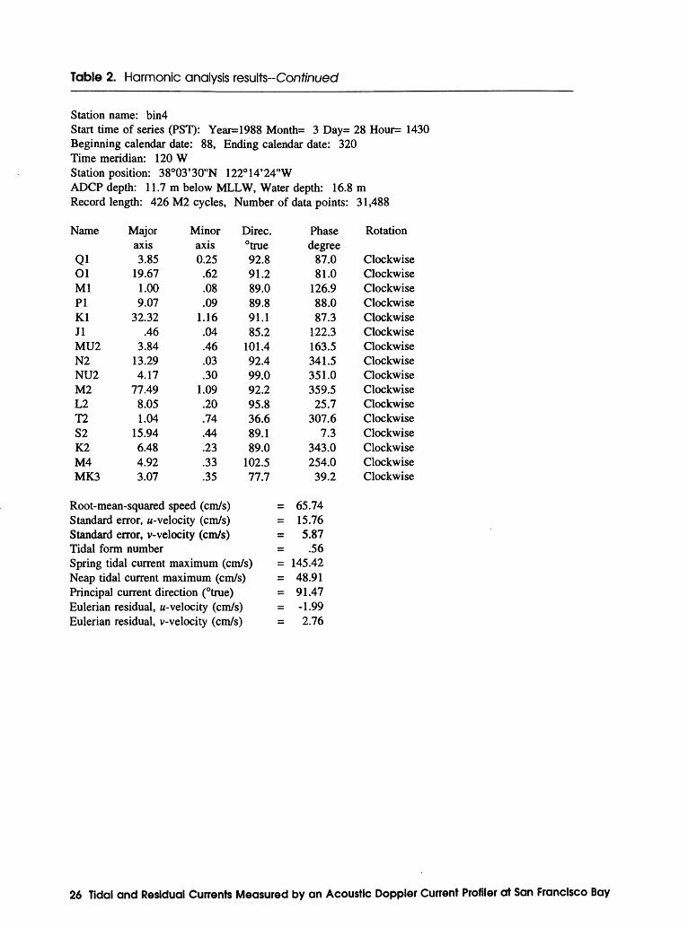
Table 2. Harmonic analysis results-Confinuec/

Station name: bin4Start time of series (PST): Year=1988 Month= 3 Day= 28 Hour= 1430Beginning calendar date: 88, Ending calendar date: 320Time meridian: 120 WStation position: 38°03'30"N 122°14'24"WADCP depth: 11.7 m below MLLW, Water depth: 16.8mRecord length: 426 M2 cycles, Number of data points: 31,488

Name Major Minor Direc.axis axis °true

Ql 3.85 0.25 92.8Ol 19.67 .62 91.2Ml 1.00 .08 89.0PI 9.07 .09 89.8Kl 32.32 1.16 91.1Jl .46 .04 85.2MU2 3.84 .46 101.4N2 13.29 .03 92.4NU2 4.17 .30 99.0M2 77.49 1.09 92.2L2 8.05 .20 95.8T2 1.04 .74 36.6S2 15.94 .44 89.1K2 6.48 .23 89.0M4 4.92 .33 102.5MK3 3.07 .35 77.7

Root-mean-squared speed (cm/s) =Standard error, a-velocity (cm/s) =Standard error, v-velocity (cm/s) =Tidal form number =Spring tidal current maximum (cm/s) =Neap tidal current maximum (cm/s) =Principal current direction (°true) =Eulerian residual, a-velocity (cm/s) =Eulerian residual, v-velocity (cm/s) =

Phasedegree

87.081.0

126.988.087.3

122.3163.5341.5351.0359.525.7

307.67.3

343.0254.0

39.2

65.7415.765.87

.56145.4248.9191.47-1.992.76

Rotation

ClockwiseClockwiseClockwiseClockwiseClockwiseClockwiseClockwiseClockwiseClockwiseClockwiseClockwiseClockwiseClockwiseClockwiseClockwiseClockwise


Table 2. Harmonic analysis results- Continued


Rotation

ClockwiseClockwiseClockwiseCounterclockwiseClockwiseCounterclockwiseClockwiseCounterclockwiseClockwiseClockwiseClockwiseClockwiseClockwiseClockwiseClockwiseClockwise


Ql 3.95 0.21 92.2 Ol 20.31 .50 90.8Ml 1.02 .07 87.0PI 9.40 .11 88.9Kl 33.54 .93 90.6Jl .49 .04 85.0MU2 4.14 .39 99.9N2 13.96 .04 92.4NU2 4.42 .23 99.5M2 81.31 .91 91.8L2 8.60 .14 95.5T2 1.10 .85 39.9S2 16.57 .50 89.3K2 6.81 .09 88.9M4 4.66 .30 00.8MK3 3.41 .41 81.1

Root-mean-squared speed (cm/s) = Standard error, u-velocity (cm/s) = Standard error, v- velocity (cm/s) = Tidal form number =Spring tidal current maximum (cm/s) = Neap tidal current maximum (cm/s) = Principal current direction (°true) = Eulerian residual, «-velocity (cm/s) = Eulerian residual, v-velocity (cm/s) =

Phase degree

87.7 81.6

128.488.787.9

116.5167.9342.0353.2

.628.0

308.58.0

344.6262.2

53.7

68.65 15.75 5.68

.55151.72 51.51 91.15 -3.98 3.46

Table 2 27

Table 2. Harmonic analysis results-Corrf/nuecf


Rotation

ClockwiseClockwiseClockwiseCounterclockwiseClockwiseCounterclockwiseClockwiseCounterclockwiseClockwiseClockwiseClockwiseClockwiseClockwiseCounterclockwiseClockwiseClockwise


Ql 4.00 0.15 91.8 Ol 20.90 .34 90.6Ml 1.04 .05 85.2PI 9.75 .33 88.2Kl 34.63 .66 90.4Jl .49 .11 88.6MU2 4.42 .36 98.0N2 14.56 .09 92.6NU2 4.61 .21 99.6M2 84.63 .85 91.6L2 9.03 .10 94.8T2 1.15 .97 49.8S2 17.09 .57 89.8K2 7.07 .02 89.2M4 4.42 .42 98.9MK3 3.82 .38 85.4

Root-mean-squared speed (cm/s) = Standard error, u-velocity (cm/s) = Standard error, v-velocity (cm/s) = Tidal form number =Spring tidal current maximum (cm/s) = Neap tidal current maximum (cm/s) = Principal current direction (°true) = Eulerian residual, w-velocity (cm/s) = Eulerian residual, v-velocity (cm/s) =

Phase degree

88.3 82.2

129.089.388.5

110.9172.1342.6355.5

1.730.2

316.38.8

346.4271.1

65.1

71.26 15.58 5.61

.55157.25 53.81 91.01 -6.10 3.99


Table 2. Harmonic analysis results-Con//ni/ed

Station name: bin?Start time of series (PST): Year=1988 Month= 3 Day= 28 Hour= 1430Beginning calendar date: 88, Ending calendar date: 320Time meridian: 120 WStation position: 38°03'30"N 122°14'24"WADCP depth: 8.7 m below MLLW, Water depth: 16.8 mRecord length: 426 M2 cycles, Number of data points: 31,488

Rotation

ClockwiseClockwiseClockwiseCounterclockwiseClockwiseCounterclockwiseClockwiseCounterclockwiseClockwiseClockwiseClockwiseClockwiseClockwiseCounterclockwiseClockwiseClockwise


Ql 4.03 0.11 91.4 Ol 21.48 .18 90.5Ml 1.05 .02 84.8PI 10.12 .56 87.7Kl 35.69 .40 90.3Jl .44 .13 94.2MU2 4.64 .34 96.1N2 15.09 .12 92.8NU2 4.77 .18 99.1M2 87.57 .84 91.6L2 9.38 .05 93.7T2 1.21 1.05 71.2S2 17.55 .63 90.4K2 7.27 .10 89.5M4 4.27 .63 98.3MK3 4.27 .30 89.6

Root-mean-squared speed (cm/s) Standard error, w-velocity (cm/s) Standard error, v-velocity (cm/s) Tidal form numberSpring tidal current maximum (cm/s) Neap tidal current maximum (cm/s) Principal current direction (°true) Eulerian residual, w-velocity (cm/s) Eulerian residual, v-velocity (cm/s)

Phase degree

88.6 82.5

128.789.989.2

103.0176.2343.2357.4

2.932.3

335.79.6

348.5281.3

73.7

= 73.67 = 15.32 = 5.62

.54= 162.29 = 55.82 = 91.01 = -8.30 = 4.36

Table 2 29

Table 2. Harmonic analysis results-Contfnued


Rotation

ClockwiseCounterclockwiseCounterclockwiseCounterclockwiseClockwiseCounterclockwiseClockwiseCounterclockwiseClockwiseClockwiseCounterclockwiseClockwiseClockwiseCounterclockwiseClockwiseClockwise


Ql 4.08 0.06 90.8 Ol 22.13 0 90.5Ml 1.07 .01 84.5PI 10.58 .80 87.1Kl 36.82 .11 90.3Jl .41 .11 101.6MU2 4.87 .33 94.0N2 15.61 .11 93.1NU2 4.87 .14 98.8M2 90.35 .88 91.5L2 9.64 .03 93.0T2 1.29 1.12 84.9S2 17.96 .74 91.1K2 7.47 .17 90.2M4 4.22 .84 98.0MK3 4.70 .21 93.7

Root-mean-squared speed (cm/s) = Standard error, w-velocity (cm/s) = Standard error, v-velocity (cm/s) = Tidal form number =Spring tidal current maximum (cm/s) = Neap tidal current maximum (cm/s) = Principal current direction (°true) = Eulerian residual, w-velocity (cm/s) = Eulerian residual, v-velocity (cm/s) =

Phase degree

88.5 82.7

127.490.789.991.7

180.1343.7359.2

4.134.3

346.610.3

350.9290.9

79.4

76.11 15.09 5.79

.54167.26 57.71 91.05

-10.59 4.47


Table 2. Harmonic analysis results-Con#nuec/


Rotation

ClockwiseCounterclockwiseCounterclockwiseCounterclockwiseCounterclockwiseCounterclockwiseClockwiseCounterclockwiseClockwiseClockwiseCounterclockwiseClockwiseClockwiseCounterclockwiseClockwiseClockwise


Ql 4.04 0.01 89.9 Ol 22.48 .21 90.4Ml 1.06 .04 84.8PI 10.96 .99 86.4Kl 37.77 .24 90.2Jl .32 .08 112.2MU2 5.07 .30 91.7N2 16.03 .17 93.2NU2 4.89 .10 98.8M2 92.60 .74 91.4L2 9.92 .16 92.2T2 1.31 1.13 110.8S2 18.17 .86 91.7K2 7.69 .26 91.3M4 4.06 .99 99.2MK3 5.19 .08 97.0


Phase degree

87.5 82.623.590.690.276.1

184.7344.0

.75.3

35.812.411.0

354.3304.7

87.4

78.16 15.15 6.05

.54171.02 59.14 91.03

-12.63 4.23

Table 2 31


Station name: bin 10Start time of series (PST): Year=1988 Month= 3 Day= 28 Hour= 1430Beginning calendar date: 88, Ending calendar date: 320Time meridian: 120 WStation position: 38003'30"N 1220 14'24"WADCP depth: 5.7 m below MLLW, Water depth: 16.8 mRecord length: 426 M2 cycles, Number of data points: 31,488

Rotation

CounterclockwiseCounterclockwiseCounterclockwiseCounterclockwiseCounterclockwiseCounterclockwiseClockwiseCounterclockwiseClockwiseClockwiseCounterclockwiseClockwiseClockwiseCounterclockwiseClockwiseCounterclockwise


Ql 3.99 0.04 89.4 Ol 22.65 .41 90.8Ml 1.03 .06 85.8PI 11.31 1.14 86.0Kl 38.46 .60 90.5Jl .32 .02 117.3MU2 5.01 .29 89.9N2 16.33 .20 93.5NU2 4.93 .05 98.8M2 93.85 .71 91.5L2 9.99 .38 92.0T2 1.37 1.18 132.7S2 18.37 1.05 92.8K2 7.92 .41 92.9M4 3.92 1.10 101.4MK3 5.85 .08 100.1


Phase degree

87.2 82.5

123.390.490.470.5

187.5344.5

.96.4

37.033.811.8

356.3320.6

92.1

79.41 15.20 6.55

.54173.33 59.67 91.33

-13.75 3.74


Table 2. Harmonic analysis results-Continued

Station name: bin 11Start time of series (PST): Year=1988 Month= 3 Day= 28 Hour= 1430Beginning calendar date: 88, Ending calendar date: 320Time meridian: 120 WStation position: 38°03'30"N 122°14'24"WADCP depth: 4.7 m below MLLW, Water depth: 16.8 mRecord length: 426 M2 cycles, Number of data points: 31,488

Rotation

CounterclockwiseCounterclockwiseCounterclockwiseCounterclockwiseCounterclockwiseClockwiseClockwiseCounterclockwiseClockwiseClockwiseCounterclockwiseClockwiseClockwiseCounterclockwiseClockwiseCounterclockwise


Ql 3.98 0.08 89.1 01 22.51 .69 91.5Ml 1.04 .09 88.3PI 11.68 1.30 85.5Kl 38.84 1.11 90.7Jl .35 .02 119.4MU2 4.77 .31 90.2N2 16.55 .22 93.5NU2 4.91 .09 99.5M2 94.30 .48 92.0L2 9.93 .40 92.6T2 1.50 1.13 140.2S2 18.56 1.03 93.5K2 8.02 .53 94.2M4 4.01 .69 105.0MK3 6.10 .39 99.9

Root-mean-squared speed (cm/s) = Standard error, ^-velocity (cm/s) = Standard error, v-velocity (cm/s) = Tidal form number =Spring tidal current maximum (cm/s) = Neap tidal current maximum (cm/s) = Principal current direction (°true) = Eulerian residual, ^-velocity (cm/s) = Eulerian residual, v-velocity (cm/s) =

Phase degree

87.3 82.5

123.790.690.765.5

187.8344.8

1.56.9

37.440.812.8

358.0328.995.2

79.90 14.91 6.92

.54174.20 59.41 91.78

-14.56 2.87

Table 2 33


Station name: bin 12Start time of series (PST): Year=1988 Month= 3 Day= 28 Hour= 1430Beginning calendar date: 88, Ending calendar date: 320Time meridian: 120 WStation position: 38°03'30"N 122°14'24"WADCP depth: 3.7 m below MLLW, Water depth: 16.8 mRecord length: 426 M2 cycles, Number of data points: 31,488


Ql 4.01 0.06 88.3 Ol 22.57 .71 90.9Ml 1.04 .06 86.4PI 11.69 1.03 87.1Kl 38.91 .74 91.4Jl .35 .04 116.7MU2 4.84 .29 87.6N2 16.55 .02 94.5NU2 4.95 .06 99.3M2 94.46 1.15 92.6L2 9.99 .50 92.9T2 1.46 1.03 130.8S2 18.55 1.06 94.0K2 8.02 .38 94.5M4 3.89 1.16 99.0MK3 6.06 .14 101.7


Phase degree

87.1 82.5

124.090.490.860.7

188.0345.0

1.47.0

37.930.212.8

358.2327.996.2

80.10 15.02 7.12

.54174.49 59.58 92.24

-14.89 2.02

Rotation

Counterclockwise CounterclockwiseCounterclockwiseCounterclockwiseCounterclockwiseClockwiseClockwiseCounterclockwiseClockwiseClockwiseCounterclockwiseClockwiseClockwiseCounterclockwiseClockwiseClockwise


(Q c <p I <D" co o O & CL

g_ Q

Q.

S

co CL C

Q O C 1

SPEED, IN C

ENTI

METE

RS P

ER S

ECON

D

RE

SID

UA

L (F

ILT

ER

ED

) V

ELO

CIT

IES

DIRECTION, IN DEGREES

TRUE

ME

AS

UR

ED

VE

LOC

ITIE

S

SPEED, IN CE

NTIM

ETER

S PER

SECOND

DIRECTION, IN D

EGREES TR

UE

<D

00 5* Q

O ro <D a

a I 00

OO o c_ C 00 f <D & Ox o 00

00

I a a I a a O O a cr *< a 3 O

O i o o

o TO

TO

<D O o -o

5 2

o a. CO a 3 a 3 o «/>'

o o 0

9 a

(Q

O

ME

AS

UR

ED

VE

LOC

ITIE

S

SPEE

D, IN C

ENTIMETERS PER

SECOND

DIRE

CTIO

N, IN D

EGRE

ES TR

UE

8 g

en ff =£ o Q p

5 0» < *, O

Q

O a Q a Os o (Q CA Q o Q.

Q ^ I 10 a

Station name: Binl, August 22 (calendar day 235) to November 6 (calendar day 311), 1988

235 240 245 250 255 260 265 270 275 280 285 290 295 300 305 310 315


265 270 275 280 285 290


Figure 14. Time-series plots of tidal and residual currents--Conf/nL/ed

Figure 14 37

Station name: Bin2, March 28 (calendar day 88) to June 8 (calendar day 160), 1988

MS 120 125 130 135


US 120 1ZS 130


Figure 14. Time-series plots of tidal and residual currents-Conf/nued


Station name: Bin2, June 8 (calendar day 160) to August 22 (calendar day 235), 1988

160 165 170 175 190 195 200 205 210 215 220 225 230 235



Figure 14. Time-series plots of tidal and residual currents-Conf/nuecf

Figure 14 39

Station name: Bin2, August 22 (calendar day 235) to November 6 (calendar day 311), 1988

235 240 MS 250 255 260 26S 270 275 280 285 290 295 300


215 250 305 3IO


Figure 14. Time-series plots of tidal and residual currents-Continued


(Q C

(Q 3 O a

o_ Q

CL

CD CO CL c Q.

O C

-^ CD D 5 c CD

Q.

SPEED,

IN CE

NTIM

ETER

S PE

R SECOND

g s

RE

SID

UA

L (F

ILT

ER

ED

) V

ELO

CIT

IES

DIRECTION, IN D

EGREES TR

UE

§ s

a a

ME

AS

UR

ED

VE

LOC

ITIE

S

SPEED, IN CE

NTIM

ETER

S PE

R SECOND


TRUE

a i

i 8

CO cf O*

Q

<D

o>

O> Q

O 10

0»

_<D 3

Q

. Q 00 00

.O

Q

.<D I a

Q OO 00


190 195 200 205


UJ

o oUJ ~

UJ CC UJ

190 195 200 205


Figure 14. Time-series plots of tidal and residual currents-Conf/nt/ed


Station name: Bln3, August 22 (calendar day 235) to November 6 (calendar day 311), 1988

210

160

</) " _ 6QUJ £ 6°t S -90OO - |2°W -ISO

S 2s0

D °

^ Im i^ 20°2 <*

S: 150

265 270 275 260 285


265 270 275 280 285


Figure 14. Time-series plots of tidal and residual currents-Conf/nued

Figure 14 43


US 120 125 130 135


115 120 125 130


Figure 14. Time-series plots of tidal and residual currents-Conf/nt/ed


<Q

(Q

3 CD CO CD < CD'

CO Q. O a- o ( > s Q Q D

Q. CD CO Q."

Q.

O 8 S Q.

SPEED, IN CE

NTIM

ETER

S PE

R SECOND

RE

SID

UA

L (

FIL

TE

RE

D)

VE

LO

CIT

IES

DIRECTION, IN D

EGREES TR

UE

ME

AS

UR

ED

VE

LO

CIT

IES

SPEED, IN C

ENTI

METE

RS P

ER SE

COND

DI

RECT

ION,

IN DEGREES

TRUE

Station name: Bin4, August 22 (calendar day 235) to November 6 (calendar day 311), 1988


235 240 245 250 255 265 270 275 280 285 290 295 300 305 310 315




(Q

O

(Q c 5 O h a

o_ Q Q_

CD C/J

_

C Q O

C CD sr c: CD Q.

SPEED, IN CENTIMETERS

PER

SECOND

RE

SID

UA

L (F

ILT

ER

ED

) V

ELO

CIT

IES

DIRECTION, IN

DEGREES

TRUE

ME

AS

UR

ED

VE

LOC

ITIE

S

SP

EE

D,

IN

CE

NTI

ME

TER

S

PER

SE

COND

D

IRE

CT

ION

, IN

DE

GRE

ES

TRU

E

CO c?

o' Q

<D S

D*

Cfl

Q

O ro

oo c?

5T

CL Q CL

Q Oo

Oo

C <D

Oo .

<D CL

Q CL

Q Oo

Oo

Station name: BjnS, June 8 (calendar day 160) to August 22 (calendar day 235), 1988

195 200 205

, IN CALENDAR DAYS

160 165 165 190 195 200 205 210 215 220

TIME, IN CALENDAR DAYS225 230



(Q

I

(Q C o ? co CD g.

o co

O O_

Q Q D

Q. CD

co O."

C Q O C 1 9 c CD

Q.

SPEED, IN CE

NTIM

ETER

S PE

R SECOND

5 S

8 3

S

RE

SID

UA

L (F

ILT

ER

ED

) V

ELO

CIT

IES

DIRE

CTIO

N, IN DEGREES

TRUE

ME

AS

UR

ED

VE

LOC

ITIE

S

SPEE

D, IN CE

NTIM

ETER

S PER

SECOND


TRUE

o

o

o

S

ooooooooooo

=±

o D D

Q <D

Jg

01 (Q c 10 10 s^. o fi

<D Q.

Q Q.

Q IO

0> en Z

O <D C7

<D O

Q <D D

Q. Q Q.

Q O 0000


210

180

CO111

o2111aiiiDC

I 111

-90

-120

115 120 125 130 135


COill

ill

aiiiDC111

180

150

120

90

60

30

0

-30

-60

-90

-120

-150

7Z u

US 120 12S 130


Figure 14. Time-series plots of tidal and residual currents-Conftni/ec/


(Q cn

(Q c CD 3 o o" tn O Q.

Q Q D

Q. (D C Q O C

SPEE

D, IN CE

NTIM

ETER

S PER

SECOND

RE

SID

UA

L (F

ILT

ER

ED

) V

ELO

CIT

IES

DIRE

CTIO

N, IN DEGREES

TRUE

ME

AS

UR

ED

VE

LOC

ITIE

S

SPEE

D, IN CENTIMETERS

PER

SECOND


TRUE

m g m

&

I3:

COC

(D

Q.

Q

CD

OJ c D O 00

^^

O Q O D

Q.

Q Q.

Q O

^x o" > (Q 2*. 10

ro a o D Q.

Q Q.

Q < ro G)

On

c

Q J2.

Q. o I c Q

<D

Q. O O o TJ o o i o

SPEED,

IN CE

NTIM

ETER

S PER

SECOND

5 8

3 S

RE

SID

UA

L (F

ILT

ER

ED

) V

ELO

CIT

IES

DIRE

CTIO

N, IN D

EGREES TR

UEM

EA

SU

RE

D V

ELO

CIT

IES

SPEED, IN CE

NTIM

ETER

S PER

SECOND

DIRECTION, IN D

EGREES TR

UE

s s

sO

Q 5!

a. (Q (A X"X

Q. Q ^ Q.

Q < ro Oi en C7 ^

O> X"X o Q. Q ^ Q.

Q < Oi O

Oo

Oo

<Q 8

(Q C O g.

o a

Q Q D a (D CO a c Q O

C (D

SPEED,

IN CE

NTIM

ETER

S PER

SECOND

RE

SID

UA

L (

FIL

TE

RE

D)

VE

LO

CIT

IES


TRUE

ME

AS

UR

ED

VE

LO

CIT

IES

w

SPEED,

IN CE

NTIM

ETER

S PER

SECO

ND

DIRECTION, IN

DE

GREE

S TRUE

Q

O

O

O

O

OOOOOOOOOOOOO

(D

CL

Q

<D CD 3' Q o ro

oo O*

Q

<D a Q a Q Oo

Oo c ® 00

x^ O

Q

<D a.

Q GK O O

00

Oo

2-n

<5

'

=!

5

d

Q)SPEED, IN C

ENTI

METE

RS PE

R SECOND

RE

SID

UA

L (F

ILT

ER

ED

) V

ELO

CIT

IES

DIRECTION, IN D

EGREES TR

UE

ME

AS

UR

ED

VE

LOC

ITIE

S

a a TO <D

S2. a

a O c o if a

a 8 i o o

o T3

D

O O a § n

Q O ff O

9 co

(D O

co"

O h

^J- a

Q Q a (D

co a c Q O

C (D s a

gss

gsss

SPEED, IN CE

NTIM

ETER

S PER

SECO

ND

g 8

DIRECTION, IN D

EGRE

ES TR

UE

m g m o 5 w

Q 00 3' C

<D 00 Q

<D a Q « a

a ON

O

(Q

v> ro

10 >«^ O

Q a> a a ^ a

a jo

c*>

en 00 00

(Q C <D CD

co

CD O"

CO g. o^ CO o o_ Q_ Q D o_ CD CD Q.

SPEE

O, IN CENTIMETERS

PER

SECO

ND

5 a

a s

RE

SID

UA

L (F

ILT

ER

ED

) V

ELO

CIT

IES

DIRE

CTIO

N, IN D

EGREES TR

UEM

EA

SU

RE

D V

ELO

CIT

IES

SPEE

D, IN CE

NTIM

ETER

S PER

SECOND

DIRECTION, IN D

EGREES TRUE

g §

g

O > r~

m z

o JJ

o to

(Q

<D

3 Q <D CO 5* (Q CA o Q.

<D a Q a

Q < ro

o>

a; 5" I <X

x-^ O o a

Q a

Q O) 00

00


210

US 120 125 130


01

01

a 111 cc 01

o0501 CC

180 -

ISO -

120

90

60

30

0

-30

-60

-90

-120

-150

Q 10

110 US 120 125 130


Figure 14. Time-series plots of tidal and residual currents-Conf/ni/eaf


(Q C o

£

cn

(Q 5 Q.

Q Q 13

Q. CD o § CD Q.

SPEE

D, IN CENTIMETERS

PER

SECOND

RE

SID

UA

L (F

ILT

ER

ED

) V

ELO

CIT

IES

DIRE

CTIO

N, IN DEGREES

TRUE

g*

m O

> m o

> 3 o

> CO

S 8

gggg

0ygg8S

gT

I

I

I .1 r

ME

AS

UR

ED

VE

LOC

ITIE

SSP

EED,

IN CENTIMETERS

PER

SECOND


TRUE

S S

8

o' Q

<D

00 00 3 00

x-x o Q.

<D CL

Q CL

Q (Q c w o Q.

<D CL

Q CL

Q cn <o

oo

oo

Station name: Bind, August 22 (calendar day 235) to November 6 (calendar day 311), 1988

210

90

60 illillillill lii! Ijju1iii1IIIUillilliiiiInmflnnnmriiii ilii.........VliiViiiLi1mm iiiittl Irani H

::H I

wILJ

LU

aUJcc.LU

LJJ CC

180

150

120

90

60

30

0

-30

-60

-90

-120

-150

50

a 10

265 270 275 280 285


235 240 245 250 255 265 270 275 280 285 290 295 300 305 310 315


Figure 14. Time-series plots of tidal and residual currents-Con/y'nueaf


(Q C 5

£

en

(Q

O O

c/T

O O_

Q O_

CD

co cL c Q O C CD I Q.

SPEED,

IN CENTIMETERS

PER

SECOND

RE

SID

UA

L (F

ILT

ER

ED

) V

ELO

CIT

IES

DIRE

CTIO

N, IN DEGREES

TRUE

8 g

3 8

5

ME

AS

UR

ED

VE

LOC

ITIE

SSP

EED

, IN

C

ENTI

MET

ERS

PER

SECO

ND

DIR

EC

TIO

N,

IN

DEG

REES

TR

UE

g i

s

m z

o 33

O to

5'

Q

<D 09 5'

10 00 Q_

<D

D

Q.

Q Q.

Q 00

00 c

<D 00 Q

<D Q.

Q Q.

Q 00

O

O


210

190 195 200 205


UJ

t o oUJ

Q UJ DC UJ

180 -

ISO

120

90

60

30

0

-30

-BO

-90

-120

-150

50

i B

a: 30

a 10

160 165 180 185 190 195 200 205 210 215 220 225 230 235




(Q c

(Q C

0 a Q Q a (D CO a c Q O

C (D D I Q.

SPEED, IN C

ENTI

METE

RS P

ER SE

COND

RE

SID

UA

L (F

ILT

ER

ED

) V

ELO

CIT

IES


TRUE

S S

oS

S 5

ME

AS

UR

ED

VE

LOC

ITIE

SSP

EED,

IN CE

NTIM

ETER

S PER

SECO

ND

DIRE

CTIO

N, IN DEGREES

TRUE

s s

s

m g m o

> 33 a

> CO

O Q

<D

CO 5' (Q (A

IO IO D a

a a

a 10

o Os cT a

a a

a < o>

Station name: Bin 10, March 28 (calendar day 88) to June 8 (calendar day 160), 1988

US 120 125 130


HI -30

77 ui -60

OQ -90

111

a atDC 111

O CO111 cc

-120

-150


Figure 14. Time-series plots of tidal and residual currents--Con/y'ni/ec/


(Q

O O CA>

(Q c o 9 co

(D 0

co Q_

Q Q

O.

CD

co CL C

Q.

O

C CD D CD Q.

SPEED, IN CE

NTIM

ETER

S PE

R SECOND

O

O

O

O

RE

SID

UA

L (F

ILT

ER

ED

) V

ELO

CIT

IES


TRUE

ME

AS

UR

ED

VE

LOC

ITIE

SSP

EED

, IN

C

ENTI

MET

ERS

PER

SECO

ND

DIR

EC

TIO

N,

IN

DEG

REES

TR

UE

S 8

S 8

3S

S£3gog3£§g§

m I CO

O Q

O 3

O c

o 00 x-x a o Q.

Q Q.

Q (Q 10

10 Q

O Q.

Q IO o»

Station name: Bin 10, August 22 (calendar day 235) to November 6 (calendar day 311), 1988


180

150

120

90

60

30

0

-30

-60

-90

-120

-150

SO

C/J

d UJ OC UJ

a c/jOJ DC

235 240 215 250 255 260 265 270 275 280 285 290 295 300 305 310


Figure 14. Time-series plots of tidal and residual currents--Continued


(Q C 5 S Ol

(Q

I CD

in 0 0"

co g. o a-

o a

Q Q

a

(B CO CL

Q o c ^ CD 13

SPEED, IN C

ENTIMETERS P

ER SE

COND

inouiauioin

RE

SID

UA

L (F

ILT

ER

ED

) V

EL

OC

ITIE

SDI

RECT

ION,

IN DEGREES

TRUE

ME

AS

UR

ED

VE

LOC

ITIE

S

SPEED, IN C

ENTI

METE

RS P

ER SECOND

DIRECTION, IN D

EGREES TR

UE

CD Q.

9. 00 5' Q O sr 10 Oo & Oo

Oo O

Q_ O & < i O

Oo

Oo

Os

Os

Q.

Q Q Q.

TO <D

</> a

a. O c o <D a o" O o o T3 a> O c I -o o CO Q Q 3

O

35" o o 00 Q

(Q

0

RE

SID

UA

L (F

ILT

ER

ED

) V

ELO

CIT

IES

DIRECTION, IN D

EGRE

ES TR

UESPEE

D, IN CENTIMETERS

PER

SECOND

ME

AS

UR

ED

VE

LOC

ITIE

SSP

EED,

IN CENTIMETERS

PER

SECOND

DIRECTION, IN D

EGRE

ES TR

UE

(D

0' O"

c7?"

O Q D a (D

en a c

Q O

C (D O 8 =£ c (D

Q.

CO 5' 3

Q (D

(P 5' c (D

00 o1 Q ® Q.

Q O

O c (Q C 2J- ro

ro Q O Q. Q -* Q.

Q ro CA> en 0>

(Q c 5

(Q i o h a Q

Q

Q.

(D CO CL c

Q.

O

C (D

SPEED, IN CE

NTIM

ETER

S PER

SECO

ND

RE

SID

UA

L (F

ILT

ER

ED

) V

ELO

CIT

IES

DIRECTION, IN

DEGREES

TRUE

ME

AS

UR

ED

VE

LO

CIT

IES

SPEE

D, IN

CE

NTIM

ETER

S PER

SECOND


TRUE

Q

ui

o

en

01

ro

CD

m

OJ

uotp

o

o

o

oooooooooa

CD

Q.

o Q

<D

CD 5' (Q (A ro

ro Q

<D Q.

Q Q.

Q < ro CA>

en O

Q.

<D Q.

Q Q.

Q < CO O 00

00

Station name: Bin 12, March 28 (calendar day 88) to June 8 (calendar day 160), 1988

115 120 125 130



Figure 14. Time-series plots of tidal and residual currents--Con/y'nuec/


(Q

O 9 CO 0 0" CO g. o a

o_ Q D a

0 CO a c Q O

C 0 D O S Q.

SPEED,

IN CE

NTIM

ETER

S PER

SECO

ND

RE

SID

UA

L (F

ILT

ER

ED

) V

ELO

CIT

IES

DIRECTION, IN D

EGREES TR

UESP

EED,

IN CENTIMETERS

PER

SECOND

S8S

ME

AS

UR

ED

VE

LOC

ITIE

S

<£DIRECTION, IN DEGREES

TRUE

Q. O Q

O ro c o Oo

_ O a Q a

Q <Q

c

2J- ro

ro Q.

O a

a a

a < ro

o>

01 o

o>

oo

Station name: Bin!2, August 22 (calendar day 235) to November 6 (calendar day 311), 1988

265 270 275 280 285


265 270 275 280 285


Figure 14. Time-series plots of tidal and residual currents-Conf/nuecf


APPENDIX A.--ADCP ERROR SOURCES

Because of the nonintrusive nature of the measurements made by acoustic Doppler current profiler (ADCP) systems, they are not subject to many of the error sources that plague conventional current meters (fouling, vertical motion, and rotor or propeller rating errors); however, the complexity of Doppler shift determinations introduces sources of error that are unique to ADCP systems. Although a rigorous error analysis of ADCP systems is beyond the scope of this report, major sources of random and systematic error in ADCP systems will be discussed. The ADCP used in this study will be referred to as ADCP S/N 159 in the rest of this section of the report.

RANDOM ERROR

Random errors can be reduced by data averaging. The complex covariance estimator used by the ADCP to determine Doppler frequency shifts must deduce the center of power (in the frequency domain) of the reflected signal to determine water velocity. The reverberation spectrum from the water-velocity field is composed of many echoes of the transmitted signal from discrete particles moving with the water whose dimensions are much smaller than the spatial pulse volume; therefore, a single determination of velocity (ping) has a high variance. Fortunately, the ADCP system has a ping rate of 8 or 9 pings per second, and the standard error of a velocity determination can be reduced quickly by averaging. For ADCP S/N 159, short-term (random) precision of velocity determinations made at an individual bin can be expressed in terms of standard error (Gordon, 1989):

o - L6 X '°5 . (5)

where a, = standard error of a water- velocity determination in bin, (meters per second),F - transmit frequency (in Hertz),D - discrete vertical bin height (meters), andN = number of pings averaged to obtain a water-velocity estimate.

The relevant ADCP parameters used during this study were F=\ .2xl06, D=\ , and N=2\76. Using these parameters, the standard error of a single bin velocity determination is 0.30 cm/s. Field measurements (Simpson, 1986) using a similar ADCP have supported this random error model although it should be considered only approximate.

An additional source of random error is short time-scale turbulence (0-2 minutes) in the water- velocity field. However, random error due to this source probably was insignificant because of the 10-minute averaging period used in this study (Carter and Anderson, 1963).

SYSTEMATIC ERROR

Effects of systematic, or bias, errors are significant because they cannot be reduced by data averaging. When small residual velocities are derived from large tidal velocities, as in this study, bias errors that are constant or additive over time can significantly reduce the accuracy of the derived residual velocities. Major ADCP bias errors can be caused by uncompensated pitch, roll, and heading information, improper beam geometry, a category of sources that can be loosely labeled as receiver chain effects (Hansen, 1986), mispositioning of receiver tracking filters, and a problem that existed in older systems (as was ADCP S/N 159) due to mistuning of a transmit filter (J.A. Gast, RD Instruments, oral commun., 1989;. The exact magnitude of these systematic errors can only be approximated, so the authors have chosen to discuss the "worst case" effect of these errors on the data collected during this study and presented in this report. For a more detailed discussion of these and other ADCP error sources, see Appel and others (1988), Chereskin and others (1989), Hansen (1986), Regier (1982), and Theriault (1986).

Appendix A 71

ERRORS DUE TO UNCOMPENSATED PITCH, ROLL, AND HEADING

Errors due to the uncompensated pitch and roll of the data collection platform probably had a negligible effect on the accuracy of data presented in this report. Pitch and roll sensors were incorporated into the ADCP, and velocity data were corrected using algorithms in the ADCP firmware 1 . The platform did not move significantly during data collection so dynamic errors due to attitude sensor response were not present. Inaccuracies in heading information provided by the internal flux gate compass would provide a consistent directional error in both the tidal flux data and the residual data; however, the magnitude of this error was no more than 2 or 3 degrees.

ERRORS DUE TO IMPROPER BEAM GEOMETRY

Errors can be introduced into the computation of horizontal velocities because of incorrect transducer beam axis angles. For example, if an ADCP (similar to ADCP S/N 159) is manufactured with a 31.0° pointing angle on all transducers instead of 30.0°, and the conversion algorithms were not corrected, measured horizontal water velocities would be 3.0 percent more than actual velocities. Errors in the included angles between opposing and adjacent beams can also cause direction-dependent errors. Transducer pointing angles can be measured in the laboratory and that data used to apply corrections to ADCP measured horizontal velocities; however, ADCP S/N 159 was manufactured before beam angle calibration procedures were instituted by the manufacturer. At the author's request, the beam pointing angles were measured by the manufacturer after ADCP retrieval and errors due to pointing angles were computed. Horizontal velocities measured by the fore and aft beams (beams 3 and 4, respectively) were overestimated by 1.2 percent. Horizontal velocities measured by the starboard and port beams (beams 1 and 2, respectively) were overestimated by 1.8 percent. Horizontal velocity components crossing the beam pattern at arbitrary azimuths were overestimated, on the average, by 1.5 percent. The manufacturer estimates that laboratory beam angle measurements are accurate to within 0.15°.

RECEIVER CHAIN EFFECTS

Receiver chain effects are hardware-associated errors that influence the reverberation spectra of the measured velocity field (Hansen, 1986). Among the most significant are

1. Nonlinearities caused by mismatched transducers, uneven or defective transducer coatings, misaligned receiver electronics, and "ringing" due to various sources.

2. Spectral windowing effects caused by the response of fixed receiver input bandpass filters.3. Noise-induced errors.4. Magnitude transfer function coloring caused by a non 'white' or nonlinear magnitude

transfer function of the receiver bandpass filters and their interaction with the spectral moment estimation technique used in the ADCP.

5. Quadrature channel amplitude and phase imbalances.

!In this case, firmware is defined as a collection of machine-executable programs and operating parameters stored in nonvolatile memory in the ADCP and used by the ADCP microcomputer as an operating system.


These and other receiver-caused errors are termed by Hansen (1986) as receiver chain effects. The magnitude of errors introduced by receiver chain effects are dependent, to a certain extent, on the algorithm used to calculate the center of power (in the frequency domain) of the water parcel reverberation spectra. These errors are extremely hard to quantify individually, and prior to 1989, few attempts were made to do so.

The manufacturer doubts that the combined error in the measurement of horizontal velocity due to receiver chain effects, excluding noise-induced error, exceeds 0.5 percent of the actual velocity (for ADCP S/N 159), but it is agreed that more tests are needed to confirm this value (J.A. Gast, RD Instruments, oral commun., 1989). Laboratory tests done by Appel and others (1988) that compute error from lumped sources indicate that the 0.5 percent error, although optimistic, is reasonable. Many of the errors caused by receiver chain effects can be reduced by optimized circuit design, proper quality control during ADCP manufacture, and stringent calibration procedures. Because of properties of fixed bandpass filters, however, two important error sources discussed by Hansen (1986) (errors 2 and 3) are always present in ADCP systems of the type used in this study and tend to bias the computed horizontal velocities towards the center of the fixed bandpass filter (zero velocity). Thus, these errors most often cause underestimated horizontal velocities. This hypothesis was partially confirmed by laboratory tests (Appel and others, 1988).

ERRORS DUE TO THE MISPOSITIONING OF RECEIVER TRACKING FILTERS

ADCP S/N 159 employs broad bandpass filters at the receiver "front ends" that are the source of some error due to receiver chain effects (as previously discussed). Also implemented are signal-tracking lowpass filters implemented just ahead of the analog-to-digital conversion section of the receiver. These filters have a much narrower bandwidth than the input bandpass filters so as to improve signal to noise ratio (which increases range). The filters are centered at a fixed frequency, and the input signal is shifted towards that frequency by being heterodyned with a variable reference signal. Because these filters can be thought of as movable in the frequency domain, they are called tracking filters. Errors caused by mispositioning tracking filters could be classed as receiver chain effects and are the same type of errors that affect receiver input bandpass filters. However, because tracking filters are movable and have narrower bandwidths than the receiver input bandpass filters, the errors produced are dynamic in nature and deserve a separate discussion. Chereskin and others (1989) describe two sources of error due to tracking filter mispositioning:

1. Skew error caused when the center frequency of the received signal is located either outside of, or in, the nonsymmetrical portion of the tracking filter bandwidth. The magnitude of this error is a nonlinear function of the difference between the center frequency of the acquired signal and the center frequency of the filter.

2. Noise-induced error, due to the tendency of the complex covariance estimator to bias the estimated center of power toward the mean filter frequency when the signal to noise ratio is low and "white" noise dominates the filter envelope.

The starting center frequency of these filters is computed by an algorithm using information from initial ADCP pings and setup parameters in the ADCP firmware. ADCP S/N 159 contained firmware algorithms that used default values that provided poor results under current shear conditions. RD Instruments, ADCP firmware release versions 16.07 and earlier, contained default firmware values that were only appropriate for open ocean or lake profiling. This firmware calculated the starting frequency of the filter as discussed in the following paragraphs.

Appendix A 73

The starting filter center frequency was computed by using the average of 30 percent of the data from the total number of bins collected (in this case 20) starting with bin2, or (more simply) the average of velocity data collected from bins 2 through 7. In a typical profile, as recorded in this study, the center of the filter was positioned approximately +20 cm/s from the actual velocity in the lowest bin (binl). The filter positioning algorithm then shifted to the bin-to-bin tracking mode, and attempts were made to center the filter on the incoming signals in each successive bin. The filter converged on the input signal at a rate computed from the output of a low-pass filter algorithm. In ADCP S/N 159 the default firmware parameters were set for open ocean profiling where current shear is much less than in the Carquinez Strait. The low-pass filter time constant was so long that the filter did not move significantly during the entire profile. Because of this current shear, (in a typical profile) the filter was positioned approximately -30 crn/s or so from the actual velocity in the near surface bin.

Because of the tracking error, the recorded profiles were skewed slightly toward the center frequency of the filter; this was especially apparent near the top and bottom of the profile. The magnitude of this error for ADCP S/N 159 (using ADCP parameters previously described) can be approximated using the following equation (J.A. Cast, RD Instruments, oral commun., 1989):

Vb = 0.019 AV + 0.0009 AV 2 , (6) e

where V^ _ error jn beam velocity, in centimeters per second, andAV = difference between the filter center frequency (velocity) and the actual velocity, in

centimeters per second.

In this study, noise bias was not a significant source of error. Signal levels were well above the noise threshold for the entire measured profile in all the cases examined. However, had the backscattered amplitude levels on any beam dropped below 40 decibels, the tracking loop would have been disabled and the tracking filter switched to narrow-band mode (default parameter settings). These settings would have introduced errors of much greater magnitude. To reduce both filter skew and noise-induced bias, ADCP tracking loop parameters should be thoroughly analyzed before an ADCP is deployed in conditions of current shear.

Although tracking loop parameters were not optimal, errors due to tracking filter mispositioning incurred during this study probably were not greater than 2.5 cm/s and, in many cases, were partly canceled due to errors that had opposing effects.

ERROR DUE TO TRANSMIT FILTER MISTUNING

The ADCP manufacturer has reported an error that existed in ADCP units delivered prior to autumn 1989 (that includes ADCP S/N 159). The error is due to a mistuned transmit filter that causes an apparent skew in the transmit frequency envelope. Because internal ADCP reference signals are offsets of the true transmit frequency and not the biased transmit frequency, and because the reverberation spectrum is Doppler shifted based on the biased transmitted frequency, computations of horizontal velocity are biased. The measured horizontal velocity (using ADCP S/N 159 and the ADCP parameters previously described) was biased approximately -0.7 cm/s from the actual horizontal velocity. This error estimate is a "conservative" guess, based on the manufacturer's experience (J.A. Cast, RD Instruments, oral commun., 1989). The magnitude of this offset was relatively independent of the magnitude of the actual velocity. A small amount of scale factor error (error as a percentage of true velocity) was also added because of this effect. However, because the transmit filter's bandwidth is four times greater than the tracking filter's bandwidth, the scale factor error effects are minimal.


EFFECTS OF ADCP ERROR ON GROSS TIDAL AND RESIDUAL VELOCITY DATA

A small computer error model was developed to assess the effects of the systematic errors previously described on the data presented in this report. Figure 15 shows an ADCP measured profile taken from the study data. The dashed line depicts a profile as affected by systematic errors (as previously described) and the solid line depicts the profile adjusted for errors. Examination of data collected during periods when maximum current shear exists (maximum errors are introduced during these periods) has revealed that measured tidal velocities are probably underestimated by 1.5 percent in the uppermost bins, not affected near midprofile, and overestimated by 1.6 percent in the lowermost bins.

14

12

DCLLJ

LJJ

Q LJJ OQ

O DC LLI

DL LJJ Q

40 50 60 70 80 90 100

VELOCITY, IN CENTIMETERS PER SECOND

110

Figure 15. Combined effects of acoustic Doppler current profiler bias errors on a typical water- velocity profile taken from the study data.

Residual velocities are derived from filtering tidal velocities, and errors not correlated with direction tend to be self canceling if tidal ebb and flood magnitudes are somewhat symmetrical over the filtered period. Because the ratio of freshwater inflow to tidal flow was low during the study period, the self-canceling effect helped reduce the effects of error on the residual velocity determinations. Errors in the residual determinations were roughly estimated by applying corrections to recorded peak tidal velocities over a 24.8 hour period when maximum current shear existed.

Averages of the corrected peak tidal velocities were compared with unconnected versions of the same data. Error in horizontal residual velocity was greatest in the uppermost bin and probably did not exceed 4 percent. This error decreased with depth and probably did not exceed 1 percent in the lowermost bin. It is likely that these errors were all positive, that is, all residual horizontal velocities were overestimated by values that decrease with depth. This overestimation is explained by effects of incorrect beam pointing angles, which are the greatest source of error (for ADCP S/N 159) described in this section. Other errors (receiver chain errors, transmit skew errors, and tracking filter mispositioning errors) underestimate horizontal velocities and tend to cancel the errors caused by improper beam pointing angles.

Appendix A 75

The data presented in this report were not corrected for systematic errors because the exact magnitude of many of these errors was impossible to determine following damage to the ADCP. The magnitude of many of the systematic errors described above is unique to individual ADCP systems and must be quantified or minimized by proper calibration procedures.

Appel and others (1988) developed a calibration method using a tow tank facility that may identify the error (in lumped form) of many of the error sources previously discussed. The validity of this laboratory test procedure is being scrutinized, but preliminary results look promising. Many of the errors described had not been identified prior to this study, and future studies employing ADCPs will include calibration procedures and techniques that will improve the investigator's ability to eliminate, mitigate, or quantify ADCP errors.


APPENDIX B. DOPPLER DATA FORMATS

(1) ASCII data directly from the RDI ADCP

1 222 A COMPENSATE FOR: RPH (roll, pitch, and heading)A

v88 328 1418 1169 1288 1999919999 -<1234567891011121314151617181920

> 8812

-733-804-865-925-982

-1015-1054-1093-1121-1129-1013-1022-865

-1116-1144-1090-1110-402

19999199993 28-733-804

-154-206-212-257-271-292-298-329-366-380-408-479-609-529-390-286-320245

199991999914 18-154-206

105124138142145151164167169175186199109165209245213241

199991999911 69105124

-8-50

-17-11-19-16-126

435053

-226-8414

91400

19999199991 288

-8-5

8410010010010010010010010010097978

92568575900

1999984100

2322142021891821731651581511441451601501331321129893890

19999^232214

( Year+-- Month1 +-- Day1 1 +-- Hour1 11 11 11 11 1I 11 11 13 28

-733-804-865

1 +--1 11 1I |1 1| |I 11 114 18

-154-206-212

Minute+-- Second

1 +-- 1/100| |1 1 +--1 1 11 1 11 1 111 69 1

105 -8124 -5138 0

Second

Ensemble number+-- Number of e

+-- Not Us1 1 +288 19999 1<

84 22100 21100 2C

+-- Not Used 19999^

I I +-- Backscattered amplitude I +-- Percent good +-- Error beam check

! ! +-- Vertical velocity(*10) +Up, -Down ! +-- North veiocity(* 10) +N, -S +--East velocity(* 10)+E,-W

bin number

Appendix B 77

(2) ADCP data with unacceptable bins removed

2126.30322 10 88 3 28 14 18 111 -73.3 -15.42 -80.4 -20.63 -86.5 -21.24 -92.5 -25.75 -98.2 -27.16 -101.5 -29.27 -105.4 -29.88 -109.3 -32.99 -112.7 -36.6

10 -112.9 -38.02126.46973 9 88 3 28 14 28 10

1 -77.4 -10.62 -90.4 -15.83 -99.1 -20.0

+ ~ Number of hours since Jan. 1, 1988 +-- Number of usable bins

I I +-- Year I I I +-- Month I 111+.. Day I | | | | +.. Hour I | | | | | +.. Minute I I I I I I I +-- Second I I I I I I I I

2126.46973 9 88 3 28 14 28 101 -77.4 -10.62 -90.4 -15.83 -99.1 -20.0

I I +-- North velocity +N, -S I +-- East velocity +E, -W +-- bin number


(3) Data format for binwise time-series for both raw and filtered data

+ Location, collecting agency.

<-+ <-.- +

I I I I

bin-11SUISUN BAY ,USGS bin-12RDI UPWARD DOPPLER bin-13 88-320,1988.SHIP, RANTZ bin-1380330N1221424W 482 550

79 9281301 73 34 79928135175 30 79 9281401 77 29

79928145180 2879 9281501 76 2279 9281551 66 1579 9281601 80 9

I I +> SpeedxlO (cm/s) I +> Direction (° Degrees, true) I (°T - Degrees, temperature) +> Hour

+> Day +> Month

+>Year

+> Station Name

+ Current meter type.II + First and last; calendar day,

I year, ship name.I+ Latitude, longitude, sensorI depth below MLLW, water

column depth MLLW.

Appendix B 79

tidal and residual currents measured by an

Documents

Transcript of tidal and residual currents measured by an