energies

Article

Thermal Cycling in Converter IGBT Modules with DifferentCooling Systems in Pitch- and Active Stall-ControlledTidal Turbines

Faisal Wani 1,*,† , Udai Shipurkar 2, Jianning Dong 3 and Henk Polinder 4

Citation: Wani, F.; Shipurkar, U.;

Dong, J.; Polinder, H. Thermal

Cycling in Converter IGBT Modules

with Different Cooling Systems in

Pitch- and Active Stall-Controlled

Tidal Turbines. Energies 2021, 14, 6457.

https://doi.org/10.3390/en14206457

Academic Editor: Ui-Min Choi

Received: 10 July 2021

Accepted: 16 September 2021

Published: 9 October 2021

Publisher’s Note: MDPI stays neutral

with regard to jurisdictional claims in

published maps and institutional affil-

iations.

Copyright: © 2021 by the authors.

Licensee MDPI, Basel, Switzerland.

This article is an open access article

distributed under the terms and

conditions of the Creative Commons

Attribution (CC BY) license (https://

creativecommons.org/licenses/by/

4.0/).

1 Huygens Engineers, 2516 AH The Hague, The Netherlands; F.Wani@huygens-engineers.nl2 Ships, Maritime Research Institute Netherlands (MARIN), 6708 PM Wageningen, The Netherlands;

U.Shipurkar@marin.nl3 Electrical Sustainable Energy, Delft University of Technology, 2628 CD Delft, The Netherlands;

J.Dong-4@tudelft.nl4 Maritime and Transportation Technology, Delft University of Technology, 2628 CD Delft, The Netherlands;

H.Polinder@tudelft.nl* Correspondence: f.wani@huygens-engineers.nl; Tel.: +31-85-0802801† Current address: Mekelweg 2, 2628 CD Delft, The Netherlands.

Abstract: This paper compares active and passive cooling systems in tidal turbine power electronicconverters. The comparison is based on the lifetime of the IGBT (insulated gate bipolar transistor)power modules, calculated from the accumulated fatigue due to thermal cycling. The lifetimeanalysis accounts for the influence of site conditions, namely turbulence and surface waves. Resultsindicate that active cooling results in a significant improvement in IGBT lifetime over passive cooling.However, since passive cooling systems are inherently more reliable than active systems, passivesystems can present a better solution overall, provided adequate lifetime values are achieved. Onanother note, the influence of pitch control and active speed stall control on the IGBT lifetime wasalso investigated. It is shown that the IGBT modules in pitch-controlled turbines are likely to havelonger lifetimes than their counterparts in active stall-controlled turbines for the same power rating.Overall, it is demonstrated that passive cooling systems can provide adequate cooling in tidal turbineconverters to last longer than the typical lifetime of tidal turbines (>25 years), both for pitch-controlledand active speed stall-controlled turbines.

Keywords: forced water cooling; insulated gate bipolar transistors; lifetime estimation; passivecooling; reliability; submerged power electronic converter; thermal cycling; tidal turbines; turbulence;waves

1. Introduction

Tidal energy is a predictable source of energy, which gives it an advantage overother renewable forms of energy. Among methods of harvesting tidal energy, tidal streamturbines (TSTs) are becoming popular compared to tidal dams. Currently, however, the costof energy from TSTs is high compared to traditional forms of clean energy [1]. To minimizethe cost of energy, improving reliability and/or minimizing maintenance expenses isnecessary [1]. In this regard, this paper investigates the reliability of power electronicconverters in different TST energy conversion systems. The TST systems in this paperare classified based on the cooling system in the power electronic converters (passive andforced-water cooling) and the power regulation scheme employed in the turbine (pitch andstall control).

A typical tidal stream turbine system is shown in Figure 1. For array instalments,a submerged converter is more suitable than onshore converters; this makes converterreliability even more critical [2]. Power converters require cooling in order to prevent theirearly failure from thermo-mechanical stress. Such failures occur mostly in IGBT (insulated

Energies 2021, 14, 6457. https://doi.org/10.3390/en14206457 https://www.mdpi.com/journal/energies

Energies 2021, 14, 6457 2 of 25

gate bipolar transistors) power modules from thermal cycling [3,4]. The time to failurefrom this failure mechanism can be prolonged by providing adequate cooling to the IGBTpower modules. For a submerged power converter, an active cooling method, such asforced-water cooling, is undesirable due to the limited opportunities for maintenance [5].On the other hand, passive cooling systems offer a higher degree of reliability, albeit at alower cooling efficacy [3,5]. Therefore, a comparison between different cooling systemsbecomes imperative.

Figure 1. Tidal turbine drive train with a direct-drive permanent magnet synchronous generator(PMSG) and a power electronic (PE) converter [2].

In a passively cooled system, IGBT modules can be mounted directly on the interiorwalls of the sealed enclosure via a mounting plate, as shown in Figure 2 [5,6]. The externalwalls of the enclosure directly exchange heat with the seawater via natural convection. Foractively cooled systems, the modules are mounted on a heat sink through which a coolantis driven by means of a pump [3], as seen in Figure 3.

Figure 2. Passive cooling: IGBT module in a submerged and hermetically sealed power converter [5].

Sealed Enclosure Figure 3. Active cooling: Water is passed through a heat sink on which the IGBT modules are

mounted. The coolant then exchanges the heat with the ambient seawater through a separate heatexchanger, which may be embedded in the enclosure walls. This is only a representative diagram;heat exchangers on the cabinet surface can look differently than presented here.

This paper furthers the work done in [2], where the lifetime analysis of IGBT modulesin a passively cooled converter was studied. In this paper, the feasibility of the passivecooling system is evaluated by comparing it with an active cooling system. Here, by activecooling system, a forced-water cooling system is implied. The reason is that forced-water

Energies 2021, 14, 6457 3 of 25

cooling is the standard choice in tidal turbine converters, whereas passive cooling offershigher reliability, is cheaper, and involves no energy consumption. The cooling systems arecompared in terms of the mean junction temperatures, the amplitude of thermal cycling,annual losses in the IGBT modules, and damage distribution with respect to the tidalvelocity. We also overrate the forced-water cooling system to show how it can be used tofurther improve the lifetime.

Furthermore, the lifetime of the IGBT modules is evaluated in two similarly rated(power and speed) tidal turbines. The turbines differ in the mechanism of power regulationbeyond the rated speed. One of the turbines utilizes active speed stall control, whereasthe other employs pitch control [7,8]. Both these systems can be found in commercial tidalturbines [9].

The main contributions from this paper can be summarized as:

• Evaluating active and passive cooling systems in terms of the lifetime of IGBT modulesin tidal turbine converters;

• Studying the impact of active speed stall and pitch control on the IGBT lifetime.

To the best of our knowledge, these factors have not been addressed in the literature beforefor the TST applications. The paper does not claim any novelty in terms of methodology ormeasurement techniques. The contribution is primarily presenting trade-offs in the selec-tion of power electronic converter rating and topology from the viewpoint of improvingthe reliability of TST systems.

The rest of the paper is structured as follows. The following section gives a literaturereview of active and passive cooling systems used for the cooling of power semiconductordevices (including IGBT modules) and lifetime analyses of IGBT modules. In doing so,Section 2 also justifies the system selected for this study. In Section 3, the description of thetidal stream turbine system used for analysis in this paper is given. Section 4 describes themethodology adopted for the calculation of IGBT module lifetime. Section 5 briefly explainsthe thermal model for active (forced-water) and passive cooling systems. Section 6 givesthe results for the IGBT lifetimes for active and passive cooling systems on two 110 kWtidal turbine systems (active speed stall- and pitch-controlled turbines). Conclusions fromthe paper are given in Section 7.

2. Literature Review

Few data are available regarding the failures of power electronics in tidal turbines.Due to the similarity with wind turbines, it is reasonable to assume that similar failureswould occur in TSTs. For direct drive generators with fully rated converters, a majority ofthe converter failures relate to the cooling system [10–12].

IGBT modules are one of the most commonly failing components in powerconverters [13–15]. Multiple studies suggest that IGBT modules fail due to fatigue ac-cumulated from thermal cycling [15–17]. Such failures are mainly due to ageing of bond-wires [16,18] and solder fatigue [16,19].

However, recently, Fischer et al. [14] claimed that most failures in wind turbinesoccurred from moisture and humidity, rather than thermal cycling. Because the submergedconverter is hermetically sealed, the moisture amount in the enclosure can be controlled.No fresh air circulates in the cabinet, and the moisture already present inside can beabsorbed by materials, such as silica. Another alternative could be to fill the cabinet withdehumidified air before submersion. Under these circumstances, thermal cycling can beexpected to be a major failure mode in subsea power electronics.

The cooling methods for IGBTs can broadly be classified into active and passivecooling methods. Active methods are comprised of [3]:

• Forced-air cooling;• Forced-liquid cooling;• Micro-channel heat sinks;• Two-phase forced convection cooling;• Jet impingement and spray cooling;

Energies 2021, 14, 6457 4 of 25

• Hybrid solid and liquid cooling.

Active cooling systems can also be adaptively controlled to improve the lifetime of IGBTmodules [20,21] by controlling the sink-to-ambient thermal resistance. Most activelycooled systems utilize rotating components, such as pumps, which compromise reliability.However, an exception can be found in [22], where a liquid metal coolant is driven by amagnetohydrodynamic pump. However, this system comes with its own set of challengesand is not examined here.

On the other hand, passive cooling could be either of the following:

• Air cooling [3];• Submerged water cooling [5,6].

Of these aforementioned cooling techniques, this paper compares forced-liquid (water)cooling with submerged water cooling. This is because these two systems are more likelyto be found in submerged TST power converters.

In addition to cooling, the lifetime of converters can also be enhanced by using dif-ferent converter topologies [15,23] in three-level converters. This paper, however, focuseson a two-level back-to-back converter. Two-level converters are widely used for lowvoltage applications owing to their simplicity [24]. Other methods of improving lifetimeinclude control of modulation strategies, switching frequency, reactive current circula-tion, active gate gate-driver control, and, in the case of parallel converters, power lossredistribution [25–31]. These methods are not investigated in this paper, and the focus issolely on cooling system.

Ma and Blaabjerg [32] compared thermal performance in a three-level NPC converterwith IGBT module, IGBT press-pack, and IGCT press-pack packaging technologies. IGBTmodules were shown to have the lowest losses and lowest temperature cycling compared tothe other two technologies. Furthermore, IGBT modules exhibit better insulation betweenthe chip and heat sink and are cheaper and easier to maintain [4,32]. For these reasons,IGBT modules are more prevalent in renewable energy applications and are thus analysedin this paper.

Lifetime estimation during the design phase is a critical step in ensuring long termreliability [33]. Lifetime evaluation of IGBT modules mostly falls under either a priorilifetime assessment or condition monitoring techniques [13,18]. The former requires priorknowledge of loading patterns and system parameters and is mainly done for an estimateof lifetime prior to deployment. The latter is more concerned with real-time measurementsand monitoring ageing in the modules. This paper deals with the lifetime assessment priorto deployment.

The aforementioned literature addresses several aspects related to the lifetime analysisof power semiconductor devices. However, none of the research has analysed IGBTlifetimes either in the context of comparing passive and active cooling systems or in thecontext of active speed stall and pitch control in submerged TSTs. Furthermore, assuminga passive cooling system is inherently more reliable than an active cooled one, the objectiveis to study the feasibility of the passive system over the active one. This paper addressesthese questions by means of investigating a TST system described in the following section.

3. System Description

The lifetime of IGBT modules depends strongly on their loading mission profileas well as the system design [2,27]. Thus, defining the site conditions and the turbine-generator-converter specifications is mandatory to contextualize the obtained lifetimeresults.

3.1. Site Conditions

The main characteristics of a tidal site pertinent for lifetime analysis are the mean tidalvelocity, turbulence in the tidal stream velocity, and surface waves [2]. The parametersused in this paper are the same as those used in [2].

Energies 2021, 14, 6457 5 of 25

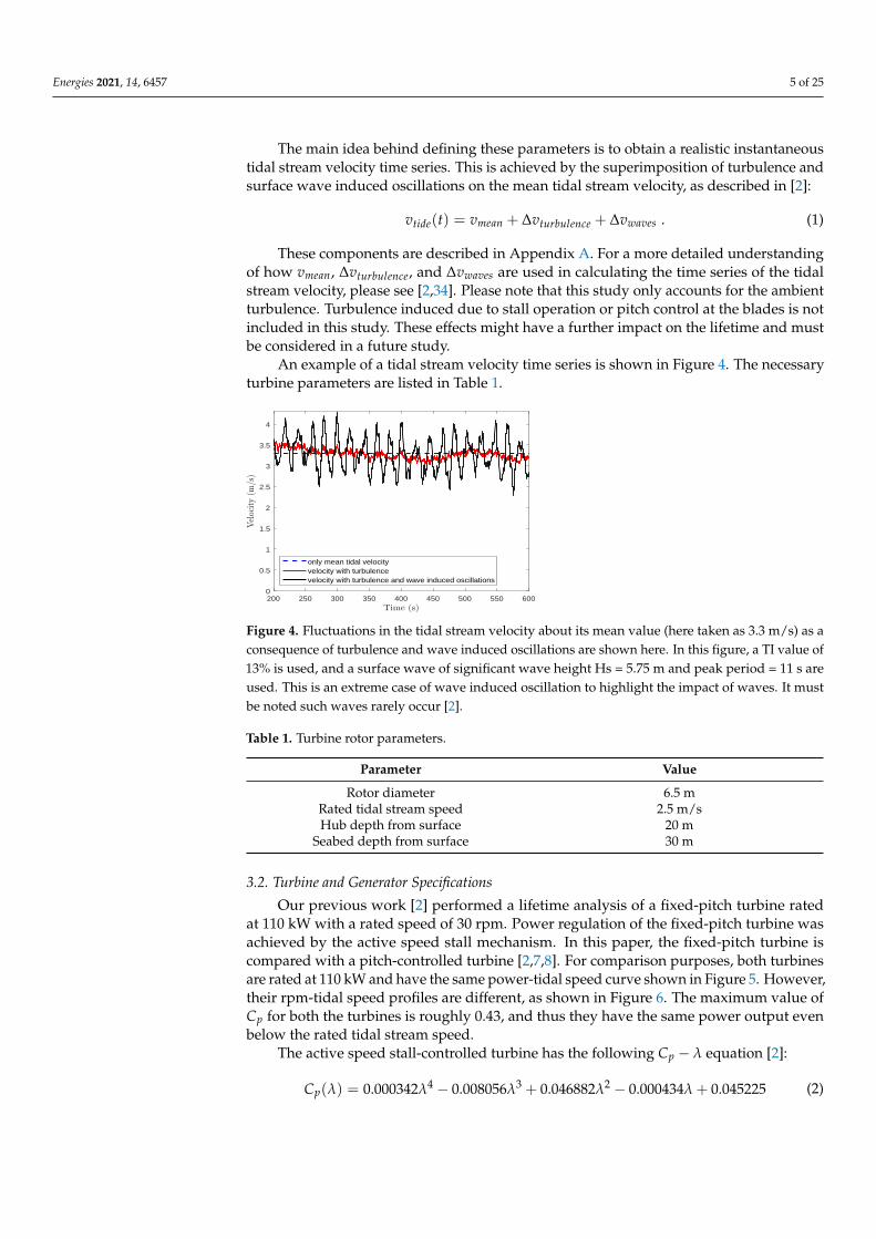
The main idea behind defining these parameters is to obtain a realistic instantaneoustidal stream velocity time series. This is achieved by the superimposition of turbulence andsurface wave induced oscillations on the mean tidal stream velocity, as described in [2]:

vtide(t) = vmean + ∆vturbulence + ∆vwaves . (1)

These components are described in Appendix A. For a more detailed understandingof how vmean, ∆vturbulence, and ∆vwaves are used in calculating the time series of the tidalstream velocity, please see [2,34]. Please note that this study only accounts for the ambientturbulence. Turbulence induced due to stall operation or pitch control at the blades is notincluded in this study. These effects might have a further impact on the lifetime and mustbe considered in a future study.

An example of a tidal stream velocity time series is shown in Figure 4. The necessaryturbine parameters are listed in Table 1.

200 250 300 350 400 450 500 550 6000

0.5

1

1.5

2

2.5

3

3.5

4

only mean tidal velocityvelocity with turbulencevelocity with turbulence and wave induced oscillations

Figure 4. Fluctuations in the tidal stream velocity about its mean value (here taken as 3.3 m/s) as aconsequence of turbulence and wave induced oscillations are shown here. In this figure, a TI value of13% is used, and a surface wave of significant wave height Hs = 5.75 m and peak period = 11 s areused. This is an extreme case of wave induced oscillation to highlight the impact of waves. It mustbe noted such waves rarely occur [2].

Table 1. Turbine rotor parameters.

Parameter Value

Rotor diameter 6.5 mRated tidal stream speed 2.5 m/sHub depth from surface 20 m

Seabed depth from surface 30 m

3.2. Turbine and Generator Specifications

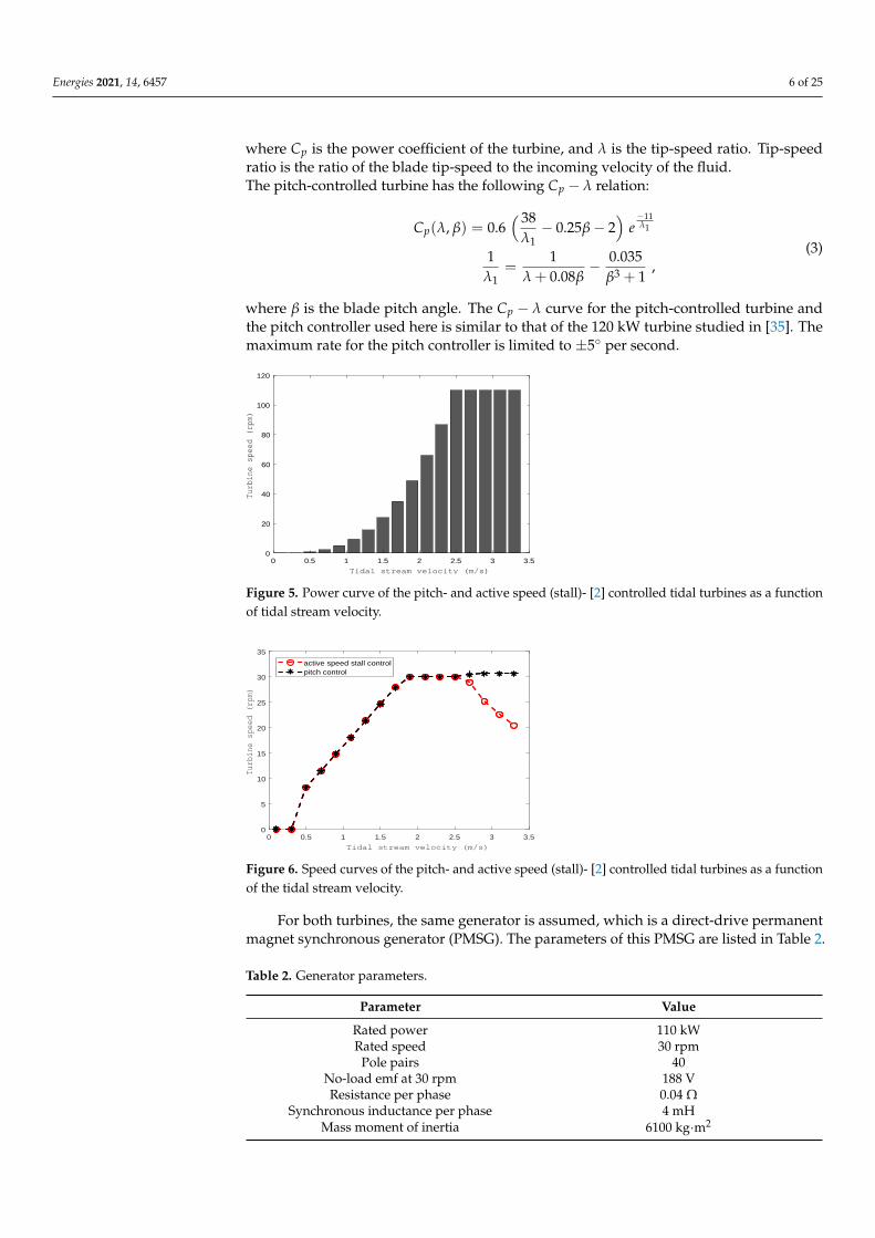
Our previous work [2] performed a lifetime analysis of a fixed-pitch turbine ratedat 110 kW with a rated speed of 30 rpm. Power regulation of the fixed-pitch turbine wasachieved by the active speed stall mechanism. In this paper, the fixed-pitch turbine iscompared with a pitch-controlled turbine [2,7,8]. For comparison purposes, both turbinesare rated at 110 kW and have the same power-tidal speed curve shown in Figure 5. However,their rpm-tidal speed profiles are different, as shown in Figure 6. The maximum value ofCp for both the turbines is roughly 0.43, and thus they have the same power output evenbelow the rated tidal stream speed.

The active speed stall-controlled turbine has the following Cp − λ equation [2]:

Cp(λ) = 0.000342λ4 − 0.008056λ3 + 0.046882λ2 − 0.000434λ + 0.045225 (2)

Energies 2021, 14, 6457 6 of 25

where Cp is the power coefficient of the turbine, and λ is the tip-speed ratio. Tip-speedratio is the ratio of the blade tip-speed to the incoming velocity of the fluid.The pitch-controlled turbine has the following Cp − λ relation:

Cp(λ, β) = 0.6( 38

λ1− 0.25β − 2

)e−11λ1

1λ1

=1

λ + 0.08β− 0.035

β3 + 1,

(3)

where β is the blade pitch angle. The Cp − λ curve for the pitch-controlled turbine andthe pitch controller used here is similar to that of the 120 kW turbine studied in [35]. Themaximum rate for the pitch controller is limited to ±5 per second.

0 0.5 1 1.5 2 2.5 3 3.5

Tidal stream velocity (m/s)

0

20

40

60

80

100

120

Turbine speed (rpm)

Figure 5. Power curve of the pitch- and active speed (stall)- [2] controlled tidal turbines as a functionof tidal stream velocity.

0 0.5 1 1.5 2 2.5 3 3.5

Tidal stream velocity (m/s)

0

5

10

15

20

25

30

35

Turbine speed (rpm)

active speed stall controlpitch control

Figure 6. Speed curves of the pitch- and active speed (stall)- [2] controlled tidal turbines as a functionof the tidal stream velocity.

For both turbines, the same generator is assumed, which is a direct-drive permanentmagnet synchronous generator (PMSG). The parameters of this PMSG are listed in Table 2.

Table 2. Generator parameters.

Parameter Value

Rated power 110 kWRated speed 30 rpm

Pole pairs 40No-load emf at 30 rpm 188 VResistance per phase 0.04 Ω

Synchronous inductance per phase 4 mHMass moment of inertia 6100 kg·m2

Energies 2021, 14, 6457 7 of 25

Both turbines operate in the maximum power point tracking (MPPT) mode until theyreach their rated speed. In the MPPT region, the required torque is given by

T∗ = Kω2r , (4)

where K is a constant depending on factors such as nominal turbine speed and power,maximum value of power coefficient Cp, and the optimal tip-speed ratio, etc. [36]. ωr is therotational speed of the turbine. Torque control is achieved by employing the classical PIcontrol strategy in generator dq-axes. The q-axis current is obtained from the desired torquerequirement of the generator [2]. If possible, d-axis current is kept at zero. Otherwise, a fluxweakening strategy is employed to ensure that the required output voltage is deliverablefrom the converter [2,37].

Beyond rated speed, the pitch-controlled turbine keeps operating at the rated rpm,using the blade pitch angle to maintain the rated power [35]. On the other hand, in thestall-controlled turbine, the speed of the turbine is reduced to lower Cp and regulate theoutput power [2].

3.3. Converter Specifications

For the power rating and the voltage level used in this study, a two-level low voltageback-to-back converter is suitable. A representative diagram of this converter is shownin Figure 7. The specifications of interest in the converter are the power loss and thermalparameters of the IGBT modules and the thermal parameters of the cooling system. In thissection the specifications for the IGBT modules are given; cooling system specifications aregiven later in Section 5.

T1

+

-

SA

SB

SC

SD

SE

SF

Grid End Generator End

D1

T4 T6T2D2

D4 D6

D5D3T3 T5

Figure 7. A representative diagram of a two-level voltage source converter [2].

The loss parameters can be determined from the IGBT module datasheet. It is clearthat the current rating of the IGBTs in the active stall-controlled must be higher, owingto its lower rpm at rated power. For comparison purposes, the same IGBT module in thepitch-controlled turbine as in the active stall-controlled one is used. The selection of theproper IGBT module for the active stall-controlled turbine is explained in our previouswork [2]. For this analysis, Infineon’s IGBT module FF600R12ME4 (1200 V, 600 A) is anappropriate choice. The parameters corresponding to this module are listed in Table 3.

Energies 2021, 14, 6457 8 of 25

Table 3. Converter parameters.

Parameter Value

DC-link voltage 600 VSwitching frequency 2 kHzDC-link capacitance 102 mF

IGBT part number FF600R12ME4

Voltage and current rating (rms) 1200 V, 600 AModule dimensions 0.057 m × 0.110 mIGBT thermal resistance Rth,j−c (4-layer Foster form) [0.0038 0.0312 0.0001 0.0020] K/WIGBT thermal time constant τth (4-layer Foster form) [0.0007 0.0247 0.050 3.485] sDiode thermal resistance Rth,j−c (4-layer Foster form) [0.0008 0.0489 0.002 0.0057] K/WDiode thermal time constant τth (4-layer Foster form) [0.0006 0.0245 0.0733 0.9951] s

4. Methodology

This section briefly describes how the lifetime of the IGBT module can be estimatedbased on thermal cycling. The approach used here has been adopted in various studiesacross applications [15,38–42].

The procedure can be broadly divided into three modelling layers:

1. Estimation of power loss in IGBT modules;2. Thermal modelling of the IGBT modules;3. Lifetime estimation based on thermal cycling.

4.1. Estimation of Power Loss

For this purpose, first the converter currents must be determined. This is done usingthe information about the tidal stream velocity time series, turbine characteristics, andgenerator and converter parameters, as described in [2,15]. The algorithm is summarisedin Figure 8 [2].

Time Series of Tidal Stream Velocity

Turbine Model

Converter Control

Converter Model

Converter current, duty ratio

Loss Model

PM Generator Model

Speed

Duty RatiosVoltage

Figure 8. Calculating converter currents and duty ratios for loss calculation in IGBT modules; imageadapted from [2].

IGBTs and diodes in a power module experience conduction and switching losses [15,27].Both of these losses are a function of the junction temperature [43]. Figure 9 shows the

Energies 2021, 14, 6457 9 of 25

loss calculation flowchart. More details on the loss calculation can be found in multiplereferences [15,44,45].

SwitchingLoss

Conduction Loss

Thermal Model

Tj Σ

Current, i

Voltage, v

Duty cycle, d

Switching frequency, fs

Ploss

Current, i

DC Voltage, Vdc

Figure 9. Loss calculation in IGBT and diode. The diagram shows that losses also depend on thejunction temperature Tj; hence, the feedback loop from the thermal model.

4.2. IGBT Thermal Modelling

From the power loss in the IGBT modules, thermal models are used to estimate thejunction temperature (mean and amplitude). Thermal modelling must be performed foreach operating point corresponding to Figure 5, in conjunction with the knowledge ofturbulence and surface waves.

Thermal models for IGBT modules can be categorized into three types, namely an-alytical, numerical, and thermal network models [3]. Analytical models are primarilybased on analytical solutions of the heat diffusion equation. These models are fast but canonly be applied for simple geometries and with simplified boundary conditions [46,47].Numerical models are usually based on finite element analysis, sometimes coupled withcomputational fluid dynamics (CFD) analysis [48,49]. These models are extremely timeconsuming and are unsuitable for dynamic electro-thermal simulations.

When it comes to using thermal models for lifetime analysis, thermal network modelsbased on RC elements are the most suitable way forward [2,50–52]. The simplicity of thesemodels, fast results, and the possibility of combining RC elements of different individualcomponents (especially in the Cauer form) into a combined RC network of the wholesystem are their main advantages [51,52]; this is described in Section 5. A main drawbackof the simplified one-dimensional RC network models is that the thermal cross-couplingbetween different IGBT chips within the same module are neglected [4,53]. This mayresult in an error in junction temperature estimation. However, this error is more likely tocontribute to mean junction temperature rather than amplitude of temperature cycling. Inother words, such an approximation has little consequence for the final conclusions of thispaper.

4.3. Lifetime Estimation

After knowing the junction temperature values, the thermal fatigue accumulated foreach operating point is calculated. This is done using the lifetime models for the IGBTpower modules as explained below.

The lifetime estimation technique used in this paper is the same as adopted in [2,15].The number of cycles to failure N f is estimated based on the models presented in [15,54],given by the equation

N f = A · ∆Tβ1j · e

β2Tj,m+273 · tβ3

on · Iβ4 · Vβ5 · Dβ6 . (5)

where Tj,m is the mean junction temperature, ton is the on-pulse duration, I is the currentper wire, V is the chip blocking voltage, and D is the bonding wire diameter. The constants

Energies 2021, 14, 6457 10 of 25

A and β1 to β6 are obtained from [4] and take the following values: A = 9.34 × 1014 forIGBT4 modules, [β1, . . . , β6] = [−4.416, 1.285 × 103, −0.463, −0.716, −0.761, −0.5].

For each operating point in Figure 5, different values of N f ,i and ni are calculated usingthe rainflow counting algorithms. Here, ni is the number of cycles experienced annually,and N f ,i is the number of cycles to failure for ith operating point. Subsequently, the netaccumulated damage corresponding to all the operating point within a year is estimatedfrom the Miner’s rule [38]:

Annual Damage = ∑i

niN f , i (6)

The number of cycles for each thermal cycling amplitude is obtained from Equation (5).Figure 10 shows how N f typically varies with ∆Tj for constant Tj,m. The number of yearsto failure or lifetime (in years) is then calculated as

Li f etime (in years) =1

Annual Damage(7)

Figure 10. Number of cycles to failure is presented as a function of temperature cycling for a constantmean junction temperature [21].

To take into account the effects of both long term cycling (daily variation in tidalvelocity) as well as high frequency cycling due to turbulence and waves, the models aredivided into two sections as shown in Figure 11. Multiplying the fatigue for each operatingpoint with the probability of occurrence of each operating point, the net fatigue in the yearis calculated. From this information, the number of years to failure is estimated.

Mean Tide Velocity (in steps of 0.2 m/s from

0.5 – 3.3 m/s)

PTO Model Lifetime Model

Converter Thermal Model

Loss

Surface Wave induced oscillations

Short‐term tidal velocity profile

(Stochastic 20 min tidal profile)

Turbulence Intensity

Long‐term tidal velocity profile

(Averaged daily/monthly tidal profile)

PTO Model Lifetime Model

Converter Thermal Model

Σ Total Lifetime Consumption

Tm , ΔTj Short‐term Damage

Σ Loss

Tm , ΔTj Long‐term Damage

Low frequency cycling

High frequency cycling

Figure 11. Methodology for lifetime calculations: low and high frequency thermal cycling. Imageadapted from [2].

To simplify the calculations, the following assumptions are made.

Energies 2021, 14, 6457 11 of 25

• The ambient seawater temperature throughout the year is assumed to be 15 C. Thisis the maximum temperature at the Orkney (UK) tidal site [55].

• A constant turbulence value has been used for each mean tidal velocity, as describedin Appendix A.

• The performance of the turbine is same during the flood and ebb tides [2].• At the beginning of each flood and ebb tide cycle, the junction temperature of the

IGBT module is the same as the ambient temperature.• Effects of varying reactive power on the thermal cycling of the grid-side converter

have been neglected. A constant value (0.9) is assumed [21].

5. Thermal Models for Active and Passive Cooling Systems

In this section a brief explanation is given of how the active (forced-water cooling)and passive cooling systems are modelled into the thermal models for the IGBT modules ina submerged power converter. Furthermore, the specifications of the two cooling systemsare also presented, along with necessary assumptions made in the thermal models.

In both active and passive systems, constant thermal resistances (junction-to-case)for the IGBT module are used in this study. In practice, this thermal resistance varieswith the temperature [56]. However, when combined with the case-to-ambient thermalresistance, the net variation in junction-to-ambient thermal resistance will not be more than5% for the extremities observed in this case study. In other words, it is possible that thejunction temperature estimation will have an error of 5%. Still, this error is too little to havesignificant ramifications for the lifetime analysis conducted in this paper.

5.1. Forced-Water Cooling

For the forced-water cooling system, IGBT modules are mounted on a water cooledheat sink. The water is circulated in and out of the heat sink using a pump, as shown inFigure 3. Two different configurations of the forced cooling system were evaluated in thispaper:

• Six-pass system;• Four-pass system.

Two different forced-water cooling systems are evaluated to demonstrate that furtherimprovement in lifetime is possible by overrating the heat sink. There is also a possibilityof overrating a heat sink by increasing the flow rate of the coolant. However, the latter isnot investigated here.

In the 6-pass system, three modules (each corresponding to one phase of the generatorside converter) are mounted on a single heat sink. This is shown in Figure 12. In the 4-passsystem, only one phase module is mounted on a single heat sink. The necessary thermalparameters corresponding to each of these cooling configurations are listed in Table 4. Theheat sinks correspond to the commercial manufacturer Wakefield-Vette [57].

Figure 13 shows the thermal circuit for the IGBT module coupled with the watercooled heat sink. The combined Cauer–Foster network used in Figure 13 is based on [5,58].For simplification, uniform heat sink temperatures are assumed for all the modules (IGBTsas well as diodes) mounted on the same heat sink [45].

Energies 2021, 14, 6457 12 of 25

Figure 12. Three phase modules of the generator side converter mounted on a single water cooledheat sink (6-pass cold plate from Wakefield-Vette). In the case of 4-pass cold plate, only one phasemodule is mounted on each cold plate.

Table 4. Forced-water cooling parameters.

Parameter Value

6-pass cold plate

No. of dual IGBT modules per heat sink 3

Rated fluid flow rate 5 litre/min

Fluid inlet temperature 15C

Thermal resistance Rth,c−a 0.01 K/W

Thermal capacitance 1930 W.s/K

Cold plate dimensions 0.304m x 0.177 m x 0.0152 m

4-pass cold plate

No. of dual IGBT modules per heat sink 1

Rated fluid flow rate 5 litre/min

Fluid inlet temperature 15C

Thermal resistance Rth,c−a 0.02 K/W

Thermal capacitance 690 W.s/K

Cold plate dimensions 0.152m x 0.127 m x 0.0152 m

Liquid Cold plate

IGBT module1-layer Cauer Model

Ploss Tamb Ambient temperature

Case Temperature

jT

Module 4 Layer - Foster Model(From Datasheet)

Tcase

Tamb

Ploss

Figure 13. Thermal circuit for determining IGBT and diode junction temperatures in an activelycooled converter, adapted from [5]. Tj, shown in the figure, is the junction temperature of interest inthe lifetime model used in this paper. This Tj can correspond to either the junction temperature ofthe IGBT or the diode, depending on which 4-layer Foster network is used.

Energies 2021, 14, 6457 13 of 25

5.2. Passively Cooled System

Figure 14 shows the placement of the switches in the passively cooled converter. Eachmodule corresponds to a phase leg of the generator side converter and is mounted on aseparate mounting plate. The mounting plate is made of a thermally conductive material,such as copper [5]. The dimensions of the mounting plate are listed in Table 5. For sake ofbrevity, the detailed modelling of the passive cooling system is omitted here. The systemused here is the same as in [2], and the modelling of the passively cooled system can befound in the same paper.

Sealed Enclosure

Figure 14. Three phase IGBT modules for generator side converter mounted on the inner walls ofthe submerged cabinet via a copper mounting plate. The copper mounting plate minimizes thespreading thermal resistance [5].

There is an important point of difference between the active and the passive coolingsystems. Whereas in the active cooling system, Rs−a (sink-to-ambient thermal resistance)is assumed to be constant, the same cannot be done in the passively cooled system. Thereason is that the external convective heat transfer coefficient in Figure 15 is a function of theheat flux from the IGBT power module [5,59]. As a result, the spreading thermal resistancesin the enclosure frame and the mounting plate are modelled as variable resistances inFigure 15 [5,60].

Table 5. Passive water cooling parameters.

Parameter Value

Enclosure wall thickness 0.010 m

Enclosure height 1.5 m

Enclosure width 0.5 m

Enclosure length 1.5 m

Cu mounting plate dimensions 0.171 m × 0.330 m

Cu mounting plate thickness 0.020 m

Thermal resistance Rth,c−a (function of heatloss) including thermal paste 0.05–0.13 K/W [2]

Thermal capacitance 7862 W·s/K

Energies 2021, 14, 6457 14 of 25

EnclosureFrame

Mounting Plate

IGBT module1-layer Cauer Model

Ploss

Convective heat transfer

coefficient

Tamb

Ambient temperatureCase Temperature Wall temperature

jT

Module 4 Layer - Foster Model(From Datasheet)

Tcase

Tamb

Ploss

Figure 15. Thermal circuit for determining IGBT and diode junction temperatures in a passivelycooled converter, from [5]. Tj, shown in the figure, is the junction temperature of interest in thelifetime model used in this paper. This Tj can correspond to either the junction temperature of theIGBT or the diode, depending on which 4-layer Foster network is used.

6. Case Study: Lifetime Analysis of 110 kW Tidal Turbines

In this section, the cooling systems in the submerged power converter for a 110 kWtidal turbine described in Section 3 are compared. The analysis is divided into two parts.Section 6.1 compares different cooling systems in terms of mean junction temperatures,temperature cycling amplitudes, lifetime of the IGBT modules, and annual losses in theIGBT modules for the active stall-controlled tidal turbine. On the other hand, Section6.2 compares IGBT lifetimes in pitch-controlled and active stall-controlled turbines. Inboth cases, the lifetime of the IGBT modules is taken to be the lifetime of the diodes in thegenerator side converter. This is because the lifetime of the diodes on the generator sideconverter is the minimum of all IGBTs and diodes in the back-to-back converter shown inFigure 7 [2].

6.1. Comparison of Different Cooling Systems

Figure 16 demonstrates the speed variation of the generator as a consequence of thevariation in the tidal stream velocity for the active speed stall-controlled turbine. The tidalvelocity variations correspond to a part of Figure 4. Because the velocity at all times inFigure 16 is greater than the rated speed of 2.5 m/s, the generator power is maintained at110 kW. Consequently, the rise/fall in the generator speed is reflected by correspondingfall/rise in the rms value of the generator phase currents, as seen in Figure 17.

300 310 320 330 340 350 3600

0.5

1

1.5

2

2.5

3

3.5

4

4.5

0

5

10

15

20

25

30

35

40

45

Gen

erat

or S

peed

(rpm

)

velocity with turbulencevelocity with turbulence and wave induced oscillationsrpm with turbulencerpm with turbulence and wave induced oscillations

Figure 16. Active speed stall control of generator speed as a function of change in tidal streamvelocity. Mean tidal velocity in this image is set at 3.3 m/s [2].

Energies 2021, 14, 6457 15 of 25

300 310 320 330 340 350 3600

200

400

600

I phas

e (A)

with turbulence

300 310 320 330 340 350 360

Time (s)

0

200

400

600

I phas

e (A)

with turbulence and wave induced oscillations

Figure 17. Generator phase currents (rms values). The variations in the phase current value are adirect consequence of the generator speed variations in Figure 16. This also illustrates why an IGBTmodule with 600 A rating was selected in this paper. The above graph would have depicted a flatline (about 380 A) without any velocity oscillations.

Figure 18 shows the estimated lifetime for the IGBT modules including the effectsof turbulence, with and without the impact of surface waves. Clearly, forced-water cool-ing systems show significantly improved lifetime values over passive cooling systems.However, this increase in lifetime reduces when waves are also considered, in addition toturbulence.

without Waves with Waves0

50

100

150

200

Lifetime (in years)

Passive CoolingForced Cooling (6-pass)Forced Cooling (4-pass)

Figure 18. Estimated lifetime of the IGBT modules on the generator side converter with differentcooling systems.

Even though there seems to be a significant difference in lifetime, the annual IGBTmodule losses in the generator side converter do not seem to be that different. This canbe seen in Table 6. The losses in the passive cooling system are higher because higherjunction temperatures also mean more losses in the IGBT modules. Figure 19 shows themean junction temperatures as a function of tidal stream velocity. The passive coolingsystem has higher thermal resistance (sink-to-ambient) compared to forced-water coolingsystems. Therefore, similar magnitudes of losses result in a higher temperature comparedto the forced-water cooling systems.

Energies 2021, 14, 6457 16 of 25

0 0.5 1 1.5 2 2.5 3 3.5

tidal stream velocity (m/s)

0

10

20

30

40

50

60

70

80

90

100

110

Tem

pera

ture

(° C

)

Passive CoolingForced Water Cooling (6-pass)Forced Water Cooling (4-pass)

Figure 19. Comparison of mean junction temperatures between different cooling systems as afunction of tidal stream velocity. Data for passive cooling is taken frommbox[2].

Table 6. Annual loss in the generator side converter for passive and active cooling systems, withoutwaves.

Cooling System IGBTs Loss (in MWh) Diodes Loss (in MWh)

Passive cooling 2.11 2.53

Forced-water cooling (6-passcold plate) 1.90 2.36

Forced-water cooling (4-passcold plate) 1.89 2.35

There is not much difference between the mean temperatures of 4-pass and 6-passcooling systems, except at higher tidal velocities. The difference in lifetimes of 6-pass and4-pass cooling systems is because bulk lifetime consumption also occurs at higher tidalvelocities. This is shown in Figure 20. This predominant lifetime consumption at high ve-locities is a consequence of the active stall control mechanism. In the active control strategy,at higher tidal velocities, rated power is delivered at a lower rpm and higher currents. Thismeans more losses in the IGBT modules and hence more lifetime consumption. In otherwords, lifetime consumption below rated tidal speed can be neglected.

0.5 0.7 0.9 1.1 1.3 1.5 1.7 1.9 2.1 2.3 2.5 2.7 2.9 3.1 3.3

Tidal stream velocity (m/s)

0

20

40

60

80

100

Nor

mal

ized

Dam

age

Dis

tribu

tion

(%) Passive Cooling

Forced Water Cooling (6-pass)Forced Water Cooling (4-pass)

Figure 20. Annual damage distribution between different cooling systems as a function of tidalstream velocity. The values are normalized with respect to annual damage in passively cooledsystems. Lifetime consumption mostly happens at higher tidal velocities.

Figures 21 and 22 show the diode junction temperature variation corresponding to thevelocity variations in Figure 16. The amplitude of thermal cycling appears similar in all thethree cases. Although passive systems have a higher thermal time constant for the heat

Energies 2021, 14, 6457 17 of 25

sink, for cycling of the junction temperature, IGBT/diode thermal capacitances are moreinfluential.

Figure 21. Comparison of cooling systems in terms of diode junction temperature cycling consideringonly turbulence in tidal stream velocity shown in Figure 16. This plot only corresponds to a timeduration of 60 s under certain turbulence conditions. Results at different time instants and differentvalues of mean tidal velocity and turbulence will give different values.

From the above discussion, we conclude that the difference in the lifetime for differentcooling systems is primarily due to the difference in mean junction temperatures, and notso much due to thermal cycling. This is shown more clearly in Figure 23. On the otherhand, considering the same cooling system, the lifetime reduction when including wavesis due to the higher amplitude of thermal cycling.

Energies 2021, 14, 6457 18 of 25

Figure 22. Comparison of cooling systems in terms of diode junction temperature cycling consideringboth turbulence and waves in tidal stream velocity shown in Figure 16.

PC

FWC (6-pass)

FWC (4-pass) PC

FWC (6-pass)

FWC (4-pass)30

40

50

60

70

80

90

100

110

120

130

T D1, G

en (° C)

without wave with wave

Figure 23. Diode junction temperature swing for different cooling systems at mean velocity of3.3 m/s and TI value of 13%. Temperature swing is shown without waves and with a wave ofHs = 5.75 m and Tp = 11 s. For different cooling systems with same wave conditions, the temperatureswing is nearly the same, albeit with a difference in mean temperatures. However, for the samecooling system, with and without waves, the mean temperature is the same but with a difference intemperature swing. PC—passive cooling; FWC—forced-water cooling.

6.2. Comparing Active Speed Stall and Pitch Control

Here, the comparison of the lifetime of IGBT modules in active stall- and pitch-controlled turbines is given. This analysis has only been done considering the forced-watercooling (6-pass coldplate) system. Table 7 shows the lifetime values for pitch and active

Energies 2021, 14, 6457 19 of 25

stall turbines. Lifetime values of pitch-controlled turbines are large because the device(IGBT) selection was done considering the active stall control (i.e., at high rms currentvalues). The main reason for this is the lower mean junction temperature and temperaturecycling experienced in pitch-controlled turbines, especially at higher tidal velocities, seeFigure 24. Because the IGBT was overrated for the pitch-controlled turbine, it can be saidthat overrating the IGBT also improves the lifetime.

Table 7. IGBT lifetime comparison between active speed stall-controlled and pitch-controlled tur-bines.

Turbine Lifetime (in years)

Active speed stall control 55

Pitch control 30 x 103

0 0.5 1 1.5 2 2.5 3 3.5

tidal stream velocity (m/s)

0

10

20

30

40

50

60

Tem

pera

ture

(° C

)

active speed stall controlpitch control

Figure 24. Mean junction temperatures of the diode (in the generator side converter) as a function oftidal stream velocity. Both turbines deliver the same power, albeit at different generator speeds. Below2.5 m/s, active stall-controlled turbine operates at higher speed and thus has a lower temperature.Above 2.5 m/s, pitch-controlled turbine runs at higher speed. See Figure 6.

For the similar power rating and turbine size, pitch-controlled turbines draw a lowerphase current above the rated speed because of smaller oscillations and a higher mean valueof generator speed (see Figures 25 and 26). Consequently, the diode junction temperaturehas a lower mean value and lower amplitude of temperature cycling, as seen in Figure 27.Another point to note is the distribution of the lifetime damage with respect to the tidalstream velocity in active speed stall and pitch-controlled turbines, as shown in Figure 28.

300 310 320 330 340 350 3600

0.5

1

1.5

2

2.5

3

3.5

4

4.5

0

5

10

15

20

25

30

35

Gen

erat

or S

peed

(rpm

)

velocity with turbulencevelocity with turbulence and wave induced oscillationsrpm with turbulencerpm with turbulence and wave induced oscillations

Figure 25. Variation of generator speed as a function of change in tidal stream velocity in a pitch-controlled turbine. Compare this with the generator speed variations in Figure 16.

Energies 2021, 14, 6457 20 of 25

300 310 320 330 340 350 3600

200

400

600

I phas

e (A)

active speed stall control

300 310 320 330 340 350 360

Time (s)

0

200

400

600

I phas

e (A)

pitch control

Figure 26. Generator phase currents (rms values) in the active speed stall- and the pitch-controlledturbine, under the influence of turbulence and wave-induced tidal stream velocity oscillation (asshown in Figure 4).

300 310 320 330 340 350 36030

40

50

60

70

T D1, G

en (° C)

active speed stall control

300 310 320 330 340 350 36030

40

50

60

70

T D1, G

en (° C)

pitch control

Figure 27. Comparison of the diode junction temperatures in turbines with active stall controland pitch control. It is clearly seen that pitch control mitigates the diode temperature cycling bymaintaining nearly the same current even under significant wave-induced oscillations by virtue ofmaintaining nearly the same generator speed.

0.5 0.7 0.9 1.1 1.3 1.5 1.7 1.9 2.1 2.3 2.5 2.7 2.9 3.1 3.3

Tidal stream velocity (m/s)

0

20

40

60

80

100

Nor

mal

ized

Dam

age

Dis

tribu

tion

(%) active speed stall control

pitch control

Figure 28. Damage distribution in active stall-controlled and pitch-controlled turbines (each normal-ized to 100%). Overall IGBT lifetime in the pitch-controlled turbine is much higher than in the activestall-controlled turbine. Whereas the lifetime consumption is concentrated at higher tidal velocitiesin the active stall-controlled turbine, it is more distributed in the pitch-controlled turbine.

Energies 2021, 14, 6457 21 of 25

7. Conclusions

In this paper, active and passive cooling systems for TST converters were comparedbased on the useful lifetime. The cooling systems were compared for the active stall-controlled as well as pitch-controlled tidal turbines. The comparison assumed thermalcycling as the main failure mode in IGBT modules. The results indicate that the forced-water cooling (active) system can yield a significant improvement in the lifetime of IGBTmodules over passive systems; this result is valid for stall-controlled as well as pitch-controlled turbines. This improvement is primarily due to the decrease in the meanjunction temperature of the IGBT modules rather than the decrease in the amplitude ofthermal cycling. In other words, the amplitude of the thermal cycling is determined by theIGBT thermal capacitance (junction-to-case) and not the capacitance of the cooling system.When comparing the stall-controlled and pitch-controlled turbines, it was observed thatthe lifetime of the IGBT modules increases significantly when pitch control is used insteadof the active stall control. Furthermore, in the pitch-controlled turbine, lifetime damage ismore widespread over the tidal velocity range rather than just being concentrated at highertidal velocities, as is the case in the active stall-controlled turbine. These conclusions holdtrue irrespective of the type of cooling system used in the converter.

Compared to the active cooling system, the passive cooling system is inherently morereliable, but it results in a lower estimated lifetime of IGBT modules. However, throughthis work, it is shown that passive cooling systems can still achieve acceptable lifetimes inTST converters and hence must be considered in future TST systems to lower the cost oflevelized energy.

In the future, for a better understanding of the performance of cooling systems, it isimportant that the effect of natural processes, such as biofouling on the converter cabinetsurface, is also investigated. This study neglected any deterioration in the cooling efficiencyof the system over time due to biofouling. A way forward could be to estimate a reliablesafety factor to account for the effects of biofouling, as such processes are generally difficultto model and heavily dependent on site conditions.

Author Contributions: Conceptualization, F.W.; Data curation, F.W.; Formal analysis, F.W.; Fundingacquisition, H.P.; Investigation, F.W.; Methodology, F.W. and U.S.; Project administration, H.P.;Software, F.W. and U.S.; Supervision, J.D. and H.P.; Validation, J.D. and H.P.; Writing—original draft,F.W.; Writing—review and editing, F.W., U.S., J.D., and H.P. All authors have read and agreed to thepublished version of the manuscript.

Funding: The authors have been supported by the TiPA project (Tidal turbine Power take-offAccelerator), which has received funding from the European Union’s Horizon 2020 research andinnovation programme under grant agreement No 727793, managed by the Innovation and NetworksExecutive Agency. This paper reflects only the authors’ views; the Agency is not responsible for anyuse that may be made of the information the paper contains.

Institutional Review Board Statement: Not applicable.

Informed Consent Statement: Not applicable.

Data Availability Statement: Models used in this study can be found on https://data.4tu.nl/info/en/.

Acknowledgments: The authors would like to Antonio Jarquin-Laguna and George Lavidas for theirhelp in securing necessary data for this study.

Conflicts of Interest: The authors declare no conflict of interest.

Appendix A

Appendix A.1. Mean Tidal Velocity

A typical tidal site with the frequency of occurrence as a function of tidal streamvelocity is shown in Figure A1 [2].

Energies 2021, 14, 6457 22 of 25

0 0.5 1 1.5 2 2.5 3 3.5 4 4.5

Tidal current speed (m/s)

0

100

200

300

400

500

600

700

800

Num

ber o

f hou

rs p

er y

ear

Figure A1. Tidal velocity distribution at EMEC site, Orkney [61].

Appendix A.2. Turbulence in the Sea

Different values of turbulence intensity (TI) are used for flood and ebb tides [2,62].Table A1 lists TI values used in this paper. Please note that this analysis only uses theaverage value of TI; in reality, different values of TI are possible for the same mean tidalvelocity.

Table A1. TI values used to generate time series of tidal stream velocity [2].

Mean Velocity Range (m/s) Mean TI Values (%)

Ebb tide0.5 ≤ u ≤ 1.1 13.91.3 ≤ u ≤ 3.3 11.7

Flood tide0.5 ≤ u ≤ 1.1 14.51.3 ≤ u ≤ 3.3 12.0

Appendix A.3. Surface Waves

The surface wave conditions used in this analysis are listed in Tables A2 and A3, withtheir probability densities [2]. JONSWAP spectrum is chosen for the surface waves, inaccordance with [2,63], with a peak enhancement factor, γ = 3.3 [2,34].

The probabilities are given to ensure all waves are included in proportion to theiroccurrence; neglecting this could result in grossly miscalculated lifetime values. In addition,because different wave conditions occur in summer and winter, two probability densitytables, each corresponding to a representative summer (May) and winter month (Nov),were used in this study [64].

Table A2. Probability density (%) of waves according to significant wave heights (Hs) and peak time periods (Tp) for May2009 at Orkney [2].

Tp(s),Hs(m) 0.25 0.75 1.25 1.75 2.25 2.75 3.25 3.75 4.25 4.75 5.25 5.75 6.25

3 6.92 2.82 2.35 0 0 0 0 0 0 0 0 0 05 4.97 0.27 0.87 0.47 0 0 0 0 0 0 0 0 07 3.96 0 0.07 1.75 1.01 0 0.74 0 0 0 0 0 09 5.98 0 1.81 0.34 0.2 0 0.94 0.87 0.40 0 0 0 0

11 2.48 3.76 4.77 6.72 6.18 3.96 2.08 0.07 1.61 0.27 0.27 0.13 013 0.47 1.07 2.89 4.91 2.22 2.01 4.57 4.30 0.27 0 0 0.13 0.2015 0.47 0.67 0.13 0.34 0 0.20 0.13 2.55 0.87 0.40 0.20 0.34 017 0 0 0 0 0 0 0.13 0.26 1.14 0 0 0 0

Energies 2021, 14, 6457 23 of 25

Table A3. Probability density (%) of waves according to significant wave heights (Hs) and peak time periods (Tp) forNovember 2009 at Orkney [2].

Tp(s),Hs(m) 0.25 0.75 1.25 1.75 2.25 2.75 3.25 3.75 4.25 4.75 5.25 5.75 6.25

3 0 0.27 2.22 0 0 0 0 0 0 0 0 0 05 0 0.69 6.11 1.04 1.32 0.07 0 0 0 0 0 0 07 0 0 0.55 1.25 1.87 3.61 2.22 0.42 0 0 0 0 09 0 0 0.83 0 0.35 0.76 1.53 1.11 0 0 0 0 0

11 0 2.64 3.40 7.22 7.29 0.35 0 0 0 0 0 0 013 0 2.15 2.29 4.30 13.95 10.07 2.78 0.69 0 0 0 0 015 0 0 1.46 0.63 1.18 7.5 1.87 1.39 0 0 0 0 017 0 0 0.21 0 0 0.35 2.01 0 0 0 0 0 0

References1. Magagna, D.; Monfardini, R.; Uihlein, A. JRC Ocean Energy Status Report; Publications Office of the European Union: Luxembourg,

2016. Available online: https://setis.ec.europa.eu/sites/default/files/reports/ocean_energy_report_2016.pdf (accessed on 1June 2020)

2. Wani, F.; Shipurkar, U.; Dong, J.; Polinder, H.; Jarquin-Laguna, A.; Mostafa, K.; Lavidas, G. Lifetime analysis of IGBT powermodules in passively cooled tidal turbine converters. Energies 2020, 13, 1875.

3. Qian, C.; Gheitaghy, A.; Fan, J.; Tang, H.; Sun, B.; Ye, H.; Zhang, G. Thermal management on IGBT power electronic devices andmodules. IEEE Access 2018, 6, 12868–12884.

4. Wintrich, A.; Nicolai, U.; Tursky, W.; Reimann, T. Application Manual Power Semiconductors. SEMIKRON International GmbH.2015. Available online: https://www.semikron.com/dl/service-support/downloads/download/semikron-application-manual-power-semiconductors-english-en-2015/ (accessed on 10 January 2020).

5. Wani, F.; Shipurkar, U.; Dong, J.; Polinder, H. A study on passive cooling in subsea power electronics. IEEE Access 2018, 6,67543–67554.

6. Toma, D.; Mànuel-Làzaro, A.; Nogueras, M.; Del Rio, J. Study on heat dissipation and cooling optimization of the junction box ofOBSEA seafloor observatory. IEEE/ASME Trans. Mechatron. 2014, 20, 1301–1309.

7. Whitby, B.; Ugalde-Loo, C. Performance of pitch and stall regulated tidal stream turbines. IEEE Trans. Sustain. Energy 2014, 5,64–72.

8. Polinder, H.; Bang, D.; Van Rooij, R.P.; McDonald, A.S.; Mueller, M. 10 MW wind turbine direct-drive generator design with pitchor active speed stall control. In Proceedings of the IEEE International Electric Machines and Drives Conference, Antalya, Turkey,3–5 May 2007; pp. 1390–1395

9. Wani, F.; Polinder, H. A Review of Tidal Current Turbine Technology: Present and Future. In Proceedings of the 12th EuropeanWave and Tidal Energy Conference (EWTEC 2017), Cork, Ireland, 27 August–1 September 2017.

10. Carroll, J.; McDonald, A.; McMillan, D. Reliability comparison of wind turbines with DFIG and PMG drive trains. IEEE Trans.Energy Convers. 2015, 30, 663–670.

11. Spinato, F.; Tavner, P.; van Bussel, G.; Koutoulakos, E. Reliability of wind turbine subassemblies. IET Renew. Power Gener. 2009, 3,387–401.

12. CATAPULT. Portfolio Review 2016: System Performance, Availability and Reliability Trends Analysis (SPARTA). 2016. Availableonline: https://s3-eu-west-1.amazonaws.com/media.ore.catapult/wp-content/uploads/2017/03/28102600/SPARTAbrochure_20March-1.pdf (accessed on 15 April 2020)

13. Yang, S.; Xiang, D.; Bryant, A.; Mawby, P.; Ran, L.; Tavner, P. Condition monitoring for device reliability in power electronicconverters: A review. IEEE Trans. Power Electron. 2010, 25, 2734–2752.

14. Fischer, K.; Pelka, K.; Puls, S.; Poech, M.; Mertens, A.; Bartschat, A.; Tegtmeier, B.; Broer, C.; Wenske, J. Exploring the causes ofpower-converter failure in wind turbines based on comprehensive field-data and damage analysis. Energies 2019, 12, 593.

15. Shipurkar, U.; Lyrakis, E.; Ma, K.; Polinder, H.; Ferreira, J. Lifetime comparison of power semiconductors in three-level convertersfor 10MW wind turbine systems. IEEE J. Emerg. Sel. Top. Power Electron. 2018, 6, 1366–1377.

16. Choi, U.; Blaabjerg, F.; Iannuzzo, F.; Jørgensen, S. Junction temperature estimation method for a 600 V, 30 A IGBT module duringconverter operation. Microelectron. Reliab. 2015, 15, 2022–2026.

17. Ma, K.; Blaabjerg, F.; Liserre, M. Thermal analysis of multilevel grid-side converters for 10-MW wind turbines under low-voltageride through. IEEE Trans. Ind. Appl. 2013, 49, 909–921.

18. Hu, Z.; Ge, X.; Xie, D.; Zhang, Y.; Yao, B.; Dai, J.; Yang, F. An aging-degree evaluation method for IGBT bond wire with onlinemultivariate monitoring. Energies 2019, 12, 3962.

19. Hu, Y.; Shi, P.; Li, H.; Yang, C. Health condition assessment of base-plate solder for multi-chip IGBT module in wind powerconverter. IEEE Access 2019, 7, 72134–72142.

Energies 2021, 14, 6457 24 of 25

20. De Rijck, A.; Huisman, H. Power Semiconductor Device Adaptive Cooling Assembly. U.S. Patent 8,547,687. 2013. Availableonline: https://patentimages.storage.googleapis.com/cf/bf/f1/f8fd4113102d38/US8547687.pdf (accessed on 5 April 2020).

21. Shipurkar, U. Improving the Availability of Wind Turbine Generator Systems. Ph.D. Thesis, Delft University of Technology, Delft,The Netherlands, 2019.

22. Yerasimou, Y.; Pickert, V.; Ji, B.; Song, X. Liquid metal magnetohydrodynamic pump for junction temperature control of powermodules. IEEE Trans. Power Electron. 2018, 33, 10583–10593.

23. Choi, U.; Lee, J. Comparative evaluation of lifetime of three-level inverters in grid-connected photovoltaic systems. Energies 2020,13, 1227.

24. Rajashekara, K.; Krishnamoorthy, H.; Naik, B. Electrification of subsea systems: Requirements and challenges in power distribu-tion and conversion. CPSS Trans. Power Electron. Appl. 2017, 2, 259–266.

25. Andresen, M.; Ma, K.; Buticchi, G.; Falck, J.; Blaabjerg, F.; Liserre, M. Junction temperature control for more reliable powerelectronics. IEEE Trans. Power Electron. 2017, 33, 765–776.

26. Chen, G.; Cai, X. Adaptive control strategy for improving the efficiency and reliability of parallel wind power converters byoptimizing power allocation. IEEE Access 2018, 6, 6138–6148.

27. Weckert, M.; Roth-Stielow, J. Chances and limits of a thermal control for a three-phase voltage source inverter in tractionapplications using permanent magnet synchronous or induction machines. In Proceedings of the 14th European Conference onPower Electronics and Applications, IEEE, Birmingham, UK, 30 August–1 September 2011; pp. 1–10.

28. Ma, K.; Blaabjerg, F. Thermal optimised modulation methods of three-level neutral-point-clamped inverter for 10 mw windturbines under low-voltage ride through. IET Power Electron. 2012, 5, 920–927.

29. Andresen, M.; Kuprat, J.; Raveendran, V.; Falck, J.; Liserre, M. Active thermal control for delaying maintenance of powerelectronics converters. Chin. J. Electr. Eng. 2018, 33, 13–20.

30. Ma, K.; Liserre, M.; Blaabjerg, F. Reactive power influence on the thermal cycling of multi-mw wind power inverter. IEEE Trans.Ind. Appl. 2013, 49, 922–930.

31. Wu, L.; Castellazzi, A. Temperature adaptive driving of power semiconductor devices. In Proceedings of the 2010 IEEEInternational Symposium on Industrial Electronics, Bari, Italy, 4–7 July 2010; pp. 1110–1114.

32. Ma, K.; Blaabjerg, F. The impact of power switching devices on the thermal performance of a 10 MW wind power NPC converter.Energies 2012, 5, 2559–2577.

33. Yang, Y.; Wang, H.; Sangwongwanich, A.; Blaabjerg, F. Design for reliability of power electronic systems. In Power ElectronicsHandbook; Elsevier: Amsterdam, The Netherlands, 2018; pp. 1423–1440.

34. Chen, H.; Xie, W.; Chen, X.; Han, J.; Ait-Ahmed, N.; Zhou, Z.; Tang, T.; Benbouzid, M. Fractional-order PI control of dfig-basedtidal stream turbine. J. Mar. Sci. Eng., 2020, 8, 1875.

35. Gu, Y.; Liu, H.; Li, W.; Lin, Y.; Li, Y. Integrated design and implementation of 120-kW horizontal-axis tidal current energyconversion system. Ocean Eng. 2017, 37, 684–703.

36. Jahromi, M.; Maswood, A.; Tseng, K. Design and evaluation of a new converter control strategy for near-shore tidal turbines.IEEE Trans. Ind. Electron. 2012, 60, 5648–5659.

37. Zhou, Z.; Scuiller, F.; Charpentier, J.F.; El, M.; Benbouzid, H.; Tang, T. Power control of a non-pitchable PMSG-based marinecurrent turbine at overrated current speed with flux-weakening strategy. IEEE J. Ocean. Eng. 2015, 40, 536–545.

38. Ma, K.; Liserre, M.; Blaabjerg, F.; Kerekes, T. Thermal loading and lifetime estimation for power device considering missionprofiles in wind power converter. IEEE Trans. Power Electron. 2014, 30, 590–602.

39. Givaki, K.; Parker, M.; Jamieson, P. Estimation of the power electronic converter lifetime in fully rated converter wind turbine foronshore and offshore wind farms. In Proceedings of IET Power Electronics, Machines and Drives (PEMD 2014), Manchester, UK,8–10 April 2014.

40. Denk, M.; Bakran, M. Comparison of counting algorithms and empiric lifetime models to analyze the load-profile of an IGBTpower module in a hybrid car. In Proceedings of the IEEE 2013 3rd International Electric Drives Production Conference (EDPC),Nuremberg, Germany, 29–30 October 2013; pp. 1–6.

41. Wang, Y.; Jones, S.; Dai, A.; Liu, G. Reliability enhancement by integrated liquid cooling in power IGBT modules for hybrid andelectric vehicles. Microelectron. Reliab. 2014, 54, 1911–1915.

42. Thoben, M.; Sauerland, F.; Mainka, K.; Edenharter, S.; Beaurenaut, L. Lifetime modeling and simulation of power modules forhybrid electrical vehicles. Microelectron. Reliab. 2014, 54, 1806–1812.

43. I. Technologies, IGBT Modules. Available online: https://www.infineon.com/cms/en/product/power/igbt/igbt-modules/(accessed on 10 January 2020).

44. Zhou, Z.; Khanniche, M.; Igic, P.; Kong, S.; Towers, M.; Mawby, P. A fast power loss calculation method for long real time thermalsimulation of IGBT modules for a three-phase inverter system. In Proceedings of the European Conference on Power Electronicsand Applications, Dresden, Germany, 11–14 September 2005.

45. Lemmens, J.; Vanassche, P.; Driesen, J. Optimal control of traction motor drives under electrothermal constraints. IEEE J. Emerg.Sel. Top. Power Electron. 2014, 2, 249–263.

46. Musallam, M.; Johnson, C. M. Real-time compact thermal models for health management of power electronics. IEEE Trans. PowerElectron. 2010, 25, 1416–1425.

Energies 2021, 14, 6457 25 of 25

47. Reichl, J.; Ortiz-Rodriguez, J. M.; Hefner, A.; Lai, J. S. 3D thermal component model for electrothermal analysis of multichippower modules with experimental validation. IEEE Trans. Power Electron. 2014, 30, 3300–3308.

48. Riccio, M.; De Falco, G.; Maresca, L.; Breglio, G.; Napoli, E.; Irace, A.; Iwahashi, Y.; Spirito, P. 3d electro-thermal simulations ofwide area power devices operating in avalanche condition. Microelectron. Reliab. 2012, 52, 2385–2390.

49. Xu, S.Z.; Peng, Y.F.; Li, S.Y. Application thermal research of forced-air cooling system in high-power NPC three-level inverterbased on power module block. Case Stud. Therm. Eng. 2016, 8, 387–397.

50. Yun, C.S.; Malberti, P.; Ciappa, M.; Fichtner, W. Thermal component model for electrothermal analysis of igbt module systems.IEEE Trans. Adv. Packag. 2001, 24, 401–406.

51. Ma, K. Electro-thermal model of power semiconductors dedicated for both case and junction temperature estimation. In PowerElectronics for the Next Generation Wind Turbine System; Springer: Berlin/Heidelberg, Germany, 2015; pp. 139–143.

52. Luo, Z.; Ahn, H.; Nokali, M. A thermal model for insulated gate bipolar transistor module. IEEE Trans. Power Electron. 2004, 19,902–907.

53. Bahman, A.; Ma, K.; Blaabjerg, F. Thermal impedance model of high power IGBT modules considering heat coupling ef-fects. In Proceedings of the International Power Electronics and Application Conference and Exposition, Shanghai, China,5–8 November 2014; pp. 1382–1387.

54. Bayerer, R.; Herrmann, T.; Licht, T.; Lutz, J.; Feller, M. Model for power cycling lifetime of IGBT modules—Various factorsinfluencing lifetime. In Proceeding of the 5th International Conference on Integrated Power Systems (CIPS), Nuremberg, Germany,11–13 March 2008; pp. 1–6.

55. Climate-data.org.Climate: Kirkwall. [Online]. Available online: https://en.climate-data.org/location/56552/ (accessed on5 October 2019).

56. Wu, R.; Wang, H.; Pedersen, K.; Ma, K.; Ghimire, P.; Iannuzzo, F.; Blaabjerg, F. A Temperature-Dependent Thermal Model of IGBTModules Suitable for Circuit-Level Simulations. IEEE Trans. Indstrl Appl. 2016, 52, 3306–3314.

57. Wakefield-vette. Exposed Tube Liquid Cold Plates. Tech. Rep. 2016. [Online]. Available online: https://eu.mouser.com/datasheet/2/433/Wakefield-Vette_Exposed_Tube_Liquid_Cold_Plates_Fi-1500597.pdf (accessed on 25 March 2020).

58. Ma, K.; Yang, Y.; Blaabjerg, F. Transient modelling of loss and thermal dynamics in power semiconductor devices. In Proceedingsof the Energy Conversion Congress and Exposition (ECCE), Pittsburg, PA, USA, 14–18 September 2014; pp. 5495–5501.

59. Cengel, Y. A.; Ghajar, J. Heat and Mass Transfer, Fundamentals & Application, Fifth Edition in SI Units; McGraw-Hill: New York, NY,USA, 2014.

60. Muzychka, Y.; Culham, J.; Yovanovich, M. Thermal spreading resistance of eccentric heat sources on rectangular flux channels. J.Electron. Packag. 2003, 125, 178–185.

61. CATAPULT. ReDAPT—Public Domain Report: Final (MC7.3). Technical Report. 2015. Available online: http://redapt.eng.ed.ac.uk/library/eti/reports/MC7.3%20Operations%20Final%20Report.pdf (accessed on 1 April 2020).

62. Sellar, B.; Wakelam, G.; Sutherland, D.; Ingram, D.; Venugopal, V. Characterisation of tidal flows at the european marine energycentre in the absence of ocean waves. Energies 2018, 11, 176.

63. Zhou, Z.; Scuiller, F.; Charpentier, J.F.; Benbouzid, M.; Tang, T. Power smoothing control in a grid-connected marine currentturbine system for compensating swell effect. IEEE Trans. Sust. Ener. 2013, 4, 816–826.

64. Lavidas, G.; Venkatesan, V. Characterising the wave power potential of the scottish coastal environment. Intl. J. Sust. Ener. 2017,37, 684–703.