TI20110300005 91286914 (2)

Technology and Investment, 2011, 2, 211-221 doi:10.4236/ti.2011.23022 Published Online August 2011 (http://www.SciRP.org/journal/ti)

Copyright © 2011 SciRes. TI

Optimization of Supply Chain Planning with Considering Defective Rates of Products in Each Echelon

Behin Elahi1*, Yaser Pakzad-Jafarabadi2, Leila Etaati3, Seyed-Mohammad Seyedhosseini1 1Department of Industrial Engineering, Iran University of Science and Technology, Tehran, Iran

2Department of Engineering at Saipa Press Company, Institute of Management and Planning Studies, Tehran, Iran 3Department of Industrial Engineering, Branch of Science and Research, Islamic Azad University, Tehran, Iran

E-mail: {Behinelahi, Seyedhoseini}@yahoo.com, {Yaser.pakzad, Leila.etaati}@gmail.com Received April 14, 2011; revised May 21, 2011; accepted May 30, 2011

Abstract Supply Chain Planning has recently received considerable attention in both academia and industry. The ma-jor targets of supply chain planning are to reduce production costs, risks, delays and maximize or improve profit, quality of product, customer service which result in increased competitiveness, more customer satis-faction and portability. In this study, a new bi-objective mathematical modeling for a four-echelon supply chain, consisting multi-supplier, assembler, distribution center and retailer, with considering the defective rates of products is proposed. Then, fuzzy compromise programming method is applied to solve the non-linear mixed-integer bi-objective model. Finally, a numerical example is given to illustrate application of the proposed algorithm and the efficacy and efficiency of that are verified through this section. It has been shown that such an approach can significantly help the managers to decide properly toward economic supply chain planning. Keywords: Supply Chain Management; Supply Chain Planning, Mathematical Model, Non-linear Mixed

Integer Programming, Fuzzy Compromise Programming

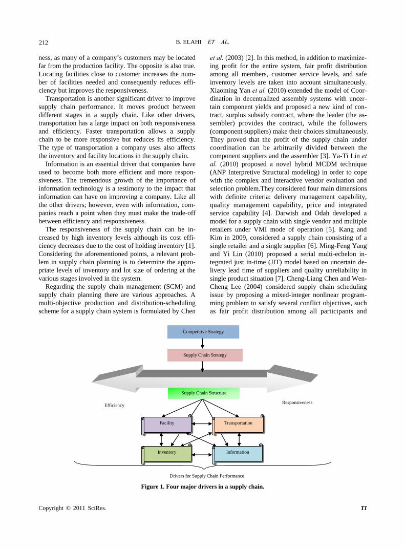
1. Introduction Supply chain planning is one of the most vital decisions in today’s global market as companies are forced to gain a competitive advantage by focusing attention to their entire supply chain. The notable concentration in the supply chain planning related research in the last decade has been owing to its potential to improve the efficiency and efficacy of operations and reduce costs. In real world, variety of activities are involved in supply chain planning issue such as supplier selection, inventory management, purchasing and transportation of materials, components and finished products in a multi-echelon supply chain. Suppliers are the significant link to any supply chain and subsequently sourcing decision is one of the essential decisions to be taken at the planning stage. Ac- cording to Chopra and Meindl (2007), inventory is rec- ognized as one of the four major drivers in a supply chain (Figure 1). Most successful companies begin with a competitive strategy and then decide what their supply chain strategy ought to be. The supply chain strategy determines how the supply chain should perform with

respect to efficiency and responsiveness. The supply chain must then utilize the three drivers to reach the performance level the supply chain strategy dictates and maximize the supply chain profit. Inventory is one of the key drivers of supply chain performance. It exists in the supply chain because of a mismatch between supply and demand. An important role that inventory plays in a supply chain is to increase the amount of demand that can be satisfied by having the product ready and available when customer wants it. Another significant role that inventory plays is to reduce cost by exploiting economics of scale that may exist during production and distribution. Inven- tory is held throughout the supply chain in form of raw material, work in process and final goods. Inventory is a major source of cost in supply chain and has huge impact on responsiveness.

Facility is another important driver of supply chain performance in terms of responsiveness and efficiency. For instance, companies can gain economies of scale when a product is manufactured or stored in only one location; this centralization increases efficiency. The cost reduction; however, comes at the expense of responsive-

212 B. ELAHI ET AL.

ness, as many of a company’s customers may be located far from the production facility. The opposite is also true. Locating facilities close to customer increases the number of facilities needed and consequently reduces efficiency but improves the responsiveness.

Transportation is another significant driver to improve supply chain performance. It moves product between different stages in a supply chain. Like other drivers, transportation has a large impact on both responsiveness and efficiency. Faster transportation allows a supply chain to be more responsive but reduces its efficiency. The type of transportation a company uses also affects the inventory and facility locations in the supply chain.

Information is an essential driver that companies have used to become both more efficient and more responsiveness. The tremendous growth of the importance of information technology is a testimony to the impact that information can have on improving a company. Like all the other drivers; however, even with information, companies reach a point when they must make the trade-off between efficiency and responsiveness.

The responsiveness of the supply chain can be increased by high inventory levels although its cost efficiency decreases due to the cost of holding inventory [1]. Considering the aforementioned points, a relevant problem in supply chain planning is to determine the appropriate levels of inventory and lot size of ordering at the various stages involved in the system.

Regarding the supply chain management (SCM) and supply chain planning there are various approaches. A multi-objective production and distribution-scheduling scheme for a supply chain system is formulated by Chen

et al. (2003) [2]. In this method, in addition to maximize- ing profit for the entire system, fair profit distribution among all members, customer service levels, and safe inventory levels are taken into account simultaneously. Xiaoming Yan et al. (2010) extended the model of Coor- dination in decentralized assembly systems with uncertain component yields and proposed a new kind of contract, surplus subsidy contract, where the leader (the assembler) provides the contract, while the followers (component suppliers) make their choices simultaneously. They proved that the profit of the supply chain under coordination can be arbitrarily divided between the component suppliers and the assembler [3]. Ya-Ti Lin et al. (2010) proposed a novel hybrid MCDM technique (ANP Interpretive Structural modeling) in order to cope with the complex and interactive vendor evaluation and selection problem.They considered four main dimensions with definite criteria: delivery management capability, quality management capability, price and integrated service capability [4]. Darwish and Odah developed a model for a supply chain with single vendor and multiple retailers under VMI mode of operation [5]. Kang and Kim in 2009, considered a supply chain consisting of a single retailer and a single supplier [6]. Ming-Feng Yang and Yi Lin (2010) proposed a serial multi-echelon integrated just in-time (JIT) model based on uncertain delivery lead time of suppliers and quality unreliability in single product situation [7]. Cheng-Liang Chen and Wen- Cheng Lee (2004) considered supply chain scheduling issue by proposing a mixed-integer nonlinear programming problem to satisfy several conflict objectives, such as fair profit distribution among all participants and

Responsiveness Efficiency

Competitive Strategy

Supply Chain Strategy

Supply Chain Structure

Inventory Information

Drivers for Supply Chain Performance

Facility Transportation

Figure 1. Four major drivers in a supply chain.


B. ELAHI ET AL.


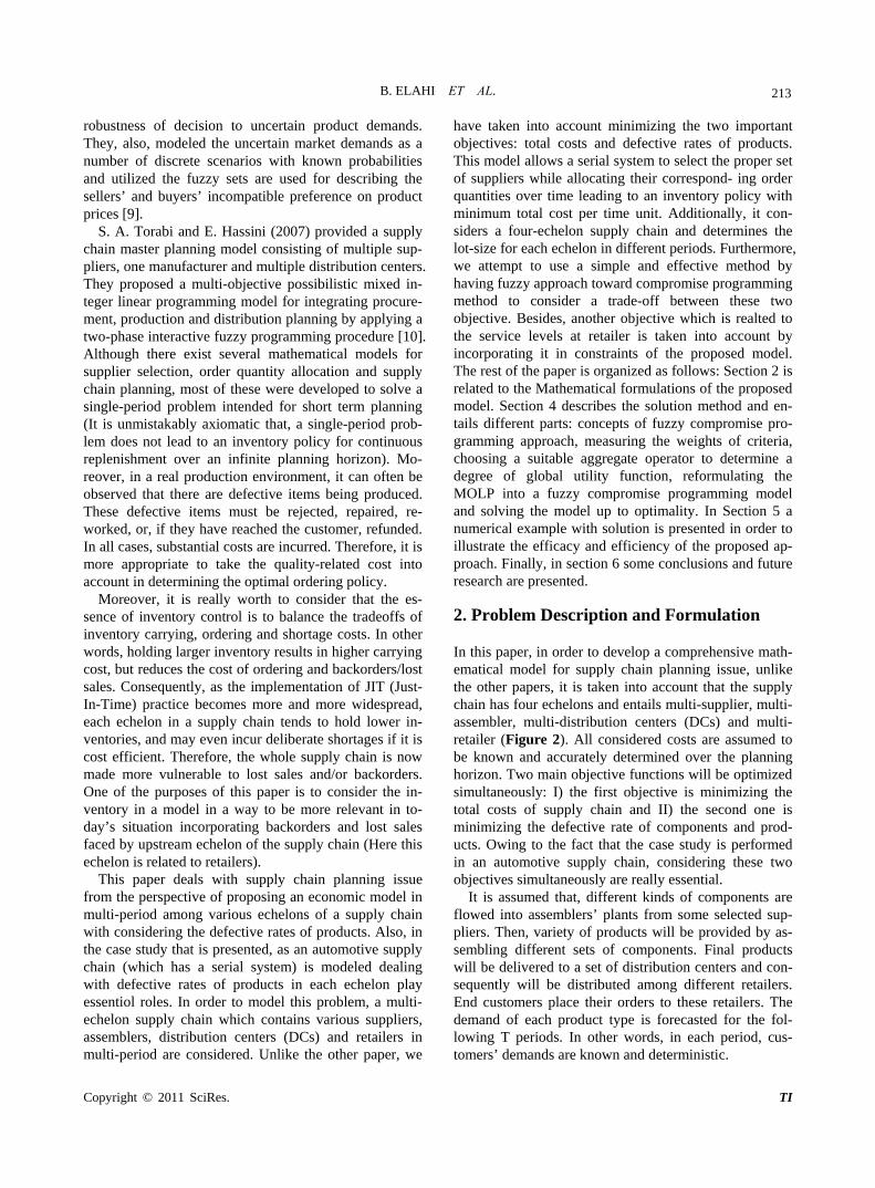
213 robustness of decision to uncertain product demands. They, also, modeled the uncertain market demands as a number of discrete scenarios with known probabilities and utilized the fuzzy sets are used for describing the sellers’ and buyers’ incompatible preference on product prices [9].

S. A. Torabi and E. Hassini (2007) provided a supply chain master planning model consisting of multiple suppliers, one manufacturer and multiple distribution centers. They proposed a multi-objective possibilistic mixed integer linear programming model for integrating procure- ment, production and distribution planning by applying a two-phase interactive fuzzy programming procedure [10]. Although there exist several mathematical models for supplier selection, order quantity allocation and supply chain planning, most of these were developed to solve a single-period problem intended for short term planning (It is unmistakably axiomatic that, a single-period problem does not lead to an inventory policy for continuous replenishment over an infinite planning horizon). Mo- reover, in a real production environment, it can often be observed that there are defective items being produced. These defective items must be rejected, repaired, re- worked, or, if they have reached the customer, refunded. In all cases, substantial costs are incurred. Therefore, it is more appropriate to take the quality-related cost into account in determining the optimal ordering policy.

Moreover, it is really worth to consider that the es- sence of inventory control is to balance the tradeoffs of inventory carrying, ordering and shortage costs. In other words, holding larger inventory results in higher carrying cost, but reduces the cost of ordering and backorders/lost sales. Consequently, as the implementation of JIT (Just- In-Time) practice becomes more and more widespread, each echelon in a supply chain tends to hold lower in- ventories, and may even incur deliberate shortages if it is cost efficient. Therefore, the whole supply chain is now made more vulnerable to lost sales and/or backorders. One of the purposes of this paper is to consider the inventory in a model in a way to be more relevant in today’s situation incorporating backorders and lost sales faced by upstream echelon of the supply chain (Here this echelon is related to retailers).

This paper deals with supply chain planning issue from the perspective of proposing an economic model in multi-period among various echelons of a supply chain with considering the defective rates of products. Also, in the case study that is presented, as an automotive supply chain (which has a serial system) is modeled dealing with defective rates of products in each echelon play essentiol roles. In order to model this problem, a multi- echelon supply chain which contains various suppliers, assemblers, distribution centers (DCs) and retailers in multi-period are considered. Unlike the other paper, we

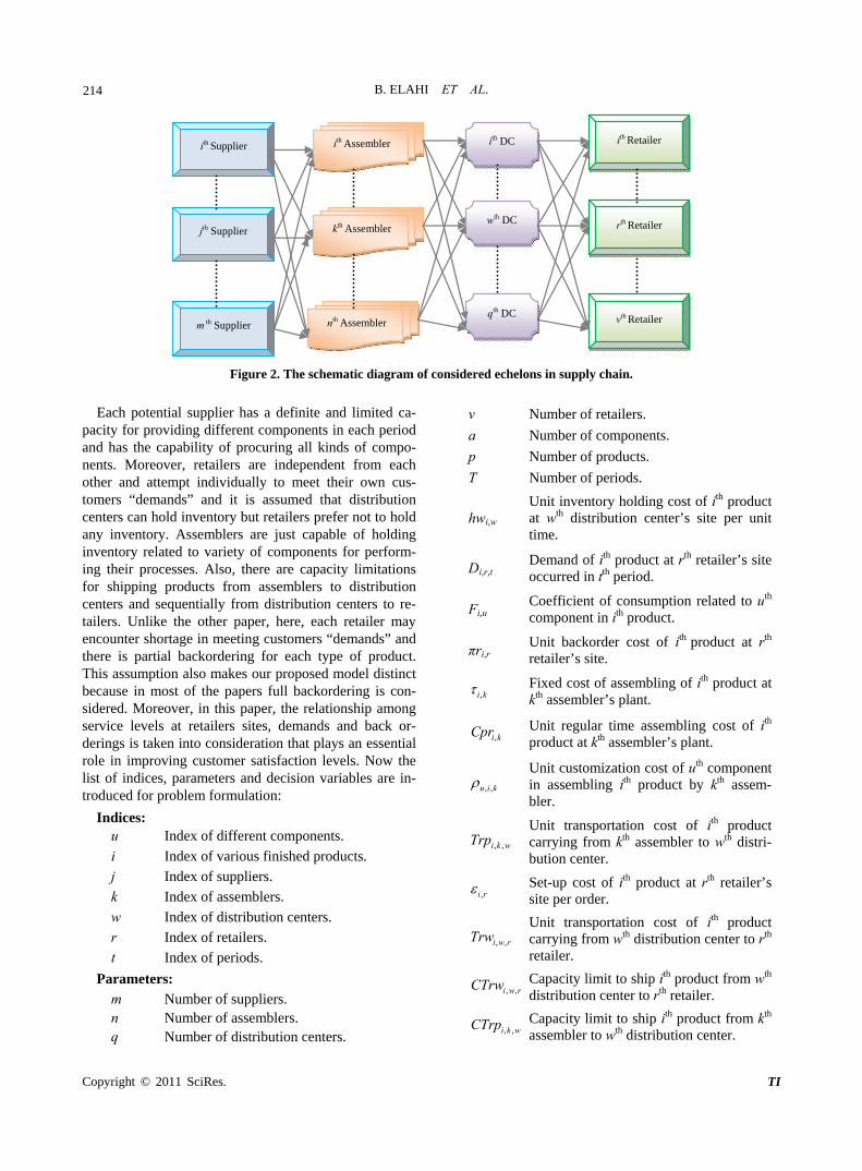
have taken into account minimizing the two important objectives: total costs and defective rates of products. This model allows a serial system to select the proper set of suppliers while allocating their correspond- ing order quantities over time leading to an inventory policy with minimum total cost per time unit. Additionally, it con- siders a four-echelon supply chain and determines the lot-size for each echelon in different periods. Furthermore, we attempt to use a simple and effective method by having fuzzy approach toward compromise programming method to consider a trade-off between these two objective. Besides, another objective which is realted to the service levels at retailer is taken into account by incorporating it in constraints of the proposed model. The rest of the paper is organized as follows: Section 2 is related to the Mathematical formulations of the proposed model. Section 4 describes the solution method and entails different parts: concepts of fuzzy compromise programming approach, measuring the weights of criteria, choosing a suitable aggregate operator to determine a degree of global utility function, reformulating the MOLP into a fuzzy compromise programming model and solving the model up to optimality. In Section 5 a numerical example with solution is presented in order to illustrate the efficacy and efficiency of the proposed approach. Finally, in section 6 some conclusions and future research are presented. 2. Problem Description and Formulation In this paper, in order to develop a comprehensive mathematical model for supply chain planning issue, unlike the other papers, it is taken into account that the supply chain has four echelons and entails multi-supplier, multi- assembler, multi-distribution centers (DCs) and multi- retailer (Figure 2). All considered costs are assumed to be known and accurately determined over the planning horizon. Two main objective functions will be optimized simultaneously: I) the first objective is minimizing the total costs of supply chain and II) the second one is minimizing the defective rate of components and products. Owing to the fact that the case study is performed in an automotive supply chain, considering these two objectives simultaneously are really essential.

It is assumed that, different kinds of components are flowed into assemblers’ plants from some selected suppliers. Then, variety of products will be provided by assembling different sets of components. Final products will be delivered to a set of distribution centers and consequently will be distributed among different retailers. End customers place their orders to these retailers. The demand of each product type is forecasted for the following T periods. In other words, in each period, customers’ demands are known and deterministic.

B. ELAHI ET AL.


214

ith Supplier

jth Supplier

m th Supplier

ith Assembler

kth Assembler

nth Assembler

ith DC

wth DC

qth DC

ith Retailer

rth Retailer

vth Retailer

Figure 2. The schematic diagram of considered echelons in supply chain.

Each potential supplier has a definite and limited ca-

pacity for providing different components in each period and has the capability of procuring all kinds of components. Moreover, retailers are independent from each other and attempt individually to meet their own customers “demands” and it is assumed that distribution centers can hold inventory but retailers prefer not to hold any inventory. Assemblers are just capable of holding inventory related to variety of components for perform- ing their processes. Also, there are capacity limitations for shipping products from assemblers to distribution centers and sequentially from distribution centers to re-tailers. Unlike the other paper, here, each retailer may encounter shortage in meeting customers “demands” and there is partial backordering for each type of product. This assumption also makes our proposed model distinct because in most of the papers full backordering is considered. Moreover, in this paper, the relationship among service levels at retailers sites, demands and back orderings is taken into consideration that plays an essential role in improving customer satisfaction levels. Now the list of indices, parameters and decision variables are introduced for problem formulation:

Indices: u Index of different components.

i Index of various finished products.

j Index of suppliers.

k Index of assemblers.

w Index of distribution centers.

r Index of retailers.

t Index of periods.

Parameters: m Number of suppliers. n Number of assemblers. q Number of distribution centers.

v Number of retailers.

a Number of components.

p Number of products.

T Number of periods.

hwi,w Unit inventory holding cost of ith product at wth distribution center’s site per unit time.

Di,r,t Demand of ith product at rth retailer’s site occurred in tth period.

Fi,u Coefficient of consumption related to uth

component in ith product.

πri,r Unit backorder cost of ith product at rth

retailer’s site.

,i k Fixed cost of assembling of ith product at kth assembler’s plant.

,i kCpr Unit regular time assembling cost of ith

product at kth assembler’s plant.

, ,u i k Unit customization cost of uth component in assembling ith product by kth assem-bler.

, ,i k wTrp Unit transportation cost of ith product carrying from kth assembler to wth distri-bution center.

,i r Set-up cost of ith product at rth retailer’s site per order.

, ,i w rTrw Unit transportation cost of ith product carrying from wth distribution center to rth

retailer.

, ,i w rCTrw Capacity limit to ship ith product from wth

distribution center to rth retailer.

, ,i k wCTrp Capacity limit to ship ith product from kth

assembler to wth distribution center.

B. ELAHI ET AL.

215

,i wStw Store capacity of ith product at wth distri-bution center.

,i kG Maximum capacity of assembling of ith

product at kth assembler’s site.

min, ,i r tSL Minimum desired service level of ith pro-

duct at rth retailer’s site in tth period.

,u khu Unit inventory holding cost of uth com-ponent at kth assembler’s site per unittime.

j Ordering set-up cost of jth supplier.

,u jS Unit selling price of uth component of-fered by jth supplier to assembler.

,u jCs Capacity of providing uth component at jth

supplier’s site.

MIu,k,t Maximum holding capacity of uth com-ponent at kth assembler’s site in tth period.

,u js Unit defective rate of components sent toassemblers by each supplier.

,i kp Unit defective rate of products sent to distribution centers by each assembler.

,i wd Unit defective rate of products sent to retailers by each DC.

Decision variables:

Xi,k,t The amount of produced units which is related to the ith product at kth assembler’s site in tth period.

BRi,r,t The amount of ith product backordered by rth retailer in the end of tth period.

Vi,k,w,t The amount of units which is related to the ith product delivered from kth assem-bler to wth distribution center in tth period.

Qi,w,r,t The amount of units which is related to the ith product dispatched to rth retailer by wth distribution center in tth period.

, , ,u j k tZ The amount of units which is related to the uth component ordered by kth assem-bler from jth supplier in tth period.

, ,i r tSL Desired service level at rth retailer’s site related to ith product in tth period.

, ,i w tIW Amount of inventory related to ith product at wth distribution center’s site in the end of tth period.

, ,u k tIU Amount of inventory related to uth com-ponent at kh assembler’s site in the end of tth period.

If rth retailer places assembly order for ith product in tth period.

, ,i r t 1

0

Otherwise.

If assembling of ith product at kth

assembler’s plant has been set up in tth period. , ,i k t

1

0

Otherwise.

If rth retailer places order to wth dis-tribution centers.

,w r

1

0

Otherwise

If wth distribution center places order to kth assembler.

,k w

1

0

Otherwise

If kth assembler places order to jth

supplier in tth period. , ,j k tY

1

0

Otherwise

Considering the aforementioned assumptions and no-

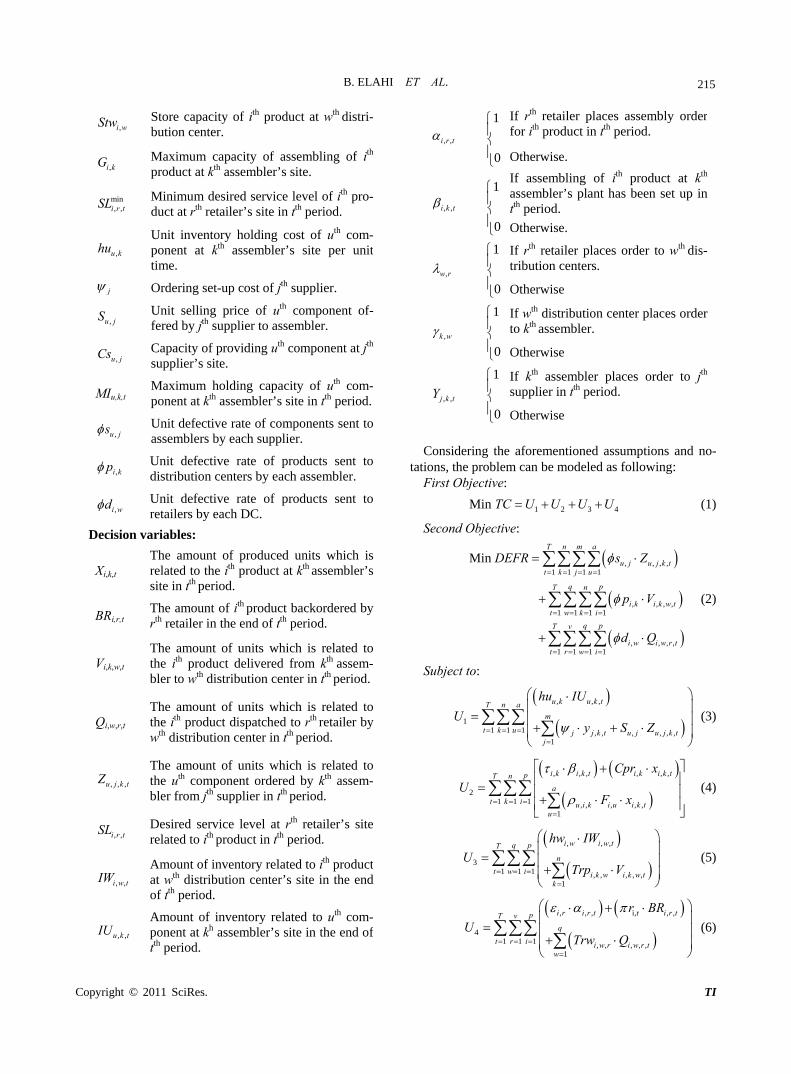
tations, the problem can be modeled as following: First Objective:

1 2 3Min TC U U U U4 (1)

Second Objective:

, , , ,1 1 1 1

, , , ,1 1 1 1

, , , ,1 1 1 1

Min

T n m a

u j u j k tt k j u

q pT n

i k i k w tt w k i

q pT v

i w i w r tt r w i

DEFR s Z

p V

d Q

(2)

Subject to:

, , ,

11 1 1 , , , , , ,

1

u k u k tT n a

m

t k u j j k t u j u j k tj

hu IU

Uy S Z

(3)

, , , , , ,

21 1 1 , , , , ,

1

i k i k t i k i k tpT n

a

t k i u i k i u i k tu

Cpr x

UF x

(4)

, , ,

31 1 1 , , , , ,

1

i w i w tq pT

n

t w i i k w i k w tk

hw IW

UTrp V

(5)

, , , i,r , ,

41 1 1 , , , , ,

1

i r i r t i r tpT v

q

t r i i w r i w r tw

r BR

UTrw Q

(6)


216 B. ELAHI ET AL.

, , , , 1 , , , , , ,1 1

.

, ,

m P

u k t u k t u j k t i u i k tj i

IU IU Z F x

u k t

(7)

, , , ,1

, ,n

u j k t u jk

Z Cs u j t

(8)

(9) , , , , , ,u k t u k tIU MI u k t

, , , , , , , ,1

, , ,

T P

i u i k t j k t u j k tl t i

F X Y Z

u j k t

(10)

, ,1

, ,

, ,1

1 , ,

t

i r tl

i r t t

i r tl

BRSL i r t

D

(11)

min, , 1 , ,i r tSL SL i r t (12)

(13)

t (15)

w r t

, , , , 1 , , , , ,1

, ,

q

i r t i r t i r t i w r tw

BR BR D Q

i r t

, , , , 1 , , , , , ,1 1

, ,

n v

i w t i w t i k w t i w r tk r

IW IW V Q

i w t

(14)

, , , , ,1

, ,q

i k w t i k tw

V X i k

, , , , , , , , ,i w r t w r i w rQ CTrw i (16)

k w, , , , , , , ,i k w t k w i k wV CTrp i , t (17)

, , , , ,i w t i wIW Stw i w t (18)

, , , , , ,i k t i k tX M i k t

i r t (

(19)

, , , , , ,i r t i r tD M 20)

, , , , ,i k t i kX G i k t (21)

, , , , , , , , , , ,

, , , , , ,

, , , ,

, , 0

, , , , , ,

u k t u j k t i w r t i k w t

i k t i r t i w t

IU Z Q V

X BR IW Z

i j u k r w t

(22)

, , , , , , , , ,, , , , {0,1}

, , , ,

u j k t w r k w i k t i r tY

i k r w t

(23)

As it can be observed, in the proposed mathematical model, the first objective function (Equation (1)) demonstrates the considered total costs of supply chaincludes four different parts: 4 . Termreco

ar time assembli us

. It in- 1 2 3, , , U U U U 1U

fers to the costs of components which include holding sts of inventory at assemblers’ sites, fixed ordering

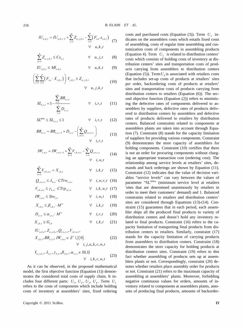
costs and purchased costs (Equation (3)). Term 2U indicates on the assemblers costs which entails fixed costs of assembling, costs of regul ng and c - tomization costs of components in assembling products (Equation 4). Term 3U is related to distribution centers’ costs which consists of holding costs of inventory dis-tribution centers’ sites and transportation costs of prod-ucts carrying from assemblers to distribution centers (Equation (5)). Term 4U is associated with retailers costs that includes set-up sts of products at retailers’ sites per order, backordering costs of products at retailers’ sites and transportation costs of products carrying from distribution centers to retailers (Equation (6)). The second objective functio Equation (2)) refers to minimizing the defective rates of components delivered to assemblers by suppliers, defective rates of products delivered to distribution centers by assemblers and defective rates of products delivered to retailers by distribution centers. Balanced constraints related to components at assemblers plants are taken into account through Equa- tion (7). Constraint (8) stands for the capacity limitation of suppliers for providing various components. Constraint (9) demonstrates the store capacity of assemblers for holding components. Constraint (10) certifies that there is not an order for procuring components without charg- ing an appropriate transaction cost (ordering cost). The relationship among service levels at retailers’ sites, demands and back orderings are shown by Equation (11). Constraint (12) indicates that the value of decision vari-ables “service levels” can vary between the values of parameter “SLmin” (minimum service level at retailers 'sites that are determined unanimously by retailers in order to meet their customers’ demand) and 1. Balanced constraints related to retailers and distribution centers’ sites are considered through Equations (13)-(14). Con- straint (15) guarantees that in each period, each assembler ships all the produced final products to variety of distribution centers and doesn’t hold any inventory related to final products. Constraint (16) refers to the capacity limitation of transporting final products from distribution centers to retailers. Similarly, constraint (17) stands for the capacity limitation of carrying products from assemblers to distribution centers. Constraint (18) demonstrates the store capacity for holding products at distribution centers sites. Constraint (19) refers to this fact whether assembling of products sets up at assemblers plants or not. Correspondingly, constraint (20) de- notes whether retailers place assembly order for products or not. Constraint (21) refers to the maximum capacity of assembling at assemblers’ plants. Moreover, forbidding negative continuous values for orders, amounts of inventory related to components at assemblers plants, amounts of producing final products, amounts of backorder-

at

co

n (


B. ELAHI ET AL.

217

3.

s a simple fuzzy approach which applied by Li t al. (2000) toward a multi-objective transportation

achieve a more reasonable ompromise solution [11]. One of the advantages of this

ing and amounts of holding inventory at distribution centers site has been satisfied through constraint (22). Furthermore, constraint (23) sets the values of binary variables.

In the next section, fuzzy compromise programming is introduced in order to deal with solving this non-linear mixed-integer bi-objective mathematical modeling efficiently.

Solution Method In this study, the concept of optimal compromise solution besideeproblem will be utilized tocform of modeling is that the multi-objective problem has converted to a single objective programming problem and the ordinary optimization techniques can be used to solve it. Another advantage is related to this matter that employing fuzzy compromise programming can facilitate the generation of a more objective compromise solution by preventing the presence of non-homogeneous measuring scales among the two different objectives that are considered in supply chain planning system. At first a fuzzy approach to multi-objective problem will be introduced in order to obtain the degree of marginal utility for each objective. Secondly, by applying a proper combina- tion of decision-making parameters, these degrees of marginal utility can be aggregated in order to achieve a global utility for all objectives. Thirdly, on the basis of obtained global utility, it will be possible to form a fuzzy compromise programming approach toward multi-objective problem. According to this consideration that the value of each objective function Zs changes linearly from

minsZ to Nadir

sZ (which obtain by solving the multi-objective problem as a single objective, while ignoring the other objectives, and forming a pay-off table for all objective functions), it is possible to take into account this value as a fuzzy number with a linear membership func-

base preference or utility. Also, the membership function of each objective utility can be defined by Equation (24).

tion d on

min

minmin

1 if

if

s s

Nadirs s

0 if

Nadirs s s sNadir

s s

Z x Z

Z x ZU x Z Z x Z

Z Z

Nadirs sZ x Z

(24)

Moreover, we can define the degree of global utility of the multi-objective problem as Equation (25). U x

1

1

S

s ss

U x w U x

where:

1

0 ,S

ss

w

1 (25)

In Equation (25),

pplied em

consfined

is a parameter and its valdemakerstion operators are a to deal with the multi-objective problem. One of th maximizes the tal utility ex-

s of idering the sum of the utility of es and is de as a weighted additive operator

ue is termine in accordance with preference of decision

. In practical perspective, normally two aggrega-

topressed in termobjectiv( 1 ). The other rator maximi

all objectiv which is defiope

es, zes the least utility ned as a max-min among

operator ( ). M eover, or sw represents the weight of sth criterion and demonstrates the decision makers’ preferences over the relative importance among the objectives and the way of its calculation will be discussed in the next section. Thus, the multi-objective problem stated in Equations (1)-(23), can be formulated as the following fuzzy compromise programming problem (Equa- tion (26)).

1

1

MaximizeS

s ss

U x w U x

(26)

Subject to: X

Let *x X be an optimal solution for this model (Equation (26)). That is * maxU x U x : ( x X ).

*x is a non-dominated (Pareto) compromise solution in which the synthetic membership degree of optimum for all objectives is maximal. In this paper, it is assumed that there are L decision makers (DMs) who have similar importance. They state their opinion towardportance of objectives via pair-wise comparisonOne analytical approach often suggested for solving a co x probl

wide variety of deci

relative im- matrix.

mple em is AHP, first introduced by Saaty in 1980. It has been applied in a - sion-making contexts. It also provides a structured approach for determining the weights of criteria. Here, by employing such an extended pair wise comparisons, appropriate set of weights will be generated, owing to this fact that the relative importance of various objectives is considered. Consequently, more reasonable solutions will be obtained.

Let 1 2, , , sV v v v be a set of objectives. Each decision maker’s pair-wise comparison matrix (which is a reciprocal matrix) can be defined as Equation (27).

Also, Table 1 demonstrates the measurement scale which is used for verbal judgment or preference of DMs.

Moreover in order to aggregate DMs’ opinion, Geo-metric mean operator is applied and a single matrix is formed (Equation (28)).


218 B. ELAHI ET AL.

Table 1. Measurement scale for verbal judgment or preference.

Verbal judgment or preference Numerical rating

Extremely preferred 9

Very strongly preferred 7

Strongly preferred 5

Moderately preferred 3

Equally preferred 1

1,1 1,

', '

,1 ,

s

i j

s s s

a a

a a

A a

7)

w

(2

here:

', 'i ja ia

', '

1for all ', ' 1, 2, ,

j i

j s

1,1 1,

', '

,1 ,

' '

' '

' '

s

i j

s s

a a

A a

a a

s

(28)

where: 1

', ' ', '1

'L L

i j i jl

a a

for all and ', ' 1, 2, ,i j s 1, 2, ,l L .

Furthermore, in order to calculate the weights of criteria, referring to Saaty’s theorem that tion (29) and his proposed heuristic method, for each row of matrix

is shown by Equa-

'A the sum of elements is obtained and the are computed [12]. weights

elim

e

K

T Kk

AW

A

e

is a pair-wise , W is the n alized prin- ht eigenvector ix A and )

s

(29)

where A matrix ormcipal rig of matr e (1, ,1T .

Therefore, after computing the weights of objectives, every parameters in the fuzzy compromise programming is definite and Equation (30) indicates on the extended form of thi model (when the value of is assumed equal 1. 1 )

min1

s ss Nadir

s s s

, ,1 1

min1

m in

Maximize

NadirS

s Nadiri j i j sS

i js Nadir

s

c x Z

wZ Z

s s

U x

Z x Zw

Z Z

( ),sm in S

s i jw c,min

1 1 1

min1

i jNadiri j s s s

NadirSs s

Nadirs s s

xZ Z

w Z

Z Z

(30)

Subject to:

X In the next section, in order to illustrate the efficacy

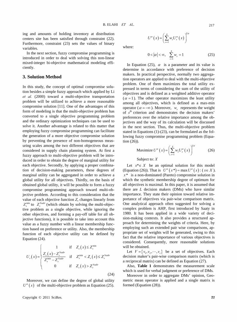
and efficiency of proposed model and solution, a numerical example is applied for a data set. 4. Numerical Example Consider a supply chain system with four ectaining three suppliers, three assemblers, three tion center and three retailers. There are three different components which are applied to form three finished pr assumed that the supply chain planning w

posed mathematical odel (Equations (1)-(23)) and then has been solved by

ise programming solution rocedure. LINGO software is applied (ran on an Intel

helons con- distribu-

oducts. It isill be determined for three periods. This real numerical

example which is related to an automotive supply chain has been formulated by using the promutilizing the fuzzy comprompCore 2 Duo 2.8 GHz PC) to form the pay-off table related to the three objective functions. The result of this stage is shown in Figures 3-4 and Table 3. In this table, each column is related to the different value of objective Zs by setting the optimum solution of other objective functions, also the minimum value of each objective function (disregarding other objective functions) has been bold.

Figure 3. The output of solving model by considering the first objective.


B. ELAHI ET AL.


219

Considering the result of Table 2, we can identify the

values of NadirsZ for s = 1, 2 as below: 1

NadirObjective

2242974.5 , Obje 1 192.73Nadirctive .

In this stage the marginal utility of each criterion is formed and the pair-wise comparison matrixes related to

rs’ opinion. Also, the Geometric mean op

atrix , 2) indicates ontotal cost and defective rates of pro n order.) Be- sides,

the two objectives are obtained through collecting three decision make

erator is utilized to aggregate their preferences. (In the pair-wise m es, sth objective (for s = 1

ducts, ithe weights of objectives are calculated.

11

1

2242974.5

1697850 2242974.50

Objective xU x

1

1

1

1697850

1697850 2242974.5

2242974.5

Objective x

Objective x

Objective x

22

1

192.73

19.255 192.730

Objective xU x

2

2

2

19.255

19.255 192.73

192.73

Objective x

Objective x

Objective x

1 2.213

0.452 1aggregationA

1 2

1

0.689, 0.311

1S

ss

w w

w

Then, by assuming 1 (Using weighted additive

operator), the global utility in accordance with Equation 30 is formulated and the fuzzy compromise programming model is constructed.

min1

1 1

min1 1

2 2

min2

+0.311*Objec x Objecti

Objective Object

Maximize

0.689 *

=

NadirSs s

s Nadirs s s

Nadir

Nadir

Nadir

U x

Objective x Objectivew

Objective Objective

Objective x Objective

Objective Objective

tive

ve

2

1 2242974.50.689 *

1697850

Nadirive

Objective x

2

2242974.5=

192.73+0.311*

19.255 192.73

Objective x

Subject to:

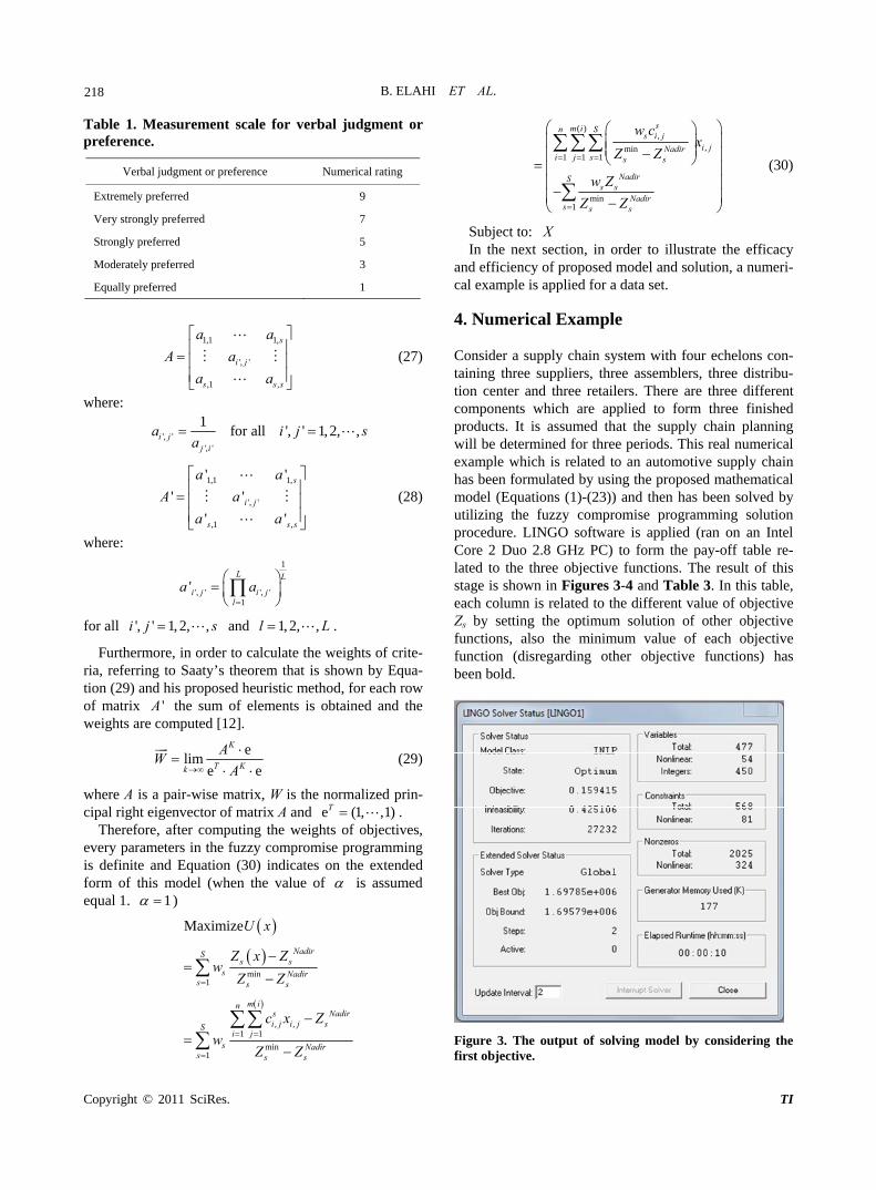
Figure 4. The output of solving model by considering the second objective.

Table 2. Pay-off Matrix related to the two objectives.

Pay-off Matrix Objective1 Objective2

X

After solving the reformulated mathematical model, the achieved results related to the value of utility function and the two objectives are shown through Table 3. Terms U1 and U2 show the extent of closeness related to the achieved values for objective1 and objective2 to their optimal values which obtained by solving the multi-objective problem as a single objective, while ignoring the other objectives.

min

1Objective 1697850 192.73

min

2Objective 2242974.5 19.255

220

Ta

B. ELAHI ET AL.

ble 3. Achieved values for utility function and the two objectives.

Variable U(x) = Utility

function Objective1 Objective2 U1 U2

Value 0.7422616 1738700 128.905 0.925 0.367

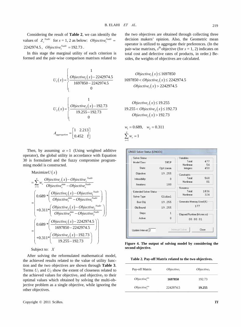
Moreover, variety of values which are obtained for

service levels at retailers’ sites (R1, R2 and R3) for each type of products (F, G or H) in each period (1, 2 or 3) are demonstrated through Figure 5. As the weight of the first objective has been more than the weight of the second objective in the multi objective mathematical modeling, the values of service levels that are achieved by the utility function (which is substituted for the two object- tives and has taken into account the weights of objectives efficiently) are more similar to the values of service levels obtained by considering the first objective separately rather than the values of service levels computed by tak- ing into account of second objective independently. 5. Conclusions and Future Research Nowadays, variety of factors in today’s global market has forced companies to gain a competitive advantage by focusing attention to their entire supply chain. Of the various activities involved in supply chain managementintegrative planning among various echelons of a suppl

ce costs and consequently increase rofits. In this paper, it is attempted to propose an effi-

cie c- tives, minimizing the total costs of supply chain and minimizing the defective productsered and the proposed mathematical model solved by applying Fuzzy comprom gramming over, the achieved result of numerical example verifies the efficacy of tha h a kind of modeling

properly for splitting orders among various suppliers wh variety of products. Regarding th s v s tio n large scales se u ing a set of

olut mes avai e, deci n m v

, y

chain is one of the most strategic because it provides opportunities to redup

nt model for supply chain planning. Two major obje

rates to were consid-

ise pro . More

t. Suc and solution method, can prepare an efficient opportunity for managers to decide

ile there are ed model deis propo eloping an optimal olu n i

ems difficions beco

lt. Also, if aclabl

hievsiovari

eous s akers can

aluate the pros and cons of each solution considering variety of qualitative or technical parameters in real situation in order to somehow overcome the uncertainty of environment. Therefore, according to the aforementioned points, it can be stated that this supply chain planning model involves a complex shape of search space with many candidate solutions. Thus, meta-heuristic methods such as genetic algorithm (GA) are applicable for fast exploration and can be considered as an efficient research in future. Also, dealing with variety of robust opti-

Figure 5. Various values of service levels by objective1, ob-jective2 and utility function. timization toward the proposed mathematical model can be taken into account as the other future research. 6. References [1] S. Chopra and P. Meindl, “Supply Chain Management:

Strategy, Planning, and Operations,” Prentice Hall, Upper Saddle River, 2007.

[2] L. Cheng, E. Subrahmanian and A. W. Westerberg, “De-sign and Planning under Uncertainty: Issues on Problem Formulation and Solution,” Computer and Chemical En-gineering, Vol. 27, No. 6, 2003, pp. 781-801. doi:10.1016/S0098-1354(02)00264-8

[3] X. Yan, M. Zhang and K. Liu, “A Note on Coordination in Decentralized Assembly Systems with Uncertain Component Yields,” European Journal of Operational Research, Vol. 205, No. 2, 2010, pp. 469-478. doi:10.1016/j.ejor.2009.12.011

[4] Y. T. Lin, C. L. Lin, H. C. Yu and G. H. Tzeng, “A Novel Hybrid MCDM Approach for Outsourcing Vendor Selec-tion: A Case Study for a Semiconductor Company in Taiwan,” Expert Systems with Applications, Vol. 37, No. 7, 2010, pp. 4796-4804. doi:10.1016/j.eswa.2009.12.036

[5] M. A. Darwish and O. M. Odah, “Vendor Managed In-ventory Model for Single-Vendor Multi-retailer Supply Chains,” European Journal of Operational Research, Vol. 204, No. 3, 2010, pp. 473-484.


B. ELAHI ET AL.


221

doi:10.1016/j.ejor.2009.11.023

[6] J. K. Kang and Y. D. Kim, “Inventory Replenishment andDelivery Planning in a Two-Level Supply Chain withCompound Poisson Demands,” The International Journalof Advanced Manufacturing Technology, Vol. 49, No. 9-12, 2009, pp. 1107-1118.

[7] M. F. Yang and Y. Lin, “Applying the Linear ParticleSwarm Optimization to a Serial Multi-echelon Inventory Model,” Expert Systems with Applications, Vol. 37, No.2010, pp. 2599-2608. doi:10.1016/j.eswa.2009.08.021

3,

[8] W. Xia and Z. Wu, “Supplier Selection with MultipleCriteria in Volume Discount Environments,” Omega-In-ternational Journal of Management Science, Vol. 35, No. 5, 2007, pp. 494-504. doi:10.1016/j.omega.2005.09.002

[9] C. L. Chen and W. C. Lee, “Multi-objective Optimizationof Multi-echelon Supply Chain Networks with Uncertain

144. 3.09.014

Product Demands and Prices,” Computers and Chemical Engineering, Vol. 28, No. 6-7, 2004, pp. 1131-1doi:10.1016/j.compchemeng.200

[10] S. A. Torabia and E. Hassini, “An Interactive Possibilistic Programming Approach for Multiple Objective Supply Chain Master Planning,” Fuzzy Sets and Systems, Vol. 159, No. 2, 2008, pp. 193-214. doi:10.1016/j.fss.2007.08.010

[11] L. Li and K. K. Lai, “A Fuzzy Approach to the Multi- Objective Transportation Problem,” Computer and Op-erations Research, Vol. 27, No. 1, 2000, pp. 43-57. doi:10.1016/S0305-0548(99)00007-6

ow to Make a Decision:

[12] T. L. Saaty and J. M. Katz, “HThe Analytic Hierarchy Process,” European Journal of Operational Research, Vol. 48, No. 1, 1990, pp. 9-26.

TI20110300005 91286914 (2)

Documents

Transcript of TI20110300005 91286914 (2)