Geophysical Prospecting, 2008, 56, 587–600 doi:10.1111/j.1365-2478.2008.00711.x

Three-dimensional kinematic depth migration of converted waves:application to the 2002 Molise aftershock sequence (southern Italy)

Diana Latorre1∗, Pasquale De Gori1, Claudio Chiarabba1, Alessandro Amato1,Jean Virieux2 and Tony Monfret3

1Istituto Nazionale di Geofisica e Vulcanologia, CNT, Roma, Italy, 2LGIT, Universite Joseph Fourier, Grenoble, France, and 3UMRGeosciences Azur, Sophia-Antipolis, France

Received February 2007, revision accepted February 2008

ABSTRACTMigration techniques, currently used in seismic exploration, are still scarcely appliedin earthquake seismology due to the poor source knowledge and sparse, irregular ac-quisition geometries. At the crustal scale, classical seismological studies often performinversions based on the arrival time of primary phases (P- and S-waves) but seldomexploit other information included in seismic records. Here we show how migrationtechniques can be adapted to earthquake seismology for converted wave analysis.As an example, we used data recorded by a dense local seismic network during the2002 Molise aftershock sequence. In October and November 2002, two moderatemagnitude earthquakes struck the Molise region (southern Italy), followed by an af-tershock sequence lasting for about one month. Local earthquake tomography hasprovided earthquake hypocenter locations and three-dimensional models of P andS velocity fields. Strong secondary signals have been detected between first-arrivalsof P- and S-waves and identified as SP transmitted waves. In order to analyse thesewaves, we apply a prestack depth migration scheme based on the Kirchhoff sum-mation technique. Since source parameters are unknown, seismograms are equalizedand only kinematic aspects of the migration process are considered. Converted wavetraveltimes are calculated in the three-dimensional (3D) tomographic models usinga finite-difference eikonal solver and back ray tracing. In the migrated images, thearea of dominant energy conversion corresponds to a strong seismic horizon that weinterpreted as the top of the Apulia Carbonate Platform and whose geometry and po-sition at depth is consistent with current structural models from existing commercialseismic profiles, gravimetric and well data.

I N T R O D U C T I O N

One of the aims of earthquake seismology is the study of phys-ical phenomena related to the earthquakes and their effect onthe Earth’s surface. The achievement of these goals requiresdetailed knowledge of the subsurface structure, especially inseismogenic areas. At the crustal scale, a common tool forsubsurface imaging is local earthquake tomography, in which

∗E-mail: latorre@ingv.it

parameters of earthquake hypocenters and velocities of P- andS-waves are simultaneously inverted using first-arrival delay-times (e.g., Thurber 1983; Michelini and McEvilly 1991; Hole1992; Le Meur, Virieux and Podvin 1997, among others).

Besides the analysis of traveltimes of some phases (mainlydirect and surface waves), common tools of earthquake seis-mology seldom exploit other information included in seis-mic records. Nevertheless, recent studies demonstrate thatreflected, transmitted and mode-converted waves from mi-croearthquakes (hereafter called passive sources) can be usedfor crustal-scale imaging (James, Clarke and Meyer 1987;

C© 2008 European Association of Geoscientists & Engineers 587

588 D. Latorre et al.

Chavez-Perez S. and Louie 1997; Stroujkova and Malin 2000;Chavarria et al. 2003; Latorre et al. 2004a; Nisii, Zollo andIannaccone 2004).

One of the major problems in using passive data for seis-mic reflection/transmission imaging is the sparse and irregulardistribution of sources and receivers and the poor knowledgeof the source, which includes magnitude, focal mechanism,earthquake hypocenter location and origin time. In mostpassive seismic surveys, receiver coverage is sparse and irregu-lar because seismic networks are generally designed for earth-quake monitoring rather than for seismic imaging. Neverthe-less, Louie et al. (2002) showed, through synthetic tests, thatpassive-source migration approaches are able to image mainfeatures of the subsurface structure, despite artefacts due tothe poor geometrical coverage.

Hypocentral parameters (earthquake location and origintime) represent one of the main causes of error in focusingand positioning reflected/transmitted energies. Uncertainty inearthquake location is strictly correlated to our knowledge ofboth the P- and S-wave velocity structures. Moreover, earth-quake location in seismogenic areas requires lateral variations

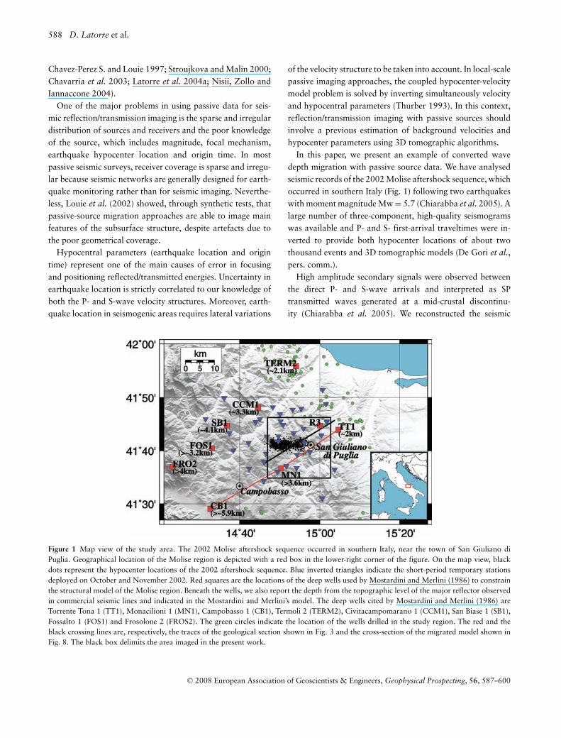
Figure 1 Map view of the study area. The 2002 Molise aftershock sequence occurred in southern Italy, near the town of San Giuliano diPuglia. Geographical location of the Molise region is depicted with a red box in the lower-right corner of the figure. On the map view, blackdots represent the hypocenter locations of the 2002 aftershock sequence. Blue inverted triangles indicate the short-period temporary stationsdeployed on October and November 2002. Red squares are the locations of the deep wells used by Mostardini and Merlini (1986) to constrainthe structural model of the Molise region. Beneath the wells, we also report the depth from the topographic level of the major reflector observedin commercial seismic lines and indicated in the Mostardini and Merlini’s model. The deep wells cited by Mostardini and Merlini (1986) areTorrente Tona 1 (TT1), Monacilioni 1 (MN1), Campobasso 1 (CB1), Termoli 2 (TERM2), Civitacampomarano 1 (CCM1), San Biase 1 (SB1),Fossalto 1 (FOS1) and Frosolone 2 (FROS2). The green circles indicate the location of the wells drilled in the study region. The red and theblack crossing lines are, respectively, the traces of the geological section shown in Fig. 3 and the cross-section of the migrated model shown inFig. 8. The black box delimits the area imaged in the present work.

of the velocity structure to be taken into account. In local-scalepassive imaging approaches, the coupled hypocenter-velocitymodel problem is solved by inverting simultaneously velocityand hypocentral parameters (Thurber 1993). In this context,reflection/transmission imaging with passive sources shouldinvolve a previous estimation of background velocities andhypocenter parameters using 3D tomographic algorithms.

In this paper, we present an example of converted wavedepth migration with passive source data. We have analysedseismic records of the 2002 Molise aftershock sequence, whichoccurred in southern Italy (Fig. 1) following two earthquakeswith moment magnitude Mw = 5.7 (Chiarabba et al. 2005). Alarge number of three-component, high-quality seismogramswas available and P- and S- first-arrival traveltimes were in-verted to provide both hypocenter locations of about twothousand events and 3D tomographic models (De Gori et al.,pers. comm.).

High amplitude secondary signals were observed betweenthe direct P- and S-wave arrivals and interpreted as SPtransmitted waves generated at a mid-crustal discontinu-ity (Chiarabba et al. 2005). We reconstructed the seismic

C© 2008 European Association of Geoscientists & Engineers, Geophysical Prospecting, 56, 587–600

3D kinematic depth migration of converted waves 589

image of this discontinuity by migrating and stacking SP-transmitted energies with an algorithm based on the Kirch-hoff summation technique (Latorre 2004). Passive sourcemigration was performed using P and S velocity modelsand passive source locations (position at depth and ori-gin time) previously estimated by the tomographic studyof De Gori et al. (pers. comm.). Tomographic results wereused as background models to account for the complex-ity of the P- and S-wave seismic structure in our traveltimecomputation.

As a result of the large amount of geological surveys, ex-ploration wells data, gravimetric modelling and commercialseismic profiles, the geological structure of the Molise regionis fairly well known down to 4–6 km depth (e.g., Mostardiniand Merlini 1986; Roure, Casero and Vially 1991; Improtaet al. 2006; Nicolai and Gambini 2007, among others). In thelight of the present knowledge of the Molise structural model,we analyse the migrated images and we discuss the sensitivityof our results with respect to the choice of some input param-eters in the migration procedure.

M E T H O D

Our migration scheme is based on the Kirchhoff summa-tion technique. The migrated image is reconstructed in thespace domain by summing weighted trace energies alongquasi-hyperbolic trajectories in the time domain, whose shape

Figure 2 a) Simplified sketch showing the migration scheme applied in this work. The target volume is divided into a regular grid of imagepoints (black dots). Each of them is associated to an oriented local interface identified by its normal vector. The grey line represents the raypathfrom the source to the image point and from the image point to the receiver. By assuming a given incident wave at the local interface, we cancompute its predicted specular rays (transmitted or reflected), i.e., the rays satisfying Snell’s law at the interface. For a given propagation mode,the angle θ represents the distance of the computed ray direction from the specular condition. b) The Snell’s weighting function decreases fromone towards zero. In the present study, we have applied a threshold corresponding to the angle θ equal to 45◦, which selects for summation onlytraces having a Snell’s weight value greater than 0.5.

is governed by the velocity distribution of the medium(e.g., Yilmaz 2000).

The target volume is divided into a 3D regular grid of imagepoints. Each of them is associated with a locally oriented in-terface where we assume that seismic reflections/transmissionsmay occur (Fig. 2a). A table of traveltime τ (i.e., the travel-time along the raypath source-image point-receiver) is com-puted taking into account the fastest P- and S-waves at everyimage point. Traveltime calculation is performed in the 3DP- and S-velocity models. First, we apply a finite-differenceeikonal solver to construct P- and S- first-arrival traveltimefields everywhere in the model (Podvin and Lecomte 1991).Then, following the gradient of the time fields, we trace therays backward from each source and receiver to each im-age point and we re-compute more accurate traveltimes alongthe raypaths (Latorre et al. 2004b). Finally, at a given imagepoint, the migrated image is obtained by summing the seismicenergy of the trace segments that are corrected by the timeτ , computed along each source-image point-receiver raypath.Moreover, in addition to the traveltimes, we obtain all theP- and S-rays from each source-receiver pair to each imagepoint.

During summation, we multiply the trace energies by a kine-matic weight factor based on Snell’s law. At each image point,we assume an oriented interface and, for each source-receiverpair, we consider the rays hitting this interface. Then, we cal-culate the ray angles with respect to the interface as well as the

C© 2008 European Association of Geoscientists & Engineers, Geophysical Prospecting, 56, 587–600

590 D. Latorre et al.

predicted specular ray direction, i.e., the ray satisfying Snell’slaw locally (Fig. 2a). The Snell’s weight factor is then defined asthe function cos2θ , where θ is the angle between the computedimage point-receiver ray direction and the predicted specularray at the interface. Thus, the weight value decreases fromone towards zero as the computed ray direction moves fur-ther away from the specular condition (Fig. 2b). Optionally,we can add a threshold to the weighting factor, which selectsthe trace segments before summation. In our analysis of theMolise aftershock sequence, we use a threshold correspondingto the angle θ equal to 45◦ (Fig. 2b): only traces that have aSnell’s weight value greater than 0.5 are selected for summa-tion. Of course, this threshold acts as a filter, which reduces thesampling of the migrated model but improves our capabilityto focus seismic energies.

In general, we observe that the Snell’s weight factor allows usto smear out ‘smiles’ generated by our limited recordings andcorresponding limited ‘fold’ of contributions to the migratedimage. However, with more recordings, the accumulation ofdata in the migrated image increases and reduces the influenceof the Snell’s factor. The Snell’s weight factor is always relatedto the concept of a local interface at the image point. When weanalyse rays hitting the local interface, we can theoretically dis-criminate among different propagation modes (PS-/SP- reflec-tion or transmission propagation mode) and therefore analysethem separately.

When we deal with microearthquake records, we do notknow the source time function, which is necessary to per-form appropriate data correction before migration. Generally,microearthquakes show various magnitudes and complex ra-diation patterns, which require a large number of data to beadequately resolved. Since these source parameters are notavailable for our study, we need to overcome the lack of sourcecorrection by applying a different data pre-processing. There-fore, in order to compare records with different source timefunctions, in one hand, we apply a three-component traceequalization, based on the three-components vector sum, toaccount for the differences in magnitude. On the other hand,the trace summation is done by selecting finite time windowscentred on the traveltime τ and stacking the maximum energyof this window. Thus, we mitigate waveform differences in thesource time function of different records. In some way, we losethe concept of true amplitude but we may argue that we pre-serve the energy balance between adjacent time windows oftraces. In this work, only kinematic and geometrical aspects ofthe migration procedure are considered, while other weightingfactors like spherical spreading and wavelet-shaping factor areneglected.

T H E 2 0 0 2 M O L I S E A F T E R S H O C KS E Q U E N C E

On October 31 and November 1, 2002, two Mw 5.7 earth-quakes occurred in the Molise region (southern Italy), fol-lowed by a sequence of aftershocks lasting one month. A tem-porary network of 37 short period, three-component, digitalstations was deployed around the epicentral region (Fig. 1).The network covered an area of 60 km × 60 km and recordedmore than two thousand earthquakes with local magnitudesranging between 2.0 and 4.2. The two main shocks nucleatedat about 18–22 km depth along two nearly vertical, strike-slipfault segments. In agreement with the main shock focal mech-anisms, the aftershock distribution highlights a 15 km long,E–W trending fault system (Chiarabba et al. 2005).

The epicentral area of the 2002 Molise earthquakes is lo-cated in the eastern part of the southern Apennines, an Adria-verging fold-and-thrust belt developed in Neogene times abovethe westward-dipping slab of the Apulia continental litho-sphere (Roure et al. 1991). The foreland domain of thesouthern Apennines is represented by the Apulia CarbonatePlatform, which outcrops to the east of the Molise region andconsists of a 4–7 km thick Mesozoic carbonate unit overly-ing Permo-Triassic volcanoclastic deposits and metamorphicrocks. On commercial seismic lines, the top of the ApuliaCarbonate Platform corresponds to a major reflector, whoseseismic signature can be followed along the profiles from theforeland to the internal Apennines, even when the Apulia Car-bonate Platform is hidden beneath thick deposits of the over-thrust belt (Mostardini and Merlini 1986; Sella, Turci and Riva1988; Roure et al. 1991; Nicolai and Gambini 2007). More-over, a recent teleseismic receiver-function analysis reveals theApulia Carbonate Platform M as a strong discontinuity able togenerate PS-converted waves that are clearly recognizable onthe seismic waveforms (Steckler et al. 2008).

A simplified geological cross-section, modified fromMostardini and Merlini (1986), is shown in Fig. 3. The sec-tion intersects the southern Apenninic belt from northeast tosouthwest in the region of the 2002 Molise aftershock se-quence. Deep wells at the location shown in Fig. 1 revealthat the Apulia Carbonate Platform is buried beneath Plio-Pleistocene terrigenous deposits in the external zone (TorrenteTona and Termoli 2 wells) and beneath the Lagonegro-MoliseBasin units in the internal zone (San Biase 1 and Civita Campo-marano wells). The Lagonegro-Molise Basin units are 3–5 kmthick terrigenous deposits, mainly composed by marly-calcareous and siliciclastic rocks. According to Demanetet al. (1998) and Chiarabba et al. (2005), the top of the Apulia

C© 2008 European Association of Geoscientists & Engineers, Geophysical Prospecting, 56, 587–600

3D kinematic depth migration of converted waves 591

Figure 3 Simplified geological cross-section of the study area modified after Mostardini and Merlini (1986). The geographical position of thiscross-section is illustrated in Fig. 1. The main tectonic units of the NE-verging Apenninic orogenic belt are displayed. The brown line delimits theLagonegro-Molise Basin units, which overthrust the Apulia Carbonate Platform. The yellow line indicates the Plio-Pleistocene deposits, whichoutcrop in the northeastern region. In the external part of the Apenninic belt, the Apulia Carbonate Platform top is located at shallow depths(about 2 km), as reported by data from the Torrente Tona well. Westward, the Apulia Carbonate Platform dips gradually and it is involved inthe overthrust belt of the internal Apenninic chain. Seismic reflection data indicate that the Apulia Carbonate Platform top from the topographiclevel is deeper than 3.6 km beneath the Monacilioni well and deeper that 5.9 km beneath the Campobasso well (Mostardini and Merlini 1986).Grey open circles indicate the projection of the 2002 Molise aftershock sequence along the SW–NE cross-section. The question mark representsthe hypothetical position of the deeper limit of the Apulia Carbonate Platform.

Carbonate Platform is the likely seismic horizon where strongSP-converted waves may be generated.

SP-converted phases are recorded at almost all the sta-tions of the temporary network between P and S first-arrivals(Fig. 4). The observed SP-phase represents the most energeticsecondary wave and has high characteristic frequencies (up toabout 40–50 Hz). At some stations, also PS-arrivals can beidentified between the P and S first-arrivals (Fig. 5). However,their energy is lower than the SP-wave energy and shows dif-ferent characteristic frequencies, generally in the range of 1–10 Hz. Most of the SP-energy is polarized on the vertical com-ponents, which implies that SP-wavefronts, recorded at thestation network, propagate along nearly vertical directions.Since in this paper we analyse the data in a SP-transmissionmode, we concentrate on migrated images of the vertical com-ponent, even though we use three-component records whenpre-processing the data.

Before migration, traces are arranged in a common receivergather. Figure 5 shows vertical and radial seismic sectionsthat collected seismograms of more than four thousand well-located earthquakes recorded at the MON9 station. In orderto enhance spatial correlation of SP-energies, traces are firstsorted by the S-P time difference (i.e., the time distance be-tween observed first-arrival times of P- and S-waves) and arethen shifted according to the observed P first-arrival time. Be-

fore plotting, traces have been normalized to make equal theseismic records of different source magnitudes.

In our migration approach, traveltime computation is per-formed using previously computed 3D velocity models andpassive source locations. Background P- and S-wave velocitydistributions and source locations (position at depth x,y,z andorigin time t0) are deduced from the tomographic results of DeGori et al. (pers. comm.). In their study, De Gori et al. used theSimulps code (Thurber 1993) to invert 21 594 P- and 14 441of S-first arrival times and estimate both hypocenter locationparameters (x,y,z and t0) of 1332 selected microearthquakesand velocity parameters of Vp and Vp/Vs (Fig. 6). The to-mographic models image a target volume of about 60 km× 60 km × 20 km around the epicentral area. A regularlyspaced grid with a linear interpolation function parameter-izes the velocity field: grid nodes have a minimum distance of2.5 km in the horizontal direction and 2 km in the verticaldirection. A complete analysis of the resolution matrix pro-vides information on the reliability of the tomographic results.We quantify the model resolution by computing the spreadfunction as defined by Michelini and McEvilly (1991). In thetomographic models, we assume a spread function thresh-old of 2.0, below which the reliability of the model is high(for further details of resolution estimation, see Toomey andFoulger 1989). Figure 6 shows two representative NE–SW

C© 2008 European Association of Geoscientists & Engineers, Geophysical Prospecting, 56, 587–600

592 D. Latorre et al.

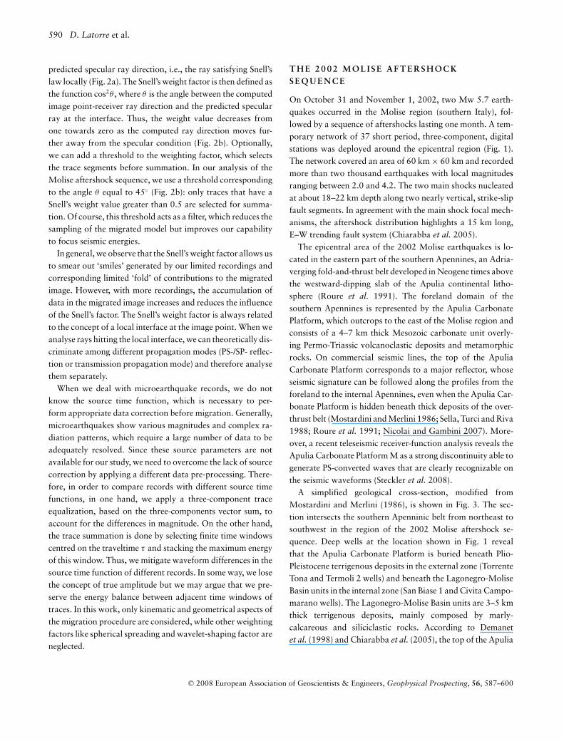
Figure 4 Example of seismograms recordedat four stations of the temporary net-work. Seismograms are rotated in thevertical-radial-transversal system by usingthe hypocenter location from 3D tomo-graphic inversion. Vertical (Z) and Radial(R) components are represented for eachpanel. The red lines point out observed Pand S first-arrival times, whereas the yellowwindows highlight the SP-arrivals. The mapview illustrates both stations (black trian-gles) and earthquake locations (grey dots).Seismograms are band-pass filtered between1 and 50 Hz.

trending cross-sections of Vp and Vp/Vs tomographic models.Tomographic results indicate that the hypocenters of the2002 Molise sequence are mainly located between 7 km and18 km depth. Under these conditions, we can use records of theMolise aftershock sequence to migrate SP-transmitted wavesand image seismic horizons in the well-resolved part of thetomographic volume.

S P T R A N S M I S S I O N M I G R AT I O N O F T H E2 0 0 2 M O L I S E S E Q U E N C E

Our target area extends to the eastern part of the epicentralregion (Fig. 1). We have selected this study area because ofthe opportunity to compare our migrated images with resultsof existing commercial seismic profiles, gravimetric and ex-ploration well data (Mostardini and Merlini 1986; Sella et al.

1988; Roure et al. 1991; Fracassi et al. 2004; Nicolai andGambini 2007).

Our migration model is divided into a grid of 195 435 imagepoints, which are 500 m spaced in the horizontal direction and100 m spaced in the vertical direction. The image points aredistributed in a volume of 22 km × 21 km × 10 km. A locally-horizontal interface is associated with each grid point.

We have analysed three-component seismograms of 789well-located earthquakes recorded at eight receivers of thetemporary network (Fig. 1). We first selected data by storingseismograms with high signal-to-noise level and high-qualityP- and S-wave first-arrival time picks. Then, by using thepassive source locations from the tomographic inversion, wecomputed P and S first-arrival traveltimes in the backgroundvelocity models and rejected data with residual of P and Sfirst-arrival times greater than 0.3 s. Thus, we only used data

C© 2008 European Association of Geoscientists & Engineers, Geophysical Prospecting, 56, 587–600

3D kinematic depth migration of converted waves 593

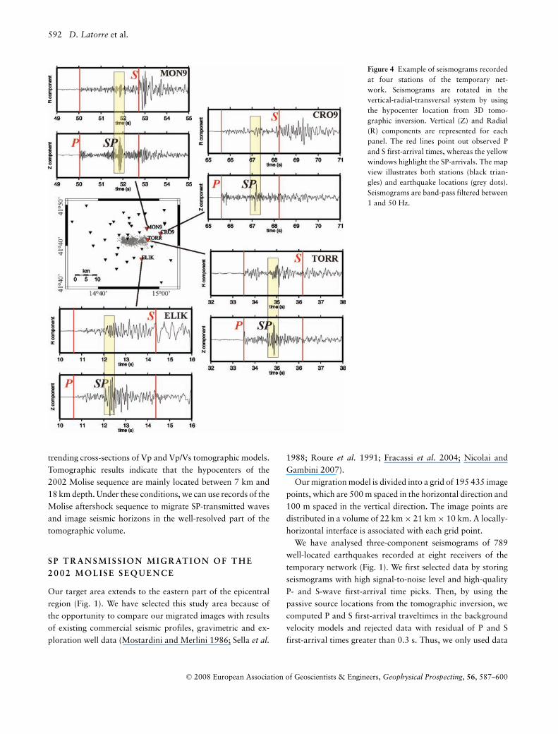
Figure 5 Seismic sections of earthquakes recorded at MON9 station (Fig.1): a) vertical component and b) radial component. Traces are sortedby their S-P time difference (see text) and shifted according to the observed P first-arrival time. Before plotting, traces are normalized andband-pass filtered with a two-pole, zero-phase shift Butterworth filter. We select a frequency band of 25–40 Hz to enhance SP-arrivals on verticalcomponents and frequencies between 1 and 10 Hz to point out S- and PS-arrivals on radial components. In order to analyse the data in a SPconversion mode, we apply a filter with a frequency band of 25–40 Hz.

kinematically consistent with our background velocity mod-els, source locations and origin time. By considering the com-puted residual times of all the selected data, we estimated aroot-mean-square (rms) value of 0.125 s.

Data pre-processing consisted in filtering, normalizing andmuting three-component records. Since we need to enhanceSP-energies and reduce amplitudes associated with PS-arrivals,we filtered data using a band-pass, zero-phase shift But-terworth filter with corner frequencies of 25 Hz and 40 Hz(Fig. 5). First arrivals of P- and S-waves were muted toavoid any interference of their energy with the migrationof SP-waves. Thus, only signals included in the window be-tween P- and S-wave arrivals contributed to the migratedimage. This choice reduces the sampling of the target vol-ume but suppresses artefacts due to misinterpretations of mi-grated signals. Finally, we applied a three-component trace-equalization, which consists in normalizing the traces for themaximum value of the vector sum computed at each pointin time on the three-component signal. In this way, we cor-rect seismograms for different source magnitudes and receiverresponses.

Data migration is performed by assuming a SP-transmissionpropagation mode, i.e., we migrate and sum the trace energiesby supposing that only SP-waves propagate in the medium andconvert to potential transmitting boundaries. Therefore, in ouranalysis, we reject energies associated to possible reflectionsat the image points.

Figure 7 shows some map views of the SP-migrated imagefrom the vertical-component seismograms. Each pixel rep-resents an image point and the colours indicate the relativeamount of focused SP-energy, i.e., the migrated and stackedSP-energy is normalized with respect to the maximum valueof the model. High relative values indicate high SP-energy fo-cusing and can be interpreted as the most likely transmittingboundaries where observed SP-signals may be generated. Wealso note that part of the migrated image is not sampled (greypixels). This arose from several causes, including 1) the mutingapplied in the data pre-processing, 2) the Snell’s weight factorwith threshold, 3) the trace selection due to the assumption ofa SP-transmission propagation mode and 4) a threshold usedto reject those parts of the image that only have a few inputtraces contributing to them (we used a minimum threshold of30 traces). Although these constraints limit the coverage of the

C© 2008 European Association of Geoscientists & Engineers, Geophysical Prospecting, 56, 587–600

594 D. Latorre et al.

Figure 6 NE–SW trending cross-sections of the tomographic models from De Gori et al. (pers. comm.): a) P-velocitymodel, b) Vp/Vs model and c) location of the cross-section with respect to the aftershock sequence (dots) and the tomographic inversiongrid (dark, cross-shaped symbols). The dashed black line on the cross-sections depicts the spread function contouring for values lower or equalto 2.0. This contour delimits the well-resolved area of the tomographic models.

imaged volumes, they avoid artefacts that blur the migratedimage.

The main features of our results are the high SP-focusingzones that are concentrated between 1 km and 6 km depth.Shallower SP-focusing zones are located in the northeasternpart of the investigated area (about 1–2 km depth), whereasthese zones deepen progressively towards the southwest up to5–6 km depth. All the high SP-focusing zones seem to delin-eate an almost continuous seismic horizon, which gently dipstowards the southwest.

In order to analyse and validate our results in the light ofindependent data, we have compared a vertical cross-sectionof the migrated model with a profile extracted from a 3D mapof the Apulia Carbonate Platform top, recently published byNicolai and Gambini (2007). This 3D reconstruction has beenobtained by combining well data and proprietary oil industryseismic data with geological and geophysical published infor-mation.

Figure 8 shows a vertical cross-section of the migrated im-age and the superimposed Apulia Carbonate Platform top pro-file that we have extracted from the 3D map of Nicolai andGambini (2007). Both the vertical cross-section of the mi-grated image and the Apulia Carbonate Platform top profilehave the same geographical location, as indicated in Figs 1and 7. Our selected cross-section is located about 1 km SE of

the Rotello 3 well and 4 km NW of Monacilioni 1 and Tor-rente Tona 1 wells. Mostardini and Merlini (1986) used datafrom Monacilioni 1 and Torrente Tona 1 wells to constraintheir structural model (Fig. 3).

By taking into account the limits of our parameterization,we note that both the geometry and depth of the high SP-focusing zones are consistent with some areas of the Apu-lia Carbonate Platform top. High SP-focusing zones correctlymatch the Apulia Carbonate Platform top in the northeast-ern part of the model, between the town of San Giuliano andthe well of Torrente Tona (Fig. 8). High SP-focusing zonescan also be correlated to the Apulia Carbonate Platform topin the area of the Monacilioni well (southwestern part of themodel). Here, the seismic horizon shows the same geometry ofthe Apulia Carbonate Platform top but appears slightly deeper(from 100 m to 300 m), even though this discrepancy can beconsidered small compared to the vertical spacing grid of ourmigration model (100 m).

By contrast, the seismic horizon seems to follow a differ-ent trend just above seismogenic areas. Its geometry seems tobe more complicated than the Apulia Carbonate Platform topprofile from Nicolai and Gambini (2007), while its depth isgenerally greater, showing a maximum discrepancy that ex-ceeds 1000 m. In this part of our migrated model, the seismichorizon geometry seems to be more similar to the Mostardini

C© 2008 European Association of Geoscientists & Engineers, Geophysical Prospecting, 56, 587–600

3D kinematic depth migration of converted waves 595

Figure 7 Horizontal sections of the SP-transmission migrated image for vertical-component seismograms. Layers intersect the migrated volumeat different depths (Z = 1–6 km depth). The target area (coloured part of each layer) is located inside the tomographic model volume, whichcovers a region of about 60 km × 60 km (Fig. 6). Each point of the migrated image is represented by a pixel, whose colour indicates the relativeamount of focused SP-energy. The grey colour represents pixels not sampled by our data. Inverted triangles and black dots indicate the projectionof station and earthquake locations, respectively. The black crossing line is the trace of the NE–SW vertical section shown in Fig. 8.

and Merlini’s model (Fig. 3), in which SW-dipping normalfaults create a step-like geometry of the Apulia CarbonatePlatform top beneath the San Giuliano town and a NE-vergingthrust system increases the complexity of the Apulia Carbon-ate Platform tectonic structure. Different hypotheses can beinvoked to explain the discrepancy between the migrated seis-mic horizon and the Apulia Carbonate Platform top fromNicolai and Gambini (2007) in the seismogenic area of the2002 Molise sequence; we will discuss them after the sensitiv-ity analysis of our model.

S E N S I T I V I T Y O F T H E M I G R AT E D M O D E L

In this last section, we discuss the different results obtained bymodifying some input parameters in our migration procedure.The first parameter is the length of the trace segment, whichis selected to perform the sum of the migrated energies. Whenconstructing an image point, we stack energies corresponding

to the trace segment centred on the traveltime τ , i.e., the trav-eltime along the total raypath from the source to the imagepoint and from the image point to the receiver (Fig. 2a). Thechoice of this segment length (here called twin) can influencethe final migrated image (Fig. 9).

When we choose a segment length equal to the samplingrate of our seismic records (twin = ±dt, where dt is the sam-pling rate of 0.008 s), the image is not well focused every-where (Fig. 9a). However, if we increase the segment lengthsize, we enhance the SP-focusing zones around the Apulia Car-bonate Platform top profile (Figs 9b and 9c). The use of asmall segment length should imply that computed traveltimesare perfectly consistent with both background velocity modelsand source hypocenter locations (position at depth and origintime). Nevertheless, this is an ideal condition. Actually, ourselected data show P and S residual first-arrival times such asto have a rms of 0.125 s, which suggests some discrepancy ofour data with respect to the background velocity models and

C© 2008 European Association of Geoscientists & Engineers, Geophysical Prospecting, 56, 587–600

596 D. Latorre et al.

Figure 8 Comparison between a NE–SW trending cross-section ofthe migrated model and a vertical profile of the Apulia CarbonatePlatform top extracted from the 3D reconstruction by Nicolai andGambini (2007). The Apulia Carbonate Platform top is representedby a black line. Both the vertical cross-section of the migrated modeland the Apulia Carbonate Platform top profile intersect the studyarea along the same trace plotted in Figs 1 and 7. In this NW–SEvertical cross-section are plotted the projections of the Monacilioniwell, located ∼4 km SE of the profile, the Rotello 3 well (R3), located∼1 km NW and the Torrente Tona 1 well, located ∼4 km SE. Thestations used in this work are also plotted (inverted triangles) and theevents located close to the cross-section (black open circles). As inFig. 7, the colour bar indicates the relative amount of focused SP-energy (values equal to 1 represent the highest value in the migratedmodel).

the passive source locations. Therefore, in order to take intoaccount this discrepancy, it is reasonable to increase the tracesegment length, while requiring its size to be lower than therms value computed on the residual times.

The second aspect we want to outline concerns the use ofthe Snell’s factor in weighting migrated trace energies beforesummation (Fig. 2). As an example, we have applied thesame migration procedure to our data without imposing anyweighting factor (Fig. 10a). This condition is equivalent toconsidering each grid point as a scattering point. The migratedimage of Figure 10(a) shows a large amount of SP-energy,which is spread out along complex trajectories. By comparingthis image with the APC top, we note that only a part ofthe SP-focusing zone matches the target horizon, whereaslateral branches probably arise from the poor coverage of the

Figure 9 Sensitivity of the migrated image with respect to our choice ofthe length (twin) of the trace segment used in the migration procedure(see text for further details). Three NE–SW cross-sections of the SP-transmission migration image are plotted: a) migrated image obtainedby using a twin = ±dt (dt is the seismogram sampling rate), b) migratedimage obtained by using a twin = ±5dt and c) migrated image obtainedby using a twin = ±0.1 s (±12.5dt). Symbols are the same as in Figs 7and 8. The model plotted in Fig. 9(c) is the same as in Fig. 8.

C© 2008 European Association of Geoscientists & Engineers, Geophysical Prospecting, 56, 587–600

3D kinematic depth migration of converted waves 597

Figure 10 Sensitivity of the migrated image to the application of aweight factor in the migration procedure. Both the NE–SW cross-sections represent the migrated images obtained by applying the samemigration procedure but different weight factors: (a) migrated imagewithout weight factors and (b) migrated image with weight factors. Inthe first model (a), we assume that image points are scattering points,while in the second (b) we assume that image points are potentialtransmission boundaries. The model plotted in Fig. 10(b) is the sameas in Figs 8 and 9(c).

migrated volume, which is related to the sparse distribution ofboth sources and receivers. By contrast, the use of the Snell’sweight factor greatly improves the SP-focusing on the targethorizon (Fig. 10b). In this second case, we have assumed thateach image point corresponds to an oriented local interface.In particular, we have chosen a locally-horizontal interface be-cause it is the simplest geometry as possible and because weexpect that the target horizon is not steeply-dipping, consis-

tent with the regional geology (Mostardini and Merlini 1986;Roure et al. 1991; Nicolai and Gambini 2007).

It is important to highlight the effects of the weighting func-tion in our migrated image. By using a weighting functionfor a horizontal interface, we do not prevent our capabilityto focus seismic energies generated at moderately dipping in-terfaces. Indeed, we have shown that we correctly image thegently dipping structure of the Apulia Carbonate Platform topin the area located between the town of San Giuliano and theTorrente Tona well and are able to identify the geometry ofthe structure beneath the Monacilioni well (Fig. 8). In practice,the Snell’s weight function acts as a filter that modulates thetrace energies as the ray direction moves farther away from thespecular condition. By imposing a horizontal interface and athreshold of θ = 45◦, we suppress seismic energies associatedto very steeply dipping seismic structures (with dips greaterthan 45◦) but we are always able to focus transmitted en-ergy from seismic horizons dipping less than 45◦, althoughthis energy is weighted differently. Of course, we have to beaware that the weight factor can bias the results by reducingthe brightness of the seismic horizon when it is dipping insteadthan locally horizontal. Nevertheless, the weighting factor hasnot an effect on the depth of the seismic horizon, which isactually controlled by the kinematics of the wave propaga-tion in the background velocity model. Thus, although wecannot interpret our results in terms of amplitude variationsalong a seismic horizon, we show that kinematic aspects of mi-gration are enough to image geometry and position at depthof seismic structures with moderate dips, into the limits ofour resolution. The example of Fig. 10 also demonstrates thatthe use of the Snell’s weight factor is necessary to overcome theproblem of the sparse acquisition geometry in passive-sourceimaging.

D I S C U S S I O N A N D C O N C L U S I O N

In this study, we show and demonstrate the effectiveness of amigration technique applied to passive source data for imag-ing subsurface structure. In our example, we point out thatsome reasonable precautions should be taken into account toconveniently employ microearthquake records as controlledsources. We outline the importance of using both background3D velocity models and source parameters estimated throughfirst-arrival time tomographic inversion. Moreover, we showthat significant improvement in focusing migrated energiesand reducing image artefacts can be achieved with opportuneinput parameters and selecting data kinematically consistentwith background velocity models.

C© 2008 European Association of Geoscientists & Engineers, Geophysical Prospecting, 56, 587–600

598 D. Latorre et al.

The region of the 2002 Molise aftershock sequence has rep-resented an excellent laboratory to test our procedure withreal passive data, due to both the high quality data and thepresence of clear converted phases. The existence of indepen-dent data providing a reconstruction at depth of the majorseismic horizon allowed us to validate the results and analysethe sensitivity of the migrated models.

The seismic images obtained by SP-wave migration of the2002 aftershock sequence indicate that the observed large-amplitude SP-converted waves were generated at the top ofthe Apulia Carbonate Platform. Through our images, we areable to reconstruct the position at depth of the seismic horizonthat we associate to the top of the Apulia Carbonate Platform.

The NE and SW parts of our migrated horizons are imagedat about 2 km and 4–5 km depth respectively, showing a ge-ometry that gently dips toward southwest (Fig. 8), which isin agreement with previous studies (Mostardini and Merlini1986; Fracassi et al. 2004; Nicolai and Gambini 2007). How-ever, there are some discrepancies between our results and theApulia Carbonate Platform top from Nicolai and Gambini(2007) above the seismogenic area, which is marked by theaftershock sequence distribution (Fig. 8). In particular, ourimages outline: 1) a more complicated geometry of the Apu-lia Carbonate Platform top, which also seems to be locateddeeper than the Apulia Carbonate Platform top from Nicolaiand Gambini (2007) and 2) a weaker brightness of the SP-focused zone with respect to the external parts of the seismichorizon (i.e., the NE and SW parts).

Because the kinematic aspect of the wave propagation (trav-eltime) controls the position at depth of the high SP-focusingzones, our results may be affected by our choice of the back-ground velocity model. If we refer to the Apulia CarbonatePlatform model from Nicolai and Gambini (2007), the dis-crepancy of the migrated image may be interpreted as an in-adequacy of our background velocity model in the seismo-genic area, which does not allow us to correctly locate theseismic horizon at depth. In this sense, a further update of thebackground velocity model in this area may lead to reducethe observed discordance. On the other hand, we remark thatthe complexity of the migrated horizon is similar to that ofthe structural model of Mostardini and Merlini (1986). Inparticular, we note some similarities at NE, where the Apu-lia Carbonate Platform top appears disconnected by a systemof high-angle normal faults dipping to SW and in the area ofthe Monacilioni well, where a complex NE-verging thrust sys-tem is proposed by Mostardini and Merlini (1986) (Fig. 3). Inagreement with the latter model, we suggest that the ApuliaCarbonate Platform structure is effectively more complex than

that proposed by the Nicolai and Gambini’s model. If this isthe case, a possible explanation for the discrepancy is that themigrated horizon in the seismogenic area does not correspondto the top of the Apulia Carbonate Platform but to one ofthe seismic horizons involved in the thrust system identifiedby Mostardini and Merlini (1986). This interpretation may besupported by the fact that our image is the result of a seismicmigration that assumes a transmission propagation mode anda particular source-receiver layout and where the medium islightened differently (from depth to the surface) with respectto classical seismic reflection studies.

Changes in brightness of migrated horizons can be related tovariations of converted wave incidence angles, density and/orvelocity properties. Although our observations indicate strongcoherent lateral variations of P-wave velocity distribution inour tomographic models (Fig. 6), nevertheless, as previouslydiscussed, we have to be aware that the use of the kine-matic weight factor can bias the brightness of the reflec-tor/transmitting horizon image when we are dealing with dip-ping/undulating structures instead of locally horizontal inter-faces. For this reason, at the present, we cannot discriminatewhether this feature is an effect of our kinematic approach ora result of real changes in physical properties of the medium,as suggested by our tomographic models. This requires furtherinvestigation, through the analysis of the entire dataset of the2002 Molise aftershock sequence, the application of the mi-gration procedure to analyse PS mode-converted waves and amodified migration procedure, which also takes into accountthe amplitude in passive data analysis.

It should be noted that the reconstruction of the Apulia Car-bonate Platform top from deep wells and commercial seismicprofiles is very well constrained in productive areas, such asthe Val d’Agri region, south of our study area, or in externalregions near the coast, where a large amount of deep wells isconcentrated (Fig. 1). Nevertheless, in the internal part of theApennines, the seismic reflection coverage is still sparse andvery few wells are drilled (Fig. 1). Since depth conversion ofcommercial seismic lines was performed using average veloc-ities from well data (Nicolai and Gambini 2007), it is likelythat their Apulia Carbonate Platform top reconstruction is lessconstrained in internal Apennines, as for example the epicen-tral area of the 2002 Molise aftershock sequence, with respectto the external regions. We therefore believe that the natureof the Apulia Carbonate Platform structure in the epicentralarea of the 2002 Molise earthquake remains unresolved andrequires further investigation.

Locating crustal discontinuities has important implicationsfor geodynamical reconstruction and tectonic models, as well

C© 2008 European Association of Geoscientists & Engineers, Geophysical Prospecting, 56, 587–600

3D kinematic depth migration of converted waves 599

as for identifying potential oil and gas reservoirs. With thispurpose, the use of passive sources for seismic migration imag-ing offers considerable complementary information with re-spect to classical tomographic studies in seismogenic areas.This study demonstrates the usefulness of our migration pro-cedure and allows us to extend its application to image theseismic structure of other seismogenic areas, using aftershockdata or background seismicity.

A C K N O W L E D G E M E N T S

This work has been greatly improved thanks to the help oftwo anonymous reviewers. We thank F. Villani, U. Fracassi, G.Improta and P. Scandone for constructive discussions. Manyfigures have been drawn using the free software GMT (Wesseland Smith 1991). We used the Seismic Unix package (Cohenand Stockwell, Colorado School of Mines) to display data ofFig. 5. The CONV code for converted wave kinematic migra-tion is part of the PhD thesis of Diana Latorre at the UMR Geo-sciences Azur (Nice, France). The seismic data were recordedby the INGV mobile seismic network, managed with the sup-port of the Italian Dipartimento della Protezione Civile. Wethank the INGV staff that collected the seismic network data.Diana Latorre and Alessandro Amato acknowledge the projectAirplane (contract no. RBPR05B2ZJ, UR 3), funded by theItalian Ministero dell’Universita e della Ricerca.

R E F E R E N C E S

Chavarria J.A., Malin P.E., Catchings R.D. and Shalev E. 2003. A lookinside the San Andreas Fault at Parkfield through vertical seismicprofiling. Science 302, 1746–1748.

Chavez-Perez S. and Louie J.N. 1998. Crustal imaging in southernCalifornia using earthquake sequences. Tectonophysics 286, 223–236.

Chiarabba C., De Gori P., Chiaraluce L., Bordoni P., Cattaneo M.,De Martin M. et al. 2005. Mainshocks and aftershocks of the 2002Molise seismic sequence, southern Italy. Journal of Seismology 9,487–494.

Demanet D., Margheriti L., Selvaggi G. and Jongmans D. 1998. Uppercrustal structure in the Potenza area (Southern Apennines, Italy),using Sp converted waves. Annali di Geofisica XLI, 105–119.

Fracassi U., Burrato P., Basili R., Bencini R., Di Bucci D. andValensise G. 2004. Shallow NE–SW extension and deep E–W right-lateral slip: Coexisting seismogenic mechanisms as an expressionof southern Italy geodynamics. 23rd Gruppo Nazionale GeofisicaTerra Solida Symposium, Rome, Italy, Expanded Abstracts, pp.200–202.

Hole J.A. 1992. Nonlinear high-resolution three-dimensional seismictraveltime tomography. Journal of Geophysical Research 97, 6553–6562

James D.F., Clarke T.J. and Meyer R.P. 1987. A study of seismic reflec-tion imaging using microearthquake sources. Tectonophysics 140,65–79.

Latorre D. 2004. Imagerie sismique du milieu de propagation a partirdes ondes directes et converties: application a la region d’Aigion(Golfe de Corinthe, Grece). PhD thesis, Universite de Nice-SophiaAntipolis, France.

Latorre D., Virieux J., Monfret T. and Lyon-Caen H. 2004a.Converted seismic wave investigation in the Gulf of Corinthfrom local earthquakes. Comptes Rendus Geosciences 336, 259–267.

Latorre D., Virieux J., Monfret T., Monteiller V., Vanorio T., Got J.-L. et al. 2004b. A new seismic tomography of Aigion area (Gulfof Corinth, Greece) from the 1991 data set. Geophysical JournalInternational 159, 1013–1031.

Le Meur H., Virieux J. and Podvin P. 1997. Seismic tomography ofthe Gulf of Corinth: A comparison of methods. Annali di GeofisicaXL, 1–25.

Louie J.N., Chavez-Perez S., Henrys S. and Bannister S. 2002. Multi-mode migration of scattered and converted waves for the structureof the Hikurangi slab interface, New Zealand. Tectonophysics 355,227–246.

Michelini A. and McEvilly T.V. 1991. Seismological studiesat Parkfield, I, Simultaneous inversion for velocity structureand hypocentres using cubic b-splines parameterization. Bul-letin of the Seismological of Society of America 81, 524–552.

Mostardini F. and Merlini S. 1986. L’Appenino centro-meridionale –Sezioni geologiche e proposta di modello strutturale. Memorie dellaSocieta Geologica Italiana 35, 177–202.

Nicolai C. and Gambini R. 2007. Structural architecture of the Adriaplatform-and-basin system. Bollettino Societa Geologica Italiana 7,21–37.

Nisii V., Zollo A. and Iannaccone G. 2004. Depth of a midcrustaldiscontinuity beneath Mt. Vesuvius from the stacking of reflectedand converted waves on local earthquake records. Bulletin of theSeismological Society of America 94, 1842–1849.

Podvin P. and Lecomte I. 1991. Finite difference computation of trav-eltime in very contrasted velocity model: A massively parallel ap-proach and its associated tools. Geophysical Journal International105, 271–284.

Roure F., Casero P. and Vially R. 1991. Growth process and melangeformation in the southern Appenines accretionaly wedge. Earth andPlanetary Science Letters 102, 395–412.

Sella M., Turci C., and Riva A. 1988. Sintesi geopetrolifera della FossaBradanica (avanfossa della catena appenninica meridionale). Mem-orie della Societa Geologica Italiana 41, 87–107.

Steckler M.S., Agostinetti N.P., Wilson C.K., Roselli P., Seeber L.,Amato A. et al. 2008. Crustal structure in the Southern Apenninesfrom teleseismic receiver functions. Geology (in press).

Stroujkova A.F. and Malin P.E. 2000. A magma mass beneath CasaDiablo? Further evidence from reflected seismic waves. Bulletin ofthe Seismological Society of America 90, 500–511.

Thurber C.H. 1983. Earthquake locations and three-dimensionalcrustal structure in the Coyote Lake area, Central California. Jour-nal of Geophysical Research 88, 8226–8236.

C© 2008 European Association of Geoscientists & Engineers, Geophysical Prospecting, 56, 587–600

600 D. Latorre et al.

Thurber C.H. 1993. Local earthquake tomography: Velocity andVp/Vs-theory. In: Seismic Tomography: Theory and Pratice(edsH.M. Iyer and K. Hirahara). CRC Press, Boca Raton,FL.

Toomey D.R. and Foulger G.R. 1989. Tomographic inversion oflocal earthquake data from the Hengill-Grensdalur central vol-

cano complex, Iceland. Journal of Geophysical Research 94,17,497–17,510.

Wessel P. and Smith W.H.F. 1991. Free software helps map and displaydata. Eos Transactions, American Geophysical Union 72, 441.

Yilmaz O. 2001. Seismic Data Analysis: Processing, Inversion andInterpretation of Seismic Data. SEG.

C© 2008 European Association of Geoscientists & Engineers, Geophysical Prospecting, 56, 587–600