Simultaneous inversion of the aftershock data of the 1993 Killari

Simultaneous inversion of the aftershock data of the1993 Killari earthquake in Peninsular India and its

seismotectonic implications

S Mukhopadhyay1∗, J R Kayal2, K N Khattri3 and B K Pradhan1

1Department of Earth Sciences, Indian Institute of Technology (formerly University of Roorkee),Roorkee, Uttaranchal 247 667, India

2Geological Survey of India, Central Geophysics Division, 27 J.L.N. Road, Kolkata 700 016, India3100 Rajendra Nagar, Dehra Dun, Uttaranchal 248 001, India

∗e-mail: [email protected]

The aftershock sequence of the September 30th, 1993 Killari earthquake in the Latur district ofMaharashtra state, India, recorded by 41 temporary seismograph stations are used for estimating3-D velocity structure in the epicentral area. The local earthquake tomography (LET) method ofThurber (1983) is used. About 1500 P and 1200 S wave travel-times are inverted. The P and Swave velocities as well as VP /VS ratio vary more rapidly in the vertical as well as in the horizontaldirections in the source region compared to the adjacent areas. The main shock hypocentre islocated at the junction of a high velocity and a low velocity zone, representing a fault zone at6–7 km depth. The estimated average errors of P velocity and VP /VS ratio are ±0.07 km/s and±0.016, respectively. The best resolution of P and S-wave velocities is obtained in the aftershockzone. The 3-D velocity structure and precise locations of the aftershocks suggest a ‘stationaryconcept’ of the Killari earthquake sequence.

1. Introduction

A devastating earthquake (mb = 6.3) occurred inthe early morning (03 h 55 m local time) of Sep-tember 30th, 1993 in the southern part of the sta-ble continental region (SCR) of Peninsular India,in the Latur district of Maharashtra state, India.The earthquake caused widespread damage; about8,000 people died, 16,000 injured and more than200,000 houses were extensively damaged in 2400villages spread across 13 districts of the state ofMaharashtra (GSI 1996; Seeber et al 1996). A max-imum intensity of VIII+ (MSK scale) was assignedto this earthquake (figure 1).

The hypocentre parameters (table 1) of the mainshock were reported by the United States Geo-logical Survey (USGS), GEOSCOPE (Baumbachet al 1994), Harvard University (HRV), India Mete-

orological Department (IMD) and National Geo-physical Research Institute (NGRI). The NGRIlocation included the global network data, thenational network (IMD) data and the data of theNGRI/GEOSCOPE observatory at Hyderabad,the nearest station to the epicenter. The NGRIlocation is shown in figure 1. The epicenter lies nearthe Killari village, at the junction of the Tirna riverand its tributary. The focal depth of the main shockis, however, debated. The various estimated depthsthat range from 2.6 km to 15 km are shown in table1. Kayal (2000), based on aftershock investiga-tion results, argued that the most acceptable focaldepth of the main shock is 7±1 km as estimated byChen and Kao (1995). The fault-plane solution ofthe main shock, as reported by the USGS, revealsa reverse faulting. The Centroid Moment Tensor(CMT) solution by the HRV also shows a reverse

Keywords. Killari earthquake aftershocks; simultaneous inversion; stable continental region.

Proc. Indian Acad. Sci. (Earth Planet. Sci.), 111, No. 1, March 2002, pp. 1–15© Printed in India. 1

2 S Mukhopadhyay et al

Figure 1. Map showing the main shock epicentre (NGRI), meizoseismal zone (intensity VIII) and the fault plane (CMT)solution of the main shock (after Kayal 2000).

faulting; both the solutions suggest dip slip motionwith a small strike-slip component (figure 1).

Fortyone temporary microearthquake (MEQ)stations were established by various national andinternational organizations to monitor the after-shocks. They have analyzed their respective net-work data and reported about the seismicity pat-tern (Baumbach et al 1994; Kayal et al 1996; Gupta

Table 1. Main shock parameters.

Origin time Lat. Long. Depth Magnitude(UTC) ◦ N ◦ E km mb Source

22:25:48.6 18.07 76.45 6.8 6.3 USGS22:25:48.6 18.02 76.56 15.0 6.1 GEOSCOPE22:25:48.01 18.01 76.56 6.0 6+ NGRI22:25:48.11 18.11 76.55 15.0 HRV22:02:49.35 18.07 76.62 6–12 6.3 IMD

7 ± 1 Chen and Kao (1995)6.5 ± 0.1∗ Ramesh and Estabrook (1998)2.6 ± 1.0∗ Seeber et al (1996)

∗Centroid depth. The GEOSCOPE data are after Baumbach et al (1994).

et al 1998). No report is, however, published onthe 3-D velocity structure of the Killari earthquakesource area. In the present work, we have used thecollated seismic phase data recorded by the above41-station MEQ network for the estimation of 3-Dvelocity structure by the local earthquake tomogra-phy (LET) method, and relocated the aftershocks.Results of this study are presented here.

Aftershock data of the 1993 Killari earthquake 3

2. Geology and tectonic setting

Geologically the area belongs to the Deccan TrapPlateau basalts of the Paleocene age that are com-posed of a series of lava-flows in western and cen-tral India (Wadia 1998). The Deccan Traps lieunconformably on the Precambrian basement ofthe Indian shield. Since the Deccan Trap lava blan-keted pre-existing tectonic features over a consid-erable area, the stratigraphy of the underlying for-mations is a matter of wide speculation. If con-tinuation of the older formations exposed on thefringes of the Deccan Traps is assumed, then it maybe inferred that the underlying formations may beany one or more of the Precambrian Dharwar for-mations, Precambrian granites and gneisses, Pro-terozoic Kaladgi and Bhima sediments and Gond-wana (Permo-Carboniferous to Jurassic) sedimen-tary formations (Mohan and Rao 1994).

The ancient shields are, in general, stable exceptfor the continental margins, rift zones etc. Thesouthern part of the Peninsular India has long beendescribed as a region of low seismicity. Recentlythe 1997 Jabalpur earthquake (mb 6.0) occurredin the Narmada-Son Lineament (NSL) rift zone,and occurred in the area where seismic activity isknown to be present (Acharyya et al 1998; Rajen-dran and Rajendran 1998). On the other hand,the seismic hazard zonation map of India (Krishna1992) depicts that the Killari area falls to the southof the NSL zone, which is marked as zone-I, and isgenerally regarded to be stable.

However, it is reported that before the Killariearthquake of September 30th, 1993, there werea number of smaller magnitude shocks betweenOctober and November, 1992 (Baumbach et al1994; Gupta et al 1998). Twenty six tremorswere recorded by the NGRI/GEOSCOPE obser-vatory at Hyderabad Seismological Observatoryfrom October 18th to November 15th, 1992 in theKillari region. The largest magnitude earthquake,(M = 4.0) was recorded on October 18th, 1992.As there were no seismic stations in the vicinity ofthis activity, shocks with magnitude less than 2.0could not be recorded. Khattri (1994) attributesthe seismicity of Peninsular India to block tectonicswith a strain field being caused by the Indian platemotion. According to this hypothesis, the earth-quakes are expected to occur at the boundary ofthe two blocks. The significant faults are either inNE or NW directions.

Detailed geophysical investigations comprising ofgravity, magnetic, magnetotelluric and deep resis-tivity surveys were carried out in the Killari areaafter the main shock. The detailed gravity surveyrevealed three faults, two in the E-W and the otherin the NW-SE directions in the epicentral area(Mishra et al 1994). Ramchandran and Kesava-

mani (1997) made a detailed structural interpre-tation of the regional gravity map, and delineateda major structural discontinuity (called BLHV) insegments from west coast to east coast. They fur-ther suggested that several transverse faults tran-sect the BLHV in NE-SW, N-S and NW-SE direc-tions. In the Killari area it is in NW-SE direc-tion. Sarma et al (1994) have reported the resultsof 16 wide band range (103 Hz–10−3 Hz) magne-totelluric soundings conducted in the region. Theyfound an anomalously shallow upper crustal con-ductor in the hypocentral zone embedded in a highresistive upper crust at a depth of 6–8 km. The con-ductor is oriented in a WNW-ESE direction. In areview paper, Kayal (2000) suggested that the Kil-lari earthquake and its aftershocks involved inter-action of two faults beneath the study area.

3. Data sources

The aftershocks were recorded by both analogand digital seismographs of the temporary andpermanent networks. Fortyone temporary stationsstarted operating eight to ten days after the mainshock and continued for four months. The tempo-rary stations were installed and operated by theGeological Survey of India (GSI), the India Mete-orological Department (IMD), the Wadia Insti-tute of Himalayan Geology (WIHG), Delhi Uni-versity and by the German Task Force (GTF)team in collaboration with the National Geophys-ical Research Institute (NGRI). The GSI estab-lished a five-station MEQ network equipped withPS-2 (kinemetrics) analog recorders on October8th, 1993. This network was run till 16th February,1994 (Kayal et al 1996). The IMD also operatedfive microearthquake (MEQ) stations with analogrecorders. The WIHG and the Delhi Universityoperated two stations each with analog and digitalrecorders respectively. The NGRI installed sevensingle component analog recorders. All the ana-log seismographs were operated with vertical com-ponent seismometer. The GTF team establishedfive 3-channel digital data acquisition systems, fourthree-component strong-motion recording instru-ments, and eleven analog systems; these stationswere run till the end of December 1993 (Baumbachet al 1994).

The three permanent stations, viz., those atHyderabad, Bombay and Poona, were the nearest(distance < 300 km) observatories which recordedonly a few aftershocks of relatively greater magni-tude (MD > 2.5). As these stations are too far awayfrom the study area, the few aftershock phase-datawere not enough to provide adequate ray cover-age between the aftershock zone and these stations.


Figure 2. Examples of Wadati diagrams showing good fit of the data.

Hence, the permanent station data were ultimatelynot used in this study.

A total number of 210 aftershocks recorded bythe temporary stations were selected for initialanalysis. For all the aftershocks Wadati diagramswere drawn to check the quality of the data. Tworepresentative Wadati diagrams are shown in fig-ures 2(a) and (b). The S phase data for stationsfor which the data points in the Wadati diagramshowed large fluctuation from a straight line fit(more than 1 standard deviation) were removed.

After careful examination of the P - and S-phasedata, it was found that 22 events provide inade-quate information required for simultaneous inver-sion; these events were discarded. Finally, 188events with about 1500 P -arrival and 1200 S-arrival data were used for the inversion.

4. Data analysis

In order to use the LET program to find 3Dvelocity structure as well as improved estimates of


Figure 3. Map showing initial estimates of the aftershock epicenters using a 1-D velocity model and HYPO-71 pro-gram (see text). The NGRI and USGS estimates of the main shock are shown by inverted open and filled triangles,respectively.

hypocentral parameters, one needs to know at leasta 1D velocity model of the area, and the prelim-inary estimates of hypocentral parameters. Prad-han (1999) used the Wadati-Riznichenko method(Simpson and Nicholson 1985) to determine the 1Dvelocity structure and used the HYPO71 program(Lee and Lahr 1975) for obtaining preliminary esti-mates of hypocentral parameters. He obtained avelocity of 4.95 km/s for the upper most 2 km,5.82 km/s for the next 10 km and 6.61 km/s for thecrust below 10 km.

For the final analysis, the method of LET, asgiven by Thurber (1983) and later modified byEberhart-Phillips (1993), was used. This methodparallels that of Aki and Lee (1976). The fun-damental improvement by Thurber (1983) usedin this method is the use of 3D ray-tracing tocalculate P -wave travel time (forward modelling).This permits the treatment of laterally varyingvelocity structure, which in turn allows for iter-ative improvement of the solution of earthquakelocations and three dimensional earth structure.Eberhart-Phillips (1993) modified the program sothat S-wave arrivals could also be incorporatedfor the estimation of 3-D variation of S velocityand that of the VP /VS ratio. The inverse prob-lem to be formulated is generally overdetermined

and the earth structure is represented in threedimensions by the velocity defined at a large num-ber of discrete grid points, in contrast to themodel of Aki and Lee (1976) where velocities aredescribed inside the volume of each block. Thevelocity at a given point is determined by inter-polation among the surrounding grid points. Theincorporation of the 3D ray tracing permits thesolution to be achieved iteratively. An importantconsequence is that the variance reduction achievedat each iteration can be directly computed ratherthan merely estimated as in the case of Aki andLee (1976).

For choosing the area for 3D velocity study,the initial HYPO71 estimates of epicenters andthe seismograph-station locations were plottedon a map (figure 3). Their areal distributionwas considered to fix the spread of the modelalong EW and NS directions. Along both thesedirections the model area was restricted within100 km, keeping the center of the model at 18◦Nand 76◦30′ E. Figures 4(a) and (b) show theE-W and N-S oriented depth sections, respec-tively, of the initial hypocentres located by usingthe 1D velocity model (table 2). It shows thatfor a number of earthquakes, fixed-depth solu-tions were obtained. The vertical extent of the


Fig

ure

4(a)

E-W

and

(b)

N-S

dept

hse

ctio

nsof

the

afte

rsho

cks

infig

ure

3.M

any

afte

rsho

cks

are

loca

ted

wit

hfix

edde

pth

at10

kmby

the

HY

PO

-71

prog

ram

.T

heN

GR

Ian

dU

SGS

esti

mat

esof

the

mai

nsh

ock

are

show

nby

inve

rted

open

and

fille

dtr

iang

les,

resp

ecti

vely

.


Table 2. Initial velocity model used for preliminary location usingHYP071 (Lee and Lahr 1975) and as a starting model for LET(Thurber 1983).

Depth to the top of the layer P wave velocityin km in km/s

0 4.952 5.82

12 6.61

Figure 5. Map showing the relocated epicentres of the aftershocks using the 3-D simultaneous inversion technique. TheNGRI and USGS estimates of the main shock are shown by inverted open and filled triangles, respectively.

model volume was constrained to be 14 kmfrom the maximum depth of the events in fig-ure 4.

5. Results

The epicenters of the aftershocks located by theLET are shown in figure 5. It appears that mostof the aftershocks occurred in a cluster. The NGRIestimated epicenter of the main shock falls on theSE corner of this cluster, whereas the USGS esti-mated epicenter of the main shock is located about4 to 5 km NW of this cluster. Figures 6 (a and b)show the E-W and N-S depth sections of the after-shocks located by the LET on which the estimated3-D velocity models along 18◦ N and 76.5◦ E respec-tively are superimposed. It is plotted on a 1:1 scale.

If we join the trace of the coseismic surface rup-ture on this section with the main shock hypocen-tre as determined by the NGRI then we find thatthe aftershocks are mostly clustered around thisline. We infer this line to be the projection of thethrust plane on which the main shock occurred forthe following reasons.• The dip of this thrust plane (50◦ S) is compatible

with that of the fault plane (47◦ S) of the mainshock inferred from the CMT solution by HRV.

• The coseismic rupture zone and the main shocklie on this plane.

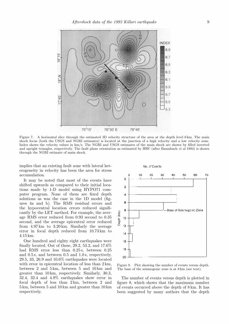
• Most of the aftershocks cluster around thisplane.A horizontal slice at the depth level 6 km through

the estimated velocity model shows that the focusof the main shock falls on the boundary between alow velocity and a high velocity zone (figure 7). It


(a)

(b)

Fig

ure

6.E

-W(a

)an

dN

-S(b

)de

pth

sect

ions

ofth

eaf

ters

hock

s(fi

gure

5),w

hich

are

relo

cate

db y

the

3-D

sim

ulta

neou

sin

vers

ion

tech

niqu

e.T

hese

ctio

nsin

corp

orat

eth

eve

loci

type

rtur

bati

ons

(thi

nlin

es)

obta

ined

byth

ein

vers

ion

tech

niqu

eal

ong

76.5

◦E

and

18◦N

resp

ecti

vely

.T

heN

GR

Ian

dU

SGS

esti

mat

esof

the

mai

nsh

ock

are

show

nby

inve

rted

open

and

fille

dtr

iang

les,

resp

ecti

vely

.A

fter

sho c

ksar

esh

own

byop

enci

rcle

s.


Figure 7. A horizontal slice through the estimated 3D velocity structure of the area at the depth level 6 km. The mainshock focus (both the USGS and NGRI estimates) is located at the junction of a high velocity and a low velocity zone.Index shows the velocity values in km/s. The NGRI and USGS estimates of the main shock are shown by filled invertedand upright triangles, respectively. The fault plane orientation as estimated by HRV (after Baumbach et al 1994) is shownthrough the NGRI estimate of main shock.

implies that an existing fault zone with lateral het-erogeneity in velocity has been the area for stressaccumulation.

It may be noted that most of the events haveshifted upwards as compared to their initial loca-tions made by 1-D model using HYPO71 com-puter program. None of them are fixed depthsolutions as was the case in the 1D model (fig-ures 4a and b). The RMS residual errors andthe hypocentral location errors reduced signifi-cantly by the LET method. For example, the aver-age RMS error reduced from 0.93 second to 0.35second, and the average epicentral error reducedfrom 4.97 km to 3.20 km. Similarly the averageerror in focal depth reduced from 10.73 km to4.15 km.

One hundred and eighty eight earthquakes werefinally located. Out of these, 29.2, 53.2, and 17.6%had RMS error less than 0.25 s, between 0.25and 0.5 s, and between 0.5 and 1.0 s, respectively.29.5, 33, 26.9 and 10.6% earthquakes were locatedwith error in epicentral location of less than 2 km,between 2 and 5 km, between 5 and 10 km andgreater than 10 km, respectively. Similarly, 30.3,32.4, 32.4 and 4.9% earthquakes show error infocal depth of less than 2 km, between 2 and5 km, between 5 and 10 km and greater than 10 kmrespectively.

Figure 8. Plot showing the number of events versus depth.The base of the seismogenic zone is at 8 km (see text).

The number of events versus depth is plotted infigure 8, which shows that the maximum numberof events occurred above the depth of 8 km. It hasbeen suggested by many authors that the depth


Figure 9. E-W oriented vertical slices through the estimated 3-D velocity structure of the study area. Contoured values ofvelocities are in km/s. The slices are 10 km apart; figure 9(a) is the northernmost and figure 9(e) is the southernmost slice,respectively. The central slice (figure 9c) is along latitude 18◦ N. The centre of the section shown by 0 is at 76.5◦ E. Indexshows velocity values in km/s. The NGRI and USGS estimates of the main shock are shown by filled inverted and uprighttriangles respectively.

up to which 90% of the earthquakes occur is thebase of the seismogenic zone (e.g. Sibson 1986; Layand Wallace 1995). They have also suggested thatlarger magnitude earthquakes tend to nucleate atthe base of the seismogenic zone, at the ‘fault end’.Different depth values were reported for the mainshock (table 1). On the basis of our analysis (e.g.figure 8), we believe that the main shock occurredat a depth range 6–8 km, at the base of the seis-mogenic zone, and 90% aftershocks occurred abovethis zone.

The 3D velocity model estimated in the studyarea by the LET method is shown in figures 9 and10. The velocity values along with their error esti-mates and spatial resolutions were obtained for thespecified grid nodes. The average error in the esti-mated P wave velocity values at the grid nodes

is ±0.07 km/s and that in the estimated VP /VS

values are ±0.016 respectively. The velocity vari-ation along vertical slices in E-W and N-S direc-tions through the center of the grid as well asthrough two profiles 10 km and 20 km on eitherside are shown in figures 9 and 10 respectively.The aftershocks as well as the main shock locationsare superimposed on the central vertical slices (fig-ures 6a and b). It is observed from these slices thatmost of the earthquakes occur in a region wherevelocity variation is most rapid both in vertical andlateral directions.

Figure 11(a and b) show the variation of resolu-tion for P wave data in the central E-W and N-S sections respectively. From this figure it is clearthat velocity inversion is the best in the central(40 km × 40 km areal extent) area, and it becomes


Figure 10. N-S oriented vertical slices through the estimated 3-D velocity structure of the study area. Contoured valuesof velocities are in km/s. The slices are 10 km apart; figure 10(a) is the easternmost and figure 10(e) is the westernmostslice respectively. The central slice (figure 10c) is along longitude 76.5◦ E. The centre of the section shown by 0 is at 18◦ N.Index shows velocity values in km/s. The NGRI and USGS estimates of the main shock are shown by filled inverted andupright triangles respectively.

poorer as we go further away from the centre in thelateral direction. This is attributed to the poor raycoverage laterally as most of the events are concen-trated about the center of the study region. Below8 km depth the resolution is again poor becausethe number of earthquakes below this depth is lessthereby giving poor ray coverage.

Figure 12(a and b) show the variation of S wavevelocity along E-W and N-S sections through thecentre of the grid. It shows a pattern broadly sim-ilar to respective sections for P wave velocity (fig-ures 9c and 10c). Figure 13(a and b) show thevariation of VP /VS along E-W and N-S sectionsthrough the center of the grid. The hypocentre ofthe main shock is located in a zone characterizedby low value of VP /VS (∼ 1.64). Comparing thisfigure with figure 6 (a) and (b) we find that theaftershocks too occur within this low VP /VS zone.

6. Discussion

The primary benefits of the LET method are thejoint evaluation of the three dimensional velocitystructure and the earthquake hypocenters, and anunderstanding of the seismogenic fault(s) from theseismic tomography structure.

The E-W and N-S depth sections of the P wavevelocity tomography (figures 9 and 10) show anabrupt change in the velocity structure at the cen-ter of the study area (18◦ N, 76.5◦ E). The N-Sdepth section reveals the presence of a south dip-ping fault at about five kilometers north of the cen-tre (figure 10); the high velocity zones are foundto be displaced vertically by about two kilometers.The hypocentre section in the N-S direction alsoshows that most of the aftershocks occur along asouth dipping plane which meets the surface rup-


Figure 11. E-W (a) and N-S (b) sections through the center (18◦ N, 76.5◦ E, shown as 0) of the study area showingvariations of resolution for P wave velocity. The resolution values are shown along the contours and also in the index. TheNGRI and USGS estimates of the main shock are shown by filled inverted and upright triangles respectively.

Figure 12. E-W (a) and N-S (b) sections through the center (18◦ N, 76.5◦ E, shown as 0) of the study area showingvariations of S-wave velocity. The velocity values are shown along the contours in km/s and also in the index. The NGRIand USGS estimates of the main shock are shown by filled inverted and upright triangles respectively.

ture (figure 6b). This dipping plane is inferred asthe fault plane. Its dip and orientation matcheswith that of the fault plane inferred from the CMTsolution by HRV (figure 1). The E-W depth sec-tions for the velocity structure also show an abruptlateral change in velocity near the fault zone (fig-ure 9c). Three faults, two in nearly E-W directionand the other in NW-SE direction, were inferred inthe epicentral area from the gravity survey (Mishraet al 1994). These fault zones are reflected in thevelocity structure. Kayal (2000) interpreted thatthe main shock as well as the deeper aftershocks(depth ≥ 6 km) were generated by reverse fault-ing along an E-W fault, and the shallower after-

shocks (depth < 6 km) were generated by strike-slip mechanism along the NW-SE fault. He sug-gested a fault interaction model with a ‘stationaryconcept’ rather than a non-stationary concept ofSeeber et al (1996). Rajendran et al (1996) alsoproposed a ‘stationary concept’, i.e., existing faultswere activated to generate the main shock and theaftershocks.

The post earthquake MT investigation hasbrought out the existence of a well defined uppercrustal conductor in the main shock hypocentreregion at an estimated depth of 6–10 km (Sarmaet al 1994). The conductor is interpreted to be afluid enriched rock matrix. They suggested that


Figure 13. E-W (a) and N-S (b) sections through the center (18◦ N, 76.5◦ E, shown as 0) of the study area showingvariation of VP /VS . The VP /VS values are shown along the contours and also in the index. The NGRI and USGS estimatesof the main shock are shown by filled inverted and upright triangles respectively.

the fluid filled rock matrix might be visualized as a‘weak intrusive’ into a hard granitic rock medium.These evidences support a substantial decrease inseismic wave velocity in the hypocentral area. Inthe seismic tomography, the horizontal slice ata depth of 6 km reveals these low velocity zones(figure 7).

The N-S sections, which show the variations ofvelocity with depth, reveal the presence of a lowvelocity zone (LVZ) at a shallower depth at thecentre (figures 10c, d), which is comparable withthe inferred E-W fault/the Tirna river. This zonelaterally extends to about 30 km in the east-westdirection. At a depth of about 6 km a high velocityzone (HVZ) is observed 10 km north of the 18◦ Nlatitude in the three N-S sections (figures 10a, band c). This HVZ becomes smaller and it shiftstowards a shallower depth (figure 10d). A HVZ isobserved at about 8 km depth at 18◦ N in the cen-tral section (figure 10c). This HVZ seems to extendSW at a shallower depth (figure 10b). This indi-cates a lateral shift of the HVZ due to faulting.Maximum lateral heterogeneities are observed inthe main shock hypocentre region along the N-Ssections, where both vertical and lateral variationsare evident.

The E-W depth sections show progressive shift-ing of the HVZ from east to west (figure 9b to d) aswe go from the northern section (figure 9b) to thesouthern section (figure 9d). The near surface EWlow-velocity trend in figure 9(c) may be associatedwith the roughly EW-trending Tirna river, whichis inferred as surface geomorphological evidence ofthe E-W fault (Kayal 2000).

It is further observed that in all the sections thevelocity variation shows almost a layered structure,away from the earthquake source region. The veloc-

ity structure, on the other hand, is quite complex inthe main shock hypocentre region. At 6 km depthslice the main shock hypocentre is located at thejunction of the LVZ and the HVZ (figures 7 and10c). It is inferred that the main shock occurred onthe fault plane which separates the LVZ and HVZlaterally. Below the depth of 10 km, the spatial dis-tribution of hypocentres is poor, and it does notallow for proper inversion of the velocity values dueto poor ray coverage.

Ninety per cent of the earthquakes occurredabove 8 km, which may be attributed to the depthof the seismogenic zone, or the ‘fault end’. Themain shock nucleated at the ‘fault end’ at 7 ±1 km depth (Kayal 2000). The concentration of theaftershocks above 6 km (figure 6a and b), on theother hand, indicates that the rupture propagatedupwards from the focus of the main shock lead-ing to the surface rupture (Kayal 2000). Estimatedcentroid depth at 2.6 ± 1.0 km (Seeber et al 1996)is compatible with this observation, which impliesthat the maximum moment release occurred at thisdepth.

7. Conclusions

The aftershock data of 1993 Killari earthquake,recorded by 41 temporary seismograph stations,were used to estimate 3-D velocity structure in thesource region by the LET method. The accuracyof earthquake location improved considerably. Themain shock occurred at the junction of a LVZ and aHVZ. The lateral heterogeneity has been the sourcearea for stress concentration. The HVZ shows avertical shift of about 2 km to the south in the N-Sdepth section, clearly indicating a fault dipping to


the south. The hypocentre region also shows a lowVP /VS value (∼ 1.64). The main shock hypocentreis located near the base of the seismogenic zone, atthe ‘fault end’, at a depth of 6–8 km, which is verymuch in agreement with the focal depth 7 ± 1 kmdetermined by Chen and Kao (1995).

The velocity values show better resolution inthe central 40 km by 40 km region with maximumamount of ray coverage. Beyond this area, resolu-tion progressively decreases due to poor ray cov-erage. Further, most of the earthquakes occurredabove 8 km, hence resolution is also better abovethis depth level.

Most of the relocated aftershocks fall along aplanar zone dipping towards south at an angle ofabout 50◦. The main shock location estimated bythe NGRI falls on this plane. This plane intersectsthe surface at the location where surface ruptureoccurred during the main shock. The aftershocksoccurred even up to very shallow depths.

This study reveals that the velocity in the sourcearea varies rapidly in vertical as well as in hori-zontal direction compared to the adjacent areas.It is attributed to the crustal heterogeneities atthe junction of the two faults at the source regiondue to successive episodes of faulting. This investi-gation supports the stationary concept, i.e., exist-ing faults with crustal velocity heterogeneity havebeen the source area for accumulating slow tectonicstress due to the NNE movement of the Indianplate, and the Killari earthquake sequence is a typ-ical example of shallow Stable Continental Region(SCR) earthquakes.

Acknowledgements

The collated data of the Killari earth-quake sequence was obtained from the IMD.S Mukhopadhyay and B K Pradhan are thank-ful to the Head, Department of Earth Sciences,Indian Institute of Technology, Roorkee (India),and J R Kayal is thankful to the Deputy Direc-tor General (Geophysics), GSI, for kind support.Constructive reviews by journal referees helped inimproving the manuscript.

References

Acharyya S K, Kayal J R, Roy A and Chaturvedi R K 1998Jabalpur earthquake of May 22, 1997: constraint fromaftershock study; J. Geol. Soc. India 51 295–304

Aki K and Lee W H K 1976 Determination of three dimen-sional velocity anomalies under a seismic array using firstP-arrival times from local earthquakes; J. Geophys. Res.81 4381–99

Baumbach M, Grosser H, Schmidt H G, Paulat A, RietbrockA, Ramakrishna Rao C V, Solomon Raju P, Sarkar Dand Mohan I 1994 Study of foreshocks and aftershocks ofthe intraplate Latur earthquake of September 30, 1993,India; In: Latur Earthquake (ed) H K Gupta, Geol. Soc.India Mem. 35 33–63

Chen W P and Kao H 1995 Seismotectonics of Asia: somerecent progress; In: The Tectonic Evaluation of Asia (eds)A Yin and M Harrison, (New York: Cambridge Univ.Press), 37–62

Eberhart-Phillips D 1993 Local earthquake tomography:earthquake source regions; In: Seismic Tomography: The-ory and Practice (eds) H M Iyer and K Hirahara (London:Chapman and Hall), 613–643

GSI 1996 Killari Earthquake, 30 September 1993; Geol.Surv. India Sp Pub. 37 282pp

Gupta H K, Rastogi B K, Mohan I, Rao C V R K, Sarma S VS and Rao R N M 1998 An investigation into Latur earth-quake of September 29, 1993 in Southern India; Tectono-physics 287 299–318

Kayal J R 2000 Seismotectonic study of the two recent SCRearthquakes in central India; J. Geol. Soc.India 55 123–138

Kayal J R, De R, Das B, and Chowdhury S N 1996 After-shock monitoring and focal mechanism studies, Killariearthquake, 30 September 1993. In: Geol. Surv. India Sp.Publ. (eds) P L Narula, S K Sharma and B S R Murthy,37 165–185

Khattri K N 1994 A hypothesis for the origin of Peninsularseismicity; Curr. Sci. 67 590–597

Krishna J 1992 Seismic zoning maps of India; Curr. Sci. 6217–23

Lay T and Wallace T C 1995 Modern Global Seismology;(New York, USA: Academic Press), 521 pp

Lee W H K and Lahr J C 1975 HYPO71 (revised): a com-puter program for determining hypocentre, magnitudeand first motion pattern of local earthquakes; U.S. Geol.Surv. open file Rep. 75-311 1–116

Mishra D C, Gupta S B and Rao M B S V 1994 Space andtime distribution of gravity field in earthquake affectedareas of Maharashtra, India; In: Latur Earthquake (ed) HK Gupta; Geol. Soc. India Mem. 35 119–126

Mohan I and Rao M N 1994 A field study of Latur (India)earthquake of 30th September 1993; In: Latur Earthquake(ed) H K Gupta; Geol. Soc. India Mem. 35 7–32

Pradhan B K 1999 Seismic tomographic image of Latur andits surroundings; unpubl. M.Tech. Dissertation, Univer-sity of Roorkee. 70p.

Rajendran C P Rajendran K and John B 1996 The 1993Killari (Latur) – Central India earthquake: An exampleof fault reactivation in the Precambrian crust; Geology24 651–654

Rajendran K and Rajendran C P 1998 Characteristics ofthe 1997 Jabalpur earthquake and their bearing on itsmechanism; Curr. Sci. 74 168–174

Ramchandran C and Keshavani M 1997 Fault segmentationand earthquake hazard zones in Deccan Trap Region :gravity evidence; J. Geol. Soc. India 49 23–32

Ramesh D S and Estabrook C H 1998 Rupture histories oftwo stable continental region earthquakes of India; Proc.Indian Acad. Sci. (Earth Planet. Sci.) 107 l225–233

Sarma S V S, Virupakshi G, Harinarayan T, Murthy D N,Pravakar S, Rao E, Veeraswamy K, Rao M, Sarma MV C and Gupta K R B 1994 A wide band magnetotel-luric study of the Latur earthquake region, Maharashtra,India; In: Latur Earthquake (ed) H K Gupta; Geol. Soc.India Mem. 35 101–118

Seeber L, Ekstrom G, Jain S K, Murthy C V R, ChandakN and Armbruster J G 1996 The 1993 Killari earthquake


in central India: A new fault in Mesozoic basalt flows?;J. Geophys. Res. 101 8543–8560

Sibson R H 1986 Earthquakes and rock deformation incrustal fault zones; Ann. Rev. Earth Planet Sci. 14 149–175

Simpson D W and Nicholson C 1985 Changes in VP /VS

with depth: Implications for appropriate velocity models,

improved earthquake locations, and material propertiesof upper crust; Bull. Seism. Soc. Am. 75 1105–1123

Thurber C H 1983 Earthquake location and three dimen-sional crustal structure in the Coyote Lake Area, CentralCalifornia; J. Geophys. Res. 88 8226–8236

Wadia D N 1998 Geology of India; Tata McGraw-Hill Edi-tion 508 p.

MS received 17 January 2001; revised 15 July 2001

Simultaneous inversion of the aftershock data of the 1993 Killari

Documents

Transcript of Simultaneous inversion of the aftershock data of the 1993 Killari