Three-dimensional viscoelastic finite element model for postseismic

deformation of the great 1960 Chile earthquake

Y. Hu,1 K. Wang,2,3 J. He,2 J. Klotz,4 and G. Khazaradze5

Received 4 May 2004; revised 14 September 2004; accepted 1 October 2004; published 7 December 2004.

[1] We develop a three-dimensional viscoelastic finite element model to studypostseismic deformation associated with the 1960 great Chile earthquake. GPSobservations 35 years after the earthquake show that, while all coastal sites are movinglandward, a group of inland sites 200–400 km from the trench are moving seawardand that coastal velocities in the 1960 rupture area are distinctly smaller than those to thenorth. We explain these observations in terms of mantle stress relaxation. The earthquakestretches the upper plate to move seaward, but elastic stresses coseismically inducedin the upper mantle resist this motion. Stress relaxation allows seaward motion to takeplace in the inland area for several decades following the earthquake. With a viscosity of2.5 � 1019 Pa s for the continental upper mantle, the model well explains the GPSobservations. Numerical tests suggest that the continental mantle viscosity value isreasonably well constrained. The model shows the prolonged postseismic seaward motionof the inland area to be a unique feature of earthquakes with very long rupture along strikeand large coseismic fault slip. For short rupture and small coseismic slip, the motionwill stop very quickly after the earthquake, explaining why this phenomenon is not morecommonly observed. With an oceanic mantle viscosity of 1020 Pa s, the model alsoprovides an explanation for tide-gauge constrained postseismic uplift 200 km from thetrench that had previously been explained using a model of prolonged afterslip of a deepsegment of the Chile subduction fault. INDEX TERMS: 1236 Geodesy and Gravity: Rheology of

the lithosphere and mantle (8160); 1242 Geodesy and Gravity: Seismic deformations (7205); 3230

Mathematical Geophysics: Numerical solutions; 7209 Seismology: Earthquake dynamics and mechanics; 7260

Seismology: Theory and modeling; KEYWORDS: postseismic deformation, viscoelastic stress relaxation, GPS,

finite element modeling, Chile subduction zone, upper mantle viscosity

Citation: Hu, Y., K. Wang, J. He, J. Klotz, and G. Khazaradze (2004), Three-dimensional viscoelastic finite element model for

postseismic deformation of the great 1960 Chile earthquake, J. Geophys. Res., 109, B12403, doi:10.1029/2004JB003163.

1. Introduction

[2] To use geodetic data to investigate subductiondynamics and earthquake hazard, it is important to under-stand how the Earth’s rheology controls the deformationprocess in subduction earthquake cycles. Deformation mod-els applied to explain geodetic observations often assumethat the subduction system is purely elastic, and thereforethe deformation of the crust instantaneously respondsto the motion of the fault, and any time dependenceof the deformation is attributed to time-dependent fault slip.

However, in the real Earth, the mantle and possibly thelower crust as well approximate a Maxwell viscoelasticbehavior; that is, any imposed stress will relax with time. Inresponse to a subduction earthquake, the crust will firstdeform as an elastic body, but the deformation will continuebecause of stress relaxation [Thatcher and Rundle, 1984;Cohen, 1994; Wang, 2004]. For this reason, the strainaccumulation and release process throughout subductionearthquake cycles has a complex time-dependent behavior.In this work, we employ viscoelastic finite element model-ing to study postseismic crustal deformation associated withthe 1960 Chile earthquake of Mw (moment magnitude) 9.5.Following Savage [1983] and many other workers, we onlymodel the perturbation field associated with the earthquakeprocess, and steady subduction and other long-term geo-logical processes are assumed not to result in significantdeformation at a decadal timescale.[3] ‘‘Relaxation’’ means that stress decreases with time

subject to an externally imposed and fixed displacementfield. A schematic model in Figure 1a is used to illustratethe effect of stress relaxation. Trench-normal displace-ments along surface line AB in response to an instanta-neous (coseismic) fault slip are schematically shown in

JOURNAL OF GEOPHYSICAL RESEARCH, VOL. 109, B12403, doi:10.1029/2004JB003163, 2004

1School of Earth and Ocean Sciences, University of Victoria, Victoria,British Columbia, Canada.

2Pacific Geoscience Centre, Geological Survey of Canada, Sidney,British Columbia, Canada.

3Also at School of Earth and Ocean Sciences, University of Victoria,Victoria, British Columbia, Canada.

4GeoForschungsZentrum Potsdam, Kinematics/Neotectonics, Telegra-fenberg, Potsdam, Germany.

5Department of Geodynamics and Geophysics, University of Barcelona,Barcelona, Spain.

Copyright 2004 by the American Geophysical Union.0148-0227/04/2004JB003163$09.00

B12403 1 of 14

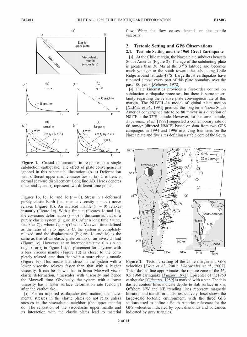
Figures 1b, 1c, 1d, and 1e (t = 0). Stress in a deformedpurely elastic Earth (i.e., mantle viscosity h = 1) neverrelaxes (Figure 1b). An inviscid mantle (h = 0) relaxesinstantly (Figure 1c). With a finite h (Figures 1d and 1e),the coseismic deformation (t = 0) is the same as that of apurely elastic system (Figure 1b). After a long time t = 1,i.e., t � TM, where TM = h/G is the Maxwell time definedas the ratio of h to rigidity G, the system is completelyrelaxed, and the displacement (Figures 1d and 1e) is thesame as that of an elastic plate on top of an inviscid fluid(Figure 1c). However, at an intermediate time 0 < t < 1(e.g., t1 or t2 in Figure 1d), displacement for a system witha less viscous mantle (Figure 1d) is closer to the com-pletely relaxed state than that with a more viscous mantle(Figure 1e). This means that stress in the system with alower viscosity relaxes faster than that with a higherviscosity. It can be shown that in linear Maxwell visco-elastic deformation, timescales with viscosity and hencethe Maxwell time. Obviously, the system with a lowerviscosity has a faster surface deformation rate (velocity)after the earthquake.[4] For an imposed earthquake deformation, the incre-

mental stresses in the elastic plates do not relax unlessstresses in the viscoelastic neighbor (the upper mantle)do. The relaxation of the viscoelastic upper mantle andits interaction with the elastic plates lead to material

flow. When the flow ceases depends on the mantleviscosity.

2. Tectonic Setting and GPS Observations

2.1. Tectonic Setting and the 1960 Great Earthquake

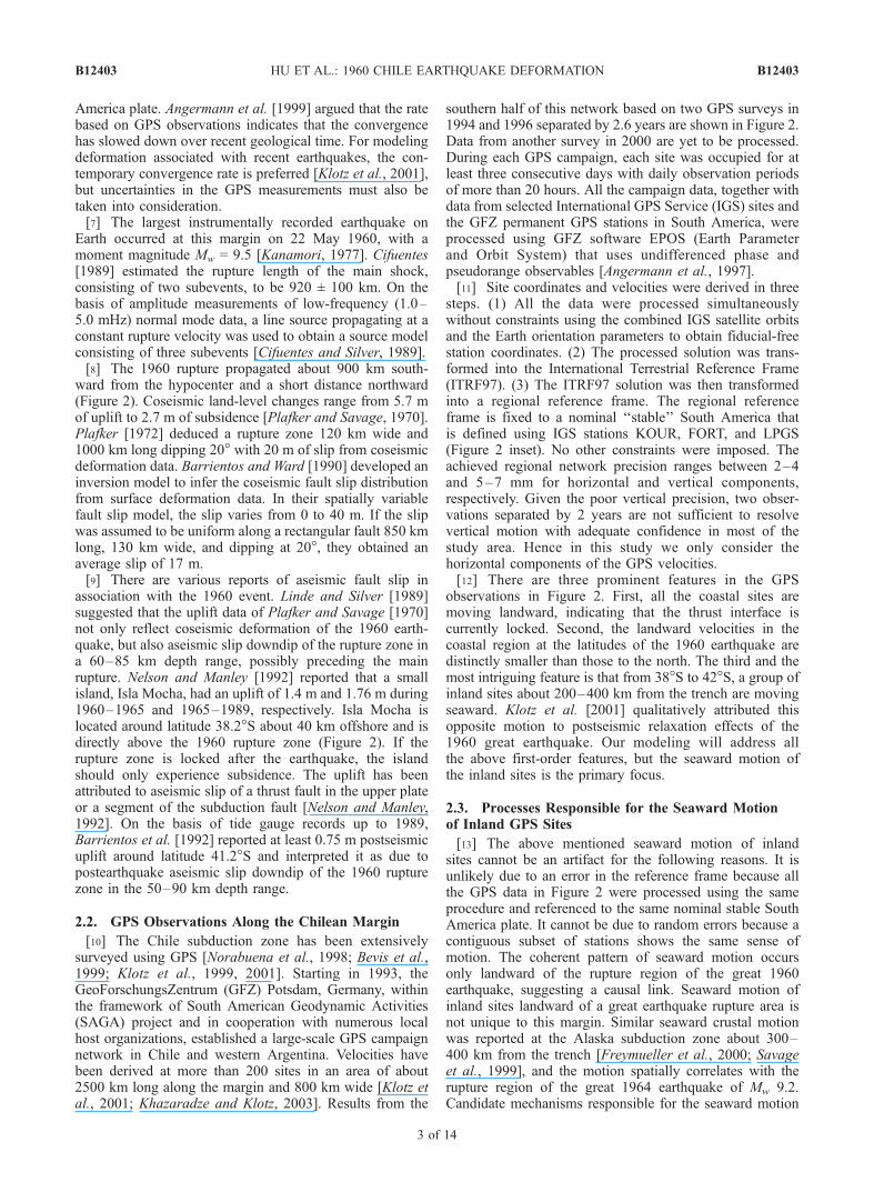
[5] At the Chile margin, the Nazca plate subducts beneathSouth America (Figure 2). The age of the subducting plateis greater than 30 Ma at the 37�S latitude and becomesmuch younger to the south toward the subducting ChileRidge around latitude 47�S. Large thrust earthquakes haveruptured almost every part of this plate boundary over thepast 100 years [Kelleher, 1972].[6] Plate kinematics provides a first-order control on

subduction earthquake processes, but there is some uncer-tainty regarding the relative plate convergence rate at thismargin. The NUVEL-1a model of global plate motion[DeMets et al., 1994] predicts the long-term Nazca-SouthAmerica convergence rate to be 80 mm/yr in a direction ofN81�E at the 32�S latitude. However, for the same latitude,Angermann et al. [1999] suggested a contemporary rate of66 mm/yr (directed N80�E) based on data from two GPScampaigns in 1994 and 1996 involving four sites on theNazca plate and five sites defining a stable core of the South

Figure 1. Crustal deformation in response to a singlesubduction earthquake. The effect of plate convergence isignored in this schematic illustration. (b–e) Deformationwith different upper mantle viscosities h. (a) U is trench-normal seaward displacement along line AB. Here t denotestime, and t1 and t2 represent two different time points.

Figure 2. Tectonic setting of the Chile margin and GPSvelocities [Klotz et al., 2001; Khazaradze et al., 2002].Thick dashed line approximates the rupture zone of the Mw

9.5 1960 earthquake [Plafker, 1972]. Epicenter of the1960earthquake [Cifuentes, 1989] is marked with a star. The thindashed contour lines indicate depths to slab surface in km.Offshore NW and NE trending lines represent magneticlineation and transform faults, respectively. Inset shows thelarge-scale tectonic environment, with the three GPSstations used to define a South America reference for theGPS velocities indicated by open diamonds and volcanoesindicated by gray triangles.

B12403 HU ET AL.: 1960 CHILE EARTHQUAKE DEFORMATION

2 of 14

B12403

America plate. Angermann et al. [1999] argued that the ratebased on GPS observations indicates that the convergencehas slowed down over recent geological time. For modelingdeformation associated with recent earthquakes, the con-temporary convergence rate is preferred [Klotz et al., 2001],but uncertainties in the GPS measurements must also betaken into consideration.[7] The largest instrumentally recorded earthquake on

Earth occurred at this margin on 22 May 1960, with amoment magnitude Mw = 9.5 [Kanamori, 1977]. Cifuentes[1989] estimated the rupture length of the main shock,consisting of two subevents, to be 920 ± 100 km. On thebasis of amplitude measurements of low-frequency (1.0–5.0 mHz) normal mode data, a line source propagating at aconstant rupture velocity was used to obtain a source modelconsisting of three subevents [Cifuentes and Silver, 1989].[8] The 1960 rupture propagated about 900 km south-

ward from the hypocenter and a short distance northward(Figure 2). Coseismic land-level changes range from 5.7 mof uplift to 2.7 m of subsidence [Plafker and Savage, 1970].Plafker [1972] deduced a rupture zone 120 km wide and1000 km long dipping 20� with 20 m of slip from coseismicdeformation data. Barrientos and Ward [1990] developed aninversion model to infer the coseismic fault slip distributionfrom surface deformation data. In their spatially variablefault slip model, the slip varies from 0 to 40 m. If the slipwas assumed to be uniform along a rectangular fault 850 kmlong, 130 km wide, and dipping at 20�, they obtained anaverage slip of 17 m.[9] There are various reports of aseismic fault slip in

association with the 1960 event. Linde and Silver [1989]suggested that the uplift data of Plafker and Savage [1970]not only reflect coseismic deformation of the 1960 earth-quake, but also aseismic slip downdip of the rupture zone ina 60–85 km depth range, possibly preceding the mainrupture. Nelson and Manley [1992] reported that a smallisland, Isla Mocha, had an uplift of 1.4 m and 1.76 m during1960–1965 and 1965–1989, respectively. Isla Mocha islocated around latitude 38.2�S about 40 km offshore and isdirectly above the 1960 rupture zone (Figure 2). If therupture zone is locked after the earthquake, the islandshould only experience subsidence. The uplift has beenattributed to aseismic slip of a thrust fault in the upper plateor a segment of the subduction fault [Nelson and Manley,1992]. On the basis of tide gauge records up to 1989,Barrientos et al. [1992] reported at least 0.75 m postseismicuplift around latitude 41.2�S and interpreted it as due topostearthquake aseismic slip downdip of the 1960 rupturezone in the 50–90 km depth range.

2.2. GPS Observations Along the Chilean Margin

[10] The Chile subduction zone has been extensivelysurveyed using GPS [Norabuena et al., 1998; Bevis et al.,1999; Klotz et al., 1999, 2001]. Starting in 1993, theGeoForschungsZentrum (GFZ) Potsdam, Germany, withinthe framework of South American Geodynamic Activities(SAGA) project and in cooperation with numerous localhost organizations, established a large-scale GPS campaignnetwork in Chile and western Argentina. Velocities havebeen derived at more than 200 sites in an area of about2500 km long along the margin and 800 km wide [Klotz etal., 2001; Khazaradze and Klotz, 2003]. Results from the

southern half of this network based on two GPS surveys in1994 and 1996 separated by 2.6 years are shown in Figure 2.Data from another survey in 2000 are yet to be processed.During each GPS campaign, each site was occupied for atleast three consecutive days with daily observation periodsof more than 20 hours. All the campaign data, together withdata from selected International GPS Service (IGS) sites andthe GFZ permanent GPS stations in South America, wereprocessed using GFZ software EPOS (Earth Parameterand Orbit System) that uses undifferenced phase andpseudorange observables [Angermann et al., 1997].[11] Site coordinates and velocities were derived in three

steps. (1) All the data were processed simultaneouslywithout constraints using the combined IGS satellite orbitsand the Earth orientation parameters to obtain fiducial-freestation coordinates. (2) The processed solution was trans-formed into the International Terrestrial Reference Frame(ITRF97). (3) The ITRF97 solution was then transformedinto a regional reference frame. The regional referenceframe is fixed to a nominal ‘‘stable’’ South America thatis defined using IGS stations KOUR, FORT, and LPGS(Figure 2 inset). No other constraints were imposed. Theachieved regional network precision ranges between 2–4and 5–7 mm for horizontal and vertical components,respectively. Given the poor vertical precision, two obser-vations separated by 2 years are not sufficient to resolvevertical motion with adequate confidence in most of thestudy area. Hence in this study we only consider thehorizontal components of the GPS velocities.[12] There are three prominent features in the GPS

observations in Figure 2. First, all the coastal sites aremoving landward, indicating that the thrust interface iscurrently locked. Second, the landward velocities in thecoastal region at the latitudes of the 1960 earthquake aredistinctly smaller than those to the north. The third and themost intriguing feature is that from 38�S to 42�S, a group ofinland sites about 200–400 km from the trench are movingseaward. Klotz et al. [2001] qualitatively attributed thisopposite motion to postseismic relaxation effects of the1960 great earthquake. Our modeling will address allthe above first-order features, but the seaward motion ofthe inland sites is the primary focus.

2.3. Processes Responsible for the Seaward Motionof Inland GPS Sites

[13] The above mentioned seaward motion of inlandsites cannot be an artifact for the following reasons. It isunlikely due to an error in the reference frame because allthe GPS data in Figure 2 were processed using the sameprocedure and referenced to the same nominal stable SouthAmerica plate. It cannot be due to random errors because acontiguous subset of stations shows the same sense ofmotion. The coherent pattern of seaward motion occursonly landward of the rupture region of the great 1960earthquake, suggesting a causal link. Seaward motion ofinland sites landward of a great earthquake rupture area isnot unique to this margin. Similar seaward crustal motionwas reported at the Alaska subduction zone about 300–400 km from the trench [Freymueller et al., 2000; Savageet al., 1999], and the motion spatially correlates with therupture region of the great 1964 earthquake of Mw 9.2.Candidate mechanisms responsible for the seaward motion

B12403 HU ET AL.: 1960 CHILE EARTHQUAKE DEFORMATION

3 of 14

B12403

include deep aseismic fault slip and viscoelastic stressrelaxation.[14] An interplate great earthquake may induce aseismic

afterslip of the fault downdip of the rupture segment thatmay continue for sometime after the event. Zweck et al.[2002] explained the present-day seaward motion of inlandGPS sites at the Alaska subduction zone by proposingafterslip in a purely elastic Earth model that lasted at leastfor several decades. Sato et al. [2003] showed that someviscoelastic stress relaxation is also required to explain theseobservations.[15] It is generally difficult to distinguish between

contributions to postseismic deformation from fault after-slip and mantle relaxation [Pollitz et al., 1998; Wang,2004], but it is usually assumed that transient fault slipmay be important for a timescale of months to years, andviscoelastic stress relaxation is important for a timescaleof decades to centuries. It is clear that the timescale forsignificant afterslip of a downdip extension of the rupturezone of the 1994 Sanriku-oki earthquake off NE Japan isindeed very short, no more than two years [Uchida etal., 2003] or even within 100 days after the earthquake[Yagi et al., 2003]. The afterslip slows down or stopsafterward.[16] In addition to the timescale consideration, to use the

afterslip model to explain the GPS data at the Chile marginwould require a very deep slip zone because of the largedistance of the seaward moving GPS stations to the 1960rupture zone. Hu [2004] conducted simple tests using a 3-Dmodel of dislocation in a uniform elastic half space [Okada,1985] to assess spatial relations between the seawardmotion of inland GPS sites and possible long-term afterslipat the Chile margin. He found that, unlike at the Alaskamargin where the slab dips shallowly, the afterslip segmentat the Chile margin would have to be over 100 km deep andbelow the volcanic front in order to explain the seawardmotion. It is questionable whether an elastic fault model isapplicable at such depth where deformation along the plateinterface is expected to be ductile because of the hightemperatures. If a shallower afterslip zone was assumed,no reasonable afterslip rate could be found to matchsimultaneously the GPS patterns in both the landwardmoving coastal area and the seaward moving inland area.Therefore prolonged afterslip in a purely elastic Earth isunlikely to be a dominant mechanism for the seawardmotion of the inland area for this margin. Barrientos et al.[1992] assumed afterslip in a 50–90 km depth rangedowndip of the 1960 Chile earthquake rupture in order toexplain postseismic uplift indicated by tide gauge observa-tions within 30 years of the earthquake, but as we willdemonstrate subsequently, the uplift may alternatively beexplained as due to viscoelastic stress relaxation.[17] Downdip of the seismogenic zone, a subduction fault

may slip aseismically and episodically during the interseis-mic period [Dragert et al., 2001; Ozawa et al., 2002]. Suchslip may cause brief episodes of seaward motion of GPSstations. The physical mechanism of these silent events isnot understood and is under intense investigation. The depthrange of these slips is about 30 to 50 km. An elastic modelof silent slip that explains the seaward motion of GPS sitesat the Chile margin will be similar to the afterslip modelexcept for a different time of slip occurrence. Therefore it

has the same requirement for a deep slip zone, which is atodds with all silent slip observations and models.[18] Viscoelastic stress relaxation, as explained in the

Introduction, is our preferred mechanism. We have pub-lished some preliminary results of a 3-D viscoelasticfinite element model to explain the GPS observations[Khazaradze et al., 2002]. In the present paper, we presenta revised model and a much more detailed investigationof the mechanical process. As we will demonstrate subse-quently, the same process also explains the second featureof the GPS observations (section 2.2), i.e., the amplitudecontrast of coast velocities between the region of the 1960earthquake and the area to the north. This strengthens ourcontention that viscoelastic stress relaxation is a fundamen-tal process common to all large earthquakes. Only twosubduction earthquakes (1960 Chile, 1964 Alaska) recordedin the past century have moment magnitude above 9 andrupture zones over 900 km long. It is probably not acoincidence that in both cases seaward crustal motion hasbeen observed landward of the rupture region severaldecades after the events. In a 3-D viscoelastic finite elementmodel of Cascadia great subduction earthquake cycles[Wang et al., 2001], there was a seaward motion of inlandsites 50 years after the 1700 great earthquake that was alsoestimated to be Mw � 9.

3. Finite Element Model

3.1. Geometry

[19] Finite element models that include the heterogeneityof the real Earth may produce a good fit to crustaldeformation observations. However, the purpose of thiswork is to study the first-order postseismic deformation,and fine details of the heterogeneity are ignored. Simplifi-cations allow us to focus on the essential aspects of thefundamental physical process. Our model consists of anelastic upper plate, an elastic subducting plate including theslab, a viscoelastic oceanic mantle, and a viscoelasticcontinental mantle, as schematically shown in Figure 1a.The material is assumed to be uniform within each of thesetectonic units. The x axis is northward positive in the strikedirection (N3.2�E). The y axis is landward positive.[20] The elastic over-riding plate includes the crust and the

lithospheric mantle. The effective elastic thickness of oldcontinental lithosphere is estimated to be 35–40 km [Burovand Diament, 1995]. This thickness may not be uniform. Thevery low heat flow in subduction zone forearcs may makethe elastic thickness larger, and high heat flow in thevolcanic arc and back arc may make the thickness smaller.We assume a thickness of the elastic continental upper plateof 40 km, but uncertainty in this choice is large. Other valueswill be tested for sensitivity analysis. The thickness of theelastic oceanic plate (including the subducting slab) isassumed to be 30 km as in the work of Khazaradze et al.[2002], consistent with the elastic thickness of an oceanicplate of 20–30 Ma age [Watts and Zhong, 2000]. Changingthis value by 10 km makes little difference to model resultsfor the region of GPS measurements.[21] The shape of the subducting slab is based on pub-

lished slab contours [Dewey and Lamb, 1992; Cahill andIsacks, 1992]. A generalized shape of the subducting slab isobtained by fitting these data with a parabolic function. The

B12403 HU ET AL.: 1960 CHILE EARTHQUAKE DEFORMATION

4 of 14

B12403

resultant 2-D slab shape is then used for all the trench-normal profiles of the 3-D model. The simplification that alltrench-normal cross sections are identical is consistent withthe fact that there is little observed variation of the slabgeometry south of 35�S. The younger age of the subductingplate may lead to a decrease in slab dip toward the triplejunction around 47�S, but there is no observation toconstrain it.[22] We construct a finite element mesh that conforms to

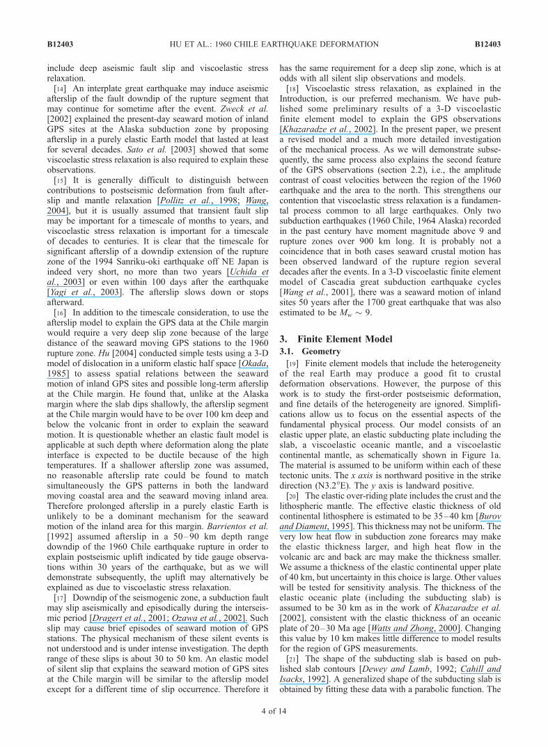
the expected geometry of the subduction zone (Figure 3).The bottom of the mesh is set at 500 km depth, in themiddle of the mantle transition zone. Except for the freeupper surface, displacement perpendicular to each modelboundary is fixed to be zero, and displacements parallel tothe boundary are not constrained. The mesh extends from650 km seaward of the trench to 650 km landward of thetrench and is 3000 km long in the along-strike dimension.There are a total of 27,170 trilinear eight-node elements,with grid spacing ranging from 0.4 km around the subduc-tion fault to over 200 km at the model boundaries.

3.2. Prescribed Fault Slip

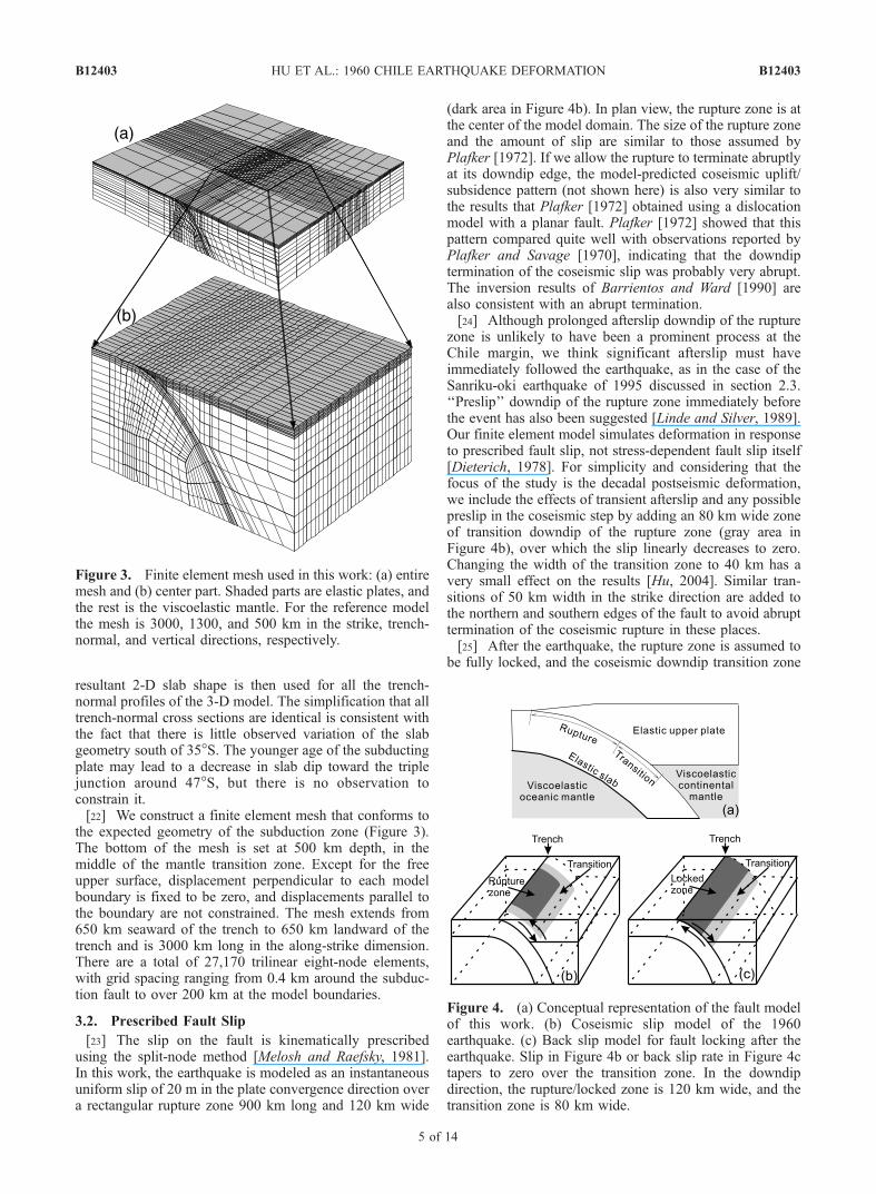
[23] The slip on the fault is kinematically prescribedusing the split-node method [Melosh and Raefsky, 1981].In this work, the earthquake is modeled as an instantaneousuniform slip of 20 m in the plate convergence direction overa rectangular rupture zone 900 km long and 120 km wide

(dark area in Figure 4b). In plan view, the rupture zone is atthe center of the model domain. The size of the rupture zoneand the amount of slip are similar to those assumed byPlafker [1972]. If we allow the rupture to terminate abruptlyat its downdip edge, the model-predicted coseismic uplift/subsidence pattern (not shown here) is also very similar tothe results that Plafker [1972] obtained using a dislocationmodel with a planar fault. Plafker [1972] showed that thispattern compared quite well with observations reported byPlafker and Savage [1970], indicating that the downdiptermination of the coseismic slip was probably very abrupt.The inversion results of Barrientos and Ward [1990] arealso consistent with an abrupt termination.[24] Although prolonged afterslip downdip of the rupture

zone is unlikely to have been a prominent process at theChile margin, we think significant afterslip must haveimmediately followed the earthquake, as in the case of theSanriku-oki earthquake of 1995 discussed in section 2.3.‘‘Preslip’’ downdip of the rupture zone immediately beforethe event has also been suggested [Linde and Silver, 1989].Our finite element model simulates deformation in responseto prescribed fault slip, not stress-dependent fault slip itself[Dieterich, 1978]. For simplicity and considering that thefocus of the study is the decadal postseismic deformation,we include the effects of transient afterslip and any possiblepreslip in the coseismic step by adding an 80 km wide zoneof transition downdip of the rupture zone (gray area inFigure 4b), over which the slip linearly decreases to zero.Changing the width of the transition zone to 40 km has avery small effect on the results [Hu, 2004]. Similar tran-sitions of 50 km width in the strike direction are added tothe northern and southern edges of the fault to avoid abrupttermination of the coseismic rupture in these places.[25] After the earthquake, the rupture zone is assumed to

be fully locked, and the coseismic downdip transition zone

Figure 3. Finite element mesh used in this work: (a) entiremesh and (b) center part. Shaded parts are elastic plates, andthe rest is the viscoelastic mantle. For the reference modelthe mesh is 3000, 1300, and 500 km in the strike, trench-normal, and vertical directions, respectively.

Figure 4. (a) Conceptual representation of the fault modelof this work. (b) Coseismic slip model of the 1960earthquake. (c) Back slip model for fault locking after theearthquake. Slip in Figure 4b or back slip rate in Figure 4ctapers to zero over the transition zone. In the downdipdirection, the rupture/locked zone is 120 km wide, and thetransition zone is 80 km wide.

B12403 HU ET AL.: 1960 CHILE EARTHQUAKE DEFORMATION

5 of 14

B12403

becomes the interseismic transition zone. The 1960 earth-quake only ruptured a segment of the Chilean margin, butthe Chilean subduction fault is believed to be locked alongits entire length at present. Therefore the locked andinterseismic transition zones are extended from the rupturezone to the northern and southern mesh boundaries asshown by the dark and gray areas in Figure 4c. The lockingof the fault is modeled using the method of back slip[Savage, 1983]. A back slip at the plate subduction rateassigned to the locked zone represents a fully locked fault.Over the downdip transition zone, the back slip rate linearlydecreases to zero. If the subduction process is assumed to bepurely seismic, it will take 300 years to accumulate enoughslip deficit for the next 20-m rupture event with a back sliprate of 66 mm/yr, or 250 years with a rate of 80 mm/yr. Theconvergence rate of 66 mm/yr is used, but a faster rate willalso be tested.

3.3. Material Properties

[26] Following Wang et al. [2001], the Young’s modulusof the elastic plates and mantle are assumed to be 120 GPaand 160 GPa, respectively, and the Poisson’s ratio and rockdensity are assumed to be 0.25 and 3.3 g/cm3, respectively,for the entire system. The gravitational acceleration is

assumed to be 10 m/s2. Gravity is not directly modeled asa body force, but its effect of tending to bring a perturbedsystem back to the hydrostatic state is modeled using aprestress advection approach [Peltier, 1974; Wang et al.,2001].[27] Assuming a viscosity of 2.5� 1019 Pa s and a Young’s

modulus of 160 GPa, the mantle Maxwell relaxation time is�12 years. Justifications for this viscosity value will bediscussed later. Although there are earthquakes in 1737 and1835 in this area [Nishenko, 1985], the last great earthquakeof comparable size to the 1960 event occurred in 1575[Atwater et al., 2003]. The almost 400 years time intervalbetween the two great earthquakes is much larger than theMaxwell relaxation time. We assume that the stress inducedby the 1575 earthquake was largely relaxed in 1960 and thatthe effects of the 1737 and 1835 events are small. Thereforeprevious earthquakes are not included in the model.[28] The model with parameters described above is

called the reference model. Various changes will be madeto the reference model for sensitivity tests. The effects ofthe earthquake and of the subsequent locking of the faultare modeled separately. The combined effect of the earth-quake and fault locking is obtained using a linear combi-nation of the results of the two models (Figure 4). We

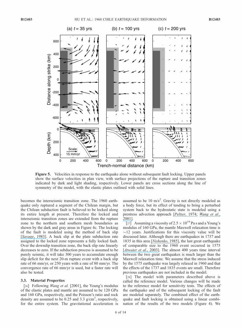
Figure 5. Velocities in response to the earthquake alone without subsequent fault locking. Upper panelsshow the surface velocities in plan view, with surface projections of the rupture and transition zonesindicated by dark and light shading, respectively. Lower panels are cross sections along the line ofsymmetry of the model, with the elastic plates outlined with solid lines.

B12403 HU ET AL.: 1960 CHILE EARTHQUAKE DEFORMATION

6 of 14

B12403

think that the only way to explain the mechanism clearlyis to discuss the earthquake and fault-locking effectsseparately as follows.

4. Model Results

4.1. Deformation Due to the Earthquake Alone

[29] The system’s response to the earthquake is modeledby prescribing an instantaneous coseismic slip on the faultwithout subsequent fault locking. That is, the relativedisplacements of the nodes on the full-rupture zone of thefault are fixed at 20 m with no subsequent back slip.[30] The earthquake instantaneously stretches the forearc

and induces a shear stress in the mantle. Note that the‘‘stretch’’ is incremental to a background stress field anddoes not represent absolute stress. The incremental stretch-ing force tends to pull the rest of the upper plate to moveseaward, but the induced shear stress provides a resistanceto this motion. As discussed in the introduction, if the uppermantle were purely elastic (viscosity h = 1), the resistivestress would never relax, and deformation in response to theearthquake would always be confined to a small area aroundthe rupture. However, also as discussed in the Introduction,if the upper mantle were a pure fluid with no shear strength(viscosity h = 0), no stress would be induced in the uppermantle, and the crustal deformation would instantaneouslyextend to a large distance. The mantle viscosity of 2.5 �1019 Pa s represents intermediate behavior, as in Figure 1d.[31] The instantaneous stretch of the forearc and the

subsequent stress relaxation cause seaward velocities in

areas landward of the trench (Figure 5). In this paper, allmodel velocities are relative to the fixed model boundaries.The seaward velocities decrease with time as the stretchingstress in the elastic plate decreases. The surface velocitieslandward of the rupture zone along the line of symmetry areslightly oblique because of the oblique plate convergence atChile, but the strike-parallel component quickly diminishes(Figures 5b and 5c). Displacement (not shown) is firstlimited to near the rupture but gradually involves a broaderlandward area [Hu, 2004].

4.2. Deformation Due to Fault Locking Alone

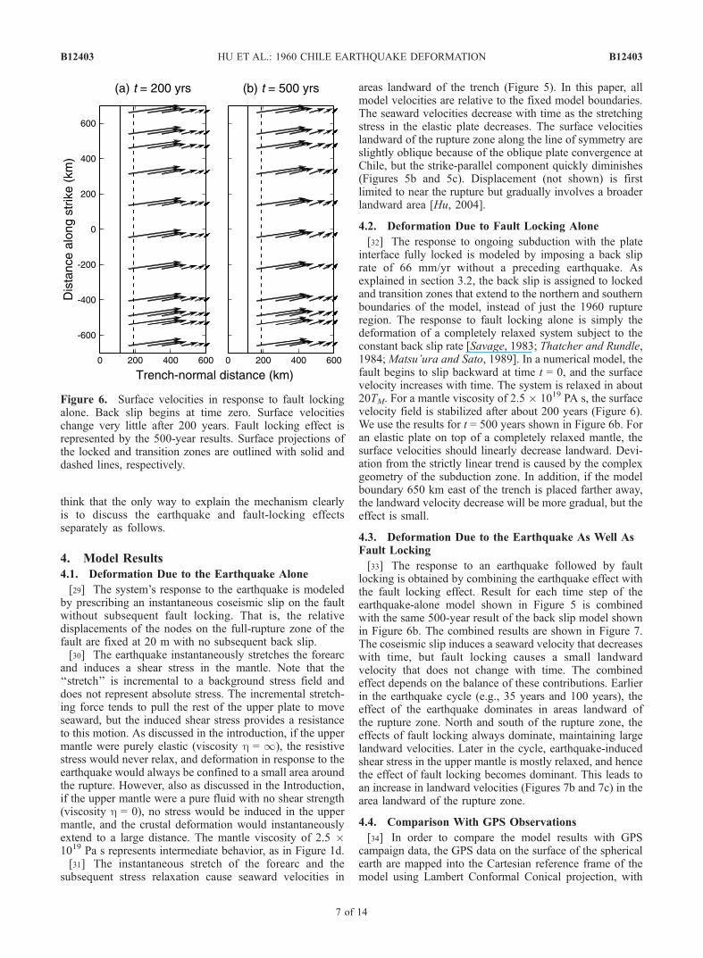
[32] The response to ongoing subduction with the plateinterface fully locked is modeled by imposing a back sliprate of 66 mm/yr without a preceding earthquake. Asexplained in section 3.2, the back slip is assigned to lockedand transition zones that extend to the northern and southernboundaries of the model, instead of just the 1960 ruptureregion. The response to fault locking alone is simply thedeformation of a completely relaxed system subject to theconstant back slip rate [Savage, 1983; Thatcher and Rundle,1984;Matsu’ura and Sato, 1989]. In a numerical model, thefault begins to slip backward at time t = 0, and the surfacevelocity increases with time. The system is relaxed in about20TM. For a mantle viscosity of 2.5 � 1019 PA s, the surfacevelocity field is stabilized after about 200 years (Figure 6).We use the results for t = 500 years shown in Figure 6b. Foran elastic plate on top of a completely relaxed mantle, thesurface velocities should linearly decrease landward. Devi-ation from the strictly linear trend is caused by the complexgeometry of the subduction zone. In addition, if the modelboundary 650 km east of the trench is placed farther away,the landward velocity decrease will be more gradual, but theeffect is small.

4.3. Deformation Due to the Earthquake As Well AsFault Locking

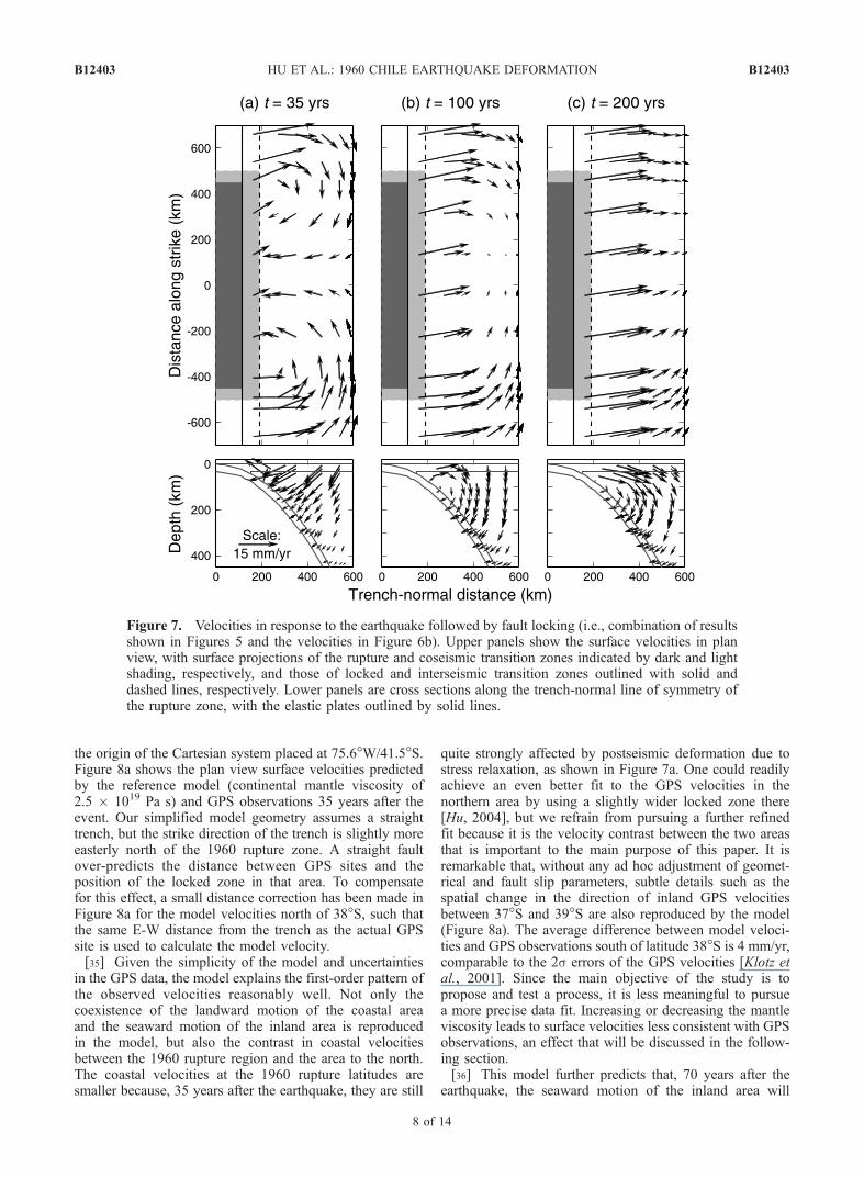
[33] The response to an earthquake followed by faultlocking is obtained by combining the earthquake effect withthe fault locking effect. Result for each time step of theearthquake-alone model shown in Figure 5 is combinedwith the same 500-year result of the back slip model shownin Figure 6b. The combined results are shown in Figure 7.The coseismic slip induces a seaward velocity that decreaseswith time, but fault locking causes a small landwardvelocity that does not change with time. The combinedeffect depends on the balance of these contributions. Earlierin the earthquake cycle (e.g., 35 years and 100 years), theeffect of the earthquake dominates in areas landward ofthe rupture zone. North and south of the rupture zone, theeffects of fault locking always dominate, maintaining largelandward velocities. Later in the cycle, earthquake-inducedshear stress in the upper mantle is mostly relaxed, and hencethe effect of fault locking becomes dominant. This leads toan increase in landward velocities (Figures 7b and 7c) in thearea landward of the rupture zone.

4.4. Comparison With GPS Observations

[34] In order to compare the model results with GPScampaign data, the GPS data on the surface of the sphericalearth are mapped into the Cartesian reference frame of themodel using Lambert Conformal Conical projection, with

Figure 6. Surface velocities in response to fault lockingalone. Back slip begins at time zero. Surface velocitieschange very little after 200 years. Fault locking effect isrepresented by the 500-year results. Surface projections ofthe locked and transition zones are outlined with solid anddashed lines, respectively.

B12403 HU ET AL.: 1960 CHILE EARTHQUAKE DEFORMATION

7 of 14

B12403

the origin of the Cartesian system placed at 75.6�W/41.5�S.Figure 8a shows the plan view surface velocities predictedby the reference model (continental mantle viscosity of2.5 � 1019 Pa s) and GPS observations 35 years after theevent. Our simplified model geometry assumes a straighttrench, but the strike direction of the trench is slightly moreeasterly north of the 1960 rupture zone. A straight faultover-predicts the distance between GPS sites and theposition of the locked zone in that area. To compensatefor this effect, a small distance correction has been made inFigure 8a for the model velocities north of 38�S, such thatthe same E-W distance from the trench as the actual GPSsite is used to calculate the model velocity.[35] Given the simplicity of the model and uncertainties

in the GPS data, the model explains the first-order pattern ofthe observed velocities reasonably well. Not only thecoexistence of the landward motion of the coastal areaand the seaward motion of the inland area is reproducedin the model, but also the contrast in coastal velocitiesbetween the 1960 rupture region and the area to the north.The coastal velocities at the 1960 rupture latitudes aresmaller because, 35 years after the earthquake, they are still

quite strongly affected by postseismic deformation due tostress relaxation, as shown in Figure 7a. One could readilyachieve an even better fit to the GPS velocities in thenorthern area by using a slightly wider locked zone there[Hu, 2004], but we refrain from pursuing a further refinedfit because it is the velocity contrast between the two areasthat is important to the main purpose of this paper. It isremarkable that, without any ad hoc adjustment of geomet-rical and fault slip parameters, subtle details such as thespatial change in the direction of inland GPS velocitiesbetween 37�S and 39�S are also reproduced by the model(Figure 8a). The average difference between model veloci-ties and GPS observations south of latitude 38�S is 4 mm/yr,comparable to the 2s errors of the GPS velocities [Klotz etal., 2001]. Since the main objective of the study is topropose and test a process, it is less meaningful to pursuea more precise data fit. Increasing or decreasing the mantleviscosity leads to surface velocities less consistent with GPSobservations, an effect that will be discussed in the follow-ing section.[36] This model further predicts that, 70 years after the

earthquake, the seaward motion of the inland area will

Figure 7. Velocities in response to the earthquake followed by fault locking (i.e., combination of resultsshown in Figures 5 and the velocities in Figure 6b). Upper panels show the surface velocities in planview, with surface projections of the rupture and coseismic transition zones indicated by dark and lightshading, respectively, and those of locked and interseismic transition zones outlined with solid anddashed lines, respectively. Lower panels are cross sections along the trench-normal line of symmetry ofthe rupture zone, with the elastic plates outlined by solid lines.

B12403 HU ET AL.: 1960 CHILE EARTHQUAKE DEFORMATION

8 of 14

B12403

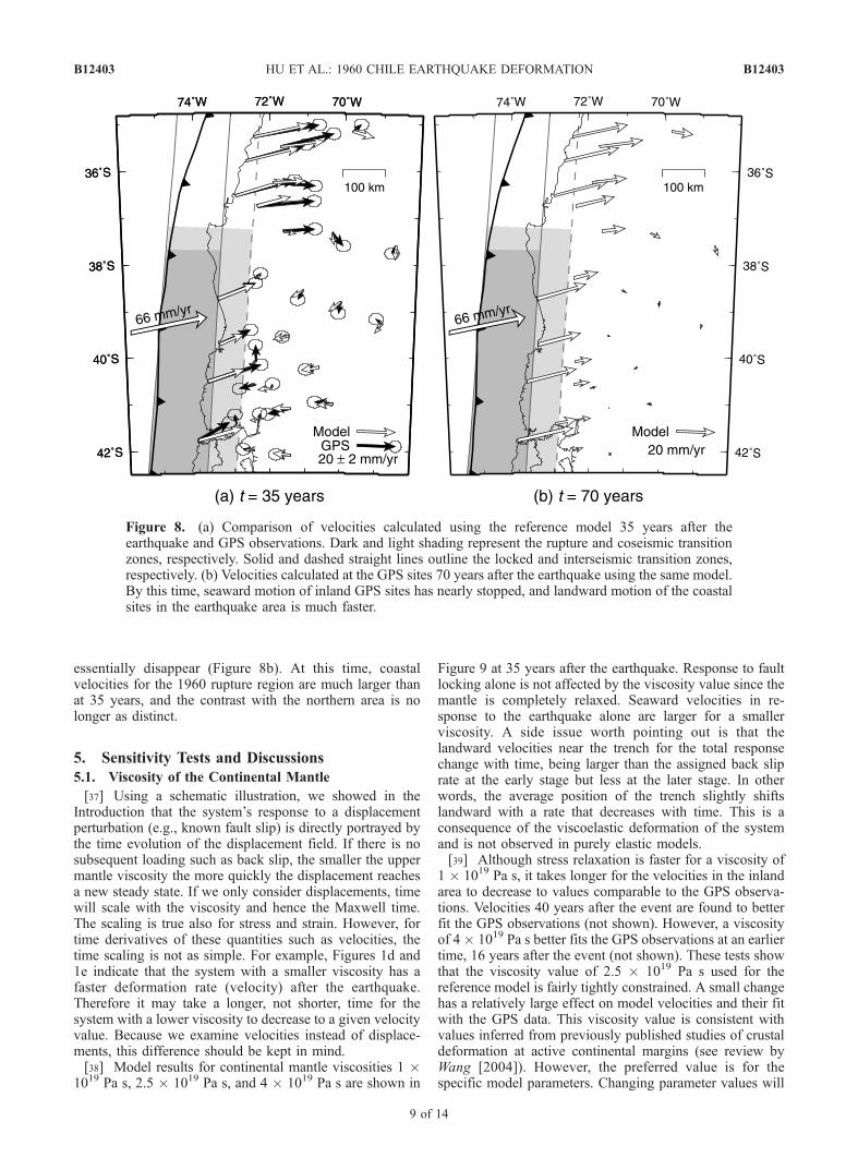
essentially disappear (Figure 8b). At this time, coastalvelocities for the 1960 rupture region are much larger thanat 35 years, and the contrast with the northern area is nolonger as distinct.

5. Sensitivity Tests and Discussions

5.1. Viscosity of the Continental Mantle

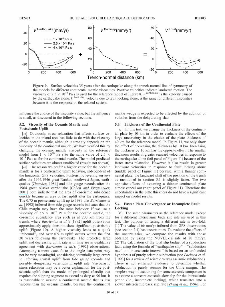
[37] Using a schematic illustration, we showed in theIntroduction that the system’s response to a displacementperturbation (e.g., known fault slip) is directly portrayed bythe time evolution of the displacement field. If there is nosubsequent loading such as back slip, the smaller the uppermantle viscosity the more quickly the displacement reachesa new steady state. If we only consider displacements, timewill scale with the viscosity and hence the Maxwell time.The scaling is true also for stress and strain. However, fortime derivatives of these quantities such as velocities, thetime scaling is not as simple. For example, Figures 1d and1e indicate that the system with a smaller viscosity has afaster deformation rate (velocity) after the earthquake.Therefore it may take a longer, not shorter, time for thesystem with a lower viscosity to decrease to a given velocityvalue. Because we examine velocities instead of displace-ments, this difference should be kept in mind.[38] Model results for continental mantle viscosities 1 �

1019 Pa s, 2.5 � 1019 Pa s, and 4 � 1019 Pa s are shown in

Figure 9 at 35 years after the earthquake. Response to faultlocking alone is not affected by the viscosity value since themantle is completely relaxed. Seaward velocities in re-sponse to the earthquake alone are larger for a smallerviscosity. A side issue worth pointing out is that thelandward velocities near the trench for the total responsechange with time, being larger than the assigned back sliprate at the early stage but less at the later stage. In otherwords, the average position of the trench slightly shiftslandward with a rate that decreases with time. This is aconsequence of the viscoelastic deformation of the systemand is not observed in purely elastic models.[39] Although stress relaxation is faster for a viscosity of

1 � 1019 Pa s, it takes longer for the velocities in the inlandarea to decrease to values comparable to the GPS observa-tions. Velocities 40 years after the event are found to betterfit the GPS observations (not shown). However, a viscosityof 4� 1019 Pa s better fits the GPS observations at an earliertime, 16 years after the event (not shown). These tests showthat the viscosity value of 2.5 � 1019 Pa s used for thereference model is fairly tightly constrained. A small changehas a relatively large effect on model velocities and their fitwith the GPS data. This viscosity value is consistent withvalues inferred from previously published studies of crustaldeformation at active continental margins (see review byWang [2004]). However, the preferred value is for thespecific model parameters. Changing parameter values will

Figure 8. (a) Comparison of velocities calculated using the reference model 35 years after theearthquake and GPS observations. Dark and light shading represent the rupture and coseismic transitionzones, respectively. Solid and dashed straight lines outline the locked and interseismic transition zones,respectively. (b) Velocities calculated at the GPS sites 70 years after the earthquake using the same model.By this time, seaward motion of inland GPS sites has nearly stopped, and landward motion of the coastalsites in the earthquake area is much faster.

B12403 HU ET AL.: 1960 CHILE EARTHQUAKE DEFORMATION

9 of 14

B12403

influence the choice of the viscosity value, but the influenceis small, as discussed in the following sections.

5.2. Viscosity of the Oceanic Mantle andPostseismic Uplift

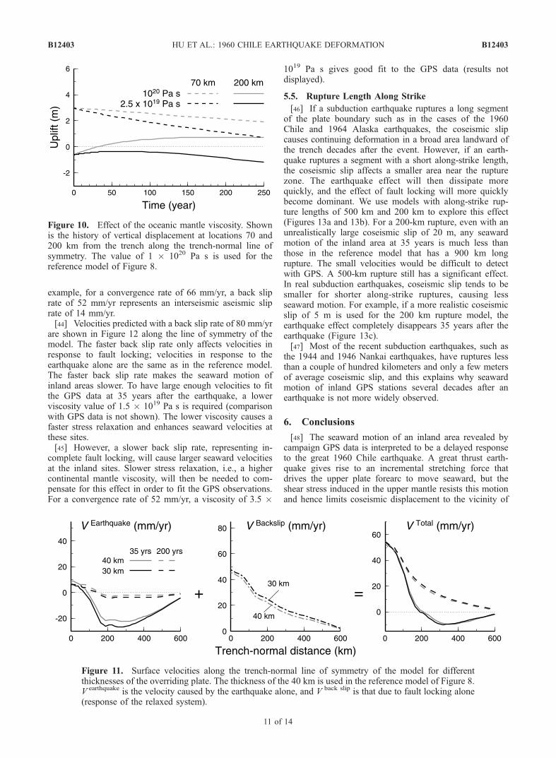
[40] Obviously, stress relaxation that affects surface ve-locities in the inland area has little to do with the viscosityof the oceanic mantle, although it strongly depends on theviscosity of the continental mantle. We have verified this bychanging the oceanic mantle viscosity in the referencemodel from 1 � 1020 Pa s to the same value of 2.5 �1019 Pa s as for the continental mantle. The model-predictedsurface velocities are almost unaffected (results not shown).[41] The reason we prefer a higher value for the oceanic

mantle is for a postseismic uplift behavior, independent ofthe horizontal GPS velocities. Postseismic leveling surveysafter the 1944/1946 great Nankai, southwest Japan, earth-quakes [Thatcher, 1984] and tide gauge records after the1964 great Alaska earthquake [Cohen and Freymueller,2001] both indicate that the area of coseismic subsidencequickly became an area of fast uplift after the earthquake.The 0.75 m postseismic uplift up to 1989 that Barrientos etal. [1992] inferred from tide gauge records indicates that theChile margin may have the same behavior. If we use aviscosity of 2.5 � 1019 Pa s for the oceanic mantle, thecoseismic subsidence area such as at 200 km from thetrench, where Barrientos et al.’s [1992] uplift observationapproximately apply, does not show significant postseismicuplift (Figure 10). A higher viscosity leads to a quick‘‘rebound’’, and over 0.5 m uplift occurs within the first30 years following the earthquake. The predicted largeuplift and decreasing uplift rate with time are in qualitativeagreement with Barrientos et al.’s [1992] observations.Attempting a more exact fit to the single data point maynot be very meaningful, considering potentially large errorsin inferring crustal uplift from tide gauge records andpossible along-strike variations in uplift rate. Viscoelasticstress relaxation may be a better explanation for the post-seismic uplift than the model of prolonged afterslip thatrequires the slipping segment to extend as deep as 90 km. Itis reasonable to assume a continental mantle that is lessviscous than the oceanic mantle, because the continental

mantle wedge is expected to be affected by the addition ofvolatiles from the dehydrating slab.

5.3. Thickness of the Continental Plate

[42] In this test, we change the thickness of the continen-tal plate by 10 km in order to evaluate the effects of thelarge uncertainty in the choice of the plate thickness of40 km for the reference model. In Figure 11, we only showthe effect of decreasing the thickness by 10 km. Increasingthe thickness by 10 km has the opposite effect. The smallerthickness results in greater seaward velocities in response tothe earthquake alone (left panel of Figure 11) because of thefaster stress relaxation. However, it also results in greaterlandward velocities in response to fault locking alone(middle panel of Figure 11) because, with a thinner conti-nental plate, the landward shift of the position of the trenchas mentioned in section 5.1 is slightly faster. The twoopposite effects of assuming a thinner continental platealmost cancel out (right panel of Figure 11). Therefore theuncertainties in the plate thickness do not have a significantimpact on model results.

5.4. Faster Plate Convergence or Incomplete FaultLocking

[43] The same parameters as the reference model exceptfor a different interseismic back slip rate are used in thistest. The purpose of testing a different rate is two-fold.(1) The value of 66 mm/yr inferred from GPS observations(see section 2.1) has uncertainties. To evaluate the effects ofthe uncertainties, we compare the results with thoseobtained by using the NUVEL-1a rate of 80 mm/yr.(2) The calculation of the total slip budget of a subductionfault using the formula of ‘‘earthquake slip’’ = ‘‘subductionrate’’ � ‘‘interseismic interval’’ is based on an unfoundedhypothesis of purely seismic subduction (see Pacheco et al.[1993] for a review of seismic versus aseismic subduction).There is not sufficient evidence to determine whethersubduction is purely seismic for the Chile margin. Thesimplest way of accounting for some aseismic component isto assume a constant aseismic slow slip for the interseismicperiod (i.e., incomplete locking), which translates into aslower interseismic back slip rate [Zheng et al., 1996]. For

Figure 9. Surface velocities 35 years after the earthquake along the trench-normal line of symmetry ofthe models for different continental mantle viscosities. Positive velocities indicate landward motion. Theviscosity of 2.5 � 1019 Pa s is used for the reference model of Figure 8. V earthquake is the velocity causedby the earthquake alone. V back slip, velocity due to fault locking alone, is the same for different viscositiesbecause it is the response of the relaxed system.

B12403 HU ET AL.: 1960 CHILE EARTHQUAKE DEFORMATION

10 of 14

B12403

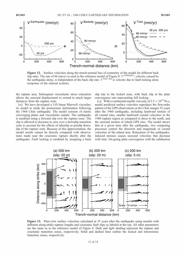
example, for a convergence rate of 66 mm/yr, a back sliprate of 52 mm/yr represents an interseismic aseismic sliprate of 14 mm/yr.[44] Velocities predicted with a back slip rate of 80 mm/yr

are shown in Figure 12 along the line of symmetry of themodel. The faster back slip rate only affects velocities inresponse to fault locking; velocities in response to theearthquake alone are the same as in the reference model.The faster back slip rate makes the seaward motion ofinland areas slower. To have large enough velocities to fitthe GPS data at 35 years after the earthquake, a lowerviscosity value of 1.5 � 1019 Pa s is required (comparisonwith GPS data is not shown). The lower viscosity causes afaster stress relaxation and enhances seaward velocities atthese sites.[45] However, a slower back slip rate, representing in-

complete fault locking, will cause larger seaward velocitiesat the inland sites. Slower stress relaxation, i.e., a highercontinental mantle viscosity, will then be needed to com-pensate for this effect in order to fit the GPS observations.For a convergence rate of 52 mm/yr, a viscosity of 3.5 �

1019 Pa s gives good fit to the GPS data (results notdisplayed).

5.5. Rupture Length Along Strike

[46] If a subduction earthquake ruptures a long segmentof the plate boundary such as in the cases of the 1960Chile and 1964 Alaska earthquakes, the coseismic slipcauses continuing deformation in a broad area landward ofthe trench decades after the event. However, if an earth-quake ruptures a segment with a short along-strike length,the coseismic slip affects a smaller area near the rupturezone. The earthquake effect will then dissipate morequickly, and the effect of fault locking will more quicklybecome dominant. We use models with along-strike rup-ture lengths of 500 km and 200 km to explore this effect(Figures 13a and 13b). For a 200-km rupture, even with anunrealistically large coseismic slip of 20 m, any seawardmotion of the inland area at 35 years is much less thanthose in the reference model that has a 900 km longrupture. The small velocities would be difficult to detectwith GPS. A 500-km rupture still has a significant effect.In real subduction earthquakes, coseismic slip tends to besmaller for shorter along-strike ruptures, causing lessseaward motion. For example, if a more realistic coseismicslip of 5 m is used for the 200 km rupture model, theearthquake effect completely disappears 35 years after theearthquake (Figure 13c).[47] Most of the recent subduction earthquakes, such as

the 1944 and 1946 Nankai earthquakes, have ruptures lessthan a couple of hundred kilometers and only a few metersof average coseismic slip, and this explains why seawardmotion of inland GPS stations several decades after anearthquake is not more widely observed.

6. Conclusions

[48] The seaward motion of an inland area revealed bycampaign GPS data is interpreted to be a delayed responseto the great 1960 Chile earthquake. A great thrust earth-quake gives rise to an incremental stretching force thatdrives the upper plate forearc to move seaward, but theshear stress induced in the upper mantle resists this motionand hence limits coseismic displacement to the vicinity of

Figure 10. Effect of the oceanic mantle viscosity. Shownis the history of vertical displacement at locations 70 and200 km from the trench along the trench-normal line ofsymmetry. The value of 1 � 1020 Pa s is used for thereference model of Figure 8.

Figure 11. Surface velocities along the trench-normal line of symmetry of the model for differentthicknesses of the overriding plate. The thickness of the 40 km is used in the reference model of Figure 8.V earthquake is the velocity caused by the earthquake alone, and V back slip is that due to fault locking alone(response of the relaxed system).

B12403 HU ET AL.: 1960 CHILE EARTHQUAKE DEFORMATION

11 of 14

B12403

the rupture area. Subsequent viscoelastic stress relaxationallows the seaward displacement to extend to much largerdistances from the rupture zone.[49] We have developed a 3-D linear Maxwell viscoelas-

tic model to study the postseismic deformation followingthe 1960 Chile earthquake. The model consists of elasticconverging plates and viscoelastic mantle. The earthquakeis modeled using a forward slip over the rupture zone. Theslip is allowed to decrease to zero over a downdip transitionzone to account for the effects of afterslip or preslip down-dip of the rupture zone. Because of this approximation, themodel results cannot be directly compared with observa-tions made near the coseismic rupture shortly after theearthquake. Fault locking is modeled by assigning a back

slip rate to the locked zone, with back slip at the plateconvergence rate representing full locking.[50] With a continental mantle viscosity of 2.5� 1019 Pa s,

model predicted surface velocities reproduce the first-orderpattern of the GPS observations at the Chile margin 35 yearsafter the 1960 earthquake, including landward motion ofall coastal sites, smaller landward coastal velocities in the1960 rupture region as compared to those to the north, andthe seaward motion of inland GPS sites. The model showsthat at a given time after the earthquake, two competingprocesses control the direction and magnitude of crustalvelocities of the inland area. Relaxation of the earthquake-induced stresses causes seaward velocities that decreasewith time. On-going plate convergence with the subduction

Figure 12. Surface velocities along the trench-normal line of symmetry of the model for different backslip rates. The rate of 66 mm/yr is used in the reference model of Figure 8. V earthquake, velocity caused bythe earthquake alone, is independent of the back slip rate. V back slip is velocity due to fault locking alone(response of the relaxed system).

Figure 13. Plan-view surface velocities calculated at 35 years after the earthquake using models withdifferent along-strike rupture lengths and coseismic fault slips as labeled at the top. All other parametersare the same as in the reference model of Figure 8. Dark and light shading represent the rupture andcoseismic transition zones, respectively. Solid and dashed lines outline the locked and interseismictransition zones, respectively.

B12403 HU ET AL.: 1960 CHILE EARTHQUAKE DEFORMATION

12 of 14

B12403

fault locked leads to landward velocities. Not too long afterthe earthquake, such as 35 years, velocities in the inlandarea are dominated by the earthquake effect and are in theseaward direction. At later stages, the effect of fault lockingbecomes predominant, the velocities decrease and eventu-ally change to the landward direction. The model predictsthat the seaward motion would disappear into the noise ofthe surface deformation data 70 years after the earthquake.The model also indicates that if the along-strike rupturelength of the earthquake is smaller, such as 200 km,especially if the coseismic fault slip is correspondingly less,such as 5 m, the seaward motion becomes insignificant veryquickly after the earthquake. The behavior of the inland areadepends on the viscosity of the continental mantle and noton the oceanic mantle, for obvious reasons. However, with ahigher oceanic mantle viscosity, the model can also explainpostseismic uplift determined from tide gauge records.[51] Although there is trade-off with other model param-

eters, the value of 2.5 � 1019 Pa s for the continental mantleviscosity is fairly robust. Increasing or decreasing the valueby 1.5 � 1019 Pa s gives much poorer fit to the GPSobservations. The model results are not sensitive to thethicknesses of the converging plates. If we increase the backslip rate from 66 mm/yr to the NUVEL-1a convergence rateof 80 mm/yr, a viscosity of 1.5 � 1019 Pa s will fit the GPSdata. A lower back slip rate, representing incomplete lock-ing, has the opposite effect. A viscosity value of the order of1019 Pa s is consistent with findings in other subductionmargins [Wang, 2004] and the results of postglacial reboundanalyses for southern South America [Ivins and James,1999], but it is in contrast with values of 1020–1021 Pa sassumed in global postglacial rebound models that are morerelevant to regions of continental interiors.

[52] Acknowledgments. Comments by B. Atwater, W. Thatcher, andD. Schmidt significantly improved the manuscript. YH was partiallysupported by NSERC grant 227412-01 to KW. Geological Survey ofCanada contribution 2004069.

ReferencesAngermann, D., G. Baustert, R. Galas, and S. Y. Zhu (1997), EPOS.P.V3(Earth Parameter & Orbit System): Software user manual for GPS dataprocessing, Tech. Rep. STR97/14, GeoForschungsZentrum, Potsdam,Germany.

Angermann, D., J. Klotz, and C. Reigber (1999), Space-geodetic estimationof the Nazca-South America Euler vector, Earth Planet. Sci. Lett., 171,329–334.

Atwater, B. F., M. Cisternas, I. Salgado, G. Machuca, M. Lagos, A. Eipert,and M. Shishikura (2003), Incubation of Chile’s 1960 earthquake, EosTrans. AGU, 84(46), Fall Meet. Suppl., Abstract G22E-01.

Barrientos, S. E., and S. N. Ward (1990), The 1960 Chile earthquake;inversion for slip distribution from surface deformation, Geophys.J. Int., 103, 589–598.

Barrientos, S. E., G. Plafker, and E. Lorca (1992), Postseismic coastal upliftin southern Chile, Geophys. Res. Lett., 19, 701–704.

Bevis, M., E. C. Kendrick, R. Smalley Jr., T. Herring, J. Godoy, andF. Galban (1999), Crustal motion north and south of the Arica deflection:Comparing recent geodetic results from the central Andes, Geochem.Geophys. Geosyst., 1 doi:10.1029/1999GC000011.

Burov, E. B., and M. Diament (1995), The effective elastic thickness (Te) ofcontinental lithosphere: What does it really mean?, J. Geophys. Res., 100,3905–3927.

Cahill, T., and B. L. Isacks (1992), Seismicity and shape of the subductedNazca plate, J. Geophys. Res., 97, 17,503–17,529.

Cifuentes, I. L. (1989), The 1960 Chilean earthquakes, J. Geophys. Res.,94, 665–680.

Cifuentes, I. L., and P. G. Silver (1989), Low-frequency source character-istics of the great 1960 Chilean earthquake, J. Geophys. Res., 94, 643–663.

Cohen, S. C. (1994), Evaluation of the importance of model features forcyclic deformation due to dip-slip faulting, Geophys. J. Int., 119, 831–841.

Cohen, S. C., and J. T. Freymueller (2001), Crustal uplift in the southcentral Alaska subduction zone: New analysis and interpretation of tidegauge observations, J. Geophys. Res., 106(B6), 653–668.

DeMets, C., R. G. Gordon, D. F. Argus, and S. Stein (1994), Effect ofrecent revisions to the geomagnetic reversal time scale on estimates ofcurrent plate motions, Geophys. Res. Lett., 21(20), 2191–2194.

Dewey, J. F., and S. H. Lamb (1992), Active tectonics of the Andes,Tectonophysics, 205, 79–95.

Dieterich, J. H. (1978), Time-dependent friction and the mechanics of stick-slip, Pure Appl. Geophys., 116, 790–806.

Dragert, H., K. Wang, and T. S. James (2001), A silent slip event on thedeeper Cascadia subduction interface, Science, 292, 1525–1528.

Freymueller, J. T., S. C. Cohen, and H. J. Fletcher (2000), Spatial variationsin present-day deformation, Kenai Peninsula, Alaska, and their implica-tions, J. Geophys. Res., 105, 8079–8101.

Hu, Y. (2004), 2-D and 3-D viscoelastic finite element models for subduc-tion earthquake deformation, M.S. thesis, Univ. of Victoria, Victoria,B. C., Canada.

Ivins, E. R., and T. S. James (1999), Simple models for late Holocene andpresent-day Patagonian glacier fluctuations and predictions of a geodeti-cally detectable isostatic response, Geophys. J. Int., 138(3), 601–624.

Kanamori, H. (1977), The energy release in great earthquakes, J. Geophys.Res., 82, 2981–2987.

Kelleher, J. A. (1972), Rupture zones of large South American earthquakesand some predictions, J. Geophys. Res., 77, 2087–2103.

Khazaradze, G., and J. Klotz (2003), Short and long-term effects of GPSmeasured crustal deformation rates along the south-central Andes,J. Geophys. Res., 108(B6), 2289, doi:10.1029/2002JB001879.

Khazaradze, G., K. Wang, J. Klotz, Y. Hu, and J. He (2002), Prolongedpost-seismic deformation of the 1960 great Chile earthquake and impli-cations for mantle rheology, Geophys. Res. Lett., 29(22), 2050,doi:10.1029/2002GL015986.

Klotz, J., et al. (1999), GPS-derived deformation of the central Andesincluding the 1995 Antofagasta Mw = 8. 0 earthquake, Pure Appl. Geo-phys., 154, 3709–3730.

Klotz, J., G. Khazaradze, D. Angermann, C. Reigber, R. Perdomo, andO. Cifudentes (2001), Earthquake cycle dominates contemporary crustaldeformation in central and southern Andes, Earth Planet. Sci. Lett., 193,437–446.

Linde, A. T., and P. G. Silver (1989), Elevation changes and the great 1960Chilean earthquake: Support for aseismic slip, Geophys. Res. Lett., 16,1305–1308.

Matsu’ura, M., and T. Sato (1989), A dislocation model for the earthquakecycle at convergent plate boundaries, Geophys. J. Int., 96, 23–32.

Melosh, H. J., and A. Raefsky (1981), A simple and efficient method forintroducing faults into finite element computations, Bull. Seismol. Soc.Am., 71, 1391–1400.

Nelson, A. R., and W. F. Manley (1992), Holocene coseismic and aseismicuplift of Isla Mocha, south-central Chile, Q. Int., 15/16, 61–76.

Nishenko, S. P. (1985), Seismic potential for large and great interplateearthquakes along the Chilean and southern Peruvian margins of SouthAmerica: A quantitative reappraisal, J. Geophys. Res., 90(B5), 3589–3615.

Norabuena, E., L. Leffler-Griffin, A. Mao, T. Dixon, S. Stein, S. I. Sacks,L. Ocola, and M. Ellis (1998), Space geodetic observations of Nazca-South America convergence across the central Andes, Science, 279,358–362.

Okada, Y. (1985), Surface deformation due to shear and tensile faults in ahalf-space, Bull. Seismol. Soc. Am., 75, 1135–1154.

Ozawa, S., M. Murakami, M. Kaidzu, T. Tada, T. Sagiya, Y. Hatanaka,H. Yarai, and T. Nishimura (2002), Detection and monitoring of ongoingaseismic slip in the Tokai region, central Japan, Science, 298, 1009–1012.

Pacheco, J. F., L. R. Sykes, and C. H. Scholz (1993), Nature of seismiccoupling along simple plate boundaries of the subduction type, J. Geo-phys. Res., 98, 14,133–14,159.

Peltier, W. R. (1974), The impulse response of a Maxwell Earth, Rev.Geophys., 12, 649–668.

Plafker, G. (1972), Alaskan earthquake of 1964 and Chilean earthquake of1960: Implications for arc tectonics, J. Geophys. Res., 77, 901–925.

Plafker, G., and J. C. Savage (1970), Mechanism of the Chilean earthquakesof May 21 and 22, 1960, Geol. Soc. Am. Bull., 81, 1001–1030.

Pollitz, F. F., R. Burgmann, and P. Segall (1998), Joint estimation of after-slip rate and postseismic relaxation following the 1989 Loma Prieta earth-quake, J. Geophys. Res., 103(B11), 26,975–26,992.

Sato, H., J. T. Freymueller, and S. C. Cohen (2003), 3-D viscoelastic FEMmodeling of postseismic deformation caused by the 1964 Alaska earth-

B12403 HU ET AL.: 1960 CHILE EARTHQUAKE DEFORMATION

13 of 14

B12403

quake, southern Alaska, Eos Trans. AGU, 84(46), Fall Meet. Suppl.,Abstract G21B-0260.

Savage, J. C. (1983), A dislocation model of strain accumulation andrelease at a subduction zone, J. Geophys. Res., 88, 4984–4996.

Savage, J. C., J. L. Svarc, and W. H. Prescott (1999), Deformation acrossthe Alaska-Aleutian subduction zone near Kodiak, Geophys. Res. Lett.,26, 2117–2120.

Thatcher, W. (1984), The earthquake deformation cycle at the NankaiTrough, southwest Japan, J. Geophys. Res., 89, 3087–3101.

Thatcher, W., and J. B. Rundle (1984), A viscoelastic coupling model forthe cyclic deformation due to periodically repeated earthquakes at sub-duction zones, J. Geophys. Res., 89, 7631–7640.

Uchida, N., T. Matsuzawa, and A. Hasegawa (2003), Interplate quasi-staticslip off Sanriku, NE Japan, estimated from repeating earthquakes, Geo-phys. Res. Lett., 30(15), 1801, doi:10.1029/2003GL017452.

Wang, K. (2004), Elastic and viscoelastic models of crustal deformationin subduction earthquake cycles, in The Seismogenic Zone Experiment,edited by T. Dixon, Columbia Univ. Press, in press.

Wang, K., J. He, H. Dragert, and T. S. James (2001), Three-dimensionalviscoelastic interseismic deformation model for the Cascadia subductionzone, Earth Planets Space, 53, 295–306.

Watts, A. B., and S. Zhong (2000), Observations of flexure and the rheol-ogy of oceanic lithosphere, Geophys. J. Int., 142, 855–875.

Yagi, Y., M. Kikuchi, and T. Nishimura (2003), Coseismic slip, postseismicslip, and largest aftershock associated with the 1994 Sanriku-haruka-oki,Japan, earthquake, Geophys. Res. Lett., 30(22), 2177, doi:10.1029/2003GL018189.

Zheng, G., R. Dmowska, and J. R. Rice (1996), Modeling earthquakecycles in the Shumagin segment, Alaska, with seismic and geodeticconstraints, J. Geophys. Res., 101, 8383–8392.

Zweck, C., J. T. Freymueller, and S. C. Cohen (2002), Three-dimensionalelastic dislocation modeling of the postseismic response to the 1964Alaska earthquake, J. Geophys. Res., 107(B4), 2064, doi:10.1029/2001JB000409.

�����������������������J. He and K. Wang, Pacific Geoscience Centre, Geological Survey of

Canada, 9860 W Saanich Rd., Sidney, BC, Canada V8L 4B2. (kwang@nrcan.gc.ca)Y. Hu, School of Earth and Ocean Sciences, University of Victoria,

Victoria, BC, Canada V8W 3P6.G. Khazaradze, Department of Geodynamics and Geophysics, University

of Barcelona, Barcelona E-08028, Spain.J. Klotz, GeoForschungsZentrum Potsdam, Kinematics/Neotectonics,

Telegrafenberg, Potsdam D-14473, Germany.

B12403 HU ET AL.: 1960 CHILE EARTHQUAKE DEFORMATION

14 of 14

B12403